bounded dataflow networks and latency-insensitive circuits

Bounded Dataflow Networks and Latency-InsensitiveCircuits

Citation Vijayaraghavan, Muralidaran, and Arvind. “Bounded DataflowNetworks and Latency-Insensitive circuits.” Formal Methods andModels for Co-Design, 2009. MEMOCODE '09. 7th IEEE/ACMInternational Conference on. 2009. 171-180. ©2009 Institute ofElectrical and Electronics Engineers.

As Published http://dx.doi.org/10.1109/MEMCOD.2009.5185393

Publisher Institute of Electrical and Electronics Engineers

Version Final published version

Accessed Wed May 11 06:07:56 EDT 2011

Citable Link http://hdl.handle.net/1721.1/58834

Terms of Use Article is made available in accordance with the publisher's policyand may be subject to US copyright law. Please refer to thepublisher's site for terms of use.

Detailed Terms

http://dx.doi.org/10.1109/MEMCOD.2009.5185393

http://hdl.handle.net/1721.1/58834

Bounded Dataflow Networks andLatency-Insensitive Circuits

Muralidaran Vijayaraghavan, and Arvind

Computation Structures GroupComputer Science and Artificial Intelligence Lab

Massachusetts Institute of Technology{vmurali, arvind}@csail.mit.edu

Abstract—We present a theory for modular refinement ofSynchronous Sequential Circuits (SSMs) using Bounded DataflowNetworks (BDNs). We provide a procedure for implementing anySSM into an LI-BDN, a special class of BDNs with some goodcompositional properties. We show that the Latency-Insensitiveproperty of LI-BDNs is preserved under parallel and iterativecomposition of LI-BDNs. Our theory permits one to makearbitrary cuts in an SSM and turn each of the parts into LI-BDNs without affecting the overall functionality. We can furtherrefine each constituent LI-BDN into another LI-BDN which maytake different number of cycles to compute. If the constituent LI-BDN is refined correctly we guarantee that the overall behaviorwould be cycle-accurate with respect to the original SSM. Thusone can replace, say a 3-ported register file in an SSM by aone-ported register file without affecting the correctness of theSSM. We give several examples to show how our theory supportsa generalization of previous techniques for Latency-Insensitiverefinements of SSMs.

I. INTRODUCTION

Synchronous designs or clocked sequential circuits are veryrigid in their timing specifications because the behavior of thesystem at every clock cycle is specified. Modular refinement ofsuch systems is difficult; if the timing characteristic of a singlemodule is changed then the functional correctness of the wholesystem has to be re-established. Architects often talk aboutthe benefits of latency-insensitive or decoupled designs. Thebenefits include greater flexibility in physical implementationbecause the latency of communication or the number of clockcycles a particular module takes can be changed withoutaffecting the correctness of the whole design. Once the overalldesign is set up as a collection of latency-insensitive modules,different people or teams can do refinements of their modulesindependently of others. In this paper we will show how asynchronous specification can be implemented in a latency-insensitive manner using Bounded Dataflow Networks (BDNs).In the rest of the paper we will refer to both synchronous speci-fications and their implementations as Synchronous SequentialMachines (SSMs).

BDNs are a class of circuits representing dataflow networks[1], [2] where the nodes of the network are connected bybounded FIFOs. Nodes can enqueue into a FIFO only whenthe FIFO is not full and dequeue from a FIFO only when itis not empty. In contrast to the cycle-by-cycle synchronousinput-output behavior of an SSM, the behavior of a BDN is

characterized by the sequence of values that are enqueuedin the input FIFOs and the sequence of values that aredequeued from the output queues. We will define what itmeans to implement an SSM as a BDN, and show how a BDNimplementation of an SSM relaxes the timing constraints ofthe SSM, while preserving its functionality. The theory whichwe have developed can be used to solve several importantimplementation problems:1. The timing-closure problem: Carloni et. al [3]–[6] haveproposed a methodology which provides flexibility in changingthe communication latency between synchronous modules.Their approach is to start with an SSM and identify somewires whose latency needs to be changed without affecting theoverall correctness of the SSM. The circuit is essentially cutin two parts such that the cut includes the wire. Each of theseparts is treated as a black box and a wrapper is created foreach black box. The wrappers contain shift registers (similar tobounded FIFOs) for each input and output wire, and effectivelyallow the wire latencies to be changed without affecting theoverall correctness. We will show that our approach is ageneralization of Carloni’s work in two ways. First, in additionto changing the latencies of wires, we can change the timingbehavior of any module without affecting the functionalityof the original SSM. Second, we allow arbitrary cuts fordecomposing SSMs while Carloni’s method restricts wherecuts can be made.2. The multiple FPGA problem: The predominant modelfor programming FPGAs is RTL, e.g., Verilog. There area number of tools that can generate good implementationsfor an FPGA provided the design fits in a single FPGA.When the design does not fit in a single FPGA then eitherthe designer modifies the design to reduce its area at theexpense of fidelity with respect to the timing of the originaldesign or he tries to decompose the design to run on multipleFPGAs. The latter often involves serious verification issues, inaddition to the timing fidelity issues. The implementation onmultiple FPGAs is not difficult if the design itself is latencyinsensitive and the modules that are mapped onto differentFPGAs are connected using latency insensitive FIFOs. BDNscan be used to implement an SSM in a manner that makes itstraightforward to map the resulting BDN onto a multi-FPGAplatform and preserve its functional and timing characteristics.

171978-1-4244-4807-4/09/$25.00 ©2009 IEEE

Authorized licensed use limited to: MIT Libraries. Downloaded on April 21,2010 at 14:47:15 UTC from IEEE Xplore. Restrictions apply.

3. The cycle-accurate modeling of processors on FPGAs:Our development of BDNs was inspired by HASim [7], [8],an ongoing project at Intel to develop cycle-accurate FPGAsimulators for synchronous multi-core processors. The goalis to develop FPGA based simulators that are three ordersof magnitude faster than software simulators of comparablefidelity. There are similar efforts underway at other institutions(University of Texas at Austin [9], Berkeley [10] and at IBMResearch). So far the Intel group has demonstrated cycle-accurate simulators for in-order and out-of-order pipelinesfor a single-core with the Alpha ISA. The modules in thesimulator communicate via A-Ports which represent a fixed-latency communication link. The behavior of the modules isdictated by the following rule: first, all the input A-Ports areread; second, the module does some processing; and finally,all the output A-Ports are written. This rule is identical toCarloni’s firing rule. In order to avoid deadlocks, an A-Port network is not allowed to contain 0-latency cycles. Thisrestriction is similar to Carloni’s restrictions on cuts. Othergroups have experienced deadlocks and have avoided them inan ad-hoc manner [11]. In our work, we focus on developingthe rules for the behavior of the modules that guarantees theabsence of deadlocks. These rules are captured as restrictionson BDNs and can be enforced by a tool or by the designer ofthe BDN.

The collective experience of aforementioned projects hasshown that one always has to modify the design to implementit efficiently on FPGAs. Some hardware structures such asmulti-ported register files and content addressable memories(CAMs) are not well matched for FPGAs. Others, such aslow-latency multiply and divide can take up enormous FPGAresources. In order to conserve FPGA resources, there is aneed to implement hardware structures which take one cyclein the target model to take multiple clock cycles on FPGAs bytime-multiplexing the resources. The BDN theory developedin this paper can help one implement designs to run efficientlyon FPGAs and still be able to reconstruct the timing of theoriginal model. The problem essentially translates into beingable to make latency-insensitive modular refinements.

As an alternative to starting with a rigid SSM like specifi-cation, BDNs can also be used to express a design directly.The specifications of complex synchronous digital systemshave a built-in tension. On one hand one wants precise timingspecifications to study performance but one also wants theflexibility of changing the timing to study its effect. We thinkthat the specification of a design in terms of BDNs may helpalleviate this tension and may be a much better starting pointthan RTL or other formal and informal ways of describingSSMs. In this paper, however, we focus exclusively on the nar-row technical question of implementation of SSMs in terms oflatency-insensitive BDNs such that the timing characteristicsof the original SSM can be reconstructed accurately.

Paper Organization: We give a brief recap of SSMs inSection II. We then introduce BDNs in Section III. We giveseveral examples to show what it means for a BDN to im-plement an SSM. We discuss some of the properties of nodes

CombinationalLogic

...CombinationalLogic

...

...

...

...

Out

puts

Out

puts

Inpu

ts

Enable

...

Inpu

ts

Fig. 1: Converting a normal SSM into a patient SSM

of BDN networks and also give a procedure to convert anySSM into a BDN. In Section IV, we discuss LI-BDNs whichare composable, deadlock-free, latency-insensitive implemen-tations of SSMs. In Section V, we describe a methodologyfor developing latency insensitive designs and give examplesmodular refinements. We offer some conclusions in SectionVI.

II. SYNCHRONOUS SEQUENTIAL MACHINES

We begin with some definitions and notations.

Definition 1. (Synchronous Sequential Machine (SSM))An SSM is a network of combinational operators or gates

such as AND, OR, NOT, and state elements such as registers,provided the network does not contain any cycles which hasonly combinational elements.

Notation: I = {I1, I2, . . . , IkI}, O = {O1, O2, . . . , OkO

} ands = {s1, s2, . . . , sks

} represent the inputs, outputs and states(registers) of an SSM, respectively.

Ii(n) represents the value of input Ii during the nth cycle.I(n) represents the values of all inputs during the nth cycle.Similarly, Oj(n) represents the value of output Oj during thenth cycle and O(n) represents the values of all the outputs inthe nth cycle.

s(n) represents the value of all the registers during the nth

cycle. s(1) represents the initial value of all these registers,i.e., the value of the states during the first cycle.

A. Operational Semantics of SSMs

Assume that the initial values for all the registers of theSSM are given. An SSM computes as follows: the outputsof a combinational block at time n ≥ 1 is determined by thevalue of its inputs at time n, and the value of a register at timen is determined by its inputs at time n − 1. Mathematically,it is assumed that combinational gates compute in zero time.

B. Patient SSMs

We will show later that in order to implement these SSMsin a latency-insensitive manner, we need a global control overthe update of all the state elements of an SSM. One oftenrepresents registers so that they have a separate enable signalsand the state of the register changes only when the enablesignal is high. We can provide global control over an SSM

172


S

S1

S2...... ...

...

S1

S2...... ...

...

(a) Parallel composition of SSMs (S1 + S2)

S

S1... ...S1... ...

Ii Oj Ii Oj

(b) Iterative composition of SSMs ((Ii, Oj) · S1)

Fig. 2: Composition of SSMs

... ...Inpu

ts

Out

puts

Patient SSM

Wrapper

Fig. 3: A primitive BDN

by conjoining the enable signal of each register with a globalenable signal. We will call an SSM with such a global enableas a patient SSM [4]. No state change in a patient SSM cantake place without the global enable signal. Any SSM can betransformed into a patient SSM as shown in Figure 1.

C. A structural definition of SSMs

Any SSM can be defined structurally in terms of paralleland iterative compositions of SSMs. The starting point of therecursive composition is the set of combinational gates, forksand registers. Since we do not allow pure combinational cyclesin SSMs we need to place some restrictions on the iterativecomposition.

Definition 2. (Structural definition of SSMs)1) Combinational gates, forks and registers are SSMs.2) If S1 and S2 are SSMs, then so is the parallel compo-

sition of S1 and S2, written as S1 + S2, (Figure 2a).3) If S1 is an SSM, then so is the (Ii, Oj) iterative

composition of S1 written as (Ii, Oj)·R1, provided thereis no combinational path from Ii to Oj , (Figure 2b).

We will use structural definitions in our proofs.

III. BOUNDED DATAFLOW NETWORKS

A. Preliminaries

Bounded Dataflow Networks (BDNs) are Dataflow Net-works [1], [2] where nodes are connected by bounded FIFOsof any size ≥ 1. The nodes of the network, which we refer to

full

value

enq

empty

first

deq

Fig. 4: A FIFO interface

as primitive BDNs, implement SSMs (Figure 3). A FIFO canbe enqueued only when it is not full and dequeued only whenit is not empty (Figure 4). We do not draw the control wiresassociated with the FIFOs in figures to avoid unnecessaryclutter. All FIFOs start out empty. At most one node canenqueue in a given FIFO and at most one node can dequeuefrom a given FIFO. BDNs also cannot contain the equivalentof combinational loops; a restriction that we define formallylater.

Throughout the paper we will make the assumption ofinfinite source for each input FIFO and infinite sink for eachoutput FIFO. The infinite source assumption implies that thereis an infinite supply of inputs and an input FIFO can besupplied a value whenever it is not full. The infinite sinkassumption implies that whenever a value is present in anoutput FIFO it can be dequeued anytime.

Definition 3. (Deadlock-free BDN)Assuming all input FIFOs are connected to infinite sources

and all outputs are connected to infinite sinks, a BDN is said tobe deadlock-free iff a value is enqueued into each input FIFOthen eventually a value will be enqueued into each output FIFOand dequeued from each input FIFO.

We now define what it means for a BDN to implement anSSM.

Notation: Ii(n) represents the nth value enqueued into Ii. I(n)represents the nth values enqueued into all inputs. Similarly,Oj(n) represents the nth value enqueued into Oj . O(n)represents the nth values enqueued into all outputs. n doesnot correspond to the nth cycle in the BDN. For example,values I(n) and I(n + 1) can exist simultaneously in a BDNunlike an SSM.

Definition 4. (BDN partially implementing an SSM)A BDN R partially implements an SSM S iff

1) There is a bijective mapping between the inputs of S andR, and a bijective mapping between the outputs of S andR.

2) The output histories of S and R matches whenever theinput histories matches, i.e.,

∀n > 0,

I(k) for S and R matches (1 ≤ k ≤ n)⇒O(j) for S and R matches (1 ≤ j ≤ n)

Definition 5. (BDN implementing an SSM)A BDN R implements an SSM S iff R partially implements

S and R is deadlock-free.

Note that there may be many BDNs which implement thesame SSM.

One often thinks of a large SSM in terms of a compositionof smaller SSMs. We will first tackle the problem of imple-menting an SSM as a single BDN node and then later discussthe parallel and iterative compositions of BDNs in a mannersimilar to the composition of SSMs (Section II-C).

173


fa

b

c

(a) SSM for a Gate

f

a

b

c

rule GateOutCwhen (¬a.empty ∧ ¬b.empty ∧ ¬c.full)⇒ c.enq(f(a.first, b.first)); a.deq; b.deq

(b) BDN for a Gate

f valuefirst

first

not-fullnot-empty

not-emptydeq

deqenq

(c) The synchronous circuit implementing the BDN gate

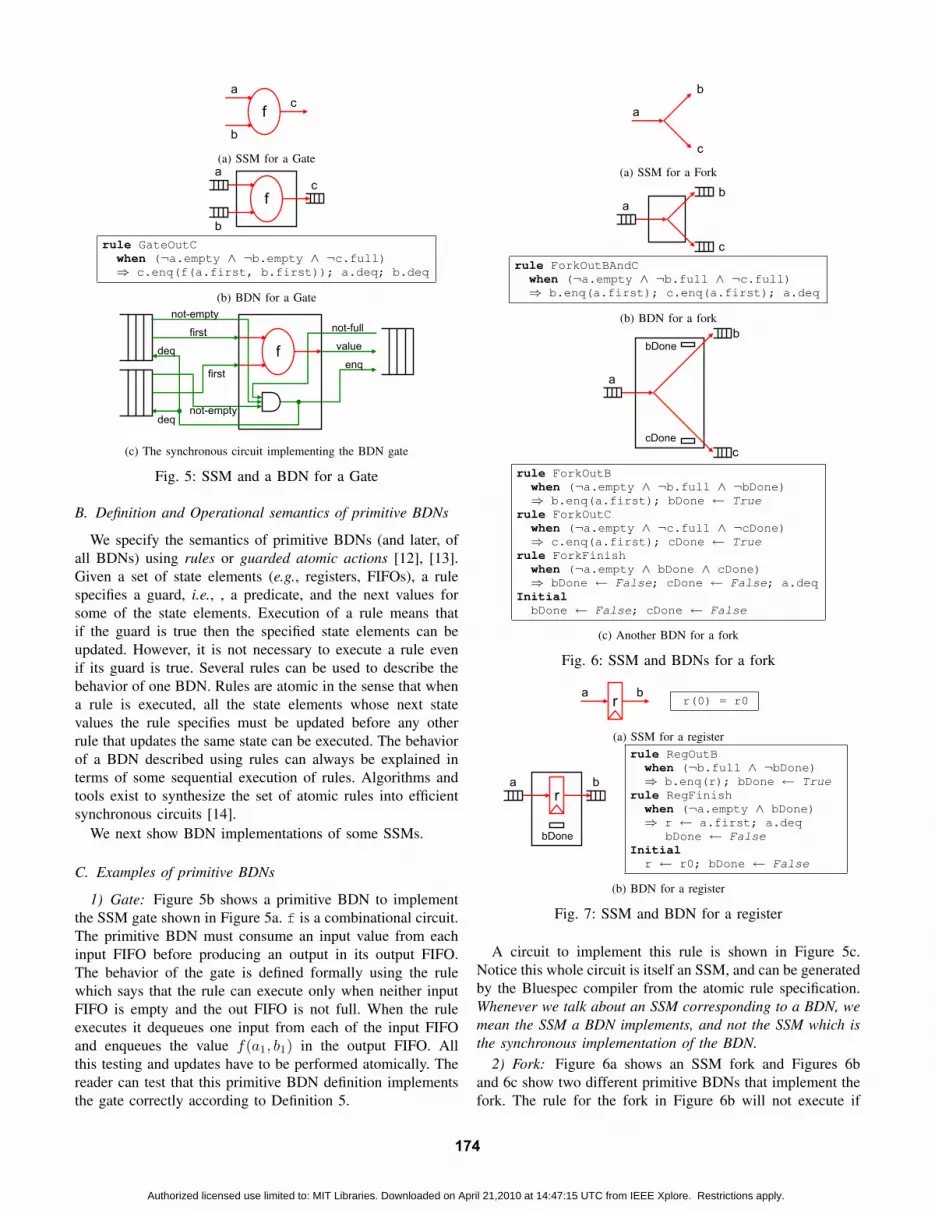
Fig. 5: SSM and a BDN for a Gate

B. Definition and Operational semantics of primitive BDNs

We specify the semantics of primitive BDNs (and later, ofall BDNs) using rules or guarded atomic actions [12], [13].Given a set of state elements (e.g., registers, FIFOs), a rulespecifies a guard, i.e., , a predicate, and the next values forsome of the state elements. Execution of a rule means thatif the guard is true then the specified state elements can beupdated. However, it is not necessary to execute a rule evenif its guard is true. Several rules can be used to describe thebehavior of one BDN. Rules are atomic in the sense that whena rule is executed, all the state elements whose next statevalues the rule specifies must be updated before any otherrule that updates the same state can be executed. The behaviorof a BDN described using rules can always be explained interms of some sequential execution of rules. Algorithms andtools exist to synthesize the set of atomic rules into efficientsynchronous circuits [14].

We next show BDN implementations of some SSMs.

C. Examples of primitive BDNs

1) Gate: Figure 5b shows a primitive BDN to implementthe SSM gate shown in Figure 5a. f is a combinational circuit.The primitive BDN must consume an input value from eachinput FIFO before producing an output in its output FIFO.The behavior of the gate is defined formally using the rulewhich says that the rule can execute only when neither inputFIFO is empty and the out FIFO is not full. When the ruleexecutes it dequeues one input from each of the input FIFOand enqueues the value f(a1, b1) in the output FIFO. Allthis testing and updates have to be performed atomically. Thereader can test that this primitive BDN definition implementsthe gate correctly according to Definition 5.

a

b

c

(a) SSM for a Fork

ab

crule ForkOutBAndCwhen (¬a.empty ∧ ¬b.full ∧ ¬c.full)⇒ b.enq(a.first); c.enq(a.first); a.deq

(b) BDN for a fork

a

b

c

bDone

cDone

rule ForkOutBwhen (¬a.empty ∧ ¬b.full ∧ ¬bDone)⇒ b.enq(a.first); bDone ← True

rule ForkOutCwhen (¬a.empty ∧ ¬c.full ∧ ¬cDone)⇒ c.enq(a.first); cDone ← True

rule ForkFinishwhen (¬a.empty ∧ bDone ∧ cDone)⇒ bDone ← False; cDone ← False; a.deq

InitialbDone ← False; cDone ← False

(c) Another BDN for a fork

Fig. 6: SSM and BDNs for a fork

ra br(0) = r0

(a) SSM for a register

ra

bDone

b

rule RegOutBwhen (¬b.full ∧ ¬bDone)⇒ b.enq(r); bDone ← True

rule RegFinishwhen (¬a.empty ∧ bDone)⇒ r ← a.first; a.deq

bDone ← FalseInitialr ← r0; bDone ← False

(b) BDN for a register

Fig. 7: SSM and BDN for a register

A circuit to implement this rule is shown in Figure 5c.Notice this whole circuit is itself an SSM, and can be generatedby the Bluespec compiler from the atomic rule specification.Whenever we talk about an SSM corresponding to a BDN, wemean the SSM a BDN implements, and not the SSM which isthe synchronous implementation of the BDN.

2) Fork: Figure 6a shows an SSM fork and Figures 6band 6c show two different primitive BDNs that implement thefork. The rule for the fork in Figure 6b will not execute if

174


either of the output forks is full. While the rules for the forkin Figure 6c can enqueue in either of the output forks as andwhen that output becomes non-full. The Done flags ensurethat enqueuing in each output FIFO can happen only once foreach input and the input can be dequeued only when both theoutputs have accepted the input.

Each of these primitive BDNs implements the SSM forkcorrectly but exhibit different operational properties - forexample the fork in Figure 6c can tolerate more slack andmay result in better performance.

3) Register: Figure 7a shows an SSM register and Fig-ure 7b shows a primitive BDN that implements it. In theprimitive BDN, the value in input a is written into registerr and consumed only after the output b has accepted theprevious value in the register.

In an SSM, at every clock cycle all the state elements in theSSM get updated, and all the output values are obtained. Wecan see in the above examples that the clock cycle of the SSMis transformed into dequeue of all the inputs and enqueue of allthe outputs in a primitive BDN, and the state elements in theprimitive BDN corresponding to the SSM are updated exactlyonce during this period. This ensures that each primitive BDNin the examples implements the corresponding SSM accordingto Definition 5.

We will later describe a procedure to implement any SSMas a primitive BDN.

D. Properties of primitive BDNs

We have already seen that several different primitive BDNscan implement an SSM. Besides their differences in perfor-mance, these primitive BDNs behave differently when com-posed with other BDNs to form larger BDNs. We illustratethis via some examples.

1) The No-Extraneous Dependency (NED) property: Fig-ure 8 shows an SSM and four different primitive BDNimplementations for the SSM. Implementation #1 is perhapsthe most straightforward; it waits for all the inputs to becomeavailable and all the output FIFOs to have space and thensimultaneously produces both outputs and consumes bothinputs. Contrast this with implementation #2 which is mostflexible operationally; for each output it only waits for theinputs actually needed to compute that output. It dequeues theinputs after both the outputs have been produced. We needthe Done flags to ensure that each output is produced onlyonce for each set of inputs. Implementations #3 and #4 arevariants of this and contain some extraneous input or outputdependencies as compared to implementation #2. For example,implementation #3 unnecessarily waits for the availabilityof input a to produce output d while implementation #4unnecessarily waits for the availability of space in output FIFOd to produce output c.

Such extraneous dependencies can create deadlocks whenthis primitive BDN is used as a node in a bigger BDN. Con-sider the composition shown in Figure 9b which implementsthe SSM shown in Figure 9a which can be formed by connect-ing d to a in Figure 8a. The BDN in Figure 9b will deadlock if

a

b

c

d

f

(a) An example SSM

fa

b

c

d

cDone

dDone

(b) Figure for BDN implementations #1 to #4rule Out

when (¬a.empty ∧ ¬b.empty ∧ ¬c.full ∧ ¬d.full)⇒ c.enq(f(a.first, b.first));

d.enq(b.first); a.deq; b.deq

(c) BDN implementation #1 (Does not use Done registers)rule OutCwhen (¬a.empty ∧ ¬b.empty ∧ ¬c.full ∧ ¬cDone)⇒ c.enq(f(a.first, b.first)); cDone ← True

rule OutDwhen (¬b.empty ∧ ¬d.full ∧ ¬dDone)⇒ d.enq(b.first); dDone ← True

rule Finishwhen (¬a.empty ∧ ¬b.empty ∧ cDone ∧ dDone)⇒ a.deq; b.deq; cDone ← False; dDone ← False

InitialcDone ← False; dDone ← False

(d) BDN implementation #2rule OutD

when (¬b.empty ∧ ¬a.empty ∧ ¬d.full ∧ ¬dDone)⇒ d.enq(b.first); dDone ← True

(e) BDN implementation #3 (Same as #2 except for rule OutDrule OutC

when (¬a.empty ∧ ¬b.empty ∧¬c.full ∧ ¬cDone ∧ ¬d.full)

⇒ c.enq(f(a.first, b.first)); cDone ← True

(f) BDN implementation #4 (Same as #2 except for rule OutC)

Fig. 8: An example to illustrate the NED property

a

b

c

d

f

(a) SSM compositionR

f

b

ccDone

dDone

a

d

(b) BDN implementing the composition

Fig. 9: Illustrating deadlock when composing BDNs withoutNED property

R uses implementation #1 or #3 because a becomes availableonly when d is produced. Using implementation #4 for Rwill also cause a deadlock if d is a single element FIFO,since FIFO d has to have space for rule Out to consume a.If we do not want our BDN implementations to depend uponthe size of various FIFOs then even implementation #4 is notsatisfactory.

We now define the NED property formally:

Definition 6. (Combinationally-connected relation for primi-tive BDNs)

For any output Oi of a primitive BDN R which implementsSSM S, Combinationally-connected(Oi) is the inputs of R

175


r1a b

r2

r1(t+1) = a(t)r2(t+1) = r1(t)

b = r2(t)r1(0) = r10

r2(0) = r20

(a) An example SSM

a b

bDone

r1 r2

rule OutBwhen (¬b.full ∧ ¬bDone)⇒ b.enq(r2); bDone ← True

rule Finishwhen (bDone ∧ ¬a.empty)⇒ r2 ← r1; r1 ← a.first; a.deq;

bDone ← FalseInitialr1 ← r10; r2 ← r20;bDone ← False

(b) BDN implementation #1

a b

bCnt

aCnt

r1 r2

rule Out1when (¬b.full ∧ bCnt = 0)⇒ b.enq(r2); bCnt ← 1

rule Out2when (¬b.full ∧ bCnt = 1)⇒ b.enq(r1); bCnt ← 2

rule In1when (¬a.empty ∧ bCnt = 2 ∧ aCnt = 0)⇒ r2 ← a.first; a.deq; aCnt ← 1

rule In2when (¬a.empty ∧ bCnt = 2 ∧ aCnt = 1)⇒ r1 ← a.first; a.deq; bCnt ← 0; aCnt ← 0;

(c) BDN implementation #2

Fig. 10: An example illustrating the SC property

corresponding to those inputs of S that are combinationallyconnected to the output Oi in S.

Definition 7. (No-Extraneous Dependencies (NED) propertyfor primitive BDNs)

A primitive BDN has the NED property if all output FIFOshave been enqueued at least n− 1 times and for each outputOi, and if all the FIFOs for the inputs in Combinationally-connected(Oi) are enqueued n times, and all other input FIFOsare enqueued at least n − 1 times, then Oi FIFO must beenqueued n times.

According to this definition only implementation #2 satisfiesthis property.

2) The Self-Cleaning (SC) property: Figure 10 shows anSSM and two different primitive BDN implementations. Boththe implementations obey the NED property. In implementa-tion #1, after an output is produced, the Done flag is set. Thenthe input is consumed and the state is updated accordingly.In implementation #2, two outputs have to be produced, and

r1a b

r2

(a) SSM compositionR

r1a b

r2

(b) BDN implementing the composition

Fig. 11: Illustrating deadlock when composing BDNs withoutSC property

then two inputs are consumed. The Cnt counters keeps trackof how many outputs are produced and how many inputs areconsumed, and they get reset once two outputs are producedand two inputs are consumed.

Implementation #2 does not dequeue its inputs every timean output is produced. This can create deadlocks when thisprimitive BDN is used as a node in a bigger BDN. Consider thecomposition shown in Figure 11b, which implements the SSMshown in Figure 11a which can be formed by connecting b toa. If b is a single element FIFO, then the implementation #2for R will cause a deadlock as it can not dequeue inputs unlesstwo outputs are produced, but there is no space to produce twooutputs.

We now define the SC property formally:

Definition 8. (Self-Cleaning (SC) property for primitiveBDNs)

A primitive BDN has the SC property, if when all theoutputs are enqueued n times, all the input FIFOs mustbe dequeued n times, assuming an infinite source for eachinput.

According to this definition only implementation #1 is self-cleaning.

Definition 9. (Primitive Latency-Insensitive (LI) BDNs)A primitive BDN is said to be a primitive LI-BDN if it has

the NED and the SC properties.

Note that according to this definition of primitive LI-BDNs,the fork in Figure 6b is not an LI-BDN while the fork inFigure 6c is. As it turns out both the BDN forks work wellunder composition because both the outputs have the sameCombinationally-Connected inputs. We could have given amore complicated definition of the NED property which wouldadmit the fork in Figure 6b also as an LI-BDN. For lack ofspace we won’t explore this more complicated definition ofthe NED property.

E. Implementing any SSM as a primitive LI-BDN

We will now describe a procedure to implement any SSMas a primitive LI-BDN. Let the SSM be described as follows:

Oi(t) = fi(s(t), ICCi1(t),. . ., ICCik(t))

s(t+1) = g(s(t), I1(t),. . ., InI(t))s(1) = s0

where {ICCi1 , . . . ICCik} are inputs combinationally con-

nected to Oi

We associate a donei flag with every output Oi. These flagsinitially start out as False. We have a rule for each output Oi

176


done

Depends-on(Oj)

Oj

Alldones

All inputdeqs

deq

not-full

1 0

enq

not-e

mpt

yIi

value

first Patient SSM

enable

Fig. 12: A wrapper to turn a patient SSM into an LI-BDN

as follows:rule OutOi

when (¬ICCi1.empty ∧ . . . ∧ ¬ICCik.empty ∧

¬Oi.full ∧ ¬donei)⇒ Oi.enq(fi(s, ICCi1.first,. . ., ICCik

.first));donei ← True

Finally we have a rule to dequeue all the inputs:rule Finishwhen (done1 ∧ . . . ∧ donenO ∧

¬I1.empty ∧ . . . ∧ ¬InI.empty)⇒ s ← g(s, I1.first, . . ., InI.first);

I1.deq; . . .; InI.deq;done1 ← False; . . .; donenO ← False

Initialdone1 ← False; . . .; donenO ← False; s ← s0

The BDN described above can be implemented as a syn-chronous hardware circuit by converting the original SSM intoa Patient SSM, and creating a wrapper around it, treating itas a black-box. Figure 12 shows the circuit representing thewrapper.

IV. THEORY FOR MODULAR REFINEMENT OF BDNS

Large SSMs are often designed by composing smallerSSMs. In this section we develop the theory needed tosupport a design methodology where each smaller SSM canbe implemented as a primitive LI-BDN and the large SSMcan be constructed simply by composing these LI-BDNs. Wewill further show that any constituent primitive LI-BDN canbe refined to improve some implementation aspect such asarea, timing, etc without affecting the overall correctness ofthe BDN.

A. Preliminaries

Definition 10. (Bounded Dataflow Network (BDN))A BDN is a network of primitive BDN nodes such that

1) At most one node can enqueue in a given FIFO and atmost one node can dequeue from a given FIFO.

2) For any FIFO X in the network, the transitive closure ofCombinational-connected(X) is well defined, i.e., X is notin the transitive closure of Combinationally-connected(X).

The transitive closure restriction formally says that a BDNdoes not contain any “combinational loops”. Note the similar-ity of this definition with that of SSMs (Definition 1).

Lemma 1. If an SSM is formed as a network of smaller SSMs,then a BDN can be formed as a corresponding network ofprimitive BDNs that implement the smaller SSMs.

Proof: Since an SSM formed from smaller SSMs does notcontain a combinational loop, neither does the correspondingnetwork of the primitive BDNs; thus it forms a BDN.

We now extend several definitions that we had for primitiveBDNs to larger BDNs.

Definition 11. (Depends-on relation for BDNs)For any output Oi of a BDN R, Depends-on(Oi) is the in-

puts of R that are in the transitive closure of Combinationally-connected(Oi).

Definition 12. (NED property for BDNs)A BDN has the NED property if all outputs have been

enqueued atleast n − 1 times and for each output Oi, all theinputs in Depends-on(Oi) are enqueued n times, and all otherinputs are enqueued at least n − 1 times, then Oi must beenqueued n times.

Definition 13. (SC property for a BDN)A BDN has the SC property, if all the outputs are enqueued

n times, then all the inputs must be dequeued n times,assuming an infinite source for each input.

Definition 14. (Latency-Insensitive (LI) BDNs)An LI-BDN is a BDN which has the NED and SC proper-

ties.

A natural equivalence relation between BDNs can be de-fined in terms of their input-output behavior as follows:

Definition 15. (Equivalence of BDNs)BDNs R1 and R2 are said to be equivalent iff

1) There is a bijective mapping between the inputs of R1 andR2, and a bijective mapping between the outputs of R1

and R2.2) The output histories of R1 and R2 matches whenever the

input histories matches, i.e.,∀n > 0,

I(k) for R1 and R2 matches (1 ≤ k ≤ n)⇒O(j) for R1 and R2 matches (1 ≤ j ≤ n)

Our theory rests on the fact that this equivalence relationbecomes a congruence for LI-BDNs, i.e., if two LI-BDNs areequivalent then there is no way to tell them apart regardlessof the context.

B. Structural composition of BDNs

Just like SSMs, any BDN can be formed inductively usingparallel and iterative compositions of BDNs starting withprimitive BDNs.

Definition 16. (Structural definition of BDNs)1) Primitive BDNs are BDNs2) If R1 and R2 are BDNs, then so is the parallel composition

of R1 and R2, written as R1 ⊕ R2 (Figure 13a). Thesemantics of parallel composition of two BDNs is defined

177


R

R1

R2...... ...

...

R1

R2...... ...

...

(a) Parallel composition of BDNs

S

S1... ...S1... ...

Ii Oj Ii Oj

(b) Iterative composition of BDNs

Fig. 13: Composition of BDNs

by the union of the two sets of disjoint rules (i.e., ruleswith no shared state) for the two BDNs.

3) If R1 is an BDN then so is the (Ii, Oj) iterative composi-tion of R1 written as (Ii, Oj)�R1 (Figure 13b), providedthat Ii /∈ Depends-on(Oj). The semantics of the iterativecomposition of a BDN is defined by aliasing the name ofa pair of an input and an output FIFO in the set of rulesassociated with the BDN.

The following two theorems are the main theorems of thispaper:

Theorem 1. (Modular Composition Theorem)If R1 and R2 are LI-BDNs implementing SSMs S1 and S2,

respectively, then• R = R1⊕R2 is an LI-BDN that implements S = S1+S2.• R = (Ii, Oj) � R1 is an LI-BDN that implements S =

(Ii, Oj) · S1.

Theorem 2. (Modular Refinement Theorem)Equivalence of two LI-BDNs is preserved under parallel

and iterative composition, i.e. if R1 and R2 are LI-BDNsequivalent to BDNs R′1 and R′2, then• R = R1⊕R2 is an LI-BDN equivalent to R′ = R′1⊕R′2.• R = (Ii, Oj) � R1 is an LI-BDN equivalent to R′ =

(Ii, Oj)�R′1.

The proofs of the two theorems are very similar; we onlygive the proof of Theorem 1.

Proof:1) Compositions of LI-BDNs are LI-BDNs. (Lemma 2)2) LI-BDNs are deadlock-free. (Lemma 3)3) If R is a composition of LI-BDNs R1 and R2 then R

partially implements the composition of S1 and S2 whereS1 and S2 are the SSMs corresponding to R1 and R2,respectively. (Lemma 4)

Lemma 2. (Closure property of LI-BDNs) If R1 and R2 areLI-BDNs then so are R1 ⊕R2 and (Ii, Oj)�R1.

Proof: The proof is obvious for the parallel composition.

For the iterative composition, we show by induction on n,Oj will be enqueued and dequeued n times if all the inputs areenqueued n times and all the outputs are enqueued n times.This is trivial as Oj will not wait for Ii (as R1 has the NEDproperty). All output FIFOs of R1 can now be enqueued andso all input FIFOs of R1 can be dequeued (R1 has the SCproperty).

We now prove again by induction on n that for an outputOk 6= Oj , Ok will be enqueued n times if all the inputs inDepends-on(Ok) are enqueued n times, and all the other inputsare enqueued at least n − 1 times, and all the other outputsare enqueued at least n− 1 times (NED property). There aretwo cases to consider:

1) Ii /∈ Depends-on(Ok): trivial as R1 is an LI-BDN.2) Ii ∈ Depends-on(Ok): Oj is not full because of the SC

property of R1 and it will be enqueued n times becauseof NED property of R1, which makes Ii and hence Ok

enqueued n times.By a similar induction on n we can show that if all the

inputs are enqueued n times, and all the outputs are enqueuedn times, then all the inputs will be dequeued n times (SCproperty).

Lemma 3. (Deadlock-free Lemma) LI-BDNs are deadlock-free.

Proof: Given infinite sinks for outputs and infinite sourcefor inputs, by induction on the number of inputs and outputsenqueued it can be shown using the NED and SC propertiesof an LI-BDN that it will not deadlock.

Lemma 4. If R1 and R2 are LI-BDNs then R1⊕R2 partiallyimplements S1 + S2 and (Ii, Oj) � R1 partially implements(Ii, Oj) · S1

Proof: The proof is obvious for the parallel composition.For iterative composition, we first show by induction on n

Oj(n) matches for R and S whenever the input histories for Rand S match upto n values. Oj(n) does not depend on Ii(n)in S1. So Oj(n) matches in R1 and S1 whenever the rest ofthe inputs match upto n− 1 as R1 implements S1.

We show by induction on n, for an output Ok 6= Oj , Ok

will have the same nth values in the SSM and the LI-BDN ifthe input histories match upto n values. There are two casesto consider:

1) Ii /∈ Depends-on(Ok): trivial as R1 implements S1.2) Ii ∈ Depends-on(Ok): Oj(n) matches. Since all the nth

inputs are the same for R1 and S1, all the nth outputswill be the same in both.

V. CYCLE-ACCURATE REFINEMENTS OF SSMS USINGLI-BDNS

One way to apply the theory that we have developed is torefine parts of an existing SSM (referred to as the model SSMin this section) into more area-efficient hardware structures.Such modular refinements, in general, are quite difficult be-cause the refined module may take a different number of cycles

178


cuts

S3

(big)S2

(big)S1

(a) Model SSM

R2 R3R1

S1S2

(big)S3

(big)

(b) Turning the model SSM into an LI-BDN

R’2(small)

R1

S1 R’3(small)

(c) Refining R2 and R3

Fig. 14: Modular Refinement

than the original module. Under such circumstances even ifone proves the functional correctness of the refined modulewith respect to the original module, there is no guarantee thatthe functionality of the model SSM would be preserved bythe modularly refined design. This problem is faced by manydesigners who are trying to use FPGAs.

Based on the theory we have presented, a designer can makeone or more cuts in his model SSM to separate the moduleshe wishes to change. Each such module can be converted intoan LI-BDN using the procedure given in Section III-E. Oncethe SSM is implemented as a network of LI-BDN nodes, theneach node can be refined into a different but equivalent LI-BDN (Figure 14). There is no need to verify the entire LI-BDN again for correctness, just the changed node has to bevalidated. Thus one can do true modular refinements usingLI-BDNs. In this section, we give examples of some usefulrefinements of LI-BDNs.

Example 1: Optimizing the multiplexor

Figure 15a shows an SSM for a multiplexor and Figures15b and 15c show primitive BDNs which implement themultiplexor. Figure 15b is the standard primitive BDN whilein Figure 15c the rule waits only for the input indicated bythe predicate. The output will be enqueued by the rule even ifthe other input takes longer to get enqueued. When the otherinput finally arrives, it will be discarded; the counters keeptrack of how many inputs to discard. A similar multiplexorwas considered using A-Ports [15]. The BDN is an LI-BDNbecause it obeys the NED and SC properties. In general, thisidea can be used to “run-ahead” in any LI-BDN, withoutwaiting for all the inputs, thereby improving the performanceof the whole system. This is shown in Figure 15d. If functiong is implemented as a multi-cycle function, then the outputin d has to wait till g is computed every time if we usethe multiplexor in Figure 15b. If we use the multiplexor inFigure 15c, then the multiplexor has to wait for g only if thepredicate c is false.

a

b

c

d

(a) Multiplexor SSM

a

b

c

daCnt

bCnt

rule OutDwhen (¬d.full ∧ ¬c.empty ∧ ¬a.empty ∧ ¬b.empty)⇒ if(c.first) then d.enq(a.first);

else d.enq(b.first);a.deq; b.deq; c.deq

(b) A multiplexor BDN (Does not use the Done flags)rule OutD

when (¬d.full ∧ ¬c.empty)⇒ if(c.first ∧ ¬a.empty ∧ bCnt 6= max) then

d.enq(a.first); a.deq; c.deq; bCnt ← bCnt+1;else if(¬b.empty ∧ aCnt 6= max)d.enq(b.first); b.deq; c.deq; aCnt ← aCnt+1;

rule DiscardAwhen (aCnt > 0 ∧ ¬a.empty)⇒ a.deq; aCnt ← aCnt-1

rule DiscardBwhen (bCnt > 0 ∧ ¬b.empty)⇒ b.deq; bCnt ← bCnt-1

InitialaCnt ← 0; bCnt ← 0

(c) A performance-optimized multiplexor BDN

a

b

c

daCnt

bCnt

f

g

x

y

(d) Illustrating the performance optimized multiplexor

Fig. 15: Optimizing the multiplexor BDN

Example 2: Multicycle implementation of Content AddressableMemory (CAM)

Figure 16a shows a synchronous CAM lookup. The CAMis an array of n elements, where each element stores a (key,value) pair. Every cycle, the synchronous CAM returns a valueand the index of the search-key in the CAM-array if the keyis found; otherwise it returns an Invalid. If the upd signalis enabled, then the CAM array is updated with uKey anduVal at the position given by uIdx. Single cycle CAMs areexpensive structures in terms of area and critical path. If theCAM is implemented as an LI-BDN, then it can be refinedto do a sequential lookups taking several cycles to lookup thevalue corresponding to a key (Figure 16b). See [16] for othermulti-cycle implementations of CAM. This keeps the rest ofthe system using the CAM unchanged, while resulting in acircuit with lesser area and lesser critical path than the originalunrefined LI-BDN. If the CAM lookup is not done frequently,

179


arra

y

key

upd

uIdx

uKey

uVal

Invalid/(val_idx)

(a) A single cycle CAM lookup SSM

arra

ykey

upd

uIdx

uKey

uVal

Invalid/(val_idx)done

idx

rule OutValueIndexwhen (¬key.empty ∧ ¬val_idx.full ∧ ¬done)⇒ if(idx = LastIdx+1)

val_idx.enq(Invalid); idx ← 0;done ← True

else if(array[idx].key = key.first)val_idx.enq(array[idx].value, idx);idx ← 0; done ← True

else idx ← idx + 1rule Finishwhen (¬key.empty ∧ ¬upd.empty ∧

¬uKey.empty ∧ ¬uVal.empty ∧¬uIdx.empty ∧ done = True)

⇒ if(upd.first)array[uIdx.first].key = uKey.first;array[uIdx.first].val = uVal.first;

key.deq; upd.deq; uKey.deq; uVal.deq;uIdx.deq; done ← False

(b) Multicycle LI-BDN implementing the CAM

Fig. 16: CAM lookup as a multicycle LI-BDN

then using the multiplexor that we discussed above we canensure that even the performance degradation is minimized.

VI. CONCLUSIONS

We have presented a theory using Bounded Dataflow Net-works (BDNs) that can help in modular latency-insensitiverefinements of synchronous designs. The theory should helpimplementers avoid deadlocks in implementing latency insen-sitive circuits, especially when refinements involve changes indesign that affect the timing.

In future we wish to explore the use of BDNs even inthe absence of a clearly specified model SSM. For example,it is not clear how the timing requirements for a moderncomplex processor should be specified. One can use the RTLof the microprocessor as a timing specification but usuallyRTL is not available at the time when modelers do theirarchitectural explorations. Furthermore, architects want to beable to modify their micro-architectures and study its effecton performance (i.e., the number of cycles it takes to executea program) without having to worry about the correctness ofvarious models. We doubt that RTL for the many variants ofthe models that an architect wants to study can be providedto the architect. It is quite common to set up the design in away that latency insensitive aspects of the design are clear to

the modeler. However, a modeler probably would not want tomake any changes in its design to accommodate the vagariesof an FPGA implementation because mixing of these twoconcerns may destroy his intuition about the performance ofthe machine to be studied. We think BDNs can provide therequired separation between these two types of timing changes.

ACKNOWLEDGEMENT

The authors would like to thank Intel Corporation andNSF grant Generating High-Quality Complex Digital Systemsfrom High-level Specification (No. 0541164) for funding thisresearch. The discussions with the members of ComputationStructures Group at MIT, especially Joel Emer, Mike Pellauer,Asif Khan and Nirav Dave have helped in refining the ideaspresented in this paper.

REFERENCES

[1] G. Kahn, “The semantics of a simple language for parallel program-ming,” in Information Processing ’74: Proceedings of the IFIP Congress,J. L. Rosenfeld, Ed. New York, NY: North-Holland, 1974, pp. 471–475.

[2] J. B. Dennis and D. P. Misunas, “A preliminary architecture for abasic data-flow processor,” in ISCA ’75: Proceedings of the 2nd annualsymposium on Computer architecture. New York, NY, USA: ACM,1975, pp. 126–132.

[3] L. P. Carloni and A. L. Sangiovanni-Vincentelli, “Performance analysisand optimization of latency insensitive systems,” in DAC ’00: Proceed-ings of the 37th conference on Design automation. New York, NY,USA: ACM, 2000, pp. 361–367.

[4] L. Carloni, K. McMillan, and A. Sangiovanni-Vincentelli, “Theoryof latency-insensitive design,” Computer-Aided Design of IntegratedCircuits and Systems, IEEE Transactions on, vol. 20, no. 9, pp. 1059–1076, Sep 2001.

[5] L. P. Carloni, K. L. Mcmillan, and A. L. Sangiovanni-vincentelli,“Latency insensitive protocols,” in in Computer Aided Verification.Springer Verlag, 1999, pp. 123–133.

[6] L. Carloni, K. McMillan, A. Saldanha, and A. Sangiovanni-Vincentelli,“A methodology for correct-by-construction latency insensitive de-sign,” Computer-Aided Design, 1999. Digest of Technical Papers. 1999IEEE/ACM International Conference on, pp. 309–315, 1999.

[7] M. Pellauer, M. Vijayaraghavan, M. Adler, Arvind, and J. Emer, “A-ports: an efficient abstraction for cycle-accurate performance models onfpgas,” in FPGA ’08: Proceedings of the 16th international ACM/SIGDAsymposium on Field programmable gate arrays. New York, NY, USA:ACM, 2008, pp. 87–96.

[8] ——, “Quick performance models quickly: Closely-coupled partitionedsimulation on fpgas,” April 2008, pp. 1–10.

[9] D. Chiou, D. Sunwoo, J. Kim, N. Patil, W. H. Reinhart, D. E. Johnson,and Z. Xu, “The fast methodology for high-speed soc/computer simula-tion,” in ICCAD ’07: Proceedings of the 2007 IEEE/ACM internationalconference on Computer-aided design. Piscataway, NJ, USA: IEEEPress, 2007, pp. 295–302.

[10] K. Asanovic. (2008, January) RAMP Gold. RAMP Retreat. [Online].Available: http://ramp.eecs.berkeley.edu/Publications/RAMP%20Gold%20(Slides,%201-16-2008).ppt

[11] D. Chiou, private Communication.[12] J. Hoe and Arvind, “Operation-centric hardware description and synthe-

sis,” Computer-Aided Design of Integrated Circuits and Systems, IEEETransactions on, vol. 23, no. 9, pp. 1277–1288, Sept. 2004.

[13] J. C. Hoe and Arvind, “Synthesis of operation-centric hardware descrip-tions,” in ICCAD ’00: Proceedings of the 2000 IEEE/ACM internationalconference on Computer-aided design. Piscataway, NJ, USA: IEEEPress, 2000, pp. 511–519.

[14] Bluespec System Verilog. Bluespec Inc. [Online]. Available: http://www.bluespec.com

[15] M. Pellauer, private Communication.[16] K. Fleming and J. Emer, “Resource-efficient fpga content-addressable

memories,” in WARP, 2007.

180


bounded dataflow networks and latency-insensitive circuits

Documents