LawrenceLivermoreNationalLaboratory

U.S. Department of Energy

PreprintUCRL-JC-144550

A Memory InsensitiveTechnique for Large ModelSimplification

P. Lindstrom and C. T. Silva

To appear in Proceedings of IEEE Visualization 2001,San Diego, California, October 21-26, 2001

August 7, 2001

Approved for public release; further dissemination unlimited

DISCLAIMER

This document was prepared as an account of work sponsored by an agencyof the United States Government. Neither the United States Government northe University of California nor any of their employees, makes any warranty,express or implied, or assumes any legal liability or responsibility for the ac-curacy, completeness, or usefulness of any information, apparatus, product, orprocess disclosed, or represents that its use would not infringe privately ownedrights. Reference herein to any specific commercial product, process, or ser-vice by trade name, trademark, manufacturer, or otherwise, does not necessarilyconstitute or imply its endorsement, recommendation, or favoring by the UnitedStates Government or the University of California. The views and opinions ofauthors expressed herein do not necessarily state or reflect those of the UnitedStates Government or the University of California, and shall not be used for ad-vertising or product endorsement purposes.

This report has been reproduced directly from the best available copy.

Available to DOE and DOE contractors from theOffice of Scientific and Technical Information

P.O. Box 62, Oak Ridge, TN 37831Prices available from (423) 576-8401

http://apollo.osti.gov/bridge/

Available to the public from theNational Technical Information Service

U.S. Department of Commerce5285 Port Royal Rd., Springfield, VA 22161

http://www.ntis.gov/

OR

Lawrence Livermore National LaboratoryTechnical Information Department’s Digital Library

http://www.llnl.gov/tid/Library.html

A Memory Insensitive Technique for Large Model Simplification

Peter Lindstrom∗LLNL

Claudio T. Silva†

AT&T

Abstract

In this paper we propose three simple, but significant improve-ments to the OoCS (Out-of-Core Simplification) algorithm of Lind-strom [20] which increase the quality of approximations and extendthe applicability of the algorithm to an even larger class of computesystems.

The original OoCS algorithm has memory complexity that de-pends on the size of the output mesh, but no dependency on the sizeof the input mesh. That is, it can be used to simplify meshes ofarbitrarily large size, but the complexity of the output mesh is lim-ited by the amount of memory available. Our first contribution isa version of OoCS that removes the dependency of having enoughmemory to hold (even) the simplified mesh. With our new algo-rithm, the whole process is made essentially independent of theavailable memory on the host computer. Our new technique usesdisk instead of main memory, but it is carefully designed to avoidcostly random accesses.

Our two other contributions improve the quality of the approxi-mations generated by OoCS. We propose a scheme for preservingsurface boundaries which does not use connectivity information,and a scheme for constraining the position of the “representativevertex” of a grid cell to an optimal position inside the cell.

CR Categories: E.5 [Files]: Sorting; I.3.5 [Computer Graphics]:Computational Geometry and Object Modeling—Surface and ob-ject representations.

Keywords: polygonal surface simplification, large data, out-of-core algorithms, external sorting, quadric error metrics.

1 INTRODUCTION

In recent years there has been a rapid increase in the raw size ofpolygonal datasets. Several technological trends are contributing tothis effect, such as the development of high-resolution 3D scanners,and the need to visualize ASCI-size (Accelerated Strategic Com-puting Initiative) datasets. A useful paradigm for visualizing largedatasets is to generate levels of detail. Over the last decade, therehas been substantial research in designing algorithms for generat-ing level-of-detail approximations of triangle meshes. In this paper,our focus is on algorithms which have low memory complexity.

A simplification algorithm receives an input mesh of complexityn, and outputs a mesh of complexitym (wherem< n). Often, theuser sets the target size of the output, and the algorithm attemptsto minimize the overall error of the approximation. One impor-tant aspect of the design of a surface simplification algorithm is its

∗Center for Applied Scientific Computing, Lawrence Livermore Na-tional Laboratory, 7000 East Avenue, L-560, Livermore, CA 94551, USA;pl@llnl.gov.

†AT&T Labs-Research, 180 Park Avenue, Room D265, PO Box 971,Florham Park, NJ 07932, USA; csilva@research.att.com.

memory usage. In general, different algorithms have different mainmemory dependencies onn andm. For different applications, it isuseful to have algorithms which are memory efficient with respectto n or m (but ideally both). The memory dependency onn affectsthe usefulness of a given algorithm in the sense that it limits the sizeof models that can be simplified.

In general the memory requirement of a given algorithm growswith both m andn (for exceptions, see e.g. [29, 30]). The depen-dency onm has direct implications on the maximum accuracy ofthe approximation. As an example, an efficient terrain simplifica-tion algorithm is presented in [13], whose memory complexity isanalyzed to be 3n+192m bytes, wheren andm are the number ofvertices in the input and output, respectively. In order to generatea high-quality approximation with one eighth of the input points,i.e.,m= 1

8n, one would need to have 27n bytes of memory, or ninetimes as much as the size of the input. Often, the memory com-plexity is much higher on bothn andm (e.g., [21] uses 160n bytesfor general surface simplification), and generating approximationsof large datasets is usually quite hard.

The OoCS algorithm proposed by Lindstrom [20] is a big stepforward in that it has no dependency onn, thus allowing for simpli-fication of extremely large datasets. One contribution of our workis to remove the main memory dependency onm from OoCS, thusallowing for an arbitrarily accurate approximation of an arbitrarilylarge dataset. Our new algorithm, OoCSx, usesconstant memory,no matter how large the dataset or approximation error.

One might argue that the ability to produce simplified modelsthat are still too large to represent in-core is of little practical value,since the main reason for simplifying the model in the first placeis to reduce its complexity to something more manageable. How-ever, we see several important uses of our new algorithm. First, inmany situations it is not known beforehand how much RAM will beavailable on the client machine on which the simplified mesh is tobe used, as is generally the case with multi-level-of-detail datasetsprovided through data repositories. Second, OoCS does not pro-vide a mechanism for specifying the exact sizem of the simplifiedmodel, and trial and error may be necessary to find a grid resolutionthat leads to a detailed simplification that, along with the auxiliarydata structures used in OoCS, fits in-core. Our memory insensitivealgorithm, on the other hand, is able to finish and output a simpli-fied model regardless of the grid resolution. Third, many applica-tions demand a strict error bound, in which case trading memory formesh accuracy is not a practical option. As we shall see, even whenan explicit error bound is not given, the mesh may be so geometri-cally complex that the most detailed simplification to fit in-core is ofunacceptable visual quality. Finally, our work nicely complementsthe recent trend of developing efficient out-of-core scientific visu-alization techniques (see, e.g., [7, 11, 32]). With tools like these inhand, further out-of-core processing of a simplified mesh becomespractical.

Our new technique uses disk instead of main memory. In fact,OoCSx generally needs more disk space than OoCS needs mainmemory. On the other hand, disk is often much cheaper and morereadily available than random access memory. The naive use of diskhas the potential for considerable slowdown (as in the case of oper-ating system paging). Our algorithm is carefully designed to avoid

random accesses, thus achieving simplification speeds which, al-though slower than OoCS, are still quite practical. Our experimentsshow that OoCSx is typically between two to five times slower thanOoCS, while using constant main memory. However, when insuf-ficient main memory is available for OoCS to store the simplifiedmodel, OoCSx runs faster. Of course, for large enough models,OoCS is not able to finish at all.

Because OoCS does not make use of connectivity information, ithas no way of detecting whether an edge is a boundary edge or not.As a consequence, boundaries are generally poorly preserved byOoCS. We propose a technique for preserving boundaries that doesnot use any connectivity information. Finally, we sketch a tech-nique for enforcing maximum errors, which constrains the optimalcluster representative to lie inside its grid cell while minimizing theapproximation error.

2 RELATED WORK

Polygonal simplification has been a hot topic of research over thelast decade, with a vast number of published algorithms. Many ofthe early simplification algorithms were designed to handle modestsize datasets of a few tens of thousands of triangles. Recent im-provements in scanning and storage technology, however, have leadto datasets as large as billions of triangles [19, 23]. As a result, anumber of methods, particularly for out-of-core visualization, havebeen proposed for coping with models that are too large to fit inmain memory, e.g. [3,5–8,17,24,28,31,32].

Rossignac and Borrel proposed one of the earliest simplificationalgorithms [26]. Their algorithm partitions space into cube-likecells from a uniform rectilinear grid, and replaces all mesh verticeswithin a grid cell by a single representative vertex. While simpleand fast, their method produces rather low quality meshes, in partdue to the simple vertex positioning scheme used in their originalalgorithm. Lindstrom’s OoCS algorithm [20] is also based on ver-tex clustering on a uniform grid, but has a lower time and memorycomplexity, and uses a quadric error metric to improve the meshquality. This method was recently extended by Shaffer and Gar-land [27], who make two passes over the input mesh. During thefirst pass, the surface is analyzed and an adaptive (instead of uni-form) partitioning of space is made. Using this approach, a largernumber of irregular grid cells (and thus samples) can be allocated tothe more detailed portions of the surface. However, their algorithmrequires more RAM than OoCS in order to maintain a BSP-tree andadditional quadric information in-core.

Bernardini et al. describe a radically different approach to out-of-core simplification [4]. Their method splits the model up intoseparate patches that are small enough to be simplified individuallyin-core using a conventional simplification algorithm. Special carehas to be taken along the patch boundaries. A similar techniquewas proposed by Hoppe for creating hierarchical levels of detail forheight fields [15], which was later generalized by Prince to arbitrarymeshes [25]. While conceptually simple, the time and space over-head of partitioning the model and later stitching it together adds toan already expensive in-core simplification process, rendering sucha method less suitable for simplifying very large meshes.

El-Sana and Chiang [10] propose an external-memory algorithmto support view-dependent simplification of datasets that do not fitin main memory. Similar to [4,15,25], they segment the model intosub-meshes that can be simplified independently and later mergedin a preprocessing phase. The segmentation and stitching are madesimple by ensuring that edges are collapsed in edge-length order,and guaranteeing that sub-mesh boundary edges are longer thaninterior edges. During run-time, only the portions of the view-dependence tree that are necessary to render the given level of detailare kept in main memory.

3 OUT-OF-CORE SIMPLIFICATION

In order to describe our new simplification algorithm, we will firstprovide a brief review of OoCS. For full details see [20]. The inputto the algorithm is a set of triangles, stored as triplets of vertex coor-dinates in a file, and the resolution of a three-dimensional grid. (Seethe appendix for a disk-based technique on how to transform fromindexed meshes to thisdereferencedformat.) The algorithm, whichis loosely based on the clustering algorithm by Rossignac and Bor-rel [26], computes for each cluster grid location a representativevertex. (A set of vertices constitute a “cluster” if they all lie insidethe same grid cell.) The position of the representative vertex is cho-sen so as to minimize thequadric error[14] measured with respectto the triangles in the cluster. For each trianglet = (xt

1,xt2,x

t3), an

associatedquadric matrixQt is computed:

Qt = nt nTt (1)

nt =(

xt1×xt

2 +xt2×xt

3 +xt3×xt

1−[xt1,x

t2,x

t3]

)(2)

wherent is a 4-vector made up of the area-weighted normal oft andthe scalar triple product of its three vertices.1 Qt is then distributedto the clusters associated with each oft ’s three vertices by addingQt to their quadric matrices.

After summing up all per-triangle quadric matrices in a cluster,we obtain a quadric matrixQS that contains shape information forthe piece of surface passing through the grid cell:

QS = ∑t

Qt =(

A−bT

−bc

)(3)

Using this decomposition ofQS, the 3×3 linear systemAx = b issolved for the “optimal” representative vertex positionx that min-imizes the quadric error. That is,x is the position that minimizesthe sum of squared volumes of the tetrahedra formed byx and thetriangles in the cell. When clustering vertices together, the majorityof triangles degenerate into edges or points and can be discarded,thereby reducing the complexity of the model.

3.1 OoCSx

The main idea of our modification of the OoCS algorithm is to elim-inate the list of occupied clusters which OoCS allocates in mainmemory and uses for keeping track of their quadrics. Instead ofdirectly computing quadrics, OoCSx computesnt for the currenttrianglet and outputs this information to a file, three times for eachof the three vertices, together with the information for what grid cellthe vertex belongs to. At the same time, we also output another filewhich contains the non-degenerate triangles (those triangles thathave vertices in three different clusters) represented as indices tothe grid cells. Then, we externally sort the file containing the vec-torsnt using the grid locations as the primary key. After this, all theinformation related to one grid cell is placed contiguously in thefile. By scanning it, it is possible to compute the quadrics and theoptimum location of the representative vertex for a particular gridcell. After the vertices in the simplified mesh have been computed,we are left with the task of associating the grid cell references inthe triangle file with vertex representatives. This step is describedin more detail below.

Here are the steps of OoCSx in detail:

(1) Read triangles, compute quadric information for later use.For each trianglet = (xt

1,xt2,x

t3) in the input mesh, we com-

pute nt (Equation 2). Note that we do not compute any

1In this paper,a denotes a 4-vector, anda is a unit-length 3-vector.

quadric matrices at this point. For each vertexxti of t, we

also determine the grid locationG(xti ) (as an integer ID) that

the vertex will be mapped to. As triangles are read, we outputthis information to two files:

– A “plane equation” file, which contains 3 entries foreach triangle, one for each vertex. Each entry is of theform: 〈G(xt

i ), nt〉. Using 32-bit integers to representGand 32-bit floats fornt , this file takes 20 bytes of diskper entry.

– A “triangle cluster” file, which contains records ofthe form 〈G(xt

1),G(xt2),G(xt

3)〉. Each record takes12 bytes, and is written only whenG(xt

1) 6= G(xt2) 6=

G(xt3).

(2) Sort “plane equation” file using G as the sort key. Thisstep is performed using an external sort algorithm, which isdiscussed below.

(3) Compute quadrics and output optimal vertices. In order tofind the representative vertex for a given cluster, we need tosum up all the quadrics that contribute to its position. Becausethe “plane equation” file has been sorted on cluster IDs (i.e.,G ), all the vectorsnt that contribute to a given grid cell aretogether in the file. That is, in a single scan, we can sum allthe nt nT

t into a quadric matrixQS, which is used to computethe representative vertex position.2

As we find the representative vertexx for a given grid cellG ,we output 16-byte records〈G(x),x〉. Note that we get this filealready in “sorted” order for free.

(4) Replace cluster IDs in triangle file with corresponding ver-tices. At this point, the file with the representative vertices andthe “triangle cluster” file hold the complete simplified mesh.A more useful format for this data is to “dereference” the tri-angle cluster file and create a file which lists the vertices ofeach triangle. This can be done in three passes, one for each ofthe three fieldsG(xt

i ). In each pass, the triangle file is sortedon the current vertex field. After each sort, the cluster IDsare scanned and replaced with entries from the representativevertex file, which is read sequentially, in tandem. Many appli-cations prefer an indexed mesh representation, for which onewould replace the cluster IDs with vertex indices.

Time and Space Complexity

The memory usage of the OoCSx algorithm we have described doesnot depend on the size of the input dataset. The algorithm just needsto have enough memory to hold the data structures for one triangleand perform the other calculations for computing the quadrics andoptimal vertices. In fact, we use slightly more memory in our exter-nal sort implementation, which by default uses four megabytes ofmemory. Overall, on a PC running Linux, the code never uses morethan five megabytes of memory (eight megabytes on IRIX due tolarger executables) regardless of the size of the input dataset or thelevel of approximation desired.

The time complexity of OoCS isO(n), since it only performsa single scan over the mesh file and keeps all the information re-garding the quadrics in main memory. Because of the need to sortseveral files, OoCSx has time complexityO(nlogn).

2Although our input and output files use single-precision floating pointnumbers, we perform the in-memory computations in double precision. 32-bit floats do not provide enough precision for the computations done forvery large models like the St. Matthew statue and fluid isosurface.

External Sorting

At the center of OoCSx are a series of external sorts. External sortalgorithms are very important for the design and implementationof I/O-efficient algorithms (see [1, 16]). There are several issuesin implementing external memory algorithms, and these issues cangreatly affect the overall performance of a system. In general tryingto mimic the interface of the Cqsort routine, although often pur-sued, does not seem the most efficient implementation technique. Inour experience with different external sorts [2,12,18], the most ef-ficient implementation uses a combination of radix and merge sort,for which the keys are compared lexicographically. A particularlyefficient external sort isrsort written by John Linderman at AT&TResearch [18]. We usersort for the results presented in this pa-per. Luckily, it is relatively easy to generate keys which can becompared lexicographically (see the man page forfixcut, also fromLinderman). In OoCSx, we only need integer keys. For these, wesimply have to write them in big-endian format.

3.2 Quality Improvements

Surface Boundary Preservation

Because OoCS does not make use of connectivity information, ithas no way of detecting whether an edge is a boundary edge ornot. Consequently, surface boundaries are not well preserved bythe method. We propose a variation on the technique used by Gar-land and Heckbert [14], which makes use of planes parallel to theboundary edges and orthogonal to their incident triangles.

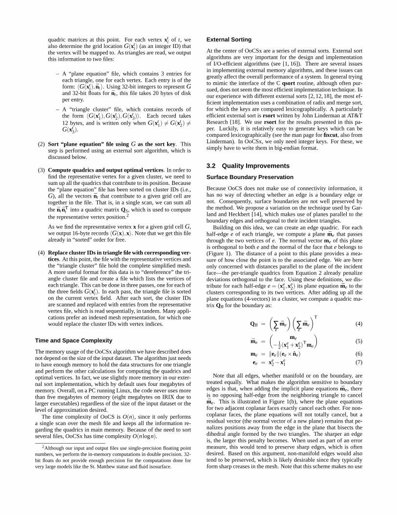
Building on this idea, we can create an edge quadric. For eachhalf-edgee of each triangle, we compute a planeme that passesthrough the two vertices ofe. The normal vectorme of this planeis orthogonal to bothe and the normal of the face thate belongs to(Figure 1). The distance of a point to this plane provides a mea-sure of how close the point is to the associated edge. We are hereonly concerned with distances parallel to the plane of the incidentface—the per-triangle quadrics from Equation 2 already penalizedeviations orthogonal to the face. Using these definitions, we dis-tribute for each half-edgee= (xe

1,xe2) its plane equationme to the

clusters corresponding to its two vertices. After adding up all theplane equations (4-vectors) in a cluster, we compute a quadric ma-trix QB for the boundary as:

QB =(

∑e

me

)(∑e

me

)T

(4)

me =(

me

− 12(xe

1 +xe2)

Tme

)(5)

me = ‖ee‖(ee× ne) (6)

ee = xe2−xe

1 (7)

Note that all edges, whether manifold or on the boundary, aretreated equally. What makes the algorithm sensitive to boundaryedges is that, when adding the implicit plane equationsme, thereis no opposing half-edge from the neighboring triangle to cancelme. This is illustrated in Figure 1(b), where the plane equationsfor two adjacent coplanar faces exactly cancel each other. For non-coplanar faces, the plane equations will not totally cancel, but aresidual vector (the normal vector of a new plane) remains that pe-nalizes positions away from the edge in the plane that bisects thedihedral angle formed by the two triangles. The sharper an edgeis, the larger this penalty becomes. When used as part of an errormeasure, this would tend to preserve sharp edges, which is oftendesired. Based on this argument, non-manifold edges would alsotend to be preserved, which is likely desirable since they typicallyform sharp creases in the mesh. Note that this scheme makes no use

n

em

(a) vectorm orthogonal to boundary edge

m

−m

(b) coplanar faces

m1

m2m1 + m2

(c) non-coplanar faces

Figure 1: Illustration of the vectors used for surface boundary preservation. The boundary normalm is orthogonal to the face normaln and the vectore alongthe edgee. For manifold edges that share two coplanar faces, the boundary normals cancel. In the case of non-coplanar faces, the residual vectorm1 +m2 liesin the plane that bisectse’s dihedral angle.

of connectivity information, yet implicitly accounts for the featureedges in the mesh.

The final quadric for the cluster is computed as a linear combi-nationλQS+(1−λ)QB of the surface quadric and the new bound-ary quadric. Note that we have been careful to weight the bound-ary quadric so as to ensure scale invariance and compatibility withthe area-squared weighted triangle quadrics. We have found thatweighting the quadrics equally (λ = 1

2) tends to give good results.

Constrained Optimization over Cell Boundaries

As discussed in [20], the minimum quadric error sometimes fallsoutside the cluster’s grid cell. While rare, the minimum may bearbitrarily far from the grid cell given the right conditions. Our pre-vious approach to handling these degeneracies was to use one ofa number of ad hoc methods for clamping the vertex coordinates,such as projecting the vertex onto the grid cell boundary. To ensurethat the vertex is contained in the grid cell, but also results in thesmallest possible quadric error, we perform a linearly constrainedoptimization over the grid cell boundary whenever the global opti-mum is outside it. Because the quadric functional is quadratic andthe grid cell constraints are linear, the solution to this optimizationproblem can be found by solving a set of linear equations (cf. [22]).This optimization problem is made particularly easy by the fact thatthe linear constraints are all perpendicular to each other and parallelto the coordinate axes, and can therefore generally be solved as a2D or 1D problem.

4 EXPERIMENTAL RESULTS

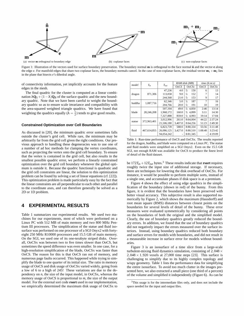
Table 1 summarizes our experimental results. We used two ma-chines for our experiments, most of which were performed on aLinux PC with 512 MB of main memory and two 800 MHz Pen-tium III processors. The simplification of the statue and fluid iso-surface was performed on one processor of a SGI Onyx2 with forty-eight 250 MHz R10000 processors and 15.5 GB of main memory.On the SGI, we used one of its one-terabyte striped disks. Over-all, OoCSx was between two to five times slower than OoCS, butsometimes the speed difference was even smaller. In one case, for ahigh-resolution simplification of the blade, OoCSx was faster thanOoCS. The reason for this is that OoCS ran out of memory, andnumerous page faults occurred. This happened while trying to sim-plify the blade to one quarter of its initial size. The ratio in memoryusage of OoCS and disk usage of OoCSx varied widely, going froma low of 6 to a high of 245! These variations are due to the de-pendency onn, the size of the input model, in OoCSx, whereas thememory usage of OoCS is proportional tom, the size of the outputmodel. For the external sort codersort used in our implementation,we empirically determined the maximum disk usage of OoCSx to

model Tin ToutRAM:disk (MB) time (h:m:s)

OoCS OoCSx OoCS OoCSx

dragon 871,30647,236 4:0 5: 150 6 13

113,058 9:0 5: 152 7 14244,568 21:0 5: 153 9 17

buddha 1,087,71662,346 5:0 5: 187 7 16

204,766 20:0 5: 191 10 19

blade 28,246,208507,104 49:0 5: 4,850 2:46 13:14

1,968,172 160:0 5: 4,899 3:11 14:307,327,888 859:0 5: 4,993 19:14 17:04

statue 372,963,4013,012,996 261:0 8:64,004 44:22 2:37:24

21,506,180 3,407:0 8:64,256 51:23 2:49:30

fluid 467,614,8556,823,739 588:0 8:80,334 55:56 3:11:48

26,086,125 3,427:0 8:80,510 1:08:48 3:23:4294,054,242 - 8:81,345 - 4:19:09

Table 1: Run-time performance of OoCS and OoCSx. The results reportedfor the dragon, buddha, and blade were computed on a Linux PC. The statueand fluid models were simplified on a SGI Onyx2. Even on the 15.5 GBSGI, not enough RAM was available for OoCS to produce the finest levelof detail of the fluid dataset.

be 172Tin +12Tout bytes.3 These results indicate thatrsort requiresroughly twice the input size of additional storage. If necessary,there are techniques for lowering the disk overhead of OoCSx. Forinstance, it would be possible to perform multiple sorts, instead ofa single one, and accumulate phases if disk space is at a premium.

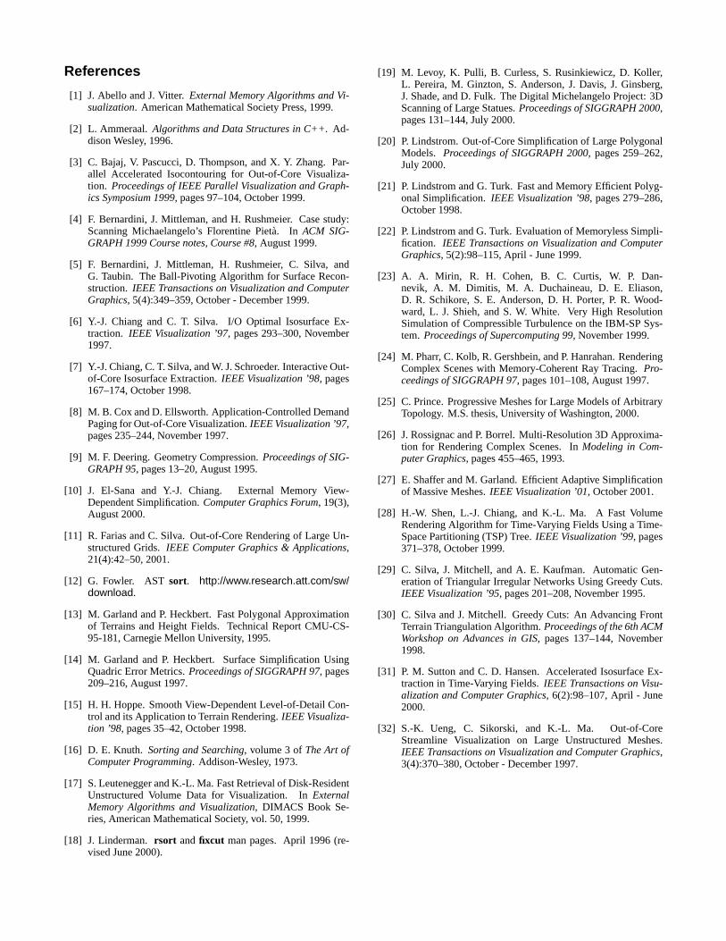
Figure 4 shows the effect of using edge quadrics in the simpli-fication of the boundary (shown in red) of the bunny. From thisfigure, it is evident that the boundaries have been preserved withbetter visual accuracy. This subjective result is also supported nu-merically by Figure 2, which shows the maximum (Hausdorff) androot mean square (RMS) distances between closest points on theboundaries for several levels of detail of the bunny. These errormeasures were evaluated symmetrically by considering all pointson the boundaries of both the original and the simplified model.Clearly, the use of boundary quadrics greatly reduced the bound-ary errors. In addition, we found that the use of boundary quadricsdid not negatively impact the errors measured over the surface in-teriors. Instead, using boundary quadrics reduced both boundaryand surface errors for models with boundaries, and did not result ina measurable increase in surface error for models without bound-aries.

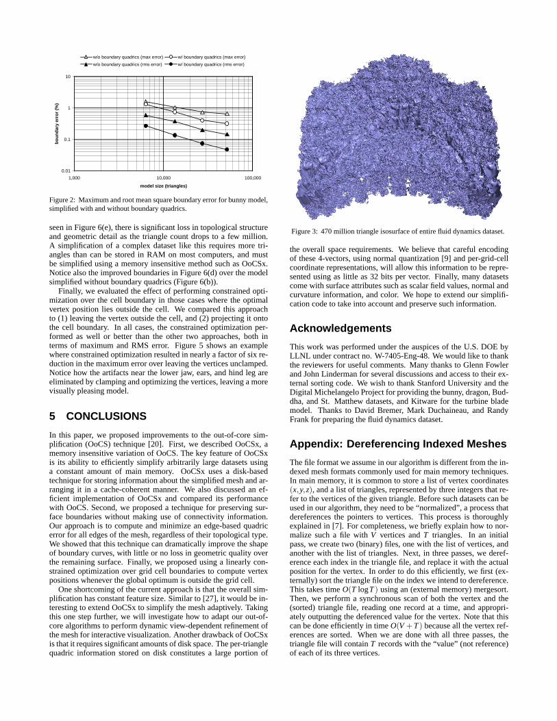
Figure 3 is an isosurface of a time slice from a large-scaleturbulent-mixing fluid dynamics simulation, consisting of 2,048×2,048× 1,920 voxels at 27,000 time steps [23]. This surface ischallenging to simplify due to its highly complex topology andwispy geometry. Table 1 lists the performance data for simplifyingthe entire isosurface. To avoid too much clutter in the images pre-sented here, we also extracted a small piece (one third of a percent)of the volume and simplified it independently (Figure 6). As can be

3This usage is for the intermediate files only, and does not include thespace needed for the input and output files.

0.01

0.1

1

10

1,000 10,000 100,000

model size (triangles)

bo

un

dar

y er

ror

(%)

w/o boundary quadrics (max error) w/ boundary quadrics (max error)

w/o boundary quadrics (rms error) w/ boundary quadrics (rms error)

Figure 2: Maximum and root mean square boundary error for bunny model,simplified with and without boundary quadrics.

seen in Figure 6(e), there is significant loss in topological structureand geometric detail as the triangle count drops to a few million.A simplification of a complex dataset like this requires more tri-angles than can be stored in RAM on most computers, and mustbe simplified using a memory insensitive method such as OoCSx.Notice also the improved boundaries in Figure 6(d) over the modelsimplified without boundary quadrics (Figure 6(b)).

Finally, we evaluated the effect of performing constrained opti-mization over the cell boundary in those cases where the optimalvertex position lies outside the cell. We compared this approachto (1) leaving the vertex outside the cell, and (2) projecting it ontothe cell boundary. In all cases, the constrained optimization per-formed as well or better than the other two approaches, both interms of maximum and RMS error. Figure 5 shows an examplewhere constrained optimization resulted in nearly a factor of six re-duction in the maximum error over leaving the vertices unclamped.Notice how the artifacts near the lower jaw, ears, and hind leg areeliminated by clamping and optimizing the vertices, leaving a morevisually pleasing model.

5 CONCLUSIONS

In this paper, we proposed improvements to the out-of-core sim-plification (OoCS) technique [20]. First, we described OoCSx, amemory insensitive variation of OoCS. The key feature of OoCSxis its ability to efficiently simplify arbitrarily large datasets usinga constant amount of main memory. OoCSx uses a disk-basedtechnique for storing information about the simplified mesh and ar-ranging it in a cache-coherent manner. We also discussed an ef-ficient implementation of OoCSx and compared its performancewith OoCS. Second, we proposed a technique for preserving sur-face boundaries without making use of connectivity information.Our approach is to compute and minimize an edge-based quadricerror for all edges of the mesh, regardless of their topological type.We showed that this technique can dramatically improve the shapeof boundary curves, with little or no loss in geometric quality overthe remaining surface. Finally, we proposed using a linearly con-strained optimization over grid cell boundaries to compute vertexpositions whenever the global optimum is outside the grid cell.

One shortcoming of the current approach is that the overall sim-plification has constant feature size. Similar to [27], it would be in-teresting to extend OoCSx to simplify the mesh adaptively. Takingthis one step further, we will investigate how to adapt our out-of-core algorithms to perform dynamic view-dependent refinement ofthe mesh for interactive visualization. Another drawback of OoCSxis that it requires significant amounts of disk space. The per-trianglequadric information stored on disk constitutes a large portion of

Figure 3: 470 million triangle isosurface of entire fluid dynamics dataset.

the overall space requirements. We believe that careful encodingof these 4-vectors, using normal quantization [9] and per-grid-cellcoordinate representations, will allow this information to be repre-sented using as little as 32 bits per vector. Finally, many datasetscome with surface attributes such as scalar field values, normal andcurvature information, and color. We hope to extend our simplifi-cation code to take into account and preserve such information.

Acknowledgements

This work was performed under the auspices of the U.S. DOE byLLNL under contract no. W-7405-Eng-48. We would like to thankthe reviewers for useful comments. Many thanks to Glenn Fowlerand John Linderman for several discussions and access to their ex-ternal sorting code. We wish to thank Stanford University and theDigital Michelangelo Project for providing the bunny, dragon, Bud-dha, and St. Matthew datasets, and Kitware for the turbine blademodel. Thanks to David Bremer, Mark Duchaineau, and RandyFrank for preparing the fluid dynamics dataset.

Appendix: Dereferencing Indexed Meshes

The file format we assume in our algorithm is different from the in-dexed mesh formats commonly used for main memory techniques.In main memory, it is common to store a list of vertex coordinates(x,y,z), and a list of triangles, represented by three integers that re-fer to the vertices of the given triangle. Before such datasets can beused in our algorithm, they need to be “normalized”, a process thatdereferences the pointers to vertices. This process is thoroughlyexplained in [7]. For completeness, we briefly explain how to nor-malize such a file withV vertices andT triangles. In an initialpass, we create two (binary) files, one with the list of vertices, andanother with the list of triangles. Next, in three passes, we deref-erence each index in the triangle file, and replace it with the actualposition for the vertex. In order to do this efficiently, we first (ex-ternally) sort the triangle file on the index we intend to dereference.This takes timeO(T logT) using an (external memory) mergesort.Then, we perform a synchronous scan of both the vertex and the(sorted) triangle file, reading one record at a time, and appropri-ately outputting the deferenced value for the vertex. Note that thiscan be done efficiently in timeO(V +T) because all the vertex ref-erences are sorted. When we are done with all three passes, thetriangle file will containT records with the “value” (not reference)of each of its three vertices.

References

[1] J. Abello and J. Vitter.External Memory Algorithms and Vi-sualization. American Mathematical Society Press, 1999.

[2] L. Ammeraal. Algorithms and Data Structures in C++. Ad-dison Wesley, 1996.

[3] C. Bajaj, V. Pascucci, D. Thompson, and X. Y. Zhang. Par-allel Accelerated Isocontouring for Out-of-Core Visualiza-tion. Proceedings of IEEE Parallel Visualization and Graph-ics Symposium 1999, pages 97–104, October 1999.

[4] F. Bernardini, J. Mittleman, and H. Rushmeier. Case study:Scanning Michaelangelo’s Florentine Pieta. In ACM SIG-GRAPH 1999 Course notes, Course #8, August 1999.

[5] F. Bernardini, J. Mittleman, H. Rushmeier, C. Silva, andG. Taubin. The Ball-Pivoting Algorithm for Surface Recon-struction. IEEE Transactions on Visualization and ComputerGraphics, 5(4):349–359, October - December 1999.

[6] Y.-J. Chiang and C. T. Silva. I/O Optimal Isosurface Ex-traction. IEEE Visualization ’97, pages 293–300, November1997.

[7] Y.-J. Chiang, C. T. Silva, and W. J. Schroeder. Interactive Out-of-Core Isosurface Extraction.IEEE Visualization ’98, pages167–174, October 1998.

[8] M. B. Cox and D. Ellsworth. Application-Controlled DemandPaging for Out-of-Core Visualization.IEEE Visualization ’97,pages 235–244, November 1997.

[9] M. F. Deering. Geometry Compression.Proceedings of SIG-GRAPH 95, pages 13–20, August 1995.

[10] J. El-Sana and Y.-J. Chiang. External Memory View-Dependent Simplification.Computer Graphics Forum, 19(3),August 2000.

[11] R. Farias and C. Silva. Out-of-Core Rendering of Large Un-structured Grids.IEEE Computer Graphics & Applications,21(4):42–50, 2001.

[12] G. Fowler. ASTsort. http://www.research.att.com/sw/download.

[13] M. Garland and P. Heckbert. Fast Polygonal Approximationof Terrains and Height Fields. Technical Report CMU-CS-95-181, Carnegie Mellon University, 1995.

[14] M. Garland and P. Heckbert. Surface Simplification UsingQuadric Error Metrics.Proceedings of SIGGRAPH 97, pages209–216, August 1997.

[15] H. H. Hoppe. Smooth View-Dependent Level-of-Detail Con-trol and its Application to Terrain Rendering.IEEE Visualiza-tion ’98, pages 35–42, October 1998.

[16] D. E. Knuth. Sorting and Searching, volume 3 ofThe Art ofComputer Programming. Addison-Wesley, 1973.

[17] S. Leutenegger and K.-L. Ma. Fast Retrieval of Disk-ResidentUnstructured Volume Data for Visualization. InExternalMemory Algorithms and Visualization, DIMACS Book Se-ries, American Mathematical Society, vol. 50, 1999.

[18] J. Linderman. rsort andfixcut man pages. April 1996 (re-vised June 2000).

[19] M. Levoy, K. Pulli, B. Curless, S. Rusinkiewicz, D. Koller,L. Pereira, M. Ginzton, S. Anderson, J. Davis, J. Ginsberg,J. Shade, and D. Fulk. The Digital Michelangelo Project: 3DScanning of Large Statues.Proceedings of SIGGRAPH 2000,pages 131–144, July 2000.

[20] P. Lindstrom. Out-of-Core Simplification of Large PolygonalModels. Proceedings of SIGGRAPH 2000, pages 259–262,July 2000.

[21] P. Lindstrom and G. Turk. Fast and Memory Efficient Polyg-onal Simplification.IEEE Visualization ’98, pages 279–286,October 1998.

[22] P. Lindstrom and G. Turk. Evaluation of Memoryless Simpli-fication. IEEE Transactions on Visualization and ComputerGraphics, 5(2):98–115, April - June 1999.

[23] A. A. Mirin, R. H. Cohen, B. C. Curtis, W. P. Dan-nevik, A. M. Dimitis, M. A. Duchaineau, D. E. Eliason,D. R. Schikore, S. E. Anderson, D. H. Porter, P. R. Wood-ward, L. J. Shieh, and S. W. White. Very High ResolutionSimulation of Compressible Turbulence on the IBM-SP Sys-tem. Proceedings of Supercomputing 99, November 1999.

[24] M. Pharr, C. Kolb, R. Gershbein, and P. Hanrahan. RenderingComplex Scenes with Memory-Coherent Ray Tracing.Pro-ceedings of SIGGRAPH 97, pages 101–108, August 1997.

[25] C. Prince. Progressive Meshes for Large Models of ArbitraryTopology. M.S. thesis, University of Washington, 2000.

[26] J. Rossignac and P. Borrel. Multi-Resolution 3D Approxima-tion for Rendering Complex Scenes. InModeling in Com-puter Graphics, pages 455–465, 1993.

[27] E. Shaffer and M. Garland. Efficient Adaptive Simplificationof Massive Meshes.IEEE Visualization ’01, October 2001.

[28] H.-W. Shen, L.-J. Chiang, and K.-L. Ma. A Fast VolumeRendering Algorithm for Time-Varying Fields Using a Time-Space Partitioning (TSP) Tree.IEEE Visualization ’99, pages371–378, October 1999.

[29] C. Silva, J. Mitchell, and A. E. Kaufman. Automatic Gen-eration of Triangular Irregular Networks Using Greedy Cuts.IEEE Visualization ’95, pages 201–208, November 1995.

[30] C. Silva and J. Mitchell. Greedy Cuts: An Advancing FrontTerrain Triangulation Algorithm.Proceedings of the 6th ACMWorkshop on Advances in GIS, pages 137–144, November1998.

[31] P. M. Sutton and C. D. Hansen. Accelerated Isosurface Ex-traction in Time-Varying Fields.IEEE Transactions on Visu-alization and Computer Graphics, 6(2):98–107, April - June2000.

[32] S.-K. Ueng, C. Sikorski, and K.-L. Ma. Out-of-CoreStreamline Visualization on Large Unstructured Meshes.IEEE Transactions on Visualization and Computer Graphics,3(4):370–380, October - December 1997.

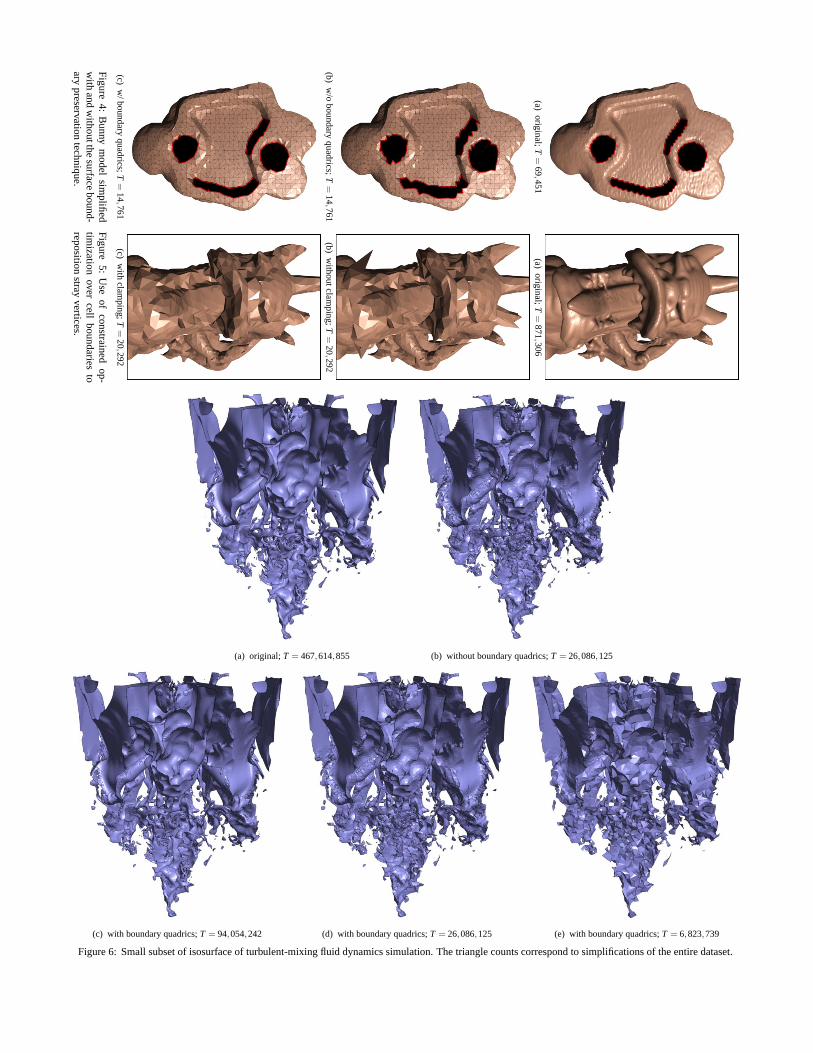
(a)original;T

=69,451

(b)w

/oboundary

quadrics;T=14,761

(c)w

/boundaryquadrics;T=

14,761

Figure

4:B

unnym

odelsim

plifiedw

ithand

withoutthe

surfacebound-

arypreservation

technique.

(a)original;T

=871,306

(b)w

ithoutclamping;T

=20,292

(c)w

ithclam

ping;T=

20,292

Figure

5:U

seof

constrainedop-

timization

overcell

boundariesto

repositionstray

vertices.

(a) original;T = 467,614,855 (b) without boundary quadrics;T = 26,086,125

(c) with boundary quadrics;T = 94,054,242 (d) with boundary quadrics;T = 26,086,125 (e) with boundary quadrics;T = 6,823,739

Figure 6: Small subset of isosurface of turbulent-mixing fluid dynamics simulation. The triangle counts correspond to simplifications of the entire dataset.