Simplification of Tetrahedral Meshes with Accurate Error Evaluation

P. Cignoni, D. Costanza, C. Montani, C. Rocchini, R. ScopignoIstituto Scienza e Tecnologia dell’Informazione – Consiglio Nazionale delle Ricerche∗

Abstract

The techniques for reducing the size of a volume datasetby preserving both the geometrical/topological shape andthe information encoded in an attached scalar field areattracting growing interest. Given the framework of incre-mental 3D mesh simplification based on edge collapse, thepaper proposes an approach for the integrated evaluationof the error introduced by both the modification of thedomain and the approximation of the field of the originalvolume dataset. We present and compare various tech-niques to evaluate the approximation error or to producea sound prediction. A flexible simplification tool has beenimplemented, which provides different degree of accuracyand computational efficiency for the selection of the edgeto be collapsed. Techniques for preventing a geometric ortopological degeneration of the mesh are also presented.

Keywords: Simplicial Complexes, Mesh Simplification,Volume Visualization, Unstructured Grids

1 Introduction

Many papers have been published over the last few yearsconcerning the simplification of simplicial complexes. Mostof them concern the simplification of 2D simplicial meshesembedded in 3D space, hereafter called surfaces. Only aminor subset are concerned with 3D simplicial decomposi-tions, hereafter called meshes. In particular, we consider inthis paper the class of irregular volume datasets, either con-vex or non convex, with scalar field values associated withthe vertices of the tetrahedral cells. Let D = (V,Σ,Φ) be ourdataset where V is a set of n vertices, Σ = σ1, σ2, . . . , σmis a tetrahedralization of m cells with vertices in V , andΦ = φ1, φ2, . . . , φm is a set of functions such that eachfunction φi is defined over cell σi of Σ. All functions of Φ arelinear interpolants of the scalar field known at the verticesof V . Given an irregular dataset D, the term simplificationrefers to the problem of building an approximate represen-tation D′ of D with a smaller size, built by choosing a setof vertices V ′ (usually V ′ ⊂ V ) and a new triangulation Σ′

of V ′ that covers [almost] the same domain. This problemhas some similarities with scattered data interpolation andthinning techniques [10], but the main problem of these ap-proaches is that the shape of the data domain is not takeninto account (erroneous interpolation between unconnecteddata becomes possible).Surface/mesh simplification can be driven by two differentobjectives: producing a more compact mesh which is suffi-ciently similar in terms of visual appearance, or to producea model which satisfies a given accuracy. In the first case the

∗CNR Research Park, S. Cataldo - 56100 Pisa,ITALY. Email:cignoni | montani | rocchini@iei.pi.cnr.it,roberto.scopigno@cnuce.cnr.it

main goal is to reduce visualization time. In the second case,special emphasis is given to data quality and representationaccuracy; this is often the case for scientific visualization ap-plications, where the user requires measurable and reliabledata quality.Our goal is therefore to design and evaluate different tetra-hedral mesh simplification methods in the framework of sci-entific visualization applications, with a special commitmentto the quality of the mesh obtained (considering both geom-etry and the associated scalar field). The approach adoptedlies in the general class of incremental simplification meth-ods: simplification proceeds through a sequence of localmesh updates which, at each step, reduces the mesh sizeand [monotonically] decreases the approximation precision.Specifically, we adopt an approach based on iterative edgecollapse. The main contributions of this paper are as follows:

• The geometric/topology correctness of the mesh pro-duced. Topology and geometry are preserved, andchecks are introduced to prevent possible inconsisten-cies in the simplified mesh (cell flipping, degeneration,self-intersections);

• The evaluation of the approximation error. We intro-duce a characterization of the approximation error, us-ing two conceptually different classes of domain-errorand field-error, and propose a new approach for the in-tegrated evaluation of domain-error and field-error;

• Different criteria to predict and evaluate the approxima-tion error are proposed and compared with the directevaluation approach. In particular, we propose an ex-tension of the quadrics error metric to the case of fielderror evaluation on 3D meshes;

• Finally, the computational efficiency of the techniquesproposed is evaluated empirically on sample datasets.

The work takes also into account the constraints intro-duced when the goal is the construction of a multiresolutionrepresentation of the dataset.

2 Related Works

Many different simplification methods have been developedfor the simplification of surfaces. These methods gener-ally try to select the smallest set of points approximatinga dataset within a given error. A detailed review of thesealgorithm is beyond the scope of this document, and for asurvey on this subject see [12]. Very briefly, we can sum-marize by saying that effective solutions to the simplifica-tion problem have often been obtained through incrementaltechniques, based on either a refinement strategy (refine acoarse representation by adding points [11]) or a decimation(or coarsening) strategy (simplify the dataset by removingpoints [21, 17]).

Many of these techniques could be extended to the 3D case,i.e. to volume data simplification. In the following we reviewthe specific results regarding tetrahedral meshes. We do notconsider here the many lossless compression solutions thathave appeared in the last few years, because the focus hereis on simplification and multiresolution.

2.1 Refinement Strategies

Hamann and Chen [16] adopted a refinement strategy forthe simplification of tetrahedral convex complexes. Theirmethod is based on the selection of the most importantpoints (based on curvature) and their insertion into theconvex hull of the domain of the dataset. When a pointis inserted into the triangulation, local modifications (byface/edge swapping) are performed in order to minimize alocal approximation error.Another technique, based on the Delaunay refinement

strategy, was proposed by Cignoni et al. [5]; here the vertexselection criterion was to choose the point causing the largesterror with respect to the original scalar field. This techniquewas successively extended in [6] to the management of non-convex complexes obtainable by the deformation of convexdomains (e.g. curvilinear grids).The refinement-based strategy was also used by Grosso

and Greiner [15]. Starting from a coarse triangulation cover-ing the domain, a hierarchy of approximations of the volumeis created by a sequence of local adaptive mesh refinementsteps. A very similar approach based on selective refinement,but limited to regular datasets, was presented in [24].All the techniques based on the refinement strategy share

a common problem: the domain of the dataset has to beconvex (or at least it has to be defined as a warping of a reg-ular computational grid [6]). The reason lies in the intrinsicdifficulty in fulfilling strict geometric constraints while refin-ing a mesh (from coarse to fine) and using just the verticesof the dataset.

2.2 Decimation Strategies

Renze and Oliver in [19] proposed the first 3D mesh decima-tion algorithm based on vertex removal. Given a tetrahedralcomplex Σ, they evaluate the internal vertices of the meshfor removal, in random order. The re-triangulation of thehole left by the removal of a vertex v is done by buildingthe Delaunay triangulation Σv of the vertices adjacent to v,and searching for, if it exists, a subset of the tetrahedra ofΣv whose (d-1)-faces match the faces of Σ. If such a subsetdoes not exist the vertex is not removed. The latter con-dition may very often hold if the original complex is not aDelaunay one. This method neither measures the approxi-mation error introduced in the reduced dataset, nor tries toselect the vertex subset in order to minimize the error.Popovic and Hoppe [18] have extended the ProgressiveMeshes (PM) algorithm [17], a surface simplification strat-egy based on edge-collapse, to the management of genericsimplicial complexes. However, their work is very general,and it does not consider in detail the impact on the approx-imation accuracy of a possible scalar field associated withthe mesh. The PM approach has been recently extended byStaadt and Gross [22]. They introduce various cost functionsto drive the edge-collapsing process and present a techniqueto check (and prevent) the occurrence of intersections andinversions of the tetrahedra involved in a collapse action.The approach is based on a sequence of tests that guaran-tees the construction of a robust and consistent progressive

tetrahedralization. A simplification technique based on iter-ative edge collapsing has also been sketched by Cignoni etal. in [6].A technique based on error-prioritized tetrahedra collapsewas proposed by Trotts et al. [23]. Each tetraedron isweighted based on a predicted increase in the approximationerror that would result after its collapse; tetraedral cell col-lapse is implemented via three edge collapses. The algorithmgives an approximate evaluation of the scalar field error in-troduced at each simplification step (based on the iterativeaccumulation of local evaluations, following the approachproposed by Bajaj et al. for the simplification of 2D surfaces[3], which gives an overestimation of the actual error). Themesh degeneration caused by the modification of the (possi-bly not convex) mesh boundary and the corresponding errorare managed by forcing every edge collapse that involves aboundary vertex to be performed on the boundary vertex,and avoiding the collapse of corner vertices. This approachpreserves the boundary in the case of regular datasets, butcannot be used to decimate the boundary of a dataset witha more complex domain (e.g. non rectilinear or not convex,as occurs frequently on irregular datasets).

3 Incremental Simplification via Edge Col-lapse

We adopt an iterative simplification approach based on edgecollapse: at each iteration, an edge is chosen and collapsed.The atomic edge collapse action is conceived here as a sim-ple vertex unification process. Given a maximal1 3-simplicialcomplex Σ and an edge e connecting two vertices vs and vd

(the source and destination vertices), we impose that vs be-comes equal to vd and we consequently modify the complex

2.This operation causes the edge (vs − vd) to collapse to thepoint vd and all the tetrahedra incident on the edge (vs − vd)to collapse to triangles. Again, these new triangles are uni-fied with the corresponding identical triangles contained inΣ.This simplification process is always limited to a local por-tion of the complex: the set of simplices incident in vs or vd.We introduce the following terminology: given a edge col-lapse e = (vs, vd) we define: D(e) the set of deleted tetrahe-dra incident in e; M(e) the set of modified tetrahedra, i.e.those tetrahedra incident in vs but not in vd. Therefore, anedge collapse step results in some modified and some deletedtetrahedra. The geometric information is simply updated bythe unification of the vertex coordinates. The topology up-date is somehow slightly more complex; relations TV, VT,EV and VE have to be updated after each atomic collapseaction.The order in which edges are collapsed is critical with re-spect to the simplified mesh accuracy. The result of theiterative simplification is a sequence Σ0,Σ1, . . . ,Σi, . . . ,Σn

of complexes [17, 4]. When the goal is the production of ahigh quality multiresolution output, the approximation errorshould increase slowly and smoothly. Analogously to manyother simplification approaches, we adopt a heap to storethe edges which are to be collapsed. At the beginning, allthe edges are inserted in the heap and sorted with respect

1I.e., a complex which does not contain dangling non-maximalsimplices.

2The position and the field value of the vertex vd can also bechanged, obtaining the so-called interpolatory edge collapse. Wedo not adopt this approach because the choice of the vd optimallocation is not easy with most of the error evaluation criteria.

to an estimated error, known in the following sections as thepredicted error (see Section 5). The edges in the heap areoriented, that is we have both the oriented edges (vj , vi) and(vi, vj) in the heap, because they identify different collapses.For each simplification step: the edge e with the lowest erroris extracted from the heap; the collapse of e is tested, check-ing the topological and geometric consistency of the meshafter the collapse. If the geo-topological checks are verified,the following actions are performed:

• the tetrahedra in D(e) are deleted;

• the topology relation TV is updated, i.e. vs is replacedwith vd in all tetrahedra σ ∈ M(e);

• the VT relation is updated on vertex vd: V T (vd) =V T (vd) ∪ M(e) \ D(e);

• the VE relation is updated by setting V E(vd) =V E(vd) ∪ V E(vs) \ (vs, vd);

• the EV relation is updated by substituting vs with vd

on all the edges in V E(vs);

• a new estimated error is evaluated for all former edgesV E(vs) in the heap.

Otherwise, we reject the edge collapse and continue with thenext edge in the heap.Consistency checks are evaluated before updating the mesh.There are two classes of consistency conditions: topologicaland geometrical. The first one ensures that the edge collapsewill not change the topological type of our complex. Thesecond one ensures geometric consistency, i.e. that no self-intersecting or badly-shaped (e.g. slivery) tetrahedra areintroduced by the edge collapse.

3.1 Topology Preserving Edge Contraction

Given an edge collapse, a set of necessary and sufficient con-ditions that preserves the topological type of our complexhas recently been proposed in [9]. We adopted this approachin our simplification system to guarantee the topological cor-rectness of the simplification process.Let St(σ) be the set of all the co-faces of σ, i.e. St(σ) =τ ∈ Σ | σ is a face of τ. Let Lk(σ) be the set of all thefaces belonging to St(σ) but not incident on σ (i.e. the setof all the faces of the co-faces of σ disjoint from σ).Let Σi be a 3-simplicial complex without boundary, e =(vs, vd) an edge of the complex, and Σi+1 the complex af-ter the collapse of edge e. According to [9], the followingstatements are equivalent:

1. Lk(vs) ∩ Lk(vd) = Lk(e)

2. Σi,Σi+1 are homeomorphic

It is therefore sufficient to check statement (1) to prove thatstatement (2) holds, that is to ensure the topological cor-rectness of the current simplification step (see Figure 1).If Σi is a complex with boundary (which is the usual case),

we can go back to the previous case by ideally adding adummy vertex w and its cone of simplices to the boundary(i.e. we add a dummy simplex for each boundary 2-faceof Σi).The insertion of w and the corresponding simplicesallows us to also manage the boundary faces of Σi with theprevious checking rule.

Figure 1: Topology checks: in the example on the left,the condition Lk(a) ∩ Lk(b) = x, y = Lk(ab) indicatesa valid collapse. Conversely, an invalid collapse is detectedin the configuration on the right because Lk(a) ∩ Lk(b) =x, y, z, zx = Lk(ab).

3.2 Preserving Geometric Consistency

Three possible dangerous situations should be prevented inthe simplification process:

• tetrahedra inversion;

• generation of slivery/bad shaped tetrahedra,

• self-intersection of the mesh boundary.

The first two situations are easy to check. In the first case itis sufficient to check that each modified tetrahedron in M(e)preserves the original orientation (the first vertex sees theother three ones counterclockwise), or in other words thecell volume does not become negative.In the second case, we reject every collapse that produces oneor more tetrahedra in M(e) having an aspect ratio smallerthan a given threshold ρ. Note that, in order to allow thesimplification of meshes which contain slivery tetrahedra, itis useful to allow the collapse of an edge also if the aspectratio of modified tetrahedra improves after the collapse.The detection of self-intersections is the most complex sub-task, because this is the only case where the effects of anedge collapse can be non-local. After an edge collapse, someboundary faces that are topologically non-adjacent but ge-ometrically close can become self-intersecting. The intrinsicnon-locality of this kind of degeneration makes it difficult toefficiently and correctly prevent it without using auxiliarystructures. To speedup self-intersection checks (a quadraticproblem in its naive implementation) a uniform grid [1] couldbe adopted, to store all the vertices of the current boundaryof the mesh. For each edge collapse (vs,vd) that involves aboundary edge, we should check whether after the collapse,all the edges on the boundary incident in vd do not intersectthe mesh boundary. If an intersection is found, the collapseis aborted and the original state of the mesh before the col-lapse is restored.

4 Error Characterization and Evaluation

When an atomic simplification action is performed, a newmesh Σi+1 is generated from Σi with, in general, a higherapproximation error. The approximation error can be de-scribed by using two measures: the domain error and thefield error.

4.1 Domain Error

The collapse of an edge lying on (or adjacent to) the bound-ary of the mesh can cause a deformation of the boundary ofthe mesh. In other words, Σi and Σi+1 can span different

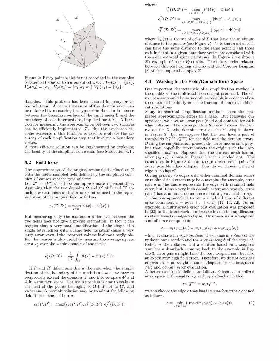
Figure 2: Every point which is not contained in the complexis assigned to one or to a group of cells, e.g.: VD(x1) = σh,VD(x2) = σi, VD(x3) = σi, σj , σk VD(x4) = σk.

domains. This problem has been ignored in many previ-ous solutions. A correct measure of the domain error canbe obtained by measuring the symmetric Hausdorff distancebetween the boundary surface of the input mesh Σ and theboundary of each intermediate simplified mesh Σi. A func-tion for measuring the approximation between two surfacescan be efficiently implemented [7]. But the overheads be-come excessive if this function is used to evaluate the ac-curacy of each simplification step that involves a boundaryvertex.A more efficient solution can be implemented by deployingthe locality of the simplification action (see Subsection 4.4).

4.2 Field Error

The approximation of the original scalar field defined on Σwith the under-sampled field defined by the simplified com-plex Σ′ causes another type of error.Let D′ = (V ′,Σ′,Φ′) be our approximate representation.Assuming that the two domains Ω and Ω′ of Σ and Σ′ co-incide, we can measure the error εf introduced in the repre-sentation of the original field as follows:

εf (D,D′) = maxx∈Ω

(|Φ(x)− Φ′(x)|)

But measuring only the maximum difference between thetwo fields does not give a precise estimation. In fact it canhappen that a very small modification of the shape of asingle tetrahedron with a large field variation cause a verylarge error, even if the incorrect volume is almost negligible.For this reason is also useful to measure the average squareerror εq

f over the whole domain of the mesh:

εqf (D,D′) =

1

|Ω|∫

Ω

|Φ(x)− Φ′(x)|2 dv

If Ω and Ω′ differ, and this is the case when the simpli-fication of the boundary of the mesh is allowed, we have toreciprocally extend the domains Ω′ and Ω to compare Φ′ andΦ in a common space. The main problem is how to evaluatethe field of the points belonging to Ω but not to Ω′, andviceversa. A possible solution may be to adopt the followingdefinition of the field error:

εf (D,D′) = max(ε′f (D,D′), εDf (D,D′), εD′

f (D,D′))

where:ε′f (D,D′) = max

x∈ Ω ∩ Ω′(|Φ(x)− Φ′(x)|)

εDf (D,D′) = maxx∈ Ω\Ω′, σ∈VD′ (x)

(|Φ(x)− φ′σ(x)|)

εD′

f (D,D′) = maxx∈ Ω′\Ω, σ∈VD(x)

(|φσ(x)− Φ′(x)|)

where VD(x) is the set of cells of Σ that have the minimumdistance to the point x (see Figure 2). Note that a set of cellscan have the same distance to the same point x (all thosecells incident in a given boundary vertex are associated withthe same external space partition). In Figure 2 we show a2D example of some VD() sets. There is a strict relationbetween this partitioning scheme and the Voronoi Diagram[2] of the simplicial complex Σ.

4.3 Walking in the Field/Domain Error Space

One important characteristic of a simplification method isthe quality of the multiresolution output produced. The er-ror increase should be as smooth as possible in order to allowthe maximal flexibility in the extraction of models at differ-ent resolutions.Many incremental simplification methods store the esti-mated approximation errors in a heap. But following ourapproach, we have an error pair (field and domain) for eachedge collapse. The corresponding 2D error space (field er-ror on the X axis, domain error on the Y axis) is shownin Figure 3. Let us suppose that the user fixes a pair ofthresholds (εmax

f , εmaxd ) for the field and the domain errors.

During the simplification process the error moves on a poly-line that [hopefully] interconnects the origin with the user-specified maxima. Suppose that the current mesh has anerror (εd, εf ), shown in Figure 3 with a circled dot. Theother dots in Figure 3 denote the predicted error pairs forevery possible edge-collapse. How do we choose the nextedge to collapse?Giving priority to edges with either minimal domain errorsor minimal field errors may be a mistake (for example, errorpair a in the figure represents the edge with minimal fielderror, but it has a very high domain error; analogously, errorpair b has a minimal domain error but a great field error).A common approach is to use a weighted sum of differenterror estimates, ε = w1ε1 + .. + wkεk [17, 14, 22]. As anexample, a multivariate error cost evaluation was proposedin [22] in the framework of a tetrahedra mesh simplificationsolution based on edge-collapse. This measure is a weightedsum of three components:

ε = w1εgrad(ei) + w2εvol(ei) + w3εequi(ei)

which evaluate the edge gradient, the change in volume of theupdates mesh section and the average length of the edges af-fected by the collapse. But a solution based on a weightedsum has a drawback: coming back to the example in Fig-ure 3, error pair c might have the best weighed sum but alsoan excessively high field error. Therefore, we do not considercriteria based on weighted sums adequate for the integratedfield and domain error evaluation.A better solution is defined as follows. Given a normalizederror space with weights wd and wf defined such that:

wdεmaxd = wf εmax

f ,

we can choose the edge e that has the smallest error ε definedas follows:

ε = mine∈Heap

( max(wdεd(e), wf εf (e))). (1)

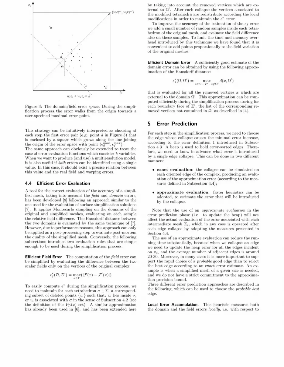
Figure 3: The domain/field error space. During the simpli-fication process the error walks from the origin towards auser-specified maximal error point.

This strategy can be intuitively interpreted as choosing ateach step the first error pair (e.g. point d in Figure 3) thatis enclosed by a square which grows along the line joiningthe origin of the error space with point (εmax

d , εmaxf ).

The same approach can obviously be extended to treat thecase of error evaluation functions which consider k variables.When we want to produce (and use) a multiresolution model,it is also useful if both errors can be identified using a singlevalue. In this case, it should exist a precise relation betweenthis value and the real field and warping errors.

4.4 Efficient Error Evaluation

A tool for the correct evaluation of the accuracy of a simpli-fied mesh, taking into account the field and domain errors,has been developed [8] following an approach similar to theone used for the evaluation of surface simplification solutions[7]. It applies Montecarlo sampling on the domains of theoriginal and simplified meshes, evaluating on each samplethe relative field difference. The Hausdorff distance betweenthe two domains is evaluated by the same technique of [7].However, due to performance reasons, this approach can onlybe applied as a post-processing step to evaluate post-mortemthe quality of the simplified mesh. Conversely, the followingsubsections introduce two evaluation rules that are simpleenough to be used during the simplification process.

Efficient Field Error The computation of the field error canbe simplified by evaluating the difference between the twoscalar fields only on the vertices of the original complex:

ε∗f (D,D′) = maxx∈V

(|F(x)−F ′(x)|)

To easily compute ε∗ during the simplification process, weneed to maintain for each tetrahedron σ ∈ Σ′ a correspond-ing subset of deleted points vi such that: vi lies inside σ,or vi is associated with σ in the sense of Subsection 4.2 (seethe definition of the VD(x) set). A similar approximationhas already been used in [6], and has been extended here

by taking into account the removed vertices which are ex-ternal to Ω′. After each collapse the vertices associated tothe modified tetrahedra are redistribute according the localmodifications in order to maintain the ε∗ error.To improve the accuracy of the estimation of the εf error

we add a small number of random samples inside each tetra-hedron of the original mesh, and evaluate the field differencealso on these samples. To limit the time and memory over-head introduced by this technique we have found that it isconvenient to add points proportionally to the field variationof the original meshes.

Efficient Domain Error A sufficiently good estimate of thedomain error can be obtained by using the following approx-imation of the Hausdorff distance:

ε∗d(Ω,Ω′) = maxx∈V −V ′, x/∈Ω′

d(x,Ω′)

that is evaluated for all the removed vertices x which areexternal to the domain Ω′. This approximation can be com-puted efficiently during the simplification process storing foreach boundary face of Σ′, the list of the corresponding re-moved vertices not contained in Ω′ as described in [4].

5 Error Prediction

For each step in the simplification process, we need to choosethe edge whose collapse causes the minimal error increase,according to the error definition 1 introduced in Subsec-tion 4.3. A heap is used to hold error-sorted edges. There-fore, we need to know in advance what error is introducedby a single edge collapse. This can be done in two differentmanners:

• exact evaluation: the collapse can be simulated oneach oriented edge of the complex, producing an evalu-ation of the approximation error (according to the mea-sures defined in Subsection 4.4);

• approximate evaluation: faster heuristics can beadopted, to estimate the error that will be introducedby the collapse.

Note that the use of an approximate evaluation in theerror prediction phase (i.e. to update the heap) will notaffect the actual evaluation of the error associated with eachintermediate mesh Σi, which in any case is operated aftereach edge collapse by adopting the measures presented inSection 4.4.The use of an approximate evaluation can reduce the run-

ning time substantially, because when we collapse an edgewe need to update the heap error for all the edges incidenton vd, and the average number of adjacent edges is around20-30. Moreover, in many cases it is more important to sup-port the rapid choice of a probable good edge than to selectthe best edge according to an exact error estimate. An ex-ample is when a simplified mesh of a given size is needed,and we do not have a strict commitment to the approxima-tion precision bound.Three different error prediction approaches are described inthe following, which can be used to choose the probable bestedge.

Local Error Accumulation. This heuristic measures boththe domain and the field errors locally, i.e. with respect to

the vertex that has been unified and removed in the cur-rent edge collapse action. These error estimates are thenaccumulated during the simplification process to give an ap-proximate global estimate.

Gradient Difference. In order to estimate the error in-crease, we pre-compute the field gradient ∇v at each vertexv of the input mesh. This can be done by computing theweighted average of gradients in all tetrahedra incident at v.The weight to be associated with the contribution of eachtetrahedron σ is given by the solid angle of σ at v. Then, foreach vertex v in the mesh, we search the vertex w, amongthose adjacent to v, such that the difference ∆∇v,w betweenthe gradient vectors ∇v and ∇w is minimal. Value ∆∇v,w

gives a rough estimate of how far from linear the field is inthe neighborhood of v (in particular, on the edge (v,w) di-rection). The smaller ∆∇v,w is, the smaller the expectederror increase is if v is removed by collapsing it onto w. Thevalue (∆∇v,w · L(e)), where L(e) is the length of the edgeto be collapsed, is therefore used as an estimate of the fielderror.This solution is more precise and more complex in terms ofspace (because gradients have to be explicitly stored) thanthe one proposed in [22], which takes into account only thedifference of the field values on the collapsed edge extremes.

Quadric Error. Another approximate measure can be de-fined by extending the quadric error metric introduced byGarland et al. [13]. This metric was proposed to measure thegeometric error introduced on a surface during the simplifi-cation process. We use it to measure not only the domainerror, but also the field error. The main idea of the quadricerror metric is to associate a set of planes with each vertexof the mesh. The sum of the squared distances from a vertexto all the planes in its set defines the error of that vertex.Initially each vertex v is associated with the set of planespassing through the faces incident in v. When, for each col-lapse of a given vs onto vd, the resulting set of planes is theunion of the sets of vs and vd. The most innovative con-tribution in [13] (and the main improvement over [20]) isthat these sets of planes are not represented explicitly. Letnv + d = 0 be the equation representing a plane, where nis the unit normal to the plane and d its distance from theorigin. The squared distance of a vertex v to this plane isgiven by:

D = (nv + d)2 = v(nn)v + 2dnv + d2

According to [13] we can represent this quadric Q, whichdenotes the squared distance of a plane to a vertex, as:

Q = (A, b, c) = (nn, dn, d2)

Q(v) = vAv + 2bv + c

The sum of a set of quadrics can easily be computed by thepairwise component sum of their terms, therefore for eachvertex we maintain only the quadric representing the sum ofthe squared distances of all the planes implicitly associatedwith that vertex, which is just ten coefficients.In the case of 3D mesh simplification the domain error can

be easily estimated by providing a quadric for each boundaryvertex of the 3D mesh. Quadrics can also be used to measurethe field error. In this case we associate with each vertexv a set of linear functions φi (that is, the linear functionsassociated with the cells incident in v), and we measure thesum of squared differences between the linear functions and

the field on v. Each linear function can be represented byφ(v) = nv + d where, analogously to the geometric case,n is a 3D vector (not unitary in this case and representingthe gradient of the field) and d is a constant (the value ofthe scalar field in the origin).The management of this kind of quadric is therefore exactlythe same as the previous case, but with a slightly differentmeaning. In this case the quadric represents the sum ofsquared differences between the linear functions and the fieldon v. In this way with two quadrics, one for the field and onefor the domain error, we can have a measure of both errors,which are then composed as described in Subsection 4.3.

6 Results

We have implemented and tested some of the possiblecombinations of the error evaluation strategies proposedabove. We present in the following some results concerningthe combinations of different techniques for the errorprediction phase and the post-collapse error evaluationphase:

LN : we use the Local error accumulation for the errorprediction phase, and the approximation error obtainedafter the collapse is Not evaluated (that is, simplification isdriven by the mesh reduction factor).

GN : we use the Gradient Difference for the error predic-tion phase, and the approximation error obtained after thecollapse is Not evaluated.

QN : we use the Quadric measure of error for the errorprediction phase, and the approximation error obtainedafter the collapse is Not evaluated.

BF : Brute Force, we apply a full simulation of all possiblecollapses, using the efficient error evaluation described inSection 4.4.

BFS : Brute Force with added Samples, a set of randomsample points are added in each tetrahedron of the originalmesh; the domain and field errors are evaluated on thesesample points and on the original mesh vertices.

These solutions represent various mixes of accuracy andspeed. The last one (BFS) is the slowest but the most accu-rate (especially if a very accurate management of the domainerror is requested). But its running times are so high (6x- 10x with respect to the running time of the BF method),that the improvement in terms of precision does not justifyits adoption in many applications. The first three techniques(LN, GN, QN) do not precisely evaluate the error during thesimplification, and therefore we cannot guarantee the meshapproximation to be lower than the given threshold. Thisallows much faster and lighter algorithms, but also preventsthe generation of a high quality multiresolution output.We have chosen four datasets to benchmark the presented

algorithms: Fighter (13,832 vertices, 70,125 tetrahedra)which is the result of an air flow simulation over a jet fighter,courtesy of Nasa; Sf5 (30169 vertices, 151173 tetrahedra)that represents wave speed in the simulation of a quake inthe San Fernando valley, courtesy of Carnegie Mellon Uni-versity (http://www.cs.cmu.edu/∼quake); Turbine Blade(106,795 vertices, 576,576 tetrahedra), dataset courtesy ofAvs Inc. (tetrahedralized by O. G. Staadt).

Fighter Dataset (input mesh: 13,832 vertices 70,125 tetrahedra)

vert. input BF BFS LN GN QN% εf εq

ftime εf εq

ftime εf εq

fεf εq

fεf εq

ftime

6,916 50 40.58 1.34 61.0 17.61 1.54 654 47.46 1.42 52.11 1.65 66.70 1.63 27.02,766 20 65.34 2.58 88.9 29.27 2.28 1155 54.17 2.55 66.13 1.85 60.99 2.23 39.81,383 10 65.34 2.70 99.9 39.13 2.48 1395 50.87 3.15 67.54 1.99 69.20 2.41 45.2

Table 1: Results of the simplification of the Fighter mesh. Errors are expressed as a percentage of the field range, times arein seconds.

The numerical results are presented in Tables 1, 2, and 3.The code was run on a 450MHz PII personal computer with512MB RAM and running WinNt. Various mesh sizes areshown in the tables, out of the many different resolutionsproduced. The tables show the processing time in secondsof each different algorithm3, and the actual approximationerror of each simplified mesh. The errors reported in thetables are the maximum error εf and the mean square errorεqf , which have been evaluated using the Metro3D tool [8].Metro3D performs a uniform sampling on the high resolu-tion dataset (i.e. the number of samples taken for each cellis proportional to the cell volume); for each sample pointit measures the difference between the fields values interpo-lated on the high resolution and the simplified mesh.Some different simplified representations of the Turbine

Blade dataset, produced using the different error evaluationheuristics, are shown in Figure 4 in Color Plates. The figurealso shows how complex simplification is: for example, theTurbine dataset contains some very small regions where thefield values change abruptly (near the blue blades the fieldspans over the 70% of the whole field range). This meansthat a slightly incorrect collapse action, localized in one ofthese these regions, may introduce a very large maximal er-ror.Having introduced a combined field and domain error

evaluation allows us to simplify meshes with very complexdomain, preserving its boundary with high accuracy. See anexample in Figure 5 in Color Plates.

7 Conclusions

The main results that we have presented consist of the defi-nition of a new methodology to measure the approximationerror introduced in the simplification of irregular volumedatasets, used to prioritize potential atomic simplificationactions. Given the framework of the incremental 3D meshsimplification based on edge collapse, the paper proposesan approach for the integrated evaluation of the error in-troduced by both the modification of the domain and theapproximation of the field of the original volume dataset.These two different errors, the domain error and field error,are used as components of a unified error evaluation func-tion. Using a multi-variate error evaluation function is not anew idea, but we have shown that the adoption of a simpleweighted sum can lead to a non optimal priority selectionof the elements to be collapsed. A new error function isdevised by considering the two-dimensional (domain, field)error space and introducing an original heuristic.In this framework, we present and compare various tech-niques to precisely evaluate the approximation error or to

3Times of LN and GN techniques were not reported becausethey were obtained using a quick modification of the BF code;therefore, the corresponding times are not adequate for a faircomparison.

produce a sound prediction. These solutions represent var-ious mixes of accuracy and speed in the choice of the edgeto be collapsed. They have been tested on some commondatasets, measuring their effectiveness in terms of simplifi-cation accuracy and time efficiency. Moreover, techniquesfor preventing geometric or topological degeneration of themesh have also been presented.

After testing these simplification techniques on a set of dif-ferent datasets, one could feel that the problem of accuratesimplification of a tetrahedral mesh is harder than the sim-plification of standard 3D surfaces. In fact, for most meshes,obtaining high simplification rates introducing a low or neg-ligible error is not easy, even if a slow but accurate errorcriterion is adopted. Conversely, there are many good tech-niques that can produce a drastic simplification of 2D sur-face meshes while maintaining a very good accuracy. This isprobably due to the fact that a common habit is to comparethe simplification of a standard 2D mesh (pure geometry)against the simplification of a 3D mesh supporting also ascalar field. A more correct comparison would be to con-sider the performances of simplification codes on 2D mesheswhich also have an attribute field attached (e.g. vertex col-ors). Analogously to the results obtained in this work, it hasbeen demonstrated that in the latter case a drastic simplifi-cation cannot easily be obtained, unless the color field has avery simple distribution on the surface. Therefore, the qual-ity of attribute-preserving simplification strongly depends onthe distribution of the scalar attribute over the mesh and,at the same time, on the mesh structure. In many casesa drastic reduction cannot be obtained unless we decreasethe accuracy constraint. Unfortunately, data accuracy is amore critical requirement in scientific visualization than instandard interactive computer graphics: when we visualizescientific results we must be sure that what we are seeingis correct and not only seems correct. For this reason wethink that data simplification can be safely used in scientificvisualization only if it is coupled with sophisticated dynamicmultiresolution techniques that easily/efficiently allow to re-cover the original data when (and, hopefully, where and how)needed. In this way the user can safely exploit the advan-tages of simplification technology (less data to be rendered)because he is also able to use locally the original data onrequest (e.g. in small selected focus regions).

References

[1] V. Akman, W.R. Franklin, M. Kankanhalli, andC. Narayanaswami. Geometric computing and uniformgrid technique. Computer-Aided Design, 21(7):410–420,Sept. 1989.

[2] F. Aurenhammer. Power diagrams: Properties, algorithmsand applications. Siam J. Comput., 16(1):78–96, February1987.

sf5 Dataset (input mesh: 30,169 vertices, 151,173 tetrahedra)

% orig. BF BFS LN GN QNvert. vert. εf εq

ftime εf εq

ftime εf εq

fεf εq

fεf εq

ftime

15,084 50 9.93 0.21 127.55 2.51 0.20 419.47 9.93 0.20 8.59 0.45 23.95 0.23 746,033 20 11.55 0.37 202.39 5.53 0.37 895.19 11.55 0.35 18.25 0.82 34.27 0.43 1013,016 10 11.32 0.53 234.99 5.65 0.58 1208.15 12.46 0.49 25.52 1.06 35.29 0.67 1101,508 5 13.10 0.74 264.87 6.85 0.69 1538.14 15.95 0.68 39.63 1.23 51.78 1.29 114603 2 22.11 1.19 296.82 9.99 1.57 1945.57 16.43 1.19 51.80 3.86 49.67 1.60 118

Table 2: Results of the simplification of the sf5 mesh. Errors are expressed as a percentage of the field range, times are inseconds.

Turbine Dataset (input mesh: 106,795 vertices, 576,576 tetrahedra)

vert. input BF BFS LN GN QN% εf εq

ftime εf εq

ftime εf εq

fεf εq

fεf εq

ftime

53,397 50 71.3 0.10 587.3 78.3 0.04 1117.7 78.7 0.23 78.7 0.09 74.3 1.50 330.221,359 20 78.3 0.63 954.5 78.7 0.18 2859.9 78.7 0.49 78.6 0.39 81.7 2.85 459.210,679 10 78.7 0.58 1098.9 78.1 0.38 4270.2 78.7 0.79 85.7 2.40 80.6 4.31 511.85,339 5 78.7 0.86 1193.2 78.7 0.71 5120.9 74.7 1.04 97.3 7.21 90.9 6.54 539.72,135 2 76.1 1.42 1276.4 24.1 1.25 5222.0 74.4 2.78 97.3 8.59 97.3 10.26 545.31,067 1 81.3 2.92 1318.8 68.6 4.97 6742.2 80.0 9.14 97.3 10.74 93.2 11.71 549.3

Table 3: Results of the simplification of the Turbine mesh. Errors are expressed as a percentage of the field range, times arein seconds.

[3] C. L. Bajaj and D.R. Schikore. Error bounded reduction oftriangle meshes with multivariate data. SPIE, 2656:34–45,1996.

[4] A. Ciampalini, P. Cignoni, C. Montani, and R. Scopigno.Multiresolution decimation based on global error. The VisualComputer, 13(5):228–246, June 1997.

[5] P. Cignoni, L. De Floriani, C. Montani, E. Puppo, andR. Scopigno. Multiresolution modeling and rendering of vol-ume data based on simplicial complexes. In Proceedingsof 1994 Symposium on Volume Visualization, pages 19–26.ACM Press, October 17-18 1994.

[6] P. Cignoni, C. Montani, E. Puppo, and R. Scopigno. Mul-tiresolution modeling and visualization of volume data. IEEETrans. on Visualization and Comp. Graph., 3(4):352–369,1997.

[7] P. Cignoni, C. Rocchini, and R. Scopigno. Metro: measur-ing error on simplified surfaces. Computer Graphics Forum,17(2):167–174, June 1998.

[8] P. Cignoni, C. Rocchini, and R. Scopigno. Metro 3D: Mea-suring error on simplified tetrahedral complexes. TechnicalReport B4-35-00, I.E.I. – C.N.R., Pisa, Italy, May 2000.

[9] T.K. Dey, H. Edelsbrunner, S. Guha, and D.V. Nekhayev.Topology preserving edge contraction. Technical ReportRGI-Tech-99, RainDrop Geomagic Inc. Champaign IL.,1999.

[10] M. S. Floater and A. Iske. Thinning algorithms for scattereddata interpolation. BIT Numerical Mathematics, 38(4):705–720, December 1998.

[11] R.J. Fowler and J.J. Little. Automatic extraction of irregularnetwork digital terrain models. ACM Computer Graphics(Siggraph ’79 Proc.), 13(3):199–207, Aug. 1979.

[12] M. Garland. Multiresolution modeling: Survey & future op-portunities. In EUROGRAPHICS’99, State of the Art Re-port (STAR). Eurographics Association, Aire-la-Ville (CH),1999.

[13] M. Garland and P.S. Heckbert. Surface simplification us-ing quadric error metrics. In Turner Whitted, editor, SIG-GRAPH 97 Conference Proceedings, Annual Conference Se-ries, pages 209–216. ACM SIGGRAPH, Addison Wesley, Au-gust 1997. ISBN 0-89791-896-7.

[14] M. Garland and P.S. Heckbert. Simplifying surfaces withcolor and texture using quadric error metrics. In Proceedingsof the 9th Annual IEEE Conference on Visualization (VIS-98), pages 264–270, New York, October 18–23 1998. ACMPress.

[15] R. Grosso, C. Luerig, and T. Ertl. The multilevel finite el-ement method for adaptive mesh optimization and visual-ization of volume data. In IEEE Visualization ’97, pages387–394, Phoenix, AZ, Oct. 19-24 1997.

[16] B. Hamann and J.L. Chen. Data point selection for piecewisetrilinear approximation. Computer Aided Geometric Design,11:477–489, 1994.

[17] H. Hoppe. Progressive meshes. In SIGGRAPH 96 Confer-ence Proceedings, Annual Conference Series, pages 99–108.ACM SIGGRAPH, Addison Wesley, August 1996.

[18] J. Popovic and H. Hoppe. Progressive simplicial complexes.In ACM Computer Graphics Proc., Annual Conference Se-ries, (Siggraph ’97), pages 217–224, 1997.

[19] K.J. Renze and J.H. Oliver. Generalized unstructured deci-mation. IEEE C.G.&A., 16(6):24–32, 1996.

[20] R. Ronfard and J. Rossignac. Full-range approximation oftriangulated polyhedra. Computer Graphics Forum (Euro-graphics’96 Proc.), 15(3):67–76, 1996.

[21] W.J. Schroeder, J.A. Zarge, and W.E. Lorensen. Decimationof triangle meshes. In Edwin E. Catmull, editor, ACM Com-puter Graphics (SIGGRAPH ’92 Proceedings), volume 26,pages 65–70, July 1992.

[22] O. G. Staadt and M.H. Gross. Progressive tetrahedraliza-tions. In IEEE Visualization ’98 Conf., pages 397–402, 1998.

[23] I.J. Trotts, B. Hamann, K.I. Joy, and D.F. Wiley. Simplifica-tion of tetrahedral meshes. In IEEE Visualization ’98 Conf.,pages 287–295, 1998.

[24] Y. Zhou, B. Chen, and A. Kaufman. Multiresolution tetra-hedral framework for visualizing volume data. In IEEE Visu-alization ’97 Proceedings, pages 135–142. IEEE Press, 1997.Roni Yagel and Hans Hagen.

Figure 4: Different simplified meshes produced from the Turbine Blade dataset. The different meshes shown, of size 10,679vertices, were produced with the BF, BFS, LN and QD techniques (from top-left, clockwise).

Figure 5: Different simplified meshes produced from the fighter dataset using the BFS technique; the mesh shown arecomposed, respectively, of 13,832, 6,916, 2,766 and 1,383 vertices; the corresponding errors are shown in Table 1. Note howwell the boundary is preserved even on the coarsest simplified model.