optimal banking sector recapitalization
TRANSCRIPT
IOWA STATE UNIVERSITY
Department of Economics Working Papers Series
Ames, Iowa 50011
Iowa State University does not discriminate on the basis of race, color, age, religion, national origin, sexual orientation, gender identity, sex, marital status, disability, or status as a U.S. veteran. Inquiries can be directed to the Director of Equal Opportunity and Diversity, 3680 Beardshear Hall, (515) 294-7612.
Optimal Banking Sector Recapitalization
P. Marcelo Oviedo, Shiva Sikdar
January 2008
Working Paper # 08002
Optimal Banking Sector Recapitalization∗
P. Marcelo Oviedo† Shiva Sikdar‡
Iowa State University National University of Singapore
October 23, 2008
Abstract
Government-financed bank restructuring programs, occasionally costing up to 50% of GDP,are commonly used to resolve banking crises. We analyze the Ramsey-optimal paths of bankrecapitalization programs that weigh recapitalization benefits and costs under different financ-ing options. In our model bank credit is essential, due to a working capital constraint onfirms, and banks are financial intermediaries that borrow from households and lend to firms.A banking crisis produces a disruption of credit and a fall in output equivalent to those indeveloping countries affected by banking crises. Full recapitalization of the banking systemimmediately after the crisis is optimal only if international credit is available. One-shot re-capitalization is not optimal with domestically-financed programs, even if the government hasaccess to non-distortionary taxes. The welfare cost of a crisis is substantial: the equivalentpermanent decline in the no-crisis steady state consumption ranges between 0.51% and 0.65%,depending on the source of financing the recapitalization program.
JEL classification codes: E44, E62, H21, G21.Key words: bank recapitalization; banking crises; financial intermediation; banking capital.
∗We are thankful to Joydeep Bhattacharya, Patrick Honohan, Harvey Lapan, Filippo Occhino and Rajesh Singhfor helpful comments. We have also benefited from comments by participants at the 8th Public Economic TheoryMeetings, 72nd Midwest Economics Association Meetings and seminar participants at Iowa State University.†Oviedo: Department of Economics, Iowa State University, 279 Heady Hall, Ames, IA 50011; Tel: +1 (515)
294-5438; FAX: +1 (515) 294-0221; E-mail address: [email protected].‡Sikdar: Department of Economics, National University of Singapore, 1 Arts Link, AS 2, Level 6, Singapore
117570; Tel: +65 6516-3944; FAX: +65 6775-2646; E-mail address: [email protected].
1 Introduction
Banking sector problems leading to bank insolvencies have been frequent in recent decades in
developed and developing countries alike. Lindgreen et al. (1996) report that, between 1980
and 1996, 133 of the 181 of IMF’s member countries have experienced significant banking sector
problems, including numerous banking crises. Along the same lines, Caprio and Klingebiel (2003)
report that between the late 1970s and 2002, there were 117 systemic banking crises - defined as
much or all of the banking capital being exhausted - in 93 countries. The currently unraveling
banking crisis only adds to this rather long list.
The macroeconomic consequences of banking crises are well documented. In their study of
36 banking crises in 35 countries between 1980 and 1995, Demiirguc-Kunt et al. (2006) define a
“banking crisis as a period in which segments of the banking system become illiquid or insolvent”
and find that banking crises commonly cause sharp declines in output growth rates. Moreover,
financial distress helps in propagating the adverse shocks to the real sectors of the economy
when banks reduce lending to creditworthy borrowers. Likewise, the harmful macroeconomic
consequences of banking sector problems have been identified in the U.S. economic history during
periods of banking-sector distress. Romer (1993), for instance, suggests that “. . . the banking crises
of 1931 and later were a crucial cause of the deepening and sustaining of the Great Depression in
the United States . . . ”. Nowadays, there is a large consensus that the current meltdown of the
world financial system will lead to a worldwide recession whose depth and duration are only to
be seen.
The real effects of banking crises are worse for sectors that have very limited alternatives to
bank financing, something that applies across the board in developing countries. The evidence in
this regard found by Dell’Ariccia et al. (2005) lead them to subscribe to the view that banks need
to be supported during distress in order to prevent a vicious circle in which banking distress and
economic contraction reinforce each other.
A sound banking system is often considered a public good that is essential for macroeconomic
stability, so it is not surprising to see governments get drawn into the costly process of recapitaliz-
ing bankrupt banks in the aftermath of a banking crisis. Honohan and Klingebiel (2000) find that
in their sample of 40 crisis-countries, governments end up bearing most of the direct costs of the
crises1. Fiscal resolution costs average about 13% of GDP in general, and 14.3% in developing1The recapitalization of banks in the United States and Europe currently being undertaken by respective gov-
1

countries. However, these fiscal costs are, at best, a lower bound on the resources involved in
remedying the effects of a banking crisis since actual costs are substantially higher due to indirect
methods of government assistance, and the buildup of direct liabilities from state owned banks
and of contingent liabilities from deposit and credit guarantees (see Daniel et al., 1997). Accord-
ing to Caprio and Klingebiel (1996), an overall estimate of the amount of resources involved in
bank restructuring programs is between 10 and 20% of GDP in most cases and occasionally as
much as 40-55% of GDP.
Not only is the expenditure side of the fiscal balance affected by a banking crisis, the revenue
side is hit as well. The general slowdown of the economy following a banking crisis substantially
reduces tax bases and therefore tax revenues. All in all, a banking crisis is a costly (and recurrent
in some countries) phenomenon that produces serious adverse macroeconomic consequences and
has enormous negative effects on fiscal balances, mostly because the public-good aspect of a well
functioning banking system leads the government to restore the system after a crisis.
This paper characterizes Ramsey-optimal bank restructuring programs from the public finance
viewpoint and seeks to answer the following question: once a government decides to recapitalize
a bankrupt banking sector, what is the optimal path of a program that weights the recapitalization
benefits and the program’s costs? To the best of our knowledge, this is the first attempt at
formally analyzing the problem of recapitalizing a bankrupt banking system in the aftermath of
a banking crisis that takes into account the fact that the costs of recapitalization depend on the
government’s sources of funding the program.
To focus on the public finance aspect of the problem, we abstract from the causes of the
banking crises and the moral hazard problems arising from government intervention in a finan-
cial system. Instead, we analyze the resolution of a banking crisis once it has occurred and the
government has already decided to restructure the economy’s bankrupt banking system.2 Thus,
instead of focusing on panics or serious liquidity dry-outs, we focus on the aftermath of a banking
crisis when a large fraction of the banking capital stock has already been eroded and the banking
system is providing just a fraction of the efficient level of financial intermediation. By recapital-
izing undercapitalized banks we refer to the injection of banking capital that restores the ability
of these banks to intermediate financial credit at an efficient level.
ernments extends this list.2Although we abstract from the these moral hazard problems, it must be said that recapitalizing undercapitalized
banks does not necessarily mean maintaining the management nor the ownership of the bank charter.
2
We conduct our analysis by modeling a perfect foresight economy that is hit by an unforeseen
banking crisis. Following the empirical literature, we define a banking crisis as an event in which
much or all of the bank capital is depleted (see Caprio and Klingebiel, 2003). We model banks
following Cole and Ohanian (2000) and, in our model, the banking sector is a financial intermediary
that borrows from households and lends to firms. Bank deposits are the only saving mechanism
available to households; banks intermediate these deposits to lend to the firms, which face a
working-capital constraint that requires them to pay their wage bill before cashing their sales.
Government outlays comprise of a fixed unproductive government consumption and, in the event
of a banking crisis, the costs of recapitalizing the banking system. These features would be
representative of conditions in developing countries.
The mechanism through which output and employment plummet in the aftermath of a crisis
is as follows. A decline in the stock of banking capital leads to a decline in the loan supply. The
consequent rise in the interest rate on working-capital loans leads firms to reduce their demand
for inputs, which in turn causes a decline in production. Hence, replenishing bank capital raises
the volume of financial intermediation, increases loan supply, reduces interest rates, and thereby
stimulates output and employment in the aftermath of a crisis.
To characterize efficient programs, we formulate a Ramsey planner’s problem in which the
government has to choose a bank restructuring program that can be implemented as a compet-
itive equilibrium. The government’s objective, in the aftermath of a banking crisis, is to endow
the economy with the benefits of a well running banking system but internalizing the direct and
indirect resource costs of the recapitalization program. Thus, the optimal program hinges upon
the means by which the government funds it. In particular, we characterize the optimal bank
restructuring program under three alternative sources of public revenue. In the first case, rebuild-
ing the banking sector can only be financed with distortionary labor taxes. Second, we allow
the government to resort to lump-sum taxes to fund the restructuring program. Finally, we rule
out lump-sum taxes, but the government has access to international debt markets to finance the
recapitalization program.
We find that only when the government has access to international credit, is it optimal to fully
recapitalize the banking system in the period following the crisis. With domestically-financed
recapitalization programs, however, even when non-distortionary taxes are available, it is not
optimal to recapitalize the banks in one period. Our results contrast those found in the literature
3
dealing with the microeconomic aspects of bank restructuring policy which, by abstracting from
the public finance aspect of the problem, always recommends an immediate, full recapitalization
of banks to prevent further loss of confidence in the problem-ridden banking system.
To fix ideas about our results, consider the case where the government has access to inter-
national debt to fund the bank recapitalization program. The banking system is bankrupt in
the initial period and the loss of banking capital submerges the economy into a recession in that
period. By borrowing abroad, the government is able to secure the funds necessary to recapitalize
the banks, so the economy quickly recovers from the recession in the next period. Moreover,
using international debt, the government can also provide subsidies to the households to alleviate
the effects of the recession until the banking crisis is resolved in the next period. From then
on it is optimal to smooth out the distortionary taxes so that the debt incurred to finance the
bank restructuring program is rolled over forever. Thus, with access to international credit, full,
one-period recapitalization of the banks is optimal and the government is able to achieve perfect
consumption smoothing.
Results are different when the economy lacks access to external credit to finance the recap-
italization program and the government has to resort to domestic taxation. Assume first that
lump-sum taxes are available. Fully recapitalizing the banks in one period is not optimal because
lump-sum taxes, despite being non-distortionary, withdraw large amounts of resources from the
private sector which causes a decline in consumption and hence in welfare. Consumption smooth-
ing thus entails that the government replenish the stock of banking capital gradually. When only
distortionary labor taxes are available, recapitalization of the bankrupt banking sector is even
slower. This is because labor-income taxation, apart from withdrawing resources from consump-
tion, distorts the consumption-leisure choice of the households.
Quantitative results from the numerical solution of the model, calibrated to match basic
macroeconomic ratios in developing countries, indicate the following: a banking crisis results in
a welfare loss equivalent to a 5.51% permanent decline in the no-crisis steady state consumption
if the government does not intervene. When the recapitalization program is financed by labor-
income taxes, the economy reaches the new steady state in 23 periods, and the resulting welfare
loss is 0.65%. With lump-sum taxes available to the government, convergence to the new steady
state occurs in 22 periods, with the welfare loss being reduced to 0.63%. Access to international
debt mitigates the above welfare loss to 0.51% reduction in the no-crisis steady state consumption
4
and the new steady state is reached in two periods.
The rest of the paper is organized as follows. In the next section we present the perfect-
foresight, decentralized, general equilibrium model. We formulate the corresponding Ramsey
problem in Section 3. Section 4 presents the quantitative results and Section 5 concludes.
2 The Model
We model a perfect-foresight economy with four types of agents: households, goods-producing
firms, banks and the government. Firms, which along with the banks, are owned by the house-
holds, need working capital to pay their wage bill before cashing their output’s sale proceeds.
Banks intermediate by borrowing savings from households and by lending working capital to the
firms. Firms’ technology combine capital and labor to produce output, while banks’ technology
uses deposits and bank capital to produce loans.
To guarantee the consistency of the intertemporal household’s deposit decisions with the (es-
sentially) atemporal banks’ and firms’ optimization problems involving credit, we follow Neumeyer
and Perri (2005) to assume that there are two times within each period t. One at the beginning
of the period, denoted by t−, and one at the end of the period, denoted by t+. We assume that
t+ and (t + 1)− are arbitrarily close. At t− banks accept deposits, dt, from the households and
use them along with the stock of banking capital, At, to produce loans instantaneously. Firms
need to borrow from the banks to fulfill their working capital constraint at t−. Labor is hired
and paid using loans from the banks at t−. Firms use the hired labor and the capital stock to
produce the final good which becomes available at t+. Firms repay their loans along with interest,
Rbtbt, to the banks at t+. Firms’ and banks’ profits, πft and πbt respectively, are distributed to the
households, along with the gross interest income, Rtdt. The household allocates these resources
between consumption, ct, and savings, in the form of one-period deposits in the banks, dt+1.
Within each period, the government collects taxes and uses the proceeds to pay for its outlays
which include the fixed government expenditure, g, and may also include other transfers related
to the recapitalization of the banking system.
5
2.1 Households
The representative household has an infinite life and chooses sequences of consumption, labor
supply, and bank deposits, {ct, ht, dt+1}∞t=0, to maximize the following lifetime discounted utility
∞∑t=0
βtU(ct, lt) (1)
where β is a standard discount factor and U is a strictly concave, increasing, and differentiable
utility index that depends on consumption, ct, and leisure, lt. The time endowment is normalized
to 1, hence labor effort is ht = 1− lt. The utility maximization problem is subject to a flow budget
constraint,
ct + dt+1 + Tt ≤ (1− τt)wtht +Rtdt + [πft + πbt ]; t ≥ 0 (2)
that restricts the household’s expenditure to not exceed its income at any time. The sources of
income are net labor income, gross return on deposits, and dividends. Net labor income depends
on the wage rate, wt, the amount of labor supplied, ht, and the tax rate on labor income, τt. Bank
deposits, dt, are the only savings vehicle available to the household and they are remunerated at
the gross rate Rt. Furthermore, as the household owns all firms and banks in the economy, it
collects the respective profits, πft and πbt . The household allocates its resources between savings,
dt+1, i.e., deposits payable next period, consumption, ct, and the payment of the lump-sum tax,
Tt.
A sequence {ct, ht, dt+1}∞t=0 is optimal from the household’s standpoint if it satisfies the re-
source constraint in eq. (2) with equality and if the following conditions hold at t ≥ 0:
Ul(t)Uc(t)
= (1− τt)wt (3)
Uc(t) = βUc(t+ 1)Rt+1 (4)
where Uc(t) and Ul(t) are the marginal utilities of consumption and leisure at time t. Eq. (3)
equates the marginal rate of substitution of leisure for consumption to the wage rate net of
taxes, and eq. (4) is a standard dynamic efficiency condition for savings that governs the optimal
allocation of deposits. The tax on labor income lowers the net wage received by the households,
which reduces the consumption-leisure ratio. Thus the substitution effect of a labor tax results
in a fall in consumption and labor effort.
6

2.2 Firms and the Working Capital Constraint
The representative firm owns a fixed capital stock, k, which is combined with labor, ht, to produce
the final good, yt, using a constant returns to scale production function:
yt = f(k, ht) (5)
The firm faces a working capital constraint on its wage bill: it has to borrow from banks to finance
its labor costs before cashing its sales. Hence firms borrow bt (= wtht) from the banks. Due to
rents accruing to the fixed capital stock, the firm makes positive profits that are distributed to
the households. The firm chooses ht to maximize its profits, πft = yt − Rbtwtht, taking as given
the wage rate, wt, and the gross interest rate on its borrowing, Rbt. Optimality requires that:
Rbtwt = fh(k, ht) (6)
and linear homogeneity of the production function allows us to write the firm’s profit as:
πft = kfk(k, ht) (7)
which is the return to the stock of physical capital.
2.3 Banks and Banking Crises
Following Cole and Ohanian (2000), we model the representative bank as follows. The bank
accepts one-period deposits, dt, from households and uses them along with banking capital to
produce loans, bt, using a Leontief production function3:
bt = min(γAt, dt); γ ∈ (0,∞) (8)
where At is the banking capital stock that is owned by the bank and it is in fixed supply (A) in the
pre-crisis equilibrium. The bank chooses dt to maximize its profits, πbt = (Rbt− 1)bt− (Rt− 1)dt,3This functional form intends to capture that banking capital serves as a buffer to protect depositors against
loan losses. The quantity of banking capital, thus, influences a bank’s ability to acquire (uninsured) deposits andhence, affects its lending capacity. Furthermore, given capital adequacy ratio requirements that banks face, thereis practically no substitutability between banking capital and other inputs (deposits) in a bank’s loan productionfunction.
7
taking as given the lending rate, Rbt, and the deposit rate, Rt. The bank’s maximization problem
leads to the following optimality condition:
bt = dt = γAt (9)
which equates the volume of loans to that of deposits and to γ times the banking capital stock.
We model a banking crisis by assuming an unanticipated exogenous decrease in the stock of
banking capital. This is in keeping with the banking crises documented in Chava and Purnanan-
dam (2006) and the definitions of Caprio and Klingebiel (2003). If a crisis occurs in period tc,
the stock of banking capital declines from At = A during the non-crisis times (i.e., ∀t < tc), to
Atc = A at the crisis time. It can then be seen from eq. (9) that a crisis that erodes a portion
of the banking capital stock results in a decline in the supply of loans. We do not model why
nor how the crisis happens4; instead, we take the crisis as given and carry out our analysis from
period tc on to consider the optimal path of banking capital injections.
2.4 Government
Regardless of the existence of a crisis or of an ongoing bank recapitalization program, we assume
that the government has a constant level of unproductive expenditures, g, which it finances by
resorting to lump-sum taxes. This assumption pursues a two-fold goal: it permits matching the
normal level of government expenditures to output ratio in developing countries while isolating
the effects of financing a bank recapitalization program from that of financing normal government
expenditures.
Following what has been observed in countries that have faced banking crises, including the
current financial crisis, we assume that the government gets drawn into restructuring the banking
sector, although this is shown to be optimal in the model above when the private sector is
ruled out from recapitalizing the banks. When a crisis triggers the implementation of a bank
recapitalization program, in addition to g, the government has to spend xt to inject capital to
the banking system5. Capital injections make the banking capital stock evolve according to
At+1 = At + xt. We characterize the optimal path of xt under alternative source of financing the4See Demiirguc-Kunt and Detragiache (1998) for a discussion of the causes of banking crises.5Although the government does not get equity in the banks in return for these transfers, the return to these
injections accrue, implicitly, to the households in the economy in the form of dividends from the banks. Hence, thetaxpayers who fund the bank recapitalization program do, in fact, get returns from this recapitalization program.
8
recapitalization program. Implicit in this formulation of bank capital injections is the assumption
that only the government can recapitalize the banks. We take this assumption as an extreme
characterization of the difficulties that banks face in issuing equity to recapitalize themselves in
the aftermath of a banking crisis.6
The general form of the government budget constraint is:
g + xt +R∗bgt = τtwtht + bgt+1 + Tt (10)
where bgt is the time t stock of international debt issued by the government and R∗ is the gross
interest rate on international debt. We will later specialize this constraint according to the funding
sources available to the government.
2.5 Competitive Equilibrium
A competitive equilibrium is a sequence of allocations, {ct, ht, dt+1, At+1}∞t=0; a sequence of prices,
{wt}∞t=0; a sequence of interest rates, {Rt, Rbt}∞t=0; and a sequence of government policies, {xt,
τt, Tt, bgt+1}∞t=0, such that: a) households solve their constrained lifetime utility-maximization prob-
lem, i.e., eq.’s (2) - (4) hold; b) firms maximize their profits, i.e., eq. (6) and the working capital
constraint on the firm hold with equality; c) banks maximize their profits, i.e., eq. (9) holds; d)
the government budget constraint is satisfied; and e) the labor, output, deposit, and loan markets
clear.
3 Optimal Bank Recapitalization Programs: A Ramsey Approach
We characterize alternative bank recapitalization programs that differ in their source of funding
by formulating a Ramsey planner’s problem. The reason we use this strategy is straightforward:
from the precedent equilibrium definition, note that for each bank recapitalization and funding
programs, or more generally, for each sequence of government policies, there is a consequent
competitive equilibrium. It is then natural to seek the policy that maximizes the household’s
welfare while satisfying the conditions for a competitive equilibrium, which is precisely what a
Ramsey planner does.
It is worth emphasizing that our Ramsey planner’s problem is different from the standard6These difficulties have been apparent in the ongoing financial meltdown around the world.
9
version where the government has to fund a stream of unproductive government expenditures. In
our case the government needs to raise resources to recapitalize the banking system, and given
that banking capital is an essential input in the loan production function, the government needs
to finance a productive expenditure7. At designing the optimal recapitalization path, the planner
needs to balance the benefit of recapitalizing the banking system with the costs of raising the
resources to do so. On the cost side, apart from withdrawing resources from consumption, the
planner must also consider the additional distortions its policy choice introduces in the economy.
The benefit of recapitalizing the banks is a better capitalized banking system that is able to extend
more loans at a lower interest rate to the firms, which in turn leads to economywide increases in
employment, output, and consumption.
We formulate the Ramsey problems corresponding to each of three sources of recapitalization
financing: i) the recapitalization is undertaken using revenue from labor-income taxes, ii) lump-
sum taxes finance the recapitalization, and iii) the government borrows in international debt
markets to recapitalize the banking sector and only distortionary taxes are available to repay the
contracted debt.
3.1 Labor Income Taxation
Consider the Ramsey planner’s problem when the government has to resort to taxation of labor
income to finance the recapitalization of the banking system. Here, ∀t, Tt = g and bgt = 0, so the
government budget constraint, eq. (10), becomes:
xt = At+1 −At = τtwtht (11)
The implementability constraint for the Ramsey planner is derived by substituting the household’s,
firm’s and bank’s optimality conditions along with the expressions for the profits of firms and banks
into the household budget constraint:
Uc(t)[ct + γAt+1 + g − f(k, ht)] = Ul(t)ht (12)
The resource constraint for the economy is derived by combining the household and the7Recent papers that consider Ramsey planner’s problems with productive public expenditure include Riascos and
Vegh (2004), and Klein et al. (2007) where government expenditure provides utility to consumers, while Azzimontiet al. (2006) focus on time consistency issues when public capital is an input in private production.
10
government budget constraints:
ct + g + (1 + γ)At+1 = (1 + γ)At + f(k, ht) (13)
The Ramsey planner’s problem is
max{ct,ht,At+1}∞t=0
∞∑t=0
βtU(ct, lt) s.t. (12), and (13)
Let βtµt be the multiplier on the implementability constraint and βtνt be the multiplier on the
resource constraint. Assuming Ulc(.) = Ucl(.) = 0, the optimality conditions are the imple-
mentability and resource constraints, eq.’s (12) and (13), along with the following:
Uc(t) = µt[Uc(t) + Ucc(t){ct + γAt+1 + g − f(k, ht)}] + νt (14)
Ul(t) = µt[Ul(t)− Ull(t)ht + Uc(t)fh(k, ht)] + νtfh(k, ht) (15)
µtUc(t)γ + νt(1 + γ) = βνt+1(1 + γ) (16)
where eq.’s (14), (15), and (16) are the first order conditions with respect to ct, ht, and At+1,
respectively.
It in this version of the Ramsey planner’s problem the government incorporates in its com-
putation of the cost of recapitalizing banks the fact that the tax on labor income distorts the
consumption-leisure choice. This cost component disappears when the government has access to
lump-sum taxes although the household still needs to give up a significant fraction of its con-
sumption to direct resources towards recapitalization of banks.
3.2 Lump-sum Taxes
When the planner has access to lump-sum taxes to finance the recapitalization program but the
economy is excluded from international debt markets, bgt = τt = 0; in this case, the government
budget constraint can be written as:
g +At+1 −At = Tt (17)
11

where it is understood that absent any recapitalization program, Tt = g. The household budget
constraint, eq. (2), is now
ct + dt+1 + Tt ≤ wtht +Rtdt + [πft + πbt ]; t ≥ 0 (18)
In a standard Ramsey problem, when the planner has access to lump-sum taxes, and there are
no other distortions in the economy, the solution involves maximizing the household’s objective
function subject to the economywide resource constraint. In our case, however, the working
capital constraint acts as another distortion in the economy that requires imposing the following
implementability constraint on the Ramsey planner’s problem:
Uc(t)[ct + (1 + γ)At+1 + g − f(k, ht)−At] = Ul(t)ht (19)
This constraint arises from substituting into the household’s budget constraint, eq. (18), the
profit functions for the firms and banks, the household and bank optimality conditions, and the
value of the government capital injections. The resource constraint for the economy is the same
as before, and is repeated here for convenience:
ct + g + (1 + γ)At+1 = (1 + γ)At + f(k, ht) (20)
The Ramsey planner’s problem is
max{ct,ht,At+1}∞t=0
∞∑t=0
βtU(ct, lt) s.t. (19), and (20)
Let βtµt and βtνt be the multipliers on the implementability constraint and the resource con-
straint, respectively . Under the assumption that Ulc(.) = Ucl(.) = 0, optimality requires satisfy-
ing the implementability and the resource constraints, eq.’s (19) and (20), as well as the following
conditions:
Uc(t) = µt[Uc(t) + Ucc(t){ct + (1 + γ)At+1 + g − f(k, ht)−At}] + νt (21)
Ul(t) = µt[Ul(t)− Ull(t)ht + Uc(t)fh(k, ht)] + νtfh(k, ht) (22)
µtUc(t)(1 + γ) + νt(1 + γ) = βµt+1Uc(t+ 1) + βνt+1(1 + γ) (23)
12
where eq.’s (21), (22), and (23) are the first order conditions with respect to ct, ht, and At+1,
respectively.
Although the taxes are non-distortionary, the recapitalization program involves withdrawing
resources that, otherwise, would be allocated to consumption. The planner needs to balance the
cost of the current reduction in consumption with the current and future benefits of a better
capitalized banking system and this characterizes the optimal recapitalization path.
3.3 Government Access to International Debt
When the government has access to international debt and lump-sum taxes are available only to
fund the constant level of government expenditures, g, the resource constraint for the economy is
the following:
ct + g + (1 + γ)At+1 +R∗bgt = (1 + γ)At + f(k, ht) + bgt+1 (24)
The implementability constraint in this case is:
Uc(t)[ct + γAt+1 + g − f(k, ht)] = Ul(t)ht (25)
Thus, the Ramsey planner’s problem, when the government has access to international debt, is
max{ct,ht,At+1,b
gt+1}∞t=0
∞∑t=0
βtU(ct, lt) s.t. (24), and (25)
As before, let βtµt be the multiplier on the implementability constraint and βtνt be the multiplier
on the resource constraint, and assume that Ulc(.) = Ucl(.) = 0. Optimality now requires satisfying
the constraints (24) and (25) and the following conditions:
Uc(t) = µt[Uc(t) + Ucc(t){ct + γAt+1 + g − f(k, ht)}] + νt (26)
Ul(t) = µt[Ul(t)− Ull(t)ht + Uc(t)fh(k, ht)] + νtfh(k, ht) (27)
µtUc(t)γ + νt(1 + γ) = βνt+1(1 + γ) (28)
νt = βνt+1R∗ (29)
where eq.’s (26), (27) (28), and (29) are the first order conditions with respect to ct, ht At+1, and
13

bgt+1, respectively.
When the planner weighs the benefits and costs of the banks’ recapitalization program, he
knows that by borrowing from international debt markets, he can secure the funds necessary to
recapitalize the banks, and thereby overcome the need of withdrawing all the required resources
from consumption. The cost of this strategy is, however, that in the future, the repayment of the
debt incurred to recapitalize the banks will require resorting to distortionary labor-income taxes.
4 Quantitative Results
In this section we analyze the quantitative implications of a banking crisis, provide the post-crisis
transition paths and discuss the welfare effects of government intervention in each of the three
considered sources of resources to recapitalize the banks.
4.1 Functional Forms and Parameters
To solve the model numerically we assume the following functional forms. The utility function is
separable in consumption and leisure:
U(ct, lt) = ln ct + θ ln lt
and the production function is Cobb Douglas:
yt = Bkαh1−αt , α ∈ (0, 1)
The baseline parameter values, which are shown in Table 1, are chosen to be representative
of the main macroeconomic and banking conditions in developing countries. The annual net rate
of interest on international debt is set at 5%. The household discount factor is set equal to 1/R∗,
which gives β = 0.9879. The parameter, θ, that determines the share of leisure in the household
utility function is set to 1.5, so that work effort is approximately 1/3 of the total time endowment.
Following the standard in the literature, the share of physical capital in production of the final
good, α, is set at 1/3. The capital stock, k, and the productivity parameter, B, are set such that
the capital-output ratio, on annual basis, is about 2. The banking capital to deposit ratio in the
loan production function is set at 1/10, i.e., γ = 10, although we later compare the welfare effects
14
for different values of γ. The fixed component of government outlays, g, is set equal to 2, so that
the steady-state government consumption is equal to about 14% of output, as reported by the
United Nations for developing countries8. The initial steady state level of banking capital, A, is
calibrated to match an annual net interest rate on loans of 8.5%, which generates A = 0.9222.
One period in the model is interpreted as one quarter.
4.2 Transition Dynamics
The timing of events is as follows: at the beginning of period 0 the economy is in steady state
and at the end of that period the economy is hit by a banking crisis, hence tc = 0+; in this same
time period, the government initiates its optimal bank recapitalization program. In the empirical
literature, a banking crisis is defined as much or all of the banking capital being exhausted (see,
for instance, Caprio and Klingebiel, 2003). Taking an approximate mid-point, we discuss the
results for a 50% decline in banking capital under the three financing methods.
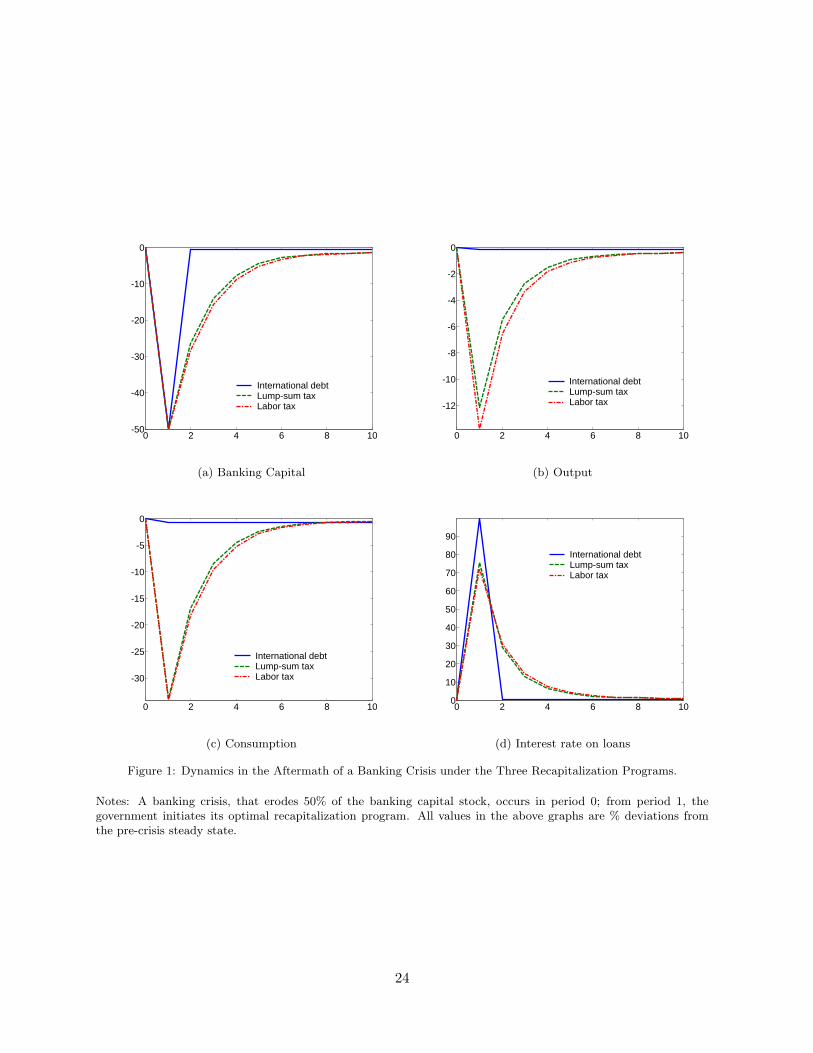
Figure 1 plots the transitional dynamics induced by the banking crisis and the subsequent
government intervention for the three sources of financing discussed above. Given the Leontief
structure of the bank-loan production technology, deposits and bank loans follow the same path
as banking capital. Also, given the fixed physical capital stock, the path of employment and
output are similar.
Consider first the case where the recapitalization is financed by labor-income taxes. In the
first period, which is the period of unraveling of the banking crisis, the low stock of bank capital
constrains the credit that banks can extend to the firms, which in turn reduces employment and
output. Recapitalizing the banks requires a high tax on labor income, which decreases labor
supply via the substitution effect, adding another negative effect on labor and output. All in
all, consumption declines. The maximum amount of banking capital injections occurs during
the first period because the marginal benefit of increasing the stock of banking capital is at its
highest level. As the stock of banking capital increases, the marginal benefit of further injections
declines. From the second period onward, as the amount of injections decline, so does the tax
rate on labor income. Due to the increasing banking capital stock, and hence bank loans, firms
are able to borrow and produce more, so the economy starts recovering from the recession caused8See the United Nations Online Network in Public Administration and Finance data on government consump-
tion as a percentage of GDP in developing countries. See http://unpan1.un.org/intradoc/groups/public/ docu-ments/un/unpan014054.pdf.
15

by the banking crisis. Owing to the high resource cost and the distortionary nature of financing
the recapitalization program, the optimal recapitalization path is a gradual one.
Consider now the case where lump-sum taxes are available; this is equivalent to the government
issuing domestic bonds to pay for the recapitalization program and having access to taxes on
the rents accruing to the stocks of capital. On impact, employment, consumption and output
decline as the economy responds to the high interest rate on working-capital loans. Since the
resources for recapitalization are raised using non-distortionary methods, employment, and hence
output, fall less than in the case of distortionary taxes. Although the method of taxation is
non-distortionary, consumption smoothing entails a gradual recapitalization path due to the large
amount of resources involved. Again, the amount of injections decline over time due to the
declining marginal benefit of these injections as the stock of banking capital increases.
When the government has access to international lending, even if the only taxes available
are distortionary, the optimal recapitalization is undertaken in one shot and, at the same time,
the government is able to smooth consumption completely by borrowing from abroad. Banking
capital, and hence bank loans, reach their new steady state level in period 2, while consumption
and employment (hence, output) adjust to their new steady state levels in period 1 itself. Al-
though the banking capital stock, and hence the amount of bank loans, is low and the firms are
working-capital constrained, the government borrows from international debt markets to subsidize
employment in period 1. Due to this, households are willing to supply labor to the firms even
at a low gross wage rate, wt. Hence, even with a low banking capital stock in period 1, due to
the subsidy to labor income, consumption, employment and output are at their new steady-state
levels.
Table 2 reports the steady state levels of banking capital, output and consumption. Given
the real resource cost of increasing the stock of banking capital, optimality dictates that the
marginal cost of financing the bank recapitalization be equated to the marginal benefit of an
extra unit of banking capital. When labor-income taxes finance the recapitalization program,
apart from having large resource costs, these taxes further distort the economy. With access
to lump-sum taxes, the government is able to avoid the distortions caused by the labor-income
taxes, but the resources for recapitalization still need to be financed domestically. Only when
borrowing from international debt markets is allowed, can the government completely spread out
the recapitalization costs over time. Hence, the steady state levels of banking capital, deposits,
16
loans, employment and output are the highest when there is access to international debt markets,
followed by the case of non-distortionary taxes. However, steady state consumption is the lowest
with access to international debt, in spite of employment and output being the highest: this is
because part of the output is used to pay interest on the country’s debt obligations, which in turn
requires the households to work more.
4.3 Welfare Effects
We compute a number of measures of the welfare effects of a banking crisis (for the different
sources of financing) to highlight different aspects of the welfare costs of a crisis. In all cases the
no-crisis equilibrium is the benchmark. First, following Lucas (1987), we define the net welfare
effects of a banking crisis, λ1, as the permanent, constant decrease in the no-crisis steady state
consumption, c, for t = 0, 1, . . . ,∞, that leaves households indifferent between the lifetime utility
obtained in the no-crisis equilibrium and lifetime utility under the crisis equilibria, inclusive of
the transitional dynamics of consumption, ct, and leisure, lt:
∞∑t=1
βt−1[ln {(1− λ1)c}+ θ ln l
]=∞∑t=1
βt−1 [ln ct + θ ln lt] (30)
where l is the no-crisis steady state leisure.
While the post-crisis consumption is lower than the no-crisis consumption, the post-crisis em-
ployment is always lower than the pre-crisis level. In computing welfare, this drop in employment
(increase in leisure) compensates, to some extent, for the lower consumption. To highlight the
effect of lower consumption alone, on welfare, we also compute the above welfare effects holding
leisure fixed at the pre-crisis steady state level. Thus we define the welfare measure, λ2, as:
∞∑t=1
βt−1[ln {(1− λ2)c}+ θ ln l
]=∞∑t=1
βt−1[ln ct + θ ln l
](31)
In all cases, the welfare loss computed using our second measure is higher than the one using the
first measure because in both methods the consumption profile is the same, given the financing
method, but in the second measure employment (leisure) is higher (lower), which reduces the
crisis utility level.
To highlight the fact that the transitional costs of a bank recapitalization program, due to
decline in consumption, are more severe than the lifetime cost of the crisis, we compute the welfare
17
loss arising purely from the transitional dynamics of the movement to the post-crisis steady state,
under different programs. Note that the times of convergence to the new steady states, tss, are
different for the different financing methods, reflecting the difference in distortions under different
recapitalization programs. We characterize welfare loss as the equivalent permanent reduction in
the no-crisis steady state consumption, defining λ3 such that:
tss∑t=1
βt−1[ln {(1− λ3)c}+ θ ln l
]=
tss∑t=1
βt−1 [ln ct + θ ln lt] (32)
Finally, to characterize the effect of lower consumption alone on welfare, in computing the
welfare loss induced by the transitional dynamics of a bank restructuring program, we hold leisure
fixed at the no-crisis steady state level, and define λ4 to satisfy:
tss∑t=1
βt−1[ln {(1− λ4)c}+ θ ln l
]=
tss∑t=1
βt−1[ln ct + θ ln l
](33)
The results for the welfare comparisons are presented in Table 3. We discuss these results for
our baseline calibration of a banking capital to deposit ratio of 1/10, i.e., γ = 10, and we use other
values of γ for sensitivity analysis. If the government does not recapitalize the banking system in
the aftermath of a crisis and the banking capital stock stays at the crisis level infinitely, then the
welfare loss is a decline of 5.51% in the no-crisis steady state consumption using our first measure
and 22.08% using the second measure. Recall that the reason for the higher value of welfare loss
using the second measure is that, while consumption is at the crisis level, we hold employment
(leisure) fixed at the high (low) no-crisis level.
The net welfare loss of a crisis with recapitalization financed by distortionary taxes are 0.65%
and 1.42% of the no-crisis consumption using the first and second measures, respectively. The
welfare loss purely due to the transitional dynamics involved in the movement to the new steady
state is 2.69% of the no-crisis consumption, and is higher at 4.46% if employment (leisure) is held
constant at the no-crisis level.
Financing the recapitalization with non-distortionary taxes results in a welfare loss of 0.63%
(1.35%) of the no-crisis consumption using our first (second) measure. The welfare loss is to the
order of 2.74% due to the transitional dynamics alone, and it is 4.35% if we also hold employment
fixed at the no-crisis level.
Access to international debt eases the welfare cost of a banking crisis considerably, and the
18
welfare loss of a banking crisis is 0.51% of steady state consumption using our first and third
measures, while it is 0.72% using the second and fourth measures. The lifetime and transition
measures coincide in the case of international debt access because the government, by borrowing
from international markets, is able to achieve intertemporal smoothing, and consumption and
employment jump to the new steady state values in period 1 itself, while banking capital reaches
the new steady state in period 2.
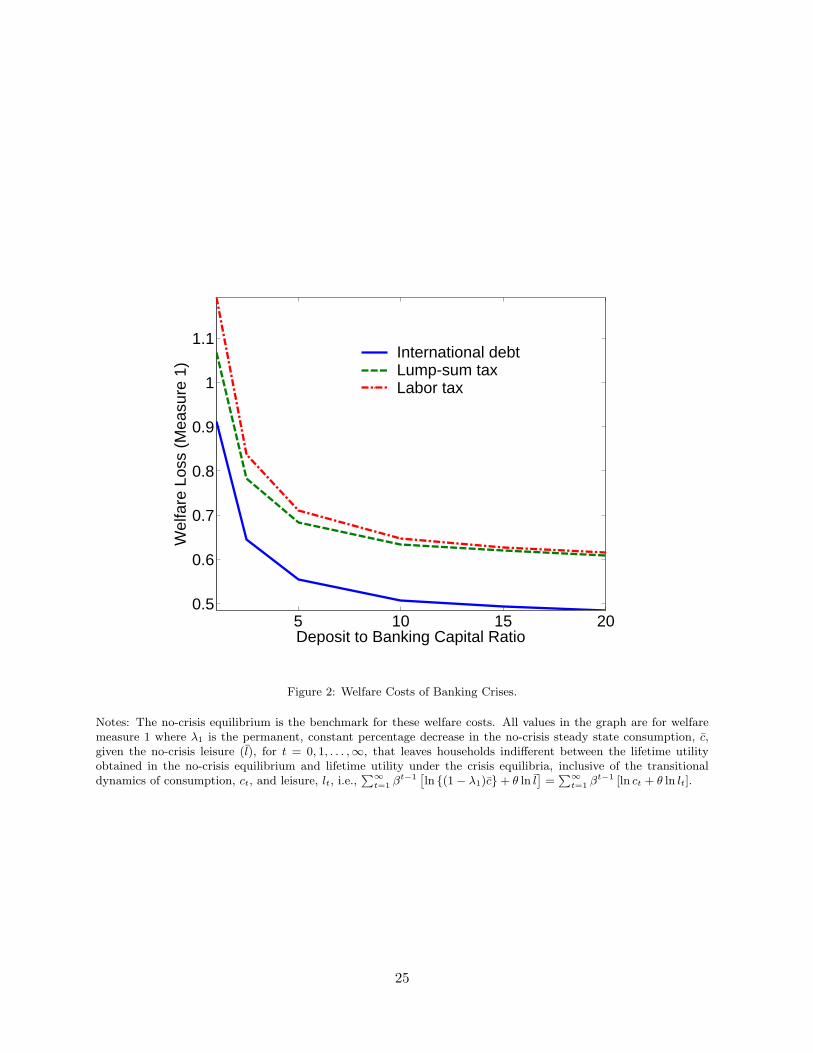
Apart from the welfare effects in the benchmark case, we also compute the above welfare
measures for other values of the banking capital to deposit ratio. As shown in Table 3, the welfare
losses due to a banking crisis, given the method of financing of the recapitalization program, is
increasing (decreasing) in the banking capital-deposit ratio (γ). Figure 2 plots the welfare costs
of banking crises, using measure 1, for different values of γ. As γ increases, i.e., as the banking
capital to deposit ratio in the economy declines, the pre-crisis steady state banking capital stock
declines. This is because, given the other parameters, the amount of banking capital required
to produce the same amount of loans declines. Hence, the welfare loss due to a crisis, given the
recapitalization program, declines because amount of resources required for the recapitalization
program decreases with the decline in the initial loss of banking capital.
5 Concluding Remarks
Banking sector crises, which have been prevalent in both developing and developed countries, have
presented a stiff challenge to policy makers and continue to do so. Given the public-good aspect
of a well running financial system, governments almost invariably end up bearing the burden of
financing the restructuring programs necessary to recapitalize a bankrupt banking system. The
high fiscal cost of these programs warrants careful analysis of the financing options used by the
government.
In this paper we undertook a first attempt at examining the public-finance aspect of the gov-
ernment’s recapitalization of a bankrupt banking sector in a dynamic general equilibrium setting.
We formulate the Ramsey planner’s problems under three different scenarios: recapitalizations
financed with distortionary taxes, with non-distortionary taxes and by borrowing from interna-
tional debt markets. The Ramsey problems were solved numerically and the welfare costs of a
banking crisis were found to be substantial.
The post restructuring levels of banking capital are different under the three regimes, reflecting
19

the difference in distortions due to the different financing options of the recapitalization program.
It has often been suggested that the government should restructure the banking system in one
shot, but our analysis of the Ramsey planner’s problems shows that optimality requires a gradual
approach unless the economy can borrow from international markets. This is because the high
resource cost typically involved in bank a restructuring program should be spread out over time
to minimize the distortions introduced in funding the program. This highlights the importance of
having access to international debt markets during period of financial distress; furthermore, the
results discussed here may also justify why under some circumstances it might be highly convenient
to have international organizations extending emergency financing to developing countries hit by
banking crises. This financing could alleviate the effects of a banking crisis and avoid a rather
painful and long-drawn adjustment process in the post-crisis scenario.
We have not considered the moral hazard problems arising from the government intervention
in financial markets, nor have we incorporated the different methods used for recapitalization9,
which can have different effects on the government budget. These issues are important and present
avenues for future research. Another possible avenue for future research is the explicit modeling of
why private agents do not accumulate banking capital, that necessitates government intervention.
9For details on the latter, see Daniel et al. (1997).
20
References
Azzimonti, M., Sarte, P.-D., and Soares, J. (2006). Distortionary taxes and public investmentwhen government promises are not enforceable. Working Paper.
Caprio, G. and Klingebiel, D. (1996). Bank insolvencies: Cross country experience. World BankPolicy Research Working Paper, (No. 1620).
Caprio, G. and Klingebiel, D. (2003). Episodes of systemic and borderline banking crises. WorldBank.
Chava, S. and Purnanandam, A. (2006). The effect of banking crisis on bank-dependent borrowers.Working Paper.
Cole, H. and Ohanian, L. (2000). Re-examining the contribution of money and banking shocks tothe U.S. Great Depression. In: NBER Macroeconomics Annual, pages 183–227. Vol 15. Eds.Ben Bernanke and Kenneth Rogoff.
Daniel, J., Davis, J., and Wolfe, A. (1997). Fiscal accounting of bank restructuring. IMF Paperon Policy Analysis and Assessment.
Dell’Ariccia, G., Detragiache, E., and Rajan, R. (2005). The real effect of banking crises. IMFWorking Paper.
Demiirguc-Kunt, A. and Detragiache, E. (1998). The determinants of banking crises in developingand developed countries. IMF Staff Papers, 45(1):81–109.
Demiirguc-Kunt, A., Detragiache, E., and Gupta, P. (2006). Inside the crisis: An empiricalanalysis of banking systems in distress. Journal of International Money and Finance, 25(5):702–718.
Honohan, P. and Klingebiel, D. (2000). Controlling the fiscal costs of banking crises. World BankPolicy Research Working Paper.
Klein, P., Krusell, P., and Rıos-Rull, J.-V. (2007). Time-consistent public policy. Working Paper.
Lindgreen, C.-J., Gillian, G., and Saal, M. (1996). Bank Soundness and Macroeconomic Policy.IMF.
Lucas, R. E. (1987). Models of Business Cycles. Blackwell.
Neumeyer, P. and Perri, F. (2005). Business cycles in emerging economies: the role of interestrates. Journal of Monetary Economics, 52:345–380.
Riascos, A. and Vegh, C. (2004). Procyclical fiscal policy in developing countries: The role ofcapital market imperfections. Working Paper.
Romer, C. (1993). The Nation in Depression. Journal of Economic Perspectives, 7(2):19–39.
21

Table 1: Baseline Parameter Values
Parameters Values
β Discount factor 0.988θ Leisure share in utility 1.5B Productivity parameter 6k Physical capital stock 115α Capital’s share in output 1/3γ Ratio of deposits to banking capital 10g Fixed government consumption 2R∗ Quarterly world interest rate 1.012
Table 2: Steady State Values under Baseline Parameters
Variable Pre-crisis Post-crisis
No intervention Labor tax Lump-sum Tax International Debt
A 0.922 0.461 0.910 0.910 0.918y 14.118 11.443 14.062 14.063 14.091c 12.118 9.443 12.062 12.063 12.030h 0.337 0.246 0.335 0.335 0.336
Notes: The steady state levels of the variables are different for the different programs reflecting the differencein distortions due to the different financing options of the recapitalization programs. For the time period inwhich the economy converges to the new steady state, under different financing methods, see Table 3.
22
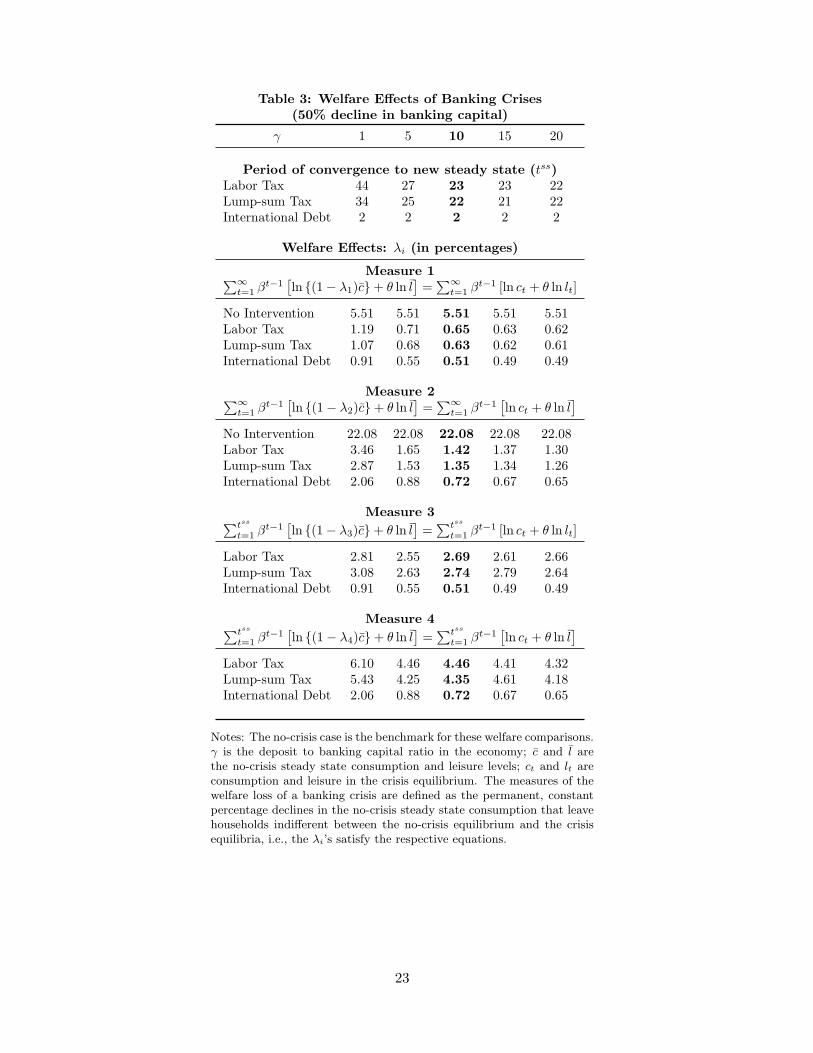
Table 3: Welfare Effects of Banking Crises(50% decline in banking capital)
γ 1 5 10 15 20
Period of convergence to new steady state (tss)Labor Tax 44 27 23 23 22Lump-sum Tax 34 25 22 21 22International Debt 2 2 2 2 2
Welfare Effects: λi (in percentages)
Measure 1∑∞t=1 β
t−1[ln {(1− λ1)c}+ θ ln l
]=∑∞
t=1 βt−1 [ln ct + θ ln lt]
No Intervention 5.51 5.51 5.51 5.51 5.51Labor Tax 1.19 0.71 0.65 0.63 0.62Lump-sum Tax 1.07 0.68 0.63 0.62 0.61International Debt 0.91 0.55 0.51 0.49 0.49
Measure 2∑∞t=1 β
t−1[ln {(1− λ2)c}+ θ ln l
]=∑∞
t=1 βt−1[ln ct + θ ln l
]No Intervention 22.08 22.08 22.08 22.08 22.08Labor Tax 3.46 1.65 1.42 1.37 1.30Lump-sum Tax 2.87 1.53 1.35 1.34 1.26International Debt 2.06 0.88 0.72 0.67 0.65
Measure 3∑tss
t=1 βt−1[ln {(1− λ3)c}+ θ ln l
]=∑tss
t=1 βt−1 [ln ct + θ ln lt]
Labor Tax 2.81 2.55 2.69 2.61 2.66Lump-sum Tax 3.08 2.63 2.74 2.79 2.64International Debt 0.91 0.55 0.51 0.49 0.49
Measure 4∑tss
t=1 βt−1[ln {(1− λ4)c}+ θ ln l
]=∑tss
t=1 βt−1[ln ct + θ ln l
]Labor Tax 6.10 4.46 4.46 4.41 4.32Lump-sum Tax 5.43 4.25 4.35 4.61 4.18International Debt 2.06 0.88 0.72 0.67 0.65
Notes: The no-crisis case is the benchmark for these welfare comparisons.γ is the deposit to banking capital ratio in the economy; c and l arethe no-crisis steady state consumption and leisure levels; ct and lt areconsumption and leisure in the crisis equilibrium. The measures of thewelfare loss of a banking crisis are defined as the permanent, constantpercentage declines in the no-crisis steady state consumption that leavehouseholds indifferent between the no-crisis equilibrium and the crisisequilibria, i.e., the λi’s satisfy the respective equations.
23
0 2 4 6 8 10-50
-40
-30
-20
-10
0
International debtLump-sum taxLabor tax
(a) Banking Capital
0 2 4 6 8 10
-12
-10
-8
-6
-4
-2
0
International debtLump-sum taxLabor tax
(b) Output
0 2 4 6 8 10
-30
-25
-20
-15
-10
-5
0
International debtLump-sum taxLabor tax
(c) Consumption
0 2 4 6 8 100
10
20
30
40
50
60
70
80
90
International debtLump-sum taxLabor tax
(d) Interest rate on loans
Figure 1: Dynamics in the Aftermath of a Banking Crisis under the Three Recapitalization Programs.
Notes: A banking crisis, that erodes 50% of the banking capital stock, occurs in period 0; from period 1, thegovernment initiates its optimal recapitalization program. All values in the above graphs are % deviations fromthe pre-crisis steady state.
24
5 10 15 200.5
0.6
0.7
0.8
0.9
1
1.1
Deposit to Banking Capital Ratio
Wel
fare
Los
s (M
easu
re 1
) International debtLump-sum taxLabor tax
Figure 2: Welfare Costs of Banking Crises.
Notes: The no-crisis equilibrium is the benchmark for these welfare costs. All values in the graph are for welfaremeasure 1 where λ1 is the permanent, constant percentage decrease in the no-crisis steady state consumption, c,given the no-crisis leisure (l), for t = 0, 1, . . . ,∞, that leaves households indifferent between the lifetime utilityobtained in the no-crisis equilibrium and lifetime utility under the crisis equilibria, inclusive of the transitionaldynamics of consumption, ct, and leisure, lt, i.e.,
∑∞t=1 β
t−1[ln {(1− λ1)c}+ θ ln l
]=∑∞
t=1 βt−1 [ln ct + θ ln lt].
25