on the accuracy of digital bathymetric data

JOURNAL OF GEOPHYSICAL RESEARCH, VOL. 98, NO. B6, PAGES 9591-9603, JUNE 10, 1993

On the Accuracy of Digital Bathymetric Data

WALTER H. F. SMITH 1

Institute of Geophysics and Planetary Physics, Scripps Institution of Oceanography, University of California, San Diego

The global 5-arcmin gridded topography data ETOPO-5 are based on contour maps rather than original soundings and have large errors. The artificial statistical distribution generated by digitizing contours makes these data unsuitable for use in regression models for depth-age variations. Their amplitude spectrum is bounded by a (frequency) -4 power law, so that they should not be used when the gravity-topography transfer function is important, such as in studies of flexural isostasy and mantle convection. I assess the accuracy of 14,491,069 digital ship soundings in 2253 cruise surveys collected between 1955 and 1992 in the Lamont- Doherty Earth Observatory on-line data base by analyzing 329,058 crossover errors (COEs) at intersecting ship tracks. Five percent of cruises with internal COEs yield root-mean-square COE amplitudes exceeding 500 m; all of these have errors in digitizing two-way travel time from analog precision depth recorder traces. Twenty-eight cruises were found which had errors caused by misinterpretation of the nominal sound velocity used when travel times were reported as nominal depths. Two nominal sound velocities in common use differ by 2.5%, an amount which is often undetectable, producing uncertainties in depth of this magnitude. Ship data have been acquired at different rates over time, with the peak of activity in the early 1970s. Although present technologies can yield very accurate data, these are acquired at a rate which is small with respect to the total available data; the cumulative median global COE has remained constant at 26 m since the late 1970s. Most recent data acquisition has been in the northern hemisphere oceans, and the oldest and least accurate data are in the southern oceans where median COEs are 100 - 250 m. The majority of the data in the South Pacific were acquired before the advent of satellite navigation.

INTRODUCTION

Topography is the fundamental physical characteristic of any planet. Topographic data are essential to the study of planetary dynamics, not only as the principal boundary condition but also because surface relief is indicative of nonhydrostatic stress in the planer's interior [Bowie, 1927; Jeffreys, 1976]. The elevations of the surfaces of Mars [Carr et al., 1977] and Venus [Ford and Pettengill, 1992] are better known than those of some areas of Earth. Two factors make Earth's topography difficult to measure. Nearly three-quarters of the surface lies under water and cannot be observed by airborne or orbiting vehicles using electromagnetic means; it must be sensed acoustically by surface or sub-surface craft. Much of the land area is in the northern hemisphere and the southern oceans are remote; there are areas of the southern hemisphere larger than 10,000 km 2 for which no digital ship sounding data are available.

Ocean basin- and global-scale investigations of Earth's fundamental dynamic processes require bathymetric data in a computerized form because of the large quantity of data involved and the nature of the calculations required. Digital bathymetric data are available in two forms, as sequences of soundings collected by oceanographic ships, and in a grid array of values for 5 arcmin "squares" of latitude and longitude (the Synbaps, or DBDB-5, data set [Van Wyckhouse, 1973], now part of ETOPO-5 [National Geophysical Data Center, 1988]).

1Now at Geosciences Laboratory, National Ocean Service, National Oceanic and Atmospheric Administration, Silver Spring, Maryland.

Copyright 1993 by the American Geophysical Union.

Paper number 93JB00716. 0148-0227/93/93 JB-00716505.00

The 5 arcmin gridded data create the illusion of global coverage; to the extent that they are faithful to actual soundings they offer a convenient synthesis of the ship data. Because they are widely available and convenient to use, most recent studies of isostasy and thermal boundary layer cooling have been based on these data. The original ship sounding data have been difficult to use and accessible only through research institutions which have the facilities to maintain a large data bank; furthermore, only in the last few years have computer processing and storage media evolved to the point where it is practical to maintain a comprehensive global collection of these data in an "on-line" searchable manner. The U.S.

National Geophysical Data Center (NGDC) has recently released its digital bathymetric data on CD-ROM [National Geophysical Data Center, 1992], and it is now possible for the scientific community to have access to these original soundings "on-line".

The accuracy and spatial distribution of digital bathymetric data is of fundamental importance to all scientists interested in Earth physics, yet the errors and limitations of these data are not widely appreciated. In this paper, I illustrate some peculiarities of the ETOPO-5 gridded data which argue against their use in geophysical studies. I present an analysis of global crossover errors in the original ship sounding data, and remark upon the limitations of their accuracy and distribution. This analysis is of the soundings in the on-line data bank at Columbia University's Lamont-Doherty Earth Observatory (Figure 1). I used these data because they are available over Internet through the view-server system [Menke et al., 1991], and because a crossover error study of the gravity data in this data bank was made earlier by Wessel and Watts [1988]. These data are very similar to those available from NGDC. The LDEO data bank includes some data not held at NGDC and probably lacks some that NGDC has, particularly the most recent contributions. However, as will be shown, the accuracy of the data is determined by soundings made before the mid-1980s,

9591

9592 SMITH: ACCURACY OF DIGITAL BATHYMETRIC DATA

60 ø

30 ø

o

_30 ø

o ß

30 ø 60 ø 90 ø 120 ø150 ø180 ø210 ø240 ø270 ø300 ø330 ø360 ø

.j

60 ø

30 ø

_30 ø

_60 ø

30 ø 60 ø 90 ø 120 ø 150 ø

i

180 ø 210 ø 240 ø 270 ø 300 ø 330 ø 360 ø

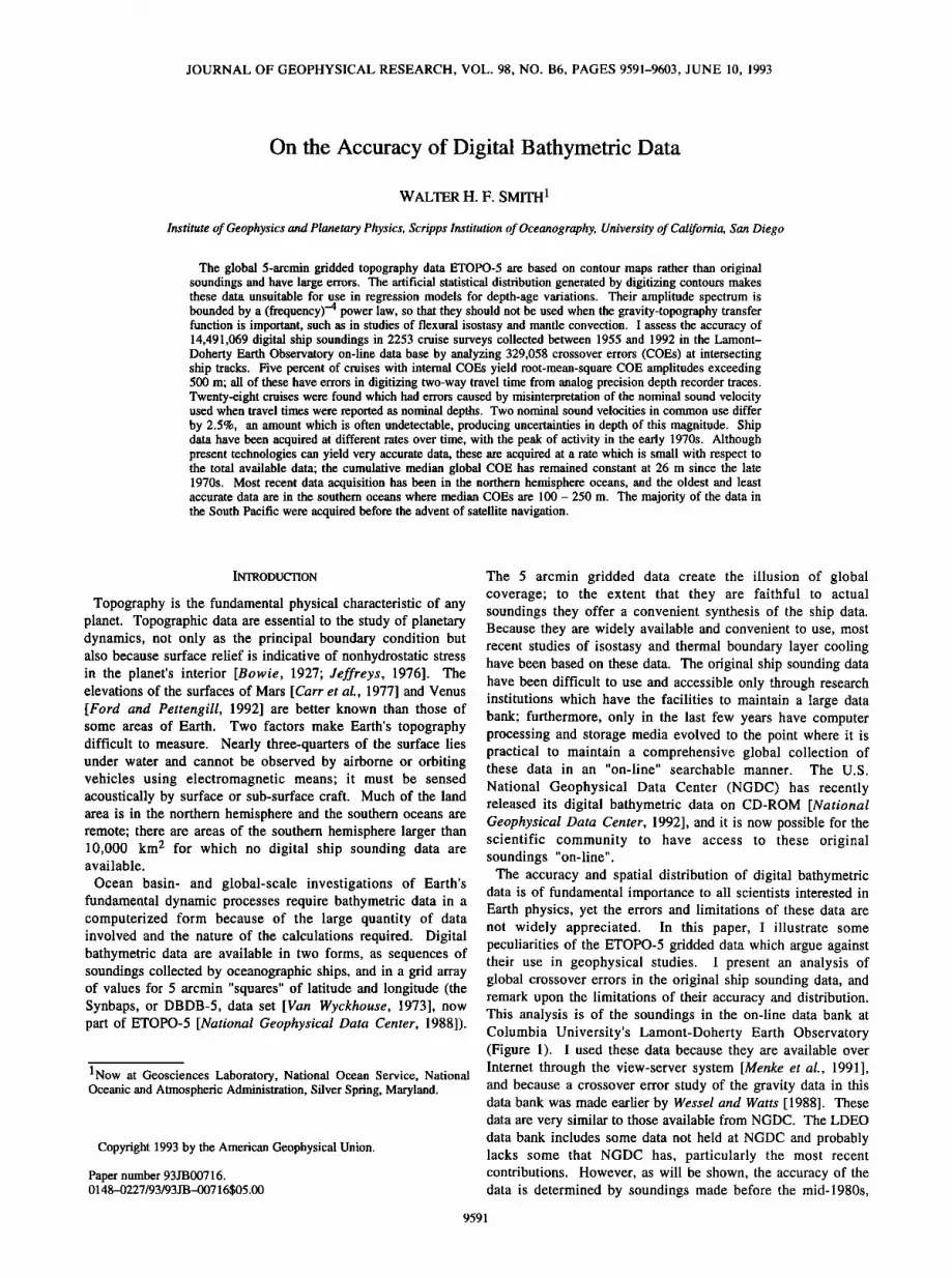
Fig. 1. Track lines of 2253 cruises in the Lamont-Doherty Earth Observatory on-line marine geophysical data base, with 14,491,069 soundings collected between 1955 and 1992. Accuracy of these data is assessed in this paper by analysis of 329,058 crossover errors (COEs).

_60 ø

and for data of this vintage the LDEO data bank is representative of the NGDC holdings. For this reason also, most of the data examined here are digitized from wide-beam echo sounder profiles, and the precision of multi-beam acoustic swath mapping systems is not discussed in this study.

THREE CAVEATS CONCERNING ETOPO-5

ETOPO-5 bathymetry has been used to analyze the variation of depth with age [Renkin and Sclater, 1988; Hayes, 1988; Marty and Cazenave, 1989; Stein and Stein, 1992], mantle convection [Cazenave et al., 1986, 1992; Cazenave and Dominh, 1987], compensation of oceanic plateaus and hot spot swells [McNutt and Shure, 1986; McNutt, 1988; Sandwell and Renkin, 1988; Fleitout et al., 1989; Sandwell and MacKenzie, 1989; Sheehan and McNutt, 1989; McNutt and

Judge, 1990; Monnereau and Cazenave, 1990], and flexure of the lithosphere [Calmant and Cazenave, 1986; Goslin and Diament, 1987; Maia et al., 1990]. I wish to make geoscientists aware of three facts about ETOPO-5 which suggest that these data should be interpreted with care: (1) ETOPO-5 was gridded from contours, not soundings; (2)

ETOPO-5 has a peculiar statistical distribution; and (3) the amplitude spectrum of these data is influenced by the algorithm used to grid the data.

Gridded From Contours, Not Original Data

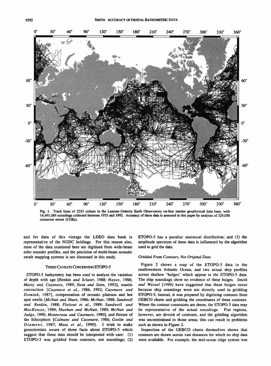
Figure 2 shows a map of the ETOPO-5 data in the southwestern Atlantic Ocean, and two actual ship profiles across shallow "bulges" which appear in the ETOPO-5 data. The ship soundings show no evidence of these bulges. Smith and Wessel [1990] have suggested that these bulges occur because ship soundings were not directly used in gridding ETOPO-5; instead, it was prepared by digitizing contours from GEBCO charts and gridding the coordinates of these contours. Where the contour constraints are dense, the ETOPO-5 data may be representative of the actual soundings. Flat regions, however, are devoid of contours, and the gridding algorithm was unconstrained in those areas; this can result in problems such as shown in Figure 2.

Inspection of the GEBCO charts themselves shows that contours are drawn across vast distances for which no ship data were available. For example, the mid-ocean ridge system was

SMITH: ACCURACY OF DIGITAL BATHYMETRIC DATA 9593

_40 ø

_45 ø

_50 ø

290 o 295 o 300 o 305 o 310 ø

A

Falkland Is.

-100 -

-200 -

-300 -

-400

i I ,

A

-100 -

-200

-300

-400

, I ,

B

0 200 41 )0

Distance (km)

Fig. 2. (Top) ETOPO-5 data in the southwest Atlantic Ocean are contoured (1000 m) and shaded where shallower than 200 m. Erroneous "bulges" occur (A and B, showing profile locations) because ETOPO-5 is gridded from contour maps, not original soundings. (Lower) Profiles A and B show depth profiles across the Argentine continental shelf and slope. Solid line, actual ship soundings; dashed line, ETOPO-5 data.

more points to constrain the gridding than would the original ship data, and so the strategy of gridding contours rather than data may seem advantageous in these areas. However, it must be remembered that in areas of sparse data, the contours are drawn based upon human prejudice; there are no data which can prove or disprove their location.

Statistical Distribution

Gridded contours are a problem for geophysical studies because the contour values influence the statistical distribution

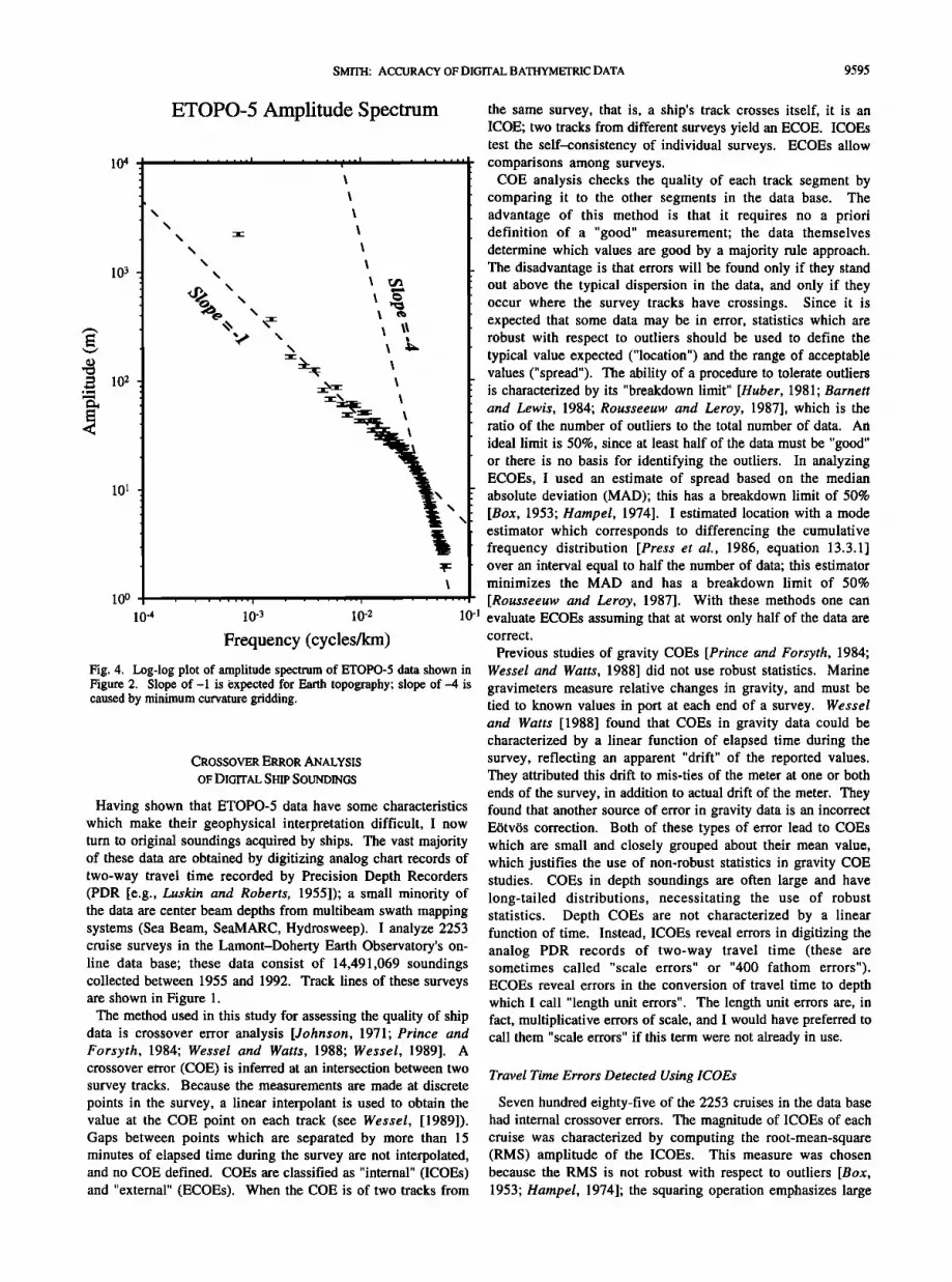
of the data. Figure 3 (top) is a histogram showing the frequency (% of surface area of Earth) of values in 50 m bins for the (global) ETOPO-5 data. Because the data below sea level were prepared by digitizing contours, certain values corresponding to these contours occur with unusual frequency in the data. Note that values corresponding to multiples of 1000 m are particularly prominent, with less prominent spikes at multiples of 500 and 200 m. These values occur everywhere, so that when ETOPO-5 data are plotted versus the age of the seafloor (Figure 3, middle), these values form horizontal streaks spread across a wide range of ages. Ship soundings do not show these streaks (Figure 3, bottom).

The increase of seafloor depth with age may yield information about the cooling of a thermal boundary layer [Parsons and Sclater, 1977], and so geoscientists perform regression analyses which "fit" a parameterized function of age to depth data. Implicit in this regression procedure is the assumption that the component of depth which is not explained by the age function is random and uncorrelated. The streaks of Figure 3 (middle) will introduce correlation in the residuals of a fitted model, and thus may bias the estimated model parameters. To illustrate this bias, I have fit a regression model of the form a + b •/t to the data in Figure 3. Here a is the depth at zero age, b is a subsidence rate, and t is the age of the seafloor. These data are taken from a "tectonic corridor" in the South Atlantic which is

subsiding asymmetrically [Morgan and Smith, 1992], so there are two values of b, one on each side of the ridge, constrained to share a common value of a at the ridge crest. (The effect of seamounts and rises was removed by ignoring data shallower than 4 km at ages older than 50 Ma.) Values of b obtained for the right-hand flank in Figure 3 are similar for the two data sets: 241 m (m.y.) -1/2 for the ETOPO-5 data and 248 m (m.y.) -1/2 for the ship data. On the opposite flank, however, the values are much different: 344 m (m.y.) -m for the ETOPO-5 data and 376 m (m.y.) -•/2 for the ship data. The zero age depths are also different: 2522 m for the ETOPO-5 data and 2202 m for

the ship data. Assuming that the ship data give "correct" values and the ETOPO-5 data give biased values, the error caused by the streaking is 3% on the fight flank, 9% on the left flank, and 15% in the zero age elevation. If these biased values were interpreted in terms of mantle temperature, the inferred temperature would be biased by 40 to 200øC. The sign of the bias in this example leads to underestimated values, and hence a mantle that is too cold; however, data from some other area

might show a bias of the opposite sign.

drawn as a continuous feature (perhaps guided by earthquake epicenters) and deeper contours flanking the ridge were then drawn parallel to the ridge axis, assuming that the depth increased away from the ridge in a regular manner. In areas of sparse ship coverage, the digitized contours actually provide

Amplitude Spectrum

Physical models for the dynamical mechanisms of mantle convection, isostasy and flexure of the lithosphere suggest correlations between planetary topography and gravity fields which are functions of spatial wavelength. These effects are often studied by analyzing the transfer function between

9594 SMITH: ACCURACY OF DIG1TAL BATHYMETRIC DATA

Elevation (km) -6 -5 -4 -3 -2 - 1 0 1 2 3

3 ' . , . , . , . , . • . , . , . , , I

ETOPO-5

2

-6

ETOPO-5

2522 m

344 m (m.y.)4/2 241 m (m.y.) 4/2

Ship -2

Age (m.y.) Fig. 3. Statistical distribution of ETOPO-5 shows influence of contours. (Top) Histogram of global ETOPO-5 elevations in 50 m bins. Note spikes at multiples of 1000 m, also 500 m and 200 m below sea level. (Middle) ETOPO-5 depth versus age in a tectonic corridor in the South Atlantic; note horizontal streaks at contour values. (Bottom) Ship data in the same corridor. Numbers in middle and bottom panels are ridge elevations and subsidence rates estimated by regression.

gravity and topography data, a method which relies on the spectra of topography and gravity data being representative of the actual fields which the data are supposed to measure. The

spectrum of ETOPO-5 is influenced by the minimum-curvature gridding algorithm used to construct it, as I show here.

The minimum curvature surface [Briggs, 1974] z(x), x=[x,y] T a point in the x,y plane, satisfies

V4z(x) = Zfmfi(X-Xm) (1) rn

where

3 4 3 4 3 4 V4= +2•+ •x 4 •x2•y2 •y4

is the biharmonic operator, fi(x) is the Dirac delta function, x m are knot points, and fm are scalar constants chosen to make z(x) satisfy certain data constraints. Define the Fourier transform in the plane with wavevector k=[kx, ky] T by

Z(k)=Ifz(x) expli(k. x)l dxdy. (2) Then the Fourier transform of equation (1) is

Ikl4Z (k) = Z fm exp [i (k. Xm)] (3) rn

and from equation (3) the squared modulus I ZI 2 = Z Z* is

I z (k)l 2 = Ikl -a Z Z fm fn cos [k. (Xm - Xn)I. (4) rn n

Since

I• • fmfn cos [k. (Xm - Xn)] I <- • n•lfmf• = [mZIfMl 2= C 2 (5) n rn

we have

IZ(k)l <_ c (6) Ikl -4

for some constant c, and thus the amplitude spectrum of any data which are gridded using minimum curvature must be bounded by the power law (6).

Earth's actual topography may have a spectrum very different from (6). Many studies have found that Earth topography resembles fractional Brownian motion, having an amplitude

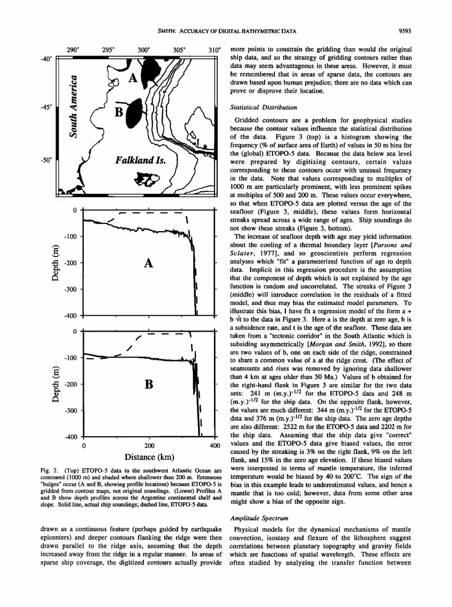
spectrum proportional to Ikl with [5 nearly equal to 1 [Bell, 1975; Fox and Hayes, 1985; Malinverno, 1989; and references therein]. Figure 4 shows the amplitude spectrum of the ETOPO- 5 data in Figure 2 (top). These data represent a mixture of processes in addition to minimum curvature gridding; they include the values over land, obtained by an unknown process, and also the effect of truncating the shelf break bulges (Figure

2, top). The spectrum in Figure 4 is proportional to [ k-• at wavelengths greater than 30 - 50 km, and Ik1-4 at shorter wavelengths. Equation (6) is an upper bound only, and the actual spectrum will be determined by the control data which are input to the gridding procedure. I conclude from Figure 4 that the typical spacing of control data input to ETOPO-5 was 30- 50 km in this area, so that at wavelengths greater than 30- 50 km the ETOPO-5 data have an amplitude spectrum appropriate for Earth topography, while at shorter wavelengths the spectrum is determined by the minimum curvature constraint (6). Spectra obtained from other areas of ETOPO-5 show "corner" wavelengths larger than 100 km in some cases. Thus ETOPO-5 data are smoother, and have less variance, than Earth topography they are meant to represent.

SMrrH: ACCURACY OF DIGITAL BATHYMETRIC DATA 9595

ETOPO-5 Amplitude Spectrum

10 4

10 3

10 2

101

100

\

\

\ -r

\

\

10-4 10-3 10-2 10-•

Frequency (cycles/km)

Fig. 4. Log-log plot of amplitude spectrum of ETOPO-5 data shown in Figure 2. Slope of-1 is expected for Earth topography; slope of -4 is caused by minimum curvature gridding.

CROSSOVER ERROR ANALYSIS

OF DIGITAL SHIP SOUNDINGS

Having shown that ETOPO-5 data have some characteristics which make their geophysical interpretation difficult, I now turn to original soundings acquired by ships. The vast majority of these data are obtained by digitizing analog chart records of two-way travel time recorded by Precision Depth Recorders (PDR [e.g., Luskin and Roberts, 1955]); a small minority of the data are center beam depths from multibeam swath mapping systems (Sea Beam, SeaMARC, Hydrosweep). I analyze 2253 cruise surveys in the Lamont-Doherty Earth Observatory's on- line data base; these data consist of 14,491,069 soundings collected between 1955 and 1992. Track lines of these surveys are shown in Figure 1.

The method used in this study for assessing the quality of ship data is crossover error analysis [Johnson, 1971; Prince and Forsyth, 1984; Wessel and Watts, 1988; Wessel, 1989]. A crossover error (COE) is inferred at an intersection between two survey tracks. Because the measurements are made at discrete points in the survey, a linear interpolant is used to obtain the value at the COE point on each track (see Wessel, [1989]). Gaps between points which are separated by more than 15 minutes of elapsed time during the survey are not interpolated, and no COE defined. COEs are classified as "internal" (ICOEs) and "external" (ECOEs). When the COE is of two tracks from

the same survey, that is, a ship's track crosses itself, it is an ICOE; two tracks from different surveys yield an ECOE. ICOEs test the self-consistency of individual surveys. ECOEs allow comparisons among surveys.

COE analysis checks the quality of each track segment by comparing it to the other segments in the data base. The advantage of this method is that it requires no a priori definition of a "good" measurement; the data themselves determine which values are good by a majority rule approach. The disadvantage is that errors will be found only if they stand out above the typical dispersion in the data, and only if they occur where the survey tracks have crossings. Since it is expected that some data may be in error, statistics which are robust with respect to outliers should be used to define the typical value expected ("location") and the range of acceptable values ("spread"). The ability of a procedure to tolerate outliers is characterized by its "breakdown limit" [Huber, 1981;Barnett and Lewis, 1984; Rousseeuw and Leroy, 1987], which is the ratio of the number of outliers to the total number of data. An

ideal limit is 50%, since at least half of the data must be "good" or there is no basis for identifying the outliers. In analyzing ECOEs, I used an estimate of spread based on the median absolute deviation (MAD); this has a breakdown limit of 50% [Box, 1953; Hampel, 1974]. I estimated location with a mode estimator which corresponds to differencing the cumulative frequency distribution [Press et al., 1986, equation 13.3.1] over an interval equal to half the number of data; this estimator minimizes the MAD and has a breakdown limit of 50%

[Rousseeuw and Leroy, 1987]. With these methods one can evaluate ECOEs assuming that at worst only half of the data are correct.

Previous studies of gravity COEs [Prince and Forsyth, 1984; Wessel and Watts, 1988] did not use robust statistics. Marine gravimeters measure relative changes in gravity, and must be tied to known values in port at each end of a survey. Wessel and Watts [1988] found that COEs in gravity data could be characterized by a linear function of elapsed time during the survey, reflecting an apparent "drift" of the reported values. They attributed this drift to mis-ties of the meter at one or both ends of the survey, in addition to actual drift of the meter. They found that another source of error in gravity data is an incorrect E6tv6s correction. Both of these types of error lead to COEs which are small and closely grouped about their mean value, which justifies the use of non-robust statistics in gravity COE studies. COEs in depth soundings are often large and have long-tailed distributions, necessitating the use of robust statistics. Depth COEs are not characterized by a linear function of time. Instead, ICOEs reveal errors in digitizing the analog PDR records of two-way travel time (these are sometimes called "scale errors" or "400 fathom errors"). ECOEs reveal errors in the conversion of travel time to depth which I call "length unit errors". The length unit errors are, in fact, multiplicative errors of scale, and I would have preferred to call them "scale errors" if this term were not already in use.

Travel Time Errors Detected Using ICOEs

Seven hundred eighty-five of the 2253 cruises in the data base had internal crossover errors. The magnitude of ICOEs of each cruise was characterized by computing the root-mean-square (RMS) amplitude of the ICOEs. This measure was chosen because the RMS is not robust with respect to outliers [Box, 1953; Hampel, 1974]; the squaring operation emphasizes large

9596 SMrH-I: ACCURACY OF DIGITAL BATHYMETRIC DATA

errors, and so the RMS is large for cruises with problems of internal consistency. 95% of the cruises had an RMS ICOE less than 500 m. The 39 cruises with an RMS ICOE exceeding 500 m were examined, and all were found to have errors in the

digitization of two-way travel time to the bottom. These travel time errors arise because of an ambiguity in

analog PDR records. The recorders have an electrical circuit for gating and delaying a received signal from a sonar transducer, and a rotating belt which moves a stylus across the chart paper. The stylus receives the electric current from the transducer, and marks the returned energy on the paper. The belt circumference is typically three times the paper width and has three styli arranged so that one stylus is always in contact with the paper. This means that the trace of the mark on the paper may move off one edge of the paper and reappear at the other edge; the relationship between travel time and mark location is

x = (t-d) modulo s (7) w s

where x is the position of the mark on the paper, measured from the near edge, w is the paper width, t is the two-way time, d is the delay time in the circuit, if any, and s is the sweep time, the time it takes the stylus to move across the paper. The sweep time may be varied to adjust the precision of the record; a faster sweep time means a smaller At for a given Ax, but this results in the mark running off the edge of the paper more frequently. The delay time may be varied to adjust the location of the mark on the paper; if the mark is near one edge, for example, changing the delay time by half the sweep time will place the mark near the middle of the paper. On some modern installations, both values are adjusted frequently and automatically as bottom conditions change and to avoid interference with other acoustic devices.

Equation (7) cannot be solved uniquely for t, given x; if t l solves (7), then so does any t = tl + Ns, where N is an integer. Digital data on the two-way travel time to the seafloor are obtained by digitizing x from the chart paper and then converting x to t by knowing d and s and choosing a value for N. In principle, if the record is obtained continuously, N can be determined uniquely from the constraint that t should be a continuous function. In practice, over rough topography or in rough seas the record is noisy or absent and t is not a continuous function. Therefore personnel aboard the ship should annotate the chart paper to indicate d, s, and N every time there is a change in one of these values. Failure to do this may result in an incorrect solution for the travel time. Common practice is to annotate the travel time corresponding to the near and far edges of the paper (actually, travel times are indicated by "nominal depths", discussed below); these markings are said to determine the "scale" of the record. Thus, errors in t are commonly called "scale errors". They are also known as "400 fathom errors", because an error of one second

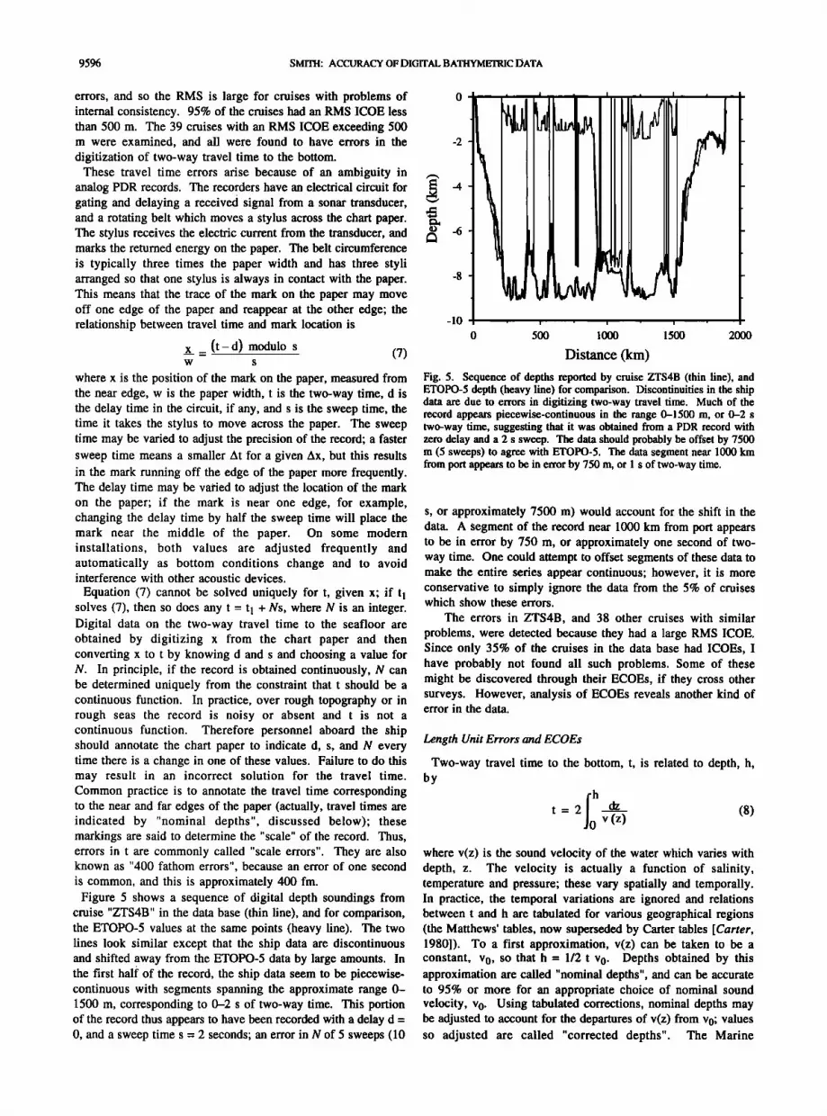
is common, and this is approximately 400 fm. Figure 5 shows a sequence of digital depth soundings from

cruise "ZTS4B" in the data base (thin line), and for comparison, the ETOPO-5 values at the same points (heavy line). The two lines look similar except that the ship data are discontinuous and shifted away from the ETOPO-5 data by large amounts. In the first half of the record, the ship data seem to be piecewise- continuous with segments spanning the approximate range 0- 1500 m, corresponding to 0-2 s of two-way time. This portion of the record thus appears to have been recorded with a delay d = 0, and a sweep time s = 2 seconds; an error in N of 5 sweeps (10

0 i I • I i I a

-2

-]0

0 500 1000 1500 2000

Distance (krn)

Fig. 5. Sequence of depths reported by cruise ZTS4B (thin line), and ETOPO-5 depth (heavy line) for comparison. Discontinuities in the ship data are due to errors in digitizing two-way travel time. Much of the record appears piecewise-continuous in the range 0-1500 m, or 0-2 s two-way time, suggesting that it was obtained from a PDR record with zero delay and a 2 s sweep. The data should probably be offset by 7500 m (5 sweeps) to agree with ETOPO-5. The data segment near 1000 km from port appears to be in error by 750 m, or 1 s of two-way time.

s, or approximately 7500 m) would account for the shift in the data. A segment of the record near 1000 km from port appears to be in error by 750 m, or approximately one second of two- way time. One could attempt to offset segments of these data to make the entire series appear continuous; however, it is more conservative to simply ignore the data from the 5% of cruises which show these errors.

The errors in ZTS4B, and 38 other cruises with similar

problems, were detected because they had a large RMS ICOE. Since only 35% of the cruises in the data base had ICOEs, I have probably not found all such problems. Some of these might be discovered through their ECOEs, if they cross other surveys. However, analysis of ECOEs reveals another kind of error in the data.

Length Unit Errors and ECOEs

Two-way travel time to the bottom, t, is related to depth, h, by

t= 2 dz (8) v(z)

where v(z) is the sound velocity of the water which varies with depth, z. The velocity is actually a function of salinity, temperature and pressure; these vary spatially and temporally. In practice, the temporal variations are ignored and relations between t and h are tabulated for various geographical regions (the Matthews' tables, now superseded by Carter tables [Carter, 1980]). To a first approximation, v(z) can be taken to be a constant, v 0, so that h = 1/2 t v 0. Depths obtained by this approximation are called "nominal depths", and can be accurate to 95% or more for an appropriate choice of nominal sound velocity, v 0. Using tabulated corrections, nominal depths may be adjusted to account for the departures of v(z) from v0; values so adjusted are called "corrected depths". The Marine


Geophysical Data Exchange Format [Hittlernan et al., 1989] calls for the distribution of digital depth sounding data in two forms: as two-way travel times, and as corrected depths. In practice, however, these guidelines are often ignored and nominal depths are the commonly communicated data. Travel times may be recovered from nominal depths if the v 0 used is known. However, analysis of ECOEs shows that there are problems with this approach.

There are 329,058 ECOEs among the cruises in the data base. Examination of the data from surveys which yielded large ECOEs suggests that these ECOEs indicate errors in communicating the nominal depths between the institutions and data centers and the LDEO data base. Figure 6 shows ECOEs

from four cruises in the data base. Each ECOE is plotted as a point in the (x,y) plane, with the cruise's reported value on the y axis and the value reported by the ship it crossed on the x axis. Errors in the ship's values will produce errors in y, and there will also be errors in x if the ship crosses other ships which have erroneous values. The points in the lower right area of the "KK078" panel of Figure 6 exemplify this latter phenomenon. One expects that the dimensionless ratio r = y / x should be near 1 in the majority of the ECOEs. For each cruise I formed a set of r values and estimated the location

(mode) and spread (3 MAD) of this set. Robust estimates of location and spread were used because I expected that there would be some r which were from a different population than

KK078 P7106

Depth in database (km) Depth in database (km) -12 -10 -8 -6 -4 -2 0 -6 -5 -4 -3 -2 -1 0

0 ! ! ! • • ! • 0 i+.+,

i + i +

• -4• ............................................... ! .................. • ................ ! ................................................. '""• :-'"":•' ................................................................................ 1-

• -6 .................................................................................. ß ................................. • ........................................................................................ -3

O -8 ......... -4

I • -5

C2511 FM014

o / , , , , , , , o

• ............................................................................................. • ................................ ,........• ......................................... i ............................................................................................... -3

................................. .................................................................................................................... ................................................................................................................................................................................................. -4

-5

-7 -6 -5 -4 -3 -2 -1 0 -6 -5 -4 -3 -2 -1 0

Depth in database (km) Depth in database (km)

Fig. 6. ECOEs of four cruises, with the cruise's depth value on the y axis and the value of the ship crossed on the x axis. A mistake in interpretation of the nominal sound velocity used to scale travel-time into depth causes the ECOEs to indicate a ratio other than one (see text). Two sound velocities in common use differ by 2.5%, producing an error which is difficult to detect statistically except in fortuitous circumstances (FM014, lower right).


the rest; these are the r which come from x obtained from an erroneous cruise.

Eighty-nine cruises yielded an r value which was different from unity by more than three times the MAD. The ECOEs from each of these were plotted as in Figure 6, and twenty-eight of them were found to cluster tightly around a line with a slope r equal to some value that could be attributed to a plausible error in the length unit. Examples of four of these are shown in Figure 6. Cruise "KK078" yields r = 0.75' this is the ratio of meters of depth to milliseconds of two-way travel time. It seems that in this case depths in meters were printed in the travel time column. Cruise "P7106" yields r = 0.547; this is the ratio of one fathom to one meter. Evidently, data written in fathoms were interpreted to be meters when the data were placed in the data base. Cruise "C2511" yields r = 0.533, or 8:15; this is the ratio of nominal fathoms with v 0 = 800 fm s -], to nominal meters with v0 = 1500 m s -]. Institutions which commonly report depths in nominal meters generally use v 0 - 1500 m s -•, which is a good approximation to v(z) in most areas. This value of v 0 corresponds to approximately 820 fm s -•. Institutions which commonly report depths in nominal fathoms often use v 0 = 800 fm s -1, although some use v0 = 820 fm s -•. Many cruises yielded r values of 1.025 (820:800) or 0.975 (800:820) (FM014 in Figure 6)' I believe these indicate misinterpretation of the value of v 0 used in reporting nominal depths.

I do not think all v 0 errors can be found through analysis of ECOEs. Errors as small as 2.5% are detectable only when there are many ECOEs in deep water among well-navigated and otherwise very accurate data (FM014 in Figure 6). This is because the ECOEs must cluster so well around a line of slope 1.025 that one can be confident that r = 1.025 and not 1. Thus

it is possible that the 2.5% error pervades the data but has gone undetected in most cases. Data from the 28 cruises for which I

were certain of an explanation for an r unequal to one were rescaled by 1/r. However, there remain 61 cruises which show a significant r unequal to one for which there is no plausible explanation. These cruises were placed on a list of data to be ignored.

Comparison to Gravity ECOEs

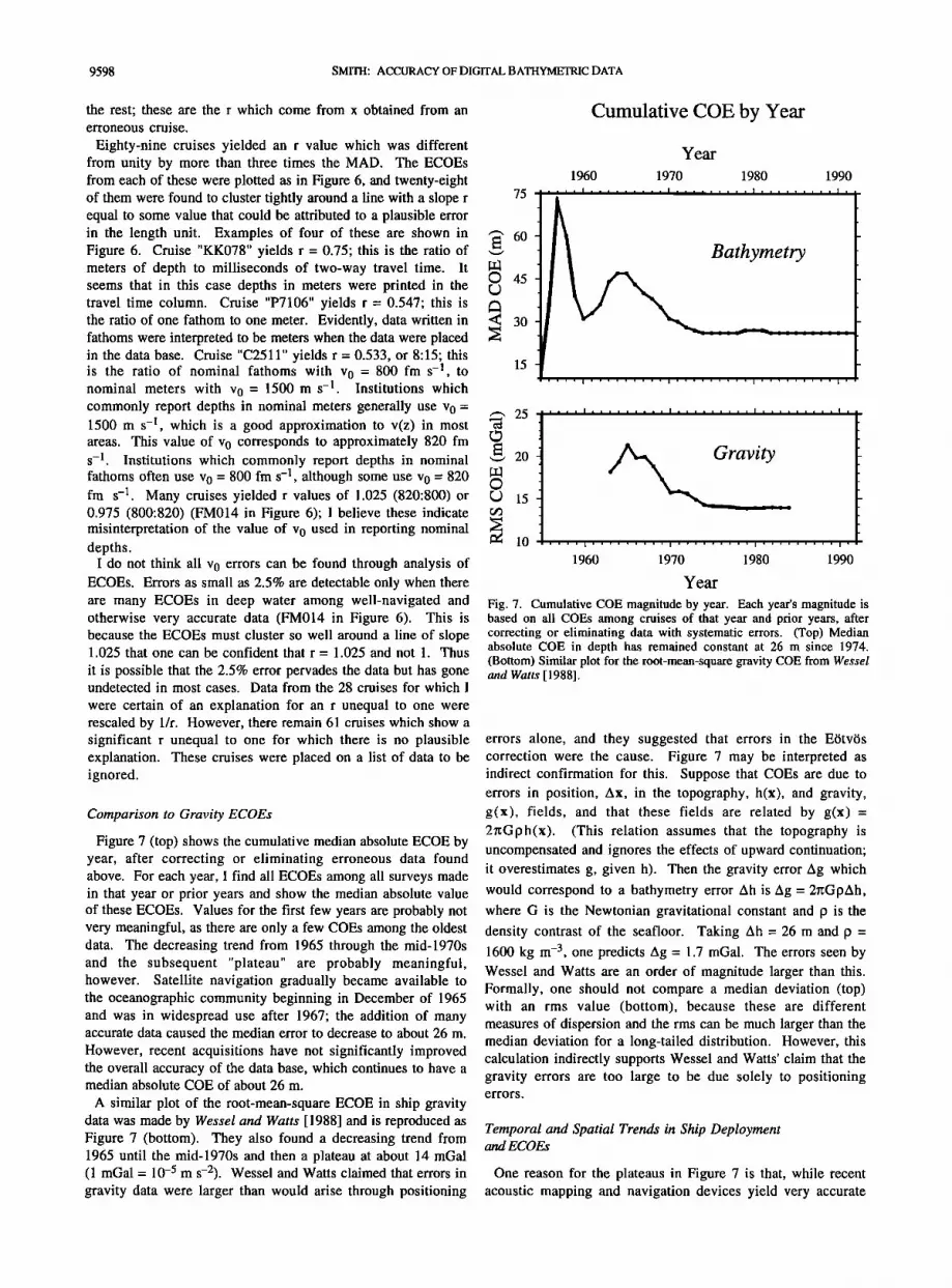
Figure 7 (top) shows the cumulative median absolute ECOE by year, after correcting or eliminating erroneous data found above. For each year, I find all ECOEs among all surveys made in that year or prior years and show the median absolute value of these ECOEs. Values for the first few years are probably not very meaningful, as there are only a few COEs among the oldest data. The decreasing trend from 1965 through the mid-1970s and the subsequent "plateau" are probably meaningful, however. Satellite navigation gradually became available to the oceanographic community beginning in December of 1965 and was in widespread use after 1967; the addition of many accurate data caused the median error to decrease to about 26 m.

However, recent acquisitions have not significantly improved the overall accuracy of the data base, which continues to have a median absolute COE of about 26 m.

A similar plot of the root-mean-square ECOE in ship gravity data was made by Wessel and Watts [ 1988] and is reproduced as Figure 7 (bottom). They also found a decreasing trend from 1965 until the mid-1970s and then a plateau at about 14 mGal (1 mGal = 10 -5 m s-2). Wessel and Watts claimed that errors in gravity data were larger than would arise through positioning

Cumulative COE by Year

75

• 60

15

Year

1960 1970 1980 1990 .... I ......... I ....

,

•, 25

20

L) 15

• 10

ra.vity .... i ......... i ......... i ......... i .

1960 1970 1980 1990

Year

Fig. 7. Cumulative COE magnitude by year. Each year's magnitude is based on all COEs among cruises of that year and prior years, after correcting or eliminating data with systematic errors. (Top) Median absolute COE in depth has remained constant at 26 m since 1974. (Bottom) Similar plot for the root-mean-square gravity COE from Wessel and Watts [1988].

errors alone, and they suggested that errors in the E6tv6s correction were the cause. Figure 7 may be interpreted as indirect confirmation for this. Suppose that COEs are due to errors in position, Ax, in the topography, h(x), and gravity, g(x), fields, and that these fields are related by g(x)= 2nGph(x). (This relation assumes that the topography is uncompensated and ignores the effects of upward continuation; it overestimates g, given h). Then the gravity error Ag which

would correspond to a bathymetry error Ah is Ag = 2nGpAh, where G is the Newtonian gravitational constant and p is the

density contrast of the seafloor. Taking Ah = 26 m and p =

1600 kg m -3, one predicts Ag = 1.7 mGal. The errors seen by Wessel and Watts are an order of magnitude larger than this. Formally, one should not compare a median deviation (top) with an rms value (bottom), because these are different measures of dispersion and the rms can be much larger than the median deviation for a long-tailed distribution. However, this calculation indirectly supports Wessel and Watts' claim that the gravity errors are too large to be due solely to positioning errors.

Temporal and Spatial Trends in Ship Deployment and ECOEs

One reason for the plateaus in Figure 7 is that, while recent acoustic mapping and navigation devices yield very accurate

SMITH: ACCURACY OF DIG1TAL BATHYMETRIC DATA 9599

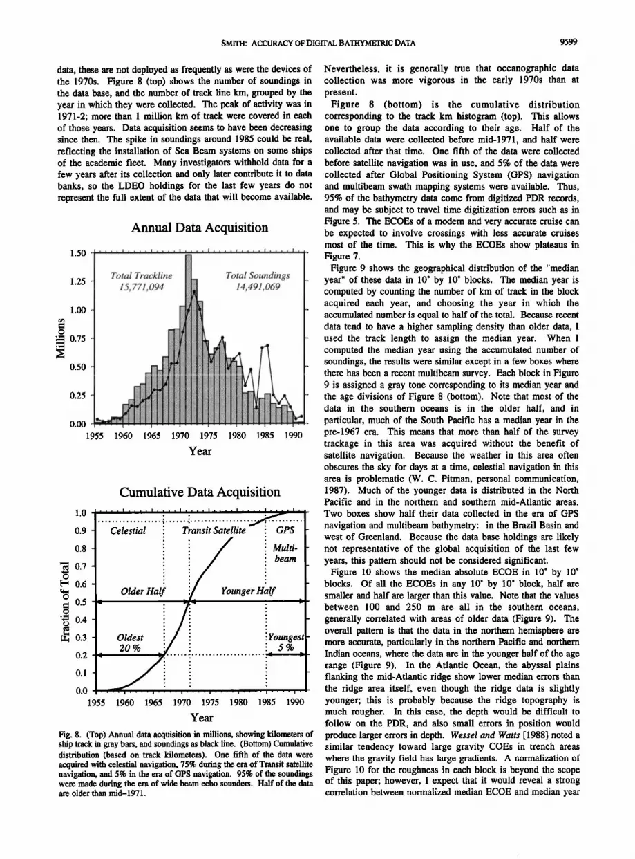
data, these are not deployed as frequently as were the devices of the 1970s. Figure 8 (top) shows the number of soundings in the data base, and the number of track line km, grouped by the year in which they were collected. The peak of activity was in 1971-2; more than 1 million km of track were covered in each of those years. Data acquisition seems to have been decreasing since then. The spike in soundings around 1985 could be real, reflecting the installation of Sea Beam systems on some ships of the academic fleet. Many investigators withhold data for a few years after its collection and only later contribute it to data banks, so the LDEO holdings for the last few years do not represent the full extent of the data that will become available.

Annual Data Acquisition

Total Trackline :iii!• Total Soundings 1.25 - 15, 77 ,491,069 -

1.00 - -

0.75

0.50

0.25 1955 1960 1965 1970 1975 1980 1985 1990

Year

1.0

0.9 -

0.8 -

0.7-

0.6-

0.5 0.4-

0.25

0.2

0.1 -

0.0

1955 1960 1965 1970 1975 1980 1985

Cumulative Data Acquisition ,,,, I ,,, , I, ,,, I i •' . I .... I .... ! ....

Celestial ' Transit Satellite ß GPS ß

: ::Multi- :: !beam .

ß

Older Half • . nger H•If .• ß

Oldest Youngest

20 % ..................... i• 5 % •

.... i .... i .... i .... i .... i .... I .... i ,

1990

Year

Fig. 8. (Top) Annual data acquisition in millions, showing kilometers of ship track in gray bars, and soundings as black line. (Bottom) Cumulative distribution (based on track kilometers). One fifth of the data were acquired with celestial navigation, 75% during the era of Transit satellite navigation, and 5% in the era of GPS navigation. 95% of the soundings were made during the era of wide beam echo sounders. Half of the data are older than mid-1971.

Nevertheless, it is generally true that oceanographic data collection was more vigorous in the early 1970s than at present.

Figure 8 (bottom) is the cumulative distribution corresponding to the track km histogram (top). This allows one to group the data according to their age. Half of the available data were collected before mid-1971, and half were collected after that time. One fifth of the data were collected

before satellite navigation was in use, and 5% of the data were collected after Global Positioning System (GPS) navigation and multibeam swath mapping systems were available. Thus, 95% of the bathymetry data come from digitized PDR records, and may be subject to travel time digitization errors such as in Figure 5. The ECOEs of a modern and very accurate cruise can be expected to involve crossings with less accurate cruises most of the time. This is why the ECOEs show plateaus in Figure 7.

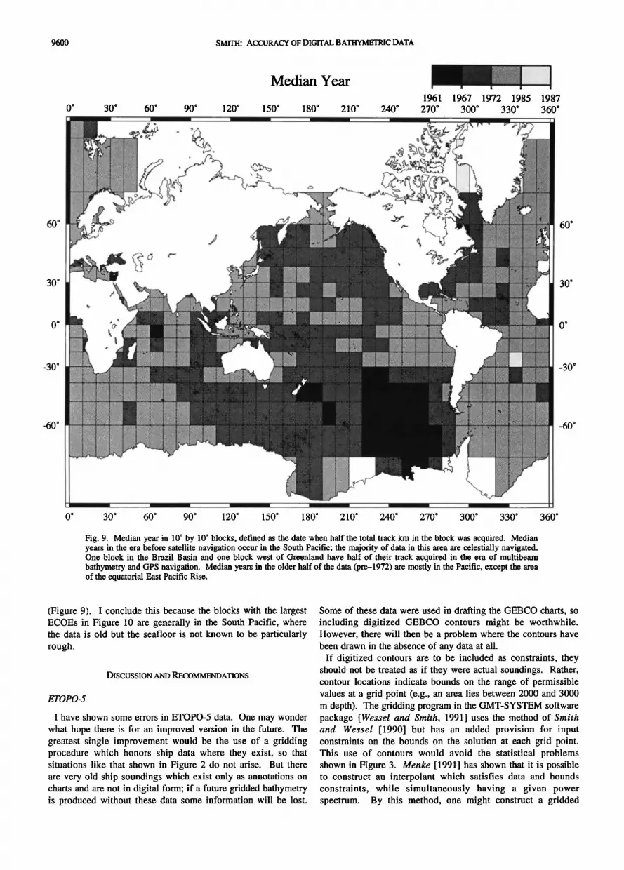
Figure 9 shows the geographical distribution of the "median year" of these data in 10 ø by 10 ø blocks. The median year is computed by counting the number of km of track in the block acquired each year, and choosing the .year in which the accumulated number is equal to half of the total. Because recent data tend to have a higher sampling density than older data, I used the track length to assign the median year. When I computed the median year using the accumulated number of soundings, the results were similar except in a few boxes where there has been a recent multibeam survey. Each block in Figure 9 is assigned a gray tone corresponding to its median year and the age divisions of Figure 8 (bottom). Note that most of the data in the southern oceans is in the older half, and in

particular, much of the South Pacific has a median year in the pre-1967 era. This means that more than half of the survey trackage in this area was acquired without the benefit of satellite navigation. Because the weather in this area often obscures the sky for days at a time, celestial navigation in this area is problematic (W. C. Pitman, personal communication, 1987). Much of the younger data is distributed in the North Pacific and in the northern and southern mid-Atlantic areas.

Two boxes show half their data collected in the era of GPS

navigation and multibeam bathymetry: in the Brazil Basin and west of Greenland. Because the data base holdings are likely not representative of the global acquisition of the last few years, this pattern should not be considered significant.

Figure 10 shows the median absolute ECOE in 10 ø by 10 ø blocks. Of all the ECOEs in any 10 ø by 10 ø block, half are smaller and half are larger than this value. Note that the values between 100 and 250 m are all in the southern oceans,

generally correlated with areas of older data (Figure 9). The overall pattern is that the data in the northern hemisphere are more accurate, particularly in the northern Pacific and northern Indian oceans, where the data are in the younger half of the age range (Figure 9). In the Atlantic Ocean, the abyssal plains flanking the mid-Atlantic ridge show lower median errors than the ridge area itself, even though the ridge data is slightly younger; this is probably because the ridge topography is much rougher. In this case, the depth would be difficult to follow on the PDR, and also small errors in position would produce larger errors in depth. Wessel and Watts [1988] noted a similar tendency toward large gravity COEs in trench areas where the gravity field has large gradients. A normalization of Figure 10 for the roughness in each block is beyond the scope of this paper; however, I expect that it would reveal a strong correlation between normalized median ECOE and median year


o

60 ø

30 ø

o

_30 ø

_60 ø

30 ø 60 ø

Median Year

90 ø 120 ø 150 ø 180 ø 210 ø 240 ø 1961

270 ø

q

1967

300 ø 1972 1985 1987

330 ø 360 ø

60 ø

30 ø

o

_30 ø

_60 ø

0 ø 30 ø 60 ø 90 ø 120 ø 150 ø 180 ø 210 ø 240 ø 270 ø 300 ø 330 ø 360 ø

Fig. 9. Median year in 10 ø by 10 ø blocks, defined as the date when half the total track km in the block was acquired. Median years in the era before satellite navigation occur in the South Pacific; the majority of data in this area are celestially navigated. One block in the Brazil Basin and one block west of Greenland have half of their track acquired in the era of multibeam bathymetry and GPS navigation. Median years in the older half of the data (pre-1972) are mostly in the Pacific, except the area of the equatorial East Pacific Rise.

(Figure 9). I conclude this because the blocks with the largest ECOEs in Figure 10 are generally in the South Pacific, where the data is old but the seafloor is not known to be particularly rough.

DISCUSSION AND RECOMMENDATIONS

ETOPO-5

I have shown some errors in ETOPO-5 data. One may wonder what hope there is for an improved version in the future. The greatest single improvement would be the use of a gridding procedure which honors ship data where they exist, so that situations like that shown in Figure 2 do not arise. But there are very old ship soundings which exist only as annotations on charts and are not in digital form; if a future gridded bathymetry is produced without these data some information will be lost.

Some of these data were used in drafting the GEBCO charts, so including digitized GEBCO contours might be worthwhile. However, there will then be a problem where the contours have been drawn in the absence of any data at all.

If digitized contours are to be included as constraints, they should not be treated as if they were actual soundings. Rather, contour locations indicate bounds on the range of permissible values at a grid point (e.g., an area lies between 2000 and 3000 m depth). The gridding program in the GMT-SYSTEM software package [Wessel and Smith, 1991] uses the method of Smith and Wessel [1990] but has an added provision for input constraints on the bounds on the solution at each grid point. This use of contours would avoid the statistical problems shown in Figure 3. Menke [1991] has shown that it is possible to construct an interpolant which satisfies data and bounds constraints, while simultaneously having a given power spectrum. By this method, one might construct a gridded


60 ø

30 ø

o

_30 ø

_60 ø

o 30 ø 60 ø

Median ECOE

90 ø 120 ø 150 ø 180 ø 210 ø 240 ø 0 25 50 75

270 ø 300 ø 330 ø 100 250

360 ø

60 ø

30 ø

o

_30 ø

_60 ø

0 ø 30 ø 60 ø 90 ø 120 ø 150 ø 180 ø 210 ø 240 ø 270 ø 300 ø 330 ø 360 ø

Fig. 10. Median absolute ECOE in 10 ø by 10 ø blocks. In the South Pacific, half the COEs are larger than 100-250 m. In many areas of the northern hemisphere, where the data are younger, half of the COEs are smaller than 25 m. There is a tendency for the median error to be larger over ridges than over abyssal plains.

bathymetry which agrees with ship data and contour charts and

also has a Ikl½spectrum, for any choice of Recently declassified Geosat Geodetic Mission altimeter data

have revealed gravity anomalies over the southern oceans in unprecedented detail [Sandwell, 1992; McAdoo and Marks, 1992; Marks and McAdoo, 1992; Sandwell and Smith, 1992]. Because the marine gravity field is highly correlated with seafloor topography in the waveband 15 - 150 km, it is possible to use these gravity data to predict bathymetry in this band [Smith and Sandwell, 1992]. If this were done, the improvement in ETOPO-5 might be considerable, but the bathymetry so obtained would be unsuitable for investigations of the transfer function between topography and gravity, because the bathymetry would have been crafted a priori to maximize its correlation with bathymetry. Thus, while bathymetric prediction from satellite altimeter data may yield detailed charts, these should not be used in geodynamic studies.

ETOPO-5 is still the only global, digital representation of the Earth's topography, and it will continue to be used. It makes good index maps for the introduction of presentations. I recommend that investigators who want to use these data for research purposes construct histograms, maps, and spectra as in Figures 2-4, to see if their region has problems which will affect their study. Those who require data for regression may be able to design a resampling scheme in which data are selected from ETOPO-5 at random in a manner which yields a more reasonable distribution of depth values than that of the data set as a whole. Those who will make analyses of topography in the frequency domain should be aware of the [k[ -4 effect in ETOPO-5, and plot the spectrum corresponding to their region before proceeding to analyze the data. After finding the corner frequency, they may filter their data kernels to examine only data outside the Ik1-4 band, or add blue noise to the data. Those who are fitting elastic models should be particularly cautious,


because the Ikl effect comes from an elastic flexure equation and mimics plate flexure. The best thing to do, however, would be to use original ship data where possible.

Ship Data

I have examined crossover errors in bathymetric data in the Lamont-Doherty Earth Observatory's on-line data, which are available over Internet under the view-server system [Menke et al., 1991]. Wessel and Watts [1988] made a similar study of the COEs in gravity data in this data bank. Now that the NGDC data are available on CD-ROM, one may ask whether the LDEO and NGDC versions of the data are similar. Lamont scientists

request data from the NGDC frequently, and so the LDEO data include most of the NGDC data, except perhaps the most recently contributed cruises. Unfortunately, it is difficult to verify this directly, because the LDEO data bank uses five character names for cruises, rather than the eight digit numbers used by NGDC. The NGDC numbers encode the ship, operating institution, and cruise number; the LDEO names are somewhat ad hoc, and often cannot be unambiguously matched to an NGDC number. When a match can be made, it is not always true that the two versions of the data are equivalent. For example, for some cruises operated by the Scripps Institution of Oceanography (SIO) in the 1960s, the LDEO version includes gravity data, while the SIO and NGDC versions do not. Apparently, at that time SIO sent their gravimeter records to LDEO for processing (S. M. Smith, personal communication, 1992). In this instance, the archive at the institution which operated the ship is less complete than the LDEO archive.

One error reported here should be absent from the NGDC data. The data in Figure 6 (panel "C2511") are from the R/V Conrad operated by LDEO, and this error reflects a misunderstanding between the data reduction and data archiving personnel within LDEO. I corrected these data at LDEO and I believe the revised

version was sent to NGDC. This was included in Figure 6 as an example of a common length unit error.

When Wessel and Watts made their COE analysis of gravity data, they found that time was often repeated or out of sequence in the ship data files obtained from NGDC. This happens because the data were originally archived on punched cards, which would get dropped on the floor and shuffled. Wessel and I corrected these problems in the LDEO version of the data before making our studies. Those who access the LDEO data over Internet will have the benefit of these corrections. Those

who use NGDC data should verify that time is a strictly increasing sequence in the data records of each cruise, and compute the velocity from the navigation time series to look for time or position problems.

Cross-over error analysis will not find all problems, so users of either data set should be on the lookout for travel time and

length unit errors. In illustrating travel time errors (Figure 5), I have used the ETOPO-5 data for comparison. I do not mean to suggest that these errors can be detected by comparing ship data against ETOPO-5, as the latter is a poor standard of measurement (Figure 2). One might search for large differences between adjacent values, but this might not detect errors of only a few sweeps in rough terrain, where large differences would be expected. Visual inspection of a plot of the time series of depth values is the best method for detecting travel time errors. Length unit errors may not become obvious until the erroneous data are combined with other data.

The vast quantities of data involved in ocean basin- and global- scale investigations preclude direct inspection of all data. From the results shown here, we may expect that about 5% of the cruises will have travel time errors, and about 4% will have length unit errors. Therefore non-parametric methods which are robust with respect to outliers should be used to estimate geophysical quantities from these data. In particular, least-squares procedures can be expected to have problems with these data.

There is one temporal trend in data acquisition evident in Figure 9 which I believe deserves mention: The majority of southern ocean data are old, and the majority of data in the South Pacific were acquired using only celestial navigation. These data were acquired in an era of block funding to oceanographic institutions which permitted the operation of ships worldwide without concern for the costs of individual surveys. More recently, ship time has been allocated competitively on a cruise by cruise basis, and there has been a trend toward programs which focus on particular environments, and the visiting and revisiting of sites near convenient ports. While this strategy has produced a wealth of data in a few regions, the global distribution of data has grown uneven.

CONCLUSIONS

ETOPO-5 data must be interpreted with caution. First, they are based on contour maps rather than original soundings, which can lead to large errors (Figure 2). Second, their statistical distribution may lead to biased estimates if they are used in regression models for depth-age functions (Figure 3).

Third, their amplitude spectrum is bounded by a Ikl power law (Figure 4), so that they are smoother and have less total variance than the Earth's actual topography. This has an important bearing on gravity-topography transfer function studies of flexural isostasy and mantle convection.

Digital ship soundings may contain travel-time digitization errors (Figure 5). Errors also arise because of misinterpretation of the nominal sound velocity used to report travel time in nominal depth units (Figure 6). These kinds of errors may occur in 4-5% of cruises. Two nominal sound velocities in

common use differ by 2.5%, leading to ambiguities in depth of this magnitude. These are probably too small to detect statistically in most instances. Ship data have been acquired at different rates over time, with the peak of activity in the early 1970s (Figure 8). Although present technologies can yield very accurate data, these are acquired at a rate which is small with respect to the total available data, so that the overall accuracy of the global holdings has remained constant since the late 1970s (Figure 7). Most recent data acquisition has been in the northern hemisphere oceans, and the oldest and least accurate data are in the southern oceans (Figures 9 and 10). The majority of the data in the South Pacific were acquired without the benefit of satellite navigation.

Acknowledgments. This work was begun at the Lamont-Doherty Earth Observatory with support from Office of Naval Research contract N00014-89-J-1191 and was completed with a post-doctoral scholarship from the Cecil H. and Ida Green Foundation for the Earth Sciences at the

Scripps Institution of Oceanography. It would not have been possible without COE software from P. Wessel. R. L. Parker suggested the approach taken in equations (1)-(6). I thank J. Phipps Morgan, D. T. Sandwell, J. G. Sclater, S. Stein, A. B. Watts, P. Wessel, and anonymous reviewers and editors for helpful comments.


REFERENCES

Barnett, V., and T. Lewis, Outliers in Statistical Data, 2nd ed., 463pp., John Wiley, New York, 1984.

Bell, T. H., Statistical features of sea floor topography, Deep Sea Res., 22, 883-892, 1975.

Bowie, W., Isostasy, 275 pp., E. P. Dutton, New York, 1927. Box, G. E. P., Non-normality and tests on variances, Biometrika, 40,

318-335, 1953. Briggs, I. C., Machine contouring using minimum curvature, Geophysics,

39, 39-48, 1974. Calmant, S., and A. Cazenave, The effective elastic lithosphere under

the Cook-Austral and Society Islands, Earth Planet. Sci. Lett., 77, 187- 202, 1986.

Carr, M. H., G. Greeley, K. R. Blasius, J. E. Guest, and J. B. Murray, Some Martian features as viewed from the Viking orbiter, J. Geophys. Res., 82, 3985-4015, 1977.

Carter, D. J. T., Echo Sounding Correction Tables: Formerly Matthews' Tables, 150 pp., Hydrographic Department, Ministry of Defence, Taunton, Somerset, England, 1980.

Cazenave, A., and K. Dominh, Global relationship between oceanic geoid and sea floor depth: New results, Geophys. Res. Lett., 14, 1-4, 1987.

Cazenave, A., K. Dominh, C. J. All•gre, and J. G. Marsh, Global relationship between oceanic geoid and topography, J. Geophys. Res., 91, 11,439-11,450, 1986.

Cazenave, A., S. Houry, B. Lago, and K. Dominh, Geosat-derived geoid anomalies at medium wavelength, J. Geophys. Res., 97, 7081-7096, 1992.

Fleitout, L., C. Dalloubeix, and C. Moriceau, Small-wavelength geoid and topography anomalies in the South Atlantic Ocean-A clue to new hot-spot tracks and lithospheric deformation, Geophys. Res. Lett., 16, 637-640, 1989.

Ford, P. G., and G. H. Pettengill, Venus topography and kilometer-scale slopes, J. Geophys. Res., 97, 13,103-13,114, 1992.

Fox, C. G., and D. E. Hayes, Quantitative methods for analyzing the roughness of the seafloor, Rev. Geophys., 23, 1-48, 1985.

Goslin, J., and M. Diament, Mechanical and thermal isostatic response of the Del Cano Rise and Crozet Bank (southern Indian Ocean) from altimetry data, Earth Planet. Sci. Lett., 84, 285-294, 1987.

Hampel, F. R., The influence curve and its role in robust estimation, J. Am. Stat. Assoc., 69, 383-393, 1974.

Hayes, D. E., Age-Depth relationships and depth anomalies in the Southeast Indian Ocean and Atlantic Ocean, J. Geophys. Res., 93, 2937-2954, 1988.

Hittleman, A.M., R. C. Groman, R. T. Haworth, T. L. Holcombe, G. McHendrie, and S. M. Smith, The Marine Geophysical Data Exchange Format MGD77, Key to Geophysical Records Documentation 10, National Geophysical Data Center, National Oceanographic and Atmospheric Administration, Boulder, Colo., 1977. (Revised edition, 1989.)

Huber, P. J., Robust Statistics, 308 pp., John Wiley, New York, 1981. Jeffreys, H., The Earth, 6th ed., 574 pp., Cambridge University Press,

New York, 1976. Johnson, R. H., Reduction of discrepancies at crossing points in

geophysical surveys, J. Geophys. Res., 76, 4892-4896, 1971. Luskin, B., and A. C. Roberts, Precision Depth Recorder Mk IV-A,

Lamont Doherty Earth Obs., Tech. Rep. 6, CU-tS-55-N6 onr 27124 Geol., Columbia Univ., Palisades, N.Y., 1955.

Maia, M., J. Diament, and M. Recq, Isostatic response of the lithosphere beneath the Mozambique Ridge (SW Indian Ocean) and geodynamic implications, Geophys. J. lnt., 100, 337-348, 1990.

Malinverno, A., Testing linear models of sea-floor topography, Pure Appl. Geophys., 131,139-155, 1989.

Marks, K. M., and D.C. McAdoo, Marine gravity from Geosat GM data south of 30øS, EOS Trans. AGU, 73 (43), Fall Meeting Suppl., 133, 1992.

Marty, J. C., and A. Cazenave, Regional variations in subsidence rate of oceanic plates: a global analysis, Earth Planet. Sci. Lett., 94, 301-315, 1989.

McAdoo, D.C., and K. M. Marks, Gravity fields of the southern ocean from Geosat data, J. Geophys. Res., 97, 3247-3260, 1992.

McNutt, M. K., Thermal and mechanical properties of the Cape Verde Rise, J. Geophys. Res., 93, 2784-2794, 1988.

McNutt, M. K., and A. V. Judge, The superswell and mantle dynamics beneath the South Pacific, Science, 248, 933-1048, 1990.

McNutt, M. K., and L. Shure, Estimating the compensation depth of the Hawaiian Swell with linear filters, J. Geophys. Res., 91, 13,915- 13,923, 1986.

Menke, W., Applications of the POCS inversion method to interpolating topography and other geophysical fields, Geophys. Res. Lett., 18, 435- 438, 1991.

Menke, W., P. Friberg, A. Lerner-Lam, D. Simpson, R. Bookbinder, and G. Karner, Sharing data over Internet with the Lamont view-server system, EOS Trans. AGU, 72, 409, 413-414, 1991.

Monnereau, M., and A. Cazenave, Depth and geoid anomalies over oceanic hotspot swells: A global survey, J. Geophys. Res., 95, 15,429- 15,438, 1990.

Morgan, J.P., and W. H. F. Smith, Flattening of the sea-floor depth-age curve as a response to asthenospheric flow, Nature, 359, 524-527, 1992.

National Geophysical Data Center, ETOPO-5 bathymetry/topography data, Data Announc. 88-MGG-02, Natl. Oceanic and Atmos. Admin., U.S. Dep. Commer., Boulder, Colo., 1988.

National Geophysical Data Center, GEODAS CD-ROM worldwide marine geophysical data, Data Announc. 92-MGG-02, Natl. Oceanic and Atmos. Admin., U.S. Dep. Commer., Boulder, Colo., 1992.

Parsons, B. and J. Sciater, An analysis of the variation of ocean floor bathymetry and heat flow with age, J. Geophys. Res., 82, 803-827, 1977.

Press, W. H., B. P. Flannery, S. A. Teukolsky, and W. T. Vetterling, Numerical recipes, 818 pp., Cambridge Univ. Press, New York, 1986.

Prince, R. A., and D. W. Forsyth, A simple objective method for minimizing crossover errors in marine gravity data, Geophysics, 49, 1070-1083, 1984.

Renkin, M. L., and J. G. Sclater, Depth and age in the North Pacific, J. Geophys. Res., 93, 2919-2935, 1988.

Rousseeuw, P. J., and A.M. Leroy, Robust Regression and Outlier Detection, 329 pp., John Wiley, New York, 1987.

Sandwell, D. T., Antarctic marine gravity field from high-density satellite altimetry, Geophys. J. Int., 109, 437-448, 1992.

Sandwell, D. T., and K. R. MacKenzie, Geoid height versus topography for oceanic plateaus and swells, J. Geophys. Res., 94, 7403-7418, 1989.

Sandwell, D. T., and M. L. Renkin, Compensation of swells and plateaus in the North Pacific: No direct evidence for mantle convection, J. Geophys. Res., 93, 2919-2935, 1988.

Sandwell, D. T., and W. H. F. Smith, Global marine gravity from ERS-1, Geosat, and Seasat reveals new tectonic fabric, EOS Trans. A GU, 73 (43), Fall Meeting Suppl., 133, 1992.

Sheehan, A. F., and M. K. McNutt, Constraints on thermal and mechanical structure of the ocean lithosphere at the Bermuda Rise from geoid height and depth anomalies, Earth Planet. Sci. Lett., 93, 377-391, 1989.

Smith, W. H. F., and D. T. Sandwell, Charting the remote southern oceans with satellite altimetry and shipboard bathymetry, EOS Trans AGU, 73 (14), Spring Meeting Suppl., 85, 1992.

Smith, W. H. F., and P. Wessel, Gridding with continuous curvature splines in tension, Geophysics, 55, 293-305, 1990.

Stein, C. A., and S. Stein, A model for the global variation in oceanic depth and heat flow with lithospheric age, Nature, 359, 123-129, 1992.

Van Wyckhouse, R., SYNBAPS, Tech. Rep. TR-233, U.S. Natl. Oceanogr. Off., Stennis Space Center, Miss., 1973.

Wessel, P., XOVER: A cross-over error detector for track data, Cornput. Geosci., 15, 333-346, 1989.

Wessel, P. and A. B. Watts, On the accuracy of marine gravity measurements, J. Geophys. Res., 93, 393-413, 1988.

Wessel, P., and W. H. F. Smith, Free software helps map and display data, EOS Trans. Amer. Geophys. U., 72, 441-446, 1991.

W. H. F. Smith, NOAA N/OES12, SSMC IV Sta. 8423, 1305 East-West Highway, Silver Spring, MD 209 i0.

(Received May 29, 1992; revised March 1, 1993;

Accepted March 8, 1993.)

on the accuracy of digital bathymetric data

Documents