on spontaneous baryogenesis and transport phenomena
TRANSCRIPT
arX
iv:h
ep-p
h/94
0636
9v1
22
Jun
1994
DFPD 94/TH/39SISSA 94/82-A
On Spontaneous Baryogenesis and Transport Phenomena
D. Comellia,b,1 , M. Pietronic,2 and A. Riottoc,d,3
(a)Dipartimento di Fisica Teorica Universita di Trieste,
Strada Costiera 11, 34014 Miramare, Trieste, Italy
(b) Istituto Nazionale di Fisica Nucleare,
Sezione di Trieste, 34014 Trieste, Italy
(c)Istituto Nazionale di Fisica Nucleare,
Sezione di Padova, 35100 Padua, Italy.
(d)Instituto de Estructura de la Materia, CSIC,
Serrano, 123, E-20006 Madrid, Spain
Abstract
The spontaneous baryogenesis mechanism by Cohen, Kaplan and Nelson is reconsidered takinginto account the transport of particles inside the electroweak bubble walls. Using linear response
theory, we calculate the modifications on the thermal averages of the charges of the systemdue to the presence of a space time dependent ‘charge potential’ for a quantum number not
orthogonal to baryon number. The local equilibrium configuration is discussed, showing that,as a consequence of non zero densities for conserved charges, the B +L density is driven to non
zero values by sphaleronic processes.Solving a rate equation for the baryon number generation, we obtain an expression for
the final baryon asymmetry of the Universe containing the relevant parameters of the bubblewall, i.e. its velocity, its width, and the width of the region in which sphalerons are active.
Compared to previous estimates in which transport effects were not taken into account, we findan enhancement of nearly three orders of magnitude in the baryon asymmetry.
Finally, the role of QCD sphalerons in cooperation with transport effects is analyzed, show-
ing that the net result depends crucially on the particle species which enter into the chargepotential.
1Email: [email protected]; supported by Schweizerischen national funds.2Email: [email protected]; address after September 1, 1994: Deutsches Elektronen - Synchrotron,
DESY, Hamburg, Germany3Email: [email protected]; on leave of absence from International School for Advanced Studies (ISAS),
Trieste, Italy
1. Introduction
The possibility of a baryogenesis at the electroweak scale is a very popular but controversial
topic. Despite the large number of related publications [1], none of the key aspects of this
subject can be considered to be on firm ground. First, it is well known that the requirement
that the anomalous ‘sphaleronic’ processes which violate baryon number (B) go out of equilib-
rium soon after the transition translates into a lower bound on the ratio between the vacuum
expectation value (VEV) of the Higgs field, v(T ), and the critical temperature of the transition,
Tc, v(Tc)/Tc >∼1. In the standard model, improved perturbative evaluations of this ratio [2] give
a value which is badly less than unity for values of the mass of the Higgs scalar compatible with
LEP results. The situation in the minimal supersymmetric standard model is slightly better,
however the allowed region of the parameter space is very small, and is likely to be excluded
by future LEP data [3]. On the other hand, the perturbative expansion cannot be trusted
any more for values of the Higgs masses of the order of the W boson mass or larger [4], and
preliminary results based on non perturbative methods (lattice simulations [5], 1/ε expansion
[6], effective action [7]) give indications of strong differences of the results with respect to those
obtained perturbatively. Clearly, much work is still needed on this issue.
Another aspect of the problem is CP violation. This has been the subject of a recent debate
in the literature about the need of further complex phases in the theory besides the one in the
Cabibbo-Kobayashi-Maskawa mixing matrix (see. [8]). In models with more than one Higgs
doublet, like the minimal supersymmetric standard model, further sources of CP violation can
emerge naturally from the Higgs sector. In particular, the possibility of a spontaneous CP
violation at finite temperature has been emphasized [9, 10, 11]. This effect could give enough
contribution for the baryogenesis and at the same time satisfy the upper bounds on CP violation
coming from the electric dipole moment of the neutron.
Even assuming that the phase transition is strong and that CP violation is enough, we
must face the other key issue, namely what is the mechanism responsible for the generation
of baryons during the phase transition. The most significant departure from thermodynamic
equilibrium takes place at the passage of the walls of the expanding bubbles which convert
the unbroken into the broken phase. According to the size and speed of the bubble walls, two
different mechanisms are thought to be dominant. In the case of “thin” (width ∼ 1/T ) walls,
typical of a very strong phase transition, the creation of baryons occurs via the asymmetric
(in baryon number) reflection of quarks from the bubble wall, which biases the sphaleronic
transitions in the region in front of the expanding bubble [12]. If the walls are “thick” (width∼(10 − 100)/T ) then the relevant mechanism takes place inside the bubble walls rather than
1

in front of them. In this case we can make a distinction between ‘fast’ processes (mediated
by gauge, flavour diagonal, interactions and by top Yukawa interactions) and ‘slow’ processes
(mediated by Cabibbo suppressed gauge interactions and by light quarks Yukawa interactions).
The former are able to follow adiabatically the changing of the Higgs VEV inside the bubble
wall, while, in first approximation, the latter are frozen during the passage of the wall. If CP
violation, explicit or spontaneous, is present in the scalar sector then a space-time dependent
phase for the Higgs VEVs is turned on inside the wall. The time derivative of this phase
couples with the density of a quantum number non orthogonal to baryon number (e.g. fermion
hypercharge density) 4 and then can be seen as an effective chemical potential, named “charge
potential”, which has the effect of biasing the rates of the sphaleronic processes, creating an
asymmetry proportional to ϑ, where ϑ is the phase of the VEVs.
This “adiabatic scenario”, originally due to Cohen, Kaplan, and Nelson (CKN) [14], has been
recently reconsidered by different authors in different but related aspects. First, Giudice and
Shaposhnikov have shown the dramatic effect of non perturbative, chirality breaking, transitions
induced by the so called “QCD sphalerons” [15]. If these processes were active inside the bubble
walls, then the equilibrium value for baryon number in the adiabatic approximation would be
proportional to that for the conserved quantum number B − L (L is the lepton number), up
to mass effects suppressed by ∼ (mtop(T )/πT )2. Then, imposing the constraint 〈B − L〉 = 0
(here 〈· · ·〉 represents the thermal average) we obtain zero baryon number (up to mass effects).
Dine and Thomas [16] have considered the two Higgs doublets model in which the same
doublet couples both to up and down quarks, the same model considered in the original work
by CKN. These authors have pointed out that ϑ couples also to the Higgs density, so that the
induced charge potential is for total hypercharge rather than for fermion hypercharge. As long
as effects proportional to the temperature dependent VEV v(T ) are neglected, hypercharge
is a exactly conserved quantum number and then, again imposing the constraint that all the
conserved charges have zero thermal averages, no baryon asymmetry can be generated. So, we
again find a mtop(T )2/T 2 suppression factor.
Finally, Joyce, Prokopec and Turok (JPT) have emphasized the very important point that
the response of the plasma to the charge potential induced by ϑ is not simply that of a system
of fixed charges, because transport phenomena may play a crucial role [17]. When a space time
dependent charge potential is turned on at a certain point, hypercharged particles are displaced
from the surrounding regions, so that even the thermal averages of conserved quantum numbers
become locally non vanishing. As a consequence, the equilibrium properties of the system have
to be reconsidered taking into account the local ‘violation’ of the conserved quantum numbers.
4The phase also couples to Chern-Simons number but this coupling induces an effect which is suppressed bymtop(T )2/T 2 with respect to the one which we are presently discussing [13], so we will neglect it.
2
In this paper we analyze the adiabatic scenario using linear response theory [18, 23] in order
to take transport effects into account. We assume that a spacetime dependent charge potential
for fermion hypercharge is generated inside the bubble wall, without discussing its origin, and
investigate its effect on the thermal averages of the various quantum numbers of the system.
We find that transport phenomena are really crucial, but we disagree with JPT’s conclusion
that as a consequence of the local ‘violation’ of global quantum numbers there is no biasing
of the sphaleronic processes. Actually, in the adiabatic approximation the local equilibrium
configuration of the system is determined by the thermal averages of the charges conserved by
all the fast interactions. The effect of transport phenomena is to induce space time dependent
non zero values for these averages. We calculate these averages using linear response theory and
then determine the local equilibrium configuration, showing that it corresponds to 〈B+L〉 6= 0.
As we will discuss, JPT’s result corresponds to freezing out any interaction inside the bubble
wall, which is in contradiction with the adiabatic hypothesis. Then we write down a rate
equation in order to take into account the slowness of the sphaleron transitions and obtain
an expression for the final baryon asymmetry explicitly containing the parameters describing
the bubble wall, such as its velocity, vw, its width, and the width of the region in which the
sphalerons are active.
The inclusion of transport phenomena also sheds a new light on the strong sphaleron ef-
fects and on the effect of a charge potential for total rather than fermionic hypercharge. The
dramatic suppressions found by Giudice and Shaposhnikov and by Dine and Thomas respec-
tively, are both a consequence of taking zero averages for conserved quantum numbers. Since
these averages are no more locally zero we will find a non zero 〈B + L〉 6= 0, even in the case
in which the charge potential is for total rather than for fermion hypercharge. In the case
of QCD sphalerons we find that the final result depends in a crucial way on the form of the
charge potential which is considered. For example, if all the left handed fermions plus the right
handed quarks contributed to the charge potential according to their hypercharge, then no bias
of sphaleron processes would be obtained. In this case, we would find a non zero value for B+L
inside the bubble wall but no baryon asymmetry far from it inside the broken phase. On the
other hand, if only right and left handed top quarks participate to the charge potential, then a
final asymmetry is found and QCD sphalerons are harmless.
The plan of the paper is as follows: in section 2 we will develop a chemical potential
analysis for the equilibrium properties of the plasma inside the bubble wall in the adiabatic
approximation, and we will write down the rate equation fro the production of B + L due to
sphaleron transitions; in sect. 3 we will introduce our application of linear response analysis
to the calculation of the variations of the thermal averages induced by ϑ. In particular we will
show that the fundamental quantity to evaluate is the retarded two points Green’s function for
3

fermion currents. In section 4 we will solve the rate equation, finding an expression for the final
baryon asymmetry in terms of the various bubble wall parameters. In this context, we will also
discuss the screening effects on the electric charge. In sect. 5 we will discuss the role of QCD
sphalerons in cooperation with transport phenomena, and finally we will discuss our results in
section 6.
2. Local equilibrium inside the wall
For definiteness, we will work in the two Higgs doublet model in which one doublet couples
to up quarks and the other one to down quarks. The phase transition is assumed to be strong
enough so that sphaleron processes freeze out somewhere inside the bubble wall (see the end
of sect. 4 and ref. [16] for a discussion about this point).
The relevant timescale for baryogenesis is given by the passage of the bubble wall, which
takes ∆tw = ∆z/vw ≃ (200)/T [19], where ∆z is the wall thickness. During this time the
phase of the Higgs VEV’s changes of an amount ∆ϑ. Thus, we can discriminate between fast
processes, which have a rate >∼1/∆tw and then can equilibrate adiabatically with ϑ, and slow
interactions, which feel that ϑ is changing only when the bubble has already passed by and
sphalerons are no more active. Next, we introduce a chemical potential for any particle which
takes part to fast processes, and then reduce the number of linearly independent chemical
potentials by solving the corresponding system of equations, in a way completely analogous to
that followed for example in refs. [20], the main difference here being that light quark Yukawa
interactions and Cabibbo suppressed gauge interactions are out of equilibrium. Finally, we
can express the abundances of any particle in equilibrium in terms of the remaining linear
independent chemical potentials, corresponding to the conserved charges of the system.
Since strong interactions are in equilibrium inside the bubble wall, and since the current
coupled to ϑ is color singlet, we can chose the same chemical potential for quarks of the same
flavour but different color, and set to zero the chemical potential for gluons. Moreover, since
inside the bubble wall SU(2) × U(1) is broken, the chemical potential for the neutral Higgs
scalars vanishes5.
The other fast processes, and the corresponding chemical potential equations are:
i) top Yukawa:tL + H0
2 ↔ tR + g (µtL = µtr)bL + H+ ↔ tR + g (µtR = µbL
+ µH+)(1)
5This is true if chirality flip interactions, or processes like Z → Z∗h, are sufficiently fast; since the corre-sponding rates depend on the Higgs VEV, they will be suppressed by factors of (v(T )/T )2 with respect forexample to the rate for htL ↔ tRg. This has led the authors of refs.[15, 17] to consider the system in theunbroken phase. Anyway, this choice does not lead to dramatic changes to the conclusion of this paper.
4
ii) SU(2) flavour diagonal:
eiL ↔ νi
L + W− (µνiL
= µeiL
+ µW+)
uiL ↔ di
L + W+ (µuiL
= µdiL
+ µW+)
H02 ↔ H+ + W− (µH+ = µW+)
H01 ↔ H− + W+ (µH− = −µW+)
(i = 1, 2, 3) (2)
Neutral current gauge interactions are also in equilibrium, so we have zero chemical potential
for the photon and the Z boson.
Imposing the above constraints, we can reduce the number of independent chemical po-
tentials to four, µW+, µtL , µuL≡ 1/2
∑2i=1 µui
L, and µeL
≡ 1/3∑3
i=1 µeiL. These quantities
correspond to the four linearly independent conserved charges of the system. Choosing the
basis Q′, (B − L)′, (B + L)′, and BP ′ ≡ B′3 − 1/2(B′
1 + B′2), where the primes indicate that
only particles in equilibrium contribute to the various charges, and introducing the respective
chemical potentials, we can go to the new basis using the relations
µQ′ = 3µtL + 2µuL− 3µeL
+ 11µW+
µ(B−L)′ = 3µtL + 4µuL− 6µeL
− 6µW+
µ(B+L)′ = 3µtL + 4µuL+ 6µeL
µBP ′ = 3µtL − 2µuL
(3)
If sphaleron transitions were fast, then we could eliminate a further chemical potential
through the constraint
23∑
i=1
µuiL
+3∑
i=1
µdiL
+3∑
i=1
µeiL
= 0. (4)
In this case, the value of (B + L)′ would be determined by that of the other three charges
according to the relation
(B + L)′EQ =3
80Q′ +
7
20BP ′ − 19
40(B − L)′ (5)
where we have indicated charge densities by the corresponding charge symbols. We have ne-
glected mass effects, which means that the excess of particle over antiparticle density is related
to the chemical potentials according to the relation [20] n+ − n− = agT 3/6(µ/T ), where a = 1
for fermions and a = 2 for bosons, and g is the number of spin and color degrees of freedom.
The above result should not come as a surprise, since we already know from ref. [20] that a
non zero value for B − L gives rise to a non zero B + L at equilibrium. Stated in other words,
sphaleron transitions erase the baryon asymmetry only if any conserved charge of the system
has vanishing thermal average, otherwise the equilibrium point lies at (B + L)EQ 6= 0.
Actually, sphaleron rates are too small to allow (B + L)′ to reach its equilibrium value (5),
τsp ≃ (α4WT )−1 ≫ ∆tW , so equilibrium thermodynamics cannot be used to describe baryon
5
number generation inside the bubble wall. Following refs. [21, 14] we shall make use of the rate
equationd
dt(B + L)′SP = −ΓSP
T
∂F
∂(B + L)′(6)
where ΓSP = k(αW T )4 exp(−φ/gWT ) is the rate of the sphaleron transitions when the value
of the Higgs field is φ (k ≃ (0.1 − 1) from numerical simulations [22]), F is the free energy of
the system, and the derivative with respect to (B + L)′ must be taken keeping Q′, (B − L)′,
and BP ′, constant. The meaning of eq. (6) is straightforward. Sphaleron transitions (which
change (B + L)′ but conserve Q′, (B − L)′, and BP ′) will be turned on only if they allow the
total free energy of the system to get closer to its minimum, i.e. equilibrium, value. At high
temperature (µi ≪ T ) the free energy of the system is given by
F = T 2
12
[3µ2
eL+ 3µ2
νL+ 6µ2
uL+ 3µ2
tL+ 3µ2
tR+ 6µ2
dL+ 3µ2
bL
+6µ2W+ + 2µ2
H+ + 2µ2H0
1
+ 2µ2H0
2
].
(7)
Using (1), (2) and (3) to express the chemical potentials in terms of the four conserved charges
in (3) we obtain the free energy as a function of the density of (B + L)′ = µB+LT 2/6,
F [(B + L)′] = 0.46
[(B + L)′ − (B + L)′EQ
]2
T 2+ constant terms (8)
where the “constant terms” depend on Q′, (B−L)′, and BP ′ but not on (B+L)′, and (B+L)′EQ
is given by (5). The total amount of (B + L)′ present in a certain point at a certain time is
made up by two contributions: (B + L)′SP , generated by sphaleron transitions, and (B + L)′TR,
which is not generated but is transported from nearby regions in response to the perturbation
introduced by ϑ. So, eq. (6) now takes the form
d
dt(B + L)′SP = −0.92
ΓSP
T 3
[(B + L)′SP + (B + L)′TR − (B + L)′EQ
](9)
with the initial condition (B + L)′SP = 0 before ϑ is turned on.
Let us summarize our discussion up to this point. Consider an observer in the plasma
reference frame during the phase transition. When a bubble wall passes by the observer, he
measures a space time dependent charge potential for, say, fermionic hypercharge, which induces
transport phenomena and then local asymmetries in particle numbers. The Q′, (B − L)′, and
BP ′ components of these asymmetries remain unaffected by fast interactions, while the other
components are reprocessed as to obtain their equilibrium values. In the case of (B + L)′ the
reprocessing is slow, so we have to use the rate equation in (9) to describe it. The generation of
(B + L)′SP will go on until either ΓSP goes to zero or the local equilibrium value is reached i.e.
(B + L)′SP + (B + L)′TR = (B + L)′EQ. After the passage of the wall, (B + L)′EQ and (B + L)′TR
6
go rapidly to zero since ϑ vanishes, and so the final asymmetry is given by the (B + L)′SP
generated until that time.
As we can see, the crucial question is now to calculate the induced values for Q′, (B − L)′,
BP ′, and (B + L)′TR. We will do that in the next section by using linear response analysis
[18, 23].
3. Linear response analysis
In this paragraph we want to discuss the effect on the thermal averages of the term induced
in the lagrangian when ϑ is active, which we assume to have the form
L → L + ϑJ0YF
, (10)
with
J0YF
=∑
i′yi
FJ0i (11)
where∑′
i means that the sum extends on particles in equilibrium with ϑ only. The standard
procedure [14] is to consider ϑ as an effective chemical potential, so that particle abundances
at equilibrium are given by
ρi = qiµQ + (b − l)iµB−L + bpiµBP + yFi ϑ, (12)
and then imposing
〈Q′〉 = 〈(B − L)′〉 = 〈BP ′〉 = 0 (13)
so that any particle abundance can be expressed in terms of ϑ only. The point is that taking
transport phenomena into account, the above thermal averages are not zero, but depend on ϑ
themselves. So we must first calculate their values and then use them to determine the chemical
potentials. Our starting point is the generating functional
Z[JO; ϑ] =∫
P (A)BCDφ exp
{i∫
Cdτ∫
Vd3~x
[L + ϑJ0
YF+ JOO + ‘sources′
]}(14)
where Dφ is the integration measure, O is the operator of which we want to calculate the
thermal average and JO the corresponding source. C is any path in the complex τ plane
connecting the point τin to τout = τin − iβ (β = 1/T ) such that the imaginary part of τ is never
increasing on the path [24]. P(A)BC means that periodic (antiperiodic) boundary conditions
must be imposed on bosonic (fermionic) fields on the path.
The thermal average of the operator O(τ, ~x) in presence of ϑ is obtained in the usual way
〈O(tx, ~x)〉ϑ 6=0 =1
i
δZ[JO; ϑ]
δJO(tx, ~x)
∣∣∣∣∣JO=0
. (15)
7
Im(τ)0
R⌉(τ)
τin = tx
τout −iβ
s -
?
s
6
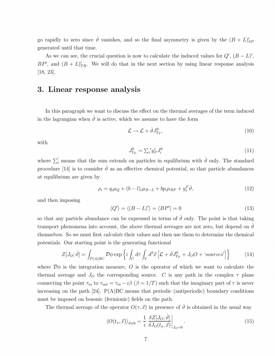
Figure 1: The path C corresponding to imaginary time formalism of thermal field theory.
where all the field sources are set to zero. Now we make a functional expansion of (15) in ϑ
and truncate it at the linear term,
〈O(tx, ~x)〉ϑ 6=0 =1
i
δ
δJO(tx, ~x)
{Z[JO; ϑ = 0]
+∫
Cdτ ′
∫
Vd3~y ϑ(τ ′, ~y)
δZ[JO; ϑ]
δϑ(τ ′, ~y)
∣∣∣∣∣ϑ=0
+ . . .
}∣∣∣∣∣JO=0
= 〈O(tx, ~x)〉ϑ=0 + i∫
Cdτ ′
∫
Vd3~y ϑ(τ ′, ~y) 〈TCJ0
YF(τ ′, ~y) O(tx, ~x)〉ϑ=JO=0
(16)
where TC is the ordering along the path C.
Different choices for the ‘time’ contour C lead to different formulations of thermal field
theory. One possibility is to take the vertical line connecting tx to tx − iβ, so that τ ′ − tx is
pure imaginary on any point of the path.
This choice corresponds to the imaginary time formalism (ITF) of thermal field theory
[24], and in this case we have to evaluate the euclidean two point thermal Green’s function
〈TJ0YF
(zE), O(0)〉 (z2E = −z2
0 −|~z|2). This can be done in Matsubara formalism, where Feynman
rules are straightforwardly obtained [23]. But, in this case, we would have to calculate ϑ for
complex times, whereas we are interested in its values at real times, during the passage of the
wall. So, in order to get a more direct physical interpretation of what we are calculating, we
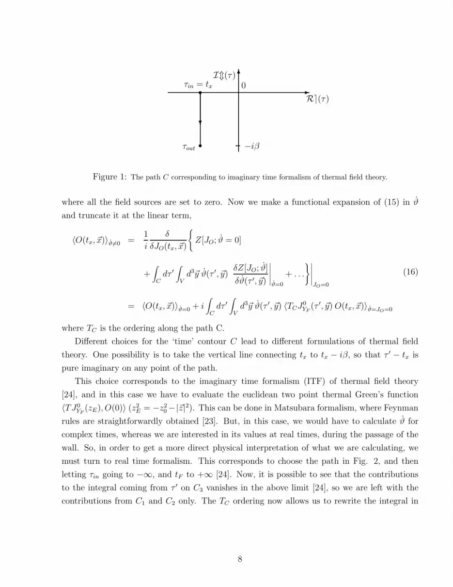
must turn to real time formalism. This corresponds to choose the path in Fig. 2, and then
letting τin going to −∞, and tF to +∞ [24]. Now, it is possible to see that the contributions
to the integral coming from τ ′ on C3 vanishes in the above limit [24], so we are left with the
contributions from C1 and C2 only. The TC ordering now allows us to rewrite the integral in
8
C3
C2
Im(τ)C10
R⌉(τ)
tFτin tx
τout −iβ
s ss
s
s --�
?
6
Figure 2: The path C corresponding to real time formulation of thermal field theory. C2 lies infinitesimallybeneath the real axis.
(16) as
i∫
C1⊕C2
dty
∫
Vd3~y ϑ(ty, ~y) 〈TCJ0
YF(ty, ~y) O(tx, ~x)〉ϑ=JO=0
= i∫ tx
−∞dty
∫
Vd3~y ϑ(ty, ~y) 〈
[J0
YF(ty, ~y), O(tx, ~x)
]〉ϑ=JO=0.
(17)
Defining as usual the retarded Green’s function
iDRO,YF
(tx, ~x; ty, ~y) ≡ 〈[O(tx, ~x), J0
YF(ty, ~y)
]〉Θ(tx − ty) (18)
where Θ(x) is the step function, we arrive at the result
〈O(tx, ~x)〉ϑ 6=0 = 〈O(tx, ~x)〉ϑ=0 +∫ +∞
−∞dty
∫
Vd3~y ϑ(ty, ~y)DR
O,YF(tx, ~x; ty, ~y). (19)
The operators we are interested in are fermionic charge densities (Q′, (B −L)′, (B + L)′, BP ′)
of the form Q′A =
∑′i q
Ai J0
i . Inserting it in (19), and using definition (11) we get
〈Q′A(tx, ~x)〉ϑ6=0 =
∑′ijq
Ai yF
i
∫ +∞
−∞dty
∫
Vd3~y ϑ(ty, ~y) DR
ij(tx, ~x; ty, ~y) (20)
where DRij is the current-current retarded Green’s functions for fermion i and j (i and j are
flavour and color indices) and we used the fact that 〈Q′A(tx, ~x)〉ϑ=0 = 0. Note that the Green’s
function has to be evaluated for ϑ = 0, i.e. we must use the unperturbed lagrangian with
the charge potential turned off and all the chemical potentials equal to zero in the partition
function.
The problem of calculating the effect of the charge potential in (10) on the thermal averages
for the particles in equilibrium is then reduced to the evaluation of the retarded Green’s func-
tions which enter in (20). As we have discussed, the more natural framework for this calculation
is real time thermal field theory, in which the physical sense of the various quantities is evident.
Anyway, we have also seen that we can calculate the euclidean Green’s function in the imagi-
nary time formalism and then continue analytically to real times, thus obtaining the DRij ’s (this
9
relation was established for the first time by Baym and Mermyn [25]). In energy-momentum
space the analytical continuation is accomplished by the substitution
iωn → ω + iε ε → 0+ (21)
where ωn = 2πnT are Matsubara frequencies and ω is the real energy.
4. Solution of the rate equation
Since the rate of the sphaleronic transition is suppressed by α4w, the asymmetry in (B + L)′
generated by the sphalerons, (B + L)′SP , is generally much smaller than both (B + L)′EQ and
(B + L)′TR (we can check it a posteriori), so we can approximate the rate equation in (9) by
d
dt(B + L)′SP ≃ 0.92
ΓSP
T 3
[(B + L)′EQ − (B + L)′TR
]. (22)
Using the equations (5) and (20) we can determine (B + L)′LR ≡ (B + L)′EQ − (B + L)′TR as
(B + L)′LR(tx, ~x) = 〈J0(B+L)′(tx, ~x)〉 =
∑′ijcij
∫ +∞
−∞dty
∫
Vd3~y ϑ(ty, ~y) DR
ij(tx, ~x; ty, ~y) (23)
where
cij ≡ yFj
(3
80qi +
7
20bpi −
19
40(b − l)i − (b + l)i
).
Integrating eq. (22) in time from −∞ to +∞ we get the final density of (B + L)′,
∆(B + L)′SP =∫ +∞
−∞dtx
d
dtx(B + L)′SP (tx, ~x)
= 0.922π
T 3
∫ +∞
−∞dω ΓSP (−ω, ~x) ˜(B + L)
′
LR(ω, ~x)
(24)
where ΓSP (−ω, ~x) and ˜(B + L)′
LR(ω, ~x) are the Fourier transformed of ΓSP (tx, ~x) and (B +
L)LR(tx, ~x) with respect to time.
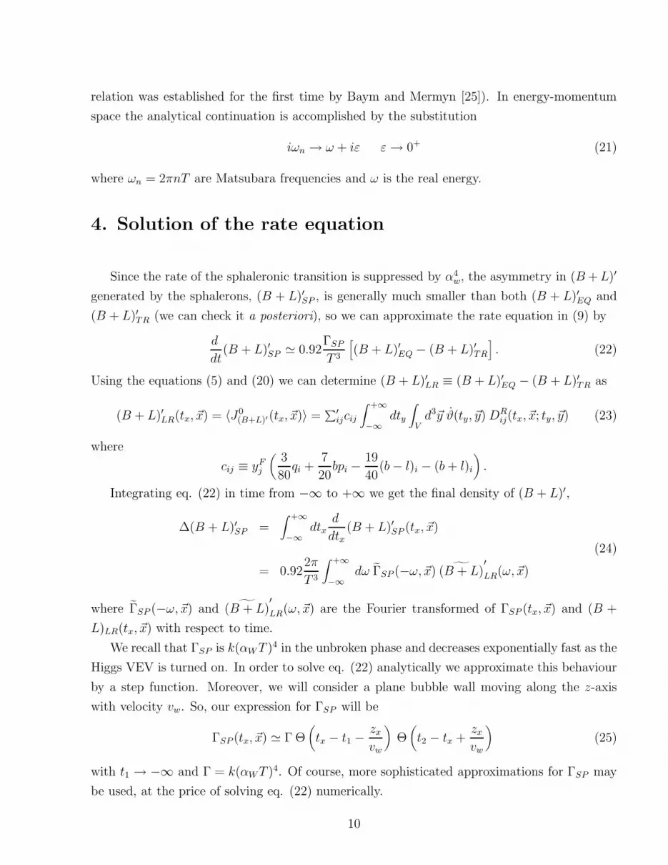
We recall that ΓSP is k(αWT )4 in the unbroken phase and decreases exponentially fast as the
Higgs VEV is turned on. In order to solve eq. (22) analytically we approximate this behaviour
by a step function. Moreover, we will consider a plane bubble wall moving along the z-axis
with velocity vw. So, our expression for ΓSP will be
ΓSP (tx, ~x) ≃ Γ Θ(tx − t1 −
zx
vw
)Θ(t2 − tx +
zx
vw
)(25)
with t1 → −∞ and Γ = k(αWT )4. Of course, more sophisticated approximations for ΓSP may
be used, at the price of solving eq. (22) numerically.
10

ΓSP (tx, ~x)
Γt1
t2 0 tx
~x = 0
−∆zvw
0 tx
ϑ(tx, ~x)
θ
-
6
6
-
�
Figure 3: Schematic representation of the behaviour of ϑ and of the rate of the sphaleronic transitions at thepoint ~x = 0.
Analogously, we approximate ϑ in such a way that it is constant in a region of width ∆z
inside the bubble wall, and is zero outside,
ϑ(ty, ~y) = θ Θ(zy − vwty) Θ(vwty − zy + ∆z) (26)
where θ = vw ∆ϑ/∆z. So, if we are at the point ~x = 0, we observe an interaction of the form
(10) turned on from t = −∆z/vw to t = 0, while the sphalerons are active till t = t2, as we
have shown in Fig. 3.
Putting all together we obtain
∆(B + L)′SP = 0.92(2π)3
T 3Γθ∑′
ijcij
∫ +∞
−∞dω
e−iωt2 − e−iωt1
ω
1 − e−iω∆z/vw
ωDR
ij(px = py = 0, pz =ω
vw
, ω).
(27)
Note the peculiar relationship between pz and ω in the argument of DRij , due to the spacetime
dependence of ϑ(ty, ~y), see (26). A consideration of the general properties of retarded Green’s
functions [26] ensures that the imaginary part of DRij is a even function of ω, while its imaginary
part is odd. As a consequence the integral in (27) will always give a real result.
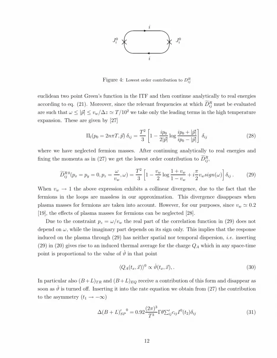
The lowest order contribution to DRij comes from the fermion loop in Fig. 4, where the two
crosses indicate the zero components of the fermion current. We may evaluate the corresponding
11
J0i J0
i
i
i
'&
$%
�@ �@
-
�
Figure 4: Lowest order contribution to DRij
euclidean two point Green’s function in the ITF and then continue analytically to real energies
according to eq. (21). Moreover, since the relevant frequencies at which DRij must be evaluated
are such that ω ≤ |~p| ≤ vw/∆z ≃ T/102 we take only the leading terms in the high temperature
expansion. These are given by [27]
Πl(p0 = 2nπT, ~p) δij =T 2
3
[1 − ip0
2|~p| logip0 + |~p|ip0 − |~p|
]δij (28)
where we have neglected fermion masses. After continuing analytically to real energies and
fixing the momenta as in (27) we get the lowest order contribution to DRij,
DR 0ij (px = py = 0, pz =
ω
vw, ω) =
T 2
3
[1 − vw
2log
1 + vw
1 − vw+ i
π
2vwsign(ω)
]δij . (29)
When vw → 1 the above expression exhibits a collinear divergence, due to the fact that the
fermions in the loops are massless in our approximation. This divergence disappears when
plasma masses for fermions are taken into account. However, for our purposes, since vw ≃ 0.2
[19], the effects of plasma masses for fermions can be neglected [28].
Due to the constraint pz = ω/vw the real part of the correlation function in (29) does not
depend on ω, while the imaginary part depends on its sign only. This implies that the response
induced on the plasma through (29) has neither spatial nor temporal dispersion, i.e. inserting
(29) in (20) gives rise to an induced thermal average for the charge QA which in any space-time
point is proportional to the value of ϑ in that point
〈QA(tx, ~x)〉0 ∝ ϑ(tx, ~x), . (30)
In particular also (B+L)TR and (B+L)EQ receive a contribution of this form and disappear as
soon as ϑ is turned off. Inserting it into the rate equation we obtain from (27) the contribution
to the asymmetry (t1 → −∞)
∆(B + L)′SP0
= 0.92(2π)3
T 3Γθ∑′
ijcijI0(t2)δij (31)
12

J0i J0
j
i
i
j
j@
@
@@
@@ @
@@
@@
@@
@@
@ @@
@@@
@@
@@⌣ ⌣ ⌣⌢ ⌢ ⌣ ⌣ ⌣⌢ ⌢
'&
$%
'&
$%
'&
$%��@@ @@��
-
�
-
�
-
�
Figure 5: The contribution to DRij due to photon exchange.
where
I0(t2) =2π
3T 2(1 − vw
2log
1 + vw
1 − vw
)×
0 (t2 < −∆zvw
)
(t2 + ∆z
vw
) (−∆z
vw< t2 < 0
)
∆zvw
(t2 > 0)
(32)
We recall that t2 is the time at which sphaleron transitions are turned off, while the charge
potential induced by ϑ is active for −∆z/vw < t < 0. So the asymmetry calculated in this
approximation for DRij grows linearly with t2 until t2 = 0 (for t2 < −∆z/vw the asymmetry is
obviously zero since there is no overlap between sphalerons and ϑ). The result for t2 > 0 is an
artifact of our approximation (B + L)′SP ≪ (B + L)′LR, which is no more appropriate in this
case. Actually, from (30) we know that when ϑ goes to zero, as is the case for t > 0, (B +L)′EQ
and (B + L)′TR vanish too, and the rate equation (9) becomes
d
dt(B + L)′SP = −0.92
ΓSP
T 3[(B + L)SP ] (t > 0) (33)
so that the asymmetry produced before decreases exponentially from t = 0 to t = t2 with rate
Γ. However, due to the smallness of Γ, and to the fact that t2 cannot be much larger than
O(∆z/vw), we can safely neglect this decreasing and take the result in (32).
Next, we consider the contribution to DRij due to gauge bosons exchange. Since we are
in the broken phase, and since the perturbation (10) induced by ϑ is colorless, we will take
into account only photons, which contribute through the graph in Fig. 5. The blob in the
middle represents the sum of all possible insertion of fermion loops. In calculating the blob,
we have to include not only the fermions which enter in Q′, (B − L)′, and BP ′, i.e. the ones
with fast flavour, or chirality, changing interactions, but we must instead take into account the
contributions of all the charged fermions of the theory. This is because QED interactions are
fast and then, for instance, pair production is in equilibrium also for right handed light quarks.
The ‘QED’ contribution of Fig. 5 gives
DR, QEDij (ω, ~p) = e2qiqjΠ
2l (ω, ~p)
D00(ω, ~p)
1 −∑k(eqk)2D00Πl
(34)
13
where eqi is the electric charge of the fermion i. D00(ω, ~p) is the tree level (0, 0) component of
the photon propagator in the Coulomb gauge
Dµν =−1
p2P µν
T − 1
|~p|2uµuν , (35)
where p2 = ω2 − |~p|2, uµ = (1, 0, 0, 0) identifies the plasma reference frame, while
P 00T = P 0i
T = P i0T = 0
P ijT = δij − pipj/|~p|2
As we have discussed, the sum in the denominator of (34) must be extended over all the charged
quarks and leptons. Setting pz = ω/vw we get
DR, QEDij (ω, ~p) = −e2qiqj v2
w
Π2l (ω, pz = ω/vw)
ω2 + v2w
∑k(eqk)2Πl(ω, pz = ω/vw)
. (36)
Note that unlike the ‘direct’ contribution (29) the ‘QED’ one is not flavour (or color) diag-
onal, so that even particles which do not enter into the expression for the charge potential (10)
get a non zero thermal average depending on ϑ. Moreover, this contribution has a genuine ω
dependence. Two points retarded Green’s function are analytic in the upper half of the complex
ω plane. DR, QEDij (ω, pz = ω/vw) may then have poles of the form ω = ωp − iγp, with γp > 0.
In order to determine them we have to solve the following equations
ω2p − γ2
p = −CR⌉Πl(ω)
ωp =CImΠl(ω)
2γp
(37)
where C = v2w
∑k(eqk)
2. Since the RHS of the first of eqs. (37) is negative, and vw ≃ 0.2 < 1,
we can approximate the solutions by
ω1, 2 = ±ωp + iγp
ωp =π
4vwγp
γp ≃ [CR⌉Πl(ω)]1/2 ≃ vweT√
3
(∑
k
(qk)2
)1/2
(38)
where γp > 0 as it should be.
Inserting (36) in eq. (27) we obtain the ‘QED’ contribution to the asymmetry
∆(B + L)′SPQED ≃ 0.92
(2π)3
T 3Γθ∑′
ijcijIQED(t2) (39)
14
where, now,
IQED(t2) = −2π
3T 2(1 − vw
2log
1 + vw
1 − vw
)qiqj∑k(qk)2
×
0 (t2 < −∆zvw
)
[t2 +
∆z
vw+ cos ωp
(t2 +
∆z
vw
)e−γp(t2+∆z/vw)
γp
] (−∆z
vw< t2 < 0
)
[∆z
vw− e−γpt2
γp
(cos ωpt2 − e−γp∆z/vw cos ωp
(t2 +
∆z
vw
))](t2 > 0),
(40)
The same considerations about the case t2 > 0 made after eq. (32) apply also here. We can
notice that photon exchange gives two different types of contributions. The first one has the
same behaviour of that in (32), i.e. a linearly increasing asymmetry from t2 = −∆z/vw to
t2 = 0. On the other hand, the second term exhibits a well known feature of plasma physics,
namely, plasma damped oscillations induced by an external perturbation [23]. The damping
rate here is given by γp. In the case −∆z/vw < t2 < 0, we see that the oscillating term
dominates over the linear one only for t2 → −∆z/vw, and is rapidly damped as t2 → 0, since
exp(−γp∆z/vw) ≃ exp(−T∆z) ≃ exp−(40). When t2 > 0 the amplitude of the oscillation is
always suppressed at least by a factor 10−1 ÷ 10−2 with respect to the linear one, and then
we can conclude that the effect of the oscillating term is negligible unless t2 is very near to
−∆z/vw .
An interesting feature of our results (32) and (40) can be appreciated if we calculate, by
means of eq. (20), the electric charge Q′ induced by the phase ϑ, taking into account both the
direct contribution (29) and the ‘QED’ one (34) to DRij . It is easy to see that it is given by
〈Q′〉 ∝[∑′
i yiqi
(∑k q2
k −∑′
k q2k
)× “linear contribution”
]
+“damped contribution”,
(41)
then, when every fermion is in equilibrium, the linear contribution to the thermal average of Q′
vanishes, and we are left with the damped one. The reason is that in this case Q′ coincides with
the total fermion electric charge, and this is perfectly screened as in the usual QED plasma.
Since in the real situation not all the fermions are in equilibrium, the linear contribution to (41)
does not cancel. Anyway, this considerations are valid for electric charge only, while the other
interesting charges, (B+L)′, (B−L)′, and, BP ′, would have non zero linear contributions even
if all the fermions were in equilibrium.
15

Putting all together, and neglecting the damped contribution, we find the final asymmetry
in (B + L)′
∆(B + L)′SP = −0.9237
240(2π)4Γθ
T
(1 − vw
2log
1 + vw
1 − vw
)(t2 +
∆z
vw
), (42)
where we have assumed that the sphalerons turn off when the phase is still active (−∆z/vw <
t2 < 0). Recalling that θ = ∆ϑvw/∆z, and assuming that sphalerons cease to be active after a
time interval t2 + ∆z/vw = f∆z/vw from the turning on of ϑ we get
∆(B + L)′SP ≃ −2.3 · 102kT 3α4w∆ϑf (43)
where we have taken the reasonable value vw ≃ 0.2 [19]. The above value is enhanced by nearly
three orders of magnitude with respect to the original estimates by CKN [14] where transport
phenomena were not taken into account.
The predicted baryon asymmetry of the Universe then comes out to be
ρB
S≃ −10−6k∆ϑf. (44)
k is estimated in the range 0.1÷ 1 from numerical simulations [22], while the value of f is still
an open question. Following Dine and Thomas [16] we chose
f ≃ αw
g≃ 5 · 10−2. (45)
The observed baryon asymmetry, ρB/S = (4 ÷ 7) · 10−11, can then be reproduced for ∆ϑ ≃10−2÷10−3, values which can be obtained either by explicit CP violation or by spontaneous CP
violation at finite temperature [9] without entering in conflict with the experimental bounds
on the electric dipole moment of the neutron.
The result (42) was obtained considering a charge potential of the form (10) where the sum
extends on all the left handed fermions plus the right handed quark. Considering the more
physical situation in which only the top quarks (left and right handed) feel the effect of ϑ the
coefficient 37/240 in (42) should be changed into 9/32, thus leading to an enhancement of a
factor 1.8.
5. The effect of QCD sphalerons.
It is well known that the axial vector current of QCD has a triangle anomaly, therefore one
can expect axial charge violation due to topological transitions analogous to the sphaleronic
16
transitions of the electroweak theory. The rate of these processes at high temperature may be
estimated as [29, 15]
Γstrong =8
3
(αs
αW
)4
ΓSP =8
3k(αsT )4 (46)
where αs is the strong fine structure constant, leading to a characteristic time of order
τstrong =1
192kα4sT
. (47)
Since k ≃ 0.1 ÷ 1 [22], we see that τstrong is comparable to the time of passage of the bubble
wall, and might also be smaller.
Recently, Giudice and Shaposhnikov have analyzed the effect of these ‘QCD sphalerons’
on the adiabatic baryogenesis scenario. They showed that, as long as these transitions are in
equilibrium and fermion masses are neglected, no baryon asymmetry can be generated. Thus,
the final result will be suppressed by a factor ∼ (mtop(T )/πT )2. In this paragraph we will
reconsider the issue taking transport phenomena into account.
The effect of QCD sphalerons may be represented by the operator
Π3i=i(uL u†
R dL d†R)i (48)
where i is the generation index. Assuming that these processes are in equilibrium, we get the
following chemical potentials equation
3∑
i=1
(µuiL− µui
R+ µdi
L− µdi
R) = 0. (49)
Eq. (49) contains the chemical potentials for all the quarks, and imposes that the total right-
handed baryon number is equal to the total left-handed one. Using eqs. (1) and (2) we can
rewrite it as
4µuL+ µtL − µbR
− 2µdR− 2µuR
− 3µW+ = 0, (50)
where µuL,R≡ 1/2
∑2i=1 µui
L,R, and µdR
≡ 1/2∑2
i=1 µdiR. One of the three new chemical poten-
tials, µbR, µdR
, and µuR, can be eliminated using eq. (50), while the remaining two correspond
to two more conserved charges that must be taken into account besides Q′, BP ′, and (B − L)′
(now the primes mean that the summation has to be performed on right handed quarks too,
but not on right handed leptons). We can choose
X ≡3∑
i=1
diR − 3
2
2∑
i=1
uiR, (51)
Y ≡ bL + tL + tR +1
2
2∑
i=1
uiR −
3∑
j=1
(ejL + νj
L), (52)
17
corresponding respectively to A3 and A2 in the notation of ref. [15]. Following the usual
procedure, we can now express the abundance of any particle number at equilibrium as a linear
combination of Q′, (B − L)′, BP ′, X, and Y . For (B + L)′ we obtain the result
(B + L)′EQ = −1
5(B − L)′, (53)
to be compared to eq. (5), which we obtained considering QCD sphalerons out of equilibrium.
Thus, the equilibrium value for (B + L)′ depends only on the the density of (B − L)′, in
agreement with what was obtained in ref. [15]6. If transport phenomena were not present, as it
was assumed in ref. [15], we could set (B−L)′ to zero and then conclude that QCD sphalerons
allow no non vanishing (B +L)′ density, at equilibrium and in the massless approximation. On
the other hand, including transport effects, we can easily calculate the (B−L)′ density induced
by ϑ using eq. (20), and then, through (53), the equilibrium value (B + L)′EQ, which, unlike in
ref. [15], comes out to be non vanishing inside the bubble wall. However this is not sufficient to
conclude that we will have a non zero final baryon asymmetry when the bubble wall has passed
by. As we discussed in Sect. 2., the generation of baryons inside the bubble walls is described
by eq. (9), with the initial condition (B + L)′SP = 0. Then we must calculate (B + L)′TR, i.e.
the contribution to (B + L)′ due to transport. If all the particles in equilibrium participated
to the charge potential then we would find
(B + L)′TR(tx, ~x) = (B + L)′EQ(tx, ~x) (54)
so that the system would always be on the minimum of the free energy inside the bubble wall
and there would be no bias of the (electroweak) sphaleronic transitions. As a consequence,
(B + L)SP would remain zero and no asymmetry would survive after the passage of the wall
up to fermion mass effects, in agreement with what was find in ref. [15].
On the other hand, including only left and right handed top quarks into the charge potential,
eq. (54) is no more satisfied and a non zero result for the final baryon asymmetry is recovered.
In this case, the factor 37/240 in eq. (42) should be changed to 25/72.
6. Conclusions
In this paper we have analyzed the impact of transport phenomena on the so called ‘spon-
taneous baryogenesis’ mechanism of Cohen, Kaplan, and Nelson. We have assumed that inside
6Incidentally, note that this is not a general property due to the insertion of QCD sphalerons into the setof processes in equilibrium, but is due to the fact that only top Yukawa interactions are fast. If, for instance,bottom quark Yukawa interactions were also fast, then we would find that (B +L)′EQ is not simply proportional
to (B − L)′, but depends also on the values of the other charges in equilibrium.
18
the walls of the bubbles nucleated during the electroweak phase transition a space time depen-
dent ‘charge potential’ for (partial) fermionic hypercharge is generated. We stress again that
no discussion about the origin of the charge potential has been given; in particular, since in
the limit in which all the Yukawa couplings go to zero there is no communication between the
Higgs and the fermion sectors, we expect that in this limit also the charge potential should go
to zero. In the traditional approach of CKN there is no trace of this behaviour, and moreover
we have shown that the results change in a sensible way according to the precise form of the
charge potential which is considered. We reserve a discussion on this subject for a forthcoming
publication. Our main interest here was to set a scheme for calculations in the the adiabatic
scenario in the case in which such a charge potential is present, in order to determine the
variations in the thermal averages induced by transport effects and the production of baryon
number by sphalerons inside the bubble walls.
The main physical point of the paper is that the system should be regarded as a collection
of subsystems in local equilibrium, in which the thermal averages for the conserved charges are
not zero but are driven to non vanishing values by transport phenomena. In particular, the
local equilibrium configurations will correspond to non zero values for (B +L)′. We have deter-
mined the local equilibrium configuration by means of a chemical potential analysis, calculating
the values of the thermal averages for the conserved charges by using linear response theory.
We have considered only the dominant contribution to these averages, in particular, we have
neglected any fermion mass effect and also the coupling of the Higgs field to the Chern-Simons
number.
We find that, in contrast with previous claims [17], the presence of transport phenomena does
not prevent baryon number generation inside the bubble walls. The main source of disagreement
with JPT is the following. In their paper, JPT consider the rate equation in the form
B = −ΓSP
2T(3µtL + 3µbL
+ µτL+ µντ ), (55)
where the term on the right hand side has been obtained by considering the variation of the free
energy of the system due to a ‘sphaleron-like’ transition involving only the third generation,
i.e. due to the processes tLtLbLτL ↔ 0 and tLbLbLντ ↔ 0. Then these authors impose that
the chemical potential of any particle is proportional to the value of its hypercharge, and so
they find that the right hand side vanishes as a consequence of the conservation of hypercharge
(and of fermion hypercharge) in any sphaleronic transition. The point is that, assuming local
equilibrium of the fast interactions, the chemical potentials of the single particle species are not
proportional to their hypercharge. In fact, since the single particle numbers are not conserved
quantities of the system, their abundances are reprocessed by fast interactions as to obtain their
local equilibrium values. On the other hand, imposing that the particle chemical potentials are
19

proportional to hypercharge, would be equivalent to freeze out any interaction inside the bubble
wall, both the fast and the slow ones, leaving transport phenomena as the only relevant process.
Also, if a charge potential for fermionic or total hypercharge is present, transport phenomena
allow the generation of the baryon asymmetry even in the limit in which the Higgs VEV’s go to
zero. The reason is again that the thermal averages for Q′, (B−L)′ and BP ′ are non vanishing
and then a (B +L) asymmetry can be generated even if the electroweak symmetry is unbroken.
This is strictly analogous to the well known result of the survival of a B + L asymmetry when
a B − L density, eventually of GUT origin, is present [20]. Of course, in the limit in which
the VEV’s go to zero, also the charge potential should go to zero, since no complex phase can
emerge from the Higgs sector in this case. Then, also this suppression, like the one due to
vanishing htop, should be made evident by an accurate discussion on the origin of the charge
potential. As a consequence, our results for the baryon asymmetry, eq. (43) should be probably
multiplied by a further suppression factor roughly of order (mtop(T )/T )2.
Acknowledgments
One of us (M.P.) is very grateful to the DESY theory group for the kind hospitality during
the last stage of this work.
References
[1] For a review see A. Cohen, D. Kaplan, and A. Nelson, Ann. Rev. Nuc. Part. Sci. 43, 106
(1993).
[2] J.R. Espinosa, M. Quiros and F. Zwirner, Phys Lett. B314, 206 (1993); W. Buchmuller,
Z. Fodor, T. Helbig and D. Walliser, DESY 93-21 preprint (1993), to be published on Ann.
Phys.
[3] J.R. Espinosa, M. Quiros and F.Zwirner, Phys. Lett. B307, 106 (1993); A. Brignole, J.R.
Espinosa, M. Quiros. and F. Zwirner, CERN preprint CERN-TH 7057/93.
[4] J.E. Bagnasco and M. Dine, Phys. Lett. B303, 308 (1993); P. Arnold and O. Espinosa,
Phys. Rev. D47, 3546 (1993); Z. Fodor and A. Hebecker, DESY preprint, DESY 94-025
(1994)
[5] K. Kajantie, K. Rummukainen, and M.E. Shaposhnikov, Nucl. Phys. B407, 356 (1993);
M.E. Shaposhnikov, Phys. Lett. B316, 112 (1993).
20

[6] J. March-Russell, Phys. Lett. B296, 364 (1992); P. Arnold and L.G. Yaffe Seattle Preprint
UW/PT-93-24 (1993);
[7] M. Alford and J. March-Russell, LBL preprint, LBL-34573 (1993); K. Farakos, K. Kajantie,
K. Rummukainen, and M.E. Shaposhnikov, CERN preprint, CERN-TH 6973/94.
[8] G.R. Farrar and M.E. Shaposhnikov, CERN preprint, CERN-TH 6732/92 (1993); M.B.
Gavela, P. Hernandez, J. Orloff, and O. Pene, Mod. Phys. Lett. A9, 795 (1994); P. Huet
and E. Sather, SLAC preprint, SLAC-PUB-6479 (1994).
[9] D. Comelli and M. Pietroni, Phys. Lett. B306, 67 (1993); D. Comelli, M. Pietroni, and
A. Riotto, Nucl. Phys. B412, 441 (1994).
[10] J.R. Espinosa, J.M. Moreno, and M. Quiros, Phis. Lett. B319, 505 (1993).
[11] D. Comelli, M. Pietroni, and A. Riotto, Padova University preprint, DFPD 94/TH/38.
[12] A. Cohen, D. Kaplan, and A. Nelson, Nucl. Phys. B373, 453 (1992), Phys. Lett. B294,
57 (1992).
[13] L. McLerran, M.E. Shaposhnikov, N. Turok, and M. Voloshin, Phys. Lett. B256, 451
(1991); M. Dine, P. Huet, R. Singleton, and L. Susskind, Phys. Lett. B256, 86 (1991); S.
Abel, W. Cottingham, and I. Whittingham, Nucl. Phys. B410, 173 (1993).
[14] A. Cohen, D. Kaplan, and A. Nelson, Phys. Lett. B263, 86 (1991).
[15] G.F. Giudice and M.E. Shaposhnikov, preprint CERN, CERN-TH 7080/93 (1993)
[16] M. Dine and S. Thomas, Santa Cruz preprint, SCIPP 94/01 (1994), hep-ph 9401265.
[17] M. Joyce, T. Prokopec, and N. Turok, Princeton preprint, PUP-TH-1436 (1993), hep-ph
9401302.
[18] A.L. Fetter and J.D. Walecka, Quantum theory of many-particle systems (Mc Graw-Hill,
1971).
[19] M. Dine, R. Leigh, P. Huet, A. Linde, and D. Linde, Phys. Rev. D46, 550 (1992).
[20] J.A. Harvey and M.S. Turner, Phys. Rev. D42, 3344 (1990); H. Dreiner and G.G. Ross,
Nucl. Phys. B410, 188 (1993).
[21] S. Yu. Khlebnikov and M.E. Shaposhnikov, Nucl. Phys. B308, 885 (1988); M. Dine, O.
Lechtenfeld, B. Sakita, W. Fischler and J. Polchinski, Nucl. Phys. B342, 381 (1990).
21

[22] J. Ambjorn, M. Laursen, and M.E. Shaposhnikov, Phys. Lett. B197, 49 (1987), Nucl.
Phys. B299, 483 (1989); J. Ambjorn, T. Askgaard, H. Porter, and M.E. Shaposhnikov,
Phys. Lett. B244, 479 (1990); Nucl. Phys. B353, 346 (1991).
[23] J.I. Kapusta, Finite temperature field theory (Cambridge University Press, Cambriidge,
England, 1989).
[24] K.C. Chou, Z.B. Su, B.L. Hao, and L. Yu, Phys. Rep. 118, 1(1985); N.P. Landsman and
Ch.G. van Weert, Phys. Rep. 145, 141 (1987); R. Baier and A. Niegawa, Bielfeld University
preprint, BI-TP-93-39 (1993), hep-ph 9307362.
[25] G. Baym and N.D. Mermin, J. Math. Phys. 2, 232 (1961).
[26] R.D. Pisarski, Nucl. Phys. B309, 476 (1988).
[27] R.D. Pisarski, Physica A158, 146 (1989).
[28] V.V. Lebedev and A.V. Smilga, Physica A181, 187 (1992).
[29] L. Mc Lerran, E. Mottola, and M. Shaposhnikov, Phys. Rev. D43, 2027 (1991).
22