PUBLS. INST. GEOPHYS. POL. ACAD. SC., E-7 (401), 2007

Transport Phenomena in Hydraulics

Preface

Paweł M. ROWIŃSKI Institute of Geophysics, Polish Academy of Sciences

Ks. Janusza 64, 01-452 Warszawa, Poland e-mail: pawelr@igf.edu.pl

This volume concerns various aspects of research that contributes to the knowl-

edge of a large number of engineering processes and also some natural processes that involve the transformation and transport of momentum, matter and energy. Those problems constitute the basis of the studies performed within the Project of the Minis-try of Higher Education and Science Grant No. 2 P04D 026 29; it has also been the basic theme of the 27th International School of Hydraulics held from 18th to 21st Sep-tember 2007 in Hucisko in the Jura Region in Southern Poland. It has been decided to combine the experience gained by the participants of the meeting and the results achieved within the project to provide the reader with a broad overview of the men-tioned problems.

In hydraulics one may deal with various aspects of transport processes. It is a well-known notion that the hydraulic transport concerns a transport method where solid particles are suspended in a fluid and transported through pipelines. But we have been definitely interested in a much broader range of problems. Our aim has been to discuss research that involves the development of fundamental engineering principles, mathe-matical models, and experimental techniques, with an emphasis on approaches that have the potential for innovation and broad application in areas such as the hydraulic engineering and environmental hydraulics. Of particular interest has been the physics of transport of various constituents in flowing surface waters. All the mixing mecha-nisms such as advection, molecular diffusion and turbulent diffusion have been con-sidered from various perspectives. Mathematical models and experimental results that account for all the transport processes and reflect the principle of conservation of mass have been discussed. We realize that all transport processes in aquatic environment are governed by water flow itself, so all the problems related to the water movement un-der steady and unsteady conditions were of interest as well. The problems of the in-herent uncertainties were also presented.

4

We do realize how important are the problems of transport of matter, from cogni-tive but also from practical viewpoints. Substantial amounts of solids (sand, gravel, clay, coal, tailings or mineral ores) are transported hydraulically all over the world and, for example, the dredging companies are the ones to handle a great deal of the transported solids. Then the economy and safety are of major concern in the planning and executing of solids transport projects. In nature we deal with sediments and a va-riety of pollutants that are transported by streams and those processes are also of great importance and inspire researchers, engineers, environmentalists and designers to gain more understanding and to find solutions to different problems. The need to predict and control the transport of mass and energy requires greater knowledge of the proc-esses that govern the flow of a solids-water mixture in such various environments.

This volume gathers the experience of numerous researchers from all over Europe and various aspects of the problem are considered. With a view to the scope of our work and its wide perspective, we were very much aware of the need to put together a highly qualified team to provide the reader with a truly up to date overview of the subject. The leaders in their fields not only wrote excellent chapters but also delivered fantastic lectures during the International School of Hydraulics. I would particularly like to acknowledge Keith J. Beven from the Department of Environmental Science of Lancaster University (UK), Włodzimierz Czernuszenko from the Institute of Geophys-ics of the Polish Academy of Sciences, Tom O'Donoghue and Dubravka Pokrajac from the Environmental Hydraulics Research Group of the University of Aberdeen (UK), Wim S.J. Uijtewaal from Environmental Fluid Mechanics Section of Delft Uni-versity of Technology (The Netherlands) and Volker Weitbrecht from the Institute of Hydromechanics of the University of Karlsruhe (Germany).

I am sincerely grateful to everyone who has made such important contributions to this volume. Let me thank all the authors for their patience, dedication and hard work. My particular gratitude goes to all my colleagues from the Institute of Geophysics PAS who went above and beyond the call of duty to assist me. Particular thanks go to Anna Zdunek, Anna Łukanowska, Monika Kalinowska and Agata Mazurczyk. Their enthusiasm and dedication knew no limits. I want also to acknowledge the reviewers of all the papers – their hard work ensured high quality of all the contributions. That important work was done by Professors Włodzimierz Czernuszenko, Janusz Kubrak, Wojciech Majewski, Marek Mitosek, Jarosław Napiórkowski and Romuald Szym-kiewicz.

This book was financially supported in part by The Ministry of Higher Education and Science Grant No. 2 P04D 026 29 and in part by the Institute of Geophysics, Pol-ish Academy of Sciences.

PUBLS. INST. GEOPHYS. POL. ACAD. SC., E-7 (401), 2007

Uncertainty in Predictions of Floods and Hydraulic Transport

Keith BEVEN Environmental Science/Lancaster Environment Centre,

Lancaster University, UK, and Geocentrum, Uppsala University, Sweden e-mail: k.beven@lancs.ac.uk

Abstract

This paper provides a review of work within the Generalised Likelihood Un-certainty Estimation (GLUE) methodology on estimating uncertainties in predict-ing flood frequency, flood inundation, and hydraulic transport of solutes in rivers and soils. The issue of prediction uncertainty as an input decision making is also discussed. It is concluded that in real applications it is unlikely that a fully objec-tive approach to uncertainty estimation is possible. It is therefore important that the assumptions made are stated explicitly so that they can be agreed or disputed with the users of the resulting predictions. It is also important that the modelling process be considered as a learning process of constraining uncertainty by adding new information.

1. Uncertainty about uncertainty in flood and transport predictions

There is currently significant debate about how to estimate the uncertainties associated with environmental predictions. This discussion has been prompted by the more wide-spread availability of computer power, especially Beowulf-type parallel systems of cheap PCs, that has allowed the application of Monte Carlo methods of different types to a wider range of environmental models. Clearly, there are still some limitations. Fine grid scale 2D and 3D hydrologic and hydraulic models with very large numbers of elements, still cannot easily be run in Monte Carlo experiments without access to very large scale resources, but we can probably expect computer power to continue to increase more quickly than changes in modelling concepts for the foreseeable future, so that the uncertainty analysis will become feasible for more and more model applica-tions.

This raises some interesting questions: in particular, is it possible to agree on an uncertainty estimation methodology and how should prediction uncertainties be used in decision making? A full discussion of these questions is the subject of a forthcom-ing book (Beven 2008) and only a brief outline can be given here. Arguments for the routine application of uncertainty analysis can be found in Pappenberger and Beven (2006).

6

With respect to the first question, the answer is – as yet – no; though some sugges-tions can be given about different methods for use in different circumstances (see the Risk and Uncertainty Decision Tree Wiki pages at www.floodrisknet.org.uk/methods/Introduction). There are many people who believe that statistics is the only way of estimating uncertainties associated with model predic-tions (see O’Hagan and Oakley 2004, Mantovan and Todini 2006) but it is clear that in many applications of environmental models there are sources of uncertainty that are not statistical (aleatory) in nature (see Beven 2005, 2006a) and the use of formal statis-tical assumptions might lead to misleading results even in near-ideal cases (Beven et al. 2007). In non-ideal cases (i.e. nearly all real applications), non-statistical (epis-temic) uncertainties may dominate. Examples of epistemic uncertainties are bias and nonstationarity in input errors, model structural errors and commensurability errors (where a variable or parameter in a model is different to an equivalent quantity that can be measured in the field, see Beven 1989, 2002, 2006a, b, Freer et al. 1996, 2004).

It can be easily shown that in all real applications it is impossible to separate out different sources of aleatory and epistemic uncertainties unless very strong (and diffi-cult to justify) assumptions are made (Beven 2006a). This leaves plenty of scope for uncertainty about how to estimate prediction uncertainties. In what follows we will consider only one methodology, the Generalised Likelihood Uncertainty Estimation (GLUE) first proposed by Beven and Binley (1992). This is a very flexible technique for model conditioning given some past observations of system responses (it includes both formal statistical and fuzzy methods as special cases) but one that has been criti-cised as being based on too many subjective assumptions. It is based on the equifinal-ity thesis: the concept that in real applications there may be many different model structures and sets of parameter values for each model structure that produce accept-able or behavioural predictions of the system of interest (Beven 1993, 2006a). Equifi-nality can be visualised in plots of some evaluation measure, such as residual variance or Nash-Sutcliffe efficiency, against single parameter values (e.g. Figs. 1 and 2). Such plots represent projections of points on a response surface in the model space onto the single parameter axes. As such they cannot reveal all the complex parameter interac-tions within a model structure that lead to behavioural or non-behavioural perform-ance; they can reveal that very often the best model performances are found across a wide range of individual parameter values.

The GLUE methodology is essentially very simple in concept. A large number of runs of a model are made using randomly generated sets of effective parameter values (chosen from defined prior distributions if that information is available, otherwise from uniform prior distributions). The outputs from each model run are compared with the observational data, taking account of observational error where appropriate (see, e.g. Beven 2006a, Freer et al. 2004). Those models providing acceptable or behav-ioural results are retained for use in prediction; those that do not are rejected. Each behavioural model is assigned a likelihood weight dependent on performance (zero for non-behavioural models) that is used to weight the predictions of that model in a for-mal cumulative distribution of predictions over the whole set of behavioural models. Different model structures as well as different parameter sets can be included in this process if the same methods of evaluation and likelihood assignment can be applied.

7

Different types of evaluation (analogous to multi-criteria calibration) are easily com-bined in this methodology, using either Bayes equation or some other chosen combi- nation method (e.g. fuzzy union/intersection). Demonstration software for GLUE can be found at http://www.es.lancs.ac.uk/hfdg/freeware/hfdg_freeware_glue.htm.

The use of GLUE will be demonstrated in applications to flood frequency estima-tion, flood inundation predictions for risk mapping, and hydraulic transport predic-tions. A final section considers the use of prediction uncertainties in decision making, with a focus on inundation predictions.

Fig. 1. Dotty plots of a coefficient of determination in a pesticide transport model fitted to observed atrazine concentrations in a large undisturbed soil column. Each dot represents one run of the model with different randomly chosen parameter values. The four parameters are: (top) an effective pore water velocity, a dispersion coefficient (the ranges for which were previously determined by fitting bromide concentration data assumed to be a near conservative tracer on the same kolumn), (bottom) a retardation coefficient and a degradation coefficient. The best models of the realisations simulated by uniform sampling in the model space are at the top of each plot. The error bars shown on the bottom plots are ± 2 standard errors on the parameters estimated by nonlinear regression (after Zhang et al. 2006).

2. Uncertainty in flood frequency estimation Flood frequency estimation is often considered as a statistical problem. Given a se-quence of historical flood events, a statistical distribution is fitted using either annual maximum or peaks over threshold data so that an estimate of the flood peak for any

8

given return period can be estimated. If done properly, this can also yield a statistical estimation of the uncertainty in the predicted peak discharges, the uncertainty that in-creases rapidly for return periods longer than the length of the historical series (and that therefore might be important in decisions based on 100 year return period events or longer).

Fig. 2. Dotty plots for channel and flood plain roughness coefficients in an application of the 1D HEC-RAS model for the flood of 1997 on the River Morava, Czech Republic. Each dot represents one run of the model with randomly chosen roughness coefficients, assumed constant for the whole reach. The combined likelihood reflects model performance in reproducing both observed inundation extent and the downstream hydrograph (after Pappen-berger et al. 2005a).

This is a nice example where different sources of uncertainty and statistical as-sumptions might affect the result significantly. There is little agreement in the litera-ture on what distribution should be chosen, and different distributions fitting the data more or less equally well might result in quite different predictions at higher return periods (this is an epistemic uncertainty analogous to model structural error). It is (usually) necessary to assume that the historical flood data are correct, even though it is known that out-of-bank flows are notoriously difficult to estimate accurately (again

9

a form of epistemic uncertainty). It is necessary to assume that the historical data are samples from a stationary distribution even where a catchment is known to have un-dergone significant land use change and been subject to longer time scale climate vari-ability (again a form of epistemic uncertainty). Fitting a statistical distribution also necessarily deals with any hydrological and hydraulic process changes in different flood events (e.g., extent of surface and subsurface runoff contributing areas, transition to overbank flow) implicitly (again a form of epistemic uncertainty – though there have been rare examples of trying to fit mixed distributions for different runoff gen-eration mechanisms, where the distributional assumptions then apply to each mecha-nism). Finally, it is not often realised that the parameter values for the fitted distribu-tion (and consequent predictions and uncertainties) depend strongly on very specific assumptions about the statistical nature of the residuals that may or may not be valid – they are rarely checked.

Fig. 3. Flood frequency predictions for the Dolni Kralovice sub-catchment of the Zelivka River catchment, Czech Republic, using continuous 10000 year Topmodel simulations driven by a stochastic rainfall model using behavioural parameter sets after conditioning on observed flood peaks, flow duration curves and maximum snow water equivalents, combined within GLUE using a fuzzy rules method. Grey lines represent frequencies predicted by different parameter sets, dashed lines the 5 and 95% likelihood weighted prediction bounds derived from these simulations, circles represent frequencies estimated from observed annual maxima, dotted lines represent statistical estimates based on observed annual maxima assuming a Wakeby distribution (after Blazkova and Beven 2004).

10

This is clearly not only a statistical problem − even if we have been happy to use statistical fitting for convenience in the past – there are too many epistemic uncertain-ties. There is an alternative approach which can reflect the nonlinearities in the hydro-logical and hydraulic responses more directly and, as a result, might be more useful in predicting the effects of future change. This is the continuous simulation rainfall-runoff modelling approach, first used by Beven (1986, 1987) and more recently by Cameron et al. 1999, 2000, Lamb 1999, Blazkova et al. 2002, 2004, Lamb and Kay 2004, Cameron 2006). The papers by Cameron and Blazkova have applied this ap-proach within the GLUE methodology (Figs. 3 and 4).

Fig. 4. River Wye catchment, Wales: Cumulative distributions of the 100 year return period flood peak estimated within the GLUE methodology using 1000 year continuous simulations with different behavioural parameter sets in the rainfall-runoff model Topmodel driven by a stochastic rainfall model for different climate change scenarios. Scenario Z (current conditions); Scenario A1 (2020s); Scenario B1 (2050s); Scenario C1 (2080s) (after Cameron et al. 2000).

3. Uncertainty in flood inundation predictions

Flood inundation predictions are required for a variety of purposes including flood risk mapping and real-time forecasting. Many different 1D and 2D models are available for

11

making these predictions which are often presented without any attempt to assess the associated uncertainties. There are again, however, a number of different sources of epistemic (non-statistical) uncertainties in real applications of such models. These in-clude the uncertainty in the estimation of the upstream hydrograph, the estimation of effective roughness coefficients for different sections of channel and flood plain (which might be quite different from estimates derived at single points on the chan-nel), the representation of the flood plain geometry, the effects of infrastructure on the flood plain, and the implementation of the numerical algorithm (where different algo-rithms generally involve more or less numerical dispersion). In real-time predictions there might also be issues of embankment failures, blockages of culverts and bridges, predictions of wind and surge effects in tidal situations, etc. that might also have a significant effect on flood levels. Again, it is difficult to allow that these types of un-certainties are easily handled by a purely statistical approach. 1D and 2D flood inun-dation models have been applied in the GLUE methodology by Romanowicz et al. 1996, Romanowicz and Beven 1998, 2003, Aronica et al. 1998, Bates et al. 2004, Pappenberger et al. 2004, 2005a, b, 2006a, b (see Figs. 5 and 6).

Fig. 5. The 5 and 95% Inundation Quantiles for an example reach of the River Morava, Czech Republic, determined within the GLUE methodology using the HEC-RAS model after conditioning on both observed inundation and downstream hydrograph data (see also Fig. 2) (after Pappenberger et al. 2005a).

12

Fig. 6. Flood hazard map for part of the flood plain of the Alzette River, Luxembourg, conditioned on inundation extent derived from EnviSat ASAR images for a flood event in January 2003. 5% and 95% quantiles determined within the GLUE methodology using the 1D HEC-RAS model are shown (after Pappenberger et al. 2006a).

13

The experience of using such distributed hydraulic models within GLUE has been interesting. In particular, it rapidly becomes clear that equifinality is an issue in the application of such models when used with global or individual reach scale evaluation measures (e.g. Fig. 2 above). It also becomes clear that there are some reaches or cross-sections where it is very difficult for any of the models tried to reproduce the historical flood data. This might be a problem of the observational data itself (in one case in the application of Pappenberger et al. 2005a, this was obvious as the recorded water levels on the two banks of the large Morava river were 10 m different at one cross-section but in many cases this might not be so obvious). It might also be a result of any of the other sources of epistemic uncertainty noted above. In such cases, all the models tried could be rejected as non-behavioural. This could provoke a review of the modelling strategy and data – it is perhaps more likely, however, to result in the ne-glect of extreme errors as “outliers” or the use of global evaluation measures where the effects of local failures are not so obvious (e.g. Romanowicz et al. 1998, Ro-manowicz and Beven 2003, Bates et al. 2004, Hunter et al. 2005). Rejecting all the models is not a good result in presenting a report to a decision maker, of course. One strategy for retrieving such a situation is discussed in Section 5 below.

4. Uncertainty in hydraulic transport predictions

Similar issues arise in distributed hydraulic solute transport predictions. Such predic-tions are often based on an implementation of the advection-dispersion equation (ADE), either assuming a steady discharge in the channel or linked to the velocities predicted by a hydraulic flow model. The ADE can be justified theoretically on the basis of shear dispersion due to a logarithmic vertical velocity profile, once a solute is well mixed with the flow (e.g. Rutherford 1994). For steady flow conditions it predicts a concentration distribution for an impulse input that is Gaussian in space at any par-ticular point in time, and slightly skewed in time at any particular cross-section down-stream of the mixing length. These characteristics are often quite different from obser-vations of real tracer concentration curves which very often are skewed in both time and space and have very long tails. It seems that in real rivers shear mixing is often dominated by “dead zone” mixing. The result is that a simple transfer function model might provide much more accurate predictions than the ADE, which simply has the wrong process assumptions (see, for example, the review of Young and Wallis 1993). The ADE can be modified to include dead zone effects (e.g. Bencala and Walters 1983) at the expense of adding additional parameters that will need to be fitted in the same way as the roughness coefficients in flood inundation models above, and which will be subject to similar equifinality. Dispersion model calibration within the GLUE framework has been considered by Hankin and Beven 1998a, b, Hankin et al. 2001, 2002, Kettle and Beven 2002, Kettle et al. 2002 (e.g. Fig. 7), and for the case of solute transport in soils by Zhang et al. 2006 (see Figs. 1 and 8).

5. Uncertain predictions as an input to decision making

There are two main reasons for using models in hydrology and hydraulics. The first is to show that we understand how a system is working (although even if a model does

14

A

B

Fig. 7. 2D predictions of tracer transport in a short reach of the River Severn at Leighton, UK, based on velocity fields produced by Telemac-2D. A. Concentration patterns at time 600 s after end of tracer input for 8 different runs of the model using randomly chosen parameter values. B. Pattern of uncertainty in concentration predictions, relative to mean concentration field after fuzzy conditioning on point tracer concentration observations (after Hankin et al. 2001, copyright John Wiley and Sons Limited. Reproduced with permission).

15

Fig. 8. A comparison of prediction bounds from GLUE and CXTFIT (which uses a nonlinear regression method) after fitting parameters to atrazine pesticide breakthrough curves from four large undisturbed soil columns (see also Fig. 1). The model is the same in both cases. Dots are observed data (after Zhang et al. 2006).

give good predictions of the available observations it might still not be doing so for the right reason Beven 2001, Kirchner 2004). The second is to provide predictions to inform a decision. But if, as argued above, predictions of hydrological and hydraulic models are intrinsically uncertain, how should estimates of that uncertainty be pre-sented to decision makers and used in the decision making process, especially when there are many ways of estimating the uncertainty? This has caused some recent de-bate in the hydrological literature (Beven 2006, Hall et al. 2007, Mantovan et al. 2007). Uncertainty appears at first sight to making the decision making more difficult, but this is not necessarily the case. Decision makers always make decisions under un-certainty, whether they do so formally or informally. Most will already have a healthy scepticism about any predictions provided to them by the modeller, whether the pre-dictions are presented as a single deterministic outcome or as an uncertain (probabilis-tic or possibilistic) range.

In fact, what the decision maker is really interested in is not the uncertainty of a prediction but the risk of a potential outcome and its potential impact or consequences for the decision. There is no doubt that taking proper account of such risks can affect the decision made (see for example Todini 2004). This is therefore a reason why un-certainty estimation should be part of any and every modelling exercise. The debate arises because the risk, in formal risk-based decision making theory, is normally de-fined as the product of probability * consequences (very often economic conse-

16

quences). This would appear to be a major argument for the use of probabilistic as-sessments of uncertainties. Thinking more deeply, however, if the assumptions re-quired for such a formal probabilistic assessment cannot easily be justified in the face of the type of epistemic uncertainties described above, then perhaps other approaches might be useful (see for example the evidential reasoning approach of Wang et al. 2006, and the Info-Gap approach of Ben-Haim 2006). Use of these alternative deci-sion making techniques is described in more detail in those references and Beven (2008).

6. Uncertain futures

Many decisions are, of course, concerned with the impacts of future change. Particular current issues are the impacts of land management practices and future climate change. Assessing such changes necessarily depends on assumptions both about the changes to boundary conditions and changes in model structure or effective values of parameters. The type of conditioning against data, such as that of Figs. 1 and 2, can only be carried out for current (or historical) conditions. There is an implication, how-ever, that if the complex interactions between parameters and boundary conditions that lead to behavioural models for current conditions, then similarly the complex interac-tions will be involved in making predictions of future conditions. Such interactions are local in the model space, not easily described by either a single point or global covari-ance matrices.

In some cases where only the boundary conditions are assumed to change (e.g., in assessing the impacts of climate change on flood frequency in Cameron et al. 2000, Cameron 2006), then the behavioural parameter sets for current conditions can be used in predicting future impacts. Where it is expected that future change will result in changed parameter values, then it might not be possible to change single parameter values independently of others to form new “behavioural” parameter sets. What is needed is to “drift” the (complex) cloud of behavioural parameters sets through the model space to where they might best represent the new conditions. There does not as yet seem to be an easy way of doing this, but the task can be set up as a learning proc-ess. We know the starting point (the best estimate of a set of behavioural models under current conditions). As time evolves and more data is gathered we can start to study whether any resultant drift is apparent in the evolving parameter sets.

A similar approach can be taken to the ungauged site problem. Initial estimates of parameter sets can be conditioned on either quantitative or qualitative observations to gradually refine the representations of the site: in particular, parameter sets that are clearly inconsistent with the observations can be rejected (this might sometimes be all the models tried, e.g. Choi and Beven 2007). This type of learning process will be-come increasingly necessary as models of everywhere are implemented (Beven 2007).

This brief review of uncertainty estimation for flood inundation and transport cal-culations based on the GLUE methodology can only serve as an illustrated introduc-tion to a complex subject area where the answers you get are dependent on the as-sumptions you make. Since it is difficult to be at all sure about the real nature of dif-ferent sources of uncertainty in real applications then many different sets of assump-

17

tions could be argued for. It is unlikely in real applications that a fully objective ap-proach to uncertainty estimation is possible. It is therefore important that the assump-tions made are stated explicitly so that they can be agreed or disputed with the users of the resulting predictions. In the present state of the science, this requirement of making assumptions quite open to encourage a thoughtful approach to uncertainty estimation is probably more important than the differences between different methods. The topic will be discussed in much more detail in Beven (2008).

References

Aronica, G., B.G. Hankin and K.J. Beven, 1998, Uncertainty and equifinality in cali-brating distributed roughness coefficients in a flood propagation model with lim-ited data, Adv. Water Resour. 22 (4), 349-365.

Bates, P.D., M.S. Horritt, G. Aronica and K.J. Beven, 2004, Bayesian updating of flood inundation likelihoods conditioned on flood extent data, Hydrological Proc-esses 18, 3347-3370.

Bencala, K.E., and R.A. Walters, 1983, Simulation of solute transport in a mountain pool-and-riffle stream: A transient storage model, Water Resour. Res. 19, 718–724.

Ben-Haim, Y., 2006, Info-Gap Decision Theory, 2nd Edition, Academic Press: Am-sterdam.

Beven, K.J., 1986, Runoff production and flood frequency in catchments of order n: an alternative approach. In: V.K. Gupta, I. Rodriguez-Iturbe and E.F. Wood (Eds.) Scale Problems in Hydrology, Reidel, Dordrecht, 107-131.

Beven, K.J., 1987, Towards the use of catchment geomorphology in flood frequency predictions. Earth Surf. Process. Landf. V12(1), 69-82.

Beven, K.J., 1989, Changing ideas in hydrology: the case of physically based models. J. Hydrol. 105, 157-172.

Beven, K.J., 1993, Prophecy, reality and uncertainty in distributed hydrological mod-elling, Adv. Water Resour. 16, 41-51.

Beven, K.J., 2001, On explanatory depth and predictive power, Hydrol. Process. 15, 3069-3072.

Beven, K.J., 2002, Towards a coherent philosophy for environmental modelling, Proc. Roy. Soc. Lond. A458, 2465-2484.

Beven, K.J., 2005, On the concept of model structural error, Water Science and Tech-nology 52, 165-175.

Beven, K.J., 2006, A manifesto for the equifinality thesis, J. Hydrol. 320, 18-36. Beven, K.J., 2006b, The Holy Grail of Scientific Hydrology: ( )tQ H S R A= as clo-

sure, Hydrology and Earth Systems Science, Discussions 10, 609-618. Beven, K.J., 2006c, On undermining the science?, Hydrol. Process. 20, 3141-3146.

18

Beven, K.J., 2007, Working towards integrated environmental models of everywhere: uncertainty, data, and modelling as a learning process, Hydrology and Earth Sys-tem Science 11, 460-467.

Beven, K.J., 2008, Environmental Modelling: An Uncertain Future?, Routledge/Tay-lor and Francis, forthcoming.

Beven, K.J., and A.M. Binley, 1992, The future of distributed models: model calibra-tion and uncertainty prediction, Hydrol. Process. 6, 279-298.

Beven, K.J., P.J. Smith and J.E. Freer, 2007, Comment on “Hydrological Forecasting Uncertainty Assessment: Incoherence of the GLUE methodology” by Peitro Man-tovan & Ezio Todini, J. Hydrol. 338, 315-318, doi: 10.1016/j.jhydrol.2007.02.023.

Blazkova, S., and K.J. Beven, 2002, Flood Frequency Estimation by Continuous Simulation for a Catchment treated as Ungauged (with Uncertainty), Water Resour. Res. 38, doi: 10.1029/2001/WR000500.

Blazkova, S., and K.J. Beven, 2004, Flood frequency estimation by continuous simu-lation of subcatchment rainfalls and discharges with the aim of improving dam safety assessment in a large basin in the Czech Republic, J. Hydrol. 292, 153-172.

Cameron, D., 2006, An application of the UKCIP02 climate change scenarios to flood estimation by continuous simulation for a gauged catchment in the northeast of Scotland, UK (with uncertainty), J. Hydrol. 328, 212-226.

Cameron, D., K.J. Beven, J. Tawn, S. Blazkova and P. Naden, 1999, Flood frequency estimation by continuous simulation for a gauged upland catchment (with uncer-tainty), J. Hydrol. 219, 169-187.

Cameron, D., K. Beven and P. Naden, 2000, Flood frequency estimation under climate change (with uncertainty), Hydrology and Earth System Sciences 4, 393-405.

Choi, H.T., and K.J. Beven, 2007, Multi-period and Multi-criteria Model Conditioning to Reduce Prediction Uncertainty in Distributed Rainfall-Runoff Modelling within GLUE framework, J. Hydrol. 332, 316-336.

Freer, J.E., K.J. Beven and B. Ambroise, 1996, Bayesian estimation of uncertainty in runoff prediction and the value of data: an application of the GLUE approach, Wa-ter Resour. Res. 32 (7), 2161-2173.

Freer, J.E., H. McMillan, J.J. McDonnell and K.J. Beven, 2004, Constraining Dy-namic TOPMODEL responses for imprecise water table information using fuzzy rule based performance measures, J. Hydrol. 291, 254-277.

Hall, J.W., P.E. O’Connell and J. Ewen, 2007, On not undermining the science: coher-ence, validation and expertise. Discussion of Invited Commentary by Keith Beven. Hydro.l Process., 21: 985-988

Hankin, B., and K.J. Beven, 1998, Modelling dispersion in complex open channel flows: 1. Equifinality of model structure, Stochastic Hydrology and Hydraulics 12 (6), 377-396.

Hankin, B., and K.J. Beven, 1998, Modelling dispersion in complex open channel flows: 2. Fuzzy calibration, Stochastic Hydrology and Hydraulics 12 (6), 397-412.

19

Hankin, B.G., R. Hardy, H. Kettle, and K.J. Beven, 2001, Using CFD in a GLUE framework to model the flow and dispersion characteristics of a natural fluvial dead zone, Earth Surface Processes and Landforms 26 (6), 667-688.

Hankin, B.G., M.J. Holland, K.J. Beven, P.A. Carling, 2002, Computational fluid dy-namics modelling of flow and energy fluxes for a natural fluvial dead zone, J. Hy-draul. Res. 40 (4), 389-401.

Hunter, N.M., P.D. Bates, M.S. Horritt, A.P.J. De Roo, M.G.F. Werner, 2005, Utility of different data types for calibrating flood inundation models within a GLUE framework, Hydrol. Earth Syst. Sci. 9, 412-430.

Kettle, H., and K.J. Beven, 2002, Fuzzy Rules Based Model for Solute Dispersion in an Open Channel Dead Zone, Journal of Hydroinformatics 4 (1), 39-51.

Kettle, H., B. Hankin and K. Beven, 2002, Fuzzy Rule-based Model for Contaminant Transport in a Natural River Channel, Journal of Hydroinformatics 4 (1), 53-62.

Kirchner, J.W., 2006, Getting the right answers for the right reasons: linking meas-urements, analyses and models to advance the science of hydrology, Water Resour. Res. 42, W03S04, doi. 10.1029/2005WR004362.

Lamb, R., 1999, Calibration of a conceptual rainfall-runoff model for flood frequency estimation by continuous simulation, Water Resour. Res. 35 (10), 3103-3114, 10.1029/1999WR900119.

Lamb, R., and A.L. Kay, 2004, Confidence intervals for a spatially generalized, con-tinuous simulation flood frequency model for Great Britain, Water Resour. Res. 40, W07501, doi:10.1029/2003WR002428.

Mantovan, P., and E. Todini, 2006, Hydrological Forecasting Uncertainty Assessment: Incoherence of the GLUE methodology, J. Hydrol. 330, 368-381.

O’Hagan, A., and A.E. Oakley, 2004, Probability is perfect but we can’t elicit it per-fectly, Reliability Engineering and System Safety 85, 239-248.

Pappenberger, F., and K.J. Beven, 2006, Ignorance is bliss: 7 reasons not to use uncer-tainty analysis, Water Resour. Res. 42, W05302, doi:10.1029/2005WR004820.

Pappenberger, F., K.J. Beven, A. de Roo, J. Thielen and G. Gouweleeuw, 2004, Un-certainty analysis of the rainfall runoff model LisFlood within the Generalized Likelihood Uncertainty Estimation (GLUE), J. River Basin Management 2, 123-133.

Pappenberger, F., K. Beven, M. Horritt and S. Blazkova, 2005a, Uncertainty in the calibration of effective roughness parameters in HEC-RAS using inundation and downstream level observations, J. Hydrol. 302, 46-69.

Pappenberger, F., K.J. Beven, N. Hunter, B. Gouweleeuw, P. Bates, A. de Roo and J. Thielen, 2005b, Cascading model uncertainty from medium range weather fore-casts (10 days) through a rainfall-runoff model to flood inundation predictions within the European Flood Forecasting System (EFFS), Hydrology and Earth Sys-tem Science 9 (4), 381-393.

Pappenberger, F., P. Matgen, K.J. Beven, J.-B. Henry, L. Pfister and P. de Fraipont, 2006a, Influence of uncertain boundary conditions and model structure on flood

20

inundation predictions, Advances in Water Resources 29 (10), 1430-1449, doi:10.1016/j.advwatres.2005.11.012.

Pappenberger, F., K. Frodsham, K.J. Beven, R. Romanovicz and P. Matgen, 2006b, Fuzzy set approach to calibrating distributed flood inundation models using remote sensing observations, Hydrology and Earth System Sciences 10, 1-14.

Pappenberger, F., K.J. Beven, K. Frodsham, R. Romanovicz and P. Matgen, 2006c, Grasping the unavoidable subjectivity in calibration of flood inundation models: a vulnerability weighted approach, J. Hydrol. 333, 275-287.

Romanowicz, R., K.J. Beven and J. Tawn, 1996, Bayesian calibration of flood inunda-tion models. In: M.G. Anderson, D.E. Walling and P.D. Bates (Eds.), Floodplain Processes, 333-360.

Romanowicz, R., and K.J. Beven, 1998, Dynamic real-time prediction of flood inun-dation probabilities, Hydrol. Sci. J. 43, 181-196.

Romanowicz, R., and K.J. Beven, 2003, Bayesian estimation of flood inundation prob-abilities as conditioned on event inundation maps, Water Resour. Res. 39, W01073 doi:10.1029/2001WR001056.

Rutherford, J., 1994, River Mixing, Wiley: Chichester. Todini, E., 2004, Role and treatment of uncertainty in real-time flood forecasting, Hy-

drological Processes 18, 2743-2746. Todini, E., and P.E. Mantovan, 2007, Comment on: On undermining the science? By

Keith Beven, Hydrological Processes 21, 1633-1638. Wang, Y.-M., J.-B. Yang and D.-L. Xu, 2006, Environmental impact assessment using

the evidential reasoning approach, European J. Operational Research 174, 1885-1913.

Young, P.C., and S.G. Wallis, 1993, Solute transport and dispersion in channels. In: K.J. Beven and M.J. Kirkby (Eds.), Channel Network Hydrology, Wiley: Chiches-ter, 129-175.

Zhang, D., K.J. Beven and A. Mermoud, 2006, A comparison of nonlinear least square and GLUE for model calibration and uncertainty estimation for pesticide transport in soils, Adv. Water Resour. 29, 1924-1933.

PUBLS. INST. GEOPHYS. POL. ACAD. SC., E-7(401), 2007

Numerical Analysis of Lagrangian Particle Saltation Model

Robert J. BIALIK and Włodzimierz CZERNUSZENKOInstitute of Geophysics Polish Academy of Science

Ks.Janusza 64, 01-452 Warsaw, Polandemail:rbialik@igf.edu.pl

Abstract

A numerical model for the random process of the particle impact and reboundfrom the regular channel bed based on Lagrangian approach is developed. This modelreflects the balance of drag force, lift force, gravity, buoyancy, virtual mass force,Magnus force. Stochastic method of collision angle and bed-load velocity based onMonte Carlo simulation is used. Possible trajectories of various particles in an openchannel flow are discussed. It is shown that the particle-bed collision mechanismdepends on particle sizes and position at the beginning of saltation. An influence ofthe Magnus effect on saltation height is shown.

1 Introduction

To describe the behavior of particles suspended or entrainded into a flowing water, mostresearchers use the equation of motion of a single spherical particle in a fluid. Two worksare the most important: Tchen (1947) who synthesized the work of Basset, Boussinesqand Oseen and Maxey and Riley (1983) based on an analysis similar to that of Corssinand Lumley (1956).

This paper presents the gravel saltation model. A governing equation of this modelis shown, together with the collision process of the particle impact and rebound from thechannel bed. A more realistic random process of particle impact and rebound is proposed.The numerical description of trajectories followed by saltating particles in water allows todescribe mean saltation length and height. Possible trajectories of a particle are discussed.At the end of this work, influence of Magnus effect is considered.

2 System of equations for particle saltation

Using the Maxey and Riley (1983) form of the governing equations for the motion of asmall spherical particle in an unbounded fluid, Nino and Garcia (1994b) proposed the fol-lowing system of dimensionless equations for 2D mean trajectory of the saltating particlein a turbulent boundary layer:

d2up

dt2= −3

4λCD|Vr |(up − u f ) + λCm

du f

dyvp +

λ sin ατ∗

+ FB; (1)

d2vp

dt2= −3

4λCD|Vr |vp +

34λCL

(|Vr |2T − |Vr |2B

)− λ cosα

τ∗+ FM + FB; (2)

where the variables have been made dimensionless using the particle diameter, d, as alength scale, the flow shear velocity, u∗, as a velocity scale and the ratio d/u∗ as a timescale. The first terms on the right in eq. (1) and eq. (2) represent the drag force FD, thesecond terms in eq. (1) the virtual mass force FV and in eq. (2) the lift force FL, and thethird terms denote submerged weight FG; FM is the Magnus force and FB is the Bassetforce.

FL

FD

FG

Vr

Fv FB+ +

w

a

Figure 1: Forces acting on saltating particle

Other symbols have the following meaning: up and vp denote the dimensionless longitu-dinal and vertical velocities of particles, u f is longitudinal velocity of water, ω is angularvelocity of the particle, α is a slope of the channel, and Vr denotes the dimensionlessmagnitude of the particle slip velocity evaluated at the particle centroid, defined as:

|Vr | =√

(up − u f )2 + v2p , (3)

with |Vr |T and |Vr |B denoting the dimensionless magnitude of the particle slip velocityevaluated on the top and bottom of the particle, CL = 0.2 and Cm = 0.5 denote the lift

22

and added mass coefficients, respectively, and CD is drag coefficient defined by Nino andGarcia (1994b) as:

CD =24Rep

(1 + 0.15(Rep)1/2 + 0.017Rep

)− 0.208

1 + 104Re−0.5p. (4)

The dimensionless parameters appearing in the above equations are defined as:

λ = (1+R+Cm)−1, R = (ρs/ρ f −1), τ∗ = u2∗ /(gRd), Rep = |Vr |d/ν, (5)

where Rep is particle Reynolds number, τ∗ is bed shear stress, ρs and ρ f denote particle andfluid densities, respectively, g denotes the gravitation acceleration, d the particle diameterand ν denotes the fluid kinematic viscosity.

The flow velocity distribution can be described by the logarithmic law (Schlichting,1968):

u f (z)u∗

=1κ

lnzks

+ 5.3, (6)

where κ = 0.4 is Karman’s constant.

3 Initial and boundary condition of saltation

The striking particle velocity is resolved into normal and tangential components with re-spect to the collision surface uN|in and uT|in, respectively, and it is assumed that thesecomponents are reduced after the collision, so that (Nino and Garcia, 1994a):

uN|in = f uN|out uT|in = −euT|out (7)

where e and f are restitution and friction coefficients, respectively. In such a case, theparticle rebounds with an angle θr given by

tanθr =ef

tan (θin + θb) (8)

where θin is the angle of incidence of collision, θb is the angle between tangent in thepoint of collision to the contact surface (all three angles are defined in Figure 2):

The particle velocity components immediately after the collision, up|out and vp|out, canbe expressed in terms of the particle velocity components before the collision, up|in andvp|in, as follows (Nino and Garcia, 1994a):

up|out = f

√(u2

p|in + v2p|in

)cos (θin + θb)

cos (θr + θb)cosθr.

(9)

23

vp|out = f

√(u2

p|in + v2p|in

)cos (θin + θb)

sin (θr + θb)cosθr.

(10)

Q

Qr

InQb

Figure 2: Scheme of a particle collision with the bed

Based on the analysis of experimental results presented by Nino and Garcia (1994b),a constant value of the friction coefficient f = 0.73 is used in the numerical simulation, aswell as a linear relationship for the variation of the restitution coefficient e with τ∗, whichcan be expressed as:

e = A − Bτ∗ for A = 0.84 and B = 4.84. (11)

0 10 20 30 40 50 60−60

−40

−20

0

20

40

60

θin

θ out

τ=0.1334τ*=0.1190

τ*=0.1487

(a)

0 10 20 30 40 50 60 70 80 90−40

−30

−20

−10

0

10

20

30

40

θin

θ b

(b)

Figure 3: (a) Incidence and takeoff angles at collision θout = θb + θr, (b) Maximumand minimum values of θb as a function of θin, dotted line represents the values obtainedby Nino and Garcia (1994a), dashed lines represent values obtained by Rowinski andCzernuszenko (1999), and solid line represents values obtained with formula 12.

24

Based on the work by Rowinski and Czernuszenko (1999) and geometrical consider-ations, the following expression for the lower limit of the angle θb|in was obtained:

θb|in = arctan

a2 + a

√a2 + 1 ±

√−a

(a +

√2(a2 + 1)

)

a ± a√−a

(a + 2

√a2 + 1

)+√

a2 + 1

, (12)

where a = − tanθin. Index b|in denotes the conditional probability of the obtained θb ifthe θin appeared. This result differs from the ones obtained by Nino and Garcia (1994a)and Rowinski and Czernuszenko (1999). According to this work, takeoff angles can bealso negative and the θb boundary should be lower.

4 Analysis of the equation for the particle saltation

Equation 1 and 2 are easily solved numerically using a fourth-order Runge-Kutta scheme.The initial condition are: xp = 0, zp = 0.6d, up = 2u∗ and vp = 2u∗. The θb angle isdetermined with the use of a random number generator.

4.1 Example trajectories

A succession of simulated saltation of a sediment particle is shown in Fig. 4 as an exampleof the results obtained. We can see the difference between saltation of particles withdifferent diameters (Figs. 4 and 5). For smaller particles, mean saltation length and heightis higher than for bigger ones. Table 1 shows that the momentum equations are preservedafter collision.

Table 1: Sample collision parameters

C. No. uin[ms ] uout[m

s ] vin[ms ] vout[m

s ] |uin| |uout| θin[] θb[] θr[]1 1.22 0.91 -0.38 -0.18 1.29 0.93 17.4 -12.1 0.92 0.91 0.64 -0.19 0.11 0.93 0.65 11.2 6.35 3.03 0.95 0.54 -0.11 -0.35 0.95 0.65 6.7 -28.7 -3.84 0.54 0.33 -0.35 0.11 0.65 0.36 32.5 9.2 8.35 0.71 0.51 -0.12 -0.09 0.72 0.53 9.35 -9.7 -0.056 0.51 0.31 -0.09 0.12 0.52 0.34 9.8 18.42 5.07 0.45 0.31 -0.25 0.17 0.55 0.35 18.5 10.2 7.38 0.31 0.14 -0.22 0.12 0.34 0.18 10.35 9.7 6.059 0.62 0.41 -0.19 0.12 0.65 0.48 9.8 11.42 2.9

25

0 100 200 300 400 5000

1

2

3

4

5

x/d

z/d

0 100 200 300 400 5000

1

2

3

4

5

x/d

z/d

d=0.015m, τ*=0.15

d=0.03m, τ*=0.15

Figure 4: Simulated succession of saltation

0 0.5 1 1.5 2 2.5 3 3.5 40

0.5

1

1.5

2

2.5

3

τ*/τ

c*

λ s

Bialik & CzernuszenkoNino & Garcia (1997)Lee & Hsu (1994)

(a) dimensionless saltation height

0 0.5 1 1.5 2 2.5 3 3.5 40

5

10

15

20

25

τ*/τ

c*

λ s

Bialik & CzernuszenkoNino & Garcia (1997)Lee & Hsu (1994)

(b) dimensionless saltation length

Figure 5: Mean values of saltation length and height as a function of bed shear stress

26

4.2 Including Magnus effect

The Magnus force is produced by a rotating particle in which the rotation produces atransverse pressure differential and a lift force. Rubinov and Keller (1961) derived theequation for the Magnus lift force on a sphere moving in a non-rotating fluid as:

FM = CMρ f d3|Vr |ω, (13)

where CM = 3/4 is the lift coefficient.

Nino and Garcia (1997) proposed the following expression for Magnus force:

FM =34λCL|VR|

(S − 1

2∇ × v f

), (14)

where the mean value of S is:

S = 5.11 − 1.11τ∗/τc. (15)

0 2 4 6 8 10 12 140

1

2

3

x/d,d=0.015m, τ*=0.149, S=0.31

z/d

0 1 2 3 4 5 6 7 8

0.5

1

1.5

2

x/d,d=0.022m, τ*=0.102, S=1.837

z/d

0.5 1 1.5 2 2.5 3 3.5 4 4.5

0.6

0.8

1

1.2

1.4

x/d, d=0.03m, τ*=0.074, S=2.704

z/d

without Magnus

with Magnus

with Magnus

without Magnus

without Magnus

with Magnus

Figure 6: Effect of Magnus term on particle saltation

27

In Fig. (6) we show the influence of the Magnus effect on the characteristics of theparticle saltation. A comparison of this result with the case without including the Magnuseffect shows that the saltation length and height increase for the larger particles by about20% and 7%, respectively. For the particles with diameter about d = 0.015m, this effectmay be neglected.

5 Conclusion

A mathematical model to calculate the saltation trajectory, particularly particle-bed colli-sion model was considered. The model shows that takeoff angles can be also negative andthe θb boundary should be lower than proposed by Nino and Garcia (1994a) and Rowinskiand Czernuszenko (1999), as showed in Figure 3. The study also showed that the meansaltation length and height is higher for particles bigger than d = 0.015. Mean values ofHs are in the range from 0.5 to 2.2, mean values of λs are in the range from 4 to 20. TheMagnus effect increases the saltation height and length by to 20% for particles larger thand = 0.015m, for smaller ones can be neglected. This present study is a preliminary workto build a model of solid particles transport in turbulent open-channel flows.

Acknowledgments

This work was supported by grant of the Polish Ministry of Science and Higher Education-Grant No. 2 P04D 026 29.

References

Corssin S., Lumely J., (1956), On the equation of motion of solid particles in a turbulentfuid. Applied Scientific Research, A6,pp. 114.

Lee H., Hsu I., (1994), Investigation of saltatin particle motion, Journal of Hydraulic Eng.,120, pp. 831-845.

Maxey M.R., Riley J.J., (1983), Equation of Motion of a Small Rigid Sphere in a Nonuni-form Flow, (Physic Fluids), 26(4), pp. 883-889

Nino Y., Garcia M., (1994a), Gravel Saltation. 1.Experiments, Water Resour. Research,30(6), pp. 1907-1914.

Nino Y., Garcia M., (1994b), Gravel Saltation. 2.Modeling, Water Resour. Research, 30(6),pp. 1915-1924.

Nino Y., Garcia M., (1997), Eperiments on saltation of fine sand in water, Journal ofHydraulic Eng., 21(6).

28

Nino Y., Garcia M., (1998), Using Lagrangian particle saltation observations for bedloadsediment transport modelling, Hydrological Processes, 12, pp. 1197-1218.

Rowinski P.M., Czernuszenko W., (1999), Modelling of sand grains paths in a turbulentopen channel flow, Proc. 28th IAHR Congress, Graz, Austria.

Rubinov S., Keller J., (1961), The Transverse Force on a Spinning Sphere Moving in aViscous Fluis, Journal Fluid Mechanics, 11, pp. 447-459.

Schlichting H., (1968), Boundary-Layer Theory, McGraw-Hill Book Company, New York.

Tchen C.M., (1947), Mean value and correlation problems connected with the motionof small particles suspended in a turbulent fluid. The Hague: Marinus Nijhoff. (PhDThesis)

29

PUBLS. INST. GEOPHYS. POL. ACAD. SC., E-7(401), 2007

Patterns of Vertical Exchange Flux Between a MeanderingRiver and the Hyporheic Zone

Fulvio BOANO, Carlo CAMPOREALE, Roberto REVELLI and Luca RIDOLFIDepartment of Hydraulics, Transports, and Civil Infrastructures - Politecnico di Torino

Corso Duca degli Abruzzi 24, 10129 Turin, Italyemail: fulvio.boano@polito.it

Abstract

The curvature of a meandering river influences both the level of the water sur-face and the topography of the river bed. This work discusses how the interactionbetween these two factors determines an exchange of water between the river and thehyporheic zone through the bed surface. An analytical solution for the exchange fluxthat is valid for low-curvature streams is presented. The model allows to describethe main features of the pattern of hyporheic exchange, and provides a useful tool toinvestigate the links between the river geometry and its effects on the ecology of thehyporheic zone.

1 Introduction

In the last years, the exchange of water and solutes between the river and the surround-ing aquifer – i.e., the hyporheic zone – has become a relevant research topic. The mainreason is the relevance of the hyporheic exchange for the stream ecology. The hyporheiczone constitute an ecotone that receives oxygen and nutrients from the river and hosts agreat variety of microorganisms in its pores (Boulton et al., 1998; Hancock et al., 2005).The low velocity in the hyporheic zone provides long contact times between the water-borne nutrients and the microorganisms on the surface of the sediment grains (Jones andMulholland, ed., 2000).

Unfortunately, a clear understanding of the ecological effects of the hyporheic ex-change has often been prevented by the complexity of the interactions between surfaceand subsurface water. To overcome these difficulties, a number of studies have investi-gated the physical processes that induce an exchange flow between rivers and hyporheic

zones. It is now recognized that surface-subsurface exchange arise, when the stream in-teracts with morphological features of different size. The resulting pattern of hyporheicflow covers a very wide range of scales. Local exchange flow usually occurs because ofsmaller features like bedforms (Elliott and Brooks, 1997; Marion et al., 2002; Boano etal., 2007) and step-and-pool sequences (e.g., Harvey and Bencala, 1993; Tonina and Buff-ington, 2007). Land topography induces longer hyporheic flowpaths up to the catchmentscale (Worman et al., 2006; Cardenas, 2007; Worman et al., 2007). The identification ofthe manifold processes that generate an exchange with the hyporheic zone is thus improv-ing our understanding of the stream ecology.

A theoretical analysis of the vertical hyporheic exchange in a meandering river is heredescribed. The river sinuosity has already been observed to induce an exchange of water ina few field studies (e.g., Wroblicky et al., 1998; Kasahara and Wondzell, 2003). This fluxcan be divided in a horizontal component at the scale of the meander wavelength (Boanoet al., 2006), and a vertical one at the shorter scale of the stream width (Cardenas et al.,2004). This work presents an analytical, physically-based model for the evaluation of thevertical component of the hyporheic flux through the stream bed. The hydraulic head inthe stream and the topography of the stream bed are obtained from a previously publishedmorphodynamic model (Zolezzi and Seminara, 2001), and a solution for the induced fluxof water through stream-sediment interface is then derived.

2 Model

In a meandering river, the river bed topography is modified by the development of pointbars at the inner side of each bend because of the localized deposition and erosion pro-cesses. The water surface profile is influenced by the centrifugal forces that act on thewater particles, that induce a lateral slope of the water surface. The gradients of the eleva-tion of the stream surface are the cause of the water exchange flux through the stream bed.These gradients are a direct consequence of the sinuosity of the river itself. The resultingwater flux through the bed surface is expected to be strongly correlated with the shape ofthe river planimetry.

A sinuous river with wavelength λ is considered in order to analyze the main featuresof the patterns of hyporheic exchange in meandering rivers. The river bed is formed by alayer of sediments of thickness γ and hydraulic conductivity K. The tilde symbol meansthat the corresponding variables are dimensional. Seepage of water in the subsurface isgoverned by the Laplace equation, ∇2h = 0, where h(x, y, z) is the hydraulic head in thesubsurface. This equation should be solved in a sediment domain that is characterized by acomplex geometry. This problem can be avoided switching from the Cartesian coordinatesystem, x, y, z, to the intrinsic system, s, n, z, where s and n are the streamwise andspanwise coordinates, respectively. A further simplification derives from the introduction

of the normalized quantities

x, y, s,n,C =x, y, s, n, C

bz, h, η, γ =

z, h, η, γ

Dζ =

z − ηη + γ

(1)

where C(s) is the local stream curvature, i.e., the inverse of the local curvature radius, b isthe river half-width, D is the average stream depth, and η(s,n) is the bed topography. Inthe new system s,n, ζ, the Laplace equation becomes

N∂2h∂s2 +N

3 ∂2h∂n2 + β

2 N2

η + γ∂2h∂z2 − n

∂C∂s∂h∂s+ CN2 ∂h

∂n= 0 (2)

whereN(s,n) = 1 + nC(s) is a metric coefficient, and β = b/D is the river aspect ratio.

The gradients of the stream surface that are responsible of the hyporheic exchangemust be considered in order to correctly determine the exchange between the river and thehyporheic zone. In this work, the stream surface level, H, and the bed topography, η, havebeen modeled with the solutions provided by Zolezzi and Seminara (2001):

H(s,n) =HD= H0 − βSs + 2ν

∞∑m=0

Hmm sin(Mn) exp(iαs) (3)

η(s,n) = νη1(s,n) = 2ν∞∑

m=0

ηmm sin(Mn) exp(iαs) (4)

where H0 is the dimensionless elevation of the stream surface at s = 0, S is the slope ofriver bed, ν = b/R is the dimensionless maximum stream curvature, α = 2πb/λ is thedimensionless river wavenumber, M = (2m + 1)π/2, and the coefficients Hmm and ηmmcan be found in Zolezzi and Seminara (2001). Notice that the complex notation is used forthe sake of convenience, and only the real part of (3)-(4) is meaningful.

Equation (2) should be solved for s ∈ [0, λ/b], n ∈ [−1, 1], and ζ ∈ [−1, 0], togetherwith the forcing on the stream bed imposed by the surface water elevation,

h(s,n, 0) = H(s,n) (5)

where the level of the river surface is given by (3). At the bottom of the domain a no-flowcondition is imposed

∂h(s,n,−1)∂ζ

= 0. (6)

The exchange flux is also influenced by the level of the groundwater table in the surround-ing aquifer, that depends on the watershed properties and on the rainfall history. In orderto better focus on the exchange driven by the river sinuosity, the boundary condition

∂h(s,±1, ζ)∂n

= 0 (7)

is imposed. This means that the effect of the groundwater table on the hyporheic exchangeis not considered in the present analysis. This assumption is not restrictive as the lateralexchange flux can be evaluated separately (e.g., Boano et al. (2006)) and then summedin virtue of the linearity of equation (2). The last boundary condition derives from theperiodicity of the domain

h(s,n, ζ) = h(s +λ

b,n, ζ

)+ βS

λ

b(8)

where the second term represents the head loss that occurs along a wavelength because offriction within the stream.

Equation (2) is the physically-based partial differential equation that governs the con-sidered problem. Its analytical solution cannot be straightforwardly obtained because ofits complexity. However, since the curvature of a meandering river is often small, a pertur-bation method can be applied to linearize equation (2). The parameter that is used for thelinearization is the (dimensionless) maximum stream curvature, ν = b/R 1. A solutionis sought in the form h = h0 + νh1 + ν2h2 + O(ν3). Substitution in eq. (2), together with(3)-(4) and the boundary conditions (5)-(8), leads to n coupled differential equations thatcan be analytically solved, obtaining

h0(s) = H0 − βSs (9)

h1(s,n, ζ) = 2∞∑

m=0

(a1 + a2 cosh[a3(1 + ζ)]

)sin(Mn) exp(iαs) (10)

h2(s,n, ζ) = 2∞∑

m=0

[(a4 + a2 cosh[a3(1 + ζ)] + a5 cosh[a6(1 + ζ)]

)n sin(Mn]) +

+(a7 + a8 cosh[a3(1 + ζ)] + a9 cosh[a6(1 + ζ)] +

+a10

(ζ sinh[a6(2 + ζ)] + (2 + ζ) sinh[a6 ζ]

))cos(M n)

+a11(1 + ζ) sinh[a3(1 + ζ)] sin(M n)2]exp(i2αs) (11)

where the symbols a1, . . . , a11 are listed in the Appendix.

The solution for the hydraulic head in the subsurface allows to evaluate the hyporheicexchange flux, q(s, n). The latter is defined as the water flux per unit stream bed area, andis given by

q = v · N (z = η) (12)

where the vector v(s, n, z = η) is the Darcy velocity at the stream-sediment interface,and N is a unit vector normal to the bed surface. The Darcy velocity is evaluated asv = −K∇h, where the (dimensionless) head is given by (9)-(11), and it can be expressedas v = v0 + ν v1 + ν2v2 + O(ν3). The stream-sediment interface is described by (4),and its normal vector can be written in the form N0 + ν N1 + ν2N2 + O(ν3). From theseexpansions, it results that the hyporheic exchange flux given by (12) can be expressed as

q = ν q1 + ν2q2 +O(ν3), (13)

where

q1 =KSβ

∂η1

∂s+

Kγ∂h1

∂ζ(ζ = 0) (14)

q2 = −Kβ2

(∂η1

∂s∂h1

∂s+∂η1

∂n∂h1

∂n

)+

Kγ

(∂h2

∂ζ−η1

γ∂h1

∂ζ

)(ζ = 0) (15)

where the derivatives of the bed topography and the head can be evaluated from equations(4) and (10)-(11), respectively.

3 Example

The results of a numerical example that considers a river with constant width, 2b = 30 m,and normal depth D = 1 m, are described. The river bed has an average slope S = 7 ·10−4,and it is formed by non-cohesive sediments with characteristic diameter ds = 5 mm andhydraulic conductivity K = 10−3 m/s. The presence of an impervious bedrock at depthγ = 5 m under the sediment layer is assumed. This stream develops a meandering patternbecause of a straight planimetric configuration is unstable. A meander wavelength λ = 130m, that corresponds to the dimensionless wavenumber α = 0.05, is estimated from theresults of the theory of morphodynamic evolution (e.g., Zolezzi and Seminara, 2001). Thechosen value of the dimensionless curvature is ν = 4 · 10−3.

The exchange flux with the hyporheic zone is estimated as the real part of (13)-(15).The first of these equations states that the exchange flux increases with the stream curva-ture, ν, that in turn grows as the meander evolves. This happens because the head gradientsthat induce the hyporheic exchange are proportional to the river sinuosity, as expressed byeq. (3). However, the solution has been derived with a perturbation method and it may notbe valid when the stream curvature is high.

The first-order approximation of the exchange flux, ν · q1, for the examined river ispresented in Fig. 1. The figure shows the pattern of hyporheic exchange that is inducedby the stream curvature. The exchange flux is higher in correspondence the bends, whileit tends to decrease in the straight parts of the reach. Downwelling of water into the

hyporheic zone mainly occurs at the outer side of each bank, while the inner sides arecharacterized by an upwelling of water to river.

Figure 1: First-order approximation of the hyporheic exchange flux through the streambed (L/day/m2). Positive values indicate downwelling. The scales of the x and the y axesare different.

Figure 2: Second-order correction to the hyporheic exchange flux through the stream bed(L/day/m2). Positive values indicate downwelling. The scales of the x and the y axes aredifferent.

The contribution of second-order correction to the exchange flux, ν2q2, is shown inFig. 2. Comparison with Fig. 1 reveals that the second-order term can practically be ne-glected. This means that the overall flux could be estimated just as q ≈ ν q1, at least when

the value stream curvature is small. The second-order correction determines a more com-plex pattern of hyporheic flux, that is characterized by an exchange of water the centralpart of the river. This pattern suggests that the ecological importance of these zones islikely to increase in rivers with higher sinuosity, i.e., when the values of ν are higher.

4 Conclusion

A model has been presented for the evaluation of the hyporheic exchange in a meanderingriver. The model considers the exchange of water through the river bed, and it predictsthe occurrence of a pattern of hyporheic flux induced by the gradients of water surfaceelevation. Water exchange is localized at the bends of low-curvature streams, with down-welling (upwelling) of water occurring at the outer (inner) banks. It should be stressed thatother factors – e.g., bedforms – that induce hyporheic exchange exist in natural streams,and they are likely to generate more complex patterns. In these cases, the fluxes inducedby the different factors can be separately evaluated and then summed together. In thiscontext, our approach allows to gain a better understanding of the hydrodynamics of thehyporheic zone in a meandering river, and will contribute to develop more reliable toolsfor the analysis of the coupling between surface and subsurface water systems.

5 Appendix: Coefficients

a1 =iAmαβSM2 + α2 a2 =

Hmm − a1

cosh(a3)a3 =

γ√

M2 + α2

βa4 = −

3a1M2

M2 + 4α2 (16)

a5 = −a2 cosh(a3) + a4

3 cosh(a6)a6 =

γ√

M2 + 4α2

βa7 =

M(a1 + 2a4)M2 + 4α2 a8 =

a2Mα2 (17)

a9 = −[a7 + a8 cosh(a3)]

cosh(a6)a10 = −

a5Mγ2

2a6β2 cosh(a6))a11 =

a2a3ηmm

γAm =

2(−1)m

M2 (18)

Acknowledgments

The authors would like to thank Fondazione CRT and Regione Piemonte for the finan-cial support of this study.

References

Boano F., Camporeale C., Revelli R. and Ridolfi L., (2006), Sinuosity-DrivenHyporheic Exchange in Meandering Rivers, Geophys. Res. Lett., 33, L18406,doi:10.1029/2006GL027630.

Boano F., Revelli R. and Ridolfi L., (2007), Bedform-Induced Hyporheic Exchange withUnsteady Flows, Adv. Water Resour., 30, 148-156.

Boulton A., Findlay S., Marmonier P., Stanley E. and Valett H., (1998), The FunctionalSignificance of the Hyporeic Zone in Streams and Rivers, Annu. Rev. Ecol. Syst., 29,59-81.

Cardenas M. B., Wilson J. L. and Zlotnik V. A., (2004), Impact of Heterogeneity, BedForms, and Stream Curvature on Subchannel Hyporheic Exchange, Water Resour. Res.,40, W08307, doi:10.1029/2004WR003008.

Cardenas M., (2007), Potential contribution of topography-driven regional groundwaterflow to fractal stream chemistry: Residence time distribution analysis of Tth flow, Geo-phys. Res. Lett., 34, L05403, doi:10.1029/2006GL029126.

Elliott A. H. and Brooks N. H., (1997), Transfer of Nonsorbing Solutes to a Streambedwith Bed Forms: Theory, Water Resour. Res., 33, 123-136.

Hancock P., Boulton A. and Humphreys W., (2005), Aquifers and Hyporheic Zones: To-wards an Ecological Understanding of Groundwater (2005), Hydrogeol. J, 23, 98-111.

Harvey J. W. and Bencala K. E., (1993), The Effect of Streambed Topography on Surface-Subsurface Water Exchange in Mountain Catchments, Water Resour. Res., 29, 89-98.

Jones J. B. and Mulholland P. J., editors, (2000), Streams and Ground Waters, Academic(San Diego, California, 2000).

Kasahara T. and Wondzell S. M., (2003), Geomorphic Controls on Hyporheic ExchangeFlow in Mountain Streams, Water Resour. Res., 39, 1005, doi:10.1029/2002WR001386.

Marion A., Bellinello M., Guymer I. and Packman A., (2002), Effect of Bed Form Geom-etry on the Penetration of Nonreactive Solutes Into a Streambed, Water Resour. Res.,38, 1209, doi:10.1029/2001WR000264.

Tonina D. and Buffington J. M., (2007), Hyporheic exchange in gravel bed rivers withpool-riffle morphology: Laboratory experiments and three-dimensional modeling, Wa-ter Resour. Res., 43, W01421, doi:10.1029/2005WR004328.

Worman A., Packman A. I., Marklund L., Harvey J. W. and Stone S. H.,(2006), Exact Three-Dimensional Spectral Solution to Surface-Groundwater In-teractions with Arbitrary Surface Topography, Geophys. Res. Lett., 33, L07402,doi:10.1029/2006GL025747.

Worman A., Packman A., Marklund L., Harvey J. and Stone S., (2007), Fractal topographyand subsurface water flows from fluvial bedforms to the continental shield, Geophys.Res. Lett., 34, L07402, doi:10.1029/2007GL029426.

Wroblicky G. J., Campana M. E., Valett H. M. and Dahm C. N., (1998), Seasonal Vari-ations in Surface-Subsurface Water Exchange and Lateral Hyporheic Area of TwoStream-Aquifer Systems, Water Resour. Res., 34, 317-328.

Zolezzi G. and Seminara G., (2001), Downstream and Upstream Influence in River Mean-dering. Part 1. General Theory and Application to Overdeepening, J. Fluid Mech.,438,183-211.

PUBLS. INST. GEOPHYS. POL. ACAD. SC., E-7 (401), 2007

Determination of Sediment Transport Characteristic Diameter

for the Odra River Section

Ryszard COUFAL and Zygmunt MEYER Szczecin University of Technology

Al. Piastów 50, 70-310 Szczecin, Poland e-mail: coufal@ps.pl; meyer@ps.pl

Abstract

The paper presents a method of calculation of the grain diameter which should be used for the evaluation of sediment stream according to Ackers-White formulae. Based upon sieve curve for the sediment taken from the river bottom, the authors give the formula how to calculate Dopt which should be taken to the Ackers-White method instead of the recommended D35 which is not satisfactory.

1. Mathematical description of flow phenomenon

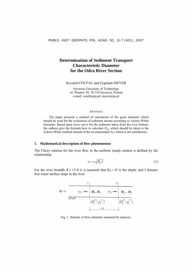
The Chezy relation for the river flow in the uniform steady motion is defined by the relationship:

.Hc R I=υ (1)

For the river breadth B ≥ 15 H it is assumed that RH = H is the depth, and I denotes free water surface slope in the river

H ,1 2B1 B2H ,

D ; p i i(2) (2)D ; p i i

(1) (1)

Q ⇐

1 2

1 2

x

Fig. 1. Scheme of flow elements assumed for analysis.

42

In each cross-section of the river, υ is the velocity of flowing water B is the breadth of the river bed and Di ; pi is the set of values representing sieve curve, i.e., the diameter of certain fraction and percentage.

For further consideration two cross-sections in the river were taken, 1 and 2. In uniform flow the slope of energy line I* is equal to the free water surface slope in the river. To estimate the energy losses, in general case, in the river flow it is commonly accepted that if the distance Δx between the two cross-sections, 1 and 2, is small, and the term 2Δ( /2 ) Δg xυ can be neglected, I* can be taken from Chezy equation. So we have

2 2

2 10 / 3 .*sQ nI

B H= (2)

In the above equation, ns denotes roughness coefficient after Manning and Q is the flow. The aim of the paper is to consider sediment transport in the river. The sediment stream was estimated according to the Ackers-White formulae (Ackers and White 1973, Meyer 1981). Various formulae of different authors were checked by Pluta and Meyer (2003) for Odra river. The Ackers-White formulae are in a good agreement with the other results; this has an advantage because it includes two flow factors such as mean velocity in the given cross-section υ0 and the shear velocity υ∗. So we have

0 ,QBH

=υ (3)

and

* ,b*gHI= =

τυ

ρ (4)

and in further calculation I* can be taken according to the previous assumptions from Chezy Eq. (2).

To introduce to the analysis the sediment grains diameter D, Manning roughness coefficient according to Strickler was applied:

1 61 .26sn D= (5)

Previous research (Roszak 1998, Kotiasz 2001) indicates that the roughness coef-ficient ns is a function of the ratio Dz/H. So they proposed to modify Strickler equa-tion. According to Kotiasz research verified for lower Odra River we have

1/ 6

,zs

Dn MH

⎛ ⎞= ⎜ ⎟⎝ ⎠

(6)

where M varies practically for lower Odra river from 0.13 to 0.15. The representative diameter Dz can be evaluated according to Roszak (1998) in the following form:

43

0

0

1

,iz p

n

i i

DDDD=

=⎛ ⎞⎜ ⎟⎝ ⎠

Π (7)

where the symbol Π denotes multiplication of all the terms from i = 1 till i = n and

01

(n

i ii

).D p D=

=∑ (8)

Further research aims to estimate an appropriate value of D which should be taken to the sediment stream calculation based on the sieve curve data pi, Di. This can be achieved by combining two curves: the one representing water flow and the other rep-resenting sediment stream based upon samples taken from the bottom sediment. The curve for water flow based upon Eq. 2 is given in Fig. 2, and the curve for sediment stream will be presented in the next section. In Fig. 2, Hm and I*m are the measured depth and slope, respectively.

H [m]

I*I*m

mH

Fig. 2. Plot of the function H = H(I*).

2. Model of sediment transport

Assuming that flow intensity, sediment transport rate in the cross-section and river depth as well as the corresponding slope which has been measured in the steady mo-tion conditions, are constant, i.e.,

,Q const= ,const=ω ,H const= I const∗ =

and using Ackers-White’s method (Ackers and White 1973), the total sediment trans-port rate in the river can be evaluated as follows:

44

,Q g X=ω ρ (9)

where:

0 ,n

grsDX GH ∗

⎛ ⎞= ⎜ ⎟

⎝ ⎠

υυ

1 ,m

grgr

FG C

A⎛ ⎞

= −⎜ ⎟⎝ ⎠

(10)

( )2log 2.86log log 3.53 ,gr grC D D= − −

9.66 1.34,gr

mD

= + and ,s

w

s = ρρ

0 *

0

1 32log ,( 1) 32log

n

grHF H DgD s

D

⎡ ⎤⎢ ⎥ ⎡ ⎤

= ⋅ ⋅ ⋅⎢ ⎥ ⎢ ⎥− ⎣ ⎦⎢ ⎥⋅

⎣ ⎦

υ υ αα υ

(11)

and the values of υ0 and υ∗ were estimated earlier (Eqs. 3 and 4). The value of g is acceleration due to gravity and D is grain size diameter which is the matter of consid-eration, and s is the ratio of density of sediment ρs to the water density ρw.

Furthermore

0.23 0.14,gr

AD

= +

1 0.56log ,grn D= −

( ) 1/ 3

2

1,gr

g sD D

⎡ ⎤−= ⎢ ⎥

⎣ ⎦ν

and v = 1.3 ⋅ 10−6 is the kinematics viscosity coefficient of water [m2/s]. In dependence on the value of Dgr, the following cases will be considered:

− for Dgr ≤ 1 floated sediment (n = 1), − for 1 < Dgr ≤ 60 totally floated and dragged sediment, − for Dgr > 60 only dragged sediment (n = 0; A = 0.17; m = 1.50; C = 0.025).

In the original Ackers-White’s method it is recommended to put D = D35 (from the sieve curve of bottom sediment). From the previous research (Pluta and Meyer 2003)

45

it comes that fixed value of D35 does not allow to calculate properly the sediment transport for various river cross-sections (Coufal 1995, Coufal and Meyer 1997).

The reference value of D which should be taken to the evaluation of sediment stream should be the matter of further research, to specify D = Dopt.

The dependence of the depth H on the value I* for constant ω for various grains size diameters D is given in Fig. 3 (Meyer and Skorupska 2004, 2005). On this figure, the cure H(I*) from Fig. 2 is additionally plotted. So one can see that if the measured depth is equal to Hm and the corresponding slope is equal to I*m , D must be equal to Dopt .

H [m]

I*m

H m

D =0,6 mmopt

D =0,5 mm1D =0,55 mm2

Dn

D = 0,7 mm3

I* Fig. 3. Optimal diameters satisfying the Chezy equation.

3. Evaluation of Dopt

The analyses show that the optimal sediment diameter Dopt which will satisfy the Chezy condition and will “close” the equation of Ackers-White’s sediment transport model by terms of quantity, can be described for each river cross-section based on the determined value of depth and slope.

The optimal sediment diameter Dopt, was evaluated from the full sieve curve, and can be described by the statistical parameters (mean value, standard deviation and skewness of the curve) as follows:

1 2 3 ( , ) ,k

opt

z

Dc c c f

D⎛ ⎞

= + + =⎜ ⎟⎝ ⎠

δ ε δ ε (12)

where the sieve curve distribution factors were chosen as follows: standard deviation

20

1( )

n

ii

,iD D p=

= − ⋅∑δ skewnees 33 1 01

( )n

ii

,D D p=

= − ⋅∑ε and D0 is given by Eq. 8.

46

The results of calculations are presented both in Table 1 and some examples in Figs. 4 and 5. In Table 1 the values are: Q = 185 m3/s and Im = 0.000283.

Table 1

The results of calculations for the set of 554÷566 km

km B [m] H [m] Dz Dopt Dopt /Dz

552 113.50 2.250 0.0005379 0.00063351 1.1777 550 107.20 2.020 0.0005447 0.00069001 1.2668 548 105.85 2.170 0.0007167 0.00084681 1.1815 546 106.75 2.150 0.0005874 0.00052811 0.8991 544 109.00 2.210 0.0005327 0.0004904 0.9206 542 90.25 2.300 0.000589 0.00067484 1.1457

0

0,2

0,4

0,6

0,8

1

1,2

1,4

1,6

0 0,5 1 1,5 20

0,20,40,60,8

11,21,41,61,8

0 0,5 1 1,5 2

f( )δ,εf( )δ,ε 578÷617 km 554÷566 km

opt

z

DD

opt

z

DD

Fig. 4. Statistical optimization results for sets of 578÷617 km and 554÷566 km.

f( )δ,ε

542.4÷617 km

opt

z

DD

opt

z

DDf( )=δ,ε

0,31

Fig. 5. Statistical optimization results for all the sets.

47

Combining all the data for all cross-sections over the whole analyzed distance we have: C1 = 0.622; C2 = −497.33; C3 = 537.61 and k = 0.31. The resulting formulae takes the form

0.31

0.622 497.33 537.61 .opt

z

DD

⎛ ⎞= − ⋅ + ⋅⎜ ⎟

⎝ ⎠δ ε (13)

4. Conclusions

1. The experimental research of sediment transport in lower Odra River is pre-sented. The experiments concern estimation of representative grain diameter in sediment transport calculation.

2. The basic assumption of the method was the steady flow and constant sediment stream along tested river distance. The sieve curve for sediment samples taken from the bottom of the river was the background for verification.

3. The statistical analysis of the sieve curves leads to the conclusion that it is pos-sible to relate the optimal grain-size diameter for sediment stream calculation upon sieve curve distribution factors. The mathematical formulae for this rela-tionship is also given. It gives good agreement with experimental data for the whole analyzed distance.

References

Ackers, P., and W.R. White, 1973, Sediment transport. New Approach and Analysis. Journal of the Hydraulics Division, ASCE Vol. 99.

Coufal, R., 1995, Zmiany położenia dna w ujściowym odcinku rzeki wywołane ruchem rumowiska, Wyd. Uczelniane Politechniki Szczecińskiej, Szczecin.

Coufal, R., and Z. Meyer, 1997, Badanie zależności pomiędzy natężeniem przepływu a średnicą miarodajną dla odcinka Odry Środkowej, Instytut Budownictwa Wod-nego Polskiej Akademii Nauk w Gdańsku, XVII Ogólnopolska Szkoła Hydrauliki, Gdańsk-Sobieszewo.

Kotiasz, W., 2001, Wpływ zabudowy regulacyjnej koryta na zmiany położenia dna rzeki, PhD Thesis Politechnika Szczecińska.

Meyer, Z., 1981, Hydraulika stosowana, cz. I. Podstawy ruchu rumowiska oraz obli-czanie stabilności dna rzeki, Wyd. Politechniki Szczecińskiej, Szczecin.

Meyer, Z., and W. Skorupska, 2004, Analysis of substitutive sediment diameter changes under circumstances of the Lower Odra, XXIV International School of Hydraulics, Jastrzębia Góra, September 13-17, Poland.

Meyer, Z., and W. Skorupska, 2005, Analysis of representative diameter, describing sediment transport rate in the Middle Odra River section, XXV International School of Hydraulics, Debrzyno, September 12-16, Poland.

48

Pluta, M., and Z. Meyer, 2003, Ocena przydatności wzorów empirycznych dla ok-reślenia natężenia rumowiska w Odrze, XXIII Ogólnopolska Szkoła Hydrauliki, Współczesne Problemy Hydrauliki Wód Śródlądowych, Tleń, wrzesień 12-16.

Roszak, A., 1998, Hydrauliczne warunki rozdziału strumienia rumowiska w rozwidle-niu rzecznym w warunkach przepływu wielkich wód na przykładzie węzła wodnego Widuchowa na Odrze, PhD Thesis Politechnika Szczecińska.

PUBLS. INST. GEOPHYS. POL. ACAD. SC., E-7 (401), 2007

Open-Channel Turbulence Measurements with a Three-Component Acoustic Doppler Velocimeter

Włodzimierz CZERNUSZENKO1 and Edward. R. HOLLEY2 1 Institute of Geophysics, Polish Academy of Sciences

Ks. Janusza 64, 01-452 Warsaw, Poland e-mail: wczer@igf.edu.pl

2 Department of Civil, Architectural, and Environmental Engineering University of Texas at Austin, Austin, TX USA

e-mail: HolleyE@mail.utexas.edu

Abstract

The aim of this article is to familiarize the readers (e.g., civil and environ-mental engineers) with the current statistical theory of turbulence for river flows. The authors want to give sufficient theoretical information not only for studying the specialized literature but also for experimental investigations on those envi-ronmental problems in which turbulence plays an essential part, such as erosion and sediment transport, resistance to flow, and pollutant dispersion.

The paper describes comprehensive turbulence measurements in an experi-mental channel where instantaneous velocities were measured with use of a three-component acoustic Doppler velocity meter. The basic definition of the primary turbulence parameters as well as methods of estimating those parameters are discussed. Also, the fundamental relations for the primary velocity, the dis-tribution of turbulent intensities, the Reynolds stresses, the autocorrelation func-tions, the turbulent scales, and the energy spectra are discussed.

1. Introduction

Turbulence is the most common, the most important, and the most complicated kind of fluid motion. For at least a quarter of century we have observed an increasing rec-ognition of the role of turbulent fluid motion in controlling river processes of interest to engineers. These processes include erosion and sediment transport, resistance to flow, and pollutant dispersion. Also, recent investigations emphasize the significance of turbulence in river ecology, e.g. Larned et al. (2004). Despite these advances in understanding, turbulence remains one of the least understood phenomena in the proc-ess-based earth sciences, a state of affairs that continues to retard the formulation of realistic, physically-based models of sediment transport on the earth’s surface.

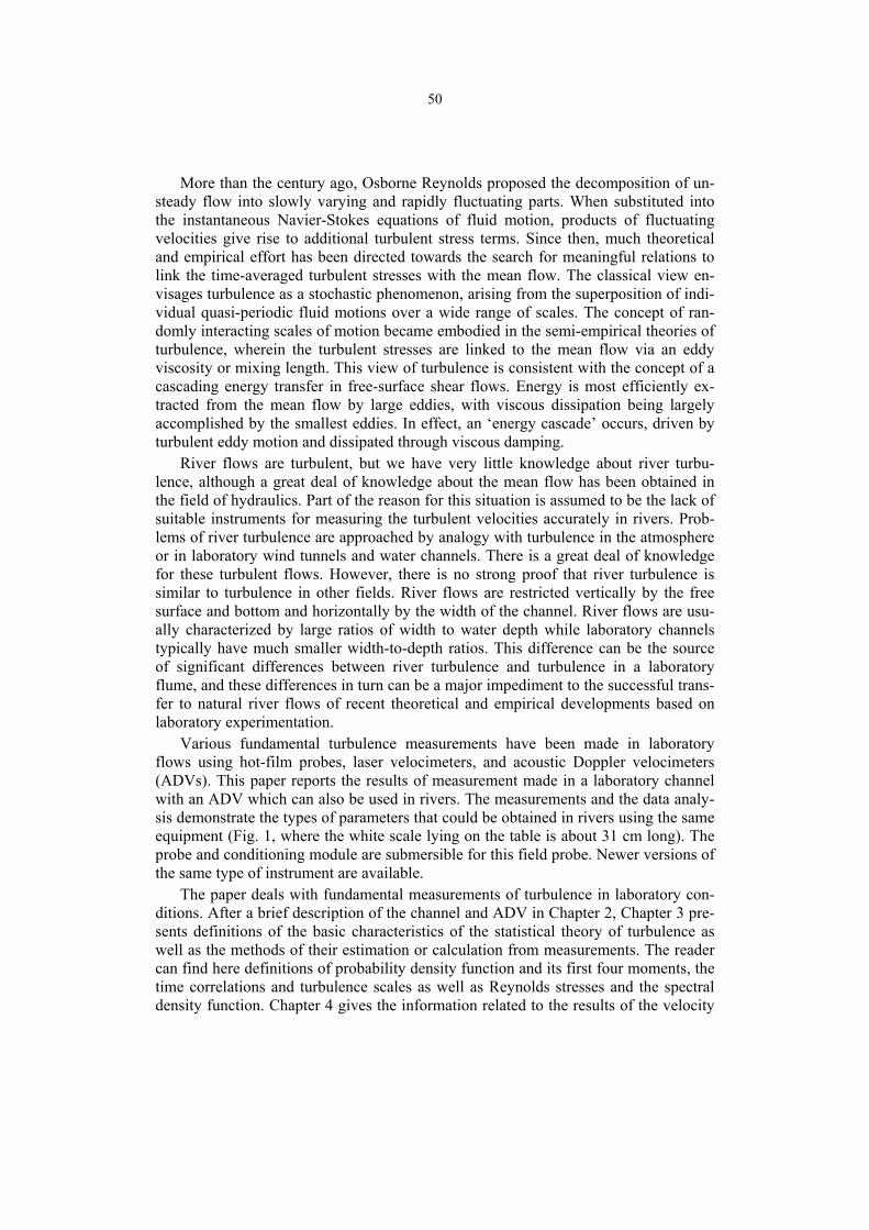
50

More than the century ago, Osborne Reynolds proposed the decomposition of un-steady flow into slowly varying and rapidly fluctuating parts. When substituted into the instantaneous Navier-Stokes equations of fluid motion, products of fluctuating velocities give rise to additional turbulent stress terms. Since then, much theoretical and empirical effort has been directed towards the search for meaningful relations to link the time-averaged turbulent stresses with the mean flow. The classical view en-visages turbulence as a stochastic phenomenon, arising from the superposition of indi-vidual quasi-periodic fluid motions over a wide range of scales. The concept of ran-domly interacting scales of motion became embodied in the semi-empirical theories of turbulence, wherein the turbulent stresses are linked to the mean flow via an eddy viscosity or mixing length. This view of turbulence is consistent with the concept of a cascading energy transfer in free-surface shear flows. Energy is most efficiently ex-tracted from the mean flow by large eddies, with viscous dissipation being largely accomplished by the smallest eddies. In effect, an ‘energy cascade’ occurs, driven by turbulent eddy motion and dissipated through viscous damping.

River flows are turbulent, but we have very little knowledge about river turbu-lence, although a great deal of knowledge about the mean flow has been obtained in the field of hydraulics. Part of the reason for this situation is assumed to be the lack of suitable instruments for measuring the turbulent velocities accurately in rivers. Prob-lems of river turbulence are approached by analogy with turbulence in the atmosphere or in laboratory wind tunnels and water channels. There is a great deal of knowledge for these turbulent flows. However, there is no strong proof that river turbulence is similar to turbulence in other fields. River flows are restricted vertically by the free surface and bottom and horizontally by the width of the channel. River flows are usu-ally characterized by large ratios of width to water depth while laboratory channels typically have much smaller width-to-depth ratios. This difference can be the source of significant differences between river turbulence and turbulence in a laboratory flume, and these differences in turn can be a major impediment to the successful trans-fer to natural river flows of recent theoretical and empirical developments based on laboratory experimentation.

Various fundamental turbulence measurements have been made in laboratory flows using hot-film probes, laser velocimeters, and acoustic Doppler velocimeters (ADVs). This paper reports the results of measurement made in a laboratory channel with an ADV which can also be used in rivers. The measurements and the data analy-sis demonstrate the types of parameters that could be obtained in rivers using the same equipment (Fig. 1, where the white scale lying on the table is about 31 cm long). The probe and conditioning module are submersible for this field probe. Newer versions of the same type of instrument are available.

The paper deals with fundamental measurements of turbulence in laboratory con-ditions. After a brief description of the channel and ADV in Chapter 2, Chapter 3 pre-sents definitions of the basic characteristics of the statistical theory of turbulence as well as the methods of their estimation or calculation from measurements. The reader can find here definitions of probability density function and its first four moments, the time correlations and turbulence scales as well as Reynolds stresses and the spectral density function. Chapter 4 gives the information related to the results of the velocity

51

measurements as well as analysis and discussions of these results. One can find here some basic information on the logarithmic law, the turbulence intensities, skewness and kurtosis, scales of turbulence, turbulent stresses, and the spectral density function.

Fig. 1. ADV probe and conditioning module.

2. Experimental facilities

2.1 Channel The measurements were made in a rectangular channel which is 1.52 m wide, 0.81 m deep, and 33.5 m long, at the University of Texas at Austin, TX, USA (Fig. 2). The channel has a concrete bed and concrete-block walls with Manning’s n = 0.011. The bed is approximately horizontal. The channel is outdoors but was covered with corru-gated fiberglass sheets during measurements to minimize wind effects. A tailgate at the downstream end of the channel allows modification of the flow depth. The meas-urement cross section was about 20 m from the channel entrance. This location and the channel length meant the flow was established upstream of the measurements and also not disturbed by the tail gate.

The flow rate was determined using propeller-type flow meters installed in the three supply pipes. A thin-plate weir in the return channel was used to check the rate obtained from the propeller meters. The meters were calibrated volumetrically. The static ports in 24 Pitot tubes at 10 cross sections were connected to a manometer board inclined at 1V:5H for measuring the water surface elevations.

conditioning module

cm

probe

52

Fig. 2. Experimental channel looking upstream.

For the experiments, the flow rate was 0.558 m3/s and the flow depth was 48.8 cm, giving an average flow velocity of 0.75 m/s. The Reynolds number using four times the hydraulic radius was 9×105. The tail gate was adjusted so that the flow was ap-proximately uniform. Truly uniform flow could not be achieved since the bed was not exactly plain and the channel could not be tilted.

2.2 Acoustic Doppler Velocimeter The velocity measurements were made with a downward-looking, three-component SonTek 10-MHz Acoustic Doppler Velocimeter (ADV, Fig. 1). The ADV had a Field probe with a rigid shaft and a 5-cm sensor and was mounted vertically on a traversing mechanism that allowed vertical, transverse, and longitudinal movement. Measure-ments were made at maximum available rate of 25 Hz, so that the Nyquist frequency was 12.5 Hz. A data acquisition program provided by the manufacturer was used to collect the velocity data for at least 60.44 seconds for each sampling point. The sam-pling volume of the probe is about 5 cm below the tip of the probe and, according to the manufacturer, the minimum distance to a flat boundary that still permits data col-lection is 4 to 6 cm. Therefore the probe cannot measure velocities within approxi-mately the top and bottom 6 cm of the flow depth. The measurement points are shown in Fig. 3.

3. Parameters for turbulence

3.1 Velocity as a random process The instantaneous longitudinal (x) velocity at any point in a turbulent flow is a random variable U(t). The values of U(t) are called a time series. For a large number of sets of

53

measurements, there will be a set of random variables or a time series of variables that can be indicated by braces, i.e., U(t). The measured velocity at this point at time t is one of the infinity of values which U(t) might have at t. The behavior of U(t) can be described by a probability density function (pdf). A stochastic process consists of U(t) and its probability distributions. The area under the pdf for an infinitesimal velocity interval represents the probability of occurrence of the value of the velocity at the center of the interval.

Turbulence is inherently three dimensional. While parts of the paper use only the longitudinal velocity, the velocity (V) in the transverse (y) direction and the velocity (W) in the vertical (z) direction are addressed in several of the sections. The actual velocity is a continuous time series, but measurements usually give a discrete time series of values measured at some time interval Δt. The type of instrumentation nor-mally determines whether Δt is constant. In the present measurements, Δt is constant.

Fig. 3. Measurement points with flow into the paper.

The following discussion of each of the statistical parameters begins with the basic definition and a physical interpretation. The definitions are based on a continuous time series of infinite duration. The estimators used for the discrete, finite time series of velocity measurements follow each of the basic discussions. The equations are written for the longitudinal velocity, but similar equations apply for the other two components also. The pdf and the statistical moments in this paper depend on only the magnitudes of the velocity measured at one point in the flow, not on the sequence in which the

15.230.530.530.530.5

4.88

9.75

9.75

9.75

6.30

15.2

1

2

3

4

51

9

15

14

20

19

81318

16

17 12 7

11 6

25

24

23

22

21

8.37

IIIIIIIVV

x

y

z

152.4

48.8

All dimensions are in cm.

10

54

values occur. The correlation and energy spectrum depend on the sequence in which the magnitudes occur. The Reynolds stresses depend on the simultaneous velocities in two directions at a point, but not on the sequence of values.

3.2 Statistical moments

Definitions

An analytical expression for the pdf for turbulent flows is not easy to establish. Never-theless, for most practical (engineering) purposes, the function can be characterized by statistical moments of different orders that can be obtained relatively easily from ex-periments. A statistical moment of n-th order for data collected at one point for any random variable (ξ) can be defined by

n nE[ ] p( )d∞

−∞ξ = ξ ξ ξ∫ (1)

where E[ ] represents the expected value, p(ξ) is the pdf, and n = 1,2,3… For a sta-tionary, ergodic process, E[ξn] is also given by

t To

to

n n nT

1E[ ] lim dtT

+

→∞ξ = ξ = ξ∫ (2)

where the overbar indicates a time-averaged value, t = to at the beginning of the data series being analyzed, and T = duration of the data.

Equation 1 with n = 1 gives the mean value (also called the expected or time-averaged value) of a random variable. The mean value is indicated by an overbar, e.g., U . The turbulent fluctuations of velocity (u, v, w) in the x, y, z directions are defined by

u U U

v V V

w W W

= −

= −

= −

(3)

Even in a straight laboratory channel, secondary circulation can cause V and W to be non-zero.

The first central moments of the turbulent velocities are zero because the average turbulent velocity is zero in each direction. The second moment represents the mean-square departure from the time-averaged velocity and is called the variance (σ2) or mean square, e.g., in the x direction

2 2x uσ = (4)

The square root (σ) of the variance is the standard deviation or root-mean-squared velocity fluctuation, which is sometimes called the turbulence intensity. The second, the third and the forth moments are often replaced by their non-dimensional forms, namely

55

2uu '

U= (5)

3

x 2 3/ 2

uS(u )

= (6)

4

x 2 2

uK 3(u )

= − (7)

These non-dimensional parameters are called relative turbulence intensity (u′), skew-ness (Sx) and flatness factor, excess, or kurtosis (Kx). These terms have specific physi-cal interpretations. The skewness is related to the asymmetry in the distribution of turbulent velocities. Sx = 0 for a Gaussian distribution and any other symmetrical dis-tribution. Sx is positive when large positive values of u are less frequent than large negative values. The excess is related to the flatness of distribution. For reference, Kx = 0 for a Gaussian distribution when the definition in Eq. (7) is used. Larger values of Kx imply that p(u) has a narrower peak and broader tails than a Gaussian distribu-tion with the same standard deviation. That is, both very small and very large values of the random variable are more probable than for a normal distribution.

Calculation

To determine u using Eq. (3) and the discrete time series of measured U values with constant Δt, U is first calculated from

N

k 1

1U U(k t)N =

= Δ∑ (8)

where N = total number of Uk values in the time series. The moments can then be estimated from the values of u (Eq. 3) by

nN

n

k 1

1u u (k t)N =

= Δ∑ (9)

The most important features of any estimator are the bias, which represents the sys-tematic portion of the error of the estimation, and the variance, which is the random portion of the error. Note that in this paragraph “variance” relates to possible errors in the estimator, not to the variance or mean-squared velocity in Eq. (4). Both bias and variance contribute to the mean square error of the estimate. It is natural to choose an estimator with a small or zero bias, but it is not always wise to insist that an estimator be unbiased. Making the bias small usually increases the variance of the estimator. Therefore, a compromise is necessary between variance and bias (Jenkins and Watts 1969). Equation (8) is an unbiased estimator for calculation of the mean velocity. Un-fortunately, for calculation of the second (n = 2), third (n = 3) and fourth (n = 4) mo-ments, Eq. (9) is biased estimator. However, for the duration of the observations in

56

these measurements, Eq. (9) has a smaller mean square error than the unbiased estima-tor.

3.3 Time correlations and turbulence scales

Definitions

We may define an Eulerian autocorrelation coefficient (rE) for the values of a given velocity component, say the longitudinal component, at a fixed point in the flow field but at two different times t and t′. Since we are working with stationary variables, rE can depend only on the time difference τ, which is equal to t′ − t, and it must be a sym-metrical function of Δt. Using Eq. (2) for time averaging, rE for the longitudinal veloc-ity is defined by

2

EE

R ( t)r ( t)u

ΔΔ = , (10)

where

ER ( t) u(t)u(t t).Δ = + Δ (11)

The maximum value is rE(0) = 1, while rE approaches zero for large Δt, but frequently decreasing oscillations are obtained as rE is approaching zero. The autocorrelation coefficient can be used to define an Eulerian integral time scale (TE) as

E E0T r ( t)d( t).

∞= Δ Δ∫ (12)

TE may be considered as an indication of the time interval over which the longitudinal velocity component at a point is correlated with itself.

Let us consider a stationary and homogeneous turbulent flow with a small relative intensity. Then the hypothesis of “frozen turbulence” is valid and an integral length scale (Λx) can be calculated from the Eulerian time scale as (Hinze 1975)

x EUT .Λ = (13)

Calculation

The sample autocorrelation function for the discrete time series of measured u values with a constant Δt between the measurements was estimated from

( )N m

i i mi 1

1R(m) u u , k 1,2,3,...N

−

+=

= =∑ (14)

where m is the lag number. It can be shown that Eq. (14) is only asymptotically an unbiased estimator, but it has a smaller mean square error than the unbiased estimator obtained from Eq. (14) with the coefficient 1/N replaced by 1/(N-m) (Jenkins and Watts 1969).

57

3.4 Transport of turbulent kinetic energy

Definition

The turbulent kinetic energy (TKE) per unit volume of fluid is

2 2 2 2u v w qTKE ,

2 2+ +

= ρ ≡ ρ (15)

where q2 = u2 + v2 + w2. Although Eq. (15) gives the proper definition of TKE per unit volume, frequently the term “energy” or “power” is used when referring to only

2q or to 2u when only one velocity component is being used. The rate at which the TKE is transported in each of the coordinate directions by the turbulent velocity fluc-tuations is

2

jq ufor j x, y,z.

2ρ = (16)

Calculation

The estimator for the TKE per unit volume using discrete measurements is

( )N^

2 2 2i i i

i 1TKE u v w .

2N =

ρ= + +∑ (17)

Similarly, the estimator for the turbulent flux of TKE per unit volume for the velocity uj in the j direction is

( )^

2 Nj 2 2 2

i j i i j i i j ii 1

q uu (u ) v (u ) w (u ) .

2 2N =

ρρ = + +∑ (18)

3.5 Reynolds stresses

Definitions

A phenomenological view of turbulence treats the turbulent motion of parcels of fluid as being analogous to molecular motion in gases. That is, parcels of fluid can be viewed as moving from a region with a higher time-averaged velocity to a region with a lower time-averaged velocity and then speeding up the slower moving fluid. When only the time-averaged motion of the fluid is considered, this turbulent action appears as a shear stress, which is called an apparent, turbulent, or Reynolds stress.

This apparent stress can be related to the turbulent velocities by using Eq. (3) to eliminate the instantaneous velocities in the three-dimensional differential momentum equations (or equations of motion) and then time averaging the equation for each co-ordinate direction. The resulting equations are called the Reynolds equations and give the nine stress (τ) terms as

58

2xx xy xz

2yx yy yz

2zx zy zz

U Up u uv uwy z

V Vvu p v vwx zW Wwu wv p w .x y

∂ ∂τ = − ρ τ = μ − ρ τ = μ − ρ

∂ ∂

∂ ∂τ = μ − ρ τ = − ρ τ = μ − ρ

∂ ∂∂ ∂

τ = μ − ρ τ = μ − ρ τ = − ρ∂ ∂

(19)

For each term, the first subscript indicates the normal to the surface on which the stress is acting and the second one indicates the direction of action. On the right-hand side of each definition, the first term represents the molecular action while the second term is the contribution of the turbulence. From basic mechanics, it is known that

xyτ = yxτ , xzτ = zxτ , and yzτ = zyτ . The Reynolds normal stresses ( xxτ , etc.) are directly related to the turbulence intensities in each direction. The Reynolds shear stresses come from the cross correlations of orthogonal velocity components.

Calculations

The Reynolds shear stresses were calculated in essentially the same way as other simi-lar terms. For example,

N

xy i ii 1

ˆ (u v ).N =

ρτ = ∑ (20)

3.6 Energy spectrum

Definitions

The moments (Eq. (1)) and the autocorrelation (Eq. (10)) are useful in analyzing tur-bulence, and they are relatively easy to obtain from velocity measurements. Spectral analysis is another useful tool, but the spectra are more difficult to calculate. The spec-trum of turbulent kinetic energy and the correlation coefficient are related by the Fou-rier transformation, e.g, see Hinze (1975). The spectrum and the correlation put em-phasis on different aspects of the process, but the potential flexibility available via the spectrum and the Fourier transform is much greater than with the correlation function approach. There are two types of spectra that are of interest, namely the frequency spectra and the wave-number spectra. We shall introduce only the frequency spectra and only for the x-component of velocity. This spectral analysis allows us to describe the distribution of TKEx, i.e., the TKE associated with only the x component of the turbulent velocity, with frequency (f) in the turbulence.

The essence of the turbulence spectrum is to consider the continuous, irregular turbulent fluctuations of velocity to be the superposition of many different frequency components. For example, the time series of u values is considered to be the superpo-sition of many frequency components. Then the amount of energy in each of the com-ponents is determined. For example, let

59

1 2 3 4f f f fu(t) u (t) u (t) u (t) u (t) . . .= + + + + (21)

where each fk is a different frequency and each frequency component has a sinusoidal temporal variation with an amplitude that changes with time. To get the total TKEx associated with u, Eq. (15) shows that the mean squared value of Eq. (21) is needed. Squaring Eq. (21), taking the time average, and using the orthogonality of the sine functions gives

1 2 3

2 2 2 2f f fu u u u . . .= + + + (22)

The spectral density function (Gx(f)) for a continuous variation of f is defined so that

2x0

G (f )df u∞

=∫ (23)

where

2x fG (f )df u= (24)

and Gx(f)df is proportional to the TKEx in the bandwidth f to f + df. The normalized spectral density function (Fx(f)) is

xx 2

G (f )F (f )u

= (25)

so that

x0F (f )df 1.

∞=∫ (26)

Calculations Spectral density function has been explained in the practical context of filtering, squaring, and averaging sample records. One method for calculating spectral density functions is from the Fourier transform of the correlation function (Bendat and Piersol 1971). In this paper, the fast Fourier transform (FFT) procedures are used to compute estimates of power spectral density function directly from the original data values.

It has already been assumed that the turbulence velocity u(t) is a stationary random variable that is sampled over a finite time period T. A finite-range Fourier transform of the velocity sample as defined by Bendat and Piersol (1971) is

T

0U(f ,T) u(t)exp( j2 ft)dt ,= − π∫ (27)

where j = 1− . The quantity U(f,T) represents finite Fourier transform of u(t). That finite-range Fourier transform exists for general stationary records. The one-sided power spectral density function Gx(f), where f varies only over (0, ∞), is defined by

2x T

1G (f ) 2 lim E U(f ,T) for f 0.T→∞

⎡ ⎤= ≥⎣ ⎦

(28)

60

An estimate of Gx(f) can be obtained by simply omitting the limiting and expectation operations in the above equation (Bendat and Piersol 1971) to obtain

2x

2G (f ) U(f ,T) for f 0.T

= ≥ (29)

Since the sample of u(t) is taken over a finite time interval, xG (f) is called the sample

spectrum, and it is only an estimator of the actual Gx, which is defined for an infinite length of record (Eqs. (23) and (24)).

Equation (29) must be used with care because it is a statistically inconsistent esti-mator of the power spectral density function. Furthermore, the random error of the estimate is substantial. The standard deviation of the estimate is as great as the quan-tity being estimated when no frequency smoothing is performed (Bendat and Piersol 1971). Therefore, if a power spectrum is estimated by direct Fourier transform opera-tions, a smoothing operation is required to obtain a consistent estimate. The normal-ized standard error of the estimate will be on the order of (Te/T)0.5, where Te is the width of a smoothing operation and T is the record length.

To present the method, it is convenient to let u(t) be defined over the time interval (−T/2, T/2) instead of (0,T). Then the finite range Fourier transform (Eq. (27)) can be viewed as a transformation of an infinitely long record u∞(t) defined over (−∞, +∞), multiplied by window function φ(t) defined over (−T/2, T/2), i.e.

T / 2

T / 2U(f ,T) u(t)exp( j2 ft)dt

u (t) (t)exp( j2 ft)dt ,

−∞

∞−∞

= − π

= φ − π

∫

∫ (30)

where φ(t) is a function or window that is nonzero in the measurement interval, 0 ≤ t ≤ T, and zero otherwise.

A very simple window is a rectangular window defined by

1 T / 2 t T / 2

(t)0 otherwise

− ≤ ≤⎧φ = ⎨

⎩ (31)

This rectangular window, especially for small T, may give a very distorted picture of the spectrum. This effect is caused by large negative side lobe leakage associated with the discontinuity of the function at the edges of the window. A smooth filter or win-dow shape to reduce leakage can be obtained by tapering the window at each end. In place of the rectangular window, it is suggested by (Bendat and Piersol 1971) that a cosine taper be used over 0.1 T at each end of the window. An effect of this tapering is to reduce the variance (error of the estimate) compared to using a rectangular window. The cosine tapering procedure used in this paper is defined by

61

⎪⎪⎪⎪

⎩

⎪⎪⎪⎪

⎨

⎧

≤≤π

≤≤−

−≤≤−π

=φ

otherwise0

2/Tt10/T4T

t5cos

10/T4t10/T41

10/T4t2/TT

t5cos

)t( 2

2

(32)

which is taken from Otnes and Enochson (1972). The calculated values of the power spectral density function ( xG ) using a window must be corrected by dividing them by ratio of the area under the tapered window to that under the rectangular window. The area under the window in Eq. (32) is 0.875T.

There are other windows with similar properties. All of them introduce tapering at the ends of the window. The purpose of tapering when viewed from its effect in the frequency domain is to suppress large side lobes in the effective filter obtained with the rectangular window transform. When viewed from the time domain, the object of tapering is to “round off” potential discontinuities at each end of the finite segment of the time history being analyzed.

Assume now that the turbulent velocity is sampled at N equally spaced time points with the time interval between samples being Δt. Then, for an arbitrary f, a discrete version of the Fourier transform of the velocity sample is (Bendat and Piersol 1971)

[ ]N 1

i 0U(f ,T) t u(i t) (i t)exp( j2 fi t) ,

−

=

= Δ Δ φ Δ − π Δ∑ (33)

where )T,f(U is an estimator of U(f,T) in Eq. (27).

The Fourier transform is calculated at discrete frequencies fk, where

kk Nf for k 0,1,2,..., .

N t 2= =

Δ (34)

The practical upper limit of the frequencies is the Nyquist cutoff frequency at f = 1/(2Δt). However, for turbulence, there is no energy at zero frequency since only variations from the mean velocity are included in u.

Equations (29) and (33) give the power spectrum estimator as

2 2

x k k k2 2 tˆ ˆ ˆG (f ) U(f ,T) U ,

N t NΔ

= =Δ

(35)

where

kk

U(f ,T)U .t

=Δ

(36)

62

To show the distribution of TKE with frequency, usually a graph of x kG (f ) vs. fk or

x kG (f ) /Δt vs. k/N is plotted.

Each individual value of x kG (f ) may have a very large variance so that the spec-trum has very large oscillations from point to point. To decrease the variance, fre-quency smoothing is applied using spectral windows. There are many spectral win-dows in the literature (e.g., Otnes and Enochson 1972, and Jenkins and Watts 1969). In this paper, the Tukey spectral window is used. This window has a weighting func-tion for the averaging that is a cosine function with a half wavelength equal to the width (B) of the window and with the maximum weighting being at the center of the window. B was chosen by trial and error to be 25/T in order to minimize the fluctua-tions in the spectra without losing the essential aspects of the shape of the spectral distributions. In fluid mechanics, the relative shape of the spectrum is often more im-portant than the actual values since only the shape is needed to identify the frequencies for things like the Kolmogorov inertial subrange and the Heisenberg viscous dissipa-tion range.

4. Experimental results

4.1 Mean velocity distributions Typical time series of the instantaneous velocities are shown in Fig. 4. These meas-ured velocities were time averaged (Eq. (2) with n = 1); the average velocities are indicated by the dashed lines in Fig. 4. The vertical distributions of the time-averaged velocities are shown in Fig. 5, where z is the distance from the bed and h is the flow depth. In spite of a long approach section, the velocity distributions were not symmet-rical about the vertical centerline of the channel. Measurements were not made close to the bottom, side boundaries, or water surface. Thus, the velocity distributions in Fig. 5 do not explicitly show the ‘velocity-dip’, which is the name applied to the im-portant feature for narrow open channel flows (B/h < 5) where the maximum velocity occurs just below the free surface rather than at the free surface. This characteristic is peculiar to open channel flows.

The hypothesis of the vertical distribution of mean velocity indicates that the log-law is applicable only in the wall region (z/h < 0.2) and that the deviation from this law should be represented by adding a wake function (Nezu and Rodi 1986). How-ever, one can assume that the wake function is practically equal to zero if the flow is close to uniform in a very wide rectangular channel (which this channel was not) and has no suspended sediment. The log-law for turbulent flow is

*

*

zuU 1 ln A,u

= +κ ν

(37)

where u* is the friction velocity, κ is the von Karman constant, ν is the kinematic vis-cosity, and A is a constant. The value of A depends on the type and geometry of the flow system and on the boundary roughness. For boundaries in the hydraulically rough

63

regime or in the transition regime between smooth and rough, A depends on u*. By differentiating Eq. (37),

*dUu .

ln(10) d(log z)κ

= (38)

Fig. 4. Typical instantaneous velocities.

Fig. 5. Vertical distributions of longitudinal velocity.

Point 9

0.7

0.8

0.9

1.0

1.1

0 5 10 15 20 25 30 35 40 45t (s)

U (m

/s)

Point 21

0.5

0.60.7

0.8

0.9

0 5 10 15 20 25 30 35 40 45t (s)

U (m

/s)

0.0

0.2

0.4

0.6

0.8

1.0

0.0 0.2 0.4 0.6 0.8 1.0

U bar (m/s)

z/h

IIIIIIIVV

U (m/s)

64

Using Eq. (38) and assuming κ = 0.4, u* can be found from the slope of a semi-

logarithmic graph of U vs. z. Equation (37) approximates the three measured mean velocities for z/h from 0.1 to

0.5 (Fig. 6). Using the straight lines in Fig. 6 and Eq. (38), the values of u* in Table 1 were obtained.

Table 1

Friction velocities from Fig. 6 and Eq. (38)

Vertical u* (m/s)

I 0.035 II 0.031 III 0.031 IV 0.031 V 0.038

Fig. 6. Vertical distributions of longitudinal velocity (semi-logarithmic scale).

0.1

1.0

0.7 0.8 0.9 1.0

III

0.1

1.0

0.7 0.8 0.9 1.0

II

0.1

1.0

0.7 0.8 0.9 1.0

V

0.1

1.0

0.7 0.8 0.9 1.0

I

z/h

0.1

1.0

0.7 0.8 0.9 1.0

IV

z/h

U (m/s)

65

4.2 Turbulent velocities The turbulent velocity fluctuations come from the difference between the instantane-ous velocity and the time average (Eq. (3) and Fig. 4). The subsequent sections ad-dress various quantitative statistical aspects of the turbulence. However, some impor-tant aspects can be detected just by visual inspection of graphs like those in Fig. 4. For example,

• The magnitude of the fluctuations relative to the time-averaged velocity is larger near the boundary (Point 21) than near the surface (Point 9).

• The velocity fluctuations consist of both low frequencies that can be identified visually and higher frequencies that appear to be more irregular (at least for the scale of the graphs in Fig. 4).

• Frequencies at least as low as 0.1 Hz are present, as indicated by the variations with a period on the order of 10 sec. The reason for these velocity variations is unknown.

• The magnitude of the low frequency velocity variations is generally larger than for the higher frequencies.

• The magnitude of the velocity variations associated with the low frequencies is larger near the bed than near the surface.

Using the frozen turbulence assumption with a mean velocity of approximately 0.8 m/s, a 10-sec period corresponds to an eddy size of 8 m. It is difficult to conceive of this variation being turbulence because the flow was only about 0.5 m deep and 1.5 m wide. An eddy with a size 16 times larger than the flow depth should become unstable and break up into smaller eddies. On the other hand, if the low frequency variation is due to an unsteadiness in the flow, the magnitude of the variation near the bed and near the surface should be generally the same. Although the two velocity records in Fig. 4 were not obtained simultaneously, they were obtained on the same day with the same flow conditions. Without further investigation, a definitive explanation of the lowest frequencies cannot be given. Nevertheless, one possible cause is wave action in the channel. The celerity (c) of a long, gravity wave in this channel is 2.2 m/s. The channel length (L) of 35 m gives a 4L/c period of 64 sec. Higher harmonics would have smaller periods. Possible wave action could be identified by simultaneous veloc-ity measurements at two points which are separated by a distance that is large relative to the expected actual large eddy size, i.e., relative to the flow depth.

The probability density function for Point 13, which is near mid-depth on the channel centerline, is shown in Fig. 7. For this measurement point, the total number of velocities in the time series was 4182. Each point on the pdf was calculated as the average slope of the cumulative probability distribution over 49 velocity measure-ments. There is a large amount of scatter in Fig. 7. Nevertheless, it is still evident that the probability of –1 < u/σ < 0 is less than for a Gaussian distribution while the prob-ability of 0 < u/σ < 1.3 is greater than for a Gaussian distribution, i.e., the distribution has a negative skewness. Also see Section 4.4.

66

0

0.1

0.2

0.3

0.4

0.5

-3 -2 -1 0 1 2 3

u/σ

p(u)

GaussianPoint 13

Fig. 7. Probability density function.

4.3 Turbulence intensities The universal functions for the relative turbulent intensity in 2D shear layers, as in channel flows, are given by Nezu and Nakagawa (1993). The functions were obtained by adopting the k-e turbulence model, neglecting the viscous diffusion, and assuming that the turbulent energy is in local equilibrium. The function has the form

ii i

*

zD exp C for i u,v,w ,u hσ ⎛ ⎞= − =⎜ ⎟

⎝ ⎠ (39)

where C and D are constants and σ is defined in Eq. (4). For the intermediate region, i.e., 0.1< z/h < 0.6 in very wide channels, Nezu and Nakagawa (1993) suggest using the values of Table 2. The authors’ measurements gave the values in Table 3. Gener-ally, the coefficients for these measurements are smaller than those given by Nezu and Nakagawa (1993) and the coefficient C is not constant. The coefficient D is the largest for the longitudinal component of velocity and the smallest for the vertical velocity. Figure 8 shows the vertical distributions of turbulence intensities for Vertical III and the best fit straight lines that were used for determining C and D. These data generally follow the exponential relationship in Eq. (39), although σw is very nearly constant for the three points in the lower half of the flow depth. The situation is significantly dif-ferent for Vertical I (Fig. 9). The vertical variations of σu and σv are not even ap-proximately exponential. Rather the intensities decrease much more rapidly in the lower half of the flow than in the top half. In the top half, the σu and σv values in-crease with increasing z or are approximately constant. The same trends are present in the data for Vertical V. All of the values of σw increase with increasing z for Vertical I, as indicated in Fig. 9 and by the negative value of Cw in Table 3, and are approxi-mately constant for Vertical V. All of these differences from Eq. (39) are presumably

67

due to the fact that the present measurements were made for a flow with a width-to-depth ratio of only 3.1. For this type of flow, the secondary flow is upward near the sides of the channel (Schlichting 1968). The redistribution of the turbulence due to this secondary flow and the lateral shearing in addition to the vertical shearing can cause significant differences from two-dimensional flows in very wide rectangular channels. The values in Table 3 were obtained for 0.1 ≤ z/h ≤ 0.83 rather than just in the range of 0.1 to 0.6 as given by Nezu and Nakagawa (1993). This difference may have had some effect on the values of C and D, but it is not believed to be the major reason for the differences in Table 2 and Table 3.

Table 2

Values of C and D for Eq. (39) from Nezu and Nakagawa (1993)

Component C D u 1.0 2.30 v 1.0 1.63 w 1.0 1.27

Table 3

Values of C and D from measurements

Vertical I II III IV V C D C D C D C D C D

u 0.26 2.08 0.79 1.75 0.79 2.24 0.61 1.98 0.46 1.92 v 0.37 1.32 0.81 1.15 0.50 1.34 0.40 1.20 0.41 1.18 w -0.20 0.89 0.33 0.74 0.36 0.93 0.17 0.90 0.02 0.79

Fig. 8. Turbulence intensities for Vertical III.

-0.4

-0.2

0.0

0.2

0.4

0.6

0.8

0.0 0.2 0.4 0.6 0.8 1.0z/h

Ln ( σ

/u* )

U V WCu = 0.79, Du = 2.24

Cv = 0.50, Dv = 1.34

Cw = 0.36, Dw = 0.93

Ln (σ

/u*)

u v w

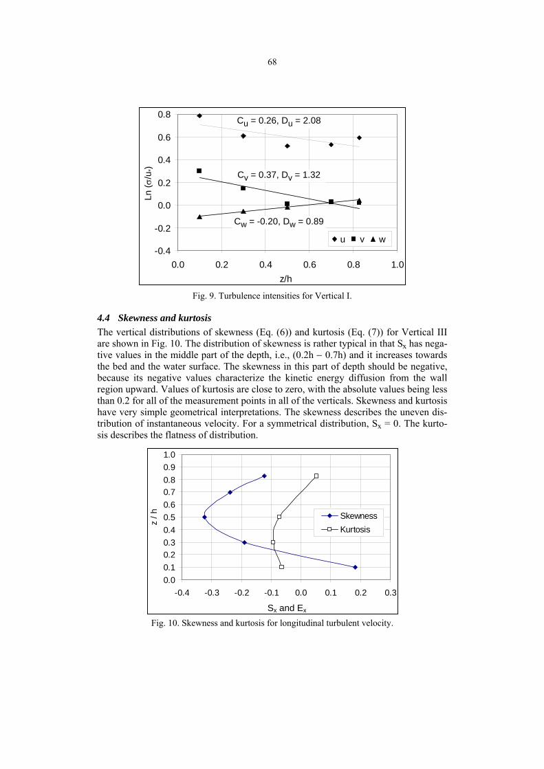
68

Fig. 9. Turbulence intensities for Vertical I.

4.4 Skewness and kurtosis The vertical distributions of skewness (Eq. (6)) and kurtosis (Eq. (7)) for Vertical III are shown in Fig. 10. The distribution of skewness is rather typical in that Sx has nega-tive values in the middle part of the depth, i.e., (0.2h − 0.7h) and it increases towards the bed and the water surface. The skewness in this part of depth should be negative, because its negative values characterize the kinetic energy diffusion from the wall region upward. Values of kurtosis are close to zero, with the absolute values being less than 0.2 for all of the measurement points in all of the verticals. Skewness and kurtosis have very simple geometrical interpretations. The skewness describes the uneven dis-tribution of instantaneous velocity. For a symmetrical distribution, Sx = 0. The kurto-sis describes the flatness of distribution.

Fig. 10. Skewness and kurtosis for longitudinal turbulent velocity.

-0.4

-0.2

0.0

0.2

0.4

0.6

0.8

0.0 0.2 0.4 0.6 0.8 1.0z/h

Ln ( σ

/u* )

U V W

Cu = 0.26, Du = 2.08

Cv = 0.37, Dv = 1.32

Cw = -0.20, Dw = 0.89

Ln (σ

/u*)

u v w

0.00.10.20.30.40.50.60.70.80.91.0

-0.4 -0.3 -0.2 -0.1 0.0 0.1 0.2 0.3Sk and Ex

z / h Skewness

Kurtosis

Sx and Ex

69

4.5 Autocorrelation function and macroscale The autocorrelation function (rE, Eq. (10)) for three of the points in Vertical III is shown with linear scales in Fig. 11. The integral time scale (TE) for these points was calculated from Eq. (12) by setting the upper limit for the integration at the value of Δt for which rE first goes to zero. The values of TE (Table 4) increase with increasing distance from the channel bed, i.e., TE ranges from 0.18 s at 4.9 cm to 0.95 s at 40.4 cm. The same is true of the length macroscale Λu calculated from Eq. (13) and given in Table 4. The last column in Table 4 gives values of

L

2uuRe ,Λ

=ν

(40)

where ReL is called the turbulence Reynolds number.

Table 4

Integral scales and related parameters on Vertical III

Point Height TE U Λu 2u ReL

cm s m/s m m/s 15 40.43 0.95 0.916 0.87 0.0466 40,500 14 34.13 0.71 0.910 0.64 0.0416 26,600 13 24.38 0.43 0.890 0.38 0.0524 19,800 12 14.63 0.30 0.845 0.25 0.0635 15,900 11 4.88 0.18 0.750 0.135 0.0768 10,100

Fig. 11. Autocorrelation coefficients for Points 11, 13, and 15 in Vertical III.

-0.2-0.10.00.10.20.30.40.50.60.70.80.91.0

0 1 2 3 4 5 6Time Lag (s)

Aut

ocor

rela

tion

Coe

ffici

ent

1113

15

15 11

1311

15

15

11

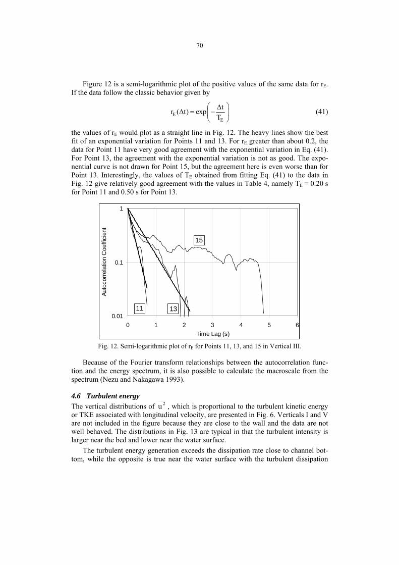
70

Figure 12 is a semi-logarithmic plot of the positive values of the same data for rE. If the data follow the classic behavior given by

EE

tr ( t) expT

⎛ ⎞ΔΔ = −⎜ ⎟

⎝ ⎠ (41)

the values of rE would plot as a straight line in Fig. 12. The heavy lines show the best fit of an exponential variation for Points 11 and 13. For rE greater than about 0.2, the data for Point 11 have very good agreement with the exponential variation in Eq. (41). For Point 13, the agreement with the exponential variation is not as good. The expo-nential curve is not drawn for Point 15, but the agreement here is even worse than for Point 13. Interestingly, the values of TE obtained from fitting Eq. (41) to the data in Fig. 12 give relatively good agreement with the values in Table 4, namely TE = 0.20 s for Point 11 and 0.50 s for Point 13.

Fig. 12. Semi-logarithmic plot of rE for Points 11, 13, and 15 in Vertical III.

Because of the Fourier transform relationships between the autocorrelation func-tion and the energy spectrum, it is also possible to calculate the macroscale from the spectrum (Nezu and Nakagawa 1993).

4.6 Turbulent energy The vertical distributions of 2u , which is proportional to the turbulent kinetic energy or TKE associated with longitudinal velocity, are presented in Fig. 6. Verticals I and V are not included in the figure because they are close to the wall and the data are not well behaved. The distributions in Fig. 13 are typical in that the turbulent intensity is larger near the bed and lower near the water surface.

The turbulent energy generation exceeds the dissipation rate close to channel bot-tom, while the opposite is true near the water surface with the turbulent dissipation

0.01

0.1

1

0 1 2 3 4 5 6Time Lag (s)

Auto

corr

elat

ion

Coe

ffici

ent

11

15 13

15

11

71

rate being larger than the generation rate. Consequently, an intermediate region should exist where there is a near-equilibrium turbulent energy budget, i.e., a region where the local rates of energy production and dissipation are approximately in local equilib-rium (Hinze 1975). In the intermediate region, the vertical flux of turbulent kinetic energy is expected to be almost constant.

Fig. 13. Vertical distributions of mean squared turbulent longitudinal velocity.

Lopez and Garcia (1999) performed experiments in a tilting open-channel flume (14 m long, 0.90 m wide at the ratio of channel width to water depth of 4.5 and larger) over a smooth bed with uniform flow conditions. They concluded that the vertical flux of TKE, 2 3

*q w/u , was almost constant and equal to 0.33 for z/h ∈ (0.1, 0.6). Our measurements were performed in a rather narrow channel (width/depth ≈ 3) and do not confirm this result (see Fig. 14). Only, for Vertical III on the channel centerline, may one conclude that the flux is approximately constant in the region of z/h ∈ (0.1, 0.6). Here it ranges from 0.33 to 0.39 with an average of 0.37. The fluxes calculated for Verticals II and IV, especially at points close to the bed (z/h = 0.1), have a lot of scat-ter. This scatter can be caused by the secondary currents and flow instability near the bed.

4.7 Reynolds stress distributions The idealized vertical distributions of Reynolds stresses can be obtained from the ba-sic momentum equations. For steady, uniform, fully developed turbulent flow in straight open channels, the time-averaged momentum equation for the primary flow direction (x) is (Nezu and Nakagawa 1993)

2U U ( uv) ( uw)V W gsin U,y z y z

∂ ∂ ∂ − ∂ −+ = θ + + + ν∇

∂ ∂ ∂ ∂ (42)

0.00.10.2

0.30.40.50.60.7

0.80.91.0

0 0.001 0.002 0.003 0.004 0.005

Turbulent kinetic energy in (m/s)^2

z/h

II

IIIIV

z/h

= R

elat

ive

dept

h

= Turbulent kinetic energy of longitudinal velocity in (m/s)2 2u

72

Fig. 14. Vertical turbulent flux of turbulent kinetic energy.

where U, V, W, and P are the time averaged values and θ = angle of inclination of the channel bottom. Integrating Eq. (42) in the vertical direction downward from the water surface (we assume that this is the direction of integration since h is the lower limit). For channels with small slopes, the equation for the xz-component of Reynolds stress when the viscous stresses are negligible is

xz

z z zxy

eh h h

Uuwz

U U gI (h z) V dz W dz dz,y z y

τ ∂≡ − + ν

ρ ∂

τ⎛ ⎞∂ ∂ ∂= − + + + −⎜ ⎟∂ ∂ ∂ ρ⎝ ⎠

∫ ∫ ∫ (43)

where the energy gradient is 2e *I sin u gR ,≡ θ = h = flow depth, and R = hydraulic

radius. In the central zone of wide open channels, the transverse gradients disappear, W = 0, and R = h so that Eq. (43) reduces to

2xze *

zgI (h z) u 1 .h

τ ⎛ ⎞= − = −⎜ ⎟ρ ⎝ ⎠ (44)

Equation 44) shows that for wide channels (aspect ratio B/h > 5), the vertical distribu-tion of the Reynolds shear stress τxz can have a linear vertical distribution from zero at the water surface to τo = ρ 2

*u at the channel bottom.

The vertical distributions of the three components of the Reynolds stresses deter-mined from the velocity measurements are shown in Fig. 15. For each vertical, the measured τ values were divided by the boundary shear stress for that vertical (τoi) from the u* values in Table 1.

0.00.10.20.30.40.50.60.70.80.91.0

-0.1 0 0.1 0.2 0.3 0.4 0.5 0.6

Turbulent energy flux, k w / U*^3

z / h

II

III

IV

z/h

= R

elat

ive

dept

h

TKE ofFlux Turbulent Vertical3

2

*u

wq =

73

The measurements show deviations of τxz from the linear relationship in Eq. (44) for all verticals. Several factors contribute to these deviations:

1. Variable τxy. To obtain Eq. (44), it was necessary to assume that the transverse gradient in the last term in Eq. (43) is zero. However, the data show that this condition is not met. Equation (43) shows that τxz has a conjugative relation with the transverse variations of the transverse Reynolds stress (τxy).

2. Secondary currents. In deriving Eq. (44) it was also assumed that the other two integral terms in Eq. (43) disappear, i.e., the second and third terms from the right-hand side. In fact, none of the integrand terms is zero due to the secon-dary currents generated by the transverse gradients of Reynolds stresses for the small width-to-depth ratio of approximately 3.

Even for a narrow channel, both the lateral velocity (V) and the xy-stresses would be zero at the channel centerline (Vertical III) if the flow were symmetrical about the centerline. However, neither of these terms is zero in this channel so both factors dis-turb the vertical distribution of xz-Reynolds stresses even in Vertical III. The Rey-nolds stresses in the remaining verticals are disturbed more severely (Fig. 15).

The equation for the τxy Reynolds stresses can be obtained by analogy to Eqs. (43) and (44). The equation would show that the τxy stresses are zero in wide channels without secondary currents. These measurements for a narrow channel show that τxy is not zero (Fig. 15).

Figure 15 shows that the τyz Reynolds stress, i.e., the vertical transport of trans-verse momentum, is close to zero compared to the other Reynolds stresses in all verti-cals. This condition exists if the gradient of normal stresses in the y direction (τyy) is negligibly small. For details, see Nezu and Nakagawa (1993).

4.8 Spectral density function The energy spectral density functions for Vertical III on the channel centerline were calculated according to the procedure described in conjunction with Eqs. (31) − (36), using a Tukey window width T = 1 s (Eq. (31)). The results are shown in Fig. 16.

Kolmogoroff’s similarity theory postulates that in a turbulent motion, at suffi-ciently high Reynolds number, there is a range of high wave numbers (equivalently, small wave lengths or high frequencies) where the characteristics of the turbulence are determined by the mean rate of energy dissipation per unit mass, ε, and the kinetic viscosity of the fluid, ν. This range of frequencies is called the universal equilibrium range. It is located far away from the range of the large energy-containing eddies and it extends till the dissipation range.

If the equilibrium range is sufficiently large, it includes an inertial subrange where the dissipation will be negligibly small compared with the flux of energy transferred by inertial effects. In this inertial subrange, the turbulence is determined by ε alone. The inertial subrange is located far away from the range of the energy-containing ed-dies and far away from the dissipation range. The average size of the energy-containing eddies is order of the integral length scale Lu (Table 4) and the average size

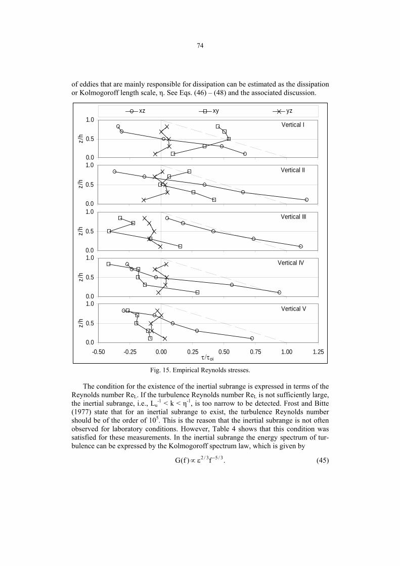
74

of eddies that are mainly responsible for dissipation can be estimated as the dissipation or Kolmogoroff length scale, η. See Eqs. (46) – (48) and the associated discussion.

Fig. 15. Empirical Reynolds stresses.

The condition for the existence of the inertial subrange is expressed in terms of the Reynolds number ReL. If the turbulence Reynolds number ReL is not sufficiently large, the inertial subrange, i.e., Lu

-1 < k < η-1, is too narrow to be detected. Frost and Bitte (1977) state that for an inertial subrange to exist, the turbulence Reynolds number should be of the order of 105. This is the reason that the inertial subrange is not often observed for laboratory conditions. However, Table 4 shows that this condition was satisfied for these measurements. In the inertial subrange the energy spectrum of tur-bulence can be expressed by the Kolmogoroff spectrum law, which is given by

2 / 3 5 / 3G(f ) f .−∝ ε (45)

0.0

0.5

1.0

-0.50 -0.25 0.00 0.25 0.50 0.75 1.00 1.25

z/h

xz xy yz

Vertical I

0.0

0.5

1.0

-0.50 -0.25 0.00 0.25 0.50 0.75 1.00 1.25t / tII

z/h

Vertical II

0.0

0.5

1.0

-0.50 -0.25 0.00 0.25 0.50 0.75 1.00 1.25t / tIII

z/h

Vertical III

0.0

0.5

1.0

-0.50 -0.25 0.00 0.25 0.50 0.75 1.00 1.25t / tIV

z/h

Vertical IV

0.0

0.5

1.0

-0.50 -0.25 0.00 0.25 0.50 0.75 1.00 1.25t / toi

z/h

Vertical V

τ/τoi

75

Fig. 16. Energy spectra for Vertical III.

With the large amount of oscillation in the spectra (Fig. 16), it is difficult to clearly identify the slope. Nevertheless, there appears to be a small range in which the slope is approximately −5/3. The spectra in the most right-hand part of the figure (perhaps above about 3 or 4 Hz) are dominated by noise. This behavior can be identified be-cause the spectra should be concave downward until reaching the dissipation range where the slope would be −1/7 at frequencies on the order of 50 Hz for this flow. See the discussion following Eq. (48).

Nikora (1999) writes about another subrange of frequencies where the spectrum decays as G(f) ∼ f −1. He suggests that this subrange is situated in the equilibrium range of frequencies, close to the energy-containing eddies. He assumed that in this subrange the energy dissipation is expressed as ε(k) ∼ u*

3k, where k is the wave number. In terms of frequency, the equivalent behavior is ε(f ) ~ u*

3f/U and G(f) ~ f−1.

The spectra in Fig. 16 were calculated by using a one-second smoothing time win-dow and show the existence of the −5/3 range of frequencies, i.e., the Kolmogoroff’s inertial subrange. However, there is also a large amount of noise in the spectra. The width of the window can be chosen by trial depending on the objective of the calcula-tion. To minimize the fluctuations in the spectra without losing the essential aspects of the shape of the spectral distributions, one should choose a rather wide window. In our analysis, the relative shape of the spectrum was more important than the actual values since only the shape was needed to identify the Kolmogoroff inertial subrange (−5/3 slope) and −1 frequency subrange.

Applying a five-second window for calculation of the spectral density function, it is possible to detect the locations of both the inertial subrange and the −1 subrange more precisely (Fig. 17 – Fig. 19). The frequency ranges in which the −1 and −5/3 power laws were obtained from these figures for the channel centerline are shown in Table 5.

0.00001

0.0001

0.001

0.01

0.1

0.01 0.1 1 10

Frequency [Hz]

Spec

tral D

ensi

ty [m

2/s] 11

13

15

11

13

15

slope = -5/3S

pect

ral D

ensi

ty [m

2 /s]

76

Table 5

Frequencies for the −1 and −5/3 subranges

Slope of frequency subrange Point Distance from bed

−1 −5/3 cm Hz Hz

11 4.9 − 1.05 − 4.0 13 24.4 0.4 − 0.7 0.9 − 4.0 15 40.45 0.5 − 0.9 1.0 − 4.0

Fig. 17. Energy spectra for Point 11, located at z = 4.9 cm.

Fig. 18. Energy spectra for Point 13, located at z = 24.4 cm.

0.00001

0.0001

0.001

0.01

0.01 0.1 1 10 100Frequency [Hz]

Spec

tral D

ensi

ty

[m2 /s

]

slope = -5/3

Spe

ctra

l Den

sity

[m2 /s

]

0.00001

0.0001

0.001

0.01

0.01 0.1 1 10 100Frequency [Hz]

Spe

ctra

l Den

sity

[m

2 /s]

slope = -5/3

slope = -1

Spe

ctra

l Den

sity

[m2 /s

]

77

For the spectrum in Fig. 19, it is possible to identify a characteristic frequency of 2 Hz, at which the slope −5/3 slope is disturbed. One can relate this disturbance to the secondary motion with a characteristic size of motion of 0.47 m for a time-averaged velocity 0.94 m/s. It is easy to notice that this kind of disturbance does not appear at the other two distances from the bed, i.e., 4.9 cm and 24.4 cm.

Fig. 19. Energy spectra for Point 15, located at z = 40.45 cm.

Kolmogoroff’s dissipation length scale is given by Hinze (1975) as

1/ 43

.⎛ ⎞ν

η = ⎜ ⎟⎜ ⎟ε⎝ ⎠ (46)

The corresponding velocity scale is

( )1/ 4u .η = νε (47)

These two scales can be combined to give a dissipation frequency scale of

1/ 2u

f .ηη

ε⎛ ⎞= = ⎜ ⎟η ν⎝ ⎠ (48)

The order of magnitude of these scales can be estimated by using dissipation rate εA for the entire flow area, where εA = gUAIe, g = acceleration of gravity, UA = cross sec-tional average velocity, and Ie = slope of the energy grade line. Using flow rate = 0.558 m3/s, channel width = 1.52 m, flow depth = 0.488 m, Manning’s n = 0.011, and kinematic viscosity = 10-6 m2/s, then εA = 0.00255 m2/s3, η ≈ 0.14 mm, uη ≈ 7 mm/s, and fη ≈ 50 Hz. Since the Nyquist frequency for the ADV used for these measure-ments is 12.5 Hz and fη is on the order of 50 Hz, it is not possible to see the dissipation range from these measurements.

0.00001

0.0001

0.001

0.01

0.01 0.1 1 10 100Frequency [Hz]

Spe

ctra

l Den

sity

[m

2 /s] slope = -1

slope = -5/3

Spe

ctra

l Den

sity

[m2 /s

]

78

5. Conclusions

Measurements show that the vertical distribution of longitudinal velocity follows the log-law for smooth wall with Karman constant 0.4 only for z/h < 0.5 and for the chan-nel centerline (Vertical III).

The probability density function (pdf) for longitudinal turbulent velocity is not Gaussian even for the central part of the channel cross section. The pdf has a negative skewness for all z/h > 0.2 with the largest negative value being at mid-depth. The kur-tosis is negative for z/h < 0.7.

The universal relationship for two-dimensional flows suggested by Nezu and Na-kagawa applies only for Vertical III but with different coefficients. The influence of the side walls on the turbulence on the remaining verticals keeps the turbulence there from following this universal relationship.

The integral time scale and the length macroscale for Vertical III increase with in-creasing distance from the bed as well as with increasing turbulence Reynolds num-ber. This is consistent with today’s knowledge about turbulent flows in open channel flows.

The vertical distributions of the turbulent kinetic energy (TKE) in Vertical III are typical, i.e., the TKE is larger near the bed and lower near the water surface. The ver-tical flux of TKE in Vertical III is almost constant and approximately equal to 0.37 in the region of z/h ∈ (0.1, 0.6), which is typical for the intermediate region.

The Reynolds stress (τxz) associated with the vertical transport of longitudinal momentum is approximately linear only in Vertical III where the transverse compo-nents of the mean velocity as well as the lateral changes of τxy (i.e., the transverse transport of longitudinal momentum) are close to zero. For the other verticals the stresses deviate from the linear relationship. The Reynolds stress (τxy) is different from zero for all verticals and the τyz Reynolds stress (i.e., the vertical transport of trans-verse momentum) is closest to zero compared to the other Reynolds stresses in all verticals.

The existence of the Kolmogoroff inertial subrange in Vertical III is confirmed by the measurements. It ranges approximately from 1Hz to 4Hz. It is not possible to con-firm the existence of the ‘−1’ frequency subrange.

Acknowledgments . This work was financially supported in part by The Min-

istry of Higher Education and Science Grant No. 2 P04D 026 29. The turbulence measurements were made as part of a research project supported by the Texas (USA) Department of Transportation and one of the authors’ work with the Institute of Geo-physics of the Polish Academy of Sciences was supported by the Stanley P. Finch Professorship in Engineering at the University of Texas at Austin.

79

References

Bendat, J.S., and A. Piersol, 1971, RANDOM DATA: Analysis and Measurement Pro-cedure, Wiley, New York.

Frost, W., and J. Bitte, 1977, Statistical Concept of Turbulence, Handbook of Turbu-lence, W. Frost and T. H. Moulden, eds., Plenum Press, New York, 53-83.

Hinze, J.O., 1975, Turbulence, McGrow-Hill Book Company, New York. Jenkins, G.M., and D.G. Watts, 1969, Spectral Analysis and its Applications, Holden-

Day, San Francisco. Larned, S.T., V.I. Nikora and J.F. Biggs, 2004, Mass-transfer-limited nitrogen and

phosphorus uptake by stream periphyton: A conceptual model and experimental evidence, Limnol. Oceanogr. 49 (6), 1992-2000.

Lopez, F., and M.H. Garcia, 1999, Wall similarity in turbulent open-channel flow, J. Engrg. Mechanics, ASCE, 125 (7), 789-796.

Nezu, I., and H. Nakagawa, 1993, Turbulence in Open-Channel Flows, A.A. Balkema, Rotterdam.

Nezu, I., and W. Rodi, 1986, Open-channel flow measurements with a laser doppler anemometer, J. Hydr. Engrg., ASCE, 112 (5), 335-355.

Nikora, V.I., 1999, Origin of the "−1" spectral law in wall-bounded turbulence, Physi-cal Review 83 (4), 734-736.

Otnes, R.K., and L. Enochson, 1972, Digital Time Series Analysis, John Wiley & Sons, New York.

Schlichting, H., 1968, Boundary-Layer Theory, Pergamon Press, London.

PUBLS. INST. GEOPHYS. POL. ACAD. SC., E-7 (401), 2007

On a Speed of Subsurface Jet Propagation in the Presence of Temperature of Maximum Density: Laboratory Experiments

Natalia DEMCHENKO Atlantic Branch of P.P. Shirshov Institute of Oceanology of Russian Academy of Sciences

Prospect Mira 1, 236000 Kaliningrad, Russia e-mail: ndemchenko@mail.ru

Abstract

We report the results of laboratory experiments on the thermal bar propaga-tion due to heating from the surface, performed in 2-m long water channel with bottom slope. Velocity and temperature fields in the presence of the 3.98oC are analyzed, demonstrating that (i) the dynamical front of the thermal bar is associ-ated with the «nose» of subsurface jet, (ii) the subsurface jet accelerates with time, passing two phases in its development, (iii) speed of propagation of the thermal bar front in “fast” stage is close to that of a convective jet.

1. Introduction

In spring period, shallow waters heat faster due to solar radiation than deeper ones (Kreiman 1989, Farrow 1995a, b). If water in a basin is still below the temperature of maximum density (exactly −3.98oC for fresh water), it leads to vertical convective mixing and formation of denser water cascade down-slope. When water temperature in the shallow-most part of the slope reaches the temperature of maximum density, a cell with stable vertical density stratification arises there. This cell enlarges with time of heating, being bordered from offshore side by the isotherm of 4oC. With an increase of a horizontal density gradient, a warm surface jet is generated from shallow to deeper part of the basin. This jet propagates towards the part where the vertical density stratification is still unstable, and slow, denser water cascades still exist further down-slope. Some water volume in-between, associated with the 4oC-isotherm, is rather inertial: near the density maximum, temperature differences do not lead to a consider-able density gradients, and water motions are very weak. This very area is in fact what one calls “the thermal bar”, meaning a barrier for water mixing. In field, a dynamical front (line of convergence, with bands of foam, floating algae etc.) is associated with this area, often called “the thermal bar” as well. This double meaning is a bit confus-ing, and we will use another terminology in this paper: we describe, separately, the propagation of the 4oC-isotherm (disregarding how does water move in this region)

82

and the propagation of the nose of the surface jet. It is clear that both of them are “as-sociated” with the thermal bar, have exact physical meaning, and do not coincide.

Laboratory modeling of Kreiman (1989) showed for the first time that the thermal bar has two phases in its propagation: initial «slow» phase and latter «fast» stage. Numerical modeling has demonstrated (Farrow 1995a, b) that the thermal bar is a complicated phenomenon. It was pointed out that it consists of (i) a surface jet, (ii) gravity current and (iii) down-welling zone. Field data (Riangin 2002) demonstrated that the thermal bar front is a 3-dimensional surface with very small angle of inclina-tion of the frontal division (about 0.001), i.e. warm stratified waters are overlying colder quasi-isothermal waters. Thus, it is already proved by field data (Riangin 2002) that the thermal bar is not a sort of vertical «wall».

Fig. 1. Sketch of water circulation in a fresh-water basin in presence of 4oC-isotherm. Solid lines mark isotherms, dashed line the 4oC-isotherm. Grey arrows indicate vertical mixing in deep open-lake waters, black arrows in the upper layer indicate subsurface jet, in the middle layer – compensating flow, in the bottom layer – gravity current.

The main goal of the presented experiments is (i) to prove that the front (zone of water convergence) of the thermal bar is associated with the «nose» of subsurface jet, (ii) to monitor vertical and horizontal variation of temperature field over the entire tank in order to obtain the time-dependent position of the 4oC-isotherm, and (iii) to demonstrate that the speed of the subsurface jet can be predicted using lows of hori-zontal convection.

2. Approach and methods

Experiments were performed in 2-m long water channel with slope at the Fluid Dy-namics Laboratory of Technical University of Eindhoven. The slope had a length of 2 m (aspect ratio ~ 0.1). The initially warm water from water supply was cooled down to 1oC using a cooling machine (ULTRA KRYOMAT TK-30D) and artificial ice, and then got warmed naturally (via heat-exchange through the surface with warmer air). Sidewalls and bottom were protected by insulator. Structure of temperature field was

83

monitored by array of verified thermistors LeCroy 8013A (5 thermistors, at fixed posi-tions), and 1 moveable thermistor was used for vertical profiling. Accuracy of the thermistors is 0.001oC. Flow structure was investigated by photographing the subse-quent tracks of potassium permanganate crystals, which were dropped into the tank to produce vertical dyelines. The propagation of the under-surface jet was monitored by digital camera. Data processing was performed using CorelDraw, Excel and Surfer.

3. Results and discussion

3.1 Structure of temperature and velocity field in «slow» and «fast» stage A typical structure of temperature and velocity fields is shown on Fig. 1. In the deeper part of the basin, there is a well-mixed core and 2 warm surface and bottom boundary layers. Their thickness is about 0.3D/0.4D (D = 18.5 cm – maximum depth of the ba-sin), and vertical temperature difference of 0.8oC/0.3oC, correspondingly. With the development of the process, vertical temperature difference increases up to 1.5-2oC, thickness of surface layer increases up to 0.5D, whilst the thickness of the bottom layer slightly decreases to the 0.15-0.2D.

Figures 2 (a, b) demonstrate that shallow waters heat faster than deeper ones; the isotherms have a tilt towards to the deep part. The 4oC-isotherm and warm surface jet propagate with time towards the deeper part of the tank.

Water particles in the upper-most layer move with almost the same speed as the subsurface jet does, thus, the subsurface jet carries warm water masses from shallow to deep part of the basin, i.e., warm stratified waters are carried into colder open area.

From analysis of Fig. 2, one can conclude that in the beginning of the experiment, the entire subsurface jet is located within the warm part of the tank and moved slower, whilst to the end, the very nose of the jet is associated with the 4oC-isotherm at the water surface, but it propagates faster and over cold waters (below 4oC). To the end of the experiment, when the entire water surface is well above the 4oC, horizontal tem-perature gradients between shallow and deep part still exist, the most dense water (4oC) is at the bottom.

3.2 Increase of the surface temperature while passing the temperature of maximum density In one of the experiments, surface temperature was monitored using the array of the thermistors in surface layer (1.5 cm) over the different depths (0.02, 0.04, 0.06, 0.1, 0.12, 0.145, 0.16 m). The data is presented in Table 1.

During the experiment, maximum horizontal temperature gradients − up to 2.5oC m−1 − were observed in the shallow part between the 2nd and 3rd thermistors; in deeper part of the basin, horizontal gradients decrease down to 1oC m−1. At the begin-ning of the process, horizontal temperature difference between 2nd and 3rd thermis-tors increases (first slowly, then faster), peaks at its maximum of about ~12oC m−1, and drops down to 3oC m−1 (see Fig. 3). After that, the same process is repeated with the thermistors 3 and 4.

84

Fig. 2. Structure of temperature and current fields in 8 min and 47 min after the beginning of the experiment. Temperature fields were obtained from the vertical profilings, performed in the vicinity of the head of the subsurface jet using movable thermistor, namely, at the locations: (a) 4, 7, 12 cm and (b) 12, 13 cm depths. Values on the pictures are water temperatures. Current fields were visualized by potassium permanganate crystals. Dotted and dashed lines mark approximate location of the 4oC-isotherm and subsurface jet.

Table 1

Time rate of the surface temperature rise for every thermistor during the experiment. Thermistor number 2 is located in the shallow-most part

Number of the thermistor

dt/dt before 4oC,

oC/min

dt/dt while passing 4oC,

oC/min

dt/dt after 4oC,

oC/min 2 0.6 1.8 0.02 3 0.03 1.8 0.03 4 0.02 0.6 0.05 5 0.02 0.3 0.06

85

0

2

4

6

8

10

12

0 1000 2000 3000 4000 5000 6000

time, sec

tem

pera

ture

, C

1

2

3

4

5

Fig. 3. Increase of surface temperature for 5 locations along the laboratory tank (distances from the “shore line” are 26, 55, 80, 138, 168 cm). Horizontal line – temperature of maximum density.

We conclude that the described temperature jump occurs when the subsurface jet reaches the location of the given thermistor. Before the arrival, horizontal motions are rather weak, large horizontal gradients in shallow part are due to the intense heating. Upon the subsurface jet arrival, the horizontal gradients decrease rather quickly, but do not vanish at all due to of persistent differential heating over sloping bottom.

3.3 Frontal zone and 4oC-isotherm speeds In one of the experiments, at the beginning of the process, in shallow part of the tank, the speed of propagation of 4oC-isotherm was 0.21 mm s−1 (depth of 0.055 m). At the midst of experiment, the 4oC-isotherm speed increases up to 0.31 mm s−1, and at the end of domain to 0.43 mm s−1. At the midst of the process, the speed of the subsurface jet was 0.26 mm s−1, and then increased up to 0.41 mm s−1.

So, we may assume that (i) the 4oC-isotherm speed is higher than the speed of sub-surface jet; (ii) the 4oC-isotherm is associated with the jet «nose» and accelerates with it, but still does not coincide.

3.4 Conclusions The experiments have demonstrated that the front of the “thermal bar” in the “fast” stage is associated with the nose of the subsurface jet. The thermal bar is not a sort of the vertical «wall» as it was considered previously (Kreiman 1989). At the initial “slow” stage of the thermal bar propagation, both the warm surface jet and the 4oC-isotherm are located near the surface and propagate towards to the deeper part. Forma-tion and deepening of the «nose» of the subsurface jet in the latter “fast” stage is its specific feature, which was not described in previous laboratory experiments (Elliot and Elliot 1970, Kreiman 1989). We suggest that the increase of the thickness and speed of the subsurface jet is caused by the development of the process of horizontal convective water exchange between shallow and deep parts of the basin: its magnitude

86

0

1000

2000

3000

4000

5000

6000

0 200 400 600 800 1000 1200 1400 1600 1800coordinate, mm

time,

s

Fig. 4. Coordinate variations with time of subsurface jet (empty triangle) and 4oC-isotherm (black diamond).

and intensity are governed by the full depth of differentially heated/cooled layer (growing with time in our case), horizontal density gradient (which depends mainly on the steepness of the bottom slope) and by imposed buoyancy flux through the surface. Propagation of the 4oC-isotherm (which is associated, but does not coincide with the nose of subsurface jet) in the beginning of the experiments is slower than that in the latter “fast” stage; with the formation of active warm jet, it is transported offshore by its nose much faster. Thus, mixing between the shallow and deep water masses is in-tensified rather than restricted by the presence of the maximum density line (how it was suggested before by Kreiman 1989).

Acknowledgments . I would like to express great thanks to Technical Univer-sity of Eindhoven, Fluid Dynamics Laboratory, especially to Professor GertJan van Heijst, for the possibility to perform these experiments, and to my supervisor Dr. Irina Chubarenko for her constant support and help. This work is supported by INTAS 06-1000014-6508, RFBR 07-05-00850, 06-05-64138.

References Elliot, G.H., and J.A Elliot, 1970, Laboratory studies on the thermal bar, Proc. 13th

Conf. Great Lakes Res., 413-418. Kreiman, K.D., 1989, Thermal bar based on laboratory experiments, Oceanology 29,

695-697. Riangin, P.I, 2002, Lake Ladoga: Past, Present, Future, Petrozavodsk, 355 pp. Farrow, D.E., 1995a, An asymptotic model for the hydrodynemics of the thermal bar

J. Fluid Mech. 289, 129-140. Farrow, D.E., 1995b, A numerical model for the hydrodynamics of the thermal bar,

J. Fluid Mech. 303, 279-295.

PUBLS. INST. GEOPHYS. POL. ACAD. SC., E-7 (401), 2007

Modelling of a Two-Dimensional Velocity Field for the Water Flow in the Lake of Dobczyce

Paweł S. HACHAJ Institute of Water Engineering and Management

ul. Warszawska 24, 31-155 Kraków, Poland e-mail: pawel.hachaj@iigw.pl

Abstract

This article describes an attempt to model the water flow velocity field for the Dobczyce retention water body. To solve the case, a finite element approach is used. Mathematical model and observational base are described, as well as their application to the problem. Potential difficulties are outlined. First results are shown along with the plans for further research and possibilities of practical applications of the generated data.

1. Introduction

Rapid development of computational techniques and fast increase of computing power available to engineers which happened during the recent couple of years allow us to apply mathematical models to more and more complex objects. We are able not only to simulate the behavior of abstract simplified systems, but nowadays we are capable to compute – with reasonable accuracy – how much more compound “real life” sys-tems behave.

The aim of this article is to show an approach to simulate the water flow velocity field for the whole Dobczyce lake; an attempt is based on actual data gathered during a series of topographic and bathymetric measurements. The results to be obtained are intended to constitute the fundamentals for practical environmental engineering appli-cations including pollution spreading prognoses, sediment and rubble transport predic-tions, banks erosion warning systems and so on. This paper shows the theoretical and observational basis of the model under development along with some recently ob-tained first results.

2. The lake of Dobczyce

The Dobczyce lake is a retention reservoir placed at 60th kilometer of the Raba river. Table 1 sums up some basic data about that lake (Nachlik et al. 2006), (ODGW, un-

88

dated) and Fig. 1 shows the shape of the lake for minimal, nominal and maximal water levels.

Table 1

Dobczyce Lake – basic data

Parameter Value

Total capacity 14.5 ÷ 125 *106 m3

Flooded area 3.35 ÷ 10.65 km2

Total flow (possible range) 1.8 ÷ 2717 m3/s Yearly average flow 10.6 m3/s Design (0.3%) flow 1560 m3/s Range of surface level changes 15.9 m Average depth (at average water level) 10.2 m Covered watershed area 768 km2

Fig. 1. The shape of the Dobczyce lake at different water levels: minimal (light grey), average (grey), and maximal (dark grey). The symbol shows the position of dam inlets while denotes the location of the water supply inlet.

The main inflow into the lake is the Raba river. There are several streams that also flow into this lake (out of which Wolnica is the most important one), but their contri-bution to the total flow is less than 5% and most of them can be neglected during the preliminary analysis. There is a number of outflows from the lake:

89

· Four bottom sluices at the base of the dam; · A three-section open spillway in the dam; · One power plant sluice close to the dam; · One water supply sluice placed about 0.5 km from the dam. As the considered water body occupies a flooded mountain valley, its banks are

well developed: their slope varies greatly and their shape is complex (as shown on Fig. 1); the total length of the banks (for average water level) is about 40 km. The bed bathymetry is also multifaceted. For all the calculations described in this article a digi-tal GPS-based bathymetric map of the area (Mazoń et al. 1998) has been used.

3. Governing equations and the solving method

The equations used to model the flow of water in the considered lake are based on mass and momentum conservation concepts. They are reduced to two-dimensional ones as the vertical movement can be neglected (Froehlich 2003). Thus, the vertical z dimension is treated as a parameter the x, y-plane velocity is dependent on. The veloc-ity components for both horizontal coordinates are then:

0 0

1 ;s sz z

x x yz z

V v dz V v dzH H

= =1

y∫ ∫ (1)

where: Vx, Vy = averaged (2D) velocity components in appropriate directions, H = wa-ter depth, z0 = bed elevation, zs = surface elevation, vx, vy = real (3D) horizontal veloc-ity components in appropriate directions.

After the integration, the continuity (mass conservation) equation takes the follow-ing form:

ys xm

qz q qt x y

∂∂ ∂+ + =

∂ ∂ ∂ (2)

where: = unit flow rate in the x direction, x xq V H= y yq V H= = unit flow rate in the y direction, qm = mass flow rate per unit area (positive for inflow, negative for outflow).

Momentum transport equations for both horizontal directions are symmetrical to each other. That in the x-direction is as follows:

20

2

1 0

x yx a x

bx sx xx xy y

q qq z p qH gHgHt x x x H y H

H H qx y

⎛ ⎞⎛ ⎞∂ ∂ ∂ ∂ ∂+ + + + + ⎜ ⎟⎜ ⎟∂ ∂ ∂ ∂ ∂⎝ ⎠ ⎝

⎛ ⎞∂ ∂+ − − − −Ω =⎜ ⎟∂ ∂⎝ ⎠

ββρ

τ τ τ τρ

⎠ (3)

where: g = Earth gravity, ρ = water density (considered constant), pa = atmospheric pressure at the surface level, β = momentum correction coefficient, τbx = bed shear stress (x component), τsx = surface shear stress (x component), τxx, τxy = turbulence

90

shear stresses acting in the x direction on planes perpendicular to the x and y directions respectively, Ω = Coriolis parameter responsible for Earth rotation effects.

In order to simplify the model, the Coriolis effect, the atmospheric pressure vari-ability, and the surface stress (usually caused by wind) are considered very small and their appropriate formulas are taken out of the equations to solve. Moreover, the mo-mentum flux is taken without any corrections (β = 1). The simplified equation is then:

20

2

1 0

x yx x

xyxxbx

q qq z q gHgHt x x H y H

HHx y

⎛ ⎞⎛ ⎞∂ ∂ ∂ ∂+ + + + ⎜ ⎟⎜ ⎟∂ ∂ ∂ ∂⎝ ⎠ ⎝

∂⎛ ⎞∂+ − − =⎜ ⎟∂ ∂⎝ ⎠

τττ

ρ

⎠ (4)

The bed stress is calculated as follows:

22 2 22

0 02 3

( ); ; 1x x y

bx

cmq q q z zgnc mH xH

+ ⎛ ⎞∂ ∂⎛ ⎞= = = + ⎜ ⎟⎜ ⎟∂ ∂⎝ ⎠ ⎝ ⎠

ρτ

y+ (5)

where n = Manning roughness coefficient. For turbulent stresses, the following general formula is used:

t

V V∂ ∂⎛ ⎞= +⎜ ∂ ∂⎝ ⎠

ϕ ψϕψτ ρν ⎟ψ ϕ

(6)

where φ and ψ represent any coordinate symbol, and:

2 22

2

11 0.12

yx xt

V VV Vmvs x y y

∂ ∂⎛ ⎞ ⎛ ⎞∂ ∂⎛ ⎞⎡ ⎤= + + + +⎜ ⎟ ⎜ ⎟⎜ ⎟⎢ ⎥ ∂ ∂ ∂ ∂⎣ ⎦ ⎝ ⎠ ⎝ ⎠ ⎝ ⎠.y

x (7)

The whole method is called “two-dimensional depth-averaged flow analysis” or sometimes “two-and-a-half-dimensional flow analysis”; see e.g. (Zienkiewicz and Taylor 2002, A, p. 219-223, 237-239). In order to solve its equations the finite element method is used. The calculation performed on a discrete mesh consisted of quadrilat-erals (wherever possible) and triangles. The procedure is supplemented by the method of weighted residuals – see e.g. (Zienkiewicz and Taylor 2002, B, p. 42-60) in order to provide better convergence.

To execute the calculations the “Depth-averaged Flow and Sediment Transport Model – FESWMS” program (Froehlich 2003) has been chosen due to its high versa-tility and stability. This tool is also capable of calculating sediment transport and pol-lution spreading which may be crucial in further applications of the results. (It is a part of the Surface Water Modeling System “SMS” by the EMS-i company, obtainable at www.ems-i.com).

91

4. Finite element mesh construction

Due to the parameters of considered water body (its complex bathymetry, wide range of water level and flow rate values) it is virtually impossible to construct one finite element mesh that covers all the possible states of the lake. Even using the “element drying/wetting” option embedded in the program does not solve the case for high flow and bed slope values. The aim is then to construct a set of meshes: each of them work-ing properly for the whole flow range in a small bracket (one meter or so) of water level value.

There are still several difficulties one must face when constructing such a mesh for the Dobczyce lake. First of all the water body could not be considered uniform; it con-sists of several zones that should be treated differently. These parts are: Raba inflow zone, dam zone, long northern valley, shallow southeastern basin, bank zones, and finally the main deep body of the lake. While the last of the listed zones is relatively easy to cover with a mesh of fairly big elements (as too many small elements there make the calculations much longer and tend to cause the solutions to diverge for cer-tain flow values), the first six zones require careful creation of meshes having smaller elements fitting crucial bathymetric features of the given region (like sluices positions or areas of rapid depth changes).

This leads to another construction problem: in the non-central regions the intelli-gent mesh generation and optimization tools usually fail – leading to unstable or even diverging models. Significant fraction of elements has to be manually designed and semi-automatically created. All these partial meshes have then to fit each other not to cause computational troubles at the junction nodes.

Finally the mesh needs to be checked whether it provides stable and consistent (changing continuously) results in the whole range of boundary condition values (mostly inflow/outflow rates). The obtained results also should not change rapidly for small changes of the model parameters (like eddy viscosity or Manning roughness coefficients). Moreover, it should be checked if two meshes created for neighboring water level values (e.g. 1m difference) give similar flow maps as their output for simi-lar boundary conditions imposed.

5. First results Applying the described methodology to the Dobczyce lake case has brought us prom-ising outcome so far. This chapter presents some of the early obtained results. The mesh has been made to work for high water levels (about 272 meters above sea level), and the velocity field simulation boundary conditions have been set to a 0.3% flood (reliable flow, 1560 m3/s total). All the outflows are considered working (with their appropriate effectiveness) and 8 streams (besides the Raba river) are considered as contributing to the total inflow. The mesh used is shown in Fig. 2.

Figure 3 shows a map of the resulting velocity field. Shading of any given area is proportional to the logarithm of the water velocity there. Obtained picture passes a common sense test as well as a comparison to the results of simple qualitative kinema-tical analysis. A series of observational comparisons is planned when velocity maps for various flow values and for several water levels are ready.

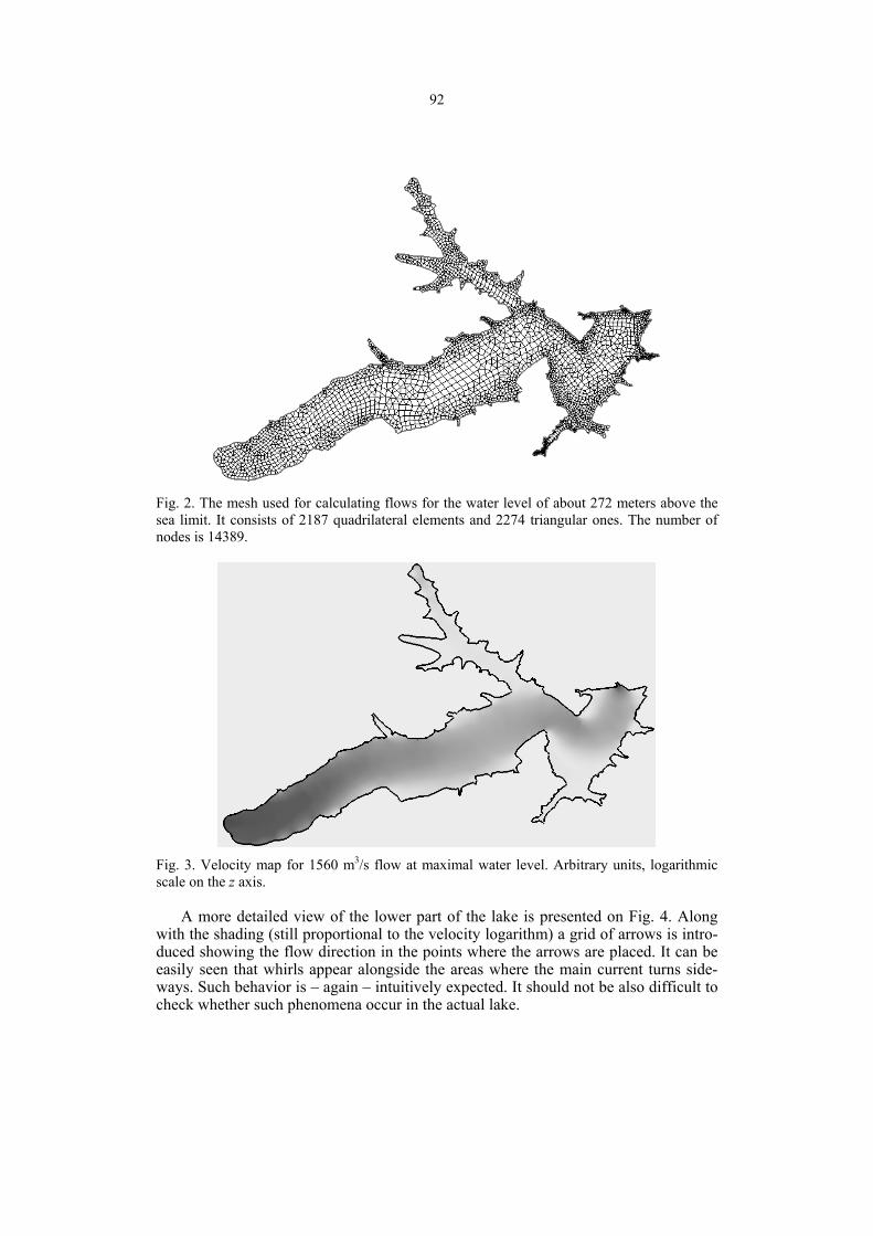
92

Fig. 2. The mesh used for calculating flows for the water level of about 272 meters above the sea limit. It consists of 2187 quadrilateral elements and 2274 triangular ones. The number of nodes is 14389.

Fig. 3. Velocity map for 1560 m3/s flow at maximal water level. Arbitrary units, logarithmic scale on the z axis.

A more detailed view of the lower part of the lake is presented on Fig. 4. Along with the shading (still proportional to the velocity logarithm) a grid of arrows is intro-duced showing the flow direction in the points where the arrows are placed. It can be easily seen that whirls appear alongside the areas where the main current turns side-ways. Such behavior is – again – intuitively expected. It should not be also difficult to check whether such phenomena occur in the actual lake.

93

Fig. 4. Close-up of the dam region of the map shown on Fig.2. Arrows show the flow direction. A few whirl areas are visible.

6. Conclusions and perspectives

The finite element method described in Chapter 3 and embedded in the FESWMS program proved to be useful in calculating water flow in the lake of Dobczyce at least as long as computational meshes are constructed with care. One such mesh can be used to perform calculations for the whole possible range of flow values but only in very limited bracket of water level. First obtained results are reasonable and consis-tent; they well qualify for further analysis and calibration. They show characteristic features of the velocity field that should subject to observational verification leading to consecutive tuning of the model.

Among various possible uses of generated velocity maps two should be outlined now: First – prognoses obtained for high flow values could give us a clue about such phenomena as rubble transport and banks/bed erosion during floods. Second – results computed for average flows could lead us to better understanding of sediment and pollution transport in the considered retention water body working under normal, av-erage circumstances. This is very important because of the presence of water supply system inlet and several recreation zones in this area, that have to be appropriately protected against any contamination. Water flow maps may help in determining loca-tions and sizes of necessary protective zones.

References

Froechlich, D.C., 2003, Two-dimensional Depth-averaged Flow and Sediment Trans-port Model, 207 pp.

Mazoń, S., et al., 1998, Dobczyce Lake – digital map in Badanie przebiegu procesu abrazji i stanu zalądowania Zbiornika Dobczyce oraz ocena stanu technicznego

94

czaszy zbiornika (Investigation of abrasion In the Dobczyce Lake and rating of its technical state), Kraków 43 pp.

Nachlik, E., et al., 2006, Studium możliwości zmiany funkcji Zbiornika Dobczyckiego i jego zlewni z uwzględnieniem ochrony czystości wody w zbiorniku (Study on possi-bilities of function change of the Dobczyce Lake, including water purity protec-tion), Kraków, 170 pp.

ODGW Kraków, undated, Zbiornik wodny Dobczyce (The Dobczyce Water Body), informational brochure.

Zienkiewicz, O.C., and R.L. Taylor, 2002, A, The Finite Element Method – Fluid Dy-namics, Oxford, 334 pp.

Zienkiewicz, O.C., and R.L. Taylor, 2002, B, The Finite Element Method – The Basis, Oxford, 689 pp.

PUBLS. INST. GEOPHYS. POL. ACAD. SC., E-7 (401), 2007

Evaluation of River Bed Geometry Under Nautical Aspects by Application of a 2D-HN-Routing-Program

Martin HENNING1, Bernd HENTSCHEL2 and Thorsten DETTMANN2 1 TU Braunschweig, Leichtweiss-Institut für Wasserbau

Beethovenstrasse 51a, D-38106 Braunschweig e-mail: m.henning@tu-bs.de

2 Bundesanstalt für Wasserbau, Kussmaulstrasse 17, D-76185 Karlsruhe e-mails: bernd.hentschel@baw.de; thorsten.dettmann@baw.de

Abstract

This paper presents an approach for the quantification of navigable water-depths by applying a 2D-numerical model originally developed for automated waterways route planning to results of a physical bedload-model. Topography and water level data of the physical model of the River Odra with movable bed material are used as input for the model in order to determine navigable water depths as a function of river bed geometry. The methodology is proved success-fully by comparing the influence of different maintenance strategies on shipping conditions. The results indicate also that the methodology may be used for the assessment of river bed stability.

1. Introduction

An important aspect in applied river engineering is the improvement of shipping con-ditions and in particular the provision of navigable water depths. This task is compli-cated in rivers which are characterized by a highly dynamical bed, since water depth cannot be classified unambiguously due to bed form migration and the appearance of transient dunes. Hence, the average water depth does not represent the available navi-gable water depth and the location of maximum water depths, defined as the distance from the water surface to the bed level along the thalweg may meander heavily, mak-ing navigation along its course impossible.

One task of the Federal Waterways Engineering and Research Institute (BAW) is the investigation of shipping conditions in the River Odra. For this purpose, a bed load transport model of an 8 km long section of the River Odra (km 654.7–662.5) is oper-ated by BAW (Hentschel 2006) on contract of the Federal Waterways and Shipping Administration (WSV). This particular reach of the River Odra is characterized by a highly dynamical morphological behavior due to its fine-gravel/coarse-sand bed mate-rial and associated bed forms.

96

The model contains a 5 km long straight section which causes meandering banks moving several meters per day. Furthermore, some groynes in this reach are heavily damaged and scours of considerable sizes can be observed at the groyne heads. Thus, navigation is complicated at low water levels because the position of the banks is dif-ficult to determine and the scours cause an expansion of the cross-sectional profile leading to biasing navigable water depths. The intention of the BAW investigations is the development of maintenance strategies for this reach in order to improve shipping conditions. Several strategies are investigated, e.g., (i) maintaining the existent groy-nes; (ii) narrowing the flow profile by flattening the groyne heads; and (iii) rerouting the riverbed completely.

In this paper, we develop a methodology to judge the influence of these strategies on shipping conditions by analyzing data from the physical model with a 2D-model which was originally developed for automated waterways route planning.

2. Data and methods

In total, six different maintenance strategies were investigated in the bed-load-transport-model (height scale Hr = 40, length scale Lr = 100) to improve the present situation. In the investigations, the natural bed-load material was substituted by syn-thetic granules (polystyrene) with lesser density and coarser diameter but comparable inhomogeneity, to achieve naturelike transport conditions. Table 1 summarizes the natural and artificial bed material properties and Fig. 1 presents an overview of the physical model. The description of the basic model laws is beyond the scope of this paper and can be found in standard text books such as Zanke (1982) and Kobus (1984).

Table 1

Properties of nature and model bed-load material

Parameter Nature Model Hr = 40 Material Coarse sand/ fine gravel Polystyrene

Mean grain diameter dm 0.92 mm (0.5 to 1.4 mm)

2.1 mm (1 to 4 mm)

Density 2.65 g/cm³ 1.055 g/cm³ Inhomogeneity d60/d10

2.3 (1.9 to 3.1) 2.0

Specific density Δ 1.65 0.055

Dimensionless grain diameter D* 21.2 (12 to 34) 14.8

Experiments were carried out for each investigated maintenance strategy by apply-

ing three steady discharges resulting in low, mean and high water depths. Each dis-charge was run for several hours during which water level data were collected at 19 different places at 15-second intervals. At the end of each experiment, the model was

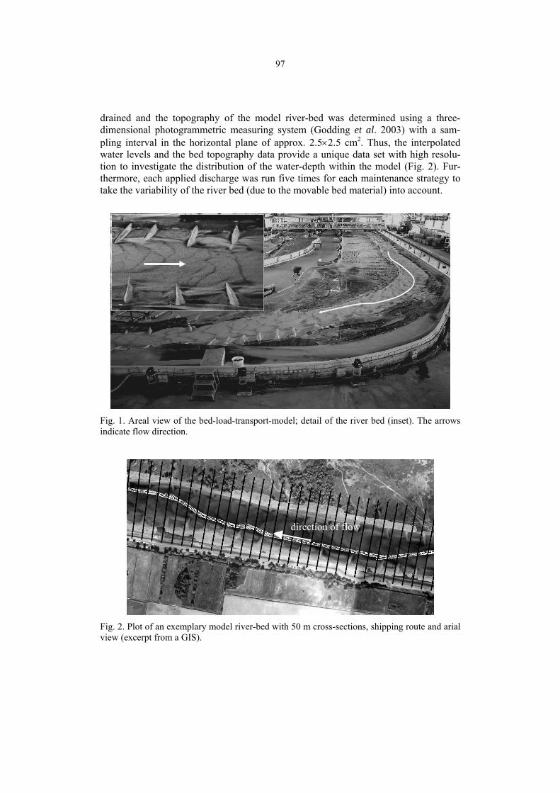
97

drained and the topography of the model river-bed was determined using a three-dimensional photogrammetric measuring system (Godding et al. 2003) with a sam-pling interval in the horizontal plane of approx. 2.5×2.5 cm2. Thus, the interpolated water levels and the bed topography data provide a unique data set with high resolu-tion to investigate the distribution of the water-depth within the model (Fig. 2). Fur-thermore, each applied discharge was run five times for each maintenance strategy to take the variability of the river bed (due to the movable bed material) into account.

Fig. 1. Areal view of the bed-load-transport-model; detail of the river bed (inset). The arrows indicate flow direction.

Fig. 2. Plot of an exemplary model river-bed with 50 m cross-sections, shipping route and arial view (excerpt from a GIS).

direction of flow

98

A systematic analysis of the water-depth information to judge the different main-tenance strategies for the benefit of shipping is difficult. On the one hand, areas of optimum water-depths vary from experiment to experiment and, on the other hand, the permanent observation of defined river bed sections (e.g. applying areal filters) is im-possible since the river-navigation route differs substantially within the investigated alternatives. Furthermore, although average depth can be determined easily, it pro-vides little information for navigational purposes due to the appearance of banks and scours. The easiest way to detect largest water depths along the flow path of the river would be the determination of the thalweg by connecting deepest points of subsequent cross-sections (with minimum distance) to a longitudinal stretch. However, this proce-dure cannot be applied here since the thalweg meanders heavily due to the influence of banks and scours (see Fig. 1). Hence, a chaotic course of the thalweg would be ob-tained along which navigation is impossible. Additionally, the needed width for ship-ping is not necessarily available along the thalweg.

In fact, the evaluation of navigational requirements is difficult and therefore the navigational software PeTra (Pegelabhängige Trassierung) has been applied in this study. This software package was originally developed for automated waterways route planning and considers ship movement within radii from the size of a ship-length to straight motion. It computes the optimum shipping way under mathematicaly identical conditions considering the impact of flow velocity as well as vessel velocity and direc-tion, and navigational traffic (Dettmann and Zentgraf 2002). The generated shipping route also comprises typical reactions of the skipper. Results of the computations are displayed using the CAD-system MicroStation. The program requires waterway boundaries and widths, turning radii, traffic rules, waterway disposition and particu-larities like brigde passages etc. as input data for the generation of the shipping route. Additionally, information on vessel characteristics such as length, width, and naviga-tional dynamics is required. The governing factors for the shipping route resulting from the river morphology are the distribution of water-depths and flow-velocities along the river cross-section.

The consistent evaluation of the above parameters requires the introduction of a navigability potential. Therefore, all parameters are transferred into a potential and are standardized on a scale from 0 to 100 (0 = not navigable; 100 = optimum). This pro-cedure allows the assessment of navigability of each point within the considered sec-tion dependent on the chosen parameter. At the same time, it is possible to consider the combined influence of various parameters by superposing the potential courses. The result of such a multi-parameter analysis is the overall quantification of navigabil-ity. Additionally, threshold values may be assigned to the parameters water-depth, waterway boundaries and right-hand-traffic. If the computed value is larger than the threshold, the corresponding area of the cross-section is marked as impassable. It is worth mentioning that the program offers also the opportunity to weigh each parame-ter in order to control its impact on the calculated result.

The area of the cross-section with the highest potential is considered as a gate, i.e., it provides best navigational conditions and is considered as a potential part of the shipping route. If areas with comparable potentials in one or more cross-sections are

99

determined, multiple gates are marked, resulting in different possibilities for naviga-tion. In this case, the shortest way will be determined, if not defined otherwise by the operator of the program. Note that, in the present study, we focused on the analysis of largest water depths only, i.e., we did not consider traffic situations (e.g., overtaking and encountering ships).

For the present study, cross-sectional profiles were cut out of the model topogra-phy at a (scaled) distance of 50 m (Fig. 2). A typical vessel for the River Odra has been used for calculation (82×11.4 m2 at 1.6 m draft). Calculations using PeTra were carried out only for low discharges (i.e., low water depths), which represent the worst case scenario with regard to water depth. After all passable gates were detected, the navigation route with the largest water depth was determined. The minimum water depth along this route was identified and labeled as transit-depth. The average transit-depth for all five experimental runs at the same discharge for each investigated alter-native was calculated. The mean values were used to compare the results of the differ-ent measures, since they enable the identification of problematic areas in terms of lowest available water-depths.

Another approach included the detection of the easiest navigable way. That way, not the optimum water-depths were relevant, but the effort for the virtual skipper. If banks prevent straight forward motion, the vessel evades shoals by maneuvering around them. If necessary water-depths are throughout available, the calculated route will be straight forward. The analysis of navigational effort (e.g. by determining the angle of the vessel compared to its previous position) indicates the quality of the maintanance strategy.

3. Results and analysis

Figure 3 presents calculated routing courses within an exemplarily chosen cross-section for the five experimental runs of experiment V0 and V2a, respectively. The solid lines represent observed bed-levels and the bars indicate the position of the gates within this particular cross-section. The river-bed within the experimental series of V0

Fig. 3. Cross-sections of the same profile with “gates” and river-bed-profiles in each case of the five experiments of two alternatives V0 (actual-state), showing high, and V2a, showing low river bed diversity.

100

varies significantly and, therefore, the gates are located at different positions. As a consequence, the potential navigation course diverges for identical boundary condi-tions due to the influence of bed-dynamics. In contrast, almost identical positions of the gates are observed within the experimental series of V2a and the distribution of bed elevation within the cross-sections is similar.

Hence, it becomes possible to use computed vessel positions to assess river bed stability. If navigation courses for all five experimental runs with the same discharge are similar, it can be concluded that the bed geometry must also be similar within these runs, i.e., the alternating dunes are stable. If the navigation courses differ sub-stantially, the dunes are instable and the bed is characterized by a dynamic behavior. This is visualized in Fig. 4, where the calculated navigation courses are shown for V0 and V2a along a part of the investigated river section. For V0, different navigation paths are observed and, as indicated by Fig. 3, the bed is instable. In contrast, for V2a, where stable bed levels were observed (Fig. 3), almost identical navigation paths were determined. The variability of the vessel positions can be assessed from Fig. 4 by cal-culating the average distance among the vessels within the five runs with the same discharge. For this purpose, the ship position was estimated for each cross section as distance to the datum of the cross section, enabling a reliable estimate of the distances of vessels during the experimental runs.

Fig. 4. Estimation of river-bed stability by means of reproducibility of calculated shipping routes.

The results of this analysis show that the best maintenance strategy (V2a) en-hances navigable water depths by more than 0.5 m compared to the present situation (V0). In contrast, the analysis of mean water depths within the fairway (identical to area between groynes) indicated an improvement of only one fifth this value (Fig. 5). The other investigated maintenance strategies showed lesser differences in mean wa-ter-depths compared to the present situation as well. However, the proposed method showed that navigable water depths were enhanced and detoriated, respectively, far more than the analysis of average depths would have revealed. Furthermore, for the best case scenario (V2a), maximum average distances between the vessel positions of only 15 m were observed while in the worst case (V3a), the average distance was as

101

large as 35 m (Fig. 6). Analysis of the navigational effort indicated the alternative V2a as best scenario (Fig. 6).

-0.30

-0.20

-0.10

0.00

0.10

0.20

0.30

0.40

0.50

0.60

V1b V1c V2a V2b V3a V3b

maintenance strategy

chan

ge in

dep

ths

com

pare

d to

ac

tual

-sta

te-m

odel

[m]

PeTra calculated depths

average depths within fairway

Fig. 5. Comparison of water-depths received from PeTra analysis and from calculation of average depths within fairway.

0

5

10

15

20

25

30

35

40

V0 V1c V2a V2b V3a V3b

maintenance strategy

aver

age

dist

ance

am

ong

vess

els

[m]

0.00

0.20

0.40

0.60

0.80

1.00

1.20

navi

gatio

nal e

ffort

[° to

pr

evio

us p

ositi

on]

vessel distancesturning angle

Fig. 6. Calculated average vessel distances and navigational effort (average angle in degree to vessel’s previous position).

4. Summary and conclusions

In this paper, a method for the estimation of navigable water depth along a river with a high morphological activity was proposed. The proposed methodology is based on combining requirements for navigation and bed morphology and was derived using results of a physical bed load model together with a 2D-numerical model originally developed for automated waterways route planning. The physical model and the 2D model were described in detail and the method was applied successfully to detect navigation courses based on the requirement of sufficient water depth for navigation. The data analysis showed that the proposed methodology may also be applied to as-sess river bed stability by comparing computed navigation courses for experimental runs with identical boundary conditions. If the shipping routes can be reproduced, the variability of the bed surface within the different runs is small, indicating stable bed forms such as alternating banks and dunes.

102

The methodology was developed by investigating the discharge in the model which resulted in lowest water depths. To eliminate uncertainties of model laws the analysis concentrated on comparison of model results. To assess absolute water-depths in nature it is necessary to relate the results to hydrological values such as short fall probabilities of water levels in days per year. Nonetheless, the methodology showed that it is applicable to judge the success of different maintenance strategies for naviga-ble waterways which are characterized by a high morphological potential.

Acknowledgements . The investigations in the present paper were carried out on contract of the German Federal Waterways Engineering and Research Institute (BAW).

References

Dettmann, T., and R. Zentgraf, 2002, Pegelabhängige Fahrspurberechnung in fließen-den Gewässern, BAW Mitteilungen 84, 127-140.

Godding, R., B. Hentschel and K. Kauppert, 2003, Videometrie im wasserbaulichen Versuchswesen, Wasserwirtschaft 4/2003, S. 36-40.

Hentschel, B., 2006, Physikalisches Geschiebetransportmodel der Oder zur Untersu-chung der Wechselwirkung von Stromregelungsbauwerken, Sohlformen und nauti-schen Bedingungen, Wasserbauliche Mitteilungen Heft 32, TU Dresden, 87-94.

Kobus, H., (ed.), 1984, Wasserbauliches Versuchswesen, DVWK 39, Verlag Paul Pa-rey, Hamburg und Berlin, 353 pp.

Zanke, U., 1982, Grundlagen der Sedimentbewegung, Springer Verlag, Berlin, Hei-delberg, New York, 402 pp.

PUBLS. INST. GEOPHYS. POL. ACAD. SC., E-7 (401), 2007

Experimental Determination of Characteristic Transportation Speeds in Designed Sewage Siphon

Apoloniusz KODURA Institute of Water Supply and Hydraulic Engineering Warsaw University of Technology

20 Nowowiejska St, 00-653 Warsaw, Poland e-mail: apoloniusz.kodura@is.pw.edu.pl

Abstract

The article presents the results of empirical tests of the designed sewage transmission system in Warsaw. At the design stage, a number of questions ap-peared, pertaining to transportation of sewage in a siphon pipe. One of them was the question about the transportation capabilities of a geometrically graded sys-tem in the context of transportation of sewage which is a random mixture of liq-uids and solid particles of different origin. In order to analyze the phenomena, a laboratory model was built, whereon a number of experiments was performed. The purpose was to determine characteristic speeds: minimum non-silting, trans-portation, and minimum self-purification speeds. The research was preceded with a discussion on adoption of a criterion of similarity. Experiments were car-ried out on a physical model enabling visualization of the phenomenon, made of transparent pipes. The working liquid was a mixture of water and sand from the Vistula river. Verification measurements were also carried out, using sewage samples. Results of empirical tests confirmed the adopted assumptions and made it possible to make corrections in the design.

1. Introduction

Continuous urbanization entails the necessity to design and build infrastructure-forming engineering facilities. Such facilities include the sewer system.

A number of sewage systems is used in the engineering practice. The knowledge of construction and principles of operation of sewage pipes is based to a large extent on practical experience. The problem of variable physical and chemical composition of the transported medium is a major difficulty. This variability demonstrates some features of recurrence in the form of daily cycles, but not without random variations.

One of the largest investments in the area of water management and sewage dis-posal in recent years is the sewage pipe modernization system. The capital of Poland, as one of Europe’s capitals, does not have a system for comprehensive sewage treat-

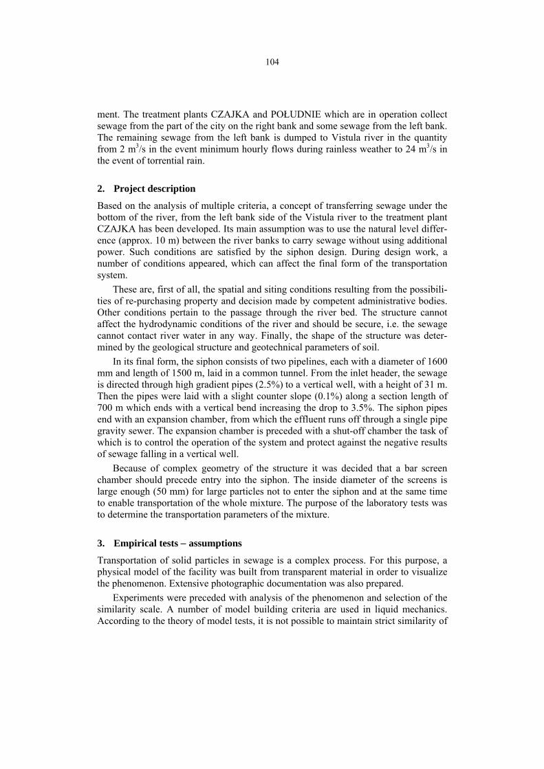
104

ment. The treatment plants CZAJKA and POŁUDNIE which are in operation collect sewage from the part of the city on the right bank and some sewage from the left bank. The remaining sewage from the left bank is dumped to Vistula river in the quantity from 2 m3/s in the event minimum hourly flows during rainless weather to 24 m3/s in the event of torrential rain.

2. Project description

Based on the analysis of multiple criteria, a concept of transferring sewage under the bottom of the river, from the left bank side of the Vistula river to the treatment plant CZAJKA has been developed. Its main assumption was to use the natural level differ-ence (approx. 10 m) between the river banks to carry sewage without using additional power. Such conditions are satisfied by the siphon design. During design work, a number of conditions appeared, which can affect the final form of the transportation system.

These are, first of all, the spatial and siting conditions resulting from the possibili-ties of re-purchasing property and decision made by competent administrative bodies. Other conditions pertain to the passage through the river bed. The structure cannot affect the hydrodynamic conditions of the river and should be secure, i.e. the sewage cannot contact river water in any way. Finally, the shape of the structure was deter-mined by the geological structure and geotechnical parameters of soil.

In its final form, the siphon consists of two pipelines, each with a diameter of 1600 mm and length of 1500 m, laid in a common tunnel. From the inlet header, the sewage is directed through high gradient pipes (2.5%) to a vertical well, with a height of 31 m. Then the pipes were laid with a slight counter slope (0.1%) along a section length of 700 m which ends with a vertical bend increasing the drop to 3.5%. The siphon pipes end with an expansion chamber, from which the effluent runs off through a single pipe gravity sewer. The expansion chamber is preceded with a shut-off chamber the task of which is to control the operation of the system and protect against the negative results of sewage falling in a vertical well.

Because of complex geometry of the structure it was decided that a bar screen chamber should precede entry into the siphon. The inside diameter of the screens is large enough (50 mm) for large particles not to enter the siphon and at the same time to enable transportation of the whole mixture. The purpose of the laboratory tests was to determine the transportation parameters of the mixture.

3. Empirical tests − assumptions

Transportation of solid particles in sewage is a complex process. For this purpose, a physical model of the facility was built from transparent material in order to visualize the phenomenon. Extensive photographic documentation was also prepared.

Experiments were preceded with analysis of the phenomenon and selection of the similarity scale. A number of model building criteria are used in liquid mechanics. According to the theory of model tests, it is not possible to maintain strict similarity of

105

all phenomena at the same time. The selection of scale results from the analysis of naturally dominant hydrodynamic phenomena.

Flow phenomena in pressure pipes are modeled based on the Reynolds criterion, which best describes the friction phenomena. This number is the measure of similarity of the forces of viscosity and inertia. In the investigated case, it was important not only to determine the resistance to motion but also the phenomena accompanying transportation of solid particles, which results from the effects of forces of viscosity, inertia and gravity.

The adopted geometrical scale (αL = 1:21.6) resulted from the available diameter of plexi pipes (74 mm). It is large enough to enable assessment of the phenomenon of solid particle transportation.

Keeping the Reynolds criterion resulted in a significant speed increase (speed val-ues from 3.7 m/s to 19.5 m/s − Table 1). In this situation, the parameters of the trans-ported particles should be increased significantly, including weight, in order to obtain forces of inertia corresponding with the model speed, so that transportation is similar to the natural environment.

Table 1

The values of speed in the model and in “real life” and the corresponding Re number for the investigated cases

Flow in the model conditions Flow in the conditions of the designed siphon Reynolds criterion Automodel

Q [m3/s]

v [m/s]

Re [103]

v [m/s]

Re [103]

v [m/s]

Re [103]

0.342 0.170 208 3.676 208 0.170 9.63 0.402 0.200 245 4.324 245 0.200 11.3 0.503 0.250 306 5.405 306 0.250 14.2 1.005 0.500 613 10.811 613 0.500 28.3 1.206 0.600 735 12.973 735 0.600 34.0 1.608 0.800 980 17.297 980 0.800 45.3 1.810 0.900 1100 19.459 1100 0.900 51.0

The adopted criterion of similarity affects not only the model flow values but also

the parameters of solid particles transported in the model. It was decided that sand from the Vistula river should be used as the representative type of transported solid particles. This was another reason why an alternative criterion of similarity had to be used.

Finally, it was decided that an automodel should be used, i.e. that the model should reproduce the same speed values as expected in natural conditions, with main-taining the turbulent flow character. The speed scale is equal αv = 1:1 an the discharge scale is equal αQ = 1:467.7.

106

4. Model

Considering the spatial conditions of the laboratory, the model (Fig. 1) reproduced the counter slope section (1), the shut-off chamber (2) and the expansion chamber (3), where the largest changes in geometry occur and are conducive to difficulties in trans-portation of solid particles.

Fig. 1. (a) Cross-section of the model. (b) Layout of the model.

The Vistula sand was the model of solid particles (Fig. 2a). This sand is sprayed on roads in winter and large quantities of it return to the sewer with precipitation wa-ter. Additionally, fine gravel was used for tests (Fig. 2b). The obtained speed values were verified with the prepared sewage samples. Half of the volume of each sample was comprised of sewage taken from the Warsaw combined sewage system, ¼ was the sediment taken from settling tanks in the sewage treatment plant CZAJKA, and the remaining part was the Vistula sand. Samples prepared this way were mixed and left for the physical and chemical processes to occur.

During experiments the flow discharge was measured by using a triangular sharp-crested weir (4). This weir was located on the end of model.

(a) (b) Fig. 2. (a) Vistula river sand used for tests. The sand was taken from the dredger cutter in Łomianki area. (b) Fine gravel used for tests.

1

1

2 3

2 3

(a)

(b)

4

4

107

5. Results of empirical tests

Three series of empirical tests were performed. In the first and second series, transpor-tation of a two-phase mixture of water and mineral particles was analyzed. In the third series, the prepared sewage samples were used, with organic and mineral particles, after adequate seasoning.

In the first series, a model was created of the initial flow in the siphon pipe filled with a mixture of water and mineral particles. After the system was initially filled with water, mineral particles were added, filling a section with a ¾ of model pipe length with a layer of thickness of approx. ½ diameter. Then water flow was supplied, start-ing with the lowest speeds. Observation of the phenomenon consisted in measuring the delivery rate for characteristic speeds, corresponding with starting transportation, bulk motion, and the self-purification speed.

The purpose of the second series was to verify the obtained results by measuring the delivery rate for characteristic speeds in the situation of continuous supply of the mixture of water and mineral particles to the model. In this case, solid particles were added to flowing water through a charging hopper in the volumetric flow quantity (2% of volume discharge). Analogical values of characteristic speeds were determined.

In the third series, a sewage sample was installed in the model and it was checked whether the values of characteristics speeds are different than in the case of the mix-ture of mineral particles and water.

In all cases, the values of characteristic speeds are similar. At the flow rate equal to 0.18 m/s approx. beginning of motion of solid particles was noted in the form of entrainment and rolling of single grains As speed increased, the intensity of the proc-ess was also higher, and at the speed equal to 0.60 m/s approx. a major part of solid particles was affected by the phenomenon. Another speed increase made it possible not only to maintain the continuity of the process, but also to remove layers of mineral material. At the speed equal to 0.80 m/s approx. all solid particles were removed from the pipe, regardless of the grain size.

It must be emphasized that the observed speeds applied both to the horizontal sec-tion and the section laid with a counter slope. In the counter slope section, reduction of intensity of transportation was noted, the particles moved somewhat slower, creating characteristic layers at the point of change in slope.

In the case of sewage samples, no changes in the transportation speed and self-purification speed were found. No relationship was found between the time of sample seasoning (from 4 to 127 hours) and the speed values. However, it should be empha-sized that the sewage samples used cannot be considered as representative of the sew-age carried in the future by the designed system. Randomness of their composition and physical-chemical properties make it possible only to perform a comparative analysis.

6. Analysis of results

Obtained results were compared with data available in reference literature. Kar-nowski’s research results were used (Błaszczyk et al. 1988), according to which the

108

non-silting characteristic speeds and the self-purification speeds depend both on grain size and on the diameter of sewer pipe. The lower the diameter, the lower the charac-teristic speeds.

The figures show the data taken from reference literature (Figs. 3 and 4). The re-search results were interpolated with a polynomial function. The literature data per-tained to pipe diameters from 150 mm to 2000 mm and particle grains: 1 mm, 3 mm and 5 mm. The diameter used in the model does not belong to the data range, however by using extrapolation of the area marked with the grey rectangle it was possible to determine approximate values of characteristic speeds of the model. The speeds meas-ured in experimental conditions are contained in the ranges mentioned in reference literature. Using the chart, you can estimate that the characteristic speeds in the pipe with a diameter of 1600 mm are 1.44-times greater than the corresponding characteris-tic speeds in a pipe with a diameter of 74 mm.

Fig. 3. The non-silting speeds in a circular sewage pipe depending on the pipe diameter for selected diameters of the transported grains. (1, 3, 5 mm) (Błaszczyk et al. 1988).

The characteristic speeds determined by empirical tests for use in actual conditions are:

vmin = 0.65 m/s − minimum flow rate in the siphon, the speed ensuring transporta-tion of most solid particles, the speed corresponds with the flow through one tube of the siphon Q = 1.31 m3/s.

vt = 0.9 m/s − the transportation flow rate in the siphon, the speed is characteristic of minimum sedimentation, and corresponds with the flow through one tube of the siphon Q = 1.81 m3/s.

109

vc = 1.2 m/s − the self-purification flow rate in the siphon, cleaning the pipes, it corresponds with the flow through one tube of the siphon Q = 2.41 m3/s.

Fig. 4. The self-purification speeds in a circular sewage pipe depending on the pipe diameter for selected diameters of the transported grains. (1, 3, 5 mm) (Błaszczyk et al.1988).

7. Conclusions

The laboratory tests carried out confirmed the design assumptions of the planned si-phon arrangement. They also made it possible to make adjustments and corrections in the applied solutions, by redesigning parts of the expansion well.

The most important goal of the research, i.e. determining the characteristic speeds for transportation of solid particles was attained. The analyzed characteristic speeds were comparable in the three test series, in which slightly different procedures were followed. Repeatability of obtained results made it possible to determine characteristic speeds.

Analysis of the phenomenon preceding the empirical tests allowed us to build an “automodel”, in which the obtained speeds are analogical to the “real life” conditions. Use of the classical Reynolds’ criteria of similarity was, to a large extent, difficult, considering model speed values. They should be 21-times greater than the correspond-ing characteristic speeds in a pipe with a diameter of 1600 mm. In this case, weight of the transported particles should be increased significantly, and just then the particles size should keep geometrical scale (αL = 1:21.6). In this instance the comparative ex-periments using sewage samples would be impossible.

When using an “automodel”, much attention must be paid to analysis of results and the process of conversion of experimental results to their corresponding “real life”

110

quantities. In the discussed project, the conversion used was based on extrapolation of literature data and the actual active cross-section area was taken into consideration. It must be emphasized that for the set grain size the values of transportation speed and self-purification speed are higher for the higher pipe diameters. With small diameters additional factors appear, such as the effect of the pipe wall, changing the character of particle transportation. In designing models of sewer pipe flows, much attention must be paid to the issues pertaining to selection of the pipe diameter, and at the same time the choice of geometrical scale.

References

Błaszczyk, W., H. Stamatello and P. Błaszczyk, 1988, Kanalizacja – sieci i pom-pownie, T. 1., ARKADY, Warszawa.

Bos, M.G., 1989, Discharge Measurement Structures, ILRI, Wageningen, The Nether-lands.

Imhoff, R., K., K., 1979, Taschenbuch der Stadtentwässerung, 25. verbesserte Au-flage, München Wien.

Mitosek, M., Mechanika płynów w inżynierii i ochronie środowiska, 2001, PWN, Warszawa.

PROKOM Sp. z o.o., 2007, Projekt architektoniczno-budowlany układu przesyłowego do Oczyszczalni Ścieków CZAJKA w Warszawie. “Zaopatrzenie w wodę i oczysz-czanie ścieków w Warszawie”, 2007, Warszawa.

Zupke, B., 1985, Hydromechanik im Bauwesen. Bauverlag GMBH Wiesbaden und Berlin.

PUBLS. INST. GEOPHYS. POL. ACAD. SC., E-7 (401), 2007

Statistical Analysis of Bed Surfaces in Sand Bed Rivers

Klaus KOLL1, Jochen ABERLE1, Bernd ETTMER1 and Bernd HENTSCHEL2 1 Leichtweiss-Institute for Hydraulic Engineering, Technical University of Braunschweig

Beethovenstrasse 51a, 38106 Braunschweig, Germany e-mails: klaus.koll@tu-bs.de, j.aberle@tu-bs.de, b.ettmer@tu-bs.de

2 Federal Waterways Engineering and Research Institute Kussmaulstrasse 17, 76187 Karlsruhe, Germany

e-mail: bernd.hentschel@baw.de

Abstract

This paper presents results from a preliminary investigation of the applica-bility of the random field approach to describe bed geometry in sand bed rivers. The investigations are based on high-resolution bed surface data of a physical bed load model of a longitudinal section of the river Odra. The first four statisti-cal moments are used to describe differences in bed geometry which arise due to different river maintenance strategies and discharges. The results show the po-tential of the standard elevation of bed elevations as an indicator for vertical bed form dimension. It is shown that σz is correlated to discharge and may be used to describe bed form dynamical behavior during a flood wave. The average migra-tion velocity of bed forms is estimated using cross correlation function.

1. Introduction

Sand waves play an important role for sediment transport, forming hydraulic resis-tance, and for navigability of waterways. Until today, an abundance of studies have focused on two-dimensional (2-D) bed forms with constant heights and straight crest lines transverse to the flow. However, as natural bed forms are invariably three-dimensional (3-D) in alluvial rivers, this morphological simplification has imposed limitations on the interpretation and understanding of dune form and flow dynamics (Parsons et al. 2005). Furthermore, so far most studies focused on the investigation of dune development and bed form geometry in laboratory studies (e.g., Friedrich et al. 2006) and data from natural rivers on bed form geometry and dynamics are rare (e.g., Nikora et al. 1997, Parsons et al. 2005). On the other hand, practical applications re-quire detailed information on bed geometry and dynamics in order to asses the influ-ence of different maintenance strategies on, e.g., morphological development and navigability (e.g., Henning et al. 2007, this issue).

112

The objective of this paper is the development of appropriate methods for the de-scription of the bed geometry and bed dynamics of natural river beds which are char-acterized by 3-D sand waves using the random field approach. Relevant parameters are linked to hydraulic parameters and bed dynamics are investigated by analyzing time series of digital elevation models (DEM).

2. Data

The sand bed topography data analyzed in this paper were obtained from laboratory experiments in a physical bed-load model of the River Odra in the laboratory of the Federal Waterways Engineering and Research Institute, Karlsruhe, Germany. The model was originally built to improve shipping conditions in the River Odra by focus-sing exemplarily on an 8 km long river section (km 654.7 to km 662.5; Fig. 1) which is characterized by a highly dynamical morphological behavior due to its fine-gravel/coarse-sand bed material and associated bed forms. The model contains a 5 km long straight section which causes meandering banks moving several meters per day. Additionally, some groynes in this reach are heavily damaged and scours of consider-able sizes can be observed at the groyne heads.

Fig. 1. Plane view of the model section and detailed bed topography between km 654.7 and 662.5 showing the groynes and bed topography.

The model is scaled geometrically in the x-y plane with LR = 1:100 and in vertical direction with HR = 1:40. The dynamical behaviour of the river bed was simulated by replacing the natural bed-load material with synthetic granules (polystyrene) with lesser density and coarser diameter but comparable inhomogeneity (ρp = 1055 kg/m³; d50 = 2.1 mm, d60/d10 = 2.0), to achieve similar transport conditions as in the nature.

113

The bed-material was selected following extensive preliminary experiments. Further information on the model can be found in Hentschel (2006).

In this paper we focus on bed geometry following three different maintenance strategies for the River Odra. Strategy V0 describes the present situation with strongly damaged groynes. Strategies V2a and V3a were developed in order to restore shipping conditions by re-establishing groynes in different ways (see also Henning et al. 2007). Experiments were carried out for each maintenance strategy by successively applying three steady discharges based on hydrological values of the River Odra (Q = 269, 447, and 1000 m³/s in nature scale, respectively), resulting in low, mean and high water depths. Each discharge was applied five times for each maintenance strategy to take into account the variability of the river bed (due to the movable bed material). A fur-ther experiment was carried out by simulating a typical hydrograph with a maximum discharge of Qmax = 1150 m³/s.

Each experiment started from plane bed conditions. For the steady discharge ex-periments, each discharge was run for several hours. After each discharge, the model was drained and the bed topography was measured along the total length of the model using a novel movable 3D-camera system with high resolution (see Godding et al. 2003 for details) with a grid size of 2 cm and a vertical precision of ±0.1 mm. Addi-tional topography measurements have been carried out for maintenance strategy V0 during model operation within a small section of the model (km 658.6 to 658.85). For these measurements, the 3D-camera system was in a fixed position and modified so that bed topography could be recorded through the water surface in time intervals of Δt = 14 seconds. A similar strategy was followed in a hydrograph experiment for V0, where the bed was scanned during model operation along km 659.15 to 659.93. How-ever, the longer section required movement of the 3D-camera system, and therefore, the time interval between two subsequent surface scans of this section was 3 minutes. Note that, in the following, all elevation data is presented in natural dimensions.

For the analysis of the bed topography, the 3D-beds were considered as a random field of surface elevations Z(x, y, t), where x and y are longitudinal (main flow direc-tion) and transverse coordinates, and t is time. In the following we focus on the analy-sis of the first four statistical moments and their potential to describe bed morphology. Note that a complete description of a random field of bed elevations also requires the consideration of moment functions such as structure functions or power spectral den-sity. The results of this investigation will be reported in a follow-up study.

3. Results and analysis

Table 1 presents the statistical moments mean value above sea level (ASL) z , stan-dard deviation of bed elevations σz, skewness Sk, and kurtosis Ku for the bed scans of the steady experiment series. The values in Table 1 represent mean values for the five experiments carried out for each discharge and were computed for a representative section in the straight reach of the model between km 658.10 and 659.25 to exclude the influence of the curvature on bed geometry. Furthermore, the analysis is limited to the middle section of the river reach to minimize the influence of deep scours at the

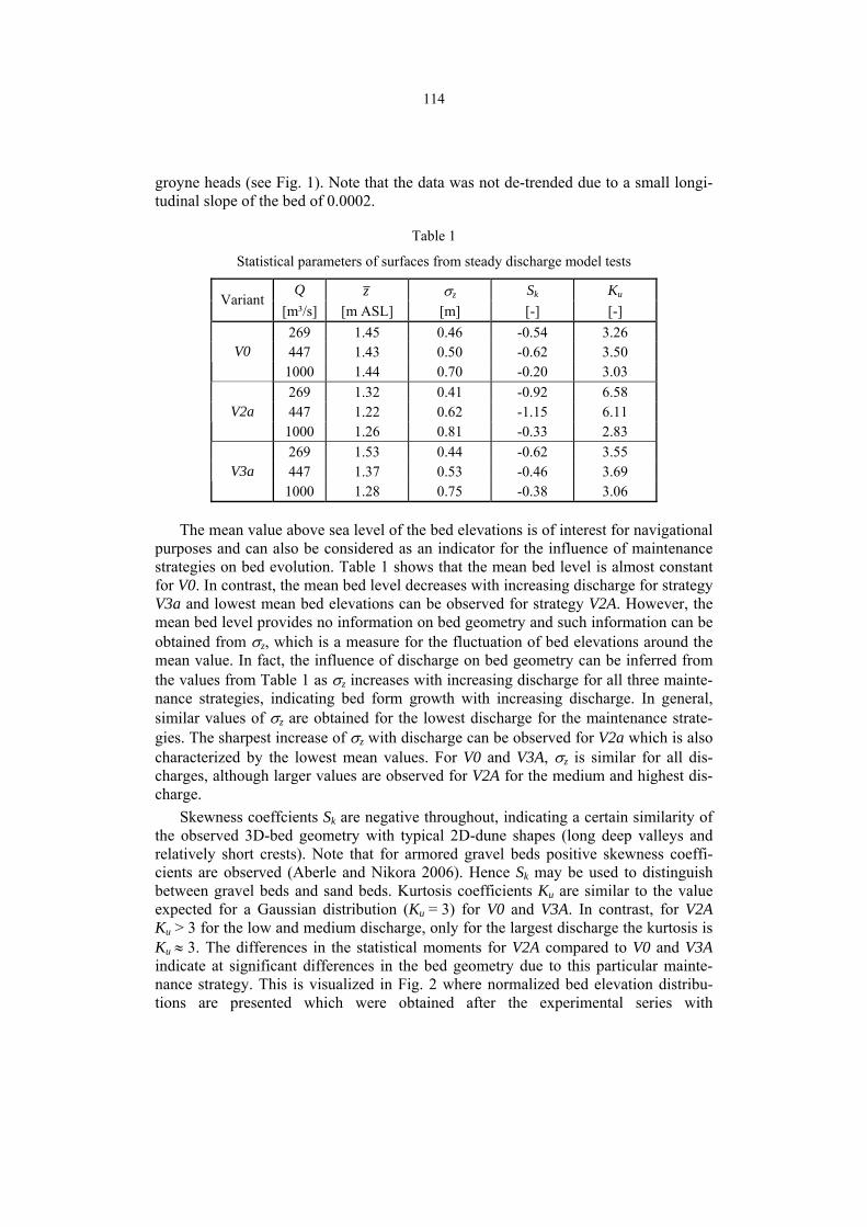
114

groyne heads (see Fig. 1). Note that the data was not de-trended due to a small longi-tudinal slope of the bed of 0.0002.

Table 1

Statistical parameters of surfaces from steady discharge model tests

Q z σz Sk Ku Variant [m³/s] [m ASL] [m] [-] [-] 269 1.45 0.46 -0.54 3.26 447 1.43 0.50 -0.62 3.50 V0

1000 1.44 0.70 -0.20 3.03 269 1.32 0.41 -0.92 6.58 447 1.22 0.62 -1.15 6.11 V2a

1000 1.26 0.81 -0.33 2.83 269 1.53 0.44 -0.62 3.55 447 1.37 0.53 -0.46 3.69 V3a

1000 1.28 0.75 -0.38 3.06

The mean value above sea level of the bed elevations is of interest for navigational purposes and can also be considered as an indicator for the influence of maintenance strategies on bed evolution. Table 1 shows that the mean bed level is almost constant for V0. In contrast, the mean bed level decreases with increasing discharge for strategy V3a and lowest mean bed elevations can be observed for strategy V2A. However, the mean bed level provides no information on bed geometry and such information can be obtained from σz, which is a measure for the fluctuation of bed elevations around the mean value. In fact, the influence of discharge on bed geometry can be inferred from the values from Table 1 as σz increases with increasing discharge for all three mainte-nance strategies, indicating bed form growth with increasing discharge. In general, similar values of σz are obtained for the lowest discharge for the maintenance strate-gies. The sharpest increase of σz with discharge can be observed for V2a which is also characterized by the lowest mean values. For V0 and V3A, σz is similar for all dis-charges, although larger values are observed for V2A for the medium and highest dis-charge.

Skewness coeffcients Sk are negative throughout, indicating a certain similarity of the observed 3D-bed geometry with typical 2D-dune shapes (long deep valleys and relatively short crests). Note that for armored gravel beds positive skewness coeffi-cients are observed (Aberle and Nikora 2006). Hence Sk may be used to distinguish between gravel beds and sand beds. Kurtosis coefficients Ku are similar to the value expected for a Gaussian distribution (Ku = 3) for V0 and V3A. In contrast, for V2A Ku > 3 for the low and medium discharge, only for the largest discharge the kurtosis is Ku ≈ 3. The differences in the statistical moments for V2A compared to V0 and V3A indicate at significant differences in the bed geometry due to this particular mainte-nance strategy. This is visualized in Fig. 2 where normalized bed elevation distribu-tions are presented which were obtained after the experimental series with

115

Q = 447 m³/s. As shown by Fig. 2, all distributions are characterized by a bell shape and the spread of the data to the left is reflected by the negative Sk-values. Figure 2 further shows that the distributions of V0 and V3A are similar, as expected from the comparison of the statistical moments. The larger values of Ku for V2A become appar-ent from the corresponding distribution shape which is steeper than the distributions for V0 and V3A. Hence, this analysis shows that the statistical moments may be used to compare the influence of the different maintenance strategies on bed geometry.

0123456789

10

-8 -6 -4 -2 0 2 4

[%]

V0V2aV3a

Fig. 2. Probability distribution functions after an applied discharge of Q = 447 m³/s (natural scale) for bed surface elevations according to maintenance strategies V0, V2A, and V3A.

In the next step we focus on σz for the analysis of the hydrograph experiments to investigate bed form development as a function of discharge. Figure 3 presents ob-served σz-values during the experiment together with the applied hydrograph. Figure 3 shows that σz correlates with Q. With increasing discharge, σz increases and when the discharge is reduced after the flood peak, σz decreases again. This shows that bed forms grow with increased hydrodynamical forcing and that, on the falling limb of the hydrograph, the magnitude of the bed forms is reduced. The range of observed σz-values varies between 0.30 m and 1.05 m (in natural scale). Compared to the results of the steady state experiments, slight differences in σz-values are observed. We attribute these differences to the influence of the hydrograph and to the fact that the analyzed surface data were recorded close to the river bend which may influence bed form movement (compared to the analyzed straight section for the steady discharge experi-ments).

σzz −

116

0.00

0.20

0.40

0.60

0.80

1.00

1.20

0 5000 10000 15000 20000 25000

t [s]

Stan

dard

dev

iatio

n [m

]

0

200

400

600

800

1000

1200

1400

Q [m

³/s]

Standard deviatonDischarge

Fig. 3. Standard deviation σz and discharge as a function of time for a selected hydrograph of the River Odra.

The time series data for the steady state discharge series may be used to estimate average migration velocity of the sand waves. For this purpose, successive bed scans were analyzed using the cross correlation function. The spatial lag in the x-y plane which provided the largest correlation coefficient was identified and assumed to pro-vide information on the average distance which the bed moved between two succes-sive bed scans (Δt = 14 sec). The results of this analysis show that the sand waves move unidirectional in the straight section, as transverse lags were almost always identical to Δy = 0. Dividing the identified spatial lag by Δt provides information on average migration velocity of the bed forms. As expected, the migration velocity is approximately constant for each applied steady discharge. Furthermore, the results of the cross correlation analysis show that the sand waves migrate fastest for the lowest discharge. With increasing discharge, bed form migration slows down. Thus, we con-clude that small bed forms move faster than large bed forms, as the bed form height correlates to σz, which is smallest for lowest discharge. However, it is worth mention-ing that the investigated part of the Odra is characterized by backwater effects for large discharges which may also contribute to reduced sand wave migration velocity.

4. Summary and conclusions

In this paper we investigated the applicability of the random field approach for the investigation of 3-D sand bed geometry in a natural river. The analyzed sand bed to-pography data were obtained from laboratory experiments in a physical bed-load model of the River Odra. In the analysis, we focused on the first four statistical mo-ments. The results showed that the mean bed elevation above sea level, standard de-viation σz, skewness Sk, and Ku provide valuable information on bed geometry and

117

may be used to assess the influence of different river maintenance strategies on bed morphology. The standard deviation σz was found to increase with increasing dis-charge indicating that the 3-D sand waves grow with increasing discharge. Similarly, in an experiment where a hydrograph was applied it was found that σz is correlated to discharge showing the potential of this parameter to describe bed form dynamics. Fur-thermore, all bed elevation distributions were characterized by negative skewness coefficients which were related to sand wave geometry. The average migration veloc-ity of the sand beds was estimated from cross-correlation analysis of time series data of bed elevations. This analysis revealed a relationship between sand wave geometry and migration velocity as smaller dunes were migrating faster than larger dunes.

In this paper we focused solely on the first four statistical moments. However, a complete description of bed geometry according to the random field approach requires also the consideration of moment functions such as structure functions or power spec-tral density (e.g., Hino 1968, Nikora and Hicks 1997, Nikora et al. 1997). This analy-sis will be reported in a follow-up study where these moment functions will be used to investigate both, spatial and temporal characteristics of 3D-sand beds. Furthermore, the statistical moments and the moment functions will be used to investigate and to develop model laws with respect to similarity of bed geometry and bed dynamics in model and nature-scale. So far, similarity in model and nature is subjectively judged and the random field approach provides a unique opportunity to improve these model laws. In a further step it is also planned to investigate if σz and the average bed migra-tion velocity may be related to sediment transport rates. If such a relationship can be established, it is possible to develop novel measuring techniques in sand-bed rivers for the determination of sediment transport rates.

Acknowledgments . The work was carried out on contract from the Federal Wa-terways Engineering and Research Institute, Karlsruhe, Germany.

References

Aberle, J., and V. Nikora, 2006, Statistical properties of armored gravel bed surfaces, Water Resour. Res. 42, W11414, doi:10.1029/2005WR004674.

Fiedrich, H., B.W. Melville, S.E. Coleman, T.M. Clunie, V. Nikora and D.G. Goring, 2006, Three-dimensional properties of laboratory sand waves obtained from two-dimensional autocorrelation analyses, River Flow 2006, Lisbon, Portugal, 1013-1022.

Godding, R., B. Hentschel and K. Kauppert, 2003, Videometrie im wasserbaulichen Versuchswesen, Wasserwirtschaft 4/2003, 36-40, in German.

Hentschel, B., 2006, Physikalisches Geschiebetransportmodel der Oder zur Untersu-chung der Wechselwirkung von Stromregelungsbauwerken, Sohlformen und nauti-schen Bedingungen, Wasserbauliche Mitteilungen Heft 32, TU Dresden, 87-94, in German.

Henning, M., B. Hentschel and A. Dettmann, 2007, Evaluation of river bed geometry under nautical aspects by application of a 2D-HN-routing-program, Monographic

118

Volume. Environmental Hydraulics. XXVII International School of Hydraulics, this issue.

Hino, M., 1968, Equlibrium-range spectra of sand waves formed by flowing water, J. Fluid Mech. 34 (3), 565-573.

Parsons, D.R., J.L. Best, O. Orfeo, R.J. Hardy, R. Kostaschuk and S.N. Lane, 2005, Morphology and flow fields of three-dimensional dunes, Rio Parana´, Argentina: Results from simultaneous multibeam echo sounding and acoustic Doppler current profiling, J. Geophys. Res. 110, F04S03, doi:10.1029/2004JF000231.

Nikora, V.I., and D.M. Hicks, 1997, Scaling relationships for sand wave development in unidirectional flow, J. Hydraul. Eng. 123 (12), 1152-1158.

Nikora, V., A. Sukhodolov and P.M. Rowiński, 1997, Statistical sand wave dynamics in one-directional water flows, J. Fluid Mech. 351, 17-39.

PUBLS. INST. GEOPHYS. POL. ACAD. SC., E-7 (401), 2007

Deterministic and Stochastic Vortex Method for Two-Dimensional Vorticity Transport Equation

Stanisław KOSTECKI Institute of Geotechnics and Hydrotechnics, Wrocław University of Technology

Wybrzeże Wyspiańskiego 27, 50-370 Wrocław, Poland e-mail: stanislaw.kostecki@pwr.wroc.pl

Abstract

This paper presents the discrete vortex method as applied to the two-dimensional flow problem. The method’s mathematical foundations are briefly summarized and its deterministic and stochastic formulations are given. The problem of boundary conditions for the simulation of flows in bounded areas is described. A way of satisfying the conditions through the potential flow solution and a procedure of generating vorticity on boundaries is provided. The efficiency of the deterministic and the stochastic method is demonstrated using as an exam-ple the two-dimensional unsteady flow around an obstacle in the shape of a square.

1. Introduction

The vortex method is used for the simulation of flows in which vortex dynamics plays a dominant role but mostly for the approximation of the Navier-Stokes problem with a high Reynolds number, in which diffusion (besides vorticity advection) plays a major role. The method’s advantage is its high accuracy in modelling the above flows, at-tained through vorticity field discretization by means of a finite number of vortex par-ticles and the direct simulation of the particles’ motion trajectory which determines vorticity and velocity field evolution.

The vorticity method was used for the first time by Rosenhad in the 1930s to cal-culate the evolution of a two-dimensional vortex sheet, corresponding to the Kelvin-Helmholtz instability problem, giving rise to the point vortex method. The solution obtained by this method is, however, singular.

Chorin (1973) developed a method of calculating viscous flows, in which to avoid point vortex singularity he replaced vortex points with vortex particles (blobs) with a compact carrier. His approximate method of solving the flow problem consists in de-composing the vorticity transport equation in such a way that in the first step the vor-ticity advection is approximated by the vortex blob method and in the second step the

120

vorticity diffusion is simulated by the random walk (Monte Carlo) method. Chorin’s method is often called the stochastic vortex method and his research work spurred the intensive development of vortex methods.

In the following years new solutions emerged; among others, it became possible to directly solve the vorticity transport equation (with liquid viscosity taken into account) without decomposing it. This method was first proposed by Fishelov (1990). Subse-quently, it was used and modified by other authors (Cortez 1999, Ploumhans and Winckelmans 2000). Since the deterministic formulation is more general the determi-nistic vortex method will be presented first here.

2. Discrete vortex method – deterministic formulation

The deterministic approach consists in simultaneously solving two systems of differ-ential equations corresponding, respectively, to the vorticity advection problem and the vorticity diffusion problem. The evolution of vorticity through the motion of vor-texes along trajectories is determined from the former system while changes in their circulation are determined from the latter system.

Let us consider the two-dimensional flow of an incompressible liquid. The vortic-ity transport problem described by the Helmholtz equation is expressed by the follow-ing relations:

21 2, ( , ), 0,∂ ∂ + ⋅∇ = ∇ = >t x x tω ω ν ωu x (1)

20, , 0,∇⋅ = ∈ >R tu x (2)

200, ,

== ∈

tRω ω x (3)

2 1 1 2 ,= ∂ ∂ −∂ ∂u x u xω (4)

1 2( , ) [ , ]= =t u uu u x being a two-dimensional velocity field and ω the vorticity. Let us introduce a stream function:

2 ,∇ = −ψ ω (5)

by means of which one can express velocity as:

( )2 1, .= ∂ ∂ −∂ ∂x xψ ψu (6)

Solution (5) can be obtained in this convolution form

1, ( ) (2 ) ln ,−= ∗ = −G Gψ ω πx x (7)

where 2 21 2= +x xx and symbol ( )∗ denotes a convolution operation. Then the liq-

uid velocity can be calculated using relation (6):

2

( , ) ( ) ( , ) ( ) ( , ) ,′ ′ ′= ∗ = −∫R

t t t dω ωu x K x K x x x x (8)

121

and the kernel has the form

( )2 1 2 1( ) , ( , ) (2 ) .= ∂ ∂ −∂ ∂ = −G x G x x x πK x x (9)

Because of the singularity of kernel K, it is replaced with a new smooth kernel = ∗fε εK K formed in the process of standard regularization. Here convolution factor

fε has the form 2 1( ) ( )− −= ⋅f fε ε εx x , where function f is a proper smooth function called a cut-off function, ε > 0 is a parameter called cut-off radius. The approximating properties of ( )xεK stem from the fact that fε approximates the δ-Dirac distribution when ε → 0. For computational reasons, the cut-off function is usually axially sym-metric and satisfies specific conditions (Hald 1987, Majda and Bertozzi 2002) ensur-ing that the method is convergent and stable. In this paper, Cauchy function f(x) = (1+|x|2)−2/π is adoped, which can be directly integrated without using numerical quadrature,.

For trajectory ( , )tαX of a liquid particle located at the initial instant in point

1 2( , )=α α α one gets the relation:

21 2( , ) , ( ,0) , ( , ) .= = = ∈

d t Rdt

α α α α αX u X X (10)

Hence, from formula (8) one gets ( )2

( , ) ( , ) ' ( ', ) '.≈ −∫R

d t t t ddt εα α ωX K X x x x By sub-

stituting ' ( ', ),= tαx X 2' ,∈Rα into the integral one gets

( ) ( ) ( )2

( , ) ( , ) ( ', ) ( ', ) , det ( ', ) '.≈ − ∇∫R

d t t t t t X t ddt ε αα α α ω α α αX K X X X (11)

Since for an incompressible liquid | det ( , ) | 1,∇ =X tα α one can equivalently formulate problem (1)-(4) in the form of the integral-differential equation (Hald 1987)

( ) ( )2

( , ) ( , ) ( ', ) ( ', ), '.≈ −∫R

d t t t X t t ddt εα α α ω α αX K X X (12)

Considering the evolution of vorticity along an arbitrary trajectory one gets the following relation from Eq. (1)

( ) 2( , ), .∂= + ⋅∇ = ∇∂

d t tdt tω ωα ω ν ωX u (13)

Similarly in the case of Eq. (5), let us replace 2ω∇ with its convolution approxi-mation 2 2( ) ( )f fδ δω ω∇ ∗ = ∇ ∗

( ) ( )2( , ), ( ) ( , ), .≈ ∇ ∗d t t f t tdt δω α ν ω αX X (14)

122

On the basis of the definition of convolution it is concluded that:

( ) ( ) ( )2

2( , ), ( , ) ( ', ) ( ', ), '.≈ ∇ −∫R

d t t f t t t t ddt δω α ν α α ω α αX X X X (15)

The essence of the vortex method is the approximation of the continuous vorticity field with a set of vorticity particles – the so-called vortex blobs. For this purpose, the problem is discretized through initial division of the area by means of a grid of squares

( , ).Λhi hα In each mesh with side h, a vortex blob with circulation corresponding to

the field value in this point, which is also the initial point of trajectory iα , is placed. Approximate trajectories ( )i tX and vorticities ( )i tω follow now from Eqs. (12) and (15) as solutions of the system of the ordinary differential equations

( ) 2( ) ( ) ( ) ( ) ,= −∑ii j j

j

d t t t t hdt ε ω

X K X X (16)

( )2 2( ) ( ) ( ) ( ) , , .= ∇ − ∈Λ∑ hii j j

j

d t f t t t h i jdt εω

ν ωX X (17)

In numerical calculations the system is solved approximately, e.g. by the Runge-Kutta method. From formulas (7) and (8) one calculates an approximate stream func-tion and an approximate velocity field for all x ∈ R2 and t > 0:

( ) 2( , ) ( ) ( ) , ,= − = ∗∑ j jj

t G t t h G G fε ε ε εψ ωx x X (18)

( ) 2( , ) ( ) ( ) .= −∑ j jj

t t t hε ε ωu x K x X (19)

Since 2 *G f fε ε εδ∇ = − = − the proper approximate vorticity field determined from formulas (7) and (15) assumes the form

( ) 2( , ) ( ) ( ) .∈Λ

= − −∑h

j jj

t f t t hε εω ωx x X (20)

Vorticity ( , )tεω x approaches ( , ),tω x and similarly ( , )tεψ x and ( , ),tεu x when both, ε and h, simultaneously approach zero. This happens when one assumes an addi-tional relation between the above parameters, e.g. in the form of ε = Chp, where 1 > p > 0.5.

3. Vortex method – stochastic formulation

3.1 Solution of the vorticity advection problem The vorticity transport equation can be solved by the splitting method, which consists in decomposing Eq. (1) into vorticity advection and diffusion:

123

0,= ∂ ∂ + ⋅∇ =d dt tω ω ωu (21)

2 .∂ ∂ = ∇tω ν ω (22)

The solution procedure is such that in time step Δt the vorticity field evolution is subject to advection and then in the same time step the vorticity is modified in the process of diffusion. This approach has significant consequences for the physical in-terpretation of the system of equations and affects the vortex method calculation algo-rithm. If follows from the advection equation that vorticity is invariable over time, i.e. ω (X(α, t), t) = ω0(α), where ω0(α), α ∈ R2 is the vorticity distribution at the initial instant. Then expression (17) disappears and only one system of ordinary differential equations remains to be solved:

( ) 20

( ) ( ) ( ) ( ) , , .= − ∈Λ∑ hii j j

j

d t t t h i jdt ε ω α

X K X X (23)

Expression (23) will be used to determine approximate advective trajectories ( ).i tX The system can be approximately solved by any method, e.g. the explicit Euler

method. Then the vorticity field evolution, expressed by the displacement of vortex blobs, will be calculated according to the step scheme:

( ) 20( ) ( ) , ( ) ( ) ( ) ( ) .+ Δ = +Δ = −∑i i i i i j j

jt t t t t t t hε ω αX X u u K X X (24)

3.2 Solution of the vorticity diffusion problem In the deterministic method the diffusion process would cause a change in the vorticity of liquid particles. In the stochastic Chorin method (1973) the vorticity of liquid parti-cles remains unchanged but the particles during diffusion are subject to Brownian movement, similarly as in gases.

The fundamental solution of Eq. (22) in an unbounded area is the Green function (Batchelor 1967):

( )2 21 2 1 2

2 21 2 1 1 1 2

( , , ) exp 4 4

exp 4 4 exp 4 4 ( , ) ( , ).

x x t x x t t

x t t x t t G x t G x t

⎡ ⎤= − +⎣ ⎦

⎡ ⎤ ⎡ ⎤= − ⋅ − =⎣ ⎦ ⎣ ⎦

ω ν πν

ν π ν ν π ν (25)

Equation (25) is at the same time the probability density of the random variables of the Gaussian distribution G1 with the expected value equal to zero and variance

2tν . Hence the solution of Eq. (22) can be expressed in the form of random dis-placement of vortex particles η = (η1, η2) which now depends on the viscosity coeffi-cient and time step Δt.

Thus, in the stochastic method the advection-diffusion problem is solved in two stages. In the first stage the displacement of vortex particles is determined according to the advection process (24). In the second stage a random component is added in

124

order to determine the evolution of the vorticity field taking into account the diffusion displacement of the vortex particles η = (η1, η2 ):

*( ) ( ) .i it t t t+ Δ = +Δ +X X η (26)

Knowing approximate trajectories ( )i tX one assigns the other quantities: the vorticity field, the stream function and the velocity field as follows

( ) 20( , ) ( ) ( ) ,= −∑i j j

jt t hε ω αu x K x X (27)

( ) 20( , ) ( ) ( ) ,= − −∑ j j

jt f t hεω ω αx x X (28)

( ) 20( , ) ( ) ( ) .= −∑ j j

jt G t hεψ ω αx x X (29)

4. Vorticity transport in bounded areas

In the two presented methods the problem of vorticity transport was considered as-suming that vorticity advection and diffusion take place in the whole plane (two-dimensional space) where liquid particles being vorticity carriers (vortex blobs) can freely displace. In order to determine the flow in bounded areas one must modify the solution method. Let us analyze this for the flow in area D partially bounded by boundary ∂D on which u = Ub. For this purpose we shall use Helmholtz’s idea consist-ing in decomposing velocity field u into two components

,= +u w v (30)

where component w has zero divergence and is smooth and defined in the whole space while v is a gradient component: v = ∇ϕ and ∇ × v = 0. Since u and w are non-divergence fields, also v is a non-divergence field. Applying the divergence operator to Eq. (30) one gets:

2 0.∇ =ϕ (31)

Applying the formula to velocity field evolution in interval (t, t + Δt) one proceeds as follows:

1. Using the vortex method, from the initial data at flow area instant t one gener-ates auxiliary smooth velocity field w ∈ R2 which actually constitutes the first component resulting from the Helmholtz decomposition of field u.

2. At instant t + Δt the smooth field is modified by adding gradient field v = ∇ϕ so that the resultant flow velocity field satisfies the boundary condition:

( )+∇ ⋅ = ⋅bϕw n U n (32)

on the boundary ∂D, where n is a vector normal to the boundary.

125

In order to solve the vorticity transport problem one must now calculate potential ϕ satisfying (31) and boundary condition (32):

( ) .∂= − ⋅

∂ bϕ U w nn

(33)

Instead of the velocity potential one can calculate the potential stream function. As a result, one will get the trajectories of the evolving vortexes in the form

*( ) ( ) ( ),i i i it t t t+Δ = + Δ +X X w v (34)

*( ) ( ) ,i it t t t+Δ = + Δ +X X η (35)

where wi and vi are respectively the potential and vortex velocity component, and η is the diffusion displacement of the particles.

The additional velocity field allows one to zero the velocity component normal to the impermeable boundary. The vorticity transport problem in a bounded area (1)-(4) should be supplemented with an additional boundary condition which physically stems from the fact that a vortex sheet forms along the boundary. The vortex sheet is a line along which the velocity field is discontinuous and velocity jump [u] = u+ − u− (where u+ and u− are velocities tangent to the vortex sheet on its both sides) occurs (Majda 2002). This leads to the concentration of vorticity on this layer. Vortex sheet intensity γ is expressed in terms of circulation Γ of the velocity field and satisfies relation dΓ = γ ⋅ ds, where ds is an infinitesimal length of the curve segment. When applying this definition to the velocity zeroing boundary condition one should note that on the side of the boundary the velocity tangent to the vortex sheet will be equal to zero and on the side of domain it will follow from the general equations which describe the flow and it will be calculated by the vortex method.

The model of generating vorticity along the boundary (Chorin 1973) consists in discretizing the vortex sheet by segments of specific length. It is assumed that in the middle of each segment there are vortex particles whose circulation corresponds to one layer segment:

[ ] ,Γ = − ⋅i si idsu (36)

where Γi is a circulation of a vortex blob formed from the vortex sheet of boundary segment dsi and the average tangent component of velocity jump [usi] on the segment. The particles generated in this way are subject to the advection and diffusion de-scribed above.

In practical calculations, the flow area has boundaries which can be made up of the boundaries of liquids, e.g., the inlet and the outlet and impermeable walls. If a vortex crosses the outlet boundary, it is usually eliminated from calculations. Vortexes which go beyond impermeable walls can be eliminated or reflected from the area’s interior, but the latter approach may lead to excessive vorticity concentration. A boundary in the form of a free surface of water has the properties of a slippery boundary, i.e., no velocity jump and so no vortex sheet occurs on it.

126

5. Exemplary calculations of flow around square obstacle

Simulations carried out by the two methods for a square obstacle with a side length of 1.0 (in the nondimensional system) were compared. The computations were performed for the Reynolds number of 104 and a zero initial area vorticity. The flow around the body for selected time steps is visualized in Fig. 1. The comparison shows that only the stochastic method reproduces flow-around instability (in the form of a vortex path with a vortex structure typical for Kárman vortexes) along the whole length of the calculation area. When the flow around the body was calculated using the determinis-tic method, a similar vortex path shape was obtained but only in the proximity of the obstacle – further away the path undergoes deformation. In both cases the frequency of vortex separation from the obstacle is similar, amounting to about 10 s of dimen-sionless time. Figure 2 shows the velocity profile along the obstacle’s axis in the flow direction. In the case of simulation by the stochastic method the recirculation zone length (the distance from the obstacle, where velocity changes its sign to positive) initially increases and then oscillates within 2. The lowest velocity was obtained at a distance of 1 from the obstacle. The results are close to the ones reported in a paper by Otsuka et al. (1999). For the calculations by the deterministic method the two quanti-ties are much lower, but the lowest velocity is the same, amounting to −0.8.

Fig. 1. Vortex path downstream of square obstacle for time t = 5, 20, 35.

Fig. 2. Profile of longitudinal velocity downstream of square obstacle for time t = 1, 2, 4, 8, 16.

127

6. Conclusion

The two-dimensional unsteady flow around an obstacle in the shape of a square was investigated using the deterministic vortex method and the stochastic vortex method. The deterministic method forms more concentrated vortex paths and is less stable, which is due to the approximation of vortex blobs by a convolution expression with a cut-off function. Because of this function’s general form given by the formula fε (x) = ε −2 ⋅ f(ε −1x) and small cut-off radius ε, its double differentiation causes the ε−4 factor to appear in Eq. (17). If ε and h are not properly correlated then the ε factor has a significant impact on the approximation range. Thus, in our numerical experiments, better results were obtained when the relation ε = h0.95 was used for trajectories ap-proximation and ε = h0.5 for vorticity approximation. The stability problem of determi-nistic vortex method can also be solved by adopting a different way of approximating vorticity (Ploumhans and Winckelmans 2000). No such problems exist in the case of the stochastic solution. The flow around the body is very well reproduced and if the constraints imposed on the cut-off function are maintained, the method is stable.

The presented stochastic vortex method can be applied to solve practical high Rey-nolds number flow problems. The calculation results can be used as input data for determining the pressure field and the uplift and resistance forces resulting from the flow (Kostecki 2006).

Acknowledgments : This research has been carried out as part of research pro-ject MNiI no.4T07E 071 29.

References Batchelor, G.K., 1967, An Introduction to Fluid Dynamics, Cambridge Univ. Press. Chorin, A.J., 1973, Numerical study of slightly Viscous flow, J. Fluid Mech. 57,

785-796. Fishelov, D., 1990, A new vortex scheme for viscous flows, J. Comput. Phys. 86,

211-234. Cortez, R., 2000, A Vortex/Impulse Method for Immersed Boundary Motion in High

Reynolds Number Flows, J. of Computational Physics 160, 385-400. Hald, O.H., 1979, Convergence of vortex methods for Euler’s equations II, SIAM

J. Numer. Anal. 16, 726-755. Majda, A.J., and A.L. Bertozzi, 2002, Vorticity and Incompressible Flow. Cambridge

Univ. Press, Cambridge. Kostecki, S., 2006, 2-D vortex method for pressure evaluation on protruding wall for

high Reynolds flow. Flow Simulation in Hydraulic Engineering. Ann. Int. Conf. on Hydraulic Engineering. Dresden.

Ploumhans, P., and G.S. Winckelmans, 2000, Vortex methods for high-resolution simulation of viscous flow past bluff bodies of general geometry, J. Comp. Physics 167, 354-406.

Otsuka, M., T. Kida and M. Kurata, 1999, Two-dimensional transient flows around a rectangular cylinder by a vortex method. In: Kamemoto and Tsutahara (eds.) Vor-tex Methods, World Scientific, Singapore, 50-56.

PUBLS. INST. GEOPHYS. POL. ACAD. SC., E-7 (401), 2007

Some Practical Aspects of Flood Inundation Modelling

Martin KRUPKA, Steve WALLIS, Gareth PENDER and Sylvain NÉELZ Heriot-Watt University

Riccarton, Edinburgh, EH14 4AS, UK e-mail: mk48@hw.ac.uk

Abstract

In recent years, the response to the threat of flooding has changed from a de-fence based approach to one of risk management. This has generated the need for very rapid simulations of potential flood event scenarios. The paper describes volume-based rapid computational method, and considers its application to an embayment of the River Thames in England. Comparison of results with those obtained using TUFLOW indicated that the rapid method could be improved by simulating friction effects by inhibiting the transfer of water between flood cells. Further results showed that under certain conditions the results of the enhanced rapid method were sensitive to the spatial representation of topography.

1. Introduction

Parts of the UK, in common with many areas of Europe, are prone to flooding either from rivers bursting their banks, from overloaded urban drainage systems or from extreme tide levels. Predictions of climate change suggest that the frequency and scale of flooding incidents are likely to increase in the future; hence, these issues are high on the political and economic agendas of most governments. In the UK the water in-dustry now recognizes that the risk of flooding cannot be completely eliminated. As a result, a philosophy of flood risk management has been introduced in which the prob-ability of occurrence, and the consequences of, a range of flood event scenarios are estimated for each location (HR Wallingford 2002, Sayers 2002). For example, loca-tions that are prone to being flooded from the failure of several flood defence struc-tures will experience a degree of flooding that will vary according to which defence fails (HR Wallingford 2004). In order to estimate the consequences of such events, mathematical models are required to simulate the most important hydraulic compo-nents of catchment response, such as, for example, the propagation of flood waves along river systems and the inundation of rural and urban floodplains. Since many scenarios need to be considered, it is very desirable that such models run quickly.

130

This paper concerns the development and application of one type of flood model that simulates the spreading of water over a floodplain in order, primarily, to estimate the final extent of the inundation resulting from the breach or overtopping of a flood defence structure. The following sections of the paper give background information on flood inundation modelling, describe the main features of the new model and discuss its application to an embayment on the River Thames with particular focus on some practical issues.

2. Flood inundation modelling

2.1 Background

The prediction of flooding in rural and/or urban floodplain areas has been the subject of much research over the last few decades. Ever since one-dimensional computational modeling of unsteady flow in channels became an almost routine task by the 1970s and 1980s, there have been several attempts to develop models that would also cater for floodplain hydraulics and for main channel-floodplain interaction. Until about 2000, many of these models belonged in one of two categories: quasi-two-dimensional models; and fully two-dimensional models. In the former, the floodplain was repre-sented by a series of inter-connected cells which may simply act to store water or which may also allow water to spread across the floodplain by connecting the cells to each other and to the river by conveyance links represented by weir equations. In the latter, the full two-dimensional shallow water equations were solved. Although in principle this gives a better description of the hydraulic processes, since it caters for both mass and momentum conservation, neither approach has been particularly suc-cessful. There are several reasons for this, including a lack of knowledge of main channel-floodplain hydraulic interaction, difficulties in the parameterisation of head losses for floodplain flows and, until recently, the lack of detailed topographic data for floodplain areas.

With the increasing availability of remotely sensed digital elevation data, however, full two-dimensional modelling is becoming popular again, particularly since models run faster on present day computers. At the same time, there has been the emergence of the so-called raster routing models (Bates and De Roo 2000) that thrive on high resolution digital maps of catchment topography. However, the needs of modellers has continued to evolve, driven in Europe and the UK by the recent change in emphasis from flood defence to flood risk management. As a result, possibly the most important characteristic of any model of floodplain inundation is computational speed. Fast models allow flood risk to be enumerated in a probabilistic sense by simulating the consequences of hundreds, possibly thousands, of different flood event scenarios.

In the quest for speed, the authors have developed a rapid flood inundation model that is based on spreading a volume of floodwater over a floodplain. The primary out-put of the model is the final degree of inundation, characterized by the spatial extent of the flooded area and the depth of water within the inundated area.

131

2.2 Development of the rapid flood inundation model The rapid flood inundation model consists of two parts: a pre-calculation routine, in which an array of flood storage cells is constructed from a digital elevation map (DEM) of the flood risk area; and an inundation routine, in which a specified volume of flood water is distributed across the storage cells (Krupka et al. 2007).

In the pre-calculation routine, an imaginary horizontal water surface is laid across the DEM. Starting at the lowest point of the DEM, the imaginary surface is raised in increments, and its intersections with the terrain surface create a number of flood stor-age cells that grow in size as the imaginary surface rises. The modeler determines the order of magnitude of the flood storage cells by specifying limits on the water depth and surface area for a cell to be viable. Thus by varying these limits the terrain can be represented at several different spatial resolutions ranging from very many small pools to very few large pools. Once the flood risk area is covered with viable cells, links (potential flow paths) between neighbouring cells are identified by searching for the lowest elevations on the inter-cell boundaries. Finally, volume-elevation curves are constructed for each cell from its topography, for use in the inundation routine.

Fig. 1. Progress of flood spreading in the inundation routine.

In the inundation routine, water is transferred between the cells in a way that mim-ics the spreading of a flood from a breach in, or overtopping of, a flood defence struc-ture. The entry point of the water to the flood risk area and the total volume of flood-water to be spread are determined by the modeller. The inundation calculation begins by filling the cell containing the entry point. When the lowest link to a neighbouring cell is reached, the entry cell stops filling (becomes inactive) and the neighbouring cell fills (becomes active) until its water level reaches its lowest link, at which point the next cell begins to fill (see Fig. 1). This process continues until all the floodwater has been transferred to cells. Cases where links between cells are at relatively high eleva-tions may require that several cells fill simultaneously (see Fig. 1).

Although the pre-calculation routine is rather slow, it only needs to be run once for each spatial resolution required. On the other hand, the inundation routine is very fast

132

so that it is feasible to study the flood extent arising from hundreds of combinations of entry points and floodwater volumes.

3. Application to the River Thames

The rapid flood inundation model was used to investigate flooding of the Thamesmead embayment on the south bank of the River Thames. A series of simulations was un-dertaken in order to compare the spatial extent of flooding predicted by the rapid flood inundation model against those obtained using a full two-dimensional model, namely TUFLOW (Néelz and Pender 2007). Attention was focused on the merits of incorpo-rating a simple representation of flow resistance in the rapid flood inundation model and on the sensitivity of the rapid flood inundation model results to the resolution at which the floodplain (available as a 1m grid size DEM) was represented.

4. Results and discussion

Initial results show that the rapid flood inundation model allowed more spreading than TUFLOW, which is logical because no head is needed to drive flow between cells, thus overcoming resistance to flow. Hence, the model was modified to include such effects by requiring the water level to rise above the elevation of a flow link before transfer begins. This has the effect of storing more water in the cells, thus the area inundated is reduced. Figure 2 shows the effect of different values of extra driving head on the final flood extent. The small value of head (20 cm) permits the water to spread further from the breach, whereas when a large head (80 cm) is used the flood extent is remarkably smaller, but all the flooded cells contain a greater depth of water. The sensitivity of the quality of inundation prediction to the additional head is ex-plored below.

The effect of the resolution at which the floodplain is delineated was also studied. The rapid flood inundation model was tested on resolutions ranging from 12 to 82 flood cells. Figure 3 shows the number of cells as a function of two main precalcula-tion parameters – the minimum plan area of the flood cell and the minimum flood cell depth. The deeper and larger the flood cells are, the smaller is their number.

The agreement between the rapid flood inundation model results and those ob-tained with TUFLOW is shown in Fig. 4, using the following measure of fit, F:

)()(

TUFLOWRFIM

TUFLOWRFIM

SSNumSSNum

F∪∩

= (1)

where SRFIM and STUFLOW represent the sets of pixels classified as wet by rapid flood inundation model and by TUFLOW, respectively, and the Num function gives the number of members of the set.

The measure of fit does not say much about the quality of the water depth predic-tion and therefore the following root mean squared error (RMSE) criterion was chosen as a second descriptor of prediction quality:

133

Fig. 2. Inundation extents predicted by rapid inundation model (a) 20 cm of additional water head introduced to all links, (b) 80 cm of additional water head introduced to all links.

Fig. 3. Number of flood cells (contours) as a function of the two main flood cell distribution parameters – minimum depth and minimum plan area of flood cell.

134

( )2

1

1∑=

−=n

iTUFLOWRFIM ii

hhn

RMSE (2)

where i is the i-th pixel of the domain consisting of n pixels; hRFIMi and hTUFLOWi are predicted water depths in the i-th pixel in rapid flood inundation model and TUFLOW, respectively. The RMSE was calculated from the set of pixels, in which at least one model predicted flooding. This was done in order to remove the effect of large areas that were predicted to be dry by both models. The effect of the size of the domain is also minimized. To ensure a realistic comparison between the models, the same vol-ume of floodwater entering the floodplain was used in all simulations.

Fig. 4. Measure of fit, F, of flood extent and root mean square error of water depth between rapid inundation flood model and TUFLOW.

As can be seen in both graphs (Fig. 4), 20 cm or 40 cm of additional head resulted in relatively poor predictions, and RMSE is almost independent of the number of flood cells. In these cases water spread to all the flood cells, regardless of their number and distribution because there was insufficient flow resistance. It can be expected that there would be no prediction improvement if the values of additional water head were lower than 20 cm. This over-prediction of flood extent can be avoided by using a higher additional head. For example, 60 cm and 80 cm of extra head caused Thamesmead to be only partially flooded. In this case, the quality of prediction can be further improved by varying the number of flood cells. Both F and RMSE show that as long as a reasonable estimate of extra head is used, the higher number of flood cells gives better agreement with TUFLOW, but at the cost of longer run time. However, the run time of the rapid flood inundation model was shorter than one second for all of the simulations.

5. Conclusions

The paper has described the introduction of a simple representation of flow resistance to a water volume conservation based rapid flood inundation model. This was achieved by applying an additional driving head to flow links between flood cells. The

135

sensitivity of this parameter on the final flood extent predictions was tested on the Thamesmead site by comparing results with those from TUFLOW. It was found that a range of extra heads existed in which similar flood extent predictions to those obtained by TUFLOW could be obtained while maintaining the run time of the simulation lower than one second. The sensitivity of the model to the topography delineation was also tested, showing that when using a realistic extra head the quality of the flood ex-tent calculation increased by increasing the number of flood cells. Future work will focus on exploring the estimation of the extra head parameter.

Acknowledgements . The research reported in this paper was conducted as part of the Flood Risk Management Research Consortium. The FRMRC is supported by grant GR/S76304 from the Engineering and Physical Sciences Research Council, in partnership with the Natural Environment Research Council, the DEFRA/EA Joint Research Programme on Flood and Coastal Defence, UKWIR, the Scottish Executive and the Rivers Agency (Northern Ireland). This financial support is gratefully ac-knowledged. The authors are also grateful to Environment Agency (UK) for providing LiDAR data for Thamesmead, to WBM for the use of their TUFLOW software, and Ordnance Survey for providing Mastermap® data.

References

Bates, P.D, and A.P.J. De Roo, 2000, A simple raster-based model for flood inunda-tion simulation, Journal of Hydrology, 236, 54-77.

HR Wallingford, 2002, ‘Risk Performance and Uncertainty in Flood and Coastal De-fence: A defining review’, HR Wallingford Report SR587, Environment Agency Report FD2302/TR1.

HR Wallingford, 2004, RASP – Risk Assessment for Strategic Planning – A summary, Environment Agency Report R&D Technical Report W5B-030/TR.

Krupka, M., G. Pender, S. Wallis, P.B. Sayers and J. Mulet-Marti, 2007, A Rapid Flood Inundation Model, Proc. 32th IAHR Congress, Venice, 1-6 July, paper SS05-04-O.

Néelz, S.P.F., and G. Pender, 2007, Parameterisation of square-grid hydrodynamic models of inundation in the urban area, Proc.32nd IAHR Congress, Venice, 1-6 July, paper SS05-17-O.

Sayers, P.B., J.W. Hall and I.C. Meadowcroft, 2002, Towards risk-based flood hazard management in the UK, Proceedings of ICE, 150, 36-42, Paper 12803.

PUBLS. INST. GEOPHYS. POL. ACAD. SC., E-7 (401), 2007

Effects of Variation of Banks Roughness in Open Channels on Flow Conveyance

Janusz KUBRAK1, Paweł M. ROWIŃSKI2

1 Faculty of Engineering and Environmental Science, Warsaw Agricultural University, Nowoursynowska 159, 02-776 Warszawa, Poland

e-mail: janusz_kubrak@sggw.pl 2 Institute of Geophysics, Polish Academy of Sciences,

Ks. Janusza 64, 01-452 Warszawa, Poland e-mail: pawelr@igf.edu.pl

Abstract

The method for predicting the velocity and discharge in straight channels with smooth and rough banks using the eddy viscosity concept is applied to dif-ferent sets of experimental results. The one-dimensional flow equation was solved using finite differences. Experimental confirmation of these theoretical results is presented for data from laboratory trapezoidal channels with smooth and rough banks as well as from selected actual river reach.

1. Introduction

Various approaches have been proposed to calculate flow of water in channels with roughness varying along the wetted perimeter which is in fact a feature of most natural streams. The computations of bulk velocities and the flow are usually based upon the uniform flow formulae such as the ones named after Chezy, Manning or Darcy and Weisbach.

Various estimates of equivalent or composite roughness may be used in computa-tions (e.g., Chow 1959, French 1996, US Army Corps of Enginners 1994). The other extreme is the use of complex 3D turbulence models. Some kind of a compromise between the simplest and those complex approaches may be the model derived by Shiono and Knight (1991) describing the depth-averaged velocity across a section of a channel. That very important work demonstrated that the eddy viscosity concept could be used effectively in compound channels. In the present paper, the original equation derived by Shiono and Knight (1991) has been solved numerically and applied to both laboratory data from a straight trapezoidal channel and a selected cross-section of a river.

138

2. Applied mathematical model

The basis for further analyses is the model derived by Shiono and Knight (1991). They combined the depth-averaged longitudinal momentum equation together with the con-tinuity equation to predict the lateral variation of depth-mean velocity and boundary shear stress in open channels:

0 ( ) ( ),U V U W gS uv uwy z y z

⎡ ⎤+ = + − + −⎢ ⎥

⎣ ⎦

∂ρ ∂ρ ∂ ∂ρ ρ ρ∂ ∂ ∂ ∂

(1)

where x, y, z are streamwise, lateral and normal directions, respectively, ,U ,V W are temporal mean velocity components corresponding to x, y, z; u, v, w are turbulent fluctuations of velocity of water with respect to the mean, ρ is the density of water, g is the gravitational acceleration, S0 is the bed slope gradient (S0 = sin Θ where Θ = angle of the channel bed relative to the horizontal direction), uvρ and uwρ are rele-vant shear stresses (overbar denotes time averaging). It has been assumed, that viscous shear is negligible.

H

s=s

1

bB

8

ηz x

y

Fig. 1. Cross-section of trapezoidal channel.

After integrating (1) over the water depth η (Fig. 1) and provided that ( )W η = (0) 0W = on the bed and at the water surface and that there is no wind shear on the

water surface, Shiono and Knight (1991) show that (1) becomes:

1/ 2

0 2

( )[ ( ) ] 11 ,dyxdb

U V g Sy y s

∂ ητ∂ η ρ ⎛ ⎞= ρ η + − τ +⎜ ⎟∂ ∂ ⎝ ⎠ (2)

where τb is the bed shear stress as a function of y, s is the side slope (l:s, vertical : horizontal), subscript d denotes depth-averaging,

0

1( )dU V U Vdzη

ρ = ρη ∫ (3)

and

0

1 ( ) .dyx uv dz

η

τ = −ρη ∫ (4)

Based on the eddy viscosity approach and neglecting the secondary flow contribu-tion, i.e., ( ( ) / 0)dU V y∂ ηρ ∂ = , Knight and Shiono (1991) gave the analytical solutions

139

to Eq. (2). Further, to make the notation simpler, the overbars in mean velocities will be omitted. The depth-averaged transverse shear stress

dyxτ is expressed in terms of

the lateral gradient of the depth-averaged velocity:

.d

dyxyx

Uy

∂τ = ρε

∂ (5)

The eddy viscosity is related to the local shear velocity, U*(y), and local depth, η, by the dimensionless eddy viscosity coefficient, λ, defined by:

yx * .ε = λ ηU (6)

It is important to remember that the local shear velocities may differ from the bulk values significantly (Rowiński et al. 2005). The local shear velocity ( ) 2/1

* /ρτ= bU is affected by the free shear layer turbulence and the secondary flows. In regions of high lateral shear Shiono and Knight argued that *U in (6) should be replaced by the pri-mary or shear velocity difference between the two regions.

In order to express (2) in terms of one variable (only Ud or τb), the Darcy-Weisbach friction factor, f, is used to link U* and Ud giving

dUfU2/1

* 8⎟⎠⎞

⎜⎝⎛= (7)

and

2*Ub ρ=τ . (8)

The depth-averaged eddy viscosity in (6) may be then expressed in the form:

1/ 21

8xy df U⎛ ⎞= ⎜ ⎟

⎝ ⎠ε λη . (9)

Substituting (5) and (9) into (2), neglecting the secondary flow contribution, gives:

08111

81 2/1

22/1

22

0 =⎥⎥⎦

⎤

⎢⎢⎣

⎡

∂∂

⎟⎠⎞

⎜⎝⎛ρλη

∂∂

+⎟⎠⎞

⎜⎝⎛ +ρ−ηρ

yU

Ufys

fUSg ddd . (10)

In (10), the downstream component of weight of a unit volume of water (term 1) is assumed to be balanced by frictional bed shear (term 2) and lateral shear (term 3). Secondary flow term and terms with derivatives in the longitudinal direction are, how-ever, neglected from this analysis which does not have to be justified in every situa-tion.

The derivatives in Eq. (10) are approximated by the corresponding finite differ-ences between the computational grid points, so that the differential equations are approximated by algebraic equations and then solved numerically. To solve Eq. (10), the following simple finite difference operators for terms of Eq. (10) have been used:

140

1 iid dd

ii

U UUy y

+−⎛ ⎞∂

=⎜ ⎟∂ Δ⎝ ⎠ (11)

1/2 1/22 2

1/22 1

1 18 81

8

d dd d

d i id

ii

U Uf U f Uy yUf U

y y y+

⎛ ⎞ ⎛ ⎞∂ ∂⎛ ⎞ ⎛ ⎞λη − λη⎜ ⎟ ⎜ ⎟⎜ ⎟ ⎜ ⎟⎜ ⎟ ⎜ ⎟⎛ ⎞ ∂ ∂⎡ ⎤ ⎝ ⎠ ⎝ ⎠∂∂ ⎛ ⎞ ⎝ ⎠ ⎝ ⎠⎜ ⎟λη =⎢ ⎥⎜ ⎟⎜ ⎟∂ ∂ Δ⎝ ⎠⎢ ⎥⎣ ⎦⎝ ⎠ (12)

where

1

2 11/ 2 1/ 2

2 21 1 1

11

1 18 8 I

i id dd

d i i i dii

U UUf U f Uy y+

+ ++ + +

++

−⎛ ⎞∂⎛ ⎞ ⎛ ⎞λη = λ η⎜ ⎟⎜ ⎟ ⎜ ⎟⎜ ⎟∂ Δ⎝ ⎠ ⎝ ⎠⎝ ⎠ (13)

11/ 2 1/ 2

2 21 18 8 i

i id dd

d i i i dii

U UUf U f Uy y

+−⎛ ⎞∂⎛ ⎞ ⎛ ⎞λη = λ η⎜ ⎟⎜ ⎟ ⎜ ⎟⎜ ⎟∂ Δ⎝ ⎠ ⎝ ⎠⎝ ⎠

(14)

and yΔ is the distance between calculation points.

The non-slip boundary conditions (Ud = 0) at the outer boundaries of the channel banks have been assumed. The solution of the resulting system of non-linear algebraic equations is performed using the Newton-Raphson method.

In (12) all the terms except for the Darcy-Weisbach friction factor (f) and dimen-sionless eddy viscosity coefficient (λ) can be evaluated. Shiono and Knight (1990) determined for the case of differentially roughened trapezoidal channels with rough-ened side walls and a smooth bed that λ values generally are between 0.1 and 1.0. For the case of ( ( ) / 0dU V y∂ ηρ ∂ = ) (i.e. negligible momentum transfer in the secondary circulation), the values of λ, based on turbulence stresses alone are much lower and they are closer to the value of 0.067 from a logarithmic velocity distribution for wide channels (Knight et al. 1994). The dimensionless eddy viscosity coefficient λ is usu-ally taken as approximately 0.07 for the floodplains and 0.15 for the main channel (Darby and Thorne 1996).

3. Flume experiments

The investigations were performed in the Hydraulic Laboratory of the Department of Hydraulic Structures, Faculty of Land Reclamation and Environmental Engineering at the Warsaw Agricultural University in a straight channel L = 16 m long and 2.10 m in width (Kubrak and Żbikowski 1995). Within experimental accuracy, the water surface was parallel to the bed of the flume, which has a 0.0005 slope. Two series of experi-ments were performed. The first one was made in a concrete channel in which both banks and the bottom were smooth. In the second one the bottom was smooth and the banks rough, covered by cement mortar containing gravel. The cross-sections of the channel in both situations are shown in Fig. 2. The water level in the channel was measured manually with the use of point gauges. The depth of water was controlled by

141

a)

b)

Fig. 2. Cross-sections of trapezoidal channel for various tests. Test 1: smooth channel; test 2: smooth bottom with rough banks.

a line of adjustable wicker-type gates at the end of the flume. The velocity compo-nents were measured at 584 points in 76 verticals with a programmable electromag-netic liquid velocity meter. The distance between the verticals where the velocities were measured was 0.05 m above the bottom and 0.025 m above the sloping banks. The equivalent sand roughness of the bank and bottom as well as the measured water depth and discharges are given in Table 1.

Table 1

Main characteristics of the flow in both variants of the experiment

Case Depth /stage in main channel

H [m]

Mesaured dis-charge Q [m3/s]

Equivalent sand roughness of the bot-

tom ks [m]

Equivalent sand roughness of the

banks ks [m] 0.0691 0.0081 0.0004 0.0004 0.0845 0.0113 0.0004 0.0004 0.0963 0.0143 0.0004 0.0004 0.1011 0.0152 0.0004 0.0004 0.1172 0.0199 0.0004 0.0004

Smooth banks and bottom of the channel

0.1375 0.0269 0.0004 0.0004 0.0562 0.0038 0.0004 0.01 0.0812 0.0071 0.0004 0.01 0.1155 0.0125 0.0004 0.01 0.1286 0.0153 0.0004 0.01

Rough banks and smooth bottom of the channel 0.1440 0.0185 0.0004 0.01

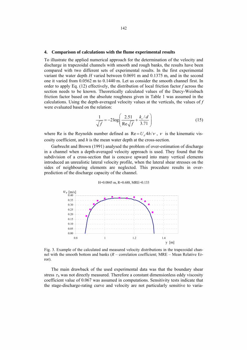
142

4. Comparison of calculations with the flume experimental results

To illustrate the applied numerical approach for the determination of the velocity and discharge in trapezoidal channels with smooth and rough banks, the results have been compared with two different sets of experimental results. In the first experimental variant the water depth H varied between 0.0691 m and 0.1375 m, and in the second one it varied from 0.0562 m to 0.1440 m. Let us consider the smooth channel first. In order to apply Eq. (12) effectively, the distribution of local friction factor f across the section needs to be known. Theoretically calculated values of the Darcy-Weisbach friction factor based on the absolute roughness given in Table 1 was assumed in the calculations. Using the depth-averaged velocity values at the verticals, the values of f were evaluated based on the relation:

/1 2.512log3.71Re

⎛ ⎞= − +⎜ ⎟⎜ ⎟

⎝ ⎠

sk df f

(15)

where Re is the Reynolds number defined as Re 4 /dU h= ν , ν is the kinematic vis-cosity coefficient, and h is the mean water depth at the cross-section.

Garbrecht and Brown (1991) analysed the problem of over-estimation of discharge in a channel when a depth-averaged velocity approach is used. They found that the subdivision of a cross-section that is concave upward into many vertical elements introduced an unrealistic lateral velocity profile, when the lateral shear stresses on the sides of neighbouring elements are neglected. This procedure results in over-prediction of the discharge capacity of the channel.

H=0.0845 m, R=0.688, MRE=0.133

0.000.05

0.100.15

0.200.25

0.300.35

0.40

0.8 1 1.2 1.4y [m]

U d [m/s]

Fig. 3. Example of the calculated and measured velocity distributions in the trapezoidal chan-nel with the smooth bottom and banks (R – correlation coefficient; MRE – Mean Relative Er-ror).

The main drawback of the used experimental data was that the boundary shear stress τ b was not directly measured. Therefore a constant dimensionless eddy viscosity coefficient value of 0.067 was assumed in computations. Sensitivity tests indicate that the stage-discharge-rating curve and velocity are not particularly sensitive to varia-

143

tions in the dimensionless eddy viscosity coefficient taken from the 0.01-0.64 (Darby and Torne 1996). Comparisons of the calculated velocity distributions from Eq. (10) for a smooth channel and the experimental results are shown in Fig. 3 and the obtained agreement was reasonably good. Correlation coefficients R and Mean Relative Error MRE were respectively equal 0.688 and 0.133 for the case with H = 0.0845 m; 0.983 and 0.114 for H = 0.1172 m and 0.847, 0.062 for H = 0.1375 m.

H=0.1155 m, R=0.748, MRE=0.121

0.00

0.05

0.10

0.15

0.20

0.25

0.30

0.35

0.8 1 1.2 1.4y [m]

U d [m/s]

Fig. 4. Example of the calculated and measured velocity distributions in trapezoidal cross-section channel with the smooth bottom and the rough banks.

0.00

0.010.02

0.03

0.040.05

0.06

0.070.08

0.09

0.100.11

0.12

0.130.14

0.15

0.00 0.01 0.02 0.03Q [m3/s]

H [m]

calculated measurements

smooth banks

raugh banks

Fig. 5. Calculated and measured discharges in the trapezoidal channel with the smooth bottom and the rough banks.

144

In case of the smooth channel with rough banks a similar procedure was applied. The obtained results (Fig. 4) are also acceptable although the Mean Relative Error increased and the obtained correlation coefficient was in general larger (R = 0.748 and MRE = 0.121 for H = 0.1155 m; R = 0.800 and MRE = 0.106 for H = 0.1286 m; R = 0.898 and MRE = 0.135 for H = 0.1440 m).

Figure 5 shows the resulting stage discharge relationship calculated from Eq. (10) and obtained from the experiments and the agreement was extremely good. Interesting information is provided by the variation of local values of the Darcy-Weisbach friction factor, calculated using depth-averaged velocity data and it reveals substantial differ-ences above the sloping banks (Figs. 6 and 7).

0.00

0.05

0.10

0.15

0.20

0.25

0.30

0.8 1.0 1.2 1.4y [m]

f [-]

H=0.0691 m H=0.0845 m H=0.0963 m

H=0.1011 m H=0.1172 m H=0.1375 m

Fig. 6. Calculated the Darcy-Weisbach friction factor in the trapezoidal channel with smooth bottom banks.

0.00.51.01.52.02.53.03.5

0.8 1.0 1.2 1.4y [m]

f [-]

H=0.0562 m H=0.0812 m H=0.1155 m

H=0.1286 m H=0.1440 m

Fig. 7. Calculated the Darcy-Weisbach friction factor in trapezoidal channel with the smooth bottom and rough banks.

The calculated bed shear stress distributions are shown in Figs. 8 and 9. The model reveals the increase of the bed shear stress above the edge between the bottom and the banks. The presented model provides yet another method of the evaluation of the bed shear stresses and the comparison with other computations (as reviewed by Rowiński et al. 2005) will be given elsewhere.

145

0.0

0.1

0.2

0.3

0.4

0.5

0.6

0.8 1.0 1.2 1.4y [m]

tau [N/m2]

H=0.0691 m H=0.0845 m H=0.0963 m

H=0.1011 m H=0.1172 m H=0.1375 m

Fig. 8. Calculated boundary shear stress τb in the trapezoidal channel with smooth bottom and banks.

0.0

0.1

0.2

0.3

0.4

0.5

0.6

0.7

0.8 1.0 1.2 1.4y [m]

tau [N/m2]

H=0.0562 m H=0.0812 m H=0.1155 m

H=0.1286 m H=0.1440 m

Fig. 9. Calculated boundary shear stress τb in trapezoidal channel with smooth bottom and rough banks.

5. Model application for an actual river reach

The verification of the model performance should be completed for a natural channel data for which in fact it has been constructed. An example of the comparison with the measurements performed in a selected cross-section of the Ihme River at Hannover, Germany (Rickert 1986), will be given herein and more examples covering a variety of roughness and hydraulic conditions will be provided in a separate publication.

The mean flow depths in the river main channel and the absolute roughness of d90 = 0.6 mm (90th percentile diameter of bed material) for sand sediment were used for the estimates of the Darcy-Weisbach friction factor. Figure 11 presents the com-parison between the calculated and measured velocity distributions in the given cross-section taking into account a variety of the assumed equivalent sand roughness or ab-solute roughness height (which may be for example evaluated as the difference be-tween elevation of roughness crest and trough). The relationship between roughness height and sediment size and distribution of sediment has been studied and the rela-tions with different sediment sizes, particularly with d50, d65, d84, d90 (defined as the sediment size equal to or exceeding that of 50, 65, 84 or 90% of the stream bed parti-

146

cles by weight) were given by various authors (see for example the review of Ritter-bach, 1991). The following propositions were considered in this study:

Taylor and Brooks – ks = d50 Einstein – ks = d65 Engelund i Hansen – ks = 2 d65 Hey – ks = 3,5 d84 Garbrecht – ks = d90 Kamphuis – ks = 2 d90 Van Rijn – ks = 3 d90

Those concepts led to the following values of the roughness height in the considered Ihme river reach (see Fig. 10):

0.8 1.22.4

4.8

9.610.5

14.4

0

5

10

15

Tayl

or &

Bro

oks

ks=d

50

Ein

stei

nks

=d65

Enge

lund

& H

anse

nks

=2d6

5

Gar

brec

htks

=d90

Kam

phui

sks

=2d9

0

Hey

ks=3

.5d8

4

Van

Rijn

ks=3

d90

ks [mm]

Fig. 10. Roughness height computed for the river Ihme based on various concepts.

0.00

0.50

1.00

1.50

2.00

2.50

3.00

0 5 10 15 20 25 30 35 40x [m]

Y [m], Ud [m/s]

cross-section Ud-meas 1.2mm 2.4 mm 4.8 mm

9.6 mm 10.5 mm 12 mm 14.4 mm Fig. 11. Computed velocity distributions in the Ihme River based on the various values of roughness height.

147

Note that the largest difference between the calculated and measured velocities is when ks = 1.2 mm is assumed. The best concept turned out to be the one proposed by Van Rijn which is also reflected in Fig. 12 showing the Mean Relative Error and Cor-relation Coefficient for the comparison of the computed and measured velocity distri-butions.

37

27 29

7 6 5 4

0

10

20

30

40

Tayl

or &

Bro

oks

ks=d

50

Eins

tein

ks=d

65

Enge

lund

& H

anse

nks

=2d6

5

Gar

brec

htks

=d90

Kam

phui

sks

=2d9

0

Hey

ks=3

.5d8

4

Van

Rijn

ks=3

d90

MRE [%]

0.150

0.3900.437

0.965 0.975 0.985 0.991

0.0

0.2

0.4

0.6

0.8

1.0

Tayl

or &

Broo

ksks

=d50

Ein

stei

nks

=d65

Enge

lund

& H

anse

nks

=2d6

5

Gar

brec

htks

=d90

Kam

phui

sks

=2d9

0

Hey

ks=3

.5d8

4

Van

Rijn

ks=3

d90

R

Fig. 12. Mean Relative Error and correlation coefficient of the computed and measured velocity distributions for the selected cross-section of the River Ihme assuming various values of roughness height.

6. Concluding remarks

The purpose of this work has been to confirm a useful method by Knight and Shiono (1991) for predicting the discharge given for homogeneously smooth and non-homogeneously roughened trapezoidal channels by neglecting the secondary flow contribution, i.e. ( d( U V) / y 0∂ ηρ ∂ = ). The local friction factor f values vary along the wetted perimeter; they are different in the main channel and above the channel banks. However, given that f values were taken as constant over the main channel and flood-plains, the numerical predictions of Ud and Q in channels are shown to be in close agreement with the experimental data. The applicability of the method is restricted by the range of data that were used to develop the friction factor. The Darcy-Weisbach equation predicts the values of friction factor for sandy bed channels. Computations proved to provide reasonable results also for an actual river but the results turned out to be very sensitive to the assumed method of the evaluation of the roughness height.

Acknowledgements . The present paper is a result of a collaborative work for which funding was sponsored by two grants from The Ministry of Higher Education and Science, Grant No. 2 P04D 026 29 and 6 P06H 043 20.

References

Brookes, A., 1988, Channelized rivers: perspectives for environmental management, John Wiley & Sons Ltd.

Darby, S.E., and C.R. Thorne, 1996, Predicting Stage-Discharge Curves in Channels with Bank Vegetation, J. Hydraul. Eng. 122 (10), 583-586.

148

Garbrecht, J., and G.O. Brown, 1991, Calculation of total conveyance in natural chan-nels, J. Hydraul. Eng. 117 (6), 788-799.

Knight, D.W., K.W.H. Yuen and A.A.I. Al-Hamid, 1994, Boundary Shear Stress Dis-tributions in Open Channel Flow. Mixing and Transport in the Environment. Ed-ited by K.J. Beven, P.C. Chatwin and J.H. Millbank, John Wiley & Sons Ltd, 51-87.

Kubrak, J., and F. Tönsmann, 2001, Velocity and discharge prediction in straight compound channels using the eddy viscosity concept, Journal Water and Land De-velopment, 5, 107-121.

Kubrak, J., and A. Żbikowski, 1995, Investigation into the Hydraulic Characteristics of Channels with Flood Plains, Archives of Hydro-Engineering and Environmental Mechanics 43 (3-4), 31-37.

Lambert, M.F., and R.H.J. Sellin, 1996, Discharge prediction in straight compound channels using the mixing length concept, J. Hydraul. Res. 34 (3), 381-394.

Mohamed, H.I., 2004, Effect of lateral variation of roughness on flow conveyance within a trapezoidal channel cross-section. River Flow 2004-Greco, Carravetta and Della Morte (eds.), 363-369.

Rickert, K., 1986, Der Einfluss von Gehölzen auf die Lichtverhältnisse und das Ab-flussverhalten in Fliessgewässern. Ph.D. Thesis, Fachbereich Bauingenieur- u. Vermessungswesen der Universität Hannover.

Ritterbach, E., 1991, Wechselwirkungen zwischen Auenökologie und Fließgewässer-hydraulik und Möglichkeiten der integrierenden computergestützten Plannung. Mitteilungen für Wasserbau und Wasserwirtschaft, Rheinish-Westfälische Tech-nische Hochschule Aachen.

Rowiński, P.M., J. Aberle and A. Mazurczyk, 2005, Shear velocity estimation in hy-draulic research, Acta Geophys. Pol. 53 (4), 567-583.

Shiono, K., and D.W. Knight, 1990, Mathematical models of flow in two or multi stage straight channels. Proc. Int. Conf. on River Flood Hydraulics (Ed. W.R. White). Wiley, Chichester. 229-238.

Shiono, K., and D.W. Knight, 1991, Turbulent open-channel flows with variable depth across the channel, Journal Fluid Mechanics 222, 617-646.

U.S. Army Corps of Engineers, 1994, Methods for Predicting n values for Manning Equation. EM 1110-2-1601.

PUBLIS. INST. GEOPHYS. POL. ACAD. SC., E-7 (401), 2007

New Approach to Flood Management

Wojciech MAJEWSKI Institute of Meteorology and Water Management, Warsaw

Podleśna 61, 01-673 Warsaw, Poland e-mail: wojciech.majewski@imgw.pl

Abstrakt

Floods are one of the most important natural hazards for people, economy and ecology. Can disastrous floods be avoided ? No, and we are even unable to fully protect against these natural phenomena. However, research on the course and consequences of floods is helping us to mitigate their impact, and above all to avoid human fatalities. In recent years the number and frequency of floods considerably increased in Poland, Europe and over the whole world. An essential feature is the fact that floods appear in the most densely inhabited areas includ-ing river valleys. The paper presents changes in the approach to flood protection. Poland is the country where floods are very frequent and their origin and run are very differentiated. The approach to flood protection based on new Flood Direc-tive of EU is presented. The paper concerns mainly floods in river valleys and urban areas.

Key words: floods, natural hazards, flood protection, flood mitigation, EU Flood Directive.

1. Introduction

What is flood? A flood is an excess level or flow of water that spills out of the river channel resulting in economic, social and ecological damages and sometimes even taking a toll of human life. This definition is used in Poland (Polish Water Act 2001). The current degree of flood danger is estimated in Poland in terms of two specific water levels: a warning level, after which a state of flood preparation is announced, and an alarm level entailing a real flood threat, after which a state of flood alarm is announced.

Recently issued EU Flood Directive (2007) on the Assessment and Management of Floods gives the following two definitions.

1. Flood means the temporary covering by water of land not normally covered by water, as a result of heavy rainfall leading to the inundation of inhabited and/or industrial areas.

150

2. Flood risk means the likelihood of a flood event together with the potential damage to human health and life and the economic activity associated with that flood event.

Floods as natural element of the hydrological cycle have always been with us and will surely continue to be part of our lives. Still, recent years have witnessed an in-creased frequency of extreme hydrological and meteorological phenomena, such as hurricanes, high/low temperatures, storm surges, tsunamis, severe rains or droughts, and above all floods.

The final decade of the last century and the beginning of the new millennium brought many flood cataclysms. Here we can mention the flood on the Rhine River in 1993, on the Rhine and Moselle in 1995, on the Oder and upper Vistula in 1997, on the Yangtze in 1998, on the upper Vistula and in the city of Gdańsk in 2001, on Elbe in 2003, the extraordinary flooding of New Orleans in 2005, and the flood along the Danube in the spring of 2006.

As an excellent indication of the importance of this problem, is the fact that 2004 World Water Day – a yearly event designated by the UN in 1992 to water problems – took the theme “water and disasters”. Ninety percent of the natural cataclysms occur-ring in 1992–2001 resulted from hydrological and meteorological phenomena. More than a billion and a half individuals worldwide have been affected by floods. Yet as the number of floods and the scope of the economic damage increased, the number of fatalities has simultaneously decreased (World Water Day 2004). That success can be put down to more accurate flood forecasts and better flood control measures.

Floods usually result from extreme hydro-meteorological phenomena, such as se-vere rainfalls over small areas, or long-lasting rains over large areas, the melting of snow and ice, storm surges, and ice jams on rivers. However, floods sometimes are caused by design mistakes or human error in the operation of hydraulic facilities.

The greatest devastation is caused by floods occurring in densely populated river valleys. Note that many of our cities are situated on rivers, thus gaining the advantage of easy water access, navigation and fishing potential, and even such factors as sport and recreation. Since such regions generate the highest economic income, the disad-vantage is that they are most under threat, yet most favourable in economic terms. The people inhabiting such areas have to be aware of this trade-off. Property and accident insurance, with rates depending on the degree of the threat, are increasingly used to offset the threat.

2. Floods in Poland

Poland is a country that has to face a very high and at the same time very diverse flood hazard. Floods are most commonly caused by concentrated rains – the 2001 flood in Gdańsk being the result of such rainfall or long-lasting rains over large areas (flood 1997 on the Odra River). Floods may also be caused by ice related phenomena, such as frazil-ice jams, which occur in the autumn-winter period, and ice jams, which occur in the springtime when the ice cover on rivers breaks up and flows downstream. An ice jam at the mouth of Vistula River in 1829 resulted in flooding of the city of

151

Gdańsk up to the first-story level. In 1844, another ice jam on the Gdańska Vistula led to the creation of a new mouth to the sea − the Śmiała Vistula (Bold Vistula). To re-duce the threat of flooding in the Gdańsk region and the Vistula Delta, an artificial channel of the Vistula called the Przekop was constructed in 1895, a solution that proved very effective (Fig. 1). The arrows in Fig. 1 indicate three main directions of flood hazard to the surrounding area called Żuławy: from the Bay of Gdańsk (storm surges), from the main channel of Vistula (high discharge or ice jams) and from the moraine hills (e.g. flash flood 2001 in Gdańsk). Previous main channel of Vistula River was closed by navigation lock in Przegalina and at present there is no river flow. Therefore this river section is now called Martwa Vistula, which means Dead Vistula.

Fig. 1. Present layout of the Vistula delta.

Numerous small rivers and channels, which discharge to Martwa Vistula have storm gates. These gates close automatically in case of storm surge to prevent saline waters from the Gulf of Gdańsk to enter inland streams.

In 1934 a catastrophic flood in the Dunajec River catchment caused vast material losses and took a toll of many lives. To alleviate similar floods in the future, the Rożnów and Czorsztyn dams and reservoirs were designed and built. The Rożnów dam was finished in 1942, while the Czorsztyn dam, after being under construction for more than 20 years, was completed and commissioned in 1997, just before another high flood wave. Czorsztyn-Niedzica reservoir significantly reduced the flood wave arriving from the mountain part of Dunajec River.

In 1982 a severe flood caused by ice jam on the Lower Vistula in the region of Płock resulted in flooding of large agricultural area and part of the city. This flood resulted from very unfortunate coincidence of hydro-meteorological phenomena, which appeared simultaneously. The main problem was to find out why during rela-tively low discharge water levels were so high and breached flood dykes (Fig. 3) in-

152

undating large areas. This study required intensive and complicated field measure-ments as well as theoretical analysis and numerous calculations (Majewski 1987).

Fig. 2. Rożnów dam on Dunajec River.

Fig. 3. Ice-jam flood on Vistula River near Płock.

On the upper and middle Odra and lower Vistula, the 1997 flood caused damages of 14 billion PLN and the deaths of 54 individuals. Indirect losses came to nearly 3 billion PLN.

In 2001, a sudden flash flood caused by severe rainfall in Gdańsk within the course of 4 hours caused 50 million USD of damage to city infrastructure alone. Three hundred families lost their homes and property, although fortunately no lives were lost (Majewski 2003, Majewski 2006).

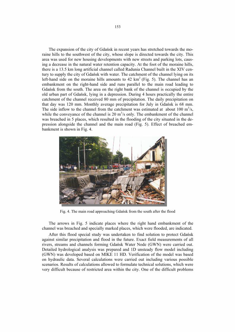
153

The expansion of the city of Gdańsk in recent years has stretched towards the mo-raine hills to the southwest of the city, whose slope is directed towards the city. This area was used for new housing developments with new streets and parking lots, caus-ing a decrease in the natural water retention capacity. At the foot of the moraine hills, there is a 13.5 km long artificial channel called Radunia Channel built in the XIV cen-tury to supply the city of Gdańsk with water. The catchment of the channel lying on its left-hand side on the moraine hills amounts to 42 km2 (Fig. 5). The channel has an embankment on the right-hand side and runs parallel to the main road leading to Gdańsk from the south. The area on the right bank of the channel is occupied by the old urban part of Gdańsk, lying in a depression. During 4 hours practically the entire catchment of the channel received 80 mm of precipitation. The daily precipitation on that day was 120 mm. Monthly average precipitation for July in Gdańsk is 68 mm. The side inflow to the channel from the catchment was estimated at about 100 m3/s, while the conveyance of the channel is 20 m3/s only. The embankment of the channel was breached in 5 places, which resulted in the flooding of the city situated in the de-pression alongside the channel and the main road (Fig. 5). Effect of breached em-bankment is shown in Fig. 4.

Fig. 4. The main road approaching Gdańsk from the south after the flood

The arrows in Fig. 5 indicate places where the right hand embankment of the channel was breached and specially marked places, which were flooded, are indicated.

After this flood special study was undertaken to find solution to protect Gdańsk against similar precipitation and flood in the future. Exact field measurements of all rivers, streams and channels forming Gdańsk Water Node (GWN) were carried out. Detailed hydrological analysis was prepared and 1D unsteady flow model including (GWN) was developed based on MIKE 11 HD. Verification of the model was based on hydraulic data. Several calculations were carried out including various possible scenarios. Results of calculations allowed to formulate technical solutions, which were very difficult because of restricted area within the city. One of the difficult problems

154

was the situation when simultaneous flood comes from moraine hills and storm surge in the Gulf of Gdańsk. This concerned the operation of storm gates.

Fig. 5. The catchment of Radunia Channel, Radunia Channel, breached embankment and flooded areas in 2001.

Finally it was decided to construct 18 small impounding reservoirs in the catch-ment of the channel, 3 by-passes from the channel and 2 additional flood polders. A special system of precipitation and water level measurements was proposed. These solutions are shown in Fig. 6.

Fig. 6. Technical solutions proposed after the flood 2001.

155

3. Evolution of flood protection

Flood control has always been an important field of hydraulic engineering and water resources management. One of the earliest approaches involved the notion of keeping water away from people, i.e. constructing of flood dykes, retention reservoirs, relief channels, dry reservoirs, and flood polders (Majewski 2006a).

Flood dykes are earthen constructions running alongside rivers, meant to protect against any excessive high stages of flood waters. Retention reservoirs, in turn, are meant to catch part or all of a flood wave, thus limiting the degree of flooding down-stream from the reservoir. Relief channels are constructed to protect urban areas or other places of specific economic or cultural value, and come into operation whenever a flood wave approaches.

Dry reservoirs are designed in the upper sections of rivers, which are automatically filled whenever high discharge approaches, at other times being utilized as meadows or grazing land. Flood polders are artificial basins situated alongside riverbanks which become filled automatically by side spillways upon the arrival of a flood wave, thereby reducing its height, and are then drained after the water level recedes. At other times polders often serve as recreational areas.

All of these hydraulic structures are expensive to construct hydraulic structures and to keep them in good conditions – maintaining many kilometres of flood dykes being a very costly endeavour. In the past it was often thought, albeit mistakenly, that such constructions provide complete flood protection. Very often hydraulic analysis indicated that the height of flood dykes should be increased, as well as capacity of impounding reservoirs. Yet, once economic analyses began to be performed about the feasibility and efficiency of raising the level of existing flood dykes or increasing the capacity of retention reservoirs, the conclusion often reached was that doing so simply did not pay. It had also been frequently neglected that increasing flood control in one place might worsen it in others. Constructing flood dykes along an upper river section often simply turned out to accelerate the flow and cause higher water levels down-stream.

Later on another solution was proposed i.e. make more room for the rivers. This means to displace existing flood dykes further from the river bank. It is a very good solution, however very costly and not always possible, because of existing infrastruc-ture just behind flood dyke.

Once these shortcomings were realized, other solutions began to be developed, fol-lowing the notion of keeping people away from water, i.e. removing human settle-ments and industrial facilities from flood-prone areas. While often economically justi-fied, such efforts have also been very costly. Consideration of the previous and new approach to flood protection was a very long trend, bringing often numerous contro-versies, especially when ecological objectives were taken into account.

Finally, consideration began to be given to the possibility of temporary flooding of defined areas, together with existing infrastructure, paying greater attention to the protection of buildings against flooding and damage, as well as reinforcing existing infrastructure against flood damage. Efforts of this sort can be described as learning to live with floods. A necessary condition here is that the accurate meteorological and

156

hydrological forecast is absolutely necessary, to give people time to prepare ade-quately for flood advent. For private homes, for instance, this method involves pro-tecting basement windows and entry doors with special closures that prevent flood-water from penetrating inside – a solution that is widely employed in many European countries (e.g. Netherlands). Then, after a flood subsides, work must be efficiently planned to quickly eliminate the damages caused, bringing life back to normal as soon as possible.

4. Integrated flood management

The new approach to flood control is known as integrated flood management (Ma-jewski 2006b). Previously, all flood control efforts concentrated on the river channel itself, or its immediate vicinity. This new approach encompasses efforts undertaken throughout the entire catchment. On the one hand, this means such aspects as spatial planning, forestation, land cultivation, and urbanization – efforts which may be de-scribed as technical, since they deal with buildings, constructions, and land manage-ment. Yet on the other hand, research has shown that a significant reduction in flood impact can be achieved through non-technical means, i.e. investing in forecasting and warning systems or making organizational preparations (accumulating the necessary equipment and drafting evacuation plans in case of flood). It is likewise very impor-tant to educate society about what flooding can mean for them, about how floods may occur and proceed, and about what every citizen should know to protect themselves and their property. Such non-technical efforts take significantly less funding than technical means, but often yield more tangible results.

After the devastating 1997 flood on the Odra and Upper Vistula, Poland began re-inforcing its means of hydro-meteorological protection. This consists of automatic water level gauges and meteorological monitoring stations, plus a system of meteoro-logical radar devices providing early warning of oncoming clouds, fronts, storms and precipitation. These are maintained by the State Hydrological-Meteorological Service, operated by the Institute of Meteorology and Water Management in Warsaw. Local flood warning systems and crisis reaction centres were established in numerous flood-prone areas, with all these elements being coordinated by the National or Provincial Rescue and Protection Centres.

Following a number of catastrophic floods in Europe, the European Commission has initiated joint action aimed at improving flood control measures Europe-wide, and a special EU Flood Directive was issued. The current approach envisions a system of safeguards, which can ensure that losses are minimized and that life can proceed rela-tively normally, regardless of the degree of flooding intensity. That will above all re-quire good meteorological and hydrological forecasts, as well as power and communi-cation systems that operate reliably under flood conditions.

5. EU Directive on the Assessment and Management of Floods

The new EU Flood Directive (2007) was adapted after long discussions and negotia-tions. It was stated that at present there is no legal instrument for protection against

157

flood risk. That risk, which will become more frequent in future as a result of climate change. Concerted and coordinated action at the level of Community would bring considerable added value and improve the overall level of flood protection.

Most river basins in Europe are split between Member States, and effective pre-vention against floods requires a cross-border cooperation. Moreover, throughout the Community different floods occur and damage caused by flood events may also vary across the countries and regions of the Community. Hence, objectives regarding flood management should be based on the local and regional circumstances.

River basin flood management should aim to create common responsibility and solidarity within the Community. To that end Member States should endeavour to raise awareness and encourage cooperation among all stakeholders. The following tasks are foreseen:

• maps of river basin districts including borders of river basins, sub basins and coastal areas,

• description of floods which occurred in the past, • an assessment of the likelihood of future floods based on available information

(e.g. climate changes), • a forecast of the estimated consequences of future floods, • flood risk management measures, especially those related to the infrastructure, • an assessment of the effectiveness of existing man-made flood defence infra-

structure.

6. Conclusions

• Floods are one of the most important natural hazards for people, economy and ecology.

• The frequency and severity of floods is increasing and this trend will persist tak-ing into account possible climate changes.

• There is no possible flood protection by means of technical measures only and non-technical measures should be also considered.

• New approach to flood assessment, management and mitigation is proposed in EU Flood Directive and will be obligatory in EU countries.

• The new approach to flood protection should take into account not only river channel or its valley but also the whole river catchment.

• Preparation of flood protection plans requires work of comprehensive teams consisting of technical specialists (hydrology, meteorology, hydraulics, water resources management), specialists of spatial planning, ecologists, economists and sociologists.

• Flood problems require detailed hydrological and hydraulic analysis as well as field measurements and hydro-meteorological observations (precipitation, water stages).

158

References

EU Flood Directive 2007. Majewski, W., 1987, Influence of ice cover on hydraulic characteristics of run-of-

reservoirs on lowland rivers on the example of Włocławek Reservoir (in Polish). Publication of IBW PAN Gdańsk.

Majewski, W., 2003, The Gdańsk Flood of 2001 (in Polish). Gdańsk Scientific Soci-ety.

Majewski, W., 2006, Measures and Solutions for Flood Managemenet. A Local Case: Flash Flood 2001 in Gdańsk, Poland. Journal of Irrigation and Drainage No 55.

Majewski, W., 2006a, Changes in the Approach to Flood Control (in Polish), 52 nd Research Conference of the Committee for Civil and Hydro Engineering, Scientific Proceedings of the Gdańsk University of Technology.

Majewski, W., 2006b, Floods, from Defence to Management, 3rd International Sym-posium on Flood Defence, Nijmegen, Netherlands, Balkema.

Polish Water Act 2001. World Water Day 2004, UNESCO, (in Polish) Proceedings of the IBW PAN Gdańsk.

PUBLS. INST. GEOPHYS. POL. ACAD. SC., E-7 (401), 2007

The Impact of Hydraulic Conductivity on Topography Driven Groundwater Flow

Lars MARKLUND and Anders WÖRMAN Royal Institute of Geophysics Technology

Teknikringen 76, SE-100 44 Stockholm, Sweden e-mail: larsmark@kth.se

Abstract

Landscape topography is the most important driving force for groundwater flow and all scales of topography contribute to groundwater movement. Here we present results of how different scales of topography affect the groundwater flow at different depths. The study is based on a spectral analysis of the topography and a couple of exact 3-D solutions of the groundwater flow. We are also analyz-ing how different heterogeneities of the subsurface hydraulic conductivity impact the groundwater flow at different depths and alter the relative importance of dif-ferent topographic scales on the groundwater flow. Quaternary deposits are ex-tremely important for the infiltration at the ground surface, but the effect is pri-marily constrained to the deposit strata. Depth dependent hydraulic conductivity has a major impact on the size and depth of the groundwater flow cells, but it also affects the infiltration at the surface. Depth dependent hydraulic conductiv-ity tends to counteract the effect of the large-scale topography on the groundwa-ter flow more effectively than the smaller landscape scales.

1. Introduction

Freshwater is the most important natural resource for human life and, even if surface water reservoirs are refilled much more rapidly than groundwater reservoirs, ground-water (GW) constitutes 98% of all non-frozen freshwater (Shiklomanov 1998) and are therefore an important source for freshwater in many countries (i.e. Hutson et al. 2004). Due to the increasing demand of freshwater that follows from the world’s rapid population growth there is an ever greater need for a better understanding of the proc-esses controlling the groundwater recharge. Recharge of new groundwater is perhaps the most important factor for sustainable water resource management.

In humid climates, where the groundwater surface tends to follow the ground sur-face, differences in hydraulic potential created by topography are the main driving force for groundwater flow. The impact of different scales of topography on ground-water flow has been investigated for different reasons (i.e. Alley et al. 2002, Zilj

160

2002). Recently we developed a method to represent the topography in three dimen-sions by a spectrum of harmonic functions (Wörman et al. 2006). With this approach we can estimate the relative impact of a certain scale of topography on groundwater movement at a specified depth.

In this study we have developed new three-dimensional, exact solutions to investi-gate how the scale effect of topography changes when more realistic representations of the subsurface are induced, especially depth dependent hydraulic conductivity and quaternary deposits on top of bedrock. By doing so, our aim is to give a better under-standing of the relationship between topography and groundwater flow. This under-standing is important, not only for water resourse management, but also for many technical implementations; drainage in tunnel constructions, the performance of nu-clear waste repositories (Marklund et al. 2007) etc.

In this study we investigate to what degree various scales of topography are con-trolling the recharge and, especially, how different depth-dependent conductivities as well as presence of Quaternary deposits control infiltration. For various representa-tions of the subsurface, we study how different scales of topography control the groundwater movement at different depths.

2. Methods

Groundwater re- and discharges are controlled by landscape topography because the groundwater surface tends to follow the ground surface. We characterize the effects of the land surface topography on subsurface flow in terms of the vertical flux. This is done by performing a spectral analysis of the topography (Wörman et al. 2006) in three domains with different sizes and resolutions (Table 1).

Table 1

Sizes and resolution of the study-areas

Name Size Resolution L 350×350 km 141×141 M 100×100 km 201×201 S 30×30 km 241×241

All three domains are located in Sweden (Fig. 1) and the largest domain surrounds the middle-sized domain which is surrounding the smallest domain.

The result of the spectral analysis is a representation of the ground surface topog-raphy in a Fourier-series spectrum. Assuming a groundwater surface that follows the ground surface gives us the hydraulic potential as a boundary condition. Hence, the Fourier-series spectrum combined with the hydraulic conductivity provides an exact solution of the underlying three-dimensional groundwater flows induced by these to-pographic features over a wide range of spatial scales. According to Wörman and col-leagues (2006), the solution to the vertical groundwater velocity component (vertical flux) in a homogeneous subsurface becomes:

161

( ) ( )( )

2 2 2 2, , ,,

,2 21 1, ,

2 2, , , ,

exp exp ( 2 )( , , ) ( )

1 exp 2

sin( )cos( )

y zx NN x i x i y jy jm i j

j ix i y j

x i y j x i y j

k k k k zw x y z h K

k k

k k k x k y

ε= =

+ + + − ε −= ⋅

+ − +

⋅ +

∑∑ (1)

in which hm = amplitude coefficients [m], h = hydraulic head [m], <…> = arithmetic average value, N = number of wavelengths in the x- and y-directions, ε [m] = the depth to a no-flow condition boundary, K = hydraulic conductivity and (x, y, z) are Cartesian coordinates.

Fig. 1. Map of Sweden showing the three different study-domains: L, M and S.

2.1 Impact of depth dependent hydraulic conductivity

To quantify the groundwater recharge we integrate the absolute value of the vertical velocities over the entire domain area. This was performed in all three domains and at three different depths; z = 0, z = −500 and z = −1000 meters. The vertical flux at the different depths is calculated for two different representations of the hydraulic conduc-tivity (K). First we use a homogeneous conductivity, K = 10−6 m/s. The second repre-sentation is a depth dependent function described by Eq. 2.

0czK K e= (2)

where K0 is the conductivity at the surface, z is the depth and c is a positive constant. For such hydraulic conductivity we have derived an exact solution for the vertical flow velocity:

162

( )

( )

2 2 2, ,

,1 1

2 2 2, ,

, ,

4( , , ) ( )

2

4exp sin( )cos( )

2

yx NNx i y j

m i jj i

x i y j

x i y j

c c k kw x y z h K

c c k kz k x k y

= =

+ + += ⋅

⎛ ⎞+ + +⎜ ⎟⋅ −⎜ ⎟⎜ ⎟⎝ ⎠

∑∑ (3)

By comparing Eqs. (1) and (3), we can evaluate how the depth dependent hydraulic conductivity affects the groundwater movement at certain depths and for different scales of topography. We based the values of c and K0 on borehole data from Sweden ranging down to approximately 1600 m depth (Rhen et al. 2006), c = 0.00641 and K0 = 1.925×10−7.

2.2 Groundwater recharge through soil-rock interface

To study the effect of Quaternary deposits we have derived an exact solution for the groundwater flow with a layered representation of the subsurface consisting of two layers; the Quaternary deposits and the bedrock. Here we study how different thick-nesses and different conductivities of the Quaternary deposits affect the flux at the interface between soil and rock. Since the analytical method (Eq. 4) we use here can only cope with soil layers of constant thickness, we have chosen to study the two dif-ferent thicknesses: 2 and 10 m. We also study two different soil types, till (K ~ 10−6) which is the dominating soil type in Sweden and sandy sediments (K ~ 10−5) (Domenico and Schwartz 1998). The vertical velocity in the Quaternary deposits (w1) and in the bedrock (w2), are given in the following expression:

( )

( )( ) ( )( )( )( )

2 21 , 1 , , , ,

1 1

2 2 2 21 , , , ,

2 2, ,

( , , ) ( ) sin( )cos( )

exp exp

exp

yx NN

m i j x i y j x i y jj i

x i y j x i y j

x i y j

w x y z h K k k k x k y

A k k z k k z

k k z

= =

= + ⋅

⎡ ⎛ ⎞⋅ + + − +⎜ ⎟⎢ ⎝ ⎠⎣⎤− − + ⎥⎦

∑∑

(4)

( )

( )

2 , 2 , ,1 1

2 2 2, ,

2

2 2 2, ,

( , , ) ( ) sin( )cos( )

4exp

2

4

2

yx NN

m i j x i y jj i

x i y j

x i y j

w x y z h K k x k y

c c k kA z

c c k k

= =

= ⋅

⎛ ⎞− + + +⎜ ⎟⋅ ⋅⎜ ⎟⎜ ⎟⎝ ⎠

− + + +⋅

∑∑

163

where: K1 is the hydraulic conductivity in the Quaternary deposits, K2 = K0‗2 ecz is the hydraulic conductivity in the bedrock, A1 = f(c, K1, K2, εQD, kx, ky), A2 = f(A1, εQD, kx, ky), εQD is the thickness of the Quaternary deposits.

The constant soil depth is a shortcoming because the thickness of Quaternary de-posits often differs widely. In areas covered by thick layers of Quaternary deposits, the undulation of the topography is often smaller compared to areas with more shallow deposits. The thickness of the deposits is often determined by the topography, where more material is deposed in lower areas. However, the thickness of the glacial till does not fluctuate much and is seldom larger than four meters. Larger deposits are concen-trated to lakes and rivers and consist of well sorted sediments.

3. Result

3.1 Impact of depth dependent hydraulic conductivity

The importance of different scales of topography on the groundwater flow is depth dependence (Fig. 2). The impact of the shorter wavelengths on the groundwater flow decreases faster with depth in relation to longer wavelengths.

1,E-21

1,E-20

1,E-19

1,E-18

1,E-17

1,E-16

1,E-15

1,E-14

1,E-13

1,E-12

1,E-11

1,E-10

1,E-09

1,E-081,E+02 1,E+03 1,E+04 1,E+05 1,E+06

Wavelength (m)

Verti

cal f

lux

(m/s

)

z=0z=-500z=-1000

Fig. 2. The vertical flux at different depths driven by topography of different wavelengths, where diamonds indicates flux at the surface, squares at 500 m depth and triangles at 1000 m depth.

The relationship between topographic scale and water fluxes at various depths change when we account for depth dependent hydraulic conductivity (Fig. 3). Figure 3 also shows that groundwater fluxes generated by topography of larger wavelengths are more affected by the decreasing conductivity than fluxes associated with shorter wavelengths.

164

1,E-231,E-221,E-211,E-201,E-191,E-181,E-171,E-161,E-151,E-141,E-131,E-121,E-111,E-101,E-09

1,E+02 1,E+03 1,E+04 1,E+05

wavelength (m)

vert

ical

flux

(m/s

)

Constant K z=0

Constant K z=-1000

Variable K z=0

Variable K z=-1000

Fig. 3. The vertical flux at different depths (0 and −1000 m) driven by topography of different wavelengths.

Because larger wavelengths dominate the groundwater flow at greater depths, the decrease of conductivity has a relatively larger impact on the absolute flux with depth in bedrock (Table 2).

Table 2

Vertical fluxes (W-flux) at different depths and with different representation of the bedrock hydraulic conductivity

Area Hydraulic conductivity

W-flux (mm/year) at

z = 0

W-flux (mm/year) at

z = −500

W-flux (mm/year) at

z = −1000 Constant 121 90 71

L Depth dependent 14 0.51 0.019 Constant 31 13 8.6

M Depth dependent 12 0.18 0.046 Constant 92 25 14

S Depth dependent 52 0.42 0.011

3.2 Groundwater recharge through soil-rock interface

The infiltration at z = 0 is found to depend both on the conductivity and the thickness of the Quaternary deposits. As shown in Table 3, a higher conductivity of the QD only increases the flux at the ground surface but at great depths the flux is only slightly affected. The same effect is created by larger thickness of the deposits (Table 3). The impact of the QDs is independent of the topographic scales (Fig. 4).

165

Table 3

Sizes and resolution of the study-areas

Area Hydraulic

conductivity in QD (m/s)

Depth of QD (m)

U-flux (mm/year) at

z = 0

U-flux (mm/year) at

z = −50

U-flux (mm/year) at

z = −100 2 30 7.6 4.8

10-5 10 104 7.7 4.9 2 14 7.6 4.8

L 10-6

10 21 7.7 4.9 2 30 7.6 4.8

10-5 10 104 7.7 4.9 2 15 10 7.2

M 10-6

10 19 10 7.2 2 250 24 13

10-5 10 1124 25 13 2 72 24 13

S 10-6

10 121 24 13

1,E-11

1,E-10

1,E-09

1,E-08

1,E-07100 1000 10000 100000

wavelength (m)

verti

cal f

lux

(m/s

)

QD2_K10 -5QD10_K10 -5QD2_K10 -6QD10_K10 -6

Fig. 4. The vertical flux at the groundwater surface driven by topography of different wave-lengths, of four different representations of the Quaternary deposits: two different depths, 2 and 10 m, combined with two different hydraulic conductivities, 10−5 and 10−6.

4. Discussion and conclusions

Landscape topography is the most important driving force for groundwater flow and all scales of topography contribute to groundwater movement. At the groundwater surface the contribution to the groundwater flow is rather equal for all scales (Fig. 2),

166

but the impact of shorter topographical scales decay faster with depth than longer scales.

The depth dependent hydraulic conductivity is another important factor for the groundwater movement. By controlling how deep the groundwater flow cells become, it also determines the residence time for groundwater. In addition, it controls how different scales of topography affect the groundwater flow at different depths and even at the surface. The decreasing hydraulic conductivity with depth blocks out more effectively the impact of the larger landscape features compared to the smaller fea-tures. This is most obvious at flows at great depths (z = −1000 m), but the effect is also present at the surface.

The recharge of groundwater is driven by topography, but the physical properties of Quaternary deposits are controlling the magnitude of the recharge. The higher con-ductivity of the Quaternary deposits creates a much larger infiltration rate compared to a geological representation of the subsurface where the bedrock reaches up all the way to the ground surface. However, even if the infiltration is increased up to a hundred times, fluxes at 50 m depth are not significantly affected. We note here that this study was performed with a depth dependent hydraulic conductivity in the bedrock and most likely the effects of the Quaternary deposits would reach deeper with a homogeneous representation of the bedrock but the depth dependency of the hydraulic conductivity is more realistic in most areas (Ingebritsen and Manning 1999).

Acknowledgments . Acknowledgments are due to the financial support of the Nuclear Power Inspectorate and the Swedish Radiation Protection Authority.

References

Alley, W.A., R.W. Healy, J.W. LaBaugh and T.E. Reilly, 2002, Flow and storage in groundwater systems, Science 296, no. 5575, 1985-1990.

Domenico, P.A., and W. Schwartz, 1998, Physical and Chemical Hydrogeology, 2nd edition, Wiley, New York.

Hutson, S.S., N.L. Barber, J.F. Kenny, K.S. Linsey, D.S. Lumia and M.A. Maupin, 2004, Estimated use of water in the United States in 2000, U.S. Geological Survey Circular 1268.

Marklund, L., A. Wörman, J. Geier, E. Simic and B. Dverstorp, 2007, Impact of land-scape topography and Quaternary overburden on the performance of a geological repository of nuclear waste, In press: Nuclear Technology.

Rhén, I., T. Forsmark, I. Forssman and M. Zetterlund, 2006, Evaluation of hydro-geological properties for Hydraulic Conductor Domains (HCD) and Hydraulic Rock Domains (HRD). Prelimanary site description, Laxemar subarea – vesion 1.2. SKB R-06-22. Swedish Nuclear Fuel and Waste Management Company.

Shiklomanov, I-A., 1998, Global renawble water resourses. In: H. Zebedi (ed), Water: A Looming Crisis? Proceedings of the International Conference on World Water Resources at the Beginning of the 21st Century, Unesco/IHP, Paris, 25 pp.

167

Wörman, A., A.I. Packman, L. Marklund, JW. Harvey and S. Stone, 2006, Exact three-dimensional spectral solution to surface-groundwater interactions with arbitrary surface topography, Geophys. Res. Lett., vol. 33, doi:10.1029/2006GL025747.

Zijl, W., 1999, Scale aspects of groundwater flow and transport systems, Hydrogeol-ogy J., 7, 139-150.

PUBLS. INST. GEOPHYS. POL. ACAD. SC., E-7 (401), 2007

Scales of Turbulence in Compound Channels with Trees on Floodplains

Agata MAZURCZYK Institute of Geophysics Polish Academy of Sciences

Ks. Janusza 64, 01-452 Warsaw, Poland e-mail: agatam@igf.edu.pl

Abstract

The results of experimental studies, aimed at the recognition of the scales of turbulent eddies in channels with the simulated riparian woody vegetation, are discussed in the paper. The analyses include temporal scales of macroeddies, longitudinal spatial scales of macroeddies, scales of Taylor’s microeddies as well as internal scale of turbulence by means of sizes of Kolmogoroff microeddies. To this end, flume experiments were used with model vegetation consisting of regular arrays of stiff vertical cylinders with variation in cylinder spacing em-ployed. Different flow geometries were considered.

1. Introduction

Nowadays, occurrence of vegetation on river floodplains is advisable due to its envi-ronmental functions, but brings additional complexity of hydraulic processes (Nepf 1999). We are, however, still lacking a comprehensive theory allowing to describe the turbulence structure in vegetated channels and the experimental studies in that direc-tion are highly demanded.

Turbulence is a key factor determining the character and intensity of mass and momentum transport in rivers. A great deal of research has been recently devoted to the experimental studies of turbulence in vegetated channels (e.g. Baptist 2005, Ghisalberti and Nepf 2002, Rowiński and Mazurczyk 2006, Velasco et al. 2003). The scales of eddies in flows are crucial for determining sediment transport and redeposi-tion, bed formation and other processes in rivers. Although recently quite many au-thors have been involved in studying the turbulence structure in vegetated flows, their findings are diversified.

170

2. Experimental setup

2.1 Laboratory channels’ description Experiments were performed in two channels of different geometries. First part of investigations was carried out in the Hydraulic Laboratory of the Department of Hy-draulic Structures, Faculty of Environmental Science at the Warsaw Agriculture Uni-versity (further named WAU channel). In a straight open channel 16 m long and 2.10 m wide with symmetrical trapezoidal cross-section (Fig. 1.) emergent aluminum pipes of 0.8 cm diameter were evenly placed in an uniform pattern (m = 42 trees/m2) on two floodplains. The bed slope was 0.0005 and water level was constant – 28 cm in the main channel, 12 cm on the floodplains. One cross-section in the middle of the flume with 23 verticals was selected for measurements (Fig. 1.).

Fig. 1. Cross-section of the laboratory channel in Warsaw (WAU).

Second part of investigations was conducted in the Institute for Hydraulic Engi-neering at Braunschweig Technical University in Germany in a compound laboratory channel 30 m long, 2 m wide, with 1 m wide one-side floodplain (Fig. 2.) (further denoted as BTU channel).

Fig. 2. Cross-section of the laboratory channel in Braunschweig (BTU).

A 9-m-long side-pocket (angle 45°) was constructed on the floodplain. Plastic, rigid sticks with diameter of 1 cm were evenly placed in a floodplain-pocket. The ex-periment was carried out under steady-state conditions. The tests were run for the dis-charge 100 l/s and different arrangements of simulated trees (two sticks’ densities: 95 and 45 sticks/m2 and a case with no vegetation were considered). The slope was fixed

[cm]

H

28

measuringverticals treesV.19 V.25 V.39 V.40 V.65

Sand

bfl

trees

200 cm

100 cm 95 cm

immobile bed

main channel

5 cm

floodplain

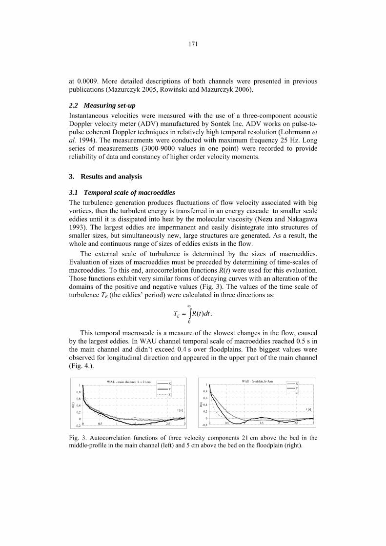
171

at 0.0009. More detailed descriptions of both channels were presented in previous publications (Mazurczyk 2005, Rowiński and Mazurczyk 2006).

2.2 Measuring set-up Instantaneous velocities were measured with the use of a three-component acoustic Doppler velocity meter (ADV) manufactured by Sontek Inc. ADV works on pulse-to-pulse coherent Doppler techniques in relatively high temporal resolution (Lohrmann et al. 1994). The measurements were conducted with maximum frequency 25 Hz. Long series of measurements (3000-9000 values in one point) were recorded to provide reliability of data and constancy of higher order velocity moments.

3. Results and analysis

3.1 Temporal scale of macroeddies The turbulence generation produces fluctuations of flow velocity associated with big vortices, then the turbulent energy is transferred in an energy cascade to smaller scale eddies until it is dissipated into heat by the molecular viscosity (Nezu and Nakagawa 1993). The largest eddies are impermanent and easily disintegrate into structures of smaller sizes, but simultaneously new, large structures are generated. As a result, the whole and continuous range of sizes of eddies exists in the flow.

The external scale of turbulence is determined by the sizes of macroeddies. Evaluation of sizes of macroeddies must be preceded by determining of time-scales of macroeddies. To this end, autocorrelation functions R(t) were used for this evaluation. Those functions exhibit very similar forms of decaying curves with an alteration of the domains of the positive and negative values (Fig. 3). The values of the time scale of turbulence TE (the eddies’ period) were calculated in three directions as:

0

( ) .ET R t dt∞

= ∫

This temporal macroscale is a measure of the slowest changes in the flow, caused by the largest eddies. In WAU channel temporal scale of macroeddies reached 0.5 s in the main channel and didn’t exceed 0.4 s over floodplains. The biggest values were observed for longitudinal direction and appeared in the upper part of the main channel (Fig. 4.). Fig. 3. Autocorrelation functions of three velocity components 21 cm above the bed in the middle-profile in the main channel (left) and 5 cm above the bed on the floodplain (right).

WAU - main channel, h = 21 cm

-0,2

0

0,2

0,4

0,6

0,8

1

0 0,5 1 1,5 2 2,5 3

t [s]

R(t)

XYZ

WAU - floodplain, h=5cm

-0,2

0

0,2

0,4

0,6

0,8

1

0 0,5 1 1,5 2 2,5 3

t [s]

R(t)

XYZ

172

0 20 40 60 80 100 120 140 160 180 2000

10

20

0.05

0.1

0.15

0.2

0.25

0.3

0.35

0.4

0.45

z [cm]

y [cm]

[s ]

Fig. 4. Contour map of time scales of turbulence in streamwise direction [s] (WAU channel).

3.2 Spatial scales of macroeddies By means of the Taylor hypothesis of “frozen turbulent structures” one can obtain spatial longitudinal scale of eddies. In flows of low level of turbulence (with small turbulence intensities) the spatial scale Lx can be evaluated as follows:

,x ExL T u=

where u is the mean-time longitudinal velocity. Rods simulating trunks of trees cause creation of a wake behind them. Eddies in

wakes are much smaller. Additionally occurrence of rods causes that sizes of eddies on floodplains are much uniformly distributed at verticals than those in main channels (Figs. 5 and 6).

Fig. 5. Contour map of sizes of macroeddies [m] (WAU channel).

Fig. 6. Vertical distribution of sizes of macroeddies in WAU channel in main channel and on floodplain.

WAU - main channel

0

0,1

0,2

0,3

0,4

0,5

0,6

0,7

0,8

0,9

1

0 2 4 6 8 10 12 14size of macroeddies [cm]

z/H

WAU - floodplain

0

0,1

0,2

0,3

0,4

0,5

0,6

0,7

0,8

0,9

0 2 4 6 8 10 12

size of macroeddies [cm]

z/H

0 20 40 60 80 100 120 140 160 180 2000

10

200 0.015

0.03

0.045

0.06

0.075

0.09

0.105

0.12

0.135 [m]

173

In the channel in Braunschweig the sizes of macroeddies differ greatly for differ-ent density of trees (Fig. 7). In case of very dense vegetation the eddies on floodplain are generally smaller than 1 cm, whereas in case without trees their sizes reach 15 cm and are similar to those in the main channel. Fig. 7. Vertical distribution of sizes of macroeddies in BTU channel in main channel and on floodplain with and without trees.

Reduced sizes of macroeddies foster an increase of turbulent energy dissipation. Energy dissipation rate was calculated from energy spectra in Kolmogoroff inertial subrange by means of:

2 / 3

5/ 3( ) 0.48 ,2uS f f −⎛ ⎞= ⎜ ⎟π⎝ ⎠ε

where S(f) is the energy spectra, u the mean-time longitudinal velocity; ε the energy dissipation ratio, and f the frequency.

Dissipation ratios calculated for measuring points on floodplains in WAU channel were several times higher than those in main channel, what confirms the argument of Grinvald and Nikora (1988) that vegetation influences greatly the dissipation ratio rather than energy production.

Nepf (1999) proposed the following relation between macroeddies and stems’ di-ameter:

1.5xL d ≈

where d is the stem diameter. This relation is roughly fulfilled in BTU channel, where mean sizes of macroeddies were 1 cm for maximum trees’ density and 1.5 cm for half of trees with stem diameter equal 1 cm. But in WAU channel the calculated sizes of macroeddies exceeded stem diameter several times.

3.3 Spatial scales of microeddies Taylor proposed spatial scale of microeddies λT:

in the main channel

0,0

0,1

0,2

0,3

0,4

0,5

0,6

0,7

0 10 20 30

size of macroeddies [cm]

z/H

on floodplain with all trees

0,0

0,1

0,2

0,3

0,4

0,5

0,6

0 0,5 1 1,5

size of macroeddies [cm]

z/H

on floodplain without trees

0,0

0,1

0,2

0,3

0,4

0,5

0,6

0 5 10 15 20

size of macroeddies [cm]

z/H

174

215

Tu′

≡νλε

where v is the kinematic viscosity, u′ the fluctuating component of longitudinal veloc-ity, and ε [cm2/s3] is the energy dissipation rate. Taylor’s microscale depends both on macroscopic motion by means of fluctuating velocity and on dissipative characteris-tics.

Kolmogoroff proposed a scale of microeddies η depending only on dissipative and viscous characteristics:

( )1/ 43 .≡η ν ε

Nezu and Nakagawa (1993) suggested that macroeddies to microeddies ratios are functions of Reynolds number ReL defined as:

2

xL

u LRe′

=ν

and the relations are:

0.750.91 ,xL

L Re≈η

0.50.21 .xL

L Re≈λ

These relations determine that inertial range, which can be indicated by „−5/3” Kolmogoroff’s law and in which large eddies transfer turbulent energy to small ed-dies, widen with increasing Reynolds number ReL. Relation Lx/η from Reynolds num-ber in WAU channel is close to those proposed by Nezu and Nakagawa (1993) for measuring points in the main channel, whereas over floodplains a coefficient

0.5( )x LL a Re≈η should be smaller (Fig. 8a).

Relation with Taylor’s microeddies xL η over floodplains differs strongly from that proposed by Nezu and Nakagawa (Fig. 8b). (a) (b) Fig. 8. Relation between sizes of macroeddies to (a) Kolmogoroff microeddies and (b) Taylor microeddies ratio from Reynolds number in WAU channel.

WAU channel

a=0,2679R2 = 0,7349

a = 0,4425R2 = 0,8143

0

2

4

6

8

10

12

14

16

30 35 40 45 50 55 60

Re0,5

L x/λ

on floodplain

main channel

WAU channel

a= 0,918R2 = 0,895

a = 0,752R2 = 0,9393

0

50

100

150

200

250

300

350

400

450

0 50 100 150 200 250 300 350 400

Re0,75

L x/η

on floodplain

main channel

175

4. Conclusions

Introducing rigid, emergent vegetation causes generation of wakes behind each stem. Sizes of macroeddies In wakes are strongly reduced and much more uniformly distrib-uted at verticals than those in main channels. Smaller sizes of eddies foster an increase of energy dissipation.

The connection between sizes of macroeddies on floodplains and stem’s diameter – proposed by Nepf (1999) – does not have a universal character. Even for similar stems diameter and density (the case of WAU channel and BTU channel with half of stems) the results were completely different. It suggests that the sizes of eddies are controlled not only by stem’s diameter but also by other hydraulic conditions, for ex-ample mean velocities, which differed much in both cases.

Both relations proposed by Nezu and Nakagawa (1993) quite well describe the sizes of eddies in main channel, even in the presence of trees on the floodplains. This suggests that introducing vegetation in some parts of flow does not influence consid-erably the structure of eddies in the main flow free of vegetation. Whereas for flow through vegetation other relations are needed. Such relations should be proposed bas-ing on great number of measuring data from channels of different geometries and dif-ferent densities of vegetation.

Acknowledgments . This study was supported by the Polish Ministry of Edu-cation and Science - grant no 2 P04E 006 30.

References

Baptist, M., 2005, Modelling floodplain biogeomorphology, Delft University Press, 195 p.

Ghisalberti, M., and H.M. Nepf, 2002, Mixing layers and coherent structures in vege-tated aquatic flows, Journal of Geophysical Research, 107 (C2), 3-1-3-11.

Grinvald, D.I., and V.I. Nikora, 1988, River turbulence (in Russian). Hydrometeoiz-dat, Leningrad, Russia.

Lohrmann, A., R. Cabrera and N. Kraus, 1994, Acoustic-Doppler Velocimeter (ADV) for Laboratory Use, Fundamentals and Advacements in Hydraulic Measurements and Experimentation; Proc., Buffalo, New York: 351-365.

Mazurczyk, A, 2005, Flow turbulence characteristics in a vegetated channel, 25th International School of Hydraulics, Hydraulic problems in Environmental Engi-neering (ed. W. Majewski), 147-155.

Nepf, H.M., 1999, Drag, turbulence and diffusion in flow through emergent vegeta-tion, Water Resources Research, 35 (2), 479-489.

Nezu, I., and H. Nakagawa, 1993, Turbulence in open-channel flows, Rotterdam, Balkema.

Rowiński, P.M., and A. Mazurczyk, 2006, Turbulent characteristics of flows through emergent vegetation. In: Ferreira R.M.L., Alves E.C.T.L., Leal J.G.A.B I Cardoso

176

A.H., River Flow 2006. Proceedings of the International Conference of Fluvial Hy-draulics, Lisbon, Portugal, pp. 623-630.

Velasco, D., A. Bateman, J.M. Redondo and V. Demedina, 2003, An open channel flow experimental and theoretical study of resistance and turbulent characterization over flexible vegetated linings, Flow, Turbulence and Combustion, 70, 69-88.

PUBLS. INST. GEOPHYS. POL. ACAD. SC., E-7 (401), 2007

Laboratory Experiments and the Development of Wave-Driven Sand Transport Models

Tom O’DONOGHUE1 and Jan S. RIBBERINK2 1 School of Engineering, University of Aberdeen, King’s College

Aberdeen AB24 3UE, Scotland e-mail: t.odonoghue@abdn.ac.uk

2 University of Twente, Faculty of Engineering, Water Engineering and Management PO Box 217, 7500 AE Enschede, The Netherlands

e-mail: j.s.ribberink@utwente.nl

Abstract

The paper presents an overview of results from large-scale laboratory ex-periments on sand transport processes under sea waves. The experiments, espe-cially those carried out in recent years in the Aberdeen Oscillatory Flow Tunnel at Aberdeen University and the Large Oscillating Water Tunnel at Delft Hydrau-lics, provide insights into the underlying processes for both the ripple and sheet flow regimes. Insights and data from the experiments are used to inform the de-velopment of predictive models. The paper includes an account of recent model-ing developments, especially of semi-unsteady models used for practical applica-tions.

Key words: laboratory experiments, sediment transport, waves, oscillatory flow, ripples, sheet flow.

1. Introduction

Sand transport under sea waves is determined by processes occurring close to the sea-bed, often within the bottom few centimetres where vertical gradients of flow velocity and sand concentration are high. The processes are complex and for this reason the development of predictive models relies on laboratory experiments in which detailed measurements can be made under well controlled flow and sand conditions. The most useful laboratory results have come from large experimental facilities in which the flow and sand conditions are the same as full-scale, i.e. flows in the facilities have a typical period range of 4 to 12 s and sands used in the experiments have a typical size range of 0.1 to 0.5 mm. The combined experimental results cover a wide range of flow and sand conditions and, in addition to measurements of net sand transport rates for given wave and sand conditions, include measurements of detailed processes that can-

178

not yet be measured in the field. In this paper we present an overview of important results from these experiments, covering the ripple and sheet flow transport regimes, and we describe key processes which need to be accounted for in predictive models. An account is given of modeling approaches, especially recent development of semi-unsteady models used for practical applications, where the development is based on insights and data from the large-scale laboratory experiments.

2. Large-scale laboratory experiments

Full-scale laboratory studies of wave-driven sand transport are carried out in large wave flumes and oscillatory flow tunnels. In wave flumes, free-surface waves with periods in the range 4 to 15 s and heights up to 2.5 m are generated in a long flume, traveling over a sand bed as they propagate from the wave paddle to a dissipating beach at the flume end. Examples of such flumes include the 230 m long Delta Flume of Delft Hydraulics in The Netherlands and the 300 m long GWK of the University of Hannover and the Technical University of Braunschweig in Germany. In flow tunnels, oscillatory flow is generated over a sand bed by piston motion within an enclosed tunnel. For the larger tunnels, the range of flow periods is typically 3 to 15 s and the amplitude of water motion within the tunnel test section can reach approximately 2 m. Oscillatory flow in the test section corresponds therefore to near-bed flow generated by large, non-breaking full-scale waves in a range of shoaling water depths. Examples of large tunnels include the Aberdeen Oscillatory Flow Tunnel (AOFT, Fig. 1) at Ab-erdeen University (O’Donoghue and Clubb 2001) and the Large Oscillating Water Tunnel (LOWT) at Delft Hydraulics in the Netherlands (Ribberink and Al-Salem 1994).

Fig. 1. The Aberdeen Oscillatory Flow Tunnel (AOFT). The tunnel is 16 m long with a glass-sided test-section that is 10 m long, 0.3 m wide and 0.75 m high.

Schretlen and van der Werf (2006) compiled a database of results from large-scale laboratory experiments on sand transport processes. The database contains results from approximately 750 experiments, the majority conducted in the LOWT, AOFT and the Tokyo University water tunnel. The most detailed experiments, involving measurements of fundamental processes, have been carried out in the LOWT and AOFT. By far the majority of these experiments involved wave-only conditions with sinusoidal or velocity-skewed oscillatory flows. The latter are defined by

750500

2000

980

860

405

705

TO

POWERPACK

940

870

45005500101011207501125

PISTONHYDRAULIC CYLINDER CHANGE OF SECTION

179

1 2( ) sin cos2u t u t u t= ω − ω (1)

where: 2 Tω= π , T being flow period. The degree of skewness, R, is

max1 2

1 max min2uu uR

u u u+

= =−

(2)

where: umax, umin = maximum positive, negative velocity (Fig. 2).

0 0.2 0.4 0.6 0.8 1−1

−0.5

0

0.5

1

t/T

u/u m

ax

Fig. 2. Velocity-skewed flow used in many oscillatory flow tunnel experiments (R = 0.63 in example shown). Note higher ‘onshore’, positive velocity and longer-duration ‘offshore’, negative velocity.

3. Experimental results

3.1 Sand transport regime For a given sand size and flow period, vortex ripples form as the amplitude of wave-induced flow velocity increases beyond the threshold velocity for sediment motion. As the flow amplitude increases, ripples increase in size, reach a maximum and then de-crease in size at higher velocities. For sufficiently high velocity, the ripples are washed out completely and sand transport takes place within a thin, high concentration layer of sand over an essentially flat bed. This is the so-called sheet flow condition. Because the sand transport processes are very different between the ripple and sheet flow regimes, it is important to be able to predict which regime will occur for given wave and sand conditions.

O’Donoghue et al. (2006) looked at reported bed type from a wide range of large-scale laboratory tunnel and wave flume experiments. Classifying the beds as 3-d rip-pled, 2-d rippled, bimodal or flat (3D, 2D, BM or FB, Fig. 3), they found that bed type is reasonably well characterised by mobility number based on the high velocities in the flow, i.e. by

2max

max50( 1)

us gD

=−

ψ (3)

for regular flows, and by

21 10

1 1050( 1)

us gD

=−

ψ (4)

180

101

102

103

3D

2D

BM

FB

ψmax

or ψ1/10

Bed

type

Fig. 3. Bed type as function of mobility number for a large number of full-scale flow tunnel and wave flume laboratory experiments (O’Donoghue et al. 2006). Different symbols refer to different types of flows.

for irregular flows, where: 101u = mean of highest one tenth velocities in the irregular velocity time-series; s = sediment specific gravity (2.65 for sand); g = acceleration due to gravity; D50 is the sediment size for which 50% of the sediment sample is finer. Ripple regime occurs for 190, 10/1max ≤ψψ and sheet-flow for 300, 10/1max ≥ψψ . In the transition regime, 300,190 10/1max << ψψ , it seems that the bed type is sensitive to the detailed experimental conditions and a variety of bedforms have been observed to occur. Within the ripple regime, ripples may be 2-d or 3-d and it is clear that mobility number does not determine which type occurs. Sand size is the primary factor deter-mining whether ripples will be 3-d or 2-d in full-scale oscillatory flows, with 3-d rip-ples occurring when the sand is fine (<~0.2 mm) and 2-d ripples occurring when the sand is relatively coarse (>~0.3 mm).

3.2 Ripple dimensions The dimensions of ripples play a crucial role in determining net sand transport in the ripple regime. Indeed, ripple height is often an explicit parameter in wave-driven sand transport models. A substantial body of field- and laboratory-based research has been devoted to measuring ripples and developing predictive formulae for ripple dimen-sions. Commonly-used formulae include those of Mogridge et al. (1994), Nielsen (1981) and Wiberg and Harris (1994). O’Donoghue et al. (2006) tested these formulae against a large set of full-scale tunnel and wave flume laboratory data. By focusing on full-scale laboratory experiments, they avoid the scale effects associated with small-scale experiments and the uncertainties associated with bed history effects and meas-urement difficulties in the field. Ripple dimensions predicted using Wiberg and Harris (1994) were found to be in poor agreement with the data; predictions based on Mogridge et al. (1994) and Nielsen (1981) are in better agreement, especially for rip-ple length, but both methods over-estimate the dimensions of 3-d ripples and Nielsen under-stimates ripple dimensions at high mobility and in irregular flows.

181

O’Donoghue et al. (2006) proposed modifications to the Nielsen equations, based on the extensive dataset of large-scale experimental data. For ripple height, η:

0.42

2 3 2

0.275 0.022 and 0.55D D Da a a= − =

η η ηψ (5)

where for regular flow: 2od

a = , max ;=ψ ψ for irregular flow: π2rmspuT

a = , 10/1ψψ = ;

od = flow orbital diameter for regular flow; pT = spectral peak period; rmsu = rms ve-locity. For ripple length, λ:

0.21

2 3 2

1.97 0.44 and 0.73D D Da a a= − =

λ λ λψ (6)

The equations apply for 190,10 10/1max ≤≤ ψψ . Figure 4 shows the comparison be-tween the measured ripple dimensions and calculated dimensions using Nielsen and using equations (5) and (6).

0 0.05 0.1 0.15 0.20

0.05

0.1

0.15

0.2

ηm

(m)

η p (m

)

Nielsen

Ripple height

0 0.5 10

0.2

0.4

0.6

0.8

1

1.2

λm

(m)

λ p (

m)

Nielsen

Ripple length

0 0.05 0.1 0.15 0.20

0.05

0.1

0.15

0.2

ηm

(m)

η p (m

)

New formula

0 0.5 10

0.2

0.4

0.6

0.8

1

1.2

λm

(m)

λ p (

m)

New formula

Fig. 4. Predicted versus measured ripple dimensions for a wide range of full-scale laboratory conditions. Top panels: predictions based on Nielsen (1983). Bottom panels: predictions based on modified Nielsen equations as proposed by O’Donoghue et al. (2006). Different symbols correspond to different flow type (regular, irregular) and ripple type (2-d, 3-d).

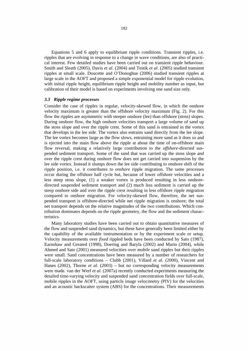
182

Equations 5 and 6 apply to equilibrium ripple conditions. Transient ripples, i.e. ripples that are evolving in response to a change in wave conditions, are also of practi-cal interest. Few detailed studies have been carried out on transient ripple behaviour. Smith and Sleath (2005), Davis et al. (2004) and Testik et al. (2005) studied transient ripples at small scale. Doucette and O’Donoghue (2006) studied transient ripples at large scale in the AOFT and proposed a simple exponential model for ripple evolution, with initial ripple height, equilibrium ripple height and mobility number as input, but calibration of their model is based on experiments involving one sand size only.

3.3 Ripple regime processes Consider the case of ripples in regular, velocity-skewed flow, in which the onshore velocity maximum is greater than the offshore velocity maximum (Fig. 2). For this flow the ripples are asymmetric with steeper onshore (lee) than offshore (stoss) slopes. During onshore flow, the high onshore velocities transport a large volume of sand up the stoss slope and over the ripple crest. Some of this sand is entrained in the vortex that develops in the lee side. The vortex also entrains sand directly from the lee slope. The lee vortex becomes large as the flow slows, entraining more sand as it does so and is ejected into the main flow above the ripple at about the time of on-offshore main flow reversal, making a relatively large contribution to the offshore-directed sus-pended sediment transport. Some of the sand that was carried up the stoss slope and over the ripple crest during onshore flow does not get carried into suspension by the lee side vortex. Instead it slumps down the lee side contributing to onshore shift of the ripple position, i.e. it contributes to onshore ripple migration. The same processes occur during the offshore half cycle but, because of lower offshore velocities and a less steep stoss slope, (1) a weaker vortex is produced resulting in less onshore-directed suspended sediment transport and (2) much less sediment is carried up the steep onshore side and over the ripple crest resulting in less offshore ripple migration compared to onshore migration. For velocity-skewed flow, therefore, the net sus-pended transport is offshore-directed while net ripple migration is onshore; the total net transport depends on the relative magnitudes of the two contributions. Which con-tribution dominates depends on the ripple geometry, the flow and the sediment charac-teristics.

Many laboratory studies have been carried out to obtain quantitative measures of the flow and suspended sand dynamics, but these have generally been limited either by the capability of the available instrumentation or by the experiment scale or setup. Velocity measurements over fixed rippled beds have been conducted by Sato (1987), Earnshaw and Greated (1998), Doering and Baryla (2002) and Marin (2004), while Ahmed and Sato (2001) measured velocities over mobile sand ripples but their ripples were small. Sand concentrations have been measured by a number of researchers for full-scale laboratory conditions – Clubb (2001), Villard et al. (2000), Vincent and Hanes (2002), Thorne et al. (2003) – but no corresponding velocity measurements were made. van der Werf et al. (2007a) recently conducted experiments measuring the detailed time-varying velocity and suspended sand concentration fields over full-scale, mobile ripples in the AOFT, using particle image velocimetry (PIV) for the velocities and an acoustic backscatter system (ABS) for the concentrations. Their measurements

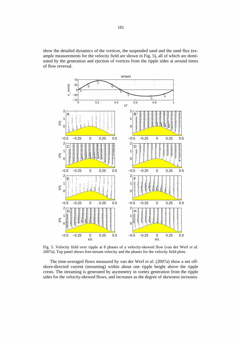
183

show the detailed dynamics of the vortices, the suspended sand and the sand flux (ex-ample measurements for the velocity field are shown in Fig. 5), all of which are domi-nated by the generation and ejection of vortices from the ripple sides at around times of flow reversal.

0 0.2 0.4 0.6 0.8 1−70

−35

0

35

70

A

BC

D

E

FG

Hu ∞ (

cm/s

)

t/T

Mr5b63

−0.5 −0.25 0 0.25 0.5

0

1

2

z/η

A

−0.5 −0.25 0 0.25 0.5

0

1

2B

−0.5 −0.25 0 0.25 0.5

0

1

2

z/η

C

−0.5 −0.25 0 0.25 0.5

0

1

2D

−0.5 −0.25 0 0.25 0.5

0

1

2

z/η

E

−0.5 −0.25 0 0.25 0.5

0

1

2F

−0.5 −0.25 0 0.25 0.5

0

1

2

x/λ

z/η

G

−0.5 −0.25 0 0.25 0.5

0

1

2

x/λ

H

Fig. 5. Velocity field over ripple at 8 phases of a velocity-skewed flow (van der Werf et al. 2007a). Top panel shows free-stream velocity and the phases for the velocity field plots.

The time-averaged flows measured by van der Werf et al. (2007a) show a net off-shore-directed current (streaming) within about one ripple height above the ripple crests. The streaming is generated by asymmetry in vortex generation from the ripple sides for the velocity-skewed flows, and increases as the degree of skewness increases.

184

The magnitude of the streaming is low (less than 10% of maximum free-stream veloc-ity for flows with high skewness) but is important because it contributes a “current-related” flux to the net transport: for the van der Werf et al. experiment, the current-related flux contributes ~30% to the total suspended net transport.

Ribberink et al. (submitted) argue that the relative dominance of offshore-directed suspended transport and onshore-directed bedload transport (ripple migration) for velocity-skewed flow depends on a ripple regime “phase lag parameter”, pr, given by

rs

pw

=ηω (7)

where: ws = sand fall velocity. The greater the value of pr (higher ripples/finer sand/shorter flow period), the stronger the phase lag effect and, for velocity-skewed flow, the greater the tendency towards suspension-dominated, offshore-directed net sand transport. Based on results from experiments conducted in the AOFT and LOWT, they show that net transport is bedload-dominated, onshore-directed when pr ≥ 0.8 and suspension-dominated, offshore-directed for pr < 0.8.

0 2 4 6−2

0

2MA7515

u (m

/s)

0 2 4 61000

1500

2000

c (g

/l)

−4.05 to −2.85mm

0 2 4 6900

1400

1900

c (g

/l)

−2.65 to −1.65mm

0 2 4 6600

1100

1600

c (g

/l)

−1.45 to −0.45mm

0 2 4 60

500

1000

c (g

/l)

−0.25 to 0.75mm

t (s)0 2 4 6

0

500

1000

c (g

/l)

0.95 to 1.95mm

t (s)

Fig. 6. CCM-measured time-series of sheet flow concentration at z = −4 mm to z = 2 mm for 0.27 mm sand in velocity-skewed flow (top left) (O’Donoghue and Wright, (2004a).

3.4 Sheet flow processes Sheet flow conditions prevail when the wave-generated bed shear stress is high and the sand transport takes place within a “sheet flow layer” consisting of a water-sediment mix moving over a flat, ripple-free bed. Detailed measurements of velocities and concentrations within the sheet flow layer provide insights and data for the devel-

185

opment of models. The most detailed measurements have come from experiments carried out in recent years in the AOFT and LOWT, involving measurements of sheet flow concentrations and, to a lesser degree, sheet flow velocities. Figure 6 shows ex-ample sheet flow concentration measurements made by O’Donoghue and Wright (2004a) in the AOFT using concentration conductivity probes (CCMs) for a 0.27 mm sand in a velocity-skewed flow with T = 7 s and umax = 1.5 m/s. Time-series of concen-tration are shown for z positions ranging 24 ≤≤− z mm, where z = 0 corresponds to the no-flow bed level.

Two regions can be identified within the sheet flow layer: (1) the “inner” or “pick-up” layer where concentration decreases at times of high velocity as sand is picked up and increases at times of low velocity as sand settles back to the bed; (2) the upper sheet flow layer where concentration increases around times of high velocity as sand is carried up from the pick-up layer. At some z between the pick-up layer and the up-per sheet flow layer (between −1 and +1 mm for the O’Donoghue and Wright experi-ments) the concentration stays reasonably constant with time.

0 0.5 1 1.5−5

0

5

c/Cb

z (m

m)

FINE

0 0.5 1 1.5−5

0

5

c/Cb

z (m

m)

MEDIUM

0 0.5 1 1.5−5

0

5

c/Cb

z (m

m)

COARSE

0 0.5 1 1.5−5

0

5

c/Cb

z (m

m)

MIX 1

Fig. 7. Example CCM-measured concentration profiles for 4 sands at time of maximum onshore (positive) velocity of a velocity-skewed flow (O’Donoghue & Wright, 2004a). Circles are data, solid line is fit of equation (8) to the data. Cb is concentration in undisturbed bed.

Example instantaneous concentration profiles from O’Donoghue and Wright (2004a) are shown in Fig. 7. They found that the profile within the sheet flow layer is well characterised by

0

1

11 1 1e

cz

c

=⎧ ⎫ ⎛ ⎞

+ − +⎨ ⎬ ⎜ ⎟⎩ ⎭ ⎝ ⎠

α

δ

(8)

186

where: c = concentration normalised by the undisturbed bed concentration; 0c = normalized concentration at z = 0; eδ = instantaneous erosion depth; 1.5.≅α If all

of the mobilised sand is contained in the sheet flow layer (which is close to true for relatively coarse sand but not so for fine sand) then 0c in Eq. (8) is determined by the value of eδ because the integrated concentration profile must then equal the eroded volume of sediment. eδ itself depends on the flow and sand conditions. For relatively coarse sands, the erosion depth behaves in a near quasi-steady way, i.e. it is deter-mined by the instantaneous bed shear stress:

50

( ) ( )e t tD

=δ

φ θ (9)

where ( )tθ is the instantaneous Shields parameter:

50

( )( )( 1)

tts g D

=−τθρ

(10)

with: τ = bed shear stress; s = sand specific gravity (~2.65). However, for relatively fine sand with low settling velocity, sand that is entrained by high velocities is slow to settle back to the bed as the velocity decreases to zero and a proportion of the sand remains in suspension for transport in the opposite direction when the flow reverses. In such cases, δe depends on flow history as well as θ (t). This unsteady behaviour is seen in the case of fine sand in the example erosion depth and sheet flow layer thick-ness time-series shown in Fig. 8.

Dohmen-Janssen et al. (2001) argue that the degree of unsteadiness depends on the sand settling velocity, the flow period and the sheet flow layer thickness: they charac-terise the degree of unsteadiness by (2π times) the ratio of the time taken for a sand grain to settle through the sheet flow layer to the flow period, i.e.,

ss

s

pw

=δ ω (11)

where: δs is the thickness of the sheet flow layer defined as the distance from the (maximum) erosion depth to the elevation where the volumetric concentration is 8%. Unsteady effects become increasingly important for increasing ps (finer sand, shorter flow periods, thicker sheet flow layer). Ribberink et al. (submitted) show that for ps > 0.3 the degree of unsteadiness is such that for velocity-skewed flows the net sand transport direction is negative, i.e. opposite to the direction of the higher velocities.

Velocity measurements within the sheet flow layer are difficult because of the presence of high sand concentrations. O’Donoghue and Wright (2004b) used an ultra-sonic velocity profiler (UVP) to measure sheet flow velocities and report measure-ments reaching quite far into the sheet flow layer (as far as the z = 0 level). Combining their velocity and concentration measurements, they obtained measures of the vertical profiles of the time-varying sand flux. For coarse sand in velocity-skewed flow (Fig. 2), unsteady effects are negligible, the bed responds in a quasi-steady way, sand flux is

187

confined to a narrow layer close to z = 0 and the net sand transport is positive. In con-trast, for fine sand the bed behaves in an unsteady manner, the sand flux extends rela-tively high above the bed and net transport in the sheet flow layer is strongly negative in velocity-skewed flow.

Fig. 8. Example time-series of erosion depth δe and sheet flow layer thickness δs for fine (0.13 mm) and medium (0.27 mm) sands in two (T = 5 s and T = 7 s) velocity skewed flows (O’Donoghue and Wright 2004a). Broken thin line: velocity. Broken thick line: sheet flow layer thickness. Solid thin line: top of sheet flow layer. Thick solid line: erosion depth. Shaded area: the sheet flow layer.

As for flow over ripples, the time-averaged velocity profiles for velocity-skewed flows show an offshore-directed near-bed streaming with magnitude of order 10% of maximum free-stream velocity. For this flat-bed case the streaming is caused by the asymmetry in the turbulent stresses between the two half-cycles of the flow. As for rippled beds, associated with the streaming is a current-related net sand flux, but in the case of sheet flow the current-related flux can be greater than the wave-related flux (Ribberink et al., submitted). This means that differences between near-bed streaming in tunnels and near-bed streaming under real waves could be very significant. Indeed, Dohmen-Janssen and Hanes (2002) concluded, from a set of experiments conducted in the full-scale GWK wave flume in Hannover, that sheet flow net sand transport rates under real waves may be up to 2.5 times greater than the transport rates in “equiva-lent” tunnel oscillatory flow and they attribute the difference to differences in the near-bed streaming.

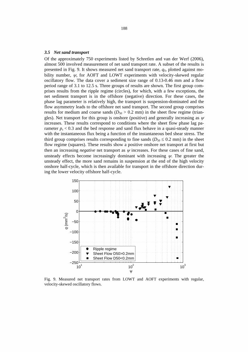
188

3.5 Net sand transport Of the approximately 750 experiments listed by Schretlen and van der Werf (2006), almost 500 involved measurement of net sand transport rate. A subset of the results is presented in Fig. 9. It shows measured net sand transport rate, qS, plotted against mo-bility number, ψ, for AOFT and LOWT experiments with velocity-skewed regular oscillatory flow. The data cover a sediment size range of 0.13-0.46 mm and a flow period range of 3.1 to 12.5 s. Three groups of results are shown. The first group com-prises results from the ripple regime (circles), for which, with a few exceptions, the net sediment transport is in the offshore (negative) direction. For these cases, the phase lag parameter is relatively high, the transport is suspension-dominated and the flow asymmetry leads to the offshore net sand transport. The second group comprises results for medium and coarse sands (D50 > 0.2 mm) in the sheet flow regime (trian-gles). Net transport for this group is onshore (positive) and generally increasing as ψ increases. These results correspond to conditions where the sheet flow phase lag pa-rameter ps < 0.3 and the bed response and sand flux behave in a quasi-steady manner with the instantaneous flux being a function of the instantaneous bed shear stress. The third group comprises results corresponding to fine sands (D50 ≤ 0.2 mm) in the sheet flow regime (squares). These results show a positive onshore net transport at first but then an increasing negative net transport as ψ increases. For these cases of fine sand, unsteady effects become increasingly dominant with increasing ψ. The greater the unsteady effect, the more sand remains in suspension at the end of the high velocity onshore half-cycle, which is then available for transport in the offshore direction dur-ing the lower velocity offshore half-cycle.

101

102

103

−250

−200

−150

−100

−50

0

50

100

150

ψ

q (

mm

2 /s)

Ripple regimeSheet Flow D50>0.2mmSheet Flow D50<0.2mm

Fig. 9. Measured net transport rates from LOWT and AOFT experiments with regular, velocity-skewed oscillatory flows.

189

4. Modelling wave-driven sand transport

Models for wave-driven sand transport range from relatively simple “practical” mod-els based on empirical formulae to “process” models which aim to explicitly model the detailed intra-wave processes. The full-scale laboratory data previously discussed are used to test and develop both types of model.

4.1 Process Models Process models vary widely in their degree of complexity. For sheet flow, process models range from 1DV advection-diffusion boundary layer models (e.g. Ribberink and Al-Salem 1995, Davies and Li 1997, Dohmen-Janssen et al. 2001), which solve the momentum equation for the flow and the diffusion equation for the suspended sediment concentration, to more complex two-phase models which model the full diffusive and collisional processes within the sheet flow layer (e.g. Dong and Zhang 1999, Hsu et al. 2004, Liu and Sato 2006). The advection-diffusion models use an empirical reference concentration formula near the bed and do not model the sheet flow layer. A practical compromise between the advection-diffusion and the two-phase models is to couple a simple model of the essential sheet flow processes with an advection-diffusion model higher up (e.g. Kaczmarek and Ostrowski 2002, Malarkey et al. 2003).

For the ripple regime, a 2DV modeling approach is needed to properly capture the vortex shedding process. Ripple regime process models include RANS models with various turbulence closure schemes (e.g. Eidsvik 2006) and discrete vortex models (e.g. Malarkey and Davies 2002). Since 2DV models are too complex for practical application, Davies and Thorne (2005) proposed a simple 1DV two-layer model, in which vortex shedding in the lower layer is represented by a time-varying eddy vis-cosity, and a standard turbulence-closure formulation is used for the upper layer. As for the sheet flow RANS models, the ripple models require an empirical reference concentration or sand pickup function.

4.2 Practical Models Formula-based models are used for practical applications of sand transport calcula-tions in the coastal zone. There are two main classes of model: (1) quasi-steady mod-els in which the instantaneous transport rate is directly related to some power of the instantaneous bed shear stress or near bed flow velocity (e.g. Bailard 1981, van Rijn 1993, Ribberink 1998), and (2) semi-unsteady models which account for unsteady (phase lag) effects of the kind described above without modeling the detailed time-dependent horizontal velocity and concentration vertical profiles (e.g. Dibajnia and Watanabe 1996, Dohmen-Janssen et al. 2002, Camenen and Larson 2006, da Silva et al. 2006, van der Werf et al. 2007b).

Considering the quasi-steady model of form

( )( ) ( )( )

n tt m tt

=θφ θθ

(13)

190

where 3

( )( )( 1)

sq tts gD

= =−

φ non-dimensional transport rate, it can be shown that the

net transport for a velocity-skewed oscillatory flow (equation 1) is

221 (2 1)

nN n urms

m

R=⎡ ⎤+ −⎣ ⎦

αφ θ (14)

where 3

0

( )1 ;( 1)

Ts

Nq t dt

T s gD=

−∫φ

2

2

0.5 ( 2 ) ;( 1)

w rmsurms

f us gD

=−

θ α depends on n and the

degree of skewness R. For m = 11, n = 1.65 (as per Ribberink 1998) and skewness R = 0.63, 65.1

212.2 urmsN θφ = . Quasi-steady models always predict a net onshore (posi-tive) transport for velocity-skewed flow, increasing with increasing Shields parameter. Predictions agree reasonably well with measured transport rates for relatively coarse sand in sheet flow conditions (low ps), but, because of unsteady phase lag effects, pre-dictions are poor for ripple regime and sheet flow regime with relatively fine sand.

A number of semi-unsteady models have been proposed in recent years in an at-tempt to account for unsteady effects. Dohmen-Janssen et al. (2002) applied a phase lag correction factor (based on the lag parameter given by equation 11) to the quasi-steady model of Ribberink (1998). A number of other models are based on the “half-cycle approach” proposed by Dibajnia and Watanabe (1992, 1996, 1998). In this ap-proach the quantity of sand transported in the onshore direction comprises (1) sand that is entrained and transported during the onshore half-cycle (Ωc, “c” for crest) and (2) sand that was entrained during the preceding offshore half-cycle but did not settle back to the bed by the end of the offshore half-cycle ( tΩ′ , “t” for trough). Similarly, sand transported in the offshore direction comprises Ωt and cΩ′ . The concept has been applied for sheet flow conditions by Dibajnia and Watanabe (1996), Camenen and Larson (2006) and da Silva et al. (2006), and for ripple regime by van der Werf et al. (2006). A unified model, i.e. covering both ripple and sheet flow regimes, waves and waves plus currents, has recently been proposed by van der Werf et al. (2007b), based on the dataset of large-scale laboratory data compiled by Schretlen and van der Werf (2006).

In van der Werf et al. (2007b), the net sand transport is

( ) ( )c tN c t t c

mT mTT T

′ ′= Ω +Ω − Ω +Ωφ (15)

where: T = wave period; Tc = wave crest duration (duration of onshore, positive veloc-ity); Tt = wave trough duration (duration of offshore, negative velocity); m = calibra-tion factor. The first term on the right hand side of Eq. (15) is the onshore transport with two contributions ( )c t′Ω +Ω and the second term is the offshore transport with two contributions ( )t c′Ω +Ω . The magnitudes of the contributions within each half-cycle depend on the excess shear stress ( )cr−θ θ and the value of the phase lag pa-

191

rameter p for the half-cycle, where for rippled bed r ri s

p pT w

= =ηα (Eq. 7) and for

sheet flow si

sss wT

ppδ

α== (Eq. 11), where i = c or t for crest or trough respectively

and αr, αs are calibration factors. Sub-models for bed shear stress, ripple size, sheet flow layer thickness are based on results from the large-scale experiments as described earlier in this paper.

Figure 10 shows predicted-versus-measured net sand transport rates using the van der Werf et al. (2007b) model. The model does better in the sheet flow regime than in the ripple regime. In sheet flow, predicted transport rates are generally within a factor two of measured transport rates and the model captures unsteady effects quite well, as evidenced by the reasonable agreement between the measured and predicted negative net transport rates. Agreement is not as good in the ripple regime: some very high measured negative transport rates are underpredicted and a number of cases of meas-ured onshore transport are predicted as being offshore, although the transport magni-tudes in the latter cases are mostly small. Good agreement in the ripple regime is more difficult to achieve because of limited predictability of ripple height (the model gives better agreement if measured ripple heights are used rather than predicted ripple heights) and because sand transport rates are often very low in the ripple regime.

−250 −200 −150 −100 −50 0 50 100 150 200

−200

−100

0

100

200

Sheet flow

Meas qs (10−6 m2/s)

Pre

d q s (

10−

6 m2 /s

)

−40 −30 −20 −10 0 10−40

−30

−20

−10

0

10Ripple regime

Meas qs (10−6 m2/s)

Pre

d q s (

10−

6 m2 /s

)

Fig. 10. Predicted-versus-measured net sand transport rates using van der Werf (2007b). Solid line is line of perfect agreement; dashed lines are factor two of measured.

192

5. Conclusions

Large-scale laboratory experiments have produced valuable data and insights used to develop process and practical models for sand transport under waves. The majority of the experiments have been conducted in oscillatory flow tunnels and mostly with ve-locity-skewed flows. For this reason knowledge of some fundamental questions is still somewhat lacking. Two questions in particular need further study. (1) The first con-cerns the difference between oscillatory flow in a tunnel and near-bed flow under real waves. Phase differences in wave orbital motion, vertical orbital motions, wave-induced boundary layer streaming (Longuet-Higgins 1953) and undertow at higher levels above the bed are not reproduced in flow tunnels. Of these, the wave-induced streaming is likely to be of most significance because although the magnitude of streaming is small compared to the orbital velocities, the streaming-related sand flux can be high, especially for sheet flow. (2) The second question concerns the effects of flow acceleration. Non-zero net transport rates have been measured in experiments with acceleration-skewed flow (sawtooth-type velocity time-series), with higher trans-port in the direction of higher flow acceleration (e.g. Watanabe and Sato 2004) caused by enhanced bed shear stress (Nielsen 2002). Models in which the bed shear stress is a function of free-stream velocity cannot account for the acceleration effect. More de-tailed large-scale experimental data are needed to improve understanding of accelera-tion effects and to test recent suggestions (e.g. da Silva et al. 2006, Rodriguez and Madsen 2007) for incorporating acceleration effects in practical models. Both these issues − real wave and acceleration effects − are being studied as part of a current UK-Dutch collaborative research project (SANTOSS).

Acknowledgment . Most of the work reported in this overview paper was con-

ducted in recent years by researchers Graeme Clubb, Scott Wright and Jeff Doucette at Aberdeen University and Marjolein Dohmen-Janssen, Wael Hassan and Jebbe van der Werf at the University of Twente. Our on-going research on wave-driven sand trans-port is being carried out within the ‘SANTOSS’ project, funded by EPSRC in the UK (GR/T28089/01) and by STW in The Netherlands (TCB 1586).

References

Ahmed, A.S.M., and S. Sato, 2001, Investigation of bottom boundary layer dynamics of movable bed by using enhanced PIV technique, Coastal Engineering Journal 43 (4), 239-258.

Bailard, J.A., 1981, An energetics total load sediment transport model for a plane slop-ing beach, J. Geoph. Research 86, C11, 10938-10954.

Camenen, B., and M. Larson, 2006, Phase-lag effects in sheet flow transport, Coastal Engineering 53, 531-542.

Clubb, G.S., 2001, Experimental study of vortex ripples in full-scale sinusoidal and asymmetric flows, PhD thesis, University of Aberdeen, Scotland.

193

Da Silva, P.A., A. Temperville and F.S. Santos, 2006, Sand transport under combined wave and current conditions: A semi-unsteady, practical model, Coastal Engineer-ing 53, 897-913.

Davies, A.G., and P.D. Thorne, 2005, Modeling and measurement of sediment trans-port by waves in the vortex ripple regime, J. Geophysical Research 110, C5, Art. No. C05017.

Davies, A.G., and Z. Li, 1997, Modeling sediment transport beneath regular symmet-rical and asymmetrical waves above a plane bed, Cont. Shelf Research 17 (5), 555-582.

Davis, J.P., D.J. Walker, M. Townsend and I.R. Young, 2004, Wave-formed sediment ripples: Transient analysis of ripple spectral development, J. Geophysical Research 109, C07020, doi:10.1029/2004JC002307.

Dibajnia, M., and A. Watanabe, 1992, Sheet flow under non-linear waves and cur-rents, Proc. of 23rd Int. Conf. on Coast. Eng., ASCE, Venice, Italy, 2015-2028.

Dibajnia, M., and A. Watanabe, 1996, A transport rate formula for mixed sands, Proc. 25th ICCE, Orlando, ASCE, Vol 3, 3791-3804.

Dibajnia, M., and A. Watanabe, 1998, Transport rate under irregular sheet flow condi-tions, Coastal Engineering 35, 167-183.

Doering, J.C., and A.J. Baryla, 2002, An investigation of the velocity field under regu-lar and irregular waves over a sand beach, Coastal Engineering 44, 275-300.

Dohman-Janssen, C.M., and D.M. Hanes, 2002, Sheet flow dynamics under mono-chromatic non-breaking waves, J. of Geophysical Research 107 (C10), 3149, doi:10.1029/2001/JC001045.

Dohmen-Janssen, C.M., W.N. Hassan and J.S. Ribberink, 2001, Mobile-bed effects in oscillatory sheet flow, J. of Geophysical Research 106 (C11), 27103-27115.

Dohmen-Janssen, C.M., D.F. Kroekenstoel, W.N.M. Hassan and J.S. Ribberink, 2002, Phase lags in oscillatory sheet flow: experiments and bed load modeling, Coastal Engineering 46, 61-87.

Dong, P., and K. Zhang, 1999, Two-phase modeling of sediment motions in oscilla-tory sheet flow, Coastal Engineering 36, 87-109.

Doucette, J.S., and T. O’Donoghue, 2006, Response of sand ripples to change in oscil-latory flow, Sedimentology 53, 581-596.

Earnshaw, H.C., and C.A. Greated, 1998, Dynamics of ripple bed vortices, Experi-ments in Fluids 25, 265-275.

Eidsvik, K.J., 2006, Large scale modelling of oscillatory flows over a rippled bottom, Cont. Shelf Res. 26, 318-337.

Hsu, T.J., J.T. Jenkins and P.L.-F Liu, 2004, On two-phase sediment transport: sheet flow of massive particles, Proc. Royal Soc. London Series A 460 (2048), 2223-2250.

Kaczmarek, L.M., and R. Ostrowski, 2002, Modelling intensive near-bed sand trans-port under wave-current flow versus laboratory and field data, Coastal Engineering 45 (1), 1-18.

194

Liu, H., and S. Sato, 2006, A two-phase flow model for asymmetric sheetflow condi-tions, Coastal Engineering 53, 825-843.

Longuet-Higgins, M.S., 1953, Mass transport in water waves, Philos. Trans. Royal Soc. .London Series A 245 (903), 535-581.

Malarkey, J., A.G. Davies, and Z. Li, 2003, A simple model of unsteady sheet flow sediment transport, Coastal Engineering 48, 171-188.

Malarkey, J., and A.G. Davies, 2002, Discrete vortex modeling of oscillatory flows over ripples, Applied Ocean Research 24, 127-145.

Marin, F., 2004, Eddy viscosity and Eulerian drift over rippled beds in waves, Coastal Engineering 50, 139-159.

Mogridge, G.R., M.H. Davies and D.H. Willis, 1994, Geometry prediction for wave-generated bedforms, Coastal Engineering 22, 255-286.

Nielsen, P., 1981, Dynamics and geometry of wave-generated ripples, J. Geophysical Research 86 (C7), 6467-6472.

Nielsen, P., 2002, Shear stress and sediment transport calculations for swash zone modelling, Coastal Engineering 45, 53-60.

O’Donoghue, T., and G.S. Clubb, 2001, Sand ripples generated by regular oscillatory flow, Coastal Engineering 44, 101-115.

O’Donoghue, T., J.S. Doucette, J.J. Van der Werf and J.S. Ribberink, 2006, The di-mensions of sand ripples in full-scale oscillatory flows, Coastal Engineering 53, 997-1012.

O’Donoghue, T., and S. Wright, 2004a, Concentrations in oscillatory sheet flow for well sorted and graded sands, Coastal Engineering 50, 117-138.

O’Donoghue, T., and S. Wright, 2004b, Flow tunnel measurements of velocities and sand flux in oscillatory sheet flow for well-sorted and graded sands, Coastal Engi-neering 51, 1163-1184.

Ribberink, J.S., 1998, Bed-load transport for steady flows and unsteady oscillatory flows, Coastal Engineering 25, 205-225.

Ribberink, J.S., and A.A. Al-Salem, 1994, Sediment transport in oscillatory boundary layers in cases of rippled beds and sheet flow, J. Geophysical Research 99 (C6), 12707-12727.

Ribberink, J.S., and A.A. Al-Salem, 1995, Sheet flow and suspension of sand in oscil-latory boundary layers, Coastal Engineering 25, 205-225.

Ribberink, J.S., J.J. van der Werf and T. O’Donoghue, submitted, Sand motions in-duced by oscillatory flows: sheet flow and vortex ripples, J. of Turbulence.

Rodriguez, D.G., and O.S. Madsen, 2007, Seabed shear stress and bedload transport due to asymmetric and skewed waves, Coastal Engineering 54, 12, 914-928.

Sato, S., 1987, Oscillatory boundary layer flow and sand movement over ripples, PhD thesis, University of Tokyo, Japan.

Smith, D., and J.F.A. Sleath, 2005, Transient ripples in oscillatory flows, Cont. Shelf Res. 25, 485-501.

195

Schretlen, J.L.M., and J.J. van der Werf, 2006, SANTOSS Database: Existing data from experiments in oscillatory flow tunnels and large wave flumes, Report SANTOSS_UT_IR1, University of Twente, The Netherlands.

Testik, F.Y., S.I. Voropayev and H.J.S. Fernando, 2005, Adjustment of sand ripples under changing water waves, Physics of Fluids 17 (7), Art. No. 072104.

Thorne, P.D., A.G. Davies and J.J. Williams, 2003, Measurements of near-bed intra-wave sediment entrainment above vortex ripples, Geophysical Research Letters 30 (20): Art. No. 2028.

Villard, P.V., P.D. Osborne and C.E. Vincent, 2000. Influence of wave groups on SSC patterns over vortex ripples, Cont. Shelf Res. 20 (17), 2391-2410.

Vincent, C.E., and D.M. Hanes, 2002, The accumulation and decay of near-bed sus-pended sand concentration due to waves and wave groups, Cont. Shelf Res. 22 (14), 1987-2000.

Watanabe, A., and S. Sato, 2004, A sheet-flow transport rate formula for asymmetric, forward-leaning waves and currents, World Scientific, Proc. ICCE’04, Lisbon, Vol 2, 1703-1714.

Wiberg, P.L., and C.K. Harris, 1994, Ripple geometry in wave-dominated environ-ments, J. Geophys. Res. 99 (C1), 775-789.

van der Werf, J.J., J.S. Doucette, T. O’Donoghue and J.S. Ribberink, 2007a, Detailed measurements of velocities and suspended sand concentrations over full-scale ripples in regular oscillatory flow, J. of Geophysical Research 112, F02012, doi:10.1029/2006JF000614.

van der Werf, J.J., J.S. Ribberink and T. O’Donoghue, 2007b, Development of a new practical model for sand transport induced by non-breaking waves and currents, ASCE, Proceedings Coastal Sediments, New Orleans, USA, 42-55.

van der Werf, J.J., J.S. Ribberink, T. O’Donoghue and J.S. Doucette, 2006, Modelling and measurement of sand transport processes over full-scale ripples in oscillatory flow, Coastal Engineering 53, 657-673.

Van Rijn, L.C., 1993, Principles of sediment transport in rivers , estuaries and coastal seas, Aqua Publications, Oldemarkt.

PUBLS. INST. GEOPHYS. POL. ACAD. SC., E-7 (401), 2007

Sensitivity Analysis of Transient Storage Model Predictions – Narew National Park Case Study

Marzena OSUCH, Adam KICZKO, Jarosław NAPIÓRKOWSKI and Renata ROMANOWICZ

Institute of Geophysics Polish Academy of Sciences Ks. Janusza 64, 01-452 Warsaw, Poland

e-mail: marz@igf.edu.pl

Abstract

A fluorescent dye-tracer study was performed under steady-state flow condi-tions on a 16.8 km reach of an anastomosing section of the Upper Narew River in order to better understand the solute-transport processes in a wetland system. The procedure consisted of the instantaneous injection of a known quantity of the solution of Rhodamine WT into a stream and observation of the variation in concentration of the tracer as it moved downstream. The paper describes the sen-sitivity analysis of a transient storage model applied to the experimental data. Special emphasis is given to ecologically related measures, such as estimates of the peak of tracer concentrations at cross-sections along the river and the length of time when the concentrations exceed specified threshold.

1. Introduction

The present study has been motivated by the need for estimating the risk involved with the spread of pollutants in a unique river system situated within the Narew National Park.

The advection-dispersion model with dead zones that can adequately describe the process of transport of pollutants in a single-channel river with multiple storages (Bencala and Walters 1983, Rowiński et al. 2003a, b) was applied to the data from a dye-tracer experiment performed on a 16.8 km reach of an anastomosing section of the Upper Narew River.

The chosen model is deterministic, i.e., it assumes that observations are without errors and the model structure perfectly describes the process of transport. In order to take into account the model and observation errors, an uncertainty analysis is required. Following the discussion presented by Romanowicz and Macdonald (2005), the first step of the uncertainty analysis consists of a sensitivity analysis of the model output followed by an estimation of parameter uncertainty conditioned on the available ob-

198

servations. The uncertainty of model predictions is estimated on the basis of paramet-ric conditional uncertainty. In this paper we discuss the first step of an uncertainty analysis which is the application of the Global Sensitivity Analysis (GSA), introduced by Archer et al. (1997). This concerns the relationship between the parameters and supports the choice of parameters which contribute the most to the model predictive uncertainty. The influence of different model parameters on ecologically-related measures such as maximum concentrations at cross-sections along the river and time periods with concentration exceeding the ecologically safe threshold is also investi-gated.

2. Distributed transient storage model

The present paper is based on a tracer test performed on a unique multi-channel sys-tem on the Narew River reach within the Narew National Park in northeast Poland (Fig. 1). A detailed description of the experiment is presented in Rowiński (2003a, b). The One-dimensional Transport with Inflow and Storage model (OTIS) introduced by Bencala and Walters (1983) was applied here. The OTIS model is formed by writing mass balance equations for two conceptual areas, the stream channel and the storage zone. The stream channel is defined as that portion of the stream in which advection and dispersion are the dominant transport mechanisms. The storage zone is defined as the portion of the stream that contributes to transient storage, i.e. stagnant pockets of

k

k

k

k

k

k7-N

6-N

5-N

3-N

2-N

0-N

SURAŻ

ŁAPY

UHOWO

BOKINY

0 1 20.5Kilometers

·Legend

k cross-sectionsriverriver main stream

Fig. 1. Map of the experimental reach of Upper Narew River.

199

water and porous areas of the streambed. Water in the storage zone is considered im-mobile relative to water in the stream channel. The exchange of solute mass between the stream channel and the storage zone is modelled as a first-order mass transfer process.

Since it is not possible to estimate solute transport parameters reliably from hy-draulic variables and channel characteristics, application of the transient storage model requires the estimation of model parameters for each particular river reach (2N-3N, 3N-5N, 5N-6N and 6N-7N; Fig. 1) based on data from tracer experiment and meas-urements of lateral inflow and discharge. Estimation of model parameters, namely the coefficient of longitudinal dispersion D, the main channel cross-sectional area A, the storage zone cross-sectional area AS, and the exchange coefficient α was performed by minimizing the residuals between the simulated and observed concentrations. A gen-eral least square objective function and Nealder-Mead minimization algorithm was used.

The results of the estimation procedure are given in Table 1. They are similar to those obtained by Rowiński et al. (2004) for a similar model but different numerical scheme.

Table 1

Parameters of transient storage models

Sections Parameters

2N-3N 3N-5N 5N-6N 6N-7N D [m2/s] 10.31 1.65 6.96 1.59 A [m2] 9.71 34.70 11.29 25.02 AS [m2] 6.13 22.62 4.46 7.05 α [1/s] 0.482* 10-5 1.7863* 10-5 1.2913* 10-5 6.5701* 10-5

Note that values of the parameters differ from reach to reach. These big differ-ences in parameter values result from the high variability of geometric and hydraulic conditions between the reaches.

The ordinary least squares criterion is used to ensure that the model reproduces adequately the observed transport processes. However, from the point of view of the ecology of the wetlands, for each cross section i, the estimation of maximum concen-tration of the tracer Cmax,j = max (Ci(t)) and time periods Tthr,i(Cthr), during which a safe threshold level of concentration Cthr is exceeded, are very important.

3. Sensitivity analysis

Generally, the sensitivity analysis consists of an evaluation of the relation between input and output variations. In this assessment we have used the variance based Global Sensitivity Analysis approach introduced by Archer et al. (1997). According to this method, the whole set of model parameters acquired from the Monte Carlo sampling is

200

analysed simultaneously and there is no restriction on the monotonicity or additivity of the model. Therefore this approach is suitable for over- parameterized, nonlinear, spa-tially distributed models.

According to this methodology, the variance of an output Y depending on the vari-able input set Xi, is based on estimating the fractional contribution of each input factor to the variance of the model output. In order to calculate the sensitivity indices for each factor, the total variance V of the model output is decomposed as:

12i ij ijm ki i j i j m

V V V V V< < <

= + + + +∑ ∑ ∑ …… (1)

where

))(( *iii xXYEVV == (2)

* * * *( ( , )) ( ( )) ( ( ))ij i i j j i i j jV V E Y X x X x V E Y X x V E Y X x= = = − = − = (3)

In above formulas, Y denotes the output variable, Xi denotes an input factor, )( *

ii xXYE = denotes the expectation of Y conditional on Xi having fixed value xi

and others are normally varying. The decomposition is unique if the Xi are independ-ent from each other.

The direct sensitivity of output Y to the input Xi, represents the Sobol first order sensitivity index Si which takes the following form:

*[ ( )]

( )i i

i

V E Y X xS

V Y

== (4)

where *( ( ( ))i iV E V Y X x= is the variance of estimated Y output where Xi parameters are fully fixed and others are normally varying. First order sensitivity index represents the average output variance reduction that can be achieved when Xi becomes fully known and is fixed.

The model sensitivity to the interactions among subsets of factors, the so-called higher order effects, are investigated with the use of the Sobol total sensitivity indices: STi. They represent the whole range of interactions which involve Xi and are defined as:

*( ( )]

( )i i

Ti

E V Y X xS

V Y− −=

= (5)

where *( ( ))i iE V Y X x− −= is estimated variance in case when all parameters are fixed, except Xi which is varying.

The use of total sensitivity indices is advantageous, because there is no need for the evaluation of a single indicator for every possible parameter combination. On the basis of these two indices, Si and STi, it is possible to trace the significance of each model parameter in an efficient way.

201

4. Discussion

Sobol first order and Sobol total order sensitivity indices for the parameters of the OTIS model predictions are shown in Fig. 2. The order of parameters for any particu-lar river reach is the same. The main channel cross-sectional area A has the largest influence on the output. The exchange coefficient (α) and the storage zone area (AS) have smaller values of indices indicating smaller influence on the model output and smaller identifiability of these parameters. The lowest values of Sobol first and total sensitivity indices are obtained for dispersion coefficient (D).

0.0

0.1

0.2

0.3

0.4

0.5

0.6

0.7

0 1 2 3 4 5

Si-DSi-AsSi-αSi-ASti-DSti-AsSti-αSti-A

2N - 3N 3N - 5N 5N - 6N 6N - 7N

Fig. 2. Sobol first and total order sensitivity indices for OTIS model predictions for all cross-sections. Circles, squares, triangles and diamonds denote dispersion coefficient D, area of stor-age zone AS, exchange coefficient α, and area of the main channel A, respectively.

Table 2

Results of the GSA sensitivity analysis on maximum concentration

Si STi River reach D AS α A D AS α A

N2-N3 0.028 0.072 0.164 0.637 0.049 0.110 0.208 0.633 N3-N5 0.028 0.068 0.143 0.640 0.040 0.108 0.206 0.645 N5-N6 0.026 0.122 0.186 0.615 0.039 0.148 0.222 0.590 N6-N7 0.047 0.130 0.173 0.578 0.053 0.171 0.211 0.565

The sensitivity indices of the first ecologically related measure, maximum concen-

tration of the tracer, on model parameter are shown in Table 2. The values of sensitiv-ity indices are similar for all four analyzed river reaches and they resemble the results obtained for model predictions. There is a relationship between the area of the main channel and the values of maximum concentration. In the case of the exchange coeffi-

202

cient and the storage zone area this relationship is weaker and the dispersion coeffi-cient shows the smallest influence on maximum concentrations.

Results for the “over the threshold” periods depend on the threshold value. Figure 3 presents the first and total order sensitivity indices of the OTIS parameter variations as a function of the threshold value. It is interesting to note that the sensitivity of the “over the threshold” period for small and large threshold values shows different be-haviour, shown in Fig. 3 as multiple minima/maxima. This behaviour is the result of two different processes. One is the direct influence of parameters on different parts of the dynamic response of the system. The other is the dependence of the maximum peak concentration at each cross-section on the parameter values, i.e., for high thresh-old values, the number of realisations with a non-zero “over the threshold” period decreases.

0 100 200 300 4000

0.2

0.4

0.6

0.8

1D

0 100 200 300 4000

0.2

0.4

0.6

0.8

1As

0 100 200 300 4000

0.2

0.4

0.6

0.8

1α

0 100 200 300 4000

0.2

0.4

0.6

0.8

1A

concentration threshold

Fig. 3. Sensitivity indices for “over the threshold” period to OTIS parameters variations as a function of the threshold value. Blue and red lines denote Sobol first and total order sensitivity indices, respectively.

In order to explain this behaviour, we shall analyse the projections of the response surface for the parameter AS for four different values of the threshold, 10, 60, 100 and 200 ppb (Fig. 4a-d). For small threshold values (Fig. 4a) the storage zone area influ-ences the number of time periods over the threshold due to its influence on the tails of the dynamic response of the system (Wagener et al. 2002). This influence decreases with an increase of the threshold value, resulting in the minimum index value at the threshold of about 60 ppb (Fig. 4b). Above this threshold, due to the dependence of maximum concentration on the storage zone area AS for higher values of this parame-

203

ter, there is an increasing number of realizations for which the threshold concentration of 100 ppb is not reached (Fig. 4c).

0 5 10 15 20 25 30200

300

400

500

600

700

0 5 10 15 20 25 3080

100

120

140

160

180

200

0 5 10 15 20 25 300

20

40

60

80

100

120

0 5 10 15 20 25 300

10

20

30

40

50

60

a) b)

c) d)

Fig. 4. Sensitivity analyses for the “over the threshold” period for the 6N-7N river reach. Dot-ted plots a, b, c and d show the projection of the response surface (number of time steps with concentration over the threshold) into the parameter AS dimension for four threshold values: 10, 60, 100, and 200 ppb, respectively.

10 20 30 40200

300

400

500

600

700

10 20 30 4080

100

120

140

160

180

200

10 20 30 400

20

40

60

80

100

120

10 20 30 400

10

20

30

40

50

60

a) b)

c) d)

Fig. 5. Sensitivity analyses for the “over the threshold” period for the 6N-7N river reach. Dot-ted plots a, b, c and d show the projection of the response surface (number of time steps with concentration over the threshold) into the parameter A dimension for four threshold values: 10, 60, 100, and 200 ppb, respectively.

204

As a result, the number of realizations with decreasing or equal to zero “over the threshold” periods increases, giving a rise of the sensitivity index for this parameter. With further increase of the threshold value, the number of realizations with “over the threshold” period stabilizes, as there are zero-length “over the threshold” periods over the whole parameter range (Fig. 4d). It is interesting to note nearly opposite relation-ship for parameter A (main channel cross-sectional area), shown in detail in Figs. 5 a-d for threshold values equal to 10, 60, 100, and 200 ppb, respectively. This parame-ter influences higher parts of the dynamic response of the system giving a rise of the sensitivity index with an increase of the threshold value (Fig. 5a and b). With further increase of the threshold values, zero periods appear that counteract the increase of the number of over the threshold periods, thus decreasing the sensitivity index (Fig. 5c). This influence is limited to the higher values of that parameter, which results in subse-quent rise of the sensitivity index for values of the threshold higher than 100 ppb (Fig. 5d).

5. Conclusions

The results of tracer experiments can give an insight into the processes of transport of pollutants in the complex River Narew system. However, the uncertainty of tracer observations and model parameters due to the unavoidable simplifications in process description should be taken into account. In this paper we show that deterministic model predictions span the whole range of values and will differ depending on the model output. We applied sensitivity analysis to define the most sensitive parameters and their ranges. Apart from the time trajectory, maximum concentrations and the length of time period with concentrations exceeding the specified threshold were also used as ecologically related model outputs. In particular, the sensitivity analysis of the latter shows an interesting relationship for threshold values below 200 ppb. The results of this analysis can be used to specify of the best parameter ranges and their prior dis-tributions for the evaluation of predictive model uncertainty using the Generalised Likelihood Uncertainty Analysis (GLUE) of Beven and Binley (1992).

Acknowledgments . This work was supported in part by grant 2 P04D 009 29 and 2 P04D 026 29 from the Ministry of Science and Higher Education.

References

Archer, G., A. Saltelli and I.M. Sobol, 1997, Sensitivity measures, anova-like tech-niques and the use of bootstrap, Journal of Statistical Computation and Simulation, 58:99-120.

Bencala, K.E., and R.A. Walters, 1983, Simulation of solute transport in a mountain pool-and-riffle stream: a transient storage model, Water Resources Research, 19(3), 718-724.

Beven, K.J., and A. Binley, 1992, The future of distributed models: model calibration and uncertainty prediction, Hydrological Processes, 6, 279-298.

205

Romanowicz, R.J., and R. Macdonald, 2005, Modelling uncertainty and variability in environmental systems, Acta Geophysica Polonica, 53, 401-417.

Rowiński, P.M., J. Napiórkowski and J. Szkutnicki, 2003, Transport of passive admix-ture in a multi-channel river system- the Upper Narew case study. Part 1. Hydro-logical survey, Ecology and Hydrobiology, 3, 371-379.

Rowiński, P.M., J. Napiórkowski and A. Owczarczyk, 2003, Transport of passive admixture in a multi-channel river system- the Upper Narew case study. Part 2. Application of dye tracer method, Ecology and Hydrobiology, 3, 381-388.

Rowiński, P.M., J. Napiórkowski and T. Dysarz, 2004, Transport pollution in the riv-ers flowing thought wetland areas. In: Model application for wetlands hydrology and hydraulics, Warsaw Agricultural University Press.

Wagener, T., L.A. Camacho and H.S. Wheater, 2002, Dynamic identifiability analysis of the transient storage model for solute transport in rivers, Journal of Hydroinfor-matics, 4(3), 199-211.

PUBLS. INST. GEOPHYS. POL. ACAD. SC., E-7 (401), 2007

Momentum Transfer between a Free-surface Turbulent Flow and a Turbulent Flow within an Underlying Porous Medium

Dubravka POKRAJAC University of Aberdeen, School of Engineering

Fraser Noble Building, King’s College, Aberdeen AB24 3UE, Scotland, United Kingdom e-mail: d.pokrajac@abdn.ac.uk

Abstract

This paper presents a macroscopic description of turbulent open channel flow above and within a rough permeable bed. The flow domain consists of two regions: the stream region above the bed, which contains only water, and a po-rous medium region within the bed, which contains both water and grains. The two regions are separated by a macroscopic boundary. The macroscopic descrip-tion contains the double-averaged Navier-Stokes equations valid within the stream and within the porous medium, as well as the conditions for macroscopic flow variables at the interface.

1. Introduction

Turbulent streams often have very permeable gravel beds with substantial pore space, which allows extensive mass and momentum exchange between the stream and the water flowing within the bed. Because of the high permeability it is possible to have turbulent, therefore highly time-dependent flow both above and within the bed. Fur-thermore, at the scale of a fluid particle (microscopic scale) flow is always spatially heterogeneous, both within and above the wall. Within the wall the flow domain is also discontinuous. It is impossible, or at least impractical to use instantaneous and microscopic flow variables to investigate flows above and within rough permeable beds.

The difficulty is overcome by averaging. Time variability is addressed by using classical time/ensemble averaging, while spatial heterogeneity is smoothed by spatial averaging, which provides a continuous flow description at the scale of averaging volume (macroscopic scale). The theory of spatial averaging was first developed for multi-phase porous media flows (Grey and Lee 1977, Whitaker 1999) with the as-sumption of laminar flow, so that time averaging was not necessary. Later on it was recognised that spatial averaging can be applied to time/ensemble averaged equations describing turbulent flows (Wilson and Show 1977, Gimenez-Curto and Corniero Lera

208

1996, Smith and McLean 1977, Nikora et al. 2001). This formed the basis for the double-averaging methodology, which provides macroscopic description of the mean flow by averaging fundamental equations twice, once in time and once in space. Be-cause of its ability to deal with the spatial flow heterogeneity the double-averaging methodology is very convenient for investing turbulent flows above and within gravel beds.

Figure 1 shows the definition sketch for the flow above and within a rigid gravel bed. Gravel is assumed impermeable, with zero fluid velocity at the surface of the individual grains. A surface connecting the crests of the tallest bed roughness elements is called bed surface and for simplicity assumed flat. A coordinate that measures the level relative to the bed surface is denoted with z. The region between the bed surface and the free surface ( 0 z H≤ ≤ ) is called the stream. The flow region below the bed surface is called the porous medium and may have a finite or an infinite depth.

Fig. 1. Definition sketch for flow above and within a porous bed: porosity profile; flow layers within the bed; averaging volumes.

In order to provide physically meaningful averages the size of the volume used for spatial averaging has to satisfy the requirements for the Representative Elementary Volume (Bear 1979): it has to be large enough to capture statistically significant sam-ple of the flow domain and hence produce stable results of averaging and at the same time small enough to avoid smoothing macroscopic flow heterogeneity. Velocity gra-dients normal to the bed surface within the stream are high, so the appropriate height of the averaging volume which preserves them is very small, i.e. the averaging volume should be a thin disc of height Δ and area 2∝ (Fig. 1). Deep within the porous bed the known flow parameter is the bulk resistance so the appropriate averaging volume is thicker, 3∝ . Within the porous bed, but close to the bed surface, the height of the averaging volume may gradually vary between Δ and .

209

Above the bed the averaging volume contains only fluid, whereas within the bed it contains both fluid and the solid matrix. The ratio of the volume of fluid within an averaging volume and the averaging volume itself is porosity, φ. Above the bed sur-face 0 z H< ≤ porosity is one. It starts to decrease just below the bed surface, at z = 0−, and reaches a stable value at a certain depth δ (Fig. 1). The space between the bed surface and the position of stable porosity, −δ < z < 0, will be called the ‘interface region’. It is important to distinguish between this region and the layer influenced by the free-fluid flow, which is usually called the ‘transition layer’ and in some papers also the ‘Brinkman layer’. While the interface region refers to the space necessary for the solid matrix to achieve the geometrical properties of the porous medium, the tran-sition layer is associated with the depth of penetration of turbulence from the free-fluid region. The interface region may also be hence defined by the geometry of the pore space while the transition layer is related to flow conditions.

Numerous researchers (e.g. Beavers and Joseph 1967, Shaffman 1971, Sahraoui and Kaviany 1992, Ochoa-Tapia and Whitaker 1995) have studied the interface be-tween laminar flow above and inside a permeable wall. The conditions at the interface between a turbulent boundary layer and a porous medium have received much less attention. The exception is the work of de Lemos and Silva (Silva and de Lemos 2003, de Lemos and Silva 2006 etc.) who proposed, but without derivation, to extend the stress condition of Ochoa-Tapia and Whitaker 1995 by adding turbulent viscosity.

This paper presents the macroscopic description of turbulent open channel flow above and within a very permeable gravel bed. The description consists of the double-averaged Navier-Stokes equations applicable to both the stream region, 0 z H< ≤ , and the porous bed below the interface region, −∞ < z <−δ, combined with the condi-tions for macroscopic flow variables across the interface region, −δ < z < 0. These conditions can be used directly, or assigned to a nominal interface between the stream and the porous bed situated somewhere within the interface region.

2. Double-averaged equations

Time averaging is performed over a time interval sufficiently long to produce stable statistics for all flow quantities. Spatial averaging is performed over representative volumes described above. Appendix A contains the definition of all averaging opera-tors and the list of averaging rules and theorems.

The double-averaged balance equations are derived by averaging the equations valid for the motion of a microscopic fluid particle twice, once in time and once in space. Spatial and temporal averages are denoted with square brackets and straight over-bar, respectively, while deviations from the spatial and temporal average are denoted with the wavy over-bar and prime, respectively.

The double-averaged continuity equation for incompressible fluid is obtained from the microscopic continuity equation by applying spatial-averaging theorem (A.18)

0 1,2,3.i

i

ui

xφ∂

= =∂

(1)

210

The double-averaged momentum balance equation is obtained from the Reynolds-averaged Navier-Stokes equation (B.1) with the use of the theorems (A.16), (A.18) and the rules (A.9) and (A.10), as shown in Appendix B. The result is

, , 1,2,3,j j i ijj j

i j i

u u u pg f i j

t x x x

∂ ∂ ∂∂+ = − + − =

∂ ∂ ∂ ∂

φ φ φτφρ ρ ρφ (2)

where t = time, xi = Cartesian coordinates, uj = velocity component in the j-th direc-tion, gj = gravity acceleration in the j-th direction, p = pressure, ρ = density, and Ein-stein summation convention applies. The fluid stress on the right hand side was ob-tained by grouping macroscopic viscous stress and the two additional terms that arise from the two averaging steps:

' ' , , 1, 2,3,jij i j i j

i

uu u u u i j

x∂

= − − =∂

τ μ ρ ρ (3)

where μ = viscosity. The last term on the right hand side of (2) contains the total drag force jf exerted by the fluid on the roughness, per unit averaging volume. It is equal:

1 1 , , 1,2,3,jsf sfj j i

iS S

uf p n dS n dS i j

V V x∂

= − + =∂∫ ∫ μ (4)

where S is the surface of the grains within the averaging volume defined by the unit normal vector sf

in (Fig. A.1).

Due to commuting properties of all averaging and deviation operators (A.11) – (A.14) the double-averaged momentum equation obtained using a reverse order of averaging steps i.e. by averaging Navier-Stokes equation first in space and then in time is identical to (2) (Pedras and de Lemos 2001).

In order to obtain a useful form of the double-averaged equations the terms that contain microscopic variables have to be parameterized. In analogy with the free-fluid flow at a point, spatially averaged turbulent stress can be parameterized using turbu-lent viscosity and macroscopic deformation tensor (de Lemos and Silva 2006). Param-eterisation for the form-induced stress term is at present not available. In porous media flow a common model for the drag term is

, 1,2,3,s s sF

j j j jcf u u u j

K K= + =

φρμφ (5)

where K is the intrinsic permeability of the porous medium and the constant cF is known as the non-liner Forcheimer coefficient. The effect of flow unsteadinessn be modelled by adding the term ∂ ∂

s

A jc u t to the r.h.s. of Eq. (5). The superscript s on

the spatial averaging symbol denotes the superficial average defined by (A.2a). In

classical porous media literature s

ju is usually called Darcy velocity, whereas s

j ju u= φ is called pore velocity or linear velocity. The values of the linear and

non-linear coefficient depend on the flow regime within the porous medium, which

211

can be inferred from the pore Reynolds number. Dybbs and Edwards, 1984 classify flow regimes as: Darcian or viscous drag dominated (Rep < 1), Forchheimer (1~10 < Rep < 150), post-Forchheimer or unsteady laminar (150 < Rep < 300), and turbulent (Rep > 300). In Darcian regime the Forcheimer coefficient cF in the second term on the right-hand side of (5) is zero. In all other regimes cF differs from zero and may have different values for different flow regimes, due to the different mechanisms of generating drag (e.g. viscous drag in unsteady laminar flow and form drag in turbu-lent flow).

Equations (1)-(4) are valid for averaging volumes covering either solely the stream, where porosity is one so it vanishes from the equations, or solely the porous medium below the interface region. The macroscopic description of a flow field is obtained by moving an averaging volume over each of them and assigning the result-ing double-averaged quantities to the position of its centre. The lowest position within the stream is such that the bottom of the averaging volume coincides with the bed surface (Fig. 2). The highest position is such that porosity is still unaffected by the interface. The interface region, situated between the centres of the averaging volumes at these two positions, requires a special treatment, which is outlined in the following section.

Fig. 2. Definition sketch for the condition at the interface. The interface region covers the vol-ume between the centre of the lowest averaging volume in the stream region and the centre of the highest volume in the homogeneous part of the porous medium shown on the left. Height of the averaging volume gradually increases across the interface region.

3. Conditions at the macroscopic boundary

Over the interface region spatial averaging, with the use of the averaging volume that gradually grows between the stream and the homogeneous porous medium, gives mathematically correct results but their physical meaning is unclear because they de-pend on the size of the averaging volume. It is therefore beneficial to derive the bal-ance conditions for the interface region as a whole, which can be used to couple the two flow regions.

The right-hand Cartesian coordinate system is used, with x1 and x2 axes parallel with the interface and x3 perpendicular to it. For simplicity, the axis x3 is shifted downwards (compared to z in Fig. 1) so that x3 = 0 at the bottom of the interface re-gion. The surface enclosing the interface region consists of the following three parts (Fig. 2):

212

1. A+: ‘Stream’ part with the outward unit vector, jn+ , in +x3 direction

( 1 2 30, 1n n n+ + += = = ),

2. A −: ‘Porous medium’ part with the normal, jn− , in –x3 direction

( 1 2 30, 1n n n− − −= = = − ),

3. Side surface with the outward unit vector ns in the plane x3 = const. The area of the side surface is equal δ L where L is the curve enclosing the area of the inter-face in the plan view (Fig. 2).

The macroscopic conditions at the interface are derived by integrating the double-averaged balance equations (1) and (2) over the interface region.

3.1 Continuity Integrating (1) over the volume of the interface region with the use of the divergence theorem gives

3 3 30

0, 1,2 .+ −

+ − = =∫ ∫ ∫ ∫sk k

L A A

u n dx dl u dA u dA kδ

φ φ φ (6)

Porosity along A+ is one, along A − it is φp, whereas along the interface thickness δ it changes between the two values. The first integral on the left-hand side of (6) can be simplified by introducing unit volume flux averaged over the interface thickness,

30

1= ∫s

k kU u dxδ

φδ

and by using the area divergence theorem. The result is

3 3free-fluid porous medium0, 1,2 .

⎛ ⎞∂− + = =⎜ ⎟⎜ ⎟∂⎝ ⎠

∫sk

pkA

Uu u dA kx

δφ (7)

Shrinking the area of the interface yields the following continuity condition at the interface:

3 3free-fluid porous medium0, 1,2 .

sk

pk

Uu u kx

∂− + = =

∂δ

φ (8)

3.2 Momentum balance Momentum balance Eq. (2) is integrated over the interface region. The local accelera-tion term is dropped because of the flow steadiness. The resulting equation is

3 3 30 + −

⎛ ⎞⎜ ⎟+ − =⎜ ⎟⎝ ⎠∫ ∫ ∫ ∫s

j k k j jL A A

u u n dx dl u u dA u u dAδ

ρ φ φ φ

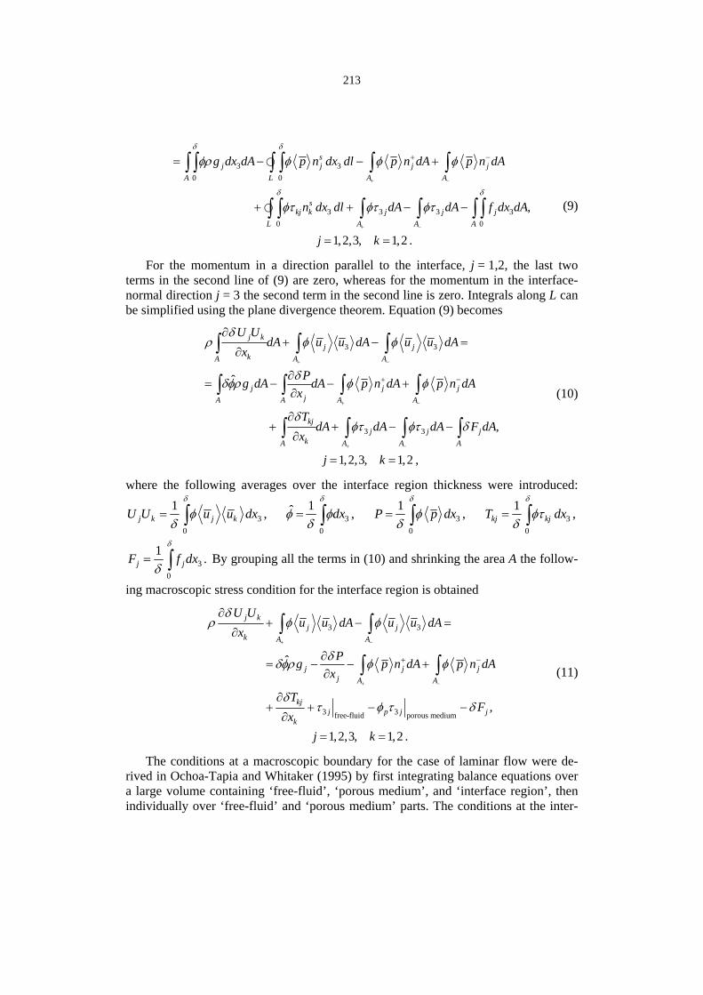
213

3 30 0

3 3 3 30 0

,

1,2,3, 1,2 .

+ −

+ −

+ −= − − +

+ + − −

= =

∫ ∫ ∫ ∫ ∫ ∫

∫ ∫ ∫ ∫ ∫ ∫

sj j j j

A L A A

skj k j j j

L A A A

g dx dA p n dx dl p n dA p n dA

n dx dl dA dA f dx dA

j k

δ δ

δ δ

φρ φ φ φ

φτ φτ φτ (9)

For the momentum in a direction parallel to the interface, j = 1,2, the last two terms in the second line of (9) are zero, whereas for the momentum in the interface-normal direction j = 3 the second term in the second line is zero. Integrals along L can be simplified using the plane divergence theorem. Equation (9) becomes

3 3

3 3

ˆ

,

1,2,3, 1,2 ,

j kj j

kA A A

j j jjA A A A

kjj j j

kA A A A

U UdA u u dA u u dA

x

Pg dA dA p n dA p n dAx

TdA dA dA F dA

x

j k

+ −

+ −

+ −

+ −

∂+ − =

∂

∂= − − +

∂

∂+ + − −

∂

= =

∫ ∫ ∫

∫ ∫ ∫ ∫

∫ ∫ ∫ ∫

δρ φ φ

δδφρ φ φ

δφτ φτ δ

(10)

where the following averages over the interface region thickness were introduced:

30

1 ,= ∫j k j kU U u u dxδ

φδ

30

1ˆ ,= ∫ dxδ

φ φδ

30

1 ,= ∫P p dxδ

φδ

30

1 ,= ∫kj kjT dxδ

φτδ

30

1 .= ∫j jF f dxδ

δ By grouping all the terms in (10) and shrinking the area A the follow-

ing macroscopic stress condition for the interface region is obtained

3 3

3 3free-fluid porous medium

ˆ

,

1,2,3, 1,2 .

j kj j

k A A

j j jj A A

kjj p j j

k

U Uu u dA u u dA

x

Pg p n dA p n dAx

TF

xj k

+ −

+ −

+ −

∂+ − =

∂

∂= − − +

∂

∂+ + − −

∂

= =

∫ ∫

∫ ∫

δρ φ φ

δδφρ φ φ

δτ φ τ δ

(11)

The conditions at a macroscopic boundary for the case of laminar flow were de-rived in Ochoa-Tapia and Whitaker (1995) by first integrating balance equations over a large volume containing ‘free-fluid’, ‘porous medium’, and ‘interface region’, then individually over ‘free-fluid’ and ‘porous medium’ parts. The conditions at the inter-

214

face were then obtained by subtracting the latter two from the first one. In the above derivations the analogous result for turbulent flow is instead obtained by integrating directly over the interface region.

4. Uniform two-dimensional open channel flow with the sub-surface flow parallel to the interface

At this point tensorial notation is replaced with hydraulics notation ( 1x x≡ = stream-wise, 2y x≡ = lateral and 3z x≡ = interface-normal coordinate, u, v, w, correspond-ing respective velocity components). The analysis is limited to the case of steady ( 0t−∂ ∂ = ), uniform ( )0x∂ ∂ = , two-dimensional ( )0y∂ ∂ = turbulent flows

above and inside an immobile porous matrix. In that case the macroscopic continuity equation reduces to

0, 0,∂

= = =∂

uv w

xφ

(12)

so that the only direction with non-zero fluid momentum is interface-parallel direction x.

The double-averaged x momentum equation simplifies to

,xzxgS f

z∂

= +∂φτ

ρφ (13)

where sinS ≅ α is the bed slope. The fluid shear stress is

' ' ,xzu u w u wz

∂= − −

∂τ μ ρ ρ (14)

and the total drag force exerted by the fluid on the roughness per unit volume is

1 1 , 1,2,3.sf sfx x i

iS S

uf p n dS n dS iV V x

μ ∂= − + =

∂∫ ∫ (15)

Equation (13) applies to both stream region, where porosity is one, and the homoge-neous part of the permeable bed, where porosity is φp. It states that the change of the macroscopic fluid shear stress in the bed-normal direction is due to the net momentum added to a control flow volume of the height dz (= supply by gravity – extraction by the roughness).

The macroscopic continuity condition at the interface (8) reduces to

free-fluid porous medium

0,pw w= =φ (16)

and the momentum balance condition (11) becomes, in x direction

215

0 0

free-fluid porous medium.

− −

+ = +∫ ∫zx p zx xgSdz f dzδ δ

τ φρ φ τ (17)

Condition (17) is usually referred to as stress jump condition at the interface. It states that the change of macroscopic fluid stress across the interface region is due to the change of porosity, as well as to momentum sink, and momentum supply within the interface region.

It is interesting to consider a case of a very thin interface region which exists at the top of the roughness of constant height and constant porosity. In that case

0

0, 0,→ →∫ gSdzδ

δ φρ 30

1 .−

−

∂→

∂∫ ∫A

xS

uf dx dAA z

δ

μ

The condition at the interface becomes

free-fluid porous medium

1 .−

−

∂= +

∂∫A

zx p zxS

u dAA z

τ φ τ μ (18)

Fluid shear stress consists of viscous stress, form-induced stress and turbulent stress (the three respective terms in Eq. 14). The local turbulent stress and form-induced momentum flux ( )u wρ are zero across the top area of the roughness ele-ments while viscous stress is probably negligible above the gap between the elements. Thus across the roughness tops the only component of the fluid stress is viscous stress and it transfers momentum to the roughness via viscous drag. Across the gap between the roughness elements viscous stress is negligible and momentum is transferred into the gap via turbulent and form-induced momentum flux. This implies that for rough-ness elements of constant height with significant plan area across the interface local turbulent stress and form-induced momentum flux above the gap have to be higher than their spatial average. This was indeed confirmed in experimental data of Djenidi et al. (1994) and LES data of Stosser et al. (2004).

The double-averaged momentum Eq. (13) applied to flow above and within the porous bed, together with the interface condition (17) or (18) forms a macroscopic description of turbulent flow above and within the gravel bed.

In order to explore the fluid shear stress profile (13) is integrated between the free-surface and an arbitrary bed-parallel plane z = const. For a plane above the roughness top the total driving force or momentum supply (per unit plan area) between the plane and the free water surface is

( )sin d ,≅ −∫h

z

g z gS H zρ α ρ (19)

where z = height of the plane above the roughness top and S = bed slope (Fig. 3). It is in balance with the momentum flux through the plane at the height z, τxz(z), so τxz in-creases linearly, starting from the zero at the free surface. Far away from the rough-

216

ness both viscous stress and form-induced stress are negligible so τxz is turbulent shear stress. Near the roughness crests persistent vortices behind roughness elements cause form-induced momentum flux so momentum is transferred from the flow above by both turbulent and form-induced shear stress. At the roughness crest, z = 0, the mo-mentum flux from the flow above the roughness is just sufficient to balance ρghS, so the fluid shear stress is

0 .gHS≅τ ρ (20)

Fig. 3. Momentum transfer between a stream and a permeable bed. Fluid shear stress has a step change across the interface region.

Below the roughness crest, in the interface region between the plane z = 0 and a bed-parallel plane at level = −δ, porosity changes from one to φp, with the average value ˆ.φ Due to the change of porosity, an additional momentum supply of ˆ g Sφρ δ and the momentum sink due to drag, fluid shear stress may have a step change de-scribed with (17). So far there are very few experimental data on the fluid shear stress inside permeable beds so not enough is known about the relative importance of the turbulent, form-induced and viscous stresses there.

Deeper within the permeable bed flow gradually reaches the conventional porous media regime where all of the additional momentum supply is extracted by the drag so that the fluid shear stress becomes constant (Fig. 3). The depth of the transition layer mentioned at the beginning of the paper can now be defined as the point where the fluid shear stress becomes constant.

217

The velocity gradient is likely to follow the shear stress profile, so it is expected to have maximum at the bed surface, and then gradually change until in the porous media regime it becomes constant. At the interface between the stream flow and the flow within its permeable bed velocity gradient may change, in accordance with the step change in fluid shear stress.

5. Conclusion

At a microscopic scale the turbulent flow above and within a permeable wall is spa-tially heterogeneous, the flow domain has a complex geometry and the flow boundary condition is zero velocity across the surface of the solid matrix. Double-averaging methodology is very convenient for investigating such flows. Time-averaging smoothes temporal variability due to turbulence, while spatial averaging smoothes the spatial heterogeneity: the details of the microscopic flow vanish in a macroscopic model. The influence of small-scales, however, remains and hence has to be expressed using the appropriate parameterizations.

Spatial averaging also reveals the two distinct flow regions with the macroscopic boundary between them. The boundary splits the flow domain into two sub-domains, the ‘stream’ region and the ‘porous medium’ region. A complete macroscopic flow description contains the double-averaged balance equations for both regions and the conditions at the macroscopic boundary between them. At the boundary fluid shear stress and the velocity gradient may have a step change due to the change of porosity and the action of drag.

References

Beavers, G.S., and D.D. Joseph, 1967, Boundary conditions at a naturally permeable wall. J. Fluid Mech. 30 (1), 197-207.

Bear, J., 1979, Hydraulics of groundwater: New York, McGraw-Hill Book Company. de Lemos, M.J.S., and M.S. Mesquita, 2003, Turbulent mass transport in saturated

rigid porous media, Int. Comm. Heat Mass Transfer 30 (1), 105-113 de Lemos, M.J.S., and R.A. Silva, 2006, Turbulent flow over a layer of highly perme-

able medium simulated with a diffusion-jump model for the interface, Int. J. Heat Mass Transfer 49, 546-556.

Djenidi, L., F. Anselmet and R.A. Antonia, 1994, LDA measurements in a turbulent boundary layer over a d-type rough wall, Expts. Fluids. 16, 323-329.

Dybbs, A., and R.V. Edwards, 1984, A new look at porous media fluid mechanics – Darcy to turbulent. In: J. Bear and M. Y. Corapcioglu (eds.), Fundamentals of Transport Phenomena in Porous Media, pp. 199-256. Martinus Nijhoff, Amstre-dam.

Gimenez-Curto, L.A., and M.A. Corniero Lera, 1996, Oscillating turbulent flow over very rough surfaces, J. Geophys. Res. 101, 20745-20758.

218

Gray, W.G., and P.C.Y. Lee, 1977, On the theorems for local volume averaging of multiphase systems, Int. J. Multiphase Flow 3, 333-340.

Hasanizadeh, M., and W.G. Gray, 1979, General conservation equations for multi-phase systems: 1. Averaging procedure, Adv. Wat. Resour. 2, 131-144.

Nikora, V., D. Goring, I. McEwan and G. Griffiths, 2001, Spatially-averaged open-channel flow over rough bed, J. Hydr. Eng., ASCE, 127, 2, 123-133.

Ochoa-Tapia, A.J., and S. Whitaker, 1995, Momentum transfer at the boundary be-tween a porous medium and a homogeneous fluid. I: Theoretical development. Int. J. Heat Mass Transfer 38 (14), 2635-2646.

Pedras, M.H.J., and M.J.S. de Lemos, 2001, Macroscopic turbulence modelling for incompressible flow through undeformable porous media, Int. J. Heat and Mass Transfer 44, 1081-1093.

Pedras, M.H.J., and M.J.S. de Lemos, 2001, Macroscopic turbulence modelling for incompressible flow through undeformable porous media, Int. J. Heat Mass Trans-fer 44, 1081-1093.

Sahraoui, M., and M. Kaviany, 1992, Slip and no-slip velocity boundary conditions at the interface of porous, plain media, Int. J. Heat Mass Transfer 35, 927-943.

Shaffman, p.g., 1971, On the boundary condition at the surface of a porous medium, Stud. Appl. Math. L(2), 93-101.

Silva, R.A., and M.J.S. de Lemos, 2003, Turbulent flow in a channel occupied by a porous layer considering the stress jump at the interface, Int. Jour. Heat Mass Transfer 46, 5113-5121.

Slattery, J.C., 1999, Advanced transport phenomena,. Cambridge University Press, Cambridge.

Smith, J. D., and S.R. McLean, 1977, Spatially-averaged flow over a wavy surface, J. Geophys. Res. 83 (12), 1735-1746.

Stosser, T., and W. Rodi, 2004, LES of bar and rod roughened channel flow. Proceed-ings of The 6th Int. Conf. on Hydroscience and Engineering (ICHE-2004), May30-June 3, Brisbane, Australia.

Whitaker, S., 1967, Diffusion and dispersion in porous media. AlChE J. 13, 420. Whitaker, S., 1999, The method of volume averaging. Kluwer Academic Publishers,

Dordrecht. Wilson, N.R., and R.H. Shaw, 1977, A higher order closure model for canopy flow.

J. Appl. Meteorology 16, 1197-1205.

219

Appendix A: Averaging Rules An averaging volume V (Fig. A1) contains volume of the fluid, Vf , and volume of the solid, Vs. The area enclosing V, A, is defined by the unit outward vector ni. The area of interface between solid and fluid contained within V is denoted with S and its geome-try is defined by the unit vector sf

in pointing into fluid, which is not to be mixed with ni. The position vector of the centre of the averaging volume is denoted with xi, and the position vector of any point within the averaging volume with ri (Fig. A1). Geome-try of fluid within the averaging volume is defined by a distribution function

1 if

0 if i f

fi s

r V

r V

∈⎧⎪= ⎨∈⎪⎩

γ (A.1)

Fig. A1. Averaging volume.

The most important spatial averaging operators are the superficial volume average operator, ,s and intrinsic volume average operator, , defined as (Hassanizadeh and Gray 1979)

V

1( , ) ( , ) ( , ) ,si i f ix t r t r t dV

V= ∫ϕ ϕ γ (A.2a)

V

1( , ) ( , ) ( , ) ,i i f if

x t r t r t dVV

= ∫ϕ ϕ γ (A.2b)

where dV is the infinitesimal element of V. These two averaging operators are related through porosity

,s =ϕ φ ϕ (A.3)

where porosity is equal

220

.sf

fVV

= =φ γ (A.4)

Intrinsic spatial averaging splits a property at a point in space into a sum of its spa-tial average and spatial disturbance (denoted with a wavy overbar):

.= +ϕ ϕ ϕ (A.5)

Temporal averaging operator is denoted with overbar and defined as

1 .t t

t

dtt

+Δ

=Δ ∫ϕ ϕ (A.6)

It splits an instantaneous property into the sum of its temporal average and fluctuation (denoted with prime):

'.= +ϕ ϕ ϕ (A.7)

Spatial average is associated with the centre of the averaging window, and the temporal average with the centre of the averaging time interval. Obviously

' 0, 0.= =ϕ ϕ (A.8)

For any two fluid properties, ϕ, ψ, the following rules of sum and average of a product apply:

, ,+ = + + = +ϕ ψ ϕ ψ ϕ ψ ϕ ψ (A.9)

' ', .ϕψ ϕψ ϕ ψ ϕψ ϕ ψ ϕψ= + = + (A.10)

This discussion is limited to the case of microscopically incompressible fluid flow-ing over and within fixed porous bed with no-slip condition for microscopic velocity at the interface between the fluid and the porous matrix. In this case the averaging volume does not change with time, the averaging windows Δ t and Vf are independent, so the two averaging operators commute, i.e.

.=ϕ ϕ (A.11)

It can be easily shown that then the following operators also commute (Pedras, de Lemos 2001):

' ',=ϕ ϕ (A.12)

,ϕ = ϕ (A.13)

' .′=ϕ ϕ (A.14)

Finally, averaging of flow equations requires the knowledge of the relationship be-tween the averages of derivatives and the derivatives of the averages. In temporal av-

221

eraging of momentum equations for flow over and inside fixed porous bed, averaging window does not change with either space or time, so the temporal averages of all derivatives and the derivatives of the temporal averages commute. The same applies to volume averaging above the roughness crest.

Below the roughness crest, the volume averaging domain changes in space, thus spatial averaging operator does not commute with the spatial derivatives and the local averaging theorem has to be invoked to yield

1 , 1,2,3,s s

sfi

i i S

n dS ix x V

∂∂= − =

∂ ∂ ∫∫ϕϕ ϕ (A.15)

or, using the relationship between volume average and intrinsic volume average,

1 1 , 1,2,3.sfi

i i f S

n dS ix x V

φ ϕϕ ϕφ

∂∂= − =

∂ ∂ ∫∫ (A.16)

The theorem has been proved several times (e.g. Whitaker 1967, Slattery 1969, Gray and Lee 1977). For non-moving fluid-solid interface spatial averaging domain does not change with time so the volume averaging operator commutes with the time de-rivative:

,ss

t t∂∂

=∂ ∂

ϕϕ (A.17)

or, with intrinsic volume averages

1 .t t

∂∂=

∂ ∂φ ϕϕ

φ (A.18)

Appendix B: Spatial averaging of the RANS equation The Reynolds-averaged Navier Stokes equation (RANS) for incompressible fluid is

2

2

1 , 1,2,3,j i j j i jj

i j i i

u u u u u upg i jt x x x x

′ ′∂ ∂ ∂ ∂∂+ = − + + =

∂ ∂ ∂ ∂ ∂ν

ρ (B.1)

where uj = velocity component in the xj-th direction, gj = gravity acceleration in the xj-th direction, ρ = density, p = pressure, ν = kinematic viscosity. The double-averaged Navier-Stokes equation, DANS, is derived by finding the intrinsic average of each term in the RANS equation (B.1), with the use of the theorems (A.16), (A.18) and the rules (A.9) and (A.10). The result is

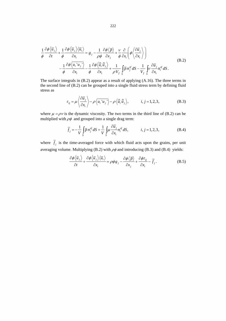
222

1 1 1

' '1 1 1 1 .

j j i jj

i j i i

i j i j jsf sfj i

i i f f iS S

u u u upg

t x x x x

u u u u up n dS n dS

x x V V x

∂ ∂ ⎛ ⎞∂∂ ∂+ = − + ⎜ ⎟⎜ ⎟∂ ∂ ∂ ∂ ∂⎝ ⎠

∂ ∂ ∂− − + −

∂ ∂ ∂∫ ∫

φ φ φ ν φφ φ ρφ φ

φ φν

φ φ ρ

(B.2)

The surface integrals in (B.2) appear as a result of applying (A.16). The three terms in the second line of (B.2) can be grouped into a single fluid stress term by defining fluid stress as

' ' , , 1,2,3,jij i j i j

i

uu u u u i j

x∂

= − − =∂

τ μ ρ ρ (B.3)

where μ = ρν is the dynamic viscosity. The two terms in the third line of (B.2) can be multiplied with ρφ and grouped into a single drag term:

1 1 , , 1,2,3,jsf sfj j i

iS S

uf p n dS n dS i j

V V x∂

= − + =∂∫ ∫ μ (B.4)

where jf is the time-averaged force with which fluid acts upon the grains, per unit averaging volume. Multiplying (B.2) with ρφ and introducing (B.3) and (B.4) yields:

.j j i ijj j

i j i

u u u pg f

t x x x

∂ ∂ ∂∂+ = − + −

∂ ∂ ∂ ∂

φ φ φτφρφ (B.5)

PUBLS. INST. GEOPHYS. POL. ACAD. SC., E-7 (401), 2007

A State Dependent Nonlinear Approach to Flood Forecasting

Renata J. ROMANOWICZ1, 2, Adam KICZKO1 and Florian PAPPENBERGER3 1 Institute of Geophysics Polish Academy of Sciences

Ks. Janusza 64, 01-452 Warsaw, Poland e-mail: renatar@igf.edu.pl

2 Department of Environmental Sciences, Lancaster University, Lancaster, U.K 3 ECMWF, Shinfield Park, Reading, U.K

Abstract

This paper presents an alternative to distributed inundation models for real-time flood forecasting that provides fast and accurate medium- to short-term forecasts. The methodology applies a State Dependent Parameter approach to de-rive a nonlinear dependence between the water levels measured at gauging sta-tions along the river. The transformation of water levels depends on the relative geometry of the channel cross-sections, without the need to apply rating curve transformations to discharge. The relationship obtained is used to transform wa-ter levels as an input to an adaptive, variable time lag routing model. The paper provides an account of the uncertainties involved and describes the conditions for its application. The approach is illustrated using an 80 km reach of the River Severn, UK.

1. Introduction

Flood warning systems require accurate water level forecasts over a range of forecast-ing horizons, from days to hours. The accuracy of the forecast varies with the forecast lead time. Therefore, the forecast should include not only water level values but also an assessment of its probable range (i.e., accuracy). Flood forecasting models apply data assimilation techniques and operate with varying accuracy decreasing with fore-cast lead times. Even though deterministic forecasts are still in use in some flood warning systems, real-time adaptive probabilistic forecasts are in increasing demand (Young 2002, Romanowicz et al. 2006). The on-line updated, stochastic data assimila-tion model presented in the second paper aimed for the longest possible forecast lead times. Forecasts for the river reach were combined together in order to prolong the forecast lead time downstream, thus forming an equivalent to a distributed flood fore-casting system with the advantage of fast performance and probabilistic forecasts. However, the applied linear stage routing models were not able to give the same fore-

224

cast quality for both high and low water levels. Among different nonlinear approaches to flood forecasting, models applying artificial neural networks (NN) have become popular recently (Park et al. 2005). In particular, NN models allow for online data assimilation and give probabilistic forecasts (Chen and Yu 2007). The latter authors applied deterministic, NN based water level forecast and a probabilistic error assess-ment. The main disadvantage of NN models lies in the complex, non-transparent model structure. It makes it very difficult to find a physical interpretation of the model structure and to extrapolate model results to situations not included in the training sets applied for the model parameters estimation. Following experience gained during the derivation of stage routing models (Romanowicz et al. 2006, Young et al. 2006), we propose here an approach which applies both nonlinear transformation of the upstream stages and an advective time delay being a function of the water level. This approach allows the nonlinearity of the stage-stage relations to be captured, as well as account-ing for the varying speed of the wave peak. The approach was tested on the River Sev-ern, UK, reach between Welsh Bridge and Bewdley.

2. Methodology

The water levels at gauging stations along a river are usually highly correlated but they also show a nonlinear relationship, resulting from variable channel and floodplain geometry. Let us consider a river reach between two gauging stations. We shall denote the water level measurements upstream at discrete time period k as input variable uk and water levels at downstream location as an output yk. We want to find the nonlinear water level transformation between these two locations in order to account for nonlin-ear channel geometry and other nonlinear processes which influence the flow. The shape of this nonlinear transformation is derived from the observations at the down-stream end, using a State Dependent Parameter (SDP) approach (Young et al. 2001). In order to account for variations of wave celerity, we introduce a varying with water level advective time delay. A mathematical description of the proposed water level routing process is as follows:

( ) ( )( )k k k kk k u k u

k k k

x h u u

y xδ δ

ζ− −= ⋅

= + (1)

where h(⋅) denotes the nonlinear transformation of water levels at the input to the reach uk at discrete time period k, derived using SDP approach; δk = d(uk) denotes the delay related to the celerity of the flood wave, or the travel time of the wave peak and changing with the peak height, and ζk is a random Gaussian error, usually coloured with heteroscedastic variance. The schematic presentation of the modelling approach is shown in Fig. 1.

The SDP relationship is first estimated in a nonparametric (graphical) manner us-ing CAPTAIN toolbox for MATLAB™ (Taylor et al. 2007), in order to identify its characteristic nonlinear form, prior to parameterisation and final estimation of this identified relationship based on suitable parametric forms, such as a combination of power, exponential and piecewise linear analytical relations or the use of more general parameterisations, such as radial basis functions (Martin et al. 2003).

225

Fig. 1. Schematic representation of State Dependent Nonlinear model for flood forecasting.

It is worth noting that the model (1) is derived off-line. The nonlinear relationship between the water levels at two cross-sections may change with time, and the travel time of the wave peak also varies. In order to account for small modelling errors, the data assimilation procedure is used in the form of on-line adaptive gain. Namely, the on-line N-step ahead level forecast applies an on-line gain updating based on observa-tions up to date, using real-time recursive estimation (Young 2002). Therefore, the forecast equation has the following form: ˆ ˆk N k k N k Ny g x+ + += ⋅ +η (2)

Here, ˆk Nx + is the deterministic N steps ahead water level estimate, obtained from vari-able delay routing model, and k Nη + is the noise term that represents the error in the estimation (lack of fit); ˆkg denotes an estimate of adaptive gain gk which is assumed to vary stochastically as a Random Walk (RW) process with variance hyper-parameter qk associated with the stochastic input to the RW model. With this assumption, the gain gk can be estimated in real-time using the scalar Recursive Least Squares (RLS) algorithm (Young 1984), conditioned on the observations up to time k. In calibration, we use the minimisation of N-step-ahead forecast error as the optimisation criterion for the gain hyper-parameter qk. The 0.95 confidence bounds of the N-step ahead fore-cast are identified using a Monte Carlo based estimation technique (Romanowicz and Beven 2006).

The procedure for developing an on-line SDP-based flood forecasting model for two neighbouring gauging stations is as follows:

1. Estimate the relationship between the height of the wave peak upstream and the travel time δ required for that peak to reach the downstream station.

2. Determine the nonlinear transformation for the relationship (Eq. 1) between the water levels using an SDP approach.

3. Parameterize the obtained function using, e.g., radial basis functions. 4. Derive hyper-parameters for on-line updating of the forecast gain and 0.95 con-

fidence bounds for the N-step ahead forecast.

3. Introducing the nonlinear water level transformation: River Severn case study

We apply the proposed approach to the River Severn reach, U.K., between Welsh Bridge and Bewdley. There are available 15 min water level measurements at Welsh

Nonlinear transformation

( )kk kx h u δ−=

ku ,ku δDelay

( )k kd uδ =

ky

kζ

+

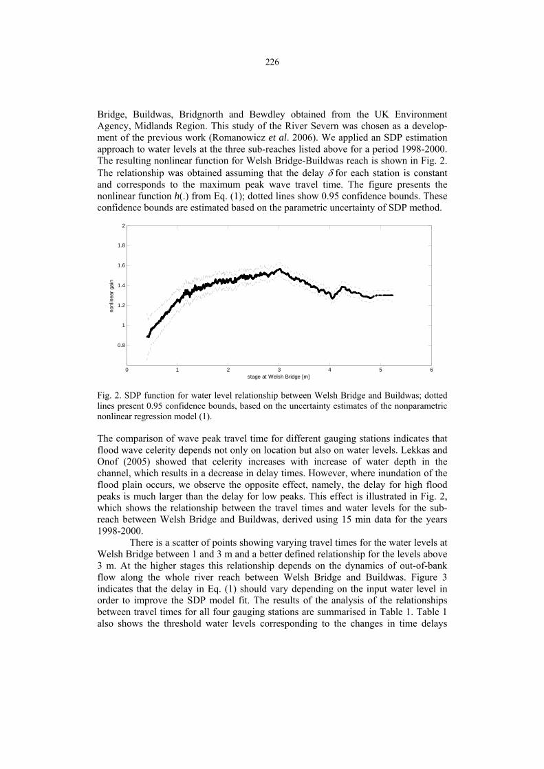
226

Bridge, Buildwas, Bridgnorth and Bewdley obtained from the UK Environment Agency, Midlands Region. This study of the River Severn was chosen as a develop-ment of the previous work (Romanowicz et al. 2006). We applied an SDP estimation approach to water levels at the three sub-reaches listed above for a period 1998-2000. The resulting nonlinear function for Welsh Bridge-Buildwas reach is shown in Fig. 2. The relationship was obtained assuming that the delay δ for each station is constant and corresponds to the maximum peak wave travel time. The figure presents the nonlinear function h(.) from Eq. (1); dotted lines show 0.95 confidence bounds. These confidence bounds are estimated based on the parametric uncertainty of SDP method.

0 1 2 3 4 5 6

0.8

1

1.2

1.4

1.6

1.8

2

stage at Welsh Bridge [m]

nonl

inea

r gai

n

Fig. 2. SDP function for water level relationship between Welsh Bridge and Buildwas; dotted lines present 0.95 confidence bounds, based on the uncertainty estimates of the nonparametric nonlinear regression model (1).

The comparison of wave peak travel time for different gauging stations indicates that flood wave celerity depends not only on location but also on water levels. Lekkas and Onof (2005) showed that celerity increases with increase of water depth in the channel, which results in a decrease in delay times. However, where inundation of the flood plain occurs, we observe the opposite effect, namely, the delay for high flood peaks is much larger than the delay for low peaks. This effect is illustrated in Fig. 2, which shows the relationship between the travel times and water levels for the sub-reach between Welsh Bridge and Buildwas, derived using 15 min data for the years 1998-2000.

There is a scatter of points showing varying travel times for the water levels at Welsh Bridge between 1 and 3 m and a better defined relationship for the levels above 3 m. At the higher stages this relationship depends on the dynamics of out-of-bank flow along the whole river reach between Welsh Bridge and Buildwas. Figure 3 indicates that the delay in Eq. (1) should vary depending on the input water level in order to improve the SDP model fit. The results of the analysis of the relationships between travel times for all four gauging stations are summarised in Table 1. Table 1 also shows the threshold water levels corresponding to the changes in time delays

227

from the minimum to maximum values, as illustrated in Fig. 3 for the Welsh Bridge to Buildwas case.

Fig. 3. Relationship between wave peak travel times (no. of 15 minute time steps) and water levels at Welsh Bridge (1998-2000) for the Severn reach between Welsh Bridge and Buildwas.

Table 1

Minimum and maximum travel times for each of the sub-reaches and corresponding water levels at the upstream gauging stations (Welsh Bridge, Buildwas

and Bridgnorth, respectively)

Min time[h]

Water level[m]

Max time[h]

Water level [m]

Welsh Bridge − Buildwas 8 2 14 3.5 Buildwas Bridgnorth 3 3.5 5 5

Bridgnorth − Bewdley 4 1.7 6 3.5

The flow (level) routing process in an open channel combines the processes of advec-tion (translation of the wave in time) and dispersion which, in text book cases, leads to attenuation of the flood peak. Under over-bank flow conditions, the energy balance in the reach is influenced by local velocities, secondary flows, momentum transfer, and interface vortices between channel and flood bank and boundary shear stress (Knight et al. 1989). In this particular research, no attempt is made to model such effects ex-plicitly. Instead the complex interactions between water level and flood wave dis-charges are taken into account through the nonlinear transformation of the input water levels to deal with the momentum loss of the wave and the (possibly complex) changes in cross-section geometry and storage along the river reach. Therefore, as shown in Fig. 2, this transformation can result in a downstream response with a higher relative change in water levels (an increase in gain at higher flows), especially at man-

228

made structures or other constrictions, as well as the textbook downstream attenuation of the flood peak.

The application of the proposed methodology to the River Severn reach between Welsh Bridge and Bewdley resulted in improved on-line water level forecasts. Table 2 presents the results of validation of the models on 2002 flood event based on the model (1), with the variable transport delay (travel time) as given in Table 1. In Table 2, forecast success is reported in terms of the percentage of the output variance ex-plained by the forecast 2 2 21 /N N yR σ σ= − , where 2

Nσ and 2yσ denote the variances of N

step ahead forecast error and observed water level, respectively and Root Mean Square Error (RMSE).

Table 2

The goodness of fit 2fR and RMSE criteria for the validation stage of on-line forecasts

for the 2002 flood event

River Severn Reach Lead time [h] 2NR [%] RMSE [m]

Welsh Bridge − Buildwas 8 99.45 0.106

Buildwas − Bridgnorth 3 99.93 0.038

Bridgnorth − Bewdley 4 99.76 0.054

Buildwas − Bewdley 7 99.65 0.067

Welsh Bridge − Bridgnorth 11 98.81 0.117

Welsh Bridge − Bewdley 15 98.65 0.129

Fig. 4. Validation of SDP based, variable time delay model: 11-hour-ahead forecast for the Bewdley, November 2002 event, with on-line updating of the forecast gain (99.22% of output variation explained).

229

Since a nonlinear SDP transformation is applied to the upstream water levels at each sub-reach, the forecasts can be prolonged, as in Romanowicz et al. (2006), by using the forecast upstream instead of measurements. Obviously, the quality of the forecasts decreases with the increase of the lead time. The last three rows of Table 2 show the goodness of fit obtained after combining the individual reach forecasts. Therefore, the Bewdley forecast may be extended to a maximum 11 hours when the 5- hour-ahead forecast for Bridgnorth is used, and up to a maximum of 25 hours when using the 19-hour-ahead forecast for Bridgnorth. The maximum lead times shown in brackets correspond to the wave peak time travel. Figure 4 shows the 11-hour-ahead validation forecast for Bewdley based on forecasts for the Buildwas-Bridgnorth-Bewdley reaches, together with 0.95 confidence bounds.

4. Conclusions

We have shown that a high precision on-line forecast can be obtained from a simple, easily implemented, and transparent on-line data assimilation system, based on a nonlinear transformation of water level observations upstream and advective time delay varying with input water levels. The approach requires a wide range of input and output data to give robust predictions. From this point of view it resembles a neural network approach. However, in contrast with neural network models, the approach presented here is more straightforward and gives the possibility of generalisation of a nonlinear relation between water levels depending on river channel geometry. This generalisation is the subject of ongoing work.

Acknowledgments . This work was supported partly by the UK Flood Risk Management Research Consortium Research Priority Area 3 on Real-time Forecasting and grant 2 P04D 009 29 from the Polish Ministry of Higher Education and Science. We thank Professors Peter Young and Keith Beven for advice and discussion. Our colleagues from the UK Environment Agency are thanked for supplying the rainfall and flow data, which were used in this research.

References

Chen, Shien-Tsung, and Yu. Pao-Shan, 2007, Real-time probabilistic forecasting of flood stages, 2007, J. Hydrol., 340, 43-77.

Knight, D.W., K. Shiono and J. Pirt, 1989, Prediction of depth mean velocity and dis-charge in natural rivers with overbank flow, Proc. Int. Conf. on Hydraulic and En-vironmental Modelling of Coastal, Estuarine and River Waters, (Ed. R.A. Fal-coner, P. Goodwin, R.G.S. Matthew), Gower Technical, University of Bradford, September, Paper 38, 419-428.

Lekkas, D.F., and C. Onof, 2005, Introducing the variation of advective time delay (ATD) to Transfer Function models, Environmental Modelling and Software doi:10.1016/j.envsoft.2005.06.005.

Martin, D., M. Buhmann and J. Ablowitz, 2003, Radial Basis Functions: Theory and Implementations, Cambridge University.

230

Park, J., J. Obeysekera and R. VanZee, 2005, Prediction boundaries and forecasting of nonlinear hydrologic stage data, J. Hydrol., 312, 79-94.

Romanowicz, R.J., and K.J. Beven, 2006, Comments on Generalised Likelihood Un-certainty Estimation, Reliability Engineering and System Safety, doi: 10.1016/j.ress.2005.11.030.

Romanowicz, R.J., P.C. Young and K.J. Beven, 2006, Data assimilation and adaptive forecasting of water levels in the river Severn catchment, United Kingdom, Water Res. Research, 42, doi:10.1029/2005WR004373.

Taylor, C.J., D.J. Pedregal, P.C. Young and W. Tych, 2007, Environmental time series analysis and forecasting with the Captain toolbox, Environmental Modelling and Software 22, 797-814.

Young, P., 2002, Advances in real-time flood forecasting, Philosophical Transactions: Mathematical, Physical and Engineering Sciences, 360, 1433-1450.

Young, P.C., 1984. Recursive Estimation and Time Series Analysis, Springer, Berlin. Young, P.C., P. Mckenna and J. Bruun, 2001, Identification of non-linear stochastic

systems by state dependent parameter estimation, International Journal of Control, 74 (18): 1837-1857.

Young, P., R.J. Romanowicz and K.J. Beven, 2006, Updating Algorithms in Flood Forecasting, Flood Risk Management Research Consortium, Report UR5, Decem-ber 2006; www.floodrisk.org.uk.

PUBLS. INST. GEOPHYS. POL. ACAD. SC., E-7 (401), 2007

Analysis of Flow in a Rectangular Channel with a Bypass

Tomasz SIUTA Institute of Engineering and Water Management

Warszawska 24, 31-155 Kraków, Poland e-mail: tomasz.siuta@iigw.pl

Abstract

In the paper, flows in the uniform rectangular channel with a bypass are ex-amined for three different geometries of junction zones. The 2D, depth averaged Navier-Stokes equations were applied to solve flow field. The special attention was focused on changes of water surface profile along a river reach and dis-charge split as a result of bypass channel introduction. Finally results of 2D modeling are compared with results achieved by simplified 1D model.

1. Introduction

The bypass channel may be created naturally by meandering river or designed for different purposes, such as flood mitigation, water supply or navigation.

In recent years, more and more floods are observed in the same regions of the world. These floods constitute the threat for urbanized area and people living there. Efficient management and designing of flood protection system is getting very diffi-cult. One of possibilities might be a use of bypass channel to enlarge conveyance of a river channel. Designing of bypass channels requires hydrodynamic studies to evalu-ate its impact on flow condition changes in natural river. Bypass channel and river reach create the loop network where most abrupt flow changes occur in the split and the junction zones.

In the paper, special attention is focused on the water level changes as a result of different α angle values (Fig. 1) which determine geometry of junction zones. In real designing of junction geometry, flow direction change is realized by gradual curvature and it is the matter of radius magnitude examination rather than angle α value (Dam-muller et al. 1989); however, for preliminary studies the examination of the impact of angle α values on a flow field maybe helpful for designing purposes.

Additionally, comparison between 2D and 1D water surface modeling results is presented to show the cases of meaningful differences.

232

α α

2 km

upstream river

d 2 km 5 km d

middle r. downstream r.

bypass chanel

Fig. 1. The loop network scheme.

2. Flow computing method

Flow computation was realized by the FST2DH model (Froechlich 2002). Within this model, the Navier-Stokes 2D depth averaged equations are adopted in the following form:

1 2 ,∂ ∂∂+ + =

∂ ∂ ∂ mq qh q

t x y (1)

( )2 2

1 1 1 2 1 0,2

⎛ ⎞ ∂∂ ∂ ∂ ⎛ ⎞+ + + + + τ − =⎜ ⎟ ⎜ ⎟∂ ∂ ∂ ∂ ρ⎝ ⎠⎝ ⎠b

bx xzq q q qgh gh T

t x h y h x (2)

( )2 2

2 1 2 2 1 0,2

⎛ ⎞ ∂∂ ∂ ∂⎛ ⎞+ + + + + τ − =⎜ ⎟⎜ ⎟∂ ∂ ∂ ∂ ρ⎝ ⎠ ⎝ ⎠b

by yzq q q q gh gh T

t x h y h y (3)

where: q1 = unit flow rate in the x direction; q2 = unit flow rate in the y direction; q = mass inflow/outflow rate; zb = bed level; h = depth; τbx, τby = bed shear stresses acting in the x and y directions, respectively, and

( )( ) ,∂ τ∂ τ

= +∂ ∂

xyxxx

hhTx y

( ) ( )

,∂ τ ∂ τ

= +∂ ∂

yx yyy

h hT

x y (4)

where τxx, τxy, τyx, τyy = shear stresses caused by turbulence. Bed shear stresses are computed based on Manning’s roughness coefficient

(Chaudhry 1993). Depth-averaged lateral shear stresses caused by turbulence are computed using Boussinesq’s eddy viscosity concept whereby the turbulent stresses are considered proportional to gradients of the velocities. Kinematic eddy viscosity is related to the scales of motion being resolved by a mesh. It is computed by Smagorin-sky formula. FST2DH model uses the Galerkin finite element method to solve the governing equations. The two-dimensional mesh elements may be either triangles or quadrilaterals.

The 1D model is represented by energy and mass balance equations which are ap-plied within Hec-Ras 3.1 software (Brunner 2002). In that approach, nodal geometry doesn’t influence flow computation, so it is not possible to take into account the α value directly. Bernoullie equations are solved step by step for given boundary condi-tions. In the case of flow split the optional optimization procedure was turned on.

233

Flow discharge is divided in iterative way until energy at the upstream cross section of the split junction based on separate calculation for two downstream reaches has the same value (in the cases of subcritical flow which are considered in the paper).

3. Numerical experiment

Both the bypass channel and the river reach have the same uniform rectangular cross section of width b = 40 m and bed slope i = 0.1%. Total length of the river reaches is 9.2 km and the bypass length is about 5 km (Fig. 1).

3.1 Geometry of the junction zones Three variants of the loop channel for different α angle values (15, 30 and 60 degrees) were examined. Because the conveyance of river and bypass is the same it implies entrance length value d (Fig. 1) changing with respect to α values in the range from 70 m to 200 m.

Fig. 2. Velocity field at the split junction for α = 15 degrees.

Fig. 3. Velocity field at the split junction for α = 60 degrees.

3.2 Boundary conditions For every loop channel variant, two cases of steady flows were examined alterna-tively. At upstream boundary condition total discharge Q = 500 m3/s and Q = 2500 m3/s were considered. At downstream boundary condition, water depth

234

h = 4.5 m and h = 10 m was applied, respectively. Manning coefficient single value (n = 0.03) was kept the same for all cases. Additionally, for every flow cases the refer-ence water level were calculated for a single river reach without bypass channel.

Fig. 4. Velocity field at the confluence for α = 60 degrees.

3.3 Results and discussion In the junction zones of the loop network one may observe the water threshold at the split zone, and the water drop at the confluence zone (Fig. 5). At the steady flow con-ditions, the threshold is hydraulic jump alike but for all cases Froud number is less than 0.9. The consequence of this fact is that the total water profile is in subcritcal regime.

Q=2500 m3/s

8

10

12

14

16

18

20

22

24

26

0 2000 4000 6000 8000 10000

distance [m]

WSE

[m

]

reference15 degree30 degree60 degree1D Hec

a = 15

a = 60

a = 30

Fig. 5. Water surface profiles at the river reach for different α angles and Q = 2500 m3/s.

235

For the case with smaller discharge (500 m3/s), the influence of α value on the threshold height is similar for all cases of α values but in the second case of discharge 2500 m3/s (Fig. 5) differences are significant at some locations. The lower the α value, the higher the discharge in the bypass channel and the higher the threshold (Table 1).

Table 1

Discharge split percentage

Discharge split percentage

500 m3/s 2500 m3/s α value

[degrees] middle river bypass channel middle river bypass channel

15 51 49 50 50 30 55 45 60 40 60 58 42 62 38

The threshold results in water level decrease below the reference level (computed for the single river without the bypass) and this depressed water profile continuous in upstream direction. On the other hand, at the confluence zone one may observe the highest water level increase above the reference level, which results in backwater ef-fect reaching even 1 km distance in upstream direction; however, the water level does not vary with α values so strongly as for the split junction and the upstream river reach. The water level increase at the confluence does not influence significantly the water level at the split junction (at the 2000 m of channel length) because the flow regime is almost critical there.

In the case of α = 15 degrees velocities are much more averaged at the junction zones in comparison with the case of α = 60 degrees (Figs. 2 and 3) where the secon-dary flow zone is highly extended at the bypass entrance (Fig. 3). Besides, in the case of α = 60 degrees, strongly separated flow streams occur at the entrance of the down-stream river reach (Fig. 4). Analysis of a flow field may help to find an optimal shape of the bypass entrance and exit to avoid the flow ineffective zones and minimizing ‘choking’ effect.

The 1D model gives similar results as the 2D model in the case of α = 15 degrees (Fig. 5). This may be explained by fact that for such α value the discharge is divided nearly into half at the split junction (Table 1) and both models capture this effect simi-larly.

4. Conclusion

The loop network flows were analyzed only in qualitative manner since flow variables are strongly related to the bed slope, Manning coefficients and channel cross-section geometry. The magnitude of α angle which determines the geometry of considered nodal zones may influence water level profile significantly if flow velocity values are large enough (in the considered example, larger than 5 m/s). However, the impact of α magnitude is declining downstream from the split junction.

236

It is worth to notice that in the case of large α values, flow circulation zones may occur. Natural way to avoid it is to apply the curved bypass joint with large enough curvature radius.

References

Chaudhry, M.H., 1993, Open channel flow, Prentice-Hall, Englewood Cliffs, N.J. Dammuller, D.C., S.M Bhallmudi and M.H. Chaudhry, 1989, Modelling of unsteady

flow in curved channel, Journal Hydr. Engrg., ASCE, 115 (11), 1479-1495. Froehlich, D.C., 2002, User’s manual for FESWMS FST2DH two dimensional depth-

averaged flow and sediment transport model, Publication No. FHWA-RD-03053. Brunner, G., 2002, HEC-RAS, river analysis system hydraulic reference manual,

Computer program documentation, U.S. Army Corps of Engineers.

PUBLS. INST. GEOPHYS. POL. ACAD. SC., E-7 (401), 2007

Unsteady 1D Flow Model of Natural Rivers with Vegetated Floodplain

Dorota SWIATEK Warsaw Agricultural University

Nowoursynowska 159, 02-786 Warsaw, Poland e-mail: dorotams@levis.sggw.pl

Abstract

An unsteady 1D flow model was developed for a channel with vegetated floodplains. The basic form of the non-linear St. Venant equations combined with retention effects of the vegetated areas on flood wave conveyance were used in the model. In this approach, friction caused by vegetation and additional resistance caused by interaction between the main channel and vegetated areas are taken into account. The Pasche method was used to calculate the total Darcy-Weisbach friction factor for each cross-section according to the type of vegeta-tion and flow interaction between the main channel and vegetated areas. The model was applied to a 50 km long double trapezoidal channel, and the obtained results show variations of the water level, velocities, discharges, and friction fac-tors depending on the type of vegetation in floodplains and the main channel.

1. Introduction

Present studies on renaturalization of river valleys, river beds, as well as quantitative estimation of water demand of protected hydrogenic habitats exposed to flooding, require in many cases application of flooding flow models. Mathematical modelling of river flow with water levels not exceeding a bank elevation is widespread and de-scribed by many authors (Cunge et al. 1980, Szymkiewicz 2000, and others). Hydrau-lic models applications, particularly for lowland river valleys flooding with water overflowing the main channel, flooding adjacent areas, and flowing in the floodplains covered with various vegetation, are not widely used. The models used usually apply simplified approaches to the influence of land use in river valleys on flow conditions. Flow resistance, as well in river as in floodplains covered with vegetation, is usually described with generalized Manning’s coefficient values subject to plants vegetative alterations. In another simplified approach widely used, flooplains are considered re-tention areas with no water flowing. In a one-dimensional model, floodplains geome-try is accounted for in only one of Saint Venant’s equations – a continuity equation, and the momentum equation reduces to hydraulic parameters within the main channel geometry (Cunge et al. 1980).

238

The developed model, as opposed to many existing commercial models, with-draws from a simplified description of flow resistance expressed by the spatially dif-ferentiated Manning’s coefficient and the use of the Darcy-Weisbach relationship. It also enables introducing a water mass and momentum exchange process between the main channel and floodplains, and parts of a cross-section covered with vegetation and those with no vegetation. To this end, additional flow resistance along imaginary ver-tical boundaries between the main channel and floodplains was introduced (Nuding 1991, Mertens 1989, Pasche 1984, Pasche and Rouve 1985). Thus, the developed model enables, in unsteady flow calculations, to account for flow resistance resulting from both vegetation covering a cross-section and momentum exchange between the main channel and the floodplains, proposed in the Pasche approach (Pasche 1984).

2. Numerical model development

2.1 The unsteady flow model Unsteady flow in natural rivers is usually treated as a one-dimensional flow in prac-tice, and is based on St. Venant equations. St. Venant equations consist of the dynamic equation and the continuity equation. When water discharge and water level are de-pendent variables, these equations are written in the form, respectively:

2

2 0,Q QQ Q h QgA A q

t x A x K A⎛ ⎞∂ ∂ β ∂

+ + + + =⎜ ⎟∂ ∂ ∂⎝ ⎠ (1a)

,h QB qt x

∂ ∂+ =

∂ ∂ (1b)

where: Q = discharge; h = water level; x = distance; t = time; A = cross area of flow; B = width of water surface; K = conveyance factor; g = gravitational acceleration; q = lateral inflow; β = momentum correction factor.

The conveyance factor K is expressed as

1/ 28 ,gRK A⎛ ⎞= ⎜ ⎟λ⎝ ⎠

(2)

where: R = hydraulic radius; λ = friction factor. Equation (1) requires also determining of boundary conditions as well as initial

conditions. Boundary conditions refer to hydraulic properties at the upstream and downstream ends of a river. The developed model enables only a subcritical flow de-scription. The upstream boundary condition is determined as a discharge hydrograph Q(t). A water level hydrograph h(t), discharge hydrograph Q(t), rating curve Q(h) or friction slope Sf can be used as the downstream boundary condition.

The initial condition refers to the state of flow in the river when the simulation starts. In the model presented in this paper a steady flow in the channel is used as the initial condition (Swiatek et al. 2006).

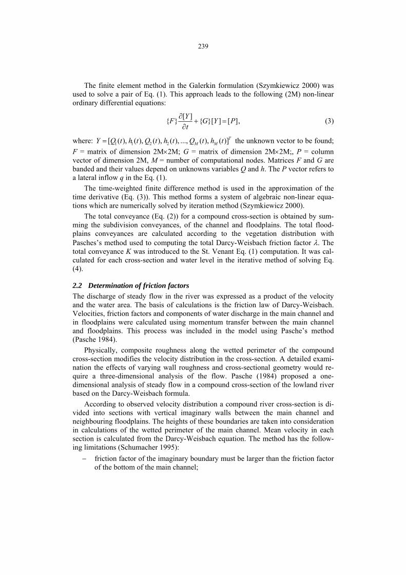
239

The finite element method in the Galerkin formulation (Szymkiewicz 2000) was used to solve a pair of Eq. (1). This approach leads to the following (2M) non-linear ordinary differential equations:

[ ] [ ] [ ],YF G Y Pt

∂+ =

∂ (3)

where: 1 1 2 2[ ( ), ( ), ( ), ( ), ..., ( ), ( )]TM MY Q t h t Q t h t Q t h t= the unknown vector to be found;

F = matrix of dimension 2M×2M; G = matrix of dimension 2M×2M;, P = column vector of dimension 2M, M = number of computational nodes. Matrices F and G are banded and their values depend on unknowns variables Q and h. The P vector refers to a lateral inflow q in the Eq. (1).

The time-weighted finite difference method is used in the approximation of the time derivative (Eq. (3)). This method forms a system of algebraic non-linear equa-tions which are numerically solved by iteration method (Szymkiewicz 2000).

The total conveyance (Eq. (2)) for a compound cross-section is obtained by sum-ming the subdivision conveyances, of the channel and floodplains. The total flood-plains conveyances are calculated according to the vegetation distribution with Pasches’s method used to computing the total Darcy-Weisbach friction factor λ. The total conveyance K was introduced to the St. Venant Eq. (1) computation. It was cal-culated for each cross-section and water level in the iterative method of solving Eq. (4).

2.2 Determination of friction factors The discharge of steady flow in the river was expressed as a product of the velocity and the water area. The basis of calculations is the friction law of Darcy-Weisbach. Velocities, friction factors and components of water discharge in the main channel and in floodplains were calculated using momentum transfer between the main channel and floodplains. This process was included in the model using Pasche’s method (Pasche 1984).

Physically, composite roughness along the wetted perimeter of the compound cross-section modifies the velocity distribution in the cross-section. A detailed exami-nation the effects of varying wall roughness and cross-sectional geometry would re-quire a three-dimensional analysis of the flow. Pasche (1984) proposed a one-dimensional analysis of steady flow in a compound cross-section of the lowland river based on the Darcy-Weisbach formula.

According to observed velocity distribution a compound river cross-section is di-vided into sections with vertical imaginary walls between the main channel and neighbouring floodplains. The heights of these boundaries are taken into consideration in calculations of the wetted perimeter of the main channel. Mean velocity in each section is calculated from the Darcy-Weisbach equation. The method has the follow-ing limitations (Schumacher 1995):

− friction factor of the imaginary boundary must be larger than the friction factor of the bottom of the main channel;

240

− distance between plants along the flow, ax, must be less than the length of the Karmann path, aNL, formed at a single plant submerged;

− ratio of the main channel and the floodplain width must be less than 40. Flow resistance in parts of channel sections overgrown with vegetation depends on

both vegetation and bed roughness and is calculated as a sum of the channel bed λs and submerged vegetation λv friction factors (Indlekofer 1981). Friction factors for high vegetation, λv, were the aim of investigations by Kaiser (1984), Lindner (1982) and Pasche (1984), and is computed according to the concept issued by these authors.

3. Example of calculations

In order to check correctness of the developed algorithms and calculation procedures, the elaborated model was used for an unsteady flow simulation in a very simple ex-ample. A channel of L = 50 km and a bottom slope of J = 0.0005 is studied. A com-pound river cross-section is stable and its geometry and growth of vegetation (Fig. 1) were taken from (Kubrak and Nachlik 2003). The left floodplain is 20 m wide and covered with shrubs of dp = 0.03 m diameter and an average distance between individ-ual shrubs of ax = ay = 0.25 m. The channel slopes are covered with low vegetation of roughness height ks = 0.09 m. The bottom of the main channel is covered with small and medium-grain sand of roughness height ks = 0.05 m. The right flooplain is 33 m wide and planted with shrubs and trees of an average diameter dp = 0.04 m and aver-age spacing ax = ay = 0.3 m. The roughness height of the foodplains is 0.10 m.

Fig. 1. A sketch of a compound cross-section (Kubrak and Nachlik 2003).

A numerical mesh with a constant space step Δx = 1000 m and with 51 nodes was used. The time step Δt was constant and equal to 180 seconds. The simulation was performed for the following initial and boundary conditions:

241

− at the moment t = 0 there was a steady flow in the analyzed channel of dis-charge Q = 15 m3/s.

− at the cross-section x = 0 starting the channel a discharge hydrograph Qx=0(t) was given, as presented in Fig. 3 (Q0 curve).

− at the end of the river (x = 50 km) a boundary condition was assumed in the form of a rating curve Q(H) calculated from channel discharge computation at the slope J = 0.0005 (Fig. 2).

81

82

83

84

85

86

87

0 20 40 60 80 100Q [m3/s]

H [m

asl

.]

Fig. 2. Rating curve − downstream boundary conditio.

In Fig. 3, discharge hydrographs are presented calculated at the cross-sections x = 0, x = 20 km, and x = 40 km. Calculated discharges for the main river channel and floodplains for forecast time t = 18 h are shown in Fig. 4.

10

20

30

40

50

60

70

80

0 6 12 18 24 30 36 42 48t [h]

Q [m

3/s]

Q0 Q20 Q40 Fig. 3. Discharge hydrograph Q0 for boundary condition x = 0 and flow hydrographs Q20 and Q40 calculated for x = 20 km and Q40 for x = 40 km.

242

0

10

20

30

40

50

60

0 10 20 30 40 50x [km]

Q[m

3/s]

Qlf Qch Qrf Fig. 4. Discharges Qch in the main river channel, Qlf in the left floodplain and Qrf in the right floodplain, calculated for forecast time t = 18 h.

In Fig. 5, discharge variability is shown for selected forecast time. In the ana-lysed example, the maximum water discharge in floodplains is about 15% of the total discharge. The developed model enables calculating water velocity in the main river channel, as well as in floodplains. In the analysed example, for forecast time t = 12 h, when hydrograph at x = 0 equals the maximum value of 80 m3/s, water velocity at this cross-section for the left floodplain is 0.15 m/s, for the main channel – 1.74 m/s, and for the right floodplain – 0.14 m/s, at the water depth in floodplains of 1.7 m and in the river channel of 3.7 m. The velocity VT in the imaginary walls between the main channel and its floodplains is 0.38 m/s and 0.37 m/s for a left and right part, respec-tively. The calculated water mass balance error for the total time simulation (t = 60 h) was 0.09% and shows that the developed numerical scheme well fulfils the mass bal-ance equation.

10

20

30

40

50

60

70

80

90

0 10 20 30 40 50x [km]

Q[m

3/s]

t=12h t=18h t=24h

Fig. 5. River flow rates calculated for forecast time t = 12, 18, and 24 h.

243

4. Conclusions

The developed model enables finding a solution for unsteady flow problems in natural rivers with vegetated floodplains. It may be used as a tool to estimate new water sur-face level for renaturalized rivers, especially for flood conditions, as well as to ensure suitable conditions for habitat diversity in projects of environmental flood manage-ment. It is an appropriate tool to estimate floodplain vegetation influence on flow con-ditions.

The model in which Pasche’s method was combined with St. Venant equations was stable and computationally fast. Contrary to the traditional approach, where floodplains are considered as storage areas, the proposed model computes velocities, discharges and friction factors for each specified part depending on the type of vegeta-tion in floodplains and the main channel.

The model was used for a relatively simple reach. In this case, the floodplains do not convey a significant part of the total discharge. Over 15% of the total discharge was transported in the floodplains. The obtained results allow to analyze variations of water level and discharges in the main channel as well as on the floodplains. Actual measurement data will be used for calibration and verification of the model in future development.

References Cunge, J.A., F.M. Holly and A. Verwey, 1980, Practical aspect of computational ri-

ver hydraulics, Boston, 420 pp. Indlekofer, H., 1981, Überlagerung von Rauhigkeitseinflüssen beim Abfluß in offenen

Gerinnen. Mitt. Institut für Wasserbau und Wasserwirtschaft, RWTH Aachen, Heft 37, 105-145.

Kaiser, W., 1984, Flieβwiderstandsverhalten in Gerinnen mit durchströmten Uferge-hölzzonen. Thesis presented for the degree of Doctor in Applied Sciences TH Darmstadt.

Kubrak, J., and E. Nachlik, 2003, Hydrauliczne podstawy obliczania przepustowości koryt rzecznych, Wydawnictwo SGGW, 317 pp.

Lindner, K., 1982, Der Strömungswiderstand von Pflanzenbeständen. Mitteilungen aus dem Leichtweiss - Institut für Wasserbau der TU Braunschweig, H. 75.

Mertens, W., 1989, Zur Frage hydraulischer Berechnungen naturnaher Flieβgewasser. Wasserwirtschaft 79 (4), 170-179.

Nuding, A., 1991, Flieβwiederstandsverhalten in Gerinnen mit Ufergebusch. Entwick-lung eines Flieβgewasser mit und ohne Geholzufer, unter besonderer Berucksichti-gung von Ufergebusch, Wasserbau-Mitteilugen Nr.35, Technische Hochschule Darmstadt.

Pasche, E., 1984: Turbulenzmechanismen in naturnahen Fließgewässern und die Mög-lichkeit ihrer mathematischen Erfassung. Thesis presented for the degree of Doctor in Applied Sciences, RWTH, Aachen.

244

Pasche, E., and G. Rouve, 1985, Overbank flow with vegetatively roughened flood plains. Journal of Hydraulic Engineering 111 (9), 1262-1278.

Rickert, K., 1988, Hydraulische Berechnung naturnaher Gewässer mit Bewuchs. DVWK-Fortbildung, H. 13.

Rouvé, G., DFG Deutsche Forchungsgemeinschaft, 1987: Hydraulische Probleme beim naturnahen Gewässerausbau Ergebnisse aus Schwerpunktprogramm "Anthro-pogene Einflüsse auf hydrologische Prozesse", Band 2.

Schumacher, F., 1995, Zur Durchfluβberechnung gegliederter naturnah gestalteter Flieβgewasser. Mitteilung Nr. 127, TU Berlin.

Swiatek, D., J. Kubrak and J. Chormański, 2006, Steady 1 D water surface model of natural rivers with vegetated floodplain: An application to the Lower Biebrza, Pro-ceedings of the International Conference on Fluvial Hydraulics River Flow, Vol. 1, p. 545-553.

Szymkiewicz, R., 2000, Modelowanie matematyczne przepływów w rzekach i kanałach, Warszawa PWN, 321 pp.

PUBLS. INST. GEOPHYS. POL. ACAD. SC., E-7 (401), 2007

Inundated Flood Planes and the Flow over Groynes and Oblique Weirs

Wim S.J. UIJTTEWAAL Faculty of Civil Engineering and Geosciences,

Delft University of Technology, The Netherlands e-mail: w.s.j.uijttewaal@tudelft.nl

Abstract

At high water stages the flow in groyne fields is highly affected by the water flowing over the groyne. For those conditions the groyne acts as an (im)perfect weir. In a similar way local elevations in the flood planes can be considered as weirs. The arbitrary orientation of those obstacles with respect to the flow pro-hibits the use of straightforward weir formulations. By considering the generic case of the flow over oblique weirs, a simple analytical approach already gives good insight and acceptable estimates, whereas a 3D numerical model clearly shows the complexities of flow separation and non-hydrostatic effects.

1. Introduction

The winter-bed of many lowland rivers contains a variety of obstacles that affect the flow and its conveyance capacity. Training works such as groynes and summer em-bankments are build for the purpose of guiding the water at low and moderately high stages. Groynes are constructed in order to stabilize the river banks and to keep the main channel navigable. Summer embankments prevent the flooding of the whole flood plane in the case of incidental high water during summer. During very high dis-charges both types of obstacles are submerged and will have an effect on the convey-ance capacity of the river (stage discharge relation). Despite the fact that the geometry of a trained river has not undergone many changes over the last decades (or even cen-turies), little is known about the flow details around groynes and other obstacles that induce a sudden change in flow direction, either horizontally or vertically (Bos 1989, Fritz and Hager 1998).

In this paper attention will be paid to groyne field flow patterns as occurring with emerged and submerged conditions. Especially the dynamics of sudden vertical varia-tions will be addressed, as it occurs with submerged summer embankments and groy-nes.

246

2. Flow patterns

2.1 Groyne fields Bank protection by means of groynes is established by keeping the high flow veloci-ties in a river away from the bank. Blocking the flow in the near-bank region confines the cross-sectional area which leads to higher velocities in the centre of the river with a consequent deepening of the main channel. This provides a second purpose for groynes. The equilibrium bed level in the main channel can be ‘tuned’ locally by choosing the proper length for the groynes. The standard flow field in groyne fields with an aspect ratio close to unity consists of a single gyre that fills up the whole groyne field (Fig. 1). The circulation is driven by the momentum exchange through the mixing layer.

Mixing layerMixing layer

Primary gyreSec.gyre

l

w

Fig. 1. Patterns as observed with dye exchange experiment for two different aspect ratios w/l = 0.7 left, w/l = 0.3 right.

In the corners near the bank small counter rotating gyres are found. With this ge-ometry a stable circulation is obtained which flows rather smoothly at about 30% of the main stream velocity. When the distance between the groynes increases to an as-pect ratio of about 3, the circulation cell becomes elongated and separates from the bank (Uijttewaal et al. 2005a). This provides room for a secondary gyre rotating in the opposite direction. The secondary gyre gets its momentum from the primary gyre via an intermediate mixing layer, resulting in a velocity of approximately 30% of the speed of the primary gyre. There appears to be little interaction between the secondary gyre and the main stream. Its flow velocity and the exchange with the main stream are therefore very small. A much stronger interaction is found in the region where the primary gyre is in contact with the main stream. The mixing layer grows to a bigger width than in the square groyne field. This is due to the vortex shedding that occurs downstream of the groyne tip and the velocity gradient sustaining the vortical motion.

2.2 Submerged groynes When the water level increases, the groynes become submerged and water starts flow-ing over the groyne crest. The recirculating flow pattern of the emerged case interacts with the unidirectional flow in the top layer. Therefore the momentum balance in the groyne field has two sources that can cause a strongly fluctuating flow field when they are of the same order of magnitude (Uijttewaal 2005b).

247

cres

t

bank

Main stream

tip

Fig. 2. Velocity contours (m/s) for flow over a submerged groyne. Lab experiment with 30 cm water depth in the main stream and 5 cm above the groyne crest (Uijttewaal 2005b).

Figure 2 shows the contours of the velocity magnitude over a groyne that is 5 cm submerged. It shows that near the bank the water flows uniformly over the crest whereas near the tip the exchange of momentum with the main stream is clearly visi-ble in the much higher velocity there. The larger region with higher velocity down-stream of the crest is caused by separation of the flow in the vertical plane. The verti-cal recirculation provides no room for the surface layer to decelerate.

A further interpretation of the flow dynamics around submerged groynes is sketched in Fig. 3. With high water levels the flow over the groynes is stationary with almost parallel streamlines. The flow will detach in the vertical plane just downstream of the groyne crest. When the groynes are slightly submerged, the dynamics in the flow pattern is caused by the large eddies that move through the groyne field thereby governing the amplitude variations of the flow over the groyne.

eddy path

Fig. 3. Flow patterns for submerged groynes. Fully submerged; with smooth stationary flow (left), small submergence level causing a dynamic flow field governed by the interfacial vortex (right).

248

In the idealized configurations, as described above, the mean flow direction is generally perpendicular to the groyne crest. In that case the flow over the groyne shows strong similarities with that over a weir, when the effects of the tip are necleg-ted. The discharge over the groyne crest will be affected by the energy losses due to wall friction and de- and acceleration of the flow. In practice the direction of the groyne crest is not always perpendicular to the flow. Especially for submerged condi-tions where the flood plane configuration has a great influence on the mean flow di-rection, it is likely that the flow is oblique with respect to the crest. In order to be able to understand the processes related to the flow over submerged groynes we consider the generic problem of flow over oblique weirs.

2.3 Oblique weirs From a standard analysis using energy conservation the specific discharge over a perfect weir (i.e. critical flow over the weir crest) is readily obtained:

2 20 03 3dvq C H gH⊥ = where H0 is the upstream energy height above the crest and Cdv

the discharge coefficient. The imperfect (sub-critical) condition can straightforwardly be analysed using momentum conservation for the downstream part. Though this ap-proach leads to exact solution, the downstream energy loss is quite often described

multiplying with an extra loss coefficient 2*

01

pHC H⎛ ⎞= − ⎜ ⎟⎝ ⎠

where H2 is the down-

stream energy height and p an adjustable parameter (Villemonte 1947).

When a weir is situated under an angle with the main flow direction the length of the weir, denoted kB , is larger than the width of the stream sB resulting in a decreased discharge per unit weir length. This geometrical effect is often used to increase the discharge capacity of perfect weirs used for regulation of the water level. Also, from the viewpoint of inundating floodplains, we are mainly interested in the specific dis-charge for the weir kq Q B= rather than sQ B (see also Fig. 4).

BsBkφ

hdaweir1:41:4

H0 Lk

Top view

Side view

Fig. 4. Flow configuration with definitions of weir dimensions and flow properties. The dash-dotted line represents the energy height while the upper solid line is the free surface.

249

The approaches for the oblique weirs as found in literature are not very attractive mainly because of their highly empirical character. Aichel (1953) suggested that the specific discharge q for an oblique weir relates to the specific discharge q⊥ of a per-pendicular weir in accordance with:

01 Ah aq

q a⊥

−= − β (1)

All effects of the obliqueness are captured in a single coefficient Aβ . This method was extended by Borghei et al. (2003) using a large number of coefficients and cali-brating them for small values of 0( )h a a− only. It was found that for free flow the discharge coefficient increases with upstream water level for inclinations 45<ϕ whereas dC decreases for 45>ϕ . For submerged conditions the inclination gave slight increases of the discharge. Since Borghei et al. did not account for the effects of the upstream velocity it is difficult to read their results in terms of energy loss.

In order to better understand the physics, we look for a very simple approach and see how well this explains reality. For an inclination of the weir with respect to the approaching streamlines the flow is decomposed in a component perpendicular to the weir and a component parallel to the weir (see Fig. 5). The component parallel to the weir is assumed not to be affected by the weir because away from the wall significant pressure gradients in that direction are absent. The effects of bed friction are neglected for the smooth-bed cases while short downstream distances are considered. The above described weir behaviour can now be applied to the perpendicular velocity component straightforwardly.

β

Φ

Φ

v0v1

v2

v0,p

v0,n

v1,p

v1,n

v2,p

v2,n

γ

Fig. 5. Decomposition of velocities parallel and perpendicular with respect to the oblique weir.

The increased velocity above the weir results in a change in flow direction towards the crest-normal direction. For perfect weir conditions and small values of 2( ) ,h a a− the upstream velocity is small and the flow will be directed almost perpendicular to the weir (see Fig. 5). For increasing water levels the relative increase of the velocity above the weir is smaller resulting in a large angle with respect to the weir crest. In the

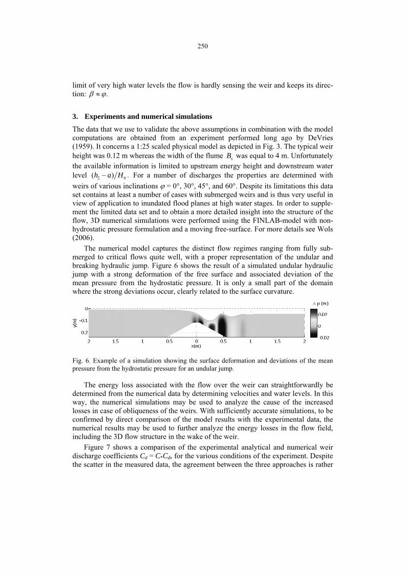
250

limit of very high water levels the flow is hardly sensing the weir and keeps its direc-tion: .≈β ϕ

3. Experiments and numerical simulations

The data that we use to validate the above assumptions in combination with the model computations are obtained from an experiment performed long ago by DeVries (1959). It concerns a 1:25 scaled physical model as depicted in Fig. 3. The typical weir height was 0.12 m whereas the width of the flume sB was equal to 4 m. Unfortunately the available information is limited to upstream energy height and downstream water level 2 0( ) .h a H− For a number of discharges the properties are determined with weirs of various inclinations ϕ = 0°, 30°, 45°, and 60°. Despite its limitations this data set contains at least a number of cases with submerged weirs and is thus very useful in view of application to inundated flood planes at high water stages. In order to supple-ment the limited data set and to obtain a more detailed insight into the structure of the flow, 3D numerical simulations were performed using the FINLAB-model with non-hydrostatic pressure formulation and a moving free-surface. For more details see Wols (2006).

The numerical model captures the distinct flow regimes ranging from fully sub-merged to critical flows quite well, with a proper representation of the undular and breaking hydraulic jump. Figure 6 shows the result of a simulated undular hydraulic jump with a strong deformation of the free surface and associated deviation of the mean pressure from the hydrostatic pressure. It is only a small part of the domain where the strong deviations occur, clearly related to the surface curvature.

Fig. 6. Example of a simulation showing the surface deformation and deviations of the mean pressure from the hydrostatic pressure for an undular jump.

The energy loss associated with the flow over the weir can straightforwardly be determined from the numerical data by determining velocities and water levels. In this way, the numerical simulations may be used to analyze the cause of the increased losses in case of obliqueness of the weirs. With sufficiently accurate simulations, to be confirmed by direct comparison of the model results with the experimental data, the numerical results may be used to further analyze the energy losses in the flow field, including the 3D flow structure in the wake of the weir.

Figure 7 shows a comparison of the experimental analytical and numerical weir discharge coefficients Cd = C*Cdv for the various conditions of the experiment. Despite the scatter in the measured data, the agreement between the three approaches is rather

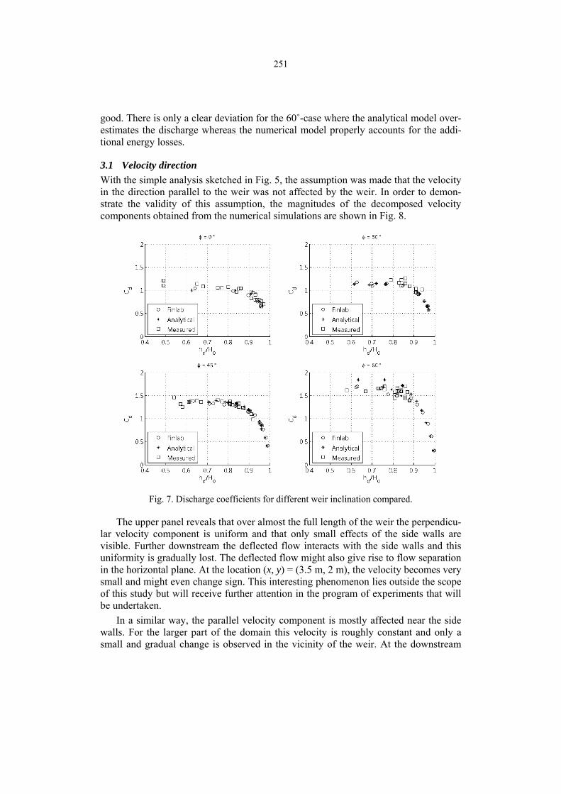
251

good. There is only a clear deviation for the 60˚-case where the analytical model over-estimates the discharge whereas the numerical model properly accounts for the addi-tional energy losses.

3.1 Velocity direction With the simple analysis sketched in Fig. 5, the assumption was made that the velocity in the direction parallel to the weir was not affected by the weir. In order to demon-strate the validity of this assumption, the magnitudes of the decomposed velocity components obtained from the numerical simulations are shown in Fig. 8.

Fig. 7. Discharge coefficients for different weir inclination compared.

The upper panel reveals that over almost the full length of the weir the perpendicu-lar velocity component is uniform and that only small effects of the side walls are visible. Further downstream the deflected flow interacts with the side walls and this uniformity is gradually lost. The deflected flow might also give rise to flow separation in the horizontal plane. At the location (x, y) = (3.5 m, 2 m), the velocity becomes very small and might even change sign. This interesting phenomenon lies outside the scope of this study but will receive further attention in the program of experiments that will be undertaken.

In a similar way, the parallel velocity component is mostly affected near the side walls. For the larger part of the domain this velocity is roughly constant and only a small and gradual change is observed in the vicinity of the weir. At the downstream

252

side of the weir the non-uniformity is the largest. Nevertheless, the results show that the assumption of a constant weir-parallel velocity is valid for the locations not too close to the wall.

Fig. 8. Contour plots of decomposed velocities for a 45° weir. The flow is from left to right and the weir crest is located between (x, y) = (−2 m, −2 m) and (x, y) = (2 m, 2 m).

3.2 Flow separation It turns out that for the imperfect flow over an oblique weir, the detailed flow field downstream of the weir is highly affected by the angle of the weir with respect to the approach flow. Even if the submergence is relatively large, the weir causes a strong deflection of the flow. The inclination, in combination with the separation zone at the downstream side, gives rise to helical streamlines transporting mass and momentum along the weir. Figure 9 shows that through this effect material can be advected over large distances across the flow. Near the bed, high velocities can occur that can give rise to bed scour.

The simulated shape of the recirculation zone is highly affected by the inclination of the weir. In Fig. 10, the flow separates in the area of strong deceleration. For the perpendicular case (left) the downward directed momentum leaves little room for a separation bubble. There seems to be an almost stagnant region but it is not very con-vincing. It should be noted that the limited resolution puts restrictions on the flow details that can be reproduced. Keeping the total discharge constant while changing

253

the inclination of the weir to 60° results in a more pronounced separation bubble. With the same total discharge the greater length of the weir leads to a smaller velocity per-pendicular to the weir and a smaller associated momentum transport.

Fig. 9. Free surface (light grey) and streamlines (black) around an oblique weir (dark grey).

Fig. 10. Flow pattern downstream of the weir in the plane perpendicular to the weir crest (left) perpendicular weir, (middle) oblique 60°, with the same total discharge, (right) oblique 60° weir with same specific discharge as the perpendicular weir left.

This might enhance the separation and give a larger recirculation zone. For a fair comparison also the flow pattern around the inclined weir is shown where the specific discharge and velocities perpendicular to the weir are kept the same (right). In this case a clear separation bubble is found. Since the total velocity over the inclined weir is much bigger, wall friction will play a bigger role. It is also seen that the depression in the free surface is not as deep as in the case of a perpendicular weir. These details show that the velocity component parallel to the weir crest affects the flow separation and results in a slightly smaller energy loss reflected in a higher downstream water level. It must be noted here that the details that are resolved by the numerical model are not compared with experimental data because these were not available. Clearly, detailed data are necessary in order to find out whether the modeling details including the turbulence model, resolution and boundary conditions are correct.

-0.5 0 0.5 1s[m]

φ

-0.5 0 0.5 1s[m]

-0.5 0 0.5 1s[m]

254

4. Conclusions

Groynes have a profound effect on the flow in rivers and give rise to a large variety of flow phenomena. The momentum exchange driving the circulations is governed by separation. Depending on the relative submergence, the mixing layer at the groyne field interface is capable to sustain a gyre pattern including a return flow near the bank. With increasing water level, the flow over the groyne crest dominates resulting in a unidirectional flow through the groyne field. Depending on the direction of the approach flow in relation to the groyne crest, the flow will be deflected in the accel-eration phase.

Separation in the vertical plane is governing the discharge over the groyne. A nu-merical model used for estimating discharge capacity and dispersion should therefore account for the observed complex flow phenomena. This requires a non-hydrostatic model with a moving free surface and advanced turbulence modeling. The latter is important for the vertical separation of the flow downstream of the groyne crest but also for the large-scale horizontal separation near the groyne tip.

Acknowledgments . The author would like to acknowledge the contributions to this work by B. Wols and R.J. Labeur. Rijkswaterstaat RIZA is gratefully acknowl-edged for their financial contribution (project RI-4379).

References

Aichel, O.G., 1953, Abflusszahlen fuer schiefe Wehre, Z.VDI 95, 1. Borghei, S.M., Z. Vatannia, N. Ghodsian and M.R. Jalili, 2003, Oblique rectangular

sharp-crested weir, Water and Maritime Eng., 156, 185-191. Bos, M.G., 1989, Discharge measurement structures, 3rd edition ILRI, Wageningen,

The Netherlands. Fritz, H.M., and W.H. Hager, 1998, Hydraulics of embankment weirs, J. Hydraul.

Eng., 124(9), 963-971. Uijttewaal, W.S.J., 2005a, Effects of groyne layout on the flow in groyne fields: Labo-

ratory experiments, J. Hydraul. Eng., 131(9), 782-791. Uijttewaal, W.S.J., 2005b, The Flow in Groyne Fields, Water Quality Hazards and

Dispersion of Pollutants, W. Czernuszenko and P.M. Rowiński (eds.), Springer, 231-245.

Villemonte, J.R., 1947, Submerged-weir discharge studies, Eng. News-Record, 139, 54-56.

De Vries, M., 1959, Oblique weirs, report WL|Delft Hydraulics, in Dutch. Wols, B., W.S.J. Uijttewaal, R.-J. Labeur and G. Stelling, 2006, Rapidly varying flows

over oblique weirs, Proceedings of the Seventh International Conference on Hy-droscience and Engineering, Philadelphia, PA, September 2006.

PUBLS. INST. GEOPHYS. POL. ACAD. SC., E-7 (401), 2007

Cellular Automata Approach for Flood Forecasting in a Bifurcation River System

Tri P.D. VAN 1(*), Paul A. CARLING 1, Tom J. COULTHARD 2 and Peter M. ATKINSON 1

1 School of Geography, University of Southampton, Southampton, SO17 1BJ, UK (*) e-mail: pdtv@soton.ac.uk

2 School of Geography, University of Hull, Hull, HU6 7RX, UK

Abstract

Bifurcations in river networks are key components of anastomosing river systems. However, most research has investigated bifurcations in meandering and braided river systems but not in anastomosing ones. In addition, numerical modelling has been mainly conducted for a single reach. This paper is to investi-gate the use of a numerical modelling approach (i.e. cellular automata (CA) paradigm) for a large bifurcation in the Mekong River system at the Siphandone Wetlands, Laos. The main characteristics of this river system are: (i) multiple complex channel; (ii) the combination of bedrock and alluvial river bed; (iii) flooding is quite fixed in terms of timing annually but extremely variable in terms of peak discharge; and, (iv) more than 60% of the river banks are unstable. The CA approach is relatively simple and has the ability to address some of the shortcomings of other types of numerical model. Via a CA model with a proper flow routing scheme, channel dynamics can be accounted, with the relevant pre-diction of inundation patterns, and water depths. The results show the application of a CA model for predicting the scale of flood inundation according to different scenarios of discharge from upstream. Finally, the discussion is used to argue how to successfully apply a CA model in such a complicated hydraulic system, as a bifurcation pattern.

Key words: Numerical modelling, cellular automata (CA), discharge rout-

ing, bifurcation river system, water surface, flood inundation pattern.

1. Introduction

The cellular automata (CA) approach represents a simple dynamical system approach, which can describe the properties of a physical system at different levels of concern.

256

In other words, the CA approach is a powerful method to describe, understand, and simulate the behaviour of a complex system (Chopard and Droz 1998). Moreover, in the CA approach, a set of specific rules are identified to show the relationship between a cell and its neighbours (Murray and Paola 1997).

Even though 1D, 2D, and even 3D hydraulic models are common, due to some limitations such as (i) the complexity of solving complex Navier-Stoke equations; and, (ii) the difficulty of defining finite element lattices, application of this type of hydrau-lic model is limited (Coulthard et al. 1999). The CA approach appears as a promising one that can be used to perform different types of hydraulic calculation (Murray and Paola 1994, Coulthard et al. 1996, Nicholas 2000). This type of numerical model does not require complex, but quite simple data input (i.e. a Digital Elevation Model (DEM) of the study area and the hydraulic-related data such as a hydrograph, and sedimentation transportation pattern). Among these CA-family models, CAESAR (Cellular Automaton Evolutionary Slope And River) firstly developed by Coulthard (1996) can be used to estimate the scale of flood inundation which can then be used for catchments management purposes and ecological studies. In addition, while most research so far has been done for a single river reach, CAESAR can be applied for a large river system.

The overall aim of this paper is to test if CAESAR is suitable for simulating a bi-furcation river system. In specific, this paper is to estimate the behaviours of a bifurca-tion river system via the application of CAESAR with different scenarios of upstream discharge.

2. Approach and methods

2.1 Study area At the global scale, the Mekong River is ranked the twelfth in terms of the length (i.e. approximately 2,500 km in total) and the eighth in terms of the mean discharge (i.e. approximately 475 km3 yr−1) (Gupta et al. 2002). Downstream from Tibet and China, the Mekong flows through other five countries (i.e. Myanmar, Laos, Thailand, Cam-bodia, and Vietnam). At the southernmost part of Laos, the Mekong has an anastomos-ing river pattern with a maximum width measured across islands and channels of about 15 km (i.e. the Siphandone Wetlands) (Fig. 1B).

The main characteristics of the river system within the Siphandone Wetlands are: (i) multiple complex channel; (ii) the combination of bedrock and alluvial river bed; (iii) flooding is relatively fixed in terms of timing annually, but extremely variable in terms of peak discharge; and, (iv) more than 60% of the river banks are unstable. In addition, along the Mekong, there are 23 gauging stations where hydraulic features of the river are collected daily. However, in the study area, there are no station and the nearest upstream station is at Pakse (Fig. 1A). Because there are no main tributaries between Pakse and the Siphandone Wetlands, the discharge at Pakse is used as the main input to the Siphandone Wetlands in this paper.

Due to the limitation of topographic data, portions of the Siphandone Wetlands in the south and south-west cannot be considered at this time (Fig. 1B). Therefore, only a

257

bifurcation within the main channel is of concern in this paper. The size of the avail-able DEM of the study area is 315×135 cells and the resolution of each cell is 80 m2.

no avaiable data area Fig. 1. Pakse station (A), and Siphandone Wetlands (B), Laos.

From historical data, three representative peaks of water discharge during the monsoon flooding period are used as the main scenarios for the hydraulic model. They are: (1) the highest discharge of 56,000 cumecs (in 1978); (2) the average of the peak discharges from 1978 to 2005 (i.e. 39,791 cumecs); and (3) the lowest discharge of 26,797 cumecs (in 1998).

2.2 Methods To route water along a river, CAESAR uses a four dimensional scanning algorithm as illustrated in the following figure (Fig. 2).

Fig. 2. Schematic of the scanning algorithm after Coulthard et al., 2002. Copyright John Wiley and Sons Limited. Reproduced with permission.

258

At each iteration, four scans are successively taken as shown in Fig. 2. The first scan (Box 1) is taken from right to left (looking downstream) and water is routed from the current cell to a set of neighbouring cells with lower elevation. In the case where there is no cell with lower elevation relative to the current cell, but the combination of the elevation and water column (of the current cell) is higher than the elevation of the neighbouring cells, water is retained in the current cell up to the height of the obstruc-tion whilst the rest is routed on. When the valley is reached, the scan continues “up-hill” without moving any water (Box 2); this is the intermediary step to start Box 3. Next, Box 3 is performed with the same calculation, but in the opposite direction of that of Box 1. Finally, the last scan is to direct water downstream (Box 4).

In this paper, only one process of discharge routing is presented as it is relevant to the objectives of the study. The water depth at the cell exit is calculated using a rear-rangement of the Manning’s equation (Eq. 1). The differences in slope between di-agonal neighbours are accounted for dividing by 2Dx (where, Dx is the size of grid cell). The surface flow is then routed as in the described scanning routing and the pro-portion routed to the neighbouring cells (i.e. Qi) is calculated as follows (Eq. 2):

3/ 5

0.5

QndS

⎛ ⎞= ⎜ ⎟⎝ ⎠

(1)

[( ) ][( ) ]

ii

i

e d eQ Qe d e+ −

=+ −∑

(2)

where d is water depth in the cell exit; n is Manning’s coefficient; S is the average slope; e is the elevation of the current cell; ei is the elevation of the neighbouring cell i; Q is discharge of the current cell; and Qi is the proportion of discharge delivered to the neighbouring cell i from the discharge at the current cell.

3. Results

Calibration data will be available in due course from nine daily read stage boards and from local information on the lateral extent of annual flooding. This means that later on, modelled water surface elevations and lateral extent to flooding can be checked for accuracy. At the present the calibration data have not been validated. So, the tests were done to estimate the changes of flooding extent and water depth due to different scenarios of discharge upstream.

A test was undertaken to simulate the inundation pattern for different scenarios (i.e. Scenario 1 – the highest discharge; Scenario 2 – the average discharge; and Sce-nario 3 – the lowest discharge) of upstream discharges (Fig. 3). By looking at the in-undation pattern, it is clear that the higher the discharge, the more the area along river banks is flooded. At Scenario 3 – the lowest discharge scenario, the wetted area is narrower and water is not able to route along the central (noted as “A”) cross channel of the river system. In addition, the river bed of lower branch (noted as “II” in Fig 3, Scenario 1) of the river system has lower elevation compare to that of the upper one (noted as “I” in Fig 3, Scenario 1) therefore the water depth at the lower branch is greater than that at the upper one.

259

Fig. 3. Flooding extent and water depth at different discharges from upstream.

The following figure (Fig. 4) shows the water depths at three different cross-sections (see Fig. 3, Scenario 1) with three scenarios of discharge. It can be seen that even though the obtained results have not been validated yet, they are quite accept-able. The water depth across the cross-section increases while the upstream discharge increases and the water depth changes quite consistently at all three cross-sections.

4. Discussion

CAESAR is a useful model to estimate the change of river morphology as one compo-nent of catchments (Coulthard et al. 2007). To use CAESAR to achieve an acceptable

260

inundation pattern and water depth along a complex river system, the code of the model can be further adjusted. This possibility is being explored.

Fig. 4. Diagram of water depths at three cross-sections with three scenarios of upstream discharge.

Even though the requirement of input data is quite simple, CAESAR requires that flow direction must be from the left to right hand side of a DEM and river system must fully exist on a DEM as well. However, the current version of the DEM for this study has no information about the elevation for the lower branch at the later segment of the river (see Fig. 3). The lack of the elevation information would cause the accu-mulation of water at the end of the lower branch and would result in the “up-hill” flows at the surrounding areas. To overcome this problem, an “extended channel” was inserted to route water after running through the end of this branch to the right side of the DEM.

CAESAR is a CA model using a simple approach to simulate the action of a river system over time. In this paper, the results show that the model can be used to simu-late the inundation pattern and water surface (WS) of a bifurcating river system with different levels of discharge from upstream. An advantage of this model is that it automatically includes Manning’s n in its calculation of WS based on the user-specified grain size, or other roughness length, of the river bed as well as the rough-

261

ness of the riparian vegetation. In addition, a pit-filling algorithm included in the model can help achieve an acceptable WS. However, to achieve acceptable water sur-faces that are close to real ones, tests must be done by applying different input values of different parameters (i.e. water discharge from upstream, Manning’s n, WS smooth radius, flow distribution width as well as the iterations of simulation) to determine a suitable set of parameters for a specific river system before any calibration tests are conducted.

CA models can readily deal with deposition and erosion in anastomosing channels where the radius of curvature is large, but small-radius meandering river systems where bends always occur along the river are difficult to accommodate. However, in CAESAR, attention has been paid to overcome this problem. Thus, additional calcula-tion will be very important in the case of consideration for erosion and deposition along the river banks because bifurcations in the Mekong River system do not only include multiple channels, but also involve some tightly meandering patterns.

The possibility to communicate with GIS (e.g. Arc GIS) means that CAESAR can be applied widely. The outputs from CAESAR can be directly imported into GIS for further spatial analysis or display (i.e. to calculate and demonstrate, for example, areas of inundation for different discharge values).

By using simple empirical flow equations, such as Manning’s n or Chezy, the terms of momentum are lost within the CAESAR calculation. However, the relation-ship between empirical roughness determination, field data and CAESAR model for-mulation is the subject of current research.

5. Conclusion

CAESAR is not only a useful CA model to estimate changes of river morphology (Coulthard and van de Wiel, 2006), but can also be used to estimate the flooding scale for a large and complicated river system (e.g. the bifurcation river system for a range of discharge values, from low to extreme). At present, there are various additional CA models available based on different theories as well as being used for different pur-poses which poorly reproduce water surfaces. CAESAR is able to simulate the water depth of a river system and therefore it is useful for obtaining a reliable water surface and for flooding estimation as well. Nevertheless, water depth is not the main objec-tive of CAESAR’s simulation. The model needs to be further adjusted and test to ob-tain reliable water depth, which then can be used to interpolate the water surface. Fur-thermore, intensive sensitivity analysis and calibration are needed to make sure the model matches reality closely.

CAESAR can also be used to estimate the erosion and deposition of the river banks and to simulate the evolution of the river bed. It is suggested that this model should be used in its full capacity (i.e. not only to simulate the inundation patterns and water depths of the river system) to simulate the “real” behaviours of the complicated river system (i.e. the anastomosing river system within the Siphandone Wetlands, Laos).

262

Acknowledgments . We would like to thank the Mekong River Commission (MRC) for their support in data input. We also thank the MRC, the Dorothy Hodgkin Award, and the Engineering and Physical Sciences Research Council (EPSRC) for financial support to perform this research. In addition, CAESAR is an open-source model which can be freely adjusted for individual studies. Users are welcome to download the model as well as its source code. Further information related to CAESAR can be found at www.coulthard.org.uk.

References

Chopard, B., and M. Droz, 1998, Cellular Automata Modeling of Physical Systems, Cambridge University Press, 341pp.

Coulthard, T.J, M.J. Kirkby and M.G. Macklin, 1996, A cellular automaton landscape evolution model. In: R.J. Abrahart (eds.), Proceedings of the first International Conference on GeoComputation (Vol. 1), School of Geography, University of Leeds. pp. 248-281.

Coulthard, T.J., M.J. Kirkby and M.G. Macklin, 1999, Modelling the impacts of Holo-cene environmental change in an upland river catchment, using a Cellular Automa-ton Approach. In: A.G. Brown and T.A. Quine (eds.), Fluvial processes and envi-ronmental change, Jonh Wiley and Sons.

Coulthard, T.J., M.G. Macklin and M.J. Kirby, 2002, A cellular model of holocene upland river basin and alluvial fan evolution, Earth Surf. Process. Landforms 27, 269-288.

Coulthard, T.J., and M.J. van de Wiel, 2006, A cellular model of river meandering, Earth Surf. Process. Landforms 31, 123-132.

Coulthard, T.J., D.N. Hicks and M.J. van de Wiel, 2007, Cellular modelling of river catchments and reaches: advantages, limitations and prospects, Geomorphology in press, Accepted manuscript.

Gupta, A., L. Hock, H. Xiaojing and C. Ping, 2002, Evaluation of part of the Mekong River using satellite imagery, Geomorphology 44, 221-239.

Murray, A. B., and C. Paola, 1994, Cellular model of braided rivers, Nature 371, 54-57.

Murray, A.B., and C. Paola, 1997, Properties of cellular braided-stream model, Earth Surf. Process. Landforms 22, 1001-1025.

Nicholas, A.P., 2000, Modelling bedload yield in braided gravel bed rivers, Geomor-phology 36, 89-106.

PUBLS. INST. GEOPHYS. POL. ACAD. SC., E-7 (401), 2007

On the Numerical Solution of the ADZ Model

Steve WALLIS Heriot-Watt University

Riccarton, Edinburgh, EH14 4AS, UK e-mail: s.g.wallis@hw.ac.uk

Abstract

The ADZ model is a simple and effective tool for simulating solute transport in rivers. The study reported here concerns the model's numerical algorithm. Tracer data from the Murray Burn in Edinburgh is used to compare the perform-ance of three alternative formulations. The theoretical advantages of a new algo-rithm are borne out by simulations of the tracer data, although improvements in simulations, compared to those obtained with the standard algorithm, are proba-bly only significant when the problem is poorly resolved in time. Nevertheless, the new algorithm can be recommended on the grounds that little extra effort is required to use it and simulations so obtained are generally more robust.

1. Introduction

The Aggregated Dead Zone (ADZ) model is an alternative approach to the Advection-Dispersion Equation (ADE) for simulating solute transport in rivers (Rutherford, 1994). Since the model's inception, little attention has been paid to the model's nu-merical algorithm. The aim of this paper is to draw readers' attention to this aspect of the model. This is achieved by showing how the algorithm is derived, and by explor-ing some straightforward alternatives. The performance of three algorithms is illus-trated by applying the model to tracer data collected in the Murray Burn, which is a small stream that runs through the Heriot-Watt University Campus at Riccarton in Edinburgh.

The following sections present relevant details of the ADZ model, its application to the Murray Burn, presentation and discussion of illustrative results and, finally, some conclusions.

264

2. The ADZ Model

2.1 Background The ADZ model originated in the work of Beer and Young (1983), where it was de-scribed within the framework of the physically-based ADE model (Rutherford 1994). In that era, possibly the major disadvantage of the ADE model was that it did not ex-plicitly account for the action of transient storage (TS) on the transport of solutes in rivers. It had been postulated that transient storage in dead zones was responsible for the elevated tails of, and the persistence of skewness in, observed concentration pro-files that were not catered for by the ADE model. However, although (a) it was rela-tively straightforward to include transient storage caused by dead zones in the ADE model (Bencala and Walters 1983) and (b) as a result better agreement with observa-tions could be obtained, two additional model coefficients were introduced that were difficult to relate to measurable physical features.

More recently, this ADE+TS model has become more popular (Hart 1995, Ro-wiński et al. 2004). However, since transient storage may occur not only through the action of re-circulating flow within dead zones, but also through exchange with the hyporheic zone (Marion et al. 2003, Worman et al. 2002), the physical significance of the model coefficients remain a subject of debate (Czernuszenko and Rowiński 1997, Hart 1995, Schmid 2002).

In the ADZ model, in contrast to simulating the action of a complex system of physical interactions, a conceptually simpler (but less well physically-based) approach is taken. Several matters are simplified, but crucially dispersion is modelled as if it were created by the action of a single transient storage zone that represents the aggre-gated effect of all the physical dispersive mechanisms taking place in a reach. Previ-ous studies (Wallis et al. 1989) have shown the benefits of this rather radical ap-proach. Interestingly, the ADZ model coefficients have a simple physical interpreta-tion, and have generally been found to be robust.

2.2 Derivation Under steady flow conditions, the ADZ model is based on the following reach scale dynamic solute mass balance equation:

[ ]( ) ( ) ( )= −dS t Q u t y t

dt V (1)

where V is the volume of water in a reach, S(t) is the reach average solute concentra-tion, Q is the flow rate of water through the reach, u(t) is the cross-sectional average solute concentration at the upstream boundary of the reach, y(t) is the cross-sectional average solute concentration at the downstream boundary of the reach and t is time.

To model dispersion in the reach by the action of a (single effective) transient storage zone, the reach is represented by a continuously stirred tank (Chapra 1997). With this, any solute that enters the tank is immediately and uniformly mixed throughout the entire tank volume such that any change in the input concentration causes an immediate change in the output concentration. As it stands, this is not a

265

good representation of solute transport in a river, however, because there is no delay to represent the time it takes for the leading edge of a solute cloud to be advected through a reach. Similarly, if the continuously stirred tank is assumed to contain the same vol-ume of water as the reach this is also inconsistent with reality, because it is certainly not the case that all the water in a reach is so well mixed longitudinally that the solute concentration in it is uniform.

Both the above difficulties are overcome by assuming that the continuously stirred tank contains only a fraction of the total reach volume, and that the remaining water is contained in a plug flow tank (Chapra 1997) in series with the continuously stirred tank. With the plug flow tank there is no longitudinal mixing, but it introduces the required advective time delay.

If γ is the fraction of the reach volume contained in the continuously stirred tank, and τ is the time delay associated with the plug flow tank, Eq. (1) can be modified by (a) replacing S(t) with γy(t) and (b) moving the origin of u(t) forward in time by τ. Thus the ADZ model equation that describes advection and dispersion is:

[ ]( ) 1 ( ) ( )dy t u t y tdt T

= − τ − (2)

where T is the residence time of the transient storage zone (= γV/Q). A moment analy-sis (Wallis 1994) reveals that: t T= + τ (3) where t is the reach travel time (V/Q). γ is termed the dispersive fraction.

2.3 Numerical algorithms Equation (3) can be used to predict the temporal solute concentration profile at the downstream boundary of a reach assuming that the model coefficients (T and τ) and the corresponding temporal solute concentration profile at the upstream boundary of the reach are known. Since the latter is usually in discrete form, a numerical solution algorithm for Eq. (2) is required.

There are many numerical methods that are appropriate for such a straightforward ordinary differential – delay equation, including the well-known Euler and Runge-Kutta algorithms. The approach used here, however, comes from linear dynamical systems theory (Schwarzenbach and Gill 1984). Consider, initially, the general first order linear dynamical system equation (with no time delay) shown below:

( ) )()( tUtYdt

tdYβ+α= (4)

where Y(t) is the system output, U(t) is the system input and α and β are constant coef-ficients. A general numerical solution for this equation that relates the output at time t+Δt to the output at time t (where Δt is a short time interval or time step) is:

( ) ( ) ( ) λλβ+=Δ+ ∫Δ λ−ΔαΔα dUeetYttY

t tt

0)( (5)

where λ is a dummy integration variable. Applying these ideas to Eq. (2) gives:

266

T1

−=β−=α (6)

The accuracy of Eq. (5) depends on how U(λ) is approximated over Δt and on the product αΔt. Three treatments of U(λ) are now considered for the ADZ model.

The simplest (and most natural) treatment of the input is to assume that it is con-stant over a time step and that it takes the value corresponding with the start of the time step, i.e. u(t). Using this, Algorithm 1 (the standard algorithm) for Eq. (2) is:

δ−+ += kkk buayy 1 (7)

where: ( )Tta Δ−= exp (8)

ab −=1 (9)

( ) 1−Δτ=δ t (10)

and yk+1 is the downstream concentration at the time (k+1)Δt , yk is the downstream concentration at the time kΔt and uk−δ is the upstream concentration at an earlier time corresponding to a time delay of τ. Note that Eq. (10) allows for the fact that Eq. (7) automatically introduces a time delay of one time step. An equally valid treatment of the input assumes that it is constant over a time step and that it takes the value corre-sponding with the end of the time step, i.e. u(t+Δt). Hence, Algorithm 2 is defined by Eqs. (7)−(9), but the time delay is now defined as:

( )tΔτ=δ (11)

A theoretically better treatment of the input would consider its variation over the time step. The simplest variation is a linear one, i.e.:

[ ]t

tuttutuUΔλ

−Δ++=λ )()()()( (12)

Using this, Algorithm 3 for Eq. (2) is:

δ−+δ−+ ++= 11 kkkk cubuayy (13)

where: ( )Tta Δ−= exp (14)

tTatTab Δ−Δ+−= (15)

tTatTc Δ+Δ−=1 (16)

( )tΔτ=δ (17)

Differences in simulations obtained with these three algorithms are discussed below in relation to observed solute transport in the Murray Burn, which is a small stream run-ning through the Heriot-Watt University Campus in Edinburgh.

267

3. Application to the Murray Burn

Data were available from a series of tracer experiments (Burke 2002). Each experi-ment consisted of the (gulp) injection of a known mass of Rhodamine WT dye fol-lowed by the measurement of tracer concentration-time profiles at up to four meas-urement sites. The profiles were obtained by measuring tracer concentrations in water samples (from the stream centre) using a calibrated Turner Designs fluorometer.

The three ADZ model algorithms were used to simulate the solute transport in the reach between the first and second sampling sites. This reach is 137 m long with a mean width of 3.7 m, a mean longitudinal slope of 0.025 and a bed covered with cob-bles of nominal size between the order of 1 cm and the order of 15 cm. In applying the algorithms, the values of T and τ were adjusted until an optimum agreement was found between predicted and observed tracer data at Site 2, under the constraint pro-vided by Eq. 3 (reach travel times were evaluated as the time delay between the cen-troids of the tracer data at the two sites). Note also that with the ADZ model, values of τ are constrained to be integer multiples of the time step. Eighteen experiments pro-vided reliable data: experiments containing incomplete profiles were not used.

4. Results and discussion

Some clear trends emerged from the simulations. For example, the peak concentration and the overall shape of the observed concentration-time profiles were generally re-produced well by all three algorithms for all eighteen experiments. However, simula-tions with Algorithm 1 tended to show a phase lead, simulations with Algorithm 2 tended to show a phase lag, while simulations with Algorithm 3 tended to show little phase error and were, therefore, consistently better. These features are illustrated well in Figs. 1 and 2. Table 1 shows a measure of the agreement between the observed and simulated concentration profiles for each algorithm, evaluated over all experiments. The data in the table are based on the coefficients of determination for each simula-tion, calculated as 1-(e/var), where e is the mean square error and var is the variance of the observed concentration profile, respectively (a value of unity indicating a perfect

0.0

0.5

1.0

1.5

2.0

2.5

3.0

4 6 8 10 12 14 16 18

Elapsed time (min)

Con

cent

ratio

n ( μ

g/l)

Downstream data Algorithm 1 Algorithm 2

Fig. 1. Comparison of observed and simulated concentrations: experiment 24.

Coefficients of determination Algorithm 1 0.9620 Algorithm 2 0.9445

268

0.0

0.5

1.0

1.5

2.0

2.5

3.0

4 6 8 10 12 14 16 18

Elapsed time (min)

Con

cent

ratio

n ( μ

g/l)

Downstream data Algorithm 3

Fig. 2. Comparison of observed and simulated concentrations: experiment 24.

fit). The table suggests that there is little to choose between Algorithms 1 and 2, but that Algorithm 3 is better. Of course, it is difficult to judge the significance of the dif-ferences between the values in Table 1, but the individual coefficients of determina-tion shown on Figures 1 and 2 help to put them into perspective. In addition to these overall data, consideration of the individual experiments showed that in all but one experiment, Algorithm 3 produced the largest coefficient of determination.

Table 1

Coefficients of determination

Algorithm 1 Algorithm 2 Algorithm 3

Mean Standard deviation Mean Standard

deviation Mean Standard deviation

0.9686 0.0243 0.9668 0.0211 0.9889 0.0113

The superiority of Algorithm 3 reflects its inherently more accurate treatment of the upstream concentration data. Also, Algorithm 3 is better suited to cases where there is some ambiguity in the time delay, δ, due to τ/Δt not being close to an integer value. As would be expected, the differences between the simulations obtained with Algorithm 3 and those obtained with either of the other two algorithms reduced as (a) the temporal resolution of the problem increased and (b) the ratio T/Δt increased. Since both of these parameters decrease with increasing river flow, it is probably more important to use Algorithm 3 for higher flow events. Alternatively, tracer experiments at high flows could be designed to employ a reduced sampling interval, as indeed had been attempted in the Murray Burn experiments.

5. Conclusions

This paper has focused attention on numerical algorithms for simulating solute trans-port in rivers with the ADZ model. Some advantages of using an algorithm that uses

Coefficients of determination Algorithm 3 0.9974

269

two values of upstream concentration (Algorithm 3) in contrast to the standard algo-rithm that uses only one upstream concentration value have been discussed. Although Algorithm 3 generally provides better simulations, the differences are perhaps not significant unless the time step used is not matched satisfactorily to the river flow. On the other hand, the extra effort required to implement Algorithm 3 is negligible, so there is no impediment to using it, and by doing so ADZ model simulations would always tend to be more robust.

References

Beer, T., and P.C. Young, 1983, Longitudinal dispersion in natural streams, J. Envi-ron. Eng. ASCE, 109(5), 1049-1067.

Bencala, K.E., and R.A. Walters, 1983, Simulation of solute transport in a mountain pool-and-riffle stream: a transient storage model, Water Resour. Res., 19(3), 718-724.

Burke, N.A., 2002, Travel Time and Flow Characteristics of a Small Stream System, PhD Thesis, Heriot-Watt University, Edinburgh (unpublished).

Chapra, S.C., 1997, Surface Water Quality Modelling, McGraw-Hill, 844pp. Czernuszenko, W., and P.M. Rowiński, 1997, Properties of the dead-zone model of

longitudinal dispersion in rivers, J. Hydraul. Res., 35(4), 491-504. Hart, D.R., 1995, Parameter estimation and stochastic interpretation of the transient

storage model for solute transport in streams, Water Resour. Res., 31(2), 323-328. Marion, A., M. Zaramella, and A.I. Packman, 2003, Parameter estimation of the tran-

sient storage model for stream-subsurface exchange, J. Environ. Eng. ASCE, 129(5), 456-463.

Rowinski, P.M., T. Dysarz, and J.J. Napiórkowski, 2004, Estimation of longitudinal dispersion and storage zone parameters, Proc. 2nd Intern. Conf. Fluvial Hydraulics, Naples, 23-25 June, 1201-1210.

Rutherford, J.C., 1994, River Mixing, Wiley, 347pp. Schmid, B.H., 2002, Persistence of skewness in longitudinal dispersion data: can the

dead zone model explain it after all? J. Hydraul. Eng. ASCE, 128(9), 848-854. Schwarzenbach, J. and K.F. Gill, 1984, System Modelling and Control, Edward Ar-

nold, 322pp. Wallis, S.G., 1994, Simulation of solute transport in open channel flow. In K.J. Beven,

P.C. Chatwin and J. Millbank (eds), Mixing and Transport in the Environment, Wiley, 458pp.

Wallis, S.G., P.C. Young and K.J. Beven, 1989, Experimental investigation of the aggregated dead zone model for longitudinal solute transport in stream channels, Proc. Inst. Civ. Engin. Part 2, 87, 1-22.

Worman, A., A.I. Packman, H. Johansson and K. Jonsson, 2002, Effect of flow-induced exchange in hyporheic zones on longitudinal transport of solutes in streams and rivers, Water Resour. Res., 38(1), 1-15.

PUBLS. INST. GEOPHYS. POL. ACAD. SC., E-7 (401), 2007

Numerical Particle Tracking Simulations to Determine Mass Transport Characteristics in Rivers

Volker WEITBRECHT and Gerhard H. JIRKA Institute of Hydromechanics, University of Karlsruhe

Kaiserstrasse 12, 76131 Karlsruhe, Germany e-mail: weitbrecht@ifh.uka.de, jirka@uka.de

Abstract

To determine the mass transport characteristics in rivers, a Lagrangian-Particle-Tracking-Method (LPTM) based on random walk simulations has been developed. In a first step the accuracy of this model formulation has been tested using analytical results for horizontal shear flow in an infinite wide channel. To implement the effect of second order processes as they are given for example by the mass exchange with dead-water zones, a modified boundary condition has been introduced that allows to reduce the transport velocity of the tracer mass in the system. The model has been used to determine transport characteristics in a section of the river Rhine. The results are compared with tracer experiments that have been performed for different hydrological conditions.

1. Introduction

Accidental pollutant spills can influence the water quality in natural rivers over very long distances. To aid decision makers, river alarm models are used to predict trans-port scenarios in the case of accidental pollutant spills. Channel heterogeneities, such as dead zones or retarded flow zones caused by overbank flows, meanders, hyporheic flow, partially vegetated areas, and groin fields cause additional flow non-uniformities which result in increased stretching of the pollutant cloud, i.e. increased dispersion once a new asymptotic stage has been reached. These effects occur in combination with a reduction (retardation) of the effective transport velocity below the cross sec-tional mean velocity. No consistent, mechanistically justifiable approaches to this problem of channel heterogeneities have been developed to date. A high degree of empiricism prevails on that issue in current practice, e.g. on river alarm models im-plementation and operation, since heterogeneities in channel morphology are usually irregularly distributed along the river. For the calibration of the Rhine Alarm Model (RAM), which has been developed by the ICPR/CHR (International Commission for the Protection of the Rhine / International Commission for the Hydrology of the Rhine

272

basin) as a consequence of the disastrous chemical accident in 1986 in Basel, a series of extensive tracer experiments under various hydrological conditions (van Mazijk 2002, Behr 2001) were necessary. A reduction of needed tracer experiments for the implementation of new river alarm models is the overall goal of this work.

Groin fields form – depending on their geometry – more or less “dead-zones”, i.e. the mean field-averaged forward convective velocity is zero. However, there is an effective shear zone at the groin field boundary to the mean channel: these causes both a net circulatory mechanism as well as intermittent turbulent exchange between the main river and the groin field. When a pollutant cloud propagates in the main channel a fraction of the cloud mass gets advected into the groin field, is temporarily retained and finally gradually returned into the main river. This leads to increased dispersion, skewness and reduced transport velocity. Thus, understanding the intensity of the ex-change mechanism as a function of groin field morphology is key to quantifying the aggregate effect of groin field sequences on dispersion.

To predict the transport of dissolved tracer mass in rivers different approaches are used.

• 3-D Advection Diffusion Equation: not possible to solve for long river stretches

• 1-D Advection Dispersion Equation (ADE) Taylor model (Taylor 1953): Taylor regime is only achieved after long travel times, result is always Gaussian, which is contradictory to results from tracer experiments.

• 1-D Dead-Zone-Model (DZM): Difficult to solve numerically, calibration is necessary (Hays et al. 1966, Czernuszenko and Rowiński 1997)

• Simplifications of Dead-Zone-Model like the 1-D Rhine Alarm Model, only valid under fully mixed conditions, a constant skewness coefficient is given. Needs extensive calibration, (van Mazik 2002).

Lagrangian-Particle-Tracking-Methods (LPTM) or random walk models (Sullivan 1971, Kinzelbach 2001) represent another alternative to simulate transport problems. The principle of these models is to track numerically a large number of particles that move through a virtual representation of a flow field. In every time step the particles follow an advective motion due to the mean flow field and a random component rep-resenting diffusion. These models are computationally very simple compared to nu-merical solutions of the ADE and the DZM. Much research has been performed to establish solid and robust methods to solve the ADE numerically correct (Abbott and Basco 1989) in an Eulerian coordinate scheme. The problem of numerical diffusion and grid-scale oscillations within numerical solutions of the ADE remain. LPTM models do not have the problem of numerical diffusion and computational instabili-ties. The accuracy of these models is mainly determined by the number of particles. As input parameters random walk models need mean velocity fields and diffusion coefficients. In addition to the simple implementation of a random walk model, this approach has the advantage of simulating directly the physical processes, such that the interpretation of the results is very clear.

273

2. Model formulation

A 2-dimensional Lagrangian-Particle-Tracking-Method (LPTM) has been developed. The method represents a random walk approach as has been used, for example, by Sullivan (1971) to model turbulent shear flow based on statistical mechanical transport theories presented by Taylor (1921). As the present transport problem is basically a problem of longitudinal dispersion, we assume that the dominating processes in this case are longitudinal shear and transverse diffusion. Thus, the behavior of discrete particles under the influence of advection in longitudinal direction and of transverse diffusion is determined in a 2-dimensional domain. The idea is to initiate a cloud of particles that is advected within a known mean flow profile. This advective movement is superimposed by a random movement in transverse direction, representing turbulent diffusion. The characteristic transport parameters, like dispersion coefficient, transport velocity and skewness coefficient, can be determined by analyzing the statistics of such a particle cloud at any position of the simulation. In addition to 1-dimensional information this method yields concentration distributions in transverse direction in order to describe near-field phenomena.

A random walk simulation can be understood as the tracking of discrete particles, under the influence of the governing flow processes. Typically, the particle displace-ment dXi is described by a deterministic and a stochastic part, leading to the so called Langevin equation (Gardiner 1985)

( , ) ( ) ( , ) ,i i idX f X t dt Z t g X t dt= + (1)

where Xi is the position x, y and z, f(Xi, t) represents the advective or drift component, which can be interpreted as the mean flow velocity field. The expression g(Xi, t) de-scribes the diffusive or noise component of the particle movement that represents the strength of the turbulent diffusion in space. The stochastic part sits in the Langevin force Z, which is a Gaussian distributed variate with a mean quantity of zero and a variance equal to one.

In order to simplify the mathematical description of our transport model in equa-tion 1 we have to recall the dominating transport processes for the given problem. In a first step we look at pure channel flow without the influence of dead-water zones or groin fields. In case of instantaneous tracer releases, as it is often the case for acciden-tal pollutant spills, the tracer distribution in longitudinal and transverse direction as well as the decay rate of the peak concentration is dominated by the two following processes: 1st differential advection in longitudinal direction depending on the trans-verse position of particle and related to the mean velocity profile across the channel; 2nd transverse mixing or turbulent diffusion due to the fluctuating or turbulent part of the flow. The first process (differential advection) leads to a stretching of the particle cloud in longitudinal direction, where transverse mixing is counteracting and leading to a homogeneous tracer cloud. Turbulent diffusion in longitudinal direction as well dispersion due to the vertical velocity shear only have a very small influence on the transport characteristics downstream of the tracer source and might only play an im-portant role in the very near field. Therefore, we can neglect the drift component in y-direction and the noise component in x-direction in Eq. 1.

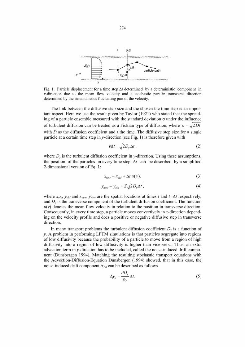
274

Fig. 1. Particle displacement for a time step Δt determined by a deterministic component in x-direction due to the mean flow velocity and a stochastic part in transverse direction determined by the instantaneous fluctuating part of the velocity.

The link between the diffusive step size and the chosen the time step is an impor-tant aspect. Here we use the result given by Taylor (1921) who stated that the spread-ing of a particle ensemble measured with the standard deviation σ under the influence of turbulent diffusion can be treated as a Fickian type of diffusion, where 2 Dt=σ with D as the diffusion coefficient and t the time. The diffusive step size for a single particle at a certain time step in y-direction (see Fig. 1) is therefore given with

2 ,yv t D tΔ = Δ (2)

where Dy is the turbulent diffusion coefficient in y-direction. Using these assumptions, the position of the particles in every time step Δt can be described by a simplified 2-dimensional version of Eq. 1:

( ) ,new oldx x t u y= + Δ (3)

2 ,new old yy y Z D t= + Δ (4)

where xold, yold and xnew, ynew are the spatial locations at times t and t+Δt respectively, and Dy is the transverse component of the turbulent diffusion coefficient. The function u(y) denotes the mean flow velocity in relation to the position in transverse direction. Consequently, in every time step, a particle moves convectively in x-direction depend-ing on the velocity profile and does a positive or negative diffusive step in transverse direction.

In many transport problems the turbulent diffusion coefficient Dy is a function of y. A problem in performing LPTM simulations is that particles segregate into regions of low diffusivity because the probability of a particle to move from a region of high diffusivity into a region of low diffusivity is higher than vice versa. Thus, an extra advection term in y-direction has to be included, called the noise-induced drift compo-nent (Dunsbergen 1994). Matching the resulting stochastic transport equations with the Advection-Diffusion-Equation Dunsbergen (1994) showed, that in this case, the noise-induced drift component Δyn can be described as follows

.yn

Dy t

y∂

Δ = Δ∂

(5)

275

If Eq. 4 is extended with the given expression for the noise-induced drift compo-nent (Eq. 5), the transport problem with varying diffusivity is described consistently with the Advection-Diffusion-Equation.

( )

2 ( ) ynew old y

D yy y Z D y t t

y∂

= + Δ + Δ∂

(6)

The outcome of a LPTM simulation are x and y-positions of every single particle at every time step. By analyzing the statistics of the particle positions, information about the transport characteristics can be determined. The one-dimensional longitudi-nal dispersion coefficient DL, as a measure of the spatially averaged spreading rate of a tracer cloud, can be determined by calculating the time change of the longitudinal variance of the particle distribution (Rutherford 1994) as follows

2 2

2 1

2 1

( ) ( )1 .2

x xL

t tDt t

σ − σ=

− (7)

Further results would be the skewness of the particle cloud and the transport velocity.

2.1 Boundary conditions The boundaries of the calculation domain and how they act on the particles have to be defined. The inflow and outflow boundaries do not affect the particles as in our case the domain has an infinite length. In y-direction there are two possibilities for the boundaries. If we analyze the effect of vertical shear on dispersion, we have the water surface as well as the channel bottom. In case of horizontal shear flow the boundaries represent the channel banks. For both situations the boundaries act as reflective walls. The effect of dead-water zones on the mass transport is increased stretching of the tracer cloud in longitudinal direction and reduced transport velocity. Both effects sit in the typical time that a particle needs to get back into the main stream after it was trapped in the dead-water zone. This time is called the storage time TD. In the present study this effect is introduced into the LPTM with a modified boundary condition, such that this boundary simulates the behavior of mass trapping and mass release. Thus, the interface between main channel and dead-water zone has to act as a tran-sient-adhesion boundary, which means that particles that reach such a boundary are fixed to that position until TD has passed.

2.2 Model verification A quantitative verification of the LPTM is presented in the following by comparing the results with analytical solutions of the Advection-Diffusion-Equation. In order to test also the formulation of the drift-noise adjustment a case with inhomogeneous dif-fusion regime has to be used. Such a case is the solution of the ADE equation given by Elder (1959) for unbounded shear flow, where the turbulent diffusivity is assumed to follow a parabolic distribution over the water depth.

(1 / )yD u y y h∗= κ − (11)

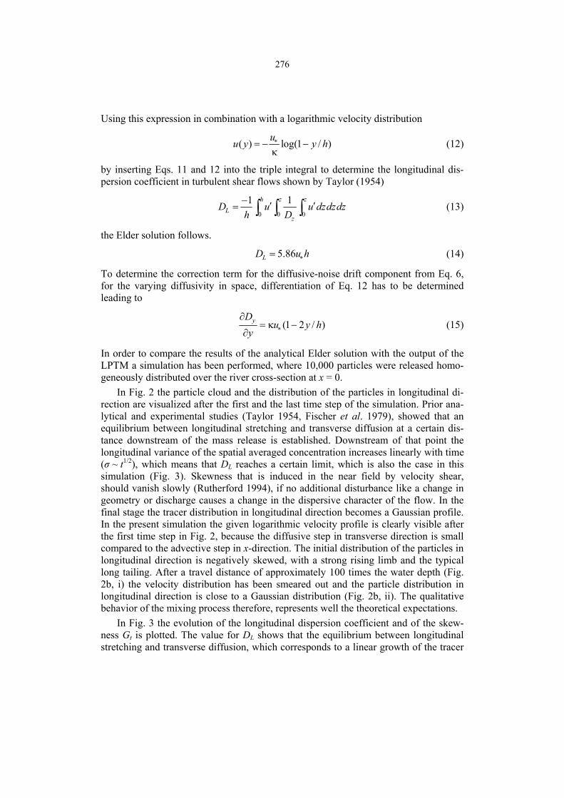
276

Using this expression in combination with a logarithmic velocity distribution

( ) log(1 / )uu y y h∗= − −κ

(12)

by inserting Eqs. 11 and 12 into the triple integral to determine the longitudinal dis-persion coefficient in turbulent shear flows shown by Taylor (1954)

0 0 0

1 1h z z

Lz

D u u dzdzdzh D− ′ ′= ∫ ∫ ∫ (13)

the Elder solution follows.

5.86LD u h∗= (14)

To determine the correction term for the diffusive-noise drift component from Eq. 6, for the varying diffusivity in space, differentiation of Eq. 12 has to be determined leading to

(1 2 / )yDu y h

y ∗

∂= κ −

∂ (15)

In order to compare the results of the analytical Elder solution with the output of the LPTM a simulation has been performed, where 10,000 particles were released homo-geneously distributed over the river cross-section at x = 0.

In Fig. 2 the particle cloud and the distribution of the particles in longitudinal di-rection are visualized after the first and the last time step of the simulation. Prior ana-lytical and experimental studies (Taylor 1954, Fischer et al. 1979), showed that an equilibrium between longitudinal stretching and transverse diffusion at a certain dis-tance downstream of the mass release is established. Downstream of that point the longitudinal variance of the spatial averaged concentration increases linearly with time (σ ~ t1/2), which means that DL reaches a certain limit, which is also the case in this simulation (Fig. 3). Skewness that is induced in the near field by velocity shear, should vanish slowly (Rutherford 1994), if no additional disturbance like a change in geometry or discharge causes a change in the dispersive character of the flow. In the final stage the tracer distribution in longitudinal direction becomes a Gaussian profile. In the present simulation the given logarithmic velocity profile is clearly visible after the first time step in Fig. 2, because the diffusive step in transverse direction is small compared to the advective step in x-direction. The initial distribution of the particles in longitudinal direction is negatively skewed, with a strong rising limb and the typical long tailing. After a travel distance of approximately 100 times the water depth (Fig. 2b, i) the velocity distribution has been smeared out and the particle distribution in longitudinal direction is close to a Gaussian distribution (Fig. 2b, ii). The qualitative behavior of the mixing process therefore, represents well the theoretical expectations.

In Fig. 3 the evolution of the longitudinal dispersion coefficient and of the skew-ness Gt is plotted. The value for DL shows that the equilibrium between longitudinal stretching and transverse diffusion, which corresponds to a linear growth of the tracer

277

cloud, is reached after approximately 12 water depths. At this distance, DL has attained its final value of 5.86u*h in agreement with the analytical prediction by Elder. The DL curve has been smoothed, in order to show the mean behavior of the tracer cloud. Without filtering an increased scatter could be observed, due to the increasing error that is produced by determining the standard deviation σx that gets larger with increas-ing width of the tracer cloud.

Fig. 2. Lagrangian particle tracking simulation of the Elder’s case with unbounded shear flow and a parabolic distribution of the diffusivity over the water depth; (i) side view into the chan-nel, showing the particle positions after the first (a) and the last (b) time step; (ii) showing the particle density cross-sectionally averaged in longitudinal direction.

Fig. 3. Evolution of the longitudinal dispersion coefficient DL and the skewness Gt during the LPTM simulation. DL is smoothed with a sliding average filter of increasing window size.

3. Application

In the following the proposed method is used to predict the transport characteristics in the river Rhine near Karlsruhe between km 351 and km 376. The results are compared with tracer experiments (van Mazijk 2002, Behr 2001) that have been performed to calibrate the Rhine Alarm Model (RAM) (Spreafico et al. 1993).

Fig. 4 shows a downstream view of the Rhine at km 362 at low water conditions, where the groins are emerged and the flow in the groin fields is very weak.

278

Fig. 4. Downstream view of a groin regulated river reach at low water conditions (river Rhine near Karlsruhe at km 362).

In that reach the Rhine is about 315 m wide (including the groin fields), the mean discharge Q is around 1200 m³/s and the bottom slope is approximately 0.015% (Behr 2001). The groin fields cover approximately 30% of the channel width B so that the effective width of the main channel is about 210 m in case of low water conditions (see Table 1). An averaged groin field in this river section has been determined to a distance L between two groins to 190 m and a width of the groin field W of 105 m.

Table 1

Averaged flow conditions in the River Rhine between km 351 and km 376 for tracer test 9/90 4/89 and 6/91 (Behr 2001)

Tracer test

River section

Bottom slope Discharge Width

B Main

ChannelWaterdepth

Flow vel.U

Groin fields L W

[km] [m³/s] [m] [m] [m] [m/s] [m] [m]

9/90 351−376 0.015% 628 315 210 1.9 1.05 190 105 emerged

4/89 351−376 0.015% 1560 315 315 3.5 1.42 190 105 submerged

6/91 351−376 0.015% 1811 315 315 3.8 1.50 190 105 submerged

An LPTM simulation has been performed first, to reproduce the transport charac-teristics determined with the tracer test 9/90 for low water conditions where the groins are emerged. The transverse depth averaged velocity profile is approximated with a parabolic velocity profile

18

max( ) 1 2 1 ,yu y UB

⎛ ⎞⎛ ⎞⎜ ⎟= − −⎜ ⎟⎜ ⎟⎝ ⎠⎜ ⎟

⎝ ⎠

(15)

where Umax is the maximum velocity in the main channel, W the river width, or the main channel width. In the simulation Umax is adjusted to match the overall discharge.

The transverse diffusivity Dy is set constant, according to Fischer (1979) to D = 0.6u*h with u* as the bottom shear velocity and h the mean water depth. Because in the case of low water conditions the groins are emerged, the river width B repre-

279

senting the simulation domain is reduced from 315 m to the effective main channel width of 210 m. To model the effect of dead-water zones as they are given in this river reach by groin fields in one of the channel banks the modified reflective boundary namely the transient adhesion-boundary (see Section 2.1) is introduced using three different Storage times TD, namely 0, 130 and 515 seconds. The simulation parameters are listed in Table 2.

Table 2

Parameter values for LPTM simulation and resulting dispersion coefficients

Run No.

Tracer test Q River

width u(y) No. of time steps Δt Dy

No. of particles

Storage time TD

Dispersion coefficient

[m³/s]

[m]

[m/s]

[ ]

[s]

[m²/s]

[ ]

[s]

LPTM [m²/s]

Tracer [m²/s]

1 9/90 628 210 Eq 15 2 105 2 0.6 u* h 3000 0 1500 8300

2 9/90 628 210 Eq 15 2 105 2 0.6 u* h 3000 130 8400 8300

3 9/90 628 210 Eq 15 2 105 2 0.6 u* h 3000 515 40000 8300

4 4/89 1560 315 Eq 15 2 105 2 0.6 u* h 3000 130 6400 6700

5 6/91 1811 315 Eq 15 2 105 2 0.6 u* h 3000 130 7100 6600

Run No. 1 with TD = 0 s represents pure channel flow. The simulations 2 and 3 with TD = 130 and 515 s represent channel flow plus the interaction with dead-water zones. The resulting dispersion coefficients are summarized in Table 2. In run 2 the residence time TD = 130 has been fitted to match the measured dispersion coefficient from tracer test 9/90 (see Table 1 and Table 2). For run No. 3 the time TD = 515 s has been determined using the proposed relation from Jirka and Weitbrecht (2005) be-tween the dimensionless exchange coefficient k and a morphometric parameter RD based on a hydraulic radius like dimension of a typical groin field.

0.005 0.0035 DRkh

= + (16)

with

D

WkT U

= (17)

and

( )D

WLRW L

=+

(18)

where W is the length of a groin and L the distance between two groins. The resulting dispersion coefficients show, that dispersion due to pure channel flow (Run No. 1) strongly underestimates the stretching of the tracer cloud. On the other hand the simu-lation No. 3 using the proposed relation to predict the storage time TD strongly overes-timates the stretching effect and the corresponding dispersion coefficient by a factor of

280

four. One explanation could be that only a fraction of the total groin field volume is affecting the mass exchange (Lehmann et al. 1999). Van Mazijk (2005) concluded that ‘Natural Dead Zones’, comprising the effect of all regions in a river with low flow velocities, are strongly dominating the stretching effect compared to the specific effect of groin fields. Following that argument the determined storage time TD is much less depending on the existence or the shape of groin fields than the overall heterogeneity of the river.

In a second step the same river stretch has simulated for the high water conditions (tracer study 6/91 and 4/89, see Table 1 and Table 2), where the groins are submerged. Under these conditions a clear distinction between main channel and the complete river width is not possible any more. In that case the effective width of the main chan-nel is set equal to the overall width of the river. The storage time TD = 130 s has not been changed compared to the calibrated one in run No. 2. The resulting dispersion coefficients of simulations 4 and 5 are still comparable to the determined values measured in the field. If the storage effect in the groin fields would be a dominant effect, the resulting storage time should be considerably different, compared to the emerged conditions. Under submerged conditions, depending on the submergence level the storage effect should vanish more and more, until the groin represents just a roughness element on the river bed.

4. Conclusions

In the current study a Lagrangian-Particle-Tracking-Method (LPTM) based on random walk simulations has been evaluated for the prediction of mass transport characteris-tics in turbulent channel flow. Analytical solutions of the Advection-Diffusion-Equation can be reproduced with the given model formulation, if a sufficient number of particles is used and the chosen time steps are appropriate. Biasing effects due to varying diffusivity in the simulation domain have to be suppressed by a correction term for the diffusive-noise drift component To include the effect of dead-water zones, one of the reflective boundaries has been modified to a transient adhesion boundary condition. This boundary contains information about the typical residence time of mass in the dead-water zone.

The LPTM has been applied to a river stretch of the Rhine where extensive tracer tests have been performed during the development of the Rhine-Alarm-Model (Spre-afico 1993). Without the additional effect of a certain storage capacity the dispersive effect is strongly underestimated. The prediction of the storage time using the relation given by Jirka and Weitbrecht (2005), leads to a strong overestimation of the disper-sion coefficient. Using a calibrated moderate storage time the dispersive character could be represented for different hydrological conditions, leading to the conclusion that the mass exchange between main stream and groin field is not the dominating dead-water effect, which is in agreement with observations made by van Mazijk and Veling (2005).

In order to predict mass transport in case of accidental pollutant spills a sound un-derstanding of the different physical transport processes and especially their relative

281

influence compared to each other is important. On the other hand it can be concluded that errors in the representation of the hydrological conditions will always control the accuracy of the predicted transport scenario.

References

Aris, R., 1959, The longitudinal diffusion coefficient in flow through a tube with stag-nant pockets, Chemical Engineering Science 11, 194-198.

Behr, M., 2001, Analyse der Verzögerung des Strofftransportes im Rhein zwischen Speyer und Mainz, Diploma Thesis, TU Delft and TU Darmstadt.

Czernuszenko, W., and P.M. Rowiński, 1997, J of Hydr. Res. (4), 491-504. Dunsbergen, D.W., 1994, Particle Models for Transport in Three-Dimensional Shal-

low Water Flow, PhD thesis, Tu-Delft, Faculty of Civil Engineering. Elder, J., 1959, The dispersion of marked fluid in turbulent shear flow, J. Fluid Mech.

5, 544-560. Fischer, H.B., E.J. List, R.C.Y. Kohl, J. Imberger and N.H. Brooks, 1979, Mixing in

Inland and Coastal Waters, Academic Press, New York. Hays, J.R., P.A. Krenkel and K.B. Schnelle, 1966, Mass transport mechanisms in

open-channel flow, Technical Report 8, Vanderbildt University, Nashville Tennes-see.

Hunter, J., P. Graig and H. Phillips, 1993, On the use of random walk models with spatially variable diffusivity, Computational Physics 106, 366-376.

Jirka, G.H., and V. Weitbrecht, 2005, Mixing Models for Water Quality Management in Rivers: Continuous and Instantaneous Pollutant Releases. In: W. Czernuszenko and P. Rowiński, (Eds.), Water Quality Hazards and Dispersion of Pollutants, pp. 1-34, ISBN 0387233210, Springer, New York.

Kinzelbach, W., S. Zimmerman and P. Koumoutsakos, 2001, Simulation of pollutant transport using a particle method, J. of Computational Physics 173, 322-347.

Lehmann, D., W. Uijttewaal, A. van Mazijk and V. Weitbrecht, 1999, Auswirkung von Buhnenfeldern auf den Transport gelöster Stoffe in Flüssen, TU-Delft, Dept. of Fluid Mechanics.

Rutherford, J.C., 1994, River Mixing, Wiley, Sussex, England. Spreafico, M., and A. van Mazijk, 1993, Alarmmodell Rhein; Ein Modell für die ope-

rationelle Vorhersage des Transportes von Schadstoffen im Rhein, CHR-Report Nr. 1-12.

Sullivan, P.J., 1979, Longitudinal dispersion within a two-dimensional turbulent shear flow, J. of Fluid Mechanics 49, 551-576.

Taylor, G.I., 1954, The dispersion of matter in turbulent flow through a pipe, Proc. Royal Soc., London, Vol. 233, pp. 446-468.

Taylor, G.I., 1921, Diffusion by continuous movements, Proc. London Math Soc. 20, 196-211.

282

van Mazijk, A., and E.J.M. Veling, 2005, Tracer experiments in the Rhine Basin: evaluation of the skewness of observed concentration distributions, Journal of Hy-drology 307 (2005) (1-4), pp. 60–78.

Van Mazijk A., 2002, Modelling the effects of groyne fields on the transport of dis-solved matter within the Rhine Alarm-Model, J. of Hydrology 264, 213-229.