UNIVERSIDADE DE LISBOA

FACULDADE DE CIÊNCIAS

DEPARTAMENTO DE FÍSICA

Synchronization Phenomena withNonlinear Oscillators

Dissertação

José Manuel Macedo Cota Barros

Mestrado em Física

(Área de Especialização Física Estatística e Não Linear)

2013

UNIVERSIDADE DE LISBOA

FACULDADE DE CIÊNCIAS

DEPARTAMENTO DE FÍSICA

Synchronization Phenomena withNonlinear Oscillators

Dissertação

José Manuel Macedo Cota Barros

Mestrado em Física(Área de Especialização Física Estatística e Não Linear)

Orientação: Professora Doutora Ana Maria Ribeiro Ferreira Nunes

2013

∼ To The Memory Of My Father ∼

Contents

1 Introduction 1

1.1 Motivation . . . . . . . . . . . . . . . . . . . . . . . . . . . . 21.1.1 The van der Pol Oscillator . . . . . . . . . . . . . . . . 21.1.2 Coupling . . . . . . . . . . . . . . . . . . . . . . . . . 2

1.2 Background . . . . . . . . . . . . . . . . . . . . . . . . . . . . 41.2.1 Topology . . . . . . . . . . . . . . . . . . . . . . . . . 41.2.2 Detuning . . . . . . . . . . . . . . . . . . . . . . . . . 51.2.3 Phase . . . . . . . . . . . . . . . . . . . . . . . . . . . 61.2.4 Coupling Function . . . . . . . . . . . . . . . . . . . . 6

1.3 Krylov-Bogoliubov Averaging Method . . . . . . . . . . . . . 71.3.1 First Approximation . . . . . . . . . . . . . . . . . . . 8

2 Synchronization 11

2.1 Equation of Motion for Two Oscillators . . . . . . . . . . . . 122.1.1 Topology . . . . . . . . . . . . . . . . . . . . . . . . . 122.1.2 Output Functions . . . . . . . . . . . . . . . . . . . . 122.1.3 Mutual Synchronization . . . . . . . . . . . . . . . . . 13

2.2 Phase Dierence . . . . . . . . . . . . . . . . . . . . . . . . . 142.2.1 Quasi-Harmonic Solutions . . . . . . . . . . . . . . . . 142.2.2 Derivation of the Phase Dierence Equation . . . . . . 16

2.3 Numerical Study . . . . . . . . . . . . . . . . . . . . . . . . . 182.4 Resume of the Chapter . . . . . . . . . . . . . . . . . . . . . . 20

3 Coupling Circuits 21

3.1 The van der Pol Oscillator . . . . . . . . . . . . . . . . . . . . 223.1.1 Voltage Equation . . . . . . . . . . . . . . . . . . . . . 23

3.2 The Coupling Function . . . . . . . . . . . . . . . . . . . . . . 253.2.1 Simplifying the Variables . . . . . . . . . . . . . . . . 27

4 On the Two Oscillators 31

4.1 Background . . . . . . . . . . . . . . . . . . . . . . . . . . . . 314.1.1 Scaling of Time . . . . . . . . . . . . . . . . . . . . . . 324.1.2 Amplitude Dependence on the Parameter µ . . . . . . 33

i

4.1.3 κ Parameter . . . . . . . . . . . . . . . . . . . . . . . 334.1.4 Attributing Values to the Parameters . . . . . . . . . 34

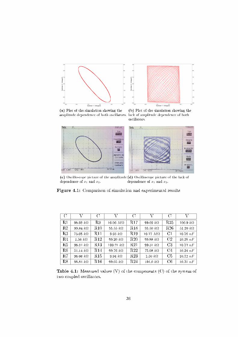
4.2 The Coupled Circuit . . . . . . . . . . . . . . . . . . . . . . . 354.3 Mathematical Enforcement . . . . . . . . . . . . . . . . . . . 37

4.3.1 Denition of the Phase . . . . . . . . . . . . . . . . . . 374.4 Plot of the Solutions . . . . . . . . . . . . . . . . . . . . . . . 38

5 On the Three Oscillators 41

5.1 One More . . . . . . . . . . . . . . . . . . . . . . . . . . . . . 415.1.1 Equation of Motion . . . . . . . . . . . . . . . . . . . 425.1.2 Krylov-Bogoliubov Averaging Method . . . . . . . . . 435.1.3 Numerical Study . . . . . . . . . . . . . . . . . . . . . 44

5.2 The circuit . . . . . . . . . . . . . . . . . . . . . . . . . . . . 455.2.1 Coupling Function . . . . . . . . . . . . . . . . . . . . 455.2.2 Results and Discussion . . . . . . . . . . . . . . . . . . 47

6 A Lot of Oscillators 51

6.1 The Interaction . . . . . . . . . . . . . . . . . . . . . . . . . . 516.1.1 Nearest Neighbours Interaction . . . . . . . . . . . . . 53

6.2 Integration . . . . . . . . . . . . . . . . . . . . . . . . . . . . 556.3 Frequency Vector . . . . . . . . . . . . . . . . . . . . . . . . . 57

6.3.1 Range . . . . . . . . . . . . . . . . . . . . . . . . . . . 576.3.2 Order . . . . . . . . . . . . . . . . . . . . . . . . . . . 57

6.4 Closure . . . . . . . . . . . . . . . . . . . . . . . . . . . . . . 59

A Equivalence Between van der Pol Equations 63

B Limit Cycle of the van der Pol Oscillator 65

C Perturbation Theory 67

D Fourier Coecients 71

E Derivation of the Approximate Equation of Motion 73

F Derivation of the Output Expressions of Electronic Parts 75

G The Circuits 79

ii

List of Figures

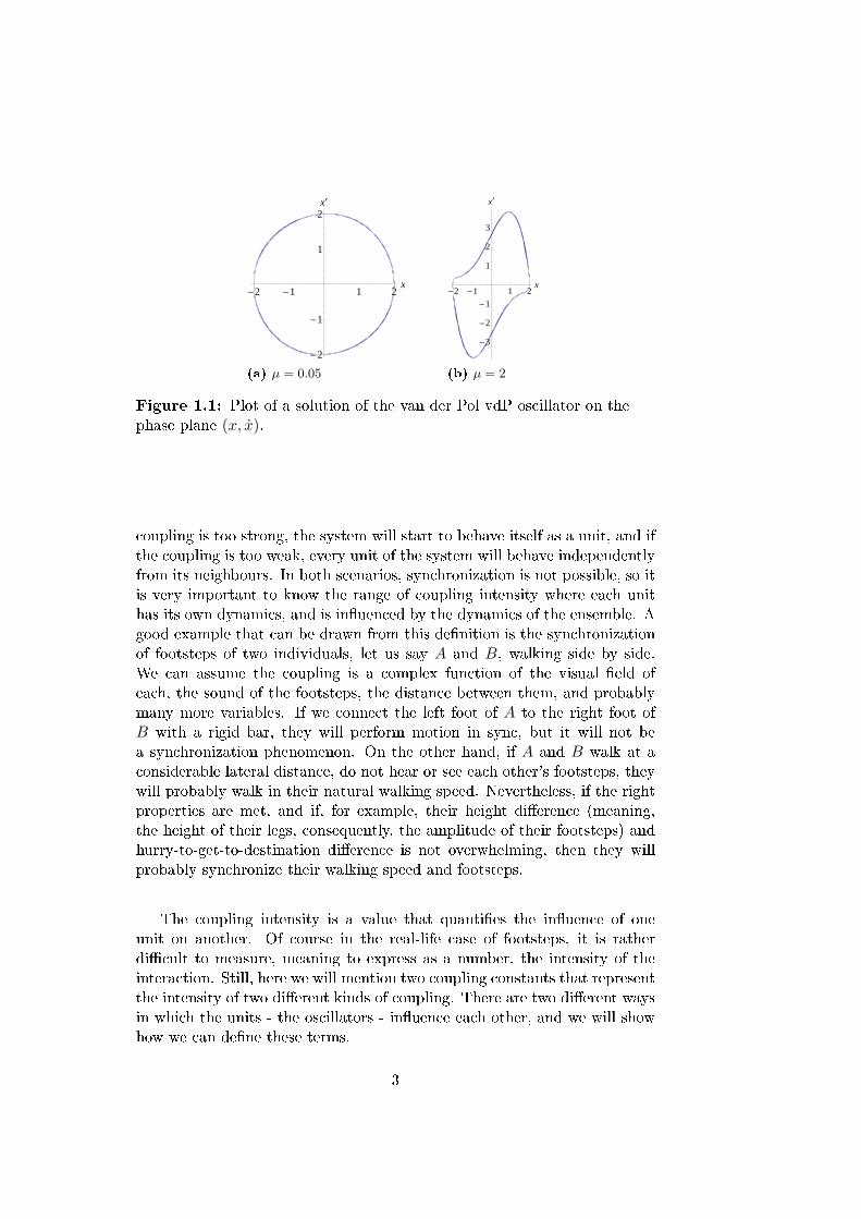
1.1 Plot of a solution of the van der Pol vdP oscillator on thephase plane (x, x). . . . . . . . . . . . . . . . . . . . . . . . . 3

1.2 Example of a graph with 5 nodes. . . . . . . . . . . . . . . . . 5

2.1 Graph with two nodes (vertices) and a line (edge). . . . . . . 12

3.1 Parts of the vdP Circuit . . . . . . . . . . . . . . . . . . . . . 223.2 Circuit model of the vdP oscillator, representing the oscillator

1. . . . . . . . . . . . . . . . . . . . . . . . . . . . . . . . . . . 233.3 Circuit model of the vdP oscillator, representing the oscillator

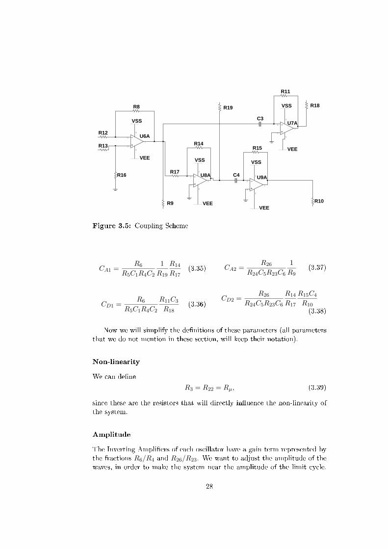
1. . . . . . . . . . . . . . . . . . . . . . . . . . . . . . . . . . . 253.4 Parts of the Coupling Function . . . . . . . . . . . . . . . . . 273.5 Coupling Scheme . . . . . . . . . . . . . . . . . . . . . . . . . 28

4.1 Comparison of simulation and experimental results . . . . . . 364.2 Plot of the solutions representing the phase dierence, using

numerical N and KB methods. . . . . . . . . . . . . . . . . . 39

5.1 Graph with Three Simply Connected Nones . . . . . . . . . . 425.2 Plot of a solution for three coupled oscillators with KB method 455.3 Numerical integration of three coupled vdP oscillators . . . . 465.4 Comparison between KG and numerical integration of three

coupled vdP oscillators . . . . . . . . . . . . . . . . . . . . . . 465.5 Non-Inverting Weighted Summer . . . . . . . . . . . . . . . . 475.6 Non-Inverting Amplier . . . . . . . . . . . . . . . . . . . . . 485.7 Scheme of the coupling function needed for each oscillator in

the coupling of three units . . . . . . . . . . . . . . . . . . . . 495.8 Comparison of dierent approaches for the three coupled os-

cillators . . . . . . . . . . . . . . . . . . . . . . . . . . . . . . 50

6.1 Graphs with ten nodes each . . . . . . . . . . . . . . . . . . . 536.2 Two dierent graphs with 4 and 5 nodes respectively, to il-

lustrate which nearest neighbours terms will aect each unit . 546.3 Plot on the unit circle of the phase dierence between every

pair of oscillators in a ring of ten oscillators . . . . . . . . . . 56

iii

6.4 Plot of the nal conguration (at t = 500) of the phase dif-ferences from ωi ∈ [0.99, 1.01] to ωi ∈ [0.8, 1.2]. . . . . . . . . 58

6.5 Plots with ω ∈ [0.85, 1.15] random (R) and optimised (O) . . 606.6 Plots with ω ∈ [0.90, 1.10] random (R) and optimised (O) . . 616.7 Plots with ω ∈ [0.95, 1.05] random (R) and optimised (O) . . 62

C.1 Numerical (blue, thick line) and perturbative (purple, dashedline) solutions of the vdP oscillator for ω = 1 and µ = 0.05. . 69

G.1 Picture of the whole circuit of 2 and 3 coupled oscillators . . 79G.2 Circuit scheme of two coupled oscillators. . . . . . . . . . . . 80

iv

Nomenclature

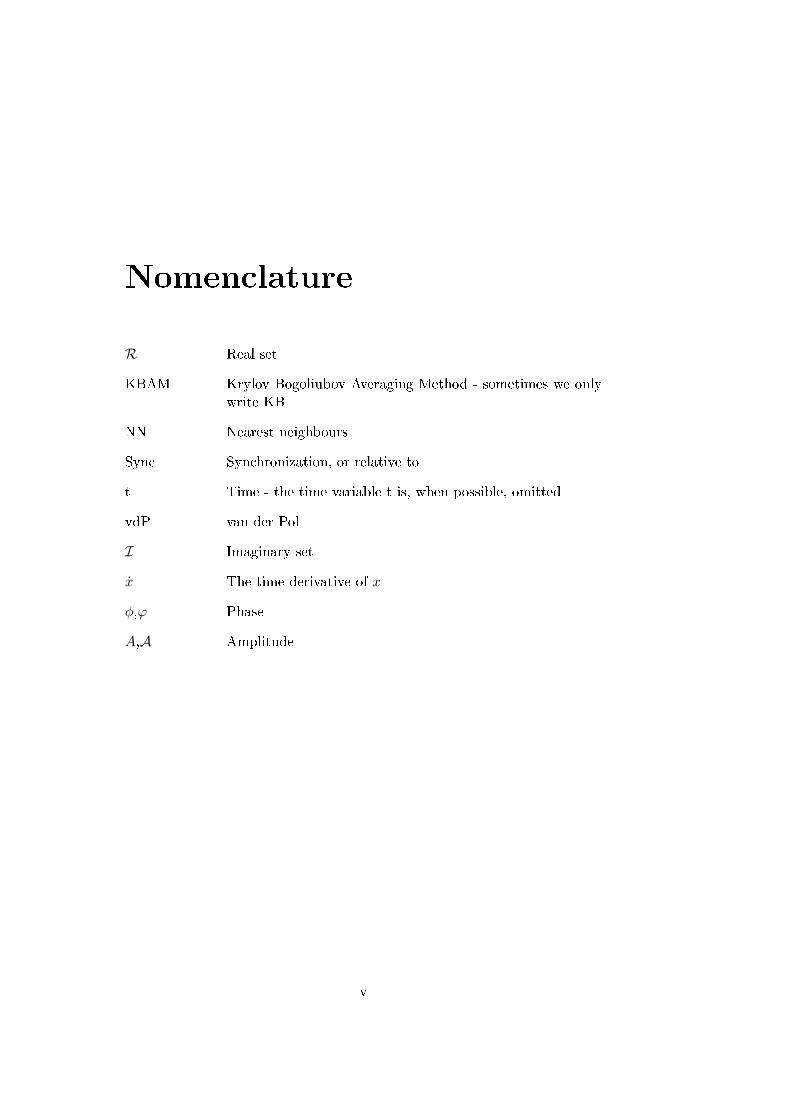
R Real set

KBAM Krylov Bogoliubov Averaging Method - sometimes we onlywrite KB

NN Nearest neighbours

Sync Synchronization, or relative to

t Time - the time variable t is, when possible, omitted

vdP van der Pol

I Imaginary set

x The time derivative of x

φ,ϕ Phase

A,A Amplitude

v

Preface

The energy of a single thought may determine the motion of

a universe.

NIKOLA TESLA

Nature is an innite network of interacting objects. The idea of interactingitself is redundant - interaction is what we can observe, but in fact we arewatching the result of nature's dynamical motion as a whole, in a particulardomain. In this work we discuss synchronization, a state where dierentunits in nature evolve together. The goal is to provide information aboutthis subject, and it is directed to anyone. The language herein is trulysimple, and every complicated detail is explained. In the margins you willnd names of les contained in the multimedia appendix - these les wereprogrammed by me inMathematica. Sync is linked to topics in mathematics,physics, chemistry, biology, psychology, sociology, and many more, so anyonewho wants to know more will enjoy this work.

The opportunity to do this work came up before the end of my bachelorsdegree, when I had to choose a topic to do a sort of short bachelor's thesis.This topic and its vastness intrigued me so much that I decided to do it as mymaster's thesis. It has been two and a half years of blood, sweat and tears, ,pardon the cliché. There were some good and bad moments, and the truth isthat in science the word easy is rare, being much more frequent words likehard or impossible. That emphasizes the beauty of nature. Sometimes,after weeks of trying to understand small issues, the answer would somewhatmagically emerge in my head, like it was inevitable to look that way andgure out that all previous thoughts were too manufactured to the naturalcomplexity. Understanding, or trying to understand, the dynamics of life isastonishing. Together with my supervisor, we tried to deliver a simple, easyto read, work, based on our dedication to clarify this topic. Small organizedchapters will lead the reader from the rst word of Introduction, to the lastword of the Conclusion, with the help of guided appendices at the end.

This very work would not be possible without the help and guidanceof my supervisor Ana Nunes, who built the idea from scratch. Even withtremendous troubles found during the project, was always present to dodge

vii

them and be the mastermind of the project. Her determination and ambitionare a reection of her amazing background and curriculum, which led herto a place only a few can attain, conquered by the hard workers.

I am very thankful to all Professors who, somehow, helped me in myacademic or personal life, especially to Guiomar Evans who helped me withthe experimental parts.

I want to thank Marta for the review on the thesis, without which itwould look a lot worst. Also her love and support were essential to progressand nish my work, and I am thankful for that.

My colleagues know what I have been doing for the past few years, andmost of them participated directly in the quest for answering the complexquestions this work delivered. Some of the questions we found in our workoriginated long and healthy arguments between me and my colleagues, whichconsequently led to a lot of very nice afternoons. Their help and supportwere essential to keep my mental health sane. To all of them, and theircritical thinking, my deepest thank you.

To all my family who always supported me in order to succeed in theacademic life, and believed I could become someone they could be proud ofsomeday. Hopefully I can deliver that feeling from now on.

My dearest friends and their unstoppable love. All the moments thatwould make the problems seem small or just fade away for a while, weredenitely due to you. Without you this work would be impossible, becauseno person can live without his chosen family. I thank you for your love.

I want to thank Monte Abraão, a place where people learn the hard life,where connections are more important than money, and where you have togrow up really quick. Without my childhood, I would probably had becomesomeone incapable of facing such a hard goal. It helped me realise, reallysoon, that what matters is that you do not give up on your dreams. If youkeep working for them, you will win.

One very important acknowledgement has to be done to the reader.The reason why people learn and science is made, is to develop commonknowledge by delivering it to the world. So, I want to thank the reader,for caring enough to learn and spread information, and making this world alittle better and more informed.

Finally, I want to thank nature itself, for being the most interesting,complex, innocent, pure, amazing, and magnicent thing of all. All my loveand hard work is fruit of your beautiful mysteries.

José BarrosAugust 2013, Lisboa, Portugal

viii

Abstract

Synchronization is a state in nature in which a dynamical system of multipleobjects evolve together in a coupled motion. The most fundamental case inmathematics is the case of two coupled self-sustained oscillators, which isthe starting point of this work. Coupled nonlinear oscillators is a subjectrelated to many areas of science, from biology to economy. In this study weemphasize nearest neighbours coupling of systems of van der Pol oscillators,with an arbitrary coupling we refer in the text. In chapter 1 we introducesome denitions that are important to the understanding of the basic ideasbehind synchronization. Some notions are related to topology and graphtheory. Next, we develop a method to analyse coupled nonlinear dierentialequations, the Krylov-Bogoliubov method. We end chapter 1 discussing theimportance of an equation for the phase dierence, which should result ina constant value after transient into a synchronous regime. The mathemat-ical tools showed in chapter 1 are used in chapter 2 in a analytical (polarcoordinates transformation) and numerical (Krylov-Bogoliubov) analysis oftwo coupled van der Pol oscillators. The experimental part comes in chapter3, where we build a circuit model which reproduces the coupled equations.The idea is to analyse, experimentally, the synchronization of oscillators,with a mathematical basis. In chapter 4 we end the analysis of two oscil-lators with a résumé of the theoretical and experimental results, with plotsand conclusions. In chapter 5 we repeat the whole study for three coupledoscillators, in order to simulate the coupling terms for this case, and see thedierences from the two oscillators case. This will result in the basis forthe n oscillators case we deal in chapter 6, where we analyse ten coupledoscillators and its stability to changes in frequency range, and the order ofthe units in the ensemble.

Keywords: Synchronization, van der Pol, Dierential Equations, NonLinear, Coupling, Circuits

ix

Resumo

A sincronização é um fenómeno sobre organização, ou estados organizados, eque pode ser observado na natureza. Neste trabalho foi imposto o objetivo deestudar e observar este fenómeno, usando ferramentas matemáticas e labo-ratoriais. Como base para o trabalho foi escolhido o caso de dois osciladoresacoplados. Este é o estado fundamental da dinâmica coletiva de sistemasacoplados, ou seja, mesmo no estudo de vários osciladores acoplados (n > 2),a dinâmica fundamental é a de primeiros vizinhos. Sabendo as condiçõesnecessárias, nomeadamente, a necessidade de um oscilador autossustentado,seguiu-se o modelo do oscilador de van der Pol, que é representado por umaequação diferencial não linear e homogénea.

A dinâmica de osciladores acoplados é um estudo atualmente bastantedesenvolvido, o que o torna muito diversicado. Sabendo que um modelomatemático um oscilador autossustentado pode modelar o batimentocardíaco, as reações químicas, os pêndulos, e muitos outros casos, o problemainicial é tentar compreender numa expressão geral o acoplamento. Sem levaro estudo da estabilidade à exaustão, referimos que para sistemas da formado oscilador de van der Pol, com um acoplamento arbitrário que dependadas posições e velocidades, o sistema apresenta regimes estáveis. Destaforma, achámos interessante estudar, em particular, um acoplamento deprimeiros vizinhos, através de uma constante denominada de constante deacoplamento.

No capítulo 1 é apresentada uma introdução ao tópico de sincronização,ao oscilador de van der Pol, e à função de acoplamento. São utilizadas noçõesde topologia, de teoria de grafos, e dos sistemas dinâmicos na construçãode uma base sólida para escrever as equações acopladas, justicando os ter-mos de acoplamento. Neste mesmo capítulo são introduzida outras noçõesimportantes na compreensão do fenómeno e dos seus resultados, tal comofase, detuning, matriz de Kirchho e matriz de output. Como queremos sa-ber resultados para as equações, foi igualmente necessária uma pesquisa demétodos perturbativos para resolução de equações diferenciais não linearesacopladas, a qual resultou no método desenvolvido por Nikolay Krylov e Ni-kolay Bogoliubov. Este é um método que mostra que, para certas condições,podemos considerar a fase e a amplitude constantes durante um período daoscilação, e como tal, podemos tomar a média temporal. Este método é

xi

desenvolvido no nal do capítulo 1. É também justicada a necessidade de,para dois osciladores, encontrarmos uma equação da evolução da sua dife-rença de fase, o que nos dará uma medida para determinar se ocorreu, ounão, sincronização, visto que o sucesso implica que a diferença de fase, apóstransiente, deverá ser constante. Para o caso de mais osciladores, trataremosde estudar a diferença de fase entre cada 2 vizinhos.

No capítulo 2 tratamos a sincronização em sua plenitude, voltando aapresentar as equações e resolvendo-as analiticamente e usando o métodoaproximado de Krylov-Bogoliubov de forma a se obter a expressão para adiferença de fase, mostrando passo-a-passo a sua dedução. Depois voltamosa resolver as equações mas desta feita numericamente, utilizando uma mu-dança de variáveis para coordenadas polares e obtendo expressões explícitaspara as fases e as amplitudes de cada oscilador, e integrando a diferença defase entre eles. Neste capítulo o objetivo passa por derivar estas equações,sendo que os resultados são apresentados no capítulo 4 depois de se realizara parte experimental no capítulo 3.

No capítulo 3 começamos por desenvolver as bases necessárias à apli-cação experimental que traduza o comportamento do sistema acoplado. Ouso de circuitos para comprovar experimentalmente a teoria é algo que foisempre aceite no meio cientíco, e serve de aplicação prática rápida. Éapresentado um circuito e justicada a correspondência matemática a umoscilador de van der Pol, para o qual se denem as quantidades essenciaiscomo amplitude, e são apresentados os resultados de simulação e experimen-tais para o circuito. Em seguida é construído um circuito de acoplamentoque respeite a função matemática de acoplamento mostrada nos capítulosanteriores, chegando-se a um complicado modelo. Na última parte destecapítulo é apresentado o sistema completo, com dois osciladores e o aco-plamento, onde se faz o paralelismo entre os resultados de simulação e acorrespondente componente experimental. De notar que a base para talconstrução foi sempre um modelo teórico de um oscilador autossustentado,e um modelo teórico de uma função de acoplamento, e que o objetivo eracomprovar a base teórica apresentada nos capítulos 1 e 2, usando componen-tes físicas que não respeitam a 100% as expressões matemáticas, no entanto,o leitor poderá vericar que os resultados são muito satisfatórios.

No capítulo 4 confrontamos as ideias dos métodos teóricos e experimen-tais até então apresentados. O capítulo começa por um desenvolvimentodas ferramentas essenciais para se vericar a correspondência da teoria coma prática. O essencial problema neste tópico foi a denição das variáveise parâmetros da equação do oscilador de van der Pol como componentesdo circuito acoplado. Depois de uma analise pormenorizada ao circuito,mostram-se as guras de Lissajous que comprovam o fenómeno de sincroni-zação e a ligação com a teoria.

No capítulo 5 é apresentado um estudo similar ao conjunto dos capítulosanteriores, mas desta feita para 3 osciladores. A razão de se mostrar este

xii

caso particular baseia-se principalmente nos termos do acoplamento, que semodicam pelas alterações às partes teóricas e experimentais. São mostra-das as equações para o método numérico e o de Krylov-Bogoliubov, tantonos estados desacoplados como síncronos, e no m do capítulo, é apresentadoo procedimento experimental para 3 osciladores.

No capítulo 6 fechamos o nosso trabalho com a extensão do estudo amais osciladores acoplados segundo primeiros vizinhos. Depois de uma in-trodução a grafos mais complexos, surge a integração de 10 unidades deforma numérica. Em seguida estuda-se o fenómeno de sincronização sujeitoà variação dos parâmetros. É tomada especial atenção à distribuição defrequências naturais, ou seja, à heterogeneidade do sistema. Este capítuloserve também de conclusão, apesar de que depois o leitor pode encontrar umconjunto de anexos que servem de complementação ao apresentado durantea tese.

Palavras-Chave: Sincronização, van der Pol, Equações Diferenciais,Não Linear, Acoplamento, Circuitos

xiii

Chapter 1

Introduction

Nature performs complex phenomena in all scales. Scientists attemptto create theoretical, mathematical and computational models in or-der to know how these events work, and apply them to all subjects,

from physics and biology to sociology and psychology. One of nature's com-plex phenomenon is the core of this very work - synchronization. Synchron-ization is a complex dynamical process [1], that describes the adjustmentof rhythms, due to some coupling, between dierent objects that have somekind of oscillatory motion. This general denition encompasses a varietyof systems in nature, like the synchronous periodical ash of an ensembleof reies (biological oscillators [2]), in man-made systems, like electricaland chemical engineering [3], or a combination of both, like neuroscience [4],robotics [5], among many others. In the last ten years, a great enthusiasmfrom the scientic community, and the general public, has emerged. Still, wehave to go a few centuries back to 1660's to name its discoverer - ChristiaanHuygens [6]. He noticed that two pendula clocks with a non-rigid commonsupport connecting them, would synchronize.

The area of mathematics primarily involved in these studies is called dy-namical systems. The oscillatory objects mentioned above are modelled asautonomous dynamical systems, specically self-sustained oscillators. Theirmain characteristics are: an energy input to balance the dissipation in theoscillatory motion; no explicit time dependence - which implies that if f(t)is a solution, f (t+ ξ) is also a solution, for all ξ; and a well-dened amp-litude of the oscillations. If the system is perturbed, it returns to its stabletrajectory after a small transient. This reason will allow us to avoid study-ing the behaviour and evolution of the amplitude of the dynamical system.Moreover, these properties mean that stable regime does not depend oninitial conditions, and that the equations of motion have to be nonlinear -linear systems do not exhibit self-sustained oscillations. These self-sustainedoscillations correspond to limit cycles in the phase space of the system, i.e.,closed curves that represent the values taken by the variables associated

1

with the degrees of freedom.In this chapter we will discuss the fundamental ideas behind synchron-

ization, and the coupling of oscillators. We start with a description of thevan der Pol oscillator and its properties, and then move on to notions oncoupling, topology of the dynamical system, and a method that ensures thereliability of the procedures of the following chapters - the KBAM .

1.1 Motivation

The main character of this thesis is the van der Pol oscillator that is modelledby the following equation:

x (t)− µ(1− x2 (t)

)x (t) + ω2x (t) = 0, (1.1)

which can also be written as:

x (t)−(µ− x2 (t)

)x (t) + ω2x (t) = 0, (1.2)

with a change of variables x(t) = 1õx(t) - their equivalence is shown in

Appendix A. The parameters ω and µ are the natural frequency of theoscillator and a control parameter, respectively. The goal of this work is toshow, with an intensive analytical, numerical and experimental study, thatsynchronization emerges when vdP oscillators are coupled. The choice ofthis particular oscillator is not important, since we draw attention to thenearly harmonic oscillations in the small non-linearity range.

1.1.1 The van der Pol Oscillator

The van der Pol oscillator was introduced in the 1920′s by Balthasar van derPol (1889− 1959), and is an oscillator with nonlinear damping, expressedin equation 1.1, that exhibits self-sustained oscillations - a limit cycle in thephase space around its xed point (x, x) = (0, 0) (see Appendix B).

According to Liénard's theorem, the vdP oscillator has a unique stablelimit cycle, and a plot for µ = 0.05 can be seen in gure 1.1a . Although in

C1 & ApC - Limit Cycle

and Perturbative Solu-

tion.nb

this work we emphasize quasi-harmonic oscillations, i.e., the regime for µ1, the vdP oscillator is also known for its particular relaxation oscillations,i.e., for large µ - a corresponding plot of relaxation oscillations for µ = 2 isshown in gure 1.1b.

1.1.2 Coupling

In many complex systems, the complexity arises from the interplay of largenumber of constituents parts, or units, whose isolated behaviour may besimple and well understood. The interaction between the dierent units ofthe system is represented, in strength and in form, by coupling terms. If the

2

-2 -1 1 2x

-2

-1

1

2x¢

(a) µ = 0.05

-2 -1 1 2x

-3

-2

-1

1

2

3

x¢

(b) µ = 2

Figure 1.1: Plot of a solution of the van der Pol vdP oscillator on thephase plane (x, x).

coupling is too strong, the system will start to behave itself as a unit, and ifthe coupling is too weak, every unit of the system will behave independentlyfrom its neighbours. In both scenarios, synchronization is not possible, so itis very important to know the range of coupling intensity where each unithas its own dynamics, and is inuenced by the dynamics of the ensemble. Agood example that can be drawn from this denition is the synchronizationof footsteps of two individuals, let us say A and B, walking side by side.We can assume the coupling is a complex function of the visual eld ofeach, the sound of the footsteps, the distance between them, and probablymany more variables. If we connect the left foot of A to the right foot ofB with a rigid bar, they will perform motion in sync, but it will not bea synchronization phenomenon. On the other hand, if A and B walk at aconsiderable lateral distance, do not hear or see each other's footsteps, theywill probably walk in their natural walking speed. Nevertheless, if the rightproperties are met, and if, for example, their height dierence (meaning,the height of their legs, consequently, the amplitude of their footsteps) andhurry-to-get-to-destination dierence is not overwhelming, then they willprobably synchronize their walking speed and footsteps.

The coupling intensity is a value that quanties the inuence of oneunit on another. Of course in the real-life case of footsteps, it is ratherdicult to measure, meaning to express as a number, the intensity of theinteraction. Still, here we will mention two coupling constants that representthe intensity of two dierent kinds of coupling. There are two dierent waysin which the units - the oscillators - inuence each other, and we will showhow we can dene these terms.

3

1.2 Background

1.2.1 Topology

From the point of view of its inner structure, a system may be represented bya graph or network in which nodes are the units and links are the couplings.The simplest non-trivial example is the graph formed by two connectednodes - two oscillators represented by two nodes, with a simple couplingbetween them, represented by a link. This case will be considered in thenext chapter.

In order to study the coupling function, we need to use three matrices:Adjacency, Degree and Kirchho matrices.

Adjacency Matrix

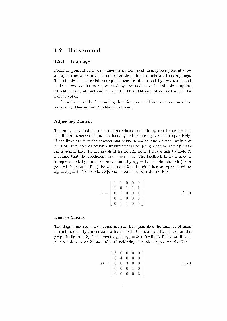
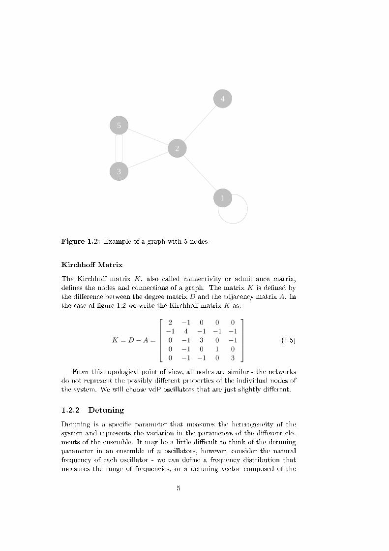
The adjacency matrix is the matrix whose elements aij are 1′s or 0′s, de-pending on whether the node i has any link to node j, or not, respectively.If the links are just the connections between nodes, and do not imply anykind of preferable direction - unidirectional coupling - the adjacency mat-rix is symmetric. In the graph of gure 1.2, node 1 has a link to node 2,meaning that the coecient a12 = a21 = 1. The feedback link on node 1is represented, by standard convection, by a11 = 1. The double link (or ingeneral the n-tuple link), between node 3 and node 5 is also represented bya35 = a53 = 1. Hence, the adjacency matrix A for this graph is:

A =

1 1 0 0 01 0 1 1 10 1 0 0 10 1 0 0 00 1 1 0 0

(1.3)

Degree Matrix

The degree matrix is a diagonal matrix that quanties the number of linksin each node. By convention, a feedback link is counted twice, so, for thegraph in gure 1.2, the element a11 is a11 = 3: a feedback link (two links),plus a link to node 2 (one link). Considering this, the degree matrix D is:

D =

3 0 0 0 00 4 0 0 00 0 3 0 00 0 0 1 00 0 0 0 3

(1.4)

4

1

2

3

4

5

Figure 1.2: Example of a graph with 5 nodes.

Kirchho Matrix

The Kirchho matrix K, also called connectivity or admittance matrix,denes the nodes and connections of a graph. The matrix K is dened bythe dierence between the degree matrix D and the adjacency matrix A. Inthe case of gure 1.2 we write the Kirchho matrix K as:

K = D −A =

2 −1 0 0 0−1 4 −1 −1 −10 −1 3 0 −10 −1 0 1 00 −1 −1 0 3

(1.5)

From this topological point of view, all nodes are similar - the networksdo not represent the possibly dierent properties of the individual nodes ofthe system. We will choose vdP oscillators that are just slightly dierent.

1.2.2 Detuning

Detuning is a specic parameter that measures the heterogeneity of thesystem and represents the variation in the parameters of the dierent ele-ments of the ensemble. It may be a little dicult to think of the detuningparameter in an ensemble of n oscillators, however, consider the naturalfrequency of each oscillator - we can dene a frequency distribution thatmeasures the range of frequencies, or a detuning vector composed of the

5

detuning parameter associated with each pair of oscillators.

1.2.3 Phase

Phase is a variable that measures the fraction of the period correspondingto a certain periodic state. We are interested in the evolution of the phasedierence for each pair, i.e., if it tends to a constant value the oscillatorswill be synchronized.

The amplitude of an autonomous oscillator is well-dened (see AppendixC), and hence its motion is completely described by the phase along the limitcycle. A dierent scenario is found for the phase. The phase can easily bechanged by a longitudinal perturbation, which travels along the limit cycle.Denoting the phase by ϕ, and dening it in such a way that it changesuniformly along the limit cycle, we can write the equation for the phase as:

dϕ

dt= ω, (1.6)

where ω = 2π/T is the frequency and T is the period.The study of the evolution of the phase, and especially the phase dif-

ference between identical coupled units, has shown two signicant stablepoints in a wide range of systems: Zero, denoted by in-phase synchrony, andπ, denoted analogously by anti-phase synchrony. For instance, ChristiaanHuygens noticed that the pendula he observed reached a state of anti-phasesynchronization. Nevertheless, if we have a non-zero detuning parameter wemay have slightly dierent values for the phase dierence.

1.2.4 Coupling Function

The behaviour of a system of n uncoupled units is governed by a system ofdierential equations:

~x = ~f (~x) , (1.7)

in which ~x is dened as ~x = (x1, x1, ..., xn, xn), and ~f (~x) will have the formof the vdP equations. In addition, we will dene an extra 2× 2 matrix, theoutput matrix H, that will help us to construct and understand the couplingterm. Basically, the output matrix H selects which terms of ~x we want toinclude in the coupling function. Since we want bidirectional coupling, bothin amplitudes as in their derivatives, we will need two output functions H1

and H2, and also two coupling coecients, so we can manipulate whichcoupling term is the most important by varying these coecients.

The general form for adding a linear coupling in system 1.7 is due toPecorra and Carrol [7], and states:

~x = ~f (~x) + (K ⊗ (σH)) ~x, (1.8)

6

in which σ is the coupling coecient, ⊗ is the Kronecker direct product,and σH is dened as:

σH = σ1H1 + σ2H2 + . . .+ σnHn. (1.9)

All other variables retain the previous denitions.In our work we consider two types of coupling coecients, one that

is denoted by amplitude coupling CA, and the other which is denoted byderivative coupling CD. Therefore:

σ = (σ1, σ2) = (CA, CD) , (1.10)

is the coupling vector. Also, two output functions (H1, H2) to collect theright terms in the positions and derivatives. Thus, the general form of thesystem of n coupled units, with coupling function formed by the couplingterms CA and CD, and with output matrices H1 and H2, respectively, is:

~x = ~f (~x) + CA (K ⊗H1) ~x+ CD (K ⊗H2) ~x. (1.11)

Every output function may give us dierent coupling terms, so dierentresults can emerge, which may, or may not, have physical meaning. Thegoal here is to build a theory based on mutual synchronization, and thatwill be our concern when dening these matrices. Unlike the case of ex-ternal forced synchronization, where an autonomous oscillator synchronizesits rhythm with an external oscillating mechanism, mutual synchronizationimplies that the inuence of all units have the same order of magnitude -bidirectional coupling - and is concerned with the study of oscillating objectsthat inuence each other in this way.

1.3 Krylov-Bogoliubov Averaging Method

In order to study our mutual synchronization model we will use the Krylov-Bogoliubov averaging method [8], to derive an equation for the evolutionof the phase dierence. In this section, our goal is to prove that KB isappropriate for the type of systems under consideration in the followingchapter. This method applies to systems in the form (please consider thesimplied notation of the following equation as a system of any dimensionyou desire):

x+ ω2x+ µf (x, x) = 0, (1.12)

where µ is a small parameter, so that µf (x, x) is considered as a perturbationof the harmonic oscillator. Recalling the vdP equation, with f (x, x) =(x2 − 1

)x, we realise that the vdP oscillator can be represented by the

family of equations 1.12.

7

We will start by considering the simplest case with µ = 0. One solutionfor equation 1.12 is:

x = A cos (ωt+ ϕ)

x = −Aω sin (ωt+ ϕ)(1.13)

where A and ϕ are constants that represent the amplitude and the phase,respectively. The corresponding solutions for A and ϕ time-dependent:

x = A (t) cos (ωt+ ϕ (t)) , (1.14)

x = A (t) cos (ωt+ ϕ (t))−A (t) (ω + ϕ (t)) sin(ωt+ ϕ (t)), (1.15)

are of more interest to us, because the method takes them as a basis toconstruct approximate solutions for the case with µ 6= 0. In this work, thecase with µ < 0 is not considered, because it represents a chaotic regime, sowe will just consider the case with µ > 0 - self-sustained oscillations occuronly in this regime.

1.3.1 First Approximation

In a n-order dierential equation we have n degrees of freedom. In 1.12 wehave two degrees of freedom which we explicit in the harmonic-like solutionsof 1.13, and now we want to choose the terms from equation 1.15 that aredierent from x in equation 1.13, and equalize them to zero. Hence:

A cos (ωt+ ϕ)−Aϕ sin (ωt+ ϕ) = 0. (1.16)

So:x = −Aω sin (ωt+ ϕ) ,

and the derivative x:

x = −Aω sin (ωt+ ϕ)−Aω (ω + ϕ) cos (ωt+ ϕ) . (1.17)

We substitute x and x in the equation of motion 1.12:

−Aω sin (ωt+ ϕ)−Aω (ω + ϕ) cos (ωt+ ϕ)+ω2A cos (ωt+ ϕ)+µf (x, x) = 0,(1.18)

The terms with ω2 cancel out. Adding condition 1.16 we can solve a systemof two equations with two variables, A and ϕ:

A cos (ωt+ ϕ) = Aϕ sin (ωt+ ϕ)

Aω sin (ωt+ ϕ) +Aωϕ cos (ωt+ ϕ) = µf (x, x)

(1.19)

After some algebra:

8

A = µωf (x, x) cos (ωt+ ϕ)

ϕ = µAωf (x, x) sin (ωt+ ϕ)

(1.20)

They depend on the small parameter µ, hence are functions that vary slowlyduring one period T = 2π

ω . Writing them in a more convenient form usingFourier expansions for the second members (explicit Fourier coecients inAppendix D - with ϕ = ωt+ ϕ):

f (x, x) cos (ϕ) = K0(A) +∑∞

n=1Kn(A) cos(nϕ) + Ln(A) sin(nϕ),

f (x, x) sin (ϕ) = P0(A) +∑∞

n=1 Pn(A) cos(nϕ) +Qn(A) sin(nϕ)(1.21)

equation 1.20 become:

A = µωK0 (A) + µ

ω

∑∞n=1Kn (A) cos (n (ωt+ ϕ)) + Ln (A) sin (n (ωt+ ϕ))

ϕ = µωAP0 (A) + µ

ωA

∑∞n=1 Pn (A) cos (n (ωt+ ϕ)) +Qn (A) sin (n (ωt+ ϕ))

(1.22)For n integer:

t+Tˆ

t

cos (n (ωt+ ϕ)) dt =

t+Tˆ

t

sin (n (ωt+ ϕ)) dt = 0, (1.23)

so, we can integrate A = dAdt and ϕ = dϕ

dt :

t+Tˆ

t

Adt =

t+Tˆ

t

µ

ωK0 (A) dt, (1.24)

where the function being integrated on the right-hand-side is time-independent.Simple integration will lead us to:

A(t+ T )−A(t)

T=

µ

ωK0 (A) (1.25)

and doing the same to ϕ:

ϕ(t+ T )− ϕ(t)

T=

µ

ωAK0(A) (1.26)

Now, we recall that ∆A and ∆ϕ do not vary much in the interval [t, t+ T ]due to µ being small, we can write these expressions as derivatives:

dAdt = µ

ωK0(A)

dϕdt = µ

ωAP0(A)

(1.27)

9

Comparing these equations with the 1.22, we conclude that equations 1.27are the result, by 1.23, of averaging the former over one period.

In the next chapter we will introduce the van der Pol coupled system andsolve it analytically and numerically. Understanding the basic ideas behindthe Krylov-Bogoliubov method is essential, in a way that the time average isthe crucial step to obtain the analytical approximated solutions. It is trivialto notice that for systems of the type of equation 1.12, for small µ, boththe amplitude and the phase will vary slowly (µ - dependent) in one period,allowing us to perform simplications without losing much information. Wewill combine this approximate result with a polar coordinate transformation,aiming at deriving the equations for the evolution of the amplitude and thephase. Our purpose is to prove that the approximated method is appropriatefor our system, and that systems of this type can be coupled to performsynchronized motion.

After completing the theoretical and experimental studies for two coupledoscillators, we will use these general considerations to perform an extensionto this work by increasing the number of oscillators, in Chapters 5 and 6.

10

Chapter 2

Synchronization

After the discovery by Huygens, more and more thinkers became inter-ested in the ideas of organization, or lack of it. One of them, risingin the early twentieth century, was William Gibbs, who described

the phenomenon of entropy as Mixed-up-ness. The common idea of entropytell us that its variation in an isolated system will never decrease. Addingthe idea of disorder to the entropy one (as is usually attributed), it makesa major milestone in science, leading to huge discussions whenever someonetries to talk about the natural organization or decrease of entropy. However,the universe is not a completely random set of particles wandering the vast-ness of the darkness. There are galaxies, solar systems, and living beings,like us humans. Somehow order wins the battle of nature's complexity, andnatural organization emerges everywhere. Wherever we look, we see thepulsating rhythm of nature, at all scales, with its melody and tempo, likesynchronization is an intrinsic maestro of the universe.

Synchronization is a natural process that any person can understand. Aset of dierent individuals in interaction will perform their work with lowerlosses of energy if they perform it in unison, i.e., two people walking side byside in the street will be very tired (at least one of them) if they walk in theirnatural speed, and then, every few seconds, stop or speed up to catch theother one, rather than if both walk in an average speed. The idea is simpleand the conclusions are very interesting, mainly when we can observe someevent where, unexpectedly, dierent units start to behave as a group, likethe previously mentioned ash of reies.

In this chapter our goal is to provide the basic mathematical knowledgeof how to look for mutual synchronization of two coupled oscillators. In thenext chapters we will need these notions to perform the study thereafter, soit is important, for the reader, to know the basics herein.

11

OscillatorOscillator

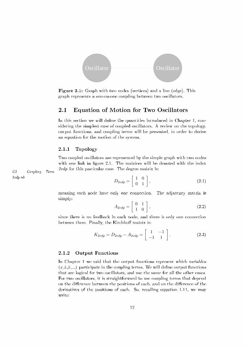
Figure 2.1: Graph with two nodes (vertices) and a line (edge). Thisgraph represents a one-on-one coupling between two oscillators.

2.1 Equation of Motion for Two Oscillators

In this section we will dene the quantities introduced in Chapter 1, con-sidering the simplest case of coupled oscillators. A review on the topology,output functions, and coupling terms will be presented, in order to derivean equation for the motion of the system.

2.1.1 Topology

Two coupled oscillators are represented by the simple graph with two nodeswith one link in gure 2.1. The matrices will be denoted with the index2vdp for this particular case. The degree matrix is:

C2 - Coupling Term

2vdp.nbD2vdp =

[1 00 1

], (2.1)

meaning each node have only one connection. The adjacency matrix issimply:

A2vdp =

[0 11 0

], (2.2)

since there is no feedback in each node, and there is only one connectionbetween them. Finally, the Kirchho matrix is:

K2vdp = D2vdp −A2vdp =

[1 −1−1 1

]. (2.3)

2.1.2 Output Functions

In Chapter 1 we said that the output functions represent which variables(x,x,x,...) participate in the coupling terms. We will dene output functionsthat are logical for two oscillators, and use the same for all the other cases.For two oscillators, it is straightforward to use coupling terms that dependon the dierence between the positions of each, and on the dierence of thederivatives of the positions of each. So, recalling equation 1.11, we maywrite:

12

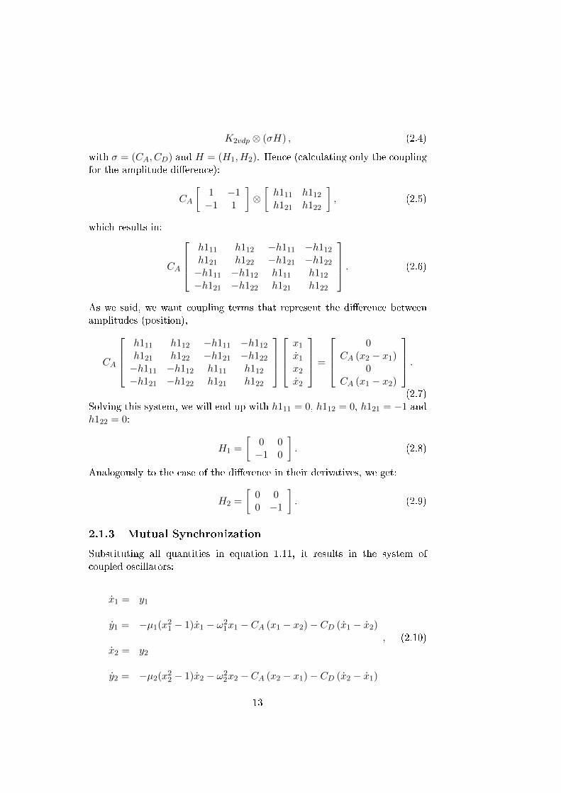
K2vdp ⊗ (σH) , (2.4)

with σ = (CA, CD) and H = (H1, H2). Hence (calculating only the couplingfor the amplitude dierence):

CA

[1 −1−1 1

]⊗[h111 h112h121 h122

], (2.5)

which results in:

CA

h111 h112 −h111 −h112h121 h122 −h121 −h122−h111 −h112 h111 h112−h121 −h122 h121 h122

. (2.6)

As we said, we want coupling terms that represent the dierence betweenamplitudes (position),

CA

h111 h112 −h111 −h112h121 h122 −h121 −h122−h111 −h112 h111 h112−h121 −h122 h121 h122

x1x1x2x2

=

0

CA (x2 − x1)0

CA (x1 − x2)

.(2.7)

Solving this system, we will end up with h111 = 0, h112 = 0, h121 = −1 andh122 = 0:

H1 =

[0 0−1 0

]. (2.8)

Analogously to the case of the dierence in their derivatives, we get:

H2 =

[0 00 −1

]. (2.9)

2.1.3 Mutual Synchronization

Substituting all quantities in equation 1.11, it results in the system ofcoupled oscillators:

x1 = y1

y1 = −µ1(x21 − 1)x1 − ω21x1 − CA (x1 − x2)− CD (x1 − x2)

x2 = y2

y2 = −µ2(x22 − 1)x2 − ω22x2 − CA (x2 − x1)− CD (x2 − x1)

, (2.10)

13

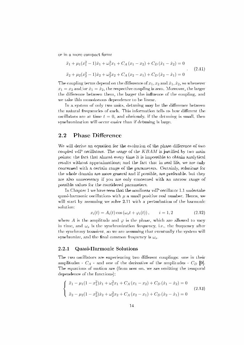
or in a more compact form:

x1 + µ1(x21 − 1)x1 + ω2

1x1 + CA (x1 − x2) + CD (x1 − x2) = 0

x2 + µ2(x22 − 1)x2 + ω2

2x2 + CA (x2 − x1) + CD (x2 − x1) = 0. (2.11)

The coupling terms depend on the dierence of x1, x2 and x1, x2, so wheneverx1 = x2 and/or x1 = x2, the respective coupling is zero. Moreover, the largerthe dierence between them, the larger the inuence of the coupling, andwe take this monotonous dependence to be linear.

In a system of only two units, detuning may be the dierence betweenthe natural frequencies of each. This information tells us how dierent theoscillators are at time t = 0, and obviously, if the detuning is small, thensynchronization will occur easier than if detuning is large.

2.2 Phase Dierence

We will derive an equation for the evolution of the phase dierence of twocoupled vdP oscillators. The usage of the KBAM is justied by two mainpoints: the fact that almost every time it is impossible to obtain analyticalresults without approximations; and the fact that in real life, we are onlyconcerned with a certain range of the parameters. Certainly, solutions forthe whole domain are more general and if possible, are preferable, but theyare also unnecessary if you are only concerned with an narrow range ofpossible values for the considered parameters.

In Chapter 1 we have seen that the nonlinear vdP oscillator 1.1 undertakequasi-harmonic oscillations with µ a small positive real number. Hence, wewill start by assuming we solve 2.11 with a perturbation of the harmonicsolution:

xi(t) = Ai(t) cos (ωst+ ϕi(t)) , i = 1, 2 (2.12)

where A is the amplitude and ϕ is the phase, which are allowed to varyin time, and ωs is the synchronization frequency, i.e., the frequency afterthe synchrony transient, so we are assuming that eventually the system willsynchronize, and the nal common frequency is ωs.

2.2.1 Quasi-Harmonic Solutions

The two oscillators are experiencing two dierent couplings: one in theiramplitudes - CA - and one of the derivative of the amplitudes - CD [9].The equations of motion are (from now on, we are omitting the temporaldependence of the functions):

x1 − µ1(1− x21)x1 + ω21x1 + CA (x1 − x2) + CD (x1 − x2) = 0

x2 − µ2(1− x22)x2 + ω22x2 + CA (x2 − x1) + CD (x2 − x1) = 0

(2.13)

14

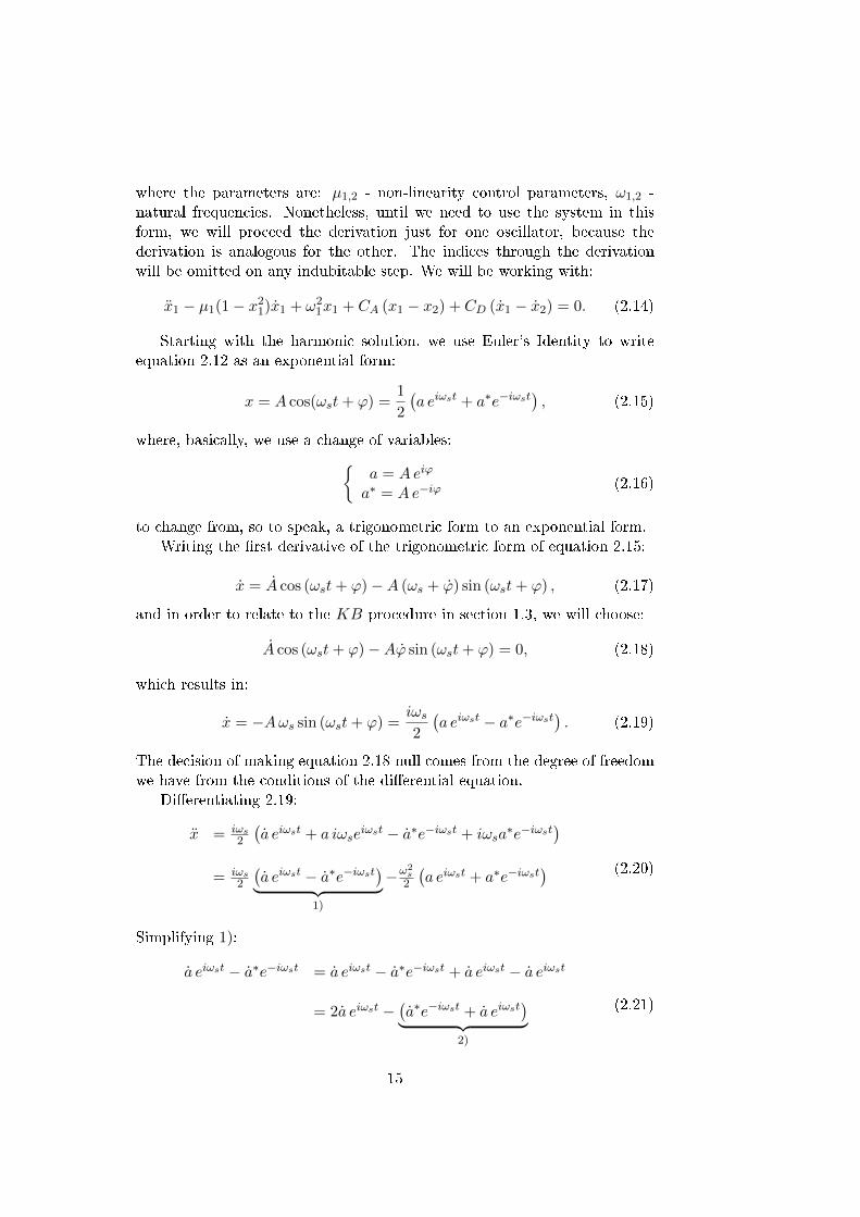
where the parameters are: µ1,2 - non-linearity control parameters, ω1,2 -natural frequencies. Nonetheless, until we need to use the system in thisform, we will proceed the derivation just for one oscillator, because thederivation is analogous for the other. The indices through the derivationwill be omitted on any indubitable step. We will be working with:

x1 − µ1(1− x21)x1 + ω21x1 + CA (x1 − x2) + CD (x1 − x2) = 0. (2.14)

Starting with the harmonic solution, we use Euler's Identity to writeequation 2.12 as an exponential form:

x = A cos(ωst+ ϕ) =1

2

(a eiωst + a∗e−iωst

), (2.15)

where, basically, we use a change of variables:a = Aeiϕ

a∗ = Ae−iϕ(2.16)

to change from, so to speak, a trigonometric form to an exponential form.Writing the rst derivative of the trigonometric form of equation 2.15:

x = A cos (ωst+ ϕ)−A (ωs + ϕ) sin (ωst+ ϕ) , (2.17)

and in order to relate to the KB procedure in section 1.3, we will choose:

A cos (ωst+ ϕ)−Aϕ sin (ωst+ ϕ) = 0, (2.18)

which results in:

x = −Aωs sin (ωst+ ϕ) =iωs2

(a eiωst − a∗e−iωst

). (2.19)

The decision of making equation 2.18 null comes from the degree of freedomwe have from the conditions of the dierential equation.

Dierentiating 2.19:

x = iωs2

(a eiωst + a iωse

iωst − a∗e−iωst + iωsa∗e−iωst

)= iωs

2

(a eiωst − a∗e−iωst

)︸ ︷︷ ︸1)

−ω2s2

(a eiωst + a∗e−iωst

) (2.20)

Simplifying 1):

a eiωst − a∗e−iωst = a eiωst − a∗e−iωst + a eiωst − a eiωst

= 2a eiωst −(a∗e−iωst + a eiωst

)︸ ︷︷ ︸2)

(2.21)

15

and because of equation 2.18, the terms in 2) are zero (we show this relationin detail in Appendix E), resulting in the expression for 1):

a eiωst − a∗e−iωst = 2a eiωst, (2.22)

So, equation 2.20 becomes:

x = iωsa eiωst − ω2

s

2

(a eiωst + a∗e−iωst

). (2.23)

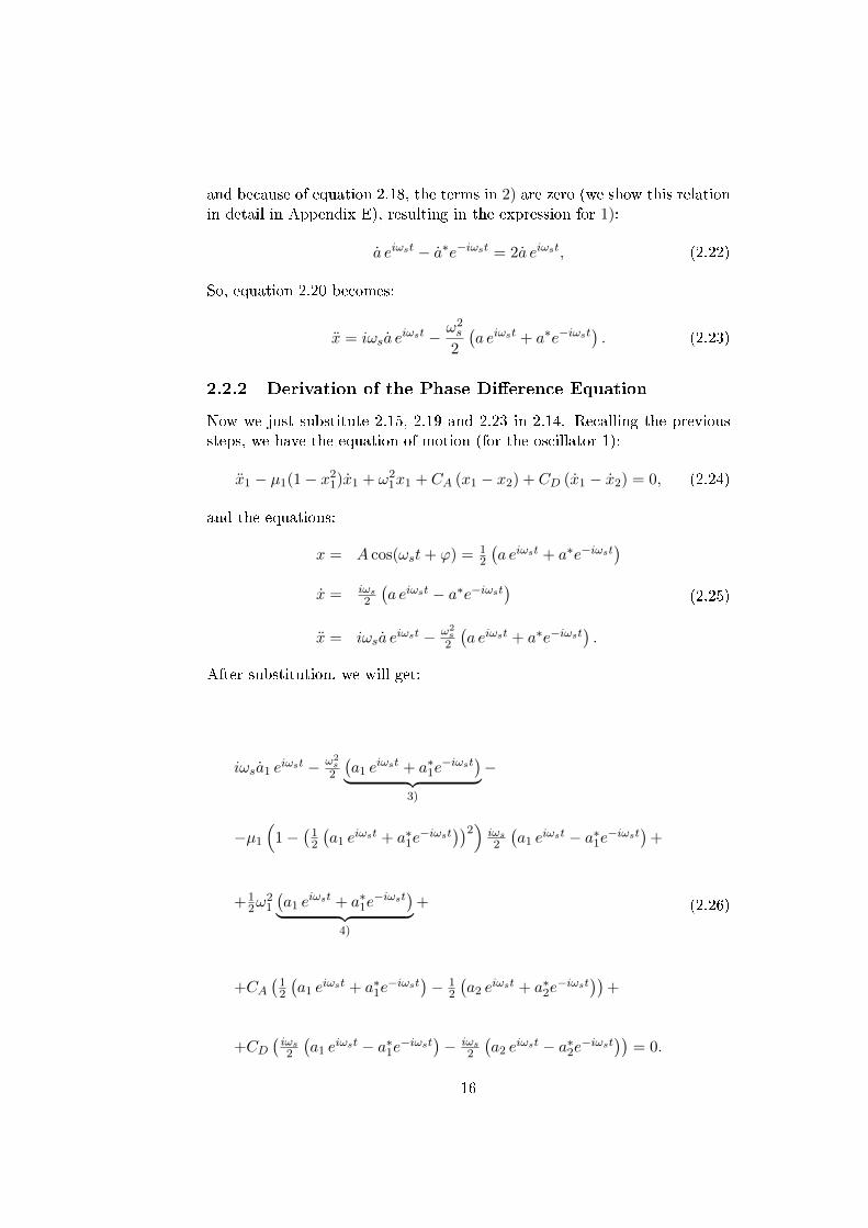
2.2.2 Derivation of the Phase Dierence Equation

Now we just substitute 2.15, 2.19 and 2.23 in 2.14. Recalling the previoussteps, we have the equation of motion (for the oscillator 1):

x1 − µ1(1− x21)x1 + ω21x1 + CA (x1 − x2) + CD (x1 − x2) = 0, (2.24)

and the equations:

x = A cos(ωst+ ϕ) = 12

(a eiωst + a∗e−iωst

)x = iωs

2

(a eiωst − a∗e−iωst

)x = iωsa e

iωst − ω2s2

(a eiωst + a∗e−iωst

).

(2.25)

After substitution, we will get:

iωsa1 eiωst − ω2

s2

(a1 e

iωst + a∗1e−iωst)︸ ︷︷ ︸

3)

−

−µ1(

1−(12

(a1 e

iωst + a∗1e−iωst

))2) iωs2

(a1 e

iωst − a∗1e−iωst)

+

+12ω

21

(a1 e

iωst + a∗1e−iωst)︸ ︷︷ ︸

4)

+

+CA(12

(a1 e

iωst + a∗1e−iωst

)− 1

2

(a2 e

iωst + a∗2e−iωst

))+

+CD(iωs2

(a1 e

iωst − a∗1e−iωst)− iωs

2

(a2 e

iωst − a∗2e−iωst))

= 0.

(2.26)

16

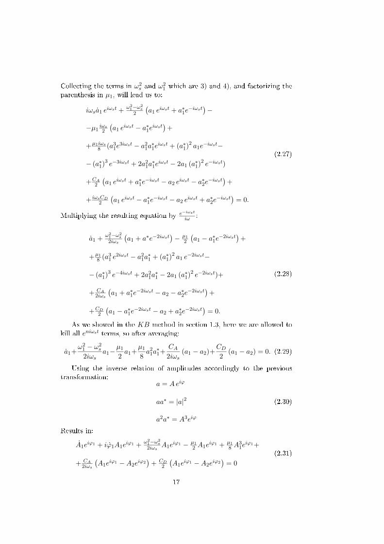
Collecting the terms in ω2s and ω2

1 which are 3) and 4), and factorizing theparenthesis in µ1, will lead us to:

iωsa1 eiωst +

ω21−ω2

s2

(a1 e

iωst + a∗1e−iωst

)−

−µ1 iωs2(a1 e

iωst − a∗1eiωst)

+

+µ1iωs8 (a31e

3iωst − a21a∗1eiωst + (a∗1)2 a1e

−iωst−

− (a∗1)3 e−3iωst + 2a21a

∗1eiωst − 2a1 (a∗1)

2 e−iωst)

+CA2

(a1 e

iωst + a∗1e−iωst − a2 eiωst − a∗2e−iωst

)+

+ iωsCD2

(a1 e

iωst − a∗1e−iωst − a2 eiωst + a∗2e−iωst

)= 0.

(2.27)

Multiplying the resulting equation by e−iωst

iω :

a1 +ω21−ω2

s2iωs

(a1 + a∗e−2iωst

)− µ1

2

(a1 − a∗1e−2iωst

)+

+µ18 (a31 e

2iωst − a21a∗1 + (a∗1)2 a1 e

−2iωst−

− (a∗1)3 e−4iωst + 2a21a

∗1 − 2a1 (a∗1)

2 e−2iωst)+

+ CA2iωs

(a1 + a∗1e

−2iωst − a2 − a∗2e−2iωst)

+

+CD2

(a1 − a∗1e−2iωst − a2 + a∗2e

−2iωst)

= 0.

(2.28)

As we showed in the KB method in section 1.3, here we are allowed tokill all eniωst terms, so after averaging:

a1+ω21 − ω2

s

2iωsa1−

µ12a1+

µ18a21a∗1+

CA2iωs

(a1 − a2)+CD2

(a1 − a2) = 0. (2.29)

Using the inverse relation of amplitudes accordingly to the previoustransformation:

a = Aeiϕ

aa∗ = |a|2

a2a∗ = A3eiϕ

(2.30)

Results in:

A1eiϕ1 + iϕ1A1e

iϕ1 +ω21−ω2

s2iωs

A1eiϕ1 − µ1

2 A1eiϕ1 + µ1

8 A31eiϕ1+

+ CA2iωs

(A1e

iϕ1 −A2eiϕ2)

+ CD2

(A1e

iϕ1 −A2eiϕ2)

= 0

(2.31)

17

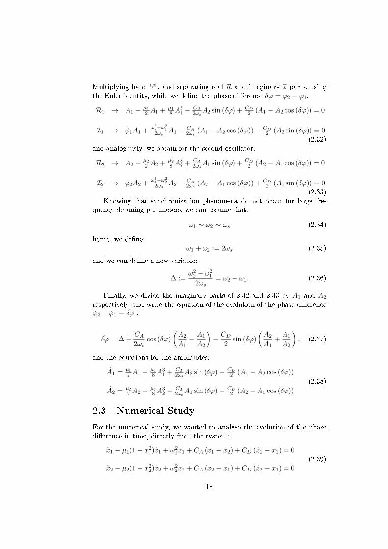
Multiplying by e−iϕ1 , and separating real R and imaginary I parts, usingthe Euler identity, while we dene the phase dierence δϕ = ϕ2 − ϕ1:

R1 → A1 − µ12 A1 + µ1

8 A31 −

CA2ωs

A2 sin (δϕ) + CD2 (A1 −A2 cos (δϕ)) = 0

I1 → ϕ1A1 +ω2s−ω2

12ωs

A1 − CA2ωs

(A1 −A2 cos (δϕ))− CD2 (A2 sin (δϕ)) = 0

(2.32)and analogously, we obtain for the second oscillator:

R2 → A2 − µ22 A2 + µ2

8 A32 + CA

2ωsA1 sin (δϕ) + CD

2 (A2 −A1 cos (δϕ)) = 0

I2 → ϕ2A2 +ω2s−ω2

22ωs

A2 − CA2ωs

(A2 −A1 cos (δϕ)) + CD2 (A1 sin (δϕ)) = 0

(2.33)Knowing that synchronization phenomena do not occur for large fre-

quency detuning parameters, we can assume that:

ω1 ∼ ω2 ∼ ωs (2.34)

hence, we dene:ω1 + ω2 := 2ωs (2.35)

and we can dene a new variable:

∆ :=ω22 − ω2

1

2ωs= ω2 − ω1. (2.36)

Finally, we divide the imaginary parts of 2.32 and 2.33 by A1 and A2

respectively, and write the equation of the evolution of the phase dierenceϕ2 − ϕ1 = ˙δϕ :

˙δϕ = ∆ +CA2ωs

cos (δϕ)

(A2

A1− A1

A2

)− CD

2sin (δϕ)

(A2

A1+A1

A2

), (2.37)

and the equations for the amplitudes:

A1 = µ12 A1 − µ1

8 A31 + CA

2ωsA2 sin (δϕ)− CD

2 (A1 −A2 cos (δϕ))

A2 = µ22 A2 − µ2

8 A32 −

CA2ωs

A1 sin (δϕ)− CD2 (A2 −A1 cos (δϕ))

(2.38)

2.3 Numerical Study

For the numerical study, we wanted to analyse the evolution of the phasedierence in time, directly from the system:

x1 − µ1(1− x21)x1 + ω21x1 + CA (x1 − x2) + CD (x1 − x2) = 0

x2 − µ2(1− x22)x2 + ω22x2 + CA (x2 − x1) + CD (x2 − x1) = 0

(2.39)

18

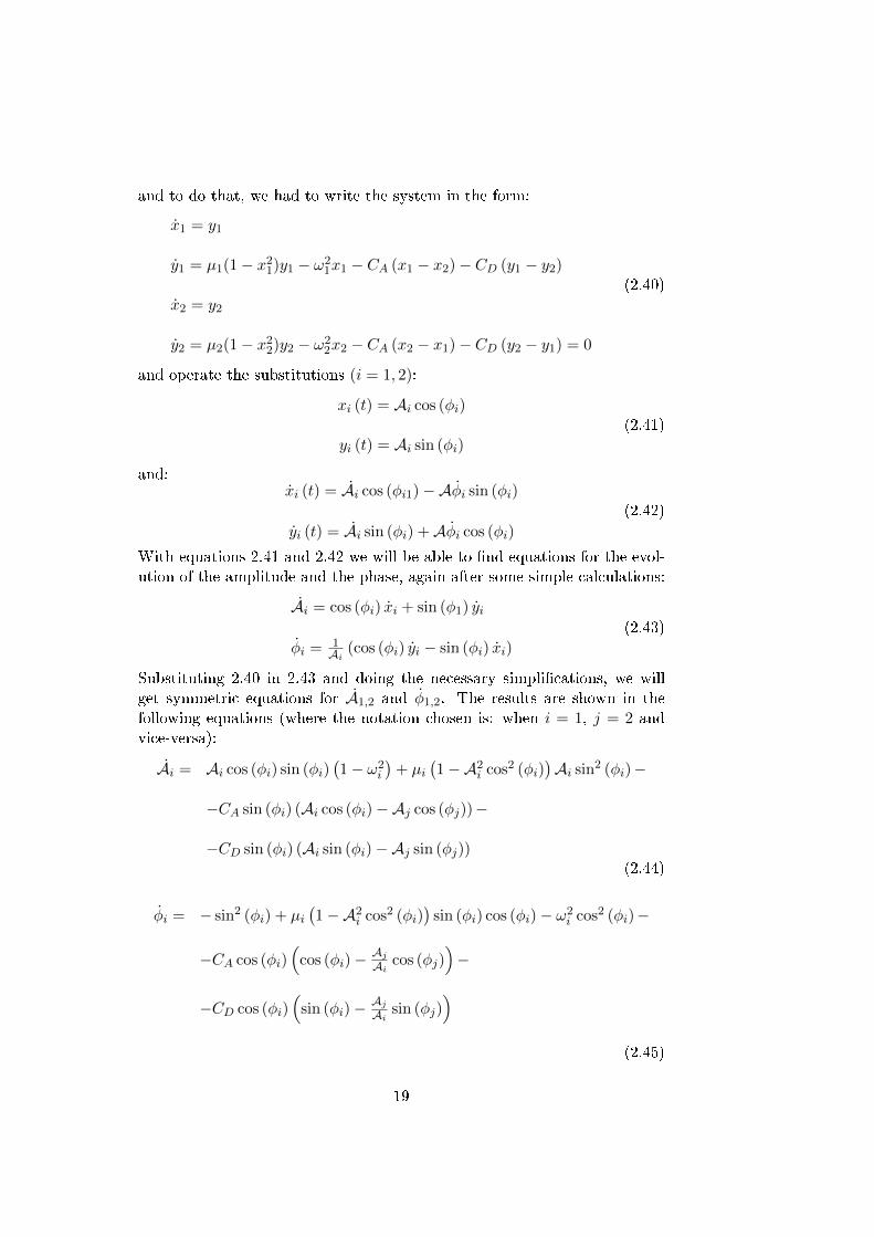
and to do that, we had to write the system in the form:

x1 = y1

y1 = µ1(1− x21)y1 − ω21x1 − CA (x1 − x2)− CD (y1 − y2)

x2 = y2

y2 = µ2(1− x22)y2 − ω22x2 − CA (x2 − x1)− CD (y2 − y1) = 0

(2.40)

and operate the substitutions (i = 1, 2):

xi (t) = Ai cos (φi)

yi (t) = Ai sin (φi)(2.41)

and:xi (t) = Ai cos (φi1)−Aφi sin (φi)

yi (t) = Ai sin (φi) +Aφi cos (φi)

(2.42)

With equations 2.41 and 2.42 we will be able to nd equations for the evol-ution of the amplitude and the phase, again after some simple calculations:

Ai = cos (φi) xi + sin (φ1) yi

φi = 1Ai (cos (φi) yi − sin (φi) xi)

(2.43)

Substituting 2.40 in 2.43 and doing the necessary simplications, we willget symmetric equations for A1,2 and φ1,2. The results are shown in thefollowing equations (where the notation chosen is: when i = 1, j = 2 andvice-versa):

Ai = Ai cos (φi) sin (φi)(1− ω2

i

)+ µi

(1−A2

i cos2 (φi))Ai sin2 (φi)−

−CA sin (φi) (Ai cos (φi)−Aj cos (φj))−

−CD sin (φi) (Ai sin (φi)−Aj sin (φj))(2.44)

φi = − sin2 (φi) + µi(1−A2

i cos2 (φi))

sin (φi) cos (φi)− ω2i cos2 (φi)−

−CA cos (φi)(

cos (φi)− AjAi cos (φj))−

−CD cos (φi)(

sin (φi)− AjAi sin (φj))

(2.45)

19

2.4 Resume of the Chapter

In this chapter our goal was to present the mathematical background fortwo coupled oscillators, how to obtain an approximated equation for thephase dierence using the KB method, and analytical equations for theamplitudes and phases of the oscillators. The mathematical backgroundhere depicted will support future work, since the study of two interactingunits is the fundamental dynamical approach to the dynamics of a system -pairwise interaction.

In Chapter 3, an analogous study from the experimental point of view, ispresented, using tools from electronics to analyse the coupling of oscillators.Later, in Chapter 4, we will show the results for Chapters 2 and 3.

20

Chapter 3

Coupling Circuits

Times when scientists used pendula for almost everything are over.Now they look into electrical circuits as the future of mathemat-ical engineering, in a way of creating physical structures that could

behave like the mathematical equations. Sure it is impossible to physic-ally reproduce the mathematical equations with zero error, but the eort ofour ancestors led us to believe that working towards the reduction of theerror is worthy. Hence, from the past one hundred years, electronics haveevolved from an idea, to something indispensable in our everyday life - tele-visions, phones, cars, medical instruments, security control systems, and anever ending list of objects one avoids the need to think about its work andinvention, although some of them are used all the time.

Coupling circuits, just as mentioned before, is also a powerful tool inelectronics. A group of circuits working together to perform a task is incor-porated basically almost in everything. One of the simplest examples is thetransformer, which is used to charge, or power, the objects. The transformeris plugged into the socket and electrical current enters, travelling in an in-ductor which creates a magnetic eld. The inductor is made of a certainnumber of coils that inuence the range of the magnetic eld. This allows toplace another inductor in the range of the rst one's magnetic eld, whichinduces a current in the second inductor. This is called magnetic coup-ling. The current that enters through the plug do not reach your device,instead, both inductors are in magnetic coupling and the current created inthe second one is the one that charges your device. Obviously, this is nota case of synchronization. When you unplug the transformer, the magneticeld vanishes after a transient, and therefore so does the current. The in-ductors are not self-sustained components. This is a perfect example of afalse synchronization mechanism. Nevertheless, it helps to understand whatsync is, and what is not, and it also points to an idea of coupling circuits.In this chapter we will develop a form of self-sustained electronic oscillators,with an electronic coupling.

21

R

C

OPAMP3

2

4

8

1y-int

a

(a) Inverting Integrator

AD633X1X2Y1Y2 VS-

ZW

VS+

(b) Multiplier

OPAMP

3

2

4

8

1

R1

R2

y-inva

(c) Inverting Amplier

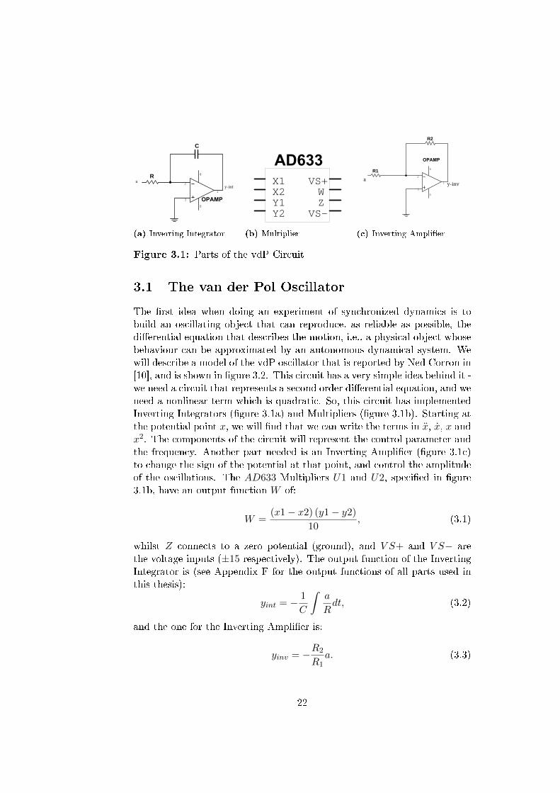
Figure 3.1: Parts of the vdP Circuit

3.1 The van der Pol Oscillator

The rst idea when doing an experiment of synchronized dynamics is tobuild an oscillating object that can reproduce, as reliable as possible, thedierential equation that describes the motion, i.e., a physical object whosebehaviour can be approximated by an autonomous dynamical system. Wewill describe a model of the vdP oscillator that is reported by Ned Corron in[10], and is shown in gure 3.2. This circuit has a very simple idea behind it -we need a circuit that represents a second order dierential equation, and weneed a nonlinear term which is quadratic. So, this circuit has implementedInverting Integrators (gure 3.1a) and Multipliers (gure 3.1b). Starting atthe potential point x, we will nd that we can write the terms in x, x, x andx2. The components of the circuit will represent the control parameter andthe frequency. Another part needed is an Inverting Amplier (gure 3.1c)to change the sign of the potential at that point, and control the amplitudeof the oscillations. The AD633 Multipliers U1 and U2, specied in gure3.1b, have an output function W of:

W =(x1− x2) (y1− y2)

10, (3.1)

whilst Z connects to a zero potential (ground), and V S+ and V S− arethe voltage inputs (±15 respectively). The output function of the InvertingIntegrator is (see Appendix F for the output functions of all parts used inthis thesis):

yint = − 1

C

ˆa

Rdt, (3.2)

and the one for the Inverting Amplier is:

yinv = −R2

R1a. (3.3)

22

U5A

3

2

4

8

1

R5R7

R4

C1 C2R6

R3

U1X1X2Y1Y2 VS-

ZW

VS+

U2X1X2Y1Y2 VS-

ZW

VS+

R1

R2

VEE

VEE

VEE

VEE

VEEVEE

VSS

VSS

VSS VSS

VSS

U3A

3

2

4

8

1

U4A

3

2

4

8

1

x1

a1

b1

c1

y1x1'

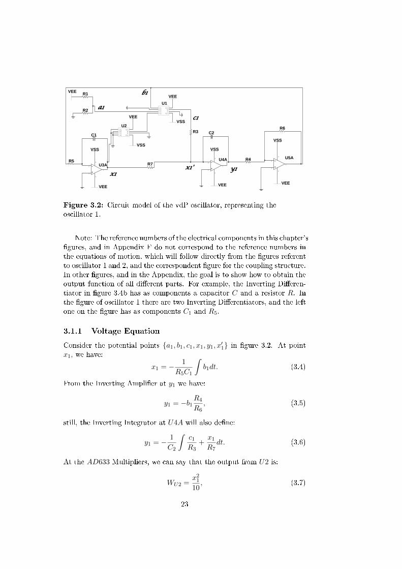
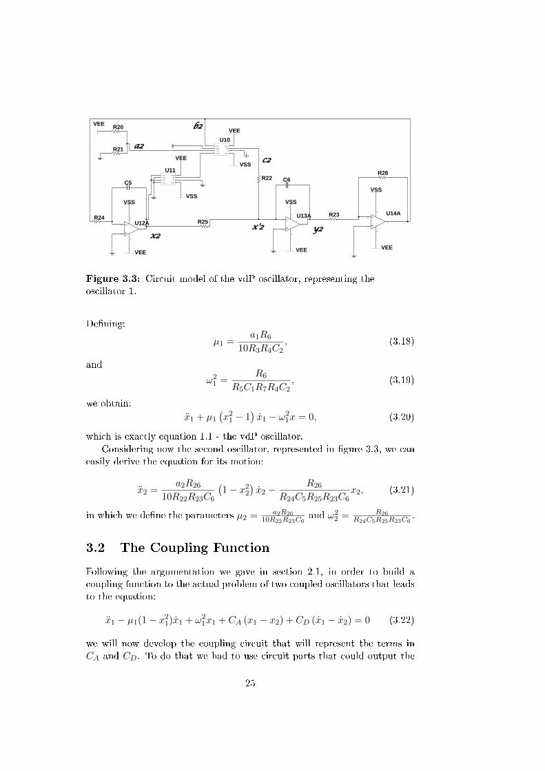
Figure 3.2: Circuit model of the vdP oscillator, representing theoscillator 1.

Note: The reference numbers of the electrical components in this chapter'sgures, and in Appendix F do not correspond to the reference numbers inthe equations of motion, which will follow directly from the gures referentto oscillator 1 and 2, and the correspondent gure for the coupling structure.In other gures, and in the Appendix, the goal is to show how to obtain theoutput function of all dierent parts. For example, the Inverting Dieren-tiator in gure 3.4b has as components a capacitor C and a resistor R. Inthe gure of oscillator 1 there are two Inverting Dierentiators, and the leftone on the gure has as components C1 and R5.

3.1.1 Voltage Equation

Consider the potential points a1, b1, c1, x1, y1, x′1 in gure 3.2. At pointx1, we have:

x1 = − 1

R5C1

ˆb1dt. (3.4)

From the Inverting Amplier at y1 we have:

y1 = −b1R4

R6, (3.5)

still, the Inverting Integrator at U4A will also dene:

y1 = − 1

C2

ˆc1R3

+x1R7dt. (3.6)

At the AD633 Multipliers, we can say that the output from U2 is:

WU2 =x2110, (3.7)

23

and at U1, recognizing that WU1 = c1 (from gure 3.2):

c1 =b1

(a1 − x21

10

)10

. (3.8)

Deriving 3.4 we get:x1R5C1 = −b1. (3.9)

From equation 3.5, and replacing in the previous equation:

x1R5C1 = y1R6

R4(3.10)

and now replacing 3.8 in 3.6, and then the nal y1 in 3.10:

x1R5C1 = − R6

R4C2

ˆ −x1R5C1

(a1−

x2110

)10

R3+x1R7dt (3.11)

Taking the derivative of equation 3.11, we get:

x1R5C1 = − R6

R4C2

−x1R5C1

(a1−

x2110

)10

R3+x1R7

. (3.12)

Rearranging the terms:

x1 = − R6

R4R5C1C2

(−x1R5C1a1

10R3+x1R5C1x

21

100R3+x1R7

), (3.13)

which is equal to:

x1 =R6

R4C2

(a1 −

x2110

)x1

10R3− x1R5C1R7

R6

R4C2(3.14)

Now we re-scale the dierential equation by a factor α in order to eliminatethe factor 1

10 on the x21 term. We do that by replacing x1 → γx1, so:

γ ¨x1 =R6

10R3R4C2

(a1 −

γ2x2110

)γ ˙x1 − γ

R6

R5C1R7R4C2x1, (3.15)

and by making γ2 = 10, we get:

¨x1 =R6

10R3R4C2

(a1 − x21

)˙x1 −

R6

R5C1R7R4C2x1. (3.16)

Now we apply again the same trick we presented in Appendix A, to transformthis equation in (we change the notation back from x1 to x1 to a more usualperspective):

x1 =a1R6

10R3R4C2

(1− x21

)x1 −

R6

R5C1R7R4C2x1. (3.17)

24

U14A

3

2

4

8

1

R24R25

R23

C5 C6R26

R22

U10X1X2Y1Y2 VS-

ZW

VS+

U11X1X2Y1Y2 VS-

ZW

VS+

R20

R21

VEE

VEE

VEE

VEE

VEEVEE

VSS

VSS

VSS VSS

VSS

U12A

3

2

4

8

1

U13A

3

2

4

8

1

x2

a2

b2

c2

y2x'2

Figure 3.3: Circuit model of the vdP oscillator, representing theoscillator 1.

Dening:

µ1 =a1R6

10R3R4C2, (3.18)

and

ω21 =

R6

R5C1R7R4C2, (3.19)

we obtain:x1 + µ1

(x21 − 1

)x1 − ω2

1x = 0, (3.20)

which is exactly equation 1.1 - the vdP oscillator.Considering now the second oscillator, represented in gure 3.3, we can

easily derive the equation for its motion:

x2 =a2R26

10R22R23C6

(1− x22

)x2 −

R26

R24C5R25R23C6x2, (3.21)

in which we dene the parameters µ2 = a2R2610R22R23C6

and ω22 = R26

R24C5R25R23C6.

3.2 The Coupling Function

Following the argumentation we gave in section 2.1, in order to build acoupling function to the actual problem of two coupled oscillators that leadsto the equation:

x1 − µ1(1− x21)x1 + ω21x1 + CA (x1 − x2) + CD (x1 − x2) = 0 (3.22)

we will now develop the coupling circuit that will represent the terms inCA and CD. To do that we had to use circuit parts that could output the

25

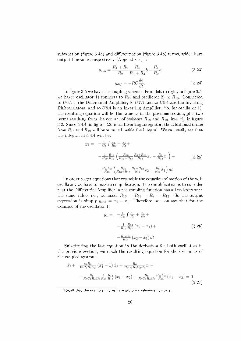
subtraction (gure 3.4a) and dierentiation (gure 3.4b) terms, which haveoutput functions, respectively (Appendix F) 1:

ysub =R1 +R2

R2

R4

R3 +R4b− R1

R2a (3.23)

ydif = −RCdadt. (3.24)

In gure 3.5 we have the coupling scheme. From left to right, in gure 3.5,we have: oscillator 1) connects to R12 and oscillator 2) to R13. Connectedto U6A is the Dierential Amplier, to U7A and to U9A are the InvertingDierentiators, and to U8A is an Inverting Amplier. So, for oscillator 1),the resulting equation will be the same as in the previous section, plus twoterms resulting from the contact of resistors R18 and R19, into x′1, in gure3.2. Since U4A, in gure 3.2, is an Inverting Integrator, the additional termsfrom R18 and R19 will be summed inside the integral. We can easily see thatthe integral in U4A will be:

y1 = − 1C2

´c1R3

+ x1R7

+

− 1R19

R14R17

(R16

R16+R13

R8+R12R12

x2 − R8R12

x1

)+

−R11C3R18

(R16

R16+R13

R8+R12R12

x2 − R8R12

x1

)dt

(3.25)

In order to get equations that resemble the equation of motion of the vdPoscillator, we have to make a simplication. The simplication is to considerthat the Dierential Amplier in the coupling function has all resistors withthe same value, i.e., we make R16 = R13 = R8 = R12. So the outputexpression is simply ysub = x2 − x1. Therefore, we can say that for theexample of the oscillator 1:

y1 = − 1C2

´c1R3

+ x1R7

+

− 1R19

R14R17

(x2 − x1) +

−R11C3R18

(x2 − x1) dt

(3.26)

Substituting the last equation in the derivation for both oscillators inthe previous section, we reach the resulting equation for the dynamics ofthe coupled system:

x1+a1R6

10R3R4C2

(x21 − 1

)x1 + R6

R5C1R4C2R7x1+

+ R6R5C1R4C2

1R19

R14R17

(x1 − x2) + R6R5C1R4C2

R11C3R18

(x1 − x2) = 0

(3.27)

1Recall that the example gures have arbitrary reference numbers.

26

R1

UR2

R3

R4

a

b y-sub

(a) Dierential Amplier

R

C Ua

y-dif

(b) Inverting Dierentiator

Figure 3.4: Parts of the Coupling Function

Recalling equations 2.11, 3.18 and 3.19, we can write:

CA1 = R6R5C1R4C2

1R19

R14R17

CD1 = R6R5C1R4C2

R11C3R18

. (3.28)

Analogously for the second oscillator:

x2+a2R26

10R22R23C6

(x22 − 1

)x2 + R26

R24C5R25R23C6x2+

+ R26R24C5R23C6

1R9

(x2 − x1) + R26R24C5R23C6

R14R17

R15C4R10

(x2 − x1) = 0,

(3.29)with:

CA2 = R26R24C5R23C6

1R9

CD2 = R26R24C5R23C6

R14R17

R15C4R10

. (3.30)

3.2.1 Simplifying the Variables

Until now, we have as main variables the non-linearity control parameter,the frequency and the coupling terms, whose expressions are:

µ1 =a1R6

10R3R4C2(3.31)

ω21 =

R6

R5C1R7R4C2(3.32)

µ2 =a2R26

10R22R23C6(3.33)

ω22 =

R26

R24C5R25R23C6(3.34)

27

U7A

3

2

4

8

1

VEE

VEE

VEE

VEE

VSS

VSS

VSS

VSS

U9A

3

2

4

8

1

U6A

3

2

4

8

1

U8A

3

2

4

8

1

R12

R8

R16

R13

R9

C3

R11

R17

R14

C4

R15

R18R19

R10

Figure 3.5: Coupling Scheme

CA1 =R6

R5C1R4C2

1

R19

R14

R17(3.35)

CD1 =R6

R5C1R4C2

R11C3

R18(3.36)

CA2 =R26

R24C5R23C6

1

R9(3.37)

CD2 =R26

R24C5R23C6

R14

R17

R15C4

R10

(3.38)

Now we will simplify the denitions of these parameters (all parametersthat we do not mention in these section, will keep their notation).

Non-linearity

We can dene

R3 = R22 = Rµ, (3.39)

since these are the resistors that will directly inuence the non-linearity ofthe system.

Amplitude

The Inverting Ampliers of each oscillator have a gain term represented bythe fractions R6/R4 and R26/R23. We want to adjust the amplitude of thewaves, in order to make the system near the amplitude of the limit cycle.

28

Since we just want to inuence the phase, we can dene:

R6

R4=R26

R23= κ, (3.40)

where κ is a constant.

Coupling

As we said before, we want the system to be symmetric, so the correspondingcoupling terms have to be the same. The resistors that control the coupling- R9, R10, R18 and R19 - have to be equal for each coupling type, for bothoscillators. Hence,

R9 = R19 = RA, (3.41)

andR10 = R18 = RD. (3.42)

The resistors R11 and R15, which belong to the Inverting Dierentiators inthe coupling function, have also to be the same, because they inuence CD:

R11 = R15 = Rdif . (3.43)

The Inverting Amplier, in the coupling function, will be dened with gaing = 1, so:

R14 = R17. (3.44)

Frequency

The resistors that inuence the frequency of each oscillators will have thesame values in each oscillator, meaning,

R5 = R7 = Rx1 , (3.45)

andR24 = R25 = Rx2 . (3.46)

All the capacitors can have the same value: C.

Control Voltage

Considering the parameters a1 and a2, and noting that V EE is the inputvoltage (gure 3.2 and 3.3):

a1 =R2

R1 +R2V EE, (3.47)

a2 =R20

R21 +R20V EE, (3.48)

we can dene all resistors with the same value, resulting in:

a1 = a2 =V EE

2= a. (3.49)

29

Result

These are the simplied terms:

µ = µ1 = µ2 = κa

10RµC(3.50)

ω21 =

k

R2x1C

2(3.51)

ω22 =

k

R2x2C

2(3.52)

CA1 =k

Rx1C2

1

RA(3.53)

CD1 = κ1

Rx1C

RdifRD

(3.54)

CA2 =k

Rx2C2

1

RA(3.55)

CD2 = κ1

Rx2C

RdifRD

(3.56)

In the next chapter we will show the results for two coupled oscillators,by plotting their phase dierence. Analogously, we analyse the experimentalresults for the same case, with pictures of the oscilloscope, and realise thatthe theoretical and experimental studies match. It is extremely importantthat, after analysing all theoretical conditions, the study has a practicalapplication that conrms its results.

30

Chapter 4

On the Two Oscillators

Ubiquitously, from fundamental particles to major clusters of galax-ies, synchronization results from cooperative interaction - an inter-action between all types of objects. Since the sixteen hundreds,

when Christiaan Huygens reported the synchronization between two pen-dula clocks hanging in the same wood wall, people have been very keen onthe study of the dynamics of coupled units at all scales. Over the years,the number of reports of situations in nature that represented sync grewexponentially. Usually, the macroscopic phenomena involve a large num-ber of units like the periodic blinking of reies, which is one of the mostappreciated events. Yet, starting the study of synchronization by a nitelarge number of biological units is insanely hard. No eld of science aroseby one of its most complicated case. Thereafter, this study starts by itsmost fundamental case, which is the case of two oscillators with a simplecoupling. Though simple, this case is very important, since the interactionof two lone units can be a rst approximation to the interaction of everypair in an ensemble of any size - nearest neighbours interaction.

On this chapter we will recall the theoretical and experimental proper-ties derived in the previous chapters, and present the corresponding resultsfor the interaction of two coupled vdP oscillators connected by a simplecoupling. This is a review chapter on what we have been working and itsymbolises the basis for the following chapters, where the cases of moreoscillators are considered.

4.1 Background

The study of two coupled oscillators is rather old. Nevertheless, it is thefundamental interaction theory of modern dynamics. With this work wewant to show that a simple autonomous oscillator can be used in all branches(theory and practice) in agreement, and extrapolate to more than two units.Here, we present the nal details for the study of two coupled van der Pol

31

oscillators, with the theoretical and experimental results.

4.1.1 Scaling of Time

We have a coupling system that is govern by the equation:

xi + µi(x2i − 1

)xi + ω2

i xi + CAi (xi − xj) + CDi (xi − xj) = 0, (4.1)

with i = 1, 2, and j = 1, 2 6= i. In our theoretical work, we have studiedthe dynamics of this system in the regime near ω ∼ 1. In the experimentalstudy, such low frequencies can be a problem, considering that the majorityof electronic parts do not work for extreme values of the frequency. So wehave to scale this equation, in order to make the frequency near ω ∼ 1000our baseline. So, we scale the time variable:

t→ sτ, (4.2)

where τ is the new time variable, and s is the scale factor. Equation 4.1becomes:

1

s2xi + µi

(x2i − 1

) 1

sxi + ω2

i xi + CA (xi − xj) +1

sCD (xi − xj) = 0. (4.3)

Multiplying this equation by s2:

xi + sµi(x2i − 1

)xi + s2ω2

i xi + s2CA (xi − xj) + sCD (xi − xj) = 0, (4.4)

which can be written as:

xi + µi(x2i − 1

)xi + ω2

i xi + CA (xi − xj) + CD (xi − xj) = 0. (4.5)

Recalling the denition of our parameters, we to need to guarantee we canwrite the new ones as (i = 1, 2):

µi = sµi = sκa10RµC

,

ωi = sωi = skRxiC

,

CAi = s2CAi = s2kRxiC

21RA,

CD = sCD = sκRxiC

RdifRD

.

(4.6)

In order to make ω ∼ 1000, we need s = 1000.Take into consideration that we have omitted any information about

the parameter κ, because we consider it just a scaling parameter on theamplitude, and we will dene it in the following sections.

32

4.1.2 Amplitude Dependence on the Parameter µ

Generically, a system like the vdP oscillator:

x− µ(1− x2

)x+ ω2x = 0, (4.7)

when treated perturbatively, has as a solution for the zeroth order (AppendixC) like:

x = 2 cos (t) . (4.8)

All other orders will depend on µ, and µ is small. Therefore, the limit cyclehas its amplitude around 2.

With the change of variables x → x√µ we already used throughout this

work, we get:x = 2

õ cos (t) , (4.9)

which shows that the dependence of the amplitude on the parameter µ isproportional

õ.

4.1.3 κ Parameter

With the zeroth order solution just showed, we see (before the change ofvariables) that the amplitude (for the zeroth order) is equal to 2. This willbe the main contribution to the amplitude, so we can assume that otherorder will just inuence perturbatively this value.

With the denition of µ we have reached:

µ = κa

10RµC, (4.10)

we can think of the gain κ as a constant of proportionality. So, we basicallyhave:

µ = κµ0, (4.11)

with µ0 as the fundamental value - when gain is equal to unity (κ = 1). Weare saying that we can dene a parameter µ for the case gain = 1 in theInverting Amplier. However, we need gain to push the magnitude of theelectronic oscillators to near the amplitude of the theoretical limit cycle, toavoid great transients or experimental problems.

As we have seen before, a small nonlinear parameter is mandatory, soit can be µ0 = 0.05 - quasi-harmonic solution. We also know that fromequation 4.9:

A0 = 2õ0, (4.12)

where A0 is the fundamental amplitude. We know that we need to have theamplitude near the stable value of the limit cycle (A = 2), so we need tomake sure that:

A = 2õ, (4.13)

33

hence, we want a system with a gain κ, such that its nonlinear parameter isµ = 0.05. Due to the denitions of A0 and µ, we have:

A0 = 2

õ

κ, (4.14)

so: õ

κ= 1, (4.15)

which results in:

κ = 0.05. (4.16)

4.1.4 Attributing Values to the Parameters

As we have seen, s = 1000, µ0 = 0.05, and for the frequency ω0 = 1. Wewant to focus on the coupling in the derivatives, so we can choose a verysmall CA (CA = 0.01 ), and a larger value to CD (CD = 0.20). You mayask why these values?. First, we have studied the case for CA = 0, but inthis particular experimental case it is impossible to mount the circuit for thecoupling and make it physically zero - it would require an innite resistor.Although we could remove the amplitude coupling part of the circuit, thatwould make the study less general - a simple change of the values of thecomponents allows anyone interested to study dierent regimes. With theprevious denitions, we can choose resistors and capacitors that will respectthese properties. The choice will be always made to the fundamental case,i.e., when the gain (κ = 1), because it is the most simple case. The gain willinuence, in the same way, all values, so it is not eectively important.

Frequency

For the parameter ω we used the unity, but now we scaled it by a factor of1000:

ω0 = 1000. (4.17)

Hence, for the case with no gain (κ = 1):

sωi =1

RxiC

so we just have to choose any values. We chose C = 10nF = 10−8nFbecause it is a good, standard value for rapid oscillation. This results in:

Rxi = 100kΩ. (4.18)

34

Non-linearity

For the parameter µ we have µ = sκµ0, but recalling conditions 4.11 and4.15, we have µ = s, so:

µ = 1000 =a

10RµC, (4.19)

and because a = 7.5 (V EE = 15V , so a has the mathematical expressiona = V EE

2 = 7.5), we get the condition:

Rµ = 75kΩ. (4.20)

Coupling

For the coupling term in the amplitudes, we have CA0 = s2CA0, hence:

CA0 = 10002 × 0.01 =1

RxiC2

1

RA, (4.21)

which results in:RA = 10MΩ. (4.22)

And for the coupling term in the derivatives, we do as we did for the non-linear control parameter. So, we have CD0 = sCD0, with CD0 = 0.20:

CD = 1000× 0.20 =1

RxiC

RdifRD

, (4.23)

which results in:RdifRD

= 5 (4.24)

and dening Rdif = 10kΩ, we get:

RD = 50kΩ. (4.25)

4.2 The Coupled Circuit

The full scheme of the circuit in the simulator representing the two oscillatorsand the coupling function can be seen in gure G.2 of Appendix G. A plot ofthe amplitude dependence, on the simulator, of both oscillators can be seenin gure 4.1a. From this gure we can clearly see that both oscillators havetheir motion in agreement. If the coupling were less intensive, i.e., changingR10 and R18 to 200kΩ, their motion would be independent, and the resultis showed in gure 4.1b.

In table 4.1 we can see the true values of every component of the coupledsystem. The reason we chose to measure this is to show that an autonomoussystem has to be stable for the perturbations of the parameters (as discussed

35

Oscillator 1 - Voltage(V)-5.0 5.0-3.0 3.0-1.0 1.0

Osc

illat

or 2

- V

olta

ge(V

)

-3.0

3.0

-2.0

2.0

-1.0

1.0

0.0

-3.0

3.0

-2.0

2.0

-1.0

1.0

0.0

(a) Plot of the simulation showing theamplitude dependence of both oscillators.

Oscillator 1 - Voltage(V)-5.0 5.0-3.0 3.0-1.0 1.0

Osc

illat

or 2

- V

olta

ge(V

)

-3.0

3.0

-2.0

2.0

-1.0

1.0

0.0

-3.0

3.0

-2.0

2.0

-1.0

1.0

0.0

(b) Plot of the simulation showing thelack of amplitude dependence of bothoscillators.

(c) Oscilloscope picture of the amplitudedependence of x1 and x2.

(d) Oscilloscope picture of the lack ofdependence of x1 and x2.

Figure 4.1: Comparison of simulation and experimental results

C V C V C V C V

R1 98.98 kΩ R9 10.06 MΩ R17 99.09 kΩ R25 100.9 kΩ

R2 99.84 kΩ R10 55.55 kΩ R18 55.50 kΩ R26 51.20 kΩ

R3 75.05 kΩ R11 9.95 kΩ R19 10.17 MΩ C1 10.76 nF

R4 1.50 kΩ R12 99.20 kΩ R20 99.88 kΩ C2 10.28 nF

R5 98.84 kΩ R13 100.21 kΩ R21 99.51 kΩ C3 10.72 nF

R6 51.14 kΩ R14 99.76 kΩ R22 75.08 kΩ C4 10.24 nF

R7 98.60 kΩ R15 9.94 kΩ R23 1.50 kΩ C5 10.72 nF

R8 98.84 kΩ R16 99.05 kΩ R24 101.0 kΩ C6 10.31 nF

Table 4.1: Measured values (V) of the components (C) of the system oftwo coupled oscillators.

36

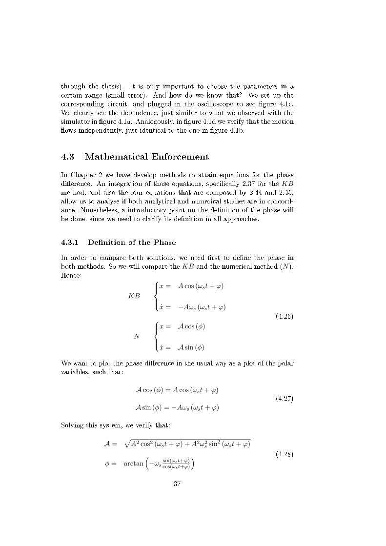
through the thesis). It is only important to choose the parameters in acertain range (small error). And how do we know that? We set up thecorresponding circuit, and plugged in the oscilloscope to see gure 4.1c.We clearly see the dependence, just similar to what we observed with thesimulator in gure 4.1a. Analogously, in gure 4.1d we verify that the motionows independently, just identical to the one in gure 4.1b.

4.3 Mathematical Enforcement

In Chapter 2 we have develop methods to attain equations for the phasedierence. An integration of those equations, specically 2.37 for the KBmethod, and also the four equations that are composed by 2.44 and 2.45,allow us to analyse if both analytical and numerical studies are in concord-ance. Nonetheless, a introductory point on the denition of the phase willbe done, since we need to clarify its denition in all approaches.

4.3.1 Denition of the Phase

In order to compare both solutions, we need rst to dene the phase inboth methods. So we will compare the KB and the numerical method (N).Hence:

KB

x = A cos (ωst+ ϕ)

x = −Aωs (ωst+ ϕ)

N

x = A cos (φ)

x = A sin (φ)

(4.26)

We want to plot the phase dierence in the usual way as a plot of the polarvariables, such that:

A cos (φ) = A cos (ωst+ ϕ)

A sin (φ) = −Aωs (ωst+ ϕ)(4.27)

Solving this system, we verify that:

A =√A2 cos2 (ωst+ ϕ) +A2ω2

s sin2 (ωst+ ϕ)

φ = arctan(−ωs sin(ωst+ϕ)cos(ωst+ϕ)

) (4.28)

37

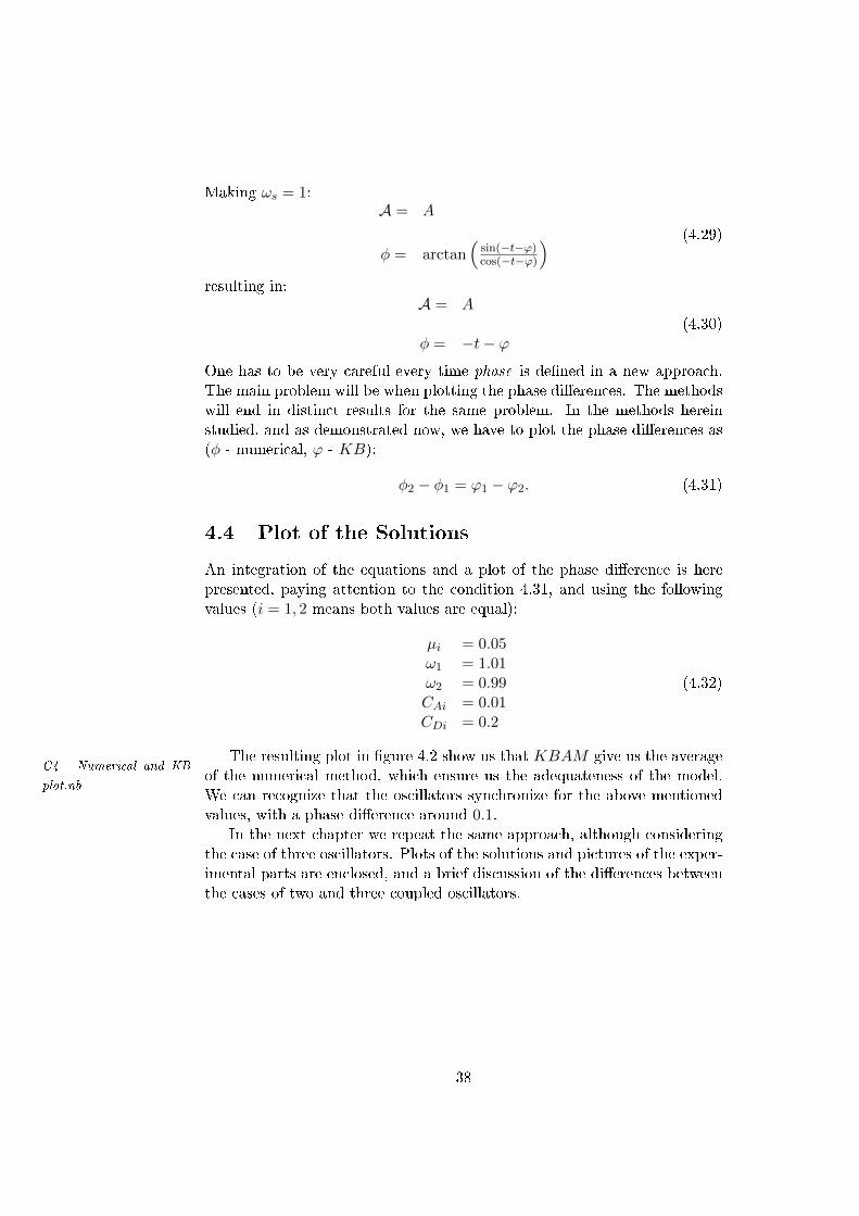
Making ωs = 1:A = A

φ = arctan(

sin(−t−ϕ)cos(−t−ϕ)

) (4.29)

resulting in:A = A

φ = −t− ϕ(4.30)

One has to be very careful every time phase is dened in a new approach.The main problem will be when plotting the phase dierences. The methodswill end in distinct results for the same problem. In the methods hereinstudied, and as demonstrated now, we have to plot the phase dierences as(φ - numerical, ϕ - KB):

φ2 − φ1 = ϕ1 − ϕ2. (4.31)

4.4 Plot of the Solutions

An integration of the equations and a plot of the phase dierence is herepresented, paying attention to the condition 4.31, and using the followingvalues (i = 1, 2 means both values are equal):

µi = 0.05ω1 = 1.01ω2 = 0.99CAi = 0.01CDi = 0.2

(4.32)

The resulting plot in gure 4.2 show us that KBAM give us the averageC4 - Numerical and KB

plot.nbof the numerical method, which ensure us the adequateness of the model.We can recognize that the oscillators synchronize for the above mentionedvalues, with a phase dierence around 0.1.

In the next chapter we repeat the same approach, although consideringthe case of three oscillators. Plots of the solutions and pictures of the exper-imental parts are enclosed, and a brief discussion of the dierences betweenthe cases of two and three coupled oscillators.

38

0 10 20 30 40 50

-0.4

-0.2

0.0

0.2

0.4

Time

DPh

ase

KB

N

Figure 4.2: Plot of the solutions representing the phase dierence, usingnumerical N and KB methods.

39

Chapter 5

On the Three Oscillators

Reality itself is ambiguous - one cannot say if something really existsor not with one hundred percent certainty. All we can do is observe,study, think, and try to understand what is going on. So, what we

call reality, is something that we cannot prove that it is real. What people,and in particular scientists, try to do is to improve the notion of what isobserved (directly or not), and approaching what someone courageous mightcall the truth. Of course the truth with 100% certainty does not exist dueto the awed mathematics we have nowadays, however, it is not necessary.We can approach this enigmatic truth with a really tiny error. Here, weare trying to convince the reader that a dynamical world is surroundingus and everything interacts with everything (or almost everything, so aparticle physicists would say), and its interaction results, many times, insynchronization.

In order to study an ensemble with a reasonable number of elements,we now focus on the three elements case, which is a very important middlestep. In this and the next chapter we will show that the study of twooscillators is the base for any number of oscillators interacting in a ensemble,and that sync appears with few conditions. Every couple of units interact,independently that if they interact with others. The main idea is that everyinteraction happen between two units at a time, i.e., the coupling of threeunits is the sum of 3 pairs of two coupled units: 1+2, 2+3, and 1+3.

The following pages present our work on three coupled oscillators. Thecase of three oscillators is, obviously, equal for the NN interaction andthe all-to-all interaction, just like in the two oscillators case (more on thedierent kinds of interaction, and the correspondent terms, on Chapter 6).

5.1 One More

The study of the coupling of three oscillators is based on the pairwise inter-action discussed so far in this work. The reason we choose to shed light on

41

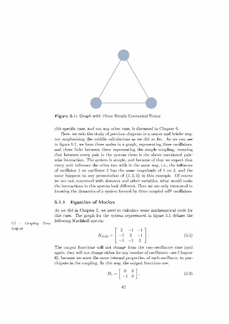
Figure 5.1: Graph with Three Simply Connected Nones

this specic case, and not any other case, is discussed in Chapter 6.Here, we redo the study of previous chapters in a neater and briefer way,

not emphasizing the middle calculations as we did so far. As we can seein gure 5.1, we have three nodes in a graph, representing three oscillators,and three links between them representing the simple coupling, meaningthat between every pair in the system there is the above mentioned pair-wise interaction. The system is simple, and because of that we expect thatevery unit inuence the other two with in the same way, i.e., the inuenceof oscillator 1 on oscillator 2 has the same magnitude of 1 on 3, and thesame happens to any permutation of 1, 2, 3 in this example. Of coursewe are not concerned with distances and other variables, what would makethe interactions in this system look dierent. Here we are only interested inknowing the dynamics of a system formed by three coupled vdP oscillators.

5.1.1 Equation of Motion

As we did in Chapter 2, we need to calculate some mathematical tools forthis case. The graph for the system represented in gure 5.1 denes thefollowing Kirchho matrix:

C5 - Coupling Term

3vdp.nb

K3vdp =

2 −1 −1−1 2 −1−1 −1 2

. (5.1)

The output functions will not change from the two oscillators case (andagain, they will not change either for any number of oscillators - see Chapter6), because we want the same internal properties, of each oscillator, to par-ticipate in the coupling. In this way, the output functions are:

H1 =

[0 0−1 0

], (5.2)

42

H2 =

[0 00 −1

]. (5.3)

The vector of the internal variables is:

~x =

x1x1x2x2x3x3

(5.4)

and so, the coupling function (recall from 2.4) is:

0CA (−2x1 + x2 + x3) + CD (−2x1 + x2 + x3)

0CA (−2x2 + x1 + x3) + CD (−2x2 + x1 + x3)

0CA (−2x3 + x2 + x1) + CD (−2x3 + x2 + x1)

(5.5)

and the consequent equations of motion (recall 1.11):

x1 + µ1(x21 − 1)x1 + ω21x1 − CA (−2x1 + x2 + x3)− CD (−2x1 + x2 + x3) = 0

x2 + µ2(x22 − 1)x2 + ω22x2 − CA (−2x2 + x1 + x3)− CD (−2x2 + x1 + x3) = 0

x3 + µ3(x23 − 1)x3 + ω23x3 − CA (−2x3 + x2 + x1)− CD (−2x3 + x2 + x1) = 0

(5.6)

It is interesting to notice that the interaction of three units is equal to thesum of the interaction of two pairs of units, i.e., x1 − x2 and x1 − x3, forexample. In Chapter 6 we explain the interests in this new coupling term.For now, we are only interest in deriving the numerical and approximatedequations for the phase, and plotting them to see if we keep the concordance.

5.1.2 Krylov-Bogoliubov Averaging Method

The KB model for the case of more than two oscillators lacks the needof emphasizing its relevance. Since it works for two oscillators case, andthe only thing we are changing is the number of oscillators. The equationsfor each pair, in an ensemble, remain the same, so the method must work.Nevertheless, here we write the resulting approximated equations for threeoscillators. Recalling the derivation of the method in Chapter 2, and nowwith coupling 5.5, we get three amplitude equations:

A1 = µ12 A1 − µ1

8 A31 + CA

2ωs(A2 sin (ϕ2 − ϕ1) +A3 sin (ϕ3 − ϕ1)) +

+CD2 (A2 cos (ϕ2 − ϕ1)− 2A1 +A3 cos (ϕ3 − ϕ1))

(5.7)

43

A2 = µ12 A2 − µ1

8 A32 + CA

2ωs(A3 sin (ϕ3 − ϕ2) +A1 sin (ϕ1 − ϕ2)) +

+CD2 (A3 cos (ϕ3 − ϕ2)− 2A2 +A1 cos (ϕ1 − ϕ2))

(5.8)

A3 = µ12 A3 − µ1

8 A33 + CA

2ωs(A1 sin (ϕ1 − ϕ3) +A2 sin (ϕ2 − ϕ3)) +

+CD2 (A1 cos (ϕ1 − ϕ3)− 2A3 +A2 cos (ϕ2 − ϕ3))

(5.9)

and three phase equations:

ϕ1 =ω21−ω2

s2ωs

− CA2ωs

(A2 cos (ϕ2 − ϕ1)− 2A1 +A3 cos (ϕ3 − ϕ1)) +

+CD2 (A2 sin (ϕ2 − ϕ1) +A3 sin (ϕ3 − ϕ1))

(5.10)

ϕ2 =ω22−ω2

s2ωs

− CA2ωs

(A3 cos (ϕ3 − ϕ2)− 2A2 +A1 cos (ϕ1 − ϕ2)) +

+CD2 (A3 sin (ϕ3 − ϕ2) +A1 sin (ϕ1 − ϕ2))

(5.11)

ϕ3 =ω23−ω2

s2ωs

− CA2ωs

(A1 cos (ϕ1 − ϕ3)− 2A3 +A2 cos (ϕ2 − ϕ3)) +

+CD2 (A1 sin (ϕ1 − ϕ3) +A2 sin (ϕ2 − ϕ3))

(5.12)Here, we decided to integrate with random variables, i.e., a random numbergenerator, let us call it rand(low,top), which result is a random real numberbetween low and top. All other variables take previous denitions:

ωi → rand (0.95, 1.05) µi = 0.05

Ai (0) → rand (1.7, 2.3) CD = 0.2

ϕi (0) → rand (0, 2π) CA = 0.01

ωs = 1

(5.13)

An example of integration with this method and these values can be seen ingure 5.2. A deeper discussion on random variables is provided in Chapter

C5 - KB Integration

3vdp.nb6.

5.1.3 Numerical Study

The numerical study of this case follows the straightforward idea we men-tioned in Chapter 2. We use polar coordinates, to change everything insystem 5.6 and after a pile of calculations (that any software can do for you)

44

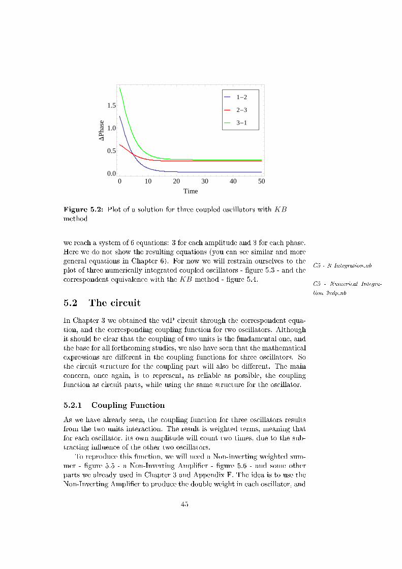
0 10 20 30 40 500.0

0.5

1.0

1.5

Time

DPh

ase 3-1

2-3

1-2

Figure 5.2: Plot of a solution for three coupled oscillators with KBmethod

we reach a system of 6 equations: 3 for each amplitude and 3 for each phase.Here we do not show the resulting equations (you can see similar and moregeneral equations in Chapter 6). For now we will restrain ourselves to the

C5 - N Integration.nbplot of three numerically integrated coupled oscillators - gure 5.3 - and thecorrespondent equivalence with the KB method - gure 5.4.

C5 - Numerical Integra-

tion 3vdp.nb

5.2 The circuit

In Chapter 3 we obtained the vdP circuit through the correspondent equa-tion, and the corresponding coupling function for two oscillators. Althoughit should be clear that the coupling of two units is the fundamental one, andthe base for all forthcoming studies, we also have seen that the mathematicalexpressions are dierent in the coupling functions for three oscillators. Sothe circuit structure for the coupling part will also be dierent. The mainconcern, once again, is to represent, as reliable as possible, the couplingfunction as circuit parts, while using the same structure for the oscillator.

5.2.1 Coupling Function

As we have already seen, the coupling function for three oscillators resultsfrom the two units interaction. The result is weighted terms, meaning thatfor each oscillator, its own amplitude will count two times, due to the sub-tracting inuence of the other two oscillators.

To reproduce this function, we will need a Non-inverting weighted sum-mer - gure 5.5 - a Non-Inverting Amplier - gure 5.6 - and some otherparts we already used in Chapter 3 and Appendix F. The idea is to use theNon-Inverting Amplier to produce the double weight in each oscillator, and

45

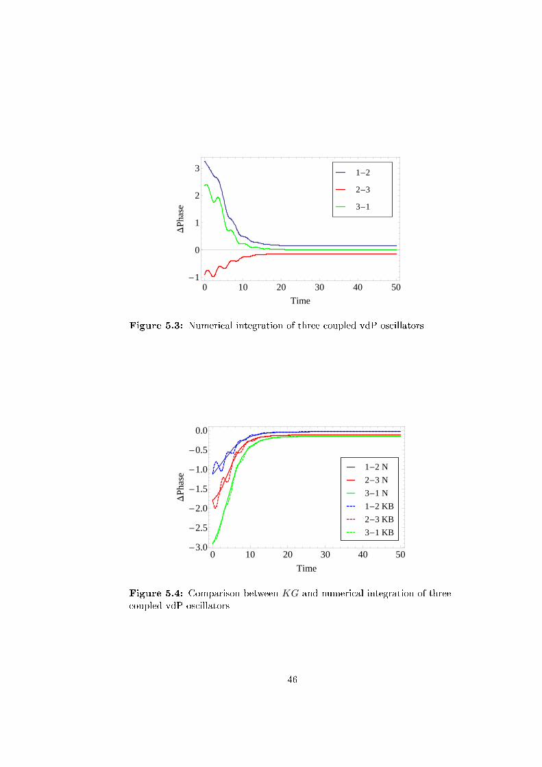
0 10 20 30 40 50-1

0

1

2

3

Time

DPh

ase 3-1

2-3

1-2

Figure 5.3: Numerical integration of three coupled vdP oscillators

0 10 20 30 40 50-3.0

-2.5

-2.0

-1.5

-1.0

-0.5

0.0

Time

DPh

ase

3-1 KB

2-3 KB

1-2 KB

3-1 N

2-3 N

1-2 N

Figure 5.4: Comparison between KG and numerical integration of threecoupled vdP oscillators

46

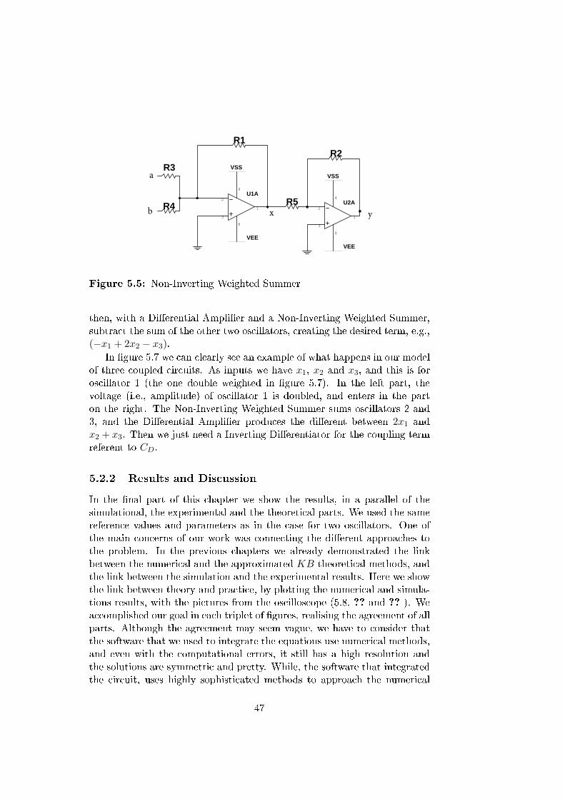
VEE

VEE

VSS

VSS

U1A

3

2

4

8

1

R3

R1

R4 U2A

3

2

4

8

1

R2

R5

a

b yx

Figure 5.5: Non-Inverting Weighted Summer

then, with a Dierential Amplier and a Non-Inverting Weighted Summer,subtract the sum of the other two oscillators, creating the desired term, e.g.,(−x1 + 2x2 − x3).

In gure 5.7 we can clearly see an example of what happens in our modelof three coupled circuits. As inputs we have x1, x2 and x3, and this is foroscillator 1 (the one double weighted in gure 5.7). In the left part, thevoltage (i.e., amplitude) of oscillator 1 is doubled, and enters in the parton the right. The Non-Inverting Weighted Summer sums oscillators 2 and3, and the Dierential Amplier produces the dierent between 2x1 andx2 + x3. Then we just need a Inverting Dierentiator for the coupling termreferent to CD.

5.2.2 Results and Discussion

In the nal part of this chapter we show the results, in a parallel of thesimulational, the experimental and the theoretical parts. We used the samereference values and parameters as in the case for two oscillators. One ofthe main concerns of our work was connecting the dierent approaches tothe problem. In the previous chapters we already demonstrated the linkbetween the numerical and the approximated KB theoretical methods, andthe link between the simulation and the experimental results. Here we showthe link between theory and practice, by plotting the numerical and simula-tions results, with the pictures from the oscilloscope (5.8, ?? and ?? ). Weaccomplished our goal in each triplet of gures, realising the agreement of allparts. Although the agreement may seem vague, we have to consider thatthe software that we used to integrate the equations use numerical methods,and even with the computational errors, it still has a high resolution andthe solutions are symmetric and pretty. While, the software that integratedthe circuit, uses highly sophisticated methods to approach the numerical

47

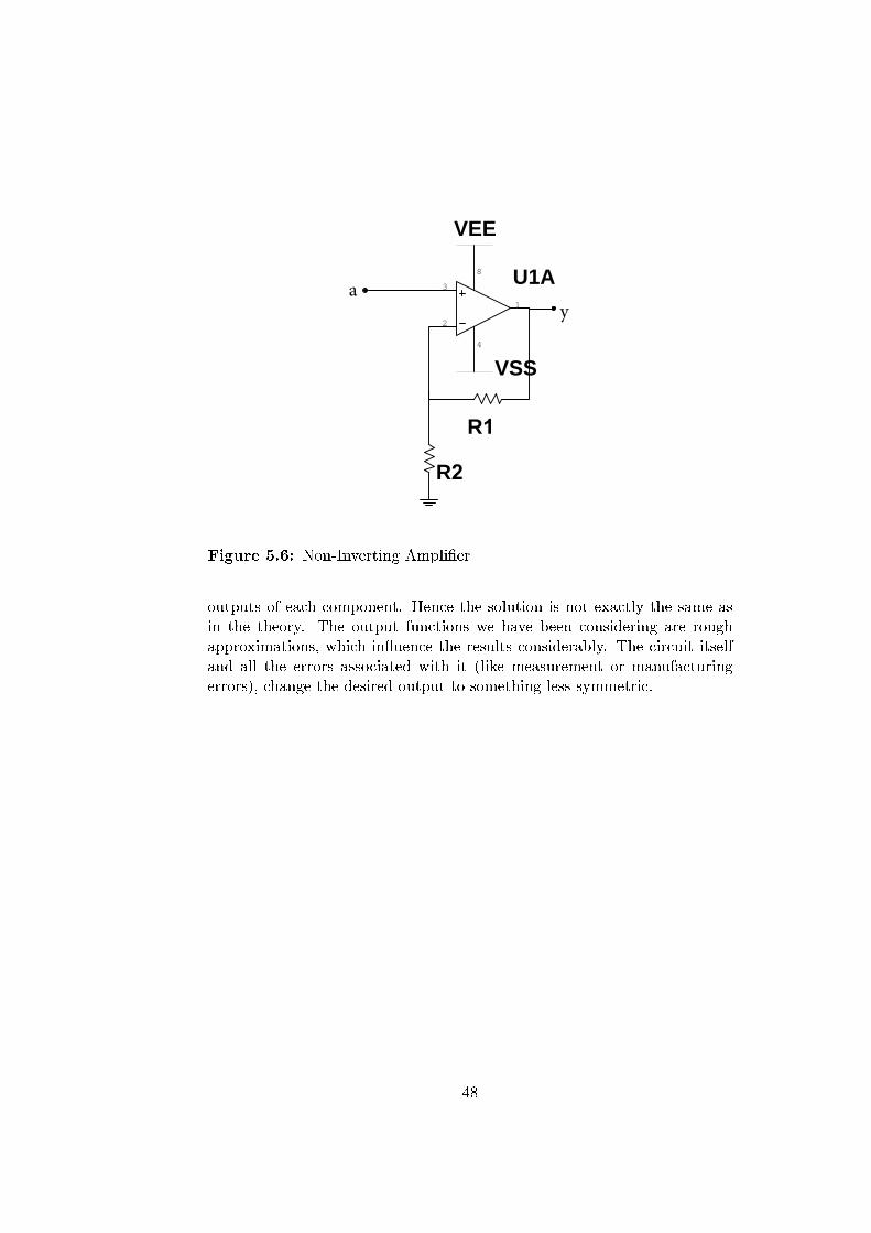
VEE

VSS

U1A3

2

4

8

1

R1

R2

ay

Figure 5.6: Non-Inverting Amplier

outputs of each component. Hence the solution is not exactly the same asin the theory. The output functions we have been considering are roughapproximations, which inuence the results considerably. The circuit itselfand all the errors associated with it (like measurement or manufacturingerrors), change the desired output to something less symmetric.

48

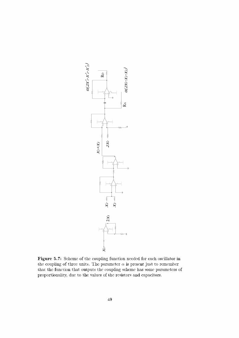
3 2

48

1

32

4 8

1

32

4 8

1

32

4 8

1

32

4 8

1

RA

RDx1

2x1

x2

x3

x2+x3

2x1

α(2x

1-x2-x3)

α(2x'1-x'2-x'3)

Figure 5.7: Scheme of the coupling function needed for each oscillator inthe coupling of three units. The parameter α is present just to rememberthat the function that outputs the coupling scheme has some parameters ofproportionality, due to the values of the resistors and capacitors.

49

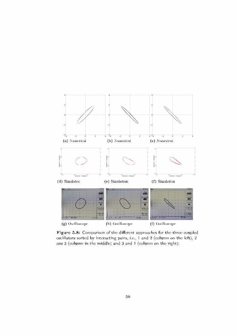
-4 -2 0 2 4-4

-2

0

2

4

(a) Numerical

-4 -2 0 2 4-4

-2

0

2

4

(b) Numerical

-4 -2 0 2 4-4

-2

0

2

4

(c) Numerical

Oscillator 1 - Voltage(V)-6.0 6.0-2.0 2.0

Osc

illat

or 2

- V

olta

ge(V

)

-6.0

6.0

-2.0

2.0

-6.0

6.0

-4.0

4.0

-2.0

2.0

0.0

(d) Simulator

Oscillator 2 - Voltage(V)-6.0 6.0-2.0 2.0

Osc

illat

or 3

- V

olta

ge(V

)

-6.0

6.0

-2.0

2.0

-6.0

6.0

-4.0

4.0

-2.0

2.0

0.0

(e) Simulation

Oscillator 3 - Voltage(V)-6.0 6.0-2.0 2.0

Osc

illat

or 1

- V

olta

ge(V

)

-6.0

6.0

-2.0

2.0

-6.0

6.0

-4.0

4.0

-2.0

2.0

0.0

(f) Simulation

(g) Oscilloscope (h) Oscilloscope (i) Oscilloscope

Figure 5.8: Comparison of the dierent approaches for the three coupledoscillators sorted by interacting pairs, i.e., 1 and 2 (column on the left), 2ans 3 (column in the middle) and 3 and 1 (column on the right).

50

Chapter 6

A Lot of Oscillators

Ernest Hemingway wrote in his letters A man's got to take a lot of

punishment to write a really funny book. [11]. A man who did writea really funny, and also educational, book, is one of the greatest

leaders of synchronization study, Steven Strogatz. Concerning the beautyand complexity of nature, he wrote Most of everyday life is nonlinear, and

the principle of superposition fails spectacularly. If you listen to your two

favorite songs at the same time, you won't get double pleasure! [12]. Weare not trying to approach the genius of Hemingway or Strogatz, however,this thesis has brought a lot of positive punishment, and we are trying toshow you that this spectacular nonlinear world is full of rhythm and pace.Every oscillating thing might synchronize with other oscillating things in itsenvironment. The sucient conditions to attain a synchronize state are veryweak, as we have learnt from this work, and considering the great amountof synchronized motion we observe, at all scales in nature, we can denitelysay it is a master law of this dynamical universe.

The present work tries to deliver an idea to the common non-scienticreader, and a well-fundamented notion to the scientist, that we can jumpto any case of synchronization one can imagine and still nd sync. In thischapter, we will explore an idea on how to make the dynamical approachmore general, increasing the number of oscillators to the hard cases cat-egory. We already mentioned that extreme number of oscillators (too littleor too many), are simple and old cases. Our main focus here is the casefor ten coupled van der Pol oscillators, reaching the main goal: obtainingpositive results in a more complex and general case, starting from the realbasic example.

6.1 The Interaction

In a ensemble of oscillating constituents, the main part is trying to under-stand how they are correlated, which is the correlation term, how to measure

51

the interaction, and all questions concerning how dierent units interact.The global dynamics of the system can be understood from the propertiesof each individual. So far, we have neglected the concept of distance, and wewill keep the main study that way, so we can consider that every pair has thesame mutual interaction - same distance. This is called nearest neighbours

interaction. As an alternative, we could have what is called all-to-all inter-action. Up to three units case, both approaches are the same. But whilewe add more units, the approaches start to diverge. For example, for a 10units case, the nearest neighbours interaction is drawn in gure 6.1a and

C6 - Coupling Term

10vdp - nn.nbthe all-to-all interaction is in gure 6.1b. As another example, the Kirchho

C6 - Coupling Term

10vdp - all-to-all.nb

matrices1 for these cases are:

KNN10vdp =

2 −1 0 0 0 0 0 0 0 −1−1 2 −1 0 0 0 0 0 0 00 −1 2 −1 0 0 0 0 0 00 0 −1 2 −1 0 0 0 0 00 0 0 −1 2 −1 0 0 0 00 0 0 0 −1 2 −1 0 0 00 0 0 0 0 −1 2 −1 0 00 0 0 0 0 0 −1 2 −1 00 0 0 0 0 0 0 −1 2 −1−1 0 0 0 0 0 0 0 −1 2

(6.1)

Kall10vdp =

9 −1 −1 −1 −1 −1 −1 −1 −1 −1−1 9 −1 −1 −1 −1 −1 −1 −1 −1−1 −1 9 −1 −1 −1 −1 −1 −1 −1−1 −1 −1 9 −1 −1 −1 −1 −1 −1−1 −1 −1 −1 9 −1 −1 −1 −1 −1−1 −1 −1 −1 −1 9 −1 −1 −1 −1−1 −1 −1 −1 −1 −1 9 −1 −1 −1−1 −1 −1 −1 −1 −1 −1 9 −1 −1−1 −1 −1 −1 −1 −1 −1 −1 9 −1−1 −1 −1 −1 −1 −1 −1 −1 −1 9

(6.2)

All-to-all interaction will not be considered since it is not obvious that asystem of n units can perform this kind of coupling. It would mean that,in a huge system, the interaction strength would inuence the units withinstantaneous speed. In a more classical case of pairwise interaction, theinuence of a unit propagates through the other units.

1In appendix, you can nd two more examples of coupling terms for an all-to-all coup-ling: C6 - Coupling Term 20vdp - all-to-all.nb, and C6 - Coupling Term 30vdp - all-to-

all.nb

52

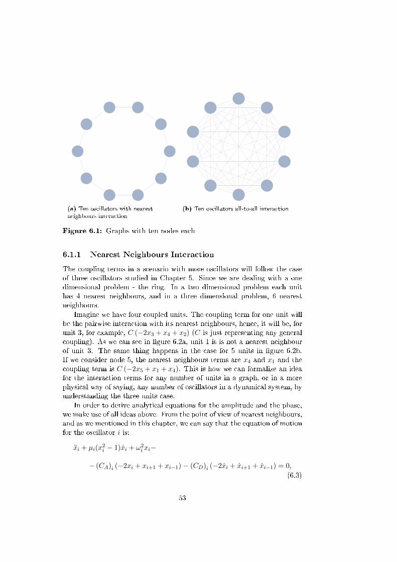
(a) Ten oscillators with nearestneighbours interaction

(b) Ten oscillators all-to-all interaction

Figure 6.1: Graphs with ten nodes each

6.1.1 Nearest Neighbours Interaction

The coupling terms in a scenario with more oscillators will follow the caseof three oscillators studied in Chapter 5. Since we are dealing with a onedimensional problem - the ring. In a two dimensional problem each unithas 4 nearest neighbours, and in a three dimensional problem, 6 nearestneighbours.

Imagine we have four coupled units. The coupling term for one unit willbe the pairwise interaction with its nearest neighbours, hence, it will be, forunit 3, for example, C (−2x3 + x4 + x2) (C is just representing any generalcoupling). As we can see in gure 6.2a, unit 1 it is not a nearest neighbourof unit 3. The same thing happens in the case for 5 units in gure 6.2b.If we consider node 5, the nearest neighbours terms are x4 and x1 and thecoupling term is C (−2x5 + x1 + x4). This is how we can formalize an ideafor the interaction terms for any number of units in a graph, or in a morephysical way of saying, any number of oscillators in a dynamical system, byunderstanding the three units case.

In order to derive analytical equations for the amplitude and the phase,we make use of all ideas above. From the point of view of nearest neighbours,and as we mentioned in this chapter, we can say that the equation of motionfor the oscillator i is:

xi + µi(x2i − 1)xi + ω2

i xi−

− (CA)i (−2xi + xi+1 + xi−1)− (CD)i (−2xi + xi+1 + xi−1) = 0,

(6.3)

53

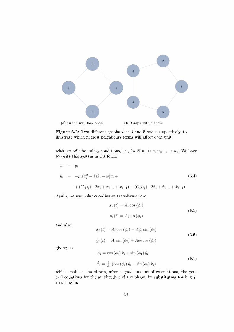
1

2

3

4

(a) Graph with four nodes

1

2

3

4

5

(b) Graph with 5 nodes

Figure 6.2: Two dierent graphs with 4 and 5 nodes respectively, toillustrate which nearest neighbours terms will aect each unit

with periodic boundary conditions, i.e., for N units u, uN+1 → u1. We haveto write this system in the form:

xi = yi

yi = −µi(x2i − 1)xi − ω2i xi+

+ (CA)i (−2xi + xi+1 + xi−1) + (CD)i (−2xi + xi+1 + xi−1)

(6.4)

Again, we use polar coordinates transformation:

xi (t) = Ai cos (φi)

yi (t) = Ai sin (φi)(6.5)

and also:xi (t) = Ai cos (φi)−Aφi sin (φi)

yi (t) = Ai sin (φi) +Aφi cos (φi)

(6.6)

giving us:Ai = cos (φi) xi + sin (φ1) yi

φi = 1Ai

(cos (φi) yi − sin (φi) xi)

(6.7)

which enable us to obtain, after a good amount of calculations, the gen-eral equations for the amplitude and the phase, by substituting 6.4 in 6.7,resulting in:

54

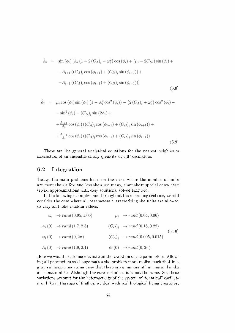
Ai = sin (φi) [Ai(1− 2 (CA)i − ω2

i

)cos (φi) + (µi − 2CDi) sin (φi) +

+Ai+1 ((CA)i cos (φi+1) + (CD)i sin (φi+1)) +

+Ai−1 ((CA)i cos (φi−1) + (CD)i sin (φi−1))]

(6.8)

φi = µi cos (φi) sin (φi)(1−A2

i cos2 (φi))−(2 (CA)i + ω2

i

)cos2 (φi)−

− sin2 (φi)− (CD)i sin (2φi) +

+Ai+1

Aicos (φi) ((CA)i cos (φi+1) + (CD)i sin (φi+1)) +

+Ai−1

Aicos (φi) ((CA)i cos (φi−1) + (CD)i sin (φi−1))

(6.9)

These are the general analytical equations for the nearest neighboursinteraction of an ensemble of any quantity of vdP oscillators.

6.2 Integration

Today, the main problems focus on the cases where the number of unitsare more than a few and less than too many, since these special cases havetrivial approximations with easy solutions, solved long ago.

In the following examples, and throughout the remaining sections, we willconsider the case where all parameters characterizing the units are allowedto vary and take random values:

ωi → rand (0.95, 1.05) µi → rand (0.04, 0.06)

Ai (0) → rand (1.7, 2.3) (CD)i → rand (0.18, 0.22)

ϕi (0) → rand (0, 2π) (CA)i → rand (0.005, 0.015)

Ai (0) → rand (1.9, 2.1) φi (0) → rand (0, 2π)

(6.10)

Here we would like to make a note on the variation of the parameters. Allow-ing all parameters to change makes the problem more realist, such that in agroup of people one cannot say that there are n number of humans and makeall humans alike. Although the core is similar, it is not the same. So, thesevariations account for the heterogeneity of the system of identical oscillat-ors. Like in the case of reies, we deal with real biological living creatures,

55

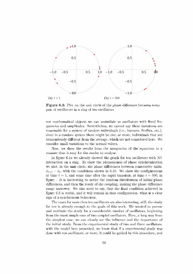
-1.0 -0.5 0.5 1.0

-1.0

-0.5

0.5

1.0

(a) t = 1

-1.0 -0.5 0.5 1.0

-1.0

-0.5

0.5

1.0

(b) t = 500

Figure 6.3: Plot on the unit circle of the phase dierence between everypair of oscillators in a ring of ten oscillators

not mathematical objects we can assimilate as oscillators with xed fre-quencies and amplitudes. Nevertheless, we cannot say these variations arereasonable for a system of random individuals (i.e., humans, reies, etc.),since in a random system there might be one, or more, individuals that aretremendously dierent from the average, which are not considered here. Weconsider small variations to the normal values.

Now, we show the results from the integration of the equations in amanner that is easy for the reader to analyse.

In gure 6.1a we already showed the graph for ten oscillators with NNinteraction on a ring. To show the phenomenon of phase synchronizationwe plot, in the unit circle, the phase dierences between consecutive units,φi+1 − φi, with the conditions shown in 6.10. We show the congurationsat time t = 1, and some time after the rapid transient, at time t = 500, ingure . It is interesting to notice the random distribution of initial phasedierences, and then the result of the coupling, making the phase dierencerange narrower. We also need to say, that the nal condition achieved ingure 6.3 is stable, and it will remain in that conguration, what is a clearsign of a synchronous behaviour.

The cases for more then ten oscillators are also interesting, still, the studyfor ten is already enough to the goals of this work. We wanted to pursueand motivate the study for a considerable number of oscillators, beginningfrom the most simple case of two coupled oscillators. Here, a long way fromthe simplest case, we can clearly see the inuence and the importance ofthe initial study. From the experimental study of two and three oscillators,with the model here presented, we know that if a experimental study wasdone with ten oscillators, or more, it could be guided by this procedure, and

56

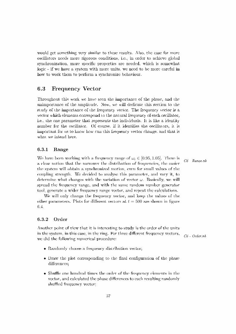
would get something very similar to these results. Also, the case for moreoscillators needs more rigorous conditions, i.e., in order to achieve globalsynchronization, more specic properties are needed, which is somewhatlogic - if we have a system with more units, we need to be more careful inhow to work them to perform a synchronize behaviour.

6.3 Frequency Vector

Throughout this work we have seen the importance of the phase, and theunimportance of the amplitude. Now, we will dedicate this section to thestudy of the importance of the frequency vector. The frequency vector is avector which elements correspond to the natural frequency of each oscillator,i.e., the one parameter that represents the individuals. It is like a identitynumber for the oscillator. Of course, if it identies the oscillators, it isimportant for us to know how can this frequency vector change, and that iswhat we intend here.

6.3.1 Range

We have been working with a frequency range of ωi ∈ [0.95, 1.05]. There isC6 - Range.nb

a clear notion that the narrower the distribution of frequencies, the easierthe system will obtain a synchronized motion, even for small values of thecoupling strength. We decided to analyse this parameter, and vary it, todetermine what changes with the variation of vector ω. Basically, we willspread the frequency range, and with the same random number generatortool, generate a wider frequency range vector, and repeat the calculations.

We will only change the frequency vector, and keep the values of theother parameters. Plots for dierent vectors at t = 500 are shown in gure6.4.

6.3.2 Order

Another point of view that it is interesting to study is the order of the unitsin the system, in this case, in the ring. For three dierent frequency vectors,

C6 - Order.nbwe did the following numerical procedure:

• Randomly choose a frequency distribution vector;

• Draw the plot corresponding to the nal conguration of the phasedierences;

• Shue one hundred times the order of the frequency elements in thevector, and calculated the phase dierences to each resulting randomlyshued frequency vector;

57

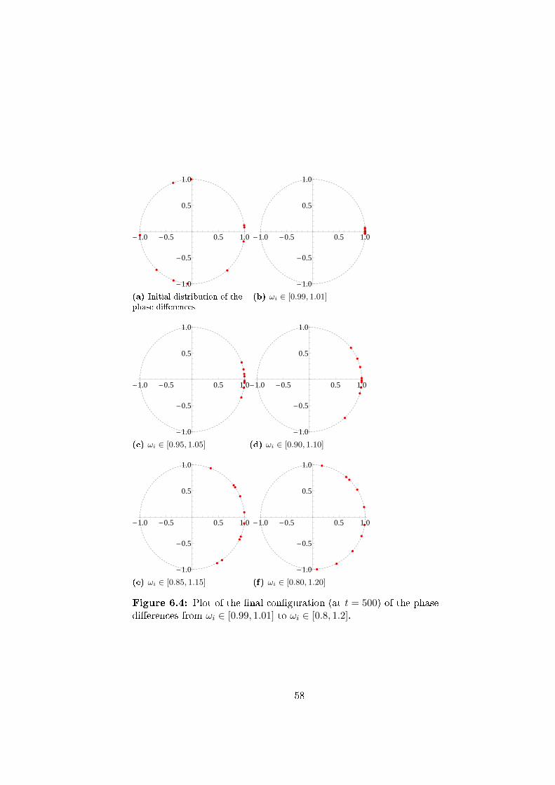
-1.0 -0.5 0.5 1.0

-1.0

-0.5

0.5

1.0

(a) Initial distribution of thephase dierences

-1.0 -0.5 0.5 1.0

-1.0

-0.5

0.5

1.0

(b) ωi ∈ [0.99, 1.01]

-1.0 -0.5 0.5 1.0

-1.0

-0.5

0.5

1.0

(c) ωi ∈ [0.95, 1.05]

-1.0 -0.5 0.5 1.0

-1.0

-0.5

0.5

1.0

(d) ωi ∈ [0.90, 1.10]

-1.0 -0.5 0.5 1.0

-1.0

-0.5

0.5

1.0

(e) ωi ∈ [0.85, 1.15]

-1.0 -0.5 0.5 1.0

-1.0

-0.5

0.5

1.0

(f) ωi ∈ [0.80, 1.20]

Figure 6.4: Plot of the nal conguration (at t = 500) of the phasedierences from ωi ∈ [0.99, 1.01] to ωi ∈ [0.8, 1.2].

58

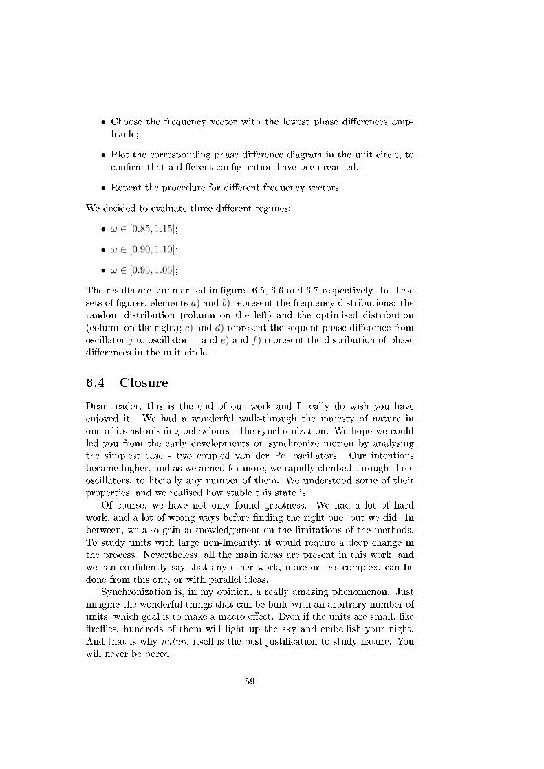
• Choose the frequency vector with the lowest phase dierences amp-litude;

• Plot the corresponding phase dierence diagram in the unit circle, toconrm that a dierent conguration have been reached.

• Repeat the procedure for dierent frequency vectors.

We decided to evaluate three dierent regimes:

• ω ∈ [0.85, 1.15];

• ω ∈ [0.90, 1.10];

• ω ∈ [0.95, 1.05];

The results are summarised in gures 6.5, 6.6 and 6.7 respectively. In thesesets of gures, elements a) and b) represent the frequency distributions: therandom distribution (column on the left) and the optimised distribution(column on the right); c) and d) represent the sequent phase dierence fromoscillator j to oscillator 1; and e) and f) represent the distribution of phasedierences in the unit circle.

6.4 Closure

Dear reader, this is the end of our work and I really do wish you haveenjoyed it. We had a wonderful walk-through the majesty of nature inone of its astonishing behaviours - the synchronization. We hope we couldled you from the early developments on synchronize motion by analysingthe simplest case - two coupled van der Pol oscillators. Our intentionsbecame higher, and as we aimed for more, we rapidly climbed through threeoscillators, to literally any number of them. We understood some of theirproperties, and we realised how stable this state is.

Of course, we have not only found greatness. We had a lot of hardwork, and a lot of wrong ways before nding the right one, but we did. Inbetween, we also gain acknowledgement on the limitations of the methods.To study units with large non-linearity, it would require a deep change inthe process. Nevertheless, all the main ideas are present in this work, andwe can condently say that any other work, more or less complex, can bedone from this one, or with parallel ideas.

Synchronization is, in my opinion, a really amazing phenomenon. Justimagine the wonderful things that can be built with an arbitrary number ofunits, which goal is to make a macro eect. Even if the units are small, likereies, hundreds of them will light up the sky and embellish your night.And that is why nature itself is the best justication to study nature. Youwill never be bored.

59

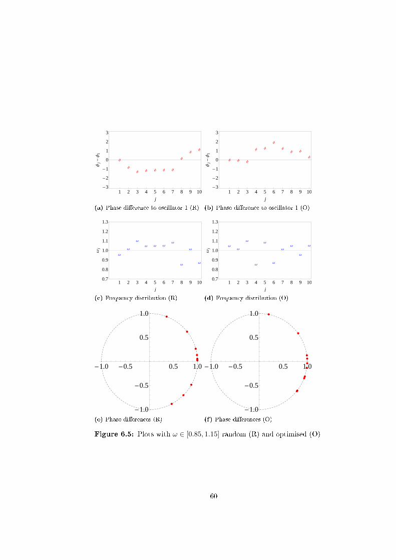
Φ

Φ

Φ Φ Φ Φ Φ

Φ

ΦΦ

1 2 3 4 5 6 7 8 9 10-3

-2

-1

0

1

2

3

j

Φj-

Φ1

(a) Phase dierence to oscillator 1 (R)

Φ Φ Φ

Φ Φ

Φ

ΦΦ Φ

Φ

1 2 3 4 5 6 7 8 9 10-3

-2

-1

0

1

2

3

j

Φj-

Φ1

(b) Phase dierence to oscillator 1 (O)

Ω

Ω

Ω

Ω Ω ΩΩ

Ω

Ω

Ω

1 2 3 4 5 6 7 8 9 100.7

0.8

0.9

1.0

1.1

1.2

1.3

j

Ωj

(c) Frequency distribution (R)

ΩΩ

Ω

Ω

Ω

Ω

ΩΩ

Ω

Ω

1 2 3 4 5 6 7 8 9 100.7

0.8

0.9

1.0

1.1

1.2

1.3

j

Ωj

(d) Frequency distribution (O)

-1.0 -0.5 0.5 1.0

-1.0

-0.5

0.5

1.0

(e) Phase dierences (R)

-1.0 -0.5 0.5 1.0

-1.0

-0.5

0.5

1.0

(f) Phase dierences (O)

Figure 6.5: Plots with ω ∈ [0.85, 1.15] random (R) and optimised (O)

60

Φ ΦΦ

Φ

ΦΦ

Φ

Φ

Φ Φ

1 2 3 4 5 6 7 8 9 10-3

-2

-1

0

1

2

3

j

Φj-

Φ1

(a) Phase dierence to oscillator 1 (R)

Φ

Φ Φ

ΦΦ

ΦΦ

ΦΦ

Φ

1 2 3 4 5 6 7 8 9 10-3

-2

-1

0

1

2

3

j

Φj-

Φ1

(b) Phase dierence to oscillator 1 (O)

Ω Ω

ΩΩ

Ω

Ω Ω Ω

Ω

Ω

1 2 3 4 5 6 7 8 9 100.7

0.8

0.9

1.0

1.1

1.2

1.3

j

Ωj

(c) Frequency distribution (R)

Ω

Ω Ω

Ω

Ω

Ω

Ω

ΩΩ

Ω

1 2 3 4 5 6 7 8 9 100.7

0.8

0.9

1.0

1.1

1.2

1.3

j

Ωj

(d) Frequency distribution (O)

-1.0 -0.5 0.5 1.0

-1.0

-0.5

0.5

1.0

(e) Phase dierences (R)

-1.0 -0.5 0.5 1.0

-1.0

-0.5

0.5

1.0

(f) Phase dierences (O)

Figure 6.6: Plots with ω ∈ [0.90, 1.10] random (R) and optimised (O)

61

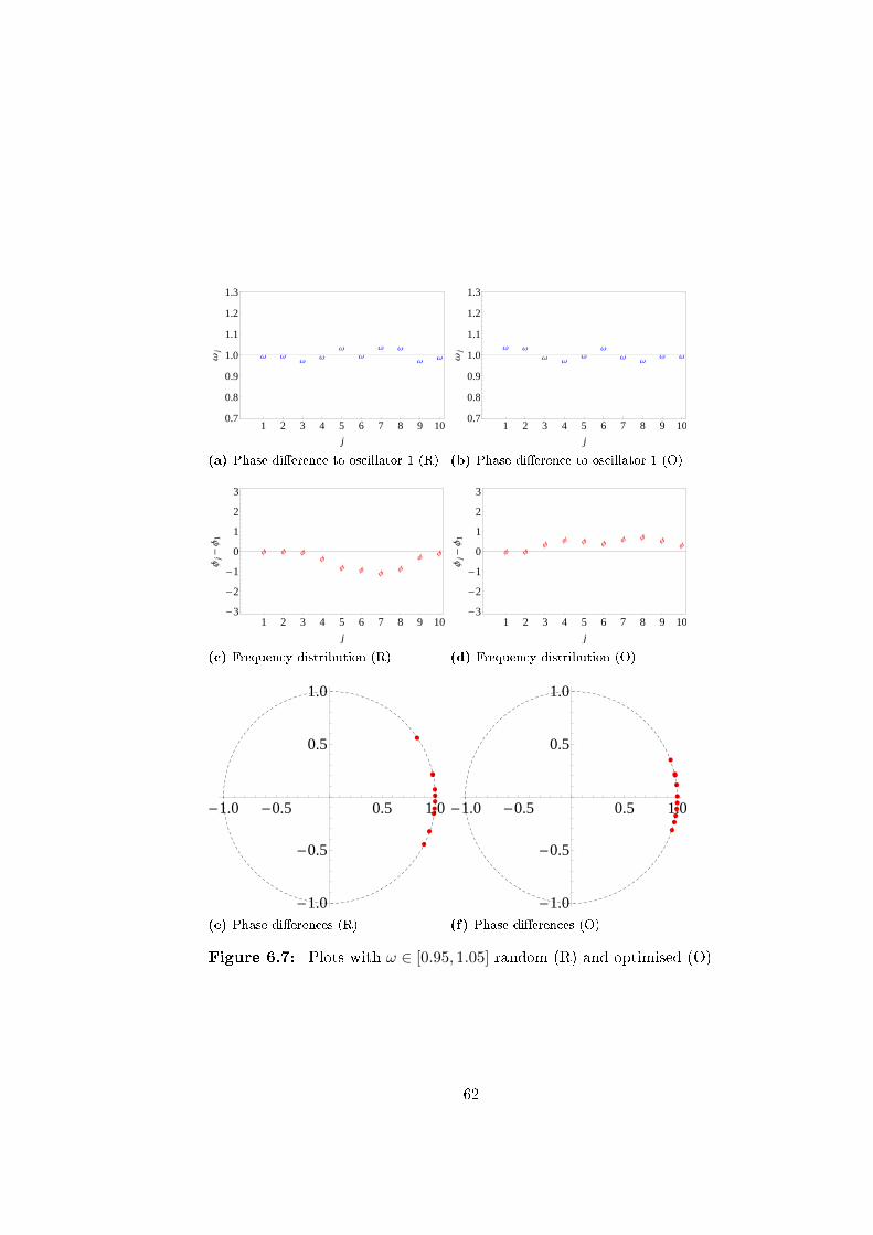
Ω ΩΩ

Ω

Ω

Ω

Ω Ω

ΩΩ

1 2 3 4 5 6 7 8 9 100.7

0.8

0.9

1.0

1.1

1.2

1.3

j

Ωj

(a) Phase dierence to oscillator 1 (R)

Ω Ω

ΩΩ

Ω

Ω

ΩΩ

Ω Ω

1 2 3 4 5 6 7 8 9 100.7

0.8

0.9

1.0

1.1

1.2

1.3

jΩ

j(b) Phase dierence to oscillator 1 (O)

Φ Φ ΦΦ

Φ Φ ΦΦ

ΦΦ

1 2 3 4 5 6 7 8 9 10-3

-2

-1

0

1

2

3

j

Φj-

Φ1

(c) Frequency distribution (R)

Φ ΦΦ

Φ Φ ΦΦ Φ

ΦΦ

1 2 3 4 5 6 7 8 9 10-3

-2

-1

0

1

2

3

j

Φj-

Φ1

(d) Frequency distribution (O)

-1.0 -0.5 0.5 1.0

-1.0

-0.5

0.5

1.0

(e) Phase dierences (R)

-1.0 -0.5 0.5 1.0

-1.0

-0.5

0.5

1.0

(f) Phase dierences (O)

Figure 6.7: Plots with ω ∈ [0.95, 1.05] random (R) and optimised (O)

62

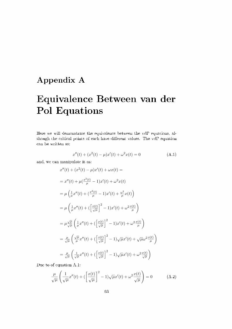
Appendix A

Equivalence Between van der

Pol Equations

Here we will demonstrate the equivalence between the vdP equations, al-though the critical points of each have dierent values. The vdP equationcan be written as:

x′′(t) + (x2(t)− µ)x′(t) + ω2x(t) = 0 (A.1)

and, we can manipulate it as:

x′′(t) + (x2(t)− µ)x′(t) + ωx(t) =

= x′′(t) + µ(x2(t)µ − 1)x′(t) + ω2x(t)

= µ(

1µx′′(t) + (x

2(t)µ − 1)x′(t) + ω2

µ x(t))

= µ

(1µx′′(t) + (

[x(t)õ

]2− 1)x′(t) + ω2 x(t)

µ

)

= µ√µ√µ

(1µx′′(t) + (

[x(t)õ

]2− 1)x′(t) + ω2 x(t)

µ

)

= µ√µ

(√µµ x′′(t) + (

[x(t)õ

]2− 1)√µx′(t) +

√µω2 x(t)

µ

)

= µ√µ

(1√µx′′(t) + (

[x(t)õ

]2− 1)√µx′(t) + ω2 x(t)√

µ

)Due to of equation A.1:

µ√µ

(1√µx′′(t) + (

[x(t)õ

]2− 1)√µx′(t) + ω2x(t)

õ

)= 0 (A.2)

63

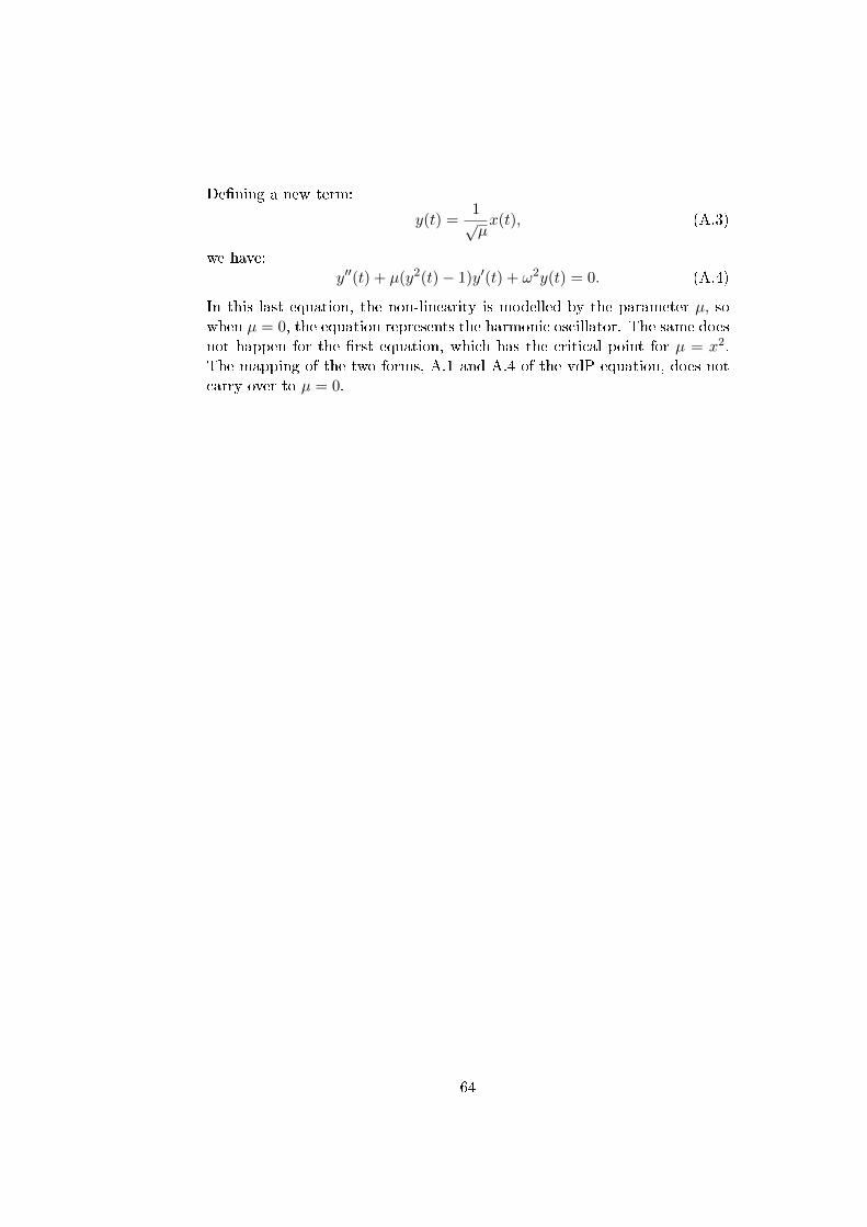
Dening a new term:

y(t) =1õx(t), (A.3)

we have:y′′(t) + µ(y2(t)− 1)y′(t) + ω2y(t) = 0. (A.4)

In this last equation, the non-linearity is modelled by the parameter µ, sowhen µ = 0, the equation represents the harmonic oscillator. The same doesnot happen for the rst equation, which has the critical point for µ = x2.The mapping of the two forms, A.1 and A.4 of the vdP equation, does notcarry over to µ = 0.

64

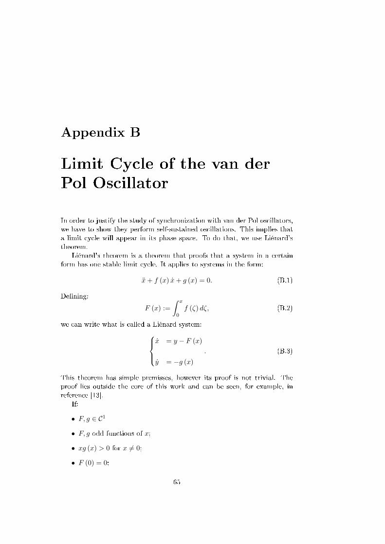
Appendix B

Limit Cycle of the van der

Pol Oscillator

In order to justify the study of synchronization with van der Pol oscillators,we have to show they perform self-sustained oscillations. This implies thata limit cycle will appear in its phase space. To do that, we use Liénard'stheorem.

Liénard's theorem is a theorem that proofs that a system in a certainform has one stable limit cycle. It applies to systems in the form:

x+ f (x) x+ g (x) = 0. (B.1)

Dening:

F (x) :=

ˆ x

0f (ζ) dζ, (B.2)

we can write what is called a Liénard system:x = y − F (x)

y = −g (x)

. (B.3)

This theorem has simple premisses, however its proof is not trivial. Theproof lies outside the core of this work and can be seen, for example, inreference [13].

If:

• F, g ∈ C1

• F, g odd functions of x;

• xg (x) > 0 for x 6= 0;

• F (0) = 0;

65

• F (0) < 0;

• F has one root at x = a;

• and F is monotonically increasing for x ≥ a;

then, system B.3 has exactly one limit cycle, and it is stable. If we recallthe vdP oscillator:

x+ µ(x2 − 1

)x+ ω2x = 0, (B.4)

we observe that we can write it as a Liénard system:x = y − µ

(x3

3 − x)

y = −x(B.5)

So, F (x) = µ(x3

3 − x)and g (x) = x, do verify all of Liénard's theorem

conditions, meaning that the vdP oscillator has an unique stable limit cycle.Also, we see that (x, y) = (0, 0), hence the search for xed points is onlysatised for (x, y) = (0, 0).

66

Appendix C

Perturbation Theory

Perturbation theory is widely used in all branches of science. The complex-ity of many subjects requires the usage of such topic, and, for the sake ofknowledge, it does work acceptably well. The main idea is linked to the ad-vantage of certain domain regions, i.e., we do not need to know every state ofthe universe, since the big bang, to study how the sun will explode - we canconcentrate in a narrow range of time. In perturbation theory, one simplychooses a particular interval of some parameter, and study the simpliedsystem. In specic, here we will derive an approximated analytical solutionfor the van der Pol oscillator in the small non-linearity range (µ 1). Ofcourse it will not work for other values of µ, but those values lie outside ofour interests.

Many studies on perturbation theory have been made over the years,and many dierent ways of studying systems have been used. Here, we willuse a generic method - for more examples and methods, see, for example,reference [8]. We start by recalling the equation of the vdP oscillator:

x+ µ(x2 − 1

)x+ x = 0. (C.1)

The core of perturbation theory sets on the following idea: we can choose asolution x that is dened by a series on the small parameter, in this case µ.Hence:

x = x0 + µx1 + ... (C.2)

where x0 is the zeroth order solution, x1 is the rst order solution, and soon. Now we substitute x in the equation of motion, and we collect the termswith the same order in µ, and at the same time we eliminate all terms withµn : n ≥ 2. The result for µ0 is:

x0 + x0 = 0, (C.3)

and for µ1:x1 + x1 = −

(x20 − 1

)x0. (C.4)

67

We know because of what we showed in Appendix B, that the vdP oscillatorhas a stable limit cycle. So, as initial conditions, we assume that for thezeroth order on the amplitude it will reach a stable value a, hence, we canchoose this value as:

x0 (0) = a. (C.5)

We have only reduced the transient - there is no problem at all in choosingthe destination point as the initial condition. The other initial conditionsare zero (x1 (0), x0 (0) and x1 (0)). We can now solve this problem. Thesolution for µ0 equation is:

x0 (t) = a cos (t) , (C.6)

and using this solution in C.4 we have:

x1 + x1 = −(a2 cos2 (t)− 1

)a sin (t) . (C.7)

Using the trigonometric relation:

cos2 (t) sin (t) =1

4(sin (t) + sin (3t)) , (C.8)

we write:

x1 + x1 = a sin (t)

(1− a2

4

)− a3

4sin (3t) . (C.9)

The term proportional to sin (t) will resonate with the zeroth order solution(proportional to cos (t)) - secular term. We need to avoid this resonance andeliminate this term. We do that by choosing a = 2, which leave us with:

x1 + x1 = −2 sin (3t) . (C.10)

Solving this equation and adding it in the solution, we get:

x = 2 cos (t)− µ sin3 (t) .

We can compare this approximated solution with the numerical solution ingure C.1.

68

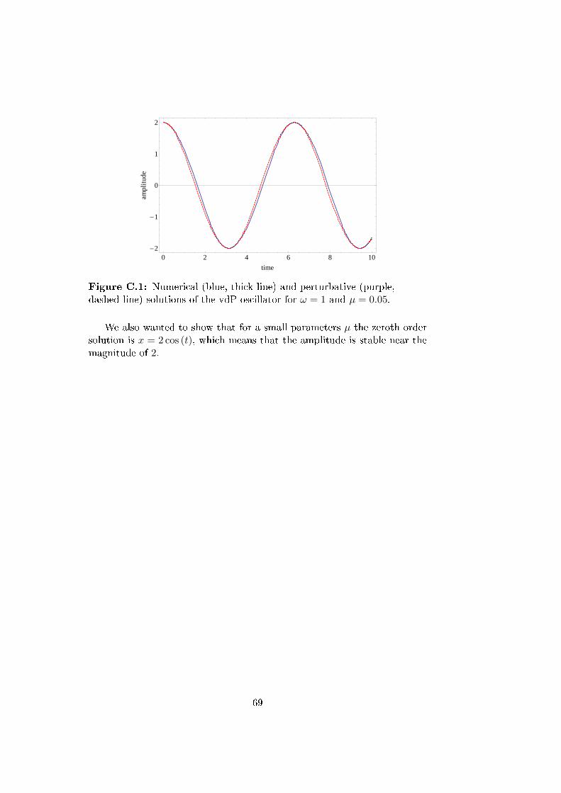
0 2 4 6 8 10-2

-1

0

1

2

time

ampl

itude

Figure C.1: Numerical (blue, thick line) and perturbative (purple,dashed line) solutions of the vdP oscillator for ω = 1 and µ = 0.05.

We also wanted to show that for a small parameters µ the zeroth ordersolution is x = 2 cos (t), which means that the amplitude is stable near themagnitude of 2.

69

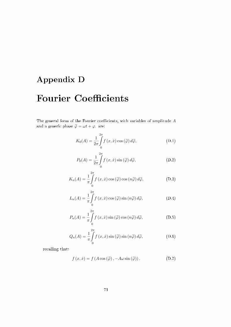
Appendix D

Fourier Coecients

The general form of the Fourier coecients, with variables of amplitude Aand a generic phase ϕ = ωt+ ϕ. are:

K0(A) =1

2π

2π

0

f (x, x) cos (ϕ) dϕ, (D.1)

P0(A) =1

2π

2π

0

f (x, x) sin (ϕ) dϕ, (D.2)

Kn(A) =1

π

2π

0

f (x, x) cos (ϕ) cos (nϕ) dϕ, (D.3)

Ln(A) =1

π

2π

0

f (x, x) cos (ϕ) sin (nϕ) dϕ, (D.4)

Pn(A) =1

π

2π

0

f (x, x) sin (ϕ) cos (nϕ) dϕ, (D.5)

Qn(A) =1

π

2π

0

f (x, x) sin (ϕ) sin (nϕ) dϕ, (D.6)

recalling that:

f (x, x) = f (A cos (ϕ) ,−Aω sin (ϕ)) . (D.7)

71

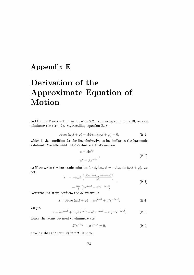
Appendix E

Derivation of the

Approximate Equation of

Motion

In Chapter 2 we say that in equation 2.21, and using equation 2.18, we caneliminate the term 2). So, recalling equation 2.18:

A cos (ωst+ ϕ)−Aϕ sin (ωst+ ϕ) = 0, (E.1)

which is the condition for the rst derivative to be similar to the harmonicsolutions. We also used the coordinate transformation:

a = Aeiϕ

a∗ = Ae−iϕ, (E.2)

so if we write the harmonic solution for x, i.e., x = −Aωs sin (ωst+ ϕ), weget:

x = −ωsA(ei(ωst+ϕ)−e−i(ωst+ϕ)

2i

)= iωs

2

(a eiωst − a∗e−iωst

) . (E.3)

Nevertheless, if we perform the derivative of:

x = A cos (ωst+ ϕ) = a eiωst + a∗e−iωst, (E.4)

we get:x = a eiωst + iωsa e

iωst + a∗e−iωst − iωsa∗e−iωst, (E.5)

hence the terms we need to eliminate are:

a∗e−iωst + a eiωst = 0, (E.6)

proving that the term 2) in 2.21 is zero.

73

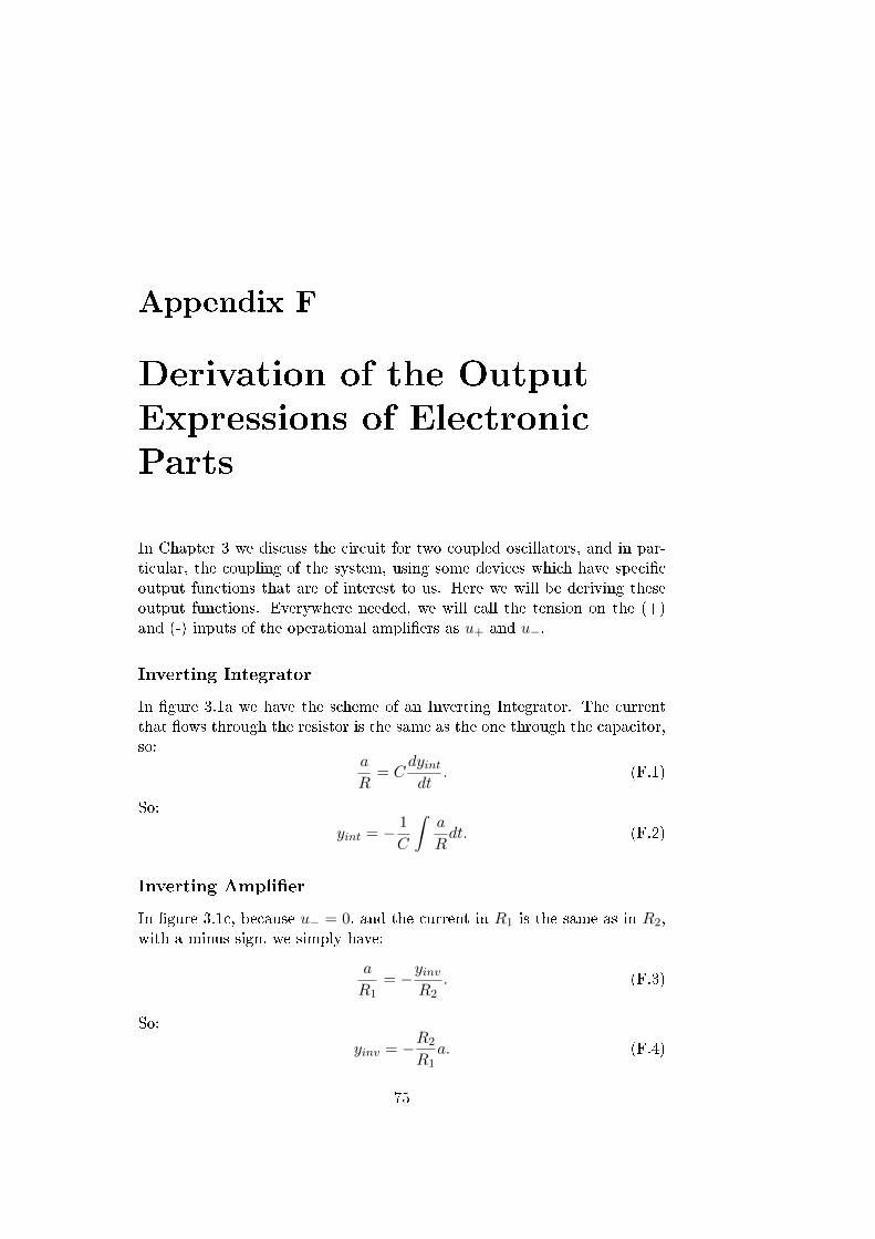
Appendix F

Derivation of the Output

Expressions of Electronic

Parts

In Chapter 3 we discuss the circuit for two coupled oscillators, and in par-ticular, the coupling of the system, using some devices which have specicoutput functions that are of interest to us. Here we will be deriving theseoutput functions. Everywhere needed, we will call the tension on the (+)and (-) inputs of the operational ampliers as u+ and u−.

Inverting Integrator

In gure 3.1a we have the scheme of an Inverting Integrator. The currentthat ows through the resistor is the same as the one through the capacitor,so:

a

R= C

dyintdt

. (F.1)

So:

yint = − 1

C

ˆa

Rdt. (F.2)

Inverting Amplier

In gure 3.1c, because u− = 0, and the current in R1 is the same as in R2,with a minus sign, we simply have:

a

R1= −yinv

R2. (F.3)

So:

yinv = −R2

R1a. (F.4)

75

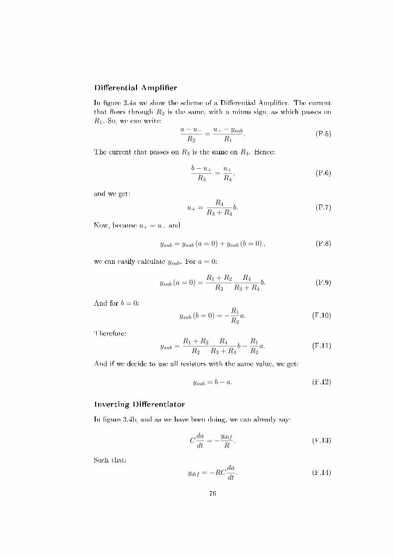
Dierential Amplier

In gure 3.4a we show the scheme of a Dierential Amplier. The currentthat ows through R2 is the same, with a minus sign, as which passes onR1. So, we can write:

a− u−R2

=u− − ysub

R1. (F.5)

The current that passes on R3 is the same on R4. Hence:

b− u+R3

=u+R4

, (F.6)

and we get:

u+ =R4

R3 +R4b. (F.7)

Now, because u+ = u− and

ysub = ysub (a = 0) + ysub (b = 0) , (F.8)

we can easily calculate ysub. For a = 0:

ysub (a = 0) =R1 +R2

R2

R4

R3 +R4b. (F.9)

And for b = 0:

ysub (b = 0) = −R1

R2a. (F.10)

Therefore:

ysub =R1 +R2

R2

R4

R3 +R4b− R1

R2a. (F.11)

And if we decide to use all resistors with the same value, we get:

ysub = b− a. (F.12)

Inverting Dierentiator

In gure 3.4b, and as we have been doing, we can already say:

Cda

dt= −

ydifR

. (F.13)

Such that:

ydif = −RCdadt. (F.14)

76

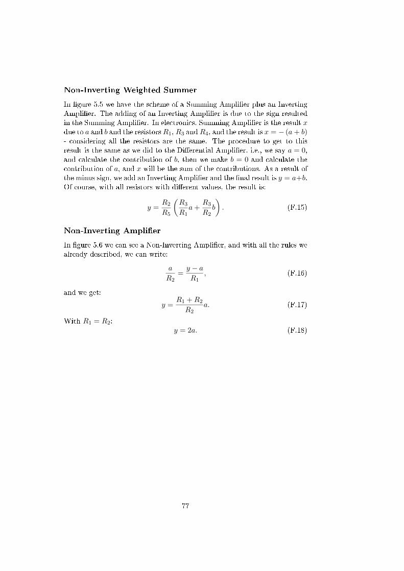
Non-Inverting Weighted Summer

In gure 5.5 we have the scheme of a Summing Amplier plus an InvertingAmplier. The adding of an Inverting Amplier is due to the sign resultedin the Summing Amplier. In electronics, Summing Amplier is the result xdue to a and b and the resistorsR1, R3 andR4, and the result is x = − (a+ b)- considering all the resistors are the same. The procedure to get to thisresult is the same as we did to the Dierential Amplier, i.e., we say a = 0,and calculate the contribution of b, then we make b = 0 and calculate thecontribution of a, and x will be the sum of the contributions. As a result ofthe minus sign, we add an Inverting Amplier and the nal result is y = a+b.Of course, with all resistors with dierent values, the result is:

y =R2

R5

(R3

R1a+

R3

R2b

). (F.15)

Non-Inverting Amplier

In gure 5.6 we can see a Non-Inverting Amplier, and with all the rules wealready described, we can write:

a

R2=y − aR1

, (F.16)

and we get:

y =R1 +R2

R2a. (F.17)

With R1 = R2:y = 2a. (F.18)

77

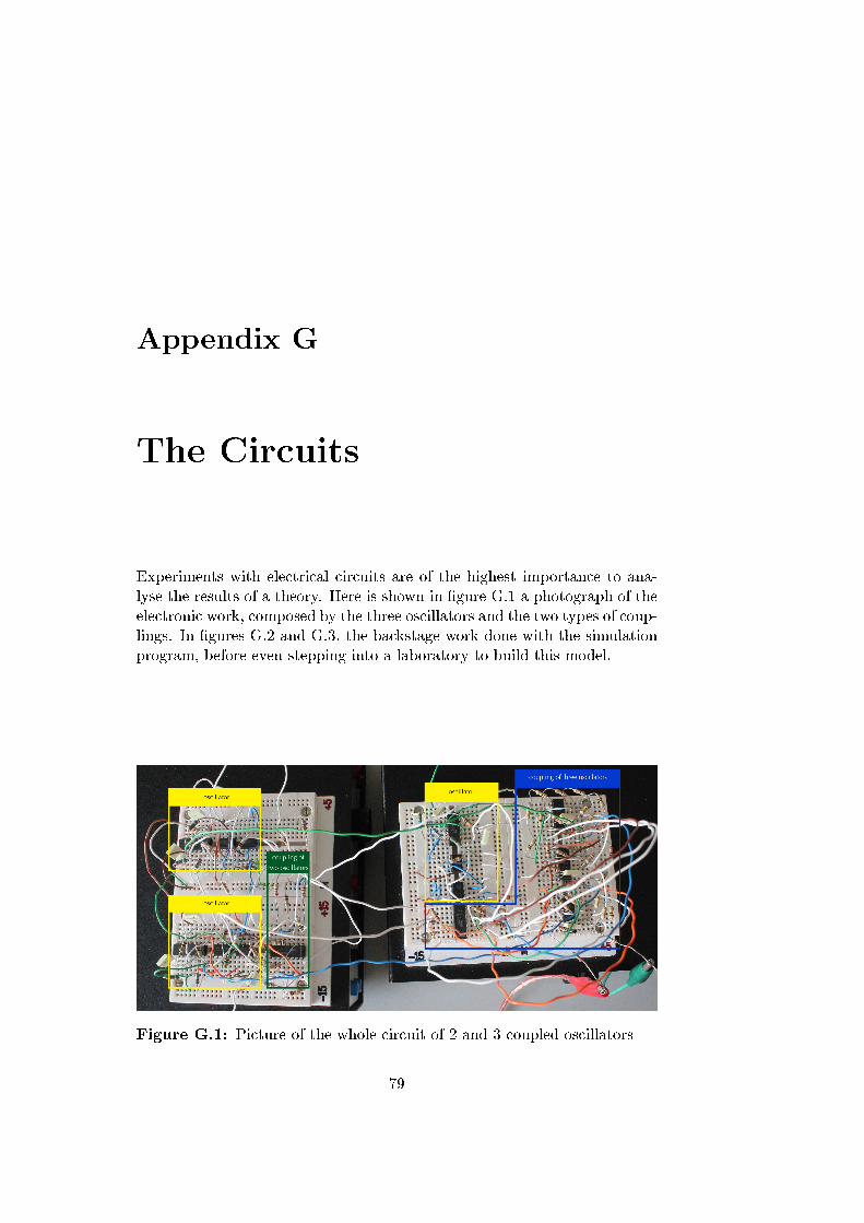
Appendix G

The Circuits

Experiments with electrical circuits are of the highest importance to ana-lyse the results of a theory. Here is shown in gure G.1 a photograph of theelectronic work, composed by the three oscillators and the two types of coup-lings. In gures G.2 and G.3, the backstage work done with the simulationprogram, before even stepping into a laboratory to build this model.

Figure G.1: Picture of the whole circuit of 2 and 3 coupled oscillators

79

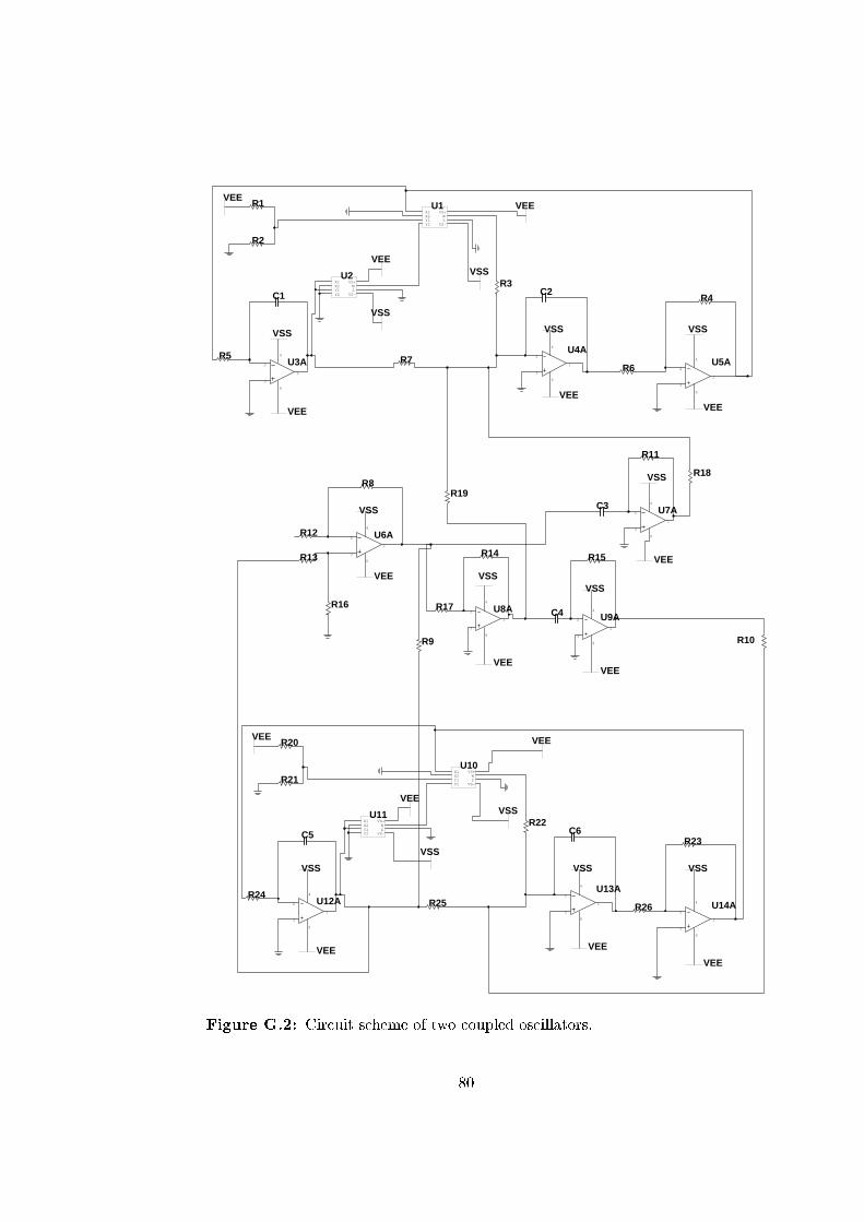
U7A

3

2

4

8

1

VEE

VSS

U9A

3

2

4

8

1

VEE

VSS

U6A

3

2

4

8

1

VEE

VSS

U8A

3

2

4

8

1

VEE

VSS

R12

R8

R16

R13

R9

C3

R11

R17

R14

C4

R15

R18

R19

R10

U5A

3

2

4

8

1

R5 R7R6

C1 C2R4

R3

U1X1X2Y1Y2 VS-

ZW

VS+

U2X1X2Y1Y2 VS-

ZW

VS+

R1

R2

VEE

VEE

VEE

VEE

VEE VEE

VSS

VSS

VSS VSS VSS

U3A

3

2

4

8

1

U4A

3

2

4

8

1

U14A

3

2

4

8

1

R24R25 R26

C5 C6R23

R22

U10X1X2Y1Y2 VS-

ZW

VS+

U11X1X2Y1Y2 VS-

ZW

VS+

R20

R21

VEE

VEE

VEE

VEE

VEEVEE

VSS

VSS

VSS VSS VSS

U12A

3

2

4

8

1

U13A

3

2

4

8

1

Figure G.2: Circuit scheme of two coupled oscillators.

80

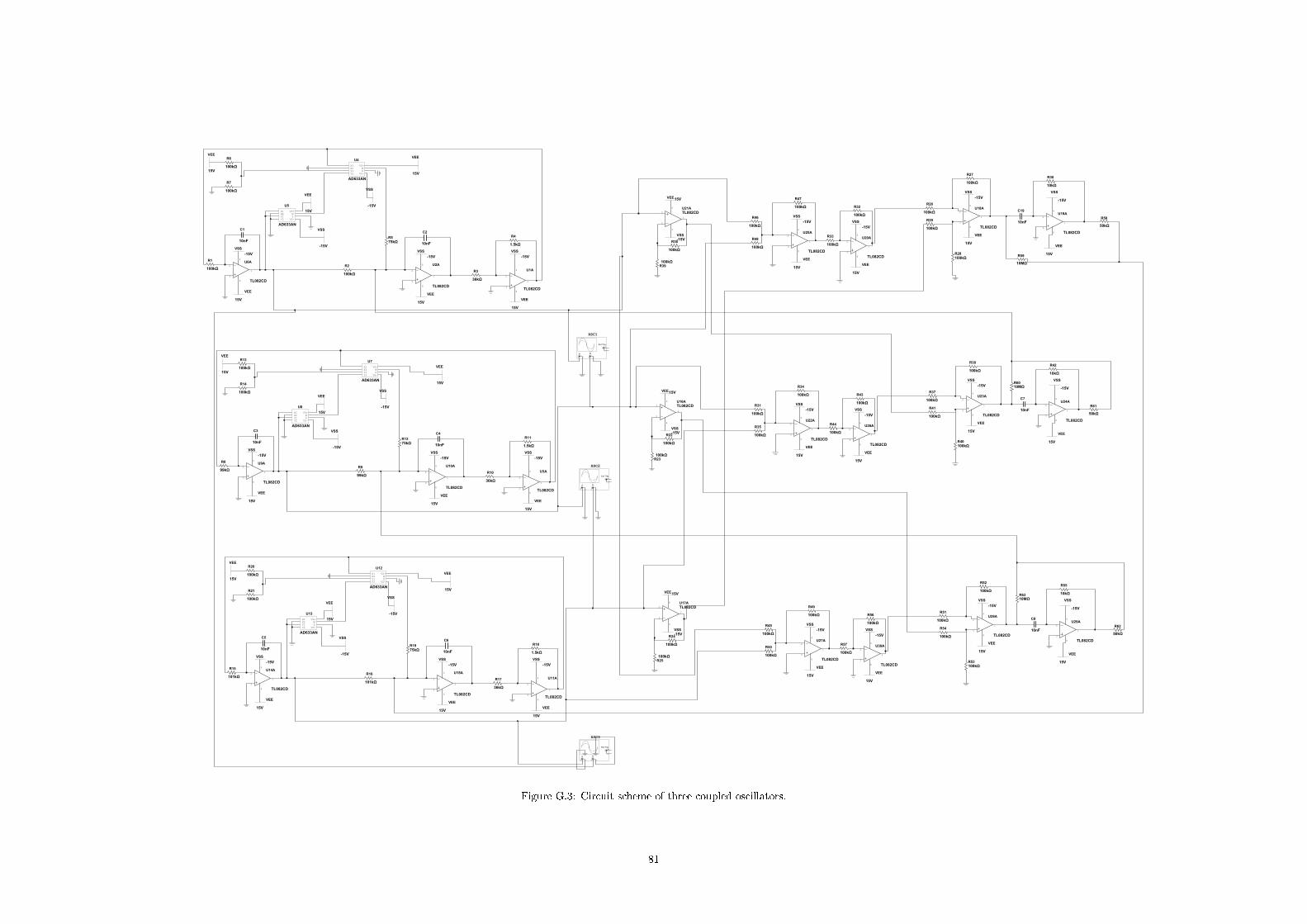
U1A

TL082CD3

2

4

8

1

R1

100kΩR2

100kΩR3

36kΩ

C1

10nF

C2

10nF

R4

1.5kΩ

R575kΩ

U4

AD633AN

X1X2Y1Y2 VS-

ZW

VS+

U5

AD633AN

X1X2Y1Y2 VS-

ZW

VS+

R6

100kΩ

R7

100kΩVEE

15V

VEE

15V

VEE

15V

VEE

15V

VEE

15V VEE

15V

VSS

-15V

VSS

-15V

VSS-15V

VSS-15V

VSS-15V

U6A

TL082CD3

2

4

8

1

U2A

TL082CD3

2

4

8

1

U3A

TL082CD3

2

4

8

1

R8

99kΩR9

99kΩR10

36kΩ

C3

10nF

C4

10nF

R11

1.5kΩ

R1275kΩ

U7

AD633AN

X1X2Y1Y2 VS-

ZW

VS+

U8

AD633AN

X1X2Y1Y2 VS-

ZW

VS+

R13

100kΩ

R14

100kΩVEE

15V

VEE

15V

VEE

15V

VEE

15V

VEE

15V VEE

15V

VSS

-15V

VSS

-15V

VSS-15V

VSS-15V

VSS-15V

U9A

TL082CD3

2

4

8

1

U10A

TL082CD3

2

4

8

1

U11A

TL082CD3

2

4

8

1

R15

101kΩR16

101kΩR17

36kΩ

C5

10nF

C6

10nF

R18

1.5kΩ

R1975kΩ

U12

AD633AN

X1X2Y1Y2 VS-

ZW

VS+

U13

AD633AN

X1X2Y1Y2 VS-

ZW

VS+

R20

100kΩ

R21

100kΩVEE

15V

VEE

15V

VEE

15V

VEE

15V

VEE

15V VEE

15V

VSS

-15V

VSS

-15V

VSS-15V

VSS-15V

VSS-15V

U14A

TL082CD3

2

4

8

1

U15A

TL082CD3

2

4

8

1

VEE15V

VSS-15V

U21ATL082CD3

2

4

8

1

R36

100kΩ

R39100kΩ

VEE15V

VSS-15V

U16ATL082CD3

2

4

8

1

R22

100kΩ

R23100kΩ

VEE15V

VSS-15V

U17ATL082CD3

2

4

8

1

R24

100kΩ

R25100kΩ

VEE

15V

VEE

15VVEE

15V

VSS-15V

VSS-15V

VSS

-15V

U25A

TL082CD3

2

4

8

1

R46

100kΩ

R47

100kΩ

R48

100kΩ

U18A

TL082CD3

2

4

8

1

R26

100kΩ

R27

100kΩ

R28100kΩ

R29

100kΩ

U19A

TL082CD3

2

4

8

1

C19

10nF

R30

10kΩ

VEE

15V

VSS-15V

U20A

TL082CD3

2

4

8

1

R32

100kΩ

R33

100kΩ

VEE

15V

VEE

15VVEE

15V

VEE

15V

VSS-15V

VSS-15V

VSS

-15V

VSS-15V

U22A

TL082CD3

2

4

8

1

R31

100kΩ

R34

100kΩ

R35

100kΩ

U23A

TL082CD3

2

4

8

1

R37

100kΩ

R38

100kΩ

R40100kΩ

R41

100kΩ

U24A

TL082CD3

2

4

8

1

C7

10nF

R42

10kΩ

U26A

TL082CD3

2

4

8

1

R43

100kΩ

R44

100kΩ

VEE

15V

VEE

15VVEE

15V

VEE

15V

VSS-15V

VSS-15V

VSS

-15V

VSS-15V

U27A

TL082CD3

2

4

8

1

R45

100kΩ

R49

100kΩ

R50

100kΩ

U28A

TL082CD3

2

4

8

1

R51

100kΩ

R52

100kΩ

R53100kΩ

R54

100kΩ

U29A

TL082CD3

2

4

8

1

C8

10nF

R55

10kΩ

U30A

TL082CD3

2

4

8

1

R56

100kΩ

R57

100kΩ

XSC1

A B

Ext Trig+

+

_

_ + _

R58

50kΩ

R59

10MΩ

R6010MΩ

R61

50kΩ

R62

50kΩ

R6310MΩ

XSC2

A B

Ext Trig+

+

_

_ + _

XSC3

A B

Ext Trig+

+

_

_ + _

Figure G.3: Circuit scheme of three coupled oscillators.

81

Bibliography

[1] A. Pikovsky, M. Rosenblum, J. Kurths, Synchronization - A Universal

Concept in Nonlinear Sciences, Cambridge University Press, 2001

[2] R. Mirollo, S. Strogatz, Synchronization of Pulse-Coupled Biological

Oscillators, SIAM J. Appl. Math., vol. 50 no. 6, 1990

[3] N. Kopell, B. Ermentrout, Chemical and Electrical Synapses Perform

Complementary Roles in the Synchronization of Interneuronal Net-

works, PNAS - vol. 101 - no. 43, 2004

[4] J. Shuai, D. Durand, Phase Synchronization In Two Coupled Chaotic

Neurons, Phys. Let. A 264, 2004

[5] H. Nijmeijer, A. Rodriguez-Angeles, Synchronization of Mechanical

Systems, World Scientic Publishing Co. Pte. Ltd., 2003

[6] C. Huygens (Hugenii), Horologium Oscillatorium, Apud F. Muguet,Parisiis, France, 1673. English translation: The Pendulum Clock, IowaState University Press, Ames, 1986

[7] L. Pecora, T. Carrol, Master Stability Functions for Synchronized

Coupled Systems, Phys. Rev. Lett. 80, 2109, 1998

[8] N. Minorsky, Introduction to Non-Linear Mechanics, Edwards Brothers,Inc., 1947

[9] A. Balanov, N. Janson, D. Postnov, O. Sosnovtseva, Synchronization:From Simple to Complex, Springer, 2009

[10] N. Corron, A Simple Circuit Implementation of a van der Pol Oscil-

lator, Creative Consulting for Research and Education, 2006

[11] E. Hemingway, C. Baker, Ernest Hemingway Selected Letters 1917-

1961, Scribner Classics, 2003

[12] S. Strogatz, Nonlinear Dynamics and Chaos, Perseus Books Publishing,LLC, 1994

[13] L. Perko, Dierential Equations and Dynamical Systems, Springer, 2000

83