1§3 class and home problems )

r The object of this column is to enhance our readers ' collections of interesting and novel

problems in chemical engineering. We request problems that can be used to motivate student learning by presenting a particular principle in a new light, can be assigned as novel home

problems, are suited for a collaborative learning environment, or demonstrate a cutting-edge application or principle. Manuscripts should not exceed 14 double-spaced pages and should be accompanied by the originals of any figures or photographs. Please submit them to Dr. Daina Briedis (e-mail: briedis@egr.msu .edu), Department of Chemical Engineering and Materials

Science, Michigan State University, East Lansing, MI 48824-1226. \.

TRANSPORT PHENOMENA PROJECTS: Natural Convection Between Porous, Concentric Cylinders

-A Method To Learn and To Innovate

ESTEBAN SAATDJIAN, FRAN<;:OIS LESAGE, AND JOSE PAULO B. MOTA 1

ENSIC - Ecole Nationale Superieure des Industries Chimiques • 54001 Nancy Cedex, France 1 Universidade Nova de Lisboa • 2829-516 Caparica, Portugal

It is well recognized worldwide that transport phenomena courses are of fundamental importance in the chemical engineering curriculum of major universities at both

the undergraduate and the graduate level. As defined in the pioneering text Transport Phenomena by Bird, Stewart, and Lightfoot,1'1 which was first published in 1960, this science is concerned with the balance of momentum (fluid mechanics), energy, and mass in a wide variety of elementary and industrial processes . An undergraduate program in chemical engineering would typically have two required courses related to transport phenomena (fluid flow, heat and mass transfer) and perhaps several optional courses on some more advanced topics such as non-Newtonian fluid mechanics , radiation heat transfer, two-phase flow, rheology, etc. Although the basic conservation of mass , energy, and momentum equations have not changed since they were formulated a long time ago and an instructor can still confidently use Reference 1 as background material to his or her course, a modem transport phenomena curriculum at the senior or graduate level could profit greatly from some of the major research results that have been published over the last 50 years . Furthermore, as illustrated below, many different aspects of transport phenomena can be studied via the solution of a well-defined project.

Today (and it was not the case 50 years ago) every un­dergraduate owns a laptop computer; a student can solve numerically practically all 2-D coupled transport phenomena

Vol. 47, No . 1, Winter 2013

problems that, 50 years ago, required the use of the computing facilities of the university. Although the solution of partial dif­ferential equations is part of a course on numerical methods, as in the many excellent textbooks on numerical methods such as Reference 2, adding or revisiting this material in a course on transport phenomena makes a lot of sense today. The use of an upwind scheme for the advection terms in a transport equation is a good example of the symbiosis between these two subjects .

A domain where considerable progress has been made over the last 50 years is natural convection. Half a century ago an undergraduate course on natural convection would focus mainly on the dimensionless numbers of importance (Rayleigh number,

Esteban Saatdjian is, since 1989, a professor of chemical engineering at ENSIC in Nancy, France, and an adjunct professor at Georgia Tech. He teaches transport phenomena and computational fluid dynamics (CFO) to undergraduate and graduate students. His current research interests are in mixing of viscous fluids, magnetohydrodynamic flows, and micro-fluidics.

Franfois Lesage is an associate professor of chemical engineering at ENSIC. He teaches process control, CFO, and numerical methods to un­dergraduate students. His research interests are in process optimization and two-phase flow.

Jose Paulo Mota is, since 1997, a professor of chemical engineering at Universidade Nova de Usboa, Usbon, Portugal. He teaches transport phe­nomena, process control, and optimization. His current research interests are in adsorption, mixing, and molecular simulations. He graduated from the University of Porto in 1991 and obtained his Ph.D. in Nancy, France.

© Copyright ChE Division of ASEE 2013

59

Grashot number), on the Boussinesq approximation and on experimental correlations available for different geometries. Experimental and numerical results obtained over the last 30 years have radically increased our knowledge on this subject. The same argument is also valid for mixed convection, i.e., combined forced and natural convection.

Here we present a numerical natural convection project that we have given to our senior/graduate students, it is based on researchl31 published about 20 years ago . We highlight the different aspects of transport phenomena that need to be mastered in order to obtain a solution and discuss what the students can learn from this work. We feel that this project is in total agreement with the opinion of W.M. Kaysc41 on what problems for graduate students should be. Almost 50 years ago he wrote, "At some point, and the earlier the bet­ter, the student must face up to the analysis of problems that may require considerable time, possibly extensive outside study, and that are incompletely stated or specified so that individual judgement must be exercised." Although the first PC appeared more than 10 years later he also wrote "Many of the problems require numerical or graphical integrations or iterative calculation procedures. If (the students) have access to a computer they ought to develop the habit of using it in their problem work."

In a planned follow-up paper we will discuss different variations to this problem for use in future years or in a graduate course. These variations are fluid layers, heat flow reduction, and a change in geometry. Natural convec­tion also permits the instructor to introduce the student to hydrodynamic stability.

NATURAL CONVECTION BETWEEN CONCENTRIC POROUS CYLINDERS

The subject that we gave to our senior/graduate students in the fall semester of 2011 was:

Consider two very long, horizantal, concentric cylinders maintained at constant but different temperatures with ~" > T,,,,,· A saturated porous material,for example glass wool insulation, occupies the annular region between the two cylinders. Write the appropriate conservation equations for this natural convection problem and determine numeri­cally the temperature and velocity fields in the annular layer. Calculate the heat loss to the surroundings. Suggest improvements in order to reduce these heat transfer losses. Assume that the temperature difference between the two walls (actually the Rayleigh number) is not too high so that the flow inside the annular region is not turbulent.

Below we discuss the major steps involved in the solution of this project.

Conservation equations and boundary conditions

The governing conservation equations must first be written and simplified. The student must start by writing the continuity

60

equation in a porous medium. In vector notation and without any assumptions it is:

Eop +VpV=0 at (1)

where £ is the porosity of the porous medium, p is the fluid density and V is the velocity vector. To simplify the above equation to V ·V = 0, the continuity equation for an incom­pressible fluid, the students will have to understand the dif­ference between a fluid whose density depends on pressure and a fluid whose density depends on temperature. We explain this in the classroom by discussing the flow of air over a verti­cal radiator in the winter, when the radiators are turned on. The air flow rises along the radiator and the entrained dust particles stick to the wall just on top of the radiator usually in a parabolic velocity distribution shape. A review of vector analysis will be necessary to write this equation in cylindrical coordinates and, as we shall see later on, in other orthogonal coordinate systems.

The simplest equation of motion for a fluid in a porous medium is Darcy 's law:

k V =--[VP-pg.]

µ (2)

We have deliberately chosen a porous medium instead of a pure fluid to simplify the numerical work for senior students. When the annular layer is saturated with a pure fluid, the 2-D numerical solution can be obtained using either a vorticity­stream function formulation or by solving the primitive equa­tions using a SIMPLE algorithm. The number of coupled pdes to be solved is higher (three instead of two) and the treatment of variables for which boundary conditions are not known (vorticity or pressure) is required. Nevertheless, a pure fluid such as a gas could be used in projects for graduate students with a more solid background in numerical methods for partial differential equations and on the solution of the Navier-Stokes equations in particular. (We plan to discuss this topic in detail in a later paper.)

Darcy's law is a linear relationship between fluid velocity and pressure drop, the permeability of the porous medium k is determined experimentally. Again a review of vector analysis is necessary to write the (r, 8) components of this equation, special care must be made both to express the gravity vector in cylindrical coordinates and to define the origin of the tangential coordinate 8. In natural convection and for moderate Rayleigh numbers the flow velocity is relatively small so that Darcy's law is more than adequate. Deviations from Darcy 's law oc­cur mainly when the flow rate through the porous medium is high. Other more complicated flow equations for use in these conditions (Brinkman equation, Forchheimer equation) exist,CSl and the students and the instructor can spend some time in the classroom discussing these and deciding whether the use of a more elaborate (empirical) equation is warranted.

Chemical Engineering Education

A control volume, on which a heat balance will be per­formed, needs to be defined before a heat balance is written . The control volume that was used in this project is partially occupied by the fluid and partially occupied by the immobile solid phase . The temperatures of the solid and fluid phases are assumed equal for simplicity. The student must recognize that both the accumulation of heat and the heat conduction terms involve both the solid and fluid phases; however, the advec­tion terms involve only the fluid phase. In this problem the conditions are such that viscous heat dissipation is negligible. The instructor and the students should spend some time in the classroom discussing these assumptions and eventually trying to develop a model where the temperatures of the fluid and solid phases are different.

The conservation of energy equation that was used in our project is:

where "A* is the thermal conductivity of the porous medium. In this equation fluid properties are marked with subscript f and properties of the porous medium as a whole (solid and fluid) are labeled with superscript *. The properties of the porous medium as a whole could be evaluated using:

(pcJ =(1-E)(pcp), +E(pcpt

'),,* =(1-E)\ +£Ar

but other alternatives are also possible.f51

The linear equation of state for an incompressible fluid whose density varies with temperature is:

p=pJ1-l3(T-T0)] (4)

where 13 is the thermal expansion coefficient. Natural con­vection is driven by gravity forces, the fluid density is as­sumed constant everywhere except in the body force term in Darcy's law, this is the Boussinesq approximation. As Joseph Boussinesq (1842-1929) wrote ( originally in French): "One must know that in most fluid movement provoked by heating, volume and density are practically constant even though the difference in weight of the fluid is the cause of the movement under analysis. From there results the pos­sibility of neglecting density variations when they are not multiplied by the gravitational acceleration g, although one must take into account in the calculations the product of these two quantities ."

The Boussinesq approximation was tested some 30 years ago when experiments were realized in the Skylab where there is practically zero gravity. When a liquid was heated from below, no convective movement was observed. Because of this, the time required to boil water under zero gravity is much longer than on earth. This experiment confirms that the Boussinesq approximation is relevant in most practical cases .

Vol. 47, No. 1, Winter 2013

The next step consists in defining appropriate reference quantities for both dependent and independent variables and to render the equations dimensionless in order to highlight important dimensionless numbers. Here we chose Rin' the

inner cylinder radius as reference length, (pCJ R~" /')1,'

as reference time , '),,' I R;" (pCP)r as reference velocity, ).,'µ/k(pCP) as reference pressure. We also defined a dimensionlesi temperature 0 = (T - T )/(T - T ) which

out m out

varies between O and 1. The number of dimensionless equa-tions to be solved can be reduced by recognizing that, for 2-D incompressible fluids , it is possible to define a stream func­tion (which automatically satisfies the continuity equation). In dimensionless variables the stream function is defined as:

1 a'l' a'l' V =-- V =--

' r as ' 8 ar (5)

The two velocity components are thus replaced by just one independent variable , the stream function 'ljl. In the govern­ing equations there is one dependent variable, pressure P, for which it is not possible to write boundary conditions; the same is true for the Navier-Stokes equations . In both cases this dependent variable can be eliminated from the equations by recognizing the vector identity:

V X VP=O.

The final dimensionless equations to be solved are:

ae +V ae + V8 ae = a2

8 +! ae +__!__ a2

8 (6) at ' ar r as ar2 r ar r 2 as2

a2 ~ +! a'l' +__!__ a

2

\JI= Ra' (sin Sae+ cosS ae). (7) ar r ar r2 as2 ar r as

The sole dimensionless number appearing in the equations is Ra* = ( pC )r gl3(T - T )kR /"A *v, the Rayleigh number. p ,n o~ 1n

The two above dimensionless equations are to be solved for increasing (and decreasing) values of the Rayleigh number and for different values of the radius ratio R = R

0ui/Rin'

The domain where the equations (6 , 7) are to be solved must be defined first. In other words , is there an axis of symmetry in this problem? If there is one, then the equations can be solved either over the entire domain or, preferably, one can double the accuracy by using the same grid size to cover just one half of the domain. In the latter case appropriate boundary conditions must be written at the symmetry axis. The student must recognize that the governing dimensionless equations can be solved on a domain that is cut in half by a vertical line. Why is this not true for a horizontal line?

The dimensionless temperature boundary conditions on the inner and outer cylinders are:

0(r=l ,S)=l, 0(r=R,8)=0 .

On the symmetry axis the temperature distribution is linear because both velocity components are zero there. This implies that the fluid cannot travel from one side to the other of the

61

symmetry axis. The boundary conditions on the stream func­tion are very easy to formulate once the student recognizes that the periphery of the entire half-domain is a streamline, an arbitrary value of 'ljJ = 0 can be set.

Numerical solution

Depending on whether the numerical solution of partial dif­ferential equations is part of the transport phenomena course or not, the instructor can choose between allowing the use of a commercial CFD code based on a finite volume formulation or asking the students to develop a finite difference code to solve the governing equations. When a finite volume code is employed, the primitive equations are solved and the convec­tion terms are discretized using an upwind scheme, preferably of second order. Below we discuss the case where students develop their own code using a finite difference method. This method was implemented in our course.

The partial differential equations are converted into alge­braic equations by an appropriate discretization of the deriva­tives. When a finite difference code is employed, students should use second order, central difference Taylor series formulas for spatial derivatives and a first order time marching scheme for the time derivatives. The transient conservation of energy equation can be solved numerically in 2-D by an implicit alternating direction scheme. The solution of a tri­diagonal system of equations at each half step is required. If a very fine grid is employed, for example when half the tangential direction is totally defined by 200 grid points , the student could use an iterative scheme instead of the Thomas algorithm to solve the tri-diagonal system of linear equa­tions . There is no roundoff error when iterative methods of solution are employed and the user can control the accuracy of the obtained solution via a convergence test. The stream function equation can be solved using an iterative method of solution (Jacobi, Gauss-Seidel, under/over relaxation) or, alternatively, one can add a transient term to the equation and solve it using an ADI scheme.

Finally, the code will require several convergence tests . At each time step the stream function equation is solved by an iterative scheme such as the Gauss-Seidel method. The con­vergence criterion here does not have to be very strict since this equation is solved at each time step. The convergence criterion on the heat equation should be based on the fact that, at steady state, the average heat flow into the inner cylinder ct:

- . ="A.· f .;nl de q,n O Or c=R;,

should be equal to the average heat flow out of the cylinder q0

:

- =-"A.' f •OTI d0. g out O ar r= Rout

This leads to the definition of the Nusselt number which is simply the ratio between the heat flow into the porous layer

62

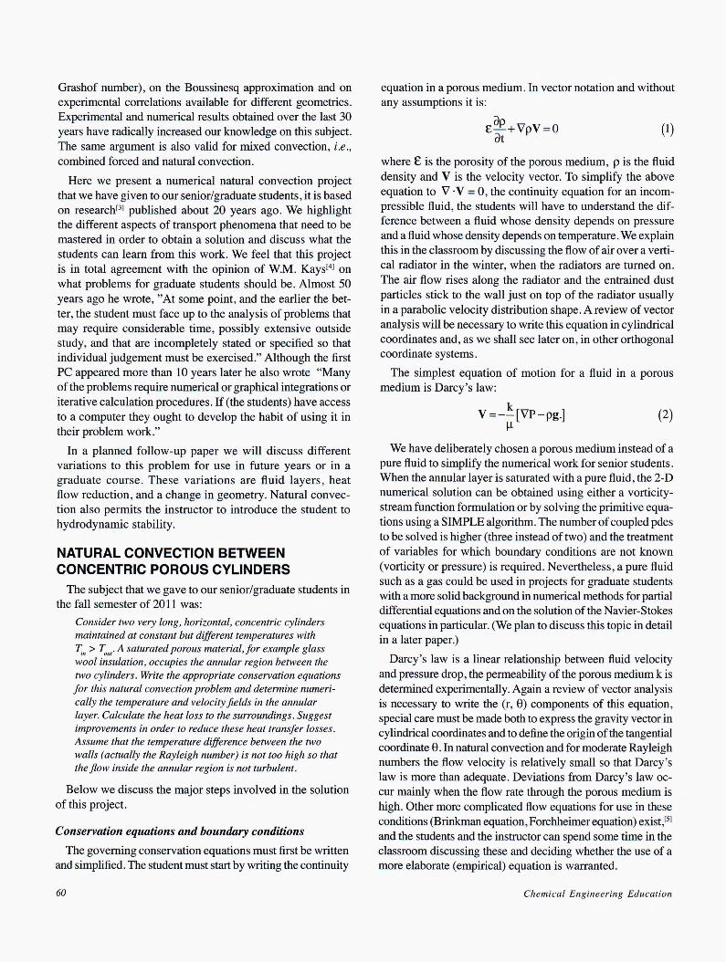
Figure 1. Streamlines and isotherms in an annular po­rous medium, Ra= 100 and R = 2. For this value of the Rayleigh number there are two possible hydrodynamic regimes, a two-cell regime (left) and a four-cell regime

Nu

(right). This figure is taken, with permission, from Reference 8.

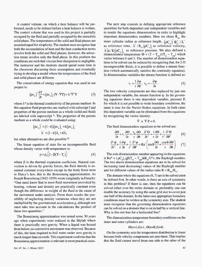
Figure 2. Average Nusselt number Nu as a function of Rayleigh number Ra in an annular porous medium, R =

2. The additional cell leads to a Nusselt number increase. This figure is taken, with permission, from Reference 8.

(by convection) and the heat flow into the layer by conduction, i.e., when there is no motion of the fluid inside the annulus . Both local and average Nusselt numbers were calculated by the students.

RESULTS AND DISCUSSION The developed numerical code is first run for a small value of

the Rayleigh number until convergence is attained. The results obtained are used as initial conditions to calculate the profiles for a slightly higher Rayleigh number. This procedure was rec­ommended to the students in order to speed up the calculations.

For a radius ratio R0u,/Rin = 2 and a Rayleigh number of

100, Figure la shows the streamline pattern and the isotherms within the annular region on increasing the Rayleigh number. The cell is rotating in a clockwise direction. For lower values of the Rayleigh number the streamline pattern and the form of the isotherms is similar; the center of the vortex moves upwards as the Rayleigh number increases.

Chemical Engineering Education

When the Rayleigh number is increased beyond a certain limit, a secondary cell appears on the top of the layer (Figure lb), the secondary cell rotates in a counter-clockwise direc­tion. Experiments where the temperature field in the layer was visualizedC61 have clearly shown that this multi-cellular flow regime does indeed exist. Now, if the two-cell regime is used as an initial condition and if the Rayleigh number is decreased slowly, one observes that this two-cell regime remains in the layer until the Rayleigh number drops below a value of about 65 ± 2.

In other words, for R = 2 and for a Rayleigh number between 65 ± 2 and a value of about 120, there are two possible flow regimes in the layer. This is a hysteresis loop. Although the upper limit value of the Rayleigh number in the hysteresis loop is not clearly established (the transition value depends on the fineness of the grid employed), experimentsC6-71 and a hydrodynamic stability analysis (to be discussed in a later paper) confirm the lower limit value of 65 ± 2.

Figure 2 shows a plot of the Nusselt number as a function of the Rayleigh number. The dotted line corresponds to the two-cell regime ( one cell per cylinder half) and the black line to the four-cell regime. When the flow regime changes from two cells to four cells, the additional circulation at the top of the layer leads to an increase in the average Nusselt number. The experimental Nusselt numbers obtained by Caltagirone[7J have also been included in the figure .

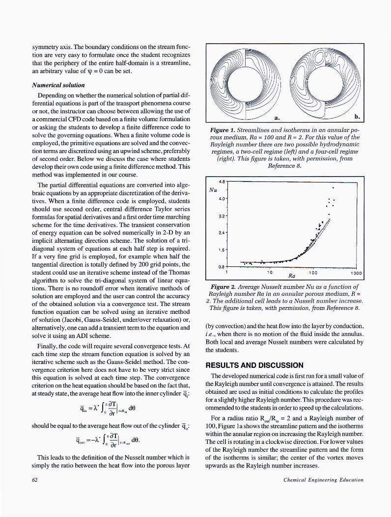
When the radius ratio R0u,/Rin is close to unity (for example

R=l.1), additional cells are formed at the top of the annular region; this is true in both porous and fluid media. This can be explained by recognizing that as the radius ratio R decreases to 1, the cylindrical geometry tends toward the two parallel flat plate geometry and additional cells appear if the Rayleigh number is high enough. Figure 3 shows the streamlines and the isotherms in a porous medium for R

0u,/Rin = 1.2, a 6 cell

flow appears at around Ra= 300 and an 8 cell hydrodynamic regime appears at Ra = 800.

We did not specifically ask our students to calculate the pressure distribution in the porous layer in this project. Taking the divergence of Darcy's law and recognizing that V · V = 0, the obtained result is:

(8)

This equation can be used to calculate the pressure field (see Reference 8) .

STUDENT RESPONSE The above project was given in our senior/graduate student

course on numerical transport phenomena. The accompanying textbooks for this course are Reference 9 or 10 depending on the mother tongue of the student. The students in our gradu­ate program come from different countries of Europe and South America, from Northern Africa, and from the Middle

Vol . 47, No. I , Winter 2013

East. Obviously they have very different mathematical and computer backgrounds and some have to put in quite an initial effort. In order to compensate for this , we asked the students to work in groups of four. We also asked the students to form cosmopolitan groups if possible; this worked quite well. The choice of computer language/software was open; all groups used MATLAB.

The students had one full semester to work on the project and they could (and did) consult the instructors outside the classroom all along . The other courses that were taught to our students during the semester did not require too much outside work and were graded via exams. The students were required to write a report that had to include the way they proceeded, the numerical methods chosen, their analysis of results , and proposals for improvement as well as the program itself.

As mentioned above, the problem presented here is in the spirit ofwhatW.M. Kays wrote in his textbook. This problem could also be included in a future edition of the excellent chemical engineering/numerical methods textbook by Car­nahan, Luther, and Wilkes.121

CONCLUSIONS

Different aspects of transport phenomena can be taught to senior/graduate students via a project requiring the numerical solution of the appropriate conservation equations . The study of natural convection in enclosed surfaces is one example of such a project. After finishing the project described in this paper, the student should feel much more confident in several important aspects of transport phenomena such as vector analysis, the physics of the phenomenon ofnatural convection, the development of a code to solve the coupled pdes , and the analysis of results. As we hope to show in a later paper, this project is also an excellent method to introduce more difficult but important related subjects such as hydrodynamic stability, heat loss reduction, and choice of geometry.

Figure 3. Streamlines and isotherms for a porous annular layer, R /R = 1.2. a) 6 cell regime, Ra=300,

B cell regime, Ra:_Boo'.nThis figure is taken, with permis­sion, from Reference 8.

63

REFERENCES

64

1. Bird, R.B., W.E. Stewart, and E.N. Lightfoot, Transport Phenomena, John Wiley and Sons, New York (1960), 2nd edition (2007)

2. Camahan,B., H.A. Luther, and J .O. Wilkes ,AppliedNumerical Meth­ods , John Wiley and Sons, New York (1969)

3. Barbosa Mota, J .P., and E. Saatdjian , "Natural convection in a porous , horizontal cylindrical annulus ," J . Heat Transf er , 116, 621-626 (1994)

4. Kays , W.M., Convective Heat and Mass Transf er, McGraw-Hill, New York (1966)

5. Nield , D., and A. Bejan, Convection in Porous Media , Springer-Verlag, New York (1992)

6. Charrier-Mojtabi, M.C., et al ., "Numerical and experimental study of multi-cellular free convection flows in an annular porous layer," Int . J. Heat Mass Transfer, 34(12), 3061 (1991)

7. Caltagirone, J .P., "Thermo-convective instabilities in a porous medium bounded by two concentric horizontal cylinders ," J. Fluid Mech. , 76(2) , 337 (1976)

8. Roache , PJ., Fundamentals of Computational Fluid Dynamics, Her­mosa Publishers, Albuquerque , N .M . (1998)

9. Saatdjian, E., Transport Phenomena: Equations and Numerical Solu­tions , John Wiley and Sons , Chichester, UK (2000)

10. Saatdjian, E., Les Bases de la Mecanique des Fluides et des Transf erts de Chaleur et de Masse pour l'Ingenieur, Editions Sapientia, Paris , (2009) 0

Chemical Engineering Education