cost-benefit rules for transport projects when labor supply is endogenous and taxes are...
TRANSCRIPT
MPRAMunich Personal RePEc Archive
Cost-benefit rules for transport projectswhen labor supply is endogenous andtaxes are distortionary
Mogens Fosgerau and Ninette Pilegaard
Technical University of Denmark
18. June 2007
Online at http://mpra.ub.uni-muenchen.de/3902/MPRA Paper No. 3902, posted 8. July 2007
Cost-bene�t rules for transport projects
when labor supply is endogenous and
taxes are distortionary∗
Mogens Fosgerau, [email protected]
Ninette Pilegaard, [email protected]
Technical University of Denmark
June 18, 2007
AbstractWe embed a stylized tra�c model within a general equilibrium
model in which labor supply is endogenous and income taxes are dis-
tortionary. Within this framework we derive simple rules for per-
forming a cost-bene�t analysis that can be applied knowing only the
output of the tra�c model and a factor that accounts for the labor
market distortion in a consistent manner. Thus the rules that we de-
rive should be applicable in the large number of cost-bene�t analyses
that are performed based on the output of tra�c models. Such anal-
yses are routinely performed and guide the allocation of a large share
of public investment in many countries of the world as well as the as-
sessment of policies such as road user charging. We �nd that the rules
for leisure transport are exactly the same as in a conventional CBA
that includes the marginal cost of public funds. For business travel
and commuting we �nd new rules as a result of the assumption that
transport costs have the same distortionary e�ect as income taxes.
KEYWORDS: Cost-bene�t; Transport; General Equilibrium
JEL codes:∗We thank Bruno De Borger for comments.
1
1 Introduction
Welfare economic evaluations of projects or policies in the transport sector
often proceed by �rst running a tra�c model to predict the consequences
for tra�c demand and transport costs and next by performing a cost-bene�t
analysis (CBA). Tra�c models are often large and complicated things, com-
prising networks with thousands of links and nodes. The CBA is based on
a simple theoretical economic model, such that the tra�c model is, in a
sense, embedded in the economic model. The point of this paper is to ex-
tend this framework to take into account tax distortion on the labor market
and then derive consistent CBA rules that can be applied to the output of
a tra�c model.
The tra�c project may a�ect the level of general taxation, either be-
cause there is an investment to be �nanced or because the project otherwise
has an impact on government revenues. The level of taxation a�ects the
labor supply and creates a distortion of the labor market. This distortion
is likely to be signi�cant relative to the outcome of a CBA. This motivates
the inclusion of the marginal cost of public funds in the analysis.
The wedge between the gross and the net wage comprises not only
income taxes but also the costs of commuting. Furthermore, the trans-
port costs to �rms has an impact on labor productivity and hence on em-
ployment and wages. Hence, transport costs are tightly connected to the
marginal cost of public funds. So when we consider the distortionary e�ect
on the labor market of �nancing the tra�c project via taxes we must also
consider the distortionary e�ect of the project itself.
In this paper we formulate a consistent theoretical framework in which a
tra�c model is embedded within a stylized general equilibrium model. The
general equilibrium model incorporates endogenous labor supply and hence
accounts for the distortionary e�ect of taxation on the labor market. From
this framework we derive simple rules that can be applied in CBAs using
the output of a tra�c model. These rules apply not only to investment
projects that increase the capacity of links in the tra�c network but also
to projects such as road user charging. We have not been able to �nd
such rules in the literature and therefore see a clear demand for the present
2
analysis.
We are concerned with evaluating transport policies and not with the
general tax system. Thus we are content to consider just one generic tax
instrument, an income tax, to balance the government budget. We de�ne
the marginal cost of public funds relative to this instrument. In this we
follow the arguments of Sandmo (1998) that when the MCPF is to be
used as a practical tool to policymakers for di�erent projects, then the
de�nition of the MCPF must not be project speci�c. Hence, the potential
tax revenue e�ects of the public spending must be kept out of the de�nition
of the MCPF and instead be incorporated on the bene�t side in the CBA.
The general equilibrium model presented in this paper does not com-
prise other labor market imperfections besides the tax wedge. This sim-
pli�cation allows us to obtain simple cost-bene�t rules. Research exists to
show that other labor market imperfections may be quite important. Thus,
Venables (2007) shows that agglomeration e�ects may be quite signi�cant,
while Pilegaard and Fosgerau (2008) similarly shows that the e�ects of
search unemployment may be large relative to the outcome of a CBA.
The structure of the paper is as follows. In section 2 we �rst formulate
a stylized tra�c model and specify the endogenous variables of that model.
We then proceed to formulate a general equilibrium model comprising a
representative leisure traveler, a representative commuter with endogenous
labor supply, a representative �rm and a government. In section 3 we
then analyze a range of policies. We �rst analyze the e�ect of a marginal
change in government spending �nanced through a distortionary income
tax. This gives us the marginal cost of public funds (MCPF). Then we
consider marginal changes in travel times for leisure travelers, commuters
and �rms and compute the welfare e�ects using the MCPF. Next, we an-
alyze the welfare e�ects of a marginal change in the resource travel costs
for commuters, leisure travelers and �rms. The model allows for taxes on
transport such that an analysis of the welfare e�ects of, e.g., road pricing
or fuel taxes is accommodated. Again we analyze the welfare e�ects of
marginal changes to transport taxes for commuters, leisure travelers and
�rms. We conclude this section by summarizing the CBA rules that we
derive. Section 4 discusses the interpretation of the present theoretical
3
model in an application and we extend the rules to the situation with non-
marginal changes. Section 5 concludes.
2 Theoretical framework
2.1 The traffic model
The basis of the type of CBAs that we consider is a tra�c model. In this
section we describe a stylized tra�c model that is then embedded in a
general equilibrium model.
A basic component of a tra�c model is a description of the tra�c net-
work. This comprises, e.g., the road network including costs and travel
times on each link as a function of tra�c volumes and/or a public trans-
port network including fares, travel times and timetables. The costs to
travelers can be divided into resource costs and taxes and charges. An-
other basic component is an origin-destination matrix, giving information
about the number of trips from all origins to all destinations in the area un-
der consideration. The origin-destination matrix comprises di�erent types
of trips, we consider leisure travel, commuting and business travel. The
volume of leisure travel may be determined endogenously within the tra�c
model. We take the volume of commuting and business travel to be given
exogenously from the perspective of the tra�c model such that the tra�c
model does not tell us the level of employment and the activity of �rms.
The tra�c model is allowed to shift commuting and business travel between
modes and routes.
The tra�c model then predicts how trips are executed in the tra�c
network. It thus predicts for each trip the choice of transport mode and
further the route choice. This information is then collected to a prediction
of tra�c loads on the links of the tra�c network. Furthermore, the tra�c
model computes travel times and costs for each trip, where the travel costs
for each trip are divided into resource costs and taxes and charges.
Formally, let s be a state variable that summarizes the exogenous infor-
mation about the tra�c network. Then the tra�c model delivers the travel
time t(s) for a speci�c trip as a function of the state variable, it further
4
delivers the use of resources m(s) such as petrol and vehicles and the tax
and charge payment ρ(s) related to a trip.
The number of trips H in a speci�c origin-destination relation may in
some cases be given exogenously. We take this to be the case for commuting
travel and freight/business travel. This is necessary for consistency with
the general equilibrium model to be formulated in the following because
the labor supply will be endogenous in the general equilibrium model. For
leisure travel we leave open the possibility that the number of trips may
be endogenous to the tra�c model.
2.2 Two representative consumers
We now turn to the formulation of the general equilibrium model. We begin
by describing two representative consumers. We normalize the number of
consumers of each type to 1. One is a leisure traveler, he travels for activ-
ities out of home and does not work. The other is a commuter, he chooses
his level of employment and pays income tax. Thus we ignore substitution
between travel for di�erent purposes and we suggest the resulting error
is likely to be small.1 We use superscripts n (for not working) to denote
that variables relate to the representative leisure traveler. Superscripts c
indicate variables that relate to the representative commuter.
2.2.1 The leisure traveler
Our leisure traveler derives utility Un(Hnl , Cn, Hn
o) from leisure Hnl at home,
consumption Cn and time spent out of home Hno . Time spent out of home
requires travel taking time. We may interpret the consumer as an average
over many travelers, each consumer carries out an activity of �xed duration,
such that the travel time is proportional to the time spent out of home,
tnHno .
All his income is spent on consumption and on transport. The price
level of consumption is (1 + v)p, where v is a value-added tax and p is the
factor price level. The transport costs cover the cost of a transport good,
1It is only so-called activity-based tra�c models that include substitution between
travel purposes (Ben-Akiva et al., 1996; Fosgerau, 2001).
5
which we interpret as comprising resources such as petrol and vehicles, as
well as transport taxes. Denoting the use of the transport good per leisure
trip by mn we �x units such that the factor price p of the transport good
is the same as the factor price of consumption. Then the resource cost of
leisure travel is pmnHno in factor prices. We allow for a tax on leisure travel
with revenue ρnHno . This tax includes all taxes and charges such as petrol
duties, annual charges, vehicle registration taxes as well as road pricing and
value added tax.
As the leisure traveler does not work his only income is a lump sum
transfer from the government of τn. His money budget thus becomes
(1 + v)pCn + pmnHno + ρnHn
o = τn. (1)
His total time available �Hn is spent on leisure and travel such that his time
budget becomes�Hn = Hn
l + Hno + tnHn
o . (2)
The leisure traveler maximizes utility by choosing Hnl , Cn and Hn
o . Taking
everything else as given, the lagrangian becomes
λ(Hnl , Cn, Hn
o) =Un(Hnl , Cn, Hn
o)
+µnI (τn − (1 + v)pCn − ρnHn
o − pmnHno)
+µnT (�Hn − Hn
l − Hno − tnHn
o),
The �rst-order conditions for this problem are
UnHl
= µnT (3)
UnC = µn
I (1 + v)p (4)
UnHo
= µnI (ρn + pmn) + µn
T (1 + tn) (5)
where µnI is the marginal utility of income and µn
T is the marginal utility
of time. We note that the leisure traveler's marginal value of time is
Vn =µn
T
µnI
=(1 + v)pUn
Hl
UnC
.
6

2.2.2 The commuter
The representative commuter derives utility Uc(Hcl , C
c) from leisure Hcl and
consumption Cc.2 We may again interpret him as an average over many
potential commuters. When working, they work a �xed number of hours
per working day and they commute once per working day, such that the
time spent commuting is proportional to the average hours worked. So any
change in employment takes place on the extensive margin, deciding on
how many days to work.3 The model does not allow workers to decide how
many hours to work on a working day.4 The representative commuter then
works Hcw hours and commuting takes a total of tcHc
w hours.
Like the leisure traveler, all the commuter's income is spent on con-
sumption and on transport. The resource cost of commuting is pmcHcw in
factor prices and the tax on commuting has the revenue ρcHcw.
The commuter receives a gross hourly wage of w out of which he pays
income taxes at the rate of σ. He further receives a lump sum transfer from
the government of τc. Altogether his money budget constraint becomes
(1 + v)pCc + ρcHcw + pmcHc
w = w(1 − σ)Hcw + τc (6)
His total time available �Hc is spent on leisure, work and commuting, which
takes tc hours per trip. Thus his time budget becomes
�Hc = Hcw + Hc
l + tcHcw (7)
The commuter maximizes utility by choosing Hcw, Cc and Hc
l taking
everything else as given. The lagrangian becomes
Λ(Hcw, Hc
l , Cc) =Uc(Hc
l , Cc)
+µcI (w(1 − σ)Hc
w + τc − (1 + v)pCc − ρcHcw − pmcHc
w)
+µcT (�Hc − Hc
w − Hcl − tcHc
w), (8)
2So he does not derive utility or disutility from working time or commuting time
(DeSerpa, 1971).3We base this on recent studies like, e.g., Kleven and Kreiner (2006) and the references
therein that �nd that the extensive responses for the labor force (participation) are more
important than the intensive responses (hours of work).4This assumption was also used in, e.g., Parry and Bento (2001).
7
where µcI is the marginal utility of income and µc
T is the marginal utility of
time. The �rst-order conditions for this problem are
µcI(w(1 − σ) − ρc − pmc) = µT (1 + tc) (9)
UcHl
= µcT (10)
UcC = µc
I(1 + v)p (11)
We note that the value of leisure time in the model is
Vc = µcT/µc
I =w(1 − σ) − ρc − pmc
1 + tc,
i.e. the net wage rate after allowing for commuting time and cost. The net
wage of the commuter is �w = w(1 − σ) − ρc − pmc. We shall denote the
sensitivity of his labor supply with respect to the net wage by ε = ∂Hcw
∂ �w.
Since the net wage is determined by a number of factors, we can express
the sensitivity of the labor supply with respect these variables in terms of
ε.
∂Hcw
∂σ= −wε,
∂Hcw
∂w= (1 − σ)ε,
∂Hcw
∂ρc= −ε,
∂Hc
∂mc= −pε,
∂Hcw
∂tc= −εVc.
(12)
These relationships will be useful in the following.
2.3 A representative firm
We assume a representative �rm producing under conditions of perfect com-
petition with constant returns to scale, and labor and the transport good
as the only inputs. For simplicity we formulate the use of the transport
good such that the �rm buys this on the market and such that production
depends only on the input of labor.5 Output then equals a constant pro-
ductivity times labor. Labor productivity in turn depends on the input of
transport, such that output becomes Y = (α − βtf)Hcw. The interpretation
5We could just as well make the interpretation that the transport resource is imported
while trade balance is enforced.
8
here is that part of the labor input is spent on transport, which can be
business travel or transport of goods.
The �rm pays transport taxes of ρfHcw and buys the transport good for
pmfHcw. Perfect competition yields the zero pro�t condition
pY = wHcw + ρfHc
w + pmfHcw. (13)
This equation shows that the hourly wage is �xed at w = p(α−βtf)−ρf −
pmf.
It is convenient to consider the market clearing conditions at this place.
The output is used solely for private consumption C = Cc + Cn, public
consumption G and resources for transport M = mcHcw + mnHn
o + mfHcw
and we write
C + G + M = Y = (α − βtf)Hcw. (14)
2.4 The government
The government receives the value added tax, the income tax and transport
taxes and spends on public consumption G. The budget is balanced by the
lump sum transfers.
vpC + σwHcw + ρcHc
w + ρnHno + ρfHc
w = pG + τc + τn. (15)
The �nal item needed to close the model is to �x the price level p.
It is convenient to add the government balance to the zero pro�t con-
dition for the �rm to obtain
(1 + v)pG + τc + τn = T cHcw + (ρn − vpmn)Hn
o (16)
where
T c = (v + σ)w + ρc + (1 + v)ρf − vpmc (17)
is the tax revenue in market prices per unit of labor supplied.
3 Policies
In the analysis of policies we will formulate rules that can be applied to the
output of tra�c models, i.e. to changes in tra�c levels and in travel times
9
and costs. We will assume that the government budget is always balanced
by changing the income tax rate. This is the most relevant change to
consider since non-distorting tax changes are generally not available outside
the world of the model. Furthermore, the rules are intended to be applied
to the analysis of transport projects, where the general tax policy is not an
issue to be considered. So we use the income tax in the model to represent
a generic distortionary tax that is used to balance the government budget
under all transport policies considered (Sandmo, 1998).
We proceed in two steps. First, in the next section, we compute the
welfare e�ect of a change in the income tax, where the use of the change
in tax revenues has no e�ect on welfare. This exercise provides us with the
marginal cost of public funds (MCPF).
The subsequent sections then analyze a range of policies by �rst com-
puting the direct welfare e�ects using government spending to balance the
budget and second by using the MCPF to �nd the full e�ects. For the
analysis we assume that we have available the outputs from a tra�c model
as well as an estimate of the MCPF.
3.1 Government spending
We begin by considering a marginal increase in government spending dG
without any direct e�ect on utilities. This policy could represent spending
on infrastructure, considered separately from the resulting improvements.
Since the increase in spending is �nanced by the income tax σ we only need
to consider the e�ect on the utility of the commuter.
The change in consumer utility in monetary terms is as follows, using
the �rst-order conditions for utility maximization.
dUc
µcI
=Uc
Hl
µcI
dHcl +
UcC
µcI
dCc
= VcdHcl + (1 + v)pdCc. (18)
Combine �rst with the commuter's time budget in (7) to �nd that
dUc
µcI
= −(w(1 − σ) − ρc − pmc)dHcw + (1 + v)pdCc
10
and next with the commuter's monetary budget in (6) such that
dUc
µcI
= −wHcwdσ (19)
That is, the loss to the commuter is equal to the change in income tax
payment. It is possible to compute the corresponding change in government
spending. Use the balance in (16) to �nd
(1 + v)pdG = Hcw
∂T c
∂σdσ + T c ∂Hc
w
∂σdσ
= wHcwdσ − wεT cdσ
Insert this twice into (19) to see that
dUc
µcI
= −(1 + v)pdG − wεT cdσ
= −(1 +εT c
Hcw − εT c
)(1 + v)pdG
= −Hc
w
Hcw − εT c
(1 + v)pdG
Thus to �nd the welfare loss of an increase in public spending of dG �nanced
by an increase in the income tax σ we need to multiply the spending change
by 1 + v to convert to market prices and next to multiply by the marginal
cost of public funds (in market prices) of Hcw
Hcw−εTc to account for the labor
market distortion. De�ning 1 + λ = Hcw
Hcw−εTc we say that λ = εTC
Hcw−εTc is
the distortionary loss of taxation. We assume this parameter is known.6
We note that taxes on commuting and business travel contribute to the
distortion as part of T c.
3.2 Transport improvements - time use
3.2.1 Leisure travelers
We turn now to the case where the leisure travel time tn is changed
marginally by dtn and inspect the welfare consequences. We initially bal-
6It is available for standardized cost-bene�t analyses at least in Denmark
(Tra�kministeriet, 2003), Sweden (SIKA, 2000) and the US (of Management and Bud-
get, 1992).
11
ance the budget through G at no consequence for welfare. The leisure
traveler experiences a welfare gain of
dUn
µnI
= −VnHnodtn.
This is immediately recognizable as the leisure travelers value of time times
the number of leisure travelers times the negative of the change in travel
time.
The resulting change in leisure travel has e�ects on the government
balance, which must also be accounted for. We compute the e�ect on
the government balance by using (16) and the change in the government
balance is simply
(1 + v)p∂G = (ρn − vpmn)dHno .
i.e. the change in revenue as a consequence of a changed leisure travel
behaviour. Now the change in government balance is to be �nanced through
the income tax. Applying the MCPF we �nd that the total e�ect on welfare
is
−VnHnodtn + (1 + λ) (ρn − vpmn)dHn
o .
This result is identical to the conventional analysis. We note that the
change in leisure travel dHno is available from the tra�c model.
3.2.2 Commuters
We consider now the case where the commuting travel time tc is changed
marginally by dtc and inspect the welfare consequences. We initially bal-
ance the budget through G at no consequence for welfare. Combine again
(18) with the time and money budgets to �nd that
dUc
µcI
= −VcHcwdtc
Again, this is immediately recognisable as the commuter value of time times
the number of commuters times the negative of the change in commuting
time. Use (16) to �nd that
(1 + v)pdG = T cdHcw,
12
such that the change in the government balance is a function of the em-
ployment change resulting from the policy.7 Applying the MCPF we �nd
that the total e�ect on welfare is
−VcHcwdtc + (1 + λ) T cdHc
w
We have assumed that the change in employment resulting from the change
in commuting time is not available from the tra�c model. However, we
may use that ∂Hcw
∂tc = −εVc (from (12)) to �nd the total welfare e�ect as
−(1 + λ)VcHcwdtc.
Here the term 1+λ yields an additional bene�t from commuting time reduc-
tions compared to the conventional analysis. The additional bene�t arises
from increased employment leading to increased income tax payments.
3.2.3 Firms
We then consider a change to the travel time for �rms of dtf. We �nd that
the commuter experiences a wage change of −pβdtf and hence a utility
change of
−(1 − σ)pβHcwdtf.
The e�ect on the government balance is
(1 + v)pdG = T cdHcw − (v + σ)pβHc
wdtf
such that the welfare e�ect becomes
−(1 − σ)pβHcwdtf + (1 + λ)(T cdHc
w − (v + σ)pβHcwdtf).
Assuming still that the employment change resulting from the policy is not
available from the tra�c model we may use that
dHcw =
∂Hcw
∂tfdtf =
∂Hcw
∂w
∂w
∂tfdtf = −(1 − σ)εpβdtf
7Remember that our model only includes labor market e�ects from the extensive mar-
gin, so there is no e�ect resulting from a changed number of work-hours.
13
such that the welfare e�ect becomes
− (1 − σ)pβHcwdtf − (1 + λ)((1 − σ)εpβT c + (v + σ)pβHc
w)dtf (20)
= − (1 + λ) (1 + v)pβHcwdtf. (21)
In this case the net e�ect is the change in transport costs for the �rm of
pβHcwdtf, converted to market prices by 1+v and multiplied by the MCPF
factor 1 + λ. This result parallels the result for commuters; we will return
to this issue later.
3.3 Transport improvements - resources
In this section we consider the second policy where the resource costs of
transport are changed. This corresponds, e.g., to the situation where an
existing road is replaced by a new road of di�erent length. Like before we
consider commuters, leisure travelers and �rms in turn. Also like before,
we �rst compute the direct welfare e�ect of the changes and then use the
e�ect on the government balance to �nd the welfare e�ect of compensation
through the income tax.
3.3.1 Leisure travelers
Now we consider a change in leisure transport resource costs. We �nd the
direct welfare e�ect to be
dUn
µnI
= −Hnopdmn.
The e�ect on the government balance is
(1 + v)pdG = (ρn − vpmn)dHno − Hn
ovpdmn
and the e�ect on total welfare after compensation through the income tax
is therefore
−Hnopdmn + (1 + λ) [(ρn − vpmn)dHn
o − Hnovpdmn] .
14
3.3.2 Commuters
First we �nd that the direct welfare e�ect of changing the resource costs of
commuting transport is
dUc
µcI
= −pHcwdmc.
The e�ect on the government balance is
(1 + v)pdG = T cdHcw + Hc
wdT c
= T cdHcw − vpHc
wdmc
such that the welfare e�ect after compensation through the income tax is
−pHcwdmc + (1 + λ) [T cdHc
w − vpHcwdmc]
We now use that dHcw = ∂Hc
w
∂mc dmc = −pεdmc and �nd the welfare e�ect
to be
−Hcwpdmc + (1 + λ) [−εT cpdmc − Hc
wvpdmc]
= −(1 + λ)(1 + v)Hcwpdmc
Thus the total welfare e�ect of a change in the resource cost of commuting
is �rst the direct cost of the resource Hcwpdmc converted to market prices
with 1 + v and multiplied by 1 + λ to account for the distortionary e�ect
through the labor market.
3.3.3 Firms
We then consider the e�ect of changing the resource costs of �rms' trans-
port. From the wage equation we see that the commuters experience a
wage change of −pdmf leading to a utility change of
dUc
µcI
= (1 − σ)Hcwdw
= − (1 − σ)Hcwpdmf
15
The government balance and the zero pro�t condition gives us
(1 + v)pdG = T cdHcw + Hc
wdT c
= T cdHcw + (v + σ)Hc
wdw
= T cdHcw − (v + σ)Hc
wpdmf.
The total welfare e�ect after compensation through the income tax is there-
fore given by
−(1 − σ)Hcwpdmf + (1 + λ)
[T cdHc
w − (v + σ)Hcwpdmf
].
We now use that dHcw = ∂Hc
w
∂mf dmf = ∂Hcw
∂w∂w∂mf dmf = − (1 − σ) εpdmf and
rewrite the expression to
−(1 − σ)Hcwpdmf + (1 + λ)
[−(1 − σ)εT cpdmf − (v + σ)Hc
wpdmf]
= −(1 + λ) (1 + v)Hcwpdmf.
So again we �nd the welfare e�ect to be the direct cost e�ect of Hcwpdmf
converted to market prices with 1 + v and multiplied by 1 + λ to account
for the labor market distortion.
3.4 Taxes on transport
In this section we consider changes in the three forms of transport taxes
present in the model. Like before we consider commuters, leisure travelers
and �rms in turn. We �rst compute the direct welfare e�ect of the changes
and then use the e�ect on the government balance to �nd the welfare e�ect
of compensation through the income tax.
3.4.1 Leisure travelers
Consider now a change in the transport tax for leisure travelers. We �nd
that the direct e�ect when G absorbs the e�ect on the government balance
is justdUn
µnI
= −Hnodρn. (22)
16
The e�ect on the government balance is
(1 + v)pdG = Hnodρn + (ρn − vpmn)dHn
o
such that the total e�ect on welfare after compensation through the income
tax is
− Hnodρn + (1 + λ) [Hn
odρn + (ρn − vpmn)dHno ]
= λHnodρn + (1 + λ)(ρn − vpmn)dHn
o .
Note again that dHno and dρn are outputs from the tra�c model. The
result indicates two e�ects on welfare of increasing the transport tax for
leisure travelers. The �rst e�ect is the increase in revenues which may be
used to lower the income tax and reduce the distortion on the labor market.
The second e�ect is that leisure travel will be reduced, which leads to a
decrease in tax revenues. Thus the sign of the overall e�ect is ambiguous.
The welfare e�ect of increasing the leisure travel tax is positive when the
tax is small but becomes negative at some point where the tax exceeds the
VAT on the transport good. Thus the optimal tax on a leisure trip exceeds
the VAT of the resource cost of the trip and the di�erence between the
optimal tax and the VAT is large if the price elasticity of the demand for
leisure trips is small.
3.4.2 Commuters
From the commuter's utility maximization problem we �nd that the direct
welfare e�ect of changing the tax on commuting by dρc is
dUc
µcI
= −Hcwdρc (23)
The e�ect on the government balance is
(1 + v)pdG = T cdHcw + Hc
wdT c
= T cdHcw + Hc
wdρc
such that the total welfare e�ect after compensation through the income
tax is
−Hcwλdρc + (1 + λ)T cdHc
w.
17

The welfare e�ect clearly reduces to zero in the case when λ = 0 and
dHcw = 0. This is also true in the general case. Using that ∂Hc
w
∂ρc = −ε we
�nd the welfare e�ect to be
−Hcwλdρc + (1 + λ)εT cdρc = 0.
This result is unsurprising given our assumption that labor supply is only
a�ected at the extensive margin such that the income tax and the com-
muting transport tax act in the same way on commuters.
The result is also in line with the double-dividend literature (e.g. Goulder,
1995), where most studies �nd that when assuming no involuntary unem-
ployment a double dividend is not feasible since the distortionary costs of
introducing a new pollution tax equal or exceed the gains or reducing the
existing distortionary taxes. The reason is that the tax burden cannot be
shifted away from the employed workers. If it is possible to shift the tax
burden away from employed workers to other groups of consumers there is
a possibility of a double-dividend. In our model we have no environmental
externality but it could easily be included and we would expectedly get the
same result with respect to double dividend.
3.4.3 Firms
We consider now an increase in the transport tax on �rms ρf. In this
situation there is the special complication that the change in the cost to
�rms of transport changes the wage. The leisure traveler is not a�ected by
this policy.
Find from the commuter's utility maximization problem that dUc
µcI
=
(1 − σ)Hcwdw. From the wage equation �nd that dw = −dρf. Then use
zero pro�t and the government balance to �nd that
(1 + v)pdG = T cdHcw + Hc
wdT c
= T cdHcw + (1 − σ)Hc
wdρf
such that the total welfare e�ect after compensation through the income
tax becomes
−(1 − σ)Hcwdρf + (1 + λ)
[T cdHc
w + (1 − σ)Hcwdρf
].
18
We may use dHcw = ∂Hc
w
∂ρf dρf = ∂Hcw
∂w∂w∂ρf dρf = −(1 − σ)εdρf to �nd the
employment change such that the total welfare e�ect becomes
−(1 − σ)Hcwdρf + (1 + λ)(1 − σ) [Hc
w − T cε]dρf = 0.
This result is unsurprising since we are considering a tax that a�ects the
wage which is compensated through the income tax. Note that the result
depends on the assumption that the volume of �rms' transport is linked
directly to the level of employment, such that there is no possibility for
substituting �rms' transport with another input.
3.5 Summary of policies
3.5.1 Marginal changes
We conclude this section with a brief summary of the welfare e�ects of
the policies that we have analyzed. We consider a simultaneous change in
travel time, transport tax and resource use and note that we may just add
the e�ects since we are considering marginal changes.
The total welfare e�ect for leisure travelers is the most complicated.
−VnHnodtn + λHn
odρn − (1 + v + λv)Hnopdmn + (1 + λ)(ρn − vpmn)dHn
o
There is �rst the change in time consumption; second, the change in trans-
port taxes only has a net e�ect through the labor market distortion; third,
the change in resource use has a direct e�ect in market prices as well as an
e�ect due to the change in distortion associated with the change in govern-
ment revenues. Finally, the change in the number of leisure travelers has
an e�ect on the government balance.
In comparison the total welfare e�ect for commuters is more simple and
it is quite intuitive. We have found the total welfare e�ect to be
−(1 + λ)Hcw[Vcdtc + (1 + v)pdmc].
This is intuitively interpretable as the change in generalized travel costs
net of taxes other than VAT and multiplied by the number of commuters
and multiplied by 1 + λ to take account of the labor market distortion.
19
The total welfare e�ect for �rms' travel is comparable to the e�ect for
commuters.
−(1 + λ)(1 + v)Hcw(pβdtf + pdmf)
This is just the change in total transport costs for the �rm, net of transport
taxes, converted to market prices and multiplied by the MCPF to take
account of the labor market distortion.
Note that the e�ects for �rms and commuters are equal. This can be
seen, as the last term for the �rms(pβdtf + pdmf
)is de�ned in factor
prices while the multiplication with (1 + v) converts it to market prices.
The term pβ is the value of time in factor prices for the �rms and thus
(1 + v)pβ is the value of time for �rms in market prices. The corresponding
last term for the commuters, (Vcdtc + (1 + v)pdmc) is already de�ned in
market prices as the value of time by de�nition is in market prices, while
the factor cost is multiplied with (1 + v).
3.5.2 Non-marginal changes
At this point we will consider the application of these rules to non-marginal
changes. We consider a change in the state of the world from s0 to s1. The
tra�c model provides us with tc(s), mc(s), ρc(s), Hcw, tn(s), mn(s), ρn(s),
Hno(s), tf(s), mf(s) and ρf(s). We proceed by integrating the expressions
for the welfare e�ects from s0 to s1. As is standard in CBA we interpolate
all relevant functions linearly between the endpoints such that the familiar
rule-of-a-half obtains.
As an example we show the integration for tax changes for leisure travel
holding the other travel costs constant. We use the notation ∆f = f(s1) −
f(s0) and f = (f(s0) + f(s1))/2.
∫ s1
s0
[λHn
o(s)
(dρn(s)
ds
)+ (1 + λ)(ρn(s) − vpmn)
dHno(s)
ds
]ds
≈ λHno∆ρn + (1 + λ)(ρn − vpmn)∆Hn
o
= −Hno∆ρn + (1 + λ)∆(Hn
oρn) − (1 + λ)vpmn∆Hno
We note that this expression is completely standard, corresponding to the
20
change in surplus for travelers, the direct e�ect on revenues and the indirect
e�ect on revenues due to the change on leisure travel.
In the derivation of the rules in the paper we have maintained that the
aggregate labor supply and the aggregate business travel demand is con-
stant in the tra�c model and we have only considered one route. However,
a tra�c model usually covers a network with several mode and route op-
tions for a given origin-destination combination. Therefore, the number of
commuting trips or �rms' trips on a speci�c route is not necessarily con-
stant in the tra�c model. When we compute the formulas for non-marginal
changes for commuting and business travel we must therefore take into ac-
count that the number of commuting and business trips on any route may
change.
The rules for the welfare e�ects of non-marginal changes for a single
mode and route can now be summarized as follows.
For leisure travelers we �nd
−Hno(Vn∆tn + ∆ρn + p∆mn)
+ (1 + λ)Hno(∆ρn − vp∆mn)
+ (1 + λ)(ρn − vpmn)∆Hno .
For commuters we �nd
−(1 + λ)Hcw[Vc∆tc + (1 + v)p∆mc].
That is, one must compute the change in generalized travel costs where
only the VAT rate is applied to the resource cost, this must be multiplied
by the average number of travelers before and after and then corrected by
the MCPF to take account of the labor market distortion.
Finally, for business travel we �nd
−(1 + λ)(1 + v)Hcw[pβ∆tf + p∆mf].
So one must compute the change in generalized travel costs net of trans-
port taxes, multiply by the average number of trips before and after, then
convert to market prices and multiply by the MCPF. Note here again the
21
similarity with the formula for commuting as the value of time for com-
muters are assumed to be in market prices while the time costs for the
�rms pβ∆tf is in factor prices and therefore need to be corrected with the
(1 + v).
The contributions of all modes and routes must be summed to obtain
the total e�ect.
4 Example
In this section we present a small numerical illustration of the application
of the rules to the output of a tra�c model. A further purpose of the
illustration is to demonstrate the signi�cance of accounting for the e�ect
on the labor market.
We consider a tra�c model with two routes, i = a, b, connecting two
points (one origin and one destination). This is of course simplistic in
relation to a real application but su�cient for our purposes. We need
just consider leisure transport and commuting since the CBA rules for
�rms' transport are essentially identical to those for commuters. The two
routes have identical characteristics ex ante and the travelers distribute
evenly between them. The ex ante travel time for each route is txi (s0) = 1
hour, x = n, c. The routes are both 100 kilometers long and both the
resource cost and the tax per kilometer is 1 DKK. Thus mxi (s0) = 100 and
ρxi (s0) = 100.
We now consider three cases where respectively the travel time, the
transport cost and the transport tax is reduced by 10 per cent on route b.
In all three situations, we assume the policy moves 10 per cent of tra�c
towards the improved route b such that the ex post split becomes 40 per
cent on route a and 60 per cent on route b. We further assume that only
the route choice, not the total demand for leisure travel, is a�ected by
the policy; for commuting we have already assumed that the total travel
demand is �xed from the perspective of the tra�c model.
The numbers so far are available from the tra�c model, perhaps supple-
mented with information on average costs per kilometer. We also need to
know the distortionary loss λ, the indirect tax correction factor v and the
22
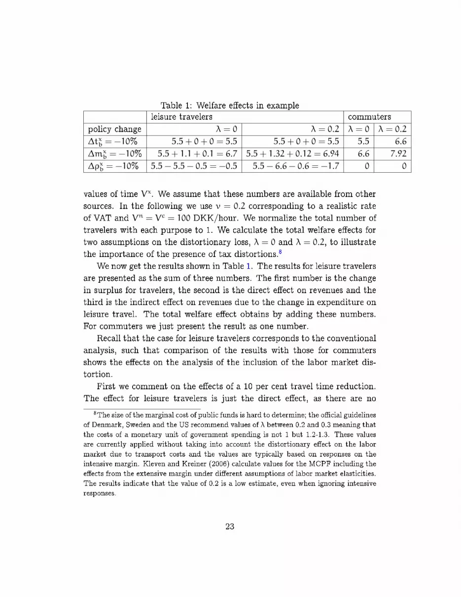
Table 1: Welfare e�ects in exampleleisure travelers commuters
policy change λ = 0 λ = 0.2 λ = 0 λ = 0.2
∆txb = −10% 5.5 + 0 + 0 = 5.5 5.5 + 0 + 0 = 5.5 5.5 6.6
∆mxb = −10% 5.5 + 1.1 + 0.1 = 6.7 5.5 + 1.32 + 0.12 = 6.94 6.6 7.92
∆ρxb = −10% 5.5 − 5.5 − 0.5 = −0.5 5.5 − 6.6 − 0.6 = −1.7 0 0
values of time Vx. We assume that these numbers are available from other
sources. In the following we use v = 0.2 corresponding to a realistic rate
of VAT and Vn = Vc = 100 DKK/hour. We normalize the total number of
travelers with each purpose to 1. We calculate the total welfare e�ects for
two assumptions on the distortionary loss, λ = 0 and λ = 0.2, to illustrate
the importance of the presence of tax distortions.8
We now get the results shown in Table 1. The results for leisure travelers
are presented as the sum of three numbers. The �rst number is the change
in surplus for travelers, the second is the direct e�ect on revenues and the
third is the indirect e�ect on revenues due to the change in expenditure on
leisure travel. The total welfare e�ect obtains by adding these numbers.
For commuters we just present the result as one number.
Recall that the case for leisure travelers corresponds to the conventional
analysis, such that comparison of the results with those for commuters
shows the e�ects on the analysis of the inclusion of the labor market dis-
tortion.
First we comment on the e�ects of a 10 per cent travel time reduction.
The e�ect for leisure travelers is just the direct e�ect, as there are no
8The size of the marginal cost of public funds is hard to determine; the o�cial guidelines
of Denmark, Sweden and the US recommend values of λ between 0.2 and 0.3 meaning that
the costs of a monetary unit of government spending is not 1 but 1.2-1.3. These values
are currently applied without taking into account the distortionary e�ect on the labor
market due to transport costs and the values are typically based on responses on the
intensive margin. Kleven and Kreiner (2006) calculate values for the MCPF including the
e�ects from the extensive margin under di�erent assumptions of labor market elasticities.
The results indicate that the value of 0.2 is a low estimate, even when ignoring intensive
responses.
23
consequences for tax revenues when total leisure travel is constant. We �nd
a total saving of 5.5 of which 5 is bene�t to ex ante leisure travelers and
0.5 is bene�t to new travelers who change from route a. The same is true
for commuters in the case with no distortion. However, when distortion
is allowed for, a further bene�t of the travel time reduction is revealed
such that the bene�t for commuters is λ times higher than the bene�t
for leisure travelers in identical circumstances. The reason is that travel
time improvements increase the incentive for commuters to work and this
increase in labor supply leads to an additional welfare gain usually not
included in the CBA.
Next, we comment on the e�ects of a 10 per cent resource cost reduction.
For the leisure traveler this represents a welfare gain which is slightly higher
in the situation with tax distortions. While the direct e�ect for travelers is
the same, the revenue e�ects are obviously a�ected by the tax distortions.
The revenue e�ects give a welfare gain as the travelers save money on
transport that is alternatively used on other consumption which is taxed
with the VAT. Note that for commuters, the welfare e�ect in the situation
without tax distortions is slightly smaller than for leisure travelers. The
reason is that the indirect tax e�ect on revenue needs to be �nanced via
changed income taxes. Turning to the situation with distortionary taxes
the welfare e�ect is higher for commuters than for leisure travelers. The
reason is now as before that the direct e�ect on the consumer surplus for
commuters a�ects the supply of labor and thus leads to an additional gain.
Finally, we consider the e�ects of a 10 per cent transport tax reduction.
Consider �rst leisure travel in the situation without distortion. The direct
welfare gain of 5.5 is exactly counterbalanced by the direct revenue e�ect
for the government. The increase in leisure travel leads to a loss of revenues
through general indirect taxation worth 0.5, such that the net loss is 0.5.
The size of the net loss depends on the assumptions we have made for
this example concerning the demand reaction to the policy change and in
general it is not the case that decreasing the tax on leisure travel will always
lead to a net welfare loss as discussed in section 3.4.1.
Allowing for distortion increases the e�ect of the revenue loss for gov-
ernment and hence the welfare loss from the transport tax reduction for
24
leisure travelers becomes larger.
For commuters, the e�ect of changing the transport tax is zero, both
with and without allowing for distortion. This is natural since the transport
tax change is �nanced through the income tax and both taxes have exactly
the same e�ect on commuters within the model.
Thus we have a large di�erence between the conventional analysis and
the the present. The conventional analysis would indicate a welfare gain
from increasing the transport tax in almost any circumstances, since the
distortionary e�ect of the transport tax itself was not recognized. The
present analysis shows that the welfare gain disappears when the distor-
tionary e�ect of the transport tax is taken into account.
It is obvious from the tables above that the e�ects for travelers with
di�erent purposes must be treated di�erently as a consequence of their
e�ect on labor supply and production.
5 Conclusion
We have derived simple rules for CBA that can be applied to the output
of a tra�c model and that account for distortion on the labor market in
a consistent manner. For leisure transport, the rules are exactly the same
as in a conventional analysis that includes the marginal cost of funds. For
commuting and business travel including freight transport we �nd a new
rule. The di�erence relative to the conventional analysis results from the
assumption that income taxes and transport costs a�ect both the net wage
and hence employment at the extensive margin. Thus transport costs have
the same distortionary e�ect as income taxes. We have used Kleven and
Kreiner (2006) to argue that this is a fair assumption.
Comparing the results obtained by the conventional rules and rules pro-
vided here for commuting and business travel, we �nd that the conventional
CBA rules underestimate the welfare gains from reducing travel times or
resource costs under realistic assumptions. The di�erences between the
two sets of rules are substantial. It hence makes a large di�erence for the
outcome of a CBA whether the distortionary e�ect of transport costs is
taken into account.
25
The conventional CBA rules also indicate that changing transport taxes
will have direct consequences for welfare through the distortionary e�ect
of income taxes. However, there is no welfare e�ect when the distortionary
e�ect of the transport tax is taken into account. It should be emphasized
that there may in fact be indirect welfare e�ects of changing the transport
tax for, say, commuters if the resulting change in behavior a�ects travel
times and costs. These e�ects are handled by the tra�c model.
A criticism that may be raised against our framework is the lack of
feedback from the general equilibrium e�ects on employment to the tra�c
model. In the case of congestion there will be an e�ect on travel times
and costs that we do not account for. This is unavoidable given that we
consider the CBA as a separate calculation performed after running the
tra�c model. The issue is likely to be minor when the tra�c project is
local and the general equilibrium e�ects concern a whole country. It is
important in our framework that there is a clear division between the tasks
of the tra�c model and of the general equilibrium model. If it is desired
to have the tra�c model also predict changes in volume of commuting and
business travel then the rules derived here do no longer apply, while a host
of issues arise on the modeling of production and employment within a
tra�c model.
The assumption that transport costs a�ect labor supply only at the
extensive margin is important for the simplicity of the CBA rules that we
derive. This simplicity we believe is crucial for the context that we consider
where the CBA rules are to be applied to the output of a tra�c model.
It does however seem to be an interesting issue to pursue how transport
costs interact with the labor supply decision both at the intensive and the
extensive margin.
References
Ben-Akiva, M., Bowman, J. L. and Gopinath, D. (1996) Travel demand
model system for the information era Transportation 23(3), 241{266.
26
DeSerpa, A. C. (1971) A Theory of the Economics of Time The Economic
Journal 81, 828{845.
Fosgerau, M. (2001) PETRA - an Activity-based Approach to Travel De-
mand Analysis in L.-G. Mattson and L. Lundquist (eds), National
Transport Models Advances in Spatial Science Springer Verlag.
Goulder, L. H. (1995) Environmental Taxation and the Double Dividend:
A Reader's Guide International Tax and Public Finance 2, 157{183.
Kleven, H. J. and Kreiner, C. T. (2006) The marginal cost of public funds:
Hours of work versus labor force participation Journal of Public Eco-
nomics 90(10-11), 1955{1973.
of Management and Budget, O. (1992) Transmittal Memo No. 64.
Parry, I. W. and Bento, A. (2001) Revenue Recycling and the Wel-
fare E�ects of Road Pricing Scandinavian Journal of Economics
103(4), 645{671.
Pilegaard, N. and Fosgerau, M. (2008) Cost-bene�t analysis of a transport
improvement in the case of search unemployment Journal of Trans-
port Economics and Policy Forthcoming.
Sandmo, A. (1998) Redistribution and the marginal cost of public funds
Journal of Public Economics 70(3), 365{382.
SIKA (2000) Summary of ASEK estimates SIKA Stockholm.
Tra�kministeriet (2003) Manual for samfundskonomisk analyse Den-
mark.
Venables, A. J. (2007) Evaluating urban transport improvements: cost-
bene�t analysis in the presence of agglomeration and income taxation
Journal of Transport Economics and Policy (Forthcoming).
27