A Random Walk Approach for Investigating Near- and Far-FieldTransport Phenomena in Rivers with Groin Fields

Volker Weitbrecht1, Wim Uijttewaal2 & Gerhard H. Jirka11 Institute for Hydromechanics, University of Karlsruhe, Germany2 Environmental Fluid Mechanics Section, Faculty of Civil Engineering and Geosciences,

Delft University of Technology The Netherlands

ABSTRACT Dead-water-zones in rivers formed by groin fields strongly influence the dispersive mass transportof dissolved pollutants. The cause for this influence is the exchange process between groin fields and mainstream. With the help of laboratory experiments the most important parameters, such as storage time, velocitydistribution and distribution of the diffusivity have been investigated. A transport model using a Lagrangian-Particle-Tracking-Method (LPTM) has been developed, to transfer the locally obtained experimental results fora single dead-water-zone into the global parameters of a one-dimensional far field model that comprises theaction of many dead water zones. It is shown that in the presence of large dead water zones at the river banks,an equilibrium between longitudinal dispersion and transverse diffusion can be reached if the morphologicconditions do not change. The simulations result in a cross sectional averaged concentration distribution thatconverges asymptotically to a Gaussian distribution over the longitudinal coordinate. Due to the presence ofdead water zones the distribution of tracer material becomes inhomogeneous in transverse direction.

1 INTRODUCTION

Predicting the transport of dissolved pollutants inrivers is difficult, because of the various effects of themorphological conditions. In rivers with strong mor-phological heterogeneities, like extensive dead-water-zones, the prediction of transport velocities, maxi-mum concentration and skewness contains strong un-certainties that need to be reduced. The River-Rhine-Alarm-Model (Spreafico and van Mazijk 1993) hasbeen developed by the ”International Commissionfor the Hydrology of the River Rhine” (CHR) andthe ”International Commission for the Protection ofthe Rhine” (ICPR). For this kind of predictive mod-els, much effort and money is spent on calibrationby means of extensive in-situ tracer measurements(van Mazijk 2002). In the case of the River RhineAlarm Model, which uses a one-dimensional analyt-ical approximation for the travel time and concentra-tion curve, a dispersion coefficient and a lag coef-ficient have to be calibrated. The model works wellfor cases of similar hydrological situations. However,variations in discharge, and thus, changes in watersurface levels, lead to increased errors if the same cal-ibrated parameters are used for different hydrologicalsituations. Insufficient knowledge about the relation

between river morphology and transport processes arethe reason for these uncertainties. Hence, predictivemethods that are appropriate for variable flows andchanging morphological conditions are needed.

With the present work we focus on the influenceof dead water zones, such as groin fields, on the dis-persive mass transport in the far field of pollutant re-leases. Longitudinal dispersion in rivers that can betreated as shallow flows is controlled by two pro-cesses. First, the longitudinal stretching due to thehorizontal shear, and second, transverse homogeniza-tion by turbulent diffusion (Fischer et al. 1979). De-tailed velocity and concentration measurements havebeen performed in the laboratory in order to deter-mine typical flow patterns and local mass transportphenomena. Direct measurements of dispersion coef-ficients are problematic because the dispersive char-acter of a transport phenomena reaches its final be-havior only after a very long travel time (Fischer et al.1979), which is determined by the width of the flowand the intensity of the transverse turbulent diffusion.In most cases laboratory flumes are far too short, toexamine longitudinal dispersion in the far field. To ad-dress this problem, laboratory and numerical experi-ments have been combined in such a way that the ef-

1

River Flow, 2004, IAHR, Naples

fect of local phenomena that have been measured, aretranslated into the behavior of tracer clouds in the farfield with the help of Lagrangian-Particle-Tracking-Method (LPTM).

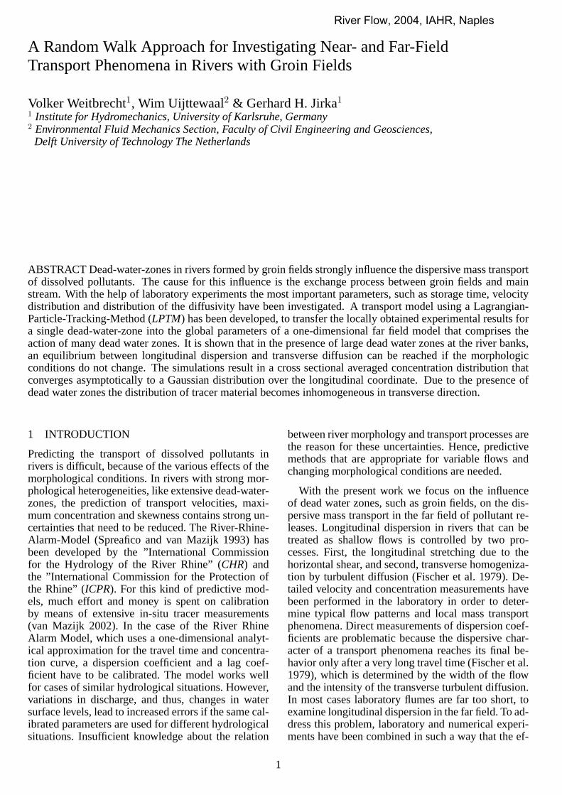
2 EXPERIMENTSIn the present study the experiments have been per-formed in a laboratory flume of 20m length and 1.8mwidth, which has an adjustable bottom slope. In allthe experiments only half of the channel width hasbeen modelled, which means that only on one sideof the flume groins have been placed. The shape ofthe groins was chosen to be very simple due to thefact that earlier investigations suggest that there is nosignificant effect of the groin shape on the exchangeprocesses (Lehmann 1999). Using a simple geome-try leads to a small number of parameters, which al-lows clear understanding of the basic relations be-tween geometry and flow or transport phenomena, re-spectively.

20 m

1.82 m

PC-controlled3-D positioningsystem

Diffusor

Dam

pin

gsc

reen

Groins

Lamellaweir

Sieve

ax

LW

B/2

y

Figure 1: Schematic top view of the laboratory flume showingthe groins placed on one side

The flume bottom consists of a plastic laminatewith small roughness elements< 0.2 mm. Levelchanges in x- and y-direction (Fig. 1) of the flumebottom are smaller than 0.2 mm. The flume is con-nected to a system of a water storage tank and a con-stant head tank, which is supplied by three differentpumps, enabling discharges up to 100`/s. The dis-charge is controlled by an inductive-flow-meter to-gether with an PC controlled gate valve. In the presentcase, only very small discharges of up to 10`/s areneeded. Therefore, the gate valve is equipped with apentagonal regulating orifice, which leads to constantdischarges (changes smaller than 0.5%), even if thevalve is opened only 5%.

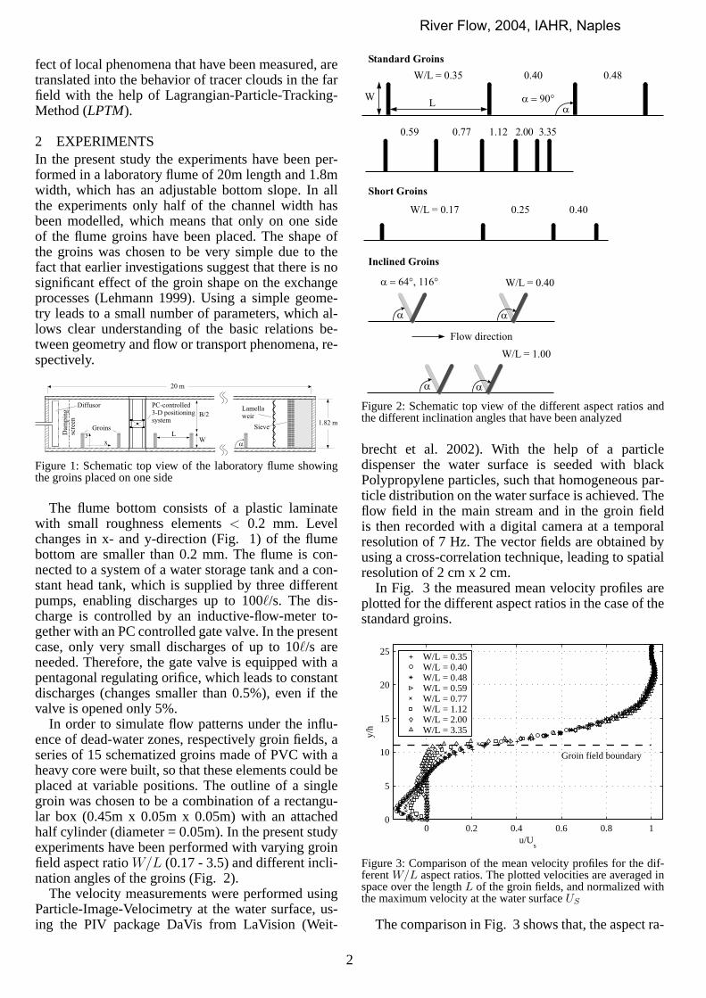
In order to simulate flow patterns under the influ-ence of dead-water zones, respectively groin fields, aseries of 15 schematized groins made of PVC with aheavy core were built, so that these elements could beplaced at variable positions. The outline of a singlegroin was chosen to be a combination of a rectangu-lar box (0.45m x 0.05m x 0.05m) with an attachedhalf cylinder (diameter = 0.05m). In the present studyexperiments have been performed with varying groinfield aspect ratioW/L (0.17 - 3.5) and different incli-nation angles of the groins (Fig. 2).

The velocity measurements were performed usingParticle-Image-Velocimetry at the water surface, us-ing the PIV package DaVis from LaVision (Weit-

W/L = 0.35

W/L = 0.17 0.25 0.40

LW

0.59

W/L = 0.40

W/L = 1.00

Flow direction

a = 64°, 116°

a

a

a

a = 90°

0.77 1.12 2.00 3.35

0.40 0.48

a

a

Standard Groins

Short Groins

Inclined Groins

Figure 2: Schematic top view of the different aspect ratios andthe different inclination angles that have been analyzed

brecht et al. 2002). With the help of a particledispenser the water surface is seeded with blackPolypropylene particles, such that homogeneous par-ticle distribution on the water surface is achieved. Theflow field in the main stream and in the groin fieldis then recorded with a digital camera at a temporalresolution of 7 Hz. The vector fields are obtained byusing a cross-correlation technique, leading to spatialresolution of 2 cm x 2 cm.

In Fig. 3 the measured mean velocity profiles areplotted for the different aspect ratios in the case of thestandard groins.

0 0.2 0.4 0.6 0.8 10

5

10

15

20

25

u/Us

y/h

Groin field boundary

W/L = 0.35W/L = 0.40W/L = 0.48W/L = 0.59W/L = 0.77W/L = 1.12W/L = 2.00W/L = 3.35

Figure 3: Comparison of the mean velocity profiles for the dif-ferentW/L aspect ratios. The plotted velocities are averaged inspace over the lengthL of the groin fields, and normalized withthe maximum velocity at the water surfaceUS

The comparison in Fig. 3 shows that, the aspect ra-

2

River Flow, 2004, IAHR, Naples

tio of the groin field has limited influence on the meanflow properties in the main stream. Above the groinfield boundary no significant differences between thenormalized velocity profiles can be observed. The ve-locity profile in Fig. 3 in the main stream part of theflow has the typical shape of a mixing layer velocityprofile and can be approximated using a hyperbolictangent function of the form

u(y)

Us

= a tanh(

y

hS

b)

+ c (1)

wherea,b andc are constants that have to be adapted.In the present case the profile for the reference caseW/L = 0.4 leads to the following values:a = 0.82,b = 0.24 and c = 0.17. hS is the water depth in themain stream. This equation represents the velocityprofile that is responsible for the stretching mecha-nism of a tracer cloud in the main stream.

In Fig. 4 the normalized rms-velocities of the trans-verse componentv′/u∗ measured with the PIV systemare plotted. These values indicate the strength of thetransverse turbulent mixing, which is the second im-portant parameter influencing longitudinal dispersion.

0 0.5 1 1.5 20

5

10

15

20

y/h

v′/u*

Groin field boundary

W/L = 0.35W/L = 0.40W/L = 0.48W/L = 0.59W/L = 0.77W/L = 1.12W/L = 2.00W/L = 3.35

Figure 4: Comparison of the normalized strength of the velocityfluctuationsv′/u? for the different aspect ratiosW/L

Additional concentration measurements have beenperformed to measure the mean residence timeTD oftracer material in the dead-water-zones (Kurzke et al.2002) using a depth averaged adsorptive technique.With the help of a multi-port injection-device tracerhas been injected instantaneously into one groin field.The evolution of concentration distribution has beenrecorded with a CCD-camera. Gray scale analysis,which takes into account inhomogeneous illuminationand changing background intensities, finally leads toan exponential decay function for every groin fieldsetup

C(t) = Co e− t

TD (2)

whereC is the spatial averaged concentration in thedead zone,Co the initial concentration. The residence

time TD is used in the LPTM transport model to pa-rameterize the influence of dead-water zones on themass transport in the river.

TD can be normalized with the width of the groinfield W and the main stream velocityU to give a di-mensionless exchange coefficientk

k =W

TDU(3)

The resulting exchange coefficientsk for the differ-ent groin field setups are shown in Fig. 5.

0 0.5 1 1.5 2 2.5 3 3.50

0.005

0.01

0.015

0.02

0.025

0.03

0.035

0.04

k

W/L

Standard groinsBackward inclined groinsForward inclined groinsShort groins

Figure 5: Dimensionless exchange coefficientk against the as-pect ratioW/L.

Figure 5 shows thatk reduces with increasingW/L, which means that the residence timeTD islonger in the very narrow cases of groin fields. An-other results is the increased mass exchange for back-ward inclined groins compared to downward inclinedor regular groins. For short groins Fig. 5 showsalso the tendency towards smaller exchange valueswith increasingW/L. However, the k-values for shortgroins are noticeably smaller for the same aspect ratioW/L than in the standard case. This shows, that thegroin field volume has to be taken into account for theprediction ofk.

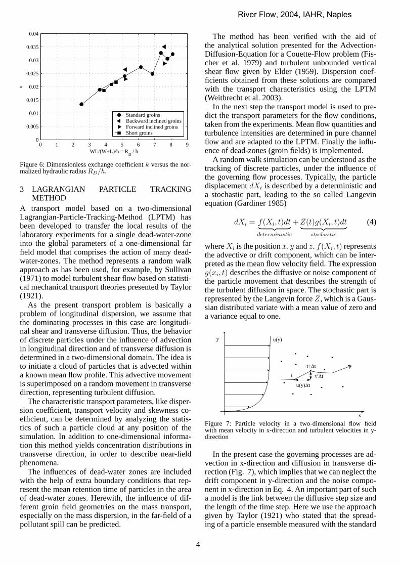
A slight modification of the scaling factorW/LintoWL/(W +L), which can be interpreted as a kindof hydraulic radiusRD of the dead-water-zone, leadsto a better normalization shown in Fig. 6. Why theexchange coefficients should scale with the hydraulicradiusRD can be explained by the following: In thecase of very long groin fields withL→∞ the expres-sionWL/(W + L) tends toW . Therefore, in the caseof very long groin fields the recirculating flow is onlydetermined by the widthW of the groin field. In theother extreme case forW →∞ the hydraulic radiusRD tends toL, which means that the mass exchangein this case is only determined by the length of themixing layer.

3

River Flow, 2004, IAHR, Naples

0 1 2 3 4 5 6 7 8 90

0.005

0.01

0.015

0.02

0.025

0.03

0.035

0.04

k

WL/(W+L)/h = RD

/ h

Standard groinsBackward inclined groinsForward inclined groinsShort groins

Figure 6: Dimensionless exchange coefficientk versus the nor-malized hydraulic radiusRD/h.

3 LAGRANGIAN PARTICLE TRACKINGMETHOD

A transport model based on a two-dimensionalLagrangian-Particle-Tracking-Method (LPTM) hasbeen developed to transfer the local results of thelaboratory experiments for a single dead-water-zoneinto the global parameters of a one-dimensional farfield model that comprises the action of many dead-water-zones. The method represents a random walkapproach as has been used, for example, by Sullivan(1971) to model turbulent shear flow based on statisti-cal mechanical transport theories presented by Taylor(1921).

As the present transport problem is basically aproblem of longitudinal dispersion, we assume thatthe dominating processes in this case are longitudi-nal shear and transverse diffusion. Thus, the behaviorof discrete particles under the influence of advectionin longitudinal direction and of transverse diffusion isdetermined in a two-dimensional domain. The idea isto initiate a cloud of particles that is advected withina known mean flow profile. This advective movementis superimposed on a random movement in transversedirection, representing turbulent diffusion.

The characteristic transport parameters, like disper-sion coefficient, transport velocity and skewness co-efficient, can be determined by analyzing the statis-tics of such a particle cloud at any position of thesimulation. In addition to one-dimensional informa-tion this method yields concentration distributions intransverse direction, in order to describe near-fieldphenomena.

The influences of dead-water zones are includedwith the help of extra boundary conditions that rep-resent the mean retention time of particles in the areaof dead-water zones. Herewith, the influence of dif-ferent groin field geometries on the mass transport,especially on the mass dispersion, in the far-field of apollutant spill can be predicted.

The method has been verified with the aid ofthe analytical solution presented for the Advection-Diffusion-Equation for a Couette-Flow problem (Fis-cher et al. 1979) and turbulent unbounded verticalshear flow given by Elder (1959). Dispersion coef-ficients obtained from these solutions are comparedwith the transport characteristics using the LPTM(Weitbrecht et al. 2003).

In the next step the transport model is used to pre-dict the transport parameters for the flow conditions,taken from the experiments. Mean flow quantities andturbulence intensities are determined in pure channelflow and are adapted to the LPTM. Finally the influ-ence of dead-zones (groin fields) is implemented.

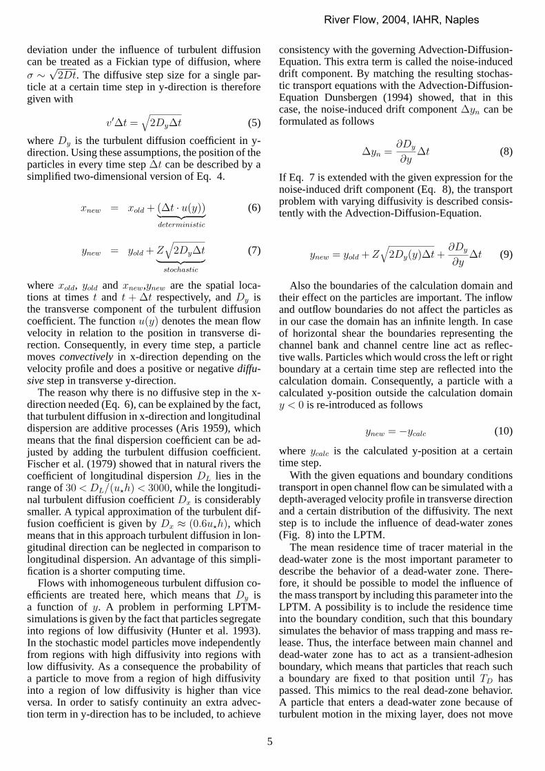
A random walk simulation can be understood as thetracking of discrete particles, under the influence ofthe governing flow processes. Typically, the particledisplacementdXi is described by a deterministic anda stochastic part, leading to the so called Langevinequation (Gardiner 1985)

dXi = f(Xi, t)dt︸ ︷︷ ︸deterministic

+Z(t)g(Xi, t)dt︸ ︷︷ ︸stochastic

(4)

whereXi is the positionx, y andz. f(Xi, t) representsthe advective or drift component, which can be inter-preted as the mean flow velocity field. The expressiong(xi, t) describes the diffusive or noise component ofthe particle movement that describes the strength ofthe turbulent diffusion in space. The stochastic part isrepresented by the Langevin forceZ, which is a Gaus-sian distributed variate with a mean value of zero anda variance equal to one.

y

x

t

t+ tD

u(y)

u(y) tD

v' tD

Figure 7: Particle velocity in a two-dimensional flow fieldwith mean velocity in x-direction and turbulent velocities in y-direction

In the present case the governing processes are ad-vection in x-direction and diffusion in transverse di-rection (Fig. 7), which implies that we can neglect thedrift component in y-direction and the noise compo-nent in x-direction in Eq. 4. An important part of sucha model is the link between the diffusive step size andthe length of the time step. Here we use the approachgiven by Taylor (1921) who stated that the spread-ing of a particle ensemble measured with the standard

4

River Flow, 2004, IAHR, Naples

deviation under the influence of turbulent diffusioncan be treated as a Fickian type of diffusion, whereσ ∼ √

2Dt. The diffusive step size for a single par-ticle at a certain time step in y-direction is thereforegiven with

v′∆t =√

2Dy∆t (5)

whereDy is the turbulent diffusion coefficient in y-direction. Using these assumptions, the position of theparticles in every time step∆t can be described by asimplified two-dimensional version of Eq. 4.

xnew = xold + (∆t · u(y))︸ ︷︷ ︸deterministic

(6)

ynew = yold + Z√

2Dy∆t︸ ︷︷ ︸

stochastic

(7)

wherexold, yold and xnew,ynew are the spatial loca-tions at timest and t + ∆t respectively, andDy isthe transverse component of the turbulent diffusioncoefficient. The functionu(y) denotes the mean flowvelocity in relation to the position in transverse di-rection. Consequently, in every time step, a particlemovesconvectivelyin x-direction depending on thevelocity profile and does a positive or negativediffu-sivestep in transverse y-direction.

The reason why there is no diffusive step in the x-direction needed (Eq. 6), can be explained by the fact,that turbulent diffusion in x-direction and longitudinaldispersion are additive processes (Aris 1959), whichmeans that the final dispersion coefficient can be ad-justed by adding the turbulent diffusion coefficient.Fischer et al. (1979) showed that in natural rivers thecoefficient of longitudinal dispersionDL lies in therange of30 < DL/(u?h) < 3000, while the longitudi-nal turbulent diffusion coefficientDx is considerablysmaller. A typical approximation of the turbulent dif-fusion coefficient is given byDx ≈ (0.6u?h), whichmeans that in this approach turbulent diffusion in lon-gitudinal direction can be neglected in comparison tolongitudinal dispersion. An advantage of this simpli-fication is a shorter computing time.

Flows with inhomogeneous turbulent diffusion co-efficients are treated here, which means thatDy isa function of y. A problem in performing LPTM-simulations is given by the fact that particles segregateinto regions of low diffusivity (Hunter et al. 1993).In the stochastic model particles move independentlyfrom regions with high diffusivity into regions withlow diffusivity. As a consequence the probability ofa particle to move from a region of high diffusivityinto a region of low diffusivity is higher than viceversa. In order to satisfy continuity an extra advec-tion term in y-direction has to be included, to achieve

consistency with the governing Advection-Diffusion-Equation. This extra term is called the noise-induceddrift component. By matching the resulting stochas-tic transport equations with the Advection-Diffusion-Equation Dunsbergen (1994) showed, that in thiscase, the noise-induced drift component∆yn can beformulated as follows

∆yn =∂Dy

∂y∆t (8)

If Eq. 7 is extended with the given expression for thenoise-induced drift component (Eq. 8), the transportproblem with varying diffusivity is described consis-tently with the Advection-Diffusion-Equation.

ynew = yold + Z√

2Dy(y)∆t +∂Dy

∂y∆t (9)

Also the boundaries of the calculation domain andtheir effect on the particles are important. The inflowand outflow boundaries do not affect the particles asin our case the domain has an infinite length. In caseof horizontal shear the boundaries representing thechannel bank and channel centre line act as reflec-tive walls. Particles which would cross the left or rightboundary at a certain time step are reflected into thecalculation domain. Consequently, a particle with acalculated y-position outside the calculation domainy < 0 is re-introduced as follows

ynew = −ycalc (10)

whereycalc is the calculated y-position at a certaintime step.

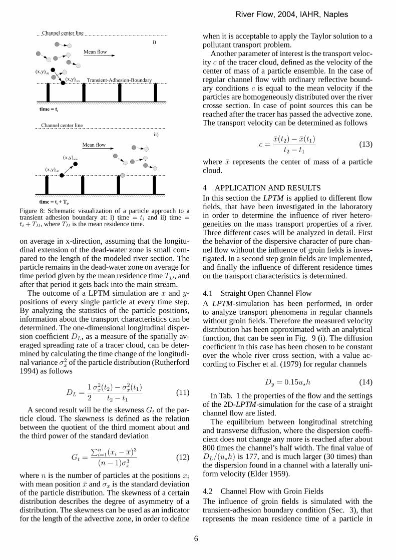
With the given equations and boundary conditionstransport in open channel flow can be simulated with adepth-averaged velocity profile in transverse directionand a certain distribution of the diffusivity. The nextstep is to include the influence of dead-water zones(Fig. 8) into the LPTM.

The mean residence time of tracer material in thedead-water zone is the most important parameter todescribe the behavior of a dead-water zone. There-fore, it should be possible to model the influence ofthe mass transport by including this parameter into theLPTM. A possibility is to include the residence timeinto the boundary condition, such that this boundarysimulates the behavior of mass trapping and mass re-lease. Thus, the interface between main channel anddead-water zone has to act as a transient-adhesionboundary, which means that particles that reach sucha boundary are fixed to that position untilTD haspassed. This mimics to the real dead-zone behavior.A particle that enters a dead-water zone because ofturbulent motion in the mixing layer, does not move

5

River Flow, 2004, IAHR, Naples

(x,y)old

time = ti

(x,y)new Transient-Adhesion-Boundary

Mean flow

Channel center line

i)

(x,y)old

time = t +i

TD

Mean flow

Channel center line

(x,y)new

ii)

Figure 8: Schematic visualization of a particle approach to atransient adhesion boundary at: i) time= ti and ii) time =ti + TD, whereTD is the mean residence time.

on average in x-direction, assuming that the longitu-dinal extension of the dead-water zone is small com-pared to the length of the modeled river section. Theparticle remains in the dead-water zone on average fortime period given by the mean residence timeTD, andafter that period it gets back into the main stream.

The outcome of a LPTM simulation arex andy-positions of every single particle at every time step.By analyzing the statistics of the particle positions,information about the transport characteristics can bedetermined. The one-dimensional longitudinal disper-sion coefficientDL, as a measure of the spatially av-eraged spreading rate of a tracer cloud, can be deter-mined by calculating the time change of the longitudi-nal varianceσ2

x of the particle distribution (Rutherford1994) as follows

DL =1

2

σ2x(t2)− σ2

x(t1)

t2 − t1(11)

A second result will be the skewnessGt of the par-ticle cloud. The skewness is defined as the relationbetween the quotient of the third moment about andthe third power of the standard deviation

Gt =

∑ni=1(xi − x)3

(n− 1)σ3x

(12)

wheren is the number of particles at the positionsxi

with mean positionx andσx is the standard deviationof the particle distribution. The skewness of a certaindistribution describes the degree of asymmetry of adistribution. The skewness can be used as an indicatorfor the length of the advective zone, in order to define

when it is acceptable to apply the Taylor solution to apollutant transport problem.

Another parameter of interest is the transport veloc-ity c of the tracer cloud, defined as the velocity of thecenter of mass of a particle ensemble. In the case ofregular channel flow with ordinary reflective bound-ary conditionsc is equal to the mean velocity if theparticles are homogeneously distributed over the rivercrosse section. In case of point sources this can bereached after the tracer has passed the advective zone.The transport velocity can be determined as follows

c =x(t2)− x(t1)

t2 − t1(13)

where x represents the center of mass of a particlecloud.

4 APPLICATION AND RESULTSIn this section theLPTM is applied to different flowfields, that have been investigated in the laboratoryin order to determine the influence of river hetero-geneities on the mass transport properties of a river.Three different cases will be analyzed in detail. Firstthe behavior of the dispersive character of pure chan-nel flow without the influence of groin fields is inves-tigated. In a second step groin fields are implemented,and finally the influence of different residence timeson the transport characteristics is determined.

4.1 Straight Open Channel FlowA LPTM-simulation has been performed, in orderto analyze transport phenomena in regular channelswithout groin fields. Therefore the measured velocitydistribution has been approximated with an analyticalfunction, that can be seen in Fig. 9 (i). The diffusioncoefficient in this case has been chosen to be constantover the whole river cross section, with a value ac-cording to Fischer et al. (1979) for regular channels

Dy = 0.15u?h (14)

In Tab. 1 the properties of the flow and the settingsof the 2D-LPTM-simulation for the case of a straightchannel flow are listed.

The equilibrium between longitudinal stretchingand transverse diffusion, where the dispersion coeffi-cient does not change any more is reached after about800 times the channel’s half width. The final value ofDL/(u?h) is 177, and is much larger (30 times) thanthe dispersion found in a channel with a laterally uni-form velocity (Elder 1959).

4.2 Channel Flow with Groin FieldsThe influence of groin fields is simulated with thetransient-adhesion boundary condition (Sec. 3), thatrepresents the mean residence time of a particle in

6

River Flow, 2004, IAHR, Naples

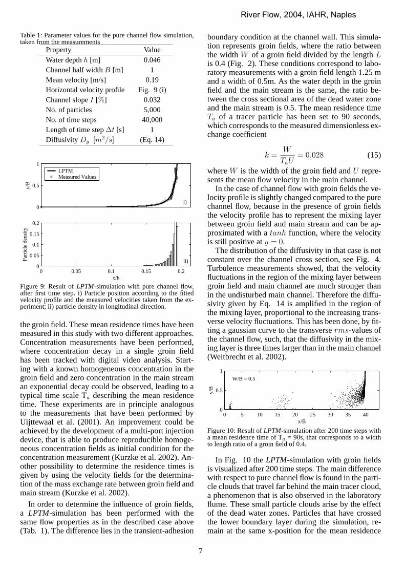
Table 1: Parameter values for the pure channel flow simulation,taken from the measurements

Property ValueWater depthh [m] 0.046Channel half widthB [m] 1Mean velocity [m/s] 0.19Horizontal velocity profile Fig. 9 (i)Channel slopeI [%] 0.032No. of particles 5,000No. of time steps 40,000Length of time step∆t [s] 1Diffusivity Dy [m2/s] (Eq. 14)

0

0.5

1

y/B

i)

LPTMMeasured Values

0 0.05 0.1 0.15 0.20

0.05

0.1

0.15

0.2

x/h

Part

icle

den

sity

ii)

Figure 9: Result ofLPTM-simulation with pure channel flow,after first time step. i) Particle position according to the fittedvelocity profile and the measured velocities taken from the ex-periment; ii) particle density in longitudinal direction.

the groin field. These mean residence times have beenmeasured in this study with two different approaches.Concentration measurements have been performed,where concentration decay in a single groin fieldhas been tracked with digital video analysis. Start-ing with a known homogeneous concentration in thegroin field and zero concentration in the main streaman exponential decay could be observed, leading to atypical time scale Ta describing the mean residencetime. These experiments are in principle analogousto the measurements that have been performed byUijttewaal et al. (2001). An improvement could beachieved by the development of a multi-port injectiondevice, that is able to produce reproducible homoge-neous concentration fields as initial condition for theconcentration measurement (Kurzke et al. 2002). An-other possibility to determine the residence times isgiven by using the velocity fields for the determina-tion of the mass exchange rate between groin field andmain stream (Kurzke et al. 2002).

In order to determine the influence of groin fields,a LPTM-simulation has been performed with thesame flow properties as in the described case above(Tab. 1). The difference lies in the transient-adhesion

boundary condition at the channel wall. This simula-tion represents groin fields, where the ratio betweenthe widthW of a groin field divided by the lengthLis 0.4 (Fig. 2). These conditions correspond to labo-ratory measurements with a groin field length 1.25 mand a width of 0.5m. As the water depth in the groinfield and the main stream is the same, the ratio be-tween the cross sectional area of the dead water zoneand the main stream is 0.5. The mean residence timeTa of a tracer particle has been set to 90 seconds,which corresponds to the measured dimensionless ex-change coefficient

k =W

TaU= 0.028 (15)

whereW is the width of the groin field andU repre-sents the mean flow velocity in the main channel.

In the case of channel flow with groin fields the ve-locity profile is slightly changed compared to the purechannel flow, because in the presence of groin fieldsthe velocity profile has to represent the mixing layerbetween groin field and main stream and can be ap-proximated with atanh function, where the velocityis still positive aty = 0.

The distribution of the diffusivity in that case is notconstant over the channel cross section, see Fig. 4.Turbulence measurements showed, that the velocityfluctuations in the region of the mixing layer betweengroin field and main channel are much stronger thanin the undisturbed main channel. Therefore the diffu-sivity given by Eq. 14 is amplified in the region ofthe mixing layer, proportional to the increasing trans-verse velocity fluctuations. This has been done, by fit-ting a gaussian curve to the transverserms-values ofthe channel flow, such, that the diffusivity in the mix-ing layer is three times larger than in the main channel(Weitbrecht et al. 2002).

0 5 10 15 20 25 30 35 400

0.5

1

y/B

x/B

W/B = 0.5

Figure 10: Result ofLPTM-simulation after 200 time steps witha mean residence time of Ta = 90s, that corresponds to a widthto length ratio of a groin field of 0.4.

In Fig. 10 theLPTM-simulation with groin fieldsis visualized after 200 time steps. The main differencewith respect to pure channel flow is found in the parti-cle clouds that travel far behind the main tracer cloud,a phenomenon that is also observed in the laboratoryflume. These small particle clouds arise by the effectof the dead water zones. Particles that have crossedthe lower boundary layer during the simulation, re-main at the same x-position for the mean residence

7

River Flow, 2004, IAHR, Naples

time Ta. After Ta has elapsed the particles get backto the flow. The mean distance between those cloudscorresponds to the mean residence time Ta.

The final stage of mixing in the case with groinsshows again, that after a long period the tracer cloudapproximates a Gaussian distribution in longitudinaldirection Fig. 11.

0

0.5

1

y/B

i)

0 1000 2000 3000 4000 5000 6000 7000 80000

0.05

0.1

x/h

Part

icle

den

sity

ii)

Figure 11: Result ofLPTM-simulation after 40000 time stepswith a mean residence time of Ta = 90s, that corresponds to awidth to length ratio of a groin field of 0.4 andW/B = 0.5; i)particle position; ii) particle density in longitudinal direction

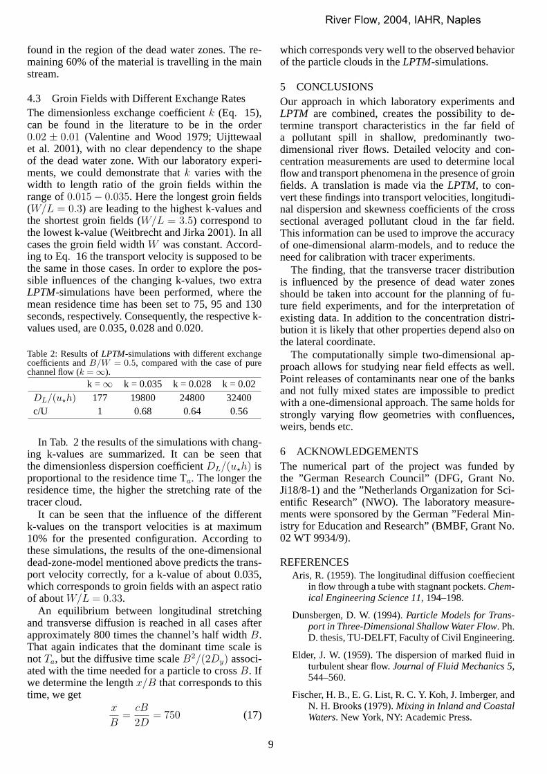
The interesting properties of this simulation arethe evolution of the dispersion coefficient and of theskewness, as visualized in Fig. 12. The final value ofDL/(u?h) is in that case approximately 24.800 whichis a factor 140 higher than in the case of pure chan-nel flow, and about ten times higher than the valuescommon for natural rivers without groin fields. Thiscan be explained by the exaggerated ratio between thecross sectional area of the dead water zone and thecross sectional area of the main channel, which is 0.5for this experiment, a value rather high compared tonatural rivers.

The equilibrium between longitudinal stretchingand transverse diffusion is achieved after approxi-mately 800 times the channel width (Fig. 12), whichindicates that the advective zone has the same lengthirrespective of the presence of groins.

0 1000 2000 3000 4000 5000 6000−3

−2

−1

0

1

2

3

x/h

Gt

DL/u

*h 10

−4

DL

Gt

Figure 12: Evolution of Dispersion coefficientDL · 10−4 nor-malized with theu? and the water depthh and the evolution ofthe skewness.DL is smoothed with a sliding average filter ofincreasing window size. (W/B = 0.5)

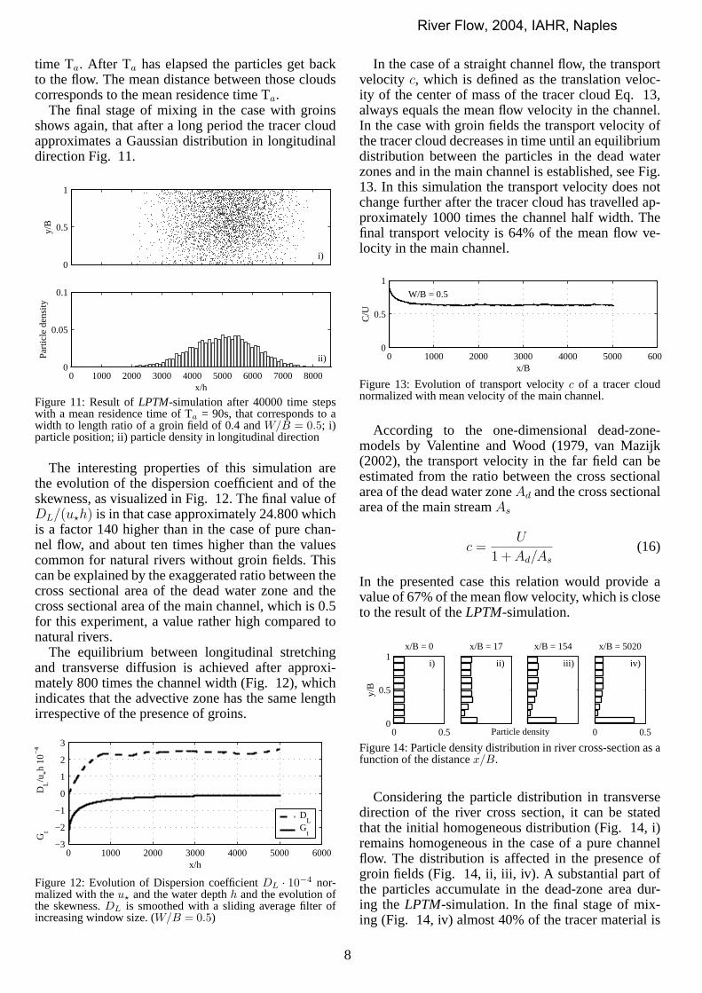
In the case of a straight channel flow, the transportvelocity c, which is defined as the translation veloc-ity of the center of mass of the tracer cloud Eq. 13,always equals the mean flow velocity in the channel.In the case with groin fields the transport velocity ofthe tracer cloud decreases in time until an equilibriumdistribution between the particles in the dead waterzones and in the main channel is established, see Fig.13. In this simulation the transport velocity does notchange further after the tracer cloud has travelled ap-proximately 1000 times the channel half width. Thefinal transport velocity is 64% of the mean flow ve-locity in the main channel.

0 1000 2000 3000 4000 5000 60000

0.5

1

x/B

W/B = 0.5

C/U

Figure 13: Evolution of transport velocityc of a tracer cloudnormalized with mean velocity of the main channel.

According to the one-dimensional dead-zone-models by Valentine and Wood (1979, van Mazijk(2002), the transport velocity in the far field can beestimated from the ratio between the cross sectionalarea of the dead water zoneAd and the cross sectionalarea of the main streamAs

c =U

1 + Ad/As

(16)

In the presented case this relation would provide avalue of 67% of the mean flow velocity, which is closeto the result of theLPTM-simulation.

0 0.50

0.5

1x/B = 0

i)

y/B

x/B = 17

ii)

Particle density

iii)

x/B = 154

0 0.5

iv)

x/B = 5020

Figure 14: Particle density distribution in river cross-section as afunction of the distancex/B.

Considering the particle distribution in transversedirection of the river cross section, it can be statedthat the initial homogeneous distribution (Fig. 14, i)remains homogeneous in the case of a pure channelflow. The distribution is affected in the presence ofgroin fields (Fig. 14, ii, iii, iv). A substantial part ofthe particles accumulate in the dead-zone area dur-ing theLPTM-simulation. In the final stage of mix-ing (Fig. 14, iv) almost 40% of the tracer material is

8

River Flow, 2004, IAHR, Naples

found in the region of the dead water zones. The re-maining 60% of the material is travelling in the mainstream.

4.3 Groin Fields with Different Exchange RatesThe dimensionless exchange coefficientk (Eq. 15),can be found in the literature to be in the order0.02 ± 0.01 (Valentine and Wood 1979; Uijttewaalet al. 2001), with no clear dependency to the shapeof the dead water zone. With our laboratory experi-ments, we could demonstrate thatk varies with thewidth to length ratio of the groin fields within therange of0.015− 0.035. Here the longest groin fields(W/L = 0.3) are leading to the highest k-values andthe shortest groin fields (W/L = 3.5) correspond tothe lowest k-value (Weitbrecht and Jirka 2001). In allcases the groin field widthW was constant. Accord-ing to Eq. 16 the transport velocity is supposed to bethe same in those cases. In order to explore the pos-sible influences of the changing k-values, two extraLPTM-simulations have been performed, where themean residence time has been set to 75, 95 and 130seconds, respectively. Consequently, the respective k-values used, are 0.035, 0.028 and 0.020.

Table 2: Results ofLPTM-simulations with different exchangecoefficients andB/W = 0.5, compared with the case of purechannel flow (k =∞).

k =∞ k = 0.035 k = 0.028 k = 0.02DL/(u?h) 177 19800 24800 32400c/U 1 0.68 0.64 0.56

In Tab. 2 the results of the simulations with chang-ing k-values are summarized. It can be seen thatthe dimensionless dispersion coefficientDL/(u?h) isproportional to the residence time Ta. The longer theresidence time, the higher the stretching rate of thetracer cloud.

It can be seen that the influence of the differentk-values on the transport velocities is at maximum10% for the presented configuration. According tothese simulations, the results of the one-dimensionaldead-zone-model mentioned above predicts the trans-port velocity correctly, for a k-value of about 0.035,which corresponds to groin fields with an aspect ratioof aboutW/L = 0.33.

An equilibrium between longitudinal stretchingand transverse diffusion is reached in all cases afterapproximately 800 times the channel’s half widthB.That again indicates that the dominant time scale isnot Ta, but the diffusive time scaleB2/(2Dy) associ-ated with the time needed for a particle to crossB. Ifwe determine the lengthx/B that corresponds to thistime, we get

x

B=

cB

2D= 750 (17)

which corresponds very well to the observed behaviorof the particle clouds in theLPTM-simulations.

5 CONCLUSIONSOur approach in which laboratory experiments andLPTM are combined, creates the possibility to de-termine transport characteristics in the far field ofa pollutant spill in shallow, predominantly two-dimensional river flows. Detailed velocity and con-centration measurements are used to determine localflow and transport phenomena in the presence of groinfields. A translation is made via theLPTM, to con-vert these findings into transport velocities, longitudi-nal dispersion and skewness coefficients of the crosssectional averaged pollutant cloud in the far field.This information can be used to improve the accuracyof one-dimensional alarm-models, and to reduce theneed for calibration with tracer experiments.

The finding, that the transverse tracer distributionis influenced by the presence of dead water zonesshould be taken into account for the planning of fu-ture field experiments, and for the interpretation ofexisting data. In addition to the concentration distri-bution it is likely that other properties depend also onthe lateral coordinate.

The computationally simple two-dimensional ap-proach allows for studying near field effects as well.Point releases of contaminants near one of the banksand not fully mixed states are impossible to predictwith a one-dimensional approach. The same holds forstrongly varying flow geometries with confluences,weirs, bends etc.

6 ACKNOWLEDGEMENTSThe numerical part of the project was funded bythe ”German Research Council” (DFG, Grant No.Ji18/8-1) and the ”Netherlands Organization for Sci-entific Research” (NWO). The laboratory measure-ments were sponsored by the German ”Federal Min-istry for Education and Research” (BMBF, Grant No.02 WT 9934/9).

REFERENCESAris, R. (1959). The longitudinal diffusion coeffiecient

in flow through a tube with stagnant pockets.Chem-ical Engineering Science 11, 194–198.

Dunsbergen, D. W. (1994).Particle Models for Trans-port in Three-Dimensional Shallow Water Flow. Ph.D. thesis, TU-DELFT, Faculty of Civil Engineering.

Elder, J. W. (1959). The dispersion of marked fluid inturbulent shear flow.Journal of Fluid Mechanics 5,544–560.

Fischer, H. B., E. G. List, R. C. Y. Koh, J. Imberger, andN. H. Brooks (1979).Mixing in Inland and CoastalWaters. New York, NY: Academic Press.

9

River Flow, 2004, IAHR, Naples

Gardiner, C. W. (1985).Handbook of Stochastic Meth-ods. Springer-Verlag.

Hunter, J., P. Craig, and H. Phillips (1993). On the useof random walk models with spacially variable dif-fusivity. Computational Physics 106, 366–376.

Kurzke, M., V. Weitbrecht, and G. Jirka (2002). Labora-tory concentration measurements for determinationof mass exchange between groin fields and mainstream. In D. Bousmar and Y. Zech (Eds.),RiverFlow 2002, Volume 1, Louvain-la-Neuve, Belgium,pp. 369–376. IAHR.

Lehmann, D. (1999). Auswirkung von Buhnenfeldernauf den Transport geloster Stoffe in Flussen. Mas-ter’s thesis, University of Karlsruhe, Inst. for Hy-dromechanics and TU-Delft, Hydromechanics Sec-tion.

Rutherford, J. C. (1994).River Mixing. Sussex, Eng-land: Wiley.

Spreafico, M. and A. van Mazijk (1993). AlarmmodellRhein. Ein Modell fur die operationelle Vorhersagedes Transportes von Schadstoffen im Rhein. Techni-cal Report I-12, Internationale Kommission zur Hy-drologie des Rheingebiets, Lelystad.

Sullivan, P. J. (1971). Longitudinal dispersion withina two-dimensional turbulent shear flow.Journal ofFluid Mechanics 49, 551–576.

Taylor, G. I. (1921). Diffusion by continuous move-ments.Proc. London Math. Soc. 20, 196–211.

Uijttewaal, W., D. Lehmann, and A. van Mazijk (2001).Exchange processes between a river and its groynefields: Model experiments.Journal of HydraulicEngineering 127(11), 928–936.

Valentine, E. M. and I. R. Wood (1979). Experiments inlongitudinal dispersion with dead zones.Journal ofthe Hydraulics Division 105(HY8), 999–1016.

van Mazijk, A. (2002). Modelling the effects of groynefields on the transport of dissolved matter within therhine alarm-model.Journal of Hydrology 264, 213–229.

Weitbrecht, V. and G. Jirka (2001). Flow patterns andexchange processes in dead zones of rivers. InXXIXIAHR Congress, Beijing, China.

Weitbrecht, V., G. Kuhn, and G. H. Jirka (2002). Largescale piv-measurements at the surface of shallowwater flows.Flow Measurements and Instrumenta-tion 13(5-6), 237–245.

Weitbrecht, V., W. Uijttewaal, and G. Jirka (2003). 2-dparticle tracking to determine transport characteris-tics in rivers with dead zones. InInternational Sym-posium on Shallow Flows, Delft, The Netherlands.

10

River Flow, 2004, IAHR, Naples