Available online at www.sciencedirect.com

Information Sciences 178 (2008) 1479–1497

www.elsevier.com/locate/ins

Random walk biclustering for microarray data

Fabrizio Angiulli, Eugenio Cesario, Clara Pizzuti *

ICAR-CNR, Via P. Bucci 41C, 87036 Rende, CS, Italy

Received 20 March 2007; received in revised form 16 November 2007; accepted 16 November 2007

Abstract

A biclustering algorithm, based on a greedy technique and enriched with a local search strategy to escape poor localminima, is proposed. The algorithm starts with an initial random solution and searches for a locally optimal solutionby successive transformations that improve a gain function. The gain function combines the mean squared residue, therow variance, and the size of the bicluster. Different strategies to escape local minima are introduced and compared. Exper-imental results on several microarray data sets show that the method is able to find significant biclusters, also from a bio-logical point of view.� 2007 Elsevier Inc. All rights reserved.

Keywords: Biclustering; Microarray data; Local search

1. Introduction

In the past recent years, DNA microarray technology has captured the attention of scientific communitybecause of its capability of simultaneously measuring the activity and interactions of thousands of genes.The relative abundance of the mRNA of a gene under a specific experimental condition (or sample) is calledthe expression level of a gene. The expression level of a large number of genes of an organism under variousexperimental conditions can be arranged in a data matrix, also known as gene expression data matrix, whererows correspond to genes and columns to conditions. Thus each entry of this matrix is a real number repre-senting the expression level of a gene under a specific experiment. One of the objectives of gene expression dataanalysis is to group genes according to their expression under multiple conditions.

Clustering [15,33,7] is an important gene expression analysis method that has been extensively used togroup either genes, to search for functional similarities, or conditions, to find samples characterized by homo-geneous gene expression levels. However, generally, genes are not relevant for all the experimental conditions,but groups of genes are often co-regulated and co-expressed only under specific conditions. This importantobservation has lead the attention towards the design of clustering methods that try to simultaneously group

0020-0255/$ - see front matter � 2007 Elsevier Inc. All rights reserved.

doi:10.1016/j.ins.2007.11.007

* Corresponding author.E-mail addresses: angiulli@icar.cnr.it (F. Angiulli), cesario@icar.cnr.it (E. Cesario), pizzuti@icar.cnr.it (C. Pizzuti).

1480 F. Angiulli et al. / Information Sciences 178 (2008) 1479–1497

genes and samples. The approach, named biclustering or co-clustering [25,32,9], detects subsets of genes thatshow similar patterns under a specific subset of experimental conditions. This simultaneous clustering thussearches for sub-matrices whose rows show some kind of coherence with respect to the conditions appearingin the same sub-matrix.

The concept of bicluster is analogous to that of subspace clustering in data mining [3,2,1,26,13,14], thoughthere exist important differences regarding the criteria adopted to measure the coherence among the rows andthe type of biclusters found, that generally do not overlap, i.e. a row or a column can participate to only onebicluster.

Biclustering was first defined by Hartigan [21] and called direct clustering. His aim was to find a set of sub-matrices having zero variance, that is with constant values. This concept was then adopted by Cheng andChurch [11] by introducing a similarity score, called mean squared residue, to measure the coherence of rowsand columns in the bicluster. A group of genes is considered coherent if their expression levels varies simul-taneously across a set of conditions. Biclusters with a high similarity score and, thus, with low residue, indicatethat genes show similar tendency on the subset of the conditions present in the bicluster.

In this paper a greedy search algorithm, named Random Walk Biclustering (RWB), to find k biclusters witha fixed degree of overlapping is proposed. The method is motivated by that of [11] because it uses the conceptof mean squared residue to evaluate the similarity of gene activity under a specific subset of experimental con-ditions. However, it introduces the notion of gain that combines the mean squared residue, the row variance,and the size of the bicluster to guide the algorithm towards those parts of the search space that contain localoptimal solutions. The method, in fact, is enriched with an heuristic that avoids to get trapped at poor localminima. The algorithm starts with an initial random bicluster and searches for a locally optimal solution bysuccessive transformations that improve a gain function. The gain guarantees that the transformation of asolution to a local neighborhood is done only if there is either a reduction of the residue, or an increase ofthe row variance, or an enlargement of the volume. In order to escape poor local minima, that is low qualitybiclusters having negative gain in their neighborhood, random moves with given probability are executed.These moves delete or add a row/column on the base of different strategies introduced in the method.

To obtain k biclusters the algorithm is executed k times by controlling the degree of overlapping among thebiclusters.

In order to assess the validity of the approach proposed, an extensive experimental study on several real lifedata sets has been performed. A performance analysis showed that the algorithm is able to find significant andcoherent biclusters. Furthermore, a quantitative and qualitative comparison of our approach with that ofCheng and Church has pointed out that the RWB algorithm is able to obtain biclusters with lower residueand higher volume than those found by their algorithm. Indeed the presented algorithm is able to find highlycoherent genes and conditions which lead to low residue, while that of [11] tends to find smaller biclusters withless coherence, i.e. larger residue.

The paper is organized as follows. The next section defines the problem of biclustering and the notationused. Section 3 describes the algorithm proposed. Section 4 discusses time and space complexity of themethod. In Section 5 an overview of the existing approaches to biclustering is given. Finally, Section 6 reportsthe experiments on some real life data sets and the comparison with the Cheng and Church algorithm.

2. Notation and problem definition

In this section the notation used in the paper is introduced and a formal definition of bicluster is provided[11]. Let X ¼ fI1; . . . ; INg be the set of genes and Y ¼ fJ 1; . . . ; J Mg be the set of conditions. The data can beviewed as an N �M matrix A of real numbers. Each entry aij in A represents the relative abundance (generallyits logarithm) of the mRNA of a gene I i under a specific condition J j. A bicluster is a subset of rows that showsa coherent behavior across a subset of columns and vice versa.

Definition 2.1. A bicluster is a sub-matrix B ¼ ðI ; JÞ of A, where I � X is a subset of the rows X of A, and J is asubset of the columns Y of A.

The problem of biclustering can then be formulated as follows: given a data matrix A, find a set k of bicl-usters Bi ¼ ðI i; J iÞ, i ¼ 1; . . . ; k that satisfy some homogeneity characteristics. The kind of homogeneity a

F. Angiulli et al. / Information Sciences 178 (2008) 1479–1497 1481

bicluster must fulfil depends on the approach adopted. In the next the notion of mean squared residue, intro-duced by Cheng and Church, is recalled.

Definition 2.2. Given a bicluster B ¼ ðI ; JÞ, let aiJ ¼ 1jJ jP

j2J aij denote the mean of the ith row of B,

aIj ¼ 1jI jP

i2I aij the mean of the jth column of B, and aIJ ¼ 1jI jjJ j

Pi2I ;j2J aij the mean of all the elements in the

bicluster, where jIj and jJj denote the number of rows and columns of B respectively.

Definition 2.3. The residue rij of an element aij of the matrix A is defined as rij ¼ aij � aiJ � aIj þ aIJ .

The residue of an element provides the difference between the actual value of aij and its expected value pre-dicted from its row, column, and bicluster mean. The residue of an element reveals its degree of coherence withthe other entries of the bicluster it belongs to. The lower the residue, the higher the coherence. The quality of abicluster can thus be evaluated by computing the mean squared residue rIJ , i.e. the sum of all the squared res-idues of its elements.

Definition 2.4. The volume vIJ of a bicluster B ¼ ðI ; JÞ is the number of entries aij such that i 2 I and j 2 J , thatis vIJ ¼ jI j � jJ j.

Definition 2.5. The residue of a bicluster B ¼ ðI ; JÞ is rIJ ¼P

i2I ;j2JðrijÞ2

vIJ, where rij is the residue of an element aij

of B and vIJ is its volume.

The mean squared residue of a bicluster, as outlined by Cheng and Church in [11], provides the similarityscore of a bicluster. The lower the residue, the larger the coherence of the bicluster, and thus better its quality.

Definition 2.6. Given a threshold d P 0, a sub-matrix B ¼ ðI ; JÞ is said a d-bicluster, if rIJ < d.

The aim is then to find large biclusters with scores below a fixed threshold d. However, low residue biclus-ters should be accompanied with a sufficient variation of the gene values with respect to the row mean value,otherwise trivial biclusters having almost all constant values could be determined. To this end a relatively highvariance could be preferred to discard biclusters with almost constant values.

Definition 2.7. The row variance varIJ of a bicluster B ¼ ðI ; JÞ is defined as

varIJ ¼P

i2I;j2J ðaij � aiJ Þ2

vIJ:

The problem of biclustering can then be re-formulated as: given a data matrix A, find a set k of biclustersBi ¼ ðI i; J iÞ, i ¼ 1; . . . ; k having large volume, a relatively high variance, and a mean squared residue lowerthan a given threshold d.

A quality measure of a bicluster based on volume, variance, and residue allows to detect maximal sub-matrices having rows, thus genes, coherent though different. In the next section the Random Walk Biclustering

(RWB) algorithm is presented. The method adopts the concept of gain, that combines mean squared residue,row variance, and volume to improve the quality of a bicluster.

3. Algorithm description

In this section we present RWB, a biclustering algorithm based on a greedy technique enriched with a localsearch strategy to escape poor local minima (see Fig. 1). The basic schema of our method derives from theWSAT algorithm of Selman et al. for the Satisfiability problem [28], opportunely modified to deal with thebiclustering problem.

Local search is a well known optimization technique devised to solve NP-hard combinatorial optimizationproblems. Given an initial point, a local minimum is found by searching for a local neighbor which improvesthe value of the object function. The main problem in applying local search methods to combinatorial prob-lems is that the search space presents many local optima and, consequently, the algorithm can get trapped atlocal minima. Some heuristics have been implemented to overcome this problem. Some of them are based on

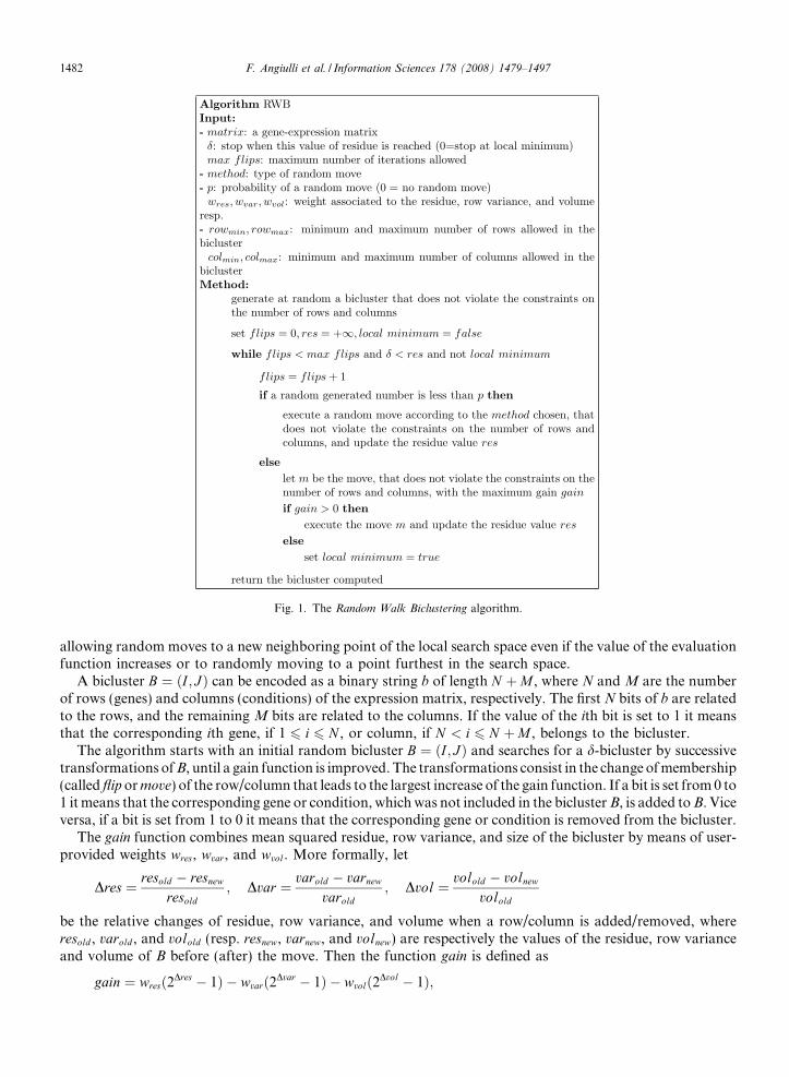
Fig. 1. The Random Walk Biclustering algorithm.

1482 F. Angiulli et al. / Information Sciences 178 (2008) 1479–1497

allowing random moves to a new neighboring point of the local search space even if the value of the evaluationfunction increases or to randomly moving to a point furthest in the search space.

A bicluster B ¼ ðI ; JÞ can be encoded as a binary string b of length N þM , where N and M are the numberof rows (genes) and columns (conditions) of the expression matrix, respectively. The first N bits of b are relatedto the rows, and the remaining M bits are related to the columns. If the value of the ith bit is set to 1 it meansthat the corresponding ith gene, if 1 6 i 6 N , or column, if N < i 6 N þM , belongs to the bicluster.

The algorithm starts with an initial random bicluster B ¼ ðI ; JÞ and searches for a d-bicluster by successivetransformations of B, until a gain function is improved. The transformations consist in the change of membership(called flip or move) of the row/column that leads to the largest increase of the gain function. If a bit is set from 0 to1 it means that the corresponding gene or condition, which was not included in the bicluster B, is added to B. Viceversa, if a bit is set from 1 to 0 it means that the corresponding gene or condition is removed from the bicluster.

The gain function combines mean squared residue, row variance, and size of the bicluster by means of user-provided weights wres, wvar, and wvol. More formally, let

Dres ¼ resold � resnew

resold; Dvar ¼ varold � varnew

varold; Dvol ¼ volold � volnew

volold

be the relative changes of residue, row variance, and volume when a row/column is added/removed, whereresold , varold , and volold (resp. resnew, varnew, and volnew) are respectively the values of the residue, row varianceand volume of B before (after) the move. Then the function gain is defined as

gain ¼ wresð2Dres � 1Þ � wvarð2Dvar � 1Þ � wvolð2Dvol � 1Þ;

F. Angiulli et al. / Information Sciences 178 (2008) 1479–1497 1483

with wres þ wvar þ wvol ¼ 1. This function assumes values in the interval ½�1;þ1�. In fact, relative changes Dres,Dvar, and Dvol range in the interval ½�1;þ1�, consequently the terms 2Dres, 2Dvar, and 2Dvol range in the inter-val ½0; 2�, and the whole function assumes values between �1 and +1. The weights wres, wvar, and wvol provide atrade-off among the relative changes of residue, row variance, and volume. When wres ¼ 1 (and thuswvar ¼ wvol ¼ 0), the algorithm searches for a minimum residue bicluster, since the gain monotonically increaseswith the residue of the bicluster. Decreasing wres and increasing wvar and wvol, biclusters with higher row var-iance and larger volume can be obtained.

Notice that when the residue after a flip diminishes, and the row variance and volume increase, Dres is posi-tive, while Dvar and Dvol are negative. Thus, when the gain function is positive, RWB is biased towards largebiclusters with a relatively high variance, and low residue. A negative gain, on the contrary, means a deteri-oration of the bicluster because there could have been either an augmentation of the residue or a decrease ofthe row variance or volume.

During its execution, in order to avoid get trapped into poor local minima (i.e. low quality biclusters withnegative gain in their neighborhood), instead of performing the flip maximizing the gain, with a user-providedprobability p the algorithm is allowed to execute a random move. We introduced three types of random moves:

� NOISE: with probability p, choose at random a row/column of the matrix and add/remove it to/from B;� REMOVE: with probability p, choose at random a row/column of B and remove it from B;� REMOVE-MAX: with probability p, select the row/column of B scoring the maximum value of residue,

and remove it from B.

Thus, the NOISE is a purely random strategy that picks a row/column from the overall matrix, and notonly from the bicluster, and adds or removes the row/column to the bicluster if it belongs or it does not belongto it. The REMOVE strategy removes at random a row/column already present in the bicluster, thus it couldaccidentally delete a worthless gene/condition from the current solution, and the REMOVE-MAX removesthat row/column already present in the bicluster having the highest value of the residue, i.e. mostly contrib-uting to worsen the gain.

Fig. 3 shows the algorithm RWB. The algorithm receives in input a gene expression matrix, a thresholdvalue (d) for the residue of the bicluster, the maximum number of times (max flips) that a flip can be done,the kind of random move the algorithm can choose (method), the probability (p) of executing a random move,the weight to assign to residue (wres), variance (wvar), and volume (wvol), and some optional constraints (rowmin,rowmax, colmin, colmax) on the size of the bicluster to find.

The flips are repeated until either a preset of maximum number of flips (max flips) is reached, or a d-biclusteris found, or the solution cannot ulteriorly be improved (get trapped into a local minimum). Until the stop con-dition is not reached, it executes a random move with probability p, and a greedy move with probability (1� p).

In the experimental section the three strategies will be compared on two data sets and the advantages ofeach discussed. When a greedy move is executed, the current value res of the mean squared residue is updated.It is used to check if a bicluster having residue below d has been found. On the contrary, if the value of resmin iszero, then the algorithm continues the execution until the gain can be improved.

In order to compute k biclusters, we execute k times the algorithm RWB by fixing two frequency thresholds,frow and fcol, that allow to control the degree of overlapping among the biclusters. The former binds a genericrow to participate to at most k � frow biclusters among the k to be found. Analogously, fcol limits the presenceof a column in at most k � fcol biclusters. During the k executions of the algorithm, whenever a row/columnexceeds the corresponding frequency threshold, it is removed from the matrix and not taken into accountany more in the subsequent executions.

4. Computational complexity

In this section the time and space complexity of the method is discussed.As far as the temporal cost of the algorithm is concerned, it is upper bounded by

max flips� Cu � ½ð1� pÞ � ðN þMÞ þ p�

1484 F. Angiulli et al. / Information Sciences 178 (2008) 1479–1497

where Cu is the cost of computing the new residue and the new row variance of the bicluster after performing amove. In order to reduce the complexity of Cu, we maintain, together with the current bicluster B ¼ ðI ; JÞ, themean values aiJ and aIj, for each i 2 I , the summation

Pj2J a2

ij, and the total sum of the row variances. Thecomputation of the new residue of each element involves recomputing the jI j þ jJ j mean values aiJ

(1 6 i 6 jI j) and aIj (1 6 j 6 jJ j) after performing the move. This can be done efficiently, in timemaxfjI j; jJ jg, by exploiting the values maintained together with the current bicluster.

Computing the residue resnew of the new bicluster, requires the computation of the squares of its elementresidues, a time proportional to the volume of the new bicluster. We note that, usually, jI j jJ j � NM , andin general it is dominated by the number N of genes of the overall matrix.

Computing the new row variances can be done in a fast way by exploiting the summationsP

j2J a2ij already

stored. Indeed, if a column is added or removed, the new row variances can be obtained quickly by evaluatingthe jI j expressions 1

jJ jP

ijða2ijÞ � a2

iJ (1 6 i 6j I j). For example, if the qth column is added, in order to compute

the new variance of the row i, the following expression must be evaluated:

1

jJ j þ 1

Xj2J

ða2ijÞ þ a2

iq

!� jJ jaiJ þ aiq

jJ j þ 1

� �2

:

Analogously if a column is removed. Otherwise, if a row is added (removed resp.) the corresponding row var-iance must be computed and added (subtracted resp.) to the overall sum of row variances.

Before concluding, we note that the cost of a random move is negligible, as it consists in generating a randomnumber, when the NOISE or REMOVE strategies are selected, while the row/column with the maximum res-idue, selected by the REMOVE-MAX strategy, is computed, with no additional time requirements, during theupdate of the residue of the bicluster at the end of each iteration, and, hence, it is always immediately available.

5. Related work

Biclustering approaches [21,24,17,11,8,34,31,35,23,12,10,30,29,27], also called co-clustering, are receiving alot of attention in the research community and are tightly related to subspace clustering in data mining andtext mining [3,2,1,26,13,14]. In the following we review the main proposals for biological data analysis. Sur-veys on biclustering algorithms for gene expression data can be found in [25,32,9]. In particular, in [25] biclu-stering approaches are classified with respect to the type of bicluster found and the search method adopted.

Hartigan [21] first suggested a partition-based algorithm, called direct clustering, that splits the data matrixto find sub-matrices having zero variance, that is with constant values. The variance of a bicluster is used toevaluate its quality and the algorithm stops when K sub-matrices are found. Though the aim of the approachwas to obtain constant biclusters, Hartigan proposed to modify his algorithm to find biclusters with constantrows, constant columns or coherent values in rows and columns.

Cheng and Church [11] were the first who introduced the new paradigm of biclustering to gene expressiondata analysis. They proposed some greedy search heuristics that generate suboptimal biclusters satisfying thecondition of having the mean squared residue below a threshold d. Cheng and Church proved that the prob-lem of finding biclusters with low mean squared residue, in particular maximal biclusters with scores under afixed threshold, is NP-hard because it includes the problem of finding a maximum biclique in a bipartite graphas a special case [16]. Therefore, they proposed some heuristics that are able to generate good quality biclus-ters. The algorithm, in the following referred as CC, starts with the original data matrix and removes highestscoring rows and columns as long as the mean squared residue is above the threshold d. After that, rows andcolumns are added provided that they do not increase the residue above the threshold. The approach is deter-ministic, thus to discover more than one cluster, in order to avoid to reobtain the same biclusters, the algo-rithm is repeated on a modified data matrix where the values of those elements aij already inserted in abicluster are substituted with random numbers. This choice, however, has the negative effect of precludingthe discovery of new biclusters, in particular those having significant overlaps with those already found.The CC algorithm assumes that the data matrix does not contain missing values.

Yang et al. [35] extended the definition of d-bicluster to cope with missing values and to avoid the problemscaused by random numbers. They defined a probabilistic move-based algorithm flexible overlapped bicluster-

F. Angiulli et al. / Information Sciences 178 (2008) 1479–1497 1485

ing (FLOC) that generalizes the concept of mean squared residue and it is based on the concept of action andgain. Given a row (or a column) x and a bicluster c, the action Actionðx; cÞ is defined as the change of mem-bership of x to c. Thus if x already belongs to the bicluster c, Actionðx; cÞ denotes the removal of x from c,otherwise it denotes the addition. The algorithm consists of two phases. In the first phase, k biclusters are gen-erated. In the second phase the quality of the biclusters is improved by performing the best action for eachbicluster, as the one that produces the highest gain for all the k biclusters. The gain of an actionActionðx; cÞ is defined as a function of the relative reduction of the c’s residue and the relative enlargementof the c’s volume after performing it. After the best action is identified for each row and column, theN þM actions are performed sequentially. However, in order to avoid local optimal solutions, a randomweighted ordering is introduced. This ordering assigns higher probability to actions with positive gains withrespect to those with negative gain.

Though our concept of flip in RWB is similar to that of Action in FLOC, the two algorithms are sub-stantially different. In fact, RWB finds one cluster at a time and the change of membership of a row/column is done locally with respect to the current bicluster, FLOC obtains k biclusters at the same timeand executes the action that globally improves the gain. Furthermore, the approaches to escape localminima are completely different. RWB performs random moves, while FLOC relies on random actionordering.

Cho et al. [12] propose two iterative co-clustering algorithms that use two different squared residue mea-sures, one is that adopted by Hartigan [21], the second is that defined by Cheng and Church [11]. The twoalgorithms are based on the k-means clustering method. The authors formulate the problem of minimizingthe residue as a trace optimization problem and use the spectral relaxation of such problem to initialize theirmethods.

Getz et al. [17] presented the Coupled Two-Way Clustering (CTWC) algorithm that uses a standard hierar-chical clustering method separately on each dimension to discover significant clusters, called stable. Theapproach selects a subset of rows and columns and applies the one-dimensional algorithm iteratively on themuntil the columns detected are only those used to cluster the corresponding rows, or vice versa. This allows todetect stable sub-matrices, i.e. biclusters, that partition the data matrix. The approach avoids the regenerationof the same row and column subsets by dynamically maintaining a list of stable clusters and a list of pairs ofrow and column subsets.

Lazzeroni and Owen [24] introduced the Plaid model. The basic idea of this approach is that each elementin the data matrix is viewed as a sum of terms called layers, where a layer corresponds to a bicluster. Thus thedata matrix is described as a linear function of layers and the objective is to minimize a merit function thattake into account the interactions between the biclusters.

Tanay et al. [31,30,29] presented statistical-algorithmic method for bicluster analysis (SAMBA), a biclu-stering algorithm that combines graph theory and statistics. The data matrix is represented as a bipartitegraph where the nodes are conditions and genes, and edges denote significant expression changes. Vertexpairs are associated with a weight according to a probabilistic model, and heavy subgraphs correspond tosignificant biclusters. The problem of finding biclusters reduces thus to that of finding the heaviestsubgraphs in the bipartite graph. Since this problem is NP-hard, to reduce the execution time, SAMBAapplies some restrictions on the size of the biclusters and employs a heuristic to search for heavysubgraphs.

6. Experimental results

In order to evaluate the method proposed, we performed an experimental study on several benchmarks. Weemployed two well known gene expression data sets, the Yeast Saccharomyces cerevisiae cell cycle and thehuman B-cell Lymphoma, to study the behavior of RWB when the different random move strategies areadopted. Other seven data sets, Colon Rectal Tumor, Lung Cancer, Prostate Cancer, Ovarian Cancer, ALL-

AML Leukemia, Colon Tumor, and the Central Nervous System, were used to compare our approach with thatof Cheng and Church from a point of view of both quantitative and qualitative parameters. In fact we com-pared the biclusters found by RWB and CC with respect to residue, variance, and volume, and then we eval-uated the ability of both the methods to produce biclusters conforming to prior biological knowledge.

1486 F. Angiulli et al. / Information Sciences 178 (2008) 1479–1497

The RWB algorithm has been implemented by using the C programming language. As regards the CC algo-rithm, we employed the Java implementation publicly available on the web site of the authors.1 All the exper-iments have been performed on a Pentium Mobile 1700 MHz based machine.

6.1. Evaluation of random move strategies

This first set of experiments aims at comparing the three random move strategies introduced when differentprobabilities and input parameters are given and to discuss the advantages of each of them. For this experi-ment we used the Yeast Saccharomyces cerevisiae cell cycle expression data set, and the human B-cell Lym-

phoma data set. The preprocessed gene expression matrices can be obtained from [11] at http://arep.med.harvard.edu/biclustering. The yeast cell cycle data set contains 2884 genes and 17 conditions. Thehuman lymphoma data set has 4026 genes and 96 conditions.

We computed k ¼ 100 biclusters varying the probability p of a random move in the interval ½0:1; 0:6�, fortwo different configurations of the weights, i.e. w1 ¼ ðwres;wvar;wvolÞ ¼ ð1; 0; 0Þ (dashed lines in Fig. 2) andw2 ¼ ðwres;wvar;wvolÞ ¼ ð0:5; 0:3; 0:2Þ (solid lines in Fig. 2). Notice that wres ¼ 1 and wvar ¼ wvol ¼ 0 means thatthe gain function is completely determined by the residue value. We set max flips to 100, d to 0, and the fre-quency thresholds to frow ¼ 10% and fcol ¼ 100%, i.e. a row can participate in at most 10 biclusters, while acolumn can appear in all the 100 biclusters. The initial random generated biclusters are of size 14� 14 for theYeast data set and of size 20� 20 for the Lymphoma data set, while we constrained biclusters to have at leastrowmin ¼ 10 rows and colmin ¼ 10 columns.

Fig. 2 shows the behavior of the algorithm on the two above mentioned data sets. From the top to the bot-tom, the figures show the average residue, row variance and volume of the 100 biclusters computed, the aver-age number of flips performed by the method, and the average execution time. Figures on the left concern theYeast data set, and figures on the right the Lymphoma data set.

We can observe that, as regards the residue, the REMOVE-MAX method performs better than the twoothers, as expected. In fact, its random move consists in removing the gene/condition having the highest res-idue. Furthermore, increasing the random move probability p improves the value of the residue. The residue ofthe NOISE method, instead, deteriorates when the probability increases. The REMOVE strategy, on theYeast data set is better than the NOISE one, but worse than the REMOVE-MAX. On the Lymphoma dataset, the value of the residue increases until p ¼ 0:3 but then it decreases. The residue scored for parameters w1

(dashed lines) is lower with respect to that obtained for w2 (solid lines), for the two strategies NOISE andREMOVE, while, for REMOVE-MAX the difference is negligible.

As regards the variance, we can note that the variance of REMOVE is greater than that of NOISE, and thatof NOISE is greater than that of REMOVE-MAX for both w1 and w2. This is of course expected, since in theformer case we do not consider the variance in the gain function in order to obtain the biclusters, while in thelatter the weight of the variance is almost as important as that of the residue (0.3 w.r.t. 0.5).

Analogous considerations hold for the volume, whose value is higher for w2. Furthermore, the volume isalmost constant for the NOISE strategy, because the probability of adding or removing an element in thebicluster is more or less the same, but it decreases for the REMOVE and REMOVE-MAX strategies. Thesetwo strategies tend to discovery biclusters having the same size when the probability p increases.

As for the average number of flips, we can note that 100 flips are never sufficient for the NOISE method toreach a local minimum, while the other two methods do not execute all the 100 flips. In particular, the RAN-DOM-MAX strategy is the fastest since it is that which needs less flips before stopping.

As regards the execution time, the algorithm is faster for w1 w.r.t. w2, but, in general, the execution timedecreases when the probability p increases and they are almost the same for higher values of p because thenumber of random moves augments for both.

Finally some consideration on the quality of the biclusters obtained. We noticed that the NOISE strategy,which works in a purely random way, gives biclusters with higher residue and it requires more execution time.On the contrary, REMOVE-MAX is positively biased by the removal of those elements in the bicluster having

1 Downloadable on http://cheng.ececs.uc.edu/biclustering/Biclustering.java.

0.1 0.2 0.3 0.4 0.5 0.60

100

200

300

400

500

600

700Yeast data set (k=100)

Probability

Ave

rage

res

idue

NOISEREMOVEREMOVE−MAX

0.1 0.2 0.3 0.4 0.5 0.60

500

1000

1500

2000

2500

3000

3500

4000

4500

5000Lymphoma data set (k=100)

Probability

Ave

rage

res

idue

NOISEREMOVEREMOVE−MAX

0.1 0.2 0.3 0.4 0.5 0.60

200

400

600

800

1000

1200

1400

1600

1800

2000Yeast data set (k=100)

Probability

Ave

rage

var

ianc

e

NOISEREMOVEREMOVE−MAX

0.1 0.2 0.3 0.4 0.5 0.6102

103

104

105Lymphoma data set (k=100)

Probability

Ave

rage

var

ianc

e

NOISEREMOVEREMOVE−MAX

0.1 0.2 0.3 0.4 0.5 0.60

500

1000

1500Yeast data set (k=100)

Probability

Ave

rage

vol

ume

NOISEREMOVEREMOVE−MAX

0.1 0.2 0.3 0.4 0.5 0.60

500

1000

1500

2000

2500Lymphoma data set (k=100)

Probability

Ave

rage

vol

ume

NOISEREMOVEREMOVE−MAX

0.1 0.2 0.3 0.4 0.5 0.630

40

50

60

70

80

90

100Yeast data set (k=100)

Probability

Ave

rage

num

ber

of fl

ips

NOISEREMOVEREMOVE−MAX

0.1 0.2 0.3 0.4 0.5 0.640

50

60

70

80

90

100Lymphoma data set (k=100)

Probability

Ave

rage

num

ber

of fl

ips

NOISEREMOVEREMOVE−MAX

0.1 0.2 0.3 0.4 0.5 0.60

5

10

15

20

25Yeast data set (k=100)

Probability

Ave

rage

exe

cutio

n tim

e [s

ec]

NOISEREMOVEREMOVE−MAX

0.1 0.2 0.3 0.4 0.5 0.60

5

10

15

20

25

30

35

40

45

50Lymphoma data set (k=100)

Probability

Ave

rage

exe

cutio

n tim

e [s

ec]

NOISEREMOVEREMOVE−MAX

Fig. 2. Average residue, variance, volume, number of flips and execution time for Yeast (on the left) and Lymphoma (on the right) data sets.

F. Angiulli et al. / Information Sciences 178 (2008) 1479–1497 1487

1488 F. Angiulli et al. / Information Sciences 178 (2008) 1479–1497

the worst residue, thus it is able to obtain biclusters with lower values of residue, while the REMOVE strategyextracts biclusters with higher variance.

To show the quality of the biclusters found by RWB, Fig. 3 depicts some of the biclusters discovered in theexperiments of Fig. 2 by using the REMOVE-MAX strategy for ðwres;wvar;wvolÞ ¼ ð0:5; 0:3; 0:2Þ. The x axiscorresponds to conditions, while the y axis gives the gene expression level. The figures point out the good qual-ity of the biclusters obtained. In fact, their expression levels vary homogeneously under a subset of conditions,thus they present a high degree of coherence. Fig. 4a shows the heatmap of the overall Lymphoma data set. Tocreate the map we used the Heatmap Builder software [22]. Fig. 4b displays the heatmap of a subset of thegenes and samples, obtained by choosing ten biclusters among the 100 returned by the experiment. The figurehas been generated by the BIVOC software [18], that searches for an optimal reordering of rows and columnsbefore creating the picture. It is worth to note that, since RWB tries to minimize the residue and maximize rowvariance, the heatmap of a bicluster found cannot show a uniform color, instead the bicluster should presentcoherent values on both rows and columns, i.e., as reported in [25], each row or column can be obtained byadding a constant to each of the others or by multiplying each of the others by a constant value. In fact thebiclusters showed in Fig. 4b have columns of the same color, confirming the presence of coherent values.

6.2. Comparative analysis of RWB and CC

There exist several studies to compare and validate clustering approaches [36,5,6]. Generally they make useof validity indices [19,20] to assess their quality. Validity indices are classified in internal, external, and relative.Internal indices rely on the input data and are mainly based on the concepts of homogeneity and separationbetween the groups, external indices use additional data to validate the clustering outcomes, and relative indi-ces measure the influence of the input parameters on the results. In the context of gene expression data there isno general agreement on which validity indices to adopt because of the different types of biclusterings the algo-rithms detect: constant values, coherent values, coherent evolutions, checkerboard structure, overlapping, etc.[25]. However, internal indices meaningful for comparing our approach and that of Cheng and Church clearlyare the residue, volume, and variance values. Furthermore, external criteria correspond to prior biologicalknowledge on the data set being studied.

In the following we compare RWB and CC first with respect to these internal indices, and then we evaluatethem with respect to some external indices by studying the ability of both the algorithms to obtain biologicallysignificant biclusters. To this end we used six real life data sets coming from the Kent Ridge Bio-medical Data

Set Repository,2 and one (Colon Rectal Cancer) used in [4].3 A brief description of each data set follows.The Colon Rectal Cancer contains the expression of the 2000 genes with highest minimal intensity across 62

parts of the colon. Each entry is a gene intensity derived from 20 feature pairs that correspond to the gene onthe chip of the tissue.

The Lung Cancer data set collects 181 tissue samples, described by 12,533 genes, representing classified databetween malignant pleural mesothelioma and adenocarcinoma of the lung.

The Prostate Cancer data set contains the RNA values of 12,600 genes collected on 136 human samplesclassified as normal and having prostate tumor. The prostate tumor samples came from patients undergoingradical prostatectomy between 1995 and 1997.

The Ovarian Cancer Tumor data set contains values of 253 women (91 no-ovarian cancer and 162 ovariancancer), described by 15,154 proteomic features. This dataset is of a great interest for women who have a highrisk of ovarian cancer due to family or personal history of cancer.

The Leukemia data set contains the RNA value of 7129 probes of human genes collected on 72 acute leu-kemia patients. From a biological point of view, such subjects are classified as Acute Lymphoblastic Leukemia(ALL) and Acute Myeloid Leukemia (AML). In this data set there are 47 ALL and 25 AML.

The Colon Tumor data set contains the RNA values of 2000 (selected from around 6500) human genes col-lected from 62 cancer-patients. Among them, 40 tumor biopsies are from tumor-unhealthy parts (labelled as

2 http://sdmc.lit.org.sg/GEDatasets/Datasets.html.3 http://microarray.princeton.edu/oncology/affydata/index.html.

1 2 3 4 5 6 7 8 9 1050

100

150

200

250

300

350

1 2 3 4 5 6 7 8 9 100

50

100

150

200

250

300

350

400

450

1 2 3 4 5 6 7 8 9 1050

100

150

200

250

300

350

400

450

1 2 3 4 5 6 7 8 9 100

50

100

150

200

250

300

350

1 2 3 4 5 6 7 8 9 1050

100

150

200

250

300

350

400

1 2 3 4 5 6 7 8 9 100

50

100

150

200

250

300

350

0 2 4 6 8 10 12 140

50

100

150

200

250

300

350

1 2 3 4 5 6 7 8 9 1050

100

150

200

250

300

350

400

450

1 2 3 4 5 6 7 8 9 10–150

–100

–50

0

50

100

1 2 3 4 5 6 7 8 9 10 11–100

–80

–60

–40

–20

0

20

40

60

80

100

1 2 3 4 5 6 7 8 9 10–100

–50

0

50

100

150

200

1 2 3 4 5 6 7 8 9 10–150

–100

–50

0

50

100

150

1 2 3 4 5 6 7 8 9 10–150

–100

–50

0

50

100

150

1 2 3 4 5 6 7 8 9 10–100

–50

0

50

100

150

200

1 2 3 4 5 6 7 8 9 10–150

–100

–50

0

50

100

150

1 2 3 4 5 6 7 8 9 10–100

–50

0

50

100

150

Fig. 3. Biclusters obtained by using the REMOVE-MAX strategy with ðwres;wvar;wvolÞ ¼ ð0:5; 0:3; 0:2Þ in the experiments of Fig. 2. Thefirst two rows show eight biclusters of the Yeast data set (p ¼ 0:3), while the subsequent two rows show eight biclusters of the Lymphomadata set (p ¼ 0:5). From left to right and from top to bottom the values of (residue, variance, volume) are the following: (70.14, 590.65,460), (99.51, 705.58, 530), (160.89, 834.79, 360), (113.47, 674.25, 630), (83.04, 439.81, 310), (136.31, 788.27, 580), (180.03, 545.23, 518), and(111.01, 356.24, 640) for the Yeast data set, and (214.63, 1414.45, 150), (169.96, 1626.74, 165), (366.18, 2012.5, 190), (181.34, 2135.5, 140),(323.17, 2472.65, 170), (182.45, 1499.95, 160), (200.24, 3412.19, 130), and (172.94, 1197.03, 220) for the Lymphoma data set.

F. Angiulli et al. / Information Sciences 178 (2008) 1479–1497 1489

‘‘Negative”) and 22 normal biopsies are from healthy parts (labelled as ‘‘Positive”) of the colons of the samepatients.

Embryonal tumors of the Central Nervous System represent an heterogeneous group of tumors about whichlittle is known biologically, and whose diagnosis, based on morphologic appearance alone, is controversial.The Central Nervous System data set contains the RNA value of 7129 genes of 60 diseased patients, aftera medical treatment. Patients are labelled as ‘‘Survivors” (21) or ‘‘Failures” (39), depending on the outcomeof the treatment.

Fig. 4. Heatmap of the original Lymphoma data set (on the left) and biclusters found on a subset of the genes and samples.

1490 F. Angiulli et al. / Information Sciences 178 (2008) 1479–1497

6.2.1. Quantitative analysis

This set of experiments aims at evaluating and comparing the behavior of the RWB algorithm and that ofCheng and Church (CC, for short, in the following) when different values of some input parameters are used.

The experiments analyze the biclusters obtained by the two algorithms when the number of biclusters k,and the maximum residue value d are varied. In particular, we asked the two algorithms to find a numberof biclusters from 5 to 50, that is for k ¼ 5; 10; 20; 30; 50, when the residue threshold d is fixed to 0, 500,800 and 1000. For all of experiments the RWB algorithm used the weight configuration w ¼ ð0:6; 0:1; 0:3Þ,a maximum number of flips max flips of 3000, the frequency threshold frow ¼ 100% and fcol ¼ 100%, i.e. eachrow and column can potentially participate in all the k biclusters. Even though such a constrain could lead toheavy overlapping between biclusters, we verified that the rate of overlapping is marginal, below the 2%.Finally, we fixed the probability of random move to p ¼ 0:5 and, for all the experiments, we adopted theREMOVE-MAX strategy. Both RWB and CC algorithms have been executed 10 times and the valuesobtained by averaging these 10 executions are reported.

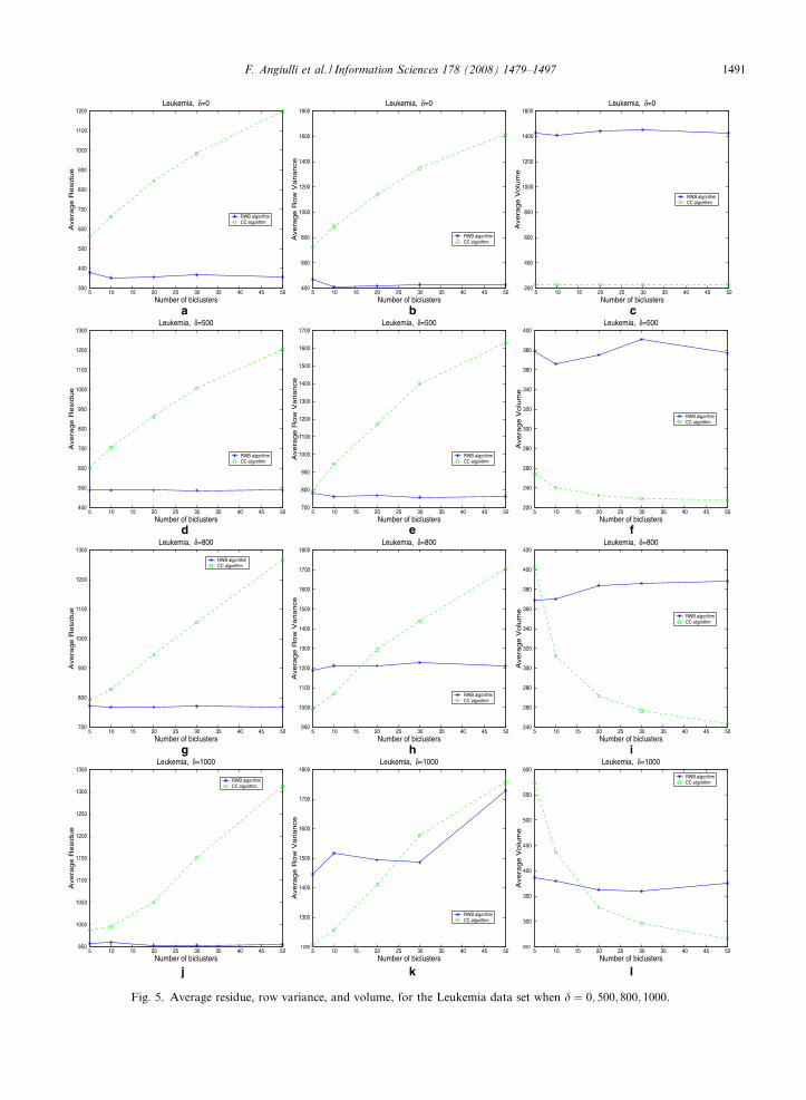
Figs. 5–7 show, for the Leukemia, Colon Tumor, and Central Nervous System data sets respectively, theaverage residue, average row variance, and average volume of the biclusters extracted by the algorithmswhen the residue threshold assumes the values d ¼ 0; 500; 800; 1000. From the Fig. 5 we can observe thatthe RWB algorithm, on the Leukemia data set, always obtains biclusters with lower residue (Fig. 5a,d,gand j), higher volume (Fig. 5c,f,i and l), and lower variance (Fig. 5b,e,h, and k) than the CC algorithm. Thismeans that the former algorithm is able to find highly coherent genes and conditions which lead to low res-idue while the latter tends to find smaller biclusters with less coherence, i.e. larger residue. Lower varianceresults for RWB are due to the fixed weight value of 0.1. Another important observation to point out is thatRWB maintains a residue value very near to the threshold requested as long as the number of biclusters tofind increases. Analogously, the volume of biclusters do not sensibly varies along the executions. On the con-trary, CC is not able to satisfy the threshold requirement because, though when we ask for few biclusters theaverage residue does not significantly move away from the fixed value, when the number of biclusters aug-ments, the residue sensibly increases while the volume decreases. This behavior probably is due to the intro-duction of random numbers adopted by CC to bias the algorithm to find non overlapping biclusters. Asregards RWB, the random strategy employed allows to explore different parts of the search space thus assur-ing low levels of overlapping, although the frequency thresholds of 100% enable each row and column totake part to all the biclusters.

5 10 15 20 25 30 35 40 45 50300

400

500

600

700

800

900

1000

1100

1200Leukemia, δ=0

Number of biclusters

Avera

ge R

esid

ue

RWB algorithmCC algorithm

5 10 15 20 25 30 35 40 45 50400

600

800

1000

1200

1400

1600

1800Leukemia, δ=0

Number of biclustersA

vera

ge R

ow

Variance

RWB algorithmCC algorithm

5 10 15 20 25 30 35 40 45 50200

400

600

800

1000

1200

1400

1600Leukemia, δ=0

Number of biclusters

Avera

ge V

olu

me

RWB algorithmCC algorithm

5 10 15 20 25 30 35 40 45 50400

500

600

700

800

900

1000

1100

1200

1300Leukemia, δ=500

Number of biclusters

Avera

ge R

esid

ue

RWB algorithmCC algorithm

5 10 15 20 25 30 35 40 45 50700

800

900

1000

1100

1200

1300

1400

1500

1600

1700Leukemia, δ=500

Number of biclusters

Avera

ge R

ow

Variance

RWB algorithmCC algorithm

5 10 15 20 25 30 35 40 45 50220

240

260

280

300

320

340

360

380

400Leukemia, δ=500

Number of biclustersA

vera

ge V

olu

me

RWB algorithmCC algorithm

5 10 15 20 25 30 35 40 45 50700

800

900

1000

1100

1200

1300Leukemia, δ=800

Number of biclusters

Avera

ge R

esid

ue

RWB algorithmCC algorithm

5 10 15 20 25 30 35 40 45 50900

1000

1100

1200

1300

1400

1500

1600

1700

1800Leukemia, δ=800

Number of biclusters

Avera

ge R

ow

Variance

RWB algorithmCC algorithm

5 10 15 20 25 30 35 40 45 50240

260

280

300

320

340

360

380

400

420Leukemia, δ=800

Number of biclusters

Avera

ge V

olu

me

RWB algorithmCC algorithm

5 10 15 20 25 30 35 40 45 50950

1000

1050

1100

1150

1200

1250

1300

1350Leukemia, δ=1000

Number of biclusters

Avera

ge R

esid

ue

RWB algorithmCC algorithm

5 10 15 20 25 30 35 40 45 501200

1300

1400

1500

1600

1700

1800Leukemia, δ=1000

Number of biclusters

Avera

ge R

ow

Variance

RWB algorithmCC algorithm

5 10 15 20 25 30 35 40 45 50250

300

350

400

450

500

550

600Leukemia, δ=1000

Number of biclusters

Avera

ge V

olu

me

RWB algorithmCC algorithm

a b c

d e f

g h i

j k l

Fig. 5. Average residue, row variance, and volume, for the Leukemia data set when d ¼ 0; 500; 800; 1000.

F. Angiulli et al. / Information Sciences 178 (2008) 1479–1497 1491

5 10 15 20 25 30 35 40 45 5050

100

150

200

250

300

350Colon Tumor, δ=0

Number of biclusters

a b c

d e f

g h i

j k l

Ave

rage

Res

idue

RWB algorithmCC algorithm

5 10 15 20 25 30 35 40 45 50200

300

400

500

600

700

800

900Colon Tumor, δ=0

Number of biclustersA

vera

ge R

ow V

aria

nce

RWB algorithmCC algorithm

5 10 15 20 25 30 35 40 45 50200

300

400

500

600

700

800

900Colon Tumor, δ=0

Number of biclusters

Ave

rage

Vol

ume

RWB algorithmCC algorithm

5 10 15 20 25 30 35 40 45 50450

500

550

600

650

700

750

800Colon Tumor, δ=500

Number of biclusters

Ave

rage

Res

idue

RWB algorithmCC algorithm

5 10 15 20 25 30 35 40 45 50800

1000

1200

1400

1600

1800

2000Colon Tumor, δ=500

Number of biclusters

Ave

rage

Row

Var

ianc

e

RWB algorithmCC algorithm

5 10 15 20 25 30 35 40 45 50200

400

600

800

1000

1200

1400

1600

1800

2000

2200Colon Tumor, δ=500

Number of biclustersA

vera

ge V

olum

e

RWB algorithmCC algorithm

5 10 15 20 25 30 35 40 45 50700

750

800

850

900

950

1000

1050

1100

1150

1200Colon Tumor, δ=800

Number of biclusters

Ave

rage

Res

idue

RWB algorithmCC algorithm

5 10 15 20 25 30 35 40 45 501200

1400

1600

1800

2000

2200

2400

2600

2800

3000Colon Tumor, δ=800

Number of biclusters

Ave

rage

Row

Var

ianc

e

RWB algorithmCC algorithm

5 10 15 20 25 30 35 40 45 500

500

1000

1500

2000

2500

3000Colon Tumor, δ=800

Number of biclusters

Ave

rage

Vol

ume

RWB algorithmCC algorithm

5 10 15 20 25 30 35 40 45 50900

1000

1100

1200

1300

1400

1500Colon Tumor, δ=1000

Number of biclusters

Ave

rage

Res

idue

RWB algorithmCC algorithm

5 10 15 20 25 30 35 40 45 501600

1800

2000

2200

2400

2600

2800

3000

3200

3400Colon Tumor, δ=1000

Number of biclusters

Ave

rage

Row

Var

ianc

e

RWB algorithmCC algorithm

5 10 15 20 25 30 35 40 45 500

500

1000

1500

2000

2500

3000

3500

4000Colon Tumor, δ=1000

Number of biclusters

Ave

rage

Vol

ume

RWB algorithmCC algorithm

Fig. 6. Average residue, row variance, and volume, for the Colon Tumor data set when d ¼ 0; 500; 800; 1000.

1492 F. Angiulli et al. / Information Sciences 178 (2008) 1479–1497

5 10 15 20 25 30 35 40 45 50400

600

800

1000

1200

1400

1600Central Nervous System, δ=0

Number of biclusters

Avera

ge R

esid

ue

RWB algorithmCC algorithm

5 10 15 20 25 30 35 40 45 50600

800

1000

1200

1400

1600

1800

2000

2200Central Nervous System, δ=0

Number of biclustersA

vera

ge R

ow

Variance

RWB algorithmCC algorithm

5 10 15 20 25 30 35 40 45 50200

400

600

800

1000

1200

1400

1600Central Nervous System, δ=0

Number of biclusters

Avera

ge V

olu

me

RWB algorithmCC algorithm

5 10 15 20 25 30 35 40 45 50400

600

800

1000

1200

1400

1600Central Nervous System, δ=500

Number of biclusters

Avera

ge R

esid

ue

RWB algorithmCC algorithm

5 10 15 20 25 30 35 40 45 50600

800

1000

1200

1400

1600

1800

2000

2200Central Nervous System, δ=500

Number of biclusters

Avera

ge R

ow

Variance

RWB algorithmCC algorithm

5 10 15 20 25 30 35 40 45 50200

300

400

500

600

700

800

900Central Nervous System, δ=500

Number of biclustersA

vera

ge V

olu

me

RWB algorithmCC algorithm

5 10 15 20 25 30 35 40 45 50700

800

900

1000

1100

1200

1300

1400

1500

1600

1700Central Nervous System, δ=800

Number of biclusters

Avera

ge R

esid

ue

RWB algorithmCC algorithm

5 10 15 20 25 30 35 40 45 501100

1200

1300

1400

1500

1600

1700

1800

1900

2000

2100Central Nervous System, δ=800

Number of biclusters

Avera

ge R

ow

Variance

RWB algorithmCC algorithm

5 10 15 20 25 30 35 40 45 50220

240

260

280

300

320

340

360

380

400

420Central Nervous System, δ=800

Number of biclusters

Avera

ge V

olu

me

RWB algorithmCC algorithm

5 10 15 20 25 30 35 40 45 50900

1000

1100

1200

1300

1400

1500

1600

1700Central Nervous System, δ=1000

Number of biclusters

Avera

ge R

esid

ue

RWB algorithmCC algorithm

5 10 15 20 25 30 35 40 45 501200

1300

1400

1500

1600

1700

1800

1900

2000

2100

2200Central Nervous System, δ=1000

Number of biclusters

Avera

ge R

ow

Variance

RWB algorithmCC algorithm

5 10 15 20 25 30 35 40 45 50220

240

260

280

300

320

340

360Central Nervous System, δ=1000

Number of biclusters

Avera

ge V

olu

me

RWB algorithmCC algorithm

RWB algorithmCC algorithm

RWB algorithmCC algorithm

RWB algorithmCC algorithm

RWB algorithmCC algorithm

RWB algorithmCC algorithm

RWB algorithmCC algorithm

RWB algorithmCC algorithm

RWB algorithmCC algorithm

RWB algorithmCC algorithm

RWB algorithmCC algorithm

a b c

d e f

g h i

j k l

Fig. 7. Average residue, row variance, and volume, for the Central Nervous System data sets when d ¼ 0; 500; 800; 1000.

F. Angiulli et al. / Information Sciences 178 (2008) 1479–1497 1493

1494 F. Angiulli et al. / Information Sciences 178 (2008) 1479–1497

Figs. 6 and 7 show a similar behavior of the two algorithms on the Central Nervous System, and Colon

Tumor data sets. In particular, Fig. 7a,d,g and j confirm that the biclusters found by RWB have lower residue,lower variance (Fig. 7b,e,h and k) than those found by the CC algorithm, and higher volume (Fig. 7c,f,i and l).As regards the Colon Tumor data set, Fig. 6a,d,g and j show that the biclusters obtained by RWB have almostalways lower residue than CC, though, for a threshold greater than zero, the volume of the biclusters found byCC is higher. It is worth to note that when RWB is executed with a threshold value different than zero it meansthat the algorithm is forced to an early stopping. This could preclude RWB to continue to explore the searchspace and reach a better local optimal solution.

Finally, in Table 1 we summarize the results obtained by running RWB and CC, besides the three alreadydiscussed data sets, on other four data sets well known in the literature. For this experiment the residue thresh-old is fixed to 0, and the number of biclusters varies from 5 to 50. The table confirms the good behavior ofRWB that obtains biclusters of lower residue and higher or comparable volume with respect to CC. Notablyis the result for Prostate Cancer where the residue is between 1 and 2, while the volume is more than sixteenthousand elements.

Table 1Comparison between RandomWalk and Cheng–Church algorithms on all the datasets

RandomWalk Cheng–Church

N. biclusters Residue Variance Volume Residue Variance Volume

C. Rectal cancer 5 120.03 520.79 786 257.80 486.91 89110 152.79 399.50 855 385.81 780.79 91220 323.50 3411.19 707 641.48 1302.16 89730 229.43 918.03 502 1008.79 2023.27 94550 137.04 1186.59 319 3083.84 5472.27 966

Lung cancer 5 5.11 6.07 1411 13.85 18.25 22510 5.18 6.34 1436 19.97 26.20 22520 5.09 6.06 1418 29.10 38.13 22530 5.13 6.20 1421 35.94 49.07 22550 5.07 6.18 1392 47.13 63.27 225

Prostate cancer 5 1.64 1.69 16873 1009.59 3354.20 720410 1.70 1.75 16926 1659.35 5032.73 728820 1.82 1.87 16278 2955.64 7820.32 713230 1.78 1.99 16125 4548.19 10831.76 703150 2.34 2.00 16258 8596.91 16421.69 7287

Ovarian cancer 5 4.89 3.05 11451 5.09 6.28 1299610 5.38 4.02 10728 4.76 6.12 1219220 5.55 9.88 12054 4.99 6.07 1189430 6.48 7.11 11008 7.13 5.10 1207750 4.99 8.73 11451 5.01 6.34 13500

Leukemia 5 378.76 468.07 1428 556.99 688.99 22510 352.17 408.56 1410 671.53 853.97 22520 355.66 417.72 1441 858.69 1156.26 22530 366.14 429.86 1451 1006.11 1361.89 22550 358.97 427.28 1427 1201.15 1602.16 225

Colon tumor 5 122.19 412.51 814 74.29 207.91 22510 128.55 493.34 816 105.47 338.06 22520 115.40 464.76 721 166.14 464.87 22530 117.03 438.75 763 196.53 573.37 22550 117.86 458.71 762 313.78 923.59 225

C. nervous system 5 583.44 720.66 1500 798.61 1006.19 22510 590.64 726.76 1488 1081.11 1394.86 22520 591.10 740.22 1472 1194.65 1568.29 22530 571.34 698.27 1487 1357.35 1781.19 22550 593.84 755.79 1493 1609.93 2122.25 225

F. Angiulli et al. / Information Sciences 178 (2008) 1479–1497 1495

6.2.2. Biological evaluation

In this section we want to qualitatively evaluate the capability of our algorithm with respect to that ofCheng and Church to extract biclusters meaningful from a biological point of view. Assessing the biologicalrelevance of the results, however, is not a trivial task because there do not exist general guidelines in the lit-erature. An approach that can be pursued when the gene are annotated with their functional category consistsin verifying whether the biclusters discovered represents biological functional modules, that is whether eachbicluster contains a large portion of similar genes, i.e. belonging to the same functional class. Annotated datasets, however, are not easily available. In general data sets with experimental conditions classified as eitherbelonging to a positive or a negative class, where the meaning of positive and negative depends on the dataset, are more common.

The data sets used in the previous section are such that each experimental condition corresponds to apatient presenting a kind of pathology. For example, the Leukemia data set discriminates patients affectedby either Lymphoblastic or Myeloid leukemia, the Colon Tumor data set if a patient is positive or negativeto colon tumor, and the C. nervous system data set if a patient survives or not after a clinical treatment. Thuswe do not know the biological correlation between rows (genes), while we know the medical classification ofcolumns. In this case, we can evaluate the ability of an algorithm to separate the samples according to theirknown classification. To this end, we can compute the number of columns labelled with the same class andbelonging to the same bicluster. Obviously, higher the number of columns in a bicluster labelled with the sameclass label, higher its biological quality. In fact, this means that many patients with the same diagnosis aregrouped together with respect to a subset of genes, thus we could induce that those genes probably have sim-ilar functional category and characterize the majority class of patients.

In our experiments we used the biological information on the experimental conditions to assign a qualita-tive significance to the biclustering results by using a well known validity index, that is the Purity [17].

Suppose a set of experimental conditions be classified in two classes C1, C2, and let B1; . . . ;Bk be the k bicl-usters found by an algorithm. A k � 2 confusion matrix M can be built where a row corresponds to a biclusterand a column to a class label. The term mij of the confusion matrix represents the number of conditions of theexpression matrix A belonging to the bicluster Bi and labelled as class Cj. Each bicluster Bi is considered asrepresenting the biological class Cj of the most frequent label associated with its columns, that is the class labelj such that mij is maximal in the bicluster Bi.

Consider, for example, Table 2 where the confusion matrices obtained by running the RWB and CC algo-rithms on the Leukemia data sets, for k ¼ 5 and d ¼ 0, are reported.

The table shows that the bicluster 1 obtained by RWB contains 14 columns labelled ALL and only one col-umn labelled AML. From a biological point of view this means that this bicluster is able to identify a biolog-ically relevant partition of genes and conditions since it is characterized by a high coherence on the columns.Thus the genes participating to this bicluster better characterize ALL type Leukemia rather than AML type.These genes deserve deeper investigation because could be determinant for this kind of pathology. On the

Table 2Confusion matrices obtained by running RWB and CC on the Leukemia data set for k ¼ 5

Bicluster No. No. of ALL No. of AML

(a) RWB

1 14 12 12 33 12 34 13 25 14 3

(b) CC

1 13 22 11 43 13 24 13 25 9 6

5 10 15 20 25 30 35 40 45 500.5

0.55

0.6

0.65

0.7

0.75

0.8

0.85

0.9

0.95

1Leukemia, δ=0

Number of biclusters

Aver

age

Purit

y

RWB algorithmCC algorithm

5 10 15 20 25 30 35 40 45 500.5

0.55

0.6

0.65

0.7

0.75

0.8

0.85

0.9

0.95

1Colon Tumor, δ=0

Number of biclustersAv

erag

e Pu

rity

RWB algorithmCC algorithm

5 10 15 20 25 30 35 40 45 500.5

0.55

0.6

0.65

0.7

0.75

0.8

0.85

0.9

0.95

1Central Nervous System, δ=0

Number of biclusters

Aver

age

Purit

y

RWB algorithmCC algorithm

a b c

Fig. 8. Average purity for the Leukemia, Colon Tumor, and Central Nervous System data sets when d ¼ 0.

1496 F. Angiulli et al. / Information Sciences 178 (2008) 1479–1497

other hand, the bicluster 5 found by CC contains nine ALL and six AML columns. In such a case it has alower biological meaning than the bicluster 1 found by CC because there is not a good separation betweenits columns, thus genes do not show similar activity patterns.

The purity of a bicluster Bi reveals how much the assignment of a sample to a bicluster corresponds to itseffective classification. Thus

purityi ¼j Bi

TC j

j Bi j

where C is the dominant class in that bicluster. Then

average purity ¼Xk

i¼1

purityi

!=k

Obviously, high values of purity correspond to higher homogeneity of the biclusters, and thus betterpartitioning.

Fig. 8a–c plots the average purity value on the three data sets for an increasing number of biclusters whenthe residue threshold d is fixed to 0. We can observe that for the Leukemia data set, Fig. 8a, the purity obtainedby RWB is always higher than that obtained by CC, while for the other two data sets they are comparable. Inparticular, the results obtained on the Leukemia data set are quite interesting because show the capability ofthe gain function in grouping experimental conditions having similar patterns with respect to a subset of all thegenes.

7. Conclusions

The paper presented a greedy search algorithm to find overlapped biclusters enriched with a local searchstrategy to escape poor local minima. The proposed algorithm is guided by a gain function that combinesthe mean squared residue, the row variance, and the size of the bicluster through user-provided weights. Dif-ferent strategies to escape local minima have been introduced and compared. Experimental results showedthat the algorithm is able to obtain groups of genes co-regulated and co-expressed under specific conditions.

References

[1] C.C. Aggarwal, C.M. Procopiucand, J.L. Wolf, P.S. Yu, J.S. ParkG, Fast algorithms for projected clustering, in: Proceedings of theACM International Conference on Management of Data (SIGMOD’99), 1999, pp. 61–72.

[2] C.C. Aggarwal, P.S. Yu, Finding generalized projected clusters in high dimensional spaces, in: Proceedings of the ACM InternationalConference on Management of Data (SIGMOD’00), 2000, pp. 70–81.

F. Angiulli et al. / Information Sciences 178 (2008) 1479–1497 1497

[3] R. Agrawal, J.C. Gehrke, D. Gunopulos, P. Raghavan, Automatic subspace clustering of high dimensional data for data miningapplications, in: Proceedings of the ACM International Conference on Management of Data (SIGMOD’98), 1998, pp. 94–105.

[4] U. Alon, N. Barkai, D.A. Notterman, K. Gish, S. Ybarra, D. Mack, A.J. Levine, Broad patterns of gene expression revealed byclustering of tumor and normal colon tissues probed by oligonucleotide arrays, Proceedings of the National Academy of Sciences,USA 96 (12) (1999) 6745–6750.

[5] F. Azuaje, A cluster validity framework for genome expression data, Bioinformatics 18 (2) (2002) 319–320.[6] F. Azuaje, N. Bolshakova, Clustering genomic expression data: design and evaluation principles, in: D.P. Berrar, W. Dubitzky, M.

Granzow (Eds.), A Practical Approach to Microarray Data Analysis, Kluwer, 2003, pp. 230–245.[7] A. Ben Dor, R. Shamir, Z. Yakhini, Clustering gene expression patterns, Journal of Computational Biology 6 (3–4) (1999) 281–297.[8] S. Busygin, G. Jacobsen, E. Kramer, Double conjugated clustering applied to leukemia microarray data, in: SIAM Data Mining

Workshop on Clustering High Dimensional Data and its Applications, 2002.[9] S. Busygin, O. Prokopyev, P.M. Pardalos, Biclustering in data mining, Computers and Operations Research, in press.

[10] S. Busygin, O. Prokopyev, P.M. Pardalos, Feature selection for consistent biclustering via fractional 0–1 programming, Journal ofCombinatorial Optimization 10 (1) (2005) 7–21.

[11] Y. Cheng, G.M. Church, Biclustering of expression data, in: Proceedings of the 8th International Conference on Intelligent Systemsfor Molecular Biology (ISMB’00), 2000, pp. 93–103.

[12] H. Cho, I.S. Dhillon, Y. Guan, S. Sra, Minimum sum-squared residue co-clustering of gene expression data, in: Proceedings of theFourth SIAM International Conference on Data Mining (SDM’04), 2004.

[13] I.S. Dhillon, Co-clustering documents and words using bipartite spectral graph partitioning, in: Proceedings of the SeventhInternational ACM SIGKDD Conference on Knowledge Discovery and Data Mining (KDD’01), 2003, pp. 269–274.

[14] I.S. Dhillon, S. Mallela, D. Modha, Information-theoretic co-clustering, in: Proceedings of the Ninth International ACM SIGKDDConference on Knowledge Discovery and Data Mining (KDD’03), 2003, pp. 89–98.

[15] M.B. Eisen, P. Spellman, P.O. Brown, P. Botstein, Cluster analysis and display of genome-wide expression pattern, Proceedings of theNational Academy of Sciences, USA 8 (1998) 14863–14868.

[16] M.R. Garey, D.S. Johnson, Computers and Intractability: A Guide to the Theory of NP-Completeness, Freeman, San Francisco,1979.

[17] G. Getz, E. Levine, E. Domany, Coupled two-way cluster analysis of gene microarray data, in: Proceedings of the National Academyof Sciences, USA, 2000, pp. 12079–12084.

[18] Gregory Grothaus, Adeel Mufti, T.M. Murali, Automatic layout and visualisation of biclusters, Algorithms for Molecular Biology 21(15) (2006).

[19] M. Halkidi, Y. Batistakis, M. Vazirgiannis, Cluster validity methods: Part I, SIGMOD Record 31 (2) (2002) 40–45.[20] M. Halkidi, Y. Batistakis, M. Vazirgiannis, Cluster validity methods: Part II, SIGMOD Record 31 (3) (2002) 19–27.[21] J.A. Hartigan, Direct clustering of a data matrix, Journal of the American Statistical Association 67 (337) (1972) 123–129.[22] J.Y. King, R. Ferrara, Pathway analysis of coronary atherosclerosis, Physiological Genomics 23 (1) (2005) 103–118.[23] Y. Kluger, R. Basri, J.T. Chang, M. Gerstein, Spectral biclustering of microarray data: coclustering genes and conditions, Genome

Research 13 (4) (2003) 703–716.[24] L. Lazzeroni, A. Owen, Plaid models for gene expression data, Statistica Sinica 12 (1) (2002) 61–86.[25] S.C. Madeira, A.L. Oliveira, Biclustering algorithms for biological data analysis: a survey, IEEE Transactions on Computational

Biology and Bioinformatics 1 (1) (2004) 24–45.[26] H. Nagesh, S. Goil, A. Choundhary, Mafia: efficient and scalable subspace clustering for very large datasets, Technical report 9906-

010, Northwestern University, 1999.[27] D.J. Reiss, N.S. Baliga, R. Bonneau, Integrated biclustering of heterogeneous genomewide datasets for the inference of global

regulatory networks, BMC Bioinformatics 7 (280) (2006).[28] B. Selman, H.A. Kautz, B. Cohen, Noise strategies for improving local search, in: Proceedings of the 12th Nation Conference on

Artificial Intelligence (AAAI’94), 1994, pp. 337–343.[29] A. Tanay, Computational Analysis of Transcriptional Programs: Function and Evolution, Ph.D. Thesis, August 2005.[30] A. Tanay, R. Sharan, M. Kupiec, R. Shamir, Revealing modularity and organization in the yeast molecular network by integrated

analysis of highly heterogeneous genomewide data, Proceedings of the National Academy of Science 101 (2004) 2981–2986.[31] A. Tanay, R. Sharan, R. Shamir, Discovering statistically significant biclusters in gene expression data, Bioinformatics 18 (Suppl. 1)

(2002) S136–S144.[32] A. Tanay, R. Sharan, R. Shamir, Biclustering algorithms: a survey, in: Srinivas Aluru (Ed.), Handbook of Computation Molecular

Biology, 2006.[33] S. Tavazoie, J.D. Hughes, M. Campbell, R.J. Cho, G.M. Church, Systematic determination of genetic network architecture, Natural

Genetics 22 (1999) 281–285.[34] J. Yang, W. Wang, H. Wang, P. Yu, d-clusters: capturing subspace correlation in a large data set, in: Proceedings of the 18th IEEE

International Conference on Data Engineering, 2002, pp. 517–528.[35] J. Yang, W. Wang, H. Wang, P. Yu, Enhanced biclustering on expression data, in: Proceedings of the 3rd IEEE Conference on

Bioinformatics and Bioengineering (BIBE’03), 2003, pp. 321–327.[36] K.Y. Yeung, D.R. Haynor, W.L. Ruzzo, Validating clustering for gene expression data, Bioinformatics 17 (4) (2001) 309–318.