on multivariate likelihood ratio ordering among generalized order statistics and their spacings

JIRSS (2014)

Vol. 13, No. 1, pp 1-29

On Multivariate Likelihood Ratio Ordering

among Generalized Order Statistics and

their Spacings

Maryam Sharafi, Baha-Eldin Khaledi, Nasrin Hami

Department of Statistics, Razi University, Kermanshah, Iran.

Abstract. The most of the results obtained about stochastic propertiesof generalized order statistics and their spacings in the literature arebased on equal model parameters. In this paper, with less restrictiveconditions on the model parameters, we prove some new multivariatelikelihood ratio ordering results between two sub-vectors of GOS’s aswell as two sub-vectors of p-spacings based on two continuous distribu-tion functions. In particular, we apply the new results to obtain somecomputable bounds on the mean residual life of some unobserved pro-gressive type II censored order statistics.

Keywords. Hazard rate order, log-convex density, MTP2 and TP2

functions, progressive Type-II censored order statistics, residual lifetimeand univariate likelihood ratio order.

MSC: 60E15, 62G30, 62N01, 62N05.

Maryam Sharafi([email protected]), Baha-Eldin Khaledi(�)([email protected]), Nasrin Hami(n [email protected])Received: July 2013; Accepted: February 2014

2 Sharafi et al.

1 Introduction

Let X(1,n,m,k), · · · ,X(n,n,m,k) be n generalized order statistics (GOS’s)based on distribution function F with joint density function

f(x1, . . . , xn) = k

⎛⎝n−1∏j=1

γj

⎞⎠ n−1∏j=1

(1− F (xj)mj (1− F (xn))

k−1n∏

j=1

f(xj),

(1.1)where n ∈ N, k > 0, m1, · · · ,mn−1 ∈ R, Mr =

∑n−1j=r mj, 1 ≤ r ≤

n − 1, γr = k + n − r + Mr > 0 for all r ∈ {1, · · · , n − 1}, and letm = (m1, . . . ,mn−1) if n ≥ 2 (m ∈ R arbitrary, if n = 1) (see Kamps,1995a,b). It is known that the distribution of GOS’s from F is the sameas that of

(F−1(U(1, n, m, k)), F−1(U(2, n, m, k)), . . . , F−1(U(n, n, m, k))), (1.2)

where (U(1, n, m, k), U(2, n, m, k), . . . , U(n, n, m, k)), is the vector of GOS’sfrom a uniform distribution over (0, 1) with density function

h(u1, u2, . . . , un) = k

⎛⎝n−1∏j=1

γj

⎞⎠ n−1∏j=1

(1− uj)mj (1− un)

k−1, u1 ≤ . . . ≤ un.

(1.3)

From Eq. (1.3), upon integrating out appropriate variables, we obtainthe joint density function of (U(1, n, m, k), U(2, n, m, k), . . . , U(i, n, m, k)),for 1 ≤ i ≤ n, as

h(u1, u2, . . . , ui) = ci−1

⎛⎝i−1∏j=1

(1 − uj)mj

⎞⎠ (1− ui)γi−1, 0 ≤ u1 ≤ . . . ≤ ui < 1.

where the constant ci−1 is defined by ci−1 =∏i

j=1 γj, i = 1, · · · , n− 1,c0 = 0, and γn = k.

Using specific set of parameters mi’s and k, various ordered statisti-cal data like usual order statistics, record values, progressive censoring,sequential order statistics among others are special cases of GOS’s. Formore details the reader is referred to Kamps (1995a) and Khaledi (2005).

As defined in Xie and Hu (2009), for a given positive integer p ≤ n,let denote the vector of p-spacings of X(i,n,m,k)’s by

DX(p) = (D

(p)X,1,n,D

(p)X,2,n, . . . ,D

(p)X,n−p,n),

On Multivariate Likelihood Ratio Ordering among ... 3

whereD(p)X,r,n = X(r+p,n,m,k)−X(r,n,m,k), r = 0, 1, · · · , n−p andX(0,n,m,k)

= 0.Stochastic comparisons of GOS’s as well as spacings of GOS’s in one

sample as well as two sample problems were discussed in Belzunce etal. (2005), Khaledi (2005), Khaledi and Kochar (2005), Hu and Zhuang(2005), Hu and Zhuang (2006), Fang et al. (2006), Hu et al. (2007),Zhuang and Hu (2007), Xie and Hu (2009) and Torrado et al. (2012).Recently, Balakrishnan et al. (2010) established some new stochastic or-dering results among GOS’s according to univariate as well as multivari-ate likelihood ratio orders, from which they obtained some interestingnew results about stochastic comparisons of conditional GOS’s whichcover many results for usual order statistics obtained by Khaledi andShaked (2007), Li and Zhao (2008), Zhao and Balakrishnan (2009) andmany results for record values obtained by Khaledi and Shojaei (2007)and Khaledi et al. (2009).

The most of the results obtained about stochastic properties of GOS’sand their spacings in the above mentioned references are based on thecondition that the parameters mi’s in (1.1) are all equal. In this paperwith less restrictive conditions on themi’s, we prove some new multivari-ate likelihood ratio ordering results between two sub-vectors of GOS’s aswell as two sub-vectors of p-spacings based on two distribution functionsF and G.

The notion of multivariate likelihood ratio order and univariate like-lihood ratio order is defined next.

Definition 1.1. Let X and Y be two n-dimensional random vectorswith density functions fX and fY, respectively. We say that X is lessthan Y in the multivariate likelihood ratio order, denoted by X ≤lr Y,if

fX(x1, x2, · · · , xn)fY(y1, y2, · · · , yn)≤ fX(x1 ∧ y1, x2 ∧ y2, · · · , xn ∧ yn)fY(x1 ∨ y1, x2 ∨ y2, · · · , xn ∨ yn)

for all (x1, x2, . . . , xn) and (y1, y2, . . . , yn) in Rn, where ∧ and ∨ denote

the minimum and maximum operations, respectively.

Given a random vector X with density function fX, we say that Xor fX is MTP2 (multivariate totally positive of order 2) if X ≤lr X. Itis known that the multivariate likelihood ratio order as well as MTP2

property of a random vector is closed under the marginal operator.In the univariate case, given two random variables X and Y with

density functions f and g, respectively, we say that X is less than Y in

4 Sharafi et al.

the likelihood ratio order, denoted by X ≤lr Y , if f(t)g(s) ≤ f(s)g(t)for all s < t ∈ R. For more details about these orderings the reader isreferred to Shaked and Shanthikumar (2007, chapters 1 and 6).

Balakrishnan et al. (2010) considered the problem of stochastic com-parisons of GOS’s and proved the following result.

Theorem 1.2. (Balakrishnan et al. (2010)) Let X and Y be twoabsolutely continuous random variables with distribution functions F andG, densities f and g, and hazard rates rF and rG, respectively. LetX = (X(1,n,m,k), · · · ,X(n,n,m,k)) and Y = (Y(1,n′,m,k), · · · , Y(n′,n′,m,k)) berandom vectors of m-GOS’s based on distributions F and G, respectively.For r1 ≤ r2 < · · · ≤ ri ≤ n, r′1 ≤ r′2 ≤ · · · ≤ r′i ≤ n′, r′1 − r1 = r′2 − r2 =· · · = r′i − ri ≥ max{0, n′ − n}, if either(i) X ≤lr Y and m ≥ 0, or

(ii) X ≤hr Y , rG(x)/rF (x) is increasing in x, and −1 ≤ m < 0,

then

(X(r1,n,m,k),X(r2,n,m,k), . . . ,X(ri,n,m,k)) ≤lr

(Y(r′1,n′,m,k), Y(r′2,n′,m,k), . . . , Y(r′i,n′,m,k)).

Let F denote an absolutely distribution function of a non-negativerandom variable X and assume that the vector of parameters mX =(m1,m2, . . . ,mn−1) in (1.1) for r1 < r2 < · · · < ri, {r1, r2, . . . , ri} ⊂{1, 2, 3, . . . , n}, satisfy that

m1 = m2 = · · · = mr1−1 = μ1, mr1 = μ(r1),mr1+1 = mr1+2 = · · · = mr2−1 = μ2 , mr2 = μ(r2),mr2+1 = mr2+2 = · · · = mr3−1 = μ3 , mr3 = μ(r3), . . . ,mri−1+1 = mri−1+2, · · · = mri−1 = μi, mri = μ(ri),and mri+l = μri+l, l = 1, · · · , n− 1− ri. That is

mX = (μ1, . . . , μ1, μ(r1)1 , μ2, . . . , μ2, μ

(r2)2 , . . . , μi, . . . , μi, μ

(ri),

μri+1 , μri+2 , . . . , μn−1). (1.4)

Similarly, we assume that G denote an absolutely distribution function ofa non-negative random variable Y . Let, the vector of parameters mY =(m1,m2, . . . ,mn−1) in (1.1) for r1 < r2 < · · · < ri, {r1, r2, . . . , ri} ⊂{1, 2, 3, . . . , n}, satisfy that

m1 = m2 = · · · = mr1−1 = γ1, mr1 = γ(r1),mr1+1 = mr1+2 = · · · = mr2−1 = γ2 , mr2 = γ(r2),mr2+1 = mr2+2 = · · · = mr3−1 = γ3 , mr3 = γ(r3),. . . ,


mri−1+1 = mri−1+2, · · · = mri−1 = γi, mri = γ(ri),and mri+l = γri+l, l = 1, · · · , n− 1− ri. That is

mY = (γ1, . . . , γ1, γ(r1)1 , γ2, . . . , γ2, γ

(r2)2 , . . . , γi, . . . , γi, γ

(ri),

γri+1 , γri+2 , . . . , γn−1). (1.5)

In Section 2, we generalize Theorem 1.2 to the cases when the set ofparameters of GOS’s based on F is mX and that of GOS’s based on G ismY (Theorem 2.6). In particular, we applied this result to obtain somecomputable bounds on the mean residual of some unobserved progressivetype II censored order statistics.

Hu and Zhuang (2006) considered the problem of stochastic com-parisons of p-spacings of GOS’s when m1 = m2 = . . . mn−1 = mand proved that if X ≤lr Y and either X or Y has log-convex den-

sity, then D(p)X,r,n ≤lr D

(p)Y,r,n, r = 0, . . . , n − p. Xie and Hu (2009)

further studied this problem and in one sample problem proved thatif m1 ≥ m2 ≥ . . . ≥ mn−1 ≥ 0 and F has log-convex density, then

D(p)X,r,n ≤lr D

pX,r+1,n and D

(p)X,r,n+1 ≤lr D

(p)X,r,n. Fang et al. (2006) ob-

tained a multivariate likelihood ratio order result between two vectorsof 1-spacings of GOS’s in one sample problem. They showed that if Fhas log-convex density and mj ≥ 0, j = 1, . . . , n, then

(D(1)X,1,n+1,D

(1)X,2,n+1, . . . ,D

(1)X,n,n+1) ≤lr (D

(1)Y,1,n,D

(1)Y,2,n, . . . ,D

(1)Y,n,n)

In Section 3, we prove that if X ≤lr Y and either X or Y has log-convexdensity, then

(D(p)X,r1,n

,D(p)X,r2,n

, . . . ,D(p)X,rn−p,n) ≤lr (D

(p)Y,r′1,n

,D(p)Y,r′2,n

, . . . ,D(p)Y,r′n−p,n),

where D(p)X,rj ,n

is the jth p-spacing of GOS’s based on distribution func-

tion F with parameter mX given in (1.4) andD(p)Y,r′j ,n

is the jth p-spacing

of GOS’s based on distribution function G with parameter mY given in(1.5).

2 Multivariate lr Ordering among GOS’s

We shall be using the notion of totally positive of order 2 in this paper.We say that a function h(x, y) is totally positive of order 2 (TP2) ifh(x, y) ≥ 0 and ∣∣∣∣ h(x1, y1) h(x1, y2)

h(x2, y1) h(x2, y2)

∣∣∣∣ ≥ 0, (2.1)

6 Sharafi et al.

whenever x1 < x2 , y1 < y2. We use the following lemma of Karlin (1968p. 99).

Lemma 2.3. Let A, B and C be subsets of the real line and letL(x, z) be TP2 in (x, z) and M(x, y, z) be TP2 in each pairs of (z, x),(z, y) and (x, y) for x ∈ A, z ∈ B and y ∈ C. Then K(x, y) =∫L(x, z)M(x, y, z) dμ(z) is TP2 in (x, y) for x ∈ A, y ∈ C. Here μ

is a sigma-finite measure.

To prove the main results in this section we also need the followinglemma which is a modified version of Lemma 2.5 in Balakrishnan et al.(2010).

Lemma 2.4. Given random variables X and Y with distributionfunctions F and G, if μ ≥ γ and

(i) X ≤lr Y , γ ≥ 0 or

(ii) X ≤hr Y , rG(x)/rF (x) is increasing in x, −1 ≤ γ < 0,

then

(a) hγ(G(x))/hμ(F (x)) is increasing in x ∈ R, and

(b) for μ ≥ γ, the function

l(x, y) =hγ(G(y))− hγ(G(x))

hμ(F (y))− hμ(F (x))

is increasing in (x, y) ∈ R, where

hm(x) =

{ 1m+1 (1− (1− x)m+1), m �= −1

− log(1− x), m = −1.(2.2)

Proof. Let for μ �= −1, γ �= −1, h∗1(x) and h∗2(x) be derivatives ofhμ(F (x)) and hγ(G(x)) with respect to x, respectively. That is h∗1(x) =f(x)(F (x))μ, h∗2(x) = g(x)(G(x))γ .

Let (i) holds, we give the proofs of parts (a) and (b).(a) For x ≥ 0 and i = 1, 2 denote

ϕi(x) =

∫ ∞

0h∗i (w).I(0<w≤x)(w)dw.

Since the likelihood ratio order implies the hazard rate order and μ ≥ γ,it follows that

h∗2(x)h∗1(x)

=g(x)

f(x)

[G(x)

F (x)

]γ [1

F (x)

]μ−γ


is increasing in x ∈ +. That is, the function h∗i (w) is TP2 in (i, w) ∈{1, 2} × +. On the other hand, the function I(0<w≤x)(w) is TP2 in(w, x) ∈ (0, x) × +. Combining these observations, it follows fromLemma 2.3 that ϕi(x) is TP2 in (i, x) ∈ {1, 2}×+ which is the requiredresult.

(b) For y ≥ x and i = 1, 2, let

ψi(x, y) =

∫ ∞

0h∗i (w)I(x<w≤y)(w)dw.

From part (a), the function h∗i (w) is TP2 in (i, w) ∈ {1, 2} × +. Itis easy to show that the indicator function I(x<w≤y) is TP2 in (w, x) ∈+ × (0, y) for each fixed y ∈ +, and is TP2 in (w, y) ∈ + × (x,∞)for each fixed x ∈ +. Therefore, by Lemma 2.3, the function ψi(x, y)is TP2 in (i, x) ∈ {1, 2} × (0, y) for each fixed y ∈ + and is TP2 in(i, y) ∈ {1, 2} × (x,∞) for each fixed x ∈ + which are equivalent tothat

l(x, y) =ψ2(x, y)

ψ1(x, y)

is increasing in (x, y) ∈ 2+, y ≥ x.

Now, let (ii) holds. It is seen that� For −1 < γ < 0,

h∗2(x)h∗1(x)

=g(x)

f(x)

[G(x)/g(x)

F (x)/f(x)

]γ [g(x)

f(x)

]γ=

[g(x)

f(x)

]γ+1

×[rF (x)

rG(x)

]γ×[

1

F (x)

]μ−γ

(2.3)

is increasing in x ∈ +, since if rG(x)/rF (x) is increasing in x andX ≤hr Y then X ≤lr Y (cf. Belzunce et al., (2001), Lemma 3.5).� For γ = −1 and μ = −1, if rG(x)/rF (x) is increasing in x, then

h−1(G(x))

h−1(F (x))=

− log G(x)

− log F (x)

=

∫ u0 rG(u)du∫ x0 rF (u)du

(2.4)

is increasing in x ∈ +.Now, the required results follows by the same arguments used to provethe results under the assumptions given in (i).

8 Sharafi et al.

� For γ = −1 and μ > −1, define derivative of h−1(G(x)) by h∗3(x) =g(x)G(x)

, and

ςi(x) =

∫ ∞

0h∗i (w).I(0<w≤x)(w)dw,

where x ≥ 0 and i = 1, 3. Since the hazard rate order satisfies andμ+ 1 > 0, thus

h∗3(x)h∗1(x)

=rG(x)

rF (x)

[1

F (x)

]μ+1

is increasing in x ∈ +. That is, the function h∗i (w) is TP2 in (i, w) ∈{1, 3} × +. On the other hand, the function I(0<w≤x)(w) is TP2 in(w, x) ∈ (0, x) ×+. With using these observations and again applyingLemma 2.3, we conclude that ςi(x) is TP2 in (i, x) ∈ {1, 3} × +. Thiscompletes the proof of the Lemma.

Let X(i)mX = (X(r1,n,mX,k),X(r2,n,mX,k), . . . ,X(ri,n,mX,k)) be a sub-

vector of GOS’s based on absolutely continuous distribution function F ,where mX is the same as that in (1.4). To prove the main results we

need to derive an expression for the density function of X(i)mX , denoted

by fr1,r2,...,ri , which is of independent interest, includes the m-GOS’s asan special case, covers the results of Lemma 2.6 in Balakrishnan et al.(2010) and generalizes the result of Lemma 3.1.7. in Kamps (1995a).

Lemma 2.5. Given a random vector (X(1,n,mX,k), · · · ,X(n,n,mX,k)) ofGOS’s from an absolutely continuous distribution function F and density

function f , the joint density of X(i)mX for r1 < r2 < · · · < ri, i ≤ n and

xr1 < xr2 < · · · < xri is given by

f(r1,r2,...,ri)(xr1 , xr2 , . . . , xri)

=cri−1

(r1 − 1)!∏i−1

j=1(rj+1 − rj − 1)!(F (xri))

k+n−ri+Mri−1f(xri)h

r1−1μ1

(F (xr1))

×i−1∏j=1

(F (xrj ))μ(rj )

[hμj+1 (F (xrj+1 ))− hμj+1(F (xrj ))]rj+1−rj−1f(xrj ),(2.5)

where cri−1 =∏ri

i=1 γi and hm and mX are as given in (2.2) and (1.4),respectively.

Proof. It follows from (1.2) that the distribution of

(X(r1,n,mX,k),X(r2,n,mX,k), . . . ,X(ri,n,mX,k))


is the same as that of

(F−1(U(r1, n,mX, k)), F−1(U(r2, n,mX, k)), . . . , F

−1(U(ri, n,mX, k))).(2.6)

The joint density function of

(U(r1, n,mX, k), U(r2, n,mX, k), . . . , U(ri, n,mX, k))

can be derived as follows:

h(r1,r2,...,ri)(ur1 , ur2 , . . . , uri)

=

∫ ur1

0

∫ ur1

u1

· · ·∫ ur1

ur1−2

∫ ur2

ur1

∫ ur2

ur1+1· · ·∫ ur2

ur2−2· · ·∫ uri−1

uri−1−2

∫ uri

uri−1

∫ uri

uri−1+1

· · ·∫ uri

uri−3

∫ uri

uri−2

h(u1, u2 · · · , uri)

duri−1duri−2 · · · duri−1+2duri−1+1duri−1−1 . . .

dur2−1 · · · dur1+2dur1+1dur1−1 · · · du2du1=

∫ ur1

0

∫ ur1

u1

· · ·∫ ur1

ur1−2

∫ ur2

ur1

∫ ur2

ur1+1· · ·∫ ur2

ur2−2· · ·∫ uri−1

uri−1−2

∫ uri

uri−1

∫ uri

uri−1+1

· · ·∫ uri

uri−3

∫ uri

uri−2

cri−1(1− uri)k+n−ri+Mri−1Πr1−1

j=1 h′μ1(uj)(1 − ur1)

mr1

×Πr2−1j=r1+1h

′μ2(uj)(1 − ur2)

mr2Πr3−1j=r2+1h

′μ3(uj) · · ·

×(1− uri−1)mri−1Πri−1

j=ri−1+1h′μi(uj)

duri−1duri−2 · · · duri−1+2duri−1+1duri−1−1 . . . dur2−1 · · ·dur1+2dur1+1dur1−1 · · · du2du1

= cri−1(1− uri)k+n−ri+Mri−1

×∫ ur1

0

∫ ur1

u1

· · ·∫ ur1

ur1−2

Πr1−1j=1 h

′μ1(uj)(1− ur1)

mr1∫ ur2

ur1

∫ ur2

ur1+1· · ·∫ ur2

ur2−2

Πr2−1j=r1+1h

′μ2(uj)(1− ur2)

mr2 · · ·∫ uri−1

uri−1−2

∫ uri

uri−1

∫ uri

uri−1+1

· · ·∫ uri

uri−3

∫ uri

uri−2

Πri−1j=ri−1+1h

′μi(uj)(1− uri−1)

mri−1

10 Sharafi et al.

duri−1duri−2 · · · duri−1+2duri−1+1duri−1−1 . . . dur2−1 · · ·dur1+2dur1+1dur1−1 · · · du2du1

=cri−1

(ri − ri−1 − 1)!(ri−1 − ri−2 − 1)! . . . (r2 − r1 − 1)!(r1 − 1)!

×(1− uri)k+n−ri+Mri−1(1− uri−1)

mri−1 . . . (1− ur1)mr1

×[hμi(uri)− hμi(uri−1)]ri−ri−1−1

×[hμi−1(uri−1)− hμi−1(uri−2)]ri−1−ri−2−1 · · ·

×[hμ2(ur2)− hμ2(ur1)]r2−r1−1hr1−1

μ1(ur1)

=cri−1

(r1 − 1)!∏i−1

j=1(rj+1 − rj − 1)!(1− uri)

k+n−ri+Mri−1hr1−1μ1

(ur1)

×i−1∏j=1

(1− urj)mrj [hμrj+1

(urj+1)− hμj+1(urj )]rj+1−rj−1. (2.7)

The result in (2.5) follows by using (2.6) in (2.7).

It is well known that for specific sets of parameters, n, k and mi,i = 1, . . . , n−1, the GOS’s are reduced to the well known ordered randomvariables. Below we discuss the ordinary order statistics, k record valuesand Pfeifer’s record values.

(A) Order Statistics corresponding to a random sample from an abso-lutely continuous distribution function F denoted by X1:n ≤ . . . ≤Xn:n are special cases of GOS’s with m1 = . . . = mn−1 = 0, k = 1.In this case γr = n−r+1, r = 1, . . . , n−1. With these settings thejoint density function given in (2.5) is reduced to the joint densityfunction of Xr1:n, . . . ,Xri:n and it is given by

fXr1:n,...,Xri:n(xr1 , . . . , xri)

=n(n− 1) . . . (n− ri + 1)

(r1 − 1)!∏i−1

j=1(rj+1 − rj − 1)!f(xr1)F (x)

r1−1

×i−1∏j=1

(F (xrj+1)− F (xrj ))rj+1−rj−1

×f(xrj)f(xri)F n−ri(xri). (2.8)

It was used in Yao et al. (2008) to investigate dependence proper-ties of generalized spacings of ordinary order statistics.

(B) k-Records. Let {Xi, i ≥ 1} be a sequence of i.i.d random variablesfrom an absolutely continuous distribution F and let k be a posi-


tive integer. The random variables L(k)(n) given by L(k)(1) = 1,

L(k)(n+1) = min{j ∈ N ;Xj:j+k−1 > XL(k)(n):L(k)((n)+k−1)}, n ≥ 1,

are called the nth k-th record times and the quantitiesXL(k)(n):L(k)((n)+k−1) which we denote by Rk

n are termed the nthk-records (cf. Kamps, 1995a, p.34).

In the case m1 = . . . = mn−1 = −1 and k ∈ N , the first n GOS’sbased on the distribution F are reduced to the first n k-recordscorresponding to a sequence of independent random variables fromF . In this case γr = k, r = 1, . . . , n − 1. With these settings thejoint density function given in (2.5) is reduced to the joint densityfunction of Rk

r1 , . . . , Rkri and is given by

fRkr1

,...,Rkri(xr1 , . . . , xri)

=kri

(r1 − 1)!∏i−1

j=1(rj+1 − rj − 1)!

×(F (xri)k−1f(xri))(− log(F (xr1)))

r1−1

×⎛⎝i−1∏

j=1

((− log(F (xrj+1))) − (− log(F (xrj )))

) f(xrj)F (xrj )

⎞⎠ .(2.9)

According to the best of our knowledge the above result is onlyavailable in the literature for the case when i = 2 (cf. Kampsa,1995, p. 68).

(C) Pfeifer Model For k = 1 the k-records model reduces to thewell know classic record model and for this model it is known thatsuccessive record values follows the conditional distribution givenby

P (Rn > x|Rn−1 = x) =1− F (y)

1− F (x), for y > x. (2.10)

Pfeifer (1982a) generalized the above model and consider a modelin which the successive (upper) records values constitute a Markovchain with nonstationary transition distribution given by

P (R∗r > x|R∗

r−1 = x) =1− Fr(y)

1− Fr(x), for y > x.

Such a dependence structure for the record value sequence canbe produced as follows. Suppose we have a double array of in-dependent random variables {Xl,j ; l, j ≥ 1} such that Xl,j dis-tribution function Fl, l ≥ 1. Now take R∗

1 = X1,1 and define

12 Sharafi et al.

δl+1 = min{j : Xl+1,j > R∗l } and R∗

l = Xl,δl for l ≥ 1, such thatδ1 = 1. This setting is called Pfeifer record model (cf. Arnold, Bal-akrishnan and Nagaraja, 1998, p.198 and Kampsa, 1995, p. 36).Pfeifer (1982b) showed that the sequence of jump-time generatedby a pure birth process is identically distributed with records fromPfeifer models. Therefore the new results obtained here can beapplied to this kind of Process.

For given positive real numbers β1, . . . βn, the model of GOS’sbased on distribution F with parameters mi = βi − βi+1 − 1,i = 1, . . . , n − 1, k = βn and therefore γi = βi, i = 1, . . . , n− 1, isreduced to the Pfeifer’s record model based on distribution

Fr(t) = 1− (1 − F (t))βr , (2.11)

where Fr is the underlying distribution function until the rthrecord occurs.

Now, let for r1 < r2 < r3 < n, β1 = . . . = βr1 , βr1+1 = . . . = βr2 ,βr2+1 = . . . = βr3 and βl > 0, l = r3 + 1, . . . , n. That is mX in(1.4) is

(−1, . . . ,−1, βr1 − βr1+1 − 1,−1, . . . ,−1, βr2 − βr2+1 − 1, (2.12)

−1, . . . ,−1, βr3 − βr3+1 − 1, βl − βl+1 − 1, l = r3 + 1, . . . n− 1).

Therefore, μ1 = μ2 = μ3 = −1, μ(r1)1 = βr1 − βr1+1 − 1, μ

(r2)2 =

βr2−βr2+1−1 and μ(r3)3 = βr3−βr3+1−1. Using these observations,

then the joint density function of R∗r1 , R

∗r2 and R∗

r3 is

fR∗r1

,R∗r2

,R∗r3(xr1 , xr2 , xr3)

=βr1r β

r2−r1r+1 βr3−r2

r3

(r1 − 1)!(r2 − r1 − 1)!(r3 − r2 − 1)!(2.13)

× (F (xr3)βn−1f(xr3))(− log(F (xr1)))

r1−1

× F (xr1)βr1−βr1+1−1

(− log(F (xr2 ))− (− log(F (xr1))))r2−r1−1

f(xr1)

× F (xr2)βr2−βr2+1−1

(− log(F (xr3 ))− (− log(F (xr2))))r3−r2−1

f(xr2).

In this section we use this new expression to compare the abovevector of Pfeifer records with that of classic records values accord-ing to the multivariate likelihood ratio ordering.

As discussed in Kamps (1995a,b), there are many other models likesequential order statistics, order statistics with non-integral sample sizeetc which can also be expressed as special cases of GOS’s.


Next result generalizes the results of Theorem 3.19 in Balakrishnanet al. (2010).

Theorem 2.6. Let X and Y be two absolutely continuous randomvariables with distribution F and G, densities f and g, and hazardrates rF and rg, respectively. Let (X(1,n,mX,k), · · · ,X(n,n,mX,k)) and(Y(1,n,mY,k′), · · · , Y(n,n,mY,k′)) be random vectors of GOS’s based on dis-

tributions F and G, respectively, where mX and mY are as given in (1.4)and (1.5). Let also r1 ≤ r2 < · · · ≤ ri ≤ n, r′1 ≤ r′2 < · · · ≤ r′i ≤ n′ andr′1 − r1 = r′2 − r2 = · · · = r′i − ri ≥ max{0, n′ − n}. For j = 1, . . . , i,

γj ≤ μj , γ(r′j) ≤ μ(rj), k ≥ k

′and (n− n′) + (r′i − ri) + (Mri −Mr′i) ≥ 0

if

(i) X ≤lr Y and γj ≥ 0,γ(r′j ) ≥ 0 or

(ii) X ≤hr Y , rG(x)/rF (x) is increasing in x, and −1 ≤ γj ≤ 0,−1 ≤ γ(rj) ≤ 0,

then

(X(r1,n,mX,k),X(r2,n,mX,k), . . . ,X(ri,n,mX,k))

≤lr (Y(r′1,n′,mY,k′), Y(r′2,n′,mY,k′), . . . , Y(r′i,n′,mY,k′)). (2.14)

Proof. (i). It is known that the vector of GOS’s is MTP2 (cf. Belzunceet al. (2005)). It is also known that any sub-vector of a MTP2 vec-tor is MTP2. That is MTP2 property is preserved under marginal-ization. Combining these observations, it follows that both vectors(X(r1,n,mX,k),X(r2,n,mX,k), . . . ,X(ri,n,mX,k)) and(Y(r′1,n′,mY,k

′), Y(r′2,n′,mY,k

′), . . . , Y(r′i,n′,mY,k

′)) are MTP2. Using this ob-

servation, to prove the required result, we only need to show that

gr′1,r′2,··· ,r′i(x1, x2, . . . , xi)fr1,r2,··· ,ri(x1, x2, . . . , xi)

is increasing in (x1 < x2 < . . . < xi) ∈ Ri,

(2.15)where fr1,r2,··· ,ri and gr′1,r′2,··· ,r′i denote the joint densities of (X(r1,n,mX,k),X(r2,n,mX,k), . . . ,X(ri,n,mX,k)) and(Y(r′1,n′,mY,k

′), Y(r′2,n′,mY,k

′), . . . , Y(r′i,n′,mY,k

′)), respectively (cf. Hu,

Khaledi and Shaked (2003), Remark 3.1).

Let δ1 = μ(rj)−γ(r′j) and δ2 = (k−k′)+(n−n′)+(r′i−ri)+(Mri−Mr′i).

14 Sharafi et al.

Now, using (2.5), for x1 < x2 < . . . < xi,

gr′1,r′2,··· ,r′i(x1, x2, . . . , xi)fr1,r2,··· ,ri(x1, x2, . . . , xi)

∝ g(xi)

f(xi)

(G(xi)

F (xi)

)k′+n′−r′i+Mr′

i

×(

1

F (xi)

)δ2 i−1∏j=1

(G(xj)

F (xj)

)γ(r′j) (

1

F (xj)

)δ1 g(xj)

f(xj)

×((hγ1(G(x1)))

r′1−1

(hμ1(F (x1)))r1−1

)i−1∏j=1

((hγj+1(G(xj+1))− hγj+1(G(xj)))

r′j+1−r′j−1

(hμj+1 (F (xj+1))− hμj+1(F (xj)))rj+1−rj−1

).

Under the assumptions given in (i),

g(xi)

f(xi),g(xj)

f(xj),G(xi)

F (xi)

k′+n′−r′i+Mr′

i

,

(1

F (xi)

)δ2

,

(1

F (xj)

)δ1

and

(G(xj)

F (xj)

)γ(r′j)

(2.16)

are increasing in xi ∈ R. On the other hand, for γ1 ≤ μ1, it follows

from Lemma 2.4 (a) that(hγ1 (G(x1)))

r′1−1

(hμ1 (F (x1))r1−1 is increasing in x1 ∈ R and for

γj ≤ μj , it follows from Lemma 2.4 (b) that(hγj+1(G(xj+1))− hγj+1(G(xj))

)r′j+1−r′j−1(hμj+1(F (xj+1))− hμj+1(F (xj))

)rj+1−rj−1

is increasing function in xj as well as xj+1.

Combining these observations, (2.15) is proved.

The proof of part (ii) is similar to that of part (i) and is omitted.

Example 2.7. Let {Rkn, n ≥ 1} be the sequence of k record val-

ues introduced in (B) based on an absolutely continuous distributionfunction G and {R∗

n, n ≥ 1} be the sequence of Pfeifer’s record valuesintroduced in (C). If βi ≥ βi+1, i = 1, . . . , n − 1, k ≥ βn. That ismX and mY in the statement of Theorem 2.6 are respectively givenby (2.12) and (−1,−1, . . . ,−1, k). With these setting if F ≤hr G andrG(x)/rF (x) is increasing in x, then it follows from Theorem 2.6 (ii) thatfor r1 < r2 < r3,

(R∗r1 , R

∗r2 , R

∗r3) ≤lr (R

kr1 , R

kr2 , R

kr3)


Theorem 2.8. Under the assumptions of Theorem 2.6

[X(r1,n,mX,k),X(r2,n,mX,k), . . . ,X(ri,n,mX,k)|X(r1,n,mX,k),X(r2,n,mX,k), . . . ,X(ri,n,mX,k) ∈ L] ≤lr

[Y(r′1,n′,mY,k′), Y(r′2,n′,mY,k′), . . . , Y(r′i,n′,mY,k′)|Y(r′1,n′,mY,k′), Y(r′2,n′,mY,k′), . . . , Y(r′i,n′,mY,k′) ∈ L]

for all sublattices L ⊆ Rn.

Proof. Using (2.14), the required result follows from Theorem 6.E.2 ofShaked and Shanthikumar (2007).

The reader is referred to Balakrishnan et al. (2010) for various exam-ples of this result, given the different interesting sublattices. An exampleis given next.

Example 2.9. Let (X(r1,n,mX,k),X(r2,n,mX,k), . . . ,X(ri,n,mX,k)) and(Y(r′1,n′,mY,k), Y(r′2,n′,mY,k), . . . , Y(r′i,n′,mY,k)) be two sub-vectors of GOS’sdefined under the setup of Theorem 2.6. Let also that (x(1) ≤ · · · ≤x(n)) denote a non-decreasing arrangement of the components of a vector(x1, · · · , xn) ∈ R

n. Now, consider the sublattice L1 = [(x(1), · · · , x(n)) ∈Rn|x(1) > t1, x(3) < t2]. Then, from Theorem 2.8 for t1, t2 ∈ R and

t1 ≤ t2, we have that

[X(r2,n,mX,k) − t1|X(r1,n,mX,k) > t1,X(r3,n,mX,k) < t2]

≤lr [Y(r′2,n′,mY,k) − t1|Y(r′1,n′,mY,k) > t1, Y(r′3,n′,mY,k) < t2].

In particular, let r′1 = 4, r′2 = 6, r′3 = 8, r1 = 2, r2 = 4, r3 = 6 then

[X(4,n,mX,k) − t1|X(2,n,mX,k) > t1,X(6,n,mX,k) < t2]

≤lr [Y(6,n′,mY,k) − t1|Y(4,n′,mY,k) > t1, Y(8,n′,mY,k) < t2].

Note that this comparison does not follow from the results obtainedin Balakrishnan et al. (2010).

3 Multivariate lr Ordering among Spacings of

GOS’s

A random variable X with density function f is decreasing likelihoodratio (DLR) if f is log-convex and is increasing likelihood ratio (ILR) iff is log-concave. It is known that if f is DLR, then F is log-convex and

f(x+ δ)

f(x)is increasing in x ≥ 0;

16 Sharafi et al.

and if f is ILR, then F is log-concave and

f(x+ δ)

f(x)is decreasing in x ≥ 0.

For more details of DLR and ILR, the reader is referred to Barlowand Proschan(1981), Shaked and Shanthikumar (1987) and Righter andShanthikumar (1992).We need the following lemma to prove the main result in this section.

Lemma 3.10. Let X be a DLR (ILR) nonnegative random variablewith distribution function F and λ ≥ 1. Then,

(a) for, x > 0 and u2 > u1 > 0,

φ(x, u) =F λ(x+ u2)− F λ(u2)

F λ(x+ u1)− F λ(u1)(3.1)

is increasing [decreasing] in x.

(b) The function

ψδ(x, u) =F λ(x+ u+ δ) − F λ(u+ δ)

F λ(x+ u)− F λ(u)(3.2)

is increasing [decreasing] in (x, u) ∈ R2+ for each δ > 0.

(c) For u > 0 and x2 > x1 > 0, the function

ψδ(x, u) =F λ(x2 + u+ δ)− F λ(u+ δ)

F λ(x1 + u)− F λ(u)(3.3)

is increasing [decreasing] in u.

Proof. Let Y be a random variable with survival function G(x) = [F (x)]λ

(λ ≥ 1) and density function g(x) = (λ)f(x)F λ−1(x). Now, for anyδ > 0,

g(x+ δ)

g(x)= λ

f(x+ δ)

f(x)

(F (x+ δ)

F (x)

)λ−1

is increasing in x. That is the random variable Y is DLR. Now, part(a) follows from Lemma 2.2 in Xu and Li (2006) and parts (b) and (c)follow from Lemma 2.3 in Yao et al. (2008).

Let (X(r1,n,mX,k),X(r2,n,mX,k), . . . ,X(ri,n,mX,k)) be an i-dimensionalsub-vectors of GOS’s as given in Lemma 2.5. With rj − rj−1 = p,


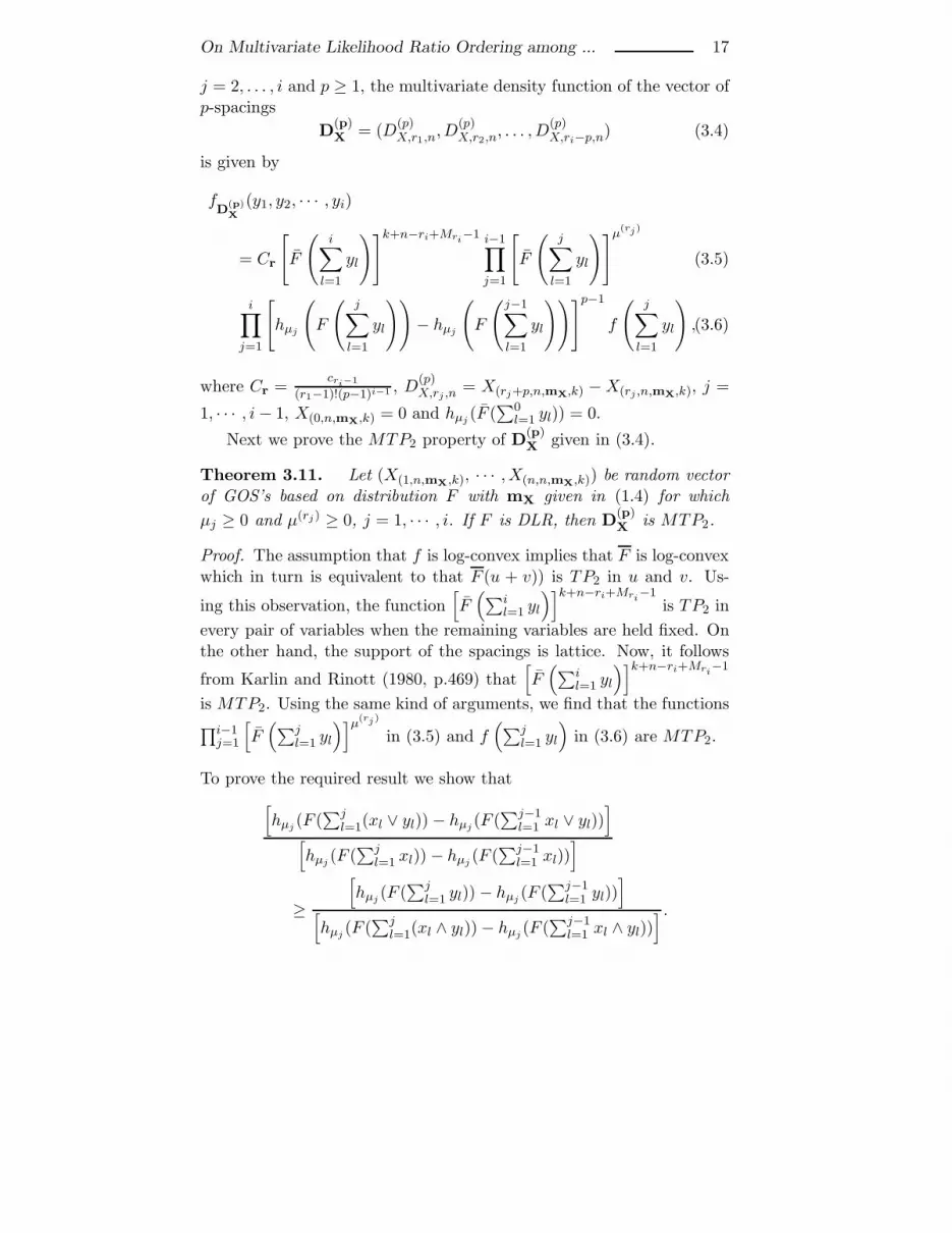
j = 2, . . . , i and p ≥ 1, the multivariate density function of the vector ofp-spacings

D(p)X = (D

(p)X,r1,n

,D(p)X,r2,n

, . . . ,D(p)X,ri−p,n) (3.4)

is given by

fD

(p)X

(y1, y2, · · · , yi)

= Cr

[F

(i∑

l=1

yl

)]k+n−ri+Mri−1 i−1∏j=1

[F

(j∑

l=1

yl

)]μ(rj )

(3.5)

i∏j=1

[hμj

(F

(j∑

l=1

yl

))− hμj

(F

(j−1∑l=1

yl

))]p−1

f

(j∑

l=1

yl

),(3.6)

where Cr =cri−1

(r1−1)!(p−1)i−1 , D(p)X,rj ,n

= X(rj+p,n,mX,k) −X(rj ,n,mX,k), j =

1, · · · , i− 1, X(0,n,mX,k) = 0 and hμj (F (∑0

l=1 yl)) = 0.

Next we prove the MTP2 property of D(p)X given in (3.4).

Theorem 3.11. Let (X(1,n,mX,k), · · · ,X(n,n,mX,k)) be random vectorof GOS’s based on distribution F with mX given in (1.4) for which

μj ≥ 0 and μ(rj) ≥ 0, j = 1, · · · , i. If F is DLR, then D(p)X is MTP2.

Proof. The assumption that f is log-convex implies that F is log-convexwhich in turn is equivalent to that F (u + v)) is TP2 in u and v. Us-

ing this observation, the function[F(∑i

l=1 yl

)]k+n−ri+Mri−1is TP2 in

every pair of variables when the remaining variables are held fixed. Onthe other hand, the support of the spacings is lattice. Now, it follows

from Karlin and Rinott (1980, p.469) that[F(∑i

l=1 yl

)]k+n−ri+Mri−1

is MTP2. Using the same kind of arguments, we find that the functions∏i−1j=1

[F(∑j

l=1 yl

)]μ(rj )

in (3.5) and f(∑j

l=1 yl

)in (3.6) are MTP2.

To prove the required result we show that[hμj (F (

∑jl=1(xl ∨ yl))− hμj (F (

∑j−1l=1 xl ∨ yl))

][hμj (F (

∑jl=1 xl))− hμj (F (

∑j−1l=1 xl))

]≥

[hμj (F (

∑jl=1 yl))− hμj (F (

∑j−1l=1 yl))

][hμj (F (

∑jl=1(xl ∧ yl))− hμj (F (

∑j−1l=1 xl ∧ yl))

] .

18 Sharafi et al.

Now, for (x1, . . . , xj) and (y1, . . . , yj), let δ =∑j−1

l=1 (xl ∨ yl)−∑j−1

l=1 xl.Since

j−1∑l=1

(xl ∨ yl) +j−1∑l=1

(xl ∧ yl) =j−1∑l=1

xl +

j−1∑l=1

yl,

then

δ =

j−1∑l=1

yl −j−1∑l=1

(xl ∧ yl). (3.7)

First, assume that xj ≥ yj, then

[hμj (F (


∑j−1l=1 xl ∨ yl))

][hμj (F (


∑j−1l=1 xl))

]=

[hμj (F (xj +

∑j−1l=1 xl + δ)) − hμj (F (

∑j−1l=1 xl + δ))

][hμj (F (xj +

∑j−1l=1 xl))− hμj (F (

∑j−1l=1 xl))

]=Fμj+1(xj +

∑j−1l=1 xl + δ) − Fμj+1(

∑j−1l=1 xl + δ))

Fμj+1(xj +∑j−1

l=1 xl))− Fμj+1(∑j−1

l=1 xl))

≥ Fμj+1(xj +∑j−1

l=1 xl ∧ yl + δ)− Fμj+1(∑j−1

l=1 xl ∧ yl + δ)

Fμj+1(xj +∑j−1

l=1 xl ∧ yl)− Fμj+1(∑j−1

l=1 xl ∧ yl)

=Fμj+1(xj +

∑j−1l=1 yl)− Fμj+1(

∑j−1l=1 yl)

Fμj+1(xj +∑j−1

l=1 xl ∧ yl)− Fμj+1(∑j−1

l=1 xl ∧ yl)(3.8)

≥ Fμj+1(∑j

l=1 yl)− Fμj+1(∑j−1

l=1 yl)

Fμj+1(∑j

l=1 xl ∧ yl)− Fμj+1(∑j−1

l=1 xl ∧ yl)

=

[hμj (F (


∑j−1l=1 yl))

][hμj (F (


∑j−1l=1 xl ∧ yl))

] (3.9)

The first inequality follows from Lemma 3.10 (b), since∑j−1

l=1 xl ≥∑j−1l=1 xl ∧ yl. The equality in (3.8) follows from (3.7). The second

inequality follows from Lemma 3.10 (a), since xj ≥ yj.


Now, let xj ≤ yj,[hμj (F (


∑j−1l=1 xl ∨ yl))

][hμj (F (


∑j−1l=1 xl))

]=

[hμj (F (yj +

∑j−1l=1 xl + δ)) − hμj (F (

∑j−1l=1 xl + δ))

][hμj (F (xj +

∑j−1l=1 xl))− hμj (F (

∑j−1l=1 xl))

]=Fμj+1(yj +

∑j−1l=1 xl + δ)− Fμj+1(

∑j−1l=1 xl + δ))

Fμj+1(xj +∑j−1

l=1 xl))− Fμj+1(∑j−1

l=1 xl))

≥ Fμj+1(yj +∑j−1

l=1 xl ∧ yl + δ) − Fμj+1(∑j−1

l=1 xl ∧ yl + δ)

Fμj+1(xj +∑j−1

l=1 xl ∧ yl)− Fμj+1(∑j−1

l=1 xl ∧ yl)(3.10)

=Fμj+1(yj +

∑j−1l=1 yl)− Fμj+1(

∑j−1l=1 yl)

Fμj+1(xj +∑j−1

l=1 xl ∧ yl)− Fμj+1(∑j−1

l=1 xl ∧ yl)(3.11)

=Fμj+1(

∑jl=1 yl)− Fμj+1(

∑j−1l=1 yl)

Fμj+1(∑j

l=1 xl ∧ yl)− Fμj+1(∑j−1

l=1 xl ∧ yl)

=

[hμj (F (


∑j−1l=1 yl))

][hμj (F (


∑j−1l=1 xl ∧ yl))

] (3.12)

The inequality (3.10) follows from part (c) of Lemma 3.10, since xj < yjand

∑j−1l=1 xl ≥

∑j−1l=1 (xl ∧ yl). The equality (3.11) follows from (3.7).

Therefore, the density function of D(p)X given in (3.4) is a product

of four non-negative MTP2 functions which in turn is MTP2. Thiscompletes the proof of the required result.

Remark 3.12. Theorem 3.11 generalized the result of Theorem 3.1in Yao et al. (2008) from the particular case of usual order statistics toGOS’s.

Let (Y(r′1,n′,mY,k), Y(r′2,n′,mY,k), . . . , Y(r′i,n′,mY,k)) be another i-dimensionalvector of GOS’s based on distribution G as given in the statement ofTheorem 2.6. With r′j − r′j−1 = p, j = 2, . . . , i, p ≥ 1, the correspondingvector of p-spacings is denoted by

D(p)Y = (D

(p)Y,r′1,n

,D(p)Y,r′2,n

, . . . ,D(p)Y,r′i−p,n

), (3.13)

where D(p)Y,r′j ,n

= Y(r′j+p,n,mY,k) − Y(r′j ,n,mY,k), j = 1, · · · , i− 1 and

Y(0,n,mY,k) = 0.

20 Sharafi et al.

Theorem 3.13. Let D(p)X and D

(p)Y be as defined by (3.4) and (3.13).

If either X or Y is DLR then under the assumptions of Theorem 2.6,

D(p)X ≤lr D

(p)Y . (3.14)

Proof. If we show that the ratio

fD

(p)Y

(y1, y2, · · · , yi)fD

(p)X

(y1, y2, · · · , yi) (3.15)

is increasing in yj, j = 1, · · · , i, then the required result follows from

Remark 3.1 in Hu et al. (2003), since by Theorem 3.11 the vector D(p)X

is MTP2. That is we have to show that the ratio

fD

(p)Y

(y1, y2, · · · , yi)fD

(p)X

(y1, y2, · · · , yi)

∝[G(∑i

l=1 yl)

F (∑i

l=1 yl)

]n′−r′i+Mr′i

(1

F (∑i

l=1 yl)

)δ2 i−1∏j=1

(G(∑j

l=1 yl)

F (∑j

l=1 yl)

)γ(r′j )

(3.16)

×(

1

F (∑j

l=1 yl)

)δ1g(∑j

l=1 yl)

f(∑j

l=1 yl)(3.17)

×i∏

j=1

⎡⎣[hμj

(G(∑j

l=1 yl

))− hμj

(G(∑j−1

l=1 yl

))][hγj

(F(∑j

l=1 yl

))− hγj

(F(∑j−1

l=1 yl

))]⎤⎦p−1

(3.18)

is increasing yj, j = 1, . . . , i. Using the assumption that X ≤lr Y

and X ≤hr Y , we get that the functionsg(∑j

l=1 yl)

f(∑j

l=1 yl)and

G(∑j

l=1 yl)

F (∑j

l=1 yl)are

increasing in yj, j = 1, . . . , i. On the other hand, using the facts that thefunction I(x+yk,x+yk+yj)(w) is TP2 in x and w, X ≤lr Y and the similararguments used to prove Lemma 2.4, we observe that for j = 1, . . . , iand x =

∑j−1l �=k yl, the function[hγj

(G(∑j

l=1 yl

))− hγj

(G(∑j−1

l=1 yl

))][hμj

(F(∑j

l=1 yl

))− hμj

(F(∑j−1

l=1 yl

))]=hγj (G(x+ yk + yj))− hγj (G(x+ yk))

hμj (F (x+ yk + yj))− hμj (F (x+ yk)),

is increasing in yk, k = 1, . . . , j−1 and yj. Combining these observations,it follows that the ratio given in (3.15) is increasing in each yk, k =


1, . . . , i, when the remaining arguments are held fixed. This completethe proof of the required result.

4 An Application

In this section we introduce an important particular case of GOS’s calledprogressive type II censored order statistics and applied some of the newresults to obtain some computable bounds on the mean residual life ofunobserved progressive type II censored order statistics.

Let X1, . . . ,XN be independent lifetimes of N identical units, withXi having absolutely continuous distribution function F . These unitsare placed on test at time t = 0. At the time of the ith failure, Ri,1 ≤ i ≤ n, number of surviving units are randomly withdrawn from theexperiment . Thus, if n failures are observed then R1+ . . .+Rn numberof units are progressively censored; hence N = n +R1 + . . . +Rn. The

censoring scheme is denoted by the vector R = (R1, . . . , Rn) and XRi:n:N ,

i = 1, . . . , n, the ith failure time, is called the ith progressive type IIcensored order statistic. The progressive type II censored order statisticare special cases of GOS’s withmi = Ri, i = 1, . . . , n−1 and k = Rn+1.For a detailed description of other special cases the readers is referredto Kamps (1995a, b), Balakrishnan and Aggarwala (2000), Belzunce etal. (2005), Balakrishnan (2007) and Balakrishnan et al. (2010).

Let n ≥ 2 (and hence N ≥ 2 ),

cri−1,n =

ri∏j=1

γj,n, 1 ≤ ri ≤ n and

al,ri,n =

ri∏j=1,j �=l

1

γj,n − γl,n, 1 ≤ l ≤ ri ≤ n, (4.1)

where γj,n = n−j+1+∑n

k=j Rk, for j = 1, . . . , n and the empty product∏∅ is defined to be 1. From the definition of the γ’s it can be easily

derived that N = γ1,n > . . . > γn,n ≥ 1 such that γj,n �= γl,n for l �= j.

The marginal survival function of XRri:n:N

based on F is given by

F RXri:n:N

(x) = cri−1,n

ri∑l=1

al,ri,nγl,n

[F (x)

]γl,n , ri = 1, . . . , n (4.2)

(cf. Kamps and Cramer, 2001, Lemma 1). If F is absolutely continuous

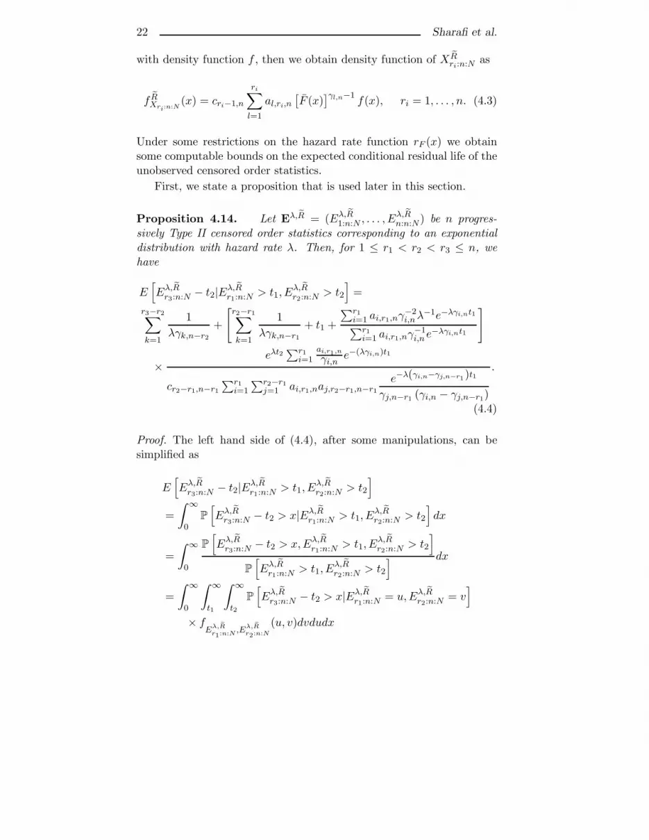
22 Sharafi et al.

with density function f , then we obtain density function of XRri:n:N

as

f RXri:n:N(x) = cri−1,n

ri∑l=1

al,ri,n[F (x)

]γl,n−1f(x), ri = 1, . . . , n. (4.3)

Under some restrictions on the hazard rate function rF (x) we obtainsome computable bounds on the expected conditional residual life of theunobserved censored order statistics.

First, we state a proposition that is used later in this section.

Proposition 4.14. Let Eλ,R = (Eλ,R1:n:N , . . . , E

λ,Rn:n:N) be n progres-

sively Type II censored order statistics corresponding to an exponentialdistribution with hazard rate λ. Then, for 1 ≤ r1 < r2 < r3 ≤ n, wehave

E[Eλ,R

r3:n:N− t2|Eλ,R

r1:n:N> t1, E

λ,Rr2:n:N

> t2

]=

r3−r2∑k=1

1

λγk,n−r2

+

[r2−r1∑k=1

1

λγk,n−r1

+ t1 +

∑r1i=1 ai,r1,nγ

−2i,nλ

−1e−λγi,nt1∑r1i=1 ai,r1,nγ

−1i,ne

−λγi,nt1

]

×eλt2

∑r1i=1

ai,r1,nγi,n e−(λγi,n)t1

cr2−r1,n−r1

∑r1i=1

∑r2−r1j=1 ai,r1,naj,r2−r1,n−r1

e−λ(γi,n−γj,n−r1)t1

γj,n−r1 (γi,n − γj,n−r1)

.

(4.4)

Proof. The left hand side of (4.4), after some manipulations, can besimplified as

E[Eλ,R

r3:n:N− t2|Eλ,R

r1:n:N> t1, E

λ,Rr2:n:N

> t2

]=

∫ ∞

0P

[Eλ,R

r3:n:N− t2 > x|Eλ,R

r1:n:N> t1, E

λ,Rr2:n:N

> t2

]dx

=

∫ ∞

0

P

[Eλ,R

r3:n:N− t2 > x,Eλ,R

r1:n:N> t1, E

λ,Rr2:n:N

> t2

]P

[Eλ,R

r1:n:N> t1, E

λ,Rr2:n:N

> t2

] dx

=

∫ ∞

0

∫ ∞

t1

∫ ∞

t2

P

[Eλ,R


r1:n:N= u,Eλ,R

r2:n:N= v

]× f

Eλ, ˜Rr1:n:N ,Eλ, ˜R

r2:n:N

(u, v)dvdudx


=

∫ ∞

0

∫ ∞

t1

∫ ∞

t2

P

[Eλ,R


r2:n:N= v

]P

[Eλ,R

r1:n:N> t1, E

λ,Rr2:n:N

> t2

]× f


r2:n:N

(u, v)dvdudx

=

∫ ∞

0

∫ ∞

t1

∫ ∞

t2

P

[Eλ,R

r3:n:N− v + v − t2 > x|Eλ,R

r2:n:N= v

]P

[Eλ,R

r1:n:N> t1, E

λ,Rr2:n:N

> t2

]× f


r2:n:N

(u, v)dvdudx

=

∫ ∞

0

∫ ∞

t1

∫ ∞

t2

P

[Eλ,R

r3−r2:n−r2:N−∑r2l=1 Rl−r2

+ v − t2 > x]

P

[Eλ,R

r1:n:N> t1, E

λ,Rr2:n:N

> t2

]× f


r2:n:N

(u, v)dvdudx (4.5)

=

∫ ∞

t1

∫ ∞

t2

{E[Eλ,R


]+ v − t2}

P

[Eλ,R

r1:n:N> t1, E

λ,Rr2:n:N

> t2

]× f


r2:n:N

(u, v)dvdu

= E[Eλ,R


]+ E

[Eλ,R

r2:n:N− t2|Eλ,R

r1:n:N> t1, E

λ,Rr2:n:N

> t2

](4.6)

The second expression of the bracket in (4.6) can be simplified as follows:

=P

[Eλ,R

r1:n:N> t1

]P

[Eλ,R

r1:n:N> t1, E

λ,Rr2:n:N

> t2

]×∫ ∞

0

∫ ∞

t1

P

[Eλ,Q

r2:n:N> t2 + x|Eλ,R

r1:n:N= u

] fEλ, ˜Rr1:n:N

(u)

FEλ, ˜R

r1:n:N

(t1)dudx

=P

[Eλ,R

r1:n:N> t1

]P

[Eλ,R

r1:n:N> t1, E

λ,Rr2:n:N

> t2

]×∫ ∞

0

∫ ∞

t1

P

[Eλ,R


+ u− t2 > x] fEλ, ˜R

r1:n:N

(u)

FEλ, ˜R

r1:n:N

(t1)dudx

24 Sharafi et al.

=P

[Eλ,R

r1:n:N> t1

]P

[Eλ,R

r1:n:N> t1, E

λ,Rr2:n:N

> t2

]×⎡⎣E [Eλ


− t2

]+

∫ ∞

t1

ufEλ, ˜R

r1:n:N

(u)

FEλ, ˜R

r1:n:N

(t1)du

⎤⎦ . (4.7)

Eλ,R

j−i:n−i:N−∑il=1 Rl−i

st=∑j−i

k=1 Z′k, where Z

′ks are the corresponding nor-

malized spacings Z ′1 = NEλ,R

1:n:N and Z ′k = (n − k + 1 − R1 − . . . −

Rk−1)(Eλ,Rk:n:N − Eλ,R

k−1:n:N), for k = 2, . . . , n.

It is known that Z ′k are independent exponential random variables

with hazard rate λγk,n−i (cf. Cramer and Kamps, 2003, Theorem 3.1;Hu and Zhuang, 2005a, Lemma 2.1). Using these observations, the firstand the second terms in (4.5) and (4.7), respectively, can be written as

E

[Eλ,R

(r3−r2:n−r2:N−∑r2l=1 Rl−r2)

]=

r3−r2∑k=1

1

λγk,n−r2

, (4.8)

and

E

[Eλ,R

(r2−r1:n−r1:N−∑r1l=1 Rl−r1)

]=

r2−r1∑k=1

1

λγk,n−r1

. (4.9)

On the other hand,

∫ ∞

t1

ufEλ, ˜R

r1:n:N

(u)

FEλ, ˜R

r1:n:N (t1)

du = E[Eλ,R

r1:n:N|Eλ,R

r1:n:N> t1

]= t1 + E

[Eλ,R

r1:n:N− t1|Eλ,R

r1:n:N> t1

]= t1 +

∫ ∞

0

P

[Eλ,R

(r1:n:N) > x+ t1

]P

[Eλ,R

r1:n:N> t1

] dx

= t1 +

∫ ∞

0

∑ri=1 ai,r1,nγ

−1i,ne

−λγi,n(x+t1)∑r1i=1 ai,r1,nγ

−1i,n e

−λγi,nt1dx

= t1 +

∑r1i=1 ai,r1,nγ

−2i,nλ


−1i,n e

−λγi,nt1, (4.10)


P

[Eλ,R

r1:n:N> t1, E

λ,Rr2:n:N

> t2

]=

∫ ∞

t1

∫ ∞

t2

fEλ, ˜R

r1:n:N ,Eλ, ˜Rr2:n:N

(u, v)dvdu

=

∫ ∞

t1

∫ ∞

t2

fEλ, ˜R

r2:n:N |Eλ, ˜Rr1:n:N

(v|u)fEλ, ˜R

r1:n:N

(u)dvdu

=

∫ ∞

t1

∫ ∞

t2

cr2−r1−1,n−r1

r2−r1∑j=1

aj,r2−r1,n−r1

×[F (v)

F (u)

]γj,n−r1−1

f(v)

F (u)cr1−1,n

r1∑i=1

ai,r1,n[F (u)

]γi,n−1f(u)dvdu

= cr2−r1−1,ncr1−1,n

r1∑i=1

r2−r1∑j=1

ai,r1aj,r2−r1

×∫ ∞

t1

∫ ∞

t2

e−λ(v−u)(γj,n−r1−1)λeλ(v−u)e−λu(γi,n−1)λe−λudvdu

= cr2−r1−1,n−r1cr1−1,n

r1∑i=1

r2−r1∑j=1

ai,r1,naj,r2−r1,n−r1

×∫ ∞

t1

∫ ∞

t2

λ2e−λγjveλ(γi,n−γj,n−r1)udvdu

= cr2−r1−1,n−r1cr1−1,ne−λt2

r1∑i=1

r2−r1∑j=1

ai,r1,naj,r2−r1,n−r1

× e−λ(γi,n−γj,n−r1)t1

γj,n−r1 (γi,n − γj,n−r1)(4.11)

and

P

[Eλ,R

r1:n:N : > t1

]= cr1−1,n

r1∑i=1

ai,r1,nγi,n

e−(λγi,n)t1 . (4.12)

Now, substituting(4.8), (4.9), (4.10), (4.11) into (4.5), the required resultfollows.

Theorem 4.15. Let {XRi:n:N , i = 1, . . . , n} be n progressively type

II censored order statistics based on distribution function F with non-increasing hazard rate function rF such that for a positive constant λ

26 Sharafi et al.

and each x > 0, rF (x) ≥ λ. Let also

R = (

r1−1︷︸︸︷R1, R1, · · · , R1, R

(r1),

r2−r1−1︷︸︸︷R2, R2, · · · , R2, R

(r2), · · · ,r1−ri−1−1︷︸︸︷

Ri−1, Ri−1, · · · , Ri−1, R(ri),

n−ri−1︷︸︸︷Ri+1, · · · , Rn).

Then, for t1 ≤ t2,

E[XR

r3:n:N − t2|XRr1:n:N > t1,X

Rr2:n:N > t2

]≤

r3−r2∑k=1

1

λγk,n−r2

+

[r2−r1∑k=1

1

λγk,n−r1

+ t1 +

∑r1i=1 ai,r1,nγ

−2i,nλ


−1i,ne

−λγi,nt1

]

× {eλt2

∑r1i=1

ai,r1,nγi,n

e−(λγi,n)t1

cr2−r1,n−r1

∑r1i=1

∑r2−r1j=1 ai,r1,naj,r2−r1,n−r1

e−λ(γi,n−γj,n−r1)t1

γj,n−r1 (γi,n − γj,n−r1)

}

(4.13)

Proof. Let {Eλ,Ri:n:N} be n progressive type II censored order statistics

based on an exponential distribution with the hazard rate λ. The as-sumptions that rF (x) is non-increasing in x and rF (x) ≥ λ implies thatX ≤lr E

λ (cf. Lemma 3.5 in Belzunce et al., (2001)). Using this andthe sublattice L = [(x(1), . . . , x(n)) ∈ R

n|x(i) > t1, x(j) > t2] in Theorem2.8, where x(1) ≤ . . . ≤ x(n), t1, t2 ∈ R and t1 ≤ t2, we obtain that

E[XR

r3:n:N − t2|XRr1:n:N > t1,X

Rr2:n:N > t2

]≤

E[Eλ,R

r3:n:N− t2|Eλ,R

r1:n:N> t1, E

λ,Rr2:n:N

> t2

].

Now the required results follows from Proposition 4.14.

Moreover, the joint density function of every subset from XRi:n:N ’s

can be derived from Lemma (2.5).

Remark 4.16. In particular, the result of Theorem 4.15 can also beapplied to the case when

R = (

r1︷︸︸︷R1, R1, · · · , R1,

r2−r1︷︸︸︷R2, R2, · · · , R2, · · · ,

r1−ri−1︷︸︸︷Ri−1, Ri−1, · · · , Ri−1,

n−ri︷︸︸︷Ri+1, · · · , Rn),

which is of practical importance.


Acknowledgments

We are grateful to the referees and the Editor for their helpful andvaluable comments that improved the presentation of this paper. Theresearch of Baha-Eldin Khaledi is partially supported by Ordered andSpatial Data Center of Excellence of Ferdowsi University of Mashhad.

References

Balakrishnan, N. (2007), Progressive censoring methodology: an ap-praisal (with discussions). Test, 16, 211-296.

Balakrishnan, N. and Aggarwala, R. (2000), Progressive Censoring:Theory Methods and Applications. Boston: Birkhauser.

Balakrishnan, N., Belzunce, F., Hami, N., and Khaledi, B. (2010),Univariate and multivariate likelihood ratio ordering of generalizedorder statistics and associated conditional variables. Probabilityin the Engineering and Informational Sciences, 24, 441-445.

Barlow, R. E. and Proschan, F. (1981), Statistical Theory of Reliabilityand Life Testing. MD: To Begin With, Silver Spring.

Belzunce, F., Lillo, R. E., Ruiz, J. M., and Shaked, M. (2001), Stochas-tic comparisons of nonhomogeneous processes. Probability in theEngineering and Informational Sciences, 15, 199-224.

Belzunce, F., Mercader, J. A., and Ruiz, J. M. (2005), Stochastic com-parisons of generalized order statistics. Probability in the Engi-neering and Informational Sciences, 19, 99-120.

Fang, Z. B., Hu, T., Wu, Y. H., and Zhuang, W. (2006), Multivariatestochastic orderings of spacings of generalized order statistic. Chi-nese Journal of Applied Probability and Statistics, 22, 295-303.

Hu, T., Khaledi, B. E., and Shaked, M. (2003), Multivariate hazardrate orders. Journal of Multivariate Analysis, 84, 173-189.

Hu, T., Jin, W., and Khaledi, B.-E. (2007), Ordering conditional dis-tributions of generalized order statistics. Probability in the Engi-neering and Informational Sciences, 21, 401-417.

Hu, T. and Zhuang, W. (2005), Stochastic properties of p-spacings ofgeneralized order statistics. Probability in the Engineering andInformational Sciences, 19, 257-276.

28 Sharafi et al.

Hu, T. and Zhuang, W. (2006), Stochastic orderings between p-spacingsof generalized order statistics from two samples. Probability in theEngineering and Informational Sciences, 20, 465-479.

Kamps, U. (1995a), A Concept of Generalized Order Statistics, Stuttgart:Teubner.

Kamps, U. (1995b), A concept of generalized order statistics. Journalof Statistical Planning and Inference, 48, 1-23.

Karlin, S. (1968), Total Positivity. Stanford University Press, PaloAlto, California.

Karlin, S. and Rinott, Y. (1980), Classes of orderings of measures andrelated correlation inequalities I. Multivariate totally positive dis-tributions, Journal of Multivariate Analysis, 10, 467-498.

Khaledi, B. E. (2005), Some new results on stochastic comparisonsbetween generalized order statistics. Journal of the Iranian Statis-tical Society, 4, 35-49.

Khaledi, B. E., Amiripour, F., Hu, T ,and Shojaei, R. (2009), Somenew results on stochastic comparisons of record values. Commu-nications in Statistics - Theory and Methods, 38, 2056-2066.

Khaledi, B. E. and Kochar, S. C. (2005), Dependence orderings forgeneralized order statistics. Statistics & Probability Letters, 73,357-367.

Khaledi, B. E. and Shaked, M. (2007), Ordering conditional lifetimesof coherent systems. Journal of Statistical Planning and Inference,137, 1173-1184.

Khaledi, B. E. and Shojaei, R. (2007), On stochastic orderings betweenresidual record values. Statistics & Probability Letters, 77, 1467-1472.

Li, X. and Zhao, P. (2008), Stochastic comparison on general inactivitytime and general residual life of k-out-of-n systems. Communica-tions in Statistics - Simulation and Computation, 37, 1005-1019.

Righter, R. and Shanthikumar, J. G. (1992), Extremal properties of theFIFO discipline in queueing networks. Journal of Applied Proba-bility, 29, 967-978.


Shaked, M. and Shanthikumar, J. G. (1987), Multivariate hazard ratesand stochastic ordering. Advances in Applied Probability, 19,123-137.

Shaked, M. and Shanthikumar, J. G. (2007), Stochastic Orders. NewYork: Springer-Verlag.

Torrado, N., Lillo, R. E., and Wiper, M. P. (2012), Sequential orderstatistics: Ageing and Stochastic Orderings. Methodology andComputing in Applied Probability, 14, 579-596.

Xie, H. and Hu, T. (2009), Ordering p-spacings of generalized orderstatistics revisited. Probability in the Engineering and Informa-tional Sciences, 23, 1-16.

Xu, M. and Li, X. (2006), Likelihood ratio order of m-spacings fortwo samples. Journal of Statistical Planning and Inference, 136,4250-4258.

Yao, J., Burkschat, M., Chen, H., and Hu, T. (2008), Dependence struc-ture of spacings of order statistics. Communications in Statistics- Theory and Methods, 37, 2390-2403.

Zhao, P. and Balakrishnan, N. (2009), Stochastic comparisons of condi-tional generalized order statistics. Journal of Statistical Planningand Inference, 139, 2920-2932.

Zhuang, W. and Hu, T. (2007), Multivariate stochastic comparisonsof sequential order statistics. Probability in the Engineering andInformational Sciences, 21, 47-66.

on multivariate likelihood ratio ordering among generalized order statistics and their spacings

Documents