CONDITION-BASED SPARES ORDERING FOR CRITICAL

COMPONENTS

Darko Louit, Rodrigo Pascual1

Centro de Minería, Pontificia Universidad Católica de Chile

Av. Vicuña Mackenna 4860, Santiago, Chile

Dragan Banjevic and Andrew K.S. Jardine

Department of Mechanical and Industrial Engineering, University of Toronto

5 King’s College Road, Toronto, Ontario, Canada M5S 3G8, Canada

It is widely accepted that one of the potential benefits of Condition-Based Maintenance

(CBM) is the expected decrease in inventory as the procurement of parts can be triggered by

the identification of a potential failure. For this to be possible, the interval between the

identification of the potential failure and the occurrence of a functional failure (P-F interval)

needs to be longer than the lead time for the required part. In this paper we present a model

directed to the determination of the ordering decision for a spare part when the component in

operation is subject to a condition monitoring program. In our model the ordering decision

depends on the Remaining Useful Life (RUL) estimation obtained through (i) the assessment

of component age and (ii) condition indicators (covariates) that are indicative of the state of

health of the component, at every inspection time. We consider a random lead time for 1 Corresponding author: rpascual@ing.puc.cl

1

spares, and a single-component, single-spare configuration that is not uncommon for very

expensive and highly critical equipment.

Keywords: stochastic models, spare parts, ordering time, condition-based maintenance,

remaining useful life.

2

CONDITION-BASED SPARES ORDERING FOR CRITICAL COMPONENTS

1. INTRODUCTION

The main principle behind the use of condition monitoring techniques for the

maintenance of industrial equipment is that of anticipating the occurrence of failures. When

condition-based maintenance programs are in place, the removal of a component from

operation is ideally triggered by the detection of a degradation process within the equipment

(when resistance to failure has started to decrease). If we are able to detect the start of this

failure process (i.e. the occurrence of a Potential Failure) early enough so that the expected

lead time to receive a spare part on-site is less than the expected time to failure, then there is

no need to stock a spare component. Using Reliability-Centred Maintenance (RCM)

terminology (see Moubray, 1997), when the P-F interval is longer than the lead time there is

no need to stock a spare. This idea constitutes a widely accepted potential benefit of

Condition-Based Maintenance (CBM) policies (see e.g. Crespo-Marquez and Gupta, 2006,

Pedregal and Carnero, 2006), and creates an opportunity for the optimization of the ordering

time of spares when demand can be anticipated. Gains can be important as in several

industries, spare related holding costs are huge. For example, the commercial aviation

industry has more than 40 billion dollars worth of spare parts on stock (Kilpi et al., 2009).

The use of condition monitoring techniques in industry has largely increased over the

last few years (Mobley, 2003). The use of the condition information collected in the

determination of optimal spare parts ordering could therefore generate significant savings in

3

stockholding related costs. The latter statement is of particular importance to the case of

expensive, complex components. However, the incorporation of condition information in the

spare parts stockholding decision (i.e. the impact of condition-based maintenance policies in

spare parts inventories) has seldom been approached in the literature. In fact, our literature

survey only identified recent efforts by Ghodrati and Kumar (2005a and 2005b), which are

based in the use of external conditions to adjust demand estimations for spare parts (a more

detailed account of these works is given in section 6). The latter might be explained by the

little integration between the areas of maintenance and reliability engineering and that of

inventory and logistics, as examples of stockholding decisions with respect to maintainability

or reliability parameters are, in general, scarce.

The opportunity to reduce inventory levels via the implementation of condition-based

decision programs (based on the internal state of health of the equipment) has not been

addressed in the literature, to the best of our knowledge.

In this article, we present a model resulting in the decision to order a spare or to

continue to operate without ordering until the next inspection, based on estimations of the

remaining life of the item given its age and internal condition. We concentrate in a single-

system, single-spare configuration, which is not unreasonable for very expensive, highly

critical components.

The remainder of the article is structured as follows. In the following section we

review the concepts of conditional reliability function and remaining useful life of a

4

component. Then we discuss methods for the calculation of these functions, taking into

account condition monitoring information. Next we present an original decision model for

spares ordering, which results in the decision to order a spare and the optimal ordering time,

so that costs are minimized. We then present a case study from a mining application. We

conclude the article, identifying areas for further development and providing some final

remarks.

2. CONDITIONAL RELIABILITY AND REMAINING USEFUL LIFE

The reliability function of an item is defined as the probability of survival of the item

over an interval of time, say . Typically, two cases for this function have concentrated

interest in reliability analysis: the unconditional case (which assumes that the item has not

yet been put into operation) and the conditional case (which assumes that the item has been

operated for some time, say

t

x ). That is, for the unconditional case the figure of interest is

, whereas for the conditional case it is (P T t> ) ( )P T t T x> > , where T is the lifetime of

the item.

In the case of condition-based maintenance decisions, we are interested in the

conditional reliability of the item, given that it has been in operation up until the moment of

inspection. In addition, since condition of the item is being monitored via different

measurements (e.g. vibration levels, concentration of metals in the oil, noise levels,

temperatures), these measurements should be included in the calculation of the conditional

reliability.

5

In order for the reliability function to be calculated, an appropriate model for the

hazard rate (or alternatively for the probability density function of the time to failure) should

be constructed. In particular, we are interested in a model capable of representing the hazard

rate of the equipment, combining usage information (age) with condition information

(through condition indicators or covariates). Such a model would help to provide better

prediction of the remaining life of the item, thus improving the anticipation of demand for

spare parts.

In general, covariates can be classified as internal and external. Internal covariates

relate to the internal state of the equipment. External covariates can be observed

independently of the failure process (e.g. variables indicating conditions of the environment

where components operate). In addition, covariates can be fixed (i.e. time-independent) or

time-varying (i.e. time-dependent).

A widely accepted method to incorporate condition monitoring information in

lifetime analysis is the proportional hazards model (PHM, see Cox, 1972). Kumar and

Klefsjö (1994) provide a comprehensive review of applications of the PHM in the reliability

field.

The PHM models the hazard rate function, ( )tλ , as

6

( ) ( ) ( )0 exp i ii

t h t Z tλ ⎛ ⎞= ⎜

⎝ ⎠∑γ ⎟ , (1)

where is a deterministic baseline hazard function (which depends on the age of the

item only) and

( )0h t

( ) ( ) ( )( 1 2, ,Z t Z t Z t= K) is a vector of time-dependent covariates, which can

be internal or external.

The model in equation (1) implies that the hazard rate function is conditioned on a

stochastic process that is related to the condition (state of health) of the item. A common

model used to represent the state of a system is the discrete Markov process (see e.g. Ross,

2003).

Banjevic and Jardine (2006) indicate that in condition-based maintenance

applications, the use of a non-homogeneous Markov process (NHMP) is of particular

interest, as it allows for the rate of change of the system state to be dependent on the system’s

age. In their paper, they present theoretical and numerical methods for the calculation of the

reliability function of an item under the assumption of a Markov process model. They use a

PHM to model the hazard rate of the equipment, and introduce a reliability function model

for the case of time-dependent, internal covariates (which is the case of our interest in this

article). Furthermore, they consider the case of a NHMP, allowing for the transition rates of

the condition process to change in different periods within the life of the item (e.g. early-life,

normal-life, wear-out). We will use their results for the calculation of the reliability function.

7

In the following section, we briefly present the procedures introduced by Banjevic

and Jardine (2006), as they are relevant for the discussion of the condition-based ordering

model presented afterwards. Presentation follows the paper closely and uses a similar

notation. However, full details are not provided here.

2.1. Basic Definitions

Let the condition (state) of an item be represented by ( ){ }, 0Z x x ≥

0,1,2,=

, a continuous

time discrete process. Let the state of the item be denoted by , with , i ,i mK m < ∞ .

That is, we consider that the state set is finite. These states may represent numerical values

for a covariate of interest (or for multiple covariates), qualitative states such as ‘normal’,

‘warning’, ‘danger’, environmental conditions. Note that the assumption of a finite state set is

not restrictive, as typically the state of health of the system will be classified into few

categories. In the case of numerical values of covariates, discretization into covariate bands

generates a finite number of states (each band defines a state) and is a common practice that

also results in reduced computational intensity (see e.g. Banjevic et al., 2001). For

multidimensional values of Z , each covariate can be discretisized and the total state space

will be defined by the combinations of all possible individual states (bands) for each

covariate in Z .

A failure process will be called a Markov failure time process (MFTP) if

( ) ( ) ( ) ( ) ( )( ) (1 1 2 2, , , , , , l l ijP T t Z t j T x Z x i Z a i Z a i Z a i L x t> = > = = = = =K ), , (2)

8

where denotes the transition probability from state i into state ( ,ijL x t ) j , in the interval

[ ],x t , for x t T< <

la<

. For the process to be a MFTP, equation (2) has to be valid for all

and , where are times at which

information of the covariate process is available and are condition states (e.g.

covariate bands). In other words, a process is a MFTP if the distribution of any future state

1 2a a≤ < <L0 x< < t 1 2, , , , ,li i i i jK 1 2, , , , ,la a a x t

1 2, , , ,i i i i jK

K

, l

j

depends only on the current state i . This is reasonable for deterioration processes of

equipment.

Note also that equation (2) implies that the item will still be in operation at time (as

we are considering the case when T ). In other words,

t

t> ( ),ijL x t are the transition

probabilities of the MFTP ( ) ( ) ( )( )Z t= ,N tV t , where ( ) (I T )N t t= > . That is, the

condition state ( )Z t cannot be assessed after a failure (or suspension). This is the most

common case in practice. Only in very few condition monitoring schemes it is possible to

assess the prior to failure condition once the item has failed and is no longer in operation

(e.g. oil analysis when no contamination of the oil occurs after failure).

As equation (1) represents the hazard rate of a MFTP, we may write:

( ) ( )( ,t h t Z tλ = ) , (3)

9

given that is a function with ( ),h t i ( ),h t i ≥ 0 and ( )0

,h t i dt∞

= ∞∫ . Obviously, and 0t ≥

{ }i S∈ , where { }S is the state space for the condition process.

The transition probabilities ( ),ijL x t permit the calculation of all other functions of

interest, including the conditional reliability function and also the remaining useful life of the

item.

2.2. Calculation of the Reliability Function

A variant of the conditional reliability function of the item is given by

( ) ( ) ( ), ,ij

L x t R t x i L x t⋅ = =∑ ,ij , (4)

that is, the probability of the item surviving , given current age t x and condition ( )Z x i= .

Let ( ) ( ), ij ,x t L x t⎡Ω = ⎣ ⎤⎦

)

be a matrix whose elements are the transition probabilities

( ,ijL x t . We assume that ( ) ( ), lim ,ijt xx L x t

↓1ijL x = = , when i j= , and , when

. Since we are considering a MFTP, due to the Markov property we have that

, for

( ),ijL x x = 0

i j≠

( )ijL x t ( ) ( ), ,ik kjk

L x u L u t∑ , 0= x u t≤ ≤ ≤ . In matrix form, this is equivalent to

( ) ( ) ( ), , ,x t x u u tΩ ×ΩΩ = . It is easy to see that

10

( ) ( ) ( ) ( ), , , ,x t t x t x t t t t I⎡ ⎤Ω + Δ −Ω = Ω × Ω + Δ −⎣ ⎦ . (5)

The transition probabilities of the condition process ( )Z t , given that the item

survives up until time t , , can be calculated from ( ,ijp x t )

( ) ( ) ( )(, ,ij )p x t P Z t j T t Z x i= = > = . (6)

With this, we can re write equation (2) as

( ) ( )( (, ,ij ijL x t P T t T x Z x i p x t= > > = ) ), . (7)

If we now let ( ) ( ), lim ,ij ijt xp x x p x t

↓1= = when i j= , and when i j( ),ijp x x = 0 ≠ ,

we can define a diagonal matrix ( ) ( ) ( ),x x, ijD x i ph x⎡ ⎤= ⎣ ⎦ . Also, letting

( ) ( ),ij ij t xx p x tt

λ =∂

=∂

exist, we can define the matrix ( ) ( )ijx xλ⎡ ⎤Λ = ⎣ ⎦ and proof that:

( ) ( ) ( ) (, , ,ij t x ij ijL x t h x i p x x xt

λ=∂

= − +∂

) ,

or in matrix form

11

( ) ( ) ( ) ( ), t xx x t x D xt =∂

Ω = Ω = Λ −∂

. (8)

Combining this result with equation (5), it is easy to see that functions , with ( ,ijL x t )

x t≤ , satisfy the system of differential equations:

( ) ( ) ( ) ( ) (, , , ,ij ij ik kjk

L x t h t j L x t L x t tt

λ∂+ =

∂ ∑ ) ,

or in matrix form,

( ) ( ) ( ) ( ) ( ) ( )(, , , )x t x t t x t t D tt∂Ω = Ω ×Ω = Ω × Λ −

∂. (9)

To solve the system in Eq. (9), two cases are identified:

(i) Case I: the condition process ( )Z t is ‘conditionally homogeneous’ in the sense

that ( )ij ijxλ λ= (that is they are not dependent on time) and the hazard rate for the MFTP is a

function of the condition process only, i.e. ( ) ( )( )t g Z t=λ (it only depends on the current

state ). In this case, considered by Cheng and He (1987), i ( ) (, 0, )x t t xΩ = Ω − thus

and . Therefore, solution for system (Eq. 9) is given by ( )x = ΛΛ ( )D x D=

. (10) ( ) ( )0, expt ⎡Ω = Λ −⎣ D t⎤⎦

12

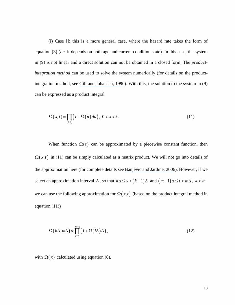
(i) Case II: this is a more general case, where the hazard rate takes the form of

equation (3) (i.e. it depends on both age and current condition state). In this case, the system

in (9) is not linear and a direct solution can not be obtained in a closed form. The product-

integration method can be used to solve the system numerically (for details on the product-

integration method, see Gill and Johansen, 1990). With this, the solution to the system in (9)

can be expressed as a product integral

( ) ( )(( ],

,x t

)x t I u dΩ = +Ω∏ u , 0 x t< < . (11)

When function can be approximated by a piecewise constant function, then ( )tΩ

( , )x tΩ in (11) can be simply calculated as a matrix product. We will not go into details of

the approximation here (for complete details see Banjevic and Jardine, 2006). However, if we

select an approximation interval Δ , so that ( )1k x kΔ ≤ < + Δ and ( )1m t m− Δ ≤ < Δ , k m< ,

we can use the following approximation for ( ),x tΩ (based on the product integral method in

equation (11))

( ) ( )(1

,m

i k

k m I i−

=

Ω Δ Δ ≈ +Ω Δ Δ∏ ) , (12)

with ( )xΩ calculated using equation (8).

13

Note that the approximation in (12) requires the calculation of the transition rates for

the condition of the item, (ij kλ )Δ , for every (as they are needed to calculate k ( )iΩ Δ ).

Banjevic et al. (2001) discuss the procedure for estimation of the transition rates. In practical

applications, transition rates might change over different time periods (e.g. early life vs. other

stages in the component’s life), thus defining different ranges of interest for . Consider, for

example, the case where the transition rate of the concentration of iron in the oil of a diesel

engine is fairly constant between 0 and 8000 hours of operation, then it is higher (faster

changes) between 8000 and 12000 hours of operation (when the engine is removed from

operation). In this case, two ranges for k are defined:

k

80000,⎡ ⎤Δ⎣ ⎦ and ( .

However, it is unlikely that many different periods can be identified. Furthermore,

differences might be small enough so that they can be ignored. As an example, Banjevic and

Jardine (2006) present a case study based on transmissions for transporters in a mining

operation, using oil analysis data. Though they report small differences between the

transition rates in early life (up to 2000-3000 hours) and later life, they were ignored in the

calculations (i.e., they assumed

8000 12000, ⎤Δ Δ⎦

( )ij x ijλ λ≡ ).

The approximation in (12) is accurate for small values of Δ . In their case study,

Banjevic and Jardine (2006) indicate that the approximation gave satisfactory results for

hours (with an average life cycle of 8000 hours). They also present a second

approximation, numerically more complex (though more precise for large values of

500Δ ≤

Δ ). We

will not discuss this second approximation here. For additional details and discussion on the

approximation accuracy, the reader is referred also to Møller (1992).

14

2.3. Calculation of the Remaining Useful Life

The remaining useful life (RUL), also called the mean residual life, is the expected

time to failure, given that the item has survived up until current time t , or

( ) ( ) ( )RUL t e t E T t T t= = − > . For further details and further references to applications of

the use of the RUL in reliability analysis, see Reinersten (1996), who gives a complete

review of research related to residual life of non-repairable and repairable systems.

In the case treated here, since condition of the item is monitored, then the RUL can be

defined as ( )( ) ( )( ) ( )( ), , ,RUL t Z t e t Z t E T t T t Z t= = − > . The calculation of the residual

life of an item in presence of a condition monitoring program has received little attention in

the literature (recent examples are Banjevic and Jardine, 2006, Elsayed, 2003 or Yuen et al.,

2003). An alternative approach is the direct modeling of the residual life of an item T t− ,

given condition information. Wang and Zhang (2003) and Wang (2002) adopt the latter

avenue, through a model they call ‘proportional residual model’.

Once a reliability function has been calculated, then the RUL of an item can be

obtained from

( )( ) ( )(, ,t

e t Z t R x t Z t dx∞

= ∫ ) , (13)

15

where ( , ( ) )R x t Z t i= is calculated through equation (4). This is a simple method of

calculating the RUL, as the reliability function can be calculated for several points and then

numerical integration methods can be used to calculate ( )( ),e t Z t (this is the procedure

adopted by Banjevic and Jardine (2006) in their case study).

3. CONDITION-BASED STOCKHOLDING DECISIONS

We have mentioned that the examples of integration between condition information

and spare parts stockholding decisions are scarce. In fact, our literature survey only identified

the following works, where the impact of external conditions is assessed in the calculations

of optimal stock levels.

In Ghodrati and Kumar (2005a) a constant baseline hazard and time-independent

covariates in a PHM are assumed. The result is an adjusted constant hazard rate that

incorporates the effect of covariates. Calculation of the optimal stock levels can then be

performed using Poisson demand ( )1,S S− models (lot-for-lot replenishment), with the

environmental condition-based hazard rate used as demand rate for the spare component.

The extension to non-constant baseline hazard is given by Ghodrati and Kumar

(2005b), who use a Weibull baseline hazard and, once again, time-independent covariates in

a PHM. In this case, the adjusted hazard rate is also Weibull, with the same shape parameter

as the original baseline (dependent only on time), but with a different scale parameter (which

is affected by the influencing covariates). Further they assume a normally distributed number

of failures (that defines demand for spares) over an interval of interest, T . Both the mean and

16

the variance of this spares-demand distribution are obtained from the parameters of the

adjusted Weibull hazard rate.

In summary, the work of Ghodrati and Kumar allows for the incorporation of external

conditions into the estimation of spares demand, and the resulting adjusted demand rate is

used in Poisson or normally distributed demand inventory models. Opposite to

Ghodrati and Kumar, we wish to incorporate internal condition of the item into the

stockholding decision.

( 1,S S− )

Elwany and Gebraeel (2008) propose a spare ordering model for a single-unit system

considering a policy that keeps at most one spare in inventory. As ours, their methodology

also uses condition data (a single covariate) to update the conditional failure probability

distribution, using a Bayesian approach. Their model considers two sequential decisions: the

replacement decision (when should it be made?), and then the ordering decision (when

should the spare be ordered?). Their methodology defines updating epochs for the

conditional failure probability distribution. To do so, they estimate the interval on which the

covariate will attain a user-defined threshold level and use expected cost per unit time as

optimization criterion. In their model, lead time is deterministic.

Wang, Chu and Mao (2008) propose a condition-based order-replacement policy for a

single unit system. They consider a monotonically increasing degradation process, and use a

control limit policy to establish the threshold levels that trigger the order and replacement of

the component under analysis. They jointly optimize the inspection interval, the ordering

threshold and the preventive replacement threshold, which remain constant at each inspection

epoch. Their optimization criterion is the expected long run global cost rate. Our model

17

allows for non monotonic degradation process using a PHM based reliability estimation. It

also permits considering several internal and external covariates affecting component

conditional reliability.

Alternatively to the referred methodologies, we use the conditional reliability and the

RUL of an item described in the previous section, along with a series of decision rules, to

define the ordering of a spare component.

3.1. Proposed Condition-based ordering decision model

The decision we are faced with is that of when to order a spare for a component

whose condition is being monitored. We assume that the spare will replace the unit in

operation once it fails (or equivalently, when a failure is about to occur, as detected by the

condition monitoring program). Should a spare be available at the time of failure

(replacement) the system does not incur downtime, although inventory holding costs might

need to be considered in the case when the spare is delivered before failure. In the opposite

case, shortage costs are accrued.

Combination of maintenance policies and spares ordering has been primarily

approached in the literature through order-replacement models. An order-replacement policy

is one that defines the optimal ordering time for a spare part, along with the optimal

replacement time for the item in operation, considering that there is a delay between

placement of the order and delivery of the spare (i.e. positive lead time). Determination of

optimal order-replacement policies (under block and age replacement, see e.g. Barlow and

18

Proschan, 1965) has been addressed by numerous researchers. Many of the models available

are extensions of Osaki (1977), and to the best of our knowledge, none considers condition

information in the spares ordering decision. For a recent comprehensive review of order-

replacement models, considering continuous and discrete time models, see Dohi et al. (2005)

or the bibliography provided by Csenki (1998).

In the context of CBM, maintenance actions are triggered by the occurrence of a

potential failure (or when the risk of continuing operation reaches unacceptable levels). We

assume that a decision can only be made at inspection times, based on the age of the unit in

operation, t , and its condition state, ( )Z t , at the time of inspection. Furthermore, in our case

the decision to order a spare is based on the conditional reliability function of the item (we

also discuss the case when an optimal condition-based replacement policy is in place).

For simplicity, we will assume a deterministic lead time, . This assumption is not

very restrictive as in this case we are not concerned about repair turn-around times. In this

situation, we concentrate on the delivery time of an item from the manufacturer or retailer.

The main component of lead time in this case is transportation time, and it is not

unreasonable to consider a very low variability of the delivery time (which we approximate

by the use of a deterministic value). The model discussed in this section is valid both for

ordering a complete spare unit or for ordering a repair kit (i.e. the maintenance action is the

replacement of the sub-components in the kit, not complete replacement). We assume that

replacement is instantaneous, both for the complete unit and for the repair kit.

L

19

Note that a decision to order will be made only when the condition of the item

suggests a likely need for a spare part in the relatively near future. Obviously, the decision to

order might be delayed until a later inspection if the condition of the item is such that a

spares shortage situation is very unlikely. The period of interest (the relatively near future) is

, where TBI is the deterministic time between inspections (note that T defined

here is not the lifetime of the item, as in the previous sections).

T TBI L= +

Therefore, a decision to order a spare will be made at inspection time , if as a result

of the condition assessment of the item the probability of needing a spare over the next T

time units is not negligible. In order to define what is ‘not negligible’, the user can specify a

reliability requirement for the operation of the item,

t

p , so that a decision to order will be

made only if

( , ( ) )R t T t Z t i p+ = < . (14)

When the inequality in equation (14) does not hold, the conditional reliability of the

item over the next T time units exceeds the requirement, thus the decision to order could be

delayed until the next inspection. Note that if the decision is delayed, the item might still fail

during . Probability of failure is T ( )( )1 , 1R t T t Z t i p− + = ≤ − , in which case a spares

shortage will occur. Assuming that an order is placed immediately once the item fails and no

spare is at hand, the system will suffer from downtime over . Let L sc be the shortage cost

20

rate (opportunity cost due to machine downtime), thus the expected shortage cost of delaying

the decision, Dc

cs

, can be obtained from

Cd = L × 1− R(t + Tint | t,Z(t) = i)[ ] (15)

In addition, if the occurrence of a failure involves a maintenance cost Kpf CCC += ,

where is the maintenance cost of replacing the item prior to failure, then the expected

additional maintenance cost of delaying the decision, is

pC

aC

[ ))(,|(1 itZtTtRCa ]CK =+−×= (16)

The sum of the costs in equations (15) and (16) might be interpreted as a measure of

the risk exposure of a particular policy. It is evident that this cost will decrease the more

demanding the policy. That is, the higher p is, the lower the risk associated with the delay.

We assume that the user will always delay the decision should the inequality in Eq. (14) hold

for a given reliability requirement, p .

Note that in the case when the costs of preventive replacement and failure of the item

are known (assuming that a spare is available to perform the preventive replacement), an

optimal policy that minimizes the maintenance cost per unit time can be obtained (see e.g.

Makis and Jardine, 1992; Banjevic et al., 2001). The minimization of maintenance costs in

this case does not consider inventory-related costs such as spares shortage or inventory

21

holding costs (which we will consider for the spares ordering decision). The optimal policy

as defined by Banjevic et al. (2001) finds an optimal level such that the item is preventively

replaced once the hazard (as given in equation (3)) reaches this optimal level. If such a policy

is in place, the ‘economic remaining life’ (i.e. the time until the item reaches the optimal

hazard level), PRT , can be calculated. In this case, the decision rule in equation (14) can be

replaced by a new one, stating that the decision to order a spare will be delayed until the next

inspection only if the unit is not expected to be replaced over the next T time units, that is,

when . PRT T>

It is not uncommon in industrial practice that the user might schedule an additional

inspection (earlier than the ‘regular’ inspection) whenever the condition assessment indicates

that a failure might occur soon (or alternatively that the ‘economic remaining life’ is short).

In this case, the decision to delay has to be re-evaluated using the ‘new’ TB (and obviously

‘new’ T ). Scheduling of additional inspections is done to monitor more closely the condition

of the item and maximize the utilization of the asset, such that the maintenance action is

performed just before failure, when a potential failure has occurred. We will assume in our

calculations that this is the case (which is not necessarily true, but in our opinion a good

approximation which also simplifies the model significantly).

I

If the decision to order is not delayed, then the time until an order is placed, , needs

to be defined at the inspection time (with

ot

0 ot TBI≤ < ). Once has been defined, the

following three cases are identified:

ot

22

(i) Case I, the item fails before the ordering time (ordering time is simply ot t+ ): an

order is immediately placed at the failure time and a shortage period of length L

is incurred. The time until replacement in this case is X L+ , where X is a

random variable representing the remaining life of the item, from the current

inspection time, t .

(ii) Case II, the item survives the ordering time, but fails at or before the delivery of

the spare: a shortage of length ot L X+ − is incurred. The time until replacement

in this case is ot L+ .

(iii) Case III, the item survives the delivery time: inventory costs are accrued for a

period of oX t L− − . The time until replacement is X .

Considering the cases above, the expected shortage cost until the maintenance action,

, can therefore be obtained from SC

( )((1 ,o

o

t t L

st t

SC c R x t Z t i dx+ +

+

= − =∫ )) . (16)

Letting be the holding cost rate of one spare, the expected inventory holding cost

until the maintenance action,

hc

IC , can be obtained from (assuming that the maintenance

action is not performed until just before a failure occurs – i.e. when a potential failure occurs)

23

( )( ,o

ht t L

)IC c R x t Z t i dx∞

+ +

= ∫ = . (17)

Since we assume that if a spare is available the item is replaced just before failure at a

cost of , a failure only occurs in Cases I and II. Thus, the probability of incurring pC fC is

( )( )1 oR t t− + ,L t Z t i+ = . Let be the cost of placing an order (fixed cost). Therefore, the

total expected cost until replacement (when a decision is not delayed), , is:

OC

eC

[ ]))(,|(1 itZtLttRCCICSCCC oKPOe =++−×++++= (19)

The expected time until replacement, , is: eT

( )( ) ( )((, 1 ,o

o

t t L

et t t

T R x t Z t i dx R x t Z t i dx+ +∞

+

= = + − =∫ ∫ )) . (20)

The expected total cost per unit time (until next replacement), , can be calculated

as,

ec

e

ee T

Cc = (21)

Equation (21) is more general than the one used in Makis and Jardine as it considers

spare related costs and associated decisions. Note that in general, for this class of items (very

24

expensive items) the cost of placing an order will be small compared to the price of the spare,

and in some cases it might even be negligible. We assume that an order can be placed only at

discrete points in time ( ){ }0, , 2 ,3 , , 1ot u u u k∈ −K u , where TBIuk

= (i.e. result of dividing

into k sub-intervals of equal length, with 1TBI k≤ < ∞ ). That is, we discretize the time

between inspections so that the expected cost of a finite set of possible ordering times can be

evaluated, using equation (21).

The ‘optimal’ ordering time will be the one with the lower total expected cost until

replacement. This cost will not be the real optimum, as it is affected by the decision rule for

delaying the ordering decision. Using larger values for will result in a better selection of

, yet at the cost of increasing the required calculations. However, a decision model such as

the one discussed here is believed to be beneficial in the case of very expensive components

subject to a condition monitoring program, with large associated stockholding costs.

k

ot

Note that the decision of ordering a spare can be greatly simplified if we limit the

ordering time to be concurrent with an inspection. The decision to order is thus automatic if

the decision rule in equation (14) holds. In this case, obviously 0ot = .

25

4. CASE STUDY

To illustrate the proposed model, we present a case study adapted from Banjevic et al.

(2006). The system under analysis is a (single-unit) mining shovel transmission. The

expected lead-time for its main component (the main gear) is ~20 weeks. This translates into

2500 operational hours (hours in what follows) for an average equipment utilization of 17.8

hr/day. Oil analysis is used to assess its health condition periodically. The inspection interval

is 600 hr. The control limit policy in place (baseline) is based on the oil iron-content in ppm

(z). Following vendors’ advice, a warning is issued if z≥40 ppm and an order for a spare part

is sent. If z≥50 (emergency), an immediate preventive replacement is performed if a spare

part is available in stock. If it is not the case, an order is issued. A flowchart of the decision

process is shown in Figure 1.a. As alternative policy, the risk-based methodology here

proposed is tested (Figure 1.b).

26

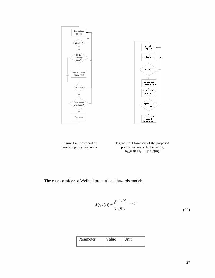
Inspection epoch

Replace

Order already sent?

Order a new spare part

z(t)≤40?

z(t)≥50?

Spare partavailable?

no

yes

no

yes

no

yes

yes

The case considers a Weibull proportional hazards model:

)(1

))(,( tzettzt γβ

ηηβλ

−

⎟⎟⎠

⎞⎜⎜⎝

⎛=

(22)

Parameter Value Unit

Figure 1.b: Flowchart of the proposed policy decisions. In the figure,

Rint=R(t+Tbi+Tl|t,Z(t)=i).

Figure 1.a: Flowchart of baseline policy decisions.

27

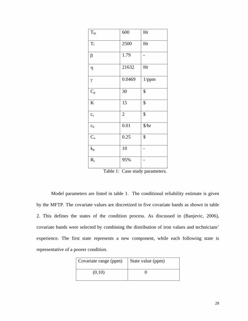
Tbi 600 Hr

Tl 2500 Hr

β 1.79 -

η 21632 Hr

γ 0.0469 1/ppm

Cp 30 $

K 15 $

cs 2 $

ch 0.01 $/hr

Co 0.25 $

kp 10 -

Rc 95% -

Table 1: Case study parameters.

Model parameters are listed in table 1. The conditional reliability estimate is given

by the MFTP. The covariate values are discretized in five covariate bands as shown in table

2. This defines the states of the condition process. As discussed in (Banjevic, 2006),

covariate bands were selected by combining the distribution of iron values and technicians’

experience. The first state represents a new component, while each following state is

representative of a poorer condition.

Covariate range (ppm) State value (ppm)

(0,10) 0

28

(10,20) 15

(20,40) 30

(40,70) 55

(70, ∞) 85

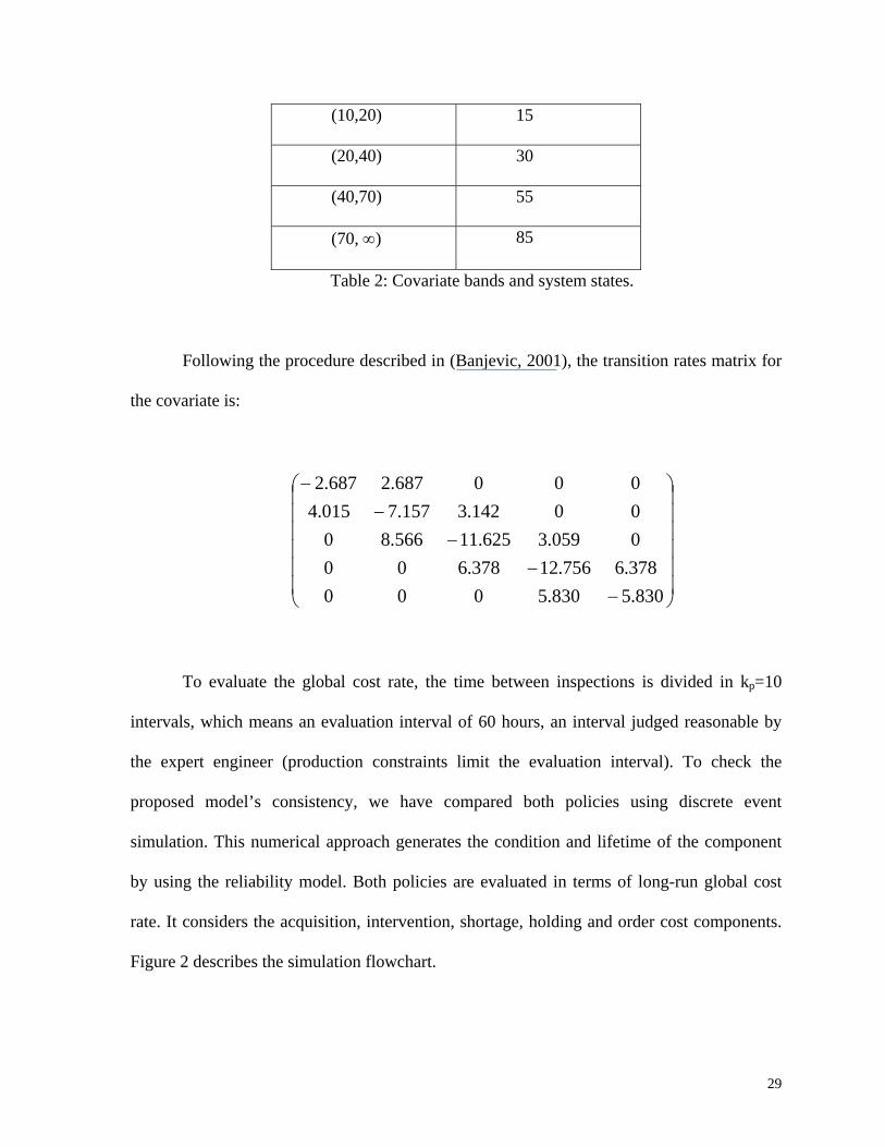
Table 2: Covariate bands and system states.

Following the procedure described in (Banjevic, 2001), the transition rates matrix for

the covariate is:

⎟⎟⎟⎟⎟⎟

⎠

⎞

⎜⎜⎜⎜⎜⎜

⎝

⎛

−−

−−

−

830.5830.5000378.6756.12378.6000059.3625.11566.8000142.3157.7015.4000687.2687.2

To evaluate the global cost rate, the time between inspections is divided in kp=10

intervals, which means an evaluation interval of 60 hours, an interval judged reasonable by

the expert engineer (production constraints limit the evaluation interval). To check the

proposed model’s consistency, we have compared both policies using discrete event

simulation. This numerical approach generates the condition and lifetime of the component

by using the reliability model. Both policies are evaluated in terms of long-run global cost

rate. It considers the acquisition, intervention, shortage, holding and order cost components.

Figure 2 describes the simulation flowchart.

29

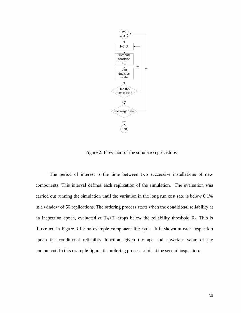
t=t+dt

Computecondition

z(t)

Has the item failed?

End

Convergence?

no

yes

noUse decisionmodel

yes

t=0z(t)=0

Figure 2: Flowchart of the simulation procedure.

The period of interest is the time between two successive installations of new

components. This interval defines each replication of the simulation. The evaluation was

carried out running the simulation until the variation in the long run cost rate is below 0.1%

in a window of 50 replications. The ordering process starts when the conditional reliability at

an inspection epoch, evaluated at Tbi+Tl drops below the reliability threshold Rc. This is

illustrated in Figure 3 for an example component life cycle. It is shown at each inspection

epoch the conditional reliability function, given the age and covariate value of the

component. In this example figure, the ordering process starts at the second inspection.

30

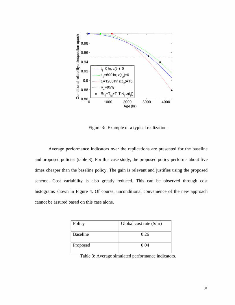
0 1000 2000 3000 40000.86

0.88

0.9

0.92

0.94

0.96

0.98

1

Age (hr)

Con

ditio

nal r

elia

bilit

y at

insp

ectio

n ep

och

t1=0 hr, z(t1)=0

t 2=600 hr, z(t 2)=0

t3=1200 hr, z(t 3)=15

Rc=95%

R(ti+Tbi+Tl|T>ti, z(ti))

Figure 3: Example of a typical realization.

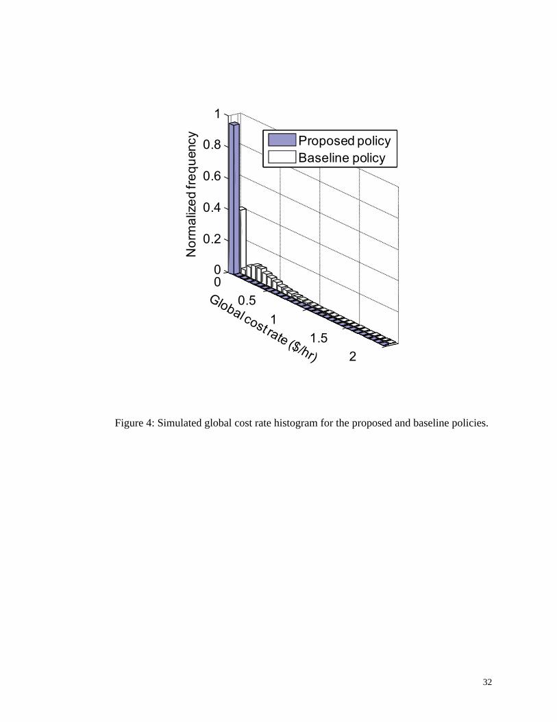
Average performance indicators over the replications are presented for the baseline

and proposed policies (table 3). For this case study, the proposed policy performs about five

times cheaper than the baseline policy. The gain is relevant and justifies using the proposed

scheme. Cost variability is also greatly reduced. This can be observed through cost

histograms shown in Figure 4. Of course, unconditional convenience of the new approach

cannot be assured based on this case alone.

Policy Global cost rate ($/hr)

Baseline 0.26

Proposed 0.04

Table 3: Average simulated performance indicators.

31

00.5

11.5

2

0

0.2

0.4

0.6

0.8

1

Nor

mal

ized

freq

uenc

y Proposed policyBaseline policy

Figure 4: Simulated global cost rate histogram for the proposed and baseline policies.

32

5. CONCLUSIONS AND OPPORTUNITIES FOR FURTHER RESEARCH

In this article, we have presented a model to integrate internal condition monitoring

information (considering the case of time-dependent covariates) into the area of spare parts

stockholding decisions. The model presented here is viewed as a first step in what appears as

a very interesting area of future research. Wide opportunities for model improvement and

extension are identified.

We suggest the evaluation of expected costs for various ordering times to find the

‘optimal’. Evaluation of more efficient optimization algorithms is an interesting area for

further development.

In the model discussed, we assume deterministic lead times and consider the case of a

single (regular) supply alternative. Incorporation of expedited orders appears as an interesting

extension for the model, since it makes business sense that if the cost of placing the

expedited order is less than the expected savings due to an earlier delivery of the spare, an

expedited order will be placed whenever a failure occurs before the ordering time (Case I).

This scenario does not consider speeding-up an order already placed, which would be another

possible extension.

Another area for evaluation is the natural extension to the case of multiple systems (or

multi-component systems). A possible avenue for this is the use of penalty (loss) functions to

evaluate orders of multiple parts when systems are operated in groups (or when multiple

components in the system might be replaced/ordered concurrently). Dekker (1995) discusses

33

the use of penalty functions to combine maintenance activities. Through the use of penalty

functions, the cost associated with different ordering/replacement alternatives could be

assessed.

Extension to the case of stochastic lead times might also be considered for future

research, though additional complexity of the model might prevent this from being

worthwhile.

ACKOWLEDGEMENT This work was conducted with the financial support of the Natural Sciences and Engineering Research Council (NSERC) of Canada, Materials and Manufacturing Ontario (MMO) of Canada, the CMORE Consortium of the University of Toronto and the National Fund for Scientific and Technologic Development of the Chilean Government (FONDECYT, Fondo Nacional de Desarrollo Científico y Tecnológico), project 1090079. We thank the reviewers for comments that helped to sharpen the final version of the article. REFERENCES

Armstrong, M.J. and Atkins, D.A. (1998) A note on joint optimization of maintenance and

inventory, IIE Transactions 30: 143-149.

Banjevic, D., Jardine, A.K.S., Makis, V. and Ennis, M. (2001) A control-limit policy and

software for condition-based maintenance optimization, INFOR 39: 32-50.

34

Banjevic, D. and Jardine, A.K.S. (2006) Calculation of reliability function and remaining

useful life for a Markov failure time process, IMA Journal of Management Mathematics 17:

115-130.

Barlow, R.E. and Proschan, F. (1965) Mathematical Theory of Reliability. Wiley, New York.

Cheng, K. and He, Z. (1987) On the first failure time of a system in a randomly varying

environment, in Osaki, S. and Cao, J. (Eds.), Reliability Theory and Applications:

proceedings of the China-Japan Reliability Simposium. World Scientific, Singapore.

Cox, D.R. (1972) Regression models and life-tables, Journal of the Royal Statistical Society

B34: 187-220.

Crespo-Marquez, A. and Gupta, J.N.D. (2006) Contemporary maintenance management:

process, framework and supporting pillars, Omega 34: 313-326.

Csenki, A. (1998) Refined asymptotic analysis of two basic order-replacement models for a

spare unit, IMA Journal of Mathematics Applied in Business and Industry 9: 177-199.

Dekker, R. (1995) Integrating optimization, priority setting, planning and combining of

maintenance activities, European Journal of Operational Research 82: 225-240.

35

Dohi, T., Kaio, N. and Osaki, S. (1998) On the optimal ordering policies in maintenance

theory – survey and applications, Applied Stochastic Models & Data Analysis 14: 309-321.

Dohi, T., Kaio, N. and Osaki, S. (2005) Cost-effective analysis of optimal order-replacement

policies, in: N. Balakrishan, N. Kannan and H.N. Nagaraja (Eds.) Advances in Ranking and

Selection, Multiple Comparisons, and Reliability. Birkhauser, Boston.

Elsayed, E.A. (2003) Mean residual life and optimal operating conditions for industrial

furnace tubes, in Blischke, W.R. and Murthy, D.N.P. (Eds.) Case Studies in Reliability and

Maintenance. Wiley, New York.

Elwany, A.H. and Gebraeel, N.Z.(2008) Sensor-driven prognostic models for equipment

replacement and spare parts inventory, IIE Transactions 40: 629-639

Ghodrati, B. and Kumar, U. (2005a) Operating environment-based spare parts forecasting

and logistics: a case study, International Journal of Logistics: Research and Applications 8:

95-105.

Ghodrati, B. and Kumar, U. (2005b) Reliability and operating environment-based spare parts

estimation approach: a case study in Kiruna mine, Sweden, Journal of Quality in

Maintenance Engineering 11: 169-184.

36

Gill, R.D. and Johansen, S. (1990) A survey of product-integration with a view toward

application in survival analysis, Annals of Statistics 18: 1501-1556.

Kilpi, J., Toyli, J., Vepsalainen, A. (2009) Cooperative strategies for the availability service

of repairable aircraft components, International Journal of Production Economics 117 360–

370

Kumar, D. and Klefsjö, B. (1994) Proportional hazards model: a review, Reliability

Engineering and System Safety 44: 177-188.

Makis, V. and Jardine, A.K.S. (1992) Optimal replacement in the proportional hazards

model, INFOR 30: 172-183.

Mobley, R.K. (2003) An introduction to predictive maintenance (2nd ed.). Butterworth

Heinemann, Boston.

Møller, C.M. (1992) Numerical evaluation of Markov transition probabilities based on

discretized product-integral, Scandinavian Actuarial Journal 1: 76-87.

Moubray, J. (1997) Reliability-centered maintenance (2nd ed.), Butterworth Heinemann,

Oxford.

37

Osaki, S. (1977) An ordering policy with lead time, International Journal of Systems Science

8: 1091-1095.

Pedregal, D.J. and Carnero, M.C. (2006) State space models for condition monitoring: a case

study, Reliability Engineering and System Safety 91: 171-180.

Reinersten, R. (1996) Residual life of technical systems; diagnosis, prediction and life

extension, Reliability Engineering and System Safety 54: 23-34.

Scarf, P.A. (1997) On the application of mathematical models in maintenance, European

Journal of Operational Research 99: 493-506.

Smith, M.A.J. and Dekker, R. (1997) On the (S-1,S) stock model for renewal demand

processes, Probability in the Engineering and Informational Sciences, 11: 375-386.

Wang, W. (2002) A model to predict the residual life of rolling element bearings given

monitored condition information to date, IMA Journal of Management Mathematics 13: 3-16.

Wang, W. and Zhang, W. (2003) A model to predict the residual life of aircraft engine based

upon oil analysis data, in Srivastava, O.P. and Al-Najjar, B. (Eds.) Proceedings of

COMADEM 2003, The 16th International Congress and Exhibition on Condition Monitoring

and Diagnostic Engineering Management. Växjö University Press: Växjö, Sweden.

38

39

Wang, L., Chu, J. and Mao, W. (2008) A condition-based order-replacement policy for a

single-unit system, Applied Mathematical Modelling, 32: 2274–2289.

Yuen, K.C., Zhu, L.X. and Tang, N.Y. (2003) On the mean residual life regression model,

Journal of Statistical Planning and Inference 113: 685-698.