Nonlinear Dynamic Response Variability and Reliability of Frames with Stochastic Non-Gaussian Parameter Uncertainty

George Stefanou and Michalis Fragiadakis

Abstract Current research efforts for the efficient prediction of the dynamic re-sponse of structures with parameter uncertainty concentrate on the development of new and the improvement of existing methods. However, they are usually limited to linear elastic analysis considering only monotonic loading. In order to investi-gate realistic problems of structures subjected to transient seismic actions, a novel approach has been recently introduced by the authors. This approach is used here to assess the nonlinear stochastic response and reliability of a 3-storey steel mo-ment-resisting frame in the framework of Monte Carlo simulation (MCS) and translation process theory. The structure is modeled with a mixed fiber-based, beam-column element, whose kinematics is based on the natural mode method. The adopted formulation leads to the reduction of the computational cost required for the calculation of the element stiffness matrix, while increased accuracy com-pared to traditional displacement-based elements is achieved. The uncertain pa-rameters of the problem are the Young modulus and the yield stress, both de-scribed by homogeneous non-Gaussian translation stochastic fields that vary along the element. The frame is subjected to natural seismic records that correspond to three levels of increasing seismic intensity. Under the assumption of a pre-specified power spectral density function of the stochastic fields that describe the two uncertain parameters, the response variability of the frame is computed using MCS. Moreover, a parametric investigation is carried out providing useful conclu-sions regarding the influence of the correlation length of the stochastic fields on the response variability and reliability of the frame.

Institute of Structural Analysis & Seismic Research, National Technical Universi-ty of Athens, 15780 Athens, Greece, e-mail: stegesa@mail.ntua.gr (George Stefa-nou), mfrag@mail.ntua.gr (Michalis Fragiadakis)

2

1 Introduction

In the last few years, the problems of dynamic response analysis and reliability as-sessment of structures with uncertain system and excitation parameters have been the subject of extensive research. The case of deterministic and stochastic linear systems subjected to random excitation has been studied first and is well repre-sented in the literature [1-3]. An approximate method for the response variability calculation of dynamical systems with uncertain stiffness and damping ratio ap-pears can be found in [1]. This approach is based on complex mode analysis where the variability of each mode is analyzed separately and can efficiently treat a variety of probability distributions assumed for the system parameters. The time-varying reliability evaluation of uncertain structures subjected to stochastic earth-quake ground motion is treated in [2] using conditional crossing rate estimation and the perturbation-based stochastic finite element method. Recently, an exact non-statistical method has been proposed for the dynamic analysis of FE-discretized uncertain linear structures in the frequency domain [3].

In contrast to the linear case, the efficient prediction of the nonlinear dynamic response of structures with uncertain system properties still poses a major chal-lenge in the field of computational stochastic mechanics [4-6]. This can be ex-plained by the fact that most of the methods developed for the analysis of linear systems are inefficient or inappropriate for the nonlinear case. For example, the analysis of uncertain nonlinear systems is generally not feasible using frequency domain analysis techniques [7]. The existing methods for response statistics calcu-lation in this case are mostly based on simulation [4,8] or on the perturbation ap-proach [9]. Applications of the response surface method have also been proposed [10], while studies can be found on the statistical equivalent linearization (EQL) method for the response variability and reliability estimation of discrete nonlinear systems [11]. Alternatively, a probability density evolution method (PDEM) has been developed for this purpose [12] and a neural network-based approach has been proposed for the efficient fragility assessment of steel frames with uncertain material properties modeled as normal random variables [13]. It is worth noting that the theory of non-Gaussian translation processes (used here for the uncertain system properties) has also been applied directly to the reliability analysis of dy-namic systems under limited information. This method delivers accurate results for the case of linear and nonlinear dynamic systems assuming stationary output but can be easily extended to a special class of non-stationary, non-ergodic output [14].

It is well known that the main drawback of the perturbation approach is the significant loss of accuracy when the level of uncertainty of the system properties is high. On the other hand, the computational effort required by statistical ap-proaches such as Monte Carlo simulation (MCS) for the analysis of large-scale structures is considerable thus making essential the use of efficient solution strate-gies and parallel processing [6]. In addition, the validity of EQL is questionable in

3

some cases and the method may even produce misleading results [15]. Based on the aforementioned observations, it is concluded that an approach combining ac-curacy and computational efficiency is still very desirable in this area.

In order to investigate realistic problems of structures subjected to seismic loading, a novel approach, combining MCS and nonlinear response history analy-sis with the stochastic field theory, has been recently introduced [16]. The pro-posed methodology is used here to assess the response variability and reliability of a benchmark 3-storey steel moment-resisting frame [17]. The structure is modeled with a mixed fiber-based, beam-column element, whose kinematics is based on the natural mode method. The adopted formulation leads to the reduction of the computational cost required for the computation of the element stiffness matrix, while increased accuracy compared to traditional displacement-based elements is achieved [18,19]. The uncertain parameters are the Young modulus and the yield stress, both described by homogeneous non-Gaussian translation stochastic fields [20]. The frame is subjected to natural seismic records that correspond to three levels of increasing seismic intensity. Under the assumption of a pre-specified power spectral density function of the stochastic fields describing the two uncer-tain parameters, the response variability and reliability of the frame is computed using MCS. Finally, a parametric investigation is carried out providing useful conclusions regarding the influence of the spectral characteristics of the stochastic fields on the response variability.

2 Force-based formulation of the beam-column element

Inelastic analysis of frame structures can be performed either with a lumped or with a distributed plasticity formulation. Distributed plasticity elements are con-sidered more accurate and, in general, are distinguished to displacement-based and to force-based elements. The latter approach, also known as flexibility formula-tion, has a number of distinct features over the former, especially if it is adopted in the framework of a mixed beam-column formulation [21]. The force-based formu-lation requires a single beam-column element per member to simulate its material nonlinear response, since it uses force interpolation functions. Consequently, the element equilibrium is always satisfied, while compatibility of deformations is sat-isfied by integrating the section deformations to obtain the element deformations and the nodal displacements. In order to numerically calculate the stiffness matrix, a number of sections along the beam-column element are chosen, while every sec-tion is divided to a number of monitoring sections, known as fibers. Fibers are simply integration points of a low order quadrature at the section level and are used to evaluate the section stiffness as follows:

4

sec sec sec sec sec2

1A

yσ dAy yε

⎛ − ⎞⎡ ⎤∂= ⇔ = ⎜ ⎟⎢ ⎥−∂ ⎣ ⎦⎝ ⎠∫D k d D d (1)

where y is the distance of a fiber from the neutral axis, Dsec are the section forces and dsec=[εx, κ]T is the vector of section deformations that consists of the axial strain εx and the curvature κ. If the response is linear elastic, the diagonal terms of the section stiffness matrix become equal to EA and EI, respectively, while the off-diagonal terms are zero. If the section flexibility matrix is fsec=

1sec−k , the ele-

ment flexibility matrix F=K-1 is obtained as follows:

1 1T -1 T T

sec sec sec1 11

= = ( ) ( ) ( )NP

i i i ii

d d wξ ξ ξ ξ ξ− −

=

= =∑∫ ∫-1F K b k b b f b b f b (2)

The above equation implies that numerical integration is required in order to obtain the element flexibility matrix, where NP is the number of integration points along the element. In force-based elements, the Gauss-Lobatto quadrature is pre-ferred because it considers as sections of integration the beam ends where the bending moment is maximum (provided that no other element loads are present). This integration scheme requires at least three integration sections, while typically four to six sections are chosen.

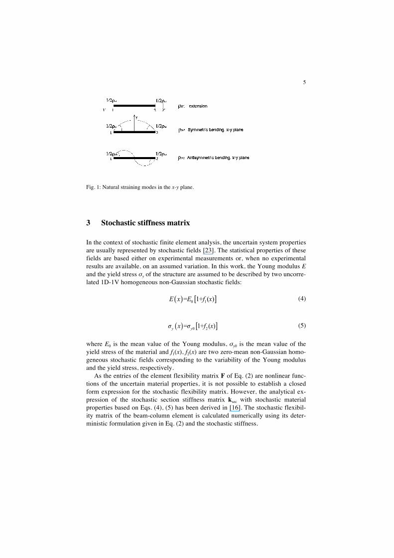
The kinematics of the element used in this study follow the principles of the natural mode method proposed by Argyris [22]. According to the natural mode method, the displacement field can be decomposed into three rigid body modes ρ0 and three straining modes ρN shown in Fig. 1. In a flexibility-based element the calculation of the natural element forces is performed iteratively for each element. The first step of the iterative procedure is to determine the vector of the natural forces. Then using force interpolation functions, the section forces are obtained and subsequently they are corrected according to the constitutive law. From the corrected forces the section deformations are obtained using Eq. (1) and are then integrated according to

1

TN sec

1

( )ξ dξ−

= ∫ρ b d (3)

in order to obtain the residual natural modes. b is the interpolation matrix, which is a function of the natural coordinate [ 1,1]ξ ∈ − along the element. The iterative process in the element level is terminated when an energy convergence criterion is satisfied.

5

Fig. 1: Natural straining modes in the x-y plane.

3 Stochastic stiffness matrix

In the context of stochastic finite element analysis, the uncertain system properties are usually represented by stochastic fields [23]. The statistical properties of these fields are based either on experimental measurements or, when no experimental results are available, on an assumed variation. In this work, the Young modulus E and the yield stress σy of the structure are assumed to be described by two uncorre-lated 1D-1V homogeneous non-Gaussian stochastic fields:

( ) [ ]0 1= 1+ ( )E x E f x (4)

( ) [ ]0 2= 1+ ( )y yσ x σ f x (5)

where E0 is the mean value of the Young modulus, σy0 is the mean value of the yield stress of the material and f1(x), f2(x) are two zero-mean non-Gaussian homo-geneous stochastic fields corresponding to the variability of the Young modulus and the yield stress, respectively.

As the entries of the element flexibility matrix F of Eq. (2) are nonlinear func-tions of the uncertain material properties, it is not possible to establish a closed form expression for the stochastic flexibility matrix. However, the analytical ex-pression of the stochastic section stiffness matrix ksec with stochastic material properties based on Eqs. (4), (5) has been derived in [16]. The stochastic flexibil-ity matrix of the beam-column element is calculated numerically using its deter-ministic formulation given in Eq. (2) and the stochastic stiffness.

6

4 Simulation of uncertain parameters using non-Gaussian translation fields

In this work, a non-Gaussian assumption is made for the distribution of the uncer-tain parameters of the frame. This choice is in accordance to the fact that several quantities arising in practical engineering problems (e.g. material and geometric properties of structural systems, soil properties, wind loads, waves) are found to exhibit non-Gaussian probabilistic characteristics. In addition, the non-Gaussian assumption permits to efficiently treat the case of large input variability without violating the physical constraints of the material properties.

A number of studies in the literature have been focused on producing a realistic definition of a non-Gaussian sample function from a simple transformation of an underlying Gaussian field with known second-order statistics. Thus, if g(x) is a homogeneous zero-mean Gaussian field with unit variance and spectral density function (SDF) Sgg(κ) (or equivalently autocorrelation function Rgg(ξ)), a homoge-neous non-Gaussian stochastic field f(x) with power spectrum ( )T

ffS κ is defined as:

1( ) [ ( )]f x F g x−= ⋅Φ (6)

where Φ is the standard Gaussian cumulative distribution function and F is the non-Gaussian marginal cumulative distribution function (CDF) of f(x). The trans-form 1F − ⋅Φ is a memory-less translation since the value of f(x) at an arbitrary point x depends on the value of g(x) at the same point only and the resulting non-Gaussian field is called a translation field [20].

Translation fields have a number of useful properties such as the analytical cal-culation of crossing rates and extreme value distributions. They also have some shortcomings, the most important of which from a practical point of view is the possible incompatibility between their marginal distribution F and correlation structure ( )T

ffS κ . F and ( )TffS κ (or ( )T

ffR ξ ) of a translation field have to satisfy a specific compatibility condition derived directly from the definition of its autocor-relation function [20]. If these two quantities are proven to be incompatible i.e. if ( )T

ffR ξ has certain values lying outside a range of admissible values and/or Rgg(ξ) is not positive definite and therefore not admissible as an autocorrelation function, there is no translation field with the prescribed characteristics. In this case, one has to resort to translation fields that match the target marginal distribution and/or SDF approximately. Since experimental data can lead to a theoretically incompat-ible pair of F and ( )T

ffS κ , iterative algorithms have been recently developed, which extend the translation field concept and lead to the generation of non-Gaussian fields having the prescribed characteristics [24-26]. It is worth noting that the theory of non-Gaussian translation fields has been recently applied direct-

7

ly to the reliability analysis of linear and nonlinear dynamic systems under limited information [14].

In the present work, Eq. (6) is used for the generation of non-Gaussian transla-tion sample functions representing the uncertain parameters of the problem. Sam-ple functions of the underlying Gaussian field g(x) are generated using the spectral representation method [27]. The SDF Sgg(κ) of g(x) used in the numerical example is assumed to correspond to an autocorrelation function of square exponential type and is given by:

2 2 2

( ) exp42

ggg

b bSσ κκ

π⎛ ⎞

= −⎜ ⎟⎝ ⎠

(7)

where σg is the standard deviation of the stochastic field and b denotes the parame-ter that influences the shape of the spectrum and is proportional to the correlation length of the stochastic field along the x-axis. The SDF of the translation field ob-tained from Eq. (6) will be slightly different from Sgg(κ) (see e.g. [28]).

Using the procedure described in this section, a large number NSAMP of non-Gaussian sample functions are produced, leading to the generation of a set of sto-chastic stiffness matrices. The associated structural problem is solved NSAMP times and the response variability and reliability can finally be calculated by obtaining the statistics of the NSAMP simulations.

5 Numerical examples

In this section, the three-storey steel moment-resisting frame shown in Fig. 2 is used for a numerical implementation of the above described methodology. The frame has been designed for a Los Angeles site, following the 1997 NEHRP (Na-tional Earthquake Hazard Reduction Program) provisions in the framework of the SAC/FEMA program [29]. The dynamic response of the building is dominated by the fundamental mode which has a period value equal to T1=1.02 sec when the mean value of the modulus of elasticity is used. All response history analyses were performed using a force-based, beam-column fiber element with five integration sections implemented on a general purpose finite element program [30]. Geomet-ric nonlinearities were not considered in the analysis. Rayleigh damping is used to obtain a damping ratio of 2% for the first and the fourth mode. The material law is considered to be bilinear with pure kinematic hardening, where the properties of each integration section differ according to the stochastic fields of Eqs. (4) and (5). The frame section properties are given in Table 1. The gravity loading applied is 32.22 kN/m for the first two stories and 28.76kN/m for the top storey. These values are used also to obtain the nodal masses resulting to a lumped mass matrix.

8

Three sets of five strong ground motion records are used as input to the nonlin-ear dynamic procedure (Table 2). The three sets correspond to three levels of in-creasing hazard: low, medium and high (Fig. 3). Although the predominant fre-quencies of the records lie at period values less than the fundamental elastic period of the frame, it is clear that for many of the records the amplification at the vicini-ty of 1.0 sec is rather significant. The records chosen differ in terms of amplitude, frequency content, duration, etc and therefore this variability is expected to be transferred to the statistics of the analysis, producing significant record-to-record variability. The 15 natural records are used as input to the analysis in order to compute the mean response quantities, the dispersion and the reliability of the frame for the three intensity levels.

5.1 Response variability and reliability of the frame

The spatial variability in Young modulus and yield stress of the frame is described by two uncorrelated 1D-1V homogeneous non-Gaussian translation stochastic fields with zero mean and coefficient of variation (COV) equal to 0.10. A slightly skewed shifted lognormal distribution defined in the range [-1,+∞ ] is assumed for the two stochastic fields. The skewness of the lognormal distribution is equal to 0.30. E and σy are simultaneously varying in all the cases examined. The repre-sentative response quantity whose statistics are monitored is the maximum inter-storey drift, which for brevity will be simply referred as drift and denoted as θmax. This parameter is a well-known engineering demand parameter (EDP) that cap-tures the seismic demand and its distributions along the height of the structure. The response statistics have been calculated using 1000 Monte Carlo simulations. This number of simulations represents sufficiently well the prescribed first two moments of the stochastic fields, while as shown in Fig. 4, statistical convergence is practically achieved after 400 simulations. This trend was observed for all ground motions considered.

The sensitivity of θmax with respect to the scale of correlation of the stochastic fields, quantified with the aid of the correlation length parameter b of the underly-ing Gaussian field, is examined for the ground motions of the three sets. For this purpose, several sets of sample functions of E and σy are generated using Eq. (6) each for a different value of parameter b. Six representative values of b varying from weak to strong correlation are considered (b = 0.2, 1.0, 2.0, 10, 20 and 100).

9

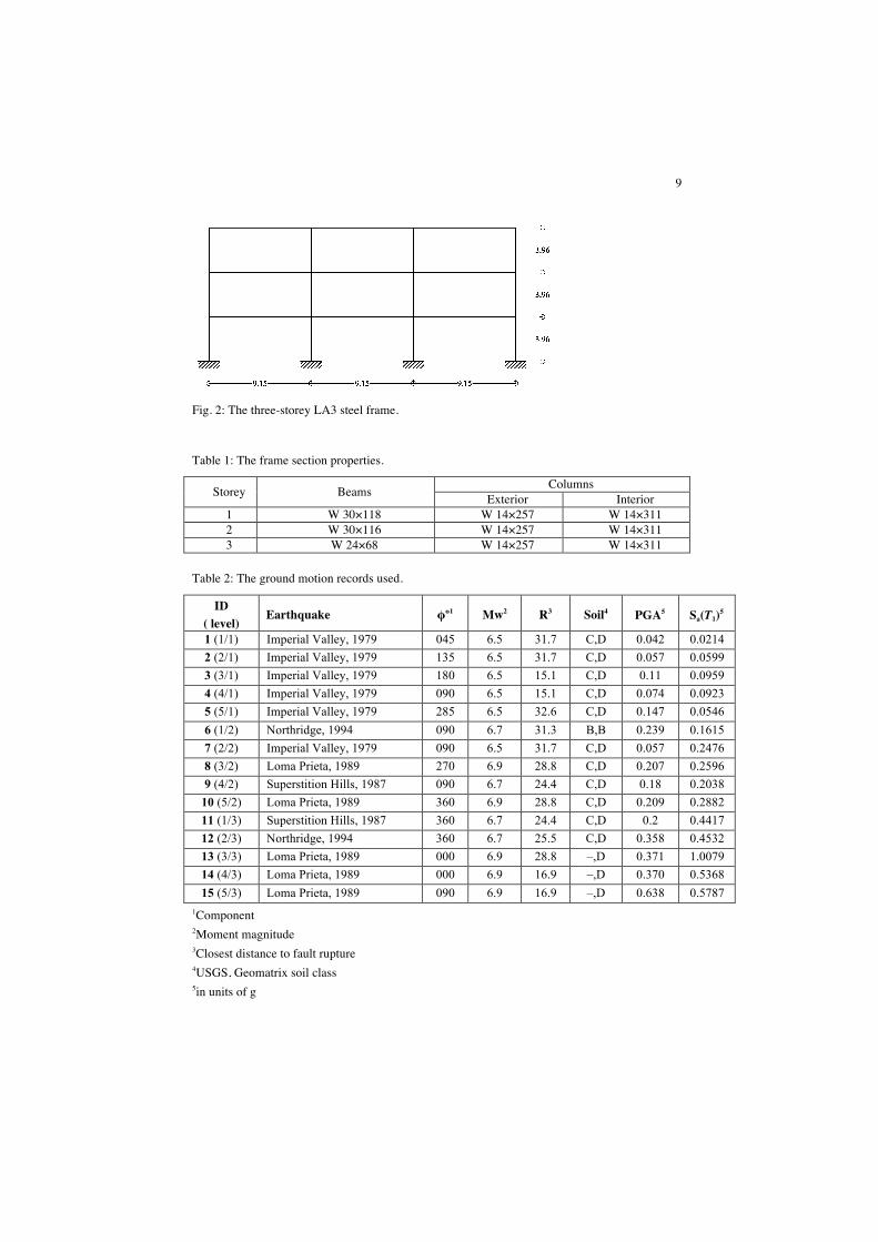
Fig. 2: The three-storey LA3 steel frame.

Table 1: The frame section properties.

Storey Beams Columns Exterior Interior

1 W 30×118 W 14×257 W 14×311 2 W 30×116 W 14×257 W 14×311 3 W 24×68 W 14×257 W 14×311

Table 2: The ground motion records used.

ID ( level)

Earthquake φο1 Mw2 R3 Soil4 PGA5 Sa(T1)5

1 (1/1) Imperial Valley, 1979 045 6.5 31.7 C,D 0.042 0.0214 2 (2/1) Imperial Valley, 1979 135 6.5 31.7 C,D 0.057 0.0599 3 (3/1) Imperial Valley, 1979 180 6.5 15.1 C,D 0.11 0.0959 4 (4/1) Imperial Valley, 1979 090 6.5 15.1 C,D 0.074 0.0923 5 (5/1) Imperial Valley, 1979 285 6.5 32.6 C,D 0.147 0.0546 6 (1/2) Northridge, 1994 090 6.7 31.3 B,B 0.239 0.1615 7 (2/2) Imperial Valley, 1979 090 6.5 31.7 C,D 0.057 0.2476 8 (3/2) Loma Prieta, 1989 270 6.9 28.8 C,D 0.207 0.2596 9 (4/2) Superstition Hills, 1987 090 6.7 24.4 C,D 0.18 0.2038

10 (5/2) Loma Prieta, 1989 360 6.9 28.8 C,D 0.209 0.2882 11 (1/3) Superstition Hills, 1987 360 6.7 24.4 C,D 0.2 0.4417 12 (2/3) Northridge, 1994 360 6.7 25.5 C,D 0.358 0.4532 13 (3/3) Loma Prieta, 1989 000 6.9 28.8 –,D 0.371 1.0079 14 (4/3) Loma Prieta, 1989 000 6.9 16.9 –,D 0.370 0.5368 15 (5/3) Loma Prieta, 1989 090 6.9 16.9 –,D 0.638 0.5787

1Component 2Moment magnitude 3Closest distance to fault rupture 4USGS, Geomatrix soil class 5in units of g

10

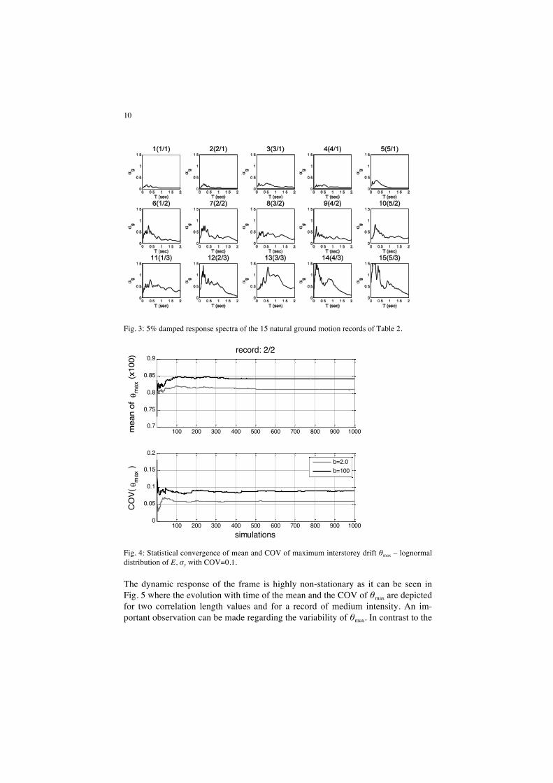
Fig. 3: 5% damped response spectra of the 15 natural ground motion records of Table 2.

100 200 300 400 500 600 700 800 900 10000.7

0.75

0.8

0.85

0.9record: 2/2

mea

n of

θm

ax (x

100)

100 200 300 400 500 600 700 800 900 10000

0.05

0.1

0.15

0.2

simulations

CO

V( θ

max

)

b=2.0b=100

Fig. 4: Statistical convergence of mean and COV of maximum interstorey drift θmax – lognormal distribution of E, σy with COV=0.1.

The dynamic response of the frame is highly non-stationary as it can be seen in Fig. 5 where the evolution with time of the mean and the COV of θmax are depicted for two correlation length values and for a record of medium intensity. An im-portant observation can be made regarding the variability of θmax. In contrast to the

11

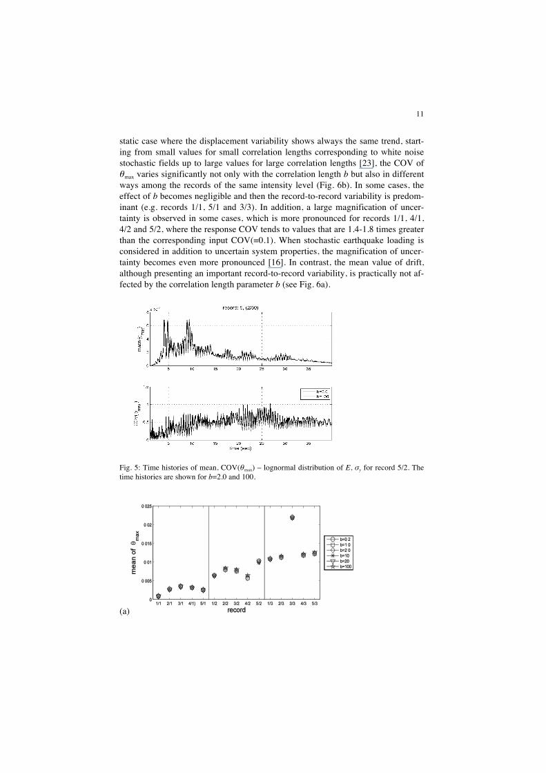
static case where the displacement variability shows always the same trend, start-ing from small values for small correlation lengths corresponding to white noise stochastic fields up to large values for large correlation lengths [23], the COV of θmax varies significantly not only with the correlation length b but also in different ways among the records of the same intensity level (Fig. 6b). In some cases, the effect of b becomes negligible and then the record-to-record variability is predom-inant (e.g. records 1/1, 5/1 and 3/3). In addition, a large magnification of uncer-tainty is observed in some cases, which is more pronounced for records 1/1, 4/1, 4/2 and 5/2, where the response COV tends to values that are 1.4-1.8 times greater than the corresponding input COV(=0.1). When stochastic earthquake loading is considered in addition to uncertain system properties, the magnification of uncer-tainty becomes even more pronounced [16]. In contrast, the mean value of drift, although presenting an important record-to-record variability, is practically not af-fected by the correlation length parameter b (see Fig. 6a).

Fig. 5: Time histories of mean, COV(θmax) – lognormal distribution of E, σy for record 5/2. The time histories are shown for b=2.0 and 100.

(a)

12

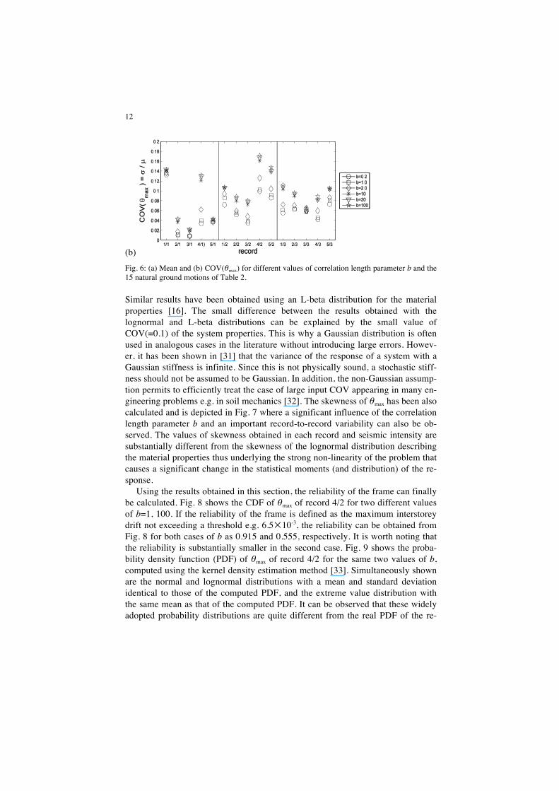
(b)

Fig. 6: (a) Mean and (b) COV(θmax) for different values of correlation length parameter b and the 15 natural ground motions of Table 2.

Similar results have been obtained using an L-beta distribution for the material properties [16]. The small difference between the results obtained with the lognormal and L-beta distributions can be explained by the small value of COV(=0.1) of the system properties. This is why a Gaussian distribution is often used in analogous cases in the literature without introducing large errors. Howev-er, it has been shown in [31] that the variance of the response of a system with a Gaussian stiffness is infinite. Since this is not physically sound, a stochastic stiff-ness should not be assumed to be Gaussian. In addition, the non-Gaussian assump-tion permits to efficiently treat the case of large input COV appearing in many en-gineering problems e.g. in soil mechanics [32]. The skewness of θmax has been also calculated and is depicted in Fig. 7 where a significant influence of the correlation length parameter b and an important record-to-record variability can also be ob-served. The values of skewness obtained in each record and seismic intensity are substantially different from the skewness of the lognormal distribution describing the material properties thus underlying the strong non-linearity of the problem that causes a significant change in the statistical moments (and distribution) of the re-sponse.

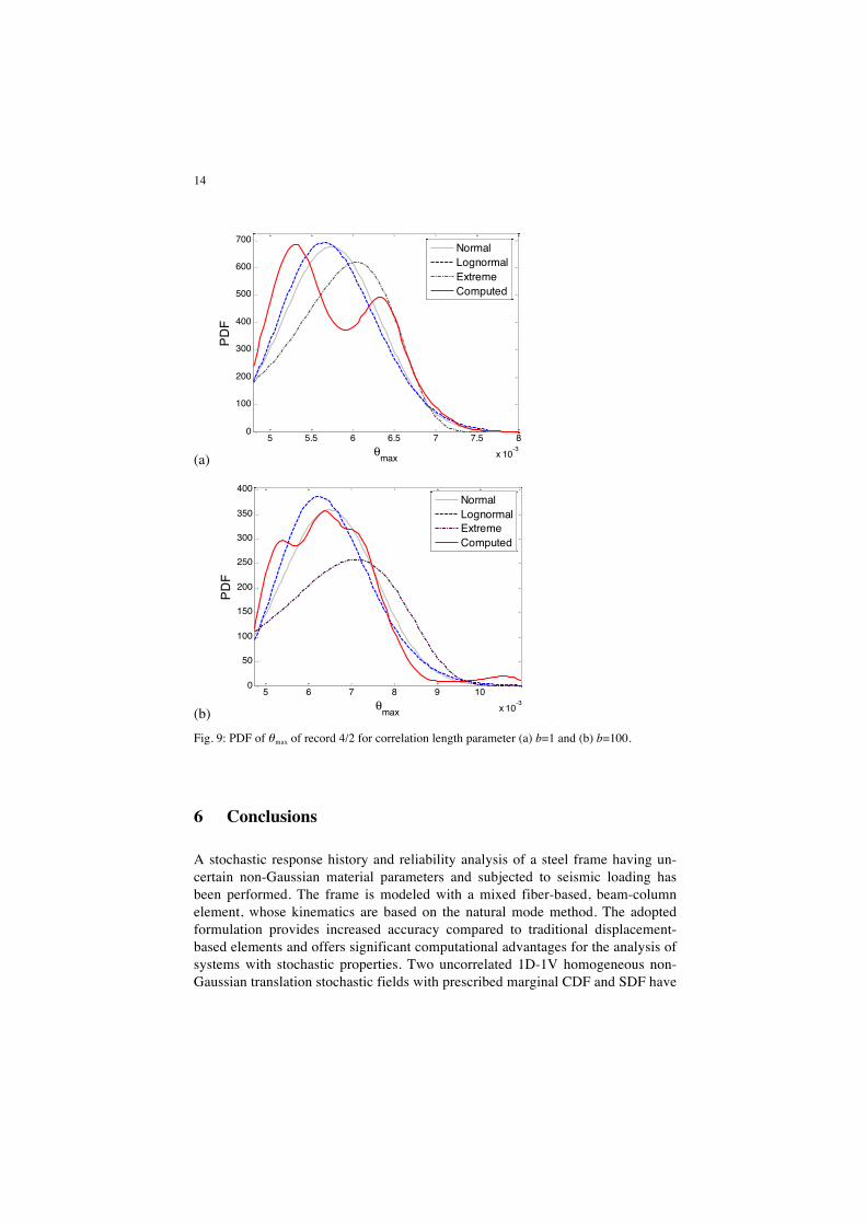
Using the results obtained in this section, the reliability of the frame can finally be calculated. Fig. 8 shows the CDF of θmax of record 4/2 for two different values of b=1, 100. If the reliability of the frame is defined as the maximum interstorey drift not exceeding a threshold e.g. 6.5×10-3, the reliability can be obtained from Fig. 8 for both cases of b as 0.915 and 0.555, respectively. It is worth noting that the reliability is substantially smaller in the second case. Fig. 9 shows the proba-bility density function (PDF) of θmax of record 4/2 for the same two values of b, computed using the kernel density estimation method [33]. Simultaneously shown are the normal and lognormal distributions with a mean and standard deviation identical to those of the computed PDF, and the extreme value distribution with the same mean as that of the computed PDF. It can be observed that these widely adopted probability distributions are quite different from the real PDF of the re-

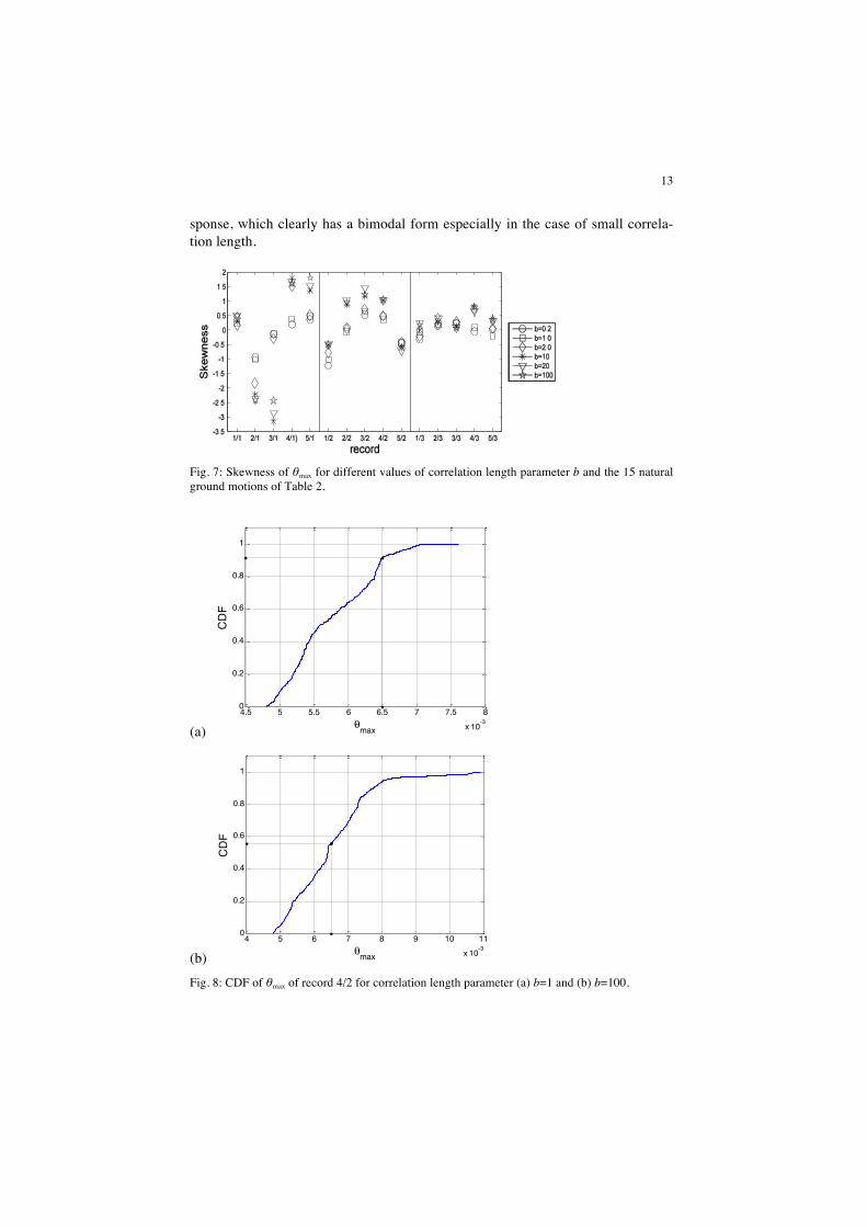
13

sponse, which clearly has a bimodal form especially in the case of small correla-tion length.

Fig. 7: Skewness of θmax for different values of correlation length parameter b and the 15 natural ground motions of Table 2.

(a)4.5 5 5.5 6 6.5 7 7.5 8

x 10-3

0

0.2

0.4

0.6

0.8

1

θmax

CD

F

(b)4 5 6 7 8 9 10 11

x 10-3

0

0.2

0.4

0.6

0.8

1

θmax

CD

F

Fig. 8: CDF of θmax of record 4/2 for correlation length parameter (a) b=1 and (b) b=100.

14

(a)5 5.5 6 6.5 7 7.5 8

x 10-3

0

100

200

300

400

500

600

700

θmax

PDF

NormalLognormalExtremeComputed

(b)5 6 7 8 9 10

x 10-3

0

50

100

150

200

250

300

350

400

θmax

PDF

NormalLognormalExtremeComputed

Fig. 9: PDF of θmax of record 4/2 for correlation length parameter (a) b=1 and (b) b=100.

6 Conclusions

A stochastic response history and reliability analysis of a steel frame having un-certain non-Gaussian material parameters and subjected to seismic loading has been performed. The frame is modeled with a mixed fiber-based, beam-column element, whose kinematics are based on the natural mode method. The adopted formulation provides increased accuracy compared to traditional displacement-based elements and offers significant computational advantages for the analysis of systems with stochastic properties. Two uncorrelated 1D-1V homogeneous non-Gaussian translation stochastic fields with prescribed marginal CDF and SDF have

15

been used for the description of the random spatial fluctuation of the material properties. The variability of the maximum interstorey drift θmax and the reliability of the frame have been computed using MCS.

A parametric investigation revealed the significant influence of the scale of cor-relation of the stochastic fields (quantified via the correlation length parameter b) and of the different seismic records on the response variability: the COV and skewness of θmax have been found to vary quantitatively with b and in many dif-ferent ways between the records of the same intensity level. Finally, a large mag-nification of uncertainty has been observed in some cases, leading to response COV values that were 1.4-1.8 times greater than those of the input COV. This magnification of uncertainty can be even more pronounced when stochastic earth-quake loading is considered in addition to uncertain system properties. These ob-servations underline the importance of a realistic uncertainty quantification and propagation in nonlinear dynamic analysis of engineering systems.

References

[1] Papadimitriou C, Katafygiotis LS, Beck JL (1995) Approximate analysis of response varia-bility of uncertain linear systems. Probab Engrg Mech 10:251-264.

[2] Chaudhuri A, Chakraborty S (2006) Reliability of linear structures with parameter uncer-tainty under non-stationary earthquake. Struct Safe 28:231-246.

[3] Falsone G, Ferro G (2007) An exact solution for the static and dynamic analysis of FE dis-cretized uncertain structures. Comput Methods Appl Mech Engrg 196:2390-2400.

[4] Schuëller GI, Pradlwarter HJ (1999) On the stochastic response of nonlinear FE models. Arch Appl Mech 69:765-784.

[5] Manolis GD, Koliopoulos PK (2001) Stochastic Structural Dynamics in Earthquake Engi-neering, WIT Press, UK.

[6] Johnson EA, Proppe C, Spencer BF Jr, Bergman LA, Székely GS, Schuëller GI (2003) Par-allel processing in computational stochastic dynamics. Probab Engrg Mech 18:37-60.

[7] Iwan WD, Huang CT (1996) On the dynamic response of nonlinear systems with parameter uncertainties. Internat J Non-Linear Mech 31:631-645.

[8] Muscolino G, Ricciardi G, Cacciola P (2003) Monte Carlo simulation in the stochastic analysis of nonlinear systems under external stationary Poisson white noise input. Internat J Non-Linear Mech 38:1269-1283.

[9] Liu WK, Belytschko T, Mani A (1986) Probability finite elements for nonlinear structural dynamics. Comput Methods Appl Mech Engrg 56:61-81.

[10] Huh J, Haldar A (2001) Stochastic finite element-based seismic risk of nonlinear structures. J Struct Engrg (ASCE) 127:323-329.

[11] Proppe C, Pradlwarter HJ, Schuëller GI (2003) Equivalent linearization and Monte Carlo simulation in stochastic dynamics. Probab Engrg Mech 18:1-15.

[12] Li J, Chen JB (2006) The probability density evolution method for dynamic response analy-sis of nonlinear stochastic structures. Int J Numer Methods Engrg 65:882-903.

[13] Lagaros ND, Fragiadakis M (2007) Fragility assessment of steel frames using neural net-works. Earthq Spectra 23:735-752.

[14] Field RV Jr, Grigoriu M (2009) Reliability of dynamic systems under limited information. Probab Engrg Mech 24:16-26.

16

[15] Bernard P (1998) Stochastic linearization: what is available and what is not. Comput & Struct 67:9-18.

[16] Stefanou G, Fragiadakis M (2009) Nonlinear dynamic analysis of frames with stochastic non-Gaussian material properties. Engrg Struct 31:1841-1850.

[17] Gupta A, Krawinkler H (2000) Behavior of ductile SMRFs at various seismic hazard levels. J Struct Engrg (ASCE) 126:98-107.

[18] Papaioannou I, Fragiadakis M, Papadrakakis M. Inelastic analysis of framed structures us-ing the fiber approach. Proceedings of the 5th International Congress on Computational Mechanics (GRACM 05), Limassol, Cyprus, 29 June-1 July 2005, Vol. I, pp. 231-238.

[19] Barbato M, Conte JP (2005) Finite element response sensitivity analysis: a comparison be-tween force-based and displacement-based frame element models. Comput Methods Appl Mech Engrg 194:1479-1512.

[20] Grigoriu M (1998) Simulation of stationary non-Gaussian translation processes. J Engrg Mech (ASCE) 124:121-126.

[21] Spacone E, Filippou FC, Taucer FF (1996) Fiber beam-column model for non-linear analy-sis of R/C frames: Part I. Formulation. Earthq Eng Struct Dyn 25:711-725.

[22] Argyris J, Tenek L, Mattsson A (1988) BEC: A 2-node fast converging shear-deformable isotropic and composite beam element based on 6 rigid-body and 6 straining modes. Com-put Methods Appl Mech Engrg 152:281-336.

[23] Stefanou G, Papadrakakis M (2004) Stochastic finite element analysis of shells with com-bined random material and geometric properties. Comput Methods Appl Mech Engrg 193:139-160.

[24] Deodatis G, Micaletti RC (2001) Simulation of highly skewed non-Gaussian stochastic pro-cesses. J Engrg Mech (ASCE) 127:1284-1295.

[25] Lagaros ND, Stefanou G, Papadrakakis M (2005) An enhanced hybrid method for the simu-lation of highly skewed non-Gaussian stochastic fields. Comput Methods Appl Mech Engrg 194:4824-4844.

[26] Bocchini P, Deodatis G (2008) Critical review and latest developments of a class of simula-tion algorithms for strongly non-Gaussian random fields. Probab Engrg Mech 23:393-407.

[27] Shinozuka M, Deodatis G (1991) Simulation of stochastic processes by spectral representa-tion. Appl Mech Rev (ASME) 44:191-203.

[28] Papadopoulos V, Stefanou G, Papadrakakis M (2009) Buckling analysis of imperfect shells with stochastic non-Gaussian material and thickness properties. Int J Solids Struct 46:2800-2808.

[29] SAC (2000) State of the art report on system performance of steel moment frames subjected to earthquake ground shaking. FEMA-355C, Federal Emergency Management Agency, Washington, DC.

[30] Taylor RL (2000) “FEAP: A Finite Element Analysis Program,” User Manual, Version 7.3., Department of Civil and Environmental Engineering, University of California at Berkeley, Berkeley, Calif., http://www.ce.berkeley.edu/~rlt/feap/.

[31] Schevenels M, Lombaert G, Degrande G (2004) Application of the stochastic finite element method for Gaussian and non-Gaussian systems. Proc. of ISMA 2004 Conference, pp. 3299-3313.

[32] Fenton GA, Griffiths GV (2003) Bearing-capacity prediction of spatially random c-φ soils. Can Geotech Journal 40:54-65.

[33] Bowman AW, Azzalini A (1997) Applied Smoothing Techniques for Data Analysis, Ox-ford University Press, UK.