on the gaussian q-distribution
TRANSCRIPT
arX
iv:0
807.
1918
v4 [
mat
h.PR
] 2
2 Ju
n 20
09
On the Gaussian q-Distribution
Rafael Dıaz and Eddy Pariguan
Abstract
We present a study of the Gaussian q-measure introduced by Dıaz and Teruel from aprobabilistic and from a combinatorial viewpoint. A main motivation for the introductionof the Gaussian q-measure is that its moments are exactly the q-analogues of the doublefactorial numbers. We show that the Gaussian q-measure interpolates between the uniformmeasure on the interval [−1, 1] and the Gaussian measure on the real line.
1 Introduction
The main goal of this work is to describe explicitly the Gaussian q-measure and show that it
fits into a diagram
Lebesgue on [−1, 1] Gaussian q-measure on [−ν, ν]q→1
//
q→0oo Gaussian on R,
where ν = ν(q) = 1√1−q
. That is we are going to construct a q-analogue for the Gaussian
measure and show that as q moves from 0 to 1 the Gaussian q-measure interpolates, in the
appropriated sense, from the uniform measure on the interval [−1, 1] to the normal measure
on the real line. If we think of the parameter q as time, we see that the Gaussian q-measure
provides a transition from the uniform distribution on the interval [−1, 1] to the normal dis-
tribution centered at the origin, so it describes a process of specialization at the origin with a
simultaneous spread of probabilities towards infinity.
Let us make a couple of remarks about terminology. We shall use q-density, q-distribution, etc,
to refer to the q-analogues of the corresponding classical notions. The point to keep in mind
is that we always replace Lebesgue measure dx by the Jackson q-measure dqx. Unfortunately,
to our knowledge, there is not available axiomatic definition for the later object. So, to that
extent, our terminology should be taken heuristically. The problem of justifying axiomatically
the terminology used, although of great value for understanding the foundations of our approach
to the Gaussian q-distribution, will not be further discussed in this work. Next we remark that
the object of study of this work – the Gaussian q-measure – is not the same, despite the choice
of name, as the q-Gaussian measures that have been studied in the literature. As far as we know
there are two different distributions that are called the q-Gaussian distribution. One of them
was introduced by Tsallis et all in [19, 22], and has been developed in many works, see the book
1
[15] and the references therein. That construction is motivated by the fact that the q-Gaussian
distribution is the maximum entropy distribution with prescribed mean and dispersion for the
so called Tsallis or extended entropy [21]; also the q-Gaussian distribution is an exact stable
solution of the nonlinear Fokker-Planck equation [18, 20]. Recently, a central limit theorem
involving the q-Gaussian measure has been proven by Umarov, Tsallis and Steinberg [23]. The
other definition has been studied by several researchers in various works such as [4, 6, 5, 16].
This type of q-Gaussian measure is motivated by the fact that it is the orthogonal measure
associated with a certain family of polynomials called the q-Hermite polynomials. A key fact
is that, in both cases, the q-Gaussian measure is a piecewise absolutely continuous measure
with respect to the Lebesgue measure; in contrast the Gaussian q-measure studied in this
work is piecewise absolutely continuous with respect to the Jackson q-measure, i.e. we are not
just changing the density to be integrated, we are simultaneously changing the very notion of
integration. Our generalization is motivated mainly by the fact it yields the right moments, i.e.
the moments of the Gaussian q-measure are the q-analogues of the Pochhammer 2-symbol, as
one may expect [11, 13].
2 Gaussian q-measure
The construction of the q-analogue of the Gaussian measure introduced in [13] and further
studied in [9, 10] requires only a few basic notions from q-calculus [1, 2, 7, 14]. Fix a real
number 0 ≤ q < 1. The q-derivative of a map f : R −→ R at x ∈ R \ {0} is given by
∂qf(x) =f(qx) − f(x)
(q − 1)x.
Notice that for q = 0, a case often ruled out in the literature, one gets that:
∂0f(x) =f(x) − f(0)
x.
For an integer n ≥ 1 we have that ∂qxn = [n]qx
t−1 where [n]q =qn − 1
q − 1= 1 + q + ... + qn−1.
Inductively one can show that
∂nq xn = [n]q[n − 1]q[n − 2]q...[2]q = [n]q! = (1 − q)−n
n∏
i=1
(1 − qi) =(1 − q)nq(1 − q)n
,
where we have made use of the notation
(a + b)nq =
n−1∏
i=0
(a + qib).
A right inverse for the q-derivative is obtained via the Jackson integral or q-integral. For
a, b ∈ R, the Jackson or q-integral of f : R −→ R on [a, b] is given by∫ b
a
f(x)dqx = (1 − q)
∞∑
n=0
qn(bf(qnb) − af(qna)).
2
Notice that for good enough functions if one lets q approach 1 then the q-derivative approach
the Newton derivative, and the Jackson integral approach the Riemann integral. Note also that
for q = 0 we get that:∫ b
a
f(x)d0x = bf(b) − af(a).
It is easy to show that q-integration has the following properties.
Proposition 1. For a, b, c ∈ R the following identities hold:
1.
∫ b
0f(x)dqx = (1 − q)b
∞∑
n=0
qnf(qnb). 2.
∫ b
a
f(x)dqx = −∫ a
b
f(x)dqx.
3.
∫ bc
ac
f(x)dqx = c
∫ a
b
f(cx)dqx. 4.
∫ 0
−b
f(x)dqx =
∫ b
0f(−x)dqx.
5.
∫ c
a
f(x)dqx =
∫ b
a
f(x)dqx +
∫ c
b
f(x)dqx. 6.
∫ b
−b
f(x)dqx =
∫ b
0(f(x) + f(−x))dqx.
The identities above show the similitude between the Riemann and Jackson integrals. How-
ever the reader should be aware of the sharp distinctions between them. Notice that the
q-integral of a function f on an interval [a, b] depends on the values of f on the interval [0, b].
Consider the q-measure of the interval [a, b]; by definition it is given by
mq[a, b] =
∫ b
a
1[a,b]dqx = (b − a) + qa − qlb,
where l is the smallest integer such that ql < ba. Note that for q = 0 we get that
m0[a, b] = b − a.
Therefore, for intervals, m0 agrees with the Lebesgue measure. One can check that mq is
additive, i.e. if a < b < c < d then
mq([a, b] ⊔ [c, d]) = mq[a, b] + mq[c, d],
and also that mq is well-behaved under re-scalings, i.e. for c > 0 we have that
mq[ca, cb] = cmq[a, b].
However the measures mq for 0 < q < 1 fail to be translation invariant, indeed we have that:
mq[a + c, b + c] = mq[a, b] + c(q − ql).
In order to find the q-analogue of the Gaussian measure we should find q-analogues for the
main characters appearing in the Gaussian measure, namely:
√2π, ∞, e−
x2
2 , xn, dx.
3
The Lebesgue measure dx is replaced by the Jackson q-measure dqx. The monomial xn remains
unchanged. The q-analogue of e−x2
2 is constructed in several steps. The q-analogue of the
exponential function ex is
exq =
∞∑
n=0
xn
[n]q!=
∞∑
n=0
(1 − q)n
(1 − q)nqxn.
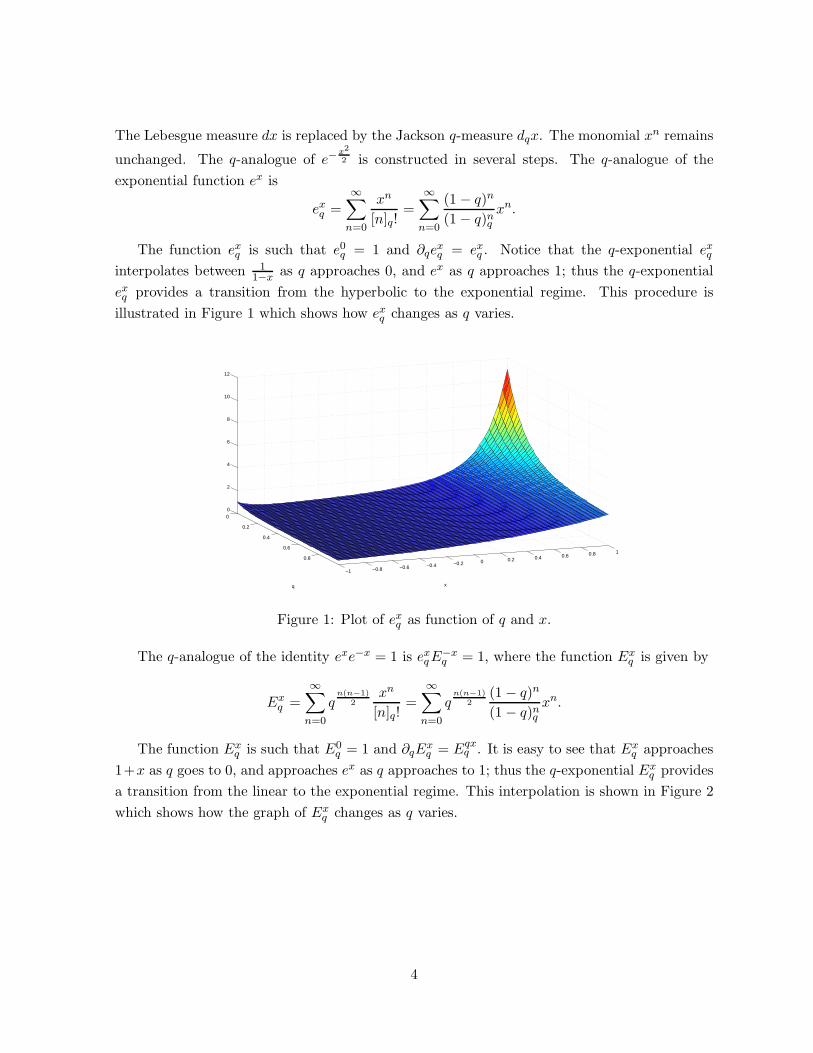
The function exq is such that e0
q = 1 and ∂qexq = ex
q . Notice that the q-exponential exq
interpolates between 11−x
as q approaches 0, and ex as q approaches 1; thus the q-exponential
exq provides a transition from the hyperbolic to the exponential regime. This procedure is
illustrated in Figure 1 which shows how exq changes as q varies.
0
0.2
0.4
0.6
0.8
−1 −0.8 −0.6 −0.4 −0.2 0 0.2 0.4 0.6 0.8 1
0
2
4
6
8
10
12
xq
Figure 1: Plot of exq as function of q and x.
The q-analogue of the identity exe−x = 1 is exqE−x
q = 1, where the function Exq is given by
Exq =
∞∑
n=0
qn(n−1)
2xn
[n]q!=
∞∑
n=0
qn(n−1)
2(1 − q)n
(1 − q)nqxn.
The function Exq is such that E0
q = 1 and ∂qExq = E
qxq . It is easy to see that Ex
q approaches
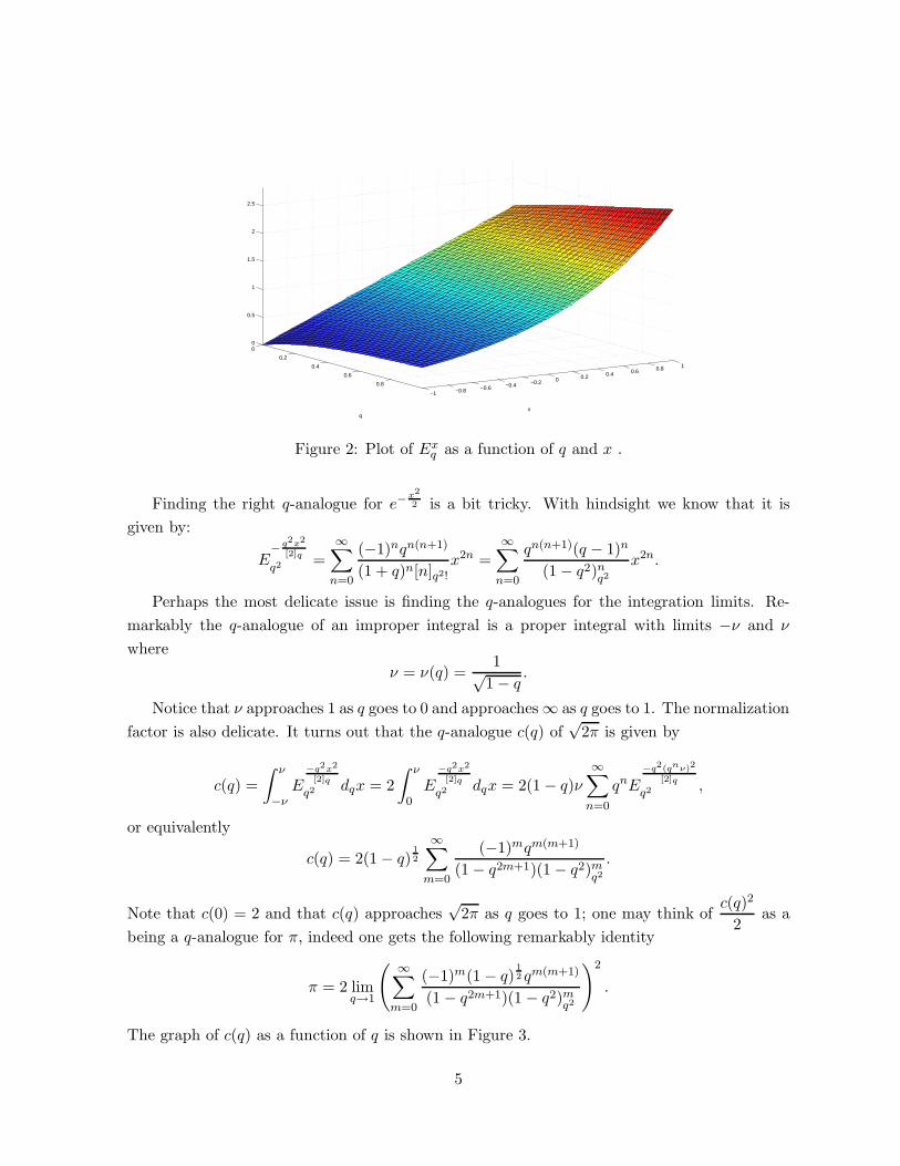
1+x as q goes to 0, and approaches ex as q approaches to 1; thus the q-exponential Exq provides
a transition from the linear to the exponential regime. This interpolation is shown in Figure 2
which shows how the graph of Exq changes as q varies.
4
0
0.2
0.4
0.6
0.8
−1 −0.8 −0.6 −0.4 −0.2 0 0.2 0.4 0.6 0.8 1
0
0.5
1
1.5
2
2.5
xq
Figure 2: Plot of Exq as a function of q and x .
Finding the right q-analogue for e−x2
2 is a bit tricky. With hindsight we know that it is
given by:
E− q2x2
[2]q
q2 =∞∑
n=0
(−1)nqn(n+1)
(1 + q)n[n]q2!x2n =
∞∑
n=0
qn(n+1)(q − 1)n
(1 − q2)nq2
x2n.
Perhaps the most delicate issue is finding the q-analogues for the integration limits. Re-
markably the q-analogue of an improper integral is a proper integral with limits −ν and ν
where
ν = ν(q) =1√
1 − q.
Notice that ν approaches 1 as q goes to 0 and approaches ∞ as q goes to 1. The normalization
factor is also delicate. It turns out that the q-analogue c(q) of√
2π is given by
c(q) =
∫ ν
−ν
E
−q2x2
[2]q
q2 dqx = 2
∫ ν
0E
−q2x2
[2]q
q2 dqx = 2(1 − q)ν
∞∑
n=0
qnE
−q2(qnν)2
[2]q
q2 ,
or equivalently
c(q) = 2(1 − q)12
∞∑
m=0
(−1)mqm(m+1)
(1 − q2m+1)(1 − q2)mq2
.
Note that c(0) = 2 and that c(q) approaches√
2π as q goes to 1; one may think ofc(q)2
2as a
being a q-analogue for π, indeed one gets the following remarkably identity
π = 2 limq→1
( ∞∑
m=0
(−1)m(1 − q)12 qm(m+1)
(1 − q2m+1)(1 − q2)mq2
)2
.
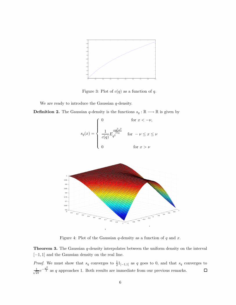
The graph of c(q) as a function of q is shown in Figure 3.
5
0 0.1 0.2 0.3 0.4 0.5 0.6 0.7 0.8 0.92
2.05
2.1
2.15
2.2
2.25
2.3
2.35
2.4
2.45
2.5
Figure 3: Plot of c(q) as a function of q.
We are ready to introduce the Gaussian q-density.
Definition 2. The Gaussian q-density is the functions sq : R −→ R is given by
sq(x) =
0 for x < −ν,
1
c(q)E
−q2x2
[2]q
q2 for − ν ≤ x ≤ ν
0 for x > ν
00.1
0.20.3
0.40.5
0.60.7
0.80.9
1 −1−0.8
−0.6−0.4
−0.20
0.20.4
0.60.8
10.6
0.65
0.7
0.75
0.8
0.85
0.9
0.95
1
x
q
Figure 4: Plot of the Gaussian q-density as a function of q and x.
Theorem 3. The Gaussian q-density interpolates between the uniform density on the interval
[−1, 1] and the Gaussian density on the real line.
Proof. We must show that sq converges to 121[−1,1] as q goes to 0, and that sq converges to
1√2π
e−x2
2 as q approaches 1. Both results are immediate from our previous remarks.
6
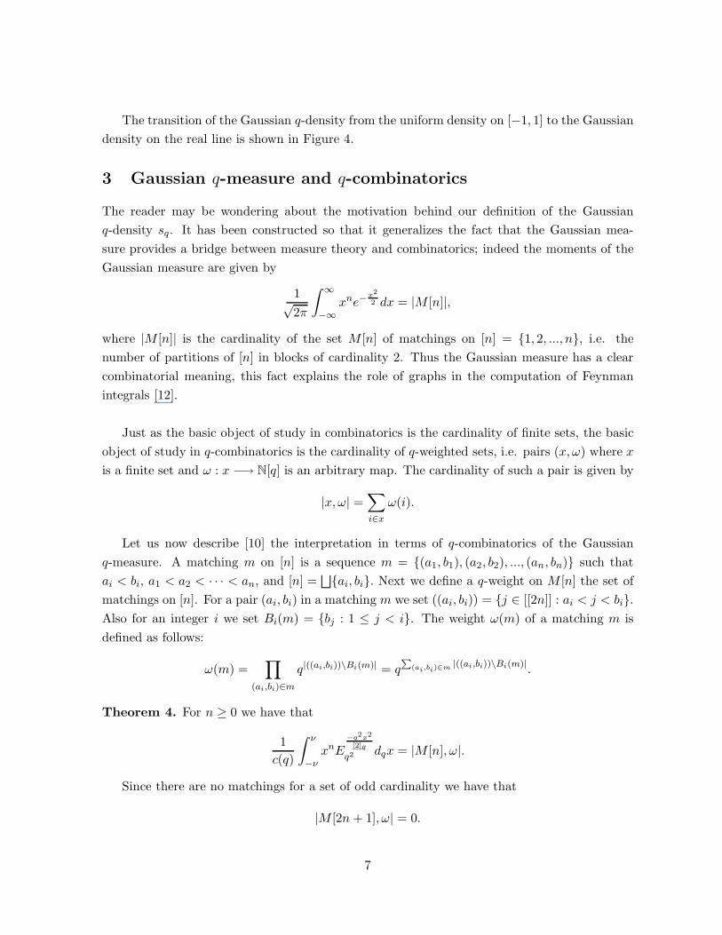
The transition of the Gaussian q-density from the uniform density on [−1, 1] to the Gaussian
density on the real line is shown in Figure 4.
3 Gaussian q-measure and q-combinatorics
The reader may be wondering about the motivation behind our definition of the Gaussian
q-density sq. It has been constructed so that it generalizes the fact that the Gaussian mea-
sure provides a bridge between measure theory and combinatorics; indeed the moments of the
Gaussian measure are given by
1√2π
∫ ∞
−∞xne−
x2
2 dx = |M [n]|,
where |M [n]| is the cardinality of the set M [n] of matchings on [n] = {1, 2, ..., n}, i.e. the
number of partitions of [n] in blocks of cardinality 2. Thus the Gaussian measure has a clear
combinatorial meaning, this fact explains the role of graphs in the computation of Feynman
integrals [12].
Just as the basic object of study in combinatorics is the cardinality of finite sets, the basic
object of study in q-combinatorics is the cardinality of q-weighted sets, i.e. pairs (x, ω) where x
is a finite set and ω : x −→ N[q] is an arbitrary map. The cardinality of such a pair is given by
|x, ω| =∑
i∈x
ω(i).
Let us now describe [10] the interpretation in terms of q-combinatorics of the Gaussian
q-measure. A matching m on [n] is a sequence m = {(a1, b1), (a2, b2), ..., (an, bn)} such that
ai < bi, a1 < a2 < · · · < an, and [n] =⊔{ai, bi}. Next we define a q-weight on M [n] the set of
matchings on [n]. For a pair (ai, bi) in a matching m we set ((ai, bi)) = {j ∈ [[2n]] : ai < j < bi}.Also for an integer i we set Bi(m) = {bj : 1 ≤ j < i}. The weight ω(m) of a matching m is
defined as follows:
ω(m) =∏
(ai,bi)∈m
q|((ai,bi))\Bi(m)| = qP
(ai,bi)∈m |((ai,bi))\Bi(m)|.
Theorem 4. For n ≥ 0 we have that
1
c(q)
∫ ν
−ν
xnE
−q2x2
[2]q
q2 dqx = |M [n], ω|.
Since there are no matchings for a set of odd cardinality we have that
|M [2n + 1], ω| = 0.
7
One can show by induction that
|M [2n], ω| = [2n − 1]q!! = [2n − 1]q[2n − 3]q.....[3]q .
Therefore we have that
• 1c(q)
∫ ν
−ν
x2n+1E
−q2x2
[2]q
q2 dqx = 0.
• 1c(q)
∫ ν
−ν
x2nE
−q2x2
[2]q
q2 dqx = [2n − 1]q!!.
The q-combinatorial interpretation of the Gaussian q-measure is the starting point for our
construction of q-measures of the Jackson-Feynman type in [9, 10]. It would be interesting
to study the categorical analogues of these q-measures along the lines of [3, 12]. The reader
should note that the formula above provides a q-integral representation the q-analogue of the
Pochhammer k-symbol with k = 2. A q-integral representation for the general Pochhammer
q, k-symbol is treated in [13]. The integral representation of the Pochhammer k-symbol is
studied in [11].
4 Gaussian q-distribution
Let us study how probabilities are distributed on the real line according to the Gaussian q-
distribution.
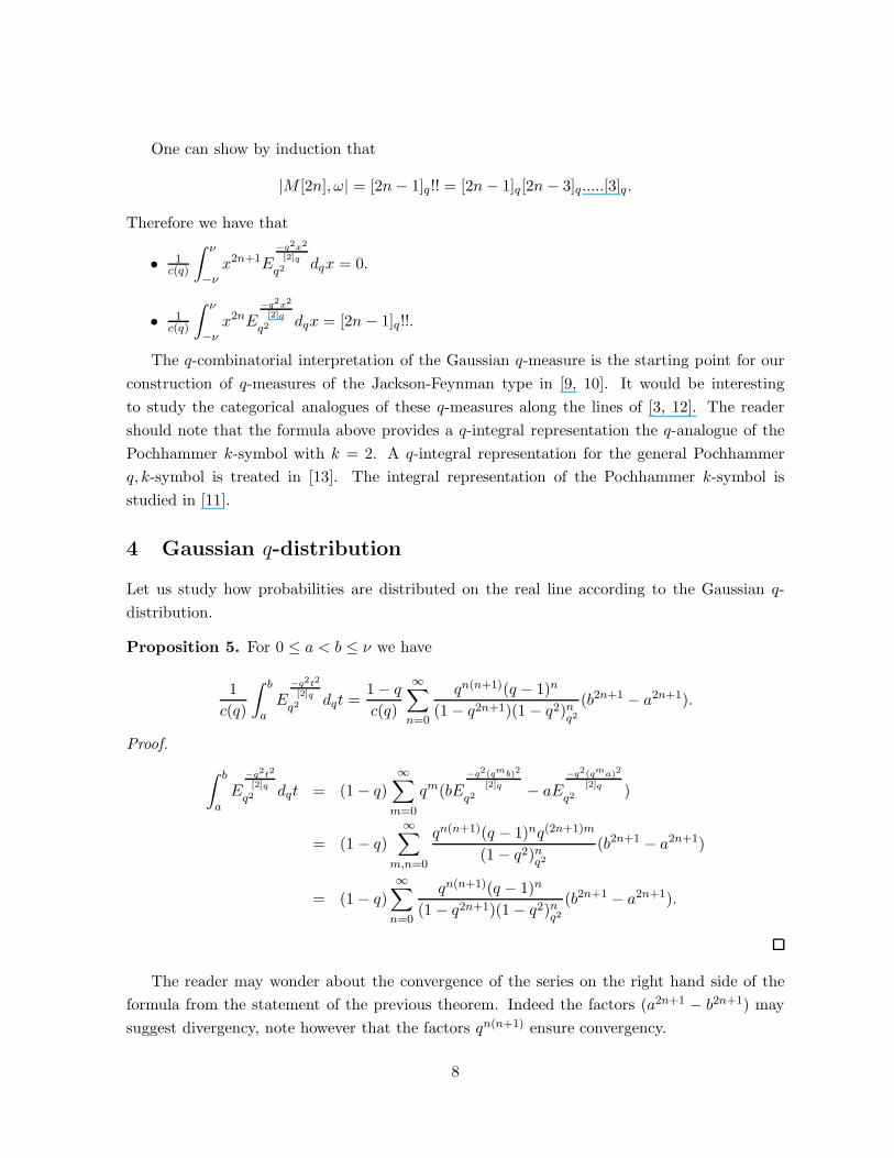
Proposition 5. For 0 ≤ a < b ≤ ν we have
1
c(q)
∫ b
a
E
−q2t2
[2]q
q2 dqt =1 − q
c(q)
∞∑
n=0
qn(n+1)(q − 1)n
(1 − q2n+1)(1 − q2)nq2
(b2n+1 − a2n+1).
Proof.
∫ b
a
E
−q2t2
[2]q
q2 dqt = (1 − q)∞∑
m=0
qm(bE−q2(qmb)2
[2]q
q2 − aE
−q2(qma)2
[2]q
q2 )
= (1 − q)
∞∑
m,n=0
qn(n+1)(q − 1)nq(2n+1)m
(1 − q2)nq2
(b2n+1 − a2n+1)
= (1 − q)∞∑
n=0
qn(n+1)(q − 1)n
(1 − q2n+1)(1 − q2)nq2
(b2n+1 − a2n+1).
The reader may wonder about the convergence of the series on the right hand side of the
formula from the statement of the previous theorem. Indeed the factors (a2n+1 − b2n+1) may
suggest divergency, note however that the factors qn(n+1) ensure convergency.
8
Definition 6. The Gaussian q-distribution Gq : R −→ R is given by
Gq(x) =
0 for x < −ν,
1
c(q)
∫ x
−ν
E
−q2t2
[2]q
q2 dqt for − ν ≤ x ≤ ν
1 for x > ν
Below we need the following notation, if A ⊆ R then as usual we define the characteristic
function 1A as follows:
1A(x) =
0 for x not in A,
1 for x in A.
Next result provides explicit formulae for the Gaussian q-distribution.
Theorem 7. For x ∈ R we have that:
Gq(x) = 1[−(1−q)−1/2,(1−q)−1/2](x)
(
1
2+
1 − q
c(q)
∞∑
n=0
qn(n+1)(q − 1)n
(1 − q2n+1)(1 − q2)nq2
x2n+1
)
+1((1−q)−1/2 ,∞)(x).
Proof. The result follow from the previous proposition, the fact that sq(x) is symmetric about
the origin, and the straightforward set theoretical identities:
[−ν, x] ⊔ [x, 0] = [−ν, 0] for − ν ≤ x ≤ 0;
[−ν, x] = [−ν, 0] ⊔ [0, x] for 0 ≤ x ≤ ν.
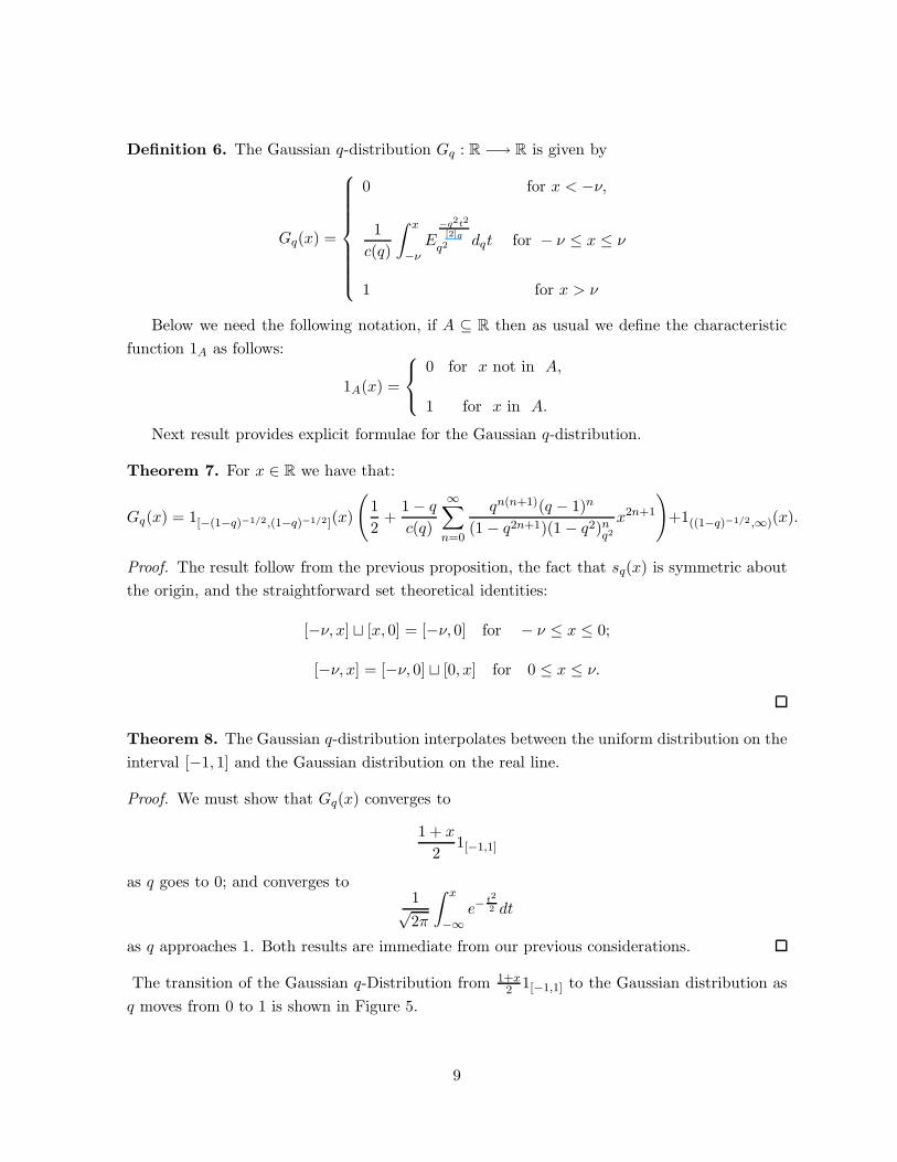
Theorem 8. The Gaussian q-distribution interpolates between the uniform distribution on the
interval [−1, 1] and the Gaussian distribution on the real line.
Proof. We must show that Gq(x) converges to
1 + x
21[−1,1]
as q goes to 0; and converges to1√2π
∫ x
−∞e−
t2
2 dt
as q approaches 1. Both results are immediate from our previous considerations.
The transition of the Gaussian q-Distribution from 1+x2 1[−1,1] to the Gaussian distribution as
q moves from 0 to 1 is shown in Figure 5.
9
0.1
0.2
0.3
0.4
0.5
0.6
0.7
0.8
0.9−1 −0.8 −0.6 −0.4 −0.2 0 0.2 0.4 0.6 0.8 1
0
0.1
0.2
0.3
0.4
0.5
0.6
0.7
0.8
0.9
1
xq
Figure 5: Plot of the Gaussian q-distribution for −1 ≤ x ≤ 1.
5 Conclusion
The countless applications of the Gaussian measure in mathematics, science and engineering,
suggest that the Gaussian q-measure may also find its share of applications. We showed that as
q moves from 0 to 1 the Gaussian q-density and the Gaussian q-distribution interpolate between
the uniform density and the uniform distribution on the interval [−1, 1] to the Gaussian density
and the Gaussian distribution. Note that the transition from specialization to uniformity is a
common phenomena both in nature and in mathematics. Indeed, we are used the see objects
breaking apart but we seldom see them coming back together to form a unity from the many
pieces. Likewise in mathematics the transfer of heat in a compact manifold will eventually end
up with a uniform temperature trough out the manifold, regardless of the fact that the initial
distribution of heat many have been localized around some point. The reverse transition form
uniformity to specialization occurs less often, yet it is a standard phenomena in certain domains
of nature, phenomena of such type play a most fundamental role in some chemical interactions
and in microbiology. For that reason we believe that our Gaussian q-measure may find some
applications in those fields of study.
Acknowledgment
Our thanks to Nicolas Vega and Camilo Ortiz for assisting us with the figures which were drawn
using the computer software MATLAB.
References
[1] G. Andrews, The theory of partitions, Cambridge Univ. Press, Cambridge 1938.
10
[2] G. Andrews, R. Askey, R. Roy, Special functions, Cambridge Univ. Press, Cambridge 1999.
[3] H. Blandın, R. Dıaz, Rational combinatorics, Adv. Appl. Math. 40 (2008) 107-126.
[4] M. Bozejko, B. Kummerer, R. Speicher, q-Gaussian Processes: Non-commutative and
Classical Aspects, Comm. Math. Phys. 185 (1997) 129154.
[5] W. Bryc, Classical versions of q-Gaussian processes: conditional moments and Bell’s in-
equality, Comm. Math. Phys. 219 (2001) 259-270.
[6] W. Bryc, W. Matysiak, P. Szablowski, Probabilistic Aspects of al-SalamChihara Polyno-
mials, Proc. Amer. Math. Soc. 133 (2005) 1127-1134.
[7] P. Cheung, V. Kac, Quantum calculus, Springer-Verlag, Berlin 2002.
[8] A. De Sole, V. Kac, On integral representations of q-gamma and q-beta functions, Atti.
Accad. Naz. Lincei Cl. Sci. Fis. Mat. Natur. Rend. Lincei 9. Mat. Appl. 16 (2005) 11-29.
[9] R. Dıaz, E. Pariguan, An example of Feynman-Jackson integral, J. Phys. A 40 (2007)
1265-1272.
[10] R. Dıaz, E. Pariguan, Feynman-Jackson integrals, J. Nonlinear Math. Phys. 13 (2006)
365-376.
[11] R. Dıaz, E. Pariguan, On hypergeometric functions and Pochhammer k-symbol, Divulg.
Mat. 15 (2007) 179-192.
[12] R. Dıaz, E. Pariguan, Super, Quantum and Non-commutative Species, preprint,
arXiv:math.CT/0509674.
[13] R. Dıaz, C. Teruel, q,k-generalized gamma and beta functions, J. Nonlinear Math. Phys.
12 (2005) 118–134.
[14] G. Gasper, M. Rahman, Basic hypergeometric series, Cambridge Univ. Press, Cambridge
1990.
[15] M. Gell-Mann, C. Tsallis (Eds.), Nonextensive Entropy: Interdisciplinary Applications,
Oxford Univ. Press, New York 2004.
[16] H. van Leeuven, H. Maassen, A q-Deformation of the Gauss distribution, J. Math. Phys.
36 (1995) 4743-4756
[17] B. Kupershmidt, q-Probability: I. Basic Discrete Distributions, J. Nonlinear Math. Phys.
7 (2000) 73-93.
11
[18] A. R. Plastino, A. Platino, Non-extensive statistical mechanics and generalized Fokker-
Planck equation, Physica. A 222 (1995) 347.
[19] D. Prato, C. Tsallis; Nonextensive foundation of Levy distributions, Phys. Rev. E 60 (1999)
2398.
[20] C. Tsallis, D. Bukman, Anomalous diffusion in the presence of external forces: exact time-
dependent solutions and their thermostatistical basis, Phys. Rev. E 54 (1996) R2197.
[21] C. Tsallis, Possible generalization of Boltzmann-Gibbs statistics, J. Stat. Phys. 52 (1988)
479-487.
[22] C. Tsallis, S. V. F. Levy, A. M. C. de Souza, R. Maynard; Statistical-mechanical foundation
of the ubiquity of Levy distributions in nature, Phys. Rev. Lett. 75 (1995) 3589; 77 (1996)
5442 (erratum).
[23] S. Umarov, C. Tsallis, S. Steinberg, A generalization of the central limit theorem consistent
with nonextensive statistical mechanics, preprint, arXiv:cond-mat/0603593.
[24] D. Zeilberger, Proof of the Refined Alternating Sing Matrix Conjecture, New York J. Math.
2 (1996) 59-68.
Facultad de Administracion, Universidad del Rosario, Bogota, Colombia
Departamento de Matematicas, Pontificia Universidad Javeriana, Bogota, Colombia.
12