Distribution of charge carrier transport properties in organic semiconductors with Gaussiandisorder

Jens Lorrmann,1, ∗ Manuel Ruf,1 David Vocke,1 Vladimir Dyakonov,1, 2 and Carsten Deibel1, †

1Experimental Physics VI, Julius Maximilian University of Wurzburg, 97074 Wurzburg, Germany2Bavarian Center for Applied Energy Research e.V. (ZAE Bayern), 97074 Wurzburg, Germany

(Dated: May 1, 2014)

The charge carrier drift mobility in disordered semiconductors is commonly graphically extracted from time-of-flight (TOF) photocurrent transients yielding a single transit time. However, the term transit time is ambigu-ously defined and fails to deliver a mobility in terms of a statistical average. Here, we introduce an advancedcomputational procedure to evaluate TOF transients, which allows to extract the whole distribution of transittimes and mobilities from the photocurrent transient, instead of a single value. This method, extending thework of Scott et al. (Phys. Rev. B 46, 8603), is applicable to disordered systems with a Gaussian density ofstates (DOS) and its accuracy is validated using one-dimensional Monte Carlo simulations. We demonstratethe superiority of this new approach by comparing it to the common geometrical analysis of hole TOF tran-sients measured on poly(3-hexyl thiophene-2,5-diyl) (P3HT). The extracted distributions provide access to avery detailed and accurate analysis of the charge carrier transport. For instance, not only the mobility given bythe mean transit time, but also the mean mobility can be calculated. Whereas the latter determines the macro-scopic photocurrent, the former is relevant for an accurate determination of the energetic disorder parameterσ within the Gaussian disorder model (GDM). σ derived by using the common geometrical method is, as weshow, underestimated instead.

I. INTRODUCTION

Disordered or amorphous semiconductors provide the po-tential of cheap future electronics with a wide variance ofphysical properties, e.g., the absorption spectrum. This flexi-bility allows to design them for specific areas of application,ranging from transistors and light emitting diodes to sunlightharvesting and converting solar cells. A common key featuredetermining the electrical device performance in these mate-rials is the hopping type charge carrier transport. Therefore,during the last decades a lot of effort has been put into studiesto understand the detailed transport mechanism, experimen-tally and theoretically.1–6

In classical descriptions the charge transport is based onthe electrostatic force induced drift and on diffusion due toa spatial charge carrier density gradient. The related pa-rameters are the charge carrier mobility µ and charge car-rier diffusivity or diffusion constant D, respectively, whichare connected by the classical Einstein7–Smoluchowski8 re-lation D/µ = kBT/e. Here, kB is the Boltzmann coefficient,e the elementary charge and T the temperature. This conceptsuccessfully describes semiconductor devices coupling con-tinuity and Poisson equations9,10 in combination with phys-ical models concerning, e.g., dissociation11,12 or recombina-tion.13,14

However, in the case of disordered systems it is known thatthe concept of mobility can be ill-defined15 or, in other words,the transport is determined by a broad distribution of mobili-ties. This fact is due to the random nature of the charge car-rier transport in an energetically and spatially disordered en-vironment. It leads to energetic relaxation of the charge car-riers with time,15–18 and to an inhomogeneous distribution of

∗ jens@lorrmann.de† deibel@disorderedmatter.eu

transport properties throughout thin-film devices.19–22 A de-tailed experimental investigation of the relation between themacroscopic behaviour and the microscopic transport statis-tics, however, requires the extraction of transport parameterdistributions. Furthermore, conclusions in terms of the energydistribution of the DOS may be drawn from the shape of thesedistributions. Such an approach should significantly improvethe ability to evaluate the consistency between experimentaldata and various theoretical models. In turn, we consider itas a fundamental step towards a more general functional de-scription of the charge carrier transport in disordered systemsin terms of drift and diffusion. In several cases, such descrip-tions are already available,15,16,18,21,23–26 but not in the generalform presented here.

First attempts to experimentally extract mobility distribu-tions from time-of-flight (TOF)27–29 measurements or fromthe turn-on dynamics of polymer photo-cells where publishedby Scott et al.30 and Rappaport et al.,20,31 respectively. Un-fortunately, the method by Scott et al. was seldom used sinceits publication in 1992.32,33 The same holds for the methodpublished by Rappaport et al. Moreover the full potential util-ising the statistics of the extracted parameter distributions washardly ever discussed. In the case of Scott’s method this isprobably due to the fact that the method in the original formis not suitable for systems exhibiting a Gaussian density ofstates (DOS), found in many organic semiconductors, suh asthe widely used conjugated polymer poly(3-hexyl thiophene-2,5-diyl) (P3HT).

In this paper we extend the method by Scott et al. with re-spect to a Gaussian DOS and reveal the advantages of this ap-proach over the conventional geometrical technique to extractmobilities. The geometrical method determines the chargecarrier mobility from a particular transit time, which is graph-ically extracted from TOF transients. This transit time is de-fined by the intersection of the fits to the pre- and the post-transit sections of the photocurrent transient, respectively15,34.

arX

iv:1

209.

1922

v5 [

cond

-mat

.dis

-nn]

30

Apr

201

4

2

Henceforth we refer to the methods compared in this work asthe modified Scott method and the geometric method, respec-tively. To verify the accuracy of the our new approach and themodifications to Scott’s method we utilise a one-dimensionalMonte Carlo simulation. Generally, the justification of an al-ternative approach is best demonstrated in comparison to awell-established standard method. Hence, the comparison isdone here by evaluating the hole TOF transients measured onP3HT with the modified Scott and the geometric method, re-spectively. Subsequently, we identify the statistical averagesof the transit times and the mobilities from the transit timeand mobility distributions, and match them against the transittimes and mobilities determined from the geometric analysisof TOF transients.

Although convenient to use, it is, however, well knownthat the geometric method extracts single value transit timeswhich account for the fastest carriers only.35,36 We demon-strate below, that the corresponding mobilities are not relatedto the average values and that the relative deviation dependsstrongly on temperature and electric field. Furthermore, thegeometric method is more prone to evaluation errors, as, inthe case of systems exhibiting a Gaussian DOS, the fitted re-gions just span over a very small part of the current transientand the regions’ boundaries are judged by the eye, which maylead to huge uncertainties on a double-logarithmic scale. Onthe other hand, the modified Scott method, as will be shownbelow, needs just one fit spanning over more than one orderof magnitude in time. Novikov et al. explicitly discussed theconsequences of using poorly defined transit times or mobili-ties in Ref. 37 and asked for a safe and reliable procedure forthe analysis of TOF data. We believe that the new approachpresented here fulfils this request, by experimentally provid-ing detailed and comprehensive information, as it is usuallyonly known from Monte Carlo simulations.

In Sec. II, we describe the experimental method, whereasthe new approach of data evaluation is described in Sec. III.The modeling approach is explained in Sec. IV. Sec. V con-tains the results: In part A we verify Eqn. (1), in part B thenew approach is used to analyse the measured TOF transientsand the findings are compared with the results obtained by theconventional geometric analysis in part C, while in part D theenergetic disorder parameter σ of the P3HT hole DOS is de-rived.

II. EXPERIMENTAL METHOD

The studied devices were prepared in a diode configura-tion, with P3HT 4002E (∼ 94% regioregular; Rieke MetalsInc., without further purification) as the active material, dropcast on ITO covered glass with an aluminium electrode ther-mally evaporated on top. The sample thickness and excitationintensity were chosen in a way to ensure a photogenerationof charge carriers confined to the first 10% of the bulk thick-ness. For TOF measurements the sample was mounted in aHe closed-cycle cryostat allowing field and temperature de-pendent studies. For the optical excitation we used the secondharmonic of a pulsed Nd:YAG laser emitting at λ = 532nm,

close to the absorption maximum of the polymer,38 togetherwith optical intensity attenuators.

Adjusting the polarity of the applied constant electric field,one can select the type of the charge carriers being draggedthrough the bulk and extracted at the counter-electrode.TheTOF transients for holes in P3HT where measured in the tem-peratures range between T = 110− 300K and at differentelectric fields between F = 1.3×107−1.9×108 V

m .

III. EVALUATION METHOD

Before describing the modified Scott method, it is worthhaving a closer look at the photocurrent decay prior to extrac-tion of charge carriers, as its functional approximation is anessential part of our modification.

In general the photogenerated excitons dissociate under theinfluence of the applied electric field, which directs the sepa-rated charge carriers to the corresponding electrodes. Whileone sort of charge carriers is being extracted at the illuminatedelectrode resulting, the other sort of charge carriers movesthrough the device to the counterelectrode, where they are ex-tracted. This motion of charge carriers yields the photocur-rent in the external circuit. Due to the extraction, the pho-tocurrent steeply drops towards zero until no mobile chargecarriers are left within the device. However, the photocur-rent decreases even before extraction due to energetic relax-ation of the charge carriers within the DOS.16–18,21 Associatedwith this relaxation is a dispersion of the charge carrier pack-age being stronger than predicted for purely Gaussian (non-dispersive) transport, together with a decreasing mean driftvelocity with time.16,39 As a consequence, the distribution oftransit times is broadened and thus the drop in the photocur-rent at the extraction is blurred.

In case of a purely exponential DOS the scenario describedabove can be explained within the framework of Scher andMontroll15 yielding a power law for the pre-transit ( j0(t) ∝

t−(1−αpre)) photocurrent. Note that this behaviour in combi-nation with the predicted post-transit current j(t) ∝ t−(1+αpost )

builds the basis of the geometric analysis.34 In contrast to theexponential DOS, where transient measurements strictly fol-low these power laws at least “as long as one would be ableto measure”,40 it is well known that a Gaussian DOS yieldsa saturation of the transient photocurrent in time, thus it is apower law with a time dependent exponent j0(t) ∝ tα(t). Thetime dependence of α(t) is related to experimental parame-ters, such as the temperature and the applied electric field, andmaterial properties (energetic and spatial disorder).16,39 Un-fortunately, a plain functional description of α(t) and, thus,the photocurrent decay j0(t), similar to the power law relationfor a exponential DOS, is not available. However, taking intoaccount that α(t) is a gradually decreasing function and thatlimt→∞

α(t) = 0, we suggest the following empirical approxima-

3

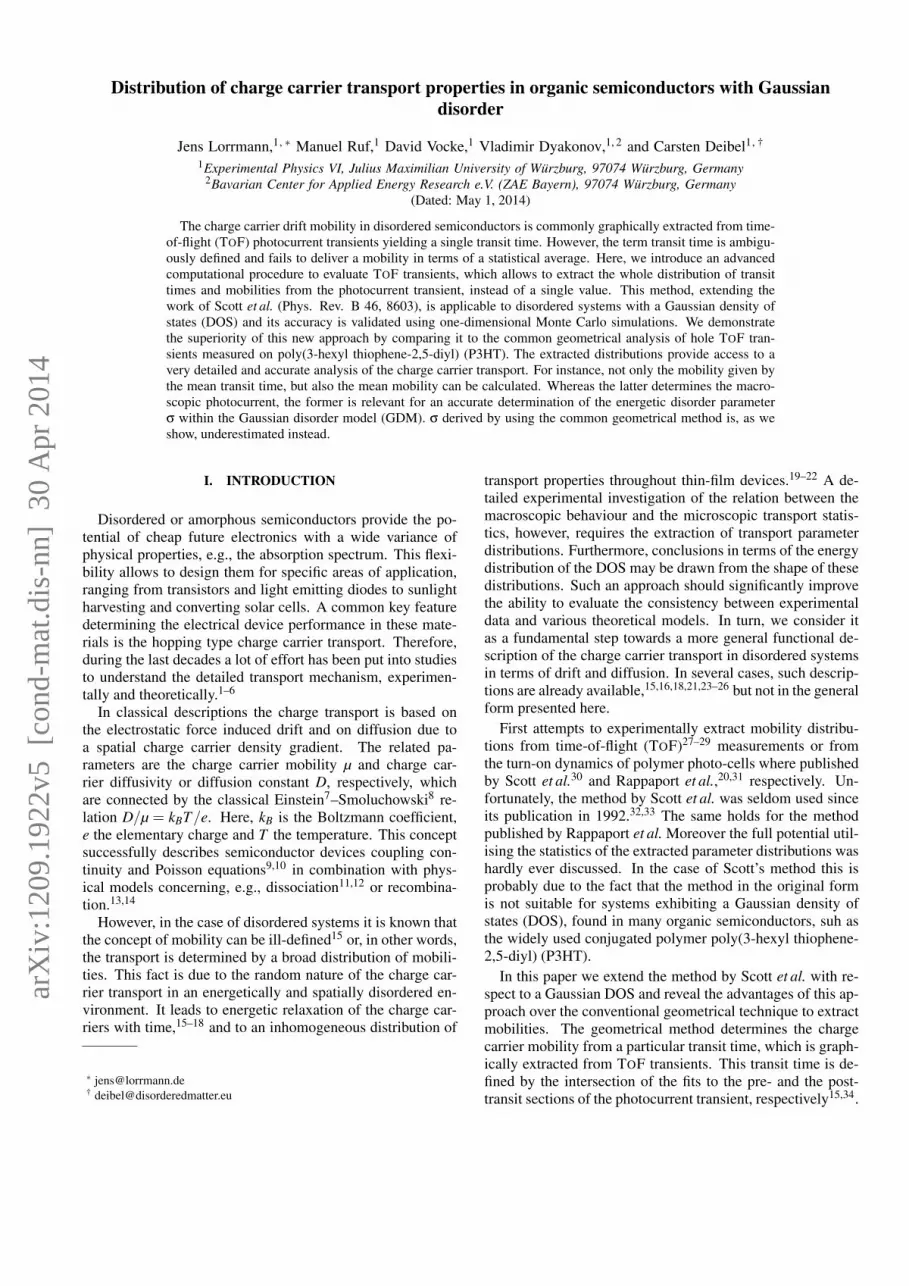
TABLE I. Overview over the four different mobility definitions used throughout this Paper.

Name relation to transit time physical context Scheme

modified Scott method

log(t)

log(j)j(t)

j0(t)

ptr(t)

〈ttr〉〈ttr 〉-1

µm ∝

⟨1ttr

⟩ensemble average mobility; determinesthe macroscopic photocurrent

µtr,m ∝1〈ttr〉

related to average transit time; oftenused in Monte Carlo simulations

geometric method

log(t)

log(j)j(t)

ttr,geo ttr,1/2

jpost

jpre

1/2∙jpre

µgeo ∝1

ttr,geo

time at which the first charge carriersreach the counterelectrode

µ1/2 ∝1

ttr,1/2

time at which ∼ 50% of the charge car-riers were extracted

tion of j0(t):

j0(t) = j∗0t−α(t) (1a)

α(t) =(

τ

t

)β

. (1b)

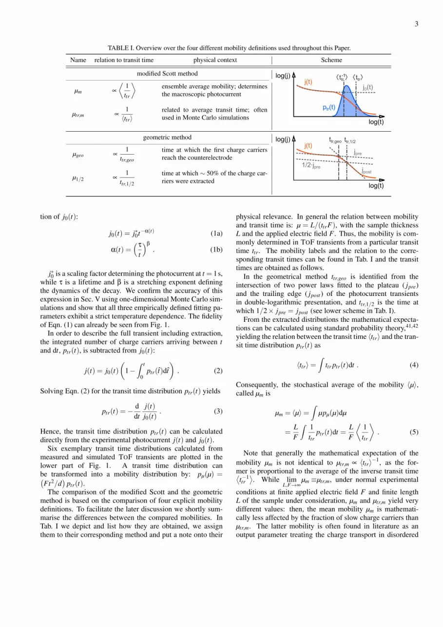
j∗0 is a scaling factor determining the photocurrent at t = 1s,while τ is a lifetime and β is a stretching exponent definingthe dynamics of the decay. We confirm the accuracy of thisexpression in Sec. V using one-dimensional Monte Carlo sim-ulations and show that all three empirically defined fitting pa-rameters exhibit a strict temperature dependence. The fidelityof Eqn. (1) can already be seen from Fig. 1.

In order to describe the full transient including extraction,the integrated number of charge carriers arriving between tand dt, ptr(t), is subtracted from j0(t):

j(t) = j0(t)(

1−∫ t

0ptr(t)dt

). (2)

Solving Eqn. (2) for the transit time distribution ptr(t) yields

ptr(t) =−ddt

j(t)j0(t)

. (3)

Hence, the transit time distribution ptr(t) can be calculateddirectly from the experimental photocurrent j(t) and j0(t).

Six exemplary transit time distributions calculated frommeasured and simulated TOF transients are plotted in thelower part of Fig. 1. A transit time distribution canbe transformed into a mobility distribution by: pµ(µ) =(Ft2/d

)ptr(t).

The comparison of the modified Scott and the geometricmethod is based on the comparison of four explicit mobilitydefinitions. To facilitate the later discussion we shortly sum-marise the differences between the compared mobilities. InTab. I we depict and list how they are obtained, we assignthem to their corresponding method and put a note onto their

physical relevance. In general the relation between mobilityand transit time is: µ = L/(ttrF), with the sample thicknessL and the applied electric field F . Thus, the mobility is com-monly determined in TOF transients from a particular transittime ttr. The mobility labels and the relation to the corre-sponding transit times can be found in Tab. I and the transittimes are obtained as follows.

In the geometrical method ttr,geo is identified from theintersection of two power laws fitted to the plateau ( jpre)and the trailing edge ( jpost ) of the photocurrent transientsin double-logarithmic presentation, and ttr,1/2 is the time atwhich 1/2× jpre = jpost (see lower scheme in Tab. I).

From the extracted distributions the mathematical expecta-tions can be calculated using standard probability theory,41,42

yielding the relation between the transit time 〈ttr〉 and the tran-sit time distribution ptr(t) as

〈ttr〉=∫

ttr ptr(t)dt . (4)

Consequently, the stochastical average of the mobility 〈µ〉,called µm is

µm = 〈µ〉=∫

µpµ(µ)dµ

=LF

∫ 1ttr

ptr(t)dt =LF

⟨1ttr

⟩. (5)

Note that generally the mathematical expectation of themobility µm is not identical to µtr,m ∝ 〈ttr〉−1, as the for-mer is proportional to the average of the inverse transit time⟨t−1tr⟩. While lim

L,F→∞µm ≡µtr,m, under normal experimental

conditions at finite applied electric field F and finite lengthL of the sample under consideration, µm and µtr,m yield verydifferent values: then, the mean mobility µm is mathemati-cally less affected by the fraction of slow charge carriers thanµtr,m. The latter mobility is often found in literature as anoutput parameter treating the charge transport in disordered

4

materials using Monte Carlo21 or Master Equation1,24 sim-ulations. In case of quasi-Gaussian (non-dispersive) trans-port the gaussian shaped charge carrier package drifts exactlywith the velocity µtr,mF through the device and µtr,m is inde-pendent of the sample thickness L and the applied electricfield F . µm, instead, is linked to the average charge carriertransport and determines the macroscopic current density byj = enF

∫µpµ(µ)dµ = enFµm.

IV. SIMULATION METHOD

In order to verify our approach, a one-dimensional MonteCarlo simulation43,44 was implemented to study charge carriertransport by hopping. It considers the capture and the emis-sion of charge carriers according to the multiple trapping andrelease (MTR) model. Before further specifying the simula-tion procedure, we first recall some details of the MTR-modeldeveloped by Schmidlin et al.45 and Noolandi et al.46

Originally the presence of extended states in the valenceand conduction bands and localised trapping states in the bandgap were considered. In general to model the charge carriertransport any localised state in the band gap needs to be con-sidered as a possible target for a charge carrier jump. This,e.g. by kinetic Monte Carlo simulation in three dimensions,requires considerable amounts of both computer memory andcomputation time. However, transport within the band gapis very unlikely due to the fact that the transfer rate betweentwo states depends exponentially on the electronic coupling,which is very small in between states in the band gap. Thus,a charge carrier in the band gap will most probably be ther-mally excited to the mobility edge, which separates the lo-calised states with a low density from the extended states witha high density. The MTR model replaces the full picture ofhopping by a quasi-free transport until trapping of charge car-riers above the mobility edge and a thermal emission back toextended states of charge carriers below.

In disordered organic semiconductors instead, the valenceand conduction bands are described in terms of a Gaussiandistribution of localised states. Transport in these localisedstates occurs via hopping. The hopping transport resemblesthe MTR process near and below a temperature dependenttransport energy Etrans.47 Hence, in such a system, the trans-port energy Etrans plays the role of the mobility edge.17,48

In our simulation we model the transport of noninteractingcharge carriers. A charge carrier is either transfered to thetransport energy Etrans by thermal excitation from a trap stateor moves quasi-free above the transport energy Etrans until itis trapped again or reaches an electrode and is extracted. Byintegrating the duration of each individual process the modelgets a time dependence. This allows the simulation of tran-sient measurement techniques such as TOF.

Initially, all charge carriers are set in vicinity to the illumi-nated electrode and reside at the transport energy Etrans. Dur-ing the time until capture

τc =ln(ζ)

τ0(6)

the charge carriers at the transport energy move quasi-freewith the mobility µ0(F,T ) for a distance ∆x = τc×µ0(F,T )×F . Where τ0 = [ν0× exp(−2× γ×ax)]

−1 is the trapping ratewith the attempt-to-escape frequency ν0, the inverse localisa-tion length γ and the intermolecular distance ax. ζ is a uni-formly distributed random number between ]0,1], F is theelectric field and T the temperature. The charge carrier is thenrandomly trapped into one of the trapping levels Etrap with aprobability according to the Gaussian energy distribution ofthese levels. The release time from a trap level is given by

τr = τ0 exp(

Etrans−Etrap−axFkBT

)ln(ζ) , (7)

where kB the Boltzmann constant. To accurately fit the fielddependence of our TOF transients we included an exponen-tial field reduction factor axF/(kBT ) in Eqn. (7) accountingfor a field-induced detrapping.50–52 This factor yields the wellknown Poole-Frenkel effect53 by effectively reducing the hop-ping barrier for a charge carrier in direction of the electricfield.54 Tyutnev et al. implement an equivalent modification intheir MTRg-model55 to consistently explain the Pool-Frenkeleffect in accordance with three-dimensional kinetic MonteCarlo simulations.5,21,49.

From the temporal evolution of the charge carriers’ po-sitions in the sample, a mean current can be calculated byj(t) = en0v(t) where e is the elementary charge, n0 the num-ber of initially generated carriers and v(t) the carriers’ meanvelocity.

By suitable parameterisation of the model, experimentalmeasurements were reconstructed by simulation, offering adeeper insight into microscopic charge transport phenomena.To decrease the number free fitting parameters we firstly fixeda couple of the parameters to experimentally determined val-ues as well as physically reasonable literature values.

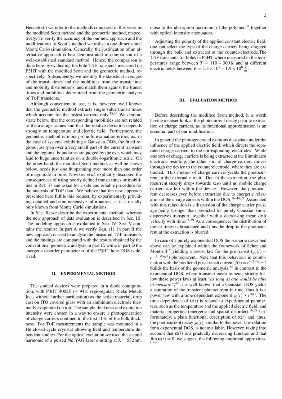
The energetic disorder parameter was set to be σ =69.9meV. This value was calculated from the temperaturedependence of the zero-field mobility in terms of the Gaus-sian disorder model.21 The attempt-to-escape frequency waschosen equal to ν0 = 1× 1013 s−1 from Ref. 49. We as-sumed a fixed transport energy at Etrans = 0eV. Fixed, be-cause we found just little impact of a temperature dependenttransport energy for the temperature range considered andequal to 0eV, because the effect of the real transport energyvalue on the transient shape is implicitly considered in the twofree fitting parameters ax and µ0(F,T ). In accordance with

TABLE II. Simulation parameters. The parameters were determinedby reconstruction of experimental TOF transients.

Parameter Value Unit Source

σ 69.9 meV see Textν0 1×1013 s−1 Ref. 49

Etrans 0.0 eV Approx.γ 3.91×109 m−1 Fitax 1.26×10−9 m Fit

µ0(F,T ) (0.8−2.15)×10−8 m2(Vs)−1 Fit

5

our experience Germs et al. found a temperature dependenceof the transport energy comparable to the fitting uncertaintyfor σ/(kBT ) < 5.1,39 — this is in our case T > 160K. Fur-ther input parameters are the inverse localisation length γ andthe intermolecular distance ax and the charge carrier mobilityµ0(F,T ).

To fully calibrate the simulation we simultaneously fit-ted a set of measurements at different temperatures betweenT = 175− 300K and at different electric fields F = 1.3×107 − 1.9× 108 V

m using the global minimisation algorithmof differential evolution.56 The used parameters are listed inTab. II, where we explicitly mark a parameter as fixed or fit-ted.

Note that from the one-dimensional Monte Carlo simula-tions the transit time distribution ptr(t) can be calculated di-rectly by the monitored gradual decrease of the number ofcharge carriers inside the device N(t). The relation is

ptr(t) =−dN(t)

dt. (8)

V. RESULTS

A. Verifying the initial photocurrent approximation Eqn. (1)

At first we demonstrate the quality of the empirical expres-sion Eqn. (1) of j0(t). To this end, we simulated a set oftemperature dependent (T = 200K− 300K) TOF transientsusing our one-dimensional Monte Carlo simulation and com-pare the transit time distributions obtained by the modifiedScott method with the temporal decrease of charge carriersinside the device according to Eqn. (8). The parameterisedvalues used in the simulation are listed in Tab. II. In the up-per right part of Fig. 1 the fit of Eqn. (1) to the simulatedpre-transit photocurrent decay is plotted together with the fullsimulated transients. The approximation of the photocurrentby j0(t) is excellent over up to four orders of magnitude intime. The equivalence of the extracted distributions is shownin the lower right part of Fig. 1: both transit time distributionsmatch perfectly well over the whole studied temperature rangeand verify the validity of the extrapolation of j0(t) to post-transit times. The corresponding average transit times of thesimulated ensemble of charge carriers and the values extractedfrom the transit time distributions ptr(t) by Eqn. (4) are equalwithin the range of numerical precision (∆〈ttr〉/〈ttr〉< 0.5%).Further testing of Eqn. (1) is provided in Appendix A.

Based on these results, we conclude that Eqn. (1) is a suit-able parametric approximation for the photocurrent decay andthat, thus, the modified Scott method can be applied to sys-tems with a Gaussian DOS.

B. Evaluating hole photocurrents with the new approach

We examined TOF transients measured on P3HT utilis-ing the presented approach. The findings are compared withthe results obtained by the conventional geometric analysis in

12

46

102

46

1002

curr

ent d

ensi

ty j

/ a.u

.

10-7

10-6

10-5

time t / s

6

4

2

0

trans

it tim

e di

strib

utio

n p t

r

0.01

0.1

1

10

100

curr

ent d

ensi

ty j

/ a.u

.

0.8

0.6

0.4

0.2

0.0

trans

it tim

e di

strib

utio

n p t

r

10-7 10

-5 10-3

time t /s

inc. field

inc. field

inc. temperature

inc. temperature

Experiment MC-Simulation

ToF transient fit to eq.(1)

ptr(t) after eq.(3)

ptr(t) after eq.(7)

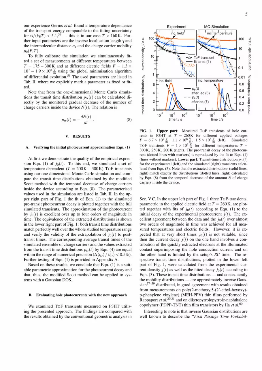
FIG. 1. Upper part: Measured TOF transients of hole cur-rents in P3HT at T = 260K for different applied voltagesF = 6.7 × 107 V

m , 1.1 × 108 Vm , 1.5 × 108 V

m (left). SimulatedTOF transients F = 1 × 107 V

m for different temperatures T =300K, 250K, 200K (right). The pre-transit decay of the photocur-rent (dotted lines with markers) is reproduced by the fit to Eqn. (1)(lines without markers). Lower part: Transit-time distribution ptr(t)for the experimental (left) and the simulated (right) transients calcu-lated from Eqn. (3). Note that the extracted distributions (solid lines,right) match exactly the distributions (dotted lines, right) calculatedby Eqn. (8) from the temporal decrease of the amount N of chargecarriers inside the device.

Sec. V C. In the upper left part of Fig. 1 three TOF-transients,parametric in the applied electric field at T = 260K, are plot-ted together with fits of j0(t) according to Eqn. (1) to theinitial decay of the experimental photocurrent j(t). The ex-cellent agreement between the data and the j0(t) over almosttwo orders of magnitude in time was achieved for all mea-sured temperatures and electric fields. However, it is ex-pected that at very short times j0(t) is not suitable, sincethen the current decay j(t) on the one hand involves a con-tribution of the quickly extracted electrons at the illuminatedcontact superimposing the hole conduction current and onthe other hand is limited by the setup’s RC time. The re-spective transit time distributions, plotted in the lower leftpart of Fig. 1, were calculated from the experimental cur-rent density j(t) as well as the fitted decay j0(t) according toEqn. (3). These transit time distributions — and consequentlythe mobility distributions — are approximately inverse Gaus-sian57–59 distributed, in good agreement with results obtainedfrom measurements on poly(2-methoxy,5-(2’-ethyl-hexoxy)-p-phenylene vinylene) (MEH-PPV) thin films performed byRappaport et al.20,31 and on diketopyrrolopyrrole-naphthalenecopolymer (PDPP-TNT) thin film transistors by Ha et al.60

Interesting to note is that inverse Gaussian distributions arewell known to describe the “First Passage Time Probabil-

6

1.2

1.0

0.8

0.6

0.4

0.2

0.0 m

obili

ty d

istri

butio

n p µ

10-11

10-10

10-9

10-8

mobility µ / m2V

-1s

-1

0.6

0.5

0.4

0.3

0.2

0.1

0.0cond

uctiv

ity d

istri

butio

n µ·p

µµtr,m µ1/2

µm

µgeo

T = 130K T = 190K T = 300K

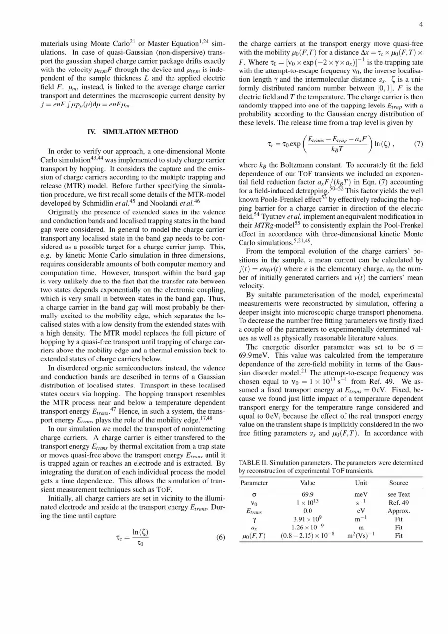
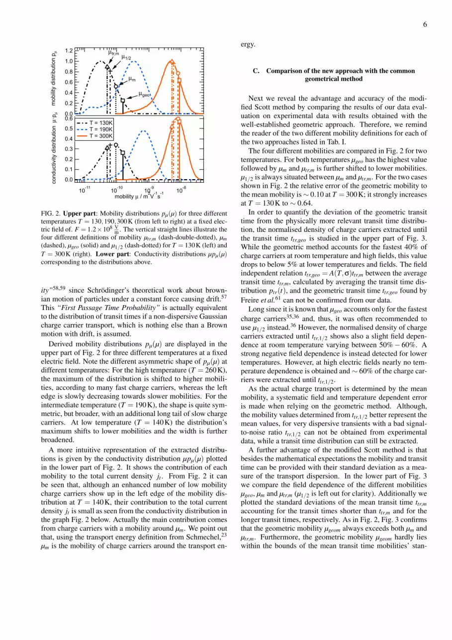
FIG. 2. Upper part: Mobility distributions pµ(µ) for three differenttemperatures T = 130,190,300K (from left to right) at a fixed elec-tric field of. F = 1.2×108 V

m . The vertical straight lines illustrate thefour different definitions of mobility µtr,m (dash-double-dotted), µm(dashed), µgeo (solid) and µ1/2 (dash-dotted) for T = 130K (left) andT = 300K (right). Lower part: Conductivity distributions µpµ(µ)corresponding to the distributions above.

ity”58,59 since Schrodinger’s theoretical work about brown-ian motion of particles under a constant force causing drift.57

This “First Passage Time Probability” is actually equivalentto the distribution of transit times if a non-dispersive Gaussiancharge carrier transport, which is nothing else than a Brownmotion with drift, is assumed.

Derived mobility distributions pµ(µ) are displayed in theupper part of Fig. 2 for three different temperatures at a fixedelectric field. Note the different asymmetric shape of pµ(µ) atdifferent temperatures: For the high temperature (T = 260K),the maximum of the distribution is shifted to higher mobili-ties, according to many fast charge carriers, whereas the leftedge is slowly decreasing towards slower mobilities. For theintermediate temperature (T = 190K), the shape is quite sym-metric, but broader, with an additional long tail of slow chargecarriers. At low temperature (T = 140K) the distribution’smaximum shifts to lower mobilities and the width is furtherbroadened.

A more intuitive representation of the extracted distribu-tions is given by the conductivity distribution µpµ(µ) plottedin the lower part of Fig. 2. It shows the contribution of eachmobility to the total current density jt . From Fig. 2 it canbe seen that, although an enhanced number of low mobilitycharge carriers show up in the left edge of the mobility dis-tribution at T = 140K, their contribution to the total currentdensity jt is small as seen from the conductivity distribution inthe graph Fig. 2 below. Actually the main contribution comesfrom charge carriers with a mobility around µm. We point outthat, using the transport energy definition from Schmechel,23

µm is the mobility of charge carriers around the transport en-

ergy.

C. Comparison of the new approach with the commongeometrical method

Next we reveal the advantage and accuracy of the modi-fied Scott method by comparing the results of our data eval-uation on experimental data with results obtained with thewell-established geometric approach. Therefore, we remindthe reader of the two different mobility definitions for each ofthe two approaches listed in Tab. I.

The four different mobilities are compared in Fig. 2 for twotemperatures. For both temperatures µgeo has the highest valuefollowed by µm and µtr,m is further shifted to lower mobilities.µ1/2 is always situated between µm and µtr,m. For the two casesshown in Fig. 2 the relative error of the geometric mobility tothe mean mobility is∼ 0.10 at T = 300K; it strongly increasesat T = 130K to ∼ 0.64.

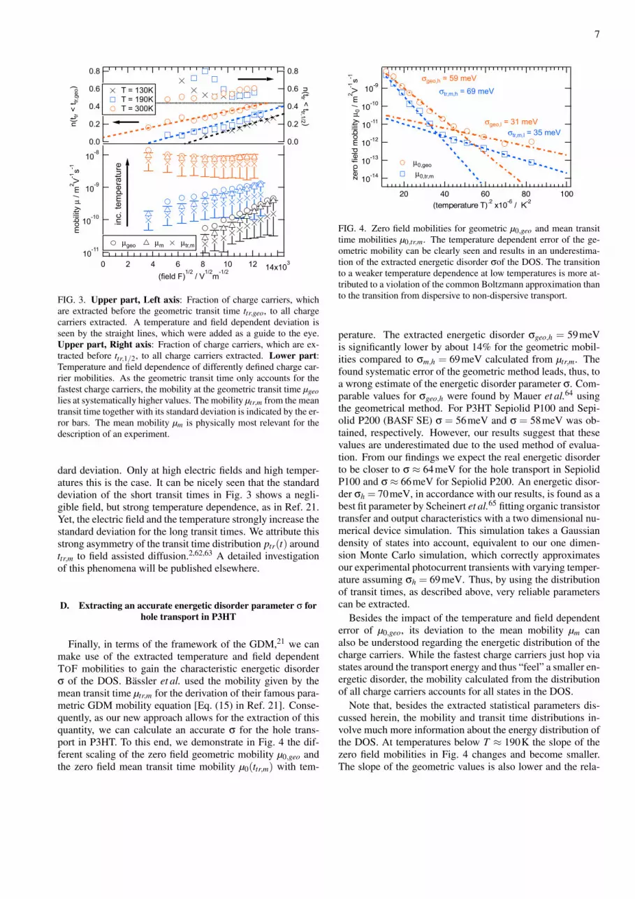
In order to quantify the deviation of the geometric transittime from the physically more relevant transit time distribu-tion, the normalised density of charge carriers extracted untilthe transit time ttr,geo is studied in the upper part of Fig. 3.While the geometric method accounts for the fastest 40% ofcharge carriers at room temperature and high fields, this valuedrops to below 5% at lower temperatures and fields. The fieldindependent relation ttr,geo = A(T,σ)ttr,m between the averagetransit time ttr,m, calculated by averaging the transit time dis-tribution ptr(t), and the geometric transit time ttr,geo found byFreire et al.61 can not be confirmed from our data.

Long since it is known that µgeo accounts only for the fastestcharge carriers35,36 and, thus, it was often recommended touse µ1/2 instead.36 However, the normalised density of chargecarriers extracted until ttr,1/2 shows also a slight field depen-dence at room temperature varying between 50%− 60%. Astrong negative field dependence is instead detected for lowertemperatures. However, at high electric fields nearly no tem-perature dependence is obtained and∼ 60% of the charge car-riers were extracted until ttr,1/2.

As the actual charge transport is determined by the meanmobility, a systematic field and temperature dependent erroris made when relying on the geometric method. Although,the mobility values determined from ttr,1/2 better represent themean values, for very dispersive transients with a bad signal-to-noise ratio ttr,1/2 can not be obtained from experimentaldata, while a transit time distribution can still be extracted.

A further advantage of the modified Scott method is thatbesides the mathematical expectations the mobility and transittime can be provided with their standard deviation as a mea-sure of the transport dispersion. In the lower part of Fig. 3we compare the field dependence of the different mobilitiesµgeo, µm and µtr,m (µ1/2 is left out for clarity). Additionally weplotted the standard deviations of the mean transit time ttr,maccounting for the transit times shorter than ttr,m and for thelonger transit times, respectively. As in Fig. 2, Fig. 3 confirmsthat the geometric mobility µgeom always exceeds both µm andµtr,m. Furthermore, the geometric mobility µgeom hardly lieswithin the bounds of the mean transit time mobilities’ stan-

7

10-11

10-10

10-9

10-8

mob

ility

µ /

m2 V

-1s-1

14x103121086420

(field F)1/2

/ V1/2

m-1/2

0.8

0.6

0.4

0.2

0.0

n(t tr

< t t

r,geo

)0.8

0.6

0.4

0.2

0.0

n(ttr < ttr,1/2 )

inc.

tem

pera

ture

T = 130KT = 190KT = 300K

µgeo µm µtr,m

FIG. 3. Upper part, Left axis: Fraction of charge carriers, whichare extracted before the geometric transit time ttr,geo, to all chargecarriers extracted. A temperature and field dependent deviation isseen by the straight lines, which were added as a guide to the eye.Upper part, Right axis: Fraction of charge carriers, which are ex-tracted before ttr,1/2, to all charge carriers extracted. Lower part:Temperature and field dependence of differently defined charge car-rier mobilities. As the geometric transit time only accounts for thefastest charge carriers, the mobility at the geometric transit time µgeolies at systematically higher values. The mobility µtr,m from the meantransit time together with its standard deviation is indicated by the er-ror bars. The mean mobility µm is physically most relevant for thedescription of an experiment.

dard deviation. Only at high electric fields and high temper-atures this is the case. It can be nicely seen that the standarddeviation of the short transit times in Fig. 3 shows a negli-gible field, but strong temperature dependence, as in Ref. 21.Yet, the electric field and the temperature strongly increase thestandard deviation for the long transit times. We attribute thisstrong asymmetry of the transit time distribution ptr(t) aroundttr,m to field assisted diffusion.2,62,63 A detailed investigationof this phenomena will be published elsewhere.

D. Extracting an accurate energetic disorder parameter σ forhole transport in P3HT

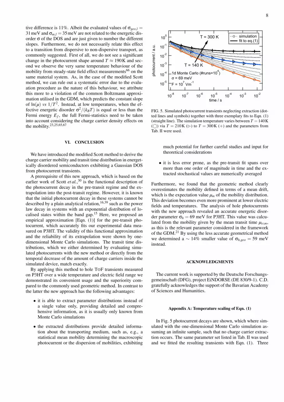
Finally, in terms of the framework of the GDM,21 we canmake use of the extracted temperature and field dependentTOF mobilities to gain the characteristic energetic disorderσ of the DOS. Bassler et al. used the mobility given by themean transit time µtr,m for the derivation of their famous para-metric GDM mobility equation [Eq. (15) in Ref. 21]. Conse-quently, as our new approach allows for the extraction of thisquantity, we can calculate an accurate σ for the hole trans-port in P3HT. To this end, we demonstrate in Fig. 4 the dif-ferent scaling of the zero field geometric mobility µ0,geo andthe zero field mean transit time mobility µ0(ttr,m) with tem-

10-14

10-13

10-12

10-11

10-10

10-9

zero

fiel

d m

obilit

y µ 0

/ m

2 V-1

s-1

10080604020(temperature T).2 x10-6 / K-2

µ0,geo

µ0,tr,m

σgeo,h = 59 meV

σgeo,l = 31 meV

σtr,m,h = 69 meV

σtr,m,l = 35 meV

FIG. 4. Zero field mobilities for geometric µ0,geo and mean transittime mobilities µ0,tr,m. The temperature dependent error of the ge-ometric mobility can be clearly seen and results in an underestima-tion of the extracted energetic disorder σof the DOS. The transitionto a weaker temperature dependence at low temperatures is more at-tributed to a violation of the common Boltzmann approximation thanto the transition from dispersive to non-dispersive transport.

perature. The extracted energetic disorder σgeo,h = 59meVis significantly lower by about 14% for the geometric mobil-ities compared to σm,h = 69meV calculated from µtr,m. Thefound systematic error of the geometric method leads, thus, toa wrong estimate of the energetic disorder parameter σ. Com-parable values for σgeo,h were found by Mauer et al.64 usingthe geometrical method. For P3HT Sepiolid P100 and Sepi-olid P200 (BASF SE) σ = 56meV and σ = 58meV was ob-tained, respectively. However, our results suggest that thesevalues are underestimated due to the used method of evalua-tion. From our findings we expect the real energetic disorderto be closer to σ ≈ 64meV for the hole transport in SepiolidP100 and σ≈ 66meV for Sepiolid P200. An energetic disor-der σh = 70meV, in accordance with our results, is found as abest fit parameter by Scheinert et al.65 fitting organic transistortransfer and output characteristics with a two dimensional nu-merical device simulation. This simulation takes a Gaussiandensity of states into account, equivalent to our one dimen-sion Monte Carlo simulation, which correctly approximatesour experimental photocurrent transients with varying temper-ature assuming σh = 69meV. Thus, by using the distributionof transit times, as described above, very reliable parameterscan be extracted.

Besides the impact of the temperature and field dependenterror of µ0,geo, its deviation to the mean mobility µm canalso be understood regarding the energetic distribution of thecharge carriers. While the fastest charge carriers just hop viastates around the transport energy and thus “feel” a smaller en-ergetic disorder, the mobility calculated from the distributionof all charge carriers accounts for all states in the DOS.

Note that, besides the extracted statistical parameters dis-cussed herein, the mobility and transit time distributions in-volve much more information about the energy distribution ofthe DOS. At temperatures below T ≈ 190K the slope of thezero field mobilities in Fig. 4 changes and become smaller.The slope of the geometric values is also lower and the rela-

8

tive difference is 11%. Albeit the evaluated values of σgeo,l =31meV and σm,l = 35meV are not related to the energetic dis-order σ of the DOS and are just given to number the differentslopes. Furthermore, we do not necessarily relate this effectto a transition from dispersive to non-dispersive transport, ascommonly suggested. First of all, we do not see a significantchange in the photocurrent shape around T ≈ 190K and sec-ond we observe the very same temperature behaviour of themobility from steady-state field effect measurements66 on thesame material system. As, in the case of the modified Scottmethod, we can rule out a systematic error due to the evalu-ation procedure as the nature of this behaviour, we attributethis more to a violation of the common Boltzmann approxi-mation utilised in the GDM, which predicts the constant slopeof ln(µ) vs 1/T 2. Instead, at low temperatures, when the ef-fective energetic disorder σ2/(kBT ) is equal or less than theFermi energy E f , the full Fermi-statistics need to be takeninto account considering the charge carrier density effects onthe mobility.23,25,65,67

VI. CONCLUSION

We have introduced the modified Scott method to derive thecharge carrier mobility and transit time distribution in energet-ically disordered semiconductors exhibiting a Gaussian DOSfrom photocurrent transients.

A prerequisite of this new approach, which is based on theearlier work of Scott et al.,30 is the functional description ofthe photocurrent decay in the pre-transit regime and the ex-trapolation into the post-transit regime. However, it is knownthat the initial photocurrent decay in these systems cannot bedescribed by a plain analytical relation,16,39 such as the powerlaw decay in systems with an exponential distribution of lo-calised states within the band gap.15 Here, we proposed anempirical approximation [Eqn. (1)] for the pre-transit pho-tocurrent, which accurately fits our experimental data mea-sured on P3HT. The validity of this functional approximationand the reliability of its extrapolation were shown by one-dimensional Monte Carlo simulations. The transit time dis-tributions, which we either determined by evaluating simu-lated photocurrents with the new method or directly from thetemporal decrease of the amount of charge carriers inside thesimulated device, match exactly.

By applying this method to hole TOF transients measuredon P3HT over a wide temperature and electric field range wedemonstrated its convenient usage and the superiority com-pared to the commonly used geometric method. In contrast tothe latter the new approach has the following advantages:

• it is able to extract parameter distributions instead ofa single value only, providing detailed and compre-hensive information, as it is usually only known fromMonte Carlo simulations

• the extracted distributions provide detailed informa-tion about the transporting medium, such as, e.g., astatistical mean mobility determining the macroscopicphotocurrent or the dispersion of mobilities, exhibiting

10-5

10-4

10-3

10-2

10-1

100

phot

ocur

rent

/ a.

u.

10-8

10-7

10-6

10-5

10-4

10-3

10-2

time / s

T = 300 K

T = 140 K

simulation fit to eq.(1)

1d Monte Carlo (#runs=104)

σ = 69 meVF = 10

7 Vm

-1

FIG. 5. Simulated photocurrent transients neglecting extraction (dot-ted lines and symbols) together with three exemplary fits to Eqn. (1)(straight line). The simulation temperature varies between T = 140K(©) via T = 210K (B) to T = 300K (+) and the parameters fromTab. II were used.

much potential for further careful studies and input fortheoretical considerations

• it is less error prone, as the pre-transit fit spans overmore than one order of magnitude in time and the ex-tracted stochastical values are numerically averaged

Furthermore, we found that the geometric method clearlyoverestimates the mobility defined in terms of a mean drift,which is the expectation value µm of the mobility distribution.This deviation becomes even more prominent at lower electricfields and temperatures. The analysis of hole photocurrentswith the new approach revealed an accurate energetic disor-der parameter σh = 69 meV for P3HT. This value was calcu-lated from the mobility given by the mean transit time µtr,m,as this is the relevant parameter considered in the frameworkof the GDM.21 By using the less accurate geometrical methodwe determined a ∼ 14% smaller value of σh,geo = 59 meVinstead.

ACKNOWLEDGMENTS

The current work is supported by the Deutsche Forschungs-gemeinschaft (DFG), project EiNDORSE (DE 830/9-1). C.D.gratefully acknowledges the support of the Bavarian Academyof Sciences and Humanities.

Appendix A: Temperature scaling of Eqn. (1)

In Fig. 5 photocurrent decays are shown, which where sim-ulated with the one-dimensional Monte Carlo simulation as-suming an infinite sample, such that no charge carrier extrac-tion occurs. The same parameter set listed in Tab. II was usedand we fitted the resulting transients with Eqn. (1). Three

9

10-22

10

-20

10-18

10

-16

10-14

10

-12

10-10

10

-8lif

etim

e τ

/ s, i

nitia

l cur

rent

j 0*

/ a.u

.

3025201510(σ/kbT)

2

0.25

0.20

0.15

0.10

0.05

0.00

expo

nent

β

0.120.080.04(kbT/σ)

2

β from fit (eq.(1)) τ from fit (eq.(1)) j0* from fit (eq.(1))

exponential fit linear fit

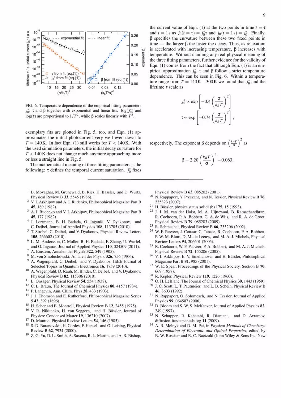
FIG. 6. Temperature dependence of the empirical fitting parametersj∗0 , τ and β together with exponential and linear fits. log( j∗0) andlog(τ) are proportional to 1/T 2, while β scales linearly with T 2.

exemplary fits are plotted in Fig. 5, too, and Eqn. (1) ap-proximates the initial photocurrent very well even down toT = 140K. In fact Eqn. (1) still works for T < 140K. Withthe used simulation parameters, the initial decay curvature forT < 140K does not change much anymore approaching moreor less a straight line in Fig. 5.

The mathematical meaning of three fitting parameters is thefollowing: τ defines the temporal current saturation. j∗0 fixes

the current value of Eqn. (1) at the two points in time t = τ

and t = 1s as j0(t = τ) = j∗0τ and j0(t = 1s) = j∗0. Finally,β specifies the curvature between these two fixed points intime — the larger β the faster the decay. Thus, as relaxationis accelerated with increasing temperature, β increases withtemperature. Without claiming any real physical meaning ofthe three fitting parameters, further evidence for the validity ofEqn. (1) comes from the fact that although Eqn. (1) is an em-pirical approximation j∗0, τ and β follow a strict temperaturedependence. This can be seen in Fig. 6. Within a tempera-ture range from T = 140K− 300K we found that j∗0 and thelifetime τ scale as

j∗0 ∝ exp

[−0.4

(σ

kBT

)2]

τ ∝ exp

[−0.74

(σ

kBT

)2],

respectively. The exponent β depends on(

kBTσ

)2as

β = 2.20(

kBTσ

)2

−0.063.

1 B. Movaghar, M. Grunewald, B. Ries, H. Bassler, and D. Wurtz,Physical Review B 33, 5545 (1986).

2 V. I. Arkhipov and A. I. Rudenko, Philosophical Magazine Part B45, 189 (1982).

3 A. I. Rudenko and V. I. Arkhipov, Philosophical Magazine Part B45, 177 (1982).

4 J. Lorrmann, B. H. Badada, O. Inganas, V. Dyakonov, andC. Deibel, Journal of Applied Physics 108, 113705 (2010).

5 T. Strobel, C. Deibel, and V. Dyakonov, Physical Review Letters105, 266602 (2010).

6 L. M. Andersson, C. Muller, B. H. Badada, F. Zhang, U. Wurfel,and O. Inganas, Journal of Applied Physics 110, 024509 (2011).

7 A. Einstein, Annalen der Physik 322, 549 (1905).8 M. von Smoluchowski, Annalen der Physik 326, 756 (1906).9 A. Wagenpfahl, C. Deibel, and V. Dyakonov, IEEE Journal of

Selected Topics in Quantum Electronics 16, 1759 (2010).10 A. Wagenpfahl, D. Rauh, M. Binder, C. Deibel, and V. Dyakonov,

Physical Review B 82, 115306 (2010).11 L. Onsager, Physical Review 54, 554 (1938).12 C. L. Braun, The Journal of Chemical Physics 80, 4157 (1984).13 P. Langevin, Ann. Chim. Phys 28, 433 (1903).14 J. J. Thomson and E. Rutherford, Philosophical Magazine Series

5 42, 392 (1896).15 H. Scher and E. Montroll, Physical Review B 12, 2455 (1975).16 V. R. Nikitenko, H. von Seggern, and H. Bassler, Journal of

Physics: Condensed Matter 19, 136210 (2007).17 D. Monroe, Physical Review Letters 54, 146 (1985).18 S. D. Baranovskii, H. Cordes, F. Hensel, and G. Leising, Physical

Review B 62, 7934 (2000).19 Z. G. Yu, D. L. Smith, A. Saxena, R. L. Martin, and A. R. Bishop,

Physical Review B 63, 085202 (2001).20 N. Rappaport, Y. Preezant, and N. Tessler, Physical Review B 76,

235323 (2007).21 H. Bassler, physica status solidi (b) 175, 15 (1993).22 J. J. M. van der Holst, M. A. Uijttewaal, B. Ramachandhran,

R. Coehoorn, P. A. Bobbert, G. A. de Wijs, and R. A. de Groot,Physical Review B 79, 085203 (2009).

23 R. Schmechel, Physical Review B 66, 235206 (2002).24 W. F. Pasveer, J. Cottaar, C. Tanase, R. Coehoorn, P. A. Bobbert,

P. W. M. Blom, D. M. de Leeuw, and M. A. J. Michels, PhysicalReview Letters 94, 206601 (2005).

25 R. Coehoorn, W. F. Pasveer, P. A. Bobbert, and M. A. J. Michels,Physical Review B 72, 155206 (2005).

26 V. I. Arkhipov, E. V. Emelianova, and H. Bassler, PhilosophicalMagazine Part B 81, 985 (2001).

27 W. E. Spear, Proceedings of the Physical Society. Section B 70,669 (1957).

28 R. Kepler, Physical Review 119, 1226 (1960).29 O. H. LeBlanc, The Journal of Chemical Physics 30, 1443 (1959).30 J. C. Scott, L. T. Pautmeier, and L. B. Schein, Physical Review B

46, 8603 (1992).31 N. Rappaport, O. Solomesch, and N. Tessler, Journal of Applied

Physics 99, 064507 (2006).32 D. Bloom and S. W. S. McKeever, Journal of Applied Physics 82,

249 (1997).33 N. Schupper, R. Kahatabi, R. Diamant, and D. Avramov,

diffusion-fundamentals.org 11 (2009).34 A. R. Melnyk and D. M. Pai, in Physical Methods of Chemistry:

Determination of Electronic and Optical Properties, edited byB. W. Rossiter and R. C. Baetzold (John Wiley & Sons Inc, New

10

York, 1993) 2nd ed., Chap. 5, pp. 321–386.35 J. M. Marshall, J. Berkin, and C. Main, Philosophical Magazine

Part B 56, 641 (1987).36 G. Seynhaeve, G. J. Adriaenssens, H. Michiel, and H. Overhof,

Philosophical Magazine Part B 58, 421 (1988).37 S. V. Novikov and A. V. Vannikov, The Journal of Physical Chem-

istry C 113, 2532 (2009).38 A. Baumann, J. Lorrmann, C. Deibel, and V. Dyakonov, Applied

Physics Letters 93, 252104 (2008).39 W. C. Germs, J. J. M. van der Holst, S. L. M. van Mensfoort,

P. A. Bobbert, and R. Coehoorn, Physical Review B 84, 165210(2011).

40 N. Tessler and Y. Roichman, Organic Electronics 6, 200 (2005).41 J. v. Neumann, The Annals of Mathematics 33, 574 (1932).42 P. R. Halmos and J. von Neumann, The Annals of Mathematics

43, 332 (1942).43 M. Silver, K. Dy, and I. Huang, Physical Review Letters 27, 21

(1971).44 J. M. Marshall, Philosophical Magazine 36, 959 (1977).45 F. W. Schmidlin, Physical Review B 16, 2362 (1977).46 J. Noolandi, Physical Review B 16, 4466 (1977).47 M. Grunewald and P. Thomas, Physica Status Solidi (b) 94, 125

(1979).48 S. D. Baranovskii, T. Faber, F. Hensel, and P. Thomas, Journal of

Physics: Condensed Matter 9, 2699 (1997).49 C. Deibel, T. Strobel, and V. Dyakonov, Physical Review Letters

103, 036402 (2009).50 J. Cottaar, R. Coehoorn, and P. A. Bobbert, Physical Review B

82, 205203 (2010).51 A. Miller and E. Abrahams, Physical Review 120, 745 (1960).52 M. Schubert, E. Preis, J. C. Blakesley, P. Pingel, U. Scherf, and

D. Neher, Physical Review B 87, 024203 (2013).53 J. Frenkel, Physical Review 54, 647 (1938).54 D. H. Dunlap, V. Kenkre, and P. Parris, The Journal of imaging

science and technology 43, 437 (1999).55 A. P. Tyutnev, R. Ikhsanov, V. Saenko, and E. Pozhidaev, Chem-

ical Physics 404, 88 (2012).56 R. Storn and K. Price, Journal of global optimization 11, 341

(1997).57 E. Schrodinger, Physikalische Zeitschrift 16, 289 (1915).58 M. C. K. Tweedie, Nature 155, 453 (1945).59 A. Siegert, Physical Review 81, 617 (1951).60 T.-J. Ha, P. Sonar, and A. Dodabalapur, Applied Physics Letters

100, 153302 (2012).61 J. A. Freire and M. G. E. da Luz, The Journal of Chemical Physics

119, 2348 (2003).62 A. V. Nenashev, F. Jansson, S. D. Baranovskii, R. Osterbacka,

A. V. Dvurechenskii, and F. Gebhard, Physical Review B 81,115203 (2010).

63 A. V. Nenashev, F. Jansson, S. D. Baranovskii, R. Osterbacka,A. V. Dvurechenskii, and F. Gebhard, Physical Review B 81,115204 (2010).

64 R. Mauer, M. Kastler, and F. Laquai, Advanced Functional Ma-terials 20, 2085 (2010).

65 S. Scheinert, M. Grobosch, G. Paasch, I. Horselmann,M. Knupfer, and J. Bartsch, Journal of Applied Physics 111,064502 (2012).

66 R. Winter, M. S. Hammer, C. Deibel, and J. Pflaum, AppliedPhysics Letters 95, 263313 (2009).

67 G. Paasch and S. Scheinert, Journal of Applied Physics 107,104501 (2010).