Gaussian Process Model Re-Use

Tom Diethe, Niall Twomey, and Peter Flach

Intelligent Systems Laboratory, University of Bristol{tom.diethe,niall.twomey,peter.flach}@bristol.ac.uk

Abstract. Consider the situation where we have some pre-trained classificationmodels for bike rental stations (or any other spatially located data). Given a newrental station (deployment context), we imagine that there might be some rentalstations that are more similar to this station in terms of the daily usage patterns,whether or not these stations are close by or not. We propose to use a GaussianProcess (GP) to model the relationship between geographic location and the typeof the station, as determined by heuristics based on the daily usage patterns. Fora deployment station, we then find the closest stations in terms of the GaussianProcess (GP) function output, and then use the models trained on these stationson the deployment station. We compare against several baselines, and show thatthis method is able to outperform those baselines.

1 Introduction

Automated tracking in “smart environments” (including smart homes and smart cities)is fast becoming an interesting area of research, with numerous research groups princi-pal interests rooted in this area. Notable examples include CASAS1 [1], the RUBICONproject2 [2], and SPHERE 3 [3,4].

There are at least two major challenges for machine learning in this setting. Firstly,the deployment context will necessarily be very different to the context in which learn-ing occurs, due to both individual differences in typical daily patterns, and also due tosensor configurations, positioning, or layouts. Secondly, accurate labelling of trainingdata is often an extremely time-consuming process, and the resulting labels are poten-tially noisy and error-prone.

From this we can see that the re-use of learnt knowledge, particularly in the form ofmodels and model parameters, is of critical importance in the majority of knowledge-intensive application areas, particularly because of the expected deviations between theoperating contexts in training and deployment. The REFRAME project4 is particularlyconcerned with this issue, and is the sponsor of the Model Reuse with Bike rental Sta-tion data (MoReBikeS) challenge, which focuses on model reuse and context change.

1 http://ailab.wsu.edu/casas/2 http://fp7rubicon.eu/3 http://www.irc-sphere.ac.uk4 http://reframe-d2k.org/

2 Tom Diethe, Niall Twomey, and Peter Flach

1.1 MoReBikeS Challenge

The task in this challenge is to predict the number of available bikes in every bike rentalstations 3 hours in advance. There are at least two use cases for such predictions. Firstly,a user may plans to rent/return a bike in 3 hours time and wants to choose a bike stationwhich is not empty or full. Secondly, the company operating the bike hire wants to avoidsituations where a station is empty or full and therefore needs to move bikes betweenstations, meaning that they need to know which stations are more likely to be emptyor full soon. In both these cases the prediction can be based on contextual informationsuch as the time of the day, week, or year, or the current weather conditions, as wellas information about the current status of the station. One might hypothesise that thequality of predictions would be the better given more historical information.

In this challenge there are 200 stations which have been running for > 2 years and75 stations which have been open for a month. The task is to reuse the models learnt on200 “old” stations in order to improve prediction performance on the 75 “new” stations,so the evaluation is based on these 75 stations. Pre-built classification models on the200 stations are provided without the full training data (although full training data isavailable for 10 stations). Data for one month is provided, also to help in deciding howthe models can be reused.

1.2 Daily patterns

In Figure 1 we can see that different stations clearly exhibit different daily patterns.Most obviously, there are stations that tend to be full in the night and emptier duringthe day, as in stations 26 and 28 (columns 1 and 3). Essentially these are stations thatare on the outer areas of the city, and the bikes are used during the day to travel intomore central parts of the city. There are also stations that exhibit the opposite pattern,such as station 29 (column 4). These stations are left empty at night, since the operatorsknow that the will fill up during the day as people travel into the city. There are ofcourse stations that fall between these two extremes, of which station 27 (column 2) isan example.

Fig. 1: Comparison of the daily patterns of several different stations. The blue line showsthe mean of the daily capacity and the grey lines show ± one standard deviation.

Gaussian Process Model Re-Use 3

Our proposal is that given a new station, if we are to use existing models trainedon stations in known locations, the best predictions will be given by models trained onstations that exhibit a similar day/night pattern as the station in question. Note that thesestations may be geographically close to each other, or they may be in a different part ofthe city but effectively play the same role. We will therefore leverage the locations ofthe deployment stations, but none of training data given in the challenge regarding thestations, simply in order to find the most similar stations.

2 Related Work

A major assumption in the majority of machine learning methods is that the training anddeployment data are drawn from the same underlying distribution. For the smart-cityapplication this assumption clearly does not hold. In such cases, knowledge transfer,if done successfully, would greatly improve the performance of learning by avoidingthe costly acquirement of labels. In recent years, transfer learning has emerged as anew learning framework to address this problem, and is related to areas such as domainadaptation, multi-task learning, sample selection bias, and covariate shift [5].

Definitions for domain and task have been provided by [6]. A domain D is a pair(X , p(S )). X is the feature space of D and p(S ) is the marginal distribution of adata-set. A task T is a pair (Y , f ) for some given domain D . Y is the label space of Dand f is an unknown objective predictive function for D to be learnt from data, whichhere we write as the conditional probability distribution p(y|x).

It is well known that the hierarchical Bayesian framework can be readily adapted tosequential decision problems [7], and it has also been shown more recently that it pro-vides a natural formalisation of transfer learning [8]. The results of the latter of theseshow that a hierarchical Bayesian Transfer framework significantly improves learningspeed when tasks are hierarchically related within the domain of reinforcement learn-ing. In another study [9], the authors formulated a kernelised Bayesian transfer learningframework that is a combination of kernel-based dimensionality reduction models withtask-specific projection matrices, and aims to find a shared subspace and a coupledclassification model for all of the tasks in this subspace.

In our setting, since we were not the original creators of the models (i.e. pre-trainedmodels have been provided), we do not have freedom to choose the overall frameworkin this way. However, we take the flavour of these ideas, and show how we can usekernelised Bayesian methods to re-use existing models.

3 Concepts and Notation

Here we briefly review the application of Gaussian Processes (GPs) for vector-valuedregression, and then show how we will employ these for model re-use.

3.1 Gaussian Process for Vector-Valued Regression

In the vector-valued regression framework, we assume that we are given an examplexi ∈ Rn, and the goal is to make a prediction yi ∈ Ro that approximates the true output

4 Tom Diethe, Niall Twomey, and Peter Flach

yi ∈ Ro, where n is the dimensionality of the input space and o is the dimensionality ofthe output space. We will assume that we have m instances such that X = {xi}m

i=1 andY = {yi}m

i=1.A Gaussian Process (GP) is defined as a Gaussian distribution over latent functions.

Given the consistency property of Gaussian distributions, whereby marginals are alsoGaussian, point-wise evaluations at the data-points f = [ f (x1), ..., f (xm)]

m are jointlyGaussian. By specifying a covariance function C(x,x′) and a mean function h(x), wesee that f ∼N (h,K) where h = [h(x1, ...,xm)] and K is the covariance matrix whichis equivalent to the Gram matrix in kernel methods (see subsection 3.2 below). Sincethe data-points only appear in the expression through the covariance matrix, and hencethrough inner products, any nonlinear mapping that produces valid covariances (ker-nels) can be used, as with other kernel methods. For regression, it is assumed that thetargets are observed independently. The (intractable) posterior is then,

p(f|X,Y) =1Z

p(f|X)T

∏t=1

g(yt | f (xt)),

where the normalising constant Z = p(Y|X) is the marginal likelihood. Currently themost accurate deterministic approximation to this is through the use of ExpectationPropagation (EP) [10]. In EP, the likelihood is approximated by an un-normalised Gaus-sian to give,

p(f|X,Y) =1

ZEPp(f|X)

m

∏i=1

1Zi

g(yi| f (xi)),

=1

ZEPp(f|X)N (f|h, C),

= N (f|h,C),

where ZEP and Zt are normalisation coefficients, ˜g(yi| f (xi)) and N (f|h, C) are theGaussian approximations to g(yi| f (xi)) at each site xi. In order to obtain the full (ap-proximate) posterior q(f|X,Y), one would start by using the prior, i.e. q(f|X,Y) =p(f|X) and update each site approximation g(·) sequentially. In order to do this, theso-called cavity distribution q(f|X,Yt) is used - i.e. the current posterior with the pointxi removed. In “online” methods (c.f. [11]) the full posterior approximation is onlyachieved after (at least one) full pass through the dataset.

GP inference in all cases was done using the GPy library for GP in python [12].

3.2 Kernel Methods

Briefly, a kernel function [13] is a function that for all x,z ∈ X satisfies κ (x,z) =〈φ(x),φ(z)〉, where φ : X 7→H is a mapping from X to an (inner product) Hilbertspace H . This allows inner products between nonlinear mappings (when φ(·) is a non-linear function), as long as the inner product κ(xi,x j) =

⟨φ(xi),φ(x j)

⟩can be evaluated

efficiently. In many cases, this inner product or kernel function can be evaluated muchmore efficiently than the feature vector itself, which can even be infinite dimensional

Gaussian Process Model Re-Use 5

in principle. For a given kernel function the associated feature space is not necessarilyunique. A commonly used kernel function for which this is the case is the Radial BasisFunction (RBF) kernel, which is defined as:

κγ(x,z) = exp(−‖x− z‖2

γ

). (1)

The RBF kernel projects the data into a (non-unique) infinite-dimensional Hilbert Space.We will also use a Periodic Exponential (PE) kernel, which is defined as:

κγ,σ ,ω(x,z) = σ exp(−2cos

(πω(x− z)

γ

)), (2)

where γ is the length-scale, σ is the amplitude, and ω is the period. Note that here x andz are scalars, as this kernel function is defined for scalar inputs only.

3.3 GPs for Model Re-Use

We now describe how GPs will be employed for model re-use. The key insights fromsubsection 1.2 are that different bike rental stations clearly exhibit different daily pat-terns. We need to characterise these different patterns in a way that can be provided asa target to the GP.

A rough way to characterise these differences is to simply assume that there isa periodic daily pattern which is sinusoidal, but varies in amplitude and phase. Wepropose therefore to fit a sinusoidal function to the first week of data of each of thetraining stations using a GP with a PE kernel, with ω fixed to 24 (the number of hoursin the day. The input X to the GP then is simply (24d)+h where d is the day and h is thehour of day, and the targets Y are the number of bikes (so in this case the dimensionalityof the output space o = 1). For each of the stations, we then extract the amplitude andthe phase as learnt by the GP.

Two examples of functions fitted (posterior means of the GP) in this manner aregiven in Figure 2. Note that the phase of the sinusoid for station 21 is almost the oppositeof that of station 22, indicating that this has accurately captured the differences betweenthese stations along this axis. In this figure the y-axis was scaled to the range [0,1] whichobscures any differences in amplitude, but we are interested in this value too: the phaseindicates whether the station is one that is regularly ”commuted to” or ”commutedfrom”, and the amplitude indicates the daily business of the station.

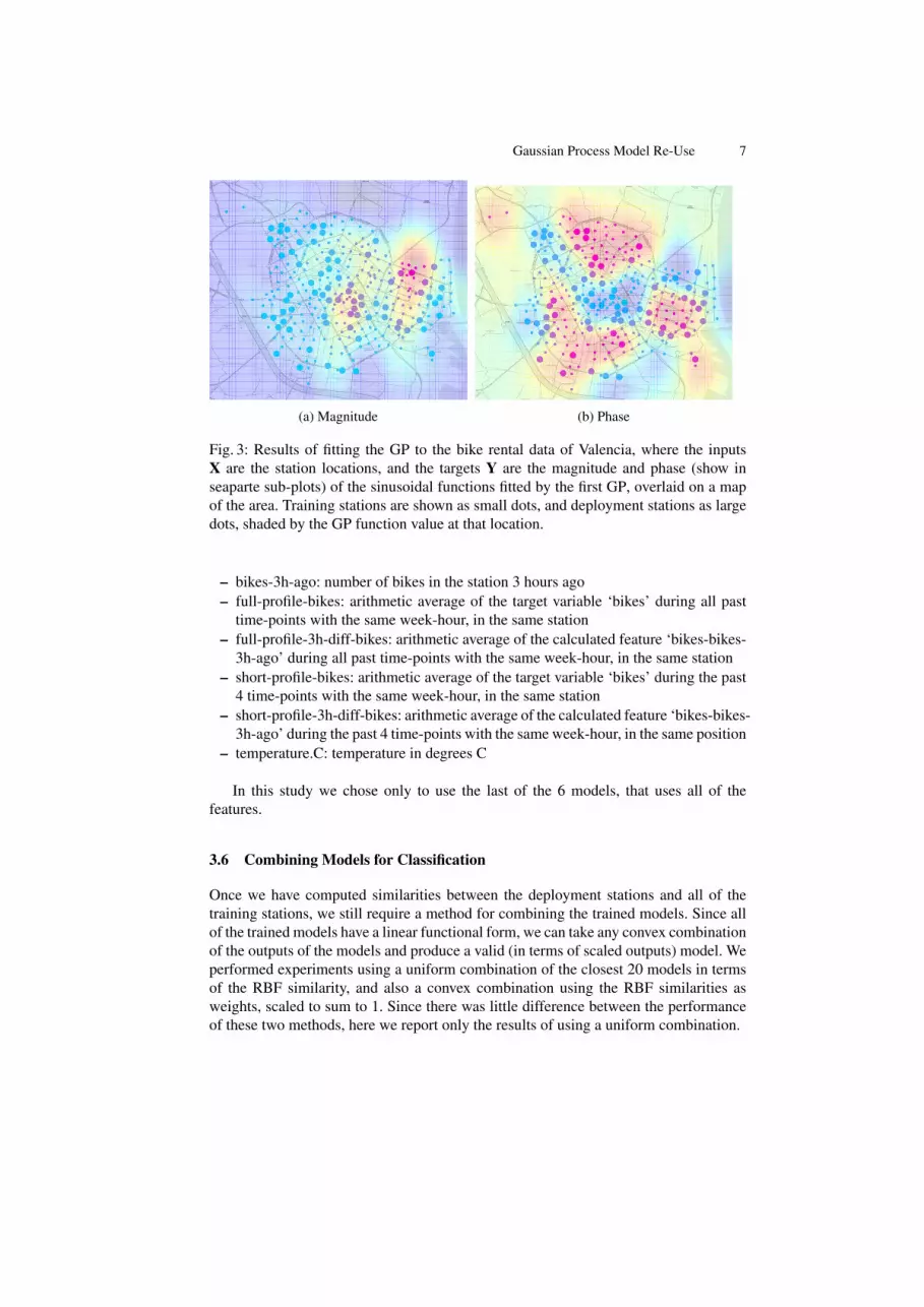
We then fit a further GP, using the decimal values of the latitude and longitude ofthe locations of the stations as the inputs X, and the targets Y are the amplitude andthe phase as learnt by the previous GP (so here the dimensionality of the output spaceo = 2). In Figure 3 we have plotted the functions fitted (posterior means of the GP) ineach of the output dimensions, where Figure 3a shows the magnitude and Figure 3bshows the phase.

In order to decide which models we want to re-use, we need to characterise thesimilarity of a given deployment station to the training stations. Here we use the GPto compute the marginal likelihood of the magnitude and phase of the sinusoid of thedaily pattern, given the station’s location. We then compute the similarity between the

6 Tom Diethe, Niall Twomey, and Peter Flach

Fig. 2: Results of fitting the GP using a PE kernel to the hour of day of the bike rentaldata for two of the stations in Valencia.

marginal likelihood and the posterior means of the magnitude and phase of the sinu-soidal functions of the daily patterns of the training stations. The similarity metric thatwe employ is again the RBF function as given in Equation 1. Since we are simply usingthis function to map differences in magnitude and phase to a weighting for the stations,we are free to choose the γ to adjust the effective number of stations to include in de-ployment. As a heuristic, we selected the γ that meant that 90% of the weight was givento the first 20 stations. Note that after rescaling such that they have the same range, herewe treat the magnitude and the phase equally.

Figure 4 shows the similarity function as computed for two example deploymentstations (221 and 222). Note that these stations are in some sense “opposite”, in thattheir similarity patterns are almost inverted. Also note that the regions of highest simi-larity are not restricted to a single geographical region, and are not spherical in nature.

3.4 Baseline Method

As a baseline method, we also compute similarities between stations simply using theRBF function with latitudes and longitudes as inputs. This has the effect of putting aspherical Gaussian “blob” around the deployment station, and then choosing stationsaccording distance in this space. Note that in many cases, the GP method will coincidewith this baseline method, since close-by stations will often exhibit similar patterns.However the GP method also has the ability to select stations that are far away geo-graphically, but still exhibit similar daily usage patterns. We note, however, that this isquite a strong baseline.

3.5 Base Models

For each training station there are 6 linear models, all built using R function rlm from thepackage MASS, with missing value imputation using function na.roughfix from pack-age randomForest. The models use a subset of the following features (plus an interceptterm):

Gaussian Process Model Re-Use 7

(a) Magnitude (b) Phase

Fig. 3: Results of fitting the GP to the bike rental data of Valencia, where the inputsX are the station locations, and the targets Y are the magnitude and phase (show inseaparte sub-plots) of the sinusoidal functions fitted by the first GP, overlaid on a mapof the area. Training stations are shown as small dots, and deployment stations as largedots, shaded by the GP function value at that location.

– bikes-3h-ago: number of bikes in the station 3 hours ago– full-profile-bikes: arithmetic average of the target variable ‘bikes’ during all past

time-points with the same week-hour, in the same station– full-profile-3h-diff-bikes: arithmetic average of the calculated feature ‘bikes-bikes-

3h-ago’ during all past time-points with the same week-hour, in the same station– short-profile-bikes: arithmetic average of the target variable ‘bikes’ during the past

4 time-points with the same week-hour, in the same station– short-profile-3h-diff-bikes: arithmetic average of the calculated feature ‘bikes-bikes-

3h-ago’ during the past 4 time-points with the same week-hour, in the same position– temperature.C: temperature in degrees C

In this study we chose only to use the last of the 6 models, that uses all of thefeatures.

3.6 Combining Models for Classification

Once we have computed similarities between the deployment stations and all of thetraining stations, we still require a method for combining the trained models. Since allof the trained models have a linear functional form, we can take any convex combinationof the outputs of the models and produce a valid (in terms of scaled outputs) model. Weperformed experiments using a uniform combination of the closest 20 models in termsof the RBF similarity, and also a convex combination using the RBF similarities asweights, scaled to sum to 1. Since there was little difference between the performanceof these two methods, here we report only the results of using a uniform combination.

8 Tom Diethe, Niall Twomey, and Peter Flach

(a) Station 221 (b) Station 222

Fig. 4: Similarity of deployment stations 221 and 222, as computed using the RBF func-tion with respect to the training stations (in terms of magnitude and phase of the fittedsinusoid), overlaid on a map of the area. The γ value for the RBF function as selectedby the heuristic method was 0.1 in both cases. The deployment station is shown as ablack dot, and the training stations are shown as dots coloured by the similarity.

4 Results

The task is to predict the number of bikes in the stations 3 hours in advance. The metricfor performance we will be using is the mean absolute error (MAE), defined as follows:

MAE =1m

m

∑i=1|yi− yi|=

1m

m

∑i=1|ei| , (3)

where yi is the prediction and yi the true value. We report the mean µ and standarddeviation σ of the MAE over the 75 deployment stations in Table 1 below.

Table 1: mean absolute error (MAE) obtained by the three methods investigated.MAEµ σ

Gaussian Process 0.15 0.03Euclidean Distance 0.15 0.04Random Station 0.15 0.04

We note that the performance of the GP-based method and the baseline methodsare basically equivalent. We surmise that there are two reasons for this. Firstly, we notethat the base models are all fairly similar in terms of their performance. This is due tothe fact that the base models only have a few features (see subsection 3.5) and are alllinear models, so may not be capturing non-linearity (particularly in the changes in bikeprofile throughout the day and week).

Gaussian Process Model Re-Use 9

5 Conclusions and Future Work

We have examined a situation where we have some pre-trained classification modelsfor bike rental stations, for which we know the geographical location as well some in-formation about the daily patterns of activity. Given a new rental station (deploymentcontext), we imagine that there might be some rental stations that are more similar tothis station in terms of the daily usage patterns, whether or not these stations are closeby or not. We proposed to use two Gaussian Processes (GPs), the first to model thecharacteristic daily usage pattern of the station, and the second to model the relation-ship between geographic location and a characterisation of the type of the station, asdetermined by the first GP. For a deployment station, we then find the closest stationsin terms of the GP function output, and then use the models trained on these stationson the deployment station. We compared against several baselines, and showed that thismethod is able to outperform those baselines.

As further work, we would like to consider different measures of the daily usagepatterns, since the single sinusoid that we fit using the first GP is clearly a rough ap-proximation. We could also imagine computing similarities based on other contextualinformation, such as the season, or day of week (weekday versus weekend). This couldallow a more refined selection from the pool of training models. Furthermore, we wouldlike to explore whether this method might work better with more varied base models(which we do not have access to here), such as non-linear GP, as we surmise that thebase models are too similar to highlight the differences between the approaches.

Acknowledgement

This work was performed under the Sensor Platform for HEalthcare in Residential Envi-ronment (SPHERE) Interdisciplinary Research Collaboration (IRC) funded by the UKEngineering and Physical Sciences Research Council (EPSRC), Grant EP/K031910/1.

References

1. Diane J Cook and M Schmitter-Edgecombe. Assessing the quality of activities in a smartenvironment. Methods Inf Med, 48(5):480–5, 2009.

2. Davide Bacciu, Paolo Barsocchi, Stefano Chessa, Claudio Gallicchio, and Alessio Micheli.An experimental characterization of reservoir computing in ambient assisted living applica-tions. Neural Computing and Applications, 24(6):1451–1464, 2014.

3. P. Woznowski, X. Fafoutis, T. Song, S. Hannuna, M. Camplani, L. Tao, A. Paiement, E. Mel-lios, M. Haghighi, N. Zhu, G. Hilton, D. Damen, T. Burghardt, M. Mirmehdi, R. Piechocki,D. Kaleshi, and I. Craddock. A multi-modal sensor infrastructure for healthcare in a residen-tial environment. In IEEE International Conference on Communications (ICC), Workshopon ICT-enabled services and technologies for eHealth and Ambient Assisted Living, 2015.

4. N. Zhu, T. Diethe, M. Camplani, L. Tao, A. Burrows, N. Twomey, D. Kaleshi, M. Mirmehdi,P. Flach, and I. Craddock. Bridging eHealth and the internet of things: The SPHERE project.IEEE Intelligent Systems, 30, 2015.

5. Sinno Jialin Pan. Transfer learning. In Data Classification: Algorithms and Applications,pages 537–570. 2014.

10 Tom Diethe, Niall Twomey, and Peter Flach

6. Sinno Jialin Pan and Qiang Yang. A survey on transfer learning. IEEE Transactions onKnowledge and Data Engineering, 22(10):1345–1359, October 2010.

7. Manfred Opper. On-line learning in neural networks. chapter A Bayesian Approach toOn-line Learning, pages 363–378. Cambridge University Press, New York, NY, USA, 1998.

8. Aaron Wilson, Alan Fern, and Prasad Tadepalli. Transfer learning in sequential decisionproblems: A hierarchical Bayesian approach. In Unsupervised and Transfer Learning -Workshop held at ICML 2011, Bellevue, Washington, USA, July 2, 2011, pages 217–227,2012.

9. Mehmet Gonen and Adam A. Margolin. Kernelized Bayesian transfer learning. In Pro-ceedings of the Twenty-Eighth AAAI Conference on Artificial Intelligence, July 27 -31, 2014,Quebec City, Quebec, Canada., pages 1831–1839, 2014.

10. Carl Edward Rasmussen and Christopher K. I. Williams. Gaussian Processes for MachineLearning (Adaptive Computation and Machine Learning). The MIT Press, 2005.

11. Ricardo Henao and Ole Winther. PASS-GP: Predictive Active Set Selection for GaussianProcesses. In 2010 IEEE International Workshop on Machine Learning for Signal Process-ing, 02 2010.

12. The GPy authors. GPy: A gaussian process framework in python. http://github.com/SheffieldML/GPy, 2012–2014.

13. John Shawe-Taylor and Nello Cristianini. Kernel Methods for Pattern Analysis. CambridgeUniversity Press, Cambridge, U.K., 2004.