Gaussian process regression for transition statesearch

Alexander Denzel and Johannes Kastner∗

Institute for Theoretical Chemistry, University of Stuttgart, Pfaffenwaldring 55, 70569Stuttgart,Germany

E-mail: kaestner@theochem.uni-stuttgart.de

Abstract

We implemented a gradient-based algorithm fortransition state search which uses Gaussian pro-cess regression (GPR). Besides a descriptionof the algorithm we provide a method to findthe starting point for the optimization if onlythe reactant and product minima are known.We perform benchmarks on 27 test systemsagainst the dimer method and partitioned ra-tional function optimization (P-RFO) as im-plemented in the DL-FIND library. We foundthe new optimizer to significantly decrease thenumber of required energy and gradient evalu-ations.

Introduction

The investigation of reaction mechanisms is acentral goal in theoretical chemistry. Any reac-tion can be characterized by its potential energysurface (PES) E(~x), the energy depending onthe nuclear coordinates of all atoms. Minimaon the PES correspond to reactants and prod-ucts. The minimum-energy path, the path oflowest energy that connects two minima, can beseen as an approximation to the mean reactionpath. It proceeds through a first-order saddlepoint (SP). Such a SP is the point of highestenergy along the minimum-energy path. Theenergy difference between a minimum and a SPconnected to the minimum is the reaction bar-rier, which can be used in transition state the-ory to calculate reaction rate constants. SPs are

typically located by iterative algorithms, withthe energy and its derivatives calculated byelectronic structure methods in each iteration.Thus, SP searches are typically the computa-tionally most expensive procedures in the theo-retical study of reaction mechanisms. Thus, ef-ficient black-box algorithms are required to in-crease the efficiency of such simulations. Here,we present such an algorithm based on machinelearning techniques.

A fist-order saddle point is characterized by avanishing gradient of the energy with respect toall coordinates and a single negative eigenvalueof the respective Hessian. The eigenmode ~vmin

corresponding to that negative eigenvalue is thetransition mode, a tangent of the minimum-energy path. The SP can be seen as an approx-imation of the transition state. While a generaltransition state is a surface that encapsulatesthe reactant minimum, the lowest-energy pointon such a general transition state that mini-mizes recrossing is in many cases a fist-orderSP. Thus, a SP is often referred to as transitionstructure or simply as transition state (TS).

Since the search for transition states is such acentral task in computational chemistry, manyalgorithms have been proposed. The most gen-eral one is probably a full Newton search. Thishas the disadvantage that it converges to anySP, not necessarily first-order ones. Moreover,it requires to calculate the Hessian of the poten-tial energy with respect to the coordinates ateach step, which is computationally rather ex-pensive. An algorithm, which also requires Hes-

1

arX

iv:2

009.

0646

2v1

[ph

ysic

s.ch

em-p

h] 9

Sep

202

0

sian information, but converges specifically tofirst-order SPs is the partitioned rational func-tion optimization1 (P-RFO), which is based onthe rational function approximation to the en-ergy of the RFO method.2 It typically showsexcellent convergence properties, but its re-quirement for Hessians renders P-RFO imprac-tical in many cases. Algorithms that find first-order SPs without Hessian information are theso-called minimum mode following methods.3

They find ~vmin by rotating a dimer on thePES4 or the Lanczos method.5,6 By reversingthe component of the force ~F in the direc-tion of ~vmin one can build a new force ~F eff =~F − 2(~F ·~vmin)~vmin that takes the algorithms toa first-order SP.

Previous work compared P-RFO andgradient-based minimum mode following meth-ods and found the latter to be advantageousin many cases.7 Even if they need more stepsuntil convergence, this is compensated by thefact that no Hessians have to be calculated.

The P-RFO-based optimization technique wepresent in this paper locates SPs without Hes-sian information. It uses energy and gradientinformation in the methodology of Gaussianprocess regression (GPR).8 This allows us touse P-RFO on an interpolated PES that is muchcheaper to evaluate than the original PES with-out ever calculating Hessians on the originalPES. Kernel-based methods like GPR are in-creasingly used in theoretical chemistry to pre-dict different kinds of chemical properties.9–18

Among these are minimization algorithms onthe PES,19,20 in some cases even without the re-quirement for analytical gradients.19 Especiallyinteresting for our case is that GPR was al-ready used to search for SPs: the efficiency ofthe nudged elastic band method (NEB)21,22 wasdrastically improved using GPR.23,24 In con-trast to that approach, we use a surface walkingalgorithm, focusing on the SP rather than op-timizing the whole path.

Sometimes it can be difficult to make a goodfirst guess for the SP to start the algorithm. Forthe NEB method a procedure was introducedto provide a starting path using only geometri-cal properties of the system at two known min-ima. It is called image-dependent pair potential

(IDPP).25 If we know the two minima that thewanted TS connects, we will make use of thatpotential to find an initial guess for our TS tostart the optimization.

This paper is organized as follows. We brieflyintroduce the methodology of GPR in the nextsection. Subsequently we describe in detailhow our optimizations make use of GPR. Thenwe show some benchmarks of the new opti-mizer and compare it to the well-establisheddimer method and P-RFO in DL-FIND.26,27

The complete algorithm presented in this paperis implemented in DL-FIND and accessible viaChemShell.28,29 The code will be made publiclyavailable.

All properties in this paper are expressed inatomic units (Bohr for positions and distances,Hartree for energies), unless other units arespecified.

Methods

Gaussian process regression. The idea ofGPR is described at length in the literature8

and we will only briefly review the basic idea.One can build a surrogate model for the PESusing N energies E1, E2, ..., EN at certain con-figurations of the molecule ~x1, ~x2, ..., ~xN ∈ Rd.These configurations are called training points.In Cartesian coordinates the dimension d ofthe system is d = 3n, while n is the num-ber of atoms in the system. The key elementof the GPR scheme is the covariance functionk(~xi, ~xj). The covariance function describes thecovariance between two random variables at thepoints ~xi and ~xj that take on the value of theenergies. In simplified terms, the covariancefunction is a similarity measure between thesetwo energies. In our case we use a form of theMatern covariance function30

kM(r) =

(1 +

√5r

l+

5r2

3l2

)exp

[−√

5r

l

](1)

in which we abbreviated r = |~xi − ~xj|. The pa-rameter l describes a characteristic length scaleof the Gaussian process (GP). It determineshow strongly the covariance between two ran-

2

dom variables (describing energies) decreaseswith distance.

Given a prior estimate Eprior(~x) of the PES,before we have included the training points inthe interpolation, one can build the GPR-PESas follows.

E(~x) =N∑

n=1

wnk(~x, ~xn) + Eprior(~x) (2)

The vector ~w = (w1 w2 ... wN)T is the solutionof the linear system

N∑n=1

Kmnwn = Em − Eprior(~xm) (3)

for all m = 1, 2, ..., N . The elements

Kmn = k(~xm, ~xn) + σ2eδmn (4)

are the entries of the so called covariance matrixK in which δmn is the Kronecker delta. Theparameter σe describes a noise that one assumeson the energy data. If one includes gradientsin the scheme, one can introduce an additionalparameter σg for the noise on the gradient data.

Since the kernel function is the only depen-dency of x, we can obtain gradients and Hes-sians of the GPR-PES. For the first derivativein dimension k, i.e. in the direction of the k-thunit vector we get

dE(~x)

dxk=

N∑n=1

wndk(~x, ~xn)

dxk(5)

and similarly

d2E(~x)

dxkdxl=

N∑n=1

wnd2k(~x, ~xn)

dxkdxl(6)

for second derivatives, in dimensions k and l.In a previous paper we explicitly describe howone can include gradient information into thisscheme.20 In this paper we always use energyand gradient information at the training points.In order to build the GPR-PES we then have tosolve a linear system with a covariance matrixof size N(d + 1). We solve this linear systemvia Cholesky decomposition. This yields a scal-

ing of O (N3d3). In our case we can decreasethe formal scaling to O (d3) with a multi-levelapproach described below.

The optimization algorithm. In our opti-mization algorithm we take a similar approachas the P-RFO optimizer and built up a surro-gate model for the PES. In contrast to P-RFOwe only use energy and gradient information.We do not need any second derivatives. We useGPR to build the surrogate model by interpo-lating the energy and gradient information weobtain along the optimization procedure. Onthe resulting GPR-PES we can cheaply obtainthe Hessian and therefore, also perform a P-RFO optimization. Our algorithm can be seenas a GPR-based extension to P-RFO to dis-pense the need for Hessian evaluations. The re-sult is used to predict a SP on the real PES.We perform all optimizations in Cartesian co-ordinates.

Convergence criteria. We call the vectorthat points from the last estimate of the TS tothe current estimate of the TS the step vector~s, while the gradient at the current estimate ofthe TS is referred to as ~g. DL-FIND uses a com-bination of convergence criteria, given a singletolerance value, δ. The highest absolute valueof all entries and the Euclidean norm of both,~g and ~s, have to drop below certain thresholds:

maxi

(gi) < δmax(g) := δ (7)

|~g|d< δ|g| :=

2

3δ (8)

maxi

(si) < δmax(s) := 4 δ (9)

|~s|d< δ|s| :=

8

3δ (10)

In these equations d stands for the number ofdimensions in the system. If all these criteria arefulfilled, the TS is considered to be converged.These are the same criteria that are used forother TS optimizers in DL-FIND.

Parameters. We chose a length scale of l =20 during all optimization runs. The noise pa-rameters were chosen as σe = σg = 10−7. De-

3

spite accounting for numerical errors in the elec-tronic structure calculations they also functionas regularization parameters to guarantee con-vergence of the solution in Equation (3). Wechose the noise parameters as small as possiblewithout compromising the stability of the sys-tem. We generally found small values for thenoise parameters to work better for almost allsystems. As the prior mean, Eprior(~x), of Equa-tion (2), we set the mean value of all trainingpoints.

Eprior(~x) =1

N

N∑i=1

Ei (11)

The parameter smax, the maximum step size,must be specified by the user.

Converging the transition mode. Westart the optimization at an initial guess ~xtrans

0

for the SP. At this point we obtain an approx-imate Hessian from a GPR-PES constructedfrom gradient calculations. This is done in sucha way that we try to converge the eigenvector tothe smallest eigenvalue of the Hessian, the tran-sition mode ~v. An estimate of that transitionmode at the point ~xtrans

0 is found according tothe following procedure, which is the equivalentof dimer rotations in the dimer method.

1. Calculate the energy and the gradient atthe point ~xtrans

0 and also at the point

~xrot1 = ~xtrans

0 +∆

|~v0|~v0 (12)

with ~v0 arbitrarily chosen. We generallychose ~v0 = (1 1 ... 1)T . The results areincluded as training points in a new GPR-PES. We set ∆ = 0.1 for our optimizer.Let i = 1.

2. Evaluate the Hessian Hi(xtrans0 ) of the re-

sulting GPR-PES at the point ~xtrans0 .

3. Compute the smallest eigenvalue of Hi

and the corresponding eigenvector ~vi.

4. As soon as∣∣∣∣ (~vi · ~vi−1)

|~vi| · |~vi−1|

∣∣∣∣ > 1− δrtol (13)

we assume that the transition mode isconverged, this procedure is terminated,and we move ~xtrans

0 on the PES as we de-scribe in the next section.

5. If the transition mode is not converged,calculate the energy and gradient at thepoint

~xroti+1 = ~xtrans

0 +∆

|~vi|~vi (14)

and include the results to build a newGPR-PES. Increment i by one and goback to step 2.

The procedure to converge the transition modeis not repeated after each movement of ~xtrans

on the PES but only after 50 such moves. Inthese cases we start at the second step of thedescribed procedure with the evaluation of theHessian at the respective point. The initialguess for the transition mode after 50 steps isthe vector ~vi of the last optimization of the tran-sition mode. We use δrtol = 10−4 (an anglesmaller than 0.81◦) at the very first point x0

and δrtol = 10−3 (an angle smaller than 2.56◦)at every subsequent point at which we want toconverge the transition mode.

Performing steps on the PES. In agree-ment with the minimum-mode following meth-ods we assume that we have enough Hessian-information available to move on the PES tothe SP as soon as the transition mode is found.We call the points that are a result from thesemovements on the PES ~xtrans

i , with i = 0, 1, ....The points ~xtrans

i correspond to the midpointsin the dimer method. We use a user-definedparameter smax to limit the step size along theoptimization. The step size can never be largerthan smax. The steps on the PES, starting atthe point ~xtrans

j , are performed according to thefollowing procedure.

1. Find the SP on the GPR-PES using a P-RFO optimizer. This optimization on theGPR-PES is stopped if one of the follow-ing criteria is fulfilled.

• The step size of this optimization isbelow δmax(s)/50.

4

• We found a negative eigenvalue(smaller than −10−10) and the high-est absolute value of all entries ofthe gradient on the GPR-PES dropsbelow δmax(g)/100.

• The Euclidean distance betweenthe currently estimated TS and thestarting point of the P-RFO opti-mization is larger than 2smax.

If none of these are fulfilled after 100 P-RFO steps, we use a simple dimer transla-tion. The dimer translation is done untilone of the criteria above is fulfilled or theEuclidean distance between the currentlyestimated TS and the starting point islarger than smax. The P-RFO methodconverged in less than 100 steps in all ofthe presented test cases of this paper.

2. Overshooting the estimated step, accord-ing to the overshooting procedures de-scribed in the next section, resulting in~xtransj+1 .

3. Calculate the energy and gradient at~xtransj+1 and build a new GPR-PES.

The used P-RFO implementation for this pro-cedure is the same as used in DL-FIND (withHessians of the GPR-PES re-calculated in eachstep). P-RFO tries to find the modes cor-responding to overall translation and rotationof the system and ignores them. Numerically,it is not always clear which modes these are.Therefore, we found it to be very beneficial toproject the translational modes out of the in-ferred Hessian. This yields translational eigen-values that are numerically zero. Otherwise,the TS search via P-RFO tends to translate thewhole molecule, leading to an unnecessary largestep size.

Overshooting. As we have done in the op-timization algorithm for minimum search,20 wetry to shift the area in which we predict theSP to an interpolation regime rather than anextrapolation regime. This is because machinelearning methods perform poorly in extrapola-tion. The overshooting is done, dependent on

the angle between the vectors along the opti-mization: let ~s ′N be the vector from the point~xtransN−1 to the next estimate for the TS accord-

ing to the first step in the procedure describedin the previous section. Let ~sN−1 be the vec-tor pointing from ~xtrans

N−2 to ~xtransN−1 . If ~xtrans

N−1 = ~x0,the point ~xtrans

N is simply calculated according tothe procedure described in the previous sectionwith no overshooting. We calculate an angle

αN =(~sN−1 · ~s ′N)

|~sN−1||~s ′N |(15)

and introduce a scaling factor

λ(αN) = 1 + (λmax − 1)

(αN − 0.9

1− 0.9

)4

(16)

that scales~sN = λ(αN)~s ′N (17)

as soon as αN > 0.9. The scaling limit λmax ischosen to be 5. But it is reduced if the algo-rithm is close to convergence and it is increasedif αN > 0.9 for two consecutive steps, i.e. weovershoot more than once in a row. We referto our previous work for a more detailed de-scription of the calculation of λmax.20 We alsouse the separate dimension overshooting pro-cedure from that paper: if the value of a co-ordinate along the steps ~xtrans

i changed mono-tonically for the last 20 steps, a one dimen-sional GP is used to represent the developmentof this coordinate along the optimization. It isoptimized, independent from the other coordi-nates. To account for coupling between the co-ordinates in succeeding optimization steps thisprocedure is suspended for 20 steps after it wasperformed. After these two overshooting pro-cedures the step is scaled down to smax. Thechosen overshooting procedures might seem tooaggressive at first glance. But the accuracy ofthe GPR-PES is largely improved if we over-shoot the real TS. This is a crucial differenceto conventional optimizers: a step that is toolarge/in the wrong direction can still be usedto improve the next estimate of the TS.

Multi-level GPR. Just like in our previouswork20 we include a multi-level scheme to re-

5

duce the computational effort of the GPR. Amore detailed explanation of the multi-level ap-proach can also be found there. The mostdemanding computational step in the GPRscheme is solving Equation (3). The computa-tional effort to solve this system can be reducedby limiting the size of the covariance matrix.Our multi-level scheme achieves this by solv-ing several smaller systems instead of one sin-gle large system. This eliminates the formalscaling with the number of steps in the opti-mization history. To achieve this, we take theoldest m training points in the GP to builda separate GP called GP1. This is done assoon as the number of training points reachesNmax. The predicted GPR-PES from GP1 isused as Eprior(~x) in Equation (2) for the GPbuilt with the remaining Nmax − m trainingpoints that we call GP0. The new trainingpoints are added to GP0. When GP0 eventu-ally has more than Nmax training points we re-name GP1 to GP2 and use the m oldest trainingpoints in GP0 to build a new GP1. We alwaystake GPi+1 as the prior to GPi. The GPq withthe highest index q just uses the mean of allenergy values at the contained training pointsas its prior. The number of levels increasesalong the optimization but since the numberof points in all GPi is kept below a certain con-stant the formal scaling of our GPR scheme isO (d3). Splitting the points which were used toconverge the smallest eigenvalue of the Hessian(according to the procedure for the convergingof the transition mode described above) leadsto a loss in accuracy of the second order infor-mation of the GPR-PES and consequently, toinaccurate predictions of the step direction bythe underlying P-RFO. Therefore, we increaseNmax and m by one if those points would besplit into different levels and try the splittingagain after including the next training point.When we successfully performed the splitting,the original values of Nmax and m are restored.We set the values Nmax = 60 and m = 10 forall tests performed in this paper. We also wantto guarantee that we always have informationabout the second derivative in GP0. Therefore,we start our Hessian approximation via Proce-dure 1 after Nmax −m = 50 steps on the PES.

As a result, the points that belong to the lastHessian approximation are always included inGP0. The method described so far is referredto as GPRTS in the following.

Finding a starting point via IDPP. If oneintends to find a TS that connects two knownminima, the algorithm tries to find a good guessfor the starting point of the TS search auto-matically. To that end we optimize a nudgedelastic band (NEB)21,22 in the image depen-dent pair potential (IDPP).25 The constructionof this potential does not need any electronicstructure calculations, but is a good first guessfor a NEB path based on geometrical consid-erations. Given M images ~xIDPP

i , i = 1, ...,Mof the optimized NEB in the IDPP, our algo-rithm calculates the energy and gradient of thereal PES at image ~xIDPP

j with j = M/2 for evenand j = (M − 1)/2 for odd M . Only from thispoint on we perform energy evaluations of thereal PES. Then we calculate the scalar productbetween the gradient ~γj at point ~xIDPP

j and thevector to the next image on the NEB path.

β = ~γj · (~xIDPPj+1 − ~xIDPP

j ) (18)

If β > 0, we calculate the energy and the gradi-ent at ~xIDPP

j+1 , otherwise at ~xIDPPj−1 in order to aim

at a maximum in the energy. This is repeateduntil we change the direction along the NEBand would go back to a point ~xIDPP

best at whichwe already know the energy and the gradient.The point ~xIDPP

best we found in this procedure isassumed to be the best guess for the TS onthe NEB and is the starting point for our opti-mizer. All the energy and gradient informationacquired in this procedure is used to build theGPR-PES. The optimization technique includ-ing the usage of the NEB in the IDPP potentialwill be abbreviated as GPRPP.

Results

To benchmark our TS search we chose 27 testsystems: first of all, 25 test systems suggestedby Baker.31 The starting points of the optimiza-tions were chosen following Ref. 31 close to a

6

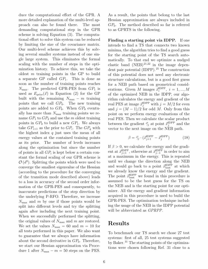
TS on Hartree–Fock level. However, we use thesemi-empirical AM132 method for the electronicstructure calculations. We plot all the TSs wefound in the Baker test set in Fig. 1. These TSswere found by GPRTS except for the TS in sys-tem 4, 10, and 15 for which we used the dimermethod. These exceptions were made since theGPRTS method finds a different transition thanimplied by the test set for system 4 and 10. Forsystem 15 GPRTS does not converge.

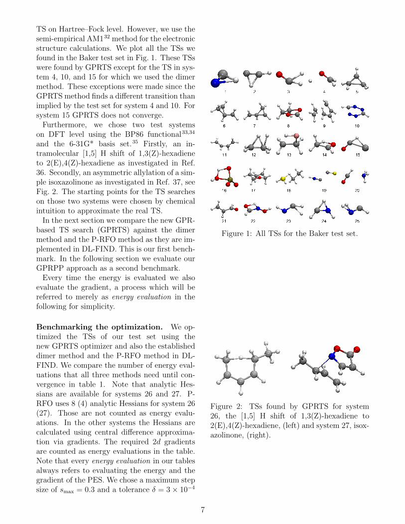
Furthermore, we chose two test systemson DFT level using the BP86 functional33,34

and the 6-31G* basis set.35 Firstly, an in-tramolecular [1,5] H shift of 1,3(Z)-hexadieneto 2(E),4(Z)-hexadiene as investigated in Ref.36. Secondly, an asymmetric allylation of a sim-ple isoxazolinone as investigated in Ref. 37, seeFig. 2. The starting points for the TS searcheson those two systems were chosen by chemicalintuition to approximate the real TS.

In the next section we compare the new GPR-based TS search (GPRTS) against the dimermethod and the P-RFO method as they are im-plemented in DL-FIND. This is our first bench-mark. In the following section we evaluate ourGPRPP approach as a second benchmark.

Every time the energy is evaluated we alsoevaluate the gradient, a process which will bereferred to merely as energy evaluation in thefollowing for simplicity.

Benchmarking the optimization. We op-timized the TSs of our test set using thenew GPRTS optimizer and also the establisheddimer method and the P-RFO method in DL-FIND. We compare the number of energy eval-uations that all three methods need until con-vergence in table 1. Note that analytic Hes-sians are available for systems 26 and 27. P-RFO uses 8 (4) analytic Hessians for system 26(27). Those are not counted as energy evalu-ations. In the other systems the Hessians arecalculated using central difference approxima-tion via gradients. The required 2d gradientsare counted as energy evaluations in the table.Note that every energy evaluation in our tablesalways refers to evaluating the energy and thegradient of the PES. We chose a maximum stepsize of smax = 0.3 and a tolerance δ = 3× 10−4

Figure 1: All TSs for the Baker test set.

Figure 2: TSs found by GPRTS for system26, the [1,5] H shift of 1,3(Z)-hexadiene to2(E),4(Z)-hexadiene, (left) and system 27, isox-azolinone, (right).

7

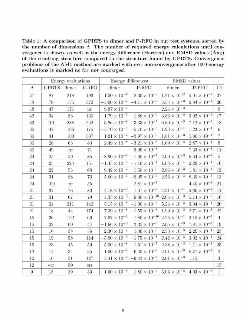
Table 1: A comparison of GPRTS to dimer and P-RFO in our test systems, sorted bythe number of dimensions d. The number of required energy calculations until con-vergence is shown, as well as the energy difference (Hartree) and RMSD values (Ang)of the resulting structure compared to the structure found by GPRTS. Convergenceproblems of the AM1 method are marked with err, non-convergence after 1000 energyevaluations is marked nc for not converged.

Energy evaluations Energy differences RMSD values

d GPRTS dimer P-RFO dimer P-RFO dimer P-RFO ID

57 87 218 193 1.00× 10−7 −2.30× 10−6 1.21× 10−2 5.01× 10−3 27

48 79 155 372 −5.00× 10−7 −4.11× 10−2 3.54× 10−3 9.84× 10−1 26

48 47 171 nc 9.97× 10−7 2.24× 10−3 9

42 34 83 130 1.79× 10−7 −1.86× 10−6 3.83× 10−3 3.02× 10−3 17

33 101 288 232 3.96× 10−8 3.33× 10−5 6.30× 10−3 7.12× 10−2 18

30 47 106 175 −5.70× 10−3 −5.70× 10−3 1.23× 10−1 1.23× 10−1 6

30 41 100 507 1.21× 10−7 −3.97× 10−2 1.81× 10−3 5.80× 10−1 7

30 28 63 83 2.49× 10−8 −3.21× 10−8 1.69× 10−3 2.87× 10−4 8

30 49 err 71 −3.05× 10−3 7.33× 10−1 11

24 25 59 85 −8.90× 10−9 −1.60× 10−7 2.00× 10−3 6.64× 10−4 5

24 25 224 151 −1.45× 10−3 −1.16× 10−1 1.03× 10−1 2.29× 10−1 10

24 22 53 68 9.42× 10−7 1.50× 10−9 2.86× 10−3 1.81× 10−4 12

24 31 88 73 5.80× 10−7 −9.05× 10−9 2.56× 10−3 8.39× 10−5 13

24 100 err 55 −2.81× 10−7 4.40× 10−3 21

21 34 76 80 4.18× 10−8 1.07× 10−8 4.21× 10−1 2.36× 10−4 14

21 31 67 79 4.33× 10−8 9.00× 10−10 2.05× 10−3 5.14× 10−5 16

21 24 211 142 5.15× 10−8 −1.06× 10−7 5.24× 10−3 3.04× 10−1 20

21 18 44 174 7.39× 10−8 −1.55× 10−3 1.99× 10−3 2.71× 10−1 22

15 36 152 66 7.97× 10−2 1.80× 10−10 2.25× 10−1 3.18× 10−5 4

15 22 69 44 −1.66× 10−8 3.35× 10−6 2.05× 10−3 7.81× 10−3 19

15 16 38 56 2.30× 10−7 1.06× 10−8 2.53× 10−3 2.20× 10−4 23

15 19 58 114 −5.80× 10−9 −1.75× 10−8 2.42× 10−3 3.92× 10−4 24

15 23 45 59 5.00× 10−8 1.51× 10−7 2.38× 10−3 1.11× 10−3 25

12 14 34 35 1.00× 10−9 6.40× 10−9 2.91× 10−3 6.77× 10−5 2

12 16 31 127 3.41× 10−9 −9.43× 10−2 2.61× 10−3 1.15 3

12 err 59 err 15

9 18 39 30 1.60× 10−9 −1.80× 10−9 3.03× 10−3 4.03× 10−5 1

8

for all optimizations.The P-RFO method calculates the Hessian at

the first point and then only every 50 followingsteps. All other Hessians are inferred via theupdate mechanism by Bofill.38

We see that the GPRTS method generally re-quires fewer energy evaluations than the othermethods and has the least convergence prob-lems. In table 1 we also show the energy differ-ences (the energy from the respective methodminus the energy from GPRTS) and root meansquared deviations (RMSD) of the found TSs,compared to the TSs found by GPRTS. Lookingat the specific systems with relevant deviationsfor the found TSs we observe the following dif-ferences, compare Fig. 1:

• System 3: P-RFO finds a different TS inwhich H2 is completely abstracted. Its en-ergy is 9.34×10−2 Hartree lower than thatof the TS found by GPRTS.

• System 4: GPRTS and P-RFO yield asmaller distance of the H-Atom to the re-maining O atom. which corresponds to adifferent transition than intended: a rota-tion of the OH group.

• System 6: GPRTS finds a different angleH–C–C at the carbene end.

• System 7: P-RFO finds an opening of thering structure which remains closed in theother cases.

• System 10: GPRTS finds a TS in that N2

is abstracted, the dimer method finds thedepicted opening of the ring. The openingof the ring is also found via GPRTS if oneuses a smaller step size. P-RFO finds aclosed ring structure as the TS.

• System 11: P-RFO finds a more planarstructure.

• System 14: The dimer method finds amirror image of the TS found by the othermethods, thus the high RMSD.

• System 20: P-RFO finds a different ori-entation of NH3, rotated relative to HCO,and also with a slightly different distance.

• System 22: P-RFO finds a different angleof the attached OH group. The result-ing molecule is not planar. The result-ing structures of GPRTS and the dimermethod are planar.

• System 26: P-RFO does not find the H-transfer but an opening of the ring.

10-5

10-4

10-3

10-2

10-1

|gra

dien

t|

GPRTS Dimer P-RFO

System 09 System 17

10-6

10-5

10-4

10-3

10-2

0 20 40 60 80 100Number of steps

System 18

10 20 30 40 50

System 06

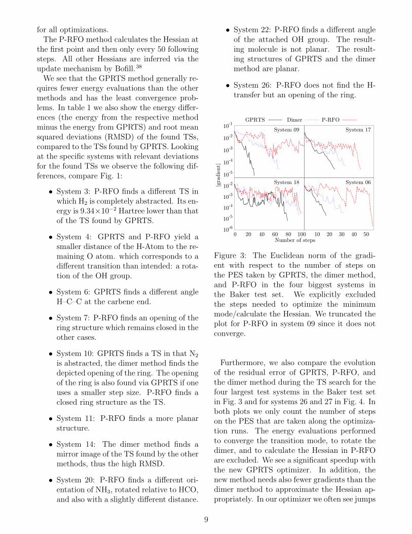
Figure 3: The Euclidean norm of the gradi-ent with respect to the number of steps onthe PES taken by GPRTS, the dimer method,and P-RFO in the four biggest systems inthe Baker test set. We explicitly excludedthe steps needed to optimize the minimummode/calculate the Hessian. We truncated theplot for P-RFO in system 09 since it does notconverge.

Furthermore, we also compare the evolutionof the residual error of GPRTS, P-RFO, andthe dimer method during the TS search for thefour largest test systems in the Baker test setin Fig. 3 and for systems 26 and 27 in Fig. 4. Inboth plots we only count the number of stepson the PES that are taken along the optimiza-tion runs. The energy evaluations performedto converge the transition mode, to rotate thedimer, and to calculate the Hessian in P-RFOare excluded. We see a significant speedup withthe new GPRTS optimizer. In addition, thenew method needs also fewer gradients than thedimer method to approximate the Hessian ap-propriately. In our optimizer we often see jumps

9

10-5

10-4

10-3

10-2

10-1

|gra

dien

t|

GPRTS Dimer PRFO

System 26

10-5

10-4

10-3

10-2

10-1

0 20 40 60 80 100 120 140 160 180Number of steps

System 27

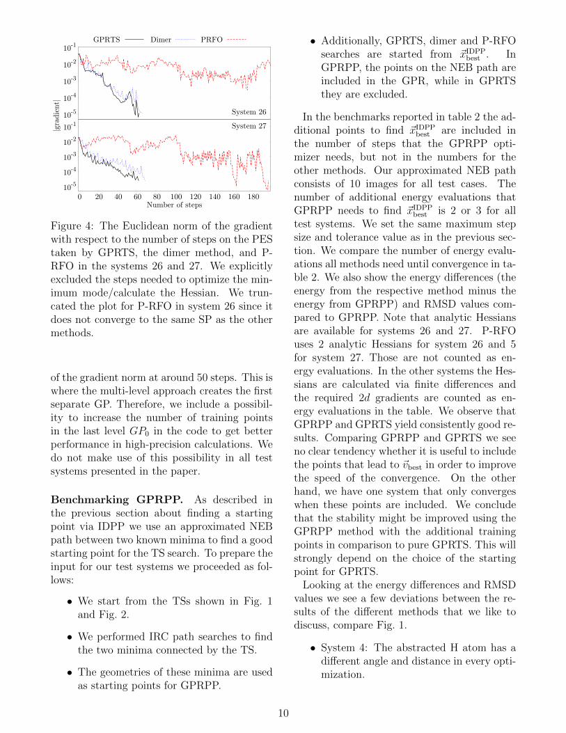
Figure 4: The Euclidean norm of the gradientwith respect to the number of steps on the PEStaken by GPRTS, the dimer method, and P-RFO in the systems 26 and 27. We explicitlyexcluded the steps needed to optimize the min-imum mode/calculate the Hessian. We trun-cated the plot for P-RFO in system 26 since itdoes not converge to the same SP as the othermethods.

of the gradient norm at around 50 steps. This iswhere the multi-level approach creates the firstseparate GP. Therefore, we include a possibil-ity to increase the number of training pointsin the last level GP0 in the code to get betterperformance in high-precision calculations. Wedo not make use of this possibility in all testsystems presented in the paper.

Benchmarking GPRPP. As described inthe previous section about finding a startingpoint via IDPP we use an approximated NEBpath between two known minima to find a goodstarting point for the TS search. To prepare theinput for our test systems we proceeded as fol-lows:

• We start from the TSs shown in Fig. 1and Fig. 2.

• We performed IRC path searches to findthe two minima connected by the TS.

• The geometries of these minima are usedas starting points for GPRPP.

• Additionally, GPRTS, dimer and P-RFOsearches are started from ~xIDPP

best . InGPRPP, the points on the NEB path areincluded in the GPR, while in GPRTSthey are excluded.

In the benchmarks reported in table 2 the ad-ditional points to find ~xIDPP

best are included inthe number of steps that the GPRPP opti-mizer needs, but not in the numbers for theother methods. Our approximated NEB pathconsists of 10 images for all test cases. Thenumber of additional energy evaluations thatGPRPP needs to find ~xIDPP

best is 2 or 3 for alltest systems. We set the same maximum stepsize and tolerance value as in the previous sec-tion. We compare the number of energy evalu-ations all methods need until convergence in ta-ble 2. We also show the energy differences (theenergy from the respective method minus theenergy from GPRPP) and RMSD values com-pared to GPRPP. Note that analytic Hessiansare available for systems 26 and 27. P-RFOuses 2 analytic Hessians for system 26 and 5for system 27. Those are not counted as en-ergy evaluations. In the other systems the Hes-sians are calculated via finite differences andthe required 2d gradients are counted as en-ergy evaluations in the table. We observe thatGPRPP and GPRTS yield consistently good re-sults. Comparing GPRPP and GPRTS we seeno clear tendency whether it is useful to includethe points that lead to ~vbest in order to improvethe speed of the convergence. On the otherhand, we have one system that only convergeswhen these points are included. We concludethat the stability might be improved using theGPRPP method with the additional trainingpoints in comparison to pure GPRTS. This willstrongly depend on the choice of the startingpoint for GPRTS.

Looking at the energy differences and RMSDvalues we see a few deviations between the re-sults of the different methods that we like todiscuss, compare Fig. 1.

• System 4: The abstracted H atom has adifferent angle and distance in every opti-mization.

10

Tab

le2:

AC

om

pari

son

of

GP

RP

Pto

GP

RT

S,dim

er,

and

P-R

FO

inour

test

syst

em

s,so

rted

by

the

num

ber

of

dim

ensi

ons

d.

Th

enum

ber

of

requir

ed

en

erg

yca

lcula

tions

unti

lco

nverg

ence

issh

ow

n,

as

well

as

the

energ

ydiff

ere

nce

(Hart

ree)

and

RM

SD

valu

es

(An

g)

of

the

resu

ltin

gst

ruct

ure

com

pare

dto

the

stru

cture

found

by

GP

RP

P.

Converg

ence

pro

ble

ms

of

the

AM

1m

eth

od

are

mark

ed

wit

herr

,non-c

onverg

ence

aft

er

1000

energ

yevalu

ati

ons

ism

ark

ed

nc

fornotco

nverged

.

Ener

gyev

aluat

ions

Ener

gydiff

eren

ces

RM

SD

valu

esd

GP

RP

PG

PR

TS

dim

erP

-RF

OG

PR

TS

dim

erP

-RF

OG

PR

TS

dim

erP

RF

OID

5787

111

339

210

−4.

00×

10−

71.

40×

10−

6−

3.30×

10−

69.

06×

10−

31.

25×

10−

27.

02×

10−

127

4854

5211

959

1.40×

10−

69.

00×

10−

7−

2.00×

10−

71.

34×

10−

21.

27×

10−

24.

75×

10−

326

4840

52nc

nc

−1.

51×

10−

76.

21×

10−

49

4288

115

err

225

2.84×

10−

7−

4.35×

10−

76.

88×

10−

41.

17×

10−

317

3346

5215

119

0−

8.13×

10−

5−

9.10×

10−

5−

9.10×

10−

58.

70×

10−

21.

28×

10−

11.

28×

10−

118

3041

4712

117

4−

1.21×

10−

6−

9.49×

10−

7−

1.23×

10−

62.

54×

10−

32.

30×

10−

32.

55×

10−

36

3039

4011

417

5−

1.82×

10−

7−

8.00×

10−

10−

2.41×

10−

79.

85×

10−

41.

07×

10−

31.

04×

10−

37

3029

2874

71−

5.38×

10−

84.

50×

10−

8−

9.23×

10−

85.

52×

10−

48.

28×

10−

44.

73×

10−

48

3069

65nc

69−

1.43×

10−

8−

2.92×

10−

32.

03×

10−

46.

93×

10−

111

2425

2660

759.

87×

10−

81.

31×

10−

7−

2.04×

10−

84.

77×

10−

45.

93×

10−

42.

61×

10−

45

2434

31er

r86

1.16×

10−

15.

91×

10−

72.

29×

10−

11.

34×

10−

310

2493

82er

r15

26.

00×

10−

10

1.00×

10−

10

4.64×

10−

53.

56×

10−

512

2440

3912

292

−6.

73×

10−

97.

23×

10−

81.

48×

10−

71.

18×

10−

43.

67×

10−

48.

80×

10−

413

2469

129

err

554.

96×

10−

9−

2.77×

10−

72.

60×

10−

44.

49×

10−

321

2131

3168

739.

04×

10−

82.

84×

10−

7−

4.93×

10−

94.

21×

10−

14.

22×

10−

14.

22×

10−

114

2130

3175

689.

16×

10−

75.

02×

10−

83.

80×

10−

92.

13×

10−

36.

52×

10−

43.

48×

10−

416

2151

205

nc

nc

2.45×

10−

22.

9920

2135

3290

76−

1.00×

10−

10

3.13×

10−

81.

38×

10−

81.

05×

10−

42.

82×

10−

41.

50×

10−

422

1587

55nc

142

1.43×

10−

31.

41×

10−

35.

76×

10−

15.

29×

10−

14

1523

2268

450.

003.

07×

10−

84.

40×

10−

71.

31×

10−

42.

99×

10−

43.

32×

10−

319

1535

95er

r37

7−

1.01×

10−

1−

1.01×

10−

19.

84×

10−

17.

44×

10−

123

1523

2560

63−

8.00×

10−

10

5.49×

10−

87.

80×

10−

93.

12×

10−

55.

51×

10−

41.

48×

10−

424

1520

2154

563.

37×

10−

81.

16×

10−

84.

10×

10−

93.

61×

10−

41.

07×

10−

42.

54×

10−

425

1216

1737

35−

1.00×

10−

10−

1.00×

10−

10

5.50×

10−

93.

54×

10−

54.

31×

10−

58.

26×

10−

52

1229

1729

669.

50×

10−

10

2.05×

10−

83.

35×

10−

99.

33×

10−

51.

31×

10−

41.

27×

10−

43

1228

err

err

err

159

2019

4037

8.00×

10−

10−

1.00×

10−

10

0.00

4.47×

10−

52.

45×

10−

52.

03×

10−

61

11

• System 10: GPRPP and P-RFO found aclosed, symmetric ring structure. GPRTSfound a similar ring as in the referencestructure depicted in Fig. 1, only withlarger distance of the two nitrogen atomsto the carbons. The dimer method leadsto a problem with the AM1 SCF conver-gence.

• System 11: P-RFO finds a more planarstructure.

• System 12: The dimer method does notconverge. All other methods yield thesame TS, in which the two hydrogenatoms that get abstracted are moved moretowards one of the carbon atoms.

• System 14: Dimer, GPRTS and P-RFOall find the mirror image of the TS foundby GPRPP.

• System 15: GPRPP converges to the cor-rect SP but the suggested starting pointleads all other methods to a configurationfor which the AM1 SCF cycles do not con-verge anymore.

• System 18: Dimer and P-RFO yieldslightly different angles between theatoms.

• System 20: GPRTS yields unrealisticlarge distances of the two molecules. Theother two methods do not converge. Theystart unrealistically increasing the dis-tance of the two molecules as well.

• System 23: GPRPP finds the same TS asdepicted in Fig. 1, only with a differentangle of the hydrogen that is attached tothe nitrogen. All other methods find toolarge, and each a different, distance of theH2 that is abstracted.

• System 27: P-RFO finds a different orien-tation of the ring structure correspondingto a different TS.

The clear superiority of the new optimizer inthe test systems indicates that the GPR-basedrepresentation of the Hessian is very well suited

for finding the minimum mode. The suggestedstarting points ~xIDPP

best for the TS searches areplausible in most systems. Overall the initialguess for the TS search using the IDPP seemsto be sufficient for our usage in the GPRPPmethod but is generally not advisable for otherTS-search algorithms. In some test cases it canonly be used if one manually corrects for chem-ically unintuitive TS estimates.

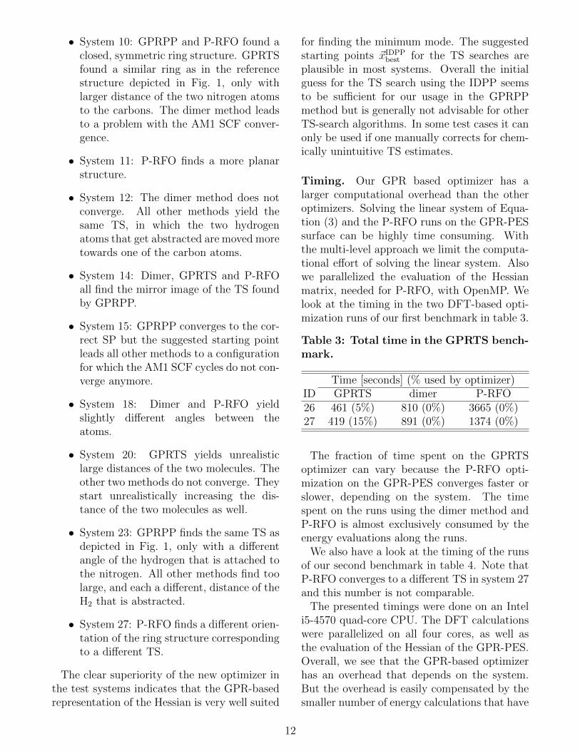
Timing. Our GPR based optimizer has alarger computational overhead than the otheroptimizers. Solving the linear system of Equa-tion (3) and the P-RFO runs on the GPR-PESsurface can be highly time consuming. Withthe multi-level approach we limit the computa-tional effort of solving the linear system. Alsowe parallelized the evaluation of the Hessianmatrix, needed for P-RFO, with OpenMP. Welook at the timing in the two DFT-based opti-mization runs of our first benchmark in table 3.

Table 3: Total time in the GPRTS bench-mark.

Time [seconds] (% used by optimizer)ID GPRTS dimer P-RFO26 461 (5%) 810 (0%) 3665 (0%)27 419 (15%) 891 (0%) 1374 (0%)

The fraction of time spent on the GPRTSoptimizer can vary because the P-RFO opti-mization on the GPR-PES converges faster orslower, depending on the system. The timespent on the runs using the dimer method andP-RFO is almost exclusively consumed by theenergy evaluations along the runs.

We also have a look at the timing of the runsof our second benchmark in table 4. Note thatP-RFO converges to a different TS in system 27and this number is not comparable.

The presented timings were done on an Inteli5-4570 quad-core CPU. The DFT calculationswere parallelized on all four cores, as well asthe evaluation of the Hessian of the GPR-PES.Overall, we see that the GPR-based optimizerhas an overhead that depends on the system.But the overhead is easily compensated by thesmaller number of energy calculations that have

12

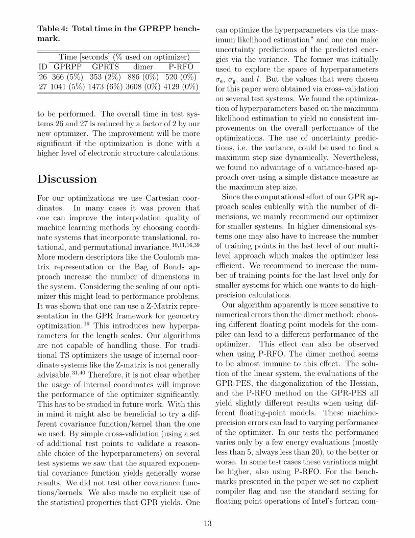
Table 4: Total time in the GPRPP bench-mark.

Time [seconds] (% used on optimizer)ID GPRPP GPRTS dimer P-RFO26 366 (5%) 353 (2%) 886 (0%) 520 (0%)27 1041 (5%) 1473 (6%) 3608 (0%) 4129 (0%)

to be performed. The overall time in test sys-tems 26 and 27 is reduced by a factor of 2 by ournew optimizer. The improvement will be moresignificant if the optimization is done with ahigher level of electronic structure calculations.

Discussion

For our optimizations we use Cartesian coor-dinates. In many cases it was proven thatone can improve the interpolation quality ofmachine learning methods by choosing coordi-nate systems that incorporate translational, ro-tational, and permutational invariance.10,11,16,39

More modern descriptors like the Coulomb ma-trix representation or the Bag of Bonds ap-proach increase the number of dimensions inthe system. Considering the scaling of our opti-mizer this might lead to performance problems.It was shown that one can use a Z-Matrix repre-sentation in the GPR framework for geometryoptimization.19 This introduces new hyperpa-rameters for the length scales. Our algorithmsare not capable of handling those. For tradi-tional TS optimizers the usage of internal coor-dinate systems like the Z-matrix is not generallyadvisable.31,40 Therefore, it is not clear whetherthe usage of internal coordinates will improvethe performance of the optimizer significantly.This has to be studied in future work. With thisin mind it might also be beneficial to try a dif-ferent covariance function/kernel than the onewe used. By simple cross-validation (using a setof additional test points to validate a reason-able choice of the hyperparameters) on severaltest systems we saw that the squared exponen-tial covariance function yields generally worseresults. We did not test other covariance func-tions/kernels. We also made no explicit use ofthe statistical properties that GPR yields. One

can optimize the hyperparameters via the max-imum likelihood estimation8 and one can makeuncertainty predictions of the predicted ener-gies via the variance. The former was initiallyused to explore the space of hyperparametersσe, σg, and l. But the values that were chosenfor this paper were obtained via cross-validationon several test systems. We found the optimiza-tion of hyperparameters based on the maximumlikelihood estimation to yield no consistent im-provements on the overall performance of theoptimizations. The use of uncertainty predic-tions, i.e. the variance, could be used to find amaximum step size dynamically. Nevertheless,we found no advantage of a variance-based ap-proach over using a simple distance measure asthe maximum step size.

Since the computational effort of our GPR ap-proach scales cubically with the number of di-mensions, we mainly recommend our optimizerfor smaller systems. In higher dimensional sys-tems one may also have to increase the numberof training points in the last level of our multi-level approach which makes the optimizer lessefficient. We recommend to increase the num-ber of training points for the last level only forsmaller systems for which one wants to do high-precision calculations.

Our algorithm apparently is more sensitive tonumerical errors than the dimer method: choos-ing different floating point models for the com-piler can lead to a different performance of theoptimizer. This effect can also be observedwhen using P-RFO. The dimer method seemsto be almost immune to this effect. The solu-tion of the linear system, the evaluations of theGPR-PES, the diagonalization of the Hessian,and the P-RFO method on the GPR-PES allyield slightly different results when using dif-ferent floating-point models. These machine-precision errors can lead to varying performanceof the optimizer. In our tests the performancevaries only by a few energy evaluations (mostlyless than 5, always less than 20), to the better orworse. In some test cases these variations mightbe higher, also using P-RFO. For the bench-marks presented in the paper we set no explicitcompiler flag and use the standard setting forfloating point operations of Intel’s fortran com-

13

piler, version 16.0.2. That is, using “more ag-gressive optimizations on floating-point calcu-lations”, as can be read in the developer guidefor ifort.

The overall result of our benchmark is verypromising. The big advantage of the newGPRTS optimizer is twofold: firstly, one canget a quite precise representation of the secondorder information with GPR that seems to besuperior to traditional Hessian update mecha-nisms. Secondly, our algorithm is able to dovery large steps, as part of the overshootingprocedures. Doing large steps and overshoot-ing the estimated solution does not hinder theconvergence since the optimizer can use that in-formation to improve the predicted GPR-PES.Therefore, even bad estimates of the next pointcan lead to an improvement in the optimizationperformance.

Our GPRPP method of finding a startingpoint for the TS search seems to work quitewell. It is generally not advisable to use theestimated starting point in other optimizationalgorithms. But it is sufficiently accurate forour GPRPP method. Also the additional pointsof the NEB in the IDPP seem to improve thestability of the optimization in many cases. Ifchemical intuition or some other method leadsto a starting point very close to the real TS, thepure GPRTS method might still be faster.

Conclusions

We presented a new black box optimizer to findSPs on energy surfaces based on GPR. Only amaximum step size has to be set manually bythe user. It outperforms both well establishedmethods (dimer and P-RFO). The speedup inthe presented test systems is significant and willbe further increased when using higher leveltheory for the electronic structure calculations.We also presented an automated way of find-ing a starting geometry for the TS search usingthe reactant and product geometries. We ad-vise to use this approach for systems in whichthe two minima are known and the estimate ofthe TS is not straightforward. In the presentedtest systems the method is very stable and fast.

Acknowledgments

We thank Bernard Haasdonk for stimulat-ing discussions. This work was financiallysupported by the European Union’s Horizon2020 research and innovation programme (grantagreement No. 646717, TUNNELCHEM)and the German Research Foundation (DFG)through the Cluster of Excellence in Simula-tion Technology (EXC 310/2) at the Universityof Stuttgart.

References

(1) Baker, J. An algorithm for the location oftransition states. J. Comput. Chem. 1986,7, 385–395.

(2) Banerjee, A.; Adams, N.; Simons, J.;Shepard, R. Search for stationary pointson surfaces. J. Phys. Chem. 1985, 89, 52–57.

(3) Plasencia Gutierrez, M.; Argaez, C.;Jonsson, H. Improved Minimum ModeFollowing Method for Finding First OrderSaddle Points. J. Chem. Theory Comput.2017, 13, 125–134.

(4) Henkelman, G.; Jonsson, H. A dimermethod for finding saddle points on highdimensional potential surfaces using onlyfirst derivatives. J. Chem. Phys. 1999,111, 7010–7022.

(5) Lanczos, C. An iteration method for thesolution of the eigenvalue problem of lin-ear differential and integral operators. J.Res. Natl. Bur. Stand. B 1950, 45, 255–282.

(6) Zeng, Y.; Xiao, P.; Henkelman, G. Uni-fication of algorithms for minimum modeoptimization. J. Chem. Phys. 2014, 140,044115.

(7) Heyden, A.; Bell, A. T.; Keil, F. J. Effi-cient methods for finding transition states

14

in chemical reactions: Comparison of im-proved dimer method and partitioned ra-tional function optimization method. J.Chem. Phys. 2005, 123, 224101.

(8) Rasmussen, C. E.; Williams, C. K. Gaus-sian processes for machine learning ; MITpress Cambridge, 2006; Vol. 1.

(9) Alborzpour, J. P.; Tew, D. P.; Haber-shon, S. Efficient and accurate evaluationof potential energy matrix elements forquantum dynamics using Gaussian pro-cess regression. J. Chem. Phys. 2016, 145,174112.

(10) Bartok, A. P.; Kondor, R.; Csanyi, G. Onrepresenting chemical environments. Phys.Rev. B 2013, 87, 184115.

(11) Ramakrishnan, R.; von Lilienfeld, O. A.Reviews in Computational Chemistry ;JWS, 2017; pp 225–256.

(12) Mills, M. J.; Popelier, P. L. Intramolec-ular polarisable multipolar electrostaticsfrom the machine learning method Krig-ing. Comput. Theor. Chem. 2011, 975, 42– 51.

(13) Handley, C. M.; Hawe, G. I.; Kell, D. B.;Popelier, P. L. A. Optimal constructionof a fast and accurate polarisable wa-ter potential based on multipole momentstrained by machine learning. Phys. Chem.Chem. Phys. 2009, 11, 6365–6376.

(14) Fletcher, T. L.; Kandathil, S. M.; Pope-lier, P. L. A. The prediction of atomickinetic energies from coordinates of sur-rounding atoms using kriging machinelearning. Theor. Chem. Acc. 2014, 133,1499.

(15) Ramakrishnan, R.; von Lilienfeld, O. A.Many molecular properties from one ker-nel in chemical space. CHIMIA 2015, 69,182–186.

(16) Hansen, K.; Biegler, F.; Ramakrish-nan, R.; Pronobis, W.; von Lilien-feld, O. A.; Muller, K.-R.; Tkatchenko, A.

Machine Learning Predictions of Molec-ular Properties: Accurate Many-BodyPotentials and Nonlocality in ChemicalSpace. J. Phys. Chem. Lett. 2015, 6,2326–2331.

(17) Dral, P.; Owens, A.; Yurchenko, S.;Thiel, W. Structure-based sampling andself-correcting machine learning for accu-rate calculations of potential energy sur-faces and vibrational levels. J. Chem.Phys. 2017, 146, 244108.

(18) Deringer, V. L.; Bernstein, N.;Bartok, A. P.; Cliffe, M. J.; Kerber, R. N.;Marbella, L. E.; Grey, C. P.; Elliott, S. R.;Csanyi, G. Realistic Atomistic Structureof Amorphous Silicon from Machine-Learning-Driven Molecular Dynamics. J.Phys. Chem. Lett. 2018, 9, 2879–2885.

(19) Schmitz, G.; Christiansen, O. Gaussianprocess regression to accelerate geome-try optimizations relying on numerical dif-ferentiation. J. Chem. Phys. 2018, 148,241704.

(20) Denzel, A.; Kastner, J. Gaussian processregression for geometry optimization. J.Chem. Phys. 2018, 148, 094114.

(21) Mills, G.; Jonsson, H. Quantum and ther-mal effects in H2 dissociative adsorption:Evaluation of free energy barriers in multi-dimensional quantum systems. Phys. Rev.Lett. 1994, 72, 1124–1127.

(22) Henkelman, G.; Uberuaga, B. P.;Jonsson, H. A climbing image nudgedelastic band method for finding saddlepoints and minimum energy paths. J.Chem. Phys. 2000, 113, 9901–9904.

(23) Koistinen, O.-P.; Maras, E.; Vehtari, A.;Jonsson, H. Minimum energy path calcu-lations with Gaussian process regression.Nanosystems: Phys. Chem. Math. 2016,7, 925–935.

(24) Koistinen, O.-P.; Dagbjartsdottir, F. B.;Asgeirsson, V.; Vehtari, A.; Jonsson, H.

15

Nudged elastic band calculations acceler-ated with Gaussian process regression. J.Chem. Phys. 2017, 147, 152720.

(25) Smidstrup, S.; Pedersen, A.; Stokbro, K.;Jonsson, H. Improved initial guess for min-imum energy path calculations. J. Chem.Phys. 2014, 140, 214106.

(26) Kastner, J.; Carr, J. M.; Keal, T. W.;Thiel, W.; Wander, A.; Sherwood, P. DL-FIND: An Open-Source Geometry Opti-mizer for Atomistic Simulations. J. Phys.Chem. A 2009, 113, 11856–11865.

(27) Kastner, J.; Sherwood, P. Superlinearlyconverging dimer method for transitionstate search. J. Chem. Phys. 2008, 128,014106.

(28) Sherwood, P.; de Vries, A. H.;Guest, M. F.; Schreckenbach, G.; Cat-low, C. A.; French, S. A.; Sokol, A. A.;Bromley, S. T.; Thiel, W.; Turner, A. J.et al. QUASI: A general purpose imple-mentation of the QM/MM approach andits application to problems in catalysis.J. Mol. Struct. Theochem. 2003, 632, 1 –28.

(29) Metz, S.; Kastner, J.; Sokol, A. A.;Keal, T. W.; Sherwood, P. ChemShell-a modular software package for QM/MMsimulations. Wiley Interdiscip. Rev. Com-put. Mol. Sci. 2014, 4, 101–110.

(30) Matern, B. Spatial variation; SSBM, 2013;Vol. 36.

(31) Baker, J.; Chan, F. The location of transi-tion states: A comparison of Cartesian, Z-matrix, and natural internal coordinates.J. Comput. Chem. 1996, 17, 888–904.

(32) Dewar, M. J.; Zoebisch, E. G.;Healy, E. F.; Stewart, J. J. Develop-ment and use of quantum mechanicalmolecular models. 76. AM1: a newgeneral purpose quantum mechanicalmolecular model. J. Am. Chem. Soc.1985, 107, 3902–3909.

(33) Becke, A. Density-functional exchange-energy approximation with correct asymp-totic behavior. Phys. Rev. A 1988, 38,3098–3100.

(34) Perdew, J. P. Density-functional approx-imation for the correlation energy of theinhomogeneous electron gas. Phys. Rev. B1986, 33, 8822–8824.

(35) Hariharan, P. C.; Pople, J. A. The influ-ence of polarization functions on molecu-lar orbital hydrogenation energies. Theor.Chem. Acc. 1973, 28, 213–222.

(36) Meisner, J.; Kastner, J. Dual-Level Ap-proach to Instanton Theory. J. Chem.Theory Comput. 2018, 14, 1865–1872.

(37) Rieckhoff, S.; Meisner, J.; Kastner, J.;Frey, W.; Peters, R. Double Regioselec-tive Asymmetric C-Allylation of Isoxa-zolinones: Iridium-Catalyzed N-AllylationFollowed by an Aza-Cope Rearrangement.Angew. Chem. Int. Ed. 2017, 57, 1404–1408.

(38) Bofill, J. M. Updated Hessian matrix andthe restricted step method for locatingtransition structures. J. Comput. Chem.1994, 15, 1–11.

(39) Behler, J. J. Chem. Phys. 2016, 145,170901.

(40) Baker, J.; Hehre, W. J. Geometry op-timization in cartesian coordinates: Theend of the Z-matrix? J. Comput. Chem.1990, 12, 606–610.

16