reliability of the parameters in the resolution of overlapped gaussian peaks

Analytica Chitnica Acta, 281(1993) 197-206 Elsevier Science Publishers B.V., Amsterdam

197

Reliability of the parameters in the resolution of overlapped Gaussian peaks

Guido Crisponi, Franc0 Cristiani and Valeria Nurchi

Dipartimento di Chimka e Tecnologie Inorganiche e Metalb~aniche, University di Cagliari, Vii OspedaIe 72, 09124 CagIiari (Italy)

(Received 7th September 1992; revised manuscript received 22nd February 1993)

Abstract

The reliability of the parameters obtained in the decomposition of two overlapped Gaussian peaks has been studied both as a function of the degree of overlapping between them and of the height and halfband width ratios. To do this a method based on the examination of the elements of dispersion matrix, obtained in a Gauss Newton non linear least squares procedure has been adopted. This is a potent tool for pointing out the functional dependence of the parameter errors on the set of numerical values defining the model and on the choice of experimental conditions. It has been shown that the ratio between haifband widths and the degree of overlapping of the bands are the leading factors affecting the reliability of results in this kind of curve decomposition.

&ywom!r: Gaussian peaks, Least squares; Optimal design

The resolution of a composite function in the constituent peaks and the estimation of the relative parameters is valuable in many fields of science, in particular in analytical chemistry for handling chromatographic and spectrophotometric data. Since the availability of computing facili- ties, various methods of analysis have been proposed [l-71; at the same time different studies on the sources of errors affecting the fitting procedure have been carried out [8-141.

In this paper we propose an approach to the study of the factors affecting the precision of the parameters, based on the analysis of the elements of the dispersion matrix.

This kind of study has been already proposed in order to obtain an optimal experimental design [15], and also to observe how some particular sets of the parameters can lead to unreliable results, even with the highest experimental precision and accuracy [16].

Correspondence to: G. Crisponi, Dipartimento di Chimica e Tecnologie Inorganiche e Metallorganiche, Universit?t di Cagliari, Via Gspedale 7209124 Cagliari (Italy).

It allows to gain information on the precision which can be obtained both using different experimental designs and as a function of the degree of peak overlapping.

CURVE FITTING

The Gaussian density function for a random variable is defined in statistics [17,181 as follows:

1 O(x) =

(x-P)*

a&r) 1/2=Q - za2

I I

in which P and o are the expectation value and the standard deviation respectively.

When this mathematical formula is used to describe an experimental signal (for example a spectral band or a chromatographic peak) the easily handled form is used:

0003-2670/93/$06.00 8 1993 - Elsevier Science Publishers B.V. All rights reserved

198 G. Crisponi et al /Anal. Chim. Acta 281 (1993) 197-206

where H is the height of the peak, X’ is the abscissa of maximum, W is the width of the band at half height (halfbandwidth) and k = 8 In 2 = 5.545 is the proportionality factor for the substi- tution of u with W. In order to obtain the parameters H, X’, W of a peak from N measurements of Xi, Y, the sum of the squares of residuals SZ=$ I_l,N[x - Y,,(H, X’, W, X,)1’ has to be minimized. This sum being non-linear with respect to the parameters, the non-linear least squares procedure of Gauss-Newton 119,201 is used. Knowing the estimates Ho, X”, W” of the parameters to be determined, the Y, term can be expanded as a Taylor series truncated to the first term

ci = x”(Ho, X”, W”, Xi) + (GY/SH) - AH

+ (SY/aX’) . AX’ + (SY/SW) * AW (2)

A linear function in the correction terms AH =H-Ha, AX’=X’-X” and AW= W- W”

is thus obtained. Then a linear least squares procedure can be applied. In this way the vector A of the correction terms can be calculated as

A=(ZT.Z)-l.ZT.(Yc-Y) (3)

where Z is the matrix of derivatives, ZT its trans- pose matrix, Y, and Y the vectors of the calculated and experimental signal intensities, respectively.

The matrix C = (ZT * Z)- ’ called dispersion matrix, is furthermore useful in estimating the variances of the parameter as

%j=Cjj*[~2/(~-~P)] (4)

NP being the number of optimized parameters, and the correlation coefficients between each pair of parameters as

rjlj2 = cjlj*/(cjljl ' cj2j2)1'2 (5)

From Eqn. 4 it is clear that the error variances are the product of two independent terms: one S2/(N - Nr) is a measure of the error involved in the experimental measurements, the other Cjj, which does not depend on the Y values, is a function of the way in which the values of the independent variable X are chosen, i.e. a function of the experimental design.

In order to gain the best estimates of the parameters (those affected by the minimum y7 values), S2 has to be minimized by a proper choice of experimental apparatus and proce- dures. Then the experiments have to be planned for obtaining the least values of the Cjj terms in the limits of their experimental restraints (work- ing time, number of measurements, etc.).

Knowledge of the behaviour of the dispersion matrix in the actual system studied is therefore necessary. In the following section we will first present a study on the dispersion matrix for a single Gaussian peak, and then for two overlapped Gaussian peaks.

This could give a clear measure of the precision which can be achieved in the determination of the peak parameters in a representative sam- ple of possible real situations (i.e., in a wide variability of ratios between heights, widths and distances of the peaks).

SINGLE GAUSSIAN PFiAK

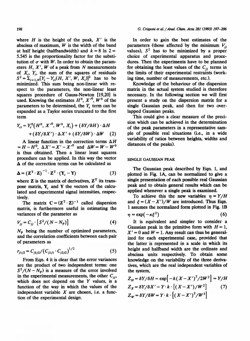
The Gaussian peak described by Eqn. 1, and plotted in Fii. 149, can be normalized to give a single presentation of each possible real Gaussian peak and to obtain general results which can be applied whenever a single peak is examined.

To achieve this the new variables 1 = Y/H and .$ = (X - X’)/W are introduced. Thus Eqn. 1 assumes the normalized form plotted in Fig. 1B

77 = ew( --KS’) (6) It is equivalent and simpler to consider a

Gaussian peak in the primitive form with H = 1, X’ = 0 and W = 1. Any result can thus be general- ized for each experimental case, provided that the latter is represented in a scale in which its height and halfband width are the ordinate and abscissa units respectively. To obtain some knowledge on the variability of the three derivatives, which are the real independent variables of the system,

ZH=GY/SH=exp[-k(X-X’)2/2W2] =Y/H

Z,=t?Y/iSX’=Y.k. [(X-Xr)/W2] (7)

Z,=6Y/6W=Y.k.[(X-X’)2/W3]

G. Crisponi et al. /Anal. Chim. Acta 281 (1993) 197-206

mm sa3.m uu.00 w.m X

1.00

0.75

0.w

OU

0.m . -2.W -l.w Oh 1. 1.

Fig. 1. (A) A Gaussian peak is reported, centred at X= X’, with height H and halfband width W. (B) The same Gaussian peak as in (A) is reported in the normalized variables ,y and 7.

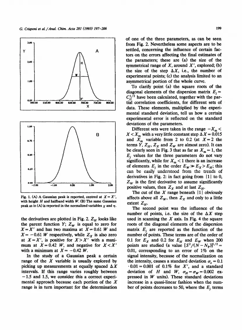
the derivatives are plotted in Fig. 2. 2, looks like the parent function Y; 2, is equal to zero for X=X’ and has two maxima at X-O.61 Wand X= -0.61 W respectively, while 2, is also zero at X=X’, is positive for X > X’ with a maximum at X- 0.42 W, and negative for X <X’ with a minimum at X = -0.42 W.

In the study of a Gaussian peak a certain range of the X variable is usually explored by picking up measurements at equally spaced AX intervals. If this range varies roughly between - 1.5 and 1.5, we consider this a correct experimental approach because each portion of the X range is in turn important for the determination

199

of one of the three parameters, as can be seen from Fig. 2. Nevertheless some aspects are to be settled, concerning the influence of certain factors on the errors affecting the final estimates of the parameters; these are (a) the size of the symmetrical range of X, around X’, explored; (b) the size of the step AX, i.e., the number of experimental points; Cc) the analysis limited to an asymmetrical portion of the whole curve.

To clarify point (al the square roots of the diagonal elements of the dispersion matrix Ei = Ch’” have been calculated, together with the partial correlation coefficients, for different sets of data. These elements, multiplied by the experimental standard deviation, tell us how a certain experimental error is reflected on the standard deviations of the parameters.

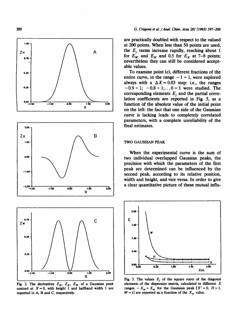
Different sets were taken in the range -X, < X < X, with a very little constant step AX = 0.015 and X, variable from 2 to 0.2 (at X = 2 the terms Y, Z,, Zx and Z, are almost zero). It can be clearly seen in Fig. 3 that as far as X, = 1, the fj values for the three parameters do not vary significantly, while for X,,, < 1 there is an increase of elements Ej in the order E, B- E, > EH; this can be easily understood from the trends of derivatives in Fig. 2: in fact going from I1 I to 0, Z, is the first derivative to assume significantly positive values, then Zx and at last Z,.

The cut of the X range beneath 111 obviously affects above all Z,, then Z, and only to a little extent Z,.

The second point was the influence of the number of points, i.e. the size of the AX step used in scanning the X axis. In Fig. 4 the square roots of the diagonal elements of the dispersion matrix Ej are reported as the function of the number of points. These terms are of the order of 0.1 for E, and 0.2 for EH and E, when 200 points are studied (a value [S’/(N - NP)]1/2 = 0.01, corresponding to an error of 1% on the signal intensity, because of the normalization on the intensity, causes a standard deviation cr, = 0.1 - 0.01 = 0.001 of 0.1% for X’, and a standard deviation of H and W, a, = c+= 0.002 ex- pressed in W units). These standard deviations increase in a quasi-linear fashion when the number of points decreases to 50, where the Ej terms

ml G. Crispmi et al. /Anal. Chim. Acta 281 (1993) 197-206

1.00 -

Ztl am-

a.50 -

010 -

OAm , -1.m -t’oa Oh0 da x’. da

Loo-

zx 1.w -

ODO-

-t.OO-

-LoQ I

-Y.lm -1011 O&Y x’ &I Yao

0.n -

Fig. 2. The derivatives Z,,, Z,, ZW of a Gaussian peak centred at X = 0, with height 1 and halfband width 1 are reported in A, B and C, respectively.

are practically doubled with respect to the valued at 200 points. When less than 50 points are used, the Ej terms increase rapidly, reaching about 1 for E, and EH and 0.5 for E, at 7-8 points; nevertheless they can still be considered accept- able values.

To examine point (cl, different fractions of the entire curve, in the range - 1 + 1, were explored always with a AX= 0.03 step: i.e., the ranges -0.9+1; -0.8+1;... 0 + 1 were studied. The corresponding elements Ej and the partial correlation coefficients are reported in Fig. 5, as a function of the absolute value of the initial point on the left: the fact that one side of the Gaussian curve is lacking leads to completely correlated parameters, with a complete unreliability of the final estimates.

TWO GAUSSIAN PEAK

When the experimental curve is the sum of two individual overlapped Gaussian peaks, the precision with which the parameters of the first peak are determined can be influenced by the second peak, according to its relative position, width and height, and vice versa. In order to give a clear quantitative picture of these mutual influ-

W 1::: H

tl X

0 I 1. 1

Xm

Fig. 3. The values Ej of the square roots of the diagonal elements of the dispersion matrix, calculated in different X ranges - X,,, t X,,, for the Gaussian peak [X’ = 0, H = 1, W= l] are reported as a function of the X,,, value.

G. Chpmi et d/Anal. Chim. Acta 281 (1993) 197-206

1110

E

0.n

000

0t0

om I 1 wh) 1OO.W 1W m0.w

N

Fig. 4. The values Ej of the square roots of the diagonal elements of the dispersion matrix, calculated in the X range -1~1 for the Gaussian peak [X’-0, H-l, W=l], with a variable number of points N are reported as a function of N.

ences, the Ej elements have been calculated for a representative set of relative widths, positions and heights of the second peak. Also in this case a normalization procedure was adopted. For the two peaks I and II, the signal is given by the sum

Y=H,.exp[ -k(X-X{)2/2Wt]

+H,exp[ -k(X-X;)2/2W,2] (8)

Assuming the new variables q = Y/H, and 5 = (X-X,‘)/W, with respect to peak I, Eqn. 8 takes the form

Xexp[ -k(t-Xl)2/2Wl] (9

where XT = (Xi -X;)/IV, and IV, = W,/W,. Peak I on the left is therefore the leading one in the normalization procedure, and its height and

TABLE 1

0.00 040 ok 030 ok Id0 Xm

_.--

El

-,.oo O.d, 0.35 040 oh Ido

Xm

Fig. 5. The values E, of the square. roots of the diagonal elements of the dispersion matrix, calculated in the X range -X,+1 for the Gaussian peak IX’-0, H-1, W-l] are reported as a function of X, in (A). The corresponding partial correlation coefficients r are reported in (B).

width are the units of vertical and horizontal axis respectively.

To obtain a representative set of experimental

The marks used to distinguish the fifteen studied cases of hvo overlapped Gaussian peaks reported vs. height and width of peak II. Height and width of peak I have unitary values

WZ Ha

4 2 1 0.5 0.25

1 Ml, 4) Ml, 21 Ml, 1) Ml. 0.5) Ml, 0.25) 0.5 MO.5,4) M(O.5,2) MO.5, 1) M(O.5,0.5) M(O.5,0.25) 0.25 MO.25,4) M(O.25,2) M(O.25,1) M(0.25.0.5) M(O.25,0.25)

Oso- kl ..--.w -......- II

Y------L . . . ..a..-... x

I .w

: I P I

M(0.25.i)

I

O.Mad, OS.0 l.& 64 ._.

‘. x*121

I .w

o.5o b . . . . . . . . . . “I I?.-=%_ P II

M(O.25.4)

II

0.00 0. ------!-- -l. ===YYqr 0.

I.00 1 P II

-\

M(0.25.0.25)

k.

7 l *s. . . . . . . . W

0.50 . . . . . . . . . . . . . H

1 . . . . . ...* --- . . . . . . . . . . . . . x

I 09: o.!la i&J 1do xo(*3.6o . ..-

P I

M(0.5.i)

x’d

do

P II

r X II

3.00 P I

~1.50 M( 1 .i)

2.00

.; *Lb I.50

I.00

0.50

“3. 0. I.

**i

‘. X’(2f

:; 3.00 2.50 0.50 2.00 1.50

P II

M( 1.0.25)

J&g -X

W I.00

II

o.O?B. 0. I. ‘. X’(2f

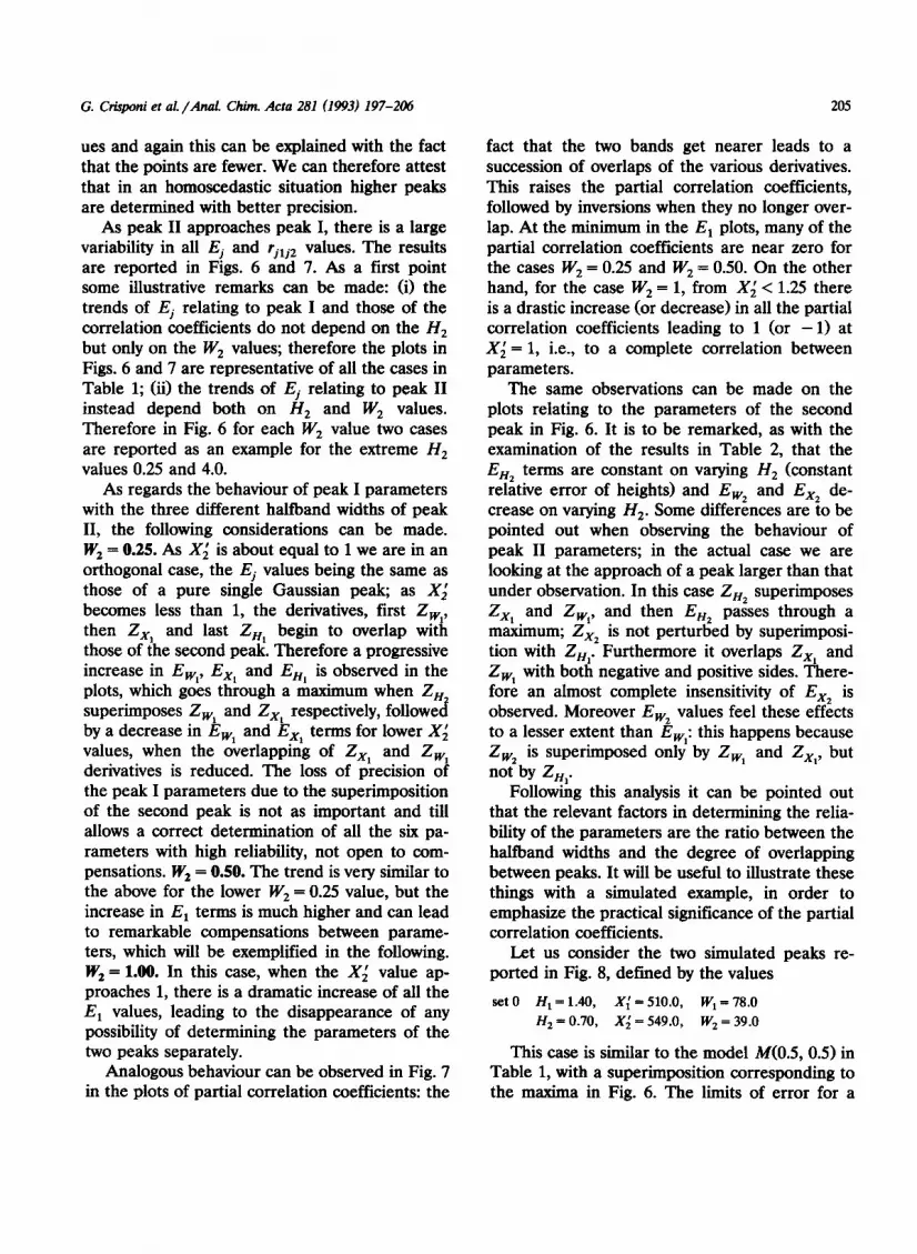
Fig. 6. The values Ej of the square roots of the diagonal elements of the dispersion matrix for hvo Gaussian peaks are reported as a function of the position of the second peak. The index of the peak and the case according to Table 1, are shown in the figures.

G. Crisponi et al. /Anal. Chim. Acta 281 (1993) 197-206

204

situations, the parameters of peak II were al- lowed to vary according to the scheme reported in Table 1. To obtain a fixed precision of the parameters of peak I, a AX step 0.03 was always used. In this way a width of 0.25 for peak II was chosen as the smallest, otherwise too few representative points for peak II would have been scanned, and 1.0 was the biggest because the effect of a larger peak could be inferred by re- versing the results for peak I and peak II. The relative positions vary from one in which the two peaks do not overlap (this is chosen according to the width df peak II) to a distance between maxima of 0.1 in which the two peaks can be considered completely overlapping. The ratio H./H1 was varied from l/4 to 4 in order to have a large set of situations. Considering for example a spectrophotometric determination with an available range of absorbances 0 f 4, both peaks can be measured with a fairly good precision; moreover the distribution of errors can be considered homoscedastic and then the term S2/(ZV- NP) can be assumed constant for all the set of measurements.

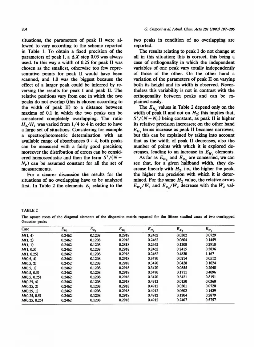
For a clearer discussion the results for the situations of no overlapping have to be analyzed first. In Table 2 the elements Ej relating to the

G. Crisponi et a,! /Anal. Chim. Acta 281 (1993) 197-206

two peaks in condition of no overlapping are reported.

The results relating to peak I do not change at all in this situation; this is correct, this being a case of orthogonality in which the independent variables of one peak vary totally independently of those of the other. On the other hand a variation of the parameters of peak II on varying both its height and its width is observed. Never- theless this variability is not in contrast with the orthogonality between peaks and can be explained easily.

The EH, values in Table 2 depend only on the width of peak II and not on H2; this implies that, S2/(N - A$.) being constant, as peak II is higher its relative precision increases; on the other hand EH, terms increase as peak II becomes narrower, but this can be explained by taking into account that as the width of peak II decreases, also the number of points with which it is explored decreases, leading to an increase in EHz elements.

As far as Ew2 and Ex2 are concerned, we can see that, for a given halfband width, they decrease linearly with H,, i.e., the higher the peak, the higher the precision with which it is determined. For the same H, value, the relative errors Ew2/W2 and E&W, decrease with the W, val-

TABLE 2

The square roots of the diagonal elements of the dispersion matrix reported for the fiieen studied cases of two overlapped Gaussian peaks

CaSe E Hl E Xl EW, Eff2 Ex, EW2 Ml, 4) 0.2462 0.1208 0.2918 0.2462 0.0302 0.0729

Ml; 2) 0.2462 0.1208 0.2918 0.2462 0.0604 0.1459

MU, 1) 0.2462 0.1208 0.2818 0.2462 0.1208 0.2918

M(1,0.5) 0.2462 0.12#8 0.2918 0.2462 0.2415 0.5836

M(1,0.25) 0.2462 0.1208 0.2918 0.2462 0.4830 1.167

M(O.5,4) 0.2462 0.1208 0.2918 0.3470 0.0214 0.0512

M(O.5, 2) 0.2452 0.1208 0.2918 0.3470 0.042J3 0.1024

M(O.5,1) 0.2462 0.1208 0.2918 0.3470 0.0855 0.2048

M(O.5,0.5) 0.2462 0.1208 0.2918 0.3470 0.1711 0.4096

M(O.5,0.25) 0.2462 0.1208 0.2918 0.3470 0.3421 0.8191

M(O.25,4) 0.2462 0.1208 0.2918 0.4912 0.0150 0.0360

M(O.25,2) 0.2462 0.1208 0.2918 0.4912 0.0301 0.0720

M(0.25, 1) 0.2462 0.1208 0.2918 0.4912 0.0602 0.1439

M(O.25,0.5) 0.2462 0.1208 0.2918 0.4912 0.1204 0.2879

M(O.25,0.25) 0.2462 0.1208 0.2918 0.4912 0.2407 0.5757

G. Criponi et al./Anal. Chim. Acta 281 (1993) 197-206 205

ues and again this can be explained with the fact that the points are fewer. We can therefore attest that in an homoscedastic situation higher peaks are determined with better precision.

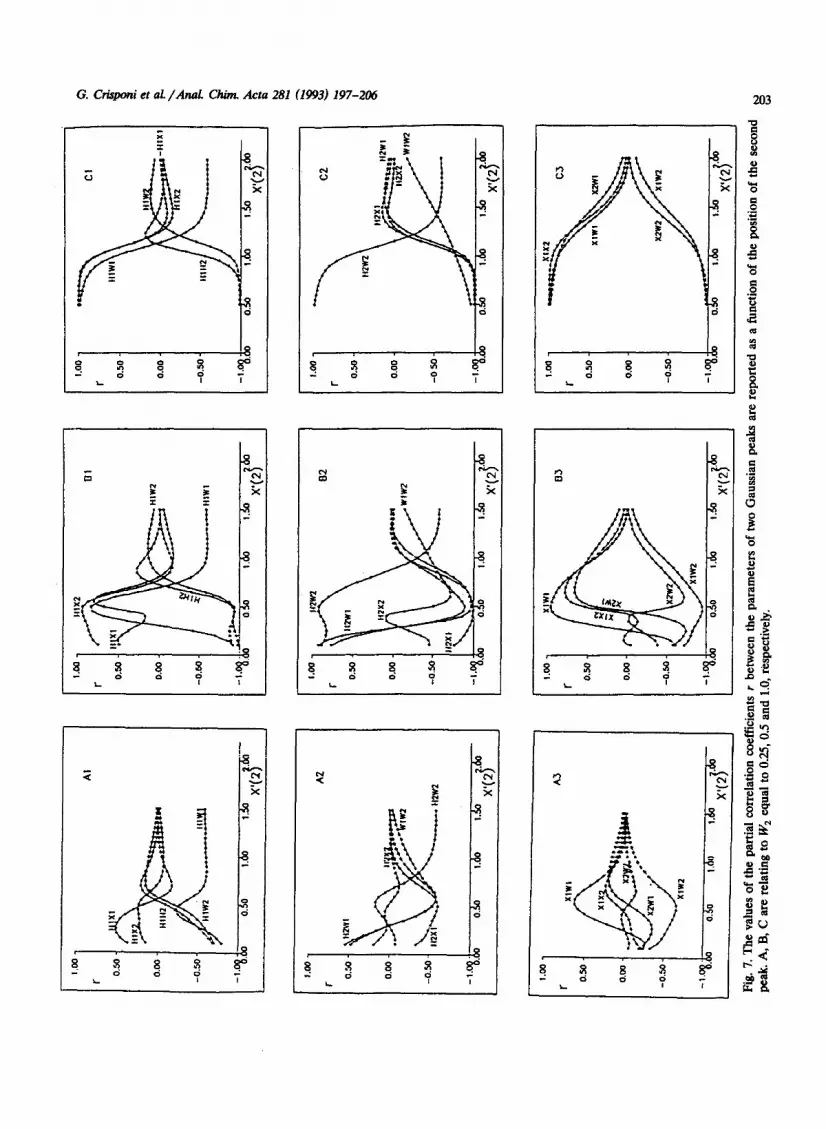
As peak II approaches peak I, there is a large variability in all Ej and rjljz values. The results are reported in Figs. 6 and 7. As a first point some illustrative remarks can be made: (i) the trends of Ej relating to peak I and those of the correlation coefficients do not depend on the H, but only on the W, values; therefore the plots in Figs. 6 and 7 are representative of all the cases in Table 1; (ii) the trends of Ej relating to peak II instead depend both on H, and W, values. Therefore in Fig. 6 for each W, value two cases are reported as an example for the extreme H2 values 0.25 and 4.0.

As regards the behaviour of peak I parameters with the three different halfband widths of peak II, the following considerations can be made. W. = 0.25. As Xi is about equal to 1 we are in an orthogonal case, the Ej values being the same as those of a pure single Gaussian peak; as Xi becomes less than 1, the derivatives, first Z,,, then Zx, and last ZH, begin to overlap with those of the second peak. Therefore a progressive increase in Ewl, Exl and EH, is observed in the plots, which goes through a maximum when ZH, superimposes Zwl and Zx, respectively, followed by a decrease in Ewl and Ex, terms for lower Xi values, when the overlapping of Zx, and Zwl derivatives is reduced. The loss of precision of the peak I parameters due to the superimposition of the second peak is not as important and till allows a correct determination of all the six parameters with high reliability, not open to compensations. W, = 0.50. The trend is very similar to the above for the lower W, = 0.25 value, but the increase in E, terms is much higher and can lead to remarkable compensations between parameters, which will be exemplified in the following. W, = 1.00. In this case, when the Xi value approaches 1, there is a dramatic increase of all the E, values, leading to the disappearance of any possibility of determining the parameters of the two peaks separately.

Analogous behaviour can be observed in Fig. 7 in the plots of partial correlation coefficients: the

fact that the two bands get nearer leads to a succession of overlaps of the various derivatives. This raises the partial correlation coefficients, followed by inversions when they no longer overlap. At the minimum in the E, plots, many of the partial correlation coefficients are near zero for the cases W, = 0.25 and W, = 0.50. On the other hand, for the case W, = 1, from Xi < 1.25 there is a drastic increase (or decrease) in all the partial correlation coefficients leading to 1 (or - 1) at Xi = 1, i.e., to a complete correlation between parameters.

The same observations can be made on the plots relating to the parameters of the second peak in Fig. 6. It is to be remarked, as with the examination of the results in Table 2, that the EH, terms are constant on varying H, (constant relative error of heights) and Ew2 and Ex, decrease on varying H,. Some differences are to be pointed out when observing the behaviour of peak II parameters; in the actual case we are looking at the approach of a peak larger than that under observation. In this case ZHz superimposes Zx, and Zwl, and then EH, passes through a maximum; Zx, is not perturbed by superimposition with Z,,. Furthermore it overlaps Zx, and Zwl with both negative and positive sides. There- fore an almost complete insensitivity of Ex, is observed. Moreover Ew2 values feel these effects to a lesser extent than E,: this happens because Z,* is superimposed only by Zwl and Zx,, but not by ZH,.

Following this analysis it can be pointed out that the relevant factors in determining the reliability of the parameters are the ratio between the halfband widths and the degree of overlapping between peaks. It will be useful to illustrate these things with a simulated example, in order to emphasize the practical significance of the partial correlation coefficients.

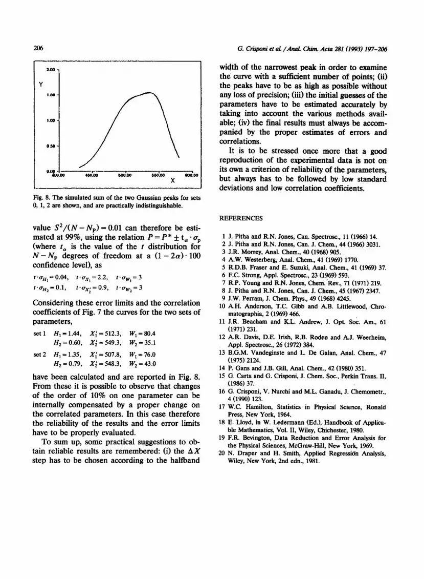
Let us consider the two simulated peaks reported in Fig. 8, defined by the values

set0 H,=lAO, Xi = 510.0, WI = 78.0

Hz = 0.70, X; = 549.0, W, = 39.0

This case is similar to the model M(0.5, 0.5) in Table 1, with a superimposition corresponding to the maxima in Fig. 6. The limits of error for a

G. Ckponi et aL /Ad Chim. Acta 281(1993) 197-206

am-

Y

1.00 -

tm-

OSO-

v~mo r-r-- 4W.W bW.W 000.00 w0.w

X -

Fig. 8. The simulated sum of the two Gaussian peaks for sets 0, 1, 2 are shown, and are practically indistinguishable.

value S2/(N - Nr) = 0.01 can therefore be estimated at 99%, using the relation P = P * f t, - up (where t, is the value of the t distribution for N - NP degrees of freedom at a (1 - 2cr) * 100 confidence level), as

tY7,,=0.04, tv,,=2.2, Pow,=3

tY+,=0.1, tv,,=0.9, tv,,=3 2

Considering these error limits and the correlation coefficients of Fig. 7 the curves for the two sets of parameters,

set1 H,=1.44, X; = 512.3, W, = 80.4

H, = 0.60, X, = 549.3, W, = 35.1

set2 H,=1.35, X; = 507.8, W, = 76.0

Hz = 0.79, X; = 548.3, W, = 43.0

have been calculated and are reported in Fig. 8. From these it is possible to observe that changes of the order of 10% on one parameter can be internally compensated by a proper change on the correlated parameters. In this case therefore the reliability of the results and the error limits have to be properly evaluated.

To sum up, some practical suggestions to obtain reliable results are remembered: (i) the AX step has to be chosen according to the halfband

width of the narrowest peak in order to examine the curve with a sufficient number of points; (ii) the peaks have to be as high as possible without any loss of precision; (iii) the initial guesses of the parameters have to be estimated accurately by taking into account the various methods available; (iv) the final results must always be accom- panied by the proper estimates of errors and correlations.

It is to be stressed once more that a good reproduction of the experimental data is not on its own a criterion of reliability of the parameters, but always has to be followed by low standard deviations and low correlation coefficients.

REFERENCES

1 2 3 4 5 6 7 8 9

10

11

12

13

14 15

16

17

18

19

20

J. Pitha and R.N. Jones, Can. Spectrosc., 11 (1966) 14. J. Pitha and R.N. Jones, Can. J. Chem., 44 (1966) 3031. J.R. Morrey, Anal. Chem., 40 (1966) 905. A.W. Westerberg, Anal. Chem., 41 (1969) 1770. R.D.B. Fraser and E. Suzuki, Anal. Chem., 41 (1969) 37. F.C. Strong, Appl. Spectrosc., 23 (1969) 593. R.P. Young and R.N. Jones, Chem.‘Rev., 71 (1971) 219. J. Pitha and R.N. Jones, Can. J. Chem., 45 (1967) 2347. J.W. Perram, J. Chem. Phys., 49 (1968) 4245. A.H. Anderson, T.C. Gibb and A.B. Littlewood, Chro- matographia, 2 (1%9) 466. J.R. Beacham and K.L. Andrew, J. Opt. Sot. Am., 61 (1971) 231. AR. Davis, D.E. Irish, R.B. Roden and A.J. Weerheim, Appl. Spectrosc., 26 (1972) 384. B.G.M. Vandeginste and L. De Galan, Anal. Chem., 47 (197512124. P. Gans and J.B. Gill, Anal. Chem., 42 (1980) 351. G. Carta and G. Crisponi, J. Chem. Sot., Perkin Trans. II, (1986) 37. G. Crisponi, V. Nurchi and ML. Ganadu, J. Chemometr., 4 (19901 123. W.C. Hamilton, Statistics in Physical Science, Ronald Press, New York, 1964. E. Lloyd, in W. Ledermann (Ed.), Handbook of Applica- ble Mathematics, Vol. II, Wiley, Chichester, 1980. F.R. Bevington, Data Reduction and Error Analysis for the Physical Sciences, McGraw-Hill, New York, 1969. N. Draper and H. Smith, Applied Regression Analysis, Wiley, New York, 2nd edn., 1981.

reliability of the parameters in the resolution of overlapped gaussian peaks

Documents