no bank, one bank, several banks: does it matter for investment?
TRANSCRIPT

NO BANK, ONE BANK, SEVERAL BANKS: DOES IT MATTER FOR INVESTMENT?
Alexander Karaivanov, Sonia Ruano,Jesús Saurina and Robert Townsend
Documentos de Trabajo N.º 1003
2010

NO BANK, ONE BANK, SEVERAL BANKS: DOES IT MATTER FOR INVESTMENT?

NO BANK, ONE BANK, SEVERAL BANKS: DOES IT MATTER FORINVESTMENT? (*)
Alexander Karaivanov
SIMON FRASER UNIVERSITY
Sonia Ruano (**) and Jesús Saurina
BANCO DE ESPAÑA
Robert Townsend
MIT
(*) Research support from the US National Science Foundation, the National Institute of Health, John Templeton Foundation, the Gates Foundation through the University of Chicago Consortium on Financial Systems and Poverty and the Social Sciences and Humanities Research Council is gratefully acknowledged. This paper is the sole responsibility of its authors and the views presented here do not necessarily reflect those of Banco de España or the Eurosystem. We thank V. Salas for his comments and suggestions on preliminary versions of this paper. We also appreciate theexcellent comments received from the Editor and an anonymous referee of the Banco de España Working Paper Series,the 2009 Far East Meeting of the Econometric Society and the 24th Annual Congress of the European EconomicAssociation. Any remaining errors are our own.
(**) Address for correspondence: Banco de España, Alcalá 48, 28014 Madrid, Spain. Tel.: + 34 91 338 62 39; e-mail: [email protected].
Documentos de Trabajo. N.º 1003
2010

The Working Paper Series seeks to disseminate original research in economics and fi nance. All papers have been anonymously refereed. By publishing these papers, the Banco de España aims to contribute to economic analysis and, in particular, to knowledge of the Spanish economy and its international environment.
The opinions and analyses in the Working Paper Series are the responsibility of the authors and, therefore, do not necessarily coincide with those of the Banco de España or the Eurosystem.
The Banco de España disseminates its main reports and most of its publications via the INTERNET at the following website: http://www.bde.es.
Reproduction for educational and non-commercial purposes is permitted provided that the source is acknowledged.
© BANCO DE ESPAÑA, Madrid, 2010
ISSN: 0213-2710 (print)ISSN: 1579-8666 (on line)Depósito legal: M. 14140-2010 Unidad de Publicaciones, Banco de España

Abstract
This paper examines whether fi nancial constraints affect fi rms’ investment decisions for
older (larger) fi rms. We compare a group of unbanked fi rms to fi rms that rely on formal
fi nancing. Specifi cally, we combine data from the Spanish Mercantile Registry and the
Bank of Spain Credit Registry (CIR) to classify fi rms according to their number of banking
relations: one, several, or none. Our empirical strategy combines two approaches based
on a common theoretical model. First, using a standard Euler equation adjustment cost
approach to investment, we fi nd that single-banked fi rms in our sample are most likely to
exhibit cash fl ow sensitivity while unbanked fi rms are not. Second, using structural maximum
likelihood estimation, we fi nd that unbanked fi rms have a fi nancial structure which is close
to credit subject to moral hazard with unobserved effort, whereas single-banked fi rms have
a fi nancial structure which is more limited, as in an exogenously imposed traditional debt
model. Firms in the unbanked category do not rely on bonds, equity, or formal fi nancial
markets, but rather on other fi rms in a fi nancial or family-tied group (with either pyramidal
or informal structure). We are among the fi rst to document the importance of such groups
in a European country. We control for reverse causality by treating bank relationships as
endogenous and/or by appropriate stratifi cations of the sample.
Keywords: inancial constraints, bank lending, investment Euler equations, moral hazard,
structural estimation and testing.
JEL classifi cation: C61, D82, D92, G21, G30.

BANCO DE ESPAÑA 9 DOCUMENTO DE TRABAJO N.º 1003
1 Introduction
Over the past two decades the bulk of the literature on investment, at the micro level, has
focused on the influence of financial constraints on firms’ investment decisions.1 Theorists
have used models of information and incentive problems in capital markets to motivate the
role and origin of financial constraints. Both adverse selection due to asymmetric
information between the borrower and potential lenders about the quality of the investment
project and moral hazard (due to the costly monitoring of managers’ allocation of resources)
can introduce a wedge between the cost of internal and external finance.2 Ultimately, this
results in limited access to external finance, so that firms have to restrict investment when
internal cash is insufficient to invest at the first-best level.3
The empirical literature has documented that, in addition to the fundamentals
determining investment dynamics (expected future profitability and the user cost of capital),
firms’ internal funds affect in a positive and significant manner their investment decisions,
with more intensity for firms affected by capital market imperfections. Since the seminal
paper of Fazzari, Hubbard and Petersen (1988), an extensively used empirical strategy
consists of separating “constrained” and “unconstrained” firms according to a priori
assumptions on the likelihood that firms are subject to information or incentive problems,
then testing whether the neoclassical investment equation derived under the assumption of
perfect capital markets with adjustment costs describes the behaviour of financially
unconstrained firms but not that of financially constrained firms.4 Some firm characteristics
used in this stratification as a priori proxies of the importance of capital market imperfections
are firm’s size, age, and dividend policy.5 A few stratify by relationship with industrial or
financial groups, and this turns out to be related to our findings here.6
In parallel, a literature on relationship banking has developed based on the idea
that information about borrowers is extremely important in the lending process, especially
for small firms who are considered “informationally opaque”.7 Banks are thought to have a
comparative advantage in producing information about borrowing firms [Diamond (1984);
Bond (2004)]. To the extent that bank relationships mitigate asymmetric information
1. Schiantarelly (1996) and Hubbard (1998) provide extensive reviews of the literature.
2. On adverse selection see Jaffee and Russell (1976) or Stiglitz and Weis (1981). Myers and Majluf (1984) focus on
informational problems affecting equity financing. The effects of moral hazard are treated in Jensen and Meckling
(1976). Williamson (1987) derives the possibility of credit rationing in the context of optimally designed contracts under
the assumption that profit outcomes can only be observed at a cost. On costly state verification see also Townsend
(1979) and Diamond (1984).
3. The gap between the cost of external debt and of internal funds can be explained by information costs but it could
also be due to tax factors or other transaction costs.
4. There are two main empirical approaches, pioneered by Fazzari, Hubbard and Petersen (1988) and Bond and
Meghir (1994) respectively. The first approach is based on the estimation of the Q model of investment, extended by
including a proxy for the availability of internal funds and testing for differences in the sensitivity of investment to cash
flow between “constrained” and “unconstrained” firms. The second approach estimates the standard investment
Euler equation which should be valid for unconstrained firms but mis-specified for constrained firms. In both cases,
the investment equations are derived from the neoclassical model under the assumptions of perfect competition,
constant returns to scale, and quadratic adjustment costs.
5. Schiantarelli (1996) provides an exhaustive list of the criteria employed in the literature to partition firms according to
their likelihood of being subject to financial constraints and discusses the empirical literature for every criterion.
6. Although, we do not stratify by relationship with industrial or financial groups, we find that a sizeable number of
older, larger firms are unbanked. A major source of funds for these firms is debt with other enterprises in a financial
group and persistently unbanked firms tend to be family-tied (in either pyramidal or informal structures).
7. For a comprehensive review of the literature on relationship banking see Boot (2000) and Elyasiani and
Goldberg (2004).

BANCO DE ESPAÑA 10 DOCUMENTO DE TRABAJO N.º 1003
problems between creditors and borrowers and facilitate monitoring, the incidence of
financial constraints on firms’ investment decisions and, consequently, on the sensitivity of
investment to cash flow, could differ across groups of firms classified according to the
strength of their banking relationships.8
Although empirical research evaluating the costs and benefits of banking
relationships has been extensive, papers connecting differences in firms’ investment
behaviour with bank-firm relationships are relatively scarce.9 In most cases, the results
suggest that close bank relationships are associated with reduction in the sensitivity of
investment to cash flow [Elston (1996), for Germany; García-Marco and Ocaña (1999),
for Spain;10 and Houston and James (2001), for the USA]. In one case the authors find
no significant effects of bank relationships [Fuss and Vermeulen (2006), for Belgium].
In another case the result is the opposite [Fohlin (1998), for Germany during the formative
years of universal banking].11
Our empirical findings are in line with those of Fohlin (1998) who documents that
investment is less sensitive to internal resources in unbanked firms, contrary to what is
reported in the rest of the papers for other countries, including Spain. One reason is that
most of the authors compare banked and unbanked firms defined according to the
presence of banks in the list of shareholders or on the board. This is a valid but, in our
opinion, restrictive way of distinguishing banked vs. unbanked firms. In this paper, we define
unbanked firms simply as those not borrowing from any bank. In contrast to the few papers
which define bank relationships the same way we do, we also study unbanked firms and
not just a comparison between single- and multiple-banked firms12.
With respect to the literature on Spanish firms [García-Marco and Ocaña (1999)],
discrepancies in the results are likely due to differences in the definition of bank relationships,
differences in the size and composition of the sample which was limited to a few large and listed
manufacturing firms, and/or differences in the sample period.
Another substantial difference we have with the previous literature is that we
restrict attention to firms that are at least ten years old. Our sample thus features unbanked
firms that are older, if not larger, than small start-ups and young firms without credit history,
possibly unbanked for that reason. The latter group is a priori likely to be more constrained
than any other group, and we do not want to mix such firms in our sample of unbanked
8. The strength of firms’ banking relationship has been defined in the literature as: the relationship’s length ([Petersen
and Rajan (1994); Harhoff and Körting (1998); Berger and Udell, 1995 and Degryse and Van Cayseele (2000)],
the relationship’s scope, i.e., type and number of financial services [Petersen and Rajan (1994) and Degryse and
van Cayseele (2000)], bank’s ownership [Elston (1996); García-Marco and Ocaña (1999); Fohlin (1998) and Chirinko
and Elston (2006)], and the number of banks [Petersen and Rajan (1994); Harhoff and Körting (1998); Houston and
James (2001) and Fuss and Vermeulen (2006)].
9. With the exception of Houston and James (2001) and Fuss and Vermeulen (2006) who differentiate between single
and multiple banked firms, the rest of the papers only consider the presence of banks as shareholders or on the board
of directors.
10. Carbó, Rodríguez and Udell (2008) use a disequilibrium model to classify Spanish firms as constrained
and unconstrained and find that investment is predicted by bank loans for unconstrained firms and by trade
credit for constrained ones. Although not specifically focused on the influence of banking relationships,
the influence of financial constraints on investment decisions for Spanish firms has also been previously analysed
by Alonso-Borrego (1994), Estrada and Vallés (1998) and Hernando and Tiorno (2002).
11. Other papers investigate differences in the role of bank relationships in alleviating financial constraints in different
stages of the credit cycle. As an example, see Vickery (2005), which presents evidence that benefits of relationships
are higher when credit conditions are poor or deteriorating.
12. On the determinants of the number of bank relationships see Ongena and Smith (2000) and Guiso and
Minetti (2007).

BANCO DE ESPAÑA 11 DOCUMENTO DE TRABAJO N.º 1003
firms, which may be unbanked because, in contrast, they have other sources of finance and
choose not to borrow.
We use data from the Spanish Mercantile Registry and the Bank of Spain Credit
Registry (CIR) to classify firms according to whether they have borrowed from a single
Spanish credit institution, from several institutions, or from none. We restrict our attention to
firms that are at least ten years old and not listed on the stock exchange. We find that a
significant number of those firms (more than 3,500 firms every year, or 10% of our sample)
are unbanked, that is, they do not borrow from any bank (domestic or foreign branch) in
Spain. These firms’ debt is non-trivial, but it comes in large part from trade credit and
from other firms which are members of a group of family-related firms. Banked firms are
in turn divided into single-banked and multiple-banked according to the number of banks
from which they borrow. We then examine whether there are financial constraints for each
of these types of firms using two related but distinct empirical approaches, both based on a
common overall theoretical model.
Our first approach is based on the standard Euler equation adjustment cost
approach to investment, [Bond and Meghir (1994)]. We find that single- and multiple-
banked firms are most likely subject to financial constraints. Unbanked firms are not. Our
results are consistent with the literature which argues that bond markets are accessible only
for larger firms. Yet in Spain higher levels of finance beyond bank borrowing comes not from
bonds but from trade credit and the Spanish analogue to chaibols or keiretzu business
groups [Hoshi, Kashyap and Scharfstein (1990)]. Though these relationships are not
necessarily official nor formal in many cases, we find evidence of the importance of family
ties.13 Specifically, we find that firms which persistently finance their investment projects not
relying on banks, bonds, or other financial markets tend to be linked to other firms through
family connections. We draw this conclusion from several case studies in which we
tediously construct cross-firm relationships for several large persistently unbanked firms. In
spite of the variety in situations, a common pattern is that unbanked firms are part of formal
or informal family groups.14 Although the importance of family firms has been widely
studied,15 we are among the first to find the importance of unbanked financial groups in a
European country.16
Naturally, banking relationships, or the lack thereof, are likely to be endogenous
and it is difficult to establish the direction of causality. Firms that are unconstrained may be
happy within business groups as they do not need to worry about financing, for example.
The group may not be playing an active role in alleviating constraints. Likewise, constrained
firms may be precisely those that are unable to participate in a group and thus are likely to
13. Other authors have also suggested that group membership relaxes financial constraints, see Schiantarelli (1996)
for a review and Samphantharak (2003) for an application to Thailand. Additionally, other papers recognise the
existence of “tunnelling” (transfer of resources across firms in a pyramidal structure from a lower level firm to a higher
level firm) and “propping” (transfer of resources in the opposite direction) and its impact on the relationship between
controlling shareholders and minority ones (e.g., see Bertrand, Mehta and Mullainathan, 2002).
14. We label formal those structures in which firms are linked by a pyramidal structure through shareholder/subsidiary
relationships and with one or more individuals of the same family being at the same time shareholders and members
of firms’ boards. We label informal relations those cases in which several firms, not linked in a pyramidal structure,
have common shareholders or boards, which tend to be members of the same family. On the nature of the agency
problems within pyramids see Bertrand and Mullainathan (2003).
15. Bertrand and Schoar (2006) provide a survey of empirical world-wide evidence on family controlled businesses.
At the same time, they contrast theoretical arguments for the higher efficiency of family firms vs. ‘cultural’ theories
sustaining the contrary.
16. The literature on family firms in European countries includes Cronqvist and Nilsson (2003) for Sweden, Sraer and
Thesmar (2004) for France and Maury (2006) for a sample of western European countries, among others.

BANCO DE ESPAÑA 12 DOCUMENTO DE TRABAJO N.º 1003
go to a bank. In that sense, limited observed finance by single banks per se may not be the
cause of the constraint. The Bond and Meghir approach allows the econometrician to
control for the endogeneity of bank relationships using appropriate lags of this variable as
instruments in GMM estimation.
In our second approach, we estimate structural models of four financial regimes
(autarky, non-contingent debt, moral hazard constrained credit and full information /
complete markets), using simulated maximum likelihood methods. The advantage of this
structural approach is that we can get inside the “black box” of the credit relationship.
Indeed, we first see how far we can get without imposing adjustment costs, so that all the
“action” is in the explicitly modelled financial or information constraints. In effect, we
combine theoretical dynamic models of credit constraints in investment with applied
empirical work. We then allow both adjustment costs and distinct financial regimes. Without
adjustment costs we find that risk-neutral unbanked firms have a financial structure that is
close to moral hazard with unobserved effort (full information comes second), while risk-
neutral single-banked firms have a financial structure which is more limited, essentially as in
an exogenously imposed traditional debt model. The non-contingent debt model also fits
the data best for the whole sample. Allowing for quadratic adjustment costs in each regime
weakly improves their fit with the data, but reassuringly the best-fitting regimes in each data
sub-sample by number of banking relationships remains the same as without adjustment
costs.
To control for endogenous bank relationships in this second approach we feature
firms that have been continuously in a single category for the entire sample. For these firms
the dynamic programming problems imply that they would behave approximately as if they
were destined to be in that category forever, especially if at the end of the sample they are
still not near making a transition. The latter assumption cannot be tested, however. Further,
firms in one category of relationships may be substantially different from those in another
category for other reasons, and such heterogeneity is not yet incorporated into our models.
But at least we follow literally the dictates of the theory that does allow for some (if not all)
heterogeneity.
Though the sensitivity of investment to cash flow has been widely interpreted as
evidence of the existence of financial constraints determining firms’ investment decisions,
the literature is not without controversy. As argued by Kaplan and Zingales (1997 and
2000)17, a firm is either constrained or unconstrained, a binary variable, and the degree of
cash flow sensitivity does not necessarily indicate the severity of the financial constraint.
Recent work by Gomes (2001), Cooper and Ejarque (2003) and others have challenged the
Fazzari et al. (1988) interpretation and demonstrated that financing constraints can be
neither necessary nor sufficient for cash flow effects.18 On the other hand, Schmid (2009)
shows that, in a model with endogenously incomplete financial markets due to limited
commitment, the cash flow term is significant and thus suitably modelled financial frictions
can indeed rationalize the evidence on cash flow sensitivity.
Our results contribute to this debate given that we look at both sensitivity to cash
flow and estimation of the underlying financial regime. Our complementary structural
estimation results for groups of firms differentiated according to the number of banking
17. For a response to the critique of Kaplan and Zingales, see Fazzari, Hubbard and Petersen (2000).
18. Papers that reject the linear relationship between cash flow sensitivity and financial constraints include Fohlin
(1998), Cleary (1999), Houston and James (2001), and Fuss and Vermeulen (2006).

BANCO DE ESPAÑA 13 DOCUMENTO DE TRABAJO N.º 1003
relations reinforces the interpretation that the cash flow sensitivity of single-banked firms
is associated with stricter financial constraints on investment decisions. To our knowledge,
this combination of approaches is unique to our paper and, again, provides consistent
evidence of financial market imperfections for banked firms.

BANCO DE ESPAÑA 14 DOCUMENTO DE TRABAJO N.º 1003
2 The model
The firm maximizes its ‘utility’ function, z,cu where c is dividends to the owner, similar to
consumption and z is labour effort in management and production, as if the firm were run
by a single person or were a conglomerate with perfect markets within, so that we have
Gorman aggregation. The utility z,cu is separable in c and z and we allow it to be linear
in c, hence accommodating risk neutrality.
Specifically, under the functional form z1c
z,cu1
, parameter 0 is the
risk aversion parameter (with =0 corresponding to risk neutrality), parameter is the utility
trade-off between consumption and effort, and parameter is the curvature of the disutility
of effort.
The firm’s production function maps effort, z and capital, k into output, q.
The general notation is ),z,k(Fq q , where q is a firm-specific productivity shock. The
firm’s net profit, q, equals revenues less hired labour and other material costs, which we do
not write explicitly. This general setup allows the shock q to be auto-correlated, but we
focus the exposition here on the case where shocks are i.i.d. over time, and over firms.
Specifically, supposing net profits q can take on a finite number of realizations, qi, i = L,…,
#Q, then for qi at it lowest value qL
1
L ))-(1 ( -1)|( Prob zkz,kqq .
For any other qi, i=L+1,,…, #Q, or i L, we have,
1
i ))-(1 (1#
1)|( Prob zkQ
z,kqq .
There are constant returns to scale. For simplicity, assume 0Lq so that some
borrowing is always possible, with the loan being repaid out of earnings, even when the firm
is in the worst qL state forever. Note that with #Q=2 (so that either Lqq or Hqq )
expected profits are CES, with the elasticity of substitution: 0 means effort z and
capital k are substitutes, 0 is the Cobb-Douglas special case, and 0 implies
inputs are complements.
Capital depreciates at rate so we have the usual law of motion for capital,
with It denoting investment, namely, tt1t Ik)1(k . In our preferred specification,
investment It adds at the end of the period to capital used in the following period.19
There is a marginal cost, 0g of adjusting away from the current capital level. It is
subtracted from firm’s profits q. Under the standard quadratic functional form assumption,
we write:
19. In Bond and Meghir (1994) investment is available for use immediately and subtracted as a cost in the net profit
function. Note also that our q, as net profits, is already net of wages and other costs. In Bond and Meghir (1994),
this non-capital input decision is explicit.

BANCO DE ESPAÑA 15 DOCUMENTO DE TRABAJO N.º 1003
2
21);,( j
II bkIbkkIg
Here, I is a shock to the investment adjustment cost, bj is a firm-j specific term,
and b and are parameters to be calibrated or estimated.
The firm discounts future profits with factor . Sometimes we take as the inverse
of the market rate for borrowing and lending, 1/R, where r1R is the gross rate of
interest, but more generally, we allow and 1/R to differ, for example, 1R , so that the
firm can achieve higher utility in the future by saving at the market rate. Further, we can
introduce two rates, one (RB) for borrowing and the other (RS) for saving, with SB RR .
Finally, we could also let the schedule of borrowing rates depend on the amount borrowed
B through some marginal cost function, B .
To gain intuition, consider first a two-period, t0 and t0+1, specialized version of the
model with risk neutrality and effort z supplied inelastically at zz . Let the initial, period t0
conditions for capital0t
k , “previous” savings 10tS , and “previous” borrowing 10t
B be
given. Then, the firm’s problem is:
subject to:
),0,(),,(1 111111 00000000Ittt
St
Bqtttt kgSRBRzkFkc
where 10tS , 10t
B and 10tI are all zero; q
tt zkF00
,, denotes net profits; and where
00tc , 010tc , 0
0tS , 0
0tB and
00011 ttt kkI . Suppose the firm starts
with a low level of capital ot
k , so that the marginal product of capital (net of the adjustment
cost), at t0+1 is sufficiently high,
1)1(,0,,,
1
11
1
11
0
00
0
00 SB
t
Itt
t
qtt
RRk
kgE
k
zkFE ,
Such a firm would like to invest, but is bounded by current period resources.
Thus, 00t
c and 010tc . The constraint that dividends, c at t0 be non-negative is
binding, with a positive Lagrange multiplier, 00t
. To augment resources for investing
further, the firm will borrow up to the point where the expected net marginal product of
capital is equated to the marginal cost of borrowing,
00
00
0
00
'1)1(
,0,,,
1
11
1
11
t
B
t
Itt
t
qtt
BR
kkg
Ek
zkFE .
)(max 1,,,, 000100000
tttccIBScc
ttttt
),,(,,1
00000
0000000
1
11Itttttt
Stt
Bt
qtttt
IkgBSSRBBRkzkFkc
o

BANCO DE ESPAÑA 16 DOCUMENTO DE TRABAJO N.º 1003
Evidently, with increasing marginal borrowing costs, the tendency is for the firm
to stay small and grow slowly.
On the other hand, suppose the firm starts with relatively high level of capital,20 say
at the steady state value,
SB
t
Itt
t
qtt RR
kkg
Ek
zkFE )1(
,0,,,
1
11
1
11
0
00
0
00 .
Such firm would only invest to replace depreciated capital and does not borrow. If
SB RR , the firm is also indifferent about the path of dividends, and so 00t
. These
large size and older firms would show up as unconstrained.
Bond and Meghir (1994) establish more generally that investment is sensitive to
profits (cash flow) precisely when 00t
. They also allow for default on debt with
a bankruptcy cost, a variety of taxes on dividends received by owners, and advantages
for interest paid to lenders and for capital gains. Here, we follow Bond et al. (2003)
assuming that there are no cash flow constraints or tax considerations and test empirically
whether the unconstrained benchmark with a zero Lagrange multiplier on dividends is
rejected against the alternative.
Formally, let ),,(),,(),,,,( IqIq IkgzkFzIk . The firm maximizes expected
present discounted value at time t of current and future cash flows,
subject to: jt1jtjt Ik)1(k for all j.
This implies the following benchmark Euler equation characterizing the optimal
investment path for any t0
.
Assuming constant returns to scale (inclusive of labour and other inputs),
competitive markets, and using the quadratic form for the adjustment costs function g, we
obtain,
20. The adjustment cost function g is increasing in It0 which implies that the left hand side is increasing in kt0.
),,,,(max0}{
Iq
jjtjt
jt
jtkzIkE
0100
0
)1(tt
tt kI
EI
0t
31t
t2
2
t1
t 0000kq
kIE
kI
kI

BANCO DE ESPAÑA 17 DOCUMENTO DE TRABAJO N.º 1003
Current investment is positively related to expected future investment and to
current average profits reflecting the marginal productivity of capital. Thus, all expectation
terms are captured by the one-step-ahead forecast. To implement this equation empirically,
replace the expectation by its realised value 10t
kI
plus a forecast error, move this term to
the left-hand side and backdate. Adding the subscript j for firm-specific variables and
generalising the time index to t, we obtain the following empirical specification,
[1]
The output-to-capital ratio term, 1jtk
yis introduced to allow for either
non-constant returns to scale or monopolistic competition in the product market. The term
dt captures common components in expectations, e.g., commonly observed aggregate
shocks and, finally, j is a firm-specific effect. Equation [1] is the specification that we use
extensively in this paper. Under the null of no financial constraints, Bond et al. (2003) argue
that 11 , 12 , 03 and (under constant returns to scale), .04
On the other hand, firms could be risk averse and, even under risk neutrality,
there could be other credit market imperfections not captured by limited debt with
borrowing costs, as assumed above. As in Karaivanov and Townsend (2009), we capture
this here by considering a larger number of financial regimes. One extreme is autarky in
which there is no borrowing and no saving. A second financial regime we consider is a
borrowing (non-contingent debt) without default (i.e., no risk contingencies of any kind).
Further, to study more complex credit regimes which allow for risk-contingent
premia, transfers, and debt, we write the firm’s objective function
'),( Wzcu ,
where 'kk)1(c and where primes denote next period variables. Here it is as if
all profits go to the lender, but some part of these profits is then returned to the firm
via the (contingent) transfer . The firm also bears changes in the capital stock, i.e., pays for
investment, but assuming full observability, k and I are under the control of the lender.
The variable W’ reflects next period promised utility, that is, discounted expected future
utility. In the risk neutral case it equals expected dividends from next period onward.
Importantly, effort z is not observed by the lender, and so the firm must be given incentives
to perform a moral hazard problem is present.
Writing c as a function of observed profits, )(qc as in a profit sharing arrangement,
we have, for all k and all zz the following incentive compatibility constraints,
(ICC)
jtjtjtjtjtjtjt
dky
kq
kI
kI
kI
14
13
2
12
11
)]('ˆ),()[,ˆ|(Prob)]('),()[,|(Prob qWzqcukzqqWzqcukzqqq

BANCO DE ESPAÑA 18 DOCUMENTO DE TRABAJO N.º 1003
Generally, it is easier to compute solutions to this moral hazard regime by using the
joint probability distribution )( W' q, z, k',, and writing the problem as a dynamic linear
program in the probabilities [see Karaivanov and Townsend (2009) for more details].
We assume all variables ( , q, z, k, W) belong to discrete finite grids. With a large number
(continuum) of firms, will also be the histogram, or frequency distribution we see in the
data, if all variables were observed. In practice, we see only k, k’ and q so their joint
distribution is obtained from the model by integrating out the unobservables. In terms of
these joint probabilities, the moral hazard constraints (ICC) can be written for k , z,z as
Here W denotes the promised utility in the entering period (capturing past history).
This promise must be met, so for k we must have (“promise keeping”):
WWzkkuW, k'q, z, k',WWkzq
]',')1()[|,(',',,,
For consistency, we also compute the solutions to the autarky and borrowing
regimes using the same linear programming numerical method. In the fourth and final
regime we drop the incentive constraint on effort (ICC), which corresponds to the full
information (full insurance, perfect credit markets) setting.
The lender (or collection of lenders) is modelled as a risk neutral principal
maximizing discounted expected returns when facing a long-term contract with a firm of
type (W, k):
This objective function is maximised subject to the above promise keeping
constraint, the incentive constraint (ICC) (for the moral hazard regime only), and, in addition,
to the Bayes-rule compatibility constraints,
and an “adding-up” constraint for the joint probabilities:
',',,, . 1 )(
Wkzq,W'|W, k, q, z, k'
]'ˆ,')1([)(Prob)ˆProb()|',(]',')1()[|,(
',',,',',,Wzkku
,kzq|,kzq|W, k, k',Wzq, WzkkuW, k, k',W'z q,
WkqWkq
',',,,','1,|',',,,),(
WkzqkWV
RqkWWkzqkWV
',',,',', allfor )()Prob()(
WkqWkz, q k, k',W'|W,z, q, ,kz|q, k, k', W'|Wz, q,

BANCO DE ESPAÑA 19 DOCUMENTO DE TRABAJO N.º 1003
In sum, the financial regimes range from most constrained (autarky) to least
constrained (full information) in terms of availability of credit and, if firms are risk averse,
insurance. We study these four regimes and their implications for firms’ investment
behaviour and sensitivity to cash flow using structural estimation techniques in Section 4.2.
We could also make the interbank market less than perfect, to distinguish the
situation of the lender. The more difficult it is for the lender to acquire funds and pass
along risk, the less can be done for the borrower.
Finally, though this goes beyond the scope of the empirical analysis in the current
paper, we can allow transitions across financial regimes. The Euler equation approach
is already consistent with this, in the sense that Dt can vary with t, including taking on the
value of zero, that is, the firm is constrained at some times and not at other times. As noted
in the example above, there is a tendency for this to happen over time as small firms pay
out no dividends and have Dt positive, while large unconstrained firms have D
t = 0.
Likewise, the Karaivanov and Townsend approach can be generalized to allow for
transitions. Imagine that there is a fixed cost )(f FBt
B for banking with formal financial
institutions and a cost )(f FUt
U for the “unbanked” regime. In some specifications, firms
have less reason to borrow from the formal sector as they get larger, because their needs
are smaller, as illustrated earlier. In this case, with 0f U and 0f B , they exit the banked
sector at some point. In the extreme, the costs )(f FUt
U may be persistently low relative to
)(f FBt
B and the firm will never be observed to be borrowing from the formal sector.
On the other hand, there could be a cost of exiting the banking system or,
equivalently, cost to joining an alternative financial arrangement. Still, one can formalize
the overall problem. Returning to the earlier borrowing model, for example, if remaining
in the banking system at t, but facing that decision again next period
where
If when transitioning at time t to regime “U” (unbanked) previous debt obligations
are met, then only current investment need be decided:
where
and where tt1t I)1(kk throughout.
Though there may be long run tendencies to move toward the unbanked state,
shocks to profits, adjustment costs and entry or exit costs will motivate some transitions.
On the other hand, if those transitions are distant in expectation and time, the value
).(),,(),,()1( 111FB
tBI
ttttBttS
ttB
tq
ttttt fIkgBSSRBBRkzkFkc
,),,(),,()1( 111FUUI
ttttS
tB
tq
ttttt tfIkgSRBRkzkFkc
.,.maxmax,,, ,11BU
tI
Ittt
qtt
U WWEcSBkWt
.,.maxmax,,,,,,11
BUtSBI
Ittt
qtt
B WWEcSBkWttt

BANCO DE ESPAÑA 20 DOCUMENTO DE TRABAJO N.º 1003
functions BW and UW can be approximated by imagining that the firm is in one status or
the other forever [see Townsend and Ueda (2007), for an illustration].
BANCO DE ESPAÑA 21 DOCUMENTO DE TRABAJO N.º 1003
3 Data and descriptive analysis
3.1 The dataset on bank-firm relationships
The overall database contains information drawn from two main micro-datasets. The first
source is SABI-INFORMA that mainly provides economic and financial information reported
annually by Spanish firms in their public financial statements deposited at the Spanish
Mercantile Registry. In addition, SABI-INFORMA provides static21 information on some firm
characteristics such as location (province), age, and business activity (4-digit CNAE-93
code, 488 industries in total) of the firm. Additionally, using information drawn from
SABI-INFORMA, firms are categorised into private/public and listed/unlisted.
The second source of data we use is the Credit Register (CIR) of Banco de España
(the Spanish Central Bank). This database is a census of the loans granted by Spanish
credit institutions (mainly, commercial banks, savings banks and credit cooperatives) or
subsidiaries and branches of foreign banks operating in Spain to Spanish firms.22
The combination of these two data sets allows a categorization of firms according
to their number of credit relationships with banks (those included in the SABI-INFORMA
sample that have at least one loan registered at CIR) vs. firms that are unbanked
(otherwise). In the case of banked firms, we further differentiate between single-banked and
multiple-banked firms. The resulting database contains annual information on economic
characteristics and banking relationships for a large sample of Spanish non-financial
firms during the period 1992-2004. In the rest of the paper, we refer to this database
as SABI-CIR23. It is an unbalanced panel, as a consequence of entry and exit of firms.
These are due, first, to the natural processes of “births” and “deaths”; second, to changes
in the composition of the firms’ portfolio for which INFORMA collects information from
the Spanish Mercantile Registry and, finally, to the filtering24 we implemented on the raw
data that could lead to dropping some, but not necessarily all, observations for a given firm.
The complete database contains approximately 3,621,000 observations, corresponding
to around 773,000 firms which are observed in different time intervals over the period
1992-2004.
Since government-owned firms’ investment decisions could be taken according to
different criteria than those used by private firms, we do not include firms owned by central,
regional or local governments in our analysis. This means dropping around 1,200 firms,
which represent only 0.33% of the non-financial firms in the SABI-CIR sample. Additionally,
21. Information is static in the sense that it reflects the status of the firm at the moment the information was drawn
which does not necessarily coincide with the status of the firm over the years -though we do construct a panel and
use it, below.
22. The Bank of Spain Credit Registry (CIR) contains monthly information on all credits over a minimum threshold
granted by credit institutions operating in Spain to Spanish borrowers. Given that the minimum threshold has been
very low over the whole period, especially after 1995 (6,000 euros), this database can be considered as a census of
the banking loans granted to non-financial firms. For a detailed analysis of the characteristics of this database
see the Memoria de la Central de Información de Riesgos, published by Banco de España since year 2005 as well as
Jiménez et al. (2006) and Jiménez et al. (2009).
23. An exhaustive list of all variables contained in our dataset and their definitions is provided in Appendix 1.
24. We have dropped, for any given year, observations corresponding to firms declaring interest payments equal
or higher than the amount of total debt and negative equity. Moreover, we have dropped the value of a variable if the
variable is, for example by definition, non-negative, but the firm declares a negative value for it. To be precise, we have
applied this type of filter to the following variables: sales, total assets, tangible assets, financial income, financial
expenses, short term debt, long term debt, commercial debt and cash.
BANCO DE ESPAÑA 22 DOCUMENTO DE TRABAJO N.º 1003
we exclude publicly listed firms (around 165 firms) since we think that their access to funds
from capital equity markets, as an alternative to bank loans, could have shown up as a
different financing mechanism and would blur the overall sample.
A priori, the properties of the unbalanced panel, characterised by a wide coverage
of age, size and industry categories,25 make it attractive for studying the existence of
financing restrictions influencing investment patterns. Of particular interest is the role
of banking relationships in alleviating, or not, financial constraints on Spanish non-financial
firms which, as non-listed companies, tend to be informationally opaque. Nevertheless,
in practice, initial results based on the entire panel, including young and small firms, were
rather unsatisfactory. We were mixing two very distinct categories of unbanked firms, young
start-ups with older, more established entities. Thus we decided to concentrate on the
latter, older group.
In sum, we focus on the balanced panel of firms that, by construction, excludes
start ups entering after 1997. In particular, we have selected those firms for which we have
information on the dependent and the explanatory variables (the list of explanatory variables
includes lags and squared lags of the firm’s relative investment) for all years between 1997
and 2004.26 The selection procedure generates a balanced panel containing information
on 44,644 firms observed each year between 1996 and 2004.27
Second, we have filtered the sample by eliminating firms younger than ten years
old in 1997. The resulting sample represents 18% of the firms in the balanced panel.28
We extend the information in the database for those firms selected according to the
above-described procedure including observations corresponding to the period 1993-1995
(1993 is the first year for which investment level can be computed). The latter is necessary
to construct the lags of the predetermined variables in the Euler equations.
The final dataset we use contains 410,882 observations corresponding to all firms
in the SABI-CIR database with ten or more observations available for period 1993-2004
that, in year 1997, are at least ten years old (from now on we refer to this sample as the
“selective sample”). Table 1 provides the distribution of firms in our sample according to
the number of years in which the firm is present in the dataset. Firms in this selective sample
represent, on average, 10.6% of the firms in the SABI-CIR database, covering around 25%
of aggregate total assets, aggregate debt and aggregate banking debt. With respect to the
whole population of Spanish non-financial firms, the coverage of our sample is, on average,
25. In terms of age, the SABI-CIR sample is mostly composed of firms not older than 10 years (63% of total firms).
In terms of the size of the firms, the data base contains a high proportion of small firms with an average percentage
of 93% of the firms in the sample, where small firms are defined as those with total assets not higher than €5 million or
total sales not exceeding €7 million.
26. 1997 is the earliest year available to estimate the investment equations using 3- and/or 4-year lags of the variables
on the right-hand side of equation [1] as instruments for the predetermined variables in the first-difference equation.
27. Note that picking out just those firms with complete data could cause sample selection bias because the
probability of having complete data is likely higher for larger firms which possibly assign more resources to satisfy
the informational requirements of the Mercantile Registry. For a comparison of the distributions across age, size and
industries in the balanced and the unbalanced datasets, see Appendix 2.
28. Most of the firms in the INFORMA database do not report information on their date of founding. Consequently,
to filter by age we have only considered the age for those firms reporting this information (around 40% of the firms
in the balanced panel) but, generally, we kept in our sample all the firms that do not report their age.
BANCO DE ESPAÑA 23 DOCUMENTO DE TRABAJO N.º 1003
around 16% of the aggregate total assets and around 17% of the total amount of loans
given by Spanish credit institutions29 to Spanish non-financial firms.
Below we investigate the association of banking relations with firm’s investment
decisions. For this purpose, we distinguish among three groups of firms depending on the
number of banking relations maintained by the firm in a given year. The number of banking
relations is defined as the number of banks reporting at least one loan to the Bank of Spain
Credit Registry (CIR) for this firm and time period. According to this definition of banking
relations, the firms in our sample can be separated, each year, into the categories of
“unbanked firms”, those with no banking loans registered in CIR), and “banked firms”,
those with at least one loan registered at CIR. Additionally, within the category of banked
firms, we distinguish between firms with loans to a single bank only (“single-banked firms”)
and firms funded by two or more banks (“multiple-banked firms”).
Alternatively, we use a second criterion to classify firms according to their
number of banking relations over the whole studied period (1997-2004). In particular,
we classify firms in the categories of “continuing unbanked”, “continuing banked”
and “switching-status”. Within the group of continuing banked firms we sometimes also
differentiate among continuing single-banked firms, continuing multiple-banked firms and
other continuing banked firms.
3.2 Descriptive analysis
In this section we present descriptive statistics on the composition of our selective
sample by firm types defined according to the number of banking relations in a given
year and according to the time trajectory in this number over the studied period. Second,
we examine the differences and similarities in i) firms’ characteristics (i.e. age, size and
activity); ii) investment patterns; and, iii) firms’ economic and financial ratios for unbanked,
single-banked and multiple-banked firms. Finally, at the end of the section, we explore how
unbanked firms finance their activity.
The year-by-year composition of the sample according to the number of firms’
relations with banks is shown in Table 2. The most remarkable feature is the predominance
of firms maintaining simultaneous relations with two or more different banks, which
represent around 72% of the firms in the sample. In this category, approximately one half of
the firms have banking debt granted by no more than four banks.30 Around 18% of the firms
have a unique bank relationship. Finally, around 10% of firms are unbanked.
This distribution of firms across the three categories defined by the number of
banking relations is stable over time and is very similar for homogenous groups of firms in
terms of age. Table 3 provides the distribution of the number of banking relations
conditioned on firm age. In particular, we show the distribution across types for firms
with ages in the intervals [10, 20), [20, 30), older than 30 years and, for firms that do not
report age. The numbers in the table indicate no remarkable differences in the distribution
of firms across the categories of unbanked, single-banked and multiple-banked. Only the
29. Commercial banks, savings banks, credit cooperatives and credit financial establishments. Credits to Spanish
firms granted by branches and subsidiaries of foreign banks in Spain have also been taken into account.
30. The importance of the main bank in multiple banked firms is decreasing with the number of banking relations.
In particular, the weight of the main bank for the median multiple banked firm goes from around 80%, in firms with
two relations, to around 30%, in firms with 10 or more relations.

BANCO DE ESPAÑA 24 DOCUMENTO DE TRABAJO N.º 1003
category of medium-aged firms differs slightly in composition from the rest of groups with a
somewhat higher fraction of multiple banked firms (75.2%).
The banking status of the firm is highly persistent over time, as shown in the
transition matrices presented in Table 4. Persistence is especially remarkable for
the category of multiple-banked firms in which an average percentage of 93.6% remains
in the same category one year later. This percentage decreases only slightly with the time
horizon to 86.4% five years ahead. Firms that leave the category of multiple banked
firms are more likely to go into the single-banked category than into the unbanked category.
Persistence is somewhat lower but also high in the category of unbanked firms for
which 72.5% of the firms remain in this category one year later, around 63% two years later
and almost one-half five years later. A majority of the firm’s exiting this category go to
the category of single-banked firms (around three-quarters after one year). Nonetheless, the
fraction of firms moving to the category of multiple-banked firms increases progressively
with the time horizon (almost 40% after five years). This suggests a trajectory from
unbanked status toward single-banked or eventually multiple-banked.
In contrast, having a single bank relation is, on average, a relatively more
transitory status. In particular, the percentage of single-banked firms that remain in the
same category in subsequent years varies from 68%, after one year to around 43%, after
5 years. Additionally, a great majority of single-banked firms switching to other categories
moves to the multiple-banked status (above 67%). In spite of that, a significant fraction of
single-banked firms turn unbanked.
Table 5 reports the distribution of the number of years in which the firm is classified
in the unbanked category over the period 1997-2004. Remarkable is the presence of a
large fraction of firms in the sample, 76.7% on average, that are always, in all eight
years, classified as “continuing banked” (zero years unbanked). At the other extreme,
only 2.4% of the firms in the sample are continuously unbanked during the analysed period.
Within the group of continuously banked firms, a large fraction remains
multiple-banked over the entire period. Firms in this sub-category, labelled
“continuing multiple-banked”, represent 68% of all continuously banked firms. In contrast,
firms remaining single-banked firms in all years (that is, “continuing single-banked” firms)
represent only a small fraction (3.3%) of continuously banked firms. The residual
subcategory, named “other continuing banked” firms, includes all continuing banked
firms that change from the single to the multiple-banked category or vice versa at least once
in the period and represents around 29% of the sample of continuing banked firms.
A further important category contains firms that switch their banked/unbanked
status at least once between 1997 and 2004. These firms are around twenty percent of the
sample. As shown further in Table 6, within this category, most firms (more than 50%)
change their banked/unbanked status once or twice in the sample period (switching three
times adds another 13%, four times -6% and the rest of the numbers are negligible).
3.2.1 DIFFERENCES AMONG UNBANKED, SINGLE-BANKED AND MULTIPLE-BANKED FIRMS
3.2.1.1. Firm characteristics
According to Table 7, multiple-banked firms tend to be slightly older than unbanked and
single-banked firms, as revealed by, first, their median age of 19.5, that is 1.5 years higher

BANCO DE ESPAÑA 25 DOCUMENTO DE TRABAJO N.º 1003
than the medians for the other two groups31 and, second, the higher dispersion in the
upper tail of the age distribution, suggesting that older firms in the whole sample tend
to be concentrated in the category of multiple-banked firms.
In terms of size, measured by total assets, there are important differences among
the three compared groups (Table 8). Multiple-banked firms are the largest, followed by
single-banked firms. Unbanked firms are the smallest. As shown in Table 8, the firm-level
distribution of total assets for multiple-banked firms is shifted to the right relative to that
for single-banked firms, which in turn is shifted to the right relative to the distribution for
unbanked firms. Finally, the distribution of firms across industries is similar in the three
categories, as can be seen in Table 9. Perhaps the most remarkable features of the data
are the presence of the older unbanked firms we study in all industries and the higher
relative weight of manufacturing and quarrying for multiple-banked firms.
3.2.1.2 Investment patterns
Table 10 reports the averages, over the period 1997-2004, of the firm-level distributions of
relative investment, defined as the ratio of absolute investment to capital (for definitions
of all variables see Appendix 1) for the entire (selective) sample of firms and for the
sub-samples defined according to the number of bank relations. Most remarkable is
the wide heterogeneity in investment across firms in any category. Focusing on the entire
sample, the median firm invests, on average, an amount that represents 18.5% of the value
of its fixed assets.
Firms’ investment ratios range, on average, from a minimum value of -0.58,
indicating the presence of firms with negative investment32, to a maximum of 1.4. Based
on banking status, the 25th, 50th, and 75th percentiles of the investment ratio are higher for
multiple-banked firms than for the rest of the firms in the sample. Additionally, compared to
single-banked firms, the investment ratio distribution percentiles for unbanked firms
are lower. Differences in the investment patterns suggest that there may be distinctive
technologies across firm categories and/or the influence of financial constraints affecting
firms from different groups in a different manner. For example, unbanked firms may operate
technologies that require less investment and hence demand less outside finance. This is,
of course, an empirical question. When we stratify by bank status we implicitly allow for
different technologies across firms.
Regarding gross investment (Table 11), the most remarkable feature is the
existence of differences in the fractions of firms choosing gross investment equal to zero
across groups. Among unbanked firms this fraction raises to 11.5%, which is around
5 percentage points higher than the corresponding fraction for the single-banked firms
and more than 9 percentage points higher than that for multiple-banked firms. Unfortunately
the theory does not distinguish investment events on the extensive margin versus the size of
investment on the intensive margin. This would require a fixed cost that makes the model
31. Note that the distribution of age in the selective sample is rightwardly-biased due to the exclusion of new firms
entering the market after 1996 and also, to the exclusion of firms younger than 10 in 1997. The conclusions
about the differences in the age composition of the sub-samples of unbanked, single-banked and multiple-banked
firms that can be drawn considering the unbalanced panel are analogous to that for the selective balanced panel.
In particular, the median firms are 8.3, 6.1 and 5.8 years old, in the categories of unbanked, single-banked
and multiple-banked firms, respectively. In this case, there are also remarkable differences in the same direction in the
lower tale of the distribution, as illustrated by differences in the first quartile equal to 2 in unbanked firms, 2.9 in single
banked firms and 4.4 in multiple banked firms.
32. Investment has been defined as the sum of the absolute variation in physical assets and depreciation.
So, negative values of investment correspond to sales of physical assets.
BANCO DE ESPAÑA 26 DOCUMENTO DE TRABAJO N.º 1003
less tractable. We report this here as a priori evidence that unbanked firms may be less
constrained, i.e., they choose not to expand.
Autocorrelation analysis of relative investment (not reported in the tables) shows
that investment decisions are more persistent for multiple-banked firms than for unbanked
and single-banked firms. The former is consistent with adjustment costs, if not different
demand shocks. Additionally, there are narrow differences between unbanked and
single-banked firms with changing sign depending on the time horizon (results available
upon request).
3.2.1.3 Economic and financial ratios
As shown in Table 12 (first row), all percentiles of the distribution of the leverage ratio for
multiple-banked firms are higher than those for single-banked firms which in turn are higher
than those for unbanked firms. To illustrate these differences, the leverage ratio of the
median multiple-banked firm equals 66.4%, which is 15 and 29 percentage points higher
than that for single-banked and for unbanked firms, respectively. This indicates that,
naturally, firms’ leverage tends to increase with the number of banks providing them with
funds. In spite of having lower leverage ratios than the rest of the firms, unbanked firms do
obtain external funds from non-bank creditors (such as associated or affiliated companies
and trade credit)33 in a significant amount, which for 50% of the firms varies between 20%
(25th percentile) and the 58% (75th percentile) of their assets. Thus, one should not think
of unbanked firms as necessarily needing less credit, but rather as them obtaining credit
from alternative sources.
Single-banked and multiple-banked firms also exhibit clear differences in their
degree of dependence defined as the ratio of banking debt to total debt (second row
of Table 12). In particular, multiple-banked firms tend to rely more heavily on banking
debt than single-banked firms. The median is 44.2% in the first group, more than twice that
of the second group. The wide dispersion of the distributions of this ratio in both groups
indicates that firms within each group are highly heterogeneous in terms of their
dependence on banking debt as a source of external funds.
Next, the cross-group comparison of the distribution of the liquidity ratio
(short term assets-to-short term liabilities, third row of Table 12) suggests that unbanked
firms tend to hold higher liquidity levels than firms in the other two categories, with a ratio of
43.8% for the median unbanked firms. Additionally, within the banked firms there are wide
differences related to the number of bank relations. Liquidity is much lower for multi-banked
firms (with a median ratio around 8%) than in single-banked firms (with a median above
23%). In sum, the liquidity ratio moves inversely with the intensity of banking relations.
There are no remarkable differences among the three groups in terms of the
cash-flow to capital ratio, which is a proxy for the availability of internal funds,
the sales to capital ratio, which proxies the output level relative to firms’ tangible assets
(i.e., the productivity of assets), and the return on assets (ROA) ratio, a measure of
the profitability of the firm.
33. Debt with associated and affiliated companies and, to a lower extent, trade credit, are the two main sources
of funds for unbanked firms. For instance, in 1997 both types of debt represent around 72% and 10% of unbanked
firms’ debt, respectively. This conclusion is drawn from the aggregated balance sheets built with data for the
subsample of firms that report to the Spanish Commercial Register detailed information on the itemization of debt,
which represent around 1% of the firms in our SABI-INFORMA database for 1997. The numbers are similar for
other years.

BANCO DE ESPAÑA 27 DOCUMENTO DE TRABAJO N.º 1003
Finally the last row of Table 12, presents the default ratio (on banking debt).34
Here, there are notable differences. For the median firm, the default ratio is higher
in single-banked firms (100%) than in multiple-banked firms (35.3%). The default ratio is
computed conditioning on the subsamples of firms that default on their banking loans.
The fractions of firms in this situation are very small (below 1%) in both single- and
multiple-banked firms.
3.2.2 HOW DO UNBANKED FIRMS FINANCE THEIR INVESTMENT PROJECTS?
As the above results indicate, the unbanked firms in our sample do invest. Consequently,
a pertinent question is how unbanked firms obtain the necessary funds, in addition to
internal resources, to finance their projects? In this section, we provide more detailed
evidence on this point via two complementary approaches. First, we use SABI-INFORMA
to itemize debts available in the firms’ public financial statements and draw some
conclusions from the aggregated numbers. Second, we performed several detailed
“case studies” of formal and informal relationships with other firms for several large,
continuously unbanked firms in our sample. For these case studies, we mainly explore
information provided by SABI-INFORMA on the members of the firms’ boards and the firms’
shareholders and subsidiaries.35
3.2.2.1 Aggregated debt
Information about the itemization of debt as reported in financial statements is non-existent
for most firms because by law only audited firms must report such detailed information.
Still, given our interest in unbanked firms, and our estimation results below, it is crucial to do
our best to find out more about the structure of these firms’ debt. In particular, taking
as an example 1997, we have data on the itemization of debt for 2,468 firms out of a total
of 236,301.36 That is, only around 1% of the firms in the SABI-INFORMA dataset report
detailed financial statements and, consequently, detailed information on the itemization
of their debts. Within this set of firms, a further 1% (248 firms) report no borrowing from
banks.37 Restricting attention to this subsample of unbanked firms, we aggregate their debt
and its itemization to learn about the sources of funds used by unbanked firms to finance
investment projects. Results are presented in Table 13.
On the aggregate, around 72% of unbanked firms’ debt is provided by
other associated and affiliated companies. The next important source of funds is trade
credit,38 followed by government funding (for example, delay in tax payments), which
represent 10.5% and 3.5% of aggregate debt, respectively. In contrast, the two most
important sources of funds for banked firms are bank loans and trade credit representing
approximately one-third of total debt each. The third most important source of
funds is ‘other firms in the group’, which represents around 17.1% of aggregate debt
in banked firms, much less than the number for the unbanked group. It is followed by
government funds that represent 9.5%. Again, these numbers come from a relatively low
number of firms but represent our most accurate firm debt decomposition data.
34. The default ratio is a measure of the amount of non-performing bank loans expressed in terms of the total amount
of banking loans.
35. This information is static in SABI-INFORMA in the sense that it is available only for the last information reported
by the firm. Results presented in this section are based on the October, 2009 update of the database.
36. Structural characteristics are stable over time.
37. Here we refer to the information on bank loans reported in firms’ public financial statements.
38. Carbó, Rodriguez and Udell (2008) report evidence on the use of bank loans by unconstrained firms to finance
trade credit provided to other firms.

BANCO DE ESPAÑA 28 DOCUMENTO DE TRABAJO N.º 1003
3.2.2.2 Case Studies
We thoroughly studied 18 large continuing unbanked firms randomly drawn from the
list of the 25 largest continuing unbanked firms, according to total assets in year 2004.
The results are presented in Appendix 3. For each firm, we used the report available in the
SABI-INFORMA database that contains all available financial and non-financial information
for that firm. In particular, the report provides lists of all firm’s shareholders and subsidiaries.
When a shareholder or subsidiary is also contained in the SABI-INFORMA database,
the reports were linked. Thus, manually combining these reports allows recovering networks
of formally related firms (e.g., in a pyramid structure). In addition, we discovered relations
across firms, taking into account connections across their Boards (e.g., whether the
president and/or chief executive are the same, or whether they are family members) and
other coincidences such as, common address and telephone number (a more “informal”
group structure). For firms in any such (formal or informal) structure, we complemented the
information drawn from SABI-INFORMA with that from CIR to check whether or not these
related firms are banked.
The above procedure, while time-consuming, allows us to conclude that
persistently unbanked firms in our sample belong, to a significant extent, to a formal
complex structure of firms. Another frequent pattern is for linked firms to be owned and/or
managed by the same person or by members of the same family. These familial structures
of firms can be pyramidal (in which predominant ties across the firms are of the type
shareholders-subsidiaries) or “informal”. In the latter case we call firms “informally related”
if board members are the same or belong to the same family or if the firms report the same
address or telephone/fax number.
In general, these family firms are very well capitalized and do not need banks’
funding to develop their business plans, although occasionally some firms within their
structure get loans from banks. Finally, looking at the object of business of these firms,
there is significant diversity not only across them but also across members of the same
group. Appendix 3 provides detailed description of our findings for one illustrative case.

BANCO DE ESPAÑA 29 DOCUMENTO DE TRABAJO N.º 1003
4 Results
4.1 Estimation results based on the investment Euler equations
4.1.1 EMPIRICAL STRATEGY
We adopt the standard Euler equation approach to examine whether firms’ investment
behaviour and sensitivity to cash flow fluctuations varies with the firm’s number of banking
relations. For this purpose we rely on the version of the Euler equation presented in
Equation [1], which is based on the model of Bond and Meghir (1994) and has been
previously applied by Bond et al. (2003).
As Bond and Meghir (1994) show, under the presence of financial constraints,
the basic Euler Equation given by [1] is mis-specified and, in particular, the predicted
negative sign on the cash flow term may be expected to fail. The explanation is that, in the
presence of financial constraints, the cash flow term reflects, in addition to the marginal
productivity of capital, the influence of financing restrictions, manifested in a positive
correlation between investment and cash flow.39 In essence, our approach consists of
specifying different Euler equations for firms with different numbers of banking relations,
and testing whether or not the differences in parameter estimates corresponding to
different sub-samples of firms are significant. Our main interest is the coefficient on the
cash-flow term.
As a first step, we generalize the basic Euler Equation in [1] to allow for differences
in the model parameters for the categories of unbanked and banked firms, so as not to
focus all differences on the cash flow term, as in Equation [2],
[2]
where D0jt denotes a dummy variable which equals one if firm j is banked in year t, and zero
otherwise. The parameters l, l=1,…,4, characterise the dynamics of investment in the
reference group of unbanked firms, while the parameter l, l=1,…, 4, quantifies differences
in l between the group of banked and unbanked firms.
Second, we generalize the theoretical model to allow for differences in investment
patterns within the category of banked firms, since we distinguish between single and
multiple-banked firms in the data. To estimate and test the differences in the investment
Euler equations across unbanked, single-banked and multiple-banked firms, we consider
an extended version of the Euler equation that includes interactions of the four observable
39. Under the null of no financial constraints, Bond and Meghir (1994) demonstrates that 1 1, 2 -1 and 3 < 0
(depending on the magnitude of the adjustment costs). The output-to-capital ratio term controls for possible
imperfect competition in the output market or non-constant returns to scale. Under constant returns to scale and
perfect competition, we must have 4 = 0. Otherwise, the sign of 4 is determined by the relative sizes of the markup
and the parameter for returns to scale.
.00001
41
3
2
12
11
14
13
2
12
11 jtjtjt
jtjt
jtjt
jtjt
jtjtjtjtjtjt
dDkyD
kqD
kID
kI
ky
kq
kI
kI
kI

BANCO DE ESPAÑA 30 DOCUMENTO DE TRABAJO N.º 1003
explanatory variables with two dummy variables: DS, S = 1, 2, where D1 (D2) equals 1 if the
firm has only one (more than one) bank relation in a given year, and 0 otherwise:
[3]
where, as in [2] above, the coefficients l, l = 1,…, 4, are parameters for the reference group
of unbanked firms, the coefficients 1l, l = 1,…, 4, quantify differences in the corresponding
j between single-bank relation firms and unbanked firms, and the 2l, l = 1,…, 4, quantify
differences in the corresponding l between unbanked and multiple-banked firms.
The inclusion of firm-specific effects in Euler Equations [1], [2] and [3] implies that
the lagged values of relative investment on the right-hand side are correlated with
these firm-specific effects. Therefore, consistent estimation of the model parameters
requires employing accurate panel data techniques, such as the GMM method applied
by Arellano and Bond (1991) to control for biases due to unobservable firm-specific
effects (the j) and endogenous explanatory variables. The method requires estimating
a first-differenced specification of Equation [1] to remove firm-specific effects. Then,
in the first-differenced model, predetermined variables (the lagged investment, cash flow
and output ratios) become endogenous and, therefore, should be instrumented.
Following Arellano and Bond (1991), the first differences of the predetermined variables
(I/k, q/k and y/k) are instrumented with suitable lags of those same variables. Under the
assumption that it is serially uncorrelated, the error term in first differences is MA(1) and
lagged variables dated t-s, for s 2, will be valid instruments for predetermined
and endogenous variables. If the error term in levels is itself MA(1), only instruments
dated t-3 and earlier will be valid and so on. In practice, very remote lags are unlikely
to be informative instruments and, hence, not all the available moment restrictions are used.
We test the validity of the instruments used40 by reporting both the direct test of serial
correlation in the residuals and the over-identifying restrictions Hansen-J test (robust to
heteroskedasticity and autocorrelation).41
4.1.2 ESTIMATION RESULTS
Table 14 provides the parameter estimates for Equation [1] and their p-values (in brackets)
for the whole sample. The results indicate that the coefficients associated with the first lags
of relative investment and squared relative investment satisfy the restrictions imposed by
the theory. In particular, the coefficients associated with (I/k)jt-1 and (I/k)2jt-1 are significant
for any conventional significance level and have the correct sign. Moreover, the 95%
confidence intervals for both parameters include a range of values higher than 1 in absolute
value. The coefficient of the sales-to-capital ratio is positive and significant, consistent with
absence of perfect competition in the output market.
40. We find evidence of first and second order autocorrelation in the error term corresponding to the first differenced
equation. This is consistent with the use of instruments dated t-3 and earlier. In particular, we have used the
third and fourth lags of I/k and other endogenous or predetermined variables, such as, q/k and y/k. Older lags have not
been included in the instruments matrix because they tend to be uninformative and unnecessarily increase the size
of the number of orthogonality conditions and the computation time, which given the large size of the sample is
very high.
41. The null hypothesis of the autocorrelation test is the absence of autocorrelation of a given order. The null
hypothesis of the Hansen-J test of the over-identifying restrictions is the global validity of the instruments.
.2,1 1
41
3
2
12
11
14
13
2
12
11 jtjt
sjt
jt
sjt
jt
sjt
jt
sjt
jt
s
jtjtjtjtjt
dDSkyDS
kqDS
kIDS
kI
ky
kq
kI
kI
kI

BANCO DE ESPAÑA 31 DOCUMENTO DE TRABAJO N.º 1003
The most remarkable departure from the restrictions imposed by the theory on
the parameters in Equation [1] is that the estimate of the cash flow coefficient reported
in Table 14 is positive and significant at the 1% level. This is contrary to the theoretical
prediction that, under the null of no financial restrictions, the coefficient for the cash flow
variable should be negative. This excess sensitivity of investment to cash flow is usually
interpreted as preliminary evidence in favour of the presence of some firms in the sample
being financially constrained and, consequently for which the standard Euler equation does
not hold. The low p-values associated with the Hansen-J over-identifying restrictions test,
in spite of the absence of autocorrelation in the errors of the first-differenced equation for
orders higher than 2, can be interpreted as further evidence of model misspecification.42
We hypothesize that the presence and number of banking relationships affects the
ability of the firm to get external funds to finance its investment projects. Consequently,
distinguishing across categories of firms defined by the number of banking relationships
could be a useful criterion to separate the unobservable categories of financially constrained
and financially unconstrained firms. We assume that the decision whether to have or not
have a banking relationship and the decision on the number of those relationships are
determined endogenously with the level of investment in period t.
Table 15 provides the Arellano and Bond GMM estimates43 of the investment Euler
equation for several alternative specifications. Columns (1) and (2) provide coefficient
estimates for the specifications in Equations [2] and [3], respectively, which differentiate
between the parameters of the Euler equation for unbanked and banked firms, in the former
case, and among those for unbanked, single-banked and multiple-banked firms, in the
latter case.44 The results in column (1) of Table 15 indicate that, overall, the coefficients
for the reference category of firms in Equation [2], i.e., unbanked firms (D0=0), satisfy the
restrictions imposed by the Bond and Meghir model. In particular, the 95% confidence
intervals for the parameters associated with (I/k)jt-1 and (I/k)2jt-1 include a range of values
higher than 1 and, second, the coefficient associated with the cash flow term, q/k,
is negative and significant for standard significance levels, in line with the null of absence
of financial constraints. Further, the coefficient associated to the output term is positive and
significant, consistent with imperfect competition in the output market.
Differences in the parameters of the Euler equation for banked firms (D0=1) relative
to unbanked firms are significant for all four coefficients, suggesting different models
behind firms’ investment decisions for the two categories. In particular, in contrast to that
for unbanked firms, the coefficient for the cash-flow rate for banked firms is significantly
positive, traditionally interpreted as suggestive for the existence of financial constraints
affecting firms in the banked category.45 The autocorrelation and Hansen-J tests validate
the use of third and further lags of the endogenous and predetermined variables as
instruments. We interpret the relatively low p-value of the Hansen-J test statistic (3.7%)
as consequence of some misspecification due to the restriction in model [2] that there are
no differences between single- and multiple-banked firms.
42. Bond and Meghir (1994) argue that the overidentifying restrictions test statistic has some power to detect
misspecification in this type of models.
43. The instruments matrix has been built using the 3rd and 4th lags of I/k, q/k and y/k. Additionally, the dummy
variable in the first-differenced model [2], that is D0, have been instrumented with the 3rd lag of the firm’s number
of banking-relationships.
44. Every year, firms are assigned to a group, depending on the number of bank-relationships maintained by the firm
in the year.
45. The coefficients on the time dummy variables are assumed to be equal across unbanked and banked firms.

BANCO DE ESPAÑA 32 DOCUMENTO DE TRABAJO N.º 1003
Column (2) of Table 15 provides the results from GMM estimation of Equation [3],46
which allows estimating in a single regression the basic Euler equation for the
reference group of unbanked firms, as well as differences in the parameters of
the investment equation for the categories of single-banked and multiple-banked firms
relative to unbanked firms. After relaxing the assumption of equality between single-banked
and multiple-banked firms the p-value for the Hansen-J test rises to 12.7%. This fact,
together with the autocorrelation tests results, analogous to those discussed for column (1),
validates the set of instruments for endogenous and predetermined variables and supports
our conclusion of misspecification problems in the model estimated in column (1) due to
differences between the investment models for single-banked and multiple-banked firms.
The results for unbanked firms, used as the reference group (D1=0 and D2=0), are
similar to those discussed for column (1). Nonetheless, the coefficients on (I/k)jt-1 and (I/k)2jt-1
become non significant. The coefficients measuring the difference in parameters
between the Euler equations for single- and multiple-banked firms relative to unbanked
firms ( 1l and 2
l) suggest the existence of investment differences within the category of
banked firms, depending on the number of banking relations. The coefficient on the cash
flow term is, in both cases, significantly positive and higher in absolute value than that for
unbanked firms, suggesting the presence of financial constraints in both groups. Further,
the estimate for the parameters measuring cash flow sensitivity is higher for single-banked
firms (the coefficient associated to cash flow is 0.10, the sum of -0.16 and 0.26) than for
multiple-banked firms (that coefficient is 0.05, the sum of -0.16 and 0.21). These results
appear to indicate that financial constraints affecting investment decisions could be more
important for single-banked firms than for multiple-banked firms, although the difference
between the groups in this parameter is non-significant (p-value of 0.63).47 The rest of
the estimates for coefficients measuring differences for single- and multiple-banked firms,
relative to unbanked firms are not significant.
In column (3) of Table 15, we report results from the GMM estimation of a
restricted version of Equation [3] after imposing the null of no differences in the parameters
of the Euler equation for single-banked firms with respect to unbanked firms, except for the
cash flow term (i.e., we impose ,01i for i=1, 2 and 4).48 These results are similar to those
for column (2) with the exception of that, as expected, the p-values diminish.49
All parameters are significant for conventional significance levels. As before, cash flow
sensitivity appears to be higher for single-banked firms (the coefficient associated with cash
flow is 0.06, the sum of -0.14 and 0.20) than in multiple-banked firms (that coefficient
is 0.05, the sum of -0.14 and 0.19) but, in this case the difference is narrower and
non-significant (p-value of 95%). Finally, although the coefficients for (I/k)jt-1 and (I/k)2jt-1
for multiple-banked firms are significantly different from those for unbanked and
single-banked firms they are not significantly different from 0 (p-values of 31.3% and 21.5%,
respectively). Nonetheless, the theory restrictions on the coefficients of the Euler equation
under the null of no financial constraints appear not to hold for multiple-banked firms.50
46. Dummy variables in first-differenced model [3] ( D1 and D2), have been instrumented with the 3rd lag of the firm’s
number of banking relationships. The coefficients associated with the time dummy variables are assumed to be equal
for the categories of unbanked, single-banked and multiple-banked firms.
47. Our results, suggesting that financial constraints are stricter when bank relationships are closer (a single bank),
contrasts with the findings in other papers analysing bank relationships, such as Petersen and Rajan (1994),
Detragiache, Garella and Guiso (1997) and Houston and James (2001).
48. The p-value associated to the test statistic for this hypothesis is 79.97%.
49. Under the null 1=0, 2=0 and 4=0 imposed in Equation [3], the efficiency of the parameter estimates improves.
50. The p-value for the null that the parameter measuring the sensitivity of investment to cash flow for multiple banked
firms is equal to zero (H0: 3+ 23=0) is 6.94%. Consequently, this parameter can be considered positive and significant.

BANCO DE ESPAÑA 33 DOCUMENTO DE TRABAJO N.º 1003
Finally, the autocorrelation and the Hansen-J tests confirm the validity of the list of
instruments.
4.1.2.1 Differences across firms with different trajectories in and out of the unbanked status
In Table 16, firms are grouped in four categories: continuing unbanked firms, continuing
single-banked firms, continuing multiple-banked firms and rest of the firms. We define as
continuing unbanked firms those that are unbanked for most of the years in the sample (six
or more years).51 The category of the rest of the firms, including both “switching” firms and
“other continuing banked firms,” is the reference group (for definitions see Section 3).
The first column of Table 16 reports the parameters for the investment Euler
equation corresponding to the reference group of firms (switching and other continuing
banked firms). The remaining three columns report the differences between the parameters
for a given category of firms relative to those for the reference group.
Results in the first column indicate that, for the reference group, all theoretical
restrictions on the parameters of the Euler equation are satisfied except for that on the sign
of the coefficient on the cash flow term, which is positive and significant (p-value 0.014)
suggesting the presence of financially constrained firms in that group.
The results for continuing unbanked firms (the second column in Table 16) indicate
significant differences (p-value 0.033) in the coefficient associated with the cash flow term.
It is negative and higher in absolute value than the coefficient for the reference group.
This implies that the parameter associated with the cash flow term is significantly negative
in continuing unbanked firms (-0.31, equal to the sum of 0.15 and -0.46), suggesting the
absence of financial constraints for firms in this category. In sharp contrast, the results
reported in the third column imply no significant differences between single-banked
firms and the reference group. This suggests that continuing single-banked firms
are financially constrained.
Finally, the results in the fourth column of Table 16 indicate significant differences
in the Euler equation for continuing multiple-banked firms relative to the reference group,
except for the coefficients associated with the cash flow and output terms. In particular,
the absence of significant differences at standard significance levels in the cash flow
sensitivity parameter with respect to that for the reference group (p-value 0.125) indicates
that continuing multiple-banked firms are also constrained. This interpretation is reinforced
by the fact that the coefficients for (I/k)jt-1 and (I/k)2jt-1 do not satisfy the theory restrictions on
both parameters under the null of no financial constraints. In particular, the 95% confidence
intervals do not include the values 1 and -1, respectively. The autocorrelation and Hansen-J
tests validate globally the specification and the list of instruments.
4.2 Structural Estimation
4.2.1 EMPIRICAL METHODOLOGY
In this section we estimate the four models of credit access from Section 2 (autarky,
hereafter A, borrowing, B, moral hazard, MH, and full information, FI) using the structural
51. Although we do not report the results in Table 16, we also did estimation runs where we defined continuing
unbanked firms more strictly as never banked in the studied period. The results are similar but the significance
of the estimates deteriorates as the number of observations goes down.

BANCO DE ESPAÑA 34 DOCUMENTO DE TRABAJO N.º 1003
techniques from Karaivanov and Townsend (2009). To save space we describe only the
basic methodology here.
Essentially, we write down a likelihood function criterion that measures the
goodness of fit between each of the alternative models of financial markets and the data.
We then use the maximized likelihood value for each model (i.e., at the best fitting
parameters) and perform a statistical test [Vuong (1989)] to try and distinguish between
the models. That is, we approach the data as if we do not know which theoretical model fits
best and let the data determine this. In the process, we use the full structure of the models,
i.e. the fit is based on an overall likelihood (given available data) between each of the
theoretical regimes and the data.
More specifically, our panel data are }q,i,k{ jtjtjt for j=1,...,n and t=0,...,T, where
subscripts j and t denote firm and time, respectively; k is capital, i is investment, and q is
cash flow. We use the first period data }k{ 0j to form the initial frequency distribution
over the asset grid K, )}k(h),...,k(h{)k(H K#0100 and initialize our dynamic models. For the
unobservable state variables, b (debt) and W (promised utility) we assume that they are
drawn (independently of k) from some parametric initial distribution (e.g., Normal or mixture
of Normals) the parameters of which will be estimated.
What we do next is take (a subset of) the data, n1jj }y{ , i.e., the triple }q,i,k{ jtjtjt
for
some time period t, and form the likelihood function. Specifically, suppose that our model
grids imply M mutually exclusive frequency “cells” over which we approximate (discretize)
the joint distribution of the data. Call these cells Ym. For example, in our baseline estimation
runs we use grids of five points for each of k, i and q, so that we have 125 mutually
exclusive cells (a 5-by-5-by-5 grid over k, i and q), the observed frequencies over which the
data approximate the joint probability distribution of the data jy .
Now suppose the model we estimate (one of A through FI) generates the
probability distribution function ))k(H,|y(f 0 over the variables y (e.g., k, i, q) which
we are fitting, given the parameters, (these include the model’s structural parameters
and the distributional parameters for the unobserved state variables d and W), and the initial
distribution over the observable state, )k(H0 . We also allow for additive measurement error
in the model variables with a mean of zero and a standard deviation parameterized by me
—also a parameter included in .
The likelihood of the observed data (assuming they are i.i.d. over firms) is:
Taking logs, we can rewrite the above as:
,
i.e., the probability of the vector of variables y from the model belonging to the cell jY
(one of Y1 through YM) to which data point jy belongs, given the initial observable state
distribution and given the parameters (above in the example M=125). Rewriting the above
))ˆ(,|ˆ()( 01
kHyfLn
jj
))ˆ(,|ˆ(ln)( 01
kHYyprobn
jj
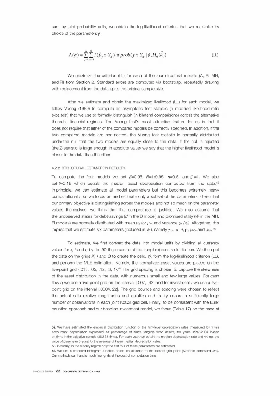
BANCO DE ESPAÑA 35 DOCUMENTO DE TRABAJO N.º 1003
sum by joint probability cells, we obtain the log-likelihood criterion that we maximize by
choice of the parameters :
))ˆ(,|(ln)ˆ()( 01 1
kHYyprobYyIn
jm
M
mmj (LL)
We maximize the criterion (LL) for each of the four structural models (A, B, MH,
and FI) from Section 2. Standard errors are computed via bootstrap, repeatedly drawing
with replacement from the data up to the original sample size.
After we estimate and obtain the maximized likelihood (LL) for each model, we
follow Vuong (1989) to compute an asymptotic test statistic (a modified likelihood-ratio
type test) that we use to formally distinguish (in bilateral comparisons) across the alternative
theoretic financial regimes. The Vuong test’s most attractive feature for us is that it
does not require that either of the compared models be correctly specified. In addition, if the
two compared models are non-nested, the Vuong test statistic is normally distributed
under the null that the two models are equally close to the data. If the null is rejected
(the Z-statistic is large enough in absolute value) we say that the higher likelihood model is
closer to the data than the other.
4.2.2 STRUCTURAL ESTIMATION RESULTS
To compute the four models we set =0.95, R=1/0.95; =0.5; and =1. We also
set =0.16 which equals the median asset depreciation computed from the data.52
In principle, we can estimate all model parameters but this becomes extremely heavy
computationally, so we focus on and estimate only a subset of the parameters. Given that
our primary objective is distinguishing across the models and not so much on the parameter
values themselves, we think that this compromise is justified. We also assume that
the unobserved states for debt/savings (d in the B model) and promised utility (W in the MH,
FI models) are normally distributed with mean b (or w) and variance b ( w). Altogether, this
implies that we estimate six parameters (included in ), namely me, , , , b/w and b/w.53
To estimate, we first convert the data into model units by dividing all currency
values for k, i and q by the 90-th percentile of the (tangible) assets distribution. We then put
the data on the grids K, I and Q to create the cells, Yj, form the log-likelihood criterion (LL),
and perform the MLE estimation. Namely, the normalized asset values are placed on the
five-point grid {.015, .05, .12, .3, 1}.54 The grid spacing is chosen to capture the skewness
of the asset distribution in the data, with numerous small and few large values. For cash
flow q we use a five-point grid on the interval [.007, .42] and for investment i we use a five-
point grid on the interval [.0004,.22]. The grid bounds and spacing were chosen to reflect
the actual data relative magnitudes and quintiles and to try ensure a sufficiently large
number of observations in each joint KxQxI grid cell. Finally, to be consistent with the Euler
equation approach and our baseline investment model, we focus (Table 17) on the case of
52. We have estimated the empirical distribution function of the firm-level depreciation rates (measured by firm’s
accountant depreciation expressed as percentage of firm’s tangible fixed assets) for years 1997-2004 based
on firms in the selective sample (36,585 firms). For each year, we obtain the median depreciation rate and we set the
value of parameter equal to the average of these median depreciation rates.
53. Naturally, in the autarky regime only the first four of these parameters are estimated.
54. We use a standard histogram function based on distance to the closest grid point (Matlab's command hist). Our methods can handle much finer grids at the cost of computation time.

BANCO DE ESPAÑA 36 DOCUMENTO DE TRABAJO N.º 1003
risk neutral firms (i.e., we set =0 and do not estimate it), but in Table 18 we also report
results allowing for risk-averse firms.
Table 17 contains the model comparison results. We maximize the likelihood
between each of the four models and the data based on the joint probability/frequency
distribution of current period assets (k), investment (i), and cash flow (q). That is,
we evaluate the model fit based on firms’ investment behavior jointly with cash flow (q)
conditional on firm’s asset (k). Each column of Table 17 contains the test statistics of
the Vuong test for our baseline specification comparing a pair of the four models
(six possible pairs in total). A statistically significant test statistic (in the table we report 1%,
5%, and 10% significance levels) indicates that we reject the null hypothesis of both models
being equally close to the data, i.e., the model listed in the parentheses fits the data better
than the alternative model with which we compare.
The first section of Table 17 uses data from 1997, the initial year of our panel.
For these baseline runs we also impose risk neutrality, i.e., we set = 0. The findings
indicate that in the whole sample the models rank in terms of best to worst as: borrowing
(B), moral hazard (MH), full information (FI) and autarky (A). That is, the non-contingent debt
borrowing model comes closest to the data in terms of its likelihood based on the joint
distribution of (k, i, q) in 1997.
More importantly, the results from the same exercise when the data are
stratified by firm type according to the number of bank relations reveal patterns that
confirm and reinforce our results from the Euler equation GMM analysis in Section 4.1.
We compare the fitness of the financial regimes with the data across four categories
of firms, defined according to the number of relations with banks over the entire period
1997-2004. Specifically, we explore differences among the categories of “continuing
unbanked” firms,55 “continuing single-banked” firms and “continuing multiple-banked” firms.
Additionally, we consider a fourth category that includes the remainder of the firms in
the sample (this group is used as the reference group in the Euler equation estimates
presented in Table 16 and includes “switching firms” and “other continuing banked firms”),
referred to in Table 17 as “rest of the firms”. Our results reveal that for continuously
unbanked firms the moral hazard (MH) specification fits the data best, with full information
coming a close second and indistinguishable at the 5% confidence level. This result
is coherent with the significantly negative cash flow sensitivity parameter in the Euler
equations approach presented in Section 4.1.2.
In stark contrast, continuing single-banked firms, continuing multiple-banked and
firms in the residual category of rest of the firms are revealed to be the more financially
constrained, with the borrowing, non-contingent debt model coming out on top in terms of
fit with the data, relative to the moral hazard, full information or autarky models. Though the
borrowing regime fits the data best for single-banked, multiple-banked and rest of the firms,
the estimated parameter values vary across the regimes, which is the way the structural
model accommodates the diversity in the data across the firms. These results confirm
the evidence of financial constraints affecting these three categories relying on the Euler
equations framework (Table 16 in Section 4.1.2).
55. Here we use the less restrictive definition of continuing unbanked firms that includes firms that are unbanked six
or more years during the period 1997-2004.

BANCO DE ESPAÑA 37 DOCUMENTO DE TRABAJO N.º 1003
We obtain very similar results for the four firm types by number of banking
relationships when we use 2004 data (see Section 2 of Table 17). The only difference is that
now the full information, perfect credit markets regime is not so close to the moral hazard
constrained credit regime for the unbanked firms.
To check robustness, we also estimate and carry out the Vuong tests when we
allow for quadratic adjustment costs, risk aversion, and a coarser cash flow grid (Table 18).
We first explicitly include quadratic adjustment costs to investment in each of the four
financial regimes using the equation for g(I, k; I) from Section 2. We estimated the
adjustment cost parameter b and, for simplicity, set ç, I and bi to zero. Our previous results
reported above (without allowing adjustment costs) can be interpreted as fixing b=0.
Including explicit adjustment costs improves the fit to the data for the B and A financial
regimes for the groups of continuously “unbanked” and “others”. However, allowing for
adjustment costs interestingly did not improve the fit of the moral hazard and full information
regimes (the likelihood maximization chose to set the parameter b to zero corresponding to
no adjustment costs). As a result, the best fitting regimes when such exogenous adjustment
costs are allowed do not change compared to our no-adjustment cost benchmark
—compare Table 17, section 1 and Table 18, section 1.
Section 2 of Table 18 shows that our results for the group of continuously
unbanked firms can be sensitive to the assumption of risk neutrality, which seems to be
implicit but key in the Euler equations approach and most of the literature. Specifically,
when we allow for risk aversion and let the risk aversion coefficient to vary by including it
in the list of estimated parameters, we find that the borrowing model is best fitting for all firm
groups. Even though the best fitting regime does not vary, the actual best fitting parameter
estimates differ significantly across the firm types.
Finally, we also performed runs with a simpler specification of the cash flow
process in the model, consisting of only two possible values —“high” (equal to 0.1) and
“low” (equal to 0.03). The Vuong test statistics are presented in section 3 of Table 18.
We find that the coarser cash flow grid inhibits the ability of the models to distinguish
among themselves relative to the common data, and our ability to statistically distinguish
across the alternative financial regimes. This deterioration is especially pronounced in the
group of single-banked firms for which our sample size is the smallest. Still, the results
we obtain are consistent with our baseline runs, giving indication for the best fit of the B
and MH regimes. The moral hazard regime achieves the highest likelihood (although it is
statistically tied with B) for unbanked firms, while the non-contingent debt (B) regime
achieves highest likelihood for the multiple-banked firms.

BANCO DE ESPAÑA 38 DOCUMENTO DE TRABAJO N.º 1003
5 Summary and conclusions
We use data from the Spanish Mercantile Registry and from the Bank of Spain Credit
Registry (CIR) to classify firms according to whether they have loans from a formal Spanish
credit institution, from several institutions, or from none. We restrict attention to firms that
are at least ten years old and find, nevertheless, that a significant number are unbanked.
We find evidence that firms’ debt is non-trivial, but it comes in part from borrowing
from other firms which are members of the same group. In the case of persistently
unbanked firms, we document that many firms belong to family groups, which facilitate
funding through channels alternative to formal bank credit. We then examine the existence
and magnitude of financial constraints for each firm type (unbanked, single-banked or
multiple-banked) using two related but distinct approaches based on a common overall
model.
First, we use a standard Euler equation approach to investment. We find that
single-banked firms are most likely to exhibit investment cash flow sensitivity. Unbanked
firms are not. What we find is consistent with the literature arguing that access to bond
markets comes only for larger firms. But in Spain higher level finance beyond bank loans is
not obtained issuing bonds but, instead, from the Spanish analogue to chaibols and keiretzu
(i.e., large and diversified groups of firms). Our results also provide weak evidence for
differences in cash flow sensitivities among single-banked and multiple-banked firms
suggesting that the intensity of financial constraints affecting firms’ investment decisions
is higher for single-banked firms.
In our second approach, we estimate four structural dynamic models of
non-nested financial regimes ranging from complete markets to financial autarky for firms
with different numbers of banking relations using maximum likelihood methods. Our results
from this structural approach are much in line with the results from the Euler equations
approach. In particular, we find that continuously unbanked firms have a financial structure
that fits best the moral hazard constrained credit model, whereas continuously single-
and continuously multiple-banked firms have a financial structure that best fits the
non-contingent borrowing regime.
Our contribution in this paper is two-fold. First, to the best of our knowledge, our
combination of empirical approaches, Euler and structural, is unique. Second, the two
approaches give us a consistent story of financial market imperfections: single-banked
firms are more severely financial constrained than older unbanked firms.

BANCO DE ESPAÑA 39 DOCUMENTO DE TRABAJO N.º 1003
REFERENCES
ALONSO-BORREGO, C. (1994). Estimating dynamic investment models with financial constraints, Working Paper No.
9418, CEMFI.
ARELLANO, M., and S. BOND (1991). “Some tests of specification for panel data: Monte Carlo evidence and an
application to employment equations”, Review of Economic Studies, 58, pp. 277-297.
BANCO DE ESPAÑA (2006). Memoria de la Central de Información de Riesgos, 2005. BERGER, A. N., and G. F. UDELL (1995). “Relationship lending and lines of credit in small firm finance”, Journal of
Business, 68, pp. 351-382.
BERTRAND, M., P. MEHTA and S. MULLAINATHAN (2002). “Ferreting out Tunnelling: An application to Indian
business groups”, Quarterly Journal of Economics, 117 (1), pp.121-148
BERTRAND, M., and S. MULLAINATHAN (2003). “Pyramids”, Journal of the European Economic Association, 1 (2-3),
pp. 478-483.
BERTRAND, M., and A. SCHOAR (2006). “The Role of Family in Family Firms”, Journal of Economic Perspectives, 20,
2, pp. 73-96.
BOND, P. (2004). “Bank and non-bank financial intermediation”, Journal of Finance, 59, 6, pp. 2489-2529.
BOND, S., J. A. ELSTON, J. MAIRESSE and B. MULKAY (2003). “Financial factors and investment in Belgium, France,
Germany and the United Kingdom: A comparison using company panel data”, Review of Economics and Statistics, 85, 1, pp. 153-165.
BOND, S., and C. MEGHIR (1994). “Dynamic investment models and the firms’ financial policy”, Review of Economic Studies, 61, 2, pp. 197-222.
BOOT, A. W. A. (2000). “Relationship banking: What do we know?”, Journal of Financial Intermediation, 9, pp. 7-25.
CARBÓ, S., F. RODRÍGUEZ and G. F. UDELL (2008). Bank lending, financing constraints and SME investment, mimeo.
CHIRINKO, R. S., and J. A. ELSTON (2006). “Finance, control and profitability: the influence of German banks”,
Journal of Economic Behaviour and Organization, 59, pp. 69-88.
CLEARY, S. (1999). “The relationship between firm investment and financial status”, Journal of Finance, 54,
pp. 673-692.
COOPER, R., and J. EJARQUE (2003). “Financial Frictions and Investment: A Requiem in Q”, Review of Economic Dynamics, 6, pp. 710-728.
CRONQVIST, H., and M. NILSON (2003). “Agency costs and minority shareholder”, Journal of Financial and Quantitative Analysis, 38, 4, pp. 695-719.
DEGRYSE, H., and P. VAN CAYSEELE (2000).”Relationship lending with a bank-based system: Evidence from
European small business data”, Journal of Financial Intermediation, 9, pp. 90-109.
DETRAGIACHE, E., P. G. GARELLA and L. GUISO (1997). “Multiple vs single banking relationship: theory and
evidence”, Journal of Finance, 55, 3, pp. 1133-1161.
DIAMOND, D. W. (1984). “Financial intermediation and delegated monitoring”, Review of Economic Studies, 51,
pp. 393-414.
ELSTON, J. A. (1996). Investment, liquidity constraints and bank relationships: evidence from German manufacturing firms, Discussion Paper No. 1329, CEPR.
ELYASIANI, E., and L. W. GOLDBERG (2004). “Relationship lending: a survey of the literature”, Journal of Economics and Business, 56, pp. 315-330.
ESTRADA, Á., and J. VALLÉS (1998). “Investment and Financial Structure in Spanish Manufacturing Firms”,
Investigaciones Económicas, 22 (3), pp. 337-359.
FAZZARI, F. M., R. G. HUBBARD and B. C. PETERSEN (1988). “Financing Constraints and corporate investment”,
Brooking Papers on Economic Activity, 1, pp. 141-206.
— (2000). “Investment-cash flow sensitivities are useful: a comment on Kaplan and Zingales”, Quarterly Journal of Economics, 115, 2, pp. 695-705.
FOHLIN, C. (1998). “Relationship banking, liquidity and investment in the German industrialization”, Journal of Finance, 53, 5, pp. 1737-1758.
FUSS, C., and P. VERMEULEN (2006). The response of firms’ investment and financing to adverse cash flow shocks: the role of bank relationships, Working Paper No. 658, European Central Bank.
GARCÍA-MARCO, T., and C. OCAÑA (1999). “The effect of bank monitoring on the investment behaviour of Spanish
firms”, Journal of Banking and Finance, 23, pp. 1579-1603.
GOMES, J. (2001). “Financing Investment”, American Economic Review, 90, 5, pp. 1263-1285.
GUISO, L., and R. MINETTI (2007). The structure of multiple credit relationships: Evidence from US firms, Working
Paper No. 2007/46, European University Institute.
HARHOFF, D., and T. KÖRTING (1998). “Lending relationships in Germany: empirical evidence form survey data”,
Journal of Banking and Finance, 22, pp. 1317-1353.
HERNANDO, I., and A. TIORNO (2002). “Financial constraints and investment in France and Spain: A comparison
using firm-level data”, in French and Spain industrial corporations over the period 1991-1999: a comparative study based on their financial statements, Central de Balances, Banco de España.
HOSHI, T., A. KASHYAP and D. SCHARFSTEIN (1990). “The role of banks in reducing the costs of financial distress in
Japan”, Journal of Financial Economics, 27, pp. 67-88.
HOUSTON, J. F., and C. M. JAMES (2001). “Do relationship have limits? Bank relationships, financial constraints and
investment”, Journal of Business, 74, 3, pp. 347-374.

BANCO DE ESPAÑA 40 DOCUMENTO DE TRABAJO N.º 1003
HUBBARD, R. G. (1998). “Capital Market imperfections and investment”, Journal of Economic Literature, 36, March,
pp. 193-225.
JAFFEE, D., and T. RUSSELL (1976). “Imperfect information, uncertainty and credit rationing”, Quarterly Journal of Economics, 91, pp. 651-666.
JENSEN, M., and W. MECKLING (1976). “Theory of the firm: managerial behaviour, agency costs, and ownership
structure”, Journal of Financial Economics, 1 pp. 305-360.
JIMÉNEZ, G., V. SALAS and J. SAURINA (2006). “Determinants of collateral”, Journal of Financial Economics, 81,
pp. 255-281.
JIMÉNEZ, G., and J. SAURINA (2004). “Collateral, type of lender and relationship lending as determinant of credit
risk”, Journal of Banking and Finance, 18 (9), pp. 2191-2212.
KAPLAN, S. N., and L. ZINGALES (1997). “Do investment-cash flow sensitivities provide useful measures of financing
constraints”, Quarterly Journal of Economics, 112, 1, pp. 169-215.
— (2000). “Investment-cash flow sensitivities are not valid measures of financing constraints”, Quarterly Journal of Economics, 115, 2, pp. 707-712.
KARAIVANOV, A., and R. M. TOWNSEND (2009). Enterprise dynamics and finance: distinguishing mechanism design from exogenously incomplete market models, mimeo.
MAURY, B. (2006). “Family ownership and firm performance: empirical evidence from Western European
corporations”, Journal of Corporate Finance, 12, pp. 321-341.
MYERS, S. C., and N. S. MAJLUF (1984). “Corporate financing and investment decisions when firms have information
that investors do not have”, Journal of Financial Economics, 13, pp. 187-221.
ONGENA, S., and D. SMITH (2000). “What determines the number of bank relationships? Cross-country evidence”,
Journal of Financial Intermediation, 9, 1, pp. 26-56.
PETERSEN, M. A., and R. G. RAJAN (1994). “The Benefits of Lending Relationships: Evidence from Small Business
Data”, Journal of Finance, 49, March, pp. 3-37.
SAMPHANTHARAK, K. (2003). Internal capital markets in business groups, Thesis (Ph.D.) University of Chicago.
SCHIANTARELLI, F. (1996). “Financial constraints and investment: Methodological issues and international evidence”,
Oxford Review of Economic Policy, 12, 2, pp. 70-89.
SCHMID, L. (2009). A Quantitative Dynamic Agency Model of Financing Constraints, Working Paper, Duke University.
SRAER, D., and D. THESMAR (2004). Performance and behaviour of family firms: Evidence from the French stock market, Discussion Paper Series, CEPR, London.
STIGLITZ, J. E., and A. WEIS (1981). “Credit rationing in markets with imperfect information”, American Economic Review, 71, pp. 393-410.
TOWNSEND, R. (1979). “Optimal contracts and competitive markets with costly state verification”, Journal of Economic Theory, 21, pp. 265-293.
TOWNSEND, R., and K. UEDA (2007). Welfare gains from financial liberalization, Working Paper No. 07/154, IMF.
VICKERY, J. (2005). Banking relationship and the credit cycle. Evidence from the Asian financial crisis, mimeo.
VUONG, Q. (1989). “Likelyhood ratio tests for model selection and non-nested hypotheses”, Econometrica, 57, 2,
pp. 307-333.
WILLIAMSON, S. D. (1987). “Costly monitoring, optimal contracts and equilibrium credit rationing”, Quarterly Journal of Economics, 102, pp. 135-145.
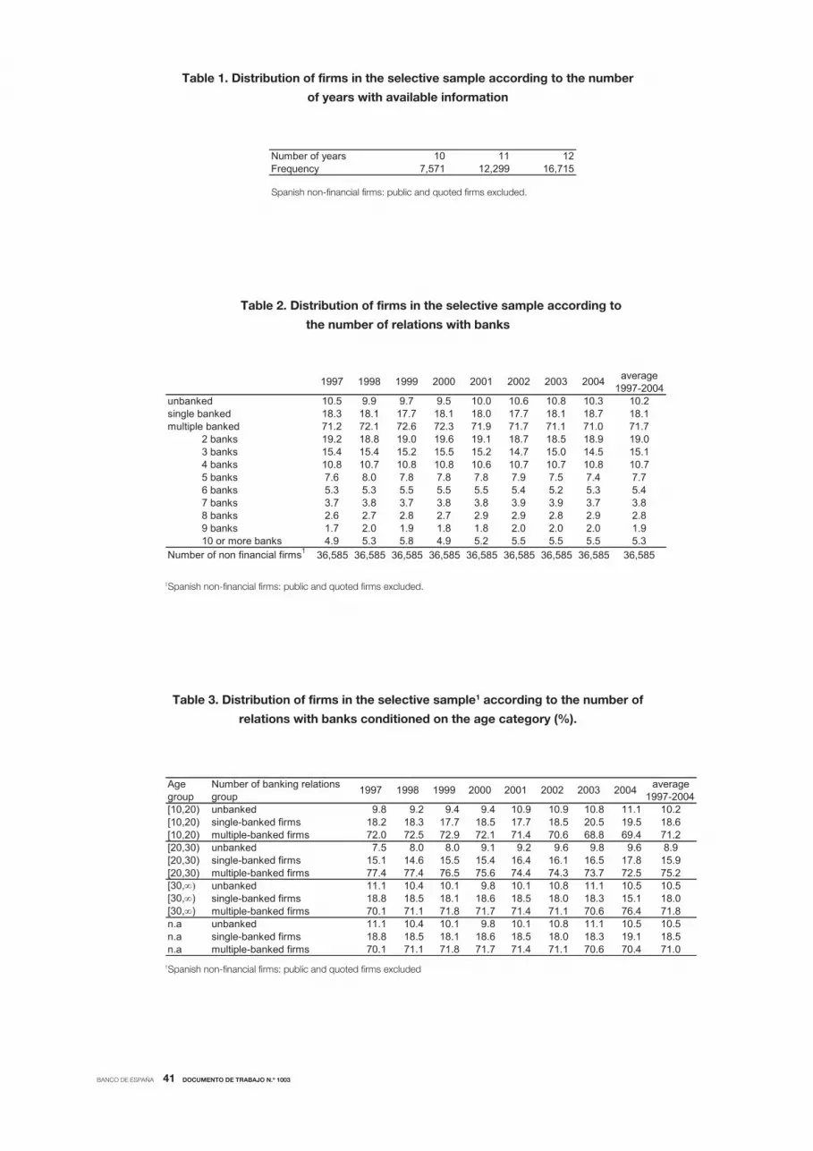
BANCO DE ESPAÑA 41 DOCUMENTO DE TRABAJO N.º 1003
Table 1. Distribution of firms in the selective sample according to the number
of years with available information
Spanish non-financial firms: public and quoted firms excluded.
Table 2. Distribution of firms in the selective sample according to
the number of relations with banks
1Spanish non-financial firms: public and quoted firms excluded.
Table 3. Distribution of firms in the selective sample1 according to the number of
relations with banks conditioned on the age category (%).
1Spanish non-financial firms: public and quoted firms excluded
Number of years 10 11 12Frequency 7,571 12,299 16,715
average1997-2004
unbanked 10.5 9.9 9.7 9.5 10.0 10.6 10.8 10.3 10.2single banked 18.3 18.1 17.7 18.1 18.0 17.7 18.1 18.7 18.1multiple banked 71.2 72.1 72.6 72.3 71.9 71.7 71.1 71.0 71.7
2 banks 19.2 18.8 19.0 19.6 19.1 18.7 18.5 18.9 19.03 banks 15.4 15.4 15.2 15.5 15.2 14.7 15.0 14.5 15.14 banks 10.8 10.7 10.8 10.8 10.6 10.7 10.7 10.8 10.75 banks 7.6 8.0 7.8 7.8 7.8 7.9 7.5 7.4 7.76 banks 5.3 5.3 5.5 5.5 5.5 5.4 5.2 5.3 5.47 banks 3.7 3.8 3.7 3.8 3.8 3.9 3.9 3.7 3.88 banks 2.6 2.7 2.8 2.7 2.9 2.9 2.8 2.9 2.89 banks 1.7 2.0 1.9 1.8 1.8 2.0 2.0 2.0 1.910 or more banks 4.9 5.3 5.8 4.9 5.2 5.5 5.5 5.5 5.3
Number of non financial firms1 36,585 36,585 36,585 36,585 36,585 36,585 36,585 36,585 36,585
20041997 1998 1999 2000 2001 2002 2003
Age Number of banking relations averagegroup group 1997-2004[10,20) unbanked 9.8 9.2 9.4 9.4 10.9 10.9 10.8 11.1 10.2[10,20) single-banked firms 18.2 18.3 17.7 18.5 17.7 18.5 20.5 19.5 18.6[10,20) multiple-banked firms 72.0 72.5 72.9 72.1 71.4 70.6 68.8 69.4 71.2[20,30) unbanked 7.5 8.0 8.0 9.1 9.2 9.6 9.8 9.6 8.9[20,30) single-banked firms 15.1 14.6 15.5 15.4 16.4 16.1 16.5 17.8 15.9[20,30) multiple-banked firms 77.4 77.4 76.5 75.6 74.4 74.3 73.7 72.5 75.2[30, unbanked 11.1 10.4 10.1 9.8 10.1 10.8 11.1 10.5 10.5[30, ) single-banked firms 18.8 18.5 18.1 18.6 18.5 18.0 18.3 15.1 18.0[30, ) multiple-banked firms 70.1 71.1 71.8 71.7 71.4 71.1 70.6 76.4 71.8n.a unbanked 11.1 10.4 10.1 9.8 10.1 10.8 11.1 10.5 10.5n.a single-banked firms 18.8 18.5 18.1 18.6 18.5 18.0 18.3 19.1 18.5n.a multiple-banked firms 70.1 71.1 71.8 71.7 71.4 71.1 70.6 70.4 71.0
2001 2002 2003 20041997 1998 1999 2000

BANCO DE ESPAÑA 42 DOCUMENTO DE TRABAJO N.º 1003
Table 4. Transition matrices across unbanked firms, single-banked firms
and multiple-banked firms (%)
One-year time horizon
Two-year time horizon
Five-year time horizon
Average percentages in period 1997-2004.
single banked multiple banked unbanked Total
single banked 67.8 5.3 20.0 18.1multiple banked 21.3 93.6 7.5 71.8unbanked 10.9 1.1 72.5 10.1Total 100.0 100.0 100.0 100.0
category in year t-1
category in year t
single banked multiple banked unbanked Totalsingle banked 56.2 7.5 25.2 18.1multiple banked 29.5 90.7 11.9 71.8unbanked 14.3 1.8 62.9 10.2Total 100.0 100.0 100.0 100.0
category in year t-2
category in year t
single banked multiple banked unbanked Total
single banked 43.2 10.3 29.8 18.2multiple banked 38.9 86.4 20.5 71.2unbanked 17.9 3.3 49.7 10.6Total 100.0 100.0 100.0 100.0
category in year t-5
category in year t

BANCO DE ESPAÑA 43 DOCUMENTO DE TRABAJO N.º 1003
Table 5. Distribution of firms in the selective sample1 according to the number of
years in which the firm is classified as unbanked during period 1997-2004
1Spanish non-financial firms: public and quoted firms excluded. 2Relative to all the firms. 3Relative to the number of firms in the subtotal (continuing banked firms or switching firms). Annual averages for period 1997-2004.
Table 6. Distribution of switching firms according to the number of changes
in the banked/unbanked status over the studied period
1Spanish non-financial firms: public and quoted firms excluded 2 Relative to the subsample of switching firms. 3 Relative to the entire sample of firms.
Number of Absolute Relative Relativeyears frequency1 frequency2 frequency3
Continuing banked 0 28,050 76.7 100.0Continuing single-banked 0 914 2.5 3.3Continuing multiple-banked 0 19,083 52.2 68.0Other continuing banked firms 0 8,053 22.0 28.7
1 2,440 6.7 31.92 1,459 4.0 19.13 1,096 3.0 14.34 838 2.3 11.05 709 1.9 9.36 617 1.7 8.17 480 1.3 6.3[1,7] 7,639 20.9 100.0
Continuing unbanked 8 896 2.4All firms 36,585 100.0
Switching firms
Number of Absolute Relative Relativechanges frequency frequency2 frequency3
1 3,264 42.7 8.92 2,856 37.4 7.83 964 12.6 2.64 440 5.8 1.25 94 1.2 0.36 21 0.3 0.17 0 0.0 0.0Switching firms 7,639 100.0 20.9All firms1 36,585 100.0
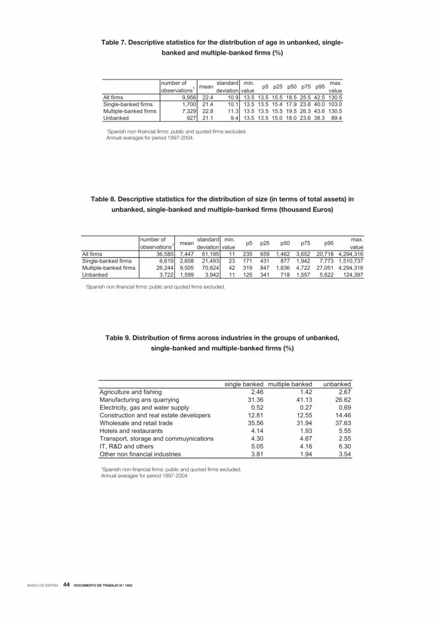
BANCO DE ESPAÑA 44 DOCUMENTO DE TRABAJO N.º 1003
Table 7. Descriptive statistics for the distribution of age in unbanked, single-
banked and multiple-banked firms (%)
1Spanish non-financial firms: public and quoted firms excluded. Annual averages for period 1997-2004.
Table 8. Descriptive statistics for the distribution of size (in terms of total assets) in
unbanked, single-banked and multiple-banked firms (thousand Euros)
1Spanish non financial firms: public and quoted firms excluded.
Table 9. Distribution of firms across industries in the groups of unbanked,
single-banked and multiple-banked firms (%)
1Spanish non-financial firms: public and quoted firms excluded. Annual averages for period 1997-2004.
number of standard min. max.observations1 deviation value value
All firms 9,956 22.4 10.9 13.5 13.5 15.5 18.5 25.5 42.5 130.5Single-banked firms 1,700 21.4 10.1 13.5 13.5 15.4 17.9 23.8 40.0 103.0Multiple-banked firms 7,329 22.8 11.3 13.5 13.5 15.5 19.5 26.3 43.6 130.5Unbanked 927 21.1 9.4 13.5 13.5 15.0 18.0 23.6 38.3 89.4
p75 p95mean p5 p25 p50
number of standard min. max.observations1 deviation value value
All firms 36,585 7,447 61,195 11 235 659 1,462 3,652 20,718 4,294,316Single-banked firms 6,619 2,608 21,493 23 171 431 877 1,942 7,773 1,510,737Multiple-banked firms 26,244 9,505 70,824 42 319 847 1,836 4,722 27,051 4,294,316Unbanked 3,722 1,599 3,942 11 125 341 718 1,557 5,622 124,397
p75 p95mean p5 p25 p50
single banked multiple banked unbankedAgriculture and fishing 2.46 1.42 2.67Manufacturing ans quarrying 31.36 41.13 26.62Electricity, gas and water supply 0.52 0.27 0.69Construction and real estate developers 12.81 12.55 14.46Wholesale and retail trade 35.56 31.94 37.63Hotels and restaurants 4.14 1.93 5.55Transport, storage and commuynications 4.30 4.67 2.55IT, R&D and others 5.05 4.16 6.30Other non financial industries 3.81 1.94 3.54

BANCO DE ESPAÑA 45 DOCUMENTO DE TRABAJO N.º 1003
Table 10. Descriptive statistics for the investment-to-capital ratio:
All firms, unbanked firms, single-banked firms and multiple-banked firms
(units per unit of capital)
1Spanish non financial firms: public and quoted firms excluded. Relative investment is defined as the ratio of (gross) investment on capital. Annual averages for period 1997-2004.
Table 11. Distribution of firms according to the sign of gross investment. All firms,
unbanked firms, single-banked firms and multiple-banked firms (%)
1Spanish non-financial firms: public and quoted firms excluded. Annual averages for period 1997-2004.
number of standard min. max.observations1 deviation value value
All firms 36,585 0.253 0.257 -0.575 0.000 0.062 0.185 0.387 0.776 1.407Single-banked firms 6,619 0.237 0.262 -0.570 0.000 0.041 0.155 0.368 0.786 1.389Multiple-banked firms 26,244 0.264 0.256 -0.575 0.000 0.075 0.200 0.400 0.778 1.404Unbanked 3,722 0.204 0.250 -0.551 -0.006 0.020 0.121 0.321 0.728 1.388
p25 p50 p75 p95mean p5
number of negative zero positiveobservations1 investment investment investment
All firms 36,585 4.39 3.89 91.73Single-banked firms 6,619 4.42 6.42 89.17Multiple-banked firms 26,244 4.20 2.16 93.64Unbanked firms 3,722 5.65 11.50 82.85

BANCO DE ESPAÑA 46 DOCUMENTO DE TRABAJO N.º 1003
Table 12. Descriptive statistics for some economic and financial ratios
(% and units per unit of capital)
1Spanish non-financial firms: public and quoted firms excluded. * Subsample of firms in default. Annual averages for period 1997-2004.
Table 13. Decomposition of aggregate debt1 (%)
1 Statistics based on the sample of firms that report to the Spanish Mercantile Registry detailed financial statements which contain the itemization of debt (2,468 firms). Specifically, figures in this table refer to 2,220 firms reporting positive banking debt (“banked”) and 248 firms reporting no borrowing from banks (“unbanked”). Information referred to year 1997. * For banked firms, this category includes an adjustment of -2 percentage points which allows that the sum of items equals 100% of debt. For unbanked firms, it includes unexplained aggregate debt that represents 0.6% of total debt.
number of standard min. max.observations1 deviation value value
Leverage ratio (%) 5,984 51.3 22.9 0.7 14.0 33.5 51.4 69.2 88.1 135.6Bank debt-to-total debt ratio (%) 5,856 26.4 23.4 0.0 1.4 7.3 19.2 39.9 75.1 100.0Liquidity ratio (%) 6,523 51.6 118.0 0.0 0.0 7.3 23.4 55.1 174.1 2280.0Cash flow-to-capital ratio 6,612 0.8 1.2 -1.7 0.0 0.2 0.4 0.9 2.9 11.8Sales-to Capital ratio 6,610 14.1 21.8 0.1 0.4 2.6 6.4 15.8 54.5 225.3Return on Assets (%) 6,612 7.8 9.2 -53.2 -3.6 2.8 6.3 11.6 23.7 72.7Default ratio* (%) 12 88.9 21.9 36.7 40.9 83.8 100.0 100.0 100.0 100.0
Leverage ratio (%) 25,217 64.1 20.2 1.7 27.3 50.6 66.4 79.4 92.1 150.6Bank debt-to-total debt ratio (%) 23,914 44.7 23.8 0.0 7.0 26.0 44.2 62.1 85.9 100.0Liquidity ratio (%) 25,687 20.8 54.3 0.0 0.0 2.3 8.2 22.3 75.5 2280.0Cash flow-to-capital ratio 26,230 0.7 1.0 -1.7 0.0 0.2 0.4 0.9 2.6 12.1Sales-to Capital ratio 24,505 12.9 19.4 0.1 0.9 3.0 6.3 14.0 47.6 225.0Return on Assets (%) 26,216 7.7 7.4 -55.2 -1.2 3.7 6.5 10.6 20.6 72.7Default ratio* (%) 218 40.7 29.3 5.1 6.2 13.4 35.3 64.0 93.0 100.0
Leverage ratio (%) 2,993 40.1 24.2 0.0 5.1 20.1 37.3 58.1 83.6 99.5Bank debt-to-total debt ratio (%) --- --- --- --- --- --- --- --- --- ---Liquidity ratio (%) 3,693 95.9 202.7 0.0 2.1 17.9 43.8 94.8 318.4 2280.0Cash flow-to-capital ratio 3,713 0.9 1.4 -1.7 -0.1 0.2 0.5 1.1 3.5 11.9Sales-to Capital ratio 3,710 17.1 24.7 0.1 0.3 3.0 8.5 20.5 63.9 218.9Return on Assets (%) 3,717 8.7 10.6 -50.5 -3.8 2.8 6.9 13.2 27.3 72.7Default ratio* (%) --- --- --- --- --- --- --- --- --- ---
multiple-banked firms
p75 p95
unbanked firms
single-banked firms
mean p5 p25 p50
Banked Unbankedfirms firms
Bank debt 33.9 0.0Debt with associated and affiliated companies 17.1 71.8Trade credit 28.6 10.5Government 9.5 3.5Commercial paper 3.4 0.3Deposits and guarantees 0.6 0.4Accounts receivable 2.1 1.0Deffered debts on shares 0.1 0.2Provisions for current assets 1.2 1.5Bonds 0.1 0.0Other debts* 3.3 10.8Aggregate short and long term debt 100 100Sample size 2,220 248

BANCO DE ESPAÑA 47 DOCUMENTO DE TRABAJO N.º 1003
Table 14. GMM parameter estimates of investment Euler equation.
All firms. Period 1997-2004
I/k, q/k and y/k denote respectively the ratios of gross investment, cash-flow and output to capital. List of instruments: third and fourth lags of I/k, q/k and y/k. Specification includes time dummy variables. The number of observations corresponds to the selective panel dataset, over period 1997 to 2004.
Dependent variable:(I/k)t
1.1414(0,000)-0.8071(0,000)0.0397(0,000)0.0024(0,000)
AR(1) -18.93(0,000)
AR(2) 10.94(0,000)
AR(3) 1.36(0,175)
Hansen-J test 68.68(0,008)
Number of observations 276,174Number of firms 36,585
(I/k)t-1
(I/k)t-12
(q/k)t-1
(y/k)t-1
BANCO DE ESPAÑA 48 DOCUMENTO DE TRABAJO N.º 1003
Table 15. GMM parameter estimates of Investment Euler equations across groups
of firms with different numbers of banking relationships. Period 1997-2004
I/k, q/k and y/k denote respectively the ratios of gross investment, cash-flow and output to capital.. D0 denotes a dummy variable that equals 1 if the firm has one or more banking relationships and 0, otherwise. D1 denotes a dummy variable that equals 1 if the firm has a unique bank relationship and 0, otherwise. D2 is a dummy variable that equals 1 if the firm has more than one bank relationship and 0 otherwise. The number of bank relations, and consequently D0, D1 and D2, are treated as endogenous. List of instruments: third and fourth lags of I/k, q/k and y/k and third lag of the number of bank relations. All specifications include time dummy variables. The number of observations corresponds to the selective panel dataset, over period 1997 to 2004. P-values in parenthesis.
Dependent variable:(I/k)t
(1) (2) (3)
1.4541 0.8268 0.9624(0.000) (0.185) (0.000)-1.8685 -0.7269 -1.0050(0.001) (0.369) (0.002)-0.1902 -0.1597 -0.1401(0.005) (0.023) (0.017)
0.00876 0.0084 0.0055(0.027) (0.049) (0.005)-1.1669(0.008)2.0937(0.001)0.2504(0.001)-0.0080(0.086)
0.3493(0.728)-0.6684(0.639)0.2612 0.2007(0.019) (0.003)-0.0057(0.425)-0.5614 -0.7234(0.366) (0.011)1.0619 1.3594(0.202) (0.001)0.2100 0.1954(0.015) (0.015)-0.0078 -0.0054(0.098) (0.103)
AR(1) -20.07 -17.05 -19.75(0.000) (0.000) (0.000)
AR(2) 6.83 6.56 7.04(0.000) (0.000) (0.000)
AR(3) 0.94 0.71 0.75(0.347) (0.475) (0.450)
Hansen J test 65.71 53.71 56.77(0.037) (0.127) (0.133)
Number of observations 276,174 276,174 276,174Number of firms 36,585 36,585 36,585
(I/k)t-1*D2t
(I/k)t-12*D2t
(q/k)t-1*D2t
(y/k)t-1*D2t
(I/k)t-1*D1t
(I/k)t-12*D1t
(q/k)t-1*D1t
(y/k)t-1*D1t
(I/k)t-1*D0t
(I/k)t-12*D0t
(q/k)t-1*D0t
(y/k)t-1*D0t
(I/k)t-1
(I/k)t-12
(q/k)t-1
(y/k)t-1

BANCO DE ESPAÑA 49 DOCUMENTO DE TRABAJO N.º 1003
Table 16. Differences in investment patterns among continuing unbanked firms,
continuing single-banked firms continuing multiple-banked firms and rest of the
firms. GMM parameter estimates of investment Euler equation
1The reference group includes switching firms (i.e., firms changing their status from unbanked to banked or vice versa at least once in the analysed period) and other continuing banked firms (i.e. continuing banked firms that change from single-banked to multiple-banked or vice versa at least once in the analysed period). I/k, q/k and y/k denote respectively the ratios of gross investment, cash-flow and output to capital. List of instruments: third and fourth lags of I/k, q/k and y/k and third lag of the number of bank relations. Time dummy variables included. The number of observations corresponds to the selective panel dataset, over period 1997 to 2004. P-values in parenthesis.
Dependent variable:(I/k)t
continuing continuing continuingunbanked single-banked multi-banked
1.8415 -0.8439 -2.9426 -1.7046(0,000) (0.660) (0.385) (0.010)-1.9669 2.1953 2.3051 2.4894(0,002) (0.360) (0.503) (0.005)0.1535 -0.4645 -0.0820 -0.1705(0,014) (0.033) (0.745) (0.125)0.0036 0.0143 -0.0155 -0.0024(0,350) (0.392) (0.518) (0.737)
AR(1) -10.89(0,000)
AR(2) 4.74(0,000)
AR(3) 0.26(0,792)
Hansen-J test 45.09(0,232)
Number of observations 276,174Number of firms 36,585
Differences respect to the reference groupReference
group1
(I/k)t-1
(I/k)t-12
(q/k)t-1
(y/k)t-1

BANCO DE ESPAÑA 50 DOCUMENTO DE TRABAJO N.º 1003
Table 17. Baseline financial regime comparisons, Voung test Z-statistics1,2,3
1 ***=1%, **=5%, *=10% two-sided significance level, the “winning” regime is in the parentheses. 2 Voung Z-statistics’ cutoffs: 3 All results in this table are computed under the assumption of risk neutrality ( =0). B = borrowing or lending in non-contingent debt. MH = moral hazard constrained credit/insurance. FI = full information/complete markets. A = no access to credit (autarky).
Table 18. Financial regime comparisons - robustness, Voung test Z-statistics
1 ***=1%, **=5%, *=10% two-sided significance level, the “winning” regime is in the parentheses. 2 Voung Z-statistics’ cutoffs: 3 All results in this table are computed with 1997 data. B = borrowing or lending in non-contingent debt. MH = moral hazard constrained credit/insurance. FI = full information/complete markets. A = no access to credit (autarky).
1. using 1997 (k,i,q) data1.1. risk neutrality
2. using 2004 (k,i,q) data2.1. risk neutrality
FI v B FI v A B v A Best FitComparison MH v FI MH v B MH v A
1. allowing for quadratic adjustment costs
2. allowing for risk aversion
3. coarser cash flow grid (#Q = 2)
Comparison MH v FI MH v B MH v A FI v B FI v A B v A Best Fit

BANCO DE ESPAÑA 51 DOCUMENTO DE TRABAJO N.º 1003
Appendix 1: Variable definitions
Firm characteristics
Age (relative to the constitution date).
Industry (3 and 4 digit CNAE-93 classifications). Financial firms have been excluded.
Using this information, we have aggregated the activities into: 1) agriculture and fishing;
2) manufacturing and quarrying; 3) electricity, gas and water supply; 4) construction and
property development; 5) wholesale and retail trade; 6) hotels and restaurants;
7) transport, storage and communication; 8) IT, R&D and other; 9) other non-financial
industries. We build up a set of dummy variables controlling for heterogeneity
across industries in empirical models. Using the 3 digit CNAE-classification would
imply estimating a large number of parameters which is not viable because of capacity
constraints.
Location (province).
Firm-level economic variables
Capital (kt): The stock of capital in year t is measured by the book value of tangible
fixed assets. This variable has been deflated using the gross fixed capital investment
deflator.
(Gross) Investment (It): Defined as the sum of the absolute increase in the stock of
tangible fixed assets between t and t-1 and the depreciation in year t. Deflated using
the gross fixed capital investment deflator.
Cash flow (qt): It is defined as the sum of operating profits/losses (+/-) and
depreciation. Deflated using the GDP deflator.
Output (yt): It is measured using total sales. Deflated using the GDP deflator.
Economic and financial ratios
Relative Investment (I/k): defined as the ratio of gross investment (I) to capital (k).
The univariate series of relative investment has been truncated dropping out the 5%
of observations contained in the upper and the lower tails of the distribution, which will
greatly distort the results of the estimation of Euler equations. This data treatment
is applied before picking up firms in the selective sample.
ROA: Profitability ratio, profits before interests and taxes divided by total assets
(winsorized 1%, before picking up firms in the selective sample).
Leverage (ratio): Amount of debt with explicit cost divided by total assets
(winsorised 1%, before picking up firms in the selective sample).

BANCO DE ESPAÑA 52 DOCUMENTO DE TRABAJO N.º 1003
Liquidity (ratio): cash to short term debt ratio (winsorised 1%, before picking up firms
in the selective sample).
Firm credit risk
Banking debt: amount of debt contracted with any Spanish credit institution.
Aggregation, at firm level, of the amounts of banking debt registered by Spanish credit
Institutions in CIR.
Default banking debt: amount of non-performing loans (more than three month in
arrears) and doubtful loans (low repayment probability despite of being performing).
It is constructed by aggregating, at the firm level, the amounts of non-performing and
doubtful loans registered by Spanish credit Institutions in CIR.
Firm-level default ratio: defined as the proportion of banking debt that is
non-performing or doubtful, if this proportion exceeds 5%. If it is below this threshold,
the default ratio is assumed equal to zero and default banking debt is imputed as zero.56
Default dummy: dichotomic variable that equals one if firm-level default ratio is higher
than 5% and zero otherwise.
Firm’s banking relationships
Number of relations: number of different Spanish credit institutions granting a loan
to the firm. According to the current number of relations, we distinguish year by year
three types of firms: unbanked, in single banking relationship and in multiple banking
relationships. According to the trajectories across these three categories over the whole
period 1997-2004, we distinguish among continuing unbanked, continuing banked and
switching firms. Within the category of continuing banked firms we differentiate among
continuing single-banked, continuing multiple-banked and other continuing banked
firms. Empirically, for analysing differences across groups of firms defined according
to their trajectories in and out of the unbanked status, we consider for categories:
continuing unbanked, continuing single-banked, continuing multiple-banked and rest of
the firms (included both switching firms and other continuing banked firms).
56. The minimum threshold of 5% allows filtering “technical defaults” and mistakes, which are unrelated to the level
of credit risk of the firms. This filter has been applied in other papers that use the CIR database [e.g. Jiménez and
Saurina (2004)].

BANCO DE ESPAÑA 53 DOCUMENTO DE TRABAJO N.º 1003
Appendix 2: Descriptive statistics based on the unbalanced panel dataset
Table A2.1 exhibits the sample sizes for every cross-section in the SABI-CIR database.
Additionally, it shows some statistics about the coverage of the database relative to the
population of Spanish non-financial firms in terms of the aggregate figures of total assets
and banking loans. On average, the gross number of firms in the sample is over 297,000
firms per year. The coverage of SABI-CIR has tended to increase over time, from a minimum
of around 32%, in terms of assets, and 36.4%, in terms of banking debt, in 1994, to a
percentage that reaches a maximum close to 72% of total assets and 71.3% of aggregate
banking debt in Spanish non-financial firms, in year 2002. This increase in the coverage
is explained by the expansionary strategy of INFORMA that has widely increased the number
of firms for which it buys public statements deposited at the Mercantile Registry.
SABI-CIR database has a wide heterogeneity of the sample in terms of firms’ age,
activity and size. In terms of age, the sample is mostly composed of firms not older than
10 years, which exceed 63%. In this category, firms are concentrated to a large extent
below 5 years old (34.2%). Retail, construction, real estate development and manufacturing
are the industries in which three-quarters of all firms are concentrated. In terms of firms’ size,
measured by total assets, the database contains a high proportion of small firms. In particular,
an average percentage of 93.4% of the firms in the sample correspond to the smallest firms’
category, which includes firms with an amount of total asset not higher than 5 million € or
with total sales not higher than 7 million €. This characteristic differentiates this dataset from
alternative datasets relative to Spanish non-financial firms, which tend to under-represent
small firms (see Tables A2.2, A2.3 and A2.4).
A comparison of the selective and the unbalanced samples
Table A2.5 shows the distribution of firms across the categories of small-size, medium-size
and large-size over the period 1997-2004.57 As in the unbalanced sample, most of the firms
in the selective sample belong to the category “small firms”, with an average weight of 83%.
Still, compared with the composition of the unbalanced sample, the selective sample tends to
over-represent the categories of medium-sized firms and large-sized firms, with average
fractions of 14.9% and 2.1%, respectively, which are more than twice the corresponding
percentages for the entire SABI-CIR sample.
Additionally, as shown in Table A2.6, our sample is also more homogeneous
than the population in terms of firm age. On average, more than three quarters of the firms
in the sample58 are older than ten years. Moreover, the homogeneity of the sample in terms of
age is increasing over time, with the percentage of firms in the category of firms younger
than 10 years being below 4%. In the entire SABI-CIR sample, firms are almost equally
distributed across the three age categories (Table A2.2) over the analysed period. This is
explained by the exclusion of new cohorts of entering firms as a consequence of the selection
criteria requiring complete information for period 1997-2004.
57. Firm size classification follows EU recommendations (Bulletin EU 1/2-1996), which defines as small firms those with
total assets lower than 5 million Euros or sales lower than 7 million Euros and as large firms those with total assets
higher than 27 million Euros or sales higher than 40 million Euros.
58. The statistics about the age distribution of the firms in the sample are computed from the subsample of firms with
data available on the age of the firm, which reaches only 40% of the firms in the sample.

BANCO DE ESPAÑA 54 DOCUMENTO DE TRABAJO N.º 1003
The higher homogeneity of the sample of firms included in the selective panel is also
evident in the distribution of firms across industries.59 Statistics presented in A2.7 indicate that
firms in the selective sample are concentrated in the industries of Manufacturing and
Quarrying; Wholesale and Retail Trade and Construction and Real State Developers to a
larger extent than in the non-selective sample of firms. These three industries concentrate
84% of the firms in the sample against the 74% in the non-selective sample. The rest of the
firms are spread over the rest of industries.
Table A2.1. Coverage of the SABI-CIR sample of private and unquoted firms
(million € and %)
1. Private and non-quoted Spanish non-financial firms (after filtering). 2. Coverages in terms of bank loans are relative to the aggregated values of banking debt for Spanish non-financial firms (public and quoted firms included) computed using CIR data. 3. Coverages have been computed over the aggregated value of total assets corresponding to Spanish non-financial firms (public and quoted firms included) published in the annual reports of Central de Balances (Banco de España).
59. Classification of firms across industries according to the information provided by INFORMA is static in the sense that
it provides a unique CNAE code for every firm that does not vary over time.
bank loans2 total assets3
1993 101,290 44.51994 96,519 36.4 32.31995 170,346 58.9 51.61996 214,449 64.2 54.11997 224,811 66.3 61.91998 266,059 67.1 56.31999 306,453 66.3 60.22000 341,350 67.0 64.12001 429,952 69.8 67.32002 505,235 71.3 71.92003 515,722 72.0 68.82004 400,299 60.9 58.4
sample size1 coverage in terms of:
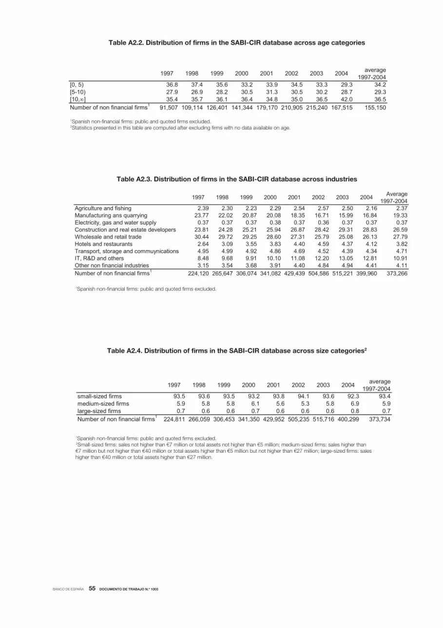
BANCO DE ESPAÑA 55 DOCUMENTO DE TRABAJO N.º 1003
Table A2.2. Distribution of firms in the SABI-CIR database across age categories
1Spanish non-financial firms: public and quoted firms excluded. 2Statistics presented in this table are computed after excluding firms with no data available on age.
Table A2.3. Distribution of firms in the SABI-CIR database across industries
1Spanish non-financial firms: public and quoted firms excluded.
Table A2.4. Distribution of firms in the SABI-CIR database across size categories2
1Spanish non-financial firms: public and quoted firms excluded. 2Small-sized firms: sales not higher than €7 million or total assets not higher than €5 million; medium-sized firms: sales higher than €7 million but not higher than €40 million or total assets higher than €5 million but not higher than €27 million; large-sized firms: sales higher than €40 million or total assets higher than €27 million.
average1997-2004
[0, 5) 36.8 37.4 35.6 33.2 33.9 34.5 33.3 29.3 34.2[5-10) 27.9 26.9 28.2 30.5 31.3 30.5 30.2 28.7 29.3[10, ] 35.4 35.7 36.1 36.4 34.8 35.0 36.5 42.0 36.5Number of non financial firms1 91,507 109,114 126,401 141,344 179,170 210,905 215,240 167,515 155,150
1997 2002 2003 20041998 1999 2000 2001
average1997-2004
small-sized firms 93.5 93.6 93.5 93.2 93.8 94.1 93.6 92.3 93.4medium-sized firms 5.9 5.8 5.8 6.1 5.6 5.3 5.8 6.9 5.9large-sized firms 0.7 0.6 0.6 0.7 0.6 0.6 0.6 0.8 0.7Number of non financial firms1 224,811 266,059 306,453 341,350 429,952 505,235 515,716 400,299 373,734
2003 20041999 2000 2001 20021997 1998
Average1997-2004
Agriculture and fishing 2.39 2.30 2.23 2.29 2.54 2.57 2.50 2.16 2.37Manufacturing ans quarrying 23.77 22.02 20.87 20.08 18.35 16.71 15.99 16.84 19.33Electricity, gas and water supply 0.37 0.37 0.37 0.38 0.37 0.36 0.37 0.37 0.37Construction and real estate developers 23.81 24.28 25.21 25.94 26.87 28.42 29.31 28.83 26.59Wholesale and retail trade 30.44 29.72 29.25 28.60 27.31 25.79 25.08 26.13 27.79Hotels and restaurants 2.64 3.09 3.55 3.83 4.40 4.59 4.37 4.12 3.82Transport, storage and commuynications 4.95 4.99 4.92 4.86 4.69 4.52 4.39 4.34 4.71IT, R&D and others 8.48 9.68 9.91 10.10 11.08 12.20 13.05 12.81 10.91Other non financial industries 3.15 3.54 3.68 3.91 4.40 4.84 4.94 4.41 4.11Number of non financial firms1 224,120 265,647 306,074 341,082 429,439 504,586 515,221 399,960 373,266
2003 20042000 2001 20021997 1998 1999
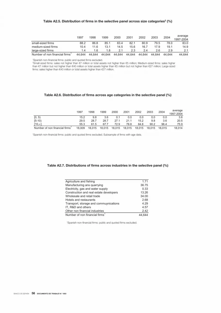
BANCO DE ESPAÑA 56 DOCUMENTO DE TRABAJO N.º 1003
Table A2.5. Distribution of firms in the selective panel across size categories2 (%)
1Spanish non-financial firms: public and quoted firms excluded. 2Small-sized firms: sales not higher than €7 million or total assets not higher than €5 million; Medium-sized firms: sales higher than €7 million but not higher than €40 million or total assets higher than €5 million but not higher than €27 million; Large-sized firms: sales higher than €40 million or total assets higher than €27 million.
Table A2.6. Distribution of firms across age categories in the selective panel (%)
1Spanish non-financial firms: public and quoted firms excluded. Subsample of firms with age data.
Table A2.7. Distributions of firms across industries in the selective panel (%)
1Spanish non-financial firms: public and quoted firms excluded.
average1997-2004
small-sized firms 88.2 86.8 85.1 83.4 82.1 80.9 79.5 78.0 83.0medium-sized firms 10.4 11.6 13.1 14.5 15.6 16.7 17.9 19.1 14.9large-sized firms 1.4 1.6 1.8 2.1 2.3 2.4 2.6 2.9 2.1Number of non financial firms1 44,644 44,644 44,644 44,644 44,644 44,644 44,644 44,644 44,644
2003 20041999 2000 2001 20021997 1998
average1997-2004
[0, 5) 15.2 9.8 3.6 0.1 0.0 0.0 0.0 0.0 3.6[5-10) 29.5 28.7 28.7 27.1 21.1 15.2 9.8 3.6 20.5[10, ] 55.3 61.5 67.7 72.9 78.8 84.8 90.2 96.4 75.9Number of non financial firms1 18,009 18,015 18,015 18,015 18,015 18,015 18,015 18,015 18,014
1997 2002 2003 20041998 1999 2000 2001
Agriculture and fishing 1.71Manufacturing ans quarrying 36.75Electricity, gas and water supply 0.33Construction and real estate developers 13.26Wholesale and retail trade 34.00Hotels and restaurants 2.68Transport, storage and commuynications 4.29IT, R&D and others 4.57Other non financial industries 2.42Number of non financial firms1 44,644

BANCO DE ESPAÑA 57 DOCUMENTO DE TRABAJO N.º 1003
Appendix 3: Case study
Firm A is an example of a continuing unbanked firm that, as can be seen in Chart A3.1, is part
of a relatively complex group of firms which are directly or indirectly owned by one
person (Mr. X) and other members of the same family (wife, sons, daughters and mother).60
To the best of our knowledge,61 the structure is composed of 11 family firms, which are
heterogeneous in terms of their age,62 size63 and activities.64
Figure A.3. provides in four separated panels the evolution over the period
1997-2004 of four key variables: total assets, Return on Assets (ROA), the investment-to-
capital ratio, and the debt-to-total assets ratio for the target firm (Firm A) and also the 25th,
75th and 95th percentiles describing the distribution of these variables in the whole sample of
firms (i.e., mature firms in the balanced or selective sample).
Firm A is a large firm in terms of total assets that exhibits an increasing trend over
the analysed period. Compared to the rest of the firms in the sample under study, the firm
is located in the upper tail of the distribution. In particular, the level of assets of this firm is
comparable to that for the 95th percentile of the firm level distribution of this variable over
the entire analysed period.
The profitability of the studied firm is, with the exception of year 2000,65 very close to
the 25th percentile of the distribution of this variable in the sample. Leverage, measured by the
ratio of debt to total assets, is low, particularly after a sharp decrease in 2000 from an
average ratio of around 51% in 1997-1999, which is close to the 25th percentile of the sample
distribution of firms’ leverage ratio to an average ratio of 3.5% in period 2000-2004, which is
even lower than the 5th percentile (in average, it is around 18%). Finally, the average
investment-to-capital ratio is 11.5% for the analysed firm which is about the 25th percentile of
the sample distribution of this variable.
Firms related with Firm A are very heterogeneous in terms of the weight of
shareholders’ funds as a percentage of total assets and also in terms of the composition
of their liabilities. As shown in Table A.3.1 the average ratio of shareholders’ funds-to-total
assets varies in a wide range across firms from 26.1% to 100%. Nonetheless, except in
one case (where it is 26.1%), the shareholders’ funds ratio is higher than the (average)
75th percentile of the firm-level sample distribution of this ratio. Consequently, it can be
60. In Spain, family names are composed by a first surname from the father and a second surname from the mother.
It allows drawing conclusions about family relationships just from the direct comparison of the two surnames.
61. We have built the structure of family related firms using SABI-INFORMA. This database provides for every firm
a summary report that, among other information, contains the list of shareholders and the list of subsidiaries.
When shareholders or subsidiaries are firms contained in the database, reports are linked. Thus, the whole structure
can be built taking into account the information reported by “linked” firms. Nonetheless, this apparent structure would be
incomplete because a given shareholder could own other “non-linked” firms, that is, firms that are not shareholders
or subsidiaries. In this case, trying to discover relationships across firms is a more handcrafted task based on the
study of clues such as similarities in firms’ names, common addresses, fax or telephone numbers, etc. In this case,
we have not identified more related firms.
62. Constitution dates ranges from 1979 to 1994.
63. Comparing the averages of the total assets in period 1997-2004 of every firm with the average percentiles of
the distribution in the sample of total assets, two of them are below the 5th percentile, four between the 5th and the
25th percentile, two between the 25th and the 50th percentile and two between the 75th and the 95th percentile.
64. According to our classification of industries: four of them are devoted to manufacturing (CNAE 2009 codes:
2599, 1103, 2599 and 2370); three to IT, R&D and others (CNAE 2009 codes: 7022), two to wholesale and/or
retail trade (CNAE 2009 codes: 1979 and 4669); and two to agriculture (CNAE 2009 code 0161) and to financial
intermediation (CNAE 2009 code 6492), respectively.
65. The anomalously high ROA in year 2000 is explained by the very high financial revenues in that year.
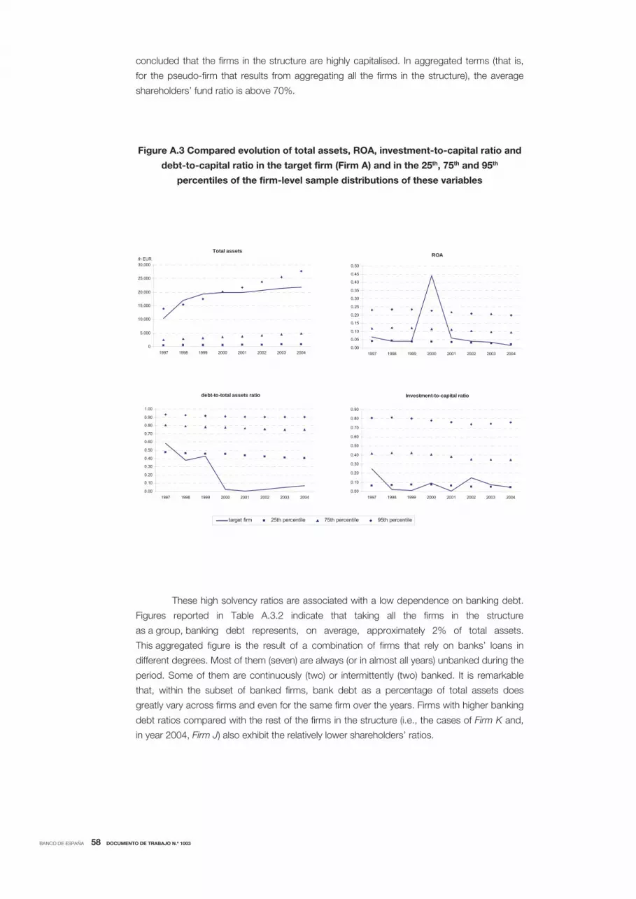
BANCO DE ESPAÑA 58 DOCUMENTO DE TRABAJO N.º 1003
concluded that the firms in the structure are highly capitalised. In aggregated terms (that is,
for the pseudo-firm that results from aggregating all the firms in the structure), the average
shareholders’ fund ratio is above 70%.
Figure A.3 Compared evolution of total assets, ROA, investment-to-capital ratio and
debt-to-capital ratio in the target firm (Firm A) and in the 25th, 75th and 95th
percentiles of the firm-level sample distributions of these variables
These high solvency ratios are associated with a low dependence on banking debt.
Figures reported in Table A.3.2 indicate that taking all the firms in the structure
as a group, banking debt represents, on average, approximately 2% of total assets.
This aggregated figure is the result of a combination of firms that rely on banks’ loans in
different degrees. Most of them (seven) are always (or in almost all years) unbanked during the
period. Some of them are continuously (two) or intermittently (two) banked. It is remarkable
that, within the subset of banked firms, bank debt as a percentage of total assets does
greatly vary across firms and even for the same firm over the years. Firms with higher banking
debt ratios compared with the rest of the firms in the structure (i.e., the cases of Firm K and,
in year 2004, Firm J) also exhibit the relatively lower shareholders’ ratios.
0 .0 0
0 .5 0
1 9 9 7 1 9 9 8 1 9 9 9 2 0 0 0 2 0 0 1 2 0 0 2 2 0 0 3 2 0 0 4
target firm 25th percentile 75th percentile 95th percentile
Total assets
0
5,000
10,000
15,000
20,000
25,000
30,000
1997 1998 1999 2000 2001 2002 2003 2004
th EURROA
0.00
0.05
0.10
0.15
0.20
0.25
0.30
0.35
0.40
0.45
0.50
1997 1998 1999 2000 2001 2002 2003 2004
debt-to-total assets ratio
0.00
0.10
0.20
0.30
0.40
0.50
0.60
0.70
0.80
0.90
1.00
1997 1998 1999 2000 2001 2002 2003 2004
Investment-to-capital ratio
0.00
0.10
0.20
0.30
0.40
0.50
0.60
0.70
0.80
0.90
1997 1998 1999 2000 2001 2002 2003 2004

BANCO DE ESPAÑA 59 DOCUMENTO DE TRABAJO N.º 1003
Table A.3.1. Shareholders’ funds-to-total assets ratio (%)
* Firm B is excluded because it reports negative shareholder funds. Firms’ names are fictitious
Table A.3.2. Bank debt-to-total assets ratio (%)1
1Information on banking debt has been drawn from CIR. Firms’ names are fictitious.
Name 1997 1998 1999 2000 2001 2002 2003 2004 averageFIRM A 41.4 62.5 57.6 97.7 99.5 97.5 94.9 93.1 80.5FIRM D 99.7 99.7 96.4 99.6 99.5 99.7 99.7 99.2FIRM E 100 100 100 100 100 100 100 100FIRM F 16.0 13.4 85.2 68.7 80.2 69.7 69.1 57.9 57.5FIRM G 61.3 65.8 71.6 69.8 66.7 67.5 65.6 66.5 66.8FIRM C 55.2 61.3 60.0 59.1 68.5 75.9 76.8 80.3 67.1FIRM I 100 100 100 100 22.8 21.3 20.2 66.3FIRM B*FIRM K 26.0 21.0 27.1 31.0 39.8 37.2 20.2 6.7 26.1FIRM H 95.0 95.0 95.0 95.0 96.6 98.6 99.3 99.3 96.7FIRM J 99.5 94.4 92.3 100 100 100 100 2.1 86.0Aggregated firm* 22.6 34.4 73.9 88.2 93.2 86.5 84.9 78.1 70.2
Shareholder funds/Total assets (%)
1997 1998 1999 2000 2001 2002 2003 2004 averageFIRM A 0 0 0 0 0 0 0 0 0.0FIRM D 0 0 0 0 0 0 0 0.0FIRM E 0 0 0 0 0 0 0 0FIRM F 0 0.1 0.2 2.1 0.6 8.5 16.5 10.0 4.7FIRM G 3.9 7.0 3.0 0 2.1 0 0 3.2 2.4FIRM C 0 0 0 0 0 0 0 0 0.0FIRM I 0 0 0 0 0 0 0 0.0FIRM B 20.6 31.9 39.1 39.2 14.8 14.1 10.7 10.7 22.6FIRM K 22.9 20.8 66.5 50.0 39.8 29.6 23.0 42.9 36.9FIRM H 0 0 0 0 0 0 0 0 0.0FIRM J 0 0 0 0 0 0 0 43.6 5.4Aggregated firm 0.5 0.7 1.5 2.0 1.0 2.9 4.8 4.5 2.2
Bank debt/Total assets (%)

BANCO DE ESPAÑA 60 DOCUMENTO DE TRABAJO N.º 1003
100%
100%
46.7
5%
17.3
5%
100%
99.7
0%
0.03
%
>50%
100%
13.7
2%9.
72%
12.2
2%
13.4
7%10
0%
23.4
4%
13.1
7%
100%
M
r. X
FIR
M B
Con
stitu
tion
date
: 199
2N
AC
E 0
9 co
de: 1
103
D.E
: Mr.
X"C
ontin
uing
ban
ked"
FIR
M A
Con
stitu
tion
date
: 198
7N
AC
E 0
9 co
de: 7
022
D.E
: Mr.
X"C
ontin
uing
unb
anke
d"
FIR
M C
Con
stitu
tion
date
: 199
0N
AC
E 0
9 co
de: 2
599
D.E
: Mr.
X"C
ontin
uing
unb
anke
d"
FIR
M E
Con
stitu
tion
date
: 199
4N
AC
E 09
cod
e: 7
022
D.E
.: M
r. X
"Con
tinui
ng u
nban
ked"
FIR
M F
Con
stitu
tion
date
: 198
6N
ACE
09
code
: 259
9D
.E.:
Mr.
X"B
anke
d": 1
998-
2004
FIR
M G
Con
stitu
tion
date
: 197
9N
AC
E 09
cod
e: 4
672
D.E
.: M
r. X
"Ban
ked"
: 199
7-99
, 200
1, 2
004
Ms.
Y (m
othe
r?)
Mr.
Z1 (s
on 1
)M
r. Z2
(son
2)
Ms.
Z3
(dau
gthe
r 1)
Ms.
Z4
(dau
gthe
r 2)
M
s. W
(wife
?)
FIR
M H
Con
stitu
tion
date
: 198
7N
ACE
09
code
: 466
9D
.E.:
Mr.
X"C
ontin
uing
Unb
anke
dFI
RM
IC
onst
itutio
n da
te: 1
988
NA
CE
09
code
: 702
2D
.E. M
r. X
"Con
tinui
ng u
nban
ked"
FIR
M J
Con
stitu
tion
date
: 198
7N
ACE
09 c
ode.
237
0D
.E.:
Mr.
X"B
anke
d": 2
004
FIR
M K
Con
stitu
tion
date
: 199
2N
ACE
09 c
ode:
016
1D
.E. M
r. X
"Con
tinui
ng b
anke
d"
FIR
M D
Con
stitu
tion
date
:198
9N
ACE
09
code
: 649
2D
.E. M
r. X
"Con
tinui
ng u
nban
ked"
othe
rs
Ch
art
A3
: A
n e
xa
mp
le o
f fa
mily f
irm
s’ str
uc
ture
:
Perc
enta
ges
ass
ocia
ted
to a
rrow
s in
dic
ate
the d
irect
ow
ners
hip
perc
enta
ge o
f a s
hare
ho
lder
(arr
ow
orig
in) in
a g
iven firm
(arr
ow
end
).
D.E
: D
irecto
r exe
cutiv
e.
Nam
es
are
fic
titio
us.

BANCO DE ESPAÑA PUBLICATIONS
WORKING PAPERS1
0901
PRAVEEN KUJAL AND JUAN RUIZ: International trade policy towards monopoly and oligopoly.
0902 CATIA BATISTA, AITOR LACUESTA AND PEDRO VICENTE: Micro evidence of the brain gain hypothesis: The case of
Cape Verde.
0903 MARGARITA RUBIO: Fixed and variable-rate mortgages, business cycles and monetary policy.
0904 MARIO IZQUIERDO, AITOR LACUESTA AND RAQUEL VEGAS: Assimilation of immigrants in Spain: A longitudinal
analysis.
0905 ÁNGEL ESTRADA: The mark-ups in the Spanish economy: international comparison and recent evolution.
0906 RICARDO GIMENO AND JOSÉ MANUEL MARQUÉS: Extraction of financial market expectations about inflation and
interest rates from a liquid market.
0907 LAURA HOSPIDO: Job changes and individual-job specific wage dynamics.
0908 M.a DE LOS LLANOS MATEA AND JUAN S. MORA: La evolución de la regulación del comercio minorista en España y
sus implicaciones macroeconómicas.
0909 JAVIER MENCÍA AND ENRIQUE SENTANA: Multivariate location-scale mixtures of normals and mean-variance-
skewness portfolio allocation.
0910 ALICIA GARCÍA-HERRERO, SERGIO GAVILÁ AND DANIEL SANTABÁRBARA: What explains the low profitability
of Chinese banks?
0911 JAVIER MENCÍA: Assessing the risk-return trade-off in loans portfolios.
0912 MAXIMO CAMACHO AND GABRIEL PEREZ-QUIROS: Ñ-STING: España Short Term INdicator of Growth.
0913 RAQUEL VEGAS, ISABEL ARGIMÓN, MARTA BOTELLA AND CLARA I. GONZÁLEZ: Retirement behaviour and
retirement incentives in Spain.
0914 FEDERICO CINGANO, MARCO LEONARDI, JULIÁN MESSINA AND GIOVANNI PICA: The effect of employment
protection legislation and financial market imperfections on investment: Evidence from a firm-level panel of EU
countries.
0915 JOSÉ MANUEL CAMPA AND IGNACIO HERNANDO: Cash, access to credit, and value creation in M&As.
0916 MARGARITA RUBIO: Housing market heterogeneity in a monetary union.
0917 MAXIMO CAMACHO, GABRIEL PEREZ-QUIROS AND HUGO RODRÍGUEZ MENDIZÁBAL: High-growth
Recoveries, Inventories and the Great Moderation.
0918 KAI CHRISTOFFEL, JAMES COSTAIN, GREGORY DE WALQUE, KEITH KUESTER, TOBIAS LINZERT,
STEPHEN MILLARD AND OLIVIER PIERRARD: Wage, inflation and employment dynamics with labour market
matching.
0919 JESÚS VÁZQUEZ, RAMÓN MARÍA-DOLORES AND JUAN-MIGUEL LONDOÑO: On the informational role of
term structure in the U.S. monetary policy rule.
0920 PALOMA LÓPEZ-GARCÍA AND SERGIO PUENTE: What makes a high-growth firm? A probit analysis using
Spanish firm-level data.
0921 FABIO CANOVA, MATTEO CICCARELLI AND EVA ORTEGA: Do institutional changes affect business cycles?
Evidence from Europe.
0922 GALO NUÑO: Technology, convergence and business cycles.
0923 FRANCISCO DE CASTRO AND JOSÉ LUIS FERNÁNDEZ: The relationship between public and private saving in
Spain: does Ricardian equivalence hold?
0924 GONZALO FERNÁNDEZ-DE-CÓRDOBA, JAVIER J. PÉREZ AND JOSÉ L. TORRES: Public and private sector
wages interactions in a general equilibrium model.
0925 ÁNGEL ESTRADA AND JOSÉ MANUEL MONTERO: R&D investment and endogenous growth: a SVAR
approach.
0926 JUANA ALEDO, FERNANDO GARCÍA-MARTÍNEZ AND JUAN M. MARÍN DIAZARAQUE: Firm-specific factors
influencing the selection of accounting options provided by the IFRS: Empirical evidence from Spanish market.
0927 JAVIER ANDRÉS, SAMUEL HURTADO, EVA ORTEGA AND CARLOS THOMAS: Spain in the euro: a general
equilibrium analysis.
0928 MAX GILLMAN AND ANTON NAKOV: Monetary effects on nominal oil prices.
1. Previously published Working Papers are listed in the Banco de España publications catalogue.

0929
0930
0931
JAVIER MENCÍA AND ENRIQUE SENTANA: Distributional tests in multivariate dynamic models with Normal and
Student t innovations.
JOAN PAREDES, PABLO BURRIEL, FRANCISCO DE CASTRO, DANIEL GARROTE, ESTHER GORDO AND
JAVIER J. PÉREZ: Fiscal policy shocks in the euro area and the US: an empirical assessment.
TERESA LEAL, DIEGO J. PEDREGAL AND JAVIER J. PÉREZ: Short-term monitoring of the Spanish Government
balance with mixed-frequencies models.
0932 ANTON NAKOV AND GALO NUÑO: Oilgopoly: a general equilibrium model of the oil-macroeconomy nexus.
0933 TERESA LEAL AND JAVIER J. PÉREZ: Análisis de las desviaciones presupuestarias aplicado al caso del
presupuesto del Estado.
0934 JAVIER J. PÉREZ AND A. JESÚS SÁNCHEZ: Is there a signalling role for public wages? Evidence for the euro
area based on macro data.
0935
1001
JOAN PAREDES, DIEGO J. PEDREGAL AND JAVIER J. PÉREZ: A quarterly fiscal database for the euro area
based on intra-annual fiscal information.
JAVIER ANDRÉS, ÓSCAR ARCE AND CARLOS THOMAS: Banking competition, collateral constraints and
optimal monetary policy.
1002 CRISTINA BARCELÓ AND ERNESTO VILLANUEVA: The response of household wealth to the risk of losing the
job: evidence from differences in firing costs.
1003 ALEXANDER KARAIVANOV, SONIA RUANO, JESÚS SAURINA AND ROBERT TOWNSEND: No bank, one bank,
several banks: does it matter for investment?
Unidad de PublicacionesAlcalá, 522; 28027 Madrid
Teléfono +34 91 338 6363. Fax +34 91 338 6488Correo electrónico: [email protected]
www.bde.es