interpolation lattices in several variables
TRANSCRIPT

“garcia de galdeano”
garcía de galdeano
seminariomatemático n. 24
PRE-PUBLICACIONES delseminario matematico 2005
J.M. CarnicerM. GascaT. Sauer
Interpolation lattices inseveral variables
Universidad de Zaragoza

Interpolation lattices in several variablesJ. M. Carnicer * , M. Gasca * and T.Sauer **
*University of Zaragoza, Spain, **University of Giessen, Germany
Abstract: Principal lattices are classical simplicial configurations of nodes suitable formultivariate polynomial interpolation in n dimensions. A principal lattice can be describedas the set of intersection points of n+1 pencils of parallel hyperplanes. Using a projectivepoint of view, Lee and Phillips extended this situation to n+1 linear pencils of hyperplanes.In two recent papers, two of us have introduced generalized principal lattices in the planeusing cubic pencils. In this paper we analyze the problem in n dimensions, consideringpolynomial, exponential and trigonometric pencils, which can be combined in different waysto obtain generalized principal lattices. We also consider the case of coincident pencils.An error formula for generalized principal lattices is discussed.
1. Introduction
In contrast to the univariate case, the solvability (and uniqueness of the solution) of poly-nomial interpolation problems in several variables depends not only on the number butalso on the geometry of the points where the function has to be interpolated. To be moreprecise, let x1, . . . ,xN ∈ Rn be a finite set of distinct points. The classical Lagrange in-terpolation problem consists of finding, for given data y1, . . . , yN ∈ R, a polynomial p suchthat p
(xj
)= yj , j = 1, . . . , N . Without further constraints, this solution is not unique,
but becomes unique for n = 1 if the degree of the polynomial is restricted to be ≤ N − 1.This fact is often stated as that the polynomial interpolation problem with respect to ar-bitrary N points is poised or correct for the space Π1
N−1 of all (univariate) polynomials ofdegree ≤ N − 1. In other words, the univariate polynomials of limited degree form a Haarspace. The natural extension would be to consider the space Πn
m of all polynomials of totaldegree ≤ m in n ≥ 1 variables. The dimension of this space is N =
(n+m
n
), but even if the
number of interpolation points coincides with the dimension, the Lagrange interpolationproblem with respect to x1, . . . ,xN need not be poised for Πn
m (just consider 3 points ona straight line in R2 and Π2
1).To overcome the problem of non–poised point configurations, there have been various
attempts to construct sets on(m+n
n
)points with respect to which the Lagrange interpo-
lation problem is poised for Πnm. Since the classical paper by Chung and Yao [5], these
constructions mainly consist of choosing the points as appropriate intersections of hyper-planes. The paper [6] provides constructions exploiting this idea. For more references see[7]. Recall that a hyperplane H ⊂ Rn is the zero set of an affine function, that is,
H = x ∈ Rn | h(x) = 0 , h(x) = v · x + c, v ∈ Rn \ 0, c ∈ R,
where the normal vector v and the constant c are unique up to normalization by a nonzeroconstant. In this paper, we will give a method to choose these hyperplanes in such a way
* Partially supported by the Spanish Research Grant BFM2003-03510, by Gobierno deAragon and Fondo Social Europeo.
1

that their intersections yield a proper set of interpolation points, forming a structure thatgeneralizes what has been named principal lattices in the literature. The bivariate casewas analyzed in [3] and [4]. Our goal is to study the case of more than two variables, whichhas turned out to be much more complex. We offer a variety of constructions here withoutclaiming to cover all possibilities.
In Section 2 we briefly review the concept of principal lattices and a generalizationof them. In Section 3 we present our method based on families of hyperplanes whichwe relate to univariate Chebyshev systems in Section 4, while Section 5 describes how toobtain lattices by combining different families. Finally, Section 6 deals with the error ofinterpolation on such a lattice, i.e., with the deviation of the interpolant from a sufficientlysmooth function, showing that principal lattices admit a rather simple and geometricallyappealing error formula as well as error estimates with a rather “univariate” flair.
2. A generalization of principal latticesWe shall denote Nm = 0, 1, . . . ,m ⊂ Z and
Snm := α = (α0, . . . , αn) ∈ Nn+1
m ; |α| = m. (1)
Principal lattices in Rn are distributions of points of the form
x =α0
ma0 + · · ·+ αn
man, α ∈ Sn
m,
where ai ∈ Rn are the vertices of a simplex in Rn (see [8] for details on the history ofthese sets). In the case of the standard simplex, this set of points is X = α/m | α ∈ Sn
m.Let us define
h0α0
(x) :=m− α0
m− (x1 + · · ·+ xn), α0 ∈ Nm,
hrαr
(x) := xr −αr
m, αr ∈ Nm, r ∈ 1, . . . , n,
and use the symbol Hrαr
for the hyperplane defined by the equation hrαr
(x) = 0. The pointxα = α/m, α ∈ Sn
m, of X is the intersection of the hyperplanes Hrαr
, r = 0, . . . , n.Lee and Phillips [9] generalized this idea introducing lattices generated by n+1 pencils
of hyperplanesHr
αr| αr ∈ Nm, r = 0, 1, . . . , n, (2)
in the projective space Pn(R). The lattice X is the set of points xα | α ∈ Snm, where xα
is the intersection of the hyperplanes Hrαr
, r = 0, . . . , n. In the general case, a projectivecoordinate system can be chosen so that the n + 1 families of m + 1 hyperplanes (2) haveequations hr
αr(x) = 0 with
hnα0
(x) := µm−α0xn − x0, α0 ∈ Nm,
hrαr
(x) := µαrxr − xr−1, αr ∈ Nm, r ∈ 1, . . . , n,
where µ ∈ R\−1, 0, 1. It can be shown that X is the set of points xα with homogeneouscoordinates
(µα1+α2+···+αn , µα2+···+αn , . . . , µαn , 1),
2

where α ∈ Snm. Principal lattices can be described as the limit case when µ → 1 (cf.
Section 4 of [9] and Section 2 of [3]).In [3, 4] a generalization of principal lattices in the plane was introduced in order to
describe principal lattices, the lattices generated by n + 1 pencils considered in [9] andfurther examples generated by cubic pencils. While in [9] all the n + 1 pencils must bedifferent, the constructions given in [3, 4] may use repeated pencils.
Let us state this definition in the n-dimensional case.
Definition 1. LetHr
i , i ∈ Nm, r = 0, . . . , n,
be n + 1 families of hyperplanes containing (n + 1)(m + 1) distinct hyperplanes such that(i) The intersection of any set of n hyperplanes Hr1
i1, . . . ,Hrn
in, corresponding to distinct
indices r1, . . . , rn ∈ 0, 1, . . . , n, consists of exactly one point.(ii) we have that
α ∈ Snm =⇒
n⋂r=0
Hrαr6= ∅. (3)
Under these assumptions the set of points
X := xα | xα :=n⋂
r=0
Hrαr
, α = (α0, . . . , αn) ∈ Snm, (4)
is a generalized principal lattice of degree m (GPLm) in Rn if it satisfies the additionalcondition(iii) for any α0, . . . , αn ∈ Nm we have that
n⋂r=0
Hrαr∩X 6= ∅ =⇒ α ∈ Sn
m. (5)
Remark 2. Let us see that a node lying on one hyperplane of each family xα =⋂n
r=0 Hrαr∩
X cannot lie on any other hyperplane Hrβr
for some r ∈ 0, 1, . . . , n, βr ∈ Nm. By (5),we have that α ∈ Sn
m. If
xα ∈ H0α0∩ · · · ∩Hr−1
αr−1∩Hr
βr∩Hr+1
αr+1∩ · · · ∩Hn
αn∩X.
we may apply (5) to(α0, . . . , αr−1, βr, αr+1, . . . , αn)
and derive that
α0 + · · ·+ αr−1 + βr + αr+1 + · · ·+ αn = m = α0 + · · ·+ αr−1 + αr + αr+1 + · · ·+ αn
and so, βr = αr.
Now, let us show that for any node xα, α ∈ Snm, there cannot exist any other index
β ∈ Snm such that xβ = xα. Take any r ∈ 0, . . . , n and then xα ∈ Hr
βr. By Remark 2, we
3

have βr = αr. Since r is arbitrary, we have β = α. So the cardinality of the set of nodesX defined in (4) is |Sn
m| =(m+n
n
).
Let us note that, in contrast to [9], we do not impose that any family of hyperplanesis contained in a linear pencil. We shall describe constructions of GPLm sets where eachfamily is not contained in a linear pencil.
Generalized principal lattices satisfy the geometric characterization of Chung and Yao[5]. This property characterizes sets of
(m+n
n
)nodes in the plane which are unisolvent for
the Lagrange interpolation problem in Πnm and whose Lagrange polynomials are products
of linear factors.
Definition 3. A set of(m+n
n
)nodes X ⊆ Rn satisfies the geometric characterization GCm
if for each node x ∈ X, there exist m hyperplanes containing all nodes in X \ x but notx.
Proposition 4. Let X be a GPLm set. Then X satisfies GCm and is unisolvent for theLagrange interpolation problem in Πn
m. A Lagrange formula for the interpolant Lmf of afunction f ∈ C(Rn) is given by
Lmf =∑
α∈Snm
f (xα)n∏
r=0
αr−1∏i=0
hri
hri (xα)
, (6)
where hri (x) = 0 is the equation of the hyperplane Hr
i , i ∈ Nm, r = 0, . . . , n.
Proof: Given α ∈ Snm, the m hyperplanes
Hri , 0 ≤ i ≤ αr − 1, r = 0, . . . , n, (7)
contain all nodes of X \ xα but not xα.
4

3. Construction of generalized principal latticesIn the bivariate case [3, 4], constructions of generalized principal lattices were obtainedparameterizing the families of lines by elements of a group G. The groups arising inthese constructions were the additive group of real numbers R, R × Zk, where Zk =0, 1, . . . , k−1 is the additive group of integers modulo k, and quotient groups like R/2πZ.
In order to extend the constructions to more than two variables, let us assume thatwe have n + 1 families of hyperplanes parameterized depending on a parameter ω ∈ G,where G is an abelian group, that is,
Hr(ω) | ω ∈ G, r = 0, . . . , n,
and assume that the following properties hold
(P1) The intersection of any n distinct hyperplanes, Hr1(ωr1), . . . , Hrn(ωrn), corresponding
to distinct indices r1, . . . , rn ∈ 0, 1, . . . , n, consists of exactly one point.
(P2) Let ω0, . . . , ωn ∈ G be such that the hyperplanes Hr(ωr), r = 0, . . . , n, are distinct.Then
⋂nr=0 Hr(ωr) 6= ∅ if and only if ω0 + · · ·+ ωn = 0.
It is important to mention that we need not require the families Hr(ω) to be distinct.In fact, the examples in Section 4 will even use coincident families
H0(ω) = H1(ω) = · · · = Hn(ω), ω ∈ G.
The following proposition shows how to construct generalized principal lattices.
Proposition 5. Let Hr(ω), ω ∈ G, r = 0, . . . , n be n + 1 families of hyperplanes suchthat (P1) and (P2) hold. Let δ ∈ G, ω0,r ∈ G, r = 0, . . . , n, be such that
ω0,0 + ω0,1 + · · ·+ ω0,n + mδ = 0. (8)
If the (n + 1)(m + 1) hyperplanes
Hri := Hr(ωi,r), ωi,r = ω0,r + iδ, i ∈ Nm, r = 0, . . . , n,
are distinct, then they define a GPLm set in Rn.
Proof: Since the hyperplanes are distinct, property (i) of Definition 1 clearly follows from(P1). Given any α ∈ Sn
m, the hyperplanes Hrαr
= H(ω0,r + αrδ) correspond to parametervalues ω0,r + αrδ. By (8), we have
n∑r=0
(ω0,r +αrδ) = ω0,0+ω0,1+· · ·+ω0,n+(α0+· · ·+αn)δ = ω0,0+ω0,1+· · ·+ω0,n+mδ = 0
and deduce from (P2), that⋂n
r=0 Hrαr6= ∅ and so (ii) of Definition 1 follows. Now we can
define X as in (4) and it only remains to check (iii) of Definition 1. Let us assume thatfor αr ∈ Nm, r = 0, . . . , n,
⋂nr=0 Hr
αr∩ X 6= ∅. By (4), the intersection point is a node
5

xβ with β ∈ Snm. So xβ =
⋂nr=0 Hr
βr=
⋂nr=0 Hr
αr∩ X. Let us show that αr = βr for all
r ∈ 0, 1, . . . , n. Taking into account that
xβ ∈ H0β0∩ · · · ∩Hr−1
βr−1∩Hr
αr∩Hr+1
βr+1∩ · · · ∩Hn
βn,
we have by (P2)
ω0,0 + ω0,1 + · · ·+ ω0,n + (β0 + · · ·+ βr−1 + αr + βr+1 + · · ·+ βn)δ = 0,
ω0,0 + ω0,1 + · · ·+ ω0,n + (β0 + · · ·+ βr−1 + βr + βr+1 + · · ·+ βn)δ = 0,
and we obtain(αr − βr)δ = 0.
Since the hyperplanes Hri , i ∈ Nm, are distinct, we must have that ωr,0 + iδ are distinct
group elements and therefore iδ 6= 0 for all i ∈ Z, 0 < |i| ≤ m. So, we have that αr = βr
for any r ∈ 0, 1, . . . , n. Therefore α = β ∈ Snm.
In order to analyze the families of hyperplanes Hr(ω), we need to consider theirequations
f1,r(ω)x1 + · · ·+ fn,r(ω)xn + f0,r(ω) = 0.
The incidence properties are invariant under projective transformations and therefore weshall rather use homogeneous coordinates to express the equations in the form
hr(x0, . . . , xn;ω) = 0,
where
hr(x0, . . . , xn;ω) =n∑
j=0
fj,r(ω)xj .
We shall omit the dependence on the variables x0, . . . , xn and also write Hr(ω) insteadof hr(x0, . . . , xn;ω). This notational convention means that we do not make a distinc-tion between the hyperplane Hr(ω) and the linear function hr(x0, . . . , xn;ω) such thathr(1, x1, . . . , xn;ω) = 0 is the equation defining Hr(ω).
We next show that principal lattices are generated by families of hyperplanes satisfying(P1) and (P2). To that end, we choose G = R and
H0(t) = tx0 − (x1 + · · ·+ xn), Hr(t) = tx0 + xr, r = 1, . . . , n.
The intersection of Hr(tr), r = 0, . . . , n, gives rise to a system of equations
A(x0, . . . , xn)T = 0,
whose coefficient matrix A is t0 −1 −1 · · · −1t1 1 0 · · · 0
t2 0 1. . .
......
.... . . . . . 0
tn 0 · · · 0 1
. (9)
6

Since any n rows of A are independent, (P1) holds. The n + 1 hyperplanes are concurrentif and only if det A = 0. Since detA = t0 + · · ·+ tn, (P2) holds.
Let us analyze the Lee and Phillips construction of lattices generated by n+1 pencils.We choose G = R× Z2 and
Hr(t, s) = xr − (−1)s exp(t)xr+1, t ∈ R, s ∈ Z2, r ∈ Zn.
Here by r ∈ Zn we mean that the indexing is cyclic and that xn+1 denotes x0. Theintersection of Hr(tr, sr), r = 0, . . . , n, corresponds to nontrivial solutions of the systemA(x0, . . . , xn)T = 0, where A is
1 −µ0 0 · · · 00 1 −µ1 · · · 0...
. . . . . . . . ....
0 · · · 0 1 −µn−1
−µn 0 · · · 0 1
, (10)
with µi = (−1)si exp(ti). Since any n rows of A are independent, (P1) holds. The hyper-planes Hr(tr) are concurrent if and only if 0 = det A = 1− µ0 · · ·µn, that is,
(−1)s0+···+sn exp(t0 + · · ·+ tn) = 1,
which is equivalent to s0 + · · ·+ sn = 0 and t0 + · · ·+ tn = 0. So (P2) is also satisfied.
4. Generalized principal lattices obtained from a single family
In this section we will provide a general construction process for an arbitrary number ofvariables with respect to the three additive groups R, R× Z2 and R/2πZ. In the sequel,G will always stand for one of these three groups that are also locally compact Hausdorffspaces, so that the tools from Approximation Theory we are going to use in this sectionare well defined and accessible, cf. [10].
The goal is to find functions fj : G → R, j = 0, . . . , n, such that, for ω0, . . . , ωn ∈ Gdistinct,
det
f0 (ω0) . . . fn (ω0)...
. . ....
f0 (ωn) . . . fn (ωn)
= 0 ⇐⇒n∑
j=0
ωj = 0, (11)
according to the concurrency condition (P2). Clearly, such conditions are very closelyrelated to the concept of Chebyshev spaces. Recall that a k-dimensional space F of functionswith basis say f1, . . . , fk is called a Chebyshev space (and the basis is called a Haar system)on a set X if for any choice of distinct points xi ∈ X, i = 1, . . . , k, one has that
Ψ (x1, . . . , xk) := det (fj (xi) : i, j = 1, . . . , k) 6= 0.
The following simple lemma is crucial to our construction.
7

Lemma 6. Let f0, . . . , fn, fn+1 be a Haar system on G and f =∑n+1
j=0 αjfj a nonzerofunction, vanishing on distinct ω0, . . . , ωn ∈ G:
f(ω0) = · · · = f(ωn) = 0.
Then
det
f0 (ω0) . . . fn (ω0)...
. . ....
f0 (ωn) . . . fn (ωn)
= 0, (12)
if and only if αn+1 = 0, that is, f is a linear combination of f0, . . . , fn.
Proof: Let ω ∈ G\ω0, . . . , ωn. The coefficients of f with respect to the basis f0, . . . , fn+1
satisfy f0(ω0) . . . fn(ω0) fn+1(ω0)
.... . .
......
f0(ωn) . . . fn(ωn) fn+1(ωn)f0(ω) . . . fn(ω) fn+1(ω)
α0...
αn
αn+1
=
0...0
f(ω)
.
Observe that f(ω) 6= 0 because f is a nonzero function vanishing on ω0, . . . , ωn, and(f0, . . . , fn+1) is a Haar system. By Cramer’s rule, we have
αn+1 =f(ω)
Ψ(ω0, . . . , ωn, ω)det
f0 (ω0) . . . fn (ω0)...
. . ....
f0 (ωn) . . . fn (ωn)
,
where
Ψ(ω0, . . . , ωn, ω) = det
f0(ω0) . . . fn(ω0) fn+1(ω0)
.... . .
......
f0(ωn) . . . fn(ωn) fn+1(ωn)f0(ω) . . . fn(ω) fn+1(ω)
.
Since f(ω) and Ψ(ω0, . . . , ωn, ω) are nonzero we have that αn+1 = 0 if and only if (12)holds.
Lemma 6 is the key to finding functions f0, . . . , fn such that (11) holds in order toconstruct pencils of hyperplanes satisfying properties (P1) and (P2).
Proposition 7. Let f0, . . . , fn, fn+1 be a Haar system on G. Assume that for any distinctω0, . . . , ωn ∈ G a nonzero function f =
∑n+1j=0 αjfj vanishing on ω0, . . . , ωn has coefficient
αn+1 in fn+1 equal to ω0 + · · ·+ ωn up to a nonzero constant. Let us define the pencil ofhyperplanes
H(ω) =n∑
j=0
fj(ω) xj , ω ∈ G.
Then we have
8
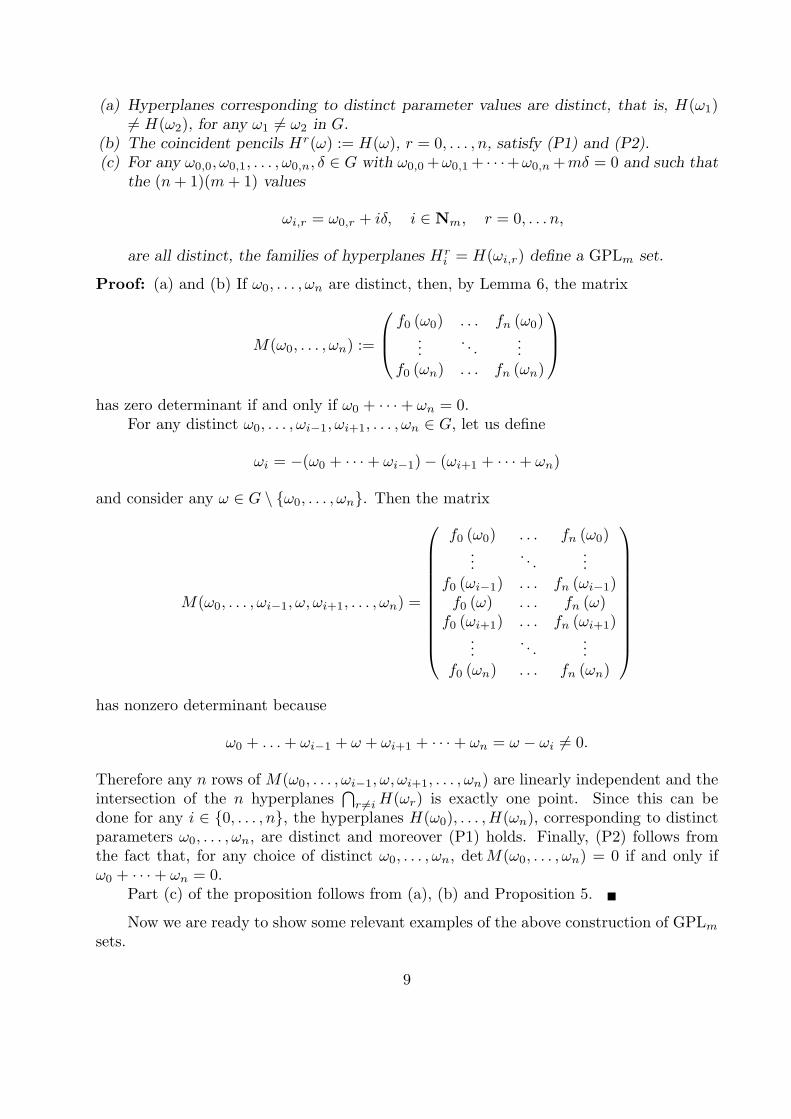
(a) Hyperplanes corresponding to distinct parameter values are distinct, that is, H(ω1)6= H(ω2), for any ω1 6= ω2 in G.
(b) The coincident pencils Hr(ω) := H(ω), r = 0, . . . , n, satisfy (P1) and (P2).(c) For any ω0,0, ω0,1, . . . , ω0,n, δ ∈ G with ω0,0 +ω0,1 + · · ·+ω0,n +mδ = 0 and such that
the (n + 1)(m + 1) values
ωi,r = ω0,r + iδ, i ∈ Nm, r = 0, . . . n,
are all distinct, the families of hyperplanes Hri = H(ωi,r) define a GPLm set.
Proof: (a) and (b) If ω0, . . . , ωn are distinct, then, by Lemma 6, the matrix
M(ω0, . . . , ωn) :=
f0 (ω0) . . . fn (ω0)...
. . ....
f0 (ωn) . . . fn (ωn)
has zero determinant if and only if ω0 + · · ·+ ωn = 0.
For any distinct ω0, . . . , ωi−1, ωi+1, . . . , ωn ∈ G, let us define
ωi = −(ω0 + · · ·+ ωi−1)− (ωi+1 + · · ·+ ωn)
and consider any ω ∈ G \ ω0, . . . , ωn. Then the matrix
M(ω0, . . . , ωi−1, ω, ωi+1, . . . , ωn) =
f0 (ω0) . . . fn (ω0)...
. . ....
f0 (ωi−1) . . . fn (ωi−1)f0 (ω) . . . fn (ω)
f0 (ωi+1) . . . fn (ωi+1)...
. . ....
f0 (ωn) . . . fn (ωn)
has nonzero determinant because
ω0 + . . . + ωi−1 + ω + ωi+1 + · · ·+ ωn = ω − ωi 6= 0.
Therefore any n rows of M(ω0, . . . , ωi−1, ω, ωi+1, . . . , ωn) are linearly independent and theintersection of the n hyperplanes
⋂r 6=i H(ωr) is exactly one point. Since this can be
done for any i ∈ 0, . . . , n, the hyperplanes H(ω0), . . . ,H(ωn), corresponding to distinctparameters ω0, . . . , ωn, are distinct and moreover (P1) holds. Finally, (P2) follows fromthe fact that, for any choice of distinct ω0, . . . , ωn, detM(ω0, . . . , ωn) = 0 if and only ifω0 + · · ·+ ωn = 0.
Part (c) of the proposition follows from (a), (b) and Proposition 5.
Now we are ready to show some relevant examples of the above construction of GPLm
sets.
9

Example 1. For the group G = R, we choose the Haar system defined by fj(t) = tj ,j = 0, . . . , n − 1, fn(t) = tn+1 and fn+1(t) = tn. For any selection of distinct pointst0, . . . , tn, the coefficient of the polynomial
f(t) = (t− t0) · · · (t− tn) =n+1∑j=0
αjfj(t),
in tn is αn+1 = −(t0 + · · ·+ tn) and therefore we find that the pencil
H(t) =n−1∑j=0
tj xj + tn+1 xn, t ∈ R, (13)
satisfies the hypotheses of Proposition 7.
Example 2. For the group G = R × Z2 we write ω = (t, s) ∈ R × Z2 and apply thetransformation µ := (−1)s exp t ∈ R∗ := R \ 0. Then we use the Haar system on themultiplicative group R∗
fj(µ) = µj , j = 0, . . . , n− 1, fn(µ) = µn − (−1)nµ−1, fn+1(µ) = µ−1
and define for distinct µ0, . . . , µn in R∗
f(µ) = µ−1n∏
j=0
(1− µ
µj
)=
n+1∑j=0
αjfj(µ).
The coefficient with respect to fn+1 is then computed to be αn+1 = 1−µ−10 · · ·µ−1
n . Thenαn+1 = 0 if and only if µ0 · · ·µn = 1, that is, s0 + · · · + sn = 0 and t0 + · · · + tn = 0.Therefore the pencil
H(t, s) =n−1∑j=0
(−1)js exp(jt)xj + [(−1)ns exp(nt)− (−1)n−s exp(−t)]xn, t ∈ R, s ∈ Z2
(14)satisfies the hypotheses of Proposition 7.
Example 3. In the last case G = R/2πZ, the function f to be considered will be
f(t) =n∏
j=0
sint− tj
2=
n+1∑j=0
αjfj(t), (15)
but the Haar system (f0, . . . , fn+1) will depend on n. If n is odd, n = 2k + 1, we setf0(t) = 1, f2j−1(t) = cos(jt) and f2j(t) = sin(jt), j = 1, . . . , k + 1, while for the even casen = 2k we choose the functions f2j(t) = sin (2j+1)t
2 and f2j+1(t) = cos (2j+1)t2 , j = 0, . . . , k.
10

In order to identify the coefficient αn+1 in both cases, we rewrite (15) in terms of complexexponentials and expand it, using the abbreviation T = t0 + · · ·+ tn, into
(2i)n+1 f(t) =n∏
j=0
(ei(t−tj)/2 − e−i(t−tj)/2
)= ei((n+1)t−T )/2 + (−1)n+1e−i((n+1)t−T )/2
−n∑
j=0
(ei((n−1)t−T+2tj)/2 + (−1)n+1e−i((n−1)t−T+2tj)/2
)+ · · ·
(16)
For n = 2k + 1, (16) yields
f(t) = (−1)(n+1)/22−n
[cos
( (n + 1)t2
− T
2
)−
n∑j=0
cos( (n− 1)t
2− T − 2tj
2
)+ · · ·
]= (−1)k+12−(2k+1)
[cos((k + 1)t) cos
T
2+ sin((k + 1)t) sin
T
2+ · · ·
].
The coefficient αn+1 is
α2k+2 = (−1)k+12−(2k+1) sinT
2and vanishes if and only if T ∈ 2πZ. Therefore the pencil
H(t) = x0 +k+1∑j=1
x2j−1 cos(jt) +k∑
j=1
x2j sin(jt)
satisfies the hypotheses of Proposition 7.
If n = 2k, on the other hand, the expansion (16) becomes
f(t) = (−1)n/22−n
sin( (n + 1)t
2− T
2
)−
n∑j=0
sin( (n− 1)t
2− T − 2tj
2
)+ · · ·
= (−1)k2−2k
[sin
(2k + 1)t2
cosT
2− cos
(2k + 1)t2
sinT
2+ · · ·
].
The coefficient αn+1 is
α2k+1 = (−1)k+12−2k sinT
2and therefore
H(t) =k∑
j=0
x2j sin(2j + 1)t
2+
k−1∑j=0
x2j+1 cos(2j + 1)t
2
satisfies the hypotheses of Proposition 7.
11

Remark 8. Changes of variables in the projective space lead to other families of hyper-planes generating GPLm sets, which are projective images of the sets defined above. Inthe first example these families are of the form
H(t) = f0(t)x0 + · · ·+ fn(t)xn,
where f0, . . . , fn form a basis of the polynomial space generated by 1, t, . . . , tn−1, tn+1. Inthe second example they can be written as
H(t, s) = f0((−1)s exp(t))x0 + · · ·+ fn((−1)s exp(t))xn,
where f0, . . . , fn form a basis of the space of Laurent polynomials generated by 1, µ, . . . ,µn−1, µn − (−1)nµ−1. Finally, in the third example a general form of the pencil is
H(t) = f0(t)x0 + · · ·+ fn(t)xn,
where f0, . . . , fn form a basis of the subspace of trigonometric polynomials generated by1, cos t, sin t, . . . , cos((n/2 − 1)t), sin((n/2 − 1)t), cos(nt/2), if n is even and of the spacegenerated by sin(t/2), cos(t/2), . . . , sin((n− 2)t/2), cos((n− 2)t/2t), sin(nt/2), if n is odd.
5. Generalized principal lattices combining different families
In the preceding section we have shown how to check conditions (P1) and (P2) for gen-eralized principal lattices, finding systems of functions satisfying (11). However, we haveused Lemma 6 to avoid the explicit computation of the determinant.
In this section we want to combine the examples of Section 4 in order to generatenew examples. In this case, it is not so easy to apply Lemma 6. A general method will beprovided for examples 1 and 2 and a particular instance will be shown for Example 3. Weshall apply Proposition 5 to check the validity of our constructions.
We introduce the notation
V (g; t0, . . . , tn) :=
1 t0 · · · tn−1
0 g(t0)1 t1 · · · tn−1
1 g(t1)1 t2 · · · tn−1
2 g(t2)...
......
...1 tn · · · tn−1
n g(tn)
and, for the usual Vandermonde matrix, we write
V (t0, . . . , tn) := V ((·)n; t0, . . . , tn).
The divided difference g[t0, . . . , tn] is the coefficient cn of tn in the interpolating poly-nomial p(t) = c0 + c1t + · · ·+ cntn of g at t0, . . . , tn. Observe that
(c0, . . . , cn)T = V (t0, . . . , tn)−1(g(t0), . . . , g(tn))T
12

for distinct t0, . . . , tn. So, it follows that
V (t0, . . . , tn)−1V (g; t0, . . . , tn) =
1 0 · · · 0 ∗0 1 · · · 0 ∗...
.... . .
......
0 0 · · · 1 ∗0 0 · · · 0 g[t0, . . . , tn]
. (17)
In Example 1, we know that the polynomial of degree at most n interpolating g(t) =tn+1 at t0, . . . , tn is
tn+1 − (t− t0) · · · (t− tn) = (t0 + · · ·+ tn)tn + lower degree terms
and sog[t0, . . . , tn] = t0 + · · ·+ tn, for g(t) = tn+1. (18)
In Example 2, the polynomial of degree not greater that n interpolating g(µ) =µn − (−1)nµ−1 at µ0, . . . , µn is
µn− (−1)nµ−1− (µ−10 µ−1) · · · (µ−1
n µ−1)µ−1 = (1−µ−10 · · ·µ−1
n )µn + lower degree terms
and sog[µ0, . . . , µn] = 1− (µ0 · · ·µn)−1, for g(µ) = µn − (−1)nµ−1. (19)
Next, we point out how to combine several families of Example 1. We choose p differentfamilies (13) of degrees k1, . . . , kp, with k1 + · · · + kp = n + 1. Let us partition the set ofindices I := 0, 1, . . . , n, into p subsets I =
⋃pl=1 Il, |Il| = kl, l = 1, . . . , p,
Il := r ∈ I | k1 + · · ·+ kl−1 ≤ r < k1 + · · ·+ kl. (20)
We take
Hr(t) =k1−2∑j=0
tjxj + tk1xn−p+1 − tk1−1n∑
j=n−p+2
xj (21)
for r ∈ I1 and
Hr(t) =kl−2∑j=0
tjxk1+···+kl−1−(l−1)+j + tklxn−p+1 + tkl−1xn−p+l (22)
for r ∈ Il, l = 2, . . . , p.Let us apply Proposition 5 to construct generalized principal lattices. In order to check
(P1) and (P2) we need to deal with the coefficient matrix of the linear system Hr(tr) = 0,r = 0, . . . , n,
A =
A11 0 · · · 0 B1 C1
0 A22. . .
... B2 C2...
. . . . . . 0...
...0 · · · 0 App Bp Cp
.
13

In the above formulaAll := (tj−1
i )i∈Il;j∈1,...,kl−1
is the kl × (kl − 1) matrix formed by the kl − 1 first columns of the Vandermonde matrixV (ti; i ∈ Il). The matrix
Bl := (tkli )i∈Il
,
is a kl × 1 matrix. The k1 × (p − 1) matrix C1 is formed by p − 1 repeated columns(−tk1−1
i )i∈I1 and the kl× (p−1) matrix Cl, l = 2, . . . , p, is formed by zero columns, exceptthe (l − 1)-th column which is of the form (tkl−1
i )i∈Il. Observe that any nonzero column
of any Cl is the last column of the Vandermonde matrix V (ti; i ∈ Il).Let us show that
det A = (−1)σ(t0 + · · ·+ tn)p∏
l=1
∏i>j∈Il
(ti − tj), σ ∈ 0, 1 (23)
where σ depends only on k1, . . . , kp. If, for some l ∈ 1, . . . , p, we have ti = tj , i, j ∈ Il,then two rows of A are equal and det A = 0 and formula (23) holds. Otherwise the matrixW := diag(V1, . . . , Vp), where Vl := V (ti; i ∈ Il), is nonsingular and
E := W−1A =
V −1
1 A11 0 · · · 0 V −11 B1 V −1
1 C1
0 V −12 A22
. . .... V −1
2 B2 V −12 C2
.... . . . . . 0
......
0 · · · 0 V −1p App V −1
p Bp V −1p Cp
.
Then
det A = det W detE = det E
p∏l=1
detVl = detE
p∏l=1
∏i>j∈Il
(ti − tj). (24)
Let us compute det E. Observe that V −1l All is the kl × (kl − 1) matrix formed by the first
kl − 1 columns of the identity. Expanding the determinant of E by the first n + 1 − pcolumns we get that det E coincides up to a sign (which only depends on the size of theblocks) with the determinant of the p× p submatrix E formed by the last p columns andthe last row of each block
E := (ek1+···+kl,n−p+j)l,j∈1,...,p. (25)
Taking into account (17) and (18) we have
el,1 = ek1+···+kl,n−p+1 = (·)kl [ti; i ∈ Il] =∑i∈Il
ti, l = 1, . . . , p.
Similarly, we can deduce that
e1,j = ek1,n−p+j = −(·)k1−1[ti; i ∈ I1] = −1, j = 2, . . . , p.
14
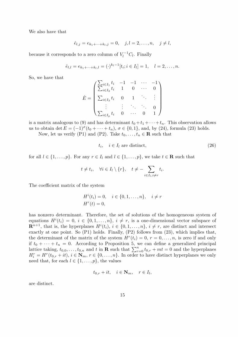
We also have that
el,j = ek1+···+kl,j = 0, j, l = 2, . . . , n, j 6= l,
because it corresponds to a zero column of V −1l Cl. Finally
el,l = ek1+···+kl,l = (·)kl−1[ti; i ∈ Il] = 1, l = 2, . . . , n.
So, we have that
E =
∑i∈I1
ti −1 −1 · · · −1∑i∈I2
ti 1 0 · · · 0∑i∈I3
ti 0 1. . .
......
.... . . . . . 0∑
i∈Ipti 0 · · · 0 1
is a matrix analogous to (9) and has determinant t0 + t1 + · · ·+ tn. This observation allowsus to obtain det E = (−1)σ(t0 + · · ·+ tn), σ ∈ 0, 1, and, by (24), formula (23) holds.
Now, let us verify (P1) and (P2). Take t0, . . . , tn ∈ R such that
ti, i ∈ Il are distinct, (26)
for all l ∈ 1, . . . , p. For any r ∈ Il and l ∈ 1, . . . , p, we take t ∈ R such that
t 6= ti, ∀i ∈ Il \ r, t 6= −∑
i∈Il,i 6=r
ti.
The coefficient matrix of the system
Hi(ti) = 0, i ∈ 0, 1, . . . , n, i 6= r
Hr(t) = 0,
has nonzero determinant. Therefore, the set of solutions of the homogeneous system ofequations Hi(ti) = 0, i ∈ 0, 1, . . . , n, i 6= r, is a one-dimensional vector subspace ofRn+1, that is, the hyperplanes Hi(ti), i ∈ 0, 1, . . . , n, i 6= r, are distinct and intersectexactly at one point. So (P1) holds. Finally, (P2) follows from (23), which implies that,the determinant of the matrix of the system Hr(ti) = 0, r = 0, . . . , n, is zero if and onlyif t0 + · · · + tn = 0. According to Proposition 5, we can define a generalized principallattice taking, t0,0, . . . , t0,n and t in R such that
∑nr=0 t0,r + mt = 0 and the hyperplanes
Hri = Hr(t0,r + it), i ∈ Nm, r ∈ 0, . . . , n. In order to have distinct hyperplanes we only
need that, for each l ∈ 1, . . . , p, the values
t0,r + it, i ∈ Nm, r ∈ Il,
are distinct.
15

Now we want to combine several families of Example 2. We choose p different families(14) corresponding to spaces of Laurent polynomials 〈µ−1, 1, . . . , µkl−1〉, l = 1, . . . , p, wherek1 + · · · + kp = n + 1. Let us partition the set of indices I = 0, 1, . . . , n, in p subsetsI =
⋃pl=1 Il, |Il| = kl, l = 1, . . . , p, as in (20). For t ∈ R, s ∈ Z2, we define the families
Hr(t, s) :=kl−2∑j=0
(−1)js exp(jt)xk1+···+kl−1−(l−1)+j + (−1)(kl−1)s exp((kl − 1)t)xn−p+l+
(−1)kl−s exp(−t)xn−p+l+1, r ∈ Il, l = 1, . . . , p− 1,
Hr(t, s) :=kp−2∑j=0
(−1)js exp(jt)xk1+···+kp−1−(p−1)+j + (−1)(kp−1)s exp((kp − 1)t)xn+
(−1)kp−s exp(−t)xn−p+1, r ∈ Ip.
(27)The coefficient matrix of the linear system Hr(tr, sr) = 0, r = 0, . . . , n, can be written inthe form
A =
A11 0 · · · 0 F1
0 A22. . .
... F2...
. . . . . . 0...
0 · · · 0 App Fp
.
Let us describe the nonzero blocks of this matrix in terms of µr = (−1)sr exp(tr), r =0, . . . , n. The block
All := (µj−1i )i∈Il;j∈1,...,kl−2
is the kl × (kl − 1) matrix formed by the kl − 1 first columns of the Vandermonde matrixV (µi; i ∈ Il). The block Fl is the kl×p matrix formed by zero columns, except for the l-thcolumn, which is of the form (µkl−1
i )i∈Il, and the (l + 1)-th column, which is of the form
((−1)klµ−1i )i∈Il
for l = 1, . . . , p−1. In the case l = p the role of the (l+1)-th column of Fl
is played by the first column, that is, all columns of Fp are zero except for the first columnwhich is of the form ((−1)kpµ−1
i )i∈Ip and the last column which is of the form (µkp−1i )i∈Ip .
Let us show that
detA = (−1)σ(1− µ−10 · · ·µ−1
n )p∏
l=1
∏i>j∈Il
(µi − µj), σ ∈ 0, 1, (28)
where σ depends only on k1, . . . , kp. As in the preceding example, we define
E := W−1A =
V −1
1 A11 0 · · · 0 V −11 F1
0 V −12 A22
. . .... V −1
2 F2
.... . . . . . 0
...0 · · · 0 V −1
p App V −1p Fp
,
16

where W := diag(V1, . . . , Vp), Vl := V (µi; i ∈ Il). Then
det A = detE
p∏l=1
∏i>j∈Il
(µi − µj).
The determinant of E coincides up to a sign with the determinant of the p× p submatrix(25) formed by the last p columns and the last row of each block. All elements of E arezero (because they correspond to zero columns of A) except for
ell = (·)kl−1[µi; i ∈ Il] = 1, l = 1, . . . , p,
el,l+1 = (−1)kl(·)−1[µi; i ∈ Il] = −∏i∈Il
µ−1i , l = 1, . . . , p− 1,
andep,1 = (−1)kp(·)−1[µi; i ∈ Ip] = −
∏i∈Ip
µ−1i ,
that is
E =
1 −∏
i∈I1µ−1
i 0 · · · 0
0 1 −∏
i∈I2µ−1
i
. . ....
... 0. . . . . . 0
0...
. . . 1 −∏
i∈Ip−1µ−1
i
−∏
i∈Ipµ−1
i 0 · · · 0 1
.
The matrix E is analogous to the matrix (10) and so we obtain
detE = (−1)σ(1− (µ0 · · ·µn)−1),
where σ ∈ 0, 1. As in the previous example, it is straightforward to check (P1) and (P2)for the families of hyperplanes defined by (27). The construction of generalized principallattices using Proposition 5 is completely analogous. We take t0,0, . . . , t0,n and t in R,s0,0, . . . , s0,n and s in Z2 such that
∑nr=0 t0,r + mt = 0,
∑nr=0 s0,r + ms = 0 and choose
the hyperplanes Hri = Hr(t0,r + it, s0,r + is), i ∈ Nm, r ∈ 0, . . . , n. In order to have
distinct hyperplanes we only need that for each l ∈ 1, . . . , p,
(t0,r + it, s0,r + is) i ∈ Nm, r ∈ Il,
are distinct group elements.Let us finish this section providing a three dimensional example, combining two fam-
ilies with G = R/2πZ
H1(t) = H2(t) = cos(t)x0 + sin(t)x1 + x2,
H3(t) = H4(t) = cos(t)x0 − sin(t)x1 + x3.
17

The intersection of Hr(tr) = 0, r = 0, 1, 2, 3, leads to a system with coefficient matrix
A =
cos(t0) sin(t0) 1 0cos(t1) sin(t1) 1 0cos(t2) − sin(t2) 0 1cos(t3) − sin(t3) 0 1
.
We have
detA = −det(
cos(t1)− cos(t0) sin(t1)− sin(t0)cos(t3)− cos(t2) − sin(t3) + sin(t2)
)= −4 sin((t1 − t0)/2) sin((t3 − t2)/2) det
(− sin((t0 + t1)/2) cos((t0 + t1)/2)− sin((t2 + t3)/2) − cos((t2 + t3)/2)
)= −4 sin((t1 − t0)/2) sin((t3 − t2)/2) sin((t0 + t1 + t2 + t3)/2).
So, if t1−t0, t3−t2 /∈ 2πZ, the determinant of A vanishes if and only if t0+t1+t2+t3 ∈ 2πZ.Hence (P1) and (P2) hold.
In contrast with the previous examples of this section, we have not been able to derivea general construction with parameterizations using trigonometric functions of the familiesof hyperplanes. Our first attempts indicate that there may be a restriction on the sizes ofthe blocks k1, . . . , kp.
6. Remainder formulas for principal lattices
In this section, we will derive some general facts on the error of interpolation, i.e., on thefunction f − Lmf , provided that f is a sufficiently smooth function. It will turn out thatthese formulas are in accordance with the geometric nature of the interpolation nodes inGPLm sets. To that end, we first note that condition (i) of Definition 1 ensures that thepoints
xα :=n⋂
j=1
Hjαj∈ Rn, α ∈ Nn
m, |α| ≤ m (29)
indexed by the dehomogeneized multiindex α = (α1, . . . , αn) are well–defined. Observethat there is no loss of information with this change of notation because we can recoverα0 by α0 = m− |α|. For |α| ≤ m we also define the polynomials
pα :=n∏
j=1
αj−1∏k=0
hjk
hjk (xα)
=:φα
φα (xα)(30)
of total degree |α| ≤ m. We observe that φα(xα) 6= 0 because the hyperplanes (7) do notcontain xα. We also introduce the semi–ordering “≤” on Nn
m, writing α ≤ β iff αj ≤ βj
for j = 1, . . . , n, and α < β iff α ≤ β and α 6= β.
18

Lemma 9. The polynomials pα and the points xα, |α| ≤ m, satisfy the following proper-ties:
(i) If pα
(xβ
)6= 0, then α ≤ β.
(ii) pα
(xβ
)= δα,β , for any α, β with |β| ≤ |α| ≤ m.
Proof: If there exists 1 ≤ j ≤ n such that βj < αj , then xβ ∈ Hjβj⊆ Hj
0 ∪ · · · ∪ Hjαj−1
and therefore hjk
(xβ
)= 0 for some 0 ≤ k ≤ αj − 1, which proves (i). Condition (ii), on
the other hand, follows from (i) and taking into account that β ≥ α implies that either|α| < |β| or α = β.
In the terminology of [11], Lemma 9 says that the polynomials pα, |α| ≤ m, forma Newton basis for interpolation in Πn
m. The coefficients λαf in the Newton form of theinterpolation polynomial
Lmf =∑
|α|≤m
λαf pα,
the so–called finite differences, measure the error of lower degree interpolation at theinterpolation nodes,
λαf =(f − L|α|−1f
)(xα) , (31)
and admit an integral representation that has been given in [11]. To state this formula, weneed some more notation. A path µ of length k + 1 is a vector (µ0, . . . , µk) of multiindicesµj ∈ Nn
m such that |µj | = j, j = 0, . . . ,m. Denoting the totality of all such paths by Λm,we associate to any path µ ∈ Λm
(i) a set Xµ := xµ0 , . . . ,xµm of interpolation nodes,(ii) an m–th order partial differential operator
Dmµ := Dxµm−xµm−1 · · ·Dxµ1−xµ0 (32)
following the directional derivatives along the path,(iii) a number
πµ :=m−1∏j=0
pµj(xµj+1) . (33)
By means of the simplex spline integral∫[X]
f =∫
∆N
f(Xu) du, X ⊂ Rn, #X = N,
where
∆N := (u1, . . . , uN ) : u1, . . . , uN ≥ 0, u1 + · · ·+ uN = 1, Xu := u1x1 + · · ·+ uNxN ,
we then obtain the announced error formula that is valid for any f ∈ Cm+1 (Rn), seeTheorem 3.4 and Theorem 3.6 of [11]:
f(x)− Lmf(x) =∑
µ∈Λm
pµm(x)πµ
∫[Xµ,x]
Dx−xµm Dmµ f. (34)
19

Note that, despite of the innocent appearance of this formula, the number of terms inthe sum is tremendous: even in two variables it is already (m + 1)! while in generalit will be of the form
(n1
)(n+1
2
)· · ·
(n+m−1
m
), which makes it very difficult to even derive
useful error estimates for the interpolation polynomial. In the case of our configurationof interpolation points formula (34) can be significantly simplified due to the very specialform of the Newton polynomials. The first observation is that, due to Lemma 9, we havethat
πµ 6= 0 ⇒ µ ∈ Λm := µ ∈ Λm : µj ≤ µj+1, j = 0, . . . ,m− 1 ,
reducing the number of terms in the sum (34) to a mere nm. A closer look at πµ revealseven more structure: by definition we have for µ ∈ Λm that
pµm(x) πµ =φµm(x)
φµm(xµm)
m−1∏j=0
φµj(xµj+1)
φµj(xµj )
= φµm(x)m−1∏j=0
φµj(xµj+1)
φµj+1 (xµj+1)(35).
Since µ ∈ Λm, we have that µj ≤ µj+1 and |µj+1| = j + 1 = |µj | + 1, hence µj+1 =µj + ε`(µ,j), where εk, k = 1, . . . , n, denotes the unit multiindices of order 1. Fixing j forthe moment and writing α = µj , ` = `(µ, j), it then follows that
φµj
φµj+1
=φα
φα+ε`
=1
h`α`
.
We write the affine functions associated to the hyperplanes as h`α`
(x) = v`,α` ·x+ c`,α`for
v`,α` ∈ Rn, c`,α`∈ R, and assume that
∥∥v`,α`∥∥
2= 1 for all of these vectors; if we want
to make them unique, we could, for example, require that the first nonzero entry of thevector is positive. Using this explicit form, we now obtain that
h`α`
(xα+ε`
)= h`
α`(xα) + v`,α` ·
(xα+ε` − xα
)= v`,α` ·
(xα+ε` − xα
),
since xα ∈ H`α`
. Let us introduce the notation vµ,j := v`,(µj)` and recall that α = µj ,α + ε` = µj + ε`(µ,j) = µj+1. The above formula can be written
φµj(xµj+1)
φµj+1 (xµj+1)=
1vµ,j · (xµj+1 − xµj )
.
Substituting back in (35), we thus find that
pµm(x) πµ = φµm
(x)m−1∏j=0
1vµ,j · (xµj+1 − xµj )
. (36)
Recall from (29) that xµj is the intersection of H1α1
, . . . ,Hnαn
while xµj+1 is the commonpoint of H1
α1, . . . ,H`−1
α`−1,H`
α`+1,H`+1α`+1
, . . . ,Hnαn
. Thus, xµj+1 − xµj is a multiple of thenormalized directional vector yµ,j of the straight line⋂
k∈1,...,n\`
Hkαk
20

and since H`α`
intersects this straight line in precisely one point, the normal vector of H`α`
cannot be perpendicular to the directional vector yµ,j and therefore we have that
0 6= vµ,j · (xµj+1 − xµj ) =: ρµ,j ‖xµj+1 − xµj‖2 ,
where ρµ,j denotes the nonzero cosine of the angle of intersection. In particular, (36) isindeed well–defined. Defining the normalized directional derivatives
Dmµ := Dyµ,m−1 . . . Dyµ,0 =
Dxµm−xµm−1
‖xµm − xµm−1‖2
· · · Dxµ1−xµ0
‖xµ1 − xµ0‖2
=ρµ,m−1
vµ,m−1 · (xµm − xµm−1)Dxµm−xµm−1 · · ·
ρµ,0
vµ,0 · (xµ1 − xµ0)Dxµ1−xµ0
and the product ρµ :=∏m−1
j=0 ρµ,j 6= 0, we thus get from (36) the error formula
f(x)− Lmf(x) =∑
µ∈Λm
φµm(x) ρ−1
µ
∫[Xµ,x]
Dx−xµm Dmµ f. (37)
This formula has a remarkable property: the part under the integral is essentially invariantunder scaling, a property very similar to the univariate case. From (37) we will finallyderive an error estimate for the interpolant. To that end, let Ω ⊂ Rn be a compact setwhich contains all the interpolation points xα, |α| ≤ n, and define the diameter of Ω asusual as
d(Ω) := maxx,y∈Ω
‖x− y‖2 .
For a function f defined on Ω we consider the following family of (semi)norms
‖f‖Ω := maxx∈Ω
|f(x)| ,∥∥∥f (k)
∥∥∥Ω
= maxx∈Ω
max|α|=k
∣∣∣∣ ∂kf
∂xα(x)
∣∣∣∣ , k = 1, 2, . . .
Moreover, letρ := min
|ρµ,j | | µ ∈ Λm, j = 0, . . . ,m− 1
denote the cosine of the smallest angle of intersection.
Theorem 10. If f ∈ Cm+1 (Rn) and Ω ⊂ Rn is a convex compact set containing theinterpolation points, then the interpolant Lmf satisfies
‖f − Lmf‖Ω ≤ n2m+1 d(Ω)m+1
ρm
∥∥f (m+1)∥∥
Ω
(m + 1)!. (38)
Proof: We set α := µm and consider
φα(x) =n∏
j=1
αj−1∏k=0
hjk(x).
21

For each j, k choose xj,k such that hjk
(xj,k
)= 0 and note that again
hjk(x) = hj
k
(xj,k
)+ vj,k ·
(x− xj,k
)= vj,k ·
(x− xj,k
),
from which we conclude for x ∈ Ω that
|φα(x)| =n∏
j=1
αj−1∏k=0
∣∣vj,k ·(x− xj,k
)∣∣ ≤ n∏j=1
αj−1∏k=0
∥∥x− xj,k∥∥
2≤ d(Ω)m. (39)
Next, we define for µ ∈ Λm the directions
ym = x− xµm , yj =xµj+1 − xµj
‖xµj+1 − xµj‖2
, j = 0, . . . ,m− 1, (40)
and consider the differential operator Dy0 · · ·Dymf on Ω, where we have that∣∣Dy0 · · ·Dymf∣∣ ≤ ∥∥y0
∥∥2
∥∥Dy1 · · ·Dym∇f∥∥
2≤
∥∥y0∥∥
2
∥∥Dy1 · · ·Dym∇f∥∥
1,
and, by induction and taking into account (40),
∣∣Dy0 · · ·Dymf∣∣ ≤ m∏
j=0
∥∥yj∥∥
2
∥∥∥f (m+1)∥∥∥
1=
m∏j=0
∥∥yj∥∥
2
∑|α|=m+1
(m + 1
α
) ∣∣∣∣∂m+1f
∂xα
∣∣∣∣≤ d(Ω) nm+1
∥∥∥f (m+1)∥∥∥
Ω.
Substituting this estimate and (39) into (37), the claim (38) follows immediately fromrecalling that
∫[x,Xµ]
1 = 1/(m + 1)!.
The error estimate (38) is indeed remarkable as it is practically the univariate one,except two “natural” multivariate ingredients: the dimension curse n2m+1 (which couldbe reduced to the more familiar nm by a modification of the seminorm
∥∥f (m+1)∥∥) and
the geometry term ρ−m depending on the angles of intersection between the hyperplanes.Note that ρ ≤ 1 and that ρ = 1 if and only if all hyperplanes intersect perpendicularlywhich essentially corresponds to the situation that xα = α
m , the triangular grid which hasalready been investigated in [1], cf. [2].
22

References
1. Biermann, O., Uber naherungsweise Kubaturen. Monatsh. Math. Phys. 14 (1903),211–225.
2. Biermann, O., Vorlesungen uber Mathematische Naherungsmethoden. F. Vieweg,Braunschweig 1905.
3. J. M. Carnicer and M. Gasca, Interpolation on lattices generated by cubic pencils,to appear in Adv. in Comp. Math.
4. J. M. Carnicer and M. Gasca, Generation of lattices of points for bivariate interpo-lation, Numer. Algor. 39 (2005), 69–79
5. K. C. Chung and T. H. Yao, On lattices admitting unique Lagrange interpolations,SIAM J. Numer. Anal. 14 (1977) 735–743.
6. M. Gasca and J. I. Maeztu, On Lagrange and Hermite interpolation in Rn, Numer.Math. 39 (1982) 1–14.
7. M. Gasca and T. Sauer, Polynomial interpolation in several variables, Adv. Comp.Math. 12 (2000) 377–410.
8. M. Gasca and T. Sauer, On the history of multivariate polynomial interpolation,JCAM, 122 (2000) 23–35.
9. S. L. Lee and G. M. Phillips, Construction of Lattices for Lagrange Interpolation inProjective Space, Constr. Approx. 7 (1991), 283–297.
10. G. G. Lorentz, Approximation of functions, Chelsea Publishing Company 1966.11. T. Sauer and Yuan Xu, On multivariate Lagrange interpolation, Math. Comp. 64
(1995) 1147–1170.
23