bivariate interpolation with quadratic box splines

MATHEMATICS OF COMPUTATIONVOLUME 51, NUMBER 183JULY 1988, PAGES 219-230

Bivariate Interpolation with Quadratic Box Splines

By Morten Daehlen and Tom Lyche

Abstract. Existence and uniqueness results are given for interpolation with translates

of a bivariate, three-directional, C°-quadratic box spline over a finite polygonal region.

A Hermite interpolation problem for a slightly more general box spline is also considered.

1. Introduction. Recently, existence and uniqueness questions for multivariate

interpolation have received considerable attention. See [2], [3], [8], and references

therein. In general, we are given an n-dimensional space of functions

S = span{<¿>i,...,0„}

on a region fi in Rs. The Lagrange interpolation problem is to determine a subset

P of fi such that the n by n collocation matrix with elements <fij(xl) is nonsingular

for any choice of distinct x1,..., xn in P. We refer to this as a unisolvence problem.

We are interested in a box spline unisolvence problem. Specifically, in this paper,

the (f>j 's will be translates of one bivariate (s = 2) box spline on a uniform 3-direction

(type 1) grid.

Given two linearly independent vectors c1 and c2 in R2, a uniform 3-direction

grid is constructed by drawing straight lines in the three directions cl,c2 and c1 +c2

through all points in R2 of the form jc1 + kc2, j, k G Z. We will only consider the

standard grid G obtained by choosing c1 = d1 = (1,0)T and c2 = d2 = (0,1)T.

(We can map any grid into the standard one by mapping c1 into d1 and c2 into d2.)

The region fi will be a bounded, convex set as shown in Figure 1.1. We obtain

any such fi by removing two triangles of size fc¡ and ku from the lower right and

upper left corner of a rectangle of size ni, n2. fi is a triangle if ni = n2 and k¡ = 0,

ku = n2 or ku =0, k¡ = ni. Similarly, we obtain a trapezoid, a pentagon, or a

hexagon depending on the values of k¡,ku,ni, and n2. We assume that ni > 0,

n2 > 0, and 0 < k¡, ku < mm{ni,n2}.

The box splines of interest in this paper are piecewise polynomials on G. Given

three integers m = (mi,m2,m3) with mi > 0, m2 > 0, and TO3 > 0, we can use

the following simple definition

, ^ í Mm. (i)Mm,(i/) ifm3 = 0,(1.1) fl<">..ma,m3)(x^y) = \ mi )' m2U"

I /0 ß(m''m2'm3-1'(a:-i,2/-i)^ otherwise.

Here, Mk(t) = Mk{t | 0,1,..., k) is the univariate B-spline of order k with knots

0,1,..., k normalized to have integral equal to one. Thus, Bm is a tensor product

B-spline if m$ = 0.

Received June 8, 1987.

1980 Mathematics Subject Classification (1985 Revision). Primary 41A05, 41A63; Secondary

65D05.Key words and phrases. Interpolation, box splines, bivariate, three-direction grid.

©1988 American Mathematical Society

0025-5718/88 $1.00 + $.25 per page

219

License or copyright restrictions may apply to redistribution; see http://www.ams.org/journal-terms-of-use

https://www.researchgate.net/publication/268492850_Multivariate_approximation_theory_Selected_topics?el=1_x_8&enrichId=rgreq-d32c2a8f30d422573f99fd850a56e08e-XXX&enrichSource=Y292ZXJQYWdlOzI0MjkyMjEwMTtBUzoxMzcyNzQzMDE4ODIzNjlAMTQwOTc0MDE1MjcxNQ==

MORTEN DjEHLEN AND TOM LYCHE

(r¡i,n2)

(0, n2 - k

(ni-k,,d) r

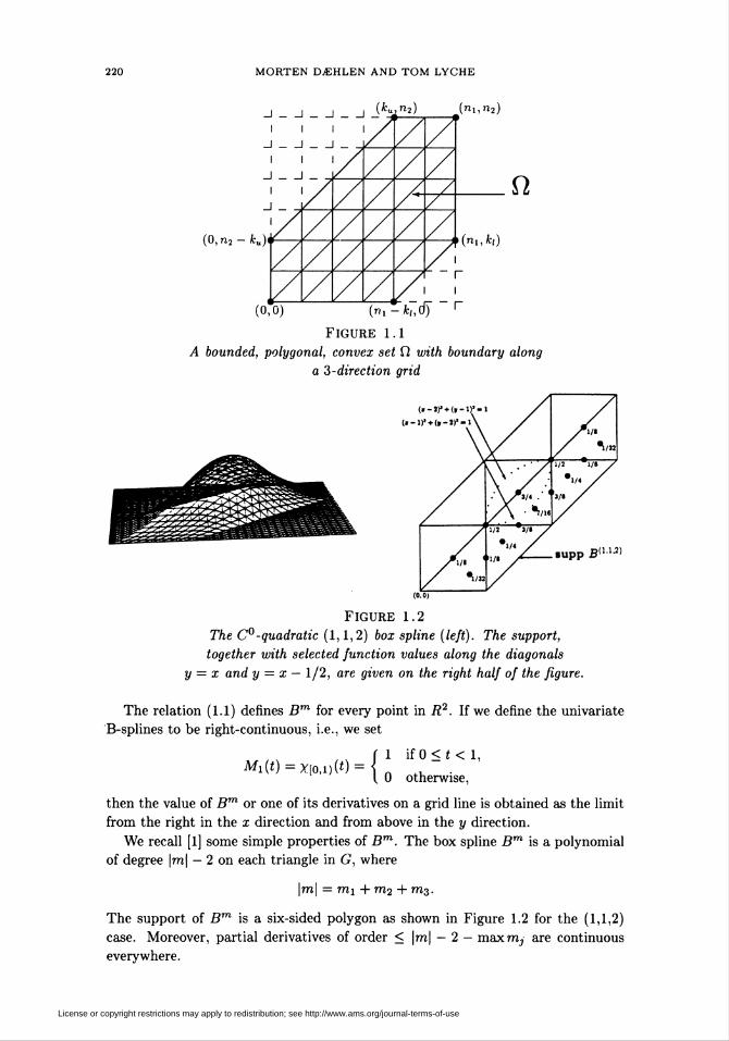
Figure 1.1

A bounded, polygonal, convex set fi with boundary along

a 3-direction grid

supp £(1.1.2)

Figure 1.2

The C°-quadratic (1,1,2) box spline (left). The support,

together with selected function values along the diagonals

y — x and y — x — 1/2, are given on the right half of the figure.

The relation (1.1) defines Bm for every point in R2. If we define the uni varíate

B-splines to be right-continuous, i.e., we set

if 0 < t < 1

otherwise,M1(0=X[o,i)(0 -il

then the value of Bm or one of its derivatives on a grid line is obtained as the limit

from the right in the x direction and from above in the y direction.

We recall [1] some simple properties of Bm. The box spline Bm is a polynomial

of degree |m| — 2 on each triangle in G, where

|m| = mi + m2 + m%.

The support of Bm is a six-sided polygon as shown in Figure 1.2 for the (1,1,2)

case. Moreover, partial derivatives of order < |m| — 2 — maxr/ij are continuous

everywhere.


BIVARIATE INTERPOLATION WITH QUADRATIC BOX SPLINES 221

The outline of this paper is as follows. In Section 2 we give a convenient formula

for the number of box splines which are nonzero on the interior of the region fi

shown in Figure 1.1. Since these functions are linearly independent on fi [1], this

number is the dimension of the space S. In Section 3 we study the unisolvence

problem for the quadratic box spline f?'1'1'2). Similar problems have been studied

in [4] (linear nonuniform) and [5] (C1-quadratic on a 4-direction grid). In Section

4 we consider a Hermite interpolation problem for the box spline (1,1, A). We

conclude the paper with an example.

(7°-quadratic box splines have been used in [9] to model objects with slope dis-

continuities along diagonals. See also [6].

For results on cardinal interpolation with box splines, see [10], [7] and references

therein. Since fi is a finite region, these results are not directly applicable.

2. The Spline Space. Let fi be as in Figure 1.1. We are interested in the

space ,

(2.1) Sm(fi) = j y cíjB^-.CíjErI,

where

B%(x,y) = Bm(x-i,y-j), x,y G R,

and

(2.2) /(fi) = {(i,j) G Z2: B™(x,y) ¿ 0 for some (x,y) G fi0}.

Here, fi° is the interior of the set fi. We recall [1] that for all (x, y) G fi° and

any m we have

(2.3) y BZ(x,y) = l;(i,i)ez*

moreover, for all (i,j) G Z2,

f B™Ax,y)dxdy = l.Jr?

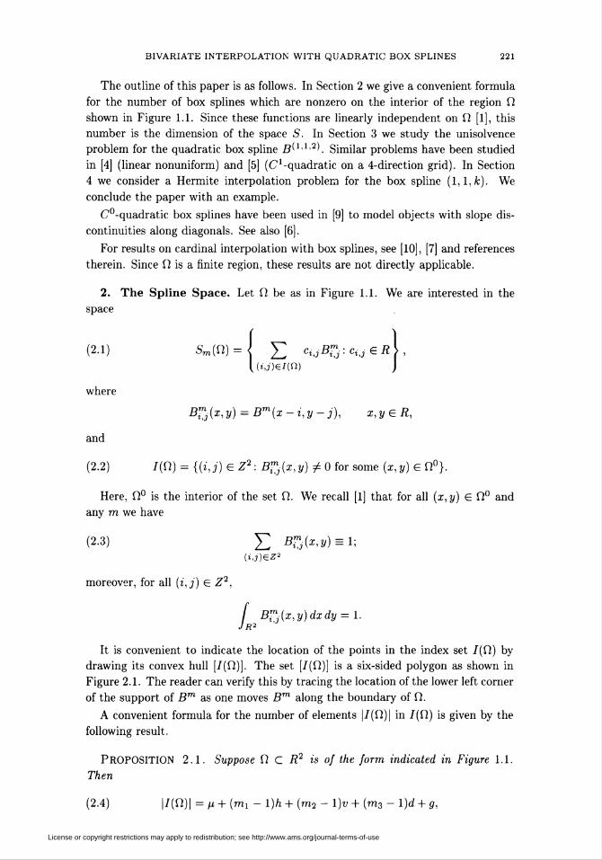
It is convenient to indicate the location of the points in the index set /(fi) by

drawing its convex hull [/(fi)]. The set [/(fi)] is a six-sided polygon as shown in

Figure 2.1. The reader can verify this by tracing the location of the lower left corner

of the support of Bm as one moves Bm along the boundary of fi.

A convenient formula for the number of elements |/(fi)| in /(fi) is given by the

following result.

PROPOSITION 2.1. Suppose fi C R2 is of the form indicated in Figure 1.1.

Then

(2.4) |/(fi)| = p + (mi- !)h + (m2 - l)w + (m3 - l)d + g,


222 MORTEN DjEHLEN AND TOM LYCHE

(fc„,n2) _(nun2)

(uj -l,n2 - 1]

(1 - mx - m3,n2 - ku - m3) /

^n

/v

iL

m2)

suppB m

(1 — m, — m3,1 — m2 — m3) (r¡! — k¡ — m3,1 — m2 — m3)

Figure 2.1

fi (solid), [/m(fi)] (dashed), and the support of Bm (dotted).

where h.v and d are respectively the number of horizontal, vertical and diagonal

lines in G n fi, and g the number of grid points. More precisely,

p = (mi - l){m2 - 1) + (mi - l)(m3 - 1) + (m2 - l)(m3 - 1),

h = n2 + 1,

v = ni + 1,

d = ni + n2 — ki — ku + 1,

g=(m + l)(n2 + 1) - \h(h + 1) - \ku(ku + 1).

Proof. |/(fi)| is equal to the number of points in a rectangle with two corners

cut off. In particular (cf. Figure 2.1), we have

|/(fi)| = (rti + mi + m3 - l)(n2 + m2 + m3 - 1)

- ¿(fc¡ + m3 - l)(fc; + m3) - i(/cu + m3 - l)(/cu + m3).

A simple rearrangement gives (2.4). D

As already mentioned, the box splines used in (2.1) are linearly independent.

Thus n = |/(fi)| is the dimension of the space 5m(fi).

It is of interest to consider the ordering of basis functions and interpolation

points. A natural way would be to pick one of the three directions, say, the diagonal

direction, and order the points in /(fi) according to which diagonal the lower left

corner of the support of the box spline lies on. There are

d = d + mi - 1 + m2 — 1

diagonals in /(fi), where d is the number of diagonals in fi.

We could start with all the points on the lower right diagonal moving from

bottom left to top right along the diagonal. Then we could continue with each of



the diagonals above in the same way. We call this the d-ordering of /(fi). We define

h-ordering and v-ordering in a similar way.

Suppose now that the box splines have been ordered in some order Bi, B2,...,

Bn. The next problem is to order the interpolation points x1, x2,..., xn. How this

should be done depends on the purpose. To limit the band width of the matrix

with elements B3(xl), one should order the a^'s in a similar way as the Bfs.

Suppose the ¿-ordering is used for the functions. If d > d, it is not clear how

to choose a d-ordering for the points. One way could be as follows. We first take

all points which are at least as close to the lower right diagonal of fi as to any

other diagonal in fi. One would then take all points which are closer to the second

diagonal in fi and at least as close to the second diagonal as to the third diagonal.

Continuing in this way, we divide the points according to which diagonal strip they

belong to. To order the points within one strip, suppose p1 and p2 are two points

in the same diagonal strip and let vi and v2 be normals to the diagonal passing

through p1 and p2, respectively. Then p1 comes before p2 if vi is below u2. If p1

and p2 both lie on the same normal, then the point closest to the diagonal would

be counted first.

We end this section by stating two convenient symmetry properties of box splines

Bm on a 3-direction grid. For all x,y G R

(2.5) Bm(x, y) = Ém(mi +m3-x,m2+m3- y),

(2.6) Bm(x,y) = Bm(y,x) ifmi=m2.

Here, Bm is the left-continuous version of Bm, i.e., we use left-continuous univariate

B-splines Mk (for k = 1, Mi = X(o,ij) in (1.1). The relations (2.5) and (2.6) follow

from (1.1) using induction on m3. Relation (2.6) is trivial for m3 = 0, and relation

(2.5), for m3 = 0, follows from the fact that for all / and k, M^(t | 0,1,..., k) =

Mfc(fc-r|0,l,...,fc).

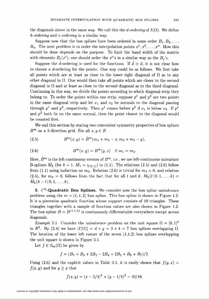
3. C°-Quadratic Box Splines. We consider now the box spline unisolvence

problem using the m = (1,1,2) box spline. This box spline is shown in Figure 1.2.

It is a piecewise quadratic function whose support consists of 10 triangles. These

triangles together with a sample of function values are also shown in Figure 1.2.

The box spline B = /?(112) is continuously differentiable everywhere except across

diagonals.

Example 3.1. Consider the unisolvence problem on the unit square fi = [0, l]2

in R2. By (2.4) we have |/(fi)| = d + 9 = 3 + 4 = 7 box splines overlapping fi.

The location of the lower left corner of the seven (1,1,2) box splines overlapping

the unit square is shown in Figure 3.1.

Let / G 5m(fi) be given by

f = (Bl+B2 + 2B3 - 2B4 + 2B5 + B& + B7)/2.

Using (2.6) and the explicit values in Table 3.1, it is easily shown that f(y,x) —

f(x,y) and for y > x that

f{x, y) = (x- 3/4)2 + (y - 1/4)2 - 10/16.


224 MORTEN DOHLEN AND TOM LYCHE

m

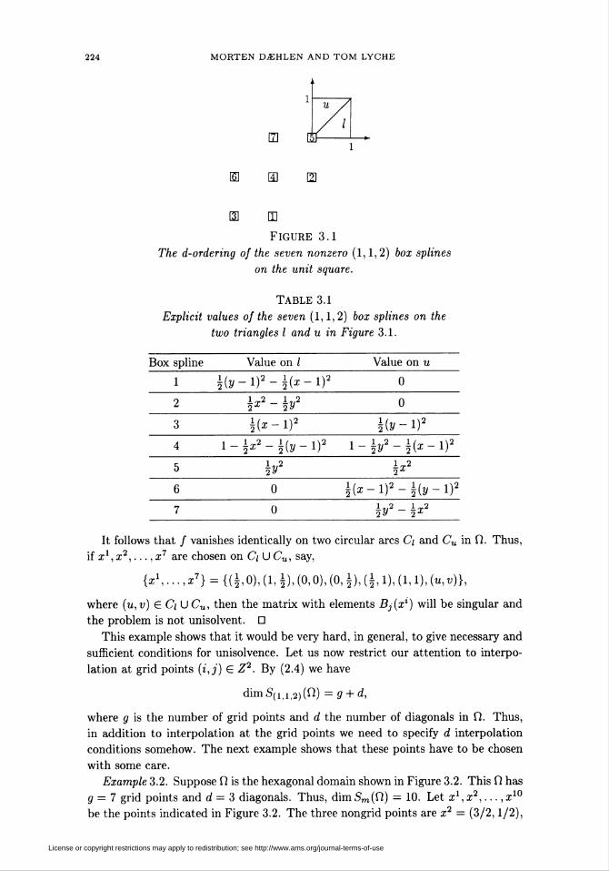
ta mFigure 3.1

The d-ordering of the seven nonzero (1,1,2) box splines

on the unit square.

TABLE 3.1

Explicit values of the seven (1,1,2) box splines on the

two triangles I and u in Figure 3.1.

Box spline Value on I Value on u

1 $y~lf-\(x-lf 0

\*2 - b2

\(x-i)2 è(y-i)

l-W-ifo-l)' 1-V-Kx-l)2

b2 lX22Z

\(x-l)2-\(y-$2

b2 ±z22-L

It follows that / vanishes identically on two circular arcs C; and Cu in fi. Thus,

if re1, x2,..., x7 are chosen on C¡ U Cu, say,

{x\ ... ,x7} = {(|,0), (1, ±), (0,0), (0, i), (i, 1), (1,1), (u,v)},

where (u,v) G Ci öCu, then the matrix with elements Bj(x%) will be singular and

the problem is not unisolvent. D

This example shows that it would be very hard, in general, to give necessary and

sufficient conditions for unisolvence. Let us now restrict our attention to interpo-

lation at grid points (i,j) € Z2. By (2.4) we have

dhn 5(1,1,2) (fi) = 9 + d,

where g is the number of grid points and d the number of diagonals in fi. Thus,

in addition to interpolation at the grid points we need to specify d interpolation

conditions somehow. The next example shows that these points have to be chosen

with some care.

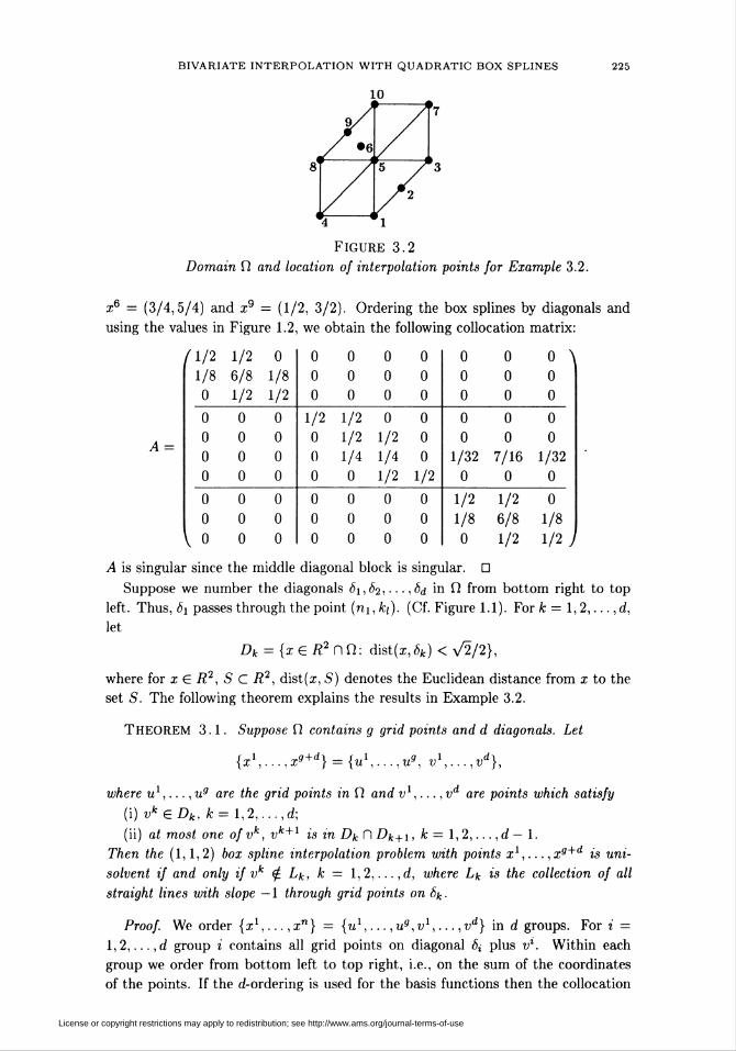
Example 3.2. Suppose fi is the hexagonal domain shown in Figure 3.2. This fi has

g = 7 grid points and d = 3 diagonals. Thus, dimSm(fi) = 10. Let xl,x2,... ,xw

be the points indicated in Figure 3.2. The three nongrid points are x2 = (3/2,1/2),



Figure 3.2

Domain fi and location of interpolation points for Example 3.2.

x = (3/4,5/4) and x9 = (1/2, 3/2). Ordering the box splines by diagonals and

using the values in Figure 1.2, we obtain the following collocation matrix:

/1/2 1/2 0

1/8 6/8 1/8

0 1/2 1/2

A =

0

0

V o

0

0

0

0

0

0

0

0

0

1/2 1/2 0 0

0 1/2 1/2 0

0 1/4 1/4 0

0 0 1/2 1/2

0

0

0

0

0

0

0

0

0

o A00

0 0 0

0 0 0

1/32 7/16 1/320 0 0

1/2 1/2 0

1/8 6/8 1/8

0 1/2 1/2 )

A is singular since the middle diagonal block is singular. D

Suppose we number the diagonals ¿i, 62,..., 8¿ in fi from bottom right to top

left. Thus, ôi passes through the point (ni, /c¡). (Cf. Figure 1.1). For k = 1,2,...,d,

let

Dk = {x G R2 n fi : dist(x, 6k) < V^},

where for x G R2, S C R2, dist(x, S) denotes the Euclidean distance from x to the

set S. The following theorem explains the results in Example 3.2.

THEOREM 3.1. Suppose fi contains g grid points and d diagonals. Let

{x\...,x9+d} = {u1,...,u9, v\...,vd},

where u1,..., u9 are the grid points in fi and v1,..., vd are points which satisfy

(i) vkGDk, k = 1,2,...,d;

(ii) at most one of vk, vk+l is in Dk n Dk+i, k = 1,2,...,d — 1.

Then the (1,1,2) box spline interpolation problem with points x1,... ,x9+d is uni-

solvent if and only if vk £ Lk, k = 1,2,...,d, where Lk is the collection of all

straight lines with slope — 1 through grid points on 6k.

Proof. We order {x1,... ,xn} = {u1,... ,u9,v1,... ,vd} in d groups. For i =

1,2,...,ri group i contains all grid points on diagonal Si plus vl. Within each

group we order from bottom left to top right, i.e., on the sum of the coordinates

of the points. If the d-ordering is used for the basis functions then the collocation



matrix A will be block tridiagonal:

Mi Ci 0

B2 A2 C2

(3.1)

0 \

0

: ' • . • 0

'■ . Cd-i

V 0 ...'... 0 Bd Ad J

The matrices Bi and Ct contain at most one nonzero row, namely the one corre-

sponding to vl. If vl is on or above the ith diagonal ¿>j, then Bi = 0. Similarly,

Ci = 0 if vl is on or below the ¿th diagonal 6¿. Moreover, assumption (ii) implies

that at most one of C,_i and Bx can be nonzero. For if C¿_i is nonzero, then v%~1

is above <5¿_i, thus v%~1 G Z?¿-i O Di. Also, if B¿ is nonzero, then v% is below <5¿

and hence vl G A-i H Dx. But (ii) implies that at most one of vl~l and vl is in

Dt-i n Di. Hence either C¿_i or Bi must be zero as asserted.

It follows that A is nonsingular if and only if all the diagonal blocks Ai,A2,...,A,¡

are nonsingular.

Let, for some i, 1 < i < d, p1,... ,pk be the interpolation points associated with

6i and assume vl = pr. The matrix A{ takes the following form, illustrated here for

fc = 10, r = 4,

Ai =

where a, b and c are the values of the basis functions which can be nonzero at pr. It

follows that Ai is nonsingular if and only if the 3x3 middle block is nonsingular.

This is equivalent to

b-a-CyiO.

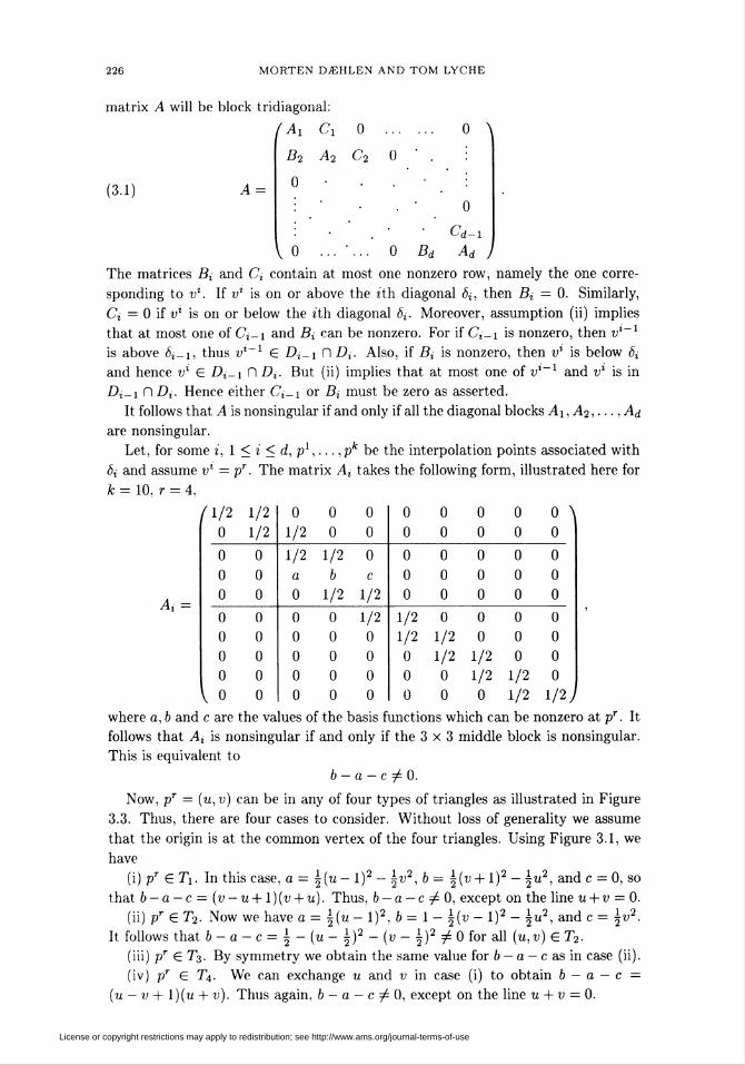
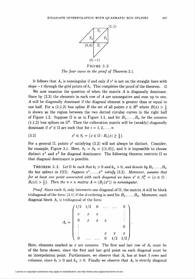
Now, pr = (u, v) can be in any of four types of triangles as illustrated in Figure

3.3. Thus, there are four cases to consider. Without loss of generality we assume

that the origin is at the common vertex of the four triangles. Using Figure 3.1, we

have

(i)prGT1. In this case, a = $u- l)2 - \v2, b = i(u-|-l)! W, and c = 0, so

that b — a — c= (v — u + l)(v + u). Thus, b — a — c^0, except on the line u + v = 0.

(ii) pT G T2. Now we have a=\(u- l)2, b = 1 - \(v - l)2 - \u2, and c= \v2.

It follows that b - a - c = ± - (u - |)2 - (v - $2 ± 0 for all (u,v) G T2.

(iii) pr GT3. By symmetry we obtain the same value for b — a — c as in case (ii)

(iv) pr G Ti. We can exchange u and v in case (i) to obtain b — a — c =

(u — v + l)(u + v). Thus again, b — a — c ^ 0, except on the line u + v = 0.



(o,-i)

Figure 3.3

The four cases in the proof of Theorem 3.1.

It follows that Ai is nonsingular if and only if vl is not on the straight lines with

slope -1 through the grid points of ¿,. This completes the proof of the theorem. D

We now examine the question of when the matrix A is diagonally dominant.

Since by (2.3) the elements in each row of A are nonnegative and sum up to one,

A will be diagonally dominant if the diagonal element is greater than or equal to

one half. For a (1,1,2) box spline B the set of all points x G R2 where B(x) > \

is shown as the region between the two dotted circular curves in the right half

of Figure 1.2. Suppose fi is as in Figure 1.1, and let Bi,...,Bn be the nonzero

(1,1,2) box splines on fi°. Then the collocation matrix will be (weakly) diagonally

dominant if x1 G fi are such that for i = 1,2,..., n

(3.2) xl GSl = {xGÜ:Bl(x)>\).

For a general fi, points xl satisfying (3.2) will not always be distinct. Consider,

for example, Figure 3.1. Here, Si = 52 = {(1,0)}, and it is impossible to choose

distinct x1 and x2 for diagonal dominance. The following theorem restricts fi so

that diagonal dominance is possible.

THEOREM 3.2. Let fi be such that k[ > 0 and ku > 0, and denote by Bi,..., Bn

the box splines in /(fi). Suppose x1,.--,1™ satisfy (3.2). Moreover, assume that

for at least one point associated with each diagonal we have xi G S¿ = {x G fi :

Bi(x) > h}- Then the n x n matrix A = (Bj(x%)) is nonsingular.

Proof. Since each St only intersects one diagonal of fi, the matrix A will be block

tridiagonal of the form (3.1) if the (/-ordering is used for Bi,..., Bn. Moreover, each

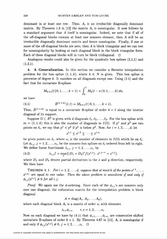
diagonal block Al is tridiagonal of the form

/1/2 1/2 0 . 0 \

xxx :

A 0 x x x :

: 0

: xxx

^ 0 . 0 1/2 1/2;

Here, elements marked as x are nonzero. The first and last row of Ai must be

of the form shown, since the first and last grid point on each diagonal must be

an interpolation point. Furthermore, we observe that Ai has at least 3 rows and

columns, since k¡ > 0 and ku > 0. Finally we observe that Ai is strictly diagonal



dominant in at least one row. Thus, Ai is an irreducible diagonally dominant

matrix. By Theorem 1.8 in [12] the matrix A, is nonsingular. It now follows by

a standard argument that A itself is nonsingular. Indeed, we note that if all of

the off-diagonal blocks contain at least one nonzero element, then A will be an

irreducible diagonally dominant matrix and hence nonsingular. Finally, if one or

more of the off-diagonal blocks are zero, then A is block triangular and we can test

for nonsingularity by looking at each diagonal block in the block triangular form.

Each of these diagonal blocks will in turn be block tridiagonal. G

Analogous results could also be given for the quadratic box splines (2,1,1) and

(1,2,1).

4. A Generalization. In this section we consider a Hermite interpolation

problem for the box spline (1,1, k), where k G N is given. This box spline is

piecewise of degree k. It vanishes on all diagonals except one. Using (1.1) and the

fact that for univariate B-splines

Mk+i (t 10,1,..., k + 1) = / Mk(t - u 10,1,..., k) du,Jo

we have

(4.1) B(1'1-*)(i,t) = Mfc+i(i|0,l,...,* + l).

Thus. S'1'1'*) is equal to a univariate B-spline of order k + 1 along the interior

diagonal of its support.

Suppose fi C R2 is given with d diagonals ¿i, 62,..., ¿<j. For the box spline with

m = (1, !,k) this is also the number of diagonals in /(fi). If p1 and p2 are two

points on 6i, we say that p1 < p2 if pl is below p2. Now, for i = 1,2,... ,d, let

x1'1 < x1'2 < ■■■< x%<">

be given points on r5¿, where Vi is the number of elements in /(fi) which lie on ¿¿.

Let <j>ij, j = 1,2,..., Vi, be the nonzero box splines on r5¿ ordered from left to right.

We define linear functionals A,j, j = 1,2,..., v%, by

(4.2) Xijf = max{(Di + D2)rf(xl<3) : x^~r = «*•»'},

where Z?i and D2 denote partial derivatives in the x and y direction, respectively.

We then have

THEOREM 4.1. For i = 1,2,... ,d, suppose that at most k of the points x1'1,...,

x1'"' are equal to one value. Then the above problem is unisolvent if and only if

<pi,j(xl'i) t¿ 0 for all i.j.

Proof. We again use the (/-ordering. Since each of the 0¿j's are nonzero only

over one diagonal, the collocation matrix for the interpolation problem is block

diagonal

A = diag(Ai,A2,...,Ad),

where each diagonal block A¿ is a matrix of order t/t with elements

Ai,r<Pi.s, r, S = 1, ¿,. . . , I/¿.

Now on each diagonal we have by (4.1) that 4>i,i, ■ ■ ■ ,<t>i,v, are consecutive shifted

univariate B-splines of order k + 1. By Theorem 4.67 in [11], At is nonsingular if

and only if 4>ij(x*'J) ^ 0, j = 1,2,..., V{. D



5. Example. As seen in Table 3.1, the (1,1,2) box spline is a piecewise quadratic

polynomial where the term xy is missing. In the following example we interpolate

points on the function f(x,y) — xy using translates of the (1,1,2) box spline as

basis functions. The error in the approximation gives an indication of how well

smooth functions can be approximated by C°-quadratic box splines.

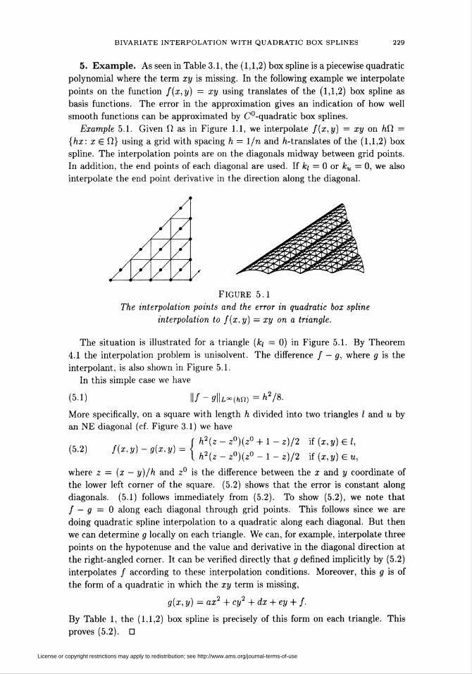
Example 5.1. Given fi as in Figure 1.1, we interpolate f(x,y) = xy on hfl =

{hx: x 6 fi} using a grid with spacing h = 1/n and /i-translates of the (1,1,2) box

spline. The interpolation points are on the diagonals midway between grid points.

In addition, the end points of each diagonal are used. If k¡ = 0 or ku = 0, we also

interpolate the end point derivative in the direction along the diagonal.

(5.2) f{x,y) -g(x,y) =j h2(z-z°)(z° + l

{ h2(z-z°)(z°-l

Figure 5.1

The interpolation points and the error in quadratic box spline

interpolation to f(x,y) = xy on a triangle.

The situation is illustrated for a triangle (k¡ = 0) in Figure 5.1. By Theorem

4.1 the interpolation problem is unisolvent. The difference / - g, where g is the

interpolant, is also shown in Figure 5.1.

In this simple case we have

(5.1) ||/ - í|U«.(mj) = h2/8.

More specifically, on a square with length h divided into two triangles / and u by

an NE diagonal (cf. Figure 3.1) we have

z)/2 \i(x,y)Gl,

')(z°-l-z)/2 iï(x,y)Gu,

where z = (x — y)/h and z° is the difference between the x and y coordinate of

the lower left corner of the square. (5.2) shows that the error is constant along

diagonals. (5.1) follows immediately from (5.2). To show (5.2), we note that

/ — g = 0 along each diagonal through grid points. This follows since we are

doing quadratic spline interpolation to a quadratic along each diagonal. But then

we can determine g locally on each triangle. We can, for example, interpolate three

points on the hypotenuse and the value and derivative in the diagonal direction at

the right-angled corner. It can be verified directly that g defined implicitly by (5.2)

interpolates / according to these interpolation conditions. Moreover, this g is of

the form of a quadratic in which the xy term is missing,

g(x, y) = ax2 + cy2 + dx + ey + f.

By Table 1, the (1,1,2) box spline is precisely of this form on each triangle. This

proves (5.2). D



In [6], Theorem 3.2 is applied to interpolate points on a pipe system. Points

on circles and ellipses corresponding to bends on the pipe system are given. In-

terpolation points given at a bend correspond to points given on a diagonal in its

respective domain fi, and a parametric (1,1,2) box spline surface interpolates the

points. Since the (1,1,2) box spline is discontinuous in the first derivative across

diagonals, the bend on the pipe system is reproduced.

Center for Industrial Research

Box 124

Blindern

0314 Oslo 3, Norway

Institutt for informatikk

University of Oslo

Box 1080

Blindern

0316 Oslo 3, Norway

1. C. DE BOOR & K. HÖLLIG, "Bivariate box splines and smooth pp functions on a three

direction mesh," J. Comput. Appl. Math., v.9, 1983, pp. 13-28.

2. C. DE BOOR, "Multivariate approximation," in The State of the Art in Numerical Analysis

(A. Iserles and M. J. D. Powell, eds.), Clarendon Press, Oxford, 1987, pp. 87-109.

3. E. W. CHENEY, Multivariate Approximation Theory: Selected topics, CBMS-NSF Regional

Conference Series in Applied Mathematics, vol. 51, SIAM, Philadelphia, Pa., 1986.

4. C. K. CHUI, T. X. HE & R. H. WANG, "Interpolation of bivariate linear splines," in Alfred

Haar Memorial Conference (J. Szabados and K. Tandori, eds.), North-Holland, Amsterdam, 1986.

5. C. K. CHUI & T. X. HE, "On location of sample points for interpolation by bivariate C1

quadratic splines," in Numerical Methods of Approximation Theory, vol. 8 (L. Collatz, G. Meinardus

and G. Nürnberger, eds.), Birkhäuser, Basel, 1987, pp. 30-43.

6. M. DOHLEN, "An example of bivariate interpolation with translates of C°-quadratic box-

splines on a three direction mesh," Comput. Aided Geom. Des., v. 4, 1987, pp. 251-255.

7. K. HÖLLIG, "Box splines," in Approximation Theory V (C. K. Chui, L. L. Schumaker and J.

Ward, eds.), Academic Press, New York, 1986, pp. 71-95.

8. C. A. MlCCHELLI, "Algebraic aspects of interpolation," in Approximation Theory, Proc.

Sympos. Appl. Math., vol. 36, Amer. Math. Soc, Providence, R.I., 1986, pp. 81-102.

9. T. I. MUELLER, Geometric Modelling with Multivariate B-splines, Dissertation, Dept. of Comp.

Sei., Univ. of Utah, 1986.

10. K. JETTER, "A short survey on cardinal interpolation by box splines," in Topics in Multi-

variate Approximation (C. K. Chui, L. L. Schumaker and F. Utreras, eds.), Academic Press, New

York, 1987, pp. 125-139.

11. L. L. SCHUMAKER, Spline Functions: Basic Theory, Wiley, New York, 1981.

12. R. S. VARGA, Matrix Iterative Analysis, Prentice-Hall, Englewood Cliffs, N.J., 1962.




bivariate interpolation with quadratic box splines

Documents