JOURNAL OF MATHEMATICAL ANALYSIS AND APPLICATIONS 101,380-396 (1984)

Vector-Valued Lg-Splines II. Smoothing Splines

GURSHARAN S. SIDHU*

Institute de Investigaciones en Matematicas Aplicadas y en Sistemas, Universidad National Autonoma de Mexico, Mexico 20, D.F.

AND

HOWARD L. WEINERT

Department of Electrical Engineering and Computer Science, The Johns Hopkins University, Baltimore, Maryland 21218

Submitted b-v L. A. Zadeh

In the first paper of this series, Lg-spline theory was extended to the vector- valued interpolating case. Here this work is complemented by giving the extension for smoothing splines. The problem is formulated as a constrained minimum norm problem in a reproducing kernel Hilbert space, and solved recursively using a congruent stochastic estimation model.

I. INTRODUCTION

In Part I of this series of papers we developed the basic theory of vector- valued Lg-splines for the interpolation problem [ 11. Here we consider the theory for the smoothing problem. As motivation let us first indicate the difference between these two problems (in the scalar case).

Let F be an unknown real-valued function on the interval W= [0, T]. Suppose we are given the values ri = F(t,) of F at some known fixed set of points ti in W, i = 1, 2 ,..., N. Then it is natural to seek a function f that is a good approximation of F. At least two situations can be proposed.

(i) Interpolation: Seek an f such that f(ti) = ri = F(ti), i = 1, 2,..., N, in other words f interpolates the data F(ti) exactly. This is a reasonable approach when the measurements ri are known to be very accurate.

(ii) Smoothing: When the measurements ri are not very accurate it may be better to seek f so that f (ti) are only “approximately” equal to the ri.

Obviously either problem, as stated, is rather vague and an infinity of solutions exists. Unique solutions can be obtained by placing more structure

* Present address: Apple Computer, 10260 Bandley Drive, Cupertino, Calif. 95014.

380 0022-247x/84 $3.00 CopyrIght 0 1984 by Academic Press, Inc. All rights of reproduction in any form reserved.

VECTOR-VALUEDLg SPLINES,II 381

on the problem. Thus, as is done in spline interpolation, we can restrict ourselves to a predefined space of functions and seek therein an f which satisfies a certain maximum “smoothness” condition. In the case of spline smoothing, an additional minimization of the errors ci = ri -f(tJ is also necessary. In [2], for the scalar case, we have given a rather complete theoretical development of smoothing Lg-splines in a Hilbert space setting. The present paper does the same for the nontrivially different case of vector- valued splines.

II. VECTOR-VALUED SMOOTHING Lg-SPLINES

As in Part I we work on the interval W = [0, T] and denote by H,, for each nonnegative integer k, the vector space of functions g on W whose k th derivative g’@ exists a.e. and is square-integrable on W. As before, for a given integer p > 1, and fixed nonnegative integers n,, n,,..., np, we define H to be the vector space of all vector-valued functions f = (f, ,f,,...,f,)’ on W such that fi E H,i, 1 <j <p; i.e., H = H,, x H, x . . . H, . (Superscript primes denote matrix transpose.) If fE H then f:“j E P2(W’j, the space of square-integrable functions on W. Let R denote the set of real numbers.

Let L be a p x p matrix of ordinary differential operators, with its ijth entry L, given by

Lij= " Uij,k(f)D",

k=O D = d/dt

where, as in [ 11, we impose the regularity condition that, for each j,

I' if i=j

aij,n.=

J 10 if i#j.

(2.1)

(2.2)

Then as before, fE H if and only if LfE Y;(W) = the p-fold Cartesian product of the space 5$(W) of square-integrable functions on W.

As shown in [ 1, Lemma 3.11, the restriction (2.2) implies that the nullspace of L denoted

NL= {j-E H:Lf=O) (2.3)

is a vector subspace of H satisfying

(2.4)

Now, let {A}? denote independent linear functionals on H. Then, for any given real numbers {ri}y we have defined, in [I], the vector-valued Lg-spline

382 SIDHU AND WEINERT

interpolating these rj with respect to the hi as the function s E U, c H such that

where

U,= {fEH:Ajf=rj, l<j<N). P-9

Existence and uniqueness conditions were developed in [ 1 ] for this spline function.

Here we shall extend this to the situation in which the “measurements” rj are inaccurate. Roughly speaking, let us say we are seeking an fry H such that rj=kjf+rj,j= 1,2 ,..., N, where the rj denote measurement errors. One could then demand that the functionsfbe smoothest in the sense of (2.5) and “minimize” the “errors” rj = rj - Aj f in some sense. This is embodied in the following definition:

DEFINITION 2.1. Let pj, 1 <j < N, be strictly positive weights (positive real numbers). Then the vector-valued smoothing Lg-spline is a function s E H such that the functional

C(f)= jT(Lf)‘(Lf)i 6 Pjtrj - ljf )’ ‘0 ,Tl

(2.7)

is minimized over H; i.e., c”(s) < c(f) for all f E H.

In this definition each weight pj reflects, in some sense, our confidence in the “accuracy” of the corresponding “measurement.”

The definition is in fact a natural generalization of the concepts introduced for the scalar case (p = 1) in various, by now, classical papers [4-61 (see also [2,3]).

The smoothing Lg-spline of Definition 2.1 is the solution of an unconstrained optimization problem. As stated, it is not easy to give existence or uniqueness results for it. Nevertheless a convenient refor- mulation leads to a situation much like that for interpolating splines [ 11.

First define an “extended” vector space Ht as

H+ = {(g,@:gE H,OER”‘}. (2.8)

Note that 8 is a real vector of size N, i.e., 19 = (0,) 8, ,..., B,,,)‘, each ej being a real number. If gt = (g, 6’) E H+ then we say g is the restriction of g+to H, denoted g = R, g+.

VECTOR-VALUED Lg SPLINES,II 383

Furthermore, let UT be defined as follows:

or: = (g+=(g,e)EH+:Af gf =~jg+e,=ri, 1 <j<N}. (2.9)

This subset of Hi is easily seen to be a linear variety, i.e., a translate of fJ~=(g’EH+:k~g’=O, l<j<N}.

It is also immediately clear that gt = (g, 0) E UF if and only if Bi = ri - /l,i g, 1 <j < N. Hence Definition 2.1 leads to the following completely equivalent constrained optimization problem in H ’ :

DEFINITION 2.2. Let S+ E U: be the vector that minimizes c ‘(f ’ ) = .ii (Lf)‘(Lf) + CT=, p.iO,f over U: , where f ’ = (A 0). Then s* = (s, MI), where s is as defined in Definition 2.1, i.e., s = R,,s’ .

Now, proceeding in a fashion analogous to that used in j 1 I. the following result is readily established. Details are left to the reader.

THEOREM 2.1. (a) Provided the (Ai, 1 <j < N} are continuous func- tionals on H, the vector-valued spline of Definition 2.1 always exists. (b) It is

unique if and on1.v if any of the following equivalent conditions holds:

(i) N,‘n U,+ = {O), where N; = (g‘ = (g,O)E H’: Lg=O}: (2.10)

(ii) N, n U,, = (O}, where U, = ( g E H: Ai g = 0, 1 <j< NJ; (2.1!)

(iii) N > n, and among the (Aj}‘: there are n jiinctionals that are linearly independent on N,,. (2.12)

In this paper we assume that the conditions of this theorem are met; in fact we assume that, possibly after rearrangement,

{A.,, 1 <j < n) are linearly independent on N, . (2.13)

III. REFORMULATION AS A MINIMUM-NORM PROBLEM

The symmetric bilinear form c” (f ’ ) is clearly always nonnegative. Nevertheless it is not a norm for H+ since any nonzero f' = (f, 0) with

f E NId gives us c’(f ‘) = 0. In [2] an especially appropriate inner product was introduced and this shall be emulated here.

It is easily seen that the following is an inner product for Ht. Let f I- = (5 19) and g+ = (g, 0); then define

.I’ .v

(f’.g+)“-=j” W’(Lg)+ - “ 4jej"j + '. (njf + ei)(ni g + Oi) (3.1) j-l z

384 SIDHU AND WEINERT

with the corresponding norm given by

Ilf+IIZ/+ =JoT CLf)‘CLf) + E Pj$ + fJ Cnif+ OiJ2* (3.2) j=l i=l

It is not hard to verify that Hf is a Hilbert space relative to this norm. Referring to (3.2) we note that whenever ft E UT, the third term, viz.,

2, is a constant. Hence the following theorem is immediately

THEOREM 3.1. The solution st = (s, w) of Definition 2.2 (s is the vector- valued smoothing Lg-spline of DejInition 2.1) is the unique minimum-norm element of the linear variety U: of H’ .

Since U,’ is a translate of the subspace Vi, it is easy to exploit this theorem and hence state that

s + = projection of any g+ E lJ: onto S,, (3.3a)

where S, = [ UJ ]I, the orthogonal complement of Ut ; and consequently

s = R,s+ = R,{projection of any g+ E U,! onto S,}. (3.3b)

This function-analytic representation can be translated into a closed formula as follows.

Let hf = (hj, wj) be the representers of AT, i.e., 1; ft = (h; , ft ),+; then it can easily be shown that

S,= [U,+]‘=span{hf, 1 <j<N). (3.4)

Thus a straightforward application of the projection theorem gives us the formula

s(-)= h’(. )r-‘r (3.5)

where h’(s) = (h,( . ), h,(.) ,..., h,J.)), r’ = (rl, r2 ,..., r,,,), and r is the N x N matrix with ijth entry equal to (h+ , hf ),+.

IV. REPRODUCING KERNEL FOR Hi

It is well known [7] that the difficult problem of finding representers for linear functionals is rendered trivial if the underlying space is a reproducing kernel Hilbert space (RKHS). This is true for H+ as shall be exhibited below.

VECTOR-VALUED Lg SPLINES, II 385

We start by defining various quantities that are required in the sequel. First, for the n-dimensional subspace NL of H define a basis (z,(a), z,(e),.... zJ*)} through, for j = 1,2 ,..., n,

LZj = 0, kizj= ):, for i =j, for i # j,

i = 1, 2,. .., IE. (4.1)

Next define the Green’s function G(., s) of L with respect to (A,,j= 1,2 ,..., n}. Thus G(., .) is the p xp matrix-valued function on W X W given by (for all r E W)

LG(., z) = Ip 6(. - t), AjG(., r) = 0, j = 1, 2 ,..., n. (4.2)

where ZP is the p x p identity matrix. Note that in (4.2), Aj operates on the columns of G(., r). It is easy to see from elementary properties of ordinary differential equations that for anyfE H we have

f(.) = 2 (2j.f) zj(*) + lor G(., t){Lf(t)} dt* (4.3) j=l

In terms of G and the zj define the following p x p matrix-valued function on Wx W:

~(1, 5) = 2 (1 + pi') Z](t) Z;(t) + lr G(t, P) G'(r, P) dP* (4.4) j=l 0

As a matter of notation we shall denote by K, and G, the ijth entries of the matrices K and G. Also superscript letters c and r shall denote columns and rows of matrices; thus KI is the jth row of K, and Gf the ith column of G.

Note first that K has a symmetry property

K,(t, t) = Kji(~, t) all i, j and all t, r E W. (4.5)

Another useful relation, readily obtained from (4.1), (4.2) and (4.4), is

L&(6 r) = G’(r, t); Ajcf,K(t, 5)~ (1 +~i’)Zj(r); j = 1, 2 ,..., n.

(4.6)

Now define

w: = WxpO, po = { 1, z..., Pi

W: = {co} x No, No = { 1, 2,..., N}

(4.7a)

(4.7b)

and, assuming T ( co,

w+=w:vw:. (4.7c)

386 SIDHU AND WEINERT

Now any g’ = I@, r 0, Y..., e,]’

Cd.>, 6) E ff+,g(.) = (g,(~),...,g,(~)l’, and 8= can be reformulated as g+ : Wt + R. Let tt = (t, j) E W+ . 7

then this redefinition of g’ is readily given through

if t’ E W:,i.e.,tE WandjEp’

if tt E Wz, i.e., t = co and jE No. (4.8)

Conversely any g+: W+ -+ R can be reformulated as g’ = (g(.). O), where g = R, g’, through

(RNg+)(t)=g(t)=

Thus forg’: Wt +R and ht: W’ and the above it is clear that

-R, such that g+, h+ EH+ -R, such that g+, h+ EH+ > > using (3.1) using (3.1)

(g+(.>, h+Ch,+ = joT MR, g+)(WWLh+)(~)l dt

+ 5 pjgt(a,j)ht(a,j)+ 2 (A: g+)(A,fh+) (4.10) j=1 i= I

where, from (2.9),

nf g’=~j(RHg+)+g+(~,j), j = 1, 2 ,..., N. (4.11)

With this preamble a reproducing kernel Kf : Wt x W+ -R can be given for Ht.

Let A(l) = -Z(t) v, p x N matrix, t E W, (4.12)

where V= diag[p; ‘, p;],..., p;‘] (4.13) , I 1 ’ z(t) = [ZlW ’ m I . ..i z,(t); 01, p x N matrix. (4.14)

I Also let z;‘](t) denote the ith entry of the p X 1 vector zj(t).

Letting t + = (t, i) and r+ = (5, j) define

Kij(ty T >

i

if t+ ,r+ E w:

K+(t+, r+) = Aij(r) if t+ E W:,r+ E W:

Aji(t) if t+E W:,s+E W: (4.15)

pi ’ 6, if t+ ,r+ E w;.

VECTOR-VALUED& SPLINES,II 387

It is then easily shown that K+ satisfies the following lemma:

LEMMA 4.1. K + as defined in (4.15) is the reproducing kernel for H+ ; i.e., for each t+ E W+,

K+(., t’) E H+ (4.16)

and

(f+(a), K+(., tt))H+ =f+(t+) for eachf+ E H+. (4.17)

ProojI Verification of (4.16) is a matter of checking the definitions of K+ and K. The verification of (4.17) follows by using (4.6), (4.10), and (4.1 l), and by realizing from (4.3), (4.8), and (4.9) that for tt = (t,j) E W:

f+(t+) = f {A,(R,f+)} #l(t) + j’G;(t, ~){L,,,R,~+(T)} dz. (4.18) i=l 0

Having shown that K+ is the reproducing kernel for H+, it is quite easy to find representers for the A,? using well-known results from [ 71:

h:(t+) =,I;,+)K+(t+, s+), i = 1, 2 ,..., N, (4.19)

and

(h:,hf)H+=~i:t+)~j:r+)K+(t+, 7’). (4.20)

The subscripts t+ and r+ on 1: and A,? indicate the variables with respect to which the functionals operate on K’. Consequently, if h; = (hl(-), oj), then

\ ‘j(‘>y hj(*)= [S(t)K(t, *>l’-~~‘~zjc(.>= 1 FL, Ktt )I, J(f) ' ' '

;;; (4.21)

wj = V[ej - {Ajj(f,Z(t))’ 1. (4.22)

Here e, = (1, 0, 0 ,..., O)‘, e2 = (0, 1, 0 ,..., O)‘,..., eN = (0, 0 ,..., 0, l)‘, and 1, operates on the columns of K and Z. For the special case of j = l,..., n we have oj = 0 and hence hf = (zj(.), 0).

Now a characterization of the smoothing spline can be given in terms ofK+:

THEOREM 4.2. For each t E W and j = 1, 2 ,..., p,

sj(t) = pPs~K+ (a, t’), t+ = (U), (4.23)

where p is the linear mapping of S, to R defined through ,uhj+ = ri, j = 1, 2,..., N, and PSN denotes orthogonal projection onto S,.

409'101 2 5

388 SIDHU AND WEINERT

Pro05 Let g+ E U: ; then from ‘(3.3b) sj(t) = (P”“g+)(t ‘) with tt = (t,j). Thus using the reproducing property and self-adjointness of PSn

Sj(f) = (P”Ngg+(-),K+(., t+))H+ = (gf(*) pS”IK+(*, t+))“+.

Expressing Ps~Kt (., t’) = Cy=, /Ii hT(.) and recalling that 1: gt = (g’(.), h:(.))H+ = ri we have

sj(t)= 5 Pi(t+)(g+(')% h:(*)),+ = i Pi(t+> ri. i=l i=l

This characterization is a vital link to the subsequent developments of this paper.

V. A STOCHASTIC CHARACTERIZATION

Henceforth we follow the general trend of ideas developed in previous work [ 1,2] to relate the vector-valued smoothing spline problem to a recursive problem of linear-squares estimation for a random process with observations in additive white noise.

Since Kt is symmetric and nonnegative definite there exists a random process X+ (.) on Wt such that, for all t’, rt E Wt

E{n+(t+)} = 0, E(z+(t+) 7c+(s+)} = K+(t+, r’) (5.1)

where E denotes probabilistic expectation with respect to the probability law of rc’(.).

The process rc ’ in turn spans a complete Hilbert space Y of zero mean random variables with the usual inner product (a, b)y = E{ab}.

In view of the reproducing property and (5.1) we have

(K+(-, t’), K+(.,T+))~+ = K+(t+, z+)= (x+(c+), ~+(t+))~. (5.2)

Since {K+(.,t’),t+ E W’} and {n+(t+), tt E W’)} are spanning sets of Ht and Y, respectively, we have the following theorem, first given by Loeve [B, p. 4081.

THEOREM 5.1. The spaces Hf and Y are congruent; i.e., there is an inner product preserving isomorphism between them. Furthermore, under this congruence f ’ E H ’ corresponds to a E Y, denoted f + - a, if and only if for every t + E W+

f+(t+)=E(a7r+(t+)}. (5.3)

VECTOR-VALUED&SPLINES,II 389

As we can see from (5.2)

Kf(., t’) - 7T+(t+), eacht+ E Wt.

and hence, for j = 1, 2 ,..., N,

hf(.)=~j:,+)K+(.,t+)~~:~+.

Thus

(5.4)

(5.5)

S,V-D,V=span(,Ifnt,j= 1,2, . . . . N) (5.6)

and as a consequence

PSvc+(..t+)-p”~71+(f’). (5.7)

In fact P”%’ (t’ ) minimizes E(a - ?I’ (t’)}’ over all a E D,. and is hence referred to as the linear least-squares estimate (1.l.s.e.) of rrt (t’ ) given (Al TT’, i= 1, 2 ,..., NJ.

Now in view of Theorem 4.2, the following is evident.

THEOREM 5.2. For each t E W and j = 1, 2,...,p

q(t) = r2 + (f * ), t+ = (t.j) (5.8)

where 7it (t ’ ) is the sample value of the i.1.s.e. of ?I . (t ’ ) given observations {/I’ T[+ = ri, i = 1, 2 ,..., N}.

To efficiently exploit this result a dynamical model must be given for rcl (a). This is done by defining zero mean random processes

Y(l) = I Y,(t),L’*(t),...,.v,(t)l’, tE w (5.9a)

v = [v,, v* ,...) v,vl (5.9b)

where

yj(t) = n + (4j), tE W, jEp” (5.9c)

vi=n+(Co,j), jE No. (5.9d)

Then from (4.15) and (5.1)

Ei Y(t) y’(r) 1 = WY 512 all t, SE W (5.10a)

E(vv’) = V=diag[p;‘,p,‘,...,p,‘] (5. lob)

E{y(t) u’) =/i(f), each t E W. (5.10~)

390 SIDHU AND WEINERT

In fact (4.12) and (5.10~) imply

Furthermore Y is spanned by the random variables in the set (l;(t); t E W, j E p”) u {ui; i E No}, and in terms of the congruence theorem if g+ = (g(e), 19) E H+ - a E Y then

In fact,

g(t) = E{cxy(t)L tE w; O=E(CW}. (5.12)

Yj(t) N K+(‘, t+), t+ = (t,j)E Wf (5.13a)

Vj4’(., t'), t+ = (a3,j) E W:. (5.13b)

Now from (4.11), (4.15), (5.5), (5.9), and (5.13)

Aj’ 71+ = Aj(r) .,V(t) + Vj, j = 1, 2,..., N (5.14)

which leads to the following statement of Theorem 5.2 in terms of processes y(.) and ui.

LEMMA 5.3.

s(t) =9(t), tE w (5.15)

where g(t) = [y l̂(t),...,jp(t)]‘,9j(t) being the Z.1.s.e. of y,/(t) given (Aj y + vj = rj, j = 1, 2 ,..., N}.

In addition it is easily seen [ 1 ] from (4.6) and (5.10) that the process y(a) is the output of the model

Ly=u on W (5.16)

where u(s) is a p x 1 vector-valued, zero mean, white process, i.e.,

E( u(t)} 3 0, E{ u(t) u’(r)} = z,s(t - r). (5.17)

As shown in [ 11, (5.16) can be recast in state space form

y(t) = C-w), $x(t) = A(t) x(t) + Bu(t) (5.18a)

VECTOR-VALUED Lg SPLINES, II 391

where u( .) is as in (5.17), and A (-), B, C are n X n, n X p, and p X n matrices given by

B = block diag[ [0 ,..., 0, 1 I’, ni x 1 ] (5.18b)

C = block diag[ [ 1,0 ,..., 01, 1 X ni] (5.18~)

A(.) = block&, n; x nj] (5.18d) I I

A ii(.) = -2- i,- ‘“,,- - - , ni X Hj (5.18e) Il.0 II.1 ... !,.?I- I

n; x nj, i+j. (5.18f)

The n x 1 vector x( .) is

I I x’= 1y,,yy . . . . . yy-“1 (1)

I Y29Y2 (IT- I)!

,.?Y2 (I) , ... I .vp,yp ,... ,yp ‘np- ‘I]. (5.18g)

I I 1

Furthermore, the processes u(s) and u satisfy

and if

E(u(t) 0’) = 0, all tEW. (5.19)

A = 11, y, f4 y,..., A” y]’ (5.20)

then

E{M’} = I + R, (5.21)

E( u(t) A’) = 0, all t E IV, (5.22)

where

R,=diag[p;‘,p;‘,..., pi’]. (5.23)

Proof of (5.17) and (5.19)-(5.22). From (5.10a) and the continuity of the Aj we have, for j= 1, 2 ,..., n, E{(LjY)Y’(r)J =Aj(t)E{Y(t)Y’(r)l = Ajct,K(t, t) = (1 + pj’) z;(r), the last step being a consequence of (4.6). Repeating the same idea, E{ (Ai y)(Aj y)} = Ai,,,E( y(t)(kj y)} = Ai(,,Zj(T) (l +P,j”)=(l +P,“)6ijT using here Eq. (4.1). This proves (5.21).

We have, using the results of the previous paragraph, E( y(t) A’) = [z,(t), z2(t),..., z,(t)](l+ R,). Thus if we define u(t) = L(,, y(t) we have E{u(f) n’l = E[{&, y(t)} A’] = L,,,E{y(t) A’1 = L,,&,(t), z2(0>-~ z,(t)] (I + R,,), which in view of (4.1) gives (5.22). Equation (5.19) follows in a similar fashion but starting with (5.10~).

392 SIDHU AND WEINERT

To prove Eq. (5.17) apply the same technique starting with E{ J+>Y’(~)~ = W, 7). Th us, recalling (4.6), E{u(t)y’(r)} = L,,,K(t, 7) = G’(r, t): and repeating the process E{u(r) u’(t)} = LCT) G(7, t) = 1,&t - r), in view of (4.2).

VI. AN ALGORITHM FOR THE CASE OF EHB DATA

The model (5.16~(5.23) does not guarantee that y(e) and v thus generated satisfy the covariance relations (5.10). This requires certain missing “initial” conditions on x.

As in our earlier work [ 1] attention shall now be restricted to Aj of the form

ljf= i f aij,,fy’(tj), tjE W, j-l,2 ,..., N, (6.1) i=l /=I

where aij,, are known real numbers, and the tj are known knots assumed to be ordered thus: 0 < t, < t, < . . . < tN < T. These functionals, which express each Ljf as a linear combination of the values of the various derivatives of the components off at the point tj E W, are a natural generalization of the so-called extended Hermite-Birkhoff (EHB) functionals to our situation. The corresponding spline constraints can thus be called EHB data.

As in [ 1 ] it is easy to show that

and

Aj y = cjx(tj), j = 1, 2,..., N (6.2)

cj = [cj, 3 cj2 Y*'*? cjp] (6.3)

Cjk = lajk.13 ajk,2 3-3 ajk,nk13 k= 1, 2 ,..., p.

In (6.2), y and x are as defined in the previous section. Now we can establish the following:

(6.4)

THEOREM 6.1. For ,lj as in (6.1)-(6.2) the model (5.18~(5.23) obeys

x(t,)=O-1 jA+f”d(<)Bz@dc;’ fl I

(6.5)

l7,=E{x(t,)x’(t,)} = 0-‘{I+R, + Q} 0-= (6.6)

E{x(t,) u’(t)} = ) o”-’ d(t) by ;,:,;;;.“I (6.7) 9

E{x(t,) u’} =-o-*p,i O] (6.8)

VECTOR-VALUED Lg SPLINES, II 393

where

and A(<) is an n x n matrix with ith row

Ai = \ ciwi, 0 IO.

tE Iti tw]

otherwise

and

Here 4 is the state transition matrix of A(.); i.e..

; #(t, 7) = A 0) ciKt> 71, qq7.7) = I,. Proof Equation (5.18) admits the integral form solution

(6.9)

(6.10)

(6.11)

(6.12)

4t) = d(t, t,) x(t,) + )-’ #(t- 0 Bu(t) &. . I,,

Thus using (6.2) it is easy to see that

A= Ox(t,) - j-l” A(<) Bu(r) d< . II

of which (6.5) is a ready consequence (in [9] the invertibility of 0 is seen to be equivalent to the uniqueness condition (2.13)). Equations (6.6)-(6.8) follow from (6.5) because of (5.17), (5.21), and (5.22).

Now as in [ 11 an algorithmic implementation of Lemma 5.3 can be given as below. The proof is a simple generalization of that in [ 11 and is thus omitted.

Dynamical Algorithm for Smoothing with EHB Data

The vector-valued Lg-spline smoothing the data {rj,j = 1, 2,..., NJ with respect to the EHB functionals Aj of (6.1) is given by

s(t) = ccqt 1 N), tE w (6.13)

the n X 1 vector function a(. / N) being computed through the following three-part algorithm:

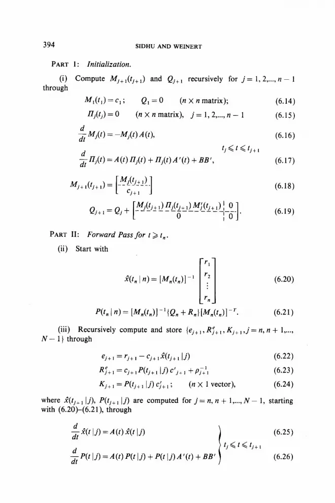
394 SIDHU AND WEINERT

PART 1: Initialization.

(9 Compute Mj+ lttj+ I) and Qj+1 recursively for j = 1, 2,..., n - 1 through

M,@,) = Cl ; Q, =O (n X n matrix);

nj(tj) = 0 (n X n matrix), j = 1, 2 ,..., n - 1

$ Mj(t) = --Mj(t) A(t),

$nj(t)=A(t)nj(t) +nj(t)A’(t) +BB’,

tj<t<tj+I

Qj+ 1 = Qj +

[

%(tjk t) !A:+ 1) M;_(tli_‘~~-~s . 1 PART II: Forward Pass for t > t,.

(ii) Start with

r1

p(t, In> = W&X’{Qn + ~nPfnMY~

(6.14)

(6.15)

(6.16)

(6.17)

(6.18)

(6.19)

(6.20)

(6.21)

(iii) Recursively compute and store {ejt 1, Rst,, Kjt , ,j = n, n + l,..., N - 1) through

ej+l =‘j+l -cj+la(tj+l Id (6.22)

RP+l =cjtIp(tj+l lAc'j+l + Pi+‘1 (6.23)

Kj+ 1 =P(tj+ I lb) Cj+ I G (n X 1 vector), (6.24)

where .f(tj+ 1 1 j), P(tj+ 1 1 j) are computed for j = n, n + l,..., N - 1, starting with (6.20)-(6.21), through

$a(t]j)=A(t)Z(tlj) (6.25)

~P(tIj)=A(t)P(tlj)+P(tIj)A’(f)+BB’

tj<t<tj+I

(6.26)

VECTOR-VALUED Lg SPLINES, II 395

'($+, Ij+ l)=a(fj+I lj)+Kj+*(Rq+l)-' e,i+,

pttj+, lj+ l)=Wj+, lj)-Kj+,(Rr+,)~‘K:+,.

(iv) Compute and store $t,V / N) using (6.27).

(6.27)

(6.28)

PART III: Computation of f(t / N).

(v) Compute Z(f 1 N) by integrating, starting at f = t, with the value of ,?(t,, / N) computed above, the equations

; i(t 1 N) = A(t) a(t / N) + BB’p(t / N) (6.29)

where ,~(t I N) is a piecewise continuous n x 1 vector-valued function given by

At I NJ = \o t < t, or t>t, ‘Pi(t I NJ, ti- 1 < t < ti ; j = 2, 3 ,.... N.

(6.30)

(vi) The pieces pui(. / N) are computed recursively, for j = N. N ~ l..... 2. through

iuj(‘j I W

where

iuz+,(t, IN)=0 (n X I vector) (6.3 1)

wi+ ,(ti I N) + cj(R;)p’(ej - K/pi+ ,(ti I N)) j>n

I(tj I N) - CiPj, j<n (6.32)

(P,v&-Pn)’ = bY,(t,)l-’ P,,, ,(t,, IN) (6.33)

-&fl N)=A’(t)pui(t IN), t;-, <r<t;. (6.34)

AS noted in [ 1 ] if two knots are coincident, i.e., ti = t.i + i , then integration of differential equations between these knots is trivialized. Thus in this case

MjCf,j+ I) = Mj(tj>3 cj(fj+ I> = cj(tj>3 a(t.j+ I lj) = i(tj lj), P(fj + 1 lj) = P(tj lj). and ~.i + I (‘j I N) = P,! + 1 (t,j + 1 I N).

Such algorithms for splines were introduced in [ 10, 111 with extensions in

[ 1, 21, and are based on the theory of Kalman filters (see, e.g., [ I2 I).

REFERENCES

I. G. S. SIDHU AND H. L. WEINERT, Vector-valued Lg-splines, J. Math. Anal. Appl. 70 (1979). 505-529.

396 SIDHU AND WEINERT

2. H. L. WEINERT, R. H. BYRD, AND G. S. SIDHU, A stochastic framework for recursive computation of spline functions. II. Smoothing splines, J. Optim. Theory Appl. 30 (1980). 255-268.

3. H. L. WEINERT, Statistical methods in optimal curve fitting, Commun. Statist. B-Simulation Compuf. 7 (1978), 417-435.

4. I. J. SCHOENBERG, Spline functions and the problem of graduation, Proc. Nat. Acad. Sci. U.S.A. 52 (1964), 947-950.

5. C. H. REINSCH, Smoothing by spline functions, I, II, Numer. Math. 10 (1967) 177-183; 16 (1971), 451-454.

6. P. M. ANSELONE AND P. J. LAURENT, A general method for the construction of inter- polating or smoothing spline functions, Numer. Math. 12 (1968), 66-82.

7. N. ARONSZAJN, Theory of reproducing kernels, Trans. Amer. Math. Sot. 68 (1950), 337404.

8. M. LO$VE, Fonctions altatoires du second ordre, in P. Levy, “Processus stochastiques et mouvement brownien,” 2nd ed., pp. 367420, Gauthier-Villars, Paris, 1965.

9. H. L. WEINERT AND G. S. SDHU, On Uniqueness conditions for optimal curve fitting, J. Optim. Theory Appl. 23 (1977), 211-216.

IO. H. L. WEINERT AND G. S. SIDHU, A stochastic framework for recursive computation of spline functions. I. Interpolating splines, IEEE Trans. inform. Theory IT-24 (1978), 45-50.

11. G. S. SIDHU AND H. L. WEINERT, Dynamical recursive algorithms for Lg-spline inter- polation of EHB data, Appl. Math. Comput. 5 (1979), 157-185.

12. A. H. JAZWINSKI, “Stochastic Processes and Filtering Theory,” Academic Press, New York, 1970.