quantum information and triangular optical lattices
TRANSCRIPT

arX
iv:q
uant
-ph/
0407
121v
1 1
5 Ju
l 200
4
Quantum information and triangular optical lattices∗
Alastair Kay,1 Derek K. K. Lee,2 Jiannis K. Pachos,1 Martin B. Plenio,2 Moritz E. Reuter,2 and Enrique Rico3
1Department of Applied Mathematics and Theoretical Physics,
University of Cambridge, Cambridge CB3 0WA, UK,2Blackett Laboratory, Imperial College, London SW7 2BW, UK,
3Department d’Estructura i Constituents de la Materia,
Universitat de Barcelona, 08028, Barcelona, Spain.
(Dated: July 31, 2013)
The regular structures obtained by optical lattice technology and their behaviour are analysedfrom the quantum information perspective. Initially, we demonstrate that a triangular optical latticeof two atomic species, bosonic or fermionic, can be employed to generate a variety of novel spin-1/2models that include effective three-spin interactions. Such interactions can be employed to simulatespecific one or two dimensional physical systems that are of particular interest for their condensedmatter and entanglement properties. In particular, connections between the scaling behaviour ofentanglement and the entanglement properties of closely spaced spins are drawn. Moreover, three-spin interactions are well suited to support quantum computing without the need to manipulateindividual qubits. By employing Raman transitions or the interaction of the atomic electric dipolemoment with magnetic field gradients, one can generate Hamiltonians that can be used for thephysical implementation of geometrical or topological objects. This work serves as a review articlethat also includes many new results.
PACS numbers: 03.75.Kk, 05.30.Jp, 42.50.-p, 73.43.-f
I. INTRODUCTION
With the development of optical lattice technology[1, 2, 3], considerable attention has been focused on therealisation of quantum computation [4, 5, 6, 7] as wellas quantum simulation of a variety of many-particle sys-tems, such as spin chains and lattices [8, 9, 10, 11]. Thistechnology provides the possibility to probe and realisecomplex quantum models with unique properties in thelaboratory. Examples that are of interest in various areasof physics are systems that include many-body interac-tions. These have been hard to study in the past due tothe difficulty in controlling them externally and isolat-ing them from the environment [12]. To overcome theseproblems, techniques have been developed in quantumoptics [13, 14, 15] which minimise imperfections and im-purities in the implementation of the desired structures,thus paving the way for the consideration of such “higherorder” phenomena of multi-particle interactions. Theirapplications are of much interest to cold atom technol-ogy as well as to condensed matter physics and quantuminformation, some of which we shall see here.
The initial point of our study is the presentation of therich dynamics that governs the behaviour of an ultra coldatomic ensemble when it is superposed with appropriateoptical lattices. For this purpose we consider the caseof two species of atoms, denoted here by ↑ and ↓ (see[8, 9, 11]), trapped in the potential minima of a peri-odic lattice. These species can be two different hyperfineground states of the same atom, coupled, via an excited
∗Based on talk presented by J. K. Pachos at CEWQO 2004.
state, by a Raman transition. The system is broughtinitially into the Mott insulator phase where the num-ber of atoms at each site of the lattice is well defined.By restricting to the case of only one atom per site, itis possible to characterise the system by pseudo-spin ba-sis states provided by the internal ground states of theatom. Interactions between atoms in different sites arefacilitated by virtual transitions. These are dictated bythe tunneling coupling, J , from one site to its neigh-bours and by collisional couplings, U , that take placewhen two or more atoms are within the same site. Even-tually the evolution of the system can be effectively de-scribed by a wide set of spin interactions with couplingcoefficients completely controlled by the tunneling andcollisional couplings. This gives rise to the considerationof several applications that are mainly related with thethree-spin interactions simulated on the lattice, which isthe main focus of the present article.
In that spirit, implementation of quantum simulation,of different physical models can be realised, with groundstates that present a rich structure, such as multiple de-generacies and a variety of quantum phase transitions[16, 17, 18]. Some of these multi-spin interactions havebeen theoretically studied in the past in the context of thehard rod boson [19, 20, 21], using self-duality symmetries[22, 23]. Phase transitions between the correspondingground states have been analysed [24, 25]. Subsequently,these phases may also be viewed as possible phases ofthe initial system, in the Mott insulator, where the be-haviour of its ground state can be controlled at will [26].In this context the so-called cluster Hamiltonian is ofconsiderable interest as its ground state exhibits uniqueentanglement properties. In this article we review thestatus quo of the existing analysis of these entanglement

2
properties as well as presenting new results that indicateinteresting links between the entanglement properties ofclosely spaced spins and the scaling of entanglement withspin separation.
To implement quantum computing, one can take ad-vantage of the three-spin interaction to construct multi-qubit gates that eventually can lead to quantum com-putation without the need to manipulate single qubits,referred to as ‘global addressing’. We use a single qubit tolocalise operations, meaning that one and two qubit gatesin a typical quantum computing scheme are replaced bytwo and three qubit gates in this scheme, which is whatmakes a triangular lattice with three-spin interactionssuch a natural environment for implementation of thisconcept. This global addressing lifts the stringent exper-imental requirement of single atom addressing for per-forming quantum gates. Moreover, error correction canbe performed without the need to make measurementsduring the computation.
The paper is organised as follows. In Section II, wepresent the physical system and the conditions requiredto obtain three-body interactions. The effective three-spin Hamiltonians for the case of bosonic or fermionicspecies of atoms in a system of three sites on a latticeare given in Sec. III. In Sec. IV we introduce com-plex couplings by considering the effect Raman transi-tions can have on the tunneling process and generalisedeffective Hamiltonians are presented that do not preservethe number of atoms of each species. In addition, theelectric dipole of the atoms is considered which, throughinteraction with an external inhomogeneous field, cangenerate chirality. In Sec. VI a variety of entanglementproperties of spin chains with three-spin interactions isanalysed, and the cluster Hamiltonian is presented alongwith novel connections between the scaling behaviour ofentanglement and the entanglement properties of closelyspaced spins. A global addressing quantum computationmodel is presented in Sec. VII and, finally, in Sec. VIIIconcluding remarks are given.
II. THE PHYSICAL MODEL
Let us consider a cloud of ultra cold neutral atoms su-perimposed with several optical lattices [8, 9, 10, 11, 27].For sufficiently strong intensities of the laser field, thissystem can be placed in the Mott insulator phase wherethe expectation value of only one particle per latticesite is energetically allowed [3]. This still allows for theimplementation of non-trivial manipulations by virtualtransitions that include energetically unfavourable states.Here, we are particularly interested in the setup of lat-tices that form an equilateral triangular configuration, asshown in Fig. 1. This allows for the simultaneous super-position of the positional wave functions of the atoms be-longing to the three sites. As we shall see in the following,this results in the generation of a three-spin interaction.
2
J J1 2
J 31 3
FIG. 1: The basic building block for the triangular latticeconfiguration. Three-spin interaction terms appear betweensites 1, 2 and 3. For example, tunneling between 1 and 3 canhappen through two different paths, directly and through site2. The latter results in an exchange interaction between 1and 3 that is influenced by the state of site 2.
The main contributions to the dynamics of the atomsin the lattice sites are given by the collisions of the atomswithin the same site and the tunneling transitions of theatoms between neighbouring sites. In particular, the cou-pling of the collisional interaction for atoms in the samesite are taken to be very large in magnitude, while theyare supposed to vanish when they are in different sites.Due to the low temperature of the system, this term iscompletely characterised by the s-wave scattering length.Furthermore, the overlap of the Wannier wave functionsbetween adjacent sites determines the tunneling ampli-tude, J , of the atoms from one site to its neighbours.Here, the relative rate between the tunneling and thecollisional interaction term is supposed to be very small,i.e. J ≪ U , so that the state of the system is mainlydominated by the collisional interaction.
The Hamiltonian describing the three lattice sites withthree atoms of species σ = ↑, ↓ subject to the aboveinteractions is given by
H = H(0) + V, (2.1)
with
H(0) =1
2
∑
iσσ′
Uσσ′a†iσa†iσ′aiσ′aiσ,
V = −∑
jσ
(Jσj a
†jσaj+1σ + H.c.),
where H.c. denotes the Hermitian conjugate, and ajσ
denotes the annihilation operator of atoms of species σ atsite j. The annihilation operator can describe fermionsor bosons, satisfying commutation or anticommutationrelations respectively, given by
[ajσ , a†j′σ′ ]± = δjj′δσσ′ ,
[ajσ , aj′σ′ ]± = [a†jσ, a†j′σ′ ]± = 0,
(2.2)
where the ± sign denotes the anticommutator or the com-mutator. The Hamiltonian H(0) is the lowest order in theexpansion with respect to the tunneling interaction.
Due to the large collisional couplings, activated whentwo or more atoms are present within the same site, the

3
weak tunneling transitions do not change the averagenumber of atoms per site. This is achieved by adiabaticelimination of higher population states during the evolu-tion, leading to an effective Hamiltonian [28]. The latterallows virtual transitions between these levels providingeventually non-trivial evolutions. According to this thelow energy evolution of the bosonic or fermionic system,up to the third order in the tunneling interaction, is givenby the effective Hamiltonian
Heff = −∑
γ
VαγVγβ
Eγ+
∑
γδ
VαγVγδVδβ
EγEδ+ O(
J4
U3). (2.3)
The indices α, β refer to states with one atom per sitewhile γ, δ refer to states with two or more atomic popu-lations per site, Eγ are the eigenvalues of the collisional
part, H(0), while we neglected fast rotating terms whichis effective for long time intervals [28].
It is instructive to estimate the energy scales involvedin such a physical system. We would like to have a signif-icant effect of the three-spin interaction within the deco-herence times of the experimental system, which we cantake here to be of the order of a few tens of ms. It ispossible to vary the tunneling interactions from zero tosome maximum value which we can take here to be of theorder of J/~ ∼1 kHz [2]. In order to have a significanteffect from the term J3/U2 within the decoherence time,one should choose U/~ ∼10 kHz. This can be achievedexperimentally by moving close to a Feshbach resonance[29, 30, 31], where U can take significantly large values.With respect to these parameters we have J/U ∼ 10−1,which is within the Mott insulator regime, while the nextorder in perturbation theory is an order of magnitudesmaller than the one considered here and hence negli-gible. This places the requirements of our proposal fordetecting the effect of three-spin interactions within therange of the possible experimental values of the state ofthe art technology.
III. THE EFFECTIVE THREE-SPIN
INTERACTIONS
The perturbative dynamics of the system is better pre-sented in terms of effective spin interactions. Indeed,within the regime of single atom occupancy per site, itis possible to switch to the pseudo-spin basis of statesof the site j given by | ↑〉 ≡ |nj↑ = 1, nj↓ = 0〉 and| ↓〉 ≡ |nj↑ = 0, nj↓ = 1〉. Hence, the effective Hamilto-nian can be given in terms of Pauli matrices acting onstates expressed in the pseudo-spin basis, as we shall seein the following.
A. The bosonic model
In this subsection and the following one, we will de-velop the Mott-Hubbard model in perturbation theory
up to third order in J/U , i.e. the ratio of the tunnel-ing rate to the interaction term. In the first case, wewill study a bosonic system, when two atoms of the samespecies are allowed to be in the same state. Eventually,our model is described by
Heff =
3∑
j=1
[
AjI +Bjσzj +
λ(1)j σz
j σzj+1 + λ
(2)j (σx
j σxj+1 + σy
j σyj+1)+
λ(3)σzj σ
zj+1σ
zj+2 + λ
(4)j (σx
j σzj+1σ
xj+2 + σy
j σzj+1σ
yj+2)
]
,
(3.1)
where σαj is the α Pauli matrix at the site j. The cou-
plings A, B, and λ(i), are given in terms of Jσ/Uσσ′ by
Aj = − J↑1J
↑2 J
↑3
( 9
2U2↑↑
+3
2U2↑↓
+3
U↑↓U↑↑
)
−
J↑j
2( 1
U↑↑+
1
2U↑↓
)
+ (↑↔↓),
Bj = −J↑
j
2+ J↑
j+2
2
U↑↑− J↑
1J↑2J
↑3
U↑↑
( 1
U↑↓+
9
2U↑↑
)
−
(↑↔↓),
λ(1)j = − J↑
1J↑2J
↑3
( 9
2U2↑↑
− 1
2U2↑↓
− 1
U↑↓U↑↑
)
−
J↑j
2( 1
U↑↑− 1
2U↑↓
)
+ (↑↔↓),
λ(2)j = − J↓
j J↑j+1J
↑j+2
( 3
2U2↑↓
+1
2U2↑↑
+1
U↑↓U↑↑
)
−
J↑j J
↓j
2U↑↓+ (↑↔↓),
λ(3) = − J↑1J
↑2J
↑3
U↑↑
( 3
2U↑↑− 1
U↑↓
)
− (↑↔↓),
λ(4)j = −
J↑j J
↑j+1J
↓j+2
U↑↑
( 1
2U↑↑+
1
U↑↓
)
− (↑↔↓),
(3.2)
where the symbol (↑↔↓) denotes the repeating of thesame term as on its left, but with the ↑ and ↓ indicesinterchanged.
Knowing the dependence of the effective couplings al-lows us to modify the dynamics of the system at will,by changing the values of the tunneling rate or couplingconstant, as seen in Fig. 2. Moreover, one body inter-actions in the Hamiltonian can be eliminated with anarbitrary Zeeman term of the form
∑
j~B · ~σj that can be
added by applying a Raman transition with the appro-priate laser fields. One can also isolate different parts ofHamiltonian (3.1), each one including a three-spin inter-action term, by varying the tunneling and/or the colli-sional couplings appropriately so that particular terms in

4
(3.1) vanish, while others are freely varied. An exampleof this can be seen in Fig. 3 where the couplings λ(1) andλ(3) are depicted. There, for the special choice of the col-lisional terms, U↑↑ = U↓↓ = 2.12U↑↓, the λ(1) coupling iskept to zero for a wide range of the tunneling couplings,while the three-spin coupling, λ(3), can take any arbitraryvalue. One can also suppress the exchange interactionsby keeping one of the two tunneling couplings zero, with-out affecting the freedom in obtaining arbitrary positiveor negative values for λ(3), as seen in Fig. 3.
00.1
0.20.3
0.4
00.1
0.20.3
0.4
−1
−0.8
−0.6
−0.4
−0.2
0
00.1
0.20.3
0.4
00.1
0.20.3
0.4
−1
−0.8
−0.6
−0.4
−0.2
0
00.1
0.20.3
0.4
00.1
0.20.3
0.4
−0.04
−0.02
0
0.02
0.04
00.1
0.20.3
0.4
00.1
0.20.3
0.4
−0.06
−0.04
−0.02
0
0.02
0.04
0.06
(b)(a)
(c) (d)
λ(1)
/U λ(2)/U
λ(3)
/U λ(4)
/U
J /U J /U J /U J /U
J /UJ /UJ /U J /U
FIG. 2: The effective couplings (a) λ(1), (b) λ(2), (c) λ(3) and
(d) λ(4) as functions of the tunneling couplings J↑/U andJ↓/U . The tunneling couplings are set to be Jσ
1 = Jσ
2 = Jσ
3
and the collisional couplings to be U↑↑ = U↑↓ = U↓↓ = U . Allthe parameters are normalised with respect to U .
B. The fermionic model
In this subsection, we will show the effective Hamilto-nian for a system where two atoms of the same speciesare not allowed to be in the same site, so that they aredescribed by fermionic operators. For the same reason,there is just one collisional coupling U↑↓ = U , and theothers can be thought to contribute with an infinite en-ergy, U↑↑, U↓↓ → ∞. After a tedious calculation andkeeping terms to third order in Jσ
i /U , the effective Hamil-tonian appears as,
Heff =
3∑
j=1
[
µ(1)j (I − σz
j σzj+1) + µ(3)(σz
j − σz1σ
z2σ
z3)+
µ(2)j (σx
j σxj+1+σ
yj σ
yj+1)+µ
(4)j (σx
j σzj+1σ
xj+2+σ
yj σ
zj+1σ
yj+2)
]
,
00.2
0.40.6
0.81
00.2
0.40.6
0.81
−0.1
−0.05
0
0.05
0.1
J /UJ /U
λ(3)/U
/Uλ(1)
FIG. 3: The effective couplings λ(1) and λ(3) are plottedagainst J↑/U and J↓/U for U↑↑ = U↓↓ = 2.12U and U↑↓ = U .
The coupling λ(1) appears almost constant and zero as theunequal collisional terms can create a plateau area for a smallrange of the tunneling couplings, while λ(3) can be variedfreely to positive or negative values.
where the effective couplings are functions of the tunnel-ing and collisional couplings, given by
µ(1)j = − 1
2U(J↑
j
2+ J↓
j
2), µ
(2)j =
1
UJ↑
j J↓j ,
µ(3) = − 1
2U2(J↑
1J↑2J
↑3 − J↓
1J↓2J
↓3 ),
µ(4)j =
3
2U2(J↑
j J↑j+1J
↓j+2 − J↓
j J↓j+1J
↑j+2).
In this case, the dependence of the coupling terms onthe parameters of the initial Hamiltonian is simpler thanin the bosonic one. If the tunneling constants do notdepend on the pseudo-spin orientation, indicated here bythe subscript j = 1, 2, 3, then any three-spin interactionvanishes. Nevertheless, when the tunneling amplitudesdepend on the spin and there is just one of the orientationwith non-zero tunneling, then, only the two- and three-spin interactions in the z direction remain. A generalpicture of their behaviour can been seen in Fig. 4.
IV. COMPLEX COUPLINGS
A. Raman activated tunneling
From the previous models, it is possible to create new,different, Hamiltonians by employing techniques avail-able from quantum optics [8, 11, 32], like the applicationof Raman transitions during the tunneling process. Ifthe lasers producing the Raman transition form stand-ing waves, it is possible to activate tunneling transitionsof atoms that simultaneously experience a change in their

5
00.1
0.20.3
0.4
00.1
0.20.3
0.4
−0.04
−0.02
0
0.02
0.04
00.1
0.20.3
0.4
00.1
0.20.3
0.4
−0.25
−0.2
−0.15
−0.1
−0.05
0
00.1
0.20.3
0.4
00.1
0.20.3
0.4
−0.06
−0.04
−0.02
0
0.02
0.04
0.06
0 0.1 0.2 0.3 0.4 0.5
0
0.2
0.4
0
0.05
0.1
0.15
0.2
0.25
(a) (b)
(c) (d)
µ(1)/U
µ(2)/U
µ(3)/U µ(4)
/U
J /U J /U
J /UJ /U
J /UJ /U
J /U J /U
FIG. 4: The effective couplings (a) µ(1), (b) µ(2), (c) µ(3) and
(d) µ(4) as functions of the tunneling couplings J↑/U andJ↓/U , where the tunneling couplings are set to be Jσ
1 = Jσ
2 =Jσ
3 .
internal state. As we shall see in the following, the result-ing Hamiltonian is given by an SU(2) rotation applied toeach Pauli matrix of the previous Hamiltonians.
Consider the case of activating the tunneling with theapplication of two individual Raman transitions. Thesetransitions consist of four paired laser beams L1, L2 andL′
1, L′2, each pair having a blue de-tuning ∆ and ∆′,
different for the two different transitions. The phasesand amplitudes of the laser beams can be properly tunedso that the Raman transitions allow the tunneling of thestates
|+〉 ≡ cos θ|a〉 + sin θe−iφ|b〉|−〉 ≡ sin θ|a〉 − cos θe−iφ|b〉,
or in a compact notation,(
|+〉|−〉
)
= g(φ, θ)
(
|a〉|b〉
)
(4.1)
with the unitary SU(2) matrix
g(φ, θ) =
(
cos θ eiφ sin θsin θ −eiφ cos θ
)
(4.2)
In the above equations, φ denotes the phase differencebetween the Li laser field, while tan θ = |Ω2/Ω1|. Ωi
are the Rabi frequencies of the laser fields. Hence, theresulting tunneling Hamiltonian can be obtained fromthe initial one via an SU(2) rotation,
Vc = gV g† = −∑
i
(J+c+i
†c+i+1 + J−c
−i
†c−i+1 + H.c.).
where the corresponding tunneling couplings are formallyidentified, i.e. J+ = J↑ and J− = J↓. Note that the col-lisional Hamiltonian is not affected by the Raman transi-tions, and hence it is not transformed under g rotations.
∆|e>
|a>|b>
L1 L 2
FIG. 5: Example of a Raman transition activated by a pairof blue detuning laser fields L1 and L2.
It is easy to derive the effective Hamiltonian for thistransformation using the perturbative expansion. From(2.3) we straightforwardly obtain the second, third and,
likewise, any order term of the Hamiltonian Heff that ap-pear after the application of the Raman transition. Theyare given by an SU(2) rotation that acts on the Paulimatrices of the initial effective Hamiltonian and read
H(n)eff (φ, θ) = g(φ, θ)H
(n)eff g†(φ, θ),
where n is the order of the perturbation.This approach provides a variety of control parameters
(e.g. the angle φ and the ratio of the couplings of the twoadded Hamiltonians) and, in addition, one can have thesevariables independent for each of the three directions ofthe two dimensional (triangular) optical lattice. Particu-lar settings of these structures have been proved to gen-erate topological phenomena [11] that support exotic an-ionic excitations, useful for the construction of topologi-cal memories [33]. In addition, the possibility of varying,arbitrarily, the control parameters gives us the naturalsetup to study such phenomena as geometrical phases inlattice systems.
B. Complex tunneling and topological effects
Consider the case where we employ complex tunnel-ing couplings [34] to the optical lattice evolution. Thiscan be performed by employing additional characteris-
tics of the atoms, like an electric moment ~de and anexternal electromagnetic field. As the external fieldcan break time reversal symmetry, new terms of theform σx
j σyj+1σ
zj+2 − σy
j σxj+1σ
zj+2 appear in the effec-
tive Hamiltonian. In particular, the minimal couplingdeduced from the electric dipole of the atom with theexternal field can be given, in general, by substituting itsmomentum by
~p→ ~p+ (~de · ~∇) ~A(~x),
where ~A is the corresponding vector potential. The new
term satisfies the Gauss gauge if we demand that ~∇· ~A =0, hence it can generate a possible phase factor for thetunneling couplings.

6
Due to an evolution dictated by the differential formof the Aharonov-Bohm effect [35] the cyclic move of anelectric moment through a gradient of a magnetic fieldcontributes the phase
φ =
∫
S
(~de · ~∇) ~A · d~s, (4.3)
to the initial state, where S is the surface enclosed bythe cyclic path of the electric moment. By inspectionof relation (4.3) we see that a nontrivial phase can beproduced if we generate an inhomogeneous magnetic fieldin the neighbourhood of the dipole. In particular, a non-zero gradient of the magnetic component perpendicularto the surface S, varying in the direction of the dipole,ensures a non-zero phase factor. For example, if we take
S to lie on the x-y plane and ~de is perpendicular to thesurface S, then a non-zero phase, φ, is produced if thereis a non-vanishing gradient of the magnetic field alongthe z direction. This is sketched in Figure 6(a), wherethe magnetic lines are plotted such that they produce theproper variation of Bz in the z direction. Alternatively,
if ~de is along the surface plane, then a non-zero phase isproduced if the z component of the magnetic field has a
non-vanishing gradient along the direction of ~de as seen inFigure 6(b), where only the z component of the magneticfield has been depicted.
B zB
y
(b)z z(a)
x x
y C Cd
de
e
FIG. 6: The path circulation of the electric dipole in theinhomogeneous magnetic field. Figure (a) depicts magneticfield lines sufficient to produce the appropriate non-vanishinggradient of Bz along the z axis. Figure (b) depicts only Bz
and how it varies along the direction of the dipole, ~de.
We can denote by J = eiφ|J | the generation of thephase factor of the tunneling coupling between two neigh-bouring sites, with
φ =
∫ ~xi+1
~xi
(~de · ~∇) ~A · d~x.
Here ~xi and ~xi+1 denote the positions of the lattice sitesconnected by the tunneling coupling J .
In order to isolate the new effects generated by theconsideration of complex tunneling couplings, we restrictourselves to purely imaginary ones, i.e. Jσ
i = ±i|Jσi |. We
also focus, initially, on the case where the optical latticesgenerate a two dimensional structure of equilateral trian-gles, as in Figure 7. Such a non-bipartite structure is nec-essary in order to manifest the breaking of the symmetryunder time reversal, T , in our model, eventually produc-ing an effective Hamiltonian that is not invariant under
complex conjugation of the tunneling couplings. More-over, as the second order perturbation theory is mani-festly T symmetric, we need to consider the third order.
B
k
jix
y
z
FIG. 7: The basic building block for the triangular latticeconfiguration. Exchange of atoms through sites i and j canhappen directly or through site k, but with a phase difference,causing the generation of the chiral three-spin interaction.
In this case, the effective Hamiltonian [36], up to thesecond order in perturbation theory, becomes
H(2)eff =
∑
i
[
AI +Bσzi + Cσz
i σzi+1
+D(σxi σ
xi+1 + σy
i σyi+1)
]
The above couplings are given in perturbation theory by
A = −|J↑|2U↑↑
− |J↓|2U↓↓
− |J↑|2 + |J↓|22U↑↓
, B = −|J↑|22U↑↑
+|J↓|22U↓↓
,
C = −|J↑|2U↑↑
− |J↓|2U↓↓
+|J↑|2 + |J↓|2
2U↑↓, D =
J↑J↓∗ + J↑∗J↓
2U↑↓.
It is easily seen that the values of the above interac-tions remain unchanged compared to the case with nomagnetic field. This is the case since, up to the sec-ond order perturbation theory, there are no contributionsfrom circular paths that can experience the magneticfield. Note that it is possible to apply Raman transi-tions that exactly cancel the σz Zeeman term. Also, onecan choose U↑↓ → ∞ (possibly by Feshbach resonances)so that C vanishes. In addition, one of the collisionalcouplings can be chosen to be attractive, satisfying e.g.
U↑↑ = −U↓↓ = −U , so that, for J↑2= J↓2
, the A cou-pling vanishes. Such attractive collisional couplings canbe achieved by Feshbach resonances [37]. Stability of thesystem is maintained if the attractive couplings are acti-vated adiabatically, while the atomic ensemble is in theMott insulator regime. Since attractive couplings mayeventually lead to pairing on the same lattice site, thisnegative U interaction can only be applied for a shortperiod.
The third order in the perturbative expansion includesinteractions between neighbouring sites via the circularpath around the elementary triangle. This brings in theeffect of the magnetic field, contributing a phase factor.While new interaction terms appear, the couplings A,B, C and D remain the same. Considering the case of

7
collisional and tunneling couplings, such that C = D = 0,the effective Hamiltonian becomes, up to global Zeemanterms,
H(3)eff =
∑
〈ijk〉
[
E(σxi σ
yj − σy
i σxj ) + Fǫlmnσ
liσ
mj σ
nk
]
where
E = iJ↑J↓
2U2(J↑ + J↓), F = i
J↑J↓
2U2(J↑ − J↓).
Here 〈ijk〉 denotes nearest neighbours, ǫlmn withl,m, n = x, y, z denotes the total antisymmetric ten-sor in three dimensions and summation over the indicesl,m, n is implied. From the expression of the effective
Hamiltonian, H(3)eff , it is apparent that the E and F cou-
plings are not invariant under time reversal, T , that is,they change sign after complex conjugation. This leadsto the breaking of the chiral symmetry between the twoopposite circulations that atoms can take around a tri-angle.
By additionally taking J↓ = −J↑ = J , one can set allthe couplings to be zero apart from F and the effectiveHamiltonian reduces to
H(3)eff = F
∑
〈ijk〉
~σi · ~σj × ~σk, (4.4)
with ~σ = (σx, σy , σz) and F = |J |3/U2. Remarkably,with this physical proposal, the interaction term (4.4)can be isolated, especially from the Zeeman terms thatare predominant in equivalent solid state implementa-tions. This interaction term is also known in the liter-ature as the chirality operator [38]. It breaks the timereversal symmetry of the system, a consequence of theexternally applied field, by effectively splitting the de-generacy of the ground state into two orthogonal sectors,namely “+” and “−”, related by time reversal, T . These
sectors are uniquely described by the eigenstates of H(3)eff
at the sites of one triangle. The lowest energy sector witheigenenergy E+ = −2
√3F is given by
|Ψ+1/2〉 =
1√3
(
| ↑↑↓〉 + ω| ↑↓↑〉 + ω2| ↓↑↑〉)
|Ψ+−1/2〉 = − 1√
3
(
| ↓↓↑〉+ ω| ↓↑↓〉+ ω2| ↑↓↓〉)
(4.5)
where ω3 = 1. The excited sector, |Ψ−±1/2〉, repre-
sents counter propagation with eigenvalue E− = 2√
3Fand it is obtained from (4.5) by complex conjugation[38, 39, 40]. It has been argued that this configuration, aresult of frustration due to the triangular lattice, and thedisorder due to the presence of the magnetic field, leadsto analogous behaviour with the fractional quantum Halleffect [38, 41] and, in particular, it can be described bythe m = 2 Laughlin wavefunction defined on the latticesites. A recent example demonstrating this analogy isgiven in [42].
V. ONE- AND TWO-DIMENSIONAL MODELS
It is also possible to employ the three-spin interactionsthat we studied in the previous sections for the construc-tion of extended one and two dimensional systems. Thetwo dimensional generalisation is rather straightforwardas the triangular system we considered is already definedon the plane. Hence, all the interactions considered sofar can be generalised for the case of a two dimensionallattice where the summation runs through all the latticesites with each site having six neighbours.
The construction of the one dimensional model is moreinvolved. In particular, we now consider a whole chainof triangles in the one dimensional pattern shown in Fig.8. In principle this configuration can extend our modelfrom the triangle to a chain. Nevertheless, a careful con-sideration of the two spin interactions shows that termsof the form σz
i σzi+2 appear in the effective Hamiltonian,
due to the triangular setting (see Fig. 8). Such Hamilto-nian terms involving nearest and next-to-nearest neigh-bour interactions are of interest in their own right [17, 18]but will not be addressed here. It is possible to introducea longitudinal optical lattice with half of the initial wave-length, and an appropriate amplitude such that it cancelsexactly those interactions generating, finally, chains withonly neighbouring couplings (for more details, see VII D).
1
2
3
6
7
4
5
FIG. 8: The one dimensional chain constructed out of equi-lateral triangles. Each triangle experiences the three-spin in-teractions presented in the previous sections.
In a similar fashion it is possible to avoid generationof terms of the form σx
i σxi+2 + σy
i σyi+2 by deactivating
the longitudinal tunneling coupling in one of the modes,e.g. the ↑ mode, which deactivates the correspondingexchange interaction.
As we are particularly interested in three-spin in-teractions we would like to isolate the chain term∑
i(σxi σ
zi+1σ
xi+2 +σy
i σzi+1σ
yi+2), the λ(4) term of Hamilto-
nian (3.1). This term includes, in addition, all the pos-sible triangular permutations. To achieve that, we coulddeactivate the non-longitudinal tunneling for one of thetwo modes, e.g. the one that traps the ↑ atoms. The in-teraction σz
i σzi+1σ
zi+2 is homogeneous, hence it does not
pose such a problem when it is extended to the one di-mensional ladder. With the above procedures, we canfinally obtain a chain Hamiltonian as in (3.1) where thesummation runs up to the total number, N , of latticesites.

8
This class of Hamiltonians gives rise to a rich varietyof ground states for the spin ladder. Let us consider, asan example, the case when the tunnelling for one of thespecies is reduced to zero. This switches off all termsinvolving σx and σy in the Hamiltonian (3.1). Supposefurther that we have used additional laser fields to can-cel out the Zeeman term Bσz . Then, the only non-zerocoefficients in the Hamiltonian (3.1) are λ(1), the Isinginteraction, and λ(3), the 3-spin interaction. The Hamil-tonian becomes
H = λ(1)∑
i
σzi σ
zi+1 + λ(3)
∑
i
σzi σ
zi+1σ
zi+2 (5.1)
Without the 3-spin interaction, the Hamiltonian de-scribes the classical Ising model. The sign of the Isinginteraction can be tuned by the relative magnitudes of therepulsive potentials U . For negative λ(1), the system isferromagnetic. The up-down symmetry in the z-directionof the spin can be spontaneously broken and there are twodegenerate ground states: all spins up, or all spins down.For positive λ(1), the ground state is the antiferromag-netic Neel state, | ↑↓↑↓↑↓ · · · 〉 or | ↓↑↓↑↓↑ · · · 〉. Notethat this breaks, spontaneously, the lattice translationalsymmetry with a spin configuration of lattice period 2.
On the other hand, if we switched off the Ising interac-tion with a suitable choice of U ’s, the 3-spin term wouldgive rise to different broken-symmetry ground states.For λ(3) < 0, there are four degenerate classical groundstates: a ferromagnetic state | ↑↑↑ · · · 〉 and three stateswith lattice period 3, | ↑↓↓↑↓↓ · · · 〉, | ↓↑↓↓↑↓ · · · 〉 and| ↓↓↑↓↓↑ · · · 〉. For λ(3) > 0, the ground states are thesame with σz reversed at each site. Note that the 3-spin term explicitly breaks spin-reversal symmetry, re-flecting the difference in the hopping amplitudes of thetwo atomic species of the original system. Nevertheless,the lattice translational symmetry is spontaneously bro-ken in the period-3 states. A small Zeeman field in thez-direction or a small antiferromagnetic Ising couplingwill select out the period-3 states from the ferromagneticstate.
We can switch directly between the period-2 andperiod-3 ground states by tuning the interaction parame-ters λ(1) and λ(3). The period-2 Neel state has an energyof −λ(1) per site while the lowest-energy period-3 stateshave an energy of −λ(1)/3−|λ(3)| per site. So, we expect afirst-order phase transition along the line 2λ(1) = 3|λ(3)|.
We can introduce quantum correlations into thesemodels by introducing a transverse Zeeman field, Bxσ
x,in the Hamiltonian at each site
H =∑
i
[
λ(1)σzi σ
zi+1 + λ(3)σz
i σzi+1σ
zi+2 +Bxσx
i
]
(5.2)
This transverse field gives rise to flipping between theup and down spin states (of the σz basis). The Isingchain (non-zero λ(1) with λ(3) = 0) in a transverse fieldis a well-known model. This is discussed extensively in[17] and it can be analytically solved using the Jordan-Wigner transformation. As we increase the transverse
field Bx from zero, the magnetisation in the z-direction(ferromagnetic or antiferromagnetic according to the signof λ(1)) is reduced. It vanishes at the quantum criticalpoint Bx = |λ(1)|. At larger values of the transversefield, the spins develops a polarisation in the x-direction.This quantum phase transition for the one-dimensionalchain belongs to the same universality class as the two-dimensional classical Ising model with no transverse field.
What happens when we introduce a weak 3-spin inter-action into the Ising chain with transverse field? Unfor-tunately, the model is not exactly solvable. As alreadymentioned, the 3-spin term breaks spin-reversal symme-try and so, just like a Zeeman field in the z-direction, itis a relevant perturbation in the renormalisation groupsense.
Indeed, considering the opposite limit where the 3-spininteraction is strong, we know that a phase transition ex-ists in the presence of a transverse field with the 3-spininteraction but no 2-spin Ising interaction [22, 23]. Atthis transition, the period-3 order parameter vanishes atBx = |λ(3)|. Although this transition looks analogous tothe one found in an Ising chain in a transverse field, itdoes not belong the same universality class as the Isingchain. It is believed that it belongs to the same univer-sality class as the classical two-dimensional 4-state Pottsmodel [19, 24].
This leads us to speculate about how the direct tran-sition between period-2 and period-3 ground states isaffected by the quantum fluctuations introduced by atransverse field. From the viewpoint of condensed mat-ter physics, it will be interesting to study the criticalbehaviour of this model. We believe that the criticalpoint belongs to the same universality class as the two-dimensional 3-state Potts model, borrowing argumentsdescribed in [43] for the melting of commensurate struc-tures.
Furthermore, we note that the phases of this spin chainare similar to the quantum hard-rod system studied in[18]. That model has the additional complexity of amacroscopically large number of classically degenerateground states at the classical transition (without trans-verse field). We believe that our system is easier to imple-ment in the context of optical lattices for neutral atoms.
From the viewpoint of quantum information, it is in-teresting to study the degree of entanglement in this sys-tem. Indeed, we can define a reduced density matrix forL contiguous spins in a system with N spins by tracingout the other spins of the system,
ρL = trN−L|Ψ0〉〈Ψ0|
where |Ψ0〉 is the ground state of the system [44]. Ameasure of how these L spins are entangled with the restof the chain is the von Neumann entropy,
SL = −tr(ρL log2 ρL)
We find that the entanglement between two halves of thesystem increases dramatically near the critical point (Fig.

9
9), similar to other studies of systems near criticality [44].It will be interesting to investigate whether the period-2 and period-3 states can be entangled by driving thesystem through the transition.
0.5 0.8
1.11.4
1.7
24
68
10
0
0.2
0.4
0.6
0.8
L B x
S L
FIG. 9: The entropy SL as a function of the length L of thereduced density matrix and the transverse magnetic field Bx
for λ(3) = 1. The critical behaviour is indicated at the pointBx ≈ 1.
VI. LOCALISABLE ENTANGLEMENT AND
CLUSTER HAMILTONIAN
In the past, Hamiltonians describing three-spin inter-actions have been of limited interest [19, 20] as theywere difficult to implement and control experimentally.The previous results demonstrate that Hamiltonians withthree-spin interactions can be implemented and parame-ters controlled across a wide intervals. One may suspectthat ground states of three-spin interaction Hamiltoniansexhibit unique properties as compared to ground statesgenerated merely by two-spin interactions. This moti-vates the study of the properties of the ground state of aparticular three-spin Hamiltonian for different paramet-ric regimes. Possible phase transitions induced by vary-ing these parameters are explored employing two possiblesignatures of critical behaviour that are quite different innature. In particular, new critical phenomena in three-spin Hamiltonians that cannot be detected on the levelof classical correlations will be demonstrated.
(i) A traditional approach to criticality of the groundstate studies two-point correlation functions between
spins 1 and L, given by Cαβ1L ≡ 〈σα
1 σβL〉 − 〈σα
1 〉〈σβL〉, for
varying L, where α, β = x, y, z. These two-point correla-tions may exhibit two types of generic behaviour, namely(a) exponential decay in L, i.e. the correlation length ξ,defined as
ξ−1 ≡ limL→∞
1
Llog Cαβ
1L , (6.1)
is finite or, (b), power-law decay in L, i.e. Cαβ1L ∼ L−q
for some q, which implies an infinite correlation length ξindicating a critical point in the system [17].
(ii) While the two-point correlation functions Cαβ1L are
a possible indicator for critical behaviour, they providean incomplete view of the quantum correlations betweenspins 1 and L. Indeed, they ignore correlations throughall the other spins, by tracing them out. Considering, forexample, the GHZ state, |GHZ〉 = (|000〉+|111〉)/
√2, al-
ready shows that this loses important information. Trac-ing out particle 2 leaves particles 1 and 3 in an unen-tangled state. However, measuring the second particle inthe σx-eigenbasis leaves particles 1 and 3 in a maximallyentangled state. Therefore one may define the localisable
entanglement E(loc)1L between spins 1 and L as the largest
average entanglement that can be obtained by perform-ing optimised local measurements on all the other spins[45]. In analogy to Eqn. (6.1) one can define the entan-glement length, ξE , by
ξ−1E ≡ lim
L→∞
1
Llog E
(loc)1L . (6.2)
It is now an interesting question whether criticality ac-cording to one of these indicators implies criticality ac-cording to the other. The localisable entanglement lengthis always larger than, or equal to, the two-point correla-tion length and indeed, it has been shown that there arecases where criticality behaviour can be revealed only bythe diverging localisable entanglement length while theclassical correlation length remains finite [16, 46]. Suchbehaviour is also expected to appear when we considerparticular three-spin interaction Hamiltonians. To seethis consider the Hamiltonian
H =∑
i
(
σxi−1σ
zi σ
xi+1 +Bσz
i
)
, (6.3)
where we assume periodic boundary conditions. The factthat σx
i−1σzi σ
xi+1 commute for different i and employing
raising operator L†k = σx
k − iσxk−1σ
ykσ
xk+1 allows to deter-
mine the entire spectrum of H for B = 0 quite easily.The unique ground state of H for B = 0 is the well-known cluster state [47, 48], which has previously beenstudied as a resource in the context of quantum compu-tation. It possesses a finite energy gap of ∆E = 2 aboveits ground state [49]. For finite B the energy eigenvaluesof the system can still be found using the Jordan-Wignertransformation and a lengthy, but straightforward, cal-culation shows that the energy gap persists for |B| 6= 1.The exact solution also shows that the system has criti-cal points for |B| = 1 at which the two-point correlationlength and the entanglement length diverge. For anyother value of B and in particular for B = 0, the sys-tem does not exhibit a diverging two-point correlationlength as is expected from the finite energy gap abovethe ground state. Indeed, correlation functions such as
Czzab = ψ2
ab − χ2ab, (6.4)

10
with
ψab ≡1
4π
∫ 2π
−2π
sin r√B2 + 1 + 2B cos r
sin(b− a)r
2dr,
(6.5)and
χab ≡1
4π
∫ 2π
−2π
B + cos r√B2 + 1 + 2B cos r
cos(b− a)r
2dr.
(6.6)can be computed and the corresponding correlationlength can be determined analytically using standardtechniques (see e.g. Fig. (10)) [50]. The two-point cor-relation functions, such as Eqn. (6.4), exhibit a power-law decay at the critical points |B| = 1 while they de-cay exponentially for all other values of B in contrast tothe anisotropic XY -model whose Cxx
1L correlation func-tion tends to a finite constant in the limit of L → ∞for |B| < 1 [50]. This discrepancy is due to the finiteenergy gap the model in Eqn. (6.3) exhibits above anon-degenerate ground state in the interval |B| < 1.
When we study three-spin interactions it is naturalto consider the behaviour of higher-order correlations.For the ground state with magnetic field B = 0, allthree-point correlation except, obviously, 〈σx
i−1σzi σ
xi+1〉
vanish. Indeed, if we consider n > 4 neighbouringsites and choose for each of these randomly one of theoperators σx, σy, σz or I then the probability that theresulting correlation will be non-vanishing is given byp = 2−(2+n). For |B| > 0, however, far more corre-lations are non-vanishing and the rate of non-vanishingcorrelations scales approximately as 0.858n. This markeddifference, which distinguishes B = 0, is due to the highersymmetry that the Hamiltonian exhibits at that point.
In the following we shall consider the localisable en-tanglement and the corresponding length as described in(ii). Compared to the two-point correlations, the com-putation of the localisable entanglement is considerablymore involved due to the optimisation process. Never-theless, it is easy to show that the entanglement lengthdiverges for B = 0. In that case the ground state of theHamiltonian (6.3) is a cluster state with the propertythat any two spins can be made deterministically max-imally entangled by measuring the σz operator on eachspin in between the target spins, while measuring the σx
operator on the remaining spins. Indeed, this propertyunderlies its importance for quantum computation as itallows us to propagate a quantum computation throughthe lattice via local measurements [48].
For finite values of B it is difficult to obtain the exactvalue of the localisable entanglement. Nevertheless, toestablish a diverging entanglement length it is sufficientto provide lower bounds that can be obtained by pre-scribing specific measurement schemes. Indeed, for theground state of (6.3) in the interval |B| < 1, considertwo spins 1 and L = 2k + 1 where k ∈ N. Measurethe σx operator on spin 2 and on all remaining spins,other than 1 and L, measure the σz operator. By know-ing the analytic form of the ground state one can ob-
tain the average entanglement over all possible measure-ment outcomes in terms of the concurrence, that tends
to E∞ =(
1 − |B|2)1/4
for k → ∞. This demonstratesthat the localisable entanglement length is infinite in thefull interval |B| < 1. This surprising critical behaviourfor the whole interval |B| < 1 is not evident from simpletwo-point or n-point correlation function which exhibitfinite correlation lengths. For |B| > 1 however, numer-ical results, employing a simulated annealing techniqueto find the optimal measurement for a chain of 16 spins,show that the localisable entanglement exhibits a finitelength scale.
−4 −3 −2 −1 0 1 2 3 40
1
2
3
4
5
6
7
8
Magnetic Field B
Cor
rela
tion\
Ent
angl
emen
t Len
gth
Entanglement lengthCorrelation length
FIG. 10: Both, the two-point correlation length for Czz
1L
(dashed line) and the localisable entanglement length (solidline) are shown for various magnetic field for chain of length16. Note that the localisable entanglement length divergesin the whole interval |B| < 1 while the two-point correlationlength is finite in this interval.
From a practical point of view it is of interest to seehow resilient these predicted features are with respectto noise. To this end, note that in Fig. (10) both thetwo-point correlation length and localisable entanglementlength are drawn versus the magnetic field. In the in-terval |B| < 1 the entanglement length diverges whilethe correlation length remains finite. For finite tempera-tures the localisable entanglement becomes finite every-where but, for temperatures that are much smaller thanthe gap above the ground state, it remains considerablylarger than the classical correlation length. This demon-strates the resilience of this phenomenon against thermalperturbations.
The preceding analysis of our three-spin interactionHamiltonian (6.3) has indicated a marked qualitativediscrepancy between the localisable entanglement lengthand the two-point correlation length with regard to varia-tions in the magnetic field strength parameter, B: acrossthe interval between the two critical points, |B| < 1,

11
the former quantity diverges while the latter remains fi-nite. We surmised that knowledge of simple two-pointcorrelation functions (such as Czz
ab ) alone is insufficientin order to arrive at a complete characterisation of crit-icality. Nevertheless, the question remains whether theaforementioned discrepancy could not be reconciled bysome non-trivial combination (motivated by quantum in-formation theory) of two-point correlation functions. Anatural and easily computable candidate for such a quan-tity is the logarithmic negativity [51] (for basic ideas ofthe theory of entanglement measures see, for example,[52]), which serves as a practical tool in the endeavourto quantify multipartite entanglement. The logarithmicnegativity of a quantum state ρ is defined as
EN ≡ log2tr|ρΓ|, (6.7)
where ρΓ denotes the partial transpose of the densityoperator and tr|.| refers to the trace-norm, i.e. the sumof the singular values of the operator.
We are interested in the entanglement, as measured bythe logarithmic negativity, between two spin- 1
2 particlesresiding at sites i and j on the chain modelled by Hamil-tonian (6.3). The composite state for the pair of spinsis described by the two-site reduced density matrix, ρij ,which is formally obtained from the total density matrix(describing the ground state of the whole chain) by trac-ing out all the spin degrees of freedom apart from thetwo spins under consideration.
In practice, however, the easiest procedure is to ex-pand the general two-site density matrix in the trace-orthogonal basis formed by the tensor products of thePauli spin operators at either site as
ρij =1
4
3∑
α,β=0
〈σαi σ
βj 〉σα
i ⊗ σβj ,
where the expansion coefficients are expectation valueswith respect to the ground state of the Hamiltonian. Itis useful to represent this operator expansion in the stan-dard two-qubit basis, |↑↑〉 , |↑↓〉 , |↓↑〉 , |↓↓〉, where |↑〉and |↓〉 represent the eigenstates of σz with eigenvalues+1 and −1, respectively. In that basis,
ρij =
3∑
α,β=0
〈sαi s
βj 〉sα
i ⊗ sβj ,
with s0 ≡ |↑〉〈↑| = 12 (I + σz), s1 ≡ |↓〉〈↓| = 1
2 (I − σz),
s2 ≡ |↑〉〈↓| = σ+, s3 ≡ |↓〉〈↑| = σ−.A priori, the construction of ρij then requires knowl-
edge of sixteen expansion coefficients, 〈sαi s
βj 〉. Owing to
symmetry properties of the Hamiltonian, however, theseare not all independent. For example, the Hamiltonianpossesses the global phase-flip symmetry [H,U ] = 0,where U = ⊗N
j=1σzj . This symmetry then carries over
directly to the two-site reduced density matrix obtainedfrom the global ground state in the form [ρij , σ
zi σ
zj ] = 0,
forcing half of its matrix elements to vanish. Further-more, translational invariance of the Hamiltonian dic-tates that ρ↑↓,↑↓ = ρ↓↑,↓↑ (here and henceforth we dropthe indices i and j). Finally, the reduced density matrixmust be a real, symmetric matrix with unity trace.
Having taken the Hamiltonian’s symmetries into con-sideration, we find that the reduced density matrix pos-sesses three distinct diagonal elements,
ρ1 ≡ ρ↑↑,↑↑ = (1 + 2〈σz〉 + 〈σzi σ
zj 〉)/4,
ρ2 ≡ ρ↑↓,↑↓ = (1 − 〈σzi σ
zj 〉)/4,
ρ3 ≡ ρ↓↓,↓↓ = (1 − 2〈σz〉 + 〈σzi σ
zj 〉)/4,
and two distinct non-zero off-diagonal elements,
ρ+ = ρ↑↑,↓↓ = 〈σ+i σ
+j 〉, ρ− = ρ↑↓,↓↑ = 〈σ+
i σ−j 〉.
The reduced density matrix is therefore uniquely deter-mined by the set of four expectation values, 〈σz〉,〈σz
i σzj 〉,
〈σ+i σ
+j 〉,〈σ+
i σ−j 〉.
Since the reduced density matrix between nearestneighbours does not exhibit entanglement for any valueof the magnetic field B we will now consider the reduceddensity matrix with respect to a “bridge pair” of spins(any pair of spins sandwiching a third). Given the trans-lational invariance of the Hamiltonian, we may restrictour study to sites 1 and 3, without loss of generality.The partial transpose of the reduced density matrix withrespect to either subsystem differs from the original ma-trix only through an interchange of ρ+ and ρ− (alongwith i,j and 1,3). Its four eigenvalues are given by
λ1,2 =(ρ1 + ρ3) ±
√
(ρ1 + ρ3)2 − 4(ρ1ρ3 − ρ2−)
2
and
λ3,4 = ρ2 ± ρ+.
In order to quantify the entanglement within ourbridge pair, all that remains is to compute the set offour simple expectation values that constitute the rawingredients for the pair’s reduced density matrix. We areespecially interested in the thermodynamic limit, whereN → ∞ and we are no longer dealing with complicatedsums, but with manageable integrals. In fact, all fourexpectation values are simple combinations of the twointegrals, Eqs. (6.5) and (6.6), defined earlier:
〈σz〉 = −χ00, 〈σz1σ
z3〉 = χ2
00 + ψ213 − χ2
13,
〈σ+1 σ
+3 〉 =
1
2ψ13〈σz〉, 〈σ+
1 σ−3 〉 =
1
2χ13〈σz〉 .
For a few special values of B, these integrals, and theassociated logarithmic negativity, can be computed pre-cisely with ease. The results are summarised in the tablebelow.

12
magnetic field strength
−∞ −1 0 1 ∞ψ13 0 4
3π12
43π 0
χ13 0 23π
12
23π 0
〈σz〉 1 2π 0 − 2
π −1
〈σz1σ
z3〉 1 16
3π2 0 163π2 1
〈σ+1 σ
+3 〉 0 4
3π2 0 − 43π2 0
〈σ+1 σ
−3 〉 0 2
3π2 0 − 23π2 0
∑
i |λi| 1 12 + 16
3π2 1 12 + 16
3π2 1
0 0.05711. . . 0 0.05711. . . 0
logarithmic negativity
For general B, the integrals are most easily computednumerically. A plot of the logarithmic negativity versusthe magnetic field strength is shown in Fig. (11).
−5 −4 −3 −2 −1 0 1 2 3 4 5
0
0.05
0.1
0.15
0.2
0.25
0.3
Magnetic Field B
Lo
gar
ith
mic
Neg
ativ
ity
FIG. 11: The logarithmic negativity is shown as a functionof the magnetic field strength parameter B in the thermody-namic limit N → ∞.
From among the features discernible in Fig. (11), weare primarily interested in the interval enclosed by thetwo critical points, |B| 6 1, where the logarithmic nega-tivity appears to vanish identically. That characteristicwould be directly analogous to the diverging localisableentanglement length encountered in Fig. (10). Close in-spection reveals, however, that the logarithmic negativ-ity grows positive even before reaching the critical points,Bc = ±1. This phenomenon already suggested itself asa result of our analytical computation of the logarith-mic negativity (c.f. the provided table), and is most dis-cernibly manifest in Fig. (12), which provides a close-upof the area immediately surrounding Bc = 1.
0.97 0.98 0.99 1 1.01 1.02 1.03
0
0.02
0.04
0.06
0.08
0.1
0.12
Magnetic Field B
Lo
gar
ith
mic
Neg
ativ
ity
FIG. 12: Here, Fig. (11) is magnified in a small intervalcentred around the point Bc = 1. The logarithmic negativityis clearly seen to take on positive values before reaching Bc =1.
Note that we may bypass many steps involved in thecomputation of the logarithmic negativity if we are notconcerned with its precise value across the whole rangeof B, but are merely interested in establishing the regionwhere it vanishes. For that purpose, it suffices to checkthat the eigenvalues corresponding to the reduced densitymatrix are all positive semi-definite. That requirementis succinctly contained in the pair of inequalities ρ1ρ3 >
ρ2− and ρ2 > |ρ+|. In the event, it turns out that the
latter inequality is all that is needed here, because theformer condition is already satisfied for all values of theparameter B.
A note of caution with regard to predictions on thebasis of spin chains with finite length: such finite chainsare prone to uncharacteristic behaviour, particularly inthe vicinity of a quantum phase transition. As an exam-ple, let us consider how the logarithmic negativity withrespect to a bridge pair of spins varies as a function ofthe spin chain’s length. Such a scenario is depicted inFig. (13), with the parameter B chosen to lie within therange of values where the logarithmic negativity is non-vanishing in the thermodynamic limit (see Fig. (12));B = 0.9875 to be precise.
Fig. (13) points to a remarkable finite-size effect: thediagram is composed of three separate curves, the middleone representing chains of odd lengths and the other twotogether making up the even lengths. Furthermore, oneof the curves (representing lengths where N +2 is a mul-tiple of four) stays identically zero to start off with, untilit abruptly rises to converge with the other two curves.The diagram sees the logarithmic negativity converge toa value around 0.0226, which is in complete agreementwith the plot of Fig. (12) at the same value of B. Forall intents and purposes, N = 700 can therefore already

13
100 200 300 400 500 600 700
0
0.005
0.01
0.015
0.02
0.025
0.03
0.035
0.04
0.045
0.05
Length of Chain
Lo
gar
ith
mic
Neg
ativ
ity
FIG. 13: The logarithmic negativity with respect to a bridgepair of spins is shown as a function of the spin chain’s length,with the magnetic field strength parameter B set to 0.9875.The graph indicates a marked finite-size effect, which van-ishes in the thermodynamic limit. The middle curve repre-sents chains with an odd number of spins, while the othertwo curves make up the even chain lengths. All three curvesconverge to a common value as the chain length increases.
be regarded as representing an infinitely long chain forthis particular value of B. Predictably, as the couplingparameter is steadily increased to Bc = 1, the threecurves converge to an increasingly higher value (reach-ing 0.5711... at Bc = 1), and the rate of convergenceincreases simultaneously. However, when we increasethe coupling parameter further still, another surprisingfinite-size effect occurs. Precisely where the coupling pa-rameter surpasses the critical point Bc = 1, the bottomcurve of Fig. (13) (now strictly positive for all N) expe-riences a dramatic jump and approaches the convergencewith the other two curves from above. The size of thisphenomenon diminishes with increasing chain length andvanishes all together for infinitely long chains, as is evi-dent from Fig. (12). So it would actually appear that themuch sought-after critical behaviour in the entanglementmeasure turns out to be a finite-size effect that vanishesin the thermodynamic limit!
In summary, we embarked upon the preceding investi-gation in quest of a simple order parameter that wouldallow us to predict the occurrence of an infinite localis-able entanglement length. A combination of two-pointcorrelation functions motivated by quantum informationscience, the logarithmic negativity was deemed to be asuitable candidate for such an order parameter, but ourfindings have since led us to conclude that this measurecannot, in general, predict the behaviour of the localis-able entanglement length. This further substantiates thebelief that the localisable entanglement length in transla-tion invariant systems is a novel concept that transcendsmere two-point correlation functions.
VII. QUANTUM COMPUTATION
We have already seen how, in an optical lattice, fora single triangle, one can manipulate, by varying suit-ably the tunneling and/or the collisional couplings, theinteraction terms of the form σx
j σxj+1 + σy
j σyj+1, σ
zj σ
zj+1,
σzjσ
zj+1σ
zj+2 and σz
j (σxj+1σ
xj+2+σ
yj+1σ
yj+2). These interac-
tions, up to common single qubit rotations, are equivalentto quantum gates where the states | ↑〉 and | ↓〉 representthe logical states | 0〉 and | 1〉 of the computation. Fromthe above interactions, one can obtain SWAP, controlled-Phase (CP ), controlled-controlled-Phase (C2P ) andcontrolled-SWAP (cSWAP) respectively. In the follow-ing subsection we shall see how this is achieved. In par-ticular, the CP and C2P gates are produced by manip-ulating one of the two optical lattice modes while theother remains with a high amplitude, corresponding tozero tunneling. The exchange interaction (SWAP) is pro-duced by lowering the barriers that trap both the | 0〉 and| 1〉 states as seen in (3.1).
We shall then proceed to show how these gates canbe combined to perform quantum computation on one-or two-dimensional structures, such as those describedin section V, without the need for targeting specific lat-tice sites i.e. we will only control fields that are appliedglobally, to the whole system [6, 53, 54, 55, 56].
There are two key ideas in targeting operations to spe-cific qubits by global addressing. Firstly, we employ aspecific qubit as a pointer and, secondly, we consider theeffect of double wavelength fields for addressing alternatetriangles. We expand on both of these ideas in subse-quent subsections.
A. Quantum Gates from Interactions
In order to create quantum gates from the interactionsthat we have, let us define
Λi =
∫ T
0
λ(i)dt
where λ(0) = B (3.1). This encapsulates the variationwith time of the coupling strengths as various opticallattices are applied. The results should always be takenmodulo 2π, due to the exponentiation procedure. Thetime, T , will be the same for each Λi for a given gate butcan, naturally, be different for the different gates that wewish to create.
Gate Λ0 Λ1 Λ2 Λ3 Λ4
CP −π
4π
40 0 0
C2P π
8−π
80 π
80
SWAP 0 0 π
20 0
cSWAP 0 0 π
40 −π
4
Indeed, the above table shows how to create the quan-tum gates from the different terms of the Hamiltonian

14
(3.1). As presented, both SWAP and cSWAP generatean extra phase gate. This effect can also be negated, buthas been left out for simplicity.
B. Organisation of the Computer
We start with a one dimensional ladder of triangles, asshown in Figure 8 and again in Figure 14(a), althoughthis can easily be extended to two dimensions. We labelone horizontal line as the register array, and the otheras the auxiliary array. The register array will containthe qubits that we perform the computation on while theauxiliary array will facilitate the transport of the pointer.The whole system is initialised such that every qubit isin the | 0〉 state. We require a pointer to help us localiseoperations. This is achieved by retaining single qubitcontrol over a single lattice site, so we can flip that qubitinto the | 1〉 state.
Auxiliary
Auxiliary
Auxiliary
Register
Register
Register
a a a
b b
(a)
(b)
(c)
Pointer
FIG. 14: (a) The one dimensional chain of triangles dividedinto a row of auxiliary and register qubits. All are initialisedas a | 0〉 apart from the pointer, which is in the state | 1〉.The interactions required to transport the pointer are alsoindicated. α and β exchange interactions can be controlledseparately. (b) Interactions required to create the CP gate,yielding σz on a single qubit. (c) Interactions required tocreate C2P gate on alternate triangles.
The basic idea is that if we can create a CP gate be-tween lattice sites along the lines shown in Figure 14(b),then this acts as a σz gate being applied only to the qubitadjacent to the pointer. If we can also create a C2P gateon alternate triangles, for example around the trianglesshown in Figure 14(c), then this is just like creating aCP gate between the two qubits on the same triangle asthe pointer without affecting at all the rest of the regis-ter qubits. These actions are the main building blocksfor performing universal quantum computation with oursetup.
C. Moving the pointer and qubits
We have specified how certain gates can be createdwhen the pointer is next to a specific qubit, or whenthe pointer and two specific qubits are all located at thevertices of the same triangle. However, we need to knowhow to move the pointer and the qubits so that they caninteract as we want them to. To achieve this, we use theSWAP operation applied to alternate qubits.
Moving the pointer is a relatively simple matter if wehave a system of SWAPs available. We just switch be-tween the two SWAP-ing modes along the top of thechain, denoted by α and β in Figure 14(a). This allowsus to move the pointer to any arbitrary position on thechain. Exactly the same idea can be applied to the regis-ter qubits, provided they are separated by an even num-ber of qubits. If they are separated by an odd number ofqubits, then applying SWAPs just causes the two qubitsto move together, with constant separation. To avoidthis, we have to use the pointer to apply a controlled-SWAP to one of the qubits so that it becomes separatedfrom the other qubit by an even number. We have al-ready shown one method for generating this cSWAP, us-ing the natural Hamiltonian of the system. It can alsobe built by standard gates, which we shall see how toconstruct in the following.
D. Superlattices
In order to activate certain Hamiltonian terms on al-ternate triangles, we need to employ the idea of superlat-tices. These are obtained by superposing on the trappingpotentials standing wave fields with a different period.The idea is illustrated in Figure 15. To generate thesesuperlattices, it is not necessary to have a large set oflasers with different wavelengths. Instead of setting themup in direct opposition, it is possible to create standingwaves with varying periodicity by introducing an anglebetween them [57, 58]. This angle determines the periodof the standing wave, di given by
di =λ
2 sin(θi/2)
The required manipulation of potentials for triangularlattices demands the activation of tunnelings along cer-tain sites, while it should be prohibited along other ones.For example, to create the alternating SWAP that werequire for moving the pointer (Figure 14(a)), we needto ensure that we don’t activate couplings between theregister and the auxiliary arrays. We also only want toactivate couplings on every other horizontal line. Hence,we specify that we require a potential of the form
Voff = cos(kx) sin
(
ky√3
)
sin
(
ky√3− kx
)
sin
(
ky√3
+ kx
)
,
15
alternative lattice sites
Couplings activated between
Atoms trapped at theminima of lattice potential
Superposed lattice withdouble wavelength
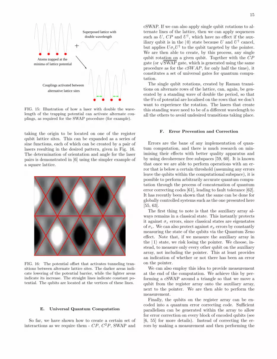
FIG. 15: Illustration of how a laser with double the wave-length of the trapping potential can activate alternate cou-plings, as required for the SWAP procedure (for example).
taking the origin to be located on one of the registerqubit lattice sites. This can be expanded as a series ofsine functions, each of which can be created by a pair oflasers resulting in the desired pattern, given in Fig. 16.The determination of orientation and angle for the laserpairs is demonstrated in [6] using the simpler example ofa square lattice.
FIG. 16: The potential offset that activates tunneling tran-sitions between alternate lattice sites. The darker areas indi-cate lowering of the potential barrier, while the lighter areasindicate its increase. The straight lines indicate constant po-tential. The qubits are located at the vertices of these lines.
E. Universal Quantum Computation
So far, we have shown how to create a certain set ofinteractions as we require them - CP , C2P , SWAP and
cSWAP. If we can also apply single qubit rotations to al-ternate lines of the lattice, then we can apply sequencessuch as U , CP and U †, which have no effect if the aux-iliary qubit is in the | 0〉 state because U and U † cancel,but applies UσzU
† to the qubit targeted by the pointer.We are then able to create, by this process, any singlequbit rotation on a given qubit. Together with the CPgate (or
√SWAP gate, which is generated using the same
procedure as for the cSWAP , for only half the time), itconstitutes a set of universal gates for quantum compu-tation.
The single qubit rotations, created by Raman transi-tions on alternate rows of the lattice, can, again, be gen-erated by a standing wave of double the period, so thatthe 0’s of potential are localised on the rows that we don’twant to experience the rotation. The lasers that createthis standing wave need to be of a different wavelength toall the others to avoid undesired transitions taking place.
F. Error Prevention and Correction
Errors are the bane of any implementation of quan-tum computation, and there is much research on min-imising their effects with better quality apparatus andby using decoherence free subspaces [59, 60]. It is knownthat once we are able to perform operations with an er-ror that is below a certain threshold (assuming any errorsleave the qubits within the computational subspace), it ispossible to perform arbitrarily accurate quantum compu-tation through the process of concatenation of quantumerror correcting codes [61], leading to fault tolerance [62].It has recently been shown that the same can be done forglobally controlled systems such as the one presented here[55, 63].
The first thing to note is that the auxiliary array al-ways remains in a classical state. This instantly protectsit against σz errors, since classical states are eigenstatesof σz . We can also protect against σx errors by constantlymeasuring the state of the qubits via the Quantum Zenoeffect. Note that, if we measure the auxiliary array inthe | 1〉 state, we risk losing the pointer. We choose, in-stead, to measure only every other qubit on the auxiliaryarray, not including the pointer. This at least providesan indication of whether or not there has been an erroron the pointer.
We can also employ this idea to provide measurementat the end of the computation. We achieve this by per-forming a cSWAP around a triangle so that we move aqubit from the register array onto the auxiliary array,next to the pointer. We are then able to perform themeasurement.
Finally, the qubits on the register array can be en-coded into a quantum error correcting code. Sufficientparallelism can be generated within the array to allowfor error correction on every block of encoded qubits (see[6, 55] for more details). Instead of correcting the er-rors by making a measurement and then performing the

16
relevant correction, these steps are performed by an algo-rithm that uses controlled-NOT gates to correct for theerrors, as determined by the error syndrome stored onancilla qubits. The problem with this method is that toperform the syndrome extraction (placing on auxiliaryqubits information about the errors), the ancilla qubitsmust be in a well–known state (| 0〉). After the errorcorrecting phase, these qubits are left in an unknownstate. Hence, it is necessary to either reset the state ofthe qubits, or have a large supply of fresh qubits. In theoptical lattice set-up, this second option is quite sensi-ble. We have so far restricted computation to a singletwo-dimensional plane. However, in a three dimensionallattice there are many of these planes, all of which containqubits in the | 0〉 state. If we perform our computation ona single plane, then this plane can be moved through allthe other planes by a series of SWAPs between alternateplanes. We can therefore access this large supply of freshqubits for the purposes to error correction without theneed to perform measurements during the computation,thus simplifying the experimental implementation.
VIII. CONCLUSIONS
In this paper we presented, initially, a variety of differ-ent spin interactions that can be generated by a system ofultra-cold atoms superposed by optical lattices and initi-ated in the Mott insulator phase. In particular, we havebeen interested in the simulation and study of variousthree-spin interactions conveniently obtained in a latticewith equilateral triangular structure. The possibility toexternally control most of the parameters of the effectiveHamiltonians at will renders our model as a unique lab-
oratory to study the relationship among exotic systemssuch as chiral spin systems, fractional quantum Hall sys-tems or systems that exhibit high-Tc superconductivity[26, 38]. Furthermore, unique properties related with thecritical behaviour of the chain with three-spin interac-tions has been analysed (see also [16]) where the two-point correlations, used traditionally to describe the crit-icality of a chain, seem to fail to identify long quantumcorrelations, suitably expressed by a variety of entangle-ment measures [45]. In particular, analysing the logarith-mic negativity, indicates a possible connection betweenthe localisable entanglement length on the one hand andentanglement properties of closely spaced spins on theother. In addition, suitable applications have been pre-sented within the realm of quantum computation [6, 27]where three-qubit gates can be straightforwardly gener-ated from the three-spin interactions.
In conclusion the three-spin interactions generated inan optical lattice offer a rich variety of applications inquantum information technology as well as in solid statephysics, worth pursuing further theoretically and exper-imentally.
Acknowledgments
J. P. would like to thank Christian D’Cruz for usefulconversations. This work was supported by a Royal Soci-ety University Research Fellowship, a Royal Society Lev-erhulme Trust Senior Research Fellowship, the EPSRCQIP-IRC, the EU Thematic Network QUPRODIS andby the Spanish grant MECD AP2001-1676. E.R. thanksthe QI group at DAMTP for their hospitality, where partof this work was done.
[1] A. Kastberg, W. D. Phillips, S. L. Rolston, R. J. C.Spreeuw, and P. S. Jessen, Phys. Rev. Lett. 74, 1542(1995); G. Raithel, W. D. Phillips, and S. L. Rolston,Phys. Rev. Lett. 81, 3615 (1998).
[2] M. Greiner, O. Mandel, T. Esslinger, T. W. Heanch, andI. Bloch, Nature 415, 39 (2002); M. Greiner, O. Mandel,T. W. Heanch, and I. Bloch, Nature 419, 51 (2002).
[3] O. Mandel, M. Greiner, A. Widera, T. Rom, T. W.Heanch, and I. Bloch, Nature 425, 937 (2003).
[4] D. Jaksch, H.-J. Briegel, J. I. Cirac, C. W. Gardiner, andP. Zoller, Phys. Rev. Lett. 82, 1975 (1999).
[5] G. K. Brennen, C. M. Caves, P. S. Jessen, and I. H.Deutsch, Phys. Rev. Lett. 82, 1060 (1999).
[6] A. Kay and J. K. Pachos, quant-ph/0406073.[7] J. Mompart, K. Eckert, W. Ertmer, G. Birkl, and M.
Lewenstein, Phys. Rev. Lett. 90, 147901 (2003).[8] D. Jaksch, C. Bruder, J. I. Cirac, C.W. Gardiner, and P.
Zoller, Phys. Rev. Lett. 81, 3108 (1998).[9] A. B. Kuklov, and B. V. Svistunov, Phys. Rev. Lett. 90,
100401 (2003).[10] D. Jaksch, and P. Zoller, New Journal Phys. 5, 56.1
(2003).
[11] L. M. Duan, E. Demler, and M. D. Lukin, Phys. Rev.Lett. 91, 090402 (2003).
[12] A. Mizel, and D. A. Lidar, cond-mat/0302018.[13] P. Rabl, A. J. Daley, P. O. Fedichev, J. I. Cirac, P. Zoller,
cond-mat/0304026.[14] S. E. Sklarz, I. Friedler, D. J. Tannor, Y. B. Band, C. J.
Williams, Phys. Rev. A 66, 053620 (2002).[15] D. C. Roberts and K. Burnett, Phys. Rev. Lett. 90,
150401 (2003).[16] J. K. Pachos, and M. B. Plenio, to appear in Phys. Rev.
Lett., quant-ph/0401106.[17] S. Sachdev, Quantum Phase Transitions, Cambridge Uni-
versity Press (1999).[18] P. Fendley, K. Sengupta, and S. Sachdev, Phys. Rev. B
69, 075106 (2004).[19] K. A. Penson, J. M. Debierre, and L. Turban, Phys. Rev.
B 37, 7884 (1988).[20] F. Igloi, Phys. Rev. B 40, 2362 (1989).[21] P. Fendley, K. Sengupta, and S. Sachdev,
cond-mat/0309438.[22] L. Turban, J. Phys. C: Solid State Phys. 15, L65 (1982).[23] K. A. Penson, R. Jullien, and P. Pfeuty, Phys. Rev. B

17
26, 6334 (1982).[24] F. Igloi, J. Phys. A: Math. Gen. 20, 5319 (1987).[25] J. Christiian, A. d’Auriac, and F. Igloi, Phys. Rev. E 58,
241 (1998).[26] R. B. Laughlin, Science 242, 525 (1988).[27] J. K. Pachos, and P. L. Knight, Phys. Rev. Lett. 91,
107902 (2003).[28] J. K. Pachos and E. Rico, quant-ph/0404048.[29] S. Inouye, M. R. Andrews, J. Stenger, H.-J. Miesner, D.
M. Stamper-Kurn, and W. Ketterle, Nature 392, 151(1998).
[30] A. Donley, N. R. Claussen, S. L. Cornish, J. L. Roberts,E. A. Cornell, and C. E. Wieman, Nature 412, 295(2001).
[31] S. J. J. M. F. Kokkelmans, and M. J. Holland, Phys. Rev.Lett. 89, 180401 (2002); T. Koehler, T. Gasenzer, and K.Burnett, cond-mat/0209100.
[32] W. V. Liu, F. Wilczek, and P. Zoller, cond-mat/0404478.[33] A. Kitaev (unpublished).[34] For an alternative method see, e.g. [10].[35] Y. Aharonov, and D. Bohm, Phys. Rev. 115, 485 (1959).[36] J. K. Pachos, cond-mat/0405374.[37] S. L. Cornish et al., Phys. Rev. Lett. 85, 1795 (2000); J.
K. Chin, J. M. Vogels, and W. Ketterle, Phys. Rev. Lett.90, 160405 (2003); M. Greiner et al., Phys. Rev. Lett.92, 150405 (2004).
[38] X. G. Wen, F. Wilczek, and A. Zee, Phys. Rev. B 39,11413 (1989).
[39] D. S. Rokhsar, Phys. Rev. Lett. 65, 1506 (1990).[40] D. Sen, and R. Chitra, Phys. Rev. B 51, 1922 (1995).[41] V. Kalmeyer and R. B. Laughlin, Phys. Rev. Lett. 59,
2095 (1987).[42] A. S. Sorensen, E. Demler, and M. D. Lukin,
cond-mat/0405079.[43] D. A. Huse and M. E. Fisher, Phys. Rev. Lett. 49, 793
(1982).[44] J. I. Latorre, E. Rico, G. Vidal, quant-ph/0304098.[45] F. Verstraete, M. Popp, and J. I. Cirac, Phys. Rev. Lett.
92, 027901 (2004).[46] F. Verstraete, M.-A. Matrin-Delgado, Phys. Rev. Lett.
92, 087201 (2004).[47] F. Verstraete, and J.I. Cirac, quant-ph/0311130.[48] R. Raussendorf, et. al., Phys. Rev. A 68, 022312 (2003)[49] In contrast to Hamiltonian eqn (6.3) the two-spin system
H =∑
i−σx
i σx
i+1 does not exhibit a finite gap for an in-finite chain and possesses a two-fold degenerate groundstate. As a consequence the ground state will not be sta-ble (see eg G. Gallavotti, Statistical Mechanics: A Short
Treatise, Springer 1999).[50] E. Barouch and B.M. McCoy, Phys. Rev. A 3, 786 (1971).[51] J. Eisert and M.B. Plenio, J. Mod. Opt. 46, 145 (1999); J.
Eisert (PhD thesis, Potsdam, February 2001); G. Vidaland R.F. Werner, Phys. Rev. A 65, 032314 (2002); K.Audenaert, M.B. Plenio, and J. Eisert, Phys. Rev. Lett.90, 027901 (2003).
[52] M.B. Plenio and V. Vedral, Contemp. Phys. 39, 431(1998); J. Eisert and M.B. Plenio, Int. J. Quant. Inf.1, 479 (2003).
[53] S. C. Benjamin, Phys Rev A 61, 020301 (2000).[54] S. C. Benjamin, Phys. Rev. Lett., 88, 017904 (2002).[55] S. C. Benjamin and A. Bririd, quant-ph/0308113.[56] S. C. Benjamin, quant-ph/0104117.[57] T. Calarco, U. Dorner, P. Julienne, C. Williams, and P.
Zoller, quant-ph/0403197.[58] S. Peile, J. V. Porto, B. Laburthe, J. M. Obrecht, B. E.
King, M. Subbotin, S. L. Rolston and W. D. Phillips,Phys. Rev. A, 67, 051603(2003).
[59] G. M. Palma, K. A. Suominen and A. K. Ekert, Proc. R.Soc. A, 452, 567 (1996).
[60] M.B. Plenio, V. Vedral and P.L. Knight, Phys. Rev. A55, 67 (1997).
[61] A. M. Steane, Phys. Rev. Lett. 77, 793 (1996).[62] A. M. Steane, quant-ph/9809054.[63] D. Aharonov and M. Ben-Or, quant-ph/9906129.