advanced calculus of several variables - wordpress.com
TRANSCRIPT
Advanced Calculus of Several Variables
C. H. E D W A R D S , JR. THE UNIVERSITY OF GEORGIA
A C A D E M I C P R E S S New York and London
A Subsidiary of Harcourt Brace Jovaiiovich, Publishers
COPYRIGHT © 1973, BY ACADEMIC PRESS, INC. ALL RIGHTS RESERVED. NO PART OF THIS PUBLICATION MAY BE REPRODUCED OR TRANSMITTED IN ANY FORM OR BY ANY MEANS, ELECTRONIC OR MECHANICAL, INCLUDING PHOTOCOPY, RECORDING, OR ANY INFORMATION STORAGE AND RETRIEVAL SYSTEM, WITHOUT PERMISSION IN WRITING FROM THE PUBLISHER.
ACADEMIC PRESS, INC. Ill Fifth Avenue, New York, New York 10003
United Kingdom Edition published by ACADEMIC PRESS, INC. (LONDON) LTD. 24/28 Oval Road, London NW1
Library Library of Congress Cataloging in Publication Data
Edwards, Charles Henry, DATE Advanced calculus of several variables.
Bibliography: p. 1. Calculus. I. Title.
QA303.E22 515 72-9325 ISBN 0 - 1 2 - 2 3 2 5 5 0 - 8
AMS (MOS) 1970 Subject Classifications: 26A57, 26A60, 26A63, 26A66
PRINTED IN THE UNITED STATES OF AMERICA
To My Parents

PREFACE
This book has developed from junior-senior level advanced calculus courses that I have taught during the past several years. It was motivated by a desire to provide a modern conceptual treatment of multivariable calculus, emphasiz-ing the interplay of geometry and analysis via linear algebra and the approxi-mation of nonlinear mappings by linear ones, while at the same time giving equal attention to the classical applications and computational methods that are responsible for much of the interest and importance of this subject.
In addition to a satisfactory treatment of the theory of functions of several variables, the reader will (hopefully) find evidence of a healthy devotion to matters of exposition as such—for example, the extensive inclusion of motiva-tional and illustrative material and applications that is intended to make the subject attractive and accessible to a wide range of" typical " science and mathe-matics students. The many hundreds of carefully chosen examples, problems, and figures are one result of this expository effort.
This book is intended for students who have completed a standard introduc-tory calculus sequence. A slightly faster pace is possible if the students' first course included some elementary multivariable calculus (partial derivatives and multiple integrals). However this is not essential, since the treatment here of multi-variable calculus is fully self-contained. We do not review single-variable calculus, with the exception of Taylor's formula in Section II.6 (Section 6 of Chapter II) and the fundamental theorem of calculus in Section IV. 1.
Chapter I deals mainly with the linear algebra and geometry of Euclidean «-space 0tn. With students who have taken a typical first course in elementary linear algebra, the first six sections of Chapter I can be omitted; the last two sections of Chapter I deal with limits and continuity for mappings of Euclidean spaces, and with the elementary topology of 0tn that is needed in calculus. The only linear algebra that is actually needed to start Chapter II is a know-ledge of the correspondence between linear mappings and matrices. With students having this minimal knowledge of linear algebra, Chapter 1 might (depending upon the taste of the instructor) best be used as a source for reference as needed.
ix

X Preface
Chapters II through V are the heart of the book. Chapters II and III treat multivariable differential calculus, while Chapters IV and V treat multivariable integral calculus.
In Chapter II the basic ingredients of single-variable differential calculus are generalized to higher dimensions. We place a slightly greater emphasis than usual on maximum-minimum problems and Lagrange multipliers—experience has shown that this is pedagogically sound from the standpoint of student moti-vation. In Chapter III we treat the fundamental existence theorems of multi-variable calculus by the method of successive approximations. This approach is equally adaptable to theoretical applications and numerical computations.
Chapter IV centers around Sections 4 and 5 which deal with iterated integrals and change of variables, respectively. Section IV.6 is a discussion of improper multiple integrals. Chapter V builds upon the preceding chapters to give a comprehensive treatment, from the viewpoint of differential forms, of the clas-sical material associated with line and surface integrals, Stokes' theorem, and vector analysis. Here, as throughout the book, we are not concerned solely with the development of the theory, but with the development of conceptual understanding and computational facility as well.
Chapter VI presents a modern treatment of some venerable problems of the calculus of variations. The first part of the Chapter generalizes (to normed vector spaces) the differential calculus of Chapter II. The remainder of the Chapter treats variational problems by the basic method of " ordinary calculus "—equate the first derivative to zero, and then solve for the unknown (now a function). The method of Lagrange multipliers is generalized so as to deal in this context with the classical isoperimetric problems.
There is a sense in which the exercise sections may constitute the most im-portant part of this book. Although the mathematician may, in a rapid reading, concentrate mainly on the sequence of definitions, theorems and proofs, this is not the way that a textbook is read by students (nor is it the way a course should be taught). The student's actual course of study may be more nearly defined by the problems than by the textual material. Consequently, those ideas and concepts that are not dealt with by the problems may well remain un-learned by the students. For this reason, a substantial portion of my effort has gone into the approximately 430 problems in the book. These are mainly concrete computational problems, although not all routine ones, and many deal with physical applications. A proper emphasis on these problems, and on the illustrative examples and applications in the text, will give a course taught from this book the appropriate intuitive and conceptual flavor.
I wish to thank the successive classes of students who have responded so enthusiastically to the class notes that have evolved into this book, and who have contributed to it more than they are aware. In addition, I appreciate the excellent typing of Janis Burke, Frances Chung, and Theodora Schultz.
I Euclidean Space and Linear Mappings
Introductory calculus deals mainly with real-valued functions of a single variable, that is, with functions from the real line 01 to itself. Multivariable calculus deals in general, and in a somewhat similar way, with mappings from one Euclidean space to another. However a number of new and interesting phenomena appear, resulting from the rich geometric structure of «-dimensional Euclidean space 0tn.
In this chapter we discuss 0ln in some detail, as preparation for the develop-ment in subsequent chapters of the calculus of functions of an arbitrary number of variables. This generality will provide more clear-cut formulations of theo-retical results, and is also of practical importance for applications. For example, an economist may wish to study a problem in which the variables are the prices, production costs, and demands for a large number of different com-modities; a physicist may study a problem in which the variables are the coor-dinates of a large number of different particles. Thus a " real-life " problem may lead to a high-dimensional mathematical model. Fortunately, modern tech-niques of automatic computation render feasible the numerical solution of many high-dimensional problems, whose manual solution would require an inordinate amount of tedious computation.
1 THE VECTOR SPACED"
As a set, 0tn is simply the collection of all ordered «-tuples of real numbers. That is,
0tn = {(*i> x2 5 · · · > *#,): each xt e 01).
1

2 I Euclidean Space and Linear Mappings
Recalling that the Cartesian product A x B of the sets A and B is by definition the set of all pairs (#, b) such that a e A and b e B, we see that 0tn can be re-garded as the Cartesian product set $ x · · · x @t (n times), and this is of course the reason for the symbol 0t.
The geometric representation of ^?3, obtained by identifying the triple (xl9 χ2, x3) of numbers with that point in space whose coordinates with respect to three fixed, mutually perpendicular ςςcoordinate axes" are xl, x2, x3 respec-tively, is familiar to the reader (although we frequently write (x, y, z) instead of (xl9 x2, X3) in three dimensions). By analogy one can imagine a similar geo-metric representation of 0t in terms of n mutually perpendicular coordinate axes in higher dimensions (however there is a valid question as to what "per-pendicular" means in this general context; we will deal with this in Section 3).
The elements of rMn are frequently referred to as vectors. Thus a vector is simply an A7-tuple of real numbers, and not a directed line segment, or equivalence class of them (as sometimes defined in introductory texts).
The set 0tn is endowed with two algebraic operations, called vector addition and scalar multiplication (numbers are sometimes called scalars for emphasis). Given two vectors x = (xu . . . , xn) and y = (>'1? . . . , yn) in ffln, their sum x + y is defined by
x + y = (*! + > Ί , . . . , x„ + >'„),
that is, by coordinatewise addition. Given a e i , the scalar multiple ax is de-fined by
ax — (ax^ . . . , axn).
For example, if x = ( 1, 0, — 2, 3) and y = ( — 2, 1,4, —5) then x + y = ( — 1, 1, 2, - 2 ) a n d 2 x = (2,0, - 4 , 6 ) . Finally we write 0 = ( 0 , . . . . , 0) and - x = ( - l ) x , and use x — y as an abbreviation for x + ( —y).
The familiar associative, commutative, and distributive laws for the real numbers imply the following basic properties of vector addition and scalar multiplication:
V1 x + (y + z) = (x + y) + z V2 x + y = y + x V3 x + 0 = x V4 x + ( - x ) = 0 V5 (ab)x = a(bx) V6 (a + b)x = ax + bx V7 a(x + y) = ax + ay V8 lx = x
(Here x, y, z are arbitrary vectors in {Mn, and a and b are real numbers.) VI-V8 are all immediate consequences of our definitions and the properties of M. For
1 The Vector Space £%n 3
example, to prove V6, let x = (xu . . . , xn). Then
{a + b)\ = ({a + b)xu . . . , (a + *)*„)
= (ufX! + bxu ...9axn + bxn)
= (axu ...,ax„) + (bxu ...,bxn)
= ax + 6x.
The remaining verifications are left as exercises for the student. A vector space is a set V together with two mappings Vx V-+ V and
0t x F-> F, called vector addition and scalar multiplication respectively, such that V1-V8 above hold for all x, y, z e V and a, b e & (V3 asserts that there exists 0 e F such that x + 0 = x for all x e V, and V4 that, given X G F , there exists — x e V such that x + ( — x) = 0). Thus VI-V8 may be summarized by saying that 0ln is a vector space. For the most part, all vector spaces that we consider will be either Euclidean spaces, or subspaces of Euclidean spaces.
By a subspace of the vector space V is meant a subset W of V that is itself a vector space (with the same operations). It is clear that the subset W of V is a subspace if and only if it is "closed" under the operations of vector addition and scalar multiplication (that is, the sum of any two vectors in IF is again in W, as is any scalar multiple of an element of W)—properties VI-V8 are then in-herited by JFfrom F Equivalently, J^is a subspace of F if and only if any linear combination of two vectors in [Fis also in iF(why?). Recall that a linear com-bination of the vectors vl5 . . . , \k is a vector of the form al\l -f · · · + ak\k9
where the at e 0t. The span of the vectors v,, . . . , \k e &n is the set S of all linear combinations of them, and it is said that S is generated by the vectors V j , . . . , νΛ.
Example 1 (%n is a subspace of itself, and is generated by the standard basis vectors
e, = ( l , 0 ,0 , . . . , 0 ) ,
e 2 = ( 0 , 1,0, . . . , 0 ) ,
e„ = ( 0 , 0 , 0 , . . . , 0,1),
since (xl9 x2, . . . , xn) = xx£2 + x\^i + " * + xnen- Als o t n e subset of 0tn con-sisting of the zero vector alone is a subspace, called the trivial subspace of 0tn.
Example 2 The set of all points in @n with last coordinate zero, that is, the set of all (* , , . . . , xn-u 0) e ^?", is a subspace of 0tn which may be identified with 0tn~\
Example 3 Given (au a2, . . . , a„) e @n, the set of all (x1, x2, . . . , xn) e 0tn
such that a{x{ + · · · + anxn = 0 is a subspace of J>" (see Exercise 1.1).
4 I Euclidean Space and Linear Mappings
Example 4 The span S of the vectors vl5 . . . , \k e 0tn is a subspace of 0t because, given elements a = £* ciiyi and b = £* 6,-v,· of 5, and real numbers r and 5*, we have ra + sb = £*(ra,· + s/^V; e S.
Lines through the origin in 0l·3 are (essentially by definition) those subspaces of ffl3 that are generated by a single nonzero vector, while planes through the origin in &3 are those subspaces of $3 that are generated by a pair of non-collinear vectors. We will see in the next section that every subspace V of 0tn
is generated by some finite number, at most n, of vectors; the dimension of the subspace V will be defined to be the minimal number of vectors required to generate V. Subspaces of 0ln of all dimensions between 0 and n will then general-ize lines and planes through the origin in ^ 3 .
Example 5 If V and W are subspaces of Mn, then so is their intersection V r\ ^ ( t h e set of all vectors that lie in both Fand W). See Exercise 1.2.
Although most of our attention will be confined to subspaces of Euclidean spaces, it is instructive to consider some vector spaces that are not subspaces of Euclidean spaces.
Example 6 Let SF denote the set of all real-valued functions on 01. If / + g and af are defined by ( / + g){x) =f{x) + g(x) and {af)(x) = af(x), then !F is a vector space (why?), with the zero vector being the function which is zero for all x e M. If # is the set of all continuous functions and 0 is the set of all poly-nomials, then 0 is a subspace of #, and <β in turn is a subspace of $F. If 0>n is the set of all polynomials of degree at most n, then 0n is a subspace of 0 which is generated by the polynomials 1, x, x1, . . . , xn.
Exercises
1.1 Verify Example 3. 1.2 Prove that the intersection of two subspaces of @tn is also a subspace. 1.3 Given subspaces V and W of ^ n , denote by V + W the set of all vectors v+ w with
v e V and w e IV. Show that V + W is a subspace of 0tn. 1.4 If V is the set of all (x, y, z) e 3?3 such that x + 2y = 0 and x + y = 3z, show that K is
a subspace of M3. 1.5 Let ώ*ο denote the set of all differentiable real-valued functions on [0, 1] such that
f(Q) = / ( ! ) = o. Show that Q)Q is a vector space, with addition and multiplication defined as in Example 6. Would this be true if the condition / (0) = f{\) = 0 were replaced by / (0) = 0 , / ( l ) = 1?
1.6 Given a set S, denote by > (5, ^ ) the set of all real-valued functions on 5, that is, all maps S-> R. Show that ^(S, ^) is a vector space with the operations defined in Example 6. Note that ^"({1, . . . , « } , ^ ) c a n be interpreted as &tn since the function 99 e «^"({1, . . . , » } , ^ ) may be regarded as the «-tuple (φ(1), <p(2), . . . , ψ(η)).
2 Subspaces of 0ln 5
2 SUBSPACES OF @n
In this section we will define the dimension of a vector space, and then show that 0tn has precisely n — 1 types of proper subspaces (that is, subspaces other than 0 and $n itself)—namely, one of each dimension 1 through n — 1.
In order to define dimension, we need the concept of linear independence. The vectors vl5 v2 , . . . , vA are said to be linearly independent provided that no one of them is a linear combination of the others; otherwise they are linearly dependent. The following proposition asserts that the vectors \l9 . . . , \k are linearly inde-pendent if and only if JC1V1 + x2 v2 + · · · + xk vfc = 0 implies that xx = x2 = - · · = xk = 0. For example, the fact that x1el + x2 e2 + ' ' ' + xnen — (*i> xi > . . . , xn) then implies immediately that the standard basis vectors el5 e2, . . . , e„ in 0tn are linearly independent.
Proposition 2.1 The vectors vl5 v2, . . . , yk are linearly dependent if and only if there exist numbers xi9 x2, . . . , xk, not all zero, such that x1\1 + x 2 v 2 + · · · -{-xkyk = Q.
PROOF If there exist such numbers, suppose, for example, that x1 Φ 0. Then
x2 xk ▼i = v2 - · · · v , ,
χ χ xl
so vl5 v2, . . . , \k are linearly dependent. If, conversely, vt = a2 \2 + · · · -f ak \k, then we have x1\l + x2 v2 + · · · + xk \k = 0 with xl = — 1 Φ 0 and xv = at· for
Example 7 To show that the vectors x = (1, 1, 0), y = (1, 1, 1), z = (0, 1, 1) are linearly independent, suppose that ax + by + cz = 0. By taking components of this vector equation we obtain the three scalar equations
a + b = 0 , a + b + c = 0,
b + c = 0.
Subtracting the first from the second, we obtain c = 0. The last equation then gives b = 0, and finally the first one gives a = 0.
Example 2 The vectors x = (1, 1, 0), y = (1, 2, 1), z = (0, 1, 1) are linearly dependent, because x — y + z = 0.
It is easily verified (Exercise 2.7) that any two collinear vectors, and any three coplanar vectors, are linearly dependent. This motivates the following definition
6 I Euclidean Space and Linear Mappings
of the dimension of a vector space. The vector space V has dimension n, dim V = n, provided that V contains a set of n linearly independent vectors, while any n + 1 vectors in Kare linearly dependent; if there is no integer n for which this is true, then V is said to be infinite-dimensional. Thus the dimension of a finite-dimensional vector space is the largest number of linearly independent vectors which it contains; an infinite-dimensional vector space is one that con-tains n linearly independent vectors for every positive integer n.
Example 3 Consider the vector space $F of all real-valued functions on 01. The functions 1, x, x2, . . . , x" are linearly independent because a polynomial α0 + αγχ + · · · + anx
n can vanish identically only if all of its coefficients are zero. Therefore 3F is infinite-dimensional.
One certainly expects the above definition of dimension to imply that Eucli-dean «-space 0tn does indeed have dimension n. We see immediately that its dimension is at least n, since it contains the n linearly independent vectors el5 . . . , e„. To show that the dimension of 0ln is precisely n, we must prove that any n 4- 1 vectors in 0tn are linearly dependent.
Suppose that vl5 . . . , \k are k > n vectors in 0tn, and write
yj = (alj,a2j, ..., anJ), j = 1, . . . , fc.
We want to find real numbers xl9 . . . , xk, not all zero, such that
0 = χιΎί +x2\2 + · · · + xk\k
k
= Σχλαυ>α2]> '",onj).
This will be the case if £*= l a^Xj = 0, / = 1, . . . , n. Thus we need to find a nontrivial solution of the homogeneous linear equations
alxx2 +a12x2 + · · · +aikxk = 0, 0 2 i * i + t f 2 2 * 2 + · " +<*2kxk = 09 . j .
««1*1 + an2*2 + · ' · + dnkXk = 0.
By a nontrivial solution (xl5 x2, . . . , xk) of the system (1) is meant one for which not all of the xt are zero. But k > n, and (1) is a system of n homogeneous linear equations in the k unknowns xu . . . , xk. (Homogeneous meaning that the right-hand side constants are all zero.)
It is a basic fact of linear algebra that any system of homogeneous linear equations, with more unknowns than equations, has a nontrivial solution. The proof of this fact is an application of the elementary algebraic technique of elimination of variables. Before stating and proving the general theorem, we consider a special case.

2 Subspaces of @n 7
Example 4 Consider the following three equations in four unknowns:
xx + 2x2 — x3 + 2x4 = 0, xi — x2 + 2x3 -f x4 = 0, (2)
2x! + x2 — *3 - XA = 0.
We can eliminate xl from the last two equations of (2) by subtracting the first equation from the second one, and twice the first equation from the third one. This gives two equations in three unknowns:
-3x2 + 3 x 3 - x 4 = 0, — 3x2 + x3 — 5x4 = 0.
Subtraction of the first equation of (3) from the second one gives the single equation
- 2 J C 3 - 4 X 4 = 0 (4)
in two unknowns. We can now choose x4 arbitrarily. For instance, if x4 = 1, then x3 = —2. The first equation of (3) then gives x2 = — y, and finally the first equation of (2) gives jq = — -2T2-. So we have found the nontrivial solution ( -V- , - f - 2 , 1) of the system (2).
The procedure illustrated in this example can be applied to the general case of n equations in the unknowns xu...,xk,k >n. First we order the n equations so that the first equation contains xl9 and then eliminate xx from the remaining equations by subtracting the appropriate multiple of the first equation from each of them. This gives a system of n — 1 homogeneous linear equations in the k — 1 variables x2 , . . . , xk. Similarly we eliminate x2 from the last n — 2 of these n — 1 equations by subtracting multiples of the first one, obtaining n — 2 equations in the k — 2 variables x 3 , x 4 , . . . , xk. After n — 2 steps of this sort, we end up with a single homogeneous linear equation in the k — n + 1 unknowns xn, xn + 1, . . . , xk. We can then choose arbitrary nontrivial values for the "extra" variables xn + i9 xn + 2> · · · > xk (such as xn + 1 = 1, xn+2 = · · · = xk = 0), solve the final equation for xn, and finally proceed backward to solve successively for each of the eliminated variables xn-u xn-2, . . . , xv The reader may (if he likes) formalize this procedure to give a proof, by induction on the number n of equa-tions, of the following result.
Theorem 2.2 If k > n, then any system of n homogeneous linear equa-tions in k unknowns has a nontrivial solution.
By the discussion preceding Eqs. (1) we now have the desired result that dim @n = n.
Corollary 2.3 Any n + 1 vectors in 0tn are linearly dependent.
(3)

8 I Euclidean Space and Linear Mappings
We have seen that the linearly independent vectors el5 e 2 , . . . , e„ generate 0tn. A set of linearly independent vectors that generates the vector space Kis called a basis for V. Since x = (xu x2, . . . , xn) = x^ + x2e2 + * * * + xnen, it is clear that the basis vectors el5 . . . , e„ generate V uniquely, that is, if x = ylei + y2 e2 + ■ " + yn
e« a'so> trien Xi = yi for each /. Thus each vector in 0tn can be expressed in one and only one way as a linear combination of el9 . . . , e„. Any set of n linearly independent vectors in an /7-dimensional vector space has this property.
Theorem 2.4 If the vectors v1? . . . , v„ in the ^-dimensional vector space Fare linearly independent, then they constitute a basis for V, and further-more generate V uniquely.
PROOF Given v e V, the vectors v, vl5 . . . , v„ are linearly dependent, so by Proposition 2.1 there exist numbers x, xl5 . . . , χη, not all zero, such that
x\ + x^ j + · · · + xn\n = 0.
If x = 0, then the fact that vls . . . , v„ are linearly independent implies that Xi = - · - = xn = 0. Therefore x φ 0, so we solve for v:
v = Vi v2 + · · · v„. X X X
Thus the vectors vl5 . . . , \n generate V, and therefore constitute a basis for V. To show that they generate V uniquely, suppose that
a1\1 + · · · + anyn = al'\1 + · · · + an\.
Then
(ßi - ai>i + "' + (<*n- <*n'K = °
So, since vx, . . . , v„ are linearly independent, it follows that a{: — a/ = 0, or at = a/, for each /. |
There remains the possibility that 0ln has a basis which contains fewer than n elements. But the following theorem shows that this cannot happen.
Theorem 2.5 If dim V = n, then each basis for V consists of exactly n vectors.
PROOF Let w1? w2, . . . , w„ be n linearly independent vectors in V. If there were a basis v1? v 2 , . . . , \m for Kwith m < n, then there would exist numbers {a^} such that
Wi =an\l + -" + amlym,
w„ = ûrlnv1 + · · · +amny,
2 Subspaces of 0tn 9
Since m < n, Theorem 2.2 supplies numbers xl, . . . , xn not all zero, such that
awx\ + " ' + a\nxn = 0,
But this implies that n
x{yvl + · · · + xn w„ = X xjfajvx + · · · + amjym)
m
= Σ(αηχι + ' " + */«*»>« i = 1
= 0,
which contradicts the fact that w l 5 . . . , w„ are linearly independent. Consequently no basis for Vcan have m <n elements. |
We can now completely describe the general situation as regards subspaces of 0tn. If F is a subspace of ffln, then k = dim V ^ n by Corollary 2.3, and if k = n, then V = &n by Theorem 2.4. If /c > 0, then any /c linearly independent vectors in V generate V, and no basis for V contains fewer than k vectors (Theorem 2.5).
Exercises
2.1 Why is it true that the vectors Vi, . . . , \k are linearly dependent if any one of them is zero ? If any subset of them is linearly dependent?
2.2 Which of the following sets of vectors are bases for the appropriate space 0tnl (a) (1,0) and (1,1). (b) (1,0, 0), (1, 1,0), and(0 , 0, 1). (c) (1, 1,1), (1, 1,0), and (1 ,0 ,0) . (d) (1, 1, 1, 0), (1, 0, 0, 0), (0, 1, 0, 0), and (0, 0, 1, 0). (e) (1, 1, 1, 1), (1, 1, 1, 0), (1, 1, 0, 0), and (1, 0, 0, 0).
2.3 Find the dimension of the subspace V of ^ 4 that is generated by the vectors (0, 1,0, 1), (1 ,0 , 1,0), and (1, 1, 1, 1).
2.4 Show that the vectors (1, 0, 0, 1), (0, 1, 0, 1), (0, 0, 1, 1) form a basis for the subspace V of ^ 4 which is defined by the equation χγ + x2 + x3 — x4 = 0.
2.5 Show that any set v t , . . . , vfc, of linearly independent vectors in a vector space V can be extended to a basis for V. That is, if k<n = dim K, then there exist vectors \k + l, . . . , v„ in F such that v l f . . . v„ is a basis for V.
2.6 Show that Theorem 2.5 is equivalent to the following theorem : Suppose that the equations
tfii*i + ··· 4- alnxn = 0,
tfni*i -I- ··· + annxn = 0
10 I Euclidean Space and Linear Mappings
have only the trivial solution xx = --- = xn = 0. Then, for each b = {bu . . . , b,X the equations
tfn*i + ··· + alnxn = bu
aniXi + ··· + ann xn = bn
have a unique solution. Hint: Consider the vectors a7 = (tfu, a2j, . . . , anj),j = 1, . . . , n. 2.7 Verify that any two collinear vectors, and any three coplanar vectors, are linearly depen-
dent.
3 INNER PRODUCTS AND ORTHOGONALITY
In order to obtain the full geometric structure of 0tn (including the concepts of distance, angles, and orthogonality), we must supply 0tn with an inner product. An inner (scalar)product on the vector space Fis a function F x F-> 0i, which associates with each pair (x, y) of vectors in F a real number <x, y>, and satisfies the following three conditions:
SP1 <x, x> > 0 if x Φ 0 (positivity). SP2 <x, y> = <y, x> (symmetry). SP3 {ax + by, z> + a{x, z> 4- b(y9 z>.
The third of these conditions is linearity in the first variable; symmetry then gives linearity in the second variable also. Thus an inner product on F is simply a positive, symmetric, bilinear function on F x V. Note that SP3 implies that <0, 0> = 0 (see Exercise 3.1).
The usual inner product on 0tn is denoted by x · y and is defined by
x - y = *iJ;i + · · · + xnyn, ( 0 where x = (xl9 . . . , x„), y = (>Ί, . . . , yn). It should be clear that this definition satisfies conditions SPl, SP2, SP3 above. There are many inner products on 0in (see Example 2 below), but we shall use only the usual one.
Example 1 Denote by %>[a, b] the vector space of all continuous functions on the interval [a, b], and define
<f,g>= ff(t)g(t)dt
for any pair of functions / , g e #[#, b]. It is obvious that this definition satisfies conditions SP2 and SP3. It also satisfies SPl, because if f(t0) φ 0, then by continuity (f(t))2 > 0 for all t in some neighborhood of t0, so
</,/> = f/(02 dt > 0. J a
Therefore we have an inner product on (6\a, b],

3 Inner Products and Orthogonality 11
Example 2 Let a, b, c be real numbers with a > 0, ac — b2 > 0, so that the quadratic form q(x) = ax2 + 2bxlx2 + cx2
2 is positive-definite (see Section II.4). Then <x, y> = axly1 + bxly2 + bx2yi + cx2y2 defines an inner product on &2 (why?). With a = c=\,b = 0we obtain the usual inner product on 0l2.
An inner product on the vector space V yields a notion of the length or " size " of a vector xe V, called its norm | x | . In general, a norm on the vector space F is a real-valued function x-> [x| on V satisfying the following con-ditions:
N1 | x | > 0 i f x ^ 0 (positivity), N2 |flx| = |a | |x | (homogeneity), N3 |x + y | ^ | x | + | y | (triangle inequality),
for all x, y e Vand ö e i Note that N2 implies that [0[ = 0.
The norm associated with the inner product < , > on V is defined by
|x|=V<ï^> (2) It is clear that SP1-SP3 and this definition imply conditions Nl and N2, but the triangle inequality is not so obvious; it will be verified below.
The most commonly used norm on 0tn is the Euclidean norm
[x | =(x12 + --+xn
2)1'2,
which comes in the above way from the usual inner product on 0tn. Other norms on 0tn, not necessarily associated with inner products, are occasionally employed, but henceforth [ x | will denote the Euclidean norm unless otherwise specified.
Example 3 ||x|| =max{ |x 1 | , . . . , |x„|}5 the maximum of the absolute values of the coordinates of x, defines a norm on 0ln (see Exercise 3.2).
Example 4 |x | x = \xl \ + \x2\ + · ·· + \xn\ defines still another norm on 0tn (again see Exercise 3.2).
A norm on V provides a definition of the distance d(x, y) between any two points x and y of V:
</(x,y) = | x - y | .
Note that a distance function d defined in this way satisfies the following three conditions:
D1 d(x, y) > 0 unless x = y (positivity), D2 d(x, y) = d(y, x) (symmetry), D3 d(x, z) ^ d(x, y) + d(y, z) (triangle inequality),
12 I Euclidean Space and Linear Mappings
for any three points x, y, z. Conditions Dl and D2 follow immediately from Nl and N2, respectively, while
d(x, z) = |x - z| = |(x - y) + (y - z)|
è | x - y | + | y - z | = d(x, y) + </(y, z)
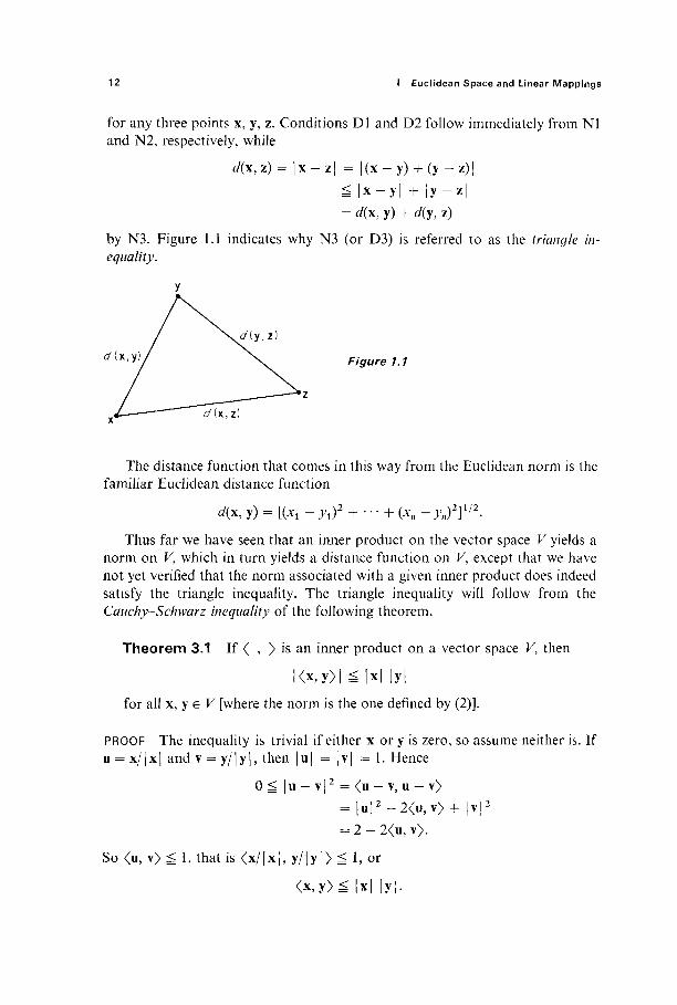
by N3. Figure 1.1 indicates why N3 (or D3) is referred to as the triangle in-equality.
d{*^/ \ Figure 1.1
The distance function that comes in this way from the Euclidean norm is the familiar Euclidean distance function
d(x, y) = [(*! - yù2 + · · · + (*. - Λ)2]1/2·
Thus far we have seen that an inner product on the vector space V yields a norm on V, which in turn yields a distance function on V, except that we have not yet verified that the norm associated with a given inner product does indeed satisfy the triangle inequality. The triangle inequality will follow from the Cauchy-Schwarz inequality of the following theorem.
Theorem 3.1 If < , > is an inner product on a vector space V, then
l<x,y>[ ^ | χ | ly l
for all x, y e V [where the norm is the one defined by (2)].
PROOF The inequality is trivial if either x or y is zero, so assume neither is. If u = x/1 x | and v = y/1 y |, then | u | = [ v | = 1. Hence
0 ^ | u — v | 2 = <u — v, u — v> = | u | 2 - 2 < u , v > + | v | 2
= 2 - 2<u, v>.
So<u, v>g l , t h a t i s < x / | x | , y / | y | > g 1, or
<x ,y>^ |x | |y | .
3 Inner Products and Orthogonality 13
Replacing x by — x, we obtain
- < x , y > ^ [χ| |y|
also, so the inequality follows. |
The Cauchy-Schwarz inequality is of fundamental importance. With the usual inner product in ^", it takes the form
k 2
(IHH5*')(J,4 while in Ή[α, b], with the inner product of Example l, it becomes
Λ6 \ 2 [ J> \ / „b
m <(/)((/)■ PROOF OF THE TRIANGLE INEQUALITY Given x, y e F note that
|x + y | 2 = <x + y,x + y| = [x |2 + 2 < x , y > + | y | 2
^ | x | 2 + 2 |x | |y| + | y | 2 (Cauchy-Schwarz) = (|x| + |y|)2,
which implies that [x + y | ^ | x | + | y | . I
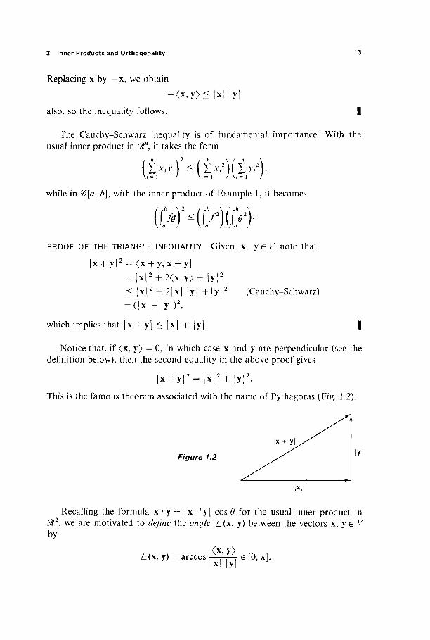
Notice that, if <x, y> = 0, in which case x and y are perpendicular (see the definition below), then the second equality in the above proof gives
|x + y | 2 = | x | 2 + | y | 2 .
This is the famous theorem associated with the name of Pythagoras (Fig. 1.2).
|x + y|
Figure 1.2
Recalling the formula x · y = |x | |y| cos 0 for the usual inner product in Î2, we are motivated to define the angle Z_(x, y) between the vectors x, y e V
by
<X y> L(x, y) = arccos ' e [0, π].
x y
14 I Euclidean Space and Linear Mappings
Notice that this makes sense because <x, y ) / | x | |y | e [— 1, 1] by the Cauchy-Schwarz inequality. In particular we say that x and y are orthogonal (or per-pendicular) if and only if x · y = 0, because then Z_(x, y) = arccos π/2 = 0.
A set of nonzero vectors vl5 v2, . . . in V is said to be an orthogonal set if
<**,*/> = 0
whenever i Φ j . If in addition each vt- is a unit vector, <vt·, v,·) = 1, then the set is said to be orthonormal.
Example 5 The standard basis vectors el5 . . . , e„ form an orthonormal set mât.
Example 6 The (infinite) set of functions
1, cos x, sin x, . . . , cos nx, sin AX, . . .
is orthogonal in <£[ — π, π] (see Example 1 and Exercise 3.11). This fact is the basis for the theory of Fourier series.
The most important property of orthogonal sets is given by the following result.
Theorem 3.2 Every finite orthogonal set of nonzero vectors is linearly independent.
PROOF Suppose that
αί\1 + · · · + ak\k = 0. (3)
Taking the inner product with v,, we obtain
*/<▼,·,▼*> = 0
because <vi5 Vj> = 0 for ιφ] if the vectors vl9 . . . , yk are orthogonal. But <vi » v/> Φ 0, so at = 0. Thus (3) implies ax = · · ■ = ak = 0, so the orthogonal vectors vl5 . . . , \k are linearly independent. |
We now describe the important Gram-Schmidt orthogonalization process for constructing orthogonal bases. It is motivated by the following elementary construction. Given two linearly independent vectors v and w1? we want to find a nonzero vector w2 that lies in the subspace spanned by v and wl5 and is orthogonal to Wj. Figure 1.3 suggests that such a vector w2 can be obtained by subtracting from v an appropriate multiple cv/l of Wj. To determine c,

3 Inner Products and Orthogonality 15
V
Figure 1.3
Wo
we simply solve the equation <w1? v — cwj> = 0 for c = <v, w1>/<w1, w^ . The desired vector is therefore
obtained by subtracting from v the "component of v parallel to w^" We imme-diately verify that <w2, Wj> = 0 , while w2 Φ 0 because v and wx are linearly independent.
Theorem 3.3 If V is a finite-dimensional vector space with an inner pro-duct, then F has an orthogonal basis.
In particular, every subspace of 0tn has an orthogonal basis.
PROOF We start with an arbitrary basis vl5 . . . , vn for V. Let w1 = \ i . Then, by the preceding construction, the nonzero vector
< v 2 , Wj>
< W l 9 Wj>
is orthogonal to w1 and lies in the subspace generated by \1 and v2. Suppose inductively that we have found an orthogonal basis wl5 . . . , wfc
for the subspace of V that is generated by vl5 . . . , \k. The idea is then to obtain \νΛ + 1 by subtracting from \k + 1 its components parallel to each of the vectors wl5 . . . , wfc. That is, define
wfc + i = νΛ + 1 - C i W i - c 2 w 2 - · · · -ckYfk9
where cf = <vfc+1, wf>/<wf, w£>. Then <wÄ + 1, w,-> = <vfc + l5 wf) - c ^ w , · , w > = 0 for / ^ /c, and W/. + 1 Φ 0, because otherwise vÄ + 1 would be a linear combination of the vectors w1? . . . , wfc, and therefore of the vectors vl5 . . . , \k. It follows that the vectors w1? . . . , wA + 1 form an orthogonal basis for the subspace of Kthat is generated by vls . . . , νΛ + 1.
After a finite number of such steps we obtain the desired orthogonal basis w1? . . . , w„ for V. |

16 I Euclidean Space and Linear Mappings
It is the method of proof of Theorem 3.3 that is known as the Gram-Schmidt orthogonalization process, summarized by the equations
Wi = Vi,
W2 =Y2
w3 = v3
W = V
defining the orthogonal basis wl9 . . . , wn in terms of the original basis vl5 . . . , v„.
Example 7 To find an orthogonal basis for the subspace V of ^*4 spanned by the vectors \l = (1, 1, 0, 0), v2 = (1, 0, 1, 0), v3 = (0, 1, 0, 1), we write
W l = V l = ( l , 1,0,0),
v 2 · Wi w2 = v2 yfx
Wj · W!
= (1, 0, 1, 0) - i ( l , 1, 0, 0) = ( i , -± ,1,0) ,
v3 · Wi v3 · w2 w3 = v3 yvl w2
= ( 0 , l , 0 , l ) - i ( l , l s 0 , 0 ) + i ( i , - i , 1,0)
Example 8 Let 0* denote the vector space of polynomials in x, with inner product defined by
<P, <7> = f P(x)q(x) d*< J - 1
By applying the Gram-Schmidt orthogonalization process to the linearly inde-pendent elements 1, x, x2,..., x",..., one obtains an infinite sequence {p„(x)}™= 0 » the first five elements of which are p0(x) = 1, px(x) = x, p2(x) = x2 - y, p3(x) = x3 — fx, p4(x) = xA — yjc2 + yy (see Exercise 3.12). Upon multiplying the polynomials {pn(x)} by appropriate constants, one obtains the famous Legendre polynomials P0(x) = p0(x), P^x) =Pi(x), P2(x) = iPi(x), Λ Μ = 2V3O), P*(x) = *rP*(x)> e t c ·
One reason for the importance of orthogonal bases is the ease with which a
<v2, Wi>
<wl5 wx>
Wi
<v3, w2> Wi - W 2 , <w2, w2>
yy — · · · — yy <Wi, w x> <w n _ 1 , w n _ 1 >
n _ 1

3 Inner Products and Orthogonality 17
vector ve V can be expressed as a linear combination of orthogonal basis vectors wt, . . . , w„ for V. Writing
v = αγΥίγ + -- + anvrni
1 cos x sin x cos nx sin nx
y/(2n)' 771 ' \Ιπ '*"' V71 V71
Writing
. . COS A7X Sin /7Jt </>*(·*) = —7— and ψπ(χ) = - — - ,
one defines the Fourier coefficients o f / e #[ — π, π] by
1 1 f'1
V 7 1 - π and
K = </» */0 = -7- ί / ί χ ) Sin ,7Λ: dx'
It can then be established, under appropriate conditions on / , that the infinite series
oo
ao + Σ (ön c o s /7·*" + £„ s in /7Λ-) / ! = 1
converges tof(x). This infinite series may be regarded as an infinite-dimensional analog of (5).
and taking the inner product with w,, we immediately obtain
so
v · wf
V · Wj V · W„ V = Wi + ' · · H W„ .
W, ' W , W„ · W„ (4)
This is especially simple if w1? . . . , w„ is an orthonormal basis for V:
v = (v · w^Wi + (v · w2)w2 + · · · + (v · wn)w„. (5)
Of course orthonormal basis vectors are easily obtained from orthogonal ones, simply by dividing by their lengths. In this case the coefficient v · w, of wt· in (5) is sometimes called the Fourier coefficient of v with respect to wf. This terminol-ogy is motivated by an analogy with Fourier series. The orthonormal functions in #[ —π, π] corresponding to the orthogonal functions of Example 6 are

18 I Euclidean Space and Linear Mappings
Given a subspace V of ffin, denote by VL the set of all those vectors in ^", each of which is orthogonal to every vector in V. Then it is easy to show that V1 is a subspace of i%n
9 called the orthogonal complement of V (Exercise 3.3). The significant fact about this situation is that the dimensions add up as they should.
Theorem 3.4 If V is a subspace of Mn, then
dim V + dim V1 = n. (6)
PROOF By Theorem 3.3, there exists an orthonormal basis vl9 . . . , vr for K, and an orthonormal basis wt, . . . , ws. for V1. Then the vectors v t , . . . , vr, wt, . . . , ws, are orthornormal, and therefore linearly independent. So in order to conclude from Theorem 2.5 that r + s = n as desired, it suffices to show that these vectors generate 0tn. Given x e Mn, define
r
y = x - X (x · ν,-Κ-. (7) i= 1
Then y · vf- = x · V; — (x · v ,·)(¥,· · ν,) = 0 for each i = 1, . . . , r. Since y is orthog-onal to each element of a basis for V, it follows easily that y e V1 (Exercise 3.4). Therefore Eq. (5) above gives
i = 1
This and (7) then yield r s
i = 1 i = 1
so the vectors vl5 . . . , vr, wl9 . . . , ws constitute a basis for 0ln. |
Example 9 Consider the system
α21χι +α22χ2 + · · · +α2ηχη = 0, (8)
**ι*ι + **2*2 + ' · · + **π*/» = 0>
of kè η homogeneous linear equations in x1? . . . , xn. If a,· = (an, . . . , fli/7), / = 1, . . . , k, then these equations can be rewritten as
*ί · χ = 0, a2 · x = 0,
a* · x = 0.
3 Inner Products and Orthogonality 19
Therefore the set S of all solutions of (8) is simply the set of all those vectors x e l " that are orthogonal to the vectors a1? . . . , ak. If V is the subspace of 0tn
generated by al9 . . . , afc, it follows that S = V1 (Exercise 3.4). If the vectors al5 . . . , a* are linearly independent, we can then conclude from Theorem 3.4 that dim S = n — k.
Exercises
3.1 Conclude from condition SP3 that <0, 0> - 0. 3.2 Verify that the functions defined in Examples 3 and 4 are norms on 0tn. 3.3 If V is a subspace of ^", prove that V1 is also a subspace. 3.4 If the vectors al5 . . . , afc generate the subspace V of Mn, and x e &n is orthogonal to each
of these vectors, show that x e VL. 3.5 Verify the "polarization identity" x * y = K | x + y|2— I x — y 12)· 3.6 Let ai, a2, . . . , a„ bean orthonormal basis for^n. If x = s&i + h sna„andy = ί ^ -f
··· + /„a„, show that x«y = srfi + ··· + s„tn. That is, in computing x«y, one may replace the coordinates of x and y by their components relative to any orthonormal basis for 0tn.
3.7 Orthogonalize the basis (1, 0, 0, 1), ( - 1 , 0, 2, 1), (0, 1, 2, 0), (0, 0, - 1 , 1) in ^ 4 . 3.8 Orthogonalize the basis
e / = ( 1 , 0 , . . . , 0), e2' = (1, 1, . . . . 0), . . . , e„' = (1, 1, . . . , 1)
in^ n .
3.9 Find an orthogonal basis for the 3-dimensional subspace V of ^ 4 that consists of all solutions of the equation xx + x2 + X3 — ** = 0. Hint: Orthogonalize the vectors V! = (1, 0, 0, 1), v2 = (0, 1, 0, 1), v3 = (0, 0, 1, 1).
3.10 Consider the two equations
xi + 2x2 — * 3 + X4 = 0, (*)
2xi -f Xi + X3 — *4 = 0. (**)
Let V be the set of all solutions of (*) and W the set of all solutions of both equations. Then W\s a 2-dimensional subspace of the 3-dimensional subspace V of &* (why?). (a) Solve (*) and (**) to find a basis vl5 v2 for W. (b) Find by inspection a vector v3 which is in V but not in W. Why is vlf v2, v3 then a basis for VI (c) Orthogonalize vl5 v2, v3 to obtain an orthogonal basis w b w 2 , w3 for V, with Wi and w2 in W. (d) Normalize wh w2, w3 to obtain an orthonormal basis Ui, u2, u3 for V. Express v = (11, 3, 6, —11) as a linear combination of ux, u2, u3. (e) Find vectors x e W and y e W1 such that v = x + y.
3.11 Show that the functions
1 cos x sin x cos nx sin nx \/(2π)' \/ττ ' \/π \/π ' \/π
are orthogonal in the inner product space #[ —77, 77] of Example 1. 3.12 Orthogonalize in #[—1, 1] the functions 1, x, x2, x3, xA to obtain the polynomials
Po(x),.. ·, PAX) listed in Example 8.
20 I Euclidean Space and Linear Mappings
4 LINEAR MAPPINGS AND MATRICES
In this section we introduce an important special class of mappings of Euclidean spaces—those which are linear (see definition below). One of the central ideas of multivariable calculus is that of approximating nonlinear mappings by linear ones.
Given a mapping/: 0tn -► 0Γ, l e t / , . . . ,fm be the component functions off. That i s , / , . . . , /m are the real-valued functions on 0t defined by writing/(x) = ( / (x) , . . . , fm(x)) e 0Γ. In Chapter II we will see that, if the component func-tions o f / a r e continuously diflferentiable at a e ^ , then there exists a linear mapping L : 0tn -► 0Γ such that
/ ( a + h )= / ( a )+L(h ) + /?(h)
with limh^0 /£(h)/|h| = 0. This fact will be the basis of much of our study of the differential calculus of functions of several variables.
Given vector spaces Kand W, the mapping L : K-> W is called linear if and and only if
L{ax + by) = aL(x) + bL(y) (1)
for all x, y e V and #, b e (ft. It is easily seen (Exercise 4.1) that the mapping L satisfies (1) if and only if
L(ax) = aL(x) (homogeneity) (2)
and
L(x + y) = L(x) + L(y) (additivity) (3)
for all x, y e V and a e l
Example 1 Given b e M, the mapping f\0l-+0t defined by f(x) = bx ob-viously satisfies conditions (2) and (3), and is therefore linear. Conversely, if / i s linear, then/(x) =f(x * 1) = x/(l), so/is of the form/(x) = bx withZ> = / ( l ) .
Example 2 The identity mapping / : K-> V, defined by /(x) = x for all xe V, is linear, as is the zero mapping x -> 0. However the constant mapping x -► c is not linear if c φ 0 (why?).
Example 3 Letf:&3-+&2 be the vertical projection mapping defined by f(x, y, z) = (;c, y). Then/ is linear.
Example 4 Let Q) denote the vector space of all infinitely difTerentiable func-tions from ^ to 01. If D(f) denotes the derivative o f / e 9, then D : 2> -» 3> is linear.
4 Linear Mappings and Matrices 21
Example 5 Let # denote the vector space of all continuous functions on [a, b]. If J(f) =γα f, then J\ (6 -> « is linear.
Example 6 Given a = (url5 tf2, tf3) e ^ 3 , the mapping/: ^ 3 -> ^ defined by / (x) = a · x = αίχ1 + α2χ2 + α3 χ3 is linear, because a- (x + y) = a - x + a*y and a · (ex) = c(a · x).
Conversely, the approach of Example 1 can be used to show that a function / : & -> M is linear only if it is of the f o r m / ^ , x2 , x3) = aix1 + a2x2 + #3*3. In general, we will prove in Theorem 4.1 that the mapping/: 0ln -» &m is linear if and only if there exist numbers a-tj, i = 1, . . . , /;?, / = 1, . . . , /?, such that the coordinate functions/l5 . . . , / „ of /are given by
/ i (x ) = * i i* i + #12*2 + · ' · + « i />(*) = #21*1 + ^ 2 2 x 2 + · · · + a 2
/«(X) = ^ 1 * 1 + «m2 *2 + * · ' + a„
(4)
for all x = (x1,..., xn) e ^". Thus the linear mapping/is completely determined by the rectangular array
# 1 2 '
a12 '
dm! '
" a m " a2n
"mn
' 2 1
of numbers. Such a rectangular array of real numbers is called a matrix. The horizontal lines of numbers in a matrix are called rows; the vertical ones are called columns. A matrix having m rows and n columns is called an m x n matrix. Rows are numbered from top to bottom, and columns from left to right. Thus the element ai} of the matrix A above is the one which is in the zth row and the/th column of A. This type of notation for the elements of a matrix is standard—the first subscript gives the row and the second the column. We frequently write A = (α^) for brevity.
The set of all m x n matrices can be made into a vector space as follows. Given two m x n matrices A = (a^) and B = (/?0·), and a number r, we define
A + B = (ai} + bij) and rA = (rau).
That is, the zyth element of A + B is the sum of the z/th elements of A and B, and the //th element of rA is r times that of A. It is a simple matter to check that these two definitions satisfy conditions V1-V8 of Section 1.
Indeed these operations for matrices are simply an extension of those for vectors. A 1 x n matrix is often called a row vector, and an m x 1 matrix is similarly called a column vector. For example, the zth row
Ai = (an ai2 - - - ain)

22 I Euclidean Space and Linear Mappings
of the matrix A is a row vector, and the /th column
AJ = I aV
of A is a column vector. In terms of the rows and columns of a matrix y4,wewil sometimes write
using subscripts for rows and superscripts for columns. Next we define an operation of multiplication of matrices which generalizes
the inner product for vectors. We define the product AB first in the special case when A is a row vector and B is a column vector of the same dimension. If
we define AB = £ ? = 1 a fè f . Thus in this case AB is just the scalar product of A and B as vectors, and is therefore a real number (which we may regard as a 1 x 1 matrix).
The product AB in general is defined only when the number of columns of A is equal to the number of rows of B. So let A = (α0·) be an m x n matrix, and B = (bij) an n x p matrix. Then the product AB of A and B is by definition the m x p matrix
AB = (AiBJ) (5)
whose //th element is the product of the /th row of A and the yth column of B (note that it is the fact that the number of columns of A equals the number of rows of B which allows the row vector A-t and the column vector BJ to be multi-plied). The product matrix AB then has the same number of rows as A, and the same number of columns as B. If we write AB = (c,·,·), then this product is given in terms of matrix elements by
m
Cij= ^aikbkj- ( 6 ) k= 1
So as to familiarize himself with the definition completely, the student should multiply together several suitable pairs of matrices.
4 Linear Mappings and Matrices 23
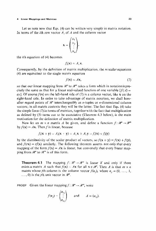
Let us note now that Eqs. (4) can be written very simply in matrix notation. In terms of the /th row vector At of A and the column vector
x =
the /th equation of (4) becomes
f(x) = Aix.
Consequently, by the definition of matrix multiplication, the m scalar equations (4) are equivalent to the single matrix equation
/ (x) = Ax, (7)
so that our linear mapping from 0tn to 0Γ takes a form which in notation is pre-cisely the same as that for a linear real-valued function of one variable [f(x) = ax]. Of course/(x) on the left-hand side of (7) is a column vector, like x on the right-hand side. In order to take advantage of matrix notation, we shall here-after regard points of 01" interchangeably as «-tuples or «-dimensional column vectors; in all matrix contexts they will be the latter. The fact that Eqs. (4) take the simple form (7) in terms of matrices, together with the fact that multiplication as defined by (5) turns out to be associative (Theorem 4.3 below), is the main motivation for the definition of matrix multiplication.
Now let an m x n matrix A be given, and define a function / : 0tn -> fflm
by/(x) = Ax. Then / i s linear, because
fix + y) = At(x + y) = Aix + A>y = f(x) + / (y )
by the distributivity of the scalar product of vectors, so / (x + y) = / (x ) +/ (y) , and f(rx) = rf(x) similarly. The following theorem asserts not only that every mapping of the form/(x) = Ax is linear, but conversely that every linear map-ping from 0in to 0Γ is of this form.
Theorem 4.1 The mapping / : 0tn -► 0Γ is linear if and only if there exists a matrix A such that fix) = Ax for all x e 0tn. Then A is that m x n matrix whose /th column is the column vector /(e,·), where e,· = (0, . . . , 1, . . . , 0) is they'th unit vector in $n.
PROOF Given the linear mapping/: 0ln -± Mm, write
and A = (a^).
24 I Euclidean Space and Linear Mappings
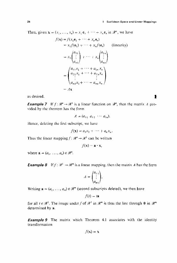
Then, given x = (xl5 . . . , xn) = xx e2 + · · · + xnen in 0tn, we have
f(\)=f(x1e1 + '-.+xnen)
= * ι /> ι ) + · ■ · + x„f(en) (linearity)
= * i ( : + · " + *,■( : V W V W
/anxl + '- + alnxn
V^ml^l + ' ' ' + β,ηηΧη ,
= Ax
as desired. |
Example 7 Iff: Mn -> 1 is a linear function on ^", then the matrix A pro-vided by the theorem has the form
A =(an a12 · · · aln).
Hence, deleting the first subscript, we have
f(x) = alxl + · · · + anxn.
Thus the linear mapping/: &n -> &1 can be written
/ (x) = a · x,
where a = (a1? . . . , an) e @tn.
Example 8 Iff: 0lx -> 0Γ is a linear mapping, then the matrix A has the form
. - (V). Writing a = (al5 . . . , am) e &m (second subscripts deleted), we then have
fit) = ia
for all t E 0tl. The image under /of ^ 1 in ST is thus the line through 0 in 0Γ
determined by a.
Example 9 The matrix which Theorem 4.1 associates with the identity transformation
/ (x) = *

4 Linear Mappings and Matrices 25
of 0tn is the n x n matrix
/ =
Ί 0> 1
1
having every element on the principal diagonal (all the elements au with / =j) equal to 1, and every other element zero. / is called the n x n identity matrix. Note that AI = I A = A for every n x n matrix A.
Example 10 Let R(oc) : M1 -> (R1 be a counterclockwise rotation of ^ 2 about 0 through the angle a (Fig. 1.4). We show that R(oc) is linear by computing its matrix explicitly. If (r, 0) are the polar coordinates of x = (xt, x2), so
χγ = r cos 0, x2 = r sin 0,
Figure 1.4
/ ? ( a ) ( x ) = ( / 1 f y 2 )
/ / x = (*,,*_)
/ . ^ ' 2
then the polar coordinates of (yl9 y2) = R(oc)(\) are (r, 0 + a), so
yx = r cos (0 + a) = r cos 0 cos a — r sin 0 sin a = xl cos a — x2 sin a
and j 2 = r sin (0 + a)
= r cos 0 sin a + r sin 0 cos a = χγ sin a + x2 cos a.
lyA _ /cos a —sin α \ / χΛ \y2J \sin a c o s a / \ x 2 /
Theorem 4.1 sets up a one-to-one correspondence between the set of all linear m a p s / : 0ln -+ 0Γ and the set of all m x n matrices. Let us denote by Mf the matrix of the linear map/ .
Therefore

26 I Euclidean Space and Linear Mappings
The following theorem asserts that the problem of finding the composition of two linear mappings is a purely computational matter—we need only multiply their matrices.
Theorem 4.2 if the mappings / : 0tn -> &Γ and g : Mm -> rMp are linear, then so is go f: ffln -> <MP, and
Mg.f = MeMf.
PROOF Let Mg = (ah) and Mf = (bh). Then Λ^ My- = (AiBJ)9 where Λ,· is the /th row of Af and £7 is the 7th column of Mf. What we want to prove is that
gof(x) = (MgMf)x, that is, that
ζ,.= Σ(Λ , .#)*; , (8) 7 = 1
where x = (xl9 ..., x„) and # o / ( x ) = (Zl, . . . , zp). Now
/ * , x \
/ ( X ) = M / X = * ? * 1 ( 9 )
\Bm\/
where Bk = {bkl- · · bkn) is the Arth row of Mf, so
Bkx=ftbkjxj. (10) J = 1
Also
^ / « = i ? ( / ( x ) ) = A i 9 ( A / / x ) =
using (9). Therefore
?pl ' ' ' ^ / W \ " | I X /
*«■ = Σ *«■*(#* x )
k= 1
IM / I l \
= Σ*/* Σ**/*/ using (10) k=i \ j = i /
= Σ Σ^Λ,Κ· j = l \ f c = l /
J = l
as desired [recall (8)]. In particular, since we have shown that g ° f(x) = (MgMf)x, it follows from Theorem 4.1 that g ° / i s linear. |

4 Linear Mappings and Matrices 27
Finally, we list the standard algebraic properties of matrix addition and multiplication.
Theorem 4.3 Addition and multiplication of matrices obey the following rules: (a) A(BC) = (AB)C (associativity). (b) A(B + C) = AB + AC\ ,.. t ., t. . . (c) (A+B)C = AC + BCJ W«tnbutivity). (d) (rA)B = r(AB) = A(rB).
PROOF We prove (a) and (b), leaving (c) and (d) as exercises for the reader. Let the matrices A, B, C be of dimensions k x /, / x m, and m x n respec-
tively. Then let f:&l^&k,g: Mm -► M\ /? : &n -► Mm be the linear maps such that Mf = A,Mg = B, Mh = C. Then
(/o(0oA))(x) =f(goh(x))
= f(9(h)x)))=(fog)(h(x))
= ((fog)oh)(x)
for all x e Mn, so f° (g ° h) = (f ° g) ° h. Theorem 4.2 therefore implies that
A(BC) = MfMgûh = Mfo(goh)
= (MfMg)Mh
= (AB)C,
thereby verifying associativity. To prove (b), let A be an / x m matrix, and B, C m x n matrices. Then let
/ : &m -> St1 and g, h : 0tn -+ $m be the linear maps such that Mf = A, Mg = B, and Mh = C. Then /o (g + //) = / o g + /Ό /?5 so Theorem 4.2 and Exercise 4.9 give
Λ(£ + C) = ΛΖ/Af, + Mh)
= MfMg + h
= Mfo(g + h) = Mfag + Mfoh
= MfMg + MfMh
= AB + AC,
thereby verifying distributivity. |
The student should not leap from Theorem 4.3 to the conclusion that the algebra of matrices enjoys all of the familiar properties of the algebra of real numbers. For example, there exist n x n matrices A and B such that AB Φ BA,

28 I Euclidean Space and Linear Mappings
so the multiplication of matrices is, in general, not commutative (see Exercise 4.12). Also there exist matrices A and B such that AB = 0 but neither A nor B is the zero matrix whose elements are all 0 (see Exercise 4.13). Finally not every non-zero matrix has an inverse (see Exercise 4.14). The n x n matrices A and B are called inverses of each other if AB = BA = L
Exercises
4.1 Show that the mapping / : V-> W is linear if and only if it satisfies conditions (2) and (3). 4.2 Tell whether or n o t / : ί#3 ->0t2 is linear, if / i s defined by
(a) f(x, y, z) = (z, x), (b) /(Λ-, y, z) = (xy, yz), (c) f(x, >>, z) = (x + y, y + z), (d) / ( * , * Z ) = (JC + ; F , Z + 1 ) , (e) f(x, y, z) = (2x — y - z, x + 7>y + z).
For each of these mappings that is linear, write down its matrix. 4.3 Show that, if b φ 0, then the function/(.v) = ax + b is not linear. Although such functions
are sometimes loosely referred to as linear ones, they should be called affine—an affine function is the sum of a linear function and a constant function.
4.4 Show directly from the definition of linearity that the composition g-fis linear if b o t h / and g are linear.
4.5 Prove that the mapping/ : &"->3?m is linear if and only if its coordinate functions/!, , / „ are all linear.
4.6 The linear mapping L : Mn -> <%n is called norm preserving if | L(x) | = | x |, and inner product preserving if L(x)«L(y) = x»y. Use Exercise 3.5 to show that L is norm preserving if and only if it is inner product preserving.
4.7 Let R(OL) be the counterclockwise rotation of Λ2 through an angle a. Then, as shown in Example 10, the matrix of R(oc) is
MR (cos a —sin a \ sin a cos ocj '
It is geometrically clear that R(a)oR(ß) = R(oc -\- ß\ so Theorem 4.2 gives MR{2)MR(P) = Μκ(*+β)> Verify this by matrix multiplication.
x
\ \ \
\ Figure 1.5 \ \
7 Ί α ) ( χ )
5 The Kernel and Image of a Linear Mapping 29
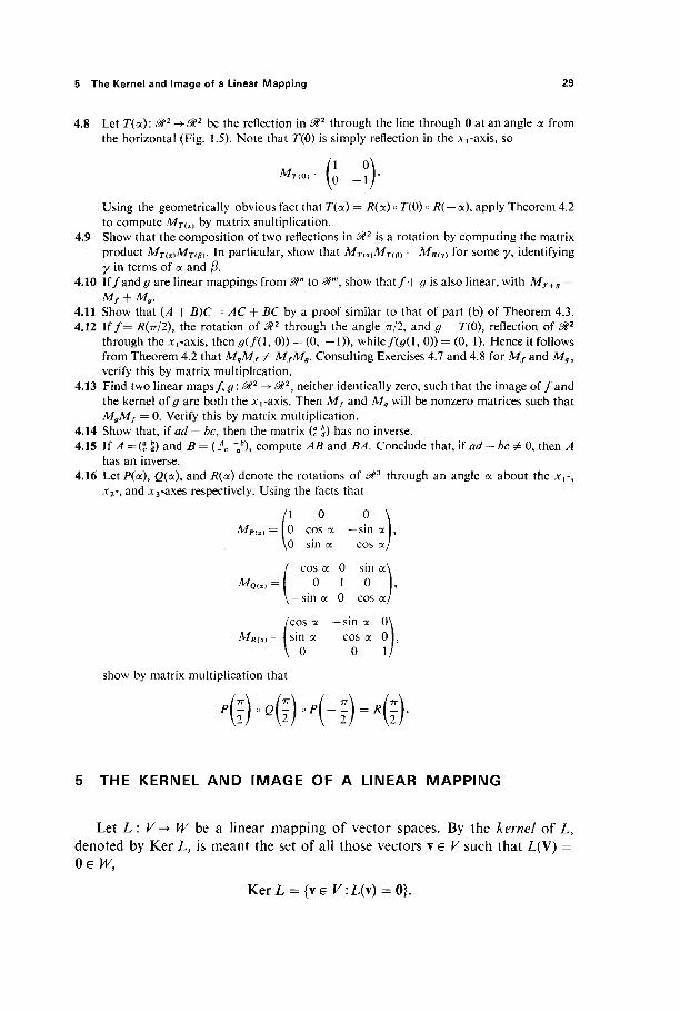
4.8 Let T(oc): &2 - > ^ 2 be the reflection in &2 through the line through 0 at an angle a from the horizontal (Fig. 1.5). Note that Γ(0) is simply reflection in the x i-axis, so
MTi0) ■ C -?)· Using the geometrically obvious fact that T(a) = R(oc) o T(0) o /?( —a), apply Theorem 4.2 to compute MT(0L) by matrix multiplication.
4.9 Show that the composition of two reflections in 8i2 is a rotation by computing the matrix product MT{0L)MT{P). In particular, show that MTWMTm = MR(y) for some y, identifying y in terms of a and β.
4.10 I f / and g are linear mappings from 0tn to ^ m , show t h a t / + g is also linear, with Mf+g = Mf + Mg.
4.11 Show that (A + B)C = AC + £ C by a proof similar to that of part (b) of Theorem 4.3. 4.12 I f / = R(TT/2), the rotation of &2 through the angle π/2, and g = Γ(0), reflection of ^ 2
through the Jd-axis, then g(f(l, 0)) = (0, - 1 ) ) , while f(g(l, 0)) = (0, 1). Hence it follows from Theorem 4.2 that MgMf φ MfMg. Consulting Exercises 4.7 and 4.8 for Mf and Mg, verify this by matrix multiplication.
4.13 Find two linear maps/ , g: &2 ^&2, neither identically zero, such that the image o f / a n d the kernel of g are both the x^axis. Then Mf and Mg will be nonzero matrices such that MgMf = 0. Verify this by matrix multiplication.
4.14 Show that, if ad = be, then the matrix (? 2) has no inverse. 4.15 If A=(a
cbd) and B=(*c " Λ compute AB and BA. Conclude that, if ad - be Φ 0, then A
has an inverse. 4.16 Let P(a), Q(ot), and R(ot) denote the rotations of ^ 3 through an angle a about the Λν,
x2-9 and *3-axes respectively. Using the facts that
/ l 0 0 MP(0L) = I 0 cos a —sin a
\0 sin a cos a
( cos a 0 sin a 0 1 0
— sin a 0 cos a
(cos a —sin a 0' sin a cos a 0
0 0 1
show by matrix multiplication that
■©•■GH-iKl· 5 THE KERNEL AND IMAGE OF A LINEAR MAPPING
Let L : F-> J47 be a linear mapping of vector spaces. By the kernel of L, denoted by Ker L, is meant the set of all those vectors \ e V such that L(V) = OeW,
KerL = {\eV:L(\) = 0}.

30 I Euclidean Space and Linear Mappings
By the image of L, denoted by Im L or/(L), is meant the set of all those vectors w G W such that w = L(v) for some vector \ ε V,
Im L = {w e W : there exists v e V such that L(v) = w}.
It follows easily from these definitions, and from the linearity of L, that the sets Ker L and Im L are subspaces of Kand W respectively (Exercises 5.1 and 5.2). We are concerned in this section with the dimensions of these subspaces.
Example 1 If a is a nonzero vector in ?JÏ'\ and L : 0ln -> 0t- is defined by L(x) = a · x, then Ker L is the (n — l)-dimensional subspace of 2ftn that is orthogonal to the vector a, and Im L = $.
Example 2 If P : ^ -► $2 is the projection P(xx, x2, *3) = (xi9 x2), then Ker P is the x3-axis and Im P = Piï1\
The assumption that the kernel of L : K-> W is the zero vector alone, Ker L = 0, has the important consequence that L is one-to-one, meaning that L(\{) = L(v2) implies that Vj = v2 (that is, L is one-to-one if no two vectors of V have the same image under L).
Theorem 5.1 Let L\V-+Whz linear, with V being /7-dimensional. If Ker L = 0, then L is one-to-one, and Im L is an /7-dimensional subspace of W.
PROOF To show that L is one-to-one, suppose L(v1)=L(v2). Then L(\{ — v2) = 0, so vt — v2 = 0 since Ker L = 0.
To show that the subspace Im L is /7-dimensional, start with a basis vl9 . . . , v„ for V. Since it is clear (by linearity of L) that the vectors / . ( v j , . . . , L(y„) generate ImL, it suffices to prove that they are linearly independent. Suppose
i1L(v1) + - - + /„L(v„) = 0.
Then
W^ + · · · + ίπνΛ) = 0,
so ί^! + · · · + tn\n = 0 because Ker L = 0. But then fx = · · · = tn = 0 because the vectors vl5 . . . , vM are linearly independent. |
An important special case of Theorem 5.1 is that in which W is also n-dimensional; it then follows that ImL = W (see Exercise 5.3).
Theorem 5.2 Let L\Mn-+ 3m be defined by L(x) = Ax, where A = (ai7) is an m x /7 matrix. Then (a) KerL is the orthogonal complement of that subspace of 0tn that is generated by the row vectors Al9 . . . , An of A, and

5 The Kernel and Image of a Linear Mapping 31
(b) Im L is the subspace of $m that is generated by the column vectors A1,..., A" of A.
PROOF (a) follows immediately from the fact that L is described by the scalar equations
L^X) = ΑγΧ, L2(x) = A2x,
Lm\X) = Am X,
so that the /th coordinate Lt(x) is zero if and only if x is orthogonal to the row vector A ,·.
(b) follows immediately from the fact that Im L is generated by the images L(e1), . . . , L(en) of the standard basis vectors in &n, whereas Lie,·) = A\ i = 1, . . . , « , by the definition of matrix multiplication. |
Example 3 Suppose that the matrix of L : ^ 3 -► ^ 3 is
/2 - 1 - 2 \ A = \\ 2 1 .
\3 1 - 1 /
Then A3 = Αγ + A2, but Ai and ^42 a r e n o t collinear, so it follows from 5.2(a)
that Ker L is 1-dimensional, since it is the orthogonal complement of the 2-dimensional subspace of 0Î1 that is spanned by Ax and A2 . Since the column vectors of A are linearly dependent, 3A1 = 4A2 — 5A3, but not collinear, it follows from 5.2(b) that Im L is 2-dimensional.
Note that, in this example, dim Ker L + dim Im L = 3. This is an illustration of the following theorem.
Theorem 5.3 If L : V-+ W is a linear mapping of vector spaces, with dim V = n, then
dim Ker L + dim Im L = n.
PROOF Let w1? . . . , wp be a basis for Im L, and choose vectors vl5 . . . , vp e V such that L(\i) = w, for / = 1, . . . , /?. Also let ul5 . . . , u9 be a basis for Ker L. It will then suffice to prove that the vectors vl5 . . . , vp, u1? . . . , u constitute a basis for V.
To show that these vectors generate V, consider v e V. Then there exist numbers ai9 *..,ap such that
L(\) = a1w1 + · · · +tfpwp,

32 I Euclidean Space and Linear Mappings
because w1? . . . , wp is a basis for Im L. Since w, = L(v,) for each /, by linearity we have
L(v)=L(ûf1v1 + ··■ + ap\p),
or
Liy-axvx - ■·· -tfpvp) = 0,
so v — αγ\t — · · · — ap \p e Ker L. Hence there exist numbers bx,..., bq such that
y -αχνγ - · · · -apyp = 4 ^ , + · · · + £iyiiiy,
or
v = ûf,v, + · · · H - t f ^ + ^ u , + · · · + Z>,yiiiy,
as desired. To show that the vectors v,, . . . , \p, u1? . . . , u9 are linearly independent,
suppose that
·*!*! + * ' ' + SP*p + 'lUl + ' ' ' + tqUq = 0.
Then
•y,w, + · · · + ^ w p = 0
because L(v,) = wf and L(u,·) = 0. Since w,, . . . , wp are linearly independent, it follows that st = · · · = sp = 0. But then fjU, + · · · + tquq = 0 implies that tx = · · · = tq = 0 also, because the vectors u1? . . . , uq are linearly independent. By Proposition 2.1 this concludes the proof. |
We give an application of Theorem 5.3 to the theory of linear equations. Consider the system
anxl + · · · + alnxn = 0, a2lxl + · · · + a2nxn = 0, (1)
Û W * I + " · + ^«^« = 0
of homogeneous linear equations in xx, ..., xn. As we have observed in Example 9 of Section 3, the space 5 of solutions (xu . . . , xn) of (1) is the orthogonal complement of the subspace of 0Γ that is generated by the row vectors of the m x n matrix A = (atJ). That is,
S = Ker L,
where L : &n -► ^Γ is defined by L(x) = Λχ (see Theorem 5.2). Now the row rank of the m x n matrix A is by definition the dimension of
the subspace of 0tn generated by the row vectors of A, while the column rank of A is the dimension of the subspace of &m generated by the column vectors of A.
5 The Kernel and Image of a Linear Mapping 33
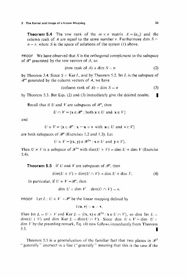
Theorem 5.4 The row rank of the m x n matrix A = (α^) and the column rank of A are equal to the same number r. Furthermore dim S = n — r, where S is the space of solutions of the system (1) above.
PROOF We have observed that S is the orthogonal complement to the subspace of Mn generated by the row vectors of A, so
(row rank of A) 4- dim S = n (2)
by Theorem 3.4. Since S = Ker L, and by Theorem 5.2, Im L is the subspace of 0Γ generated by the column vectors of A, we have
(column rank of A) + dim S = n (3)
by Theorem 5.3. But Eqs. (2) and (3) immediately give the desired results. |
Recall that if U and V are subspaces of 0F, then
U nV = {xe@n: both x e U and x e V}
and
U + K = { x e l " : x = u + v with ueU and v e V)
are both subspaces of @ln (Exercises 1.2 and 1.3). Let
U x V ={(x, y ) e f 2 " : x e t / a n d y e V}.
Then U x V is a subspace of $2n with dim((7 x V) = dim V + dim V (Exercise 5.4).
Theorem 5.5 If U and Kare subspaces of 0Γ, then
dim((/ + V) + dim(i/ n K) = dim U + dim K. (4)
In particular, if U + K = ^ n , then
dim 67 +dim V - dim(U n V) = n.
PROOF Let L : U x K-> ^ " be the linear mapping defined by
L(u, v) = u — v.
Then 1m L = U + K and Ker L = {(x, x) e ^ 2 " : x e (7 n K}, so dim Im L = dim(t/+ K) and dim Ker L = dim(U n V). Since dim £/x K=dim V + dim K by the preceding remark, Eq. (4) now follows immediately from Theorem 5.3. |
Theorem 5.5 is a generalization of the familiar fact that two planes in 09* tk generally" intersect in a line ("generally" meaning that this is the case if the
34 I Euclidean Space and Linear Mappings
two planes together contain enough linearly independent vectors to span ^ 3 ) . Similarly a 3-dimensional subspace and a 4-dimensional subspace of M1 generally intersect in a point (the origin); two 7-dimensional subspaces of ^ 1 0 generally intersect in a 4-dimensional subspace.
Exercises
5.1 5.2 5.3
5.4
5.5
5.6
5.7
If L : V^ W is linear, show that Ker L is a subspace of V. If L : V^ W is linear, show that Im L is a subspace of W. Suppose that Kand ^ a r e «-dimensional vector spaces, and that F\ V-> W\s linear, with Ker F=0. Then F is one-to-one by Theorem 5.1. Deduce that Im F= IV, so that the inverse mapping G = F~ l : W^ V is defined. Prove that G is also linear. If U and V are subspaces of ^B, prove that U x V <= 3?2n is a subspace of ^2", and that dim(i/ x K) = dim £/ + dim V. Hint: Consider bases for U and V. Let K and W be «-dimensional vector spaces. If L : K ^ W is a linear mapping with Im L = W, show that Ker L = 0. Two vector spaces K and H7 are called isomorphic if and only if there exist linear mappings S : V-> Wand T\W-> V such that 5 ° Γ and To S are the identity mappings of W and V respectively. Prove that two finite-dimensional vector spaces are isomorphic if and only if they have the same dimension. Let V be a finite-dimensional vector space with an inner product < , >. The dual space V* of V is the vector space of all linear functions V-*9t. Prove that V and V* are iso-morphic. Hint: Let \ u . . . , v„ be an orthonormal basis for V, and define 6j e V* by 0/(V() = 0 unless / =j\ djiyj) = 1. Then prove that θ{, . . . , θη constitute a basis for V*.
6 DETERMIWAWTS
It is clear by now that a method is needed for deciding whether a given A?-tuple of vectors al5 . . . , an in £ftn are linearly independent (and therefore con-stitute a basis for &n). We discuss in this section the method of determinants. The determinant of an n x n matrix A is a real number denoted by det A or \A\.
The student is no doubt familiar with the definition of the determinant of a 2 x 2 or 3 x 3 matiix. If A is 2 x 2, then
*·(* 5) - = ad — be.
For 3 x 3 matrices we have expansions by rows and columns. For example, the formula for expansion by the first row is
det [a2l a22 a~>% = a , #22
#32
#2 3
#33
#21
#31
#2 3
#33 + #.
#21
1*31 '32
6 Determinants 35
Formulas for expansions by rows or columns are greatly simplified by the following notation. If A is an n x n matrix, let Atj denote the (n — 1) x (n — 1) submatrix obtained from A by deletion of the /th row and the/th column of A. Then the above formula can be written
det A = all det An — a{2 det A{2 + # i3 det Aj3.
The formula for expansion of the n x n matrix A by the /th row is
det^ = t ( - l ) / + l7det^l7, (1)
while the formula for expansion by theyth column is
df*A = Yd(-\)i+hija*Aij. (2)
;= 1
For example, with n = 3 and / = 2, (2) gives
det A = — al2 det Al2 + a22 det A22 — a32 det A32
as the expansion of a 3 x 3 matrix by its second column. One approach to the problem of defining determinants of matrices is to de-
fine the determinant of an n x n matrix by means of formulas (1) and (2), assuming inductively that determinants of (n — 1) x (n — 1) matrices have been previously defined. Of course it must be verified that expansions along different rows and/or columns give the same result. Instead of carrying through this program, we shall state without proof the basic properties of determinants (I-IV below), and then proceed to derive from them the specific facts that will be needed in subsequent chapters. For a development of the theory of deter-minants, including proofs of these basic properties, the student may consult the chapter on determinants in any standard linear algebra textbook.
In the statement of Property I, we are thinking of a matrix A as being a function of the column vectors of A, det A = D(AX, . . . , A").
(Γ) There exists a unique (that is, one and only one) alternating, multilinear function D, from ^-tuples of vectors in Mn to real numbers, such that Z)(e„ . . . , e n ) = l .
The assertion that D is multilinear means that it is linear in each variable separately. That is, for each / = 1, . . . , / ? ,
D(*u . . . , xa, + ^b,, . . . , a„) = xZ)(al5 . . . , a,, . . . , an) + ^ ( a 1 , . . . , b i , . . . , a B ) . (3)
The assertion that D is alternating means that D(2ix, . . . , a„) = 0 if at· = a7· for some ιφ]. In Exercises 6.1 and 6.2, we ask the student to derive from the alternating multilinearity of D that
Z)(a1? . . . , raf, . . . , an) = r£>(al5 . . . , a(, . . . , a„), (4)
36 I Euclidean Space and Linear Mappings
Z)(a1? . . . , a4 + ra,·, . . . , an) = Z)(al5 . . . , a,, . . . , a„), (5)
and
D(a 1 ? . . . , a,·, . . . , ai5 . . . , a„) = - / ) ( a l 5 . . . , at, . . . , ay, . . . , a„) if /V.y. (6)
Given the alternating multilinear function provided by (I), the determinant of the « x « matrix A can then be defined by
àetA = D(A1,...,A")9 (7)
where A1, ..., An are as usual the column vectors of A. Then (4) above says that the determinant of A is multiplied by r if some column of A is multiplied by r, (5) that the determinant of A is unchanged if a multiple of one column is added to another column, while (6) says that the sign of det A is changed by an inter-change of any two columns of A. By virtue of the following fact, the word "column" in each of these three statements may be replaced throughout by the word "row."
(II) The determinant of the matrix A is equal to that of its transpose A\
The transpose Ax of the matrix A = {ah) is obtained from A by interchanging the elements atj and aji9 for each / andy. Another way of saying this is that the matrix A is reflected through its principal diagonal. We therefore write Ax = (a^ to state the fact that the element in the /th row andyth column of Ax is equal to the one in the 7th row and /th column of A. For example, if
/l 2 3\ / l 4 7 A= 4 5 6 , then A1 = 2 5 8
\7 8 9/ \3 6 9
Still another way of saying this is that A1 is obtained from A by changing the rows of A to columns, and the columns to rows.
(III) The determinant of a matrix can be calculated by expansions along rows and columns, that is, by formulas (1) and (2) above.
In a systematic development, it would be proved that formulas (1) and (2) give definitions of det A that satisfy the conditions of Property I and therefore, by the uniqueness of the function D, each must agree with the definition in (7) above.
The fourth basic property of determinants is the fact that the determinant of the product of two matrices is equal to the product of their determinants.
(IV) det AB = (det ^)(det B).
As an application, recall that the n x n matrix B is said to be an inverse of the n x n matrix A if and only if AB = BA = /, where / denotes the n x n
6 Determinants 37
identity matrix. In this case we write B = A'1 (the matrix A'1 is unique if it exists at all—see Exercise 6.3), and say A is invert ible. Since the fact that £>(el5..., e„) = 1 means that det / = 1, (IV) gives (det ^)(det A'1) = 1 # 0. So a necessary condition for the existence of A'1 is that det A Φ 0. We prove in Theorem 6.3 that this condition is also sufficient. The n x n matrix A is called nonsingular if det A φ 0, singular if det A = 0.
We can now give the determinant criterion for the linear independence of n vectors in 0tn.
Theorem 6.1 The n vectors al9 . . . , a„ in 0tn are linearly independent if and only if
PROOF Suppose first that they are linearly dependent; we then want to show that D(pu . . . , a„) = 0. Some one of them is then a linear combination of the others; suppose, for instance, that,
Then
D(*1,...,*n) = D(t2*2 + · · · + i„a„,a2, . . . ,a„) n
= X ii Dfo, a2, . . . , a„) (multilinearity) i = 2
= 0
because each D{2L{ , a2, . . . , a„) = 0, i = 2, . . . , n, since D is alternating. Conversely, suppose that the vectors a1? . . . , a„ are linearly independent.
Let A be the n x n matrix whose column vectors are al5 . . . , a„, and define the linear mapping L : 0ln -► 0ln by L(x) = Ax for each (column) vector x G ^ n . Since L(e,·) = a, for each / = 1 , . . . , n, Im L = 0tn and L is one-to-one by Theorem 5.1. It therefore has a linear inverse mapping L" 1 : 0ln -> 0tn (Exercise 5.3); de-note by B the matrix of L _ 1 . Then AB = BA = I by Theorem 4.2, so it follows from the remarks preceding the statement of the theorem that det A φ 0, as desired. |
Determinants also have important applications to the solution of linear systems of equations. Consider the system
ailx1 + '- + alnxn
<*2ΐ*ι + · · · + a2nxn
anix2 + · · · + annxn
-b29
= K
(8)
38 I Euclidean Space and Linear Mappings
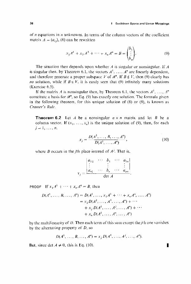
of n equations in n unknowns. In terms of the column vectors of the coefficient matrix A = (α(]), (8) can be rewritten
χ,Α1 +χ2Α2 + ···+χηΑ" = Β = [ ■ . (9)
The situation then depends upon whether A is singular or nonsingular. If A is singular then, by Theorem 6.1, the vectors A1, ..., An are linearly dependent, and therefore generate a proper subspace V of $n. If B φ K, then (9) clearly has no solution, while if B e V, it is easily seen that (9) infinitely many solutions (Exercise 6.5).
If the matrix A is nonsingular then, by Theorem 6.1, the vectors A1, . . . , An
constitute a basis for Mn, so Eq. (9) has exactly one solution. The formula given in the following theorem, for this unique solution of (8) or (9), is known as Cramer's Rule.
Theorem 6.2 Let A be a nonsingular n x n matrix and let B be a column vector. If (xl9 . . . , xn) is the unique solution of (9), then, for each y = 1, . . . , /7,
= D(A\...,B,...,An) Xj D(A\...,An)
where B occurs in they'th place instead of AJ. That is,
i i · · · * i · · ' <*\n
(10)
det A
PROOF If xxAx + ■■■ +x„A" = B, then
D(Al, ..., B, ..., A") = D(A\ ..., x,Al + ■ ■ · + χ,,Α", ..., A")
= xlD(A\...,At,...,An) + ---
+ XjD(A\...,Aj,...,An) + ···
+ xnD(A1,...,A",...,A")
by the multilinearity of D. Then each term of this sum except the/'th one vanishes by the alternating property of D, so
D(A\...,B,..., A") = Xj D(A\ ..., A\ ..., A").
But, since det A φ 0, this is Eq. (10). I
6 Determinants 39
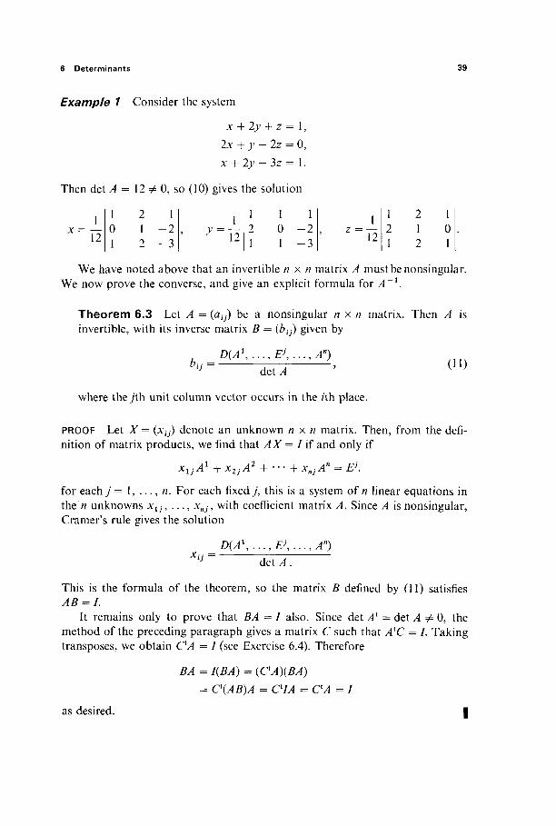
Example 1 Consider the system
x + 2y + z=\,
2x + y - 2z = 0, x + 2y- 3z = l.
Then det A = 12 Φ 0, so (10) gives the solution
* = Ï2
2 1 1 - 2 2 - 3
>> = 12
1 1 0 - 2 1 - 3
1 12
We have noted above that an invertible n x n matrix A mustbenonsingular. We now prove the converse, and give an explicit formula for A'1.
Theorem 6.3 Let A = (α^) be a nonsingular n x n matrix. Then A is invertible, with its inverse matrix B = (Z?0) given by
bls = D{A\...,E\...,An)
det A (Π)
where they'th unit column vector occurs in the /th place.
PROOF Let X = (xij) denote an unknown n x n matrix. Then, from the defi-nition of matrix products, we find that AX = I if and only if
xxjAl + x2jA
2 + · · · + xnjAn = EK
for each y = 1, . . . , n. For each fixed j , this is a system of n linear equations in the« unknowns x{j, . . . , xnj, with coefficient matrix A. Since A is nonsingular, Cramer's rule gives the solution
_D(A1,...,&,...,A") XiJ det A.
This is the formula of the theorem, so the matrix B defined by (11) satisfies AB = L
It remains only to prove that BA = I also. Since det A1 = det A Φ 0, the method of the preceding paragraph gives a matrix C such that AlC = I. Taking transposes, we obtain OA = I (see Exercise 6.4). Therefore
BA = I(BA) = (CA)(BA)
= C(AB)A =CIA =CA=I
as desired.
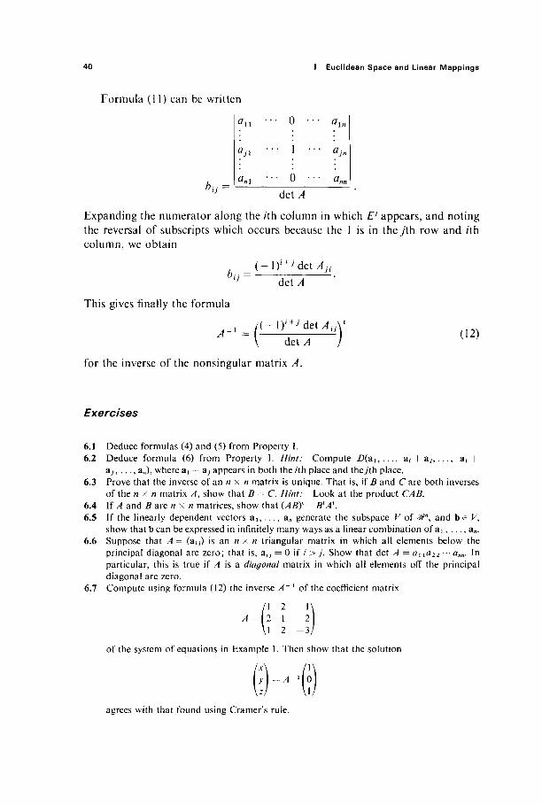
40 I Euclidean Space and Linear Mappings
Formula (11) can be written
a.n
tfyi
<*n\
... o .. . . . ! ..
. . . 0 ..
det A
a.Xn
• ajn
* <*nn
Expanding the numerator along the /th column in which Ej appears, and noting the reversal of subscripts which occurs because the 1 is in theyth row and /th column, we obtain
_ ( - l ) ' ^ d e t ^ det A
This gives finally the formula
for the inverse of the nonsingular matrix A.
Exercises
6.1 Deduce formulas (4) and (5) from Property I. 6.2 Deduce formula (6) from Property I. Hint: Compute Z) (a i , . . . , a{ 4 - a , · , . . . , a, +
âj,..., a„), where a< f a, appears in both the /th place and theyth place. 6.3 Prove that the inverse o f a n / i x n matrix is unique. That is, if B and C are both inverses
of the n x n matrix A, show that B= C. Hint: Look at the product CAB. 6.4 If A and B are n Y n matrices, show that (AB)1 =BlA\ 6.5 If the linearly dependent vectors a,, . . . , a„ generate the subspace V of atf", and be V,
show that b can be expressed in infinitely many ways as a linear combination of ax , . . . , a„. 6.6 Suppose that A = (a0) is an n x // triangular matrix in which all elements below the
principal diagonal are zero; that is, a(J = 0 if i> j . Show that det A = aua22 -·αηη· In particular, this is true if A is a diagonal matrix in which all elements off the principal diagonal are zero.
6.7 Compute using formula (12) the inverse A~ l of the coefficient matrix
(12)
Hi i :i) of the system of equations in Example 1. Then show that the solution
(Mi) agrees with that found using Cramer's rule.
7 Limits and Continuity 41
6.8 Let a, = (aii9 al2,..., ain\ i = 1 , . . . , k < n, be k linearly dependent vectors in 3Ü". Then show that every k x k submatrix of the matrix
« f c l • • • Û J k i i /
has zero determinant. 6.9 If /4 is an n x n matrix, and x and y are (column) vectors in ^", show that (Ax)·y =
X'(Aly\ and then that (Ax)-(Ay) = x-(AlAy). 6.10 The n x n matrix A is said to orthogonal if and only if A A1 = /, so /i is invertible with
A~l = A1. The linear transformation L: 3tn Mn is said to be orthogonal if and only if its matrix is orthogonal. Use the identity of the previous exercise to show that the linear transformation L is orthogonal if and only if it is inner product preserving (see Exercise 4.5)
6.11 (a) Show that the n x n matrix A is orthogonal if and only if its column vectors are othonormal. (b) Show that the n x n matrix A is orthogonal if and only if its row vectors are orthonormal.
6.12 If a i , . . . , a„ and b i , . . . , b„ are two different orthonormal bases for &n, show that there is an orthogonal transformation L:&n -> Mn with L(a,) = bf for each i = 1 , . . . , n. Hint: If A and B are the n x n matrices whose column vectors are a t , . . . , an and b 1 ? . . . , b„, re-spectively, why is the matrix BA~l orthogonal?
7 LIMITS AND CONTINUITY
We now generalize to higher dimensions the familiar single-variable defi-nitions of limits and continuity. This is largely a matter of straightforward repe-tition, involving merely the use of the norm of a vector in place of the absolute value of a number.
Let D be a subset of 0tn, a n d / a mapping of D into 0Γ (that is, a rule that associates with each point x e D a point / (x) e 0Γ). We wri te / : D -► 0tm, and call D the domain (of définition) off.
In order to define limx_>a/(x), the limit off at a, it will be necessary tha t /be defined at points arbitrarily close to a, that is, that D contains points arbitrarily close to a. However we do not want to insist that a e D, that is, tha t /be defined at a. For example, when we define the derivative f'(a) of a real-valued single-variable function as the limit of its difference quotient at a,
f (a) = hm , x^a x - a
this difference quotient is not defined at a. This consideration motivates the following definition. The point a is a limit
point of the set D if and only if every open ball centered at a contains points of D other than a (this is what is meant by the statement that D contains points
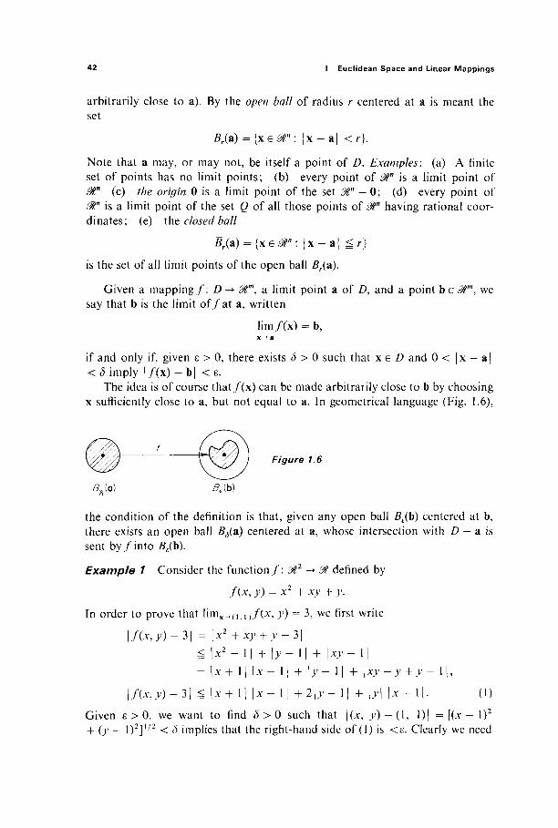
42 I Euclidean Space and Linear Mappings
arbitrarily close to a). By the open ball of radius r centered at a is meant the set
£r(a) = { x e ^ " : [ x - a | < r}.
Note that a may, or may not, be itself a point of D. Examples: (a) A finite set of points has no limit points; (b) every point of 0tn is a limit point of 0tn (c) the origin 0 is a limit point of the set 0tn — 0; (d) every point of &n is a limit point of the set Q of all those points of @tn having rational coor-dinates; (e) the closed ball
S r ( a ) = { x e f " : |x — a[ ^ r}
is the set of all limit points of the open ball £r(a).
Given a mapping/: D -> 0Γ, a limit point a of D, and a point b e 0lm, we say that b is the limit o f / a t a, written
lim/(x) = b, X - * a
if and only if, given ε > 0, there exists ô > 0 such that xe D and 0 < |x - a| < δ imply | / (x) — b| < ε.
The idea is of course that/(x) can be made arbitrarily close to b by choosing x sufficiently close to a, but not equal to a. in geometrical language (Fig. 1.6),
Figure 1.6
Bh (a) 8€{b)
the condition of the definition is that, given any open ball BE(b) centered at b, there exists an open ball /^(a) centered at a, whose intersection with D — a is sent by / in to BE(b).
Example 1 Consider the function/: $2 -> & defined by
f{x, y) = x2 + xy + y.
In order to prove that limx^(1 n / ( x , y) = 3, we first write
\f(X9y)-3\ = \χ2 +Xy+y-3\
^ \x2 - l | + \y- 1[ + \xy- l | = | χ + ΐ | \χ-ι\ + ( j ; - i | + \xy-y + y - i \ ,
\f(x,y)-3\ Z\x+l\\x-\\ + 2 | ^ - l | + b | \x-\\. (I)
Given ε > 0, we want to find δ > 0 such that |(x, y) - (l, l ) | = [(x - l)2
+ (y — l)2]1 / 2 < δ implies that the right-hand side of (I) is <ε. Clearly we need
7 Limits and Continuity 43
bounds for the coefficients |x + 11 and |>'| of \x - 11 in (1). So let us first agree to choose δ ^ 1, so
| ( x , j O - ( l , 1)[ < ( 5 = > | x - 1| < 1 and \y - 1| < 1 = > 0 < x < 2 and 0 < j ^ < 2 =>\x+ 1| < 3 and \y\ < 2,
which then implies that
1 y(^,>·) - 31 ^ 5U - 11 +2\y-l\
by (1). It is now clear that, if we take
δ = minil,-j ,
then
| ( x , ^ ) - ( l , l ) | <ô*>\f(x,y)-3\ <Ίδ = ε
as desired.
Example 2 Consider the function/: M1 -> ΡΛ defined by
—x =■ if J i ^ + V, x2-y2
0 if x = ±y.
To investigate hm(x y)^Qf(x, y), let us consider the value of / ( x , y) as (x, y) approaches 0 along the straight line y = eux. The lines y = ±x, along which f(x, y) — 0, are given by a = ± 1 . If a φ ± 1 , then
C(X2 CC / (x , ax) = -2 2~2 = 1 2 *
xz — azx 1 — a
For instance,
/ (x , 2x)=-i and / ( * , -2x ) = + $ for all x φ 0. Thus / (x , j>) has different constant values on different straight lines through 0, so it is clear that lim(JC><y)_>0/(x, y) does not exist (because, given any proposed limit b, the values — $ and + j of/cannot both be within ε of b i f e < $ ) . Example 3 Consider the function / : 0t -► ^P defined by / ( i ) = (cos i, sin t), the familiar parametrization of the unit circle. We want to prove that
lim/(0=/(0) = (l,0). r-»0
44 I Euclidean Space and Linear Mappings
Given ε > 0, we must find δ > 0 such that
\t\<ö=> [(cos t - l)2 + (sin 02]1 / 2 < ε.
In order to simplify the square root, write a = cos t — 1 and b = sin t. Then
[(cos t - l)2 + (sin 02]1 / 2 = (a2 + b2)112
^(\a\2 + 2\a\ \b\ + |Z>|2)1/2
= M + 1*1 = I cos t — 11 + [sin i | ,
so we see that it suffices to find δ > 0 such that £ £
\t\ < δ => Icos ί — 11 < - and Isin 11 < - . i i i 2 i i 2
But we can do this by the fact (from introductory calculus) that the functions cos t and sin t are continuous at 0 (where cos 0 = 1, sin 0 = 0).
Example 3 illustrates the fact that limits can be evaluated coordinatewise. To state this result precisely, consider/: D -> 0Γ, and write/(x) = (/i(x), . . . , fm(x)) e &m for each xe D. Then/ 1 ? . . . ,/m are real-valued functions on D, called as usual the coordinate functions of/, and we write / = (/l5 . . . , fm). For the function/of Example 3 we have /= (/ i , /2) where fx(t) = cos t,f2(t) = sin t, and we found that
lim/(0 = /Hm/iiO, lim/2(0) = (l, 0).
Theorem 7.1 Suppose / = (fu .. .,fm) : D ^ 0Γ, that a is a limit point of A and b = (Z>l5 . . . , bm) e 9Γ. Then
lim f(x) = b (2)
if and only if l i m / ( x ) = ^ , i = l , . . . , / i . (3) x-+a
PROOF First assume (2). Then, given ε > 0, there exists δ > 0 such that xe D and 0 < |x — a| < δ imply that | / (x) — b| < ε. But then
0 < | x - a | < δ = > | / ί ( χ ) - * ί | ^ | / ( x ) - b | < ε ,
so (3) holds for each i = 1, . . . , m. Conversely, assume (3). Then, given ε < 0, for each / = 1, . . . , m there exists
a δι > 0 such that
xeD and 0 < |x - a| < δ{ =>|/(x) - bt\ < - ^ - . (4)
7 Limits and Continuity 45
If we now choose <5 = m i n ^ , . . . , ôm), then xe D and
11/2 0 < |x - a[ < 5 => |/(x) - b| = Σ ΙΛχ) - bt\
L» = 1
< (m · —I = ε
by (4), so we have shown that (3) implies (2). |
The student should recall the concept of continuity introduced in single-variable calculus. Roughly speaking, a continuous function is one which has nearby values at nearby points, and thus does not change values abruptly. Precisely, the function/: D -► $m is said to be continuous at a e D if and only if
lim/(x) = / (a ) . (5) x->a
/ i s said to be continuous on D (or, simply, continuous) if it is continuous at every point of D.
Actually we cannot insist upon condition (5) if a e Dis not a limit point of D, for in this case the limit of/at a cannot be discussed. Such a point, which belongs to D but is not a limit point of D, is called an isolated point of D, and we remedy this situation by including in the definition the stipulation that / i s automatically continuous at every isolated point of D.
Example 4 If D is the open ball ^i(O) together with the point (2, 0), then any function/on D is continuous at (2, 0), while/is continuous at a e ^ ( 0 ) if and only if condition (5) is satisfied.
Example 5 If D is the set of all those points (x, y) of ^ 2 such that both Λ; and y are integers, then every point of D is an isolated point, so every function on D is continuous (at every point of D).
The following result is an immediate corollary to Theorem 7.1.
Theorem 7.2 The mapping/: D -> £%m is continuous at a G D if and only if each coordinate function of/ is continuous at a.
Example 6 The identity mapping π : 0ln -> 0tn, defined by π(χ) = x, is ob-viously continuous. Its z'th coordinate function, ni{x1, ..., xn) = xi9 is called the ith projection function, and is continuous by Theorem 7.2.
Example 7 The real-valued functions s and p on 011, defined by s(x, y) = x + y and p(x, y) = xy, are continuous. The proofs are left as exercises.

46 I Euclidean Space and Linear Mappings
The continuity of many mappings can be established without direct recourse to the definition of continuity—instead we apply the known continuity of the elementary single-variable functions, elementary facts such as Theorem 7.2 and Examples 6 and 7, and the fact that a composition of continuous functions is continuous. Given / : Dx -> 0Γ and g : D2^> @k, where Z)x cz âtn and D2
c Mm, the composition
gof: D-+@k
of/and g is defined as usual by g °/(x) = g(f(x)) for all x e 0tn such that x e D{
and/(x) G D2. That is, the domain of g o / is
D = { x e f : X G Dl and / (x) e D2}.
(This is simply the set of all x such that g(f(x)) is meaningful.)
Theorem 7.3 If/ is continuous at a and g is continuous at / (a) , then g°fis continuous at a.
This follows immediately from the following lemma [upon setting b =/(a)] .
Lemma 7.4 G i v e n / : Dl -> 0Γ and g\D2^mk where DY^mn and D2 a ^m , suppose that
lim/(x) = b, (6)
and that
g is continuous at b. (7)
Then
lim0o/(x) =g(b). x-+a
PROOF Given ε > 0, we must find δ > 0 suchthat \g(f(x))—g(b)\ < ε if 0 < |x — a | < δ and xe D, the domain of g of. By (7) there exists η > 0 such that
ye£>2 and |y - b | < η => \g(y) - g(b)\ < e. (8)
Then by (6) there exists δ > 0 such that
x e D j and 0 < |x - a| < δ => | / (x) - b | < η.
But then, upon substituting y = / (x ) in (8), we obtain
XGD and 0 < |x - a| < δ => \g(f(x)) -g(b)\ < ε
as desired. |
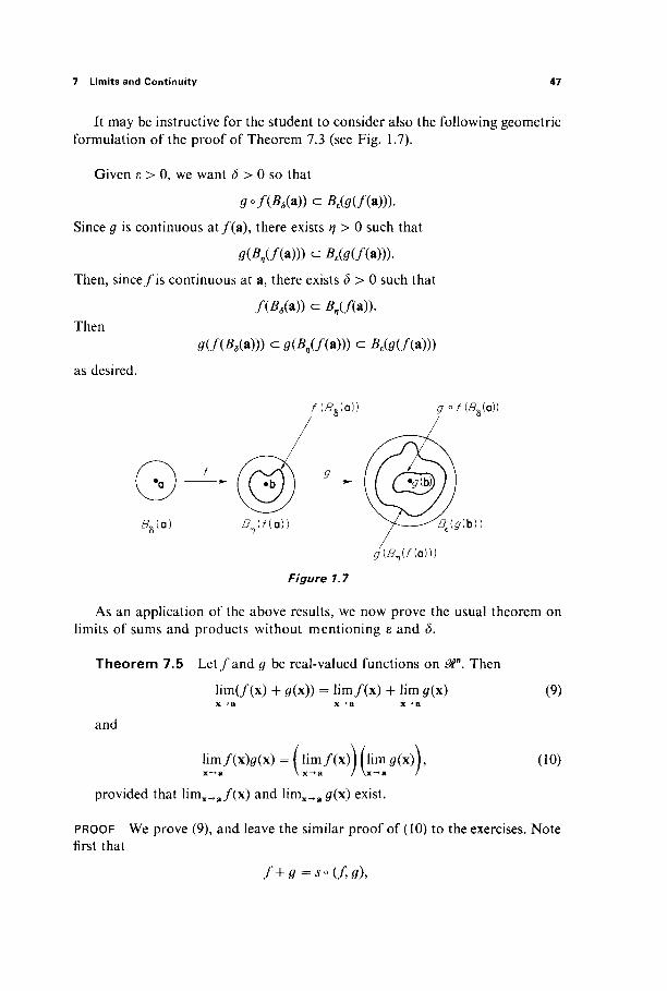
7 Limits and Continuity 47
It may be instructive for the student to consider also the following geometric formulation of the proof of Theorem 7.3 (see Fig. 1.7).
Given ε > 0, we want δ > 0 so that
ff°/(Äa(a))<=5.(0(/(a))).
Since g is continuous at / (a) , there exists η > 0 such that
g(Bn(f(m «= BMA*)))-Then, since / i s continuous at a, there exists δ > 0 such that
/(Äa(a)) c £„(/(a)). Then
as desired.
gUXBM))) =9(Βη(/(a))) c Bt{g(fW))
f{BAo) g ofiSia))
8h(o) BAgib)
giß^fiQ)
Figure 1.7
As an application of the above results, we now prove the usual theorem on limits of sums and products without mentioning ε and δ.
Theorem 7.5 Le t / and g be real-valued functions on @tn. Then
lim(/(x) + g(x)) = lim/(x) + lim g(x) (9) x->a x->a x-»a
and
lim/(x)0(x) = ( lim/(x)) (lim g(x)Y (10) x->a \ x->a / \x->a /
provided that limx_>a/(x) and limx^a#(x) exist.
PROOF We prove (9), and leave the similar proof of (10) to the exercises. Note first that
f+9 =*°(f,g)9
48 I Euclidean Space and Linear Mappings
where s(x, y) = x + j ; is the sum function on &2 of Example 7. If
bl = lim/(x) and b2 = lim g(x), x-»a x-*a
then limx^a (/(x), g(x)) = {bu b2) by Theorem 7.1, so
lim(/(x) + 0(x)) = lim j(/(x), g(x)) x-*a x->a
= s(bl,b2) = bx+b2
= lim/(x) + lim^(x) x->a x->a
by Lemma 7.4. |
Example 8 It follows by mathematical induction from Theorem 7.5 that a sum of products of continuous functions is continuous. For instance, any linear real-valued function
n
/ ( * ! , ...,X„)= ^ Ο , Χ , · , ι = 1
or polynomial in xl, . . . , xn, is continuous. It then follows from Theorem 7.1 that any linear mapping L : 0tn -> 0tm is continuous.
Example 9 To see that f:t%3-+&, defined by f(x, y, z) = sin(x + cos;z), is continuous, note that
/ = sin o (s o (π ι , cos ° p ° (π2 , π3))),
where π1? π2 , π3 are the projection functions on ^ 3 , and j and/? are the sum and product functions on M1.
Exercises
7.1 Verify that the functions s and p of Example 7 are continuous. ////7/: xy — x0y0 = (xy - xy0) + (*y0 - -Wo).
7.2 Give an ε — δ proof that the function f-M2* ^M defined by / ( * , y, z) = x2y + 2.YZ2 is continuous at (1, 1, 1). Hint: x2y + 2xz2 - 3 = (x2y - y) + O - 1 ) + (2xz2 - 2x) + (2* - 2).
7.3 Iff(x, y) = (x2 - y2)/(x2 + j>2) unless * = y = 0, and/(0 , 0) = 0, show that f\@2^m is not continuous at (0, 0). Hint: Consider the behavior of f on straight lines through the origin.
7.4 Let / ( * , y) =2x2y/(x* + y2) unless * = j> = 0, and / (0 , 0) - 0. Define <p(r) = (/, at) and 0(0 = (/,/2). (a) Show that l imt^o/(c>(0) = 0. Thus / i s continuous on any straight line through (0, 0). (b) Show that \imt^0f(ifj(t)) = 1- Conclude t h a t / i s not continuous at (0, 0).
7.5 Prove the second part of Theorem 7.5. 7.6 The point a is called a boundary point of the set D <= Mn if and only if every open ball
centered at a contains both a point of D and a point of the complementary set 0tn — D.

8 Elementary Topology of £%n 49
For example, the set of all boundary points of the open ball Br(p) is the sphere Sr(p) = {xe^ n : |x — p| = r}. Show that every boundary point of D is either a point of D or a limit point of D.
7.7 Let D* denote the set of all limit points of the set D*. Then prove that the set D u i ) * contains all of its limit points.
7.8 Let f\ &" -> @m be continuous at the point a. If {a„} ? is a sequence of points of ^" which converges to a, prove that the sequence {/(a,,)}? converges to the point/(a).
8 ELEMENTARY TOPOLOGY OF Stn
In addition to its linear structure as a vector space, and the metric structure provided by the usual inner product, Euclidean /7-space 0tn possesses a topo-logical structure (defined below). Among other things, this topological structure enables us to define and study a certain class of subsets of 0tn, called compact sets, that play an important role in maximum-minimum problems. Once we have defined compact sets, the following two statements will be established.
(A) If D is a compact set in 0tn, a n d / : D -> $m is continuous, then its image/(D) is a compact set in 0Γ (Theorem 8.7).
(B) If C is a compact set on the real line 01, then C contains a maximal element b, that is, a number b e C such that x ^ b for all x e C.
It follows immediately from (A) and (B) that, / / / : D -* 01 is a continuous real-valued function on the compact set D c 0ln, thenf(x) attains an absolute maximum value at some point a e D. For if b is the maximal element of the compact set f{D) cz ^ , and a is a point of D such that/(a) = b, then it is clear that/(a) = b is the maximum value attained by/(x) on D. The existence of maximum (and, similarly, minimum) values for continuous functions on compact sets, together with the fact that compact sets turn out to be easily recognizable as such (Theo-rem 8.6), enable compact sets to play the same role in multivariable maximum-minimum problems as do closed intervals in single-variable ones.
By a topology (or topological structure) for the set S is meant a collection £T of subsets, called open subsets of S, such that F satisfies the following three conditions:
(i) The empty set 0 and the set 5 itself are open. (ii) The union of any collection of open sets is an open set.
(iii) The intersection of a finite number of open sets is an open set.
The subset A of ffin is called open if and only if, given any point ae^ l , there exists an open ball £r(a) (with r > 0) which is centered at a and is wholly con-tained in A. Put the other way around, A is open if there does not exist a point SLEA such that every open ball £r(a) contains points that are not in A. It is
50 I Euclidean Space and Linear Mappings
easily verified that, with this definition, the collection of all open subsets of 0in
satisfies conditions (i)-(iii) above (Exercise 8.1). Examples (a) An open interval is an open subset of 01, but a closed interval
is not. (b) More generally, an open ball in 0tn is an open subset of 0tn (Exer-cise 8.3) but a closed ball is not (points on the boundary violate the definition). (c) If F is a finite set of points in 0tn, then 0tn — F is an open set. (d) Al-though 01 is an open subset of itself, it is not an open subset of the plane 0l2.
The subset B of 0Γ is called closed if and only if its complement 0tn — B is open. It is easily verified (Exercise 8.2) that conditions (i)-(iii) above imply that the collection of all closed subsets of 0ln satisfies the following three analogous conditions:
(i') 0 and 0tn are closed. (ii') The intersection of any collection of closed sets is a closed set.
(iii') The union of a finite number of closed sets is a closed set.
Examples: (a) A closed interval is a closed subset of 01. (b) More generally, a closed ball in 0tn is a closed subset of 0tn (Exercise 8.3). (c) A finite set F of points is a closed set. (d) The real line 01 is a closed subset of 0l2. (e) If A is the set of points of the sequence {l/w}?\ together with the limit point 0, then A is a closed set (why?)
The last example illustrates the following useful alternative characterization of closed sets.
Proposition 8.1 The subset A of0ln is closed if and only if it contains all of its limit points.
PROOF Suppose A is closed, and that a is a limit point of A. Since every open ball centered at a contains points of A, and 0tn — A is open, a cannot be a point of 0ln - A. Thus a e A.
Conversely, suppose that .4 contains all of its limit points. If be &n - A, then b is not a limit point of A, so there exists an open ball Br(b) which contains no points of A. Thus 0tn — A is open, so A is closed. |
If, given A c ^", we denote by Ä the union of A and the set of all limit points of A, then Proposition 8.1 implies that A is closed if and only if A = A.
The empty set 0 and 0tn itself are the only subsets of 0ln that are both open and closed (this is not supposed to be obvious—see Exercise 8.6). However there are many subsets of 0tn that are neither open nor closed. For example, the set Q of all rational numbers is such a subset of 01.
The following theorem is often useful in verifying that a set is open or closed (as the case may be).

8 Elementary Topology of 0tn 51
Theorem 8.2 The mapping / : ^Γ -> 9tm is continuous if and only if, given any open set U a @m, the inverse image/" 1(U) is open in 0tn. Also,/is continuous if and only if, given any closed set C c 0Γ, f~1(C) is closed i n ^ n .
PROOF The inverse image f~\U) is the set of points in Stn that map under / into U, that is,
f-\U)={xe®n:f(x)eU}.
We prove the "only if" part of the Theorem, and leave the converse as Exercise 8.4.
Suppose/is continuous. If U a &m is open, and a e / ~ *(£/), then there exists an open ball 2?r(/(a)) c U. Since / is continuous, there exists an open ball ^ ( a ) such that / ( ^ ( a ) ) c Brtf(&)) c U. Hence ^ ( a ) cf~\V)\ this shows that / _ 1 (£ / ) i s open.
If C c ^ m is closed, then 0tm - C is open, s o / _ 1 ( ^ m - C) is open by what has just been proved. B u t / _ 1 ( ^ m - C) =Stn -f~\C\ so it follows tha t / _ 1 (C) is closed. |
As an application of Theorem 8.2, l e t / : 0tn -> 01 be the continuous mapping defined by/(x) = |x — a|, where a e 0tn is a fixed point. Then / _ 1 ( ( —r, r)) is the open ball #r(a), so it follows that this open ball is indeed an open set. Also / _ 1 ( [0 5 r]) = ^r(a)» s o t n e closed ball is indeed closed. Finally,
f-\r) = Sr(*)={xe<Xn: | x - a | = r},
so the (« — l)-sphere of radius r, centered at a, is a closed set.
The subset A of ^ " is said to be compact if and only if every infinite subset of A has a limit point which lies in A. This is equivalent to the statement that every sequence of points of A has a subsequence {ajf which converges to a point a e Λ. (This means the same thing in ^ " as on the real line: Given δ > 0, there exists N such that « ^ TV => |a„ — a| < ε.) The equivalence of this statement and the definition is just a matter of language (Exercise 8.7).
Examples: (a) 01 is not compact, because the set of all integers is an infinite subset of ^? that has no limit point at all. Similarly, 0tn is not compact. (b) The open interval (0, 1) is not compact, because the sequence {l/n}f is an infinite subset of (0, 1) whose limit point 0 is not in the interval. Similarly, open balls fail to be compact, (c) If the set F is finite, then it is automatically compact because it has no infinite subsets which could cause problems.
Closed intervals do not appear to share the problems (in regard to compact-ness) of open intervals. Indeed the Bolzano-Weierstrass theorem says precisely that every closed interval is compact (see the Appendix). We will see presently that every closed ball is compact. Note that a closed ball is both closed and bounded, meaning that it lies inside some ball £r(0) centered at the origin.

52 I Euclidean Space and Linear Mappings
Lemma 8.3 Every compact set is both closed and bounded.
PROOF Suppose that A a &n is compact. If a is a limit point of A then, for each integer n, there is a point a„ such that |a„ — a| < l/n. Then the point a is the only limit point of the sequence {a„}J°. But, since A is compact, the infinite set {a„}f must have a limit point in A. Therefore aeA, so it follows from Proposition 8.1 that A is closed.
If A were not bounded then, for each positive integer n, there would exist a point bneA with |bn[ > n. But then {bjf would be an infinite subset of A having no limit point (Exercise 8.8), thereby contradicting the compactness oiA. |
Lemma 8.4 A closed subset of a compact set is compact.
PROOF Suppose that A is closed, B is compact, and A c B. If S is an infinite subset of A, then S has a limit point be B, because B is compact. But be A also, because b is a limit point of A, and A is closed. Thus every infinite subset of A has a limit point in A, so A is compact. |
In the next theorem and its proof we use the following notation. Given x = (xl9 . . . , xj e 0Γ and y = (yl9 . . . , yn) e mn
9 write (x, y) = (xl9 . . . , xm,yl9
. . . , yn) e @m+n. If A c ^ m and 5 c @n9 then the Cartesian product
A x B = {(a, b)e@m+n:*eA and b e B}
is a subset of @m + n.
Theorem 8.5 If A is a compact subset of Mm and i? is a compact subset of 9tn
9 then ,4 x £ is a compact subset of @m+n.
PROOF Given a sequence {c,}f ={(af, b,)}f of points of A x B, we want to show that it has a subsequence converging to a point of A x /?. Since Λ is compact, the sequence {a,·}?^ has a subsequence {a^JLi which converges to a point Sie A. Since B is compact, the sequence {!>/_.}*= i has a subsequence {b(/;k)}^= { which converges to a point be B. Then {(a(/Jk), b(ijk))}j?= { is a sub-sequence of the original sequence {(af, b , ) ^ } which converges to the point (a, b) e A x B. |
We are now ready for the criterion that will serve as our recognition test for compact sets.
Theorem 8.6 A subset of 0tn is compact if and only if it is both closed and bounded.
PROOF We have already proved in Lemma 8.3 that every compact set is closed and bounded, so now suppose that A is a closed and bounded subset of 0tn.

8 Elementary Topology of ^ " 53
£Λ(0)
Figure 1.8
Choose r > 0 so large that A c £r(0). (See Fig. 1.8.) If / = [-r, r], then A is a closed subset of the product / x / x · · · x / (n factors), which is compact by repeated application of Theorem 8.5. It therefore follows from Lemma 8.4 that A is compact. |
For example, since spheres and closed balls are closed and bounded, it follows from the theorem that they are compact.
We now prove statement (A) at the beginning of the section.
Theorem 8.7 If A is a compact subset of ffln, a n d / : A ous, then/(v4) is a compact subset of ^ m .
is continu-
PROOF Given an infinite set T of points off(A), we want to prove that T con-tains a sequence of points which converges to a point of f(A). If 5 =f~1(T)i
then Sis an infinite set of points of A. Since A is compact, S contains a sequence {&„}f of points that converges to a point a e A. Since / is continuous, {/(an)}5° is then a sequence of points of T that converges to the point / (a) ef(A) (see Exercise 7.8). Therefore/(Λ) is compact. |
Statement (B) will be absorbed into the proof of the maximum-minimum value theorem.
Theorem 8.8 If D is a compact set in 0tn, and / : D -► 0t is a continuous function, then / attains maximum and minimum values at points of D. That is, there exist points a and b of D such that /(a) ^ / ( x ) S /(b) for all x e D .
PROOF We deal only with the maximum value; the treatment of the minimum value is similar. By the previous theorem,/(D) is a compact subset of ^?, and is therefore closed and bounded by Theorem 8.6. Then / (D) has a least upper bound b, the least number such that t :g b for all t ef(D) (see the Appendix). We want to show that b e f(D). Since b is the least upper bound for f(D), either b ef(D) or, for each positive integer n, there exists a point tn ef(D) with b — \\n < tn< b. But then the sequence {tn}f of points of/(D) converges to b, so b is a limit point of/(D). Since/(D) is closed, it follows that b e / (D) as desired. If now b e D is a point such that /(b) = b, it is clear that / (x) è / ( b ) for all x e D . |
54 I Euclidean Space and Linear Mappings
For example, we now know that every continuous function on a sphere or closed ball attains maximum and minimum values.
Frequently, in applied maximum-minimum problems, one wants to find a maximum or minimum value of a continuous function/: D -> 01 where D is not compact. Often Theorem 8.8 can still be utilized. For example, suppose we can find a compact subset C of D and a number c such that f(x) ^ c for all x e D — C, whereas/attains values less than c at various points of C. Then it is clear that the minimum of /on C, which exists by Theorem 8.8, is also its mini-mum on all of D.
Two additional applications of compactness will be needed later. Theorem 8.9 below gives an important property of continuous functions defined on compact sets, while the Heine-Borel theorem deals with coverings of compact sets by open sets.
First recall the familiar definition of continuity: The mapping/: D -» $ is continuous if, given a e D and ε > 0, there exists δ > 0 such that
xe D, | x — a| < <5 => | / (x) - / ( a ) | < ε.
In general, ô will depend upon the point a e D . If this is not the case, t hen / i s called uniformly continuous on D. That i s , / : D -> & is uniformly continuous if, given ε > 0, there exists δ > 0 such that
x, ye A [x-y| <<5=>|/(x)-/(y)| < ε · Not every continuous mapping is uniformly continuous. For example, the
function / : (0, 1) -> & defined by f(x) = \/x is continuous but not uniformly continuous on (0, 1) (why?).
Theorem 8.9 If / : C-> & is continuous, and C c &n is compact, then / i s uniformly continuous on C.
PROOF Suppose, to the contrary, that there exists a number ε > 0 such that, for every positive integer n, there exist two points x„ and y„ of C such that
\xn-yn\ <\/n while |/(x„) - / ( y „ ) | ^ ε.
Since C is compact we may assume, taking subsequences if necessary, that the sequences {xj^and {yn}f both converge to the point a e C . But then we have an easy contradiction to the continuity o f / a t a. |
The Heine-Borel theorem states that, if C is a compact set in 0ln and {Ua}aeA
is a collection of open sets whose union contains C, then there is a finite sub-collection Uai, . . . , Uak of these open sets whose union contains C. We will assume that the collection {Ua}aeA is countable (although it turns out that this assumption involves no loss of generality). So let {Uk}™=l be a sequence of open sets such that C c \J?=l Uk. If Vk = (J*=i Ut for each k>\, then {Vk}«> is an
8 Elementary Topology of £%n 55
increasing sequence of sets—that is, Vk c Vk+i for each k ^ 1—and it suffices to prove that C c Vk for some integer k.
Theorem 8.10 Let C be a compact subset of 0Ln, and let {Vk}f be an increasing sequence of open subsets of 0tn such that C c (J^°= t Vk. Then there exists a positive integer /: such that C a Vk.
PROOF To the contrary suppose that, for each k ^ l, there exists a point xk of C that is not in Vk. Then no one of the sets {Vk}f contains infinitely many of the points {xj? (why?).
Since C is compact, we may assume (taking a subsequence if necessary) that the sequence {xjf converges to a point x0 e C. But then x0 e Vk for some k, and since the set Vk is open, it must contain infinitely many elements of the sequence {xk}f. This contradiction proves the theorem. |
Exercises
8.1 Verify that the collection of all open subsets of 0tn satisfies conditions (i)—(iii). 8.2 Verify that the collection of all closed subsets of &n satisfies conditions (i')—(iii'). Hint: If
{Aa} is a collection of subsets of @n, then @n - IJ Aa = f| (ßn — Aa) and
8.3 Show, directly from the definitions of open and closed sets, that open and closed balls are respectively open and closed sets.
8.4 Complete the proof of Theorem 8.2. 8.5 The point a is called a boundary point of the set A if and only if every open ball centered at
a intersects both A and Mn — A. The boundary of the set A is the set of all of its boundary points. Show that the boundary of A is a closed set. Noting that the sphere Sr(p) is the boundary of the ball i?r(p), this gives another proof that spheres are closed sets.
8.6 Show that 3tn is the only nonempty subset of itself that is both open and closed. Hint: Use the fact that this is true in the case n = 1 (see the Appendix), and the fact that £%n is a union of straight lines through the origin.
8.7 Show that A is compact if and only if every sequence of points of A has a subsequence that converges to a point of A.
8.8 If |b„ | > n for each n, show that the sequence {b„}T has no limit. 8.9 Prove that the union or intersection of a finite number of compact sets is compact. 8.10 Let {An}™ be a decreasing sequence of compact sets (that is, An + 1 <= A„ for all n). Prove
that the intersection Π^°=ι ^« ^s compact and nonempty. Give an example of a decreasing sequence of closed sets whose intersection is empty.
8.11 Given two sets C and D in 0tn, define the distance d(C, D) between them to be the greatest lower bound of the numbers | a — b | for a e C and b G D. If a is a point of &n and D is a closed set, show that there exists d e £ ) such that d(a, D) = | a — d |. Hint: Let B be an appropriate closed ball centered at a, and consider the continuous function f:BnD-+& defined by / (x) = | x — a |.
8.12 If C is compact and D is closed, prove that there exist points ce C and d e D such that d(C, D) = |c — d|. Hint: Consider the continuous function f:C->3?" defined by f(x) = d(x9 D).

π Multivariable Differential Calculus
Our study in Chapter I of the geometry and topology of 0tn provides an adequate foundation for the study in this chapter of the differential calculus of mappings from one Euclidean space to another. We will find that the basic idea of multivariable differential calculus is the approximation of nonlinear mappings by linear ones.
This idea is implicit in the familiar single-variable differential calculus. If the function / : $-± M is differentiable at a, then the tangent line at (a, f(a)) to the graph y =f(x) in 011 is the straight line whose equation is
y-f(a)=f\a){x-a).
The right-hand side of this equation is a linear function of x — a; we may regard
y
56
Figure 2.1
1 Curves in ffl 57
it as a linear approximation to the actual change f(x) —f(a) in the value of / between a and x. To make this more precise, let us write h = x — a, Afa(h) = f(a + h)-f(a), and dfa{h) =f'{a)h (see Fig. 2.1). The linear mapping dfa: 01 -► 0t, defined by dfa(h) = f'(a)h, is called the differential o f / a t a; it is simply that linear mapping 01 -► 01 whose matrix is the derivative f {a) o f / a t a (the matrix of a linear mapping ^ -► 01 being just a real number). With this ter-minology, we find that when h is small, the linear change dfa(h) is a good approxi-mation to the actual change Afa(h), in the sense that
r Afa(h) - dfa(h) f{a + h)-f(a)-f(a)h lim = lim = 0. /i-o h h^o h
Roughly speaking, our point of view in this chapter will be that a mapping f\0tn-+ 0Γ is (by definition) differentiable at a if and only if it has near a an appropriate linear approximation dfa : 0tn -* $m. In this case dfa will be called the differential o f / a t a; its (m x n) matrix will be called the derivative off at a, thus preserving the above relationship between the differential (a linear mapping) and the derivative (its matrix). We will see that this approach is geometrically well motivated, and permits the basic ingredients of differential calculus (for example, the chain rule, etc.) to be developed and utilized in a multivariable setting.
1 CURVES IN 0lm
We consider first the special case of a mapping/ : 0l^0im. Motivated by curves in 01 and 01*, one may think of a curve in 0Γ, traced out by a moving point whose position at time t is the poin t / (0 e 0tm, and attempt to define its velocity at time t. Just as in the single-variable case, m = l, this problem leads to the definition of the derivative f off. The change in position of the particle from time a to time a + h is described by the vector f(a + h) —f(a), so the average velocity of the particle during this time interval is the familiar-looking difference quotient
f(a + h)-f(a) h
whose limit (if it exists) as h -> 0 should (by definition) be the instantaneous velocity at time a. So we define
,,, , r f(a + h)-f(a) f(a) = hm (1)
if this limit exists, in which case we say that / is differentiable at a G 01. The derivative vector/ '(a) of / at a may be visualized as a tangent vector to the
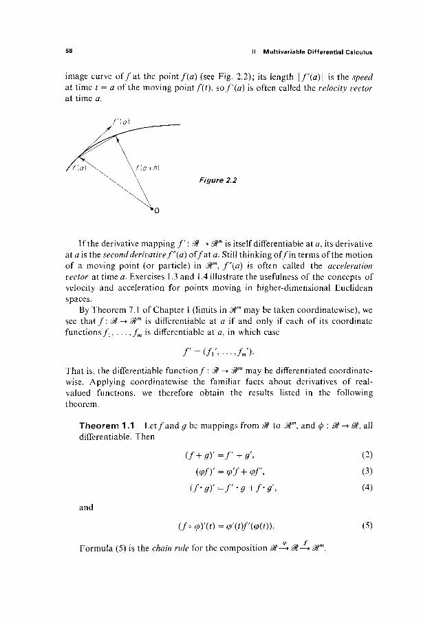
58 II Multivariable Differential Calculus
image curve o f / a t the pointf(a) (see Fig. 2.2); its length \f'(a)\ is the speed at time t = a of the moving point/(i), so/ '(#) is often called the velocity vector at time a.
f\a)
Figure 2.2
If the derivative mapping / ' : 01 -> $m is itself differentiate at #, its derivative at a is the second derivative f"{a) of /at Ö. Still thinking of/in terms of the motion of a moving point (or particle) in 0tm, f'\a) is often called the acceleration vector at time a. Exercises 1.3 and 1.4 illustrate the usefulness of the concepts of velocity and acceleration for points moving in higher-dimensional Euclidean spaces.
By Theorem 7.1 of Chapter I (limits in 0Γ may be taken coordinatewise), we see that / : 01-* 0Γ is differentiate at a if and only if each of its coordinate functions/, . . . , /m is differentiable at a, in which case
/ ' = ( / l ' , . . . J / m ' ) .
That is, the differentiable function/ : 01 -► $m may be differentiated coordinate-wise. Applying coordinatewise the familiar facts about derivatives of real-valued functions, we therefore obtain the results listed in the following theorem.
Theorem 1.1 Let /and g be mappings from 01 to 0Γ, and φ : & -► 01, all differentiable. Then
(f+g)'=f'+9', (2) (<pfY = <p'f+<pf, (3)
(f-g)'=f'-g+/·*', (4)
and
(/o ψ)'(ΐ) = (p'(t)f'(q>(t)). (5)
Ψ f Formula (5) is the chain rule for the composition 0ί—+01—*0Γ.
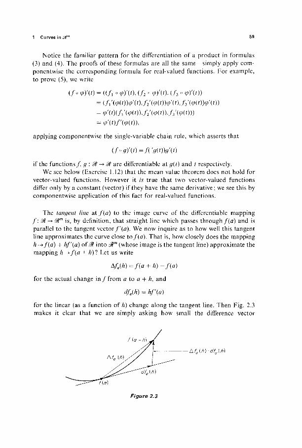
1 Curves in ^ 59
Notice the familiar pattern for the differentiation of a product in formulas (3) and (4). The proofs of these formulas are all the same—simply apply com-ponentwise the corresponding formula for real-valued functions. For example, to prove (5), we write
(fo φ)\ή = ((fx o φ)'(ί) , ( /2 o φ ) ' ( ί ) , ( /3 o φ) '( , ))
= (/ι'(φ(ί))φ'(ΐ\/2'(φ(ΐ))φ'(ΐ\/3'(φ(ί))φ'(ή)
= φ'(0(/ι,(φ(0),/2/(<Ρ(0),/3'(φ(0)) = φ W'MO),
applying componentwise the single-variable chain rule, which asserts that
(f°g)'(t)=f('g(t))g'(t)
if the functions/, g : 01 -► 01 are differentiate at g(t) and t respectively. We see below (Exercise 1.12) that the mean value theorem does not hold for
vector-valued functions. However it is true that two vector-valued functions differ only by a constant (vector) if they have the same derivative; we see this by componentwise application of this fact for real-valued functions.
The tangent line at f(a) to the image curve of the differentiate mapping f\0t-+0T is, by definition, that straight line which passes through f(a) and is parallel to the tangent vector/'(a). We now inquire as to how well this tangent line approximates the curve close to f{a). That is, how closely does the mapping A -+f(a) + hf'(a) of 01 into 0Γ (whose image is the tangent line) approximate the mapping h-+f(a + A)? Let us write
Δ/β(Λ)=/(α+ * ) - / ( * )
for the actual change in / f rom a to a + A, and
dfa{h) = hf'(a)
for the linear (as a function of A) change along the tangent line. Then Fig. 2.3 makes it clear that we are simply asking how small the difference vector
/\fa(h)-dfa(h)
f {0 +h)M
^ — n o )
Figure 2.3
60 II Multivariable Differential Calculus
A/L(A) — dfa(h) is when A is small. The answer is that it goes to zero even faster than A does. That is,
Γ Δ/β(Α) - dfa(h) f(a + h)-f(a)-hf\a) lim = lim Λ-ο A /,->o A
I f(a + h)-f(a)\ = hm -f (a)
\ Λ - Ο A /
= 0
by the definition off (a). Noting that dfa: 01 -► ^ m is a linear mapping, we have proved the "only if" part of the following theorem.
Theorem 1.2 The mapping / : M -> $m is differentiable at a e M if and only if there exists a linear mapping L : M -► ^?m such that
r f{a + h)-f(a)-L(h) hm = 0, (6) Λ-0 A
in which case L is defined by L(h) = dfa(h) = hf'(a).
To prove the " if" part, suppose that there exists a linear mapping satisfying (6). Then there exists b e l m such that L is defined by L(h) = Ab; we must show that f'(a) exists and equals b. But
f(a + A) - / ( a ) / f(a + A) - / ( a ) - Ab\ hm = I hm 1 + b = b h^o A \h^o A /
by (6). |
Iff: &->&m is differentiable at a, then the linear mapping df^ : M -> ^m, defined by #fl(A) = hf'(a), is called the differential o f / a t a. Notice that the derivative vector f'(a) is, as a column vector, the matrix of the linear mapping dfa, since
rf/e(A) = A/'(e) = ! (A). \ / . ' (e) /
When in the next section we define derivatives and differentials of mappings from 0tn to ^ m , this relationship between the two will be preserved—the dif-ferential will be a linear mapping whose matrix is the derivative.
The following discussion provides some motivation for the notation dfa for the differential o f / a t a. Let us consider the identity function 9t-*0t, and write x for its name as well as its value at x. Since its derivative is 1 everywhere, its differential at a is defined by
dxa(h) = 1 · A = A.
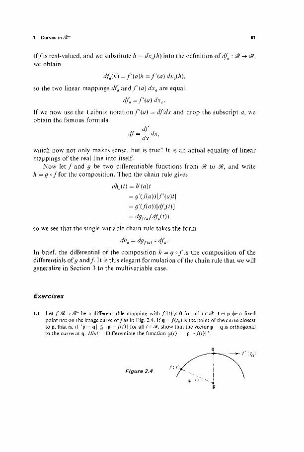
1 Curves in « ' 61
If/is real-valued, and we substitute h = dxa{h) into the definition oïdfa\ 0l^> 01, we obtain
dfa(h)=f'(ä)h=f'(a)dxa(h\
so the two linear mappings dfa and/ '(#) dxa are equal,
dfa=f'(à)dxa.
If we now use the Leibniz notation f'(a) = dfldx and drop the subscript a, we obtain the famous formula
df=fdx, dx
which now not only makes sense, but is true! It is an actual equality of linear mappings of the real line into itself.
Now let / and g be two differentiate functions from M to 0t, and write h= g of for the composition. Then the chain rule gives
dha(t) = h'(a)t
= g\M)[f'{a)t]
= g'(M)[dfa{t)}
= dgf(a)(dfa(t)),
so we see that the single-variable chain rule takes the form
dha = dgf{a) o dfa.
In brief, the differential of the composition h = g ° / i s the composition of the differentials of g and/. It is this elegant formulation of the chain rule that we will generalize in Section 3 to the multivariable case.
Exercises
1.1 Let f:@ - > ^ n be a differentiable mapping with f'(t) φ 0 for all t e &. Let p be a fixed point not on the image curve o f / a s in Fig. 2.4. If q = f(t0) is the point of the curve closest to p, that is, if | p — q | ^ | p — f(t) | for all / e &, show that the vector p — q is orthogonal to the curve at q. Hint: Differentiate the function φ(ί) = | p —f(t) | 2.
Figure 2.4
II Multivariable Differential Calculus
(a) Let / : <M -> ®n and g : M -> mn be two diflferentiable curves, with fit) Φ 0 and g\t) Φ 0 for all teM. Suppose the two points p=f(s0) and (\ = g(t0) are closer than any other pair of points on the two curves. Then prove that the vector p — q is orthogonal to both velocity vectors f'(s0) and g\t0). Hint: The point (s0, t0) must be a critical point for the function p:M2^3i defined by p(s, t) = \f(s) - g(t) | 2. (b) Apply the result of (a) to find the closest pair of points on the " skew " straight lines in ^ 3 defined by fis) = (s, 25, - s ) and git) = (t + 1, t - 2, It + 3). Let F: &n - > ^ " b e a conservative force field on ^" , meaning that there exists a continuously differentiable potential function V\@tn^0l such that F(x) = — VK(x) for all x e ^ " [recall that VV = (dV/dxl,..., dV/dxn)]. Call the curve < p : J ^ ^ " a " q u a s i - N e w t o n i a n particle" if and only if there exist constants mly m2, · . . , mn, called its " mass components," such that
F,(9>(0) = ml,<pt"(t) (F=ma)
for each / = 1, . . . , n. Thus, with respect to the xrdirection, it behaves as though it has mass mt. Define its kinetic energy K{t) and potential energy Pit) at time t by
K(t) = i t mtbpiV)]2, P(t) = ν(ψ{ί)\ i= 1
Now prove that the law of the conservation of energy holds for quasi-Newtonian particles, that is, K + P = constant. Hint: Differentiate K(t) + Pit), using the chain rule in the form P'(t) = W(<p(t))-cp'(t), which will be verified in Section 3. (n-body problem) Deduce from Exercise 1.3 the law of the conservation of energy for a system of n particles moving in M2 (without colliding) under the influence of their mutual gravitational attractions. You may take n = 2 for brevity, although the method is general. Hint: Denote by wij and m2 the masses of the two particles, and by ri = (xlt x2, *3) and r2 = (x4 , x5, xà) their positions at time /. Let r12= I ri — r21 be the distance between them. We then have a quasi-Newtonian particle in &6 with mass components ml,ml,mi, m2, m2, m2 and force field F defined by
Gm1m2 Fix 1, r2) = — - — (r2 — r i , Γι — r2)
for i"! φ r2 G 1 rti
V(tur2)=-Gmi m2
ru
verify that F= — VK Then apply Exercise 1.3 to conclude that
\m, I r/CO I 2 + \m2 \ r2'(f ) \ 2 + K M O , r2(f)) -constant .
Remark: In the general case of a system of n particles, the potential function would be
_ Gmiirii Κ ( Γ ι , . . . , Γ Π ) = - Σ Î - J
ilk i<jun rij
where ru= Ι Γ , - Γ , Ι . If/: 0t ->3ëm is linear, prove that fid) exists for all Û Ê ^ , with dfa =f. If Li and L2 are two linear mappings from 8% ro 0tn satisfying formula (6), prove that L1=L2. Hint: Show first that
r LM-L2(h) n lim = 0.
Let fg:&^3? both be differentiable at a. (a) Show that d(fg)a = gia) dfa + fia) dga.
62
1.2
1.3
1.4
1.5 1.6
1.7
2 Directional Derivatives and the Differential 63
(b) Show that
Jf\ 9(a)dfa-Ra)dga
\9]a (d(a)Y
1.8 Let y(t) be the position vector of a particle moving with constant acceleration vector Y'{t) = a. Then show that y(i) = i r 2 a + t\0 + p 0 , where p0 = y(0) and v0 = γ'(0). If a = 0, conclude that the particle moves along a straight line through p0 with velocity vector v0 (the law of inertia).
1.9 Let y : 0t ->8#n be a differentiable curve. Show that | γ(ί)\ is constant if and only if γ(ί) and γ'(ί) are orthogonal for all /.
1.10 Suppose that a particle moves around a circle in the plane M1, of radius r centered at 0, with constant speed v. Deduce from the previous exercise that γ(ί) and y"(7) are both orthogonal toy/( /) ,soit follows thaty"(/) = k(t)y(t). Substitute this result into the equation obtained by differentiating γ(ί)·γ'(ί) = 0 to obtain k = —v2/r2. Thus the acceleration vector always points towards the origin and has constant length v2/r.
1.11 Given a particle in &3 with mass m and position vector y(f), its angular momentum vector is L(0 = y(i) x my'(t), and its torque is T(0 = y(t) x my"(t). (a) Show that L'(i) = T(0, so the angular momentum is constant if the torque is zero (this is the law of the conservation of angular momentum). (b) If the particle is moving in a central force field, that is, y(t) and y"(t) are always collinear, conclude from (a) that it remains in some fixed plane through the origin.
1.12 Consider a particle which moves on a circular helix in <^3 with position vector
y(t) = (a cos a>t, a sin ωί, bœt).
(a) Show that the speed of the particle is constant. (b) Show that its velocity vector makes a constant nonzero angle with the z-axis. (c) If ti = 0 and t2 = 2π/ω, notice that yOi) = (a, 0, 0) and γ(ί2) = (a, 0, lirb), so the
vector y(/2) — y(*i) is vertical. Conclude that the equation
γ(ί2) - y('i) = (ti - tôy'ir)
cannot hold for any re(ti9 t2). Thus the mean value theorem does not hold for vector-valued functions.
2 DIRECTIONAL DERIVATIVES AND THE DIFFERENTIAL
We have seen that the definition of the derivative of a function of a single variable is motivated by the problem of defining tangent lines to curves. In a similar way the concept of differentiability for functions of several variables is motivated by the problem of defining tangent planes to surfaces.
It is customary to describe the graph in ^ 3 of a function/: ^t1 -► 0t as a "surface" lying "over" the .xy-plane 011. This graph may be regarded as the image of the mapping F': 011 -+ & defined by F(x, y) = (x, y,f(x, y)). General-izing this geometric interpretation, we will (at least in the case m > n) think of the image of a mapping F : 0in -► 0Γ as an /7-dimensional surface in $m. So here we are using the word "surface" only in an intuitive way; we defer its precise definition to Section 5.
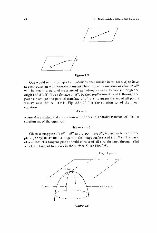
64 II Multivariable Differential Calculus
Figure 2.5
One would naturally expect an «-dimensional surface in @m (m > n) to have at each point an «-dimensional tangent plane. By an n-dimensional plane in 0tm
will be meant a parallel translate of an «-dimensional subspace (through the origin) of 0Γ. If V is a subspace of 0Γ, by the parallel translate of V through the point a e r (or the parallel translate of V to a) is meant the set of all points x e l m such that x - a e K (Fig. 2.5). If V is the solution set of the linear equation
Λχ = 0,
where A is a matrix and x a column vector, then this parallel translate of V is the solution set of the equation
A(x-a) = 0.
Given a mapping F': 3tn -► Mm and a point a e 01", let us try to define the plane (if any) in 0Γ that is tangent to the image surface S of Fa t F(a). The basic idea is that this tangent plane should consist of all straight lines through F(a) which are tangent to curves in the surface S (see Fig. 2.6).
Tangent plane
Curve Surface S
Figure 2.6
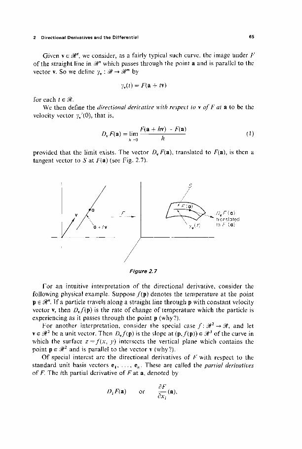
2 Directional Derivatives and the Differential 65
Given v G 0ln, we consider, as a fairly typical such curve, the image under F of the straight line in 0tn which passes through the point a and is parallel to the vector v. So we define yv : 01 -► 0tm by
7V(0 = F(a 4- /v)
for each t e 01. We then define the directional derivative with respect to v of F at a to be the
velocity vector 7/(0), that is,
Z)yF(a) = lim F{m + Av) - F(a)
Ä (1)
provided that the limit exists. The vector DyF(a), translated to ,F(a), is then a tangent vector to S at F(a) (see Fig. 2.7).
y v ( »
Ζ?νΓ(α) translated to F (a)
Figure 2.7
For an intuitive interpretation of the directional derivative, consider the following physical example. Suppose / (p) denotes the temperature at the point p G 0tn. If a particle travels along a straight line through p with constant velocity vector v, then Dyf(p) is the rate of change of temperature which the particle is experiencing as it passes through the point p (why?).
For another interpretation, consider the special c a s e / : ^ 2 - » ^2, and let v G 0t1 be a unit vector. Then Dyf(p) is the slope at (p,/(p)) G 3 of the curve in which the surface z =f(x, y) intersects the vertical plane which contains the point p e ^ 2 and is parallel to the vector v (why?).
Of special interest are the directional derivatives of F with respect to the standard unit basis vectors e1? . . . , e„. These are called the partial derivatives of F. The /th partial derivative of F at a, denoted by
Z>fF(a) or — OX;
66 II Multivariable Differential Calculus
is defined by
dF DiF(*) = — (*)=DeiF{*). (2)
If a = (tfj, . . . , an), we see that
F(a + Ae,·) - F(a) DiFia) = hm
_ -F^!, . ..,fl,- +A, . . . , # „ ) - 7 ^ , . . . ,β ,- , . . . ,αΛ) — um - , Ä-0 A
so /),·/*( a) is simply the result of differentiating F a s a function of the single variable xt, holding the remaining variables fixed.
Example 1 \ïf(x, y) = xy, then DJ'(x, y) = y and D2f(x, y) = x. If g(x, y) = ex sin y, then Dxg{x, y) = ex sin y and D2g(x, y) = ex cos y.
To return to the matter of the tangent plane to S at F(a), note that
F(a + Acv) - F(a) £>,v F(a) = hm
h->o h
,. F(a + Acv) - F(a) = c hm
A-O Ac
,. F(a + £v) - F(a) = c hm
* - > o A:
= c/)vF(a),
so DyF(a) and Z)wF(a) are collinear vectors in J*"1 if v and w are collinear in Mn. Thus every straight line through the origin in R" determines a straight line through the origin in 0tm. Obviously we would like the union
j ^ a = {/)v F(a) e Mm : for all v e ^ " } ,
of all straight lines in 0tm obtained in this manner, to be a subspace of Rm. If this were the case, then the parallel translate of J^a to F(a) would be a likely candidate for the tangent plane to S at F(a).
The set j£?a <z m is simply the image of 9ln under the mapping L\Mn-+ 0im
defined by
L(v)=Z)vF(a) (3)
for all v e 0ln. Since the image of a linear mapping is always a subspace, we can therefore ensure that i??a is a subspace of &m by requiring that L be a //>7£tfr mapping.
2 Directional Derivatives and the Differential 67
We would also like our tangent plane to " closely fit " the surface S near F(a). This means that we want L(\) to be a good approximation to F(a + v) — F(v) when | v | is small. But we have seen this sort of condition before, namely in Theorem 1.2. The necessary and sufficient condition for differentiability in the case n = 1 now becomes our definition for the general case.
The mapping F, from an open subset D of 0Γ to $m, is differentiable at the point a e D if and only if there exists a linear mapping L : 0tn -► 0Γ such that
F(a + h ) - F ( a ) - L ( h ) hm — = 0. (4) h-o |h |
The linear mapping L is then denoted by dFa, and is called the differential of F at a. Its matrix F'(a) is called the derivative of F a t a. Thus F'(a) is the (unique) m x /ί matrix, provided by Theorem 4.1 of Chapter I, such that
dFa(\) = F'(a)x (matrix multiplication) (5)
for all x e f . In Theorem 2.4 below we shall prove that the differential of F at a is well defined by proving that
(dFs . (6) F ( a ) = (ä7( a ) ) =(DJFt*V
in terms of the partial derivatives of the coordinate functions F,, . . . , Fm of F. For then if Z^ and L2 were two linear mappings both satisfying (4) above, then each would have the same matrix given by (6), so they would in fact be the same linear mapping.
To reiterate, the relationship between the differential dFa and the derivative F'(a) is the same as in Section 1—the differential dFa : $n -> $'n is a linear mapping represented by the m x n matrix F'(a).
Note that, if we write AFa(h) = F(a + h) — F(a), then (4) takes the form
r AFa(h) - dFa(h) hm — 0, h-o 1 ti I
which says (just as in the case // = 1 of Section 1) that the difference, between the actual change in the value of F from a to a -f h and the approximate change dFJh), goes to zero faster than h as h -► 0. We indicate this by writing AFa(h) Ä </Fa(h), or F(a + h) « F(a) + dFJh). We will see presently that dFa{h) is quite easy to compute (if we know the partial derivatives of F at a), so this gives an approximation to the actual value F(a + h) if |h| is small. However we will not be able to say how small |h| need be, or to estimate the "error" AFa(h) — c/Fa(h) made in replacing the actual value F(a + h) by the approximation F(a) + i/Fa(h), until the multivariable Taylor's formula is available (Section 7). The picture of the graph of F when n = 2 and m = 1 is instructive (Fig. 2.8).

68 II Multivariable Differential Calculus
a + h./Ha+h))
AFQ{h)-c/FQ(h)
Figure 2.8
Example 2 If F : 3" -► &m is constant, that is, there exists heMm such that F(x) = b for all x e 0tn, then F is diiferentiable everywhere, with dFa = 0 (so the derivative of a constant is zero as expected), because
r F(a + h) - F(a) - 0 r b - b lim ;—; = hm ——- = 0.
Example 3 If F : $n -► 0Γ is linear, then T7 is differentiable everywhere, and
dFu = F for all a G ^ W .
In short, a linear mapping is its own differential, because
r F(a + h) - F(a) - F(h) 0 hm :—: = lim -—- = 0 h->o h h->o h
Theorem 2.1 If F \ M"-+ Mm is diiferentiable at a, then the directional derivative DvF(a) exists for all v e Mn, and
DvF(a) = rfF,(v). (7)
by linearity oi F. For instance, if s : M2 -* 01 is defined by s(x, y) = x + ;\ then ds^ = s for all
a e l 2 .
The following theorem relates the differential to the directional derivatives which motivated its definition.

2 Directional Derivatives and the Dif ferent ia l 69
PROOF We substitute h = t\ into (4) and let t -> 0. Then
F(a + rv) - F(a) - rfFa(iv) 0 = lim
1 F(a + i v ) - F ( a ) ' lim dFJiy)
so it is clear that
F(a + / v ) - F ( a ) Z)vF(a) = lim
f->0 ί
exists and equals dFJjt). |
However the converse of Theorem 2.1 is false. That is, a function may possess directional derivatives in all directions, yet still fail to be diiferentiable.
Example 4 L e t / : M2 -> 0t be defined by
x + y
unless x = y = 0, and / (0 , 0) = 0. In Exercise 7.4 of Chapter 1 it was shown that / is not continuous at (0, 0). By Exercise 2.1 below it follows t h a t / i s not diiferentiable at (0, 0). However, if v = (#, b) with b φ 0, then
n rm m r f (^ bh)-f (0,0) Z)v/(0, 0) = hm
Λ-*Ο h 2h2a2b _ 2a2
exists, while clearly Dvf(0, 0) = 0 if b = 0. Other examples of nondiiferentiable functions that nevertheless possess directional derivatives are given in Exercises 2.3 and 2.4.
The next theorem proceeds a step further, expressing directional derivatives in terms of partial derivatives (which presumably are relatively easy to compute).
Theorem 2.2 If F: 0tn -> 0Γ is diiferentiable at a, and v = (v{, . . . , r„), then
Z)vF(a) = £r,Z),.F(a). (8)
70 II Multivariable Differential Calculus
PROOF
DyF(9) = dFJy) (by Theorem 2.1) = dFjvlel + · · · + r„e j
n
= Σ VJ dF*(ej) (linearity),
so/)vF(a) = X; = 1 r7.Z)ejF(a) = X; = 1 ry Z);F(a), applying Theorem 2.1 again. |
In the case m = 1 of a differentiable real-valued function / : 0tn -► M, the vector
V/(a) = (D,/(a), . . . , Z>„/(a)) G ®\ (9)
whose components are the partial derivatives of/, is called the gradient vector o f / a t a. In terms of V/(a), Eq. (8) becomes
Dv/(a) = V/(a) ■ v, (10)
which is a strikingly simple expression for the directional derivative in terms of partial derivatives.
Example 5 We use Eq. (10) and the approximation A/a(h) « dfa(h) to estimate [(13.1)2 - (4.9)2]1/2. Let/(x, y) = (x2 - >>2)1/2, a = (13, 5), h = ( ^ , - ^ ) . Then
/ (a) = 12, DJif) = |f, Z)2/(a) = - T5
T , so
[13.1)2-(4.9)2]1 / 2=/(13.1,4.9)
= 12 + (H)(TV) + ( - A ) ( - I V ) = 12.15.
To investigate the significance of the gradient vector, let us consider a differentiable function/: 0tn -► ^ and a point a e $", where V/(a) / 0. Suppose that we want to determine the direction in which/increases most rapidly at a. By a " direction " here we mean a unit vector u. Let 0U denote the angle between u and V/(a). Then (10) gives
A,/(a) = V/(a) ■ u = |V/(a)| cosöu.
But cos θη attains its maximum value of + 1 when 0U = 0, that is, when u and V/(a) are collinear and point in the same direction. We conclude that |V/(a)| is the maximum value of Du/(a) for u a unit vector, and that this maximum value is attained with u = V/(a)/1 V/(a) |.
For example, suppose that/(a) denotes the temperature at the point a. It is a common physical assumption that heat flows in a direction opposite to that of greatest increase of temperature (heat seeks cold). This principle and the above remarks imply that the direction of heat flow at a is given by the vector -V/(a) .
If V/(a) = 0, then a is called a critical point of/ I f / i s a differentiable real-
2 Directional Derivatives and the Differential 71
valued function defined on an open set D in Mn, and/attains a local maximum (or local minimum) at the point a e D, then it follows that a must be a critical point of/ For the function g^x) =f(au . . . , #,·_ u x, ai+19 . . . , an) is defined on an open interval of M containing a-t, and has a local maximum (or local mini-mum) at #t-, so A / ( a ) = 0i(ai) = 0 by the familiar result from elementary cal-culus. Later in this chapter we will discuss multivariable maximum-minimum problems in considerable detail.
Equation (10) can be rewritten as a multivariable version of the equation df= (dfjdx) dx of Section 1. Let x1, . . . , xn be the coordinate functions of the identity mapping of Mn, that is, xl : 0tn -* @t is defined by x\pu . . . , pn) = /?,·, / = 1, . . . , n. Then xl is a linear function, so
dxu\h) = x\h) = ht
for all a e 0lh, by Example 3. If/: 0tn -> 0t is differentiable at a, then Theorem 2.1 and Eq. (10) therefore give
#a(h) = A,/(a) = V/(a)-h
= £/>,/(»)*, i = 1
= ÎA/(a)</V(li), i = 1
so the linear functions dfa and £"= ! A / ( a ) dxj are equal. If we delete the sub-script a, and write dfjdx1 for Z>t/(a), we obtain the classical formula
The mapping a -» ^ , which associates with each point a e f " the linear function dfa : " -» ^ , is called a differential form, and Eq. (11) is the historical reason for this terminology. In Chapter V we shall discuss differential forms in detail.
We now apply Theorem 2.2 to finish the computation of the derivative matrix F'(a). First we need the following lemma on "componentwise differ-entiation."
Lemma 2.3 The mapping F: &n -» 0Γ is differentiable at a if and only if each of its component functions F1, . . . , Fm is, and
dFa = (dFal, ...,dF").
(Here we have labeled the component functions with superscripts, rather than subscripts as usual, merely to avoid double subscripts.)
This lemma follows immediately from a componentwise reading of the vector equation (4).
(H)
72 II Multivariable Differential Calculus
Theorem 2.4 If F: mn -> âlm is differentiable at a, then the matrix F(a) of dFa is
F(a) = (DjF\ü)y
[That is, DjFl(a) is the element in the /th row and 7th column of F'(a).]
IdF1 dF{\
οχγ dxn
F' =
/
PROOF
rfF,(v) = / ^ ( v ) \
Wam(v)/
(by Lemma 2.3)
(by Theorem 2.2)
= (DjF'(*))i ; 1
by the definition of matrix multiplication.
Finally we formulate a sufficient condition for differentiability. The mapping F : 0ln -► ^ m is said to be continuously differentiable at a if the partial derivatives DXF, . . . , JD,,/7 all exist at each point of some open set containing a, and are continuous at a.
Theorem 2.5 If JF is continuously differentiable at a, then F is differen-tiable at a.
PROOF By Lemma 2.3, it suffices to consider a continuously differentiable real-valued function/: 9ln-+ 01. Given h = (kl9 . . . , kn), let h0 = 0, hf = (ku . . . , ki9
0, . . . , 0), / = 1, . . . , n (see Fig. 2.9). Then
/ (a + h) - / ( a ) = Σ LA» + h/) " / ( « + *i-i)l

2 Directional Derivatives and the Differential 73
a + h. a + h ,
Figure 2.9
The single-variable mean value theorem gives
/ ( a + h(.) - / ( a + ht_,) =f(al + hu . . . , at_ l + h^l9 a{ + h{, ufi+1, . . . , an)-f(al + * ! , . . . , a,·.! + /*,·-„ flf, . . . , flrn)
for some c,· e (#,·, #, + /?,·), since Dtf is the derivative of the function
g{x)=f(au . . . , </,_,, x, ûrn+1, . . . , fl„).
Thus/ (a + hf) - / ( a + h^ j ) = ht Α / ( Μ for some point b, which approaches a as h -> 0. Consequently
U m 1 / ( a + h) - / ( a ) - Σ7= i ^ tr(a)// , 1 = ^ | £ ? = 1 [A/(bt-) - DJj*)]hi\
^ l im X | Z ) i . / ( b I . ) - A / ( a ) | ^ T h - o f = i n
glim X|Z);/(b;)-A/(a)| h-+0 i=]
= 0
as desired, since each b, -► a as h -> 0, and each Z^/is continuous at a. I
Let us now summarize what has thus far been said about differentiability for functions of several variables, and in particular point out that the rather com-plicated concept of differentiability, as defined by Eq. (4), has now been justified.

74 II Multivariable Differential Calculus
For the importance of directional derivatives (rates of change) is obvious enough and, if a mapping is differentiate, then Theorem 2.2 gives a pleasant expression for its directional derivatives in terms of its partial derivatives, which are com-paratively easy to compute; Theorem 2.4 similarly describes the derivative matrix. Finally Theorem 2.5 provides an effective test for the differentiability of a function in terms of its partial derivatives, thereby eliminating (in most cases) the necessity of verifying that it satisfies the definition of differentiability. In short, every continuously differentiable function is differentiable, and every differentiable function has directional derivatives; in general, neither of these implications may be reversed (see Example 4 and Exercise 2.5).
We began this section with a general discussion of tangent planes, which served to motivate the definition of differentiability. It is appropriate to conclude with an example in which our results are applied to actually compute a tangent plane.
Example 6 Let F : 0t1 -► ^ 4 be defined by
Γ ( ^ Λ | , ^ 2 / ^~ ν·^2 ' "^1? "^ 1 ^2 ' 2 1 / ·
Then F is obviously continuously differentiable, and therefore differentiable (Theorem 2.5). Let a = (1,2), and suppose we want to determine the tangent plane to the image S of F at the point F(a) = (2, 1, 2, 3). By Theorem 2.4, the matrix of the linear mapping dFA : 0t1 -► 01* is the 4 x 2 matrix
"■'-(i;) The image ifa of dFa is that subspace of 01* which is generated by the column
vectors bx = (0, 1, 2, - 2 ) and b2 = (1, 0, 1, 4) of F(a) (see Theorem 1.5.2). Since bx and b2 are linearly independent, J2?a is 2-dimensional, and so is its orthog-onal complement (Theorem 1.3.4). In order to write i^a in the form Ax = 0, we therefore need to find two linearly independent vectors at and a2 which are orthogonal to both bl and b2; they will then be the row vectors of the matrix A. Two such vectors 2LX and a2 are easily found by solving the equations
xl 4- x3 + 4x4 = 0 (bx · x = 0), x2 + 2x3 - 2x4 = 0 (b2 · x = 0) ;
for example, a, = (5, 0, - 1 , - 1 ) and a2 = (0, 10, - 4 , 1). The desired tangent plane T to S at the point F(a) = (2, 1, 2, 3) is now the
parallel translate of J5?a to F(a). That is, T is the set of all points x e l 4 such that A(x- F (a)) = 0,
/5 0 - 1 - 1 ) ^ 1 / 0 ) \0 10 - 4 \)\x3-2\ \0)·
\*4 - 3 /
2 Directional Derivatives and the Differential 75
Upon simplification, we obtain the two equations
5xx - x3 - x4 = 5, 10;c2 - 4x3 + x4 = 5.
The solution set of each of these equations is a 3-dimensional hyperplane in J*4; the intersection of these two hyperplanes is the desired (2-dimensional) tangent plane T.
Exercises
2.1 If/7: d#n -^Mm is differentiable at a, show that F\s continuous at a. Hint: Let
x F(&+h)-F(&)-dFM R(h)=- , u l — if h ^ O .
|h | Then
F(a + h) = F(a) + dFM + | h | R{h).
2.2 If p : 3l·2-> J# is defined by p(x, y)=xy, show that /? is differentiable everywhere with dp(a, b) (*> y) = bx + ay. ///AI/: Let L(x, y) = bx + fly, a = {a, b), h = (A, k). Then show that/?(a + h) - p ( a ) - L ( h ) = M. But | M | <; A2 + /V2 because \hk\<,l2J = max( |Λ | , |k\ ) .
2.3 I f / : ^ 2 ->ά? is defined by/(x, y) = xy2/(x2 + j>2) unless JC = y = 0, and/(0 , 0) = 0, show that /)v /(0, 0) exists for all v, but / i s not differentiable at (0, 0). Hint: Note first that
f(t\) = tf(y) for all / e # and v e ώ#2. Then show that Z>v/(0, 0) =f(\) for all v. Hence Dtf(0, 0) = /) 2 / (0 , 0) = 0 but A i , i ) / (0, 0) = i
2.4 Do the same as in the previous problem with the function f\M2->£% defined by f(x,y) = (xll3jry113)3.
2.5 Let / : Jt2 -> & be defined by/(* , y) = x3 sin (1/jt) + y2 for x # 0, and/(0 , y) = >>2. (a) Show t h a t / i s continuous at (0, 0). (b) Find the partial derivatives o f / a t (0, 0). (c) Show that / i s differentiable at (0, 0). (d) Show that D i / i s «0/ continuous at (0, 0).
2.6 Use the approximation V/a # ßf/a to estimate the value of (a) [(3.02)2 + (1.97)2 + (5.98)2), (b) (e*)1110 = e°* = f(L1)2-(0-9)2.
2.7 As in Exercise 1.3, a potential function for the vector field F\ä#n ->Mn is a differentiable function K : Mn -> M such that F = - V K Find a potential function for the vector field F defined for all x Φ 0 by the formula (a) F(x) = r"x, where r= | x |. Treat separately the cases n = 2 and n φ 2. (b) F(x) = [g'(r)/r]xy where g is a differentiable function of one variable.
2.8 L e t / : 3Hn ->3i be differentiable. If/(0) = 0and/ ( fx) = tf(x) for all/ e ^ a n d x G " , prove that/Xx) = V/(0)-x for all x e St. In particular/ is linear. Consequently any homogeneous function g : Mn -+ M [meaning that g(tx) = tg(x)], which is not linear, must fail to be differentiable at the origin, although it has directional derivatives there (why?).
2.9 If / : 3?" -► Mm and g : <Mn ~> Mk are both differentiable at a e dT, prove directly from the definition that the mapping h : Mn ->â$m + k, defined by h(x) = (/(x), g(x)), is differentiable at a.
2.10 Let the mapping F : M2 - > ^ 2 be defined by F(xu *2) = (sinOn — x2), cosOx -f *2)) . Find the linear equations of the tangent plane in MA to the graph of F at the point (π/4, π/4, 0, 0).
2.11 L e t / : ^2uv^^3
Xyz be the differentiable mapping defined by
x= uv, y=u2—v2, z= u + v.
76 II Multivariable Differential Calculus
Let p = (l, \)e@2 and q=/ (p) = (l, 0, 2) em3. Given a unit vector u = (w, v\ let φ„ : M -> i^2 be the straight line through p, and ipu : m -> m3 the curve through q, defined by <pu(0 = P + tu, ijju(t) =f(<pu(t)\ respectively. Then
Μ ο ) = ζ>»/(ρ) by the definition of the directional derivative.
(a) For what unit vector(s) u is the speed |*/ru'(0)| maximal? (b) Suppose that g-.m3 ^M is a differentiable function such that V#(q) = (l, 1, — 1),
and define
A»W = 0(/(p + fu)).
Assuming the chain rule result that
//u,(0)=V^(q)./)u/(p),
find the unit vector u that maximizes //„'(O). (c) Write the equation of the tangent plane to the image surface of/at the point/(l, 1) = (1,0,2).
3 THE CHAIN RULE
Consider the composition H = G o F of two differentiable mappings F : 3tn -> 3tm and G : ST -► 0*. For example, F(x) G m might be the price vector of m intermediate products that are manufactured at a factory from n raw materials whose cost vector is x (that is, the components of x e (Rn are the prices of the n raw materials), and H(x) = G(F(\)) the resulting price vector of k final products that are manufactured at a second factory from the m inter-mediate products. We might wish to estimate the change A//a(h) = //(a + h) — //(a) in the prices of the final products, resulting from a change from a to a + h in the costs of the raw materials. Using the approximations AF « ^/Fand AG « dG, without initially worrying about the accuracy of our estimates, we obtain
AHa(h) = G(F(a + h)) - G(F(a)) = G(F(a) + [F(a + h) - F(a)]) - G(F(a)) = AGF(a)(F(a 4- h) - F(a)) « dGF(Sk)(AFJh))
« </Gf(a)(</Fa(h)).
This heuristic "argument" suggests the possibility that the multivariable chain rule takes the form dHa = dGF(a) ° dF&, analogous to the restatement in Section 1 of the familiar single-variable chain rule.
Theorem 3.1 (The Chain Rule) Let U and V be open subsets of 0tn
and Mm respectively. If the mappings F: £/-► Mm and G : K-> 0lk are differ-

3 The Chain Rule 77
entiable at a e Uand F(a) e Vrespectively, then their composition H = G °F is differentiable at a, and
a l ' \linear mappings/
In terms of derivatives, we therefore have
m . ) - c w . ) ) T ( . ) (™;™icallo„). (2)
In brief, the differential of the composition is the composition of the differentials; the derivative of the composition is the product of the derivatives.
PROOF We must show that
r //(a + h) - //(a) - dGF(u) o dFa(h) lim ; ; = U.
If we define
F(a + h) - F(a) - dFa(h) <p(h) = :—: for h Φ 0 (3)
and
w = wa)-w-^,(k) for k#0>
then the fact that F and G are differentiable at a and F(a), respectively, implies that
lim <p(h) = lim ^(k) = 0. h->0 k - 0
Then
//(a + h) - //(a) = G(F(a + h)) - G(F(a)) = G(F(a) + (F(a + h) - F(a))) - G(F(a)) = </GF(a)(F(a + h) - F(a))
-f | F(a + h) - F(a) | tff(F(a + h) - F(a)),
by Eq. (4) with k = F(a + h) - F(a). Using (3) we then obtain
//(a + h) - //(a) = rfGf(a)(rfFa(/i) + | h | p(h)) + | F(a + h) - F(a) | <//(F(a + h) - F(a))
= dGF(a) o </Fa(h) + |h|rfGF(a)Mh))
+ |h| Ιί/F.f-r^-) +(/)(h)|iA(/7(a + h ) - F ( a ) ) .
(1)
(4)

78 II Multivariable Differential Calculus
Therefore
//(a + h) - //(a) - dGFiu) o dFa(h)
= rfGF(m)(9(h)) + a\\h\) dF» TTT + ^ ( h ) (A(F(a + h) - F(a)). (5)
But limh_0 i/GF(a)((/)(h)) = 0 because limh^0 φ(1ι) = 0 and the linear mapping rfG>(a) is continuous. Also limh_0 i//(F(a + h) — F(a)) = 0 because F is continu-ous at a and l im^o ^(k) = 0. Finally the number |rfFa(h/|h|) + <p(h)| remains bounded, because h/ |h | e Sn~l and the component functions of the linear map-ping dFa are continuous and therefore bounded on the unit sphere S"'1 c 0tn
(Theorem 1.8.8). Consequently the limit of (5) is zero as desired. Of course Eq. (2) follows
immediately from (1), since the matrix of the composition of two linear mappings is the product of their matrices. |
We list in the following examples some typical chain rule formulas obtained by equating components of the matrix equation (2) for various values of n, m, and k. It is the formulation of the chain rule in terms of differential linear map-pings which enables us to give a single proof for all of these formulas, despite their wide variety.
/ 9
Example 7 If n = k = 1, so we have differentiate mappings ^-»^ m —>$, then h = g of :&-*& is differentiate with
h'(t)=g'(f(t))f\t).
Here g'(f{t)) is a 1 x m row matrix, and/ ' ( i ) is an m x 1 column matrix. In terms of the gradient of g, we have
h'(t) = Wg(f(t)) -f'(t) (dot product). (6)
This is a generalization of the fact that Dyg(a) = V#(a) · v [see Eq. (10) of Section 2]. If we think of'f(t) as the position vector of a particle moving in 0lm, with g a temperature function on Mm, then (6) gives the rate of change of the temperature of the particle. In particular, we see that this rate of change depends only upon the velocity vector of the particle.
In terms of the component functions/*!, . . . ,/„ of/and the partial derivatives of g, (6) becomes
dh = dg dfj ^ dg df2 dg dfm
dt dxx dt dx2 dt dxm dt
If we write xi =fi(t) and u = g(x), following the common practice of using the symbol for a typical value of a function to denote the function itself, then the

3 The Chain Rule 79
above equation takes the easily remembered form
du du άχγ du dx2 du dxn
dt dx{ dt dx2 dt dxn dt
Example 2 Given diiferentiable mappings 011
H : M2 -> M1, the chain rule gives with composition
ίϋ,Η^) D2Hl(*)\ \ΏγΗ2(*) D2H2(*)J
(D.F^) D2Fl(*)\
If we write F(s, t) = (x, y, z) and G(x, y, z) = (u, v), this equation can be rewritten
ldHx οΗλ IdGi dGi dGA
ldF1 dFt\
ds dt
dH2 dH2
\~ds~ ~dfi
dx dz dy
dG2 dG2 dG2
\ dx dy dz J
\
ds dt
dFi dF, ds dt
d_F, d_F,
ds dt I
For example, we have
dHl _ dGt dF, 3Gi dF2 dG1 dF3
dt ~ dx dt dy dt dz dt
Writing
du
ds = DMs, 0, du dx = D&Ws, 0),
dx
Tt = D2Fl(s,t)9 etc.,
to go all the way with variables representing functions, we obtain formulas such as
du du dx du dy du dz
dt dx dt dy dt dz dt
and dv dv dx dv dy dv dz ds dx ds dy ds dz ds
The obvious nature of the formal pattern of chain rule formulas expressed in terms of variables, as above, often compensates for their disadvantage of not

80 II Multivariable Differential Calculus
containing explicit reference to the points at which the various derivatives are evaluated.
Example 3 Let T': 0Î1 -► 0l2 be the familiar "polar coordinate mapping" defined by T(r, 0) = (r cos 0, r sin 0) (Fig. 2.10). Given a differentiable function f: 011 -> ^ , define g =f° T, so g(ry 0) =f(r cos 0, r sin 0). Then the chain rule gives
idg dg\ _ Idf df\ /cos 0 - r sin 0 \ \o> 00/ ~ [ax dy) \sin 0 r cos 0/ '
so
— = — cos 0 + — sin 0, — = — —- r sin 0 + — r cos 0. or ox oy 00 ox dy
Thus we have expressed the partial derivatives of g in terms of those of/, that is, in terms of df/dx = D{f(r cos 0, r sin 0) and ô//ô> = D2f(r cos 0, r sin 0).
[r cosö, Λείπθ)
Figure 2.10
The same can be done for the second order partial derivatives. Given a differentiable mapping F\0tn-^0T, the partial derivative DtF is again a mapping from Mn to ^ w . If it is differentiable at a, we can consider the second partial derivative
DjDiFW^DjiDiFX*).
The classical notation is d2F
J ' dx:dx:
For example, the function/: 0t has second-order partial derivatives
dx2
d2f dy dx
= ^ ^ l /
= D2DJ,
d2f dx dy
and
= ΛΑί / .
ay dy 2
= ^ 2 ^ 2 /

3 The Chain Rule 81
Continuing Example 3 we have
—*- = —\ir\ c o s 0 - ^ - s i n 0 + —(v- sin 0 + i- cos 0 dOdr d0\dxj dx de\dyj dy
( d2f ■ n L d2f n\ n df ' n
= — -—r r sin 0 + -—— r cos 0 cos 0 — — sin 0 \ ox dy ox J ox
I d2f d2f \ df + — r sin 0 + —-~ r cos Ö sinO + — cos 0
\ dx dy dyz J dy
(d2f d2f\ , „ , _ 2 n „:_2m &f dx dy
= r cos 0 sin 01-^ - —τ + ^cos2 0 - sin2 0) \dyz dxz]
sin 0 + — cos 0. dx dy
Jn the last step we have used the fact that the "mixed partial derivatives" d2f/dx dy and d2f/dy dx are equal, which will be established at the end of this section under the hypothesis that they are continuous.
In Exercise 3.9, the student will continue in this manner to show that Laplace's equation
d2y d2u
dx~2 + â P V2" = ^ + ^ - 2 = 0 (7)
transforms to d2u 1 du 1 d2u
lP + r~o7r~ + 72~dë 2 + 7 ^ + ^ ^ 1 = 0 (8)
in polar coordinates. As a standard application of this fact, consider a uniform circular disk of
radius 1, whose boundary is heated in such a way that its temperature on the boundary is given by the function g : [0, 2π] -► 01, that is,
M(1,0) = 0 ( 0 )
for each 0 e [0, 2π]; see Fig. 2.11. Then certain physical considerations suggest that the temperature function u(r, 0) on the disk satisfies Laplace's equation (8) in polar coordinates. Now it is easily verified directly (do this) that, for each positive integer n, the functions r" cos ηθ and rn sin ηθ satisfy Eq. (8). Therefore, if a Fourier series expansion
oo
f(0) = ±a0 + £ (a„ cos nO + bn sin ηθ) n= 1
u(\,e)--gW)
Figure 2.11
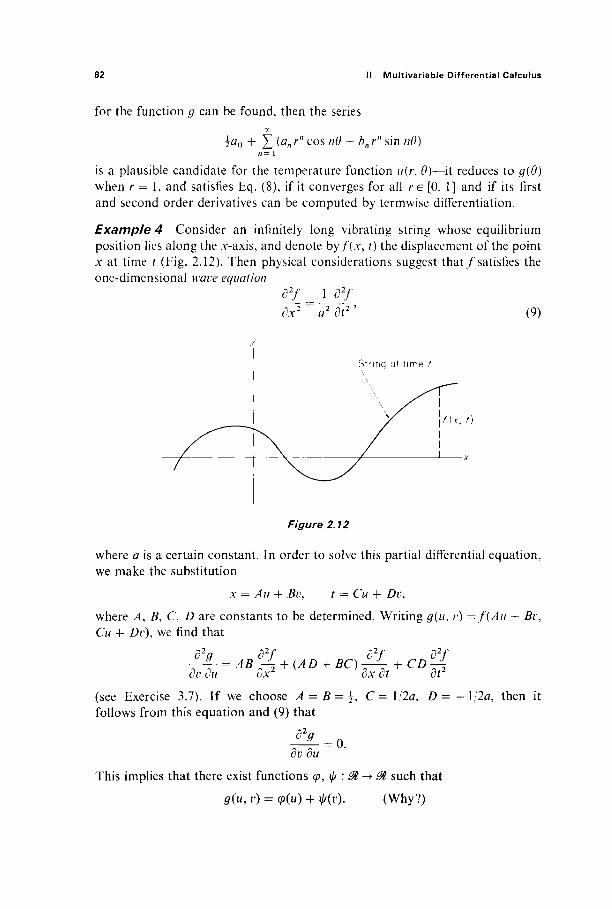
82 II Multivariable Differential Calculus
for the function g can be found, then the series
\a0 + ]T (an r" cos ηθ + Z>„ rn sin /?#) n = 1
is a plausible candidate for the temperature function i/(r, 0)—it reduces to g(0) when r = 1, and satisfies Eq. (8), if it converges for all r e [0 , 1] and if its first and second order derivatives can be computed by termwise differentiation.
Example 4 Consider an infinitely long vibrating string whose equilibrium position lies along the x-axis, and denote byf{x, t) the displacement of the point x at time t (Fig. 2.12). Then physical considerations suggest that / satisfies the one-dimensional wave equation
d2f _ 1 d2f
Jx2"?^" (9)
y
String at time /
Figure 2.12
where a is a certain constant. In order to solve this partial differential equation, we make the substitution
x = Au + Bv, t = Cu + Dv,
where A, B, C, D are constants to be determined. Writing g(u, v) =f(Au + Bv, Cu + Dv), we find that
d2g d2f d2f d2f ΊΓΤ- = AB-^ + {AD + BC) —'- + CD-{ dv cu ox ex dt or
(see Exercise 3.7). If we choose A = B = {, C= \\2a, D = —\/2a, then it follows from this equation and (9) that
—— = 0. dv du
This implies that there exist functions φ, ψ : 0t -* 0t such that
g(u, v) = φ(ύ) + ^(r). (Why?)

3 The Chain Rule 83
In terms of x and i, this means that
/(JC, t) = φ(χ + at) + φ(χ - at). (10)
Suppose now that we are given the initial position
f{x,0) = F(x)
and the initial velocity D2f(x, 0) = G(x) of the string. Then from (10) we obtain
q>(x) + iKx) = F(x) (11)
and
αφ'(χ) - αφ'(χ) = G(x),
so
αφ(χ) — a\j/(x) = G(s) ds + K (12)
by the fundamental theorem of calculus. We then solve (11) and (12) for φ(χ) and φ(χ):
<P(. x) = -F(x) + -JG(s)ds + -
<K*) = lF(x) - i - ÎG(s)ds-2 2a J0
K
Ta
K
Ta
(13)
(14)
Upon substituting x + at for x in (13), and x — at for x in (14), and adding, we obtain
fix, t) F(x + at) + F(x - at) 1 + - f G(s)ds.
2aK-nt
This is "d'Alembert's solution" of the wave equation. If G(x) = 0, the picture looks like Fig. 2.13. Thus we have two " waves" moving in opposite directions.
The last two examples illustrate the use of chain rule formulas to " trans-form" partial differential equations so as to render them more amenable to solution.
y--f{x,0) --F(x)
y--f(x,t
Figure 2.13

84 II Multivariable Differential Calculus
We shall now apply the chain rule to generalize some of the basic results of single-variable calculus. First consider the fact that a function defined on an open interval is constant if and only if its derivative is zero there. Since the function/(x, y) defined for x φ 0 by
/·, Λ (+1 if * > 0 , ' ( ^ , ) = ( - l if * < 0 ,
has zero derivative (or gradient) where it is defined, it is clear that some restric-tion must be placed on the domain of definition of a mapping if we are to generalize this result correctly.
The open set U a $n is said to be connected if and only if given any two points a and b of t/, there is a differentiate mapping φ : (% -> U such that φ(0) = a and cp(\) = b (Fig. 2.14). Of course the mapping F : U'-> @m is said to be constant on U if F(a) = F(b) for any two points a, b e i / , so that there exists c e ^ m such that F(x) = c for all xe U.
Figure 2.14
Theorem 3.2 Let U be a connected open subset of 9tn. Then the differ-entiate mapping F : U-> &m is constant on U if and only if F'(x) = 0 (that is, the zero matrix) for all xe U.
PROOF Since F is constant if and only if each of its component functions is, and the matrix F'(x) is zero if and only if each of its rows is, we may assume that F is real valued, F = / : U-+0t. Since we already know that f'(x) = 0 i f / i s constant, suppose that/ ' (x) = V/(x) = 0 for all xe U.
Given a and b e £/, let φ : 3$ -► U be a differentiate mapping with </>(0) = a, <p(l) = b.
\ϊ9=/οφ : # - ► # , then
^(f) = V/(c)(i))-^'(0 = 0
for all ί e ^£, by Eq. (6) above. Therefore g is constant on [0, 1], so
/(a) =/(<p(0)) = 0(0) = g(\) =/(φ(\)) =/(b). I
Corollary 3.3 Let F and G be two differentiate mappings of the con-nected set Ucztf" into 0Γ. If F'(x) = G'(x) for all x e U, then there exists ce$tm such that
F(x) = G(x) + c
for all xe U. That is, F and G differ only by a constant.

3 The Chain Rule 85
PROOF Apply Theorem 3.2 to the mapping F — G. |
Now consider a differentiate function/: U -+M, where U is a connected open set in 0t2. We say that / is independent of y if there exists a function g \0l^> 01 such that f(x, y) = g(x) if (x, j;) e U. At first glance it might seem tha t / i s independent of y if D2f= 0 on U. To see that this is not so, however, consider the function/defined on
U={(x,y)e@2:x>0 or y Φ 0}
by / ( * , y) = x2 if x > 0 or y > 0, and / ( * , y) = - x2 if x ^ 0 and >» < 0. Then Z)2/(JC, y) = 0 on £/. B u t / ( - l , 1) = 1, w h i l e / ( - l , - 1 ) = - 1 . We leave it as an exercise for the student to formulate a condition on U under which D2f= 0 does imply tha t / i s independent of y.
Let us recall here the statement of the mean value theorem of elementary single-variable calculus. If/ : [a, b] -» 01 is a differentiate function, then there exists a point ξ e (a, b) such that
f(b)-f(a)=f'tf)(b-a).
The mean value theorem generalizes to real-valued functions on 0tn (however it is in general false for vector-valued functions—see Exercise 1.12). In the following statement of the mean value theorem in 0tn, by the line segment from a to b is meant the set of all points in 0tn of the form (1 — f)a 4- tb for t e [0, 1].
Theorem 3.4 (Mean Value Theorem) Suppose that U is an open set in ffln, and that a and b are two points of U such that U contains the line segment L from a to b. If / is a differentiate real-valued function on U, then
/(b) - / ( a ) =/ '(c)(b - a) = V/(c) · (b - a)
for some point c e L .
PROOF Let φ be the mapping of [0, 1] onto L defined by
<p(i) = a + t(b - a) = (1 - f)a + rb, te [0, 1].
Then φ is differentiable with φ'(ί) = b — a. Hence the composition g = / o φ is differentiate by the chain rule. Since g : [0, l ] - > ^ , the single-variable mean value theorem gives a point ξ e [0, 1] such that g{\) - g(0) = #'(£). If c = φ(ξ) e L, we then have
f(b)-f(a) = g(\)-g(0)
= 9\ξ) = ν/(φ(ξ)) · φ'(£) [by Eq. (6)] = V/(c) · (b - a). |
Note that here we have employed the chain rule to deduce the mean value theorem for functions of several variables from the single-variable mean value theorem.
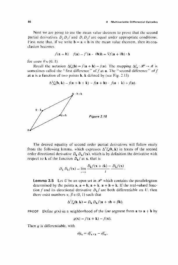
86 II Multivariable Differential Calculus
Next we are going to use the mean value theorem to prove that the second partial derivatives Dj DJ'and Dt Djf are equal under appropriate conditions. First note that, if we write b = a + h in the mean value theorem, then its con-clusion becomes
/ ( a + h) - / ( a ) = / ' ( a + Oh)h = V/(a + Oh) · h
for some 0 e (0, 1). Recall the notation A/a(h) = / ( a + h) - / ( a ) . The mapping A/a : 8t -> & is
sometimes called the "first difference" off at a. The "second difference" off at a is a function of two points h, k defined by (see Fig. 2.15)
A2/a(h, k) =/(a + h + k) - / ( a + h) - / ( a + k) +/(a).
a +h + k
a +kpx"^ /
/ ^*°+ h Figure 2.15
a
The desired equality of second order partial derivatives will follow easily from the following lemma, which expresses A2fa(h, k) in terms of the second order directional derivative Dk Z)h/(x), which is by definition the derivative with respect to k of the function Dhf at x, that is
n n , , , Γ Z)h/(x + rk) - Dhf(x) Dk Dhf(x) = hm .
Lemma 3.5 Let U be an open set in $n which contains the parallelogram determined by the points a, a + h, a + k, a + h + k. If the real-valued func-tion / and its directional derivative Dhf are both differentiate on U, then there exist numbers α, β G (0, 1) such that
A2/a(h,k)=/)kZ)h/(a + ah + ^k).
PROOF Define #(x) in a neighborhood of the line segment from a to a + h by
g(x)=f(x + k)-f(x).
Then g is differentiate, with
dgx = dfx + k-dfx,
3 The Chain Rule 87
and
A2/ .(h,k)=0(a + h ) - 0 ( a ) = #'(a + ah)h (for some a e (0, 1), by the MVT) = V#(a + ah) ·h = Dhg(a + ah) (by Eq. (10) of Section 2) = dgu + ah(h) (by Theorem 2.1)
= ^ a + ah + k ( h ) - <#a + ah( h )
= Z)h/(a + ah + k) - Dh(a + ah) = (Dhf)'(a + ah + /?k)(k) (for some j8 e (0, 1),
by the MVT) = V(Z)h/)(a + ah + /?k) · k = Z\ Z)h/(a + ah + 0k) (Section 2, Eq. (10)). |
Theorem 3.6 Le t /be a real-valued function defined on the open set U in 0ln. If the first and second partial derivatives of/exist and are continuous on U, then DiDjf = Dj DJ on U.
PROOF Theorem 2.5 implies that both/and its partial derivatives Z^/and D2f are differentiable on U. We can therefore apply Lemma 3.5 with h = Aef and k = kej, provided that A and fc are sufficiently small that U contains the rectangle with vertices a, a + Aef, a + /ce,, a + Ae,· + fce,·. We obtain (xl, ßie(0, l) such that
A2fu(hen kej) = DkejDheJ(a + ax Ae, + j ^ e , ) .
If we apply Lemma 3.5 again with h and k interchanged, we obtain a2, ß 2 e (0 , 1) suchthat
A2/.(*ey, Aef.) = DheiDkejf(* + α 2 ^ + jMe,).
But it is clear from the definition of A2/a that
A2/.(AeI.,AreJ.) = A2/.(A:e,.,Aey),
so we conclude that
hkDj DJ(a + a^e,· + ßxk^) = hkDi Djf(* + a2 kej + ß2 Aef),
using the facts that Dhe.f= AZ^/and Dkejf= kD2f. If we now divide the previous equation by A/:, and take the limit as A->0,
/: -> 0, we obtain
Dy Z>,./(a) = Z),. Z)/(a)
because both are continuous at a. |

88 II Multivariable Differential Calculus
REMARK In this proof we actually used only the facts tha t / , Dxf, D2fare differentiable on U, and that Dj DJ and Z^Z),·/are continuous at the point a. Exercise 3.16 shows that the continuity of Dj DJ and Dv Djfat a are necessary for their equality there.
Exercises
3.1 Let / : @2 ->0t be differentiable at each point of the unit circle x2 + y2 = 1. Show that, if u is the unit tangent vector to the circle which points in the counterclockwise direction, then
/>»/(*, y) = -yDifix, y) + xD2f(x, y).
3.2 If/and g are differentiable real-valued functions on Mny show that
(a) V ( /+0 )= V /+ V<7, (b) V{fg)=fVg + gVft
(c) V(f) = i i / - i y / : 3.3 Let i7, G : ^" ->^ n be differentiable mappings, and Ä : ^" - > ^ a differentiable function.
Given u, v e &tn, show that (a) Z>U(F + G) = Du F + Z)„ G, (b) Du + yF=DuF+DvF, (c) Z>„(AF) = (Z)u A)F + Ä(Z>« Z7).
3.4 Show that each of the following two functions is a solution of the heat equation du/dt = k2 82u/dx2 (k SL constant). (a) e~k2a2t s'max. (b) (1/V/) exp(-Jc2/4/c20-
3.5 Suppose that / : Sa2 ->0t has continuous second order partial derivatives. Set x = s + /, y = s — / to obtain g : ^ 2 -> 0t defined by g(s91) =f(s+ t,s — t). Show that
a2/ d2f d2g ~dx2~~dy2~ dtds'
that is, that
3.6 Show that
Drifts + t,s-t)-D2 D2f(s +t,s-t) = D2 Dtfix, t).
d2u d2u d2u d2u d2u 5 —r 4- 2 h 2 —- becomes —- H -
dx2 dx dy dy2 ds2 dt2
if we set x = 2s + f, y = s — t. First state what this actually means, in terms of functions. 3.7 If g(u, v) = {{Au -f Bv, Cu + Dv), where A, B, C, Z> are constants, show that
&n d2f d2f d2f ■ = AB-iz + (AD + BC) —^- + CD ~ 4 . du dw dx2 dx dy dy2
3.8 Let f\(M2^8% be a function with continuous second partial derivatives, so that d2f/8x dy=d2f\dy dx. If g : 0t2 -+9t is defined by/(r, 0) = / ( r cos Θ, r sin 0), show that
(SH(3)'-(!HD"-'W-This gives the length of the gradient vector in polar coordinates.

3 The Chain Rule 89
3.9 If/and g are as in the previous problem, show that
dr2 r2 δθ2 r dr dx2 dy2 '
This gives the 2-dimensional Laplacian in polar coordinates. 3.10 Given a function/: &3 -+& with continuous second partial derivatives, define
F(p, θ, φ) = f(p cos Θ sin </>, p sin Θ sin φ, ρ cos </>),
where p, 0, (/> are the usual spherical coordinates. We want to express the 3-dimensional Laplacian
a2/ a2/ a2/ V2/= — + — + —-
J dx2 dy2 dz2
in spherical coordinates, that is, in terms of partial derivatives of F. (a) First define g(r, 0, z) = f(r cos 0, r sin 0, z) and conclude from Exercise 3.9 that
7 ar2 A·2 a02 r dr dz2'
(b) Now define F(p, Θ, </>) = g(p sin 0, 0, p cos φ). Noting that, except for a change in notation, this is the same transformation as before, deduce that
32F 2 3F 1 d2F cos6 dF 1 d2F V2f = 1 1 1 L. 1
dp2 p dp p2 θφ2 p2 sin φ Βφ p2 sin2 φ δθ2 ' 3.11 (a) If/(x) - g{r\ r = \ x |, and n ^ 3, show that
for x Φ 0. (b) Deduce from (a) that, if V2/= 0, then
where a and b are constants. 3.12 Verify that the functions r" cos ηθ and r" sin ηθ satisfy the 2-dimensional Laplace equation
in polar coordinates. 3.13 If/(x, y, z) = (1/r) g(t — r/c), where c is constant and r = (x2 -f > 2 + z2)1/2, show that /
satisfies the 3-dimensional wave equation
3.14 The following example illustrates the hazards of denoting functions by real variables. Let w =f(x, y, z) and z = g(x, y). Then
since dx/dx = 1 and dy/dx = 0. Hence dw/dz dz/dx = 0. But if w = x -f y + zandz = JC + ^, then aw/az = az/a* = 1, so we have 1 = 0 . Where is the mistake?
3.15 Use the mean value theorem to show that 5.18 < [(4.1)2 + (3.2)2]1/2 < 5.21. Hint: Note first that (5)2 < x2 + y2 < (5.5)2 if 4 < x < 4.1 and 3 <y < 3.2.
dw dw dx dw dy dw dz dw dw dz
dx ~ dx dx dy dx dz dx ~ dx dz dx '
90 II Multivariable Differential Calculus
3.16 Define/ : $2 -+M by f(x, y) = xy(x2 - y2)I(x2 + y2) unless x = y = 0, and / (0 , 0) = 0. (a) Show that DjiO, y) = -y and D2f{x, 0) = * for all x and j \ (b) Conclude that DxD2f{0, 0) and D2 />i/(0, 0) exist but are wof equal.
3.17 The object of this problem is to show that, by an appropriate transformation of variables, the general homogeneous second order partial differential equation
d2u d2u d2u a— + 2b h e — - = 0 (*)
dx2 dx dy dy2
with constant coefficients can be reduced to either Laplace's equation, the wave equation, or the heat equation. (a) If ac — b2 > 0, show that the substitution s = (bx — ay)\{ac — b2)1'2, t = y changes (*) to
d2u a 2 w_ ds2 a / 1 "
(b) If ac — b2 = 0, show that the substitution s = bx — ay, t = y changes (*) to
d2u
(c) If ac — b2 < 0, show that the substitution
-b + (b2-ac) \ -b-(b2~ac)l/2
x + ay, t = \ x + ay
changes (*) to d2u/ds dt = 0. 3.18 Let F: &in-+ Mm be differentiable at a e 0tn. Given a difTerentiable curve φ : ® -> 8%n with
φ(0) = a, <p'(0) = v, define φ = fo<p, and show that ψ'(0) = dFa(\). Hence, if φ : M -> ^ " is a second curve with φ(0) = a, φ'(0) = v, and ψ = f o ^ then φ'(0) = φ'(0), because both are equal to dFJy). Consequently F maps curves through a, with the same velocity vector, to curves through F(a) with the same velocity vector.
3.19 Let φ : M->Mn, f\@n-+3#m, and g : Mm->& be differentiable mappings. \ih = gofoy show that h\t) = ν^( / (φ( ί ) ) ) . / )^ ( ί ) / (φ( ί ) ) .
4 LAGRANGE MULTIPLIERS AND THE CLASSIFICATION OF CRITICAL POINTS FOR FUNCTIONS OF TWO VARIABLES
We saw in Section 2 that a necessary condition, that the differentiable function/: eft1 -► M have a local extremum at the point p e ^ 2 , is that p be a critical point for j \ that is, that V/(p) = 0. In this section we investigate sufficient conditions for local maxima and minima of functions of two variables. The general case (functions οϊη variables) will be treated in Section 8.
It turns out that we must first consider the special problem of maximizing or minimizing a function of the form
f(x, y) = ax2 + 2bxy + cy2
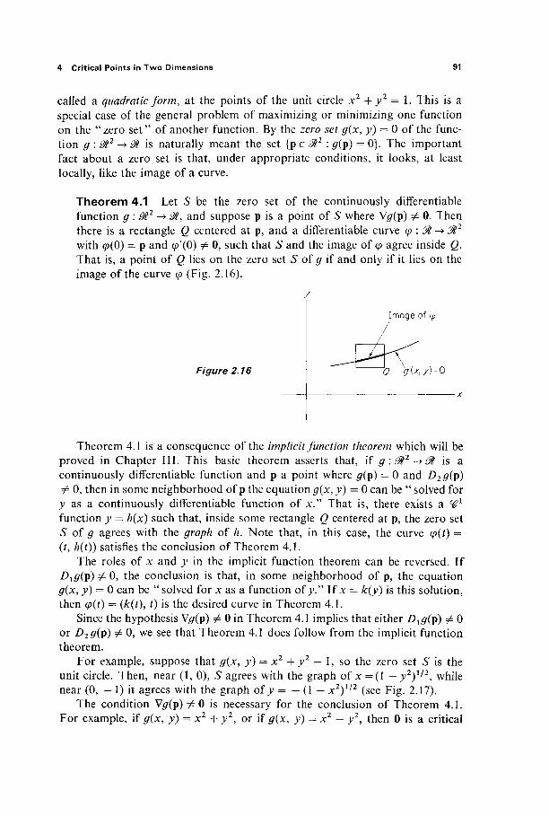
4 Critical Points in Two Dimensions 91
called a quadratic form, at the points of the unit circle x2 + y2 = 1. This is a special case of the general problem of maximizing or minimizing one function on the "zero set" of another function. By the zero set g(x, y) = 0 of the func-tion g : 0l2 -> 01 is naturally meant the set { p e ^ 2 : #(p) = 0}. The important fact about a zero set is that, under appropriate conditions, it looks, at least locally, like the image of a curve.
Theorem 4.1 Let 5 be the zero set of the continuously differentiable function g \0l2 -► ^ , and suppose p is a point of S where V#(p) Φ 0. Then there is a rectangle Q centered at p, and a differentiable curve φ : 0ί -► M2
with φ(0) = p and φ'(0) Φ 0, such that S and the image of φ agree inside Q. That is, a point of Q lies on the zero set S of g if and only if it lies on the image of the curve φ (Fig. 2.16).
Figure 2.16
Image of φ
g(x,y)--0
Theorem 4.1 is a consequence of the implicit function theorem which will be proved in Chapter III. This basic theorem asserts that, if g : 0t2 -» 01 is a continuously differentiable function and p a point where g(p) = 0 and D2g(j>) Φ 0, then in some neighborhood of p the equation g(x, y) = 0 can be " solved for y as a continuously differentiable function of x." That is, there exists a ^ 1
function y = h(x) such that, inside some rectangle Q centered at p, the zero set S of g agrees with the graph of h. Note that, in this case, the curve φ(ί) = (t, h{t)) satisfies the conclusion of Theorem 4.1.
The roles of x and y in the implicit function theorem can be reversed. If ^ι#(ρ) Φ 0, the conclusion is that, in some neighborhood of p, the equation g(x, y) = 0 can be " solved for x as a function of y." If x = k{y) is this solution, then cp(t) = (k(t), t) is the desired curve in Theorem 4.1.
Since the hypothesis V#(p) Φ 0 in Theorem 4.1 implies that either D1g(p) Φ 0 or D2g(j>) Φ 0, we see that Theorem 4.1 does follow from the implicit function theorem.
For example, suppose that g(x, y) = x2 + y2 — 1, so the zero set S is the unit circle. Then, near (1, 0), S agrees with the graph of x =(1 — y2)1/2, while near (0, — 1) it agrees with the graph of y = — (1 — x2)1 / 2 (see Fig. 2.17).
The condition V#(p) Φ 0 is necessary for the conclusion of Theorem 4.1. For example, if g(x, y) = x2 + y2, or if g(x, y) = x2 — y2, then 0 is a critical
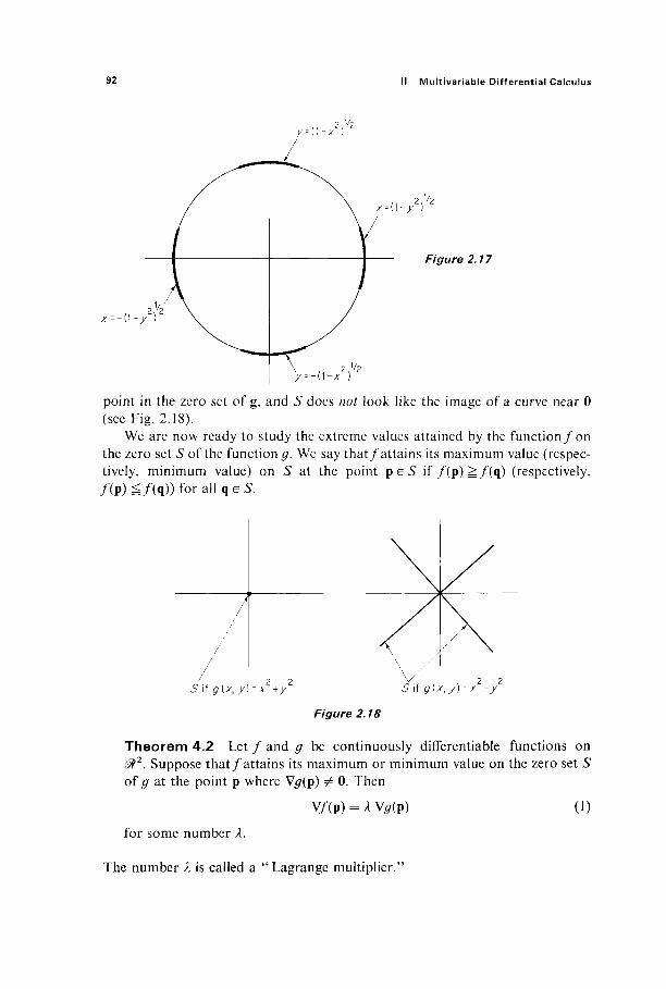
92 II Multivariable Differential Calculus
Figure 2.17
point in the zero set of g, and S does not look like the image of a curve near 0 (see Fig. 2.18).
We are now ready to study the extreme values attained by the function f on the zero set S of the function g. We say that/attains its maximum value (respec-tively, minimum value) on S at the point p e S if / (p) ^ / ( q ) (respectively, / ( p ) g / ( q ) ) f o r a l l q e S .
/ 2 2 S if g{x, y) - x +y
2 2 S if g{x, y) - x -y
Figure 2.18
Theorem 4.2 Let / and g be continuously differentiate functions on ^ 2 . Suppose that/attains its maximum or minimum value on the zero set S of g at the point p where V#(p) Φ 0. Then
V/(p) = λ V<7(p) (1)
for some number λ.
The number λ is called a " Lagrange multiplier."

4 Critical Points in Two Dimensions 93
PROOF Let φ : M -► M2 be the differentiable curve given by Theorem 4.1. Then g((p(t)) = 0 for / sufficiently small, so the chain rule gives
0 = V<7(p)· <p'(0).
Since/attains a maximum or minimum on S at p, the function h(i) =f((p(t)) attains a maximum or minimum at 0. Hence /z'(0) = 0, so the chain rule gives
0 = /ι'(0) = ν / (ρ) ·φ ' (0) .
Thus the vectors V/(p) and V#(p) Φ 0 are both orthogonal to the nonzero vector φ'(0), and are therefore collinear. This implies that (1) holds for some 2 e £ |
Theorem 4.2 provides a recipe for locating the points p = (x, y) at which/ attains its maximum and minimum values (if any) on the zero set of g (provided they are attained at points where the gradient vector Wg Φ 0). The vector equation (1) gives two scalar equations in the unknowns x, y, λ, while g(x, y) = 0 is a third equation. In principle these three equations can be solved for x, y, λ. Each solution (x, y, λ) gives a candidate (x, y) for an extreme point. We can finally compare the values o f / a t these candidate points to ascertain where its maximum and minimum values on S are attained.
Example 1 Suppose we want to find the point(s) of the rectangular hyperbola xy = 1 which are closest to the origin. Take / (x , y) = x2 + y2 (the square of the distance from 0) and g(x, y) = xy — 1. Then V/= (2x, 2y) and Vg = (y, x), so our three equations are
2x = Xy, 2y = λχ, xy = 1.
From the third equation, we see that x Φ 0 and y Φ 0, so we obtain
y χ
from the first two equations. Hence x2 = y2. Since xy = 1, we obtain the two solutions (1, 1) and (—1, —1).
Example 2 Suppose we want to find the maximum and minimum values of / (x , y) = xy on the circle g(x, y) = x2 + y2 — 1 = 0. Then V/= (y, x) and Wg = (2x, 2j/), so our three equations are
y = 2λχ, χ = 2λ}\ χ2 + y2 = 1.
From the first two we see that if either x or y is zero, then so is the other. But the third equation implies that not both are zero, so it follows that neither is. We therefore obtain
2x 2y

94 II Multivariable Differential Calculus
from the first two equations. Hence x2 = y2 = \ (since x2 + y2 = 1). This gives four solutions: (1/^2, 1/^2), ( - 1 / ^ 2 , 1/^2), ( - 1 / ^ 2 , - 1 / ^ 2 ) , (1/^2, - l / x / 2 ) . Evaluating/at these four points, we find that/at tains its maximum value of \ at the first and third of these points, and its minimum value of — \ at the other two (Fig. 2.19).
Figure 2.19
Example 3 The general quadratic form f{x, y) = ax2 + Ibxy + cy2 attains both a maximum value and a minimum value on the unit circle g(x, y) = x2 + y2 — 1 = 0, because / is continuous and the circle is closed and bounded (see Section 1.8). Applying Theorem 4.2, we obtain the three equations
ax + by = λχ, bx + cy = Ay, x2 + y2 = 1. (2) The first two of these can be written in the form
(a - X)x + by = 0, bx + (c - k)y = 0. Thus the two vectors (a — λ, b) and (b, c — λ) are both orthogonal to the vector (JC, y), which is nonzero because x2 4- y2 = 1. Hence they are collinear, and it follows easily that
(a - X)(c - λ) - b2 = 0. This is a quadratic equation whose two roots are
λι, λ2 = \{a + c + [(a - c)2 + 4b2]1/2}.
It is easily verified that Xx+X2 = a + c and ÀlÀ2 = ac — b2. (3)
If tfc — Z>2 < 0, then λλ and λ2 have different signs. If ore - b2 > 0, then they have the same sign, the sign of a and c, which have the same sign because ac ^ ac-b2> 0.
Now, instead of proceeding to solve for x and j ; , let us just consider a solution (χ4, >·,.,*,) of (2). Then
/ (* , · , j>f) = ax2 + 2bx;yt + cj>t·2
= (a*f. + byt)Xi + (èXi + cyl)yi
= lix2 + Xiy
2

4 Critical Points in Two Dimensions 95
Thus λ1 and λ2 are the maximum and minimum values of/(x, y) on x2 + y2 = 1, so we do not need to solve for x and y explicitly after all.
To summarize Example 3, we see that the maximum and minimum values of (x , y) = ax2 + 2bxy + cy2 on the unit circle
(i) are both positive if a > 0 and ac — b2 > 0, (ii) are both negative if a < 0 and ac — b2 > 0,
(iii) have different signs if ac — b2 < 0.
A quadratic form is called positive-definite if f(x, y) > 0 unless x = y = 0, negative-definite if f(x, y) < 0 unless Λ: = y = 0, and nondefinite if it has both positive and negative values. If (x, y) is a point not necessarily on the unit circle, then
Consequently we see that the character of a quadratic form is determined by the signs of the maximum and minimum values which it attains on the unit circle. Combining this remark with (i), (ii), (iii) above, we have proved the following theorem.
Theorem 4.3 The quadratic form/(x, y) = ax2 + 2bxy + cy2 is
(i) positive definite if a > 0 and ac — b2 > 0, (ii) negative-definite if a < 0 and ac — b2 > 0,
(iii) nondefinite if ac — b2 < 0.
Now we want to use Theorem 4.3 to derive a "second-derivative test" for functions of two variables. In addition to Theorem 4.3, we will need a certain type of Taylor expansion for twice continuously differentiable functions of two variables. The function/: 0t2 -> 0t is said to be twice continuously differentiable at p if it has continuous partial derivatives in a neighborhood of p, which are themselves continuously differentiable at p. The partial derivatives of Dxf are D^DJ) = Z^Vand D2 D{f, and the partial derivatives of D2fare D1D2f and D2 D2 = D2
2f. Now suppose that / is twice continuously differentiable on some disk cen-
tered at the point p = (a, b), and let q = (a + //, b + k) be a point of this disk. Define φ : [0, l ] - > ^ by <p(t)=f(a + th, b + tk), that is, φ = / o c where c(f) = {a + th,b + tk) (see Fig. 2.20).
Taylor's formula for single-variable functions will be reviewed in Section 6. Applied to φ on the interval [0, 1], it gives
φ(\) = φ(0) + φ'(0) + ±φ\τ) (4)
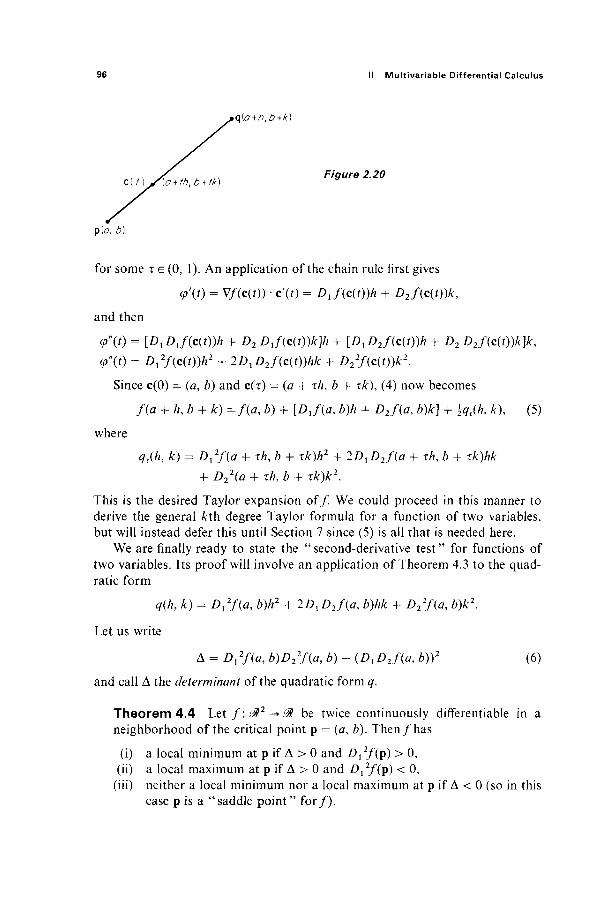
96 II Multivariable Differential Calculus
q{o+n,ô+k)
Figure 2.20
p{atö)
for some τ e (0, 1). An application of the chain rule first gives
<p'(t) = V/(c(0) ' c'(f) = DJidtm + D2f(c(t))k,
and then
<p\f) = [D.Djicit^h + D2 DJ{c{t))k]h + [D{D2f(c(t))h + D2 D2f{c(t))k]k9
φ\ί) = D,2mt))h2 + 2DxD2mt))hk + D22f(c(t))k2.
Since c(0) = (A, £) and C(T) = (α + τΑ, Ζ> + τΑ:), (4) now becomes
/ ( a + Kb + k) =f(a, b) + [DJia, b)h + Z>2/(*, b)k] + ^ ( A , *), (5)
where
<7r(A, fc) = Z V / i f l + τΑ, 6 + τ£)Α2 + 2D,D2f{a + τΑ, 6 + τΑτ)ΑΑ:
+ Z)22 (Ö + τΑ, 6 + τ£)&2.
This is the desired Taylor expansion of/. We could proceed in this manner to derive the general kth degree Taylor formula for a function of two variables, but will instead defer this until Section 7 since (5) is all that is needed here.
We are finally ready to state the "second-derivative test" for functions of two variables. Its proof will involve an application of Theorem 4.3 to the quad-ratic form
q(h, k) = Dx2f{a, b)h2 + 2D{D2f(a, b)hk + D2
2f(a, b)k2.
Let us write
Δ = DSfia, b)D22f(a, b) - {D,D2f(a, b))2 (6)
and call Δ the determinant of the quadratic form q.
Theorem 4.4 L e t / : J ? 2 - > ^ be twice continuously differentiate in a neighborhood of the critical point p = {a, b). Then/has
(i) a local minimum at p if Δ > 0 and Dx2f(p) > 0,
(ii) a local maximum at p if Δ > 0 and D^fip) < 0, (iii) neither a local minimum nor a local maximum at p if Δ < 0 (so in this
case p is a "saddle point" for / ) .
c{t) jS{o + th,b + tk)
4 Critical Points in Two Dimensions 97
If Δ = 0, then the theorem does not apply.
PROOF Since the functions Dx2f(x, y) and
A(x, y) = Dx2f{x, y)D2
2f(x, y) - (Dx D2f(x, y))2
are continuous and nonzero at p, we can choose a circular disk centered at p and so small that each has the same sign at every point of this disk. If (a + A, b + k) is a point of this disk, then (5) gives
f(a + A, A + A) =f(a, b) + \qx(h, k) (7)
because DJ(a9 b) = D2f(a, b) = 0. In case (i), both D2f{a + xh,b + rk) and the determinant A(a + τΑ, b + xk)
ofqT are positive, so Theorem 4.3(i) implies that the quadratic form qx is positive-definite. We therefore see from (7) that f (a + A, b + /:) > / (# , A). This being true for all sufficiently small A and k, we conclude t h a t / h a s a local minimum at p.
The proof in case (ii) is the same, except that we apply Theorem 4.3(ii) to show that qx is negative-definite, so f(a 4- A, b + k) <f(a, b) for all A and A: sufficiently small.
In case (iii), A(a + τΑ, A + τΑ) < 0, so </τ is nondefinite by Theorem 4.3(iii). Therefore qT(h, k) assumes both positive and negative values for arbitrarily small values of A and A, so it is clear from (7) that /has neither a local minimum nor a local maximum at p. |
Example 4 Let/(x, y) = xy + 2x — y. Then
DJ(x, y) = y + 2 and D2f(x, y) = x - 1,
so (1, - 2 ) is the only critical point. Since Dx2f= D2
2f=0 and DxD2f= 1, Δ < 0, so / h a s neither a local minimum nor a local maximum at (1, —2).
The character of a given critical point can often be ascertained without application of Theorem 4.4. Consider, for example, a function / which is de-fined on a set D in the plane that consists of all points on and inside some simple closed curve C (that is, C is a closed curve with no self-intersections). We proved in Section 1.8 that, i f / i s continuous on such a set Z>, then it attains both a maximum value and a minimum value at points of D (why?).
Now suppose in addition t h a t / i s zero at each point of C, and positive at each point inside C. Its maximum value must then be attained at an interior point which must be a critical point. If it happens that /has only a single critical point p inside C, then f must attain its (local and absolute) maximum value at at p, so we need not apply Theorem 4.4.
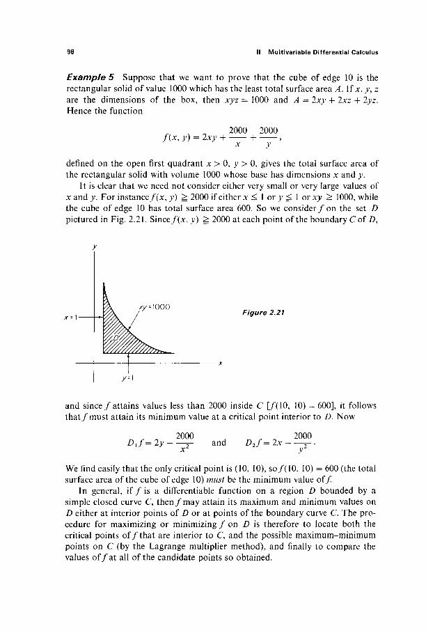
98 II Multivariable Differential Calculus
Example 5 Suppose that we want to prove that the cube of edge 10 is the rectangular solid of value 1000 which has the least total surface area A. If JC, y, z are the dimensions of the box, then xyz = 1000 and A = 2xy + 2xz + 2yz. Hence the function
x ^ 2000 2000 / ( * , y) = 2xy + + ,
x y
defined on the open first quadrant x > 0, y > 0, gives the total surface area of the rectangular solid with volume 1000 whose base has dimensions x and y.
It is clear that we need not consider either very small or very large values of x and y. For instance/(x, y) ^ 2000 if either x ^ 1 or y ^ 1 or xy ^ 1000, while the cube of edge 10 has total surface area 600. So we consider/on the set D pictured in Fig. 2.21. Since/(x, y) ^ 2000 at each point of the boundary C of D,
x--\ Figure 2.21
and since / attains values less than 2000 inside C [/(10, 10) = 600], it follows that /must attain its minimum value at a critical point interior to D. Now
DJ=2y 2000
and D2f=2x 2000
We find easily that the only critical point is (10, 10), so/(10, 10) = 600 (the total surface area of the cube of edge 10) must be the minimum value of/
In general, if / i s a differentiable function on a region D bounded by a simple closed curve C, then/may attain its maximum and minimum values on D either at interior points of D or at points of the boundary curve C. The pro-cedure for maximizing or minimizing / o n D is therefore to locate both the critical points of/ that are interior to C, and the possible maximum-minimum points on C (by the Lagrange multiplier method), and finally to compare the values o f / a t all of the candidate points so obtained.

4 Critical Points in T w o Dimensions 99
Example 6 Suppose we want to find the maximum and minimum values of f(x, y) = Xy on the unit disk D = {(*, y) : x2 + y2 ^ 1}. In Example 2 we have seen that the maximum and minimum values of/(x, y) on the boundary x2 -f y2
= 1 of Z)are / ( l / v /2 , 1/^2) = / ( - 1/^2, - 1/^/2) = ± and/ ( 1/^/2, - 1 / ^ 2 ) = /(—1/^/2, 1/^2)= —i, respectively. The only interior critical point is the origin where / (0 , 0) = 0. Thus ^ and — i are the extreme values off on Ζλ
£xerc/ses
4.1 Find the shortest distance from the point (1, 0) to a point of the parabola y2 = 4*. 4.2 Find the points of the ellipse x2/9 } >>2/4 = 1 which are closest to and farthest from the
point (1,0). 4.3 Find the maximal area of a rectangle (with vertical and horizontal sides) inscribed in the
ellipse x2/a2 + y2/b2 = 1. 4.4 The equation 73x2 -f l'2xy + 52>>2 = 100 defines an ellipse which is centered at the origin,
but has been rotated about it. Find the semiaxes of this ellipse by maximizing and mini-mizing/^, y) = x2 -f y2 on it.
4.5 (a) Show that xy <Ξ i if (x, J>) is a point of the line segment x + y= 1, x^:09 y^0. (b) If a and 6 are positive numbers, show that (ab)l/2 ^ ?{a + />). ////if; Apply (a) with x = alia + b),y = b/(a + 6).
4.6 (a) Show that log xy <i log if (JC, y) is a point of the unit circle x2 + y2 = 1 in the open first quadrant x > 0, y > 0. Hence xy <J£ for such a point. (b) Apply (a) with x = a1/2/(a -f 6)1/2, >> = /?1/2/(a + b)U2 to show again that (ab)l/2 ^ i(fl + W if a > 0, 6 > 0.
4.7 (a) Show that \ax-\-by\ 5j (a2 -f b2)l/2 if x2 + >>2 = 1 by finding the maximum and minimum values of/(x, y) = ax + 6>> on the unit circle. (b) Prove the Cauchy-Schwarz inequality
| ( f l , « . ( c , < / ) | ^ | ( f l , « | - | ( c , i / ) |
by applying (a) with x = c/(c2 -f- </2)1/2, >> = <//(c2 + d2)l/2. 4.8 Let C be the curve defined by g(x, y) = 0, and suppose Vg Φ 0 at each point of C. Let p
be a fixed point not on C, and let q be a point of C that is closer to p than any other point of C. Prove that the line through p and q is orthogonal to the curve C at q.
4.9 Prove that, among all closed rectangular boxes with total surface area 600, the cube with edge 10 is the one with the largest volume.
4.10 Show that the rectangular solid of largest volume that can be inscribed in the unit sphere is a cube.
4.11 Find the maximum volume of a rectangular box without top, which has the combined area of its sides and bottom equal to 100.
4.12 Find the maximum of the product of the sines of the three angles of a triangle, and show that the desired triangle is equilateral.
4.13 If a triangle has sides of lengths x, yy z, so its perimeter is 2s = x + y + z, then its area A is given by A2 = s(s — x)(s — y)(s — z). Show that, among all triangles with a given per-imeter, the one with the largest area is equilateral.
4.14 Find the maximum and minimum values of the function/(;c, y) = x2 — y2 on the elliptical diskx2/16-f r 7 9 ^ 1.
4.15 Find and classify the critical points of the function f(x, y) = (x2 + y2)ex2~y2. 4.16 If x, y, z are any three positive numbers whose sum is a fixed number s, show that xyz <Ξ
(s/3)3 by maximizing f(x, y) = xy(s — x — y) on the appropriate set. Conclude from
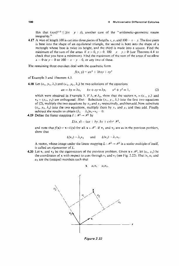
100 li Multivariable Differential Calculus
this that (xyz)1/3 ^ l(x + y + z), another case of the "arithmetic-geometric means inequality."
4.17 A wire of length 100 is cut into three pieces of lengths x, y, and 100 — x ~ y. The first piece is bent into the shape of an equilateral triangle, the second is bent into the shape of a rectangle whose base is twice its height, and the third is made into a square. Find the minimum of the sum of the areas if x > 0, y > 0, 100 — x — y > 0 (use Theorem 4.4 to check that you have a minimum). Find the maximum of the sum of the areas if we allow x = 0 or y = 0 or 100 — x — y = 0, or any two of these.
The remaining three exercises deal with the quadratic form
f(x, y) = ax2 + 2bxy + cy2
of Example 3 and Theorem 4.3.
4.18 Let (xu yu Ax) and {x2, yi, A2) be two solutions of the equations ax + by = λχ, bx + cy = Xy, x2 + y2 = 1, (2)
which were obtained in Example 3. If At φλ2, show that the vectors \i = (xu >Ί) and v2 = (x2, y2) are orthogonal. Hint: Substitute {xu yu X{) into the first two equations of (2), multiply the two equations by x2 and y2 respectively, and then add. Now substitute (*2, JF2, A2) into the two equations, multiply them by x{ and y{ and then add. Finally subtract the results to obtain (λ! — A2)v! · v2 = 0.
4.19 Define the linear mapping L : &2 ->&2 by
L(JC, y) = (ax + by, bx + cy) G M2,
and note that/(x) = x -L(x) for all x e M2. If \{ and v2 are as in the previous problem, show that
L(v1) = A1v1 and £(v2) = A2v2
A vector, whose image under the linear mapping L : M2 -> M2 is a scalar multiple of itself, is called an eigenvector of L.
4.20 Let Vi and v2 be the eigenvectors of the previous problem. Given x G ÎM2, let (wi, u2) be the coordinates of x with respect to axes through vt and v2 (see Fig. 2.22). That is, ul and u2 are the (unique) numbers such that
x = WiVi I - w 2 v 2 .
\ w
y
Figure 2.22

5 Manifolds and Lagrange Multipliers 101
Substitute this equation into/(x) = x ·£(χ), and then apply the fact that \i and v2 are eigenvectors of L to deduce that
/ ( x ) = A l W l2 + A 2 W 2
2 .
Thus, in the new coordinate system, / i s a sum or difference of squares. 4.21 Deduce from the previous problem that the graph of equation ax2 + 2bxy -f cy1 = 1 is
(a) an ellipse if ac — b2 > 0, (b) a hyperbola if ac — b2 < 0.
5 MAXIMA AND MINIMA, MANIFOLDS, AND LAGRANGE MULTIPLIERS
In this section we generalize the Lagrange multiplier method to 01". Let D be a compact (that is, by Theorem 1.8.6, closed and bounded) subset of 0tn. If the function/: D -► 01 is continuous then, by Theorem 1.8.8, there exists a point p G D at which/attains its (absolute) maximum value on D (and similarly /at tains an absolute minimum value at some point of D). The point p may be either a boundary point or an interior point of D. Recall that p is a boundary point of D if and only if every open ball centered at p contains both points of D and points of ffln — D\ an interior point of D is a point of D that is not a bound-ary point. Thus p is an interior point of D if and only if D contains some open ball centered at p. The set of all boundary (interior) points of D is called its boundary (interior).
For example, the open ball Br(p) is the interior of the closed ball Br(p); the sphere Sr(p) = 5r(p) — Z?r(p) is its boundary.
We say that the function/: D -► 01 has a local maximum (respectively, local minimum) on D at the point p e D if and only if there exists an open ball B centered at p such that / (x) ^ / ( p ) [respectively, / (x) ^ / (p ) ] for all points x e B n D. Thus /has a local maximum on D at the point p if its value at p is at least as large as at any " nearby " point of D.
In applied maximum-minimum problems the set D is frequently the set of points on or within some closed and bounded (n - l)-dimensionaI surface S in Mn\ S is then the boundary of D. We will see in Corollary 5.2 that, if the dif-ferentiate function/: D -► M has a local maximum or minimum at the interior point p E D, then p must be a critical point of / that is, a point at which all of the 1st partial derivatives of/vanish, so V/(p) = 0. The critical points of /can (in principle) be found by "setting the partial derivatives of /al l equal to zero and solving for the coordinates x^ . . . , xn" The location of critical points in higher dimensions does not differ essentially from their location in 2-dimensional problems of the sort discussed at the end of the previous section.
If, however, p is a boundary point of D at which/has a local maximum or minimum on Z), then the situation is quite different—the location of such points is a Lagrange multiplier type of problem; this section is devoted to such prob-lems. Our methods will be based on the following result (see Fig. 2.23).

102 li Multivariable Differential Calculus
V/(a)
Figure 2.23 φ'(0)
Theorem 5.1 Let 5 be a set in 0tn, and φ : ΡΛ -► S a differentiable curve with φ(0) = a. Iff is a differentiable real-valued function defined on some open set containing S, and / ha s a local maximum (or local minimum) on S at a, then the gradient vector V/(a) is orthogonal to the velocity vector φ'(0).
PROOF The composite function h =/Ό φ : 0t -► ^ is differentiable at O G ^ ? , and attains a local maximum (or local minimum) there. Therefore /?'(0) = 0, so the chain rule gives
ν/(β) ·φ ' (0) = ν/(φ(0))·φ'(0) = A'(0)
-o. I
It is an immediate corollary that interior local maximum-minimum points are critical points.
Corollary 5.2 If U is an open subset of 0tn, and a e 6/ is a point at which the differentiable function/: U'-► ^? has a local maximum or local minimum, then a is a critical point of/. That is, V/(a) = 0.
PROOF Given v e &", define φ \ & ^> Mn by φ(ί) = a + iv, so φ'(ί) = v. Then Theorem 5.1 gives
V/(a) · v = V/(a) · <p'(0) = 0.
Since V/(a) is thus orthogonal to every vector v e 0ln, it follows that V/(a) = 0. |
Example 1 Suppose we want to find the maximum and minimum values of the function/(x, j \ z) = .x: + y + z on the unit sphere
S2 = {(x, ;,, z ) e ^ 3 : x2 + y2 + z2 = 1}
in &. Theorem 5.1 tells us that, if a = (Λ\ y, z) is a point at which/attains its maximum or minimum on S2, then V/(a) is orthogonal to every curve on S2
passing through a, and is therefore orthogonal to the sphere at a (that is, to its
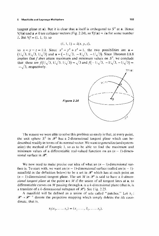
5 Manifolds and Lagrange Multipliers 103
tangent plane at a). But it is clear that a itself is orthogonal to S2 at a. Hence V/(a) and a Φ 0 are collinear vectors (Fig. 2.24), so V/(a) = 2a for some number λ. But V / = ( l , 1, 1), so
(1, 1, l) = X(x,y,z),
so x = y = z = \/λ. Since x2 + y2 + z2 = 1, the two possibilities are a = (1/^/3, 1A/3, 1/^/3) and a = ( - 1/^3, - 1/^3, - 1/^/3). Since Theorem 1.8.8 implies that / does attain maximum and minimum values on S2, we conclude that these are f(\/^3, 1/^3, 1/^3) = ^ 3 and / ( - 1/^3, - ΐ φ , - 1/^3) = —-v/3, respectively.
ν/(α)
Figure 2.24
The reason we were able to solve this problem so easily is that, at every point, the unit sphere S2 in J?3 has a 2-dimensional tangent plane which can be-described readily in terms of its normal vector. We want to generalize (and system-atize) the method of Example 1, so as to be able to find the maximum and minimum values of a difTerentiable real-valued function on an (n — l)-dimen-sional surface in 0tn.
We now need to make precise our idea of what an (n — l)-dimensional sur-face is. To start with, we want an (n — l)-dimensional surface (called an (n — 1)-manifold in the definition below) to be a set in 0tn which has at each point an (n — l)-dimensional tangent plane. The set M in 0tn is said to have a k-dimen-sional tangent plane at the point ae /Wif the union of all tangent lines at a, to differentiate curves on M passing through a, is a A-dimensional plane (that is, is a translate of a /:-dimensional subspace of 0tn). See Fig. 2.25.
A manifold will be defined as a union of sets called "patches." Let π,-: Mn-±0ln~x denote the projection mapping which simply deletes the /th coor-dinate, that is,
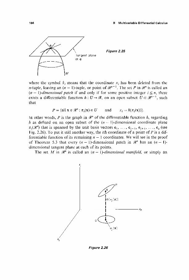
104 II Multivariable Differential Calculus
Figure 2.25
Tangent plane at a
where the symbol xt means that the coordinate xt has been deleted from the «-tuple, leaving an (n — l)-tuple, or point of 0ln~x. The set P in 0ln is called an (n — \ydimensional patch if and only if for some positive integer / n, there exists a differentiable function h : t / - > ^ , on an open subset U a &n~\ such that
P = {all x e i " : π^χ) 6 U and xt = Κπ^χ))}.
In other words, P is the graph in 0ln of the differentiable function A, regarding h as defined on an open subset of the (n — l)-dimensional coordinate plane πι(^η) that is spanned by the unit basis vectors el5 . . . , e^l9 e i + 1, . . . , en (see Fig. 2.26). To put it still another way, the /th coordinate of a point of P is a dif-ferentiable function of its remaining n — 1 coordinates. We will see in the proof of Theorem 5.3 that every (n — l)-dimensional patch in 0tn has an (n — 1)-dimensional tangent plane at each of its points.
The set M in 0ln is called an (n — \)-dimensional manifold, or simply an
P
t | / 7 ( T T . ( X ) )
T T . ( X )
Figure 2.26
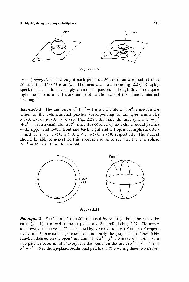
5 Manifolds and Lagrange Multipliers 105
Figure 2.27
(n — \)-manifold, if and only if each point a e M lies in an open subset U of 0ln such that U n M is an (n — l)-dimensional patch (see Fig. 2.27). Roughly speaking, a manifold is simply a union of patches, although this is not quite right, because in an arbitrary union of patches two of them might intersect "wrong."
Example 2 The unit circle x2 + y2 = 1 is a 1-manifold in ^ 2 , since it is the union of the 1-dimensional patches corresponding to the open semicircles x > 0, x < 0, y > 0, y < 0 (see Fig. 2.28). Similarly the unit sphere x2 + y2
+ z2 = 1 is a 2-manifold in ^ 3 , since it is covered by six 2-dimensional patches —the upper and lower, front and back, right and left open hemispheres deter-mined by z > 0, z < 0, x > 0, x < 0, j> > 0, y < 0, respectively. The student should be able to generalize this approach so as to see that the unit sphere S"'1 in &tn is an (n - l)-manifold.
Figure 2.28
Example 3 The " torus" T in ^ 3 , obtained by rotating about the z-axis the circle (y — l)2 + z2 = 4 in the ^z-plane, is a 2-manifold (Fig. 2.29). The upper and lower open halves of T, determined by the conditions z > 0 andz < 0 respec-tively, are 2-dimensional patches ; each is clearly the graph of a differentiable function defined on the open " annulus " 1 < x2 + y2 < 9 in the .xy-plane. These two patches cover all of T except for the points on the circles x2 + y2 = 1 and x2 + y2 = 9 in the xy-plane. Additional patches in T, covering these two circles,

106 II Multivariable Differential Calculus
/ /
/ X
Figure 2.29
must be defined in order to complete the proof that T is a 2-manifold (see Exercise 5.1).
The following theorem gives the particular property of (n — l)-manifolds in Mn which is important for maximum-minimum problems.
Theorem 5.3 If M is an (n — l)-dimensional manifold in 0tn, then, at each of its points, M has an (n — l)-dimensional tangent plane.
PROOF Given a e A/, we want to show that the union of all tangent lines at a, to differentiable curves through a on M, is an (n — l)-dimensional plane or, equivalently, that the set of all velocity vectors of such curves is an (n — 1)-dimensional subspace of 0tn.
The fact that M is an (n — l)-manifold means that, near a, M coincides with the graph of some differentiable function h : $n -► 0t. That is, for some i :g n, x. = h(xl, ..., xt, . . . , xn) for all points (xu . . . , xn) of M sufficiently close to a. Let us consider the case / = n (from which the other cases differ only by a per-mutation of the coordinates).
Let φ : & -> M be a differentiable curve with φ(0) = a, and define φ : 01 -► 0ln~1 by φ = π ° φ, where π : 0ln -► Mn~l is the usual projection. If ^(0) = b e J"" 1 , then the image of φ near a lies directly " above " the image of φ near b. That is, ψ{ΐ) = (φ(ί), Η(φ{ί)) for t sufficiently close to 0. Applying the chain rule, we therefore obtain
c)'(0) = (f(0),VA(b)-^'(0))
= xVi'iOXe,, £,*(!,)), (l) i— 1
where el5 . . . , e^.j are the unit basis vectors in 01η~γ. Consequently φ'(0) lies in the (n — l)-dimensional subspace of 0tn spanned by the n — 1 (clearly linearly independent) vectors
(e1,^1/z(b)),...,(e/J_1,/)„_1/z(b)).

5 Manifolds and Lagrange Multipliers 107
Conversely, given a vector v = ]£"=} ^(e, , Z)fA(b)) of this (n - ^-dimen-sional space, consider the differentiable curve φ : & -* M defined by
<p(t) = (b + iw, A(b + f w)),
where w = (vu . . . , yn_i) e ^ " _ 1 . It is then clear from (1) that φ'(0) = v. Thus every point of our (n — l)-dimensional subspace is the velocity vector of some curve through a o n M . |
In order to apply Theorem 5.3, we need to be able to recognize an (n — 1)-manifold (as such) when we see one. We give in Theorem 5.4 below a useful sufficient condition that a set M c @tn be an (n — l)-manifold. For its proof we need the following basic theorem, which will be established in Chapter III. It asserts that if g : 0tn -> & is a continuously differentiable function, and #(a) = 0 with some partial derivative Z);#(a) Φ 0, then near a the equation
g(xu . . . ,*„) = 0
can be "solved for xt as a function of the remaining variables." This implies that, near a, the set S = g~l(0) looks like an (n — l)-dimensional patch, hence like an (n — l)-manifold (see Fig. 2.30). We state this theorem with / = n.
Graph of F
d>
Figure 2.30
Implicit Function Theorem Let G: 0ln -+ 0t be continuously differ-entiable, and suppose that G(a) = 0 while D„ (7(a) Φ 0. Then there exists a neighborhood U of a and a differentiable function F defined on a neigh-borhood V of (au . . . , a„_i)e&ln~1, such that
U n G~\0) = { x e l " : (xu . . . , V i ) e K and xn = F(xu . . . , x^)}.

108 II Multivariable Differential Calculus
In particular,
G(xu ...,xn_uF(xu . . . ,*„_,)) = ()
for all (jq, . . . , .*„_,) Ε V.
Theorem 5.4 Suppose that g : 0in -> & is continuously differentiable. If M is the set of all those points x e S = g~l(0) at which Vg(x) φ 0, then M is an (n — l)-manifold. Given a e Λ/, the gradient vector V#(a) is orthogonal to the tangent plane to M at a.
PROOF Let a be a point of A/, so g(a) = 0 and V#(a) / 0. Then Z)^(a) = 0 for some / ^ n. Define G : âtn -► ^ by
Then G(b) = 0 and DnG(b) φ 0, where b = (ax, . . . , ai^1, tf/+1, . . . ,#„,#, ·) . Let t / c ^ " and K e f " - 1 be the open sets, and F: V-+ 31 the implicitly defined function, supplied by the implicit function theorem, so that
U n G'^O) ={xe @n : (xu ..., xn) e V and xn = F(xu . . . , χ,,-Ο}.
Now let W be the set of all points (*,, . . . , x„) e ^ " such that (x1? . . . , Xi-U
xi+ ! , . . . , x„, Xi) e U. Then If n M i s clearly an (n — l)-dimensional patch; in particular,
W n M = {xe W : Xi = F(xu . . . , X/_i, xi+i, ·. ·, *„)}·
To prove that V#(a) is orthogonal to the tangent plane to M at a, we need to show that, if φ : & -» M is a differentiable curve with φ(0) = a, then the vectors V#(a) and <p'(0) are orthogonal. But the composite function g ° φ : M -» ^ is identically zero, so the chain rule gives
V#(a) o φ'(0) = {g o φ)'(0) = 0. |
For example, if g(x) = xx2 + · · · + xn
2 - 1, then M is the unit sphere S"1-1 in 0ln, so Theorem 5.4 provides a quick proof that Sn~x is an {n — 1)-manifold.
We are finally ready to "put it all together."
Theorem 5.5 Suppose g\0ln^0l is continuously differentiable, and let M be the set of all those points x e l " at which both g(x) = 0 and V#(x) Φ 0. If the differentiable function/: 0tn -> M attains a local maximum or minimum on M at the point a e A/, then
V/(a) = A V#(a) (2)
for some number λ (called the "Lagrange multiplier").

5 Manifolds and Lagrange Multipliers 109
PROOF By Theorem 5.4, M is an (n — l)-manifold, so M has an (n — 1)-dimensional tangent plane by Theorem 5.3. The vectors V/(a) and V#(a) are both orthogonal to this tangent plane, by Theorems 5.1 and 5.4, respectively. Since the orthogonal complement to an (n — l)-dimensional subspace of &n
is 1-dimensional, by Theorem 1.3.4, it follows that V/(a) and V#(a) are collinear. Since V#(a) φ 0, this implies that V/(a) is a multiple of V#(a). |
According to this theorem, in order to maximize or minimize the function / : 0Γ -> 01 subject to the "constraint equation"
g{xu . . . ,*„) = 0,
it suffices to solve the n + 1 scalar equations
g(x) = 0, and V/(x) = XVg (x)
for the n + 1 "unknowns" x{, . . . , x„, λ. If these equations have several solu-tions, we can determine which (if any) gives a maximum and which gives a minimum by computing the value o f / a t each. This in brief is the" Lagrange multiplier method."
Example 4 Let us reconsider Example 5 of Section 4. We want to find the rectangular box of volume 1000 which has the least total surface area A. If
f(x, y, z) = 2xy + 2xz + 2yz and g(x, y, z) = xyz — 1000,
our problem is to minimize the function / on the 2-manifold in ^ 3 given by g(x, y, z) = 0. Since V/= (2y + 2z, 2x + 2z, 2x + 2y) and Vg = (yz, xz, xy), we want to solve the equations
2y + 2z = /Ijz, 2x + 2z = Axz, 2x + 2y = λχγ,
xyz = 1000.
Upon multiplying the first three equations by x, >\ and z respectively, and then substituting xyz = 1000 on the right hand sides, we obtain
xy + xz = xy + yz = xz = yz = 5002,
from which it follows easily that x = y = z. Since xyz = 1000, our solution gives a cube of edge 10.
Now we want to generalize the Lagrange multiplier method so as to be able to maximize or minimize a function/: Mn -+ 01 subject to several constraint equations
^ ( χ ) = 0, ...,gm(x) = 0, (3)
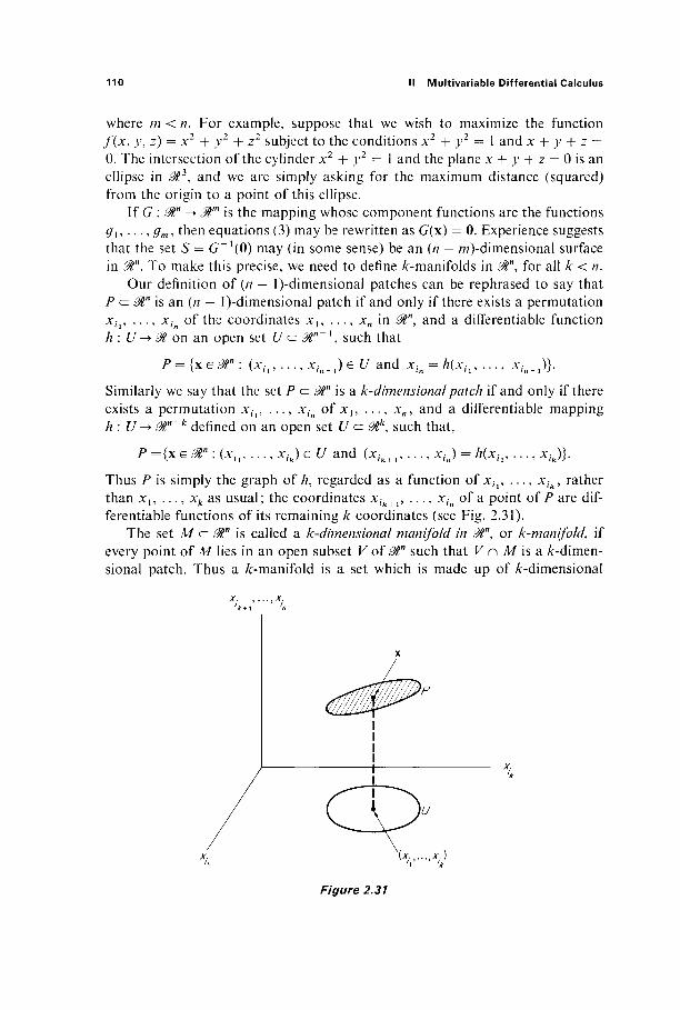
no II Multivariable Differential Calculus
where m < n. For example, suppose that we wish to maximize the function f(x, y, z) = x2 + y2 + z2 subject to the conditions x2 + y2 = 1 and x + y + z = 0. The intersection of the cylinder x2 + y2 = 1 and the plane x + j / + z = 0isan ellipse in ^ 3 , and we are simply asking for the maximum distance (squared) from the origin to a point of this ellipse.
If G : 0in -> ^ m is the mapping whose component functions are the functions gl9 . . . , gm, then equations (3) may be rewritten as G(x) = 0. Experience suggests that the set S = G~l(Q) may (in some sense) be an (n — m)-dimensional surface in 0tn. To make this precise, we need to define /:-manifolds in 0tn, for all k < n.
Our definition of (n — l)-dimensional patches can be rephrased to say that P c= ffln is an (n — l)-dimensional patch if and only if there exists a permutation xh, . . . , xin of the coordinates x{, . . . , xn in 0Γ, and a differentiate function A: t / - on an open set U c
P = { x e ^ " : (jcfl, . . .
Similarly we say that the set P
Mn \ such that
, xin_l) e Ï7 and x/n = h(xh, .. .,)}·
0Γ is a k~dimensional patch if and only if there exists a permutation x/ t , . . . , χΙη of xl5 . . . , xn, and a differentiable mapping h : U-+ 0ln~k defined on an open set £/ <
P={xe0tn:(xir
t\ such that,
*/k) e £/ and (x/k+1, . . . , xin) = h(xh, ■ , * i k ) } ·
xik, rather Thus P is simply the graph of//, regarded as a function of xfl, than *!, . . . , xk as usual; the coordinates x/k+1, . . . , x/n of a point of P are dif-ferentiable functions of its remaining k coordinates (see Fig. 2.31).
The set M c 0tn is called a k-dimensional manifold in 0ln, or k-manifold, if every point of M lies in an open subset V of 0tn such that K n M is a /r-dimen-sional patch. Thus a ^-manifold is a set which is made up of ^-dimensional
( * , . . . , * . )
Figure 2.31

5 Manifolds and Lagrange Multipliers 111
patches, in the same way that an (n — l)-manifold is made up of (n — l)-dimensional patches. For example, it is easily verified that the circle x2 + y2 = 1 in the xy-plane is a 1-manifold in &3. This is a special case of the fact that, if M is a A:-manifold in 0tn^ and $n is regarded as a subspace of 0lp (p > n), then M is a /^-manifold in 0lv (Exercise 5.2).
In regard to both its statement and its proof (see Exercise 5.16), the following result is the expected generalization of Theorem 5.3.
Theorem 5.6 If M is a /:-dimensional manifold in Mn then, at each of its points, M has a /c-dimensional tangent plane.
In order to generalize Theorem 5.4, the following generalization of the im-plicit function theorem is required; its proof will be given in Chapter III.
Implicit Mapping Theorem Let G\0ln-*Mm (m < n) be a contin-uously differentiate mapping. Suppose that G(a) = 0 and that the rank of the derivative matrix G'(a) is m. Then there exists a permutation jc f l , . . . , xin
of the coordinates in ^",an open subset U of $n containing a, an open subset V of 0ln~m containing b = (aii, . . . , ain_m), and a differentiable mapping h: V^0T such that each point x e U lies on S =G~l(0) if and only if (xil9 . . . , * i n _ J e Fand
Recall that the m x n matrix C7'(a) has rank m if and only if its m row vectors VGi(a), . . . , VGm(a) (the gradient vectors of the component functions of G) are linearly independent (Section 1.5). If m = 1, so G = g : 0tn -* ^ , this is just the condition that V#(a) ^ 0, so some partial derivative Z>,#(a) Φ 0. Thus the im-plicit mapping theorem is indeed a generalization of the implicit function theorem.
The conclusion of the implicit mapping theorem asserts that, near a, the m equations
C1(x) = 0, . . . ,Gm(x) = 0
can be solved (uniquely) for the m variables x-t , . . . , x, as differentiable functions of the variables xu, . . . , xin_m. Thus the set 5 = G_1(0) looks, near a, like an (n — w)-dimensional manifold. Using the implicit mapping theorem in place of the implicit function theorem, the proof of Theorem 5.4 translates into a proof of the following generalization.
Theorem 5.7 Suppose that the mapping G : 0ln -► 0Γ is continuously differentiable. If M is the set of all those points x e S = G_1(0) for which the rank of G"(x) is m, then M is an (n — w)-manifold. Given a G M, the gra-dient vectors VG^a), . . . , VGm(a), of the component functions of G, are all orthogonal to the tangent plane to M at a (see Fig. 2.32).
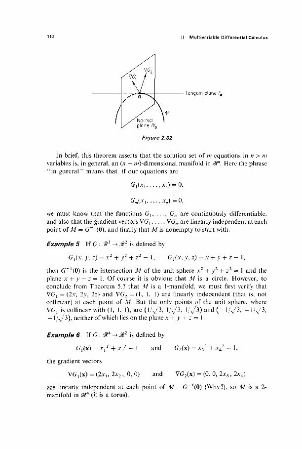
112 II Multivariable Differential Calculus
Tangent plane TQ
Normal plane A/Q
Figure 2.32
In brief, this theorem asserts that the solution set of m equations in n > m variables is, in general, an (n — w)-dimensional manifold in 0tn. Here the phrase "in general" means that, if our equations are
Gx{xx
Gm(xx . xn) = 0,
we must know that the functions Gx, . . . , Gm are continuously differentiate, and also that the gradient vectors VGl5 . . . , VGm are linearly independent at each point of M = G'1 (0), and finally that M is nonempty to start with.
Example 5 \ï G \ & is defined by
Gx(x, y, z) = x2 + y2 + z2 - 1, G2(x, y, z) = x + y + z - 1,
then G-1(0) is the intersection M of the unit sphere x2 + y2 + z2 = 1 and the plane x + y + z = 1. Of course it is obvious that M is a circle. However, to conclude from Theorem 5.7 that M is a 1-manifold, we must first verify that VC?! = (2x, 2y, 2z) and VG2 = (1, 1, 1) are linearly independent (that is, not collinear) at each point of M. But the only points of the unit sphere, where VGi is collinear with (1, 1, 1), are (1 /^3 , Ι /Λ /3 , 1/^3) and ( - 1 / ^ 3 , - l / > / 3 , — 1/Λ/3), neither of which lies on the plane x + y + z = 1.
Example 6 If G : is defined by
Gl(x) = xl2 +x2
2 - 1
the gradient vectors
V G 1 ( X ) = (2JC1,2JC2, 0,0)
and G2(x) + XA2- 1,
and VG2(x) = (0, 0, 2x3, 2x4)
are linearly independent at each point of M = G 1(0) (Why?), so M is a 2-manifold in ^ 4 (it is a torus).
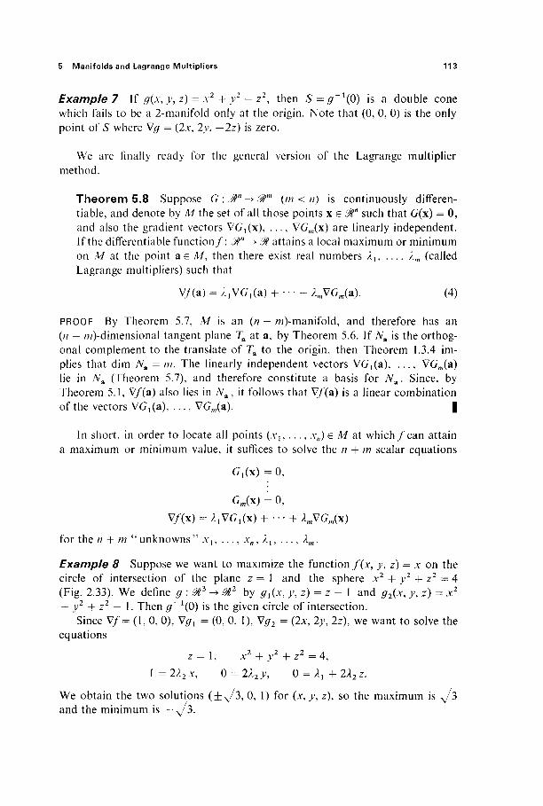
5 Manifolds and Lagrange Multipliers 113
Example 7 If g(x, y, z) = x2 + y2 — z2, then S = #_1(Ό) is a double cone which fails to be a 2-manifold only at the origin. Note that (0, 0, 0) is the only point of S where Vg = (2x, 2v, — 2z) is zero.
We are finally ready for the general version of the Lagrange multiplier method.
Theorem 5.8 Suppose G : Mn -> 0tm (m < /?) is continuously differen-tiable, and denote by M the set of all those points x e l " such that G(x) = 0, and also the gradient vectors VG^x), . . . , VG,„(x) are linearly independent. If the differentiable function/: Mn -» M attains a local maximum or minimum on M at the point a e M , then there exist real numbers λχ, . . . , λιη (called Lagrange multipliers) such that
V/(a) = / , VG,(a) + · ■ · + kmVGJ*). (4)
PROOF By Theorem 5.7, M is an (n — m)-manifold, and therefore has an (n — /77)-dimensional tangent plane Ta at a, by Theorem 5.6. If 7Va is the orthog-onal complement to the translate of Ta to the origin, then Theorem 1.3.4 im-plies that dim 7Va = m. The linearly independent vectors VG^a), . . . , VGm(a) lie in 7Va (Theorem 5.7), and therefore constitute a basis for Na. Since, by Theorem 5.1, V/(a) also lies in 7Va, it follows that V/"(a) is a linear combination of the vectors VGt(a), . . . , VG,„(a). |
In short, in order to locate all points (xx, . . . , xn) e M at which/can attain a maximum or minimum value, it suffices to solve the n + m scalar equations
C 1 (x )=0 ,
Gm(x) = 0, v/(x) = ;klvc1(x) + - + ;knvcn(x)
for the n + m "unknowns" xx, . . . , χη9 λ^ ..., ληι.
Example 8 Suppose we want to maximize the function f(x, y, z) = x on the circle of intersection of the plane z = 1 and the sphere x2 + y2 + z2 = 4 (Fig. 2.33). We define g : ^ 3 -> ®2 by gx(x, y, z) = z - 1 and g2(x, y, z) = x2
+ y2 + z2 — 1. Then g~l(0) is the given circle of intersection. Since V/= (1, 0, 0), Vg{ = (0, 0, 1), V#2 = (2JC, 2y, 2z), we want to solve the
equations
z = 1, x2 + y2 + z2 = 4 , \=2λ2χ, 0 = 2X2y, 0 = λί+2λ2ζ.
We obtain the two solutions (±>/3 , 0, 1) for (x, _y, z), so the maximum is ^/3 and the minimum is —y/3.
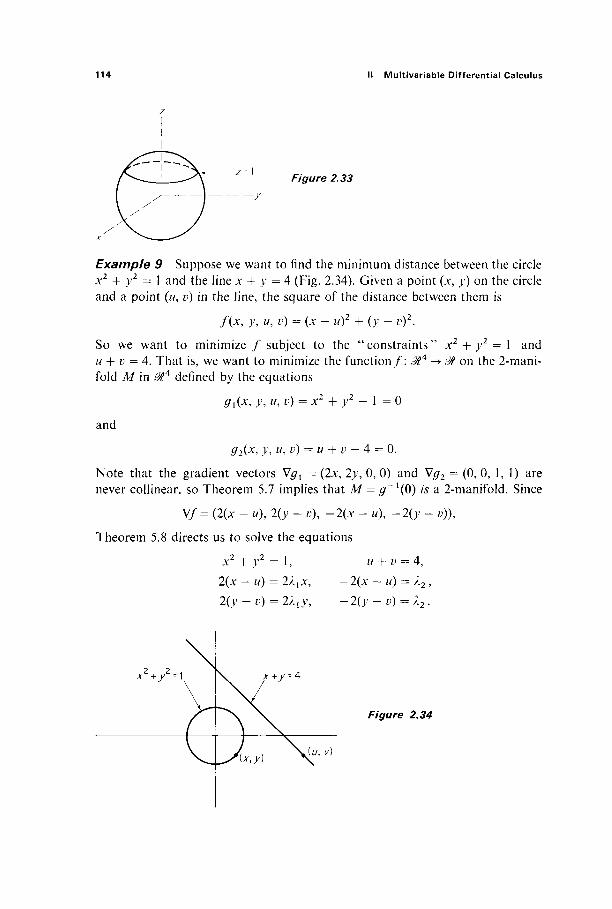
114 II Multivariable Differential Calculus
Figure 2.33
Example 9 Suppose we want to find the minimum distance between the circle χΔ + jr 1 and the line x + y = 4 (Fig. 2.34). Given a point (x, y) on the circle and a point (w, v) in the line, the square of the distance between them is
f(x, y, u, v) = (x- u)2 + (y - v)2.
So we want to minimize / subject to the "constraints" x2 + y2 = 1 and u + v = 4. That is, we want to minimize the function/: J>4 -> M on the 2-mani-fold M in ^ 4 defined by the equations
and
gx(x, y, u, v) = x2 + y2 - 1 = 0
g2(x, y, u, v) = u + v — 4 = 0.
Note that the gradient vectors Vgl = (2x, 2y, 0, 0) and V#2 = (0, 0, 1, 1) are never collinear, so Theorem 5.7 implies that M = g~l(fi) is a 2-manifold. Since
V/ = (2(x - u), 2(y - v), -2(x - «), -2{y - v%
Theorem 5.8 directs us to solve the equations
x2 + y2 = 1, « + v = 4,
2(x — u) = 2λχχ, —2(x — u) = A2, 2(y — Î;) = 2/lj^, — 2(y — v) = λ2 .
Figure 2.34

5 Manifolds and Lagrange Multipliers 115
From -2{x - u) = λ2 = —2(y- v), we see that
x — u = y — v.
If Ax were 0, we would have (x, y) = (w, v) from 2(x — u) = 2λγχ and 2(y — v) = 2Xxy. But the circle and the line have no point in common, so we conclude that λχ Φ 0. Therefore
x — u y — v
so finally u = v. Substituting x = y and u = v into x2 + y2 = 1 and u + v = 4, we obtain x = y = ± 1/^/2, u = v = 2. Consequently, the closest points on the circle and line are (1/^/2, 1/v 2) and (2, 2).
Example 10 Let us generalize the preceding example. Suppose M and TV are two manifolds in ^", defined by g{x) = 0 and A(x) = 0, where
g\0ln^ 0Γ and /? : Mn -+ mk
are mappings satisfying the hypotheses of Theorem 5.7. Let p e M and q e N be two points which are closer together than any other pair of points of M and N.
If x = (xl9 . . . , xn) and y = (yl9 . . . , yn) are any two points of M and N respectively, the square of the distance between them is
/(x, y) =£(*,-y,)2. i= 1
So to find the points p and q, we need to minimize the function/: 0l2n -► 01 on the manifold in 0t2n = Mn x 0in defined by the equation G(x, y) = 0, where
G(x, y) = (g(x), A(y)) e <%m + k = ®m x Stk.
That is, G : 0l2n -+ < m + * is defined by
G(x, y) = (^ (x) , . . . , gjx), A^y) , . . . , Afc(y)) for (x, y) e ^2".
Theorem 5.8 implies that V /= ^VC^ + · · · + Àm+k VGm+k at (p, q). Since
V/(x, y) = (x - y, y - x) e 0l2\
VG^x, y) = ( V ^ x ) , 0) e ^2",
VGJx,y) = (V#m(x),0)e^2 ' \ VGm+1(x,y) =(0,VA1(y))6«2",
VGm + A(x,y)=(0,VAf c(y))e«^
we conclude that the solution satisfies m k
x - y = Σ λι ν#.-(χ) = - Σ K+j VA/y).
116 II Multivariable Differential Calculus
Since (p, q) is assumed to be the solution, we conclude that the line joining p andq is both orthogonal to M at p and orthogonal to N at q.
Let us apply this fact to find the points on the unit sphere x2 + y2 + z2 = 1 and the plane u + v + w = 3 which are closest. The vector (x, y, z) is orthogonal to the sphere at (x, y, z), and (1, 1, 1) is orthogonal to the plane at (w, v, w). So the vector (x — u, y — v, z — w) from (x, y, z) to (w, v w) must be a multiple of both (x,y,z) and (1, 1, 1):
x — u = k: = Ix, y — v = k = ly, z — w = k = Iz.
Hence x = y = z and w = r = w. Consequently the points (1/^/3. l/>/3, l/>/3) and (1, 1, 1) are the closest points on the sphere and plane, respectively.
Exercises
5.1 Complete the proof that the torus in Example 3 is a 2-manifold. 5.2 If M is a Â:-manifold in &n, and Mn<^@p, show that M is a Âr-manifold in &tv. 5.3 If M is a /:-manifold in &tm and Λ is an /-manifold in 3tn
y show that M x N is a (k + /)-manifold in &m+n =Mm x ^" .
5.4 Find the points of the ellipse x2/9 + y2/4 = 1 which are closest to and farthest from the point (1, 1).
5.5 Find the maximal volume of a closed rectangular box whose total surface area is 54. 5.6 Find the dimensions of a box of maximal volume which can be inscribed in the ellipsoid
x2la2+y2/b2 + z2lc2 = l.
(Answer: maximum volume = Sabc/3\/3.) 5.7 Let the manifold S in Mn be defined by g(\) = 0. If p is a point not on 5, and q is the point
of S which is closest to p, show that the line from p to q is perpendicular to S at q. Hint: Minimize/(x) = | x — p | 2 on S.
5.8 Show that the maximum value of the function f(x) = xl2x2
2· ■ - xn2 on the sphere
Sn~l = { x e J " : | x | = 1} is (\fn)n. That is {χγ2 · · · xn
2)l/n ^ \\n if x e S " ' 1 . Given n positive numbers au . . . , a„, define
(a, + --- + any<2'
Then i i 2 + ··· + xn2 = 1, so
( , * ' " ' * " y ' " £ l or ( a 1 . . . f l r B ) l ' - ^ - ( a 1 + ... + fl|l).
Thus the geometric mean of n positive numbers is no greater than their arithmetic mean. 5.9 Find the minimum value of / (x ) =n~1(xl + ··· + x„) on the surface g(x) = xlx2
··· JC„ — 1 = 0. Deduce again the geometric-arithmetic means inequality. 5.10 The planes x + 2>> + z = 4 and 3x + >> + 2z = 3 intersect in a straight line L. Find the
point of L which is closest to the origin. 5.11 Find the highest and lowest points on the ellipse of intersection of the cylinder x2 + y2 = 1
and the plane x + y + z = 1. 5.12 Find the points of the line x + y = 10 and the ellipse x2 + 2y2 = 1 which are closest. 5.13 Find the points of the circle x2 + y2 = 1 and the parabola y2 = 2(4 — *) which are closest.
6 Taylor's Formula in One Variable 117
5.14 Find the points of the ellipsoid x2 + 2y2 + 3z2 = 1 which are closest to and farthest from the plane x + y + z = 10.
5.15 Generalize the proof of Theorem 5.3 so as to prove Theorem 5.6. 5.16 Verify the last assertion of Theorem 5.7.
6 TAYLOR S FORMULA FOR SINGLE-VARIABLE FUNCTIONS
In order to generalize the results of Section 4, and in particular to apply the Lagrange multiplier method to classify critical points for functions of n variables, we will need Taylor's formula for functions on $n. As preparation for the treat-ment in Section 7 of the multivariable Taylor's formula, this section is devoted to the single-variable Taylor's formula.
Taylor's formula provides polynomial approximations to general functions. We will give examples to illustrate both the practical utility and the theoretical applications of such approximations.
Iff: & -> 0t is differentiate at a, and R(h) is defined by
f(a + h)=f(a)+f'{a)h + R{h), (1)
then it follows immediately from the definition off\a) that
lim —— = 0. (2) h->0 A
With x = a + A, (1) and (2) become
f(x) =f(a) +f'(a)(x - a) + R(x - a), (Γ)
where
R(x - a) lim — = 0. (T) je-« x-a
The linear function P(x — a) =f{a) + f'{a)(x — a) is simply that first degree polynomial in (x — a) whose value and first derivative at a agree with those of / a t a. The kth degree polynomial in (x — a), such that the values of it and of its first k derivatives at a agree with those o f / a n d its first k derivatives/ ' , /" , / ( 3 ) , . . . , / ( f c ) a t ö , is
Γ(α) f(k)(a) Pk(* - a) =f(a) +f\a)(x - a) +J-±-t (x - a)2 + ■ · · + ' ' -77- ' (x - af. (3)
2! k\
This fact may be easily checked by repeated differentiation of Pk(x — a). The polynomial Pk(x — a) is called the kth degree Taylor polynomial of fat a.
The remainder f(x) — Pk(x — a ) is denoted by Rk(x — a), so
f(x) = Pk(x -a) + Rk(x - a). (4)
118 II Multivariable Differential Calculus
With x — a = /?, this becomes
f(a + h)=Pk(h) + Rk(h)9 (4')
where
PM) =f(a) +f\a)h +f-^ h2 + - + ^ hk. (3')
In order to make effective use of Taylor polynomials, we need an explicit formula for Rk(x — a) which will provide information as to how closely Pk(x — a) approximates/^) near a. For example, whenever we can show that
lim Rk(x - a) = 0,
this will mean that / is arbitrarily closely approximated by its Taylor poly-nomials; they can then be used to calculate f(x) as closely as desired. Equation (4), or (4'), together with such an explicit expression for the remainder Rk, is referred to as Taylor's formula. The formula for Rk given in Theorem 6.1 below is known as the Lagrange form of the remainder.
Theorem 6.1 Suppose that the (k + l)th derivative fik + 1) o f / : M-* M exists at each point of the closed interval / with endpoints a and x. Then there exists a point ( between a and x such that
f(k + i)(C) (k+ 1)
Hence
f(k)(a) f(k + 1)(C) f(x)= f(a) +f'(a)(x - * ) + ■■· + 7 - ^ (x - a)k + ^ - j - ^ j (* - *)* + 1
or f(k)(a) f(k + 1)(C)
f(a + A) =f(a) +f{a)h + ■ · · + J - ^ hk + ^ - ^ j ^ + 1
with h = x — a.
REMARK This is a generalization of the mean value theorem; in particular, P0(x - a) =f(a), so the case k = 0 of the theorem is simply the mean value theorem
f(a + /i)=Aa)+f(C)h
for the function/on the interval /. Moreover the proof which we shall give for Taylor's formula is a direct generalization of the proof of the mean value theorem. So for motivation we review the proof of the mean value theorem (slightly rephrased).
(5)
6 Taylor's Formula in One Variable 119
First we define R0(t) for t e [0, A] (for convenience we assume A > 0) by
*o(0 =/(* + 0 -/(*) =/(* + 0 - Λ>(0, and note that
*o(0) = 0 (6) while
Λο'(0 =f'(a + /)· (7)
Then we define φ : [0, A] -> by
<K0 = Λ0(ί) - KU (8)
where the constant K is chosen so that Rolle's theorem [the familiar fact that, i f / i s a dififerentiable function on [a, b] with/(a) =f(b) = 0, then there exists a point ξ e (a, b) where /'(ξ) = 0] will apply to φ on [0, A], that is,
* = * f , (9) A
so it follows that cp(h) = 0. Hence Rolle's theorem gives a t e (0, A) such that
0 = </>'(?) = * o ' ( ' ) ' - * by (8) = / ' ( « + ? ) - * by (7).
Hence K =/ ' (£) where ζ = α + /, so from (9) we obtain R0(h) =/'(C)A as desired.
PROOF OF THEOREM 6.1 We generalize the above proof, labeling the formulas with the same numbers (primed) to facilitate comparison.
First we define Rk(t) for t e [0, A] by
Rk(t)=f(a + t)-Pk(t)9
and note that
Rk(0) = Rk'(0) = Rk"(0) = · - - = Rk<k>(0) = 0 (60
while
*Γυ(Ο=/(*+1)(0 + Ο. (70 The reason for (60 is that the first k derivatives of Pk(x — a) at a, and hence the first k derivatives of Pk(t) dit 0, agree with those of/ at a, while (70 follows from the fact that P(
kk+ l\t) = 0 because Pk(t) is a polynomial of degree k.
Now we define φ : [0, A] -► ^ by
<p(t) = Rk(t)-Ktk + 1, (80
where the constant AT is chosen so that Rolle's theorem will apply to φ on [0, A], that is,
Ru(h) Κ = ΊΤΪΤ> (90

120 II Multivariable Differential Calculus
so it follows that φ(Ιή = 0. Hence Rolle's theorem gives a point tl e (0, h) such that φ'(ίΛ) = 0.
It follows from (6') and (7') that
φ(0) = φ'(0) = φ"(0) = ·- = φ«\0)=0Λ
while | (10)
<p<k+1Xt)=fk + 1Xa + t)-K(k+ 1)!. J Therefore we can apply Rolle's theorem to φ' on the interval [0, fx] to obtain a point l2 e (0, f j such that φ"(Ί2) = 0.
1 1 1 1 1 1 0 1k+l · · · t3 t2 tx h
By (10), φ" satisfies the hypotheses of Rolle's theorem on [0, t2], so we can continue in this way. After k + 1 applications of Rolle's theorem, we finally obtain a point tk+le (0, h) such that (p(k + 1)(tk+l) = 0. From the second equation in (10) we then obtain
K_f(k+1)(0 (k+iy.
with ζ = a + tk+l. Finally (9') gives
f(k + 1)(C)
as desired. |
Corollary 6.2 If, in addition to the hypotheses of Theorem 6.1, |/(fc + 1)(C)| ^ M for every ζ e /, then
M |ÄÄ(JC — β ) | ^ _ _ _ - (je _ β|* + ^. (11)
Rk(h) Rk(x - a) *-o hk
x-+a (x-af (12)
It follows that
In particular, (12) holds if f^k + 1) is continuous at a, because it will then necessarily be bounded (by some M) on some open interval containing a.
Example 7 As a standard first example, we take f(x) = ex, a = 0. Then fk\x) = e
x, sof(k)(0) = 1 for all k. Then
Pk(x) = ΐ + χ + ί - + . . . + ^
and eçxk + 1
6 Taylor's Formula in One Variable 121
for some ζ between 0 and x. Therefore
pxxk + 1
0 < Rk(x) <
while 0 < \Rk(x)\ <
(k+l)l
■ ( * + l ) !
In either case the elementary fact that
xk
lim - = 0 fc->oo k\
if
if
0 <
x <
ζ
ζ
<x,\
)
< 0 .
(13)
for all x e .
implies that l i m ^ ^ Rk(x) = 0 for all x, so
e* = Pk(x) + Rk(x)
= lim [/>»(*) + Rt(x)] fc-+oo
= lim Pk(x) + lim Rk(x) fc-^oo k-* oo
k v «
k-*oo n=0 HI
oo y-n
(for all k)
n = o n for all x.
[To verify the elementary fact used above, choose a fixed integer m such that | x | fm < \. If k > m, then
\k \ vim 1^1 | „ | \X\
Id ml m + 1 m + 2
1 \χΓ
A:
< ►0 2k-m w j
as Ä:-> oo.] In order to calculate the value of ex with preassigned accuracy by simply
calculating Pk(x), we must be able to estimate the error Rk(x). For this we need the preliminary estimate e < 4. Since log e = 1 and log x is a strictly increasing function, to verify that e < 4 it suffices to show that log 4 > 1. But
dt dt ' dt dt r ai ç ai ç ai ç a\
Ji t Jx t i2 t J3 t
■dt
1 1 1 = ^ + T + 7> 1·
2 3 4
while

122 II Multivariable Differential Calculus
From (13) we now see that Rk(x) < 4/(k + 1)! if x e [0, 1]; this can be used to compute e to any desired accuracy (see Exercise 6.1).
Example 2 To calculate yjl, we take f(x) = X/JC, a = 1.96, h = 0.04, and consider the first degree Taylor formula
f(a + h)=f(a)+f(a)h + Rl(h),
where R^h) =Γ(ζ)/ι2/2 for some ζ e (a, a + A). Since f\x) = jx~1 / 2 , f'\x) = - ix-" 3 / 2 , we see that R^h) < 0 and
Jl =/(1.96 + 0.04) = (1.96)1/2 + 2 ( ^ ! / 2 + *i(0.04)
= 1.4 + ^ + ^(0.04) = 1.4143 + 7^(0.04). 2.8
Since 1/^(0.04)1 = ± |/"(C) | (0.04)2 with ζ > 1.96,
1 1 1 7^(0.04) I < - x - x — - r (0.04)2 < 0.0001, 1 2 4 (1.4)3
so we conclude that
1.4142 <Jl< 1.4143
(actually ^Jl = 1.41421 to üwc places). The next two examples give a good indication of the wide range of applica-
tion of Taylor's formula.
Example 3 We show that the number e is irrational. To the contrary, sup-pose that e = p/q where p and q are positive integers. Since e = 2.718 to three decimal places (see Exercise 6.1), it is clear that e is not an integral multiple of 1, i, or ^, so q > 3. By Example 1, we can write
q 2! q\ where
0 < R„ = : — < : rr: < fo+1)! 07+1)! (<?+!)!
since 0 < ζ < 1 and e < 3. Upon multiplication of both sides of the above equation by q\, we obtain
(q-l)\p = 2{q\) +q(q-\) (4)(3) + · · · + 1 + q\ Rq.
But this is a contradiction, because the left-hand side (q - 1)1 p is an integer, but the right-hand side is not, because
0 < ^ < ? , ( Τ Π ) ! - ? - Τ Ϊ < 1
since q > 3.
6 Taylor's Formula in One Variable 123
Example 4 We use Taylor's formula to prove that, / / / " — / = 0 on R and /(0) =/ ' (0) = 0, thenf= 0 on 01.
Since/" = / , we see by repeated differentiation that/(*} exists for all k; in particular,
fik) Af i f k i s e v e n > J \f if k is odd.
Since/(0) =/ ' (0) = 0, it follows that/(fc)(0) = 0 for all k. Consequently Theorem 4.1 gives, for each k, a point (fc e (0, *) such that
f(x) = Rk(x) = fik+1\U)xl k+l
(k + \y. Since there are really only two different derivatives involved, and each is con-tinuous because it is differentiable, there exists a constant M such that
\fk + i \t) \£M for i e [0, x] and all k.
Hence |/(JC)| g M\x\k + 1/(k + 1)! for all k. But lim^«, xfc + 1/(^ + 1)! = 0, so we conclude that/(x) = 0.
Now we apply Taylor's formula to give sufficient conditions for local maxima and minima of real-valued single-variable functions.
Theorem 6.3 Suppose that f^k + 1) exists in a neighborhood of a and is continuous at a. Suppose also that
f>(a)=f"(a) = --=fk-1Xa) = 0,
butf(k\a) Φ 0. Then
(a) / h a s a local minimum at a if k is even, and/(fc)(fl) > 0; (b) / h a s a local maximum at a if k is even and/(/c)(ö) < 0; (c) / h a s neither a maximum nor a minimum at Û if k is odd.
This is a generalization of the familiar "second derivative test" which asserts that, if f\d) = 0, then / has a local minimum at a if f"(a) > 0, and a local maximum at a iff'(a) < 0. The three cases can be remembered by thinking of the three graphs in Fig. 2.35.
If f{k\a) = Q for all k, then Theorem 6.3 provides no information as to the behavior o f / in a neighborhood of a. For instance, if
, , x \e~llxl if x # 0 , / W = (o if * = 0,
then it turns out that /(fc)(0) = 0 for all k, so Theorem 6.3 does not apply. However it is obvious tha t /has a local minimum at 0, since/(JC) > 0 for x Φ 0 (Fig. 2.36).
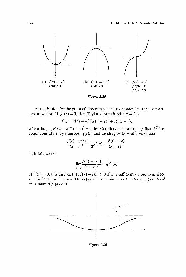
124 II Multivariable Differential Calculus
M
r(o)>o (b) f(x) = -x2
/"(O) < 0 (c) f{x) =x*
r<p) = o Γ(0) Φ 0
As motivation for the proof of Theorem 6.3, let us consider first the " second-derivative test." \ff'(a) = 0, then Taylor's formula with k = 2 is
f(x) =f(a) + ψ(α){χ - a)2 + R2(x - a\
where hmx_>a R2(x — a)/(x — a)2 = 0 by Corollary 6.2 (assuming t h a t / ( 3 ) is continuous at a). By transposing/^) and dividing by (x - a)2, we obtain
fix) - / ( a ) I , v , ^ *z(* - a) (* - «)2 (* - a)2
so it follows that
fix) -/(*) 1 H m • Λ2 = x / » ·
If/"(a) > 0, this implies that/(;c) —f(a) > 0 if x is sufficiently close to #, since (x — a)2 > 0 for all x Φ a. Thus/(#) is a local minimum. Similarly/(#) is a local maximum if f"{d) < 0.
Figure 2.36
Figure 2.35
(a) f{x) = x 2
6 Taylor's Formula in One Variable 125
In similar fashion we can show that, if/'(of) =f"(a) = 0 while f(3\a) φ 0, then/has neither a maximum nor a minimum at a (this fact might be called the "third-derivative test"). To see this, we look at Taylor's formula with k = 3,
f(x) =f(a) + lP'\a){x - a)3 + R3(x - a),
where limx_+a R3(x - a)/(x - a)3 = 0. Transposing f{a) and then dividing by
(x — a)3, we obtain
(x — a) 6 (x — Ö)
so it follows that
i^fl (x - ö)3 6 ,. y v·*; - y w * w3)/ x l i m ~ IÏ3" = 7 / (ß)·
If, for instance, f{3\a) > 0, we see that [/(x) -/(tf)]/(x - tf)3 > 0 if x is suffi-ciently close to a. Since (x — a)3 > 0 if x > a and (x — a)3 < 0 if x < a, it follows that, for x sufficiently close to a, f(x) —f(a) > 0 if x > a, and / (x) —f(a) < 0 if x < a. These inequalities are reversed i f / ( 3 ) ( u ) < 0 . Consequently/(a) is neither a local maximum nor a local minimum.
The proof of Theorem 6.3 simply consists of replacing 2 and 3 in the above discussion by k, the order of the first nonzero derivative of /a t the critical point a. If k is even the argument is the same as when k = 2, while if k is odd it is the same as when k = 3.
PROOF OF THEOREM 6.3 Because of the hypotheses, Taylor's formula takes the form
f(k)(a) fix) =fia) + J - ^ (x - af + Rk(x - a),
where limx^a Rkix - a)/ix - af = 0 by Corollary 6.2. If we transpose fia), divide by (x — af, and then take limits as x -► a, we therefore obtain
fjx)-fja) ifk\a) Ux-a)\ lim — 7— = hm I j -x-a (x-a)k
x..a\ k\ ix-a)k )
fk\a)
k\ (14)
In case (a), l i m ^ [fix) -f(a)]/(x - af > 0 by (14), so it follows that there exists a δ > 0 such that
0 < \x-a\ <d^>— -^- > 0 . (x - af
126 II Multivariable Differential Calculus
0 < I x - a | < δ => - ^ - — - ^ - > 0,
Since k is even in this case, (x — a)k > 0 whether x > a or x < a, so
0<\χ-α\<δ =>f(x) - f(a) > 0, or f(x) > f(a).
Therefore f(a) is a local minimum. The proof in case (b) is the same except for reversal of the inequalities. In case (c), supposing f(k)(a) > 0, there exists (just as above) a δ > 0 such
that
(x - af
But now, since k is odd, the sign of („v — af depends upon whether x < û o r x > a. The same is then true of f(x) —f(a), so f(x) <f{a) if x > a, and f{x) > f(a) if x > a; the situation is reversed iff{k){a) < 0. In either event it is clear that/(tf) is neither a local maximum nor a local minimum. |
Let us look at the case k = 2 of Theorem 6.3 in a bit more detail. We have
f{x) =f(a) + ψ{α){χ - a)2 + R2(x - a), (15)
where lim^,, R2(x — a)/(x — a)2 = 0. Therefore, given ε < i | /"(#) | , there exists a δ > 0 such that
which implies that
(16)
Substituting (lö) into (ID;, we obtain Ra) + [if(a) - e](x - a)2 <f(x) <f(a) + [if "(a) + s](x - a)2 (17)
Iff"{a) > 0, then \f'\a) — ε and \f"{a) + ε are both positive because ε < i\f"(a)\· I* follows that the graphs of the equations
y =f(a) + [if"(a) - ε](χ - a)2 and y =f(a) + [ψ(α) + ε](χ - a)2
are then parabolas opening upwards with vertex (a,f{a)) (see Fig. 2.37). The fact that inequality (17) holds if 0 < | x — a\ < δ means that the part of the graph of y =f(x), over the interval (a — δ, a + (5), lies between these two pa-rabolas. This makes it clear tha t /has a local minimum at a \ïf"(a) > 0.
The situation is similar if f'\d) < 0, except that the parabolas open down-ward, so / h a s a local maximum at a.
In the case k = 3, these parabolas are replaced by the cubic curves
y=f(a)+[}r(a)±e](x-a)\
which look like Fig. 2.35c above, s o / h a s neither a maximum nor a minimum at a.
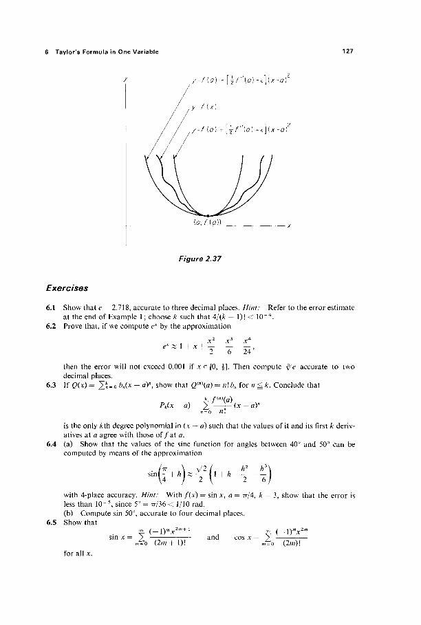
6 Taylor's Formula in One Variable 127
y--f(o) +[^f"(o)-e](x-o)Z
y--f(o) + [±f"(o)+e]lx-o)2
{aJ{o))
Figure 2.37
Exercises
6.1 Show that e = 2.718, accurate to three decimal places. Hint: Refer to the error estimate at the end of Example 1 ; choose k such that 4/(k + 1)! < 10"4 .
6.2 Prove that, if we compute ex by the approximation
1 + x -24'
then the error will not exceed 0.001 if x e [0, \]. Then compute tye accurate to two decimal places.
6.3 If Q(x) = ][* = o bn(x - a)\ show that Q(n\a) = n\bn for n <; k. Conclude that
k f(n)(n) PAx-a)= Υ-γ{χ-αΥ
is the only kih degree polynomial in (x — a) such that the values of it and its first k deriv-atives at a agree with those o f / a t a.
6.4 (a) Show that the values of the sine function for angles between 40° and 50° can be computed by means of the approximation
with 4-place accuracy. Hint: With/(.v) = sin x, a = π/4, k = 3, show that the error is less than 10"5 , since 5° = ττ/36 < 1/10 rad. (b) Compute sin 50°, accurate to four decimal places.
6.5 Show that
Σ ( - l ) ' " *
Ό ( 2 m + 1 ) ! and
- {-\)mx2
Âo (2m)! for all Λ\
128 II Multivariable Differential Calculus
6.6 Show that the kth degree Taylor polynomial off(x) = log x at a — 1 is
Pk(x-l) = (x-l) 1 1
and that lim*.,«, Rk(x — I) = 0 if xe(\, 2). Then compute log | with error < 10" 3
Hint: Show by induction that/ ( k ) (x) - ( - l ) * " 1 ^ - l)!/*fc. 6.7 \îf"(x) = f{x) for all x, show that there exist constants a and b so that
f(x) = a ex + b e~x for all x.
Hint: Let#(x) = f(x) — aex — be~x, show how to choose a and 6 so that#(0) = #'(0) = 0. Then apply Example 4.
6.8 If a is a fixed real number and n is a positive integer, show that the wth degree Taylor polynomial at a = 0 for
fix) = (1 + xY
is P„(x) = 2 J = O (*)χ]> where the "binomial coefficient" (*) is defined by
/ a \ _ a ( a - l ) - ( a - y + l )
(remember that 0! = 1). If a = /?, then
//Λ / f ( / i - l ) - ( « - y + 0 ^ 7 7'! y ! d i - y ) ! '
so it follows that
/(*) = (!+*)" = Î
since Rn(x) == 0, because f(n + n (x) =- 0. If a is not an integer, then (") Φ 0 for ally, so the series 2o(")-v-/ is infinite. The binomial theorem asserts that this infinite series converges to fix) = (1 + xY / / \x\ < 1, and can be proved by showing that limn„oo RnM = 0 for | x | < 1.
6.9 Locate the critical points of
f(x) = x3(x - l ) 4
and apply Theorem 6.3 to determine the character of each. Hint: Do not expand before differentiating.
6.10 Let fix) = x t a n - 1 x — sin2 .v. Assuming the fact that the sixth degree Taylor polynomials at a = 0 of t a n - 1 x and sin2 x are
χ^ χ5 γ4- 2 x 1 and x2 1 χβ,
3 5 3 45 respectively, prove that
f(x) = -hx* + Rix),
where l i m ^ o ^ M = 0. Deduce by the proof of Theorem 6.3 that / h a s a local minimum atO. Contemplate the tedium of computing the first six derivatives of/. If one could endure it, he would find that
/ ' ( 0 ) = / ' ( 0 ) = /<3>(0) = / ( 4 ) ( 0 ) = /<5)(0) = 0
but / ( 6 ) (0) = 112 > 0, so the statement of Theorem 6.3(a) would then give the above result.

7 Taylor's Formula in Several Variables 129
6.11 (a) This problem gives a form of "l'Hospital's rule." Suppose that / a n d g have k -f 1 continuous derivatives in a neighborhood of a, and that both / and g and their first k — 1 derivatives vanish at a. If g(k)(a) φ 0, prove that
f(x) f«\a) xl™g(x) g«\a)'
Hint: Substitute the kih. degree Taylor expansions off(x) and g(x), then divide numerator and denominator by (x — a)k before taking the limit as x ->a. (b) Apply (a) with k = 2 to evaluate
f. (sin x)2
lim—-z—-x^oe*2 - 1
6.12 In order to determine the character of/(jc) = (e~x — l)(tan_1(·*) — x) at the critical point 0, substitute the fourth degree Taylor expansions of e~x and tan- 1 x to show that
fix) = ix* + RA(x),
where limx_0 R*(x)/x* = 0. What is your conclusion?
7 TAYLOR'S FORMULA IN SEVERAL VARIABLES
Before generalizing Taylor's formula to higher dimensions, we need to dis-cuss higher-order partial derivatives. L e t / b e a real-valued function defined on an open subset U of 0tn. Then we say that / is of class ^k on U if all iterated partial derivatives off, of order at most k, exist and are continuous on U. More precisely, this means that, given any sequence ii, i2, . . . , iq, where q ^ k and each ij is one of the integers 1 through n, the iterated partial derivative
Z V V A / exists and is continuous on U.
If this is the case, then it makes no difference in which order the partial derivatives are taken. That is, if / / , i2', · . . , iq' is a permutation of the sequence il9 . . . , iq (meaning simply that each of the integers 1 through n occurs the same number of times in the two sequences), then
DiiDil-DiJ=Di[Dil-DiJ.
This fact follows by induction on q from Theorem 3.6, which is the case q = 2 of this result (see Exercise 7.1).
In particular, if for each r = 1, 2, . . . , n, jr is the number of times that r appears in the sequence iu . . . , iq9 then
DilDi2~-DiJ=D{*D»---D{«f.
If/is of class <gk on U, anaj\ + · · · +jn < k, then D{1 · · · DJn
nf is differentiable

130 II Multivariable Differential Calculus
on U by Theorem 2.5. Therefore, given h = (hu . . . , hn\ its directional derivative with respect to h exists, with
DhD{- Di»f=£f,rDrDi>·- -Dtf r= 1
= t hrDY---DÏ+l---Dtf r= 1
by Theorem 2.2 and the above remarks. It follows that the iterated directional derivative Dh
kf= Dh · · · Dhf exists, with
Dbkf=(/hDl+--+/i„D„)kf
= Σ (,· k..)hï---hJn"VÏ---Dtf, (1)
ji+ •"+jn = k\Jl JnJ
the summation being taken over all «-tuples j \ , . . . , jn of nonnegative integers whose sum is k. Here the symbol
\J\ '"JnJ
denotes the "multinomial coefficient" appearing in the general multinomial formula
Actually ji+ '·· + j n = k\Ji JnJ
( k ï = - ^ ; see Exercise 7.2.
For example, if n = 2 we have ordinary binomial coefficients and (1) gives
Dk"={hlDl+h2D2)kf
ihj\{k-j)\ 2 2
For instance, we obtain

7 Taylor's Formula in Several Variables 131
and
d3f d2f d2f d3f
with k = 2 and k = 3, respectively.
These iterated directional derivatives are what we need to state the multi-dimensional Taylor's formula. To see why this should be, consider the 1-dimen-sional Taylor's formula in the form
fia + h) =f(a) +f'(a)h +>-ψ h2 + ■ ■ ■ + 7 - ^ A* + J ^ ^ ^ (2)
given in Theorem 6.1. Since f(r\d)h' = Λ'ΖΥ/Χα) = {hDJf(a) = DJ{a) by Theorem 2.2 with n = 1, so that Dh = hDx, (2) can be rewritten
/ (a + /0 = r?o^^+7^M)!' (3)
where Dh°f{a) =f(a). But now (3) is a meaningful equation i f / i s a real-valued function on ^". If/is of class ^fc in a neighborhood of a, then we see from Eq. (1) above that
= / ( a ) + JD1/(a)A1 + --- + i)„/(a)/Jn
Ji + '" + Jn = k V/l JnJ
is a polynomial of degree at most k in the components hl9..., hn of h. Therefore Pfc(h) is called the kth degree Taylor polynomial of fat a. The kth degree remainder of f at a is defined by
*f c (h)=/(a + h ) -P k (h ) .
The notation Pk(h) and Rk(h) is incomplete, since it contains explicit reference to neither the function / nor the point a, but this will cause no confusion in what follows.
Theorem 7.1 (Taylor's Formula) If/ is a real-valued function of class <gk+1 on an open set containing the line segment L from a to a + h, then there exists a point ξ e L such that
Ζ)*+1(ξ) RM (k + \)\
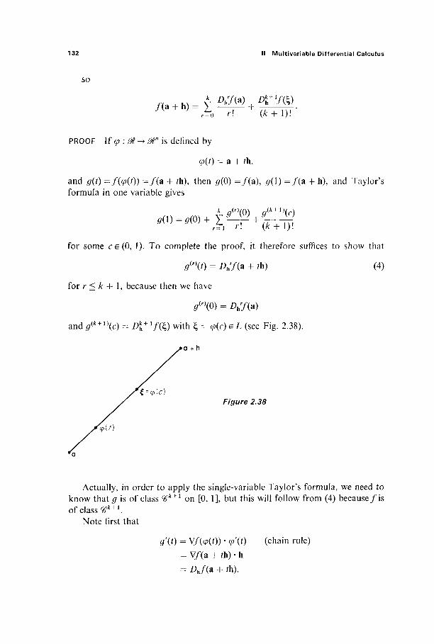
132 II Multivariable Differential Calculus
SO
*, Dhrm , ^+ ι / (ξ)
/(a + h) = X - ^ + o r\ {k+\)\
PROOF \ϊφ\Μ-+®η is defined by
φ(ή = a H- A,
and #(0 =/(<p(0) = / ( a + A), then #(0) = / (a ) , #(1) = / ( a + h), and Taylor's formula in one variable gives
^ΐ)=^(0)+Σι-7 Γ + (Γ-ί7!
for some ce(0 , 1). To complete the proof, it therefore suffices to show that
g«\t) = Dh7(a + A) (4)
for r S k + 1, because then we have
<7<'>(0) = ZV/(a)
and 0(k + 1)(c) - £>£+ 7 (ξ ) with ξ = p(c) e L (see Fig. 2.38).
»a + h
Figure 2.38
Actually, in order to apply the single-variable Taylor's formula, we need to know that g is of class ^k + 1 on [0, 1], but this will follow from (4) because/is of class #fc+1.
Note first that
9\t) = V/(<p(0) · <p\t) (chain rule) = V/(a + ih) · h = Dhf(ü + A).

7 Taylor's Formula in Several Variables 133
Then assume inductively that (4) holds for r ^ k, and le t /^x) = Dhrf(x). Then
9{r) =fi°<P, so
af(r+1)(0 = ^ ( r ) ( 0 = νΛ(φ(0) « φ\ί)
= V/i(a + ih) · h
= ZV/iia + A) = DhDh
rf(ü + th)
= Drh+if(a + th).
Thus (4) holds by induction for r ^ k -f 1 as desired. |
Jf we write x = a + h, then we obtain
/ ( x ) = P f c ( x - a ) + tffc(x-a),
where ΡΛ(χ — a) is a k\\\ degree polynomial in the components xl — ai9 x2 — a2, . . . , xn — an of h = x — a, and
*v ; (Ar+1)!
for some τ e (0, 1).
Example 1 Let/(x) = ^ , + "+*". Then each D{1 ■ ■ ■ DJ„"f(0) = 1, so
^x7(0) = Σ ( ,· .r. ; W · · · * W · · · Di-no)
ji+ '" + j n = r \Jl Jn)
= (*, + · · · + χ„γ.
Hence the kth degree Taylor polynomial of ex , + " + x" is
r=0 f\
as expected.
Example 2 Suppose we want to expand f(x, y) = xy in powers of x — 1 and y — 1. Of course the result will be
XJ; = 1 + (X - 1) + (V _ 1) + (X _ ])(y _ 1),
but let us obtain this result by calculating the second degree Taylor polynomial P2(h) of f(x, )0 at a = (1, 1) with h = (/?1, h2) = (* - 1, >· - 1). We will then

134 II Multivariable Differential Calculus
have/(x, y) = P2(x — 1, y — 1), since R3(h) = 0 because all third order partial derivatives off vanish. Now
/ ( U ) = 1,
lh j x + h2 -jf(x, y)
= h1y + h2x.
So DJ(\, 1) = Λ, + h2 = (x - 1) + (y - 1), and
£„2/(*, 30 = (AI γχ + 'h ^)2f(x> y)
= 2A,A2
= 2 ( x - l ) ( y - l ) . Hence
7>2(* - 1, y - 1) = / ( l , 1) + 0„ ' / (1 , 1) + i Z>h2/(1, 1)
= 1 + ( x - l ) + ( y - l) + ( x - l ) ( y - l ) as predicted.
Next we generalize the error estimate of Corollary 6.2.
Corollary 7.2 I f / i s of class *1"1"1 in a neighborhood £/ of a, and Rk(h) is the &th degree remainder off at a, then
PROOF If h is sufficiently small that the line segment from a to a + h lies in U, then Theorem 7.1 gives
Dk+ Via 4- τ\\) R^ = ",/Ι,Τ. [f0r SOme τ e (0' ')] (A: + 1 ) !
1 v i Λ/ (*+l)!"
But limh_0 D\l · · · Di'/(a + ih) = £>{' · · · DJnnf(a) because / is of class Vk + 1. It
therefore suffices to see that
7 Taylor's Formula in Several Variables 135
ify'i + "" + 7η = & + 1· But this is so because each |/7/|/|h| ^ 1, and there is one more factor in the numerator than in the denominator. 1
Rewriting the conclusion of Corollary 7.2 in terms of the kth degree Taylor polynomial, we have
hm ■ -k = 0. (5)
| x - a | * We shall see that this result characterizes Pk(x — a); that is, Pk(x — a) is the only kth degree polynomial in xx — au . . . , xn — an satisfying condition (5).
Lemma 7.3 If Q(x) and ö*(x) a r e t w o ^ t n degree polynomials mxi9...,xn
such that
r g(x) - e*(x) n hm :—ΓΤ = 0 , x-o |χΓ
then Q = Q*.
PROOF Supposing to the contrary that Q φ Q*, let Q(x) - β*(χ) = F(x) + G(x),
where F(x) is the polynomial consisting of all those terms of the lowest degree / which actually appear in Q(x) — Q*(x), and G(x) consists of all those terms of degree higher than /.
Choose a fixed point b Φ 0 such that F(b) Φ 0. Since | / b | z ^ |/b|fc for / sufficiently small, we have
0 = hm —— r-^0 \tb\l
,. F(tb) + G(tb) = hm
f - 0 t ' l b l '
F(b) = ——- Φ0
| t > l ' ' since each term of F is of degree /, while each term of G is of degree > /. This contradiction proves that Q = Q*. |
We can now establish the converse to Corollary 7.2.
Theorem 7.4 \ff:û$a-*M is of class c6k + l in a neighborhood of a, and Q is a polynomial of degree k such that
r / (*) - C?(x - a) ''m ; rk = 0, (6) x->a I X ~~ ä |
then Q is the kth degree Taylor polynomial o f / a t a.
136 II Multivariable Differential Calculus
PROOF Since
0 ( h ) - Pk(h) <
/(a + h) - ß(h) +
/ ( a + h) - Pk(h)
by the triangle inequality, (5) and (6) imply that
hm — = 0. h-o |n|
Since Q and Pk are both kth degree polynomials, Lemma 7.3 gives Q = Pk as desired. |
The above theorem can often be used to discover Taylor polynomials of a function when the explicit calculation of its derivatives is inconvenient. In order to verify that a given kth degree polynomial Q is the k\\\ degree Taylor poly-nomial of the class ^k + 1 function / at a, we need only verify that Q satisfies condition (6).
Example 3 We calculate the third degree Taylor polynomial of ex sin A by multiplying together those of ex and sin A. We know that
γ·-^ V Y"
ex = 1 + x H (- — + R(x) and sin x = x h R(x), 2 6 6
where limx^0 R(x)/x3 = 1πηχ_>0 R(x)/x3 = 0. Hence
ex sin x = x + x + — + R*(x),
where
R*(x) = - y2 - γ6 + (x - j)RM + (l + x + X- + j^R(x) + R(x)R(x).
Since it is clear that
,. R*(x) hm 0, J C ^ O X
it follows from Theorem 7.4 that A* + x2 + ^A·3 is the third degree Taylor polynomial of ex sin A at 0.
Example 4 Recall that
l + f + - + *(0, hm —r- = 0. r-o t2
7 Taylor's Formula in Several Variables 137
If we substitute t = x and t = y, and multiply the results, we obtain
ex+y = 1 + {x + y) + ^ (x + >02 + R*(x, y)>
where
**(*,y) = (*)*>>(* + >' + i*jO + (i + x + WWiy) + (\+y + iy2)R(x) + R(x)R(y).
Since it is easily verified that
h m ~2 2" = ^' (JC, )>)-(0, 0) * + y
it follows from Theorem 7.4 that 1 + (Λ- + >') + %(x + );)2 is t n e second degree Taylor polynomial of ex + y at (0, 0).
We shall next give a first application of Taylor polynomials to multivariable maximum-minimum problems. Given a critical point a for / : ^ " -> J>, we would like to have a criterion for determining whether/has a local maximum or a local minimum, or neither, at a. If/ is of class cßl in a neighborhood of a, we can write its second degree Taylor expansion in the form
/ ( a + h)- / (a)=<7(h) + Ä2(h),
where
4(h) = ±/>h2/(a) = ΚΛι^ι + ·■· + /'„ A,)2/(a)
and
hm — y = 0. h->o |n|
If not all of the second partial derivatives of/vanish at a, then q(h) is a (non-trivial) homogeneous second degree polynomial in hu ...,/?„ of the form
q(h)= £ aijhihj, 1 ^ i ^ j ^ n
and is called the quadratic form off at the critical point a. Note that
if h ^ O ,
if h = 0.
Since h/ |h | is a point of the unit sphere Sn~l in Mn, it follows that the quadratic form q is completely determined by its values on Sn~x. As in the 2-dimensional case of Section 4, a quadratic form is called positive-definite (respectively nega-tive-definite) if and only if it is positive (respectively negative) at every point
«Q
138 II Multivariable Differential Calculus
of S" 1 (and hence everywhere except 0), and is called nondefinite if it assumes both positive and negative values on S"'1 (and hence in every neighborhood ofO).
For example, x2 4- y2 is positive-definite and — x2 — y2 is negative-definite, while x2 — y2 and xy are nondefinite. Note that y2, regarded as a quadratic form in x and y whose coefficients of both x2 and xy are zero, is neither positive-definite nor negative-definite nor nondefinite (it is not negative anywhere, but is zero on the x-axis).
In the case n = 1, when/is a function of a single variable with critical point a, the quadratic form o f / a t a is simply
q{h) = \f\d)h2.
Note that q is positive-definite if f"{d) > 0, and is negative-definite if f"(a) < 0 (the nondefinite case cannot occur if n = 1). Therefore the "second derivative test" for a single-variable function states tha t /has a local minimum at a if its quadratic form q(h) at a is positive-definite, and a local maximum at a if q{h) is negative-definite. \ïf"{a) = 0, then<7(/7) = 0 is neither positive-definite nor nega-tive-definite (nor nondefinite), and we cannot determine (without considering higher derivatives) the character of the critical point a. The following theorem is the multivariable generalization of the "second derivative test."
Theorem 7.5 Let / be of class # 3 in a neighborhood of the critical point a. Then / h a s
(a) a local minimum at a if its quadratic form q(h) is positive-definite, (b) a local maximum at a if q(h) is negative-definite, (c) neither if q(h) is nondefinite.
PROOF Since/(a + h) - / ( a ) = q(h) + R2(h), it suffices for (a) to find a δ > 0 such that
g(h) + R2(h) ^ n
0 < h < <5 => —-p: > 0. Note that
<7(h) + R2(h) J h \ Λ2Φ) "T" 1 . 1 ? · —(i£r)
Since h/ |h | e S" \ and Sn ! is a closed and bounded set, #(h/|h|) attains a minimum value m, and m > 0 because # is positive-definite. Then
goo + *2(h) Λ2ΟΙ)
But lim^o R2(h)/\h\2 = 0, so there exists δ > 0 such that
Ä2G01 0 < Ihl <<5: m <2-

7 Taylor's Formula in Several Variables 139
Then n ^ l h , . <?(h) + R2(h) m 0 < h < δ=> ; — p 5 > m > 0 1 h 2 2
as desired. The proof for case (b) is similar. If q(h) is nondefinite, choose two fixed points h{ and h2 in
q(h{) > 0 and q(h2) < 0. Then
f(a + thi)-f(a)=q(thi) + R2(thi)
such that
i2^r(ht-) + i 2 |h t . |
= /
2^Λ , .2lU\2R2(t*l)
2 *2(*J
I A,
qQ*d+\hi\ \th;
Since l im,^ R2(thi)/\thi\2 = 0, it follows that, for t sufficiently small,
/ ( a + ih(·) —/(a) is positive if / = 1, and negative if / = 2. Hence / has neither a local minimum nor a local maximum at a. |
For example, suppose that a is a critical point of/(x, y). Then/has a local minimum at a if q(x, y) = x2 + y2, a local maximum at a if q(x, y) = —x2 — y2, and neither if q(x, y) = x2 — y2. If q(x, y) = y2 or q(x, y) = 0, then Theorem 7.5 does not apply. In the cases where the theorem does apply, it says simply that the character o f / a t a is the same as that of q at 0 (see Fig. 2.39).
q{x, y) = χ2 -f y q(x,y)= -χ2 -y2
£7 q(x, y) = x2 - y2
qixy y) = y
Figure 2.39
Example 5 Let/(x, y) = x2 + y2 + cos x. Then (0, 0) is a critical point o f / Since
cos x = 1 - — + R2(x), lim - ^ - 0,
Theorem 7.4 implies that the second degree Taylor polynomial of/ at (0, 0) is
Ρ2(χ, y) = (*2 + y2) + (i - i*2) = i + i*2 + / ,
140 II Multivariable Differential Calculus
so the quadratic form of/ at (0, 0) is
q(x, y) = \x2 + y2.
Since q(x, y) is obviously positive-definite, it follows from Theorem 7.5 t h a t / has a local minimum at (0, 0).
Example 6 The point a = (2, π/2) is a critical point for the function/(x, y) = x2 sin y — Ax. Since
D.DJ^, $j = 2, D , ß 2 / ( 2 , i ) = 0, D2 Dj{l, ^ = - 4,
the second degree Taylor expansion of/ at (2, π/2) is
/ ( a + h) = / ( a ) + i[/)22/(a)/?1
2 + 2DlD2f(a)/hh2 + £22/(a)] + /*2(h)
= - 4 4 - / 7 12 - 2 / 7 2
2 + 7 ? ( h ) .
Consequently the quadratic form o f / a t (2, π/2) is defined by
q(x, y) = x2 - 2y2
(writing q in terms of x and y through habit). Since q is clearly nondefinite, it follows from Theorem 7.5 that / has neither a local maximum nor a local minimum at (2, π/2).
Consequently, in order to determine the character of the critical point a of/ we need to maximize and minimize its quadratic form on the unit sphere 5"_ 1 . This is a Lagrange multiplier problem with which we shall deal in the next section.
Exercises
7.1 If / is a function of class ^ , and / / , . . . , /„'is a permutation of i\,..., iq, prove by induction on q that
A r · Diqf=Dll.·· ·/),,./.
7.2 Let/(x) = (*! + · · ■ + *„)*. (a) Show that Z^1 · · · DJ
nnf(x) = k\ ifj\ + · · · +y„ = k.
(b) Show that
( 0 otherwise.
(c) Conclude that

7 Taylor's Formula in Several Variables 141
7.3 Find the third degree Taylor polynomial o f / (A , y) = (A -j >03 at (0, 0) and (1, J). 7.4 Find the third degree Taylor polynomial o f / (A , y, z) = xy2z3 at (1, 0, —1). 7.5 Assuming the facts that the sixth degree Taylor polynomials of t a n - 1 x and sin2 x are
A'3 X5 , A4 2 fc x 1 and .v2 } A ,
3 5 3 45
respectively, use Theorem 7.4 to show that the sixth degree Taylor polynomial of
f(x) = x t a n - l x — sin2 x
at 0 is A * 6 · Why does it now follow from Theorem 6.3 t h a t / h a s a local minimum at 0? 7.6 Let / (A, y) = exy sin(A + y). Multiply the Taylor expansions
e*» = 1 + xy + -jy + R2(x, y)
and
sin(A + y) = (x + y ) ~ - (A + >03 t /?3(.Y, y)
together, and apply Theorem 7.4 to show that
I X + y + 3 ! ( _ Λ ' 3 + λχ2γ + 3xy2 ~ j 3 )
is the third degree Taylor polynomial o f / a t 0. Conclude that
D i 3 / ( 0 ) = / ) 23 / , ( 0 ) = - l ,
/ > I / > 2 2 / ( 0 ) = J D 12 / ) 2 / ( 0 ) = 1 .
7.7 Apply Theorem 7.4 to prove that the Taylor polynomial of degree 4/7 -f 1 for/Cv) = sin(A2) at 0 is
x2 1 - · · + ( - 1 ) " — - . 3! (2/7)!
Hint: sin x = P2n + i W + Km + i W , where
Ρ2η + Λχ) = χ-Χ- + ' ' + (-ΐΥ*" + ' and l i m ^ l ^ O . 3! (2/7+1)! x^o Α2Π + 1
Hence l i m ^ 0 Rin + ,(x2)/.v4n+1 = 0. 7.8 Apply Theorem 7.4 to show that the sixth degree Taylor polynomial o f / ( A ) = sin2 x at
0 i s A 2 - i A 4 + 42 5 A 6 .
7.9 Apply Theorem 7.4 to prove that the kth degree Taylor polynomial of f(x)g(x) can be obtained by multiplying together those of/(A) and #(A) , and then deleting from the product all terms of degree greater than k.
7.10 Find and classify the critical points of / (A, y) = (A2 + y2)ex2~y2. 7.11 Classify the critical point ( — 1, π/2, 0) o f / (A , y, z) = x sin z — z sin y. 7.12 Use the Taylor expansions given in Exercises 7.5 and 7.6 to classify the critical point
(0, 0, 0) of the function/(A, y, z) = x2 -f y2 + exy - y t an" l x + sin2 z.
142 II Multivariable Differential Calculus
8 THE CLASSIFICATION OF CRITICAL POINTS
L e t / b e a real-valued function of class # 3 on an open set U a &", and let a e U be a critical point of / In order to apply Theorem 7.5 to determine the nature of the critical point a, we need to decide the character of the quadratic form q : 0F -► 0t defined by
q(x) = iZ)x2/(a) = i(x{ D{ + "+xn Z)J2/(a)
= xlAx,
where the n x n matrix A = (ai3) is defined by a[} = \Dt Z)y/(a), and
x = I : l· χι = (·λι -·χη)·
Note that the matrix A is symmetric, that is <7/7 = #,·,·, since Di D- = Dj Dt. We have seen that, in order to determine whether q is positive-definite,
negative-definite, or nondefinite, it suffices to determine the maximum and mini-mum values of q on the unit sphere Sn~l. The following result rephrases this problem in terms of the linear mapping L : Mn -+ ffln defined by
L(x) = Ax.
We shall refer to the quadratic form q, the symmetric matrix A, and the linear mapping L as being "associated" with one another.
Theorem 8.1 If the quadratic form q attains its maximum or minimum value on S"'1 at the point v e S"'1, then there exists a real number λ such that
L(v) = λν,
where L is the linear mapping associated with q.
Such a nonzero vector v, which upon application of the linear mapping L : 0tn -> Mn is simply multiplied by some real number λ, L(v) = λ\, is called an eigenvector of L, with associated eigenvalue λ.
PROOF We apply the Lagrange multiplier method. According to Theorem 5.5, there exists a number 2 e f such that
V<7(v) = AV0(v), (1)
8 The Classification of Critical Points 143
where g(x) = £ " x2 - 1 = 0 defines the sphere Sn i. But Dkg(x) = 2xk, and
i Dkq(x) = (()··· 1 · · · 0)Λχ + χ'Λ
= Σανχ]+ Y.ajkxj
= 2 Σ fl*y x ; (because aÄy = a,.*)
= 2Akx,
where the row vector Ak is the Ath row of A, that is, ΛΛ = (akl ■ · · afcn). Conse-quently Eq. (1) implies that
Ak\ = Àvk
for each / = 1, . . . , w. But ΛΛ ν is the z'th row of >4v, while Xvk is the &th element of the column vector Av, so we have
L(v) = Α\ = λ\
as desired. |
Thus the problem of maximizing and minimizing q on Sn~1 involves the eigenvectors and eigenvalues of the associated linear mapping. Actually, it will turn out that if we can determine the eigenvalues without locating the eigen-vectors first, then we need not be concerned with the latter.
Lemma 8.2 If ve S"'1 is an eigenvector of the linear mappingL :0tn->atn
associated with the quadratic form q, then
Φ) = K where λ is the eigenvalue associated with v.
PROOF
q(\) = \lA\ = v((Av)
= AVv = λ X v2
1
= A
since v e S""1. I

144 II Multivariable Differential Calculus
The fact that we need only determine the eigenvalues of L (and not the eigenvectors) is a significant advantage, because the following theorem asserts that we therefore need only solve the so-called characteristic equation
\Α-λΙ\ = 0.
Here \A — XI\ denotes the determinant of the matrix A — XI (where / is the n x n identity matrix).
Theorem 8.3 The real number X is an eigenvalue of the linear mapping L : 0ln -* 0Γ, defined by L(x) = Ax, if and only if X satisfies the equation
\A - XI\ = 0.
PROOF Suppose first that / is an eigenvalue of L, that is,
L(v) = X\ = XI\ = A\
for some v Φ 0. Then (A — XI)\ = 0. Enumerating the rows of the matrix A — XI, we obtain
( ^ - / . e J - v ^ O ,
(An - Xen) · v = 0,
where el5 . . . , e„ are the standard unit vectors in Mn. Hence the n vectors Al — Xeu . . . , An — Xen all lie in the (n — l)-dimensional hyperplane through 0 perpendicular to v, and are therefore linearly dependent, so it follows from Theorem 1.6.1 that
\A-XI\ = 0
as desired. Conversely, if X is a solution of | A — XI\ = 0, then the row vectors Ax — Xex,
. . . , An — Xen of A — XI are linearly dependent, and therefore all lie in some (n — l)-dimensional hyperplane through the origin. If v is a unit vector perpen-dicular to this hyperplane, then
(Ai-Xei)'\ = 0, / = 1, . . . ,w.
Hence (A — XI)\ = 0, so
L(v) = A\ = XI\ = Xy
as desired. |
Corollary 8.4 The maximum (minimum) value attained by the quadratic form #(x) = x ^ x on »S"_1 is the largest (smallest) real root of the equation
\A - XI\ =0.
8 The Classification of Critical Points 145
PROOF If q(\) is the maximum (minimum) value of q on S"1-1, then v isaneigen-vector of L(x) = Ax by Theorem 8.1, and q(\) = λ, the associated eigenvalue, by Lemma 8.2. Theorem 8.3 therefore implies that^(v) is a root of \A — λΙ\ = 0. On the other hand, it follows from 8.2 and 8.3 that every root of | A — λί\ = 0 is a value of q on S"'1. Consequently q(v) must be the largest (smallest) root of \Α-λΙ\ =0. |
Example 1 Suppose a is a critical point of the function/: i the quadratic form of/ at a is
q(x, y, z) = x1 + y2 + z2 + 4yz, or q(x{, x2, -x3) - ** 2 -1 v 2
so the matrix of q is
^ and that
xl~ + *2^ + ^3 + 4·^2 ^3 5
The characteristic equation of A is then
= (1 - A)[(l - A)2 - 4] = 0, 1 -λ
0 0
0 1 -λ
2
0 2
1 - A
with roots λ = —1, 1, 3. It follows from Corollary 8.4 that the maximum and minimum values of q in S2 are +3 and —1 respectively. Since q attains both positive and negative values, it is nondehnite. Hence Theorem 7.5 implies t h a t / has neither a maximum nor a minimum at a.
The above example indicates how Corollary 8.4 reduces the study of the quadratic form q{x) = xlAx to the problem of finding the largest and smallest real roots of the characteristic equation \A — λΙ\ = 0 . However this problem itself can be difficult. It is therefore desirable to carry our analysis of quadratic forms somewhat further.
Recall that the matrix A of a quadratic form is symmetric, that is, α·ι} = a}i. We say that the linear mapping L : 0ln -► 0tn is symmetric if and only if L(x) · y = x · L(y) for all x and y in 0tn. The motivation for this terminology is the following result.
Lemma 8.5 If A is the matrix of the linear mapping L : Mn -► 0ln, then L is symmetric if and only if A is symmetric.
PROOF If x = Ytxiei, y = f > i e i , then 1 1
n n
£(χ) · y = Σ xiyjL(e;) · ey a n d x · L(y) = Σ χιyje* · L(e;)· i,j=l i,j=l
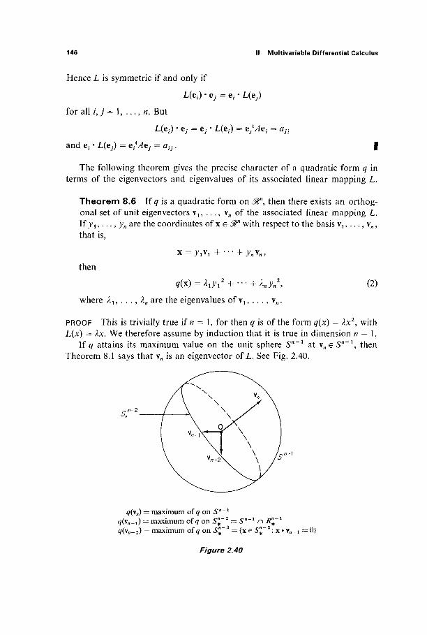
146 II Multivariable Differential Calculus
Hence L is symmetric if and only if
L(et) · ey = et- · L(e,)
for all i,j = 1, . . . , n. But
L(e;) · e; = e,· · L(e£) = e/^e,· - an
and ef · L(e,.) = e^e, · = a,·,·. |
The following theorem gives the precise character of a quadratic form q in terms of the eigenvectors and eigenvalues of its associated linear mapping L.
Theorem 8.6 If q is a quadratic form on 0ln, then there exists an orthog-onal set of unit eigenvectors v1? . . . , v„ of the associated linear mapping L. If yl9..., yn are the coordinates o f x e ^ " with respect to the basis v l 5 . . . , v„, that is,
x = yl\1 + · · · + yn\n,
then
where λί9 . . . , λη are the eigenvalues of vl5 . . . , v„.
(2)
PROOF This is trivially true if n = 1, for then q is of the form q(x) = λχ2, with L(x) = λχ. We therefore assume by induction that it is true in dimension n — 1.
If q attains its maximum value on the unit sphere Sn~x at \neSn~1, then Theorem 8.1 says that v„ is an eigenvector of L. See Fig. 2.40.
S' n-2
q(\n) = maximum of q on 5 n _ 1
q(yn-i) = maximum of q on Sl~2 = S"'1 n R^1
^(v„-2) = maximum of q on Sl~3 = {xeS^ - 2 : χ·\η-ι =0}
Figure 2.40
8 The Classification of Critical Points 147
Let M% 1 be the subspace of Mn perpendicular to v„. Then L maps 0t\ 1 into itself, because, given x e Μχ\ we have
L(x) · vn = x · L(\n)
= ληΧ'Ύη
= 0,
using the symmetry of L (Lemma 8.5). Let L* : MXί -> Μχx and </* : MXl -> i# be the " restrictions " of L and q
to Μχ\ that is,
L*(x) = L(x) and #*(x) = </(x), x e « 7k n— 1
If (w1? . . . , wn_j) are the coordinates of x with respect to an orthonormal basis for Mn~\ then by Lemma 8.5,
L*(u) = Bu,
where B is a symmetric (n — \) x (n — \) matrix. Then
<7*(u) = q(x)
= x · L(x) - u · L*(u) = uBu,
so </* is a quadratic form in wl5 . . . , ww_ t. The inductive hypothesis therefore gives an orthogonal set of unit eigen-
vectors vx, . . . , vn_! for L*. Then vl9 . . . , v„ is the desired orthogonal set of unit eigenvectors for L.
To prove the last statement of the theorem, let x = £ " y. v,. Then
q{x) = xl^x = x · L(x)
= Σ ^■J ' i^ i -v , . )
i = 1
since v,· · v · = 0 unless / =j, and vf · vt = 1. |
148 II Multivariable Differential Calculus
Equation (2) may be written in the form
The process of finding an orthogonal set of unit eigenvectors, with respect to which the matrix of q is diagonal, is sometimes called diagonalization of the quadratic form q.
Note that, independently of Corollary 8.4, it follows immediately from Eq. (2) that
(a) q is positive-definite if all the eigenvalues are positive, (b) q is negative-definite if all the eigenvalues are negative, and (c) q is nondefinite if some are positive and some are negative.
If one or more eigenvalues are zero, while the others are either all positive or all negative, then q is neither positive-definite nor negative-definite nor non-definite. According to Lemma 8.7 below, this can occur only if the determinant of the matrix of q vanishes.
Example 2 If q(x, y, z) — xy + yz, the matrix of q is
A = U 0 i).
\0 i 0/
The characteristic equation is then
\Α-λΙ\ = -λ3 + ±λ = 0 with solutions λι = — l/>/2, λ2 = 0, A3 = + l/>/2. By substituting each of these eigenvalues in turn into the matrix equation
(A - λΙ)\ = 0
(from the proof of Theorem 8.3), and solving for a unit vector v, we obtain the eigenvectors
If w, v, w are coordinates with respect to coordinate axes determined by vl5 v2, v3, that is, x = u\l + v\2 + wv3, then Eq. (2) gives

8 The Classification of Critical Points 149
Lemma 8.7 If λί9 . . . , λη are eigenvalues of the symmetric n x n matrix A, corresponding to orthogonal unit eigenvectors v1? . . . , v„, then
\A\ = V 2 · · · ^ . (3)
PROOF Let
'u\ V=(vu).
Then, since A\j = λiyj, we have
AV=(Xjvij).
It follows that
\A\ -\V\ =λιλ2-·λη\ν\.
Since | V\ φ 0 because the vectors \ l , . . . , v„ are orthogonal and therefore linearly independent, this gives Eq. (3). |
We are finally ready to give a complete analysis of a quadratic form q(x) = xlAx on 0tn for which \A\ ^ 0. Writing A = (α^) as usual, we denote by Ak the determinant of the upper left-hand k x k submatrix of A, that is,
Thus
Δι = an
A,=
Δ, = 422
, . - . ,Δ^ΜΙ .
Theorem 8.8 Let ^(x) = x l^x be a quadratic form on Then q is
with \A\ Φ0.
• · , tf, (a) positive-definite if and only if Ak > 0 for each k = l, (b) negative-definite if and only if (— l)* ΔΛ > 0 for each k = l, . . . , n, (c) nondefinite if neither of the previous two conditions is satisfied.
PROOF OF (a) This is obvious if n = l ; assume by induction its truth in dimen-sion n — l.
Since 0 < Δ„ = \A\ = λ χλ2 "' λη by Lemma 8.7, all the eigenvalues λί9..., λη
of A are nonzero. Either they are all positive, in which case we are finished, or an even number of them are negative. In the latter case, let λχ and λ} be two negative eigenvalues, corresponding to eigenvectors vf and v ·.
150 II Multivariable Differential Calculus
Let 0> be the 2-plane in 0tn spanned by vf and \j. Then, given x = y.y. + yj \j e 0, we have
q{x) = x · Ax
= (y^i + yjvj) ' {^y^i + ^y^j)
<o so q is negative on 0* minus the origin.
Now let q* : @n~l -> M be the restriction of q to ^ M - 1 , defined by q*(xu . . . , xn-0 = ?(*!, . . . , x„.u 0)
where
/ « i i · " ai,n-i \
W - i , i · · ' an-\,n-\l
Since Δχ > 0, . . . , Δ„_ j > 0, the inductive assumption implies that g* is positive-definite on 0tn~x. But this is a contradiction, since the (n — l)-plane Mn~1 and the 2-plane 0, on which q is negative, must have at least a line in common. We therefore conclude that q has no negative eigenvalues, and hence is positive-definite.
Conversely, if q is positive-definite, we want to prove that each Ak is positive. If m is the minimum value of q on 5 n _ 1 , then m > 0.
Let qk : ^fc -► ^ be the restriction of # to Mk, that is,
?*(*i> · . . ,**)= fax, . . . , ** , 0, . . . , 0)
where Ak is the upper left-hand k x k submatrix of A, so Ak = |ΛΛ|, and define ί.Λ : 0tk-*3frk by Lfc(x) = ΛΛχ. Then LA is symmetric by Lemma 8.5.
Let μί, . . . , μΛ be the eigenvalues of Lfc given by Theorem 8.6. Since by Lemma 8.2 each μ{· is the value of qk at some point of S*"1, the unit sphere in $k, and qk(x) = q(x, 0), it follows that each μ,. ^ /?? > 0. Finally Lemma 8.7 implies that
àk= \Ak\ = μ,μ2 •••μΑ^ΑΗ*>0.
PROOF OF (b) Define the quadratic form </* : &n -> ^ by <7*(x) = -#(x). Then clearly # is negative-definite if and only if g* is positive-definite. By part (a), q*
— (xl · · · χη_χ)Αλ
= {χγ · · · xk)Ak
8 The Classification of Critical Points 151
is positive-definite if and only if each Ak* is positive, where ΔΛ* = | — Ak\, Ak
being the upper left-hand k x k submatrix of A. But, since each of the k rows of — Ak is —1 times the corresponding row of Ak, it follows that
Ak*=\-Ak\ = ( - 1 ) ' | Λ | = ( - 1 ) * Δ 4 .
PROOF OF (c) Since An = λγλ2 · · · λ„ φ 0, all of the eigenvalues Xu . . . , λη are nonzero. If all of them were positive, then part (a) would imply that Ak > 0 for all k, while if all of them were negative, then part (b) would imply that (— 1)*ΔΛ > 0 for all k. Since neither is the case, we conclude that q has both positive eigenvalues and negative eigenvalues, and is therefore nondefinite. |
Recalling that, if a is a critical point of the class Ή3 function/: 0tn -► M', the quadratic form of /a t a is q(x) = \^{Di Z)7/(a))x, Theorems 7.5 and 8.8 enable us to determine the behavior o f / i n a neighborhood of a, provided that the determinant
\DtDjmi
often called the Hessian determinant o f / a t a, is nonzero. But if | Di Djf(a)\ = 0, then these theorems do not apply, and ad hoc methods must be applied.
Note that the classical second derivative test for a function of two variables (Theorem 4.4) is an immediate corollary to Theorems 7.5 and 8.8.
It will clarify the picture at this point to generalize the discussion at the end of Section 6. Suppose for the sake of simplicity that the origin is a critical point of the class # 3 function/: 0ln -► 01, and that/(0) - 0. Then
/ ( x ) = ? ( x ) + /i2(x) (4)
with
q(x) = \x\DiDjf(0))x and lim ^ = 0. 2 |x|»o |x | 2
Let v 1 ? . . . , \n be an orthogonal set of unit eigenvectors (provided by Theorem 8.6), with associated eigenvalues Xu . . . , λη. Assume that | Dt Djf(0)\ Φ 0, so Lemma 8.7 implies that each λ·ν is nonzero. Let ku ..., Xk be the positive eigen-values, and Xk+ ! , . . . , λη the negative ones (writing k = 0 if all the eigenvalues are negative). Since
q(K) = XlyS + .-. + Xnyn1 (5)
if x = y ί\ί + · · · + yn \n, it is clear that q has a minimum at 0 if k = n and a maximum if k = 0.
If 1 k < n, so that q has both positive and negative eigenvalues, denote by &\ the subspace of 0tn spanned by vl5 . . . , \k, and by Mn^k the subspace of 0ln
spanned by \k +1, . . . , v„. Then the graph of z = g(x) in 0ln +1 = {(x, z) | x e $n
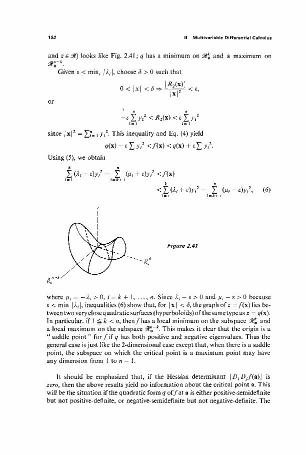
152 II Multivariable Differential Calculus
and z e &} looks like Fig. 2.41 ; q has a minimum on 0t\ and a maximum on an — k
Given ε < min^ |Af|, choose (5 > 0 such that
o < u , < ^ W < ε ,
or
-εΣ^ 2 <^(χ)<εΣ^· 2
ί = 1 i=l
since |x | 2 = £ ? = 1 ^, · 2 . This inequality and Eq. (4) yield
?(x) - ε X y,·2 < / (x ) < q(x) + ε £ yt·2.
Using (5), we obtain it
Σ Σ α , - β ) ^ 2 - Σ (/<-· + e)*2 </(χ)
<Σ(^ + %.·2- Σ fe-ΦΛ (6) i = l i = fc+l
/?, n-k/
Figure 2.41
where μ; = — λί > 0, / = & + 1, . . . , η. Since λί — ε > 0 and μ,- — ε > 0 because ε < min | Xt |, inequalities (6) show that, for | χ | < δ, the graph of z =f(x) lies be-tween two very close quadratic surfaces (hyperboloids) of the same type as z = q(x). In particular, if 1 :g k < n, then/has a local minimum on the subspace 0t% and a local maximum on the subspace &%~k. This makes it clear that the origin is a "saddle point" fo r / i f q has both positive and negative eigenvalues. Thus the general case is just like the 2-dimensional case except that, when there is a saddle point, the subspace on which the critical point is a maximum point may have any dimension from 1 to n — 1.
It should be emphasized that, if the Hessian determinant \DiDjf{2)\ is zero, then the above results yield no information about the critical point a. This will be the situation if the quadratic form q of /a t a is either positive-semidefinite but not positive-definite, or negative-semidefinite but not negative-definite. The

8 The Classification of Critical Points 153
quadratic form q is called positive-semidefinite if q(x) ^ 0 for all x, and negative-semidefinite if q{x) ^ 0 for all x. Notice that the terminology "q is nondefinite," which we have been using, actually means that q is neither positive-semidefinite nor negative-semidefinite (so we might more descriptively have said " nonsemi-definite").
Example 3 Let f(x, y) = x2 — 2xy + y2 + x4 4- y*, and g(x, y) = x2 — 2xy + y2 — x4 — y*. Then the quadratic form for both at the critical point (0, 0) is
q(x, y) = x2 - 2xy + y2 = (x - y)2,
which is positive-semidefinite but not positive-definite. Since
f{x, y) = (x- yf + x4 + y\
/ h a s a relative minimum at (0, 0). However, since
g(t,t)=-2t\ g{U-t) = 2t\2-t2\
it is clear that g has a saddle point at (0, 0). Thus, if the Hessian determinant vanishes, then anything can happen.
We conclude this section with discussion of a "second derivative test" for constrained (Lagrange multiplier) maximum-minimum problems. We first recall the setting for the general Lagrange multiplier problem : We have a differentiable function / : 0ln-+0t and a continuously differentiable mapping G : 0ln -> 0Γ (m < «), and denote by M the set of all those points x e G_1(0) at which the gradient vectors VGx(x), . . . , VGw(x), of the component functions of G, are linearly independent. By Theorem 5.7, M is an (n — m)-dimensional manifold in 0tn, and by Theorem 5.6 has an (n — m)-dimensional tangent space Tx at each point xe M. Recall that, by definition, Tx is the subspace of &n consisting of all velocity vectors (at x) to differentiable curves on M which pass through x. This notation will be maintained throughout the present discussion.
We are interested in locating and classifying those points of M at which the function/attains its local maxima and minima on M. According to Theorem 5.1, in order for/ to have a local maximum or minimum on M at a e M, it is necessary that a be a critical point f o r / o n M in the following sense. The point a G M is called a critical point for f on M if and only if the gradient vector V/(a) is ortho-gonal to the tangent space Ta of M at a. Since the linearly independent gradient vectors VGt(a), . . . , VGm(a) generate the orthogonal complement to Ta (see Fig. 2.42), it follows as in Theorem 5.8 that there exist unique numbers λί9...,λΜ
such that m
V/(a) = X^VG,(a). (7) λ=1

154 II Multivariable Differential Calculus
The translate of TQ to a
Figure 2.42
We will obtain sufficient conditions for f to have a local extremum at a by considering the auxiliary function H : tftn -> & for f at a defined by
/ / ( x ) = / ( x ) - £ A ( G , ( x ) . (8) i= 1
Notice that (7) simply asserts that V//(a) = 0, so a is an (ordinary) critical point for H. We are, in particular, interested in the quadratic form
q(h) = l f DtDjHMhihj
of H at a.
Theorem 8.9 Let a be a critical point for/on M, and denote by q : 0tn -*0t the quadratic form at a of the auxiliary function H =f— XJ"=1 ^ G , , as above. I f / and G are both of class ^ 3 in a neighborhood of a, then/has
(a) a local minimum on M at a if q is positive-definite on the tangent space Ta to M at a,
(b) a local maximum on M at a if g is negative-definite on Ta, (c) neither if q is nondefinite on Ta.
The statement, that "q is positive-definite on Ta," naturally means that g(h) > 0 for all nonzero vectors h e T a ; similarly for the other two cases.
PROOF The proof of each part of this theorem is an extension of the proof of the corresponding part of Theorem 7.5. We give the details only for part (a).
We start with the Taylor expansion
//(a + h) - //(a) = q(h) + R2(h)
8 The Classification of Critical Points 155
for the auxiliary function H. Since H(x) =f(x) if x e M, it clearly suffices to find a δ > 0 such that
o<W<4.!«±j£«>o TO
if a + h ε M.
Let ra be the minimum value attained by q on the unit sphere 5* = 5 " " I n T a
in the tangent plane Ta. Then m > 0 because # is positive-definite on Ta. Noting that
<7(h) + R2(h) / h \ t R2(h)
1 1 m l |2 - ? Ι τ ^ Ι +
we choose (5 > 0 so small that Q
, , l^2(h)| m
and also so small that 0 < |h| < δ and a + h e M together imply that h/ |h | is sufficiently near to S* that
/ h \ m
Then (9) follows as desired. The latter condition on δ can be satisfied because S* is (by definition) the set of all tangent vectors at a to unit-speed curves on M which pass through a. Therefore, if a + h e M and h is sufficiently small, it follows that h/ |h | is close to a vector in S*. |
The following two examples provide illustrative applications of Theorem 8.9.
Example 4 In Example 4 of Section 5 we wanted to find the box with volume 1000 having least total surface area, and this involved minimizing the function
f(x, y, z) = 2xy + 2xz + 2yz
on the 2-manifold M e l 3 defined by the constraint equation
g(x, y, z) = xyz - 1000 = 0.
We found the single critical point a = (10, 10, 10) f o r / o n M, with λ = f. The auxiliary function is then defined by
h(x, y, z) =f(x, y, z) - lg(x, y, z)
= 2xy + 2xz + lyz - \xyz + 400.

156 II Multivariable Differential Calculus
We find by routine computation that the matrix of second partial derivatives of A at a is
/ 0 - 2 - 2 \ - 2 0 - 2 ,
\ - 2 - 2 0/
so the quadratic form of h at a is
q(x, y, z) = — 2xy — 2xz — 2yz. (10)
It is clear that q is nondefinite on &3. However it is the behavior of q on the tangent plane Ta that interests us.
Since the gradient vector V#(a) = (100, 100, 100) is orthogonal to M at a = (10, 10, 10), the tangent plane Ta is generated by the vectors
Vl = ( i , - 1 , 0 ) and v2 =(1 ,0 , - 1 ) .
Given v e Ta, we may therefore write
v = s\l + t\2 =(s + t, — s, - 0,
and then find by substitution into (10) that
q(\) = Is2 + 1st + It2.
Since the quadratic form s2 + st + t2 is positive-definite (by the ac — b2 test), it follows that q is positive-definite on Ta. Therefore Theorem 8.9 assures us that/does indeed have a local minimum on M at the critical point a = (10, 10, 10).
Example 5 Jn Example 9 of Section 5 we sought the minimum distance be-tween the circle x2 + y2 = 1 and the straight line x + y = 4. This involved minimizing the function
/ ( * , y, u, v) = (x- u)2 + (y - v)2
on the 2-manifold M <= ^ 4 defined by the constraint equations
G^x, y, u9 v) = x2 + y2 - 1 = 0, G2(x, y, u, v) = u + v — 4 = 0.
We found the geometrically obvious critical points (see Fig. 2.43), a = (1/^2, 1/^/2,2,2) withλχ = 1 - 2x/2and λ2 = 4 - ^ 2 , and b = ( - 1 / ^ 2 , -1 /^ /2 , 2, 2) with Λ,χ = 1 + 2^/2 and λ2 = 4 +>/2 . It is obvious tha t /has a minimum at a, and neither a maximum nor a minimum at b, but we want to verify this using Theorem 8.9.
The auxiliary function H is defined by
H(x, y, u, v) = (x- uf + (y - v)2 - λ^χ2 + y2 - 1) - λ2(μ + v - 4).
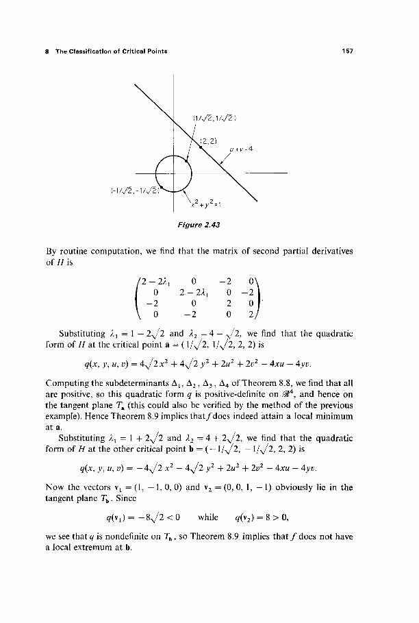
8 The Classification of Critical Points 157
Figure 2.43
By routine computation, we find that the matrix of second partial derivatives of His
2-2X, 0 - 2 0\ 0 2 - 2 ^ 0 - 2 |
- 2 0 2 0 Γ 0 - 2 0 2 /
Substituting ^ = 1 — 2^/2 and A2 = 4 — ^/2, we find that the quadratic form of H at the critical point a = ( 1/^/2, l/>/2, 2, 2) is
q(x, y, u, v) = A^/lx2 + 4^/2 y2 + 2u2 + 2y2 - 4xu - 4yv.
Computing the subdeterminants Δΐ5 Δ2 , Δ3, Δ4 of Theorem 8.8, we find that all are positive, so this quadratic form q is positive-definite on ^ 4 , and hence on the tangent plane Ta (this could also be verified by the method of the previous example). Hence Theorem 8.9 implies that/does indeed attain a local minimum at a.
Substituting At = 1 + l^/l and λ2 = 4 + 2^/2, we find that the quadratic form of H at the other critical point b = (—1/^/2, — l / \ /2 , 2, 2) is
<7(JC, y9 u, v) = - 4 ^ / 2 x2 - 4^2 y2 + 2w2 + 2v2 - 4xu - 4yv.
Now the vectors \ l = (1, — 1, 0, 0) and v2 = (0, 0, 1, —1) obviously lie in the tangent plane Tb. Since
q(\i)= - 8 ^ / 2 < 0 while q(\2) = 8 > 0,
we see that q is nondefinite on Tb, so Theorem 8.9 implies t ha t / does not have a local extremum at b.
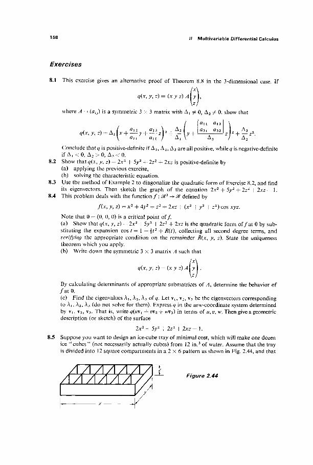
158 II Multivariable Differential Calculus
Exercises
8.1 This exercise gives an alternative proof of Theorem 8.8 in the 3-dimensional case. If
q(x,y, z)= {xy z) AI H ,
where A = (atJ) is a symmetric 3 x 3 matrix with Δί Φ 0, Δ 2 φ 0, show that
( U l i Öi2 \
Û31 Û32 L , Δ 3 y + -—*—-z + T -Δ 3 / Δ 2
q(x, y, z) = Δ^χ + — y ai
Conclude that q is positive-definite if Δ ΐ 5 Δ2 , Δ 3 are all positive, whiles is negative-definite if Δ ! < 0 , Δ 2 > 0 , Δ 3 < 0 .
8.2 Show that q(x, y, z) = 2x2 + 5y2 + 2z2 + 2xz is positive-definite by (a) applying the previous exercise, (b) solving the characteristic equation.
8.3 Use the method of Example 2 to diagonalize the quadratic form of Exercise 8.2, and find its eigenvectors. Then sketch the graph of the equation 2x2 + 5y2 + 2z2 + 2xz = 1.
8.4 This problem deals with the function / : ffl3 -+& defined by
f(x, y, z) = x2 + 4y2 + z2 + 2xz + (x2 - z2)cos xyz.
Note that 0 = (0, 0, 0) is a critical point of/. (a) Show that q(x, y, z) = 2x2 +5j>2 -f 2z2 + 2xz is the quadratic form o f / a t 0 by sub-stituting the expansion cos t = 1 — \t2 + R(t), collecting all second degree terms, and verifying the appropriate condition on the remainder R(x, y, z). State the uniqueness theorem which you apply. (b) Write down the symmetric 3 x 3 matrix A such that
q(x, y, z) -- (x y z) AI y
By calculating determinants of appropriate submatrices of A, determine the behavior of / a t O . (c) Find the eigenvalues λΐ5 λ2, λ3 of q. Let vl5 v2, v3 be the eigenvectors corresponding to λι, λ2, λ3 (do not solve for them). Express q in the mw-coordinate system determined by v1? v2, v3. That is, write q{u\Y + v\2 -r wv3) in terms of w, v, w. Then give a geometric description (or sketch) of the surface
2JC2 + 5J>2 + 2Z 2 + 2 X Z = 1 .
8.5 Suppose you want to design an ice-cube tray of minimal cost, which will make one dozen ice " c u b e s " (not necessarily actually cubes) from 12 in.3 of water. Assume that the tray is divided into 12 square compartments in a 2 x 6 pattern as shown in Fig. 2.44, and that
Figure 2.44
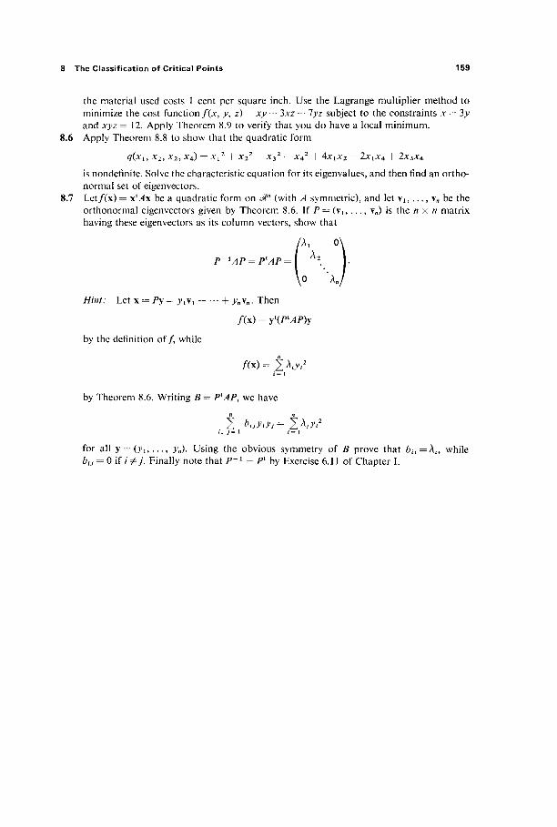
8 The Classification of Critical Points 159
the material used costs 1 cent per square inch. Use the Lagrange multiplier method to minimize the cost function f(x, y, z) = xy + 3xz + lyz subject to the constraints x = 3y and xyz= 12. Apply Theorem 8.9 to verify that you do have a local minimum.
8.6 Apply Theorem 8.8 to show that the quadratic form
q(xi, x2, X2, x*) = Xi2 + X22 — X32 — X*2 + ^XiXz — 2XiXA + 2x3*4
is nondefinite. Solve the characteristic equation for its eigenvalues, and then find an ortho-normal set of eigenvectors.
8.7 Let/(x) = xxAx be a quadratic form on 0tn (with A symmetric), and let v l 5 . . . , v„ be the orthonormal eigenvectors given by Theorem 8.6. If P= (\u . . . , v„) is the n x n matrix having these eigenvectors as its column vectors, show that
A, 0\
\° 'v Hint: Let x = Py = γχ\γ -\ h ynvn· Then
f(x) = yt(PtAP)y
by the définition of/, while
/(x)= Ϊλ^·2
/ = 1
by Theorem 8.6. Writing B= PKAP, we have n n
Σ buyiyj= Σλiyi2
for all y = 0>i,..., y„). Using the obvious symmetry of B prove that bH=Xiy while bu = 0 if ιφ]. Finally note that P~l = Pl by Exercise 6.11 of Chapter I.

m Successive
Approximations and Implicit Functions
Many important problems in mathematics involve the solution of equations or systems of equations. In this chapter we study the central existence theorems of multivariable calculus that pertain to such problems. The inverse mapping theorem (Theorem 3.3) deals with the problem of solving a system of n equations in n unknowns, while the implicit mapping theorem (Theorem 3.4) deals with a system of n equations in m + n variables xl9 . . . , xm, y1, . . . , yn, the problem being to solve for yu ..., yn as functions ofxl9...,xm.
Our method of treatment of these problems is based on a fixed point theorem known as the contraction mapping theorem. This method not only suffices to establish (under appropriate conditions) the existence of a solution of a system of equations, but also yields an explicitly defined sequence of successive approxima-tions converging to that solution.
In Section 1 we discuss the special cases n = 1, m = 1, that is, the solution of a single equation f(x) = 0 or G(x, y) = 0 in one unknown. In Section 2 we give a multivariable generalization of the mean value theorem that is needed for the proofs in Section 3 of the inverse and implicit mapping theorems. In Section 4 these basic theorems are applied to complete the discussion of manifolds that was begun in Chapter II (in connection with Lagrange multipliers).
1 NEWTON'S METHOD AND CONTRACTION MAPPINGS
There is a simple technique of elementary calculus known as Newton's method, for approximating the solution of an equation/(x) = 0, where/: 0t^>0l is a ^ 1 function. Let [a, b] be an interval on which f'(x) is nonzero and/(x)
160
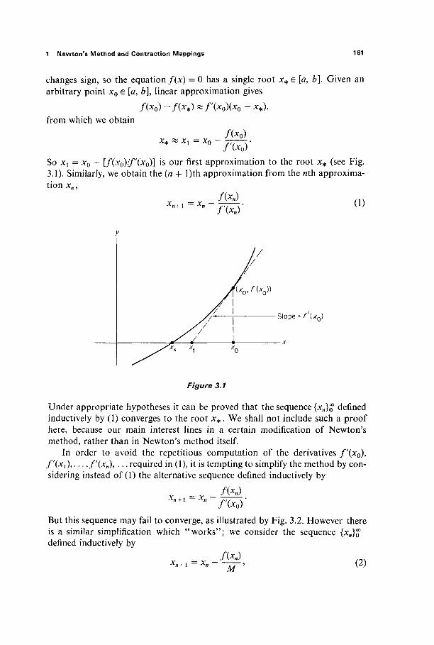
1 Newton's Method and Contraction Mappings 161
changes sign, so the equation f(x) = 0 has a single root x* e [a, b]. Given an arbitrary point x0 e [a, b], linear approximation gives
/(*o) -fix*) «/'(*o)(*o - **), from which we obtain
/ ( *o ) X^ r^ Χ^ XQ .
/ ΚΧθ)
So xx = x0 — [f(xo)/f'(xo)] is o u r ^ r s t approximation to the root x* (see Fig. 3.1). Similarly, we obtain the (n + l)th approximation from the nih approxima-tion xn,
Xn +1 — Xn /'(*.)
(1)
Slope -f ix0)
Figure 3.1
Under appropriate hypotheses it can be proved that the sequence {xn}o defined inductively by (1) converges to the root x*. We shall not include such a proof here, because our main interest lines in a certain modification of Newton's method, rather than in Newton's method itself.
In order to avoid the repetitious computation of the derivatives f'(x0), f'(xi\... ,f'(x„), . · · required in (1), it is tempting to simplify the method by con-sidering instead of (1) the alternative sequence defined inductively by
Xn ~ f'ixoY
But this sequence may fail to converge, as illustrated by Fig. 3.2. However there is a similar simplification which "works"; we consider the sequence {x„}o defined inductively by
M ' (2)

162 III Successive Approximations and Implicit Functions
y--f(x)
Figure 3.2
where M = max | f\x) | if/'(x) > 0 on [a, b], and M = - max | f'(x) | if f\x) < 0 on [a, b]. The proof that lim xn = x* if {xn}o is defined by (2) makes use of a widely applicable technique which we summarize in the contraction mapping theorem below.
The mapping φ : [a, b] -> [a, b] is called a contraction mapping with contrac-tion constant k < 1 if
\(p(x)-(p(y)\ ^k\x- y\ (3)
for all x, y e [a, b]. The contraction mapping theorem asserts that each contrac-tion mapping has a unique fixed point, that is, a point x* e [a, b] such that <p(x*) = ** » and at the same time provides a sequence of successive approxima-tions to x*.
Theorem 1.1 Let φ: [a, b] -► [a, b] be a contraction mapping with con-traction constant k < 1. Then φ has a unique fixed point x*. Moreover, given x0 e [a, b], the sequence {xJJ defined inductively by
xn + 1 = φ(χη)
converges to x* . In particular,
I * » - ** I ^ 1 -k (4)
for each «.
PROOF Application of condition (3) gives
l*n + l - * J = Ι Λ ) " Λ - ΐ ) | ^ £ | * Λ - * , ι - ΐ |
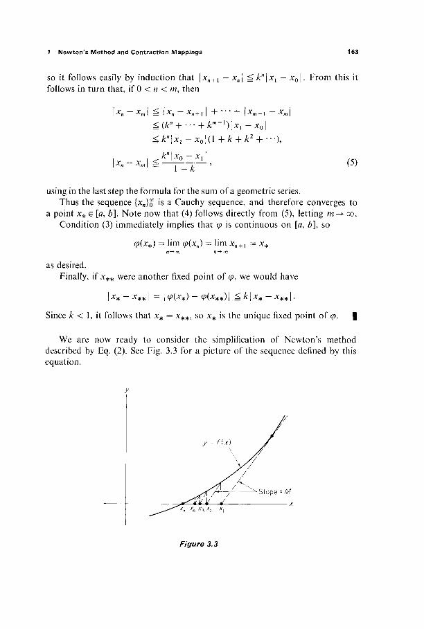
1 Newton's Method and Contraction Mappings 163
so it follows easily by induction that \xn + i — xn\ rg k"\xi — x0\. From this it follows in turn that, if 0 < n < m, then
%n Xm = %n + ' ' " + \Xm - 1 ~ Xm
Xn Xtr
^(kn + --- + km'i)\x1-x0\
^k"\Xl -x0\(\ + k + k2 + ■■■),
k \x0 — xl\ < 1 -k
(5)
using in the last step the formula for the sum of a geometric series. Thus the sequence {xn}o is a Cauchy sequence, and therefore converges to
a point x* e [a, b]. Note now that (4) follows directly from (5), letting m -> oo. Condition (3) immediately implies that φ is continuous on [a, b], so
<p(**) = lim φ(χη) = lim xn + 1 = x* n -*■ oo n -*■ oo
as desired. Finally, if x** were another fixed point of φ, we would have
I - * ^** I = | Ψ\Χ*) Φν*·**/1=^1 ·*"# - ** I ·
Since k < 1, it follows that x* = x**, so x* is the unique fixed point of φ. |
We are now ready to consider the simplification of Newton's method described by Eq. (2). See Fig. 3.3 for a picture of the sequence defined by this equation.
Figure 3.3
164 III Successive Approximations and Implicit Functions
Theorem 1.2 Let / : [a, b]->@ be a differentiable function with f(a) < 0 <f(b) and 0 < m <f'{x) ^ M for x G [a, b]. Given x0 e [a, b], the sequence {xn)o defined inductively by
Xn+l = Xn T7~ \A) M
converges to the unique root x* G [a, b] of the equation f(x) = 0. In par-ticular,
, l/(*o)l / mY m \ M)
for each n.
PROOF Define φ : [a, b] -+ SI by φ(χ) = x - [f(x)/M]. We want to show that φ is a contraction mapping of [a, b]. Since φ\χ) = 1 — [/'(x)/M], we see that
0£<p'(x)£l-%i = k<l9
M so φ is a nondecreasing function. Therefore a < a — [f(a)/M] = φ(α) ^ φ(χ) ^ φ(6) = b- [f(b)/M] < b for all x e [a, 6], because f(a) < 0 </(6) . Thus φ([α, b]) cz [A, è], and φ is a contraction mapping of [a, è].
Therefore Theorem 1.1 implies that φ has a unique fixed point
, , _ _ / ( * * ) X* — Ψ\Χ*) — ·** 77 »
which is clearly the unique root of f(x) = 0, and the sequence {xn}% defined by
converges to x*. Moreover Eq. (4) gives
* " l * o - * i l l/(*o)l *!k è (-2)" 1 — k m
upon substitution of xx = x0 - [f(x0)/M] and k = 1 -(m/M). |
Roughly speaking, Theorem 1.2 says that, if the point x0 is sufficiently near to a root x* of f(x) = 0 where f\x*) > 0, then the sequence defined by (2) converges to x*, with M being an upper bound for | f\x) | near x* .
Now let us turn the question around. Given a point x* where f(x*) = 0, and a number y close to 0, can we find a point x near x* such thatf(x) = yl More generally, supposing that/(a) = b, and that y is close to £, can we find x close to a such that/(x) = yl If so, then
7 - Ζ > = / ( * ) - / ( 0 ) * / ' ( α ) ( χ _ * ) .
(6)

1 Newton's Method and Contraction Mappings 165
Iff\a) φ 0, we can solve for
x « a fa)-y
f'iß)
Writing a = x0, the point
Xt =Xn-/(*o) - y
/'(*o) '
is then a first approximation to a point x such that / (*) = y. This suggests the conjecture that the sequence {X„}Q defined by
x0 = a, Xn+ 1 Xn f(x„)-y
converges to a point x such that f(x) = y. In fact we will now prove that the slightly simpler sequence, with/'(*„) replaced byf'(a), converges to the desired point x if y is sufficiently close to b.
Theorem 1.3 Let f\&-*9l be a ^ 1 function such that f(a) = b and f\d) Φ 0. Then there exist neighborhoods U = [a — <5, a + δ] of a and V = [b — ε, b + ε] of b such that, given >>* e V, the sequence {x„}J defined induc-tively by
x0 = a, Xn 4. i Xn
f(Xn) - y* (7)
converges to a (unique) point x*e U such that/(;t*) = y* .
PROOF Choose δ > 0 so small that
\f\a) - / ' ( * ) | ^ i l / » I if ^ £ / = [ f l - i , f l + i ] .
Then let ε = \δ \f'(ä) |. It suffices to show that
/ ( * ) - y* φ(χ) = x fia)
is a contraction mapping of U if y* e V = [b — ε, ό + ε], since </>(**) = ** clearly implies that/Xx*) = j * .
First note that
\φ'(χ)\ = 1 - /'W /'(«)
166 III Successive Approximations and Implicit Functions
if x e £/, so φ has contraction constant \. It remains to show that, if y* e V, then φ maps the interval U into itself. But
\<p(x)-a\ S \φ(χ)- φ(α)\ + \φ(α) - a\
^ - \χ-α\ + υ *' 2 ' ' | / ' (α) |
_ ε
= <5
if x e U = [a — δ, a + δ] and j>* e V = [b — ε, b + ε]. Thus <p(jc) e U as desired. |
This theorem provides a method for computing local inverse functions by successive approximations. Given y e K, define #(>>) to be that point x e U given by the theorem, such that/(je) = y. Then/and g are local inverse functions. If we define a sequence {#„}^ °f functions on K by
then we see [by setting xn = gn(y)] that this sequence of functions converges to g.
Example 1 Let/(jc) = x2 — l, a = 1, è = 0. Then (8) gives
#oO) = U
,2ω = ( ι + ^ ) - [ ( 1 + ^ / 2 ) ; - 1 ] - ^ ι ^ - ^
^ = » I + Î - Ç + ^ ) - 4 _r2
2
Thus it appears that we are generating partial sums of the binomial expansion
< , + » , Β - , + ϊ - ϊ + ίϊ +
12 of the inverse function g(y) = (1 + j ) 1
Next we want to discuss the problem of solving an equation of the form G(x9 y) = 0 for y as a function of x. We will say that y =f(x) solves the equation G(x, y) = 0 in a neighborhood of the point (a, b) if G(a, b) = 0 and the graph of /agrees with the zero set of G near (a, b). By the latter we mean that there exists a neighborhood W of (a, b), such that a point (x, y) e W lies on the zero set of G
(8)
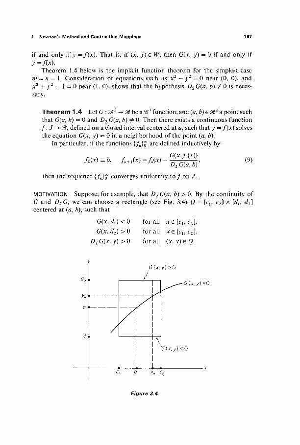
1 Newton's Method and Contraction Mappings 167
if and only if y =f(x). That is, if (x, y) e W, then G(x, y) = 0 if and only if y = / ( * ) ■
Theorem 1.4 below is the implicit function theorem for the simplest case m — n= 1. Consideration of equations such as x2 — y2 = 0 near (0, 0), and x2 + y2 — 1 = 0 near (1, 0), shows that the hypothesis D2 G(a, b) φ 0 is neces-sary.
Theorem 1.4 Let G : M2 -> M be a ^ 1 function, and (a, b) e 0l2 a point such that G(a, è) = 0 and D2 G(a, b) Φ 0. Then there exists a continuous function f\J-+ffl, defined on a closed interval centered at #, such that y =f(x) solves the equation G(x, y) = 0 in a neighborhood of the point (a, 6).
In particular, if the functions {/„} J are defined inductively by
f0(x) =b9 fn + l (x) = fn(x) -G(xJn(x))
D2G(a,b)
then the sequence {/„}£ converges uniformly to / on J.
(9)
MOTIVATION Suppose, for example, that D2G(a, b) > 0. By the continuity of G and D2G, we can choose a rectangle (see Fig. 3.4) Q = [cu c2] x [dl9 d2] centered at (a, b), such that
G(x, di) < 0 G(x, d2) > 0
D2G(x,y)>0
for all x e [cu c2],
for all xe [cl5 c2], for all (x, y) G g.
GU,y)>0
£ U , / ) = 0
Figure 3.4

168 III Successive Approximations and Implicit Functions
Given x* e [cu c2], define GXic : [dlf d2] -► @ by
Gx£y) = G(x* » )>).
Since Gx£dù < 0 < GXic(d2) and G^(y) > 0 on [rfl9 </2] the intermediate value theorem (see the Appendix) yields a unique point y* e [rfl9 */2] s u c n that
G(x*, )>*) = GxXy*) = 0.
Defining/: [cj, c2] -► ^ by/(*#) = ^ for each x* e [cu c2], we have a function such that y =f(x) solves the equation G(x, y) = 0 in the neighborhood Q of
We want to compute y* =f(x*) by successive approximations. By linear approximation we have
G(x* > J*) - G(x* , £) ~ A> G(x*, 6)0* - Z>).
Recalling that G(x*, y*) = 0, and setting y0 = b, this gives
G(x*, J o) £>2 G(x*, )>o)
so
Z>2 GO*, y0)
is our first approximation to y*. Similarly we obtain
G(x*, jQ
as the (« + l)th approximation.
What we shall prove is that, if the rectangle Q is sufficiently small, then the slightly simpler sequence {yn}o defined inductively by
, G(x*, yn)
D2 G(a, b)
converges to a point y* such that G{x*, y*) = 0.
PROOF First choose ε > 0 such that
| D2 G(x, y) - D2G(a, b)\ £i\D2 G(a, b)\
if | JC — a\ ^ ε and \y — b\ g ε. Then choose δ > 0 less than ε such that
\G(x,b)\ ^ie\D2G(a,b)\
if \x — a\ ^δ. We will work inside the rectangle W = [a — <5, a + δ] x [b — ε, Z> -f ε], assuming in addition that δ and ε are sufficiently small that W a Q.

1 Newton's Method and Contraction Mappings 169
Let Jt* be a fixed point of the interval [a — δ, a + δ]. In order to prove that the sequence {yn}o defined above converges to a point y* e [b — ε, b + ε] with G(x*, y*) = 0, it suffices to show that the function φ : [b — ε, b + ε] -> , de-fined by
Z)2 (/(fl, 0)
is a contraction mapping of the interval [b — ε, b + ε]. First note that
D2G(x*,y)\ ΐΦ#ωι = 1 -
D2G(a,b)
\D2G(a,b)-D2G(x*,y)\ 1 | />2GO,6) | ä 2
since (x*, y) e IF. Thus the contraction constant is £. It remains to show that \(p(y) — b\ ^ε if \y — b\ ^ ε . But
\cp{y)-b\uW{y)-<p{b)\ + \<p{b)-b\
2 " ' \D2G(a,b)\
ε ε
2 2
since [ x* - a | ^δ implies | G(x*, b) | ^ \ε \ D2 G(a, b) \. If we write
D2 G{a, b)
the above argument proves that the sequence {f„(x)}% converges to the unique number/(x) e [b - ε, b + ε] such that G(x, f(x)) = 0. It remains to prove that this convergence is uniform.
To see this, we apply the error estimate of the contraction mapping theorem. Since \f0(x) —fi(x)\ ^ ε because f0(x) = b andfx(x) e [b - ε, b + ε], and k = i, we find that
\fn(X)-f{x)\u:^,
so the convergence is indeed uniform. The functions {fn}o are clearly continuous, so this implies that our solution / : [a — δ, a + δ] -> 0ί is also continuous (by Theorem VI. 1.2). |
REMARK We will see later (in Section 3) that the fact that G is ^ 1 implies that / i s ^ 1 .

170 III Successive Approximations and Implicit Functions
Example 2 Let G(x, y) = x2 + y2 - 1, so G(x, y) = 0 is the unit circle. Let us solve for y =f(x) in a neighborhood of (0, 1) where D2G(0, 1) = 2. The successive approximations given by (9) are
/oW = 1,
Α(χ) = i
AW = (l - y )
*2 + (l)2 - 1 = 1 -
2 2
2^ x2 + (l - i x 2 ) 2 - l
' - y - T ·
ΛΜ-('-Τ-τ)-: _ / x2 x4 x6\
~ \ Τ~ΊΓ~Ϊ6/
/ x2 x 4 \ 2
+ ' - T - T - ' x°
Ϊ28 '
/ 4 (^) = l - y - y - y ^ - y ^ + higher order terms.
Thus we are generating partial sums of the binomial series
x6 5xs
Ϊ6 ~ Î28 v 2 v 4 v 6 c y 8
/ ( χ ) = ( 1 - χ 2 ) 1 / 2 = 1 - γ - -
The preceding discussion is easily generalized to treat the problem of solving an equation of the form
G(x,y) = G(xu ...,xm,y) = 0,
where G : @m + 1 -> ^ , for y as a function x = (JC,, . . . , x j . Given/: ^ m -> ^?, we say that y =f(x) solves the equation <7(x, >') = 0 in a neighborhood of (a, b) if G(a, b) = 0 and the graph of/agrees with the zero set of G near (a, b)e &m + 1.
Theorem 1.4 is simply the case m = 1 of the following result.
Theorem 1.5 Let G : 0lm + ' -► be a #* function, and (a, 6) G m x 9t = @m + 1 a point such that G(a, é) = 0 and Dm + lG(a, b) φ 0. Then there exists a continuous function/: J -> ^£, defined on a closed cube J c: ^ m centered at a e l m , such that y = / (x ) solves the equation (7(x, y) = 0 in a neighbor-hood of the point (a, &).
In particular, if the functions {/„}% are defined inductively by
f0(\)=b9 / n + i(x)=/„(x)- σ(χ,/,(χ))
then the sequence {/,}J converges uniformly to / o n J.
1 Newton's Method and Contraction Mappings 171
To generalize the proof of Theorem 1.4, simply replace x, a, x* by x, a, x* respectively, and the interval [a — δ, a + δ] a M by the w-dimensional interval { x e r : | x - a | ^ δ}.
Recall that Theorem 1.5, with the strengthened conclusion that the implicitly defined function / is continuously differentiable (which will be established in Section 3), is all that was needed in Section II.5 to prove that the zero set of a ^ 1
function G : 0tn -*0l is an (n — l)-dimensional manifold near each point where the gradient vector V(7 is nonzero. That is, the set
{ x e i " : G(x) = 0 and VG(x) # 0}
is an (n — l)-manifold (Theorem II.5.4).
Exercises
1.1 Show that the equation x3 + xy + y3 = 1 can be solved for y=f(x) in a neighborhood of (1,0).
1.2 Show that the set of all points (x, y) e 0t2 such that {x -f- yf — xy = 1 is a 1-manifold. 1.3 Show that the equation y3 -f x2y — 2x3 — x + y = 0 defines y as a function of x (for
all x). Apply Theorem 1.4 to conclude that y is a continuous function of x. 1.4 Let / : 9t -> # and G : ^ 2 -> # be ^ 2 functions such that G(x, /(JC)) = 0 for all x e St,
Apply the chain rule to show that
= _ DiG(x,f(x)) o r dy_ = _ dG/dx
D2G(xJ(x)Y ΟΓ dx dG/dy'
and <Py_ 1 _ dx2 ~ dG/dy
d2G dy d2G -2
dx2 dx dx dy \dx) dy2[
1.5 Suppose that G : &m + l -> ^ is a ^ 1 function satisfying the hypotheses of Theorem 1.5. Assuming that the implicitly defined function y=f(xu . . . , xm) is also ^ 1 , show that
^ / A G . — = , z = l , . . . , m . ΟΛ:, / ) m + iG
1.6 Application of Newton's method [Eq. (1)] to the function f(x) = x2 — a, where a > 0, gives the formula ^„ + i = i(xn + a/xn). If x0 > \/a, show that the sequence {X„}Q con-verges to Λ/Α» by proving that <p(x) = $(x + ajx) is a contraction mapping of [\/a, x0]. Then calculate \/2 accurate to three decimal places.
1.7 Prove that the equation 2 — x — sin x = 0 has a unique real root, and that it lies in the interval [π/6,77/2]. Show that <p(x) = 2 — sin x is a contraction mapping of this interval, and then apply Theorem 1.1 to find the root, accurate to three decimal places.
1.8 Show that the equation x -f y — z + cos xyz = 0 can be solved for z =f(x, y) in a neigh-borhood of the origin.
1.9 Show that the equation z3 + zex + y + 2 = 0 has a unique solution z =f(xt y) defined for all (x, y) e ^ 2 . Conclude from Theorem 1.5 t h a t / i s continuous everywhere.
1.10 If a planet moves along the ellipse x = a cos 0, y = b sin 0, with the sun at the focus {{a2 — b2)1'2, 0), and if t is the time measured from the instant the planet passes through (a, 0), then it follows from Kepler's laws that Θ and t satisfy Kepler's equation
kt = θ — ε sin Θ,
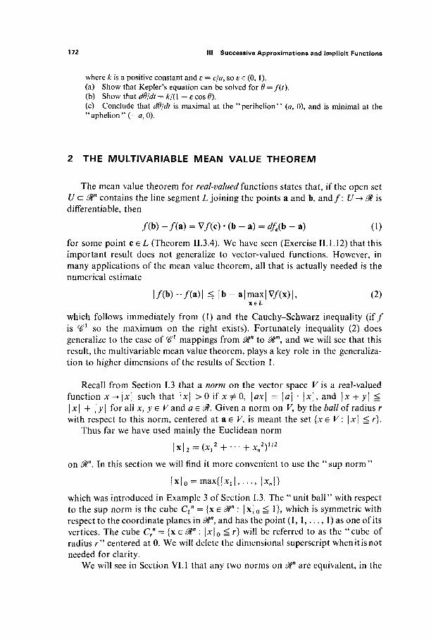
172 III Successive Approximations and Implicit Functions
where k is a positive constant and ε = c/a, so ε e (0,1). (a) Show that Kepler's equation can be solved for 9=f(t). (b) Show that dd/dt = k/(\ - ε cos Θ). (c) Conclude that dd/dt is maximal at the "perihelion" (a> 0), and is minimal at the "aphelion" (—a, 0).
2 THE MULTIVARIABLE MEAN VALUE THEOREM
The mean value theorem for real-valued functions states that, if the open set U c 0tn contains the line segment L joining the points a and b, a n d / : U->> 0t is differentiable, then
/(b) - / ( a ) = V/(c) · (b - a) = dfe(b - a) (1)
for some point c e L (Theorem II.3.4). We have seen (Exercise II. 1.12) that this important result does not generalize to vector-valued functions. However, in many applications of the mean value theorem, all that is actually needed is the numerical estimate
[ / ( b ) - / ( a ) | ^ | b - a | m a x | V / ( x ) | , (2) x e L
which follows immediately from (1) and the Cauchy-Schwarz inequality (if/ is Ή1 so the maximum on the right exists). Fortunately inequality (2) does generalize to the case of <é>1 mappings from 0ίη to ^£m, and we will see that this result, the multivariable mean value theorem, plays a key role in the generaliza-tion to higher dimensions of the results of Section 1.
Recall from Section 1.3 that a norm on the vector space F is a real-valued function x -> |x | such that \x\ > 0 if x Φ 0, \ax\ = \a\ · | x | , and \x -f y\ ^ | x | + | y | for all x, y e V and ae0l. Given a norm on V, by the ball of radius r with respect to this norm, centered at a e V, is meant the set {x e V : \x\ ^ r}.
Thus far we have used mainly the Euclidean norm
|χ|2 = (*ι2 + ··· + * . 2 ) ι / 2
on 0ln. In this section we will find it more convenient to use the " sup norm "
[x|o = max{ |x 1 | , . . . , \xn\}
which was introduced in Example 3 of Section 1.3. The "unit ball" with respect to the sup norm is the cube C ^ j x e J " : | x| 0 ^ 1}, which is symmetric with respect to the coordinate planes in 0ln, and has the point (1, 1 , . . . , 1) as one of its vertices. The cube Cr" = { x e f " : \x\0 ^ r) will be referred to as the "cube of radius r " centered at 0. We will delete the dimensional superscript when it is not needed for clarity.
We will see in Section VI. 1 that any two norms on $n are equivalent, in the
2 The Multivariable Mean Value Theorem 173
sense that every ball with respect to one of the norms contains a ball with respect to the other, centered at the same point. Of course this is "obvious" for the Euclidean norm and the sup norm (Fig. 3.5). Consequently it makes no dif-ference which norm we use in the definitions of limits, continuity, etc. (Why?)
Figure 3.5
We will also need the concept of the norm of a linear mapping L : The norm \\L\\ of L is defined by
| |L| |= max |L(x) | 0 . xedCi
is indeed a norm on the vector space S£mn of all —the only property of a norm that is not obvious
We will show presently that linear mappings from 0tn to ί is the triangle inequality.
We have seen (in Section 1.7) that every linear mapping is continuous. This fact, together with the fact that the function x -► [x0| is clearly continuous on 0Γ, implies that the composite x-> |L(x)|0 is continuous on the compact set dC^, so the maximum value ||L|| exists. Note that, if x e @tn, then x/[x| 0 e dC^, so
ΛΜο/Ιο" | |L | |=> |L(x) | 0 g | |L | | · |x |
This is half of the following result, which provides an important interpretation of||L||.
Proposition 2.1 If L : 0ίη -+0Γ is a linear mapping, then ||L|| is the least number M such that |L(x)|0 ^ M [ x | 0 for all x e ^ " .
PROOF It remains only to be shown that, if |L(x)|0 g M | x | 0 for all x e l " , then M^ \\L\\. But this follows immediately from the fact that the inequality |L(x)|0 ^ M\x| o reduces to |L(x)[0 ^ M if x e dCl9 while ||L|| = max |L(x)|0 f o rxedCi . |
In our proof of the mean value theorem we will need the elementary fact that the norm of a component function of the linear mapping L is no greater than the norm IILII of L itself.
174 III Successive Approximations and Implicit Functions
Lemma 2.2 If L = (Ll5 . . . , Lm) : 0tn -► 9Γ is linear, then \\Lt\\ g ||L|| for each / = 1, . . . , m.
PROOF Let x0 be the point of <9Q at which |^(χ)[ is maximal. Then
IILJI = |L,.(x0)| ^π ιαχ{ |Α(χο ) | , . . . , |LM(x0)|} = |L(x 0 ) |o^ max |L(x)|0 = ||L||. |
x e dCi
Next we give a formula for actually computing the norm of a given linear mapping. For this we need a particular concept of the "norm" of a matrix. If A = (dij) is an m x n matrix, we define its norm \\A\\ by
|M ||= max ( t k y l l - (3)
Note that, in terms of the " 1-norm " defined on Mn by
| x | 1 = \χ,\ + \χ2\ + · · · + | x j ,
Mil is simply the maximum of the 1-norms of the row vectors Al9 . . . , Am of A,
MU = m a x { M 1 | 1 , M 2 | l f . . . , \Am\x).
To see that this is actually a norm on the vector space Jimn of all m x n matrices, let us identify Jimn with 0Tn in the natural way:
\Xij) ~ v ^ l l » · · · > Xln > -*"21 > · · · > ·*2η > · · · > ·*τη1> · · · > ^ m n ' ·
In other words, if xu . . . , xm are the row vectors of the m x n matrix X = (x0), we identify X with the point
(xu ..., x j e 0ln x · · · x mn = ^mw. (m factors)
With this notation, what we want to show is that
||x|| =max{|x1 | 1 , | x 2 | i , . . . , |xm|i}
defines a norm on Mmn. But this follows easily from the fact that | | γ is a norm on $n (Exercise 2.2). In particular, || || satisfies the triangle inequality. A ball with respect to the 1-norm is pictured in Fig. 3.6 (for the case n = 2); a ball with respect to the above norm || || on Mmn is the Cartesian product of m such balls, one in each 0tn factor.
We will now show that the norm of a linear mapping is equal to the norm of its matrix. For example, if L : 01* -> & is defined by L(x, y, z) = (x — 3z, 2x - y - 2z, x + y)9 then ||L|| = max{4, 5, 2} = 5.

2 The Multivariable Mean Value Theorem 175
k l + | y | = i
Figure 3.6
Theorem 2.3 Let A = (αι}) be the matrix of the linear mapping L : Mn -» 9Γ, that is, L(x) = Ax for all x e 0ln. Then
||L|| = M||.
PROOF Given x = (xl9 . . . , xn)e 0ln, the coordinates (yu . . . , ym) of y = L(x) are defined by
i= 1, . . . , w.
Let | j / f c | be the largest of the absolute values of these coordinates of y. Then
|L(x)|0 = max 1 â i â m
laijxj
\takjXj
n
J = l
^ |χ|οΣ Κ·Ι g |x|o max £ |a0-|
= ΜΙ Ι · |χ|ο-
Thus | L ( x ) | 0 ^ \\A\\ · | x | 0 for all x e f , so it follows from Proposition 2.1 t h a t | | L | | g M | | .
To prove that ||L|| ^ \\A\\, it suffices to exhibit a point xedCx for which |L(x)|0 ^ \\A\\. Suppose that the k\\\ row vector Ak = (akl . . . akn) is the one whose 1-norm is greatest, so
Mll= Σ Kl · J = l
176 III Successive Approximations and Implicit Functions
For each j = 1, . . . , n, define ε,- = +1 by akj = Sj\ akj|. If x = (εΐ5 ε2, then [x | 0 = 1, and
. . . , 8n),
| L(x) 10 = max 1 < i < m
>
Σαυ4 n 1
Σαν4 7 = 1 1 n
Σ Kl
= Σ K-l
so |L(x)|o ^ IM II as desired. I
Let Φ : £Pmn -► Jimn be the natural isomorphism from the vector space of all linear mappings 0ln -> 0Γ to the vector space of all m x n matrices, Φ(Ζ,) being the matrix of L e £?mn. Then Theorem 2.3 says simply that the isomor-phism Φ is "norm-preserving." Since we have seen that || || on Jlmn satisfies the triangle inequality, it follows easily that the same is true of || || on 3?mn. Thus || || is indeed a norm on l£mn.
Henceforth we will identify both the linear mapping space $£ mn and the matrix space Jimn with Euclidean space &mn, by identifying each linear mapping with its matrix, and each m x n matrix with a point of 0Tn (as above). In other words, we can regard either symbol 5£mn as J(mn as denoting @tmn with the norm
||(xl5 . . . ,x m ) | | =max{ |x 1 1! , . . . , I x J J ,
where (xl5 . . . , x j e 0ln x · · · x &n = 0Γη. If/: Mn -► £%m is a differentiable mapping, then dfx e J2?w„, and/ '(x) e Jtmn9
so we may regard / ' as a mapping form 01* to Jimn,
and similarly dfas a mapping from 0ln to Semn. Recall t h a t / : 0ln -> 0Γ is ^ 1 at a e i " if and only if the first partial derivatives of the component functions of/ all exist in a neighborhood of a and are continuous at a. The following result is an immediate consequence of this definition.
Proposition 2.4 The differentiable mapping/ : if and only if / ' : 0ln -» Jtmn is continuous at a.
at a e ;
We are finally ready for the mean value theorem.
Theorem 2.5 Let / : U^Mm be a ^ 1 mapping, where U c mn is a neighborhood of the line segment L with endpoints a and b. Then
| / ( b ) - / ( a ) | 0 ^ | b - a | 0 m a x | | A x ) | | . (4) xe L

2 The Multivariable Mean Value Theorem 177
PROOF Let h = b - a, and define the ^ 1 curve y : [0, 1 ] -> 0Γ by
y ( 0 = / ( a + /h).
If/1, . . . ,fm are the component functions of/, then yf(0 = / ' ( a 4- ih) is the ith component function of y, and
7/(0 = rf/i+A(li) by the chain rule.
If the maximal (in absolute value) coordinate of/(b) - / ( a ) is the kth one, then
| / ( b ) - / ( a ) | 0 = | / * ( b ) - / ' ( a ) |
= lr*0)-y*(0)|
dt
\dt
(fundamental theorem of calculus) f\*'(0
= Ç\äfka + lh(h)\ dt
^ max | # a \ f h ( h ) | i e [ 0 , l ]
g | h [ 0 · max \\df*+th\\ (Proposition 2.1) i e [ 0 , l ]
= lhlo * ll^/a+rhll (maximum for / = τ)
^ | h | o - | l # . + thll (Lemma 2.2)
^ | h | 0 · max \\dfB + th\\ r e [ 0 , l ]
= | b - a | o - m a x | | / ' ( x ) | | x e L
as desired. |
If U is a convex open set (that is, each line segment joining two points of U lies in £/), a n d / : U->0Γ is a <βχ mapping such that | |/ '(x)|| ^ ε for eachxe U, then the mean value theorem says that
| / ( a + h ) - / ( a ) | 0 ^ 8 | h | 0
if a, a + h e £/. Speaking very roughly, this says that / (a + h) is approximately equal to the constant/(a) when |h|0 is very small. The following important corollary to the mean value theorem says (with λ = dfa) that the actual difference A/a(h) = / ( a + h) - / ( a ) is approximately equal to the linear difference dfa(h) when h is very small.
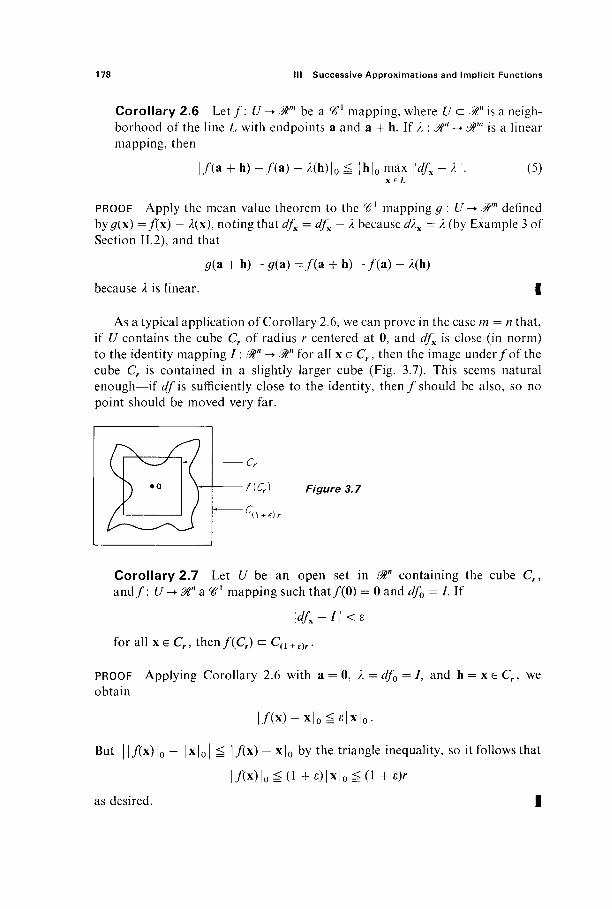
178 III Successive Approximations and Implicit Functions
Corollary 2.6 L e t / : £/-► 0Γ be a ^ 1 mapping, where U c ^ " is a neigh-borhood of the line L with endpoints a and a + h. If λ : J*'1 -► J*m is a linear mapping, then
| / ( a + h) - / ( a ) - A(h)|0 g |h|0 max \\dfx - λ\ (5) x eL
PROOF Apply the mean value theorem to the (€λ mapping g : U'-* ^ m defined by #(x) =/(x) — A(x), noting that dfx = dfx — λ because */>lx = Λ (by Example 3 of Section II.2), and that
g(a + h) - g(a) = / ( a + h) - / ( a ) - A(h)
because λ is linear. I
As a typical application of Corollary 2.6, we can prove in the case m = n that, if U contains the cube Cr of radius r centered at 0, and dfx is close (in norm) to the identity mapping / : 0tn ^ 0tn for all x e C r , then the image under/of the cube Cr is contained in a slightly larger cube (Fig. 3.7). This seems natural enough—if df is sufficiently close to the identity, then/should be also, so no point should be moved very far.
f{Cr)
( 1 + 6 ) / -
Figure 3.7
Corollary 2.7 Let U be an open set in $n containing the cube Cr, a n d / : U-+ Mn a ^ 1 mapping such that/(0) = 0 and df0 = I. If
¥L -1\\ < ε
for all x e Cr, then/(Cr) c C ( 1 + £)r.
PROOF Applying Corollary 2.6 with a = 0, λ = df0 = /, and h = x e Cr, we obtain
| / ( χ ) - χ | ο ^ ε Ι χ Ι ο ·
But | |/(x)|o — lxlo | ^ l/(x) — xlo by the triangle inequality, so it follows that
| / ( χ ) | 0 ^ ( 1 + ε ) [ χ | 0 ^ ( 1 + ε ) Γ
as desired. |
2 The Multivariable Mean Value Theorem 179
The following corollary is a somewhat deeper application of the mean value theorem. At the same time it illustrates a general phenomenon which is basic to the linear approximation approach to calculus—the fact that simple properties of the differential of a function often reflect deep properties of the function itself. The point here is that the question as to whether a linear mapping is one-to-one, is a rather simple matter, while for an arbitrary given ^1 mapping this may be a quite complicated question.
Corollary 2.8 Let / : Stn -> @m be #* at a. If dfa : @n -► &m is one-to-one, then/itself is one-to-one on some neighborhood of a.
PROOF Let m be the minimum value of |#a(X)lo f° r x e ^ n t n e n m >® because dfA is one-to-one [otherwise there would be a point x Φ 0 with^a(x) = 0]. Choose a positive number ε < m.
Since/is %>l at a, there exists δ > 0 such that
\x-*\o<S=>\\dfx-dfJ <ε.
If x and y are any two distinct points of the neighborhood
U = {xe@n: | x - a | 0 < ( 5 } ,
then an application of Corollary 2.6, with λ = dfA and L the line segment from x to y, yields
l/(x) - / ( y ) - dUx - y)10 ^ |x - y|0 max \\df - dfj < ε |x - y | 0 . ze L
The triangle inequality then gives
\WJx - y)|0 - | / ( χ ) - / ( y ) l o | < ε|χ - y | 0 , so
Ι/(χ) - / (y ) lo > !<//.(* - y)lo - β|χ - ylo
^(m-s)\x- y|0 > 0.
T h u s / ( x ) ^ / ( y ) i f x ^ y . |
Corollary 2.8 has the interesting consequence that, iff: &n -► Mn is ^ 1 with dfa one-to-one (so fis 1-1 in a neighborhood of a), and if f is "slightly per-turbed" by means of the addition of a " small " term g : £!fcn —» 0ln^ then the new mapping h =f+ g is still one-to-one in a neighborhood of a. See Exercise 2.9 for a precise statement of this result.
In this section we have dealt with the mean value theorem and its corollaries in terms of the sup norms on 0ln and 0Γ, and the resulting norm
L|| =maxx e 5 C„|L(x)|0 on JSPJ
180 III Successive Approximations and Implicit Functions
This will suffice for our purposes. However arbitrary norms | \m on 0Γ and | |„ on 0ln can be used in the mean value theorem, provided we use the norm
\\L\\mn = max |L(x)|m xedDn
on 5£mn, where Dn is the unit ball in @ln with respect to the norm | \n. The con-clusion of the mean value theorem is then the expected inequality
I/O») - / ( a ) | m S |b - a|„ · max ||/'(x)||m„. x e L
In Exercises 2.5 and 2.6 we outline an alternative proof of the mean value theorem which establishes it in this generality.
Exercises
2.1 Let | \m and | |„ be norms on £%m and £%n respectively. Prove that
|(x,y)|o = max{|xL,|y|„} for ( x , y ) e ^ + «
defines a norm on 3?m + n. Similarly prove that |(x, y)|i = |x|m + |y|„ defines a norm on # " + ".
2.2 Show that || ||, as defined by Eq. (3), is a norm on the space Jtmn of m x n matrices. 2.3 Given a e Mn, denote by La the linear function
n
La(x) = a - x = YatXi.
Consider the norms of La with respect to the sup norm | |0 and the 1-norm | |i on ", defined as in the last paragraph of this section. Show that ||La!li = |a|0 while ||Lal!o =
| a | i . 2.4 Let L : Mn -> @m be a linear mapping with matrix (au). If we use the 1-norm on @n and
the sup norm on ^m, show that the corresponding norm on ££mn is
||L||= max \atJ\,
that is, the sup norm on 0tmn. 2.5 Let y : [a, b]-> Mm be a ^ 1 mapping with \γ\ΐ)\ ^Μ for all te [a, b]y \ | being an
arbitrary norm on £%m. Prove that
\γφ)-γ(α)\ ^Μψ-α).
Outline: Given ε > 0, denote by SE the set of points x e [a, b] such that
\γ(0~γ(α)\ <,(Μ + ε)(ί-α) + ε
for all / x. Let c = lub SE. If c < b, then there exists δ > 0 such that
| y{c + h) — y(c) \ \h\<,h- <Μ + ε. h
Conclude from this that c + δ e SE, a contradiction. Therefore c = b, so
| y(b) - γ(α)\ ^ (M + e){b - a) + ε
for all ε > 0.
3 The Inverse and Implicit Mapping Theorems 181
2.6 Apply the previous exercise to establish the mean value theorem with respect to arbitrary norms on ^" and Jtm. In particular, given / : U'-> Mm where U is a neighborhood in y#" of the line segment L from a to a + h, apply Exercise 2.5 with γ(ί) = /(a + th).
2.7 (a) Show that the linear mapping T : $n -» 3m is one-to-one if and only if a = maxXeoC"|^(x)lo is positive. (b) Conclude that the linear mapping T : dân -> 3#m is one-to-one if and only if there exists a>0 such that | T(x)\0 ^ tf|x|0 for all x e Jtn.
2.8 Let T: Mn^Mm be a one-to-one linear mapping with |Γ(χ)|0Ξ>α|χ|0 for all x e f , where a > 0. If \\S - Τ\\^ε<α, show that |5(χ)|0Ξ> (a - ε)\χ\0 for all x e Mn, so S is also one-to-one. Thus the set of all one-to-one linear mappings Mn -> 3îm forms an open subset of Semn « ^mn.
2.9 Apply Corollary 2.8 and the preceding exercise to prove the following. Let / : Mn -> @n
be a if1 mapping such that dfA \ 0tn -> 0ln is one-to-one, so that/is one-to-one in a neigh-borhood of a. Then there exists ε > 0 such that if # : ί%η -> ^" is a r6l mapping with ^(a) = 0 and ||φΗ|| < ε, then the mapping h : Mn -> ^", defined by Λ(χ) =/"(x) + #(x), is also one-to-one in a neighborhood of a.
3 THE INVERSE AND IMPLICIT MAPPING THEOREMS
The simplest cases of the inverse and implicit mapping theorems were dis-cussed in Section 1. Theorem 1.3 dealt with the problem of solving an equation of the form/(x) = y for x as a function of y, while Theorem 1.4 dealt with the problem of solving an equation of the form G(x, y) = 0 for y as a function of x. In each case we defined a sequence of successive approximations which, under appropriate conditions, converged to a solution.
In this section we establish the analogous higher-dimensional results. Both the statements of the theorems and their proofs will be direct generalizations of those in Section 1. In particular we will employ the method of successive approximations by means of the contraction mapping theorem.
The definition of a contraction mapping in 0tn is the same as on the line. Given a subset C of &n, the mapping φ : C-> C is called a contraction mapping with contraction constant k if
| < p ( x ) - < p ( y ) | 0 ^ £ | x - y | 0
for all x, y e C. The contraction mapping theorem asserts that, if the set C is closed and bounded, and k < 1, then φ has a unique fixed point x* e C such that φ(χ*) = x* .
Theorem 3.1 Let φ : C-> C be a contraction mapping with contraction constant k < 1, and with C being a closed and bounded subset of 0t. Then φ has a unique fixed point x* . Moreover, given x0 6 C, the sequence {xm}^ defined inductively by
xm + i =φ(χ„)

182 III Successive Approximations and Implicit Functions
converges to x*. In particular,
The proof given in Section 1 for the case n = 1 generalizes immediately, with no essential change in the details. We leave it to the reader to check that the only property of the closed interval [a, b] a $, that was used in the proof of Theorem 1.1, is the fact that every Cauchy sequence of points of [a, b] converges to a point of [a, b]. But every closed and bounded set C <= 0Γ has this property (see the Appendix).
The inverse mapping theorem asserts that the ^ 1 mapping / : 0tn -► 0tn is locally invertible in a neighborhood of the point a e ^ " if its differential α/Λ : Mn -► $n at a is invertible. This means that, if the linear mapping df% : 0ln -► 0ln is one-to-one (and hence onto), then there exists a neighborhood U of a which / maps one-to-one onto some neighborhood V of b = /(a), with the inverse mapping # : V-+ U also being <βι. Equivalently, if the linear equations
df.l(*) = yi,
df.'OO = >·„
have a unique solution x e @tn for each y 6 ^Γ, then there exist neighborhoods U of a and V of b = / (a ) , such that the equations
f\xx, ...,x„) = yl9
frt(xi,...,x„) = yn
have a unique solution (xu . . . , xn) e U for each (yu . . . , yn) G V. Here we are writing/1, . . . , / " for the component functions off: 0ln-+0ln.
It is easy to see that the invertibility of dfa is a necessary condition for the local invertibility of/near a. For if U, K, and g are as above, then the composi-tions go fand fo g are equal to the identity mapping on U and V, respectively. Consequently the chain rule implies that
dffb ° dfa = dfi o dgh = identity mapping of 0tn.
This obviously means that dfa is invertible with df~l = dgh. Equivalently, the derivative matrix/'(a) must be invertible w i th / ' ( a ) - 1 = g'(b). But the matrix / r (a) is invertible if and only if its determinant is nonzero. So a necessary con-dition for the local invertibility of /near / ' (a ) is that | / ' ( a ) | φ 0.
The following example shows that local invertibility is the most that can be

3 The Inverse and Implicit Mapping Theorems 183
hoped for. That is, / may be ^71 on the open set G with | / ' ( a ) | φ 0 for each a e G, without /being one-to-one on G.
Example 1 Consider the ^ 1 mapping/: 0t2 -> @l2 defined by
/ ( * , y) = (x2 - y2, 2xy).
Since cos2 0 - sin2 0 = cos 20 and 2 sin 0 cos 0 = sin 20, we see that in polar coordinates/is described by
f(r cos 0, r sin 0) = (r2 cos 20, r2 sin 20).
From this it follows that /maps the circle of radius r twice around the circle of radius r2. In particular, / maps both of the points (rcos0, r sin 0) and (rcos (0 + π), r sin(0 + π)) to the same point (r2 cos 20, r2 sin 20). Thus / m a p s the open set &2 — 0 "two-to-one" onto itself. However, \f'(x, y)\ = 4(x2 + y2), so/ '(x, y) is invertible at each point of 0l2 — 0.
We now begin with the proof of the inverse mapping theorem. It will be convenient for us to start with the special case in which the point a is the origin, with /(0) = 0 and / '(0) = / (the n x n identity matrix). This is the following substantial lemma; it contains some additional information that will be useful in Chapter IV (in connection with changes of variables in multiple integrals). Given ε > 0, note that, s ince/ is ^ 1 with df0 = /, there exists r > 0 such that \\dfx — I\\ < ε for all points xe Cr (the cube of radius r centered at Cr).
Lemma 3.2 Let / : mn^0ln be a ^ 1 mapping such that /(0) = 0 and df0 = /. Suppose also that
\\dfx -I\\^e<\
for all x e Cr. Then
C(l-e)r ŒJ\^/r) c = C ( l + c ) r ·
Moreover, if V= int C(1_e)r and U= int Cr n / _ 1 ( K ) , t h e n / : C/-> F i s a one-to-one onto mapping, and the inverse mapping g : F-> £/ is dif-ferentiable at 0.
Finally, the local inverse mapping g : K-> £/ is the limit of the sequence of successive approximations {gm}£ defined inductively on V by
9oiy) = o, gm+i(y) = gm{y) -f(gm(y)) + y for y e V.
PROOF We have already shown that f(Cr) c C(1+e)r (Corollary 2.7), and it follows from the proof of Corollary 2.8 t h a t / i s one-to-one on Cr—the cube Cr satisfies the conditions specified in the proof of Corollary 2.7. Alternatively, we can apply Corollary 2.6 with λ = df0 = I to see that
l / (x) - / (y) - (x-y) lo^|x-y| 0 (i)

184 III Successive Approximations and Implicit Functions
if x, y e Cr. From this inequality it follows that
(1 - ε)|χ - y|0 ^ | / (x) - / ( y ) | 0 ^ (1 + ε)|χ - y|0 . (2)
The left-hand inequality shows that fis one-to-one on Cr, while the right-hand one (with y = 0) shows that/(Cr) c C(1+£) r .
So it remains to show that/(Cr) contains the smaller cube C(1_fi)r. We will apply the contraction mapping theorem to prove this. Given y G C(1_£)r, define φ : 0ίη -> 3P by
<P(x) = x - / ( x ) + y.
We want to show that φ is a contraction mapping of Cr; its unique fixed point will then be the desired point xe Cr such that/(x) = y.
To see that φ maps Cr into itself, we apply Corollary 2.6:
| φ ( χ ) | 0 ^ | / ( χ ) - χ | 0 + |y |0
= | / ( x ) - / ( 0 ) - ^ 0 ( x - 0 ) | a 4 - | y | o
^ | y | o + |x | 0 max \\dfx-dft\\ xeCr
S (1 — e)r + re
= r,
so if x G Cr, then φ(χ) G Cr also. Note here that, if y G int C(1_£)r, then |φ(χ)|0 < r, so φ(χ) G int Cr.
To see that φ : Cr -♦ Cr is a contraction mapping, we need only note that
|φ(χ) - φ(γ)|0 = | / (x) - / ( y ) - (x - y)lo ^ e|x - y|0
by(l) . Thus φ : Cr -► Cr is indeed a contraction mapping, with contraction constant
ε < 1, and therefore has a unique fixed point x such that/(x) = y. We have noted that φ maps Cr into int Cr if y G Κ= int C(1_e)r. Hence in this case the fixed point xlies in int Cr. Therefore, if U =f~l(V) n int Cr, then t/and Kare open neighborhoods of 0 such tha t /maps U one-to-one onto K.
The fact that the fixed point x = g(y) is the limit of the sequence {xm}o defined inductively by
x0 = 0, xm + 1 = xm - / ( x j + y,
follows immediately from the contraction mapping theorem (3.1). So it remains only to show that g : K-> U is differentiable at 0, where #(0) =
0. It suffices to show that
l i m ' ^ - ^ O ; (3) |h | -o | h | G
3 The Inverse and Implicit Mapping Theorems 185
Since fis Ήι at 0 with df0 = /, we can make ε > 0 as small as we like, simply by restricting our attention to a sufficiently small (new) cube centered at 0. Hence (4) implies (3). |
We now apply this lemma to establish the general inverse mapping theorem. It provides both the existence of a local inverse g under the condition | / ' (a) | φ 0, and also an explicit sequence {gk}f of successive approximations to g. The definition of this sequence {gk}f can be motivated precisely as in the 1-dimen-sional case (preceding the statement of Theorem 1.3).
Theorem 3.3 Suppose that the mapping / : 0ln -► 0ln is Ή1 in a neigh-borhood W of the point a, with the matrix/'(a) being nonsingular. Then/ i s locally invertible—there exist neighborhoods Ua W of a and K o f b = / ( a ) , and a one-to-one ^ 1 mapping g : V-> W such that
g(f(x)) = x for x e U,
and
Rg(y)) = y for y e K
In particular, the local inverse g is the limit of the sequence {gk}o of successive approximations defined inductively by
<7o(y) = a, gk+i(y) = gk(y) -f\*yl[f(gk{y)) - y] (5)
for y e V.
PROOF We first " alter " the mapping/so as to make it satisfy the hypotheses of Lemma 3.2. Let Ta and rb be the translations of 0tn defined by
ia(x) = x + a, rb(x) = x + b,
and let T = dfa : @n -> &a. Then define / : @n -+ mn by
Λχ) = τ ί 1 ο / ο τ , ο Γ 1 ( χ ) . (6)
this will prove that g is differentiate at 0 with dg0 = I. To verify (3), we apply (1) with y = 0, x = #(h), h = / (x ) , obtaining
We then apply the left-hand inequality of (2) with y = 0, obtaining
(4)
This follows from the fact that
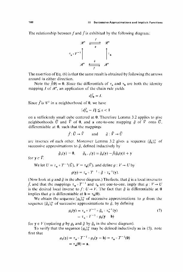
186 III Successive Approximations and Implicit Functions
The relationship between/and / i s exhibited by the following diagram: /
9
"a°T "b
/ The assertion of Eq. (6) is that the same result is obtained by following the arrows around in either direction.
Note the /(0) = 0. Since the differentials of Ta and rh are both the identity mapping / of 0tn, an application of the chain rule yields
dfo = I.
Since/is Ή1 in a neighborhood of 0, we have
\\d/x - /|| g ε < 1
on a sufficiently small cube centered at 0. Therefore Lemma 3.2 applies to give neighborhoods 0 and V of 0, and a one-to-one mapping g of V onto Î7, differentiable at 0, such that the mappings
/ : tf - K and g : V -> 0
are inverses of each other. Moreover Lemma 3.2 gives a sequence {gk}o of successive approximations to g, defined inductively by
^o(y) = 0, gk + x (y) = gk(y) -f(gk(y)) + y for y e V.
We let U= τΆοΤ~\υ\ V= τ„(Κ), and define# : K->(/by
ff(y) = TaoT~l ogo Tb_ 1(y) .
(Now look at g and g in the above diagram.) The facts, that g is a local inverse to / and that the mappings i a o T~x and rb are one-to-one, imply that g : V-+U is the desired local inverse t o / : £/-► K. The fact that g is differentiable at 0 implies that g is differentiable at b = Tb(0).
We obtain the sequence {gk}o of successive approximations to g from the sequence {gk)o of successive approximations to g, by defining
9k(y) = τ , ° Γ _ 1 ο ^ ο T- i(y) (7) = T a o r _ 1 °# f e (y-b)
for y e V (replacing g by gk and $ by ^ in the above diagram). To verify that the sequence {gk)o may be defined inductively as in (5), note
first that 0o(y) = τ3 o Γ" 1 o g0(y - b) = i a o Γ-^Ο)
= τ.(0) = a.
3 The Inverse and Implicit Mapping Theorems 187
Now start with the inductive relation
& + i(y - b) = gk(y - b) -f(g(y - b)) + (y - b).
Substituting from (6) and (7), we obtain
To I,"1 ogk + i(y) = To τ;1 ogk(y) - τ " * o /o Ta o T~\T* T^1 o ft(y)) + (y - b) = r o T a - 1 o ^ ( y ) - [ / ( ^ ( y ) ) - y ] .
Applying τ / Γ 1 to both sides of this equation, we obtain the desired inductive relation
gk+M = gk(y)-r-1[f(gk(y))-yi
It remains only to show that g : K-> If is a ^ 1 mapping; at the moment we know only that g is differentiable at the point b = / (a ) . However what we have already proved can be applied at each point of U, so it follows that g is differenti-able at each point of V.
To see that g is continuously differentiable on V, we note that, since
/te(y)) = y, yeK, the chain rule gives
g'(y) = [f'(g(y))V1
for each y e V. Now/'(#(y)) is a continuous (matrix-valued) mapping, because / i s ^ 1 by hypothesis, and the mapping # is continuous because it is differentiable (Exercise II.2.1). In addition it is clear from the formula for the inverse of anon-singular matrix (Theorem 1.6.3) that the entries of an inverse matrix A~l are continuous functions of those of A. These facts imply that the entries of the matrix g\y) = [/'(giy))]'1 are continuous functions of y, so g is Ή1.
This last argument can be rephrased as follows. We can write g' : K-> Jinn, where Mnn is the space of n x n matrices, as the composition
g' =jf of ogf
where <f(A) = A'1 on the set of invertible n x n matrices (an open subset of y//nn). J> is continuous by the above remark, and / ' : U"-► Jänn is continuous because/is ^ 1 , so we have expressed g' as a composition of continuous mappings. Thus g' is continuous, so g is <€x by Proposition 2.4. |
The power of the inverse mapping theorem stems partly from the fact that the condition det/ '(a) Φ 0 implies the invertibility of the ^ 1 mapping / in a neighborhood of a, even when it is difficult or impossible to find the local in-verse mapping g explicitly. However Eqs. (5) enable us to approximate g arbitrarily closely [near b = / (a) ] .
Example 2 Suppose the ^ l mapping/ : 0t\v -> 0t2xy is defined by the equations
x = u + (v + 2)2 + 1, y = (u - l)2 + v+ 1.
188 III Successive Approximations and Implicit Functions
Let a = (1, — 2), so b = / ( a ) = (2, - 1). The derivative matrix is
ft \ ( l Άν + 2)\ f(">v) = [2(u-l) 1 ) '
so/ ' (a) is the identity matrix with determinant 1. Therefore/is invertible near a = (1, — 2). That is, the above equations can be solved for u and v as functions of x and y, (u, v) = g(x, y), if the point (x, y) is sufficiently close to b = (2, — 1). According to Eqs. (5), the sequence of successive approximations {gk}f is defined inductively by
9o(x> y) = (U -2), gk+i(x, y) = gk(x, y) -f(gk(x, y)) + (*, y)·
Writing gk(x, y) = (wfc, vk), we have
(uk + l9 vk + l) = (uk, vk) - (uk + (vk + 2)2 + 1, (uk - l ) 2 + vk + 1) + (x, y)
= (1 + (x - 2) - (vk + 2)2, -2 + (y+l)-(uk- l)2).
The first several approximations are
u0 = 1, v0= - 2 , ul = 1 + (x - 2), vl = -2 + (y + 1), u2 = l+(x-2)-(y+ l)2, y2 = - 2 + (>> + 1) - (JC - 2)2
u3 = l+(x-2)-[(y+\)-(x-2)2]2
= 1 + (JC - 2) - (y + l)2 + 2(x - 2)2(j; + 1) — (JC — 2)4, t ; 3 = - 2 + ( ^ + l ) - [ ( x - 2 ) - ( ^ + l ) 2 ] 2
= - 2 + (y + 1) - (x - 2)2 + 2(x - 2)(y + l)2 - (y + l)4.
It appears that we are generating Taylor polynomials for the component func-tions of g in powers of (x — 2) and (y + 1). This is true, but we will not verify it.
The inverse mapping theorem tells when we can, in principle, solve the equa-tion x =/(y) , or equivalently x — /(y) = 0, for y as a function of x. The implicit mapping theorem deals with the problem of solving the general equation G(x, y) = 0, for y as a function of x. Although the latter equation may appear considerably more general, we will find that its solution reduces quite easily to the special case considered in the inverse mapping theorem.
In order for us to reasonably expect a unique solution of G(x, y) = 0, there should be the same number of equations as unknowns. So if x e &m, y e &", then G should be a mapping from &m+n to Mn. Writing out components of the vector equation G(x, y) = 0, we obtain
Gi(xi9 ...,xm,yu ...,yn) = 0,
G„(Xi, ...,xm,yl9 . . . , J Ü = 0.
We want to discuss the solution of this system of equations for yu ..., yn in terms of xl9 . . . , xm.
3 The Inverse and Implicit Mapping Theorems 189
In order to investigate this problem we need the notion of partial differential linear mappings. Given a mapping G : i$m + n -► $k wihch is differentiate at the point p = (a, b) G #m+n, the partial dijferentials of G are the linear mappings dx Gp : PÂm -* ^ and dy Gp : <*" -+ &k defined by
7 υ Ρ
dxGp(r) = dGp(r,0) and cLGJs) = dGJO,s),
respectively. The matrices of these partial differential linear mappings are called the partial derivatives of G with respect to x and y, respectively. These partial derivative matrices are denoted by
DiG(a, b) or (— cG
and D2 G(a, b) or -—,
respectively. It should be clear from the definitions that DxG(2i^ b) consists of the first m columns of (/'(a, b), while D2 G(a, b) consists of the last n columns. Thus
/ · ; ÎC , dG, \
dG ox,
\ vGk dxx
d_Gk
dx,
n and — =
<y
/
dG\
dyx
dG, dG,
dyj
Suppose now that x G Mm and y G Mn are both differentiable functions of te@\x = a(t) and y = j8(t), and define φ : @l -► ^* by
<p(t) = C(a(t), j!(t)).
Then a routine application of the chain rule gives the expected result
άφ dG dx dG dy
dt dx dt dy dt w
or
φ'(ί) = D{G(«(tl 0(t))a'(t) + D2 C(a(t), ß(t))ß'{t)
in more detail. We leave this computation to the exercises (Exercise 3.16). Note that DXG is a k x m matrix and a' is an m x / matrix, while Z)2 G is a k x A matrix and /?' is an A7 X / matrix, so Eq. (8) at least makes sense.
Suppose now that the function G : &m + n -► ^Γ is differentiable in a neigh-borhood of the point (a, b ) G ^ m + n where <7(a, b) = 0. Suppose also that the equation <7(x, y) = 0 implicitly defines a differentiable function y = li(x) for x near a, that is, h is a differentiable mapping of a neighborhood of a into $n, with
A(a) = b and <7(x, Λ(χ)) = 0.
190 III Successive Approximations and Implicit Functions
We can then compute the derivative h'(x) by differentiating the equation G(x, h(x)) = 0. Applying Eq. (8) above with x = t, a(x) = x, we obtain
Z)1G(x,y) + /)2C(x,y)A'(x) = 0.
If the n x n matrix D2 (7(x, y) is nonsingular, it follows that
A'(x) = -D2G(x,yy1D1G(x,y). (9)
In particular, it appears that the nonvanishing of the so-called Jacobian de-terminant
d(Gu . . · , Gn)
d(yi, .--,yn)
at (a, b) is a necessary condition for us to be able to solve for A'(a). The implicit mapping theorem asserts that, if G is ^ 1 in a neighborhood of (a, b), then this condition is sufficient for the existence of the implicitly defined mapping A.
Given G:@m+n->@rt and h:U-+âln, where U^3T, we will say that y = A(x) solves the equation G(x, y)) = 0 in a neighborhood W of (a, b) if the graph of/agrees in W with the zero set of G. That is, if (x, y) e W and x e U, then
G(x, y) = 0 if and only if y = A(x).
Note the almost verbatim analogy between the following general implicit mapping theorem and the case m = n = 1 considered in Section 1.
Theorem 3.4 Let the mapping G : @m+n-+@n be W1 in a neighborhood of the point (a, b) where (7(a, b) = 0. If the partial derivative matrix D2 G(a, b) is nonsingular, then there exists a neighborhood U of a in Mm, a neighbor-hood Woï(a, b) in @m+n, and a ^ 1 mapping h:U-+âln
9 such that y = A(x) solves the equation G(x, y) = 0 in W.
In particular, the implicitly defined mapping A is the limit of the sequence of successive approximations defined inductively by
A0(x) = b, Afc + 1(x) = hk(x) - D2 G(a, b ) " ^ , Afc(x))
for x e U.
PROOF We want to apply the inverse mapping theorem to the mapping/: 0Γ +n
->mm+n defined by
/ (x , y) = (x, G(x, y)),
for which/(x, y) = (x, 0) if and only if <7(x, y) = 0. Note that / i s Ή1 in a neigh-borhood of the point (a, b) where/(a, b) = (a, 0). In order to apply the inverse mapping theorem in a neighborhood of (a, b), we must first show that the matrix/'(a, b) is nonsingular.
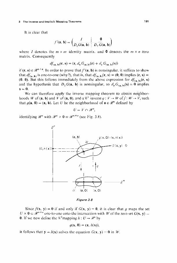
3 The Inverse and Implicit Mapping Theorems 191
It is clear that
- ( I \ ° \ j (a, b) = y-p-j^-~b)TzJ"2"G(i~,"bj]
where / denotes the m x m identity matrix, and 0 denotes the m x n zero matrix. Consequently
#la,b)(r> s) = (r, dxGiaM(r) + rfy<7(a,bJ(s))
if (r, s) e 0tm*n. In order to prove that/ ' (a, b) is nonsingular, it suffices to show that dfuh) is one-to-one (why?), that is, that df(sith)(r, s) = (0, 0) implies (r, s) = (0, 0). But this follows immediately from the above expression for df(a b)(r, s) and the hypothesis that D2 G(a, b) is nonsingular, so dyGUth)(s) = 0 implies s = 0.
We can therefore apply the inverse mapping theorem to obtain neighbor-hoods W of (a, b) and V of (a, 0), and a^ 1 inverse # : K-> Woff: W ^ V, such that #(a, 0) = (a, b). Let U be the neighborhood of a e 0Γ defined by
identifying 3Γ with i m x 0 c J>",+" (see Fig. 3.8).
(0, /?(x)) +
^ ( x , 0 ) = (x,/7(x))
£ ( x , y ) = 0
^ (α,Ο) (χ,Ο)
Figure 3.8
Since / (x , y) = 0 if and only if G(x, y) = 0, it is clear that g maps the set U x 0 c ^ '"+" one-to-one onto the intersection with W of the zero set <7(x, y) = 0. If we now define the ^ 1 mapping h : U -> ^" by
#(x, 0) = (x, A(x)),
it follows that y = Λ(χ) solves the equation G(x, y) = 0 in W.
192 III Successive Approximations and Implicit Functions
It remains only to define the sequence of successive approximations {hk}o to h. The inverse mapping theorem provides us with a sequence {gk}% of suc-cessive approximations to g, defined inductively by
g0(x, y) = (a, b), gk + i(x, y) = gk(x, y) - / ' ( a , b)-1[/(#k(x, y)) - (x, y)].
We define Ak: <7->^"by
gk(x, 0) = (x, hk(x)).
Then the fact, that the sequence {gk)o converges to g on K, implies that the sequence {hk}Q converges to h on U.
Since g0(x, y) Ξ (a, b), we see that h0(x) = b. Finally
(x,/?fc + 1(x)) = gk + l(x,0)
= gk(x, 0) - / ' ( a , « ^ [ / ( ^ ( χ , 0)) - (x, 0)] = (x, hk(x)) - / ' ( a , b r 'Lf lx , AÄ(x)) - (x, 0)] = (x, hk(x)) - / ' ( a , b)-![(x, G(x, hk(x))) - (x, 0)],
so
U+i(x)/ = U(x)/ " \Λ^;ΐΠ"^Γο(ϊΓΐ))/ Ι^χΛίχ))/ " Taking second components of this equation, we obtain
** + i(x) = A*« - ^2 G(a, b)-!G(x, ΑΛ(χ))
as desired. |
Example 3 Suppose we want to solve the equations
x2 + \y2 + z3 0,
x3 + y3 - 3y + z + 3 = 0,
for j> and z as functions of x in a neighborhood of ( — 1, 1,0). We define G : - > ^ 2 by
G(JC, >>, z) = (x2 + i / + z3 - z2 - 1, x3 + / - 3y + z + 3).
Since
d(y, z) W^l = det( >
| ( - i , i . o ) \ 3 ^ -
= d e t ( i !) =
3z2 - 2z\ 3 1 j
( - 1 , 1,0)
# 0 ,
the implicit mapping theorem assures us that the above equations do implicitly define y and z as functions of x, for x near - 1. The successive approximations
3 The Inverse and Implicit Mapping Theorems 193
for h(x) = (y(x), z(x)) begin as follows:
Ao(*) = 0 , 0 ) , hx(x) = (l, 0) - G(x9 h0(x)) = (1, 0) - G(x9 1, 0)
= (2 - x\ - 1 - x3), A2(JC) = { 2 - x \ - \ - x3) - G(x, 2 - x\ - 1 - x3).
Example 4 Let (7 : m1 x ^ 2 = ^ 4 -► ^ 2 be defined by
G(x,y) = (xly2 + *2yi~ l , * i*2 - ^ 1 ^ 2 ) ,
where x = (xl, x2) and y = (yl9 y2), and note that G(l, 0, 0, 1) = (0, 0). Since
Z)2G(1,0,0,1) = ( _ ° ^
is nonsingular, the equation G(x, y) = 0 defines y implicitly as a function of x, y = A(x) for x near (1,0). Suppose we only want to compute the derivative matrix A'(l, 0). Then from Eq. (9) we obtain
h\\9 0) = D2G{\9 0, 0, Ο ' ^ , σ ί ΐ , 0, 0, 1)
Note that, writing Eq. (9) for this example with Jacobian determinants instead of derivative matrices, we obtain the chain rule type formula
dCVi, y2) = d(Gi9G2)/d(xl9x2) d(xl9x2) d(Gl9G2)/d(yl9y2)
or d(Gl9G2)= d(Gl9G2)d(yi9y2)
d(xl9x2) d(yl9y2) d(xl9x2)'
The partial derivatives of an implicitly defined function can be calculated using the chain rule and Cramer's rule for solving linear equations. The following example illustrates this procedure.
Example 5 Let Gl9 G2 : Ms -► 0t be ^ 1 functions, with Gt(a) = G2(a) = 0 and
d(u9 v)
at the point a e &5. Then the two equations
Gr(x, y9 z, w, y) = 0, G2(x, y, z9 u9 v) = 0

194 III Successive Approximations and Implicit Functions
implicitly define u and v as functions of x, y, z:
u=f(x,y,z), v=g(x,y,z).
Upon differentiation of the equations
Gi(x, y, z,/(x, y, z), g(x9 y, z)) = 0, / = 1, 2,
with respect to x, we obtain
dG, dGx df dGl dg Λ dG2 dG2 df dG2 dg — - H — H — = 0, — - H — H — = 0. dx du dx dv dx ' dx du ôx dv dx
Solving these two linear equations for df/dx and dg/dx, we obtain
df _ ld(GuG2) a n d dg _ ld(G^G2)
dx J d(x, v) dx J d(u, x)
Similar formulas hold for df/dy, dg/dy, df/dz, dgjdz (see Exercise 3.18).
Exercises
3.1 Show that f(x, y) = (x/(x2 + y2), y/(x2 + y2)) is locally invertible in a neighborhood of every point except the origin. C o m p u t e / - 1 explicitly.
3.2 Show that the following mappings from &2 to itself are everywhere locally invertible. (a) f(x, y) = (ex + e\ ex - ey). (b) g(x, y) = (ex cos y, ex sin y).
3.3 Consider the mapping / : ^ 3 -> ^ 3 defined by f(x, y, z) = (x, y3, z5). Note that / h a s a (global) inverse gt despite the fact that the matrix / ' (0) is singular. What does this imply about the differentiability of g at 0?
3.4 Show that the mapping 3tj?yz -> M*vyf, defined by u = x + ey, v = y + ez, w = z + ex, is everywhere locally invertible.
3.5 Show that the equations
sinC* + z) + log yz2 = 0, ex + z + yz = 0
implicitly define z near — 1 , as a function of (x, y) near (1, 1).
3.6 Can the surface whose equation is
xy — y log z + sin xz = 0
be represented in the form z=f(x, y) near (0, 2, 1)?
3.7 Decide whether it is possible to solve the equations
xu2 -\- yzv + x2z = 3, xyv3 + 2zu — u2v2 = 2
for (w, i') near (1, 1) as a function of O, y, z) near (1, 1, 1). 3.8 The point (1, — 1 , 1) lies on the surfaces
x3(y3 + z3) = 0 and (* - >03 -z2 = T.
Show that, in a neighborhood of this point, the curve of intersection of the surfaces can be described by a pair of equations of the form y =f(x), z = g(x).
3 The Inverse and Implicit Mapping Theorems 195
3.9 Determine an approximate solution of the equation
z3 + 3xyz2 - 5x2y2z + 1 4 = 0
for z near 2, as a function of (x, y) near (1, — 1). 3.10 If the equations f(x, v, z) = 0, g(x, y, z) = 0 can be solved for y and z as differentiable
functions of x, show that
dy = \_ Kî\9) dz = [ 8(f,g) dx J d(z, x)' dx J d(x, y) '
where J = d(f, g)/d(y, z). 3.11 If the equations f(x, y, w, v) = 0, g(x, y, u, v) = 0 can be solved for // and v as differentiable
functions of x and y, compute their first partial derivatives. 3.12 Suppose that the equation f(x, y, z) = 0 can be solved for each of the three variables
JC, y, z as a differentiable function of the other two. Then prove that
dx dy dz
dy dz dx
Verify this in the case of the ideal gas equation pv = RT(where /?, v, Ta re the variables and R is a constant).
3.13 Let f\M\^m\ and g : M\,-> ®\ be tf1 inverse functions. Show that
% 1
dy,
dgi
dy1
1 % J dx2
J dxi '
d_g±_ 1 d_f^
dy2 J dx2 '
dy2 J dxx '
w h e r e / = d{fuf2)jd{xu x2). 3.14 Let / : J?£ -> at* and g: $%-> &l be if1 inverse functions. Show that
dyl Jd(x2,x3)' d(xuX2,X3y
and obtain similar formulas for the other derivatives of component functions of #. 3.15 Verify the statement of the implicit mapping theorem given in Section II.5. 3.16 Verify Eq. (8) in this section. 3.17 Suppose that the pressure p, volume v, temperature Γ, and internal energy M of a gas
satisfy the equations
f(p, v9 T, u) = 0, g(p, v, T, u) = 0,
and that these two equations can be solved for any two of the four variables as functions of the other two. Then the symbol du/dT, for example, is ambiguous. We denote by (du/dT)p the partial derivative of u with respect to T, with u and v considered as functions of p and Γ, and by (du/dT)v the partial derivative of u, with u and p considered as functions of v and T. With this notation, apply the results of Exercise 3.11 to show that
(du\ _ (du\ ldT\ _(du\ (dT\ (d"\
3.18 Ifyi,...,y„ are implicitly defined as differentiable functions of xi,..., xm by the equations

196 III Successive Approximations and Implicit Functions
show, by generalizing the method of Example 5, that
tyj_ 1 0 ( / i , . . · , , / } , . ■■, / , )
dxi J d(yl9...,xt, ....,yn)'
where
J = 0(Λ, . . . ,Λ, . . . ,Λ) % Ί >yj> ,ynY
4 MANIFOLDS IN
We continue here the discussion of manifolds that was begun in Section II.5. Recall that a /r-dimensional manifold in &n is a set M that looks locally like the graph of a mapping from &k to 0tn~k. That is, every point of M lies in an open subset V of 0tn such that P = F n M is a /c-dimensional patch. Recall that this means there exists a permutation xlV . . . , x/n of xu . . . , xn9 and a diiTerentiable mapping h : U -+ &n~k defined on an open set i/ c ^ k , such that
P = { x 6 « " : ( x f l , . . . , x I . k ) e l / and (x/fc+l, . . . , xj = h(xh, . . . , xik)}.
See Fig. 3.9. We will call P a Ή1 or smooth patch if the mapping A is ^ 1 . The manifold A/ will be called ^ 1 or smooth if it is a union of smooth patches.
' can appear (locally) :
. , x.
Figure 3.9
There are essentially three ways that a /:-manifold in ,
(a) as the graph of a mapping &k -> $t~k, (b) as the zero set of a mapping 0tn -> Mn~k, (c) as the image of a mapping (%k -» ^".
The definition of a manifold is based on (a), which is actually a special case of both (b) and (c), since the graph of/: 0lk -> $n~k is the same as the zero set of

4 Manifolds in 3tn 197
G(x, y) = / (x ) - y, and is also the image of F : Mk -> 0ln, where F(x) = (x,/(x)). We want to give conditions under which (b) and (c) are, in fact, equivalent to (a).
Recall that our study of the Lagrange multiplier method in Section II.5 was based on the appearance of manifolds in guise (b). The following result was stated (without proof) in Theorem II.5.7.
Theorem 4.1 Let G\0ln -*0T be a # l mapping, where k = n - m > 0. If M is the set of all those points xeG _ 1 (0 ) for which the derivative matrix G"(x) has rank ra, then M is a smooth /:-manifold.
PROOF We need to show that each point p of M lies in a smooth ^-dimensional patch on M. By Theorem 1.5.4, the fact, that the rank of the m x n matrix G'(p) is m, implies that some m of its column vectors are linearly independent. The column vectors of the matrix G' are simply the partial derivative vectors dG/dx1, . . . , ôG/dxn, and let us suppose we have rearranged the coordinates in &n so that it is the last m of these partial derivative vectors that are linearly inde-pendent. If we write
(xl5 . . . ,*„) = (x,y), where x e 0lk, y e &n~k = 0Γ, then it follows that the partial derivative matrix D2G(p) is nonsingular.
Consequently the implicit mapping theorem applies to provide us with a neighborhood V of p = (a, b) in <%n
9 a neighborhood U of a in @tk, and a Ή1
mapping/ : U'-► 0Γ such that y = / ( x ) solves the equation G(x, y) = 0 in V. Clearly the graph of / i s the desired smooth ^-dimensional patch. |
Thus conditions (a) and (b) are equivalent, subject to the rank hypothesis in Theorem 4.1.
When we study integration on manifolds in Chapter V, condition (c) will be the most important of the three. If M is a /:-manifold in 0ln, and U is an open subset of 0ik, then a one-to-one mapping φ : U-> M can be regarded as a para-metrization of the subset φ(ϋ) of M. For example, the student is probably familiar with the spherical coordinates parametrization φ : 0t\O -► S2 of the unit sphere S2 c ^ 3 , defined by
(p(u, v) = (sin u cos v, sin u sin v, cos u).
The theorem below asserts that, if the subset M of 0ln can be suitably para-metrized by means of mappings from open subsets of 0lk to M, then M is a smooth ^-manifold.
Let φ : U-► ffln be a <€γ mapping defined on an open subset U of 0tk (k ^ ri). Then we call φ regular if the derivative matrix φ\η) has maximal rank k, for each u e U. According to the following theorem, a subset M of Mn is a smooth fc-manifold if it is locally the image of a regular ^ 1 mapping defined on an open subset of 0lk.
198 III Successive Approximations and Implicit Functions
Theorem 4.2 Let M be a subset of 3t. Suppose that, given p e M , there exists an open set U ' <z 0lk(k <n) and a regular %>l mapping φ : U-► &n
such that p e φ(ϋ), with (p(U') being an open subset of M for each open set V <z U. Then M is a smooth /:-manifold.
The statement that cp(U') is an open subset of M means that there exists an open set Win &n such that W n M = (p(U'). The hypothesis that φ(1]') is open in M, for every open subset U' of U, and not just for U itself, is necessary if the conclusion that M is a /c-manifold is to follow. That this is true may be seen by considering a figure six in the plane—although it is not a 1-manifold (why?); there obviously exists a one-to-one regular mapping φ : (0, 1) -► &2 that traces out the figure six.
PROOF Given p e M and φ : U -» M as in the statement of the theorem, we want to show that p has a neighborhood (in &") whose intersection with M is a smooth ^-dimensional patch. If φ(α) = p, then the n x k matrix φ'(&) has rank k. After relabeling coordinates in £%n if necessary, we may assume that the k x k submatrix consisting of the first k rows of <p'(a) is nonsingular.
Write p = (b, c) with b e 0lk and ce@"~k, and let n:@n-*@k denote the projection onto the first k coordinates,
n(xu . . . , xn) = (*i, . . · ,**) .
If/: [/-> Mk is defined by
/=ποφ,
then/(a) = b, and the derivative matrix / ' (a) is nonsingular, being simply the k x k submatrix of <p'(a) referred to above.
Consequently the inverse mapping theorem applies to give neighborhoods U' of a and V of b such t h a t / : V -> V is one-to-one, and the inverse^ : V -► Uf
is ^ 1 . Now define h : V -+ Mn~k by
<p(g(x)) = (x, A(x)).
Since the graph of h is P = q>(U'), and there exists (by hypothesis) an open set W in 0tn with W n M = (p{U')> we see that p lies in a smooth ^-dimensional patch on M, as desired. |
REMARK Note that, in the above notation, the mapping Φ = g o π : W' -+U'
is a ^ 1 local inverse to φ. That is, Φ is a ^ 1 mapping on the open subset W of ^ n , and Φ(χ) = φ~χ(χ) for x e W f] M. This fact will be used in the proof of Theorem 4.3 below.
If M is a smooth ^-manifold, and φ : U -► M satisfies the hypotheses of Theorem 4.2, then the mapping φ is called a coordinate patch for M provided
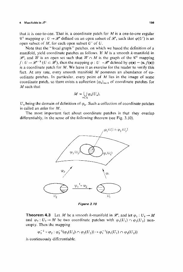
4 Manifolds in 0tn 199
that it is one-to-one. That is, a coordinate patch for M is a one-to-one regular ^ 1 mapping φ : U -> ^ n defined on an open subset of &k, such that φ(ί/') is an open subset of M, for each open subset U' of U.
Note that the '"local graph" patches, on which we based the definition of a manifold, yield coordinate patches as follows. If M is a smooth ^-manifold in f1, and W is an open set such that W n M is the graph of the ^ 1 mapping
/ : 1/ -> 0"~* (1/ c ^*) , then the mapping φ : 1/ -> äT defined by φ(μ) = (u,/(u)) is a coordinate patch for M. We leave it as exercise for the reader to verify this fact. At any rate, every smooth manifold M possesses an abundance of co-ordinate patches. In particular, every point of M lies in the image of some coordinate patch, so there exists a collection {φα}αεΛ of coordinate patches for M such that
α ε Λ
Ua being the domain of definition of φα. Such a collection of coordinate patches is called an atlas for M.
The most important fact about coordinate patches is that they overlap differentiably, in the sense of the following theorem (see Fig. 3.10).
C3 - ^ C3 Figure 3.10
Theorem 4.3 Let M be a smooth fc-manifold in Stn, and let φ1 : U1-+M and φ2 : U2->M be two coordinate patches with φ^ϋ^ η (p2(U2) non-empty. Then the mapping
ΨΪ1 ° Ψι ' (Pi\(pi(U\) n <p2(U2)) -> Ψϊ ι{φι{υχ) η (p2(U2))
is continuously differentiable.

200 III Successive Approximations and Implicit Functions
PROOF Given p G φ^ϋ^ n (p2(U2)> the remark following the proof of Theorem 4.2 provides a ^ 1 local inverse Φ to φί9 defined on a neighborhood of p in 0tn. Then φϊ1 o φ2 agrees, in a neighborhood of the point (p^iv), with the compo-sition Φ o φ2 of two ^ 1 mappings. |
Now let {<p}ieA be an atlas for the smooth /c-manifold M c ^Γ, and write
Tu = φ7ιο φ. ; φΤ^φ^ϋ,) n φ,(ί/,)) - ^ W ^ ) n φ,(ί/,))
if φ^Ι/^) n φ/t/j·) is nonempty. Then Γ0· is a ^ 1 mapping by the above theorem, and has the Ή1 inverse Tjt. It follows from the chain rule that
(det r ; i ( r i , (x)) ) (det r / (x))=l ,
so det T{j(x) Φ 0 wherever T{j is defined. The smooth /:-manifold M is called orientable if there exists an atlas {φ{} for M
such that each of the "change of coordinates" mappings T{j defined above has positive Jacobian determinant,
det Tlj > 0,
wherever it is defined. The pair (M, {φ(}) is then called an oriented Ä>manifold. Not every manifold can be oriented. The classical example of a nonorientable
manifold is the Möbius strip, a model of which can be made by gluing together the ends of a strip of paper after given it a half twist. We will see the importance of orientability when we study integration on manifolds in Chapter Y.
Exercises
4.1 Let φ : U-> @n and φ : F-> &n be two coordinate patches for the smooth /:-manifold M. Say that φ and φ overlap positively (respectively negatively) if det(<p_1 ° φ)' is positive (respectively negative) wherever defined. Now define p : @k -► £%k by
P(xu *2 , · . · , Xk) = ( — * i , Xi, · . · , **)·
If <p and i/f overlap negatively, and φ = φ ° p : p~l(V) -> &n, prove that the coordinate neighborhoods ψ and i/r overlap positively.
4.2 Show that the unit sphere Sn~l has an atlas consisting of just two coordinate patches. Conclude from the preceding exercise that S"'1 is orientable.
4.3 Let M be a smooth A>manifold in 0tn. Given p e M , show that there exists an open subset W of ^" with ρ ε ^ , and a one-to-one ^ 1 mapping / : W-> Mn, such that f(Wc\M) is an open subset of ^ k c ^".
4.4 Let M be a smooth Ar-manifold in ^", and TV a smooth (k — l)-manifold with TV <=■ M. If <p\U->M is a coordinate patch such that ψ(ϋ) r\ N is nonempty, show that (p'^icpiU) n TV) is a smooth (A: — l)-manifold in &k. Conclude from the preceding exer-cise that, given p e TV, there exists a coordinate patch ψ : V^M with p e ifj(V), such that φ-\φ(ν) n TV) is an open subset of Ä*"1 c #*.
4.5 If U is an open subset of &lv, and ψ : l/-> ^ 3 is a if1 mapping, show that <p is regular if

5 Higher Derivatives 201
and only if dm/du X δφ/dv Φ 0 at each point of U. Conclude that φ is regular if and only if, at each point of U9 at least one of the three Jacobian determinants
d(u, v) ' d(uy v) * d(u, v)
is nonzero. 4.6 The 2-manifold M in ^ 3 is called two-sided if there exists a continuous mapping n :
M-> @3 such that, for each x e M , the vector n(x) is perpendicular to the tangent plane Tx to M at x. Show that M is two-sided if it is orientable. Hint: If φ : £/-> ^ 3 is a coordinate patch for M, then 3<p/dw(u) X d<p/dv(u) is perpendicular to Γ«,(ΙΙ). If <p : (/-> ^23 and i/f : K-^ # are two coordinate patches for M that overlap positively, and ue U and \ e V are points such that φ(ύ) = ψ(\) e M, show that the vectors
dm dm dib θώ 7 « Χ ^ (u) and -f (v) X -f (v)
are positive multiples of each other.
5 HIGHER DERIVATIVES
Thus far in this chapter our attention has been confined to ^ 1 mappings, or to first derivatives. This is a brief exercise section dealing with higher de-rivatives.
Recall (from Section II.7) that the function/: U -+ât, where U is an open subset of ffln, is of class <&k if all partial derivatives of/ of order at most k, exist and are continuous on U. Equivalently,/is of class ^k if and only i f / and its first-order partial derivatives Dxf, . . . , Z>„/are all of class ^*"1 on U. This in-ductive form of the definition is useful for inductive proofs.
We say that a mapping F : U -> 0tm is of class ^k if each of its component functions is of class ^k.
Exercise 5.1 I f / a n d g are functions of class %>k on ^ n , and aeM, show that the functions f+g,fg, and α/are also of class %>k.
The following exercise gives the class ^k chain rule.
Exercise 5.2 If / : 0ln -► 3Γ and g \ 0Γ-+ml are class ^fc mappings, prove that the composition gof:&n^&l[s of class ^fe. Use the previous exercise and the matrix form of the ordinary (class ^ 1 ) chain rule.
Recall that we introduced in Section 2 the space Jlmn of m x n matrices, and showed that the differentiate mapping / : Mn -» £%m is ^ 1 if and only if its derivative/' : 0tn -> <^w„ is continuous.
Exercise 5.3 Show that the differentiate mapping / : 0ln -► ^?m is of class «* on the open set U if and only if/' : &tn -► ^T is of class ^ k _ 1 on [/.

202 III Successive Approximations and Implicit Functions
Exercise 5.4 Denote by Jf nn the open subset of J(nn consisting of all non-singular n x n matrices, and by J : Jfnn -► Jfnn the inversion mapping, *f(A) = A'1. Show that J is of class %>k for every positive integer k. This is simply a matter of seeing that the elements of A~l are ^k functions of those of A.
We can now establish <$k versions of the inverse and implicit mapping theorems.
Theorem 5.1 If, in the inverse mapping theorem, the mapping / is of class ^k in a neighborhood of a, then the local inverse g is of class ^k in a neighborhood of b =/(a) .
Theorem 5.2 If, in the implicit mapping theorem, the mapping G is of class %>k in a neighborhood of (a, b), then the implicitly defined mapping h is of class %>k in a neighborhood of a.
It suffices to prove Theorem 5.1, since 5.2 follows from it, just as in the ^ 1
case. Recall the formula
g' =Jof'o g
from the last paragraph of the proof of Theorem 3.3 (the Ή1 inverse mapping theorem). We already know that g is of class ^ 1 . If we assume inductively that g is of class ^ - 1 , then Exercises 5.2 and 5.4 imply that g' : 0ln -► Jinn is of class ^k~\ so g is of class ^k by Exercise 5.3. |
With the class ^k inverse and implicit mapping theorems now available, the interested reader can rework Section 4 to develop the elementary theory of class %?k manifolds—ones for which the coordinate patches are regular class c€k
mappings. Everything goes through with ^ 1 replaced by %>k throughout.

IV Multiple Integrals
Chapters II and 111 were devoted to multivariable differential calculus. We turn now to a study of multivariable integral calculus.
The basic problem which motivates the theory of integration is that of cal-culating the volumes of sets in 0Γ. In particular, the integral of a continuous nonnegative, real-valued function/on an appropriate set S c &n is supposed to equal the volume of the region in &" + 1 that lies over the set S and under the graph off. Experience and intuition therefore suggest that a thorough discussion of multiple integrals will involve the definition of a function which associates with each "appropriate" set A c 0in a nonnegative real number v(A) called its volume, satisfying the following conditions (in which A and B are subsets of 0ln whose volume is defined) :
(a) If A c B, then v(A) ^ v(B). (b) If A and B are nonoverlapping sets (meaning that their interiors are dis-
joint), then v(A u B) = v(A) + v(B). (c) If A and B are congruent sets (meaning that one can be carried onto the
other by a rigid motion of ^" ) , then v(A) = v(B). (d) If / is a closed interval in <Mn, that is, I = lx x I2 x · · * x /„ where Ij =
[aj, bj] a a, then v(I) = (bx - a{)(b2 - a2) · · · (bn - an).
Conditions (a)-(d) are simply the natural properties that should follow from any reasonable definition of volume, if it is to agree with one's intuitive notion of " size " for subsets of 0tn.
In Section 1 we discuss the concept of volume, or "area," for subsets of the plane ^£2, and apply it to the 1-dimensional integral. This will serve both as a review of introductory integral calculus, and as motivation for the treatment in
203

204 IV Multiple Integrals
Sections 2 and 3 of volume and the integral in 0tn. Subsequent sections of the chapter are devoted to iterated integrals, change of variables in multiple integrals, and improper integrals.
1 AREA AND THE 1-DIMENSIONAL INTEGRAL
The Greeks attempted to determine areas by what is called the " method of exhaustion." Their basic idea was as follows: Given a set A whose area is to be determined, we inscribe in it a polygonal region whose area can easily be cal-culated (by breaking it up into nonoverlapping triangles, for instance). This should give an underestimate to the area of A. We then choose another polygonal region which more nearly fills up the set A, and therefore gives a better approxi-mation to its area (Fig. 4.1). Continuing this process, we attempt to "exhaust"
Figure 4.1
the set A with an increasing sequence of inscribed polygons, whose areas should converge to the area of the set A.
However, before attempting to determine or to measure area, we should say precisely what it is that we seek to determine. That is, we should start with a definition of area. The following definition is based on the idea of approximating both from within and from without, but using collections of rectangles instead of polygons. We start by defining the area a(R) of a rectangle R to be the product of the lengths of its base and height. Then, given a boundedset S in the plane ^ 2 , we say that its area is a if and only if, given ε > 0, there exist both
(1) a finite collection Rx', ..., Rk' of nonoverlapping rectangles, each con-tained in S, with £|L l a(R/) > α - ε (Fig. 4.2a),
and
(2) A finite collection Rx'\ . . . , R/' of rectangles which together contain 5, with Σ ί = ί a(R") < a + e (Fig. 4.2b).
If there exists no such number a, then we say that the set S does not have area, or that its area is not defined.
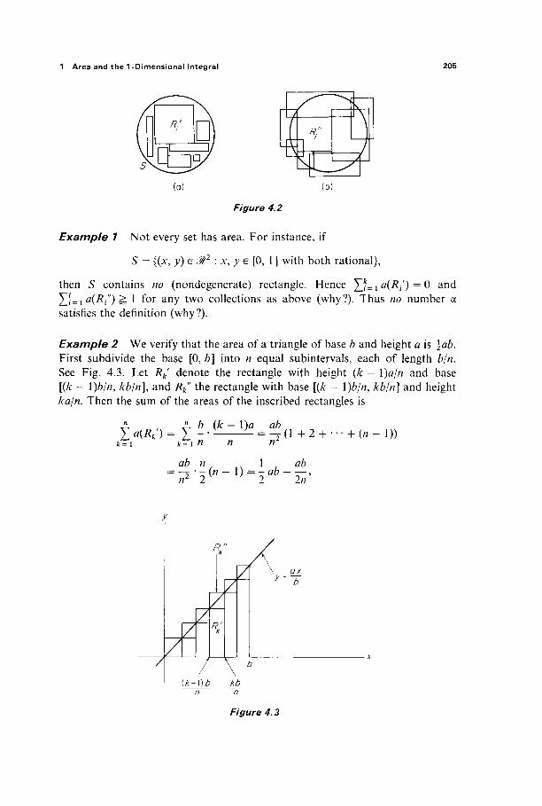
1 Area and the 1 -Dimensional Integral 205
(a) (b)
Figure 4.2
Example 1 Not every set has area. For instance, if
S = {(*, y) e M1 : Λ\ y e [0, 1 ] with both rational},
then S contains no (nondegenerate) rectangle. Hence £*= t #(/?,·') = 0 and X'=i a(R") ^ 1 for any two collections as above (why?). Thus no number a satisfies the definition (why?).
Example 2 We verify that the area of a triangle of base b and height a is jab. First subdivide the base [0, b] into A equal subintervals, each of length b/n. See Fig. 4.3. Let Rk' denote the rectangle with height (k — \)a/n and base [(k - l)b/n9 kb/n], and /?fc" the rectangle with base [(A- - l)b/n, kb/n] and height ka/n. Then the sum of the areas of the inscribed rectangles is
^ , „ " b (k-\)a ab Σ*(**')= Σ - · - — = — (i + 2 + ·-· + (/7- i»
*=i *=i n n nz
ab n \ ab = — '^(n-\) = -ab-—,
ir 2 2 2/?
y
ax
X
{k-\)b /ώ n n
Figure 4.3
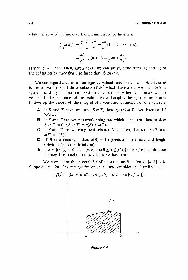
206 IV Multiple Integrals
while the sum of the areas of the circumscribed rectangles is
fc=i k=in n ηΔ
ab n 1 ab = -.-(n+l) = -ab + -
n 2 2 2/7 Hence let a = \ab. Then, given ε > 0, we can satisfy conditions (1) and (2) of the definition by choosing n so large that ab\2n < ε.
We can regard area as a nonnegative valued function a : se -> ,^, where s4 is the collection of all those subsets of 0t2 which have area. We shall defer a systematic study of area until Section 2, where Properties A-E below will be verified. In the remainder of this section, we will employ these properties of area to develop the theory of the integral of a continuous function of one variable.
A If S and T have area and S cz T, then a(S) ^ a( T) (see Exercise 1.3 below).
B If S and T are two nonoverlapping sets which have area, then so does S u T , and a(S u T) = a(S) + a{T).
C If 5 and T are two congruent sets and S has area, then so does Γ, and a(S) = a(T).
D If R is a rectangle, then a(R) = the product of its base and height (obvious from the definition).
E If S = {(x, y)e &2 : xe [a, b] and 0 ^ y ^f(x)} where/is a continuous nonnegative function on [a, b], then S has area.
We now define the integral \ba f of a continuous function / : [a, b] -► 01.
Suppose first t h a t / i s nonnegative on [a, b], and consider the "ordinate set"
Oab(f) = {(x%y)e@2:xE[a,b] and ye[0,f(x)]}
y--fix)
Figure 4.4
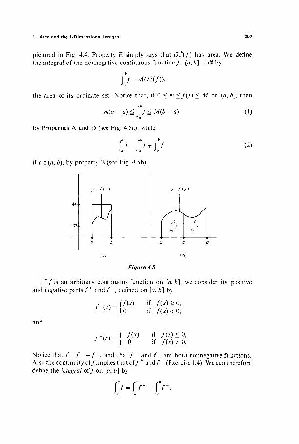
1 Area and the 1 -Dimensional Integral 207
pictured in Fig. 4.4. Property E simply says that Oab(f) has area. We define
the integral of the nonnegative continuous function/: [a,b]-+ ffl by
(f=a{Oa\f)), Ja
the area of its ordinate set. Notice that, if 0 ^ m ^f{x) ^ M on [a, b], then
m(b-a)èjféM(b-a) (1)
by Properties A and D (see Fig. 4.5a), while
ff-ff+ff Ja Ja Jc
if c e (a, b), by property B (see Fig. 4.5b).
(2)
M>
mi
y--f
>
1
C
U)
c± » 7
< L
»
Figure 4.5
If / is an arbitrary continuous function on [a, b], we consider its positive and negative p a r t s / + a n d / " , defined on [a, b] by
3 y ' \0 if f(x)<0,
and
f~(x) = -f(x) if / (JC)^0,
0 if f(x)>0.
Notice t h a t / = / + - / " , and that/"1" a n d / " are both nonnegative functions. Also the continuity of/implies that of/+ a n d / - (Exercise 1.4). We can therefore define the integral o f / o n [a, b] by
f7=fV-Jr.

208 IV Multiple Integrals
In short, J £ / i s "the area above the x-axis minus the area below the jc-axis" (see Fig. 4.6). We first verify that (1) and (2) above hold for arbitrary continuous functions.
Figure 4.6
Lemma 1.1 If c e (a, b), then
fr-U+ïf-Ja Ja Jc
PROOF This is true for/because it is true for b o t h / + a n d / " rb rb rb
J/=J/+-J/~
' -(J>+j/*)-(J>-J/-)
Lemma 1.2 If m ^ / ( x ) ^ M on [a, b], then
rb
m(b-a)<L\ f ^ M(b - a).
(2)
(1)
PROOF We shall show that \ba /<* M(b - a); the proof that m(b - a) <; \b
a / i s similar and is left as an exercise.
Suppose first that M > 0. Then
J/= jV - jV ύ fr è M(b - a)
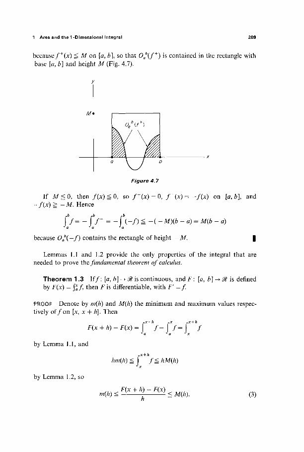
1 Area and the 1-Dimensional Integral 209
because f+(x) ^ M on [a, b]9 so that Oab(f+) is contained in the rectangle with
base [a, b] and height M (Fig. 4.7).
Figure 4.7
If M ^ O , then / (*) ^ 0, so / + ( x ) = 0, / " ( * ) = - / ( * ) on [a, b], and - / ( x ) ^ - M . Hence
f/= - fV = - f(-/) ^ -( -Λί)(* - a) = Jlf(6 - a) J a •'a J a
because Oab(-f) contains the rectangle of height —M. |
Lemmas 1.1 and 1.2 provide the only properties of the integral that are needed to prove the fundamental theorem of calculus.
Theorem 1.3 If/: [a, b]-+&is continuous, and F : [a, b] -> 01 is defined by F(x) = \x
af then F is differentiate, with F' = / .
PROOF Denote by ra(/z) and M(/z) the minimum and maximum values respec-tively of/ on [x, x + h]. Then
«χ + ή »x ,,χ + Λ
F(x + A) - F(x) = j / - J / = J / by Lemma 1.1, and
by Lemma 1.2, so
hm(h)sf f^hMih)
m{h) ^ F(X + h)- m g ^ (3)
210 IV Multiple Integrals
Since lirn,,^ m(h) = ΗηιΛ_>0 Μ(Ιή = f(x) because/is continuous at x, it follows from (3) that
F(x + h) - F(x) F (x) = hm =f(x)
as desired. |
The usual method of computing integrals follows immediately from the fundamental theorem.
Corollary 1.4 I f / i s continuous and G" = / o n [#, 6], then
f/=C?(o)-G(a).
PROOF If F(JC) = j a / o n [a, è], then
F\x) = / (*) = G'(x)
by the fundamental theorem. Hence
F(x) = G(x) + C, C constant.
Now C = F(a) - G(a) =\aaf- G (a) = -G(a), so
f V = F(6) = G(6) + C = G(b) - G(a). |
It also follows quickly from the fundamental theorem that integration is a linear operation.
Theorem 1.5 If the functions / and g are continuous on [a, b], and e e l , then
~b ~b »b »b „b
\{f+g)=\f+\ 9 and (cf) = c f.
PROOF Let F and G be antiderivatives of /and g, respectively (provided by the fundamental theorem), and let H = F + G on [a, b]. Then H' = (F + G)' = F' + G' =f+g, so
(f+g) = H(b) - //(*) (by Corollary 1.4) ^ a
= (F(6) + G(6)) - (F(a) + G(a)) = {F(b) - F(a)) + (G(b) - G(a))
= / + 9 (by Corollary 1.4 again).
The proof that γα cf = c\baf is similar. |
1 Area and the 1-Dimensional Integral 211
Theorem 1.6 lff(x) ^ g{x) on [a, b], then
cb cb
f* g· Ja J a
PROOF Since g(x) —f(x) ^ 0, Theorem 1.5 and Lemma 1.2 immediately give
\bg-ff=f(g-/)^0. | Ja Ja Ja
Applying Theorem 1.6 with g = \f\, we see that
J> ^ M(6 - a)
if l / W I ^ M o n [fir, ft]. It is often convenient to write
rb rb
I/= /Μώ, Ja J a
and we do this in the following two familiar theorems on techniques of integration.
Theorem 1.7 (Substitution) L e t / have a continuous derivative on [a, b], and let g be continuous on [c, d], where f([a, b]) c [c, of]. Then
,b „Ab)
9(f(x))f'(x) d* = Φ) du-Ja Jf(a)
PROOF Let G be an antiderivative of g on [c, d]. Then
DG(f(x)) = Gf(f{x))f\x)=g{f(x))f\x)
by the chain rule, so
Cgi/WM àx = G(f{b)) - G(f(a)) (by Corollary 1.4) Ja
[Ab)
= g (Corollary 1.4 again) Jf(a)
çf(b)
g(u)du. | Jf(a)
Example 3 Using the substitution rule, we can give a quick proof that the area of a circle of radius r is indeed A = nr2. Since π is by definition the area of the unit circle, we have (see Fig. 4.8)
4 J0
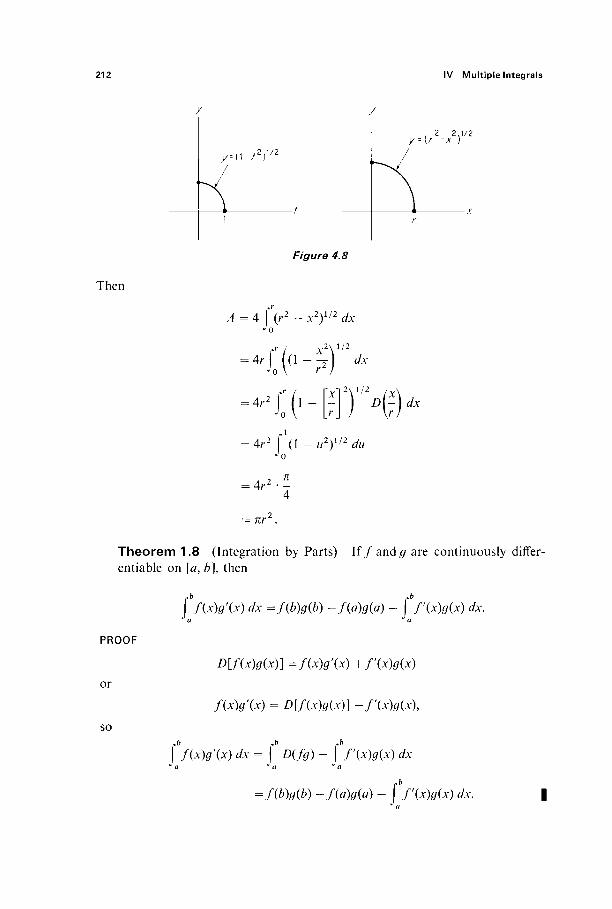
212 IV Multiple Integrals
Then
y = d - / 2 ) , / 2
, 2 2 .1 /2 y-\r -x )
Figure 4.8
A =4 \\r2 - x2)112 dx
= 4 r / 0 ( ( 1 - r - ) *
= 4/·2 f (1 -u2fl2du •Ό
= 4 r 2 · ^
7ir
Theorem 1.8 (Integration by Parts) If/and # are continuously differ-entiable on [a, b], then
\bf(x)g'{x) dx =/(%(*) -/(a)ff(fl) - fV'WiW <**·
PROOF
or
so
D[f(x)g(x)] =f(x)g'{x) +f'(x)g(x)
f(x)g'(x) = D[f(x)g(x)} -f'(x)g{x),
ff(x)g'(x) dx = Ç D(fg) - ff'(x)g(x) dx
=f{b)g(b) -f{a)g{a) - ff'(x)g(x) dx.

1 Area and the 1 -Dimensional Integral 213
The integration by parts formula takes the familiar and memorable form
\ u dv = uv — \ v du
if we write u =f(x), v = g(x), and further agree to the notation du =f'(x) dx, dv = g'(x) dx in the integrands.
Exercises
1.1 Calculate the area under y = x2 over the interval [0, 1 ] by making direct use of the defini-tion of area.
1.2 Apply the fundamental theorem to calculate the area in the previous exercise. 1.3 Prove Property A of area. Hint: Given S <= Γ, suppose to the contrary that a(T) < a(S),
and let ε = i(a(S) — a(T)). Show that you have a contradiction, assuming (as you may) that, if the rectangles /?Γ, . . . , Rm" together contain the rectangles Ri\ . . . , Rn\ then Σ?=ι *(*/') ^Σ?=ι "(*.').
1.4 Prove that the positive and negative parts of a continuous function are continuous. 1.5 If fis continuous on [a, b], and
Ô = fj on [a, b], G(x
prove that G\x) = —fix) on [a, b]. (See the proof of the fundamental theorem.) 1.6 Prove the other part of Theorem 1.5, that is, that j£ cf= c J j / i f c is a constant. 1.7 Use integration by parts to establish the "reduction formula"
sin" x dx = sin" 1x cos x -\ sin" 2 x dx. J n n J
In particular, J*o/2 sin" xdx= [in— 1 ]/n] Jô/2 sin" 2 x dx. 1.8 Use the formula in Exercise 1.7 to show by mathematical induction that
2 4 6 In
3 5 7 2>2 + l
and
Γπ/2 , 77 1 3 5 2 / 2 - 1 sin x dx = — · 2 2 4 6 In '
1.9 (a) Conclude from the previous exercise that
77 2 2 4 4 In In J0n/2 sin2" x dx
2 1 3 3 5 2 / 1 - 1 2/z+ 1 J0n/2sin2" + 1 x dx'
(b) Use the inequality
0 < sin2"+1 x <: sin2" x <, sin2" " 1 x for x G (0,7τ/2]
and the first formula in Exercise 1.8 to show that
Π;/2 sin2" * </x L ^ s i n 2 " - 1 * ^ 1 1 < — < — = 1 -\ .
| 0π / 2 sin2"+ ] x dx = \T sin2" + lxdx In
214 IV Multiple Integrals
2 VOLUME AND THE /7-DIMENSIONAL INTEGRAL
In Section 1 we used the properties of area (without verification) to study the integral of a function of one variable. This was done mainly for purposes of review and motivation. We now start anew, with definitions of volume for sub-sets of $", and of the integral for functions on ffln.
These definitions are the obvious generalizations to higher dimensions of those given in Section 1. Recall that a closed interval in M" is a set / = Ix x I2
x · · · x /„, where Ij = [ÛJ , bj] a 9Ä, j = 1, . . . , n. Thus a closed interval / in $n
is simply a Cartesian product of "ordinary " closed intervals. The volume of/ is, by definition, v(l) = (bx — ax){b2 - a2) · · · (bn - a„). Now let A be a bounded subset of 0tn. Then we say that A is a contented set with volume v(A) if and only if, given ε > 0, there exist
(a) nonoverlapping closed intervals / , , . . . , Ipc:A such that £f= i ΚΛ0 > v(A) — ε, and
;" ·
(c) Conclude from (a) and (b) that
77 ,. (2 2 4 4 2n 2n \ - = lim ( - · · - · I. 2 „-oo \1 3 3 5 2n- 1 2A/+ 1/
This result is usually written as an "infinite product," known as Wallis'product:
7 7 - 2 2 4 4 6 6 2 " ~ T ' 3 3 * 5 5 7 "
1.10 Deduce from Wallis' product that ai
r (n\)222n
lim = v 77 . B-oo(2/i)!\//f
////if; Multiply and divide the right-hand side of
_ 2 2 4 4 2#i 2n n~~\ 3 3 5 2# i - 1 " 2n + 1
by 2 · 2 · 4 · 4 (2/?) · (2A?). This yields
(K! ) 4 2 4 "
" [(2ΑΑ)!]2(2Α/ + 1 ) *
1.11 Write n\ = annn\/n e~n for each n, thereby defining the sequence {a„}f. Assuming that
urn,,-*, cin = a ^ 0, deduce from the previous problem that a = (27r)1/2. Hence n\ and (2nn)i/2(n/e)n are asymptotic as n-> oo,
meaning that the limit of their ratio is 1. This is a weak form of "'Stirling's formula."

2 Volume and the /7-Dimensional Integral 215
(b) closed intervals Jl9 . . . , Jq such that q q
A Œ U JJ a n d Σ v(Jj) < v(A) + ε·
We have seen (Example 1 of Section 1) that not all sets are contented. Con-sequently we need an effective means of detecting those that are. This will be given in terms of the boundary of a set. Recall that the boundary δΑ of the set A c ffln is the set of all those points of 0tn that are limit points of both A and Stn-A.
The contented set A is called negligible if and only if v(A) = 0. Referring to the definition of volume, we see that A is negligible if and only if, given ε > 0, there exist intervals Jl9 . . . , Jq such that A c \Jq
j=1Jj and Yj=i v(Jj) < ε. It follows immediately that the union of a finite number of negligible sets is negligible, as is any subset of a negligible set.
Theorem 2.1 The bounded set A is contented if and only if its boundary is negligible.
PROOF Let R be a closed interval containing A. By a partition of R we shall mean a finite collection of nonoverlapping closed intervals whose union is R.
First suppose that A is contented. Given ε > 0, choose closed intervals Il9 . . . , Ip and Jl9 . . . , Jq as in conditions (a) and (b) of the definition of v(A). Let ^ be a partition of R such that each I( and each Jj is a union of closed intervals of ^ . Let Ru . . . , Rk be those intervals of & which are contained in \Jj=iIi, and Rk + l, . . . , Rk + l the additional intervals of ^ which are contained in (J?=iJ;· T h e n
k + l
ÔA<= \J /?,-, i = k+l
and
Σ' «W = l ' « W - Σ «W ^ Σ C·7;) - Σ K/,) i=k+l i=l i=i j=l 7 = 1
< [φ! ) + ε] - [v(A) -ε]= 2ε.
Now suppose that dA is negligible. Note first that, in order to prove that A is contented, it suffices to show that, given ε > 0, there exist intervals Jl9 ..., Jq
containing A and nonoverlapping intervals Il9 . . . , Ip contained in A such that
i v(jj) -1 .a,) < e, 7 = 1 i = l
for then v(A) = glb{Xj=1 Γ(^·)} = lub{£f= l i;(/f)} (the greatest lower and least upper bounds for all such collections of intervals) satisfies the definition of volume for A.
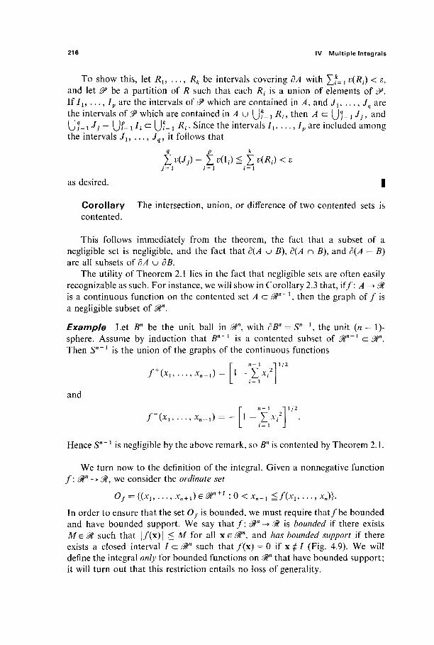
216 IV Multiple Integrals
To show this, let Ru . . . , 7?λ be intervals covering dA with £ ? = 1 K^i) < £> and let ^ be a partition of Λ such that each Rt is a union of elements of 0. If Il9 ..., lv are the intervals of 0 which are contained in A, and Jl9 . . . , Ja are the intervals of 0> which are contained in A u \J\= x R{, then A c (JJ= j J . , and U w , - U f = i V the intervals Jl9 ..
(J*= j 7?i. Since the intervals / l s . . . , /p are included among Jn, it follows that
Σ^)-Σ«ΚΙ()^Σ"(Λι)<ε
as desired. I
Corollary The intersection, union, or difference of two contented sets is contented.
This follows immediately from the theorem, the fact that a subset of a negligible set is negligible, and the fact that d(A u B)9 d(A n B), and d(A - B) are all subsets of dA u dB.
The utility of Theorem 2.1 lies in the fact that negligible sets are often easily recognizable as such. For instance, we will show in Corollary 2.3 that, if/: A -► £% is a continuous function on the contented set A a &η~λ, then the graph o f / is a negligible subset of 0ln.
Example Let Bn be the unit ball in Stn, with dB" = S"~\ the unit (n - 1> sphere. Assume by induction that Bn~l is a contented subset of 0ln~x c &". Then S"'1 is the union of the graphs of the continuous functions
f + (xi, . . . , * „ _ , ) : ι - Σ * / 1/2
and
/ (xl5 . . . , * „ - , ) = - i - Z V 1/2
Hence S" * is negligible by the above remark, so Bn is contented by Theorem 2.1.
We turn now to the definition of the integral. Given a nonnegative function / : &n -► 01, we consider the ordinate set
Of = {(xu . . . , x„ + 1)e, : 0 < χ „ + 1 ^ / (x j , . . . ,^ )} .
In order to ensure that the set Of is bounded, we must require tha t /be bounded and have bounded support. We say t h a t / : 0tn -► 01 is bounded if there exists Me 01 such that | / (x) | ^ M for all x G ", and has bounded support if there exists a closed interval I 0Γ such that / (x) = 0 if x φ I (Fig. 4.9). We will define the integral only for bounded functions on 0tn that have bounded support; it will turn out that this restriction entails no loss of generality.
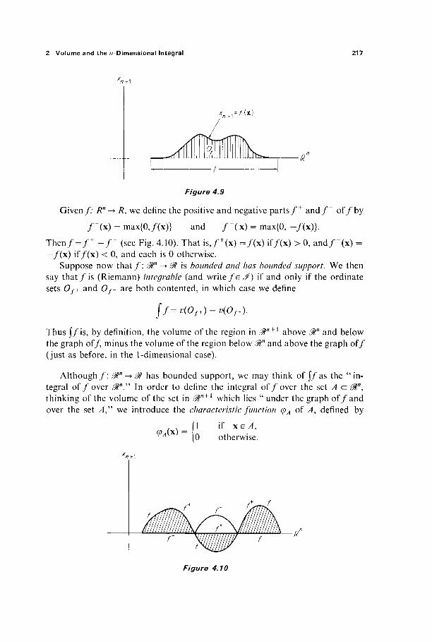
2 Volume and the /^-Dimensional Integral 217
Figure 4.9
Given/: R" -» R, we define the positive and negative p a r t s / + a n d / - o f /by
/ + ( x ) = max{0,/(x)} and / " ( x ) = max{0, - / (x )} .
T h e n / - / + - / " (see Fig. 4.10). That is , /+(x) = / (x ) if/(x) > 0, and /" (x) = —/(x) if / (x ) < 0, and each is 0 otherwise.
Suppose now t h a t / : 0tn -> 01 is bounded and has bounded support. We then say t h a t / i s (Riemann) integrable (and write fe J) if and only if the Ordinate sets Of+ and Of- are both contented, in which case we define
ff=v(Of + )-v(Of-).
Thus j / i s , by definition, the volume of the region in Mn + l above 0ln and below the graph of/ minus the volume of the region below 0tn and above the graph of/ (just as before, in the 1-dimensional case).
Although/: 0tn -► M has bounded support, we may think of j / a s the "in-tegral o f /over ^ V In order to define the integral o f /over the set A c 0Γ, thinking of the volume of the set in ^ " + 1 which lies "under the graph o f / and over the set A" we introduce the characteristic function φΑ of A, defined by
if xeA, ΨΑ(*) =
1 0 otherwise.
Figure 4.10
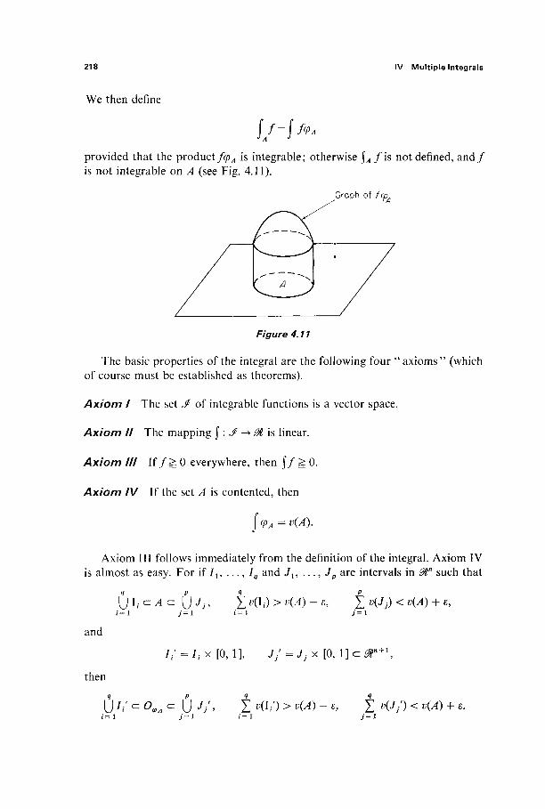
218 IV Multiple Integrals
We then define
provided that the product fcpA is integrable; otherwise j ^ / i s not defined, a n d / is not integrable on A (see Fig. 4.11).
Figure 4.11
The basic properties of the integral are the following four "axioms" (which of course must be established as theorems).
Axiom I The set J of integrable functions is a vector space.
Axiom II The mapping J : J -» 01 is linear.
Axiom III If / ^ 0 everywhere, then \f ^ 0.
Axiom IV If the set A is contented, then
j(pA = v(A).
Axiom III follows immediately from the definition of the integral. Axiom IV is almost as easy. For if Iu . . . , Iq and Jl5 . . . , Jp are intervals in &n such that
[jl^Ac: (jjj, £ »(I.) > v(A) - ε, £ !;(·/,) < K^) + ^ i = l j = l i = l i = l
and
/, ' = It x [0, 1], J / - J,. x [0, 1] c @n+\
then
U / / c O ^ c f ) J / , X KI/) > .(Λ) - ε, Σ <J/) < <A) + ε· i = l j = l i = l J = l
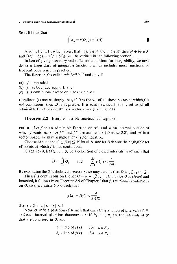
2 Volume and the /7-Dimensional Integral 219
So it follows that
\φΑ = ν(ΟφΑ) = ν(Α). I
Axioms 1 and II, which assert that, if/, g e J> and a, b e &, then af+bgeJ and \(af+ bg) = a\f'+ b$g9 will be verified in the following section.
In lieu of giving necessary and sufficient conditions for integrability, we next define a large class of integrable functions which includes most functions of frequent occurrence in practice.
The function/is called admissible if and only if
(a) / i s bounded, (b) / h a s bounded support, and (c) / i s continuous except on a negligible set.
Condition (c) means simply that, if D is the set of all those points at which/is not continuous, then D is negligible. It is easily verified that the set se of all admissible functions on 0ln is a vector space (Exercise 2.1).
Theorem 2.2 Every admissible function is integrable.
PROOF L e t / b e an admissible function on 0tn, and R an interval outside of which / vanishes. S ince / + a n d / - are admissible (Exercise 2.2), and se is a vector space, we may assume tha t / i s nonnegative.
Choose M such that 0 ^ / ( x ) ^ M for all x, and let D denote the negligible set of points at which/is not continuous.
Given ε > 0, let Qu . . . , Qk be a collection of closed intervals in &n such that k k
D^[jQi and X„(ß i)<JL.
By expanding the Q^s slightly if necessary, we may assume that D c (J{L j int β,- · Then / i s continuous on the set Q = R — (J*= { int Qt. Since Q is closed and
bounded, it follows from Theorem 8.9 of Chapter I that / is uniformly continuous on β, so there exists δ > 0 such that
if x, y G Q and | x — y | < δ. Now let & be a partition of 7? such that each Qf is a union of intervals of ^ ,
and each interval of & has diameter <δ. If /?t, . . . , Rq are the intervals of ^ that are contained in Q, and
at = gib of/(x) for xei?, · , 6,. = lub of/(x) for x e i ? , ,
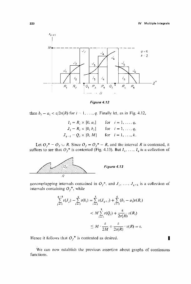
220 IV Multiple Integrals
Figure 4.12
then bi — at< e/2v(R) for / = 1, . . . , q. Finally let, as in Fig. 4.12,
/
'q +
= Rt x [Ο,Λ,·] for /' = 1, . . . , ? ,
= Ri x [0, 6f] for / = 1, ...9q9
= Qi>< [0,M] for / = ! , . . . , k.
Let Of* = Of u R. Since Of = Of* — R, and the interval R is contented, it suffices to see that Of* is contented (Fig. 4.13). But 7l5 . . . , Iq is a collection of
Figure 4.13
nonoverlapping intervals contained in Of*, and J{, . . . , Jq+k is a collection of intervals containing Oy*, while
i V , · ) - Σ κι,) = Σ °v<+i) + Σ (*< - *>(*.·) j = 1 i = 1 i = 1 i = 1
<Λ/χκβί) + ί -^ΚΛ ί ) /= i 2ϋ(Λ)
2Μ 2v(R) V ;
Hence it follows that Of* is contented as desired.
We can now establish the previous assertion about graphs of continuous functions.

2 Volume and the /7-Dimensional Integral 221
Corollary 2.3 If/: A -> & is continuous, and A c 0tn is contented, then the graph Gy o f / i s a negligible set in &n + 1.
PROOF If we extend/to &n by/(x) = 0 for x φ A, then/ i s admissible because its discontinuities lie in dA, which is negligible because A is contented. Hence Of
is contented by the Theorem, so dOf is negligible. But Gf is a subset of dOf. |
It follows easily from Corollary 2.3 that, if/: A -> 01 is a nonnegative con-tinuous function on a contented set Λ c ^Γ, then the ordinate set o f / i s a con-tented subset of &n + i (see Exercise 2.7). This is the analogue for volume of Property E in Section 1.
The following proposition shows that \A f is defined if/ \0ln -> ^ is admissible and ^ c ^ " is contented. This fact serves to justify our concentration of attention (in the study of integration) on the class of admissible functions—every function that we will have "practical" need to integrate will, in fact, be an admissible function on a contented set.
Proposition 2.4 I f / is admissible and A is contented, then fcpA is ad-missible (and, therefore, is integrable by Theorem 2.2).
PROOF If D is the negligible set of points at which/ is not continuous, then fcpA is continuous at every point not in the negligible set D u dA (see Exercise 2.3).
I
Proposition 2.5 I f / and g are admissible functions on 0ln with f^g everywhere, and A is a contented set, then
JA JA
PROOF gcpA —f(pA ^ 0 everywhere, so Axiom III gives \(g<pA —ftpA) = 0· Then Axiom II gives
j f= lf<pA^\9<pA=\ 9- I
It follows easily from Proposition 2.5 that, if 4 and B are contented sets in 0tn, with A a B, then v(A) ^ v(B) (see Exercise 2.4). This is the analog for volume of Property A of Section 1.
Proposition 2.6 If the admissible function / satisfies | / (x) | ^ M for all x e 0tn, and A is contented, then
J A
^ Mv(A).
In particular, $Af = 0 if A is negligible.
222 IV Multiple Integrals
PROOF Since — ΜφΑ S/ΨΑ = ΜφΑ, this follows immediately from Proposition 2.5 and Axioms II and IV. |
Proposition 2.7 If A and B are contented sets with A n B negligible, and / i s admissible, then
JAKJB JA JB
PROOF First consider the special case A n B = 0. Then φΑ u B = φΑ + φΒ, so
f / = \/ΨΑ U ß = Î(/<PA +/<P*) J / l u ß j J
= JM + J/<P. = / /+ / /■
If A n B is negligible, then \A nBf= 0 by Proposition 2.6. Then, applying the special case, we obtain
f / = f /+ f /+ f / J A u B ^ Λ - Β M n ß ^ β - Λ
- ( / ' + J ') + (J ' + J /) VA-B JAnB / \JAnB JB-A /
J A J B
It follows easily from Proposition 2.7 that, if A and i? are contented sets with A n B negligible, then A u B is contented, and ι;(Λ KJ B) = v(A) + i;(i?) (see Exercise 2.5). This is the analog for volume of Property B of Section 1.
Theorem 2.8 Let A be contented, and suppose the admissible functions / and g agree except on the negligible set D. Then
JA JA
PROOF Let h = / — g, so h = 0 except on D. We need to show that \Ah = 0. But
f * = Ρ Λ = f%nD = | * = ° J A J J JAnD
by Proposition 2.6, because A n D is negligible. |
This theorem indicates why sets with volume zero are called " negligible "—■ insofar as integration is concerned, they do not matter.

3 Step Functions and Riemann Sums 223
Exercises
2.1 If/and g are admissible functions on 3tn and c e M, show that f+g and cf are admis-sible.
2.2 Show that the positive and negative parts of an admissible function are admissible. 2.3 If D is the set of discontinuities of/: Mn -> &, show that the set of discontinuities of
fcpA is contained in D u dA. 2.4 If A and B are contented sets with A ^ B, apply Proposition 2.5 with / = φΑ = ψβψΑ,
g = φΒ to show that
ι?(Λ) <; Ü ( Ä ) .
2.5 Let A and i? be contented sets with A n D negligible. Apply Proposition 2.7 wi th /= ΨΑ u B to show that A u 5 is contented with
ι?(/ί u 5) = φ θ + i;(5).
2.6 If/and g are integrable functions with /(x) <Ξ #(x) for all x, prove that J / ^ J g without using Axioms I and II. Hint: f^g^f+^g + a n d / - ^> g~ => Of+^ Og+ and Og_c o,_.
2.7 If A is a contented subset of ,3?" and f\A->£# is continuous and nonnegative, apply Corollary 2.3 to show that Of is contented. ///>//: Note that the boundary of Of is the union of A <=- 3%n <=■ &n + \ the graph of/, and the ordinate set of the restriction/: dA -> ^ . Conclude that 80f is negligible, and apply Theorem 2.1.
3 STEP FUNCTIONS AND RIEMANN SUMS
As a tool for studying the integral, we introduce in this section a class of very simple functions called step functions. We shall see first that the properties of step functions are easily established, and then that an arbitrary function is in-tegrable if and only if it is, in a certain precise sense, closely approximated by step functions.
The function h : 0tn -> J> is called a step function if and only if/? can be written as a linear combination of characteristic functions φΐ9 . . . , φρ of intervals Il9 . . . , Ip whose interiors are mutually disjoint, that is,
p
h = ΣαΐΨί i= 1
with coefficients ateM. Here the intervals Il9 I2, . . . , Ip are not necessarily closed—each is simply a product of intervals in & (the latter may be either open or closed or "half-open").
Theorem 3.1 If h is a step function, h = Yj=l a^t as above, then h is integrable with
(h=taiv(Ii). J 1 = 1
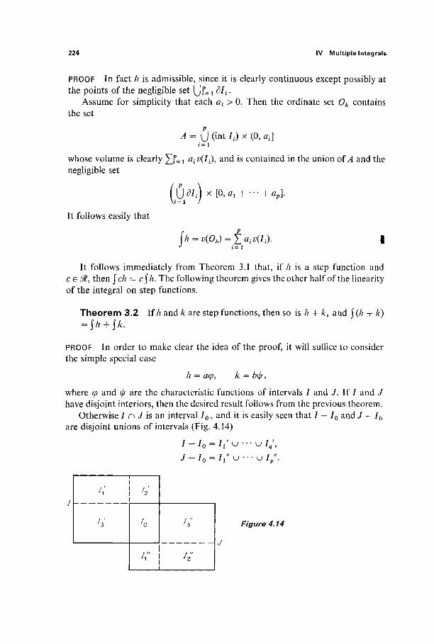
224 IV Multiple Integrals
PROOF In fact A is admissible, since it is clearly continuous except possibly at the points of the negligible set {Jf=idli.
Assume for simplicity that each ai > 0. Then the ordinate set Oh contains the set
A = U (int /,) x (0, at]
whose volume is clearly £f= i at v{I^), and is contained in the union of A and the negligible set
(H x [0, «! + ··· + a.].
It follows easily that
I
It follows immediately from Theorem 3.1 that, if A is a step function and ce 01, then \ch = c\h. The following theorem gives the other half of the linearity of the integral on step functions.
Theorem 3.2 If A and k are step functions, then so is A + k, and J(A + k) = JA + J*.
PROOF In order to make clear the idea of the proof, it will suffice to consider the simple special case
A = αφ9 k = οψ,
where φ and φ are the characteristic functions of intervals I and J. If I and / have disjoint interiors, then the desired result follows from the previous theorem.
Otherwise J n J is an interval I0, and it is easily seen that I — I0 and J — I0
are disjoint unions of intervals (Fig. 4.14)
I -I0 =It' u · · · u / / ,
1 1
1
n 7 0
/,-
4" Figure 4.14
3 Step Functions and Riemann Sums 225
Then
A + k = αφ + b\}j q p
= (a + b)cpIo + Σα(Ρΐι + Σ b(Pii"> i = l i= 1
so we have expressed A + k as a step function. Theorem 3.1 now gives
f(A + k) = (a + % ( / 0 ) + a Σ v{i;) + bf i</(")
= a[v(I0) + t «</,')] + W o ) + Σ «(/(")] i = 1 i = 1
= tfK/) + *K-0
= J A + J * as desired. The proof for general step functions A and k follows from this con-struction by induction on the number of intervals involved. |
Our main reason for interest in step functions lies in the following charac-terization of integrable functions.
Theorem 3.3 L e t / : 0tn ^> 0t be a bounded function with bounded sup-port. Then/is integrable if and only if, given ε > 0, there exist step functions A and k such that
h^f^k and j(k - A) < ε,
in which case j"A j / g \k.
PROOF Suppose first that, given ε > 0, step functions A and k exist as prescribed. Then the set
S = {(xl5 . . . , xn + 1) e @n + l : h(xu ...,xH)£ xn + 1 £ k(xl9 . . . , xn)}vdOkudOh
has volume equal to J(fc - Α)<ε. But S contains the set Gf=dOf - @n (Fig. 4.15). Thus for every ε > 0, Gf lies in a set of volume <ε. It follows easily that Gf is a negligible set. If Q is a rectangle in 0ln such t h a t / = 0 outside Q, then dOf+ and dOj- are both subsets of Q u Gf, so it follows that both are negligible. Therefore the ordinate sets Of+ and Of- are both contented, so fis integrable. The fact that j"A g J / ^ j / : follows from Exercise 2.6 (without using Axioms I and II, which we have not yet proved).
Now suppose tha t / i s integrable. Since this implies that both/4" a n d / - are integrable, we may assume without loss t h a t / ^ 0. Then the fact t ha t / i s integ-rable means by definition that Of is contented. Hence, given ε > 0, there exist

226 IV Multiple Integrals
Graph of k
Graph of h
Figure 4.15
nonoverlapping intervals Iu . . . , Iq contained in Of, and intervals Ju . . . , Jp
with Of c [j pj= ! Jj, such that
<A) -1 < Σ K/i) ^ Σ ^ - ) < ΚΛ) + !;, Λ = of.
See Fig. 4.16. Given x G Π, define
A(x) = max{j e ^ : (x, y) e [j JJ ,
£(x) = max{.y e & : (x, z) e (J Jj i f z e [0, y]},
if the vertical line in ^ " + l through x G " intersects some It (respectively, some Jj), and let Λ(χ) = 0 (respectively, k(x) = 0) otherwise. Then It and k are step
Graph of f
I. shaded; J. not shaded / ' J
Figure 4.16
3 Step Functions and Riemann Sums 227
functions such that h^f^k. Since
O^CJ/,. and ok^(jjj9
the above inequalities imply that
/ ( * - * ) = / * - / *
= v(Ok) - v(Oh)
<(v(A) + ^-(V(A)-^=s
as desired. |
Example We can apply Theorem 3.3 to prove again that continuous functions are integrable. Le t / : @tn -> M be a continuous function having compact support. Since it follows that the nonnegative functions/+ a n d / - are continuous, we may as well assume that/itself is nonnegative. Let Q a 0ln be a closed interval such t h a t / = 0 outside Q. Then/ is uniformly continuous on Q (by Theorem 8.9 of Chapter I) so, given ε > 0, there exists δ > 0 such that
| x - y | < 5 = > | / ( x ) - / ( y ) | < ^ ·
Now let ^ = {Qls . . . , Qz} be a partition of Q into nonoverlapping closed inter-vals, each of diameter less than δ. If
mi = minimum value o f / on Qi9
M{ = maximum value o f / on β ί 5
φι = the characteristic function of int Qi9
φί = the characteristic function of Qi9
and A = ^ Ι ^ / Μ ^ , · , A: = £j=i Μίφί9 then A ^ / ^ A: and
f (* - A) = t (M, - w.-MÔ,·) < - ^ : Σ KQ,) = «, j ί= ι ^ i y j i = i
so Theorem 3.3 applies.
We are now prepared to verify Axioms I and II of the previous section. Given integrable functions / and f2, and real numbers ai and a2, we want to prove that aj^ + a2f2 is integrable with
j(<*ifi + difi ) = a, JVi + a2 Jf2 .
We suppose for simplicity that al > 0, a2 > 0, the proof being similar in the other cases.
228 IV Multiple Integrals
Given ε > 0, Theorem 3.3 provides step functions hu h2, ku k2 such that
hiufiukt (1)
and \{kt - Af) < ε/2^· for / = 1, 2. Then
h = aihl + a2 h2 g ίτ,/i + a2f2 ^ α +a2k2= k, (2)
where A and /: are step functions such that
j(k - h) = βι j > , - Λ,) + fl2 j(k2 - h2) < ε.
So it follows from Theorem 3.3 that alfl + a2f2 is integrable. At the same time it follows from (1) that
jh = a1 jh1 + a2 jh2 ^ ax J/x + a2 J / 2 g β, J"^ + fl2 J* 2 = J"fc
(by Exercise 2.6), and similarly from (2) that
jh S JW, + fl2/2) g J*.
Since J"/: — j/z < ε, it follows that J(flj/i + #2/2) and tfj J/j + fl2 i/2 differ by less than ε. This being true for every ε > 0, we conclude that
JWi + «2/2) = *i J/i + <*2 J/2 · I
We now relate our definition of the integral to the " Riemann sum " definition of the single-variable integral which the student may have seen in introductory calculus. The motivation for this latter approach is as follows. Le t / : [a,b]->@ be a nonnegative function. Let the points a = x0 < xx < · · · < xk = b subdivide the interval [a, b] into k subintervals [x0, xx], [xu x2], . . . , b^ - i , **]. For each / = 1, . . . , k, choose a point xt* e [*,■_!, xt]. (Fig. 4.17). Then f(x*)(Xi — Xi-i) is the area of the rectangle of height f(x*) whose base is the /th subinterval [Xi-l9 Xi], so one suspects that the sum
i = 1
should be a "good approximation" to the area of Of if the subintervals are sufficiently small. Notice that the Riemann sum R is simply the integral of the step function
/ = 1
where φ{ denotes the characteristic function of the interval \xx-\, xt]. Recall that a partition of the interval Q is a collection &> = {Qu . . . , Qk} of
closed intervals, with disjoint interiors, such that Q = [j^=lQi. By the mesh oïSP

3 Step Functions and Riemann Sums 229
Graph of f
Figure 4.17
is meant the maximum of the diameters of the Qt. A selection for 2P is a set y = {xj, . . . , x j of points such that x,· e Q; for each /'. If/: J?rt -> ^ is afunction such t h a t / = 0 outside of Q, then the Riemann sum for/corresponding to the partition 0> and selection £f is
* ( / , ^ , ^ ) = i / ( * . > ( ß i ) . i = 1
Notice that, by Theorem 3.1, the Riemann sum R(f, &, £f) is simply the integral of the step function
h = t /(*,>,·, / = i
where φί denotes the characteristic function of Qt.
Theorem 3.4 Suppose/: 0tn -> 0t is bounded and vanishes outside the interval Q. Then / i s integrable with J / = / if and only if, given ε > 0, there exists δ > 0 such that
\I-R(f,&,y)\ <ε
whenever 3P is a partition of Q with mesh <δ and £f is a selection for ^ .
PROOF If / is integrable, choose M > 0 such that | / (x) | ^ M for all x. By Theorem 3.3 there exist step functions h and k such that h ^ / ^ A: and \{k — h) < e/2. By the construction of the proof of Theorem 3.2, we may assume that h and k are linear combinations of the characteristic functions of intervals whose closures are the same. That is, there is a partition 0^o = {Qu . . . , Qs} of Q such that
^ = Σ°ι(Ρΐ a n d £ = Σ*/^·> i = 1 / = 1

230 IV Multiple Integrals
where Qi is the closure of the interval of which φί is the characteristic function, and likewise for φ^.
Now let A = Q - \Jsi= { int Qf. Then v(A) = 0, so there exists δ > 0 such that,
if & is a partition of Q with mesh <£, then the sum of the volumes of those intervals Pu . . . , Pk of &> which intersect A is less than ε/4Μ. Let Pk + 1, . . . , Λ be the remaining intervals of ^ , that is, those which lie interior to the Q,.
If Sf = {Xi,.. . , X;} is a selection for &y then Afo) ^ /(x,·) ^ £(xf) if / = Ä: + 1, . . . , / , so that
Σ / ( χ , Μ Λ ) and ί [ /
are both between Σ*=*+ι JP. Λ and Σ;=*+ι JPi A-, so it follows that
Σ f / - Σ /(xw: i = fc+l J P ; » = Λ+1
because jQ(/: — /?) < ε/2 by assumption. Since -M ^ / ( x ) ^ M for all x, both
< (3)
Σ f / and t / (χ ,ΜΡ,) i = l J P ; i= 1
lie between -Af Σ?=ι*>(Λ-) > -ε /4 and M £?= ι ΚΛ) < ε/4, so it follows that
Σ ί / - Σ/(χΧΛ) ε <2
(4)
Since J = J / = Σ!=ι fc/' 0 ) anc^ (4) finally imply by the triangle inequality that | / - R(f, &,S?)\ < ε as desired.
Conversely, suppose @> ={Pl9 . . . , Pp} is a partition of Q such that, given any selection Sf for ^0, we have
\l-R(f,9,ST)\ <*-.
Let Qj, , Qp be disjoint intervals (not closed) such that Q. = Pi9 / = 1, . . . , p, and denote by </>,· the characteristic function of Qf. If
tff = gib of/(x) for xePi,
bi = lub of/(x) for xePt,
then
h = t,<*i<Pi and k = YJbi(Pi
are step functions such that h^f^k. Choose selections ^ ' = {x/, . . . , x /} and ^7" = {x, " , . . . , x / } for ^ such that
| ^ - / ( χ / ) | < 4KÔ)
and \bt-f(x,")\ < MQ)
3 Step Functions and Riemann Sums 231
for each /. Then
R(f,P9Sr)-jh i= 1
< ■4KÖ)iti
ε
Σ Κδ,)
and similarly
\R(f,i?,sr)-jk\ <\·
Then
j(k-h)^Uk-R(f,0>,y") + \R{f,P,ff")-l\
+ \l-R(Jt »,&>·)] +
ε ε ε ε
4 4 4 4
R(f,P,sr')-jh
so it follows from Theorem 3.3 that fis integrable. I
Theorem 3.4 makes it clear that the operation of integration is a limit process. This is even more apparent in Exercise 3.2, which asserts that, iff: &n -► 01 is an integrable function which vanishes outside the interval Q, and {^k}f *s a
sequence of partitions of Q with associated selections {Sfk}? such that l im^^ (mesh of 0>k) = 0, then
\f=\imR(f9<?k9<?k).
This observation leads to the formulation of several natural and important integration questions as interchange of limit operations questions.
(1) Let A c 0Γ and B c @n be contented sets, and / : A x B ■ tinuous function. Define g : A -> ^ by
a con-
<Kx) = f/(x,y)rfy= f/x,
where/x(y) =f(x, y). Is # continuous on /I ? This is the question as to whether
lim f / (x , y) dy = f lim / (x , y) </y x->a J ß J ß x^a
for each ae A. According to Exercise 3.3, this is true if/is uniformly continuous.

232 IV Multiple Integrals
(2) Let {fn}f be a sequence of integrable functions on the contented set A, which converges (pointwise) to the integrable function / : A ->£%. We ask whether
lim|7„= ilim/„= f/? n-+oo JA J n->oo J
According to Exercise 3.4, this is true if the sequence {fn}f converges uniformly to f on A. This means that, given ε > 0, there exists N such that
n^N=>\f„(x)-f(x)\ <ε
for all x G A. The following example shows that the hypothesis of uniform con-vergence is necessary. Let fn be the function on [0, 1 ] whose graph is pictured in Fig. 4.18. Then
lim/„(*) = 0 for all JC e [0, 1],
so Jolim,i-»oo/n = 0· However l im,,^ \xQfn = l im, ,^ 1 = 1. It is evident that the
convergence of {fn}™ is not uniform (why?).
(1/2/7,2/7) y--fn[x)
\/n
Figure 4.18
(3) Differentiating under the integral. Letf:A x i - > l be a continuous function, where A <= 0ίη is contented and J c M is an open interval. Define the partial derivative D2f\ A x J -» $ by
D2f(x, t) = lim / ( x , i + A ) - / ( x , 0
and the function g : J ^> & by g(t) = \Af{x, f ) dx. We ask whether
3 Step Functions and Riemann Sums 233
that is, whether
According to Exercise 3.5, this is true if D2fis uniformly continuous on A x J. Since differentiation is also a limit operation, this is another "interchange of limit operations1' result.
Exercises
3.1 (a) If / i s integrable, prove t h a t / 2 is integrable. Hint: Given ε > 0, let h and k be step functions such that h ^ f-^k and j" (k — h) < ε/Μ, where M is the maximum value of \k(x) + /z(x)|. Then prove that h2 and k2 are step functions with h2 ^ / 2 ^ k2 (we may assume that 0 ^ h £ / £ A' since / i s integrable if and only if | / | is—why?), and that \ (k2 — h2) < e. Then apply Theorem 3.3. (b) If / a n d g are integrable, prove that fg is integrable. Hint: Express fg in terms of ( / + g)2 and (/— g)2 ; then apply (a).
3.2 L e t / : Mn-> .^ be a bounded function which vanishes outside the interval Q. Show that / i s integrable with J / = / if and only if
\imR(f90>k9STk) = i
for every sequence of partitions {^k}f and associated selections {^Jî5 such that limk_oo(mesh of &k) = 0.
3.3 Let Λ and 5 be contented sets, and / : A x B-+ & a uniformly continuous function. If # : A -> ^ is defined by
<x) = J e / ( x , #(x) = / ( x , y)dy for all x e / 1 ,
prove that g is continuous, ////if; Write g(x) — g(a) = JB [/(x, y) — / ( a , y)] dy and apply the uniform continuity o f /
3.4 Let {/,}? be a sequence of integrable functions which converges uniformly on the con-tented set A to the integrable function/ Then prove that
lim \ fn=\ f=\ l im/n . n-*ooJA JA JA Π->ΟΟ
Hint: Note that | j V „ - j V / 1 ^ | / - / | . 3.5 L e t / : Λ x / - > ^ b e a continuous function, where A <= n is contented and / c ^ is an
open interval. Suppose that D2f= df/dt (t ej) is uniformly continuous on Λ x 7. If
prove that
#'(/) = J\D2/(x,r)</x.

234 IV Multiple Integrals
Outline: It suffices to prove that, if {tn}f is a sequence of distinct points of / converging t o a e y , then
g(tn)-g(a) r hm = D2f(x,a)dx. n-+c3o /„ a JA
For each fixed xe A, the mean value theorem gives τ„(χ) e (a, tn) such that
/ ( x , /„) - / ( x , a) = (/„ - a)D2f(x, rn(x)).
Let
f(x,tn)-f(x,a) φη(χ) = D2f(x, τπ(χ)).
/„ — tf
Now the hypothesis that Z) 2 / i s uniformly continuous implies that the sequence {«p,,}* converges uniformly on Λ to the function D2f(x, a) of x (explain why). Therefore, by the previous problem, we have
D2f(x, a) dx = lim φ, J A n-* oo J A
r /(x,/„)-/( — h m
n-+ao J A tn — a
f(x9tH)-f(x,a), ax
v g(tn)-g(a) = lim
as desired. 3.6 L e t / : [a, b] x [c, d]-> $ be a continuous function. Prove that
/ 'H V(*. >-) dx\ dy = J"ί j"7(*, >) «J Λ
of the two functions g, h : [#,
/*0 = |Y/V(*,>O^W,
by computing the derivatives of the two functions g, h: [a, b]-> & defined by
and
using Exercise 3.5 and the fundamental theorem of calculus. This is still another inter-change of limit operations.
3.7 For each positive integer n, the Bessel function Jn(x) may be defined by
xn f+1
/„ (*)= — d ~t2)n-l/2 cos xtdt.
Prove that Jn(x) satisfies Bessel's differential equation
3.8 Establish the conclusion of Exercise 3.4 without the hypothesis that the limit function/is integrable. Hint: Let Q be a rectangle containing A, and use Theorem 3.4 as follows
4 Iterated Integrals and Fubini's Theorem 235
to prove that/must be integrable. Note first that / = lim \ fn exists because {j fn}™ is a Cauchy sequence of real numbers (why?).
Given ε > 0, choose N such that both | / - J / N | < ε/3 and |/(x) - /v (x ) | < e/3v(Q) for all x. Then choose δ > 0 such that, for any partition & of mesh < δ and any selection
\fN-R(fN90>,y) ε < 3 ·
Noting that
\R(fN,P,y)-R(f,P,SO\ < |
also, conclude that | / - / ? ( / , ^ , ^ ) | < ε
as desired. The following example shows that the uniform convergence of {fn}f is necessary.
Let Q = {/*k}ï be the set of all rational numbers in the unit interval [0, 1]. If /„ denotes the characteristic function of the set {ru . . . , r„}, then \X
Q fn = 0 for each « = 1 , 2 , . . . , but the limit function
.. r/ . (l if x is rational, lim/„(A-)= L. . π-αο 10 otherwise,
is not integrable. The point is that the convergence of this sequence {/„}? is not uniform. 3.9 If cp{t) = $i[t\f(x, t) dxy apply Exercise 3.5, the fundamental theorem of calculus, and the
chain rule to prove Leibniz' rule: fA(r)
<p\t) = f{h{t\t)h\t) -f(g{t\t)g'{t) + D2f(x, t) dx Jg(t)
rhU)
Je«)
under appropriate hypotheses (state them).
4 ITERATED INTEGRALS AND FUBINI'S THEOREM
I f / i s a continuous function on the rectangle R = [a, b] x [c, d] a 0t2, then
( (C/(x'y) dy)dx=ί (^/(χ'y) dx)dy (1)
by Exercise 3.6. According to the main theorem of this section, the integral jRf is equal to the common value in (1). Thus j ^ / m a y be computed as the result of two "iterated" single-variable integrations (which are easy, using the funda-mental theorem of calculus, provided that the necessary antiderivatives can be found). In a similar way, the integral over an interval in ^ " of a continuous function of n variables can be computed as the result of/? iterated single-variable integrations (as we shall see).
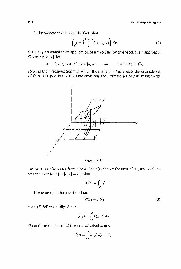
236 IV Multiple Integrals
In introductory calculus, the fact, that
S/=fe(Cnx'y)dx)dy' (2)
is usually presented as an application of a " volume by cross-sections " approach. Given t e [c, d], let
At = {(x, t,z)eât3:xe [a, b] and z e [0,f(x, t)]},
so At is the "cross-section" in which the plane y = t intersects the ordinate set of/: R^>& (see Fig. 4.19). One envisions the ordinate set o f / a s being swept
Figure 4.19
out by At as t increases from c to d. Let A(t) denote the area of At, and V(t) the volume over [Ö, b] x [c, t] = Rt, that is,
V«) = f /.
If one accepts the assertion that
V'(t) = A(t), (3)
then (2) follows easily. Since
A(t) = f f{x, 0 dx,
(3) and the fundamental theorem of calculus give
V(t) = fA(y)dy + C,

4 Iterated Integrals and Fubini's Theorem 237
SO
7(0 = £ (£/(*, y) dx) 4>,
because K(c) = 0 gives C = 0. Then
JV = K(</) = j " (J /U, >-) £fr) ^
as desired. It is the fact, that V\t) = A(t), for which a heuristic argument is sometimes
given at the introductory level. To prove this, assuming that / i s continuous on R, let
φ(χ, A) = the minimum value of f(x, y) for y e [t, t + A], φ(χ, A) = the maximum value off(x, y) for j e [t, t + A].
Then ψ and ^ are continuous functions of (x, A) and
lim φ(χ, A) = lim ψ(χ9 A) = / ( * , 0· (4) /ι-+0 Λ - 0
We temporarily fix / and A, and regard φ and i/f as functions of x, for x e [a, b]. It is clear from the definitions of φ and ψ that the volume between At and /4f+h
under z — f(x, y) contains the set
Οφ x [t, t + A] (Οφ = Ordinate set of φ)
and is contained in the set
οψ *[t,t + /?].
The latter two sets are both "cylinders" of height A, with volumes
rb rb
A φ(χ, A) dx and A i/^x, A) dx,
respectively. Therefore
rb b
h <p(x, A) dx ^ V(t + A) - 7(0 ^ A ψ(χ, Α) Λ .
We now divide through by A and take limits as A -> 0. Since Exercise 3.3 permits us to take the limit under the integral signs, substitution of (4) gives
A(t) = f f(x, 0 dx ^ V\t) ^ f / ( * , 0 ^ = Λ(0>
so 7'(0 = -4(0 a s desired. This completes the proof of (2) if/is continuous on R.

238 IV Multiple Integrals
However the hypothesis tha t / i s continuous on R is too restrictive for most applications. For example, in order to reduce J^ / to iterated integrals, we would choose an interval R containing the contented set A, and define
/ on A, 0 outside A.
Then \Af= \Rg. But even if/ is continuous on A, g will in general fail to be continuous at points of dA (see Fig. 4.20).
Graph of / Graph of g
Figure 4.20
The following version of what is known as " Fubini's Theorem " is sufficiently general for our purposes. Notice that the integrals in its statement exist by the remark that, if g : 0tk -► 0t is integrable and C c Mk is contented, then \cg exists, because the product of the integrable functions g and cpc is integrable by Exercise 3.1.
Theorem 4.1 Let / : & >m + n tf7>m be an integrable function such that, for each x e ^ m , the function/, \ &"-*&, defined by/x(y) = / (x , y), is integrable. Given contented sets A c mm and B c mn, let F : 0Γ -► 01 be defined by
f(x)= i/x= f/(x,y)^y.
Then F is integrable, and
S / - / '■

4 Iterated Integrals and Fubini's Theorem 2 3 9
That is, in the usual notation,
f /= f (\f(x,y)dy)dx.
REMARK The roles of x and y in this theorem can, of course, be interchanged. That is,
f f=\(\ f(x,y)dx)dy JAxB J BY A I
under the hypothesis that, for each y e 0ln, the function fy : &n -> 01, defined by/y(x) = / ( x , y), is integrable.
PROOF We remark first that it suffices to prove the theorem under the assump-tion that / (x , y) = 0 unless (x, y) e A x B. For if/* =f(pA*B,A* =/Χ<ΡΒ, and F*=J / x * , t hen
\ f=\ f* and f ( | 7 ( x , y) dy)dx=\ ( f /*(x, y) dy) dx. JAXB J&m + n JA \JB J J@m \J gn J
In essence, therefore, we may replace A, B, and A x B by 0Γ, 0ln, and &mxn
throughout the proof. We shall employ step functions via Theorem 3.3. First note that, if φ is the
characteristic function of an interval I x J cz 02m x ^", then
J(j**y)*) * = ((//*) * dx = f v(J)
JI
= vVMJ) = v{I x J)
- J * From this it follows that, if h = £*= 1 c^{ is a step function, then
= J (J ί>^(*> y) <fr) * = j (J^x> ^ ) d x -So the theorem holds for step functions.
Now, given ε > 0, let h and k be step functions such that h ^ / ^ A: and J(/z — k) < ε. Then for each x we have hx ^fx<^kx. Hence, if
H(x) = jhx and K(x) = jkx9

240 IV Multiple Integrals
then H and K are step functions on 0tm such that H ^ F ^ K and
( (K-H)= \ (k-h)< ε,
by the fact that we have proved the theorem for step functions. Since ε > 0 is arbitrary, Theorem 3.3 now implies that F is integrable, with §H^$F^$K. Since we now have ]"/ and J F both between \h = \H and jk = \K, and the latter integrals differ by < ε, it follows that
This being true for all ε > 0, the proof is complete. |
The following two applications of Fubini's theorem are generalizations of methods often used in elementary calculus courses either to define or to calculate volumes. The first one generalizes to higher dimensions the method of " volumes by cross-sections."
Theorem 4.2 (Cavalieri's Principle) Let A be a contented subset of $n + 1, with A cz R x [a, b], where R c (%n and [a, b] a & are intervals. Suppose
At = {x e @n : (x, t) e A} cz @n
is contented for each t e [a, b], and write A{t) = v(At). Then
v(A) = f A(t) dt. Ja
PROOF (See Fig. 4.21).
v(A) = f 1
= f <PA J R x [ a , bj
= \ I φΑ\ (by Fubini's theorem) J la, fc] V Ä /
-ro.') = J" Λ(ί)Λ.

4 Iterated Integrals and Fubini's Theorem 241
A / V I , x /
■Rn
Figure 4.21
The most typical application of Cavalierfs principle is to the computation of volumes of revolution in M2. L e t / : [a, b] -» ^ be a positive continuous func-tion. Denote by Λ the set in & obtained by revolving about the x-axis the ordinate set of/(Fig. 4.22). It is clear that A{t) = n[f(t)]2, so Theorem 4.2 gives
v(A) = nf[f(x)]2dx.
For example, to compute the volume of the 3-dimensional ball B3 of radius r, take/(x) = (r2 — x2)l/2 on [ —r, r]. Then we obtain
v(Br3) = π f (r2 - x2) dx = ±nr3
y--f(x)
a / b
Figure 4.22

242 IV Multiple Integrals
Theorem 4.3 If A c 0tn is a contented set, a n d / and/ 2 are continuous functions on A such t h a t / ^ / 2 , then
C = {(x,y)e0ln + x :XEA and / ( x ) ^ y ^/2(x)}
is a contented set. If g : C-> $ is continuous, then
f 0 = f ( f #(x> y) dy) dx. JC JA V / i ( x ) /
PROOF The fact that C is contented follows easily from Corollary 2.2. Let B be a closed interval in 01 conta in ing/^) υ/2(Λ), so that C <^ A x B (see Fig. 4.23).
B
y--fz(x)
~ϊ—~~ / = Λ ( χ )
Figure 4.23
If A = 0<pc, then it is clear that the functions A : ^ " + 1 -► M and Ax : 01 -> ^ are admissible, so Fubini's theorem gives
f g = f A = f ( f Ax ^ ) = f (\f2{X)g(x,y)dy) dx JC JAxB JA\JB } JA\Jfi(x) /
because hx(y) = 1 if y e [/(x),/2(x)], and 0 otherwise. |
For example, if g is a continuous function on the unit ball B3 c 0ί3, then
9 = \ g(x,z)dz\ dx, JB3 JB2 \ J _ ( 1 _ x 2 - y 2 ) l / 2 /
where x = (x, y) e B2. The case m = n = 1 of Fubini's theorem, with Λ = [a, b] and 5 = [c, d],
yields the formula
JA*B Ja Vc I
alluded to at the beginning of this section. Similarly, if/: Q -> 01 is continuous, and Q = [al, bt] x · · · x [an, bn] is an interval in 0tn, then « — 1 applications of
4 Iterated Integrals and Fubini's Theorem 243
Fubini's theorem yield the formula
This is the computational significance of Fubini's theorem—it reduces a multivariable integration over an interval in 0tn to a sequence of n successive single-variable integrations, in each of which the fundamental theorem of calculus can be employed.
If Q is not an interval, it may be possible, by appropriate substitutions, to "transform" J Q / Î O an integral \Rg, where R is an interval (and then evaluate JR 9 by use of Fubini's theorem and the fundamental theorem of calculus). This is the role of the "change of variables formula" of the next section.
Exercises
4.1 Let A c @m and B <= @n be contented sets, and f: iMm-+ M and g : 0tn-+ 3t integrable functions. Define h : &m + n -> M by A(x, y) =/(xfe(y), and prove that
L/-(J»(f.·)-Conclude as a corollary that φ ί x J5) = ι?(Λ)ι?(2?).
4.2 Use Fubini's theorem to give an easy proof that d2f/3x By = d2f/dy dx if these second derivatives are both continuous. Hint: If DlD2f— D2 D1f> 0 at some point, then there is a rectangle R on which it is positive. However use Fubini's theorem to calculate $R(D1D2f-D2D1f) = 0.
4.3 Define/: Ix I-+&, /={0 , 1} by
0 if either x or y is irrational,
if * and y are rational and y = p/q with p and q relatively prime.
Then show that
(a) f f=0, J / x J
(b) f /"(*, JO *> = 0 for aUjce [0, 1], Jo
(c) f(x, y) dx = 0 if y is irrational, but does not exist if y is rational. J o
4.4 Let T be the solid torus in ^ 3 obtained by revolving the circle (y — a)2 + z2 < Z>2, in the >>z-plane, about the z-axis. Use Cavalieri's principle to compute v(T) = 2π2αϋ2.
4.5 Let S be the intersection of the cylinders x2 -f z2 ^ 1 and .y2 + z2 <Ξ 1. Use Cavalieri's principle to compute v(S) = -3-.
4.6 The area of the ellipse x2/a2 + y2/b2 ^ 1, with semiaxes a and 6, is A = παο. Use this fact and Cavalieri's principle to show that the volume enclosed by the ellipsoid
x2 y2 z2
a2 b2 c2
f(x,y) =

244 IV Multiple Integrals
is v = inabc. Hint: What is the area Λ(7) of the ellipse of intersection of the plane x = t and the ellipsoid? What are the semiaxes of this ellipse?
4.7 Use the formula V = |7ττ3, for the volume of a 3-dimensional ball of radius r, and Cava-lieri's principle, to show that the volume of the 4-dimensional unit ball £4 <= 4 is 7τ2/2. Hint : What is the volume A(t) of the 3-dimensional ball in which the hyperplane X4. = t intersects B4 ?
4.8 Let C be the 4-dimensional "solid cone" in ^ 4 that is bounded above by the 3-dimen-sional ball of radius a that is centered at (0, 0, 0, h) in the hyperplane x4 = h, and below by the conical "surface" xA = (xi2 + X22 + Χι2Υ12· Show that v(C) = \Trazh. Note that this is one-fourth times the height of the cone C times the volume of its base.
5 CHANGE OF VARIABLES
The student has undoubtedly seen change of variables formulas such as
\f(x, y) dxdy = \f(r cos Θ, r sin 0)r dr d9
and
)jjf(x,y,z)dxdydz
= f(p sin φ cos 0, p sin φ sin Θ, p cos φ)ρ2 sin φ dp dcp dO,
which result from changes from rectangular coordinates to polar and spherical coordinates respectively. The appearance of the factor r in the first formula and the factor p2 sin φ in the second one is sometimes "explained" by mythical pictures, such as Figure 4.24, in which it is alleged that dA is an "infinitesimal"
Figure 4.24
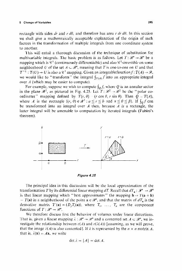
5 Change of Variables 245
rectangle with sides dr and r dO, and therefore has area r dr dO. In this section we shall give a mathemtaically acceptable explanation of the origin of such factors in the transformation of multiple integrals from one coordinate system to another.
This will entail a thorough discussion of the technique of substitution for multivariable integrals. The basic problem is as follows. Let T : Siïn -> St be a mapping which is ^ 1 (continuously difîerentiable) and also <€x-invertible on some neighborhood U of the set A a Stf\ meaning that T is one-to-one on U and that T _ 1 : T(U) -> U is also a^ 1 mapping. Given an integrablefunction/: T(A) -> Sfc, we would like to "transform" the integral \T{A)f into an appropriate integral over A (which may be easier to compute).
For example, suppose we wish to compute j " Q / , where Q is an annular sector in the plane S$2, as pictured in Fig. 4.25. Let T: S?2 -+ Sft2 be the "polar co-ordinates" mapping defined by T(r, 0) = (r cos 0, r sin Θ). Then Q = T(A), where A is the rectangle {(/% 0) e S#2 : a ^ r ^ b and α ^ θ :g /?}. If J Q / can be transformed into an integral over A then, because A is a rectangle, the latter integral will be amenable to computation by iterated integrals (Fubini's theorem).
θ y
M ί& x
Figure 4.25
The principal idea in this discussion will be the local approximation of the transformation Thy its differential linear mapping dT. Recall that dTa : Si" -> St is that linear mapping which "best approximates" the mapping h-> 7(a + h) - 7(a) in a neighborhood of the point a e St, and that the matrix of άΤΛ is the derivative matrix T'(a) = (Z^T^a)), where Ti, . . . , T„ are the component functions of Γ : ^ " -^ £T.
We therefore discuss first the behavior of volumes under linear distortions. That is, given a linear mapping λ : Sîn -> St and a contented set A cz ^", we in-vestigate the relationship between v(A) and ν{λ(Α)) [assuming, as we will prove, that the image λ(Α) is also contented]. If λ is represented by the n x n matrix A, that is, λ(χ) = Ax, we write
deU = \A\ =detA.
>
C
77
7
/(
t 1
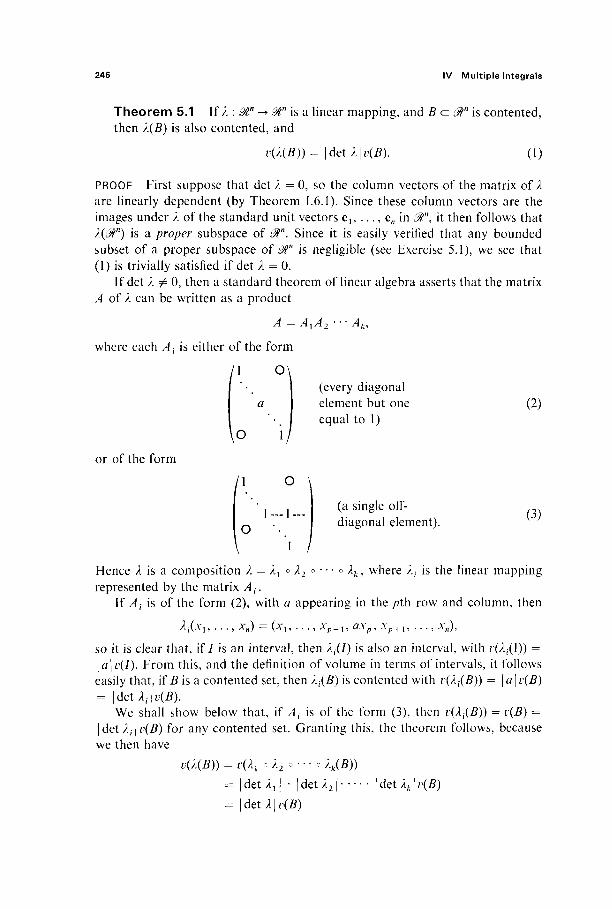
246 IV Multiple Integrals
Theorem 5.1 If A : 0tn -> 0tn is a linear mapping, and B c ^ " is contented, then λ(Β) is also contented, and
ν(λ(Β)) = | det A | <;(£). (1)
PROOF First suppose that det A = 0, so the column vectors of the matrix of A are linearly dependent (by Theorem 1.6.1). Since these column vectors are the images under A of the standard unit vectors e]9 . . . , e„ in M}\ it then follows that λ(βη) is a proper subspace of 0tn. Since it is easily verified that any bounded subset of a proper subspace of 0tn is negligible (see Exercise 5.1), we see that (1) is trivially satisfied if det A = 0.
If det A φ 0, then a standard theorem of linear algebra asserts that the matrix A of A can be written as a product
A = AlA2 ' ' ' Ak,
where each At is either of the form
a
\o i/ or of the form
l\ ° \ 1 — 1— (a single off-
n diagonal element).
\ Ί / Hence λ is a composition A = Ax ° A2 ° · · · ° λλ, where A,· is the linear mapping represented by the matrix A ,·.
If Ai is of the form (2), with a appearing in the /7th row and column, then
Α|(ΛΊ, . . . , Xn) = (ΛΊ, . . . , λ"ρ_ !, ÖA'p , λ"ρ + l 9 . . . , Λ"η),
so it is clear that, if/ is an interval, then A,-(/) is also an interval, with r(At(I)) = \a\v(I). From this, and the definition of volume in terms of intervals, it follows easily that, if B is a contented set, then A,·(/?) is contented with vU^B)) = \a\ v(B) = | det A,· | v(B).
We shall show below that, if At is of the form (3), then r(A,.(£)) = v(B) = | det Α(·|ι>(2?) for any contented set. Granting this, the theorem follows, because we then have
ν(λ(Β)) = ν{λ{ o A2 o - ·. o Xk(B))
= | det Ai | · | det A21 | det Xk \ v{B)
= |det λ\ν(Β)
(every diagonal element but one (2) equal to 1)
(3)

5 Change of Variables 247
as desired, since the determinant of a product of matrices is the product of their determinants.
So it remains only to verify that Àt preserves volumes if the matrix A{ of λ{
is of the form (3). We consider the typical case in which the οίϊ-diagonal element of At is in the first row and second column, that is,
At =
1 1 ON 0 1
1
so
■, * „ ) . (4) Ai(Xi, . . . , Xn) — (*! + X2 > Xi
We show first that Af preserves the volume of an interval
/ = [a, b ] = { x e ^ : xt e [aiybt]9 i = 1, . . . , n).
If we write I = Γ χ I" where Γ <= M1 and Γ c ^"" 2 , then (4) shows that
Xt(I) = /* x J",
where J* is the pictured parallelogram in 011 (Fig. 4.26). Since it is clear that v(I*) = ν(Γ), Exercise 4.1 gives
!<*,(/)) = ν(Ι*)ν(Γ) = ν(Γ)ν(Γ) = υ(Ι).
[a^b2) [b^b2) [ο^ + b2,b2) (a^b2,b2)
Γ
{ov o2) [bv o2) {o] + a2, a2) [by + o2,a2)
Figure 4.26
Now let B be a contented set in 0ln, and, given ε > 0, consider nonoverlapping intervals Iu . . . , Ip and intervals Jl9 . . . , Jq such that
\JIJCBC\JJJ
and ; = i
J 7 = 1
Σ v(Ij) > v(B) -ε, Σ v(Jj) < KB) + e·
248 IV Multiple Integrals
Since we have seen that λ{ preserves the volumes of intervals, we then have
Ù xt(ij) c λ-χΒ) c ΰ λμ}) 7 = 1 7 = 1
and
X üMIj)) > v(B) - e , X K W ) < v(B) + ε. 7 = 1 7 = 1
Finally it follows easily from these inequalities that λ^Β) is contented, with ν(λι(Β)) = v(B) as desired (see Exercise 5.2). |
We are now in a position to establish the invariance of volume under rigid motions.
Corollary 5.2 If A c 0ln is a contented set and p : 0ln -* 0ln is a rigid motion, then ρ(Λ) is contented and y(p(^)) = v(A).
The statement that p is a r/^W motion means that p = τ3 ο μ, where i a is the translation by a, τΛ(χ) = x + a, and μ is an orthogonal transformation, so that |det μ\ = 1 (see Exercise 1.6.10). The fact that p(A) is contented with v(p(A)) = v(A) therefore follows immediately from Theorem 5.1.
Example 1 Consider the ball
Brn ={xe@n:fjxi
2^r2} 1
of radius r in Mn. Note that Br" is the image of the unit «-dimensional ball Βγ
η c 0tn under the linear mapping T(x) = rx. Since | det T'\ = | det T| = rn, Theorem 5.1 gives
v{Brn) = rnv{Bx
n).
Thus the volume of an «-dimensional ball is proportional to the «th power of its radius. Let ocn denote the volume of the unit «-dimensional ball B^, so
v(Brn) = anr".
In Exercises 5.17, 5.18, and 5.19, we shall see that
nm 2m+1nm
ml 1 · 3 · 5 (2m + 1 )
These formulas are established by induction on m, starting with the familiar α2 = π and α3 = 4π/3.
In addition to the effect on volumes of linear distortions, discussed above, a key ingredient in the derivation of the change of variables formula is the fact
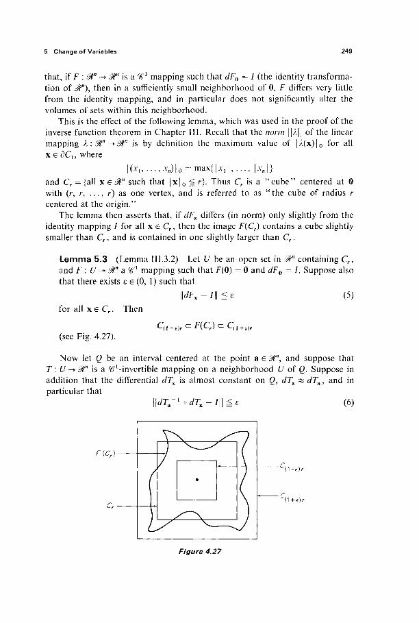
5 Change of Variables 249
that, if F : 0ίη -+ &η is a ^ 1 mapping such that dF0 = I (the identity transforma-tion of Mn), then in a sufficiently small neighborhood of 0, F differs very little from the identity mapping, and in particular does not significantly alter the volumes of sets within this neighborhood.
This is the effect of the following lemma, which was used in the proof of the inverse function theorem in Chapter III. Recall that the norm \\λ\\ of the linear mapping λ : 0tn -> 0tn is by definition the maximum value of |A(x)|0 for all x e 3Cl5 where
| (x i , . . . , * n ) |o = max{|*1| , . . . , |*n|} and Cr = {all x e 0tn such that | x | 0 <Ξ r}. Thus Cr is a "cube ' ' centered at 0 with (r, r, . . . , r) as one vertex, and is referred to as " the cube of radius r centered at the origin."
The lemma then asserts that, if dFx differs (in norm) only slightly from the identity mapping / for all x e Cr, then the image F(Cr) contains a cube slightly smaller than Cr, and is contained in one slightly larger than Cr.
Lemma 5.3 (Lemma 111.3.2) Let U be an open set in 0tn containing Cr, and F : U -> 0ln a ^ 1 mapping such that F(0) = 0 and dF0 = L Suppose also that there exists ε e (0, 1) such that
| | < / F x - / | | ^ e (5) for all x e Cr. Then
(see Fig. 4.27). Ql-e)r Œ F\Çr) Œ ^(1+ε)Γ
Now let Q be an interval centered at the point a e 0în, and suppose that T: U Mn is a ^-invertible mapping on a neighborhood U of Q. Suppose in addition that the differential dTx is almost constant on Q, dTx « dTa, and in particular that
\\dTa-'odTx-I\\^e (6)
F(Cr
( 1 - € ) Λ
( 1 + € ) Λ
Figure 4.27
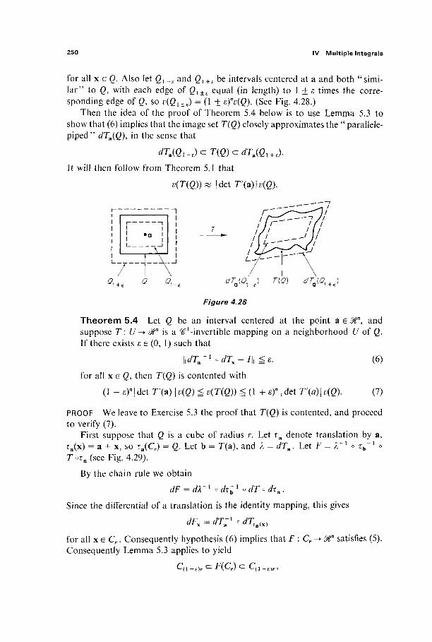
250 IV Multiple Integrals
for all x e Q. Also let Ql_e and Ql+E be intervals centered at a and both "simi-lar" to Q, with each edge of Qi±E equal (in length) to 1 ± ε times the corre-sponding edge of ρ, so v(Ql±E) = (1 ± sfv(Q). (See Fig. 4.28.)
Then the idea of the proof of Theorem 5.4 below is to use Lemma 5.3 to show that (6) implies that the image set T(Q) closely approximates the " parallele-piped" dTa(Q), in the sense that
dTu(Qi-ù<=T(Q)c=dT,(Q1+l·
It will then follow from Theorem 5.1 that
v(T(Q))* | d e t r ( a ) | K ß ) .
Figure 4.28
Theorem 5.4 Let Q be an interval centered at the point a G <%n, and suppose T: £/-» &n is a ^-invertible mapping on a neighborhood U of Q. If there exists ε e (0, 1) such that
WdT^odT^-IW^e. (6)
for all x e Q, then T(Q) is contented with
(1 - ε)"| det T'(a) | v(Q) ^ v(T(Q)) S (1 + s)n | det 7 » | v(Q). (7)
PROOF We leave to Exercise 5.3 the proof that T(Q) is contented, and proceed to verify (7).
First suppose that Q is a cube of radius r. Let t a denote translation by a, τ,(χ) = a + x, so Ta(Cr) = g. Let b = T(a), and λ = άΤΛ. Let ί = Γ 1 ο τ „ " 1 ο Γ oia (see Fig. 4.29).
By the chain rule we obtain
dF = αλ~ι odr~l odT οάχΛ.
Since the differential of a translation is the identity mapping, this gives
dF=dT;1 odTx r a ( x >
for all x e Cr. Consequently hypothesis (6) implies that F : Cr
Consequently Lemma 5.3 applies to yield Ψ satisfies (5).
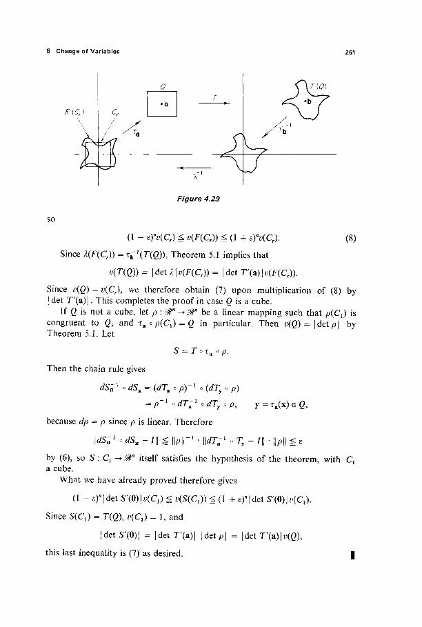
5 Change of Variables 251
τ
s Λ
Ä
j
£[Cr)
\ \ C (. r
K V.
-—
Cr
/ / -^
> J
/
X )
^ α
0
•α
- < —
Figure 4.29
SO
(1 - eyv(Cr) ^ v(F(Cr)) ^ (1 + e)MCr). (8)
Since A(F(Cr)) =τ^ ' (Tiß)) , Theorem 5.1 implies that
KnÖ)) = | d e t ^ | K F ( Q ) - |det r(a)|i>(F(Cr)).
Since i<Q) = t?(Cr), we therefore obtain (7) upon multiplication of (8) by I det T'(a)|. This completes the proof in case Q is a cube.
If Q is not a cube, let p \ 0tn-> 0ln be a linear mapping such that p(Cx) is congruent to g, and i a o p{Cx) = Q in particular. Then v(Q) = | det p | by Theorem 5.1. Let
S = T o Ta o p.
Then the chain rule gives
ί/So1 odSx = (dTMoPyio(dTyop)
= p~x o ^ r ; 1 o </ry o p, y =τ3(χ) G Q,
because dp = p since p is linear. Therefore
llrfSï1 o dSx - I\\ g llpir l · Urfr-1 o Ty - /|| · llpll S s
by (6), so S : C, -► ^ n itself satisfies the hypothesis of the theorem, with Q a cube.
What we have already proved therefore gives
(1 - e)"|det S 'WIKQ) ^ viSiC,)) ^ (1 + e)"|det S'(0)|i>(Q).
Since S(Q) = T(Q), »(Q) = 1, and
|detS'(0)| = I det T'(a) I | det p | = | det T(a) | v(Q),
this last inequality is (7) as desired. |
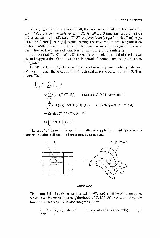
252 IV Multiple Integrals
Since (1 ± ε)π « 1 if ε is very small, the intuitive content of Theorem 5.4 is that, // dTx is approximately equal to dTa for all x e Q (and this should be true if Q is sufficiently small), then v(T(Q)) is approximately equal to \ det T'(a) | v(Q). Thus the factor |det T'(a)| seems to play the role of a "local magnification factor." With this interpretation of Theorem 5.4, we can now give a heuristic derivation of the change of variables formula for multiple integrals.
> 0tn is ^-invertible on a neighborhood of the interval is an integrable function such t ha t / o r i s also
Suppose that T : 0tn -Q, and suppose t h a t / : ύ integrable.
Let @> = {2i, . · ·, Qk} be a partition of Q into very small subintervals, and y = {al5 . . . , a j the selection for @> such that a, is the center-point of Qt (Fig. 4.30). Then
f f = t f /
Σ / σ ω Μ Γ ( 6 ί ) ) (because T(ßf) is very small)
ί X / ( T(ai)) | det T'(af) 11?(6«) (by interpretation of 5.4) i = 1
= R(\detT'\(f°T),P,SO
f | d e t T ' | ( / o T ) .
The proof of the main theorem is a matter of supplying enough epsilonics to convert the above discussion into a precise argument.
0, \
T(0.) T(o.
Xl„„ ii Figure 4.30
Theorem 5.5 Let Q be an interval in ^", and Γ : 0tn ^ 0ln a mapping which is ^-invertible on a neighborhood of Q. Iff: 9t -► ^ is an integrable function such tha t /o r i s also integrable, then
f / = f ( /o T)|det T'\ (change of variables formula). (9) 'T(Q)

5 Change of Variables 253
PROOF Let η > 0 be given to start with. Given a partition & = {Qu . . . , QJ of g, let Sf = {al5 . . . , a j be the selection consisting of the center-points of the intervals of 0*. By Theorem 3.4 there exists δί > 0 such that
R-j(foT)\ d e t r <\ (.o,
if mesh 0> < δί9 where R denotes the Riemann sum
R((fo T)\ det r |, 0», 50 = X/(T(at-))| det Γ^ΟΙΚΟ*). i = 1
Choose Λ > 0 and M > 0 such that
| det T(x) | < Λ and | /(T(x)) | < M
for all x e Q. This is possible because det T'(x) is continuous (hence bounded) on Q, a n d / o T i s integrable (hence bounded) on Q. If
mx = gib of/(T(x)) for x e g , · , M; = lub of /(T(x)) for xeQ, · ,
then
where
X /wAKß,·) ^ Λ X Μ,ΔίΚρ,.) = j8, (11)
| d e t r ( a i ) | .
By Theorem 3.4 there exists δ2 > 0 such that, if mesh & < δ2, then any two Riemann sums for /o Γ ο η ^ differ by less than η/6Α, because each differs from IQÏ°T by less than η/\2Α. It follows that
i i M i - i H . - M G i ) ^ (12)
because there are Riemann sums for / o T arbitrarily close to both £f= x Mt v(Qi) and Y}=imiv{Qi). Hence (11) and (12) give
ß-x = fj(Mi-mi)Aiv(Qi)<l (13)
because each At < A. Summarizing our progress thus far, we have the Riemann sum R which differs from J ß ( / ° T)|det T'\ by less than η/2, and lies between the two numbers a and β, which in turn differ by less than η/6.
Next we want to locate JT(Q)/ between two numbers a' and β' which are close to a and β, respectively. Since the sets T(Qt) are contented (by Exercise 5.3) and intersect only in their boundaries,
J r ( Q ) i = l ^TCQi)

254 IV Multiple Integrals
by Proposition 2.7. Therefore k k
a = Σ mATiQi)) ^ f fu Σ MAT«},)) = ß' (14) i = l JT ( Q ) i = l
by Proposition 2.5. Our next task is to estimate a — a and /?' — ß, and this is where Theorem 5.4 will come into play.
Choose ε e (0, 1) such that
(1+ε)η-^-ε)η<βΜ^Υ (15)
Since T is ^-invertible in a neighborhood of Q, we can choose an upper bound B for the value of the norm ||^TX
_1|| for x e Q. By uniform continuity there exists (53 > 0 such that, if mesh 0 < δ3, then
\\dTx - dTj < i
for all x e Qt. This in turn implies that
WdT;1 c j r x - ;u ^ μ τ ; 1 1 | · \\dTx - dTj £
<B-=e
for all xe Qt. Consequently Theorem 5.4 applies to show that v(T(Qi)) lies between
(1 -8)nAiV(Qi) and ( l+fiVAiKßi) ,
as does Aiv(Qi).
It follows that
IKnßi) ) - Afi;(ßf)| S [(1 + s)n - (1 - ε)-] Δ,ι>(β,) (16)
if the mesh of 0* is less than δ3. We now fix the partition 0 with mesh less than δ = min((5l5 δ2 , δ3). Then
|/r-/?| ^ Σ | Μ ; | Κηρ^-Δ,.ικρ,ΟΙ i = l
^ M t K l + e r - O - e n A j K ß , ) î = 1
^ΛΜί>(0[(1 + ε ) " - ( 1 -ε)"]<1 (17) 6
by (15) and (16). Similarly
| α ' - α | < | . (18)
We are finally ready to move in for the kill. If a* = min(a, a') and /?* = max(/?, β') then, by (11) and (14), both R and i r ( Q ) / l i e between a* and j8*.
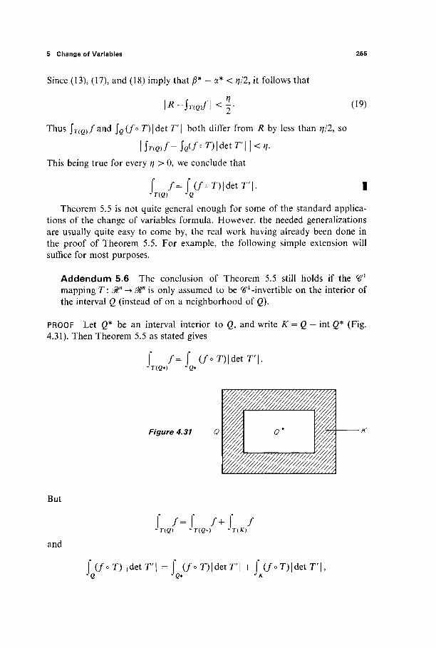
5 Change of Variables 255
Since (13), (17), and (18) imply that β* - α* < η/2, it follows that
\R-lnvf\<\· 09)
Thus jV( Q )/and JQ(/o T)|det T'\ both differ from R by less than η/2, so
I i r ( Q ) / - JQ(/o r ) |de t 7-Ί | < if-This being true for every η > 0, we conclude that
f / = f(/°T)|detr|. I JT(Q) JQ
Theorem 5.5 is not quite general enough for some of the standard applica-tions of the change of variables formula. However, the needed generalizations are usually quite easy to come by, the real work having already been done in the proof of Theorem 5.5. For example, the following simple extension will suffice for most purposes.
Addendum 5.6 The conclusion of Theorem 5.5 still holds if the Ή1
mapping T: 0tn -> @tn is only assumed to be ^-invertible on the interior of the interval Q (instead of on a neighborhood of Q).
PROOF Let 2* be an interval interior to Q, and write K = Q — int ß* (Fig. 4.31). Then Theorem 5.5 as stated gives
f f=( (f°T)\detT'\. JT(Q*)
Figure 4.31
But
and
S /=/ /+/ / JT(Q) JT(Q*) JT(K)
f ( / c T ) | d e t T ' | = f ( / c T ) | d e t r | + f ( /» T)|det T'\,
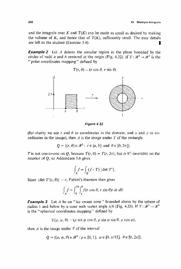
256 IV Multiple Integrals
and the integrals over K and T(K) can be made as small as desired by making the volume of K, and hence that of T(K), sufficiently small. The easy details are left to the student (Exercise 5.4). |
Example 2 Let A denote the annular region in the plane bounded by the circles of radii a and b centered at the origin (Fig. 4.32). If T: &2 -> 0l2 is the "polar coordinates mapping" defined by
T(r, 0) - (r cos 0, r sin 0)
27Γ
Υ/λη//Λ
Figure 4.32
(for clarity we use r and 0 as coordinates in the domain, and x and y as co-ordinates in the image), then A is the image under T of the rectangle
Q = {(r, 0) e m1 : r e [a, b] and 0 e [0, In]}.
7is not one-to-one on Q, because T(r, 0) = T(r, 2π), but is ^'-invertible on the interior of Q, so Addendum 5.6 gives
(7=f(/°T)|detr|.
Since | det T'(r, 0) | = r, Fubini's theorem then gives „2π „b
J f= j I f(r cos 0, r sin 0)r rfr άθ. J0 Ja
Example 3 Let A be an "ice cream cone" bounded above by the sphere of radius 1 and below by a cone with vertex angle π/6 (Fig. 4.33). If T: 01* -► ^ 3
is the "spherical coordinates mapping" defined by
T(p, φ, 0) = (p sin φ cos 0, p sin φ sin 0, p cos φ),
then A is the image under T of the interval
Q = {(p, φ, 0) e 0tz : p e [0, 1 ], φ e [0, π/12], 0 G [0, 2π]}.
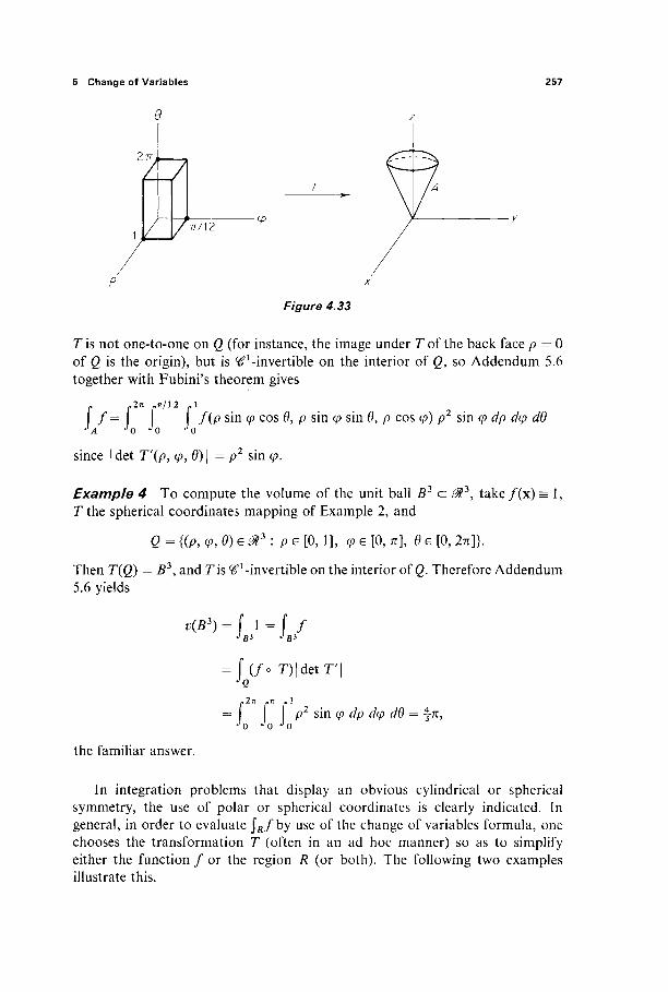
5 Change of Variables 257
% 71
y 77712 -φ
Figure 4.33
T is not one-to-one on Q (for instance, the image under T of the back face p = 0 of Q is the origin), but is ^-invertible on the interior of Q, so Addendum 5.6 together with Fubini's theorem gives
ç. Ç.2-H - π / 1 2 . 1
/ = f(p sin φ cos 0, p sin <p sin θ, ρ cos φ) ρ2 sin φ ί/ρ Λ/> έ/0
since |det T'(p, φ,θ)\ = p2 sin φ.
Example 4 To compute the volume of the unit ball B3 c ^ 3 , take/(x) = 1, T the spherical coordinates mapping of Example 2, and
Q = {(p, φ, Θ) e 0l3 : p e [0, 1], φ e [0, π], 0 e [0, 2π]}.
Then T(g) = B3, and Tis ^-invertible on the interior of Q. Therefore Addendum 5.6 yields
v(B3) = f 1 = f / JB3 JB3
= \{fo T) |detr |
= \ p2 ύη φ dp άφ άθ = \π, ο •'ο ^ο
the familiar answer.
In integration problems that display an obvious cylindrical or spherical symmetry, the use of polar or spherical coordinates is clearly indicated. In general, in order to evaluate j ^ / b y use of the change of variables formula, one chooses the transformation T (often in an ad hoc manner) so as to simplify either the function / or the region R (or both). The following two examples illustrate this.
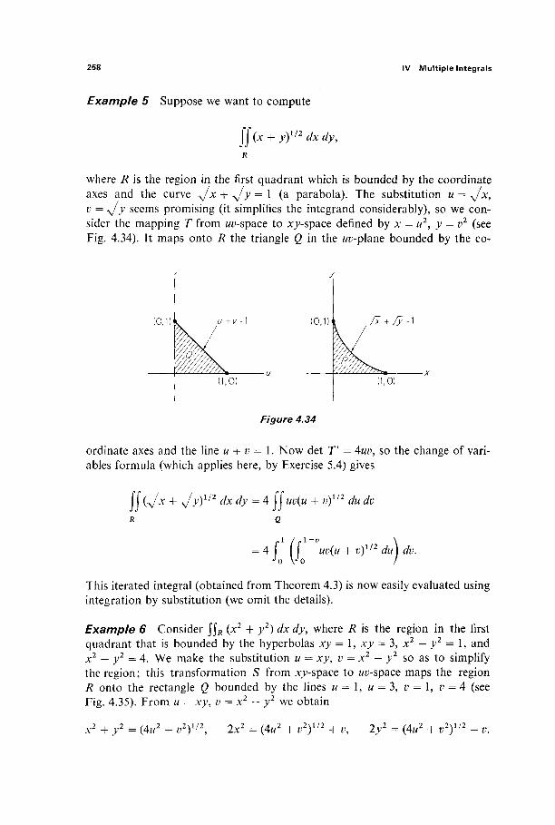
258 IV Multiple Integrals
Example 5 Suppose we want to compute
jj(x + y)l/2dxdy,
where R is the region in the first quadrant which is bounded by the coordinate axes and the curve -Jx + yfy = 1 (a parabola). The substitution u = y/x, v = y/y seems promising (it simplifies the integrand considerably), so we con-sider the mapping T from w^-space to xy-space defined by x = u2, y = v2 (see Fig. 4.34). It maps onto R the triangle Q in the wz;-plane bounded by the co-
Figure 4.34
ordinate axes and the line u 4- v = 1. Now det T" = 4uv, so the change of vari-ables formula (which applies here, by Exercise 5.4) gives
JJ ( Λ Λ + \Λθ 1 / 2 dxdy = A jjuv(u + v)1'2 du dv
4 ί ( ί υ"Ό(μ + 1/2 du) dv' This iterated integral (obtained from Theorem 4.3) is now easily evaluated using integration by substitution (we omit the details).
Example 6 Consider \\R (x2 + y2) dx dy, where R is the region in the first quadrant that is bounded by the hyperbolas xy = 1, xy = 3, x2 - y2 = 1, and x2 — y2 = 4. We make the substitution u = xy, v = x2 — y2 so as to simplify the region; this transformation S from .xy-space to w^-space maps the region R onto the rectangle Q bounded by the lines w = 1, w = 3, v = \9 v = 4 (see Fig. 4.35). From u = xy, v = x2 — y2 we obtain
jt* + y2 = (4w2 + ^ y / 2 ^ 2x2 = (Au2 + v2)112 + i\ 2 j 2 = (4w2 + v2)1/2 - v.

5 Change of Variables 259
4«
1 '
/
ü ; 3
Figure 4.35
The last two equations imply that S is one-to-one on R; we are actually interested in its inverse T = S'1. Since S o T = /, the chain rule gives S'(T(u, v)) o T'(u, v) = I, so
1 1 1 det V det S'\ 2(x2 + y2) 2(4u2 + v2Y/2'
Consequently the change of variables formula gives
1 JY(x2 + y2) dx dy = \[{Au2 + v2)l/2
2(4u2 + v2) 2x1/2 du dv
= i v(Q) = 3.
Multiple integrals are often used to compute mass. A body with mass con-sists of a contented set A and an integrable density function μ : A -► ^ ; its mû^ Λ/(Λ) is then defined by
M(A) = f μ.
Example 7 Let Λ be the ellipsoidal ball χ2/α2 + j>2/62 + z2/c2 ^ 1, with its density function μ being constant on concentric ellipsoids. That is, there exists a function g : [0, 1 ] -► & such that μ(χ) = g{p) at each point x of the ellipsoid
? + F + ? = ' ·
In order to compute M (A), we intoduce ellipsoidal coordinates by
X = ap sin φ cos 0, y = bp sin φ sin 0, z = cp cos φ.
The transformation Γ defined by these equations maps onto A the interval
Q = {(p, φ, 0) : p e [0, 1 ], φ e [0, π], 0 e [0, 2π]},
260 IV Multiple Integrals
and is invertible on the interior of Q. Since det T' = abcp2 sin φ, Addendum 5.6 gives
M(A) = abc g(p)p2 sin φ dO άφ dp J 0 JQ *>0
.1 = 4π abc ί P2#(P) Φ·
For instance, taking #(p) = 1 (uniform unit density), we see that the volume of the ellipsoid x2/a2 + y2/b2 + z2/c2 ^ 1 is \nabc (as seen previously in Exercise 4.6).
A related application of multiple integrals is to the computation of force. A force field is a vector-valued function, whereas we have thus far integrated only scalar-valued functions. The function G : 0tn -► 0Γ is said to be integrable on A <= 0tn if and only if each of its component functions gu . . . , gm is, in which case we define
i.c-(J> ί9-Ή"-Thus vector-valued functions are simply integrated componentwise.
As an example, consider a body A with density function μ : A -► M, and let ξ be a point not in A. Motivated by Newton's law of gravitation, we define the gravitational force exerted by A, on a particle of mass m situated at ξ, to be the vector
-ί γηιμ(χ)(χ-ξ) ax, <Λ | χ - ξ |
where y is the "gravitational constant."
For example, suppose that A is a uniform rod (μ = constant) coincident with the unit interval [0, 1] on the Jt-axis, and ξ ^ (0, 1). (See Fig. 4.36.) Then the gravitational force exerted by the rod A on a unit mass at ξ is
/ Λ1 γμ sin α Λ1 γμ cos a \
For a more interesting example, see Exercises 5.13 and 5.14.
We close this section with a discussion of some of the classical notation and terminology associated with the change of variables formula. Given a difTeren-tiable mapping T : Mn -► 0ln, recall that the determinant det T'(a) of the dériva-
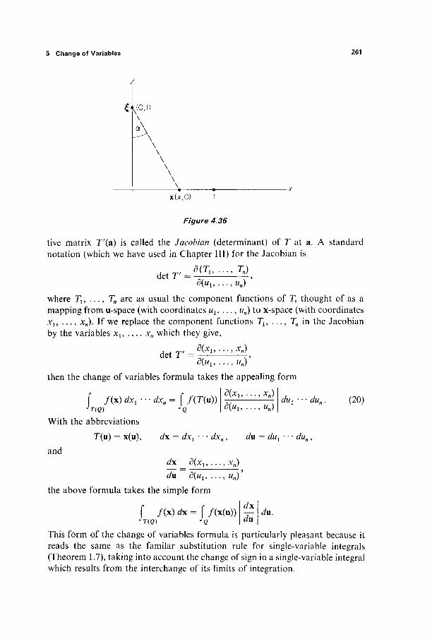
5 Change of Variables 261
► (0,1)
xU.O)
Figure 4.36
tive matrix T'(a) is called the Jacobian (determinant) of T at a. A standard notation (which we have used in Chapter III) for the Jacobian is
d(Tl9 . . . , Tn) d e t T = ~^ Γ '
where T1? . . . , T„ are as usual the component functions of T, thought of as a mapping from u-space (with coordinates ux, . . . , un) to x-space (with coordinates xi9 . . . , JC„). If we replace the component functions Tl5 . . . , TM in the Jacobian by the variables xl9 ..., xn which they give,
d e t Γ = H7 Λ ' 3(1 / ! , . . . , Wn)
then the change of variables formula takes the appealing form
d(xl9 ...,xn)
Q
f f(x)dxr~dxn= f/(T(u)) JT(Q)
With the abbreviations Φ ι , . . . , w„j
dux · · · i/w„ (20)
T(u) = x(u), and
dx = dxi - - - dxn,
dx = d(xl9 ...,xn)
du d(ul9...9uny
the above formula takes the simple form
du = du1 dun
dx
du~ du. f / ( x ) Ä = f/(x(u))
J7(Q) JQ |
This form of the change of variables formula is particularly pleasant because it reads the same as the familar substitution rule for single-variable integrals (Theorem 1.7), taking into account the change of sign in a single-variable integral which results from the interchange of its limits of integration.
262 IV Multiple Integrals
This observation leads to an interpretation of the change of variables for-mula as the result of a "mechanical" substitution procedure. Suppose T is a differentiable mapping from w^-space to Ay-space. In the integral j r ( Q ) f(x, y) dx dy we want to make the substitutions
ox dx dy dy dx = — du + — dv, dy = — du + — dv (21)
du dv du dv
suggested by the chain rule. In formally multiplying together these two "differ-ential forms," we agree to the conventions
du du = dv dv = 0 and dv du — — du di\ (22)
for no other reason than that they are necessary if we are to get the "right" answer. We then obtain
. , (dx , dx \ /dy , dy A dx dy = \—- du + —- dv\\— du + — dv)
\du dv ) \du dv /
dxdy j . , dxdy = — — du du + — — du dv
du du du dv
+ — — dvdu + — — dvdv dv du dv dv
/dx dy dx dy\
\du dv dv du/
dx dy = -—^—- du dv. d(u, v)
Note that, to within sign, this result agrees with formula (20), according to which dx dy should be replaced by | d(x, y)/d(u, v) \ du dv when the integral is trans-formed.
Thus the change of variables (x, y) = T(u, v) in a 2-dimensional integral JT(Q)/(x, y) dx dy may be carried out in the following way. First replace x and y in f(x, y) by their expressions in terms of u and v, then multiply out dx dy as above using (21) and (22), and finally replace the coefficient of du dv, which is obtained, by its absolute value,
For example, in a change from rectangular to polar coordinates, we have x = r cos Θ and y = r sin θ, so
dx dy = (cos Θ dr — r sin Θ d9)(s'm Θ dr + r cos Θ d9)
= cos Θ sin Θ dr dr + r cos2 Θ dr d9
-r sin2 Θ dOdr- r2 sin Θ cos Θ dQ άθ
= r (cos2 Θ + sin2 0) dr d0,
dx dy = r dr d0,
where the sign is correct because r ^ 0.

5 Change of Variables 263
The relation dv du = -dudv requires a further comment. Once having agreed upon u as the first coordinate and v as the second one, we agree that
I g(u, v) dudv = f g,
while
I g(u, v)dvdu= - \ g.
So, in writing multidimensional integrals with differential notation, the order of the differentials in the integrand makes a difference (of sign). This should be contrasted with the situation in regards to iterated integrals, such as
j ( j 9(u> v) dv\ du or j ( j 0(w, v) du) dv>
in which the order of the differentials indicates the order of integration. Jf parentheses are consistently used to indicate iterated integrals, no confusion be-tween these two different situations should arise.
The substitution process for higher-dimensional integrals is similar. For example, the student will find it instructive to verify that, with the substitution
dx dx dx dx = —- du + — dv H dw,
du dv dw
, fy , , 8y dy ay = — du + —- dv + — dw,
du dv dw
dz dz dz dz = — du + — dv + — dw,
du dv dw
formal multiplication, using the relations
du du = dv dv = dw dw = 0, dv du = — du dv, dw dv = — dv dw,
dw dx = — dx dw,
yields
dx dy dz = J ' y* Z\ du dv dw (23) d(u, v, w)
(Exercise 5.20). These matters will be discussed more fully in Chapter V.
Exercises
5.1 Let A be a bounded subset of ^ \ with k < n. If / : Mk -► Mn is a ^ 1 mapping, show that f(A) is negligible. Hint: Let Q be a cube in 3tk containing A, and & = {ß l t . . . , QNk) a partition of Q into Nk cubes with edgelength r/N, where r is the length of the edges of Q. Since fis &1 on Q, there exists c such that |/(x) —/(y)| ^ c\x — y| for all x, y e Q. It follows that v(f(Qt)) ^ (cr/N)n.
264 IV Multiple Integrals
5.2 Show that A is contented if and only if, given ε > 0, there exist contented sets Ai and A2
such that Ai <= A c A2 and v(A2 — Α{)<ε. 5.3 (a) If/1 c <#« is negligible and Γ : ^ " ^ &n is a tf1 mapping, show that T(A) is negligible.
Hint: Apply the fact that, given an interval Q containing A, there exists c > 0 such that |Γ(χ)-7Xy)| < f | x - y | for all x, y e Q. (b) If A is a contented set in ^" and T: Mn -> ^" is a ft ' mapping which is ft'-invertible on the interior of A, show that T(A) is contented. Hint: Show that d{T(A)) <= T(dA), and then apply (a).
5.4 Establish the conclusion of Theorem 5.5 under the hypothesis that Q is a contented set such that Tis ft '-invertible on the interior of Q. Hint: Let Qu ..., Q* be nonoverlapping
k
intervals interior to β, and K= Q— (J (?,. Then / = 1
Σί /= i f (/°r)|detr|
by Theorem 5.5. Use the hint for Exercise 5.3(a) to show that v(T(K)) can be made ar-bitrarily small by making v(K) sufficiently small.
5.5 Consider the «-dimensional solid ellipsoid
E=[xe&:t —2^l)'
Note that E is the image of the unit ball B" under the mapping T: &"->&" defined by T(xu ..., Λ'„) = (ciiXu . . . , anxn).
Apply Theorem 5.1 to show that v(E) = aia2···anv(Bn). For example, the volume of the 3-dimensional ellipsoid x2/a2 4- y2/b2 + z2/c2 ^ 1 is \nabc.
5.6 Let R be the solid torus in ^ obtained by revolving the circle (y — a)2 + z2 ^ b2, in the ;;z-plane, about the z-axis. Note that the mapping T: <%3 -> &3 defined by
x = (a + w cos r)cos u,
j> = (a 4- H> cos lOsin w, z = H> sin v,
maps the interval Q = {(«, r, w) : u, ve [0, 2π] and w e [0, b]} onto this torus. Apply the change of variables formula to calculate its volume.
5.7 Use the substitution u = x — y, v = x + y to evaluate /./» (x-y)/(x + y)
e dx dy, R
where R is the first quadrant region bounded by the coordinate axes and the line x 4- y = 1. 5.8 Calculate the volume of the region in # which is above the .vy-plane, under the parabo-
loid z = x2 4- y2, and inside the elliptic cylinder x2/9 -\- y2/4 = 1. Use elliptical coordinates x = 3r cos 6,y = 2r sin Θ.
5.9 Consider the solid elliptical rod bounded by the *j-plane, the plane z = ax + ßy + h through the point (0,0, h) on the positive z-axis, and the elliptical cylinder x2ja2 + y2\b2 = 1. Show that its volume is irabh (independent of a and j8). Hint: Use elliptical coor-dinates x = ar cos Θ, y = br sin Θ.
5.10 Use "double polar" coordinates defined by the equations Xi = r cos Θ, x2 = r sin Θ,
X3 = p cos φ, Χ4. = p sin 9?,
to show that the volume of the unit ball B4 c ^ 4 is \ττ2.

5 Change of Variables 265
5.11 Use the transformation defined by 2x 2y
to evaluate x2 + y2 ' x2 + y2
dx dy
Si (x2+y2)2'
where R is the region in the first quadrant of the JO'-plane which is bounded by the circles x2 + y2 = 6x, x2 ■■ Ax, x2 + y2 = 8>>, x2 + y2 = 2y.
5.12 Use the transformation T from r#/-space to Jtyz-space, defined by
x = - cos t >> = - sin tf, z = r%
to find the volume of the region R which lies between the paraboloids z = x2 + y2 and z = 4(x2 + y2), and also between the planes z = 1 and z = 4.
5.13 Consider a spherical ball of radius a centered at the origin, with a spherically symmetric density function d(x) = g(p). (a) Use spherical coordinates to show that its mass is
M = 4π p2g(p)dp. Jo
(b) Show that the gravitational force exerted by this ball on a point mass m located at the point ξ = (0, 0, c), with c> a/is the same as if its mass were all concentrated at the origin, that is,
yMm
Hint: Because of symmetry considerations, you may assume that the force is directed toward 0, so only its z-component need be explicitly computed. In spherical coordinates (see Fig. 4.37),
"° *n "2n ymg{p) cos a Fz = iff
J n ^ n J n
- p2 sin φ du d<p dp (why ?).
Figure 4.37
Typical point inside ball
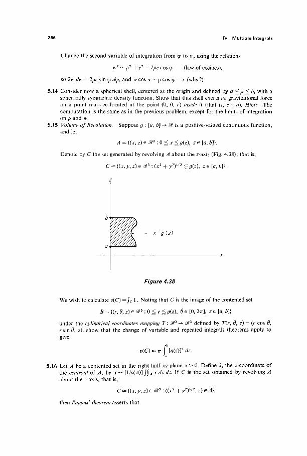
266 IV Multiple Integrals
Change the second variable of integration from φ to w, using the relations
w2 = p2 + c2 — 2pc cos φ (law of cosines),
so 2w dw = 2pc sin φ άφ, and w cos a + p cos φ = c (why?).
5.14 Consider now a spherical shell, centered at the origin and defined by a ^ p <i b, with a spherically symmetric density function. Show that this shell exerts no gravitational force on a point mass m located at the point (0, 0, c) inside it (that is, c < a). Hint: The computation is the same as in the previous problem, except for the limits of integration on p and w.
5.15 Volume of Revolution. Suppose g : [a, b]^ & is a positive-valued continuous function, and let
A = {(*, z) G m2 : 0 g * ^# (z ) , z e [a, &]}.
Denote by C the set generated by revolving A about the z-axis (Fig. 4.38); that is,
C = {(*, 7, z) G ^ 3 : (je2 + y2)112 ^ 0(2), z e [a, b]}.
Figure 4.38
We wish to calculate v(C) = j " c 1. Noting that C is the image of the contented set
B = {(r,0, z) e ^ 3 : 0 ^ r ^g{z\ 0 e [0, 2ττ], z e [a, £]}
under the cylindrical coordinates mapping T : ^ 3 -> ^ 3 defined by 7(r, 0, z) = (r cos 0, r sin 0, z), show that the change of variable and repeated integrals theorems apply to give
v(C)- ■ \\g{z)? Ja
dz.
5.16 Let A be a contented set in the right half xz-plane * > 0. Define x, the x-coordinate of the centroid of A, by x = [ l / φ θ ] J7 * dx dz. If C is the set obtained by revolving A about the z-axis, that is,
C = {(*, y, z) e ^ 3 : ((A:2 + >>2)1/2, z) e Λ},
then Pappus'' theorem asserts that
5 Change of Variables 267
aB = f l = f v(Bï-±t2n/2)dt J Bn J - 1
= 2α„_! f (1 - / 2 ) ("-1 ) / 2 ί / / = 2απ_1 | " sin" θ αθ,
a„ = 2a„_1/„.
Conclude that ocn = 4a„ _ 2 /„/,,-1. (b) Deduce from Exercise 1.8 that /„/„_i = π/2η if « ^ 1. Hence
277
a„ = — a„_2 if n ^ 2 . (# )
(c) Use the recursion formula (# ) to establish, by separate inductions on m, formulas (*), starting with α2 = π and α3 = 4π/3.
5.18 In this problem we obtain the same recursion formula without using the formulas for I2n and Ι2η + ι· Let
B2 = {{xl9x2)e&2:xi2+X22ûl}
and ß = {(jc3, . . . , Λ-Je^"-2 :each |Λ-,| <; 1}. Then Bn ^ B2 x Q. Let(p:B2xQ^& be the characteristic function of Bn. Then
a" = \ ( ^*1' ' ' ' ' *"* dXz '"dXn) dxi dXl ·
Note that, if (ΛΊ, X2) e Z?2 is a fixed point, then 99, as a function of (x3, . . . , .*„), is the characteristic function of B^~2
xl2_X22)i/2. Hence
f φ(ΛΊ, . . . , x„) dx3 . . . dxn = (1 - .V!2 - .v22)("-2)/2an_2 .
Now introduce polar coordinates in ^liX2 to show that
JB2(1 - *ι2 - χι)(η-2)12 dXl dx2 = — n
so that ocn = (2π/η)οίη_2 as before.
v(C) = 2πχν(Α\
that is, that the volume of C is the volume of A multiplied by the distance traveled by the centroid of A. Note that C is the image under the cylindrical coordinates map of the set
B = {(r, Θ, z)e^3: (r, z) e A and 0 e [0, 2ττ]}.
Apply the change of variables and iterated integrals theorems to deduce Pappus' theorem.
The purpose of each of the next three problems is to verify the formulas
(*)
given in this section, for the volume ocn of the unit «-ball Bi" c 'Mn.
5.17 (a) Apply Cavalieri's principle and appropriate substitutions to obtain
268 IV Multiple Integrals
5.19 The /z-dimensional spherical coordinates mapping T : J?n-> J#n is defined by
ΛΊ = p COS (pi,
Λ'2 = p sin (pi cos φ2,
x3 = p sin φι sin φ2 cos <p3,
.vn_i = p sin ψι ·'· sin φ„_2 cos Θ,
xn = p sin <pi · ■ · sin <p„_2 sin #,
and maps the interval
Q = {(p, ψι , <ptl-2, 0)e ^n:pe [0, 1], φ{ e [0, ττ], Θ e [0, 2π]}
onto the unit ball B". (a) Prove by induction on n that
\<\<z\T'\=pn 1 sin" 2 ψχ sin" 3 φ 2 ··· sin2 99^-3 sin ψη-2 ■
(b) Then
ocn= f 1 = ί | d e t r |
sinfc 99 ί/φ 27Γ " _ 2
- Π n k= 1
2π 0Cn= h'h' ··· In-2,
n
where / / = Jg sin*0 φ ί/99. Now use the fact that
K-Jk'--2π
and Iim-i·-2 - 4 - . . . ( 2 m - 2 ) 3 - 5 · ( 2 m - 1 )
(by Exercise 1.8) to establish formulas (*). 5.20 Verify formulas (23) of this section.
6 IMPROPER INTEGRALS AND ABSOLUTELY INTEGRABLE FUNCTIONS
Thus far in this chapter on integration, we have confined our attention to bounded functions that have bounded support. This was required by our definition of the integral of a nonnegative function as the volume of its ordinate set (if contented)—if/: 0tn -> 0t is to be integrable, then its ordinate set must be contented. But every contented set is a priori bounded, so /mus t be bounded and have bounded support.
However there are certain types of unbounded subsets of 0Γ with which it is natural and useful to associate a notion of volume, and analogously functions which are either unbounded or have unbounded support, but for which it is nevertheless natural and useful to define an integral. The following two examples illustrate this.

6 Improper Integrals 269
Example 1 L e t / : [1, oo)->^ be defined by f(x) = \/x2. Let A denote the ordinate set o f / and An the part of A lying above the closed interval [1, n] (Fig. 4.39). Then
rndx Ji x
ndx _ \_
n
Since A = \J?=i An and lim,,..^ v(An) = 1, it would seem natural to say that
despite the fact that/does not have bounded support. (Of course what we really mean is that our definitions of volume and/or the integral ought to be extended so as to make this true.)
Figure 4.39
Example 2 Let /be the unbounded function defined on (0, 1 ] by/(jc) = \j-Jx. Let A denote the ordinate set of/ and An the part of A lying above the closed interval [\/n, 1] (Fig. 4.40). Then
/ x Ç1 dx 2
l / n x n
Since A = (J*= ^ An and lim,,.^ v(An) = 2, it would seem natural to say that
dx r "X ν(Α) = ίΤΤ2=2
Jo x These two examples indicate both the need for some extension (to unbounded
situations) of our previous definitions, and a possible method of making this extension. Given a function/: V -^ 01, with ei ther/or U (or both) unbounded,

270 IV Multiple Integrals
x M//7 1
Figure 4.40
we might choose a sequence {An}™= x of subsets of U which "fill u p " U in some appropriate sense, on each of which fis integrable, and then define
|7=lim f / JU Π-+Ο0 JAn
provided that this limit exists. Of course we would have to verify that j ^ / is thereby well-defined, that is, that its value is independent of the particular chosen sequence {A„}f. Partly because of this problem of well-definition, we shall for-mulate our initial definition of Jy / in a slightly different manner, and then return later to the interpretation of j ^ / a s a sequential limit (as above).
We deal first with the necessity f o r / : U-+0t to be integrable on enough subsets of U to "fill u p " U. We say tha t / i s locally integrable on U if and only i f / i s integrable on every compact (closed and bounded) contented subset of U. For instance the function/(x) = \/x2 of Example 1 is not integrable on (1, oo), but is locally integrable there. Similarly the function/(x) = l/x1/2 of Example 2 is not integrable on (0, 1), but is locally integrable there.
It will be convenient to confine our attention to open domains of definition. So l e t / : U-► M be a locally integrable function on the open set U cz &n. We then say t h a t / i s absolutely integrable on U if and only if, given ε > 0, there exists a compact contented subset Βε of U such that
I J M / 1 < ε
for every compact contented set A cz U which contains BE. The student should verify that the sum of two absolutely integrable functions
on U is absolutely integrable, as is a constant multiple of one, so the set of all absolutely integrable functions on U is a vector space. This elementary fact will be used in the proof of the following proposition, which provides the reason for our terminology.
6 Improper Integrals 271
Proposition 6.1 If the function / : U-*dl is absolutely integrable, then so is its absolute value | / | .
We will later prove the converse, so / i s absolutely integrable if and only if l/l is-
PROOF Writing/ = / + - / " , it suffices by the above remark to show that/"1" a n d / - are both absolutely integrable, since | / | = / + + / ~ . We consider/"1". Given ε > 0, choose BE as in the definition, such that A ID BE implies
< ε
if A is a compact contented subset of U. It will suffice to show that A => BE also implies that
|7+-f p < ε.
Given a compact contented set A with BEa A a U, define
A+ =BEu{xeA:f(x)^0},
so that/(x) = / + ( x ) for xeA+ - BE, and
ί f + = i f+ JA-BC
JA+-BR
because/ + (x) = 0 if x e A — A +. Then
f f+ - i f+\ = \ i f+
J A J n I \ JA-BE
S r* JA+-BE
s A J f~\f J A+ JR_
< ε
as desired, because A+ is a compact contented set such that BEa A+ a U. |
The number /, which the following theorem associates with the absolutely integrable function/on the open set U cz ^", will be called the improper (Rie-mann) integral o f / o n U. It will be temporarily denoted by Ivf (until we have verified that Ivf= J^ / in case/ is integrable on V).
The following definition will simplify the interpretation o f / ^ / a s a sequential limit of integrals o f / o n compact contented subsets of U. The sequence {A^}™

272 IV Multiple Integrals
of compact contented subsets of U is called an approximating sequence for V if (a) Ak + i z> Ak for each k^l, and (b) V = \J?=1 intAk.
Theorem 6.2 Suppose/is absolutely integrable on the open set U c 0t. Then there exists a number / = i^/with the property that, given ε > 0, there exists a compact contented set Cz such that
J A < ε
for every compact contented subset A of U containing Ct. Furthermore
/„ /= lim f / fc-*oo J,4 k
for every approximating sequence {Ak}f for U.
PROOF To start with, we choose a (fixed) approximating sequence {Ck}f for U (whose existence is provided by Exercise 6.16). Given η > 0, the Heine-Borel theorem (see the Appendix) implies that Ck => Βη/2 if k is sufficiently large. Here Βη/2 is the compact contented subset of U (provided by the definition) such that B, η/2 A cz U implies that
< 1
<η.
JA JBn/2
Consequently, if k and / are sufficiently large, it follows that
f /- f /Ul i / - f /Ulf / - f / Jck
Jct I I Jck JBn/2 I | JCi JBtl/2
Thus {Jck/}i° is a Cauchy sequence of numbers, and therefore has a limit / (see the Appendix).
Now let Cz = Βε/3. Given a compact contented subset A of U which contains Ce, choose a fixed k sufficiently large that Ck => CE and | / — JC k/ | < ε/3. Then
/ - / /NI / -L / l + l / , / - / , / l + lL / - / / Jck
ε ε ε
3 3 3 as desired. This completes the proof of the first assertion.
Now let {Ak}f be an arbitrary approximating sequence for U. Given δ > 0, choose AT sufficiently large that Ck=> CE, for all k ^ AT. Then what we have just proved gives | / — \Akf\ < ε ^or all k ^ K, so it follows that
/ = limf / k~* oo Ak
I
6 Improper Integrals 273
We can now show that / ^ / a n d JL,/are equal when both are defined. Note that, if/ is integrable on the open set Ua ^'\ then it follows from Exercise 3.1 that / i s locally integrable on V (why?).
Theorem 6.3 If U c $tn is open and / : U -* $ is integrable, then / is absolutely integrable, and
vf= f / J I!
I
PROOF Let M be an upper bound for the values of | / (x) | on U. Given ε > 0, let Βε be a compact contented subset of U such that v(U — Βε) < ε/Μ. If A is a compact contented subset of U which contains Βε, then
\f-\f\=\\ A=S ΐΊ JA JΒε | \ JA-BC I JA-Bc
g f f^Mv(U-Ac)<e, J I! - R JU-BC
so it follows tha t / i s absolutely integrable on U. If in addition A contains the set C£ of Theorem 6.2, then
\lvf- \ f\u\lvf- \f\ + \\f-\f
<e + j l/l JU-A
S s + f l/l < 2ε.
This being true for all ε > 0, it follows that Ivf= \vf. I
In order to proceed to compute improper integrals by taking limits over ap-proximating sequences as in Theorem 6.2, we need an effective test for absolute integrability. For nonnegative functions, this is easy to provide. We say that the improper integral j ^ / i s bounded (whether or not it exists, that is, whether or not / i s absolutely integrable on U) if and only if there exists M > 0 such that
J A < M (1)
for every compact contented subset A of U.
Theorem 6.4 Suppose that the nonnegative function / is locally in-tegrable on the open set U. Then / i s absolutely integrable on U if and only if Jry/is bounded, in which case JV/is the least upper bound of the values \Af, for all compact contented sets A c JJ.
274 IV Multiple Integrals
PROOF Suppose first that (1) holds, and denote by / the least upper bound of {JA/} f° r a ^ compact contented A c U. Given ε > 0, / — ε is not an upper bound for the numbers {jAf}9 so there exists a compact contented set BEa U such that
I* f>I-e.
If A is any compact contented set such that BE a A c U then, since / ^ 0, we have
so it follows that both
f / - f f\ < 6 and I / - f / < fi.
The first inequality implies that / is absolutely integrable, and then the second implies that J l / / = / as desired (using Theorem 6.2).
Conversely, if / is absolutely integrable on I/, then it is easily seen that \Af^ J i / / f ° r every compact contented subset U of A, so we can take M = \vf in (1). |
Corollary 6.5 Suppose the nonnegative function/is locally integrable on the open set U, and let {Ak}f be an approximating sequence for U. Then / is absolutely integrable with
f / = Hm f /, (2) JU fc->oo JAk
provided that this limit exists (and is finite).
PROOF The fact that the monotone increasing sequence of numbers {j^/}'? is bounded (because it has a finite limit) implies easily that j ^ / i s bounded, so / i s absolutely integrable by Theorem 6.4. Hence (2) follows from Theorem 6.2. |
As an application, we will now generalize Examples 1 and 2 to 0tn. Let A denote the solid annular region Bb
n — int Ban cz 0ln (see Fig. 4.41), and l e t / b e
a spherically symmetric continuous function on A. That is,
/ o T(p, φΐ9 ..., φη-2, Θ) = g(p)
for some function g, where T : &n -> 9tn is the «-dimensional spherical coordi-nates mapping of Exercise 5.19. By part (a) of that exercise, and the change of variables theorem, we have
f / = f f · " ί ί 9(Ρ)Ρη~1 s in"~2 <Pi , , , s i n Ψη-ι dO άφχ '-άφη_2άρ
= ση\ g(p)pn~1dP, (3)
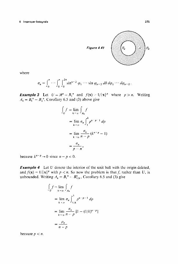
6 Improper Integrals 275
Figure 4.41
where
►<0 J0 J0 ση = \ · · · sin"-2 ψι "' sin φη_2 αθ αφί · · · αφη_2 ·
Example 3 Let U = Μη - Bf and / (χ ) = 1/|χ|ρ where p>n. Writing Ak = Bk — Β^, Corollary 6.5 and (3) above give
f / = Hm f / JU k-+cc JAk
= Ηηισ„ pn~p~l dp fc->oo * ί
= lim —^-(kn~p- 1) fc^oo n — p
p — n
because kn~p -> 0 since n — p < 0.
Example 4 Let JJ denote the interior of the unit ball with the origin deleted, and/(x) = l / | x | p with p < n. So now the problem is that/ , rather than U, is unbounded. Writing Ak = B^ - B"/k, Corollary 6.5 and (3) give
17= Hm f / J U k-+oo JAk
= lim ση f pn~p-x dp
= lim - ^ - [ 1 ~(\/k)n-p] jt^oo n — p
= Pn
n — p
because p <n.
276 IV Multiple Integrals
For nonnegaîive locally integrable functions, Corollary 6.5 plays in practice the role of a " working definition." One need not worry in advance about whether the improper integral j^/actually exists (that is, whether/is absolutely integrable on U). Simply choose a convenient approximating sequence {Ak}™ for U9 and compute lirm.^ \AJ\ If this limit is finite, then \vf does exist, and its value is the obtained limit.
In the case of an arbitrary (not necessarily nonnegative) function, one must know in advance that fis absolutely integrable on U. Once this has been estab-lished, Theorem 6.2 enables us to proceed as above—choose an approximating sequence {Ak}f for U, and then compute l im^^ $Akf.
The simplest way to show that a given locally integrable function/: U -> @t is absolutely integrable is to compare it with a function g : U -» @t which is already known to be absolutely integrable, using the comparison test stated below. First we need the converse of Proposition 6.1.
Corollary 6.6 L e t / : U ^> & be locally integrable. If | / | is absolutely integrable on U, then so i s /
PROOF Write/ = / + - / " " , so | / | = / + + / ~ . Since | / | is absolutely integrable, Jc/I/I is bounded (by Theorem 6.4). It follows immediately that \vf
+ and \vf~ are bounded. Hence Theorem 6.4 implies t h a t / + a n d / - are both absolutely integrable on U, s o / = / + — / " is also. |
The import of Corollary 6.6 is that, in practice, we need only to test non-negative functions for absolute integrability.
Corollary 6.7 (ComparisonTest) Suppose tha t / and^ are locally integ-rable on U with 0 ^ / ^ g. If g is absolutely integrable on (7, then so i s /
PROOF Since g is absolutely integrable, \vg is bounded (by Theorem 6.4). But then the fact that 0 ^ / ^ g implies immediately that J^/is also bounded, so / i s also absolutely integrable. |
Example 5 The functions
1 x sin x / W = ^T1' / W =^TT' / w = e_x' and / ( * ) = = ^
are all absolutely integrable on U = (1, oo), by comparison with the absolutely integrable function g(x) = \/x2 of Examples 1 and 3. For the latter, we note that
sin x x2
1 < — = x2
so I sin x/x21 is absolutely integrable by Corollary 6.7. But then it follows from Corollary 6.6 that (sin x)/x2 itself is absolutely integrable on (1, oo).
6 Improper Integrals 277
Similarly the functions
1 cos x / W = (7TT)^ and / w = ^
are absolutely integrable on U = (0, 1), by comparison with the function g(x) = \/xl/2 of Examples 2 and 4.
Next we want to define a different type of improper integral for the case of functions of a single variable. Suppose that / is locally integrable on the open interval (a, b), where possibly a = — oo or b = +oo or both. We want to define the improper integral denoted by
Çf(x)dx,
to be contrasted with the improper integral j ( a b)f{x) dx which is defined if / i s absolutely integrable on (a, b). It will turn out that \b
af{x) dx exists in some cases where/is not absolutely integrable on {a, b), but that \b
af{x) dx = j ( a > b)f(x) dx if both exist.
The new improper integral \baf(x) dx is obtained by restricting our attention
to a single special approximating sequence for {a, b), instead of requiring that the same limit be obtained for all possible choices of the approximating sequence (as, by Theorem 6.2, is the case if/ is absolutely integrable). Separating the four possible cases, we define
~b -b-l/n ,,οο „n
| / = lim f /, f= lim | /,
r<x) rn rb rb-l/n
f /=lim f /, f /=limf /
(where a and b are finite), provided that the appropriate limit exists (and is finite) and say that the integral converges', otherwise it diverges.
Example 6 The integral J^œ[(l + x)/(\ + x2)] dx converges, because
r00 1 +x , ,. rn 1+x , dx = lim ^ dx
n->oj • ' - B 1 + 1 ~r X n-> co — n *■ i X
= lim [arctan x + \ log(l + x2)]_n n-+ oo
= 2 lim arctan n n-* oo
= 71.
278 IV Multiple Integrals
However/(x) = (1 + x)/(\ + x2) is not absolutely integrable on (— oo , oo) = 01. If it were, we would have to obtain the same limit π for any approximating se-quence {An}f for &. But, taking An = [ — n9 In], we obtain
limf / = l i m f τ—^dx
= lim [arctan x + \ log(l + x2)]2"» n~* oo
= lim arctan In — lim arctan( — n) n-* oo n-> oo
,. 1 1+4/72
+ hm - log 2
= π + log 2.
Example 7 Consider J^[(sin x)/x] dx. Since \\ναχ^0[{ΰηχ)Ιχ] = 1, sin x/x is continuous on [0, 1 ]. So we need only consider the convergence of
r00 sin* , t. r" sin x , ax = hm dx Γ s i n
= hm n-*oo M X
" Λ " COS X Ϊ lim n-+ oo
COS X
X
(integration by parts)
rn cos x = cos 1 — lim —r— dx. - lim f
n^oo M
But (cos x)/x2 is absolutely convergent on (1, oo), by comparison with 1/x2. Therefore j j [(sin x)/x] i/x converges; its actual value is π/2 (see Exercise
6.14). However the function f(x) = (sin x)/x is not absolutely integrable on (0, oo) (see Exercise 6.15).
The phenomenon illustrated by Examples 6 and 7, of \baf converging despite
the fact that /"is not absolutely convergent on (#, b), does not occur when/ i s nonnegative.
Theorem 6.8 Suppose/: (a, b) -» $ is locally integrable w i t h / ^ 0. Then / i s absolutely integrable if and only if \b
af converges, in which case
I t-U-J(a,b) Ja
PROOF This follows immediately from Theorem 6.2 and Corollary 6.5. |

6 Improper Integrals 279
Example 8 We want to compute fêe χ1 dx, which converges because e~x2 ^ e~x if x ^ 1, while
f00 f" e x dx = lim <? * rfx
To obtain the value, we must resort to a standard subterfuge. Consider/: ^ 2 -> 0 defined by/(x, j>) = e~xl~y\ Since
(x2 + / ) 2
when jc2 + y2 is sufficiently large, it follows from Example 3 and the comparison test that e~x2~yl is absolutely integrable on 0l2. If Dn denotes the disk of radius n in M2, then
f / = lim f / = lim f * fVr2rrfrrf0 ^ St2 n-+co JDn π->οο ^Ο •'Ο
= 2n\\m[-\e-rl]l = n. n-> oo
On the other hand, if Sn denotes the square with edgelength 2n centered at the origin, then
f /=lim f / = lim f f f e"*2-'2 </*</?)
Comparing the two results, we see that
e~xl dx = yjn. ^ - 0 0
Since e~x2 is an even function, it follows that
fe-dx = £.. (4)
Example 9 The important gamma function Γ : (0, oo) -> ^ is defined by
r(jc)= f V " 1 e~x dt. (5)
We must show that this improper integral converges for all x > 0. Now
tx~' e-'dt= fx_1 e-'dt+i tx-xe~xdt. J Q J Q J J

280 IV Multiple Integrals
I f x ^ 1, t h e n / ( 0 = / x - 1 ^~r is continuous on [0, 1]. If xe(0, 1), then tx~x e~l
^ tx~\ so the first integral on the right converges, because g(t) = tx~x is abso-lutely convergent on (0, 1) by Example 4, since 1 — x < 1.
To consider the second integral, note first that jx-l e-t tx+\
lim = lim —p = 0, ί->οο 1 / * r-*oo £
SO
~ r for ί sufficiently large. Since \/t2 is absolutely convergent on (1, oo), it follows that j f tx~l e~* dt converges.
The fundamental property of the gamma function is that Y{x + 1) = xY{x) i f x > 0 :
Γ(χ+ 1)= lim f txe'xdu
= limjT-VT + f xtx~l e-'dt) n - > o o \ L £ J f = l / n ^ 1 /ΛΪ /
= lim x \ tx 1 e ' Λ, n->oo M / H
T(x + 1)=*Γ(*) .
Since Γ(1) = 1, it follows easily that
Γ(/ι+ 1) = IÎ!
if « is a positive integer (Exercise 6.1).
Example 10 The beta function is a function of two variables, defined on the open first quadrant Q of the .xy-plane by
B(x,y)= f ί χ - ! (1 -t)y-1 dt. (6)
If either .x < 1 or y < 1 or both, this integral is improper, but can be shown to con-verge by methods similar to those used with the gamma function (Exercise 6.9).
Substituting t = sin2 Θ in (6) (before taking the limit in the improper cases), we obtain the alternative form
B(JC, y) = 2 f sin2*-1 θ cos 2 ' - 1 Θ άθ. (7)
The beta function has an interesting relation with the gamma function. To see this, we first express the gamma function in the form
Γ(χ) = 2 a2*"1 e-"2 du (8)
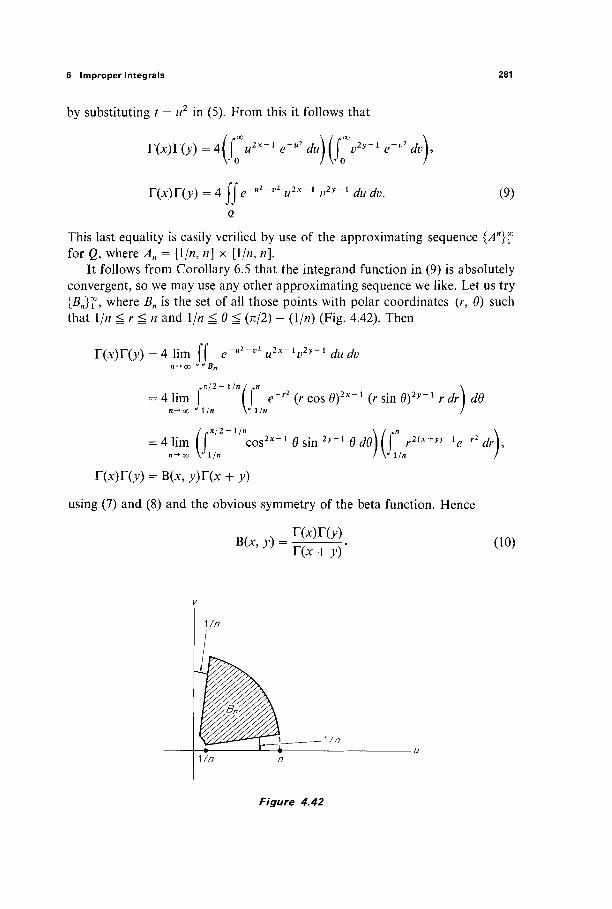
6 Improper Integrals 281
by substituting t = u2 in (5). From this it follows that
Γ(*)ΓΟ0 - A{CU1X~1 e~ul du\ (fv2y~l e~v2 dü\,
T(x)T(y) = 4 jje~u2'v2 u2x~l v2y~l du dv. (9) Q
This last equality is easily verified by use of the approximating sequence {An}f for Q, where A„ = [\/n, n] x [1//7, n].
It follows from Corollary 6.5 that the integrand function in (9) is absolutely convergent, so we may use any other approximating sequence we like. Let us try {B„}f, where Bn is the set of all those points with polar coordinates (/, 0) such that l/n^r^n and Ι/η^Θ^ (π/2) - (\/n) (Fig. 4.42). Then
Γ(χ)Γ(>0 = 4 lim ff e~ul-v2 u2x~lv2y-1 dudv n-*ao JJBn
= 4 lim f "if e~r2 (r cos Θ)2*-1^ sin θ)2*-1 rdr) dO
= 4 lim if "cos2*-1 Θ sin2*-1 ede)(f r2(x+y)-le-
r2 dr)9
n->oo \Jl/n / Vl/B /
Γ(*)Γ0κ) = B(x, y)T(x + y)
using (7) and (8) and the obvious symmetry of the beta function. Hence
r(*)roo B(jf, y) =
τ{χ + y) (10)
Figure 4.42
282 IV Multiple Integrals
As a typical application of (7) and (10), we obtain
sin5 Θ cos7 θάθ = - Β(3, 4)
_ 1 Γ(3)Γ(4) 2 Γ(7)
_ 12!3! ~2~βΓ
1 ~ Ï 2 Ô '
Another typical example of the use of gamma functions to evaluate integrals is
xU2e-x3dx = i u~il2e-"du
Lr(i) "0 ·Ό
..3 making the substitution u = x and using the fact that Γ(^) =Jn (Exercise 6.2).
Exercises
6.1 Show that Γ(1) = 1, and then deduce from Γ(* + 1) = xT(x) that Γ(Λ + 1) = n\. 6.2 Show that Γ(4) = \/π. Hint: Substitute t = u2 in the integral defining Γ(J), and
refer to Example 8. Then prove by induction on the positive integer n that
1-3 (In - 1 ) Γ(Λ + i) = ^ " ^77.
6.3 Recalling from the previous exercise section the formulas for the volume a„ of the unil «-dimensional ball Bn <= ^", deduce from the previous two exercises that
πηΙ2 _ 2πηΙ2
α " = Γ((Λ/2) + 1) ~ ΛΓ(Λ/2)
for all« ^ 1 . 6.4 Apply Exercises 6.1 and 6.2, and formulas (7) and (10), to obtain a new derivation of
C12 · 2.-1 a M 2 4 ( 2 " ~ 2 )
J0 Sln g ^ = l - 3 (21,-1)-
r t / 2
sin2" 0 </6> = 71/2 1 · 3 ( 2 / 7 - 1)77
2-4 (In) 2 '
6.5 Show that Jj x4(l - JC2)1/2 dx = ττ/32 by subtituting * = /1/2
6.6 Use the substitution / = xn to show that
J>~*-ir(=±i)
6 Improper Integrals 283
6.7 Use the substitution x = e~u to show that
f xm(\ogx)n </* = (m + l)" + 1
6.8 Show that
«/2 dx [Γ(έ)]2 r (cos x)112 2(2TT)1/2 '
6.9 Prove that the integral defining the beta function converges. 6.10 Show that the mass of a spherical ball of radius a, with density function d(x, y, z) = x2y2z2,
is M = 4πα9/945. Hint: Calculate the mass of the first octant. Introduce spherical coordinates, and use formulas (7) and (10).
6.11 Use ellipsoidal coordinates to show that the mass of the ellipsoidal ball x2/a2 + y2/b2
+ z2/c2 <j 1, with density function d(x, y, z) = x2 + y2 + z2, is
Απαοο , M=—^-(a2 + b2 + c2).
6.12 By integration by parts show that
f °° k—\ e~x2xkdx= —— | e~x2xk-2dx. 2
Deduce from this recursion formula that 1-3 (2m - 1) f - ,2 2m , 1 3 ( 2 w - l )
J « *2""& = — VTT
and
r -1 dx = -(m- 1)!.
Apply Exercises 6.1 and 6.2 to conclude that
C e ^ x ^ d x ^ - ^ . J0 2
for all integers n > 1. 6.13 The purpose of this exercise is to give a final computation of the volume a„ of the unit
ball Bn c= #». (a) Let Γ : ^" -> @tn be the «-dimensional spherical coordinates mapping of Exercise 5.19. Note by inspection of the definition of Γ, without computing it explicitly, that the Jaco-bian of T is of the form
| d e t r | =ρη-1γ(φι,···,<Ρη-ι,θ)
for some function y. (b) Let / : 0tn -> 0t be an absolutely integrable function such that g =f° T is a function of p alone. Then show that
f f=Cn\g{p)pn-'dp (*) J Ba
n J 0
for some constant Cn (independent of / ) . Setting / = g = 1 on Bn, a = 1, we see that a„ = C„//7, so it suffices to compute Cn.
284 IV Multiple Integrals
(c) Taking limits in (*) as Ö->OO, we obtain
f f=Cn\ g(P)pn-ldp,
so it suffices to find an absolutely integrable function/for which we can evaluate both of these improper integrals. For this purpose take
f(xi,...,x„) = e X1 2 _ . . . -Xn2
so g(p) = e~° . Conclude from Example 8 that j#nf= πη/2, and then apply the previous exercise to compute Cn, and thereby a„.
6.14 The purpose of the problem is to evaluate
r sin_ L x
x -dx.
(a) First show that Jo° e~xy dy = \/x if x > 0. (b) Then use integration by parts to show that
e xy sin x dx = if v > 0, L 1+v2
(c) Hence
r sin.v r/r \ dx= \ I e xy sin x dy I dx
- I I j e~xy ünxdx\ dy
dy 1 + ^ 2 '
sin x x 2
provided that the interchange of limit operations can be justified.
6.15 The object of this problem is to show that f(x) = (sin x)/x is not absolutely integrable on (0, oo). Show first that
r(2fc+1),tsinx ^ 2 dx >
] 2 k n X ~(2k + 1)77
Given any compact contented set A c= (0, oo), pick m such that A <= [0, 2m7r], and then define
Bn = [0, 2mn] n (j [2kn, (2k + 1)π] k = m
for all n> m. Now conclude, from the fact that^T^ i 1/(2/: + 1) diverges, that
f s i n * , lim dx= co. n-+oo J Bn X
Why does this imply that J(0> oo> [(sin x)/x] dx does not exist?
6 Improper Integrals 285
6.16 If U is an open subset of 2%n, show that there exists an increasing sequence {Ak}f of compact contented sets such that U = (Jfc°= i int Ak. Hint: Each point of U is contained in some closed ball which lies in U. Pick the sequence in such a way that Ak is the union of k closed balls.
6.17 Let q(x) = xxAx be a positive definite quadratic form on 0tn. Then show that
f 7Tnl2
e~qi*)dx = . ) m n (detA)1'2
Outline: Let P be the orthogonal matrix provided by Exercise II.8.7, such that PlAP = P~lAP is the diagonal matrix whose diagonal elements are the (positive) eigenvalues A], . . . , λ„ of the symmetric matrix A. Use the linear mapping L : ^y" -> ^x" defined by x = Py to transform the above integral to
Q\p(-Xiy!2 X„y„2)dy.
Then apply the fact that J*œ e~t2 dt = \/π by Example 8, and that fact that λιλ2'··λη = det A by Lemma II.8.7.

V Line and Surface Integrals ;
Differential Forms and Stokes' Theorem
This chapter is an exposition of the machinery that is necessary for the statement, proof, and application of Stokes' theorem. Stokes'theorem is a multi-dimensional generalization of the fundamental theorem of (single-variable) calculus, and may accurately be called the "fundamental theorem of multi-variable calculus." Among its numerous applications are the classical theorems of vector analysis (see Section 7).
We will be concerned with the integration of appropriate kinds of functions over surfaces (or manifolds) in ΡΛη. It turns out that the sort of "object," which can be integrated over a smooth /c-manifold in $n, is what is called a differential /c-form (defined in Section 5). It happens that to every differential /c-form a there corresponds a differential (k + l)-form den, the differential of a, and Stokes' theorem is the formula
\ doc = \ a,
where V is a compact (k + l)-dimensional manifold with nonempty boundary dV (a /c-manifold). In the course of our discussion we will make clear the way in which this is a proper generalization of the fundamental theorem of calculus in the form
(f'(t)dt=f{b)-f(a). J a
We start in Section 1 with the simplest case—integrals over curves in space, traditionally called "line integrals." Section 2 is a leisurely treatment of the 2-dimensional special case of Stokes' theorem, known as Green's theorem;
286

1 Pathlength and Line Integrals 287
this will serve to prepare the student for the proof of the general Stokes' theorem in Section 6.
Section 3 includes the multilinear algebra that is needed for the subsequent discussions of surface area (Section 4) and differential forms (Section 5). The student may prefer (at least in the first reading) to omit the proofs in Section 3—only the definitions and statements of the theorems of this section are needed in the sequel.
1 PATHLENGTH AND LINE INTEGRALS
In this section we generalize the familiar single-variable integral (on a closed interval in $) so as to obtain a type of integral that is associated with paths in Mn. By a ^ 1 path in $n is meant a continuously differentiate function y : [a, b] -► 3tn. The ^ 1 path y : [a, b] -* @n is said to be smooth if / ( i ) # 0 for all t e [a, b]. The significance of the condition /(r) Φ 0—that the direction of a ^ 1 path cannot change abruptly if its velocity vector never vanishes—is indicated by the following example.
Example 1 Consider the ^ 1 path y = (γΐ9 y2) '
x = yi(t) = t\ y = y2(t) =
• m1 defined by
if r^O, if * < 0 .
The image of y is the graph y = \x\ (Fig. 5.1). The only "corner" occurs at the origin, which is the image of the single point t = 0 at which y\t) = 0.
age of γ
Figure 5.1
We discuss first the concept of length for paths. It is natural to approach the definition of the length s(y) of the path y : [a, b] -> 0ln by means of polygonal approximations to y. Choose a partition & of [a, b],
0> = {a = t0 < tx < t2 < · · · < ffc_! <tk = b},
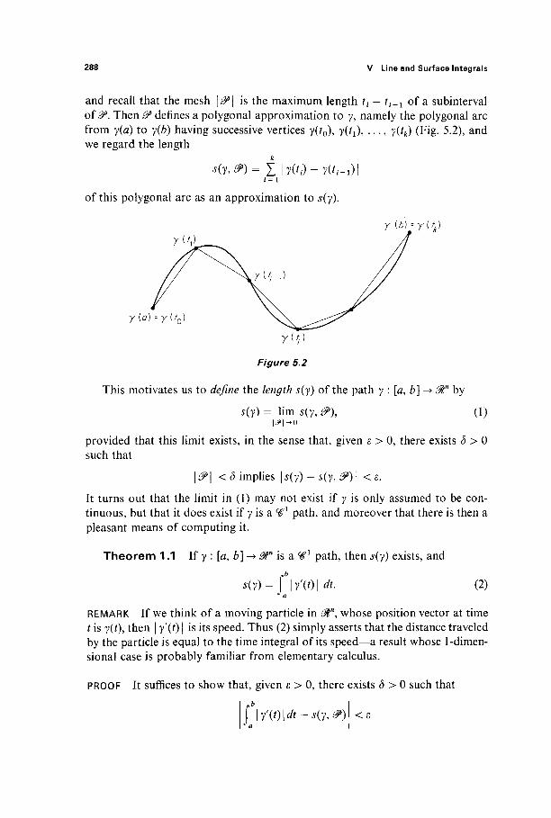
288 V Line and Surface Integrals
and recall that the mesh \&>\ is the maximum length tt — ti_1 of a subinterval of &. Then 0> defines a polygonal approximation to y, namely the polygonal arc from y(d) to y(b) having successive vertices y(f0), yf^), . . . , y(tk) (Fig. 5.2), and we regard the length
s(y,»)= Σ \y(ti)-y(ti-i)\
of this polygonal arc as an approximation to s(y).
Y (à)--y{fA)
y(a)--y(f0)
Figure 5.2
This motivates us to define the length s(y) of the path y : [a, b] -> 0ίη by
•y(y) = lim s(y9 &\ | ^ | - * 0
(1)
provided that this limit exists, in the sense that, given ε > 0, there exists δ > 0 such that
| ^ | < ô implies \s(y) - s(y, &)\ < ε.
It turns out that the limit in (1) may not exist if y is only assumed to be con-tinuous, but that it does exist if y is a ^ 1 path, and moreover that there is then a pleasant means of computing it.
Theorem 1.1 If y : [a, b] -» 0ln is a # ! path, then s(y) exists, and
s(y)= f | / ( i ) | A. (2)
REMARK If we think of a moving particle in 0tn, whose position vector at time t is y(i), then | y\t) \ is its speed. Thus (2) simply asserts that the distance traveled by the particle is equal to the time integral of its speed—a result whose 1-dimen-sional case is probably familiar from elementary calculus.
PROOF It suffices to show that, given ε > 0, there exists δ > 0 such that
\b\y'(t)\dt-s(y9P) < ε

1 Pathlength and Line Integrals 289
for every partition
0> = {a = to <tt < <tk.l <tk = b}
of mesh less than δ. Recall that
s(y,&)= Σ ΐ7(ί.·)-ν(ί/-ι)Ι / = 1
k
= Σ Σ (?,('/) - rrCi-i))2 1/2
(3)
where yu . . . , yn are the component functions of y. An application of the mean value theorem to the function yr on the /th sub-
interval [*,·_!, i,·] yields a point i,r G (*,·_!, ί,·) such that
y r ( i , ) - y r ( i i - i ) = y r ' ( i ir ) ( i f - i i - i ) .
Consequently Eq. (3) becomes
Φ> &) = £ [ i/yrX^O)2]17^/ - ί,-ι). (4)
//"the points i,·1, f,·2, . . . , iin just happened to all be the same point tt* e
[ij-i, *,·], then (4) would take the form
Σ = 1 J i = l
which is a Riemann sum for JJ | y'(t) \ dt. This is the real reason for the validity of formula (2); the remainder of the proof consists in showing that the difference between the sum (4) and an actual Riemann sum is " negligible."
For this purpose we introduce the auxiliary function F : / = [a, b]n -+ & de-fined by
1/2
r \X1, X2 , · · . , Xn) — Σ yr'M)2
Notice that F(t, t, . . . , /) = | / ( i ) | , and that F is continuous, and therefore uniformly continuous, on the «-dimensional interval /, since y is a ^ 1 path. Consequently there exists a δ1 > 0 such that
| F ( x ) - F ( y ) | < 2(b - a)
(5)
if each | xr — yr \ < δ t . We now want to compare the approximation
s(y,P)= Σ''( 'ΛίΛ.· . , '«")(' , - ' , - ι) i= 1
290 V Line and Surface Integrals
with the Riemann sum
R(y,&)= Σ \yVd\iti-ti-i) i = 1
A:
= £F(f f , f , - , . . . , ί ,-)( ί ( -* ι- ι) . / = 1
Since the points t{\ i,·2, . . . , t" all lie in the interval [/,·_!, i j , whose length ^ | ^ | , it follows from (5) that
\s(y,0>)-R(y,0>)\ ^ X \F(ti\...,tr)-F(ti,...,ti)\(ti-ti-l)
<^77 x Σ ( ί / - ί / - ι ) = Ι 2(b - a) ,· = i 2
if | ^ | < ^ . On the other hand, there exists (by Theorem IV.3.4) a δ2 > 0 such that
Λ(7,^)- f|/(OI dt ε
<-2
if \&>\ < £ 2 . If, finally, δ = min((31, (52), then \&>\ <δ implies that
!(γ,Ρ)- f 1/(01 dt rg \s(y, P) - R(y,.
ε ε 2 2
Ä(y,<?)- ίΊτ'(01 dt
as desired. I
Example 2 Writing y(t) = (χγ(ί), . . . , χ„(ί)Χ and using Leibniz notation, formula (2) becomes
s(y) -m)*-*m 1/2
dt.
Given a ^ 1 function / : [a, b] -► ^ , the graph o f / i s the image of the ^ 1 path y : [a, b] -► ^ 2 defined by y(x) = (x, /(x)). Substituting xx = t = x and x2 = y in the above formula with n = 2, we obtain the familiar formula
- i l · (I) for the length of the graph of a function.
1/2
i/x
Having defined pathlength and established its existence for Ή1 paths, the following question presents itself. Suppose that a : [a, b] -* 9tn and β : [c, d] -> ^ "

1 Pathlength and Line Integrals 291
are two ^ 1 paths that are "geometrically equivalent" in the sense that they have the same initial point α(α) = ß(c), the same terminal point a{b) = ß(d), and trace through the same intermediate points in the same order. Do a and ß then have the same length, s(cc) = s(ß)l
Before providing the expected affirmative answer to this question, we must make precise the notion of equivalence of paths. We say that the path a : [a, b] -* @n is equivalent to the path ß : [c, d] -► @n if and only if there exists a ^ 1
function φ : [a, b] -» [c, d]
such that φ([α, b]) = [c, d], ot = β o φ, and </>'(/) > 0 for all / e [a, £] (see Fig. 5.3). The student should show that this relation is symmetric (if a is equivalent to jß, then ß is equivalent to a) and transitive (if a is equivalent to ß, and ß is equivalent to y, then a is equivalent to y), and is therefore an equivalence rela-tion (Exercise 1.1). He should also show that, if the ^ 1 paths a and β are equiva-lent, then a is smooth if and only if β is smooth (Exercise 1.2).
The fact that s(a) = s(ß) if a and ß are equivalent is seen by taking / (x) = 1 in the following theorem.
Theorem 1.2 Suppose that a : [a, b]-+8tn and /?:[<% </]-»^" are equivalent ^ 1 paths, and t h a t / i s a continuous real-valued function whose domain of definition in 9tn contains the common image of a and β. Then
ff(a(t))\a'(t)\dt= (f(ß(t))\ß'(t)\dt. Ja Jc
PROOF If φ : [a, b] -► [c, d] is a ^ 1 function such that α = β ο φ and φ'(ί) > 0 for all / G [α, 6], then
fV(a(0) I a'(01 A = f7(/?M0)) I β\ψ^))φ\ΐ) | Λ (chain rule)
= f f(ß(q>(®) | /ϊ'ίφ(Ο) | φ'(ί) Λ (because <p'(t) > 0)
= I f(ß(u))\ß'(u)\ du (substitution u = <p{t)). |

292 V Line and Surface Integrals
To provide a physical interpretation of integrals such as those of the previous theorem, let us think of a wire which coincides with the image of the ^ 1 path y · fr*, b] -> 0ln, and whose density at the point y(r) is f(y(t)). Given a partition & = {a = t0 < tx < · · · < tk = b} of [a, b], the sum
m(y,f,P)= i / W / W l v W - y i i f - i ) ! i = 1
may be regarded as an approximation to the mass of the wire. By an argument essentially identical to that of the proof of Theorem 1.1, it can be proved that
lim m(y,f, 9) = f / (y(0)l /(OI dt. (6)
Consequently this integral is taken as the definition of the mass of the wire. If y is a smooth path, the integral (6) can be interpreted as an integral with
respect to pathlength. For this we need an equivalent unit-speed path, that is an equivalent smooth path y such that | f(t) | = 1 .
Proposition 1.3 Every smooth path y: [a, b] smooth unit-speed path.
is equivalent to a
PROOF Write L = s(y) for the length of y, and dehne σ : [a, b] -► [0, L] by
σ(ή= ί I / (M) I du, Ja
so σ(0 is simply the length of the path y : [a, t] -► 9tn (Fig. 5.4). Then from the fundamental theorem of calculus we see that σ is a Ή1 function with
o\t)= | / ( 0 | >0.
Therefore the inverse function τ : [0, L] -► [a, b] exists, with
1 T'(S) =
σ'(φ)) > 0 .
y{b)
γ \a Υ'-Υ'
Figure 5.4

1 Pathlength and Line Integrals 293
since | ?'(σ(ί))| = 1 and σ'(ί) > 0. Substituting s = σ(ί), we then obtain
\bf(y{ii)\yV)\dt=\Lf{y(s))ds. (7)
(This result also follows immediately from Theorem 1.2.) Since y(s) simply denotes that point whose "distance along the path" from the initial point y(a) is s, Eq. (7) provides the promised integral with respect to pathlength.
It also serves to motivate the common abbreviation
Çf(y(t))\y'(t)\dt=\ fds. (8)
Historically this notation resulted from the expression
ds = \y'(t)\ dt
for the length of the "infinitesimal" piece of path corresponding to the "in-finitesimal" time interval [t, t + dt]. Later in this section we will provide the expression ds = \ y'(t) \ dt with an actual mathematical meaning (in contrast to its "mythical" meaning here).
Now let y : [a, b] -> 0tn be a smooth path, and think of y(t) as the position vector of a particle moving in 0tn under the influence of the continuous force field F : 0tn -► ffin [so ¥(y(t)) is the force acting on the particle at time /] . We inquire as to the work Wdone by the force field in moving the particle along the path from y(a) to y{b). Let 0* be the usual partition of [a, b]. If F were a constant force field, then the work done by F in moving the particle along the straight line segment from 7(it_x) to y(i,·) would by definition be F · (γ(ί{) — •y(i/_1)) (in the constant case, work is simply the product of force and distance). We therefore regard the sum
W(y, ¥,0>)=Σ F(y(*/))· (y(td - y(if-i))
If y : [0, L] -► @tn is the equivalent smooth path defined by y = y ° τ, the chain rule gives
since σ\ί) = | / ( ί ) | .
With the notation of this proposition and its proof, we have
f /(y(0)l/(0l dt = ί /(Wff(0))irW0K(0l dt Ja Ja
= \"J\y(o{t)))a'(t) dt
\y(s)\ = \y(z(s))T(s)\ =——— = 1, \σ (T(S))\
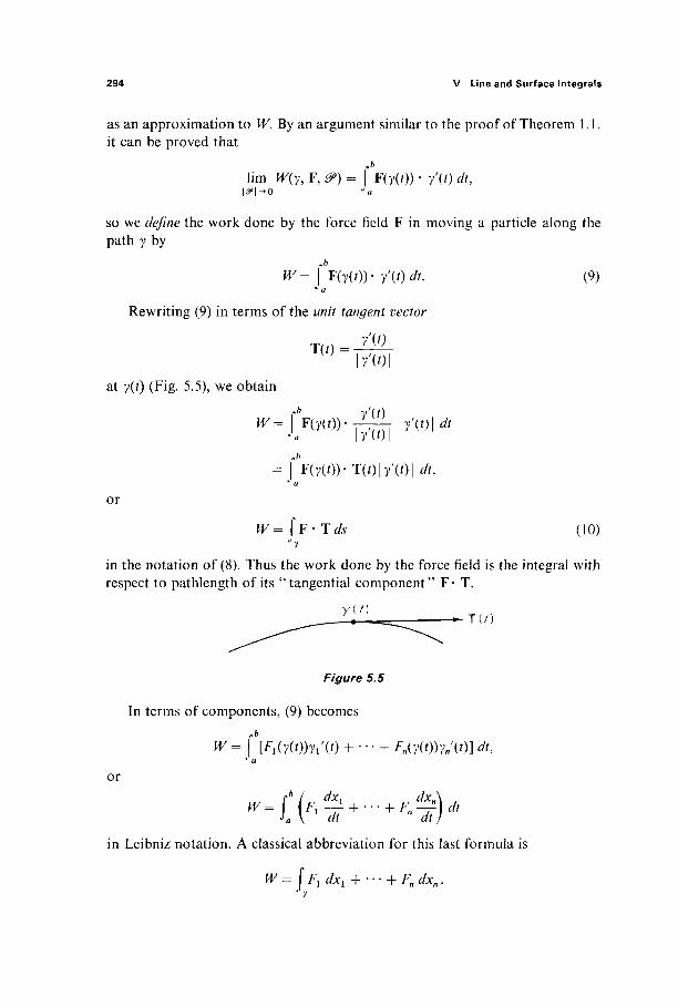
294 V Line and Surface Integrals
as an approximation to W. By an argument similar to the proof of Theorem 1.1, it can be proved that
lim W(y, F, 9) = F(y(i)) · yV) dt, \9\
so we define the work done by the force field F in moving a particle along the path y by
W= fV(y(i))· y'(t)dt.
Rewriting (9) in terms of the unit tangent vector
y'(t)
(9)
T(0 = ·
at y(t) (Fig. 5.5), we obtain
W
7'(0l
y'C) y '(01 dt = ΓΡ(Τ(0) · , ,(Λ
Ja I 7 ( 0 ,
= fV(y(0 ) -T( t ) l7 ' (0 l^
or ■ - /. ^ = F ' T é (10)
in the notation of (8). Thus the work done by the force field is the integral with respect to pathlength of its "tangential component" F· T.
/ ( / ) T ( / )
Figure 5.5
In terms of components, (9) becomes
w = | Vi(y(0)7i'(0 + · · · + fn{y(t))yn'(t)] du
or
W=[h(F/-^ + - + Fnd^\dt <{- ft) dt dt,
in Leibniz notation. A classical abbreviation for this last formula is
W= ÎFldxl + --- + Fndxn.
1 Pathlength and Line Integrals 295
This type of integral, called a line integral (or curvilinear integral), can of course be defined without reference to the above discussion of work, and indeed line integrals have a much wider range of applications than this. Given a %>l
path y : [a, b] -> @tn and n continuous functions / i , . . . , fn whose domains of definition in 9tn all contain the image of y, the line integral \yf dxl + '" +f„ dxn
is defined by
f/1 dxt + ··· +fn dx„ = fVi(y(0)yi'(0 + · · · +fMt))yn'(t)] A. (li)
Formally, we simply substitute x, = y£(i), dx{ = y{(t) dt into the left-hand side of (11), and then integrate from a to b.
We now provide an interpretation of (11) whose viewpoint is basic to sub-sequent sections. By a (linear) differential form on the set U <= 01" is meant a mapping ω which associates with each point x e ( / a linear function ω(χ) : 0tn
-+ St. Thus ω: U->£>(<%", 3t\
where J2? (£#", ^ ) is the vector space of all linear (real-valued) functions on 0Γ. We will frequently find it convenient to write
ω(χ) = ω χ .
Recall that every linear function L : $n -> 01 is of the form
= αιλι(γ) + -· + αηλη(γ), (12)
where A,· : 0tn -> is the ith projection function defined by
Xi(vu ...,vn) = vi9 i = 1, . . . , n.
If we use the customary notation A, = dxt, then (12) becomes
L = axdxx + ··· + an dxn.
If L = ω(χ) depends upon the point x e U, then so do the coefficients au . . . , an\ this gives the following result.
Proposition 1.4 If ω is a differential form on U a 0F, then there exist unique real-valued functions au . . . , an on U such that
ω(χ) = ωχ = a^x) dx1 + - · + an(x) dxn (13)
for each xe U.
Thus we may regard a differential form as simply an " expression of the form" (13), remembering that, for each xe U, this expression denotes the linear function whose value at v = (vx, . . . , vn) e $n is
ωχ(ν) = öi ixH + · · · + an(x)vn.
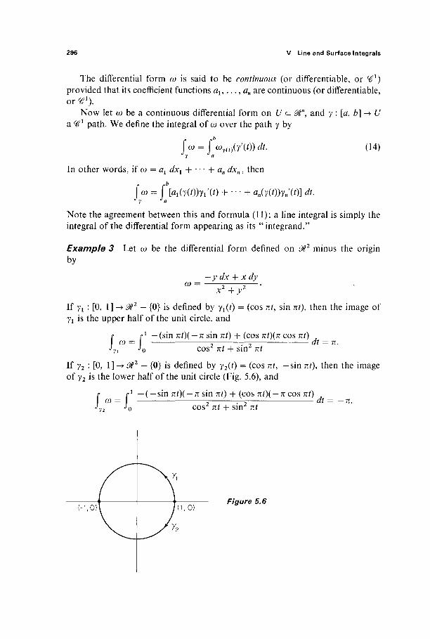
296 V Line and Surface Integrals
The differential form ω is said to be continuous (or differentiate, or Ή1) provided that its coefficient functions au . . . , an are continuous (or differentiate, or V1).
Now let ω be a continuous differential form on U c Mn, and y : [a, b]^> U a ^ 1 path. We define the integral of ω over the path y by
ί ω = f ω7( ί )(/(0) A. (14) J y J a
In other words, if ω = ax dxl + · · · + an dxn, then
f ω = ί [fli(y(0)7i'(0 + · · · + *„(y(0)y„'(0] Λ.
Note the agreement between this and formula (11); a line integral is simply the integral of the differential form appearing as its "integrand."
Example 3 Let ω be the differential form defined on 0t2 minus the origin by
ω = —ydx + xdy
x2+y2
If γί : [0, 1] -> 0ί2 — {0} is defined by yx(f) = (cos nt, sin πί), then the image of γί is the upper half of the unit circle, and
52
-(sin πί)( — π sin πί) + (cos πί)(π cos nt) cos2 πί + sin2 nt
dt = n.
If y2 : [0, \\-+0r — {0} is defined by y2(0 = ( c o s πί> —sin πί), then the image of y2 is the lower half of the unit circle (Fig. 5.6), and
J>-J, 1 — ( — sin nt)( — π sin nt) + (cos nt)( — n cos nt)
cos2 πί 4- sin2 nt dt = -n.
Figure 5.6

1 Pathlength and Line Integrals 297
In a moment we will see the significance of the fact that Jyi ω φ \Ί1 ω.
Recall that, if/is a differentiable real-valued function on the open set U cz 0ln, then its differential dfx at x e U is the linear function on 0în defined by
dfx(Y) = Dlf(x)vl + -- + Dnf(x)vn.
Consequently we see that the differential of a differentiable function is a dif-ferential form
dfx = Α / ( χ ) </*ι + " · + Dnf(x) dxn, or
df= — dxl + · · · + — dxn. oxi cxn
Example 4 Let U denote @2 minus the nonnegative x-axis; that is, (x, y) e U unless x ^ 0 and y = 0. Let 0 : (7 -> ^ be the polar angle function defined in the obvious way (Fig. 5.7). In particular,
θ(χ, y) = arctan -y
if x φ 0, so
Dfi(x, y) = y and D2 0(x, y) x2 +y2 x2 + y2'
Therefore
d0 = -y dx + x dy
x2 + y2
Figure 5.7
298 V Line and Surface Integrals
on £/; the differential of Θ agrees on its domain of definition t/with the differen-tial form ω of Example 3. Although
—y dx + x dy ω = 2 2 —
x2 + y2
is defined on M1 — {0}, it is clear that the angle function cannot be extended continuously to 0l2 — {0}. As a consequence of the next theorem, we will see that ω is not the differential of any differentiable function that is defined on all o f ^ 2 - { 0 } .
Recall the fundamental theorem of calculus in the form
J f'(t)dt=f{b) -f(a).
Now/'( i ) dt is simply the differential at t off: Si -»· 0t; dt : & -»· & is the iden-tity mapping. If y ; [a, b] -> [a, b] is also the identity, then
\df= fdft(Y(t))dt= fV,0)A= ffV)dt, Jy Ja Ja Ja
and f(b) —f(a) = f(y(b)) — f(y(a)), so the fundamental theorem of calculus takes the form
(df = f(y(b))-f(y(a)).
The following theorem generalizes this formula; it is the "fundamental theorem of calculus for paths in 0tn"
Theorem 1.5 If / is a real-valued ^ 1 function on the open set U c 0tn, and y : [a, b] -> U is a ^ 1 path, then
f df = f(y(b))-f(y(a)). (15) Jy
PROOF Define g \ [a, b]-> @ by g = / ° y. Then #'(i) = V/(y(i))· /(*) by the chain rule, so
= f*[A/(y(0)yi'(0 + · · · + DJ(y(t))7nV)] dt J a
= fV(y(0)-y'(0A
^ a (equation continues)
1 Pathlength and Line Integrals 299
= g{b)-g(a)
=f(y(b)) - / (7(e)) . I
It is an immediate corollary to this theorem that, if the differential form ω on U is the differential of some ^ 1 function on the open set U, then the integral Jy ω is independent of the path y, to the extent that it depends only on the initial and terminal points of y.
Corollary 1.6 If ω = df, where / is a Ή1 function on U, and a and β are two ^ 1 paths in U with the same initial and terminal points, then
ω = ω.
We now see that the result Jyi ω Φ \Ί1 ω of Example 3, where y1 and y2 were two different paths in 011 - {0} from (1, 0) to ( - 1 , 0), implies that the dif-ferential form
—y dx + x dy
is not the differential of any ^ 1 function on 011 — {0}. Despite this fact, it is customarily denoted by d9, because its integral over a path y measures the polar angle between the endpoints of y.
Recall that, if F : U ~+ 0ln is a force field o n i / c ^ " and y : [a, b] -~> 0ln is a ^ 1 path in U, then the work done by the field F in transporting a particle along the path y is defined by
W= ίω, Jy
where ω = Fl dxl + · · · + Fn dxn. Suppose now that the force field F is con-servative (see Exercise II. 1.3), that is, there exists a ^ 1 function g : U -► ^ such that F = Wg. Since this means that ω = dg, Corollary 1.6 implies that ^depends only on the initial and terminal points of y, and in particular that
W = g(y(b)) - 9iy{a)).
This is the statement that the work done by a conservative force field, in moving a particle from one point to another, is equal to the "difference in potential" of the two points.
We close this section with a discussion of the arclength form ds of an oriented curve in 0tn. This will provide an explication of the notation of formulas (8) and (10).
The set C in 0F is called a curve if and only if it is the image of a smooth path y which is one-to-one. Any one-to-one smooth path which is equivalent to y is then called a parametrization of C.
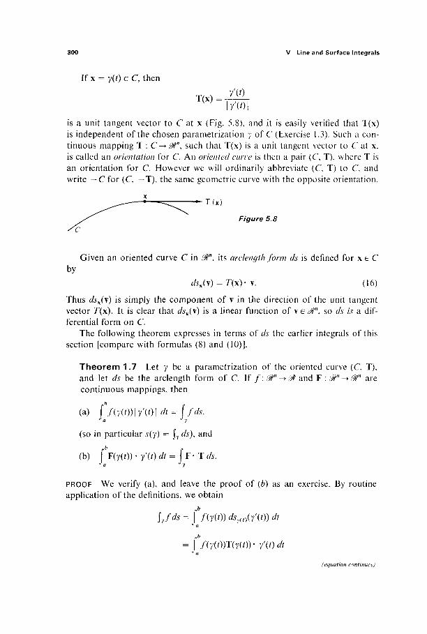
300 V Line and Surface Integrals
If x = y(t) e C, then
/(0 T(x) 1/(01
is a unit tangent vector to C at x (Fig. 5.8), and it is easily verified that T(x) is independent of the chosen parametrization y of C (Exercise 1.3). Such a con-tinuous mapping T : C-> ffln, such that T(x) is a unit tangent vector to C at x, is called an orientation for C. An oriented eurve is then a pair (C, T), where T is an orientation for C. However we will ordinarily abbreviate (C, T) to C, and write — C for (C, — T), the same geometric curve with the opposite orientation.
— Τ ( χ )
Figure 5.8
Given an oriented curve C in £#n, its arclength form ds is defined for x 6 C by
dsx(\) = T(\)- v. (16)
Thus dsx(\) is simply the component of v in the direction of the unit tangent vector Γ(χ). It is clear that dsx(\) is a linear function of v e $n, so ds is a dif-ferential form on C.
The following theorem expresses in terms of ds the earlier integrals of this section [compare with formulas (8) and (10)].
Theorem 1.7 Let y be a parametrization of the oriented curve (C, T), and let ds be the arclength form of C If / : @n -* & and F : ®n-+@n are continuous mappings, then
(a) fV(y(0) l / (0 l*=f /^
(so in particular s(y) = Jy ds), and
(b) f F(y(0) · / (0 dt = ÎF-ΤΛ. Ja Jy
PROOF We verify (a), and leave the proof of (b) as an exercise. By routine application of the definitions, we obtain
\yfds= \bf(y(t))dsy(t)(y\t))dt
= f7(y(0)T(y(/))-/(0<ft
(equation continues)
1 Pathlength and Line Integrals 301
-iV(r(0)l/(0l A I Ja
Finally notice that, if the differential form ω = Fl dxx + · · * + Fn dxn is defined on the oriented smooth curve (C, T) with parametrization y, then
\ ω = F1 dxx + · · · + Fn dxn Jy Jy
= iVi(7(0)yi'(0 + ■ · · + Fn(v(t))y«V)] dt
= ÎF· Tds
by Theorem 1.7(b). Thus every integral of a differential form, over a parametriza-tion of an oriented smooth curve, is an " arclength integral."
Exercises
1.1 Show that the relation of equivalence of paths in &η is symmetric and transitive. 1.2 If a and β are equivalent paths in ^", and a is smooth, show that β is also smooth. 1.3 Show that any two equivalent parametrizations of the smooth curve f€ induce the same
orientation of #. 1.4 If a and β are equivalent ^1 paths in ^ \ and ω is a continuous differential form, show
that Ja a> = $βω. 1.5 If a : [0,1] ->^" is a f€x path and ω is a continuous differential form, define β(ί) = α(1 — r)
for / e [0,1 ]. Then show that $αω = — J"„6Ü. 1.6 If a : [#, 6] -> &n and j8 : [c, d] -> 3#n are smooth one-to-one paths with the same image,
and a(a) = ß(c), <x(b) = ß(d), show that a and ß are equivalent. 1.7 Show that the circumference of the ellipse x2/a2 + y2/b2 = 1 is
4αΕΓ-(α2-ϋ2)ι/2, - J ,
where £(£, <ρ) = /β(1 — k2 s'm2 t)l/2 dt denotes the standard "elliptic integral of the second kind."
1.8 (a) Given ^ 1 mappings [a, b] -^ ®lv - i ^ 3 , define y = 7*° c. Show that
/ ( / ) = c/(/)Z)1r(c(r)) + <-2'(f)/>2 r(c(/))
and conclude that the length of y is
5 ( y ) = I r W +2F**+G(*)\ dt

302 V Line and Surface Integrals
where
dT 8T dT dT dT dT £ = — . — , F= — . — , G = — . — .
du du du dv dv dv
(b) Let T: @%0-+ &%z be the spherical coordinates mapping given by
x = sin φ cos 0, y = sin φ sin 0, z = cos <p.
Let y : [a, b] -> &3 be a path on the unit sphere described by giving 9? and 0 as functions of /, that is, c(t) = (<p(/), 0(r)). Deduce from (a) that
-"-Π(ΐ)'"Μ5)Γ-· 1.9 (a) Given i?1 mappings [e, 6 ] - ^ ^ l - £ ^?J, define γ = F°c. Show that
/C)=Zc«'(0J>iF(c(/)) / = 1
and conclude that the length of y is
J a
where #,·,· = (dF/dud · (dF/duj).
(b) Let Z7 : ^r3
0z -> 0t\yz be the cylindrical coordinates mapping given by
x = r cos 0, j> = r sin 0, z = z.
Let y : [a, b] -> &\yz be a path described by giving r, 0, ζ as functions of t, that is,
c(f) = (r(/),0(O,zW).
Deduce from (a) that
1.10 If F : <Mn -> ttn is a tf1 force field and y : [a, 6 ] - ^ f " a r^! path, use the fact that F(y(f )) = my"(t) to show that the work W done by this force field in moving a particle of mass m along the path y from y(#) to y{b) is
^ = i#wi?tf02 - imv(a)\
where *;(/) = | y ' ( / ) | . Thus the work done by the field equals the increase in the kinetic energy of the particle.
1.11 For each (JC, y) e PÀ2, let F(x, y) be a unit vector pointed toward the origin from (*, >>). Calculate the work done by the force field F in moving a particle from (2a, 0) to (0, 0) along the top half of the circle (x — a)2 + y2 = a2.
1.12 Let dd = (—y dx -f x dy)/(x2 + y2). Thinking of polar angles, explain why it seems "obvious" that \Ίάΰ = 2π, where y(t) = (acost, b sin t), t e [0, 2π]. Accepting this fact, deduce from it that
Γ2π dt _ 2τ7 J 0 a2 cos2 / + b2 sin2 / A6
1.13 L e t i / 0 = ( - ^ ^ v + x i / v ) / U 2 + 7 2 ) o n ^ 2 - 0. (a) If y : [0, 1 ] -> M2 — 0 is defined by γ(ί) = (cos 2/:π/, sin 2k7r/), where k is an integer, show that Jv i/0 = 2/<π.
L· ffu -r -7Γ i , j = i at at
dU
1 Pathlength and Line Integrals 303
(b) If y : [0, 1 ] -> @2 is a closed path (that is, y(0) = y(l)) whose image lies in the open first quadrant, conclude from Theorem 1.5 that Jv άθ = 0.
1.14 Let the differential form ω be defined on the open set U c ΰ#2, and suppose there exist continuous functions, f, g : iüt -> â# such that ω(χ, y) =f(x) dx + g(y) dy if (x, y) e U. Apply Theorem 1.5 to show that Jv ω = 0 if y is a closed f6 1 path in U.
1.15 Prove Theorem 1.7(b). 8 1.16 Let F : U-> i#n be a continuous vector field on U <= .^n such that |F(x) | <: M if x e £/.
If r(i is a curve in U, and y a parametrization of r6\ show that
Î F - Τ ds^Ms(y).
1.17 If y is a parametrization of the oriented curve r6 with arclength form ds9 show that dsy{t){y\t)) = | y ' ( / ) | , s o
jds= | |/(/)|«ft = j(y).
1.18 Let y(/) = (cos t, sin 0 for / e [0, 27r] be the standard parametrization of the unit circle in &2. If
(x — y) dx + (x + >>) i/y 60 = ; ;
on ^ 2 — 0, calculate Jv o>. Then explain carefully why your answer implies that there is no function/: $2 — 0 ^ ai with df= ω.
1.19 Let ω = y dx + x dy -\-2z dz on ^3. Write down by inspection a differentiable function f: ^2->^ such that <//= cu. If y : [a, b] -> M* is a tfl path from (1,0,1) to (0,1, - 1 ) , what
is the value of Jv to? 1.20 Let y be a smooth parametrization of the curve W in i%2, with unit tangent T and unit
normal N defined by
and
N (y (» ) = Π77ΤΤ (72'(0, - y i ' ( O ) . ly toi
Given a vector field F = (Fi, F2) on ^ 2 , let cu = — Fzdx^rF^ dy, and then show that
fF.Nrfs= ί ω . J γ J y
1.21 Let %' be an oriented curve in ^P", with unit tangent vector T = (fl5 . . . , tn). (a) Show that the definition [Eq. (16)] of the arclength form ds of C is equivalent to
ds= Σ ti dxi. i= 1
(b) If the vector v is tangent to C, show that
/,· ds(\) = dxi(\), i = 1, . . . , n.
(c) If F = (T7!, . . . , Fn) is a vector field, show that the 1-forms
F · T ds and £ Ft dx, i= 1
agree on vectors that are tangent to C.
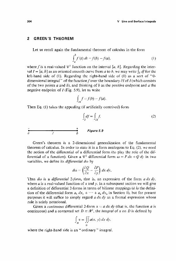
304 V Line and Surface Integrals
2 GREEN'S THEOREM
Let us recall again the fundamental theorem of calculus in the form
\bf(t)dt=f{b)-f{a\ (1)
where fis a real-valued ^ 1 function on the interval [a, b\. Regarding the inter-val / = [a, b] as an oriented smooth curve from a to b, we may write J7 df for the left-hand side of (1). Regarding the right-hand side of (1) as a sort of "0-dimensional integral " of the function/over the boundary dl of /(which consists of the two points a and b), and thinking of b as the positive endpoint and a the negative endpoint of / (Fig. 5.9), let us write
f f=f(b) -f(a). Jdl
Then Eq. (1) takes the appealing (if artificially contrived) form
|>= f /· (2) JI Jdl
Figure 5.9
Green's theorem is a 2-dimensional generalization of the fundamental theorem of calculus. In order to state it in a form analogous to Eq. (2), we need the notion of the differential of a differential form (to play the role of the dif-ferential of a function). Given a ^ 1 differential form ω = P dx + Q dy in two variables, we define its differential dœ by
Thus dœ is a differential 2-form, that is, an expression of the form a dx dy, where a is a real-valued function of x and y. In a subsequent section we will give a definition of differential 2-forms in terms of bilinear mappings (à la the defini-tion of the differential form ax άχγ + · · · + #„ dxn in Section 1), but for present purposes it will suffice to simply regard a dx dy as a formal expression whose role is solely notational.
Given a continuous differential 2-form a = a dx dy (that is, the function a is continuous) and a contented set D a 0l2, the integral of a on D is defined by
a = a(x, y) dx dy,
D
where the right-hand side is an "ordinary" integral.
2 Green's Theorem 305
Now that we have two types of differential forms, we will refer to
ax dxl + - - · + an dxn or P dx + Q dy
as a differential 1 -form. If moreover we agree to call real-valued functions 0-forms, then the differential of a 0-form is a l-form, while the differential of a l-form is a 2-form. We will eventually have a full array of differential forms in all dimen-sions, with the differential of a /c-form being a (k + l)-form.
We are now ready for a preliminary informal statement of Green's theorem.
Let D be a ''nice''' region in the plane &2, whose boundary dD consists of a finite number of closed curves, each of which is "positively oriented" with respect to D. If ω = P dx + Q dy is a ^ 1 differential \-form defined on D, then
\ dw = f ω. (3)
That is,
D
Note the formal similarity between Eqs. (2) and (3). In each, the left-hand side is the integral over a set of the differential of a form, while the right-hand side is the integral of the form over the boundary of the set. We will later see, in Stokes' theorem, a comprehensive multidimensional generalization of this phenomenon.
The above statement fails in several respects to be (as yet) an actual theorem. We have not yet said what we mean by a "nice" region in the plane, nor what it means for its boundary curves to be " positively oriented." Also, there is a question as to the definition of the integral on the right-hand side of (3), since we have only defined the integral of a l-form over a ^ 1 path (rather than a curve, as such).
The last question is the first one we will consider. The continuous path y : [a, b] -> $n is called piecewise smooth if there is a partition 0> = {a = a0
<a{ < - · - < ak = b) of the interval [a, b] such that each restriction yl of y to [α,-! , a,·], defined by
yi(t) = y(t) for / e [*,._„ a,],
is smooth. If ω is a continuous differential l-form, we then define
.ίω = Ι,.ί,ω· It is easily verified that this definition of J)f ω is independent of the partition ^ \ (Exercise 2.11).
306 V Line and Surface Integrals
A piecewise-smooth curve C in 0tn is the image of a piecewise-smooth path y : [a, b] -> 0ln which is one-to-one on (a, b)\ C is closed if y(a) = y(b). The path 7 is a parametrization of C, and the pair (C, 7) is called an oriented piecewise-smooth curve [although we will ordinarily abbreviate (C, 7) to C].
Now let ß : [c, d] -> 0ln be a second piecewise-linear smooth path which is one-to-one on (c, i/) and whose image is C. Then we write (C, 7) = (C, /?) [respec-tively, (C, 7) = — (C, /?)], and say that 7 and ß induce the same orientation [respectively, opposite orientations] of C, provided that their unit tangent vectors are equal [respectively, opposite] at each point where both are defined. It then follows from Exercises 1.4 and 1.5 that, for any continuous differential 1-form ω,
\ω=\ω (4)
if 7 and ß induce the same orientation of C, while
\ω=-\ω (5)
if 7 and ß induce opposite orientations of C (see Exercise 2.12). Given an oriented piecewise-smooth curve C, and a continuous differential
1-form ω defined on C, we may now define the integral of ω over C by
ίω =Ιω' where 7 is any parametrization of C. It then follows from (4) and (5) that j c ω is thereby well defined, and that
ί ω = - I ω, J -c J c
where C = (C, 7) and — C = — (C, 7) = (C, /?), with 7 and /? inducing opposite orientations.
Now, finally, the right-hand side of (3) is meaningful, provided that dD consists of mutually disjoint oriented piecewise-smooth closed curves Q , . . . , Cr; then
ω = Σ ω· ^dD i= 1 J Ci
A nice region in the plane is a connected compact (closed and bounded) set D a &2 whose boundary dD is the union of a finite number of mutually disjoint piecewise-smooth closed curves (as above). It follows from Exercise IV.5.1 that every nice region D is contented, so fD a exists if a is a continuous 2-form. Figure 5.10 shows a disk, an annular region (or "disk with one hole"), and a "disk with two holes"; each of these is a nice region.
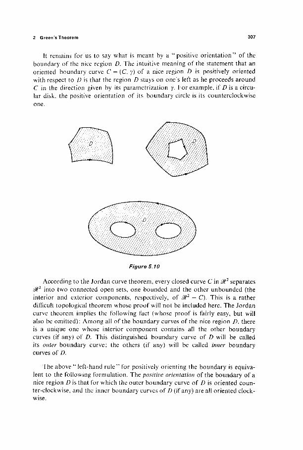
2 Green's Theorem 307
It remains for us to say what is meant by a "positive orientation" of the boundary of the nice region D. The intuitive meaning of the statement that an oriented boundary curve C = (C, y) of a nice region D is positively oriented with respect to D is that the region D stays on one's left as he proceeds around C in the direction given by its parametrization y. For example, if D is a circu-lar disk, the positive orientation of its boundary circle is its counterclockwise one.
Figure 5.10
According to the Jordan curve theorem, every closed curve C in 011 separates 0t1 into two connected open sets, one bounded and the other unbounded (the interior and exterior components, respectively, of 0t1 — C). This is a rather difficult topological theorem whose proof will not be included here. The Jordan curve theorem implies the following fact (whose proof is fairly easy, but will also be omitted): Among all of the boundary curves of the nice region D, there is a unique one whose interior component contains all the other boundary curves (if any) of D. This distinguished boundary curve of D will be called its outer boundary curve; the others (if any) will be called inner boundary curves of D.
The above " left-hand rule" for positively orienting the boundary is equiva-lent to the following formulation. The positive orientation of the boundary of a nice region D is that for which the outer boundary curve of D is oriented coun-ter-clockwise, and the inner boundary curves of D (if any) are all oriented clock-wise.
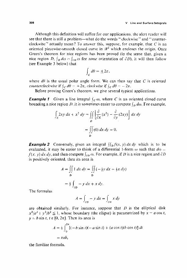
308 V Line and Surface Integrals
Although this definition will suffice for our applications, the alert reader will see that there is still a problem—what do the words " clockwise " and " counter-clockwise" actually mean? To answer this, suppose, for example, that C is an oriented piecewise-smooth closed curve in ^ 2 which encloses the origin. Once Green's theorem for nice regions has been proved (in the sense that, given a nice region Z>, JD dœ = Jf,D ω for some orientation of dD), it will then follow (see Example 3 below) that
d0= ±2π, 1c
where dO is the usual polar angle form. We can then say that C is oriented counterclockwise if Jc dO = +2π, clockwise if Jc dO = — In.
Before proving Green's theorem, we give several typical applications.
Example 1 Given a line integral j c ω, where C is an oriented closed curve bounding a nice region Z), it is sometimes easier to compute jD dœ. For example,
'ô 9 d
dx dy 2xy dx 4- x2 dy =
D
= jj(0)dxdy = 0.
dx dy
Example 2 Conversely, given an integral J jD/(*> y) dx dy which is to be evaluated, it may be easier to think of a differential l-form ω such that dœ = f(x, y) dx dy, and then compute JÖD ω. For example, if D is a nice region and dD is positively oriented, then its area is
The formulas
A = IT 1 dx dy = IT(-\y dx + \x dy) D D
= Ύ \ — y dx -\r x dy.
A = \ — y dx = \ x dy
are obtained similarly. For instance, suppose that D is the elliptical disk x2/a2 + y2/b2 S 1> whose boundary (the ellipse) is parametrized by x = a cos t, y = b sin f, t e [0, 2π]. Then its area is
A = i l(-b sin t)(-a sin t) + (a cos t)(b cos t)] dt
= nab,
the familiar formula.
2 Green's Theorem 309
Example 3 Let C be a piecewise-smooth closed curve in 0l2 which en-closes the origin, and is oriented counterclockwise. Let Ca be a clockwise-oriented circle of radius a centered at 0, with a sufficiently small that Ca lies in the interior component of 011 - C (Fig. 5.11). Then let D be the annular region bounded by C and Ca. If
-y dx 4- x dy = d0 =
x2 +
Figure 5.11
then dœ = 0 on D (compute it), so
f dO + f d0= ( ω = \ dœ = 0.
Since jCa^0 = —In, by essentially the same computation as in Example 3 of Section 1, it follows that
j d0= -j d0 = 2n.
In particular this is true if C is the ellipse of Exercise 1.12. On the other hand, if the nice region bounded by C does not contain the
origin, then it follows (upon applicaton of Green's theorem to this region) that
ί dO = 0. J c
Equation (3), the conclusion of Green's theorem, can be reformulated in terms of the divergence of a vector field. Given a (éΛ vector field F : Mn -> 0tn, its divergence div F : Mn -► M is the real-valued function defined by
div F = —- + ox, +
dFK
310 V Line and Surface Integrals
or
in case n = 2.
div F = - i + —? ox dy
Now let D c ,^2 be a nice region with dD positively oriented, and let N denote the unit outer normal vector to dD, defined as in Exercise 1.20. From that exercise and Green's theorem, we obtain
f F· Nds = f -F2dx + Fl dy
D
SO
f ¥-Nds= \\dïv F dxdy (6) D
for any ^ 1 vector field F on D. The number \£D F · N ds is called thzflux of the vector field F across dD, and it appears frequently in physical applications. If, for example, F is the velocity vector field of a moving fluid, then the flux of F across dD measures the rate at which the fluid is leaving the region D.
Example 4 Consider a plane lamina (or thin homogenous plate) in the shape of the open set U c J>2, with thermal conductivity /:, density p, and specific heat c (all constants). Let u(x, y, t) denote the temperature at the point (x, y) at time t. If D is a circular disk in U with boundary circle C, then the heat content of D at time t is
h(t) = pcu(x, y, t) dx dy.
Therefore
h ^ = JJ pC dt y
D
since we can differentiate under the integral sign (see Exercise V.3.5) assuming (as we do) that u is a ^2 function.
On the other hand, since the heat flow vector is — k Vu, the total flux of heat across C (the rate at which heat is leaving D) is
f (-A· VM)· Nds, Jc
2 Green's Theorem 311
SO
//'(/)= ί (* Vw)· Ν ώ
= jjkd\\(Wu)dxdy
by Eq. (6). Equating the above two expressions for h\t), we find that
JJ du
k div(Vw) - pc — ct
dx dy = 0.
Since D was an arbitrary disk in (7, it follows by continuity that
du kdi\(Vu) - pc— = 0,
or
d2u d2u du
dx2 dy2 dt 2 + T-2=a~ (7)
(where a = pc/k) at each point of U. Equation (7) is the 2-dimensional heat equation. Under steady state conditions, du/dt = 0, it reduces to Laplace's equation
~ d2u d2u Vu = 3? + 3? = 0- (8)
Having illustrated in the above examples the applicability of Green's theorem, we now embark upon its proof. This proof depends upon an analysis of the geometry or topology of nice regions, and will proceed in several steps. The first step (Lemma 2.1) is a proof of Green's theorem for a single nice region—the unit square I2 = [0, 1 ] x [0, 1 ] <= &2 ; each of the successive steps will employ the previous one to enlarge the class of those nice regions for which we know that Green's theorem holds.
Lemma 2.1 (Green's Theorem for the Unit Square) If ω = P dx + Qdy is a ^ 1 differential 1-form on the unit square /2, and dl2 is oriented counter-clockwise, then
ί dœ = ί ω. (9)

312 V Line and Surface Integrals
PROOF The proof is by explicit computation. Starting with the left-hand side of (9), and applying in turn Fubini's theorem and the fundamental theorem of calculus, we obtain
W.'iJ.'lHM.'O*)* = \Q(\, y) dy - ÇQ(0, y) dy - Ç P(x, 1) dx + Ç P(x, 0) dx.
JQ JQ JQ JQ
To show that the right-hand side of (9) reduces to the same thing, define the mappings yl5 y2, y3, y4 : [0, 1 ] -» ^ 2 by
yi(t) = (i, 0), y2(t) = (1, 0, y3(0 = (1 - U 1), y4(i) = (0, 1 - i);
see Fig. 5.12. Then
ω = ω + ω + ω + ω Jdl2 J
yi Jy2
Jy* J74
= f P(t, o) Λ + f ö(i, 0 <fc + ί Ρ(ΐ - M ) Λ + ί ρ(0, l - ο <Λ ^ο ^ο ^ο * ο
= \lp(x,0)dx+ \lQ(\,y)dy- Ç P(x, l) dx - \lQ(0,y)dy, JQ JQ JQ JQ
where the last line is obtained from the previous one by means of the substitu-tions x = t, y = t, x = 1 — t, y = 1 — t, respectively. |
' ΙΆ
( 1 ,1 )
Figure 5.12
Our second step will be to establish Green's theorem for every nice region that is the image of the unit square I2 under a suitable mapping. The set D c ffl2
is called an oriented {smooth) 2-cell if there exists a one-to-one ^ 1 mapping F.U^m1, defined on a neighborhood U of 72, such that F(I2) = D and the Jacobian determinant of F is positive at each point of U. Notice that the counter-clockwise orientation of df2 induces under F an orientation of dD (the positive

2 Green's Theorem 313
Figure 5.13
orcounterclockwise orientation of dD). Strictly speaking, an oriented 2-cell should be defined as a pair, consisting of the set D together with this induced orienta-tion of dD (Fig. 5.13). Of course it must be verified that this orientation is well defined; that is, if G is a second one-to-one ^ 1 mapping such that G{I2) = D and det G' > 0, then Fand G induce the same orientation of dD (Exercise 2.13).
The vertices (edges) of the oriented 2-cell D are the images under F of the vertices (edges) of the square I2. Since the differential dF': $2 -► 0l2 takes straight lines to straight lines (because it is linear), it follows that the interior angle (between the tangent lines to the incoming and outgoing edges) at each vertex is <π. Consequently dD is smooth except at the four vertices, but is not smooth at the vertices. It follows that neither a circular disk nor a triangular one is an oriented 2-cell, since neither has four " vertices" on its boundary. The other region in Fig. 5.14 fails to be an oriented 2-cell because one of its interior angles is > n.
If the nice region D is a convex quadrilateral—that is, its single boundary curve contains four straight line edges and each interior angle is <π—then it can be shown (by explicit construction of the mapping F) that D is an oriented 2-cell (Exercise 2.14). More generally it is true that the nice region D is an oriented 2-cell if its single boundary curve consists of exactly four smooth curves, and the interior angle at each of the four vertices is <n (this involves the Jordan curve theorem, and is not so easy).
The idea of the proof of Green's theorem for oriented 2-cells is as follows. Given the differential 1-form ω on the oriented 2-cell D, we will use the mapping F : I2 -> D to "pull back" ω to a 1-form F*œ (defined below) on I2. We can then apply, to F*œ, Green's theorem for I2. We will finally verify that the resulting equation j / 2 d{F*w) — jn2(F*w) is equivalent to the equation J"D dœ = j a D ω that we are trying to prove.
Figure 5.14
314 V Line and Surface Integrals
Given a (ßx mapping F : $2 -> 2 , we must say how differential forms are "pulled back." It will clarify matters to use ^-coordinates in the domain and x^-coordinates in the image, so F : $lv -► 0t\. A 0-form is just a real valued function φ(χ, y), and its pullback is defined by composition,
/Γ*(φ) = φ o F.
That is, F*(p(u, v) = ^(/^(w, v), F2{u, v)), so we are merely using the component functions x = Ft(u, v) and y = F2(u, v) oï F io obtain by substitution a function of u and v (or 0-form on &2
V) from the given function φ of x and y. Given a 1-form ω = P dx + Q dy, we define its pullback F*œ = F*(œ) under
F by
F*(co) - (F*P)F*(dx) + (F* Q)F*(dy\
where
/?*(</*) =-J-du +—± dv and F*(</y) = —± du + - 1 dv. du dv du dv
Formally, we obtain F*(co) from ω by simply carrying out the substitution
The pullback F*(a) under F of the 2-form oc = g dx dy is defined by
The student should verify as an exercise that F*(<x) is the result of making the above formal substitution in a = g dx dy, then multiplying out, making use of the relations du du = dv dv = 0 and dv du — —du dv which were mentioned at the end of Section IV.5. This phenomenon will be explained once and for all in Section 5 of the present chapter.
Example 5 Let F : MLUV -> m%y be given by
x = 2u — v, y = 3u + 2v
so det F'(u, v) = 7. If φ(χ, y) = x2 - y2, then
F*(p(u, v) = (lu - v)2 - (3M + 2v)2
= —5u2 — \6uv — 3v2.
If ω = —ydx-\-2x dy, then
F*œ = - ( 3 M + 2r)(2 du - dv) + 2(2« - v)(3du + 2 <fo) - (6M - l(to) */w + (1 1M - 2i;) ifo.
x = ^ ( M , V), y = F2(u, v),
. dx dx dy dy dx = — du H dv, dy = — duH dv.
du dv du dv
2 Green's Theorem 315
If <x = ex + ydxdy, then F* a = e(2u-v) + (3u + 2v)(dQt F ( M j ^ ^ Λ
The following lemma lists the properties of pullbacks that will be needed.
Lemma 2.2 Let F : U -+ M1 be as in the definition of the oriented 2-cell D = F(/2). Let ω be a ^ 1 differential 1-form and a a ^ 1 differential 2-form on Z). Then
(a) ω = F*œ,
(b) Γ α = f F*a,
(c) rf(F*cy) = F*(dd).
This lemma will be established in Section 5 in a more general context. How-ever it will be a valuable check on the student's understanding of the definitions to supply the proofs now as an exercise. Part (a) is an immediate consequence of Exercise 2.15. Part (b) follows immediately from the change of variables theorem and the definition of F*a (in fact this was the motivation for the definition of F*a). Fact (c), which asserts that the differential operation d "commutes" with the pullback operation F*, follows by direct computation from their definitions.
Lemma 2.3 (Green's Theorem for Oriented 2-Cells) If D is an oriented 2-cell and ω is a ^ 1 differential 1-form on D, then
ω. JdD
\ do)= f
PROOF Let D = F(l2) as in the definition of the oriented 2-cell D. Then
f dw = f F*(dœ) by 2.2(b)
= f d(F*(o) by 2.2(c)
= F*œ by Green's theorem for I1
Jdl2
= f ω by 2.2(a).
The importance of Green's theorem for oriented 2-cells lies not solely in the importance of oriented 2-cells themselves, but in the fact that a more general
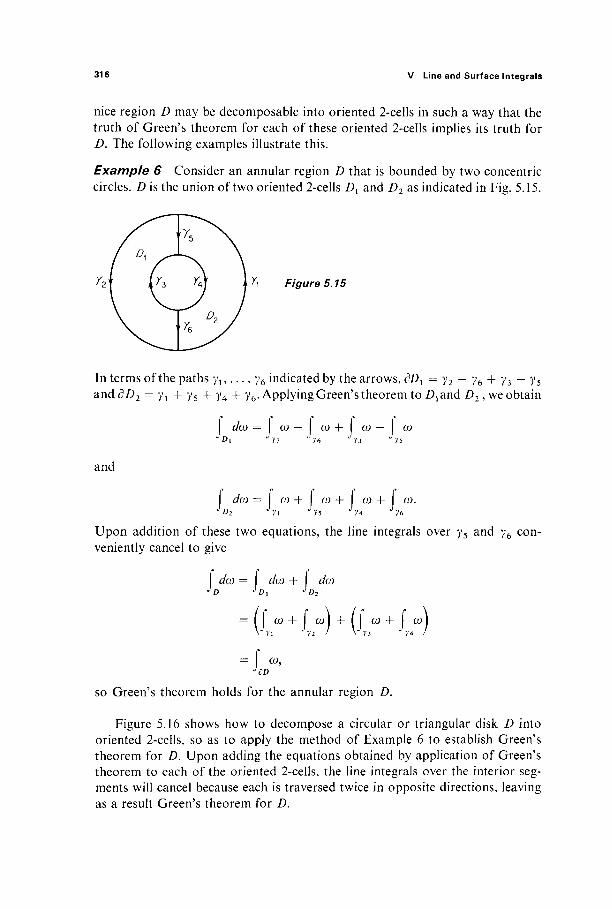
316 V Line and Surface Integrals
nice region D may be decomposable into oriented 2-cells in such a way that the truth of Green's theorem for each of these oriented 2-cells implies its truth for D. The following examples illustrate this.
Example 6 Consider an annular region D that is bounded by two concentric circles. D is the union of two oriented 2-cells Ώγ and D2 as indicated in Fig. 5.15.
Figure 5.15
In terms of the paths yl,..., yb indicated by the arrows, dDl = y2 — yb + y3 — y5
and<3Z)2 = yl + y5 + y4 + y6. Applying Green's theorem to Z^and D2, we obtain
dw = ω — ω + ω— ο
and
\ dw=\ JD2
J) ω + ω +
yi 75 "74 "ye ίω + ίω· Upon addition of these two equations, the line integrals over y5 and y6 con-veniently cancel to give
\ dœ = dœ -h άω ^ϋ ^Di J D2
-(/,."+/„")+(ίω+/„") = I ω,
so Green's theorem holds for the annular region D.
Figure 5.16 shows how to decompose a circular or triangular disk D into oriented 2-cells, so as to apply the method of Example 6 to establish Green's theorem for D. Upon adding the equations obtained by application of Green's theorem to each of the oriented 2-cells, the line integrals over the interior seg-ments will cancel because each is traversed twice in opposite directions, leaving as a result Green's theorem for D.
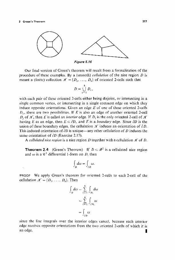
2 Green's Theorem 317
Figure 5.16
Our final version of Green's theorem will result from a formalization of the procedure of these examples. By a (smooth) cellulation of the nice region D is meant a (finite) collection X = {Z>l5 . . . , Dk} of oriented 2-cells such that
i = l
with each pair of these oriented 2-cells either being disjoint, or intersecting in a single common vertex, or intersecting in a single common edge on which they induce opposite orientations. Given an edge E of one of these oriented 2-cells D(, there are two possibilities. If E is also an edge of another oriented 2-cell Dj of Jf, then E is called an interior edge. If Dt is the only oriented 2-cell of X having E as an edge, then E <= dD, and £ is a boundary edge. Since dD is the union of these boundary edges, the cellulation C/f induces an orientation of dD. This induced orientation of dD is unique—any other cellulation of/) induces the same orientation of dD (Exercise 2.17).
A cellulated nice region is a nice region D together with a cellulation JT of D.
Theorem 2.4 (Green's Theorem) If D c and ω is a Ή1 differential 1-form on D, then
is a cellulated nice region
\ dœ = \ o J D JdD
PROOF We apply Green's theorem for oriented 2-cells to each 2-cell of the cellulation j f = {Ζ^, . . . , Dk). Then
\ dœ = Σ άω
J D i = 1 J Di
k r
= Σ J «
= ω
since the line integrals over the interior edges cancel, because each interior edge receives opposite orientations from the two oriented 2-cells of which it is an edge. |

318 V Line and Surface Integrals
Actually Theorem 2.4 suffices to establish Green's theorem for all nice regions because every nice region can be cellulated. We refrain from stating this latter result as a formal theorem, because it is always clear in practice how to cellulate a given nice region, so that Theorem 2.4 applies. However an outline of the proof would go as follows. Since we have seen how to cellulate triangles, it suffices to show that every nice region can be "triangulated," that is, decom-posed into smooth (curvilinear) triangles that intersect as do the 2-cells of a cellulation. If D has a single boundary curve with three or more vertices, it suffices to pick an interior point p of D, and then join it to the vertices of dD with smooth curves that intersect only in p (as in Fig. 5.17). Proceeding by
Figure 5.17
induction on the number n of boundary curves of the nice region D, we then notice that, if n > 1, D can be expressed as the union of an oriented 2-cell D1
and a nice region D2 having n — 1 boundary curves (Fig. 5.18). By induction, Dx and D2 can then both be triangulated.
This finally brings us to the end of our discussion of the proof of Green's theorem. We mention one more application.
Figure 5.18
Theorem 2.5 If ω = P dx + Q dy is a ^ 1 differential 1-form defined on J>2, then the following three conditions are equivalent:
(a) There exists a function/: 011 -> M such that df= ω. (b) dQ/dx = dP/dy on 0t2. (c) Given points a and b, the integral j y ω is independent of the piecewise
smooth path y from a to b.
PROOF We already know that (a) implies both (b) and (c) (Corollary 1.6), so it suffices to show that both (b) and (c) imply (a). Given (x, y) e ^ 2 , define
fix, y) = j ω, (10) v(x,y)
where γ(χ, y) is the straight-line path from (0, 0) to (x, y) (see Fig. 5.19).

2 Green's Theorem 319
U,y)
Figure 5.19
Let a(x, y) be the straight-line path from (0, 0) to (x, 0), and /?(x, y) the straight-line path from (x, 0) to (x, y). Then either immediately from (c), or by application of Green's theorem to the triangle T if we are assuming (b), we see that
ω + ω ι'α(χ, y) 7 ( χ , y)
= \ P(U 0) Λ + f (?(x, 0 <Λ.
Therefore
f = - ρ(χ, r) Λ = ρ(χ, JO rly dy - !
by the fundamental theorem of calculus. Similarly df/dx = P, so df=œ. |
The familiar form <Λ? shows that the plane M1 in Theorem 2.5 cannot be replaced by an arbitrary open subset U. However it suffices (as we shall see in Section 8) for U to be star shaped, meaning that U contains the segment γ(χ, y), for every (x, y) e U.
Example 7 If ω = y dx + x dy, then the function /"defined by (10) is given by
f(Xo* Jo) = y dx + xdy % }'(*o,>'o)
- f O'o t)(x0 dt) + (x0 t)(y0 dx)
= *o.Vo f 2tcit
*()}'(
so/(x, v) = xr (as, in the example, could have been seen by inspection).

320 V Line and Surface Integrals
Exercises
2.1 Let C be the unit circle x2 + y2 = 1, oriented counterclockwise. Evaluate the following line integrals by using Green's theorem to convert to a double integral over the unit diskD: (a) Jc Ox2 -y)dx + (x + 4y3) dy, (b) Sc(x2+y2)dy.
2.2 Parametrize the boundary of the ellipse x2/a2 + y2/b2 <[ 1, and then use the formula A= i J — >> dx + x ί/y to compute its area.
2.3 Compute the area of the region bounded by the loop of the "folium of Descartes," x3 + y3 = 3xy. Hint: Compute the area of the shaded half D (Fig. 5.20). Set y = tx to discover a parametrization of the curved part of dD.
Figure 5.20
2.4 Apply formula (10) in the proof of Theorem 2.5 to find a potential function φ (such that V<p = F) for the vector field F : ^ 2 -* ^ 2 , if (a) F(x9y) = (2xy*, 3*V), (b) F(x, y) = (sin 2x cos2 j \ —sin2 x sin 2j>).
2.5 Let/, # : [<z, 6] -> ^ be two ^ 1 functions such that/U) > #(*) > 0 on [a, b]. Let Z> be the nice region that is bounded by the graphs y = f(x), y = g(x) and the vertical lines x = a, x = b. Then the volume, of the solid obtained by revolving D about the x-axis, is
V= 7T | [f(x)]2 dx - 77- j [g(x)]2 dx
by Cavalieri's principle (Theorem IV.4.2). Show first that
V= -77 f y2 dx. J dD
Then apply Green's theorem to conclude that
V = \\ 2πγ dx dy = 2nAy, D
where A is the area of the region Z), and y is the ^-coordinate of its centroid (see Exercise IV.5.16).
2 Green's Theorem 321
2.6 Let /and g be #2 functions on an open set containing the nice region D, and denote by N the unit outer normal vector to 3D (see Exercise 1.20). The Laplacian V2/and the normal derivative df/dn are defined by
d2f e2f df V y = div (V/) = -L + - 4 and j - = V/· N.
δ*2 dy2 dn
Prove Green's formulas'.
(a) \\{fV2g + Vf*Vg)dxdy=\ f^-ds, JJ JdD dn
D
(b) J J ( / V*g - g VY) dx dy = j(f y^fff) ds. D
Hint: For (a) apply Green's theorem with P = — fdg/dy and Q = fdg/dx. 2.7 If/is harmonic on D, that is, V2/ = 0, s e t / = g in Green's first formula to obtain
df jjm>dxdy=jjlds.
I f / s O o n dD, conclude t h a t / ^ 0 on D. 2.8 Suppose that/and # both satisfy Poisson's equation on Z), that is,
V2/= V2<? = φ,
where φ(χ, j ) is given on D. I f / = g on dZ>, apply the previous exercise to/— #, to con-clude tha t /= g on D. This is the uniqueness theorem for solutions of Poisson's equation.
2.9 Given p e M2, let F : ^ 2 - p -> ^ 2 be the vector field defined by
F(x)= V l o g | x - p | 2 .
If C is a counterclockwise circle centered at p, show by direct computation that
f F . N ds = 4TT.
2.10 Let C be a counterclockwise-oriented smooth closed curve enclosing the points P i , . . . , p*. If F is the vector field defined for x Φ p, by
F ( x ) = i > V I o g | x - P l - | 2 , / = 1
where qu . . . , qk are constants, deduce from the previous exercise that
f F · N <fr = 4π(?ι + '·· +qk\
Hint: Apply Green's theorem on the region D which is bounded by C and small circles centered at the points Pi, . . . , p*.
2.11 Show that the integral Ja ω, of the differential form ω over the piecewise-smooth path γ is independent of the partition & used in its definition.
2.12 If a and β induce opposite orientations of the piecewise-smooth curve, show that Ja ω = - $β ω.
2.13 Prove that the orientation of the boundary of an oriented 2-cell is well-defined. 2.14 Show that every convex quadrilateral is a smooth oriented 2-cell.

322 V Line and Surface Integrals
2.15 If the mapping γ : [a, b]^ M2 is C6X and ω is a continuous 1-form, show that
(F*W=( ω. Jy JFoy
2.16 Prove Lemma 2.2. 2.17 Prove that the orientation of the boundary of a cellulated nice region is well-defined.
3 MULTILINEAR FUNCTIONS AND THE AREA OF A PARALLELEPIPED
In the first two sections of the chapter we have discussed 1-forms, which are objects that can be integrated over curves (or 1-dimensional manifolds) in 0tn. Our eventual goal in this chapter is a similar discussion of differential Ar-forms, which are objects that can be integrated over /c-dimensional manifolds in Mn. The definition of 1-forms involved linear functions on 0F\ the definition of &-forms will involve multilinear functions on 0tn.
In this section we develop the elementary theory of multilinear functions on 0ln, and then apply it to the problem of calculating the area of a ^-dimensional parallelepiped in $n. This computation will be used in our study in Section 4 of /:-dimensional surface area in ^".
Let {0tnf = @n x · · · x @n (k factors), and consider a function
Then M i s a function on ^-tuples of vectors in 0tn ; M (a1, . . . , a*) e (% if a1 , . . . , a* are vectors in $n. Thus we can regard M as a function of k vector variables. The function M is called k-mult[linear (or just multilinear) if it is linear in each of these variables separately, that is,
Μ{Ά\ . . . , xa + jb , . . . , a") = xAf(a\ . . . , a, . . . , a*) + yM(*\ . . . , b, . . . , a*).
We will often call M a ^-multilinear function on 0tn, despite the fact that its domain of definition is actually (0T)k. Note that a 1-multilinear function on 0tn
is just an (ordinary) linear function on 3#n. We have seen that every linear function on 0ln is a linear combination of
certain special ones, namely the projection functions dxl, — dxn. Recall that, regarding a e I " as a column vector, dx{ is the function that picks out the /th row of this vector, rfx,-(a) = a,.
We would like to have a similar description of multilinear functions on 0tn. Given a Ar-tuple i = (il, . . . , ik) of integers (not necessarily distinct) between 1 and n, 1 ^ ir ^ n, we define the function
dx{ : (Mn)k -> (M
3 Multilinear Functions 323
by
| < ah ·■■ < |
i/xjia1, . . . , a*) = j ί ; . I< 4 ··· <l
That is, if /i is the n x A: matrix whose column vectors are a1, . . . , a\
A = (a1 · · · a*)
and Ax denotes the k x k matrix whose rth row is the /rth row of A, then
i/xi(a1,...,aÄ) = d e t ^ i . Note that Ax is a k x k submatrix of A if i is an increasing /c-tuple, that is, if 1 ^ z\ < i2 < · · · < ik S. n.
It follows immediately from the properties of determinants that dx-x is a ^-multilinear function on 0tn and, moreover, is alternating. The ^-multilinear function M on 0tn is called alternating if
A/(a! , . . . ,a*) = 0
whenever some pair of the vectors a1, . . . , a* are equal, say ar = as (r Φ s). The fact that dx{ is alternating then follows from the fact that a determinant vanishes if some pair of its columns are equal.
It is easily proved (Exercise 3.1) that the ^-multilinear function M on 0tn is alternating if and only if it changes signs upon the interchange of two of the vectors a1, . . . , a*, that is,
M(a\ . . . , ar, . . . , as, . . . , a*) = - M ( a ! , . . . , as, . . . , ar, . . . , a*).
The notation dx{ generalizes the notation dxt for the z'th projection function on 0in, and we will prove (Theorem 3.4) that every alternating ^-multilinear function M on ffln is a linear combination of the dxx. That is, there exist real numbers at such that
M = £ ax d\{, i
the summation being over all /:-tuples i of integers from 1 to n. This generalizes the fact that every linear function on 0tn is of the form £ at dxi. Notice that every linear function on 0Γ is automatically alternating.
Proposition 3.1 If M is an alternating ^-multilinear function on 0ln, then
A/fa1,.. . , a*) = 0
if the vectors a1, . . . , a* are linearly dependent.

324 V Line and Surface Integrals
This follows immediately from the definitions and the fact that some one of the vectors a1, . . . , afc must be a linear combination of the others (Exercise 3.2).
Corollary 3.2 If k > n, then the only alternating /:-multilinear function on 0tn is the trivial one whose only value is zero.
The following theorem describes the nature of an arbitrary /c-multilinear function on 0t (not necessarily alternating).
Theorem 3.3 Let M be a /c-multilinear function on 0tn. If a1, . . . , a* are vectors in 0ln, a7 = (αγΚ · · ·, an
J), then n
M(a 1 , . . . , a " )= X α , ν . . , . χ α ? 2 · · · 4 , i l , . . . , Ile = 1
where
aI.1...ik = M(e , \ . . . , e i f c ) .
Here e1 denotes the /th standard unit basis vector in 0tn.
PROOF The proof is by induction on k, the case k = 1 being clear by linearity. For each r = 1, . . . , n, let Nr denote the (k — l)-multilinear function on 0tn
defined by
Nr(*\ . . . , a""1) - Mia1, . . . , a*"1, er).
Then
M(*\ . . . , a*) = £ arkM(*\ . . . , ak_1, er)
r = 1
= f α,^ίβ',..., a*"1) r= 1
= £>,*(£ tfr(e\...,e'*- ,Κ···<:,1)
r = l \ i j = l /
= £ e,*( X M(e'\ ..., e'- ', e'K · · · <"_>)
n
= Σα.ν··.·Χ··Χ as desired. I
We can now describe the structure of M in terms of the dxx, under the ad-ditional hypothesis that M is alternating.

3 Multilinear Functions 325
Theorem 3.4 If M is an alternating A-multilinear function on Mn, then
M = Σ ai dxi* [ i ]
where o = M(eh e'k). Here the notation [i] signifies summation over all increasing /r-tuples i = (/j, . . . , /fc).
For the proof we will need the following.
Lemma 3.5 Let i = (/j, . . . , ik) and j = ( /\, — jk) be increasing ^-tuples of integers from 1 to n. Then
dx-(ejl ejk) = I ! =J' tfx.ie , . . . , e ) | Q j f . # .
This lemma follows from the fact that dx{{eJ\ . . . , eJk) is the determinant of the matrix (<V), where
if i=7, <5 ·■' = - »
\0 if / # / If i = j , then (<$/) is the / e x / : identity matrix; otherwise some row of (<5/) is zero, so its determinant vanishes.
PROOF OF THEOREM 3.4 Define the alternating ^-multilinear function M on
M(a\ . . . , a*) - X «i i/x^a1, . . . , afc), [ i ]
where OL-X = A/(e'\ . . . , e'k). We want to prove that M = M. By Theorem 3.3 it suffices (because M and M are both alternating) to show
that
M(eJl, . . . , e7'k) = M(e7\ . . . , eik)
for every increasing k-tupk j = ΟΊ, . · ·, Λ). But
M(eji, . . . , eyk) = X ai i/x^e7'1, . . . , eik) [ i ]
= M(ej\ . . . , e7k)
immediately by Lemma 3.5. |
The determinant function, considered as a function of the column vectors of an n x n matrix, is an alternating «-multilinear function on 0tn. This, together with the fact that the determinant of the identity matrix is 1, uniquely charac-terizes the determinant.

326 V Line and Surface Integrals
Corollary 3.6 D = det is the only alternating /7-multilinear function on &n such that
Z) (e \ . . . , e")= 1.
PROOF Exercise 3.3. |
As an application of Theorem 3.4, we will next prove the Binet-Cauchy product formula, a generalization of the fact that the determinant of the product of two n x n matrices is equal to the product of their determinants. Recall that, if A is an n x k matrix, and i = (il, . . . , /fc), then Ax denotes that k x k matrix whose rth row is the /rth row of A.
Theorem 3.7 Let A be an k x n matrix and B an n x k matrix, where k ^ n. Then
det/IÄ = X(det/i it )(det^i) ·
[ i ]
Here A1 denotes the transpose of A and, as in Theorem 3.4, [i] signifies summation over increasing /r-tuples.
Note that the case k = n, when A and B are both n x n matrices, is
det AB = (det Al)(det B) = (det ^)(det B).
PROOF Let aj, . . . , ak be the row vectors of A, and b1, . . . , bk the column vectors of B. Since
/ a . - b 1 · · a,-b<\ AB=[\
\ a t - b ' · · · a t - b 7
we see that, by holding fixed the matrix A, we obtain an alternating /r-multi-linear function M of the vectors b1, . . . , b*,
M(b \ . . . , b* ) = det/I£.
Consequently by Theorem 3.4 there exist numbers ai (depending upon the matrix A) such that
M = Yj(xidxi. [ i ]
Then
A/(b1,...,b*) = Xairfx i (b1 , . . . ,bk) [ i ]
= X aâ(det ^ ) . [ i ]
3 Multilinear Functions 327
But
as = A/(e'\ . . . , e,k)
^ d e t ^ e ' " 1 .. . e'k)
lull! aH2 '" aUk I
I akix aki2 ' ' ' akik I
= d e t ^ 1 ,
so
dctAB = M(b\...,bk)
= Y(detAit)(detBi)
[ i ]
as desired. |
Taking A = B\ we obtain
Corollary 3.8 If A is an n x A- matrix, k ^ w, then
d e t ^ = X ( d e t ^ i ) 2 . [ i ]
Our reason for interest in the Binet-Cauchy product formula stems from its application to the problem of computing the area of an /:-dimensional parallele-piped in 0tn, Let SLU . . . , afc be k vectors in Mn. By the /c-dimensional parallele-piped P which they span is meant the set
n
P = {x e 0tn : x = X if a, with each t{ e [0, 1 ]}. t ' = 1
This is the natural generalization of a parallelogram spanned by two vectors in the plane. If k = n, then P is the image of the unit cube /", under the linear mapping S£ : 0tn -► Mn such that L(ef·) = a,·, / = 1, . . . , n. In this case the volume of P is given by the following theorem.
Theorem 3.9 Let P be the parallelepiped in @n that is spanned by the vectors a1? . . . , a„. Then its volume is
v(P) = (detAtA)i/\
where A is the n x n matrix whose column vectors are a1? . . . , a„.
328 V Line and Surface Integrals
PROOF If the linear mapping L : 0ln -> M is defined by
L(x) = Ax,
then L(ef) = a,, / = 1, . . . , n. Hence P = L(F). Therefore, by Theorem IV.5.1,
v(P) = | det A | v(F)
= \detA\
= [(detA)2]1/2
= [ d e t ^ ] 1 / 2
since
det A1 = det A. |
Now let X be a subset of a /:-dimensional subspace Kof 0tn (k < ri). A choice of an orthonormal basis vl5 . . . , vfc for V (which exists by Theorem 1.3.3) de-termines a 1-1 linear mapping φ : K - > ^ \ defined by (p(vt) = et·. We want to define the k-dimensional area a(X) by
a(X) = ν{φ{Χ)).
However we must show that a{X) is independent of the choice of basis for V. If wl5 . . . , wk is a second orthonormal basis for V, determining the one-to-one linear mapping φ : V-+ $k by ^(wt) = et-, then it is easily verified that
φ οφ~ι :@k->Mk
is an orthogonal mapping (Exercise 1.6.10). It therefore preserves volumes, by Corollary IV.5.2. Since φ ο φ~\φ(Χ)) = φ(Χ), we conclude that v(cp(X)) = ν(φ(Χ)), so tf(^) is well defined. The following theorem shows how to compute it for a ^-dimensional parallelepiped.
Theorem 3.10 If P is a /c-dimensional parallelepiped in 0tn (k <ri) spanned by the vectors al5 . . . , afc, then
a(P) = [det A{A]112,
where A is the n x k matrix whose column vectors are al5 . . . , afc.
Thus we have the same formula when k < n as when k = n.
PROOF Let V be a /:-dimensional subspace of 0tn that contains the vectors a l 9 . . . , afc, and let v l 9 . . . , vn be an orthonormal basis for 0ln such that vl9 . . . , \k
generate V. Let Φ : 3%n -> 0tn be the orthogonal mapping defined by Φ(ν,) = e,, / = 1 , . . . , n. If bj = 0(af), / = 1 , . . . , /c, then Φ(Ρ) is the ^-dimensional parallele-piped in 0lk that is spanned by bl9 . . . , bfc. Consequently, using Theorem 3.9
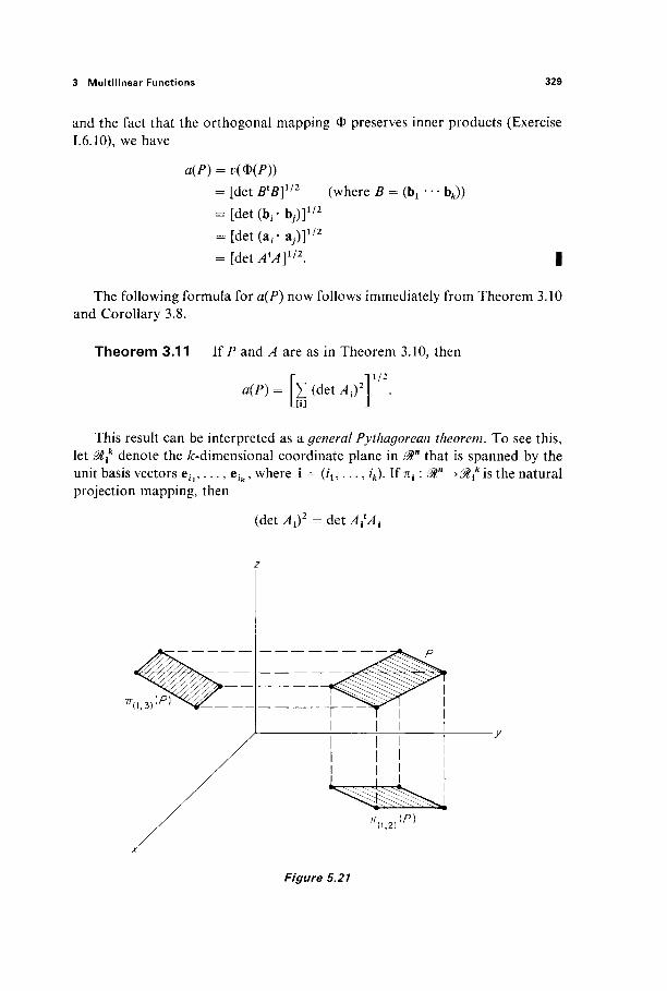
3 Multilinear Functions 329
and the fact that the orthogonal mapping Φ preserves inner products (Exercise 1.6.10), we have
a(P) = ν(Φ(Ρ))
= [det B'B]1'2 (where B = (bx · · · bfc)) = [det(bt.-b,)]1/2
= [det(a i .-ay)]1/2
= [ d e t ^ ] 1 / 2 . |
The following formula for a(P) now follows immediately from Theorem 3.10 and Corollary 3.8.
Theorem 3.11 If P and A are as in Theorem 3.10, then 11/2
a(P) = X(det^ i ) 2
This result can be interpreted as a general Pythagorean theorem. To see this, let 01* denote the /c-dimensional coordinate plane in 0tn that is spanned by the unit basis vectors eiV . . . , e/k, where i = (it,..., ik). If n{ : 0ln -+01* is the natural projection mapping, then
(det^i)2 = detAitAi
^ ( 1 , 3 ) ^
Figure 5.21
330 V Line and Surface Integrals
is the square of the ^-dimensional area of the projection n{{P) of P into $* (see Exercise 3.4). Thus Theorem 3.11 asserts that the area of the k-dimensional parallelepiped P is equal to the square root of the sum of the squares of the areas of all projections of P into k-dimensional coordinate planes of 0ln (see Fig. 5.21 for the case k = 2, n = 3). For k = 1, this is just the statement that the length of a vector is equal to the square root of the sum of the squares of its components.
Exercises
3.1 Prove that the ^-multilinear function M on Mn is alternating if and only if the value M(a*,..., afc) changes sign when ar and as are interchanged. Hint: Consider Mia1, . . . , ap + as, . . . , ar -f as,..., ak).
3.2 Prove Proposition 3.1. 3.3 Prove Corollary 3.6. 3.4 Verify the assertion in the last paragraph of this section, that det ΑΪΑι is the square of the
^-dimensional area of the projection ττ^Ρ), of the parallelepiped spanned by the column vectors of the n x k matrix A, into ^V.
3.5 Let P be the 2-dimensional parallelogram in ^ 3 spanned by the vectors a and b. Deduce from Theorem 3.11 the fact that its area is a(P) = | a X b| .
3.6 Let P be the 3-dimensional parallelepiped in ^ that is spanned by the vectors a, b, c. Deduce from Theorem 3.9 that its volume is v(P) = |a · b X c|.
4 SURFACE AREA
In this section we investigate the concept of area for /:-dimensional surfaces in 0t. A /c-dimensional surface patch in Mn is a ^ 1 mapping F : Q -> <%n, where Q is a /c-dimensional interval (or rectangular parallelepiped) in $k, which is one-to-one on the interior of Q.
Example 1 Let Q be the rectangle [0, In] x [0, π] in the οφ-plane ^ 2 , and F : Q -► ^ 4 the surface patch defined by
x = 7^(0, φ) = α sin φ cos Θ,
y = F2(6, φ) = a sin φ sin Θ,
z = F3(6, φ) = a cos Θ,
so a, θ, φ are the spherical coordinates of the point (x, y, z) = F(6, φ) e &3. Then the image of F is the sphere x2 4- y2 + z2 = a2 of radius a (Fig. 5.22). Notice that F is one-to-one on the interior of Q, but not on its boundary. The top edge of Q maps to the point (0, 0, —a), the bottom edge to (0, 0, a), and the image of each of the vertical edges is the semicircle x2 -f- z2 = a2, x ^ 0, y = 0.
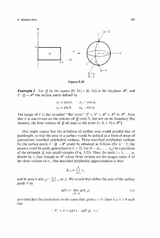
4 Surface Area 331
Figure 5.22
Example 2 Let Q be the square [0, In] x [0, 2π] in the Οφ-plane M1, and F : β -► ^ 4 the surface patch defined by
xl = cos 0,
Xi = sin Ö,
x3 = cos <p, x4 = sin φ.
in ^ r . Note The image of F is the so-called "flat torus" Sl x S1 <= 0t2 x that F i s one-to-one on the interior of β (why?), but not on its boundary [for instance, the four vertices of Q all map to the point (1,0, 1, 0) G ^?4].
One might expect that the definition of surface area would parallel that of pathlength, so that the area of a surface would be defined as a limit of areas of appropriate inscribed polyhedral surfaces. These inscribed polyhedral surfaces for the surface patch F : Q ->0tn could be obtained as follows (for k = 2; the process could be easily generalized to k > 2). Let 0> = {σι, . . . , σρ} be a partition of the rectangle Q into small triangles (Fig. 5.23). Then, for each / = 1, . . . , / ? , denote by τ< that triangle in 0tn whose three vertices are the images under F of the three vertices of oi. Our inscribed polyhedral approximation is then
K&= U *,-,
and its area is a(K&) = £ ? = j ο(τ,). We would then define the area of the surface patch F by
a(F) = lim a(K#), | # | - 0
(1)
provided that this limit exists in the sense that, given ε > 0, there is a S > 0 such that
| ^ | < ( 5 ^ | a ( F ) - a ( / ^ ) | < ε.
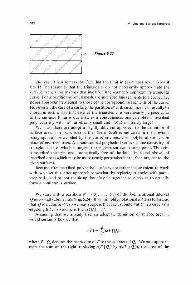
332 V Line and Surface Integrals
/ 0 Figure 5.23
However it is a remarkable fact that the limit in (1) almost never exists if k > 1 ! The reason is that the triangles τ,- do not necessarily approximate the surface in the same manner that inscribed line segments approximate a smooth curve. For a partition of small mesh, the inscribed line segments to a curve have slopes approximately equal to those of the corresponding segments of the curve. However, in the case of a surface, the partition £P with small mesh can usually be chosen in such a way that each of the triangles τζ· is very nearly perpendicular to the surface. It turns out that, as a consequence, one can obtain inscribed polyhedra K& with \&\ arbitrarily small and a(K$) arbitrarily large!
We must therefore adopt a slightly different approach to the definition of surface area. The basic idea is that the difficulties indicated in the previous paragraph can be avoided by the use of circumscribed polyhdral surfaces in place of inscribed ones. A circumscribed polyhedral surface is one consisting of triangles, each of which is tangent to the given surface at some point. Thus cir-cumscribed triangles are automatically free of the fault (indicated above) of inscribed ones (which may be more nearly perpendicular to, than tangent to, the given surface).
Because circumscribed polyhedral surfaces are rather inconvenient to work with, we alter this latter approach somewhat, by replacing triangles with paral-lelepipeds, and by not requiring that they fit together so nicely as to actually form a continuous surface.
We start with a partition £P = {Qi, . . . , Qp} of the /:-dimensional interval Q into small subintervals (Fig. 5.24). It will simplify notational matters to assume that Q is a cube in $k, so we may suppose that each subinterval Qx is a cube with edgelength h\ its volume is then v(Qt) = hk.
Assuming that we already had an adequate definition of surface area, it would certainly be true that
i= 1
where F | Q, denotes the restriction of F to the subinterval Qt. We now approxi-mate the sum on the right, replacing a(F | Q() by a(dFq.(Qi)), the area of the
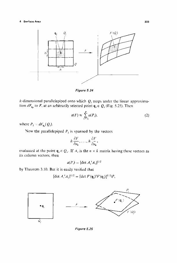
4 Surface Area 333
q, oi
V m
0
Figure 5.24
/r-dimensional parallelepiped onto which Qx maps under the linear approxima-tion dfq. to F, at an arbitrarily selected point q, e Qt (Fig. 5.25). Then
a{F) » X α(Λ), i = 1
where P , = dF^iQ,).
Now the parallelepiped Ff is spanned by the vectors
(2)
dF_
diii ' duk
evaluated at the point qt e Qt. If At is the n x k matrix having these vectors as its column vectors, then
a(Pi) = [ d e t ^ J 1 ' 2
by Theorem 3.10. But it is easily verified that
[det AtAtf12 = [det ^(ς , . ) 1 /^ , ) ] 1 ' 2 /^ ,
F
Figure 5.25
334 V Line and Surface Integrals
since the matrix F' has column vectors dF/du^ . . . , dF/duk. Upon substitution of this into (2), we obtain
i = 1
Recognizing this as a Riemann sum, we finally define the (Ar-dimensional) surface area a(F) of the surface patch F : Q -> 0ln by
a(F) = f [det F ^ f » ] 1 7 2 </u. (3)
Example 3 If Z7 is the spherical coordinates mapping of Example 1, mapping the rectangle [0, 2π] x [0, π] <^^Ιφ onto the sphere of radius a in J>3, then a routine computation yields
det F(0, φ)ιΓ(0, φ) - a2 sin </>,
so (3) gives
a(F) = a2 sin φ rfö ί/φ = 4πα2
as expected.
Example 4 If F : [α, 6] -► <#" is a ^ 1 path, then
/OF, dFn
OF, \1Γ/
so we recover from (3) the familiar formula for pathlength.
Example 5 We now consider 2-dimensional surfaces in 0tn. Let φ: Q -+ 0ln
be a 2-dimensional surface patch, where Q is a rectangle in the w^-plane. Then
/ M ΟφΛ(δ_^ ^Λ
(<P')V du du
\dv '" dv )
du dv
\ du dv I (equation continues)
4 Surface Area 335
Idcp δφ δφ δφ\
I du du du dv
I d(p dcp dip dcp
\dv du dv dv I
Equation (3) therefore yields
α(φ) = jj(EG - F2)1'1 du dv, (4)
where
du du ' F=dcp dcp
du dv ' 0 = δφ_.άφ
dv dv
If we apply Corollary 3.8 to Eq. (3), we obtain
a(F)= f [l(detF/)2]1/2, J<2L[i] J (5)
where the notation [i] signifies (as usual) summation over all increasing fc-tuples i = 0Ί, .. ·, ik), and Ff' is the k x k matrix whose rth row is the irth row of the derivative matrix F' = (dF^dUj). With the Jacobian determinant notation
det F*' = d(Fil9...,Fik)^ d(uu . . . , uk)
Eq. (5) becomes
<n = f f i ( T , , , ' ' ' , F , C ) ) T / 2 d u ^ ~ d U k - (6) JQ L[i] \Ö("i, . . . , Wfc) / J
We may alternatively explain the [i] notation with the statement that the sum-mation is over all k x k submatrices of the n x k derivative matrix F'.
In the case k = 2, n = 3 of a 2-dimensional surface patch F in &3, given by x = Ft(u9 v), y = F2(u, v), z = F3(u, v),
(6) reduces to
Example 6 We consider the graph in ^ " of a <€x function/: Q -> 01, where Q is an interval in <%n~l. This graph is the image in &n of the surface patch F : Q -> 0tn defined by
F(xu . . . , xn_x) = (x1? . . . , xn_uf(xi9 . . . , x„_!)) e ^".

336 V Line and Surface Integrals
The derivative matrix of Fis
F \
1 0
0
\dxl
e want to apply (6) to compute a
3(Ft,
/ < n, then
d{Fu .
0 1
0
δχ2
·· 0 o 1 1
—1 dXn-lj
(F). First note that
■■■,Fn.
• · , Λ .
1-'-■■■,Fn)
(8)
is the determinant of the (ft — 1) x (n — 1) matrix Ax which is obtained from F' upon deletion of its ith row. The elements of the ith column of A{ are all zero, except for the last one, which is df/dXi. Since the cofactor of df/dxi in A{ is the (ft — 2) x (>2 — 2) identity matrix, expansion by minors along the /th column of v4f gives
3 ( 7 ^ . . . ^ , . . . , ^ ) det^l:
d(xl9 . . . ,*„_!)
for / < «. Substitution of (8) and (9) into (6) gives
OX;
= f[i + |v/|2]1
2 Ί 1 / 2
I 2 1 1 / 2
(9)
(10)
over In the case n = 3, where we are considering a graph z = / ( * , }>) in Q <= ^£2, and F(x, y) = (x, y,f(x, y)), formula (10) reduces to
This, together with (4) and (7) above, are the formulas for surface area in 0lz
that are often seen in introductory texts.
Example 7 We now apply formula (10) to calculate the (ft - l)-dimensional area of the sphere Sn
r~x of radius r, centered at the origin in 0ln. The upper
4 Surface Area 337
hemisphere of 5" * is the graph in $n of the function
f(xl,...,xn_l) = [r2-xl2-----x2
n-l]m
= [r2-\x\2V'2,
defined for xeB"'1 c ^ " " 1 . / i s continuous on B?~\ and V1 on int5r"_ 1 , where
3f _ -Xi dXi [r2 - | x | 2 ] 1 / 2 '
so
and therefore
|V/(x) | 2 =
[l + | V / | 2 ] 1 / 2 =
r2
[ r 2 - | x | 2 ] 1 / 2
Hence we are motivated by (10) to define α(£"_1) by
r dxt ■ ■ · dx„-i ( r ) _ J B r - . [ r 2 - | x | 2 ] 1 / 2
This is an improper integral, but we proceed with impunity to compute it. In order to "legalize" our calculation, one would have to replace integrals over B?~x with integrals over B"Z^ , and then take limits as ε -► 0.
If Γ : ^ - 1 - ^ « ; " 1 i s defined by T(u) = ru, then T{Bn~l) = Bnr~
l and det T = r n - 1 , so the change of variables theorem gives
a(Sn-u_2( rdxx---dxn-,
r r - rn~l du^ -' dun = 2 ) B n - i [ r 2 _ r 2 | u | 2 ] l / 2
= 2rn~l f J nn
i/wj · · · dun _ j
B - ' [ 1 - | U | 2 ] 1 / 2 '
a(5,;-1) = rn-1ur(S"-1).
Thus the area of an (n — l)-dimensional sphere is proportional to the (n — l)th power of its radius (as one would expect).
Henceforth we write
wn = a(S"-1)
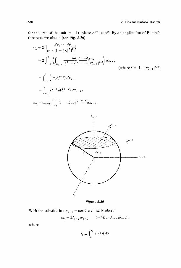
338 V Line and Surface Integrals
for the area of the unit (n — l)-sphere S" * c 0tn. By an application of Fubini's theorem, we obtain (see Fig. 5.26)
ωη = 2 dxx - · · dxn_ r αχχ · · ' *
J B — [1 - |x
1 2 i l / 2
dxi '-dxn-2
■xi-2] 1/2 I dx„-i
= f r"~3a(S"-2)dxn-J - 1
ωη = ω„.χ (\ - χΙΛ»-™1 dxn.v
(where r = [1 - J C 2 _ J 1 / 2 )
^ - 2
Figure 5.26
With the substitution *„_! = cos 0 we finally obtain
ωη = 2Ιη-2ωη-ι ( = 4/η_2/η_3ωη_2),
where
A = sin* 0 de. -r
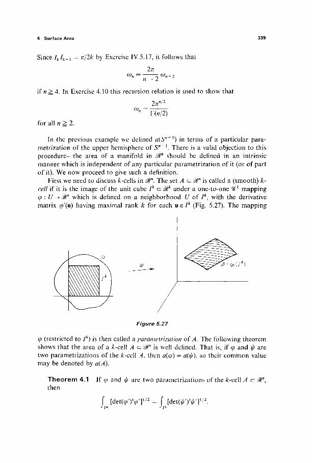
4 Surface Area 339
Since /fc4_i = njlk by Exercise IV.5.17, it follows that
In
if n ^ 4. In Exercise 4.10 this recursion relation is used to show that
2π"/2
co„ = n Γ>/2) for all n ^ 2.
In the previous example we defined a(S"-1) in terms of a particular para-metrization of the upper hemisphere of S"'1. There is a valid objection to this procedure—the area of a manifold in 0tn should be defined in an intrinsic manner which is independent of any particular parametrization of it (or of part of it). We now proceed to give such a definition.
First we need to discuss fc-cells in 0tn. The set A c 0tn is called a (smooth) k-cell if it is the image of the unit cube Ik a 0lk under a one-to-one ^ 1 mapping φ : U -► ffln which is defined on a neighborhood U of / \ with the derivative matrix <p'(u) having maximal rank /: for each u G Ik (Fig. 5.27). The mapping
Figure 5.27
φ (restricted to /*) is then called a parametrization of A. The following theorem shows that the area of a A-cell A <= ^ " is well defined. That is, if φ and ^ are two parametrizations of the k-cd\ A, then α(φ) = α(ψ), so their common value may be denoted by a(A).
Theorem 4.1 If φ and φ are two parametrizations of the k-ce\\ A cz &ny
then
f [det(<p')V']1/2 = f [det(^')V']1/2·

340 V Line and Surface Integrals
PROOF Since <p'(u) has rank k, the differential άφη maps $k one-to-one onto the tangent /c-plane to A at φ(ιι), and the same is true of d\j/u. If
T: Ik-+Ik
is defined by T= φ'1 ° φ, it follows that T is a ^ 1 one-to-one mapping with det 7"(u) # 0 for all u e /* so, by the inverse function theorem, Tk ^-invertible.
Since φ = Γ ο ψ, the chain rule gives
(«/)V) = ((φ o T)')W « D '
so
[det(ç)')V']1/2 = [det(i/OV']1/2|det T'\.
Consequently the change of variables theorem gives
f [det(<p')Vl1/2 = f [det(iA'(nu)))V'(^(u))]1/2|detr(u)|c/u JJk JJk
= f [det(^')V']1/2
J Jk
as desired. |
If M is a compact smooth /c-manifold in ^", then M is the union of a finite number of nonoverlapping /c-cells. That is, there exist Ar-cells Au . . . , Ar in 0ln
such that M ={Jri=l At and int Λ,· n int Λ,· = 0 i f ïVy. Such a collection
{>4l5 . . . , Ar} is called a paving of M. The proof that every compact smooth manifold in Mn is pavable (that is, has a paving) is very difficult, and will not be included here. However, if we assume this fact, we can define the (/c-dimensional) area a{M) of M by
a(M) = £ a(Ad. i= 1
Of course it must be verified that a(M) is thereby well defined. That is, if {Bl9..., Bs} is a second paving of M, then
ία(Α,)= ta(Bj).
The proof is outlined in Exercise 4.13.
Example 8 We now employ the above definition, of the area of a smooth manifold in 0tn, to give a second computation of ωη = aiS"'1). Let {Au . . . , Ak} be a paving of S"1"1. Let φ : F'1 -> Λ4 be a parametrization of Λ;. Then, given ε > 0 , define Φ : / " _ 1 χ [ε, l ] - > 0 " b y
0(u, r) = r<p(u) for U E / " " 1 , r e [e , 1].
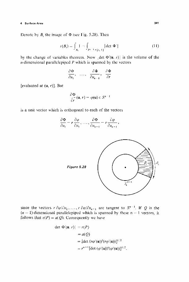
4 Surface Area 341
Denote by Bt the image of Φ (see Fig. 5.28). Then
V(B.) = Γ I = Γ |det Φ'| *' Bi J / n - l x [ £ f 1 ]
(Π)
by the change of variables theorem. Now | det Φ'(ιι, r)\ is the volume of the /7-dimensional parallelepiped P which is spanned by the vectors
5Φ ^Φ οΦ
[evaluated at (u, r)]. But
dui' ' dun-l dr
ΟΦ — (u,r) = cp(u)eSn-i
or
is a unit vector which is orthogonal to each of the vectors
δΦ dcp = r
δΦ dcp = r-du^ dux ' ' dun_l diin_i
Figure 5.28
since the vectors r οφΙοιιγ, . . . , r αφ/διιη_1 are tangent to S"~ \ If Q is the (n — l)-dimensional parallelepiped which is spanned by these n — 1 vectors, it follows that v(P) = a( Q). Consequently we have
| det 0 ' (u,r) | = v(P)
= a(Q)
= [det(r^'(u))t(r^/(u))]1/2
= r"- ! [det(^(u))V(u))]1 / 2 .
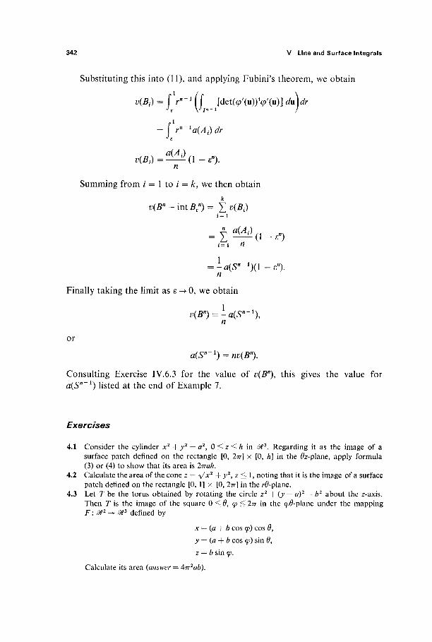
342 V Line and Surface Integrals
Substituting this into (11), and applying Fubini's theorem, we obtain
v(Bt) = fr"'1 ^ ^Χ(φ'(η)Υφ'(η)] dv^dr
= f rn~la(A^dr Jε
Κ 5 , ) = ^ ( 1 - ε « ) . n
Summing from / = 1 to / = k, we then obtain
v(B"-intBE") = ΣνΜ) i= 1
^ a(A:)
i=\ n
= -a(S"-1)(\ -εη). n
Finally taking the limit as ε -► 0, we obtain
v(Bn)=-a(Sn-l\ n
or
a{Sn~1) = nv{B%
Consulting Exercise IV.6.3 for the value of v(Bn), this gives the value for a(Sn~l) listed at the end of Example 7.
Exercises
4.1 Consider the cylinder x2 + y2 = a2, 0 <j z <Ξ h in ^ 3 . Regarding it as the image of a surface patch defined on the rectangle [0, 2π] χ [0, h] in the 0z-plane, apply formula (3) or (4) to show that its area is 2παη.
4.2 Calculate the area of the cone z = V-*2 + y2> z ^ 1, noting that it is the image of a surface patch defined on the rectangle [0, 1] x [0, 2π] in the r#-plane.
4.3 Let T be the torus obtained by rotating the circle z2 + (y — a)2 = b2 about the z-axis. Then T is the image of the square 0 ^ θ, φ ^ 2π in the φ^-plane under the mapping F : ^ 2 - > ^ 3 defined by
x= (a + b cos φ) cos Θ,
y = (a + b cos φ) sin Θ,
z = b sin φ.
Calculate its area (answer = 4n2ab).

4 Surface Area 343
4.4 Show that the area of the " flat torus " Sl x S1 <= ?4, of Example 2, is (2π)2. Generalize this computation to show that the area, of the "«-dimensional torus" S1 x ··· x S1
c ®2 x · · · x @2 = ^2", is (2π)π. 4.5 Consider the generalized torus S2 x 5 2 c ^ 3 χ ^ 3 = <^6. Use spherical coordinates in
each factor to define a surface patch whose image is S2 x S2. Then compute its area. 4.6 Let C be a curve in the j>z-plane described by y = α(/), z = ß(t) for / e [a, b]. The surface
swept out by revolving C around the z-axis is the image of the surface patch φ : [0, 2π] x [«, b] -> ^ 3 defined by
JC = a(/)cos Θ,
y = a(/) sin Θ,
z=ß(t).
Show that α(φ) equals the length of C times the distance traveled by its centroid, that is,
α(ψ) = {2iry)L where y = (\/L) y ds.
4.7 Let y(s) = (a(.s), ß(s)) be a unit-speed curve in the jcy-plane, so (α')2 + iß')1 = 1. The "tube surface" with radius r and center-line y is the image of φ : [0, L] x [0, 2π] -> ^ 3 , where φ is given by
* = oc(s) -f rj8'(j) cos 0, j> = j8(j) — ru.'(s) cos 0, z = r sin 0.
Show that a(<p) = 27irL. 4.8 This exercise gives an «-dimensional generalization of "Pappus* theorem for surface
area" (Exercise 4.6). Let φ : Q-+ &"~l be a ^-dimensional surface patch in @n~l, such that φ„_ι(ιι) Ξ> 0 for all ue Q. The (k + l)-dimensional surface patch
Φ : Q x [0, 2π] -> #",
obtained by "revolving φ about the coordinate hyperplane ^"~2," is defined by
Φ(ιι, Θ) = (<pi(u),..., <pB_2(u), 9?n-i(u) cos Θ, ç>„_i(u) sin 0)
for u e Q, 0 e [0, 2π]. Write down the matrix Q', and conclude from inspection of it that
(Φ<)·Φ'= - (ψΎψ/
V 0 - - - 0
0
0
ψη-ί/
[det (Φ')ιΦ']1/2 = <p„-i[det (φΎφΎ/2.
Deduce from this that α(Φ) = 2πχη_1α(φ),
where *„_! is the (n — l)th coordinate of the centroid of 99, defined by
xn-i = ~— f ψη-ι [det {ψΎψ'Υ12· α{ψ) JQ
344 V Line and Surface Integrals
4.9 Let T : Mn -> (Mn be the linear mapping defined by T(\) = bx. If φ : Q -> ,Άη is a Â>dimen-sional surface patch in £#", prove that ο ( ίο φ) = bka{cp).
4.10 Starting with co2 = 2π and ω 3 = 4π, use the recursion formula
2π
n-2
of Example 7, to establish, by separate inductions on m, the formulas
277 W
ω2„ ( w - D ! and
ω 2 ι ι ι + 1 :
1 - 3 - 5 ( 2 m - 1)
for ωη = Λ ( 5 " - 1 ) · Consulting Exercise IV.6.2, deduce that
2πηΙ2
Γ(/ι/2)
for all « ^ 2. 4.11 Use the «-dimensional spherical coordinates of Exercise IV.5.19 to define an (//— 1)-
dimensional surface patch whose image is Sn~{. Then show that its area is given by the formula of the previous exercise.
4.12 This exercise is a generalization of Example 8. Let M be a smooth compact (AI— 1)-manifold in ^" , and Φ : M x [a, b] -> Mn a one-to-one c6l mapping. Write Mt = Φ{Μ x {/}). Suppose that, for each x e M, the curve y x ( 0 = Φ(χ, /) is a unit-speed curve which is orthogonal to each of the manifolds Mt. If A = Φ(Μ χ [a, />]), prove that
v(A) = [ a{Mt -'a
)dt.
4.13 Let M be a smooth /c-manifold in Mn, and suppose {Au · -, AT) and {B{, ..., Bs) are two collections of nonoverlapping /c-cells such that
M= (j At= Û β,. i = 1 j = 1
Then prove that
Σ>(Λ/)=Σ>(^)· i = 1 j = 1
Hint: Let φ, and i/jj be parametrizations of At and 5,·, respectively. Define
Qu = φ,Γ H^,· n £,) and /?0 = 0 ; x (^ t n £,). Then
while
Σ « < Α ) = = Σ ( Σ f [det(«p,')V]"2). 1=1 i= 1 \j= 1 JQ,-; /
Σ « ( ^ ) = Σ ( Σ f [det(0/)'0/]"2).
Show by the method of proof of Theorem 4.1, using Exercises IV.5.3 and IV.5.4, that corresponding terms in the right-hand sums are equal.

5 Differential Forms 345
5 DIFFERENTIAL FORMS
We have seen that a differential 1-form ω on 0tn is a mapping which as-sociates with each point x e ^ " a linear function ω(χ) \0ίη^0ί, and that each linear function on 0ln is a linear combination of the differentials dxi, ..., dxn, so
ω(χ) = a^x) & ! + · · · + an(x) dxn,
where #l5 . . . , an are real-valued functions on ^". A differential k-form a, defined on the set £/ cz 0T^ is a mapping which asso-
ciates with each point x e i / a n alternating ^-multilinear function a(x) = ax on 3t. That is,
α: ί/->Λ*(«"),
where Ak(&n) denotes the set of all alternating ^-multilinear functions on 0ln. Since we have seen in Theorem 3.4 that every alternating ^-multilinear function on 0ln is a (unique) linear combination of the "multidifferentials" dxt, it follows that a(x) can be written in the form
α(χ) = ^ 1 ( χ ) ά „ (1) [ i ]
where as usual [i] denotes summation over all increasing /:-tuples i = (/l9 . . . , ik) with 1 ir ^ n, and each ÖJ is a real-valued function on £/. The differential &-form a is called continuous (or #*, etc.) provided that each of the coefficient functions a{ is continuous (or ^ 1 , etc.).
For example, every differential 2-form a on 01* is of the form
a = ^ (1 ,2 ) ^ X ( l , 2 ) + β ( 1 , 3 ) ^ X ( l , 3 ) + # ( 2 , 3 ) ^ X ( 2 , 3 ) >
while every differential 3-form /? on & is a scalar (function) multiple of the single multidifferential dx(i2,3)·>
/ ? ( X ) = £ ( 1 , 2 , 3 ) ( X ) ^ * ( 1 , 2 , 3 ) ·
Similarly, every differential 2-form on &n is of the form α = Σ oUtJ)dxiitJy
A standard and useful alternative notation for multidifferentials is
dxk = dxh A dxh Λ · · · Λ dxik (2)
if i = (/Ί, . . . , ik); we think of the multidifferential dxï as a product of the dif-ferentials dxh, . . . , dxik. Recall that, if A is the A? X k matrix whose column vectors are a1, . . . , afc, then
</xâ(a\ . . . ,a*) = det/4,,
346 V Line and Surface Integrals
where Ai denotes the k x k matrix whose rth row is the /rth row of A. If ir = is, then the rth and sth rows of Ax are equal, so
dx^\ . . . , a k ) = 0 .
In terms of the product notation of (2), it follows that
dx: Λ · · · Λ dx: = 0 » 1 lk
unless the integers /\, . . . , ik are distinct. In particular,
dxi A dxi = 0 (3)
for each / = 1, . . . , / ? . Similarly,
dxi A dxj = —dxj A dxt, (4)
since the sign of a determinant is changed when two of its rows are interchanged.
The multiplication of differentials extends in a natural way to a multiplica-tion of differential forms. First we define
dxi A ί/Xj = dxix A · · · Λ dxik A dxjx Λ · · · Λ dxjt (5)
if i = (/Ί, , ik) and j = (j\, . . . , y,). Then, given a differential /:-form
α = Σ a{ dxi [ i ]
and a differential /-form
[j]
their product α Λ j5 (sometimes called exterior product) is the differential (k + /)-form defined by
α Λ ß = Σ °Φ} ^xi Λ ^xj · (6) [i], [j]
This means simply that the differential forms a and ß are multiplied together in a formal term-by-term way, using (5) and distributivity of multiplication over addition. Strictly speaking, the result of this process, the right-hand side of (6), is not quite a differential form as defined in (1), because the typical (k + /)-tuple (i, j) = (/t, . . . , ik,j\, . . . , /,) appearing in (6) is not necessarily increasing. How-ever it is clear that, by use of rules (3) and (4), we can rewrite the result in the form
a A ß = Yjcid\i [ i ]
with the summation being over all increasing (k + /)-tuples. Note that α Λ β = 0 i f /C -h / > Λ7,

5 Differential Forms 347
It will be an instructive exercise for the student to deduce from this definition and the anticommutative property (4) that, if a is a k-fovm and ß is an /-form, then
ß Aoc = (-\)kla A ß. (7)
Example 1 Let a = av dxx + a2 dx2 + a3 dx3 and ß = bi dxx + b2 dx2 + b3 dx3
be two 1-forms on J*3. Then
α Λ ß =(al dxi 4- a2 dx2 + a3 dx3) A (bx dxx + b2 dx2 + b3 dx3)
= albl dxx A dxx + axb2 dxl A dx2 + axb3 dx1 A dx3
+ a2 bx dx2 A dxx + a2 b2 dx2 A dx2 + a2 b3 dx2 A dx3
+ a3 b^ dx3 A dxl + a3 b2 dx3 A dx2 + a3 b3 dx3 A dx3
= aj)2 dxt A dx2 -f a2 bx dx2 A dxx + axb3 dxx A dx3
+ a3bx dx3 A dxx + a2 b3 dx2 A dx3 + a3 b2 dx3 A dx2,
a Λ β = {axb2 —a2bx) dxx A dx2 + (axb3 — a3bi) dxx A dx3
+ (a2 b3 — a3 b2) dx2 A dx3 ,
using (3) and (4), respectively in the last two steps. Similarly, considéra 1-form ω = P dx + Q dy + Rdz and 2-form a = A dx A dy + B dx A dz + C dy A dz. Applying (3) to delete immediately each multidifferential that contains twice a single differential dx or dy or dz, we obtain
ω A a = PC dx A dy A dz + QB dy A dx A dz + RA dz A dx A dy
= {PC - QB + RA) dx A dy A dz.
We next define an operation of differentiation for differential £-forms, extending our previous definitions in the case of 0-forms (or functions) on $n
and 1-forms on 0l2\ Recall that the differential of the ^ 1 function f\3t-±0l is defined by
Af V A ^ _, V A df= — dxl + · · · +—-dxn .
oxl axn
Given a ^ 1 differential /:-form a = £ m a>x dx{ defined on the open set U c= 0tn, its differential don is the (k + l)-form defined on U by
dOL = X (ifoj) Λ rfXj . (8) [ i ]
Note first that the differential operation is clearly additive,
d(oc + β) = da + dß.
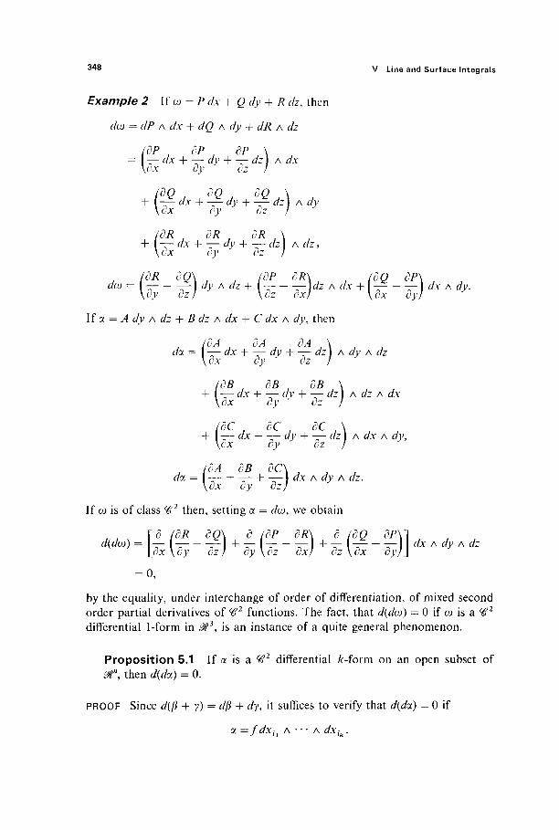
348 V Line and Surface Integrals
Example 2 If ω = P dx + Q dy + R dz, then
dœ = dP A dx + dQ A dy + dR A dz
(dP OP ] ÔP \ = — dx + — dy + — dz) A dx
\dx dy dz ] (dQ dQ dQ \
(dR J dR , dR ,\ + — dx + — dy + — dz) A dz,
\dx dy dz )
(dR dQ\ (dP dR\ (dQ dP\ J J
dw={Ty-^)dyAdz+[Tz-TxrAdx+[-x-Ty)
dxAd)'-If oc = A dy A dz + B dz A dx + C dx A dy, then
, (dA dA dA \ da = \ — dx + — dy + — dz) A dy A dz
\dx dy dz ] (dB dB j dB \
+ \ — dx + — dy + — dz) A dz A dx \ox dy dz J
(dC J dC j dC \ J j + I — dx + — dy + — dz) A dx A dy, \dx dy dz ]
_ (dA dB dC\ , j J da = -—h —- + —- ) dx A dy A dz.
\dx dy dz]
If ω is of class ^ 2 then, setting a = dw, we obtain
_\d IdR dQ\ d IdP dR\ d /dQ dP\
idx \dy dz J dy \dz dx) dz \dx dy]
= 0,
dx A dy A dz
by the equality, under interchange of order of differentiation, of mixed second order partial derivatives of ^1 functions. The fact, that d(da>) = 0 if ω is a ^ 2
differential 1-form in ^ 3 , is an instance of a quite general phenomenon.
Proposition 5.1 If a is a ^ 2 differential /:-form on an open subset of mn, then d(doc) = 0.
PROOF Since d(ß + y) = dß + dy, it suffices to verify that d(doc) = 0 if
a=fdxh Λ · · · Λ dxik.

5 Differential Forms 3 4 9
Then
ta*) ώ = Y -τ— ί/χ,.I Λ Î/Λ·,· Λ · · · Λ dx: Ik
so
" df = Σ τ~ dxr Λ ^ ΐ ι Λ · · · Λ i /x f k ,
d(da) = X I X -z—r~ rfx-s ) Λ rfx:r Λ dxh A · · · Λ É/X^ r = l \ s = 1 UXS VXr '
d2f = Y — dxK A dxr A dx: Λ · · · Λ dx: .
r,Üidxsdxr s
But since dxr A dxs = —dxs A dxr, the terms in this latter sum cancel in pairs, just as in the special case considered in Example 2. |
There is a Leibniz-type formula for the differential of a product, but with an interesting twist which results from the anticommutativity of the product operation for forms.
Propos i t ion 5.2 If a is a differential Ar-form and ß a differential /-form, both of class ^ 1 , then
d(oc A β) = (doc) A β + ( - 1)*α Λ (dß). (9)
PROOF By the additivity of the differential operation, it suffices to consider the special case
oc = a dxh Λ · · · Λ dxik, β = b dxji A · · · Λ dxjl,
where a and b are ^ 1 functions. Then
d(a A β) = d(ab) A dxh A · · · Λ dxik A dxh A · · · Λ dxjl
= (da A b + a A db) A dxh A · · · Λ dxik A · · · Λ dxh
= (da A dxh Λ · · · Λ dxik) A (b dxh A · · · Λ dXj^)
+ ( — l)k(a dxh Λ · · · Λ dxik) A (db A dxjx A · · · Λ dxj),
d((x A β) = (da) A β + ( - 1)*α A (dß),
the (— \)k coming from the application of formula (7) to interchange the 1-form db and the /c-form a in the second term. |
Recall (from Section 1) that, if ω is a Ή1 differential 1-form on @tn, and y : [a, b] -► &n is a ^ 1 path, then the integral of ω over y is defined by
jœ = j a)y(t)(y'(t))dt.
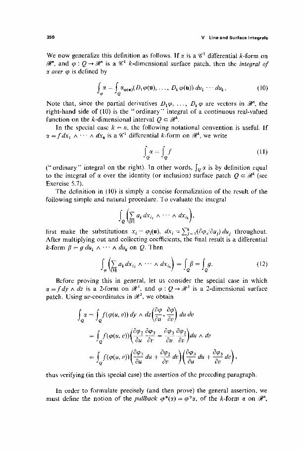
350 V Line and Surface Integrals
We now generalize this definition as follows. If a is a %>l differential A:-form on 0tn, and φ : Q -> &n is a ^ 1 ^-dimensional surface patch, then the integral of a over φ is defined by
f a = f a<p(«)(A<P(u), · · . , Dk(p(u)) dux-- duk, (10) \ JQ
Note that, since the partial derivatives Ώχφ, . . . , Dkcp are vectors in Mn, the right-hand side of (10) is the "ordinary" integral of a continuous real-valued function on the ^-dimensional interval Q c $k.
In the special case k = n, the following notational convention is useful. If oc =fdxl Λ · · · Λ dxk is a ^ 1 differential /c-form on 0tk, we write
f « = f / do ("ordinary" integral on the right). In other words, JQ a is by definition equal to the integral of a over the identity (or inclusion) surface patch Q c $k (see Exercise 5.7).
The definition in (10) is simply a concise formalization of the result of the following simple and natural procedure. To evaluate the integral
ί (X f l j i /X i , Λ ' · · Λ dxik)9 JQ \[i] /
first make the substitutions xi = (pi(u), dxi = Yj=l(dçi/dUj)duj throughout. After multiplying out and collecting coefficients, the final result is a differential A>form β = g diii A · · · Λ duk on Q. Then
f ( Σ ai dxh Λ * ' ' Λ dxt\ = \ β=\ g. (12) J<P \ [ i ] / JQ JQ
Before proving this in general, let us consider the special case in which α =fdy A dz is a 2-form on ^ 3 , and φ : Q -+& is a 2-dimensional surface patch. Using ^-coordinates in <^2, we obtain
J a = J f((p(u, v)) dy A dz\ —, —I rf« dv
= /(φ(«, ϊ?))Ι-τ- τ " - -r- T"r" Λ * JQ \ ou dv du dv /
=lmu> v))Bi du+d-Bdv) ^tdu+d2dv) ' thus verifying (in this special case) the assertion of the preceding paragraph.
In order to formulate precisely (and then prove) the general assertion, we must define the notion of the pullback <ρ*(α) = φ*α, of the k-îorm a on J?",

5 Differential Forms 351
under a ^ 1 mapping φ : 3fc™ -► ^ . This will be a generalization of the pullback defined in Section 2 for differential forms on 0l2;. We start by defining the pullback of a 0-form (or function)/or differential dxx by
<P*(f) =f°<P>
™ dipt (p*(dXi) = Σ T~ dui = d(P ·
(13)
We can then extend the definition to arbitrary /r-forms on 0ln by requiring that
<ρ*(/α) = ( /οφ)φ*α , φ*(α Λ β) = φ*α Λ φ*/?,
and
φ*(α + /?) = φ*α + φ*β.
(14)
Exercise 5.8 gives an important interpretation of this definition of the pullback operation.
Example 3 Let φ be a Ή1 mapping from &2V to 0l\yz. If ω = P dx + Q dy
+ P rfz, then
φ*ω = (P o φ)φ*{άχ) + (β ° φ)φ*(αγ) + (P o φ)φ*(αζ)
= (PoÇ)\d^du + ^dv\+(Qo<p)\d-p du + ^-2 Λ \_ou ov } |_ du dv
+ (Roφ)\8-pdu + Ô-p]dv, \_ou ov J
φ*ω = (Po ÖW (71/ C7W
L di; dy tfî?
If a = A dy A dz, then
φ*οι = (A o cp)(p*(dy) A cp*(dz)
(δφ2 d(p2
du
dv.
( A \(d(P2 A JL.d<P2 r l \ (d(P3
3l> rfw + - ^ dv I ,
ί/w Λ dv. du dv du dv,
In terms of the pullback operation, what we want to prove is that
ja=jy«, (15)
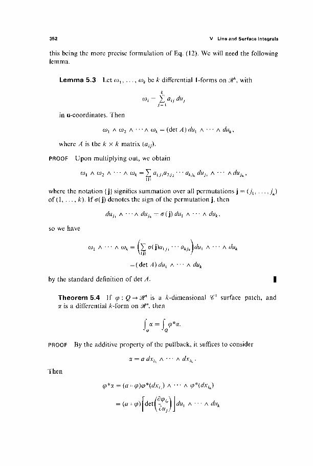
352 V Line and Surface Integrals
this being the more precise formulation of Eq. (12). We will need the following lemma.
Lemma 5.3 Let ω , , . . . , œk be k differential 1-forms on 0lk, with
k
ω,- = Σ au duj 7 = 1
in u-coordinates. Then
ωι A ω2 A - · - A ωκ = (det A) duY Λ · · · Λ duk,
where A is the k x k matrix (α^).
PROOF Upon multiplying out, we obtain
co1 A ω2 A · · · Λ wk = X aijxa2j2 · · · akjk duh A · · · Λ duJk,
where the notation {j} signifies summation over all permutations j = {j\, . . . ,jk) of (1, . . . , k). If cr( j) denotes the sign of the permutation j , then
duh Λ · · · Λ dujk = σ ( j) du{ A · · · Λ duk,
so we have
ωχ A · · · Λ œk = ί χ σ(])αυι · · · akjk\du{ A · · · Λ duk
= (det A) dui A -" A duk
by the standard definition of det A. \
T h e o r e m 5.4 If φ: Q-±0ln is a /:-dimensional ^ 1 surface patch, and a is a differential /c-form on ^ n , then
α = φ*α.
PROOF By the additive property of the pullback, it suffices to consider
a = a dxh A · - · Λ dxik.
Then
φ*α = (a o (p)(p*(dxh) A · · · Λ (p*(dxik)
m = {ao φ)\ det j — - L/wj Λ · · · Λ ώ λ
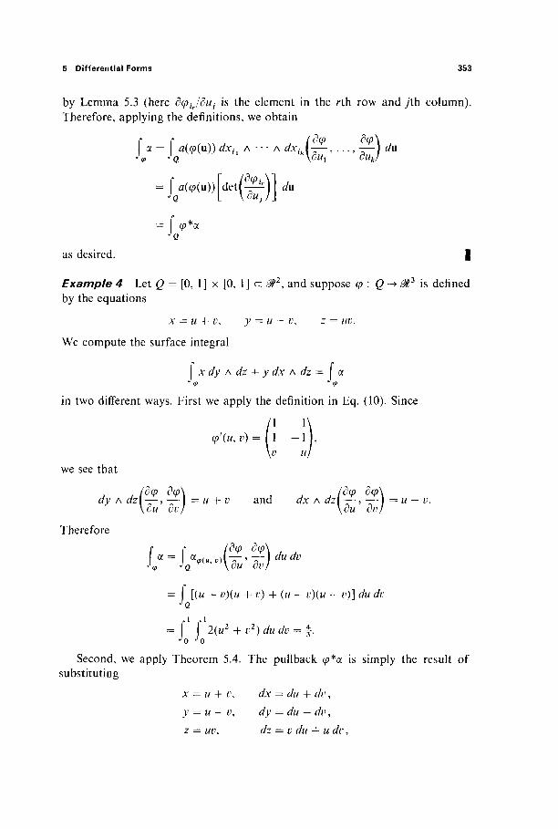
5 Differential Forms 353
by Lemma 5.3 (here dcpjduj is the element in the rth row and yth column). Therefore, applying the definitions, we obtain
f^fûf l(?W)àflA...Aa^ g *
= f α(φ(υ)) det \dujj
du
as desired.
Example 4 Let Q = [0, 1 ] x [0, 1 ] c 0t1, and suppose φ : Q by the equations
x = w + r, j> = w — i\ z = uv.
We compute the surface integral
is defined
x dy A dz + y dx A dz = a
in two different ways. First we apply the definition in Eq. (10). Since
<p'(u,v) = 11 - l ) ,
we see that
, , (dq> dq>\ (dq> dq>\ dy A dz\—,—1 = u + v and dx A dzi — ,—\ = u — v.
\cu dv/ \cu dv/ Therefore
= [(u + y)(w + v) + (w — y)(w — v)] du dv JQ
2(u2 + v2) du dv = f.
Second, we apply Theorem 5.4. The pullback φ*α is simply the result of substituting
x = u + v, dx = du + dv, y = u — v, dy = du — Λ>, z = wi?, dz = v du + u dv,

354 V Line and Surface Integrals
into a. So
φ*α = (u + v)(du - dv) A (V du + u dv) + (u - v)(du + dv) A (V du + u dv)
= 2(u2 + v2) du A dv.
Therefore Theorem 5.4 gives
Γ α = ί φ * α = ί \ 2(u2 + v2) du dv =±.
Of course the final computation is the same in either case. The point is that Theorem 5.4 enables us to proceed by formal substitution, making use of the equations which define the mapping φ, instead of referring to the original definition of \φ oc.
Theorem 5.4 is the /c-dimensional generalization of Lemma 2.2(b), which played an important role in the proof of Green's theorem in Section 2. Theorem 5.4 will play a similar role in the proof of Stokes' theorem in Section 6. We will also need the /c-dimensional generalization of part (c) of Lemma 2.2—the fact that the differential operation d commutes with pullbacks.
Theorem 5.5 If φ : £%m -► 0tn is a ^ 1 mapping and a is a ^ 1 differential fc-form on Stn, then
ί/(φ*α) = φ*(ί/α).
PROOF The proof will be by induction on k. When k = 0, a = / , a ^ 1 function on ^ n , and (p*f = f° φ, so
m d(f°(p) ™ α(φ*/)=Σ -^J»i=l
/ = i dut / = i
But
which is the same thing. Supposing inductively that the result holds for (k - l)-forms, consider the
&-form oc = a dxh A - · · A dxik = dxh A β,
&W,°V <hpj
ÔU: dU;

5 Differential Forms 355
where ß = a dxh A · · · Λ dxik. Then doc = d(dxh) Aß — dxh A dß
= —dxi{ A dß
by Proposition 5.2. Therefore
(p*(dot) = (p*(-dxii Adß)
= -<p*(dxix) A φ*{άβ)
= -(p*(dxh) A d(q>*ß),
since cp*(dß) = ά(φ*β) by the inductive assumption. Since cp*(dxh) = d(ph by (13), we now have
d(<p*a) = d(cp*{dxix) A φ*β)
= d(d(ph) A φ*β - <p*(dXil) A d(<p*ß)
= (p*(doc)
using Propositions 5.1 and 5.2. |
Our treatment of differential forms in this section has thus far been rather abstract and algebraic. As an antidote to this absence of geometry, the remainder of the section is devoted to a discussion of the " surface area form " of an orien-ted smooth (^1) /r-manifold in 0t. This will provide an example of an important differential form that appears in a natural geometric setting.
First we recall the basic definitions from Section 4 of Chapter III. A coor-dinate patch on the smooth /:-manifold M a $n is a one-to-one ^ 1 mapping φ : U' -► M, where U is an open subset of ^ \ such that άφη has rank k for each ue U: this implies that [det(<p'(u)V(u)]1/2 Φ 0· An atlas for M is a collection {φι} of coordinate patches, the union of whose images covers M. An orientation for M is an atlas {φ^ such that the "change of coordinates" mapping, corre-sponding to any two of these coordinate patches φί and φ] whose images ^ ,·(£/,·) and φ^ί//) overlap, has a positive Jacobian determinant. That is, if
Tu = Φ;Ό ψ. : ψΓΗΨΜ) Π φ^)) - φ;ί(Φι(υί) η i/,j(Uj))9
then det Γ/7 > 0 wherever Τί7 is defined (see Fig. 5.29). The pair (A/, {φ{}, is then called an oriented manifold. Finally, the coordinate patch φ : U-* M is called orientation-preserving if it overlaps positively (in the above sense) with each of the φι, and orientation-reversing if it overlaps negatively with each of the φί
(that is, the appropriate Jacobian determinants are negative at each point).
The surface area form of the oriented /r-dimensional manifold M c 0tn is the differential /c-form
dA = ]T #i i/xj, [ i ]
(16)

356 V Line and Surface Integrals
OD Figure 5.29
T.. iJ
UJ
whose coefficient functions n{ are defined on M as follows. Given i = (/1? . . . , ik) and x G A/, choose an orientation-preserving coordinate patch φ : U -► M such that x = φ(χ\) e φ(ϋ). Then
1 d((p: , . . . , ω,) 1 . x) = — -^τ-1 r = ~~ det ^i (")'
D d(u{, . . . , wfc) D where
D = [det(9'(u))V'(u)]1/2 = [X (det (p^u))2]1'2. [j]
Example 5 Let M = S2, the unit sphere in ^ 3 . We use the spherical coor-dinates surface patch defined as usual by
x = sin φ cos 0, y = sin φ sin 0, z = cos φ.
Here D = sin φ (see Example 3 in Section 4). Hence
1 d{x,y) ' ( 1 , 2 )
' ( 1 , 3 )
7 ( 2 , 3 )
sin φ δ(φ, 0)
1 3(;c, z) sin φ d(cp, 0)
1 d(y, z)
cos φ = z,
= — sin φ sin 0 = — j>,
= sin φ cos 0 = x. sin φ δ(φ, θ)
Thus the area form of S2 is dA = z dx A dy — y dx A dz + x dy A dz
= x dy A dz + y dz A dx + z dx A dy.
Of course we must prove that nk is well-defined. So let φ : V -► M be a second orientation-preserving coordinate patch with x = φ(\) e φ(Υ). If
Τ=φ-ιοφ: φ-ι(φ(ϋ) η φ(Υ)) - φ~Ηφ(υ) η φ{Υ)\
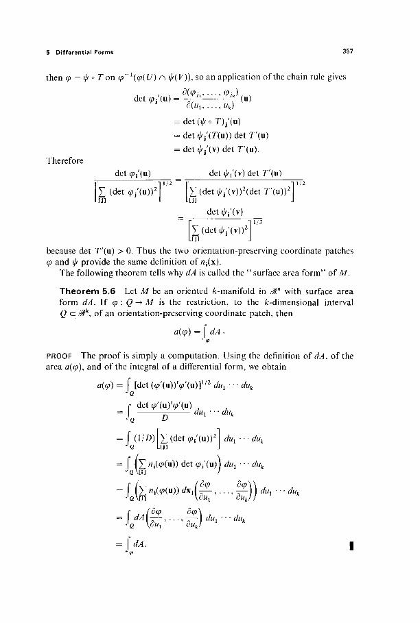
5 Differential Forms 357
then φ = φ ° T on φ ι{φ{ϋ) η φ(Υ)), so an application of the chain rule gives
3 ( 1 / ! , . . . , Wfc)
= det (φ o T)/(u) = det ^j'(r(u)) det T'(u) = det ^j'(v) det T'(u).
Therefore det (Pi'(u) det ^j'(v) det T'(u)
X (det <pi'(u))2
L[j]
1/2
X (det ^j'(v))2(det T'(u))2
[j]
det ^/(v)
1/2
X (det ιΑ/(ν))2
L[j ]
1/2
because det T'(u) > 0. Thus the two orientation-preserving coordinate patches φ and φ provide the same definition of n^x).
The following theorem tells why dA is called the " surface area form" of M.
Theorem 5.6 Let M be an oriented /r-manifold in Mn with surface area form dA. If φ : Q^M is the restriction, to the /c-dimensional interval Q a &k, of an orientation-preserving coordinate patch, then
a(cp)=j dA.
PROOF The proof is simply a computation. Using the definition of dA, of the area α(φ), and of the integral of a differential form, we obtain
α(φ) = f [det (^(u))V'(u)] , /2 dux · ■ · duk
r det φ'(ιι) V(u) = JQ 5 dux-duk
= f ( 1 / / > ) Γ Σ (det ^ / (u ) ) 2 ] £/Wl · · - £/ι/Λ JQ L[j] J
= J ( Σ ni((P(u)) det <Pi'(«) ) ^ · · · <Λ/Λ
= \ dA.
duk
358 V Line and Surface Integrals
Recall that a paving of the compact smooth /:-manifold M is a finite collec-tion se = {A ! , . . . , Ar) of nonoverlapping /c-cells such that M = (J|L x Λ;. If M is oriented, then the paving se is called oriented provided that each of the Â>cells Ai has a parametrization φί : ζ), ->/!,· which extends to an orientation-preserving coordinate patch for M (defined on a neighborhood of Qi c 0tk). Since the /:-dimensional area of M is defined by
a{M)= Σ"(Αι)= I ^ i ) , i = l i = 1
we see that Theorem 5.6 gives
a(M)= t f A4. (17) i = 1 <Pi
Given a continuous differential k-ïorm a whose domain of definition con-tains the oriented compact smooth /:-manifold A/, the integral of ot on M is defined by
ί « = Σ ί « . (18) JA# i = l " > i
where c^, . . . , (pr are parametrizations of the /c-cells of an oriented paving se of M (as above). So Eq. (17) becomes the pleasant formula
a(M)= f dA.
The proof that the integral \M a is well defined is similar to the proof in Section 4 that a(M) is well defined. The following lemma will play the role here that Theorem 4.1 played there.
Lemma 5.7 Let M be an oriented compact smooth /c-manifold in 0tn and a a continuous differential A"-form defined on M. Let φ : U -> M and ψ : V -> M be two coordinate patches on M with cp(U) = ij/(V), and write T = φ~1 ° φ : U-> V. Suppose X and y are contented subsets of U and K, respectively, with T(X) = Y. Finally let φ = φ \ X and φ = ι//1 7. Then
f a = f a
if φ and ψ are either both orientation-preserving or both orientation-reversing, while
f a = - f a
if one is orientation-preserving and the other is orientation-reversing.
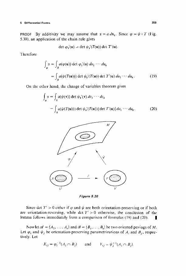
5 Differential Forms 359
PROOF By additivity we may assume that a = a dx{. Since φ = φ ° T (Fig. 5.30), an application of the chain rule gives
det (/>i'(u) = det ιΑ/(Γ(ιι)) det 7'(u).
Therefore
a = a(<p(u)) det <ρ/(ιι) dui" · duk
= f α(φ(Τ(ύ))) det φι(Τ(ύ)) det T'(u) dux-·· duk. (19) J x
On the other hand, the change of variables theorem gives
α = α(φ(\)) det φι\ν) dv1 · · · dvk
= f α(φ(Τ{α))) det ψι(Τ(η)) | det Γ(ιι) | dux · · · rfw*. (20) J V
Figure 5.30
Since det T' > 0 either if φ and φ are both orientation-preserving or if both are orientation-reversing, while det V > 0 otherwise, the conclusion of the lemma follows immediately from a comparison of formulas (19) and (20). |
Now let se = {A ! , . . . , Ar} and ^ = {Bx,..., Bs} be two oriented pavings of M. Let (pi and φ] be orientation-preserving parametrizations of A{ and Bj9 respec-tively. Let
Xij = (PrHAinBj) and Υυ = φ;ι{ΑίηΒ]).

360 V Line and Surface Integrals
If (Pij = (Pi\Xij and φ^ = ij/j\ Yij9 then it follows from Lemma 5.7 that
for any k4ovm a defined on M. Therefore
έ J « = i ( i J «) i = l Jq>i i=l Y/=l *>0· /
= i ( i N -if*
so the integral JM a is indeed well defined by (18).
Integrals of differential forms on manifolds have a number of physical applications. For example, if the 2-dimensional manifold M c &3 is thought of as a lamina with density function p, then its mass is given by the integral
f pdA.
If M is a closed surface in ^ 3 with unit outer normal vector field N, and F is the velocity vector field of a moving fluid in &3, then the "flux" integral
f F· NdA
measures the rate at which the fluid is leaving the region bounded by M. We will discuss such applications as these in Section 7.
Example 6 Let T be the "flat torus" S1 x S1 c &2 x ^ 2 , which is the image in 0tA of the surface patch F: Q = [0, 2π]2 -+ @4 defined by
*! = cos 0, x3 = cos φ, x2 = sin 0, x4 = sin φ.
The surface area form of T is
i/ 4 = χ2 χ4 dxY A dx3 + X2 X3 ί/Χ4 Λ άχγ + XjX4 ί/χ3 Λ dx2 + XxX3 rfx"2 Λ dx4
(see Exercise 5.11). If Q is subdivided into squares Qu Q2, Q3, Q4 as indicated in Fig. 5.31, and A{ = q>(Qi), then {Au A2, A3, A4} is a paving of T, so
α(Τ)= \ όΑ=Σ \ dA=\ dA.
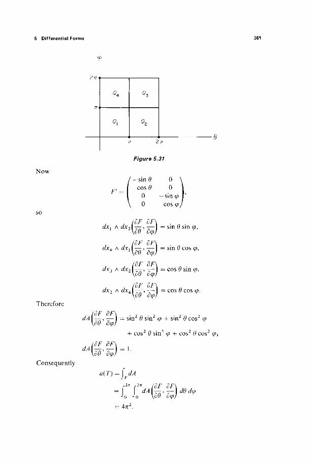
5 Differential Forms
Ziri
Now
so
Therefore
F' =
ZTT
Figure 5.31
- s i n 0 0 cos0 0
0 — sin φ 0 cos φ i
, idF dF\ dxx A dx31 —-, —- I = sin 0 sin φ, \οθ δφ/
, ldF dF\ dx4 Λ c/xi I — - , - — = sin Θ cos φ,
\οθ οφΙ
, fîF 3F\ dx3 A dx2 l —> — I = cos Θ sin <p,
\οθ οφ)
, idF dF\ dx2 A dxA — , —- = cos Θ cos φ.
\c0 οφ!
(OF dF\ ? 7 ? 7 "ΛI —, — I = sin Θ sin φ + sin 0 cos φ
\c0 οφ)
+ cos2 Θ sin2 φ + cos2 Θ cos2 <p,
, /dF ÔF\
Consequently δφ)
a(T)= I dA
In In ,dF dFX
=/0 Ι'ΑΜ'ΈΪΓ* = 4π2
361
362 V Line and Surface Integrals
Exercises
5.1 Compute the differentials of the following differential forms. (a) α = Σ 7 = 1 ( - 1 ) ί - 1 * ί ri*, Λ · · · Λ dx^x A dxi + 1 A · · · Λ dxn. (b) r~na, where r = [xY
2 + · · · + xn2]1/2.
(c) Σηι= i yt d*i, where (*i, . . . , xn, yx, . . . , yn) are coordinates in ^ 2 " . 5.2 If F : ^ " -> 3#" is a *f » mapping, show that
dF, Λ · · Λ dFn = — dxi A · ■ · Λ dxn. d(xu ...,x„)
5.3 If α =Σ?<7· #,·.,· Î/Λ·,· Λ dxj is a differential 2-form on ^" , show that
_ /da a daik dalk\ da = Σ \ ^ i - T ^ + ^\dxlhdx1hdxi.
i<j<k\oxk dxj dxtJ
5.4 The function / i s called an integrating factor for the 1-form ω if f(x) Φ 0 for all x and d{fœ) = 0. If the 1-form ω has an integrating factor, show that ω A dœ = 0.
5.5 (a) If doc = 0 and dß = 0, show that d(oc A ß) = 0. (b) The differential form ß is called exact if there exists a differential form y such that ί/y = ß. If ί/α = 0 and β is exact, prove that α Λ β is exact.
5.6 Verify formula (7) in this section. 5.7 If φ : Q -> i#fc is the identity (or inclusion) mapping on the /:-dimensional interval
Q <= *, and α =/ί/ΛΊ Λ · · · Λ ^ , show that
5.8 Let ψ : Mm -> ^?" be a ft! mapping. If a is a &-form on ·#", prove that
(φ*α)„(νι , . . . , \k) = αφ{ν)(αφα(\ι), . . . , d(pu(\k)).
This fact, that the value of φ*α on the vectors V i , . . . , \k is equal to the value of a on their images under the induced linear mapping dy, is often taken as the definition of the pull-back φ*α.
5.9 Let C be a smooth curve (or 1-manifold) in .^", with pathlength form ds. If φ : U^ C is a coordinate patch defined for / e U cz j?\ show that
<p*(ds) = [(φΛΟ)2 + · · · 4- « ( / ) ) 2 ] 1 / 2 <//.
5.10 Let M be a smooth 2-manifold in J?n, with surface area form dA. If φ : ί/-> yV/ is a coor-dinate patch defined on the open set U <= JP*,,, show that
<p*(dA) = {EG-F2)ll2dudv
with £, G, F defined as in Example 5 of Section 4. 5.11 Deduce, from the definition of the surface area form, the area form of the flat torus used
in Example 6. 5.12 Let Mi <= ^m be an oriented smooth /:-manifold with area form dAu and M2
c &n an oriented smooth /-manifold with area form dA2. Regarding dAi as a form on Mm+n
which involves only the variables xu · · ·, *„,, and dA2 as a form in the variables xm + u . . . , Λ"„Ι + Λ, show that
dA =dAx A dA2
is the surface area form of the oriented (k + /)-manifold Mi x M2 c= .^m + n . Use this result to obtain the area form of the flat torus in MA.
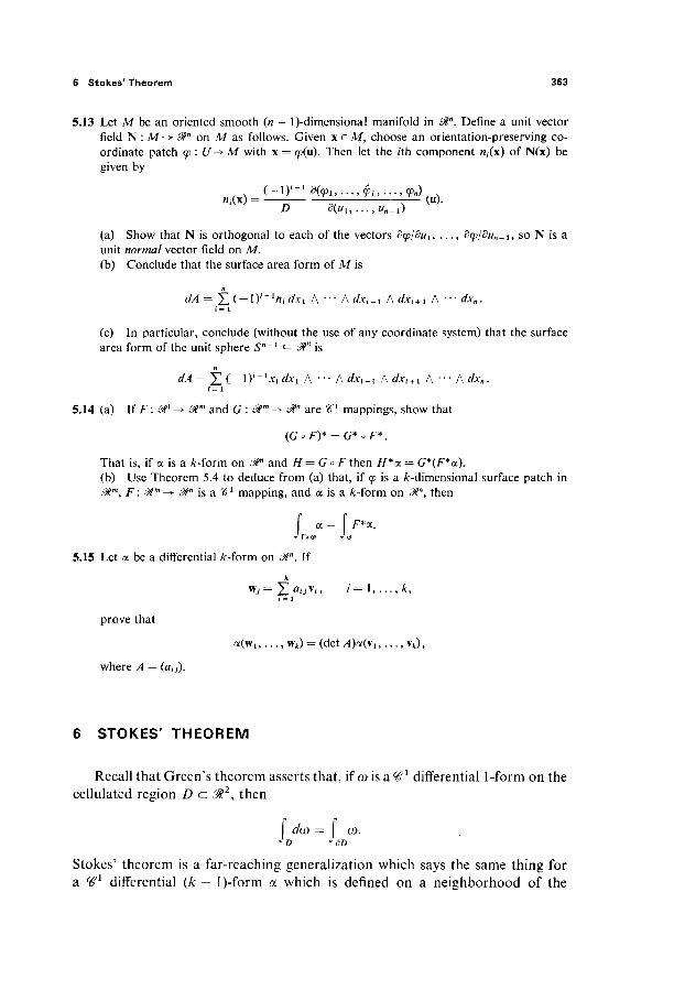
6 Stokes' Theorem 363
5.13 Let M be an oriented smooth (n — l)-dimensional manifold in 0tn. Define a unit vector field N : M-> S%n on M as follows. Given x e M , choose an orientation-preserving co-ordinate patch φ: U-> M with x = 92(11). Then let the /th component /i,(x) of N(x) be given by
"i(x) = —n ^ r~ (u)·
(a) Show that N is orthogonal to each of the vectors d<p/duu . . . , d(p/du„-iy so N is a unit normal vector field on M. (b) Conclude that the surface area form of M is
Π
dA = Σ(-Οί_1Λί^ι Λ ··· Adxi-ι Adxi + i A '" dxn. i= 1
(c) In particular, conclude (without the use of any coordinate system) that the surface area form of the unit sphere S"-1 <= 9t is
dA= Yi-iy-'xidxi Λ '·· Adxi-ι Adxi + l A ■■· Adxn. i= 1
5.14 (a) If F : M1 -> ^ m and G : ^ m -> Mn are 1 mappings, show that
(G* o F)* = G* o F*.
That is, if a is a A:-form on ^" and H = G ° F then H*a = G*(F*oc). (b) Use Theorem 5.4 to deduce from (a) that, if φ is a ^-dimensional surface patch in 0lm, F : @m -> &n is a 1 mapping, and a is a £-form on #", then
f α - ί F*a.
5.15 Let a be a differential k-ïorm on ^". If k
prove that
where A = (a0).
a(wi, . . . , wfc) = (det /l)a(vi,.. . , vk),
6 STOKES' THEOREM
Recall that Green's theorem asserts that, if ω is a 1 differential 1-form on the cellulated region D a 011;, then
ÔD
Stokes' theorem is a far-reaching generalization which says the same thing for a Ή1 differential (k — l)-form a which is defined on a neighborhood of the

364 V Line and Surface Integrals
cellulated λ-dimensional region R cz M, where M is a smooth A>manifold in 0tn. That is,
\ ch = \ <x. JR JdR
Of course we must say what is meant by a cellulated region in a smooth manifold, and also what the above integrals mean, since we thus far have defined integrals of differential forms only on surface patches, cells, and manifolds. Roughly speaking, a cellulation of R will be a collection {Al, . . . , Ar) of nonoverlapping Ar-cells which fit together nicely (like the 2-cells of a cellulation of a planar region), and the integral of a k-ïorm ω on R will be defined by
f ω = X f ω. J R / = 1 J Ai
Green's theorem is simply the case n = k = 2 of Stokes' theorem, while the fundamental theorem of (single-variable) calculus is the case n — k = 1 (in the sense of the discussion at the beginning of Section 2). We will see that other cases as well have important physical and geometric applications. Therefore Stokes' theorem may justly be called the "fundamental theorem of multi-variable calculus."
The proof in this section of Stokes' theorem will follow the same pattern as the proof in Section 2 of Green's theorem. That is, we will first prove Stokes' theorem for the unit cube Ik c &k. This simplest case will next be used to estab-lish Stokes' theorem for a /c-cell on a smooth /:-manifold in Mn, using the formal properties of the differential and pullback operations. Finally the general result, for an appropriate region R in a smooth /:-manifold, will be obtained by application of Stokes' theorem to the cells of a cellulation of R.
So we start with the unit cube
/* = {Oq, . . . , xk) e mk : each xv e [0, 1 ]}
in Rk. Its boundary dlk is the set of all those points (x1, . . . , xk) e Ik for which one of the k coordinates is either 0 or 1 ; that is, dlk is the union of the 2k dif-ferent (k — l)-dimensional/tfc<?s of/*. These faces are the sets Ik
t~l defined by
C ^ i U i ^ ) e / * : ^ = E}
for each / = 1, . . . , k and ε = 0 or ε = 1 (see Fig. 5.32). The (/, e)thface Ik~l of Ik is the image of the unit cube Ik~l <^0lk~x under the mapping iitE : /*_ 1 -> &k
defined by
'ί,ε^Ι» · · · ' Xk-l) = (Xli · · · ' xi-l> β> ·*/ ' · ' · ' - ^ Λ - ΐ ) ·
The mapping iiE serves as an orientation for the face Ik~Ex. The orientations
which the faces (edges) of I2 receive from these mappings are indicated by the
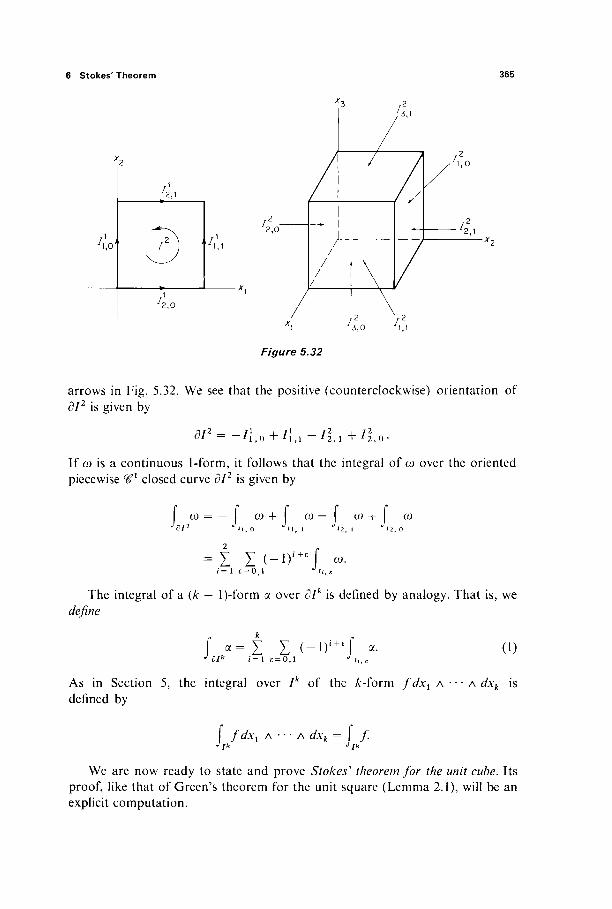
6 Stokes' Theorem 365
2,0
Figure 5.32
arrows in Fig. 5.32. We see that the positive (counterclockwise) orientation of dl2 is given by
M2= - / ί . ο + Λ \ ι - / 2 . ι + ' 2 . ο .
If ω is a continuous 1-form, it follows that the integral of ω over the oriented piecewise ^ 1 closed curve dl2 is given by
ω = — ω + ω — ω + Jdl2 JH,o ji i , i J' 2 , i Ji2
= Σ Σ ( - D ' + e f ω. i = l ε = 0.1 Ji i , c
The integral of a (k — l)-form a over dlk is defined by analogy. That is, we define
ί « = ί I (-ni + £f a ^ dlk i= 1 ε = 0 ,1 J i,·, c
(i)
As in Section 5, the integral over Ik of the £-form /É/XJ Λ · · · Λ dxk is defined by
I fdxl A · · · Λ dxk = \ f. J[k Jik
We are now ready to state and prove Stokes' theorem for the unit cube. Its proof, like that of Green's theorem for the unit square (Lemma 2.1), will be an explicit computation.
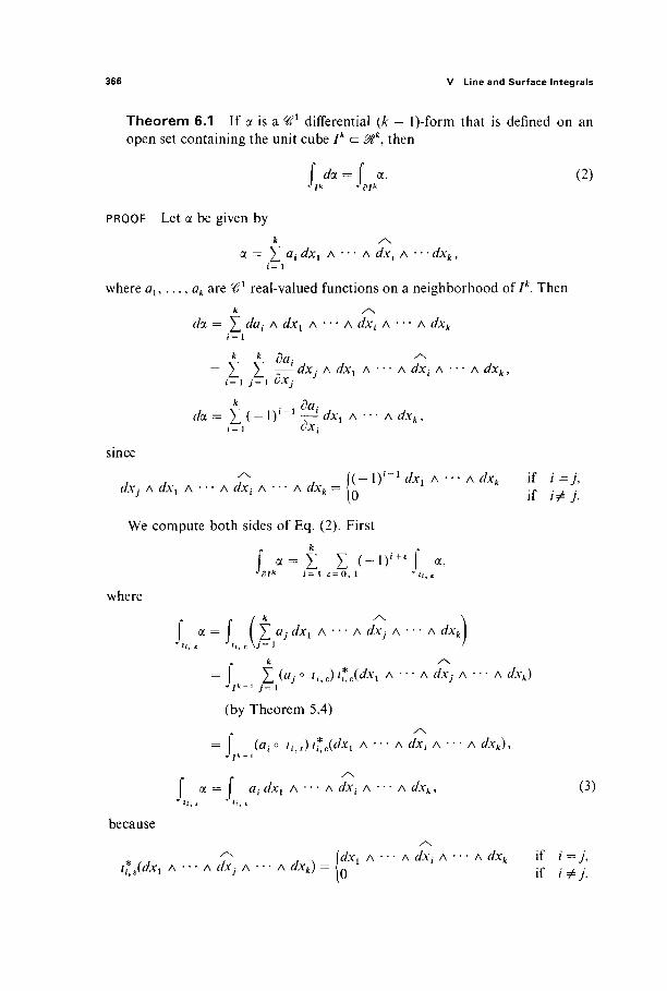
366 V Line and Surface Integrals
T h e o r e m 6.1 If a is a ^ 1 differential (k — l)-form that is defined on an open set containing the unit cube Ik cz &k, then
f da = f a. (2) JJk Jßjk
PROOF Let a be given by k / \
a = £ at dxl Λ · · · Λ dxi A · · · dxk, i = 1
where au . . . , ak are ^ 1 real-valued functions on a neighborhood of /*. Then
dot = Σ dQi Λ dxi Λ · · · Λ dx{ A · - - A dxk
i= 1 k k da-, ^
= Σ Σ τ~^ dxj A dxl Λ · · · Λ dxt A · · · Λ dxk, i = i y = i ÖXy
k ._ dat
doc = Y ( — 1 )' 1 —- dxy Λ · · · Λ dxk,
since
Γ , ( ( - l ) 1 ' " 1 ^ ! Λ · · · Adxk if i = 7 , tfJC: Λ ί / Χ , Λ · · ' Λ ά ; Λ · ' · Λ dxk = { Λ · Γ . . . J x ' * (0 if / T^y.
We compute both sides of Eq. (2). First
| « = Σ Σ ( - η ί + ε ί «, >>dlk i = 1 ε = 0 , 1 J u,c
where
f a = ( Σ ay ^ χ ι Λ " ' Λ dXj A · · · Λ rfxfcI
= I Σ (*/ ° 'ί,ε) Ί*ε (^1 A'" AdXj A'" Adxk) J /*< - « j = 1
(by Theorem 5.4)
r ^ = fa,· ° 'ί,ε) ï*eW*l Λ ' ' ' Λ dXi A ' · · Λ dxk) ,
Jjk-ί
j a = I tf ,· ί/jCi A ··· A dxt A ·-· A dxk, • ' l i , c »«, ε
(3)
because
<"- , λ ίί/x, Λ · · · Λ dxt A ■ ■ ■ A dxk if i=j, t*Jdx1 Λ · · · AdxjA ■■■ Adxk) = L· i f ^ .
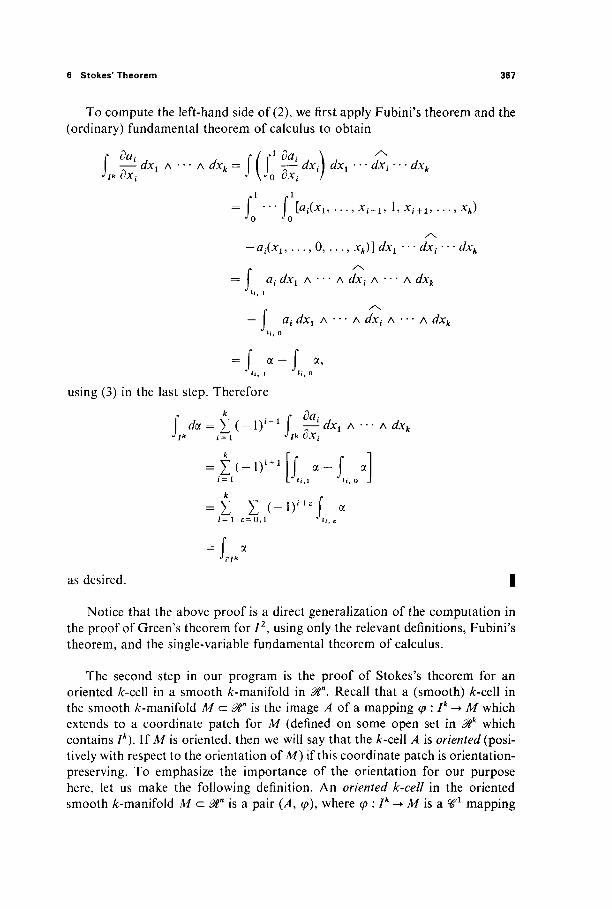
6 Stokes' Theorem 367
To compute the left-hand side of (2), we first apply Fubini's theorem and the (ordinary) fundamental theorem of calculus to obtain
—— dx{ Λ · · · Λ dxk = I TT— dxi ) dxl · · · dxt · · · dxk •V dxt J Vo oXi I
= | ' * * I lOiiXu · · ·, *i-u h */ + i, · · ·, xk)
l « , 1 If , 0
using (3) in the last step. Therefore k * da
-diixn . . . , 0, . . . , xk)] dxl-" dxi · · · dxk
C ^ = av dxl A · · · Λ dxi Λ · · · Λ dxk
— af i/xt Λ · · · Λ dxi Λ · · · Λ ö6cfc * i . 0
= 1 . α ~ ί „ α '
i/xfc f ί /α=Χ(-1) ' - 1 ί - ^ Λ Ι Λ · · · Λ
i=l ΙΛί,ι JH,o .
= Σ Σ ( -n' + ' f « f = l ε = 0,1 JU,c
= ί « as desired. |
Notice that the above proof is a direct generalization of the computation in the proof of Green's theorem for I2, using only the relevant definitions, Fubini's theorem, and the single-variable fundamental theorem of calculus.
The second step in our program is the proof of Stokes's theorem for an oriented Λτ-cell in a smooth ^-manifold in 9F. Recall that a (smooth) &-cell in the smooth /c-manifold M cz 0ln is the image A of a mapping φ : Ik -> M which extends to a coordinate patch for M (defined on some open set in 0tk which contains Ik). If M is oriented, then we will say that the &-cell A is oriented (posi-tively with respect to the orientation of M) if this coordinate patch is orientation-preserving. To emphasize the importance of the orientation for our purpose here, let us make the following definition. An oriented k-cell in the oriented smooth /^-manifold M c 3%n is a pair {A, φ), where φ : Ik -> M is a ^ 1 mapping
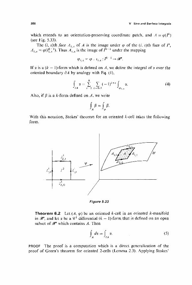
368 V Line and Surface Integrals
which extends to an orientation-preserving coordinate patch, and A = cp(Ik) (see Fig. 5.33).
The (/, s)thface AitE of A is the image under φ of the (/, e)th face of /*, AifE = (p(lk~e
l). Thus AitE is the image of Ik~l under the mapping
^ e = ^ o / i f e : / f c _ 1 - > « " .
If a is a (k — l)-form which is defined on A, we define the integral of a over the oriented boundary dA by analogy with Eq. (1),
f «= Σ Σ ( -D ' + ' f «· JdA i= 1 e = 0 , l J <Pi,c
Also, if β is a k-ΐθΐχη defined on A, we write
J A J ,n
(4)
With this notation, Stokes' theorem for an oriented A--cell takes the following form.
Figure 5.33
Theorem 6.2 Let (Λ, φ) be an oriented /c-cell in an oriented /c-manifold in 0tn, and let a be a ^ 1 differential (k - l)-form that is defined on an open subset of @tn which contains A. Then
\ doc = a. J A ^δΑ
(5)
PROOF The proof is a computation which is a direct generalization of the proof of Green's theorem for oriented 2-cells (Lemma 2.3). Applying Stokes'
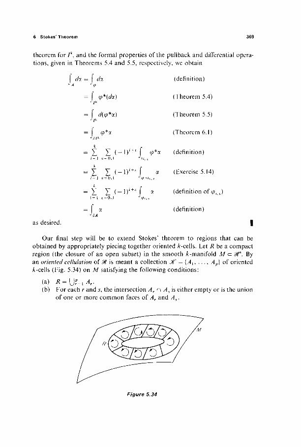
6 Stokes' Theorem 369
theorem for /*, and the formal properties of the pullback and differential opera-tions, given in Theorems 5.4 and 5.5, respectively, we obtain
da = da JA J φ
= f </>*(</«) J jk
= f ί/(φ*α) J Jk
= φ*α Jdlk
= Σ Σ < - » ) ί + ' / i = l e = 0 , l Ji ,
= Σ Σ ( - n i + c i i = l e = 0 , l Vφ
-ί
φ^α
/ = 1 c = 0 , l
α
as desired.
(definition)
(Theorem 5.4)
(Theorem 5.5)
(Theorem 6.1)
(definition)
(Exercise 5.14)
(definition of φ, ε)
(definition)
I
Our final step will be to extend Stokes' theorem to regions that can be obtained by appropriately piecing together oriented /r-cells. Let R be a compact region (the closure of an open subset) in the smooth /c-manifold M c 0tn. By an oriented cellulation of ^ is meant a collection X = {Au . . . , Ap} of oriented /c-cells (Fig. 5.34) on M satisfying the following conditions:
(a) R = \J!=1A,. (b) For each r and s, the intersection Ar n As is either empty or is the union
of one or more common faces of Ar and As.
Figure 5.34

370 V Line and Surface Integrals
(c) If B is a (k — l)-dimensional face of Ar, then either Ar is the only /r-cell of Jf having B as a face, or there is exactly one other k-ce\\ As also having B as a face. In the former case B is called a boundary face; in the latter 5 is an interior face.
(d) If B is an interior face, with Ar and Λ5 the two /c-cells of Jf having B as a face, then Ar and Λ5 induce opposite orientations on B.
(e) The boundary dR of R (as a subset of Λ/) is the union of all the bound-ary faces of k-ce\\s of X.
The pair (R, Jf ) is called an oriented cellulated region in Λ/. Although an oriented cellulation is conceptually simple—it is simply a
collection of nonoverlapping oriented /c-cells that fit together in the nicest possible way—the above definition is rather lengthy. This is due to conditions (c), (d), and (e), which are actually redundant—they follow from (a) and (b) and the fact that the /c-cells of Jf are oriented (positively with respect to the orientation of M). However, instead of proving this, it will be more convenient for us to include these redundant conditions as hypotheses.
Condition (d) means the following. Suppose that B is the (/, a)th face of Ar, and is also the (j, /?)th face of As. If
φ : Ik -> Ar and φ : Ik -► As
are orientation-preserving parametrizations of Ar and As respectively, then
Β = φί,α(ΐ'ί-1) = Ψ],β(Ι
Ιί-ί).
What we are assuming in condition (d) is that the mapping
has a negative Jacobian determinant if ( — l ) I + a = (— l)j + ß, and a positive one if ( _ i ) i + « = _ ( _ i y + 0. By the proof of Lemma 5.7, this implies that
( -1) ί + α ί û, + ( - iy+>f ω = 0 (6) </>*,« *j,ß
for any continuous (k — l)-form ω. Consequently, if we form the sum p r Σ «,
Γ = 1 JÔAr
then the integrals over all interior faces cancel in pairs. This conclusion is pre-cisely what will be needed for the proof of Stokes' theorem for an oriented cellulated region.
To see the "visual" significance of condition (d) note that, in Fig. 5.35, the arrows, indicating the orientations of two adjacent 2-cells, point in opposite directions along their common edge (or face). This condition is not (and cannot be) satisfied by the "cellulation" of the Möbius strip indicated in Fig. 5.36.

6 Stokes' Theorem 371
Figure 5.35
Figure 5.36
Orientations do not cancel along this edge
If (R, Jf ) is an oriented cellulated region in the smooth /r-manifold M c £%n, and ω is a continuous differential &-form defined on R, we define the integral of ω on R by
ί ω = X ί ω, J R r = l Jy4r
(7)
where Au ..., Λρ are the oriented /c-cells of Jf. Note that this might conceiv-ably depend upon the oriented cellulation J>f ; a more complete notation (which, however, we will not use) would be j ( K > ^ ω.
Since the boundary dR of R is, by condition (e), the union of all the boundary faces Bu ..., Bq of the &-cells of X , we want to define the integral, of a (k — 1)-form a on dR, as a sum of integrals of a over the (& — l)-cells Bl9 ..., Bq. How-ever we must be careful to choose the proper orientation for these boundary faces, as prescribed by the orientation-preserving parametrizations φ1, . . . , φρ
of the k-cdh Ax, ..., Ap of K. If Bs is the (/s, es)th face of Ars, then

372 V Line and Surface Integrals
For brevity, let us write
and
ôs = is + es.
Then (-1)*5* j ^ s a is the integral corresponding to the face Bs of Ars, which appears in the sum which defines \dA a. We therefore define the integral of the (k — l)-form a on dR by
f a= X (-1)'- Ï a. (8)
Although the notation here is quite tedious, the idea is simple enough. We are simply saying that
J « = £ Ja, JdR s= 1 J Bs
with the understanding that each boundary face Bs has the orientation that is prescribed for it in the oriented boundary ôArs of the oriented /c-cell Ars.
This is our final definition of an integral of a differential form. Recall that we originally defined the integral of the /c-form a on the /r-dimensional surface patch φ by formula (10) in Section 5. We then defined the integral of a on a Λτ-cell A in an oriented smooth /:-manifold M by
J α = \ α' where φ : Ik -* A is a parametrization that extends to an orientation-preserving coordinate patch for M. The definitions for oriented cellular regions, given above, generalize the definitions for oriented cells, given previously in this section. That is, if (R, JT) is an oriented cellular region in which the oriented cellulation j f consists of the single oriented /r-cell R = A, then the integrals
ω and a,
as defined above, reduce to the integrals
ω and a,
as defined previously. With all this preparation, the proof of Stokes' theorem for oriented cellulated
regions is now a triviality.

6 Stokes' Theorem 373
Theorem 6.3 Let (R, JT) be an oriented cellulated region in an oriented smooth /r-manifold in 0tn. If a is a ^ 1 differential (k — l)-form defined on an open set that contains R, then
PROOF Let/*!,
\ da = \ oc.
Ap be the oriented &-cells of Jf\ Then
\ dot = £ doc
JR r= 1 J Ar
P r
= Σ « r = 1 JdAr
p k r
= Σ Σ Σ ( - ΐ ) ' + ε / « r=\ i=l ε = 0,1 <Pri, c
(9)
by Theorem 6.2, φ1, last sum is equal to
φρ being the parametrizations of Al9 . . . , Ap. But this
L since by Eq. (6) the integrals on interior faces cancel in pairs, while the integral on each boundary face appears once with the "correct" sign—the one given in Eq. (8). |
The most common applications of Stokes' theorem are not to oriented cellulated regions as such, but rather to oriented manifolds-with-boundary. A compact oriented smooth k-manifold-with-boundary is a compact region V in an oriented /:-manifold M <= 0tn, such that its boundary d V is a smooth (com-pact) (k — l)-manifold. For example, the unit ball Bn is a compact «-manifold-with-boundary. The ellipsoidal ball
E= Ux,y, z)ei a bz
^ ' °
is a compact 3-manifold-with-boundary, as is the solid torus obtained by re-volving about the z-axis the disk (y — a)2 + z2 ^ b2 in the >>z-plane (Fig. 5.37). The hemisphere x2 + y2 + z2 = 1, z ^ 0 is a compact 2-rnanifold-with-bound-ary, as is the annulus a2 ^ x2 + y2 ^ b2.
If V is a compact oriented smooth /c-manifold-with-boundary contained in the oriented smooth /c-manifold M a 0ln, then its boundary d V is an orientable (k — l)-manifold; the positive orientation of d V is defined as follows. Given p e dV9 there exists a coordinate patch Φ : U-► M such that
(0 peO(C/), (ii) <S>-1(dV)c&k, and
(iii) Φ_1(ίηΐ V) is contained in the open half-space xk > 0 of @tk.
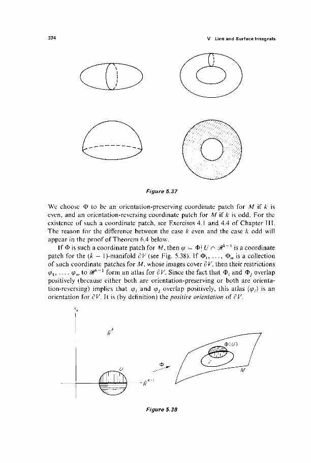
374 V Line and Surface Integrals
Figure 5.37
We choose Φ to be an orientation-preserving coordinate patch for M if A- is even, and an orientation-reversing coordinate patch for M if k is odd. For the existence of such a coordinate patch, see Exercises 4.1 and 4.4 of Chapter III. The reason for the difference between the case k even and the case k odd will appear in the proof of Theorem 6.4 below.
If Φ is such a coordinate patch for A/, then φ = Φ| £/ n ^ * - 1 is a coordinate patch for the (k — l)-manifold dV (see Fig. 5.38). If Φΐ9 . . . , 0OT is a collection of such coordinate patches for A/, whose images cover d V, then their restrictions q>u . . . , φ,η to Mk~l form an atlas for dV. Since the fact that Φ, and Φ; overlap positively (because either both are orientation-preserving or both are orienta-tion-reversing) implies that φ{ and φ] overlap positively, this atlas {<p,·} is an orientation for dV. It is (by definition) the positive orientation of dV.
Figure 5.38
6 Stokes' Theorem 375
As a useful exercise, the reader should check that this construction yields the counterclockwise orientation for the unit circle 51, considered as the bound-ary of the disk B2 in the oriented 2-manifold M2, and, more generally, that it yields the positive orientation (of Section 2) for any compact 2-manifold-with-boundary in 0l2.
A cellulation is a special kind of paving, and we have previously stated that every compact smooth manifold has a paving. It is, in fact, true that every oriented compact smooth manifold-with-boundary possesses an oriented cellulation. If we accept without proof this difficult and deep theorem, we can establish Stokes' theorem for manifolds-with-boundary.
Theorem 6.4 Let V be an oriented compact smooth /:-manifold-with-boundary in the oriented smooth /c-manifold M c @ln. If dV has the positive orientation, and a is a ^ 1 differential (k — l)-form on an open set con-taining V, then
\doi=\ a. (10) v rv
PROOF Let cff = {A1, . . . , Ap) be an oriented cellulation of V. We may assume without loss of generality that the (/:, 0)th faces Ak
xt 0 , . . . , A% 0 of the first q
of these oriented Λτ-ceüs are the boundary faces of the cellulation. Let φ1 : Ik -> A1
be the given orientation-preserving parametrization of A1. Then
(da=t(-\)ki a (11) Jy f = i V k . o
by Theorem 6.3. By the definition in Section 5, of the integral of a differential form over an
oriented manifold,
J « = X Ja,
where Bt, . . . , Bs are the oriented (k — l)-cells of any oriented paving of the oriented (k — l)-manifold dV. That is,
S *=iS* if xj/i is an orientation-preserving parametrization of /?,· , /= 1, . . . , s.
Now the boundary faces A\tQ , . . . , Aqk 0 constitute a paving of d V\ the ques-
tion here is whether or not their parametrizations cplk 0 are orientation-preserv-
ing. But from the définition of the positive orientation for dV, we see that φ[ o is orientation-preserving or orientation-reversing according as k is even or
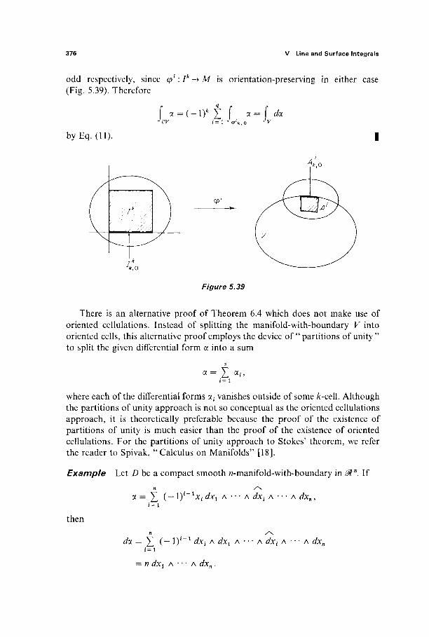
376 V Line and Surface Integrals
odd respectively, since φι : Ik -> M is orientation-preserving in either case (Fig. 5.39). Therefore
byEq. (11).
f α = (-1)* Σ f a = f i/a
</>''
Figure 5.39
There is an alternative proof of Theorem 6.4 which does not make use of oriented cellulations. Instead of splitting the manifold-with-boundary V into oriented cells, this alternative proof employs the device of " partitions of unity" to split the given differential form a into a sum
s
α = Σ ai > / = l
where each of the differential forms af vanishes outside of some k-cell. Although the partitions of unity approach is not so conceptual as the oriented cellulations approach, it is theoretically preferable because the proof of the existence of partitions of unity is much easier than the proof of the existence of oriented cellulations. For the partitions of unity approach to Stokes' theorem, we refer the reader to Spivak, "Calculus on Manifolds" [18].
Example Let D be a compact smooth «-manifold-with-boundary in 0ln. If
α = Σ (—1)ι1χί<1χι Λ · " A dxt A " - A dxn,
then
^a = Σ (— l)1 1 dxt A dxx Λ · · · Λ dXi Λ · · · Λ dxn i= 1
= n dxi Λ · · · Λ dxn.
6 S t o k e s ' T h e o r e m 377
Theorem 6.4 therefore gives
£ ( — 1 ) ' -X"; rfx-! Λ ' ' · Λ cÎX'i Λ ' ' * Λ c/.Y,, = / I dx\ Λ ' ' ' Λ i/.Vn ,
SO
v(D) = n~1 f £ ( - l ) 1 " " 1 * ^ Λ · · · Λ rfx; Λ · · · Λί/Λ·η (12) *VD i = 1
if <5Z> is positively oriented. Formula (12) is the //-dimensional generalization of the formula
^ = i — y dx 4- Λ" c/y
for the area of a region D Œ 3?2 (see Example 2 of Section 2). According to Exercise 5.13, the differential (n — l)-form
a = X ( — l ) 1 - ^ , É/*! Λ · · · Λ rfxf Λ · · · Λ dxn i= 1
is the surface area form of the unit sphere S"- 1 a j#n. With D = Bn, formula (12) therefore gives
v(Bn)=-a(Sn'1), n
the relationship that we have previously seen in our explicit (and separate) computations of v(Bn) and a(Sn~ l).
The applications of Stokes' theorem are numerous, diverse, and significant. A number of them will be treated in the following exercises, and in subsequent sections.
Exercises
6.1 Let F be a compact oriented smooth (k +1 + l)-dimensional manifold-with-boundary in 0tn. If a is a &-form and β an /-form, each f6x in a neighborhood of V, use Stokes' theorem to prove the "integration by parts" formula
ί (doc) Αβ= f α Λ β - ( - 1 ) * \ ocAciß. Jy J ey Jy
6.2 If ω is a ^ 1 differential k-ïovm on ^" such that
f ω = 0
for every compact oriented smooth /:-manifold M <= n , use Stokes' theorem to show that ω is closed, that is, dœ = 0.

378 V Line and Surface Integrals
6.3 Let a be a r^' differential (k — l)-form defined in a neighborhood of the oriented compact smooth /:-manifold M <= @tn. Then prove that
Γ da. = 0. J M
Hint: If β is a smooth /:-dimensional ball in M (see Fig. 5.40), and V=M- int 5, then
doc = ί/α + I ί/α. ^ M ^ » ^ V
Figure 5.40
6.4 Let Vi and K2 be two compact «-manifolds-with-boundary in £%n such that V2 c int Kt.
If a is a differential (n — l)-form such that da = 0 on W = Vx — int V2, show that
s « - / « ^οκι Jev2
if ôKi and dF2 are both positively oriented. 6.5 We consider in this exercise the differential (n — l)-form d® defined on 3$n — 0 by
1 n / \ d® = - Σ ( -D ' -^ i^c i Λ··· AdxtA-' Adxny
p t = i
where p2 = *i2 -f *22 H + xn2· For reasons that will appear in the following exercise,
this differential form is called the solid angle form on #", and this is the reason for the notation ί/Θ. Note that dS reduces to the familiar
dd = —y dx -\- x dy
x2+y2
in the case n = 2. (a) Show that dS is closed, d(d@) = 0. (b) Note that, on the unit sphere S""1, ί/Θ equals the surface area form of Sn~l. Con-clude from Exercise 6.3 that dS is not exact, that is, there does not exist a differential (n - 2)-form α ο η ^ " - 0 such that doc = d®. (c) If M is an oriented compact smooth (n — l)-manifold in ^" which does not enclose the origin, show that
f d® = 0.
(d) If M is an oriented compact smooth (n — l)-manifold in 0ln which does enclose the origin, use Exercise 6.4 to show that
\ dS = a(Sn-1).
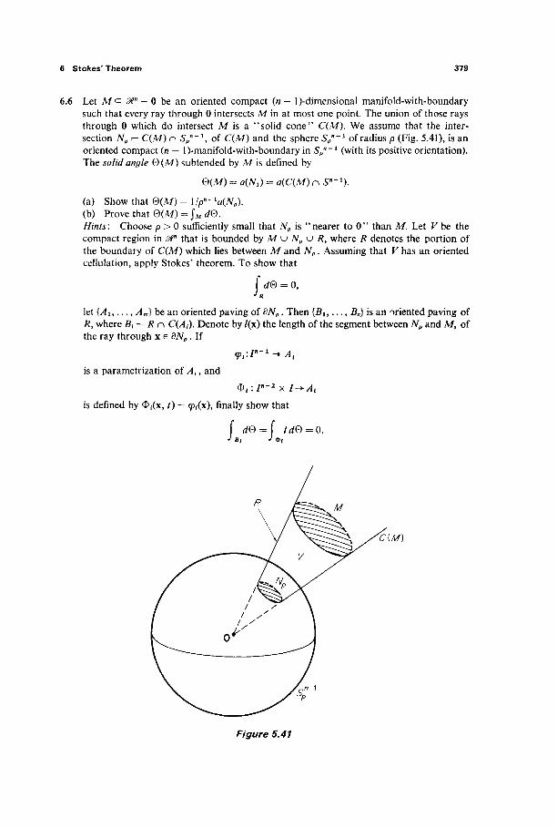
6 Stokes' Theorem 379
6.6 Let M c: ^" — 0 be an oriented compact in — 1 )-dimensional manifold-with-boundary such that every ray through 0 intersects M in at most one point. The union of those rays through 0 which do intersect M is a "solid cone" C(M). We assume that the inter-section Np = C(M) n S / - 1 , of C(M) and the sphere S / " 1 of radius p (Fig. 5.41), is an oriented compact (n — l)-manifold-with-boundary in Sp
n~1 (with its positive orientation). The solid angle Θ(Μ) subtended by M is defined by
Θ(Μ) = a^Nt) = £i(C(M) n S""1).
(a) Show that Θ(Μ ) = 1 /p" " (7VP). (b) Prove that Θ(Μ) = f M </Θ. Hints: Choose p > 0 sufficiently small that iVp is "nearer to 0" than M. Let V be the compact region in 3%n that is bounded b y M u i V p u i ? , where /? denotes the portion of the boundary of C(M) which lies between M and Np. Assuming that V has an oriented cellulation, apply Stokes' theorem. To show that
f d® = 0,
let {/4i,..., Am} be an oriented paving of dNp. Then {J5i,..., Bn) is an oriented paving of R> where B{ = R n C(^,). Denote by /(x) the length of the segment between Wp and Λ/, of the ray through x e a/Vp. If
is a parametrization of At, and Φ , : / — 2 χ / - * Λ ,
is defined by Φ{(χ, f ) = <p<(x), finally show that
f dS= f /«/Θ = 0.
Figure 5.41
380 V Line and Surface Integrals
6.7 If V is a compact smooth «-dimensional manifold-with-boundary in &n, then there are two unit normal vector fields on dV—the outer normal, which at each point of c V points out of V, and the inner normal, which points into V. On the other hand, if M is an oriented smooth (n — l)-manifold in ^", then we have seen in Exercise 5.13 that the orientation of M uniquely determines a normal vector field NonM. If M = öKis positively oriented (as the boundary of K), show that N is the outer normal vector field. Hence we can conclude from Exercise 5.13 that the surface area form of dV is
dA= Σ ( - O i _ 1 « i ^ i Λ·· · Adxt Λ·· · AdxHt 1= 1
where the nt are the components of the outer normal vector field on d V.
7 THE CLASSICAL THEOREMS OF VECTOR ANALYSIS
In this section we give the classical vector formulations of certain important special cases of the general Stokes' theorem of Section 6. The case n = 3, k = 1 yields the original (classical) form of Stokes' theorem, while the case n = 3, k = 2 yields the "divergence theorem," or Gauss' theorem.
If F : 0tn -► 0tn is a ^ 1 vector field with component functions Fu . . . , Fn, the divergence of F is the real-valued function div F : Mn -» M defined by
n dF d i v F = X — ' . (1)
i = l OXi
The reason for this terminology will be seen in Exercise 7.10. The following result is a restatement of the case k: = n — 1 of Stokes' theorem.
Theorem 7.1 Let F be a ^ 1 vector field defined on a neighborhood of the compact oriented smooth /7-manifold-with-boundary V c 0tn. Then
div F = £ ( - l)1 iFidxi A -·· A dxi A " · A dxn, (2)
PROOF If a = Yj=1(-l)i~1Fidxi A · · · Λ dxi A · · · Λ rfx„, then
" / n dFi \ ^ doc = Σ (— 0 l X I Σ T~^ dxj) A J^! Λ · · · Λ dxi A · · · Λ dxn
i=l \j=l vXj )
n ._ dF ^ = Y ( — l)1 λ -—l- dxi A dxi Λ · · · Λ dxt Λ · · · Λ dxn
i=\ dxi
= (div F) dx1 Λ · · · Λ dxn. |
The divergence theorem in ^ " is the statement that, if F and V are as in Theorem 7.1, then
ί divF = i F· NA4, (3) J y J ey

7 The Classical Theorems of Vector Analysis 381
where N is the unit outer normal vector field on ô V, and d V is positively oriented (as the boundary of V c 0ln). The following result will enable us to show that the right-hand side of (2) is equal to the right-hand side of (3).
Theorem 7.2 Let M be an oriented smooth (n — l)-manifold in 0tn with surface area form
n / \
dA = ]T (— \)l~lni dxx Λ · · · Λ dxi A · · · Λ dxn . i= 1
Then, for each / = 1, ..., n, the restrictions to each tangent plane of M9 of the differential (n — l)-forms
nt dA and (— 1)I_1 dxx A · · · Λ dxx A · · · Λ dxn,
are equal.
That is, if the vectors vls . . . , vn_t are tangent to M at some point x, then
Πι(\) dAx(\l, . . . , νη-χ) = (— 1)I_1 dx1 A - · · A dxt A · - A dxn(\l, . . . , \n-i).
For brevity we write
A7f ö U = ( — 1 ) '~ * ί/Xj Λ · ' · Λ ί/χ,- Λ * · ' Λ dxn , (4 )
remembering that we are only asserting the equality of the values of these two differential (n — l)-forms on (n — l)-tuples of tangent vectors to M.
PROOF Let vl5 . . . , \n_l be tangent vectors to M at the point x e A/, and let φ : U-+ M be an orientation-preserving coordinate patch with x = φ(ιι) e φ(ϋ). Since the vectors
- ^ ( u ) , . . . , - ^ - ( u )
constitute a basis for the tangent plane to M at x, there exists an (n — 1) x (n — 1) matrix .4 = (#0) such that
" dcp
If a is any (n — l)-multilinear function on 0tn, then
a(v1,. . . ,v l i_1) = ( d e t ^ ) a ( ^ , . . . , - ^ - )
by Exercise 5.15. It therefore suffices to show that
ndAl^P_ d(P \ VWj ' dun_1J
S\
= (—\y dxt A ' ■ ' A dxt A ■ ' ■ A dx l^L d(p \ [du/ '"" dun.J
382 V Line and Surface Integrals
We have seen in Exercise 5.13 that
where
^|i(%;;^'-;ri..))î" Consequently
n.dAΗ Ô(P ) ydu^ " ' dun_J
" . , ^ /3<p 3<p \ = n,· 2, ( - \y 1njdxl A - · · Λ dxj A - · · Λ dxn — , . . . ,
■ „Ε(_ι,,-.'.ζρ(*»·-·£··-«γ j = i £ \ 3 ( " i , . . . , « „ - i ) /
^ ( - Ι ) 1 ' - 1 ^ , . . . ,φ , . , ...,<?„) " fd(<pl9..., <pj, ...,φη)\2
D2 d(ul9 . . . , !/„_!) J = i \ 3(1*!, . . . , «„_!> /
- 1 ^ / <ty> 3φ \ = (— l)1 dxx A - - A dxt A - - A dxn -— . . . , I
\dui9 oun-J as desired. |
In our applications of this theorem, the following interpretation, of the coefficient functions nt of the surface area form
dA = X (— iy~1ni dxx A · · · Λ dxt A · · · Λ dxn » = i
of the oriented (n — l)-manifold M, will be important. 7/* M is the positively-oriented boundary of the compact oriented n-manifold-with-boundary V cz &n, then the n{ are simply the components of the unit outer normal vector field N on M = d V (see Exercise 6.7).
Example 1 We consider the case n = 3. If V is a compact 2-manifold-with-boundary in &3, and N = (ni9 nl9 n3) is the unit outer normal vector field on dV, then the surface area form of d V is
dA = n{ dy A dz + n2 dz A dx + n3 dx A dy9 (5)
7 The Classical Theorems of Vector Analysis 383
and Eq. (4) yields nl dA = dy A dz,
n2 dA = dz A dx, (6) n3 dA = dx A dy.
Now let F = (Fl9 F2, F3) be a ^ 1 vector field in a neighborhood of V. Then Eqs. (6) give
Fx dy A dz + F2 dz A dx + F3 dx A dy = Fxnx dA + .F2 w2 A4 + F3 n3 dA,
so Ft dy A dz + F2 dz A dx + F3 dx A dy = F · N dA. (7)
Upon combining this equation with Theorem 7.1, we obtain
div F = Ftdy A dz + F2 dz A dx + F3 Ac Λ Î/J;
= f F · NA4,
the divergence theorem in dimension 3. Equation (7), which in essence expresses an arbitrary 2-form on d V as a multiple of dA, is frequently used in applications of the divergence theorem.
The divergence theorem is often applied to compute a given surface integral by "transforming" it into the corresponding volume integral. The point is that volume integrals are usually easier to compute than surface integrals. The following two examples illustrate this.
Example 2 To compute \5V x dy A dz — y dz A dx, we take F = (x, —y, 0). Then div F = 0, so
x dy A dz — y dz A dx = i F · N dA
= ί div F = 0.
Example 3 To compute \si y dz A dx + xz dx A dy, take F = (0, y, xz). Then div F = 1 + x, so
y dz A dx + xz dx A dy = ( 1 + x) dx dy dz JS2 Jβ3
= v(B3) + ( xdxdydz
since the last integral is obviously zero by symmetry.
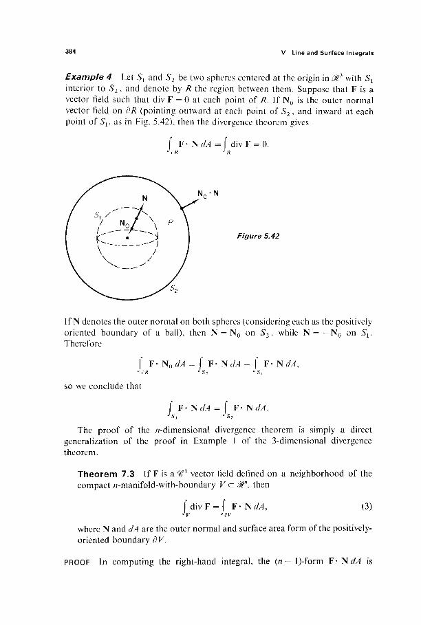
384 V Line and Surface Integrals
Example 4 Let Sx and S2 be two spheres centered at the origin in &3 with Si
interior to S2, and denote by R the region between them. Suppose that F is a vector field such that div F = 0 at each point of R. If N0 is the outer normal vector field on dR (pointing outward at each point of S2, and inward at each point of S{, as in Fig. 5.42), then the divergence theorem gives
f F · N dA = f div F = 0.
Figure 5.42
If N denotes the outer normal on both spheres (considering each as the positively oriented boundary of a ball), then N = N0 on S2* while N = — N0 on Si. Therefore
f F· N0 dA = f F· N dA - f F· N dA, JpR ^S2
v5 !
so we conclude that
f ¥-NdA = { F · NdA.
The proof of the /7-dimensional divergence theorem is simply a direct generalization of the proof in Example 1 of the 3-dimensional divergence theorem.
Theorem 7.3 If F is a ^ 1 vector field defined on a neighborhood of the compact fl-manifold-with-boundary V a 0tn, then
Γ div F = Γ F· NdA, (3) Jy Jdy
where N and dA are the outer normal and surface area form of the positively-oriented boundary d V.
PROOF In computing the right-hand integral, the (n — l)-form F-NdA is
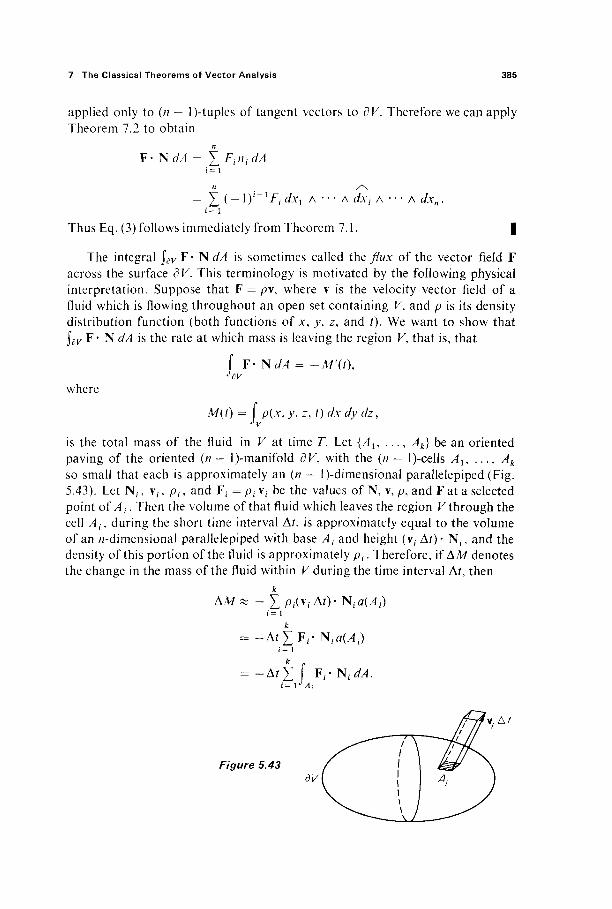
7 The Classical Theorems of Vector Analysis 385
applied only to (n — l)-tuples of tangent vectors to dV. Therefore we can apply Theorem 7.2 to obtain
F · NdA = X F.n.dA i= 1
n / \
= X ( — 1 )' ~ 1Fidxx A · · · Λ dx{ A - · - A dxn . i= 1
Thus Eq. (3) follows immediately from Theorem 7.1. |
The integral j ^ F · NdA is sometimes called the flux of the vector field F across the surface dV. This terminology is motivated by the following physical interpretation. Suppose that F = pv, where v is the velocity vector field of a fluid which is flowing throughout an open set containing K, and p is its density distribution function (both functions of x, y, z, and /). We want to show that \dv F· N dA is the rate at which mass is leaving the region V, that is, that
f F-NdA = -M'(t), hv
where
M(t) = p(x, y, z, t) dx dy dz,
is the total mass of the fluid in V at time T. Let {Al, . . . , Ak} be an oriented paving of the oriented (n — l)-manifold dV, with the (n — l)-cells Au . . . , Ak
so small that each is approximately an (n — l)-dimensional parallelepiped (Fig. 5.43). Let Nf, vf, pt, and F,· = p{ v,· be the values of N, v, p, and F at a selected point of A ;;. Then the volume ofthat fluid which leaves the region V through the cell Ai, during the short time interval At, is approximately equal to the volume of an /?-dimensional parallelepiped with base A{ and height (v,· At)- Nt-, and the density of this portion of the fluid is approximately p{. Therefore, if AM denotes the change in the mass of the fluid within V during the time interval At, then
AM* - Χ Ρ ^ . Δ Ο - Ν , . * ( / ! , . ) i= 1
= -AfXF(-N/fl(/J1) i= 1
= - Δ / £ f Fr-N, dA. i= \J Ai
Figure 5.43 dV
386 V Line and Surface Integrals
Taking the limit as At -> 0, we conclude that
M\t)= - F · NdA Jpy
as desired. We can now apply the divergence theorem to obtain
M\t) = - f Jy
div F.
On the other hand, if dpjdt is continuous, then by differentiation under the integral sign we obtain
dp M ■(i)=U·
Consequently
J>'4H Since this must be true for any region V within the fluid flow, we conclude by the usual continuity argument that
dp div(pV) + i- = 0.
ct
This is the equation of continuity for fluid flow. Notice that, for an incompressible fluid (one for which p = constant), it reduces to
div v = 0.
We now turn our attention to the special case n = 3, k = 1 which, as we shall see, leads to the following classical formulation of Stokes' theorem in & :
ί (curl F)· NdA = ί F · Τ ώ , ^D JÖD
(8)
where D is an oriented compact 2-manifold-with-boundary in ^ 3 , N and T are the appropriate unit normal and unit tangent vector fields on D and dD, respec-tively, F = (Fi, F2 , F3) is a ^ 1 vector field, and curl F is the vector field defined by
curl F (dF3 dF2 dFt dF3 dF2 dF^ \dy dz dz dx ' dx dy
) ■
This definition of curl F can be remembered in the form
curl F = V x F =
e i e 2 e 3
d d d
dx dy dz
Fi F2 F,
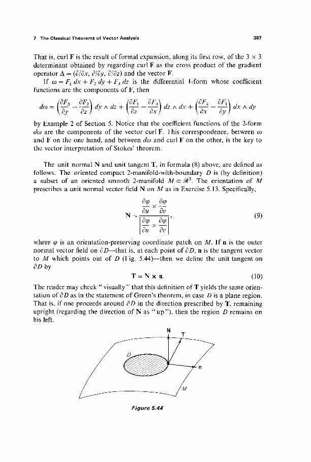
7 The Classical Theorems of Vector Analysis 387
That is, curl F is the result of formal expansion, along its first row, of the 3 x 3 determinant obtained by regarding curl F as the cross product of the gradient operator Δ = (d/dx, d/dy, d/dz) and the vector F.
If ω = Fl dx + F2 dy + F3 dz is the differential 1-form whose coefficient functions are the components of F, then
da) /dF3 dF2\ J J IdF, dF3\ J , (dF2 dFÄ ,
by Example 2 of Section 5. Notice that the coefficient functions of the 2-form dco are the components of the vector curl F. This correspondence, between ω and F on the one hand, and between dœ and curl F on the other, is the key to the vector interpretation of Stokes' theorem.
The unit normal N and unit tangent T, in formula (8) above, are defined as follows. The oriented compact 2-manifold-with-boundary D is (by definition) a subset of an oriented smooth 2-manifold M c &3. The orientation of M prescribes a unit normal vector field N on M as in Exercise 5.13. Specifically,
N =
dcp dcp
du dv
d(p d(p
du dv
(9)
where φ is an orientation-preserving coordinate patch on M. If n is the outer normal vector field on dD—that is, at each point of dD, n is the tangent vector to M which points out of D (Fig. 5.44)—then we define the unit tangent on dD by
T = N x n (10) The reader may check "visually" that this definition of T yields the same orien-tation of dD as in the statement of Green's theorem, in case D is a plane region. That is, if one proceeds around dD in the direction prescribed by T, remaining upright (regarding the direction of N as " up"), then the region D remains on his left.
Figure 5.44
388 V Line and Surface Integrals
Theorem 7.4 Let D be an oriented compact 2-manifold-with-boundary in J>3, and let N and T be the unit normal and unit tangent vector fields, on D and dD, respectively, defined above. If F is a Ή1 vector field on an open set containing D, then
f (curl F)· NdA = f F · Ύ ds. (8)
PROOF The orientation of dD prescribed by (10) is the positive orientation of 3D, as defined in Section 6. If
ω = F1dx + F2dy + F3 dz, it follows that
f ω= ί F · Tds. (11) -dD hü
See Exercise 1.21 or the last paragraph of Section 1. Applying Theorem 7.2 in the form of Eq. (6), we obtain
(ÔF3 ÔF2\ (ÔF, dF3\ (dF2 δΓΛ dœ=[^-^z-)dyAaZ+[^z--^)dZAdy +
(dF3 dF2\ , IdF, dF3\ , (dF2 dFA
\cy ox I \cz ox / \ox oy J = (curlF)· NdA,
so
f dw= f (curl F)· NdA. (12) J D J D
Since jD dœ = j Ô D ω by the general Stokes' theorem, Eqs. (11) and (12) imply Eq. (8). |
Stokes' Theorem is frequently applied to evaluate a given line integral, by "transforming" it to a surface integral whose computation is simpler.
Example 5 Let F(x, y, z) = (x, x + y, x + y + z), and denote by C the ellipse in which the plane z = y intersects the cylinder x2 + y2 = 1, oriented counter-clockwise around the cylinder. We wish to compute j c F · T ds. Let D be the elliptical disk bounded by C. The semiaxes of D are 1 and yJ2, so a(D) = Uyjl. Its unit normal is N = (0, - 1/^2, 1/^2), and curl F = (1, - 1, 1). Therefore
f F· Tds= f (curl F)· Ν ^ JC J D
2
W2' J n
-$-a(D)
= 2π.

7 The Classical Theorems of Vector Analysis 389
Another typical application of Stokes' theorem is to the computation of a given surface integral by " replacing " it with a simpler surface integral. The following example illustrates this.
Example 6 Let F be the vector field of Example 5, and let D be the upper hemisphere of the unit sphere S1. We wish to compute jD(curlF)· NdA. Let B be the unit disk in the jcy-plane, and C = dD = dB, oriented counterclockwise. Then two applications of Stokes' theorem give
f (curl F)· NdA = f F · Ύ ds J D *X
= f (curl F) · N dA J B
= ί (1, - 1 , 1)· (0,0, \)dA JB
= a{B)
= π.
We have interpreted the divergence vector in terms of fluid flow; the curl vector also admits such an interpretation. Let F be the velocity vector field of an incompressible fluid flow. Then the integral
/ , F· Tds c
is called the circulation of the field F around the oriented closed curve C. If Cr
is the boundary of a small disk Dr of radius r, centered at the point p and normal to the unit vector b (Fig. 5.45), then
ί F · T ds = f (curl F) · b dA « 7ir2(curl F(p)) · b. Jcr J D
Figure 5.45
Taking the limit as r -► 0, we see that
1 r (curlF(p))· b = lim—2 F· Tds. r-+o Tir Jcr
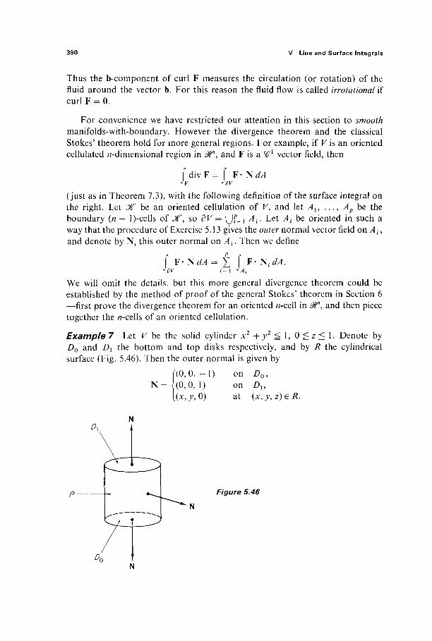
390 V Line and Surface Integrals
Thus the b-component of curl F measures the circulation (or rotation) of the fluid around the vector b. For this reason the fluid flow is called irrotational if curl F = 0.
For convenience we have restricted our attention in this section to smooth manifolds-with-boundary. However the divergence theorem and the classical Stokes' theorem hold for more general regions. For example, if Kis an oriented cellulated «-dimensional region in $n, and F is a ^ 1 vector field, then
Γ div F = Γ F· NdA Jv JdV
(just as in Theorem 7.3), with the following definition of the surface integral on the right. Let X be an oriented cellulation of K, and let Au . . . , Ap be the boundary (n — l)-cells of jf, so dV= \Jf=l At. Let At be oriented in such a way that the procedure of Exercise 5.13 gives the outer normal vector field on A ,·, and denote by Nf this outer normal on At. Then we define
ί F· NdA = £ f F· NidA. JdV i = l J At
We will omit the details, but this more general divergence theorem could be established by the method of proof of the general Stokes' theorem in Section 6 —first prove the divergence theorem for an oriented /7-cell in 0ln, and then piece together the «-cells of an oriented cellulation.
Example 7 Let V be the solid cylinder x2 + y1 ^ 1, 0 ^ z ^ 1. Denote by D0 and D1 the bottom and top disks respectively, and by R the cylindrical surface (Fig. 5.46). Then the outer normal is given by
( ( 0 , 0 , - 1 ) on D0, N = (0,0, 1) on Dt,
{(x,y,0) at (x,y,z)eR.
Figure 5.46
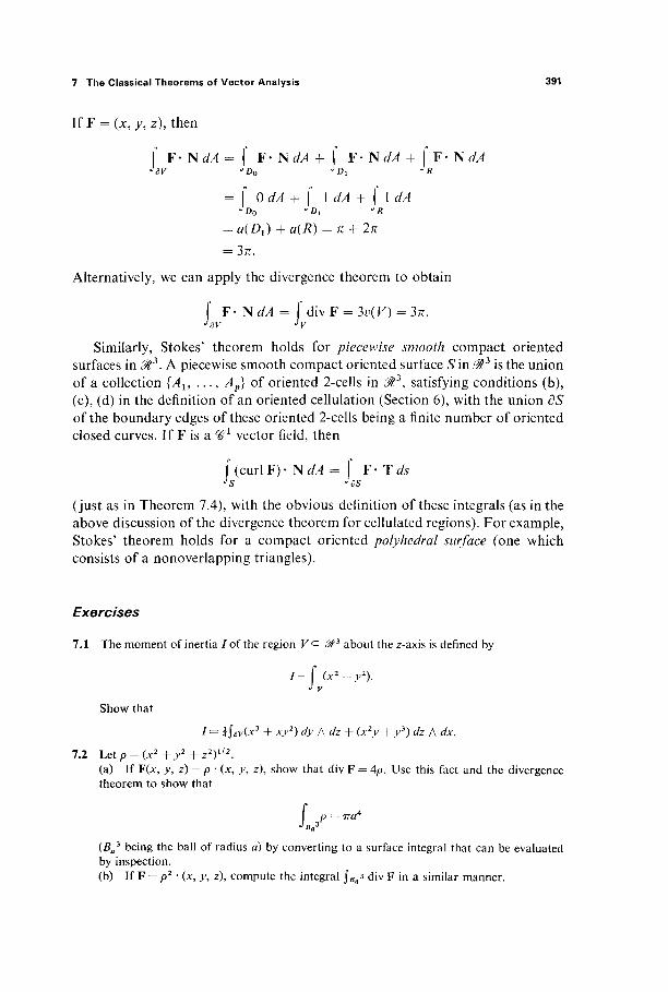
7 The Classical Theorems of Vector Analysis 391
If F = (%, y, z), then
f F· NdA = f F · NdA + f F· NdA + f F· N </Λ
= f 0 </Λ + f \dA + ( IdA JDO ^D{ JR
= a(D1) + a(R) = π + 2π = 3ττ.
Alternatively, we can apply the divergence theorem to obtain
f F-NdA= ( dWF = 3v(V) = 3n.
Similarly, Stokes' theorem holds for piecewise smooth compact oriented surfaces in ^ 3 . A piecewise smooth compact oriented surface S in & is the union of a collection {Au . . . , Ap} of oriented 2-cells in ^ 3 , satisfying conditions (b), (c), (d) in the definition of an oriented cellulation (Section 6), with the union dS of the boundary edges of these oriented 2-cells being a finite number of oriented closed curves. If F is a ^ 1 vector field, then
i (cur lF) · NdA = ( F - T ds
(just as in Theorem 7.4), with the obvious definition of these integrals (as in the above discussion of the divergence theorem for cellulated regions). For example, Stokes' theorem holds for a compact oriented polyhedral surface (one which consists of a nonoverlapping triangles).
Exercises
7.1 The moment of inertia / of the region V <= 3 about the z-axis is defined by
L p = Tree
(Ba3 being the ball of radius a) by converting to a surface integral that can be evaluated
by inspection. (b) If F = p2 - (x, y, z), compute the integral \Ba* div F in a similar manner.
I=( (x2-{-y2). J y
Show that
/ = ifavC*3 + *y2) dy Adz + (x2y + y3) dz A dx.
7.2 Let p = (x2+y2 + z2)1/2. (a) If F(x, y, z) = p · (x, j>, z), show that div F = 4p. Use this fact and the divergence theorem to show that

392 V Line and Surface Integrals
7.3 Find a function g(p) such that, if F(JC, y, z) = g(p)(x, y, z), then div F = pm [m ;> 0, p = (A:2 + y2 + z2)1 / 2 ] . Use it to prove that
f Pm = — f pm{x*y,z).NdA
if V is a compact 3-manifold-with-boundary in (M2'. For example, show that
V 2
7.4 In each of the following, let C be the curve of intersection of the cylinder x2 -\- y2 = \ and the given surface z =f(x, y), oriented counterclockwise around the cylinder. Use Stokes' theorem to compute the line integral by first converting it to a surface integral.
(a) \ y dx + z dy f x dz, z = xy. Jc
(b) \ z{x-\)dy + y{x + \)dz, z = xy + \. J c
(c) z dx — x dz, z = 1 — y. Je
7.5 Let the 2-form a be defined on ^ 3 — p, p = {a, b, c), by
O — a) dy A dz -f (^ — 6) dz A dx + (z — c) dx A dy a = [(* - a)2 + (>> - b)2 + (z - r ) 2 ] 3 / 2 '
(a) Show that doc = 0. (b) Conclude that JM a = 0 if M is a compact smooth 2-manifold not enclosing the point p. (c) Show that JM α = 4π if M is a sphere centered at p. (d) Show that $M α = 4ττ if M is any compact positively oriented smooth 2-manifold enclosing the point p.
7.6 The potential φ(χ, y, z) at x = (JC, y, z) due to a collection of charges qu . . . , q,„ at the points P i , . . . , pm is
φθ, >>, z) = £ - ,
where π = | x — p,· | . If E = — V99, the electric field vector, apply the previous problem to show that
f E · N dA = 477<tfi H Vqm)
if M is a smooth 2-manifold enclosing these charges. This is Gauss' law. 7.7 Let / and g be ^ 1 functions on an open set containing the compact w-manifold-with-
boundary V^ @n9 and let N be the unit outer normal on BV. The Laplacian V 2 /and the
normal derivative df/dn are defined by
V 2 / = div(V/) and — = Vf· N. dn

7 The Classical Theorems of Vector Analysis 393
Prove Greerfs formulas in â&n:
8g (a) f (fV2g + V/. Vg) = f / / dA,
(b) J^-evv) = Jw(/2-^)-". ////i/: For (a), apply the divergence theorem with F =fVg.
7.8 Use Green's formulas in @n to generalize Exercises 2.7 and 2.8 to &n. In particular, if/ and g are both harmonic on V <= ", V2/= V2# = 0, and / = g on δΚ, prove that / = # throughout K.
7.9 Let / be a harmonic function on the open set U c i%n (n> 2). If B is an «-dimensional ball in U with center p and radius a, and S = dß, prove that
/(P)%^)J>· «(5).
That is, the value of/at the center of the ball B is the average of its values on the bound-ary S of B. This is the average value property for harmonic functions. Outline'. Without loss of generality, we may assume that p is the origin. Define the function g : 8$n — 0 -> 31 by
Denote by SE SL small sphere of radius ε > 0 centered at 0, and by V the region between 5ε and S (Fig. 5.47).
Figure 5.47
(a) Show that # is harmonic, and then apply the second Green's formula (Exercise 7.7) to obtain the formula
ί,('2-£)Ή('2-ΊΚ (b) Notice that
J.('£-2H-^j/«-^U«·
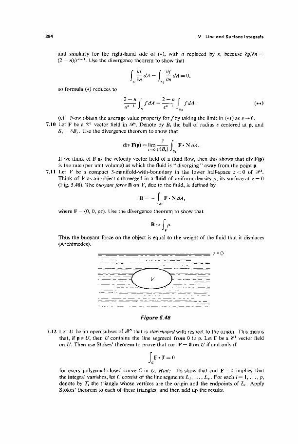
394 V Line and Surface Integrals
and similarly for the right-hand side of (*), with a replaced by ε, because dg/dn = (2 — n)/rn -l. Use the divergence theorem to show that
df JA f df
so formula (*) reduces to
[ —dA= [ — dA = 0, J v dn J., dn
2—nΓ 2 — n r T^T / < " = — r | fdA. (**)
(c) Now obtain the average value property f o r / b y taking the limit in (**) as ε ->0. 7.10 Let F be a c€x vector field in ^" . Denote by Bt the ball of radius ε centered at p, and
SE = 3Βε. Use the divergence theorem to show that
divF(p) = lim f F - Ν Λ ί . ε-+ο v{Bt) JSg
If we think of F as the velocity vector field of a fluid flow, then this shows that div F(p) is the rate (per unit volume) at which the fluid is "diverging" away from the point p.
7.11 Let V be a compact 3-manifold-with-boundary in the lower half-space z < 0 of ^ 3 . Think of V as an object submerged in a fluid of uniform density p, its surface at z = 0 (Fig. 5.48). The buoyant force B on K, due to the fluid, is defined by
B = - ί F . N Î / Λ , J ev
where F = (0, 0, pz). Use the divergence theorem to show that
B = \p. Jy
Thus the buoyant force on the object is equal to the weight of the fluid that it displaces (Archimedes).
z--0
Figure 5.48
7.12 Let U be an open subset of ^ 3 that is star-shaped with respect to the origin. This means that, if p e {/, then U contains the line segment from 0 to p. Let F be a ^ 1 vector field on U. Then use Stokes' theorem to prove that curl F = 0 on U if and only if
Î F . T = O Je
for every polygonal closed curve C in U. Hint: To show that curl F = 0 implies that the integral vanishes, let C consist of the line segments Lu . . . , Lp . For each i = 1, . . . , p, denote by Tt the triangle whose vertices are the origin and the endpoints of L f . Apply Stokes' theorem to each of these triangles, and then add up the results.

8 Closed and Exact Forms 395
8 CLOSED AND EXACT FORMS
Let ω be a %Λ differential A>form defined on the open set U in ffln. Then ω is called closed (on U) if dœ = 0, and exact (on U) if there exists a (k — l)-form a on U such that da = ω.
Since d(dœ) = 0 by Proposition 5.1, we see immediately that every exact form is closed. Our object in this section is to discuss the extent to which the converse is true.
According to Theorem 2.5, every closed 1-form, which is defined on all of 0t2, is exact. However, we have seen in Section 2 that the 1-form
—ydx + x dy ω = 2—
x2 + y2
is closed on &2 — 0, but is not exact; that is, there is no function/: 0t2 — 0 -> 0t such that df=w. These facts suggest that the question as to whether the closed 1-form ω on U is exact, depends upon the geometry of the set U.
The "Poincaré lemma" (Theorem 8.1 below) asserts that every closed form defined on a star-shaped region is exact. The open set U a 0ln is called star-shaped with respect to the point a provided that, given x e i / , the line seg-ment from a to x is contained in U. The open set U is star-shaped if there exists a e i / such that U is star-shaped with respect to a. For example, 0tn itself is star-shaped (with respect to any point), as is every open ball or open fl-dimen-sional interval in 0ln.
Theorem 8.1 Every closed Ή1 differential k-îorm defined on a star-shaped open subset U of 0tn is exact.
PROOF We may assume (after a translation if necessary) that U is star-shaped with respect to the origin 0. We want to define, for each positive integer k, a certain function /, from /:-forms on U to (k — l)-forms, such that 1(0) = 0.
First we need the following notation. Given a k-tupk i = (il9 i2, . . . , ik)9
write k XS
A'i = Σ ( - l)J~lxij dxh Λ · "dXij * ' ' Λ dxik.
Note that
άμχ = k dXi = k dxix A · · · Λ dxik (1)
and, if/i = (j, /',, . . . , ik), then
μΓι = Xj dXi — dxj A μ{ (2)

396 V Line and Surface Integrals
(Exercise 8.4). Now, given a /:-form ω = X ai d*i
[ i ]
on U, we define the (k — l)-form Ιω on U by
(3)
Note that this makes sense because U is star-shaped with respect to 0, so txe U if x e U and t e [0, 1]. Clearly 7(0) = 0, and
d(Ia>) = Σ [ i ]
= Σ [ i ]
i d ( [ i * " 1 *^ ) ώ) Λ /i, + (j tk~la^tx)dt\ άμ{
i f — I J i * - 1 ^ ) rfA </*;) Λ φ , + * ( f ^ " ^ ( r x ) dt\ dx{
d(I(o) = Σ ί Σ ( j '* ^ (ίχ) Λ ) rfxi Λ & + *(f ik"^i(ix) dt\ dx
If ω is closed on £/, then
0 = I(dœ)
0 = Σ Σ ( I <* Τ1 ( ί χ) dt) (xj α% - dxj A , , ,) . [ i ] j = i V o üxj I
Upon addition of Eqs. (4) and (5), we obtain
-1 .da. ά(Ιω) = X
[I]
= Σ
Uitkd^(tx)xjdt)+k(Ltk~lai{tx)dt). dx{
1 / J \
f \ktk'xaltx) + tk- (α,(ίχ)) I Λ JX:
^Σ^Ι^^Α)* -
(4)
(5)
= X[ifcûri(ix)V=0^i
= Σ ^i(x) ^xi^ [ i ]
d(Ico) = ω.
Thus we have found a (/: — l)-form whose differential is ω, as desired. |

8 Closed and Exact Forms 397
Example 1 Consider the closed 2-form
ω = xy dy A dz + y dz A dx — (z -f yz) dx A dy
on ^ 2 . In the notation of the proof of Theorem 8.1,
dy A dz = dx{1, 3)·> dz A dx = dx{3 1}, dx A dy = dx(l> 2 ) ,
and
ß(2,2>)=ydz-z dy\ μ(3>1} = z dx - x dz, μ(ι, 2) = x dy - y dx.
Equation (3) therefore gives
ίω = l f t(t2xy) dt\(y dz - z dy) + i f t(ty) dt\(z dx - x dz)
+ i f t(-tz - t2yz) dt\(x dy - y dx)
xy y = — (y dz — z dy) + -(z dx — x dz)
+ (-Z--y-fj(xdy-ydx),
i (2yz^y2z\j iyxz^XZ\A Axy2 xA^
a 1-form whose differential is ω.
Theorem 8.1 has as special cases two important facts of vector analysis. Recall that, if F = (P, Q, R) is a ^ 1 vector field on an open set U in M3, then its divergence and curl are defined by
v_dP dQ dR dx dy dz '
_ (dR dQ dP dR dQ dP\ curl F ' ■ - f dy dz ' dz dx' dx dy)
It follows easily that div F = 0 if F = curl G for some vector field G on U, while curl F = 0 if F = grad / = V/for some scalar function/ The following theorem asserts that the converses are true if U is star-shaped.
Theorem 8.2 Let F be a ^ 1 vector field on the star-shaped open set U c ^ 3 . Then (a) curl F = 0 if and only if there exists/: U'-» 0t such that F = g r a d / (b) div F = 0 if and only if there exists G : U -> &3 such that F = curl G.
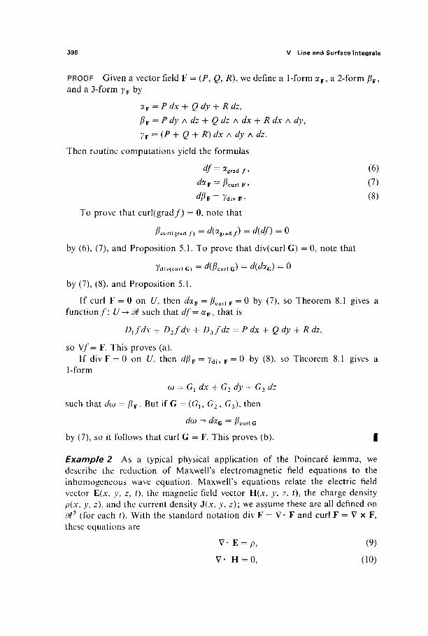
398 V Line and Surface Integrals
PROOF Given a vector field F = (P, Q, R), we define a 1-form aF, a 2-form ßF, and a 3-form yF by
aF = P rfx + ß rfy + Λ rfz, ßF = P dy A dz + Q dz A dx + R dx A dy,
yF = (P + Q + R)dx Ady Λ dz.
Then routine computations yield the formulas
df=<*gr*df> (6) docv = ß C U T l F , ( 7 )
^ F = 7 d i v F · (8 )
To prove that curl(grad/) = 0, note that
ßcurKgrad / ) = ^(«grad/) = d(df) = 0
by (6), (7), and Proposition 5.1. To prove that div(curl G) = 0, note that
7div(curl G) = é c u r i e ) = d(dOLQ) = 0
by (7), (8), and Proposition 5.1.
If curl F = 0 on U, then docF = ßcurl F = 0 by (7), so Theorem 8.1 gives a function/: U'-> 0t such that df=ocF, that is
DJdx + D2fdy + D3/ûfe = P dx + Q dy + R dz,
so V/= F. This proves (a). If div F = 0 on £/, then dßF = ydiv F = 0 by (8), so Theorem 8.1 gives a
1 -form
ω = Gx dx + G2 dy + C73 i/z
such that dœ = ßF. But if G = (G1? G2 , C73), then
dœ = docG = ß c u r l G
by (7), so it follows that curl G = F. This proves (b). |
Example 2 As a typical physical application of the Poincaré lemma, we describe the reduction of Maxwell's electromagnetic field equations to the inhomogeneous wave equation. Maxwell's equations relate the electric field vector E(x, >', z, t), the magnetic field vector H(x, y, z, i), the charge density p(x, y, z), and the current density J O , >\ z); we assume these are all defined on & (for each t). With the standard notation div F = V· F and curl F = V x F, these equations are
V - E = p, (9)
V· H = 0, (10)
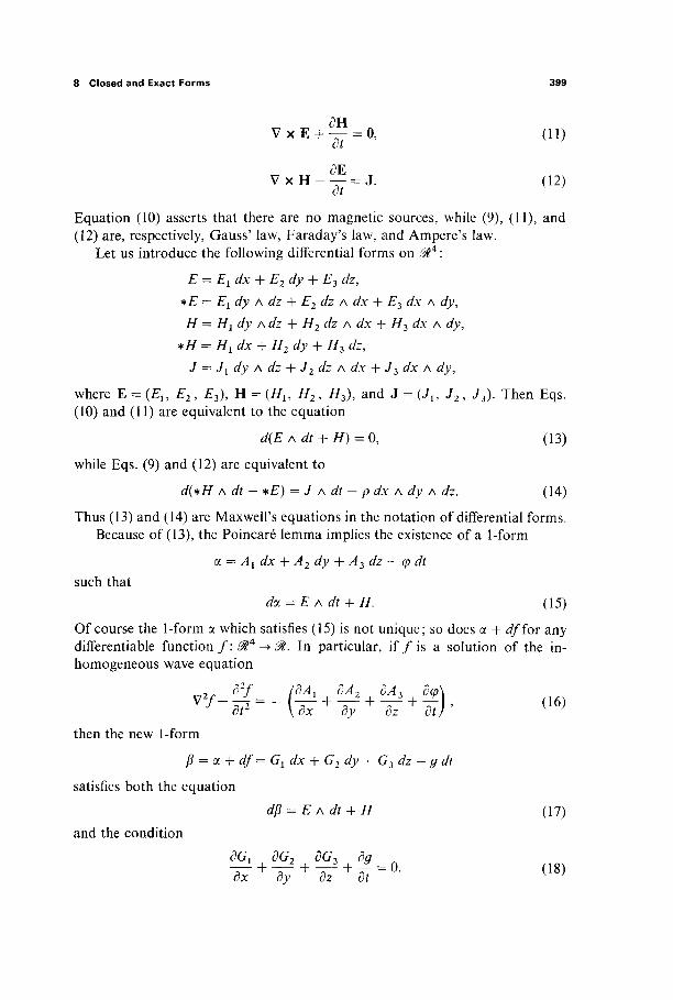
8 Closed and Exact Forms 399
<9H V x E + — = 0, (11)
dt
dE V x H - - = J. (12)
Equation (10) asserts that there are no magnetic sources, while (9), (11), and (12) are, respectively, Gauss' law, Faraday's law, and Ampere's law.
Let us introduce the following differential forms on $*:
E = E^dx + E2dy + E3 dz,
*E = Exdy A dz + E2 dz A dx -f E3 dx Λ dy,
H = H1 dy A dz + H2 dz A dx + H3 dx A dy,
*H = HY dx + H2 dy + H3 dz,
J = J1 dy A dz + J2 dz A dx + J3 dx A dy,
where E = (El9 E2, £3), H = (Hu H2, H3), and J = (JU J2, J3). Then Eqs. (10) and (11) are equivalent to the equation
d(E Adt + H)=0, (13)
while Eqs. (9) and (12) are equivalent to
d(*H A dt — *E) = J A dt — p dx A dy A dz. (14)
Thus (13) and (14) are Maxwell's equations in the notation of differential forms. Because of (13), the Poincaré lemma implies the existence of a 1-form
a = Ax dx + A2 dy + A3 dz — φ dt
such that doc = E Adt-l· H. (15)
Of course the 1-form a which satisfies (15) is not unique; so does a + dj'for any differentiable function / : ^ 4 -*0ί. In particular, i f / i s a solution of the in-homogeneous wave equation
J et2 \dx dy dz dt}' (16)
then the new 1-form
β = α + df= G1 dx + G2 dy + G3 dz — g dt
satisfies both the equation dß = E A dt + H (17)
and the condition dGx dG2 dG3 da
(18)

400 V Line and Surface Integrals
Computing dß, we find that (17) implies that
# 1
Ei
dG3 dG2
dy dz
dGl dg ~ ~~dt~~dx'
dz dx
E dG2 dg 2 dt dy'
dG2 dGi
(19) dx dy
E d°3 dg
3 dt dz'
Substituting these expressions for the components of E and // , and making use of (18), a straightforward computation gives
d(*H A dt - * £ ) - ί—γ- - V2GJ dy Adz A dt
+ I —-f - W2G2 I dz A dx A dt
+ I — ^ - V2G3I dx A dy A dt
KS) + I V V — —y I dx A dy A dz.
Comparing this result with Eq. (14), we conclude that the vector field G = (Gl, G2, G3) on &3 and the function g satisfy the inhomogeneous wave equa-tions
Ô2Q 1 A V72 Z29 7 T = — J and x g — —-=-dt2 u dt2
V 2 G - —r= - J and V2# - - f = -p. (20)
Thus the solution of Maxwell's equations reduces to the problem of solving the inhomogeneous wave equation. In particular, if G and g satisfy Eq. (18) and (20), then the vector fields
dG E = - Vg - — and H = V x G,
dt
defined by Eqs. (19), satisfy Maxwell's equations (9)—(12).
Exercises
8.1 For each of the following forms a>, find a such that dcc= ω. (a) ω = (3x2y2 + 8*>'3) dx + (2x3y + \2x2y2 + Ay) dy on Ά2. (b) ω = (y2 + 2xz2) dx + {2xy + 3y2z3) dy + {2x2z + 3y3z2) dz on ^ 3 . (c) ω = (2j> - 4) dy t\dz + (y2 - 2x) dz A dx-\-(3 - x - 2yz) dx A dy. (d) ω = to2 + j z 2 + zx2) dx A dy A dz.
8.2 Let ω be a closed 1-form on ^ 2 — 0 such that J s l cu = 0. Prove that ω is exact on J22 — 0. Hint: Given (x, y) e PÂ2 — 0, define f(x, y) to be the integral of ω along the path γ{χ,γ)
8 Closed and Exact Forms 401
which follows an arc of the unit circle from (l , 0) to (x / | x | , j | ^ | ) , and then follows the radial straight line segment to (x, y). Then show that df= ω.
8.3 If ω is closed 1-form on Λ3 — 0, prove that ω is exact on Mz — 0. Hint: Given p e Mz — 0, define/(p) to be the integral of ω along the path yp which follows a great-circle arc on S2 from (1, 0, 0) to p / | p | e S2, and then follows the radial straight line segment to p. Apply Stokes' theorem to show that / (p) is independent of the chosen great circle. Then show that df= ω.
8.4 Verify formulas (1) and (2). 8.5 Verify formulas (6), (7), and (8). 8.6 Let ω = dx + z dy on i^3. Given f(x, y, z), compute d(fœ). Conclude that ω does not
have an integrating factor (see Exercise 5.4).
VI The Calculus of Variations
The calculus of variations deals with a certain class of maximum-minimum problems, which have in common the fact that each of them is associated with a particular sort of integral expression. The simplest example of such a problem is the following. L e t / : & -+0ί be a given <ß2 function, and denote by (€λ\μ, b] the set of all real-valued ^ 1 functions defined on the interval [a, b]. Given φ e ^[a, b], define F(i/0 e m by
ηψ)= \b fm),v(t\t)A. (*)
Then F is a real-valued function on ^[a, b]. The problem is then to find that element φ e ^[a, b], if any, at which the function F : [a, b]^>& attains its maximum (or minimum) value, subject to the condition that φ has given pre-assigned values φ(α) = oc and φφ) = β at the endpoints of [a, b].
For example, if we want to find the ^ 1 function φ : [a, b]->& whose graph x = cp(t) (in the Oc-plane, Fig. 6.1) joins the points (a, a) and (b, β) and has minimal length, then we want to minimize the function F : ^[a, b\^>(% defined by
ρ(Φ) = f [i + mm2)1'2 dt.
Here the function / : 01* -> 0t is defined by f(x, y, t) = y/l + y2. Note that in the above problem the "unknown" is & function ψ Ε^ι[α, b],
rather than a point in 0tn (as in the maximum-minimum problems which we considered in Chapter II). The "function space" ^[a, b\ is, like ^Γ, a vector space, albeit an infinite-dimensional one. The purpose of this chapter is to appropriately generalize the finite-dimensional methods of Chapter II so as to treat some of the standard problems of the calculus of variations.
402

The Calculus of Variations 403
(o,a)
Figure 6.1
χ--ψ(ΐ)
•(A/5)
In Section 3 we will show that, if φ e ^[a, b] maximizes (or minimizes) the function F : ^ι[α, b\-+0l defined by (*), subject to the conditions φ(α) = oc and φφ) = β, then φ satisfies the Euler-Lagrange equation
j£(φ(ή, <p'(t), t)-^-%((KO, </>'(0, 0 = 0. ox at oy
The proof of this will involve a generalized version of the familiar technique of ''setting the derivative equal to zero, and then solving for the unknown."
In Section 4 we discuss the so-called " isoperimetric problem," in which it is desired to maximize or minimize the function
ΠΨ)= \h fm\v(t\t)dt9 J a
subject to the conditions ij/(a) = a, \p(b) = β and the "constraint"
0(Φ) = f gm\ Ψ'Φ, ή dt = c.
Here/and g are given ^2 functions on ^ 3 . We will see that, if φ e ^[a, b] is a solution for this problem, then there exists a number l e f such that φ satisfies the Euler-Lagrange equation
dh d dh ox dt oy
for the function h : ^ 3 -► 01 defined by
h(x, y, 0 =f(x, y, 0 - ig(x, y, 0·
This assertion is reminiscent of the constrained maximum-minimum problems of Section II.5, and its proof will involve a generalization of the Lagrange multiplier method that was employed there.

404 VI The Calculus of Variations
As preparation for these general maximum-minimum methods, we need to develop the rudiments of "calculus in normed vector spaces." This will be done in Sections 1 and 2.
1 NORMED VECTOR SPACES AND UNIFORM CONVERGENCE
The introductory remarks above indicate that certain typical calculus of variations problems lead to a consideration of "function spaces" such as the vector space (^i[a, b] of all continuously differentiate functions defined on the interval [a, b]. It will be important for our purpose to define a norm on the vector space ^[f l , b\ thereby making it into a normed vector space. As we will see in Section 2, this will make it possible to study real-valued functions on ^l[a, b] by the methods of differential calculus.
Recall (from Section 1.3) that a norm on the vector space V is a real-valued function JC-> \x\ on V satisfying the following conditions:
N1 | jc |>0 i fx^0,
N2 \ax\ = \a\ \x\,
N3 \x + y\^\x\ + \y\,
for all x, y e V and a e l . The norm | x\ of the vector x e V may be thought of as its length or "size." Also, given x, y e V, the norm \x — y\ of x — y may be thought of as the "distance" from x to y.
Example 1 We have seen in Section 1.3 that each of the following definitions gives a norm on 0tn\
| x | o = max( | xl |, . . . , | xn \ ) (the sup norm), | x | ! = | x{ | + · · · + | xn | (the 1-norm), I xl 2 = (*i2 + ' ' ' + xn
2)1/Z (the Euclidean norm),
where x = (χγ, . . . , xn) e 0tn. It was (and is) immediate that | 10 and | | x are norms on ^", while the verification that | | 2 satisfies the triangle inequality (Condition N3) required the Cauchy-Schwarz inequality (Theorem 1.3.1).
Any two norms on Mn are equivalent in the following sense. The two norms | | ! and | | 2 on the vector space V are said to be equivalent if there exist positive numbers a and b such that
a\x\i ^ \x\2 ^ * l * l i
for all x e V. We leave it as an easy exercise for the reader to check that this relation between norms on V is an equivalence relation (in particular, if the norms | 11 and | 12 on V are equivalent, and also | 12 and | 13 are equivalent, then it follows that | 11 and | 13 are equivalent norms on V).
1 Normed Vector Spaces and Uniform Convergence 405
We will not include here the full proof that any two norms on <%n are equivalent. However let us show that any continuous norm | | on J?" (that is, |x | is a con-tinuous function of x) is equivalent to the Euclidean norm | 12 · Since | | is continuous on the unit sphere
S""1 = { X G I " : |x | 2 = 1},
there exist positive numbers m and M such that
m\y\2 = m ti \y\ S M = M\y\2
for all y e S " - 1 . Given x e 0P\ choose a > 0 such that x = ay with y e S"'1. Then the above inequality gives
ma\y\2 ^a\y\ <^Ma\y\2, so
m\x\2 S |x | ^ M\x\ 2
as desired. In particular, the sup norm and the 1-norm of Example 1 are both equivalent to the Euclidean norm, since both are obviously continuous. For the proof that every norm on Mn is continuous, see Exercise 1.7.
Equivalent norms on the vector space V give rise to equivalent notions of sequential convergence in V. The sequence {xn}f of points of V is said to converge to x e V with respect to the norm | | if and only if
lim \xn — x\ = 0.
Lemma 1.1 Let | | { and | 12 be equivalent norms on the vector space V. Then the sequence {xn}^ c= V converges to x e V with respect to the norm | | ! if and only if it converges to x with respect to the norm | \2.
This follows almost immediately from the définitions; the easy proof is left to the reader.
Example 2 Let V be the vector space of all continuous real-valued functions on the closed interval [a, b], with the vector space operations defined by
(φ + ψ)(χ) = φ(χ) + ψ(χ), (αφ)(χ) = αφ{χ\
where φ, φ e V and Û G £ We can define various norms on K, analogous to the norms on 0Γ in Example l, by
||φ|Ιο = rnax \φ{χ)\ (the sup norm), xe[a, fc]
IIΦ111 = I^WI dx (the 1-norm), J a
IIΨII2 = (j I φ(χ)\2 dx\ (the 2-norm).

406 VI The Calculus of Variations
Again it is an elementary matter to show that || ||0 and || ||j are indeed norms on V, while the verification that || ||2 satisfies the triangle inequality requires the Cauchy-Schwarz inequality (see the remarks following the proof of Theorem 3.1 in Chapter I). We will denote by ^°[a, b] the normed vector space V with the sup norm || ||0 .
No two of the three norms in Example 2 are equivalent. For example, to show that || ||0 and || \\x are not equivalent, consider the sequence {φη}* of elements of V defined by
!
\ — nx if x e 0, - ,
L n\
0 if X E \-, l l ,
and let φ0(χ) = 0 for x e [0, 1 ] (here the closed interval [a, b] is the unit interval [0, 1]). Then it is clear that {(pn}f converges to φ0 with respect to the 1-norm || || ! because
Λ , 1 \\<Pn- ΦοΙΙι = \(pn(x) - φ0(χ)\ dx = — -^ 0.
J0 In
However {cpn}f does not converge to φ0 with respect to the sup norm || ||0
because \\ψη- ΦθΙΙθ = \\ψη\\θ = 1
for all n. It therefore follows from Lemma 1.1 that the norms || ||0 and || \x are not equivalent.
Next we want to prove that %?°[a, b\ the vector space of Example 2 with the sup norm, is complete. The normed vector space V is called complete if every Cauchy sequence of elements of V converges to some element of V. Just as in 0tn^ the sequence {x,,}* <= V is called a Cauchy sequence if, given ε > 0, there exists a positive integer TV such that
m, n ^ N=> \xm - xn\ <ε . These definitions are closely related to the following properties of sequences
of functions. Let {fn}f be a sequence of real-valued functions, each defined on the set S. Then {fn}^ is called a uniformly Cauchy sequence (of functions on S) if, given ε > 0, there exists N such that
w, n^N=>\fm(x)-fn(x)\ <ε
for every x e S. We say that {fn}f converges uniformly to the function/: S -> 9Î if, given ε > 0, there exists TV such that
n^N^\fn(x)-f(x)\ <ε for every x e S.
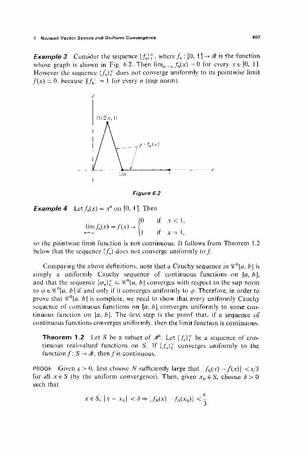
1 Normed Vector Spaces and Uniform Convergence 407
Example 3 Consider the sequence {/„}?, where /„ : [0, 1 ] -► 3t is the function whose graph is shown in Fig. 6.2. Then X\rt\n^^fn{x) = 0 for every XG [0, 1]. However the sequence {/„}f does not converge uniformly to its pointwise limit f(x) = 0, because | | / J = 1 for every n (sup norm).
y
(1/2/7,1)
y--Wx)
1 è 1 · X 1//7 1
Figure 6.2
Example 4 Let/M(jc) = xn on [0, 1 ]. Then
0 if x< 1,
1 if J C = 1,
so the pointwise limit function is not continuous. It follows from Theorem 1.2 below that the sequence {/„} does not converge uniformly t o / .
Comparing the above definitions, note that a Cauchy sequence in #°[#, b] is simply a uniformly Cauchy sequence of continuous functions on [a, b], and that the sequence {φη}* <= ^°[α, b] converges with respect to the sup norm to φ e #'°[tf, b] if and only if it converges uniformly to φ. Therefore, in order to prove that <£°[a, b] is complete, we need to show that every uniformly Cauchy sequence of continuous functions on [a, b] converges uniformly to some con-tinuous function on [a, b]. The first step is the proof that, if a sequence of continuous functions converges uniformly, then the limit function is continuous.
Theorem 1.2 Let S be a subset of @k. Let {fn}f be a sequence of con-tinuous real-valued functions on S. If {/„}? converges uniformly to the function/: S - » ^ , then/ i s continuous.
PROOF Given ε > 0, first choose N sufficiently large that \fN(x) —f(x)\ < ε/3 for all xe S (by the uniform convergence). Then, given x0 e S, choose δ > 0 such that
xeS, \x-x0\ <<5=> \fN(x)-fN{x0)\ <-
l im/„(x)=/(x) =
408 VI The Calculus of Variations
(by the continuity of fN at x0). If x e S and | x - x0 \ < δ, then it follows that
l/W -f(xo)\ ^ l/W -/*(*) I + 1/tfW -M*o)\ + |/*(*0) -/(*)l ε ε ε
< - + - + - = e, 3 3 3
s o / i s continuous at x 0 . |
Corollary 1.3 ^ ° [ Ö , 6] is complete.
PROOF Let {cpn}f be a Cauchy sequence of elements of ^°[Û, 6], that is, a uniformly Cauchy sequence of continuous real-valued functions on [a, b]. Given ε > 0, choose TV such that
ε m, n ^ N=> \\φη - φη\\ < - (sup norm).
Then, in particular, | (pm(x) — φη(χ) \ < ε/2 for each x e [a, b]. Therefore {(pn(x)}f is a Cauchy sequence of real numbers, and hence converges to some real number φ(χ). It remains to show that the sequence of functions {φη} converges uniformly to φ; if so, Theorem 1.2 will then imply that φ e #°[α, b].
We assert that η^ N (same JV as above, n fixed) implies that
| φ(χ) — φη{χ) I < ε for all x e [a, b].
To see this, choose m ^ N sufficiently large (depending upon x) that |φ(χ) — (pm(x)\ < ε/2. Then it follows that
| φ(χ) - φη(χ)\ S I φ(χ) ~ <pm(x)\ + | <pj<x) ~ <?„(*) I ε
< 2 + H m "Pil l
ε ε 2 2
Since x e [#, b] was arbitrary, it follows that \\φη — φ\\ <ε as desired. |
Example 5 Let ^ 1 [A, 6] denote the vector space of all continuously differenti-able real-valued functions on [a, 6], with the vector space operations οί%>°[α, b], but with the " ^ - n o r m " defined by
||<p||= max |φ(*)| + max |φ'(*)| xe[a, b] xe[fl, ft]
for φ e %>ι[α, b]. We leave it as an exercise for the reader to verify that this does define a norm on ^[a, b].
In Section 4 we will need to know that the normed vector space (#l[a9 b] is complete. In order to prove this, we need a result on the termwise-differentiation

1 Normed Vector Spaces and Uniform Convergence 409
of a sequence of continuously differentiable functions on [a, b]. Suppose that the sequence {fn}f converges (pointwise) to / , and that the sequence of derivatives {ΑΊΐ converges to g. We would like to know whether/ ' = g. Note that this is the question as to whether
f = D(\imfn)= \\m{Dfn)=gy n-* oo n-*· oo
an "interchange of limits" problem of the sort considered at the end of Section IV.3. The following theorem asserts that this interchange of limits is valid, provided that the convergence of the sequence of derivatives is uniform.
Theorem 1.4 Let {fn}f be a sequence of continuously differentiable real-valued functions on [a, b], converging (pointwise) t o / Suppose that the {fn)î converges uniformly to a function g. Then {f„}f converges uniformly t o / and / i s differentiable, wi th / ' = g.
PROOF By the fundamental theorem of calculus, we have
fnW =fn(a) + I"// J a
for each n and each x e [a, b]. From this and Exercise IV.3.4 (on the termwise-integration of a uniformly convergent sequence of continuous functions) we obtain
/ ( * ) = lim/„(x)
n-*■ oo " a = lim/n(û)+ lim j" / ' ,
n -* oo __.— ..„
f(x) =f(a) + (g.
Another application of the fundamental theorem yields/' = g as desired. To see that the convergence of {/„}* to / i s uniform, note that
I/„(*)-/(*) I = / > - / ; + \fa(a)-f(a)\
uj*\fn-g\ + I/„(*)-/(*) I ^{b-ä)\\fn'-g\\0+ \fn(a)-f(a)\.
The uniform convergence of the sequence {fn}f therefore follows from that of the sequence {/„'}?. |
Corollary 1.5 # l [a, b] is complete.
PROOF Let {φη}? be a Cauchy sequence of elements of # ' [a, b]. Since
max \q>m{x) - φη(χ)\ g ||(/>„, - </>J (tf'-norm), x e [ a , b ]
410 VI The Calculus of Variations
we see that {φη}™ is a uniformly Cauchy sequence of continuous functions. It follows from Corollary 1.3 that {φη}* converges uniformly to a continuous function φ : [a, ft] -» @t. Similarly
max \<pm'(x) - φ„'(χ)\ è \\<pm ~ φ„\\ («"-norm), x e [a,ö]
so it follows, in the same way from Corollary l .3, that {(pn'}f converges uniformly to a continuous function φ : [a, ft]-> 0t. Now Theorem 1.4 implies that φ is difTerentiable with φ = φ, so φ e ^x[a, ft]. Since
max \φη(χ) - φ(χ)\ = \\φ„ - φ\\0 x s la, b]
and (sup norm), max \φη\χ) - φ\χ)\ = \\φη' - φ'ΙΙο
xe[a, b]
the uniform convergence of the sequences {</>„}5° and {φπ'}5° implies that the sequence {</>„}5° converges to φ with respect to the «"-norm of %>λ[α, ft]. Thus every Cauchy sequence in ($i[a, ft] converges. |
Example 6 Let <#ι([α, ft]), 0ln) denote the vector space of all # ' paths in 0tn
(mappings φ : [Ö, ft] ->^n) , with the norm
\\φ\\= max |<p(i)|o+ m a x l < P ' ( 0 l o * te[a,b] te[a,b]
where | 10 denotes the sup norm in £%". Then it follows, from a coordinatewise application of Corollary 1.5, that the normed vector space Ήι{[α, ft], $n) is complete.
Exercises
1.1 Verify that || ||0 , II Hi, and || ||2, as defined in Example 2, are indeed norms on the vector space of all continuous functions defined on [a, b].
1.2 Show that the norms || Hi and || ||2 of Example 2 are not equivalent. Hint: Truncate the function 1/V7 near 0.
1.3 Let £and F be normed vector spaces with norms || ||£ and || ||F, respectively. Then the the product set E x F is a vector space, with the vector space operations defined coor-dinatewise. Prove that the following are equivalent norms on E x F:
ll(jc, )llo = max(||jc||£, \\y\\F), \\{x,y)\\i= II*IIE+IWIF, H(A:,>')ll2=[(lkll£)2 + (l^llF)2]1/2.
1.4 If the normed vector spaces E and F are complete, prove that the normed vector space E x F, of the previous exercise, is also complete.
1.5 Show that a closed subspace of a complete normed vector space is complete. 1.6 Denote by ^„[tf, b] the subspace of ^°[a, b] that consists of all polynomials of degree at
most n. Show that &η[α, b] is a closed subspace of #°[tf, b]. Hint: Associate the poly-nomial ψ{ΐ) = Σ " = 0
aktk with the point a = (a0 , au . . . , ak) e 3tk + \ and compare \\φ\\0
with |a | .
2 Continuous Linear Mappings and Differentials 411
1.7 If II II is a norm on ^", prove that the function x-> ||x|| is continuous on St. Hint'. If
then
ΙΙχΙΙ^Σ \χι\ lie*II-
The Cauchy-Schwarz inequality then gives
| | χ | | ^ Λ ί | χ | ,
where M = E J = 1 lie/II2]1/2 and | | is the Euclidean norm on 9tn.
2 CONTINUOUS LINEAR MAPPINGS AND DIFFERENTIALS
In this section we discuss the concepts of linearity, continuity, and differenti-ability for mappings from one normed vector space to another. The definitions here will be simply repetitions of those (in Chapters I and II) for mappings from one Euclidean space to another.
Let E and F be vector spaces. Recall that the mapping φ : E -> F is called linear if
φ(αχ + by) = αφ{χ) + b(p(y)
for all x, y e E and a, b e 01.
Example 1 The real-valued function / : ^°[a, b] -±0l, defined on the vector space of all continuous functions on [a, b] by
Kf) = fV. is clearly a linear mapping from %>°[α, b] to 0t.
If the vector spaces E and F are normed, then we can talk about limits (of mappings from E to F). Given a mapping/: E^Fand x0 e E, we say that
lim f(x) =LeF x-*xo
if, given ε > 0, there exists δ > 0 such that
0 < | jt - *01 < δ=> \ f(x) —L\ <ε.
The mapping/is continuous at x0 e E if
Y\m f(x) = f(x0). χ^χο
412 VI The Calculus of Variations
We saw in Section 1.7 (Example 8) that every linear mapping between Euclidean spaces is continuous (everywhere). However, for mappings between infinite-dimensional normed vector spaces, linearity does not, in general, imply continuity.
Example 2 Let V be the vector space of all continuous real-valued functions on [0, 1], as in Example 2 of Section 1. Let Ei denote V with the 1-norm || ||l5
and let E0 denote V with the sup norm || ||0. Consider the identity mapping λ : V -* V as a mapping from E1 to E0,
λ : El -» E0 .
We inquire as to whether λ is continuous at 0 e Ex (the constant zero function on [0, 1 ]). If it were, then, given c > 0, there would exist δ > 0 such that
M i l <δ=>\\φ\\0<ε.
However we saw in Section 1 that, given δ > 0, there exists a function φ : [0, 1 ] -► 01 such that
||<p||,<<5 while IMI 0 = 1·
It follows that λ : Ex -* E0 is not continuous at 0 e E1.
The following theorem provides a useful criterion for continuity of linear mappings.
Theorem 2.1 Let L: E-+F be a linear mapping where E and F are normed vector spaces. Then the following three conditions on L are equiva-lent:
(a) There exists a number c > 0 such that
\L(v)\ £C\v\
for all v e E. (b) L is continuous (everywhere). (c) L is continuous at 0 e E.
PROOF Suppose first that (a) holds. Then, given x0e E and ε > 0,
Ix - x01 <-=> \L(x) - L(x0)| = \L(x - x0)\ c
uc\x- x0\
< ε,
so it follows that L is continuous at x0 . Thus (a) implies (b).
2 Continuous Linear Mappings and Differentials 413
To see that (c) implies (a), assume that L is continuous at 0, and choose δ > 0 such that | JC| ^ δ implies \L(x)\ < 1. Then, given v Φ 0 e E, it follows that
J-TL(vi°) (" t e"R')
so we may take c = Ι/δ. |
Example 3 Let E0 and Ei be the normed vector spaces of Example 2, but this time consider the identity mapping on their common underlying vector space V as a linear mapping from E0 to El9
μ : E0^> E1. Since
Ml i = f \<Pif)\dt^ max |φ(ί)| = | |φ||0, J0 i e [ 0 , l ]
we see from Theorem 2.1 (with c = 1) that μ is continuous.
Thus the inverse of a one-to-one continuous linear mapping of one normed vector space onto another need not be continuous. Let L : E -» F be a linear mapping which is both one-to-one and surjective (that is, L(E) = F). Then we will call L an isomorphism (of normed vector spaces) if and only if both L and L" 1 are continuous.
Example 4 Let A, B : [α, Z?]-»^" be continuous paths in $n, and consider the linear function
defined by
L(P) = f [Ait) · ç>(0 + 5 (0 · φ\ί)} dt,
where the dot denotes the usual inner product in 0tn. Then the Cauchy-Schwarz inequality yields
\L{cp)\ = \ f W ) · <p(t) + B(t) - <p'(t)] dt I
^ f6(M(t)| k(0l + |Ä(0I W(t)\)dt J a
£(A-e)(MI|0+||2>||0)IMIi,
414 VI The Calculus of Variations
so an application of Theorem 2.1, with c = (b - ΰ)(||Λ||0 + ||2?||0), shows that L is continuous.
We are now prepared to discuss differentials of mappings of normed vector spaces. The definition of differentiability, for mappings of normed vector spaces, is the same as its definition for mappings of Euclidean spaces, except that we must explicitly require the approximating linear mapping to be continuous. The mapping/ : E-+F is differentiable at x e E if and only if there exists a continuous linear mapping L : E -> F such that
f(x + h)-f(x)-L(h) hm —= = 0. (1) /i-O I "I
The continuous linear mapping L, if it exists, is unique (Exercise 2.3), and it is easily verified that a linear mapping L satisfying (1) is continuous at 0 if and only i f / i s continuous at x (Exercise 2.4).
I f / : E-*F is differentiable at x eE, then the continuous linear mapping which satisfies (1) is called the differential o f / a t x, and is denoted by
dfx:E->F.
In the finite-dimensional case E = $n, F = 0tm that we are already familiar with, the m x n matrix of the linear mapping dfx is the derivative/'(x). Here we will be mainly interested in mappings between infinite-dimensional spaces, whose differential linear mappings are not representable by matrices, so deriva-tives will not be available.
Example 5 Iff: E -► F is a continuous linear mapping, then
f(X + h)-f(x)-f(h)_Q
\h\
for all x, h E E with h φ 0, s o / i s differentiable at x, with dfx = / . Thus a con-tinuous linear mapping is its own differential (at every point x e E).
Example 6 We now give a less trivial computation of a differential. Let g : $ -> $ be a ^ 2 function, and define
f:%°[a,b]->V°[a, b]
by f(<p) = 9°φ-
We want to show tha t / i s differentiable, and to compute its differential. I f / is differentiable at φΕ%0[α, b], then dfjji) should be the linear (in
he^°[a, b]) part o f / ( ^ + h) —f(q>). To investigate this difference, we write down the second degree Taylor expansion of g at φ(ή:
g{q>(t) + A(0) - 9{φ(ή) = g'^{t))h(t) + R(h){t\
2 Continuous Linear Mappings and Differentials 415
where *(*)(*) = wmxKt))2 (2)
for some ξ(ί) between φ(ί) and φ{ΐ) + h(t). Then
f(cp + h)-f((p)=L{h) + R{h\
where L(A) e ^°[a, b] is defined by
L{h){t)=g\9{t))h(t).
It is clear that L : ^°[<2, 6] ->^0[<ζ, &] is a continuous linear mapping, so in order to prove that / is differentiable at φ with ά/φ = L, it suffices to prove that
Note that, since g is a # 2 function, there exists M > 0 such that | #"(£(*)) | < 2M when ||A||0 is sufficiently small (why?). It then follows from (2) that
\R(h)(i)\ ^M\h(t)\2^^LU
IIAIIo IIAIIo and this implies (3) as desired. Thus the differential ά/φ : %?°[a, b] -> ^°[a, b] of / a t φ is defined by
<*£(*)(') = *'(Φ(0)Λ(0·
The chain rule for mappings of normed vector spaces takes the expected form.
Theorem 2.2 Let U and V be open subsets of the normed vector spaces E and F respectively. If the mappings f:U-+F and g : K-* G (a third normed vector space) are differentiable at x e U and f(x) e V respec-tively, then their composition h = g of is differentiable at x, and
dhx = dgf(x) o dfx.
The proof is precisely the same as that of the finite-dimensional chain rule (Theorem II.3.1), and will not be repeated.
There is one case in which derivatives (rather than differentials) are important. Let φ : 0t -» E be a path in the normed vector space E. Then the familiar limit
<p(t + h)- <p(t) φ (t) = lim e E,
Λ-Ο η if it exists, is the derivative or velocity vector of φ at t. It is easily verified that φ\ϊ) exists if and only if φ is differentiable at t, in which case dcpt{h) = (p'(t)h (again, just as in the finite-dimensional case).
416 VI The Calculus of Variations
In the following sections we will be concerned with the problem of mini-mizing (or maximizing) a differentiable real-valued function f:E -*0l on a subset M of the normed vector space E. In order to state the result which will play the role that Lemma II.5.1 does in finite-dimensional maximum-minimum problems, we need the concept of tangent sets. Given a subset M of the normed vector space E, the tangent set TMX of M at the point x e M is the set of all those vectors v e E, for which there exists a differentiable path φ : 2/t -> M cz E such that φ(0) = x and φ'(0) = v. Thus TMX is simply the set of all velocity vectors at x of differentiable paths in M which pass through x. Hence the tangent set of an arbitrary subset of a normed vector space is the natural generalization of the tangent space of a submanifold of 0Γ.
The following theorem gives a necessary condition for local maxima or local minima (we state it for minima).
Theorem 2.3 Let the function/: E-*'M be differentiable at the point x of the subset M of the normed vector space E. If f(v) ^f(x) for all v e M sufficiently close to x, then
dfx\TMx = 0.
That is, dfx(v) = 0 for all v e TMX.
PROOF Given v e TMX, let φ : 01 -> M be a differentiable path in E such that <p(0) = x and φ'(0) = v. Then the composition ^ = / o f l - > l has a local minimum at 0, so g'(0) = 0. The chain rule therefore gives
0 = ^ ( 0 ) = ^ 0 (1 ) = #φ ( 0)(#ο(1)) = dfx((p'(p))>
0 = # »
as desired. |
In Section 4 we will need the implicit mapping theorem for mappings of complete normed vector spaces. Both its statement and its proof, in this more general context, are essentially the same as those of the finite-dimensional implicit mapping theorem in Chapter III.
For the statement, we need to define the partial differentials of a differenti-able mapping which is defined on the product of two normed vector spaces E and F. The product set E x F is made into a vector space by defining
(*n y\) + (*2 » y2) = (*i + χ2, yι + y2) a n d <*(*> y) = (<**> <y) ·
I f I I E and | | F denote the norms on E and F, respectively, then
|(x, y)\ = m a x ( | x | £ , \y\F)
defines a norm on £ x F, and E x F is complete if both E and F are (Exercise 1.4). For instance, if E = jp= ^ with the ordinary norm (absolute value), then
2 Continuous Linear Mappings and Differentials 417
this definition gives the sup norm on the plane 0t x 0i = 0Î1 (see Example 1 of Section 1).
Now let the mapping
f:E xF->G
be differentiable at the point (a, b) e E x F. It follows easily (Exercise 2.5) that the mappings
φ : E -+ G and φ : F -> G,
defined by
<p(x)=f(x,b) and φ(γ) = f(a,y\ (4)
are differentiable at a e E and b e F, respectively. Then dxf(ai b) and dyJ\at b), the partial differentials off at (a, b), with respect to x e E and y e F, respectively, are defined by
dxAa, b) = d(p a and dyf(ût b) = dij/b.
Thus dxf{ab) is the differential of the mapping E-+G obtained f rom/ : E x F -► G by fixing j = 6, and dyf(ab) is obtained similarly by holding x fixed. This generalizes our definition in Chapter III of the partial differentials of a mapping from @m+n = 0Γ x @n to 0lk.
With this notation and terminology, the statement of the implicit mapping theorem is as follows.
Implicit Mapping Theorem Let/: E x F'-► G be a %l mapping, where £, F, and G are complete normed vector spaces. Suppose that f(a, b) = 0, and that
dyf(a,b) '- F-+G
is an isomorphism. Then there exists a neighborhood U of a in £, a neigh-borhood W of (Û, b) in E x F, and a Ή1 mapping φ : U -> F such that the following is true: If(x, y) e W and x e U, then f(x, y) = 0 // and only if y = φ{χ).
This statement involves ^ 1 mappings from one normed vector space to another, whereas we have defined only differentiable ones. The mapping# : E -► F of normed vector spaces is called continuously differentiable, or # ! , if it is dif-ferentiable and dgx(v) is a continuous function of (x, i;), that is, the mapping (x, y) -► dgx(v) from E x E to F is continuous.
As previously remarked, the proof of the implicit mapping theorem in complete normed vector spaces is essentially the same as its proof in the finite-dimensional case. In particular, it follows from the inverse mapping theorem for complete normed vector spaces in exactly the same way that the finite-dimensional implicit mapping theorem follows from the finite-dimensional
418 VI The Calculus of Variations
inverse mapping theorem (see the proof of Theorem III.3.4). The general inverse mapping theorem is identical to the finite-dimensional case (Theorem III.3.3), except that Euclidean space 0ln is replaced by a complete normed vector space E. Moreover the proof is essentially the same, making use of the contrac-tion mapping theorem. Finally, the only property of 0ln that was used in the proof of contraction mapping theorem, is that it is complete. It would be instruc-tive for the student to reread the proofs of these three theorems in Chapter III, verifying that they generalize to complete normed vector spaces.
Exercises
2.1 Show that the function / ( / ) = jbafis continuous on ^°[a, b].
2.2 If L : 0tn -> E is a linear mapping of 0tn into a normed vector space, show that L is con-tinuous.
2.3 Let f\E-+F be differentiable at x ε Et meaning that there exists a continuous linear mapping L : E -> F satisfying Eq. (1) of this section. Show that L is unique.
2.4 Let / : £ - > F b e a mapping and L: F-> F a linear mapping satisfying Eq. (1). Show that L is continuous if and only if/is continuous at x.
2.5 Let / : E x F-+G be a differentiable mapping. Show that the restrictions φ : E->G and φ : F-> G of Eq. (4) are differentiable.
2.6 If the mapping f:ExF^G\s differentiable at p e E x F, show that dxfp(r) = dfp(r, 0) and dyfp(s) = dfp(0y s).
2.7 Let M ^ f b e a translate of the closed subspace V of the normed vector space E. That is, given x e M, M = {* + y : >> G F). Then prove that FMX = V.
3 THE SIMPLEST VARIATIONAL PROBLEM
We are now prepared to discuss the first problem mentioned in the introduc-tion to this chapter. Given/ : & -*ffl, we seek to minimize (or maximize) the function F : ^ 1 [a, b]-+@ defined by
ΠΦ)= \hfiù{t),V(t),t)du G) " a
amongst those functions φ e ^χ[α, b] such that ψ(α) = a and \j/(b) = β (where a and β are given real numbers).
Let M denote the subset of ^[a, b] consisting of those functions φ that satisfy the endpoint conditions φ(α) = α and φφ) = β. Then we are interested in the local extrema of F on the subset M. If F is differentiable at φ e M, and F\M has a local extremum at φ, then Theorem 2.3 implies that
άΓφ\ΤΜφ = 0. (2)
We will say that the function φ e M is an extremal for F on M if it satisfies the necessary condition (2). We will not consider here the difficult matter of finding sufficient conditions under which an extremal actually yields a local extremum.
3 The Simplest Variational Problem 419
In order that we be able to ascertain whether a given function φ e M is or is not an extremal for F on M, that is, whether or not άΡφ \ ΤΜφ = 0, we must (under appropriate conditions on / ) explicitly compute the differential άΡφ of F at φ, and we must determine just what the tangent set ΤΜφ of M at φ is.
The latter problem is quite easy. First pick a fixed element φ0 e M. Then, given any φ e Λ/, the difference φ — φ0 is an element of the subspace
«Via, b] = {φ e %{[α, b] : ψ(α) = φ{ο) = 0}
of^l[a, b], consisting of those ^ 1 functions on [a, b] that are zero at both end" points. Conversely, if ψ e ^0
ι[α, b], then clearly φ0 + φ e M. Thus M is a hyper-plane in ^l[a, b], namely the translate by φ0 of the subspace %?0
{[α, b]. But the tangent set of a hyperplane is, at every point, simply the subspace of which it is a translate (see Exercise 2.7). Therefore
TM, = V0l[a,b] (3)
for every φ e M. The following theorem gives the computation of dF(p.
Theorem 3.1 Let F:^l[a, b]^@ be defined by (l), with / : ^ 3 - » ^ being a %?2 function. Then F is differentiate with
dF^h) = j ψ-χ (φ(ί), φ\ί\ t)h(t) + d£ (φ(0, φ'(ί), 0*'(θ] dt (4)
for all </>, heWl[a, b].
In the use of partial derivative notation on the right-hand side of (4), we are thinking of (x, y, t) e &3.
PROOF If F is differentiable at φ e ^l[a, b], then dFJiJi) should be the linear (in h) part of F(q> + h) — F(q>). To investigate this difference, we write down the second degree Taylor expansion off at the point (φ(ί), φ'(ί), t) e &3\
f(cp(t) + A(r), φ'(ί) + h\t\ t) -f((p(t), φ\ί% t)
= f (cp(t\ <p'(t), t)h(t) + f (φ(ί), φ\ΐ\ t)h\t) + r(A(i)), (5) ox oy
where
'WO) = ^ "Cl (ξ(ί))(Α(0)2 + 2 ^ (ί(Ο)Α(ΟΑ'(Ο + | £ (ί(0)(Α'(0)2
for some point ξ(ί) of the line segment in 0t3 from (</>(*), <p'(0> 0 t 0 (<P(0 + A(0> <p'(i) -f /ΐ'(ί)> 0· If ^ is a large ball in M3 that contains in its interior the image

420 VI The Calculus of Variations
of the continuous path t -► (φ(ί), φ'(ί), t), t e [a, b], and M is the maximum of the absolute values of the second order partial derivatives o f / a t points of B, then it follows easily that
M |r(A(0)| £ y(|A(01 + |A'(0l)2 (6)
for all t e [a, b], if ||A||0 is sufficiently small. From (5) we obtain
with
m = \
F(<p + h) - F{<p) = L(h) + R(h),
Vdf (φ(ή, tp'(t), t)h(t) + % (ψ(ή, φ'(ή, t)h'(t) ôx dy
dt
and
R(h) = r(h{t))dt.
In order to prove that F is differentiable at φ with άΡφ = L as desired, it suffices to note that L : # ' [a, b] -> M is a continuous linear function (by Example 4 of Section 2), and then to show that,
lim = 0. Ι|Λ||ι-0 W\l
But it follows immediately from (6) that
(7)
,b
R(h)\ è \r(h(t))\ dt
M r IVl
uj j(2\\h\\i)2dt = 2M(b-a)(\\h\\l)
2,
and this implies (7). I
With regard to condition (2), we are interested in the value of dFv(h) when heTM, = V0
1[a,b].
Corollary 3.2 Assume, in addition to the hypotheses of Theorem 3.1, that φ is a Ή2 function and that // e <ë0
l[a, b]. Then
dF, ;w = / b rdf d df
dx dt dy h(t) dt. (8)
3 The Simplest Variational Problem 421
PROOF If φ is a %2 function, then df/dy(<p(t), φ\ί\ t) is a # l function of / e [a, b]. A simple integration by parts therefore gives
v, f ^-(<p(t),(p'(t),t)ti'(t)dt
= [ | (<p(t), φ'«), t)h(t)J -jjt ( | > ( 0 , φΜ), θ) Α(0 Λ
= -J ^ ( |£ ( * (0 ,Ρ ' (0 ,Ο)Λ(ΟΛ
because //(#) = /z(Z>) = 0. Thus formula (8) follows from formula (4) in this case. I
This corollary shows that the # 2 function φ e M is an extremal for F on M if and only if
b
^(φ(ή,φ'(ί),ί)--ίδΑψ{ή,φ'(ή,ή ox at oy
h(t) dt = 0 (9)
for every ^ 1 function h on [a, b] such that h(a) = h(b) = 0. The following lemma verifies the natural guess that (9) can hold for all such h only if the function within the brackets in (9) vanishes identically on [a, b].
Lemma 3.3 If φ : [a, b] -> 01 is a continuous function such that
I cp(t)h(t) A = 0 * a
for every h e ^0χ[α, b]9 then φ is identically zero on [a, b].
PROOF Suppose, to the contrary, that φ(ί0) Φ 0 for some t0 G [a, b]. Then, by continuity, φ is nonzero on some interval containing t0, say, φ{ί) > 0 for * e ΙΛ> h) ^ [fl> b]. If /* is defined on [a, è] by
{(t-ti)2(t-t2)
2 if i e [ i l 9 i2],
(0 otherwise,
then h e ^ / f a , b], and
\btp(t)h(t) dt = Γφ(ί)(ί - ti)2(t - t2)
2 dt > 0,
because the integrand is positive except at the endpoints tx and t2 (Fig. 6.3). This contradiction proves that φ = 0 on [a, b]. |
The fundamental necessity condition for extremals, the Euler-Lagrange equation, follows immediately from Corollary 3.2 and Lemma 3.3.

422 VI The Calculus of Variations
graph of h
Figure 6.3
Theorem 3.4 Let F:^[a, b\-+® be defined by (1), with / : ^ 3 - > ^ being a <β2 function. Then the ^ 2 function φ e M is an extremal for F on Μ = {φΕ V1 [a9b]: φ(α) = α and φφ) = β} if and only if
d-f (φ(ί), φ\ΐ\ t)-£Jf (φ(ί), φ'(ί), 0 = 0 (10)
for all t e [a, b].
Equation (10) is the Euler-Lagrange equation for the extremal φ. Note that it is actually a second order (ordinary) differential equation for φ, since the chain rule gives
d df d2f d2f 32f dtdy δχδγφ + dy2 Ψ + dt dy'
where the partial derivatives off are evaluated at (φ(ή, φ\ϊ), t) e &3.
REMARKS The hypothesis in Theorem 3.4 that the extremal φ is a ^ 2 func-tion (rather than merely ^ 1 ) is actually unnecessary. First, if φ is an extremal which is only assumed to be 1 then, by a more careful analysis, it can still be proved that df/dy((p(t), (p'(f)9 t) is a diiferentiable function (of /) satisfying the Euler-Lagrange equation. Second, if φ is a ^ 1 extremal such that
d2f dx dy
(φ(ί), φ'(0, 0 # 0
for all t e [a, b\ then it can be proved that φ is, in fact, a # 2 function. We will not include these refinements because Theorem 3.4 as stated, with the additional hypothesis that φ is ^ 2 , will suffice for our purposes.
We illustrate the applications of the Euler-Lagrange equation with two standard first examples.
Example 1 We consider a special case of the problem of finding the path of minimal length joining the points (tf, a) and (Z>, ß) in the Dc-plane. Suppose in

3 The Simplest Variational Problem 423
particular that φ : [a, b] -> 01 is a ^ 2 function with φ(α) = α and <ρ(ό) = β whose graph has minimal length, in comparison with the graphs of all other such functions. Then φ is an extremal (subject to the endpoint conditions) of the function
FW) = \b[l+mt))2]1,2<lt,
whose integrand function is
f(x,y,t) = (l+y2)1'2.
Since df/dx = 0 and df/dy = y/(\ + y2)1/2, the Euler-Lagrange equation for φ is therefore
d φ' =o , dt [1 + (ψ')2]112
which upon computation reduces to
(1 +(<PT) 2x3 /2 = 0.
Therefore φ" = 0 on [a, b], so φ is a linear function on [a, b], and its graph is (as expected) the straight line segment from (a, a) to (b, β).
Example 2 We want to minimize the area of a surface of revolution. Suppose in particular that φ : [a, b] -> 0t is a ^2 function with φ(ά) = a and φφ) = β, such that the surface obtained by revolving the curve x = φ(ί) about the i-axis has minimal area, in comparison with all other surfaces of revolution obtained in this way (subject to the endpoint conditions). Then φ is an extremal of the function
Γ(φ)= \b2mJ,(t)[\+W(t))2]l/2dt,
whose integrand function is
f(x,y,t) = 2nx(\ + y2)l/2.
Here
df ^ _ / i , 2x1/2 —Λ df 2nxy = 2n(\+y2)1/2 and f- = dx v ' ' dx (1 +y2)112
Upon substituting x = φ(ί), y = φ'(ί) into the Euler-Lagrange equation, and simplifying, we obtain
df ddf 1 + {φ'Ϋ - φφ" --— = 2π dx dtdy [1 +(</>')2]3/2
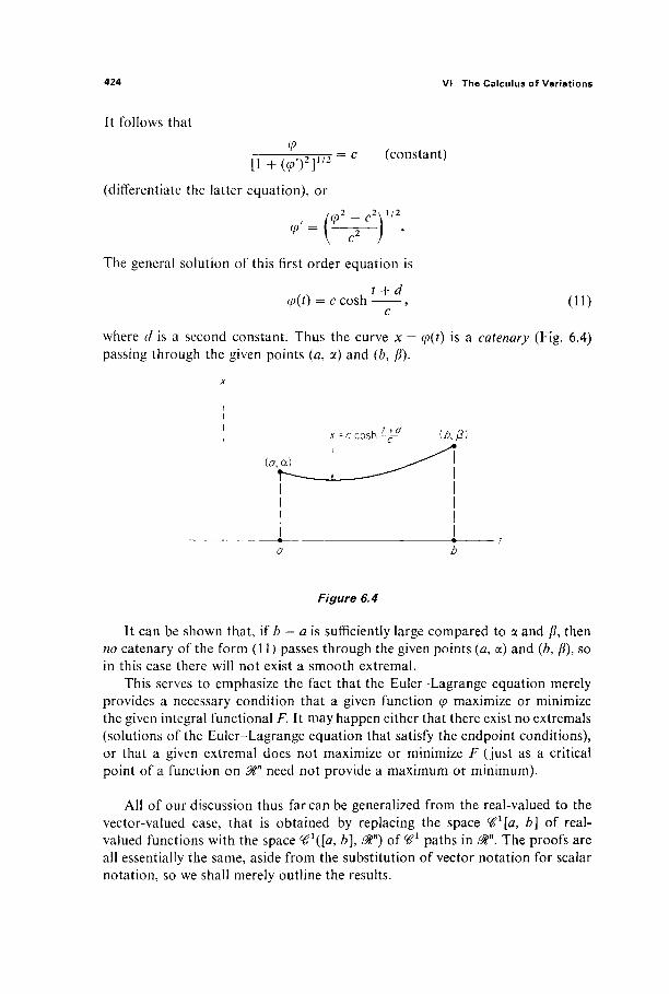
424 VI The Calculus of Variations
It follows that
Ψ [1+(<P')2]1/2
(differentiate the latter equation), or
yyj = c (constant)
2 _ . 2 χ 1 / 2
The general solution of this first order equation is
φ(ί) = c cosh , (ID
where d is a second constant. Thus the curve x = φ{ί) is a catenary (Fig. 6.4) passing through the given points (a, a) and (b, β).
>
(σ,α)
r ! 1 1 1 1 1
· a
< -c cosh ^-~— (4 0)
· b
Figure 6.4
It can be shown that, if b — a is sufficiently large compared to a and /?, then no catenary of the form (11) passes through the given points {a, a) and (b, /?), so in this case there will not exist a smooth extremal.
This serves to emphasize the fact that the Euler-Lagrange equation merely provides a necessary condition that a given function φ maximize or minimize the given integral functional F. It may happen either that there exist no extremals (solutions of the Euler-Lagrange equation that satisfy the endpoint conditions), or that a given extremal does not maximize or minimize F (just as a critical point of a function on 0tn need not provide a maximum or minimum).
All of our discussion thus far can be generalized from the real-valued to the vector-valued case, that is obtained by replacing the space ^[a, b] of real-valued functions with the space ^([a, b], 3în) of Ή1 paths in ^ n . The proofs are all essentially the same, aside from the substitution of vector notation for scalar notation, so we shall merely outline the results.

3 The Simplest Variational Problem 425
Given a ^ 2 function/: ä&n x l " x l - > l , we are interested in the extrema of the function F : <gl([a, b], @n) -+ M defined by
Ρ{φ) = ffm\nt),t)dU (12) Ja
amongst those ^ 1 paths φ : [a, b] -► 0tn such that φ(α) = a and φψ) = β, where a and β are given points in $n.
Denoting by M the subset of ^\[a, b], &n) consisting of those paths that satisfy the endpoint conditions, the path φ e M is an extremal for F on M if and only if
dF9\TM9 = 0.
We find, just as before, that M is a hyperplane. For each φ s M,
ΤΜφ = V0\[a, b], Xs) = {φβ Vl([a, b], @n) : φ(α) = φφ) = 0}.
With the notation (x, y, l ) e l " x « " x 31, let us write
V-Ά...,ν.) and dl=(K,_ÊL\ dx \dxl dxj dy \dyi dyj
so df/dx and df/dy are vectors. If φ is a tf2 path in 0tn and h e <#0l([a, b], @n),
then we find (by generalizing the proofs of Theorem 3.1 and Corollary 3.2) that
dF9(h) = f * n
df d df
ox dt dy h(i)dt· (13)
Compare this with Eq. (8); here the dot denotes the Euclidean inner product in
By an «-dimensional version of Lemma 3.3, it follows from (13) that the ^ 2
path φ G M is an extremal for F on M if and only if
/ (φ(ί), φ'(ί\ t)--TT W > ' V'M* '> = °- (14) ex dt dy
This is the Euler-Lagrange equation in vector form. Taking components, we obtain the scalar Euler-Lagrange equations
df d df dxt dt dy{ '
Example 3 Suppose that φ : [a, b] -> 3?" is a minimal-length # 2 path with end-points a = <p(a) and β = φψ). Then φ is an extremal for the function F: ^ ([a, b], Mn) - ^ defined by
*w = \imt)? + ''- + wn'{t))2]xl2du
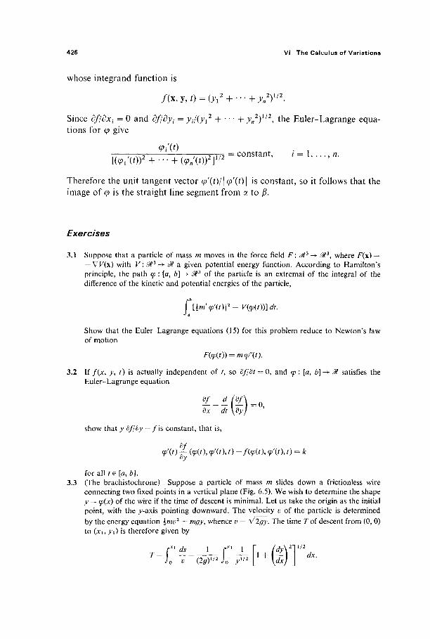
426 VI The Calculus of Variations
whose integrand function is
/ ( x , y , 0 = (^ 2 + - - '+7n2)1 / 2 .
Since df/dxi = 0 and d//dyf = yi/iyx2 + · · · + 7„2)1/2, the Euler-Lagrange equa-tions for φ give
ψ-tif)
wf + w r = constant' ' " = ' · ' · · ·n-Therefore the unit tangent vector φ'(ή/\φ'(ί)\ is constant, so it follows that the image of φ is the straight line segment from a to β.
Exercises
3.1 Suppose that a particle of mass m moves in the force field F : iß2, -> ^ 3 , where F(x) = — VK(x) with K: 3 - > a given potential energy function. According to Hamilton's principle, the path φ : [a, b] -> ^ 3 of the particle is an extremal of the integral of the difference of the kinetic and potential energies of the particle,
\\lM<pXt)\2-V(<p{t))]dt. J a
Show that the Euler-Lagrange equations (15) for this problem reduce to Newton's law of motion
F(cp(t)) = m(p"(t).
3.2 If f(x, y, t) is actually independent of /, so df/dt = 0, and φ : [a, b] -> 3? satisfies the Euler-Lagrange equation
dx dt \dyj = 0,
show that y df/dy —fis constant, that is,
<p'(t) % (φ(/), <pV), 0 - / ( ? ( ' ) , 9>'(0, t) = k dy
for all t e [A, 6]. 3.3 (The brachistochrone) Suppose a particle of mass m slides down a frictionless wire
connecting two fixed points in a vertical plane (Fig. 6.5). We wish to determine the shape y = cpix) of the wire if the time of descent is minimal. Let us take the origin as the initial point, with the j^-axis pointing downward. The velocity v of the particle is determined by the energy equation \mv2 = mgy, whence v = V2gy. The time Tof descent from (0, 0) to (*i, yi) is therefore given by
Jo v (2g)"> J0 yw [ \dx) J dx.

3 The Simplest Variational Problem 427
Figure 6.5
Show that the curve of minimal descent time is the cycloid
x = α{θ — sin 0), y = a{\ — cos 0)
generated by the motion of a fixed point on the circumference of a circle of radius a which rolls along the *-axis [the constant a being determined by the condition that it pass through the point {xu yi)]. Hint: Noting that
f(y, y\ x) -- [1+0Ό 2 ] 1
is independent of x, apply the result of the previous exercise,
df 1 y' — -f=k = . y dy' J (2a)l/2
Make the substitution y = 2a sin2 0/2 in order to integrate this equation.
Geodesies, in the following five problems we discuss geodesies (shortest paths) on a sur-face S in έ#3. Suppose that S is parametrized by R : <Mlv -> Mz
xyz, and that the curve y : [ayb]-+ S is the composition y=T°c, where c : [a, b] ~> i#lv. Then, by Exercise V.l.8, the length of γ is
s(y)- sm du dv + 2 F - - + G
dt dt ©" dU
where
dT dT dT dT dT dT £ = — · — , f= — .—9 G = — · — .
du du du dv dv dv
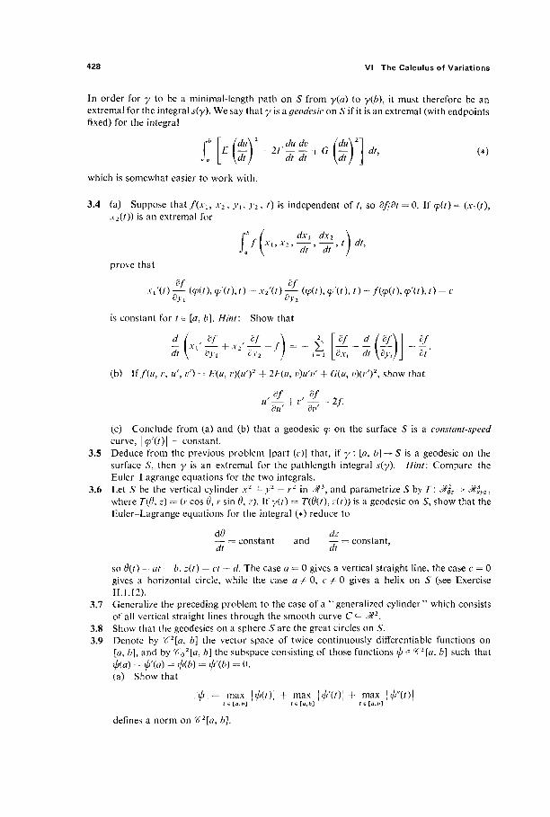
428 VI The Calculus of Variations
In order for y to be a minimal-length path on S from γ(α) to y(7>), it must therefore be an extremal for the integral s{y). We say that y is a geodesic on S if it is an extremal (with endpoints fixed) for the integral
} a |_ \dt) dt dt \dtj dU (*)
which is somewhat easier to work with.
3.4 (a) Suppose that f{xu x2, yu )'2, 0 is independent of /, so df/dt = 0. If φ(ί) = (χι(ΐ), x2(t)) is an extremal for
rb I dxx dx2 \
Lf(Xi'X2'-ä'-dr>')d'' prove that
xiV) ^- (φ{0, <p\t\t) + xiV) ^r W O , <pV), t)-fisp{t\ ψ\ί\ t) = c oyL cy2
is constant for / e [a, b]. Hint: Show that
^ \ Λ ΐ a->'i Λ2 a>'2 / ' = 1 ΙΛν<· dt\dyi) dt'
(b) If /( / / , r, M', I / ) = E(u, r ) ( i0 2 + 2F(i/, i?)«^' + G(w, i;)^')2, show that
11 V v — = 2/. du dv
(c) Conclude from (a) and (b) that a geodesic φ on the surface 5 is a constant-speed curve, \<p'(t)\ = constant.
3.5 Deduce from the previous problem [part (c)] that, if y : [a, b] -> 5 is a geodesic on the surface 5, then y is an extremal for the pathlength integral s(y). Hint: Compare the Euler-Lagrange equations for the two integrals.
3.6 Let S be the vertical cylinder x2 + y2 = r2 in .:#3, and parametrize Shy T: Mjz-> J^y z , where Γ(0, z) = (/* cos 0, r sin θ, z). If y(/) = T(6(t), z(t)) is a geodesic on S, show that the Euler-Lagrange equations for the integral (*) reduce to
άθ dz — = constant and — = constant, dt dt
so 9(t) = at + b, z(t) = ct + d. The case a = 0 gives a vertical straight line, the case c = 0 gives a horizontal circle, while the case a ^ 0, c Φ 0 gives a helix on 5 (see Exercise II.1.12).
3.7 Generalize the preceding problem to the case of a "generalized cylinder" which consists of all vertical straight lines through the smooth curve C c M2.
3.8 Show that the geodesies on a sphere 5 are the great circles on S. 3.9 Denote by r62[a, b] the vector space of twice continuously differentiable functions on
[a, b], and by V>o2[a, b] the subspace consisting of those functions φ e K2[a, b] such that φ{α) = φ'(α) = φφ) = ψ'φ) = 0. (a) Show that
\\φ\\ = max \φ{ί)\ + max \φ\ί)\+ max \φ\ί)\ r e [ a , b ] t e [ a , b ] te[a,b~i
defines a norm on %2[a, b].
4 The Isoperimetric Problem 429
(b) Given a tf2 function / : # 4 -* J \ define F :tf2 [a, 6] -> ^ by
J a
Then prove, by the method of proof of Theorem 3.1, that F is differentiable with
dFM = f (¥ A(r ) + d-L hy) 4- d£ h\tÛ dt,
where the partial derivatives o f / a r e evaluated at (<p(/), ψ\ΐ), ψ"{β\ t). (c) Show, by integration by parts as in the proof of Corollary 3.2, that
^(*)=Γ[Ι-Ι(^)+£(2). h{t)dt
ifheV02[a,b].
(d) Conclude that φ satisfies the second order Euler-Lagrange equation
8_f d. Lv dt \dy) dt2 \dz)
if φ is an extremal for F, subject to given endpoint conditions on <p and φ' (assuming that φ is of class # 4 — n o t e that the above equation is a fourth order ordinary differential equation in 99).
4 THE ISOPERIMETRIC PROBLEM
In this section we treat the so-called isoperimetric problem that was men-tioned in the introduction to this chapter. Given functions / , g : 01* -► 0, we wish to maximize or minimize the function
*w = \hfm\v(t\t)dt9 (i)
subject to the endpoint conditions φ(α) = α, φφ) = β and the constraint
rb
αψ) = /(φ(ή, ψ'(ί\ t)dt = c (constant). (2)
If, as in Section 3, we denote by M the hyperplane in ^[a, b] consisting of all those ^ 1 functions φ : [a, b] -+ 0t such that φ{α) = oc and φψ) = β, then our problem is to locate the local extrema of the function f on the set M n G~\c).
The similarity between this problem and the constrained maximum-mini-mum problems of Section II.5 should be obvious—the only difference is that here the functions F and G are defined on the infinite-dimensional normed vector space ^[a, b], rather than on a finite-dimensional Euclidean space. So our method of attack will be to appropriately generalize the method of Lagrange multipliers so that it will apply in this context.

430 VI The Calculus of Variations
First let us recall Theorem II.5.5 in the following form. Let F, G : £%n -> 01 be ^ functions such that (7(0) = 0 and VG(0) ^ 0. If F has a local maximum or local minimum at 0 subject to the constraint G(\) = 0, then there exists a number λ such that
VF(0) = λ VG(0). (3)
Since the differentials dF0, dG0 : 0tn -► 01 are given by
dF0(y) = VF(0) · v and dG0(y) = V(7(0) · v,
Eq. (3) can be rewritten
dF0 = Ao dG0, (4)
where Λ : 01 -> 01 is the linear function defined by A(t) = At. Equation (4) presents the Lagrange multiplier method in a form which is
suitable for generalization to normed vector spaces (where differentials are available, but gradient vectors are not). For the proof we will need the following elementary algebraic lemma.
Lemma 4.1 Let a and ß be real-valued linear functions on the vector space E such that
Ker a z> Ker ß and Im ß = R.
Then there exists a linear function Λ : 0t -► 01 such that α = Λ ° β. That is, the following diagram of linear functions "commutes."
/ \ E ► m
a
PROOF Given t e 01, pick xe E such that β(χ) = t, and dehne
Λ(ί) = ot(x).
In order to show that Λ is well defined, we must see that, if y is another element of E with ß(y) = t, then a(x) = <x(y). But if ß(x) = ß(y) = ί, then x - y e Ker β a Ker a, so ot(x - y) = 0, which immediately implies that x(x) = ot(y).
If β(χ) = s and ß(y) = ί, then
Λ(Ο5 + M) = a(ax + 6y) = az(x) + &a(>0 = ûfA(j) + éA(i),
so Λ is linear. I

4 The Isoperimetric Problem 431
The following theorem states the Lagrange multiplier method in the desired generality.
Theorem 4.2 Let F and G be real-valued ^ 1 functions on the complete normed vector space E, with (7(0) = 0 and dG0 φ 0 (so Im dG0 = 0ΐ). If F : E -» $ has a local extremum at 0 subject to the constraint G(x) = 0, then there exists a linear function Λ : 01 -► 0t such that
dF0=Ao dG0. (5)
Of course the statement, that " F has a local extremum at 0 subject to G(x) = 0," means that the restriction £|G_ 1(0) has a local extremum at 0 e G-1(0).
PROOF This will follow from Lemma 4.1, with a = dF0 and β = dG0, if we can prove that Ker dF0 contains Ker dG0 . In order to do this, let us first assume the fact (to be established afterward) that, given v e Ker dG0, there exists a differentiable path y : ( — ε, ε) -► E whose image lies in G~l(0), such that y(0) = 0 and y'(0) = v (see Fig. 6.6).
Then the composition h = Fo y \ ( — ε, ε)-»^? has a local extremum at 0, so h'(0) = 0. The chain rule therefore gives
0 = Α'(0) = ί/Αο(1) = ^(ο)(^ο(1)) = dFo(y'(0)\
0 = dF0(v)
as desired.
We will use the implicit function theorem to verify the existence of the dif-ferentiable path y used above. If X = Ker dG0 then, since dG0 : E -► & is con-tinuous, X is a closed subspace of £, and is therefore complete (by Exercise 1.5). Choose w E E such that dG0(w) = 1, and denote by Y the closed subspace of £ consisting of all scalar multiples of w ; then Y is a '4 copy " of 0t.
It is clear that X n Y = 0. Also, if e e E and a = dG0{e) e M, then
dG0(e — aw) = dG0(e) — adG0(w) = 0
so e — aw e X. Therefore
e = x + y
with x e X and y = aw e Y. Thus £ is the algebraic direct sum of the subspaces X and Y. Moreover, it is true (although we omit the proof) that the norm on £ is equivalent to the product norm on X x Y, so we may write £ = X x Y.
In order to apply the implicit function theorem, we need to know that
dyG0 : Y-+0t
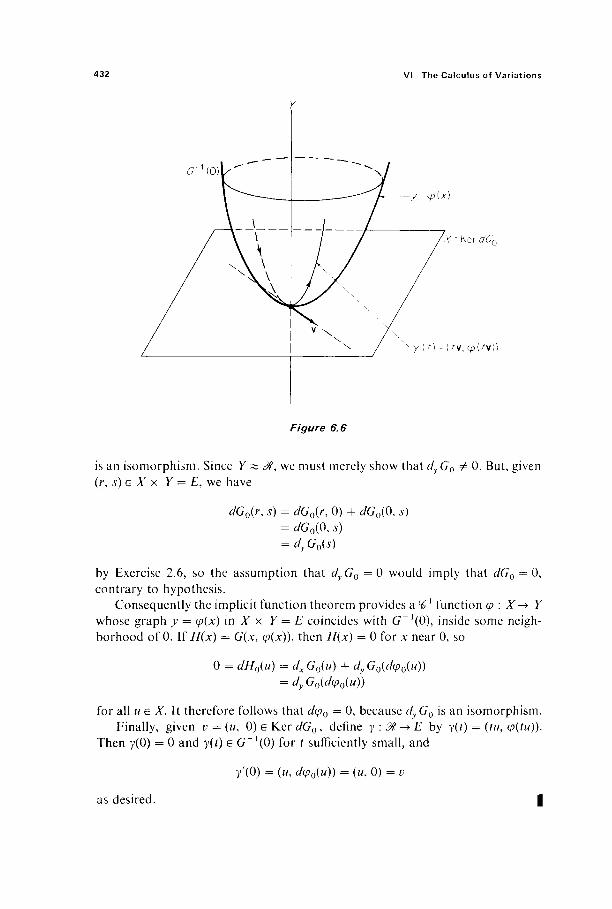
432 VI The Calculus of Variations
6^(0)1 ^ — —
\ \ Λ \ \ ^
Y
/ S \
-y - φ[χ)
/Χ = Ker dGr,
\
Figure 6.6
· / ( / ) = ( /ν ,φ( /ν) )
is an isomorphism. Since Y ^ J>, we must merely show that c/y (70 Φ 0. But, given ( r , i ) e l x Y = E, we have
dG0(r, s) = dG0(r, 0) + dGo(0, s) = </G0(0, J) = rfy G0(s)
by Exercise 2.6, so the assumption that dyG0 = 0 would imply that dG0 = 0, contrary to hypothesis.
Consequently the implicit function theorem provides a ^ 1 function φ : X -> Y whose graph y = φ{χ) in X x Y = E coincides with G-1(0), inside some neigh-borhood of 0. If H(x) = G(x, φ{χ)), then H(x) = 0 for x near 0, so
0 = dH0(u) = dxG0(u) + dyG0(d<p0(u)) = dy σ0(ί/φ0("))
for all u e X. It therefore follows that ί/φ0 = 0, because dyG0 is an isomorphism. Finally, given v = (u, 0) e Ker dG0, define y : ^* -► E by γ(0 = (tu, φ(ίιι)).
Then γ(0) = 0 and y(t) e G_1(0) for t sufficiently small, and
/(0) = (w, rf^oW) = ("* 0) = Ü
as desired. I
4 The Isoperimetric Problem 433
We are now prepared to deal with the isoperimetric problem. L e t / a n d g be real-valued Ή2 functions on ^ 3 , and define the real-valued functions F and C o n ^ [ û , b] by
ΗΦ) = f ./#('), ΦΌ), t) dt (6) J a
and
0(φ)= [ # ( 0 ^ ' ( 0 , 0 Λ - ^ (7)
where c e @. Assume that φ is a # 2 element of #* [<7, 6] at which F has a local extremum on M n G_1(0), where M is the usual hyperplane in ^x[a, b] that is determined by the endpoint conditions \j/(a) = a and \jj(b) = ß .
We have seen (in Section 3) that M is the translate (by any fixed element of M) of the subspace Ή0
ι[α, b] of %?l[a, b] consisting of these elements φ e ^χ[α, b] such that φ(α) = φφ) = 0. Let T: ^0
l[a, b] -> M be the translation defined by
Τ(φ) = ψ + φ,
and note that 7(0) = φ, while
dT0:<g0i[a,b]^V0
1[a,b] = TMtp
is the identity mapping. Now consider the real-valued functions F o Tand G o T on ^VlA ^7]· The
fact that F has a local extremum on M n (7_1(0) at φ implies that F o Thas a local extremum at 0 subject to the condition G o Τ(ψ) = 0.
Let us assume that φ is not an extremal for G on M, that is, that
so d(G o T)0 # 0. Then Theorem 4.2 applies to give a linear function A : @t -► ^ such that
rf(FoD0=Aoi/(GoT)0.
Since ί/Γ0 is the identity mapping on C0l[a, b], the chain rule gives
dF9=Ko dG(p
on <£0l[a, b]. Writing A(t) = λί and applying the computation of Corollary
3.2 for the differentials dF0 and dGiP, we conclude that
r ^ (φ(ίΙ φ\ή, t) - ^ (φ(ί\ φ\ίΧ t) ex dt oy
, rb \dg d da = X ( [ S ( # , f(0, 0 - ^ ( < P ( » . < P ' ( 0 , 0
for all« e^o 1 [«,*]·
w(0 Λ
w(i) i/r
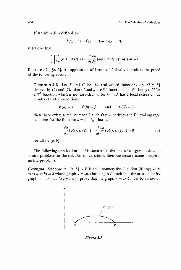
434 VI The Calculus of Variations
If h : ^ 3
it follows that
is defined by
h{x,}\t)=f(x,y,t)-lg(x,y,t),
dh d dh I — (φ(0, <p'{t\ 0 - jf Y (<K0, φ'(0, 0 I w(0 dt = 0
for all i / e ^ t û , /?]. An application of Lemma 3.3 finally completes the proof of the following theorem.
Theorem 4.3 Let F and G be the real-valued functions on ^[a, b] defined by (6) and (7), where/and g are # 2 functions on ^ 3 . Let ψ e M be a W2 function which is not an extremal for G. If F has a local extremum at φ subject to the conditions
ψ(α) = οί, ψφ) = β, and G(\//) = 0,
then there exists a real number λ such that φ satisfies the Euler-Lagrange equation for the function h =f — Xg, that is,
dh d dh — (φ(ί), φ'(0, » - - - (<p(t), <p'(t), t) = 0 dx at cy
(8)
for all t E [a, b].
The following application of this theorem is the one which gave such con-straint problems in the calculus of variations their customary name—isoperi-metric problems.
Example Suppose φ : [#, b\^M is that nonnegative function (if any) with φ(α) = φφ) = 0 whose graph x = φ(ΐ) has length L, such that the area under its graph is maximal. We want to prove that the graph x = φ(ί) must be an arc of
Figure 6.7

4 The Isoperimetric Problem 435
a circle (Fig. 6.7). If f(x, y, t) = x and g(x, y, t) = y/l + y2, then φ maximizes the integral
ff(<p(t),cp'(t),t)dt, J a
subject to the conditions
rb
(p(a) = <p(b) = 0 and g(<p(t), φ\ΐ\ t) dt = L. Jn
Since df/dx = 1, df/dy = dg/dx = 0, dg/dy = y/y/l + y2, the Euler-Lagrange equation (8) is
dt \ i + (φ'(0)2/
or <p\t) = 1
[1+(φ ' (0) 2 ] 3 / 2 A'
This last equation just says that the curvature of the curve t -► (ί, φ(ί)) is the constant Ι/λ. Its image must therefore be part of a circle.
The above discussion of the isoperimetric problem generalizes in a straight-forward manner to the case in which there is more than one constraint. Given Ή2 functions/, gl9 . . . , gk : &3 -► 0t, we wish to minimize or maximize the func-tion
Ρ(Φ) = f W(0, Ψνΐ 0 dt, (9) Ja
subject to the endpoint conditions φ(α) = oc, φφ) = β and the constraints
GW) = ί gm\ UV), 0 dt - Ci = 0. (10)
Our problem then is to locate the local extrema of F on M n G_1(0), where M is the usual hyperplane in ^x[a, b] and
G = (GU ...,Gk):^l[a,b]->^k.
The result, analogous to Theorem 4.3, is as follows.
Let ψ e M be a ^function which is not an extremal for any linear combination of the functions Gu . . . , Gk. If F has a local extremum at φ subject to the con-ditions
φ{α) = α, ΦΨ) = β, and G^) = 0,

436 VI The Calculus of Variations
then there exist numbers λ{, ..., Àk such that φ satisfies the Euler-Lagrange equation for the function
h=f~ i= 1
Inclusion of the complete details of the proof would be repetitious, so we simply outline the necessary alterations in the proof of Theorem 4.3.
First Lemma 4.1 and Theorem 4.2 are slightly generalized as follows. In Lemma 4.1 we take β to be a linear mapping from E to $k with Im ß = Mk, and in Theorem 4.2 we take G to be a (€x mapping from E to 0tk such that (7(0) = 0 and Im dG0 = &k. The only other change is that, in the conclusion of each, Λ becomes a real-valued linear function on 0lk. The proofs remain essentially the same.
We then apply the generalized Theorem 4.2 to the mappings F : 1 [a, b] -> 0t and G : ^ [ Û , b] -► 0lk, defined by (9) and (10), in the same way that the original Theorem 4.2 was applied (in the proof of Theorem 4.3) to the functions defined by (6) and (7). The only additional observation needed is that, if φ is not an extremal for any linear combination of the component functions G{, . . . , Gk, then it follows easily that dG(p maps ΤΜφ onto &k. We then conclude as before that
dF(p=AodG(p on <€0l[a,b]
for some linear function Λ : conclude that
Writing A(xu . . . , xk) = Xf=1 Xtxi9 we
~b rdf d df ^Mt),çXt),t)--^(<p(t),<p'(t\t) u(t) dt
k Λ
i = l Ja
fyi d dgi (φ(ή,φ'(ί\ί)--^(φ(ί\φΧή,ή
ox dt oy u(f) dt
for all u e ^0x[a, b]. An application of Lemma 3.3 then implies that φ satisfies
the Euler-Lagrange equation for h=f—Yjkigi.
Exercises
4.1 Consulting the discussion at the end of Section 3, generalize the isoperimetric problem to the vector-valued case as follows : Let /, g : (Mn x cMn x 0t -> ät be given functions, and suppose φ : [a, b] -> Mn is an extremal for
F(0)= iV(0(O,f(/),O^, J a
4 The Isoperimetric Problem 437
subject to the conditions φ(α) = oc, φ(ϋ) = β and
J a
Then show under appropriate conditions that, for some number λ, the path ψ satisfies the Euler-Lagrange equations
dh d dh _
Jxi ~dtHy~ ' 1,
for the function h =f— Xg. 4.2 Let ψ : [a, b] -> Ά1 be a closed curve in the plane, φ(α) = φψ), and write φ{ί) = (x(t),y(t)).
Apply the result of the previous problem to show that, if φ maximizes the area integral
»r J a
(x/ - yx') dU
subject to
(CO2 + ( / ) 2 ) 1 / 2 dt = L (constant),
4.3
4.4
then the image of φ is a circle. With the notation and terminology of the previous problem, establish the following reciprocity relationship. The closed path φ is an extremal for the area integral, subject to the arclength integral being constant, if and only if φ is an extremal for the arclength integral subject to the area integral being constant. Conclude that, if φ has minimal length amongst curves enclosing a given area, then the image of φ is a circle. Formulate (along the lines of Exercise 3.9) a necessary condition that φ : [a, b] -> M minimize
f(<p(t\<p'{t\<p"{t\t)du
subject to
4.5
4.6
4.7
g (φ(ί), φ\ί\ ψ'ΧΟ, t) dt = constant. ^α
This is the isoperimetric problem with second derivatives. Suppose that r =/(θ), Θ e [Ο,π] describes (in polar coordinates) a closed curve of length L that encloses maximal area. Show that it is a circle by maximizing
LC ■d0,
subject to the condition
J0 L U ) d6 = L.
A uniform flexible cable of fixed length hangs between two fixed points. If it hangs in such a way as to minimize the height of its center of gravity, show that its shape is that of a catenary (see Example 2 of Section 3). Hint: Note that Exercise 3.2 applies. If a hanging flexible cable of fixed length supports a horizontally uniform load, show that its shape is that of a parabola.
438 VI The Calculus of Variations
5 MULTIPLE INTEGRAL PROBLEMS
Thus far, we have confined our attention to extremum problems associated with the simple integral \b
a /(φ(ή, φ'(ΐ),ί) dt, where φ is a function of one variable. In this section we briefly discuss the analogous problems associated with a multiple integral whose integrand involves an "unknown" function of several variables.
Let D be a cellulated /7-dimensional region in 0tn. Given/ : ^2n + i -+01, we seek to maximize or minimize the function F defined by
ΠΦ) = f flxx , - . . , * „ , Φ(Χι, - . . , *„), ^ - , . . . , ^ ) Λ , (1)
amongst those ^ 1 functions φ : D -► M which agree with a given fixed function φ0 : D -► 0t on the boundary dD of the region D. In terms of the gradient vector
VWx) = (/),Wx) D i ( x ) ) ,
we may rewrite (1) as
F(iP) = f / (x , ^(x), V<A(x)) i/x. (2)
Throughout this section we will denote the first n coordinates in &2n + 1 by *!, . . . , JC„, the (n + l)th coordinate by }>, and the last A7 coordinates in ^ 2 n + 1
by zl9 . . . , zn. Thus we are thinking of the Cartesian factorization 0lln+x = Mn x ^ x ^", and therefore write (x, y, z) for the typical point of 0t2n+l. In terms of this notation, we are interested in the function
Γ(φ) = f / (x , >', z) rfx,
where >> = φ(\) and z = Vi//(x).
The function T7 is defined by (2) on the vector space <£l(D) that consists of all real-valued %>{ functions on D (with the usual pointwise addition and scalar multiplication). We make #*(/)) into a normed vector space by defining
|| φ || - max | ^(x) | + max | νψ(χ) |. (3) x e D x e D
It can then be verified that the normed vector space <^l(D) is complete. The proof of this fact is similar to that of Corollary 1.5 (that <£ι[α, b] is complete), but is somewhat more tedious, and will be omitted (being unnecessary for what follows in this section).
5 Multiple Integral Problems 439
Let M denote the subset of ^\D) consisting of those functions φ that satisfy the "boundary condition"
φ(χ) = φ0(χ) if x G dD.
Then, given any φ e M, the difference φ — φ0 is an element of the subspace
<$o\D) = {(pe(g1(D):<p(x) = 0 if x e 3D}
of ^(D), consisting of all those ^ 1 functions on D that vanish on dD. Con-versely, if çec^0
1(D), then clearly φ0 + φ e M. Thus M is a hyperplane in ^l(D), namely, the translate by the fixed element Φ0ΕΜ of the subspace #(/(/)). Consequently
TM+ = V0\D)
for all φ G M. If F : \D) -► 0t is difTerentiable at φ e M, and i7! M has a local extremum
at φ, Theorem 2.3 implies that
dF(f)(h) = 0 for all he^0\D). (4)
Just as in the single-variable case, we will call the function φ e M an extremal for F on M if it satisfies the necessary condition (4).
The following theorem is analogous to Theorem 3.1, and gives the computa-tion of the differential dF(p when F is defined by (1).
Theorem 5.1 Suppose that D is a compact cellulated «-dimensional region in 9ln, and t h a t / : @2η+ί ^Μ is a ^ 2 function. Then the function F : Η ^ ) -► ^ defined by (1) is difTerentiable with
dK ;(*) = / — · A(x) + X 5- ' T - (x) dx (5)
for all φ, h e %>\D). The partial derivatives
dy' dz^ " " ' dzn
in (5) are evaluated at the point (x, φ(χ), V<p(x)) e ^ 2 n + 1 .
The method of proof of Theorem 5.1 is the same as that of Theorem 3.1, making use of the second degree Taylor expansion off. The details will be left to the reader.
In view of condition (4), we are interested in the value of dFv(h) when h G ΤΜφ = ^Q1{D). The following theorem is analogous to Corollary 3.2.

440 VI The Calculus of Variations
Theorem 5.2 Assume, in addition to the hypotheses of Theorem 5.1, that φ is a cß2 function and that /? e WQ^D). Then
JD icy ;=i oxi \cz-J //(x) dx. (6)
Here also the partial derivatives of / a r e evaluated at (x, φ(χ), V^(x))e^ 2 " + 1 .
PROOF Consider the differential (/? - l)-form defined on D by
ω = Y ( - 1 )'+ λ —■ h dx{ Λ · · · Λ dx·. A · · · Λ dxn.
A routine computation gives
ί/ω = y (K?!L + JL(ÊL)h) .i=i \özi a*,· dx,· \dzf/ /
rfx,
where dx = dxi A · · · A dxn. Hence
(ί,ΙΙΗΗί,έίΙΗ-Substituting this into Eq. (5), we obtain
But ;„</ω = ί ÔD ω = 0 by Stokes' theorem and the fact that ω = 0 on ÔD
because h e ^0\D). Thus Eq. (7) reduces to the desired Eq. (6). |
Theorem 5.2 shows that the Ή2 function φ e M is an extremal for F on M if and only if
(7)
'D [dy Ä dxt \dz) h(x) dx = 0
for every h e ^0\D). From this result and the obvious multivariable analog of Lemma 3.3 we immediately obtain the multivariable Euler-Lagrange equa-tion.
Theorem 5.3 Lt\.F\<e\D)-+M be defined by Eq. (1), w i th / : @2n + 1 -> 0t being a ^ 2 function. Then the ^ 2 function φ e M is an extremal for F on M if and only if
^ (x, </>(x), V<p(x)) - £ j ^ - (x, </>(x), νφ(χ)) = 0
for all xe D.

5 Multiple Integral Problems 441
The equation
dy' Σ - ;(IH- (8)
with the partial derivatives of / evaluated at (x, φ(χ), V<p(x)), is the Euler-Lagrange equation for the extremal φ. We give some examples to illustrate its applications.
Example 1 (minimal surfaces) If D is a disk in the plane, and φ0 : D-* & a function, then the graph of φ0 is a disk in Mz. We consider the following question. Under what conditions does the graph (Fig. 6.8) of the function φ : D -> 0Ϊ have minimal surface area, among the graphs of all those functions φ : D -> M that agree with φ0 on the boundary curve dD of the disk Dl
Figure 6.8
We can just as easily discuss the ^-dimensional generalization of this ques-tion. So we start with a smooth compact «-manifold-with-boundary D c Mn, and a ^ 1 function φ0 : D -► 01, whose graph y = φ0(χ) ls a n ^-manifold-with-boundary in @n + 1.
The area F((p) of the graph of the function φ : D -+ M is given by formula (10) of Section V.4,
F(<p)= f [1 + | ν φ ( χ ) | 2 ] 1 / 2 Λ . J n
We therefore want to minimize the function F:(^1(D)· with
/(Χ,^,2) = (1+Ζ 12 + · · ·+Ζι ι
2 ) 1 / 2 .
defined by (1)
442 VI The Calculus of Variations
Since
δ / = ο, 5f
dy ' dz, ( 1 + ζ , 2 + · · · + ζ 42 ) 1 / 2 '
the Euler-Lagrange equation (8) for this problem is
Ι,έ&'+'^Η Upon calculating the indicated partial derivatives and simplifying, we obtain
(I+|V,|W= idf'f^ (9) itj^i dxi 0Xj ox i dXj
where
2,n - y b2l. k dXi
2
as usual. Equation (9) therefore gives a necessary condition that the area of the graph of y = φ(χ) be minimal, among all tf-manifolds-with-boundary in &n+1
that have the same boundary.
In the original problem of 2-dimensional minimal surfaces, it is customary to use the notation
z = φ(χ, y),
d2z
"'dx2'
dz
dx
d2z
dx dy
dz
dy
d2z
'~dy2
With this notation, Eq. (9) takes the form
(1 + q2)r - 2pqs + (1 + p2)t = 0.
This is of course a second order partial differential equation for the unknown function z = φ(χ, y).
Example 2 (vibrating membrane) In this example we apply Hamilton's principle to derive the wave equation for the motion of a vibrating «-dimensional "membrane." The cases n = 1 and n = 2 correspond to a vibrating string and an "actual" membrane, respectively.
We assume that the equilibrium position of the membrane is the compact /7-manifold-with-boundary
Wcûttt = âtn x {0}c:&n + 1,
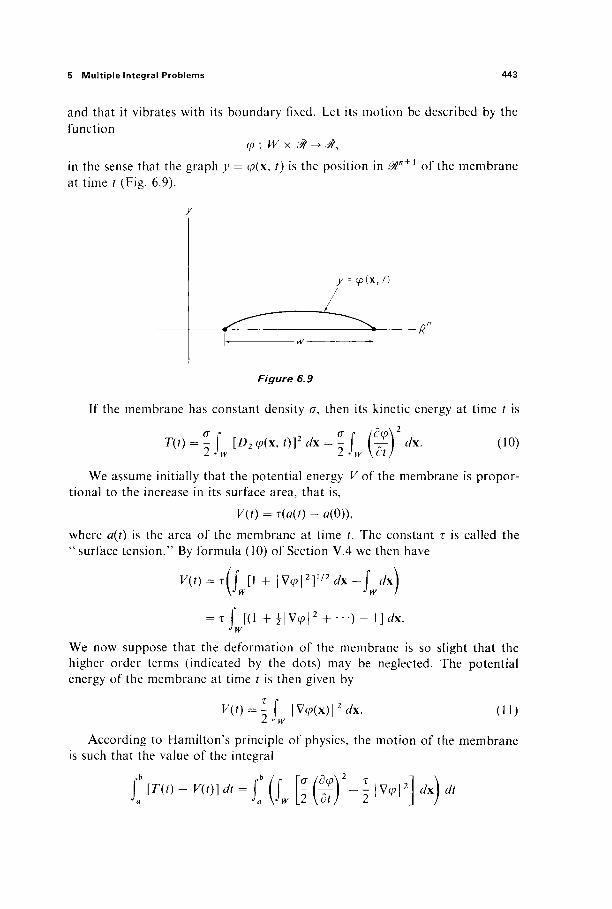
5 Multiple Integral Problems 443
and that it vibrates with its boundary fixed. Let its motion be described by the function
φ : W x ί% -> <#, in the sense that the graph y = φ(χ, /) is the position in ^ " + 1 of the membrane at time t (Fig. 6.9).
y -- φ(Χ, /)
Figure 6.9
If the membrane has constant density σ, then its kinetic energy at time t is
T(t) = °-\ [D2 φ(χ, t)]2 dx = G-\ Ά dx. (10)
We assume initially that the potential energy V of the membrane is propor-tional to the increase in its surface area, that is,
V(t) = x(a(t) - O(0)), where a(t) is the area of the membrane at time /. The constant τ is called the "surface tension." By formula (10) of Section V.4 we then have
Κ(ί) = τ ( [ [I + \V<p\2]1/2dx-j dx\
= τ f [ ( 1 + ΐ | ν φ | 2 + · · · ) - 1 ] ί / χ . Jw
We now suppose that the deformation of the membrane is so slight that the higher order terms (indicated by the dots) may be neglected. The potential energy of the membrane at time t is then given by
V(t) = T- ί |V^(x)|2r/x. Z J w
(11)
According to Hamilton's principle of physics, the motion of the membrane is such that the value of the integral

444 VI The Calculus of Variations
is minimal for every time interval [a, b]. That is, if D = W x [a, b], then the actual motion φ is an extremal for the function F : %>\D) -+01 defined by
Γ σ / # \ 2 τ (δφ\2 τ(δφ)2Ί
FM) JD [2 \dt) 2\dxJ 2\dxJ J (12)
on the hyperplane M c (^1(D) consisting of those functions φ that agree with φ on dp.
If we temporarily write t = xn + l and define / on ?>2AJ+3
■'by
f{x,y,z)= - ^ ( ζ 12 + · · · + ζ , 2 ) + ^ , ί ι .
then we may rewrite (12) as
i # ) = f f(x, y, z) Λ,
where y = φ(χ) and z = Vi^(x). Since
dy ' dzf if / ^ A?, and JL = σζη
it follows that the Euler-Lagrange equation (8) for this problem is
τ(ϊΡ)-σΡ±1=0, z = V„(x),
or
δ2ψ (13)
Equation (13) is the «-dimensional wave equation.
APPENDIX The Completeness of J%
In this appendix we give a self-contained treatment of the various conse-quences of the completeness of the real number system that are used in the text.
We start with the least upper bound axiom, regarding it as the basic com-pleteness property of 01. The set S of real numbers is bounded above (respectively below) if there exists a number c such that c ^ x (respectively c ^ x) for all x E S. The number c is then called an upper (respectively lower) bound for S. The set S is bounded if it is both bounded above and bounded below.
A least upper (respectively greatest lower) bound for S is an upper bound (respectively lower bound) b such that b ^ c (respectively b ^ c) for every upper (respectively lower) bound c for S. We can now state our axiom.
Least Upper Bound Axiom If the set S of real numbers is bounded above, then it has a least upper bound.
By consideration of the set {x e 01 : —xe S}, it follows easily that, if S is bounded below, then S has a greatest lower bound.
The sequence {xn}f of real numbers is called nondecreasing (respectively nonincreasing) if xn ^ xn + 1 (respectively xn ^ xn + 1) for each n ^ 1. We call a sequence monotone if it is either nonincreasing or nondecreasing. The following theorem gives the "bounded monotone sequence property" of 3%.
Theorem A.1 Every bounded monotone sequence of real numbers converges.
PROOF If, for example, the sequence S = {xn}f is bounded and nondecreasing, and a is the least upper bound for S that is provided by the axiom, then it follows immediately from the definitions that limn_+00 xn = a. |
445
446 Appendix
The following theorem gives the "nested interval property" of ^ .
Theorem A.2 If {In}f is a sequence of closed intervals (In = [an, bn]) such that
(i) /„ =3 In + 1 for each n ^ 1, and
(ii) IimII_>oo(ôri-i7/I) = 0,
then there exists precisely one number c such that c e In for each n, soc =
PROOF It is clear from (ii) that there is at most one such number c. The sequence {an}^ is bounded and nondecreasing, while the sequence {bn}f is bounded and nonincreasing. Therefore a = lim,,^ an and b = lim,,^^ bn exist by Theorem A.l. Since an ^ bn for each n ^ 1, it follows easily that a ^ b. But then (ii) im-plies that a = b. Clearly this common value is a number belonging to each of the intervals {I„}f. |
We can now prove the intermediate value theorem.
Theorem A.3 If the function / : [a, b] -> 01 is continuous and f{a) < 0 <f(b), then there exists c e (a, b) such that/(c) = 0.
PROOF Let lx = [a,b]. Having defined /„, let In + i denote that closed half-interval of In such thatf(x) is positive at one endpoint of In+1 and negative at the other. Then the sequence {In}f satisfies the hypotheses of Theorem A.2. If c = f}™= ! /„, then the continuity off implies that/(c) can be neither positive nor negative (why?), so/(c) = 0. |
Lemma A.4 If the function/: [a, b]-+ & is continuous, then/ is bounded on [a, b].
PROOF Supposing to the contrary t h a t / i s not bounded on / t = [a, b], let I2
be a closed half-interval of Ix on which/is not bounded. In general, let In + i be a closed half-interval of In on which/is not bounded.
If c = P|^L i /„, then, by continuity, there exists a neighborhood U of c such tha t / i s bounded on U (why?). But In c U if n is sufficiently large. This contra-diction proves tha t / i s bounded on [a, b]. |
We can now prove the maximum value theorem.
Theorem A.5 I f / : \a,b\^0l is continuous, then there exists c e [a, b] such that/(*) uf(c) for all x e [a, b\.

The Completeness of M 447
PROOF The set/([#, b]) is bounded by Lemma A.4, so let M be its least upper bound; that is, M is the least upper bound oïf(x) on [a, b]. Then the least upper bound of/(x) on at least one of the two closed half-intervals of [a, b] is also M\ denote it by Ιγ. Given /„, let In + 1 be a closed half-interval of /„ on which the least upper bound off(x) is M. If c = f)™= ί Ιη, then it follows easily from the continuity off that f(c) = M. |
As a final application of the "method of bisection," we establish the "Bolzano-Weierstrass property" of 0t.
Theorem A.6 Every bounded, infinite subset S of 0t has a limit point.
PROOF If I0 is a closed interval containing S, denote by lx one of the closed half-intervals of I0 that contains infinitely many points of S. Continuing in this way, we define a nested sequence of intervals {/„}, each of which contains in-finitely many points of S. If c = f)™= { In, then it is clear that c is a limit point of 5. |
We now work toward the proof that a sequence of real numbers converges if and only if it is a Cauchy sequence. The sequence {an}™ is called a Cauchy sequence if, given ε > 0, there exists TV such that
m, n ^ TV => \ am — an \ < ε.
It follows immediately from the triangle inequality that every convergent sequence is a Cauchy sequence.
Lemma A.7 Every bounded sequence of real numbers has a convergent subsequence.
PROOF If the sequence {an}f contains only finitely many distinct points, the the conclusion is trivial and obvious. Otherwise we are dealing with a bounded infinite set, to which the Bolzano-Weierstrass theorem applies, giving us a limit point a. If, for each integer k ^ 1, ank is a point of the sequence such that \ank — a\ < \/k, then it is clear that {a„k}™=i is a convergent subsequence. |
Theorem A.8 Every Cauchy sequence of real numbers converges.
PROOF Given a Cauchy sequence {an}™, choose N such that
m, n ^ N => \am- an\ < 1.
Then an e [aN — 1, aN + I] if n ^ N, so it follows that the sequence {an}f is bounded. By Lemma A.7 it therefore has convergent subsequence {a„}f.

448 Appendix
If a = l im^^ a„k, we want to prove that limn^0G an = a. Given ε > 0, choose M such that
ε m,n^M => \am-an\ < - .
Then choose K such that nK^ M and \a„K — a\ < ε/2. Then
n^M=>\an-a\^ \αη-αηκ\ + \αηκ-α\ < ε
as desired. |
The sequence {ajf of points in 0lk is called a Cauchy sequence if, given ε > 0, there exists TV such that
m,n^N => [am — a„| < ε
(either Euclidean or sup norm). It follows easily, by coordinatewise application of Theorem A.8, that every Cauchy sequence of points in Mk converges.

Suggested Reading
One goal of this book is to motivate the serious student to go deeper into the topics introduced here. We therefore provide some suggestions for further reading in the references listed below.
For the student who wants to take another look at single-variable calculus, we recommend the excellent introductory texts by Kitchen [8] and Spivak [17]. Also several introductory analysis books, such as those by Lang [9], Rosenlicht [13], and Smith [16], begin with a review of single-variable calculus from a more advanced viewpoint.
Courant's treatment of multivariable calculus [3] is rich in applications, in-tuitive insight and geometric flavor, and is my favorite among the older advanced calculus books.
Cartan [1], Dieudonné [5], Lang [9], and Loomis and Sternberg [10] all deal with diiferential calculus in the context of normed vector spaces. Dieudonne's text is a classic in this area; Cartan's treatment of the calculus of normed vector spaces is similar but easier to read. Both are written on a considerably more abstract and advanced level than this book.
Milnor [11] gives a beautiful exposition of the application of the inverse function theorem to establish such results as the fundamental theorem of algebra (every polynomial has a complex root) and the Brouwer fixed point theorem (every continuous mapping of the «-ball into itself has a fixed point).
The method of successive approximations, by which we proved the inverse and implicit function theorems in Chapter III, also provides the best approach to the basic existence and uniqueness theorems for diiferential equations. For this see the chapters on diiferential equations in Cartan [1], Lang [9], Loomis and Sternberg [10], and Rosenlicht [13].
Sections 2 and 5 of Chapter IV were influenced by the chapter on multiple
449

450 Suggested Reading
(Riemann) integrals in Lang [9]. Smith [16] gives a very readable undergraduate-level exposition of Lebesgue integration in 0tn. In Section IV.6 we stopped just short of substantial applications of improper integrals. As an example we recom-mend the elegant little book on Fourier series and integrals by Seeley [14].
For an excellent discussion of surface area, see the chapter on this topic in Smith [16]. Cartan [2] and Spivak [18] give more advanced treatments of differential forms; in particular, Spivak's book is a superb exposition of an alternative approach to Stokes' theorem. Flanders [6] discusses a wide range of applications of differential forms to geometry and physics. The best recent book on elementary differential geometry is that of O'Neill [12]; it employs differential forms on about the same level as in this book. Our discussion of closed and exact forms in Section V.8 is a starting point for the algebraic topology of manifolds—see Singer and Thorpe [15] for an introduction.
Our treatment of the calculus of variations was influenced by the chapter on this topic in Cartan [2]. For an excellent summary of the classical applications see the chapters on the calculus of variations in Courant [3] and Courant and Hubert [4]. For a detailed study of the calculus of variations we recommend Gel'fand and Fomin [7].
REFERENCES
[1] H. Cartan, " Differential Calculus," Houghton Mifflin, Boston, 1971. [2] H. Cartan, " Differential Forms," Houghton Mifflin, Boston, 1970. [3] R. Courant, "Differential and Integral Calculus," Vol. II, Wiley (Inter-
science), New York, 1937. [4] R. Courant and D. Hubert, " Methods of Mathematical Physics," Vol. I,
Wiley (Interscience), New York, 1953. [5] J. Dieudonné, "Foundations of Modern Analysis," Academic Press,
New York, 1960. [6] H. Flanders, "Differential Forms: With Applications to the Physical
Sciences," Academic Press, New York, 1963. [7] I. M. Geffand and S. V. Fomin, "Calculus of Variations," Prentice-Hall,
Englewood Cliffs, New Jersey, 1963. [8] J. W. Kitchen, Jr., " Calculus of One Variable," Addison-Wesley, Reading,
Massachusetts, 1968. [9] S. Lang, "Analysis I," Addison-Wesley, Reading, Massachusetts, 1968.
[10] L. H. Loomis and S. Sternberg, "Advanced Calculus," Addison-Wesley, Reading, Massachusetts, 1968.
[11] J. Milnor, "Topology from the Differentiable Viewpoint," Uni v. Press of Virginia, Charlottesville, Virginia, 1965.
[12] B. O'Neill, "Elementary Differential Geometry," Academic Press, New York, 1966.
Suggested Reading 451
[13] M. Rosenlicht, "Introduction to Analysis," Scott-Foresman, Glenview, Illinois, 1968.
[14] R. T. Seeley, "An Introduction to Fourier Series and Integrals," Benjamin, New York, 1966.
[15] I. M. Singer and J. A. Thorpe, " Lecture Notes on Elementary Topology and Geometry," Scott-Foresman, Glenview, Illinois, 1967.
[16] K. T. Smith, "Primer of Modern Analysis," Bogden and Quigley, Tarrytown-on-Hudson, New York, 1971.
[17] M. Spivak, "Calculus," Benjamin, New York, 1967. [18] M. Spivak, "Calculus on Manifolds," Benjamin, New York, 1965.
Subject Index
A
Absolutely integrable function, 270 Acceleration vector, 58 Admissible function, 219 Alternating function, 35, 323 Angle (between vectors), 13 Approximating sequence (of sets), 272 Arclength form, 300 Area
définition of, 204 of manifold, 340 of parallelepiped, 328-329 properties of, 206 of sphere, 339, 344 of surface, 330-342
Arithmetic mean, 99, 116 Atlas, 199,355 Auxiliary function, 154 Average value property, 393-394
B
Basis of vector space, 8 Beta function, 280-281 Binet-Cauchy product formula, 326 Binomial coefficient, 128 Binomial theorem, 128 Bolzano-Weierstrass theorem, 51, 447
Boundary point, 48 Boundary of set, 55, 101,215 Bounded monotone sequence property, 445 Brachistochrone, 426-427
C
f6 '-invertible mapping, 245 Cartesian product, 2 Cauchy sequence, 406, 447 Cauchy-Schwarz inequality, 12, 99 Cavalierfs principle, 240 Cell, 312, 339, 367 Cellulated region, oriented, 369-370 Cellulation of region, 317 Chain rule, 58, 76-79,415 Change of variables formula, 252 Characteristic equation, 144 Characteristic function, 217 Class Vk function, 129,201 Closed ball, 42 Closed differential form, 395 Closed interval in «#", 203, 214 Closed set, 50 Compact set, 51 Comparison test for improper integrals, 276 Complete vector space, 406 Completeness of JP, 445-448 Componentwise differentiation, 71
453
454 Subject Index
Composition of functions, 46 Connected set, 84 Conservation
of angular momentum, 63 of energy, 62
Conservative force field, 62, 299 Constraint equations, 109 Contented set, 214 Continuity, equation of, 386 Continuous function, 45, 411 Continuous linear mapping, 412 Continuously differentiable mapping, 72 Contraction mapping, 162, 181 Coordinate patch, 198, 355
orientation-preserving, 355 Cramer's rule, 38 Critical point, 70, 101, 153 Curl of a vector field, 386 Curve in 0t\ 57-60, 299
arclength form of, 300 orientation of, 300, 306 parametrization of, 299 piecewise smooth, 305
D
d'Alembert's solution (of the wave equation), 83
Derivative, 56 directional, 65 matrix, 67, 72 partial, 65 vector, 57, 415
Determinant, 34-40 Hessian, 151 Jacobian, 190, 261
Differentiable mapping, 57 continuously, 72
Differential form, 71, 262, 295, 304, 345 closed, 395 differential of, 304, 377 exact, 395 integral of, 296, 304, 350 pullbackof, 314, 350-351
Differential of form, 304, 347 Differential of function, 56, 60, 67, 414 Differentiation under integral, 232 Dimension of vector space, 6 Directional derivative, 65 Distance (in vector space), 11
between sets, 55 Divergence of vector field, 309, 380
Divergence theorem, 380-385 //-dimensional, 383 3-dimensional, 384
E
Eigenvalue, 142 Eigenvector, 100, 142 Equation of continuity, 386 Equivalent norms, 404 Equivalent paths, 291 Euclidean norm, 11 Euclidean //-space Jtn, 1-3 Euler-Lagrange equation, 422,425,434,441 Exact differential form, 395 Exterior product, 346 Extremal, 418, 425
F
Fixed point, 162 Flux of vector field, 310, 360, 385 Fourier coefficient, 17 Fubini's theorem, 238-239 Function (or mapping), 41
absolutely integrable, 270 admissible, 219 alternating, 35, 323 bounded, 216 ^-invertible, 245 classa*, 129,201 continuous, 45, 411 continuously differentiable, 72, 417 differentiable, 67, 414 harmonic, 321 integrable, 217 linear, 20 locally integrable, 270 locally invertible, 101 multilinear, 35, 322 of bounded support, 216 regular, 197 uniformly continuous, 54
Fundamental theorem of calculus, 209 for paths in Mn, 298
G
Gamma function, 279-280 Gauss' law, 392 Geodesic, 427-428
Subject Index 455
Geometric mean, 99, 116 Gradient vector, 70 Gram-Schmidt orthogonalization process,
14-16 Green's formulas, 321, 383 Green's theorem, 317
for oriented 2-cells, 315 for the unit square, 311 informal statement, 305
H
Hamilton's principle, 426, 443 Harmonic function, 321
average value property of, 393-394 Heat equation, 88, 311 Heine-Borel theorem, 54 Hessian determinant, 151 Higher derivatives, 201-202 Hyperplane, 419
I
Implicit function theorem, 91, 107-108, 167 Implicit mapping theorem, 111, 188-190,
417 Improper integral, 271-272 Independence of path, 299 Inner product, definition of, 10 Integrable function, 217 Integral
1-dimensional, 207 «-dimensional, 217
Integral of differential form over cellulated region, 371 over manifold, 358 over path, 296 over surface patch, 350
Integration axioms for, 218 by parts, 212
Interchange of limit operations, 231-232, 409
Interior point, 101 Intermediate value theorem, 446 Inverse mapping theorem, 185 Isomorphism of vector spaces, 34, 413 Isoperimetric problem, 403, 429-435 Iterated integrals, 235-239
J
Jacobian determinant, 190, 261 Jordan curve theorem, 307
K
Kepler's equation, 171 Kinetic energy, 62, 426
L
Lagrange multiplier, 92, 108, 113, 153, 430-431
Laplace's equation, 81, 89, 311 Least upper bound, 53, 445 Legendre polynomial, 16 Leibniz' rule, 235 Length of path, 288 Limit of function, 41 Limit point of set, 41 Line integral, 295 Linear approximation, 56, 60, 67 Linear combination, 3 Linear equations, solution of, 6-7 Linear independence, 5 Linear mapping, 20, 411
image of, 29 inner product preserving, 28 kernel of, 29 matrix of, 25 orthogonal, 41 space of, 173 symmetric, 145
Local maximum or minimum, 101 Locally integrable function, 270 Locally invertible mapping, 182
M
Manifold, 104-106, 110-111, 196-200 area of, 340 atlas for, 199, 355 orientation of, 200, 355 paving of, 340 smooth, 196 two-sided, 201 with boundary, 373
Mapping, see Function
456
Matrix, 21 identity, 25 inverse, 28 invertible, 37 of linear mapping, 25 orthogonal, 41 product, 22 rank of, 32 singular, 37 symmetric, 142 transpose, 36
Maximum-minimum value necessary condition for, 102, 416, 418 sufficient conditions for, 96-97, 123,
138-139, 154 theorem, 53, 446
Maxwell's equations, 398-400 Mean value theorem
for functions, 63, 85 for mappings, 176
Method of bisection, 447 of exhaustion, 204
Minimal surface, 441-442 Multilinear function, 35, 322 Multinomial coefficient, 130
N
Negligible set, 215 Nested interval property, 446 Newton's method, 160-161 Nice region, 306
cellulation of, 317 orientation of boundary, 307
Norm continuous, 405 definition of, 1, 172,404 equivalence of, 404 of linear mapping, 173 of matrix, 174
Normal derivative, 321, 392 Normal vector field, 303, 363, 380
O
Open ball, 42 Open set, 49 Ordinate set, 216 Orientation, positive, 307, 373-374 Oriented cell, 312, 367-368
Subject Index
Oriented cellulated region, 369-370 Oriented curve, 300, 306 Oriented manifold, 200, 355 Oriented paving, 358 Orthogonal complement, 18 Orthogonal matrix, 41 Orthogonal set of vectors, 14 Orthonormal set of vectors, 14
P
Pappus' theorem, 266 generalization of, 343
Parallel translate, 64 Parallelepiped, 327
area of, 328-329 volume of, 327
Parametrization of cell, 339 of curve, 300
Partial derivative, 65, 189 Partial differential, 189,417 Partition of interval, 228
selection for, 229 Patch, 104, 110 Path in Ά", 287
equivalence of paths, 291 length, 288 piecewise-smooth, 305 smooth, 387 unit-speed, 292
Pathlength, 288 Paving of manifold, 340 Plane in $\ 64 Poincaré Lemma, 395-396 Poisson's equation, 321 Positive orientation, 307, 373-374 Potential energy, 62, 392, 426 Potential function, 62 Projection function, 295 Pullback of differential form, 314, 350-351 Pythagorean theorem, generalized, 328-329
Q
Quadratic form, 91, 94-95, 137 classification of, 95, 137, 149-151 determinant of, 96 diagonalization of, 100, 146-148 of function at critical point, 137

Subject Index 457
R
Regular^ 1 mapping, 197 Riemann sum, 228-229 Rigid motion, 248 Rolle's theorem, 119
S
Selection for a partition, 229 Smooth cell, 339 Smooth manifold, 196 Smooth patch, 196 Smooth path, 287 Solid angle form, 378-379 Spherical coordinates, //-dimensional, 268 Standard basis vectors, 3 Star-shaped region, 394-395 Step function, 223-224 Stirling's formula, 214 Stokes1 theorem, 363-376
for cell, 368 for cellulated region, 373 for manifold, 375 3-dimensional, 388 for unit cube, 366
Subspace of jf\ 3, 5-9 orthogonal complement of, 18 proper, 5 trivial, 3
Successive approximations, 162, 166, 185 Sup norm, 172,405 Surface area, 330-342
definition of, 334 of manifold, 340 of sphere, 339, 344
Surface area form, 355-356 Surface of revolution, area of, 343
of minimal area, 423-424 Surface patch, 330
area of, 334 Symmetric linear mapping, 145
T
Tangent line, 59
Tangent plane, 103 Tangent set, 416 Tangent vector, 294, 387 Taylor's formula
Lagrange remainder, 118 in one variable, 117-120 in several variables, 131-133 uniqueness of, 134-135
Termwise differentiation, 408-409 Termwise integration, 233 Topological structure, 49 Topology of .#\ 49-54 Triangle inequality, 12
U
Uniform continuity, 54 Uniform convergence, 232, 406 Usual inner product (on J"1), 10
V
Vector, 2 Vector space, 3
dimension of, 6 subspace of, 3
Velocity vector, 58, 415 Vibrating membrane, 442-444 Vibrating string, 82-83 Volume, 203
definition of, 214-215 of//-dimensional ball, 248, 267-268,
283-284 of solid of revolution, 241, 266
W
Wallis' product, 214 Wave equation, 82, 444
d'Alembert's solution, 83 Work 293-294, 302