calculus ii
TRANSCRIPT

by Mark Zegarelli
Calculus IIFOR
DUMmIES‰
01_225226-ffirs.qxd 4/30/08 11:54 PM Page i

Calculus II For Dummies®
Published byWiley Publishing, Inc.111 River St.Hoboken, NJ 07030-5774www.wiley.com
Copyright © 2008 by Wiley Publishing, Inc., Indianapolis, Indiana
Published simultaneously in Canada
No part of this publication may be reproduced, stored in a retrieval system, or transmitted in any formor by any means, electronic, mechanical, photocopying, recording, scanning, or otherwise, except as per-mitted under Sections 107 or 108 of the 1976 United States Copyright Act, without either the prior writtenpermission of the Publisher, or authorization through payment of the appropriate per-copy fee to theCopyright Clearance Center, 222 Rosewood Drive, Danvers, MA 01923, 978-750-8400, fax 978-646-8600.Requests to the Publisher for permission should be addressed to the Legal Department, Wiley Publishing,Inc., 10475 Crosspoint Blvd., Indianapolis, IN 46256, 317-572-3447, fax 317-572-4355, or online athttp://www.wiley.com/go/permissions.
Trademarks: Wiley, the Wiley Publishing logo, For Dummies, the Dummies Man logo, A Reference for theRest of Us!, The Dummies Way, Dummies Daily, The Fun and Easy Way, Dummies.com and related tradedress are trademarks or registered trademarks of John Wiley & Sons, Inc. and/or its affiliates in the UnitedStates and other countries, and may not be used without written permission. All other trademarks are theproperty of their respective owners. Wiley Publishing, Inc., is not associated with any product or vendormentioned in this book.
LIMIT OF LIABILITY/DISCLAIMER OF WARRANTY: THE PUBLISHER AND THE AUTHOR MAKE NO REP-RESENTATIONS OR WARRANTIES WITH RESPECT TO THE ACCURACY OR COMPLETENESS OF THE CON-TENTS OF THIS WORK AND SPECIFICALLY DISCLAIM ALL WARRANTIES, INCLUDING WITHOUTLIMITATION WARRANTIES OF FITNESS FOR A PARTICULAR PURPOSE. NO WARRANTY MAY BE CRE-ATED OR EXTENDED BY SALES OR PROMOTIONAL MATERIALS. THE ADVICE AND STRATEGIES CON-TAINED HEREIN MAY NOT BE SUITABLE FOR EVERY SITUATION. THIS WORK IS SOLD WITH THEUNDERSTANDING THAT THE PUBLISHER IS NOT ENGAGED IN RENDERING LEGAL, ACCOUNTING, OROTHER PROFESSIONAL SERVICES. IF PROFESSIONAL ASSISTANCE IS REQUIRED, THE SERVICES OF ACOMPETENT PROFESSIONAL PERSON SHOULD BE SOUGHT. NEITHER THE PUBLISHER NOR THEAUTHOR SHALL BE LIABLE FOR DAMAGES ARISING HEREFROM. THE FACT THAT AN ORGANIZATIONOR WEBSITE IS REFERRED TO IN THIS WORK AS A CITATION AND/OR A POTENTIAL SOURCE OF FUR-THER INFORMATION DOES NOT MEAN THAT THE AUTHOR OR THE PUBLISHER ENDORSES THE INFOR-MATION THE ORGANIZATION OR WEBSITE MAY PROVIDE OR RECOMMENDATIONS IT MAY MAKE.FURTHER, READERS SHOULD BE AWARE THAT INTERNET WEBSITES LISTED IN THIS WORK MAY HAVECHANGED OR DISAPPEARED BETWEEN WHEN THIS WORK WAS WRITTEN AND WHEN IT IS READ.
For general information on our other products and services, please contact our Customer CareDepartment within the U.S. at 800-762-2974, outside the U.S. at 317-572-3993, or fax 317-572-4002.
For technical support, please visit www.wiley.com/techsupport.
Wiley also publishes its books in a variety of electronic formats. Some content that appears in print maynot be available in electronic books.
Library of Congress Control Number: 2008925786
ISBN: 978-0-470-22522-6
Manufactured in the United States of America
10 9 8 7 6 5 4 3 2 1
01_225226-ffirs.qxd 4/30/08 11:54 PM Page ii

About the AuthorMark Zegarelli is the author of Logic For Dummies (Wiley), Basic Math & Pre-Algebra For Dummies (Wiley), and numerous books of puzzles. He holdsdegrees in both English and math from Rutgers University, and lives in LongBranch, New Jersey, and San Francisco, California.
DedicationFor my brilliant and beautiful sister, Tami. You are an inspiration.
Author’s AcknowledgmentsMany thanks for the editorial guidance and wisdom of Lindsay Lefevere,Stephen Clark, and Sarah Faulkner of Wiley Publishing. Thanks also to theTechnical Editor, Jeffrey A. Oaks, PhD. Thanks especially to my friend DavidNacin, PhD, for his shrewd guidance and technical assistance.
Much love and thanks to my family: Dr. Anthony and Christine Zegarelli,Mary Lou and Alan Cary, Joe and Jasmine Cianflone, and Deseret Moctezuma-Rackham and Janet Rackham. Thanksgiving is at my place this year!
And, as always, thank you to my partner, Mark Dembrowski, for your con-stant wisdom, support, and love.
01_225226-ffirs.qxd 4/30/08 11:54 PM Page iii

Publisher’s AcknowledgmentsWe’re proud of this book; please send us your comments through our Dummies online registrationform located at www.dummies.com/register/.
Some of the people who helped bring this book to market include the following:
Acquisitions, Editorial, and MediaDevelopment
Project Editor: Stephen R. Clark
Acquisitions Editor: Lindsay Sandman Lefevere
Senior Copy Editor: Sarah Faulkner
Editorial Program Coordinator:Erin Calligan Mooney
Technical Editor: Jeffrey A. Oaks, PhD
Editorial Manager: Christine Meloy Beck
Editorial Assistants: Joe Niesen, David Lutton
Cover Photos: Comstock
Cartoons: Rich Tennant(www.the5thwave.com)
Composition Services
Project Coordinator: Katie Key
Layout and Graphics: Carrie A. Cesavice
Proofreaders: Laura Albert, Laura L. Bowman
Indexer: Broccoli Information Management
Special Help
David Nacin, PhD
Publishing and Editorial for Consumer Dummies
Diane Graves Steele, Vice President and Publisher, Consumer Dummies
Joyce Pepple, Acquisitions Director, Consumer Dummies
Kristin A. Cocks, Product Development Director, Consumer Dummies
Michael Spring, Vice President and Publisher, Travel
Kelly Regan, Editorial Director, Travel
Publishing for Technology Dummies
Andy Cummings, Vice President and Publisher, Dummies Technology/General User
Composition Services
Gerry Fahey, Vice President of Production Services
Debbie Stailey, Director of Composition Services
01_225226-ffirs.qxd 4/30/08 11:54 PM Page iv
Contents at a GlanceIntroduction .................................................................1
Part I: Introduction to Integration .................................9Chapter 1: An Aerial View of the Area Problem ...........................................................11Chapter 2: Dispelling Ghosts from the Past:
A Review of Pre-Calculus and Calculus I ....................................................................37Chapter 3: From Definite to Indefinite: The Indefinite Integral ..................................73
Part II: Indefinite Integrals ......................................103Chapter 4: Instant Integration: Just Add Water (And C) ...........................................105Chapter 5: Making a Fast Switch: Variable Substitution ...........................................117Chapter 6: Integration by Parts ...................................................................................135Chapter 7: Trig Substitution: Knowing All the (Tri)Angles ......................................151Chapter 8: When All Else Fails: Integration with Partial Fractions .........................173
Part III: Intermediate Integration Topics ....................195Chapter 9: Forging into New Areas: Solving Area Problems ....................................197Chapter 10: Pump up the Volume: Using Calculus to Solve 3-D Problems .............219
Part IV: Infinite Series .............................................241Chapter 11: Following a Sequence, Winning the Series ............................................243Chapter 12: Where Is This Going? Testing for Convergence and Divergence ........261Chapter 13: Dressing up Functions with the Taylor Series ......................................283
Part V: Advanced Topics ...........................................305Chapter 14: Multivariable Calculus .............................................................................307Chapter 15: What’s So Different about Differential Equations? ...............................327
Part VI: The Part of Tens ..........................................341Chapter 16: Ten “Aha!” Insights in Calculus II ............................................................343Chapter 17: Ten Tips to Take to the Test ...................................................................349
Index .......................................................................353
02_225226-ftoc.qxd 4/30/08 11:54 PM Page v

Table of ContentsIntroduction..................................................................1
About This Book ..............................................................................................1Conventions Used in This Book ....................................................................3What You’re Not to Read ................................................................................3Foolish Assumptions ......................................................................................3How This Book Is Organized ..........................................................................4
Part I: Introduction to Integration .......................................................4Part II: Indefinite Integrals ....................................................................4Part III: Intermediate Integration Topics ............................................5Part IV: Infinite Series ............................................................................5Part V: Advanced Topics ......................................................................6Part VI: The Part of Tens ......................................................................7
Icons Used in This Book .................................................................................7Where to Go from Here ...................................................................................8
Part I: Introduction to Integration .................................9
Chapter 1: An Aerial View of the Area Problem . . . . . . . . . . . . . . . . . .11Checking out the Area ..................................................................................12
Comparing classical and analytic geometry ....................................12Discovering a new area of study .......................................................13Generalizing the area problem ..........................................................15Finding definite answers with the definite integral .........................16
Slicing Things Up ...........................................................................................19Untangling a hairy problem by using rectangles .............................20Building a formula for finding area ....................................................22
Defining the Indefinite ..................................................................................27Solving Problems with Integration ..............................................................28
We can work it out: Finding the area between curves ....................29Walking the long and winding road ...................................................29You say you want a revolution ...........................................................30
Understanding Infinite Series ......................................................................31Distinguishing sequences and series ................................................31Evaluating series .................................................................................32Identifying convergent and divergent series ...................................32
Advancing Forward into Advanced Math ..................................................33Multivariable calculus ........................................................................33Differential equations ..........................................................................34Fourier analysis ...................................................................................34Numerical analysis ..............................................................................34
02_225226-ftoc.qxd 4/30/08 11:54 PM Page vii

Chapter 2: Dispelling Ghosts from the Past: A Review of Pre-Calculus and Calculus I . . . . . . . . . . . . . . . . . . . . . . .37
Forgotten but Not Gone: A Review of Pre-Calculus ..................................38Knowing the facts on factorials .........................................................38Polishing off polynomials ...................................................................39Powering through powers (exponents) ............................................39Noting trig notation .............................................................................41Figuring the angles with radians .......................................................42Graphing common functions .............................................................43Asymptotes ..........................................................................................47Transforming continuous functions .................................................47Identifying some important trig identities .......................................48Polar coordinates ................................................................................50Summing up sigma notation ..............................................................51
Recent Memories: A Review of Calculus I ..................................................53Knowing your limits ............................................................................53Hitting the slopes with derivatives ...................................................55Referring to the limit formula for derivatives ..................................56Knowing two notations for derivatives ............................................56Understanding differentiation ...........................................................57
Finding Limits by Using L’Hospital’s Rule ..................................................64Understanding determinate and indeterminate forms of limits ....65Introducing L’Hospital’s Rule .............................................................66Alternative indeterminate forms .......................................................68
Chapter 3: From Definite to Indefinite: The Indefinite Integral . . . . .73Approximate Integration ..............................................................................74
Three ways to approximate area with rectangles ...........................74The slack factor ...................................................................................78Two more ways to approximate area ................................................79
Knowing Sum-Thing about Summation Formulas .....................................83The summation formula for counting numbers ..............................83The summation formula for square numbers ..................................84The summation formula for cubic numbers ....................................84
As Bad as It Gets: Calculating Definite Integrals by Using the Riemann Sum Formula ............................................................85
Plugging in the limits of integration ..................................................86Expressing the function as a sum in terms of i and n .....................86Calculating the sum .............................................................................88Solving the problem with a summation formula .............................88Evaluating the limit .............................................................................89
Light at the End of the Tunnel: The Fundamental Theorem of Calculus .................................................................................89
Calculus II For Dummies viii
02_225226-ftoc.qxd 4/30/08 11:54 PM Page viii

Understanding the Fundamental Theorem of Calculus ...........................91What’s slope got to do with it? ..........................................................92Introducing the area function ............................................................92Connecting slope and area mathematically .....................................94Seeing a dark side of the FTC .............................................................95
Your New Best Friend: The Indefinite Integral ..........................................95Introducing anti-differentiation .........................................................96Solving area problems without the Riemann sum formula ............97Understanding signed area ................................................................99Distinguishing definite and indefinite integrals .............................101
Part II: Indefinite Integrals .......................................103
Chapter 4: Instant Integration: Just Add Water (And C) . . . . . . . . . .105Evaluating Basic Integrals ..........................................................................106
Using the 17 basic anti-derivatives for integrating .......................106Three important integration rules ..................................................107What happened to the other rules? ................................................110
Evaluating More Difficult Integrals ............................................................110Integrating polynomials ....................................................................110Integrating rational expressions ......................................................111Using identities to integrate trig functions ....................................112
Understanding Integrability .......................................................................113Understanding two red herrings of integrability ...........................114Understanding what integrable really means ................................115
Chapter 5: Making a Fast Switch: Variable Substitution . . . . . . . . .117Knowing How to Use Variable Substitution .............................................118
Finding the integral of nested functions .........................................118Finding the integral of a product .....................................................120Integrating a function multiplied
by a set of nested functions .........................................................121Recognizing When to Use Substitution ....................................................123
Integrating nested functions ............................................................123Knowing a shortcut for nested functions .......................................125Substitution when one part of a function
differentiates to the other part ....................................................129Using Substitution to Evaluate Definite Integrals ...................................132
Chapter 6: Integration by Parts . . . . . . . . . . . . . . . . . . . . . . . . . . . . . . . .135Introducing Integration by Parts ...............................................................135
Reversing the Product Rule .............................................................136Knowing how to integrate by parts .................................................137Knowing when to integrate by parts ...............................................138
ixTable of Contents
02_225226-ftoc.qxd 4/30/08 11:54 PM Page ix

Integrating by Parts with the DI-agonal Method .....................................140Looking at the DI-agonal chart .........................................................140Using the DI-agonal method .............................................................140
Chapter 7: Trig Substitution: Knowing All the (Tri)Angles . . . . . . . . . . . . . . . . . . . . . . . . . . . . . . . . . . . . . . . . . . .151
Integrating the Six Trig Functions .............................................................151Integrating Powers of Sines and Cosines .................................................152
Odd powers of sines and cosines ....................................................152Even powers of sines and cosines ...................................................154
Integrating Powers of Tangents and Secants ...........................................155Even powers of secants with tangents ...........................................155Odd powers of tangents with secants ............................................156Odd powers of tangents without secants ......................................156Even powers of tangents without secants .....................................156Even powers of secants without tangents .....................................157Odd powers of secants without tangents ......................................157Even powers of tangents with odd powers of secants .................158
Integrating Powers of Cotangents and Cosecants ..................................159Integrating Weird Combinations of Trig Functions .................................160
Using identities to tweak functions .................................................160Using Trig Substitution ...............................................................................161
Distinguishing three cases for trig substitution ............................162Integrating the three cases ...............................................................163Knowing when to avoid trig substitution .......................................171
Chapter 8: When All Else Fails: Integration with Partial Fractions . . . . . . . . . . . . . . . . . . . . . . . . . . . . . . . . . . . . . . .173
Strange but True: Understanding Partial Fractions ................................174Looking at partial fractions ..............................................................174Using partial fractions with rational expressions .........................175
Solving Integrals by Using Partial Fractions ............................................176Setting up partial fractions case by case .......................................177Knowing the ABCs of finding unknowns .........................................181Integrating partial fractions .............................................................184
Integrating Improper Rationals .................................................................187Distinguishing proper and improper rational expressions ..........187Recalling polynomial division ..........................................................188Trying out an example ......................................................................191
Part III: Intermediate Integration Topics ...................195
Chapter 9: Forging into New Areas: Solving Area Problems . . . . . .197Breaking Us in Two .....................................................................................198Improper Integrals ......................................................................................199
Getting horizontal .............................................................................199Going vertical .....................................................................................201
Calculus II For Dummies x
02_225226-ftoc.qxd 4/30/08 11:54 PM Page x

Solving Area Problems with More Than One Function ..........................204Finding the area under more than one function ............................205Finding the area between two functions ........................................206Looking for a sign ..............................................................................209Measuring unsigned area between curves with a quick trick .....211
The Mean Value Theorem for Integrals ....................................................213Calculating Arc Length ...............................................................................215
Chapter 10: Pump up the Volume: Using Calculus to Solve 3-D Problems . . . . . . . . . . . . . . . . . . . . . . . . . . . . . . . . . . . . . . .219
Slicing Your Way to Success ......................................................................220Finding the volume of a solid with congruent cross sections .....220Finding the volume of a solid with similar cross sections ...........221Measuring the volume of a pyramid ...............................................222Measuring the volume of a weird solid ..........................................224
Turning a Problem on Its Side ...................................................................225Two Revolutionary Problems ....................................................................226
Solidifying your understanding of solids of revolution ................227Skimming the surface of revolution ................................................229
Finding the Space Between ........................................................................230Playing the Shell Game ...............................................................................234
Peeling and measuring a can of soup .............................................235Using the shell method .....................................................................236
Knowing When and How to Solve 3-D Problems .....................................238
Part IV: Infinite Series ..............................................241
Chapter 11: Following a Sequence, Winning the Series . . . . . . . . . .243Introducing Infinite Sequences ..................................................................244
Understanding notations for sequences ........................................244Looking at converging and diverging sequences ..........................245
Introducing Infinite Series ..........................................................................247Getting Comfy with Sigma Notation ..........................................................249
Writing sigma notation in expanded form ......................................249Seeing more than one way to use sigma notation .........................250Discovering the Constant Multiple Rule for series .......................250Examining the Sum Rule for series ..................................................251
Connecting a Series with Its Two Related Sequences ............................252A series and its defining sequence ..................................................252A series and its sequences of partial sums ....................................253
Recognizing Geometric Series and P-Series .............................................254Getting geometric series ..................................................................255Pinpointing p-series ..........................................................................257
xiTable of Contents
02_225226-ftoc.qxd 4/30/08 11:54 PM Page xi

Chapter 12: Where Is This Going? Testing for Convergence and Divergence . . . . . . . . . . . . . . . . . . . . . . . . . . . . . . . .261
Starting at the Beginning ............................................................................262Using the nth-Term Test for Divergence ..................................................263Let Me Count the Ways ...............................................................................263
One-way tests .....................................................................................263Two-way tests ....................................................................................264
Using Comparison Tests .............................................................................264Getting direct answers with the direct comparison test ..............265Testing your limits with the limit comparison test .......................267
Two-Way Tests for Convergence and Divergence ...................................270Integrating a solution with the integral test ..................................270Rationally solving problems with the ratio test ............................273Rooting out answers with the root test ..........................................274
Alternating Series ........................................................................................275Eyeballing two forms of the basic alternating series ....................276Making new series from old ones ....................................................276Alternating series based on convergent positive series ..............277Using the alternating series test ......................................................277Understanding absolute and conditional convergence ................280Testing alternating series .................................................................281
Chapter 13: Dressing up Functions with the Taylor Series . . . . . . . .283Elementary Functions .................................................................................284
Knowing two drawbacks of elementary functions ........................284Appreciating why polynomials are so friendly ..............................285Representing elementary functions as polynomials .....................285Representing elementary functions as series ................................285
Power Series: Polynomials on Steroids ....................................................286Integrating power series ...................................................................287Understanding the interval of convergence ..................................288
Expressing Functions as Series .................................................................291Expressing sin x as a series ..............................................................291Expressing cos x as a series .............................................................293
Introducing the Maclaurin Series ..............................................................293Introducing the Taylor Series ....................................................................296
Computing with the Taylor series ...................................................297Examining convergent and divergent Taylor series ......................298Expressing functions versus approximating functions ................300Calculating error bounds for Taylor polynomials .........................301
Understanding Why the Taylor Series Works ..........................................303
Calculus II For Dummies xii
02_225226-ftoc.qxd 4/30/08 11:54 PM Page xii

Part V: Advanced Topics ...........................................305
Chapter 14: Multivariable Calculus . . . . . . . . . . . . . . . . . . . . . . . . . . . .307Visualizing Vectors ......................................................................................308
Understanding vector basics ...........................................................308Distinguishing vectors and scalars .................................................310Calculating with vectors ...................................................................310
Leaping to Another Dimension ..................................................................314Understanding 3-D Cartesian coordinates .....................................314Using alternative 3-D coordinate systems ......................................316
Functions of Several Variables ..................................................................319Partial Derivatives .......................................................................................321
Measuring slope in three dimensions .............................................321Evaluating partial derivatives ..........................................................322
Multiple Integrals ........................................................................................323Measuring volume under a surface .................................................323Evaluating multiple integrals ...........................................................324
Chapter 15: What’s so Different about Differential Equations? . . . .327Basics of Differential Equations ................................................................328
Classifying DEs ...................................................................................328Looking more closely at DEs ............................................................330
Solving Differential Equations ...................................................................333Solving separable equations ............................................................333Solving initial-value problems (IVPs) ..............................................334Using an integrating factor ...............................................................336
Part VI: The Part of Tens ...........................................341
Chapter 16: Ten “Aha!” Insights in Calculus II . . . . . . . . . . . . . . . . . .343Integrating Means Finding the Area ..........................................................343When You Integrate, Area Means Signed Area ........................................344Integrating Is Just Fancy Addition ............................................................344Integration Uses Infinitely Many Infinitely Thin Slices ...........................344Integration Contains a Slack Factor ..........................................................345A Definite Integral Evaluates to a Number ...............................................345An Indefinite Integral Evaluates to a Function ........................................346Integration Is Inverse Differentiation ........................................................346Every Infinite Series Has Two Related Sequences ..................................347Every Infinite Series Either Converges or Diverges ................................348
xiiiTable of Contents
02_225226-ftoc.qxd 4/30/08 11:54 PM Page xiii

Calculus II For Dummies xivChapter 17: Ten Tips to Take to the Test . . . . . . . . . . . . . . . . . . . . . . . .349
Breathe .........................................................................................................349Start by Reading through the Exam ..........................................................350Solve the Easiest Problem First .................................................................350Don’t Forget to Write dx and + C ...............................................................350Take the Easy Way Out Whenever Possible .............................................350If You Get Stuck, Scribble ...........................................................................351If You Really Get Stuck, Move On ..............................................................351Check Your Answers ...................................................................................351If an Answer Doesn’t Make Sense, Acknowledge It .................................352Repeat the Mantra “I’m Doing My Best,” and Then Do Your Best ........352
Index........................................................................353
02_225226-ftoc.qxd 4/30/08 11:54 PM Page xiv

Introduction
Calculus is the great Mount Everest of math. Most of the world is contentto just gaze upward at it in awe. But only a few brave souls attempt the
ascent.
Or maybe not.
In recent years, calculus has become a required course not only for math,engineering, and physics majors, but also for students of biology, economics,psychology, nursing, and business. Law schools and MBA programs welcomestudents who’ve taken calculus because it requires discipline and clarity ofmind. Even more and more high schools are encouraging the students tostudy calculus in preparation for the Advanced Placement (AP) exam.
So, perhaps calculus is more like a well-traveled Vermont mountain, with lotsof trails and camping spots, plus a big ski lodge on top. You may need somestamina to conquer it, but with the right guide (this book, for example!),you’re not likely to find yourself swallowed up by a snowstorm half a milefrom the summit.
About This BookYou, too, can learn calculus. That’s what this book is all about. In fact, as youread these words, you may well already be a winner, having passed a course inCalculus I. If so, then congratulations and a nice pat on the back are in order.
Having said that, I want to discuss a few rumors you may have heard aboutCalculus II:
� Calculus II is harder than Calculus I.
� Calculus II is harder, even, than either Calculus III or DifferentialEquations.
� Calculus II is more frightening than having your home invaded by zombiesin the middle of the night, and will result in emotional trauma requiringyears of costly psychotherapy to heal.
03_225226-intro.qxd 4/30/08 11:55 PM Page 1

Now, I admit that Calculus II is harder than Calculus I. Also, I may as well tellyou that many — but not all — math students find it to be harder than thetwo semesters of math that follow. (Speaking personally, I found Calc II to beeasier than Differential Equations.) But I’m holding my ground that the long-term psychological effects of a zombie attack far outweigh those awaiting youin any one-semester math course.
The two main topics of Calculus II are integration and infinite series. Integrationis the inverse of differentiation, which you study in Calculus I. (For practicalpurposes, integration is a method for finding the area of unusual geometricshapes.) An infinite series is a sum of numbers that goes on forever, like 1 + 2 + 3 + ... or 2
1 + 41 + 8
1 + .... Roughly speaking, most teachers focus on integration for the first two-thirds of the semester and infinite series for the last third.
This book gives you a solid introduction to what’s covered in a collegecourse in Calculus II. You can use it either for self-study or while enrolled ina Calculus II course.
So feel free to jump around. Whenever I cover a topic that requires informa-tion from earlier in the book, I refer you to that section in case you want torefresh yourself on the basics.
Here are two pieces of advice for math students — remember them as youread the book:
� Study a little every day. I know that students face a great temptation tolet a book sit on the shelf until the night before an assignment is due.This is a particularly poor approach for Calc II. Math, like water, tendsto seep in slowly and swamp the unwary!
So, when you receive a homework assignment, read over every problemas soon as you can and try to solve the easy ones. Go back to the harderproblems every day, even if it’s just to reread and think about them.You’ll probably find that over time, even the most opaque problemstarts to make sense.
� Use practice problems for practice. After you read through an exampleand think you understand it, copy the problem down on paper, close thebook, and try to work it through. If you can get through it from beginningto end, you’re ready to move on. If not, go ahead and peek — but thentry solving the problem later without peeking. (Remember, on exams, nopeeking is allowed!)
2 Calculus II For Dummies
03_225226-intro.qxd 4/30/08 11:56 PM Page 2

Conventions Used in This BookThroughout the book, I use the following conventions:
� Italicized text highlights new words and defined terms.
� Boldfaced text indicates keywords in bulleted lists and the action partof numbered steps.
� Monofont text highlights Web addresses.
� Angles are measured in radians rather than degrees, unless I specificallystate otherwise. See Chapter 2 for a discussion about the advantages ofusing radians for measuring angles.
What You’re Not to ReadAll authors believe that each word they write is pure gold, but you don’t haveto read every word in this book unless you really want to. You can skip oversidebars (those gray shaded boxes) where I go off on a tangent, unless youfind that tangent interesting. Also feel free to pass by paragraphs labeled withthe Technical Stuff icon.
If you’re not taking a class where you’ll be tested and graded, you can skipparagraphs labeled with the Tip icon and jump over extended step-by-stepexamples. However, if you’re taking a class, read this material carefully andpractice working through examples on your own.
Foolish AssumptionsNot surprisingly, a lot of Calculus II builds on topics introduced Calculus Iand Pre-Calculus. So, here are the foolish assumptions I make about you asyou begin to read this book:
� If you’re a student in a Calculus II course, I assume that you passedCalculus I. (Even if you got a D-minus, your Calc I professor and I agreethat you’re good to go!)
� If you’re studying on your own, I assume that you’re at least passablyfamiliar with some of the basics of Calculus I.
3Introduction
03_225226-intro.qxd 4/30/08 11:56 PM Page 3

I expect that you know some things from Calculus I, but I don’t throw you inthe deep end of the pool and expect you to swim or drown. Chapter 2 con-tains a ton of useful math tidbits that you may have missed the first timearound. And throughout the book, whenever I introduce a topic that calls forprevious knowledge, I point you to an earlier chapter or section so that youcan get a refresher.
How This Book Is OrganizedThis book is organized into six parts, starting you off at the beginning ofCalculus II, taking you all the way through the course, and ending with a lookat some advanced topics that await you in your further math studies.
Part I: Introduction to IntegrationIn Part I, I give you an overview of Calculus II, plus a review of more founda-tional math concepts.
Chapter 1 introduces the definite integral, a mathematical statement thatexpresses area. I show you how to formulate and think about an area problemby using the notation of calculus. I also introduce you to the Riemann sumequation for the integral, which provides the definition of the definite integralas a limit. Beyond that, I give you an overview of the entire book
Chapter 2 gives you a need-to-know refresher on Pre-Calculus and Calculus I.
Chapter 3 introduces the indefinite integral as a more general and often moreuseful way to think about the definite integral.
Part II: Indefinite IntegralsPart II focuses on a variety of ways to solve indefinite integrals.
Chapter 4 shows you how to solve a limited set of indefinite integrals by usinganti-differentiation — that is, by reversing the differentiation process. I showyou 17 basic integrals, which mirror the 17 basic derivatives from Calculus I.I also show you a set of important rules for integrating.
Chapter 5 covers variable substitution, which greatly extends the usefulnessof anti-differentiation. You discover how to change the variable of a function
4 Calculus II For Dummies
03_225226-intro.qxd 4/30/08 11:56 PM Page 4

that you’re trying to integrate to make it more manageable by using the inte-gration methods in Chapter 4.
Chapter 6 introduces integration by parts, which allows you to integrate func-tions by splitting them into two separate factors. I show you how to recog-nize functions that yield well to this approach. I also show you a handymethod — the DI-agonal method — to integrate by parts quickly and easily.
In Chapter 7, I get you up to speed integrating a whole host of trig functions.I show you how to integrate powers of sines and cosines, and then tangentsand secants, and finally cotangents and cosecants. Then you put these meth-ods to use in trigonometric substitution.
In Chapter 8, I show you how to use partial fractions as a way to integratecomplicated rational functions. As with the other methods in this part of thebook, using partial fractions gives you a way to tweak functions that youdon’t know how to integrate into more manageable ones.
Part III: Intermediate Integration TopicsPart III discusses a variety of intermediate topics, after you have the basics ofintegration under your belt.
Chapter 9 gives you a variety of fine points to help you solve more complexarea problems. You discover how to find unusual areas by piecing togetherone or more integrals. I show you how to evaluate improper integrals — thatis, integrals extending infinitely in one direction. I discuss how the concept ofsigned area affects the solution to integrals. I show you how to find the aver-age value of a function within an interval. And I give you a formula for findingarc-length, which is the length measured along a curve.
And Chapter 10 adds a dimension, showing you how to use integration to findthe surface area and volume of solids. I discuss the meat-slicer method andthe shell method for finding solids. I show you how to find both the volumeand surface area of revolution. And I show you how to set up more than oneintegral to calculate more complicated volumes.
Part IV: Infinite SeriesIn Part IV, I introduce the infinite series — that is, the sum of an infinitenumber of terms.
5Introduction
03_225226-intro.qxd 4/30/08 11:56 PM Page 5

Chapter 11 gets you started working with a few basic types of infinite series. Istart off by discussing infinite sequences. Then I introduce infinite series, get-ting you up to speed on expressing a series by using both sigma notation andexpanded notation. Then I show you how every series has two associatedsequences. To finish up, I introduce you to two common types of series —the geometric series and the p-series — showing you how to recognize and,when possible, evaluate them.
In Chapter 12, I show you a bunch of tests for determining whether a series isconvergent or divergent. To begin, I show you the simple but useful nth-termtest for divergence. Then I show you two comparison tests — the direct comparison test and the limit comparison test. After that, I introduce youto the more complicated integral, ratio, and root tests. Finally, I discuss alter-nating series and show you how to test for both absolute and conditionalconvergence.
And in Chapter 13, the focus is on a particularly useful and expressive typeof infinite series called the Taylor series. First, I introduce you to powerseries. Then I show you how a specific type of power series — the Maclaurinseries — can be useful for expressing functions. Finally, I discuss how theTaylor series is a more general version of the Maclaurin series. To finish up,I show you how to calculate the error bounds for Taylor polynomials.
Part V: Advanced TopicsIn Part V, I pull out my crystal ball, showing you what lies in the future if youcontinue your math studies.
In Chapter 14, I give you an overview of Calculus III, also known as multivari-able calculus, the study of calculus in three or more dimensions. First, I dis-cuss vectors and show you a few vector calculations. Next, I introduce you tothree different three-dimensional (3-D) coordinate systems: 3-D Cartesiancoordinates, cylindrical coordinates, and spherical coordinates. Then I dis-cuss functions of several variables, and I show you how to calculate partialderivatives and multiple integrals of these functions.
Chapter 15 focuses on differential equations — that is, equations with deriva-tives mixed in as variables. I distinguish ordinary differential equations frompartial differential equations, and I show you how to recognize the order of adifferential equation. I discuss how differential equations arise in science.Finally, I show you how to solve separable differential equations and how tosolve linear first-order differential equations.
6 Calculus II For Dummies
03_225226-intro.qxd 4/30/08 11:56 PM Page 6

Part VI: The Part of TensJust for fun, Part VI includes a few top-ten lists on a variety of calculus-related topics.
Chapter 16 provides you with ten insights from Calculus II. These insightsprovide an overview of the book and its most important concepts.
Chapter 17 gives you ten useful test-taking tips. Some of these tips are spe-cific to Calculus II, but many are generally helpful for any test you may face.
Icons Used in This BookThroughout the book, I use four icons to highlight what’s hot and what’s not:
This icon points out key ideas that you need to know. Make sure that youunderstand the ideas before reading on!
Tips are helpful hints that show you the easy way to get things done. Trythem out, especially if you’re taking a math course.
Warnings flag common errors that you want to avoid. Get clear where theselittle traps are hiding so that you don’t fall in.
This icon points out interesting trivia that you can read or skip over asyou like.
Where to Go from HereYou can use this book either for self-study or to help you survive and thrivein a course in Calculus II.
If you’re taking a Calculus II course, you may be under pressure to complete ahomework assignment or study for an exam. In that case, feel free to skip rightto the topic that you need help with. Every section is self-contained, so youcan jump right in and use the book as a handy reference. And when I refer to
7Introduction
03_225226-intro.qxd 4/30/08 11:56 PM Page 7

information that I discuss earlier in the book, I give you a brief review and apointer to the chapter or section where you can get more information if youneed it.
If you’re studying on your own, I recommend that you begin with Chapter 1,where I give you an overview of the entire book, and read the chapters frombeginning to end. Jump over Chapter 2 if you feel confident about yourgrounding in Calculus I and Pre-Calculus. And, of course, if you’re dying toread about a topic that’s later in the book, go for it! You can always drop backto an easier chapter if you get lost.
8 Calculus II For Dummies
03_225226-intro.qxd 4/30/08 11:56 PM Page 8

Part IIntroduction to
Integration
04_225226-pp01.qxd 4/30/08 11:57 PM Page 9

In this part . . .
I give you an overview of Calculus II, plus a reviewof Pre-Calculus and Calculus I. You discover how to
measure the areas of weird shapes by using a new tool:the definite integral. I show you the connection betweendifferentiation, which you know from Calculus I, and inte-gration. And you see how this connection provides auseful way to solve area problems.
04_225226-pp01.qxd 4/30/08 11:57 PM Page 10

Chapter 1
An Aerial View of the Area Problem
In This Chapter� Measuring the area of shapes by using classical and analytic geometry
� Understanding integration as a solution to the area problem
� Building a formula for calculating definite integrals using Riemann sums
� Applying integration to the real world
� Considering sequences and series
� Looking ahead at some advanced math
Humans have been measuring the area of shapes for thousands of years.One practical use for this skill is measuring the area of a parcel of land.
Measuring the area of a square or a rectangle is simple, so land tends to getdivided into these shapes.
Discovering the area of a triangle, circle, or polygon is also easy, but as shapesget more unusual, measuring them gets harder. Although the Greeks werefamiliar with the conic sections — parabolas, ellipses, and hyperbolas — theycouldn’t reliably measure shapes with edges based on these figures.
Descartes’s invention of analytic geometry — studying lines and curves asequations plotted on a graph — brought great insight into the relationshipsamong the conic sections. But even analytic geometry didn’t answer thequestion of how to measure the area inside a shape that includes a curve.
In this chapter, I show you how integral calculus (integration for short) devel-oped from attempts to answer this basic question, called the area problem.With this introduction to the definite integral, you’re ready to look at thepracticalities of measuring area. The key to approximating an area that youdon’t know how to measure is to slice it into shapes that you do know how tomeasure (for example, rectangles).
05_225226-ch01.qxd 4/30/08 11:58 PM Page 11

Slicing things up is the basis for the Riemann sum, which allows you to turn asequence of closer and closer approximations of a given area into a limit thatgives you the exact area that you’re seeking. I walk you through a step-by-step process that shows you exactly how the formal definition for the definiteintegral arises intuitively as you start slicing unruly shapes into nice, crisprectangles.
Checking out the AreaFinding the area of certain basic shapes — squares, rectangles, triangles, andcircles — is easy. But a reliable method for finding the area of shapes contain-ing more esoteric curves eluded mathematicians for centuries. In this sec-tion, I give you the basics of how this problem, called the area problem, isformulated in terms of a new concept, the definite integral.
The definite integral represents the area on a graph bounded by a function, thex-axis, and two vertical lines called the limits of integration. Without getting toodeep into the computational methods of integration, I give you the basics ofhow to state the area problem formally in terms of the definite integral.
Comparing classical and analytic geometryIn classical geometry, you discover a variety of simple formulas for finding thearea of different shapes. For example, Figure 1-1 shows the formulas for thearea of a rectangle, a triangle, and a circle.
width = 1
height = 2
height = 1
base = 1
Area = width ⋅ height = 2 ==Area = Area = π ⋅ radius2 = π
radius = 1
base ⋅ height2
12
Figure 1-1:Formulas forthe area of arectangle, atriangle, and
a circle.
12 Part I: Introduction to Integration
05_225226-ch01.qxd 4/30/08 11:58 PM Page 12

When you move on to analytic geometry — geometry on the Cartesiangraph — you gain new perspectives on classical geometry. Analytic geometryprovides a connection between algebra and classical geometry. You find thatcircles, squares, and triangles — and many other figures — can be repre-sented by equations or sets of equations, as shown in Figure 1-2.
You can still use the trusty old methods of classical geometry to find theareas of these figures. But analytic geometry opens up more possibilities —and more problems.
Discovering a new area of studyFigure 1-3 illustrates three curves that are much easier to study with analyticgeometry than with classical geometry: a parabola, an ellipse, and a hyperbola.
1
2
1
1
1
1
yyy
xxx
–1
–1
Figure 1-2:A rectangle,
a triangle,and a circle
embeddedon thegraph.
13Chapter 1: An Aerial View of the Area Problem
Wisdom of the ancientsLong before calculus was invented, the ancientGreek mathematician Archimedes used hismethod of exhaustion to calculate the exactarea of a segment of a parabola. Indian mathe-maticians also developed quadrature methods
for some difficult shapes before Europeansbegan their investigations in the 17th century.
These methods anticipated some of the methodsof calculus. But before calculus, no single theorycould measure the area under arbitrary curves.
05_225226-ch01.qxd 4/30/08 11:58 PM Page 13

Analytic geometry gives a very detailed account of the connection betweenalgebraic equations and curves on a graph. But analytic geometry doesn’t tellyou how to find the shaded areas shown in Figure 1-3.
Similarly, Figure 1-4 shows three more equations placed on the graph: a sinecurve, an exponential curve, and a logarithmic curve.
Again, analytic geometry provides a connection between these equations andhow they appear as curves on the graph. But it doesn’t tell you how to findany of the shaded areas in Figure 1-4.
y
x
1
y
x
1
π–π 2π 1
y
x
y = sin x y = exy = ln x
–1
Figure 1-4:A sine
curve, anexponential
curve, and alogarithmic
curveembedded
on thegraph.
1
1
–1
–1 1
1
2
–1
–2
1
–1
–1 1–1
yyy
y = x 2
xxx
= 1=x 2 y 2
4
=y 1x
Figure 1-3:A parabola,
an ellipse,and a
hyperbolaembedded
on thegraph.
14 Part I: Introduction to Integration
05_225226-ch01.qxd 4/30/08 11:58 PM Page 14

Generalizing the area problemNotice that in all the examples in the previous section, I shade each area in avery specific way. Above, the area is bounded by a function. Below, it’s boundedby the x-axis. And on the left and right sides, the area is bounded by verticallines (though in some cases, you may not notice these lines because the func-tion crosses the x-axis at this point).
You can generalize this problem to study any continuous function. To illus-trate this, the shaded region in Figure 1-5 shows the area under the functionf(x) between the vertical lines x = a and x = b.
The area problem is all about finding the area under a continuous functionbetween two constant values of x that are called the limits of integration, usu-ally denoted by a and b.
The limits of integration aren’t limits in the sense that you learned about inCalculus I. They’re simply constants that tell you the width of the area thatyou’re attempting to measure.
In a sense, this formula for the shaded area isn’t much different from thosethat I provide earlier in this chapter. It’s just a formula, which means that ifyou plug in the right numbers and calculate, you get the right answer.
The catch, however, is in the word calculate. How exactly do you calculate using this new symbol # ? As you may have figured out, the answer is on the cover of this book: calculus. To be more specific, integral calculus or integration.
∫ ƒ(x) dxArea =a
b
x
y
x = a x = b
y = ƒ(x)
Figure 1-5:A typical
areaproblem.
15Chapter 1: An Aerial View of the Area Problem
05_225226-ch01.qxd 4/30/08 11:58 PM Page 15

Most typical Calculus II courses taught at your friendly neighborhood collegeor university focus on integration — the study of how to solve the area prob-lem. When Calculus II gets confusing (and to be honest, you probably will getconfused somewhere along the way), try to relate what you’re doing back tothis central question: “How does what I’m working on help me find the areaunder a function?”
Finding definite answers with the definite integralYou may be surprised to find out that you’ve known how to integrate somefunctions for years without even knowing it. (Yes, you can know somethingwithout knowing that you know it.)
For example, find the rectangular area under the function y = 2 between x = 1and x = 4, as shown in Figure 1-6.
This is just a rectangle with a base of 3 and a height of 2, so its area is obvi-ously 6. But this is also an area problem that can be stated in terms of inte-gration as follows:
Area dx2 61
4
= =#
As you can see, the function I’m integrating here is f(x) = 2. The limits of inte-gration are 1 and 4 (notice that the greater value goes on top). You already
Area =
x
yy = 2
x = 1 x = 4
∫ 2 dx1
4
Figure 1-6:The
rectangulararea under
the functiony = 2,
between x = 1 and
x = 4.
16 Part I: Introduction to Integration
05_225226-ch01.qxd 4/30/08 11:58 PM Page 16

know that the area is 6, so you can solve this calculus problem withoutresorting to any scary or hairy methods. But, you’re still integrating, so pleasepat yourself on the back, because I can’t quite reach it from here.
The following expression is called a definite integral:
dx21
4
#
For now, don’t spend too much time worrying about the deeper meaning behind the # symbol or the dx (which you may remember from your fond
memories of the differentiating that you did in Calculus I). Just think of #and dx as notation placed around a function — notation that means area.
What’s so definite about a definite integral? Two things, really:
� You definitely know the limits of integration (in this case, 1 and 4).Their presence distinguishes a definite integral from an indefinite inte-gral, which you find out about in Chapter 3. Definite integrals alwaysinclude the limits of integration; indefinite integrals never include them.
� A definite integral definitely equals a number (assuming that its limitsof integration are also numbers). This number may be simple to find ordifficult enough to require a room full of math professors scribblingaway with #2 pencils. But, at the end of the day, a number is just anumber. And, because a definite integral is a measurement of area, youshould expect the answer to be a number.
When the limits of integration aren’t numbers, a definite integral doesn’t necessarily equal a number. For example, a definite integral whose limits ofintegration are k and 2k would most likely equal an algebraic expression thatincludes k. Similarly, a definite integral whose limits of integration are sin θand 2 sin θ would most likely equal a trig expression that includes θ. Tosum up, because a definite integral represents an area, it always equals anumber — though you may or may not be able to compute this number.
As another example, find the triangular area under the function y = x,between x = 0 and x = 8, as shown in Figure 1-7.
This time, the shape of the shaded area is a triangle with a base of 8 and aheight of 8, so its area is 32 (because the area of a triangle is half the basetimes the height). But again, this is an area problem that can be stated interms of integration as follows:
Area x dx 320
8
= =#
17Chapter 1: An Aerial View of the Area Problem
05_225226-ch01.qxd 4/30/08 11:58 PM Page 17

The function I’m integrating here is f(x) = x and the limits of integration are 0and 8. Again, you can evaluate this integral with methods from classical andanalytic geometry. And again, the definite integral evaluates to a number, whichis the area below the function and above the x-axis between x = 0 and x = 8.
As a final example, find the semicircular area between x = –4 and x = 4, asshown in Figure 1-8.
First of all, remember from Pre-Calculus how to express the area of a circlewith a radius of 4 units:
x2 + y2 = 16
dx16 − x 2
x
yy = 16 − x 2
x = −4 x = 4
∫ Area =-4
4
Figure 1-8:The semi-
circulararea
between x = –4 and
x = 4.
x
yy = x
x = 0 x = 8
∫ x dxArea =0
8
Figure 1-7:The
triangulararea under
the functiony = x,
between x = 0 and
x = 8.
18 Part I: Introduction to Integration
05_225226-ch01.qxd 4/30/08 11:58 PM Page 18

Next, solve this equation for y:
y x16 2!= -
A little basic geometry tells you that the area of the whole circle is 16π, so thearea of the shaded semicircle is 8π. Even though a circle isn’t a function (andremember that integration deals exclusively with continuous functions!), theshaded area in this case is beneath the top portion of the circle. The equationfor this curve is the following function:
y x16 2= -
So, you can represent this shaded area as a definite integral:
Area x dx π16 82
4
4
= - =-
#
Again, the definite integral evaluates to a number, which is the area under thefunction between the limits of integration.
Slicing Things UpOne good way of approaching a difficult task — from planning a wedding toclimbing Mount Everest — is to break it down into smaller and more manage-able pieces.
In this section, I show you the basics of how mathematician Bernhard Riemannused this same type of approach to calculate the definite integral, which I intro-duce in the previous section “Checking out the Area.” Throughout this sectionI use the example of the area under the function y = x2, between x = 1 and x = 5.You can find this example in Figure 1-9.
x
yy = x 2
x = 1 x = 5
∫ x 2 dxArea =1
5
Figure 1-9:The area
under thefunction
y = x2,between x = 1 and
x = 5.
19Chapter 1: An Aerial View of the Area Problem
05_225226-ch01.qxd 4/30/08 11:59 PM Page 19

Untangling a hairy problem by using rectanglesThe earlier section “Checking out the Area” tells you how to write the definiteintegral that represents the area of the shaded region in Figure 1-9:
x dx2
1
5
#
Unfortunately, this definite integral — unlike those earlier in this chapter —doesn’t respond to the methods of classical and analytic geometry that I useto solve the problems earlier in this chapter. (If it did, integrating would bemuch easier and this book would be a lot thinner!)
Even though you can’t solve this definite integral directly (yet!), you canapproximate it by slicing the shaded region into two pieces, as shown inFigure 1-10.
Obviously, the region that’s now shaded — it looks roughly like two stepsgoing up but leading nowhere — is less than the area that you’re trying tofind. Fortunately, these steps do lead someplace, because calculating the areaunder them is fairly easy.
Each rectangle has a width of 2. The tops of the two rectangles cut acrosswhere the function x2 meets x = 1 and x = 3, so their heights are 1 and 9,respectively. So, the total area of the two rectangles is 20, because
2 (1) + 2 (9) = 2 (1 + 9) = 2 (10) = 20
x
yy = x 2
x = 1 x = 5
Figure 1-10:Area
approx-imatedby two
rectangles.
20 Part I: Introduction to Integration
05_225226-ch01.qxd 4/30/08 11:59 PM Page 20

With this approximation of the area of the original shaded region, here’s theconclusion you can draw:
x dx 202
1
5
.#
Granted, this is a ballpark approximation with a really big ballpark. But, evena lousy approximation is better than none at all. To get a better approxima-tion, try cutting the figure that you’re measuring into a few more slices, asshown in Figure 1-11.
Again, this approximation is going to be less than the actual area that you’reseeking. This time, each rectangle has a width of 1. And the tops of the fourrectangles cut across where the function x2 meets x = 1, x = 2, x = 3, and x = 4,so their heights are 1, 4, 9, and 16, respectively. So the total area of the fourrectangles is 30, because
1 (1) + 1 (4) + 1 (9) + 1 (16) = 1 (1 + 4 + 9 + 16) = 1 (30) = 30
Therefore, here’s a second approximation of the shaded area that you’reseeking:
x dx 302
1
5
.#
Your intuition probably tells you that your second approximation is betterthan your first, because slicing the rectangles more thinly allows them to cutin closer to the function. You can verify this intuition by realizing that both20 and 30 are less than the actual area, so whatever this area turns out to be,30 must be closer to it.
x
yy = x 2
x = 1 x = 5
Figure 1-11:A closer
approxima-tion; the
area isapproxi-
matedby four
rectangles.
21Chapter 1: An Aerial View of the Area Problem
05_225226-ch01.qxd 5/1/08 12:00 AM Page 21

You might imagine that by slicing the area into more rectangles (say 10, or100, or 1,000,000), you’d get progressively better estimates. And, again, yourintuition would be correct: As the number of slices increases, the resultapproaches 41.3333....
In fact, you may very well decide to write:
.x dx 41 332
1
5
=#
This, in fact, is the correct answer. But to justify this conclusion, you need abit more rigor.
Building a formula for finding areaIn the previous section, you calculate the areas of two rectangles and fourrectangles, respectively, as follows:
2 (1) + 2 (9) = 2 (1 + 9) = 20
1 (1) + 1 (4) + 1 (9) + 1 (16) = 1 (1 + 4 + 9 + 16) = 30
Each time, you divide the area that you’re trying to measure into rectanglesthat all have the same width. Then, you multiply this width by the sum of theheights of all the rectangles. The result is the area of the shaded area.
In general, then, the formula for calculating an area sliced into n rectangles is:
Area of rectangles = wh1 + wh2 + ... + whn
22 Part I: Introduction to Integration
How high is up?When you’re slicing a weird shape into rectan-gles, finding the width of each rectangle is easybecause they’re all the same width. You justdivide the total width of the area that you’remeasuring into equal slices.
Finding the height of each individual rectangle,however, requires a bit more work. Start bydrawing the horizontal tops of all the rectanglesyou’ll be using. Then, for each rectangle:
1. Locate where the top of the rectanglemeets the function.
2. Find the value of x at that point by lookingdown at the x-axis directly below thispoint.
3. Get the height of the rectangle by pluggingthat x-value into the function.
05_225226-ch01.qxd 5/1/08 12:00 AM Page 22

In this formula, w is the width of each rectangle and h1, h2, ... , hn, and so forthare the various heights of the rectangles. The width of all the rectangles is thesame, so you can simplify this formula as follows:
Area of rectangles = w (h1 + h2 + ... + hn)
Remember that as n increases — that is, the more rectangles you draw — thetotal area of all the rectangles approaches the area of the shape that you’retrying to measure.
I hope that you agree that there’s nothing terribly tricky about this formula.It’s just basic geometry, measuring the area of rectangles by multiplyingtheir width and height. Yet, in the rest of this section, I transform this simpleformula into the following formula, called the Riemann sum formula for thedefinite integral:
limf x dx f x nb a*
a
b
ni
i
n
1=
-"3 =
# !^ _ ch i m
No doubt about it, this formula is eye-glazing. That’s why I build it step bystep by starting with the simple area formula. This way, you understand com-pletely how all this fancy notation is really just an extension of what you cansee for yourself.
If you’re sketchy on any of these symbols — such as Σ and the limit — readon, because I explain them as I go along. (For a more thorough review ofthese symbols, see Chapter 2.)
Approximating the definite integralEarlier in this chapter I tell you that the definite integral means area. So intransforming the simple formula
Area of rectangles = w (h1 + h2 + ... + hn)
the first step is simply to introduce the definite integral:
f x dx w h h ha
b
n1 2 f. + + +# ^ _h i
As you can see, the = has been changed to ≈ — that is, the equation has beendemoted to an approximation. This change is appropriate — the definite inte-gral is the precise area inside the specified bounds, which the area of the rec-tangles merely approximates.
Limiting the margin of errorAs n increases — that is, the more rectangles you draw — your approxima-tion gets better and better. In other words, as n approaches infinity, the area
23Chapter 1: An Aerial View of the Area Problem
05_225226-ch01.qxd 5/1/08 12:02 AM Page 23

of the rectangles that you’re measuring approaches the area that you’retrying to find.
So, you may not be surprised to find that when you express this approximationin terms of a limit, you remove the margin of error and restore the approxima-tion to the status of an equation:
limf x dx w h h ha
b
nn1 2 f= + + +
"3# ^ _h i
This limit simply states mathematically what I say in the previous section: Asn approaches infinity, the area of all the rectangles approaches the exact areathat the definite integral represents.
Widening your understanding of widthThe next step is to replace the variable w, which stands for the width of eachrectangle, with an expression that’s more useful.
Remember that the limits of integration tell you the width of the area thatyou’re trying to measure, with a as the smaller value and b as the greater. Soyou can write the width of the entire area as b – a. And when you divide thisarea into n rectangles, each rectangle has the following width:
w = nb a-
Substituting this expression into the approximation results in the following:
limf x dx nb a h h h
a
b
nn1 2 f=
-+ + +
"3# ^ _h i
As you can see, all I’m doing here is expressing the variable w in terms of a, b,and n.
Summing things up with sigma notationYou may remember that sigma notation — the Greek symbol Σ used in equa-tions — allows you to streamline equations that have long strings of numbersadded together. Chapter 2 gives you a review of sigma notation, so check itout if you need a review.
The expression h1 + h2 + ... + hn is a great candidate for sigma notation:
i
n
1=
! hi = h1 + h2 + ... + hn
So, in the equation that you’re working with, you can make a simple substitu-tion as follows:
limf x dx nb a h
a
b
ni
i
n
1=
-"3 =
# !^ h
24 Part I: Introduction to Integration
05_225226-ch01.qxd 5/1/08 12:05 AM Page 24

Now, I tweak this equation by placing nb a- inside the sigma expression (this
is a valid rearrangement, as I explain in Chapter 2):
limf x dx h nb a
a
b
ni
i
n
1=
-"3 =
# !^ ch m
Heightening the functionality of heightRemember that the variable hi represents the height of a single rectanglethat you’re measuring. (The sigma notation takes care of adding up theseheights.) The last step is to replace hi with something more functional. Andfunctional is the operative word, because the function determines the heightof each rectangle.
Here’s the short explanation, which I clarify later: The height of each individ-ual rectangle is determined by a value of the function at some value of x lyingsomeplace on that rectangle, so:
hi = f(xi*)
The notation xi*, which I explain further in “Moving left, right, or center,”means something like “an appropriate value of xi.” That is, for each hi in yoursum (h1, h2, and so forth) you can replace the variable hi in the equation foran appropriate value of the function. Here’s how this looks:
limf x dx f x nb a*
a
b
ni
i
n
1=
-"3 =
# !^ _ ch i m
This is the complete Riemann sum formula for the definite integral, so in asense I’m done. But I still owe you a complete explanation for this last substi-tution, and here it comes.
Moving left, right, or centerGo back to the example that I start with, and take another look at the way Islice the shaded area into four rectangles in Figure 1-12.
x
yy = x 2
x = 1 x = 5
Figure 1-12:Approxi-
mating areawith left
rectangles.
25Chapter 1: An Aerial View of the Area Problem
05_225226-ch01.qxd 5/1/08 12:07 AM Page 25

As you can see, the heights of the four rectangles are determined by thevalue of f(x) when x is equal to 1, 2, 3, and 4, respectively — that is, f(1), f(2),f(3), and f(4). Notice that the upper-left corner of each rectangle touches thefunction and determines the height of each rectangle.
However, suppose that I draw the rectangles as shown in Figure 1-13.
In this case, the upper-right corner touches the function, so the heights of thefour rectangles are f(2), f(3), f(4), and f(5).
Now, suppose that I draw the rectangles as shown in Figure 1-14.
This time, the midpoint of the top edge of each rectangle touches the function,so the heights of the rectangles are f(1.5), f(2.5), f(3.5), and f(4.5).
x
yy = x 2
x = 1 x = 5
Figure 1-14:Approxi-
mating areawith
midpointrectangles.
x
yy = x 2
x = 1 x = 5
Figure 1-13:Approxi-
mating areawith right
rectangles.
26 Part I: Introduction to Integration
05_225226-ch01.qxd 5/1/08 12:07 AM Page 26

It seems that I can draw rectangles at least three different ways to approxi-mate the area that I’m attempting to measure. They all lead to differentapproximations, so which one leads to the correct answer? The answer is allof them.
This surprising answer results from the fact that the equation for the definiteintegral includes a limit. No matter how you draw the rectangles, as long as thetop of each rectangle coincides with the function at one point (at least), thelimit smoothes over any discrepancies as n approaches infinity. This slack inthe equation shows up as the * in the expression f(xi*).
For example, in the example that uses four rectangles, the first rectangle islocated from x = 1 to x = 2, so
1 ≤ x1* ≤ 2 therefore 1 ≤ f(x1*) ≤ 4
Table 1-2 shows you the range of allowable values for xi when approximatingthis area with four rectangles. In each case, you can draw the height of therectangle on a range of different values of x.
Table 1-2 Allowable Values of xi* When n = 4Value of i Location of Allowable Lowest Value Highest Value
Rectangle Value of xi* of f(xi*) of f(xi*)
i = 1 x = 1 to x = 2 1 ≤ x1* ≤ 2 f(1) = 1 f(2) = 4
i = 2 x = 2 to x = 3 2 ≤ x2* ≤ 3 f(2) = 4 f(3) = 9
i = 3 x = 3 to x = 4 3 ≤ x3* ≤ 4 f(3) = 9 f(4) = 16
i = 4 x = 4 to x = 5 4 ≤ x1* ≤ 5 f(4) = 16 f(5) = 25
In Chapter 3, I discuss this idea — plus a lot more about the fine points of theformula for the definite integral — in greater detail.
Defining the IndefiniteThe Riemann sum formula for the definite integral, which I discuss in the pre-vious section, allows you to calculate areas that you can’t calculate by usingclassical or analytic geometry. The downside of this formula is that it’s quitea hairy beast. In Chapter 3, I show you how to use it to calculate area, butmost students throw their hands up at this point and say, “There has to bea better way!”
27Chapter 1: An Aerial View of the Area Problem
05_225226-ch01.qxd 5/1/08 12:07 AM Page 27

The better way is called the indefinite integral. The indefinite integral looks alot like the definite integral. Compare for yourself:
Definite Integrals Indefinite Integrals
x dx2
1
5
# x dx2#
sinx dxπ
0
# sinx dx#
dxe x
1
1
-
# dxe x#
Like the definite integral, the indefinite integral is a tool for measuring thearea under a function. Unlike it, however, the indefinite integral has no limitsof integration, so evaluating it doesn’t give you a number. Instead, when youevaluate an indefinite integral, the result is a function that you can use toobtain all related definite integrals. Chapter 3 gives you the details of howdefinite and indefinite integrals are related.
Indefinite integrals provide a convenient way to calculate definite integrals. Infact, the indefinite integral is the inverse of the derivative, which you knowfrom Calculus I. (Don’t worry if you don’t remember all about the derivative —Chapter 2 gives you a thorough review.) By inverse, I mean that the indefiniteintegral of a function is really the anti-derivative of that function. This connec-tion between integration and differentiation is more than just an odd little fact:It’s known as the Fundamental Theorem of Calculus (FTC).
For example, you know that the derivative of x2 is 2x. So, you expect that theanti-derivative — that is, the indefinite integral — of 2x is x2. This is funda-mentally correct with one small tweak, as I explain in Chapter 3.
Seeing integration as anti-differentiation allows you to solve tons of integralswithout resorting to the Riemann sum formula (I tell you about this inChapter 4). But integration can still be sticky depending on the function thatyou’re trying to integrate. Mathematicians have developed a wide variety oftechniques for evaluating integrals. Some of these methods are variable sub-stitution (see Chapter 5), integration by parts (see Chapter 6), trig substitu-tion (see Chapter 7), and integration by partial fractions (see Chapter 8).
Solving Problems with IntegrationAfter you understand how to describe an area problem by using the definiteintegral (Part I), and how to calculate integrals (Part II), you’re ready to getinto action solving a wide range of problems.
28 Part I: Introduction to Integration
05_225226-ch01.qxd 5/1/08 12:08 AM Page 28

Some of these problems know their place and stay in two dimensions. Othersrise up and create a revolution in three dimensions. In this section, I give youa taste of these types of problems, with an invitation to check out Part III ofthis book for a deeper look.
Three types of problems that you’re almost sure to find on an exam involvefinding the area between curves, the length of a curve, and volume of revolu-tion. I focus on these types of problems and many others in Chapters 9 and 10.
We can work it out: Finding the area between curvesWhen you know how the definite integral represents the area under a curve,finding the area between curves isn’t too difficult. Just figure out how to breakthe problem into several smaller versions of the basic area problem. For exam-ple, suppose that you want to find the area between the function y = sin x and y = cos x, from x = 0 to x = π
4 — that is, the shaded area A in Figure 1-15.
In this case, integrating y = cos x allows you to find the total area A + B. Andintegrating y = sin x gives you the area of B. So, you can subtract A + B – B tofind the area of A.
For more on how to find an area between curves, flip to Chapter 9.
Walking the long and winding roadMeasuring a segment of a straight line or a section of a circle is simple whenyou’re using classical and analytic geometry. But how do you measure alength along an unusual curve produced by a polynomial, exponential, or trigequation?
y
x = 0
y = sin x
y = cos x
AB
x = π4
xFigure 1-15:The area
between thefunction
y = sin x andy = cos x,
from x = 0 tox = π
4 .
29Chapter 1: An Aerial View of the Area Problem
05_225226-ch01.qxd 5/1/08 12:08 AM Page 29

For example, what’s the distance from point A to point B along the curveshown in Figure 1-16?
Once again, integration is your friend. In Chapter 9, I show you how to useintegration provides a formula that allows you to measure arc length.
You say you want a revolutionCalculus also allows you to find the volume of unusual shapes. In most cases,calculating volume involves a dimensional leap into multivariable calculus,the topic of Calculus III, which I touch upon in Chapter 14. But in a few situa-tions, setting up an integral just right allows you to calculate volume by inte-grating over a single variable — that is, by using the methods you discover inCalculus II.
Among the trickiest of these problems involves the solid of revolution of acurve. In such problems, you’re presented with a region under a curve. Then,you imagine the solid that results when you spin this region around the axis,and then you calculate the volume of this solid as seen in Figure 1-17.
y = x 2
x
y
Figure 1-17:A solid of
revolutionproduced byspinning the
function y = x2 around
the axis x = 0.
y
x = 1 x = 3
A
y = In xB
x
Figure 1-16:The
distancefrom point A
to point Balong thefunction y = ln x.
30 Part I: Introduction to Integration
05_225226-ch01.qxd 5/1/08 12:08 AM Page 30

Clearly, you need calculus to find the area of this region. Then you need morecalculus and a clear plan of attack to find the volume. I give you all this andmore in Chapter 10.
Understanding Infinite SeriesThe last third of a typical Calculus II course — roughly five weeks — usuallyfocuses on the topic of infinite series. I cover this topic in detail in Part IV.Here’s an overview of some of the ideas you find out about there.
Distinguishing sequences and seriesA sequence is a string of numbers in a determined order. For example:
2, 4, 6, 8, 10, ...
1, 21 , 4
1 , 81 , 16
1 , ...
1, 21 , 3
1 , 41 , 5
1 , ...
Sequences can be finite or infinite, but calculus deals well with the infinite, soit should come as no surprise that calculus concerns itself only with infinitesequences.
You can turn an infinite sequence into an infinite series by changing thecommas into plus signs:
2 + 4 + 6 + 8 + 10 + ...
1 + 21 + 4
1 + 81 + 16
1 + ...
1 + 21 + 3
1 + 41 + 5
1 + ...
Sigma notation, which I discuss further in Chapter 2, is useful for expressinginfinite series more succinctly:
n2n 1
3
=
!
21
n
n 1
3
=
! c m
n1
n 1
3
=
!
31Chapter 1: An Aerial View of the Area Problem
05_225226-ch01.qxd 5/1/08 12:10 AM Page 31

Evaluating seriesEvaluating an infinite series is often possible. That is, you can find out whatall those numbers add up to. For example, here’s a solution that should comeas no surprise:
n2n 1
3
=
! = 2 + 4 + 6 + 8 + 10 + ... = ∞
A helpful way to get a handle on some series is to create a related sequence ofpartial sums — that is, a sequence that includes the first term, the sum of thefirst two terms, the sum of the first three terms, and so forth. For example,here’s a sequence of partial sums for the second series shown earlier:
1 = 1
1 + 21 = 12
1
1 + 21 + 4
1 = 1 43
1 + 21 + 4
1 + 81 = 1 8
7
1 + 21 + 4
1 + 81 + 16
1 = 11615
The resulting sequence of partial sums provides strong evidence of this conclusion:
21
n
n 1
3
=
! c m = 1 21
41
81
161
+ + + + + ... 1
Identifying convergent anddivergent seriesWhen a series evaluates to a number — as does 2
1n
n 1
3
=
! c m — it’s called a convergent
series. However, when a series evaluates to infinity — like n2n 1
3
=
! — it’s called adivergent series.
Identifying whether a series is convergent or divergent isn’t always simple. Forexample, take another look at the third series I introduce earlier in this section:
n1
n 1
3
=
! = 1 21
31
41
51
+ + + + + ... = ?
This is called the harmonic series, but can you guess by looking at it whetherit converges or diverges? (Before you begin adding fractions, let me warn youthat the partial sum of the first 10,000 numbers is less than 10.)
32 Part I: Introduction to Integration
05_225226-ch01.qxd 5/1/08 12:13 AM Page 32

An ongoing problem as you study infinite series is deciding whether a givenseries is convergent or divergent. Chapter 13 gives you a slew of tests to helpyou find out.
Advancing Forward into Advanced MathAlthough it’s further along in math than many people dream of going, calcu-lus isn’t the end but a beginning. Whether you’re enrolled in a Calculus IIclass or reading on your own, here’s a brief overview of some areas of maththat lie beyond integration.
Multivariable calculusMultivariable calculus generalizes differentiation and integration to three dimen-sions and beyond. Differentiation in more than two dimensions requires partialderivatives. Integration in more than two dimensions utilizes multiple integrals.
In practice, multivariable calculus as taught in most Calculus III classes isrestricted to three dimensions, using three sets of axes and the three vari-ables x, y, and z. I discuss multivariable calculus in more detail in Chapter 14.
Partial derivativesAs you know from Calculus I, a derivative is the slope of a curve at a givenpoint on the graph. When you extend the idea of slope to three dimensions,a new set of issues that need to be resolved arises.
For example, suppose that you’re standing on the side of a hill that slopesupward. If you draw a line up and down the hill through the point you’restanding on, the slope of this line will be steep. But if you draw a line acrossthe hill through the same point, the line will have little or no slope at all.(For this reason, mountain roads tend to cut sideways, winding their way upslowly, rather than going straight up and down.)
So, when you measure slope on a curved surface in three dimensions, youneed to take into account not only the point where you’re measuring theslope but the direction in which you’re measuring it. Partial derivatives allowyou to incorporate this additional information.
Multiple integralsEarlier in this chapter, you discover that integration allows you to measurethe area under a curve. In three dimensions, the analog becomes finding thevolume under a curved surface. Multiple integrals (integrals nested insideother integrals) allow you to compute such volume.
33Chapter 1: An Aerial View of the Area Problem
05_225226-ch01.qxd 5/1/08 12:13 AM Page 33

Differential equationsAfter multivariable calculus, the next topic most students learn on their pre-cipitous math journey is differential equations.
Differential equations arise in many branches of science, including physics,where key concepts such as velocity and acceleration of an object are computed as first and second derivatives. The resulting equations containhairy combinations of derivatives that are confusing and tricky to solve.For example:
F mdtd s
2
2
=
Beyond ordinary differential equations, which include only ordinary deriva-tives, partial differential equations — such as the heat equation or the Laplaceequation — include partial derivatives. For example:
VxV
yV
zV 02
2
2
2
2
2
2
d22
22
22
= + + =
I provide a look at ordinary and partial differential equations in Chapter 15.
Fourier analysisSo much of physics expresses itself in differential equations that finding reliablemethods of solving these equations became a pressing need for 19th-centuryscientists. Mathematician Joseph Fourier met with the greatest success.
Fourier developed a method for expressing every function as the function of aninfinite series of sines and cosines. Because trig functions are continuous andinfinitely differentiable, Fourier analysis provided a unified approach to solvinghuge families of differential equations that were previously incalculable.
Numerical analysisA lot of math is theoretical and ideal: the search for exact answers withoutregard to practical considerations such as “How long will this problem taketo solve?” (If you’ve ever run out of time on a math exam, you probably knowwhat I’m talking about!)
34 Part I: Introduction to Integration
05_225226-ch01.qxd 5/1/08 12:14 AM Page 34

In contrast, numerical analysis is the search for a close-enough answer in areasonable amount of time.
For example, here’s an integral that can’t be evaluated:
dxe x 2
#
But even though you can’t solve this integral, you can approximate its solu-tion to any degree of accuracy that you desire. And for real-world applica-tions, a good approximation is often acceptable as long as you (or, morelikely, a computer) can calculate it in a reasonable amount of time. Such aprocedure for approximating the solution to a problem is called an algorithm.
Numerical analysis examines algorithms for qualities such as precision (themargin of error for an approximation) and tractability (how long the calcula-tion takes for a particular level of precision).
35Chapter 1: An Aerial View of the Area Problem
05_225226-ch01.qxd 5/1/08 12:14 AM Page 35

36 Part I: Introduction to Integration
05_225226-ch01.qxd 5/1/08 12:14 AM Page 36

Chapter 2
Dispelling Ghosts from the Past:A Review of Pre-Calculus and
Calculus IIn This Chapter� Making sense of exponents of 0, negative numbers, and fractions
� Graphing common continuous functions and their transformations
� Remembering trig identities and sigma notation
� Understanding and evaluating limits
� Differentiating by using all your favorite rules
� Evaluating indeterminate forms of limits with L’Hospital’s Rule
Remember Charles Dickens’s A Christmas Carol? You know, Scrooge andthose ghosts from the past. Math can be just like that: All the stuff you
thought was dead and buried for years suddenly pays a spooky visit whenyou least expect it.
This quick review is here to save you from any unnecessary sleepless nights.Before you proceed any further on your calculus quest, make sure that you’reon good terms with the information in this chapter.
First I cover all the Pre-Calculus you forgot to remember: polynomials, expo-nents, graphing functions and their transformations, trig identities, and sigmanotation. Then I give you a brief review of Calculus I, focusing on limits andderivatives. I close the chapter with a topic that you may or may not knowfrom Calculus I: L’Hospital’s Rule for evaluating indeterminate forms of limits.
If you still feel stumped after you finish this chapter, I recommend that youpick up a copy of Pre-Calculus For Dummies by Deborah Rumsey, PhD, orCalculus For Dummies by Mark Ryan (both published by Wiley), for a more in-depth review.
06_225226-ch02.qxd 5/1/08 12:16 AM Page 37

Forgotten but Not Gone: A Review of Pre-Calculus
Here’s a true story: When I returned to college to study math, my first degreehaving been in English, it had been a lot of years since I’d taken a mathcourse. I won’t mention how many years, but when I confided this number tomy first Calculus teacher, she swooned and was revived with smelling salts(okay, I’m exaggerating a little), and then she asked with a concerned look onher face, “Are you sure you’re up for this?”
I wasn’t sure at all, but I hung in there. Along the way, I kept refining a stack ofnotes labeled “Brute Memorization” — basically, what you find in this section.Here’s what I learned that semester: Whether it’s been one year or 20 sinceyou took Pre-Calculus, make sure that you’re comfy with this information.
Knowing the facts on factorialsThe factorial of a positive integer, represented by the symbol !, is that numbermultiplied by every positive integer less than itself. For example:
5! = 5 · 4 · 3 · 2 · 1 = 120
Notice that the factorial of every positive number equals that number multi-plied by the next-lowest factorial. For example:
6! = 6 (5!)
Generally speaking, then, the following equality is true:
(x + 1)! = (x + 1) x!
This equality provides the rationale for the odd-looking convention that 0! = 1:
(0 + 1)! = (0 + 1) 0!
1! = (1) 0!
1 = 0!
When factorials show up in fractions (as they do in Chapters 12 and 13), youcan usually do a lot of cancellation that makes them simpler to work with. Forexample:
!!
53
5 4 3 2 13 2 1
5 41
201
= = =$ $ $ $$ $
$^
^
^h
h
h
38 Part I: Introduction to Integration
06_225226-ch02.qxd 5/1/08 12:17 AM Page 38

Even when a fraction includes factorials with variables, you can usually sim-plify it. For example:
!!
!!
xx
xx x
x1 1
1+
=+
= +^ ^h h
Polishing off polynomialsA polynomial is any function of the following form:
f(x) = anxn + an–1x
n–1 + an–2xn–2 + ... + a1x + a0
Note that every term in a polynomial is x raised to the power of a nonnega-tive integer, multiplied by a real-number coefficient. Here are a few examplesof polynomials:
f(x) = x3 – 4x2 + 2x – 5
f(x) = x12 – 43 x7 + 100x – π
f(x) = (x2 + 8)(x – 6)3
Note that in the last example, multiplying the right side of the equation willchange the polynomial to a more recognizable form.
Polynomials enjoy a special status in math because they’re particularly easyto work with. For example, you can find the value of f(x) for any x value byplugging this value into the polynomial. Furthermore, polynomials are alsoeasy to differentiate and integrate. Knowing how to recognize polynomialswhen you see them will make your life in any math course a whole lot easier.
Powering through powers (exponents)Remember when you found out that any number (except 0) raised to thepower of 0 equals 1? That is:
n0 = 1 (for all n ≠ 0)
It just seemed weird, didn’t it? But when you asked your teacher why, I sus-pect you got an answer that sounded something like “That’s just how mathe-maticians define it.” Not a very satisfying answer, is it?
However if you’re absolutely dying to know why (or if you’re even mildly curi-ous about it), the answer lies in number patterns.
39Chapter 2: A Review of Pre-Calculus and Calculus I
06_225226-ch02.qxd 5/1/08 12:17 AM Page 39

For starters, suppose that n = 2. Table 2-1 is a simple chart that encapsulatesinformation you already know.
Table 2-1 Positive Integer Exponents of 2x 1 2 3 4 5 6 7 8
2x 2 4 8 16 32 64 128 256
As you can see, as x increases by 1, 2x doubles. So, as x decreases by 1, 2x ishalved. You don’t need rocket science to figure out what happens when x = 0.Table 2-2 shows you what happens.
Table 2-2 Nonnegative Integer Exponents of 2x 0 1 2 3 4 5 6 7 8
2x 1 2 4 8 16 32 64 128 256
This chart provides a simple rationale of why 20 = 1. The same reasoningworks for all other real values of n (except 0). Furthermore, Table 2-3 showsyou what happens when you continue the pattern into negative values of x.
Table 2-3 Positive and Negative Integer Exponents of 2 x –4 –3 –2 –1 0 1 2 3 4
nx
161
81
41
21 1 2 4 8 16
As the table shows, 2–x = 21
x . This pattern also holds for all real, nonzerovalues of n, so
n–x = n1
x
Notice from this table that the following rule holds:
nanb = na + b
For example:
23 ⋅ 24 = 23 + 4 = 27 = 128
40 Part I: Introduction to Integration
06_225226-ch02.qxd 5/1/08 12:18 AM Page 40

This rule allows you to evaluate fractional exponents as roots. For example:
2 2 2 2 2 2 2so21
21
21
21 1
21
= = = =+$ ` j
You can generalize this rule for all bases and fractional exponents as follows:
n nba ab=
Plotting these values for x and f(x) = 2x onto a graph provides an even deeperunderstanding (check out Figure 2-1):
In fact, assuming the continuity of the exponential curve even provides arationale (or, I suppose, an irrationale) for calculating a number raised to anirrational exponent. This calculation is beyond the scope of this book, but it’sa problem in numerical analysis, a topic that I discuss briefly in Chapter 1.
Noting trig notationTrigonometry is a big and important subject in Calculus II. I can’t cover every-thing you need to know about trig here. For more detailed information on trig,see Trigonometry For Dummies by Mary Jane Sterling (Wiley). But I do want tospend a moment on one aspect of trig notation to clear up any confusion youmay have.
When you see the notation
2 cos x
remember that this means 2 (cos x). So, to evaluate this function for x = π,evaluate the inner function cos x first, and then multiply the result by 2:
2 cos π = 2 · –1 = –2
y
y = 2 x
1
1 2–2 –1x
½
2
3
4
Figure 2-1:Graph of the
function y = 2x.
41Chapter 2: A Review of Pre-Calculus and Calculus I
06_225226-ch02.qxd 5/1/08 12:19 AM Page 41

On the other hand, the notation
cos 2x
means cos (2x). For example, to evaluate this function for x = 0, evaluate theinner function 2x first, and then take the cosine of the result:
cos (2 · 0) = cos 0 = 1
Finally (and make sure that you understand this one!), the notation
cos2 x
means (cos x)2. In other words, to evaluate this function for x = π, evaluate theinner function cos x first, and then take the square of the result:
cos2 π = (cos π)2 = (–1)2 = 1
Getting clear on how to evaluate trig functions really pays off when you’reapplying the Chain Rule (which I discuss later in this chapter) and when inte-grating trig functions (which I focus on in Chapter 7).
Figuring the angles with radiansWhen you first discovered trigonometry, you probably used degrees becausethey were familiar from geometry. Along the way, you were introduced toradians, and forced to do a bunch of conversions between degrees and radi-ans, and then in the next chapter you went back to using degrees.
Degrees are great for certain trig applications, such as land surveying. But formath, radians are the right tool for the job. In contrast, degrees are awkwardto work with.
For example, consider the expression sin 1,260°. You probably can’t tell justfrom looking at this expression that it evaluates to 0, because 1,260° is a mul-tiple of 180°.
In contrast, you can tell immediately that the equivalent expression sin7π is amultiple of π. And as an added bonus, when you work with radians, the num-bers tend to be smaller and you don’t have to add the degree symbol (°).
You don’t need to worry about calculating conversions between degrees andradians. Just make sure that you know the most common angles in bothdegrees and radians. Figure 2-2 shows you some common angles.
42 Part I: Introduction to Integration
06_225226-ch02.qxd 5/1/08 12:19 AM Page 42

Radians are the basis of polar coordinates, which I discuss later in this section.
Graphing common functionsYou should be familiar with how certain common functions look when drawnon a graph. In this section, I show you the most common graphs of functions.These functions are all continuous, so they’re integrative at all real values of x.
Linear and polynomial functionsFigure 2-3 shows three simple functions.
y
x
y = ny
x
y = x y = xy
x
Figure 2-3:Graphs oftwo linearfunctionsy = n and y = x and
the absolutevalue
function y = |x|.
y
x
y
x
y
x
y
x
y
x
y
x
30° = π6
45° = π4 60° = π
3
90° = π2 180° = π 270° = 3π
2Figure 2-2:
Somecommonangles in
degrees andradians.
43Chapter 2: A Review of Pre-Calculus and Calculus I
06_225226-ch02.qxd 5/1/08 12:19 AM Page 43

Figure 2-4 includes a few basic polynomial functions.
Exponential and logarithmic functionsHere are some exponential functions with whole number bases:
y = 2x
y = 3x
y = 10x
Notice that for every positive base, the exponential function
� Crosses the y-axis at x = 1
� Explodes to infinity as x increases (that is, it has an unbounded y value)
� Approaches y = 0 as x decreases (that is, in the negative direction the x-axis is an asymptote)
The most important exponential function is ex. See Figure 2-5 for a graph ofthis function.
y
x
y = e x
1
Figure 2-5:Graph of theexponential
function y = ex.
y
x
y = x 2 y = x 3 y = x 4
y
x
y
x
Figure 2-4:Graphs of
threepolynomial
functionsy = x2, y = x3,
and y = x4.
44 Part I: Introduction to Integration
06_225226-ch02.qxd 5/1/08 12:19 AM Page 44

The unique feature of this exponential function is that at every value of x, itsslope is ex. That is, this function is its own derivative (see “Recent Memories:A Review of Calculus I” later in this chapter for more on derivatives).
Another important function is the logarithmic function (also called the naturallog function). Figure 2-6 is a graph of the logarithmic function y = ln x.
Notice that this function is the reflection of ex along the diagonal line y = x. Sothe log function does the following:
� Crosses the x-axis at x = 1
� Explodes to infinity as x increases (that is, it has an unbounded y value),though more slowly than any exponential function
� Produces a y value that approaches –∞ as x approaches 0 from the right
Furthermore, the domain of the log functions includes only positive values.That is, inputting a nonpositive value to the log function is a big no-no, on parwith placing 0 in the denominator of a fraction or a negative value inside asquare root.
For this reason, functions placed inside the log function often get “pretreated”with the absolute value operator. For example:
y = ln |x3|
You can bring an exponent outside of a natural log and make it a coefficient,as follows:
ln (ab) = b ln a
y
x1
y = In x
Figure 2-6:Graph of thelogarithmic
function y = ln x.
45Chapter 2: A Review of Pre-Calculus and Calculus I
06_225226-ch02.qxd 5/1/08 12:19 AM Page 45

Trigonometric functionsThe two most important graphs of trig functions are the sine and cosine. SeeFigure 2-7 for graphs of these functions.
Note that the x values of these two graphs are typically marked off in multi-ples of π. Each of these functions has a period of 2π. In other words, it repeatsits values after 2π units. And each has a maximum value of 1 and a minimumvalue of –1.
Remember that the sine function
� Crosses the origin
� Rises to a value of 1 at x = π2
� Crosses the x-axis at all multiples of π
Remember that the cosine function
� Has a value of 1 at x = 0
� Drops to a value of 0 at x = π2
� Crosses the x-axis at π2
3 , π2
5 , π2
7 , and so on
The graphs of other trig functions are also worth knowing. Figure 2-8 showsgraphs of the trig functions y = tan x, y = cot x, y = sec x, and y = csc x.
y
x
y = sin x
2ππ−π
1
–1
y
x
y = cos x
1
–1
−π2
π2
3π2
−3π2
Figure 2-7:Graphs of
the trigfunctions
y = sin x andy = cos x.
46 Part I: Introduction to Integration
06_225226-ch02.qxd 5/1/08 12:19 AM Page 46

AsymptotesAn asymptote is any straight line on a graph that a curve approaches butdoesn’t touch. It’s usually represented on a graph as a dashed line. For exam-ple, all four graphs in Figure 2-8 have vertical asymptotes.
Depending on the curve, an asymptote can run in any direction, includingdiagonally. When you’re working with functions, however, horizontal and ver-tical asymptotes are more common.
Transforming continuous functionsWhen you know how to graph the most common functions, you can trans-form them by using a few simple tricks, as I show you in Table 2-4.
y
x
y = tan x
π–π
y
1
–1
x
y
x
y = cot x
y = sec x y = csc x
–π2
π2
3π2
y
1
–1
x
Figure 2-8:Graphs of
the trigfunctions y = tan x, y = cot x, y = sec x,
and y = csc x.
47Chapter 2: A Review of Pre-Calculus and Calculus I
06_225226-ch02.qxd 5/1/08 12:19 AM Page 47

Table 2-4 Five Vertical and Five Horizontal Transformations of Functions
Axis Direction Transformation Example
y-axis Shift Up y = f (x) + n y = ex + 1(vertical)
Shift Down y = f (x) – n y = x3 – 2
Expand y = nf (x) y = 5 sec x
Contract y = nf x^ h
y = sin x10
Reflect y = –f (x) y = –(ln x)
x-axis Shift Right y = f (x – n) y = ex – 2
(horizontal)
Shift Left y = f (x + n) y = (x + 4)3
Expand y = f nx
c m y = sec x3
Contract y = f (nx) y = sin (πx)
Reflect y = f (–x) y = e–x
The vertical transformations are intuitive — that is, they take the functionin the direction that you’d probably expect. For example, adding a constantshifts the function up and subtracting a constant shifts it down.
In contrast, the horizontal transformations are counterintuitive — that is,they take the function in the direction that you probably wouldn’t expect. Forexample, adding a constant shifts the function left and subtracting a constantshifts it right.
Identifying some important trig identitiesMemorizing trig identities is like packing for a camping trip.
When you’re backpacking into the wilderness, there’s a limit to what you cancomfortably carry, so you should probably leave your pogo stick and your30-pound dumbbells at home. At the same time, you don’t want to find your-self miles from civilization without food, a tent, and a first-aid kit.
I know that committing trig identities to memory registers on the Fun Metersomeplace between alphabetizing your spice rack and vacuuming the lint
48 Part I: Introduction to Integration
06_225226-ch02.qxd 5/1/08 12:20 AM Page 48

filter on your dryer. But knowing a few important trig identities can be a life-saver when you’re lost out on the misty calculus trails, so I recommend thatyou take a few along with you. (It’s nice when the metaphor really holds up,isn’t it?)
For starters, here are the three inverse identities, which you probably knowalready:
sin x = cscx1
cos x = secx1
tan x = cotx1
You also need these two important identities:
tan x = cossin
xx
cot x = sincos
xx
I call these the Basic Five trig identities. By using them, you can express anytrig expression in terms of sines and cosines. Less obviously, you can alsoexpress any trig expression in terms of tangents and secants (try it!). Both ofthese facts are useful in Chapter 7, when I discuss trig integration.
Equally indispensable are the three square identities. Most students remem-ber the first and forget about the other two, but you need to know them all:
sin2 x + cos2 x = 1
1 + tan2 x = sec2 x
1 + cot2 x = csc2 x
49Chapter 2: A Review of Pre-Calculus and Calculus I
How to avoid an identity crisisMost students remember the first square iden-tity without trouble:
sin2 x + cos2 x = 1
If you’re worried that you might forget the othertwo square identities just when you need themmost, don’t despair. An easy way to rememberthem is to divide every term in the first squareidentity by sin2 x and cos2 x :
cossin
coscos
cosxx
xx
x1
2
2
2
2
2+ =
sinsin
sincos
sinxx
xx
x1
2
2
2
2
2+ =
Now, simplify these equations using the BasicFive trig identities:
1 + tan2 x = sec2 x
1 + cot2 x = csc2 x
06_225226-ch02.qxd 5/1/08 12:22 AM Page 49

You also don’t want to be seen in public without the two half-angle identities:
sin2 x = cos x2
1 2-
cos2 x = cos x2
1 2+
Finally, you can’t live without the double-angle identities for sines:
sin 2x = 2 sin x cos x
Beyond these, if you have a little spare time, you can include these double-angle identities for cosines and tangents:
cos 2x = cos2 x – sin2 x = 2 cos2 x – 1 = 1 – 2 sin2 x
tan 2x = tan
tanx
x1
22-
Polar coordinatesPolar coordinates are an alternative to the Cartesian coordinate system. Aswith Cartesian coordinates, polar coordinates assign an ordered pair ofvalues to every point on the plane. Unlike Cartesian coordinates, however,these values aren’t (x, y), but rather (r, θ).
� The value r is the distance to the origin.
� The value θ is the angular distance from the polar axis, which corre-sponds to the positive x-axis in Cartesian coordinates. (Angular distanceis always measured counterclockwise.)
Figure 2-9 shows how to plot points in polar coordinates. For example:
� To plot the point (3, π4 ), travel 3 units from the origin on the polar axis,
and then arc π4 (equivalent to 45°) counterclockwise.
� To plot (4, π6
5 ), travel 4 units from the origin on the polar axis, and then
arc π6
5 units (equivalent to 150°) counterclockwise.
� To plot the point (2, π2
3 ), travel 2 units from the origin on the polar axis, and then arc π
23 units (equivalent to 270°) counterclockwise.
Polar coordinates allow you to plot certain shapes on the graph more simplythan Cartesian coordinates. For example, here’s the equation for a 3-unitcircle centered at the origin in both Cartesian and polar coordinates:
y x 92!= - r = 3
50 Part I: Introduction to Integration
06_225226-ch02.qxd 5/1/08 12:23 AM Page 50

Some problems that would be difficult to solve expressed in terms of Cartesianvariables (x and y) become much simpler when expressed in terms of polarvariables (r and θ). To convert Cartesian variables to polar, use the followingformulas:
x = r cos θ y = r sin θ
To convert polar variables to Cartesian, use this formula:
r x y2 2!= + arctan xyθ = d n
Polar coordinates are the basis of two alternative 3-D coordinate systems:cylindrical coordinates and spherical coordinates. See Chapter 14 for a lookat these two systems.
Summing up sigma notationMathematicians just love sigma notation (Σ) for two reasons. First, it providesa convenient way to express a long or even infinite series. But even moreimportant, it looks really cool and scary, which frightens nonmathematiciansinto revering mathematicians and paying them more money.
However, when you get right down to it, Σ is just fancy notation for adding,and even your little brother isn’t afraid of adding, so why should you be?
r
( 3, )π4
r
( 4, )5π6
r( 2, )3π
2
Figure 2-9:Plotting
points inpolar
coordinates.
51Chapter 2: A Review of Pre-Calculus and Calculus I
06_225226-ch02.qxd 5/1/08 12:23 AM Page 51

For example, suppose that you want to add the even numbers from 2 to 10. Ofcourse, you can write this expression and its solution this way:
2 + 4 + 6 + 8 + 10 = 30
Or you can write the same expression by using sigma notation:
n2n 1
5
=
!
Here, n is the variable of summation — that is, the variable that you plugvalues into and then add them up. Below the Σ, you’re given the startingvalue of n (1) and above it the ending value (5). So here’s how to expand thenotation:
n2 2 1 2 2 2 3 2 4 2 5 30n 1
5
= + + + + ==
! ^ ^ ^ ^ ^h h h h h
You can also use sigma notation to stand for the sum of an infinite number ofvalues — that is, an infinite series. For example, here’s how to add up all thepositive square numbers:
nn
2
1
3
=
!
This compact expression can be expanded as follows:
= 12 + 22 + 32 + 42 + ... = 1 + 4 + 9 + 16 + ...
This sum is, of course, infinite. But not all infinite series behave in this way. Insome cases, an infinite series equals a number. For example:
21
n
n 0
3
=
! c m
This series expands and evaluates as follows:
1 + 21 + 4
1 + 81 + ... = 2
When a series evaluates to a number, the series is convergent. When a seriesisn’t convergent, it’s divergent. You find out all about divergent and conver-gent series in Chapter 12.
52 Part I: Introduction to Integration
06_225226-ch02.qxd 5/1/08 12:25 AM Page 52

Recent Memories: A Review of Calculus IIntegration is the study of how to solve a single problem — the area problem.Similarly, differentiation, which is the focus of Calculus I, is the study of howto solve the tangent problem: how to find the slope of the tangent line at anypoint on a curve. In this section, I review the highlights of Calculus I. For amore thorough review, please see Calculus For Dummies by Mark Ryan (Wiley).
Knowing your limitsAn important thread that runs through Calculus I is the concept of a limit.Limits are also important in Calculus II. In this section, I give you a review ofeverything you need to remember but may have forgotten about limits.
Telling functions and limits apartA function provides a link between two variables: the independent variable(usually x) and the dependent variable (usually y). A function tells you thevalue y when x takes on a specific value. For example, here’s a function:
y = x2
In this case, when x takes a value of 2, the value of y is 4.
In contrast, a limit tells you what happens to y as x approaches a certainnumber without actually reaching it. For example, suppose that you’re work-ing with the function y = x2 and want to know the limit of this function as xapproaches 2. The notation to express this idea is as follows:
lim xx 2
2
"
You can get a sense of what this limit equals by plugging successively closerapproximations of 2 into the function (see Table 2-5).
Table 2-5 Approximating lim xx 2
2
"
x 1.7 1.8 1.9 1.99 1.999 1.9999
y 2.69 3.24 3.61 3.9601 3.996001 3.99960001
53Chapter 2: A Review of Pre-Calculus and Calculus I
06_225226-ch02.qxd 5/1/08 12:26 AM Page 53

This table provides strong evidence that the limit evaluates to 4. That is:
lim x 4x 2
2="
Remember that this limit tells you nothing about what the function actuallyequals when x = 2. It tells you only that as x approaches 2, the value of thefunction gets closer and closer to 2. In this case, because the function and thelimit are equal, the function is continuous at this point.
Evaluating limitsEvaluating a limit means either finding the value of the limit or showing thatthe limit doesn’t exist.
You can evaluate many limits by replacing the limit variable with the numberthat it approaches. For example:
lim xx2 2 4
48
16 1x 4
2 2
= = =" $
Sometimes this replacement shows you that a limit doesn’t exist. For example:
lim xx
3="3
When you find that a limit appears to equal either ∞ or –∞, the limit does notexist (DNE). DNE is a perfectly good way to complete the evaluation of a limit.
Some replacements lead to apparently untenable situations, such as divisionby zero. For example:
lim x 0 01e e
x
x
0
0
= ="
This looks like a dead end, because division by zero is undefined. But, in fact,you can actually get an answer to this problem. Remember that this limit tellsyou nothing about what happens when x actually equals 0, only what hap-pens as x approaches 0: The denominator shrinks toward 0, while the numer-ator never falls below 1, so the value fraction becomes indefinitely large.Therefore:
lim xe Does Not Exist DNE
x
x
0"
^ h
Here’s another example:
, , , ,lim x1 000 000 1 000 000
x 3="3
54 Part I: Introduction to Integration
06_225226-ch02.qxd 5/1/08 12:29 AM Page 54

This is another apparent dead end, because ∞ isn’t really a number, so howcan it be the denominator of a fraction? Again, the limit saves the day. It doesn’t tell you what happens when x actually equals ∞ (if such a thing werepossible), only what happens as x approaches ∞. In this case, the denomina-tor becomes indefinitely large while the numerator remains constant, so:
, ,lim x1 000 000 0
x=
"3
Some limits are more difficult to evaluate because they’re one of several inde-terminate forms. The best way to solve them is to use L’Hospital’s Rule, whichI discuss in detail at the end of this chapter.
Hitting the slopes with derivativesThe derivative at a given point on a function is the slope of the tangent lineto that function at that point. The derivative of a function provides a “slopemap” of that function.
The best way to compare a function with its derivative is by lining them upvertically (see Figure 2-10 for an example).
y
x
y = x 2
–1
y
x
y ' = 2x
–1
–2
Figure 2-10:Comparinga graph of
the functiony = x2 with
itsderivative
function y' = 2x.
55Chapter 2: A Review of Pre-Calculus and Calculus I
06_225226-ch02.qxd 5/1/08 12:29 AM Page 55

Looking at the top graph, you can see that when x = 0, the slope of the func-tion y = x2 is 0 — that is, no slope. The bottom graph verifies this because atx = 0, the derivative function y = 2x is also 0.
You probably can’t tell, however, what the slope of the top graph is at x = –1.To find out, look at the bottom graph and notice that at x = –1, the derivativefunction equals –2, so –2 is also the slope of the top graph at this point.Similarly, the derivative function tells you the slope at every point on theoriginal function.
Referring to the limit formula for derivativesIn Calculus I, you develop two formulas for the derivative of a function. Theseformulas are both based on limits, and they’re both equally valid:
limf x hf x h f x
h 0=
+ -
"
l ^^ ^
hh h
limf x x af x f a
x a= -
-
"
l ^^ ^
hh h
You probably won’t need to refer to these formulas much as you studyCalculus II. Still, please keep in mind that the official definition of a function’sderivative is always cast in terms of a limit.
For a more detailed look at how these formulas are developed, see CalculusFor Dummies by Mark Ryan (Wiley).
Knowing two notations for derivativesStudents often find the notation for derivatives — especially Leibniz notation
dxd — confusing. To make things simple, think of this notation as a unary
operator that works in a similar way to a minus sign.
A minus sign attaches to the front of an expression, changing the value ofthat expression to its negative. Evaluating the effect of this sign on theexpression is called distribution, which produces a new but equivalentexpression. For example:
–(x2 + 4x – 5) = –x2 – 4x + 5
56 Part I: Introduction to Integration
06_225226-ch02.qxd 5/1/08 12:31 AM Page 56

Similarly, the notation dxd attaches to the front of an expression, changing
the value of that expression to its derivative. Evaluating the effect of this nota-tion on the expression is called differentiation, which also produces a new butequivalent expression. For example:
dxd (x2 + 4x – 5) = 2x + 4
The basic notation remains the same even when an expression is recast as afunction. For example, given the function y = f(x) = x2 + 4x – 5, here’s how youdifferentiate:
dxdy
= dxd f(x) = 2x + 4
The notation dxdy
, which means “the change in y as x changes,” was first used by Gottfried Leibniz, one of the two inventors of calculus (the other inventorwas Isaac Newton). An advantage of Leibniz notation is that it explicitly tellsyou the variable over which you’re differentiating — in this case, x. When thisinformation is easily understood in context, a shorter notation is also available:
y' = f'(x) = 2x + 4
You should be comfortable with both of these forms of notation. I use theminterchangeably throughout this book.
Understanding differentiationDifferentiation — the calculation of derivatives — is the central topic ofCalculus I and makes an encore appearance in Calculus II.
In this section, I give you a refresher on some of the key topics of differentia-tion. In particular, the 17 need-to-know derivatives are here and, for your con-venience, in the Cheat Sheet just inside the front cover of this book. And ifyou’re shaky on the Chain Rule, I offer you a clear explanation that gets youup to speed.
Memorizing key derivativesThe derivative of any constant is always 0:
dxd n = 0
The derivative of the variable by which you’re differentiating (in most cases, x)is 1:
dxd x = 1
57Chapter 2: A Review of Pre-Calculus and Calculus I
06_225226-ch02.qxd 5/1/08 12:31 AM Page 57

Here are three more derivatives that are important to remember:
dxd ex = ex
dxd nx = nx ln n
dxd ln x = x
1
You need to know each of these derivatives as you move on in your study ofcalculus.
Derivatives of the trig functionsThe derivatives of the six trig functions are as follows:
dxd sin x = cos x
dxd cos x = –sin x
dxd tan x = sec2 x
dxd cot x = –csc2 x
dxd sec x = sec x tan x
dxd csc x = –csc x cot x
You need to know them all by heart.
Derivatives of the inverse trig functionsTwo notations are commonly used for inverse trig functions. One is the addi-tion of –1 to the function: sin–1, cos–1, and so forth. The second is the additionof arc to the function: arcsin, arccos, and so forth. They both mean the samething, but I prefer the arc notation, because it’s less likely to be mistaken foran exponent.
I know that asking you to memorize these functions seems like a cruel joke.But you really need them when you get to trig substitution in Chapter 7, so atleast have a looksie:
arcsindxd x
x11
2=
-
arccosdxd x
x11
2= -
-
arctandxd x
x11
2=+
cotdxd x
x11arc 2= -
+
58 Part I: Introduction to Integration
06_225226-ch02.qxd 5/1/08 12:33 AM Page 58

secdxd x
x x 11arc
2=
-
dxd x
x x 11arccsc
2= -
-
Notice that derivatives of the three “co” functions are just negations of thethree other functions, so your work is cut in half.
The Sum RuleIn textbooks, the Sum Rule is often phrased: The derivative of the sum offunctions equals the sum of the derivatives of those functions:
dxd [f(x) + g(x)] = dx
d f(x) + dxd g(x)
Simply put, the Sum Rule tells you that differentiating long expressions termby term is okay. For example, suppose that you want to evaluate the following:
dxd (sin x + x4 – ln x)
The expression that you’re differentiating has three terms, so by the SumRule, you can break this into three separate derivatives and solve them separately:
= dxd sin x + dx
d x4 – dxd ln x
= cos x + 4x3 – x1
Note that the Sum Rule also applies to expressions of more than two terms.It also applies regardless of whether the term is positive or negative. Somebooks call this variation the Difference Rule, but you get the idea.
The Constant Multiple RuleA typical textbook gives you this sort of definition for the Constant MultipleRule: The derivative of a constant multiplied by a function equals the productof that constant and the derivative of that function:
dxd nf(x) = n dx
d f(x)
In plain English, this rule tells you that moving a constant outside of a deriva-tive before you differentiate is okay. For example:
dxd 5 tan x
To solve this, move the 5 outside the derivative, and then differentiate:
= 5 dxd tan x
= 5 sec2 x
59Chapter 2: A Review of Pre-Calculus and Calculus I
06_225226-ch02.qxd 5/1/08 12:35 AM Page 59

The Power RuleThe Power Rule tells you that to find the derivative of x raised to any power,bring down the exponent as the coefficient of x, and then subtract 1 from theexponent and use this as your new exponent. Here’s the general form:
dxd xn = nxn–1
Here are a few examples:
dxd x2 = 2x
dxd x3 = 3x2
dxd x10 = 10x9
When the function that you’re differentiating already has a coefficient, multi-ply the exponent by this coefficient. For example:
dxd 2x4 = 8x3
dxd 7x6 = 42x5
dxd 4x100 = 400x99
The Power Rule also extends to negative exponents, which allows you to dif-ferentiate many fractions. For example:
dxd
x1
5
= dxd x–5
= –5x–6
= x5
6-
It also extends to fractional exponents, which allows you to differentiatesquare roots and other roots:
dxd x x3
131
32
= -c m
60 Part I: Introduction to Integration
06_225226-ch02.qxd 5/1/08 12:37 AM Page 60

The Product RuleThe derivative of the product of two functions f(x) and g(x) is equal to thederivative of f(x) multiplied by g(x) plus the derivative of g(x) multiplied byf(x). That is:
dxd [f(x) · g(x)]
= f'(x) · g(x) + g'(x) · f(x)
Practice saying the Product Rule like this: “The derivative of the first functiontimes the second plus the derivative of the second times the first.” Thisencapsulates the Product Rule and sets you up to remember the QuotientRule (see the next section).
For example, suppose that you want to differentiate ex sin x. Start by breakingthe problem out as follows:
dxd ex sin x = sin sindx
d e x dxd x ex x+c cm m
Now, you can evaluate both derivatives, which I underline, without much confusion:
= ex · sin x + cos x · ex
You can clean this up a bit as follows:
= ex (sin x + cos x)
The Quotient Rule
dxd
g xf x
g x
f x g x g x f x2=
-$ $l l
^
^f
^
^ ^ ^ ^
h
hp
h
h h h h
Practice saying the Quotient Rule like this: “The derivative of the top functiontimes the bottom minus the derivative of the bottom times the top, over thebottom squared.” This is similar enough to the Product Rule that you canremember it.
For example, suppose that you want to differentiate the following:
tandxd
xx 4
c m
61Chapter 2: A Review of Pre-Calculus and Calculus I
06_225226-ch02.qxd 5/1/08 12:39 AM Page 61

As you do with the Product Rule example, start by breaking the problem outas follows:
tan
tan tan
xdxd x x dx
d x x2
4 4
=-$ $c cm m
Now, evaluate the two derivatives:
tantan sec
xx x x x4
2
3 2 4
=-$ $
This answer is fine, but you can clean it up by using some algebra plus thefive basic trig identities from earlier in this chapter. (Don’t worry too muchabout these steps unless your professor is particularly unforgiving.)
= tan
tanx
x x42
3
– (x4 sec2 x cot2 x)
= tan cos sincos
xx x
x xx4 13
42 2
2
- d dn n
= 4x3 cot x – x4 csc2 x
= x3 (4 cot x – x csc2 x)
The Chain RuleI’m aware that the Chain Rule is considered a major sticking point in Calculus I,so I take a little time to review it. (By the way, contrary to popular belief,the Chain Rule isn’t “If you don’t follow the rules in your Calculus class, theteacher gets to place you in chains.” Such teaching methods are now consid-ered questionable and have been out of use in the classroom since at leastthe 1970s.)
The Chain Rule allows you to differentiate nested functions — that is, func-tions within functions. It places no limit on how deeply nested these functionsare. In this section, I show you an easy way to think about nested functions,and then I show you how to apply the Chain Rule simply.
Evaluating functions from the inside outWhen you’re evaluating a nested function, you begin with the inner functionand move outward. For example:
f(x) = e2x
In this case, 2x is the inner function. To see why, suppose that you want toevaluate f(x) for a given value of x. To keep things simple, say that x = 0. After
62 Part I: Introduction to Integration
06_225226-ch02.qxd 5/1/08 12:41 AM Page 62

plugging in 0 for x, your first step is to evaluate the inner function, which Iunderline:
Step 1: e2(0) = e0
Your next step is to evaluate the outer function:
Step 2: e0 = 1
The terms inner function and outer function are determined by the order inwhich the functions get evaluated. This is true no matter how deeply nestedthese functions are. For example:
lng x e x3 63
= -^ `h j
Suppose that you want to evaluate g(x). To keep the numbers simple, thistime let x = 2. After plugging in 2 for x, here’s the order of evaluation from theinner function to the outer:
Step 1: ln lne e( )3 2 63
03
=-` `j j
Step 2: ln ln 1e03 3
=` `j j
Step 3: ln ln1 13 3=` ^j h
Step 4: (ln 1)3 = 03
Step 5: 03 = 0
The process of evaluation clearly lays out the five nested functions of g(x)from inner to outer.
Differentiating functions from the outside inIn contrast to evaluation, differentiating a function by using the Chain Ruleforces you to begin with the outer function and move inward.
Here’s the basic Chain Rule the way that you find it in textbooks:
dxd f(g(x)) = f'(g(x)) · g'(x)
To differentiate nested functions by using the Chain Rule, write down thederivative of the outer function, copying everything inside it, and multiplythis result by the derivative of the next function inward.
This explanation may seem a bit confusing, but it’s a lot easier when youknow how to find the outer function, which I explain in the previous section,“Evaluating functions from the inside out.” A couple of examples should help.
63Chapter 2: A Review of Pre-Calculus and Calculus I
06_225226-ch02.qxd 5/1/08 12:43 AM Page 63

For example, suppose that you want to differentiate the nested function sin 2x.The outer function is the sine portion, so this is where you start:
dxd sin 2x = cos 2x · dx
d x2
To finish, you still need to differentiate the underlined portion, 2x:
= cos 2x · 2
Rearranging this solution to make it more presentable gives you your finalanswer:
= 2 cos 2x
When you differentiate more than two nested functions, the Chain Rule reallylives up to its name: As you break down the problem step by step, you stringout a chain of multiplied expressions.
For example, suppose that you want to differentiate sin3 ex. Remember fromthe earlier section, “Noting trig notation,” that the notation sin3 ex reallymeans (sin ex)3. This rearrangement makes clear that the outer function isthe power of 3, so begin differentiating with this function:
dxd (sin ex)3 = 3(sin ex)2 · dx
d (sin ex)
Now, you have a smaller function to differentiate, which I underline:
= 3(sin ex)2 · cos ex · dxd e x
Only one more derivative to go:
= 3(sin ex)2 · cos ex · ex
Again, rearranging your answer is customary:
= 3ex cos ex sin2 ex
Finding Limits by Using L’Hospital’s RuleL’Hospital’s Rule is all about limits and derivatives, so it fits better withCalculus I than Calculus II. But some colleges save this topic for Calculus II.
So, even though I’m addressing this as a review topic, fear not: Here, I giveyou the full story of L’Hospital’s Rule, starting with how to pronounceL’Hospital (low-pee-tahl).
64 Part I: Introduction to Integration
06_225226-ch02.qxd 5/1/08 12:43 AM Page 64

L’Hospital’s Rule provides a method for evaluating certain indeterminate formsof limits. First, I show you what an indeterminate form of a limit looks like,with a list of all common indeterminate forms. Next, I show you how to useL’Hospital’s Rule to evaluate some of these forms. And finally, I show you howto work with the other indeterminate forms so that you can evaluate them.
Understanding determinate and indeterminate forms of limitsAs you discover earlier in this chapter, in “Knowing your limits,” you canevaluate many limits by simply replacing the limit variable with the numberthat it approaches. In some cases, this replacement results in a number, sothis number is the value of the limit that you’re seeking. In other cases, thisreplacement gives you an infinite value (either +∞ or –∞), so the limit doesnot exist (DNE).
Table 2-6 shows a list of some functions that often cause confusion.
Table 2-6 Limits of Some Common Functions Case f(x) = g(x) = Function Limit
#1 0 ∞ g xf x^
^
h
h0
#2 0 ∞ f x(g x )
^ h 0
#3 C ≠ 0 0 g xf x^
^
h
hDNE
#4 ±∞ 0 g xf x^
^
h
hDNE
To understand how to think about these four cases, remember that a limitdescribes the behavior of a function very close to, but not exactly at, a valueof x.
In the first and second cases, f(x) gets very close to 0 and g(x) explodes to
infinity, so both g xf x^
^
h
hand f(x)g(x) approach 0. In the third case, f(x) is a con-
stant c other than 0 and g(x) approaches 0, so the fraction g xf x^
^
h
hexplodes to
infinity. And in the fourth case, f(x) explodes to infinity and g(x) approaches 0,
so the fraction g xf x^
^
h
hexplodes to infinity.
65Chapter 2: A Review of Pre-Calculus and Calculus I
06_225226-ch02.qxd 5/1/08 12:45 AM Page 65

In each of these cases, you have the answer you’re looking for — that is, youknow whether the limit exists and, if so, its value — so these are all calleddeterminate forms of a limit.
In contrast, however, sometimes when you try to evaluate a limit by replace-ment, the result is an indeterminate form of a limit. Table 2-7 includes twocommon indeterminate forms.
Table 2-7 Two Indeterminate Forms of LimitsCase f(x) = g(x) = Function Limit
#1 0 0 g xf x^
^
h
hIndeterminate
#2 ±∞ ±∞ g xf x^
^
h
hIndeterminate
In these cases, the limit becomes a race between the numerator and denomi-nator of the fractional function. For example, think about the second examplein the chart. If f(x) crawls toward ∞ while g(x) zooms there, the fractionbecomes bottom heavy and the limit is 0.
But if f(x) zooms to ∞ while g(x) crawls there, the fraction becomes topheavy and the limit is ∞ — that is, DNE. And if both functions move toward 0proportionally, this proportion becomes the value of the limit.
When attempting to evaluate a limit by replacement saddles you with eitherof these forms, you need to do more work. Applying L’Hospital’s Rule is themost reliable way to get the answer that you’re looking for.
Introducing L’Hospital’s RuleSuppose that you’re attempting to evaluate the limit of a function of the form
g xf x^
^
h
h. When replacing the limit variable with the number that it approaches
results in either 00 or !
!33 , L’Hospital’s Rule tells you that the following equa-
tion holds true:
lim limg xf x
g xf x
x c x c=
" " l
l
^
^
^
^
h
h
h
h
Note that c can be any real number as well as ∞ or –∞.
66 Part I: Introduction to Integration
06_225226-ch02.qxd 5/1/08 12:46 AM Page 66

As an example, suppose that you want to evaluate the following limit:
lim sinxx
x 0
3
"
Replacing x with 0 in the function leads to the following result:
sin00
003
=
This is one of the two indeterminate forms that L’Hospital’s Rule applies to,so you can draw the following conclusion:
lim sin limsinx
xx
xx x0
3
0
3
=" " l
l
^
_
h
i
Next, evaluate the two derivatives:
lim cosxx3
x 0
2
="
Now, use this new function to try another replacement of x with 0 and seewhat happens:
cos03 0
10
2
=_ i
This time, the result is a determinate form, so you can evaluate the originallimit as follows:
lim sinxx 0
x 0
3
="
In some cases, you may need to apply L’Hospital’s Rule more than once to getan answer. For example:
limxe
x
x
5"3
Replacement of x with ∞ results in the indeterminate form 33 , so you can use
L’Hospital’s Rule:
lim limx5e
e ex
x
x
x
5 4=" "3 3
In this case, the new function gives you the same indeterminate form, so useL’Hospital’s Rule again:
limx20
ex
x
3="3
67Chapter 2: A Review of Pre-Calculus and Calculus I
06_225226-ch02.qxd 5/1/08 12:50 AM Page 67

The same problem arises, but again you can use L’Hospital’s Rule. You canprobably see where this example is going, so I fast forward to the end:
limx60
ex
x
2="3
lim x120e
x
x
="3
lim 120e
x
x
="3
When you apply L’Hospital’s Rule repeatedly to a problem, make sure thatevery step along the way results in one of the two indeterminate forms thatthe rule applies to.
At last! The process finally yields a function with a determinate form:
120 120e 3 3= =
3
Therefore, the limit does not exist.
Alternative indeterminate formsL’Hospital’s Rule applies only to the two indeterminate forms 0
0 and !!33 .
But limits can result in a variety of other indeterminate forms for whichL’Hospital’s Rule doesn’t hold. Table 2-8 is a list of the indeterminate formsthat you’re most likely to see.
Table 2-8 Five Cases of Indeterminate Forms Where You Can’t Apply L’Hospital’s Rule Directly
Case f(x) = g(x) = Function Form
#1 0 ∞ f (x) · g (x) Indeterminate
#2 ∞ ∞ f (x) – g (x) Indeterminate
#3 0 0 f (x)g(x) Indeterminate
#4 ∞ 0 f (x)g(x) Indeterminate
#5 1 ∞ f (x)g(x) Indeterminate
Because L’Hospital’s Rule doesn’t hold for these indeterminate forms, apply-ing the rule directly gives you the wrong answer.
These indeterminate forms require special attention. In this section, I show youhow to rewrite these functions so that you can then apply L’Hospital’s Rule.
68 Part I: Introduction to Integration
06_225226-ch02.qxd 5/1/08 12:52 AM Page 68

Case #1: 0 · ∞When f(x) = 0 and g(x) = ∞, the limit of f(x) · g(x) is the indeterminate form 0 · ∞, which doesn’t allow you to use L’Hospital’s Rule. To evaluate this limit,rewrite this function as follows:
f(x) · g(x) =
g x
f x1^
^
h
h
The limit of this new function is the indeterminate form 00 , which allows you
to use L’Hospital’s Rule. For example, suppose that you want to evaluate thefollowing limit:
lim cotx xx 0"
+
Replacing x with 0 gives you the indeterminate form 0 · ∞, so rewrite the limitas follows:
lim
cotx
x1x 0
="
+
c m
This can be simplified a little by using the inverse trig identity for cot x:
lim tanxx
x 0=
"+
Now, replacing x with 0 gives you the indeterminate for 00 , so you can apply
L’Hospital’s Rule.
limtanx
xx 0
="
+ l
l
^
^
h
h
limsec x
1x 0
2="
+
At this point, you can evaluate the limit directly by replacing x with 0:
= 11 = 1
Therefore, the limit evaluates to 1.
Case #2: ∞ – ∞When f(x) = ∞ and g(x) = ∞, the limit of f(x) – g(x) is the indeterminate form∞ – ∞, which doesn’t allow you to use L’Hospital’s Rule. To evaluate thislimit, try to find a common denominator that turns the subtraction into afraction. For example:
lim cot cscx xx 0
-"
+
69Chapter 2: A Review of Pre-Calculus and Calculus I
06_225226-ch02.qxd 5/1/08 12:55 AM Page 69

In this case, replacing x with 0 gives you the indeterminate form ∞ – ∞. A littletweaking with the Basic Five trig identities (see “Identifying some importanttrig identities” earlier in this chapter) does the trick:
lim sincos
sinxx
x1
x 0= -
"+
lim sincos
xx 1
x 0=
-"
+
Now, replacing x with 0 gives you the indeterminate form 00 , so you can use
L’Hospital’s Rule:
limsin
cosx
x 1x 0
=-
"+ l
l
^
^
h
h
lim cossin
xx
x 0=
-"
+
At last, you can evaluate the limit by directly replacing x with 0.
= 10 = 0
Therefore, the limit evaluates to 0.
Cases #3, #4, and #5: 00, ∞0, and 1∞
In the following three cases, the limit of f(x)g(x) is an indeterminate form thatdoesn’t allow you to use L’Hospital’s Rule:
� When f(x) = 0 and g(x) = 0
� When f(x) = ∞ and g(x) = 0
� When f(x) = 1 and g(x) = ∞
This indeterminate form 1∞ is easy to forget because it seems weird. After all,1x = 1 for every real number, so why should 1∞ be any different? In this case,infinity plays one of its many tricks on mathematics. You can find out moreabout some of these tricks in Chapter 16.
For example, suppose that you want to evaluate the following limit:
lim xx
x
0"
As it stands, this limit is of the indeterminate form 00.
Fortunately, I can show you a trick to handle these three cases. As with so manythings mathematical, mere mortals such as you and me probably wouldn’t dis-cover this trick, short of being washed up on a desert island with nothing to do
70 Part I: Introduction to Integration
06_225226-ch02.qxd 5/1/08 12:57 AM Page 70

but solve math problems and eat coconuts. However, somebody did the hardwork already. Remembering this following recipe is a small price to pay:
1. Set the limit equal to y.
limy xx
x
0=
"
2. Take the natural log of both sides, and then do some log rolling:
ln ln limy xx
x
0=
"
Here are the two log rolling steps:
• First, roll the log inside the limit:
lim lnxx
x
0=
"
This step is valid because the limit of a log equals the log of a limit(I know, those words veritably roll off the tongue).
• Next, roll the exponent over the log:
lim lnx xx 0
="
This step is also valid, as I show you earlier in this chapter when Idiscuss the log function in “Graphing common functions.”
3. Evaluate this limit as I show you in “Case #1: 0 · ∞.”
Begin by changing the limit to a determinate form:
lim ln
x
x1x 0
="
At last, you can apply L’Hospital’s Rule:
limln
x
x
1x 01
1
="
c
^
m
h
lim
x
x1
1
x 02
=-
"
Now, evaluating the limit isn’t too bad:
lim xx
x 0
2
= -"
lim x 0x 0
= - ="
Wait! Remember that way back in Step 2 you set this limit equal to ln y.So you have one more step!
71Chapter 2: A Review of Pre-Calculus and Calculus I
06_225226-ch02.qxd 5/1/08 1:01 AM Page 71

4. Solve for y.
ln y = 0
y = 1
Yes, this is your final answer, so lim x 1x
x
0=
"
.
This recipe works with all three indeterminate forms that I talk about at thebeginning of this section. Just make sure that you keep tweaking the limit untilyou have one of the two forms that are compatible with L’Hospital’s Rule.
72 Part I: Introduction to Integration
06_225226-ch02.qxd 5/1/08 1:01 AM Page 72

Chapter 3
From Definite to Indefinite:The Indefinite Integral
In This Chapter� Approximating area in five different ways
� Calculating sums and definite integrals
� Looking at the Fundamental Theorem of Calculus (FTC)
� Seeing how the indefinite integral is the inverse of the derivative
� Clarifying the differences between definite and indefinite integrals
The first step to solving an area problem — that is, finding the area of acomplex or unusual shape on the graph — is expressing it as a definite
integral. In turn, you can evaluate a definite integral by using a formula basedon the limit of a Riemann sum (as I show you in Chapter 1).
In this chapter, you get down to business calculating definite integrals. First,I show you a variety of different ways to estimate area. All these methodslead to a better understanding of the Riemann sum formula for the definiteintegral. Next, you use this formula to find exact areas. This rather hairymethod of calculating definite integrals prompts a search for a better way.
This better way is the indefinite integral. I show you how the indefinite inte-gral provides a much simpler way to calculate area. Furthermore, you find asurprising link between differentiation (which is the focus of Calculus I) andintegration. This link, called the Fundamental Theorem of Calculus, shows thatthe indefinite integral is really an anti-derivative (the inverse of the derivative).
To finish up, I show you how using an indefinite integral to evaluate a definiteintegral results in signed area. I also clarify the differences between definiteand indefinite integrals so that you never get them confused. By the end ofthis chapter, you’re ready for Part II, which focuses on an abundance of meth-ods for calculating the indefinite integral.
07_225226-ch03.qxd 5/1/08 5:09 PM Page 73

Approximate IntegrationFinding the exact area under a curve — that is, solving an area problem (seeChapter 1) — is one of the main reasons that integration was invented. Butyou can approximate area by using a variety of methods. Approximating areais a good first step toward understanding how integration works.
In this section, I show you five different methods for approximating the solu-tion to an area problem. Generally speaking, I introduce these methods in theorder of increasing difficulty and effectiveness. The first three involve manip-ulating rectangles.
� The first two methods — left and right rectangles — are the easiest touse, but they usually give you the greatest margin of error.
� The Midpoint Rule (slicing rectangles) is a little more difficult, but it usu-ally gives you a slightly better estimate.
� The Trapezoid Rule requires more computation, but it gives an evenbetter estimate.
� Simpson’s Rule is the most difficult to grasp, but it gives the bestapproximation and, in some cases, provides you with an exact measure-ment of area.
Three ways to approximate area with rectanglesSlicing an irregular shape into rectangles is the most common approach toapproximating its area (see Chapter 1 for more details on this approach). Inthis section, I show you three different techniques for approximating areawith rectangles.
Using left rectanglesYou can use left rectangles to approximate the solution to an area problem(see Chapter 1). For example, suppose that you want to approximate theshaded area in Figure 3-1 by using four left rectangles.
To draw these four rectangles, start by dropping a vertical line from the func-tion to the x-axis at the left-hand limit of integration — that is, x = 0. Then dropthree more vertical lines from the function to the x-axis at x = 2, 4, and 6. Next,at the four points where these lines cross the function, draw horizontal linesfrom left to right to make the top edges of the four rectangles. The left and topedges define the size and shape of each left rectangle.
74 Part I: Introduction to Integration
07_225226-ch03.qxd 5/1/08 5:09 PM Page 74

To measure the areas of these four rectangles, you need the width and heightof each. The width of each rectangle is obviously 2. The height and area of eachis determined by the value of the function at its left edge, as shown in Table 3-1.
Table 3-1 Approximating Area by Using Left RectanglesRectangle Width Height Area
#1 2 02 + 1 = 1 2
#2 2 22 + 1 = 5 10
#3 2 42 + 1 = 17 34
#4 2 62 + 1 = 37 74
To approximate the shaded area, add up the areas of these four rectangles:
x dx1 2 10 34 74 1202
0
8
.+ + + + =# _ i
Using right rectanglesUsing right rectangles to approximate the solution to an area problem is vir-tually the same as using left rectangles. For example, suppose that you wantto use six right rectangles to approximate the shaded area in Figure 3-2.
To draw these rectangles, start by dropping a vertical line from the functionto the x-axis at the right-hand limit of integration — that is, x = 3. Next, dropfive more vertical lines from the function to the x-axis at x = 0.5, 1, 1.5, 2, and2.5. Then, at the six points where these lines cross the function, draw hori-zontal lines from right to left to make the top edges of the six rectangles. Theright and top edges define the size and shape of each left rectangle.
x4
yy = x 2 + 1
6 821 5
17
37Figure 3-1:Approxi-
mating
x dx12
0
8
+# _ i
by usingfour left
rectangles.
75Chapter 3: From Definite to Indefinite: The Indefinite Integral
07_225226-ch03.qxd 5/1/08 5:10 PM Page 75

To measure the areas of these six rectangles, you need the width and heightof each. Each rectangle’s width is 0.5. Its height and area are determined bythe value of the function at its right edge, as shown in Table 3-2.
Table 3-2 Approximating Area by Using Right RectanglesRectangle Width Height Area
#1 0.5 . .0 5 0 707. 0.354
#2 0.5 1 1= 0.5
#3 0.5 . .1 5 1 225. 0.613
#4 0.5 .2 1 414. 0.707
#5 0.5 . .2 5 1 581. 0.791
#6 0.5 .3 1 732. 0.866
To approximate the shaded area, add up the areas of these six rectangles:
. . . . . . .x dx 0 354 0 5 0 613 0 707 0 791 0 866 3 8310
3
. + + + + + =#
Finding a middle ground: The Midpoint RuleBoth left and right rectangles give you a decent approximation of area. So, itstands to reason that slicing an area vertically and measuring the height ofeach rectangle from the midpoint of each slice might give you a slightly betterapproximation of area.
x
y
1 2 3
y = xFigure 3-2:Approxi-
mating
x dx0
3
#
by usingsix right
rectangles.
76 Part I: Introduction to Integration
07_225226-ch03.qxd 5/1/08 5:12 PM Page 76

For example, suppose that you want to use midpoint rectangles to approxi-mate the shaded area in Figure 3-3.
To draw these three rectangles, start by drawing vertical lines that intersect both the function and the x-axis at x = 0, π
3 , π3
2 , and π. Next, find where the
midpoints of these three regions — that is, π6 , π
2 , and π6
5 — intersect the
function. Now, draw horizontal lines through these three points to make thetops of the three rectangles.
To measure these three rectangles, you need the width and height of each to compute the area. The width of each rectangle is π
3 , and the height is given inTable 3-3.
Table 3-3 Approximating Area by Using the Midpoint RuleRectangle Width Height Area
#1 π3 sin π
6 = 21 π
6
#2 π3 sin π
2 = 1 π3
#3 π3 sin π
6 = 21 π
6
To approximate the shaded area, add up the areas of these three rectangles:
.sinx dx π π π π6 3 6 3
2 2 0944π
0
. .+ + =#
x
y
π π3
2π3 y = sinx
Figure 3-3:Approxi-
mating
sin x dxπ
0
#
by usingthree
midpointrectangles.
77Chapter 3: From Definite to Indefinite: The Indefinite Integral
07_225226-ch03.qxd 5/1/08 5:14 PM Page 77

The slack factorThe formula for the definite integral is based on Riemann sums (see Chapter 1).This formula allows you to add up the area of infinitely many infinitely thin rectangular slices to find the exact solution to an area problem.
And here’s the strange part: Within certain parameters, the Riemann sum for-mula doesn’t care how you do the slicing. All three slicing methods that I dis-cuss in the previous section work equally well. That is, although each methodyields a different approximate area for a given finite number of slices, all thesedifferences are smoothed over when the limit is applied. In other words, allthree methods work to provide you the exact area for infinitely many slices.
I call this feature of measuring rectangles the slack factor. Understanding theslack factor helps you understand why using rectangles drawn at the left end-point, right endpoint, or midpoint all lead to the same exact value of an area:As you measure progressively thinner slices, the slack factor never increasesand tends to decrease. As the number of slices approaches ∞, the width ofeach slice approaches 0, so the slack factor also approaches 0.
Figure 3-4 shows the range of this slack in choosing a rectangle. In this exam-ple, to find the area under f(x), you need to measure a rectangle inside thegiven slice. The height of this rectangle must be inclusively between p and q,the local maximum and minimum of f(x). Within these parameters, however,you can measure any rectangle.
p
q ƒ(x )
Figure 3-4:For each
slice you’remeasuring,
you canuse any
rectanglethat passesthrough thefunction at
one point ormore.
78 Part I: Introduction to Integration
07_225226-ch03.qxd 5/1/08 5:14 PM Page 78

Two more ways to approximate areaAlthough slicing a region into rectangles is the simplest way to approximateits area, rectangles aren’t the only shape that you can use. For finding manyareas, other shapes can yield a better approximation in fewer slices.
In this section, I show you two common alternatives to rectangular slicing:the Trapezoid Rule (which, not surprisingly, uses trapezoids) and Simpson’sRule (which uses rectangles topped with parabolas).
Feeling trapped? The Trapezoid RuleIn case you feel restricted — dare I say boxed in? — by estimating areas withonly rectangles, you can get an even closer approximation by drawing trape-zoids instead of rectangles.
For example, suppose that you want to use six trapezoids to estimate thisarea:
x dx9 2
3
3
--
#
You can probably tell just by looking at the graph in Figure 3-5 that using trape-zoids gives you a closer approximation than rectangles. In fact, the area of atrapezoid drawn on any slice of a function will be the average of the areas ofthe left and right rectangles drawn on that slice.
y
9
1–1 2
y = 9 – x2
–2 3–3x
Figure 3-5:Approxi-
mating
x dx9 2
3
3
--
#
by using sixtrapezoids.
79Chapter 3: From Definite to Indefinite: The Indefinite Integral
07_225226-ch03.qxd 5/1/08 5:14 PM Page 79

To draw these six trapezoids, first plot points along the function at x = –3, –2,–1, 0, 1, 2, and 3. Next, connect adjacent points to make the top edges of thetrapezoids. Finally, draw vertical lines through these points.
Two of the six “trapezoids” are actually triangles. This fact doesn’t affect thecalculation; just think of each triangle as a trapezoid with one height equalto zero.
To find the area of these six trapezoids, use the formula for the area of a trape-
zoid that you know from geometry: w b b
21 2+_ i
. In this case, however, the two
bases — that is, the parallel sides of the trapezoid — are the heights on the leftand right sides. As always, the width is easy to calculate — in this case, it’s 1.Table 3-4 shows the rest of the information for calculating the area of eachtrapezoid.
Table 3-4 Approximating Area by Using TrapezoidsTrapezoid Width Left Height Right Height Area
#1 1 9 – (–3)2 = 0 9 – (–2)2 = 5 21 0 5+^ h
= 2.5
#2 1 9 – (–2)2 = 5 9 – (–1)2 = 8 21 5 8+^ h
= 6.5
#3 1 9 – (–1)2 = 8 9 – (0)2 = 9 21 8 9+^ h
= 8.5
#4 1 9 – (0)2 = 9 9 – (1)2 = 8 21 9 8+^ h
= 8.5
#5 1 9 – (1)2 = 8 9 – (2)2 = 5 21 8 5+^ h
= 6.5
#6 1 9 – (2)2 = 5 9 – (3)2 = 0 21 5 0+^ h
= 2.5
To approximate the shaded area, find the sum of the six areas of the trapezoids:
. . . . . .x dx9 2 5 6 5 8 5 8 5 6 5 2 5 352
3
3
.- + + + + + =-
#
Don’t have a cow! Simpson’s RuleYou may recall from geometry that you can draw exactly one circle throughany three nonlinear points. You may not recall, however, that the same is trueof parabolas: Just three nonlinear points determine a parabola.
Simpson’s Rule relies on this geometric theorem. When using Simpson’s Rule,you use left and right endpoints as well as midpoints as these three points foreach slice.
80 Part I: Introduction to Integration
07_225226-ch03.qxd 5/1/08 5:16 PM Page 80

1. Begin slicing the area that you want to approximate into strips thatintersect the function.
2. Mark the left endpoint, midpoint, and right endpoint of each strip.
3. Top each strip with the section of the parabola that passes throughthese three points.
4. Add up the areas of these parabola-topped strips.
At first glance, Simpson’s Rule seems a bit circular: You’re trying to approxi-mate the area under a curve, but this method forces you to measure the areainside a region that includes a curve. Fortunately, Thomas Simpson, whoinvented this rule, is way ahead on this one. His method allows you to mea-sure these strangely shaped regions without too much difficulty.
Without further ado, here’s Simpson’s Rule:
Given that n is an even number,
f x dx# ^ h ∞ f(x) dx
≈ nb a
3- [f(x0) + 4f(x1) + 2f(x2) + 4f(x0) + ... + 4f(x3) + 2f(x0) + 4f(x0) + f(x0)]
What does it all mean? As with every approximation method you’ve encoun-tered, the key to Simpson’s Rule is measuring the width and height of each ofthese regions (with some adjustments):
� The width is represented by nb a- — but Simpson’s Rule adjusts this
value to nb a
3- .
� The heights are represented by f(x) taken at various values of x — butSimpson’s Rule multiplies some of these by a coefficient of either 4 or 2.(By the way, these choices of coefficients are based on the known resultof the area under a parabola — not just picked out of the air!)
The best way to show you how this rule works is with an example. Supposethat you want to use Simpson’s Rule to approximate the following:
x dx1
1
5
#
First, divide the area that you want to approximate into an even number ofregions — say, eight — by drawing nine vertical lines from x = 1 to x = 5. Nowtop these regions off with parabolas as I show you in Figure 3-6.
81Chapter 3: From Definite to Indefinite: The Indefinite Integral
07_225226-ch03.qxd 5/1/08 5:17 PM Page 81

The width of each region is 0.5, so adjust this by dividing by 3:
nb a
3- = .
30 5 ≈ 0.167
Moving on to the heights, find f(x) when x = 1, 1.5, 2, ... , 4.5, and 5 (see thesecond column of Table 3-5). Adjust all these values except the first and thelast by multiplying by 4 or 2, alternately.
Table 3-5 Approximating Area by Using Simpson’s Rulen f(xn) Coefficient Total
0 f (1) = 1 1 f (1) = 1
1 f (1.5) = 0.667 4 4f (1.5) = 2.668
2 f (2) = 0.5 2 2f (2) = 1
3 f (2.5) = 0.4 4 4f (2.5) = 1.6
4 f (3) = 0.333 2 2f (3) = 0.666
5 f (3.5) = 0.290 4 4f (3.5) = 1.160
6 f (4) = 0.25 2 2f (4) = 0.5
7 f (4.5) = 0.222 4 4f (4.5) = 0.888
8 f (5) = 0.2 1 f (5) = 0.2
y
x1 5
y = 1x
Figure 3-6:Approxi-
mating
x dx11
5
#
by usingSimpson’s
Rule.
82 Part I: Introduction to Integration
07_225226-ch03.qxd 5/1/08 5:17 PM Page 82

Now, apply Simpson’s Rule as follows:
x dx1
1
5
#
≈ 0.167 (1 + 2.668 + 1 + 1.6 + 0.666 + 1.16 + 0.5 + 0.888 + 0.2)
= 0.167 (9.682) ≈ 1.617
So Simpson’s Rule approximates the area of the shaded region in Figure 3-6 as1.617. (By the way, the actual area to three decimal places is about 1.609 —so Simpson’s Rule provides a pretty good estimate.)
In fact, Simpson’s Rule often provides an even better estimate than this exam-ple leads you to believe, because a lot of inaccuracy arises from rounding offdecimals. In this case, when you perform the calculations with enough preci-sion, Simpson’s Rule provides the correct area to three decimal places!
Knowing Sum-Thing aboutSummation Formulas
In Chapter 1, I introduce you to the Riemann sum formula for the definiteintegral. This formula includes a summation using sigma notation (Σ). (Pleaseflip to Chapter 2 if you need a refresher on this topic.)
In practice, evaluating a summation can be a little tricky. Fortunately, threeimportant summation formulas exist to help you. In this section, I introduceyou to these formulas and show you how to use them. In the next section,I show you how and when to apply them when you’re using the Riemannsum formula to solve an area problem.
The summation formula for counting numbersThe summation formula for counting numbers gives you an easy way to findthe sum 1 + 2 + 3 + ... + n for any value of n:
in n
21
i
n
1=
+
=
! ^ h
83Chapter 3: From Definite to Indefinite: The Indefinite Integral
07_225226-ch03.qxd 5/1/08 5:18 PM Page 83

To see how this formula works, suppose that n = 9:
i 1 2 3 4 5 6 7 8 9 45i 1
9
= + + + + + + + + ==
!
The summation formula for counting numbers also produces this result:
n n2
1+^ h= 2
9 10^ h= 45
According to a popular story, mathematician Karl Friedrich Gauss discoveredthis formula as a schoolboy, when his teacher gave the class the boring taskof adding up all the counting numbers from 1 to 100 so that he (the teacher)could nap at his desk. Within minutes, Gauss arrived at the correct answer,5,050, disturbing his teacher’s snooze time and making mathematical history.
The summation formula for square numbersThe summation formula for square numbers gives you a quick way to add up1 + 4 + 9 + ... + n2 for any value of n:
in n n
61 2 1
i
n2
1=
+ +
=
! ^ ^h h
For example, suppose that n = 7:
i 1 4 9 16 25 36 49 140i
2
1
7
= + + + + + + ==
!
The summation formula for square numbers gives you the same answer:
n n n6
1 2 1+ +^ ^h h= 6
7 8 15^ ^h h= 140
The summation formula for cubic numbersThe summation formula for cubic numbers gives you a quick way to add up1 + 8 + 27 + ... + n3 for any value of n:
in n
21
i
n3
2
1=
+
=
! ^ h= G
84 Part I: Introduction to Integration
07_225226-ch03.qxd 5/1/08 5:21 PM Page 84

For example, suppose that n = 5:
i 1 8 27 64 125 225i
3
1
5
= + + + + ==
!
The summation formula for cubic numbers produces the same result:
n n2
12
+^ h= G = 2
5 62
^ h= G = 152 = 225
As Bad as It Gets: Calculating DefiniteIntegrals by Using the Riemann SumFormula
In Chapter 1, I introduce you to this hairy equation for calculating the definiteintegral:
limf x dx f x nb a*
ni
i
n
a
b
1= -
"3 =
# !^ _ ch i m= G
You may be wondering how practical this little gem is for calculating area.That’s a valid concern. The bad news is that this formula is, indeed, hairy andyou’ll need to understand how to use it to pass your first Calculus II exam.
But I have good news, too. In the beginning of Calculus I, you work withan equally hairy equation for calculating derivatives (see Chapter 2 for arefresher). Fortunately, later on, you find a bunch of easier ways to calculatederivatives.
This good news applies to integration, too. Later in this chapter, I show youhow to make your life easier. In this section, however, I focus on how to usethe Riemann sum formula to calculate the definite integral.
Before I get started, take another look at the Riemann sum formula and noticethat the right side of this equation breaks down into four separate “chunks”:
� The limit: limn "3
� The sum: i
n
1=
!
� The function: f(x*i)
� The limits of integration: nb a-
85Chapter 3: From Definite to Indefinite: The Indefinite Integral
07_225226-ch03.qxd 5/1/08 5:23 PM Page 85

To solve an integral by using this formula, work backwards, step by step, as follows:
1. Plug the limits of integration into the formula.
2. Rewrite the function f(x*i) as a summation in terms of i and n.
3. Calculate the sum.
4. Evaluate the limit.
Plugging in the limits of integrationIn this section, I show you how to calculate the following integral:
x dx2
0
4
#
This step is a no-brainer: You just plug the limits of integration — that is, thevalues of a and b — into the formula:
limx dx f x n4 0*
ni
i
n2
10
4
= -"3 =
# ! _ ci m= G
Before moving on, I know that you just can’t go on living until you simplify 4 – 0:
lim f x n4*
ni
i
n
1=
"3 =
! _ i; E
That’s it!
Expressing the function as a sum in terms of i and nThis is the tricky step. It’s more of an art than a science, so if you’re an artmajor who just happens to be taking a Calculus II course, this just might beyour lucky day (or maybe not).
To start out, think about how you would estimate x dx2
0
4
# by using right
rectangles, as I explain earlier in this chapter. Table 3-6 shows you how to dothis, using one, two, four, and eight rectangles.
86 Part I: Introduction to Integration
07_225226-ch03.qxd 5/1/08 5:25 PM Page 86

Table 3-6 Using Right Rectangles to Estimate x dx2
0
4
#
n Height Width Expression
1 42 4 i4 4i
2
1
1
=
!^ ^h h
2 22 + 42 2 i2 2i
2
1
2
=
!^ ^h h
4 12 + 22 + 32 + 42 1 i 1i
2
1
4
=
! ^ h
8 0.52 + 12 + 1.52 + 22 + 2.52 + 32 + 3.52 + 42 0.5 . .i0 5 0 5i
2
1
8
=
!^ ^h h
Your goal now is to find a general expression of the form i
n
1=
! that works for
every value of n. In the last section, you find that n4 produces the correct
width. So, here’s the general expression that you’re looking for:
ni
n4 4
i
n 2
1=
!c cm m
Make sure that you understand why this expression works for all values of nbefore moving on. The first fraction represents the height of the rectangles and the second fraction represents the width, expressed as n
b a- .
You can simplify this expression as follows:
ni64
i
n
3
2
1=
=
!
Don’t forget before moving on that the entire expression is a limit as napproaches infinity:
limn
i64n i
n
3
2
1"3 =
!
At this point in the problem, you have an expression that’s based on two vari-ables: i and n. Remember that the two variables i and n are in the sum, andthe variable x should already have exited.
87Chapter 3: From Definite to Indefinite: The Indefinite Integral
07_225226-ch03.qxd 5/1/08 5:28 PM Page 87

Calculating the sumNow you need a few tricks for calculating the summation portion of thisexpression:
limn
i64n i
n
3
2
1"3 =
!
You can ignore the limit in this section — it’s just coming along for the ride.You can move a constant outside of a summation without changing the valueof that expression:
limni64
n i
n
3
2
1=
"3 =
!
At this point, only the variables i and n are left inside the summation.
Remember that i stands for icky and n stands for nice. The variable n is nicebecause you can move it outside the summation just as if it were a constant:
limn
i64n i
n
32
1=
"3 =
!
Solving the problem with a summation formulaTo handle the icky variable, i, you need a little help. Earlier in the chapter, in“Knowing Sum-Thing about Summation Formulas,” I give you some importantformulas for handling this summation and others like it.
Getting back to the example, here’s where you left off:
limn
i64n i
n
32
1"3 =
!
To evaluate the sum ii
n2
1=
! , use the summation formula for square numbers:
limn
n n n646
1 2 1n
3
+ +
"3$
^ ^h h
A bit of algebra — which I omit because I know you can do it! — makes theproblem look like this:
lim n n364 1
31
n3+ +
"3
You’re now set up for the final — and easiest — step.
88 Part I: Introduction to Integration
07_225226-ch03.qxd 5/1/08 5:32 PM Page 88

Evaluating the limitAt this point, the limit that you’ve probably been dreading all this time turnsout to be the simplest part of the problem. As n approaches infinity, the twoterms with n in the denominator approach 0, so they drop out entirely:
lim n n364 1
31
364
n3+ + =
"3
Yes, this is your final answer! Please note that because you used the Riemannsum formula, this is not an approximation, but the exact area under the curvey = x2 from 0 to 4.
Light at the End of the Tunnel: TheFundamental Theorem of Calculus
Finding the area under a curve — that is, solving an area problem — can beformalized by using the definite integral (as you discover in Chapter 1). Andthe definite integral, in turn, is defined in terms of the Riemann sum formula.But, as you find out earlier in this chapter, the Riemann sum formula usuallyresults in lengthy and difficult calculations.
There must be a better way! And, indeed, there is.
The Fundamental Theorem of Calculus (FTC) provides the link between deriva-tives and integrals. At first glance, these two ideas seem entirely unconnected,so the FTC seems like a bit of mathematical black magic. On closer examina-tion, however, the connection between a function’s derivative (its slope) andits integral (the area underneath it) becomes clearer.
In this section, I show you the connection between slope and area. After yousee this, the FTC will make more intuitive sense. At that point, I introducethe exact theorem and show you how to use it to evaluate integrals as anti-derivatives — that is, by understanding integration as the inverse of differentiation.
Without further ado, here’s the Fundamental Theorem of Calculus (FTC) in itsmost useful form:
f x f b f aa
b
= -# l ^ ^ ^h h h
89Chapter 3: From Definite to Indefinite: The Indefinite Integral
07_225226-ch03.qxd 5/1/08 5:33 PM Page 89

The mainspring of this equality is the connection between f and its derivativefunction f'. To solve an integral, you need to be able to undo differentiationand find the original function f.
Many math books use the following notation for the FTC:
f x dx F b F a F x f xwherea
b
= - =# l^ ^ ^ ^ ^h h h h h
Both notations are equally valid, but I find this version a bit less intuitivethan the version that I give you.
The FTC makes evaluating integrals a whole lot easier. For example, supposethat you want to evaluate the following:
sinx dxπ
0
#
This is the function that you see in Figure 3-3. The FTC allows you to solvethis problem by thinking about it in a new way. First notice that the followingstatement is true:
f(x) = –cos x → f'(x) = sin x
So the FTC allows you to draw this conclusion:
sin cos cosx dx π 0π
0
= - - -# ^ ^h h
Now you can solve this problem by using simple trig:
= 1 + 1 = 2
So the exact (not approximate) shaded area in Figure 3-3 is 2 — all withoutdrawing rectangles! The approximation using the Midpoint Rule (see “Findinga middle ground: The Midpoint Rule” earlier in this chapter) is 2.0944.
As another example, here’s the integral that, earlier in the chapter, yousolved by using the Riemann sum formula:
x dx2
0
4
#
Begin by noticing that the following statement is true:
f(x) 31 x3 → f'(x) = x2
90 Part I: Introduction to Integration
07_225226-ch03.qxd 5/1/08 5:35 PM Page 90

Now use the FTC to write this equation:
x dx 31 4 3
1 02 3
0
43= -# c cm m
At this point, the solution becomes a matter of arithmetic:
364 0 3
64- =
In just three simple steps, the definite integral is solved without resorting tothe hairy Riemann sum formula!
Understanding the FundamentalTheorem of Calculus
In the previous section, I show you just how useful the Fundamental Theoremof Calculus (FTC) can be for finding the exact value of a definite integral with-out using the Riemann sum formula. But why does the theorem work?
The FTC implies a connection between derivatives and integrals that isn’tintuitively obvious. In fact, the theorem implies that derivatives and integralsare inverse operations. It’s easy to see why other pairs of operations — suchas addition and subtraction — are inverses. But how do you see this sameconnection between derivatives and integrals?
In this section, I give you a few ways to better understand this connection.
91Chapter 3: From Definite to Indefinite: The Indefinite Integral
Solving a 200-year-old problemThe connection between derivatives and inte-grals as inverse operations was first noticed byIsaac Barrow (the teacher of Isaac Newton) inthe 17th century. Newton and Gottfried Leibniz(the two key inventors of calculus) both madeuse of it as a conjecture — that is, as a mathe-matical statement that’s suspected to be truebut hasn’t been proven yet.
But the FTC wasn’t officially proven in all itsglory until your old friend Bernhard Riemanndemonstrated it in the 19th century. During this200-year lag, a lot of math — most notably, realanalysis — had to be invented before Riemanncould prove that derivatives and integrals areinverses.
07_225226-ch03.qxd 5/1/08 5:35 PM Page 91

What’s slope got to do with it?The idea that derivatives and integrals are connected — that is, the slope of acurve and the area under it are linked mathematically — seems odd until youspend some time thinking about it.
If you have a head for business, here’s a practical way to understand the con-nection. Imagine that you own your own company. Envision a graph with aline as your net income (money coming in) and the area under the graph asyour net savings (money in the bank). To keep this simple, imagine for themoment that this is a happy world where you have no expenses drainingyour savings account.
When the line on the graph is horizontal, your net income stays the same,so money comes in at a steady rate — that is, your paycheck every week ormonth is the same. So, your bank account (the area under the line) grows ata steady rate as time passes — that is, as your x-value moves to the right.
But suppose that business starts booming. As the line on the graph startsto rise, your paychecks rise proportionally. So, your bank account beginsgrowing at a faster rate.
Now suppose that business slows down. As the line on the graph starts tofall, your paychecks fall proportionally. So, your bank account still grows, butits rate of growth slows down. But beware: If business goes so sour that it canno longer support itself, you may find that you’re dipping into savings to sup-port the business, so for the first time your savings goes down.
In this analogy, every paycheck is like the area inside a one-unit-wide slice ofthe graph. And the bank account on any particular day is like the total areabetween the y-axis and that day as shown on the graph.
So, when you give it some thought, it would be hard to imagine how slopeand area could not be connected. The Fundamental Theorem of Calculus isjust the exact mathematical representation of this connection.
Introducing the area functionThis connection between income (the size of your paycheck) and savings(the amount in your bank account) is a perfect analogy for two important,connected ideas. The income graph represents a function f(x) and the sav-ings graph represents that function’s area function A(x).
92 Part I: Introduction to Integration
07_225226-ch03.qxd 5/1/08 5:35 PM Page 92

Figure 3-7 illustrates this connection between f(x) and A(x). This figure repre-sents the steady income situation that I describe in the previous section. Ichoose f(x) = 1 to represent income. The resulting savings graph is A(x) = x,which rises steadily.
In comparison, look at Figure 3-8, which represents rising income. This time,I choose f(x) = x to represent income. This function produces the area function
A(x) = 21 x2, which rises at an increasing rate.
Finally, take a peek at Figure 3-9, which represents falling income. In this case,I use f(x) = 2 – x to represent income. This function results in the area func-tion A(x) = 2x – 2
1 x2, which rises at a decreasing rate until the original func-tion drops below 0, and then starts falling.
Take a moment to think about these three examples. Make sure that you seehow, in a very practical sense, slope and area are connected: In other words,the slope of a function is the qualitative factor that governs what the relatedarea function looks like.
A (x )
x
ƒ (x )
ƒ (x ) = x
x
A (x ) = x 212Figure 3-8:
The functionf(x) = x
produces anarea
function
A(x) = 21 x2.
ƒ (x) A (x )
A (x ) = xƒ (x) = 1
x x
Figure 3-7:The function
f(x) = 1produces an
areafunctionA(x) = x.
93Chapter 3: From Definite to Indefinite: The Indefinite Integral
07_225226-ch03.qxd 5/1/08 5:35 PM Page 93

Connecting slope and area mathematicallyIn the previous section, I discuss three functions f(x) and their related areafunctions A(x). Table 3-7 summarizes this information.
Table 3-7 A Closer Look at Functions and Their Area Functions
Description Equation of Description of Equation of Derivative of of Function Function Area Function Area Function Area Function
Constant f(x) = 1 Rising steadily A(x) = x A'(x) = 1
Rising f(x) = x Rising at A(x) = 1⁄2 x2 A'(x) = xincreasing rate
Falling f(x) = 2 – x Rising at decreasing A(x) = 2x – 21 x2 A'(x) = 2 – x
rate, and then falling when f(x) < 0
At this point, the big connection is only a heartbeat away. Notice that eachfunction is the derivative of its area function:
A'(x) = f(x)
Is this mere coincidence? Not at all. Table 3-7 just adds mathematical preci-sion to the intuitive idea that slope of a function (that is, its derivative) isrelated to the area underneath it.
Because area is mathematically described by the definite integral, as I discussin Chapter 1, this connection between differentiation and integration makesa whole lot of sense. That’s why finding the area under a function — that is, integration — is essentially undoing a derivative — that is, anti-differentiation.
A (x )ƒ (x )
ƒ (x ) = 2 – x
x x
A (x ) = 2x – x 212
Figure 3-9:The function
f(x) = 2 – xproduces an
areafunction
A(x) = 2x –
21 x2.
94 Part I: Introduction to Integration
07_225226-ch03.qxd 5/1/08 5:36 PM Page 94

Seeing a dark side of the FTCEarlier in this chapter, I give you this piece of the Fundamental Theorem ofCalculus:
f x f b f aa
b
= -# l ^ ^ ^h h h
Now that you understand the connection between a function f(x) and its areafunction A(x), here’s another piece of the FTC:
A x f t dtt
s
x
= #^ ^h h
This piece of the theorem is generally regarded as less useful than the firstpiece, and it’s also harder to grasp because of all the extra variables. I won’tbelabor it too much, but here are a few points that may help you understandit better:
� The variable s — the lower limit of integration — is an arbitrary startingpoint where the area function equals zero. In my examples in the previ-ous section, I start the area function at the origin, so s = 0. This pointrepresents the day when you opened your bank account, before youdeposited any money.
� The variable x — the upper limit of integration — represents any timeafter you opened your bank account. It’s also the independent variableof the area function.
� The variable t is the variable of the function. If you were to draw a graph,t would be the independent variable and f(t) the dependent variable.
In short, don’t worry too much about this version of the FTC. The most impor-tant thing is that you remember the first version and know how to use it. Theother important thing is that you understand how slope and area — that is,derivatives and integrals — are intimately related.
Your New Best Friend: The Indefinite Integral
The Fundamental Theorem of Calculus gives you insight into the connectionbetween a function’s slope and the area underneath it — that is, between dif-ferentiation and integration.
95Chapter 3: From Definite to Indefinite: The Indefinite Integral
07_225226-ch03.qxd 5/1/08 5:36 PM Page 95

On a practical level, the FTC gives you an easier way to integrate, with-out resorting to the Riemann sum formula. This easier way is called anti-differentiation — in other words, undoing differentiation. Anti-differentiationis the method that you’ll use to integrate throughout the remainder ofCalculus II. It leads quickly to a new key concept: the indefinite integral.
In this section, I show you step by step how to use the indefinite integral tosolve definite integrals, and I introduce the important concept of signed area.To finish the chapter, I make sure that you understand the important distinc-tions between definite and indefinite integrals.
Introducing anti-differentiationIntegration without resorting to the Riemann sum formula depends uponundoing differentiation (anti-differentiation). Earlier in this chapter, in “Lightat the End of the Tunnel: The Fundamental Theorem of Calculus,” I calculatea few areas informally by reversing a few differentiation formulas that youknow from Calculus I. But anti-differentiation is so important that it deservesits own notation: the indefinite integral.
An indefinite integral is simply the notation representing the inverse of thederivative function:
dxd f x dx f x=# ^ ^h h
Be careful not to confuse the indefinite integral with the definite integral. Forthe moment, notice that the indefinite integral has no limits of integration.Later in this chapter, in “Distinguishing definite and indefinite integrals,”I outline the differences between these two types of integrals.
Here are a few examples that informally connect derivatives that you knowwith indefinite integrals that you want to be able to solve:
dxd
sin x = cos x → cos sinx dx x=#
dxd
ex = ex → dxe ex x=#
dxd
ln |x| = x1 → lnx dx x1 =#
There’s a small but important catch in this informal analysis. Notice that thefollowing three statements are all true:
dxd
sin x + 1 = cos x
dxd
sin x – 100 = cos x
dxd
sin x + 1,000,000 = cos x
96 Part I: Introduction to Integration
07_225226-ch03.qxd 5/1/08 5:38 PM Page 96

Because any constant differentiates to 0, you need to account for the possiblepresence of a constant when integrating. So, here are the more precise formu-lations of the indefinite integrals I just introduced:
cos sinx dx x C= +#
dx Ce ex x= +#
lnx dx x C1 = +#
The formal solution of every indefinite integral is an anti-derivative up to theaddition of a constant C, which is called the constant of integration. So, justmechanically attach a + C whenever you evaluate an indefinite integral.
Solving area problems withoutthe Riemann sum formulaAfter you know how to solve an indefinite integral by using anti-differentiation(as I show you in the previous section), you have at your disposal a veryuseful method for solving area problems. This announcement should come asa great relief, especially after reading the earlier section “As Bad as It Gets:Calculating Definite Integrals by Using the Riemann Sum Formula.”
Here’s how you solve an area problem by using indefinite integrals — that is,without resorting to the Riemann sum formula:
1. Formulate the area problem as a definite integral (as I show you inChapter 1).
2. Solve the definite integral as an indefinite integral evaluated betweenthe given limits of integration.
3. Plug the limits of integration into this expression and simplify to findthe area.
This method is, in fact, the one that you use for solving area problems for therest of Calculus II. For example, suppose that you want to find the shadedarea in Figure 3-10.
97Chapter 3: From Definite to Indefinite: The Indefinite Integral
07_225226-ch03.qxd 5/1/08 5:38 PM Page 97

Here’s how you do it:
1. Formulate the area problem as a definite integral:
cosx dx3π
π
2
2
-
#
2. Solve this definite integral as an indefinite integral:
sinx3x
x
π
π
2
2== -
=
I replace the integral with the expression 3 sin x, because dxd 3 sin x =
3 cos x. I also introduce the notationx
x
π
π
2
2
= -
=
. You can read it as evaluated
from x equals π2- to x equals π
2 . This notation is commonly used so that you can show your teacher that you know how to integrate and post-pone worrying about the limits of integration until the next step.
3. Plug these limits of integration into the expression and simplify:
= 3 sin π2 – 3 sin π
2-
As you can see, this step comes straight from the FTC, subtracting f(b) – f(a). Now, I just simplify this expression to find the area:
= 3 – (–3) = 6
So, the area of the shaded region in Figure 3-10 equals 6.
x
y
y = 3 cos x
π2
π2
3
Figure 3-10:The shaded
area
.cos x dx3π
π
2
2
-
#
98 Part I: Introduction to Integration
07_225226-ch03.qxd 5/1/08 5:40 PM Page 98

Understanding signed areaIn the real world, the smallest possible area is 0, so area is always a nonnega-tive number. On the graph, however, area can be either positive or negative.
This idea of negative area relates back to a discussion earlier in this chapter,in “Introducing the area function,” where I talk about what happens when afunction dips below the x-axis.
To use the analogy of income and savings, this is the moment when yourincome dries up and money starts flowing out. In other words, you’re spend-ing your savings, so your savings account balance starts to fall.
So, area above the x-axis is positive, but area below the x-axis is measured asnegative area.
The definite integral takes this important distinction into account. It providesnot just the area but the signed area of a region on the graph. For example,suppose that you want to measure the shaded area in Figure 3-11.
99Chapter 3: From Definite to Indefinite: The Indefinite Integral
No C, no problem!You may wonder why the constant of integrationC — which is so important when you’re evalu-ating an indefinite integral — gets droppedwhen you’re evaluating a definite integral. Thisone is easy to explain.
Remember that every definite integral isexpressed as the difference between a functionevaluated at one point and the same functionevaluated at another point. If this functionincludes a constant C, one C cancels out theother.
For example, take the definite integral
cos x dx
π
0
6
# . Technically speaking, this integral
is evaluated as follows:
x 0=sin x c
πx6+
=
= (sin π6 + C) – (sin 0 + C)
= 21 + C – 0 – C = 2
1
As you can clearly “C,” the two Cs cancel eachother out, so there’s no harm in dropping them atthe beginning of the evaluation rather thanat the end.
07_225226-ch03.qxd 5/1/08 5:41 PM Page 99

Here’s how you do it using the steps that I outline in the previous section:
1. Formulate the area problem as a definite integral:
cosx dx3π
π
2
23
#
2. Solve this definite integral as an indefinite integral:
sinx3x
x
π
π
2
23
==
=
3. Plug these limits of integration into the expression and simplify:
= 3 sin π2
3 – 3 sin π2
= –3 – 3 = –6
So, the signed area of the shaded region in Figure 3-11 equals –6. As youcan see, the computational method for evaluating the definite integralgives the signed area automatically.
As another example, suppose that you want to find the total area of the twoshaded regions in Figure 3-10 and Figure 3-11. Here’s how you do it using thesteps that I outline in the previous section:
1. Formulate the area problem as a definite integral:
cosx dxπ
π
2
23
-
#
x
y
y = 3 cos x dx
π2
3π2
Figure 3-11:Measuring
signed areaon the graph
cos x dx3π
π
2
23
# .
100 Part I: Introduction to Integration
07_225226-ch03.qxd 5/1/08 5:43 PM Page 100

2. Solve this definite integral as an indefinite integral:
sinx3x
x
π
π
2
23
== -
=
3. Plug these limits of integration into the expression and simplify:
= –3 sin π2
3 – 3 sin π2
= 3 – 3 = 0
This time, the signed area of the shaded region is 0. This answer makessense, because the unsigned area above the x-axis equals the unsignedarea below it, so these two areas cancel each other out.
Distinguishing definite and indefinite integralsDon’t confuse the definite and indefinite integrals. Here are the key differ-ences between them:
A definite integral
� Includes limits of integration (a and b)
� Represents the exact area of a specific set of points on a graph
� Evaluates to a number
An indefinite integral
� Doesn’t include limits of integration
� Can be used to evaluate an infinite number of related definite integrals
� Evaluates to a function
For example, here’s a definite integral:
sec x dx
π
2
0
4
#
As you can see, it includes limits of integration (0 and π4 ), so you can draw a
graph of the area that it represents. You can then use a variety of methodsto evaluate this integral as a number. This number equals the signed areabetween the function and the x-axis inside the limits of integration, as I dis-cuss earlier in “Understanding signed area.”
101Chapter 3: From Definite to Indefinite: The Indefinite Integral
07_225226-ch03.qxd 5/1/08 5:44 PM Page 101

In contrast, here’s an indefinite integral:
sec x dx2#
This time, the integral doesn’t include limits of integration, so it doesn’t rep-resent a specific area. Thus, it doesn’t evaluate to a number, but to a function:
= tan x + C
You can use this function to evaluate any related definite integral. For exam-ple, here’s how to use it to evaluate the definite integral I just gave you:
sec x dx
π
2
0
4
#
tanxx
x π
04=
=
=
= 2 tan π4 – tan 0
= 1 – 0 = 1
So, the area of the shaded region in the graph is 1.
As you can see, the indefinite integral encapsulates an infinite numberof related definite integrals. It also provides a practical means for evaluat-ing definite integrals. Small wonder that much of Calculus II focuses on evaluating indefinite integrals. In Part II, I give you an ordered approachto evaluating indefinite integrals.
102 Part I: Introduction to Integration
07_225226-ch03.qxd 5/1/08 5:45 PM Page 102

Part IIIndefinite Integrals
08_225226-pp02.qxd 5/1/08 5:46 PM Page 103

In this part . . .You begin calculating the indefinite integral as an
anti-derivative — that is, as the inverse of a deriva-tive. In practice, this is easier for some functions thanothers. So, I show you four important tricks — variablesubstitution, integration by parts, trig substitution, andintegrating with partial fractions — for turning a functionyou don’t know how to integrate into one that you do.
08_225226-pp02.qxd 5/1/08 5:46 PM Page 104

Chapter 4
Instant Integration: Just Add Water (And C)
In This Chapter� Calculating simple integrals as anti-derivatives
� Using 17 integral formulas and 3 integration rules
� Integrating more difficult functions by using more than one integration tool
� Clarifying the difference between integrative and nonintegrable functions
F irst the good news: Because integration is the inverse of differentiation,you already know how to evaluate a lot of basic integrals.
Now the bad news: In practice, integration is often a lot trickier than differen-tiation. I’m telling you this upfront because a) it’s true; b) I believe in honesty;and c) you should prepare yourself before your first exam. (Buying and read-ing this book, by the way, are great first steps!)
In this chapter — and also in Chapters 5 through 8 — I focus exclusively onone question: How do you integrate every single function on the planet?Okay, I’m exaggerating, but not by much. I give you a manageable set of inte-gration techniques that you can do with a pencil and paper, and if you knowwhen and how to apply them, you’ll be able to integrate everything but thekitchen sink.
First, I show you how to start integrating by thinking about integration asanti-differentiation — that is, as the inverse of differentiation. I give you a not-too-long list of basic integrals, which mirrors the list of basic derivatives fromChapter 2. I also give you a few rules for breaking down functions into man-ageable chunks that are easier to integrate.
After that, I show you a few techniques for tweaking functions to make themlook like the functions you already know how to integrate. By the end of thischapter, you have the tools to integrate dozens of functions quickly and easily.
09_225226-ch04.qxd 5/1/08 5:46 PM Page 105

Evaluating Basic IntegralsIn Calculus I (which I cover in Chapter 2), you find that a few algorithms —such as the Product Rule, Quotient Rule, and Chain Rule — give you the toolsto differentiate just about every function your professor could possibly throwat you. In Calculus II, students often greet the news that “there’s no ChainRule for integration” with celebratory cheers. By the middle of the semester,they usually revise this opinion.
Using the 17 basic anti-derivativesfor integratingIn Chapter 2, I give you a list of 17 derivatives to know, cherish, and above allmemorize (yes, I said memorize). Reading that list may lead you to believethat I’m one of those harsh über-math dudes who takes pleasure in cruel andunusual curricular activities.
But math is kind of like the Ghost of Christmas Past — the stuff you thoughtwas long ago dead and buried comes back to haunt you. And so it is withderivatives. If you already know them, you’ll find this section easy.
The Fundamental Theorem of Calculus shows that integration is the inverseof differentiation up to a constant C. This key theorem gives you a way tobegin integrating. In Table 4-1, I show you how to integrate a variety ofcommon functions by identifying them as the derivatives of functions youalready know.
Table 4-1 The 17 Basic Integrals (Anti-Derivatives)Derivative Integral (Anti-Derivative)
dxd n = 0 dx C0 =#
dxd x = 1 dx x C1 = +#
dxd ex = ex Ce ex x= +#
dxd ln x = x
1 lnx dx x C1 = +#
dxd nx = nx ln n lnn dx n
n Cxx
= +#
dxd sin x = cos x cos sinx dx x C= +#
106 Part II: Indefinite Integrals
09_225226-ch04.qxd 5/1/08 5:48 PM Page 106

Derivative Integral (Anti-Derivative)
dxd cos x = –sin x sin cosx dx x C= - +#
dxd tan x = sec2 x sec tanx dx x C2 = +#
dxd cot x = –csc2 x csc cotx dx x C2 = - +#
dxd sec x = sec x tan x sec tan secx x dx x C= +#
dxd csc x = –csc x cot x csc cot cscx x dx x C= - +#
arcsindxd x
x11
2=
-arcsin
xdx x C
11
2-= +#
arccosdxd x
x11
2=
-
- arccosx
dx x C1
12
--
= +#
dxd arctan x =
x11
2+arctan
xdx x C
11
2+= +#
dxd arccot x =
x11
2-+
cotx dx x C11 arc-+
= +#
secdxd x
x x 11arc
2=
-sec
x xdx x C
11 arc
2 -= +#
cscdxd x
x x 11arc
2=-
-csc
x xx C
11 arc
2-
-= +#
As I discuss in Chapter 3, you need to add the constant of integration Cbecause constants differentiate to 0. For example:
dxd
sin x = cos x
dxd
sin x + 1 = cos x
dxd
sin x – 100 = cos x
So when you integrate by using anti-differentiation, you need to account forthe potential presence of this constant:
cos sinx dx x C= +#
Three important integration rulesAfter you know how to integrate by using the 17 basic anti-derivatives inTable 4-1, you can expand your repertoire with three additional integration
107Chapter 4: Instant Integration: Just Add Water (And C)
09_225226-ch04.qxd 5/1/08 5:54 PM Page 107

rules: the Sum Rule, the Constant Multiple Rule, and the Power Rule. Thesethree rules mirror those that you know from differentiation.
The Sum Rule for integrationThe Sum Rule for integration tells you that integrating long expressions termby term is okay. Here it is formally:
f x g x dx f x dx g x dx+ = + ### ^ ^ ^ ^h h h h8 B
For example:
cos cosx x x dx x dx x dx x dx1 12 2+ - = + - #### c m
Note that the Sum Rule also applies to expressions of more than two terms.It also applies regardless of whether the term is positive or negative. (Somebooks call this variation the Difference Rule, but you get the idea.) Splittingthis integral into three parts allows you to integrate each separately by usinga different anti-differentiation rule:
= sin x + 31 x3 – ln x + C
Notice that I add only one C at the end. Technically speaking, you should addone variable of integration (say, C1, C2, and C3) for each integral that you eval-uate. But, at the end, you can still declare the variable C = C1 + C2 + C3 to con-solidate all these variables. In most cases when you use the Sum Rule, youcan skip this step and just tack a C onto the end of the answer.
The Constant Multiple Rule for integrationThe Constant Multiple Rule tells you that you can move a constant outside ofa derivative before you integrate. Here it is expressed in symbols:
nf x dx n f x dx= ## ^ ^h h
For example:
tan sec tan secx x dx x x dx3 3= ##
As you can see, this rule mirrors the Constant Multiple Rule for differentia-tion. With the constant out of the way, integrating is now easy using an anti-differentiation rule:
= 3 sec x + C
108 Part II: Indefinite Integrals
09_225226-ch04.qxd 5/1/08 5:56 PM Page 108

The Power Rule for integrationThe Power Rule for integration allows you to integrate any real power of x(except –1). Here’s the Power Rule expressed formally:
x dx n x C11n n 1=+
++#
For example:
x dx x C21 2= +#
x dx x C312 3= +#
x dx x C1011100 101= +#
The Power Rule works fine for negative powers of x, which are powers of x inthe denominator. For example:
xdx1
2#
x dx2= -#
= –x–1 + C
= – x1 + C
The Power Rule also works for rational powers of x, which are roots of x. Forexample:
x dx3#
x dx23
= #
= x52
25
+ C
x C52 5= +
The only real-number power that the Power Rule doesn’t work for is –1.Fortunately, you have an anti-differentiation rule to handle this case:
x dx1#
x dx1= -#
= ln |x| + C
109Chapter 4: Instant Integration: Just Add Water (And C)
09_225226-ch04.qxd 5/1/08 5:59 PM Page 109

What happened to the other rules?Integration contains formulas that mirror the Sum Rule, the Constant MultipleRule, and the Power Rule for differentiation. But it lacks formulas that looklike the Product Rule, Quotient Rule, and Chain Rule. This fact may sound likegood news, but the lack of formulas makes integration a lot trickier in prac-tice than differentiation is.
In fact, Chapters 5 through 8 focus on a bunch of methods that mathemati-cians have devised for getting around this difficulty. Chapter 5 focuses onvariable substitution, which is a limited form of the Chain Rule. And inChapter 6, I show you integration by parts, which is an adaptation of theProduct Rule.
Evaluating More Difficult IntegralsThe anti-differentiation rules for integrating, which I explain earlier in thischapter, greatly limit how many integrals you can compute easily. In manycases, however, you can tweak a function to make it easier to integrate.
In this section, I show you how to integrate certain fractions and rootsby using the Power Rule. I also show you how to use the trig identities inChapter 2 to stretch your capacity to integrate trig functions.
Integrating polynomialsYou can integrate any polynomial in three steps by using the rules from thissection:
1. Use the Sum Rule to break the polynomial into its terms and integrateeach of these separately.
2. Use the Constant Multiple Rule to move the coefficient of each termoutside its respective integral.
3. Use the Power Rule to evaluate each integral. (You only need to add asingle C to the end of the resulting expression.)
For example, suppose that you want to evaluate the following integral:
x x x dx10 3 2 56 3- + -# _ i
110 Part II: Indefinite Integrals
09_225226-ch04.qxd 5/1/08 5:59 PM Page 110

1. Break the expression into four separate integrals:
x dx x dx x dx dx10 3 2 56 3= - + -# # # #
2. Move each of the four coefficients outside its respective integral:
x dx x dx x dx dx10 3 2 56 3= - + -# # ##
3. Integrate each term separately using the Power Rule:
= 710 x7 – 4
3 x4 + x2 – 5x + C
You can integrate any polynomial by using this method. Many integrationmethods I introduce later in this book rely on this fact. So, practice integrat-ing polynomials until you feel so comfortable that you could do it in yoursleep.
Integrating rational expressionsIn many cases, you can untangle hairy rational expressions and integratethem by using the anti-differentiation rules plus the other three rules in thischapter.
For example, here’s an integral that looks like it may be difficult:
x
x xdx
5 32 2+ -
#_ ^i h
You can split the function into several fractions, but without the Product Ruleor Quotient Rule, you’re then stuck. Instead, expand the numerator and putthe denominator in exponential form:
xx x x x dx6 14 30 45
21
4 3 2
= - + - +#
Next, split the expression into five terms:
x x x x x dx6 14 30 4527
25
23
21
21
= - + - + -# a k
Then, use the Sum Rule to separate the integral into five separate integralsand the Constant Multiple Rule to move the coefficient outside the integral ineach case:
x dx x dx x dx x dx x dx6 14 30 4527
25
23
21
21
= - + - + -# # # # #
Now, you can integrate each term separately using the Power Rule:
= x x x x x C92
712
528 20 902
927
25
23
21
- + - + +
111Chapter 4: Instant Integration: Just Add Water (And C)
09_225226-ch04.qxd 5/1/08 6:04 PM Page 111

Using identities to integrate trig functionsAt first glance, some products or quotients of trig functions may seem impos-sible to integrate by using the formulas I give you earlier in this chapter. But,you’ll be surprised how much headway you can often make when you inte-grate an unfamiliar trig function by first tweaking it using the Basic Five trigidentities that I list in Chapter 2.
The unseen power of these identities lies in the fact that they allow you toexpress any combination of trig functions into a combination of sines andcosines. Generally speaking, the trick is to simplify an unfamiliar trig functionand turn it into something that you know how to integrate.
When you’re faced with an unfamiliar product or quotient of trig functions,follow these steps:
1. Use trig identities to turn all factors into sines and cosines.
2. Cancel factors wherever possible.
3. If necessary, use trig identities to eliminate all fractions.
For example:
sin cot secx x x dx2#
In its current form, you can’t integrate this expression by using the rules fromthis chapter. So you follow these steps to turn it into an expression you canintegrate:
1. Use the identities cot x = xx
sincos and sec x = x
1cos :
sin sincos
cosx xx
x dx12= $ $#
2. Cancel both sin x and cos x in the numerator and denominator:
sinx dx= #
In this example, even without Step 3, you have a function that you can integrate.
= –cos x + C
Here’s another example:
tan sec cscx x x dx#
112 Part II: Indefinite Integrals
09_225226-ch04.qxd 5/1/08 6:05 PM Page 112

Again, this integral looks like a dead end before you apply the five basic trigidentities to it:
1. Turn all three factors into sines and cosines:
cossin
cos sinxx
x x dx1 1= $ $#
2. Cancel sin x in the numerator and denominator:
cos xdx1
2= #
3. Use the identity cos x = x1
sec to eliminate the fraction:
sec x dx2= #
= tan x + C
Again, you turn an unfamiliar function into one of the ten trig functions thatyou know how to integrate.
I show you lots more tricks for integrating trig functions in Chapter 7.
Understanding IntegrabilityBy now, you’ve probably figured out that, in practice, integration is usuallyharder than differentiation. The lack of any set rules for integrating products,quotients, and compositions of functions makes integration something of anart rather than a science.
So, you may think that a large number of functions are differentiable, with asmaller subset of these being integrable. It turns out that this conclusion isfalse. In fact, the set of integrable functions is larger, with a smaller subset ofthese being differentiable. To understand this fact, you need to be clear onwhat the words integrable and differentiable really mean.
In this section, I shine some light on two common mistakes that studentsmake when trying to understand what integrability is all about. After that,I discuss what it means for a function to be integrable, and I show you whymany functions that are integrable aren’t differentiable.
113Chapter 4: Instant Integration: Just Add Water (And C)
09_225226-ch04.qxd 5/1/08 6:06 PM Page 113

Understanding two red herrings of integrabilityIn trying to understand what makes a function integrable, you first need tounderstand two related issues: difficulties in computing integrals and represent-ing integrals as functions. These issues are valid, but they’re red herrings —that is, they don’t really affect whether a function is integrable.
Computing integralsFor many input functions, integrals are more difficult to compute than deriva-tives are. For example, suppose that you want to differentiate and integratethe following function:
y = 3x5e2x
You can differentiate this function easily by using the Product Rule (I take anadditional step to simplify the answer):
dxdy
dxd x dx
d x3 e ex x5 2 2 5= +_ _i i; E
= 3(5x4e2x + 2e2xx5)
= 3x4e2x(2x + 5)
Because no such rule exists for integration, in this example you’re forced toseek another method. (You find this method in Chapter 6, where I discussintegration by parts.)
Finding solutions to integrals can be tricky business. In comparison, findingderivatives is comparatively simple — you learned most of what you need toknow about it in Calculus I.
Representing integrals as functionsBeyond difficulties in computation, the integrals of certain functions simplycan’t be represented by using the functions that you’re used to.
More precisely, some integrals can’t be represented as elementary functions —that is, as combinations of the functions you know from Pre-Calculus. (SeeChapter 14 for a more in-depth look at elementary functions.)
For example, take the following function:
y e x 2
=
114 Part II: Indefinite Integrals
09_225226-ch04.qxd 5/1/08 6:07 PM Page 114

You can find the derivative of the function easily by using the Chain Rule:
dxd e x 2
dxd xe x 22
= c m
x2e x 2
= ^ h
x2 e x 2
=
However, the integral of the same function, e x 2
, can’t be expressed as a function — at least, not any function that you’re used to.
Instead, you can express this integral either exactly — as an infinite series —or approximately — as a function that approximates the integral to a givenlevel of precision. (See Part IV for more on infinite series.) Alternatively,you can just leave it as an integral, which also expresses it just fine for somepurposes.
Understanding what integrablereally meansWhen mathematicians discuss whether a function is integrable, they aren’ttalking about the difficulty of computing that integral — or even whether amethod has been discovered. Each year, mathematicians find new ways tointegrate classes of functions. However, this fact doesn’t mean that previ-ously nonintegrable functions are now integrable.
Similarly, a function’s integrability also doesn’t hinge upon whether its inte-gral can be easily represented as another function, without resorting to infi-nite series.
In fact, when mathematicians say that a function is integrable, they meanonly that the integral is well defined — that is, that it makes mathematicalsense.
In practical terms, integrability hinges on continuity: If a function is continu-ous on a given interval, it’s integrable on that interval. Additionally, if a func-tion has only a finite number of discontinuities on an interval, it’s alsointegrable on that interval.
You probably remember from Calculus I that many functions — such as thosewith discontinuities, sharp turns, and vertical slopes — are nondifferentiable.Discontinuous functions are also nonintegrable. However, functions withsharp turns and vertical slopes are integrable.
115Chapter 4: Instant Integration: Just Add Water (And C)
09_225226-ch04.qxd 5/1/08 6:08 PM Page 115

For example, the function y = |x| contains a sharp point at x = 0, so the func-tion is nondifferentiable at this point. However, the same function is integrablefor all values of x. This is just one of infinitely many examples of a functionthat’s integrable but not differentiable in the entire set of real numbers.
So, surprisingly, the set of differentiable functions is actually a subset of theset of integrable functions. In practice, however, computing the integral ofmost functions is more difficult than computing the derivative.
116 Part II: Indefinite Integrals
09_225226-ch04.qxd 5/1/08 6:08 PM Page 116

Chapter 5
Making a Fast Switch:Variable Substitution
In This Chapter� Understanding how variable substitution works
� Recognizing when variable substitution can help you
� Knowing a shortcut for using substitution with definite integrals
Unlike differentiation, integration doesn’t have a Chain Rule. This factmakes integrating compositions of functions (functions within functions)
a little bit tricky. The most useful trick for integrating certain common com-positions of functions uses variable substitution.
With variable substitution, you set a variable (usually u) equal to part of thefunction that you’re trying to integrate. The result is a simplified functionthat you can integrate by using the anti-differentiation formulas and the threebasic integration rules (Sum Rule, Constant Multiple Rule, and Power Rule —all discussed in Chapter 4).
In this chapter, I show you how to use variable substitution. Then I show youhow to identify a few common situations where variable substitution is help-ful. After you get comfortable with the process, I give you a quick way to inte-grate by just looking at the problem and writing down the answer. Finally, Ishow you how to skip a step when using variable substitution to evaluate def-inite integrals.
10_225226-ch05.qxd 5/1/08 6:09 PM Page 117

Knowing How to Use VariableSubstitution
The anti-differentiation formulas plus the Sum Rule, Constant Multiple Rule,and Power Rule (all discussed in Chapter 4) allow you to integrate a varietyof common functions. But as functions begin to get a little bit more complex,these methods become insufficient. For example, these methods don’t workon the following:
sin x dx2#
To evaluate this integral, you need some stronger medicine. The stickingpoint here is the presence of the constant 2 inside the sine function. You havean anti-differentiation rule for integrating the sine of a variable, but how doyou integrate the sine of a variable times a constant?
The answer is variable substitution, a five-step process that allows you tointegrate where no integral has gone before:
1. Declare a variable u and set it equal to an algebraic expression thatappears in the integral, and then substitute u for this expression inthe integral.
2. Differentiate u to find dxdu , and then isolate all x variables on one side
of the equal sign.
3. Make another substitution to change dx and all other occurrences of xin the integral to an expression that includes du.
4. Integrate by using u as your new variable of integration.
5. Express this answer in terms of x.
I don’t expect these steps to make much sense until you see how they work inaction. In the rest of this section, I show you how to use variable substitutionto solve problems that you wouldn’t be able to integrate otherwise.
Finding the integral of nested functionsSuppose that you want to integrate the following:
sin x dx2#
118 Part II: Indefinite Integrals
10_225226-ch05.qxd 5/1/08 6:10 PM Page 118

The difficulty here lies in the fact that this function is the composition of twofunctions: the function 2x nested inside a sine function. If you were differenti-ating, you could use the Chain Rule. Unfortunately, no Chain Rule exists forintegration.
Fortunately, this function is a good candidate for variable substitution. Followthe five steps I give you in the previous section:
1. Declare a new variable u as follows and substitute it into the integral:
Let u = 2x
Now, substitute u for 2x as follows:
sin sinx dx u dx2 = ##
This may look like the answer to all your troubles, but you have onemore problem to resolve. As it stands, the symbol dx tells you that vari-able of integration is still x.
To integrate properly, you need to find a way to change dx to an expres-sion containing du. That’s what Steps 2 and 3 are about.
2. Differentiate the function u = 2x and isolate the x terms on one side ofthe equal sign:
dxdu = 2
Now, treat the symbol dxdu as if it’s a fraction, and isolate the x terms on
one side of the equal sign. I do this in two steps:
du = 2 dx
21 du = dx
3. Substitute 21 du for dx into the integral:
sinu du21# c m
You can treat the 21 just like any coefficient and use the Constant
Multiple Rule to bring it outside the integral:
sinu du21= #
4. At this point, you have an expression that you know how to evaluate:
= 21- cos u + C
119Chapter 5: Making a Fast Switch: Variable Substitution
10_225226-ch05.qxd 5/1/08 6:11 PM Page 119

5. Now that the integration is done, the last step is to substitute 2x backin for u:
21- cos 2x + C
You can check this solution by differentiating using the Chain Rule:
dxd
( 21- cos 2x + C)
= cosdxd x dx
d C21 2- +c m
= 21- (–sin 2x) (2) + 0
= sin 2x
Finding the integral of a productImagine that you’re faced with this integral:
sin cosx x dx3#
The problem in this case is that the function that you’re trying to integrate isthe product of two functions — sin3 x and cos x. This would be simple to dif-ferentiate with the Product Rule, but integration doesn’t have a Product Rule.Again, variable substitution comes to the rescue:
1. Declare a variable as follows and substitute it into the integral:
Let u = sin x
You may ask how I know to declare u equal to sin x (rather than, say, sin3 xor cos x). I answer this question later in the chapter. For now, just followalong and get the mechanics of variable substitution.
You can substitute this variable into the expression that you want tointegrate as follows:
sin cos cosx x dx u x dx3 3= ##
Notice that the expression cos x dx still remains and needs to beexpressed in terms of u.
2. Differentiate the function u = sin x and isolate the x variables on oneside of the equal sign:
dxdu = cos x
Isolate the x variables on one side of the equal sign:
du = cos x dx
120 Part II: Indefinite Integrals
10_225226-ch05.qxd 5/1/08 6:12 PM Page 120

3. Substitute du for cos x dx in the integral:
u du3#
4. Now you have an expression that you can integrate:
= 41 u4 + C
5. Substitute sin x for u:
= 41 sin4 x + C
And again, you can check this answer by differentiating with the Chain Rule:
dxd ( 4
1 sin4 x + C)
= dxd
41 sin4 x + dx
d C
= 41 (4 sin3 x) (cos x) + 0
= sin3 x cos x
This derivative matches the original function, so the integration is correct.
Integrating a function multiplied by a set of nested functionsSuppose that you want to integrate the following:
x x dx3 72 +#
This time, you’re trying to integrate the product of a function (x) and a com-position of functions (the function 3x2 + 7 nested inside a square root func-tion). If you were differentiating, you could use a combination of the ProductRule and the Chain Rule, but these options aren’t available for integration.Here’s how you integrate, step by step, by using variable substitution:
1. Declare a variable u as follows and substitute it into the integral:
Let u = 3x2 + 7
Here, you may ask how I know what value to assign to u. Here’s the shortanswer: u is the inner function, as you would identify if you were usingthe Chain Rule. (See Chapter 2 for a review of the Chain Rule.) I explainthis more fully later in “Recognizing When to Use Substitution.”
Now, substitute u into the integral:
x x dx x u dx3 72 + = ##
121Chapter 5: Making a Fast Switch: Variable Substitution
10_225226-ch05.qxd 5/1/08 6:13 PM Page 121

Make one more small rearrangement to place all the remaining x termstogether:
u x dx= #
This rearrangement makes clear that I still have to find a substitution forx dx.
2. Now differentiate the function u = 3x2 + 7:
dxdu = 6x
From Step 1, I know that I need to replace x dx in the integral:
du = 6x dx
61 du = x dx
3. Substitute du6 for x dx:
u du61= # c m
You can move the fraction 61 outside the integral:
u du61= #
4. Now you have an integral that you know how to evaluate.
I take an extra step, putting the square root in exponential form, to makesure that you see how to do this:
u du61
21
= #
u C61
32
23
= +c m
u C91
23
= +
5. To finish up, substitute 3x2 + 7 for u:
= x C91 3 72 2
3
+ +_ i
As with the first two examples in this chapter, you can always check yourintegration by differentiating the result:
dxd x C9
1 3 72 23
+ +_ i< F
dxd x dx
d C91 3 72 2
3
= + +_ i
x x91
23 3 7 6 02 2
1
= + +c _ ^m i h
x x3 72= +
As if by magic, the derivative brings you back to the function you started with.
122 Part II: Indefinite Integrals
10_225226-ch05.qxd 5/1/08 6:17 PM Page 122

Recognizing When to Use SubstitutionIn the previous section, I show you the mechanics of variable substitution —that is, how to perform variable substitution. In this section, I clarify when touse variable substitution.
You may be able to use variable substitution in three common situations. Inthese situations, the expression you want to evaluate is one of the following:
� A composition of functions — that is, a function nested in a function
� A function multiplied by a function
� A function multiplied by a computation of functions
Integrating nested functionsCompositions of functions — that is, one function nested inside another —are of the form f(g(x)). You can integrate them by substituting u = g(x) when
� You know how to integrate the outer function f.
� The inner function g(x) differentiates to a constant — that is, it’s of theform ax or ax + b.
Example #1Here’s an example. Suppose that you want to integrate the function
csc2 (4x + 1) dx
Again, this is a composition of two functions:
� The outer function f is the csc2 function, which you know how to integrate.
� The inner function is g(x) = 4x + 1, which differentiates to the constant 4.
This time the composition is held together by the equality u = 4x + 1. That is,the two basic functions f(u) = csc2 u and g(x) = 4x + 1 are composed by theequality u = 4x + 1 to produce the function f(g(x)) = csc2 (4x + 1).
Both criteria are met, so this integral is another prime candidate for substitu-tion using u = 4x + 1. Here’s how you do it:
1. Declare a variable u and substitute it into the integral:
Let u = 4x + 1
csc cscx dx u dx4 12 2+ = ## ^ h
123Chapter 5: Making a Fast Switch: Variable Substitution
10_225226-ch05.qxd 5/1/08 6:17 PM Page 123

2. Differentiate u = 4x + 1 and isolate the x term:
dxdu = 4
du4 = dx
3. Substitute du4 for dx in the integral:
csc u du412# c m
csc u du41 2= #
4. Evaluate the integral:
= 41- cot u + C
5. Substitute back 4x + 1 for u:
= 41- cot (4x + 1) + C
Example #2Here’s one more example. Suppose that you want to evaluate the followingintegral:
x dx31-
#
Again, this is a composition of two functions:
� The outer function f is a fraction — technically, an exponent of –1 —which you know how to integrate.
� The inner function is g(x) = x – 3, which differentiates to 1.
Here, the composition is held together by the equality u = x – 3. That is, the
two basic functions f(u) = u1 and g(x) = x – 3 are composed by the equality
u = x – 3 to produce the function f(g(x)) = x 31-
.
The criteria are met, so you can integrate by using the equality u = x – 3:
1. Declare a variable u and substitute it into the integral:
Let u = x – 3
x dx u dx31 1-
=# #
2. Differentiate u = x – 3 and isolate the x term:
dxdu = 1
du = dx
124 Part II: Indefinite Integrals
10_225226-ch05.qxd 5/1/08 6:19 PM Page 124

3. Substitute du for dx in the integral:
u du1#
4. Evaluate the integral:
= ln |u| + C
5. Substitute back x – 3 for u:
= ln |x – 3| + C
Knowing a shortcut for nested functionsAfter you work through enough examples of variable substitution, you maybegin to notice certain patterns emerging. As you get more comfortable withthe concept, you can use a shortcut to integrate compositions of functions —that is, nested functions of the form f(g(x)). Technically, you’re using the vari-able substitution u = g(x), but you can bypass this step and still get the rightanswer.
This shortcut works for compositions of functions f(g(x)) for which
� You know how to integrate the outer function f.
� The inner function g(x) is of the form ax or ax + b — that is, it differenti-ates to a constant.
When these two conditions hold, you can integrate f(g(x)) by using the fol-lowing three steps:
1. Write down the reciprocal of the coefficient of x.
2. Multiply by the integral of the outer function, copying the inner func-tion as you would when using the Chain Rule in differentiation.
3. Add C.
Example #1For example:
cos x dx4#
Notice that this is a function nested within a function, where the followingare true:
� The outer function f is the cosine function, which you know how to integrate.
� The inner function is g(x) = 4x, which is of the form ax.
125Chapter 5: Making a Fast Switch: Variable Substitution
10_225226-ch05.qxd 5/1/08 6:19 PM Page 125

So, you can integrate this function quickly as follows:
1. Write down the reciprocal of 4 — that is, 41 :
41
2. Multiply this reciprocal by the integral of the outer function, copyingthe inner function:
41 sin 4x
3. Add C:
41 sin 4x + C
That’s it! You can check this easily by differentiating, using the Chain Rule:
sindxd x C4
1 4 +c m
= 41 cos 4x (4)
= cos 4x
Example #2Here’s another example:
sec x dx102#
Remember as you begin that sec2 10x dx is a notational shorthand for [sec(10x)]2. So, the outer function f is the sec2 function and the inner function isg(x) = 10x. (See Chapter 2 for more on the ins and outs of trig notation.)Again, the criteria for variable substitution are met:
1. Write down the reciprocal of 10 — that is, 101 :
101
2. Multiply this reciprocal by the integral of the outer function, copyingthe inner function:
101 tan 10x
3. Add C:
101 tan 10x + C
126 Part II: Indefinite Integrals
10_225226-ch05.qxd 5/1/08 6:20 PM Page 126

Here’s the check:
tandxd x C10
1 10 +c m
tandxd x dx
d C101 10= +
= 101 sec2 10x (10) + 0
= sec2 10x
Example #3Here’s another example:
x dx7 21+
#
In this case, the outer function is division, which counts as a function, as Iexplain earlier in “Recognizing When to Use Substitution.” The inner functionis 7x + 2. Both of these functions meet the criteria, so here’s how to performthis integration:
1. Write down the reciprocal of the coefficient 7 — that is, 71 :
71
2. Multiply this reciprocal by the integral of the outer function, copyingthe inner function:
71 ln |7x + 2|
3. Add C:
71 ln |7x + 2| + C
You’re done! As always, you can check your result by differentiating, usingthe Chain Rule:
lndxd x C7
1 7 2+ +c m
x71
7 21 7=+
c ^m h
x7 21=+
127Chapter 5: Making a Fast Switch: Variable Substitution
10_225226-ch05.qxd 5/1/08 6:23 PM Page 127

Example #4Here’s one more example:
x dx12 5-#
This time, the outer function f is a square root — that is, an exponent of 21 —
and g(x) = 12x – 5, so you can use a quick substitution:
1. Write down the reciprocal of 12 — that is, 121 :
121
2. Multiply the integral of the outer function, copying down the innerfunction:
x121
32 12 5 2
3
-^ h
x181 12 5 2
3
= -^ h
3. Add C:
x C181 12 5 2
3
- +^ h
Table 5-1 gives you a variety of integrals in this form. As you look over thischart, get a sense of the pattern so that you can spot it when you have anopportunity to integrate quickly.
Table 5-1 Using the Shortcut for Integrating Nested FunctionsIntegral Evaluation
e dxx5# 51 e5x + C
sin x dx7# 71- cos 7x + C
sec x dx32# 3 tan x
3 + C
tan secx x dx8 8# 81 sec 8x + C
e dxx5 2+# 51 e5x + 2 + C
cos x dx4-# ^ h sin (x – 4) + C
128 Part II: Indefinite Integrals
10_225226-ch05.qxd 5/1/08 6:25 PM Page 128

Substitution when one part of a functiondifferentiates to the other partWhen g'(x) = f(x), you can use the substitution u = g(x) to integrate the following:
� Expressions of the form f(x) · g(x)
� Expressions of the form f(x) · h(g(x)), provided that h is a function thatyou already know how to integrate
Don’t worry if you don’t understand all this math-ese. In the following sections,I show you how to recognize both of these cases and integrate each. As usual,variable substitution helps to fill the gaps left by the absence of a Product Ruleand a Chain Rule for integration.
Expressions of the form f(x) · g(x)Some products of functions yield quite well to variable substitution. Look forexpressions of the form f(x) · g(x) where
� You know how to integrate g(x).
� The function f(x) is the derivative of g(x).
For example:
tan secx x dx2#
The main thing to notice here is that the derivative of tan x is sec2 x. This is agreat opportunity to use variable substitution:
1. Declare u and substitute it into the integral:
Let u = tan x
tan sec secx x dx u x dx2 2= ##
2. Differentiate as planned:
dxdu = sec2 x
du = sec2 x dx
3. Perform another substitution:
u du= #
129Chapter 5: Making a Fast Switch: Variable Substitution
10_225226-ch05.qxd 5/1/08 6:26 PM Page 129

4. This integration couldn’t be much easier:
= 21 u2 + C
5. Substitute back tan x for u:
= 21 tan2 x + C
Expressions of the form f(x) · h(g(x))Here’s a hairy-looking integral that actually responds well to substitution:
x tx
xdx
5
2 12 3
4
-
+#_
^
i
h
The key insight here is that the numerator of this fraction is the derivativeof the inner function in the denominator. Watch how this plays out in this substitution:
1. Declare u equal to the denominator and make the substitution:
Let u = x2 + x – 5
Here’s the substitution:
ux dx2 1
34= +#
2. Differentiate u:
dxdu = 2x + 1
du = (2x + 1) dx
3. The second part of the substitution now becomes clear:
udu1
34= #
Notice how this substitution hinges on the fact that the numerator is thederivative of the denominator. (You may think that this is quite a coinci-dence, but coincidences like these happen all the time on exams!)
4. Integration is now quite straightforward:
I take an extra step to remove the fraction before I integrate.
u du34
= -#
= –3u 31
- + C
5. Substitute back x2 + x – 5 for u:
= –3(x2 + x – 5) 31
-
+ C
130 Part II: Indefinite Integrals
10_225226-ch05.qxd 5/1/08 6:28 PM Page 130

Checking the answer by differentiating with the Chain Rule reveals how thisproblem was set up in the first place:
dxd [–3(x2 + x – 5) 3
1-
+ C]
= (x2 + x – 5) 34
- (2x + 1)
= x x
x
5
2 12 3
4
+ -
+
_ i
By now, if you’ve worked through the examples in this chapter, you’re proba-bly seeing opportunities to make variable substitutions. For example:
x x dx13 4 -#
Notice that the derivative of x4 – 1 is x3, off by a constant factor. So here’s thedeclaration, followed by the differentiation:
Let u = x4 – 1
dxdu
= 4x3
du4 = x3 dx
Now you can just do both substitutions at once:
u du41$# c m
u du41= #
At this point, you can solve the integral simply — I’ll leave this as an exercisefor you!
Similarly, here’s another example:
csc x e dxcot x2#
At first glance, this integral looks just plain horrible. But on further inspec-tion, notice that the derivative of cot x is –csc2 x, so this looks like anothergood candidate:
Let u = cot x
dxdu
= –csc2 x
–du = csc2 x dx
131Chapter 5: Making a Fast Switch: Variable Substitution
10_225226-ch05.qxd 5/1/08 6:29 PM Page 131

This results in the following substitution:
due u= -# ^ h
due u=- #
Again, this is another integral that you can solve.
Using Substitution to EvaluateDefinite Integrals
In the first two sections of this chapter, I cover how and when to evaluateindefinite integrals with variable substitution. All this information alsoapplies to evaluating definite integrals, but I also have a timesaving trick thatyou should know.
When using variable substitution to evaluate a definite integral, you can saveyourself some trouble at the end of the problem. Specifically, you can leavethe solution in terms of u by changing the limits of integration.
For example, suppose that you’re evaluating the following definite integral:
x x dx1x
x
0
12 +
=
=
#
Notice that I give the limits of integration as x = 0 and x = 1. This is just anotational change to remind you that the limits of integration are values of x.This fact becomes important later in the problem.
You can evaluate this equation simply by using variable substitution.
If you’re not sure why this substitution works, read the section “RecognizingWhen to Use Substitution” earlier in this chapter. Follow Steps 1 through 3 ofvariable substitution:
Let u = x2 + 1
dxdu
= 2xdu2 = x dx
u du21
x
x
0
2
==
-
#
132 Part II: Indefinite Integrals
10_225226-ch05.qxd 5/1/08 6:31 PM Page 132

If this were an indefinite integral, you’d be ready to integrate. But becausethis is a definite integral, you still need to express the limits of integration interms of u rather than x. Do this by substituting values 0 and 1 for x in thesubstitution equation u = x2 + 1:
u = 12 + 1 = 2
u = 02 + 1 = 1
Now use these values of u as your new limits of integration:
u du21
v
v
1
2
==
=
#
At this point, you’re ready to integrate:
u21
32
u
u
23
1
2
==
=
$
u31
v
v
23
1
2
==
=
Because you changed the limits of integration, you can now find the answerwithout switching the variable back to x:
31 2 12
323
= -a k
31 8 1= -` j
38
31= -
133Chapter 5: Making a Fast Switch: Variable Substitution
10_225226-ch05.qxd 5/1/08 6:33 PM Page 133

134 Part II: Indefinite Integrals
10_225226-ch05.qxd 5/1/08 6:33 PM Page 134

Chapter 6
Integration by PartsIn This Chapter� Making the connection between the Product Rule and integration by parts
� Knowing how and when integration by parts works
� Integrating by parts by using the DI-agonal method
� Practicing the DI-agonal method on the four most common products of functions
In Calculus I, you find that the Product Rule allows you to find the deriva-tive of any two functions that are multiplied together. (I review this in
Chapter 2, in case you need a refresher.) But integrating the product of twofunctions isn’t quite as simple. Unfortunately, no formula allows you to inte-grate the product of any two functions. As a result, a variety of techniqueshave been developed to handle products of functions on a case-by-case basis.
In this chapter, I show you the most widely applicable technique for integrat-ing products, called integration by parts. First, I demonstrate how the formulafor integration by parts follows the Product Rule. Then I show you how theformula works in practice. After that, I give you a list of the products of func-tions that are likely to yield to this method.
After you understand the principle behind integration by parts, I give youa method — called the DI-agonal method — for performing this calculationefficiently and without errors. Then I show you examples of how to use thismethod to integrate the four most common products of functions.
Introducing Integration by PartsIntegration by parts is a happy consequence of the Product Rule (discussedin Chapter 2). In this section, I show you how to tweak the Product Rule toderive the formula for integration by parts. I show you two versions of thisformula — a complicated version and a simpler one — and then recommendthat you memorize the second. I show you how to use this formula, and thenI give you a heads up as to when integration by parts is likely to work best.
11_225226-ch06.qxd 5/1/08 6:45 PM Page 135

Reversing the Product RuleThe Product Rule (see Chapter 2) enables you to differentiate the product oftwo functions:
dxd [f(x) · g(x)] = f'(x) · g(x) + g'(x) · f(x)
Through a series of mathematical somersaults, you can turn this equationinto a formula that’s useful for integrating. This derivation doesn’t have anytruly difficult steps, but the notation along the way is mind-deadening, sodon’t worry if you have trouble following it. Knowing how to derive the for-mula for integration by parts is less important than knowing when and howto use it, which I focus on in the rest of this chapter.
The first step is simple: Just rearrange the two products on the right side of theequation:
dxd [f(x) · g(x)] = f(x) · g'(x) + g(x) · f'(x)
Next, rearrange the terms of the equation:
f(x) · g'(x) = dxd [f(x) · g(x)] – g(x) · f'(x)
Now, integrate both sides of this equation:
f x g x dx dxd f x g x g x f x dx= -## l l^ ^ ^ ^ ^ ^h h h h h h8 B' 1
Use the Sum Rule to split the integral on the left in two:
f x g x dx dxd f x g x dx g x f x dx= -# ##l l^ ^ ^ ^ ^ ^h h h h h h8 B
The first of these two integrals undoes the derivative:
f x g x dx f x g x g x f x dx= - ## l l^ ^ ^ ^ ^ ^h h h h h h
This is the formula for integration by parts. But because it’s so hairy looking,the following substitution is used to simplify it:
Let u = f(x) Let v = g(x)
du = f'(x) dx dv = g'(x) dx
Here’s the friendlier version of the same formula, which you should memorize:
u dv uv v du= - ##
136 Part II: Indefinite Integrals
11_225226-ch06.qxd 5/1/08 6:48 PM Page 136

Knowing how to integrate by partsThe formula for integration by parts gives you the option to break the prod-uct of two functions down to its factors and integrate it in an altered form.
To integrate by parts:
1. Decompose the entire integral (including dx) into two factors.
2. Let the factor without dx equal u and the factor with dx equal dv.
3. Differentiate u to find du, and integrate dv to find v.
4. Use the formula u dv uv= - v du# # .
5. Evaluate the right side of this equation to solve the integral.
For example, suppose that you want to evaluate this integral:
lnx x dx#
In its current form, you can’t perform this computation, so integrate by parts:
1. Decompose the integral into ln x and x dx.
2. Let u = ln x and dv = x dx.
3. Differentiate ln x to find du and integrate x dx to find v:
Let u = ln x Let dv = x dx
dxdu = x
1 dv x dx=# #
du = x1 dx v = 2
1 x2
4. Using these values for u, du, v, and dv, you can use the formula forintegration by parts to rewrite the integral as follows:
ln lnx x dx x x x x dx21
21 12 2= -# #^ c c ch m m m
At this point, algebra is useful to simplify the right side of the equation:
lnx x x dx21
212= - #
5. Evaluate the integral on the right:
lnx x x C21
21
212 2= - +c m
You can simplify this answer just a bit:
lnx x x C21
412 2= - +
137Chapter 6: Integration by Parts
11_225226-ch06.qxd 5/1/08 6:51 PM Page 137

Therefore, lnx x dx# . To check this answer, differentiate it by using the
Product Rule:
lndxd x x x C2
1412 2- +c m
ln lndxd x x dx
d x x x21
41 22 2= + -c cm m= G
lnx x x x x21 2 1
212= + -$c m= G
Now, simplify this result to show that it’s equivalent to the function youstarted with:
ln lnx x x x x x21
21= + - =
Knowing when to integrate by partsAfter you know the basic mechanics of integrating by parts, as I show you inthe previous section, it’s important to recognize when integrating by parts isuseful.
To start off, here are two important cases when integration by parts is defi-nitely the way to go:
� The logarithmic function ln x
� The first four inverse trig functions (arcsin x, arccos x, arctan x, andarccot x)
Beyond these cases, integration by parts is useful for integrating the productof more than one function. For example:
� x ln x
� x arcsec x
� x2 sin x
� ex cos x
Notice that in each case, you can recognize the product of functions becausethe variable x appears more than once in the function.
138 Part II: Indefinite Integrals
11_225226-ch06.qxd 5/1/08 6:53 PM Page 138

Whenever you’re faced with integrating the product of functions, considervariable substitution (which I discuss in Chapter 5) before you think aboutintegration by parts. For example, x cos (x2) is a job for variable substitution,not integration by parts. (To see why, flip to Chapter 5.)
When you decide to use integration by parts, your next question is how tosplit up the function and assign the variables u and dv. Fortunately, a helpfulmnemonic exists to make this decision: Lovely Integrals Are Terrific, whichstands for Logarithmic, Inverse trig, Algebraic, Trig. (If you prefer, you canalso use the mnemonic Lousy Integrals Are Terrible.) Always choose the firstfunction in this list as the factor to set equal to u, and then set the rest of theproduct (including dx) equal to dv.
You can use integration by parts to integrate any of the functions listed inTable 6-1.
Table 6-1 When You Can Integrate by PartsFunction Example Differentiate Integrate dv
u to Find du to Find v
Log function ln x dx# ln x dx
Log times algebraic lnx x dx4# ln x x 4 dx
Log composed with algebraic ln x dx3# ln x 3 dx
Inverse trig forms arcsinx dx# arcsin x dx
Algebraic times sine sinx x dx2# x 2 sin x dx
Algebraic times cosine cosx x dx3 5# 3x 5 sin x dx
Algebraic times exponential x dx21 e x2 3# 2
1 x 2 e3 dx
Sine times exponential sin x dxex2# e
x2 sin x dx
Cosine times exponential cos x dxe x# ex cos x dx
When you’re integrating by parts, here’s the most basic rule when decidingwhich term to integrate and which to differentiate: If you only know how tointegrate one of the two, that’s the one you integrate!
139Chapter 6: Integration by Parts
11_225226-ch06.qxd 5/1/08 6:55 PM Page 139

Integrating by Parts with the DI-agonal Method
The DI-agonal method is basically integration by parts with a chart that helpsyou organize information. This method is especially useful when you need tointegrate by parts more than once to solve a problem. In this section, I showyou how to use the DI-agonal method to evaluate a variety of integrals.
Looking at the DI-agonal chartThe DI-agonal method avoids using u and dv, which are easily confused (espe-cially if you write the letters u and v as sloppily as I do!). Instead, a column fordifferentiation is used in place of u, and a column for integration replaces dv.
Use the following chart for the DI-agonal method:
As you can see, the chart contains two columns: the D column for differentia-tion, which has a plus sign and a minus sign, and the I column for integration.You may also notice that the D and the I are placed diagonally in the chart —yes, the name DI-agonal method works on two levels (so to speak).
Using the DI-agonal methodEarlier in this chapter, I provide a list of functions that you can integrate byparts. The DI-agonal method works for all these functions. I also give you themnemonic Lovely Integrals Are Terrific (which stands for Logarithmic, Inversetrig, Algebraic, Trig) to help you remember how to assign values of u and dv —that is, what to differentiate and what to integrate.
I
D
+
−
140 Part II: Indefinite Integrals
11_225226-ch06.qxd 5/1/08 6:55 PM Page 140

To use the DI-agonal method:
1. Write the value to differentiate in the box below the D and the valueto integrate (omitting the dx) in the box below the I.
2. Differentiate down the D column and integrate down the I column.
3. Add the products of all full rows as terms.
I explain this step in further detail in the examples that follow.
4. Add the integral of the product of the two lowest diagonally adjacentboxes.
I also explain this step in greater detail in the examples.
Don’t spend too much time trying to figure this out. The upcoming examplesshow you how it’s done and give you plenty of practice. I show you how touse the DI-agonal method to integrate products that include logarithmic,inverse trig, algebraic, and trig functions.
L is for logarithmYou can use the DI-agonal method to evaluate the product of a log functionand an algebraic function. For example, suppose that you want to evaluatethe following integral:
lnx x dx2#
Whenever you integrate a product that includes a log function, the log func-tion always goes in the D column.
1. Write the log function in the box below the D and the rest of the func-tion value (omitting the dx) in the box below the I.
2. Differentiate ln x and place the answer in the D column.
Notice that in this step, the minus sign already in the box attaches to x1 .
I
x 2D
In x+
−
141Chapter 6: Integration by Parts
11_225226-ch06.qxd 5/1/08 6:55 PM Page 141

3. Integrate x2 and place the answer in the I column.
4. Add the product of the full row that’s circled.
Here’s what you write:
lnx x31 3+ c m
5. Add the integral of the two lowest diagonally adjacent boxes that arecircled.
I
x 2D
In x+
− 1x
x 313
I
x 2D
In x+
− 1x
x 313
I
x 2D
In x+
−
x 313
1x
I
x 2D
In x+
− 1x
142 Part II: Indefinite Integrals
11_225226-ch06.qxd 5/1/08 6:55 PM Page 142

Here’s what you write:
lnx x31 3+ +^ ch m x x dx1
31 3-# c cm m
At this point, you can simplify the first term and integrate the second term:
lnx x x dx31
313 2= - #
lnx x x C31
31
313 3= - +c cm m
lnx x x C31
913 3= - +
You can verify this answer by differentiating by using the Product Rule:
ln
ln
ln
ln
dxd x x x C
x x x x x
x x x x
x x
31
91
31 3 1
31
31
31
3 3
2 3 2
2 2 2
2
- +
= + -
= + -
=
$
c
c
m
m
Therefore, this is the correct answer:
ln lnx x dx x x x C31
912 3 3= - +#
I is for inverse trigYou can integrate four of the six inverse trig functions (arcsin x, arccos x,arctan x, and arccot x) by using the DI-agonal method. By the way, if youhaven’t memorized the derivatives of the six inverse trig functions (which Igive you in Chapter 2), this would be a great time to do so.
Whenever you integrate a product that includes an inverse trig function, thisfunction always goes in the D column.
For example, suppose that you want to integrate
arccos x dx#
143Chapter 6: Integration by Parts
11_225226-ch06.qxd 5/1/08 6:59 PM Page 143

1. Write the inverse trig function in the box below the D and the rest ofthe function value (omitting the dx) in the box below the I.
Note that a 1 goes into the I column.
2. Differentiate arccos x and place the answer in the D column, and thenintegrate 1 and place the answer in the I column.
3. Add the product of the full row that’s circled.
Here’s what you write:
(+arccos x)(x)
I
1D
arccos x x+
− 11 − x 2
I
1D
arccos x x+
− 11 − x 2
I
1D
arccos x+
−
144 Part II: Indefinite Integrals
11_225226-ch06.qxd 5/1/08 6:59 PM Page 144

4. Add the integral of the lowest diagonal that’s circled.
Here’s what you write:
arccosx xx
x dx1
12
+ + - --
#J
L
KK^ ^ ^
N
P
OOh h h
Simplify and integrate:
arccosx xx
x dx1 2
= +-
#
Let u = 1 – x2
du = –2x dx
21- du = x dx
This variable substitution introduces a new variable u. Don’t confuse this uwith the u used for integration by parts.
arccosx xu
du121= + -# c m
arccosx x u C21 2= - +` j
arccosx x u C= - +
Substituting 1 – x2 for u and simplifying gives you this answer:
arccosx x x C1 2= - - +
Therefore, arccos arccosx dx x x x C1 2= - - +# .
A is for algebraicIf you’re a bit skeptical that the DI-agonal method is really worth the trouble,I guarantee you that you’ll find it useful when handling algebraic factors.
I
1D
arccos x x+
− 11 − x 2
145Chapter 6: Integration by Parts
11_225226-ch06.qxd 5/1/08 7:02 PM Page 145

For example, suppose that you want to integrate the following:
sinx x dx3#
This example is a product of functions, so integration by parts is an option.Going down the LIAT checklist, you notice that the product doesn’t contain alog factor or an inverse trig factor. But it does include the algebraic factor x3,so place this factor in the D column and the rest in the I column. By now,you’re probably getting good at using the chart, so I fill it in for you here.
Your next step is normally to write the following
cos cosx x x x dx33 2+ - + - -#_ ^ _ ^i h i h
But here comes trouble: The only way to calculate the new integral is bydoing another integration by parts. And, peeking ahead a bit, here’s what youhave to look forward to:
cos sin sinx x x x x x dx3 63 2= - - - - -#_ ^ _ ^ ^ ^i h i h h h; E
cos sin cos cosx x x x x x x dx3 6 63 2= - - - - - #_ ^ _ ^ ^ ^i h i h h h; E) 3
At last, after integrating by parts three times, you finally have an integral thatyou can solve directly. If evaluating this expression looks like fun (and if youthink you can do it quickly on an exam without dropping a minus sign alongthe way!), by all means go for it. If not, I show you a better way. Read on.
To integrate an algebraic function multiplied by a sine, a cosine, or an expo-nential function, place the algebraic factor in the D column and the otherfactor in the I column. Differentiate the algebraic factor down to zero, andthen integrate the other factor the same number of times. You can then copythe answer directly from the chart.
I
sin xD
−+
−
cos xx 3
3x 2
146 Part II: Indefinite Integrals
11_225226-ch06.qxd 5/1/08 7:05 PM Page 146

Simply extend the DI chart as I show you here.
Notice that you just continue the patterns in both columns. In the D column,continue alternating plus and minus signs and differentiate until you reach 0.And in the I column, continue integrating.
The very pleasant surprise is that you can now copy the answer from thechart. This answer contains four terms (+ C, of course), which I copy directlyfrom the four circled rows in the chart:
x3 (–cos x) – 3x2 (–sin x) + 6x (cos x) – 6 (sin x) + C
But wait! Didn’t I forget the final integral on the diagonal? Actually, no — but this integral is sindx x C0 =$# , which explains where that final C comes from.
Here’s another example, just to show you again how easy the DI-agonalmethod is for products with algebraic factors:
x dx3 e x5 2#
Without the DI chart, this problem is one gigantic miscalculation waiting tohappen. But the chart keeps track of everything.
I
sin xD
sin x
−+
−
cos xx 3
3x 2
cos x6x+
−
−
+
sin x6
0
147Chapter 6: Integration by Parts
11_225226-ch06.qxd 5/1/08 7:05 PM Page 147

Now, just copy from the chart, add C, and simplify:
x x x x
x C
3 21 15 4
1 60 81 180 16
1
360 321 360 64
1
e e e e
e e
x x x x
x x
5 2 4 2 3 2 2 2
2 2
= + - + -
+ - +
_ c _ c _ c _ c
^ c ^ c
i m i m i m i m
h m h m
x x x x x C23
415
215
445
445
845e e e e e ex x x x x x5 2 4 2 3 2 2 2 2 2= - + - + - +
This answer is perfectly acceptable, but if you want to get fancy, factor out 3⁄8e2x and leave a reduced polynomial:
= 83 e2x (4x5 – 10x4 + 20x3 – 30x2 + 30x – 15) + C
T is for trigYou can use the DI-agonal method to integrate the product of either a sine ora cosine and an exponential. For example, suppose that you want to evaluatethe following integral:
sinx dxex3#
When integrating either a sine or cosine function multiplied by an exponen-tial function, make your DI-agonal chart with five rows rather than four. Thenplace the trig function in the D column and the exponential in the I column.
I
e2xD
+
−
3x 5
15x 4
60x 3+
−
+
180x 2
360x
− 360
+ 0
e2x12
e2x14
e2x18
e2x116
e2x132
e2x164
148 Part II: Indefinite Integrals
11_225226-ch06.qxd 5/1/08 7:09 PM Page 148

This time, you have two rows to add, as well as the integral of the product ofthe lowest diagonal:
sin cos sinx x x dx3 9 9e e ex x x3 3 3+ - + -#^ a ^ a ^ ah k h k h k
This may seem like a dead end because the resulting integral looks so similarto the one that you’re trying to evaluate. Oddly enough, however, this similar-ity makes solving the integral possible. In fact, the next step is to make theintegral that results look exactly like the one you’re trying to solve:
sin cos sinx x x dx3 9 9e e ex x x3 3 3= + - - #^ a ^ ah k h k
Next, substitute the variable I for the integral that you’re trying to solve. Thisaction isn’t strictly necessary, but it makes the course of action a little clearer.
I = (sin x)(3ex3 ) + (–cos x)(9e
x3 ) – 9I
Now solve for I using a little basic algebra:
10I = (sin x)(3ex3 ) + (–cos x)(9e
x3 )
I = sin cosx x
10
3 9e ex x3 3+ -^ a ^ ah k h k
Finally, substitute the original integral back into the equation, and add C:
sin sin cosx dx x x C101 3 9e e e
x x x3 3 3= + - +# ^ a ^ ah k h k; E
Optionally, you can clean up this answer a bit by factoring:
sin sin cosx dx x x C103 3e e
x x3 3= - +# ^ h
I
D
+
−
sin x
cos x
(–sin x )+
3e
ex3
x3
x3
9e
149Chapter 6: Integration by Parts
11_225226-ch06.qxd 5/1/08 7:14 PM Page 149

If you’re skeptical that this method really gives you the right answer, check itby differentiating by using the Product Rule:
sin cos
sin cos sin cos
sin cos cos sin
dxd x x C
dxd x x dx
d x x
x x x x
103 3
103 3 3
103
31 3 3
e
e e
e e
x
x x
x x
3
3 3
3 3
- +
= - + -
= - + +
^c
^ ^ a
c ^ ^ a
h m
h h k
m h h k
;
=
E
G
At this point, algebra shows that this expression is equivalent to the originalfunction:
sin cos cos sin
sin cos cos sin
sin sin
sin
x x x x
x x x x
x x
x
101 3 10
3 3
101
103
103
109
101
109
e e
e e e e
e e
e
x x
x x x x
x x
x
3 3
3 3 3 3
3 3
3
= - + +
= - + +
= +
=
a ^ ^ ak h h k
150 Part II: Indefinite Integrals
11_225226-ch06.qxd 5/1/08 7:19 PM Page 150

Chapter 7
Trig Substitution: Knowing All the (Tri)Angles
In This Chapter� Memorizing the basic trig integrals
� Integrating powers of sines and cosines, tangents and secants, and cotangents and cosecants
� Understanding the three cases for using trig substitution
� Avoiding trig substitution when possible
Trig substitution is another technique to throw in your ever-expandingbag of integration tricks. It allows you to integrate functions that contain
radicals of polynomials such as x4 2- and other similar difficult functions.
Trig substitution may remind you of variable substitution, which I discuss inChapter 5. With both types of substitution, you break the function that youwant to integrate into pieces and express each piece in terms of a new variable.With trig substitution, however, you express these pieces as trig functions.
So, before you can do trig substitution, you need to be able to integrate awider variety of products and powers of trig functions. The first few parts ofthis chapter give you the skills that you need. After that, I show you how touse trig substitution to express very complicated-looking radical functions interms of trig functions.
Integrating the Six Trig FunctionsYou already know how to integrate sin x and cos x from Chapter 4, but forcompleteness, here are the integrals of all six trig functions:
12_225226-ch07.qxd 5/1/08 8:34 PM Page 151

sin cosx dx x C= - +#
cos sinx dx x C= +#
tan ln secx dx x C= +#
cot ln sinx dx x C= +#
sec ln sec tanx dx x x C= + +#
csc ln csc cotx dx x x C= - +#
Please commit these to memory — you need them! For practice, you can alsotry differentiating each result to show why each of these integrals is correct.
Integrating Powers of Sines and CosinesLater in this chapter, when I show you trig substitution, you need to knowhow to integrate powers of sines and cosines in a variety of combinations.In this section, I show you what you need to know.
Odd powers of sines and cosinesYou can integrate any function of the form sinm x cosn x when m is odd, forany real value of n. For this procedure, keep in mind the handy trig identity sin2 x + cos2 x = 1. For example, here’s how you integrate sin7 x cos 3
1x:
1. Peel off a sin x and place it next to the dx:
sin cos sin cos sinx x dx x x x dx731 6
31
= ##
2. Apply the trig identity sin2 x = 1 – cos2 x to express the rest of the sinesin the function as cosines:
cos cos sinx x x dx1 2 331
= -# _ i
3. Use the variable substitution u = cos x and du = –sin x dx:
u u du1 2 331
=- -# _ i
152 Part II: Indefinite Integrals
12_225226-ch07.qxd 5/1/08 8:38 PM Page 152

Now that you have the function in terms of powers of u, the worst is over. Youcan expand the function out, turning it into a polynomial. This is just algebra:
u u u u du1 1 12 2 231
=- - - -# _ _ _i i i
u u u u du1 3 32 4 631
=- - + -# _ i
u u u u du3 331
37
313
319
=- - + -# a k
To continue, use the Sum Rule and Constant Multiple Rule to separate thisinto four integrals, as I show you in Chapter 4. Don’t forget to distribute thatminus sign to all four integrals!
u du u du u du u du3 331
37
313
319
=- + - + ####
At this point, you can evaluate each integral separately by using thePower Rule:
u u u u C43
109
169
223
34
310
316
322
= + - + +
Finally, use u = cos x to reverse the variable substitution:
cos cos cos cosx x x x C43
109
169
223
34
310
316
322
= + - + +
Notice that when you substitute back in terms of x, the power goes next tothe cos rather than the x, because you’re raising the entire function cos x to apower. (See Chapter 2 if you’re unclear about this point.)
Similarly, you integrate any function of the form sinm x cosn x when n is odd,for any real value of m. These steps are practically the same as those in theprevious example. For example, here’s how you integrate sin–4 x cos9 x:
1. Peel off a cos x and place it next to the dx:
sin cos sin cos cosx x dx x x x dx4 9 4 8=- -# #
2. Apply the trig identity cos2 x = 1 – sin2 x to express the rest of thecosines in the function as sines:
sin sin cosx x x dx14 2 4= --# _ i
3. Use the variable substitution u = sin x and du = cos x dx:
u u du14 2 4= --# _ i
At this point, you can distribute the function to turn it into a polynomial andthen integrate it as I show you in the previous example.
153Chapter 7: Trig Substitution: Knowing All the (Tri)Angles
12_225226-ch07.qxd 5/1/08 8:43 PM Page 153

Even powers of sines and cosinesTo integrate sin2 x and cos2 x, use the two half-angle trig identities that I showyou in Chapter 2:
sin2 x = cos x2
1 2-
cos2 x = cos x2
1 2+
For example, here’s how you integrate cos2 x:
1. Use the half-angle identity for cosine to rewrite the integral in termsof cos 2x:
cos cosx dx x dx21 22 = +# #
2. Use the Constant Multiple Rule to move the denominator outside theintegral:
cos x dx21 1 2= +# ^ h
3. Distribute the function and use the Sum Rule to split it into severalintegrals:
cosdx x dx21 1 2= + ##c m
4. Evaluate the two integrals separately:
sinx x C21
21 2= + +c m
sinx x C21
41 2= + +
As a second example, here’s how you integrate sin2 x cos4 x:
1. Use the two half-angle identities to rewrite the integral in terms ofcos 2x:
sin cos cos cosx x dx x x dx21 2
21 22 4
2
= - +## c m
2. Use the Constant Multiple Rule to move the denominators outside theintegral:
cos cosx x dx81 1 2 1 2
2= - +# ^ ^h h
3. Distribute the function and use the Sum Rule to split it into severalintegrals:
cos cos cosdx x dx x dx x dx81 1 2 2 22 3= + - -# ###c m
154 Part II: Indefinite Integrals
12_225226-ch07.qxd 5/1/08 8:47 PM Page 154

4. Evaluate the resulting odd-powered integrals by using the procedurefrom the earlier section “Odd powers of sines and cosines,” and evalu-ate the even-powered integrals by returning to Step 1 of the previousexample.
Integrating Powers of Tangents and Secants
When you’re integrating powers of tangents and secants, here’s the rule toremember: Eeeven powers of seeecants are eeeasy. The threee Es in the keeeywords should help you remember this rule. By the way, odd powers of tan-gents are also easy. You’re on your own remembering this fact!
In this section, I show you how to integrate tanm x secn x for all positive inte-ger values of m and n. You use this skill later in this chapter, when I show youhow to do trig substitution.
Even powers of secants with tangentsTo integrate tanm x secn x when n is even — for example, tan8 x sec6 x — followthese steps:
1. Peel off a sec2 x and place it next to the dx:
tan sec tan sec secx x dx x x x dx8 6 8 4 2=# #
2. Use the trig identity 1 + tan2 x = sec2 x to express the remaining secantfactors in terms of tangents:
tan tan secx x x dx18 2 2 2= +# _ i
3. Use the variable substitution u = tan x and du = sec2 x dx:
u u du18 2 2+# _ i
At this point, the integral is a polynomial, and you can evaluate it as I showyou in Chapter 4.
155Chapter 7: Trig Substitution: Knowing All the (Tri)Angles
12_225226-ch07.qxd 5/1/08 8:48 PM Page 155

Odd powers of tangents with secantsTo integrate tanm x secn x when m is odd — for example, tan7 x sec9 x — followthese steps:
1. Peel off a tan x and a sec x and place them next to the dx:
tan sec tan sec sec tanx x x x x x dx7 9 6 8=# #
2. Use the trig identity tan2 x = sec2 x – 1 to express the remaining tan-gent factors in terms of secants:
sec sec sec tanx x x x dx12 3 8= -# _ i
3. Use the variable substitution u = sec x and du = sec x tan x dx:
u u du12 3 8= -# _ i
At this point, the integral is a polynomial, and you can evaluate it as I showyou in Chapter 4.
Odd powers of tangents without secantsTo integrate tanm x when m is odd, use a trig identity to convert the functionto sines and cosines as follows:
tan cossin sin cosx dx x
x dx x x dxmm
mm m= = -# # #
After that, you can integrate by using the procedure from the earlier section,“Odd powers of sines and cosines.”
Even powers of tangents without secantsTo integrate tanm x when m is even — for example, tan8 x — follow these steps:
1. Peel off a tan2 x and use the trig identity tan2 x = sec2 x – 1 to express itin terms of tan x:
tan tan secx dx x x dx18 6 2= -## _ i
2. Distribute to split the integral into two separate integrals:
tan sec tanx x dx x dx6 2 6= - ##
156 Part II: Indefinite Integrals
12_225226-ch07.qxd 5/1/08 8:51 PM Page 156

3. Evaluate the first integrals using the procedure I show you in the ear-lier section “Even powers of secants with tangents.”
4. Return to Step 1 to evaluate the second integral.
Even powers of secants without tangentsTo integrate secn x when n is even — for example, sec4 x — follow these steps:
1. Use the trig identity 1 + tan2 x = sec2 x to express the function in termsof tangents:
sec tanx dx x dx14 2 2= +# # _ i
2. Distribute and split the integral into three or more integrals:
tan tandx x dx x dx1 2 2 4= + + ###
3. Integrate all powers of tangents by using the procedures from the sec-tions on powers of tangents without secants.
Odd powers of secants without tangentsThis is the hardest case, so fasten your seat belt. To integrate secn x when nis odd — for example, sec3 x — follow these steps:
1. Peel off a sec x:
sec sec secx dx x x dx3 2=# #
2. Use the trig identity 1 + tan2 x = sec2 x to express the remainingsecants in terms of tangents:
tan secx x dx1 2= +# _ i
3. Distribute and split the integral into two or more integrals:
sec tan secx x x dx2= + ##
4. Evaluate the first integral:
ln sec tan tan secx x x x dx2= + + #
You can omit the constant C because you still have an integral that youhaven’t evaluated yet — just don’t forget to put it in at the end.
157Chapter 7: Trig Substitution: Knowing All the (Tri)Angles
12_225226-ch07.qxd 5/1/08 8:53 PM Page 157

5. Integrate the second integral by parts by differentiating tan x and inte-grating sec x tan x (see Chapter 6 for more on integration by parts):
ln sec tan tan sec secx x x x x dx3= + + - #
At this point, notice that you’ve shown the following equation to be true:
sec ln sec tan tan sec secx dx x x x x x dx3 3= + + - ##
6. Follow the algebraic procedure that I outline in Chapter 6.
First, substitute the variable I for the integral on both sides of the equation:
ln sec tan tan secI x x x x I= + + -
Now, solve this equation for I:
ln sec tan tan secI x x x x2 = + +
ln sec tan tan secI x x x x21
21= + +
Now, you can substitute the integral back for I. Don’t forget, however,that you need to add a constant to the right side of this equation, tocover all possible solutions to the integral:
sec ln sec tan tan secx dx x x x x C21
213 = + + +#
That’s your final answer. I truly hope that you never have to integratesec5 x, let alone higher odd powers of a secant. But if you do, the basic procedure I outline here will provide you with a value for sec x dx5# in terms of sec x dx3# . Good luck!
Even powers of tangents with odd powers of secantsTo integrate tanm x secn x when m is even and n is odd, transform the functioninto an odd power of secants, and then use the method that I outline in theprevious section “Odd powers of secants without tangents.”
For example, here’s how you integrate tan4 x sec3 x:
1. Use the trusty trig identity tan2 x = sec2 x – 1 to convert all the tan-gents to secants:
tan sec sec secx x dx x x dx14 3 2 2 3= -# # _ i
158 Part II: Indefinite Integrals
12_225226-ch07.qxd 5/1/08 8:57 PM Page 158

2. Distribute the function and split the integral by using the Sum Rule:
sec sec secx dx x dx x dx27 5 3= - + ###
3. Solve the resulting odd-powered integrals by using the procedurefrom “Odd powers of secants without tangents.”
Unfortunately, this procedure brings you back to the most difficult case inthis section. Fortunately, most teachers are fairly merciful when you’re work-ing with these functions, so you probably won’t have to face this integral onan exam. If you do, however, you have my deepest sympathy.
Integrating Powers of Cotangentsand Cosecants
The methods for integrating powers of cotangents and cosecants are veryclose to those for tangents and secants, which I show you in the precedingsection. For example, in the earlier section “Even powers of secants with tan-gents,” I show you how to integrate tan8 x sec6 x. Here’s how to integrate cot8
x csc6 x:
1. Peel off a csc2 x and place it next to the dx:
cot csc cot csc cscx x dx x x x dx8 6 8 4 2= ##
2. Use the trig identity 1 + cot2 x = csc2 x to express the remaining cosecant factors in terms of cotangents:
cot cot cscx x x dx18 2 2 2= +# _ i
3. Use the variable substitution u = cot x and du = –csc2 x dx:
u u du18 2 2=- +# _ i
At this point, the integral is a polynomial, and you can evaluate it as I showyou in Chapter 4.
Notice that the steps here are virtually identical to those for tangents andsecants. The biggest change here is the introduction of a minus sign in Step 3.So, to find out everything you need to know about integrating cotangents andcosecants, try all the examples in the previous section, but switch every tan-gent to a cotangent and every secant to a cosecant.
159Chapter 7: Trig Substitution: Knowing All the (Tri)Angles
12_225226-ch07.qxd 5/1/08 8:59 PM Page 159

Sometimes, knowing how to integrate cotangents and cosecants can be usefulfor integrating negative powers of other trig functions — that is, powers oftrig functions in the denominator of a fraction.
For example, suppose that you want to integrate sin
cosxx
6
2
-. The methods that
I outline earlier don’t work very well in this case, but you can use trig identi-ties to express it as cotangents and cosecants.
sincos
sincos
sincot csc
xx
xx
xx x1
6
2
2
2
42 4= =$
I show you more about this in the next section “Integrating WeirdCombinations of Trig Functions.”
Integrating Weird Combinations of Trig Functions
You don’t really have to know how to integrate every possible trig functionto pass Calculus II. If you can do all the techniques that I introduce earlier inthis chapter — and I admit that’s a lot to ask! — then you’ll be able to handlemost of what your professor throws at you with ease. You’ll also have a goodshot at hitting any curveballs that come at you on an exam.
But in case you’re nervous about the exam and would rather study thanworry, in this section I show you how to integrate a wider variety of trig func-tions. I don’t promise to cover all possible trig functions exhaustively. But Ido give you a few additional ways to think about and categorize trig functionsthat could help you when you’re in unfamiliar territory.
Using identities to tweak functionsYou can express every product of powers of trig functions, no matter howweird, as the product of any pair of trig functions. The three most useful pair-ings (as you may guess from earlier in this chapter) are sine and cosine, tan-gent and secant, and cotangent and cosecant. Table 7-1 shows you how toexpress all six trig functions as each of these pairings.
160 Part II: Indefinite Integrals
12_225226-ch07.qxd 5/1/08 9:00 PM Page 160

Table 7-1 Expressing the Six Trig Functions As a Pair of Trig Functions
Trig Function As Sines & As Tangents & As Cotangents & Cosines Secants Cosecants
sin x sin x sectan
xx
csc x1
cos x cos x sec x1
csccot
xx
tan x cossin
xx tan x cot x
1
cot x sincos
xx
tan x1 cot x
sec x cos x1 sec x cot
cscxx
csc x sin x1
tansec
xx csc x
For example, look at the following function:
sin tan seccos cot csc
x x xx x x2
3 2
As it stands, you can’t do much to integrate this monster. But try expressingit in terms of each possible pairing of trig functions:
= sincos
xx
8
6
= tansec
xx
8
2
= cot6 x csc2 x
As it turns out, the most useful pairing for integration in this case is cot6 xcsc2 x. No fraction is present — that is, both terms are raised to positivepowers — and the cosecant term is raised to an even power, so you can usethe same basic procedure that I show you in the earlier section “Even powersof secants with tangents.”
Using Trig SubstitutionTrig substitution is similar to variable substitution (which I discuss inChapter 5), using a change in variable to turn a function that you can’t inte-grate into one that you can. With variable substitution, you typically use thevariable u. With trig substitution, however, you typically use the variable θ.
161Chapter 7: Trig Substitution: Knowing All the (Tri)Angles
12_225226-ch07.qxd 5/1/08 9:02 PM Page 161

Trig substitution allows you to integrate a whole slew of functions that youcan’t integrate otherwise. These functions have a special, uniquely scary lookabout them, and are variations on these three themes:
(a2 – bx2)n
(a2 + bx2)n
(bx2 – a2)n
Trig substitution is most useful when n is 21 or a negative number — that is,
for hairy square roots and polynomials in the denominator of a fraction.When n is a positive integer, your best bet is to express the function as apolynomial and integrate it as I show you in Chapter 4.
In this section, I show you how to use trig substitution to integrate functionslike these. But, before you begin, take this simple test:
Trig substitution is:
� A) Easy and fun — even a child can do it!
� B) Not so bad when you know how.
� C) About as attractive as drinking bleach.
I wish I could tell you that the answer is A, but then I’d be a big liarmouth andyou’d never trust me again. So I admit that trig substitution is less fun than atoga party with a hot date. At the same time, your worst trig substitutionnightmares don’t have to come true, so please put the bottle of bleach backin the laundry room.
I have the system right here, and if you follow along closely, I give you thetool that you need to make trig substitution mostly a matter of filling in theblanks. Trust me — have I ever lied to you?
Distinguishing three cases for trig substitutionTrig substitution is useful for integrating functions that contain three veryrecognizable types of polynomials in either the numerator or denominator.Table 7-2 lists the three cases that you need to know about.
162 Part II: Indefinite Integrals
12_225226-ch07.qxd 5/1/08 9:02 PM Page 162

Table 7-2 The Three Trig Substitution CasesCase Radical of Polynomial Example
Sine case (a2 – bx2)n x dx4 2-#
Tangent case (a2 + bx2)n
xdx
4 91
2 2+
#_ i
Secant case (bx2 – a2)n
xdx
16 11
2 -#
The first step to trig substitution is being able to recognize and distinguishthese three cases when you see them.
Knowing the formulas for differentiating the inverse trig functions can helpyou remember these cases.
arcsindxd x
x11
2=
-
arctandxd x
x11
2=+
secdxd x
x x 11arc
2=
-
Note that the differentiation formula for arcsin x contains a polynomial thatlooks like the sine case: a constant minus x2. The formula for arctan x con-tains a polynomial that looks like the tangent case: a constant plus x2. Andthe formula for arcsec x contains a polynomial that looks like the secant case:x2 minus a constant. So, if you already know these formulas, you don’t have tomemorize any additional information.
Integrating the three casesTrig substitution is a five-step process:
1. Draw the trig substitution triangle for the correct case.
2. Identify the separate pieces of the integral (including dx) that youneed to express in terms of θ.
3. Express these pieces in terms of trig functions of θ.
4. Rewrite the integral in terms of θ and evaluate it.
5. Substitute x for θ in the result.
163Chapter 7: Trig Substitution: Knowing All the (Tri)Angles
12_225226-ch07.qxd 5/1/08 9:04 PM Page 163

Don’t worry if these steps don’t make much sense yet. In this section, I showyou how to do trig substitution for each of the three cases.
The sine caseWhen the function you’re integrating includes a term of the form (a2 – bx2)n,draw your trig substitution triangle for the sine case. For example, supposethat you want to evaluate the following integral:
x dx4 2-#
This is a sine case, because a constant minus a multiple of x2 is being raised to a power 2
1c m. Here’s how you use trig substitution to handle the job:
1. Draw the trig substitution triangle for the correct case.
Figure 7-1 shows you how to fill in the triangle for the sine case. Noticethat the radical goes on the adjacent side of the triangle. Then, to fill inthe other two sides of the triangle, I use the square roots of the twoterms inside the radical — that is, 2 and x. I place 2 on the hypotenuseand x on the opposite side.
You can check to make sure that this placement is correct by using the
Pythagorean theorem: x x4 22 22
2+ - =` j .
2. Identify the separate pieces of the integral (including dx) that youneed to express in terms of θ.
In this case, the function contains two separate pieces that contain x: x4 2- and dx.
3. Express these pieces in terms of trig functions of θ.
This is the real work of trig substitution, but when your triangle is set upproperly, this work becomes a lot easier. In the sine case, all trig func-tions should be sines and cosines.
4 − x 2
θ
x2
Figure 7-1:A trig
substitutiontriangle for
the sinecase.
164 Part II: Indefinite Integrals
12_225226-ch07.qxd 5/1/08 9:05 PM Page 164

To represent the radical portion as a trig function of θ, first build a frac-tion using the radical x4 2- as the numerator and the constant 2 as thedenominator. Then set this fraction equal to the appropriate trig function:
cosx θ2
4 2-=
Because the numerator is the adjacent side of the triangle and the
denominator is the hypotenuse HA
c m, this fraction is equal to ccs θ. Now,
a little algebra gets the radical alone on one side of the equation:
cosx θ4 22- =
Next, you want to express dx as a trig function of θ. To do so, buildanother fraction with the variable x in the numerator and the constant2 in the denominator. Then set this fraction equal to the correct trigfunction:
x2 = sin θ
This time, the numerator is the opposite side of the triangle and the
denominator is the hypotenuse HO
c m, so this fraction is equal to sin θ.
Now, solve for x and then differentiate:
x = 2 sin θ
dx = 2 cos θ dθ
4. Rewrite the integral in terms of θ and evaluate it:
x dx4 2-#
cos cos dθ θ θ2 2:#
cos dθ θ4 2= #
Knowing how to evaluate trig integrals really pays off here. I cut to thechase in this example, but earlier in this chapter (in “Integrating Powersof Sines and Cosines”), I show you how to integrate all sorts of trig func-tions like this one:
= 2θ + sin 2θ + C
5. To change those two θ terms into x terms, reuse the following equation:
x2 = sin θ
θ = arcsin x2
165Chapter 7: Trig Substitution: Knowing All the (Tri)Angles
12_225226-ch07.qxd 5/1/08 9:07 PM Page 165

So here’s a substitution that gives you an answer:
= 2 arcsin x2 + sin(2 arcsin x
2 ) + C
This answer is perfectly valid so, technically speaking, you can stop here.However, some professors frown upon the nesting of trig and inverse trig functions, so they’ll prefer a simplified version of sin(2 arcsin x
2 ). To find this, start by applying the double-angle sine formula (see Chapter 2) to sin 2θ:
sin sin cosθ θ θ2 2=
Now, use your trig substitution triangle to substitute values for sin θ and cosθ in terms of x:
x x
x x
2 2 24
21 4
2
2
=-
= -
J
L
KKc
N
P
OOm
To finish up, substitute this expression for that problematic second term toget your final answer in a simplified form:
2 θ + sin 2 θ + C
arcsin x x x C2 2 21 4 2= + - +
The tangent caseWhen the function you’re integrating includes a term of the form (a2 + x2)n,draw your trig substitution triangle for the tangent case. For example, sup-pose that you want to evaluate the following integral:
xdx
4 91
2 2+
#_ i
This is a tangent case, because a constant plus a multiple of x2 is being raisedto a power (–2). Here’s how you use trig substitution to integrate:
1. Draw the trig substitution triangle for the tangent case.
Figure 7-2 shows you how to fill in the triangle for the tangent case.Notice that the radical of what’s inside the parentheses goes on thehypotenuse of the triangle. Then, to fill in the other two sides of the trian-gle, use the square roots of the two terms inside the radical — that is, 2and 3x. Place the constant term 2 on the adjacent side and the variableterm 3x on the opposite side.
166 Part II: Indefinite Integrals
12_225226-ch07.qxd 5/1/08 9:09 PM Page 166

With the tangent case, make sure not to mix up your placement of thevariable and the constant.
2. Identify the separate pieces of the integral (including dx) that youneed to express in terms of θ.
In this case, the function contains two separate pieces that contain x:
x4 91
2 2+_ i
and dx.
3. Express these pieces in terms of trig functions of θ.
In the tangent case, all trig functions should be initially expressed as tan-gents and secants.
To represent the rational portion as a trig function of θ, build a fraction using the radical x4 9 2+ as the numerator and the constant 2 as thedenominator. Then set this fraction equal to the appropriate trig function:
secx θ2
4 9 2+=
Because this fraction is the hypotenuse of the triangle over the adjacent
side AH
c m, it’s equal to sec θ. Now, use algebra and trig identities to
tweak this equation into shape:
secx θ4 9 22+ =
secx θ4 9 82 2 4+ =_ i
secx θ4 91
81
2 2 4+
=_ i
Next, express dx as a trig function of θ. To do so, build another fractionwith the variable 3x in the numerator and the constant 2 in the denominator:
x2
3 = tan θ
2
θ
3x4 + 9x2Figure 7-2:
A trigsubstitutiontriangle forthe tangent
case.
167Chapter 7: Trig Substitution: Knowing All the (Tri)Angles
12_225226-ch07.qxd 5/1/08 9:11 PM Page 167

This time, the fraction is the opposite side of the triangle over the adja-
cent side AO
c m, so it equals tan θ. Now, solve for x and then differentiate:
x = 32 tan θ
dx = 32 sec2 θ dθ
4. Express the integral in terms of θ and evaluate it:
xdx
4 91
2 2+
#_ i
secsec dθ θ θ
81
32
42= $#
Now, some cancellation and reorganization turns this nasty-looking inte-gral into something manageable:
cos dθ θ121 2= #
At this point, use your skills from the earlier section “Even Powers ofSines and Cosines” to evaluate this integral:
sin Cθ θ241
481 2= + +
5. Change the two θ terms back into x terms:
You need to find a way to express θ in terms of x. Here’s the simplest way:
tan θ = x2
3
θ = arctan x2
3
So here’s a substitution that gives you an answer:
sin arctan sin arctanC x x Cθ θ241
481 2 24
12
3481 2 2
3+ + = + +c m
This answer is valid, but most professors won’t be crazy about that ugly secondterm, with the sine of an arctangent. To simplify it, apply the double-angle sine
formula (see Chapter 2) to sin θ481 2 :
sin sin cosθ θ θ481 2 24
1=
Now, use your trig substitution triangle to substitute values for sin θ and cosθ in terms of x:
168 Part II: Indefinite Integrals
12_225226-ch07.qxd 5/1/08 9:14 PM Page 168

xx
x
xx
xx
241
4 93
4 92
24 4 96
16 36
2 2
2
2
=+ +
=+
=+
J
L
KK
J
L
KK
_
_
N
P
OO
N
P
OO
i
i
Finally, use this result to express the answer in terms of x:
sin
arctan
C
xx
x C
θ θ241
481 2
241
23
16 36 2
+ +
= ++
+_ i
The secant caseWhen the function that you’re integrating includes a term of the form (bx2 – a2)n,draw your trig substitution triangle for the secant case. For example, supposethat you want to evaluate this integral:
xdx
16 11
2 -#
This is a secant case, because a multiple of x2 minus a constant is being raised
to a power 21-c m. Integrate by using trig substitution as follows:
1. Draw the trig substitution triangle for the secant case.
Figure 7-3 shows you how to fill in the triangle for the secant case. Noticethat the radical goes on the opposite side of the triangle. Then, to fill inthe other two sides of the triangle, use the square roots of the two termsinside the radical — that is, 1 and 4x. Place the constant 1 on the adja-cent side and the variable 4x on the hypotenuse.
You can check to make sure that this placement is correct by using the Pythagorean theorem: x x1 16 1 42 2
2 2+ - =` ^j h .
16x 2 − 1
θ
4x
1
Figure 7-3:A trig
substitutiontriangle forthe secant
case.
169Chapter 7: Trig Substitution: Knowing All the (Tri)Angles
12_225226-ch07.qxd 5/1/08 9:17 PM Page 169

2. Identify the separate pieces of the integral (including dx) that youneed to express in terms of θ.
In this case, the function contains two separate pieces that contain x:
x16 11
2 -and dx.
3. Express these pieces in terms of trig functions of θ.
In the secant case (as in the tangent case), all trig functions should beinitially represented as tangents and secants.
To represent the radical portion as a trig function of θ, build a fraction by using the radical x16 12 - as the numerator and the constant 1 asthe denominator. Then set this fraction equal to the appropriate trigfunction:
tanx θ1
16 12 -=
Notice that this fraction is the opposite side of the triangle over theadjacent side A
Oc m, so it equals tan θ. Simplifying it a bit gives you this
equation:
tanx θ16 11 1
2 -=
Next, express dx as a trig function of θ. To do so, build anotherfraction with the variable x in the numerator and the constant 1 inthe denominator:
x1
4 = sec θ
This time, the fraction is the hypotenuse over the adjacent side of the
triangle AH
c m, which equals sec θ. Now, solve for x and differentiate tofind dx:
x = 41 sec θ
dx = 41 sec θ tan θ dθ
4. Express the integral in terms of θ and evaluate it:
tan sec tanx
dx dθ θ θ θ16 1
1 141
2 -= $# #
sec dθ θ41= #
Now, use the formula for the integral of the secant function from“Integrating the Six Trig Functions” earlier in this chapter:
= 41 ln |sec θ + tan θ| + C
170 Part II: Indefinite Integrals
12_225226-ch07.qxd 5/1/08 9:19 PM Page 170

5. Change the two θ terms back into x terms:
In this case, you don’t have to find the value of θ because you alreadyknow the values of sec θ and tan θ in terms of x from Step 3. So, substi-tute these two values to get your final answer:
ln x x C41 4 16 12= + - +
Knowing when to avoid trig substitutionNow that you know how to use trig substitution, I give you a skill that can beeven more valuable: avoiding trig substitution when you don’t need it. Forexample, look at the following integral:
x dx1 4 22
-# _ i
This might look like a good place to use trig substitution, but it’s an evenbetter place to use a little algebra to expand the problem into a polynomial:
x x dx1 8 162 4= - +# _ i
Similarly, look at this integral:
xx dx
492 -#
You can use trig substitution to evaluate this integral if you want to. (You canalso walk to the top of the Empire State Building instead of taking the elevatorif that tickles your fancy.) However, the presence of that little x in the numera-tor should tip you off that variable substitution will work just as well (flip toChapter 5 for more on variable substitution):
Let u = x2 – 49
du = 2x dx
21
du = x dx
Using this substitution results in the following integral:
udu2
1 1= #
u C= +
x C492= - +
Done! I probably don’t need to tell you how much time and aggravation youcan save by working smarter rather than harder. So I won’t!
171Chapter 7: Trig Substitution: Knowing All the (Tri)Angles
12_225226-ch07.qxd 5/1/08 9:21 PM Page 171

172 Part II: Indefinite Integrals
12_225226-ch07.qxd 5/1/08 9:21 PM Page 172

Chapter 8
When All Else Fails: Integrationwith Partial Fractions
In This Chapter� Rewriting complicated fractions as the sum of two or more partial fractions
� Knowing how to use partial fractions in four distinct cases
� Integrating with partial fractions
� Using partial fractions with improper rational expressions
Let’s face it: At this point in your math career, you have bigger things toworry about than adding a couple of fractions. And if you’ve survived
integration by parts (Chapter 6) and trig integration (Chapter 7), multiplyinga few polynomials isn’t going to kill you either.
So, here’s the good news about partial fractions: They’re based on very simplearithmetic and algebra. In this chapter, I introduce you to the basics of partialfractions and show you how to use them to evaluate integrals. I illustrate fourseparate cases in which partial fractions can help you integrate functions thatwould otherwise be a big ol’ mess.
Now, here’s the bad news: Although the concept of partial fractions isn’t difficult, using them to integrate is just about the most tedious thing youencounter in this book. And as if that weren’t enough, partial fractions onlywork with proper rational functions, so I show you how to distinguish thesefrom their ornery cousins, improper rational functions. I also give you a bigblast from the past, a refresher on polynomial division, which I promise iseasier than you remember it to be.
13_225226-ch08.qxd 5/1/08 9:24 PM Page 173

Strange but True: UnderstandingPartial Fractions
Partial fractions are useful for integrating rational functions — that is, functionsin which a polynomial is divided by a polynomial. The basic tactic behind par-tial fractions is to split up a rational function that you can’t integrate into twoor more simpler functions that you can integrate.
In this section, I show you a simple analogy for partial fractions that involvesonly arithmetic. After you understand this analogy, partial fractions make alot more sense. At the end of the section, I show you how to solve an integralby using partial fractions.
Looking at partial fractionsSuppose that you want to split the fraction 15
14 into a sum of two smaller frac-tions. Start by decomposing the denominator down to its factors — 3 and 5 —and setting the denominators of these two smaller fractions to these numbers:
A B A B1514
3 5 155 3= + = +
So, you want to find an A and a B that satisfy this equation:
5A + 3B = 14
Now, just by eyeballing this fraction, you can probably find the nice integersolution A = 1 and B = 3, so:
1514
31
53= +
If you include negative fractions, you can find integer solutions like this for every fraction. For example, the fraction 15
1 seems too small to be a sum ofthirds and fifths, until you discover:
32
53
151- =
174 Part II: Indefinite Integrals
13_225226-ch08.qxd 5/1/08 9:25 PM Page 174

Using partial fractions withrational expressionsThe technique of breaking up fractions works for rational expressions. It canprovide a strategy for integrating functions that you can’t compute directly.For example, suppose that you’re trying to find this integral:
xdx
96
2 -#
You can’t integrate this function directly, but if you break it into the sum oftwo simpler rational expressions, you can use the Sum Rule to solve them sep-arately. And, fortunately, the polynomial in the denominator factors easily:
x x x96
3 36
2 -=
+ -^ ^h h
So, set up this polynomial fraction just as I do with the regular fractions inthe previous section:
x x xA
xB
x xA x B x
3 36
3 3
3 33 3
+ -=
++
-
=+ -
- + +
^ ^
^ ^
^ ^
h h
h h
h h
This gives you the following equation:
A(x – 3) + B(x + 3) = 6
This equation works for all values of x. You can exploit this fact to find thevalues of A and B by picking helpful values of x. To solve this equation for Aand B, substitute the roots of the original polynomial (3 and –3) for x andwatch what happens:
A(3 – 3) + B(3 + 3) = 6 A(–3 – 3) + B(–3 + 3) = 6
6B = 6 –6A = 6
B = 1 A = –1
Now substitute these values of A and B back into the rational expressions:
x x x x3 36
31
31
+ -= -
++
-^ ^h h
175Chapter 8: When All Else Fails: Integration with Partial Fractions
13_225226-ch08.qxd 5/1/08 9:27 PM Page 175

This sum of two rational expressions is a whole lot friendlier to integrate thanwhat you started with. Use the Sum Rule followed by a simple variable substi-tution (see Chapter 5):
x x dx31
31-
++
-# c m
x dx x dx31
31=-
++
-# #
= –ln |x + 3| + ln |x – 3| + C
As with regular fractions, you can’t always break rational expressions apartin this fashion. But in four distinct cases, which I discuss in the next section,you can use this technique to integrate complicated rational functions.
Solving Integrals by UsingPartial Fractions
In the last section, I show you how to use partial fractions to split a compli-cated rational function into several smaller and more-manageable functions.Although this technique will certainly amaze your friends, you may be won-dering why it’s worth learning.
The payoff comes when you start integrating. Lots of times, you can integratea big rational function by breaking it into the sum of several bite-sized chunks.Here’s a bird’s-eye view of how to use partial fractions to integrate a rationalexpression:
1. Set up the rational expression as a sum of partial fractions withunknowns (A, B, C, and so forth) in the numerators.
I call these unknowns rather than variables to distinguish them from x,which remains a variable for the whole problem.
2. Find the values of all the unknowns and plug them into the partialfractions.
3. Integrate the partial fractions separately by whatever method works.
In this section, I focus on these three steps. I show you how to turn a compli-cated rational function into a sum of simpler rational functions and how toreplace unknowns (such as A, B, C, and so on) with numbers. Finally, I giveyou a few important techniques for integrating the types of simpler rationalfunctions that you often see when you use partial fractions.
176 Part II: Indefinite Integrals
13_225226-ch08.qxd 5/1/08 9:28 PM Page 176

Setting up partial fractions case by caseSetting up a sum of partial fractions isn’t difficult, but there are four distinctcases to watch out for. Each case results in a different setup — some easierthan others.
Try to get familiar with these four cases, because I use them throughout thischapter. Your first step in any problem that involves partial fractions is torecognize which case you’re dealing with so that you can solve the problem.
Each of these cases is listed in Table 8-1.
Table 8-1 The Four Cases for Setting up Partial FractionsCase Example As Partial Fractions
Case #1: Distinct linear x xx
4 7+ -^ ^h h xA
xB
4 7++
-factors
Case #2: Distinct irreducible x x3 9
82 2+ +_ _i i x x
A Bxx
C Dx3 3 92
- +
+ ++
+
` `j jquadratic factors
Case #3: Repeated xx
52 2
2+
+
^ h xA
xB
5 52+
++^ hlinear factors
Case #4: Repeated xx
62
2 2
2
+
-
_ i xA Bx
xC Dx
6 62 2 2++ +
+
+
_ iquadratic factors
Case #1: Distinct linear factorsThe simplest case in which partial fractions are helpful is when the denomi-nator is the product of distinct linear factors — that is, linear factors that arenonrepeating.
For each distinct linear factor in the denominator, add a partial fraction of thefollowing form:
Alinear factor
For example, suppose that you want to integrate the following rationalexpression:
x x x2 51
+ -^ ^h h
177Chapter 8: When All Else Fails: Integration with Partial Fractions
13_225226-ch08.qxd 5/1/08 9:31 PM Page 177

The denominator is the product of three distinct linear factors — x, (x + 2),and (x – 5) — so it’s equal to the sum of three fractions with these factors asdenominators:
xA
xB
xC
2 5= ++
+-
The number of distinct linear factors in the denominator of the original expres-sion determines the number of partial fractions. In this example, the presenceof three factors in the denominator of the original expression yields three par-tial fractions.
Case #2: Distinct quadratic factorsAnother not-so-bad case where you can use partial fractions is when thedenominator is the product of distinct quadratic factors — that is, quadraticfactors that are nonrepeating.
For each distinct quadratic factor in the denominator, add a partial fractionof the following form:
A Bxquadratic factor
+
For example, suppose that you want to integrate this function:
x xx
2 35 6
2- +-
^ _h i
The first factor in the denominator is linear, but the second is quadraticand can’t be decomposed to linear factors. So, set up your partial fractionsas follows:
xA
xBx C
2 32=-
+++
As with distinct linear factors, the number of distinct quadratic factors in thedenominator tells you how many partial fractions you get. So in this example,two factors in the denominator yield two partial fractions.
Case #3: Repeated linear factorsRepeated linear factors are more difficult to work with because each factorrequires more than one partial fraction.
For each squared linear factor in the denominator, add two partial fractionsin the following form:
A Blinear factor linear factor
2+^ h
178 Part II: Indefinite Integrals
13_225226-ch08.qxd 5/1/08 9:33 PM Page 178

For each quadratic factor in the denominator that’s raised to the third power,add three partial fractions in the following form:
A B Clinear factor linear factor linear factor
32+ +^ ^h h
Generally speaking, when a linear factor is raised to the nth power, add n par-tial fractions. For example, suppose that you want to integrate the followingexpression:
x xx5 1
33
2
+ -
-
^ ^h h
This expression contains all linear factors, but one of these factors (x + 5) isnonrepeating and the other (x – 1) is raised to the third power. Set up yourpartial fractions this way:
xA
xB
xC
xD
5 1 1 12 3=
++
-+
-+
-^ ^h h
As you can see, I add one partial fraction to account for the nonrepeatingfactor and three to account for the repeating factor.
Case #4: Repeated quadratic factorsYour worst nightmare when it comes to partial fractions is when the denomi-nator includes repeated quadratic factors.
For each squared quadratic factor in the denominator, add two partial frac-tions in the following form:
Ax B Cx Dquadratic factor quadratic factor
2+ + +
_ i
For each quadratic factor in the denominator that’s raised to the third power,add three partial fractions in the following form:
Ax B Cx D Ex Fquadratic factor quadratic factor quadratic factor
2 3+ + + + +
_ _i i
Generally speaking, when a quadratic factor is raised to the nth power, add npartial fractions. For example:
x x x xx
8 1 37
2 2 2- + + +
+
^ _ _h i i
This denominator has one nonrepeating linear factor (x – 8), one nonrepeate-ing quadratic factor (x 2 + x – 1), and one quadratic expression that’s squared(x 2 + 3). Here’s how you set up the partial fractions:
xA x x x x
xD Ex
xF Gx
Σ Σ8 1 1 5 1 53 3
22 2 2=
-+ + - = - - + - - - +
++ +
+
+$J
L
KK
J
L
KKe e
_
N
P
OO
N
P
OOo o
i
179Chapter 8: When All Else Fails: Integration with Partial Fractions
13_225226-ch08.qxd 5/1/08 9:38 PM Page 179

This time, I added one partial fraction for each of the nonrepeating factorsand two partial fractions for the squared factor.
Beyond the four cases: Knowing how to set up any partial fractionAt the outset, I have some great news: You’ll probably never have to set up apartial fraction any more complex than the one that I show you in the previ-ous section. So relax.
I’m aware that some students like to get this stuff on a case-by-case basis,so that’s why I introduce it that way. However, other students prefer to beshown an overall pattern, so they can get the Zen math experience. If thisis your path, read on. If not, feel free to skip ahead.
You can break any rational function into a sum of partial fractions. You justneed to understand the pattern for repeated higher-degree polynomial fac-tors in the denominator. This pattern is simplest to understand with an exam-ple. Suppose that you’re working with the following rational function:
x x xx
7 1 2 15 1
4 5 2 2 2+ + +
+
_ ^ _i h i
In this factor, the denominator includes a problematic factor that’s a fourth-degree polynomial raised to the fifth power. You can’t decompose this factorfurther, so the function falls outside the four cases I outline earlier in thischapter. Here’s how you break this rational function into partial fractions:
xAx Bx Cx D
7 14
3 2
=+
+ + + +
xEx Fx Gx H
7 14 2
3 2
+
+ + + +_ i
xIx Jx Kx L
7 14 3
3 2
+
+ + + +_ i
xMx Nx Ox P
7 14 4
3 2
+
+ + + +_ i
x
Qx Rx Sx T
7 14 5
3 2
+
+ + ++
_ i
xU
xV
2 22+
++
+^ h
xWx X
xYx Z
1 12 2 2++ +
+
+_ _i i
180 Part II: Indefinite Integrals
13_225226-ch08.qxd 5/1/08 9:42 PM Page 180

As you can see, I completely run out of capital letters. As you can also see,the problematic factor spawns five partial fractions — that is, the samenumber as the power it’s raised to. Furthermore:
� The numerator of each of these fractions is a polynomial of one degreeless than the denominator.
� The denominator of each of these fractions is a carbon copy of the origi-nal denominator, but in each case raised to a different power up to andincluding the original.
The remaining two factors in the denominator — a repeated linear (Case #3)and a repeated quadratic (Case #4) — give you the remaining four fractions,which look tiny and simple by comparison.
Clear as mud? Spend a little time with this example and the pattern shouldbecome clearer. Notice, too, that the four cases that I outline earlier in thischapter all follow this same general pattern.
You’ll probably never have to work with anything as complicated as this —let alone try to integrate it! — but when you understand the pattern, you canbreak any rational function into partial fractions without worrying whichcase it is.
Knowing the ABCs of finding unknownsYou have two ways to find the unknowns in a sum of partial fractions. Theeasy and quick way is by using the roots of polynomials. Unfortunately, thismethod doesn’t always find all the unknowns in a problem, though it oftenfinds a few of them. The second way is to set up a system of equations.
Rooting out values with rootsWhen a sum of partial fractions has linear factors (either distinct orrepeated), you can use the roots of these linear factors to find the values ofunknowns. For example, in the earlier section “Case #1: Distinct linear fac-tors,” I set up the following equation:
x x x xA
xB
xC
2 51
2 5+ -= +
++
-^ ^h h
To find the values of the unknowns A, B, and C, first get a common denomina-tor on the right side of this equation (the same denominator that’s on the leftside):
x x x x x xA x x Bx x Cx x
2 51
2 52 5 5 2
+ -=
+ -
+ - + - + +
^ ^ ^ ^
^ ^ ^ ^
h h h h
h h h h
181Chapter 8: When All Else Fails: Integration with Partial Fractions
13_225226-ch08.qxd 5/1/08 9:43 PM Page 181

Now, multiply both sides by this denominator:
1 = A(x + 2)(x – 5) + Bx(x – 5) + Cx(x + 2)
To find the values of A, B, and C, substitute the roots of the three factors (0,–2, and 5):
1 = A(2)(–5) 1 = B(–2)(–2 – 5) 1 = C(5)(5 + 2)
A = 101- B = 14
1 C = 351
Plugging these values back into the original integral gives you:
x x x101
14 21
35 51- +
++
-^ ^h h
This expression is equivalent to what you started with, but it’s much easierto integrate. To do so, use the Sum Rule to break it into three integrals, theConstant Multiple Rule to move fractional coefficients outside each integral,and variable substitution (see Chapter 5) to do the integration. Here’s theanswer so that you can try it out:
x x xdx10
114 2
135 5
1- ++
+-
#^ ^h h
R
T
SSS
V
X
WWW
ln ln lnx x x K101
141 2 35
1 5= - + + + - +^ ^h h
In this answer, I use K rather than C to represent the constant of integrationto avoid confusion, because I already use C in the earlier partial fractions.
Working systematically with a system of equationsSetting up a system of equations is an alternative method for finding the valueof unknowns when you’re working with partial fractions. It’s not as simple asplugging in the roots of factors (which I show you in the last section), but it’syour only option when the root of a quadratic factor is imaginary.
To illustrate this method and why you need it, I use the problem that I set upin “Case #2: Distinct quadratic factors”:
x xx
xA
xBx C
2 35 6
2 32 2- +
- =-
+++
^ _h i
To start out, see how far you can get by plugging in the roots of equations.As I show you in “Rooting out values with roots,” begin by getting a commondenominator on the right side of the equation:
x xx
x xA x Bx C x
2 35 6
2 33 2
2 2
2
- +- =
- +
+ + + -
^ _ ^ _
^ _ ^ ^
h i h i
h i h h
182 Part II: Indefinite Integrals
13_225226-ch08.qxd 5/1/08 9:47 PM Page 182

Now, multiply the whole equation by the denominator:
5x – 6 = (A)(x2 + 3) + (Bx + C)(x – 2)
The root of x – 2 is 2, so let x = 2 and see what you get:
5(2) – 6 = A(22 + 3)
A = 74
Now, you can substitute 74 for A:
xx
Bx C x5 67 3
4 22- =+
+ + -_
^ ^i
h h
Unfortunately, x2 + 3 has no root in the real numbers, so you need a differentapproach. First, get rid of the parentheses on the right side of the equation:
x x Bx Bx Cx C5 6 74
712 2 22 2- = + + - + -
Next, combine similar terms (using x as the variable by which you judge simi-larity). This is just algebra, so I skip a few steps here:
x B x B C C74 2 5 7
12 2 6 02 + + - + - + - + =c ^ cm h m
Because this equation works for all values of x, I now take what appears to bea questionable step, breaking this equation into three separate equations asfollows:
74 + B = 0
–2B + C – 5 = 0
712 – 2C + 6 = 0
At this point, a little algebra tells you that B = 74- and C = 7
27 . So you can substitute the values of A, B, and C back into the partial fractions:
x xx
x x
x
2 35 6
7 24
374
727
2 2- +
- =-
++
- +
^ _ ^h i h
You can simplify the second fraction a bit:
x xx
7 24
7 34 27
2-+
+- +
^ _h i
183Chapter 8: When All Else Fails: Integration with Partial Fractions
13_225226-ch08.qxd 5/1/08 9:50 PM Page 183

Integrating partial fractionsAfter you express a hairy rational expression as the sum of partial fractions,integrating becomes a lot easier. Generally speaking, here’s the system:
1. Split all rational terms with numerators of the form Ax + B into twoterms.
2. Use the Sum Rule to split the entire integral into many smaller integrals.
3. Use the Constant Multiple Rule to move coefficients outside each integral.
4. Evaluate each integral by whatever method works.
Linear factors: Cases #1 and #3When you start out with a linear factor — whether distinct (Case #1) orrepeated (Case #3) — using partial fractions leaves you with an integral inthe following form:
ax bdx1
n+
#^ h
Integrate all these cases by using the variable substitution u = ax + b so that du = a dx and a
du = dx. This substitution results in the following integral:
a u du1 1n= #
Here are a few examples:
lnx dx x C3 51
31 3 5
+= + +#
xdx
xC
6 11
6 6 11
2-
=--
+#^ ^h h
xdx
xC
91
2 91
3 2+
=-+
+#^ ^h h
Quadratic factors of the form (ax2 + C): Cases #2 and #4When you start out with a quadratic factor of the form (ax2 + C ) — whetherdistinct (Case #2) or repeated (Case #4) — using partial fractions results inthe following two integrals:
ax Cx dxn2 +
#_ i
ax Cdx1
n2 +#_ i
184 Part II: Indefinite Integrals
13_225226-ch08.qxd 5/1/08 9:53 PM Page 184

Integrate the first by using the variable substitution u = ax2 + C so that du = ax dx and a
du = x dx. This substitution results in the following integral:
a u du1 1n= #
This is the same integral that arises in the linear case that I describe in theprevious section. Here are some examples:
lnx
x dx x C7 1 14
1 7 122
+= + +#
xx dx
xC
4 42
2 2 2+
= -+
+#_ _i i
xx dx
xC
8 2 32 8 21
2 3 2 2-
=-
- +#_ _i i
To evaluate the second integral, use the following formula:
arctanx n
dx n nx C1 1
2 2+= +#
Quadratic factors of the form (ax2 + bx + C): Cases #2 and #4Most math teachers have at least a shred of mercy in their hearts, so theydon’t tend to give you problems that include this most difficult case. Whenyou start out with a quadratic factor of the form (ax2 + bx + C ) — whetherdistinct (Case #2) or repeated (Case #4) — using partial fractions results inthe following integral:
ax bx Chx k dxn2 + +
+#_ i
I know, I know — that’s way too many letters and not nearly enough numbers.Here’s an example:
x xx dx6 13
52 + +
-#
This is about the hairiest integral you’re ever going to see at the far end ofa partial fraction. To evaluate it, you want to use the variable substitution u = x2 + 6x + 13 so that du = (2x + 6) dx. If the numerator were 2x + 6, you’d bein great shape. So you need to tweak the numerator a bit. First multiply it by2 and divide the whole integral by 2:
x xx dx2
16 13
2 102=+ +
-#
185Chapter 8: When All Else Fails: Integration with Partial Fractions
13_225226-ch08.qxd 5/1/08 9:56 PM Page 185

Because you multiplied the entire integral by 1, no net change has occurred.Now, add 16 and –16 to the numerator:
x xx dx2
16 13
2 6 162=+ ++ -#
This time, you add 0 to the integral, which doesn’t change its value. At thispoint, you can split the integral in two:
x xx dx
x xdx2
16 13
2 6 166 131
2 2=+ +
+ -+ +
##< F
At this point, you can use the desired variable substitution (which I mentiona few paragraphs earlier) to change the first integral as follows:
x xx dx u du6 13
2 6 12 + +
+ =# #
= ln |u| + C
= ln |x2 + 6x + 13| + C
To solve the second integral, complete the square in the denominator: Dividethe b term (6) by 2 and square it, and then represent the C term (13) as thesum of this and whatever’s left:
x xdx16
6 9 41
2-+ + +
#
Now, split the denominator into two squares:
xdx16
3 21
2 2=-
+ +#^ h
To evaluate this integral, use the same formula that I show you in the previ-ous section:
arctanx n
dx n nx C1 1
2 2+= +#
So here’s the final answer for the second integral:
arctan x C8 23- + +
Therefore, piece together the complete answer as follows:
x xx dx6 13
52 + +
-#
ln arctanx x x C21 6 13 8 2
32= + + - + +; E
ln arctanx x x C21 6 13 4 2
32= + + - + +
186 Part II: Indefinite Integrals
13_225226-ch08.qxd 5/1/08 10:01 PM Page 186

Integrating Improper RationalsIntegration by partial fractions works only with proper rational expressions,but not with improper rational expressions. In this section, I show you how totell these two beasts apart. Then I show you how to use polynomial divisionto turn improper rationals into more acceptable forms. Finally, I walk youthrough an example in which you integrate an improper rational expressionby using everything in this chapter.
Distinguishing proper and improper rational expressionsTelling a proper fraction from an improper one is easy: A fraction b
a is proper if the numerator (disregarding sign) is less than the denominator, and improperotherwise.
With rational expressions, the idea is similar, but instead of comparing thevalue of the numerator and denominator, you compare their degrees. Thedegree of a polynomial is its highest power of x (flip to Chapter 2 for arefresher on polynomials).
A rational expression is proper if the degree of the numerator is less than thedegree of the denominator, and improper otherwise.
For example, look at these three rational expressions:
xx 2
3
2 +
xx
3 12
5
-
xx
3 254
4
--
In the first example, the numerator is a second-degree polynomial and thedenominator is a third-degree polynomial, so the rational is proper. In thesecond example, the numerator is a fifth-degree polynomial and the denomi-nator is a second-degree polynomial, so the expression is improper. In thethird example, the numerator and denominator are both fourth-degree poly-nomials, so the rational function is improper.
187Chapter 8: When All Else Fails: Integration with Partial Fractions
13_225226-ch08.qxd 5/1/08 10:01 PM Page 187

Recalling polynomial divisionMost math students learn polynomial division in Algebra II, demonstrate thatthey know how to do it on their final exam, and then promptly forget it. And,happily, they never need it again — except to pass the time at extremely dullparties — until Calculus II.
It’s time to take polynomial division out of mothballs. In this section, I showyou everything you forgot to remember about polynomial division, both withand without a remainder.
Polynomial division without a remainderWhen you multiply two polynomials, you always get another polynomial.For example:
(x3 + 3)(x2 – x) = x5 – x4 + 3x2 – 3x
Because division is the inverse of multiplication, the following equationmakes intuitive sense:
xx x x x x x
33 3
3
5 4 22
+- + - = -_ i
Polynomial division is a reliable method for dividing one polynomial byanother. It’s similar to long division, so you probably won’t have too muchdifficulty understanding it even if you’ve never seen it.
The best way to show you how to do polynomial division is with an example.Start with the example I’ve already outlined. Suppose that you want to dividex5 – x4 + 3x2 – 3x by x3 + 3. Begin by setting up the problem as a typical longdivision problem (notice that I fill with zeros for the x3 and constant terms):
x x x x x x3 0 3 3 03 5 4 3 2+ - + + - +g
Start by focusing on the highest degree exponent in both the divisor (x3) anddividend (x5). Ask how many times x3 goes into x5 — that is, x5 ÷ x3 = ? Placethe answer in the quotient, and then multiply the result by the divisor as youwould with long division:
x x x x x xx
x x
3 0 3 3 0
3
3 5 4 3 2
2
5 2
+ - + + - +
- +_ i
g
188 Part II: Indefinite Integrals
13_225226-ch08.qxd 5/1/08 10:04 PM Page 188

As you can see, I multiply x 2 by x3 to get the result of x5 + 3x2, aligning thisresult to keep terms of the same degree in similar columns. Next, subtractand bring down the next term, just as you would with long division:
x x x x x xx
x x
x x
3 0 3 3 0
3
3
3 5 4 3 2
2
5 2
4
+ - + + - +
- +
- -
_ i
g
Now, the cycle is complete, and you ask how many times x3 goes into –x4 —that is, –x4 ÷ x3 = ? Place the answer in the quotient, and multiply the resultby the divisor:
x x x x x xx x
x x
x x
x x
3 0 3 3 0
3
3
3
3 5 4 3 2
2
5 2
4
4
+ - + + - +-
- +
- -
- - -
_
_
i
i
g
In this case, the subtraction that results works out evenly. Even if you bringdown the final zero, you have nothing left to divide, which shows the follow-ing equality:
xx x x x x x
33 3
3
5 4 22
+- + - = -
Polynomial division with a remainderBecause polynomial division looks so much like long division, it makes sensethat polynomial division should, at times, leave a remainder. For example,suppose that you want to divide x4 – 2x3 + 5x by 2x2 – 6:
x x x x x2 6 2 0 5 02 4 3 2- - + + +g
This time, I fill in two zero coefficients as needed. To begin, divide x4 by 2x2,multiply through, and subtract:
x x x x x
x
x x
x x
2 6 2 0 5 021
3
2 3
2 4 3 2
2
4 2
3 2
- - + + +
- -
- +
_ i
g
189Chapter 8: When All Else Fails: Integration with Partial Fractions
13_225226-ch08.qxd 5/1/08 10:10 PM Page 189

Don’t let the fractional coefficient deter you. Sometimes polynomial divisionresults in fractional coefficients.
Now bring down the next term (5x) to begin another cycle. Then, divide –2x3
by 2x2, multiply through, and subtract:
x x x x x
x x
x x
x x x
x x
x x
2 6 2 0 5 021
3
2 3 5
2 6
3
2 4 3 2
2
4 2
3 2
3
2
- - + + +
-
- -
- + +
- - +
-
_
_
i
i
g
Again, bring down the next term (0) and begin another cycle by dividing 3x2
by 2x2:
x x x x x
x x
x x
x x x
x x
x x
x
x
2 6 2 0 5 021
23
3
2 3 5
2 6
3 0
3 9
9
2 4 3 2
2
4 2
3 2
3
2
2
- - + + +
- +
- -
- + +
- - +
- +
- -
- +
_
_
_
i
i
i
g
As with long division, the remainder indicates a fractional amount left over:the remainder divided by the divisor. So, when you have a remainder in poly-nomial division, you write the answer by using the following formula:
Polynomial = Quotient + DivisorRemainder
If you get confused deciding how to write out the answer, think of it as amixed number. For example, 7 ÷ 3 = 2 with a remainder of 1, which you write
as 2 31 .
So, the polynomial division in this case provides the following equality:
xx x x x x
xx
2 62 5
21
23
2 69
2
4 32
2-- + = - + +
-- +
190 Part II: Indefinite Integrals
13_225226-ch08.qxd 5/1/08 10:16 PM Page 190

Although this result may look more complicated than the fraction you startedwith, you have made progress: You turned an improper rational expression(where the degree of the numerator is greater than the degree of the denomi-nator) into a sum that includes a proper rational expression. This is similarto the practice in arithmetic of turning an improper fraction into a mixednumber.
Trying out an exampleIn this section, I walk you through an example that takes you through justabout everything in this chapter. Suppose that you want to integrate the fol-lowing rational function:
x xx x x dx
2 35 4
2
4 3
- +- - +
^ _h i
This looks like a good candidate for partial fractions, as I show you earlierin this chapter in “Case #2: Distinct quadratic factors.” But before you canexpress it as partial fractions, you need to determine whether it’s proper orimproper. The degree of the numerator is 4 and (because the denominator isthe product of a linear and a quadratic) the degree of the entire denominatoris 3. Thus, this is an improper polynomial fraction (see “Distinguishing properand improper rational expressions” earlier in this chapter), so you can’t inte-grate by parts.
However, you can use polynomial division to turn this improper polynomialfraction into an expression that includes a proper polynomial fraction (I omitthese steps here, but I show you how earlier in this chapter in “Recallingpolynomial division.”):
x xx x x x
x xx x
2 35 4 1
2 32 10
2
4 3
2
2
- +- - + = + +
- +- - +
^ _ ^ _h i h i
As you can see, the first two terms of this expression are simple to integrate(don’t forget about them!). To set up the remaining term for integration, usepartial fractions:
x xx x
xA
xBx C
2 32 10
2 32
2
2- +
- - + =-
+++
^ _h i
Get a common denominator on the right side of the equation:
x xx x
x xA x Bx C x
2 32 10
2 33 2
2
2
2
2
- +- - + =
- +
+ + + -
^ _ ^ _
_ ^ ^
h i h i
i h h
191Chapter 8: When All Else Fails: Integration with Partial Fractions
13_225226-ch08.qxd 5/1/08 10:20 PM Page 191

Now multiply both sides of the equation by this denominator:
–x2 – 2x + 10 = A(x2 + 3) + (Bx + C)(x – 2)
Notice that (x – 2) is a linear factor, so you can use the root of this factor tofind the value of A. To find this value, let x = 2 and solve for A:
–(22) – 2(2) + 10 = A(22 + 3) + (B2 + C)(2 – 2)
2 = 7A
A = 72
Substitute this value into the equation:
–x2 – 2x + 10 = 72 (x2 + 3) + (Bx + C)(x – 2)
At this point, to find the values of B and C, you need to split the equation intoa system of two equations (as I show you earlier in “Working systematicallywith a system of equations”):
x x x Bx Cx Bx C
B x B C x C
2 10 72
76 2 2
72 1 2 2 7
6 2 10 0
2 2 2
2
- - + = + + + - -
+ + + - + + + - - =c ^ cm h m
This splits into three equations:
72 + B + 1 = 0
–2B + C + 2 = 0
76 – 2C – 10 = 0
The first and the third equations show you that B = 79- and C = 7
32- . Now you can plug the values of A, B, and C back into the sum of partial fractions:
x xx
7 22
7 39 32
2-+
+- -
^ _h i
Make sure that you remember to add in the two terms (x + 1) that you leftbehind just after you finished your polynomial division:
x xx x x dx x
x xx dx
2 35 4 1
7 22
7 39 32
2
4 3
2- +- - + = + +
-+
+-# #
^ _ ^ _h i h i
R
T
SSS
V
X
WWW
Thus, you can rewrite the original integral as the sum of five separate integrals:
x dx dx x dxx
x dxx
dx72
21
79
3 732
31
2 2+ +-
-+
-+
# # # ##
192 Part II: Indefinite Integrals
13_225226-ch08.qxd 5/1/08 10:24 PM Page 192

You can solve the first two of these integrals by looking at them, and the nexttwo by variable substitution (see Chapter 5). The last is done by using the fol-lowing rule:
arctanx n
dx n nx C1 1
2 2+= +#
Here’s the solution so that you can work the last steps yourself:
ln ln arctanx x x x x C21
72 2 14
9 37 332
32 2+ + - - + - +
193Chapter 8: When All Else Fails: Integration with Partial Fractions
13_225226-ch08.qxd 5/1/08 10:25 PM Page 193

194 Part II: Indefinite Integrals
13_225226-ch08.qxd 5/1/08 10:25 PM Page 194

Part IIIIntermediate
Integration Topics
14_225226-pp03.qxd 5/1/08 10:27 PM Page 195

In this part . . .
With the basics of calculating integrals under yourbelt, the focus becomes using integration as a
problem-solving tool. You discover how to solve morecomplex area problems and how to find the surface areaand volume of solids.
14_225226-pp03.qxd 5/1/08 10:27 PM Page 196

Chapter 9
Forging into New Areas:Solving Area Problems
In This Chapter� Evaluating improper integrals
� Solving area problems with more than one function
� Measuring the area between functions
� Finding unsigned areas
� Understanding the Mean Value Theorem and calculating average value
� Figuring out arc length
With your toolbox now packed with the hows of calculating integrals,this chapter (and Chapter 10) introduces you to some of the whys of
calculating them.
I start with a simple rule for expressing an area as two separate definite inte-grals. Then I focus on improper integrals, which are integrals that are eitherhorizontally or vertically infinite. Next, I give you a variety of practical strate-gies for measuring areas that are bounded by more than one function. I look atmeasuring areas between functions, and I also get you clear on the distinctionbetween signed area and unsigned area.
After that, I introduce you to the Mean Value Theorem for Integrals, whichprovides the theoretical basis for calculating average value. Finally, I showyou a formula for calculating arc length, which is the exact length betweentwo points along a function.
15_225226-ch09.qxd 5/1/08 10:32 PM Page 197

Breaking Us in TwoHere’s a simple but handy rule that looks complicated but is really very easy:
f x dx f x dx f x dxn
b
a
n
a
b
= + ### ^ ^ ^h h h
This rule just says that you can split an area into two pieces, and then add upthe pieces to get the area that you started with.
For example, the entire shaded area in Figure 9-1 is represented by the follow-ing integral, which you can evaluate easily:
sinx dxπ
0
#
cosx x π= - =
x 0=
= –cos π – –cos 0
= 1 + 1 = 2
Drawing a vertical line at x = π3 and splitting this area into two separate
regions results in two separate integrals:
sin sinx dx x dxπ
ππ
30
3
+ ##
x
y
π
π
3
y = sin x
x =
Figure 9-1:Splittingthe area
sin x dxπ
0
#into twosmallerpieces.
198 Part III: Intermediate Integration Topics
15_225226-ch09.qxd 5/1/08 10:33 PM Page 198

It should come as no great shock that the sum of these two smaller regionsequals the entire area:
x x=
= πcos cosx x
π
π3
3= - +-
x 0=x =
= –cos π3 – –cos 0 + –cos π – –cos π
3= cos 0 – cos π
= 1 + 1 = 2
Although this idea is ridiculously simple, splitting an integral into two ormore integrals becomes a powerful tool for solving a variety of the area prob-lems in this chapter.
Improper IntegralsImproper integrals come in two varieties — horizontally infinite and verti-cally infinite:
� A horizontally infinite improper integral contains either ∞ or –∞ (or both)as a limit of integration. See the next section, “Getting horizontal,” forexamples of this type of integral.
� A vertically infinite improper integral contains at least one verticalasymptote. I discuss this further in the later section “Going vertical.”
Improper integrals become useful for solving a variety of problems inChapter 10. They’re also useful for getting a handle on infinite series inChapter 12. Evaluating an improper integral is a three-step process:
1. Express the improper integral as the limit of an integral.
2. Evaluate the integral by whatever method works.
3. Evaluate the limit.
In this section, I show you, step by step, how to evaluate both types ofimproper integrals.
Getting horizontalThe first type of improper integral occurs when a definite integral has a limitof integration that’s either ∞ or –∞. This type of improper integral is easy tospot because infinity is right there in the integral itself. You can’t miss it.
199Chapter 9: Forging into New Areas: Solving Area Problems
15_225226-ch09.qxd 5/1/08 10:34 PM Page 199

For example, suppose that you want to evaluate the following improper integral:
xdx1
3
1
3
#
Here’s how you do it, step by step:
1. Express the improper integral as the limit of an integral.
When the upper limit of integration is ∞, use this equation:
limf x dx f x dxa
ca
c
="
3
3# #^ ^h h
So here’s what you do:
limx
dxx
dx1 1c
c
3
1
3
1
="
3
3# #
2. Evaluate the integral:x c=lim
x21
c2-
"3 x 1=d n
limc21
21
c2= - +
"3d n
3. Evaluate the limit:
= 21
Before moving on, reflect for one moment that the area under an infinitelylong curve is actually finite. Ah, the magic and power of calculus!
Similarly, suppose that you want to evaluate the following:
dxe x50
3-
#
Here’s how you do it:
1. Express the integral as the limit of an integral.
When the lower limit of integration is –∞, use this equation:
limf x dx f x dxb
cc
b
="
33
--
# #^ ^h h
So here’s what you write:
limdx dxe ex
c
x
c
50
50
=" 3
3-
-
# #
200 Part III: Intermediate Integration Topics
15_225226-ch09.qxd 5/1/08 10:39 PM Page 200

2. Evaluate the integral:
x =lim 51 e
c
x5 0=" 3-
x c=c m
lim 51
51e e
c
c0 5= -" 3-
c m
lim 51
51 e
c
c5= -" 3-
c m
3. Evaluate the limit — in this case, as c approaches –∞, the first term isunaffected and the second term approaches 0:
= 51
Again, calculus tells you that, in this case, the area under an infinitely longcurve is finite.
Of course, sometimes the area under an infinitely long curve is infinite. Inthese cases, the improper integral cannot be evaluated because the limitdoes not exist (DNE). Here’s a quick example that illustrates this situation:
x dx1
1
3
#
It may not be obvious that this improper integral represents an infinitelylarge area. After all, the value of the function approaches 0 as x increases.But watch how this evaluation plays out:
1. Express the improper integral as the limit of an integral:
limx dx x dx1 1c
c
1 1
, ="
3
3# #
2. Evaluate the integral:x c=lim lnx
c=
"3 x 0=
lim ln lnc 1c
= -"3
At this point, you can see that the limit explodes to infinity, so it doesn’texist. Therefore, the improper integral can’t be evaluated, because the areathat it represents is infinite.
Going verticalVertically infinite improper integrals are harder to recognize than those thatare horizontally infinite. An integral of this type contains at least one verticalasymptote in the area that you’re measuring. (A vertical asymptote is a value
201Chapter 9: Forging into New Areas: Solving Area Problems
15_225226-ch09.qxd 5/1/08 10:42 PM Page 201

of x where f(x) equals either ∞ or –∞. See Chapter 2 for more on asymptotes.)The asymptote may be a limit of integration or it may fall someplace betweenthe two limits of integration.
Don’t try to slide by and evaluate improper integrals as proper integrals. Inmost cases, you’ll get the wrong answer!
In this section, I show you how to handle both cases of vertically infiniteimproper integrals.
Handling asymptotic limits of integrationSuppose that you want to evaluate the following integral:
xdx1
0
1
#
At first glance, you may be tempted to evaluate this as a proper integral. Butthis function has an asymptote at x = 0. The presence of an asymptote at oneof the limits of integration forces you to evaluate this one as an improperintegral:
1. Express the integral as the limit of an integral:
limx
dxx
dx1 1c
c0
1
0
1
="
+# #
Notice that in this limit, c approaches 0 from the right — that is, fromthe positive side — because this is the direction of approach from insidethe limits of integration. (That’s what the little plus sign (+) in the limit inStep 2 means.)
2. Evaluate the integral:
This integral is easily evaluated as x 21
- , using the Power Rule as I showyou in Chapter 4, so I spare you the details here:
x =lim x2c 0
1="
+ x c=
3. Evaluate the limit:
lim c2 1 2c 0
= -"
+
At this point, direct substitution provides you with your final answer:
= 2
202 Part III: Intermediate Integration Topics
15_225226-ch09.qxd 5/1/08 10:44 PM Page 202

Piecing together discontinuous integrandsIn Chapter 3, I discuss the link between integrability and continuity: If a func-tion is continuous on an interval, it’s also integrable on that interval. (Flip toChapter 3 for a refresher on this concept.)
Some integrals that are vertically infinite have asymptotes not at the edgesbut someplace in the middle. The result is a discontinuous integrand — that is,function with a discontinuity on the interval that you’re trying to integrate.
Discontinuous integrands are the trickiest improper integrals to spot — youreally need to know how the graph of the function that you’re integratingbehaves. (See Chapter 2 to see graphs of the elementary functions.)
To evaluate an improper integral of this type, separate it at each asymptoteinto two or more integrals, as I demonstrate earlier in this chapter in“Breaking Us in Two.” Then evaluate each of the resulting integrals as animproper integral, as I show you in the previous section.
For example, suppose that you want to evaluate the following integral:
sec x dxπ
2
0
#
Because the graph of sec x contains an asymptote at x = π2 (see Chapter 2 for
a view of this graph), the graph of sec2 x has an asymptote in the same place,as you see in Figure 9-2.
To evaluate this integral, break it into two integrals at the value of x wherethe asymptote is located:
sec sec secx dx x dx x dxπ
ππ
π2 2 2
20
2
0
= + ###
y
x–3π
2−π2
π2
3π2
y = sec2 xFigure 9-2:
A graphof the
improperintegral
sec x dxπ
2
0
# .
203Chapter 9: Forging into New Areas: Solving Area Problems
15_225226-ch09.qxd 5/1/08 10:45 PM Page 203

Now, evaluate the sum of the two resulting integrals.
You can save yourself a lot of work by noticing when two regions are symmet-rical. In this case, the asymptote at x = π
2 splits the shaded area into two symmetrical regions. So you can find one integral and then double it to getyour answer:
sec x dx2
π
2
0
2
= #
Now, use the steps from the previous section to evaluate this integral:
1. Express the integral as the limit of an integral:
lim sec x dx2c
c
π2
2
0
="
#
In this case, the vertical asymptote is at the upper limit of integration, so c approaches π
2 from the left — that is, from inside the interval where you’re measuring the area.
2. Evaluate the integral:x c=lim tanx2
c π2
="
x = 0a k
lim tan tanc2 0c π
2
= -"
^ h
3. Evaluate the limit:
Note that tan π2 is undefined, because the function tan x has an asymptote
at x = π2 , so the limit does not exist (DNE). Therefore, the integral that
you’re trying to evaluate also does not exist because the area that it represents is infinite.
Solving Area Problems withMore Than One Function
The definite integral allows you to find the signed area under any interval ofa single function. But when you want to find an area defined by more thanone function, you need to be creative and piece together a solution.Professors love these problems as exam questions, because they test yourreasoning skills as well as your calculus knowledge.
204 Part III: Intermediate Integration Topics
15_225226-ch09.qxd 5/1/08 10:48 PM Page 204

Fortunately, when you approach problems of this type correctly, you find thatthey’re not terribly difficult. The trick is to break down the problem into twoor more regions that you can measure by using the definite integral, and thenuse addition or subtraction to find the area that you’re looking for.
In this section, I get you up to speed on problems that involve more than onedefinite integral.
Finding the area under more than one functionSometimes, a single geometric area is described by more than one function. Forexample, suppose that you want to find the shaded area shown in Figure 9-3.
The first thing to notice is that the shaded area isn’t under a single function,so you can’t expect to use a single integral to find it. Instead, the regionlabeled A is under y = sin x and the region labeled B is under y = cos x. First,set up an integral to find the area of both of these regions:
sinx dxA
π
0
4
= #
cosx dxBπ
π
4
2
= #
Now, set up an equation to find their combined area:
sin cosx dx x dxA Bπ
ππ
4
2
0
4
+ = + ##
ππ2
y
y = sin xy = cos x
A B
x = π4
x
Figure 9-3:Finding thearea under
y = sin x andy = cos x
from 0 to π2 .
205Chapter 9: Forging into New Areas: Solving Area Problems
15_225226-ch09.qxd 5/1/08 10:49 PM Page 205

At this point, you can evaluate each of these integrals separately. But there’san easier way.
Because region A and region B are symmetrical, they have the same area. Soyou can find their combined area by doubling the area of a single region:
sinx dx2 2A
π
0
4
= = #
I choose to double region A because the integral limits of integration areeasier, but doubling region B also works. Now, integrate to find your answer:
x =
cosx2π4= -
x 0=^ h
cos cosπ2 4 0= - --c m
2 22
1= - +J
L
KK
N
P
OO
.2 2 0 586.= -
Finding the area between two functionsTo find an area between two functions, you need to set up an equation witha combination of definite integrals of both functions. For example, supposethat you want to calculate the shaded area in Figure 9-4.
First, notice that the two functions y = x2 and y x= intersect where x = 1.This is important information because it enables you to set up two definiteintegrals to help you find region A:
yy = x 2
x = 1
AB
x
y = x
Figure 9-4:Finding the
areabetween
y = x2 andy x= .
206 Part III: Intermediate Integration Topics
15_225226-ch09.qxd 5/1/08 10:51 PM Page 206

x dxA B0
1
+ = #
x dxB 2
0
1
= #
Although neither equation gives you the exact information that you’re look-ing for, together they help you out. Just subtract the second equation fromthe first as follows:
x dx x dxA A B B0
12
0
1
= + - = -# #
With the problem set up properly, now all you have to do is evaluate the twointegrals:
x x32
31
x
x
x
x
23
0
13
0
1
= - -=
=
=
=
f fp p
32 0 3
1 0 31= - - - =c cm m
So the area between the two curves is 31 .
As another example, suppose that you want to find the shaded area inFigure 9-5.
This time, the shaded area is two separate regions, labeled A and B. Region A is bounded above by y = x 3
1and bounded below by y = x. However, for region B,
the situation is reversed, and the region is bounded above by y = x and bounded below by y = x 3
1. I also label region C and region D, both of which
figure into the problem.
y y = x
x = 2
A
B
DC
x
xy =13
Figure 9-5:Finding the
areabetween y = x and
y = x 31.
207Chapter 9: Forging into New Areas: Solving Area Problems
15_225226-ch09.qxd 5/1/08 10:53 PM Page 207

The first important step is finding where the two functions intersect — thatis, where the following equation is true:
x = x 31
Fortunately, it’s easy to see that x = 1 satisfies this equation.
Now, you want to build a few definite integrals to help you find the areas ofregion A and region B. Here are two that can help with region A:
x dxA C 31
0
1
+ = #
x dx 21C
0
1
= =#
Notice that I evaluate the second definite integral without calculus, usingsimple geometry as I show you in Chapter 1. This is perfectly valid and agreat timesaver.
Subtracting the second equation from the first provides an equation for thearea of region A:
x dx 21A A C C 3
1
0
1
= + - = -#
Now, build two definite integrals to help you find the area of region B:
x dx 23B D
1
2
+ = =#
x dxD 31
1
2
= #
This time, I evaluate the first definite integral by using geometry instead ofcalculus. Subtracting the second equation from the first gives an equation forthe area of region B:
x dx23B B D D 3
1
1
2
= + - = - #
208 Part III: Intermediate Integration Topics
15_225226-ch09.qxd 5/1/08 10:55 PM Page 208

Now you can set up an equation to solve the problem:
x dx x dx21
23A B 3
131
1
2
0
1
+ = - + - ##
x dx x dx 131
31
1
2
0
1
= - +##
At this point, you’re forced to do some calculus:
x x43
43 1
x
x
34
0
1
34
1
2
= - +=
=
f fp p
43 1 0 4
3 2 43 1 13
434
34
= - - - +^c ^ ^ch m h h m
The rest is just arithmetic:
43
43 16 4
3 131
= - + +^ h
25
43 16 3
1
= - ^ h
≈ 0.6101
Looking for a signThe solution to a definite integral gives you the signed area of a region (seeChapter 3 for more). In some cases, signed area is what you want, but insome problems you’re looking for unsigned area.
The signed area above the x-axis is positive, but signed area below the x-axisis negative. In contrast, unsigned area is always positive. The concept ofunsigned area is similar to the concept of absolute value. So, if it’s helpful,think of unsigned area as the absolute value of a definite integral.
In problems where you’re asked to find the area of a shaded region on agraph, you’re looking for unsigned area. But if you’re unsure whether a ques-tion is asking you to find signed or unsigned area, ask the professor. Thisgoes double if an exam question is unclear. Most professors will answer clari-fying questions, so don’t be shy to ask.
For example, suppose that you’re asked to calculate the shaded unsignedarea that’s shown in Figure 9-6.
209Chapter 9: Forging into New Areas: Solving Area Problems
15_225226-ch09.qxd 5/1/08 10:59 PM Page 209

This area is actually the sum of region A, which is above the x-axis, andregion B, which is below it. To solve the problem, you need to find the sumof the unsigned areas of these two regions.
Fortunately, both functions intersect each other and the x-axis at the sametwo values of x: x = –1 and x = 1. Set up definite integrals to find the area ofeach region as follows:
x dx1A 4
1
1
= --
# _ i
x dx1B 2
1
1
=- --
# _ i
Notice that I negate the definite integral for region B to account for the factthat the definite integral produces negative area below the x-axis. Now, justadd the two equations together:
x dx x dx1 1A B 4 2
1
1
1
1
+ = - - ---
## _ _i i
Solving this equation gives you the answer that you’re looking for (be carefulwith all those minus signs!):
x x x x51
31
x
x
x
x5
1
13
1
1
= - - -= -
=
= -
=J
L
KK f
N
P
OO p
1 51 1 5
131 1 3
1 1= - - - - - - - - - - -c c c cm m m m= =G G
54
54
32
32= + - - -c m
y
y = x 2 − 1
y = 1 − x 4
A
Bx
Figure 9-6:Finding the
areabetween y = x 2 – 1
and y = 1 – x 4.
210 Part III: Intermediate Integration Topics
15_225226-ch09.qxd 5/1/08 11:02 PM Page 210

Notice at this point that the expression in the parentheses — representingthe signed area of region B — is negative. But the minus sign outside theparentheses automatically flips the sign as intended:
58
34
1544= + =
Measuring unsigned area betweencurves with a quick trickAfter you understand the concept of measuring unsigned area (which I dis-cuss in the previous section), you’re ready for a trick that makes measuringthe area between curves very straightforward. As I say earlier in this chapter,professors love to stick these types of problem on exams. So here’s a difficultexam question that’s worth spending some time with:
Find the unsigned shaded area in Figure 9-7. Approximate your answer totwo decimal places by using cos 4 = –0.65.
The first step is to find an equation for the solution (which will probably giveyou partial credit), and then worry about solving it.
y
y = sin x
y = 4x − x 2
x = π
x = 4
A
D BC
xFigure 9-7:Finding the
areabetween
y = 4x – x2
and y = sin xfrom x = 0
to x = 4.
211Chapter 9: Forging into New Areas: Solving Area Problems
15_225226-ch09.qxd 5/1/08 11:02 PM Page 211

I split the shaded area into three regions labeled A, B, and C. I also labelregion D, which you need to consider. Notice that x = π separates regions Aand B, and the x-axis separates regions B and C.
You could find three separate equations for regions A, B, and C, but there’s abetter way.
To measure the unsigned area between two functions, use this quick trick:
Area = Integral of Top Function – Integral of Bottom Function
That’s it! Instead of measuring the area above and below the x-axis, just plugthe two integrals into this formula. In this problem, the top function is 4x – x2
and the bottom function is sin x:
sinx x dx x dx4 2
0
4
0
4
= - - ## _ i
This evaluation isn’t too horrible:
x 0=
x 4= cosx x x2 31 x2 3 4
- - -=
x 0=c am k
cos cos2 4 31 4 0 4 0
2 3= - - - - - -^ ^c ^h h m h= G
cos32 364 4 1= - + -
When you get to this point, you can already see that you’re on track, becausethe professor was nice enough to give you an approximate value for cos 4:
≈ 32 – 21.33 – 0.65 – 1 = 9.02
So the unsigned area between the two functions is approximately 9.02 units.
If the two functions change positions — that is, the top becomes the bottomand the bottom becomes the top — you may need to break the problem upinto regions, as I show you earlier in this chapter. But even in this case, youcan still save a lot of time by using this trick.
For example, earlier in this chapter, in “Finding the area between two func-tions,” I measure the shaded area from Figure 9-5 by using four separateregions. Here’s how to do it using the trick in this section.
212 Part III: Intermediate Integration Topics
15_225226-ch09.qxd 5/1/08 11:05 PM Page 212

Notice that the two functions cross at x = 1. So, from 0 to 1, the top function isx 3
1and from 1 to 2 the top function is x. So, set up two separate equations,
one for region A and another for the region B:
x dx x dxA 31
0
1
0
1
= - ##
x dx x dxB 31
1
2
1
2
= - ##
When the calculations are complete, you get the following values for A and B:
A = 41
B = 49
43 16 3
1
- ^ h
Add these two values together to get your answer:
A + B = 25
43 16 3
1
- ^ h ≈ 0.6101
As you can see, the top-and-bottom trick gets you the same answer muchmore simply than measuring regions.
The Mean Value Theorem for IntegralsThe Mean Value Theorem for Integrals guarantees that for every definite integral, a rectangle with the same area and width exists. Moreover, if yousuperimpose this rectangle on the definite integral, the top of the rectangleintersects the function. This rectangle, by the way, is called the mean-valuerectangle for that definite integral. Its existence allows you to calculate theaverage value of the definite integral.
Calculus boasts two Mean Value Theorems — one for derivatives and one forintegrals. This section discusses the Mean Value Theorem for Integrals. Youcan find out about the Mean Value Theorem for Derivatives in Calculus ForDummies by Mark Ryan (Wiley).
The best way to see how this theorem works is with a visual example. Thefirst graph in Figure 9-8 shows the region described by the definite integral
A x dx x dx31
0
1
0
1
= -# # . This region obviously has a width of 1, and you can
evaluate it easily to show that its area is 37 .
213Chapter 9: Forging into New Areas: Solving Area Problems
15_225226-ch09.qxd 5/1/08 11:07 PM Page 213

The second graph in Figure 9-8 shows a rectangle with a width of 1 and an area of 3
7 . It should come as no surprise that this rectangle’s height is also 37 ,
so the top of this rectangle intersects the original function.
The fact that the top of the mean-value rectangle intersects the function ismostly a matter of common sense. After all, the height of this rectangle repre-sents the average value that the function attains over a given interval. Thisvalue must fall someplace between the function’s maximum and minimumvalues on that interval.
Here’s the formal statement of the Mean Value Theorem for Integrals:
If f(x) is a continuous function on the closed interval [a, b], then there existsa number c in that interval such that:
f x dx f c b aa
b
= -$# ^ ^ ^h h h
This equation may look complicated, but it’s basically a restatement of thisfamiliar equation for the area of a rectangle:
Area = Height · Width
In other words: Start with a definite integral that expresses an area, and thendraw a rectangle of equal area with the same width (b – a). The height of thatrectangle — f(c) — is such that its top edge intersects the function where x = c.
The value f(c) is the average value of f(x) over the interval [a, b]. You can cal-culate it by rearranging the equation stated in the theorem:
f c b a f x dx1
a
b
=- $ #^ ^h h
y
2
y = x 2 y = x 2
1x
21x
y
73
Figure 9-8:A definite
integral andits mean-
valuerectanglehave the
same widthand area.
214 Part III: Intermediate Integration Topics
15_225226-ch09.qxd 5/1/08 11:08 PM Page 214

For example, here’s how you calculate the average value of the shaded areain Figure 9-9:
f c x dx4 21 3
2
4
=- $ #^ h
x21
41
x
x4
2
4
==
=
f p
21
41 4 4
1 24 4= -c m
21 64 4 30= - =^ h
Not surprisingly, the average value of this integral is 30, a value between thefunction’s minimum of 8 and its maximum of 64.
Calculating Arc LengthThe arc length of a function on a given interval is the length from the startingpoint to the ending point as measured along the graph of that function.
In a sense, arc length is similar to the practical measurement of driving dis-tance. For example, you may live only 5 miles from work “as the crow flies,”but when you check your odometer, you may find that the actual drive is
y
y = x 3
8
x
64y = x 3
y
4x
242
30
Figure 9-9:The definite
integral
x dx3
2
4
#and its
mean-valuerectangle.
215Chapter 9: Forging into New Areas: Solving Area Problems
15_225226-ch09.qxd 5/1/08 11:09 PM Page 215

closer to 7 miles. Similarly, the straight-line distance between two points isalways less than the arc length along a curved function that connects them.
Using the formula, however, often involves trig substitution (see Chapter 7for a refresher on this method of integration).
The formula for the arc length along a function y = f(x) from a to b is as follows:
dxdy
dx1a
b 2
+# d n
For example, suppose that you want to calculate the arc length along the func-tion y = x2 from the point where x = 0 to the point where x = 2 (see Figure 9-10).
Before you begin, notice that if you draw a straight line between these twopoints, (0, 0) and (2, 4), its length is .20 4 4721. . So the arc length should beslightly greater.
To calculate the arc length, first find the derivative of the function x2:
dxdy
x2=
Now, plug this derivative and the limits of integration into the formula as follows:
x dx1 22
0
2
+# ^ h
x dx1 4 2
0
2
= +#
y
2(0, 0)
(2, 4)
y = x 2
x
4
Figure 9-10:Measuring
the arclength along
y = x2 from(0, 0) to
(2, 4).
216 Part III: Intermediate Integration Topics
15_225226-ch09.qxd 5/1/08 11:11 PM Page 216

Calculating arc length usually gives you an opportunity to practice trig substitution — in particular, the tangent case. When you draw your trig sub-stitution triangle, place x1 4 2+ on the hypotenuse, 2x on the opposite side,and 1 on the adjacent side. This gives you the following substitutions:
secx θ1 4 2+ =
2x = tan θ
x = 21 tan θ
dx = 21 sec2 θ dθ
The result is this integral:
sec dθ θ21 3#
Notice that I remove the limits of integration because I plan to change the vari-able back to x before computing the definite integral. I spare you the details ofcalculating this indefinite integral, but you can see them in Chapter 7. Here’sthe result:
= 41 (ln |sec θ + tan θ| + tan θ sec θ) + C
Now, write the each sec θ and tan θ in terms of x:
ln x x x x x C41 1 4 2 2 1 42 2 2+ + + + + +b l
At this point, I’m ready to evaluate the definite integral that I leave off earlier:
x dx1 4 2
0
2
+#
x 2=ln x x x x41 1 4 2 2 1 42 2= + + + +
x 0=b l
ln41 1 4 2 2 2 2 2 1 4 2 0
2 2= + + + + -^ ^ ^ ^d h h h h n
You can either take my word that the second part of this substitution worksout to 0 or calculate it yourself. To finish up:
ln41 17 4 17= + +
≈ 0.5236 + 4.1231 = 4.6467
217Chapter 9: Forging into New Areas: Solving Area Problems
15_225226-ch09.qxd 5/1/08 11:14 PM Page 217

218 Part III: Intermediate Integration Topics
15_225226-ch09.qxd 5/1/08 11:14 PM Page 218

Chapter 10
Pump up the Volume: UsingCalculus to Solve 3-D Problems
In This Chapter� Understanding the meat-slicer method for finding volume
� Using inverses to make a problem easier to solve
� Solving problems with solids of revolution and surfaces of revolution
� Finding the space between two surfaces
� Understanding the shell method for finding volume
In Chapter 9, I show you a bunch of different ways to use integrals to findarea. In this chapter, you add a dimension by discovering how to use inte-
grals to find volumes and surface areas of solids.
First, I show you how to find the volume of a solid by using the meat-slicermethod, which is really a 3-D extension of the basic integration tactic youalready know from Chapter 1: slicing an area into an infinite number of piecesand adding them up.
As with a real meat slicer, this method works best when the blade is slicingvertically — that is, perpendicular to the x-axis. So, I also show you how touse inverses to rotate some solids into the proper position.
After that, I show you how to solve two common types of problems that calcu-lus teachers just love: finding the volume of a solid of revolution and findingthe area of a surface of revolution.
With these techniques in your back pocket, you move on to more complexproblems, where a solid is described as the space between two surfaces.These problems are the 3-D equivalent of finding an area between two curves,which I discuss in Chapter 9.
16_225226-ch10.qxd 5/1/08 11:15 PM Page 219

To finish up, I give you an additional way to find the volume of a solid: theshell method. Then, I provide some practical perspective on all the methodsin the chapter so you know when to use them.
Slicing Your Way to SuccessDid you ever marvel at the way in which a meat slicer turns an entire salamiinto dozens of tasty little paper-thin circles? Even if you’re a vegetarian, calcu-lus provides you with an animal-friendly alternative: the meat-slicer methodfor measuring the volume of solids.
The meat-slicer method works best with solids that have similar cross sections. (I discuss this further in the following section.) Here’s the plan:
1. Find an expression that represents the area of a random cross sectionof the solid in terms of x.
2. Use this expression to build a definite integral (in terms of dx) thatrepresents the volume of the solid.
3. Evaluate this integral.
Don’t worry if these steps don’t make a whole lot of sense yet. In this section,I show you when and how to use the meat-slicer method to find volumes thatwould be difficult or impossible without calculus.
Finding the volume of a solid with congruent cross sectionsBefore I get into calculus, I want to provide a little bit of background on find-ing the volume of solids. Spending a few minutes thinking about how volumeis measured without calculus pays off big-time when you step into the calcu-lus arena. This is strictly no-brainer stuff — some basic, solid geometry thatyou probably know already. So just lie back and coast through this section.
One of the simplest solids to find the volume of is a prism. A prism is a solidthat has all congruent cross sections in the shape of a polygon. That is, nomatter how you slice a prism parallel to its base, its cross section is the sameshape and area as the base itself.
The formula for the volume of a prism is simply the area of the base times theheight:
V = Ab · h
220 Part III: Intermediate Integration Topics
16_225226-ch10.qxd 5/1/08 11:15 PM Page 220

So, if you have a triangular prism with a height of 3 inches and a base area of2 square inches, its volume is 6 cubic inches.
This formula also works for cylinders — which are sort of prisms with a cir-cular base — and generally any solid that has congruent cross sections. Forexample, the odd-looking solid in Figure 10-1 fits the bill nicely. In this case,you’re given the information that the area of the base is 7 cm2 and the heightis 4 cm, so the volume of this solid is 28 cm3.
Finding the volume of a solid with congruent cross sections is always simpleas long as you know two things:
� The area of the base — that is, the area of any cross section
� The height of the solid
Finding the volume of a solid with similar cross sectionsIn the previous section, you didn’t have to use any calculus brain cells. Butnow, suppose that you want to find the volume of the scary-looking hyper-bolic cooling tower on the left side of Figure 10-2.
What makes this problem out of the reach of the formula for prisms andcylinders? In this case, slicing parallel to the base always results in the sameshape — a circle — but the area may differ. That is, the solid has similar crosssections rather than congruent ones.
h = 4 cm
Ab = 7 cm2
Figure 10-1:Finding the
volume ofan odd-
looking solidwith a
constantheight.
221Chapter 10: Pump up the Volume: Using Calculus to Solve 3-D Problems
16_225226-ch10.qxd 5/1/08 11:15 PM Page 221

You can estimate this volume by slicing the solid into numerous cylinders,finding the volume of each cylinder by using the formula for constant-heightsolids, and adding these separate volumes. Of course, making more slicesimproves your estimate. And, as you may already suspect, adding the limit ofan infinite number of slices gives you the exact volume of the solid.
Hmmm . . . this is beginning to sound like a job for calculus. In fact, what I hintat in this section is the meat-slicer method, which works well for measuringsolids that have similar cross sections.
When a problem asks you to find the volume of a solid, look at the picture ofthis solid and figure out how to slice it up so that all the cross sections aresimilar. This is a good first step in understanding the problem so that you cansolve it.
To measure weird-shaped solids that don’t have similar cross sections, youneed multivariable calculus, which is the subject of Calculus III. See Chapter 14for an overview of this topic.
Measuring the volume of a pyramidSuppose that you want to find the volume of a pyramid with a 6-x-6-unitsquare base and a height of 3 units. Geometry tells you that you can use thefollowing formula:
V = 31 bh = 3
1 (36)(3) = 36
Figure 10-2:Estimating
the volumeof a
hyperboliccooling
tower byslicing it into
cylindricalsections.
222 Part III: Intermediate Integration Topics
16_225226-ch10.qxd 5/1/08 11:16 PM Page 222

This formula works just fine, but it doesn’t give you insight into how to solvesimilar problems; it works only for pyramids. The meat-slicer method, how-ever, provides an approach to the problem that you can generalize to use formany other types of solids.
To start out, I skewer this pyramid on the x-axis of a graph, as shown inFigure 10-3. Notice that the vertex of the pyramid is at the origin, and thecenter of the base is at the point (6, 0).
To find the exact volume of the pyramid, here’s what you do:
1. Find an expression that represents the area of a random cross sectionof the pyramid in terms of x.
At x = 1, the cross section is 22 = 4. At x = 2, it’s 42 = 16. And at x = 3, it’s62 = 36. So generally speaking, the area of the cross section is:
A = (2x)2 = 4x2
2. Use this expression to build a definite integral that represents thevolume of the pyramid.
In this case, the limits of integration are 0 and 3, so:
x dx4V 2
0
3
= #
3. Evaluate this integral:
x 3=x34 3
x 0=
= 34 33 – 0 = 36
x
y
Figure 10-3:A pyramidskewered
on a graphand slicedinto three
pieces.
223Chapter 10: Pump up the Volume: Using Calculus to Solve 3-D Problems
16_225226-ch10.qxd 5/1/08 11:16 PM Page 223

This is the same answer provided by the formula for the pyramid. But thismethod can be applied to a far wider variety of solids.
Measuring the volume of a weird solidAfter you know the basic meat-slicer technique, you can apply it to any solidwith a cross section that’s a function of x. In some cases, these solids areharder to describe than they are to measure. For example, have a look atFigure 10-4.
The solid in Figure 10-4 consists of two exponential curves — one describedby the equation y = ex, and the other described by placing the same curvedirectly in front of the x-axis — joined by straight lines. The other sides of thesolid are bounded planes slicing perpendicularly in a variety of directions.
Notice that when you slice this solid perpendicular with the x-axis, its crosssection is always an isosceles right triangle. This is an easy shape to mea-sure, so the slicing method works nicely to measure the volume of this solid.Here are the steps:
1. Find an expression that represents the area of a random cross sectionof the solid.
The triangle on the y-axis has a height and base of 1 — that is, e0. Andthe triangle on the line x = 1 has a height and base of e1, which is e. Ingeneral, the height and base of any cross section triangle is ex.
So, here’s how to use the formula for the area of a triangle to find thearea of a cross section in terms of x:
A = 21 b · h = 2
1 ex · ex = 21 e2x
x
y = exy
1 1 x
y
Figure 10-4:A solid
based ontwo
exponentialcurves in
space.
224 Part III: Intermediate Integration Topics
16_225226-ch10.qxd 5/1/08 11:16 PM Page 224

2. Use this expression to build a definite integral that represents thevolume of the solid.
Now that you know how to measure the area of a cross section, integrateto add all the cross sections from x = 0 to x = 1:
dx21V e x2
0
1
= #
3. Evaluate this integral to find the volume.
dx21 e x2
0
1
= #
x 1=
41 e x2=
x 0=
41
41e e2 0= -
≈ 1.597
Turning a Problem on Its SideWhen using a real meat slicer, you need to find a way to turn whatever you’reslicing on its side so that it fits. The same is true for calculus problems.
For example, suppose that you want to measure the volume of the solidshown in Figure 10-5.
The good news is that this solid has cross sections that are all similar trian-gles, so the meat-slicer method will work. Unfortunately, as the problem cur-rently stands, you’d have to make your slices perpendicular to the y-axis. Butto use the meat-slicer method, you must make your slices perpendicular tothe x-axis.
x
y
y = x 4
2
y = ± x 41
x
yFigure 10-5:Using
inverses toget a
problemready for
the meat-slicer
method.
225Chapter 10: Pump up the Volume: Using Calculus to Solve 3-D Problems
16_225226-ch10.qxd 5/1/08 11:18 PM Page 225

To solve the problem, you first need to flip the solid over to the x-axis, asshown on the right side of Figure 10-5. The easiest way to do this is to use theinverse of the function y = x4. To find the inverse, switch x and y in the equationand solve for y:
x = y4
x y41
! =a k
Note that the resulting equation x y41
! =a k in this case isn’t a function of xbecause a single x-value can produce more than one y-value. However, youcan use this equation in conjunction with the meat-slicer method to find thevolume that you’re looking for.
1. Find an expression that represents the area of a random cross sectionof the solid.
The cross section is an isosceles triangle with a height of 3 and a base of x2 4
1, so use the formula for the area of a triangle:
bh x x21
21 2 3 3A 4
141
= = =a ^k h
2. Use this expression to build a definite integral that represents thevolume of the solid.
x dx3V 41
0
2
= #
3. Solve the integral.
x 2=x3 54
45
x 0=c m
x 2=x512
45
x 0=
Now, evaluate this expression:
512 2 04
5= -
512 32 4
1=
≈ 5.7082
Two Revolutionary ProblemsCalculus professors are always on the lookout for new ways to torture theirstudents. Okay, that’s a slight exaggeration. Still, sometimes it’s hard tofathom exactly why a problem without much practical use makes theCalculus Hall of Fame.
226 Part III: Intermediate Integration Topics
16_225226-ch10.qxd 5/1/08 11:20 PM Page 226

In this section, I show you how to tackle two problems of dubious practicalvalue (unless you consider the practicality passing Calculus II!). First, I showyou how to find the volume of a solid of revolution: a solid created by spin-ning a function around an axis. The meat-slicer method, which I discuss inthe previous section, also applies to problems of this kind.
Next, I show you how to find the area of a surface of revolution: a surface cre-ated by spinning a function around an axis. Fortunately, a formula exists forfinding or solving this type of problem.
Solidifying your understanding of solids of revolutionA solid of revolution is created by taking a function, or part of a function, andspinning it around an axis — in most cases, either the x-axis or the y-axis.
For example, the left side of Figure 10-6 shows the function y = 2 sin xbetween x = 0 and x = π
2 .
Every solid of revolution has circular cross sections perpendicular to the axisof revolution. When the axis of revolution is the x-axis (or any other linethat’s parallel with the x-axis), you can use the meat-slicer method directly,as I show you earlier in this chapter.
x
y
π2
y = 2 sin x
Figure 10-6:A solid of
revolution ofy = sin x
around thex-axis.
227Chapter 10: Pump up the Volume: Using Calculus to Solve 3-D Problems
16_225226-ch10.qxd 5/1/08 11:21 PM Page 227

However, when the axis of revolution is the y-axis (or any other line that’sparallel with the y-axis), you need to modify the problem as I show you in theearlier section “Turning a Problem on Its Side.”
To find the volume of this solid of revolution, use the meat-slicer method:
1. Find an expression that represents the area of a random cross sectionof the solid (in terms of x).
This cross section is a circle with a radius of 2 sin x:
sin sinr x xπ π π2 4A 2 2 2= = =^ h
2. Use this expression to build a definite integral (in terms of dx) thatrepresents the volume of the solid.
This time, the limits of integration are from 0 to π2 :
sin x dxπ4V
π
2
0
2
= #
sin x dxπ4
π
2
0
2
= #
3. Evaluate this integral by using the half-angle formula for sines, as Ishow you in Chapter 7:
cos xdxπ4 2
1 2π
0
2
=-
#^ h
cosdx x dxπ2 1 2
π π
0
2
0
2
= -# #J
L
KKK
N
P
OOO
x x= =
sinx xπ2 21 2
π π2 2= -
x x0 0= =d n
Now, evaluate:
= sinπ π π2 2 0 21 0- - -c cm m= G
= π π2 2c m
= π2
≈ 9.8696
So the volume of this solid of revolution is approximately 9.8696 cubic units.
Later in this chapter, I give you more practice measuring the volume of solidsof revolution.
228 Part III: Intermediate Integration Topics
16_225226-ch10.qxd 5/1/08 11:25 PM Page 228

Skimming the surface of revolutionThe nice thing about finding the area of a surface of revolution is that there’sa formula you can use. Memorize it and you’re halfway done.
To find the area of a surface of revolution between a and b, use the followingformula:
r dxdy
dxπ2 1Aa
b 2
= +# d n
This formula looks long and complicated, but it makes more sense when youspend a minute thinking about it. The integral is made from two pieces:
� The arc-length formula, which measures the length along the surface(see Chapter 9)
� The formula for the circumference of a circle, which measures the lengtharound the surface
So multiplying these two pieces together is similar to multiplying length andwidth to find the area of a rectangle. In effect, the formula allows you to mea-sure surface area as an infinite number of little rectangles.
When you’re measuring the surface of revolution of a function f(x) around thex-axis, substitute r = f(x) into the formula I gave you:
f x f x dxπ2 1Aa
b2
= +# l^ ^h h8 B
For example, suppose that you want to find the surface of revolution that’sshown in Figure 10-7.
x1
y
y = x3
Figure 10-7:Measuringthe surface
of revolutionof y = x3
between x = 0 and
x = 1.
229Chapter 10: Pump up the Volume: Using Calculus to Solve 3-D Problems
16_225226-ch10.qxd 5/1/08 11:26 PM Page 229

To solve this problem, first note that for f(x) = x3, f'(x) = 3x2. So set up theproblem as follows:
x x dxπ2 1 3A 3 2 2
0
1
= +# _ i
To start off, simplify the problem a bit:
x x dxπ2 1 93 4
0
1
= +#
You can solve this problem by using variable substitution:
Let u = 1 + 9x4
du = 36x3 dx
u duπ361 2
1
10
= $ #
Notice that I change the limits of integration: When x = 0, u = 1. And when x = 1,u = 10.
u duπ181
1
10
= #
Now, you can perform the integration:
u 10=uπ181
32
23
= $ u 1=
u 10=uπ271
23
=u 1=
Finally, evaluate the definite integral:
π π271 10 27
1 123
23
= -
π π271 10 10 27
1= -
≈ 3.5631
Finding the Space BetweenIn Chapter 9, I show you how to find the area between two curves by subtract-ing one integral from another. This same principle applies in three dimensionsto find the volume of a solid that falls between two different surfaces.
230 Part III: Intermediate Integration Topics
16_225226-ch10.qxd 5/1/08 11:29 PM Page 230

The meat-slicer method, which I describe earlier in this chapter, is useful formany problems of this kind. The trick is to find a way to describe the donut-shaped area of a cross section as the difference between two integrals: oneintegral that describes the whole shape minus another that describes the hole.
For example, suppose that you want to find the volume of the solid shown inFigure 10-8.
This solid looks something like a bowl turned on its side. The outer edge isthe solid of revolution around the x-axis for the function x . The inner edgeis the solid of revolution around the x-axis for the function x 3
1.
1. Find an expression that represents the area of a random cross sectionof the solid.
That is, find the area of a circle with a radius of x and subtract the areaof a circle with a radius of x 3
1:
x x x xπ π πA2
31 2
32
= - = -` a aj k k
2. Use this expression to build a definite integral that represents thevolume of the solid.
The limits of integration this time are 0 and 4:
x x dxπV 32
0
4
= -# a k
x
x = 4
y
y = x 3
y = √x1
Figure 10-8:A vase-
shaped solidbetween
twosurfaces ofrevolution.
231Chapter 10: Pump up the Volume: Using Calculus to Solve 3-D Problems
16_225226-ch10.qxd 5/1/08 11:31 PM Page 231

3. Solve the integral:
x x dxπ 32
0
4
= -# a k
x dx x dxπ 32
0
4
0
4
= - ##J
L
KK
N
P
OO
x x4 4= =x xπ 21
532
35
= -x x0 0= =c m
Now, evaluate this expression:
= π 21 4 0 5
3 4 0235
- - -c cm m= G
= ,π 8 53 1 024 3
1-c m
≈ 6.1336
Here’s a problem that brings together everything you’ve worked with fromthe meat-slicer method: Find the volume of the solid shown in Figure 10-9.This solid falls between the surface of revolution y = ln x and the surface ofrevolution y = x 4
3, bounded below by y = 0 and above by y = 1.
The cross section of this solid is shown in the right side of Figure 10-9:a circle with a hole in the middle.
x
Cross section:y = ln x
y
y = x 43
Figure 10-9:Another
solid formedbetween
twosurfaces ofrevolution.
232 Part III: Intermediate Integration Topics
16_225226-ch10.qxd 5/1/08 11:34 PM Page 232

Notice, however, that this cross section is perpendicular to the y-axis. To usethe meat-slicer method, the cross section must be perpendicular to the x-axis.Modify the problem using inverses, as I show you in “Turning a Problem onIts Side”:
x = ln y x = y 43
ex = y x 34= y
The resulting problem is shown in Figure 10-10.
Now, you can use the meat-slicer method to solve the problem:
1. Find an expression that represents the area of a random cross sectionof the solid.
That is, find the area of a circle with a radius of ex and subtract the areaof a circle with a radius of x 3
4. This is just geometry, but I take it slowly so
that you can see all the steps. Remember that the area of a circle is πr2:
A = Area of outer circle – Area of inner circle
= π (ex)2 – xπ 34 2
a k
= π e2x – πx 38
x
Cross section:
y = exy
y = x 34
Radius of outer circle = ex
Radius of inner circle = x 34
Figure 10-10:Use
inverses torotate the
problemfrom
Figure 10-9so that you
can use themeat-slicer
method.
233Chapter 10: Pump up the Volume: Using Calculus to Solve 3-D Problems
16_225226-ch10.qxd 5/1/08 11:34 PM Page 233
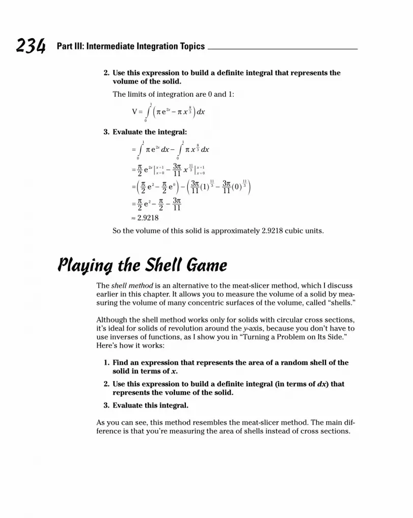
2. Use this expression to build a definite integral that represents thevolume of the solid.
The limits of integration are 0 and 1:
x dxπ πV e x238
0
1
= -# a k
3. Evaluate the integral:
dx x dxπ πe x238
0
1
0
1
= - ##
xπ π2 11
3e xx
x
x
x20
1311
0
1= -=
=
=
=
π π π π2 2 11
3 1 113 0e e2 0 3
11311
= - - -c ^ ^cm h h m
π π π2 2 11
3e2= - -
≈ 2.9218
So the volume of this solid is approximately 2.9218 cubic units.
Playing the Shell GameThe shell method is an alternative to the meat-slicer method, which I discussearlier in this chapter. It allows you to measure the volume of a solid by mea-suring the volume of many concentric surfaces of the volume, called “shells.”
Although the shell method works only for solids with circular cross sections,it’s ideal for solids of revolution around the y-axis, because you don’t have touse inverses of functions, as I show you in “Turning a Problem on Its Side.”Here’s how it works:
1. Find an expression that represents the area of a random shell of thesolid in terms of x.
2. Use this expression to build a definite integral (in terms of dx) thatrepresents the volume of the solid.
3. Evaluate this integral.
As you can see, this method resembles the meat-slicer method. The main dif-ference is that you’re measuring the area of shells instead of cross sections.
234 Part III: Intermediate Integration Topics
16_225226-ch10.qxd 5/1/08 11:37 PM Page 234

Peeling and measuring a can of soupYou can use a can of soup — or any other can that has a paper label on it —as a handy visual aid to give you insight into how the shell method works. Tostart out, go to the pantry and get a can of soup.
Suppose that your can of soup is industrial size, with a radius of 3 inches anda height of 8 inches. You can use the formula for a cylinder to figure out itsvolume as follows:
V = Ab · h = 32π · 8 = 72π
Another option is the meat-slicer method, as I show you earlier in this chap-ter. A third option, which I focus on here, is the shell method.
To understand the shell method, slice the can’s paper label vertically, andcarefully remove it from the can, as shown in Figure 10-11. (While you’re at it,take a moment to read the label so that you’re not left with “mystery soup.”)
SOUP
SOUP
x = 3 in
h = 8
8 in
6π in
Figure 10-11:Removing
the labelfrom a can
of soup canhelp you
understandthe shellmethod.
235Chapter 10: Pump up the Volume: Using Calculus to Solve 3-D Problems
16_225226-ch10.qxd 5/1/08 11:37 PM Page 235

Notice that the label is simply a rectangle. Its shorter side is equal in lengthto the height of the can (8 inches) and its longer side is equal to the circum-ference (2π · 3 inches = 6π inches). So the area of this rectangle is 48 squareinches.
Now here’s the crucial step: Imagine that the entire can is made up of infi-nitely many labels wrapped concentrically around each other, all the way toits core. The area of each of these rectangles is:
A = 2π x · 8 = 16π x
The variable x in this case is any possible radius, from 0 (the radius of thecircle at the very center of the can) to 3 (the radius of the circle at the outeredge). Here’s how you use the shell method, step by step, to find the volumeof the can:
1. Find an expression that represents the area of a random shell of thecan (in terms of x):
A = 2π x · 8 = 16π x
2. Use this expression to build a definite integral (in terms of dx) thatrepresents the volume of the can.
Remember that with the shell method, you’re adding up all the shellsfrom the center (where the radius is 0) to the outer edge (where theradius is 3). So use these numbers as the limits of integration:
x dxπ16V0
3
= #
3. Evaluate this integral:
x 3=xπ16 21 2= $ x 0=
x 3=xπ8 2= x 0=
Now, evaluate this expression:
= 8π (3)2 – 0 = 72π
The shell method verifies that the volume of the can is 72π cubic inches.
Using the shell methodOne advantage of the shell method over the meat-slicer method comes intoplay when you’re measuring a volume of revolution around the y-axis.
236 Part III: Intermediate Integration Topics
16_225226-ch10.qxd 5/1/08 11:39 PM Page 236

Earlier in this chapter I tell you that the meat-slicer method works best when asolid is on its side — that is, when you can slice it perpendicular to the x-axis.But when the similar cross sections of a solid are perpendicular to the y-axis,you need to use inverses to realign the problem before you can start slicing.(See the earlier section “Turning a Problem on Its Side” for more details.)
This realignment step isn’t necessary for the shell method. This makes theshell method ideal for measuring solids of revolution around the y-axis.For example, suppose that you want to measure the volume of the solidshown in Figure 10-12.
Here’s how the shell method can give you a solution without using inverses:
1. Find an expression that represents the area of a random shell of thesolid (in terms of x).
Remember that each shell is a rectangle with two different sides: Oneside is the height of the function at x — that is, cos x. The other is thecircumference of the solid at x — that is, 2πx. So, to find the area of ashell, multiply these two numbers together:
A = 2πx cos x
2. Use this expression to build a definite integral (in terms of dx) thatrepresents the volume of the solid.
In this case, remember that you’re adding up all the shells from the
center (at x = 0) to the outer edge (at x = π2 ).
cosx x dxπ2V
π
0
2
= #
cosx x dxπ2
π
0
2
= #
y = cos x
x
y
2π
Figure 10-12:Using the
shellmethod to
find thevolume of a
solid ofrevolution.
237Chapter 10: Pump up the Volume: Using Calculus to Solve 3-D Problems
16_225226-ch10.qxd 5/1/08 11:39 PM Page 237

3. Evaluate the integral.
This integral is pretty easy to solve using integration by parts:
x =sin cosx x xπ2+
x 0=
Now, evaluate this expression:
= sin cos sin cosπ π π2 2 2 0 0 0+ - +c ^m h
= π2 0 0 1+ - +c ^m h
= π2 1-
≈ 0.5708
So the volume of the solid is approximately 0.5708 cubic units.
Knowing When and How to Solve 3-D Problems
Because students are so often confused when it comes to solving 3-D calculusproblems, here’s a final perspective on all the methods in this chapter, andhow to choose among them.
First, remember that every problem in this chapter falls into one of these twocategories:
� Finding the area of a surface of revolution
� Finding a volume of a solid
In the first case, use the formula I provide earlier in this chapter, in“Skimming the surface of revolution.”
In the second case, remember that the key to measuring the volume of anysolid is to slice it up in the direction where it has similar cross sections whosearea can be measured easily — for example, a circle, a square, or a triangle.So, your first question is whether these similar cross sections are arrangedhorizontally or vertically.
� Horizontally means that the solid is already in position for the meat-slicer method. (If it’s helpful, imagine slicing a salami in a meat-slicer.The salami must be aligned lying on its side — that is, horizontally —before you can begin slicing.)
� Vertically means that the solid is standing upright so that the slices arestacked on top of each other.
238 Part III: Intermediate Integration Topics
16_225226-ch10.qxd 5/1/08 11:41 PM Page 238

When the cross sections are arranged horizontally, the meat-slicer method isthe easiest way to handle the problem (see “Slicing Your Way to Success” ear-lier in this chapter).
When the cross sections are arranged vertically, however, your next questionis whether these cross sections are circles:
� If the cross sections are not circles, you must use inverses to flip thesolid in the horizontal direction (as I discuss in “Turning a Problem onIts Side”).
� If they are circles, you can either use inverses to flip the solid in the hor-izontal direction (as I discuss in “Turning a Problem on Its Side”) or usethe shell method (as I discuss in “Playing the Shell Game”).
239Chapter 10: Pump up the Volume: Using Calculus to Solve 3-D Problems
16_225226-ch10.qxd 5/1/08 11:41 PM Page 239

240 Part III: Intermediate Integration Topics
16_225226-ch10.qxd 5/1/08 11:41 PM Page 240

Part IVInfinite Series
17_225226-pp04.qxd 5/1/08 11:43 PM Page 241

In this part . . .
I introduce the infinite series — that is, the sum of aninfinite number of terms. I show you the basics of work-
ing with sequences and series, and show you a bunchof ways to determine whether a series is convergent ordivergent. You also discover how to use the Taylor seriesfor expressing and evaluating a wide variety of functions.
17_225226-pp04.qxd 5/1/08 11:43 PM Page 242

Chapter 11
Following a Sequence,Winning the Series
In This Chapter� Knowing a variety of notations for sequences
� Telling whether a sequence is convergent or divergent
� Expressing series in both sigma notation and expanded notation
� Testing a series for convergence or divergence
J ust when you think the semester is winding down, your Calculus II profes-sor introduces a new topic: infinite series.
When you get right down to it, series aren’t really all that difficult. After all,a series is just a bunch of numbers added together. Sure, it happens that thisbunch is infinite, but addition is just about the easiest math on the planet.
But then again, the last month of the semester is crunch time. You’re alreadyanticipating final exams and looking forward to a break from studying. By thetime you discover that the prof isn’t fooling and really does expect you toknow this material, infinite series can lead you down an infinite spiral ofdespair: Why this? Why now? Why me?
In this chapter, I show you the basics of series. First, you wade into thesenew waters slowly by examining infinite sequences. When you understandsequences, series make a whole lot more sense. Next, I introduce you to infi-nite series. I discuss how to express a series in both expanded notation andsigma notation, and then I make sure that you’re comfortable with sigmanotation. I also show you how every series is related to two sequences.
Next, I introduce you to the all-important topic of convergence and diver-gence. This concept looms large, so I give you the basics in this chapter andsave the more complex information for Chapter 12. Finally, I introduce you toa few important types of series.
18_225226-ch11.qxd 5/1/08 11:45 PM Page 243

Introducing Infinite SequencesA sequence of numbers is simply a bunch of numbers in a particular order.For example:
1, 4, 9, 16, 25, ...
π, 2π, 3π, 4π, ...
, , , ,21
31
41
51 ...
2, 3, 5, 7, 11, 13, ...
2, –2, 2, –2, ...
0, 1, –1, 2 –2, 3, ...
When a sequence goes on forever, it’s an infinite sequence. Calculus — whichfocuses on all things infinite — concerns itself predominantly with infinitesequences.
Each number in a sequence is called a term of that sequence. So, in thesequence 1, 4, 9, 16, ... , the first term is 1, the second term is 4, and so forth.
Understanding sequences is an important first step toward understandingseries.
Understanding notations for sequencesThe simplest notation for defining a sequence is a variable with the subscriptn surrounded by braces. For example:
{an} = {1, 4, 9, 16, ...}
{bn} = {1, , , ,21
31
41 ...}
{cn} = {4π, 6π, 8π, 10π, ...}
You can reference a specific term in the sequence by using the subscript:
a1 = 1 b3 = 31 c6 = 14π
Make sure that you understand the difference between notation with andwithout braces:
� The notation {an} with braces refers to the entire sequence.
� The notation an without braces refers to the nth term of the sequence.
244 Part IV: Infinite Series
18_225226-ch11.qxd 5/1/08 11:46 PM Page 244

When defining a sequence, instead of listing the first few terms, you can statea rule based on n. (This is similar to how a function is typically defined.) Forexample:
{an}, where an = n2
{bn}, where bn = n1
{cn}, where cn = 2(n + 1)π
Sometimes, for increased clarity, the notation includes the first few termsplus a rule for finding the nth term of the sequence. For example:
{an} = {1, 4, 9, ... , n2, ...}
{bn} = {1, 21 , 3
1 , ... , n1 , ...}
{cn} = {4π, 6π, 8π, ... , 2(n + 1)π, ...}
This notation can be made more concise by appending starting and endingvalues for n:
a nn n
2
1=
3
=# #- -
b n1
nn 1
=3
=
# '- 1
c nπ2n n 2=
3
=# "- ,
This last example points out the fact that the initial value of n doesn’t haveto be 1, which gives you greater flexibility to define a number series by usinga rule.
Don’t let the fancy notation for number sequences get to you. When you’refaced with a new sequence that’s defined by a rule, jot down the first four orfive numbers in that sequence. Usually, after you see the pattern, you’ll findthat a problem is much easier.
Looking at converging anddiverging sequencesEvery infinite sequence is either convergent or divergent:
� A convergent sequence has a limit — that is, it approaches a realnumber.
� A divergent sequence doesn’t have a limit.
245Chapter 11: Following a Sequence, Winning the Series
18_225226-ch11.qxd 5/1/08 11:47 PM Page 245

For example, here’s a convergent sequence:
{an} = {1, 21 , 3
1 , 41 , 5
1 , ...}
This sequence approaches 0, so:
lim a 0n =# -
Thus, this sequence converges to 0.
Here’s another convergent sequence:
{bn} = {7, 9, 7 21 , 8 2
1 , 7 43 , 8 4
1 , ...}
This time, the sequence approaches 8 from above and below, so:
lim b 8n =# -
In many cases, however, a sequence diverges — that is, it fails to approach anyreal number. Divergence can happen in two ways. The most obvious type ofdivergence occurs when a sequence explodes to infinity or negative infinity —that is, it gets farther and farther away from 0 with every term. Here are a fewexamples:
–1, –2, –3, –4, –5, –6, –7, ...
ln 1, ln 2, ln 3, ln 4, ln 5, ...
2, 3, 5, 7, 11, 13, 17, ...
In each of these cases, the sequence approaches either ∞ or –∞, so the limitof the sequence does not exist (DNE). Therefore, the sequence is divergent.
A second type of divergence occurs when a sequence oscillates between twoor more values. For example:
0, 7, 0, 7, 0, 7, 0, 7, ...
1, 1, 2, 1, 2, 3, 1, 2, 3, 4, 1, ...
In these cases, the sequence bounces around indefinitely, never settling inon a value. Again, the limit of the sequence does not exist, so the sequence isdivergent.
246 Part IV: Infinite Series
18_225226-ch11.qxd 5/1/08 11:48 PM Page 246

Introducing Infinite SeriesIn contrast to an infinite sequence (which is an endless list of numbers), aninfinite series is an endless sum of numbers. You can change any infinitesequence to an infinite series simply by changing the commas to plus signs.For example:
1, 2, 3, 4, ... 1 + 2 + 3 + 4 + ...
1, 21 , 3
1 , 41 , ... 1 + 2
1 + 31 + 4
1 + ...
1, –1, 21 , 2
1- , 41 , 4
1- , ... 1 + –1 + 21 + 2
1- + 41 + 4
1- + ...
The two principal notations for series are sigma notation and expanded nota-tion. Sigma notation provides an explicit rule for generating the series (seeChapter 2 for the basics of sigma notation). Expanded notation gives enoughof the first few terms of a series so that the pattern generating the seriesbecomes clear.
For example, here are three series defined using both forms of notation:
. . .n2 2 4 6 8n 1
= + + + +3
=
!
. . .41 1 4
1161
641
nn 0
= + + + +3
=
!
. . .n 3 4 5e e e en
n3 4 5
3= + + +
3
=
!
As you can see, a series can start at any integer.
As with sequences (see “Introducing Infinite Sequences” earlier in this chapter), every series is either convergent or divergent:
� A convergent series evaluates to a real number.
� A divergent series doesn’t evaluate to a real number.
To get clear on how evaluation of a series connects with convergence anddivergence, I give you a few examples. To start out, consider this convergentseries:
. . .21 1 2
141
81
n
n 0= + + + +
3
=
! c m
247Chapter 11: Following a Sequence, Winning the Series
18_225226-ch11.qxd 5/1/08 11:51 PM Page 247

Notice that as you add this series from left to right, term by term, the runningtotal is a sequence that approaches 2:
1, 23 , 4
7 , 815 , ...
This sequence is called the sequence of partial sums for this series. I discusssequences of partial sums in greater detail later in “Connecting a Series withIts Two Related Sequences.”
For now, please remember that the value of a series equals the limit of itssequence of partial sums. In this case, because the limit of the sequence is 2,you can evaluate the series as follows:
21 2
n
n 0=
3
=
! c m
Thus, this series converges to 2.
Often, however, a series diverges — that is, it doesn’t equal any real number. Aswith sequences, divergence can happen in two ways. The most obvious type ofdivergence occurs when a series explodes to infinity or negative infinity. Forexample:
. . .n 1 2 3 4n 1
- = - + - + - + - +3
=
!
This time, watch what happens as you add the series term by term:
–1, –3, –6, –10, ...
Clearly, this sequence of partial sums diverges to negative infinity, so theseries is divergent as well.
A second type of divergence occurs when a series alternates between posi-tive and negative values in such a way that the series never approaches avalue. For example:
. . .1 1 1 1 1n
n 0- = + - + + - +
3
=
!^ h
So, here’s the related sequence of partial sums:
1, 0, 1, 0, ...
In this case, the sequence of partial sums alternates forever between 1 and 0,so it’s divergent; therefore, the series is also divergent. This type of series iscalled, not surprisingly, an alternating series. I discuss alternating series ingreater depth in Chapter 12.
248 Part IV: Infinite Series
18_225226-ch11.qxd 5/1/08 11:53 PM Page 248

Convergence and divergence are arguably the most important topics in yourfinal weeks of Calculus II. Many of your exam questions will ask you to deter-mine whether a given series is convergent or divergent.
Later in this chapter, I show you how to decide whether certain importanttypes of series are convergent or divergent. Chapter 12 gives you a ton ofhandy tools for answering this question more generally. For now, just keepthis important idea of convergence and divergence in mind.
Getting Comfy with Sigma NotationSigma notation is a compact and handy way to represent series.
Okay — that’s the official version of the story. What’s also true is that sigmanotation can be unclear and intimidating — especially when the professorstarts scrawling it all over the blackboard at warp speed while explainingsome complex proof. Lots of students get left in the chalk dust (or dry-erasemarker fumes).
At the same time, sigma notation is useful and important because it providesa concise way to express series and mathematically manipulate them.
In this section, I give you a bunch of handy tips for working with sigma nota-tion. Some of the uses for these tips become clearer as you continue to studyseries later in this chapter and in Chapters 12 and 13. For now, just add thesetools to your toolbox and use them as needed.
Writing sigma notation in expanded formWhen you’re working with an unfamiliar series, begin by writing it out usingboth sigma and expanded notation. This practice is virtually guaranteed toincrease your understanding of the series. For example:
n32n
n 1
3
=
!
As it stands, you may not have much insight into what this series looks like,so expand it out:
. . .n32
32
64
98
1216
1632n
n 1= + + + + +
3
=
!
249Chapter 11: Following a Sequence, Winning the Series
18_225226-ch11.qxd 5/1/08 11:54 PM Page 249

As you spend a bit of time generating this series, it begins to grow less fright-ening. For one thing, you may notice that in a race between the numeratorand denominator, eventually the numerator catches up and pulls ahead.Because the terms eventually grow greater than 1, the series explodes toinfinity, so it diverges.
Seeing more than one way to use sigma notationVirtually any series expressed in sigma notation can be rewritten in a slightlyaltered form. For example:
81
161
321
641 f+ + + +
You can express this series in sigma notation as follows:
. . .21
81
161
321
641
n
n 3= + + + +
3
=
! c m
Alternatively, you can express the same series in any of the following ways:
= 21
n
n
1
2
3 +
=
! c m
= 21
n
n
2
1
3 +
=
!c m
= 21
n
n
3
0
3 +
=
! c m
Depending on the problem that you’re trying to solve, you may find one ofthese expressions more advantageous than the others — for example, whenusing the comparison tests that I introduce in Chapter 12. For now, just besure to keep in mind the flexibility at your disposal when expressing a seriesin sigma notation.
Discovering the Constant MultipleRule for seriesIn Chapter 4, you discover that the Constant Multiple Rule for Integrationallows you to simplify an integral by factoring out a constant. This option isalso available when you’re working with series. Here’s the rule:
Σ can = c Σ an
250 Part IV: Infinite Series
18_225226-ch11.qxd 5/1/08 11:56 PM Page 250

For example:
n n7 7 1
nn2 2
11=
33
==
!!
To see why this rule works, first expand the series so that you can see whatyou’re working with:
. . .n7 7 4
797
167
n2
1= + + + +
3
=
!
Working with the expanded form, you can factor out a 7 from each term:
= 7 1 41
91
161 f+ + + +c m
Now, express the contents of the parentheses in sigma notation:
n7 1
n2
1=
3
=
!
As if by magic, this procedure demonstrates that the two sigma expressionsare equal. But, this magic is really nothing more exotic than your old friendfrom grade school, the distributive property.
Examining the Sum Rule for seriesHere’s another handy tool for your growing toolbox of sigma tricks. This rulemirrors the Sum Rule for Integration (see Chapter 4), which allows you tosplit a sum inside an integral into the sum of two separate integrals. Similarly,you can break a sum inside a series into the sum of two separate series:
Σ (an + bn) = Σ an + Σ bn
For example:
n2
1n
n 1= +
3
=
!
A little algebra allows you to split this fraction into two terms:
n2 2
1n n
n 1= +
3
=
!c m
Now, the rule allows you to split this result into two series:
n2 2
1n
nn
n1 1= +
3 3
= =
! !
251Chapter 11: Following a Sequence, Winning the Series
18_225226-ch11.qxd 5/1/08 11:59 PM Page 251

This sum of two series is equivalent to the series that you started with. Aswith the Sum Rule for Integration, expressing a series as a sum of two simplerseries tends to make problem-solving easier. Generally speaking, as you pro-ceed onward with series, any trick you can find to simplify a difficult series isa good thing.
Connecting a Series with ItsTwo Related Sequences
Every series has two related sequences. The distinction between a sequenceand a series is as follows:
� A sequence is a list of numbers separated by commas (for example: 1, 2, 3, ...).
� A series is a sum of numbers separated by plus signs (for example: 1 + 2 + 3 + ...).
When you see how a series and its two related sequences are distinct butalso related, you gain a clearer understanding of how series work.
A series and its defining sequenceThe first sequence related to a series is simply the sequence that defines theseries in the first place. For example, here are three series written in bothsigma notation and expanded notation, each paired with its defining sequence:
. . .21 1 2
141
81
n
n 1= + + + +
3
=
!c m , , , , . . .1 21
41
81
.. .nn
1 21
32
43
54
n 1 += + + + +
3
=
! , , , , . . .21
32
43
54
.. .n1 1 2
131
41
n 1= + + + +
3
=
! , , , , . . .1 21
31
41
When a sequence {an} is already defined, you can use the notation Σ an to refer
to the related series starting at n = 1. For example, when {an} = n1
2 , Σ an = 1 + 41 +
91 + 16
1 + ....
252 Part IV: Infinite Series
18_225226-ch11.qxd 5/2/08 12:03 AM Page 252

Understanding the distinction between a series and the sequence that definesit is important for two reasons. First, and most basic, you don’t want to get theconcepts of sequences and series confused. But second, the sequence thatdefines a series can provide important information about the series. SeeChapter 12 to find out about the nth term test, which provides a connectionbetween a series and its defining sequence.
A series and its sequences of partial sumsYou can learn a lot about a series by finding the partial sums of its first fewterms. For example, here’s a series that you’ve seen before:
. . .21
21
41
81
161
n
n 1= + + + +
3
=
!c m
And here are the first four partial sums of this series:
21
21
n
n 1
1
==
!c m
21
21
41
43
n
n 1
2
= + ==
!c m
21
21
41
81
87
n
n 1
3
= + + ==
!c m
21
21
41
81
161
1615
n
n 1
4
= + + + ==
!c m
You can turn the partial sums for this series into a sequence as follows:
{Sn} = , , , , , ,21
43
87
1615
2 12n
n
f f-
' 1
In general, every series Σ an has a related sequence of partial sums {Sn}. Forexample, here are a few such pairings:
. . .21
21
41
81
161
n
n 1= + + + +
3
=
!c m , , , , . . .21
43
87
1615
.. .nn
1 21
32
43
54
n 1 += + + + +
3
=
! , , , , . . .21
67
1223
60163
,. . .n1 1 2
131
41
n 1= + + +
3
=
! , , , , . . .1 23
611
1225
253Chapter 11: Following a Sequence, Winning the Series
18_225226-ch11.qxd 5/2/08 12:10 AM Page 253

Every series and its related sequence of partial sums are either both conver-gent or both divergent. Moreover, if they’re both convergent, both converge tothe same number.
This rule should come as no big surprise. After all, a sequence of partial sumssimply gives you a running total of where a series is going. Still, this rule canbe helpful. For example, suppose that you want to know whether the follow-ing sequence is convergent or divergent:
1, , , , ,23
611
1225
60137 f
What the heck is this sequence, anyway? Upon deeper examination, however,you discover that it’s the sequence of partial sums for every simple series:
1
1 21
23+ =
1 21
31
611+ + =
1 21
31
41
1225+ + + =
1 21
31
41
51
60137+ + + + =
This series, called the harmonic series, is divergent, so you can conclude thatits sequence of partial sums also diverges.
Recognizing Geometric Series and P-Series
At first glance, many series look strange and unfamiliar. But a few big cate-gories of series belong in the Hall of Fame. When you know how to identifythese types of series, you have a big head start on discovering whether they’reconvergent or divergent. In some cases, you can also find out the exact value ofa convergent series without spending all eternity adding numbers.
In this section, I show you how to recognize and work with two commontypes of series: geometric series and p-series.
254 Part IV: Infinite Series
18_225226-ch11.qxd 5/2/08 12:12 AM Page 254

Getting geometric seriesA geometric series is any series of the following form:
. . .ar a ar ar arn
n 0
2 3= + + + +3
=
!
Here are a few examples of geometric series:
. . .2 1 2 4 8 16n
n 0= + + + + +
3
=
!
, . . .101 1 10
1100
11 000
1n
n 0= + + + +
3
=
!
, , , . . .1003 3 100
310 000
31 000 000
3n
n 0= + + + +
3
=
!
In the first series, a = 1 and r = 2. In the second, a = 1 and r = 101 . And in the
third, a = 3 and r = 1001 .
If you’re unsure whether a series is geometric, you can test it as follows:
1. Let a equal the first term of the series.
2. Let r equal the second term divided by the first term.
3. Check to see whether the series fits the form a + ar2 + ar3 + ar4 + ....
For example, suppose that you want to find out whether the following seriesis geometric:
58
56
109
4027
16081
640243 f+ + + + + +
Use the procedure I outline as follows:
1. Let a equal the first term of the series:
a = 58
2. Let r equal the second term divided by the first term:
r = 56 ÷ 5
8 = 43
255Chapter 11: Following a Sequence, Winning the Series
18_225226-ch11.qxd 5/2/08 12:15 AM Page 255

3. Check to see whether the series fits the form a + ar2 + ar3 + ar4 + ... :
a 58=
ar 58
43
56= =c m
ar 56
43
1092
2
= =c m
ar 109
43
40273
3
= =c m
As you can see, this series is geometric. To find the limit of a geometric seriesa + ar + ar2 + ar3 + ..., use the following formula:
ar ra
1n
n 0=
-
3
=
!
So, the limit of the series in the previous example is:
58
43
1 43
58
58
41
532
n
n 0=
-= =
3
=$! c m
When the limit of a series exists, as in this example, the series is called convergent. So, you say that this series converges to 5
32 .
In some cases, however, the limit of a geometric series does not exist (DNE).In that case, the series is divergent. Here’s the complete rule that tells youwhether a series is convergent or divergent:
For any geometric series a + ar + ar2 + ar3 + ..., if r falls in the open set (–1, 1), the series converges to r
a1 -
; otherwise, the series diverges.
An example makes clear why this is so. Look at the following geometric series:
1 45
1625
64125
256625 f+ + + + +
In this case, a = 1 and r = 45 . Because r > 1, each term in the series is greater
than the term that precedes it, so the series grows at an ever-accelerating rate.
This series illustrates a simple but important rule of thumb for decidingwhether a series is convergent or divergent: A series can be convergent onlywhen its related sequence converges to zero. I discuss this important idea(called the nth-term test) further in Chapter 12.
Similarly, look at this example:
1 45
1625
64125
256625 f+ - + + - + +
256 Part IV: Infinite Series
18_225226-ch11.qxd 5/2/08 12:19 AM Page 256

This time, a = 1 and r = 45- . Because r < –1, the odd terms grow increasingly
positive and the even terms grow increasingly negative. So the relatedsequence of partial sums alternates wildly from the positive to the negative,with each term further from zero than the preceding term.
A series in which alternating terms are positive and negative is called an alter-nating series. I discuss alternating series in greater detail in Chapter 12.
Generally speaking, the geometric series is the only type of series that has asimple formula to calculate its value. So, when a problem asks for the value ofa series, try to put it in the form of a geometric series.
For example, suppose that you’re asked to calculate the value of this series:
75
2110
6320
18940 f+ + + +
The fact that you’re being asked to calculate the value of the series should tipyou off that it’s geometric. Use the procedure I outline earlier to find a and r :
a = 75
r = 2110
75
32
' =
So here’s how to express the series in sigma notation as a geometric series interms of a and r :
. . .75
32
75
2110
6320
18940
n
n 1= + + + +
3
=
! c m
At this point, you can use the formula for calculating the value of this series:
ra
1 1 32
75
75
31
715=
-=
-= =$
c m
Pinpointing p-seriesAnother important type of series is called the p-series. A p-series is any seriesin the following form:
. . .n1 1 2
131
41
pn
p p p1
= + + + +3
=
!
Here’s a common example of a p-series, when p = 2:
. . .n1 1 4
191
161
n2
1= + + + +
3
=
!
257Chapter 11: Following a Sequence, Winning the Series
18_225226-ch11.qxd 5/2/08 12:23 AM Page 257

Here are a few other examples of p-series:
, . . .n1 1 32
12431
1 0241
n5
1= + + + +
3
=
!
. . .n1 1
21
31
21
51
n 21
1= + + + + +
3
=
!
. . .n1 1 2 3 4
n1
1= + + + +
3
-=
!
Don’t confuse p-series with geometric series (which I introduce in the previ-ous section). Here’s the difference:
� A geometric series has the variable n in the exponent — for example,
Σ 21
n
c m .
� A p-series has the variable in the base — for example Σn1
2 .
As with geometric series, a simple rule exists for determining whether a p-series is convergent or divergent.
A p-series converges when p > 1 and diverges when p ≤ 1.
I give you a proof of this theorem in Chapter 12. In this section, I show youwhy a few important examples of p-series are either convergent or divergent.
Harmonizing with the harmonic seriesWhen p = 1, the p-series takes the following form:
. . .n1 1 2
131
41
n 1= + + + +
3
=
!
This p-series is important enough to have its own name: the harmonic series.The harmonic series is divergent.
Testing p-series when p = 2, p = 3, and p = 4Here are the p-series when p equals the first few counting numbers greaterthan 1:
. . .n1 1 4
191
161
n2
1= + + + +
3
=
!
. . .n1 1 8
1271
641
n3
1= + + + +
3
=
!
. . .n1 1 16
1811
2561
n4
1= + + + +
3
=
!
Because p > 1, these series are all convergent.
258 Part IV: Infinite Series
18_225226-ch11.qxd 5/2/08 12:28 AM Page 258

Testing p-series when p = 21
When p = 21 , the p-series looks like this:
. . .n1 1
21
31
21
51
n 21
1= + + + + +
3
=
!
Because p ≤ 1, this series diverges. To see why it diverges, notice that when n is a square number, the nth term equals n
1 . So this p-series includes every term in the harmonic series plus many more terms. Because the harmonicseries is divergent, this series is also divergent.
259Chapter 11: Following a Sequence, Winning the Series
18_225226-ch11.qxd 5/2/08 12:29 AM Page 259

260 Part IV: Infinite Series
18_225226-ch11.qxd 5/2/08 12:29 AM Page 260

Chapter 12
Where Is This Going? Testing forConvergence and Divergence
In This Chapter� Understanding convergence and divergence
� Using the nth-term test to prove that a series diverges
� Applying the versatile integral test, ratio test, and root test
� Distinguishing absolute convergence and conditional convergence
Testing for convergence and divergence is The Main Event in yourCalculus II study of series. Recall from Chapter 11 that when a series
converges, it can be evaluated as a real number. However, when a seriesdiverges, it can’t be evaluated as a real number, because it either explodesto positive or negative infinity or fails to settle in on a single value.
In Chapter 11, I give you two tests for determining whether specific types ofseries (geometric series and p-series) are convergent or divergent. In this chap-ter, I give you seven more tests that apply to a much wider range of series.
The first of these is the nth-term test, which is sort of a no-brainer. With thisunder your belt, I move on to two comparison tests: the direct comparisontest and the limit comparison test. These tests are what I call one-way tests;they provide an answer only if the series passes the test but not if the seriesfails it. Next, I introduce three two-way tests, which provide one answer if theseries passes the test and the opposite answer if the series fails it. Thesetests are the integral test, the ratio test, and the root test.
Finally, I introduce you to alternating series, in which terms are alternatelypositive and negative. I contrast alternating series with positive series, whichare the series that you’re already familiar with, and I show you how to turn apositive series into an alternating series and vice versa. Then I show you howto prove whether an alternating series is convergent or divergent by usingthe alternating series test. To finish up, I introduce you to the important con-cepts of absolute convergence and conditional convergence.
19_225226-ch12.qxd 5/2/08 12:30 AM Page 261

Starting at the BeginningWhen testing for convergence or divergence, don’t get too hung up on wherethe series starts. For example:
n1
,n 1 001
3
=
!
This is just a harmonic series with the first 1,000 terms lopped off:
, , ,1 0011
1 0021
1 0031 f= + + +
These fractions may look tiny, but the harmonic series diverges (see Chapter11), and removing a finite number of terms from the beginning of this seriesdoesn’t change this fact.
The lesson here is that, when you’re testing for convergence or divergence,what’s going on at the beginning of the series is irrelevant. Feel free to lop offthe first few billion or so terms of a series if it helps you to prove that theseries is convergent or divergent.
Similarly, in most cases you can add on a few terms to a series without chang-ing whether it converges or diverges. For example:
n 11
,n 1 000 -
3
=
!
You can start this series anywhere from n = 2 to n = 999 without changing thefact that it diverges (because it’s a harmonic series). Just be careful, because if you try to start the series from n = 1, you’re adding the term 0
1 , which is a big no-no. However, in most cases you can extend an infinite series withoutcausing problems or changing the convergence or divergence of the series.
Although eliminating terms from the beginning of a series doesn’t affectwhether the series is convergent or divergent, it does affect the sum of a convergent series. For example:
21 1 2
141
81
n
f= + + + +c m
Lopping off the first few terms of this series — say, 1, 21 , and 4
1 — doesn’t
change the fact that it’s convergent. But it does change the value that theseries converges to. For example:
. . .21
21
41
81 1
n
n 1= + + + =
3
=
!c m
262 Part IV: Infinite Series
19_225226-ch12.qxd 5/2/08 12:33 AM Page 262

Using the nth-Term Test for DivergenceThe nth-term test for divergence is the first test that you need to know. It’seasy and it enables you to identify lots of series as divergent.
If the limit of sequence {an} doesn’t equal 0, then the series Σ an is divergent.
To show you why this test works, I define a sequence that meets the neces-sary condition — that is, a sequence that doesn’t approach 0:
{an} = , , , , nn
21
32
43
1f f+
Notice that the limit of the sequence is 1 rather than 0. So, here’s the relatedseries:
nn
1 21
32
43
n 1f
+= + + +
3
=
!
Because this series is the sum of an infinite number of terms that are veryclose to 1, it naturally produces an infinite sum, so it’s divergent.
The fact that the limit of a sequence {an} equals 0 doesn’t necessarily implythat the series Σ an is convergent.
For example, the harmonic sequence 1, , ,21
31 ... approaches 0, but (as I
demonstrate in Chapter 11) the harmonic series 1 + 21 + 3
1 + ... is divergent.
When testing for convergence or divergence, always perform the nth-termtest first. It’s a simple test, and plenty of teachers test for it on examsbecause it’s easy to grade but still catches the unwary student. Remember: Ifthe defining sequence of a series doesn’t approach 0, the series diverges; oth-erwise, you need to move on to other tests.
Let Me Count the WaysTests for convergence or divergence tend to fall into two categories: one-waytests and two-way tests.
One-way testsA one-way test allows you to draw a conclusion only when a series passes thetest, but not when it fails. Typically, passing the test means that a given condi-tion has been met.
263Chapter 12: Where Is This Going? Testing for Convergence and Divergence
19_225226-ch12.qxd 5/2/08 12:34 AM Page 263

The nth-term test is a perfect example of a one-way test: If a series passes thetest — that is, if the limit of its defining sequence doesn’t equal 0 — the seriesis divergent. But if the series fails the test, you can draw no conclusion.
Later in this chapter, you discover two more one-way tests: the direct com-parison test and the limit comparison test.
Two-way testsA two-way test allows you to draw one conclusion when a series passes thetest and the opposite conclusion when a series fails the test. As with a one-way test, passing the test means that a given condition has been met. Failingthe test means that the negation of that condition has been met.
For example, the test for geometric series is a two-way test (see Chapter 11 tofind out more about testing geometric series for convergence and diver-gence). If a series passes the test — that is, if r falls in the open set (–1, 1) —then the series is convergent. And if the series fails the test — that is, if r ≤ –1or r ≥ 1 — then the series is divergent.
Similarly, the test for p-series is also a two-way test (see Chapter 11 for moreon this test).
Keep in mind that no test — even a two-way test — is guaranteed to give youan answer. Think of each test as a tool. If you run into trouble trying to cut apiece of wood with a hammer, it’s not the hammer’s fault: You just chose thewrong tool for the job.
Similarly, if you can’t find a clever way to demonstrate either the condition orits negation required by a specific test, you’re out of luck. In that case, youmay need to use a different test that’s better suited to the problem.
Later in this chapter, I show you three more two-way tests: the integral test,the ratio test, and the root test.
Using Comparison TestsComparison tests allow you to use stuff that you know to find out stuff thatyou want to know. The stuff that you know is more eloquently called a bench-mark series — a series whose convergence or divergence you’ve alreadyproven. The stuff that you want to know is, of course, whether an unfamiliarseries converges or diverges.
264 Part IV: Infinite Series
19_225226-ch12.qxd 5/2/08 12:34 AM Page 264

As with the nth-term test, comparison tests are one-way tests: When a seriespasses the test, you prove what you’ve set out to prove (that is, either con-vergence or divergence). But when a series fails the test, the result of a com-parison test in inconclusive.
In this section, I show you two basic comparison tests: the direct comparisontest and the limit comparison test.
Getting direct answers with the direct comparison testYou can use the direct comparison test to prove either convergence or diver-gence, depending on how you set up the test.
To prove that a series converges:
1. Find a benchmark series that you know converges.
2. Show that each term of the series that you’re testing is less than orequal to the corresponding term of the benchmark series.
To prove that a series diverges:
1. Find a benchmark series that you know diverges.
2. Show that each term of the series you’re testing is greater than orequal to the corresponding term of the benchmark series.
For example, suppose that you’re asked to determine whether the followingseries converges or diverges:
:n 1
121
51
101
171Benchmark series
n2
1f
+= + + + +
3
=
!
It’s hard to tell just by looking at it whether this particular series is conver-gent or divergent. However, it looks a bit like a p-series with p = 2:
. . .n1 1 4
191
161
n2
1= + + + +
3
=
!
You know that this p-series converges (see Chapter 11 if you’re not surewhy), so use it as your benchmark series. Now, your task is to show that
265Chapter 12: Where Is This Going? Testing for Convergence and Divergence
19_225226-ch12.qxd 5/2/08 12:36 AM Page 265

every term in the series that you’re testing is less than the correspondingterm of the benchmark series:
First term: 21 < 1
Second term: 51 < 4
1
Third term: 101 < 9
1
This looks good, but to complete the proof formally, here’s what you want toshow:
nth term: n 1
12 +
≤n1
2
To see that this statement is true, notice that the numerators are the same, but the denominator (n2 + 1) is greater than n2. So, the function
n 11
2 +is less
than n1
2 , which means that every term in the test series is less than the corre-
sponding term in the convergent benchmark series. Therefore, both seriesare convergent.
As another example, suppose that you want to test the following series forconvergence or divergence:
. . .n3 3 2
3 1 43
53
n 1= + + + + +
3
=
!
This time, the series reminds you of the trusty harmonic series, which youknow is divergent:
. . .n1 1 2
131
41
51Benchmark series:
n 1= + + + + +
3
=
!
Using the harmonic series as your benchmark, compare the two series termby term:
First term: 3 > 1
Second term: 23 > 2
1
Third term: 1 > 31
Again, you have reason to be hopeful, but to complete the proof formally, youwant to show the following:
nth term: n3 ≥ n
1
This time, notice that the denominators are the same, but the numerator 3 is greater than the numerator 1. So the function n
3 is greater than n1 .
266 Part IV: Infinite Series
19_225226-ch12.qxd 5/2/08 12:39 AM Page 266

Again, you’ve shown that every term in the test series is greater than the corre-sponding term in the divergent benchmark series, so both series are divergent.
As a third example, suppose that you’re asked to show whether this series isconvergent or divergent:
. . .n n1 2
161
121
201
301
n 1 + += + + + +
3
=
!^ ^h h
In this case, multiplying out the denominators is a helpful first step:
n n3 21
n2
1=
+ +
3
=
!
Now, the series looks a little like a p-series with p = 2, so make this yourbenchmark series:
. . .n1 1 4
191
161
n2
1= + + + +
3
=
!
The benchmark series converges, so you want to show that every term of thetest series is less than the corresponding term of the benchmark. This lookslikely because:
First term: 61 < 1
Second term: 121 < 4
1
Third term: 201 < 9
1
However, to convince the professor, you want to show that every term of thetest series is less than the corresponding term:
nth term: n n3 2
12 + +
≤n1
2
As with the first example in this section, the numerators are the same, butthe denominator of the test series is greater than that of the benchmarkseries. So the test series is, indeed, less than the benchmark series, whichmeans that the test series is also convergent.
Testing your limits with the limit comparison testAs with the direct comparison test, the limit comparison test works bychoosing a benchmark series whose behavior you know and using it to provide information about a test series whose behavior you don’t know.
267Chapter 12: Where Is This Going? Testing for Convergence and Divergence
19_225226-ch12.qxd 5/2/08 12:41 AM Page 267

Here’s the limit comparison test: Given a test series Σ an and a benchmarkseries Σ bn, find the following limit:
lim ba
n n
n
"3
If this limit evaluates as a positive number, then either both series convergeor both diverge.
As with the direct comparison test, when the test succeeds, what you learndepends upon what you already know about the benchmark series. If thebenchmark series converges, so does the test series. However, if the bench-mark series diverges, so does the test series.
Remember, however, that this is a one-way test: If the test fails, you can drawno conclusion about the test series.
The limit comparison test is especially good for testing infinite series basedon rational expressions. For example, suppose that you want to see whetherthe following series converges or diverges:
nn
15
n2
1 +-
3
=
!
When testing an infinite series based on a rational expression, choose abenchmark series that’s proportionally similar — that is, whose numeratorand denominator differ by the same number of degrees.
In this example, the numerator is a first-degree polynomial and the denomina-tor is a second-degree polynomial (for more on polynomials, see Chapter 2).So the denominator is one degree greater than the numerator. Therefore, Ichoose a benchmark series that’s proportionally similar — the trusty har-monic series:
n1Benchmark series:
n 1
3
=
!
Before you begin, take a moment to get clear on what you’re testing, and jot itdown. In this case, you know that the benchmark series diverges. So, if thetest succeeds, you prove that the test series also diverges. (If it fails, however,you’re back to square one because this is a one-way test.)
Now, set up the limit (by the way, it doesn’t matter which series you put inthe numerator and which in the denominator):
limn
nn
115
n
2 +-
"3
268 Part IV: Infinite Series
19_225226-ch12.qxd 5/2/08 12:43 AM Page 268

At this point, you just crunch the numbers:
limnn n
15
n2 +
-
"3
^ h
limn
n n1
5n
2
2
=+
-"3
Notice at this point that the numerator and denominator are both second-degree polynomials. Now, as you apply L’Hospital’s Rule (taking the deriva-tive of both the numerator and denominator), watch what happens:
lim nn2
2 5n
= -"3
lim 22 1
n= =
"3
As if by magic, the limit evaluates to a positive number, so the test succeeds.Therefore, the test series diverges. Remember, however, that you made thismagic happen by choosing a benchmark series in proportion to the test series.
Another example should make this crystal clear. Discover whether this seriesis convergent or divergent:
limn n
n4 2
2n 5 3
3
- --
"3
When you see that this series is based on a rational expression, you immedi-ately think of the limit comparison test. Because the denominator is twodegrees higher than the numerator, choose a benchmark series with thesame property:
n1Benchmark series:
n2
1
3
=
!
Before you begin, jot down the following: The benchmark converges, so if thetest succeeds, the test series also converges. Next, set up your limit:
lim
n
n nn
14 2
2
n2
5 3
3
- --
"3
Now, just solve the limit:
limn nn n
4 22
n 5 3
3 2
=- -
-
"3
_ i
limn nn n
4 22
n 5 3
5 2
=- --
"3
269Chapter 12: Where Is This Going? Testing for Convergence and Divergence
19_225226-ch12.qxd 5/2/08 12:48 AM Page 269

Again, the numerator and denominator have the same degree, so you’re onthe right track. Now, solving the limit is just a matter of grinding through afew iterations of L’Hospital’s Rule:
limn nn n
20 35 4
n4 2
4
--
"3
limn nn
80 620 4
n3
3
=--
"3
limnn
240 660
n2
2
=-3=
lim nn
480120
n=
"3
lim 480120
41
n= =
"3
The test succeeds, so the test series converges. And again, the success of thetest was prearranged because you chose a benchmark series in proportion tothe test series.
Two-Way Tests for Convergenceand Divergence
Earlier in this chapter, I give you a variety of tests for convergence or diver-gence that work in one direction at a time. That is, passing the test gives youan answer, but failing it provides no information.
The tests in this section all have one important feature in common: Regardlessof whether the series passes or fails, whenever the test gives you an answer,that answer always tells you whether the series is convergent or divergent.
Integrating a solution with the integral testJust when you thought that you wouldn’t have to think about integrationagain until two days before your final exam, here it is again. The good news isthat the integral test gives you a two-way test for convergence or divergence.
270 Part IV: Infinite Series
19_225226-ch12.qxd 5/2/08 12:50 AM Page 270

Here’s the integral test:
For any series of the form
f xx a
3
=
! ^ h
consider its associated integral
f x dxa
3
# ^ h
If this integral converges, the series also converges; however, if this integraldiverges, the series also diverges.
In most cases, you use this test to find out whether a series converges ordiverges by testing its associated integral. Of course, changing the series toan integral makes all the integration tricks that you already know and loveavailable to you.
For example, here’s how to use the integral test to show that the harmonicseries is divergent. First, the series:
. . .x1 1 2
131
41
x 1= + + + +
3
=
!
The integral test tells you that this series converges or diverges dependingupon whether the following definite integral converges or diverges:
x dx1
1
3
#
To evaluate this improper integral, express it as a limit, as I show you inChapter 9:
lim x dx1c
c
1
="3
#
This is simple to integrate and evaluate:
lim lnxc x
x c
1=
"3 =
=
a k
lim ln lnc 1c
= -"3
lim lnc 0c
3- ="3
271Chapter 12: Where Is This Going? Testing for Convergence and Divergence
19_225226-ch12.qxd 5/2/08 12:53 AM Page 271

Because the limit explodes to infinity, the integral doesn’t exist. Therefore,the integral test tells you that the harmonic series is divergent.
As another example, suppose that you want to discover whether the follow-ing series is convergent or divergent:
lnn n1
n 2
3
=
!
Notice that this series starts at n = 2, because n = 1 would produce the term 01 .
To use the integral test, transform the sum into this definite integral, using 2as the lower limit of integration:
lnx x dx1
2
3
#
Again, rewrite this improper integral as the limit of an integral (see Chapter 9):
lim lnx x dx1c
c
2"3
#
To solve the integral, use the following variable substitution:
u = ln x
du = x1 dx
So you can rewrite the integral as follows:
lim u du1
ln
ln
c
c
2"3
#
Note that as the variable changes from x to u, the limits of integration changefrom 2 and c to ln 2 and ln c. This change arises when I plug the value x = 2into the equation u = ln x, so u = ln 2. (For more on using variable substitutionto evaluate definite integrals, see Chapter 5.)
At this point, you can evaluate the integral:
lim lnuln
ln
c u
u c
2"3 =
=
a k
lim ln ln ln lnc 2c
3- ="3
^ ^h h
You can see without much effort that as c approaches infinity, so does ln c,and the rest of the expression doesn’t affect this. Therefore, the series thatyou’re testing is divergent.
272 Part IV: Infinite Series
19_225226-ch12.qxd 5/2/08 12:56 AM Page 272

Rationally solving problems with the ratio testThe ratio test is especially good for handling series that include factorials.Recall that the factorial of a counting number, represented by the symbol !, isthat number multiplied by every counting number less than itself. For example:
5! = 5 · 4 · 3 · 2 · 1 = 120
Flip to Chapter 2 for some handy tips on factorials that may help you in thissection.
To use the ratio test, take the limit (as n approaches ∞) of the (n + 1)th termdivided by the nth term of the series:
lim aa
1n n
n 1
+"3
+
At the risk of destroying all the trust that you and I have built between usover these pages, I must confess that there are not two, but three possibleoutcomes to the ratio test:
� If this limit is less than 1, the series converges.
� If this limit is greater than 1, the series diverges.
� If this limit equals 1, the test is inconclusive.
But I’m sticking to my guns and calling this a two-way test, because —depending on the outcome — it can potentially prove either convergenceor divergence.
For example, suppose that you want to find out whether the following seriesis convergent or divergent:
!n2n
n 1
3
=
!
Before you begin, expand the series so that you can get an idea of whatyou’re working with. I do this in two steps to make sure that the arithmeticis correct:
12
2 12 2
3 2 12 2 2
4 3 2 12 2 2 2 f= + + + +
$$
$ $$ $
$ $ $$ $ $
2 2 34
32
154 f= + + + + +
273Chapter 12: Where Is This Going? Testing for Convergence and Divergence
19_225226-ch12.qxd 5/2/08 12:58 AM Page 273

To find out whether this series converges or diverges, set up the followinglimit:
!
!lim
n
n2
12
nn
n 1
+
"3
+
^ h
As you can see, I place the function that defines the series in the denomina-tor. Then I rewrite this function, substituting n + 1 for n, and I place the resultin the numerator. Now, evaluate the limit:
!!
limn
n1 2
2n n
n 1
=+"3
+
^ _
_ ^
h i
i h
At this point, to see why the ratio test works so well for exponents and facto-rials, factor out a 2 from 2n+1 and an n + 1 from (n + 1)! :
!!
limn n
n1 2
2 2n n
n
=+"3 ^ ^ _
_ ^
h h i
i h
This trick allows you to simplify the limit greatly:
<lim n 12 0 1
n=
+=
"3
Because the limit is less than 1, the series converges.
Rooting out answers with the root testThe root test works best with series that have powers of n in both the numer-ator and denominator.
To use the root test, take the limit (as n approaches ∞) of the nth root of thenth term of the series:
lim an
nn
"3
As with the ratio test, even though I call this a two-way test, there are reallythree possible outcomes:
� If the limit is less than 1, the series converges.
� If the limit is greater than 1, the series diverges.
� If the limit equals 1, the test is inconclusive.
274 Part IV: Infinite Series
19_225226-ch12.qxd 5/2/08 1:01 AM Page 274

For example, suppose that you want to decide whether the following series isconvergent or divergent:
lnnnn
n
n 1
3
=
! ^ h
This would be a very hairy problem to try to solve using the ratio test. To usethe root test, take the limit of the nth root of the nth term:
limlnnn
nn
n
n"3
^ h
At first glance, this expression looks worse than what you started with. But itbegins to look better when you separate the numerator and denominator intotwo roots:
limln
n
nn nn
nn
="3
^ h
Now, a lot of cancellation is possible:
limlnn
nn
n
="3
Suddenly, the problem doesn’t look so bad. The numerator and denominatorboth approach ∞, so apply L’Hospital’s Rule:
<lim n1 0 1
n= =
"3
Because the limit is less than 1, the series is convergent.
Alternating SeriesEach of the series that I discuss earlier in this chapter (and most of those inChapter 11) have one thing in common: Every term in the series is positive. So,each of these series is a positive series. In contrast, a series that has infinitelymany positive and infinitely many negative terms is called an alternating series.
Most alternating series flip back and forth between positive and negativeterms so that every odd-numbered term is positive and every even-numberedterm is negative, or vice versa. This feature adds another spin onto the wholequestion of convergence and divergence. In this section, I show you what youneed to know about alternating series.
275Chapter 12: Where Is This Going? Testing for Convergence and Divergence
19_225226-ch12.qxd 5/2/08 1:03 AM Page 275

Eyeballing two forms of the basic alternating seriesThe most basic alternating series comes in two forms. In the first form, theodd-numbered terms are negated; in the second, the even-numbered termsare negated.
Without further ado, here’s the first form of the basic alternating series:
. . .1 1 1 1 1n
n 1- = - + - + -
3
=
!^ h
As you can see, in this series the odd terms are all negated. And here’s thesecond form, whose even terms are negated:
. . .1 1 1 1 1n
n
1
1- = - + - +
3-
=
!^ h
Obviously, in whichever form it takes, the basic alternating series is divergentbecause it never converges on a single sum but instead jumps back and forthbetween two sums for all eternity. Although the functions that produce thesebasic alternating series aren’t of much interest by themselves, they get inter-esting when they’re multiplied by an infinite series.
Making new series from old onesYou can turn any positive series into an alternating series by multiplying theseries by (–1)n or (–1)n – 1. For example, here’s an old friend, the harmonic series:
. . .n1 1 2
131
41
n 1= + + + +
3
=
!
To negate the odd terms, multiply by (–1) n:
. . .n1 1 1 21
31
41n
n 1- = - + - + -
3
=
!^ h
To negate the even terms, multiply by (–1)n – 1:
. . .n1 1 1 21
31
41n
n
1
1- = - + - +
3-
=
!^ h
276 Part IV: Infinite Series
19_225226-ch12.qxd 5/2/08 1:06 AM Page 276

Alternating series based on convergentpositive seriesIf you know that a positive series converges, any alternating series based onthis series also converges. This simple rule allows you to list a ton of conver-gent alternating series. For example:
. . .1 21 1 2
141
81n
n
n 0- = - + - +
3
=
!^ ch m
. . .n
1 1 1 41
91
161n
n
1
12- = - + - +
3-
=
!^ h
! . . .n1 2 2 2 34
32
154n n
n
1
1- = - + - + -
3-
=
!^ h
The first series is an alternating version of a geometric series with r = 21 . The
second is an alternating variation on the familiar p-series with p = 2. The thirdis an alternating series based on a series that I introduce in the earlier sec-tion “Rationally solving problems with the ratio test.” In each case, the non-alternating version of the series is convergent, so the alternating series isalso convergent.
I can show you an easy way to see why this rule works. As an example, I usethe first series of the three I just gave you. The value of the positive versionof this series is simple to compute by using the formula from Chapter 11:
. . .21 1 2
141
81 2
n
n 0= + + + + =
3
=
! c m
Similarly, if you negate all the terms, the value is just as simple to compute:
. . .21 1 2
141
81 2
n
n 0- = - - - - - = -
3
=
! c m
So, if some terms are positive and others are negative, the value of the resultingseries must fall someplace between –2 and 2; therefore the series converges.
Using the alternating series testAs I discuss in the previous section, when you know that a positive series isconvergent, you can assume that any alternating series based on that seriesis also convergent. In contrast, some divergent positive series become con-vergent when transformed into alternating series.
277Chapter 12: Where Is This Going? Testing for Convergence and Divergence
19_225226-ch12.qxd 5/2/08 1:11 AM Page 277

Fortunately, I can give you a simple test to decide whether an alternatingseries is convergent or divergent.
An alternating series converges if these two conditions are met:
1. Its defining sequence converges to zero — that is, it passes the nth-term test.
2. Its terms are non-increasing (ignoring minus signs) — that is, eachterm is less than or equal to the term before it.
These conditions are fairly easy to test for, making the alternating series testone of the easiest tests in this chapter. For example, here are three alternat-ing series:
. . .n1 1 1 21
31
41n
n
1
1- = - + - +
3-
=
!^ h
. . .n
1 1 12
13
121n
n
1
1- = - + - +
3-
=
!^ h
. . .ln ln ln ln lnn n1 12 2
13 3
14 4
15 5
1n
n 2- = - + - +
3
=
!^ h
Just by eyeballing them, you can see that each of them meets both criteria ofthe alternating series test, so they’re all convergent. Notice, too, that in eachcase, the positive version of the same series is divergent. This underscores animportant point: When a positive series is convergent, an alternating seriesbased on it is also necessarily convergent; but when a positive series is diver-gent, an alternating series based on it may be either convergent or divergent.
Technically speaking, the alternating series test is a one-way test: If the seriespasses the test — that is, if both conditions hold — the series is convergent.However, if the series fails the test — that is, if either condition isn’t met —you can draw no conclusion.
In practice, however — and I’m going out on a thin mathematical limb here —I’d say that when a series fails the alternating series test, you have strong circumstantial evidence that the series is divergent.
Why do I say this? First of all, notice that the first condition is the good old-fashioned nth-term test. If any series fails this test, you can just chuck it onthe divergent pile and get on with the rest of your day.
Second, it’s rare when a series — any series — meets the first condition butfails to meet the second condition. Sure, it happens, but you really have tohunt around to find a series like that. And even when you find one, the seriesusually settles down into an ever-decreasing pattern fairly quickly.
278 Part IV: Infinite Series
19_225226-ch12.qxd 5/2/08 1:13 AM Page 278

For example, take a look at the following alternating series:
. . .n1 2 21 1 8
9 1 3225
169
12849n
nn
1 2
2- = - + - + - + -
3-
=
!^ h
Clearly, this series passes the first condition of the alternating series test —the nth-term test — because the denominator explodes to infinity at a muchfaster rate than the numerator.
What about the second condition? Well, the first three terms are increasing(disregarding sign), but beyond these terms the series settles into an ever-decreasing pattern. So, you can chop off the first few terms and express thesame series in a slightly different way:
n21 1 8
9 1 1 2n
nn
1
5
2
= - + - + -3
-
=
!^ h
This version of the series passes the alternating series test with flying colors,so it’s convergent. Obviously, adding a few constants to this series doesn’tmake it divergent, so the original series is also convergent.
So, when you’re testing an alternating series, here’s what you do:
1. Test for the first condition — that is, apply the nth-term test.
If the series fails, it’s divergent, so you’re done.
2. If the series passes the nth-term test, test for the second condition —that is, see whether its terms eventually settle into a constantly-decreasing pattern (ignoring their sign, of course).
In most cases, you’ll find that a series that meets the first condition alsomeets the second, which means that the series is convergent.
In the rare cases when an alternating series meets the first condition of thealternating series test but doesn’t meet the second condition, you can drawno conclusion about whether that series converges or diverges.
These cases really are rare, but I show you one so that you know what to doin case your professor decides to get cute on an exam:
,101
91
1001
991
1 0001
9991 f- + - + - + -
,101
21
1001
31
1 0001
41 f- + - + - + -
Both of these series meet the first criteria of the alternating series test butfail to meet the second, so you can draw no conclusion based upon this test.In fact, the first series is convergent and the second is divergent. Spend alittle time studying them and I believe that you’ll see why. (Hint: Try to breakeach series apart into two separate series.)
279Chapter 12: Where Is This Going? Testing for Convergence and Divergence
19_225226-ch12.qxd 5/2/08 1:16 AM Page 279

Understanding absolute andconditional convergenceIn the previous two sections, I demonstrate this important fact: When a posi-tive series is convergent, an alternating series based on it is also necessarilyconvergent; but when a positive series is divergent, an alternating seriesbased on it may be either convergent or divergent.
So, for any alternating series, you have three possibilities:
� An alternating series is convergent, and the positive version of thatseries is also convergent.
� An alternating series is convergent, but the positive version of thatseries is divergent.
� An alternating series is divergent, so the positive version of that seriesmust also be divergent.
The existence of three possibilities for alternating series makes a new con-cept necessary: the distinction between absolute convergence and conditionalconvergence.
Table 12-1 tells you when an alternating series is absolutely convergent, con-ditionally convergent, or divergent.
Table 12-1 Understanding Absolute and Conditional Convergence of Alternating Series
An Alternating When That And Its Related Series Is: Series Is: Positive Series Is:
Absolutely Convergent Convergent Convergent
Conditionally Convergent Convergent Divergent
Divergent Divergent Divergent
Here are a few examples of alternating series that are absolutely convergent:
. . .1 21 1 2
141
81n
n
n 0- = - + - +
3
=
!^ ch m
. . .n
1 1 1 41
91
161n
n
1
21
- = - + - +3
-
=
!^ h
! . . .n1 2 2 2 34
32
154n n
n
1
1- = - + - + -
3-
=
!^ h
280 Part IV: Infinite Series
19_225226-ch12.qxd 5/2/08 1:19 AM Page 280

I pulled these three examples from “Alternating series based on convergentpositive series” earlier in this chapter. In each case, the positive version ofthe series is convergent, so the related alternating series must be convergentas well. Taken together, these two facts mean that each series convergesabsolutely.
And here are a few examples of alternating series that are conditionally convergent:
. . .n1 1 1 21
31
41n
n
1
1- = - + - +
3-
=
!^ h
. . .n
1 1 12
13
121n
n
1
1- = - + - +
3-
=
!^ h
. . .ln ln ln ln lnn n1 12 2
13 3
14 4
15 5
1n
n 2- = - + - +
3
=
!^ h
I pulled these examples from “Using the alternating series test” earlier inthis chapter. In each case, the positive version of the series diverges, but thealternating series converges (by the alternating series test). So each of theseseries converges conditionally.
Finally, here are a couple of examples of alternating series that are divergent:
. . .n1 1 2 3 4n
n
1
1- = - + - +
3-
=
!^ h
. . .nn1 1 2
132
43
54n
n
1
1-
+= - + - +
3-
=
!^ h
,101
21
1001
31
1 0001
41 f- + - + - + -
As you can see, the first two series fail the nth-term test, which is also thefirst condition of the alternating series test, so these two series diverge. Asfor the third series, it’s basically a divergent harmonic series minus a conver-gent geometric series — that is, a divergent series with a finite number sub-tracted from it — so the entire series diverges.
Testing alternating seriesSuppose that somebody (like your professor) hands you an alternating seriesthat you’ve never seen before and asks you to find out whether it’s absolutelyconvergent, conditionally convergent, or divergent. Here’s what you do:
281Chapter 12: Where Is This Going? Testing for Convergence and Divergence
19_225226-ch12.qxd 5/2/08 1:24 AM Page 281

1. Apply the alternating series test.
In most cases, this test tells you whether the alternating series is con-vergent or divergent:
a. If it’s divergent, you’re done! (The alternating series is divergent.)
b. If it’s convergent, the series is either absolutely convergent or con-ditionally convergent. Proceed to Step 2.
c. If the alternating series test is inconclusive, you can’t rule anyoption out. Proceed to Step 2.
2. Rewrite the alternating series as a positive series by:
a. Removing (–1)n or (–1)n–1 when you’re working with sigma notation.
b. Changing the minus signs to plus signs when you’re working withexpanded notation.
3. Test this positive series for convergence or divergence by using any ofthe tests in this chapter or Chapter 11:
a. If the positive series is convergent, the alternating series isabsolutely convergent.
b. If the positive series is divergent and the alternating series is con-vergent, the alternating series is conditionally convergent.
c. If the positive series is divergent but the alternating series test isinconclusive, the series is either conditionally convergent or diver-gent, but you still can’t tell which.
In most cases, you’re not going to get through all these steps and still have adoubt about the series. In the unlikely event that you do find yourself in thisposition, see whether you can break the alternating series into two separateseries — one with positive terms and the other with negative terms — andstudy these two series for whatever clues you can.
282 Part IV: Infinite Series
19_225226-ch12.qxd 5/2/08 1:24 AM Page 282

Chapter 13
Dressing up Functionswith the Taylor Series
In This Chapter� Understanding elementary functions
� Seeing power series as polynomials with infinitely many terms
� Expressing functions as a Maclaurin series
� Discovering the Taylor series as a generalization of the Maclaurin series
� Approximating expressions with the Taylor and Maclaurin series
The infinite series known as the Taylor series is one of the most brilliantmathematical achievements that you’ll ever come across. It’s also quite
a lot to get your head around. Although many calculus books tend to throwyou in the deep end with the Taylor series, I prefer to take you by the handand help you wade in slowly.
The Taylor series is a specific form of the power series. In turn, it’s helpful tothink of a power series as a polynomial with an infinite number of terms. So,in this chapter, I begin with a discussion of polynomials. I contrast polynomi-als with other elementary functions, pointing out a few reasons why mathe-maticians like polynomials so much (often, to the exclusion of their familiesand friends).
Then I move on to power series, showing you how to discover when a powerseries converges and diverges. I also discuss the interval of convergence fora power series, which is the set of x values for which that series converges.After that, I introduce you to the Maclaurin series — a simplified, but power-ful, version of the Taylor series.
Finally, the main event: the Taylor series. First, I show you how to use theTaylor series to evaluate other functions; you’ll definitely need that for yourfinal exam. I introduce you to the Taylor remainder term, which allows you to
20_225226-ch13.qxd 5/2/08 5:09 PM Page 283

find the margin of error when making an approximation. To finish up thechapter, I show you why the Taylor series works, which helps to make senseof the series, but may not be strictly necessary for passing an exam.
Elementary FunctionsElementary functions are those familiar functions that you work with all thetime in calculus. They include:
� Addition, subtraction, multiplication, and division
� Powers and roots
� Exponential functions and logarithms (usually, the natural log)
� Trig and inverse trig functions
� All combinations and compositions of these functions
In this section, I discuss some of the difficulties of working with elementaryfunctions. In contrast, I show you why a small subset of elementaryfunctions — the polynomials — is much easier to work with. To finish up,I consider the advantages of expressing elementary functions as polynomialswhen possible.
Knowing two drawbacks ofelementary functionsThe set of elementary functions is closed under the operation of differentia-tion. That is, when you differentiate an elementary function, the result isalways another elementary function.
Unfortunately, this set isn’t closed under the operation of integration. Forexample, here’s an integral that can’t be evaluated as an elementary function:
dxe x 2
#
So, even though the set of elementary functions is large and complex enoughto confuse most math students, for you — the calculus guru — it’s a rathersmall pool.
Another problem with elementary functions is that many of them are difficultto evaluate for a given value of x. Even the simple function sin x isn’t so simple
284 Part IV: Infinite Series
20_225226-ch13.qxd 5/2/08 5:09 PM Page 284

to evaluate because (except for 0) every integer input value results in an irra-tional output for the function. For example, what’s the value of sin 3?
Appreciating why polynomials are so friendlyIn contrast to other elementary functions, polynomials are just about thefriendliest functions around. Here are just a few reasons why:
� Polynomials are easy to integrate (see Chapter 4 to see how to computethe integral of every polynomial).
� Polynomials are easy to evaluate for any value of x.
� Polynomials are infinitely differentiable — that is, you can calculate thevalue of the first derivative, second derivative, third derivative, and soon, infinitely.
Representing elementary functionsas polynomialsIn Part II, I show you a set of tricks for computing and integrating elementaryfunctions. Many of these tricks work by taking a function whose integral can’tbe computed as such and tweaking it into a more friendly form.
For example, using the substitution u = sin x, you can turn the integral on theleft into the one on the right:
sin cosx x dx u du3 3= ##
In this case, you’re able to turn the product of two trig functions into a poly-nomial, which is much simpler to work with and easy to integrate.
Representing elementaryfunctions as seriesThe tactic of expressing complicated functions as polynomials (and othersimple functions) motivates much of the study of infinite series.
285Chapter 13: Dressing up Functions with the Taylor Series
20_225226-ch13.qxd 5/2/08 5:10 PM Page 285

Although series may seem difficult to work with — and, admittedly, they dopose their own specific set of challenges — they have two great advantagesthat make them useful for integration:
� First, an infinite series breaks easily into terms. So in most cases, youcan use the Sum Rule to break a series into separate terms and evaluatethese terms individually.
� Second, series tend to be built from a recognizable pattern. So, if youcan figure out how to integrate one term, you can usually generalize thismethod to integrate every term in the series.
Specifically, power series include many of the features that make polynomialseasy to work with. I discuss power series in the next section.
Power Series: Polynomials on SteroidsIn Chapter 11, I introduce the geometric series:
. . .ax a ax ax axn
n
2 3
0= + + + +
3
=
!
I also show you a simple formula to figure out whether the geometric seriesconverges or diverges.
The geometric series is a simplified form of a larger set of series called thepower series.
A power series is any series of the following form:
. . .c x c c x c x c xnn
n0 1 2
23
3
0= + + + +
3
=
!
Notice how the power series differs from the geometric series:
� In a geometric series, every term has the same coefficient.
� In a power series, the coefficients may be different — usually accordingto a rule that’s specified in the sigma notation.
Here are a few examples of power series:
. . .nx x x x x2 3 4n
n
2 3 4
0= + + + +
3
=
!
. . .x x x x2
141
81
161
321
nn
n2
2 3
0= + + + +
3
+=
!
! ! ! ! . . .n
x x x x121 1 2
141
61n n
n
2 2 4 6
0- = - + - +
3
=
! ^^
hh
286 Part IV: Infinite Series
20_225226-ch13.qxd 5/2/08 5:13 PM Page 286

You can think of a power series as a polynomial with an infinite number ofterms. For this reason, many useful features of polynomials (which I describeearlier in this chapter) carry over to power series.
The most general form of the power series is as follows:
. . .c x a c c x a c x a c x an
n
n0 1 2
2
3
3
0- = + - + - + - +
3
=
! ^ ^ ^ ^h h h h
This form is for a power series that’s centered at a. Notice that when a = 0,this form collapses to the simpler version that I introduce earlier in this sec-tion. So a power series in this form is centered at 0.
Integrating power seriesIn Chapter 4, I show you a three-step process for integrating polynomials.Because power series resemble polynomials, they’re simple to integrate byusing the same basic process:
1. Use the Sum Rule to integrate the series term by term.
2. Use the Constant Multiple Rule to move each coefficient outside itsrespective integral.
3. Use the Power Rule to evaluate each integral.
For example, take a look at the following integral:
x dx2
1n
n
n2
0
3
+=
# !
At first glance, this integral of a series may look scary. But to give it a chanceto show its softer side, I expand the series out as follows:
. . .x x x dx41
81
161
3212 3= + + + +# c m
Now you can apply the three steps for integrating polynomials to evaluatethis integral:
1. Use the Sum Rule to integrate the series term by term:
. . .dx x dx x dx x dx41
81
161
3212 3= + + + +####
2. Use the Constant Multiple Rule to move each coefficient outside itsrespective integral:
. . .dx x dx x dx x dx41
81
161
3212 3= + + + +####
287Chapter 13: Dressing up Functions with the Taylor Series
20_225226-ch13.qxd 5/2/08 5:17 PM Page 287

3. Use the Power Rule to evaluate each integral:
x x x x41
161
481
12812 3 4 f= + + + +
Notice that this result is another power series, which you can turn back intosigma notation:
nx
1 21
nn
n2
0
1=+
3
+=
+!^ h
Understanding the interval of convergenceAs with geometric series and p-series (which I discuss in Chapter 11), anadvantage to power series is that they converge or diverge according to awell-understood pattern.
Unlike these simpler series, however, a power series often converges ordiverges based on its x value. This leads to a new concept when dealing withpower series: the interval of convergence.
The interval of convergence for a power series is the set of x values for whichthat series converges.
The interval of convergence is never emptyEvery power series converges for some value of x. That is, the interval of con-vergence for a power series is never the empty set.
Although this fact has useful implications, it’s actually pretty much a no-brainer. For example, take a look at the following power series:
. . .x x x x x1n
n
2 3 4
0= + + + + +
3
=
!
When x = 0, this series evaluates to 1 + 0 + 0 + 0 + ..., so it obviously convergesto 1. Similarly, take a peek at this power series:
. . .n x x x x x5 5 2 5 3 5 4 5n
n
2 3 4
0+ = + + + + + + + +
3
=
! ^ ^ ^ ^ ^h h h h h
This time, when x = –5, the series converges to 0, just as trivially as the lastexample.
Note that in both of these examples, the series converges trivially at x = a fora power series centered at a (see the beginning of “Power Series: Polynomialson Steroids”).
288 Part IV: Infinite Series
20_225226-ch13.qxd 5/2/08 5:19 PM Page 288

Three varieties for the interval of convergenceThree possibilities exist for the interval of convergence of any power series:
� The series converges only when x = a.
� The series converges on some interval (open or closed at either end)centered at a.
� The series converges for all real values of x.
For example, suppose that you want to find the interval of convergence for:
. . .nx x x x x2 3 4n
n
2 3 4
0= + + + +
3
=
!
This power series is centered at 0, so it converges when x = 0. Using the ratiotest (see Chapter 12), you can find out whether it converges for any othervalues of x. To start out, set up the following limit:
lim nxn x1
nn
n 1+
"3
+^ h
To evaluate this limit, start out by xn in the numerator and denominator:
lim nn x1
n=
+
"3
^ h
Next, distribute to remove the parentheses in the numerator:
lim nnx x
n=
+"3
As it stands, this limit is of the form 33 , so apply L’Hospital’s Rule (see
Chapter 2), differentiating over the variable n:
lim x xn
="3
From this result, the ratio test tells you that the series:
� Converges when –1 < x < 1
� Diverges when x < –1 and x > 1
� May converge or diverge when x = 1 and x = –1
Fortunately, it’s easy to see what happens in these two remaining cases.Here’s what the series looks like when x = 1:
. . .n 1 1 2 3 4n
n 0= + + + +
3
=
! ^ h
289Chapter 13: Dressing up Functions with the Taylor Series
20_225226-ch13.qxd 5/2/08 5:22 PM Page 289

Clearly, the series diverges. Similarly, here’s what it looks like when x = –1:
. . .n 1 1 2 3 4n
n 0- = - + - + -
3
=
! ^ h
This alternating series swings wildly between negative and positive values, soit also diverges.
As a final example, suppose that you want to find the interval of convergencefor the following series:
! ! ! ! . . .n
x x x x12
1 2 4 6n n
n
2
0
2 4 6
- = - + - +3
=
! ^^
hh
As in the last example, this series is centered at 0, so it converges when x = 0.The real question is whether it converges for other values of x. Because thisis an alternating series, I apply the ratio test to the positive version of it tosee whether I can show that it’s absolutely convergent:
!
!lim
nx
nx
2
2 1
( )
nn
n
2
2 1
+
"3
+
^
^`
h
hj
First off, I want to simplify this a bit:
!
!lim
nx
nx
2
2 2n
n
n
2
2 2
=+
"3
+
^
^
h
h
!!
limnx
xn
2 22
n
n
n
2 2
2=+"3
+
$^
^
h
h
Next, I expand out the exponents and factorials, as I show you in Chapter 12:
!!
limn n n
x xxn
2 2 2 1 22
n
n
n
2 2
2=+ +"3
$^ ^ ^
^
h h h
h
At this point, a lot of canceling is possible:
limn n
x2 2 2 1
0n
2
=+ +
="3 ^ ^h h
This time, the limit falls between –1 and 1 for all values of x. This result tellsyou that the series converges absolutely for all values of x, so the alternatingseries also converges for all values of x.
290 Part IV: Infinite Series
20_225226-ch13.qxd 5/2/08 5:27 PM Page 290

Expressing Functions as SeriesIn this section, you begin to explore how to express functions as infiniteseries. I begin by showing some examples of formulas that express sin x andcos x as series. These examples lead to a more general formula for expressinga wider variety of elementary functions as series.
This formula is the Maclaurin series, a simplified but powerful version of themore general Taylor series, which I introduce later in this chapter.
Expressing sin x as a seriesHere’s an odd formula that expresses the sine function as an alternating series:
!sinx
nx1
2 1n n
x
2 1
0= -
+
3 +
=
! ^^
hh
To make sense of this formula, use expanded notation:
! ! !sinx x x x x3 5 7
3 5 7
f= - + -
Notice that this is a power series (which I discuss earlier in this chapter). Toget a quick sense of how it works, here’s how you can find the value of sin 0by substituting 0 for x:
sin 0 = ! ! !0 30
50
70 0
3 5 7
f- + - + =
As you can see, the formula verifies what you already know: sin 0 = 0.
You can use this formula to approximate sin x for any value of x to as manydecimal places as you like. For example, look what happens when you substi-tute 1 for x in the first four terms of the formula:
sin 1 ≈ ,1 61
1201
5 0401
- + -
≈ 0.841468
Note that the actual value of sin 1 to six decimal places is 0.841471, so thisestimate is correct to five decimal places — not bad!
Table 13-1 shows the value of sin 3 approximated out to six terms. Note thatthe actual value of sin 3 is approximately 0.14112, so the six-term approxima-tion is correct to three decimal places. Again, not bad, though not quite asgood as the estimate for sin 1.
291Chapter 13: Dressing up Functions with the Taylor Series
20_225226-ch13.qxd 5/2/08 5:29 PM Page 291

Table 13-1 Approximating the Value of sin 3# of Terms Substitution Approximation
1 3 3
2 3 – !33 3
–1.5
3 3 – ! !33
533 5
+ 0.525
4 3 – ! ! !33
53
733 5 7
+ - 0.09107
5 3 – ! ! ! !33
53
73
933 5 7 9
+ - + 0.14531
6 3 – ! ! ! ! !33
53
73
93
1133 5 7 9 11
+ - + - 0.14087
As a final example, Table 13-2 shows the value of sin 10 approximated out toeight terms. The true value of sin 10 is approximately –0.54402, so by anystandard this is a poor estimate. Nevertheless, if you continue to generateterms, this estimate continues to get better and better, to any level of preci-sion you like. If you doubt this, notice that after five terms, the approxima-tions are beginning to get closer to the actual value.
Table 13-2 Approximating the Value of sin 10# of Terms Substitution Approximation
1 10 10
2 10 – !3103
–156.66667
3 10 – ! !310
5103 5
+ 676.66667
4 10 – ! ! !310
510
7103 5 7
+ - –1307.460317
5 10 – ! ! ! !310
510
710
9103 5 7 9
+ - + 1448.272
6 10 – ! ! ! ! !310
510
710
910
11103 5 7 9 11
+ - + - –1056.938
7 10 – ! ! ! ! ! !310
510
710
910
1110
13103 5 7 9 11 13
+ - + - + 548.966
8 10 – ! ! ! ! ! ! !310
510
710
910
1110
1310
15103 5 7 9 11 13 15
+ - + - + - –215.750
292 Part IV: Infinite Series
20_225226-ch13.qxd 5/2/08 5:34 PM Page 292

Expressing cos x as a seriesIn the previous section, I show you a formula that expresses the value of sin xfor all values of x as an infinite series. Differentiating both sides of this for-mula leads to a similar formula for cos x:
! ! !sindxd x dx
d x dxd x
dxd x
dxd x
3 5 73 5 7
f= - + - +
Now, evaluate these derivatives:
cos x = ! ! !x x x1 3 3 5 5 7 7
2 4 6
f- + - +
Finally, simplify the result a bit:
cos x = ! ! !x x x1 2 4 6
2 4 6
f- + - +
As you can see, the result is another power series (which I discuss earlier inthis chapter). Here’s how you write it by using sigma notation:
!cosx
nx12
n n
n
2
0= -
3
=
! ^^
hh
To gain some confidence that this series really works as advertised, note thatthe substitution x = 0 provides the correct equation cos 0 = 1. Furthermore, sub-stituting x = 1 into the first four terms gives you the following approximation:
cos 1 ≈ .1 21
241
7201 0 5402777- + - =
This estimate is accurate to four decimal places.
Introducing the Maclaurin SeriesIn the last two sections, I show you formulas for expressing both sin x andcos x as infinite series. You may begin to suspect that there’s some sort ofmethod behind these formulas. Without further ado, here it is:
!f x nf
x0( )n
n
n
0=
3
=
!^^
hh
Behold the Maclaurin series, a simplified version of the much-heralded Taylorseries, which I introduce in the next section.
The notation f (n) means “the nth derivative of f.” This should become clearerin the expanded version of the Maclaurin series:
! !f x f f xf
xf
x0 0 20
302 3 f= + + + +l
ll lll^ ^ ^
^ ^h h h
h h
293Chapter 13: Dressing up Functions with the Taylor Series
20_225226-ch13.qxd 5/2/08 5:38 PM Page 293

The Maclaurin series is the template for the two formulas I introduce earlierin this chapter. It allows you to express many other functions as power seriesby following these steps:
1. Find the first few derivatives of the function until you recognize a pattern.
2. Substitute 0 for x into each of these derivatives.
3. Plug these values, term by term, into the formula for the Maclaurinseries.
4. If possible, express the series in sigma notation.
For example, suppose that you want to find the Maclaurin series for ex.
1. Find the first few derivatives of ex until you recognize a pattern:
f'(x) = ex
f"(x) = ex
f '''(x) = ex
...
f (n)(x) = ex
2. Substitute 0 for x into each of these derivatives.
f'(0) = e0
f"(0) = e0
f '''(0) = e0
...
f (n)(x) = e0
3. Plug these values, term by term, into the formula for the Maclaurinseries:
ex = e0 + e0x + !2e0
x2 + !3e0
x3 + ...
= 1 + x + x2
2
+ x6
3
+ ...
4. If possible, express the series in sigma notation:
!nxe x
n
n 0=
3
=
!
To check this formula, use it to estimate e0 and e1 by substituting 0 and 1,respectively, into the first six terms:
e0 = 1 + 0 + 0 + 0 + 0 + 0 + ... = 1
e1 ≈ 1 + 1 + 21 + 6
1 + 241 + 120
1 = 2.7166(repeating)
294 Part IV: Infinite Series
20_225226-ch13.qxd 5/2/08 5:39 PM Page 294

This exercise nails e0 exactly, and approximates e1 to two decimal places.And, as with the formulas for sin x and cos x that I show you earlier in thischapter, the Maclaurin series for ex allows you to calculate this function forany value of x to any number of decimal places.
As with the other formulas, however, the Maclaurin series for ex works bestwhen x is close to 0. As x moves away from 0, you need to calculate moreterms to get the same level of precision.
But now, you can begin to see why the Maclaurin series tends to providebetter approximations for values close to 0: The number 0 is “hardwired” intothe formula as f(0), f'(0), f"(0)x, and so forth.
Figure 13-1 illustrates this point. The first graph shows sin x approximated byusing the first two terms of the Maclaurin series — that is, as the third-degree polynomial !x x
33
- . The subsequent graph shows an approximation of sin x with four terms.
295Chapter 13: Dressing up Functions with the Taylor Series
A tale of three seriesIt’s easy to get confused about the three cate-gories of series that I discuss in this chapter.Here’s a helpful way to think about them:
� The power series is a subcategory of infi-nite series.
� The Taylor series (named for mathematicianBrook Taylor) is a subcategory of powerseries.
� The Maclaurin series (named for mathe-matician Colin Maclaurin) is a subcategoryof Taylor series.
After you have that down, consider that thepower series has two basic forms:
� The specific form, which is centered atzero, so a drops out of the expression.
� The general form, which isn’t centered atzero, so a is part of the expression.
Furthermore, each of the other two series usesone of these two forms of the power series:
� The Maclaurin series uses the specific form,so it’s:
• Less powerful
• Simpler to work with
� The Taylor series uses the general form,so it’s:
• More powerful
• Harder to work with
20_225226-ch13.qxd 5/2/08 5:39 PM Page 295

As you can see, each successive approximation improves upon the previousone. Furthermore, each equation tends to provide its best approximationwhen x is close to 0.
Introducing the Taylor SeriesLike the Maclaurin series (which I introduce in the previous section), theTaylor series provides a template for representing a wide variety of functionsas power series.
x
y
y = sin x
y = x – x3 + x5 –x7
3! 5! 7!
Figure 13-1:Approxi-
mating sin xby using the
Maclaurinseries.
x
y
y = 2x –
y = sinx
x33!
296 Part IV: Infinite Series
20_225226-ch13.qxd 5/2/08 5:39 PM Page 296

In fact, the Taylor series is really a more general version of the Maclaurinseries. The advantage of the Maclaurin series is that it’s a bit simpler to workwith. The advantage to the Taylor series is that you can tailor it to obtain abetter approximation of many functions.
Without further ado, here’s the Taylor series in all its glory:
!f x nf a
x a( )n
n
n 0= -
3
=
!^^
^hh
h
As with the Maclaurin series, the Taylor series uses the notation f (n) to indi-cate the nth derivative. Here’s the expanded version of the Taylor series:
! !f x f a f a x af a
x af a
x a2 32 3
f= + - + - + - +lll lll
^ ^ ^ ^^
^^
^h h h hh
hh
h
Notice that the Taylor series includes the variable a, which isn’t found in theMaclaurin series. Or, more precisely, in the Maclaurin series, a = 0, so it dropsout of the expression.
The explanation for this variable can be found earlier in this chapter, in“Power Series: Polynomials on Steroids.” In that section, I show you twoforms of the power series:
� A simpler form centered at 0, which corresponds to the Maclaurin series
� A more general form centered at a, which corresponds to the Taylorseries
In the next section, I show you the advantages of working with this extra variable.
Computing with the Taylor seriesThe presence of the variable a makes the Taylor series more complex to workwith than the Maclaurin series. But this variable provides the Taylor serieswith greater flexibility, as the next example illustrates.
In “Expressing Functions as Series” earlier in this chapter, I attempt toapproximate the value of sin 10 with the Maclaurin series. Unfortunately,taking this calculation out to eight terms still results in a poor estimate.This problem occurs because the Maclaurin series always takes a defaultvalue of a = 0, and 0 isn’t close enough to 10.
297Chapter 13: Dressing up Functions with the Taylor Series
20_225226-ch13.qxd 5/2/08 5:41 PM Page 297

298 Part IV: Infinite Series
This time, I use only four terms of the Taylor series to make a much betterapproximation. The key to this approximation is a shrewd choice for the variable a:
Let a = 3π
This choice has two advantages: First, this value of a is close to 10 (the valueof x), which makes for a better approximation. Second, it’s an easy value forcalculating sines and cosines, so the computation shouldn’t be too difficult.
To start off, substitute 10 for x and 3π for a in the first four terms of theTaylor series:
! !sin sin π π ππ π π π
10 3 3 10 3 23 10 3
33 10 3
sinsin sin
2 3
= + - +-
+-
lll lll
^ ^^ ^ ^ ^
h hh h h h
Next, substitute in the first, second, and third derivatives of the sine functionand simplify:
. !.
!.
sin cossin cos
π ππ π
3 3 0 5752 23 0 5752
33 0 5752
2 3
= + - -^ ^^ ^ ^ ^
h hh h h h
The good news is that sin 3π = 0, so the first and third terms fall out:
. !.
coscos
ππ
3 0 5752 33 0 5752
3
= -^ ^^ ^
h hh h
At this point, you probably want to grab your calculator:
= –1 (0.5752) – 61
- (0.5752)3
= –0.5752 + 0.0317 = –0.5434
This approximation is correct to two decimal places — quite an improvementover the estimate from the Maclaurin series!
Examining convergent and divergent Taylor seriesEarlier in this chapter, I show you how to find the interval of convergence fora power series — that is, the set of x values for which that series converges.
Because the Taylor series is a form of power series, you shouldn’t be sur-prised that every Taylor series also has an interval of convergence. Whenthis interval is the entire set of real numbers, you can use the series to findthe value of f(x) for every real value of x.
20_225226-ch13.qxd 5/2/08 5:44 PM Page 298
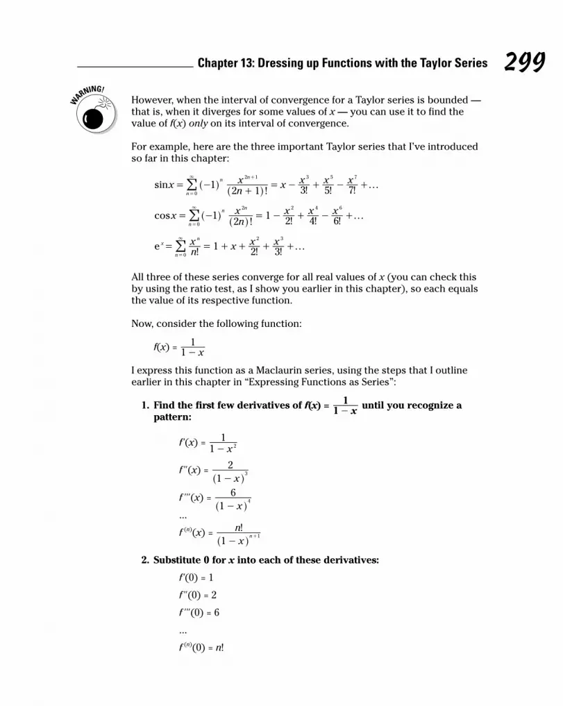
However, when the interval of convergence for a Taylor series is bounded —that is, when it diverges for some values of x — you can use it to find thevalue of f(x) only on its interval of convergence.
For example, here are the three important Taylor series that I’ve introducedso far in this chapter:
! ! ! ! . . .sinxnx x x x x1
2 1 3 5 7n n
n
2 1
0
3 5 7
= -+
= - + - +3 +
=
! ^^
hh
! ! ! ! . . .cosxn
x x x x12
1 2 4 6n
n
n
0
2 2 4 6
= - = - + - +3
=
! ^^
hh
! ! ! . . .nx x x x1 2 3e x
n
n
2 3
0= = + + + +
3
=
!
All three of these series converge for all real values of x (you can check thisby using the ratio test, as I show you earlier in this chapter), so each equalsthe value of its respective function.
Now, consider the following function:
f(x) = x11-
I express this function as a Maclaurin series, using the steps that I outline earlier in this chapter in “Expressing Functions as Series”:
1. Find the first few derivatives of f(x) = x11-
until you recognize a pattern:
f'(x) = x1
12-
f"(x) = x1
23
-^ h
f '''(x) = x1
64
-^ h...
f (n)(x) = !x
n1
n 1-
+
^ h
2. Substitute 0 for x into each of these derivatives:
f'(0) = 1
f"(0) = 2
f '''(0) = 6
...
f (n)(0) = n!
299Chapter 13: Dressing up Functions with the Taylor Series
20_225226-ch13.qxd 5/2/08 5:48 PM Page 299

3. Plug these values, term by term, into the formula for the Maclaurinseries:
! !x f f xf
xf
x11 0 0 2
03
02 3 f-
= + + + +lll lll
^ ^^ ^
h hh h
= 1 + x + x2 + x3 + ...
4. If possible, express the series in sigma notation:
x x x x x11 1n
n
2 3
0-= = + + +
3
=
!
To test this formula, I use it to find f(x) when x = 21 .
f 21 1 2
141
81 2f= + + + + =c m
You can test the accuracy of this expression by substituting 21 into x1
1-
:
f 21
1 21
1 2=-
=c m
As you can see, the formula produces the correct answer. Now, I try to use it
to find f(x) when x = 5, noting that the correct answer should be 1 51
41
-= - :
f(5) = 1 + 5 + 25 + 125 + ... = ∞ WRONG!
What happened? This series converges only on the interval (–1, 1), so the for-mula produces only the value f(x) when x is in this interval. When x is outsidethis interval, the series diverges, so the formula is invalid.
Expressing functions versusapproximating functionsIt’s important to be crystal clear in your understanding about the differencebetween two key mathematical practices:
� Expressing a function as an infinite series
� Approximating a function by using a finite number of terms of series
Both the Taylor series and the Maclaurin series are variations of the powerseries. You can think of a power series as a polynomial with infinitely manyterms. Also, recall that the Maclaurin series is a specific form of the moregeneral Taylor series, arising when the value of a is set to 0.
300 Part IV: Infinite Series
20_225226-ch13.qxd 5/2/08 5:51 PM Page 300

Every Taylor series (and, therefore, every Maclaurin series) provides the exactvalue of a function for all values of x where that series converges. That is, forany value of x on its interval of convergence, a Taylor series converges to f(x).
In practice, however, adding up an infinite number of terms simply isn’t pos-sible. Nevertheless, you can approximate the value of f(x) by adding up afinite number from the appropriate Taylor series. You do this earlier in thechapter to estimate the value of sin 10 and other expressions.
An expression built from a finite number of terms of a Taylor series is called aTaylor polynomial, Tn(x). Like other polynomials, a Taylor polynomial is iden-tified by its degree. For example, here’s the fifth-degree Taylor polynomial,T5(x), that approximates ex:
ex ≈ ! ! ! !x x x x x1 2 3 4 5
2 3 4 5
+ + + + +
Generally speaking, a higher-degree polynomial results in a better approxima-tion. And because this polynomial comes from the Maclaurin series, wherea = 0, it provides a much better estimate for values of ex when x is near 0. Forthe value of ex when x is near 100, however, you get a better estimate by usinga Taylor polynomial for ex with a = 100:
! ! !
!
x x x x
x
100 2 100 3 100 4 100
5 100
e e e e e e
e
x 100 100100 2 100 3 100 4
100 5
. + - + - + - + - +
-
^ ^ ^ ^
^
h h h h
h
To sum up, remember the following:
� A convergent Taylor series expresses the exact value of a function.
� A Taylor polynomial, Tn(x), from a convergent series approximates thevalue of a function.
Calculating error bounds for Taylor polynomialsIn the previous section, I discuss how a Taylor polynomial approximates thevalue of a function:
f(x) ≈ Tn(x)
In many cases, it’s helpful to measure the accuracy of an approximation. Thisinformation is provided by the Taylor remainder term:
f(x) = Tn(x) + Rn(x)
301Chapter 13: Dressing up Functions with the Taylor Series
20_225226-ch13.qxd 5/2/08 5:54 PM Page 301

Notice that the addition of the remainder term Rn(x) turns the approximationinto an equation. Here’s the formula for the remainder term:
Rn(x) = !n
f c1
( )n 1
+
+
^
^
h
h(x – a)n+1 c between a and x
It’s important to be clear that this equation is true for one specific value of con the interval between a and x. It does not work for just any value of c onthat interval.
Ideally, the remainder term gives you the precise difference between thevalue of a function and the approximation Tn(x). However, because the valueof c is uncertain, in practice the remainder term really provides a worst-casescenario for your approximation.
An example should help to make this idea clear. I use the sixth-degree Taylorpolynomial for cos x:
cos x ≈ T6(x) = ! ! !x x x1 2 4 6
2 4 6
- + -
Suppose that I use this polynomial to approximate cos 1:
cos 1 ≈ T6(1) = 1 21
241
7201
- + -
= .0 540277
How accurate is this approximation likely to be? To find out, utilize theremainder term:
cos 1 = T6(x) + R6(x)
Adding the associated remainder term changes this approximation into anequation. Here’s the formula for the remainder term:
R6(x) = !cos c x7 0
( )7 7-^ h
= ,sinc x5 040
7 c between 0 and x
So, substituting 1 for x gives you:
R6(1) = ,sinc5 040 c between 0 and 1
At this point, you’re apparently stuck, because you don’t know the value ofsin c. However, the sin function always produces a number between –1 and 1,so you can narrow down the remainder term as follows:
,5 0401
- ≤ R6(1) ≤ ,5 0401
302 Part IV: Infinite Series
20_225226-ch13.qxd 5/2/08 5:56 PM Page 302

Note that ,5 0401 ≈ 0.0001984, so the approximation of cos 1 given by the T6(1)
is accurate to within 0.0001984 in either direction. And, in fact, cos 1 ≈0.540302, so:
cos 1 – T6(1) ≈ 0.540302 – 0.540278 = 0.000024
As you can see, the approximation is within the error bounds predicted bythe remainder term.
Understanding Why theTaylor Series Works
The best way to see why the Taylor series works is to see how it’s con-structed in the first place. If you read through this chapter until this point,you should be ready to go.
To make sure that you understand every step along the way, however, I con-struct the Maclaurin series, which is just a tad more straightforward. Thisconstruction begins with the key assumption that a function can be expressedas a power series in the first place:
f(x) = c0 + c1x + c2x2 + c3x
3 + ...
The goal now is to express the coefficients on the right side of this equationin terms of the function itself. To do this, I make another relatively safeassumption that 0 is in the domain of f(x). So when x = 0, all but the first termof the series equal 0, leaving the following equation:
f(0) = c0
This process gives you the value of the coefficient c0 in terms of the function.Now, differentiate f(x):
f'(x) = c1 + 2c2x + 3c3x2 + 4c4x
3...
At this point, when x = 0, all the x terms drop out:
f'(0) = c1
So you have another coefficient, c1, expressed in terms of the function. Tocontinue, differentiate f'(x):
f"(x) = 2c2 + 6c3x + 12c4x2 + 20c5x
3 + ...
303Chapter 13: Dressing up Functions with the Taylor Series
20_225226-ch13.qxd 5/2/08 5:56 PM Page 303

Again, when x = 0, the x terms disappear:
f"(0) = 2c2
f2
0ll ^ h= c2
By now, you’re probably noticing a pattern: You can always get the value ofthe next coefficient by differentiating the previous equation and substituting0 for x into the result:
f '''(x) = 6c3 + 24c4x + 60c5x2 + 120c6x
3 + ...
f '''(0) = 6c3
f6
0lll ^ h= c3
Furthermore, the coefficients also have a pattern:
c0 = f(0)
c1 = f'(0)
c2 = !f
20ll ^ h
c3 = !f
30lll ^ h
...
cn = !nf 0( )n
^ h
Substituting these coefficients into the original equation results in the familiarMaclaurin series from earlier in this chapter:
f(x) = f(0) + f'(0)x + !f
20l ^ h
x2 + !f
30lll ^ h
x3 + ...
To construct the Taylor series, use a similar line of reasoning, starting withthe more general form of the power series:
f(x) = c0 + c1(x – a) + c2(x – a)2 + c3(x – a)3 + ...
In this case, setting x = a gives you the first coefficient:
f(a) = c0
Continue to find coefficients by differentiating f(x) and then repeating theprocess.
304 Part IV: Infinite Series
20_225226-ch13.qxd 5/2/08 5:57 PM Page 304

Part VAdvanced Topics
21_225226-pp05.qxd 5/2/08 5:58 PM Page 305

In this part . . .You get a glimpse of what lies beyond Calculus II.
I give you an overview of the next two semesters ofmath: Calculus III (the study of calculus in three or moredimensions) and Differential Equations (equations withderivatives mixed in as variables).
21_225226-pp05.qxd 5/2/08 5:58 PM Page 306

Chapter 14
Multivariable CalculusIn This Chapter� Visualizing vectors
� Making the leap from two to three dimensions
� Understanding cylindrical and spherical coordinates
� Using partial derivatives
� Sorting out and solving multiple integrals
Space, as Captain Kirk says during the opening credits of the televisionseries Star Trek, is the final frontier. Multivariable calculus (also known
as Calculus III) focuses on techniques for doing calculus in space — that is,in three dimensions.
Mathematicians have a variety of terms for three dimensions: 3-D, 3-space,and R3 are the most common. Whatever you call it, adding a dimension makesmultivariable calculus more interesting and useful, but also a bit more trickythan single variable calculus.
In this chapter, I give you a quick introduction to multivariable calculus,touching on the highlights usually taught in a Calculus III class. First, I showyou how vectors provide a method for linking a value with a direction. Next,I introduce you to three different 3-D coordinate systems: 3-D Cartesian coor-dinates, cylindrical coordinates, and spherical coordinates.
Building on this understanding of 3-D, I discuss functions of more than onevariable, focusing on the function of two variables z = f(x, y). With an under-standing of multivariable functions, I proceed to introduce you to the twomost important concepts in multivariable calculus: partial derivatives andmultiple integrals.
By the end of this chapter, you’ll have a great platform from which to beginCalculus III.
22_225226-ch14.qxd 5/2/08 6:01 PM Page 307

Visualizing VectorsVectors are used to link a real number (called a scalar) with a direction on theplane or in space. They’re useful for navigation, where knowing what direc-tion you’re sailing or flying in is important. Vectors also get a lot of play inphysics, where forces that push and pull are also directional. And, as youmay have guessed, Calculus III is chock full of vectors.
In this section, I introduce you to this important concept. Although I keepthis discussion in two dimensions, vectors are commonly used in threedimensions as well.
Understanding vector basicsA simple way to think of a vector is as an arrow that has both length anddirection. By convention, a vector starts at the origin of the Cartesian plane(0, 0) and extends a certain length in some direction. Figure 14-1 shows a variety of vectors.
As you can see, when a vector begins at the origin, its two components (its xand y values) correspond to the Cartesian coordinates of its endpoint. Forexample, the vector that begins at (0, 0) and ends at (3, 1) is distinguished asthe vector <3, 1>.
d = (–4, –1)
e = (2, –3)
c = (–3, 3)
b = (1, 2)
a = (3, 1)
Figure 14-1:Vectors
starting atthe origin
are distin-guishedby their
endpoints.
308 Part V: Advanced Topics
22_225226-ch14.qxd 5/2/08 6:01 PM Page 308

Don’t confuse a vector <x, y> with its corresponding Cartesian pair (x, y),which is just a point.
By convention, vectors are labeled in books with boldfaced lowercase letters:a, b, c, and so forth (see Figure 14-1). But when you’re working with vectorson paper, most teachers are happy to see you replace the boldface with alittle line or arrow over the letter.
Displacing a vector from the origin doesn’t change its value. For example,Figure 14-2 shows the vector <2, 3> with a variety of starting points.
Calculate the coordinates of a vector starting at (x1, y1) and ending at (x2, y2)as <x2 – x1, y2 – y1>. For example, here’s how to calculate the coordinates ofvectors g, h, and i in Figure 14-2:
g = <0 – –2, 4 – 1> = <2, 3>
h = <–2 – –4, –1 – –4> = <2, 3>
i = <2 – 0, 1 – –2> = <2, 3>
As you can see, regardless of the starting and ending points, these vectorsare all equivalent to each other and to f.
h = (2, 3)
i = (2, 3)
f = (2, 3)
g = (2, 3)
Figure 14-2:All vectors
with thesame length
anddirection
areequivalent,regardless
of wherethey start.
309Chapter 14: Multivariable Calculus
22_225226-ch14.qxd 5/2/08 6:01 PM Page 309

Distinguishing vectors and scalarsJust as Eskimos have tons of words for snow and Italians have even morewords for pasta, mathematicians have bunches of words for real numbers.When you began algebra, you found out quickly that a constant or a coefficientwas just a real number in a specific context.
Similarly, when you’re discussing vectors and want to refer to a real number,use the word scalar. Only the name is different — deep in its heart, a scalarknows only too well that it’s just a good old-fashioned real number.
Some types of vector calculations produce new vectors, while others result inscalars. As I introduce these calculations throughout the next section, I tellyou whether to expect a vector or a scalar as a result.
Calculating with vectorsVectors are commonly used to model forces such as wind, sea current, grav-ity, and electromagnetism. Vector calculations are essential for all sorts ofproblems where forces collide. In this section, I give you a taste of how somesimple calculations with vectors are accomplished.
Calculating magnitudeThe length of a vector is called its magnitude. The notation for absolute value(| |) is also used for the magnitude of a vector. For example, |v| refers tomagnitude of the vector v. (By the way, some textbooks represent magnitudewith double bars [|| ||] instead of single bars. Either way, the meaning isthe same.)
310 Part V: Advanced Topics
What’s in a name?A scalar is just a fancy word for a real number.The name arises because a scalar scales avector — that is, it changes the scale of avector. For example, the real number 2 scales
the vector v by a factor of 2, so that 2v is twiceas long as v. You find out more about scalar mul-tiplication in “Calculating with vectors.”
22_225226-ch14.qxd 5/2/08 6:01 PM Page 310

Calculate the magnitude of a vector v = <x, y> by using a variation of the dis-tance formula. This formula is itself a variation of the trusty Pythagorean theorem:
x yv 2 2= +
For example, calculate the magnitude of the vector n = <4, –3> as follows:
n 4 3 52 2= + - =^ h
As you can see, the use of the absolute value bars for the magnitude of vec-tors is appropriate: Magnitude, like all other distances, is always measuredas a nonnegative value. The magnitude of a vector is the distance from theorigin of a graph to its tip, just as the absolute value of a number is the dis-tance from 0 on a number line to that number.
The magnitude of a vector is a scalar.
Scalar multiplicationMultiplying a vector by a scalar is called scalar multiplication. To performscalar multiplication, multiply the scalar by each component of the vector.Here’s how you multiply the vector v = <x, y> by the scalar k:
kv = k<x, y> = <kx, ky>
For example, here’s how you multiply the vector p = <3, 5> by the scalars 2, –4, and 3
1 :
2p = 2<3, 5> = <6, 10>
–4p = –4<3, 5> = <–12, –20>
p31 = 3
1 <3, 5> = <1, 35 >
When you multiply a vector by a scalar, the result is a vector.
Geometrically speaking, scalar multiplication achieves the following:
� Scalar multiplication by a positive number other than 1 changes themagnitude of the vector but not its direction.
� Scalar multiplication by –1 reverses its direction but doesn’t change itsmagnitude.
� Scalar multiplication by any other negative number both reverses thedirection of the vector and changes its magnitude.
311Chapter 14: Multivariable Calculus
22_225226-ch14.qxd 5/2/08 6:02 PM Page 311

Scalar multiplication can change the magnitude of a vector by either increas-ing it or decreasing it.
� Scalar multiplication by a number greater than 1 or less than –1increases the magnitude of the vector.
� Scalar multiplication by a fraction between –1 and 1 decreases the magni-tude of the vector.
For example, the vector 2p is twice as long as p, the vector 21 p is half as long
as p, and the vector –p is the same length as p but extends in the oppositedirection from the origin (as shown in Figure 14-3).
Finding the unit vectorEvery vector has a corresponding unit vector, which has the same directionas that vector but a magnitude of 1. To find the unit vector u of the vector v =<x, y>, divide that vector by its magnitude as follows:
u = vv
Note that this formula uses scalar multiplication, as I show you in the preced-ing section, because the numerator is a vector and the denominator is ascalar.
p12
p2
p–
p
Figure 14-3:Scalar
multipli-cation ofa vector
changes itsmagnitude
and/or itsdirection.
312 Part V: Advanced Topics
22_225226-ch14.qxd 5/2/08 6:02 PM Page 312

As you may guess from its name, the unit vector is a vector.
For example, to find the unit vector u of the vector q = <–2, 1>, first calculateits magnitude |q| as I show you earlier in this section:
q 2 1 52 2= - + =^ h
Now, use the previous formula to calculate the unit vector:
< , > < , >u5
2 15
25
1=
-= -
You can check that the magnitude of resulting vector u really is 1 as follows:
|u|5
25
12 2
= - +J
L
KK
J
L
KK
N
P
OO
N
P
OO
54
51 1= + =
Adding and subtracting vectorsAdd and subtract vectors component by component, as follows:
<x1, y1> + <x2, y2> = <x1 + x2, y1 + y2>
<x1, y1> – <x2, y2> = <x1 – x2, y1 – y2>
For example, if r = <–1, 3> and s = <4, 2>, here’s how to add and subtract thesevectors:
r + s = <–1, 3> + <4, 2> = <–1 + 4, 3 + 2> = <3, 5>
r – s = <–1, 3> – <4, 2> = <–1 – 4, 3 – 2> = <–5, 1>
When you add or subtract two vectors, the result is a vector.
Geometrically speaking, the net effects of vector addition and subtraction areshown in Figure 14-4. In this example, the endpoint of r + s is equivalent tothe endpoint of s when s begins at the endpoint of r. Similarly, the endpoint ofr – s is equivalent to the endpoint of –s — that is, <–4, –2> — when –s beginsat the endpoint of r.
313Chapter 14: Multivariable Calculus
22_225226-ch14.qxd 5/2/08 6:03 PM Page 313

Leaping to Another DimensionMultivariable calculus is all about three (or more) dimensions. In this section,I show you three important systems for plotting points in 3-D.
Understanding 3-D Cartesian coordinatesThe three-dimensional (3-D) Cartesian coordinate system (also called 3-D rec-tangular coordinates) is the natural extension of the 2-D Cartesian graph. Thekey difference is the addition of a third axis, the z-axis, extending perpendicu-larly through the origin.
Drawing a 3-D graph in two dimensions is kind of tricky. To get a better senseabout how to think in 3-D, hold up Figure 14-5 where you can compare it withthe interior corner of a room (not a round room!). Note the following:
� The x-axis corresponds to where the left-hand wall meets the floor.
� The y-axis corresponds to where the right-hand wall meets the floor.
� The z-axis corresponds to where the two walls meet.
Just as the 2-D Cartesian graph is divided into four quadrants, the 3-D graphis divided into eight octants. From your perspective as you look at the graph,you’re standing inside the first octant, where all values of x, y, and z are positive.
– s
s
– s
r – sr
r r + s
sFigure 14-4:
Add andsubtract
vectors onthe graph by
beginningone vector
at theendpoint of
anothervector.
314 Part V: Advanced Topics
22_225226-ch14.qxd 5/2/08 6:03 PM Page 314

Figure 14-6 shows the complete 3-D Cartesian system with the point (1, 2, 5)plotted. In similarity with regular Cartesian coordinates, you plot this pointby counting 1 unit in the positive x direction, and then 2 units in the positivey direction, and finally 5 units in the positive z direction.
z
y
x
Figure 14-6:Plotting the
point (1, 2, 5)on the 3-DCartesian
coordinatesystem.
z
yx
Figure 14-5:The first
octant ofthe 3-D
Cartesiancoordinate
system.
315Chapter 14: Multivariable Calculus
22_225226-ch14.qxd 5/2/08 6:03 PM Page 315

Using alternative 3-D coordinate systemsIn Chapter 2, I discuss polar coordinates, an alternative to the Cartesiangraph. Polar coordinates are useful because they allow you to express andsolve a variety of problems more easily than Cartesian coordinates.
In this section, I show you two alternatives to the 3-D Cartesian coordinatesystem: cylindrical coordinates and spherical coordinates. As with polarcoordinates, both of these systems give you greater flexibility to solve awider range of problems.
Cylindrical coordinatesYou probably remember polar coordinates from Pre-Calculus or maybe evenCalculus I. Like the Cartesian coordinate system, the polar coordinate systemassigns a pairing of values to every point on the plane. Unlike the Cartesiancoordinate system, however, these values aren’t dependent upon two perpen-dicular axes (though these axes are often drawn in to make the graph morereadable). The key axis is the horizontal axis, which corresponds to the posi-tive x-axis in Cartesian coordinates.
While a Cartesian pair is of the form (x, y), polar coordinates use (r, θ).Cylindrical coordinates are simply polar coordinates with the addition of avertical z-axis extending from the origin, as in 3-D Cartesian coordinates (see“Understanding 3-D Cartesian coordinates” earlier in this chapter). Everypoint in space is assigned a set of cylindrical coordinates of the form (r, θ, z).
Here’s what you need to know:
� The variable r measures the distance from the z-axis to that point.
� The variable θ measures angular distance from the horizontal axis. Thisangle is measured in radians rather than degrees, so that 2π = 360°. (SeeChapter 2 for more about radians.)
� The variable z measures the distance from that point to the xy-plane.
When plotting cylindrical coordinates, plot the first coordinates (r and θ) justas you would for polar coordinates (see Chapter 2). Then plot the z-coordinateas you would for 3-D Cartesian coordinates.
Figure 14-7 shows you how to plot the point (3, π2 , 2) in cylindrical coordinates:
1. Count 3 units to the right of the origin on the horizontal axis (as youwould when plotting polar coordinates).
316 Part V: Advanced Topics
22_225226-ch14.qxd 5/2/08 6:03 PM Page 316

2. Travel counterclockwise along the arc of a circle until you reach the line drawn at a π
2 -angle from the horizontal axis (again, as with polarcoordinates).
3. Count 2 units above the plane and plot your point there.
Spherical coordinatesSpherical coordinates are used — with slight variation — to measure latitude,longitude, and altitude on the most important sphere of them all, the planetEarth.
Every point in space is assigned a set of spherical coordinates of the form(ρ, θ, φ). In case you’re not in a sorority or fraternity, ρ is the lowercase Greekletter rho, θ is the lowercase Greek letter theta (commonly used in math torepresent an angle), φ is the lower-case Greek letter phi, which is commonlypronounced either “fee” or “fye” (but never “foe” or “fum”).
z
i
r
Figure 14-7:Plotting
the point (3, π
2 , 2) incylindrical
coordinates.
317Chapter 14: Multivariable Calculus
22_225226-ch14.qxd 5/2/08 6:04 PM Page 317

The coordinate ρ corresponds to altitude. On the Earth, altitude is measuredas the distance above or below sea level. In spherical coordinates, however,altitude indicates how far in space a point is from the origin.
The coordinate θ corresponds to longitude: A measurement of angular dis-tance from the horizontal axis.
The coordinate φ corresponds to latitude. On the Earth, latitude is measuredas angular distance from the equator. In spherical coordinates, however, lati-tude is measured as the angular distance from the north pole.
Plotting φ can be tricky at first. To get a feel for it, picture a globe and imaginetraveling up and down along a single longitude line. Notice that as you travel,your latitude keeps changing, so
� At the north pole, φ = 0
� At the equator, φ = π2
� At the south pole, φ = π
Some textbooks substitute the Greek letter ρ (rho) for r. Either way, the coor-dinate means the same thing: altitude, which is the distance of a point fromthe origin. In other textbooks, the order of the last two coordinates ischanged around. Make sure that you know which convention your book uses.
Figure 14-8 shows you how to plot a point in spherical coordinates. For exam-ple, suppose that you want to plot the point (4, π
2 , π4
3 ). Follow these steps todo that:
1. Count 4 units to the right of the origin on the horizontal axis.
2. Travel counterclockwise along the arc of a circle until you reach the line drawn at a π
2 -angle from the horizontal axis (again, as with polarcoordinates).
3. Imagine a single longitude line arcing from the north pole of a spherethrough the point on the equator where you are right now andonward to the south pole.
4. Travel down to the line of latitude at an angular distance of π43 from
the north pole — that is, halfway between the equator and the southpole — and plot your point there.
318 Part V: Advanced Topics
22_225226-ch14.qxd 5/2/08 6:04 PM Page 318

Functions of Several VariablesYou know from algebra that a function y = f(x) is basically a mathematicalmachine for turning one number into another. The variable x is the input vari-able and y is the output variable so that every value of x gives you no morethan one y value.
When you graph a curve, you can use the vertical-line test to make sure thatit’s a function: Any vertical line that intersects a function intersects it atexactly one point, as illustrated in Figure 14-9.
These concepts related to functions also carry over into functions of morethan one variable. For example, here are some functions of two variables:
z = 2x + y + 5
sinz x y y= + +
z = exy – ln (1 + x2y2)
The general form for a function of two variables is z = f(x, y). Every functionof two variables takes a Cartesian pair (x, y) as its input and in turn outputs az value. Looking at the three previous examples, plugging in the input (0, 1)gives you an output of 6 for the first function, 2 for the second function, and 1for the third.
t
Figure 14-8:Plotting
the point (4, π
2 , π4
3 )in spherical
coordinates.
319Chapter 14: Multivariable Calculus
22_225226-ch14.qxd 5/2/08 6:04 PM Page 319

A good way to visualize a function of two variables is as a surface floatingover the xy-plane in a 3-D Cartesian graph. (True, this surface can cross theplane and continue below it — just as a function can cross the x-axis — butfor now, just picture it floating.) Every point on this surface looms directlyabove exactly one point on the plane. That is, if you pass a vertical linethrough any point on the plane, it crosses the function at no more thanone point. Figure 14-10 illustrates this concept.
y
z
x
Figure 14-10:The vertical-
line test fora function
in threedimensions.
y
x
ƒ(x)
Figure 14-9:The vertical-
line testshows thata function
outputs nomore than
one y valuefor every
inputted xvalue.
320 Part V: Advanced Topics
22_225226-ch14.qxd 5/2/08 6:04 PM Page 320

The concept of a function can be extended to higher dimensions. For exam-ple, w = f(x, y, z) is the basic form for a function of three variables. Becausethis function (as well as other functions of more than two variables) exists inmore than three dimensions, it’s a lot harder to picture. For now, just concen-trate on making the leap from two to three dimensions — that is, from func-tions of one variable to functions of two variables. Most of the multivariablecalculus that you study in Calculus III is in three dimensions. (Maybe it shouldbe called Calculus 3-D.)
Partial DerivativesPartial derivatives are the higher-dimensional equivalent of the derivativesthat you know from Calculus I. Just as a derivative represents the slope of afunction on the Cartesian plane, a partial derivative represents a similar con-cept of slope in higher dimensions. In this section, I clarify this notion ofslope in three dimensions. I also show you how to calculate the partial deriv-atives of functions of two variables.
Measuring slope in three dimensionsIn the earlier section “Functions of Several Variables,” I recommend that youvisualize a function of two variables z = f(x, y) as a surface floating over thexy-plane of a 3-D Cartesian graph. (See Figure 14-9 for a picture of a samplefunction.)
For example, take the function z = y, as shown in Figure 14-11. As you can see,this function looks a lot like the sloped roof of a house. Imagine yourselfstanding on this surface. When you walk parallel with the y-axis, your altitudeeither rises or falls. In other words, as the value of y changes, so does thevalue of z. But when you walk parallel with the x-axis, your altitude remainsthe same; changing the value of x has no effect on z.
So intuitively, you expect that the partial derivative mm
yz — the slope in the
direction of the y-axis — is 1. You also expect that the partial derivative mmxz —
the slope in the direction of the x-axis — is 0. In the next section, I show youhow to calculate partial derivatives to verify this result.
321Chapter 14: Multivariable Calculus
22_225226-ch14.qxd 5/2/08 6:05 PM Page 321

Evaluating partial derivativesEvaluating partial derivatives isn’t much more difficult than evaluating regu-lar derivatives. Given a function z(x, y), the two partial derivatives are m
mxz
and mm
yz . Here’s how you calculate them:
� To calculate mmxz , treat y as a constant and use x as your differentiation
variable.
� To calculate mm
yz , treat x as a constant and use y as your differentiation
variable.
For example, suppose that you’re given the equation z = 5x2y3. To find mmxz ,
treat y as if it were a constant — that is, treat the entire factor 5y3 as if it’s onebig coefficient — and differentiate x2:
mmxz = 5y3(2x) = 10xy3
To find mm
yz , treat x as if it were a constant — that is, treat 5x2 as if it’s the
coefficient — and differentiate y3:
mm
yz = 5x2(3y2) = 15x2y2
As another example, suppose that you’re given the equation z = 2ex sin y + ln x. To find m
mxz , treat y as if it were a constant and differentiate by the variable x:
mmxz = 2 sin y (ex) + x
1 = 2ex sin y + x1
y
Surface crosses thex-axis at a 45° angle
xFigure 14-11:The function
z = y.
322 Part V: Advanced Topics
22_225226-ch14.qxd 5/2/08 6:06 PM Page 322

To find mm
yz , treat x as if it were a constant and differentiate by the variable y:
mm
yz = 2 ex cos y
As you can see, when differentiating by y, the ln x term is treated as a con-stant and drops away completely.
Returning to the example from the previous section — the “sloped-roof” function z = y — here are both partial derivatives of this function:
mmxz = 0
mm
yz = 1
As you can see, this calculation produces the predicted results.
Multiple IntegralsYou already know that an integral allows you to measure area in two dimen-sions (see Chapter 1 if this concept is unclear). And as you probably knowfrom solid geometry, the analog of area in three dimensions is volume.
Multiple integrals are the higher-dimensional equivalent of the good old-fashioned integrals that you discover in Calculus II. They allow you to measure volume in three dimensions (or more).
Most of the multiple integrals that you’ll ever have to solve come in two vari-eties: double integrals and triple integrals. In this section, I show you how tounderstand and calculate both of these types of multiple integrals.
Measuring volume under a surfaceDefinite integrals provide a reliable way to measure the signed area betweena function and the x-axis as bounded by any two values of x. (I cover this indetail in Chapters 1 and 3.) Similarly, a double integral allows you to measurethe signed volume between a function z = f(x, y) and the xy-plane as boundedby any two values of x and any two values of y.
,f x y dxdy0
1
0
2
## _ i
323Chapter 14: Multivariable Calculus
22_225226-ch14.qxd 5/2/08 6:07 PM Page 323

To get a picture of this volume, look at Figure 14-12. The double integral mea-sures the volume between f(x, y) and the xy-plane as bounded by a rectangle. Inthis case, the rectangle is described by the four lines x = 0, x = 1, y = 0, and y = 2.
A double integral is really an integral inside another integral. To help you seethis, I bracket off the inner integral in the previous example:
,f x y dx dy0
1
0
2
##J
L
KK _
N
P
OOi
When you focus on the integral inside the brackets, you can see that thelimits of integration 0 and 1 correspond with the dx — that is, x = 0 and x = 1.Similarly, the limits of integration 0 and 2 correspond with the dy — that is,y = 0 and y = 2.
Evaluating multiple integralsMultiple integrals (double integrals, triple integrals, and so forth) are usuallydefinite integrals, so evaluating them results in a real number. Evaluating multiple integrals is similar to evaluating nested functions: Work from theinside out.
Solving double integralsSolve double integrals in two steps: First evaluate the inner integral, and thenplug this solution into the outer integral and solve that. For example, supposethat you want to integrate the following double integral:
xy
dy dxx
x 2
4
5
1
3
##
y
x
1
Volume
Surface
Rectangle
2
Figure 14-12:A double
integralallows you
to measurethe areaunder a
surface asbounded bya rectangle.
324 Part V: Advanced Topics
22_225226-ch14.qxd 5/2/08 6:08 PM Page 324

To start out, place the inner integral in parentheses so that you can bettersee what you’re working with:
xy
dy dxx
x 2
4
5
1
3
##J
L
KK
N
P
OO
Now, focus on what’s inside the parentheses. For the moment, you can ignorethe rest. Your integration variable is y, so treat the variable x as if it were aconstant, moving it outside the integral:
x y dy1
x
x2
4
5
#
Notice that the limits of integration in this integral are functions of x. So theresult of this definite integral will also be a function of x:
y x5=
xy3
3
= y x4=
xx
xx
xx
xx x3
534
3125
364
3613 3 3 3
2= - = - =
Now, plug this expression into the outer integral. In other words, substitute itfor what’s inside the parentheses:
x dx361 2
1
3
#
Evaluate this integral as usual:
x961
x
x3
1
3
==
=
961 3 9
61 13 3
= -^ ^h h
61 961
9488
= - =
Making sense of triple integralsTriple integrals look scary, but if you take them step by step, they’re no moredifficult than regular integrals. As with double integrals, start in the centerand work your way out. For example:
x y z dx dy dz
yz
yz
z
z3 5
24
1
2
###
Begin by separating the two inner integrals:
x y z dx dy dz
yz
yz
z
z3 5
24
1
2
###
J
L
KKKK
N
P
OOOO
R
T
SSSSS
V
X
WWWWW
325Chapter 14: Multivariable Calculus
22_225226-ch14.qxd 5/2/08 6:11 PM Page 325

Your plan of attack is to evaluate the integral in the brackets first, and thenthe integral in the braces, and finally the outer integral. First things first:
x y z dx
yz
yz
3 5
2
#
x y z41
/
/
x z y
x z y4 5
2
==
=
yz y z y
z y z41 2
41
45
45= -c cm m
Notice that plugging in values for x results in an expression in terms of y and z.Now simplify this expression to make it easier to work with:
= 4yz5 – 41 yz5 = 4
15 yz5
Plug this solution back in to replace the bracketed integral:
yz dy dz415
z
z5
4
1
2
##R
T
SSS
V
X
WWW
One integral down, two to go. This time, focus on the integral inside thebraces. This time, the integration variable is y:
yz dy415
z
z5
4
#
y z815
y z
y z2 5
4
==
=
= 815 (4z)2z5 – 8
15 z2z5
Again, simplify before proceeding:
= 30z7 – 815 z7 = 8
225 z7
Plug this result back into the integral as follows:
z dz8225 7
1
2
#
Now evaluate this integral:
z64225
z
z8
1
2
==
=
= 64225 28 – 64
225 18
= ,64
57 600 – 64225 = ,
6457 375
326 Part V: Advanced Topics
22_225226-ch14.qxd 5/2/08 6:15 PM Page 326

Chapter 15
What’s so Different aboutDifferential Equations?
In This Chapter� Classifying different types of differential equations (DEs)
� Understanding the connection between DEs and integrals
� Checking a proposed solution to a DE
� Seeing how DEs arise in the physical world
� Using a variety of methods to solve DEs
The very mention of differential equations (DEs for short) strikes a spicycombination of awe, horror, and utter confusion into nonmathematical
minds. Even intrepid calculus students have been known to consider a careerin art history when these untamed beasts come into focus on the radarscreen. Just what are differential equations? Where do they come from?Why are they necessary? And how in the world do you solve them?
In this chapter, I answer these questions and give you some familiarity withDEs. I show you how to identify the basic types of DEs so that if you’re everat a math department cocktail party (lucky you!), you won’t feel completelyadrift. I relate DEs to the integrals that you now understand so well. I showyou how to build your own DEs so that you’ll always have a hobby to passthe time, and I also show you how to check DE solutions. In addition, you dis-cover how DEs arise in physics. Finally, I show you a few simple methods forsolving some basic differential equations.
23_225226-ch15.qxd 5/2/08 6:17 PM Page 327

Basics of Differential EquationsIn a nutshell, a differential equation is any equation that includes at least onederivative. For example:
dxdy
= sin x ey
dxd y
2
2
+ 10 dxdy
+ 9y = 0
dxd y
4
4
+ dxd y
3
3
+ dxd y
2
2
+ dxdy
+ y = cos x
Solving a differential equation means finding the value of the dependent variablein terms of the independent variable. Throughout this chapter, I use y as thedependent variable, so the goal in each problem is to solve for y in terms of x.
In this section, I show you how to classify DEs. I also show you how to buildDEs and check the solution to a DE.
Classifying DEsAs with other equations that you’ve encountered, differential equations comein many varieties. And different varieties of DEs can be solved by using differ-ent methods. In this section, I show you some important ways to classify DEs.
Ordinary and partial differential equationsAn ordinary differential equation (ODE) has only derivatives of one variable —that is, it has no partial derivatives (flip to Chapter 14 for more on partial differentiation). Here are a few examples of ODEs:
dxdy
= x sin (x2) cos y
dxdy
= y csc x + ex
dxd y
2
2
+ 4xy dxdy
+ 5y = 0
In contrast, a partial differential equation (PDE) has at least one partial deriva-tive. Here are a few examples of PDEs:
mmxu + m
myu + u = ex – y
3mmxu
2 + 7 m mmx yu + 6
mmyu
2 = 0
mmtv – k
mmxv
2
328 Part V: Advanced Topics
23_225226-ch15.qxd 5/2/08 6:19 PM Page 328

Ordinary differential equations are usually the topic of a typical DifferentialEquations class in college. They’re a step or two beyond what you’re used toworking with, but many students actually find Differential Equations an easiercourse than Calculus II (generally considered the most difficult class in thecalculus series). However, ODEs are limited in how well they can actuallyexpress physical reality.
The real quarry is partial differential equations. A lot of physics gets donewith these little gems. Unfortunately, solving PDEs is one giant leap forwardin math from what the average calculus student is used to. Delving into thekind of math that makes PDEs come alive is typically reserved for graduateschool.
Order of DEsDifferential equations are further classified according to their order. This clas-sification is similar to the classification of polynomial equations by degree(see Chapter 2 for more on polynomials).
First-order ODEs contain only first derivatives. For example:
dxdy
= yex
3 dxdy
= sin y + 2e2x
ln xy dxdy
= 2x2 + y – tan x
Higher-order ODEs are classified, as polynomials are, by the greatest order oftheir derivatives. Here are examples of second-, third-, and fourth-order ODEs:
Second-order ODE: dxd y
dxdy
y4 10 e x2
2
+ - =
Third-order ODE: dxd y
dxd y
y 03
3
2
2
+ + =
Fourth-order ODE: cosxdxd y
y x24
4
+ =
As with polynomials, generally speaking, a higher-order DE is more difficult tosolve than one of lower order.
Linear DEsWhat constitutes a linear differential equation depends slightly on who youask. For practical purposes, a linear first-order DE fits into the following form:
dxdy
+ a(x)y = b(x)
329Chapter 15: What’s so Different about Differential Equations?
23_225226-ch15.qxd 5/2/08 6:20 PM Page 329

where a(x) and b(x) are functions of x. Here are a few examples of linear first-order DEs:
dxdy
+ y = x
dxdy
+ 4xy = –ln x
dxdy
– y sin x = ex
Linear DEs can often be solved, or at least simplified, using an integratingfactor. I show you how to do this later in this chapter.
A linear second-degree DE fits into the following form:
adxd y
b dxdy
cy 02
2
+ + =
where a, b, and c are all constants. Here are some examples:
dxd y
dxdy
y3 4 02
2
+ + =
dxd y
dxdy
y2 5 6 02
2
+ + =
dxd y
02
2
=
Note that the constant a can always be reduced to 1, resulting in adjustmentsto the other two coefficients. Linear second-degree DEs are usually an impor-tant topic in a college-level course in differential equations. Solving themrequires knowledge of matrices and complex numbers that is beyond thescope of this book.
Looking more closely at DEsYou don’t have to play professional baseball to enjoy baseball. Instead, youcan enjoy the game from the bleachers or, if you prefer, from a nice cushychair in front of the TV. Similarly, you don’t have to get too deep into differen-tial equations to gain a general understanding of how they work. In this sec-tion, I give you front-row seats to the game of differential equations.
How every integral is a DEThe integral is a particular example of a more general type of equation — thedifferential equation. To see how this is so, suppose that you’re working withthis nice little integral:
cosy x dx= #
330 Part V: Advanced Topics
23_225226-ch15.qxd 5/2/08 6:22 PM Page 330

Differentiating both sides turns it into a DE:
cosdxdy
x=
Of course, you know how to solve this DE by thinking of it as an integral:
y = sin x + C
So in general, when a DE is of the form
dxdy
= f(x)
with f(x) an arbitrary function of x, you can express that DE as an integral andsolve it by integrating.
Why building DEs is easier than solving themThe reason that the DE in the last section is so simple to solve is that thederivative is isolated on one side of the equation. DEs attain a new level ofdifficulty when the derivative isn’t isolated.
A good analogy can be made in lower math, when you make the jump fromarithmetic to algebra. For example, here’s an arithmetic problem:
x = 20 – (42 + 3)
Even though this is technically an algebra problem, you can solve it withoutalgebra because x is isolated at the start of the problem. However, the ball-game changes when x becomes more enmeshed in the equation. For example:
2x3 – x2 + 5x – 17 = 0
Arithmetic isn’t strong enough for this problem, so algebra takes over.Similarly, when derivatives get entangled into the fabric of an equation —as in most of the DEs I show you earlier in “Classifying DEs” — integrating isno longer effective and the search for new methods begins.
Although solving DEs is often tricky, building them is easy. For example, sup-pose that you start with this simple quadratic equation:
y = 3x2 + 4x – 5
Now, find the first and second derivatives:
dxdy
= 6x + 4
dxd y
2
2
= 6
331Chapter 15: What’s so Different about Differential Equations?
23_225226-ch15.qxd 5/2/08 6:22 PM Page 331

Adding up the left and right sides of all three equations gives you the follow-ing differential equation:
y + dxdy
+ dxd y
2
2
= 3x2 + 10x + 5
Because you built the equation yourself, you know what y equals. But if youhand this equation off to some other students, they probably wouldn’t beable to guess how you built it, so they would have to do some work to solve itfor y. For example, here’s another DE:
y + dxdy
+ dxd y
2
2
+ dxd y
3
2
= 0
This equation probably looks difficult because you don’t have much informa-tion. And yet, after I tell you the solution, it appears simple:
y = sin x dxdy
= cos x
dxd y
2
2
= –sin xdxd y
4
3
= –cos x
But even after you have the solution, how do you know whether it’s the onlysolution? For starters, y = –sin x, y = cos x, and y = –cos x are all solutions. Doother solutions exist? How do you find them? And how do you know whenyou have them all?
Another difficulty arises when y itself becomes tangled up in the equation.For example, how do you solve this equation for y?
sindxdy x
e y=
As you can see, differential equations contain treacherous subtleties that youdon’t find in basic calculus.
Checking DE solutionsEven if you don’t know how to find a solution to a differential equation, youcan always check whether a proposed solution works. This is simply a matterof plugging the proposed value of the dependent variable — I use y through-out this chapter — into both sides of the equation to see whether equality ismaintained.
For example, here’s a DE:
dxdy
= 3y + 4e3x cos x
You may not have a clue how to begin solving this DE, but imagine that anangel lands on your pen and offers you this solution:
y = 4e3x sin x
332 Part V: Advanced Topics
23_225226-ch15.qxd 5/2/08 6:24 PM Page 332

You can check to see whether this angel really knows math by plugging inthis value of y as follows:
dxdy
= 3y + 4e3x cos x
dxd 4e3x sin x = 3(4e3x sin x) + 4e3x cos x
4(3e3x sin x + e3x cos x) = 12 e3x sin x + 4e3x cos x
= 12 e3x sin x + 4e3x cos x = 12 e3x sin x + 4e3x cos x
Because the left and right sides of the equation are equal, the angel’s solutionchecks out.
Solving Differential EquationsIn this section, I show you how to solve a few types of DEs. First, you solveeverybody’s favorite DE, the separable equation. Next, you put this under-standing to work to solve an initial-value problem (IVP). Finally, I show youhow to solve a linear first-order DE by using an integrating factor.
Solving separable equationsDifferential equations become harder to solve the more entangled theybecome. In certain cases, however, an equation that looks all tangled up isactually easy to tease apart. Equations of this kind are called separable equa-tions (or autonomous equations), and they fit into the following form:
dxdy
= f(x) · g(y)
Separable equations are relatively easy to solve. For example, suppose thatyou want to solve the following problem:
sindxdy x
e y=
You can think of the symbol dxdy
as a fraction and isolate the x and y terms of
this equation on opposite sides of the equal sign:
ey dy = sin x dx
Now, integrate both sides:
sindy x dxe y = ##
ey + C1 = –cos x + C2
333Chapter 15: What’s so Different about Differential Equations?
23_225226-ch15.qxd 5/2/08 6:25 PM Page 333

In an important sense, the previous step is questionable because the variableof integration is different on each side of the equal sign. You may think “Noproblem, it’s all integration!” But imagine if you tried to divide one side of anequation by 2 and the other by 3, and then laughed it off with “It’s all divi-sion!” Clearly, you’d have a problem. The good news, however, is that fortechnical reasons beyond the scope of this book, integrating both sides bydifferent variables actually produces the correct answer.
C1 and C2 are both constants, so you can use the equation C = C2 – C1 to sim-plify the equation:
ey = –cos x + C
Next, use a natural log to undo the exponent, and then simplify:
ln e y = ln (–cos x + C)
y = ln (–cos x + C)
To check this solution, substitute this value for y into both sides of the origi-nal equation:
sindxdy x
e y=
ln cos sindxd x C x
eln cos x C- + =
- =^
]h
g
ln cos cossin
dxd x C x C
x- + =
- +^ h
cos sin cossin
x C x x Cx1 :
- +=
- +
cossin
cossin
x Cx
x Cx
- +=
- +
Solving initial-value problems (IVPs)In Chapter 3, I show you that the definite integral is a particular example of awhole family of indefinite integrals. In a similar way, an initial-value problem(IVP) is a particular example of a solution to a differential equation. Every IVPgives you extra information — called an initial value — that allows you to usethe general solution to a DE to obtain a particular solution.
334 Part V: Advanced Topics
23_225226-ch15.qxd 5/2/08 6:27 PM Page 334

For example, here’s an initial-value problem:
dxdy
= y sec2 x y(0) = 5
This problem includes not only a DE, but also an additional equation. Tounderstand what this equation tells you, remember that y is a dependent vari-able, a function of x. So, the notation y(0) = 5 means “when x = 0, y = 5.” Yousee how this information comes into play as I continue with this example.
To solve an IVP, you first have to solve the DE. Do this by finding its generalsolution without worrying about the initial value. Fortunately, this DE is aseparable equation, which you know how to solve from the last section:
y1 dy = sec2 x dx
Integrate both sides:
secy dy x dx1 2= ##
ln y = tan x + C
In this last step, I use C to consolidate the constants of integration fromboth sides of the equation into a single constant C. (If this doesn’t makesense, I explain why in “Solving separable equations” earlier in this chapter.)Next, I undo the natural log by using e:
eln y = etan x + C
y = etan x · eC
Because eC is a constant, this equation can be further simplified by using thesubstitution D = eC:
y = Detan x
Before moving on, check to make sure that this solution is correct by substi-tuting this value of y into both sides of the original equation:
dxdy
= y sec2 x
dxd Detan x = Detan x sec2 x
Detan x sec2 x = Detan x sec2 x
335Chapter 15: What’s so Different about Differential Equations?
23_225226-ch15.qxd 5/2/08 6:28 PM Page 335

This checks out, so y = Detan x is, indeed, the general solution to the DE. Tosolve the initial-value problem, however, I need to find the specific value ofthe variable D by using the additional information I have: When x = 0, y = 5.Plugging both of these values into the equation makes it possible to solvefor D:
5 = Detan 0
5 = De0
5 = D
Now, plug this value of D back into the general solution of the problem to getthe IVP solution:
y = 5etan x
This solution satisfies not only the differential equation dxdy
= y sec2 x but alsothe initial value y(0) = 5.
Using an integrating factorAs I mention earlier in this chapter, in “Classifying DEs,” a linear first-orderequation takes the following form:
dxdy
+ a(x)y = b(x)
A clever method for solving DEs in this form involves multiplying the entireequation by an integrating factor. Follow these steps:
1. Calculate the integrating factor.
2. Multiply the DE by this integrating factor.
3. Restate the left side of the equation as a single derivative.
4. Integrate both sides of the equation and solve for y.
Don’t worry if these steps don’t mean much to you. In the upcoming sections,I show you what an integrating factor is and how to use it to solve linear first-order DEs.
336 Part V: Advanced Topics
23_225226-ch15.qxd 5/2/08 6:28 PM Page 336

Getting very luckyTo help you understand how multiplying by an integrating factor works, I setup an equation that practically solves itself — that is, if you know what to do:
dxdy
xy2
+ = 0
Notice that this is a linear first-degree DE, with a(x) = x2 and b(x) = 0. I now
tweak this equation by multiplying every term by x2 (you see why shortly):
dxdy
x xy
x x2
02 2 2+ =$ $ $
Next, I use algebra to do a little simplifying and rearranging:
dxdy
· x2 + 2x · y = 0
Now, here’s where I appear to get extremely lucky: The two terms on the leftside of the equation just happen to be the result of the application of theProduct Rule to the expression y · x2 (for more on the Product Rule, seeChapter 2):
dxd (y · x2) = dx
dy· x2 + 2x · y
Notice that the right side of this equation is exactly the same as the left sideof the previous equation. So I can make the following substitution:
dxd (y · x2) = 0
Now, to undo the derivative on the left side, I integrate both sides, and then Isolve for y:
dxd y x dx dx02 =$ ## _ i; E
y · x2 = C
y = xC
2
To check this solution, I plug this value of y back into the original equation:
dxdy
xy2
+ = 0
dxd
xC
x xC2
2 2+ $ = 0
xC
xC2 2
3 3-
+ = 0
0 = 0
337Chapter 15: What’s so Different about Differential Equations?
23_225226-ch15.qxd 5/2/08 6:30 PM Page 337

Making your luckThe previous example works because I found a way to multiply the entireequation by a factor that made the left side of the equation look like a deriva-tive resulting from the Product Rule. Although this looked lucky, if you knowwhat to multiply by, every linear first-order DE can be transformed in this way.Recall that the form of a linear first-order DE is as follows:
dxdy
+ a(x)y = b(x)
The trick is to multiply the DE by an integrating factor based on a(x). Here’sthe integrating factor:
e ( )a x dx#
How the integrating factor is originally derived is beyond the scope of thisbook. All you need to know here is that it works.
For example, in the previous problem, you know that a(x) = x2 . So here’s how
to find the integrating factor:
e e e( ) lna x dx x dx x2 2= =# #
Remember that 2 ln x = ln x2, so:
e ln x 2
= x2
As you can see, the integrating factor x2 is the exact value that I multiplied byto solve the problem. To see how this process works now that you know thetrick, here’s another DE to solve:
dxdy
+ 3y = ex
In this case, a(x) = 3, so compute the integrating factor as follows:
e e e( )a x dx dx x3 3= =# #
Now, multiply every term in the equation by this factor:
dxdy
· e3x + 3y · e3x = ex· e3x
If you like, use algebra to simplify the right side and rearrange the left side:
dxdy
· e3x + 3e3x · y = e4x
338 Part V: Advanced Topics
23_225226-ch15.qxd 5/2/08 6:32 PM Page 338

Now, you can see how the left side of this equation looks like the result of theProduct Rule applied to evaluate the following derivative:
dxd (y · e3x) = dx
dy· e3x + 3e3x · y
Because the right side of this equation is the same as the left side of the pre-vious equation, I can make the following substitution:
dxd (y · e3x) = e4x
Notice that I change the left side of the equation by using the Product Rule inreverse. That is, I’m expressing the whole left side as a single derivative. Now,I can integrate both sides to undo this derivative:
dxd y dx dxe ex x3 4=$# #_ i; E
y · e3x = 4e x4
+ C
Now, solve for y and simplify:
y = C4ee
ex
x
x3
4
3+ = 4e x
+ Ce–3x
To check this answer, substitute this value of y back into the original DE:
dxdy
+ 3y = ex
dxd C C4 3 4
e e e ex
xx
x3 3+ + +- -c cm m = ex
C C4 3 43 3e e e e
xx
xx3 3- + +- - = ex
4 43e ex x
+ = ex
ex = ex
As if by magic, this answer checks out, so the solution is valid.
339Chapter 15: What’s so Different about Differential Equations?
23_225226-ch15.qxd 5/2/08 6:35 PM Page 339

340 Part V: Advanced Topics
23_225226-ch15.qxd 5/2/08 6:35 PM Page 340

Part VIThe Part of Tens
24_225226-pp06.qxd 5/2/08 6:36 PM Page 341

In this part . . .
As a special bonus, here are two top-ten lists on calculus-related topics: ten important Calculus II
“aha” moments and ten useful test-taking tips.
24_225226-pp06.qxd 5/2/08 6:36 PM Page 342

Chapter 16
Ten “Aha!” Insights in Calculus IIIn This Chapter� Understanding the key concepts of integration
� Distinguishing the definite integral from the indefinite integral
� Knowing the basics of infinite series
O kay, here you are near the end of the book. You read every single wordthat I wrote, memorized the key formulas, and worked through all the
problems. You’re all set to ace your final exam, and you’ve earned it. Good foryou! (Or maybe you just picked up the book and skipped to the end. That’sfine, too! This is a great place to get an overview of what this Calculus II stuffis all about.)
But still, you have this sneaking suspicion that you’re stuck in the middle ofthe forest and can’t see it because of all those darn trees. Forget the equa-tions for a moment and spend five minutes looking over these top ten “Aha!”insights. When you understand them, you have a solid conceptual frameworkfor Calculus II.
Integrating Means Finding the AreaFinding the area of a polygon or circle is easy. Integration is all about findingthe area of shapes with weird edges that are hard to work with. These edgesmay be the curves that result from polynomials, exponents, logarithms,trig functions, or inverse trig functions, or the products and compositionsof these functions.
Integration gives you a concrete way to look at this question, known as thearea problem. No matter how complicated integration gets, you can alwaysunderstand what you’re working on in terms of this simple question: “Howdoes what I’m doing help me find an area?”
See Chapter 1 for more about the relationship between integration and area.
25_225226-ch16.qxd 5/2/08 6:38 PM Page 343

When You Integrate, Area MeansSigned Area
In the real world, area is always positive. For example, there’s no such thingas a piece of land that’s –4 square miles in area. This concept of area is calledunsigned area.
But on the Cartesian graph in the context of integration, area is measured assigned area, with area below the x-axis considered to be negative area.
In this context, a 2-x-2-unit square below the x-axis is considered to be –4square units in signed area. Similarly, a 2-x-2-unit square that’s divided in halfby the x-axis is considered to have an area of 0.
The definite integral always produces the signed area between a curve and thex-axis, within the limits of integration. So if an application calls for the unsignedarea, you need to measure the positive area and negative area separately,change the sign of the negative area, and add these two results together.
See Chapter 3 for more about signed area.
Integrating Is Just Fancy AdditionTo measure the area of an irregularly shaped polygon, a good first step is tocut it into smaller shapes that you know how to measure — for example, tri-angles and rectangles — and then add up the areas of these shapes.
Integration works on the same principle. It allows you to slice a shape intosmaller shapes that approximate the area that you’re trying to measure, andthen add up the pieces. In fact, the integral sign # itself is simply an elon-gated S, which stands for sum.
See Chapter 1 for more about how integration relates to addition.
Integration Uses Infinitely ManyInfinitely Thin Slices
Here’s where integration differs from other methods of measuring area:Integration allows you to slice an area into infinitely many pieces, all of whichare infinitely thin, and then add up these pieces to find the total area.
344 Part VI: The Part of Tens
25_225226-ch16.qxd 5/2/08 6:38 PM Page 344

Or, to put a slightly more mathematical spin on it: The definite integral is thelimit of the total area of all these slices as the number of slices approachesinfinity and the thickness of each slice approaches 0.
This concept is also useful when you’re trying to find volume, as I show youin Chapter 10.
See Chapter 1 for more about how this concept of infinite slicing relates tointegration.
Integration Contains a Slack FactorMath is a harsh mistress. A small error at the beginning of a problem oftenleads to a big mistake by the end.
So finding out that you can thin-slice an area in a bunch of different waysand still get the correct answer is refreshing. Some of these methods for thin-slicing include left rectangles, right rectangles, and the midpoint rectangles.I cover them all in Chapter 3.
This slack factor, as I call it, comes about because integration exploits an infi-nite sequence of successive approximations. Each approximation brings youcloser to the answer that you’re seeking. So, no matter what route you taketo get there, an infinite number of such approximations brings you to theanswer.
See Chapter 3 for more about the distinction between approximating andevaluating integrals.
A Definite Integral Evaluates to a Number
A definite integral represents the well-defined area of a shape on a graph. Youcan represent any such area as a number of square units, so the definite inte-gral is a number.
See Chapter 3 for more about the definite integral.
345Chapter 16: Ten “Aha!” Insights in Calculus II
25_225226-ch16.qxd 5/2/08 6:38 PM Page 345

An Indefinite Integral Evaluates to a Function
An indefinite integral is a template that allows you to calculate an infinitenumber of related definite integrals by plugging in some parameters. In math,such a template is called a function.
The input values to an indefinite integral are the two limits of integration.Specifying these two values turns the indefinite integral into a definite inte-gral, which then outputs a number representing an area.
But if you don’t specify the limits of integration, you can still evaluate an indef-inite integral as a function. The process of finding an indefinite integral turnsan input function (for example, cos x) into an output function (sin x + C).
See Chapter 3 for more about the indefinite integral and Part II for a variety oftechniques for evaluating indefinite integrals.
Integration Is Inverse DifferentiationIntegration and differentiation are inverse operations: Either of these opera-tions undoes the other (up to a constant C). Another way to say this is thatintegration is anti-differentiation.
Here’s an example of how differentiation undoes integration:
x dx x C5 453 4= +#
dxd
45 x4 + C = 5x3
As you can see, integrating a function and then differentiating the result produces the function that you started with.
Now, here’s an example of how integration undoes differentiation:
dxd sin x = cos x
cos sinx dx x C= +#
As you can see, differentiating a function and then integrating the result pro-duces the function that you started with, plus a constant C.
346 Part VI: The Part of Tens
25_225226-ch16.qxd 5/2/08 6:39 PM Page 346

See Part II for more on how this inverse relationship between integration anddifferentiation provides a variety of clever methods for integrating compli-cated functions.
Every Infinite Series HasTwo Related Sequences
Every infinite series has two related sequences that are important for under-standing how that series works: its defining sequence and its sequence ofpartial sums.
The defining sequence of a series is simply the sequence that defines theseries in the first place. For example, the series
. . .n1 1 2
131
41
51
n 1= + + + + +
3
=
!
has the defining sequence
, , , ,n1 1 2
131
41
51 f=' '1 1
Notice that the same function — in this case, n1 — appears in the shorter
notation for both the series and its defining sequence.
The sequence of partial sums of a series is the sequence that results when yousuccessively add a finite number of terms. For example, the previous serieshas the following sequence of partial sums:
, , , , ,1 23
611
1225
60137 f
Notice that a series may diverge while its defining sequence converges, as inthis example. However, a series and its sequence of partial sums always con-verge or diverge together. In fact, the definition of convergence for a series isbased upon the behavior of its sequence of partial sums (see the next sectionfor more on convergence and divergence).
See Part IV for more about infinite series.
347Chapter 16: Ten “Aha!” Insights in Calculus II
25_225226-ch16.qxd 5/2/08 6:40 PM Page 347

Every Infinite Series Either Converges or Diverges
Every infinite series either converges or diverges, with no exceptions.
A series converges when it evaluates to (equals) a real number. For example:
. . .21
21
41
81
161 1
n
n 1= + + + + =
3
=
! c m
On the other hand, a series diverges when it doesn’t evaluate to a realnumber. Divergence can happen in two different ways. The more commontype of divergence is when the series explodes to ∞ or –∞. For example:
. . .n 1 2 3 4n 1
= + + + +3
=
!
Clearly, this series doesn’t add up to a real number — it just keeps gettingbigger and bigger forever.
Another type of divergence occurs when a series bounces forever among twoor more values. This happens only when a series is alternating (see Chapter 12for more on alternating series). For example:
. . .1 1 1 1 1n
n 1- = - + - + -
3
=
! ^ h
The sequence of partial sums (see the previous section) for this series alter-nates forever between –1 and 0, never settling in to a single value, so theseries diverges.
See Part IV for more about infinite series.
348 Part VI: The Part of Tens
25_225226-ch16.qxd 5/2/08 6:42 PM Page 348

Chapter 17
Ten Tips to Take to the TestIn This Chapter� Staying calm when the test is passed out
� Remembering those dxs and + Cs
� Getting unstuck
� Checking for mistakes
I’ve never met anyone who loved taking a math test. The pressure is on,the time is short, and that formula that you can’t quite remember is out of
reach. Unfortunately, exams are a part of every student’s life. Here are my topten suggestions to make test-taking just a little bit easier.
BreatheThis is always good advice — after all, where would you be if you weren’tbreathing? Well, not a very nice place at all.
A lot of what you may feel when facing a test — for example, butterflies inyour stomach, sweaty palms, or trembling — is simply a physical reaction tostress that’s caused by adrenalin. Your body is preparing you for a fight-or-flight response, but with a test, you have nothing to fight and nowhere to fly.
A little deep breathing is a simple physical exertion that can help dissipatethe adrenalin and calm you down. So, while you’re waiting for the professorto arrive and hand out the exams, take a few deep breaths in and out. If youlike, picture serenity and deep knowledge of all things mathematical enteringyour body on the in-breath, and all the bad stuff exiting on the out-breath.
26_225226-ch17.qxd 5/2/08 6:48 PM Page 349

Start by Reading through the ExamWhen you receive your exam, take a minute to read through it so that youknow what you’re up against. This practice starts your brain working (con-sciously or not) on the problems.
While you’re reading, see whether you can find a problem that looks easier toyou than the others (see the next section).
Solve the Easiest Problem FirstAfter the initial read-through, turn to the page with the easiest problemand solve it. This warm-up gets your brain working and usually reducesyour anxiety.
Don’t Forget to Write dx and + CRemember to include those pesky little dxs in every integration statement.They need to be there, and some professors take it very personally when youdon’t include them. You have absolutely no reason to lose points over some-thing so trivial.
And don’t forget that the solution to every indefinite integral ends with + C (orwhatever constant you choose). No exceptions! As with the dxs, omitting thisconstant can cost you points on an exam, so get in the habit of including it.
Take the Easy Way OutWhenever Possible
In Chapters 4 through 8, I introduce the integration techniques in the order ofdifficulty. Before you jump in to your calculation, take a moment to walkthrough all the methods you know, from easiest to hardest.
Always check first to see whether you know a simple formula: For example,
x xdx
11
2-# may cause you to panic until you remember that the answer
350 Part VI: The Part of Tens
26_225226-ch17.qxd 5/2/08 6:48 PM Page 350

is simply arcsec x + C. If no formula exists, think through whether a simplevariable substitution is possible. What about integration by parts? Your lastresorts are always trig substitution and integration with partial fractions.
When you’re working on solving area problems, stay open to the possibilitythat calculus may not be necessary. For example, you don’t need calculus tofind the area under a straight line or semicircle. So, before you start integrat-ing, step back for a moment to see whether you can spot an easier way.
If You Get Stuck, ScribbleWhen you look at a problem and you just don’t know which way to go, graba piece of scratch paper and scribble everything you can think of, withouttrying to make sense of it.
Use algebra, trig identities, and variable substitutions of all kinds. Writeseries in both sigma notation and expanded notation. Draw pictures andgraphs. Write it all down, even the ideas that seem worthless.
You may find that this process jogs your brain. Even copying the problem —equations, graphs, and all — can sometimes help you to notice somethingimportant that you missed in your first reading of the question.
If You Really Get Stuck, Move OnI see no sense in beating your head against a brick wall, unless you like get-ting brick dust in your hair. Likewise, I see no sense in spending the wholeexam frozen in front of one problem.
So, after you scribble and scribble some more (see the previous section) andyou’re still getting nowhere with a problem, move on. You may as well makethe most of the time you’re given by solving the problems that you can solve.What’s more, many problems seem easier on the second try. And working onother areas of the test may remind you of some important information thatyou’d forgotten.
Check Your AnswersToward the end of the test, especially if you’re stuck, take a moment to checkover some of the problems that you already completed. Does what you’ve writ-ten still make sense? If you see any missing dxs or + Cs, fill them in. Make sure
351Chapter 17: Ten Tips to Take to the Test
26_225226-ch17.qxd 5/2/08 6:48 PM Page 351

you didn’t drop any minus signs. Most important, do a reality check of youranswer compared with the original problem to see whether it makes sense.
For example, suppose that you’re integrating to find an area someplace insidea 2 x 2 region on a graph, and your answer is 7 trillion. Obviously, somethingwent wrong. If you have time to find out what happened, trace back over yoursteps.
Although fixing a problem on an exam can be tedious, it usually takes less timethan starting (and maybe not finishing) a brand-new problem from scratch.
If an Answer Doesn’t MakeSense, Acknowledge It
Suppose that you’re integrating to find an area someplace inside a 2 x 2region on a graph, and your answer is 7 trillion. Obviously, something wentwrong. If you don’t have time to find out what happened, write a note to theprofessor acknowledging the problem.
Writing such a note lets your professor know that your conceptual understand-ing of the problem is okay — that is, you get the idea that integration meansarea. So, if it turns out that your calculation got messed up because of a minormistake like a lost decimal point, you’ll probably lose only a couple of points.
Repeat the Mantra “I’m Doing MyBest,” and Then Do Your Best
All you can do is your best, and even the best math student occasionally for-gets a formula or stares at an exam question and goes “Huh?”
When these moments arrive, and they will, you can do a shame spiral aboutall the studying you shoulda, coulda, woulda done. But there’s no cheesedown that tunnel. You can also drop your pencil, leave the room, quit school,fly to Tibet, and join a monastery. This plan of action is also not recom-mended unless you’re fluent in Tibetan (which is way harder than calculus!).
Instead, breathe (see the section on breathing earlier in this chapter) andgently remind yourself “I’m doing my best.” And then do your best with whatyou have. Perfection is not of this world, but if you can cut yourself a bit ofslack when you’re under pressure, you’ll probably end up doing better thanyou would’ve otherwise.
352 Part VI: The Part of Tens
26_225226-ch17.qxd 5/2/08 6:48 PM Page 352

• Symbols & Numerics •φ spherical coordinate, 318� symbol, 17θ spherical coordinate, 318Σ symbol, 24, 51–52! symbol, 383-D coordinate, 314–3193-D problems
meat-slicer methodoverview, 220pyramids, 222–224rotating solids, 225–226solids between two surfaces, 230–234solids of revolution, 227–228solids with congruent cross sections,
220–221solids with similar cross sections,
221–222weird solids, 224–225
overview, 219–220shell method
overview, 234peeling and measuring can of soup,
235–236use of, 236–238
surface of revolution, 229–230tips for solving, 238–239
• A •absolute convergence, 280–281adding vector, 313–314advanced math
differential equations, 34Fourier analysis, 34multivariable calculus, 33numerical analysis, 34–35real analysis, 35
algebraic function, DI-agonal Method,145–148
algebraic times cosine function, 139
algebraic times exponential function, 139algebraic times sine function, 139algorithm, 35alternating series
absolute convergence, 280–281based on convergent positive series, 277conditional convergence, 280–281defined, 257divergence, 348making new series from old, 276overview, 261, 275sequence of partial sums, 248testing, 277–279, 281–282two forms of basic, 276
alternative 3-D coordinate system, 316–319alternative indeterminate forms of limits,
68–72altitude, 318analytic geometry, 12–14angle, measuring, 3angular distance, 50anti-derivative, 28, 73anti-differentiation
defined, 4indefinite integrals, 96–97in integration, 94, 346
approximate integrationoverview, 74with rectangles, 74–77Simpson’s Rule, 80–83slack factor, 78Trapezoid Rule, 79–80
approximatingarea problem, 25–27definite integrals, 23functions in Taylor series, 300–301in numerical analysis, 35
arc notation, 58arccos x function, 138, 143arccot x function, 138, 143Archimedes, 13arc-length formula, 5, 215–217, 229arcsin x function, 138, 143
Index
27_225226-bindex.qxd 5/2/08 6:51 PM Page 353

arctan x function, 138, 143area function, 92–94area problems. See also approximate
integration; definite integral; indefiniteintegral
advanced mathdifferential equations, 34Fourier analysis, 34multivariable calculus, 33numerical analysis, 34–35real analysis, 35
building formulaheight, 25limiting margin of error, 23–24other ways of approximating, 25–27overview, 22–23sigma notation, 24–25width, 24
calculating arc length, 215–217classical versus analytic geometry, 12–14generalizing, 15–16improper integral
horizontally infinite, 199–201overview, 199vertically infinite, 201–204
infinite seriesconvergent versus divergent, 32–33distinguishing sequences from, 31evaluating, 32
Mean Value Theorem for Integrals, 213–215overview, 11–12, 197rule for, 198–199slicing space into rectangles, 19–22solving with integration
finding area between curves, 29measuring curve lengths, 29–30overview, 28–29, 343solid of revolution, 30–31
solving with more than one functionfinding area between two functions,
206–209finding area under functions, 205–206measuring unsigned areas, 211–213overview, 204–205signed areas, 209–211
solving without Riemann sum formula,97–99
asymptote, 47, 202
autonomous equation, 333axe
in Cartesian coordinate system, 314in cylindrical coordinate systems, 316x
area problems, 15Cartesian coordinates, 314definite integrals, 12signed areas, 209
• B •Barrow, Isaac, 91basic anti-derivative, 106–107basic integral
basic anti-derivatives, 106–107integration rules, 107–110overview, 106
benchmark series, 264, 267boldfaced text, 3braces in notations, 244breathing exercise, 349
• C •Calculus I
derivativeslimit formula for, 56notation for, 56–57overview, 55–56
differentiationChain Rule, 62–64Constant Multiple Rule, 59memorizing key derivatives, 57–59overview, 57Power Rule, 60Product Rule, 61Quotient Rule, 61–62Sum Rule, 59
limits, 53–55overview, 37, 53
Calculus IIdefinite integrals, 345indefinite integrals, 346infinite series
convergence or divergence, 348related sequences, 347
354 Calculus II For Dummies
27_225226-bindex.qxd 5/2/08 6:51 PM Page 354

integrationas fancy addition, 344finding area, 343as inverse differentiation, 346–347signed areas, 344slack factor, 345slices, 344–345
overview, 1–8, 343Calculus III. See also vector
dimension3-D Cartesian coordinates, 314–315alternative 3-D coordinate systems,
316–319functions of several variables, 319–321multiple integrals
evaluating, 324–326measuring volume under surface,
323–324overview, 323
overview, 33, 307partial derivatives
evaluating, 322–323measuring slope in three dimensions,
321–322overview, 321
Cartesian coordinate3-D, 314–315analytic geometry, 13versus polar coordinates, 50–51vector basics, 308
case, trig substitutiondistinguishing, 162–163secant, 169–171sine, 164–166tangent, 166–169
Chain Ruledifferentiating functions, 62–64, 106finding derivative of functions, 115finding integrals
of nested functions, 120of products, 121
checking test answer, 351–352circle
area problems, 12as cross sections, 227, 239
circumference of circle formula, 229classical geometry, 12–14coefficient, 310
comma, 252comparison test
direct, 265–267limit, 267–270overview, 264–265
composition of functionChain Rule, 62–63finding integrals of, 118–120integrating function multiplied by set of,
121–122variable substitution
integrating with, 123–125overview, 117shortcut for, 125–128
computing integrals, 114conceptual understanding, 352conditional convergence, 280–281congruent cross section, volume of solids
with, 220–221conic section, 11Constant Multiple Rule
differentiation, 59finding integrals of nested functions, 119finding values using roots, 182integration
overview, 108polynomials, 110power series, 287
moving denominator, 154to separate integrals, 153for series, 250–251
constant of integration C, 97, 99constant, 310continuity, 115continuous function, 19, 47–48convergence
absolute, 280–281conditional, 280–281intervals of in power series, 288–290sequences, 245–246series, 32–33, 52, 277Taylor series, 298–300tests of
integral, 270–272nth-term, 263one-way, 263–264overview, 261ratio, 273–274
355Index
27_225226-bindex.qxd 5/2/08 6:51 PM Page 355

convergence, tests of (continued)root, 274–275starting, 262two-way, 264
coordinatealternative 3-D, 316–319Cartesian
3-D, 314–315analytic geometry, 13vector basics, 308
cylindrical, 316–317polar, 50–51, 314spherical, 317–319
cos x function, 293cosecant, 159–161cosine
double-angle identities for, 50integrating powers of, 152–155
cosine function, 46, 148cosine times exponential function, 139cotangent, 159–161counting numbers, summation formula for,
83–84cross section
circular, 227, 239horizontal, 238meat-slicer method
area between curves, 231–233congruent, 220–221rotating solids, 225–226similar, 221–222solids of revolution, 228volume of pyramids, 223weird solids, 224–225
vertical, 238cubic number, summation formula for,
84–85curve
finding area between, 29measuring lengths, 29–30measuring unsigned area between,
211–213solid of revolution, 30
cylinder, 220cylindrical coordinate, 316–317
• D •DE (differential equation)
building versus solving, 331–332checking solutions, 332–333defined, 6integrals, 330–331linear, 329–330order of, 329ordinary and partial, 328–329overview, 34, 327–328solving
initial-value problems, 334–336separable equations, 333–334using integrating factor, 336–339
defining sequence, 252–253, 347definite integral
approximate integrationoverview, 74with rectangles, 74–77Simpson’s Rule, 80–83slack factor, 78Trapezoid Rule, 79–80
approximating, 23area problem, 12, 16–19in Calculus II, 345defined, 4Fundamental Theorem of Calculus
additional part of, 95area function, 92–94connecting slope and area, 94overview, 89–91slope, 92
indefinite integralanti-differentiation, 96–97versus definite, 101–102overview, 95–96signed areas, 99–101solving without Riemann sum formula,
97–99Mean Value Theorem for Integrals, 214overview, 73Riemann sum formula
defined, 4evaluating limit, 89expressing function as sum, 86–87
356 Calculus II For Dummies
27_225226-bindex.qxd 5/2/08 6:51 PM Page 356

limits of integration, 86overview, 23–27, 85–86solving problem, 88
signed areas, 344summation formulas, 83–85unsigned areas, 210variable substitution to evaluate, 132–133
degree, 42, 187denominators in partial fraction, 181derivative. See also differentiation
defined, 33limit formula for, 56memorizing, 57–59, 106notation for, 56–57overview, 55–56partial
evaluating, 322–323measuring slope in three dimensions,
321–322in multivariable calculus, 33overview, 321
of trig functions, 58determinate form of limit, 65–66DI-agonal Method
algebraic functions, 145–148inverse trig functions, 143–145logarithmic functions, 141–143overview, 140–141trig functions, 148–150
Difference Rule, 59, 108differentiability of polynomial, 285differential equation (DE)
building versus solving, 331–332checking solutions, 332–333defined, 6integrals, 330–331linear, 329–330order of, 329ordinary and partial, 328–329overview, 34, 327–328solving
initial-value problems, 334–336separable equations, 333–334using integrating factor, 336–339
differentiationChain Rule, 62–64Constant Multiple Rule, 59formulas for inverse trig functions, 163
memorizing key derivatives, 57–59overview, 57Power Rule, 60Product Rule, 61Quotient Rule, 61–62Sum Rule, 59
dimension in multivariable calculus3-D Cartesian coordinates, 314–315alternative 3-D coordinate systems,
316–319discontinuous function, 115discontinuous integrand, 203–204distinct linear factor, 177–178distinct quadratic factor, 178divergence
sequences, 245–246series, 32–33, 52Taylor series, 298–300tests of
integral, 270–272nth-term, 263one-way, 263–264overview, 261ratio, 273–274root, 274–275starting, 262two-way, 264
division, polynomial, 188–191does not exist (DNE), limit
common functions, 65defined, 54improper integral, 201sequence, 246
double integral 323–325double-angle identies, 50dx constant, 350
• E •elementary functions
advantages of polynomials, 285drawbacks of, 284–285overview, 284representing
integrals as, 114–115as polynomials, 285as series, 285–286
ellipse, 13–14
357Index
27_225226-bindex.qxd 5/2/08 6:51 PM Page 357

equation. See also differential equation (DE)autonomous, 333heat, 34Laplace, 34separable, 333–334systems of, 182–183
error bound for Taylor series, 301–303even power integration
cosines, 154–155secants
with tangents, 155without tangents, 157
sines, 154–155tangents
with odd powers of secants, 158–159without secants, 156–157
exam-taking tips, 349–352exercise, breathing, 349expanded notation, 247, 249–250exponent
integratingcotangents and cosecants, 159–160sines and cosines, 152–155tangents and secants, 155–159
negative, 40, 109, 160Power Rule, 60in Pre-Calculus, 39–41
exponential curve, 14, 224exponential function, 44–45expressing functions, 300–301expression
of form f(x) · g(x), 129–130of form f(x) · h(g(x)), 130–132
• F •factorial, 38–39, 273first-degree polynomial, 268formula. See also Riemann sum formula
arc-length, 5, 215–217, 229building for area problems
approximating definite integral, 23height, 25limiting margin of error, 23–24other ways of approximating, 25–27overview, 22–23
sigma notation, 24–25width, 24
circumference of circle, 229for finding surface of revolution, 229–230half-angle, 228for inverse trig functions, 163limit, for derivatives, 56summation, 83–85
Fourier analysis, 34fourth-order ODE, 329fractional coefficient, 190fractional exponent, 60fraction, 38–39. See also partial fractionFTC (Fundamental Theorem of Calculus)
additional part of, 95anti-derivatives, 106–107area function, 92–94connecting slope and area, 94indefinite integrals, 73overview, 28, 89–91slope, 92
functions. See also individual functions bytype; nested function
area, in Fundamental Theorem ofCalculus, 92–94
DI-agonal Methodalgebraic, 145–148inverse trig, 143–145logarithmic, 141–143
differentiating, 63–64elementary
advantage of polynomials, 285drawbacks of, 284–285overview, 284representing as polynomials, 285representing as series, 285–286
expressing as seriescos x, 293overview, 291sin x, 291–292
graphing commonexponential, 44–45linear and polynomial, 43–44logarithmic, 45trigonometric, 46–47
358 Calculus II For Dummies
27_225226-bindex.qxd 5/2/08 6:51 PM Page 358

horizontal transformations, 48indefinite integrals, 28integrating, multiplied by set of nested,
121–122limits, 53–54, 65Maclaurin series, 293–296multiplied by functions, 123overview, 283–284power series
integrating, 287–288interval of convergence, 288–290overview, 286–287
related area functions, 94representing integrals as, 114–115Riemann sum formula, 86–87of several variables, 319–321solving area problems with more
than onefinding area between two, 206–209finding area under, 205–206measuring unsigned area, 211–213overview, 204–205signed areas, 209–211
substitution when one part differentiatesto another, 129–132
Taylor seriescalculating error bounds for, 301–303computing with, 297–298constructing, 303–304convergent and divergent, 298–300expressing versus approximating,
300–301overview, 296–297
transforming continuous, 47–48trigonometric
derivatives of, 58–59DI-agonal Method, 148–150integrating combinations of, 160–161
vertical transformations, 48Fundamental Theorem of Calculus (FTC)
additional part of, 95anti-derivatives, 106–107area function, 92–94connecting slope and area, 94indefinite integrals, 73overview, 28, 89–91slope, 92
• G •Gauss, Karl Friedrich, 84general expression, 87general form of power series, 295general solution, 334generalizing area problem, 15–16geometric series, 258, 286geometry, 12–14graphing common function
exponential and logarithmic, 44–45linear and polynomial, 43–44logarithmic, 45trigonometric, 46–47
• H •half-angle identities, 50, 154, 228harmonic series
defined, 32divergence of, 258–259making new from old, 276sequence of partial sums, 254
heat equation, 34height
area problem, 25of rectangles, 22
horizontal axes in polar coordinatesystem, 316
horizontal cross section, 238horizontal transformations of function, 48horizontally infinite improper integral,
199–201hyperbola, 14
• I •identities
integration of trig functions using, 112–113trig
even powers of sines and cosines, 156half-angle, 154important, 48–50using to integrate trig functions, 112–113
using to tweak functions, 160–161
359Index
27_225226-bindex.qxd 5/2/08 6:51 PM Page 359

improper integraldefined, 5horizontally infinite, 199–201overview, 199vertically infinite, 201–204
improper polynomial fraction, 191improper rational function
integratingdistinguishing from proper, 187overview, 187polynomial division, 188–191
overview, 173incorrect test answer, 352indefinite integral. See also integration by
parts; partial fraction; variablesubstitution
anti-differentiation, 96–97area problem, 27–28in Calculus II, 346versus definite integrals, 101–102limits of integration, 17overview, 4–5, 95–96signed areas, 99–101solving without Riemann sum formula,
97–99indeterminate forms of limit
alternative, 68–72L’Hospital’s Rule, 66–68overview, 55, 65–66
infinite improper integralhorizontally, 199–201vertically, 201–204
infinite sequenceconvergent, 245–246converting into infinite series, 31divergent, 245–246notation for, 244–245overview, 244
infinite series. See also functions; testalternating
absolute convergence, 280–281based on convergent positive series, 277conditional convergence, 280–281defined, 257divergence, 348making new series from old, 276
overview, 275sequence of partial sums, 248testing, 277–279, 281–282two forms of basic, 276
basics, 247–249in Calculus II
convergence or divergence, 348related sequences, 347
connecting with related sequences,252–254
convergent versus divergent, 32–33defined, 2distinguishing from sequences, 31evaluating, 32expressing functions as
versus approximating, 300cos x, 293overview, 291sin x, 291–292
geometric, 255–257harmonic, 258infinite sequences
convergent, 245–246divergent, 245–246notation for, 244–245overview, 244
overview, 5–6, 243power series
differentiating from other series, 295integrating, 287–288interval of convergence, 288–290overview, 286–287
p-series, 257–259representing elementary functions as,
285–286sigma notation
Constant Multiple Rule, 250–251overview, 249Sum Rule, 251–252ways to use, 250writing in expanded form, 249–250
Sum Rule, 286initial-value problem, 334–336inner function, 63, 125–128input values to indefinite integral, 346integrability, 113–116
360 Calculus II For Dummies
27_225226-bindex.qxd 5/2/08 6:51 PM Page 360

integral. See also definite integral;indefinite integral; partial fraction
computing, 114Constant Multiple Rule, 119, 153differential equations, 330–331evaluating basic
anti-derivatives, 106–107integration rules, 107–110overview, 106
improperhorizontally infinite, 199–201overview, 199vertically infinite, 201–204
Mean Value Theorem for Integrals,197, 213–215
multipleevaluating, 324–326measuring volume under surface,
323–324in multivariable calculus, 33overview, 323
Power Rule, 153representing as functions, 114–115Sum Rule, 136, 153variable substitution
to evaluate definite, 132–133of nested functions, 118–120of product, 120–121
well defined, 115integral test, 270–272integrands, discontinuous, 203–204integrating factor, 336–339integration. See also 3-D problems; area
problems; definite integral; partialfraction; trig substitution; variablesubstitution
approximateoverview, 74with rectangles, 74–77Simpson’s Rule, 80–83slack factor, 78Trapezoid Rule, 79–80
asymptotic limits of, 202in Calculus II
as fancy addition, 344finding area, 343as inverse differentiation, 346–347
signed areas, 344slack factor, 345slices, 344–345
defined, 2evaluating basic integrals
17 basic anti-derivatives, 106–107integration rules, 107–110overview, 106
integrability, 113–116overview, 4–5, 11, 105polynomials, 110–111power series, 287–288rational expressions, 111solving problems with
finding area between curves, 29measuring curve lengths, 29–30overview, 28–29solid of revolution, 30–31
of trig functions using identities, 112–113integration by parts
DI-agonal Methodalgebraic functions, 145–148inverse trig functions, 143–145logarithmic functions, 141–143overview, 140–141trig functions, 148–150
overview, 135reversing Product Rule, 136–137use of, 137–139
intervals of convergence, 288–290inverse identities, 49inverse trig function
derivatives of, 58–59DI-agonal Method, 143–145integration by parts, 139
inverses of function, 225italicized text, 3
• L •Laplace equation, 34latitude, 318left rectangle, 25, 74–75left-hand limits of integration, 74Leibniz, Gottfried, 57, 91Leibniz notation, 56–57
361Index
27_225226-bindex.qxd 5/2/08 6:51 PM Page 361

lengthcalculating arc, 215–217measuring curve, 29–30
L’Hospital’s Rulealternative indeterminate forms, 68–72determinate form of limits, 65–66indeterminate form of limits, 65–66limit comparison tests, 269overview, 64–65use of, 66–68
limitalternative indeterminate, 68–72asymptotic, of integration, 202in Calculus I, 53–55determinate form of, 65–66does not exist
common functions, 65defined, 54improper integral, 201sequence, 246
formulas for derivatives, 56indeterminate form of, 65–66of integration, 12, 15Riemann sum formula, 86, 89
linear differential equation, 329–330linear factor
distinct, 177–178integrating partial fractions, 184repeated, 178–179
linear function, 43–44log composed with algebraic function, 139log function, 139log rolling, 71log times algebraic function, 139logarithmic curve, 14logarithmic function
DI-agonal Method, 141–143integration by parts, 138overview, 45
longitude, 318
• M •Maclaurin, Colin, 295Maclaurin series, 291, 293–297magnitude, vector, 310–311margin of error, 23–24
Mean Value Theorem for Integrals,197, 213–215
meat-slicer methodoverview, 220pyramids, 222–224solids
with congruent cross sections, 220–221of revolution, 227–228rotating, 225–226with similar cross sections, 221–222between two different surfaces, 230–234weird, 224–225
memorizing derivatives, 57–59, 106method of exhaustion, 13midpoint rectangle, 26Midpoint Rule, 74, 76–77minus sign, 56monofont text, 3multiple integral
evaluating, 324–326measuring volume under surface, 323–324in multivariable calculus, 33overview, 323
multiplication, scalar, 311–312multivariable calculus. See also vector
dimension3-D Cartesian coordinates, 314–315alternative 3-D coordinate systems,
316–319functions of several variables, 319–321multiple integrals
evaluating, 324–326measuring volume under surface, 323–324overview, 323
overview, 33, 307partial derivatives
evaluating, 322–323measuring slope in three dimensions,
321–322overview, 321
• N •natural log function
DI-agonal Method, 141–143integration by parts, 138overview, 45
362 Calculus II For Dummies
27_225226-bindex.qxd 5/2/08 6:51 PM Page 362

negative area, 99, 344negative power
cotangents and cosecants, 160overview, 40Power Rule, 60, 109
nested functionChain Rule, 62–63finding integrals of, 118–120integrating function multiplied by set of,
121–122variable substitution
integrating with, 123–125overview, 117shortcut for, 125–128
Newton, Isaac, 57, 91nonnegative integer exponent, 40notation. See also sigma notation
arc, 58braces in, 244defined, 4for derivatives, 56–57expanded, 247, 249–250for infinite sequences, 244–245Leibniz, 56–57trig, 41–42with and without braces, 244
nth-term test, 256, 263, 279numerators in partial fraction, 181numerical analysis, 34–35
• O •octant, 314odd power integration
secantswith even powers of tangents, 158–159without tangents, 157–158
sines and cosines, 152–153tangents, 156
ODE (ordinary differential equation),328–329
one-way test, 261, 263–264ordinary differential equation (ODE),
328–329outer function, 63, 125–128
• P •pairing trig function, 160–161parabola, 14partial derivative
evaluating, 322–323measuring slope in three dimensions,
321–322in multivariable calculus, 33overview, 321
partial differential equation (PDE),34, 328–329
partial fractionexample, 191–193integrating improper rationals
overview, 187polynomial division, 188–191versus proper rational expressions, 187
overview, 173–174with rational expressions, 175–176solving integrals by using
distinct linear factors, 177–178distinct quadratic factors, 178finding unknowns, 181–183integrating, 184–186overview, 176repeated linear factors, 178–179repeated quadratic factors, 179–180setting up, 180–181
partial sum, sequences of, 253–254past material. See Calculus I; L’Hospital’s
Rule; Pre-CalculusPDE (partial differential equation),
34, 328–329phi, 317plotting cylindrical coordinate, 316plus sign, 252polar coordinate, 50–51, 314polynomial
advantage of, 285benchmark series, 268converting from functions, 153division, 188–191elementary functions, 285graphing common functions, 43–44integration, 110–111
363Index
27_225226-bindex.qxd 5/2/08 6:51 PM Page 363

polynomial (continued)overview, 39representing elementary functions as, 285Taylor, 301–303
positive integer exponent, 40positive series, 275, 277power
integratingcotangents and cosecants, 159–160sines and cosines, 152–155tangents and secants, 155–159
negative, 40, 109, 160Power Rule, 60in Pre-Calculus, 39–41
Power Ruledifferentiation, 60evaluating integrals, 153integrating
overview, 109polynomials, 110–111power series, 287–288
power seriesdifferentiating from other series, 295integrating, 287–288interval of convergence, 288–290overview, 286–287
practice problem, 2Pre-Calculus
asymptotes, 47exponents, 39–41factorials, 38–39graphing common functions
exponential, 44–45linear and polynomial, 43–44logarithmic, 45trigonometric, 46–47
important trig identities, 48–50overview, 37–38polar coordinates, 50–51polynomials, 39radians, 42–43sigma notation, 51–52transforming continuous functions, 47–48trig notation, 41–42
precision, 35prism, 220
product, integral of, 120–121Product Rule
differentiation, 61, 106, 114integration by parts, 135linear first-order DEs, 338reversing, 136–137, 339
proper rational expression, 173, 187pyramid, volume of, 222–224
• Q •quadratic factor
distinct, 178of form (ax2 + bx + c), 185–186of form (ax2 + c), 184–185repeated, 179–180
quadrature method, 13Quotient Rule, 61–62, 106
• R •r spherical coordinate, 318radian, 3, 42–43ratio test, 273–274rational expression
integration, 111limit comparison tests, 268partial fractions with, 174–176
rational power, 109reading through exam, 350real analysis, 7, 35rectangle
approximate integration with, 74–77approximating area with
left, 25midpoint, 26right, 26
in classical geometry, 12finding height of, 22slicing space into to calculate area, 19–22
rectangular coordinate, 3-D, 314–315remainder
polynomial division with, 189–191polynomial division without, 188–189
remainder term, Taylor, 283–284, 301–303
364 Calculus II For Dummies
27_225226-bindex.qxd 5/2/08 6:51 PM Page 364

repeated linear factor, 178–179repeated quadratic factor, 179–180reviews of past material. See Calculus I;
L’Hospital’s Rule; Pre-Calculusrevolution
solids ofmeat-slicer method, 227–228overview, 30–31
surfaces of, 229–230Riemann, Bernhard, 91Riemann sum, 12, 78Riemann sum formula
calculating definite integralcalculating sum, 88evaluating limit, 89expressing function as sum, 86–87limits of integration, 86overview, 85–86solving problem, 88
defined, 4overview, 23–27
right rectangle, 26, 75–76right-hand limit of integration, 75root, 181–182root test, 274–275rotating problems, meat-slicer method,
225–226rule. See also Constant Multiple Rule;
Power Rule; Sum Rulefor area problems, 198–199Chain Rule
differentiating functions, 106differentiation, 62–64finding derivative of functions, 115finding integral of nested functions, 120finding integral of products, 121
Difference Rule, 59, 108integration, 107–110L’Hospital’s Rule
alternative indeterminate forms, 68–72determinate form of limits, 65–66indeterminate form of limits, 65–66limit comparison tests, 269overview, 64–65use of, 66–68
Midpoint Rule, 74, 76–77Product Rule
differentiation, 61, 106, 114integration by parts, 135linear first-order DEs, 338reversing, 136–137, 339
Quotient Rule, 61–62, 106Simpson’s Rule, 74, 80–83Trapezoid Rule, 74, 79–80
Rumsey, Deborah, 37Ryan, Mark, 37, 53
• S •scalar, 308, 310scalar multiplication, 311–312scribbling during exam, 351secant, integrating powers of, 155–159secant case, trig substitution, 163–164,
169–171second-degree polynomial, 268second-order ODE, 329separable equation, 333–334sequence
connecting series with related, 252–254infinite
convergent and divergent, 245–246notations for, 244–245overview, 244
overview, 31of partial sums, 32, 248, 347
series. See infinite seriesshell method
overview, 234peeling and measuring can of soup,
235–236use of, 236–238
shortcutfor intergrating nested functions, 128for variable substitution of nested
functions, 125–128sigma notation
area problem, 24–25overview, 51–52, 247
365Index
27_225226-bindex.qxd 5/2/08 6:51 PM Page 365

sigma notation (continued)series
Constant Multiple Rule, 250–251overview, 249–252Sum Rule, 251–252use of, 250writing in expanded form, 249–250
signed area, 99–101, 209–211similar cross sections, volume of solid
with, 221–222Simpson’s Rule, 74, 80–83sine
double-angle identities for, 50expressing as series, 291–292half-angle formulas for, 228integrating powers of, 152–155pairing with cosines, 161
sine case, trig substitution, 163–166sine curve, 14sine function, 46, 148sine times exponential function, 139slack factor, approximate integration, 78slope
Fundamental Theorem of Calculus, 92, 94measuring in three dimensions, 321–322
solidmeat-slicer method to find volume of
with congruent cross sections, 220–221with similar cross sections, 221–222between two different surfaces,
230–234weird, 224–225
overview, 219solids of revolution
meat-slicer method, 227–228overview, 30–31
specific form of power series, 295spherical coordinate, 317–319square identities, 49square number, summation formula for, 84straight-line distance, 215study tip, 2substitution. See trig substitution; variable
substitutionsubtracting vector, 313–314sum formula. See Riemann sum formula
Sum Ruledifferentiation, 59even powers of tangents with secants, 159finding values using roots, 182infinite series, 251–252, 286integrating
overview, 108polynomials, 110power series, 287
to separate integrals, 153solving rational expressions, 175–176split integrals, 136splitting functions, 154
summation formula, 83–85surface, measuring under volume, 323–324surface of revolution, 229–230system of equation, 182–183
• T •tangent
double-angle identities for, 50integrating powers of, 155–159pairing with secants, 161
tangent case, trig substitution, 163–164,166–169
Taylor polynomial, 301Taylor series
calculating error bounds for, 301–303computing with, 297–298constructing, 303–304convergent, 298–300divergent, 298–300expressing versus approximating
functions, 300–301versus other series, 295overview, 296–297remainder term, 283–284, 301–303
term, 244test
alternating series, 277–279, 281–282comparison
direct, 265–267limit, 267–270overview, 264–265
366 Calculus II For Dummies
27_225226-bindex.qxd 5/2/08 6:51 PM Page 366

of convergence and divergenceintegral, 270–272nth-term, 263one-way, 263–264overview, 261ratio, 273–274root, 274–275starting, 262two-way, 264
failing, 264passing, 264of p-series, 258–259tips for taking math, 349–352
theta, 317third-order ODE, 329three-dimensional coordinate, 314–319three-dimensional problem
meat-slicer methodoverview, 220pyramids, 222–224rotating solids, 225–226solids between two surfaces, 230–234solids of revolution, 227–228solids with congruent cross sections,
220–221solids with similar cross sections,
221–222weird solids, 224–225
overview, 219–220shell method
overview, 234peeling and measuring can of soup,
235–236use of, 236–238
surface of revolution, 229–230tips for solving, 238–239
tipfor studying, 2for test-taking, 349–352
top-and-bottom trick, 212–213tractability, 35transforming continuous functions, 47–48Trapezoid Rule, 74, 79–80triangle
area problems, 12as trapezoids, 80
trig substitutioncalculating arc length, 217distinguishing cases for, 162–163integration
combinations of trig functions, 160–161
overview, 163–164powers of cotangents and cosecants,
159–160powers of sines and cosines, 152–155powers of tangents and secants,
155–159secant case, 169–171sine case, 164–166tangent case, 166–169trig functions, 151–152
overview, 151when to avoid, 171
trigonometryfunctions
derivatives of, 58–59DI-agonal Method, 148–150graphing common, 46–47integrating, 151–152, 160–161
identitieseven powers of sines and cosines, 156half-angle, 154important, 48–50using to integrate functions, 112–113
notation, 41–42triple integral, 325–326two-way test
defined, 261integrals, 270–272overview, 264ratio, 273–274root, 274–275
• U •unary operator, 56understanding, conceptual, 352unit vector, 312–313unknowns, 176, 181–183unsigned area, 209, 211–213, 344
367Index
27_225226-bindex.qxd 5/2/08 6:51 PM Page 367

• V •variable
functions of several, 319–321Fundamental Theorem of Calculus, 95
variable substitutionanti-differentiation, 4integrating rational function, 193linear factor cases, 184–185overview, 117versus trig substitution, 161–162use of
to evaluate definite integrals, 132–133finding integral of nested functions,
118–120finding integral of product, 120–121integrating function multiplied by set of
nested functions, 121–122overview, 118
when to useintegrating nested functions, 123–125overview, 123shortcut for nested functions, 125–128when one part of function differentiates
to another, 129–132vector
basics, 308–309calculating with
adding and subtracting, 313–314finding unit vector, 312–313magnitude, 310–311overview, 310scalar multiplication, 311–312
overview, 308versus scalars, 310
vertical asymptote, 201vertical cross section, 238vertical transformations of function, 48vertical z-axes in cylindrical coordinate
system, 316vertical-line test, 319–320vertically infinite improper integral,
199, 201–204
volumemeasuring under surface, 323–324meat-slicer method to find
overview, 220pyramids, 222–224rotating solids, 225–226solids between different surfaces,
230–234solids of revolution, 227–228solids with congruent cross sections,
220–221solids with similar cross sections,
221–222weird solids, 224–225
shell methodoverview, 234peeling and measuring can of soup,
235–236use of, 236–238
• W •well defined integral, 115width, 24
• X •x-axe
area problems, 15Cartesian coordinates, 314definite integrals, 12signed areas, 209
• Y •y-axe in Cartesian coordinate system, 314
• Z •z-axe in Cartesian coordinate system, 314
368 Calculus II For Dummies
27_225226-bindex.qxd 5/2/08 6:51 PM Page 368