Mixtures of g-priors for Bayesian Variable Selection

Feng Liang, Rui Paulo, German Molina, Merlise A. Clyde and Jim O. Berger ∗

August 8, 2007

Abstract

Zellner’s g-prior remains a popular conventional prior for use in Bayesian variable selection,

despite several undesirable consistency issues. In this paper, we study mixtures of g-priors as an

alternative to default g-priors that resolve many of the problems with the original formulation,

while maintaining the computational tractability that has made the g-prior so popular. We

present theoretical properties of the mixture g-priors and provide real and simulated examples

to compare the mixture formulation with fixed g-priors, Empirical Bayes approaches and other

default procedures.

Key Words: AIC, Bayesian Model Averaging, BIC, Cauchy, Empirical Bayes, Gaussian Hyper-

geometric functions, model selection, Zellner-Siow priors.

∗Feng Liang is Assistant Professor, Department of Statistics, University of Illinois at Urbana-Champaign, Cham-

paign, IL 61820 (email: liangf@uiuc.edu). Rui Paulo is Assistant Professor, Department of Mathematics, ISEG,

Technical University of Lisbon, Lisbon, Portugal (email: rui@iseg.utl.pt). German Molina is at Vega Capital Services,

Ltd., London, England. Merlise A. Clyde is Associate Professor, Department of Statistical Science, Duke University,

Durham, NC 27708-0251 (email: clyde@stat.duke.edu). Jim O. Berger is the Arts and Sciences Professor of Statistics,

Department of Statistical Science, Duke University, Durham, NC 27708-0251 (email: berger@stat.duke.edu). The

authors would like to thank Ed George and 2 anonymous referees for many helpful comments that have improved this

manuscript. This work was supported by National Science Foundation grants DMS-0112069, DMS–0422400, DMS–

0406115 and U.S. Environmental Protection Agency grants R828686-01-0. Any opinions, findings, and conclusions

or recommendations expressed in this material are those of the authors and do not necessarily reflect the views of

the National Science Foundation or the U.S. Environmental Protection Agency.

1

1 Introduction

The problem of variable selection or subset selection in linear models is pervasive in statistical

practice, see George (2000) and Miller (2001). We consider model choice in the canonical re-

gression problem with response vector Y = (y1, . . . , yn)T normally distributed with mean vector

µ = (µ1, . . . µn)T and covariance In/φ, where φ is a precision parameter (the inverse of the usual

variance) and In is a n×n identity matrix. Given a set of potential predictor variables X1, . . . ,Xp,

we assume that the mean vector µ is in the span of 1n,X1, . . . ,Xp, where 1n is a vector of ones of

length n. The model choice problem involves selecting a subset of predictor variables which places

additional restrictions on the subspace that contains the mean. We index the model space by γ, a

p-dimensional vector of indicators with γj = 1 meaning that Xj is included in the set of predictor

variables and with γj = 0 meaning that Xj is excluded. Under model Mγ , µ may be expressed in

vector form as

Mγ : µ = 1nα + Xγβγ

where α is an intercept that is common to all models, Xγ represents the n×pγ design matrix under

model Mγ , and βγ is the pγ-dimensional vector of non-zero regression coefficients.

The Bayesian approach to model selection and model uncertainty involves specifying priors on

the unknowns θγ = (α,βγ , φ) ∈ Θγ in each model, and in turn updating prior probabilities of

models p(Mγ) to obtain posterior probabilities of each model

p(Mγ |Y) =p(Mγ)p(Y | Mγ)

∑

γp(Mγ)p(Y | Mγ)

.

A key component in the posterior model probabilities is the marginal likelihood of the data under

model Mγ ,

p(Y | Mγ) =

∫

Θγ

p(Y | θγ ,Mγ)p(θγ | Mγ)dθγ

obtained by integrating the likelihood with respect to the prior distribution for model specific

parameters θγ .

Whereas Bayesian variable selection has a long history (Leamer 1978a,b; Mitchell and Beauchamp

1988; Zellner 1971, Sec 10.4), the advent of Markov chain Monte Carlo methods catalyzed Bayesian

model selection and averaging in regression models (George and McCulloch 1993, 1997; Geweke

1996; Raftery, Madigan and Hoeting 1997; Smith and Kohn 1996; Clyde and George 2004; Hoet-

ing, Madigan, Raftery and Volinsky 1999). Prior density choice for Bayesian model selection and

2

model averaging, however, remains an open area (Clyde and George 2004; Berger and Pericchi

2001). Subjective elicitation of priors for model-specific coefficients is often precluded, particularly

in high-dimensional model spaces, such as in nonparametric regression using spline and wavelet

bases. Thus, it is often necessary to resort to specification of priors using some formal method

(Berger and Pericchi 2001; Kass and Wasserman 1996). In general, the use of improper priors for

model specific parameters is not permitted in the context of model selection, as improper priors are

determined only up to an arbitrary multiplicative constant. In inference for a given model, these

arbitrary multiplicative constants cancel in the posterior distribution of the model-specific param-

eters. However, these constants remain in marginal likelihoods leading to indeterminate model

probabilities and Bayes factors (Jeffreys 1961; Berger and Pericchi 2001). To avoid indeterminacies

in posterior model probabilities, proper priors for βγ under each model are usually required.

Conventional proper priors for variable selection in the normal linear model have been based on

the conjugate Normal-Gamma family for θγ or limiting versions, allowing closed form calculations

of all marginal likelihoods (George and McCulloch 1997; Raftery et al. 1997; Berger and Pericchi

2001). Zellner’s (1986) g-prior for βγ ,

βγ | φ,Mγ ∼ N

(

0,g

φ(XT

γXγ)−1

)

(1)

has been widely adopted because of its computational efficiency in evaluating marginal likelihoods

and model search, and perhaps most importantly, because of its simple, understandable interpre-

tation as arising from the analysis of a conceptual sample generated using the same design matrix

X as employed in the current sample (Zellner 1986; George and McCulloch 1997; Smith and Kohn

1996; Fernandez, Ley and Steel 2001). George and Foster (2000) showed how g could be calibrated

based on many popular model selection criteria, such as AIC, BIC and RIC. To avoid the difficulty

of preselecting g, while providing adaptive estimates, George and Foster (2000) and Clyde and

George (2000) proposed and developed Empirical Bayes (EB) methods using a common (global)

estimate of g from the marginal likelihood of g. Motivated by information theory, Hansen and Yu

(2001) developed related approaches that use model specific (local EB) estimates of g. These EB

approaches provide automatic prior specifications that lead to model selection criteria that bridge

AIC and BIC and provide nonlinear, rather than linear, shrinkage of model coefficients, while still

maintaining the computational convenience of the g-prior formulation. As many Bayesians are

critical of Empirical Bayes methods on the grounds that they do not correspond to solutions based

3

on Bayesian or formal Bayesian procedures, a natural alternative to data-based EB priors, are fully

Bayes specifications that place a prior on g. While Zellner (1986) suggested that a prior on g

should be introduced and g could be integrated out, this approach has not taken hold in practice,

primarily for perceived computational difficulties.

In this paper, we explore fully Bayes approaches using mixtures of g-priors. As calculation

of marginal likelihoods using a mixture of g-priors involves only a one dimensional integral, this

approach provides the attractive computational solutions that made the original g-priors popular,

while providing robustness to miss-specification of g. The Zellner and Siow (1980) Cauchy priors

can be viewed as a special case of mixtures of g-priors. Perhaps because Cauchy priors do not permit

closed form expressions of marginal likelihoods, they have not been adopted widely in the model

choice community. Representing the Zellner-Siow Cauchy prior as a scale mixture of g-priors, we

develop a new approximation to Bayes factors that allows simple, tractable expressions for posterior

model probabilities. We also present a new family of priors for g, the hyper-g prior family, which

leads to closed form marginal likelihoods in terms of the Gaussian hypergeometric function. Both

the Cauchy and hyper-g priors provide similar computational efficiency, adaptivity and nonlinear

shrinkage found in EB procedures. The same family of priors has also been independently proposed

and studied by Cui and George (2007) for Bayesian variable selection where they focus on the case

of known error variance.

The paper is organized as follows: in Section 2, we review Zellner’s g-prior, with suggested

specifications for g from the literature, and discuss some of the paradoxes associated with fixed

g-priors. In Section 3, we present mixtures of g-priors. Motivated by Jeffrey’s desiderata for the

properties of Bayes factors, we specify conditions on the prior distribution for g that resolve the

Bayes factor paradoxes associated with fixed g-priors. We discuss theoretical properties of the

Zellner-Siow Cauchy and hyper-g priors and other asymptotic properties of posteriors in Section 4.

To investigate small sample performance, we compare the Zellner-Siow Cauchy and hyper-g priors

to other approaches in a simulation study (Section 5) and in examples from the literature (Section

6). Finally, in Section 7, we conclude with recommendations for priors for the variable selection

problem and unresolved issues.

4

2 Zellner’s g-priors

In constructing a family of priors for a Gaussian regression model Y = Xβ + ε, Zellner (1986)

suggested a particular form of the conjugate Normal-Gamma family, namely, a g-prior:

p(φ) ∝ 1/φ, β | φ ∼ N

(

βa,g

φ(XT X)−1

)

where the prior mean βa is taken as the anticipated value of β based on imaginary data and the

prior covariance matrix of β is a scalar multiple g of the Fisher information matrix, which depends

on the observed data through the design matrix X. In the context of hypothesis testing with

H0 : β = β0 versus H1 : β ∈ Rk, Zellner suggested setting βa = β0 in the g-prior for β under H1

and derived expressions for the Bayes factor for testing H1 versus H0.

While Zellner (1986) derived Bayes factors using g-priors for testing precise hypotheses, he did

not explicitly consider nested models, where the null hypothesis restricts the values for a sub-vector

of β. We (as have others) adapt Zellner’s g-prior for testing nested hypotheses by placing a flat

prior on the regression coefficients that are common to both models, and using the g-prior for

the regression parameters that are only in the more complex model. This is the strategy used by

Zellner and Siow (1980) in the context of other priors. While such an approach leads to coherent

prior specifications for a pair of hypotheses, variable selection in regression models is essentially

a multiple hypothesis testing problem, leading to many non-nested comparisons. In the Bayesian

solution, the posterior probabilities of models can be expressed through the Bayes factor for pairs

of hypotheses, namely,

p(Mγ | Y) =p(Mγ) BF[Mγ : Mb]

∑

γ′ p(Mγ′) BF[Mγ′ : Mb], (2)

where the Bayes factor, BF[Mγ : Mb], for comparing each of Mγ to a base model Mb is given by

BF[Mγ : Mb] =p(Y | Mγ)

p(Y | Mb).

To define the Bayes factor of any two models Mγ and Mγ′ , we utilize the “encompassing” approach

of Zellner and Siow (1980) and define the Bayes factor for comparing any two models Mγ and Mγ′

to be

BF(Mγ : Mγ′) =BF(Mγ : Mb)

BF(Mγ′ : Mb).

In principle, the choice of the base model Mb is completely arbitrary as long as the priors

for the parameters of each model are specified separately and do not depend on the comparison

5

being made. However, because the definition of common parameters changes with the choice of the

base model, improper priors for common parameters in conjunction with g-priors on the remaining

parameters lead to expressions for Bayes factors that do depend on the choice of the base model.

The null model and the full model are the only two choices for Mb which make each pair, Mγ and

Mb, a pair of nested models. We will refer to the choice of the base model being MN (the null

model) as the null-based approach. Similarly the full-based approach utilizes MF (the full model)

as the base model.

2.1 Null-Based Bayes Factors

In the null-based approach to calculate Bayes factors and model probabilities, we compare each

model Mγ with the null model MN through the hypotheses H0 : βγ = 0 and H1 : βγ ∈ Rpγ .

Without loss of generality, we may assume that the columns of Xγ have been centered, so that

1TXγ = 0, in which case the intercept α may be regarded as a common parameter to both Mγ

and MN . This, and arguments based on orthogonal parameterizations and invariance to scale and

location transformations (Jeffreys 1961; Eaton 1989; Berger, Pericchi and Varshavsky 1998), have

led to the adoption of

p(α, φ | Mγ) = 1/φ, (3)

βγ | φ,Mγ ∼ N

(

0,g

φ(XT

γXγ)−1

)

, (4)

as a default prior specification for α, βγ and φ under Mγ . Most references to g-priors in the

variable selection literature refer to the above version (Berger and Pericchi 2001; George and Foster

2000; Clyde and George 2000; Hansen and Yu 2001; Fernandez et al. 2001). Continuing with this

tradition, we will also refer to the priors in (3-4) simply as Zellner’s g-prior.

A major advantage of Zellner’s g-prior is the computational efficiency due to the closed form

expression of all marginal likelihoods. Under (3-4), the marginal likelihood is given by

p(Y | Mγ , g) =Γ(n−1

2 )√

π(n−1)√

n‖Y − Y‖−(n−1) (1 + g)(n−1−pγ)/2

[

1 + g(1 − R2γ)](n−1)/2

(5)

where R2γ

is the ordinary coefficient of determination of regression model Mγ . Though the marginal

of the null model p(Y | MN ) does not involve the hyper-parameter g, it can be obtained as a special

case of (5) with R2γ

= 0 and pγ = 0. The resulting Bayes factor for comparing any model Mγ to

6

the null model is

BF[Mγ : MN ] = (1 + g)(n−pγ−1)/2 [1 + g(1 − R2γ)]−(n−1)/2. (6)

2.2 Full-Based Bayes Factors

For comparing model Mγ with covariates Xγ to the full model, we will partition the design matrix

associated with the full model, as X = [1,Xγ ,X−γ ], so that the full model, MF , written in

partitioned form, is represented as

MF : Y = 1α + Xγβγ + X−γβ−γ+ ε

where X−γ refers to the columns of X excluded in model Mγ . Model Mγ corresponds to the

hypothesis H0 : β−γ = 0, while the hypothesis H1 : β−γ ∈ Rp−pγ corresponds to the full model

MF , where common parameters α and βγ are unrestricted under both models. For comparing these

two models, we assume (without loss of generality) that the full model has been parameterized in a

block orthogonal fashion such that 1T [Xγ ,X−γ ] = 0 and XTγX−γ = 0, in order to justify treating α

and βγ as common parameters to both models (Zellner and Siow 1980). This leads to the following

g-priors for the full-based Bayes factors,

Mγ : p(α, φ,βγ) ∝ 1/φ,

MF : p(α, φ,βγ) ∝ 1/φ, β−γ | φ ∼ N

(

0,g

φ(XT

−γX−γ)−1

)

, (7)

with the resulting Bayes factor for comparing any model Mγ to the full model given by

BF[Mγ : MF ] = (1 + g)−(n−p−1)/2

[

1 + g1 − R2

F

1 − R2γ

](n−pγ−1)/2

(8)

where R2γ

and R2F are the usual coefficients of the determination of models Mγ and MF , respec-

tively.

It should be noted that, unlike the null-based approach, the full-based approach does not lead

to a coherent prior specification for the full model, because the prior distribution (7) for β in MF

depends on Mγ , which changes with each model comparison. Nonetheless, posterior probabilities

(2) can still be formally defined using the Bayes factor with respect to the full model (8). A similar

formulation, where the prior on the full model depends on which hypothesis is being tested, has

also been adapted by Casella and Moreno (2006) in the context of intrinsic Bayes factors. Their

7

rationale is that the full model is the scientific “null” and that all models should be judged against

it. Since in most of the literature g-priors refer to the null-based approach, in the rest of this paper,

we will mainly focus on the null-based g-prior and its alternatives unless specifed otherwise.

2.3 Paradoxes of g-priors

The simplicity of the g-prior formulation is that just one hyperparameter g needs to be specified.

Because g acts as a dimensionality penalty, the choice of g is critical. As a result, Bayes factors for

model selection with fixed choices of g may exhibit some undesirable features, as discussed below.

Bartlett’s Paradox: For inference under a given model, the posterior can be reasonable even

if g is chosen very large in an effort to be noninformative. In model selection, however, this is

generally a bad idea. In fact, in the limiting case when g → ∞ while n and pγ are fixed, the Bayes

factor (6) for comparing Mγ to MN will go to 0. That is, large spread of the prior induced by the

non-informative choice of g has the unintended consequence of forcing the Bayes factor to favor

the null model, the smallest model, regardless of the information in the data. Such a phenomenon

has been noted in Bartlett (1957) and is often referred to as “Bartlett’s paradox”, which was well

understood and discussed by Jeffreys (1961).

Information Paradox: Suppose in comparing the null model and a particular model Mγ , we

have overwhelming information supporting Mγ . For example, suppose ‖βγ‖2 goes to infinity, so

that R2γ→ 1 or, equivalently, the usual F-statistic goes to ∞ with both n and pγ fixed. In any

conventional sense, one would expect that Mγ should receive high posterior probability and that

the Bayes factor BF(Mγ : MN ) would go to infinity as the information against MN accumulates.

However, in this situation, the Bayes factor (6) with a fixed choice of g tends to a constant (1 +

g)(n−pγ−1)/2, as R2γ→ 1 (Zellner 1986; Berger and Pericchi 2001). Since this paradox is related

to the limiting behavior of the Bayes factor as information accumulates, we will refer to it as the

“information paradox”.

2.4 Choices of g

Under uniform prior model probabilities, the choice of g effectively controls model selection, with

large g typically concentrating the prior on parsimonious models with a few large coefficients,

whereas small g tends to concentrate the prior on saturated models with small coefficients (George

8

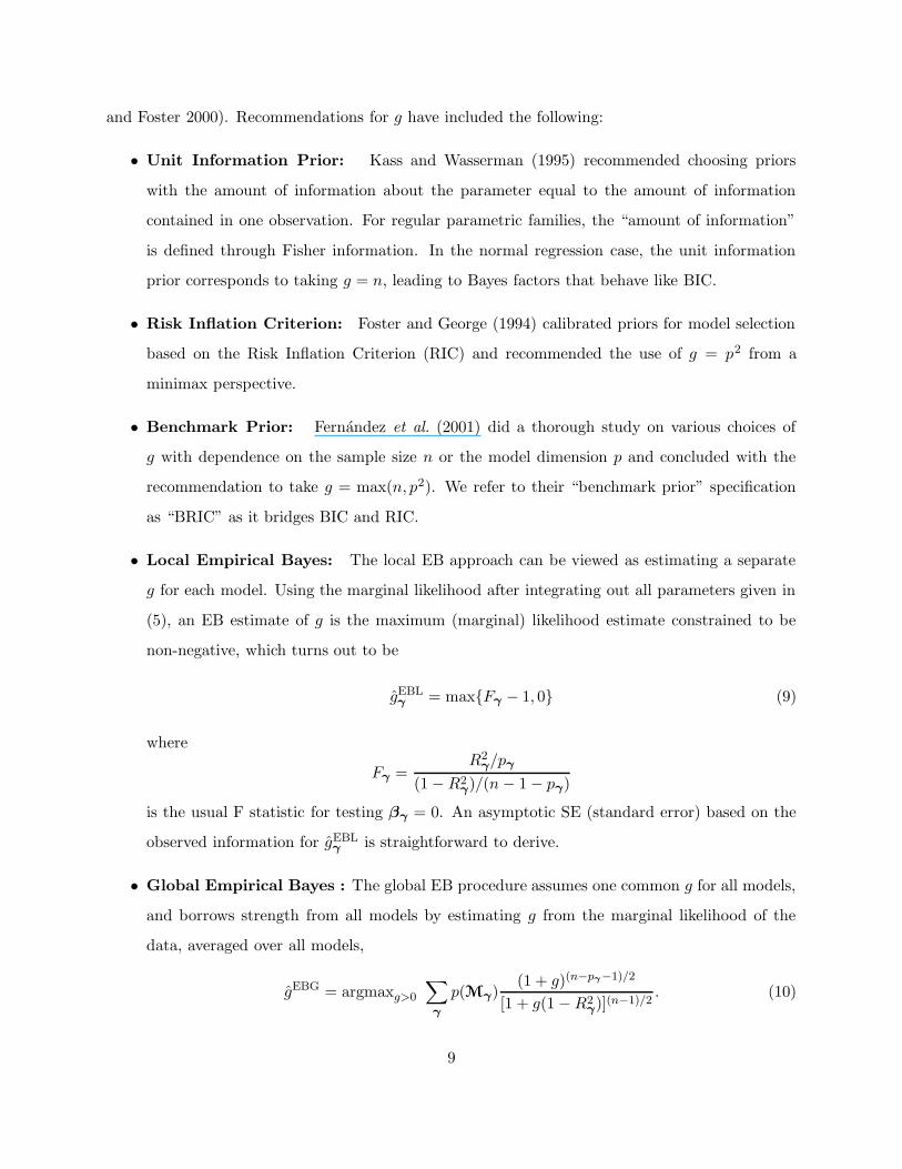
and Foster 2000). Recommendations for g have included the following:

• Unit Information Prior: Kass and Wasserman (1995) recommended choosing priors

with the amount of information about the parameter equal to the amount of information

contained in one observation. For regular parametric families, the “amount of information”

is defined through Fisher information. In the normal regression case, the unit information

prior corresponds to taking g = n, leading to Bayes factors that behave like BIC.

• Risk Inflation Criterion: Foster and George (1994) calibrated priors for model selection

based on the Risk Inflation Criterion (RIC) and recommended the use of g = p2 from a

minimax perspective.

• Benchmark Prior: Fernandez et al. (2001) did a thorough study on various choices of

g with dependence on the sample size n or the model dimension p and concluded with the

recommendation to take g = max(n, p2). We refer to their “benchmark prior” specification

as “BRIC” as it bridges BIC and RIC.

• Local Empirical Bayes: The local EB approach can be viewed as estimating a separate

g for each model. Using the marginal likelihood after integrating out all parameters given in

(5), an EB estimate of g is the maximum (marginal) likelihood estimate constrained to be

non-negative, which turns out to be

gEBLγ

= max{Fγ − 1, 0} (9)

where

Fγ =R2

γ/pγ

(1 − R2γ)/(n − 1 − pγ)

is the usual F statistic for testing βγ = 0. An asymptotic SE (standard error) based on the

observed information for gEBLγ

is straightforward to derive.

• Global Empirical Bayes : The global EB procedure assumes one common g for all models,

and borrows strength from all models by estimating g from the marginal likelihood of the

data, averaged over all models,

gEBG = argmaxg>0

∑

γ

p(Mγ)(1 + g)(n−pγ−1)/2

[1 + g(1 − R2γ)](n−1)/2

. (10)

9

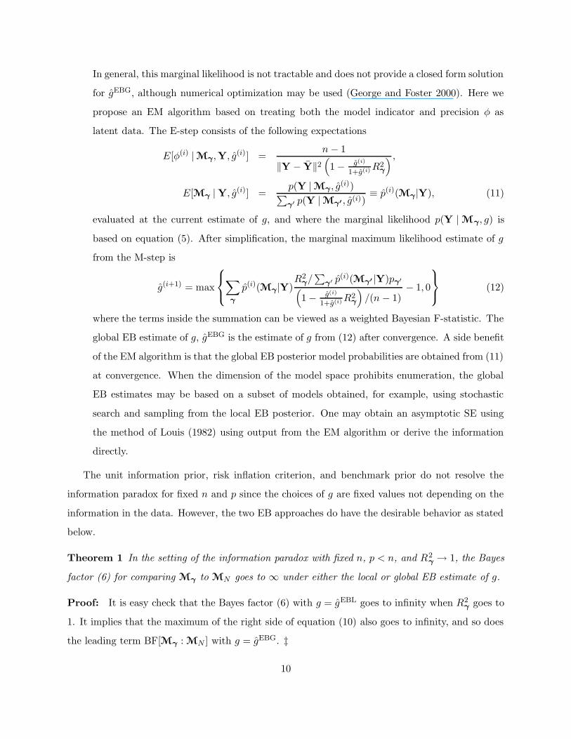
In general, this marginal likelihood is not tractable and does not provide a closed form solution

for gEBG, although numerical optimization may be used (George and Foster 2000). Here we

propose an EM algorithm based on treating both the model indicator and precision φ as

latent data. The E-step consists of the following expectations

E[φ(i) | Mγ ,Y, g(i)] =n − 1

‖Y − Y‖2(

1 − g(i)

1+g(i) R2γ

) ,

E[Mγ | Y, g(i)] =p(Y | Mγ , g(i))

∑

γ′ p(Y | Mγ′, g(i))≡ p(i)(Mγ |Y), (11)

evaluated at the current estimate of g, and where the marginal likelihood p(Y | Mγ , g) is

based on equation (5). After simplification, the marginal maximum likelihood estimate of g

from the M-step is

g(i+1) = max

∑

γ

p(i)(Mγ |Y)R2

γ/∑

γ′ p(i)(Mγ′ |Y)pγ′

(

1 − g(i)

1+g(i) R2γ

)

/(n − 1)− 1, 0

(12)

where the terms inside the summation can be viewed as a weighted Bayesian F-statistic. The

global EB estimate of g, gEBG is the estimate of g from (12) after convergence. A side benefit

of the EM algorithm is that the global EB posterior model probabilities are obtained from (11)

at convergence. When the dimension of the model space prohibits enumeration, the global

EB estimates may be based on a subset of models obtained, for example, using stochastic

search and sampling from the local EB posterior. One may obtain an asymptotic SE using

the method of Louis (1982) using output from the EM algorithm or derive the information

directly.

The unit information prior, risk inflation criterion, and benchmark prior do not resolve the

information paradox for fixed n and p since the choices of g are fixed values not depending on the

information in the data. However, the two EB approaches do have the desirable behavior as stated

below.

Theorem 1 In the setting of the information paradox with fixed n, p < n, and R2γ→ 1, the Bayes

factor (6) for comparing Mγ to MN goes to ∞ under either the local or global EB estimate of g.

Proof: It is easy check that the Bayes factor (6) with g = gEBL goes to infinity when R2γ

goes to

1. It implies that the maximum of the right side of equation (10) also goes to infinity, and so does

the leading term BF[Mγ : MN ] with g = gEBG. ‡

10

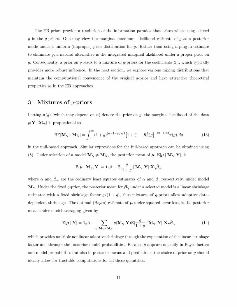
The EB priors provide a resolution of the information paradox that arises when using a fixed

g in the g-priors. One may view the marginal maximum likelihood estimate of g as a posterior

mode under a uniform (improper) prior distribution for g. Rather than using a plug-in estimate

to eliminate g, a natural alternative is the integrated marginal likelihood under a proper prior on

g. Consequently, a prior on g leads to a mixture of g-priors for the coefficients βγ , which typically

provides more robust inference. In the next section, we explore various mixing distributions that

maintain the computational convenience of the original g-prior and have attractive theoretical

properties as in the EB approaches.

3 Mixtures of g-priors

Letting π(g) (which may depend on n) denote the prior on g, the marginal likelihood of the data

p(Y | Mγ) is proportional to

BF[Mγ : MN ] =

∫ ∞

0(1 + g)(n−1−pγ)/2

[

1 + (1 − R2γ)g]−(n−1)/2

π(g) dg (13)

in the null-based approach. Similar expressions for the full-based approach can be obtained using

(8). Under selection of a model Mγ 6= MN , the posterior mean of µ, E[µ | Mγ ,Y], is

E[µ | Mγ ,Y] = 1nα + E[g

1 + g| Mγ ,Y] Xγβ

γ

where α and βγ

are the ordinary least squares estimates of α and β, respectively, under model

Mγ . Under the fixed g-prior, the posterior mean for βγ under a selected model is a linear shrinkage

estimator with a fixed shrinkage factor g/(1 + g), thus mixtures of g-priors allow adaptive data-

dependent shrinkage. The optimal (Bayes) estimate of µ under squared error loss, is the posterior

mean under model averaging given by

E[µ | Y] = 1nα +∑

γ:Mγ 6=MN

p(Mγ |Y)E[g

1 + g| Mγ ,Y] Xγβ

γ(14)

which provides multiple nonlinear adaptive shrinkage through the expectation of the linear shrinkage

factor and through the posterior model probabilities. Because g appears not only in Bayes factors

and model probabilities but also in posterior means and predictions, the choice of prior on g should

ideally allow for tractable computations for all these quantities.

11

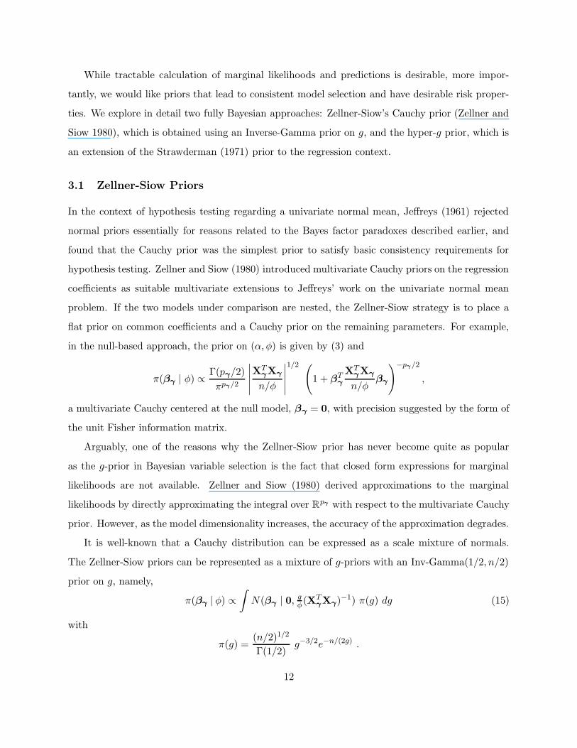
While tractable calculation of marginal likelihoods and predictions is desirable, more impor-

tantly, we would like priors that lead to consistent model selection and have desirable risk proper-

ties. We explore in detail two fully Bayesian approaches: Zellner-Siow’s Cauchy prior (Zellner and

Siow 1980), which is obtained using an Inverse-Gamma prior on g, and the hyper-g prior, which is

an extension of the Strawderman (1971) prior to the regression context.

3.1 Zellner-Siow Priors

In the context of hypothesis testing regarding a univariate normal mean, Jeffreys (1961) rejected

normal priors essentially for reasons related to the Bayes factor paradoxes described earlier, and

found that the Cauchy prior was the simplest prior to satisfy basic consistency requirements for

hypothesis testing. Zellner and Siow (1980) introduced multivariate Cauchy priors on the regression

coefficients as suitable multivariate extensions to Jeffreys’ work on the univariate normal mean

problem. If the two models under comparison are nested, the Zellner-Siow strategy is to place a

flat prior on common coefficients and a Cauchy prior on the remaining parameters. For example,

in the null-based approach, the prior on (α, φ) is given by (3) and

π(βγ | φ) ∝ Γ(pγ/2)

πpγ/2

∣

∣

∣

∣

∣

XTγXγ

n/φ

∣

∣

∣

∣

∣

1/2 (

1 + βTγ

XTγXγ

n/φβγ

)−pγ/2

,

a multivariate Cauchy centered at the null model, βγ = 0, with precision suggested by the form of

the unit Fisher information matrix.

Arguably, one of the reasons why the Zellner-Siow prior has never become quite as popular

as the g-prior in Bayesian variable selection is the fact that closed form expressions for marginal

likelihoods are not available. Zellner and Siow (1980) derived approximations to the marginal

likelihoods by directly approximating the integral over Rpγ with respect to the multivariate Cauchy

prior. However, as the model dimensionality increases, the accuracy of the approximation degrades.

It is well-known that a Cauchy distribution can be expressed as a scale mixture of normals.

The Zellner-Siow priors can be represented as a mixture of g-priors with an Inv-Gamma(1/2, n/2)

prior on g, namely,

π(βγ | φ) ∝∫

N(βγ | 0, gφ(XT

γXγ)−1) π(g) dg (15)

with

π(g) =(n/2)1/2

Γ(1/2)g−3/2e−n/(2g) .

12

One may take advantage of the mixture of g-prior representation (15) to first integrate out θγ

given g, leaving a one dimensional integral over g as in (13) which is independent of the model

dimension. This one dimensional integral can be carried out using standard numerical integration

techniques or using a Laplace approximation. The Laplace approximation involves expanding the

unnormalized marginal posterior density of g about its mode, and leads to tractable calculations

for approximating marginal likelihoods as the marginal posterior mode of g is a solution to a cubic

equation. Furthermore, the posterior expectation of g/(1 + g), necessary for prediction, can also

be approximated using the same form of Laplace approximation, and again the associated mode is

the solution to a cubic equation. Details can be found in Appendix A and are implemented in an

R package available from the authors.

3.2 Hyper-g Priors

As an alternative to the Zellner-Siow prior for the model choice problem, we introduce a family of

priors on g:

π(g) =a − 2

2(1 + g)−a/2, g > 0, (16)

which is a proper distribution for a > 2. This family of priors includes priors used by Strawderman

(1971) to provide improved mean square risk over ordinary maximum likelihood estimates in the

normal means problem. These priors have also been studied by Cui and George (2007) for the

problem of variable selection in the case of known error variance.

When a ≤ 2, the prior π(g) ∝ (1+g)−a/2 is improper; both the reference prior and the Jeffreys’

prior correspond to a = 2. When 1 < a ≤ 2, we will see that the marginal density, given below in

(17), is finite, so that the corresponding posterior distribution is proper. Even though the choice

of 1 < a ≤ 2 leads to proper posterior distributions, because g is not included in the null model,

the issue of arbitrary constants of proportionality leads to indeterminate Bayes factors. For this

reason, we will limit attention to the prior in (16) with a > 2.

More insight on hyper-parameter specification can be obtained by instead considering the cor-

responding prior on the shrinkage factor g/(1 + g), where

g

1 + g∼ Beta(1,

a

2− 1)

which is a Beta distribution with mean 2/a. For a = 4, the prior on the shrinkage factor is uniform.

Values of a greater than four, tend to put more mass on shrinkage values near 0, which is undesirable

13

a priori. Taking a = 3 places most of the mass near 1, with the prior probability that the shrinkage

factor is greater than 0.80 equal to 0.45. We will work with a = 3 and a = 4 for future examples,

although any choice 2 < a ≤ 4 may be reasonable.

An advantage of the hyper-g prior is that the posterior distribution of g given a model is

available in closed form,

p(g | Y,Mγ) =pγ + a − 2

2 2F1(n−1

2 , 1;pγ+a

2 ;R2γ)

(1 + g)(n−1−pγ−a)/2[

1 + (1 − R2γ)g]−(n−1)/2

where 2F1(a, b; c; z) in the normalizing constant is the Gaussian hypergeometric function (Abramowitz

and Stegun 1970, Section 15). The integral representing 2F1(a, b; c; z) is convergent for real |z| < 1

with c > b > 0 and for z = ±1 only if c > a + b and b > 0. As the normalizing constant in the

prior on g is also a special case of the 2F1 function with z = 0, we refer to this family of prior

distributions as the hyper-g priors.

The Gaussian hypergeometric function appears in many quantities of interest. The normalizing

constant in the posterior for g leads to the null-based Bayes factor

BF[Mγ : MN ] =a − 2

2

∫ ∞

0(1 + g)(n−1−pγ−a)/2

[

1 + (1 − R2γ)g]−(n−1)/2

dg (17)

=a − 2

pγ + a − 22F1(

n − 1

2, 1;

pγ + a

2;R2

γ)

which can be easily evaluated. The posterior mean of g under Mγ is given by

E[g | Mγ ,Y] =2

pγ + a − 4

2F1(n−1

2 , 2;pγ+a

2 ;R2γ)

2F1(n−1

2 , 1;pγ+a

2 ;R2γ)

(18)

which is finite if a > 3. Likewise, the expected value of the shrinkage factor under each model can

also be expressed using the 2F1 function,

E[g

1 + g| Y,Mγ ] =

∫

g(1 + g)n−1−pγ−a

2−1[

1 + (1 − R2γ)g]−(n−1)/2

dg∫

(1 + g)n−1−pγ−a

2

[

1 + (1 − R2γ)g]−(n−1)/2

dg(19)

=2

pγ + a

2F1(n−1

2 , 2;pγ+a

2 + 1;R2γ)

2F1(n−1

2 , 1;pγ+a

2 ;R2γ)

which unlike the ordinary g-prior leads to nonlinear data-dependent shrinkage.

While subroutines in the Cephes library (http://www.netlib.org/cephes) are available for

evaluating Gaussian hypergeometric functions, numerical overflow is problematic for moderate to

14

large n and large R2γ. Similar numerical difficulties with the 2F1 have been encountered by Butler

and Wood (2002), who developed a Laplace approximation to the integral representation

2F1(a, b; c; z) =Γ(c)

Γ(b)Γ(c − b)

∫ 1

0

tb−1(1 − t)c−b−1

(1 − tz)adt. (20)

Because the Laplace approximation involves an integral with respect to a normal kernel, we prefer

to develop the expansion after a change of variables to τ = log (g), carrying out the integration

over the entire real line. This avoids issues with modes on the boundary (as in the local Empirical

Bayes solution) and leads to an improved normal approximation to the integral as the variable of

integration is no longer restricted. Details of the fully exponential Laplace approximations (Tierney

and Kadane 1986) of order O(n−1) to the expression (17), and of order O(n−2) for the ratios in

(18) and (19) are given in Appendix A.

4 Consistency

So far in this paper, we have considered several alternatives to fixed g-priors: local and global

Empirical Bayes, Zellner-Siow priors, and hyper-g priors. In this section, we investigate the theo-

retical properties of mixtures of g-priors. In particular, three aspects of consistency are considered

here: (1) the “information paradox” where R2γ→ 1 as described in Section 2.3; (2) the asymptotic

consistency of model posterior probabilities where n → ∞ as considered in Fernandez et al. (2001);

and (3) the asymptotic consistency for prediction. While agreeing that no model is ever completely

true, many (ourselves included) do feel it is useful to study the behavior of procedures under the

assumption of a true model.

4.1 Information paradox

A general result providing conditions under which mixtures of g-priors resolve the information

paradox is given below.

Theorem 2 To resolve the information paradox for all n and p < n, it suffices to have

∫ ∞

0(1 + g)(n−1−pγ)/2π(g)dg = ∞ ∀ pγ ≤ p.

In the case of minimal sample size (i.e. n = p + 2), it suffices to have∫∞

0 (1 + g)1/2π(g)dg = ∞.

15

Proof : The integrand function in the Bayes factor (13) is a monotonic increasing function of

R2γ. Therefore when R2

γgoes to 1, it goes to

∫

(1 + g)(n−1−pγ)/2π(g)dg by the Monotone Con-

vergence Theorem. So the non-integrability of (1 + g)(n−1−pγ )/2π(g) is a sufficient and necessary

condition for resolving the “information paradox”. The result for the case with minimal sample

size is straightforward. ‡

It is easy to check that the Zellner-Siow prior satisfies this condition. For the hyper-g prior,

there is an additional constraint that a ≤ n− pγ +1, which in the case of the minimal sample size,

suggests that we take 2 < a ≤ 3. As a fixed g-prior corresponds to the special case of a degenerate

prior that is a point mass at a selected value of g, it is clear that no fixed choice of g ≤ ∞ will

resolve the paradox.

4.2 Model Selection Consistency

The following definition of posterior model consistency for model choice is considered in Fernandez

et al. (2001), namely,

plimn p(Mγ | Y) = 1 when Mγ is the true model, (21)

where “plim” denotes convergence in probability and the probability measure here is the sampling

distribution under the assumed true model Mγ . By the relationship between posterior probabilities

and Bayes factors (2), the consistency property (21) is equivalent to

plimn BF[Mγ′ : Mγ ] = 0, for all Mγ′ 6= Mγ .

For any model Mγ′ that does not contain the true model Mγ , we will assume that

limn→∞

βγTXT

γ(I − Pγ′)Xγβγ

n= bγ′ ∈ (0,∞) (22)

where Pγ′ is the projection matrix onto the span of Xγ′ . Under this assumption, Fernandez et al.

(2001) have shown that consistency holds for BRIC and BIC. Here we consider the case for mixtures

of g-priors and the Empirical Bayes approaches.

Theorem 3 Assume (22) holds. When the true model is not the null model, i.e., Mγ 6= MN ,

posterior probabilities under Empirical Bayes, Zellner-Siow priors, and hyper-g priors are consistent

16

for model selection; when Mγ = MN , consistency still holds true for the Zellner-Siow prior, but

does not hold for the hyper-g or local and global Empirical Bayes.

The proof is given in Appendix B. A key feature in the consistency of posterior model probabil-

ities under the null model with the Zellner-Siow prior is that the prior on g depends on the sample

size n; this is not the case in the EB or hyper-g priors. The inconsistency under the null model

of the EB prior has been noted by George and Foster (2000). Looking at the proof of Theorem 3

one can see that while the EB and hyper-g priors are not consistent in the sense of (21) under the

null model, the null model will still be the highest probability model, even though its posterior

probability is bounded away from 1. Thus, the priors will be consistent in a weaker sense for the

problem of model selection under a 0-1 loss.

The lack of consistency under the null model motivates a modification of the hyper-g prior,

which we refer to as the hyper-g/n prior:

π(g) =a − 2

2n(1 + g/n)−a/2

where the normalizing constant for the prior is another special case of the Gaussian hypergeometric

family. While no analytic expressions are available for the distribution or various expectations (this

form of the prior is not closed under sampling), it is straightforward to approximate quantities of

interest using Laplace approximations as detailed in Appendix A.

4.3 Prediction Consistency

In practice, prediction sometimes is of more interest than uncovering the true model. Given the

observed data (Y,X1, . . . ,Xp) and a new vector of predictors x∗ ∈ Rp, we would like to predict

the corresponding response Y ∗. In the Bayesian framework, the optimal point estimator (under

squared error loss) for Y ∗ is the BMA prediction given by

Y ∗n = α +

∑

γ

x∗γ

Tβ

γp(Mγ | Y)

∫ ∞

0

g

1 + gπ(g | Mγ ,Y)dg. (23)

The local and global EB estimators can be obtained by replacing π(g | Mγ ,Y) by a degenerate

distribution with point mass at gEBL and gEBG, respectively. When the true sampling distribution

is known, i.e., (Mγ , α,βγ , φ) are known, it is optimal (under squared error loss) to predict Y ∗ by

17

its mean. Therefore we call Y ∗n consistent under prediction, if

plimn Y ∗n = EY ∗ = α + x∗

γ

Tβγ

where plim denotes convergence in probability and the probability measure here is the sampling

distribution under model Mγ .

Theorem 4 The BMA estimators Y ∗n (23) under Empirical Bayes, the hyper-g, hyper-g/n and

Zellner-Siow priors are consistent under prediction.

Proof : When Mγ = MN , by the consistency of least squares estimators, we have ‖βγ‖ → 0, so

the consistency of the BMA estimators follows.

When Mγ 6= MN , by Theorem 3, π(Mγ | Y) goes to one in probability. Using the consistency

of the least squares estimators, it suffices to show that

plimn

∫ ∞

0

g

1 + gπ(g | Mγ ,Y)dg = 1 . (24)

The integral above can be rewritten as

∫∞

0g

1+g L(g) π(g) dg∫∞

0 L(g) π(g) dg

where L(g) = (1 + g)−pγ/2[

1 − R2γ

g1+g

]−(n−1)/2is maximized at gEBL

γgiven by (9). Applying a

Laplace approximation to the denominator and numerator of the ratio above along the lines of

(35), we have∫ ∞

0

g

1 + gπ(g | Mγ ,Y)dg =

gEBLγ

1 + gEBLγ

(1 + O(1/n)) .

It is clear that gEBLγ

goes to infinity in probability under Mγ , and hence we can conclude that the

limit in (24) is equal to 1, as we desired. The consistency of the local Empirical Bayes procedures

is a direct consequence. Because gEBG is of the same order as gEBL, the consistency of the global

Empirical Bayes follows. ‡

We have shown that Zellner-Siow and hyper-g/n priors are consistent for model selection under

a 0–1 loss for any assumed true model. Additionally, the hyper-g priors and EB procedures are

also consistent for model selection for all models except the null model. However, all of the mixture

of g-priors and EB procedures are consistent for prediction under squared error loss. Because the

18

asymptotic results do not provide any discrimination among the different methods, we conducted

a simulation study to compare mixture of g-priors with Empirical Bayes and other default model

selection procedures.

5 Simulation Study

We generated data for the simulation study as Y = 1nα + Xβ + ε, with ε ∼ N(0, In/φ), φ = 1,

α = 2, and sample size n = 100. Following Cui and George (2007) we set XTX = Ip, but took

p = 15 so that all models may be enumerated, thus avoiding extra Monte Carlo variation due to

stochastic search of the model space. For a model of size pγ , we generated βγ as N(0, g/φIpγ )

and set the remaining components of β to zero. We used g = 5, 25 as in Cui and George (2007),

representing weak and strong signal to noise ratios.

We used squared error loss

MSE(m) = ||Xβ −Xβ(m)||2

where β(m)

is the estimator of β using method m, which may entail both selection and shrinkage.

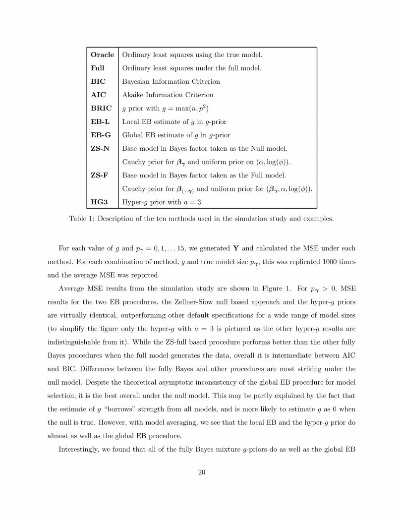
We compared ten methods listed in Table 1. Among them, the theoretical MSE for Oracle and Full

methods are known to be pγ + 1 and p + 1, respectively. For each Bayesian method, we considered

the following criteria for model choice: selection of the highest posterior probability model (HPM),

selection of the median probability model (MPM) which is defined as the model where a variable is

included if the marginal inclusion probability p(βj 6= 0 | Y) > 1/2 (Barbieri and Berger 2004), and

Bayesian Model Averaging (BMA). In both HPM and MPM, the point estimate is the posterior

mean of βγ under the selected model. For BIC, the log marginal for model Mγ is defined as

log p(Y | Mγ) ≡ −1

2{n log(σ2

γ) + pγ log(n)} (25)

where σ2γ

= RSSγ/n is the MLE of σ2 under model Mγ . These marginals are used for calculating

posterior model probabilities for determining HPM and MPM, and for calculating quantities under

model averaging. For AIC, the penalty for model complexity in the log marginal is taken as 2pγ

rather than pγ log(n) as in (25) for BIC. For both AIC and BIC, the point estimate of βγ is the

OLS estimate under model Mγ . Uniform prior probabilities on models were used throughout.

19

Oracle Ordinary least squares using the true model.

Full Ordinary least squares under the full model.

BIC Bayesian Information Criterion

AIC Akaike Information Criterion

BRIC g prior with g = max(n, p2)

EB-L Local EB estimate of g in g-prior

EB-G Global EB estimate of g in g-prior

ZS-N Base model in Bayes factor taken as the Null model.

Cauchy prior for βγ and uniform prior on (α, log(φ)).

ZS-F Base model in Bayes factor taken as the Full model.

Cauchy prior for β(−γ) and uniform prior for (βγ , α, log(φ)).

HG3 Hyper-g prior with a = 3

Table 1: Description of the ten methods used in the simulation study and examples.

For each value of g and pγ = 0, 1, . . . 15, we generated Y and calculated the MSE under each

method. For each combination of method, g and true model size pγ , this was replicated 1000 times

and the average MSE was reported.

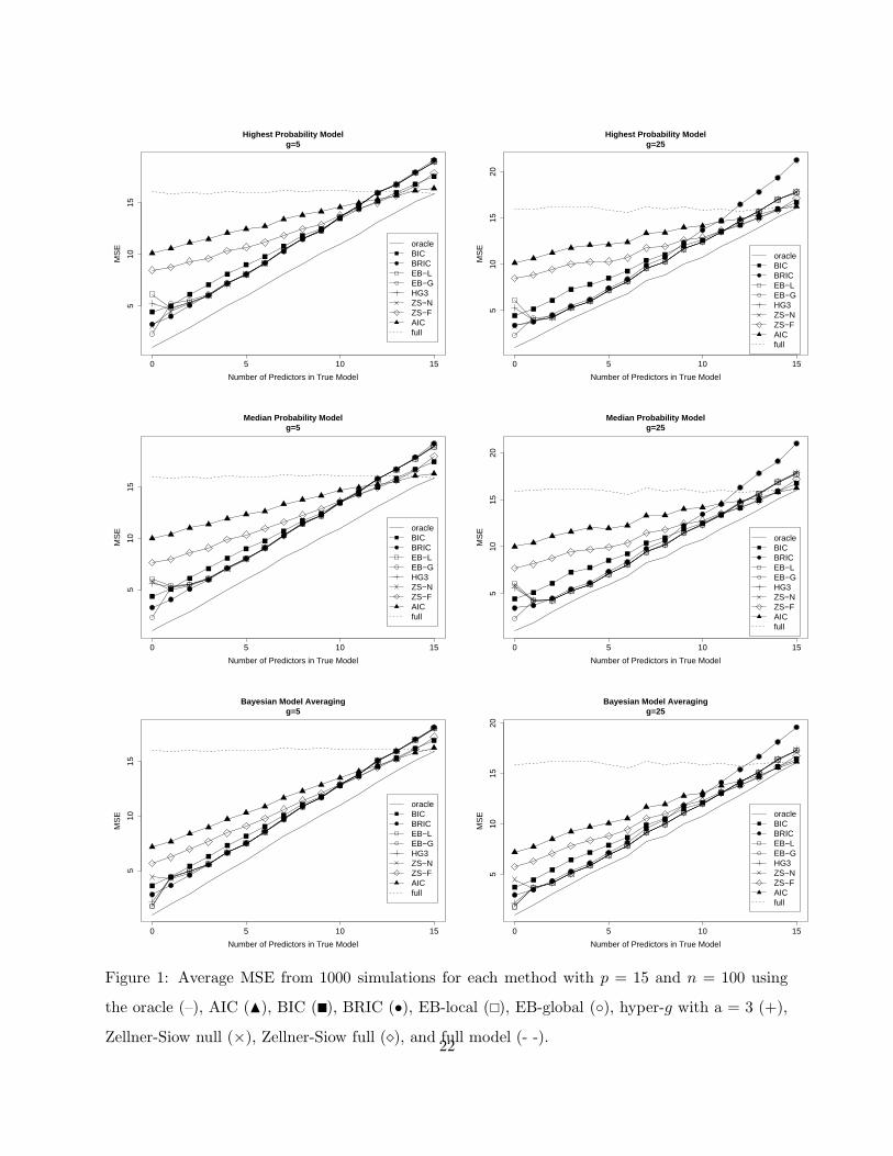
Average MSE results from the simulation study are shown in Figure 1. For pγ > 0, MSE

results for the two EB procedures, the Zellner-Siow null based approach and the hyper-g priors

are virtually identical, outperforming other default specifications for a wide range of model sizes

(to simplify the figure only the hyper-g with a = 3 is pictured as the other hyper-g results are

indistinguishable from it). While the ZS-full based procedure performs better than the other fully

Bayes procedures when the full model generates the data, overall it is intermediate between AIC

and BIC. Differences between the fully Bayes and other procedures are most striking under the

null model. Despite the theoretical asymptotic inconsistency of the global EB procedure for model

selection, it is the best overall under the null model. This may be partly explained by the fact that

the estimate of g “borrows” strength from all models, and is more likely to estimate g as 0 when

the null is true. However, with model averaging, we see that the local EB and the hyper-g prior do

almost as well as the global EB procedure.

Interestingly, we found that all of the fully Bayes mixture g-priors do as well as the global EB

20

with model selection, except under the null model, while Cui and George (2007) found that the

global EB out-performed fully Bayes procedures (under the assumption of known φ). We have

used a uniform prior on the model space (for both the EB and fully Bayes procedures), whereas

Cui and George (2007) place independent Bernoulli(ω) priors on variable inclusion, and compare

EB estimates of ω with fully Bayes procedures that place a uniform prior on ω. While we have

not addressed prior distributions over models, this is an important aspect and may explain some

of the difference in findings. Additionally, the simulations in Cui and George (2007) are for the

p = n case. Although we show that fully Bayes procedures are consistent as n → ∞ for fixed p,

additional study of their theoretical properties is necessary for the situation when p is close to the

sample size.

6 Examples with Real Data

In this section, we explore the small sample properties of the two mixture g-priors on real data sets

and contrast our results using other model selection procedures such as AIC, BIC, the benchmark

prior (BRIC), EB-local and EB-global.

6.1 Crime Data

Raftery et al. (1997) used the crime data of Vandaele (1978) as an illustration of Bayesian model

averaging in linear regression. The cross-sectional data comprise aggregate measures of the crime

rate for 47 states, and include 15 explanatory variables, leading to 215 = 36, 768 potential regres-

sion models. The prior distributions used by Raftery et al. (1997) are in the conjugate Normal-

InvGamma family, but their use requires specification of several hyper-parameters. Fernandez et al.

(2001) revisited the crime data using g-priors and explored the choice of g on model choice. Using

the benchmark prior, that compromises between BIC and RIC, (g = max{n, p2} = 152), Fernandez

et al. (2001) came to roughly the same conclusions regarding model choice and variable importance

as Raftery et al. (1997). We continue along these lines by investigating how the mixture g-priors

affect variable importance. As in the earlier analyses of this data, all variables, except the indicator

variable, have been log-transformed. The data are available in the R library MASS under UScrime

(library(MASS); data(UScrime)) and all calculations have been done with the R package BAS

available from http://wwww.stat.duke.edu/∼clyde/BAS.

21

0 5 10 15

510

15

Number of Predictors in True Model

MS

E oracleBICBRICEB−LEB−GHG3ZS−NZS−FAICfull

Highest Probability Modelg=5

0 5 10 15

510

1520

Number of Predictors in True Model

MS

E

oracleBICBRICEB−LEB−GHG3ZS−NZS−FAICfull

Highest Probability Modelg=25

0 5 10 15

510

15

Number of Predictors in True Model

MS

E oracleBICBRICEB−LEB−GHG3ZS−NZS−FAICfull

Median Probability Modelg=5

0 5 10 15

510

1520

Number of Predictors in True Model

MS

E

oracleBICBRICEB−LEB−GHG3ZS−NZS−FAICfull

Median Probability Modelg=25

0 5 10 15

510

15

Number of Predictors in True Model

MS

E

oracleBICBRICEB−LEB−GHG3ZS−NZS−FAICfull

Bayesian Model Averagingg=5

0 5 10 15

510

1520

Number of Predictors in True Model

MS

E oracleBICBRICEB−LEB−GHG3ZS−NZS−FAICfull

Bayesian Model Averagingg=25

Figure 1: Average MSE from 1000 simulations for each method with p = 15 and n = 100 using

the oracle (–), AIC (N), BIC (�), BRIC (•), EB-local (�), EB-global (◦), hyper-g with a = 3 (+),

Zellner-Siow null (×), Zellner-Siow full (�), and full model (- -).22

BRIC HG-n HG3 HG4 EB-L EB-G ZS-N ZS-F BIC AIC

log(AGE) 0.75 0.85 0.84 0.84 0.85 0.86 0.85 0.88 0.91 0.98

S 0.15 0.27 0.29 0.31 0.29 0.29 0.27 0.36 0.23 0.36

log(Ed) 0.95 0.97 0.97 0.96 0.97 0.97 0.97 0.97 0.99 1.00

log(Ex0) 0.66 0.66 0.66 0.66 0.67 0.67 0.67 0.68 0.69 0.74

log(Ex1) 0.39 0.45 0.47 0.47 0.46 0.46 0.45 0.50 0.40 0.47

log(LF) 0.08 0.20 0.23 0.24 0.22 0.21 0.20 0.30 0.16 0.34

log(M) 0.09 0.20 0.23 0.24 0.22 0.22 0.20 0.30 0.17 0.39

log(N) 0.23 0.37 0.39 0.39 0.39 0.38 0.37 0.46 0.36 0.57

log(NW) 0.51 0.69 0.69 0.68 0.70 0.70 0.69 0.75 0.78 0.92

log(U1) 0.11 0.25 0.27 0.28 0.27 0.27 0.25 0.35 0.23 0.41

log(U2) 0.45 0.61 0.61 0.61 0.62 0.62 0.61 0.68 0.70 0.86

log(W) 0.18 0.35 0.38 0.39 0.38 0.38 0.36 0.47 0.36 0.64

log(X) 0.99 1.00 0.99 0.99 1.00 1.00 1.00 0.99 1.00 1.00

log(prison) 0.78 0.89 0.89 0.89 0.90 0.90 0.90 0.92 0.95 0.99

log(time) 0.19 0.37 0.38 0.39 0.39 0.38 0.37 0.47 0.41 0.65

Table 2: Marginal inclusion probabilities for each variable under 10 prior scenarios. The median

probability model includes variables where the marginal inclusion probability is greater than or

equal to 1/2.

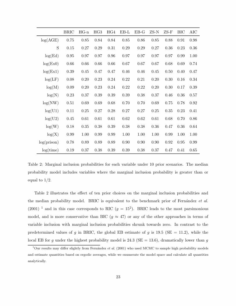
Table 2 illustrates the effect of ten prior choices on the marginal inclusion probabilities and

the median probability model. BRIC is equivalent to the benchmark prior of Fernandez et al.

(2001) 1 and in this case corresponds to RIC (g = 152). BRIC leads to the most parsimonious

model, and is more conservative than BIC (g ≈ 47) or any of the other approaches in terms of

variable inclusion with marginal inclusion probabilities shrunk towards zero. In contrast to the

predetermined values of g in BRIC, the global EB estimate of g is 19.5 (SE = 11.2), while the

local EB for g under the highest probability model is 24.3 (SE = 13.6), dramatically lower than g

1Our results may differ slightly from Fernandez et al. (2001) who used MCMC to sample high probability models

and estimate quantities based on ergodic averages, while we enumerate the model space and calculate all quantities

analytically.

23

under BRIC. The fully Bayesian mixture g-priors HG3, HG4, and ZS-null all lead to very similar

marginal inclusion probabilities as the data-based adaptive Empirical Bayes approaches EB-global

and EB-local. These all lead to the same median probability model. As is often the case, here

the marginal inclusion probabilites under AIC are larger, leading to the inclusion of two additional

variables in the AIC median probability model compared to the median probability model under

the mixture g-priors and the EB priors.

6.2 Ozone

Our last example uses the ground level ozone data analyzed in Breiman and Friedman (1985),

and more recently by Miller (2001) and Casella and Moreno (2006). The dataset consists of daily

measurements of the maximum ozone concentration near Los Angeles and 8 meteorological variables

(the description for the variables is in Appendix C). Following Miller (2001) and Casella and Moreno

(2006), we examine regression models using the 8 meteorological variables, plus interactions and

squares, leading to 44 possible predictors. Enumeration of all possible models is not feasible, so

instead we use stochastic search to identify the highest probability models using the R package BAS.

We compared the different procedures on the basis of out-of-sample predictive accuracy by taking

a random split (50/50) of the data and reserving half for calculating the average prediction error

(RMSE) under each method, where

RMSE(M) =

√

∑

i∈V (Yi − Yi)2

nV,

V is the validation set, nV is the number of observations in the validation set (nV = 165), and

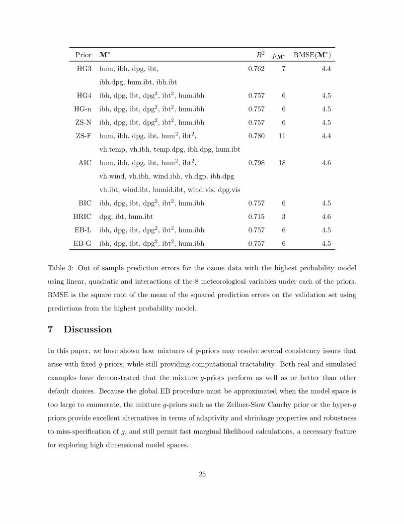
Yi is the predicted mean for Yi under the highest probability model. From Table 3, the two EB

procedures, BIC and HG (α = 4) all identify the same model. The ZS procedure with the full-

based Bayes factors and AIC lead to selection of the most complex models with 11 and 18 variables

respectively. While the hyper-g prior with α = 3 has the smallest RMSE, overall the differences

in RMSE are not enough to suggest that any method dominates the others in terms of prediction.

Based on their theoretical properties, we continue to recommend the mixtures of g-priors, such as

the hyper-g prior with α = 3.

24

Prior M∗ R2 pM

∗ RMSE(M∗)

HG3 hum, ibh, dpg, ibt, 0.762 7 4.4

ibh.dpg, hum.ibt, ibh.ibt

HG4 ibh, dpg, ibt, dpg2, ibt2, hum.ibh 0.757 6 4.5

HG-n ibh, dpg, ibt, dpg2, ibt2, hum.ibh 0.757 6 4.5

ZS-N ibh, dpg, ibt, dpg2, ibt2, hum.ibh 0.757 6 4.5

ZS-F hum, ibh, dpg, ibt, hum2, ibt2, 0.780 11 4.4

vh.temp, vh.ibh, temp.dpg, ibh.dpg, hum.ibt

AIC hum, ibh, dpg, ibt, hum2, ibt2, 0.798 18 4.6

vh.wind, vh.ibh, wind.ibh, vh.dgp, ibh.dpg

vh.ibt, wind.ibt, humid.ibt, wind.vis, dpg.vis

BIC ibh, dpg, ibt, dpg2, ibt2, hum.ibh 0.757 6 4.5

BRIC dpg, ibt, hum.ibt 0.715 3 4.6

EB-L ibh, dpg, ibt, dpg2, ibt2, hum.ibh 0.757 6 4.5

EB-G ibh, dpg, ibt, dpg2, ibt2, hum.ibh 0.757 6 4.5

Table 3: Out of sample prediction errors for the ozone data with the highest probability model

using linear, quadratic and interactions of the 8 meteorological variables under each of the priors.

RMSE is the square root of the mean of the squared prediction errors on the validation set using

predictions from the highest probability model.

7 Discussion

In this paper, we have shown how mixtures of g-priors may resolve several consistency issues that

arise with fixed g-priors, while still providing computational tractability. Both real and simulated

examples have demonstrated that the mixture g-priors perform as well as or better than other

default choices. Because the global EB procedure must be approximated when the model space is

too large to enumerate, the mixture g-priors such as the Zellner-Siow Cauchy prior or the hyper-g

priors provide excellent alternatives in terms of adaptivity and shrinkage properties and robustness

to miss-specification of g, and still permit fast marginal likelihood calculations, a necessary feature

for exploring high dimensional model spaces.

25

Priors on the model space are also critical in model selection and deserve more attention.

Many Bayesian variable selection implementations place independent Bernoulli(ω) priors on variable

inclusion. Setting ω = 1/2 corresponds to a uniform prior on the model space, which we have used

throughout. Alternatively one may specicify a hierarchical model over the model space by placing

a prior on ω and take a fully Bayesian or EB approach. For example, Cui and George (2007) use a

uniform prior on ω which induces a uniform prior over the model size and therefore favors models

with small or large sizes and contrast this to EB estimates of ω. Other types of priors include

dilution priors (George 1999) that “dilute” probabilities across neighborhood of similar models,

and priors that correct the so-called “selection effect” in choice among many models (Jeffreys 1961;

Zellner and Min 1997).

While we have assumed that Xγ is full rank, the g-prior formulation may be extended to the non-

full rank setting such as in ANOVA models by replacing the inverse of XTγXγ in the g-prior with

a generalized inverse and pγ by the rank of the projection matrix. Because marginal likelihood

calculations depend only on properties of the projection on the space spanned by Xγ (which is

unique), results will not depend on the choice of generalized inverse. For the hyper-g priors, the

rank pγ must be less than (n−3−a) in order for the Gaussian hypergeometric function to be finite

and posterior distributions to be proper. For the Zellner-Siow priors, we require pγ < n − 2. For

the p > n setting, proper posterior distributions can be ensured by placing zero prior probability

on models of rank greater than or equal to (n − 3 − a) or (n − 2) for the hyper-g and Zellner-Siow

priors, respectively. In the small n setting, this is not an unreasonable restriction.

For the large p small n setting, independent priors on regression coefficients have become popular

for inducing shrinkage (Wolfe, Godsill and Ng 2004; Johnstone and Silverman 2005). Many of these

priors are represented as scale mixtures of normals and therefore may be thought of as scale mixtures

of independent g-priors. In conjunction with point masses at zero, these independent g-priors also

induce sparsity without restricting a priori the number of variables in the model, however, the

induced prior distribution of the mean is no longer invariant to the choice of basis for a given

model. Furthermore, closed form solutions for marginal likelihoods are no longer available and

Monte Carlo methods must be used to explore both model spaces and parameter spaces. While

beyond the scope of this paper, an unresolved and interesting issue is the recommendation of

multivariate versus independent mixtures of g-priors.

26

References

Abramowitz, M. and Stegun, I. (1970) Handbook of Mathematical Functions. New York: Dover

Publications, Inc.

Barbieri, M. M. and Berger, J. (2004) Optimal predictive model selection. Ann. Statist., 32,

870–897.

Bartlett, M. (1957) A comment on D. V. Lindley’s statistical paradox. Biometrika, 44, 533–534.

Berger, J. O. and Pericchi, L. (2001) Objective Bayesian methods for model selection: Introduction

and comparison. In Model Selection, vol. 38 of IMS Lecture Notes – Monograph Series, (ed.

P. Lahiri), pp. 135–193. Institute of Mathematical Statistics.

Berger, J. O., Pericchi, L. R. and Varshavsky, J. A. (1998) Bayes factors and marginal distributions

in invariant situations. Sankhya, Ser. A, 60, 307–321.

Breiman, L. and Friedman, J. (1985) Estimating optimal transformations for multiple regression

and correlation. J. Amer. Statist. Assoc., 80, 580–598.

Butler, R. W. and Wood, A. T. A. (2002) Laplace approximations for hypergeometric functions

with matrix argument. The Annals of Statistics, 30, 1155–1177.

Casella, G. and Moreno, E. (2006) Objective Bayes variable selection. J. Amer. Statist. Assoc.,

101, 157–167.

Clyde, M. and George, E. I. (2000) Flexible empirical Bayes estimation for wavelets. J. Roy.Statist.

Soc. Ser. B, 62, 681–698.

Clyde, M. and George, E. I. (2004) Model uncertainty. Statist. Sci., 19, 81–94.

Cui, W. and George, E. I. (2007) Empirical Bayes vs. fully Bayes variable selection. J. Statist.

Plann. Inference. To appear.

Eaton, M. L. (1989) Group Invariance Applications in Statistics. Institute of Mathematical Statis-

tics.

27

Fernandez, C., Ley, E. and Steel, M. F. (2001) Benchmark priors for Bayesian model averaging. J.

Econometrics, 100, 381–427.

Foster, D. P. and George, E. I. (1994) The risk inflation criterion for multiple regression. Ann.

Statist., 22, 1947–1975.

George, E. (1999) Discussion of “Model averaging and model search strategies” by M. Clyde.

In Bayesian Statistics 6: Proceedings of the Sixth Valencia International Meeting, (eds. J. M.

Bernardo, J. O. Berger, A. P. Dawid and A. F. M. Smith), pp. 157–185. Oxford Univ. Press.

George, E. I. (2000) The variable selection problem. J. Amer. Statist. Assoc., 95, 1304–1308.

George, E. I. and Foster, D. P. (2000) Calibration and empirical Bayes variable selection.

Biometrika, 87, 731–747.

George, E. I. and McCulloch, R. E. (1993) Variable selection via Gibbs sampling. J. Amer. Statist.

Assoc., 88, 881–889.

George, E. I. and McCulloch, R. E. (1997) Approaches for Bayesian variable selection. Statist.

Sinica, 7, 339–374.

Geweke, J. (1996) Variable selection and model comparison in regression. In Bayesian Statistics

5: Proceedings of the Fifth Valencia International Meeting, (eds. J. M. Bernardo, J. O. Berger,

A. P. Dawid and A. F. M. Smith), pp. 609–620. Oxford Univ. Press.

Hansen, M. H. and Yu, B. (2001) Model selection and the principle of minimum description length.

J. Amer. Statist. Assoc., 96, 746–774.

Hoeting, J. A., Madigan, D., Raftery, A. E. and Volinsky, C. T. (1999) Bayesian model av-

eraging: a tutorial (with discussion). Statist. Sci., 14, 382–401. Corrected version at

http://www.stat.washington.edu/www/research/online/hoeting1999.pdf.

Jeffreys, H. (1961) Theory of Probability. Oxford Univ. Press.

Johnstone, I. and Silverman, B. (2005) Empirical Bayes selection of wavelet thresholds. Ann.

Statist., 33, 1700–1752.

Kass, R. E. and Raftery, A. E. (1995) Bayes factors. J. Amer. Statist. Assoc., 90, 773–795.

28

Kass, R. E. and Wasserman, L. (1995) A reference Bayesian test for nested hypotheses and its

relationship to the Schwarz criterion. J. Amer. Statist. Assoc., 90, 928–934.

Kass, R. E. and Wasserman, L. (1996) The selection of prior distributions by formal rules (Corr:

1998V93 p412). J. Amer. Statist. Assoc., 91, 1343–1370.

Leamer, E. E. (1978a) Regression selection strategies and revealed priors. J. Amer. Statist. Assoc.,

73, 580–587.

Leamer, E. E. (1978b) Specification searches: Ad hoc inference with nonexperimental data. Wiley.

Louis, T. A. (1982) Finding the observed information matrix when using the EM algorithm. Journal

of the Royal Statistical Society, Series B, Methodological, 44, 226–233.

Miller, A. J. (2001) Subset selection in regression. Chapman & Hall.

Mitchell, T. J. and Beauchamp, J. J. (1988) Bayesian variable selection in linear regression (with

discussion). J. Amer. Statist. Assoc., 83, 1023–1032.

Pauler, D. K., Wakefield, J. C. and Kass, R. E. (1999) Bayes factors and approximations for variance

component models. J. Amer. Statist. Assoc., 94, 1242–1253.

Raftery, A. E., Madigan, D. and Hoeting, J. A. (1997) Bayesian model averaging for linear regression

models. J. Amer. Statist. Assoc., 92, 179–191.

Smith, M. and Kohn, R. (1996) Nonparametric regression using Bayesian variable selection. J.

Econometrics, 75, 317–343.

Strawderman, W. E. (1971) Proper Bayes minimax estimators of the multivariate normal mean.

Ann. Math. Statist., 42, 385–388.

Tierney, L. and Kadane, J. (1986) Accurate approximations for posterior moments and marginal

densities. J. Amer. Statist. Assoc., 81, 82–86.

Vandaele, W. (1978) Participation in illegitimate activities: Ehrlich revisited. In Deterrence and

Incapacitation, pp. 270–335. US National Academy of Sciences.

29

Wolfe, P. J., Godsill, S. J. and Ng, W.-J. (2004) Bayesian variable selection and regularisation for

time-frequency surface estimation. J. Roy.Statist. Soc. Ser. B, 66, 575–589.

Zellner, A. (1971) An Introduction to Bayesian Inference in Econometrics. Wiley.

Zellner, A. (1986) On assessing prior distributions and Bayesian regression analysis with g-prior

distributions. In Bayesian Inference and Decision Techniques: Essays in Honor of Bruno de

Finetti, (eds. P. K. Goel and A. Zellner), pp. 233–243. North-Holland/Elsevier.

Zellner, A. and Min, C. (1997) Baysian analysis, model selection and prediction. In Bayesian

analysis in econometrics and statistics: the Zellner view and papers, (ed. A. Zellner), pp. 389–

399. Edward Elgar Publishing Limited.

Zellner, A. and Siow, A. (1980) Posterior odds ratios for selected regression hypotheses. In Bayesian

Statistics: Proceedings of the First International Meeting held in Valencia (Spain), (eds. J. M.

Bernardo, M. H. DeGroot, D. V. Lindley and A. F. M. Smith), pp. 585–603. Valencia: University

Press.

30

Appendices

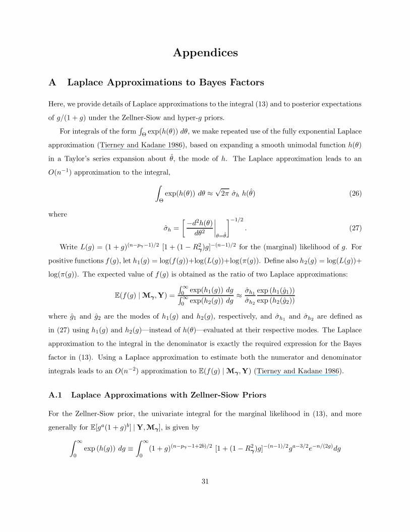
A Laplace Approximations to Bayes Factors

Here, we provide details of Laplace approximations to the integral (13) and to posterior expectations

of g/(1 + g) under the Zellner-Siow and hyper-g priors.

For integrals of the form∫

Θ exp(h(θ)) dθ, we make repeated use of the fully exponential Laplace

approximation (Tierney and Kadane 1986), based on expanding a smooth unimodal function h(θ)

in a Taylor’s series expansion about θ, the mode of h. The Laplace approximation leads to an

O(n−1) approximation to the integral,

∫

Θexp(h(θ)) dθ ≈

√2π σh h(θ) (26)

where

σh =

[−d2h(θ)

dθ2

∣

∣

∣

∣

θ=θ

]−1/2

. (27)

Write L(g) = (1 + g)(n−pγ−1)/2 [1 + (1 − R2γ)g]−(n−1)/2 for the (marginal) likelihood of g. For

positive functions f(g), let h1(g) = log(f(g))+log(L(g))+log(π(g)). Define also h2(g) = log(L(g))+

log(π(g)). The expected value of f(g) is obtained as the ratio of two Laplace approximations:

E(f(g) | Mγ ,Y) =

∫∞

0 exp(h1(g)) dg∫∞

0 exp(h2(g)) dg≈ σh1

σh2

exp (h1(g1))

exp (h2(g2))

where g1 and g2 are the modes of h1(g) and h2(g), respectively, and σh1 and σh2 are defined as

in (27) using h1(g) and h2(g)—instead of h(θ)—evaluated at their respective modes. The Laplace

approximation to the integral in the denominator is exactly the required expression for the Bayes

factor in (13). Using a Laplace approximation to estimate both the numerator and denominator

integrals leads to an O(n−2) approximation to E(f(g) | Mγ ,Y) (Tierney and Kadane 1986).

A.1 Laplace Approximations with Zellner-Siow Priors

For the Zellner-Siow prior, the univariate integral for the marginal likelihood in (13), and more

generally for E[ga(1 + g)b] |Y,Mγ ], is given by

∫ ∞

0exp (h(g)) dg ≡

∫ ∞

0(1 + g)(n−pγ−1+2b)/2 [1 + (1 − R2

γ)g]−(n−1)/2ga−3/2e−n/(2g)dg

31

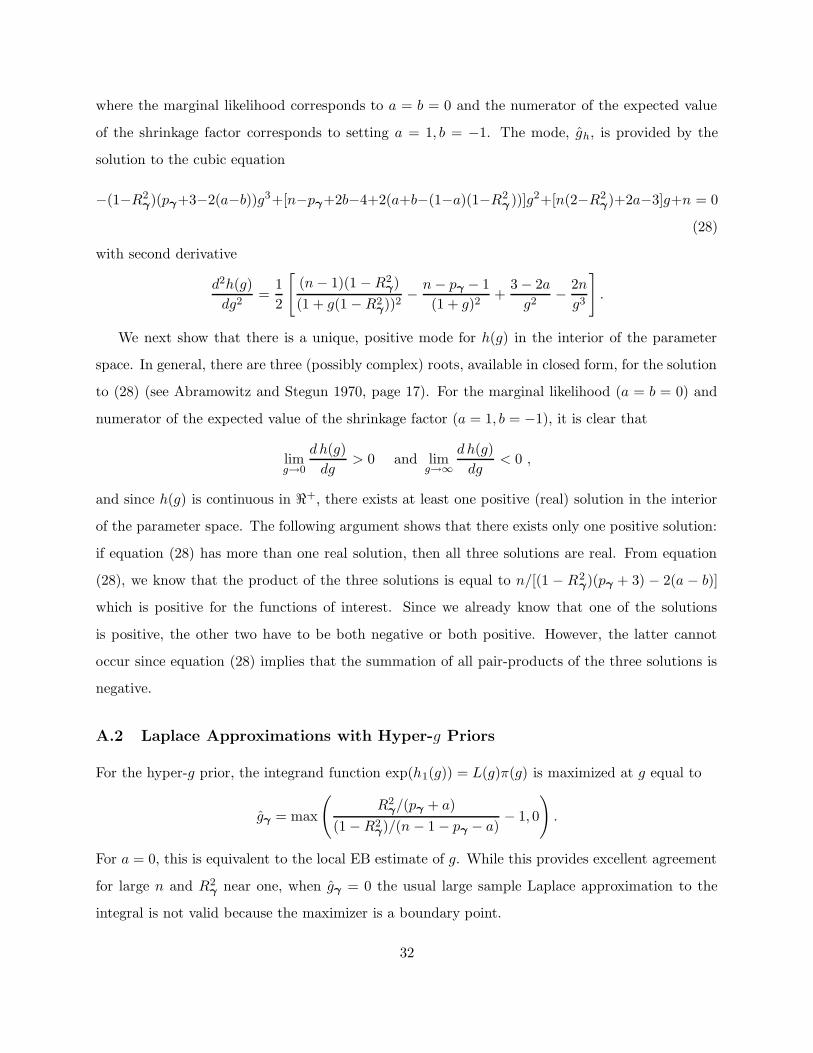
where the marginal likelihood corresponds to a = b = 0 and the numerator of the expected value

of the shrinkage factor corresponds to setting a = 1, b = −1. The mode, gh, is provided by the

solution to the cubic equation

−(1−R2γ)(pγ+3−2(a−b))g3+[n−pγ+2b−4+2(a+b−(1−a)(1−R2

γ))]g2+[n(2−R2

γ)+2a−3]g+n = 0

(28)

with second derivative

d2h(g)

dg2=

1

2

[

(n − 1)(1 − R2γ)

(1 + g(1 − R2γ))2

− n − pγ − 1

(1 + g)2+

3 − 2a

g2− 2n

g3

]

.

We next show that there is a unique, positive mode for h(g) in the interior of the parameter

space. In general, there are three (possibly complex) roots, available in closed form, for the solution

to (28) (see Abramowitz and Stegun 1970, page 17). For the marginal likelihood (a = b = 0) and

numerator of the expected value of the shrinkage factor (a = 1, b = −1), it is clear that

limg→0

d h(g)

dg> 0 and lim

g→∞

d h(g)

dg< 0 ,

and since h(g) is continuous in <+, there exists at least one positive (real) solution in the interior

of the parameter space. The following argument shows that there exists only one positive solution:

if equation (28) has more than one real solution, then all three solutions are real. From equation

(28), we know that the product of the three solutions is equal to n/[(1 − R2γ)(pγ + 3) − 2(a − b)]

which is positive for the functions of interest. Since we already know that one of the solutions

is positive, the other two have to be both negative or both positive. However, the latter cannot

occur since equation (28) implies that the summation of all pair-products of the three solutions is

negative.

A.2 Laplace Approximations with Hyper-g Priors

For the hyper-g prior, the integrand function exp(h1(g)) = L(g)π(g) is maximized at g equal to

gγ = max

(

R2γ/(pγ + a)

(1 − R2γ)/(n − 1 − pγ − a)

− 1, 0

)

.

For a = 0, this is equivalent to the local EB estimate of g. While this provides excellent agreement

for large n and R2γ

near one, when gγ = 0 the usual large sample Laplace approximation to the

integral is not valid because the maximizer is a boundary point.

32

There are several alternatives to the standard Laplace approximation. One approach when the

mode is on the boundary is to use a Laplace approximation over the expanded parameter space as in

Pauler, Wakefield and Kass (1999). The likelihood function, L(g), is well-defined over an extended

parameter space g ≥ −1 with maximizer of the function h2(g) over the expanded support given by

gγ =R2

γ/(pγ+a

(1−R2γ )/(n−1−pγ−a)

− 1. However, this gives worse behavior than the original approximation

when R2γ

is small, i.e., when gγ = 0.

To avoid problems with the boundary, we instead apply the Laplace approximation after a

change of variables to τ = log g in approximating all the integrals related with Hyper-g priors,

including the Bayes factor (17), the posterior expectation of g in (18), and the posterior shrinkage

factor (14). These integrals can all be expressed as in the following general form:

∫ ∞

0gb−1(1 + g)(n−1−pγ−a)/2

[

1 + (1 − R2γ)g]−(n−1)/2

dg

where b is some constant; for example, the Bayes factor (17) corresponds to b = 1. With the

transformation g = eτ , the integral above is equal to

∫ ∞

−∞

e(b−1)τ (1 + eτ )(n−1−pγ−a)/2[

1 + (1 − R2γ)eτ]−(n−1)/2

eτdτ,

where the extra eτ comes from the Jacobian of the transformation of variables. Denote the logarithm

of the integrand function by h(τ). Setting h′(τ) = 0 gives a quadratic equation in eτ :

(2b − pγ − a)(1 − R2γ)e2τ +

[

4b − pγ − a + R2γ(n − 1 − 2b)2b

]

eτ + 2b = 0.

It is easy to check that only one of the roots is positive, which is given by

eτ =

√

[

4b − pγ − a + R2γ(n − 1 − ab)

]2 − 8b(2b − pγ − a)(1 − R2γ) −

[

4b − pγ − a + R2γ(n − 1 − ab)

]

2(ab − pγ − a)(1 − R2γ)

.

The corresponding variance σ2h in (27) is equal to

σ2h =

1

−h′′

(τ)

∣

∣

∣

∣

τ=τ

=

[

−n − 1 − pγ − a

2

eτ

(1 + eτ )2+

n

2

(1 − R2γ)eτ

[

1 + (1 − R2γ)eτ]2

]−1∣

∣

∣

∣

∣

∣

τ=τ

.

A.3 Laplace Approximations with Hyper-g/n Priors

The integrals can be expressed in the following general form:

∫ ∞

0gb−1(1 + g)(n−1−pγ)/2

[

1 + (1 − R2γ)g]−(n−1)/2

(1 +g

n)−a/2dg

33

where b is some constant; for example, the Bayes factor (17) corresponds to b = 1. With the

transformation g = eτ , the integral above is equal to

∫ ∞

−∞

ebτ (1 + eτ )(n−1−pγ)/2[

1 + (1 − R2γ)eτ]−(n−1)/2

(1 +eτ

n)−a/2dτ.

Denote the logarithm of the integrand function by h(τ). Its derivative is equal to

2dh(τ)

dτ= 2b + (n − 1 − pγ)

eτ

1 + eτ− (n − 1)

(1 − R2γ)eτ

1 + (1 − R2γ)eτ

− aeτ/n

1 + eτ/n.

Setting h′(τ) = 0 gives a cubic equation in eτ :

2bn + (2b − pγ − a)(1 − R2γ)e3τ

+ {[(1 − R2γ)(pγ − ab) − R2

γ]n + R2

γ+ pγ + (2 − R2

γ)(a − 2b)}e2τ

+ n[R2γ(n − 1) − pγ − a/n + 2b(1/n + 2 − R2

γ)]eτ .

The second derivative of h is given by

2d2 h(τ)

dτ2= −a

neτ

(1 + neτ )2− (n − 1)

(1 − R2γ)eτ

(1 + (1 − R2γ)eτ )2

+ (n − pγ − 1)eτ

(1 + eτ )2.

B Proof for Theorem 3

We first cite some preliminary results from Fernandez, Ley and Steel (2001) without proof. Under

the assumed true model Mγ ,

1. if Mγ is nested within or equal to a model Mγ′ , then

plimn→∞

RSSγ′

n= 1/φ (29)

2. for any model Mγ′ that does not contain Mγ , under assumption (22),

plimn→∞

RSSγ′

n= 1/φ + bγ′ (30)

where RSSγ = (1 − R2γ)‖Y − Y‖2 is the residual sum of squares.

34

Case 1: Mγ 6= MN

We first show that the consistency result holds true for the local EB estimate. For any model Mγ′

such that Mγ′ ∩Mγ 6= ∅, since R2γ′ goes to some constant strictly between 0 and 1 in probability,

we have

gEBLγ′ =

[

R2γ′/pγ′

(1 − R2γ′)/(n − 1 − pγ′)

− 1

]

(1 + oP (1)), (31)

and

BFEBL[Mγ′ : MN ]P∼ 1

(1 − R2γ′)

n−1−pγ′

2

(n − 1 − pγ′)n−1−p

γ′

2

(n − 1)n−1

2

, (32)

where the notation XnP∼ Yn means that Xn/Yn goes to some nonzero constant in probability.

Therefore

BFEBL[Mγ′ : Mγ ]P∼ 1

n(pγ′−pγ)/2

(

RSSγ/n

RSSγ′/n

)n/2

. (33)

Consider the following three situations:

(a) Mγ ∩ Mγ′ 6= ∅ and Mγ * Mγ′ : Applying (29) and (22), we have

plimn→∞

(

RSSγ/n

RSSγ′/n

)n/2

= limn→∞

(

1/φ

1/φ + bγ′

)n/2

,

which converges to zero (in probability) exponentially fast with respect to n since bγ′ is a

positive constant. Therefore, no matter what value pγ′ − pγ takes, the Bayes factor (33) goes

to zero (in probability).

(b) Mγ ⊆ Mγ′ : By the result in Fernandez et al. (2001), (RSSγ/RSSγ′)n/2 converges in distri-

bution to exp(χ2p

γ′−pγ/2). Combining this result with the fact that the first term goes to zero

(since pγ′ > pγ), we have that the Bayes factor converges to zero.

(c) Mγ ∩Mγ′ = ∅. In this case, we have nR2γ′ converging in distribution to χ2

pγ′

/(1+φbγ) where

bγ is defined in (30). Since

BFEBL[Mγ′ : MN ] =(1 + g)

n−1−pγ′

2

[1 + (1 − R2γ′)g]

n−12

≤ (1 − R2γ′)−(n−1)/2,

we have BFEBL[Mγ′ : MN ] = OP (1) . On the other hand, since R2γ

goes to a constant strictly

between zero and one, by (32) we have

BFEBL[Mγ : MN ]P∼ (n − 1)−pγ/2(1 − R2

γ)−n/2,

35

where the second term goes to infinity exponentially fast. So the Bayes factor goes to zero in

probability.

Next, we show the consistency result for the global EB approach. Recall that

gEBG = argmaxg>0

∑

γ′

p(Mγ′)BF[Mγ′ : MN ].

Our result for the local EB estimate implies that maximizing the right side is equivalent to max-

imizing BF[Mγ : MN ]. So gEBG will be of the same order as gEBLγ

= OP (n). Consequently the

global Empirical Bayes approach is asymptotically equivalent to the unit information prior (BIC),

and the consistency result follows.

Finally, we prove the consistency result for three mixtures of g-priors: Zellner-Siow priors,

hyper-g priors, and hyper-g/n priors. Recall that for a π(g)-mixture g-prior,

BFπ[Mγ′ : MN ] =

∫

L(g)π(g)dg =

∫(

1 − R2γ′

g

1 + g

)−n−12 π(g)

(1 + g)pγ′/2

dg. (34)

A variation on the Laplace approximation uses the MLE and the square root of the reciprocal of

the observed Fisher information as opposed to the posterior mode and to (26). The relative error

is still O(1/n) (Kass and Raftery 1995). As such, we can write (34) as

BFπ[Mγ′ ,Mγ ] =π(gEBL

γ′ )

π(gEBLγ

)

σγ′

σγ

BFEBL[Mγ′ ,Mγ ](1 + O(1/n)), (35)

where

σγ =

[−d2L

dg2

∣

∣

∣

∣

g=gEBLγ

]−1/2

is similar to (27). When Mγ′ ∩ Mγ 6= ∅, R2γ′ converges in probability to a constant strictly

between zero and one, so we have that the first two terms are bounded in probability (since

σγ′ = OP (n), π(gEBLγ′ ) = OP (n−3/2) for the Zellner-Siow; π(gEBL

γ′ ) = OP (n−a/2) for the hyper-g

prior; and π(gEBLγ′ ) = OP (1) for the hyper-g/n prior.) In light of the consistency for the local

Empirical Bayes approach, we have established consistency in these circumstances in the mixture

case.

When Mγ′ ∩Mγ = ∅, following the same reasoning used for the local EB estimate in this case,

we have that nR2γ′ converges in distribution to χ2

pγ′

/(1 + φbγ). Then, when n is large, we have

BFπ[Mγ′ : MN ] ≤ exp(Cχ2p

γ′)(1 + ε)

∫

π(g)

(1 + g)pγ′/2

dg ≤ 2 exp(Cχ2p

γ′) (36)

36

where C is some constant. Therefore, it does not go to infinity. On the other hand, we have that

BFπ[Mγ : MN ] goes to infinity using an approximation as in (35). Therefore BFπ[Mγ′ : Mγ ] → 0.

Case 2: Mγ = MN

Both the local and global Empirical Bayes approaches are not consistent in this situation. For

any non-null model Mγ′, we have that R2γ′ goes to zero and gγ′ = max(Fp

γ′ ,n−1−pγ′

− 1, 0) where

Fpγ′ ,n−1−p

γ′denotes a random variable with an F -distribution with degrees of freedom pγ′ and

n − 1 − pγ′ . This F -distributed random variable converges in distribution to χ2p

γ′/pγ′ , and hence

gγ′ = OP (1). Therefore, since BF[Mγ′ : MN ] ≥ (1 + gγ′)−pγ/2, BF[Mγ′ : MN ] can not go to zero.

The argument for the global Empirical Bayes approach is similar.

Hyper-g priors are not consistent in this situation either. Indeed, since

BFπ[Mγ′ : MN ] ≥∫

(1 + g)−p′γ/2π(g) dg,

no proper prior which does not depend on n can lead to consistency under the null. However,

the first inequality in (36) shows that if the integral above vanishes as n goes to infinity, then we

achieve consistency. The prior on g must therefore depend on n. It is now easy to show that both

the Zellner-Siow and hyper-g/n lead to consistency under the null.

C Ozone Data

Variables used in the ozone pollution example:

ozone – Daily ozone concentration (maximum one hour average, parts per million) at Upland, CA.

vh – Vandenburg 500 millibar pressure height (m).

wind – Wind speed (mph) at Los Angeles International Airport (LAX).

hum – Humidity (percent) at LAX.

temp – Sandburg Air Force Base temperature (F o).

ibh – Inversion base height at LAX.

ibt – Inversion base temperature at LAX.

dpg – Daggett Pressure gradient (mm Hg) from LAX to Daggett, CA.

vis – Visibility (miles) at LAX.

37