bayesian parallel imaging with edge-preserving priors

Bayesian Parallel Imaging With Edge-Preserving Priors

Ashish Raj,1,2* Gurmeet Singh,3 Ramin Zabih,4,5 Bryan Kressler,5 Yi Wang,5

Norbert Schuff,1,2 and Michael Weiner1,2

Existing parallel MRI methods are limited by a fundamentaltrade-off in that suppressing noise introduces aliasing artifacts.Bayesian methods with an appropriately chosen image prioroffer a promising alternative; however, previous methods withspatial priors assume that intensities vary smoothly over theentire image, resulting in blurred edges. Here we introduce anedge-preserving prior (EPP) that instead assumes that intensi-ties are piecewise smooth, and propose a new approach toefficiently compute its Bayesian estimate. The estimation taskis formulated as an optimization problem that requires a non-convex objective function to be minimized in a space withthousands of dimensions. As a result, traditional continuousminimization methods cannot be applied. This optimization taskis closely related to some problems in the field of computervision for which discrete optimization methods have been de-veloped in the last few years. We adapt these algorithms, whichare based on graph cuts, to address our optimization problem.The results of several parallel imaging experiments on brain andtorso regions performed under challenging conditions with highacceleration factors are shown and compared with the resultsof conventional sensitivity encoding (SENSE) methods. An em-pirical analysis indicates that the proposed method visuallyimproves overall quality compared to conventional methods.Magn Reson Med 57:8–21, 2007. © 2006 Wiley-Liss, Inc.

Key words: parallel imaging; edge-preserving priors; Bayesianreconstruction; SENSE; graph cuts; regularization

The use of multiple coils in MRI to reduce scan time (andthus motion artifacts) has become quite popular recently.Current parallel imaging techniques include, inter alia,sensitivity encoding (SENSE) (1–3), simultaneous acquisi-tion of spatial harmonics (SMASH) (4,5), and generalizedautocalibrating partially parallel acquisitions (GRAPPA)(6). A good comparative review was presented in Ref. 7.While all of these methods are mathematically similar,SENSE is the reconstruction method that performs exactmatrix inversion (8) and is the focus of this work. Theseschemes use multiple coils to reconstruct (unfold) theunaliased image from undersampled data in SnFourier or

k-space. Successful unfolding relies on receiver diversity(i.e., each coil “sees” a slightly different image becauseeach coil has a different spatial sensitivity profile).

Unfortunately, the conditioning of the encoding systembecomes progressively worse with increasing accelerationfactors. Therefore conventional parallel imaging methods,especially at accelerations above 3, suffer from a funda-mental noise limitation in that unfolding is achieved at thecost of noise amplification. This effect depends on the coilgeometry and acceleration factor, and is best captured interms of the g-map, which is a spatial mapping of the noiseamplification factor. Reconstructed data can be furtherdegraded in practice by inconsistencies between encodingand decoding sensitivity due to physiological motion, mis-alignment of coils, and insufficient resolution of sensitiv-ity calibration lines. In this paper we propose a novelBayesian approach whereby an edge-preserving spatialprior is introduced to reduce noise and improve the un-folding performance of parallel imaging reconstruction.The resulting estimation task is formulated as an optimi-zation problem whose solution is efficiently obtained bygraph-based algorithms.

Methods to reduce noise and artifacts can be groupedinto two classes: 1) those that handle sensitivity errorsusing a maximum-likelihood (9) or total least squares (10)approach, and 2) those that exploit some prior informationabout the imaging target via regularization. While regular-ization is generally effective for solving ill-posed prob-lems, existing methods rarely exploit the spatial depen-dencies between pixels. Most techniques either imposeminimum norm solutions (as in regularized SENSE (11–13)), or require a prior estimate of the target. Temporalpriors for multiframe imaging have been reported (14–16),and a generalized series model was developed with the useof reduced-encoding imaging with generalized-series re-construction (RIGR) (17,18). The limitations of these reg-ularization techniques are clear: regularized SENSE makesunrealistic assumptions about the image norm, whilemethods that rely on a prior estimate of the imaging target(called the mean or reference image) (12,13,17,18) must becarefully registered to the target. In practice, the use ofsuch strong reference priors is vulnerable to errors in theirestimation, leading to reconstruction artifacts. Temporalpriors are obviously restricted to dynamic imaging. Eventhough the minimum norm prior reduces noise, it is un-satisfactory for de-aliasing in parallel imaging because itcan be shown by simple algebra that it favors a solutionwith equally strong aliases. For example, suppose we havean underdetermined aliasing system y � x1 � x2. Thenthe minimum norm solution is x � x2 � y/2, whichamounts to alias energy being equal to the desired signal

1Department of Radiology, University of California–San Francisco, San Fran-cisco, California, USA.2Veterans Affairs Medical Center, San Francisco, California, USA.3Department of Electrical Engineering, Cornell University, Ithaca, New York,USA.4Department of Computer Science, Cornell University, Ithaca, New York,USA.5Department of Radiology, Weill Medical College of Cornell University, NewYork, New York, USA.*Correspondence to: Ashish Raj, Center for Imaging of NeurodegenerativeDiseases (CIND), VA Medical Center (114M), 4150 Clement St., San Fran-cisco, CA 94121. E-mail: [email protected] 4 November 2005; revised 1 June 2006; accepted 7 June 2006.DOI 10.1002/mrm.21012Published online in Wiley InterScience (www.interscience.wiley.com).

8© 2006 Wiley-Liss, Inc.

Magnetic Resonance in Medicine 57:8–21 (2007)FULL PAPERS

energy. This is why conventional regularization tech-niques are good at reducing noise but countereffective forremoving aliasing. The introduction of spatial priors isessential for the latter task. This is possible within theTikhonov regularization framework (13), as long as it isassumed that intensities vary smoothly over the entireimaging target.

Our approach uses a spatial prior on the image thatmakes much more realistic assumptions regarding smooth-ness. Our prior model is quite general and has very fewparameters; hence, little or no effort is required to find thisprior, in contrast to image-based or temporal priors. Theprimary challenge in our formulation is a computationalone: Unlike regularized SENSE, there is no closed-formsolution, and we need to minimize a nonconvex objectivefunction in a space with thousands of dimensions. How-ever, we developed an efficient algorithm to solve thisproblem by relying on some powerful discrete optimiza-tion techniques that were recently developed in the com-puter-vision community (19,20,39).

We apply an edge-preserving prior (EPP) that assumesthat voxel intensity varies slowly within regions but (incontrast to smoothness-enforcing Tikhonov regularization)can change discontinuously across object boundaries (21).Since our piecewise smooth model imposes relationshipsonly between neighboring voxels, it can be used for a verywide range of images (for instance, it is applicable to anyMR image regardless of contrast or modality). EPPs havebeen studied quite extensively in the fields of statistics(22), computer vision (21,23,24), and image processing(25), and are widely considered to be natural image mod-els.

The computational challenge of EPPs is too difficult forconventional minimization algorithms, such as conjugategradients or steepest descent. However, EPPs have becomewidely used in the field of computer vision in the last fewyears, due primarily to the development of powerful opti-mization techniques based on graph cuts (19,20). Graphcuts are discrete methods whereby the optimization task isreformulated as the problem of finding a minimum cut onan appropriately constructed graph1. The minimum-cutproblem, in turn, can be solved very efficiently by moderngraph algorithms (26).

While graph-cut algorithms can only be applied to arestricted set of problems (19), they have proved to beextremely effective for applications such as stereo match-ing (20), where they form the basis for most of the top-performing algorithms (27). Although standard graph-cutalgorithms (19,20) cannot be directly applied to minimizeour objective function, we have developed a graph-cutreconstruction technique based on a subroutine from Ham-mer et al. (36) that is quite promising. Preliminary parallelimaging results indicate the potential and promise of thisalgorithm, which we call “edge-preserving parallel imag-ing with graph-cut minimization” (EPIGRAM).

THEORY

Summary of Parallel Imaging

Suppose the target image is given by X(r), where r is the 2Dspatial vector, and k is a point in k-space. The imagingprocess for each coil l (from L coils) is given by

Yl�k� ��dre�i2�rkSl�r�X�r� [1]

where y1 is the (undersampled) k-space data seen by thel-th coil, and Sl is its sensitivity response. For Cartesiansampling it is well known that Eq. [1] reduces to folding inimage space, such that each pixel p in Yl, the Fouriertransform of y1, results from a weighted sum of aliasingpixels in X. If phase-encoding steps are reduced by Rtimes, the N � M image will fold over into N/R � M aliasedcoil outputs. This can be easily verified by discretizing Eq.[1] and taking the Fourier transform. For i�1, K, N; ı̄ �1, K,N/R; j�1, K, M; define p�(i, j), p̄�(ı̄, j).We then have

Yl�p̄� � ��p��p̄

Sl�p�X�p� [2]

where we denote [p] � (mod(i, N/R), j). Note that as de-fined, p� spans the pixels of Yl, and p spans the pixels of X.This process is depicted in Fig. 1. Over the entire imagethis has a linear form:

y � Ex [3]

where vector x � {xp�p � P} is a discrete representation ofthe intensities of the target image X(r), p indexes the set P

1A graph is a set of objects called “nodes” joined by links called “edges.” Therelationship between graph cuts and optimization problems is described inmore detail at the end of this section, and in Refs. 19 and 20.

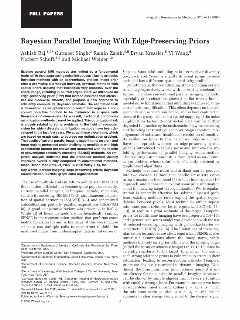
FIG. 1. Schematic of the pixelwise aliasing process for a single pairof aliasing pixels p and p, for 2� acceleration using three coils. Thealiased observations Yl are obtained by a weighted sum of thealiasing pixels, weighted by coil sensitivity values Sl. To simplify thefigure, aliasing is shown in the horizontal direction. [Color figure canbe viewed in the online issue, which is available at www.interscience.wiley.com.]

Parallel Imaging Using Graph Cuts 9

of all pixels of the image, and vector y contains the aliasedimages “seen” by the receiver coils. Matrix E encodes coilsensitivity responses and is a L � R block-diagonal matrixof the form shown in Fig. 2.

SENSE takes a least-squares approach via the pseudo-inverse of E:

x̂SENSE � �EHE��1EHy [4]

This is the maximum-likelihood estimate under the as-sumption of additive white Gaussian noise (28). Unfortu-nately, inverse problems of this form become progressivelyill-posed with increasing acceleration, leading to noiseamplification and insufficient de-aliasing in many cases.To reduce these effects and stabilize the inversion inSENSE, a Tikhonov-type regularization is introduced(10,13):

x̂regSENSE � arg minx

�Ex � y�2 � �2�A�x � xr��2� [5]

where the first term enforces agreement with observeddata, and the second penalizes nonsmooth solutionsthrough an appropriate matrix A and some prior referenceimage xr. Its closed-form solution is

x̂regSENSE � xr � �EHE � �2AHA��1EH�y � Exr� [6]

Equations [4] and [6] can both be computed very quicklyfor the Cartesian case because they readily break up intoindependent L � R sub-problems (for the standard choice

of A � I, the identity matrix). If there is no reference image(i.e., xr � 0), then with A � I this computes the minimumnorm solution (11), while more general Tikhonov forms ofA impose global smoothness.

Bayesian Reconstruction

Even with regularization there is a noise/unfolding limit. If� is too small, there will be insufficient noise reduction. If� is too high, noise will be removed but residual aliasingwill occur. This fundamental aliasing/noise limit cannotbe overcome unless more information about the data isexploited. This naturally suggests a Bayesian approach,which was the subject of a recent work (29). Given theimaging process (Eq. [3]), observation y, and the priorprobability distribution Pr(x) of the target image x, Bayes-ian methods maximize the posterior probability:

Pr�x�y� Pr�y�x� � Pr�x� [7]

The first right-hand term, called the likelihood function,comes from the imaging model (Eq. [3]), and the secondterm is the prior distribution. In the absence of a prior, thisreduces to maximizing the likelihood, as performed bySENSE. Assuming that n � y � Ex is white Gaussian noise,Eq. [3] implies a simple Gaussian distribution for Pr(y/x):

Pr�y�x� e��y�Ex�2 [8]

Similarly, we can write the prior, without loss of gener-ality, as

Pr�x� e�G�x� [9]

Depending on the term G(x), this form can succinctlyexpress both the traditional Gaussianity and/or smooth-ness assumptions, as well as more complicated but pow-erful Gaussian or Gibbsian priors modeled by Markov ran-dom fields (MRFs) (23,24). The posterior is maximized by

x̂MAP � � arg minx

��y � Ex�2 � G�x�� [10]

which is the maximum a posteriori (MAP) estimate. Con-ventional image priors impose spatial smoothness; hence,this can be viewed as the sum of a data penalty and asmoothness penalty. The data penalty forces x to be com-patible with the observed data, and the smoothness pen-alty G(x) penalizes solutions that lack smoothness. Tradi-tionally, only smoothness penalties of the kind G(x) ��Ax�2 have been used, where A is a linear differentialoperator. This corresponds to Eq. [6] if the reference imagexr � 0, and is commonly known as Tikhonov regulariza-tion (28).

However, this smoothness penalty assumes that intensi-ties vary smoothly across the entire image. Such an as-sumption is inappropriate for most images because al-though most image data change smoothly, they have dis-continuities at object boundaries. As a result, theTikhonov smoothness penalty causes excessive edge blur-ring, while we seek an edge-preserving G. To illustrate

FIG. 2. The L � R block-diagonal structure of matrix E. Eachsub-block sensitivity-encodes one aliasing band in the image. Ma-trix E is a concatenation over all coil outputs, as shown by the coillabels. [Color figure can be viewed in the online issue, which isavailable at www.interscience.wiley.com.]

10 Raj et al.

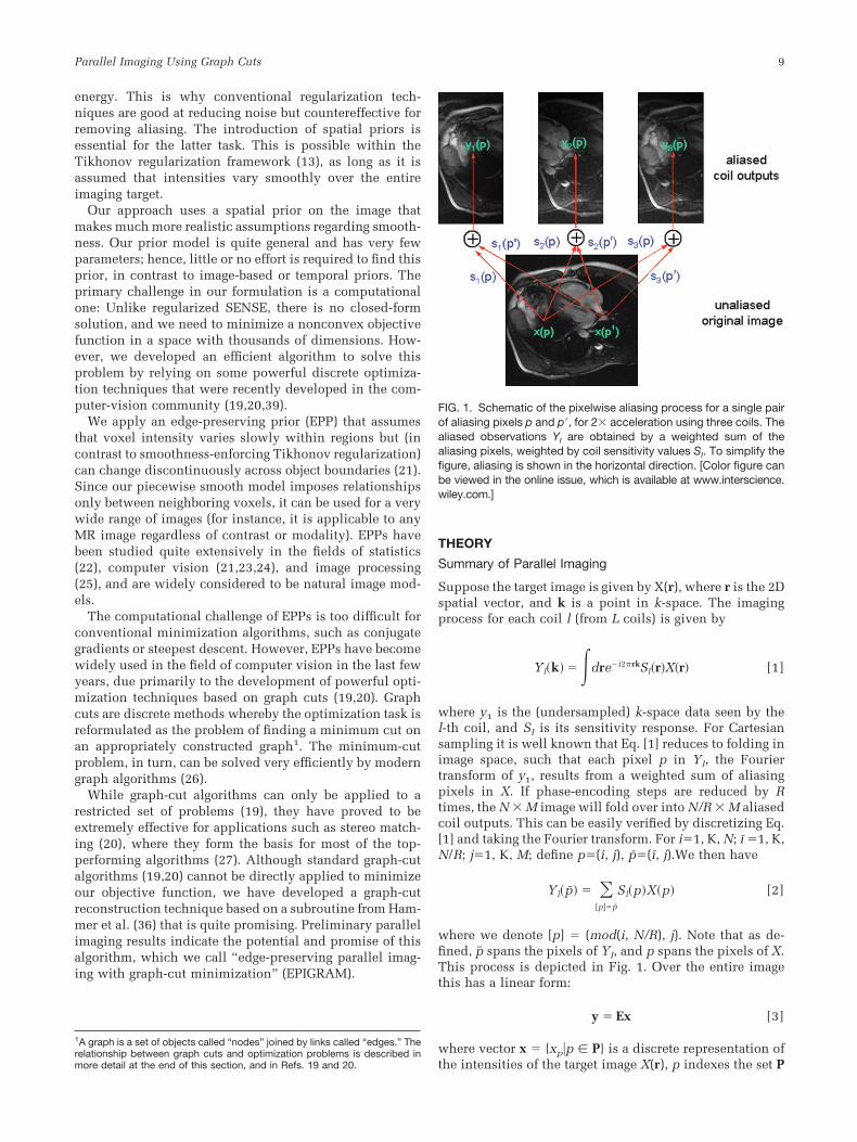
this, we show in Fig. 3 a single noisy image row and twopossible strategies to denoise it. The difference in perfor-mance between global smoothing (obtained by Gaussianblurring) and edge-preserving smoothing (via median fil-tering) is obvious: although both denoise the signal, oneoversmooths sharp transitions while the other largely pre-serves them.

EPPs in MRI

A natural class of edge-preserving smoothness penalties is

GEP�x� � ��p,q��Nss

V�xp, xq� [11]

The spatial neighborhood system Ns consists of pairs ofadjacent pixels, usually the eight-connected neighbors.The separation cost V(xp, xq) gives the cost to assign in-tensities xp and xq to neighboring pixels p and q, and the

form of this prior can be justified in terms of MRFs (23).Typically, V has a nonconvex form, such as V(xp, xq) � �min(�xp � xq�, K), for some metric � � � and constants K, �.Such functions effectively assume that the image is piece-wise smooth rather than globally smooth. Figure 4 showstwo possible choices of V: the right one preserves edges,and the left one does not. For MR data the truncated linearmodel appears to work best, and seems to present the bestbalance between noise suppression (due to the linear part)and edge-preservation (due to truncation of penalty func-tion). Therefore, neighboring intensity differences withinthe threshold K will be treated as noise and penalizedaccordingly. However, larger differences will not be fur-ther penalized, since they occur, most likely, from thevoxels being separated by an edge. Note that this is verydifferent from using a traditional convex distance, such asthe L2 norm, which effectively forbids two adjacent pixelsfrom having very different intensities, for the separationcost. Although the L2 separation cost does not preserveedges, it is widely used because its convex nature vastlysimplifies the optimization problem.

A possible problem with the truncated linear penalty isthat it can lead to some loss of texture, since the Bayesianestimate will favor images with piecewise smooth areasover those with textured areas. In the Discussion we pointout examples of this feature and suggest ways to mitigateit.

Parallel Imaging As Optimization

The computational problem we face is to efficiently min-imize

�y � Ex�2 � GEP�x� [12]

From Ref. 4 we know that E has a diagonal block structureand decomposes into separate interactions between Raliasing voxels, according to Eq. [2]. Let us first define foreach pixel p� � (ı�, j) in Yl the set of aliasing pixels in X thatcontribute to Yl (p� ), as follows: For image X of size M � Nundergoing R-fold acceleration, aliasing occurs only in thephase-encode direction, between aliasing pixels. Then

�y � Ex�2 � �p̄

�l�Yl�p̄� � �

�p��p̄

Sl�p�xp�2

[13]

FIG. 3. Typical performance of edge-preserving and edge-blurringreconstruction on a noisy image row. Image b was obtained byglobally smoothing via a Gaussian kernel, and image c was ob-tained with an edge-preserving median filter. [Color figure can beviewed in the online issue, which is available at www.interscience.wiley.com.]

FIG. 4. Two natural separation cost functions forspatial priors. The L2 cost on the left usually causesedge blurring due to an excessive penalty for high-intensity differences, whereas the truncated linearpotential on the right is considered to be edge-preserving and robust. For MR data, the truncatedlinear model appears to work best. While the L2

separation cost does not preserve edges, its con-vex nature vastly simplifies the optimization prob-lem.


This can be intuitively understood by examining the alias-ing process depicted in Fig. 1. After some rearrangement,this expands to

�y � Ex�2 � �p̄

�l

Yl2�p̄� � �

p��

l

Sl2�p��xp

2

� 2�p��

l

Sl�p�Yl��p��xp � 2 ��p,p��Na

��l

Sl�p�Sl�p��xpxp

[14]

where we define the aliasing neighborhood set Na � {(p,p), [p] � [p], p � p} over all aliasing pairs. Groupingterms under single pixel and pairwise interactions, we get

�y � Ex�2 � a2 � �p

b�p�xp2 � 2 �

p

c�p�xp

� 2 ��p,p��a

d�p, p�xpxp

for appropriately chosen functions b(p), c(p), and d(p,p).The first term is a constant and can be removed from theobjective function, the next two terms depend only on asingle pixel, and the last term depends on two pixels (bothfrom the aliasing set) at once. This last term, which we willrefer to as a “cross term,” arises due to the nondiagonalform of our system matrix E.

To perform edge-preserving parallel imaging, we need tominimize our objective function:

Ex) � a2 � �p

b�p�xp2 � 2 �

p

c�p�xp � 2 ��p,p��a

d�p, p�xpxp

� ��p,q��s

V�xp, xq� [15]

Let us first consider the simpler case of our objectivefunction that would arise if E were diagonal. In this casethere would be no cross terms (i.e., d(p,p) � 0), whichappears to simplify the problem considerably. Yet eventhis simplification results in a difficult optimization prob-lem. There is no closed-form solution, the objective func-tion is highly nonconvex, and the space over which we areminimizing has thousands of dimensions (one dimensionper pixel). Worse still, minimizing such an objective func-tion is almost certain to require an exponentially largenumber of steps2.

If E were diagonal, however, the objective functionwould be in a form that has been extensively studied in thecomputer-vision field (10,20,27), where significant recentprogress has been made. Specifically, a number of power-ful methods have been designed that employ a discreteoptimization technique called “graph cuts” (20), which webriefly summarize in the next section. Graph cuts are apowerful means of minimizing E(x) in Eq. [15], and can be

easily applied as long as E is diagonal (19). The presence ofoff-diagonal entries in E gives rise to cross terms in ourobjective function, making traditional graph-cut algo-rithms (19,20) inapplicable, and requires an extension, asdescribed in Materials and Methods.

Optimization With Graph Cuts

One can minimize objective functions similar to Eq. [15]by computing the minimum cut in an appropriately de-fined graph using the graph-cut technique. This techniquewas first used for images by Greig et al. (30), who used it tooptimally denoise binary images. A recent series of papers(19,20) extended the method significantly, and it can nowbe used for problems such as stereo matching (20,31) andimage/video synthesis (32) in computer vision, as well asmedical image segmentation (33) and fMRI data analysis(34).

The basic idea is to first discretize the continuous pixelintensities xp into a finite discrete set of labels L � {1, K,Nlabels}. Since we focus on MR reconstruction problems,we will assume that the labels are always intensities anduse the terms interchangeably; however, graph-cut algo-rithms are employed for a wide variety of problems incomputer vision and graphics, and often use labels with amore complex meaning. Then instead of minimizing overcontinuous variables xp, we minimize over individual la-bels � � L, allowing any pixel in the image to take the label�. In practice the dynamic range of intensities may have tobe reduced for computational purposes, although this isnot a requirement of our technique. The most powerfulgraph-cut method is based on expansion moves. Given alabeling x � {xp�p � P} and a label �, an �-expansion � �{�p�p�P} is a new labeling whereby �p is either xp or �.Intuitively, one constructs � from x by giving some set ofpixels the label �. The expansion-move algorithm picks alabel �, finds the lowest cost �, and moves there. This ispictorially depicted in Fig. 5.

The algorithm converges to a labeling where there is no�-expansion that reduces the value of the objective func-tion E for any �. The key subroutine in the expansion movealgorithm is to compute the �-expansion � that minimizesE. This can be viewed as an optimization problem overbinary variables, since during an �-expansion each pixeleither keeps its old label or moves to the new label �. Thisis also shown in Fig. 5. An �-expansion � is equivalent toa binary labeling

�p � xp iff bp � 0� iff bp � 1 [16]

Just as for a labeling � there is an objective function E, fora binary labeling b there is an objective function B. Moreprecisely, assuming � is equivalent to b, we define B by

B�b� � E��

We have dropped the arguments x, � for clarity, but theequivalence between the �-expansion � and the binarylabeling b clearly depends on the initial labeling x andon �.

2More precisely, it was shown in Ref. 20 to be NP-hard, which means that itis in a class of problems that are widely believed to require exponential timein the worst case.

12 Raj et al.

In summary, the problem of computing the �-expansionthat minimizes E is equivalent to finding the b that mini-mizes the binary objective function B. The exact form of Bwill depend on E. The minimization of E proceeds viasuccessive binary minimizations corresponding to expan-sion moves. The binary minimization subroutine is some-what analogous to the role of line-searching in the conju-gate-gradient algorithm, where a local minimum is repeat-edly computed over different 1D search spaces. Withgraph cuts, however, the binary subroutine efficientlycomputes the global minimum over 2�P� candidate solu-tions, where �P� is the number of pixels in the image.Therefore, in contrast to traditional minimization algo-rithms, such as conjugate gradients, trust region, simulatedannealing, etc. (28), graph cuts can efficiently optimizehighly nonconvex objective functions that arise from edge-preserving penalties (19).

Consider a binary objective function of the form

B�b� � �p

B1�bp� � �p,q

B2�bp, bq� [17]

Here B1 and B2 are functions of binary variables. Thedifference is that B1 depends on a single pixel, while B2

depends on pairs of pixels. Graph-cut methods minimize Bby reducing the computation of a minimum cut on anappropriately constructed graph. The graph consists ofnodes that are voxels of the image as well as two specialterminal nodes, as shown in Fig. 6. The voxel nodes arelabeled p, q, r, etc., and terminal nodes are indicated as Sand T. All nodes are connected to both terminals via edges,each of which have weights obtained from the B1 termsabove. Nodes are also connected to each other via edgeswith weights obtained from the pairwise interactionterm B2.

One can solve the binary optimization problem by find-ing the minimum cut on this graph (20). A cut is defined asa partition of the graph into two connected subgraphs,each of which contains one terminal. The minimum cutminimizes the sum of the weights of the edges between thesubgraphs. Fast algorithms to find the minimum cut usingmax-flow methods (26) are available. It was shown in Ref.19 that the class of B that can be can be minimized exactlyby computing a minimum cut on such a graph satisfies thecondition

B2�0, 0� � B2�1, 1� � B2�1, 0� � B2�0, 1� [18]

If B2(x, y) satisfies Eq. [18], then it is said to be “submodu-lar” with respect to x and y, and a function B is calledsubmodular if it consists entirely of submodular terms3.Single-variable terms of the form of B1 are always sub-modular. We will refer to the set of all pixel pairs forwhich B2(bp, bq) are submodular as the submodular set S.

Previous applications of graph cuts were designed fordiagonal E. This leads to no cross terms, and thus B1 comessolely from the data penalty and B2 comes only from thesmoothness penalty. It was shown in Ref. 20 that if theseparation cost is a metric, then B2 satisfies Eq. [18]. Manyedge-preserving separation costs are metrics, including thetruncated cost V used here and shown in Fig. 2b (see Ref.20 for details). However, the situation is more complicatedin parallel MR reconstruction, where E is nondiagonal. As

3Some authors (21) use the term “regular” instead of “submodular.”

FIG. 6. Graph construction to minimize a given binary objectivefunction. The graph consists of nodes corresponding to imagevoxels, as well as two special “terminal” nodes S and T. Edgesbetween nodes represent single-voxel (B1) and pairwise (B2) costterms. A minimum cut on this graph solves the binary minimizationproblem. [Color figure can be viewed in the online issue, which isavailable at www.interscience.wiley.com.]

FIG. 5. The expansion move algorithm. Start with the initial labeling of the image shown by different shades “light”, “medium” and “dark”in (a), assuming only 3 labels. Note that here labels correspond to intensities, although this need not be the case in general. First find theexpansion move on the label “dark” that most decreases objective function E, as shown in (b). Move there, then find the best “light”expansion move, etc. Done when no a-expansion move decreases the cost, for any label �. Corresponding to every expansion move (b)is a binary image (c), where each pixel is assigned 1 if its label changes, and 0 if it does not.


a result, the data penalty has pairwise interactions due tothe presence of the cross terms d(p, p) in Eq. [15]. Thisalso follows from Fig. 1, which shows how this data pen-alty arises from the joint effect of both aliasing voxels pand p in the image.

It was previously shown (35) that the binary optimiza-tion problem arising from Eq. [15] is in general submodu-lar only for a small subset of all cross terms. This necessi-tates the use of a subroutine (from Ref. 36) to accommodatecross terms arising in MR reconstruction, as described inthe next section.

MATERIALS AND METHODS

New MR Reconstruction Algorithm Based on Graph Cuts

The subroutine we use to find a good expansion move isclosely related to relaxation methods for solving integerprogramming problems (26). In these methods, if the linearprogramming solution obeys the integer constraints, itsolves the original integer problem. We compute an expan-sion move by applying the algorithm of Hammer et al. (36),which was introduced in the field of computer vision inearly 2005 by Kolmogorov and Rother (39). The theoreticalanalysis and error bounds presented in Ref. 40 help ex-plain the strong performance of this construction for MRreconstruction.

For each pixel p, we have a binary variable bp that is 1 ifp acquired the new label �, and 0 otherwise. We introducea new binary variable b̃p, which has the opposite interpre-tation (i.e., it will be 0 if p acquires the new label �, and 1otherwise). We call a pixel “consistent” if b̃p � 1 � bp .Instead of our original objective function B(b), we mini-mize a new objective function B̃(b, b̃), where b̃ is the set ofnew binary variables b̃ � {b̃p�p�P}. B̃(b, b̃) is constructedso that b̃ � 1 � bf B̃(b, b̃) � B(b) (in other words, if everypixel is consistent, the new objective function will be thesame as the old one). Specifically, we define our newobjective function by

2 � B̃�b, b̃� � �p

�B1�bp� � B1�1 � b̃p�� p,q��

�B2�bp, bq�

� B2�1 � b̃p, 1 � b̃q�� p,q��S

�B2�bp, 1 � b̃q�

� B2�1 � b̃p, bq�� [19]

Here the functions B1( � ) and B2( � ) come from our originalobjective function B in Eq. [17].

Importantly, our new objective function B̃(b, b̃) is sub-modular. The first summation only involves B1( � ), whilefor the remaining two terms simple algebra shows that

B2�b, b� is submodularf B2�1 � b, 1 � b� is submodularB2�b, b� is non-submodularf both B2�b, 1 � b�

and B2�1 � b, b� are submodular

As a result, the last two summations in Eq. [19] containonly submodular terms. Thus B̃(b, b̃) is submodular, andcan be easily minimized using the binary graph-cut sub-routine. In summary, minimizing B̃(b, b̃) is exactly equiv-

alent to minimizing our original objective function B, aslong as we obtain a solution in which every pixel is con-sistent. We note that our technique is not specific to MRreconstruction, but can compute the MAP estimate of anarbitrary linear inverse system under an edge-preservingprior GEP.

While we cannot guarantee that all pixels are consistent,in practice this is true for the vast majority of pixels (typ-ically well over 95%). In our algorithm we simply allowpixels that are not consistent to keep their original labelsrather than acquire the new label �. However, even if thereare pixels that are not consistent, this subroutine has someinteresting optimality properties. It is shown in Ref. 36that any pixel that is consistent is assigned its optimallabel. As a result, our algorithm finds the optimum expan-sion move for the vast majority of pixels.

Convergence Properties

We investigated the convergence properties of the pro-posed technique using simulated data from a Shepp-Loganphantom, with intensities quantized to integer values be-tween 0 and 255. We computed the objective function (Eq.[15]) achieved after each iteration for 3� acceleration andeight coils.

In Vivo Experiments: Setup and Parameters

High-field-strength (4 Tesla) structural MRI brain datawere obtained using a whole-body scanner (Bruker/Sie-mens Germany) equipped with a standard birdcage, eight-channel, phased-array, transmit/receive head coil local-ized cylindrically around the superior–inferior (S-I) axis.Volumetric T1-weighted images (1 � 1 � 1 mm3 resolu-tion) were acquired using a magnetization-prepared rapidgradient-echo (MPRAGE) sequence with TI/TR � 950/2300 ms timing and a flip angle of 8°. The total acquisitiontime for an unaccelerated data set was about 8:00 min. Ina separate study, images of the torso region were acquiredusing a gradient-echo sequence with a flip angle of 60° andTE/TR of 3.3/7.5 ms on a GE 1.5T Excite-11 system. Sev-eral axial and oblique slices of full-resolution data (256 �256) were acquired with an eight-channel upper body coilarranged cylindrically around the torso.

To allow quantitative and qualitative performance eval-uations, we acquired all data at full resolution and with noacceleration. The aliased images for acceleration factors of3–5 were obtained by manually undersampling in k-space.In each case we also computed the full rooted sum ofsquares (RSOS) image after dividing the coil data by therelative sensitivity maps obtained from calibration lines.We used the self-calibrating strategy for sensitivity estima-tion, whereby the center of k-space is acquired at fulldensity and used to estimate low-frequency (relative) sen-sitivity maps. We used the central 40 densely sampledcalibration lines for this purpose. These lines were multi-plied by an appropriate Kaiser-Bessel window to reduceringing and noise, zero-padded to full resolution, andtransformed to the image domain. We estimated the rela-tive sensitivity by dividing these images by their RSOS. Toavoid division by zero, we introduced a small threshold inthe denominator, which amounted to 5% of the maximum

14 Raj et al.

intensity. This also served effectively to make the sensi-tivity maps have zero signal in background regions. How-ever, further attempts to segment background/foregroundfrom these low-frequency data proved unreliable in somecases, and we did not implement background segmenta-tion.

Algorithmic parameters were chosen empirically. It wassufficient to quantize intensity labels to Nlabels � 256,since the resulting quantization error is much smaller thanobserved noise. Since the computational cost of EPIGRAMgrows linearly with Nlabels, fewer labels are preferable.Model parameters were varied (geometrically) over therange K � [Nlabels/20, Nlabels/2], � � [0.01 � max(x),1 � max(x)] to find the best values. However, we found thatthe performance was rather insensitive to these choices,and therefore used the same parameters for all casesshown in this paper. Graph-cut algorithms are typicallyinsensitive to initialization issues, and we chose the zeroimage as an initial guess. All reconstructions were ob-tained after 20 iterations. Regularized SENSE reconstruc-tion was for comparison with our method. We chose theregularization factor � after visually evaluating imagequality with a large range of values in the region � � [0.01,0.6]. The images that gave the best results are shown in thenext section, along with those obtained with a higherregularization. We obtained the latter to observe the noisevs. aliasing performance of SENSE.

Quantitative Performance Evaluation

In addition to the visual evidence presented in the nextsection, we conducted a quantitative performance evalua-tion of the reconstructed in vivo data. For in vivo data theproblem of ascertaining noise estimates or other perfor-mance measures is challenging due to the nonavailabilityof an accurate reference image. Unfortunately, none of thereconstruction methods we implemented (RSOS, regular-ized SENSE, and EPIGRAM) are unbiased estimators of thetarget. This makes it difficult to directly estimate noiseperformance, and the traditional root mean square error(RMSE) becomes inadequate. We follow instead a recentevaluation measure for parallel imaging methods proposedby Reeder et al. (37), which provides an unambiguous andfair comparison of SNR and geometry factor. Two separatescans of the same target with identical settings are ac-quired, and their sum and difference are obtained. Thelocal signal level at each voxel is computed by averagingthe sum image over a local window, and the noise level isobtained from the standard deviation (SD) of the differenceimage over the same window. Then

SNR �mean�Sum image�

2 stdev�Diff image�

Here the mean and SD are understood to be over a localwindow (in this case a 5 � 5 window around the voxel inquestion). This provides unbiased estimates that are di-rectly comparable across different reconstruction meth-ods. We perform a similar calculation, with a crucial dif-ference: instead of acquiring two scans, we use a singlescan but add random uncorrelated Gaussian noise in the

coil outputs to obtain two noisy data sets. This halves theacquisition effort without compromising estimate quality,since uncorrelated noise is essentially what the two-scanmethod also measures. Reeder et al. (37) explained thattheir method can be erroneous for in vivo data becausemotion and other physiological effects can seriously de-grade noise estimates. While our modification achieves thesame purpose, it does not suffer from this problem, andhence should be more appropriate for in vivo data. TheSNR calculation also allows the geometry factor, or g-factor, maps for each reconstruction method to be ob-tained. For each voxel p and acceleration factor R:

g�p, R� �SNRRSOS�p�

SNR�p�R

where SNRRSOS is the SNR of the RSOS reconstruction.The SNR and g-map images appeared quite noisy due tothe division step and estimation errors, and we had tosmooth them for better visualization.

Comparing EPIGRAM and Regularized SENSE

SNR and g-factor maps obtained by the method describedby Reeder et al. (37) and above are well suited for unbiasedreconstructions like unregularized SENSE because theyprovide comparable measures of noise amplification.Reeder et al. (37) demonstrated conclusively that the two-scan method gives comparable estimates to those obtainedvoxelwise by using hundreds of identical scans. Unfortu-nately, neither the SNR nor the g-factor can serve as asingle measure of performance in the case of biased recon-structions like regularized SENSE and EPIGRAM, or in-deed any Bayesian estimate. This is because there are nowtwo quite different sources of degradation: noise amplifi-cation and aliasing. While the former can be measuredaccurately by SNR and g-maps using the above technique,the latter cannot. All regularization or Bayesian ap-proaches come with external parameters, which can bethought of as “knobs” available to the user (� for SENSEand � for EPIGRAM). Depending on how much the usertweaks those knobs, it is possible to achieve any desireddegree of noise performance. To illustrate this, we show inthe Results section the effect of �, the regularization pa-rameter in SENSE. We demonstrate that any desired g-factor can be achieved by making � large enough. There-fore, for a proper comparison of reconstruction methods, itis important to fix either aliasing quality or noise quality,and then compare the other measure. In this section weadopt the following approach: we turn the “knobs” untilboth EPIGRAM and regularized SENSE produce approxi-mately similar g-maps and mean g-values. We then visu-ally evaluate how each method performed in terms ofaliasing and overall reconstruction quality. In each casewe tabulate the mean SNR and g-values achieved by thegiven settings. The results are given below.

RESULTS

Convergence Result

The convergence behavior of the objective function (Eq.[15]) against the number of iterations for R � 3, L � 8 is


shown in Fig. 7. As is typical of graph-cut algorithms (31),most of the improvement takes place in the first few (ap-proximately five) iterations. In our initial implementationof EPIGRAM, which was written primarily in MATLAB,an iteration takes about 1 min on this data set. SinceEPIGRAM is almost linear in the number of nodes, the

total running time approximately scales as N2, the imagesize.

In Vivo Results

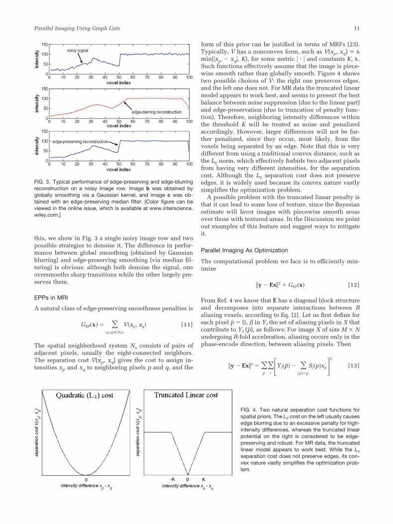
The best parameter values were consistent across all invivo data sets we tried: K � Nlabels/7, � � 0.04 � max(x).The results of several brain imaging experiments withthese parameter values are displayed in Figs. 8 and 9.Figure 8 shows the reconstruction of a MPRAGE scan of acentral sagittal slice, with an undersampling factor R � 4along the anterior–posterior (A-P) direction. The RSOSreference image is shown in Fig. 8a, regularized SENSEwith (empirically obtained optimal) � � 0.08 is shown inb, regularized SENSE with � � 0.16 is shown in c, andEPIGRAM is shown in d. Reduced noise is visually notice-able in the EPIGRAM reconstruction compared to bothSENSE reconstructions. Higher regularization in SENSEcaused unacceptable aliasing, as observed in Fig. 8c. Wenote that the unregularized (i.e., standard) SENSE resultswere always worse than those of regularized SENSE, andconsequently are not shown. Another sagittal scan result isshown in Fig. 9, this time from the left side of the patient.Image support is smaller, allowing 5� acceleration. Theoptimally regularized SENSE output (b) with � � 0.1 isnoisy at this level of acceleration, and � � 0.2 (c) intro-duced significant aliasing, especially along the centralbrain region. EPIGRAM (d) exhibits some loss of texture,but on the whole appears to outperform SENSE.

A set of torso images acquired on a GE 1.5T scannerusing a GRE sequence and acceleration factor of 3 (along

FIG. 7. Convergence behavior of the modified graph-cut algorithm(EPIGRAM) for acceleration factor R � 3, L � 8 coils, on GRE torsodata. The vertical axis shows the value of objective function (Eq.[15]) achieved after each outer iteration, which represents a singlecycle through Nlabels � 256 expansion moves. [Color figure can beviewed in the online issue, which is available at www.interscience.wiley.com.]

FIG. 8. Brain A: In vivo brain re-sult with R � 4, L � 8. Views wereacquired vertically. a: Referenceimage. b: SENSE regularized with� � 0.08. c: SENSE regularizedwith � � 0.16. d: EPIGRAM re-construction.

16 Raj et al.

the A-P direction) were resolved from 40 sensitivity cali-bration lines (Fig. 10). Various slice orientations (bothaxial and oblique) were used. These data also show thepractical limitation of SENSE when an inadequate numberof calibration lines are used for sensitivity estimation. Thereconstruction quality of SENSE is poor as a result of thecombination of ill-conditioning of the matrix inverse andcalibration error. SENSE exhibits both high noise and re-sidual aliasing. In fact, what appears at first sight to beuncorrelated noise is, upon finer visual inspection, foundto arise from unresolved aliases, as the background in Fig.10b clearly indicates. EPIGRAM was able to resolve alias-ing correctly and suppress noise, without blurring sharpedges and texture boundaries. To demonstrate the perfor-mance of these methods more clearly, we show in Fig.10d–f zoomed-in versions of the images in Fig. 10a–c.

Next we demonstrate the trade-off between noise andaliasing performance. Figure 11 shows another torso slicealong with associated g-maps computed as specified inMaterials and Methods. We investigate the effect of vari-ous regularizations of SENSE. The leftmost column (a ande) shows the SENSE result and its g-map for � � 0.1.Clearly, there is inadequate noise suppression (some re-gions of the image have a g-factor as high as 6). It is easy toreduce noise amplification by increasing regularization. In

the next column, results for � � 0.3 are shown. The g-maphas become correspondingly flatter, but the reconstructionindicates that this was achieved at the cost of introducingsome aliasing in the image. The rightmost column showsEPIGRAM results, which indicate significantly lower g-values and lower aliasing artifacts. In the third column weshow that with an appropriate choice of � it is possible tomatch the EPIGRAM g-map (c.f., Fig. 11g and h). However,with this choice of � � 0.5, SENSE yields unacceptablealiasing. Table 1 shows the mean SNR and g-factor valuesfor EPIGRAM and various regularizations of SENSE.

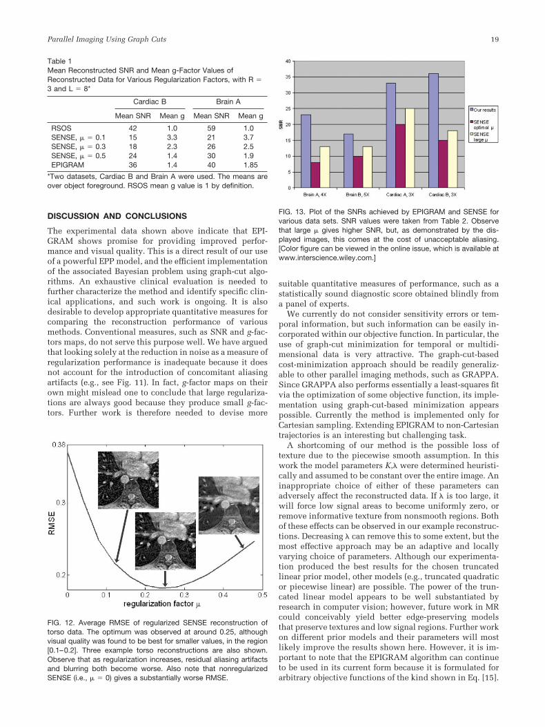
We observe that the regularization needed in SENSE tomatch the EPIGRAM g-values (approximately � � 0.5 inalmost all cases) yields unacceptable aliasing. Instead, amore modest � must be chosen empirically. The standardRMSE criterion does not really help here. In Fig. 12 weplot the average over all our torso data of the RMSE forvarious regularization factors. For this data set, the opti-mum � in terms of RMSE was found to be around 0.25,although in practice the best visual quality was observedbelow this value, at around 0.1–0.15. This suggests thatthe RMSE measure does not capture reconstruction qualityvery accurately, and in particular seems to underempha-size the effect of residual aliasing. In all experimental datashown in this section, the optimum regularization for

FIG. 9. Brain B: In vivo brain re-sult with R � 5, L � 8. Views wereacquired vertically. a: Referenceimage. b: SENSE regularized with� � 0.1. c: SENSE regularizedwith � � 0.2. d: EPIGRAM recon-struction.


SENSE was obtained empirically for each data set by vi-sual inspection as much as possible. To give an idea of thevisual quality corresponding to a certain � value, Fig. 12also shows a portion of the resulting SENSE reconstruc-tion. The mean SNRs and g-factors for all reconstructionexamples presented here are summarized in Table 2. Non-regularized SENSE data are not shown, because they werealways worse than regularized SENSE data.

In all of these examples there are regions in the EPI-GRAM data with some loss of texture, as well as regions oflow signal that appear to have been “washed out” by auniform value. Both effects result from the piecewisesmooth assumption imposed by the prior. We discussways to mitigate this problem below, but note that it istypical of most applications in which MRF priors are ap-plied.

FIG. 10. Cardiac A: In vivo result with R � 3, L � 8. Views were acquired horizontally. a: Reference image. b: SENSE regularized with � �0.16 (optimal). c: EPIGRAM reconstruction. Zoomed-in portions of a–c are shown in d–f.

FIG. 11. Cardiac B: In vivo result with R � 3, L � 8, showing the effect of regularization on g-factor maps. Views were acquired horizontally.a and e: SENSE reconstruction and its g-map for � � 0.1. There is inadequate noise suppression, with a g-factor as high as 6. Results for� � 0.3 are shown in b and f. The g-maps has become correspondingly flatter, but at the cost of aliasing. The rightmost column (d andh) shows EPIGRAM results, which indicate significantly lower g-values as well as lower aliasing artifacts. SENSE with � � 0.5 (c and g)matches the EPIGRAM g-map but yields unacceptable aliasing.

18 Raj et al.

DISCUSSION AND CONCLUSIONS

The experimental data shown above indicate that EPI-GRAM shows promise for providing improved perfor-mance and visual quality. This is a direct result of our useof a powerful EPP model, and the efficient implementationof the associated Bayesian problem using graph-cut algo-rithms. An exhaustive clinical evaluation is needed tofurther characterize the method and identify specific clin-ical applications, and such work is ongoing. It is alsodesirable to develop appropriate quantitative measures forcomparing the reconstruction performance of variousmethods. Conventional measures, such as SNR and g-fac-tors maps, do not serve this purpose well. We have arguedthat looking solely at the reduction in noise as a measure ofregularization performance is inadequate because it doesnot account for the introduction of concomitant aliasingartifacts (e.g., see Fig. 11). In fact, g-factor maps on theirown might mislead one to conclude that large regulariza-tions are always good because they produce small g-fac-tors. Further work is therefore needed to devise more

suitable quantitative measures of performance, such as astatistically sound diagnostic score obtained blindly froma panel of experts.

We currently do not consider sensitivity errors or tem-poral information, but such information can be easily in-corporated within our objective function. In particular, theuse of graph-cut minimization for temporal or multidi-mensional data is very attractive. The graph-cut-basedcost-minimization approach should be readily generaliz-able to other parallel imaging methods, such as GRAPPA.Since GRAPPA also performs essentially a least-squares fitvia the optimization of some objective function, its imple-mentation using graph-cut-based minimization appearspossible. Currently the method is implemented only forCartesian sampling. Extending EPIGRAM to non-Cartesiantrajectories is an interesting but challenging task.

A shortcoming of our method is the possible loss oftexture due to the piecewise smooth assumption. In thiswork the model parameters K,� were determined heuristi-cally and assumed to be constant over the entire image. Aninappropriate choice of either of these parameters canadversely affect the reconstructed data. If � is too large, itwill force low signal areas to become uniformly zero, orremove informative texture from nonsmooth regions. Bothof these effects can be observed in our example reconstruc-tions. Decreasing � can remove this to some extent, but themost effective approach may be an adaptive and locallyvarying choice of parameters. Although our experimenta-tion produced the best results for the chosen truncatedlinear prior model, other models (e.g., truncated quadraticor piecewise linear) are possible. The power of the trun-cated linear model appears to be well substantiated byresearch in computer vision; however, future work in MRcould conceivably yield better edge-preserving modelsthat preserve textures and low signal regions. Further workon different prior models and their parameters will mostlikely improve the results shown here. However, it is im-portant to note that the EPIGRAM algorithm can continueto be used in its current form because it is formulated forarbitrary objective functions of the kind shown in Eq. [15].

FIG. 12. Average RMSE of regularized SENSE reconstruction oftorso data. The optimum was observed at around 0.25, althoughvisual quality was found to be best for smaller values, in the region[0.1–0.2]. Three example torso reconstructions are also shown.Observe that as regularization increases, residual aliasing artifactsand blurring both become worse. Also note that nonregularizedSENSE (i.e., � � 0) gives a substantially worse RMSE.

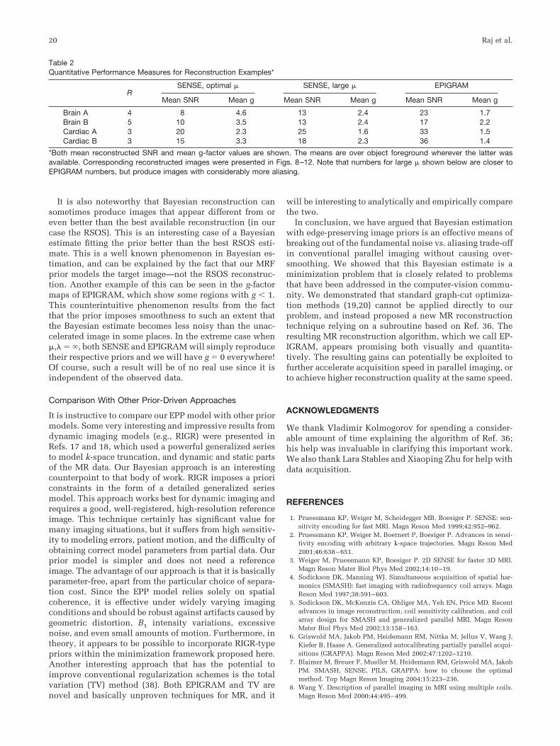
FIG. 13. Plot of the SNRs achieved by EPIGRAM and SENSE forvarious data sets. SNR values were taken from Table 2. Observethat large � gives higher SNR, but, as demonstrated by the dis-played images, this comes at the cost of unacceptable aliasing.[Color figure can be viewed in the online issue, which is available atwww.interscience.wiley.com.]

Table 1Mean Reconstructed SNR and Mean g-Factor Values ofReconstructed Data for Various Regularization Factors, with R �3 and L � 8*

Cardiac B Brain A

Mean SNR Mean g Mean SNR Mean g

RSOS 42 1.0 59 1.0SENSE, � � 0.1 15 3.3 21 3.7SENSE, � � 0.3 18 2.3 26 2.5SENSE, � � 0.5 24 1.4 30 1.9EPIGRAM 36 1.4 40 1.85

*Two datasets, Cardiac B and Brain A were used. The means areover object foreground. RSOS mean g value is 1 by definition.


It is also noteworthy that Bayesian reconstruction cansometimes produce images that appear different from oreven better than the best available reconstruction (in ourcase the RSOS). This is an interesting case of a Bayesianestimate fitting the prior better than the best RSOS esti-mate. This is a well known phenomenon in Bayesian es-timation, and can be explained by the fact that our MRFprior models the target image—not the RSOS reconstruc-tion. Another example of this can be seen in the g-factormaps of EPIGRAM, which show some regions with g � 1.This counterintuitive phenomenon results from the factthat the prior imposes smoothness to such an extent thatthe Bayesian estimate becomes less noisy than the unac-celerated image in some places. In the extreme case when�,� � �, both SENSE and EPIGRAM will simply reproducetheir respective priors and we will have g � 0 everywhere!Of course, such a result will be of no real use since it isindependent of the observed data.

Comparison With Other Prior-Driven Approaches

It is instructive to compare our EPP model with other priormodels. Some very interesting and impressive results fromdynamic imaging models (e.g., RIGR) were presented inRefs. 17 and 18, which used a powerful generalized seriesto model k-space truncation, and dynamic and static partsof the MR data. Our Bayesian approach is an interestingcounterpoint to that body of work. RIGR imposes a prioriconstraints in the form of a detailed generalized seriesmodel. This approach works best for dynamic imaging andrequires a good, well-registered, high-resolution referenceimage. This technique certainly has significant value formany imaging situations, but it suffers from high sensitiv-ity to modeling errors, patient motion, and the difficulty ofobtaining correct model parameters from partial data. Ourprior model is simpler and does not need a referenceimage. The advantage of our approach is that it is basicallyparameter-free, apart from the particular choice of separa-tion cost. Since the EPP model relies solely on spatialcoherence, it is effective under widely varying imagingconditions and should be robust against artifacts caused bygeometric distortion, B1 intensity variations, excessivenoise, and even small amounts of motion. Furthermore, intheory, it appears to be possible to incorporate RIGR-typepriors within the minimization framework proposed here.Another interesting approach that has the potential toimprove conventional regularization schemes is the totalvariation (TV) method (38). Both EPIGRAM and TV arenovel and basically unproven techniques for MR, and it

will be interesting to analytically and empirically comparethe two.

In conclusion, we have argued that Bayesian estimationwith edge-preserving image priors is an effective means ofbreaking out of the fundamental noise vs. aliasing trade-offin conventional parallel imaging without causing over-smoothing. We showed that this Bayesian estimate is aminimization problem that is closely related to problemsthat have been addressed in the computer-vision commu-nity. We demonstrated that standard graph-cut optimiza-tion methods (19,20) cannot be applied directly to ourproblem, and instead proposed a new MR reconstructiontechnique relying on a subroutine based on Ref. 36. Theresulting MR reconstruction algorithm, which we call EP-IGRAM, appears promising both visually and quantita-tively. The resulting gains can potentially be exploited tofurther accelerate acquisition speed in parallel imaging, orto achieve higher reconstruction quality at the same speed.

ACKNOWLEDGMENTS

We thank Vladimir Kolmogorov for spending a consider-able amount of time explaining the algorithm of Ref. 36;his help was invaluable in clarifying this important work.We also thank Lara Stables and Xiaoping Zhu for help withdata acquisition.

REFERENCES

1. Pruessmann KP, Weiger M, Scheidegger MB, Boesiger P. SENSE: sen-sitivity encoding for fast MRI. Magn Reson Med 1999;42:952–962.

2. Pruessmann KP, Weiger M, Boernert P, Boesiger P. Advances in sensi-tivity encoding with arbitrary k-space trajectories. Magn Reson Med2001;46:638–651.

3. Weiger M, Pruessmann KP, Boesiger P. 2D SENSE for faster 3D MRI.Magn Reson Mater Biol Phys Med 2002;14:10–19.

4. Sodickson DK, Manning WJ. Simultaneous acquisition of spatial har-monics (SMASH): fast imaging with radiofrequency coil arrays. MagnReson Med 1997;38:591–603.

5. Sodickson DK, McKenzie CA, Ohliger MA, Yeh EN, Price MD. Recentadvances in image reconstruction, coil sensitivity calibration, and coilarray design for SMASH and generalized parallel MRI. Magn ResonMater Biol Phys Med 2002;13:158–163.

6. Griswold MA, Jakob PM, Heidemann RM, Nittka M, Jellus V, Wang J,Kiefer B, Haase A. Generalized autocalibrating partially parallel acqui-sitions (GRAPPA). Magn Reson Med 2002;47:1202–1210.

7. Blaimer M, Breuer F, Mueller M, Heidemann RM, Griswold MA, JakobPM. SMASH, SENSE, PILS, GRAPPA: how to choose the optimalmethod. Top Magn Reson Imaging 2004;15:223–236.

8. Wang Y. Description of parallel imaging in MRI using multiple coils.Magn Reson Med 2000;44:495–499.

Table 2Quantitative Performance Measures for Reconstruction Examples*

RSENSE, optimal � SENSE, large � EPIGRAM

Mean SNR Mean g Mean SNR Mean g Mean SNR Mean g

Brain A 4 8 4.6 13 2.4 23 1.7Brain B 5 10 3.5 13 2.4 17 2.2Cardiac A 3 20 2.3 25 1.6 33 1.5Cardiac B 3 15 3.3 18 2.3 36 1.4

*Both mean reconstructed SNR and mean g-factor values are shown. The means are over object foreground wherever the latter wasavailable. Corresponding reconstructed images were presented in Figs. 8–12. Note that numbers for large � shown below are closer toEPIGRAM numbers, but produce images with considerably more aliasing.

20 Raj et al.

9. Raj A, Zabih R. An optimal maximum likelihood algorithm for parallelimaging in presence of sensitivity noise. In: Proceedings of the 12thAnnual Meeting of ISMRM, Tokyo, Japan, 2004 (Abstract 1771).

10. Liang ZP, Bammer R, Ji J, Pelc N, Glover G. Making better SENSE:wavelet denoising, Tikhonov regularization, and total least squares. In:Proceedings of the 10th Annual Meeting of ISMRM, Honolulu, HI,USA, 2002 (Abstract 2388).

11. Lin F, Kwang K, BelliveauJ, Wald L. Parallel imaging reconstructionusing automatic regularization. Magn Reson Med 2004;51:559–567.

12. Bammer R, Auer M, Keeling SL, Augustin M, Stables LA, Prokesch RW,Stollberger R, Moseley ME, Fazekas F. Diffusion tensor imaging usingsingle-shot SENSE-EPI. Magn Reson Med 2002;48:128–136.

13. Ying L, Xu D, Liang ZP. On Tikhonov regularization for image recon-struction in parallel MRI. Proc IEEE EMBS 2004:1056–1059.

14. Tsao J, Boesiger P, Pruessmann KP. K-T BLAST and K-T SENSE:dynamic MRI with high frame rate exploiting spatiotemporal correla-tions. Magn Reson Med 2003;50:1031–1042.

15. Hansen MS, Kozerke S, Pruessmann KP, Boesiger P, Pedersen EM, TsaoJ. On the influence of training data quality in K-T BLAST reconstruc-tion. Magn Reson Med 2004;52:1175–1183.

16. Tsao J, Kozerke S, Boesiger P, Pruessmann KP. Optimizing spatiotem-poral sampling for K-T BLAST and K-T SENSE: application to high-resolution real-time cardiac steady-state free precession. Magn ResonMed 2003;53:1372–1382.

17. Chandra S, Liang ZP, Webb A, Lee H, Morris HD, Lauterbur PC. Ap-plication of reduced-encoding imaging with generalized-series recon-struction (RIGR) in dynamic MR imaging. J Magn Reson Imaging 1996;6:783–797.

18. Hanson JM, Liang ZP, Magin RL, Duerk JL, Lauterbur PC. A comparisonof RIGR and SVD dynamic imaging methods. Magn Reson Med 1997;38:161–167.

19. Kolmogorov V, Zabih R. What energy functions can be minimized viagraph cuts? IEEE Trans Patt Anal Machine Intel 2004;26:147–159.

20. Boykov Y, Veksler O, Zabih R. Fast approximate energy minimizationvia graph cuts. IEEE Trans Patt Anal Machine Intel 2001;23:1222–1239.

21. Poggio T, Torre V, Koch C. Computational vision and regularizationtheory. Nature 1985;317:314–319.

22. Besag J. On the statistical analysis of dirty pictures (with discussion). JR Stat Soc Ser B 1986;48:259–302.

23. Li S. Markov random field modeling in computer vision. Berlin:Springer-Verlag; 1995.

24. Geman S, Geman D. Stochastic relaxation, Gibbs distributions, and theBayesian restoration of images. IEEE Trans Patt Anal Machine Intel1984;6:721–741.

25. Chellappa R, Jain A. Markov random fields: theory and applications.New York: Academic Press; 1993.

26. Cook WJ, Cunningham WH, Pulleyblank WR, Schrijver A. Combinato-rial optimization. New York: Wiley; 1998.

27. Scharstein D, Szeliski R. A taxonomy and evaluation of dense two-frame stereo correspondence algorithms. Int J Comput Vis 2002;47:7–42.

28. Press W, Teukolsky S, Vetterling W, Flannery B. Numerical recipes inC. 2nd ed. Cambridge: Cambridge University Press; 1992.

29. Raj A, Zabih R. MAP-SENSE: maximum a posteriori parallel imagingfor time-resolved 2D MR angiography. In: Proceedings of the 13thAnnual Meeting of ISMRM, Miami Beach, FL, USA, 2005 (Abstract1901).

30. Greig D, Porteous B, Seheult A. Exact maximum a posteriori estimationfor binary images. J R Stat Soc Ser B 1989;51:271–279.

31. Boykov Y, Kolmogorov V. An experimental comparison of min-cut/max-flow algorithms for energy minimization in vision. IEEE TransPAMI 2004;26:1124–1137.

32. Kwatra V, SchofieldA, Essa I, Turk G, Bobick A. Graphcut textures:image and video synthesis using graph cuts. ACM Trans Graph 2003;22:277–286.

33. Boykov Y, Jolly MP. Interactive organ segmentation using graph cuts.Proc Med Image Comput Comput Assist Interv 2000:276–286.

34. Kim J, Fisher J, Tsai A, Wible C, Willsky A, Wells W. Incorporatingspatial priors into an information theoretic approach for fMRI dataanalysis. Proc Med Image Comput Comput Assist Interv 2000:62–71.

35. Raj A, Zabih R. A graph cut algorithm for generalized image deconvo-lution. Proc Int Conf Comput Vis 2005:1901.

36. Hammer P, Hansen P, Simeone B. Roof duality, complementation andpersistency in quadratic 0-1 optimization. Math Programming 1984;28:121–155.

37. Reeder SB, Wintersperger BJ, Dietrich O, Lanz T, Greiser A, Reiser MF,Glazer GM, Schoenberg SO. Practical approaches to the evaluation ofsignal-to-noise ratio performance with parallel imaging: applicationwith cardiac imaging and a 32-channel cardiac coil. Magn Reson Med2005;54:748–754.

38. Persson M, Bone D, Elmqvist H. Total variation norm for three-dimen-sional iterative reconstruction in limited view angle tomography. PhysMed Biol 2001;46:853–866.

39. Kolmogorov V, Rother C. Minimizing non-submodular functions withgraph cuts: a review. Microsoft Research Technical Report MSR-TR-2006-100, July 2006. Redmond, WA: Microsoft; 2006.

40. Raj A, Singh G, Zabih R. MRIs for MRFs: Bayesian reconstruction of MRimages via graph cuts. IEEE Computer Vision and Pattern RecognitionConference, June 17–22, 2006. IEEE Computer Society, p 1061–1069.


bayesian parallel imaging with edge-preserving priors

Documents