eScholarship provides open access, scholarly publishingservices to the University of California and delivers a dynamicresearch platform to scholars worldwide.

University of California

Peer Reviewed

Title:Fast and stable Bayesian image expansion using sparse edge priors

Author:Raj, Ashish, University of California at San FranciscoThakur, Kailash, Industrial Research Limited

Publication Date:04-01-2007

Publication Info:Postprints, UC San Francisco

Permalink:http://escholarship.org/uc/item/2qz6w0k0

Additional Info:©2007 IEEE. Personal use of this material is permitted. However, permission to reprint/republishthis material for advertising or promotional purposes or for creating new collective works for resaleor redistribution to servers or lists, or to reuse any copyrighted component of this work in otherworks must be obtained from the IEEE.

Keywords:Bayesian estimation, edge-driven priors, image expansion, interpolation, subspace separation

Abstract:Smoothness assumptions in traditional image expansion cause blurring of edges and other high-frequency content that can be perceptually disturbing. Previous edge-preserving approaches areeither ad hoc, statistically untenable, or computationally unattractive. We propose a new edge-driven stochastic prior image model and obtain the maximum a posteriori (MAP) estimate underthis model. The MAP estimate is computationally challenging since it involves the inversion of verylarge matrices. An efficient algorithm is presented for expansion by dyadic factors. The techniqueexploits diagonalization of convolutional operators under the Fourier transform, and the sparsityof our edge prior, to speed up processing. Visual and quantitative comparison of our techniquewith other popular methods demonstrates its potential and promise.

IEEE TRANSACTIONS ON IMAGE PROCESSING, VOL. 16, NO. 4, APRIL 2007 1073

Fast and Stable Bayesian Image ExpansionUsing Sparse Edge Priors

Ashish Raj and Kailash Thakur

Abstract—Smoothness assumptions in traditional image expan-sion cause blurring of edges and other high-frequency contentthat can be perceptually disturbing. Previous edge-preservingapproaches are either ad hoc, statistically untenable, or compu-tationally unattractive. We propose a new edge-driven stochasticprior image model and obtain the maximum a posteriori (MAP)estimate under this model. The MAP estimate is computationallychallenging since it involves the inversion of very large matrices.An efficient algorithm is presented for expansion by dyadic factors.The technique exploits diagonalization of convolutional operatorsunder the Fourier transform, and the sparsity of our edge prior,to speed up processing. Visual and quantitative comparison of ourtechnique with other popular methods demonstrates its potentialand promise.

Index Terms—Bayesian estimation, edge-driven priors, imageexpansion, interpolation, subspace separation.

I. INTRODUCTION

IMAGE expansion, whether by polynomial/spline interpo-lation or by more recent model-based methods, is an im-

portant, but evolving, field. This paper presents a Bayesian ap-proach under a novel edge-driven prior image model and a real-istic observation model. A novel efficient algorithm is then pre-sented for fast processing of the computationally challengingBayesian problem.

This paper is organized as follows. The rest of this sectiondiscusses the prior art and formulates the expansion problem.Section II proposes the edge-driven prior model, derives theBayesian estimate, and describes our practical implementation.Section III develops an efficient subspace separation algorithm.Sections IV and V contain results and conclusions.

In our notation, scalar quantities are italicised (e.g., “ ”), vec-tors are straight boldface (“ ”), and matrices are upper case(“ ”). denotes the matrix transpose and the conju-gate transpose. The th element of is denoted by .

denotes the joint probability distribution of the elementsof vector , and denotes the expectation of . We use

to denote a diagonal matrix whose diagonal entries aregiven by the vector .

Manuscript received March 3, 2006; revised September 7, 2006. The asso-ciate editor coordinating the review of this manuscript and approving it for pub-lication was Thierry Blu.

A. Raj is with the Center for Imaging of Neurodegenerative Diseases (CIND),University of California at San Francisco, VA Medical Center (114M), San Fran-cisco, CA 94121 USA (e-mail: ashish.raj@ucsf.edu).

K. Thakur is with the Industrial Research Limited, Wellington, New Zealand(e-mail: k.thakur@irl.cri.nz).

Color versions of one or more of the figures in this paper are available onlineat http://ieeexplore.ieee.org.

Digital Object Identifier 10.1109/TIP.2006.891339

A. Review

Images have traditionally been expanded by interpolating in-termediate data points from the available coarse grid [1]. Piece-wise polynomial fitting [2], splines [3], or convolution kernels[4] have been used for this purpose. Generalised interpolationwas recently proposed using an approximation theory formula-tion [3], [5]. These methods have proved adequate for interpo-lation within the Nyquist rate, and for rotational or fractionalresampling. However, there are two major problems with usingthese methods for image expansion by multiple factors. First, asdescribed below, image expansion is not really the same as in-terpolation. Second, interpolation based on polynomial fitting,splines or convolution assumes global continuity and smooth-ness constraints that produce perceptually unsatisfactory resultswith blurred edges and textures.

Many ad hoc edge-preserving interpolation techniques havebeen reported to handle the second problem, including adap-tive splines [6], POCS interpolation [7], nonlinear interpolationwith edge fitting [8], and edge-directed interpolation [9]. Thelatter uses edge orientation to perform directional polynomialinterpolation so that interpolation occurs only along an edge,and not across it. Problems include the need for a separate, ac-curate edge detection step and high computational complexitydue to its use of iterative projections. The same is true of [7],another POCS method. In [8], a nonlinear interpolation is pro-posed that incorporates local edge fitting in order to avoid inter-polation across edges. Space-warped polynomial interpolation[10] reduces edge blurring by assigning smaller weight to datasamples on different sides of an edge than those on the sameside. A rough local-gradient edge measure was proposed, but themethod is highly sensitive to edge localization. The parameterchoices are ad hoc and not locally adaptable. Ad hoc methodsare nonoptimal since they do not use any underlying prior orlikelihood model.

Some principled model-based approaches have also been re-ported. Wiener [11], Kalman [12], and adaptive-filter-based [13]methods achieve spatial adaptation, but at the cost of processingtime. However, the value of these essentially causal/temporaltechniques is unproven on images, whose statistics are liable tochange abruptly and noncausally. Local statistic estimation re-quires large windows for accuracy but small windows for localadaptation, resulting in a limiting tradeoff. For instance, [11]proposed a promising way to interpolate between four neigh-boring pixels via a Wiener process to achieve sensitivity to edgeorientation. Their results are impressive but do not indicate suf-ficient sensitivity to edges due to this tradeoff. Further, covari-ance estimates were obtained from the available low-resolution

1057-7149/$25.00 © 2007 IEEE

1074 IEEE TRANSACTIONS ON IMAGE PROCESSING, VOL. 16, NO. 4, APRIL 2007

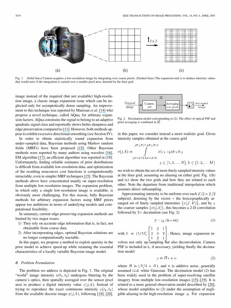
Fig. 1. (Solid lines) Camera acquires a low-resolution image by integrating over coarse pixels. (Dashed lines) The expansion task is to deduce intensity valuesthat would arise if the integration is carried over a smaller pixel area, denoted by the finer grid.

image instead of the required (but not available) high-resolu-tion image, a classic image expansion issue which can be ne-glected only for asymptotically dense sampling. An improve-ment to this technique was reported by Muresan et al. [14] whopropose a novel technique, called AQua, for arbitrary expan-sion factors. AQua constrains the signal to belong to an adaptivequadratic signal class and reportedly shows better sharpness andedge preservation compared to [11]. However, both methods ap-pear to exhibit excessive directional smoothing (see Section IV).

In order to obtain statistically sound expansion fromunder-sampled data, Bayesian methods using Markov randomfields (MRFs) have been proposed [15]. Other Bayesianmethods were reported by many authors using wavelets [16],EM algorithm [17]; an efficient algorithm was reported in [18].Unfortunately, finding reliable estimates of prior distributionsis difficult from available low-resolution data, and optimizationof the resulting nonconvex cost functions is computationallyintractable, even in simpler MRF techniques [15]. The Bayesianmethods above have concentrated mainly on super-resolutionfrom multiple low-resolution images. The expansion problem,in which only a single low-resolution image is available, isobviously more challenging. For this reason, fully Bayesianmethods for arbitrary expansion factors using MRF priorsappear too ambitious in terms of underlying models and com-putational feasibility.

In summary, current edge-preserving expansion methods arelimited by two major issues.

1) They rely on accurate edge information that is, in fact, notobtainable from coarse data.

2) After incorporating edges, optimal Bayesian solutions areno longer computationally tractable.

In this paper, we propose a method to exploit sparsity in theprior model to achieve speed-up while retaining the essentialcharacteristics of a locally variable Bayesian image model.

B. Problem Formulation

The problem we address is depicted in Fig. 1. The original“world” image intensity undergoes blurring by thecamera’s optics, then spatially averaged over the sensor pixelarea to produce a digital intensity value . Instead oftrying to reproduce the exact continuous intensityfrom the available discrete image , following [19], [20],

Fig. 2. Decimation model corresponding to (2). The effect of optical PSF andpixel averaging is combined in H .

in this paper, we consider instead a more realistic goal. Givenintensity samples obtained at the coarse grid

we wish to obtain the set of more finely sampled intensity valuesat the finer grid, assuming no aliasing on either grid. Fig. 1(b)and (c) show the two grids and how they are related to eachother. Note the departure from traditional interpolation whichassumes direct subsampling.

Approximating intensity to be uniform over eachsubpixel, denoting by the vector the lexicographically ar-ranged set of finely sampled intensities , and bythe coarser samples , this becomes a 2-D convolutionfollowed by decimation (see Fig. 2)

(1)

with . Hence, image expansion in-

volves not only up-sampling but also deconvolution. CameraPSF is included in , if necessary, yielding finally the decima-tion model

(2)

where is , and is additive noise, generallyassumed i.i.d. white Gaussian. The decimation model (2) hasbeen widely used in the problem of super-resolving satelliteimagery from multiple low-resolution images [15]–[19]. It isrelated to a more general observation model described by [20],whose model simplifies to (2) under the assumption of negli-gible aliasing in the high-resolution image . For expansion

RAJ AND THAKUR: FAST AND STABLE BAYESIAN IMAGE EXPANSION 1075

factors , , we have

but we will solve this as a series of interpolations, ig-noring the fact that noise properties actually depend on in-stead of being white Gaussian for all . Our implementationfocuses on dyadic expansion factors, but we note that this is apractical rather than theoretical restriction. In principle, a sim-ilar approach can be derived for any integer expansion factor.

Equation (2) can be solved directly via least squares methodstraditionally used in decovolution/restoration [21], [22]. Theexpansion problem (2) is similar, but is, in addition, severelyunderdetermined. The least-squares methods can handleill-posedness by introducing a regularization term whichpenalizes deviation from some a priori constraint. In Bayesianterms, this might represent knowledge of image covariance.Standard Tikhonov regularization employs global smoothnessconstraints: , where matrix represents thefinite differences operator. The stabilizing term reduces noiseamplification by preventing small singular values, acting as afilter on the matrix spectrum.

Unfortunately, Tikhonov-regularized least squares does notpreserve the integrity of sharp edges due to unrealistic globalsmoothness assumptions on images, which are, in fact, bettermodeled as nonstationary processes. We now introduce an in-teresting edge-driven prior model of images, and derive the op-timal maximum a posteriori (MAP) estimate for expansion.

C. Our Approach

MAP methods are computationally prohibitive since matrixdiagonalization is no longer possible by Fourier transforma-tion. We will model both the likelihood and the prior in termsof distances, which makes the MAP problem essentiallyquadratic. We reduce complexity by exploiting sparsity of dis-continuous transitions and obtain a “near-diagonalization” re-sult which allows fast processing. Quadratic inverses involvingvariable weights typically suffer from instability and ill-condi-tioning. Our approach divides the solution space into two or-thogonal subspaces, which allows the quadratic inverse to beobtained independently and stably within each subspace.

For a practical implementation, we further reduce computa-tional burden by tiling the image and solving a series of 1-Dproblems, first on rows, followed by columns. This is possible ifthe decimation kernel is separable into row and column vectors.The method is naturally progressive—simpler, approximate es-timates are obtained first, and fed back to obtain more exact(and expensive) estimates. Our derivations assume that a largesparse Toeplitz matrix can be replaced by a circulant one withouterror—a standard assumption in many Fourier methods. In im-ages, this assumption causes problems only near boundaries,and is easily mitigated by zero padding.

II. MAXIMUM A Posteriori (MAP) IMAGE EXPANSION

USING PRIOR EDGE INFORMATION

A. Sparse Edge-Driven Prior Model

Images are well modeled by piecewise smoothness punc-tuated with edge discontinuities [23]. Traditionally, images

have been stochastically modeled as having translation-in-variant global smoothness of the kind , where isan i.i.d. signal and matrix models the spatial correlationof the image signal and is usually expressed as a Toeplitzmatrix corresponding to some smoothing convolution kernel.It has been shown that under this model MAP reproducesTikhonov regularization with the equivalence [24].We wish to modify this model to incorporate edge priors. Theclassic difficulty of this approach is that the information aboutedge location, orientation and magnitude is data-dependent;hence, it can hardly be called a “prior” in the normal sense.Therefore, direct use of edge detection results as edge priorsmay be considered statistically unsound under noise, blur andother artifacts. Certainly, this is highly problematic for imageexpansion where the data are highly blurred and decimated,although limited justification for this approach was presentedin [11]. In this paper, we argue that although accurate edgepriors relying on steepness and resolution of edges in cannotbe obtained from available data , the approximate location andmagnitude of edges can be easily and reliably obtained. Insteadof using edge information as a hard decision step, we proposea stochastic framework to allow soft decisions.

For the purpose of edge detection, we first expand the ob-served image to the same size as desired image , and ob-tain . We used bilinear interpolation for this, but any popularmethod could be used, for instance polynomial kernel or nearestneighbor. Let us denote by is an edge in imagethe set of edge locations obtained from edge detection on .Edge set is obtained as follows; the coarse image is fil-tered by the derivative of Gaussian (DoG) to get a rough map ofintensity slopes [25]. The width of DoG was empirically chosento match the noise. A small width allows finer edges to be reg-istered, but increases false detection due to noise. Some amountof initial operator supervision is, therefore, inevitable. We donot implement complex and expensive edge detection steps orcross validation for optimal edge parameters since our aim isto minimize execution time. Simple edge detection followed byhierarchical edge linking [26] was found sufficient. Image is ablurry, low-resolution image, so more sophisticated edge detec-tion methods are not helpful; in any case, our stochastic modelshown below serves to desensitize the effect of edge detection.

We introduce a sparse, independent “edge” point process, where is an independent binomial point process which

can take the values 0 or 1, is an independent Gaussian sto-chastic process, and multiplication “ ” is point-by-point. Ourprobability model is

where is the variance of identically distributed Gaussiansand is an inverse distance specified later. Let be an i.i.d.

1076 IEEE TRANSACTIONS ON IMAGE PROCESSING, VOL. 16, NO. 4, APRIL 2007

stochastic process with variance 1 and be a Toeplitz matrixthat captures the spatial correlation of the image. Then our newimage model is

(3)

This reproduces a spatially correlated (smooth) image processinterspersed with edge point processes of random but Gaussiandistributed magnitude. This edge model may not be entirely sat-isfactory for 2-D images, but is justifiable under our separable1-D approach.

We now make the standard assumption: Process is jointly(zero mean) Gaussian, with

(4)

where is the signal covariance matrix. From(3), we have , assumingindependence between and . Using the independence ofand , and . From (3)

The diagonal matrix is given by ,

, and . For convenience we define

an edge-weighted map ,.

Since the appropriate form of is not known a priori, wehave tried various intuitive forms including Gaussian, linear,quadratic, etc. Overall, the inverted truncated linear model

seemed to work best—thisappears to mirror current literature on robust image estimation[18], [27]. For this choice of , forms a distance metric, andcan be efficiently computed in terms of a distance transformin linear time [28]. Note that and are prior model pa-rameters which are basically unknown, and such quantities aredetermined heuristically after trial and error in most Bayesianapplications. We found the best results by setting and

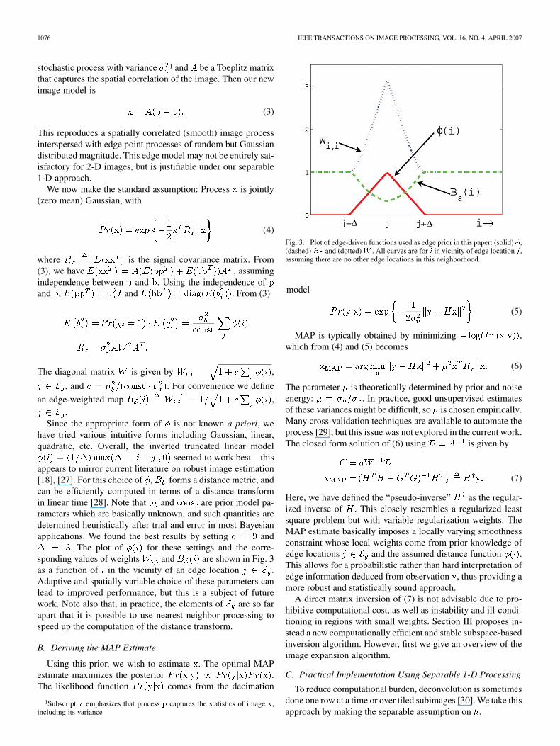
. The plot of for these settings and the corre-sponding values of weights and are shown in Fig. 3as a function of in the vicinity of an edge location .Adaptive and spatially variable choice of these parameters canlead to improved performance, but this is a subject of futurework. Note also that, in practice, the elements of are so farapart that it is possible to use nearest neighbor processing tospeed up the computation of the distance transform.

B. Deriving the MAP Estimate

Using this prior, we wish to estimate . The optimal MAPestimate maximizes the posterior .The likelihood function comes from the decimation

1Subscript x emphasizes that process p captures the statistics of image x,including its variance

Fig. 3. Plot of edge-driven functions used as edge prior in this paper: (solid) �,(dashed) B and (dotted) W . All curves are for i in vicinity of edge location j ,assuming there are no other edge locations in this neighborhood.

model

(5)

MAP is typically obtained by minimizing ,which from (4) and (5) becomes

(6)

The parameter is theoretically determined by prior and noiseenergy: . In practice, good unsupervised estimatesof these variances might be difficult, so is chosen empirically.Many cross-validation techniques are available to automate theprocess [29], but this issue was not explored in the current work.The closed form solution of (6) using is given by

(7)

Here, we have defined the “pseudo-inverse” as the regular-ized inverse of . This closely resembles a regularized leastsquare problem but with variable regularization weights. TheMAP estimate basically imposes a locally varying smoothnessconstraint whose local weights come from prior knowledge ofedge locations and the assumed distance function .This allows for a probabilistic rather than hard interpretation ofedge information deduced from observation , thus providing amore robust and statistically sound approach.

A direct matrix inversion of (7) is not advisable due to pro-hibitive computational cost, as well as instability and ill-condi-tioning in regions with small weights. Section III proposes in-stead a new computationally efficient and stable subspace-basedinversion algorithm. However, first we give an overview of theimage expansion algorithm.

C. Practical Implementation Using Separable 1-D Processing

To reduce computational burden, deconvolution is sometimesdone one row at a time or over tiled subimages [30]. We take thisapproach by making the separable assumption on .

RAJ AND THAKUR: FAST AND STABLE BAYESIAN IMAGE EXPANSION 1077

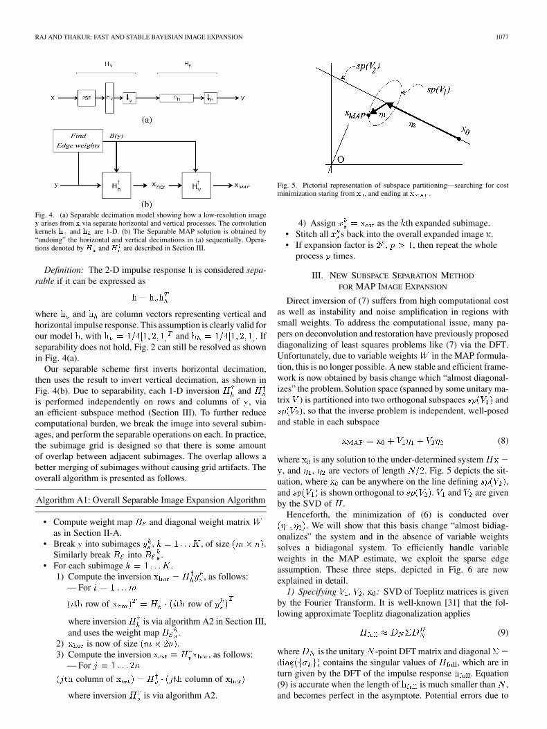
Fig. 4. (a) Separable decimation model showing how a low-resolution imagey arises from x via separate horizontal and vertical processes. The convolutionkernels h and h are 1-D. (b) The Separable MAP solution is obtained by“undoing” the horizontal and vertical decimations in (a) sequentially. Opera-tions denoted by H and H are described in Section III.

Definition: The 2-D impulse response is considered sepa-rable if it can be expressed as

where and are column vectors representing vertical andhorizontal impulse response. This assumption is clearly valid forour model , with and . Ifseparability does not hold, Fig. 2 can still be resolved as shownin Fig. 4(a).

Our separable scheme first inverts horizontal decimation,then uses the result to invert vertical decimation, as shown inFig. 4(b). Due to separability, each 1-D inversion andis performed independently on rows and columns of , viaan efficient subspace method (Section III). To further reducecomputational burden, we break the image into several subim-ages, and perform the separable operations on each. In practice,the subimage grid is designed so that there is some amountof overlap between adjacent subimages. The overlap allows abetter merging of subimages without causing grid artifacts. Theoverall algorithm is presented as follows.

Algorithm A1: Overall Separable Image Expansion Algorithm

• Compute weight map and diagonal weight matrixas in Section II-A.

• Break into subimages , , of size .Similarly break into .

• For each subimage .1) Compute the inversion , as follows:

— For

row of row of

where inversion is via algorithm A2 in Section III,and uses the weight map .

2) is now of size .3) Compute the inversion , as follows:

— For

column of column of

where inversion is via algorithm A2.

Fig. 5. Pictorial representation of subspace partitioning—searching for costminimization staring from x , and ending at x .

4) Assign as the th expanded subimage.• Stitch all s back into the overall expanded image .• If expansion factor is , , then repeat the whole

process times.

III. NEW SUBSPACE SEPARATION METHOD

FOR MAP IMAGE EXPANSION

Direct inversion of (7) suffers from high computational costas well as instability and noise amplification in regions withsmall weights. To address the computational issue, many pa-pers on deconvolution and restoration have previously proposeddiagonalizing of least squares problems like (7) via the DFT.Unfortunately, due to variable weights in the MAP formula-tion, this is no longer possible. A new stable and efficient frame-work is now obtained by basis change which “almost diagonal-izes” the problem. Solution space (spanned by some unitary ma-trix ) is partitioned into two orthogonal subspaces and

, so that the inverse problem is independent, well-posedand stable in each subspace

(8)

where is any solution to the under-determined system, and , are vectors of length . Fig. 5 depicts the sit-

uation, where can be anywhere on the line defining ,and is shown orthogonal to . and are givenby the SVD of .

Henceforth, the minimization of (6) is conducted over. We will show that this basis change “almost bidiag-

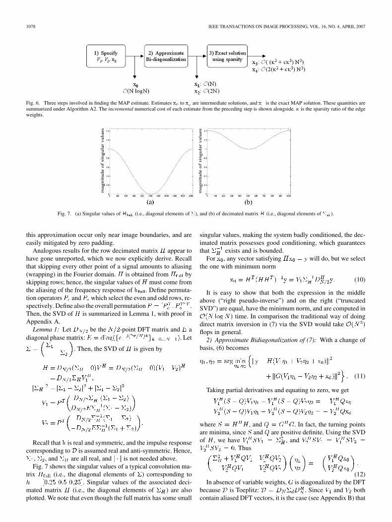
onalizes” the system and in the absence of variable weightssolves a bidiagonal system. To efficiently handle variableweights in the MAP estimate, we exploit the sparse edgeassumption. These three steps, depicted in Fig. 6 are nowexplained in detail.

1) Specifying , , : SVD of Toeplitz matrices is givenby the Fourier Transform. It is well-known [31] that the fol-lowing approximate Toeplitz diagonalization applies

(9)

where is the unitary -point DFT matrix and diagonalcontains the singular values of , which are in

turn given by the DFT of the impulse response . Equation(9) is accurate when the length of is much smaller than ,and becomes perfect in the asymptote. Potential errors due to

1078 IEEE TRANSACTIONS ON IMAGE PROCESSING, VOL. 16, NO. 4, APRIL 2007

Fig. 6. Three steps involved in finding the MAP estimate. Estimates x to x are intermediate solutions, and x is the exact MAP solution. These quantities aresummarized under Algorithm A2. The incremental numerical cost of each estimate from the preceding step is shown alongside. � is the sparsity ratio of the edgeweights.

Fig. 7. (a) Singular values of H (i.e., diagonal elements of �), and (b) of decimated matrix H (i.e., diagonal elements of � ).

this approximation occur only near image boundaries, and areeasily mitigated by zero padding.

Analogous results for the row decimated matrix appear tohave gone unreported, which we now explicitly derive. Recallthat skipping every other point of a signal amounts to aliasing(wrapping) in the Fourier domain. is obtained from byskipping rows; hence, the singular values of must come fromthe aliasing of the frequency response of . Define permuta-tion operators and which select the even and odd rows, re-spectively. Define also the overall permutation .Then, the SVD of is summarized in Lemma 1, with proof inAppendix A.

Lemma 1: Let be the -point DFT matrix and adiagonal phase matrix: . Let

. Then, the SVD of is given by

Recall that is real and symmetric, and the impulse responsecorresponding to is assumed real and anti-symmetric. Hence,

, , and are all real, and is not needed above.Fig. 7 shows the singular values of a typical convolution ma-

trix (i.e., the diagonal elements of ) corresponding to. Singular values of the associated deci-

mated matrix (i.e., the diagonal elements of ) are alsoplotted. We note that even though the full matrix has some small

singular values, making the system badly conditioned, the dec-imated matrix possesses good conditioning, which guaranteesthat exists and is bounded.

For , any vector satisfying will do, but we selectthe one with minimum norm

(10)

It is easy to show that both the expression in the middleabove (“right pseudo-inverse”) and on the right (“truncatedSVD”) are equal, have the minimum norm, and are computed in

time. In comparison the traditional way of doingdirect matrix inversion in (7) via the SVD would takeflops in general.

2) Approximate Bidiagonalization of (7): With a change ofbasis, (6) becomes

(11)

Taking partial derivatives and equating to zero, we get

where , and . In fact, the turning pointsare minima, since and are positive definite. Using the SVDof , we have , and

. Thus

(12)In absence of variable weights, is diagonalized by the DFT

because is Toeplitz: . Since and bothcontain aliased DFT vectors, it is the case (see Appendix B) that

RAJ AND THAKUR: FAST AND STABLE BAYESIAN IMAGE EXPANSION 1079

all matrices in (12) are, in fact, diagonal in the absence of .Thus, (12) becomes a bidiagonal system and is speedily solvedin linear time. However, variable weights destroy diagonaliza-tion, and (12) appears no better than the original (7). However,in practice, the variable weights are sparse, and approximate di-agonalization continues to hold, due to Theorem 1.

Theorem 1: Let , , , be as before. Let

and . Let us assume that

the diagonal entries of are mostly one, except at a smallproportion of points . Then, the system (12) can be split

into a “dominant” bidiagonal system with

diagonal , and a “residual” nonsparse .

Specifically

(13)

and . satisfy Frobenius

norm conditions .Proof: Expressions for and proof are in Appendix B.

Recall that for matrix , the Frobenius norm is. Theorem 1 is a statement on the ac-

curacy of the diagonalization of (12) in terms of Frobenius normof nondiagonal matrix elements. It basically says that for suffi-ciently sparse weights, the MAP estimate is close to the globallysmooth Tikhonov regularized estimate, and specifies a fast algo-rithm to obtain it in time (by computing ).

On the other hand, the full, exact MAP solution is compu-tationally expensive in general, requiring operations,where is usually much higher than unity. However, (12) is infact strongly decoupled for small . To see this, consider thetop block-row of (13). Due to the smallness of , we expect

. Thus, we propose a decoupled algorithm to solve(12).

1) Solve the bidiagonal system

2) Solve for

3) Finally, solve for

Step 1) is linear time since it is a bidiagonal system. The errorsdue to the use of instead of is expected to be small since weexpect . Therefore , Step 2) is reasonable. Steps 2)and 3) could be iterated in an EM-type loop for greater accuracy,but this was not found to produce additional improvement. TheMAP solution is given by

(14)

3) Efficient Inversion of (12) Using Sparsity of : We nowdescribe an efficient and stable algorithm for Step 2), involving

inversion of diagonally dominant matrices. Step 3)uses the same algorithm. Following Appendix B, is writtenas

(15)

Since most entries of the diagonal matrix are zero,is rank deficient, which implies that , where isa matrix given by . Here, wereplaced with the matrix consisting of onlynonzero diagonal elements, and the matrix isobtained by removing the corresponding columns of . Usingthe formula [32]

(16)and letting yields the inverse of . (16) al-lows us to invert a matrix instead of amatrix. Careful inspection will reveal that the total cost of com-puting this inverse is . Typically, ,and the computational cost of inverting is severalorders of magnitude smaller than direct inversion. As summa-rized below, the subspace algorithm produces four approximatesolutions that progressively build on each other. The numericalcost of each step was summarized in Fig. 6.

Algorithm A2: Progressive solutions to the full1-D MAP Expansion problem

1) Find the minimum norm/pseudo-inverse/truncated SVDsolution

2) Solve the bidiagonal system

3) Obtain as follows.(a) Create the “thin” matrix from the

nonzero columns of .(b) Compute by simple scaling and

addition.(c) Replace by simple

matrix-vector multiply.(d) Compute the “small” matrix inverse

.(e) Get by simple

matrix-vector multiply.4) Get by steps analogous to (a)–(e) above.5) Then, finally

Estimates , , and are very quickly obtained in al-most linear time, but only provide globally smooth results with

1080 IEEE TRANSACTIONS ON IMAGE PROCESSING, VOL. 16, NO. 4, APRIL 2007

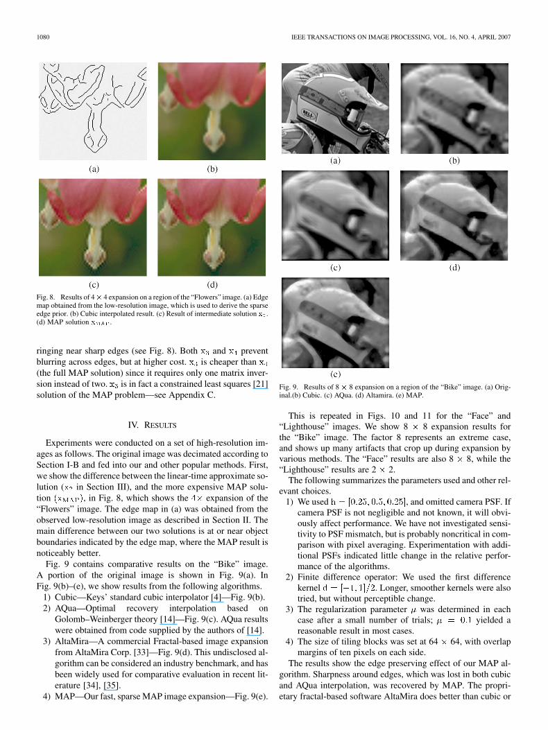
Fig. 8. Results of 4� 4 expansion on a region of the “Flowers” image. (a) Edgemap obtained from the low-resolution image, which is used to derive the sparseedge prior. (b) Cubic interpolated result. (c) Result of intermediate solution x .(d) MAP solution x .

ringing near sharp edges (see Fig. 8). Both and preventblurring across edges, but at higher cost. is cheaper than(the full MAP solution) since it requires only one matrix inver-sion instead of two. is in fact a constrained least squares [21]solution of the MAP problem—see Appendix C.

IV. RESULTS

Experiments were conducted on a set of high-resolution im-ages as follows. The original image was decimated according toSection I-B and fed into our and other popular methods. First,we show the difference between the linear-time approximate so-lution ( in Section III), and the more expensive MAP solu-tion , in Fig. 8, which shows the expansion of the“Flowers” image. The edge map in (a) was obtained from theobserved low-resolution image as described in Section II. Themain difference between our two solutions is at or near objectboundaries indicated by the edge map, where the MAP result isnoticeably better.

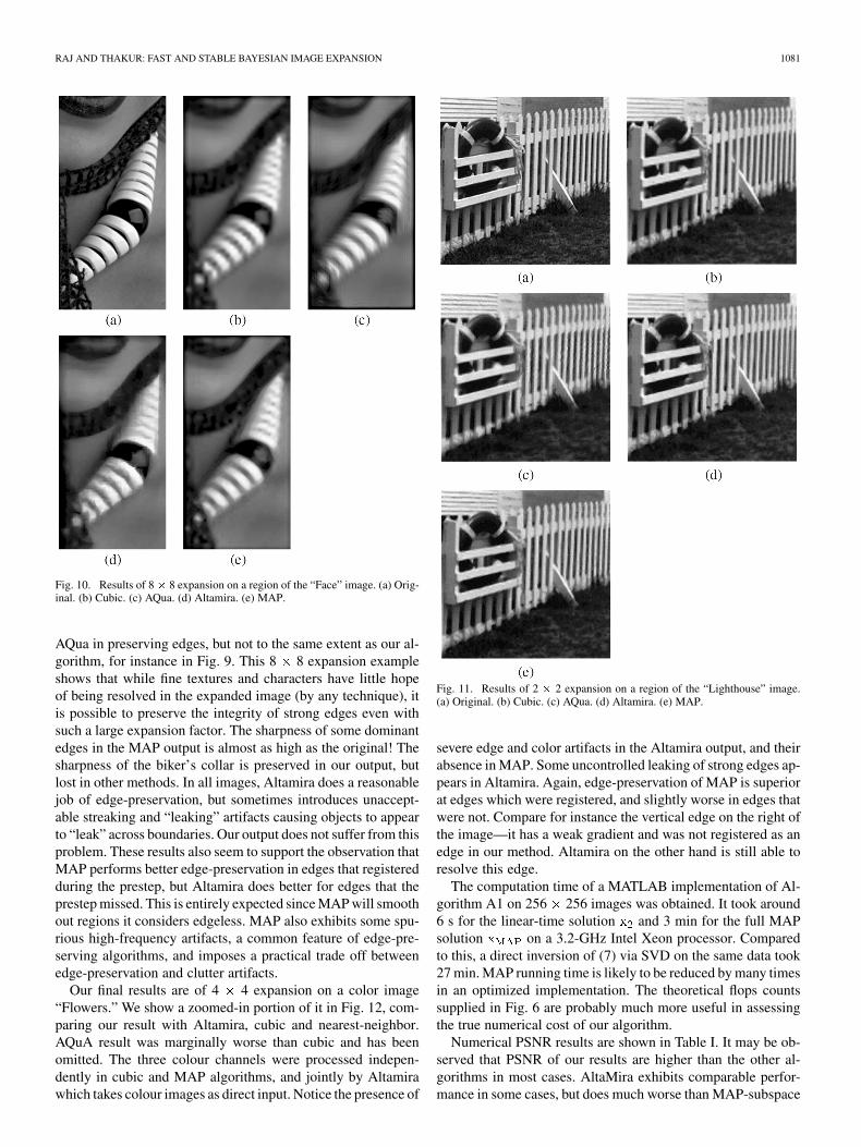
Fig. 9 contains comparative results on the “Bike” image.A portion of the original image is shown in Fig. 9(a). InFig. 9(b)–(e), we show results from the following algorithms.

1) Cubic—Keys’ standard cubic interpolator [4]—Fig. 9(b).2) AQua—Optimal recovery interpolation based on

Golomb–Weinberger theory [14]—Fig. 9(c). AQua resultswere obtained from code supplied by the authors of [14].

3) AltaMira—A commercial Fractal-based image expansionfrom AltaMira Corp. [33]—Fig. 9(d). This undisclosed al-gorithm can be considered an industry benchmark, and hasbeen widely used for comparative evaluation in recent lit-erature [34], [35].

4) MAP—Our fast, sparse MAP image expansion—Fig. 9(e).

Fig. 9. Results of 8 � 8 expansion on a region of the “Bike” image. (a) Orig-inal.(b) Cubic. (c) AQua. (d) Altamira. (e) MAP.

This is repeated in Figs. 10 and 11 for the “Face” and“Lighthouse” images. We show 8 8 expansion results forthe “Bike” image. The factor 8 represents an extreme case,and shows up many artifacts that crop up during expansion byvarious methods. The “Face” results are also 8 8, while the“Lighthouse” results are 2 2.

The following summarizes the parameters used and other rel-evant choices.

1) We used , and omitted camera PSF. Ifcamera PSF is not negligible and not known, it will obvi-ously affect performance. We have not investigated sensi-tivity to PSF mismatch, but is probably noncritical in com-parison with pixel averaging. Experimentation with addi-tional PSFs indicated little change in the relative perfor-mance of the algorithms.

2) Finite difference operator: We used the first differencekernel . Longer, smoother kernels were alsotried, but without perceptible change.

3) The regularization parameter was determined in eachcase after a small number of trials; yielded areasonable result in most cases.

4) The size of tiling blocks was set at 64 64, with overlapmargins of ten pixels on each side.

The results show the edge preserving effect of our MAP al-gorithm. Sharpness around edges, which was lost in both cubicand AQua interpolation, was recovered by MAP. The propri-etary fractal-based software AltaMira does better than cubic or

RAJ AND THAKUR: FAST AND STABLE BAYESIAN IMAGE EXPANSION 1081

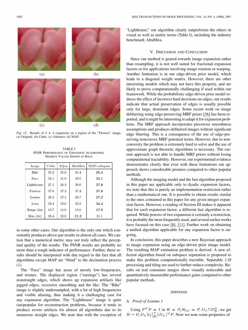
Fig. 10. Results of 8� 8 expansion on a region of the “Face” image. (a) Orig-inal. (b) Cubic. (c) AQua. (d) Altamira. (e) MAP.

AQua in preserving edges, but not to the same extent as our al-gorithm, for instance in Fig. 9. This 8 8 expansion exampleshows that while fine textures and characters have little hopeof being resolved in the expanded image (by any technique), itis possible to preserve the integrity of strong edges even withsuch a large expansion factor. The sharpness of some dominantedges in the MAP output is almost as high as the original! Thesharpness of the biker’s collar is preserved in our output, butlost in other methods. In all images, Altamira does a reasonablejob of edge-preservation, but sometimes introduces unaccept-able streaking and “leaking” artifacts causing objects to appearto “leak” across boundaries. Our output does not suffer from thisproblem. These results also seem to support the observation thatMAP performs better edge-preservation in edges that registeredduring the prestep, but Altamira does better for edges that theprestep missed. This is entirely expected since MAP will smoothout regions it considers edgeless. MAP also exhibits some spu-rious high-frequency artifacts, a common feature of edge-pre-serving algorithms, and imposes a practical trade off betweenedge-preservation and clutter artifacts.

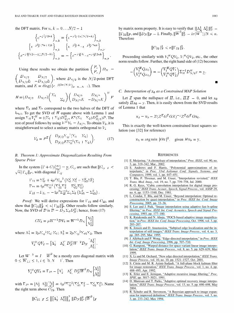
Our final results are of 4 4 expansion on a color image“Flowers.” We show a zoomed-in portion of it in Fig. 12, com-paring our result with Altamira, cubic and nearest-neighbor.AQuA result was marginally worse than cubic and has beenomitted. The three colour channels were processed indepen-dently in cubic and MAP algorithms, and jointly by Altamirawhich takes colour images as direct input. Notice the presence of

Fig. 11. Results of 2 � 2 expansion on a region of the “Lighthouse” image.(a) Original. (b) Cubic. (c) AQua. (d) Altamira. (e) MAP.

severe edge and color artifacts in the Altamira output, and theirabsence in MAP. Some uncontrolled leaking of strong edges ap-pears in Altamira. Again, edge-preservation of MAP is superiorat edges which were registered, and slightly worse in edges thatwere not. Compare for instance the vertical edge on the right ofthe image—it has a weak gradient and was not registered as anedge in our method. Altamira on the other hand is still able toresolve this edge.

The computation time of a MATLAB implementation of Al-gorithm A1 on 256 256 images was obtained. It took around6 s for the linear-time solution and 3 min for the full MAPsolution on a 3.2-GHz Intel Xeon processor. Comparedto this, a direct inversion of (7) via SVD on the same data took27 min. MAP running time is likely to be reduced by many timesin an optimized implementation. The theoretical flops countssupplied in Fig. 6 are probably much more useful in assessingthe true numerical cost of our algorithm.

Numerical PSNR results are shown in Table I. It may be ob-served that PSNR of our results are higher than the other al-gorithms in most cases. AltaMira exhibits comparable perfor-mance in some cases, but does much worse than MAP-subspace

1082 IEEE TRANSACTIONS ON IMAGE PROCESSING, VOL. 16, NO. 4, APRIL 2007

Fig. 12. Results of 4 � 4 expansion on a region of the “Flowers” image.(a) Original. (b) Cubic. (c) Altamira. (d) MAP.

TABLE IPSNR PERFORMANCE OF EXPANSION ALGORITHMS.

HIGHEST VALUES SHOWN IN BOLD

in some other cases. Our algorithm is the only one which con-sistently produces above-par results in almost all cases. We cau-tion that a numerical metric may not truly reflect the percep-tual quality of the results. The PSNR results are probably nomore than a rough indicator of performance. Further, these re-sults should be interpreted with due regard to the fact that allalgorithms except MAP are “blind” to the decimation process(1).

The “Face” image has areas of mostly low-frequencies,and texture. The displayed region (“earrings”) has severalnonstraight edges, which shows up expansion artifacts likejagged edges, excessive smoothing and the like. The “Bike”image is slightly undersampled, with a lot of high frequenciesand visible aliasing, thus making it a challenging case forany expansion algorithm. The “Lighthouse” image is quite(un)popular for reconstruction problems, because it tends toproduce severe artifacts for almost all algorithms due to itsnumerous straight edges. We note that with the exception of

“Lighthouse,” our algorithm clearly outperforms the others invisual as well as metric terms (Table I), including the industrybenchmark AltaMira.

V. DISCUSSION AND CONCLUSION

Since our method is geared towards image expansion ratherthan resampling, it is not well suited for fractional expansionfactors or for applications involving image rotation or warping.Another limitation is in our edge-driven prior model, whichleads to a diagonal weight matrix. However, there are otherinteresting models which may not have this property, and arelikely to prove computationally challenging if used within ourframework. While the probabilistic edge-driven prior model re-duces the effect of incorrect hard decisions on edges, our resultsindicate that actual preservation of edges is usually possibleonly for large, dominant edges. Some recent work on imagedeblurring using edge-preserving MRF priors [36] has been re-ported, and it might be interesting to adapt it for expansion prob-lems. The MRF approach incorporates piecewise smoothnessassumptions and produces deblurred images without significantedge blurring. This is a consequence of the use of edge-pre-serving nonconvex MRF potential terms. However, due to non-convexity the problem is extremely hard to solve and the use ofapproximate graph theoretic algorithms is necessary. The cur-rent approach is not able to handle MRF priors without losingcomputational tractability. However, our experimental evidencedemonstrates clearly that even with these limitations our ap-proach shows considerable promise compared to other popularmethods.

Although the imaging model and the fast algorithm proposedin this paper are applicable only to dyadic expansion factors,we note that this is purely an implementation restriction ratherthan a mathematical one. It is possible to obtain results similarto the ones contained in this paper for any given integer expan-sion factor. However, a reading of Section III makes it apparentthat for each expansion factor, a different fast algorithm is re-quired. While powers of two expansion is certainly a restriction,it is probably the most frequently used, and several earlier workshave focused on this case [8], [11]. Further work on obtaininga unified algorithm applicable for any expansion factor is on-going.

In conclusion, this paper describes a new Bayesian approachto image expansion using an edge-driven prior image model.The resulting MAP estimation problem is derived. A new ef-ficient algorithm based on subspace separation is proposed tomake this problem computationally tractable. Separable 1-Dprocessing and tiling are used to further reduce complexity. Re-sults on real consumer images show visually noticeable andquantitatively measurable performance gains compared to otherpopular methods.

APPENDIX

A. Proof of Lemma 1

Using in , we get. Now we note some properties of

RAJ AND THAKUR: FAST AND STABLE BAYESIAN IMAGE EXPANSION 1083

the DFT matrix. For ,

Using these results we obtain the partition

, where is the -point DFT

matrix, and . Then

where and correspond to the two halves of the DFT of. To get the SVD of equate above with Lemma 1 and

assign . Therest of proof follows by using . To obtain , it isstraightforward to select a unitary matrix orthogonal to

(17)

B. Theorem 1: Approximate Diagonalization Resulting FromSparse Prior

In the system , are such that, with diagonal

Proof: We will derive expressions for and , andshow that . Other results follow similarly.Now, the SVD of is ; hence, from (17)

where ; . Then

Let be a mostly zero diagonal matrix with, . Then

with . Namethe right term above . Then

by matrix norm property. It is easy to verify that, and . Finally, .

Therefore

Proceeding similarly with , , etc., the othernorm results follow. Further, the right hand side of (12) becomes

C. Interpretation of as a Constrained MAP Solution

Let span the nullspace of , i.e., , and letsatisfy . Then, it is easily shown from the SVD resultsof Lemma 1 that

This is exactly the well-known constrained least squares so-lution (see [32] for reference)

given

REFERENCES

[1] E. Meijering, “A chronology of interpolation,” Proc. IEEE, vol. 90, no.3, pp. 319–342, Mar., 2002.

[2] S. Andrews and F. Harris, “Polynomial approximations of in-terpolants,” in Proc. 33rd Asilomar Conf. Signals, Systems, andComputers, 1999, vol. 1, pp. 447–451.

[3] T. Blu, P. Thvenaz, and M. Unser, “Interpolation revisited,” IEEETrans. Med. Imag., vol. 19, no. 7, pp. 739–758, Jul. 2000.

[4] R. G. Keys, “Cubic convolution interpolation for digital image pro-cessing,” IEEE Trans. Acoust., Speech, Signal Process., vol. ASSP-29,no. 6, pp. 1153–1160, Dec. 1981.

[5] L. Condat, T. Blu, and M. Unser, “Beyond interpolation: Optimal re-construction by quasi-interpolation,” in Proc. IEEE Int. Conf. ImageProcessing, 2005, pp. 33–36.

[6] S. Lee and J. Paik, “Image interpolation using adaptive fast b-splinefiltering,” in Proc. IEEE Int. Conf. Acoustics, Speech and Signal Pro-cessing, 1993, pp. 177–180.

[7] K. Ratakonda and N. Ahuja, “POCS-based adaptive image magnifica-tion,” in Proc. IEEE Int. Conf. Image Processing, Oct. 1998, vol. 3, pp.203–207.

[8] K. Jensen and D. Anastassiou, “Subpixel edge localization and the in-terpolation of still images,” IEEE Trans. Image Process., vol. 4, no. 3,pp. 285–295, Mar. 1995.

[9] J. Allebach and P. Wong, “Edge-directed interpolation,” in Proc. IEEEInt. Conf. Image Processing, 1996, pp. 707–710.

[10] G. Ramponi, “Warped distance for space-variant linear image interpo-lation,” IEEE Trans. Image Process., vol. 8, no. 5, pp. 629–639, May1999.

[11] X. Li and M. Orchard, “New edge directed interpolation,” IEEE Trans.Image Process., vol. 10, no. 10, pp. 1521–1527, Oct. 2001.

[12] S. Citrin and M. R. Azimi-Sadjadi, “A full-plane block kalman filterfor image restoration,” IEEE Trans. Image Process., vol. 1, no. 4, pp.488–495, Apr. 1992.

[13] K. Erler and E. Jernigan, “Adaptive recursive image filtering,” Proc.SPIE, pp. 3017–3021, 1991.

[14] D. Muresan and T. Parks, “Adaptive optimal recovery image interpo-lation,” IEEE Trans. Image Process., vol. 13, no. 5, pp. 690–698, May2004.

[15] R. Schultz and R. Stevenson, “A Bayesian approach to image expan-sion for improved definition,” IEEE Trans. Image Process., vol. 3, no.3, pp. 233–242, May 1994.

1084 IEEE TRANSACTIONS ON IMAGE PROCESSING, VOL. 16, NO. 4, APRIL 2007

[16] R. Chan, T. Chan, L. Shen, and Z. Shen, “Wavelet algorithms for high-resolution image reconstruction,” SIAM J. Sci. Comput., vol. 24, no. 4,pp. 1408–1432, 2003.

[17] R. Molina, M. Vega, J. Abad, and A. Katsaggelos, “Parameter estima-tion in bayesian high-resolution image reconstruction with multisen-sors,” IEEE Trans. Image Process., vol. 12, no. 12, pp. 1655–1667,Dec. 2003.

[18] M. Elad and A. Feuer, “Restoration of a single superresolution imagefrom several blurred, noisy, and undersampled measured images,”IEEE Trans. Image Process., vol. 6, no. 12, pp. 1646–1658, Dec. 1997.

[19] N. Bose and K. Boo, “High-resolution image reconstruction with mul-tisensors,” Int. J. Imag. Sci. Technol., vol. 9, pp. 141–163, 1998.

[20] H. A. Aly and E. Dubois, “Specification of the observation model forregularized image up-sampling,” IEEE Trans. Image Process., vol. 14,no. 5, pp. 567–576, May 2005.

[21] T. Berber, J. Stromberg, and T. Eltoft, “Adaptive regularized con-strained least squares image restoration,” IEEE Trans. Image Process.,vol. 8, no. 9, pp. 1191–1203, Sep. 1999.

[22] A. Katsaggelos, J. Biermond, R. Schafer, and R. Mersereau, “Aregularized iterative image restoration algorithm,” IEEE Trans. SignalProcess., vol. 39, no. 4, pp. 914–929, Apr. 1991.

[23] S. Li, Markov Random Field Modeling in Computer Vision. NewYork: Springer-Verlag, 1995.

[24] V. Z. Mesarovic, N. P. Galatsanos, and M. N. Wernick, “Iterative max-imum a posteriori (MAP) restoration from partially-known blur for to-mographic reconstruction,” in Proc. IEEE Int. Conf. Image Processing,1995, pp. 512–515.

[25] J. Canny, “A computational approach to edge detection,” IEEE Trans.Pattern Anal. Mach. Intell., vol. PAMI-8, no. 6, pp. 679–698, Nov.1986.

[26] G. Borgefors, “Hierarchical chamfer matching: A parametric edgematching algorithm,” IEEE Trans. Pattern Anal. Mach. Intell., vol. 10,no. 6, pp. 849–865, Nov. 1988.

[27] C. Bouman and K. Sauer, “A generalized Gaussian image model foredge preserving MAP estimation,” IEEE Trans. Image Process., vol. 2,no. 3, pp. 296–310, Jul. 1993.

[28] D. W. Paglieroni, “Distance transforms: Properties and machine visionapplications,” Comput. Vis., Graph., Image Process.: Graph. ModelsImage Process., vol. 54, no. 1, pp. 56–74, 1992.

[29] A. Thompson, J. Brown, J. Kay, and M. Titterington, “A study ofmethods for choosing the smoothing parameter in image restorationby regularization,” IEEE Trans. Pattern Anal. Mach. Intell., vol. 13,no. 5, pp. 326–339, May 1991.

[30] M. Chen and T. Pavlidis, “Image seaming for segmentation on parallelarchitecture,” IEEE Trans. Pattern Anal. Mach. Intell., vol. 12, no. 6,pp. 588–594, Jun. 1990.

[31] R. M. Gray, Toeplitz and Circulant Matrices: A Review. Boston, MA:Now Publishers, 2006.

[32] G. Golub and C. Van Loan, Matrix Computations. Baltimore, MD:Johns Hopkins Univ. Press, 1996.

[33] Altamira, Commercial, Fractal Based Interpolation Algorithm [On-line]. Available: http://www.genuinefractals.com

[34] D. Muresan and T. Parks, “Adaptive optimal recovery image interpo-lation,” in Proc. IEEE Int. Conf. Acoustics, Speech, Signal Processing,2001, pp. 1949–1952.

[35] W. Freeman, T. Jones, and E. Pasztor, “Example-based super-resolu-tion,” IEEE Comput. Graph. Appl., vol. 22, no. 2, pp. 56–65, Mar./Apr.2002.

[36] A. Raj and R. Zabih, “A graph cut algorithm for generalized imagedeconvolution,” in Proc. Int. Conf. Computer Vision, 2005, pp.1901–1909.

Ashish Raj was born in Godda, India. He receivedthe B.S. degree (with honors) in electrical engi-neering from the University of Auckland, NewZealand, in November 1997, and the Ph.D. degreein electrical and computer engineering from CornellUniversity, Ithaca, NY, in 2004.

Since 2005, he has been working on medicalimaging at the Radiology Department, University ofCalifornia at San Francisco, where he is an AssistantProfessor. His research interests are centered aroundinverse problems that arise in signal processing,

medical imaging, and telecommunications.

Kailash Thakur received the Ph.D. and the D.Sc. de-grees in physics from the University of Allahabad,India, in 1974 and 1988, respectively.

From 1978 to 1980, he was a Postdoctoral Fellowin solid state physics at the University of Warwick,U.K. He was a Professor at Bhagalpur University,India, and Asmara University, Eritrea. Since 1993,he has been a Senior Scientist with the New ZealandInstitute for Industrial Research, where he hasworked on various research projects in microwaveand industrial vision.