Computational Visual Media Computational Visual Media

Volume 1 Issue 1 Article 5

2015

Edge-preserving image decomposition via joint weighted least Edge-preserving image decomposition via joint weighted least

squares squares

Pan Shao Department of Computer Science and Engineering, Shanghai Jiao Tong University, Shanghai 200240, China.

Shouhong Ding Department of Computer Science and Engineering, Shanghai Jiao Tong University, Shanghai 200240, China.

Lizhuang Ma Department of Computer Science and Engineering, Shanghai Jiao Tong University, Shanghai 200240, China.

Yunsheng Wu Tencent Inc., China.

Yongjian Wu Tencent Inc., China.

Follow this and additional works at: https://tsinghuauniversitypress.researchcommons.org/

computational-visual-media

Part of the Computational Engineering Commons, Computer-Aided Engineering and Design

Commons, Graphics and Human Computer Interfaces Commons, and the Software Engineering

Commons

Recommended Citation Recommended Citation Pan Shao, Shouhong Ding, Lizhuang Ma et al. Edge-preserving image decomposition via joint weighted least squares. Computational Visual Media 2015, 1(1): 37-47.

This Research Article is brought to you for free and open access by Tsinghua University Press: Journals Publishing. It has been accepted for inclusion in Computational Visual Media by an authorized editor of Tsinghua University Press: Journals Publishing.

Computational Visual Media

DOI 10.1007/s41095-015-0006-4 Vol. 1, No. 1, March 2015, 37–47

Research Article

Edge-preserving image decomposition via joint weightedleast squares

Pan Shao1, Shouhong Ding1, Lizhuang Ma1 (�), Yunsheng Wu2, and Yongjian Wu2

c© The Author(s) 2015. This article is published with open access at Springerlink.com

Abstract Recent years have witnessed the emergence

of image decomposition techniques which effectively

separate an image into a piecewise smooth base

layer and several residual detail layers. However, the

intricacy of detail patterns in some cases may result

in side-effects including remnant textures, wrongly-

smoothed edges, and distorted appearance. We

introduce a new way to construct an edge-preserving

image decomposition with properties of detail

smoothing, edge retention, and shape fitting. Our

method has three main steps: suppressing high-

contrast details via a windowed variation similarity

measure, detecting salient edges to produce an edge-

guided image, and fitting the original shape using

a weighted least squares framework. Experimental

results indicate that the proposed approach can

appropriately smooth non-edge regions even when

textures and structures are similar in scale. The

effectiveness of our approach is demonstrated in the

contexts of detail manipulation, HDR tone mapping,

and image abstraction.

Keywords detail suppression; edge extraction; edge-

preserving decomposition; shape recovery

1 Introduction

Many natural photos and artworks include

various well-structured objects with rich visual

information. These images usually contain

distinctive texture elements as well as complex

structures. Many current applications in

1 Department of Computer Science and Engineering,

Shanghai Jiao Tong University, Shanghai 200240,

China. E-mail: pshao@sjtu.edu.cn, dingsh1987@gmail.

com, ma-lz@cs.sjtu.edu.cn (�).

2 Tencent Inc., China.

Manuscript received: 2014-11-15; accepted: 2015-02-02

computational photography call for decomposition

of an image into a piecewise smooth base layer

plus one or more detail layers with different

scales. Appropriate manipulation of these layers

separately provides a basis for meeting the needs of a

wide range of applications such as image fusion and

enhancement [1, 2], tone mapping and transfer [3, 4],

and image-based editing [5, 6].

The paramount problem of image decomposition

techniques is to obtain the base layer via

some coarsening operations, following which detail

layers can be extracted. During these operations,

proper determination of edge elements and detail

elements is crucial, since edges should be preserved

while details require smoothing. Numerous edge-

preserving smoothing algorithms exist which aim

to suppress or capture details in images. As

traditional linear filters [7] are known to produce halo

artifacts near edges, several non-linear smoothing

filters [8–11] have been devised to mitigate this

shortcoming. Common approaches [12–16] depend

on gradient magnitudes or brightness differences

to distinguish edges from details. Therefore, they

lead to unsatisfactory image decomposition when

textures and structures are similar in scale. Some

studies strive to characterize details by rapid

oscillations between local minima and maxima [17] or

by relative total variation [18]. They have difficulties

in handling images with complex content despite

producing superb results in certain cases. The

drawbacks of these techniques can be generalized as:

detail residue, edge collapse, and shape distortion.

We propose a novel edge-preserving image

decomposition framework via joint weighted least

squares that effectively smooths the non-edge regions

while fitting the overall appearance. Taking the

weighted least squares (WLS) mechanism [14] as a

37

38 Pan Shao et al.

bridge, we successively remove high-contrast details,

extract salient edges, and finally recover the initial

shape. The detail suppression stage is based on the

key observation that the gradients of details always

differ widely in small local regions while those of

edges usually point in similar directions. This allows

us to repress the gradients of details to a lower

magnitude than those of edges, after which use of

edge detection methods becomes feasible to separate

edges from details. The shape recovery stage strives

to obtain the coarse base layer which, meanwhile, is

analogous to the original image.

The remainder of this paper is organized as

follows. In the next section, we discuss the related

work on base–detail decomposition and explain the

causes of some shortcomings in performance. In

Section 3, we elaborate our edge-preserving

decomposition framework via joint weighted least

squares and illuminate the principle of each

procedure. Several applications are demonstrated

in Section 4 to show the effectiveness of our

decomposition. Section 5 concludes this paper.

2 Background

The goal of edge-preserving decomposition is to

remove the high-frequency details from an input

image, while keeping both the transitions and profiles

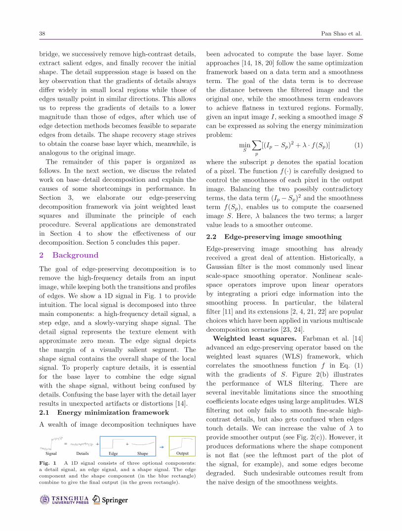
of edges. We show a 1D signal in Fig. 1 to provide

intuition. The local signal is decomposed into three

main components: a high-frequency detail signal, a

step edge, and a slowly-varying shape signal. The

detail signal represents the texture element with

approximate zero mean. The edge signal depicts

the margin of a visually salient segment. The

shape signal contains the overall shape of the local

signal. To properly capture details, it is essential

for the base layer to combine the edge signal

with the shape signal, without being confused by

details. Confusing the base layer with the detail layer

results in unexpected artifacts or distortions [14].

2.1 Energy minimization framework

A wealth of image decomposition techniques have

Signal Details Edge Shape Output

Fig. 1 A 1D signal consists of three optional components:

a detail signal, an edge signal, and a shape signal. The edge

component and the shape component (in the blue rectangle)

combine to give the final output (in the green rectangle).

been advocated to compute the base layer. Some

approaches [14, 18, 20] follow the same optimization

framework based on a data term and a smoothness

term. The goal of the data term is to decrease

the distance between the filtered image and the

original one, while the smoothness term endeavors

to achieve flatness in textured regions. Formally,

given an input image I, seeking a smoothed image S

can be expressed as solving the energy minimization

problem:

minS

∑p

[(Ip − Sp)2 + λ · f(Sp)] (1)

where the subscript p denotes the spatial location

of a pixel. The function f(·) is carefully designed to

control the smoothness of each pixel in the output

image. Balancing the two possibly contradictory

terms, the data term (Ip − Sp)2 and the smoothness

term f(Sp), enables us to compute the coarsened

image S. Here, λ balances the two terms; a larger

value leads to a smoother outcome.

2.2 Edge-preserving image smoothing

Edge-preserving image smoothing has already

received a great deal of attention. Historically, a

Gaussian filter is the most commonly used linear

scale-space smoothing operator. Nonlinear scale-

space operators improve upon linear operators

by integrating a priori edge information into the

smoothing process. In particular, the bilateral

filter [11] and its extensions [2, 4, 21, 22] are popular

choices which have been applied in various multiscale

decomposition scenarios [23, 24].

Weighted least squares. Farbman et al. [14]

advanced an edge-preserving operator based on the

weighted least squares (WLS) framework, which

correlates the smoothness function f in Eq. (1)

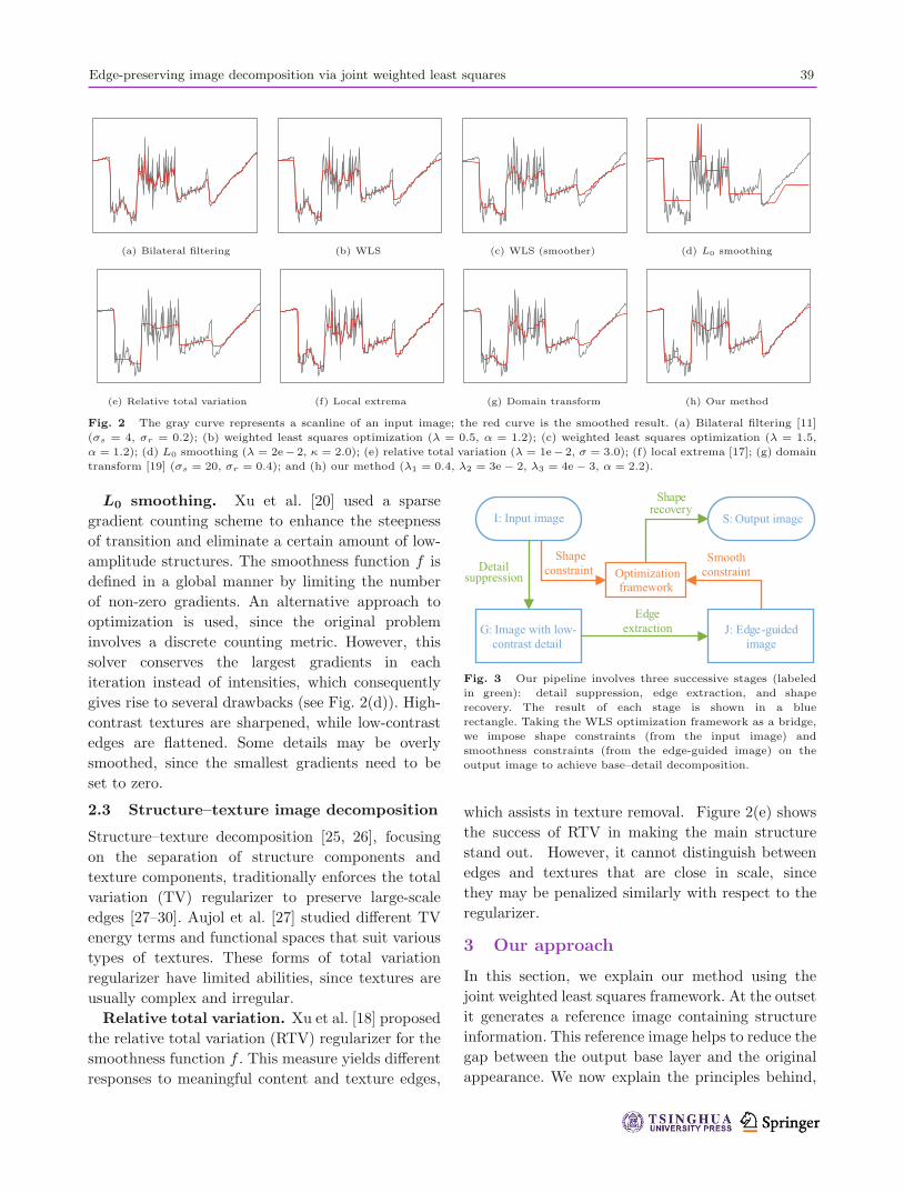
with the gradients of S. Figure 2(b) illustrates

the performance of WLS filtering. There are

several inevitable limitations since the smoothing

coefficients locate edges using large amplitudes. WLS

filtering not only fails to smooth fine-scale high-

contrast details, but also gets confused when edges

touch details. We can increase the value of λ to

provide smoother output (see Fig. 2(c)). However, it

produces deformations where the shape component

is not flat (see the leftmost part of the plot of

the signal, for example), and some edges become

degraded. Such undesirable outcomes result from

the naive design of the smoothness weights.

38

Edge-preserving image decomposition via joint weighted least squares 39

(a) Bilateral filtering (b) WLS (c) WLS (smoother) (d) L0 smoothing

(e) Relative total variation (f) Local extrema (g) Domain transform (h) Our method

Fig. 2 The gray curve represents a scanline of an input image; the red curve is the smoothed result. (a) Bilateral filtering [11]

(σs = 4, σr = 0.2); (b) weighted least squares optimization (λ = 0.5, α = 1.2); (c) weighted least squares optimization (λ = 1.5,

α = 1.2); (d) L0 smoothing (λ = 2e− 2, κ = 2.0); (e) relative total variation (λ = 1e− 2, σ = 3.0); (f) local extrema [17]; (g) domain

transform [19] (σs = 20, σr = 0.4); and (h) our method (λ1 = 0.4, λ2 = 3e− 2, λ3 = 4e− 3, α = 2.2).

L0 smoothing. Xu et al. [20] used a sparse

gradient counting scheme to enhance the steepness

of transition and eliminate a certain amount of low-

amplitude structures. The smoothness function f is

defined in a global manner by limiting the number

of non-zero gradients. An alternative approach to

optimization is used, since the original problem

involves a discrete counting metric. However, this

solver conserves the largest gradients in each

iteration instead of intensities, which consequently

gives rise to several drawbacks (see Fig. 2(d)). High-

contrast textures are sharpened, while low-contrast

edges are flattened. Some details may be overly

smoothed, since the smallest gradients need to be

set to zero.

2.3 Structure–texture image decomposition

Structure–texture decomposition [25, 26], focusing

on the separation of structure components and

texture components, traditionally enforces the total

variation (TV) regularizer to preserve large-scale

edges [27–30]. Aujol et al. [27] studied different TV

energy terms and functional spaces that suit various

types of textures. These forms of total variation

regularizer have limited abilities, since textures are

usually complex and irregular.

Relative total variation. Xu et al. [18] proposed

the relative total variation (RTV) regularizer for the

smoothness function f . This measure yields different

responses to meaningful content and texture edges,

Fig. 3 Our pipeline involves three successive stages (labeled

in green): detail suppression, edge extraction, and shape

recovery. The result of each stage is shown in a blue

rectangle. Taking the WLS optimization framework as a bridge,

we impose shape constraints (from the input image) and

smoothness constraints (from the edge-guided image) on the

output image to achieve base–detail decomposition.

which assists in texture removal. Figure 2(e) shows

the success of RTV in making the main structure

stand out. However, it cannot distinguish between

edges and textures that are close in scale, since

they may be penalized similarly with respect to the

regularizer.

3 Our approach

In this section, we explain our method using the

joint weighted least squares framework. At the outset

it generates a reference image containing structure

information. This reference image helps to reduce the

gap between the output base layer and the original

appearance. We now explain the principles behind,

40 Pan Shao et al.

and relationships of, the three main steps.

3.1 Overview

The pipeline of our approach, diagramed in Fig. 3,

includes three major procedures (indicated by green

arrows): detail suppression, edge extraction, and

shape recovery. Given an input image, we first

compress details or textures to guarantee that their

amplitudes are smaller than those of edges. Next, we

can detect salient edges using existing methods, since

the amplitudes of details have been reduced. The

consequent excessive smoothing, which will be

elaborated later, does not matter, because we just

require a guide image to reflect the structure. This

edge-guided image then supplies a smoothness

constraint, while the input image supplies a shape

constraint (indicated by orange arrows). Ultimately,

using the WLS optimization framework as a bridge,

we produce the final smoothed image which matches

the overall shape of the input image elements.

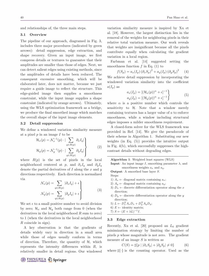
3.2 Detail suppression

We define a windowed variation similarity measure

at a pixel p in an image I to be

Hx(p) = N−1x (p) · |

∑q∈R(p)

∂xIq|

Hy(p) = N−1y (p) · |

∑q∈R(p)

∂yIq|

⎫⎪⎪⎪⎬⎪⎪⎪⎭

(2)

where R(p) is the set of pixels in the local

neighborhood centered at p, and ∂xIq and ∂yIqdenote the partial derivatives of I along the x and y

directions respectively. Each direction is normalized

viaNx(p) =

∑q∈R(p)

|∂xIq|+ ε

Ny(p) =∑

q∈R(p)

|∂yIq|+ ε

⎫⎪⎪⎪⎬⎪⎪⎪⎭

(3)

We set ε to a small positive number to avoid division

by zero; Hx and Hy both range from 0 (when the

derivatives in the local neighborhood R sum to zero)

to 1 (when the derivatives in the local neighborhood

R coincide in sign).

A key observation is that the gradients of

details widely vary in direction in a small area

while those of edges usually conform in terms

of direction. Therefore, the quantity of H, which

represents the intensity differences within R, is

relatively smaller in detail regions. Our windowed

variation similarity measure is inspired by Xu et

al. [18]. However, the largest distinction lies in the

removal of the weights for neighboring pixels in their

relative total variation measure. Our work reveals

that weights are insignificant because all the pixels

contribute equally when calculating the gradient

variation in a local region.

Farbman et al. [14] suggested setting the

smoothness function f in Eq. (1) to

f(Sp) = ax(Ip) (∂xSp)2+ ay(Ip) (∂ySp)

2(4)

We achieve detail suppression by incorporating the

windowed variation similarity into the coefficient

a(Ip) as

ax(Ip) = [(Hx(p))α + ε]−1

ay(Ip) = [(Hy(p))α + ε]−1

}(5)

where α is a positive number which controls the

sensitivity to H. Note that a window merely

containing textures has a larger value of a to enforce

smoothness, while a window including structural

edges imposes a milder smoothness requirement.

A closed-form solver for the WLS framework was

provided in Ref. [14]. We give the pseudocode of

their scheme in Algorithm 1. Substituting our new

weights (in Eq. (5)) provides the intuitive output

in Fig. 4(b), which successfully suppresses the high-

contrast details without degrading edges.

Algorithm 1: Weighted least squares (WLS)

Input: An input image I, smoothing parameter λ, and

smoothness weights ax and ay.

Output: A smoothed base layer S.

Steps:

1) Ax ← diagonal matrix containing ax;

2) Ay ← diagonal matrix containing ay;

3) Dx ← discrete differentiation operator along the x

direction;

4) Dy ← discrete differentiation operator along the y

direction;

5) L ← DTxAxDx +DT

y AyDy;

6) E ← identity matrix;

7) S ← (E + λL)−1I.

3.3 Edge extraction

Recently, Xu et al. [20] proposed an L0 gradient

minimization strategy by limiting the number of

pixels p whose magnitude is not zero. The gradient

measure of an image S is written as

C(S) = �{p | |∂xSp|+ |∂ySp| �= 0} (6)

where �{·} is the counting operator. Used as the

40

Edge-preserving image decomposition via joint weighted least squares 41

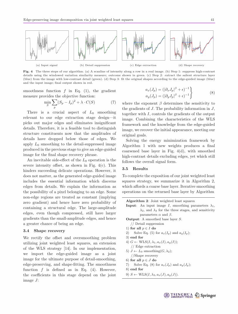
(a) Input signal (b) Detail suppression (c) Edge extraction (d) Shape recovery

Fig. 4 The three steps of our algorithm. (a) A scanline of intensity along a row in a real image. (b) Step 1: suppress high-contrast

details using the windowed variation similarity measure; outcome shown in green. (c) Step 2: extract the salient structure layer

(blue) from the image with low-contrast detail (green). (d) Step 3: fit the original shapes according to the edge-guided image (blue)

and the input image; final output shown in red.

smoothness function f in Eq. (1), the gradient

measure provides the objective function:

minS

∑p

(Sp − Ip)2 + λ · C(S) (7)

There is a crucial aspect of L0 smoothing

relevant to our edge extraction stage design—it

picks out major edges and eliminates insignificant

details. Therefore, it is a feasible tool to distinguish

structure constituents now that the amplitudes of

details have dropped below those of edges. We

apply L0 smoothing to the detail-suppressed image

produced in the previous stage to give an edge-guided

image for the final shape recovery phrase.

An inevitable side-effect of the L0 operation is the

severe intensity offset, as shown in Fig. 4(c). This

hinders succeeding delicate operations. However, it

does not matter, as the generated edge-guided image

includes the essential information which discerns

edges from details. We explain the information as

the possibility of a pixel belonging to an edge. Some

non-edge regions are treated as constant (implying

zero gradient) and hence have zero probability of

containing a structural edge. The large-amplitude

edges, even though compressed, still have larger

gradients than the small-amplitude edges, and hence

a greater chance of being an edge.

3.4 Shape recovery

We rectify the offset and oversmoothing problem

utilizing joint weighted least squares, an extension

of the WLS strategy [14]. In our implementation,

we import the edge-guided image as a joint

image for the ultimate purpose of detail-smoothing,

edge-preserving, and shape-fitting. The smoothness

function f is defined as in Eq. (4). However,

the coefficients in this stage depend on the joint

image J :

ax(Jp) = (|∂xJp|β + ε)−1

ay(Jp) = (|∂yJp|β + ε)−1

}(8)

where the exponent β determines the sensitivity to

the gradients of J . The probability information in J ,

together with I, controls the gradients of the output

image. Combining the characteristics of the WLS

framework and the knowledge from the edge-guided

image, we recover the initial appearance, meeting our

original goals.

Solving the energy minimization framework by

Algorithm 1 with new weights produces a final

coarsened base layer in Fig. 4(d), with smoothed

high-contrast details excluding edges, yet which still

follows the overall signal form.

3.5 Results

To complete the exposition of our joint weighted least

squares strategy, we summarize it in Algorithm 2,

which affords a coarse base layer. Iterative smoothing

operations on the returned base layer by Algorithm

Algorithm 2: Joint weighted least squares

Input: An input image I, smoothing parameters λ1,

λ2, and λ3 for the three stages, and sensitivity

parameters α and β.

Output: A smoothed base layer S.

// Detail suppression

1) for all p ∈ I do

2) Solve Eq. (5) for ax(Ip) and ay(Ip);

3) end for

4) G ← WLS(I, λ1, ax(I), ay(I));

// Edge extraction

5) J ← L0 smoothing(G,λ2);

//Shape recovery

6) for all p ∈ J do

7) Solve Eq. (8) for ax(Jp) and ay(Jp);

8) end for

9) S ← WLS(I, λ3, ax(J), ay(J)).

42 Pan Shao et al.

2 can provide a multiscale decomposition of an

input image, which can be a more satisfactory

result. However, we do not explore this further in

this paper.

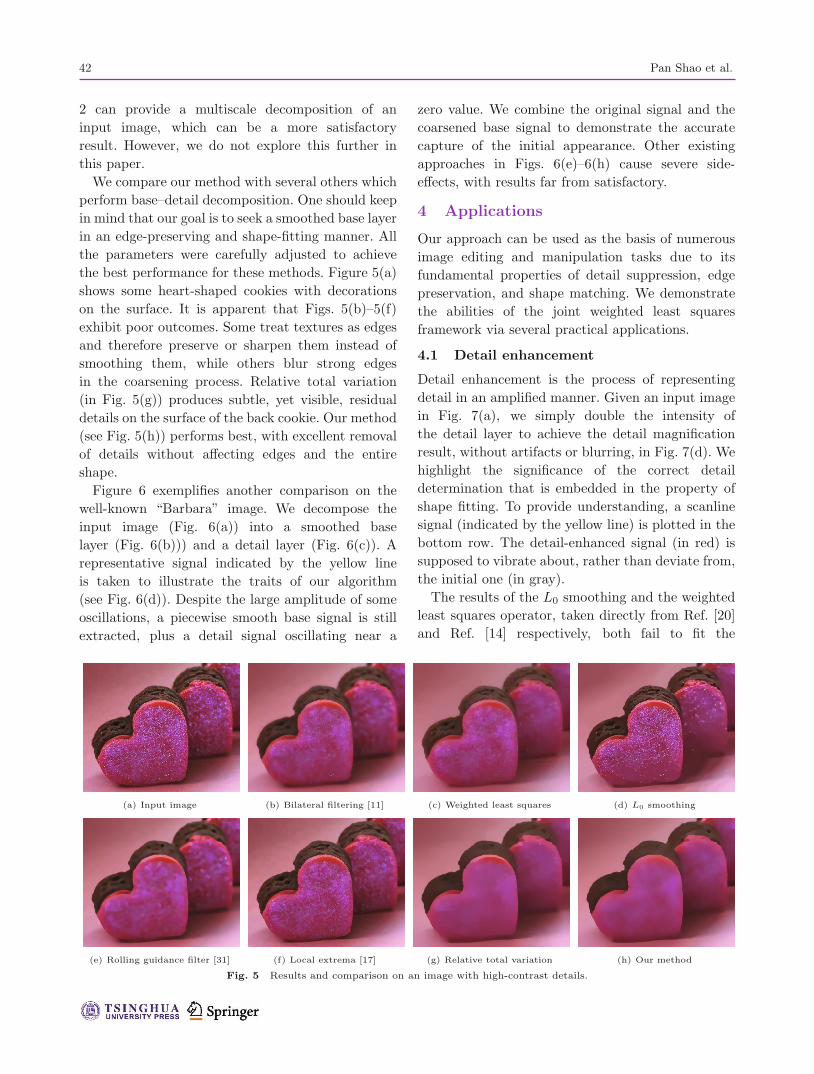
We compare our method with several others which

perform base–detail decomposition. One should keep

in mind that our goal is to seek a smoothed base layer

in an edge-preserving and shape-fitting manner. All

the parameters were carefully adjusted to achieve

the best performance for these methods. Figure 5(a)

shows some heart-shaped cookies with decorations

on the surface. It is apparent that Figs. 5(b)–5(f)

exhibit poor outcomes. Some treat textures as edges

and therefore preserve or sharpen them instead of

smoothing them, while others blur strong edges

in the coarsening process. Relative total variation

(in Fig. 5(g)) produces subtle, yet visible, residual

details on the surface of the back cookie. Our method

(see Fig. 5(h)) performs best, with excellent removal

of details without affecting edges and the entire

shape.

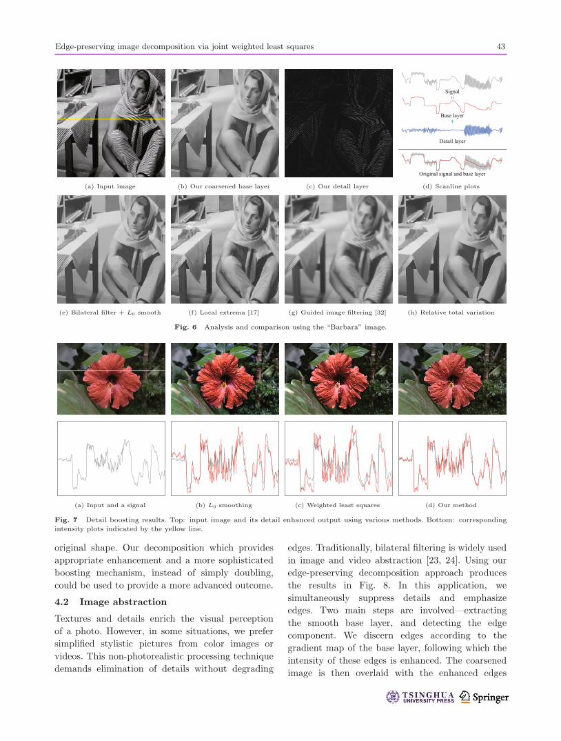
Figure 6 exemplifies another comparison on the

well-known “Barbara” image. We decompose the

input image (Fig. 6(a)) into a smoothed base

layer (Fig. 6(b))) and a detail layer (Fig. 6(c)). A

representative signal indicated by the yellow line

is taken to illustrate the traits of our algorithm

(see Fig. 6(d)). Despite the large amplitude of some

oscillations, a piecewise smooth base signal is still

extracted, plus a detail signal oscillating near a

zero value. We combine the original signal and the

coarsened base signal to demonstrate the accurate

capture of the initial appearance. Other existing

approaches in Figs. 6(e)–6(h) cause severe side-

effects, with results far from satisfactory.

4 Applications

Our approach can be used as the basis of numerous

image editing and manipulation tasks due to its

fundamental properties of detail suppression, edge

preservation, and shape matching. We demonstrate

the abilities of the joint weighted least squares

framework via several practical applications.

4.1 Detail enhancement

Detail enhancement is the process of representing

detail in an amplified manner. Given an input image

in Fig. 7(a), we simply double the intensity of

the detail layer to achieve the detail magnification

result, without artifacts or blurring, in Fig. 7(d). We

highlight the significance of the correct detail

determination that is embedded in the property of

shape fitting. To provide understanding, a scanline

signal (indicated by the yellow line) is plotted in the

bottom row. The detail-enhanced signal (in red) is

supposed to vibrate about, rather than deviate from,

the initial one (in gray).

The results of the L0 smoothing and the weighted

least squares operator, taken directly from Ref. [20]

and Ref. [14] respectively, both fail to fit the

(a) Input image (b) Bilateral filtering [11] (c) Weighted least squares (d) L0 smoothing

(e) Rolling guidance filter [31] (f) Local extrema [17] (g) Relative total variation (h) Our method

Fig. 5 Results and comparison on an image with high-contrast details.

42

Edge-preserving image decomposition via joint weighted least squares 43

(a) Input image (b) Our coarsened base layer (c) Our detail layer

Signal

Base layer

Detail layer

Original signal and base layer

(d) Scanline plots

(e) Bilateral filter + L0 smooth (f) Local extrema [17] (g) Guided image filtering [32] (h) Relative total variation

Fig. 6 Analysis and comparison using the “Barbara” image.

(a) Input and a signal (b) L0 smoothing (c) Weighted least squares (d) Our method

Fig. 7 Detail boosting results. Top: input image and its detail enhanced output using various methods. Bottom: corresponding

intensity plots indicated by the yellow line.

original shape. Our decomposition which provides

appropriate enhancement and a more sophisticated

boosting mechanism, instead of simply doubling,

could be used to provide a more advanced outcome.

4.2 Image abstraction

Textures and details enrich the visual perception

of a photo. However, in some situations, we prefer

simplified stylistic pictures from color images or

videos. This non-photorealistic processing technique

demands elimination of details without degrading

edges. Traditionally, bilateral filtering is widely used

in image and video abstraction [23, 24]. Using our

edge-preserving decomposition approach produces

the results in Fig. 8. In this application, we

simultaneously suppress details and emphasize

edges. Two main steps are involved—extracting

the smooth base layer, and detecting the edge

component. We discern edges according to the

gradient map of the base layer, following which the

intensity of these edges is enhanced. The coarsened

image is then overlaid with the enhanced edges

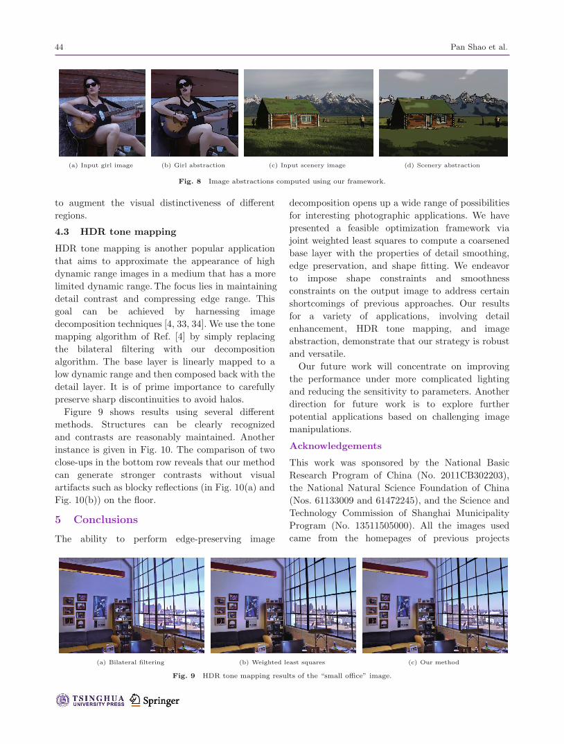
44 Pan Shao et al.

(a) Input girl image (b) Girl abstraction (c) Input scenery image (d) Scenery abstraction

Fig. 8 Image abstractions computed using our framework.

to augment the visual distinctiveness of different

regions.

4.3 HDR tone mapping

HDR tone mapping is another popular application

that aims to approximate the appearance of high

dynamic range images in a medium that has a more

limited dynamic range. The focus lies in maintaining

detail contrast and compressing edge range. This

goal can be achieved by harnessing image

decomposition techniques [4, 33, 34]. We use the tone

mapping algorithm of Ref. [4] by simply replacing

the bilateral filtering with our decomposition

algorithm. The base layer is linearly mapped to a

low dynamic range and then composed back with the

detail layer. It is of prime importance to carefully

preserve sharp discontinuities to avoid halos.

Figure 9 shows results using several different

methods. Structures can be clearly recognized

and contrasts are reasonably maintained. Another

instance is given in Fig. 10. The comparison of two

close-ups in the bottom row reveals that our method

can generate stronger contrasts without visual

artifacts such as blocky reflections (in Fig. 10(a) and

Fig. 10(b)) on the floor.

5 Conclusions

The ability to perform edge-preserving image

decomposition opens up a wide range of possibilities

for interesting photographic applications. We have

presented a feasible optimization framework via

joint weighted least squares to compute a coarsened

base layer with the properties of detail smoothing,

edge preservation, and shape fitting. We endeavor

to impose shape constraints and smoothness

constraints on the output image to address certain

shortcomings of previous approaches. Our results

for a variety of applications, involving detail

enhancement, HDR tone mapping, and image

abstraction, demonstrate that our strategy is robust

and versatile.

Our future work will concentrate on improving

the performance under more complicated lighting

and reducing the sensitivity to parameters. Another

direction for future work is to explore further

potential applications based on challenging image

manipulations.

Acknowledgements

This work was sponsored by the National Basic

Research Program of China (No. 2011CB302203),

the National Natural Science Foundation of China

(Nos. 61133009 and 61472245), and the Science and

Technology Commission of Shanghai Municipality

Program (No. 13511505000). All the images used

came from the homepages of previous projects

(a) Bilateral filtering (b) Weighted least squares (c) Our method

Fig. 9 HDR tone mapping results of the “small office” image.

44

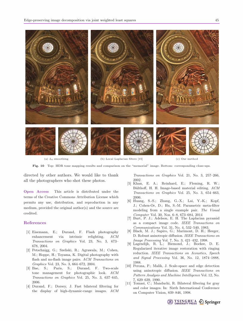
Edge-preserving image decomposition via joint weighted least squares 45

(a) L0 smoothing (b) Local Laplacian filters [15] (c) Our method

Fig. 10 Top: HDR tone mapping results and comparison on the “memorial” image. Bottom: corresponding close-ups.

directed by other authors. We would like to thank

all the photographers who shot these photos.

Open Access This article is distributed under the

terms of the Creative Commons Attribution License which

permits any use, distribution, and reproduction in any

medium, provided the original author(s) and the source are

credited.

References

[1] Eisemann, E.; Durand, F. Flash photography

enhancement via intrinsic relighting. ACM

Transactions on Graphics Vol. 23, No. 3, 673–

678, 2004.[2] Petschnigg, G.; Szeliski, R.; Agrawala, M.; Cohen,

M.; Hoppe, H.; Toyama, K. Digital photography with

flash and no-flash image pairs. ACM Transactions on

Graphics Vol. 23, No. 3, 664–672, 2004.[3] Bae, S.; Paris, S.; Durand, F. Two-scale

tone management for photographic look. ACM

Transactions on Graphics Vol. 25, No. 3, 637–645,

2006.[4] Durand, F.; Dorsey, J. Fast bilateral filtering for

the display of high-dynamic-range images. ACM

Transactions on Graphics Vol. 21, No. 3, 257–266,

2002.[5] Khan, E. A.; Reinhard, E.; Fleming, R. W.;

Bulthoff, H. H. Image-based material editing. ACM

Transactions on Graphics Vol. 25, No. 3, 654–663,

2006.[6] Huang, S.-S.; Zhang, G.-X.; Lai, Y.-K.; Kopf,

J.; Cohen-Or, D.; Hu, S.-M. Parametric meta-filter

modeling from a single example pair. The Visual

Computer Vol. 30, Nos. 6–8, 673–684, 2014[7] Burt, P. J.; Adelson, E. H. The Laplacian pyramid

as a compact image code. IEEE Transactions on

Communications Vol. 31, No. 4, 532–540, 1983.[8] Black, M. J.; Sapiro, G.; Marimont, D. H.; Heeger,

D. Robust anisotropic diffusion. IEEE Transactions on

Image Processing Vol. 7, No. 3, 421–432, 1998.[9] Lagendijk, R. L.; Biemond, J.; Boekee, D. E.

Regularized iterative image restoration with ringing

reduction. IEEE Transactions on Acoustics, Speech

and Signal Processing Vol. 36, No. 12, 1874–1888,

1988.[10] Perona, P.; Malik, J. Scale-space and edge detection

using anisotropic diffusion. IEEE Transactions on

Pattern Analysis and Machine Intelligence Vol. 12, No.

7, 629–639, 1990.[11] Tomasi, C.; Manduchi, R. Bilateral filtering for gray

and color images. In: Sixth International Conference

on Computer Vision, 839–846, 1998.

46 Pan Shao et al.

[12] Bhat, P.; Zitnick, C. L.; Cohen, M.; Curless,

B. GradientShop: A gradient-domain optimization

framework for image and video filtering. ACM

Transactions on Graphics Vol. 29, No. 2, Article No.

10, 2010.[13] Cheng, X.; Zeng, M.; Liu, X. Feature-preserving

filtering with L0 gradient minimization. Computers &

Graphics Vol. 38, 150–157, 2014.[14] Farbman, Z.; Fattal, R.; Lischinski, D.; Szeliski,

R. Edge-preserving decompositions for multi-scale

tone and detail manipulation. ACM Transactions on

Graphics Vol. 27, No. 3, Article No. 67, 2008.[15] Paris, S.; Hasinoff, S. W.; Kautz, J. Local Laplacian

filters: Edge-aware image processing with a Laplacian

pyramid. ACM Transactions on Graphics Vol. 30, No.

4, Article No. 68, 2011.[16] Li, X.-Y.; Gu, Y.; Hu, S.-M.; Martin, R. R.

Mixed-domain edge-aware image manipulation. IEEE

Transactions on Image Processing Vol. 22, No. 5,

1915–1925, 2013.[17] Subr, K.; Soler, C.; Durand, F. Edge-preserving

multiscale image decomposition based on local

extrema. ACM Transactions on Graphics Vol. 28, No.

5, Article No. 147, 2009.[18] Xu, L.; Yan, Q.; Xia, Y.; Jia, J. Structure

extraction from texture via relative total variation.

ACM Transactions on Graphics Vol. 31, No. 6, Article

No. 139, 2012.[19] Gastal, E. S. L.; Oliveira, M. M. Domain transform

for edge-aware image and video processing. ACM

Transactions on Graphics Vol. 30, No. 4, Article No.

69, 2011.[20] Xu, L.; Lu, C.; Xu, Y.; Jia, J. Image smoothing

via L0 gradient minimization. ACM Transactions on

Graphics Vol. 30, No. 6, Article No. 174, 2011.[21] Choudhury, P.; Tumblin, J. The trilateral filter

for high contrast images and meshes. In: ACM

SIGGRAPH 2005 Courses, Article No. 5, 2005[22] Su, Z.; Luo, X.; Deng, Z.; Liang, Y.; Ji, Z. Edge-

preserving texture suppression filter based on joint

filtering schemes. IEEE Transactions on Multimedia

Vol. 15, No. 3, 535–548, 2013.[23] Chen, J.; Paris, S.and ; Durand, F. Real-time edge-

aware image processing with the bilateral grid. ACM

Transactions on Graphics Vol. 26, No. 3, Article No.

103, 2007.[24] Winnemoller, H.; Olsen, S. C.; Gooch, B. Real-time

video abstraction. ACM Transactions on Graphics

Vol. 25, No. 3, 1221–1226, 2006.[25] Karacan, L.; Erdem, E.; Erdem, A. Structure-

preserving image smoothing via region covariances.

ACM Transactions on Graphics Vol. 32, No. 6, Article

No. 176, 2013.[26] Su, Z.; Luo, X.; Artusi, A. A novel image

decomposition approach and its applications. The

Visual Computer Vol. 29, No. 10, 1011–1023, 2013.[27] Aujol, J.-F.; Gilboa, G.; Chan, T.; Osher, S.

Structure-texture image decomposition—modeling,

algorithms, and parameter selection. International

Journal of Computer Vision Vol. 67, No. 1, 111–136,

2006.[28] Meyer, Y. Oscillating Patterns in Image Processing

and Nonlinear Evolution Equations: The Fifteenth

Dean Jacqueline B. Lewis Memorial Lectures. Boston,

MA, USA: American Mathematical Society, 2001.[29] Rudin, L. I.; Osher, S.; Fatemi, E. Nonlinear total

variation based noise removal algorithms. Physica D :

Nonlinear Phenomena Vol. 60, Nos. 1–4, 259–268,

1992.[30] Yin, W.; Goldfarb, D.; Osher, S. Image cartoon-

texture decomposition and feature selection using

the total variation regularized L1 functional. In:

Proceedings of the Third international conference on

Variational, Geometric, and Level Set Methods in

Computer Vision, 73–84, 2005.[31] Zhang, Q.; Shen, X.; Xu, L.; Jia, J. Rolling

guidance filter. In: Computer Vision–ECCV 2014.

Lecture Notes in Computer Science Volume 8691.

Fleet, D.; Pajdla, T.; Schiele, B.; Tuytelaars, T. Eds.

Switzerland: Springer International Publishing, 815–

830, 2014.[32] He, K.; Sun, J.; Tang, X. Guided image filtering.

IEEE Transactions on Pattern Analysis and Machine

Intelligence Vol. 35, No. 6, 1397–1409, 2013.[33] Li, Y.; Sharan, L.; Adelson, E. H. Compressing and

companding high dynamic range images with subband

architectures. ACM Transactions on Graphics Vol. 24,

No. 3, 836–844, 2005.[34] Tumblin, J.; Turk, G. LCIS: A boundary hierarchy for

detail-preserving contrast reduction. In: Proceedings

of the 26th annual conference on Computer graphics

and interactive techniques, 83–90, 1999.

Pan Shao received the B.S. degree in

computer science from Shanghai Jiao

Tong University in 2013. She is now

working toward the M.S. degree in

the Department of Computer Science

and Engineering at Shanghai Jiao Tong

University. Her research interests lie in

image editing and face recognition.

Shouhong Ding received the B.S. and

M.S. degrees from the School of

Mathematical Sciences in Dalian

University of Technology, China,

in 2008 and 2011, respectively. He

is now a Ph.D. candidate in the

Department of Computer Science

and Engineering, Shanghai Jiao Tong

University, China. His current research interests include

image/video editing, computer vision, computer graphics,

and digital media technology.

46

Edge-preserving image decomposition via joint weighted least squares 47

Lizhuang Ma received his

Ph.D. degree from Zhejiang University

in 1991. He is now a full professor,

Ph.D. tutor, and the head of the

Digital Media Technology and Data

Reconstruction Lab at the Department

of Computer Science and Engineering,

Shanghai Jiao Tong University since

2002. He is also the chairman of the Center of Information

Science and Technology for Traditional Chinese Medicine

in Shanghai Traditional Chinese Medicine University. His

research interests include computer-aided geometric design,

computer graphics, scientific data visualization, computer

animation, digital media technology, and theory and

applications for computer graphics, CAD/CAM.

Yunsheng Wu received his B.S. degree

in computer science from Peking

University, China. He is now a product

director in Tencent Inc., China. He is

responsible for QQ video, Pitu, QQ

tornado, and Watermark Camera. His

current research interest is face

recognition.

Yongjian Wu received the M.S. degree

from Computer School in Wuhan

University, China, in 2008. He is

now a senior researcher in Tencent

Inc., China. His current research

interests include computer vision,

pattern recognition, and digital media

technology.