Noninformative Priors and Nuisance ParametersAuthor(s): Bertrand Clarke and Larry WassermanSource: Journal of the American Statistical Association, Vol. 88, No. 424 (Dec., 1993), pp. 1427-1432Published by: Taylor & Francis, Ltd. on behalf of the American Statistical AssociationStable URL: http://www.jstor.org/stable/2291287 .

Accessed: 16/01/2015 11:40

Your use of the JSTOR archive indicates your acceptance of the Terms & Conditions of Use, available at .http://www.jstor.org/page/info/about/policies/terms.jsp

.JSTOR is a not-for-profit service that helps scholars, researchers, and students discover, use, and build upon a wide range ofcontent in a trusted digital archive. We use information technology and tools to increase productivity and facilitate new formsof scholarship. For more information about JSTOR, please contact support@jstor.org.

.

Taylor & Francis, Ltd. and American Statistical Association are collaborating with JSTOR to digitize, preserveand extend access to Journal of the American Statistical Association.

http://www.jstor.org

This content downloaded from 129.93.4.65 on Fri, 16 Jan 2015 11:40:21 AMAll use subject to JSTOR Terms and Conditions

Noninformative Priors and Nuisance Parameters Bertrand CLARKE and Larry WASSERMAN*

We study the conflict between priors that are noninformative for a parameter of interest versus priors that are noninformative for the whole parameter. Our investigation leads us to maximize a functional that has two terms: an asymptotic approximation to a standardized expected Kullback-Leibler distance between the marginal prior and marginal posterior for a parameter of interest, and a penalty term measuring the distance of the prior from the Jeffreys prior. A positive constant multiplying the second terms determines the tradeoff between noninformativity for the parameter of interest and noninformativity for the entire parameter. As the constant increases, the prior tends to the Jeffreys prior. When the constant tends to 0, the prior becomes degenerate except in special cases. This prior does not have a closed-form solution, but we present a simple, numerical algorithm for finding the prior. We compare this prior to the Berger-Bernardo prior.

KEY WORDS: Asymptotic information; Reference prior; Tradeoff prior.

1. INTRODUCTION

Consider the distance between a prior density ir(6) for a k-dimensional real parameter 6 and the posterior density corresponding to it. A reference prior may be defined to be

arg sup E(d(ir(, ir(' I Y))), ~rP

where d is a measure of distance, r is a set of priors, and yn = (Yl, . .. , yn) is an outcome of yn = (Y1, . . . , Yn). Here E refers to the expectation over the marginal distribution for yn induced by the prior and the model. Choices for d such as Hellinger distance (Jeffreys 1961, sec. 3.10) have been considered. Here we choose a distance that has an infor- mation theoretic motivation, the Shannon mutual infor- mation. For this choice we write

'Yn(r) 1(e; y n)

= f m(yn) f 7r( I yn)log r(60 Yf) dO dyn

= EmK(1r( I yn), i(.)),

where K is the Kullback-Leibler distance defined by K(p, q) = f p log(p/q) and m is the marginal density for the data defined by m(yn) = f 7r(O)f(yn I d0. We assume ft( Y 6) = I =t( y1 I 0), wheref( * / ) is a parametric family.

It can be proved that asymptotically maximizing Yn( ir) over prior densities results in Jeifreys's prior (see Clarke and Barron 1990b). But this assumes that all parameters are of interest. More generally, consider 6 = (w, X) where w E R k, is a parameter of interest and X E R k2 is a nuisance parameter. In this case Jeffreys's prior (Jeffreys 1961, sec. 3. 10) has been criticized for leading to unacceptable results. An example of this Yi - N(61, 1) where YI, . . ., Yn are independent and w = El 6. The Jeifreys prior for 61, ..., 6n is a flat prior, but conventional wisdom holds that better inferences result from priors that shrink toward some point.

* Bertrand Clarke is Assistant Professor, Department of Statistics, Purdue University, West Lafayette, IN 47907. Larry Wasserman is Associate Pro- fessor, Department of Statistics, Carnegie Mellon University, Pittsburgh, PA 15213. Wasserman's research was supported by National Science Foundation Grant DMS-9005858 and National Institutes of Health Grant RO 1-CA54852- 01. Part of this research was conducted at the Cornell Workshop on Con- ditional Inference sponsored by the U.S. Army Mathematical Sciences In- stitute and the Statistics Research Center (June 3-14, 1991). The authors thank Nick Polson for several helpful discussions and an associate editor and a referee for useful suggestions.

Another example where Jeffreys's prior does not work well is in estimating the product of two normal means (see Berger and Bernardo 1989). When we refer to Jeffreys's prior, we refer to the formal application of Jeffreys's rule. We remind the reader that Jeffreys did not advocate using this rule in all problems.

One possible explanation for this poor behavior of Jef- freys's prior is that is achieves optimal noninformativity for 6 at the cost of being partially informative for w. In Bernardo's (1979) terminology, Jeffreys's prior maximizes the missing information for 0 but not for w. This led Bernardo (1979) and Berger and Bernardo (1989, 1992a, 1992b) to define a reference prior that is essentially a stepwise Jeffreys's prior. Their method seems to give reasonable priors, but the mo- tivation for the method is unclear.

In this article we propose an alternative method of con- structing priors. First, we find an asymptotic expression for the Kullback-Leibler distance between the marginal prior and marginal posterior for w accurate to o(l). We then find the prior that maximizes this distance subject to a penalty term that measures distance from the Jeffreys prior so as to obtain a prior that gives up some of its noninformativity for X to become more noninformative for w. The prior depends on a scalar a that reflects the trade-off between being non- informative for X and being noninformative for w. So, we obtain a continuum of priors varying between the Jeffreys prior and the marginally noninformative prior. Although these priors cannot be expressed in closed form, we describe a simple algorithm for finding them numerically. We com- pare our solution to the Berger-Bernardo prior in two ex- amples: the bivariate binomial and the multinomial.

We should say at the outset that by a "noninformative prior" we mean a prior that has, asymptotically, large ex- pected distance from the posterior in a given experiment.

2. BACKGROUND

2.1 The Berger-Bernardo Method

We begin by reviewing the method of Bernardo (1979) and Berger and Bernardo (1992a). Recall that the Jeffreys

? 1993 American Statistical Association Journal of the American Statistical Association

December 1993, Vol. 88, No. 424, Theory and Methods

1427

This content downloaded from 129.93.4.65 on Fri, 16 Jan 2015 11:40:21 AMAll use subject to JSTOR Terms and Conditions

1428 Journal of the American Statistical Association, December 1993

prior is defined by

J(Q X) II(0)Il/2 f11(0) 111/2 dO'

where I is the Fisher information matrix and I indicates the determinant. The Berger-Bernardo method has two steps. First, use the Jeffreys prior for the nuisance parameter con- ditional on the parameter of interest; that is, set ir( XI w) OC 1122(W, X)I 112/c(X), where 122 is the lower right k2 X k2 block of I and c( X) normalizes the density over a compact set. (To use this method, one must truncate the parameter space to a compact set so that the conditional Jeffreys prior is integrable. We also truncate to compact sets as needed). To obtain a joint reference prior, note that when 7r(X I w) is as just described, then

1(0; yn) = k log n 2 2ire

+ f 7r(w)log exp(2 f 7r(X Iw)logI II I1I221 1 dX} dw

- f ir(w)log{Ir(w)} dw + o(1)

under various regularity conditions; see Lemma 3.1. Asymptotically maximizing the standardized distance I(0; y n) - (k, /2)log(n/27re) over all marginal prior densities for w gives

ir(w) = exp{ f r( I W)log1 IIIII22 I -1 dX}/c,

where c is a normalizing constant. The Berger-Bernardo prior is the product 7r( w )i7r( X I w ) .

This method achieves noninformativity over the nuisance parameter first and, subject to this, is least informative for the parameter of interest. But the Jeffreys prior achieves maximal noninformativity in an information-theoretic sense. So, using the Jeffreys prior on the nuisance parameter in the first step sacrifices noninformativity where it is needed most-on the parameter of interest.

Examination of the preceding expression for 1(0; yn) led Ghosh and Mukerjee (1992) to consider f 7r(w) log { ir(w) } X dw as a "penalty term" effectively forcing shrinkage to- wards a uniform prior. In Section 4 we use the information- theoretic formulation to motivate a single maximization of a two-term functional instead of a two-step maximization. Note that the Berger-Bernardo method, the Ghosh-Muker- jee method and our method all reduce to the Jeffreys prior when there are no nuisance parameters.

2.2 Noninformativity in the Absence of Nuisance Parameters

Bernardo's method is based on the idea that in the limit for large n, -y(ir) represents the missing information for someone using prior ir. Thus the prior that maximizes this "missing information" is the one that will be most changed by experimentation. It is in this sense that the prior is least informative.

But Bernardo (1979) noted that lim, , -y,n( 7r) is typically infinite (see also Davisson 1973; Ibrigamov and H'asminsky 1973). Berger and Bernardo sidestepped this by finding the prior 1rn* that maximizes -y, and then taking the limit of 1rn* as n -- 00. In contrast, we use a standardized version of Yn(Or) that has a finite limit. Polson (1988) and Ghosh and Mukerjee (1992) argued in a similar way.

Following Ibrigamov and H'asminsky (1973) and Clarke and Barron (1991), we may write (assuming certain regularity conditions)

k n lI0)l2d0o1 YnO(r)= -logg + 7r(0)log 1 d) +o(l), 2 2-re rO

where k is the dimension of 0. We define the standardized distanceiyn(ir) by in(lr) = Yn(Or) - (k/2)log(n/2ire) and define the asymptotic missing information by

r I1(0)1 1/2 j(7r) lim in(r)=J !r( )log 1r(0) dO.

n-* o1 'r( f )

Provided that II(011/2 is integrable, a variational argu- ment shows that 0 (ir) is maximized by choosing ir(0) oc I I(0) 1 1/2, which, when normalized, is the Jeffreys prior. In a decision-theoretic formulation, Clarke and Barron (1 990b) showed that Jeffreys's prior is least favorable under an entropy loss criterion.

3. NUISANCE PARAMETERS

Write 0 = (c, X), where c is the parameter of interest and X is a nuisance parameter. For a given joint prior ir(w, X), we compute the expected Kullback-Leibler distance between the prior and posterior for the parameter of interest. Let -y(ir) = E(K(xr(w I yn), r(w))), where 7r(w I yn)

= r(W, XI ynf) dX and ir(w) = r(w, X) dX. Then we have the following lemma.

Lemma 3. 1.

Yn() = - logn 2 27re

+ ff r( ,X)logI ) g dw dX + o(l), I 7r( wL)

where k, is the dimension of w and S = {II(w, X)I X 1122(W, X) I -1 1 1/2.

(All proofs are contained in the Appendix.) We point out that the same formula appears, without a complete proof, in Ghosh and Mukerjee (1992).

Now we define the asymptotic marginal missing infor- mation for w by 00(ir) = lim,2OI{ y(1r) - (k1/2) X log(n/2ire)} = ff r( w, X )log { S/ 7r( w)} dw d X. Because c is the parameter of interest, we begin by maximizing ~0(ir). This idea was suggested by Ghosh and Mukerjee (1992), who observed that the entropy of ir(w) appears as a penalty term in yn(ir) -(k1/2)log(n/2ire) that does not involve the nuisance parameter. They suggested that as a result, the maximizing priors would prove unsatisfactory. We verify their intuition in the next lemma.

This content downloaded from 129.93.4.65 on Fri, 16 Jan 2015 11:40:21 AMAll use subject to JSTOR Terms and Conditions

Clarke and Wasserman: Noninformative Priors 1429

Lemma 3.2. Suppose that w and X are orthogonal; that is, 112 = 121 = 0, where 112 = 121 is the upper right k, X k2 block by the Fisher information matrix:

a. If II I (w, X) is a function of w only, then any prior that satisfies 7r(w) oc VI III (w) I maximizes ' (ir).

b. If I 11 1I1 = f(w)g(X) for some fand g with g not con- stant, g is continuous, and the parameter space is com- pact, then any prior that has w marginal with density proportional to fv(W) and has conditional distribution for X given w concentrating on the set g- (sup g) max- imizes A' (ir).

Remark 1. Note that any statistical model may be re- parameterized so that the parameters are orthogonal (see Cox and Reid 1987).

Part a of Lemma 3.2 shows that when inferences about the parameters can be separated, Jeffreys's prior maximizes

00' . More generally, there is a class of priors that maximizes this quantity. In particular, Tibshirani's (1989) prior maxi- mizes A' ( r). In Example 5.1 we will see that unlike the method we will present, the Berger-Bernardo prior does not reproduce the Jeffreys prior in this situation.

Part b of Lemma 3.2 shows that maximizing j O(ir) can lead to degenerate priors that effectively assume that the nui- sance parameter is known. The reason for this behavior is that the criterion achieves noninformativity for the parameter of interest at the cost of exact knowledge for the nuisance parameter.

4. AN ALTERNATIVE METHOD

The Jeffreys prior and the degenerate priors presented in the preceding section are two extreme cases. The first does not distinguish between nuisance parameters and parameters of interest; the second assumes that the nuisance parameter is known and hence not a nuisance. To interpolate between these two extremes, we define a functional that measures distance between the marginal prior and the marginal pos- terior subject to a penalty term that measures the distance from the Jeffreys prior. We then find the prior that maximizes this functional. Our method assumes that it is generally im- possible to achieve simultaneously maximal noninformativ- ity for the whole parameter and the parameter of interest.

Definition. The tradeoff prior for w is the prior 7ray that maximizes 00 - aK(J, ira), where K( *, *) is Kullback- Leibler distance, J = J(w, X) is Jeffreys's prior, and a > 0.

Remark 2. If the conditions of Lemma 3.2.a hold and 122 is only a function of X, then it is straightforward to show that -ray is Jeffreys's prior for every a.

The parameter a reflects the relative importance of the nuisance parameters. The penalty term forces shrinkage to- wards the Jeffreys prior. When a = 0, this prior is the de- generate prior in Lemma 3.2.b. As a increases, the penalty term dominates, and the prior becomes noninformative for the whole parameter. In practice, ae must be chosen to reflect the trade-off between these two extremes. We note that Ghosh and Mukerjee ( 1992) suggested maximizing z 0 + axH( r), where H( ir) is the entropy of ir. But this prior

shrinks towards the uniform prior instead of the Jeffreys prior as a - oo0.

Theorem 4.1. Assume that 7ra is bounded away from 0. Then the prior Ira satisfies

XaJ(w, X) ira(w, X) - log(S/irx(w)) + Ca

where C. is the unique constant determined by the fact that 7ra is positive and integrates to 1.

Corollary. lim,,7ra = J as long as the limit exists.

Theorem 4.2. The trade-off prior is invariant under smooth monotone transformations of w and X.

Remark 3. In general, the trade-off prior, like the Berger- Bernardo prior, is not invariant under transformations that involve both w and X. This is to be expected, because w is being singled out as a parameter of interest.

Remark 4. In current work we have been able to show that if instead the penalty K( Ira, J) is used, then the maxi- mizing prior is

ra(w, X) = S(W, X)l/aJ(W, X) Wa(W)l/(a?l) f Wa(W)a/(a+l) dw

where

Wa(w) = f S(w, X)l/aJ(w, X) dX.

If S is a function of w only, then this prior reduces to the Berger-Bernardo prior when a tends to 0. Otherwise, it tends to a degenerate prior with density equal to S(w, X,,)/ f S(w, X,,) dw on the manifold {(w, X,); w E 0]k, } . Here X, is the point where S(w, X) is maximized for fixed w.

The form of the solution in Theorem 4.1 suggests the fol- lowing algorithm for finding Ira.

Algorithm. Step 0. Choose ir0(w, X). Set ir0(w) = ro(w, X) dX. Let

i = 1. Repeat the next three steps until convergence. Step 1. Find C such that f Z'c = 1, where

a J(w, X) ZC =

- log(S/ ri-r1 (w)) + C

Step 2. Set ri (w, X) = Zi'. Step 3. Set 7ri(w) = f 7r'(w, X) dX. Let i = i + 1. The algorithm is used for the examples in the next section.

5. EXAMPLES

5.1 The Bivariate Binomial

Consider the following model for the germination of spores. Each of m spores has a probability p of germinating. Of the r spores that germinate, each has a probability q of bending in a particular direction. Let s be the number that bend in the specified direction. The probability model is

f(r, sip, q, m) = (m)pr(l _-)mr )qs(1 - q)s

This content downloaded from 129.93.4.65 on Fri, 16 Jan 2015 11:40:21 AMAll use subject to JSTOR Terms and Conditions

1430 Journal of the American Statistical Association, December 1993

forr= 1, .. ., m and s = 1, .. ., r. This is called the bivariate binomial model. Crowder and Sweeting (1989) and Polson and Wasserman (1990) have proposed priors for this model.

The Fisher information matrix is

I(p, q) = m{p(l pp) q(l -

The Jeffreys prior is lrj(p, q) oc ( p1 -' /2q- /2

X (1 -q) Polson and Wasserman (1990) showed that when q is the

parameter of interest and p is the nuisance parameter, the Berger-Bernardo prior is 'XBB(P, q) cc p 1/2(l -p)

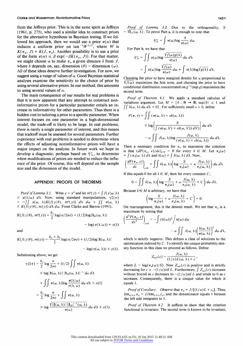
X q-/2(I - q)-2. We used the algorithm in Section 4 to find I7ra. The result is shown in Figure 1 for several values of a. The degenerate form of Ir, when a is near 0 illustrates the effect described in Lemma 3.2.b. The convergence to the overall Jeffreys prior as a increases illustrates the corollary.

5.2 The Trinomial

Suppose that y = (Yi, Y2, y3), where the yi3s are nonneg- ative integers, and that

p(yi0, n) = n!Y 02jY3 0 2 , !32t2!Y3!

where n = Yi + Y2 + Y3, 0 = (01, 02, 03), 0i > 0, i = 1, 2, 3, and 03 = 1 - 01 - 02. Thus y has a trinomial distribution. Let w = 01 and X = 02. The Jeffreys prior is J(01, 02) 1c 01282(l -01 - 02)1/2; the Berger-Bernardo prior

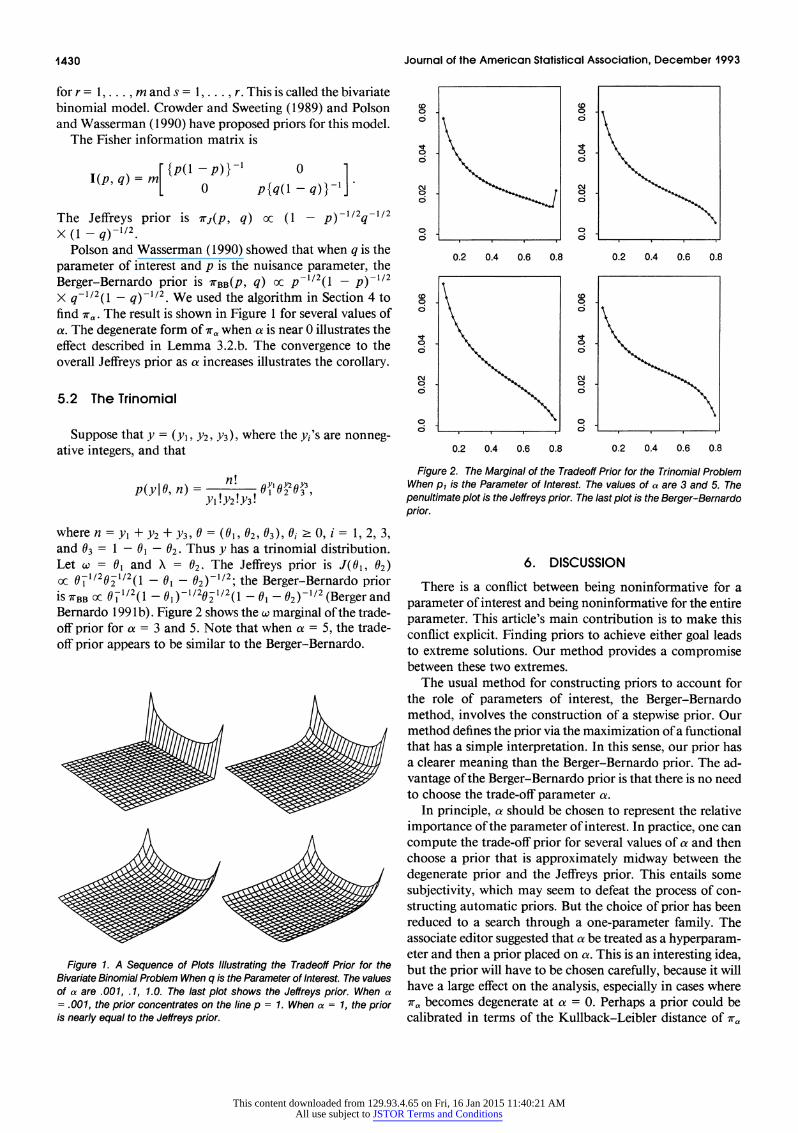
is orBBc 0C1/2(1 - 01)20'2 ( - 01 - 02) 12(Bergerand Bernardo 199 lb). Figure 2 shows the w marginal of the trade- off prior for a = 3 and 5. Note that when a = 5, the trade- off prior appears to be similar to the Berger-Bernardo.

Figure 1. A Sequence of Plots Illustrating the Tradeoff Prior for the Bivariate Binomial Problem When q is the Parameter of Interest. The values of az are .001, .1, 1.0. The last plot shows the Jeifreys prior. When ax = .001, the prior concentrates on the line p = 1. When az = 1, the prior is nearly equal to the Jeifreys prior.

o 0 6l oi

0.2 0.4 0.6 0.8 0.2 0.4 0.6 0.8

o 0

0.2 0.4 0.6 0.8 0.2 0.4 0.6 0.8

Figure 2. The Marginal of the Tradeoff Prior for the Trinomial Problem When pi is the Parameter of Interest. The values of a are 3 and 5. The penultimate plot is the Jeffreys prior. The last plot is the Berger-Bernardo prior.

6. DISCUSSION

There is a conflict between being noninformative for a parameter of interest and being noninformative for the entire parameter. This article's main contribution is to make this conflict explicit. Finding priors to achieve either goal leads to extreme solutions. Our method provides a compromise between these two extremes.

The usual method for constructing priors to account for the role of parameters of interest, the Berger-Bernardo method, involves the construction of a stepwise prior. Our method defines the prior via the maximization of a functional that has a simple interpretation. In this sense, our prior has a clearer meaning than the Berger-Bernardo p0or. The ad- vantage ofthe Berger-Bernardo prior is that there is no need to choose the trade-o0 parameter a.

In principle, az should be chosen to represent the relative importance of the parameter of interest. In practice, one can compute the trade-of prior for several values of o and then choose a prior that is approximately midway between the degenerate prior and the Jeireys prior. This entails some subjectivity, which may seem to defeat the process of con- structing automatic priors. But the choice of prior has been reduced to a search through a one-parameter family. The associate editor suggested that a be treated as a hyperparam- eter and then a pror tlaced on coz This is an interesting ideas

conlit texlctFidn priorswl avob those achievul,bue eihe goalled

baetwe thesre efetwon h nlss extremes. cse wer

therole beofe paaeteerst a of int.erest,sth Berger-Bernadob

melbrthod deine theprior via the mulaxkimiztioro aisfunction7al

This content downloaded from 129.93.4.65 on Fri, 16 Jan 2015 11:40:21 AMAll use subject to JSTOR Terms and Conditions

Clarke and Wasserman: Noninformative Priors 1431

from the Jeffreys prior. This is in the same spirit as Jeffreys (1961, p. 275), who used a similar idea to construct priors for the alternative hypothesis in Bayesian testing. If we fol- lowed his approach, then we would use a prior ir( a) that induces a uniform prior on tan- W112, where W is K(-rae, J) + K(J, ). Another possibility is to use a prior of the form ir(a) oc d exp (-f3K(-rxa, J)). For that matter, we might choose a to make Ira a given distance b from J, where S depends on, say, dimension (0) - dimension (co). All of these ideas deserve further investigation. For now, we suggest using a range of values of a. Good Bayesian statistical analyses examine the sensitivity to the choice of prior by using several alternative priors. In our method, this amounts to using several values of a.

The main consequence of our results for real problems is that it is now apparent that any attempt to construct non- informative priors for a particular parameter entails an in- crease in informativity for other parameters. Thus there is a hidden cost to tailoring a prior to a specific parameter. When interest focuses on one parameter in a high-dimensional model, the trade-off is likely to be large. In real problems, there is rarely a single parameter of interest, and this means that tradeoff must be assessed for several parameters. Further experience with real problems is needed to determine when the effects of adjusting noninformative priors will have a major impact on the analysis. In future work we hope to develop a diagnostic, perhaps based on jA' , to determine when modifications of priors are needed to reduce the influ- ence of the prior. Of course, this will depend on the sample size and the dimension of the model.

APPENDIX: PROOFS OF THEOREMS

Proof of Lemma 3.1. Write y = yf and let m@'(y) = f f(yIco, X) X r( XI c) dX. Now, using standard manipulations, y'y(1r) = -rr 1r(w, X)K(f(yl6), mw(y)) dX do + ff 7r(Wr X) X K(f(y 0), m(y)) dX dw. From Clarke and Barron (1991),

K(f(y 6), m@(y)) = - log(n/2ire) + (1/2)1og1I22(w, X)I 2

- log(ir(X I c)) + o(l)

and

K(f(y I0), m(y))= k

2 2 log(n/27re) + (1/2)logI(co, X)1 2

- log(ir(w, X)) + o(l). Substituting above, we get

'Yn(7r) = k2 log n

+ (1/2) r(cf x) n 2 2i7re J

X log1I(co, X) l 1122(CO, X)KI` do dX

+ jf 7r(C, X)log ( Ic2 dw dX + o(l)

7r(X, )

VkI(cn C) I 112 wX

Proof of Lemma 3.2. Due to the orthogonality, S = XII(C, A). To prove Part a, it is enough to note that

i = f f r(w) log ~dwo.

For Part b, we have that

i= ff rr(cw)log f( ) ( ) do dX

= f r(wc)log d+f r( X X)logg(X) dX.

Choosing the prior to have marginal density for co proportional to f( w) maximizes the first term, and choosing the prior to have

conditional distribution concentrated on g- (sup g) maximizes the second term.

Proof of Theorem 4.1. We apply a standard calculus of variations argument. Let M = {6 : 0 -* R; sup I31 ? 1 and frf (c, X) dco dX = 0}. For sufficiently small e > 0, define

F(ir, e) = ff ((, X) + e(co, X))

X lj {. (r(o X') + e(co, X')) dX')}

a JJ J((), X)log ( J(co, X) do d x (ir(wo, X) + e3(co, X)) cc X

Then a necessary condition for 7r. to maximize the criterion is that (dF(ira, e)/de),.o = 0 for every 6 E M. Let ira(Co) = X (ira(W, A) dX and 3(wo) = r(w, X) dX. Now,

(F( ira,) f JJ(, X)(log ira(4) +a ( X) /dco dX.

If this equals 0 for all 6 E M, then for every constant C,

0= f 6(, X)(log s 4 + a ( X) +C) Cd dX.

Because 3 E M is arbitrary, we have that

(log S 4) + J(c + C) 0.

On rearrangement, this is the desired result. We see that 7ra is a maximum by noting that d2 F(rra, e)' U 2/ co

(( c/a )__ =2J (M(Cu)))2 r(co) d

- a J( co, X)( X dco d X, \ r(co, X)/ which is strictly negative. This defines a class of solutions to the optimization indexed by C. To identify the unique probability den- sity function in this class we proceed as follows. Define

Z. X(C) = J(w, X) ( la/)L(w, X) + c

where L = log(ra(co)/S). Now Zj,c(c) is positive and is strictly decreasing for c > -(1 /a)inf L. Furthermore, f Z(,,,c(c) increases without bound as c decreases to - (1 /a) inf L and tends to 0 as c increases. Consequently, there is a unique value for which it equals 1.

ProofofCorollary. Observethat ira= J/[(1 /a)L +cal].Thus, lima ..00 7ra = J/lima..O Ca, and the denominator equals 1 because the left side integrates to 1.

Proof of Theorem 4.2. It suffices to show that the criterion functional is invariant. The second term is known to be invariant,

This content downloaded from 129.93.4.65 on Fri, 16 Jan 2015 11:40:21 AMAll use subject to JSTOR Terms and Conditions

1432 Journal of the American Statistical Association, December 1993

so we need only show that j. (ir) is invariant. We will prove this for w and X both scalar; the proof in higher dimensions is similar. Consider a transformation (w, X) -* (p, a), where 13 = g(w) and cr = G(X). Let h = g-1 and H = G-1. The Jacobian of the transformation is A = diag(h'(0), H'(o)), so p(fl, a) = ir(h(f), H(o))h'(fl)H'(a). Because 1(0, a) = AI(w, X)A', we have II(13, o)I = {h'(fl)H'()} 21I(w, X)I and 122(13, i)

= {H'(a) o}2I22(w, X). Thus S(fl, a) = h'(fl)S(w, X). Now

ya0(7r) = fPf03 o)log S(O a) df du

= j4 ir(h(#), H(o))h'(fl)H'(cr)

x log h'(f)S(h(fl) H(a)) df d 7r(h h(1)) h'(13)

= ff rr(w, X)h'(g(w))H'(G(X))

X log S( X) g'(W)G'(X) dv dX ir(w)

= tff ir(w, X)log S( X) dco dX = (r) [7r( CO Rv)

[Received October 1991. Revised July 1992]

REFERENCES

Berger, J., and Bernardo, J. (1989), "Estimating the Product of Means: Bayesian Analysis With Reference Priors," J. Amer. Statist. Assoc., 84, 200-207.

(1992a), "On the Development of the Reference Prior Method," in Bayesian Statistics 4, eds. J. M. Bernardo, J. 0. Berger, A. P. Dawid, and A. F. M. Smith, New York: Oxford University Press, pp. 35-60.

(1 992b), "Ordered Group Reference Priors With Application to the Multinomial Problem," Biometrika, 79, 25-38.

Bernardo, J. (1979), "Reference Posterior Distributions for Bayesian Infer- ence" (with discussion), Journal of the Royal Statistical Society, Ser. B, 41, 113-147.

Clarke, B., and Barron, A. (1 990a), "Information-Theoretic Asymptotics of Bayes Methods," IEEE Transactions on Information Theory, 36, 453- 471.

(1990b), "Bayes and Minimax Asymptotics of Entropy Risk," Technical Report 90-11, Purdue University, Dept. of Statistics.

(1991), "Entropy Risk and the Bayesian Central Limit Theorem," technical report, Purdue University, Dept. of Statistics.

Cox, D. R., and Reid, N. (1987), "Parameter Orthogonality and Approximate Conditional Inference," Journal of the Royal Statistical Society, Ser. B, 49, 1-18.

Crowder, M., and Sweeting, T. (1989), "Bayesian Inference for a Bivariate Binomial," Biometrika, 76, 599-604.

Ghosh, J. K., and Mukeree, R. (1 992), "Noninformative Priors," in Bayesian Statistics 4, ed. J. M. Bernardo, J. 0. Berger, A. P. Dawid, and A. F. M. Smith, New York: Oxford University Press, pp. 195-210.

Ibrigamov, I. A., and H'asminsky, R. Z. (1973), "On the Information Con- tained in a Sample About a Parameter," Second International Symposium on Information Theory, pp. 295-309.

Jeifreys, H. (1961), Theory ofProbability (3rd ed.). Oxford, U.K.: Clarendon Press.

Polson, N. (1988), "Bayesian Perspectives on Statistical Modeling," unpub- lished Ph.D. dissertation, University of Nottingham, Dept. of Mathematics.

Polson, N., and Wasserman, L. (1990), "Prior Distributions for the Bivariate Binomial," Biometrika, 77, 901-904.

Tibshirani, R. (1989), "Noninformative Priors for One Parameter of Many," Biometrika, 76, 604-608.

This content downloaded from 129.93.4.65 on Fri, 16 Jan 2015 11:40:21 AMAll use subject to JSTOR Terms and Conditions