Photometry in UV astronomical images of extended sourcesin crowded field using deblended images in optical visible

bands as bayesian priors

Vibert D.a, Zamojski M.b, Conseil S.a, Llebaria A.a, Arnouts S.c, Milliard B.a, Guillaume M.d

a Laboratoire d’Astrophysique de Marseille, OAMP, Universite Aix-Marseille & CNRS,Marseille, France;

bCalifornia Institute of Technology, Pasadena, United StatescCanada France Hawaii Telescope, Kamuela, Hawaii, United States

dInstitut Fresnel, Universite Aix Marseille III, Marseille, France

ABSTRACT

Photometry of astrophysical sources, galaxies and stars, in crowded field images, if an old problem , is stilla challenging goal, as new space survey missions are launched, releasing new data with increased sensibility,resolution and field of view. The GALEX mission, observes in two UV bands and produces deep sky imagesof millions of galaxies or stars mixed together. These UV observations are of lower resolution than same fieldobserved in visible bands, and with a very faint signal, at the level of the photon noise for a substantial fractionof objects. Our purpose is to use the better known optical counterparts as prior information in a Bayesianapproach to deduce the UV flux.

Photometry of extended sources has been addressed several times using various techniques: backgrounddetermination via sigma clipping,1 adaptative-aperture,2 point-spread-function photometry3,4 isophotal pho-tometry,5,6 to lists some. The Bayesian approach of using optical priors for solving the UV photometry hasalready been applied by our team in a previous work.7,8 Here we describe the improvement of using the ex-tended shape inferred by deblending the high resolution optical images and not only the position of the opticalsources.

The resulting photometric accuracy has been tested with simulation of crowded UV fields added on topof real UV images. Finally, this helps to converge to smaller and flat residual and increase the faint sourcedetection threshold. It thus gives the opportunity to work on 2nd order effects, like improving the knowledge ofthe background or point-spread function by iterating on them.

Keywords: UV astronomical imagery, photometry, Data fusion, Bayesian estimation, Point spread functionmodeling, minimization

1. INTRODUCTION

Launched in 2005 the GALEX instrument9 on board of a NASA Explorer mission, is collecting an unprecedentedset of astronomical UV images and spectral data in the far (135-175 nm) and the near (170-275 nm) UV range.The telescope continuously scans circular areas of sky of 1o75 of diameter. The key device in the imaging processis the photon counting camera providing the position of each photon in the focal plane. Knowing the telescopemovement the process re-situates positions in the field of view, with a precision in resolution of ∼ 5′′. The fieldis sampled by a grid of 3840×3840 positions or square pixels, each one of 1.5′′ wide, subsampling the PSF by atleast a factor 3. The image results from the progressive accumulation of counts in each pixel.

The observations are performed in 3 different modes corresponding to different exposure times. Here weare concerned with the 3rd Deep Imaging Survey (DIS) with a long exposure time (> 30000s). The DIS fields

Further author information: (Send correspondence to Didier Vibert)E-mail: didier.vibert@@oamp.fr, Telephone: +33 4 95 044163Address: Laboratoire d’Astrophysique de Marseille, 38 rue Frederic Joliot Curie, 13388 Marseille cedex 13, France

Computational Imaging VII, edited by Charles A. Bouman, Eric L. Miller, Ilya Pollak, Proc. of SPIE-IS&T Electronic Imaging,SPIE Vol. 7246, 72460U · © 2009 SPIE-IS&T · CCC code: 0277-786X/09/$18 · doi: 10.1117/12.810228

SPIE-IS&T/ Vol. 7246 72460U-1

Figure 1. Some examples to compare Galex images (left) and their optical counterpart (right). In these 3 cases, only oneobject was detected on Galex image using SExtractor where one can see several optical sources that obviously have UVflux.

being very sensitive, contains many faint galaxies below the confusion limit, characterized by blends, ambiguitiesand miss-identifications of the astronomical sources due to local crowding of very dim galaxies concealed in thebackground (Figure 1).

Using SExtractor6 to extract sources from Galex DIS fields yields to miss a large fraction of objects andmoreover to overestimate their flux. The morphological similarity of these UV images to their counterparts inthe visible bands suggest to use the visible high resolution counterparts as Bayesian prior information to inferthe UV flux. The DAOPHOT software package (3) include such an approach but assumes unresolved sources(objects are considered Dirac convolved by the psf) and Gaussian additive noise, whereas Galex images combineextended and unresolved objects and are dominated by Poisson photon shot noise. Then we developed a methodto address properly this inverse problem.

In a previous paper7) we presented the original procedure used to face on this challenge. This approach usesthe Poisson statistics to define the Bayes assumption and solve for the maximum posterior likelihood with theconstraint for all fluxes to be positive. Then, in a second paper,8 we discussed the photometric performancesand behavior of the method when dealing with imperfect knowledge of background, psf and object positions.

Here we will focus on improvements made on the method, using the actual optical image as prior informationrather than it’s position or elliptical shape obtained from the SExtractor catalog. After a short recall on the EMmethod we will describe the method to obtain these “stamps”, we will also discuss some improvements on psfand re-centering optimization and finally we quantify the gain of doing so.

2. METHOD

2.1 ML parametric Estimation with Priors

The specificity of the proposed photometric procedure is the Bayesian approach under the Poisson noise assump-tion. The solution is reached with an EM algorithm.

Let be xi for i ∈ {1, ...M} the observed value on pixel i of the UV image considered as a sample of the randomvariable Xi following a Poisson statistics. Let be μi = E{Xi} for i ∈ {1, ...M} the expected values for this image.Let be hk,i the known relative value of object k ∈ {1, ...K} on pixel i deduced from the visible catalog. Let beαT = (α1, . . . αk) the vector of unknown fluxes of these objects. Last, let bi be the known background level valueon pixel i of the UV image.

We define the model for the UV image as follows:

∀i ∈ {1, . . . M}{

μi =∑K

k=1 αkhk,i + bi

P{Xi = xi} = exp(−μi)µ

xii

xi!

where hk,i =∑

j

ok,jfi−j

here hk,i results from the convolution between each object known profile ok,i with the point spread function fi

of GALEX imaging system. By normalizing the function hk,i to unity, this model allows to estimate directly α,the flux vector of the set of sources in the image.

SPIE-IS&T/ Vol. 7246 72460U-2

As was shown in more detail in the first article,7 introducing the expectation maximize scheme (EM, seeHoriuchi et al., 200010) we get the iterative algorithm:

α(n+1)k = α

(n)k

∑Mi=1(xi/μ

(n)i )hk,i∑M

i=1 hk,i

where μ(n)i =

K∑j=1

α(n)j hj,i + bi (1)

The E step compares the data image xi to the projection μ(n)i of the α

(n)i estimates. The result is introduced

in the M step as the corrective ratio needed for the new set of α(n+1)k estimates. To ease the overall algorithm,

the background level b is considered known, we found it in a previous procedure, as is described in the articleof reference.7 The EM application here is closely related to classical Richardson-Lucy methods well know in theliterature of image processing for astronomy (see Burud et al,11 Stark and Bijaoui12)

The initial guess for αi is obtained by using the classical pseudo-invert to solve the over determined system:

xi =K∑

k=1

α(0)k hk,i + bi ∀i ∈ xi > bi and α

(0)k ≥ |ε(b)| (2)

To speed up this step, we can limit ourselves to the diagonal of the pseudo-inverse, which gives:

α(0)k =

∑Mi=1 hk,i(xi − bi)∑M

i=1 h2k,i

∀i ∈ xi > bi and α(0)k ≥ |ε(b)| (3)

In order to tract the large size of the problem (4000 pixels square image and more that 100 000 objects), theentire field is divided in a set of small rectangular “tiles” of identical sizes. To deal with borders, a margin ofhalf the size of the PSF is added around each tile and the margins are overlapping from one tile to a neighboringtile. The priors in the margins are only used to reduce border effects on the objects inside the tile.

2.2 Determining priors informationBefore being able to run such an algorithm one need to determine the prior information: basically bi thebackground and hk,i the contribution of each objects to each pixels, composed of the PSF fi and the objectknown profile ok,i.

2.2.1 The objects profile

In the previous implementations, the object profiles could be of two kinds: for a star like object or any unresolvedobjects, the object was modeled by a Dirac at the exact sub-pixel position given in the optical catalogue, andthe psf was interpolated to be shifted at the correct sub-pixel position. For resolved objects, we used theelliptical shape coming out from the optical SExtractor catalogue, rescaled at the Galex resolution and appliedan exponential profile along the radius of the ellipses:

P = (ab

π/2) exp(−

√[(xp − xc) cos θ + (yp − yc) sin θ

a

]2

+[−(xp − xc) sin θ + (yp − yc) cos θ

b

]2

) (4)

where (xp, yp) and (xc, yc) represent the position of the pixel and that of the object center, and a,b representthe semi-major and semi-minor axis of the object ellipse.

For this framework we described the resolved objects more precisely using the actual optical image ratherthan the catalog. The idea is simply to degrade the resolution of the image to that of the GALEX image and toconvolve each object with the GALEX PSF. However to be able to do this, we must derive the profile of everyobject independantly meaning that the optical image needs to be segmented and, most importantly, deblendedfirst. Our approach to resolve this problem has been to use a segmentation and deblending method much similarto the one SExtractor uses. Below we describe in more details the method.

SPIE-IS&T/ Vol. 7246 72460U-3

2.2.2 Deblending Optical shapes

In order to segment the optical image, we use SExtractor ellipses to define the contours of our objects. We thendeblend overlapping objects by dividing the flux of blended pixels among all objects whose contours encompassthose pixels in such a way that the fraction of the flux assigned to each object is proportional to the flux thatobject possesses in the pixel opposite (symmetrically with respect to the center) to the blended pixel. In the eventthis is not possible because one or more of the symmetric pixels are themselves blended, the objects which dohave well-defined fluxes at the location opposite to the blended pixel, are assigned the same flux, at their blendedlocation, as that of their symmetrically opposite pixel. In the case that only one object remains un-deblended ata given location, it is assigned the balance of the flux in that pixel. After this, if there is more than one objectthat remains to be deblended, then the algorithm proceeds to other pixels, until all pixels have been attempteddeblending, at which points it iterates the above process so that newly deblended pixels can be used to furtherdeblend the ones that were not completely successful in the previous iterations. So it goes until either all pixelshave been deblended or until no further deblending occurs. In the event that the procedure stops before all pixelshave been successfully deblended, the remaining pixels have their flux split among the objects that overlap themin a way that the fraction assigned to each object is proportional to the same exponential of elliptical radiusexplained in 4. This last step is more arbitrary than the first part of the procedure, but is necessary to bring thedeblending process to completion. Typically, in all but the most crowded fields, ∼ 0.1% of the initially blendedpixels will have to be deblended this way, and this fraction even often reaches zero.

Figure 2 illustrates the results of this deblending procedure. It shows how objects can be extracted from anoptical image and deblended into separate elliptical disks. The original optical image can then be interpreted asa sum of those separate disks, or more succinctly, as the sum of layers in which no two objects overlap.

Once the optical image deblended, we degrade the resolution of each object to that of GALEX, and convolvethe degraded image with the GALEX PSF, thus obtaining a GALEX prior profile for each object. These profileswill then be feeded to the EM algorithm for solving the flux. It will determine the weight of each objectcontributing to the total UV flux in each pixel that has the highest statistical likelihood given the observed data.

2.2.3 The PSF

The precise modeling of the PSF is crucial for the successful issue of the method. The detector structure for theNUV channel sustains a PSF model with a narrow kernel of 3 pixels FWHM surrounded by a very large haloup to 64 pixel of radial extension. The high dynamic range of more than 103 in the GALEX images requiresa precise determination of this halo in order to minimize the errors due to the halos of brightest stars on thefield. The standard modeling using the Sextractor package was revealed inefficient to restore accurately the haloin particular for the far UV channel where the S/N is very low. As alternative we decided to use a two stepsapproach. In the first step we look for a precise estimation of the kernel using the StarFinder13 package. Itallows for a precise re-centering and selection. In the second step the PSF is fitted by the sum of three centeredGaussians functions. The dramatic reduction in the degrees of freedom to 3× 3 parameters ensure a smoothnessand denoising of the PSF.

Despite this effort in the PSF modeling, we know that the PSF determination is not perfect as can be seen inthe residual image. Once the objects profiles infered from high resolution optical bands are included, we see inthe residual (the best EM-fitted model subtracted to the UV observed data) a systematic pattern on all brightenough objects. This clearly shows we subtracted a PSF too large. This arises for two reasons mainly. One isthe optical PSF (5 times smaller than the GALEX one) that was not deconvolved from the optical image beforebuilding the prior shapes. The second cause is due to the stacking of PSFs done by StarFinder. The stacking isperformed on manually selected unresolved-objects, whose image is supposed to contain only the PSF. Obviouslyit is hard to ensure this condition: the object might be slightly extended (a few pixels) as it is the case for manygalaxies in the GALEX DIS fields. Then the recentering needed to stack all the PSFs has a limited precisionand theses small errors in the PSFs centers, lead to a larger averaged PSF.

In order to correct for this imperfect knowledge of the PSF, we included an optimization step in the algorithm:after a first bunch of EM-iterations computed with the initial estimates of the PSF, we minimize the likelihoodwith fixed fluxes and varying PSFs parameters. In a first implementation we parameterized the initial psf withonly one parameter, doing an homothecy or dilation of the psf. We are looking forward to implement the

SPIE-IS&T/ Vol. 7246 72460U-4

Figure 2. Example of an optical image with SExtractor segmentation ellipses and our resulting deblending shown in fourrecomposed layers of non-overlapping objects.

SPIE-IS&T/ Vol. 7246 72460U-5

optimization on the whole model described above in a future work. Here, for the spatial rescaling of the psf, weemployed Brent’s method14 to minimize a function by using parabolic interpolation. This operation is done tileby tile. One need then to gather the PSF estimation on each tile into one PSF non-varying over the field. Oncethe optimization of the PSF is performed we recompute a bunch of EM-iterations to solve again the fluxes withthe newly obtained PSF.

2.2.4 The astrometry

We have seen in the previous works8 that the errors on the positions of the priors have big consequences on theprecision of the resulting photometry. We thus tried to improve the correct centering of priors in the field.

The first thing to achieve before any further processing is a correction of the distortion of the Galex image.To do so we cross-correlate the positions of the brightest objects detected with SExtractor in the Galex imagewith the brightest objects of the prior catalogue. Supposing the positions of the prior catalogue have negligibleerrors (recall they are obtained from a lot higher resolution images) we then fit the discrepancies of the twocatalogues by 2nd degree polynome on x and y. Then all the positions of the prior objects are warped using thispolynome.

The second correction for astrometry is then performed at the same stage where we optimize for the PSF.After a first bunch of EM-iterations, we use the estimated image to correct the recentering. Either we computea sub-pixel (dx, dy) displacement on each tile via oversampling and FFT cross-corelation of the observed imageand estimated one. Or we minimize the likelihood with respect to a (dx, dy) displacement of all the priors.

2.2.5 The background

Several choices can be made here. The first one is to use the background determined by the Galex data reductionpipeline. It has the advantage of being free from non-linear filtering of the original image but with the drawbackof being very smooth.

The other is to use the background as determined in8 using the inferior hull of the image found through anonlinear multiresolution top-down approach. It has the advantage of containing more high-frequency structureswith the drawback of possibly filtering out the unknown signal we are trying to recover.

The third is to use the low-frequency background knowing, it may lack some high frequency components,and try to recover these sharp components from the residual after applying the EM-iterations. Note that we aretalking here of frequency components that need be larger than the noise frequency components. The full processin then:

1. run EM solving with an initial background

2. mask-out from the residual a small region (smaller than the PSF) around all the objects (since a smallerror in flux or prior position leads to an artifact in the residual).

3. fill the masked region using the multiresolution method cited above.

4. low-pass filter out the Poisson noise high frequency components

5. redo the EM-iteration with the new background

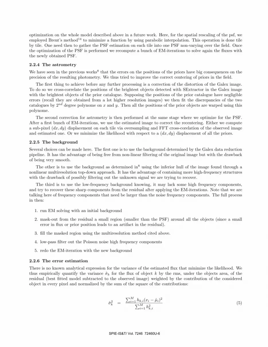
2.2.6 The error estimation

There is no known analytical expression for the variance of the estimated flux that minimize the likelihood. Wethus empirically quantify the variance σk for the flux of object k by the rms, under the objects area, of theresidual (best fitted model subtracted to the observed image) weighted by the contribution of the consideredobject in every pixel and normalized by the sum of the square of the contributions:

σ2k =

∑Mi=1 hk,i(xi − μi)2∑M

i=1 h2k,i

(5)

SPIE-IS&T/ Vol. 7246 72460U-6

4

Figure 3. Estimation of the variance on the estimated fluxes (left) from the weighted mean square of the residual (right).

where μi =∑K

j=1 αjhj,i + bi is the estimated value on pixel i for the estimated fluxes αj . We show that thisestimation is consistent with the true errors obtained from the simulation. The figure 5 shows how the qualityof the residual under objects area may be used to estimate the variance.

3. RESULTS

The figure 4 shows an example of the method applied to the Galex XMMLSS Near UV field using the CFHTLSdata as optical priors. The residual shown is a lot better compared to what could be obtained before using thefull optical image as priors and optimizing the PSF.

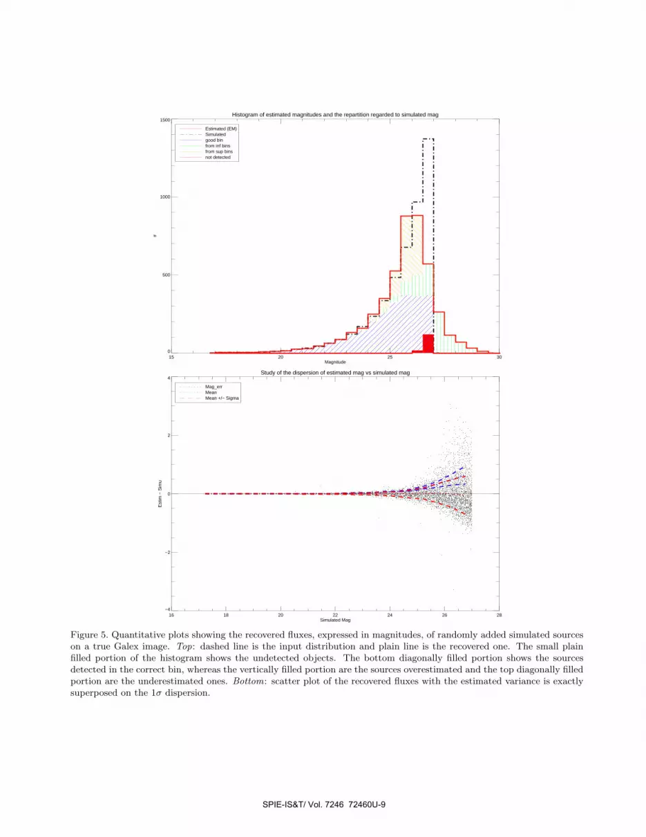
The behavior of the method is quantified using simulations. We inserted randomly in the field a large setof pseudo-stars on the original UV images. These star-like objects were built with the PSF deduced from theoriginal UV field itself. This method allows us to determine the error of magnitude vs. magnitude relationshipas well as the operational range of magnitudes. The figure 5 shows the recovered fluxes by bins of magnitude.It shows that up to magnitude ∼ 25.5 which is one magnitude higher than the original Galex catalogue themethod is complete. There is still an Eddington bias in the recovered distribution of magnitude, inherent to theassymetry of the input distribution and hard to eliminate totally.

The estimated variance from the residual on these known simulated objects appears fully consistent with thedispersion shown in figure 5.

4. CONCLUSION

Test results show a noticeable gain on magnitude limit as well as in resolution relative to the standard pipelinemethod using SExtractor. On current DIS fields , EM provides good photometry and completeness down tomagnitude 25.5 which is 1 magnitude deeper than the GALEX pipeline.

The use of shaped priors combined with a simple psf optimization improved drastically the residual. If lessimpressive, the photometry has been improved also. The dispersion has been reduced for the faint magnitudes(∼ 25).

The gain on the residual will now let us work on the background by iterating on it after masking and filteringthe residual. By doing so, we may gain sharp features that may have interesting astrophysical sense.

REFERENCES[1] Costa, G. D., “Basic photometry techniques,” in [Astronomical CCD Observing and Reduction Techniques ],

Howell, S. B., ed., ASP Conf Series 23 (1992).[2] Kron, R. G., “Photometry of a complete sample of faint galaxies,” The Astroph. Journal 43, 305–325 (June

1980).[3] Stetson, P., “Daophot a computer program for crowded field stellar photometry,” Publ. Astron. Soc. of the

Pacific 99, 191 (1987).

SPIE-IS&T/ Vol. 7246 72460U-7

4S

II

;''o®

:4h .® . -.®) ®(

- . -a

IU4

p

4

I4

U

Figure 4. Example of 100 EM iteration using deblended optical shapes. Top left : Galex XMMLSS field. Top right :corresponding CFHTLS optical U band. Middle left : same Galex field with superposed selected priors. Middle right :CFHTLS selected sources with magnitude < 26.5. Bottom left : optimal solution from EM convergence. Bottom rightresidual

SPIE-IS&T/ Vol. 7246 72460U-8

Histogram of estimated magnitudes and the repartition regarded to simulated mag

15 20 25 30Magnitude

0

500

1000

1500

#

Estimated (EM)Simulatedgood binfrom inf binsfrom sup binsnot detected

Study of the dispersion of estimated mag vs simulated mag

16 18 20 22 24 26 28Simulated Mag

−4

−2

0

2

4

Est

im −

Sim

u

Mag_errMeanMean +/− Sigma

Figure 5. Quantitative plots showing the recovered fluxes, expressed in magnitudes, of randomly added simulated sourceson a true Galex image. Top: dashed line is the input distribution and plain line is the recovered one. The small plainfilled portion of the histogram shows the undetected objects. The bottom diagonally filled portion shows the sourcesdetected in the correct bin, whereas the vertically filled portion are the sources overestimated and the top diagonally filledportion are the underestimated ones. Bottom: scatter plot of the recovered fluxes with the estimated variance is exactlysuperposed on the 1σ dispersion.

SPIE-IS&T/ Vol. 7246 72460U-9

[4] Penny, A. J. and Dickens, R. J., “CCD photometry of the globular cluster NGC 6752,” MNRAS 220,845–867 (June 1986).

[5] Beard, S. M., MacGillivray, H. T., and Thanisch, P. F., “The Cosmos System for Crowded-Field Analysisof Digitized Photographic Plate Scans,” MNRAS 247, 311–+ (Nov. 1990).

[6] Bertin, E. and Arnouts, S., “Sextractor: software for source extraction,” Astron. Astrophys. Suppl. Se-ries 117, 393–404 (1996).

[7] Guillaume, M., Llebaria, A., Aymeric, D., Arnouts, S., and Milliard, B., “Deblending of the uv photometryin galex deep surveys using optical priors in the visible wavelengths,” in [Image Processing: Algorithms andSystems, Neural Networks and Machone Learning ], Dougherty, Astola, Egiazarian, Nasrabadi, and Rizvi,eds., Proc. SPIE 6064, 11–1–11–10 (2005).

[8] Llebaria, A., Magnelli, B., Arnouts, S., Pollo, A., Milliard, B., and Guillaume, M., “Multi-channel 2D pho-tometry with super-resolution in far UV astronomical images using priors in visible bands,” in [Society ofPhoto-Optical Instrumentation Engineers (SPIE) Conference Series ], Society of Photo-Optical Instrumen-tation Engineers (SPIE) Conference Series 6812 (Mar. 2008).

[9] Martin, D., Fanson, J., Schiminovich, D., Morrisey, P., Friedman, P., Barlow, T., Conrow, T., R.Grange,Jelinsky, P. N., B.Milliard, Siegmund, O., Bianchi, L., Byun, Y., J.Donas, K.Forster, M.Heckman, T., Lee,Y.-W., Madore, B., Neff, S., Rich, R., T.Small, F.Surber, A.Szalay, B.Welsh, and Wyder, T., “The glaxyevolution explorer: A space ultraviolet survey mission,” The Astroph. Journal Letters 619, L1–L6 (2005).

[10] Horiuchi, S., Kameno, S., and Ohishi, M., “Developping a wavelet clean algorithm for radio-interferometerimaging,” in [Astronomical data analysis software and systems X ], F.R. Handen, F. P. and Payne, H., eds.,Conference Series 238, 529–532, The Astron. Soc. of the Pacific (2001).

[11] Burud, I., Stabell, R., Magain, P., Courbin, F., Ostensen, R., S.Refsdal, and Remy, J., “Three photometricmethodes tested on bround based data of q2237+0305,” Astron. Astrophys. 339, 701–708 (1998).

[12] Stark, J. and Bijaoui, A., “Multiresolution deconvolution,” J. Optical Soc. Am. A 11(5), 1580–1588 (1994).[13] Diolaiti, E., O.Bendinelli, Bonaccini, D., Close, L., Currie, D., and Parmeggiani, G., “Starfinder,” in [Adap-

tative Optical Systems technology ], Wiziniwich, P., ed., Proc. SPIE 4007, 879–888 (2000).[14] Brent, R. P., [Algorithms for Minimization without Derivatives ], Prentice-Hall (1973).

SPIE-IS&T/ Vol. 7246 72460U-10