bayesian and non-bayesian probabilistic models for medical image analysis

Bayesian and non-Bayesian probabilistic models

for medical image analysis

P.A. Bromiley*, N.A. Thacker, M.L.J. Scott, M. Pokric, A.J. Lacey, T.F. Cootes

Imaging Science and Biomedical Engineering Division, Medical School, University of Manchester, Stopford Building, Oxford Road, Manchester M13 9PT, UK

Accepted 20 March 2003

Abstract

Bayesian approaches to data analysis are popular in machine vision, and yet the main advantage of Bayes theory, the ability to incorporate

prior knowledge in the form of the prior probabilities, may lead to problems in some quantitative tasks. In this paper we demonstrate

examples of Bayesian and non-Bayesian techniques from the area of magnetic resonance image (MRI) analysis. Issues raised by these

examples are used to illustrate difficulties in Bayesian methods and to motivate an approach based on frequentist methods. We believe this

approach to be more suited to quantitative data analysis, and provide a general theory for the use of these methods in learning (Bayes risk)

systems and for data fusion. Proofs are given for the more novel aspects of the theory. We conclude with a discussion of the strengths and

weaknesses, and the fundamental suitability, of Bayesian and non-Bayesian approaches for MRI analysis in particular, and for machine

vision systems in general.

q 2003 Elsevier B.V. All rights reserved.

Keywords: Bayesian and non-Bayesian probabilistic models; Magnetic resonance image analysis; Expectation maximisation algorithm

1. Introduction

This paper discusses the use of Bayes theory in decision

systems which make use of medical image data. We concern

ourselves only with the use of the equation

PðHildataÞ ¼PðdatalHiÞPðHiÞXj

PðdatalHjÞPðHjÞð1Þ

for the interpretation of mutually exclusive hypotheses Hj;

as the basis for algorithmic design. We compare such

approaches with alternatives based on frequentist statistics.

Bayes theory is a cornerstone of modern probabilistic

data analysis, used to construct probabilistic decision

systems so that prior knowledge can be incorporated into

the data analysis in order to ‘bias’ the interpretation of the

data in the direction of expectation. The prior probabilities

therefore have the greatest influence when the data are

unable to adequately support any model hypothesis, and so

direct application of a purely data-driven solution is not

possible. The use of Bayes theory can appear to provide

spectacular improvements in the interpretation of data.

However, despite their popularity and widespread accep-

tance, there are often significant practical problems in the

application of Bayesian techniques.

First, Bayesian approaches use information regarding

the distribution of a whole group of data to influence the

interpretation of a single data set. This may lead to the

suppression of infrequently occurring data, such as

pathological data in medical image analysis, or other

novelty. Since pathological cases are often unique, skepti-

cism concerning the use of Bayesian approaches in areas

such as medical data analysis is clearly justified. We explain

the effects of bias and novelty in Bayesian estimation in

Section 2, using a Bayesian multi-dimensional MR volu-

metric measurement technique as an example.

In Section 3 we give an example of a Bayesian system

designed to evaluate the degree of atrophy in the brain

arising from a variety of dementing diseases, and use this to

motivate a discussion of some problems associated with

learning, priors and Bayes risk. First we discuss the source

of the prior probabilities, an area on which many researchers

have concentrated [3,18]. Ideally this prior information

could be established uniquely for a particular task.

However, if Bayes theory is to make predictions regarding

the likely ratio of real world events it must be accepted that

0262-8856/03/$ - see front matter q 2003 Elsevier B.V. All rights reserved.

doi:10.1016/S0262-8856(03)00072-6

Image and Vision Computing 21 (2003) 851–864

www.elsevier.com/locate/imavis

* Corresponding author.

E-mail addresses: [email protected] (P.A. Bromiley), neil.

[email protected] (N.A. Thacker).

http://www.elsevier.com/locate/imavis

the data samples used in Bayesian approaches must

represent a stratified random sample of the types of data

under analysis.1 Thus, in the absence of a deterministic

physical mechanism giving rise to the data set there can be

no theoretical justification for belief in the existence of a

unique prior. In addition, the prior distributions must change

to reflect any changes in the circumstances in which the

system is used, a situation often encountered in data analysis

problems involving biological data sets.

Secondly, we discuss the use of Bayes theory in learning

systems. In order for Bayes theory to be applied correctly

the likelihood distributions (PðdatalHiÞ) of all possible

interpretations Hi of the data must be known. Unfortunately,

in many practical circumstances these distributions are not

well known a priori. It could be regarded as a weakness if

the computational framework used in a learning system

demanded that all possible interpretations of the data were

available before a useful statistical inference could be

drawn.

Finally, any decisions based on Bayesian classification

results should also be made on the basis of the Bayes risk, in

order to minimise the cost of the decision. The aim in

clinical support systems, for example, is to provide

treatment which improves the prognosis of the patient,

rather than just providing the correct diagnosis. The

inclusion of non-stationary prior probabilities in clinical

information presented to an expert makes the process of

weighting such information with the expert’s own experi-

ence, or other data, problematic. We conclude that Bayesian

decision systems cannot form useful components of learning

systems without modifications that distance them from the

original theory. We explain how the examples in Sections 2

and 3 illustrate the difficulty of using Bayes theory for

quantitative medical image analysis tasks.

If Bayes theory cannot be used directly to provide a

useful diagnostic classification, a more appropriate method

for presenting results for clinical interpretation must be

found. We present one potential solution in the form of a

single-model statistical decision system which has its

origins in the so-called ‘frequentist’ approaches to data

analysis. The use of only one likelihood distribution avoids

the need to specify prior probabilities and sidesteps issues of

complexity. This can result in an approach to data analysis

that is more in line with the need to construct systems that

can learn incrementally, and yet still be capable of

generating useful results at early stages of training. In

Section 4 we illustrate a single model statistical analysis

technique for the problem of change detection, under

circumstances where the statistical model can be boot-

strapped from the image data. This represents a significant

step towards learning. We further describe a practical

mechanism for data fusion, and demonstrate its application

to flow abnormality detection in perfusion data in Section 5.

These systems generate data that are more quantitative than

those generated by Bayesian methods, yet the data remain

suitable for use in a Bayes risk analysis. Therefore, we

believe that such systems have advantages over Bayesian

algorithms and have great potential for use in medical image

analysis in particular, and computer vision in general.

2. Bias and novelty in multi-dimensional MR image

segmentation

Magnetic resonance imaging represents a very flexible

way of generating images from biological tissues. From the

point of view of conventional computer vision, analysis of

these images is relatively simple as, for a given protocol,

particular tissues generate a narrow range of fixed values in

the data. Bayesian probability theory has been applied by

several groups in order to devise a frequency-based

representation of different tissues [14]. The conditional

probabilities provide an estimate of the probability that a

given grey-level was generated by a particular part of the

model. The conditional probability for a particular tissue

class given the data can be derived using the knowledge of

image intensity probability density distributions for each

class and their associated priors.

The data density distributions are often assumed to be

Gaussian, but for many clinical scans there is a high

probability that individual values may be generated by

fractional contributions from two distinct tissue com-

ponents, an effect known as partial voluming. In Ref. [21]

we adopted a multi-dimensional model for the probability

density functions that can take account of this effect. The

Bloch equations, which describe the signal generation

process in MR, are linear i.e. the grey-level of a voxel

containing a mixture of tissues is a linear combination of the

pure tissue mean grey-levels, weighted by their fractional

contributions to the voxel. Therefore the conditional

probability that a grey-level g is due to a certain mechanism

k; either a pure or mixture tissue component, can be

calculated using Bayes theory,

PðklgÞ ¼dkðgÞfk

f0 þX

i

ðdiðgÞfiÞ þX

i

Xj

dijðgÞfij

; ð2Þ

where dkðgÞ; diðgÞ; and dijðgÞ are the multi-dimensional

probability density functions for tissue component k; pure

tissue i; and a mixture of tissues i and j; respectively. The

corresponding priors, fk; f0; fi and fij; are expressed as

frequencies, i.e. the number of voxels that belong to a

particular tissue type, whether pure tissues or a mixture

of tissues. Note that in the first departure from a pure

(fully justifiable) Bayesian model a fixed extra term fo;

making an arbitrary assumption of uniform distribution,

is included to model infrequently occurring outlier

data [13].

1 Strong Bayesians would argue that we can deal with degrees of belief,

but then we have to accept that the computed probabilities do not

necessarily correspond to any objective prediction of likely outcome.

P.A. Bromiley et al. / Image and Vision Computing 21 (2003) 851–864852

The parameters of the model, such as covariance

matrices, mean vectors and priors, can be iteratively

adjusted by maximising the likelihood of the data

distribution using the Expectation Maximisation (EM)

algorithm [30] (Appendix A). Once the data density models

are obtained, the conditional probabilities can be calculated

and probability maps derived for each tissue type, estimat-

ing the most likely tissue volume fraction within each voxel.

The lack of independence between the priors and the data

under analysis will introduce bias into the results. However,

the priors in this technique must represent the frequencies of

the different tissue types in the data, specific to the current

slice of the current brain. Such information could not be

accurately obtained from, for example, averages of a large

group of sample brain MRI. Instead, the prior information is

obtained from the data and, due to the amount of data under

analysis (, 10; 000 voxels per slice), the influence of any

one voxel on the prior estimation will be small, and the bias

introduced by the lack of independence will be similarly

small.

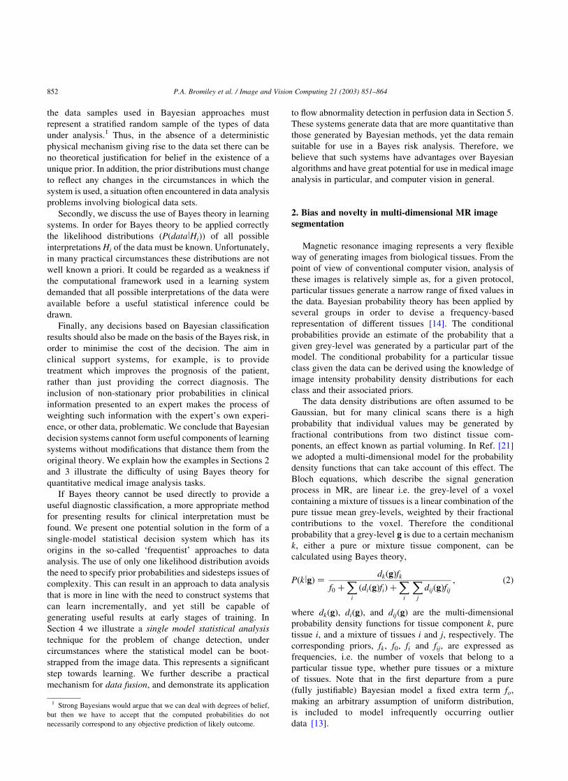
The probabilistic segmentation algorithm has been

implemented and tested on co-registered MRI brain images

of different modalities chosen for their good tissue

separation and availability in a clinical environment. The

use of multi-spectral data enables decorrelation of statistical

distributions and better estimation of partial volumes. The

images used were variable echo proton density (VE(PD)),

variable echo T2 (VE(T2)), inversion recovery turbo spin-

echo (IRTSE), and fluid attenuated inversion recovery

(FLAIR) (see Fig. 1). These images provide good separation

between air and bone, fat, soft tissue (such as skin and

muscle), cerebro-spinal fluid (CSF), grey matter (GM), and

white matter (WM). Fig. 2 shows a scatter plot of the

IRTSE and VE(PD) images, together with the model after

10 iterations of the EM algorithm. The final model agrees

well with the original data. The partial volume distributions

Fig. 1. Image Sequences: IRTSE (a), VE(PD) (b), VE(T2) (c), and FLAIR (d).

Fig. 2. Scatter plots of IRTSE vs. VE(PD): original data (a); model using initial values of parameters (b); model after 10 iterations of EM algorithm (c); and

schematic showing the origins of the data clusters (d).

P.A. Bromiley et al. / Image and Vision Computing 21 (2003) 851–864 853

link the otherwise compact pure tissue distributions along

the lines between them in accordance with the Bloch

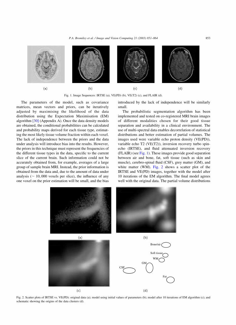
equations. The final segmentation result is represented by

probability maps for each tissue class and can be seen in

Fig. 3. The probability maps range from 0 to 1 and can be

used for boundary location extraction (e.g. a probability of

0.5 represents the boundary location between two tissues) or

volume visualisation [16].

Table 1 gives the priors (i.e. number of voxels) assigned

to each class, including both pure tissues and mixtures of

tissues. As these values represent genuine frequencies of

tissues they will change depending upon the region selected,

and so too will any estimates of tissue proportion. For

example, if the intention was to segment only the brain

tissues (i.e. CSF, WM and GM), a region of interest could be

chosen which contained only these tissues.

Fig. 4 illustrates how change in the region chosen to

generate the priors may lead to significant change in the

subsequent interpretation of the same data. Two overlapping

regions of interest were defined. The segmentation tech-

nique was applied to each region independently, using the

same initialisation values and holding the means and

variances of the tissues fixed, such that only the prior

estimation could change. This generated two sets of

probability maps for the same region (the intersection). A

subtraction of the two grey matter probability maps

produced for this region shows significant differences

between them: it can be seen from the histogram that the

probabilities differ at approximately the 10% level.

Given the arbitrary nature of the process of region

selection, it is evident that the prior information is not

unique for a particular segmentation task. This exemplifies

the prior selection problem. The common response to this,

that the results will not change much over a large range of

priors, is clearly over-simplistic as particularly important

tissues can be eliminated altogether by careless selection of

the bootstrap region. If the priors are estimated from a

bootstrap region that does not contain a particular

pathological tissue, or other novelty, then the interpretation

will be biased against the presence of this tissue in

subsequent data analysis, and towards interpretations

favoured by the priors. In the above example, the priors

must accurately represent the tissues present in the data,

rather than population-wide averages of the tissues present

in the brain. In addition, attempts to measure quantitative

changes between two data sets will be affected by any bias

introduced by inconsistent priors. Practical use of Bayes

theory in such problems therefore requires careful control of

prior estimates, particularly for quantification of small

differences between data sets [28]. Solutions such as fixing

the priors to be consistent between data sets represent a

second arbitrary and unsatisfactory extension to the theory.

One possible approach to this problem, suggested by

Laidlaw [19], involves estimating the priors locally to each

Fig. 3. Probability maps for bone and air (a), fat (b), soft tissue (c), CSF (d), GM (e), and WM (f).

Table 1

Typical priors assigned to each class (pure and mixed tissues). Zero values

are fixed to eliminate biologically implausible combinations

Air and

bone

Soft

tissue

Fatty

tissue

Cranial

fluid

Grey

matter

White

matter

Air/bone 16,012.2 1032.0 21.9 126.7 371.5 0

Soft tissue 1032.0 4076.9 1219.3 520.4 46.2 0

Fatty tissue 21.9 1219.3 1517.8 0 0 0

Cranial fluid 126.7 520.4 0 445.9 759.2 84.1

Grey matter 371.5 46.2 0 759.2 6465.8 4105.6

White matter 0 0 0 84.1 4105.6 3548.7


pixel value. Unfortunately this does not extend to the use of

partial volume models, since any region of grey-level values

can be attributed to the partial volume terms without the

need for any pure tissue components. Such problems raise

doubts about the validity, or even the need, to incorporate

the priors at this stage of the analysis.

3. Learning, estimation of priors and Bayes risk

in diagnostic classification of dementing diseases

A more conventional use of Bayes theory is in the

classification of data. One of the important tasks in medical

image analysis involves informing clinicians of the most

likely interpretation of a large or complex data set for the

process of decision support. In MR imaging of the brain, for

example, we may wish to take the data description

generated by the previous system, and perform an analysis

of structure to identify abnormality or determine a

categorisation. In previous work [24,25] we designed a

system that is capable of diagnosing dementing diseases

based on the pattern of atrophy in the brain, through analysis

of cranial fluid volumes within a standardised co-ordinate

system. After correction for head size and normal ageing,2

and having taken care to represent the data in a way which

takes correct account of the Poisson measurement process

[26], twelve measurements of corrected volume were used

in a simple Parzen classifier to estimate the probability of

class assignment between one of four groups: normal;

Alzheimers disease; Fronto-Temporal dementia; and Vas-

cular dementia. This process makes direct use of Bayes

theory and typical results are given in Table 2. Given the

difficulty of clinically identifying subjects within these

groups using psychometric tests, these results illustrate a

separation between classes that appears sufficient to provide

useful diagnostic information.

The use of Bayes theory once again requires the specifi-

cation of a prior probability, which for this illustration

has simply been assumed to be proportional to the sampled

frequency within the data set. These prior terms establish the

relative frequency of each model hypothesis and without

them any classification result will be sub-optimal, in the

sense that there will not be a minimum number of incorrect

classifications across a sample group. In a clinical diagnostic

task the prior probabilities are determined by the statistical

make-up of the classified data sample. This process is often

referred to as case adjustment.

The use of prior probabilities therefore requires a

solution to the additional problem of ensuring that they

reflect the true frequencies of occurrence of cases.

Constructing a system with fixed priors based on a national

average would be sub-optimal in any location that did not

reflect this demographic, and even regional averages may

vary over time. If the intention was to build an optimal, fully

automatic classification system, then one which attempted

to determine prior probabilities from the sample data as they

arrive could be envisaged. However, if it is accepted that for

moral reasons the data should be moderated by a medical

expert, such a system might be considered inappropriate for

the reasons outlined below.

The aim in any clinical environment must be to deliver

treatment which improves the prognosis of the patient,

rather than simply to obtain the correct diagnosis. Therefore,

any decision based on the results from a diagnostic

classification system should be made on the basis of the

Bayes risk. For example, if the diagnosis is ambiguous

between three possibilities, but two outcomes could have

the same treatment, then this should influence the patient

management. This assessment must be carried out by the

expert, through a process of weighting decision support

information with the expert’s own experience or other data.

Fig. 4. Regions of interest (a) which provide different prior probabilities for the same region (their intersection), the result (b) of subtracting the grey matter

probability maps for this region, and the histogram (c) of these differences between the grey matter probabilities for the pixels in the region.

Table 2

Disease (rows) vs. classification (columns) for a cross-validated Parzen

classifier

Disease Norm. F. T. D Vas. D. Alz.

Normal 7 2 8 1

Fronto-temporal 5 21 3 7

Vascular 3 2 13 4

Alzheimers 1 3 6 282 The normal brain typically loses tissue at a rate that results in a 1%

increase in cranial fluid volume per year after the age of 40.


Any non-stationarity in the priors will result in different

interpretations of the same data over time, and will

complicate experiential learning by the expert, whether

the expert is a clinician or a learning system. This

exemplifies the difficulty of making quantitative use of

data from a Bayesian module in a larger system.

One alternative is to construct a Bayesian classifier with

equal prior probabilities, and to train the expert in how best

to make use of the data. However, it is then difficult to

believe that the outputs from the system contain any

meaningful information beyond that present in the like-

lihoods. We must therefore conclude that the likelihoods

provide the most appropriate way to present data for clinical

interpretation. A clinician would then be in a position to

make use of either their own experience, or a separate

estimate of the current expected relative frequencies of

diseases, in order to recommend treatment on the basis of

risk.

4. Single model statistical analysis for the identification

of change in magnetic resonance brain images

The previous examples illustrate the difficulties encoun-

tered in determining all of the information needed to use

Bayes theory correctly, and the consequences in terms of

quantitative measurement. One approach to resolve these

difficulties would be to attempt to construct statistical

questions regarding expected data distributions that could

be addressed without knowledge of the priors, or with fewer

model components. Logically the minimum number of

model components required would be one, and in that case

the only quantity that can be obtained is the relative

probability that a particular data point was generated by the

model. However, this is enough to identify data that are

unlikely given the model (i.e. outlier detection).

There are several standard statistical techniques designed

to operate using only one model, for example null

hypothesis tests and the chi-squared probability. Although

such techniques have already been applied widely in MR

data analysis [11], they generally assume particular data

density distributions, and so will not be applicable to

arbitrary problems. Image analysis tasks frequently involve

large amounts of data, and our recent work [4–6] illustrates

how we might exploit this to bootstrap a statistical model of

data behaviour from the data itself. Thus the technique does

not require additional model components or prior probabil-

ities, and avoids the need to explicitly build the single

model. In addition, this technique produces output with a

uniform probability distribution, which provides routes to

both self-test and data fusion, as will be discussed in this

section and in Section 5.

The technique discussed here was designed to construct

non-parametric models in order to estimate the probability

that a particular data point was generated by a particular

process. It defines a probability that reflects how likely it

was that the grey-level values from corresponding pixels in

an image pair were drawn from the same distribution as the

rest of the data. A scattergram drawn from a sample of

image data Sðg1; g2Þ is used as a statistical model of data

behaviour. Taking a vertical cut through the scattergram

identifies a set of pixels in the first image that all have the

same grey-level value g1: The distribution of data along

this cut f ðg2; g1Þ gives the grey-levels g2 occurring at the

corresponding pixels in the second image. If the scatter-

gram is normalised along all vertical cuts, then these

distributions become the probability distributions for the

grey-level value in the second image given the grey-level

value in the first,

f ðg2; g1Þð1

21f ðg2; g1Þdg2

¼ fnðg2; g1Þ: ð3Þ

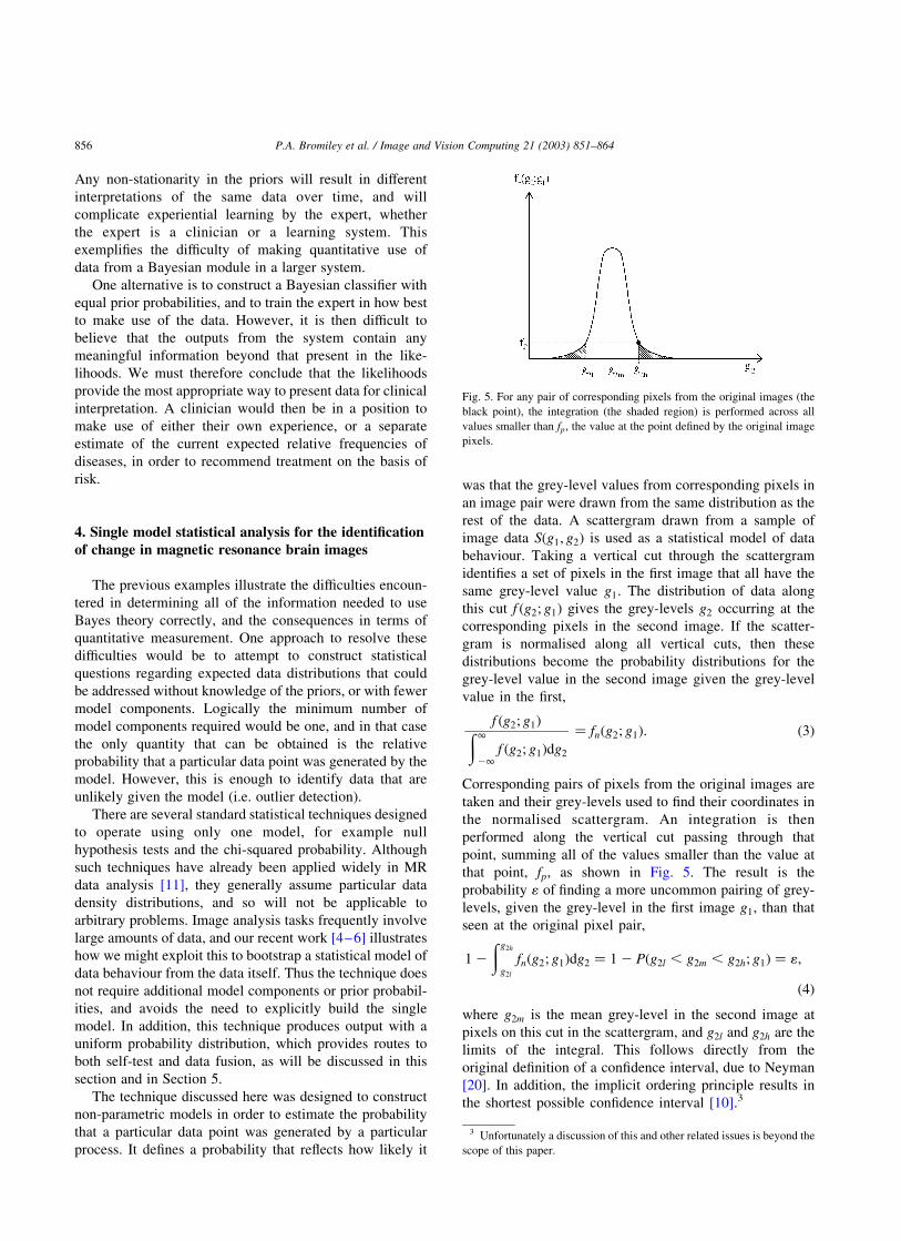
Corresponding pairs of pixels from the original images are

taken and their grey-levels used to find their coordinates in

the normalised scattergram. An integration is then

performed along the vertical cut passing through that

point, summing all of the values smaller than the value at

that point, fp; as shown in Fig. 5. The result is the

probability 1 of finding a more uncommon pairing of grey-

levels, given the grey-level in the first image g1; than that

seen at the original pixel pair,

1 2ðg2h

g2l

fnðg2; g1Þdg2 ¼ 1 2 Pðg2l , g2m , g2h; g1Þ ¼ 1;

ð4Þ

where g2m is the mean grey-level in the second image at

pixels on this cut in the scattergram, and g2l and g2h are the

limits of the integral. This follows directly from the

original definition of a confidence interval, due to Neyman

[20]. In addition, the implicit ordering principle results in

the shortest possible confidence interval [10].3

Fig. 5. For any pair of corresponding pixels from the original images (the

black point), the integration (the shaded region) is performed across all

values smaller than fp; the value at the point defined by the original image

pixels.

3 Unfortunately a discussion of this and other related issues is beyond the

scope of this paper.


The result of the integration is used as the grey-level for

the corresponding pixel in a difference image. Since it

depends on the mean grey-level for the pixels on this cut in

the second image, any process which results in global

differences between the images, such as a change in the

level of illumination, will be ignored. The grey-level values

in the difference image relate directly to the frequency of

occurrence of the pairing of grey-level values seen at the

corresponding pixels in the original images. This is exactly

the type of measure needed to identify outlying combi-

nations of grey-level values in a fully automatic manner.

The technique therefore illustrates that useful and quanti-

tative statistical analyses can be performed through

comparison with a single statistical model bootstrapped

from the data.

An important feature of this method is that, since the

integration along vertical cuts in the scattergram performs a

probability integral transform, the resulting difference

image should by definition have a uniform probability

distribution i.e. a histogram of the grey-levels in the

difference image will be flat. It follows that thresholding

the difference image at some level n will extract the 100n%

of the pixels that showed the most uncommon pairings of

grey-levels in the original images. Thus the estimated

probabilities correspond to a genuine prediction of data

frequencies. Probabilities with these characteristics have

previously been referred to in the literature as honest [9].

The importance of this feature in relation to the work

presented here is that knowledge of the expected distri-

bution of the output provides a mechanism for self-test [22].

In the case of the current technique, any departure from a

flat histogram indicates errors in either the construction or

the sampling of the scattergram. For example, if Gaussian

smoothing is applied to the scattergram, then the data

distributions in the scattergram become broader than those

in the original image data. This departure of the implicit

model from the data results in a non-uniform distribution in

the difference image. Further uses of this property are

discussed in Section 5.

A potential application of this technique is the detection

of MS lesions in MRI scans of the brain, an important issue

in relation both to tracking the progression of the subclinical

disease, and to therapeutic trials [29]. Such lesions can be

difficult to detect, but can be highlighted using a contrast

agent (Gd-DTPA), which concentrates at the lesion sites.

Scans taken before and after the contrast agent injection can

be subtracted to help identify lesions, but the presence of the

contrast agent also alters the global characteristics of the

scan, so a simple pixel-by-pixel subtraction will not remove

all of the underlying structure of the brain from the image.

Obtaining a gold standard for this work is difficult

without extensive histological investigation. In order to

simulate the imaging process, two T2 scans with slightly

different echo train times (TE) of the same region of the

brain were used. This simulated the effects of repeat

scanning on different scanners after a significant time

interval, and the small quantitative changes that occur in

the signal due to the presence of a contrast agent. The

background was removed from the image so that the

statistical model (scattergram) was estimated using only

the tissues of interest. A grey-level offset at twice the level

of noise s in the original images, too small to be detected

visually, was then added to a small circular region of one of

the brain images, simulating lesions in a testable manner.

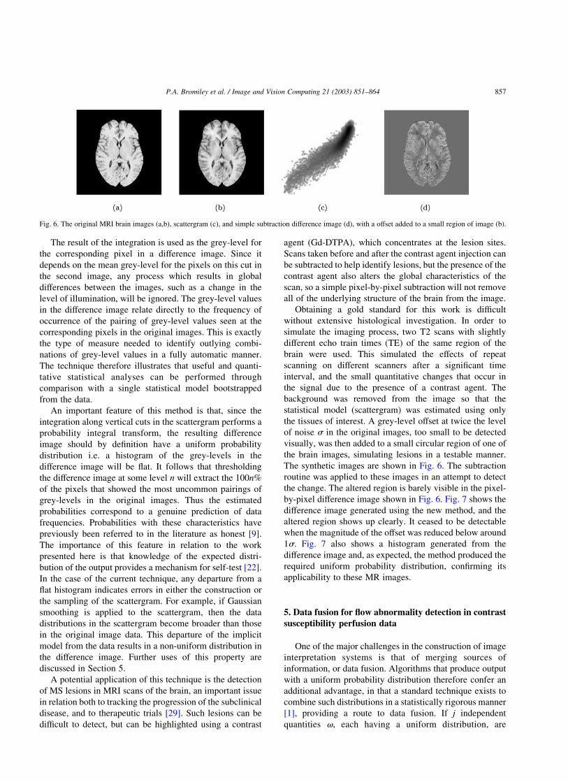
The synthetic images are shown in Fig. 6. The subtraction

routine was applied to these images in an attempt to detect

the change. The altered region is barely visible in the pixel-

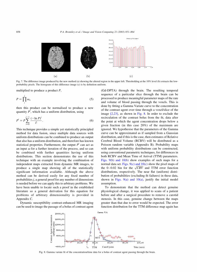
by-pixel difference image shown in Fig. 6. Fig. 7 shows the

difference image generated using the new method, and the

altered region shows up clearly. It ceased to be detectable

when the magnitude of the offset was reduced below around

1s: Fig. 7 also shows a histogram generated from the

difference image and, as expected, the method produced the

required uniform probability distribution, confirming its

applicability to these MR images.

5. Data fusion for flow abnormality detection in contrast

susceptibility perfusion data

One of the major challenges in the construction of image

interpretation systems is that of merging sources of

information, or data fusion. Algorithms that produce output

with a uniform probability distribution therefore confer an

additional advantage, in that a standard technique exists to

combine such distributions in a statistically rigorous manner

[1], providing a route to data fusion. If j independent

quantities v; each having a uniform distribution, are

Fig. 6. The original MRI brain images (a,b), scattergram (c), and simple subtraction difference image (d), with a offset added to a small region of image (b).


multiplied to produce a product P;

P ¼Yj

i

vi; ð5Þ

then this product can be normalised to produce a new

quantity P0; which has a uniform distribution, using

P0 ¼ PXj21

i¼0

ð2ln PÞi

i!: ð6Þ

This technique provides a simple yet statistically principled

method for data fusion, since multiple data sources with

uniform distributions can be combined to produce an output

that also has a uniform distribution, and therefore has known

statistical properties. Furthermore, the output P0 can act as

an input v for a further iteration of the process, and so can

be combined with further quantities having uniform

distributions. This section demonstrates the use of this

technique with an example involving the combination of

independent maps extracted from dynamic MR images, to

produce a single map showing all of the statistically

significant information available. Although the above

method can be derived easily for any fixed number of

probabilities j; a general proof for any number of dimensions

is needed before we can apply this to arbitrary problems. We

have been unable to locate such a proof in the established

literature so a general derivation for this equation for

problems of arbitrary dimensionality is provided in

Appendix C.

Dynamic susceptibility contrast-enhanced MR imaging

can be used to image the passage of a bolus of contrast agent

(Gd-DPTA) through the brain. The resulting temporal

sequence of a particular slice through the brain can be

processed to produce meaningful parameter maps of the rate

and volume of blood passing through the voxels. This is

done by fitting a Gamma Variate curve to the concentration

of the contrast agent over time through a voxel/slice of the

image [2,23], as shown in Fig. 8. In order to exclude the

recirculation of the contrast bolus from the fit, data after

the point at which the agent concentration drops below a

given fraction (in this case 20%) of the maximum are

ignored. We hypothesise that the parameters of the Gamma

curve can be approximated as if sampled from a Gaussian

distribution, and if this is the case, then estimates of Relative

Cerebral Blood Volume (RCBV) will be distributed as a

Poisson random variable (Appendix B). Probability maps

with uniform probability distributions can be constructed,

using conventional parametric techniques, for differences in

both RCBV and Mean Time of Arrival (TTM) parameters.

Figs. 9(b) and 10(b) show examples of such maps for a

normal data set. Figs. 9(c) and 10(c) show the pixel maps of

the 0–0.02 bin for theffiffiffiffiffiffiCBV

pand TTM error function

distributions, respectively. The near flat (uniform) distri-

bution of probabilities (excluding fit failures) in these data,

shown in Figs. 9(a) and 10(a), justify the initial model

assumption.

To demonstrate that the method can detect genuine

physiological change, it was applied to scans of a patient

before and after a surgical procedure to remove a carotid

stenosis. In this case, genuine change between the maps

greater than that due to error would be expected. The error

function distribution for the TTM difference map again has

Fig. 7. The difference image produced by the new method (a) showing the altered region in the upper left. Thresholding at the 10% level (b) extracts the low-

probability pixels. The histogram of this difference image (c) is by definition uniform.

Fig. 8. Gamma variate fit of the concentration/time data for a bolus of contrast agent passing through the brain.


outliers in the 0–0.02 bin (Fig. 11(a)) but is otherwise flat.

The pixel map of this bin (Fig. 11(c)) shows that most of the

outliers are due to a change on the left (right for the

observer) of the brain, due to unblocking the affected carotid

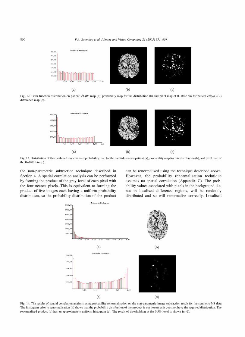
artery. The error function distribution of theffiffiffiffiffiffiCBV

pmap

(Fig. 12(a)) shows the same flat map with a peak, but the

corresponding pixel map (Fig. 12(c)) does not show a gross

change as seen in the TTM map, and is instead more similar

to the normal maps (Figs. 9(c) and 10(c)). We believe that

the changes seen on theffiffiffiffiffiffiCBV

pprobability map (and

corresponding pixel map) are predominantly due to

perfusion changes in the grey and white matter, whereas

those on the TTM map are due to changes in the time of

arrival of the blood in the feeding arteries and draining

veins.

The probability maps of the parametersffiffiffiffiffiffiCBV

pand TTM

represent two physiological aspects of the same data, which

we wish to combine in order to show the overall vascular

differences pre- and post-operatively. Since the probability

distributions of the maps are uniform, the renormalisation

technique described above can be applied to the product of

the individual maps to produce a new map showing all of the

statistically significant changes.

Fig. 13(a) shows that the combined renormalised map for

the carotid stenosis patient is uniform (demonstrating that

theffiffiffiffiffiffiCBV

pand TTM maps are independent) except for the

peak in the 0–0.02 bin. Comparing the pixel map for this

bin (Fig. 13(c)) with with those for theffiffiffiffiffiffiCBV

pand TTM

shows that the information regarding perfusion differences

has been preserved in the combined probability map

(Fig. 13(b)) and that this map now contains all of the

statistically significant information available.

In order to demonstrate the flexibility of this approach,

we have also applied the method to the results from

Fig. 9. Error function distribution onffiffiffiffiffiffiCBV

pdifference map (a), probability map for the distribution (b) and pixel map of 0–0.02 bin for erf(

ffiffiffiffiffiffiCBV

p) difference

map (c).

Fig. 10. Error function distribution on TTM difference map (a), probability map for the distribution (b), and pixel map of 0–0.02 bin for erf(TTM) difference

map (c).

Fig. 11. Error function distribution on patient TTM map (a), probability map for the distribution (b), and pixel map of 0–0.02 bin for patient erf(TTM)

difference map (c).


the non-parametric subtraction technique described in

Section 4. A spatial correlation analysis can be performed

by forming the product of the grey-level of each pixel with

the four nearest pixels. This is equivalent to forming the

product of five images each having a uniform probability

distribution, so the probability distribution of the product

can be renormalised using the technique described above.

However, the probability renormalisation technique

assumes no spatial correlation (Appendix C). The prob-

ability values associated with pixels in the background, i.e.

not in localised difference regions, will be randomly

distributed and so will renormalise correctly. Localised

Fig. 12. Error function distribution on patientffiffiffiffiffiffiCBV

pmap (a), probability map for the distribution (b) and pixel map of 0–0.02 bin for patient erf(

ffiffiffiffiffiffiCBV

p)

difference map (c).

Fig. 14. The results of spatial correlation analysis using probability renormalisation on the non-parametric image subtraction result for the synthetic MS data

The histogram prior to renormalisation (a) shows that the probability distribution of the product is not honest as it does not have the required distribution. The

renormalised product (b) has an approximately uniform histogram (c). The result of thresholding at the 0.5% level is shown in (d).

Fig. 13. Distribution of the combined renormalised probability map for the carotid stenosis patient (a), probability map for this distribution (b), and pixel map of

the 0–0.02 bin (c).


differences will result in spatially correlated low prob-

ability pixels, and will produce low probability products

that will not renormalise correctly. Therefore, the prob-

ability distribution of the image showing the renormalised

five-pixel product will feature a uniform distribution for

non-difference pixels, together with a spike close to zero

containing the pixels in localised difference regions. This

provides a simpler route to identification of the local

difference regions when compared to the original non-

parametric image subtraction result, in which the prob-

ability distribution is uniform for all pixels. Fig. 14 shows

the result of applying this technique to the non-parametric

image subtraction result for the synthetic MS data. The

spatial correlation present in the data results in a reduction

in the number of effective degrees of freedom [12], and so

the histogram for the renormalised image shows the result

of some degree of over-flattening [7]. The localised

difference region can immediately be extracted by thresh-

olding at lower probabilities than would be necessary for

the initial difference image, reducing contamination by

background pixels. In addition, since the distribution for

background pixels is uniform, the number of background

pixels extracted in the threshold is known. Therefore, this

number can be subtracted from the total number of pixels

extracted in the threshold to leave the number of pixels in

the localised difference regions, and so volumetric analysis

of the difference regions can be performed. This implies

that quantitative extraction can be performed using such

methods without the need for prior probabilities.

6. Conclusions

We have presented two distinct probabilistic methods for

medical image analysis. The first, based on Bayes theory,

has been used for both tissue quantification and categoris-

ation of the spatial distribution of data in magnetic

resonance images. We have shown how the issue of

objective definition of prior probabilities is a problem in

both cases. The use of non-objective priors raises problems

concerning direct quantitative interpretation of data,

associated with bias and suppression of pathological data

or other novelty. We have also explained how Bayesian

outputs do not form useful inputs for learning systems,

which demand stationarity. Practical solutions to these

problems reduce the role of the prior probabilities, and are

therefore distanced from the basic theory. Whilst we have

demonstrated these difficulties only on medical image

analysis problems, these simply represent a sub-set of

image analysis problems in general, with no special

characteristics. We therefore believe our conclusions

apply to machine vision tasks in general.

Having identified the main problem as the need to work

with multiple models, we have suggested an alternative

form of statistical data analysis based upon frequentist

methods. These can form useful statistical decisions using

the distribution of data from single models. For many tasks

these techniques eliminate the problems of unknown priors

in a framework which is both flexible and supports data

fusion. We have provided a general derivation for the

combination of arbitrary quantities of independent data.

The issue of self-test is also important, as it facilitates the

creation of data analysis systems that are capable of testing

the adequacy of their own assumptions. Although we have

not demonstrated the application of both frequentist and

Bayesian techniques to the same problem it is clear, at least

for the atrophic disease classification, that theoretically it

should be possible to replace the output probabilities from a

Bayesian analysis with probabilities from single model

techniques. The task of mapping these values onto a

decision process that accounts for Bayes risk is equivalent to

mapping the original Bayesian probabilities obtained from

fixed priors. In this respect the work we have presented

could be considered as possible components of a general

approach to analysis of multiple hypotheses in complex

data. The stages of this analysis would comprise:

† generation of data with uniform probability distributions

for individual data sources (by bootstrapped or other

methods),

† fusion of the data using the probability renormalisation

process,

† input of multiple hypothesis probabilities into a Bayes

risk analysis system for decision selection.

At each stage in this process the outputs should be honest

probability distributions, allowing the model assumptions

and data independence to be validated.

Any experimental data must consist both of some

measurement and some estimate of the errors on that

measurement if they are to be used to draw meaningful

conclusions [27]. Therefore, in a vision system consisting of

several modules, the data passed between them must include

knowledge of the errors if it is to be combined in a meaningful

way [8]. Approaches based upon maximum likelihood have

the techniques of covariance estimation and error propa-

gation [15] to support the control of this process. Bayesian

statistics currently has no such tool-kit as, at least in strong

Bayesian terms where the prior probabilities represent

degrees of belief, error estimates for the priors are not

available. Data fusion can only be achieved with knowledge

of the assumed prior probabilities, in order to work back to

the objective information content i.e. the likelihood distri-

butions. It is therefore our opinion that the difficulties in

utilising Bayesian results in further analysis procedures

should be regarded as a fundamental issue. This issue is

already receiving considerable attention in other fields,

notably in the area of particle physics [17].

The area of computer vision has largely managed to avoid

the Bayesian/frequentist debate which has dogged the

statistical literature for many decades. However, given that

statistical methodology is becoming the cornerstone of image


analysis, it will inevitably become necessary for those in the

area to be at least familiar with each side of the argument.

Taking all of the factors presented in this paper into account,

we conclude that the suggestion that Bayes theory should be

the preferred vehicle for the solution of medical image

analysis problems in particular, and perhaps also computer

vision problems in general, must be treated with scepticism.

Acknowledgements

The authors would like to thank Professor Alan Jackson

for his clinical guidance in the development of the

techniques presented. Patrick Courtney was involved with

development of the non-parametric subtraction technique in

the early stages and also contributed valuable insights

regarding the use of statistical modules in larger systems.

We would also like to acknowledge the support of: the

EPSRC and the MRC (IRC: From Medical Images and

Signals to Clinical Information); the DTI Medilink Scheme

(Smart Inactivity Monitor using Array Based Detectors

(SIMBAD); Wellcome (Relating Cross-Sectional and

Longitudinal changes in Brain Function to Cognitive

Function in Normal Old Age); and the European Commis-

sion (An Integrated Environment for Rehearsal and

Planning of Surgical Interventions). All software is freely

available from the TINA website www.tina-vision.net.

Appendix A. Model parameter update using expectation

maximisation

The implementation of the EM algorithm used here

involved recalculating the multi-dimensional probability

densities, dkðgÞ; for both pure and mixtures of tissues in the

expectation step, using the current parameter values. Then the

conditional probabilities, PðklgÞ; were derived and used for

re-estimation of the model parameters in the maximisation

step, in a maximum likelihood (i.e. least squares) manner.

The model parameters, which were iteratively updated,

were the priors f 0i; f 0ij; the mean vector M0i; and the

covariance matrix C0i :

f 0i ¼XV

v

PðilgvÞ; ðA1Þ

f 0ij ¼ f 0ji ¼1

2

XVv

ðPðijlgvÞ þ PðjilgvÞ; ðA2Þ

M0i ¼

1

V

XVv

PðilgvÞgv; ðA3Þ

and

C0i ¼

1

V

XVv

PðilgvÞðgv 2 MiÞ^ðgv 2 MiÞT ðA4Þ

where gv was the observed intensity value in voxel v; and V

was the total volume of all data analysed.

Using this representation it was possible to obtain the

most probable volumetric measurement Vi for each tissue i

given the observed data gv in voxel V ;

ViðgvÞ ¼ PðilgvÞ þX

i

PðijlgvÞ ðA5Þ

Appendix B. The sampled normal/Gaussian distribution

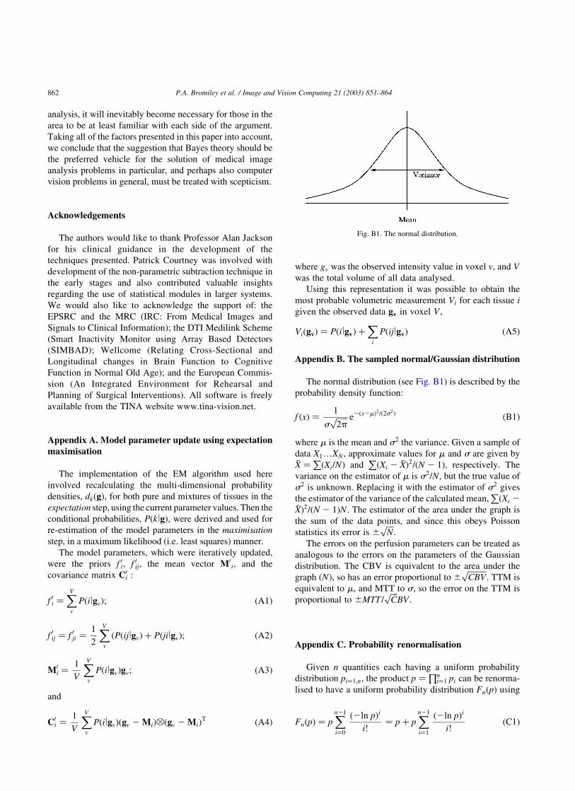
The normal distribution (see Fig. B1) is described by the

probability density function:

f ðxÞ ¼1

sffiffiffiffi2p

p e2ðx2mÞ2=ð2s2Þ ðB1Þ

where m is the mean and s2 the variance. Given a sample of

data X1…XN ; approximate values for m and s are given by�X ¼

PðXi=NÞ and

PðXi 2 �XÞ2=ðN 2 1Þ; respectively. The

variance on the estimator of m is s2=N; but the true value of

s2 is unknown. Replacing it with the estimator of s2 gives

the estimator of the variance of the calculated mean,PðXi 2

�XÞ2=ðN 2 1ÞN: The estimator of the area under the graph is

the sum of the data points, and since this obeys Poisson

statistics its error is ^ffiffiffiN

p:

The errors on the perfusion parameters can be treated as

analogous to the errors on the parameters of the Gaussian

distribution. The CBV is equivalent to the area under the

graph (N), so has an error proportional to ^ffiffiffiffiffiffiCBV

p: TTM is

equivalent to m; and MTT to s; so the error on the TTM is

proportional to ^MTT =ffiffiffiC

pBV :

Appendix C. Probability renormalisation

Given n quantities each having a uniform probability

distribution pi¼1;n; the product p ¼Qn

i¼1 pi can be renorma-

lised to have a uniform probability distribution FnðpÞ using

FnðpÞ ¼ pXn21

i¼0

ð2ln pÞi

i!¼ p þ p

Xn21

i¼1

ð2ln pÞi

i!ðC1Þ

Fig. B1. The normal distribution.


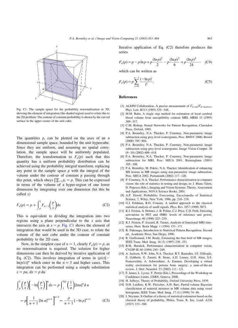
The quantities pi can be plotted on the axes of an n

dimensional sample space, bounded by the unit hypercube.

Since they are uniform, and assuming no spatial corre-

lation, the sample space will be uniformly populated.

Therefore, the transformation to FnðpÞ such that this

quantity has a uniform probability distribution can be

achieved using the probability integral transform, replacing

any point in the sample space p with the integral of the

volume under the contour of constant p passing through

this point, which obeysQn

i¼1 pi ¼ p: This can be expressed

in terms of the volume of a hyper-region of one lower

dimension by integrating over one dimension (let this be

called x)

FnðpÞ ¼ p þð1

pFn21

p

x

� �dx ðC2Þ

This is equivalent to dividing the integration into two

regions using a plane perpendicular to the x axis that

intersects the axis at x ¼ p: Fig. C1 shows the element of

integration that would be used in the 3D case, to relate the

volume of the unit cube under the contour of constant

probability to the 2D case.

Now, in the simplest case of n ¼ 1; clearly FnðpÞ ¼ p; as

no renormalisation is required. The solution for higher

dimensions can then be derived by iterative application of

Eq. (C2). This involves integration of terms in ðp=xÞ½2

lnðp=xÞ�n which enter in the n ¼ 3 and higher cases. This

integration can be performed using a simple substitution

x ¼ pu; dx ¼ p du

ð1

p

p

x

� �2ln

p

x

� � n

dx ¼ pð1=p

1

1

u

� �lnu½ �nd u

¼ p1

n þ 1½ln u�nþ1

nþ1

¼p

n þ 1½2ln p�nþ1 ðC3Þ

Iterative application of Eq. (C2) therefore produces the

series

FnðpÞ ¼ p2p ln pþpðln pÞ2

22p

ðln pÞ3

6þp

ðln pÞ4

24· · · ðC4Þ

which can be written as

FnðpÞ ¼ pXn21

i¼0

ð2ln pÞi

i!: ðC5Þ

References

[1] ALEPH Collaboration, A precise measurement of GZ!b�b=GZ!hadrons,

Phys. Lett. B313 (1993) 535–548.

[2] M.M. Bahn, A single step method for estimation of local cerebral

blood volume from susceptibility contrast MRI, MRM 33 (1995)

309–317.

[3] C.M. Bishop, Neural Networks for Pattern Recognition, Clarendon

Press, Oxford, 1995.

[4] P.A. Bromiley, N.A. Thacker, P. Courtney, Non-parametric image

subtraction using grey-level scattergrams, Proc. BMVC 2000, Bristol

(2000) 795–804.


subtraction using grey-level scattergrams, Image Vision Comput. 20

(9–10) (2002) 609–618.


subtraction for MRI, Proc. MIUA 2001, Birmingham (2001)

105–108.

[7] P.A. Bromiley, M. Pokric, N.A. Thacker, Identification of enhancing

MS lesions in MR images using non-parametric image subtraction,

Proc. MIUA 2002, Portsmouth (2002) 117–120.

[8] P. Courtney, N.A. Thacker, Performance characterisation in computer

vision: the role of statistics in testing and design, in: J. Blanc-Talon,

D. Popescu (Eds.), Imaging and Vision Systems: Theory, Assessment

and Applications, NOVA Science Books, 2001.

[9] A.P. Dawid, Probability Forecasting, Encyclopedia of Statistical

Science, 7, Wiley, New York, 1986, pp. 210–218.

[10] G.J. Feldman, R.D. Cousins, A unified approach to the classical

statistical analysis of small signals, Phys. Rev. D57 (1998) 3873.

[11] K.J. Friston, A. Holmes, J.-B. Poline, C.J. Price, C.D. Frith, Detecting

activations in PET and fMRI: levels of inference and power,

Neuroimage 40 (1996) 223–235.

[12] K.J. Friston, P. Jezzard, R. Turner, Analysis of functional MRI time-

series, Hum. Brain Mapp. 1 (1994) 153–171.

[13] K. Fukenaga, Introduction to Statistical Pattern Recognition, Second

ed., Academic Press, San Diego, 1990.

[14] R. Guillemaud, J.M. Brady, Estimating the bias field of MR images,

IEEE Trans. Med. Imag. 16 (3) (1997) 238–251.

[15] R.M. Haralick, Performance characterisation in computer vision,

CVGIP-IE 60 (1994) 245–249.

[16] A. Jackson, N.W. John, N.A. Thacker, R.T. Ramsden, J.E. Gillespie,

E. Gobbetti, G. Zanetti, R. Stone, A.D. Linney, G.H. Alusi, S.S.

Franceschini, A. Schwerdtner, A. Emmen, Developing a virtual

reality environment for petrous bone surgery: a state-of-the-art

review, J. Otol. Neurotol. 23 (2002) 111–121.

[17] F. James, L. Lyons, Y. Perrin (Eds.), Proceedings of the Workshop on

Confidence Limits, CERN, Geneva, 2000.

[18] H. Jeffreys, Theory of Probability, Oxford University Press, 1939.

[19] D.H. Laidlaw, K.W. Fleischer, A.H. Barr, Partial-volume Bayesian

classification of material mixtures in MR volume data using voxel

histograms, IEEE Trans. Med. Imag. 17 (1) (1998) 74–86.

[20] J. Neyman, X-Outline of a theory of statistical estimation based on the

classical theory of probability, Philos. Trans. R. Soc. Lond. A236

(1937) 333–380.

Fig. C1. The sample space for the probability renormalisation in 3D,

showing the element of integration (the shaded region) used to relate this to

the 2D problem. The contour of constant probability is shown by the curved

surface in the upper corner of the unit cube.


[21] M. Pokric, N.A. Thacker, M.L.J. Scott, A. Jackson, Multi-dimensional

medical image segmentation with partial voluming, Proc. MIUA,

Birmingham (2001) 77–81.

[22] I. Poole, Optimal Probabilistic Relaxation Labeling, Proceedings of

the BMVC, Oxford (1990).

[23] K.A. Remp, G. Brix, F. Wenz, C.R. Becker, F. Guckel, W.J. Lorenz,

Quantification of regional cerebral blood flow and volume with

dynamic susceptibility contrast-enhanced MR imaging, Radiology

193 (1994) 637–641.

[24] N.A. Thacker, A.R. Varma, D. Bathgate, S. Stivaros, J.S.

Snowden, D. Neary, A. Jackson, Dementing disorders: volumetric

measurement of cerebrospinal fluid to distinguish normal from

pathological findings—feasibility study, Radiology 224 (2002)

278–285.

[25] N.A. Thacker, A.R. Varma, D. Bathgate, J.S. Snowden, D. Neary, A.

Jackson, Quantification of the distribution of cerebral atrophy in

dementing diseases, Proc. MIUA, London (2000) 61–64.

[26] N.A. Thacker, F. Ahearne, I. Rockett, The Bhattacharryya metric as

an absolute similarity measure for frequency coded data, Kybernetika

34 (4) (1997) 363–368.

[27] N.A. Thacker, Using quantitative statistics for the construction of

machine vision systems, Proceedings of Opto-Ireland 2002 (Proced-

ings of the SPIE 4877), A. Shearer, F.D. Wtagh, J. Wahon, P.F.

Whelan (Eds), Galway, Ireland, (2002) 1-15.

[28] E.A. Vokurka, A. Herwadkar, N.A. Thacker, R.T. Ramsden, A.

Jackson, Using Bayesian tissue classification to improve the accuracy

of vestibular schwannoma volume and growth measurement, Am.

J. Neuroradiol. 23 (2002) 459–467.

[29] L.J. Wolansky, J.A. Bardini, S.D. Cook, A.E. Zimmer, A. Sheffel, H.J.

Lee, Triple-dose versus single dose gadoteridol in multiple sclerosis

patients, J. Neuroimag. 4 (3) (1994) 141–145.

[30] L. Xu, I. Jordan, On convergence properties of the EM algorithm for

Gaussian mixtures, Neural Comput. 8 (1) (1996) 129–151.


bayesian and non-bayesian probabilistic models for medical image analysis

Documents