M. Massink and G. Norman (Eds.): 9th Workshop onQuantitative Aspects of Programming Languages (QAPL 2011)EPTCS 57, 2011, pp. 148–162, doi:10.4204/EPTCS.57.11

c© Tracol, Desharnais, ZhiouaThis work is licensed under theCreative Commons Attribution License.

Computing Distances between Probabilistic Automata

Mathieu TracolLRI, Universite Paris-Sud, France

Josee Desharnais∗, Abir Zhioua∗

Dep. d’informatique et de genie logiciel, Universite Laval, Quebec, Canada

We present relaxed notions of simulation and bisimulation on Probabilistic Automata (PA), that al-low some error ε . When ε = 0 we retrieve the usual notions of bisimulation and simulation on PAs.We give logical characterisations of these notions by choosing suitable logics which differ from theelementary ones, L and L ¬, by the modal operator. Using flow networks, we show how to com-pute the relations in PTIME. This allows the definition of an efficiently computable non-discounteddistance between the states of a PA. A natural modification of this distance is introduced, to obtain adiscounted distance, which weakens the influence of long term transitions. We compare our notionsof distance to others previously defined and illustrate our approach on various examples. We alsoshow that our distance is not expansive with respect to process algebra operators.

Although L (¬) is a suitable logic to characterise ε-(bi)simulation on deterministic PAs, it isnot for general PAs; interestingly, we prove that it does characterise weaker notions, called a prioriε-(bi)simulation, which we prove to be NP-difficult to decide.

Keywords: Metrics, Bisimulation, Logic, Probabilistic Automata

1 Introduction

Preorders and equivalence notions between processes are central to concurrency theory. One wants tocompare terms of a process algebra for proving an axiomatisation sound, to compare processes to someabstractions of them, etc. For non-probabilistic processes, notions of bisimulation and simulation arewidely acknowledged, with, of course, many variations. In the study of probabilistic systems it has beenobserved [17] that the comparison between processes should not be based on notions that rely stronglyon exact numbers, as do the known notions of bisimulation and simulation for probabilistic systems.The most important reason is that the stochastic information in probabilistic processes often comes fromobservations, or from theoretical estimations. Hence a slight difference in the probabilities between twoprocesses should be treated differently from important ones and certainly not be simply tagged as nonequivalence. In this context, notions of approximate equivalence or distance are more useful. Distanceshave been defined for probabilistic processes [15, 4] and some have tried to estimate bisimulation witha certain degree of confidence [15]. Relaxing the definition of simulation and bisimulation is anotheravenue, which we follow.

We first extend previous work on deterministic processes [12] to their non deterministic version,Probabilistic Automata (PA) [22]. We present relaxed notions of simulation and bisimulation on themwith respect to some accuracy ε . When ε = 0 we retrieve the usual notions of bisimulation and simula-tion on PAs. Our notions rely on a definition of ε-lifting of relations, which happens to be equivalent tothe one presented in [23]. However, in this paper, the authors present different notions of ε-simulationswhich consider distributions on the set executions, whereas our relations are always between the statesof the systems, and our purpose is different. We give logical characterisations of these notions: a stateε-simulates another state if and only if it ε-satisfies every formula that the other one (exactly) satisfies;

∗Research supported by CRSNG

Tracol, Desharnais, Zhioua 149

similarly for ε-bisimulation. The extension of previous work comprises also the definition of an effi-ciently computable non-discounted distance: two states are at distance less than or equal to ε if theyare ε-bisimilar. Using flow networks, we show how to compute in PTIME our relaxed relations of(bi)simulation which helps to also compute efficiently the distance.

The nature of non determinism leads to new challenges and concepts. It is not suprising that thelogics that we prove to characterise ε-bisimulation and ε-simulation differ from the elementary ones, Land L ¬. Although L (¬) is a suitable logic to characterise ε-(bi)simulation on deterministic PAs, it isnot for general PAs; interestingly, we define weaker notions that it does characterise on PAs, called apriori ε-(bi)simulation. We also prove that a priori 0-simulation is NP-difficult to decide, contrarily toε-bi/simulation.

We propose a natural modification of our basic distance in order to discount the influence of long termtransitions. We illustrate the difference between the values of the two distances on various examples oftwo-dimensional grids. Both (pseudo-)distances are different from the ones defined in the past [11, 1,15, 4], in that differences along paths are not accumulated, even in the discounted one. The other knowndistances all accumulate differences through paths, and most of them discount the future. Those thatdo not discount the future are intractable: it has recently been proven decidable [3], but with doubleexponential complexity. Our distance is determined with a polynomial algorithm.

Finally, we prove that our distances are not expansive with respect to process algebras operators,such as parallel composition and non-deterministic choice.

2 Probabilistic Automata and ε-relations

In this section we give the definitions of our models and the relaxed relations that we study. ProbabilisticAutomata are labelled transition systems where transitions are from states to distributions and that in-volve non determinism. We generalize slightly the standard model, allowing sub-distributions instead ofdistributions, to model non responsiveness of the system and to make simulation a richer notion. Givena countable set S, we write Sub(S) for the set of sub-distributions on S: the total probability out of a sub-distribution may be less than one. Given a relation R on S×S and X ⊆ S, R(X) = {y∈ S|∃x∈ X s.t. xRy}.A set X is R-closed if R(X)⊆ X .

Definition 1 (PA [22]) A probabilistic automaton, or PA, is a tuple S = (S,Act,D) where S is a denu-merable state space, Act is a finite set of actions, and D ⊆ S×Act×Sub(S) is the transition relation. Sis finitely branching if for all s ∈ S and a ∈ Act, {µ ∈ Sub(S) | (s,a,µ) ∈D)} is finite; if it is a singletonor empty, we say that S is deterministic. The disjoint union of PAs S1, ...,Sk is the PA ]i∈[1;k]Si whosestates are the disjoint union of the Si and transitions carry through.

Closely related models restrict states to be either probabilistic or non deterministic [18]. Generalizationsto uncountable state spaces have also been studied [7, 9]. We sometimes mark a state (or a distribution)as initial. We write s a→ µ for a transition (s,a,µ) ∈D .

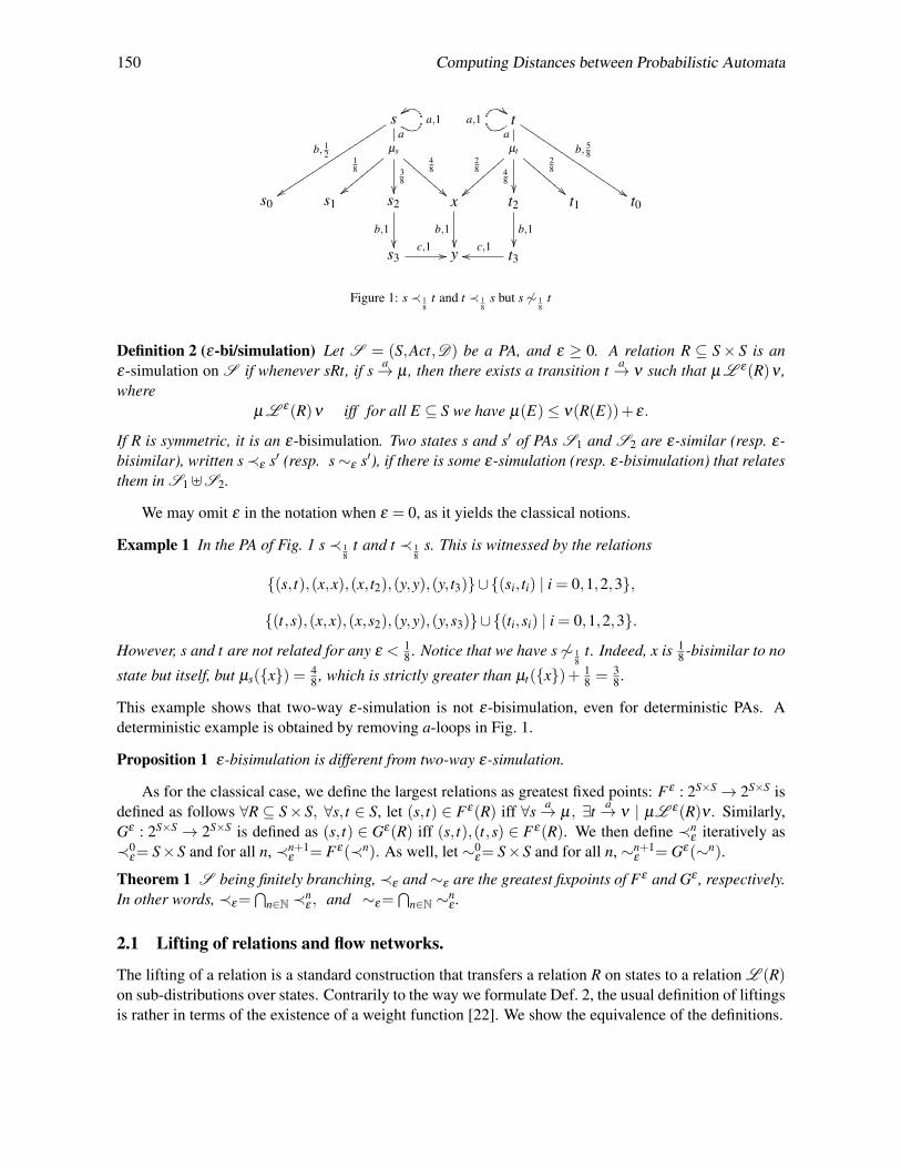
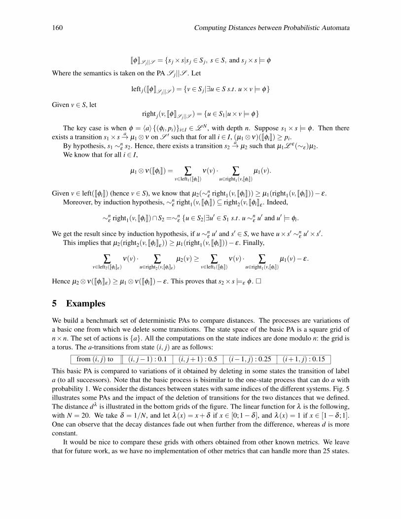
An example of PA is given in Fig. 1: an arrow labelled with action l and value r represents an l-transition of probability r; in picture representations, we omit the distributions that are concentrated inone point, as can be seen for the transitions from s to s0 and from t to itself. In contrast, state s has ana-transition to distribution µs giving s three possible successors for this a-transition.

In previous work [12], we relaxed the classical notion of simulation between deterministic PAs toε-simulation. We now generalize this approach to the context of PAs.

150 Computing Distances between Probabilistic Automata

sa

b, 12

yytttttttttttttttttt a,1zz

ta

b, 58

$$IIIIIIIIIIIIIIIIIIa,1##

µs18

||zzzz

zzzz

38

��

48

!!CCCC

CCCC

µt28

}}{{{{

{{{{

48

��

28

!!DDDD

DDDD

s0 s1 s2

b,1��

x

b,1��

t2

b,1��

t1 t0

s3c,1 // y t3

c,1oo

Figure 1: s≺ 18

t and t ≺ 18

s but s 6∼ 18

t

Definition 2 (ε-bi/simulation) Let S = (S,Act,D) be a PA, and ε ≥ 0. A relation R ⊆ S× S is anε-simulation on S if whenever sRt, if s a→ µ , then there exists a transition t a→ ν such that µ L ε(R)ν ,where

µ L ε(R)ν iff for all E ⊆ S we have µ(E)≤ ν(R(E))+ ε.

If R is symmetric, it is an ε-bisimulation. Two states s and s′ of PAs S1 and S2 are ε-similar (resp. ε-bisimilar), written s≺ε s′ (resp. s∼ε s′), if there is some ε-simulation (resp. ε-bisimulation) that relatesthem in S1]S2.

We may omit ε in the notation when ε = 0, as it yields the classical notions.

Example 1 In the PA of Fig. 1 s≺ 18

t and t ≺ 18

s. This is witnessed by the relations

{(s, t),(x,x),(x, t2),(y,y),(y, t3)}∪{(si, ti) | i = 0,1,2,3},

{(t,s),(x,x),(x,s2),(y,y),(y,s3)}∪{(ti,si) | i = 0,1,2,3}.

However, s and t are not related for any ε < 18 . Notice that we have s 6∼ 1

8t. Indeed, x is 1

8 -bisimilar to no

state but itself, but µs({x}) = 48 , which is strictly greater than µt({x})+ 1

8 = 38 .

This example shows that two-way ε-simulation is not ε-bisimulation, even for deterministic PAs. Adeterministic example is obtained by removing a-loops in Fig. 1.

Proposition 1 ε-bisimulation is different from two-way ε-simulation.

As for the classical case, we define the largest relations as greatest fixed points: Fε : 2S×S→ 2S×S isdefined as follows ∀R ⊆ S× S, ∀s, t ∈ S, let (s, t) ∈ Fε(R) iff ∀s a→ µ, ∃t a→ ν | µL ε(R)ν . Similarly,Gε : 2S×S → 2S×S is defined as (s, t) ∈ Gε(R) iff (s, t),(t,s) ∈ Fε(R). We then define ≺n

ε iteratively as≺0

ε= S×S and for all n, ≺n+1ε = Fε(≺n). As well, let ∼0

ε= S×S and for all n, ∼n+1ε = Gε(∼n).

Theorem 1 S being finitely branching,≺ε and∼ε are the greatest fixpoints of Fε and Gε , respectively.In other words, ≺ε=

⋂n∈N ≺n

ε , and ∼ε=⋂

n∈N ∼nε .

2.1 Lifting of relations and flow networks.

The lifting of a relation is a standard construction that transfers a relation R on states to a relation L (R)on sub-distributions over states. Contrarily to the way we formulate Def. 2, the usual definition of liftingsis rather in terms of the existence of a weight function [22]. We show the equivalence of the definitions.

Tracol, Desharnais, Zhioua 151

Definition 3 (ε-weight functions) Let ε ≥ 0, and µ,ν ∈ Sub(S). An ε-weight function for (µ,ν) withrespect to R is a function δ : S×S→ [0;1] such that:

• If δ (s, t)> 0 then (s, t) ∈ R.

• For all s, t ∈ S, ∑s′∈S δ (s,s′)≤ µ(s) and ∑s′∈S δ (s′, t)≤ ν(t).

• ∑s,s′∈S δ (s,s′)≥ µ(S)− ε .

Before stating the equivalence between our formulation of L ε(R) and the one with weight functions,we recall the notion of flow network, since it provides a convenient alternative definition for applica-tions [2].

A network is a tuple N = (V,E,⊥,>,c) where (V,E) is a finite directed graph in which every edge(u,v) ∈ E has a non-negative, real-valued capacity c(u,v). If (u,v) 6∈ E we assume c(u,v) = 0. Wedistinguish two vertices: a source ⊥ and a sink >. For v ∈ V let in(v) be the set of incoming edges tonode v, and out(v) the set of outgoing edges from node v. A flow function is a real function f : V×V →Rwith the two following properties for all nodes u and v:

• Capacity constraints: 0≤ f (u,v)≤ c(u,v). The flow along an edge cannot exceed its capacity.

• Flow conservation: for each node v ∈V −{⊥,>}, we have ∑e∈in(v) f (e) = ∑e∈out(v) f (e).

The flow F ( f ) of f is given by F ( f ) = ∑e∈out(⊥) f (e)−∑e∈in(>) f (e).

Definition 4 (The network N (µ,ν ,R)) Let S be a finite set, R ⊆ S× S, and µ,ν ∈ Sub(S). Let S′ ={t ′|t ∈ S}, where t ′ are pairwise distinct “new” states (i.e. t ′ 6∈ S). Let ⊥ and > be two distinct newelements not contained in S∪S′. The network N (µ,ν ,R) = (V,E,⊥,>,c) is defined as follows:

• V = S∪S′∪{⊥,>}.• E = {(s, t ′)|(s, t) ∈ R}∪{(⊥,s)|s ∈ S}∪{(t ′,>)|t ∈ S}.• The capacity function c is given by: c(⊥,s) = µ(s), c(t,>) = ν(t), and c(s, t) = 1 for all s, t ∈ S.

The following proposition gives various characterizations of the simulation relation.

Proposition 2 Let S be a finite set, R ⊆ S×S, and µ,ν ∈ Sub(S). The following properties are equiva-lent:

1. µL ε(R)ν .

2. The maximal flow in N (µ,ν ,R) is greater than or equal to µ(S)− ε .

3. There exists an ε-weight function for (µ,ν) with respect to R.

4. For all R-closed set E ⊆ S, we have µ(E)≤ ν(E)+ ε .

The equivalence with 4 applies only if the domain and image of R are considered disjoint.

Proof. 1⇔ 2 is Theorem 7 [12]. 2⇔ 3 is a slight generalization of a result of [2], in which ε = 0.1⇒ 4 is always true and 4⇒ 1 is straightforward if the domain and image of R are disjoint. �

The condition on the fourth statement may look restrictive, but it is quite natural. By taking twocopies of the state space and relating a state to the copies of the states that R relates it to, one obtainsa relation that satisfies the condition, yet representing the same relation as R. This allows to make adistinction between states that are simulated from states that are viewed as simulating.

152 Computing Distances between Probabilistic Automata

3 Logic for ε-simulation and ε-bisimulation

3.1 The logic L and its corresponding notion of simulation

In the context of deterministic PAs, ε-bi/simulation are characterized [12] by the simple logic L ¬ [19],using a relaxed semantics “up to ε”.

Definition 5 (The logics L and L ¬) The syntax of L ¬ is as follows:

L ¬ φ ::=> | ¬φ | φ1∧φ2| φ1∨φ2 | 〈a〉δ φ where δ ∈Q∩ [0;1].

We write L for the logic without negation. Given a PA with components (S,Act,D), the relaxedε-semantics |=ε is defined by structural induction on the formulas.

•∀s ∈ S,s |=ε > • s |=ε ¬θ iff s 6|=−ε θ • s |=ε φ1∧φ2 iff s |=ε φ1 and s |=ε φ2;

• s |=ε 〈a〉δ φ iff there exists a transition s a→ µ s.t. µ([[φ ]]ε)≥ δ − ε ,

where [[φ ]]ε= {s ∈ S|s |=ε φ}, and the semantics of ∨ is similar to the one of ∧. Given s ∈ S, we write

F ε(s) (resp. F ε,¬(s)) for the set of formulas in L (resp. in L ¬) ε-satisfied by s.

As for deterministic PAs, the logic is less expressive with the relaxed semantics [12] than with thestandard one. Indeed, for each φ ∈ L ¬, we can construct an associated formula φε ∈ L ¬ such that[[φ ]]ε = [[φε ]]0. Here is how this is done: >ε = >; (φ1 ∧ φ2)ε = (φ1)ε ∧ (φ2)ε ; (〈a〉δ φ)ε = 〈a〉δ−ε φε ;(¬φ)ε = ¬(φ−ε). Here we use the fact that 〈a〉λ φ is still a valid formula, even if λ < 0 or λ > 1, whichgives in turn that (φε)−ε = φ . Clearly the transformation is additive, as (φε)ε

′ = φε+ε

′ .

Example 2 If φ = 〈a〉.5 (¬〈a〉.2>), then φε = 〈a〉.5−ε (¬〈a〉.2+ε>).

The relaxed logic being less expressive is not an issue because we use the new semantics to simplifythe formulations of the logical characterisations. It implies that model checking of formulas with therelaxed semantics can be done using the same technique as for the usual semantics.

The logics L and L ¬ induce ε-simulation and ε-bisimulation relations:

Definition 6 (Logical ε-simulation.) Let ε ∈ [0;1], s, t ∈ S. We say that t Lε -simulates s, written s≺Lε t,

if for all formula φ ∈L , s |= φ implies t |=ε φ . States t and s are said ε-logically equivalent, writtens∼L ¬

ε t, if s≺L ¬ε t and t ≺L ¬

ε s.

The following theorem says that L characterizes ε-simulation on deterministic PAs. As Ex. 1 illus-trates, ε-bisimulation is different from two-way ε-simulation when ε > 0, and hence we need negationto characterize ε-bisimulation.

Theorem 2 ([12]) For deterministic PAs we have ≺ε =≺Lε and ∼ε =∼L ¬

ε

As can be expected, the logics L and L ¬ are not strong enough to characterize ε-bi/simulation forPAs. In the next section, we will present a stronger logic that will characterize these notions. Never-theless, we can present the notions that correspond to ≺L

ε and ∼L ¬ε . The name “a-priori” [1] comes

from the order of the quantifiers in the definition: sets E in the following definition are chosen before thematching transition, which contrasts with Def. 2.

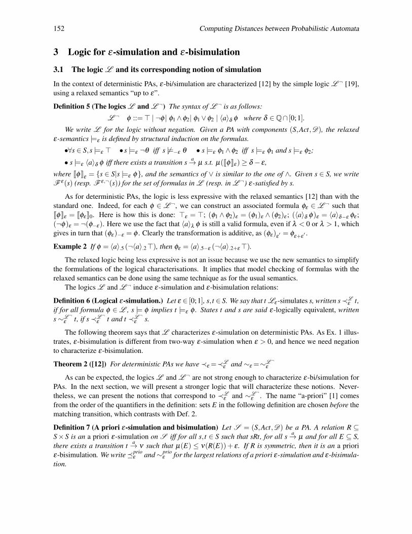
Definition 7 (A priori ε-simulation and bisimulation) Let S = (S,Act,D) be a PA. A relation R ⊆S× S is an a priori ε-simulation on S iff for all s, t ∈ S such that sRt, for all s a→ µ and for all E ⊆ S,there exists a transition t a→ ν such that µ(E) ≤ ν(R(E))+ ε . If R is symmetric, then it is an a prioriε-bisimulation. We write�prio

ε and∼prioε for the largest relations of a priori ε-simulation and ε-bisimula-

tion.

Tracol, Desharnais, Zhioua 153

Before proving that this relation is characterized by L , we introduce some notation. We define≺prio,n

ε iteratively in the same way as ≺nε , using F prio

ε : 2S×S→ 2S×S, which is defined as follows: ∀R ⊆S× S, ∀s, t ∈ S, let (s, t) ∈ F prio

ε (R) iff ∀s a→ µ, ∀E ⊆ S, ∃t a→ ν s.t. µ(E) ≤ ν(R(E)) + ε . As for≺ε=

⋂n∈N ≺n

ε , we can show that we have ≺prioε =

⋂n∈N ≺

prio,nε . The depth of a formula is the maximal

number of imbrications of 〈a〉δ operators. We write F n for the set of formulas of L of depth at most n.Given n ∈ N, given s ∈ S, F n

ε (s) is the set of formulas φ ∈L of depth at most n such that s |=ε φ andFε(s) is the set of formulas φ ∈L such that s |=ε φ . We define F n(s) = F n

0 (s) and F (s) = F0(s).The next theorem proves the logical characterization of ≺prio

ε and ∼prioε .

Theorem 3 Let S = (S,Act,D) be a PA, and let s, t ∈ S. Then:

1. s≺prio,nε t iff F n(s)⊆F n

ε (t) for all n≥ 0

2. For all n≥ 0, for all u,v ∈ S, there exists φu ∈Fn such that v |=ε φu iff u≺prio,nε v

3. ≺ε ⊆≺prioε =≺L

ε and the inclusion is strict.

4. ∼ε ⊆∼prioε =∼L ¬

ε and the inclusion is strict.

This proof generalizes to the context of countable state space systems, using a method close to themethod used in [12] to extend logic characterizations to denumerable state spaces.

Proof. Inclusions are straightforward. The proof of the strictness of inclusion is given by theexample following the proof. The structure of the proof is similar to the ones of [19] and [22] for thelogical characterisation of simulation but we adapt them to systems with non determinism. The thirdpoint is a corollary of the first one. The fourth point is not more difficult and is the same kind oftranslation as the proof of [19]. We sketch the proof of the first two points, concentrating on the “⇐”direction. The two points are proven simultaneously by induction on n. The base case follows triviallyfrom the definitions. Assume that the claims are true for n. We now prove 2 for n+ 1. Fix u ∈ S. Wedefine φu ∈Fn+1 as follows. Let v ∈ S such that u 6≺prio,n

ε v; by induction F n(u) 6⊆F nε (v), that is, there

exists a formula φ(u,v) ∈Fn, such that u |= φ(u,v) and v 6|=ε φ(u,v). The formula φu :=∧

v6≺prio,nε u φ(u,v) is in

Fn+1 because S is finite. Now, u |= φu, and any v such that u 6≺prio,n+1ε v verifies u 6≺prio,n

ε v and hencev 6|=ε φu. Since u ≺prio,n

ε w implies w |= φu by induction, we get the result; hence 2 is proven for n+ 1.As for 1, suppose F n+1(s)⊆F n+1

ε (t). Let s a→ µ be a transition from s, and let E ⊆ S. We are lookingfor a transition t a→ ν such that ν(≺prio,n

ε E)≥ µ(E)−ε . Let p = µ(E). We construct a formula φE suchthat for all u ∈ S, u |= φE iff u ∈ E. By the second claim, we just have to consider φE =

∨u∈E φu. Now,

s |= 〈a〉p φE . Since 〈a〉p φE ∈F n+1, we must have t |=ε 〈a〉p φE . Since ≺prio,nε [[φE ]]⊆ [[φ ]]E ε

, we get thatthere exists a transition t a→ ν from t such that ν(≺prio,n

ε E)≥ µ(E)− ε , which proves the result. �

Example 3 In the following PA (where the bi’s are different labels), we have s≺prio t and s 6≺ t.

sa

tannnnnnnn

aa

PPPPPPPP

µ13

wwppppppp14��

512

''NNNNNNN ν1

++WWWWWWWWWWWWWWWW

�� ''OOOOOOO ν2

wwooooooo�� ''OOOOOOO ν3

wwooooooo��ssgggggggggggggggg

s1

b1,1��

s2

b2,1��

s3

b3,1��

t1

b1,1��

t2

b2,1��

t3

b3,1��

s4 s5 s6 t4 t5 t6

t1 t2 t3ν1

724

724

512

ν238

14

38

ν313

13

13

The transitions has been chosen such that ν3(t1) = µ(s1), ν2(t2) = µ(s2), ν1(t3) = µ(s3), ν1({t1} ∪{t2}) = µ({s1}∪{s2}), ν2({t1}∪{t3}) = µ({s1}∪{s3}), ν3({t2}∪{t3}) = µ({s2}∪{s3}). Then it is

154 Computing Distances between Probabilistic Automata

easy to see that si is simulated by ti for all i = 1,2,3. Moreover, the last set of equalities shows thats ≺prio t. However, we do not have s ≺ t. Indeed for all transitions t a→ ν (combined or not) from t, wecan find a set E ⊆ ∪i∈{1,2,3} {si, ti} containing si if and only if it contains ti, and such that µ(E)> ν(E).

Remark 1 By Theorem 3 item 3, for the PA of Ex. 1, we have s≺prio18

t and t ≺prio18

s. Now, the only state18 -a-priori bisimilar to x is, here again, x itself. Hence, for s a→ µx and E = {x}, there exists no transitiont a→ ν such that µ(E)≤ ν(∼prio

18

(E))+ 18 , hence s and t are not 1

8 -a-priori bisimilar. As a consequence,

two-way a-priori simulation is different from a-priori bisimulation, and the negation is needed in thelogical characterization of bisimilarity.

Decidability of A Priori Simulation. An interesting fact is that it is NP-hard to decide a-priorisimulation and bisimulation, even when ε = 0. This contrasts with classical results on strong simulationand bisimulation whose decision procedures were proven to be in Poly-time (see [2, 24, 6]). The proofof the following theorem, not presented here due to lqck of space, is by reducing the subset sum problem,known to be NP-complete ([16]), to our problem.

Theorem 4 The following problem is NP-complete:Input: A PA S , s, t ∈ S. Question: Do we have s≺prio t?

3.2 The logic L N for PAs

We saw in the previous subsection that L is not strong enough for PAs. We now give a logic character-izing our relaxed relations ≺ε and ∼ε . The difference between this logic and L ¬ is the modal operatorthat permits to “isolate” a distribution out of a state, and write properties that it satisfies. This allows thesemantics to be defined on states, as pointed out as well by D’Argenio et al. [9]. In contrast, Parma andSegala [20] used a semantics on distributions to prove the logical characterisation of bisimulation (withε = 0).

Definition 8 (The logic L N,¬) The syntax differs by one operator from L ¬:L N,¬ φ :=>| ¬φ | φ1∧φ2| φ1∨φ2 | 〈a〉{(φi, pi)}i∈I I finite, pi ∈Q∩ [0;1].

We write L N for the same logic without negation. Let ε ∈ [0;1]. The relaxed semantics |=ε of L N,¬

is defined by structural induction on the formulas, in the same way as for L ¬ except for the modalformula: s |=ε 〈a〉{(φi, pi)}i∈I iff there exists a transition s a→ µ from s such that for all i ∈ I, we haveµ([[φi]]ε)≥ pi− ε .

As for the logic L ¬ we can, by structural induction on the formulas, construct for each φ ∈L N,¬

an associated formula φε ∈L N,¬ such that [[φ ]]ε= [[φε ]]. Hence, here again, model checking of formulas

with the relaxed semantics can be done using the same technique as for the usual semantics. The logicsL N and L N,¬ induce the relations ≺L N

ε and ∼L N

ε as in Def. 6. The following example illustrateshow this logic differs from L . The key difference is that formula 〈a〉{(φi, pi)}i∈I is not equivalent to∧i∈I〈a〉pi φi.Example 4 Consider the PAs of Ex. 3. As s≺prio t, we also have s≺L

ε t by Theorem 3, and hence everyformula of L satisfied by s is also satisfied by t. However, s 6≺ t and the formula

〈a〉{(〈b1〉1>,13),(〈b2〉1>,

14),(〈b3〉1>,

512

)}

of L N is not satisfied by t. Note how the semantics forces the νi’s to commit before the three “bi

formulas” are checked.

Tracol, Desharnais, Zhioua 155

The following theorem is a logical characterization of the ε-relations. Notice that we need negationonce again, since two-way simulation is different from bisimulation.

Theorem 5 ≺ε=≺L N

ε and ∼ε=∼L N,¬ε .

Proof. [≺ε⊆≺L N

ε ]. Let R be an ε-simulation. We prove by structural induction that for all φ ∈L N ,R([[φ ]]) ⊆ [[φ ]]

ε. We prove the case where φ = 〈a〉{(φi, pi)}i∈I , since the other cases are trivial. Let

s ∈ [[φ ]], t ∈ R({s}) and let s a→ µ be the associated transition such that for all i ∈ I, µ([[φi]])≥ pi. SinceR is an ε-simulation, there exists a transition t a→ ν such that µL ε(R)ν . Thus, for all E ⊆ S, we haveµ(E) ≤ ν(R(E))+ ε . In particular, given i ∈ I, we get that µ([[φi]]) ≤ ν(R([[φi]]))+ ε . But by inductionhypothesis, we know that for all i ∈ I, R([[φi]])⊆ [[φi]]ε . This gives us that µ([[φi]])≤ ν([[φi]]ε))+ ε hencethe result since by hypothesis µ([[φi]])≥ pi.

[≺ε⊇≺L N

ε ]. We prove that≺Lε is an ε-simulation. Suppose that s≺L

ε t, and let s a→ µ be a transitionfrom s. We need to find some t → ν such that ν(≺L

ε (X)) ≥ µ(X)− ε for all X ⊆ S. This will beconstructed from a family of t → νE for finite sets E. Let n ∈ N and let E ⊆ S be a finite set such thatµ(E)≥ µ(S)−1/n.

The key idea is to define the formula φ ke = ∧e|=φ j, j≤kφ j for every e ∈ E, and where (φ j) j∈N is an

enumeration of the formulas of L . Then for every finite set X ⊆ S, we set φ kX = ∨e∈X φ k

e , and we letpk

X := µ([[∨e∈X φ ke ]]). Since e |= φ k

e , we have [[φ ke ]]⊇≺L

ε ({e}),

pkX = µ([[∨e∈X φ

ke ]])≥ µ(≺L

ε (X))≥ µ(X),

and s |= 〈a〉{(∨e∈X φ ke , pk

X)}X⊆E for all k ≥ 1. By hypothesis, we get that t |=ε 〈a〉{(∨e∈X φ ke , pk

X)}X⊆E

for all k ≥ 1. Let νkE be the associated transition. Then for all X ⊆ E and for all k ∈ N:

νkE([[∨e∈X φ

ke ]])≥ pk

X − ε ≥ µ(X)− ε.

Now, [[∨e∈X φ ke ]]ε is decreasing to ≺L

ε (X) as k goes to infinity. Since the systems we considerare finitely branching, we can define a transition t a→ νE such that νE is the limit of a subsequence of{νk

E}k∈N. That is, there exists an increasing function ψ : N→ N such that for all set Y ⊆ S we havelimk→∞ν

ψ(k)E (Y ) = νE(Y ). This implies that: νE(≺L

ε (X)) ≥ µ(X)− ε. We have proven the following:for all s a→ µ , for all E ⊆ S finite, there exists t a→ νE such that for any X ⊆ E we have νE(≺L

ε (X)) ≥µ(X)− ε . Let Ek,k ∈N be a growing sequence of finite subsets of S such that S = ∪k∈NEk. Again, sincethe system is finitely branching, let ν be the limit of a subsequence of {νEk}k∈N. As before, we get thatfor any X ⊆ S finite, ν(≺L

ε (X))≥ µ(X)− ε .

[∼ε=∼L N¬

ε ] It can be proven that ∼L N¬

ε is an ε-bisimulation by following the proof above and using thefact that ∼L N

¬ε is a symmetric relation (which comes from the presence of negation in L N

¬ ). �

4 A Bisimulation Pseudo-Metric between PAs

4.1 The pseudo-metric d

The notion of ε-bisimulation induces a pseudo-metric on states of a PA, given by the smallest ε such thatthe states are ε-bisimilar.

Definition 9 (Bisimulation metric) Given s, t ∈ S, let d(s, t) = inf{ε | s∼ε t}.

156 Computing Distances between Probabilistic Automata

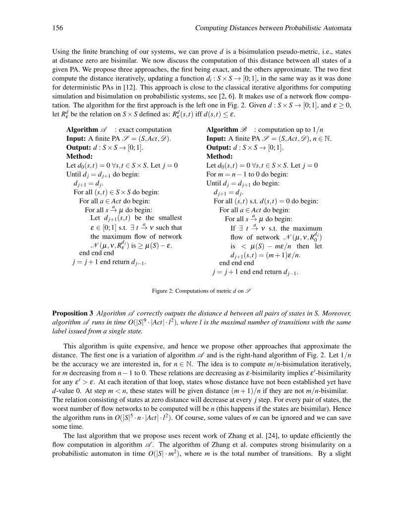
Using the finite branching of our systems, we can prove d is a bisimulation pseudo-metric, i.e., statesat distance zero are bisimilar. We now discuss the computation of this distance between all states of agiven PA. We propose three approaches, the first being exact, and the others approximate. The two firstcompute the distance iteratively, updating a function di : S× S→ [0;1], in the same way as it was donefor deterministic PAs in [12]. This approach is close to the classical iterative algorithms for computingsimulation and bisimulation on probabilistic systems, see [2, 6]. It makes use of a network flow compu-tation. The algorithm for the first approach is the left one in Fig. 2. Given d : S×S→ [0;1], and ε ≥ 0,let Rd

ε be the relation on S×S defined as: Rdε (s, t) iff d(s, t)≤ ε .

Algorithm A : exact computationInput: A finite PA S = (S,Act,D).Output: d : S×S→ [0;1].Method:Let d0(s, t) = 0 ∀s, t ∈ S×S. Let j = 0Until d j = d j+1 do begin:

d j+1 = d j.For all (s, t) ∈ S×S do begin:

For all a ∈ Act do begin:For all s a→ µ do begin:

Let d j+1(s, t) be the smallestε ∈ [0;1] s.t. ∃ t a→ ν such thatthe maximum flow of networkN (µ,ν ,Rd j

ε ) is ≥ µ(S)− ε .end end end

j = j+1 end return d j−1.

Algorithm B : computation up to 1/nInput: A finite PA S = (S,Act,D), n ∈ N.Output: d : S×S→ [0;1].Method:Let d0(s, t) = 0 ∀s, t ∈ S×S. Let j = 0For m = n−1 to 0 do begin:Until d j = d j+1 do begin:

d j+1 = d j.For all (s, t) s.t. d(s, t) = 0 do begin:

For all a ∈ Act do begin:For all s a→ µ do begin:

If ∃ t a→ ν s.t. the maximumflow of network N (µ,ν ,Rd j

0 )is < µ(S) − mε/n then letd j+1(s, t) = (m+1)ε/n.

end end endj = j+1 end end return d j−1.

Figure 2: Computations of metric d on S

Proposition 3 Algorithm A correctly outputs the distance d between all pairs of states in S. Moreover,algorithm A runs in time O(|S|9 · |Act| · l2), where l is the maximal number of transitions with the samelabel issued from a single state.

This algorithm is quite expensive, and hence we propose other approaches that approximate thedistance. The first one is a variation of algorithm A and is the right-hand algorithm of Fig. 2. Let 1/nbe the accuracy we are interested in, for n ∈ N. The idea is to compute m/n-bisimulation iteratively,for m decreasing from n−1 to 0. These relations are decreasing as ε-bisimilarity implies ε ′-bisimilarityfor any ε ′ > ε . At each iteration of that loop, states whose distance have not been established yet haved-value 0. At step m < n, these states will be given distance (m+ 1)/n if they are not m/n-bisimilar.The relation consisting of states at zero distance will decrease at every j step. For every pair of states, theworst number of flow networks to be computed will be n (this happens if the states are bisimilar). Hencethe algorithm runs in O(|S|5 ·n · |Act| · l2). Of course, some values of m can be ignored and we can savesome time.

The last algorithm that we propose uses recent work of Zhang et al. [24], to update efficiently theflow computation in algorithm A . The algorithm of Zhang et al. computes strong bisimularity on aprobabilistic automaton in time O(|S| ·m2), where m is the total number of transitions. By a slight

Tracol, Desharnais, Zhioua 157

generalization of this algorithm to our context, we can compute ε-bisimularity on S in time O(|S| ·m2),for any given ε . Using a dichotomic approach, given two states s and t, we can compute d(s, t) up to anadditive approximation factor δ in time O(|S| ·m2 · log(δ )), and thus we can compute d up to an additiveapproximation factor δ in time O(|S|3 ·m2 · log(δ )).

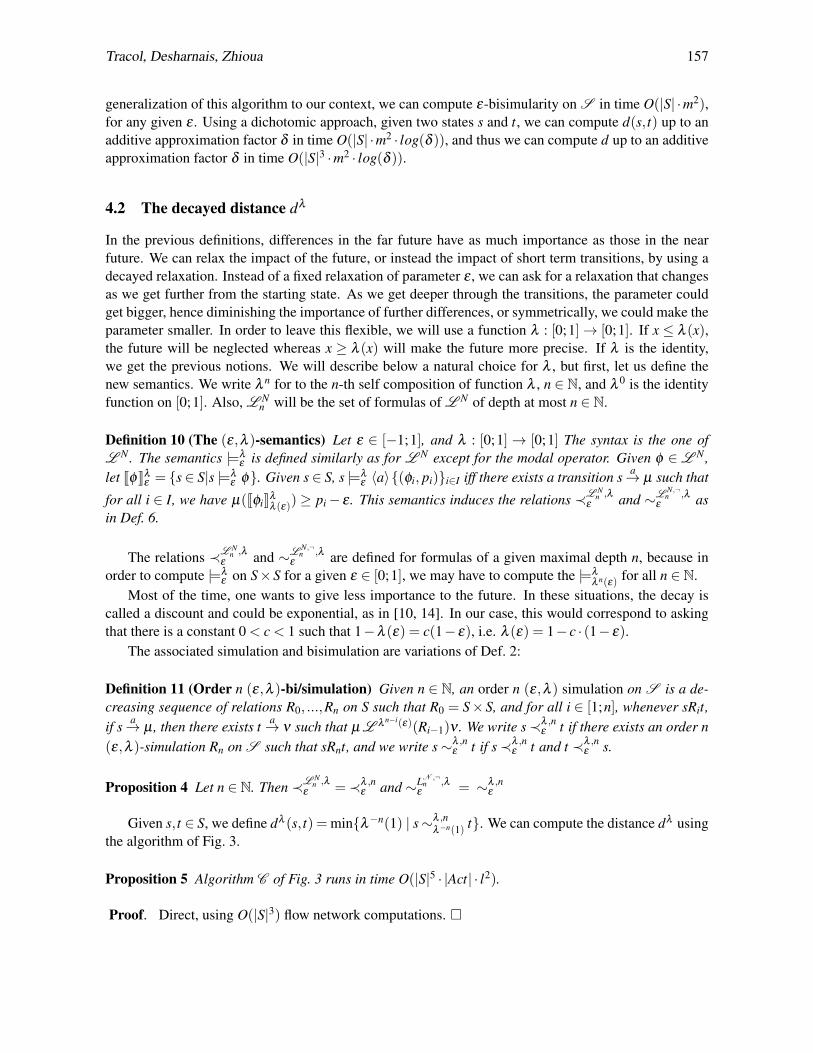
4.2 The decayed distance dλ

In the previous definitions, differences in the far future have as much importance as those in the nearfuture. We can relax the impact of the future, or instead the impact of short term transitions, by using adecayed relaxation. Instead of a fixed relaxation of parameter ε , we can ask for a relaxation that changesas we get further from the starting state. As we get deeper through the transitions, the parameter couldget bigger, hence diminishing the importance of further differences, or symmetrically, we could make theparameter smaller. In order to leave this flexible, we will use a function λ : [0;1]→ [0;1]. If x ≤ λ (x),the future will be neglected whereas x ≥ λ (x) will make the future more precise. If λ is the identity,we get the previous notions. We will describe below a natural choice for λ , but first, let us define thenew semantics. We write λ n for to the n-th self composition of function λ , n ∈ N, and λ 0 is the identityfunction on [0;1]. Also, L N

n will be the set of formulas of L N of depth at most n ∈ N.

Definition 10 (The (ε,λ )-semantics) Let ε ∈ [−1;1], and λ : [0;1]→ [0;1] The syntax is the one ofL N . The semantics |=λ

ε is defined similarly as for L N except for the modal operator. Given φ ∈L N ,let [[φ ]]λε = {s ∈ S|s |=λ

ε φ}. Given s ∈ S, s |=λε 〈a〉{(φi, pi)}i∈I iff there exists a transition s a→ µ such that

for all i ∈ I, we have µ([[φi]]λ

λ (ε)) ≥ pi− ε . This semantics induces the relations ≺L Nn ,λ

ε and ∼L N,¬n ,λ

ε asin Def. 6.

The relations ≺L Nn ,λ

ε and ∼L N,¬n ,λ

ε are defined for formulas of a given maximal depth n, because inorder to compute |=λ

ε on S×S for a given ε ∈ [0;1], we may have to compute the |=λ

λ n(ε) for all n ∈ N.Most of the time, one wants to give less importance to the future. In these situations, the decay is

called a discount and could be exponential, as in [10, 14]. In our case, this would correspond to askingthat there is a constant 0 < c < 1 such that 1−λ (ε) = c(1− ε), i.e. λ (ε) = 1− c · (1− ε).

The associated simulation and bisimulation are variations of Def. 2:

Definition 11 (Order n (ε,λ )-bi/simulation) Given n ∈ N, an order n (ε,λ ) simulation on S is a de-creasing sequence of relations R0, ...,Rn on S such that R0 = S×S, and for all i ∈ [1;n], whenever sRit,if s a→ µ , then there exists t a→ ν such that µ L λ n−i(ε)(Ri−1)ν . We write s≺λ ,n

ε t if there exists an order n(ε,λ )-simulation Rn on S such that sRnt, and we write s∼λ ,n

ε t if s≺λ ,nε t and t ≺λ ,n

ε s.

Proposition 4 Let n ∈ N. Then ≺L Nn ,λ

ε =≺λ ,nε and ∼LN ,¬

n ,λε = ∼λ ,n

ε

Given s, t ∈ S, we define dλ (s, t) = min{λ−n(1) | s∼λ ,nλ−n(1) t}. We can compute the distance dλ using

the algorithm of Fig. 3.

Proposition 5 Algorithm C of Fig. 3 runs in time O(|S|5 · |Act| · l2).

Proof. Direct, using O(|S|3) flow network computations. �

158 Computing Distances between Probabilistic Automata

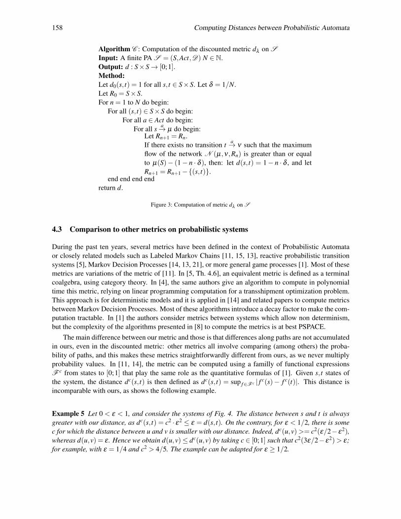
Algorithm C : Computation of the discounted metric dλ on SInput: A finite PA S = (S,Act,D) N ∈ N.Output: d : S×S→ [0;1].Method:Let d0(s, t) = 1 for all s, t ∈ S×S. Let δ = 1/N.Let R0 = S×S.For n = 1 to N do begin:

For all (s, t) ∈ S×S do begin:For all a ∈ Act do begin:

For all s a→ µ do begin:Let Rn+1 = Rn.If there exists no transition t a→ ν such that the maximumflow of the network N (µ,ν ,Rn) is greater than or equalto µ(S)− (1− n · δ ), then: let d(s, t) = 1− n · δ , and letRn+1 = Rn+1−{(s, t)}.

end end end endreturn d.

Figure 3: Computation of metric dλ on S

4.3 Comparison to other metrics on probabilistic systems

During the past ten years, several metrics have been defined in the context of Probabilistic Automataor closely related models such as Labeled Markov Chains [11, 15, 13], reactive probabilistic transitionsystems [5], Markov Decision Processes [14, 13, 21], or more general game processes [1]. Most of thesemetrics are variations of the metric of [11]. In [5, Th. 4.6], an equivalent metric is defined as a terminalcoalgebra, using category theory. In [4], the same authors give an algorithm to compute in polynomialtime this metric, relying on linear programming computation for a transshipment optimization problem.This approach is for deterministic models and it is applied in [14] and related papers to compute metricsbetween Markov Decision Processes. Most of these algorithms introduce a decay factor to make the com-putation tractable. In [1] the authors consider metrics between systems which allow non determinism,but the complexity of the algorithms presented in [8] to compute the metrics is at best PSPACE.

The main difference between our metric and those is that differences along paths are not accumulatedin ours, even in the discounted metric: other metrics all involve comparing (among others) the proba-bility of paths, and this makes these metrics straightforwardly different from ours, as we never multiplyprobability values. In [11, 14], the metric can be computed using a familly of functional expressionsF c from states to [0;1] that play the same role as the quantitative formulas of [1]. Given s, t states ofthe system, the distance dc(s, t) is then defined as dc(s, t) = sup f∈F c | f c(s)− f c(t)|. This distance isincomparable with ours, as shows the following example.

Example 5 Let 0 < ε < 1, and consider the systems of Fig. 4. The distance between s and t is alwaysgreater with our distance, as dc(s, t) = c2 · ε2 ≤ ε = d(s, t). On the contrary, for ε < 1/2, there is somec for which the distance between u and v is smaller with our distance. Indeed, dc(u,v)>= c2(ε/2−ε2),whereas d(u,v) = ε . Hence we obtain d(u,v)≤ dc(u,v) by taking c ∈ [0;1] such that c2(3ε/2−ε2)> ε;for example, with ε = 1/4 and c2 > 4/5. The example can be adapted for ε ≥ 1/2.

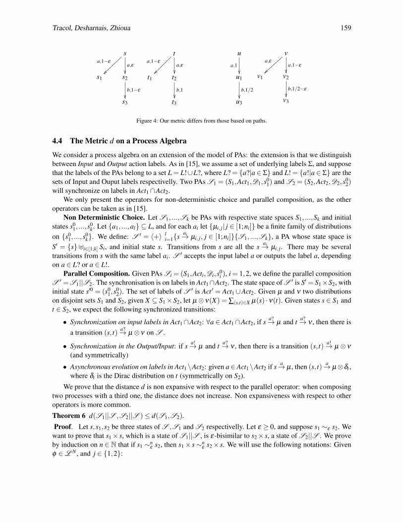
Tracol, Desharnais, Zhioua 159

sa,1−ε

~~}}}}

}}}}

a,�

ta,1−ε

������

����

a,�

u

a,1��

s1 s2

b,1−ε

��

t1 t2

b,1��

u1

b,1/2��

s3 t3 u3

va,ε

~~||||

||||

a,1−ε

��v1 v2

b,1/2−ε

��v3

Figure 4: Our metric differs from those based on paths.

4.4 The Metric d on a Process Algebra

We consider a process algebra on an extension of the model of PAs: the extension is that we distinguishbetween Input and Output action labels. As in [15], we assume a set of underlying labels Σ, and supposethat the labels of the PAs belong to a set L = L!∪L?, where L? = {a?|a ∈ Σ} and L! = {a!|a ∈ Σ} are thesets of Input and Ouput labels respectivelly. Two PAs S1 = (S1,Act1,D1,s0

1) and S2 = (S2,Act2,D2,s02)

will synchronize on labels in Act1∩Act2.We only present the operators for non-deterministic choice and parallel composition, as the other

operators can be taken as in [15].Non Deterministic Choice. Let S1, ...,Sk be PAs with respective state spaces S1, ...,Sk and initial

states s01, ...,s

0k . Let {a1, ...,al} ⊆ L, and for each ai let {µi, j| j ∈ [1;ni]} be a finite family of distributions

on {s01, ...,s

0k}. We define: S ′ = 〈+〉 l

i=1{sai→ µi, j, j ∈ [1;ni]}{S1, ...,Sk}, a PA whose state space is

S′ = {s} ]i∈[1;k] Si, and initial state s. Transitions from s are all the s ai→ µi, j. There may be severaltransitions from s with the same label ai. S ′ accepts the input label a or outputs the label a, dependingon a ∈ L? or a ∈ L!.

Parallel Composition. Given PAs Si = (S1,Acti,Di,s0i ), i = 1,2, we define the parallel composition

S ′ =S1||S2. The synchronisation is on labels in Act1∩Act2. The state space of S ′ is S′ = S1×S2, withinitial state s′0 = (s0

1,s02). The set of labels of S ′ is Act ′ = Act1∪Act2. Given µ and ν two distributions

on disjoint sets S1 and S2, given X ⊆ S1×S2, let µ⊗ν(X) = ∑(s,t)∈X µ(s) ·ν(t). Given states s ∈ S1 andt ∈ S2, we expect the following synchronized transitions:

• Synchronization on input labels in Act1∩Act2: ∀a ∈ Act1∩Act2, if s a?→ µ and t a?→ ν , then there isa transition (s, t) a?→ µ⊗ν on S .

• Synchronization in the Output/Input: if s a!→ µ and t a?→ ν , then there is a transition (s, t) a!→ µ⊗ν

(and symmetrically)

• Asynchronous evolution on labels in Act1\Act2: given a∈Act1\Act2 if s a→ µ , then (s, t) a→ µ⊗δt ,where δt is the Dirac distribution on t (symmetrically on S2).

We prove that the distance d is non expansive with respect to the parallel operator: when composingtwo processes with a third one, the distance does not increase. Non expansiveness with respect to otheroperators is more common.

Theorem 6 d(S1||S ,S2||S )≤ d(S1,S2).

Proof. Let s,s1,s2 be three states of S ,S1 and S2 respectivelly. Let ε ≥ 0, and suppose s1 ∼ε s2. Wewant to prove that s1× s, which is a state of S1||S , is ε-bisimilar to s2× s, a state of S2||S . We proveby induction on n ∈ N that if s1 ∼n

ε s2, then s1× s∼nε s2× s. We will use the following notations: Given

φ ∈L N , and j ∈ {1,2}:

160 Computing Distances between Probabilistic Automata

[[φ ]]S j||S = {s j× s|s j ∈ S j, s ∈ S, and s j× s |= φ

Where the semantics is taken on the PA S j||S . Let

left j([[φ ]]S j||S ) = {v ∈ S j|∃u ∈ S s.t. u× v |= φ}

Given v ∈ S, letright j(v, [[φ ]]S j||S ) = {u ∈ S1|u× v |= φ}

The key case is when φ = 〈a〉{(φi, pi)}i∈I ∈ L N , with depth n. Suppose s1× s |= φ . Then thereexists a transition s1× s a→ µ1⊗ν on S ′ such that for all i ∈ I, (µ1⊗ν)([[φi]])≥ pi.

By hypothesis, s1 ∼nε s2. Hence, there exists a transition s2

a→ µ2 such that µ1L ε(∼ε)µ2.We know that for all i ∈ I,

µ1⊗ν([[φi]]) = ∑v∈left1([[φi]])

ν(v) · ∑u∈right1(v,[[φi]])

µ1(v).

Given v ∈ left([[φi]]) (hence v ∈ S), we know that µ2(∼nε right1(v, [[φi]]))≥ µ1(right1(v, [[φi]]))− ε .

Moreover, by induction hypothesis, ∼nε right1(v, [[φi]])⊆ right2(v, [[φi]]ε . Indeed,

∼nε right1(v, [[φi]])∩S2 =∼n

ε {u ∈ S2|∃u′ ∈ S1 s.t. u∼nε u′ and u′ |= φi.

We get the result since by induction hypothesis, if u∼nε u′ and s′ ∈ S, we have u× s′ ∼n

ε u′× s′.This implies that µ2(right2(v, [[φi]]ε))≥ µ1(right1(v, [[φi]]))− ε . Finally,

∑v∈left2([[φi]]ε )

ν(v) · ∑u∈right2(v,[[φi]]ε )

µ2(v)≥ ∑v∈left1([[φi]])

ν(v) · ∑u∈right1(v,[[φi]])

µ1(v)− ε.

Hence µ2⊗ν([[φi]]ε)≥ µ1⊗ν([[φi]])− ε . This proves that s2× s |=ε φ . �

5 Examples

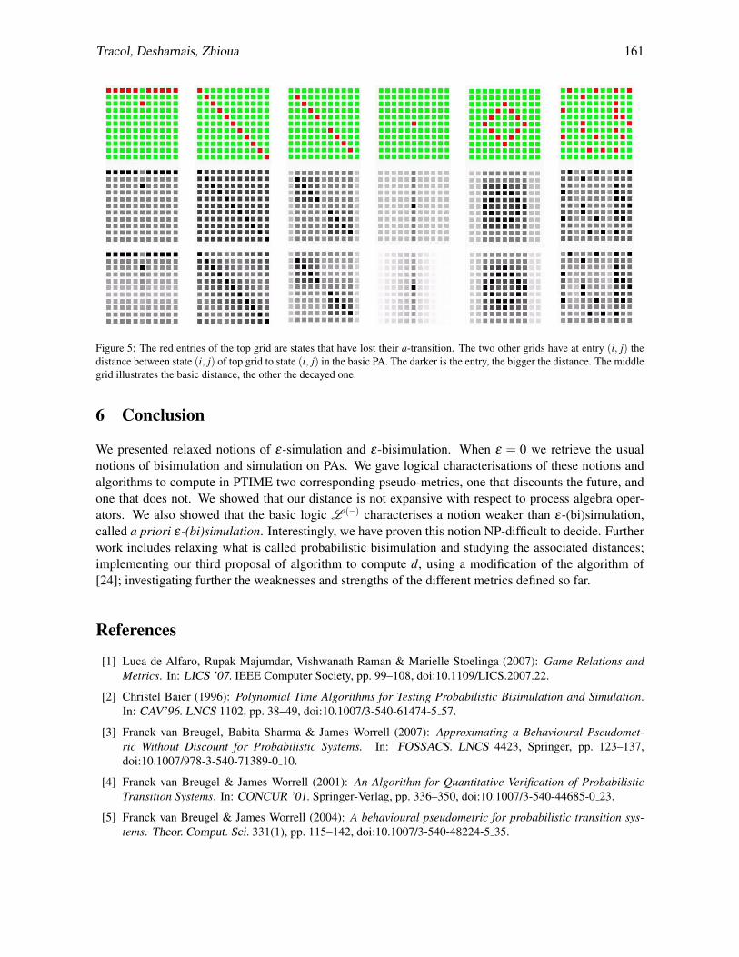
We build a benchmark set of deterministic PAs to compare distances. The processes are variations ofa basic one from which we delete some transitions. The state space of the basic PA is a square grid ofn×n. The set of actions is {a}. All the computations on the state indices are done modulo n: the grid isa torus. The a-transitions from state (i, j) are as follows:

from (i, j) to (i, j−1) : 0.1 (i, j+1) : 0.5 (i−1, j) : 0.25 (i+1, j) : 0.15

This basic PA is compared to variations of it obtained by deleting in some states the transition of labela (to all successors). Note that the basic process is bisimilar to the one-state process that can do a withprobability 1. We consider the distances between states with same indices of the different systems. Fig. 5illustrates some PAs and the impact of the deletion of transitions for the two distances that we defined.The distance dλ is illustrated in the bottom grids of the figure. The linear function for λ is the following,with N = 20. We take δ = 1/N, and let λ (x) = x+ δ if x ∈ [0;1− δ ], and λ (x) = 1 if x ∈ [1− δ ;1].One can observe that the decay distances fade out when further from the difference, whereas d is moreconstant.

It would be nice to compare these grids with others obtained from other known metrics. We leavethat for future work, as we have no implementation of other metrics that can handle more than 25 states.

Tracol, Desharnais, Zhioua 161

Figure 5: The red entries of the top grid are states that have lost their a-transition. The two other grids have at entry (i, j) thedistance between state (i, j) of top grid to state (i, j) in the basic PA. The darker is the entry, the bigger the distance. The middlegrid illustrates the basic distance, the other the decayed one.

6 Conclusion

We presented relaxed notions of ε-simulation and ε-bisimulation. When ε = 0 we retrieve the usualnotions of bisimulation and simulation on PAs. We gave logical characterisations of these notions andalgorithms to compute in PTIME two corresponding pseudo-metrics, one that discounts the future, andone that does not. We showed that our distance is not expansive with respect to process algebra oper-ators. We also showed that the basic logic L (¬) characterises a notion weaker than ε-(bi)simulation,called a priori ε-(bi)simulation. Interestingly, we have proven this notion NP-difficult to decide. Furtherwork includes relaxing what is called probabilistic bisimulation and studying the associated distances;implementing our third proposal of algorithm to compute d, using a modification of the algorithm of[24]; investigating further the weaknesses and strengths of the different metrics defined so far.

References

[1] Luca de Alfaro, Rupak Majumdar, Vishwanath Raman & Marielle Stoelinga (2007): Game Relations andMetrics. In: LICS ’07. IEEE Computer Society, pp. 99–108, doi:10.1109/LICS.2007.22.

[2] Christel Baier (1996): Polynomial Time Algorithms for Testing Probabilistic Bisimulation and Simulation.In: CAV’96. LNCS 1102, pp. 38–49, doi:10.1007/3-540-61474-5 57.

[3] Franck van Breugel, Babita Sharma & James Worrell (2007): Approximating a Behavioural Pseudomet-ric Without Discount for Probabilistic Systems. In: FOSSACS. LNCS 4423, Springer, pp. 123–137,doi:10.1007/978-3-540-71389-0 10.

[4] Franck van Breugel & James Worrell (2001): An Algorithm for Quantitative Verification of ProbabilisticTransition Systems. In: CONCUR ’01. Springer-Verlag, pp. 336–350, doi:10.1007/3-540-44685-0 23.

[5] Franck van Breugel & James Worrell (2004): A behavioural pseudometric for probabilistic transition sys-tems. Theor. Comput. Sci. 331(1), pp. 115–142, doi:10.1007/3-540-48224-5 35.

162 Computing Distances between Probabilistic Automata

[6] Stefano Cattani & Roberto Segala (2002): Decision Algorithms for Probabilistic Bisimulation. In: CONCUR’02. Springer-Verlag, pp. 371–385, doi:10.1007/3-540-45694-5 25.

[7] Stefano Cattani, Roberto Segala, Marta Kwiatkowska & Gethin Norman (2005): Stochastic transition systemsfor continuous state spaces and non-determinism. In: FOSSACS’05. LNCS 3441, Springer Verlag, pp. 125–139, doi:10.1007/978-3-540-31982-5 8.

[8] K. Chatterjee, Luca de Alfaro, Rupak Majumdar & Vishwanath Raman (2010, to appear.): Algorithms forgame metrics. LMCS: Logical Methods in Computer Science doi:10.2168/LMCS-6(3:13)2010.

[9] Pedro R. D’Argenio, Nicolas Wolovick, Pedro Sanchez Terraf & Pablo Celayes (2009): Nondeter-ministic labeled Markov processes: bisimulations and logical characterization. QEST’09 , pp. 11–20doi:10.1109/QEST.2009.17.

[10] Josee Desharnais, Abbas Edalat & Prakash Panangaden (2002): Bisimulation for Labeled Markov Processes.Information and Computation 179(2), pp. 163–193, doi:10.1.1.16.5653.

[11] Josee Desharnais, Vineet Gupta, R. Jagadeesan & P. Panangaden (1999): Metrics for Labeled Markov Pro-cesses. In: CONCUR’99. LNCS, Springer-Verlag, pp. 258–273, doi:10.1007/3-540-48320-9 19.

[12] Josee Desharnais, Francois Laviolette & Mathieu Tracol (2008): Approximate analysis of probabilis-tic processes: logic, simulation and games. In: QEST’08. IEEE Computer Society, pp. 264–273,doi:10.1109/QEST.2008.42.

[13] Josee Desharnais, Francois Laviolette & Sami Zhioua (2006): Testing Probabilistic Equivalence ThroughReinforcement Learning. In: FSTTCS’06. LNCS 4337, Springer, pp. 236–247, doi:10.1007/11944836 23.

[14] Norm Ferns, Prakash Panangaden & Doina Precup (2004): Metrics for finite Markov decision processes. In:UAI’04. AUAI Press Arlington, Virginia, United States, pp. 162–169, doi:10.1.1.87.9485.

[15] Norman Ferns, Prakash Panangaden & Doina Precup (2005): Metrics for Markov Decision Processes withInfinite State Spaces. In: UAI’05. AUAI Press, p. 201, doi:10.1007/BF01908587.

[16] Michael R. Garey & David S. Johnson (1979): Computers and Intractability: A Guide to the Theory ofNP-completeness. W. H. Freeman & Co., New York, NY, USA.

[17] Alessandro Giacalone, Chi-Chang Jou & Scott A. Smolka (1990): Algebraic Reasoning for ProbabilisticConcurrent Systems. In: Proc. IFIP TC2 Working Conference on Programming Concepts and Methods.North-Holland, pp. 443–458, doi:10.1.1.56.3664.

[18] Holger Hermanns (2002): Interactive Markov chains, and the quest for quantified quality. Springer-Verlag,Berlin, Heidelberg, doi:10.1007/3-540-45804-2.

[19] Kim G. Larsen & Arne Skou (1991): Bisimulation through Probablistic Testing. Information and Computa-tion 94, pp. 1–28, doi:10.1.1.158.9316.

[20] Augusto Parma & Roberto Segala (2007): Logical characterisation of Bisimulations for Discrete Probabilis-tic Systems. In: FOSSACS’07. LNCS 4423, Springer-Verlag, pp. 287–301, doi:10.1007/978-3-540-71389-0 21.

[21] Martin L. Puterman (1994): Markov Decision Processes: Discrete Stochastic Dynamic Programming. Wiley.[22] Roberto Segala & Nancy Lynch (1994): Probabilistic Simulations for Probabilistic Processes. In: CON-

CUR’94. LNCS 836, Springer-Verlag, pp. 481–496, doi:10.1007/BFb0015027.[23] Roberto Segala & Andrea Turrini (2007): Approximated Computationally Bounded Simulation Relations for

Probabilistic Automata. In: CSF’07. pp. 140–156, doi:10.1007/3-540-45694-5 25.[24] Lijun Zhang, Holger Hermanns, Friedrich. Eisenbrand & David N. Jansen (2007): Flow faster: efficient

decision algorithms for probabilistic simulations. In: TACAS’07. LNCS 4424, Springer-Verlag, pp. 155–169, doi:10.1007/978-3-540-71209-1 14.