alternative automata-based approaches to probabilistic
TRANSCRIPT
Fakultät Informatik
Alternative Automata-based Approaches toProbabilistic Model Checking
Dissertation
zur Erlangung des akademischen GradesDoktoringenieur (Dr.-Ing.)
vorgelegt an der Technischen Universität DresdenFakultät Informatikvon David Müller
geboren am 08.März 1987in Dresden
Betreunde Hochschullehrerin/Gutachterin:Prof. Dr. rer. nat. Christel BaierTechnische Universität DresdenGutachter:Univ.-Prof. Dr. Dr. h.c. Javier EsparzaTechnische Universität München
Tag der Verteidigung: 10.Dezember 2018Dresden im Oktober 2019

AbstractProbabilistic model checking (PMC) aims to determine the likelihood of a system to meeta specification. In this thesis we consider as models for randomized systems discrete-timeMarkov chains and discrete-time Markov decision processes (MDPs).
In this thesis we focus on linear temporal logic (LTL) for expressing specifications. Thestandard approach for non-probabilistic systems translates an LTL formula into a non-deterministic Buchi automaton (NBA) with a single-exponential number of states in theworst case. While in the non-probabilistic setting non-deterministic Büchi automata (NBA)can be used directly, the probabilistic choices are incompatible with the direct use of an NBA.In the standard approach to PMC, the NBA obtained from the LTL formula is determinized,which can lead to a double-exponential number of states in total. There are approachesfor Markov chain analysis against LTL with exponential runtime, which motivates thesearch for non-deterministic automata with restricted forms of non-determinism that makethem suitable for PMC. For MDPs, the approach via deterministic automata matches thedouble-exponential lower bound, but a practical application might benefit from approachesvia non-deterministic automata.
We first investigate good-for-games (GFG) automata. In GFG automata one can resolvethe non-determinism for a finite prefix without knowing the infinite suffix and still obtain anaccepting run for an accepted word. We explain that GFG automata are well-suited for MDPanalysis on a theoretic level, but our experiments show that GFG automata constructed bythe methods proposed by [HP06] cannot compete with deterministic automata.
We have also researched another form of pseudo-determinism, namely unambiguity,where for every accepted word there is exactly one accepting run. For unambiguous Buchiautomata (UBA) it is claimed in the literature that Markov chain analysis for a givenUBA can be done in polynomial time. We show that the proposed approach is flawedand present a new polynomial-time approach for PMC of Markov chains against UBAspecifications. Instead of identifying single states inducing probability 1 (which may notexists), we identify sets of states inducing probability 1.
Additionally, we examine the new symbolic Muller acceptance described in the HanoiOmega Automata Format, which we call Emerson-Lei acceptance. It is a positive Booleanformula over unconditional fairness constraints. We present a construction of small de-terministic automata using Emerson-Lei acceptance. Deciding, whether an MDP has apositive maximal probability to satisfy an Emerson-Lei acceptance, is NP-complete. Thisfact has triggered a DPLL-based algorithm for deciding positiveness.
For every approach we perform benchmarks on the LTL-to-automata translation itself aswell as on models of the PRISM benchmark suite.
i

AcknowledgmentsI am very thankful for the support of Christel Baier. She offered me a very interesting PhDtopic, great scientific insights and encouraged me to stick to the topic, even if the resultslooks bad. She is also a great inspiration in teaching, whether it is to prepare slides, orscripts with a clear and helpful structure. I also want to thank my colleague Joachim Klein,who never declined to discuss automata-theoretic ideas, helped me at programming, andproof-read this thesis. Christel and Joachim complemented each other in great way.
Next, I want to thank our secretaries Karina Wauer, Kerstin Achtruth, Sandy Seifarth,and Kati Michel for their support in bureaucratic stuff. They saved me a lot time, whenfilling out the reimbursement applications. Of course, I thank also my colleagues PhilippChrszon, Marcus Daum, Clemens Dubslaff, Daniel Gburek, Simon Jantsch, Lisa Kruse,Linda Leuschner, Sascha Klüppelholz, Steffen Märcker, and Jakob Piribauer for the fruitfuldiscussions and for making the past years so enjoyable.
I also want to express my gratitude to my co-authors Tomáš Babiak, František Blahoudek,Alexandre Duret-Lutz, Jan Křetínský, David Parker and Jan Strejček for the cooperationon the Hanoi-Omega Format and the Emerson-Lei acceptance.
Concerning financing my research, I’m thankful to the german research foundation byfunding my work via the research training group QuantLA (1763) and via the project BA1679/12-1.
At last, I want to show appreciation to my family for their support and believe in me.In particular, my warm-hearted uncle Volkmar taught me programming as a little childand lured in this manner into computer science. I guess, he would have made some funnyjokes, if he had seen my thesis.
iii

Contents1 Introduction 1
1.1 Literature . . . . . . . . . . . . . . . . . . . . . . . . . . . . . . . . . 31.2 Contribution . . . . . . . . . . . . . . . . . . . . . . . . . . . . . . . 8
2 Preliminaries 112.1 Linear temporal logic . . . . . . . . . . . . . . . . . . . . . . . . . . . 112.2 Automata over infinite words . . . . . . . . . . . . . . . . . . . . . . 122.3 Automata over finite words . . . . . . . . . . . . . . . . . . . . . . . 142.4 Markovian models . . . . . . . . . . . . . . . . . . . . . . . . . . . . 15
3 Good-for-games Automata 233.1 Automata-based Analysis of Markov Decision Processes . . . . . . . . 263.2 From LTL to GFG Automata . . . . . . . . . . . . . . . . . . . . . . 323.3 Implementation and Experiments . . . . . . . . . . . . . . . . . . . . 393.4 Conclusion . . . . . . . . . . . . . . . . . . . . . . . . . . . . . . . . . 52
4 Unambiguous Büchi automata 554.1 Analysis of Markov chains against UBA-specifications . . . . . . . . . 584.2 Implementation and Experiments . . . . . . . . . . . . . . . . . . . . 934.3 Conclusion . . . . . . . . . . . . . . . . . . . . . . . . . . . . . . . . . 100
5 Emerson-Lei acceptance 1035.1 Construction . . . . . . . . . . . . . . . . . . . . . . . . . . . . . . . 1055.2 End-component analysis for Emerson-Lei acceptance . . . . . . . . . 1135.3 A DPLL based positivity check . . . . . . . . . . . . . . . . . . . . . 1175.4 Implementation and Experiments . . . . . . . . . . . . . . . . . . . . 1255.5 Conclusion . . . . . . . . . . . . . . . . . . . . . . . . . . . . . . . . . 131
6 Conclusion 133
v

1 IntroductionThe growing complexity and dependence on computational systems in our every daylife renders checking their correctness and safety more complicate. Many errors andpitfalls can be avoided by testing and simulation but both methods are incomplete.Alternatively, formal methods offer an exhaustive system analysis.
One technique for formal verification is interactive theorem proving, see, e.g., [BC04;NK14]. Interactive theorem proving allows the creation of proofs in a user-supportedfashion with several benefits such as automatic code generation or automated proofsearch up to a certain depth.
Model checking belongs to the area of formal methods as well, being an automatedtechnique for the formal analysis of abstract models. In its classical form it decideswhether a model of a system satisfies a property. It has been introduced in the earlyeighties of the last century, with the notable publications [EC80; LP85; CES86], andhas spread out into different research lines by now, e.g., analysis of timed automata[AD94; LPY95; BY04] or probabilistic systems [Var85; VW86; CY95; Var99]. For abroad introduction we refer to [BK08].
One of the most basic models is Kripke structures. Kripke structures are labeledgraphs where states can be initial. One model of the behavior are paths which aresequences of states. Kripke structures offer a purely non-deterministic behavior: Thefirst state and the successors states of a path are chosen non-deterministically. Everypath can be lifted to its trace by taking the labelings instead of the states. The tracesof the paths can be seen as the possible behaviors of the Kripke structures.
For specifying properties one usually employs temporal logics. The two mostprominent temporal logics are computation tree logic (CTL) and linear temporallogic (LTL).
CTL is a branching time logic, in which one does reason about the computationtree, which is the unfolded behavior of a system. CTL can be checked in polynomialtime [CE81; CES86].
LTL focuses on the paths of a model as the semantic of LTL is defined by a set ofwords. A model satisfies an LTL formula if all the model’s traces are contained inthe set of words that satisfy the LTL formula, i.e., the model exhibits only behaviorcharacterized by the LTL formula. The typical approach for LTL model checkingemploys ω-automata. The negated LTL formula is transformed into a (possiblyexponential-sized) non-deterministic Büchi automaton (NBA). Then a product isbuilt, in which one can search for behavior that the Kripke structure displays butthat is forbidden by the specification.
Prominent model checkers for Kripke structures and LTL are SPIN [Hol04] andnuSMV [Cim+02]. In practice, the model (and the product) size can become very large
1
1 Introduction
even for simple systems, and thus actual model checking turns unfeasible very fast ifthe system’s model is saved state-by-state in the memory. This problem is called thestate space explosion problem and led to symbolic reasoning over the models. Insteadof analyzing particular states, one does analyze set of states. An important milestoneof symbolic reasoning was the introduction of binary decision diagrams (BDDs).
BDDs can serve for a compact representation of the state space of a model orautomaton. They have been introduced by [Bry86] and have found their way intoseveral applications, e.g., VLSI design [MT98]. BDDs are essentially a graph repre-sentation of Boolean functions, offering a good compromise between computationalefficiency and memory consumption. For a general introduction to BDDs we refer to[Bur+92; Weg00].
Another handling of the state explosion problem is offered by bounded modelchecking (BMC) [Bie+99; Bie+03]. BMC relies on an iterative enumeration of allfinite paths up to a certain bound k. If a counterexample for the correctness ofthe system is found, then this counterexample is returned. If k exceeds a thresholdmarking that the whole model has been explored and no counterexample can befound anymore, the BMC algorithm returns the correctness of the system. In practice,BMC outperforms BDD-based model checking if a counterexample exists, and istherefore useful for prototyping in particular.
Since the basic model checking focuses on Kripke structures and therefore asksfor a binary answer whether the specification is satisfied or not, the need for moreexpressiveness emerged quite naturally. Probabilistic model checking focuses onMarkovian models like Markov chains or Markov decision processes (MDPs for short),thus enabling answers like “The system obeys the specification with a likelihood of99.95%”. Markov chains can be seen as Kripke structures with a pure probabilistictransition structure. If one provides non-deterministic choices to Markov chains, oneobtains MDPs. Analogously to games, MDPs are called 11/2-player games, where oneplayer resolves the non-deterministic choices, and the other (half) player resolves theprobabilistic choices probabilistically.
Despite the probabilistic nature of Markovian models the syntax and semanticsof LTL remains equal. However, for CTL a probabilistic counterpart, PCTL, exists.Like CTL, PCTL can be checked efficiently in polynomial time, see, e.g., [HJ94] andthere exists model checkers focusing on PCTL (or some of its variants), such as STORM[Deh+17] and MRMC [Kat+11].
The probabilistic choices of Markovian models blocks the direct application ofNBAs in the process of model checking Markovian models against LTL formula. Asa resort to this problem, deterministic automata are usually employed.
The translation of LTL to deterministic ω-automata can cause a double-exponentialblow-up [KV05; KR11]. This double-exponential blow-up together with the polynomial-time algorithms for building the product and the analysis of it yields an overalldouble-exponential-time algorithm for the analysis of Markov decision processes(MDP) against LTL. This double-exponential time algorithm matches the lowerbound [CY95]. The case is different for Markov chains, where a PSPACE lower boundis known [Var85]. Thus, the double-exponential blow-up over deterministic automata
2
1.1 Literature
leaves a complexity gap for Markov chains.
1.1 Literature1.1.1 Markov Decision ProcessesFirst results in the area of probabilistic model checking for MDPs have been achievedfor qualitative PMC, where one wants to prove that a path property holds almostsurely for all possible or a single resolution of the non-determinism. Alternatively,one wants to prove that a path property holds with a positive probability for allpossible or a single resolution of the non-determinism. Hart, Sharir and Pnueli[HSP83] discussed the termination problem in the qualitative setting for a systemof concurrent processes. Pnueli continued this work with Zuck in [PZ86a; PZ86b]and presented a tableau-based approach for LTL. The first results on automata-based approaches for MDP analysis have been published by Vardi [Var85] and Vardiand Wolper [VW86], which was revisited by Courcoubetis and Yannakakis [CY95].They depend on so-called deterministic-in-the-limit Büchi automata, i.e., automatathat behave deterministically after reaching a final state. The construction of adeterministic-in-the-limit Büchi automaton out of an NBA resembles the breakpointconstruction [MH84], a multi subset construction, and can cause an exponentialblow-up. Thus, the overall approach for MDP analysis for LTL matches the lower2EXPTIME bound.
Probabilistic model checking suffers also from the state space explosion problem.Here, the concept of BDDs has been transferred to multi-terminal BDDs (MTBDDs),i.e., BDDs representing not only Boolean functions but multi-valued functions [CFZ93;Bah+93] as they can represent matrices with real values between 0 and 1. Theprobabilistic model checker PRISM [Par02; KNP11] supports MTBDDs by the twoengines hybrid and mtbdd. In the hybrid engine the result vector containing theprobability to obey the specification for every state is stored in an explicit manner,whereas in the mtbdd engine the result vector is stored symbolically as well. In theexplicit engine the state-space of the model is represented state-for-state, as wellas the transitions.
Besides the employment of MTBDDs, statistical model checking [LDB10; LV15]mitigates the state space explosion problem by simulating the system and sampling afinite number of runs. These runs are used to provide estimates about the correctnessof systems within certain bounds.
Recent developments have lowered the computation time for a certain fragment ofLTL to single exponential time, namely LTL\U [KV15]. This fragment describesLTL formulas in positive normal form using the operators ⃝,♦, and U with theadditional restriction that no U operator occurs in the scope of a operator. In[Kin17] the fragment LTL\U is extended to a fragment called LTLD, where therestrictions of LTL\U are loosened in the following way:
• for a formula ϕU ψ occurring inside of a operator, ψ has to contain only ♦
3
1 Introduction
and as temporal operators,
• in every formula of the form ϕ ∨ ψ occurring inside of a operator, at least ϕor ψ has to contain only ♦ and as temporal operators.
Covering full LTL, Sickert, Esparza, Jaax and Křetínský offered a new (double-exponential) construction of deterministic-in-the-limit Büchi automata [Sic+16].These deterministic-in-the-limit automata are even suitable for quantitative prob-abilistic model checking. As their implementation MoChiBa [SK16] shows, that theefficiency of MDP analysis benefits from the usage of deterministic-in-the-limit Büchiautomata.
Another tool for the generation of deterministic-in-the-limit automata is Seminator[Bla+17], which takes a non-deterministic automaton with a transition-based gener-alized Büchi acceptance as input, and transforms it into a deterministic-in-the-limitautomaton. However, the resulting automaton may be not suited for quantitativePMC, but only qualitative PMC.
The mentioned work relied on building a single ω-automaton equivalent to thespecification. The authors of [Hah+15] consider an alternative. They provide atranslation into two automata with the same graph structure, but different acceptanceconditions, under-approximating and over-approximating the languages respectively.Accordingly, one product with two acceptance conditions is built, and every maximalend-component is checked, whether it satisfies the two acceptance conditions. Ifthe two result are different, the affected automaton part is refined via breakpointconstruction or if necessary a full determinization to deliver exact results. The authorsimplemented this approach into their probabilistic model checker IscasMC [Hah+14]and in its successor ePMC [Tur17].
1.1.2 Markov chainsThe PSPACE lower bound for the analysis of Markov chains against LTL specificationsinspired several algorithms avoiding deterministic automata. Courcoubetis andYannakakis [CY88; CY95] presented an automata-less Markov chain analysis method,that can be lifted to PSPACE algorithm for qualitative analysis. We give shortoverview for its quantitative version: To calculate PrM (ϕ), the Markov chain Mand the LTL formula ϕ are refined to a Markov chainM′ and an LTL formula ϕ′
preserving the probability, i.e., PrM(ϕ) = PrM′(ϕ′). The refinement is carried outiteratively until the refined LTL formula does not contain any temporal operator,which then can be easily checked.
In a refinement step one selects a subformula ψ with a temporal operator astop-most operator (in the syntax tree of the formula) and no other temporal operator.Then, this subformula is replaced by a fresh atomic proposition in ϕ, leading to a newLTL formula ϕ′. The Markov chainM is transformed with the usage of computedprobabilities for every state of M and ψ in such a way that PrM(ϕ) = PrM′(ϕ′)holds, where we denote the transformed Markov chain asM′. The transformation ofM doubles the state space in the worst case.
4
1.1 Literature
The refinement step is repeated until ϕ′ does not contain any temporal operatoranymore. As the remaining task one has to calculate PrM′(ϕ′) for such a simpleformula ϕ′. This step just amounts to a summation over the initial distribution ι(s)for every state s satisfying ϕ′ and ι being the initial distribution ofM′.
Couvreur, Saheb and Sutre [CSS03] suggested separated automata, a special formof unambiguous automata. For a deeper consideration of [CSS03], in particular acomparison with unambiguous automata, we refer to Section 4.1.6.
Instead of a single automaton, [BRV04] takes a weak alternating ω-automatonA as input and transforms it into two ω-automata, a so-called full automaton anda local transition system. The local transition system and the Markov chain forma product, and then a state is searched with the help of the full automaton, thatcounter witnesses PrM (A) = 1.
1.1.3 ω-automataNon-deterministic Büchi automata have been introduced independently in 1962 byBüchi [Büc62] and Trakhtenbrot [Tra62] as tools for decision problems in the area ofmathematical logics.
LTL model checking of Kripke structures is usually done by building an automatonequivalent to the negated specification. Vardi and Wolper [VW86] have suggested arather simple construction method for NBA equivalent to a given LTL specification.
The constructions for NBA became more elaborate, see [GO01; Bab+12] for anapproach via alternating automata, or [Ger+95] for a tableau-based approach.
The competition between the LTL-to-NBA translations has lead to the generationof smaller NBA, yielding an improved starting point for determinization algorithms.The research for determinization algorithms follows two main lines: Safra-basedmethods [Saf88; Pit07; Sch09] (and their heuristic improvements in [KB06; KB07])and Muller-Schupp based methods [MS95; KW08; Fog+13; FL15]. A hybrid versionhas been proposed by Redziejowski [Red12].
The earliest approach [McN66] for determinization which was presented by Mc-Naughton has not been pursued much further, since it is double-exponential in thesize of the Büchi automaton and therefore does not match the single exponentiallower bound.
Since the class of languages equivalent to a deterministic Büchi automaton (alsocalled DBA-realizable languages) is a strict subset of ω-regular languages (in contrastto NBA), more expressive acceptance conditions exist: Rabin [Rab72], Streett [Str82],parity [Mos84], Muller [Mul63] among others. All acceptance conditions can be seenas a special form of a Muller acceptance, which explicitly represents every possibleacceptable set of states being visited infinitely often.
Instead of taking an intermediate step via non-deterministic Büchi automata, directtranslations from LTL to deterministic ω-automata have been proposed. Křetínskýand Esparza [KE12] offer a direct translation to a deterministic (generalized) Rabinautomaton for the LTL fragment where ♦ and are the only allowed temporaloperators. This approach has been extended [Bab+13b; KG13; EK14] until full LTL
5
1 Introduction
has been covered. Very recently at LICS 2018, Esparza, Křetínský and Sickert haveprovided a Master theorem enabling the decomposition of the language describedby an LTL formula into fragments offering a simpler translation to automata thantranslations for full LTL [EKS18].
Apart from striving to generate small deterministic automata during the construc-tion, post generation algorithms for shrinking the automaton size without changingthe accepted language have also been proposed.
Simulation delivers a general-purpose method for shrinking automata. They arebased on calculating a simulation relation on the state space that can be used tocollapse the states within the same equivalence classes and still obtain an equivalentautomaton. However, one cannot achieve a minimal number of state with thesetechniques in case of ω-automata. Prominent examples are stutter simulations [KB07;MD15], which enable to collapse states that are unnecessary finite repetitions, andbisimulation [Mil80; Par81] identifying equivalent substructures in an automaton.
A very intuitive minimization technique concerns weak deterministic Büchi au-tomata (WDBA), i.e., deterministic Büchi automata where every SCC containseither no accepting state or solely accepting states. This requirement reduces theexpressiveness of WDBA to the intersection of DBA-realizable languages and coDBA-realizable languages.1 Löding [Löd01] established the connection between WDBAand deterministic finite automata over finite words (DFA) and reduced the taskof minimizing WDBA to minimizing DFA. We have implemented his minimizationtechnique in the probabilistic model checker PRISM and could achieve a reduction in30 out of 44 cases [Kle+17].
For minimization of a wider range of ω-automata, SAT-based approaches havebeen proposed recently. Schewe proves the NP-completeness of deciding whether aDBA has a minimal number of states and analogous NP-completeness results fordeterministic co-Büchi automata, and deterministic parity automata [Sch10]. Ehlersbuilds on this result and minimizes DBA with SAT-solvers [Ehl10]. To cover fullω-regularity, Baarir and Duret-Lutz generalized this to Emerson-Lei ω-automata[BD15], which are essentially ω-automata with Muller acceptance expressed in asymbolic fashion.
In 2015 the Hanoi Omega Automata Format was published [Bab+15]. The HanoiOmega Automata Format is a unified exchange format for ω-automata tools. Thisformat allows a tool-agnostic interoperation, e.g., PRISM is now able to use every toolthat supports the Hanoi Omega Automata Format (and determinization) for thecreation of deterministic automata.
Now we turn to specific types of ω-automata discussed in this thesis. This overviewshould be seen as a collection of literature to separate our contribution. A deeperliterature review will be covered in the specific chapters.
1DBA-realizable languages are ω-regular languages for which an equivalent DBA exists. Analogously,coDBA-realizable languages are languages, for which an equivalent deterministic co-Büchi ω-automaton exists.
6
1.1 Literature
Good-for-games automata. The concept of good-for-games automata (GFG) hasbeen introduced by Henzinger and Piterman [HP06]. In a good-for-games automatonthe resolution of the non-determinism for a finite prefix of an accepted word does notrequire any look-ahead.
It was introduced for the synthesis of reactive systems where one typically solves 2-player games. Good-for-games automata were offered as a substitute to deterministicautomata.
In [HP06] a translation from NBA to GFG parity automata has been presented,which can be incorporated into a translation from LTL to GFG parity automata. Theauthors of [KS15] have shown the potential of good-for-games by exhibiting a familyof good-for-games co-Büchi automata, which are exponentially more succinct thanevery equivalent deterministic automaton. Still, [HP06] proves that a transformationfrom NBA to GFG automata can cause an exponential blow-up.
Unambiguous Büchi automata. Unambiguity in a non-deterministic automatondemands that there is exactly one accepting run for every accepted word. Thephenomenon has been widely studied in the 1980s. In particular, Stearns andHunt [SH85] have considered universality (“Is every word an accepted word?”) forunambiguous regular grammars (and automata) over finite words and could establisha polynomial time result for deciding universality. Bousquet and Löding [BL10] couldprove an analogous result for separated Büchi automata, i.e., automata that are stillunambiguous if all states have been set to initial. The first authors who looked intothe application of separated automata for Markov chain analysis were Couvreur,Sutre and Saheb [CSS03]. As one can construct a separated automaton equivalentto an LTL formula within exponential time, and the Markov chain analysis againstseparated automata specifications can be done in polynomial time, the overall timecomplexity for this approach is single exponential.
Based on [CSS03], Benedikt, Lenhardt, and Worrell [BLW13b; BLW14] proposed ageneralization to unambiguous Büchi automata. Their claim, that a polynomial-timeanalysis of Markov chains under UBA specifications is possible, is true, but theirproofs rely on a false assumption and therefore their algorithms work incorrectly.This flaw does not affect the second contribution of [BLW14], namely an algorithmfor model checking Markov chains against unambiguous automata over finite words.
Emerson-Lei acceptance. The commonly used Rabin, Streett and parity accep-tances can be seen as particular forms of Muller acceptance. Muller acceptanceexplicitly enumerates every possible set of states (or transitions) that is visitedinfinitely often in an accepting run. This explicit representation is verbose, andtherefore in [Bab+15] a more compact symbolic representation is proposed whichwe call Emerson-Lei acceptance. The idea of Emerson-Lei acceptance goes back toEmerson and Lei [EL87]. They have considered positive Boolean formulas with atomsstating that a certain atomic proposition should be seen infinitely often or only finitelyoften. Apart from small syntactical differences, the definitions of Emerson and Lei in
7
1 Introduction
[EL87] and the symbolic acceptance in [Bab+15] agree. The motivation of [EL87] isthe handling of fairness conditions in the context of model checking Kripke structuresagainst CTL. The authors show NP-completeness for checking whether there exists apath in a Kripke structure satisfying an Emerson-Lei acceptance. Additionally, in[EL87] it is proven that CTL model checking with a disjunction of Streett formulasas fairness condition can be done in linear time in the size of the CTL formula, thesize of the model and quadratic in the size of the fairness condition.
Results on model checking with different acceptance conditions does not onlyexist in the realm of Kripke structures, but in the realm of MDPs as well. Baier,Ciesinski and Größer [BGC09a] adapted the result of [EL87] for model checkingStreett acceptance to MDPs. Chatterjee, Gaiser and Křetínský [CGK13] couldimprove significantly the speed of MDP analysis by the employment of deterministicautomata with a generalized Rabin acceptance.
1.2 ContributionThis thesis offers new approaches for the analysis of Markov chains and MDPs thatavoid the typical approach via a deterministic Rabin (or Streett) automaton. Wealways assume that the Markovian models are given in a discrete-time setting, anddo not pursue a continues-time setting. For MDP analysis, the double-exponentialtime standard approach matches the lower bound, but from a practical point of view,it might still be possible to improve the efficiency by moving away from deterministicRabin automata. We study restricted forms of non-determinism and a more extensiveacceptance than Rabin acceptance.
For MDPs we turn to good-for-games automata and to Emerson-Lei acceptance. Inthis thesis we consider only deterministic Emerson-Lei automata and not combinationsof the different approaches, e.g., GFG Emerson-Lei automata.
For Markov chains, the approach via a deterministic ω-automaton leaves a complex-ity gap to the PSPACE lower bound. We present a method that runs in polynomialtime if a UBA specification is given. As LTL can be transformed into UBA with anexponential blow-up as upper bound, this algorithm runs in exponential time.
Good-for-games automata. In Chapter 3 we address the question whether good-for-games automata can be used for 11/2-player games. For this, we provide a newnon-standard product construction with the goal of quantitative analysis of MDPsagainst ω-regular specifications represented by a good-for-games automaton. In theproduct we can resort to standard reachability analysis. As the process of buildingthe product and the reachability analysis can be done in polynomial time, the overallapproach is polynomial in time if a Markov decision process and a GFG automatonare given.
We adapt in a straightforward manner the proof of the double-exponential blow-upfrom LTL to deterministic automata [KV05] to the GFG setting. This double-exponential lower bound matches the double-exponential upper bound one would
8
1.2 Contribution
obtain by combining the single-exponential translation from LTL to NBA and thesingle-exponential translation from NBA to GFG parity automata. Overall, thetime complexity of our GFG-based method for MDP analysis matches the double-exponential lower bound if we are given an MDP and an LTL formula as input.
We also report on an implementation of the transformation of LTL to good-for-games parity automata described in [HP06] as well as their utility in probabilisticmodel checking.2
The contribution in Chapter 3 is based on [Kle+14].
Unambiguous Büchi automata. In Chapter 4 we explain the mistaken assumptionof [BLW13b; BLW14] and provide an alternative polynomial time algorithm. Themain part concentrates on the case where we have a uniform Markov chain, i.e., aMarkov chain where at every position of every trace the symbols occur with the sameprobability. In this case the first step consists of an SCC analysis for every SCC in abottom-up manner. This analysis decides whether the analyzed SCC consists of statesinducing positive probability, and, if applicable, searches for a set of states withinthe SCC inducing probability 1. With the help of this state set, we can calculate theinduced probability of every SCC state. Afterwards, the induced probability of statesnot contained in a positive SCC can be derived by solving a linear equation system.
The case of a uniform Markov chain and a UBA can be easily lifted to the generalcase of an arbitrary Markov chain.
The chapter concludes with several benchmarks. At first, we provide a benchmarkon particular challenging UBA to compare the efficiency of two different positivitychecks. For benchmarking the actual model checking process, we refer to the boundedretransmission protocol from the PRISM benchmark suite as a Markov chain model.Here, we evaluate pre-generated automata, and LTL formulas as property input.In case of pre-generated automata, we compare deterministic automata againstunambiguous automata. In case of LTL, we compare the model checking approachesvia deterministic automata, unambiguous automata and the automata-less methodof [CY95]. As a last benchmark we compare the sizes of the generated automata fora selection of LTL formulas.
The contribution in Chapter 4 is based on [Bai+16].
Emerson-Lei acceptance. In Chapter 5 we consider the Emerson-Lei acceptancecondition. We present a translation from two important LTL fragments into de-terministic Emerson-Lei automata with an additional fallback to generic LTL-to-deterministic-ω-automata translators for full LTL. The two fragments are the safety-/cosafety fragment and a fragment which we call fairness fragment, and whichsubsumes the typical fairness conditions like unconditional, strong and weak fairness.Our translation features a product construction: We view an LTL formula as apositive Boolean combination of temporal formulas, i.e., formulas where the top-most
2We want to mention that the recently found problems in the value iteration (see [Bai+17]) didnot affect any of our experiments in PRISM.
9
1 Introduction
operator is a temporal operator. The temporal formulas are translated independently,and then combined via a product construction, where the acceptance reflects theBoolean structure of the input LTL formula. This product construction is enhancedby the knowledge about the subformulas, e.g., it is sufficient to check a fairness LTLformula after a cosafety LTL formula has already been satisfied if both formulas arecombined via a conjunction.
As a second contribution in the field of Emerson-Lei acceptance we show howquantitative probabilistic model checking can be done for an MDP with the aid ofDPLL-based techniques. It turns out that this DPLL-based algorithm mimics thestandard behavior for checking a Rabin or Streett acceptance, and thus, works forboth cases in polynomial time.
We conclude with a broad comparison between our newly developed tool Delagand state-of-the-art tools like Rabinizer or SPOT. This comparison takes place bothby a direct automata comparison, and by the analysis of the WLAN handshakingprotocol, an MDP model from the PRISM benchmark suite.
The contribution in Chapter 5 is based on [MS17] and not yet published materialdeveloped in a cooperation with Christel Baier, František Blahoudek, AlexandreDuret-Lutz, Joachim Klein, and Jan Strejček.
10
2 PreliminariesIn Chapter 2 we introduce the notations we use throughout the thesis.
2.1 Linear temporal logicIn this thesis we consider standard linear temporal logic (LTL) [Pnu77], a propositionallogic augmented with the temporal operators U (“until”) and ⃝ (“next”).
Definition 2.1 (Syntax of LTL). A formula of LTL over a finite set of atomicpropositions AP is given by the syntax:
ϕ ::= true | a | ¬ϕ | ϕ ∧ ψ | ⃝ϕ | ϕU ψ with a ∈ Ap
We derive the usual abbreviations:
false = ¬trueϕ ∨ ψ = ¬(¬ϕ ∧ ¬ψ)ϕ→ ψ = ¬ϕ ∨ ψ
♦ϕ = true U ϕ “finally”ϕ = ¬♦¬ϕ “globally”
ϕRψ = ¬ (¬ϕU ¬ψ) “release”.
We use LTL(M) for a set of temporal operators M to describe the fragment ofLTL, where every temporal operator occurs in M . Additionally, LTLX,Y (M) =Xϕ, Y ϕ : ϕ ∈ LTL(M).
An ω-word w over the alphabet AP is an infinite sequence of sets of symbolsσ0 σ1 σ2 . . .. We denote the symbol at position i by w[i] = σi and the infinite suffixσi σi+1 . . . by w [i . . .].
Definition 2.2 (Semantics of LTL). The satisfaction relation |= between an ω-wordw and a formula ϕ is inductively defined as follows:
w |= truew |= a ⇐⇒ a ∈ w [0]
w |= ¬ϕ ⇐⇒ w |= ϕ
w |=⃝ϕ ⇐⇒ w [1 . . .] |= ϕ
w |= ϕU ψ ⇐⇒ ∃i ≥ 0. (w [i . . .] |= ψ ∧ ∀j ∈ 0, . . . , i− 1.w [j . . .] |= ϕ)
11
2 Preliminaries
For an LTL formula ϕ we define L(ϕ) =w ∈ (2AP)ω : w |= ϕ
as the set of
satisfying words. Two formulas ϕ, ψ are called equivalent, denoted by ϕ ≡ ψ, ifL(ϕ) = L(ψ).
The positive normal form demands that every occurrence of ¬ appears directlybefore an atomic proposition. An exhaustive rewriting with the following rewriterules brings every LTL formula into positive normal form:
¬true ↦→ false ¬false ↦→ true ¬¬ϕ ↦→ ϕ
¬(ϕ ∧ ψ) ↦→ ¬ϕ ∨ ¬ψ ¬(ϕ ∨ ψ) ↦→ ¬ϕ ∧ ¬ψ ϕ→ ψ ↦→ ¬ϕ ∨ ψ¬⃝ ϕ ↦→ ⃝¬ϕ ¬(ϕU ψ) ↦→ ¬ϕR¬ψ ¬(ϕRψ) ↦→ ¬ϕU ¬ψ
2.2 Automata over infinite wordsω-automata can be seen as language acceptors for infinite words. In this thesis weconsider only ω-automata that exhibits non-deterministic branching. We do not allowuniversal branching as in alternating automata.
Definition 2.3. An ω-automaton A = (Q,Σ, δ, Q0,Φ) is a tuple, where
• Q is a non-empty, finite set of states,
• Σ is a finite alphabet,
• δ : Q× Σ→ 2Q is the (non-deterministic) transition function,
• Q0 ⊆ Q is the non-empty set of initial states and
• Φ is the acceptance condition.
We denote by A[R] for R ⊆ Q the automaton A with R as initial states, i.e.,A[R] = (Q,Σ, δ, R,Φ). In case R = q is a singleton, we omit the braces: A[q]. Weextend the transition function to δ : 2Q×Σ∗ → 2Q in the standard way for subsets ofQ and finite words over Σ. The size |A| of A denotes the number of states in A. Forcomplexity results we sometimes refer to the word length of A which is the length ofthe string when A is written in binary encoding on the tape of a Turing machine.A is said to be complete, if δ(q, σ) = ∅ for all states q ∈ Q and all symbols σ ∈ Σ.A is called deterministic, if |Q0| = 1 and |δ(q, σ)| ≤ 1 for all q ∈ Q and σ ∈ Σ. Givenstates q, p ∈ Q and a finite word x = σ1 σ2 . . . σn ∈ Σ∗ then a run for x from q to p is asequence q0 q1 . . . qn ∈ Q+ with q0 = q, qn = p and qi+1 ∈ δ(qi, σi+1) for 0 ⩽ i < n. Arun in A for an infinite word w = σ0 σ1 σ2 . . . ∈ Σω is a sequence ρ = q0
σ0−→ q1σ1−→ . . .
starting in an initial state q0 such that qi+1 ∈ δ(qi, σi) for all i ∈ N. If the word w isclear, we sometimes omit the transitions and just write ρ = q0 q1 . . ..
12
2.2 Automata over infinite words
We write inf(ρ) to denote the set of all states occurring infinitely often in ρ.A run ρ is called accepting, if it meets the acceptance condition Φ, denoted byρ |= Φ. As the syntactical description of the acceptance condition we use the syntaxpresented in [Bab+15], where the acceptance condition is denoted by a positiveBoolean combination of Fin (Z) or Inf (Z) atoms with Z ⊆ Q and with ∧ and ∨ asallowed Boolean connectives. We call this acceptance an Emerson-Lei acceptance.
The semantics of Fin (Z) and Inf (Z) are defined in straight-forward manner: Arun ρ = q0
σ0−→ q1σ1−→ . . . is accepting for Fin (Z) if and only if inf(ρ) ∩ Z = ∅ holds,
whereas ρ is accepting for Inf (Z) if and only if inf(ρ) ∩ Z = ∅ holds. Fin (·) andInf (·) are dual to each other, i.e., every run ρ is accepting for Inf (Z) if and only if itis not accepting for Fin (Z), and analogously, ρ is accepting for Fin (Z) if and onlyif it is not accepting for Inf (Z). This dualism allows an easy complementation fordeterministic Emerson-Lei automata by replacing every Inf (Z) with Fin (Z) and viceversa, and replacing every ∧ with ∨ and vice versa as well.
We consider here the following six special types of acceptance conditions in partic-ular and describe their constraints for infinite runs:
• Büchi: Φ = Inf (Z) stands for a set of states, that needs to appear infinitelyoften.
• generalized Büchi: Φ =⋀i Inf (Zi) is a conjunction of Büchi acceptances, i.e.,
each Zi has to appear infinitely often.
• co-Büchi: Φ = Fin (Z) is the dual acceptance of Büchi acceptance.
• parity: Φ can be seen as a function col : Q → N assigning to each state q aparity color and requiring that the least parity color appearing infinitely often iseven.1 As formal syntax we fix Inf (Z0)∨ (Fin (Z1)∧ (Inf (Z2)∨ (Fin (Z3)∧ . . .)))with Zi consisting of all states of color i.
• generalized Rabin: Φ is a disjunction of conjunctions, where every conjunctionhas at most one Fin (·). Formally,
Φ =⋁
i∈1,...,n
⎛⎝Fin (Ui) ∧⋀
j∈1,...,ni
Inf (L1,j)
⎞⎠ ,
i.e., requiring that for one of the conjunctions the states in Ui appear at mostfinitely often while in Li,j for every j ∈ 1, . . . , ni some state appears infinitelyoften. The term Rabin acceptance (without generalized) describes the specialcase where ni = 1 for every i in 1, . . . , n
1One can replace “least” by “maximal” and “even” by “odd” to get other versions of parity. Noversion of parity acceptance has more expressiveness, as one can change from “least” to “maximal”by reversing the colors, if they are seen as an ordered list. Analogously, for “even” and “odd”one can just add 1 to every color.
13
2 Preliminaries
• Streett: Φ is dual to Rabin, i.e., it is a strong fairness condition. Syntactically,we fix
⋀i∈1,...,n Fin (Ui) ∨ Inf (Li) as Streett acceptance.
Büchi acceptance can be seen as a special case of parity acceptance which againcan be seen as a special case of Rabin acceptance as well as Streett acceptance. Weuse the standard notations NBA (NPA, NRA, NSA) for non-deterministic Büchi(parity, Rabin, Streett) automata and DBA, DPA, DRA, DSA for their deterministicversions. In an analogous way, we define transition-based acceptance. Syntactically,transition-based acceptance uses atoms Fin (Z) and Inf (Z) with Z being a set oftransitions, the rest transfers directly.
The language of A, denoted by Lω(A), consists of all infinite words w ∈ Σω thathave at least one accepting run in A, i.e., w ∈ Lω(A) if and only if there exists arun ρ for w with ρ |= Φ. To simplify notifications, we write Lω(R) for Lω(A [R]) andLω(q) for Lω(A [q]) if A is clear from the context.
It is well-known (see [Tho97; GTW02]) that the classes of languages recognizableby DRA, DSA or DPA, their non-deterministic version, and NBA are the same (theso-called ω-regular languages), while DBA are less powerful. For each LTL formula ϕwith atomic propositions in some finite set AP, the semantics of ϕ can be describedas an ω-regular language L(ϕ) over the alphabet Σ = 2AP and there is an NBA Afor ϕ (i.e., L(ϕ) = Lω(A)) whose size is at most exponential in the formula length|ϕ| [WVS83; VW86].
There are several important subclasses of ω-regular languages, which we explainnow. A safety language L is characterized by so-called bad prefixes, i.e., a set of finitewords B such that Pref(L) ∩B = ∅ where Pref(L) = u ∈ Σ∗ : ∃w ∈ Σω.uw ∈ L.A well-known (but incomplete) LTL fragment describing ω-regular safety languages isLTL(R ,⃝). The dual of safety languages are cosafety languages, i.e., an ω-regularlanguage L is cosafety, if Σω \ L is a safety language. Analogously, every formula outof LTL(U ,⃝) describes a cosafety language, but there are LTL formulas describingcosafety languages not in LTL(U ,⃝).
As a third fragment we consider LTL♦,♦(♦,,⃝) (and the Boolean combinationsof it) which we call the fairness fragment. With this fragment one can enforce realisticbehavior for example that certain transitions are taken infinitely often.
2.3 Automata over finite wordsWe use non-deterministic finite automata (NFA) as acceptors of regular languagesover finite words. The syntax agrees with the syntax of ω-automata except that theacceptance condition is fixed to Reach (Z) with Z being a subset of Q. A run in a NFAA for a finite word w = σ0 σ1 . . . σn ∈ Σ∗ is a sequence ρ = q0
σ0−→ q1σ1−→ . . .
σn−→ qn+1
starting in an initial state q0 such that qi+1 ∈ δ(qi, σi) for all i ∈ N. The runρ = q0
σ0−→ q1σ1−→ . . .
σn−→ qn+1 is accepting if and only if qn+1 ∈ Z. A word σ0 . . . σn isaccepted, if and only if there exists an accepting run for the word. Analogously toinfinite words, we write Lfin(A) for the set of accepted words.
14
2.4 Markovian models
To obtain an equivalent deterministic finite automaton (DFA) Adet for an NFAA = (Q,Σ, δ, Q0,Reach (Z)), we apply the powerset construction, also called Rabin-Scott construction [RS59]. The powerset tracks every possible run for a finite wordin a sequence of powersets. More formally,
Adet = (2Q,Σ, δdet, Q0 ,Reach (Zdet)),
where
• δdet(P, σ) =⋃
q∈P δ(q, σ),
• Zdet =P ∈ 2Q : P ∩ Z = ∅
.
For a simpler notation, we omit unnecessary brackets for singleton sets in the caseof DFA, e.g., the above definition for δdet(P, σ) simplifies to δdet(P, σ) =
⋃q∈P δ(q, σ).
2.4 Markovian modelsMarkovian models serve to describe probabilistic behavior. In this thesis, we restrictourselves to Markov decision processes (MDP for short) as well as sometimes to asubclass of Markov decision processes, Markov chains. We only consider the discrete-time setting, i.e., the behavior evolves in discrete steps, in contrast to the continuoustime-setting where the behavior occur in reference to a real-valued timeline.
Markov chains. For a clear and easy presentation we start with (discrete-time)Markov chains (DTMCs for short) and progress afterwards to (discrete-time) Markovdecision processes.
Markov chains are an operational model for systems that exhibit solely probabilisticchoices.
Definition 2.4. A Markov chain is a tuple
M = (S, P, ι,AP, ℓ)
where
• S is a finite set of states,
• P : S × S → [0, 1] is the transition probability function satisfying:∑s′∈S
P (s, s′) ∈ 0, 1 for all s ∈ S,
• ι : S → [0, 1] is the initial distribution satisfying∑
s∈S ι(s) = 1,
• ℓ : S → 2AP is a labeling function.
15
2 Preliminaries
The size of a Markov chain, written as |M|, is defined as its number of states. Forcomplexity results we sometimes assume the Markov chain to be written in binaryencoding on the tape of a Turing machine as input. We call the length of this inputword length of the Markov chain.
Occasionally, we replace the initial distribution ι of a Markov chainM with theDirac distribution Dirac[s] for a certain state s, where Dirac[s] : S → [0, 1] denotesthe distribution mapping s to 1 and every other state to 0. We denote this Markovchain byM[s].
The last two components, AP and ℓ, serve to formalize properties of paths inM.Formally, AP is a finite set of atomic propositions and ℓ : S → 2AP assigns to eachstate s the set ℓ(s) of atomic propositions that hold in s. Paths in M are finiteor infinite sequences π = s0 s1 s2 . . . starting in the initial state s0 that are builtby consecutive steps, i.e., P (si, si+1) > 0 for all i. The trace of π is the word overthe alphabet Σ = 2AP that arises by taking the projections to the state labels, i.e.,trace(π) = ℓ(s0) ℓ(s1) ℓ(s2) . . ..
Given a finite path π = s0 s1 . . . sn the cylinder set of π, denoted Cyl(π), is the setof infinite paths π = s0 s1 . . . such that π ∈ Pref(π) (with Pref(π) as a short form forPref(π)). The set of infinite paths is supposed to be equipped with the σ-algebragenerated by the cylinder sets of the finite paths and the probability measure given byPr(Cyl(s0 s1 . . . sn)
)= ι(s0)·
∏0≤i<n P (si, si+1) where a1, . . . , an ∈ Σ. In notations
like PrM(ϕ) or PrM(A) we identify LTL formulas ϕ and ω-automata A with theirlanguages. For the mathematical details of the underlying σ-algebra and probabilitymeasure, we refer to [Put94; BK08].
Occasionally, we also consider Markov chains with transition labels in some alphabetΣ. These are defined as triplesM = (S, P, ι) where S and ι are as above and thetransition probability function is of the type P : S × Σ × S → [0, 1] such that∑
(a,s′)∈Σ×S P (s, a, s′) = 1 for all states s ∈ S. If L ⊆ Σω is measurable, then PrM(L)
denotes the probability measure of the set of infinite paths π where the projection tothe transition labels constitutes a word in L. Furthermore, ifM[Σ] = (S, P, ι) is atransition-labeled Markov chain where S = s is a singleton and P (s, a, s) = 1/|Σ|for all symbols a ∈ Σ, then PrM[Σ](L) = Pr(L) for all measurable languages L.
We refer to the positivity problem and almost universality problem every now andthen. The positivity problem asks whether a positive probability given an ω-regularlanguage L holds, i.e., whether PrM (L) > 0 holds. Complementary, the almostuniversality problem asks whether PrM (L) = 1 holds.
The terms positivity and almost-surely directly transfers to automata if we assumea uniform Markov chain, i.e., a Markov chain whose traces have at every positionevery symbol with the same probability.
Markov decision processes. MDPs are an operational model for systems thatexhibit both non-deterministic and probabilistic choices.Definition 2.5. A Markov decision process is a tuple
M = (S,Act, P, ι,AP, ℓ)
16
2.4 Markovian models
where
• S is a finite set of states,
• Act is a finite set of actions,
• P : S × Act × S → [0, 1] is the transition probability function satisfying:
∑s′∈S
P (s, α, s′) ∈ 0, 1 for all s ∈ S, α ∈ Act,
• ι : S → [0, 1] is the initial distribution satisfying∑
s∈S ι(s) = 1, and
• ℓ : S → 2AP is a labeling function.
The definitions of the size and of the word length of an MDP transfers directly.Analogously, the notionsM [µ] andM [s] for a distribution µ and a state s are thesame as for Markov chains.
We write Act(s) for the set of actions α that are enabled in s, i.e., P (s, α, s′) > 0for some s′ ∈ S, in which case s′ ↦→ P (s, α, s′) is a distribution formalizing theprobabilistic effect of taking action α in state s. We refer to the triples (s, α, s′)with P (s, α, s′) > 0 as a step. The choice between the enabled actions is viewed tobe non-deterministic. For technical reasons, we require Act(s) = ∅ for all states s.The last two components, AP and ℓ, serve to formalize properties of paths inM.Formally, AP is a finite set of atomic propositions and ℓ : S → 2AP assigns to eachstate s the set ℓ(s) of atomic propositions that hold in s. Paths inM are finite orinfinite sequences π = s0 α0 s1 α1 s2 α2 . . . starting in the initial state s0 that arebuilt by consecutive steps, i.e., P (si, αi, si+1) > 0 for all i. The trace of π is the wordover the alphabet Σ = 2AP that arises by taking the projections to the state labels,i.e., trace(π) = ℓ(s0) ℓ(s1) ℓ(s2) . . .. For an LTL formula ϕ over AP we write π |= ϕif trace(π) ∈ L(ϕ).
MDPs can be seen as stochastic games, also called a 112-player games. The first
(full) player resolves the non-deterministic choice by selecting an enabled action α ofthe current state s. The second (half) player behaves probabilistically and selectsa successor state s′ with P (s, α, s′) > 0. Strategies for the full player are calledschedulers. In general, they can be history-dependent, i.e., a scheduler is a functions : (S × Act)∗ × S → Act selecting the next action given the current path prefix. Wecall a path π = s0
α0−→ s1α1−→ . . . an s-path if αi = s(s0, α0, s1, α1, . . . , αi−1, si) for all
i ≥ 0.Since the behavior ofM is purely probabilistic if some scheduler s is fixed, one can
reason about the probability of path events. One can construct a (possibly infinite)Markov chainMs induced byM and s: Ms = (Ss, Ps, ι,AP, ℓs) where
• Ss are all finite, non-empty sequences of state-action pairs finished by a statein (S × Act)∗ S,
17

2 Preliminaries
• If s(s0α0−→ . . .
αn−1−−−→ sn) = αn:Ps(s0
α0−→ . . .αn−1−−−→ sn, s0
α0−→ . . .αn−1−−−→ sn
αn−→ sn+1) = P (sn, αn, sn+1),
• If s(s0α0−→ . . .
αn−1−−−→ sn) = αn:Ps(s0
α0−→ . . .αn−1−−−→ sn, s0
α0−→ . . .αn−1−−−→ sn
αn−→ sn+1) = 0, and
• ℓs(s0α0−→ . . .
αn−1−−−→ sn) = ℓ(sn).If L is an ω-regular language, then PrsM(L) denotes the probability under s for theset of infinite paths π with trace(π) ∈ L which equals PrMs(L).
IfM is clear from the context, we omitM in notations like PrsM and just writePrs. Analogously, Prss for PrsM[s].
For a worst-case analysis of a system modeled by an MDPM, one ranges overall schedulers (i.e., all possible resolutions of the non-determinism) and considersthe maximal or minimal probabilities for some ω-regular language L. Depending onwhether L represents a desired or undesired path property, the quantitative worst-caseanalysis amounts to computing Prmin
M (ϕ) = mins PrsM(L) or PrmaxM (L) = maxs PrsM(L).
The existence of such schedulers is well-known, see, e.g., [Put94; FV96].We introduced only deterministic schedulers, i.e., schedulers that choose a particular
action given a history. There are also randomized schedulers, that choose a distributionover the actions for a finite history. As the probability Prmax
M (L) for an ω-regularlanguage is independent whether one ranges over all randomized schedulers or onlyover all deterministic schedulers, and analogously for Prmin
M (L), it is sufficient forour purposes to consider only deterministic schedulers. For further informations onrandomized schedulers we refer to, e.g., [Put94].
Markov chains are a special case of MDPs, where |Act(s)| = 1 for every state s ∈ S.This results in the existence of exactly one scheduler, and therefore Prmin
M and PrmaxM
coincides.Analogously to Markov chains, we refer to the positivity problem and almost
universality problem every now and then. In the positivity problem we ask whethera positive probability given an ω-regular language L holds for at least one scheduler,i.e., whether Prmax
M (L) > 0 holds. Complementary, in the almost universality problemwe ask whether Prmin
M (L) = 1 holds.
2.4.1 Analysis of Markovian models under LTL specificationsThe standard automata-based analysis of Markovian model (we assume we are givenan MDP or a Markov chain) relies on a product construction of the Markovian modelwith a deterministic automaton, where the automaton serves as a monitor signalingaccepted behavior. The standard approach is agnostic to the method transforming forLTL to a deterministic ω-automaton. Therefore several methods have been developed,the two main directions being a direct translation or taking an intermediate step vianon-deterministic Büchi automata.
However, there is an unavoidable double-exponential blow-up in the transformationfrom LTL to deterministic ω-automata, see [AL04; KV05; KR11]. This raises the
18
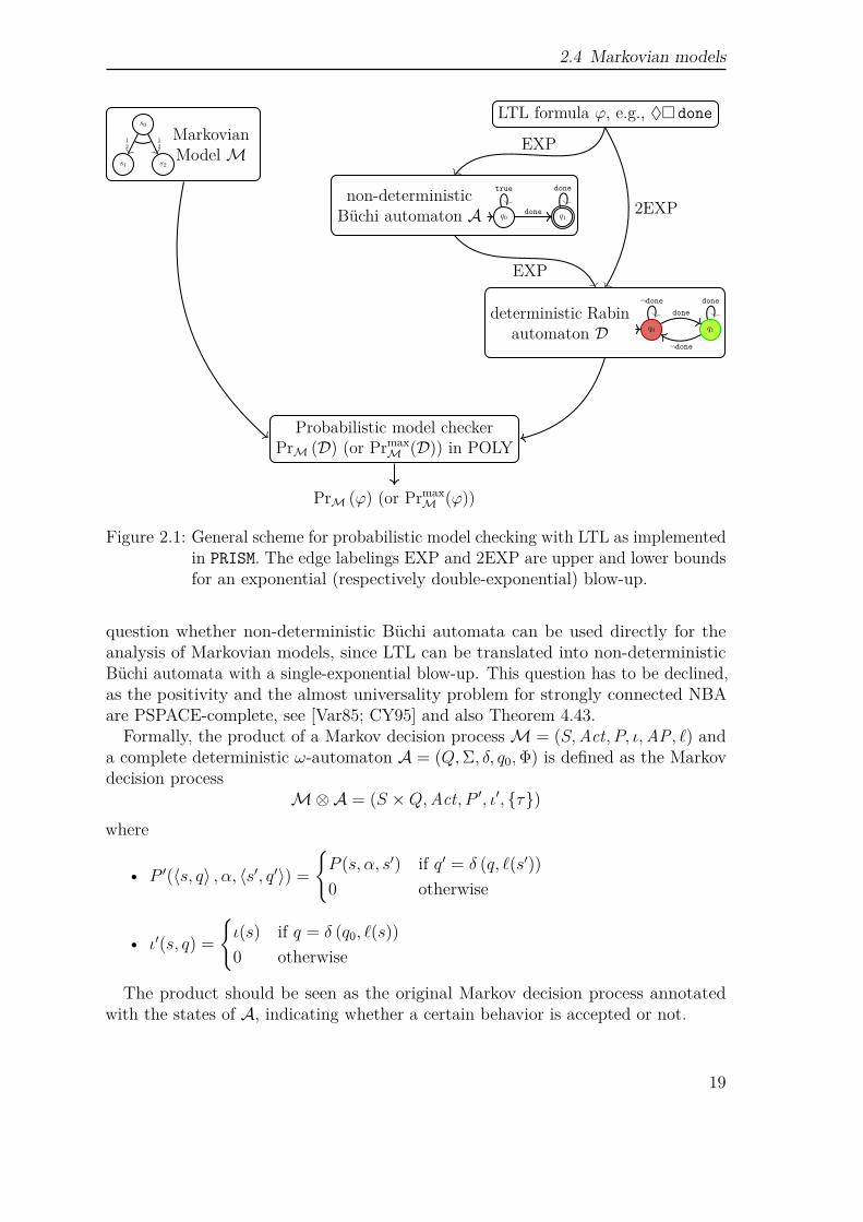
2.4 Markovian models
s0
s1 s2
MarkovianModelM
12
12
LTL formula ϕ, e.g., ♦ done
non-deterministicBüchi automaton A q0 q1
true
done
done
deterministic Rabinautomaton D q0 q1
¬donedone
¬done
done
Probabilistic model checkerPrM (D) (or Prmax
M (D)) in POLY
PrM (ϕ) (or PrmaxM (ϕ))
2EXP
EXP
EXP
Figure 2.1: General scheme for probabilistic model checking with LTL as implementedin PRISM. The edge labelings EXP and 2EXP are upper and lower boundsfor an exponential (respectively double-exponential) blow-up.
question whether non-deterministic Büchi automata can be used directly for theanalysis of Markovian models, since LTL can be translated into non-deterministicBüchi automata with a single-exponential blow-up. This question has to be declined,as the positivity and the almost universality problem for strongly connected NBAare PSPACE-complete, see [Var85; CY95] and also Theorem 4.43.
Formally, the product of a Markov decision processM = (S,Act, P, ι,AP, ℓ) anda complete deterministic ω-automaton A = (Q,Σ, δ, q0,Φ) is defined as the Markovdecision process
M⊗A = (S ×Q,Act, P ′, ι′, τ)
where
• P ′(⟨s, q⟩ , α, ⟨s′, q′⟩) =
P (s, α, s′) if q′ = δ (q, ℓ(s′))
0 otherwise
• ι′(s, q) =
ι(s) if q = δ (q0, ℓ(s))
0 otherwise
The product should be seen as the original Markov decision process annotatedwith the states of A, indicating whether a certain behavior is accepted or not.
19
2 Preliminaries
As Markov chains are essentially Markov decision processes with exactly oneenabled action per state, the product definition carries over directly.
As a second step we need to analyse the so-called end-components, since almost allpaths will end in an end-component and visit every state in it infinitely often [Alf97].An end-component is a pair (T,A) where
• T ⊆ S is a non-empty subset of states,
• A(s) ⊆ Act(s) is a non-empty set of enabled actions for every s ∈ T ,
• for every s ∈ T and α ∈ A(s) Post (s, α) = t ∈ S : P (s, α, t) > 0 ⊆ T , and
• (T,A) induces a strongly connected component.
We call an end-component (T,A) maximal (MEC for short), if there is no end-component (T ′, A′) = (T,A) with T ⊆ T ′ and A(s) ⊆ A′(s) for all s ∈ T .
For an infinite path π = s0α0−→ s1
α1−→ s2α2−→ . . . we describe its limit, denoted by
Limit(π), as the pair (T,A) with T being the set of infinitely often visited states andA : T → 2Act being the function mapping every state to its set of infinitely oftentaken actions.
Lemma 2.6 (see Theorem 3.2 of [Alf97]). LetM be an MDP, s a state inM, ands a scheduler forM. Then
PrsM[s] (π ∈ Paths(s) : Limit(π) is an end-component) = 1
In the special case of a Markov chain, the end-components degenerate to bot-tom strongly connected components (BSCCs for short), i.e., strongly connectedcomponents without outgoing transitions. Thus, Lemma 2.6 can be reformulated into
Lemma 2.7 (see Corollary 3.1 of [Alf97]). LetM be a Markov chain, and s a stateinM. Then
PrM[s](π ∈ Paths(s) : inf(π) is a BSCC) = 1
With Lemma 2.6 we can now analyse every end-component whether it is acceptingor not. In this section we restrict ourselves to the Rabin acceptance. For a deeperinspection of the MEC analysis under the Emerson-Lei acceptance, we refer toSection 5.3.
Let⋁
i∈1,...,n(Fin (Ei) ∧ Inf (Fi)) be a Rabin acceptance and (T,A) a MEC. Then,
we call (T,A) accepting if and only if it contains an end-component (T ′, A′) suchthat there is a Rabin pair Fin (Ei) ∧ Inf (Fi) with T ′ ∩ Ei = ∅ and T ′ ∩ Fi = ∅.We call the set of states being in an accepting maximal end-component U . Withthe knowledge of the accepting end-components, we can reduce MDP analysis tocalculation the probability of reaching a state in U .
Theorem 2.8. LetM be an MDP, ϕ an LTL formula, A be a DRA equivalent to ϕ,and U the set of all states in an accepting end-component inM⊗A. Then
PrmaxM (ϕ) = Prmax
M⊗A(♦U)
20
2.4 Markovian models
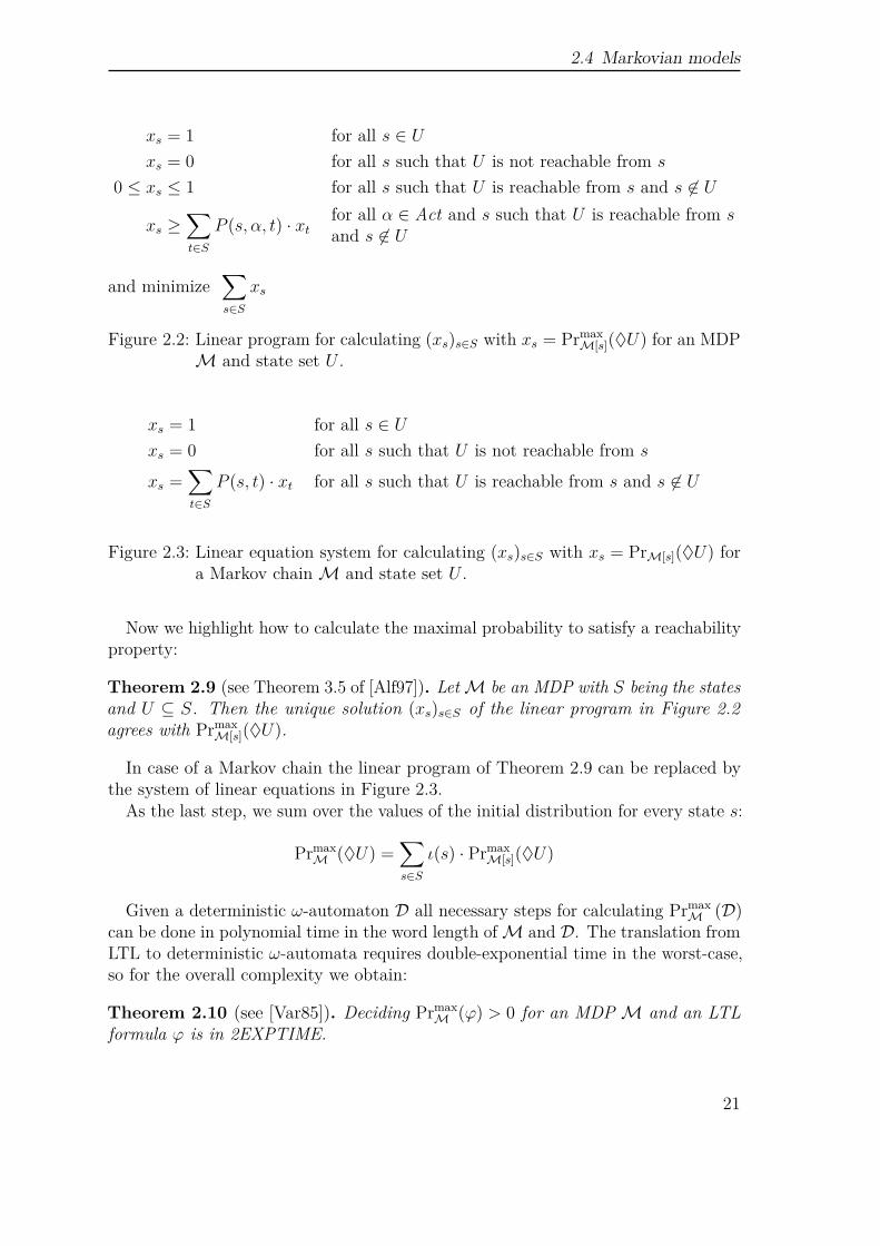
xs = 1 for all s ∈ Uxs = 0 for all s such that U is not reachable from s
0 ≤ xs ≤ 1 for all s such that U is reachable from s and s ∈ U
xs ≥∑t∈S
P (s, α, t) · xtfor all α ∈ Act and s such that U is reachable from sand s ∈ U
and minimize∑s∈S
xs
Figure 2.2: Linear program for calculating (xs)s∈S with xs = PrmaxM[s](♦U) for an MDP
M and state set U .
xs = 1 for all s ∈ Uxs = 0 for all s such that U is not reachable from s
xs =∑t∈S
P (s, t) · xt for all s such that U is reachable from s and s ∈ U
Figure 2.3: Linear equation system for calculating (xs)s∈S with xs = PrM[s](♦U) fora Markov chainM and state set U .
Now we highlight how to calculate the maximal probability to satisfy a reachabilityproperty:
Theorem 2.9 (see Theorem 3.5 of [Alf97]). LetM be an MDP with S being the statesand U ⊆ S. Then the unique solution (xs)s∈S of the linear program in Figure 2.2agrees with Prmax
M[s](♦U).
In case of a Markov chain the linear program of Theorem 2.9 can be replaced bythe system of linear equations in Figure 2.3.
As the last step, we sum over the values of the initial distribution for every state s:
PrmaxM (♦U) =
∑s∈S
ι(s) · PrmaxM[s](♦U)
Given a deterministic ω-automaton D all necessary steps for calculating PrmaxM (D)
can be done in polynomial time in the word length ofM and D. The translation fromLTL to deterministic ω-automata requires double-exponential time in the worst-case,so for the overall complexity we obtain:
Theorem 2.10 (see [Var85]). Deciding PrmaxM (ϕ) > 0 for an MDPM and an LTL
formula ϕ is in 2EXPTIME.
21
2 Preliminaries
Despite Theorem 2.10 is formulated for qualitative analysis, the quantitativeanalysis can be carried out also in 2EXPTIME with the means as explained above.
The matching lower bound has been proven by Courcoubetis and Yannakakis via areduction from the membership problem for exponential space bounded, alternatingTuring machines:
Theorem 2.11 (see Theorem 3.2.1. of [CY95]). Deciding PrmaxM (ϕ) > 0 for an MDP
M and an LTL formula ϕ is 2EXPTIME-complete.
The lower bound of Theorem 2.11 changes to a PSPACE lower bound in the caseof Markov chains:
Theorem 2.12 (see [Var85]). Deciding PrM(ϕ) > 0 for a Markov chainM and anLTL formula ϕ is PSPACE-hard.
Despite there are several algorithms with a better worst-case time-complexity than2EXPTIME (see Section 1.1.2), the usage of deterministic automata for the Markovchain analysis under LTL can be seen as standard, as it is the way PRISM and STORMdeals with Markov chains and LTL.
22
3 Good-for-games AutomataA desire to avoid deterministic ω-automata occurred not only in the area of prob-abilistic model checking, but in the area of synthesis of reactive systems as well[KV05; KPV06; PPS06; SF07]. In 2006 Henzinger and Piterman [HP06] proposedthe so-called good-for-games property for non-deterministic automata, a restrictedform of non-determinism. This property has been independently proposed by Col-combet [Col09] for weighted automata, but here it is called history-deterministic.Henzinger and Piterman also developed an algorithm, which we call HP-algorithm,for constructing a good-for-games parity automaton out of an NBA, aimed at acompact symbolic representation. Very recently, at STACS 2018, Kuperberg andMajumdar [KM18] presented a modified breakpoint construction for transformingnon-deterministic co-Büchi automata to good-for-games automata and sketched ageneralisation to non-deterministic Büchi automata.
In a good-for-games automaton, the non-determinism can be resolved in an in-cremental way for every accepted word without look-ahead. The formal definitionof GFG ω-automata [HP06] relies on a game-based view of ω-automata. Given acomplete ω-automaton A as before, we consider A as the game arena of an infinite,turn-based 2-player game, called monitor game: if the current state is q, then player 1chooses a symbol σ ∈ Σ whereas the other player (player 0) has to answer by a succes-sor state q′ ∈ δ(q, σ), i.e., resolves the non-determinism. In the next round q′ becomesthe current state. A play is a maximal alternating sequence ς = q0 σ0 q1 σ1 q2 σ2 . . . ofstates and (action) symbols in the alphabet Σ starting with an initial state q0. Intu-itively, the σi’s are the symbols chosen by player 1 and the qi’s are the states chosen byplayer 0 in round i. Player 0 wins the play ς if whenever ς|Σ = σ0 σ1 σ2 . . . ∈ Lω(A)then ς|Q = q0 q1 q2 . . . is an accepting run. A strategy for player 0 is a functionf : (Q× Σ)∗ → Q with f(. . . q σ) ∈ δ(q, σ) and f(ε) ∈ Q0. A play ς = q0 σ0 q1 σ1 q2 . . .is said to be f-conform or an f-play if qi = f(q0 σ0 . . . σi−2 qi−1σi−1) for all i ≥ 1. Anautomaton A is called good-for-games if there is a strategy f such that player 0 winseach f-play. Such strategies will be called GFG-strategies for A. Obviously, eachcomplete deterministic automaton enjoys the GFG property.
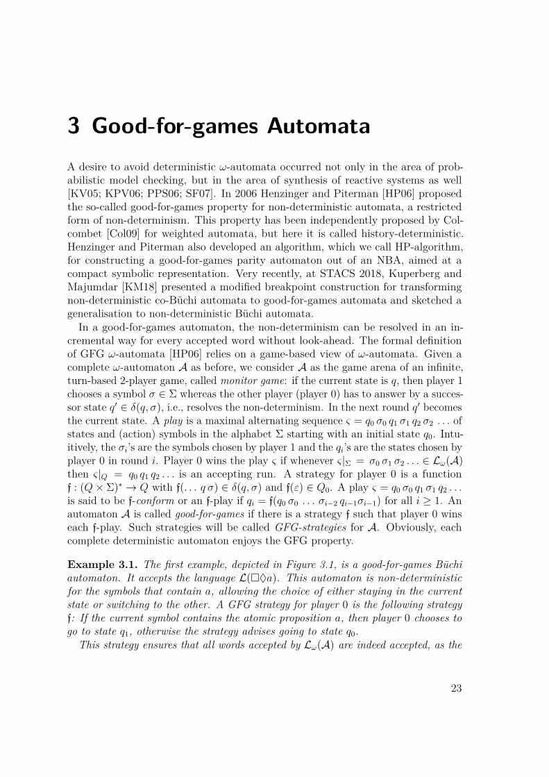
Example 3.1. The first example, depicted in Figure 3.1, is a good-for-games Büchiautomaton. It accepts the language L(♦a). This automaton is non-deterministicfor the symbols that contain a, allowing the choice of either staying in the currentstate or switching to the other. A GFG strategy for player 0 is the following strategyf: If the current symbol contains the atomic proposition a, then player 0 chooses togo to state q1, otherwise the strategy advises going to state q0.
This strategy ensures that all words accepted by Lω(A) are indeed accepted, as the
23
3 Good-for-games Automata
q0 q1true
a
a
true
Figure 3.1: Good-for-games NBA A for ♦a. Accepting Büchi states are markedwith a double circle.
only way for player 1 to generate a word w ∈ Lω(A) is to choose infinitely manysymbols with a. But then player 0 visits infinitely often the accepting state q1, sinceevery time a symbol with a is selected, player 0 moves to q1 via his strategy. So foran accepted word the f-conform play contains infinitely many accepting states q1 andthus the projection to the automata states delivers an accepting run.
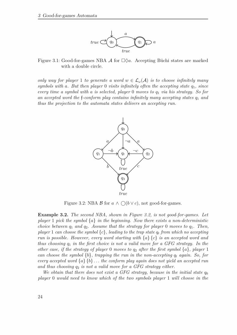
q0
qtq1 q2
q3
a a¬a
b
¬b
c
¬c
true
true
Figure 3.2: NBA B for a ∧ ⃝(b ∨ c), not good-for-games.
Example 3.2. The second NBA, shown in Figure 3.2, is not good-for-games. Letplayer 1 pick the symbol a in the beginning. Now there exists a non-deterministicchoice between q1 and q2. Assume that the strategy for player 0 moves to q1. Then,player 1 can choose the symbol c, leading to the trap state qt from which no acceptingrun is possible. However, every word starting with a c is an accepted word andthus choosing q1 in the first choice is not a valid move for a GFG strategy. In theother case, if the strategy of player 0 moves to q2 after the first symbol a, player 1can choose the symbol b, trapping the run in the non-accepting qt again. So, forevery accepted word a b . . . the conform play again does not yield an accepted runand thus choosing q2 is not a valid move for a GFG strategy either.
We obtain that there does not exist a GFG strategy, because in the initial state q0player 0 would need to know which of the two symbols player 1 will choose in the
24
second step. So player 0 would need the ability to look-ahead, which is impossible forGFG automata.
The automaton in Figure 3.1 is determinizable-by-pruning (DBP). Determinizable-by-pruning [Bok+13] means that an equivalent deterministic automaton is embedded,i.e., one can remove certain states and transitions, and obtain an equivalent deter-ministic automaton. [Bok+13] demonstrates the existence of GFG automata thatare not determinizable-by-pruning. Colcombet studied GFG automata on finitewords in more depth and discovered, that every GFG NFA is determinizable-by-pruning [Col12]. The influence of different acceptance conditions for good-for-gamesautomata has been covered in [KS15; BKS17]. The authors of [KS15] have proven,that every GFG Büchi automaton can be determinized to a DBA with a quadraticblow-up in the state space at most. Thus, GFG Büchi automata are as expressiveas DBA. The situation differs for GFG co-Büchi automata, where an exponentialblow-up may be unavoidable, but since every GFG co-Büchi automaton is also anon-deterministic co-Büchi automaton, and non-deterministic co-Büchi automatahave the same expressiveness as deterministic co-Büchi automata, GFG co-Büchiautomata and deterministic co-Büchi automata are equivalent concerning expressive-ness. For standard acceptance conditions like Rabin, Streett, Emerson-Lei, or parity,all GFG automata cover ω-regularity, since deterministic automata are trivially good-for-games. [BKS17] consider so-called typeness for (tight) good-for-games automata.Tightness enforces that a good-for-games automaton does not contain any redundantstates or transitions that are not used by any GFG strategy. For explaining typeness,we assume a good-for-games Rabin automaton A, whose language can be recognizedby a good-for-games Büchi automaton. Then, there exists an equivalent good-for-games Büchi automaton on the same graph structure as A. So, tight good-for-gamesRabin automata are Büchi-type. The same notion transfers to the co-Büchi condition:For every tight GFG Streett automaton A, that is co-Büchi-realizable, there is anequivalent GFG co-Büchi automaton on the same graph structure as A.
Contribution. We present a new approach for probabilistic model checking based ongood-for-games automata, and show how to compute maximal or minimal probabilitiesfor path properties in MDPs. If we assume that the path properties are specified by aGFG automaton, we achieve polynomial time complexity in both the word length ofthe given MDP and GFG automaton if the GFG automaton has one of the standardacceptances (Büchi, parity, Rabin, Streett). If the path properties are specified by anLTL formula, we achieve a time complexity polynomial in the size of the given MDPand double-exponential in the size of the LTL formula.
We evaluate this GFG-based approach empirically using our symbolic implementa-tion of the HP-algorithm, including several variants, using binary decision diagrams.We compare the performance of the HP-algorithm with the standard determinizationapproach of Safra, relying on the implementation ltl2dstar [KB06; KB07]. Tocompare the performance in actual probabilistic model checking, we have extended theprobabilistic model checker PRISM [KNP04] and evaluate the GFG-based approach on
25
3 Good-for-games Automata
the IEEE802.11 handshaking protocol as well as on the dining philosopher’s problem.
3.1 Automata-based Analysis of Markov DecisionProcesses
We address the task to compute the maximal or minimal probability in an MDPMfor the path property imposed by a non-deterministic ω-automaton A. The standardapproach, see, e.g., [BK08], assumes A to be deterministic and relies on a productconstruction where states in M are augmented by the current state of A. Thus,M⊗A can be seen as a refinement ofM since A does not affectM’s behaviors, butattaches information on A’s current state for the prefixes of the traces induced bythe paths ofM.
In the context of MDP analysis, we assume w.l.o.g. that a good-for-games automa-ton has exactly one initial state. For a good-for-games automaton with several initialstates, we pick an arbitrary GFG strategy f, and set the unique initial state q0 to thestate f(ε) chosen by f for the empty word.
We now modify the standard definition of the product of an MDP with a non-deterministic ω-automata (with a unique initial state). The crucial difference isthat the actions are now pairs ⟨α, p⟩ consisting of an action in M and a statein A, representing the non-deterministic alternatives in both the MDP M andthe automaton A. Formally, let M = (S,Act, P, ι,AP, ℓ) be an MDP and A =(Q,Σ, δ, q0,Φ) a complete non-deterministic ω-automaton with Σ = 2AP . The productMDP is
M⊗A = (S ×Q,Act×Q,P ′, ι′, Q, ℓ′)
where the transition probability function P ′ is given by P ′(⟨s, q⟩, ⟨α, p⟩, ⟨s′, q′⟩) =P (s, α, s′) if p = q′ ∈ δ(q, ℓ(s)). In all other cases P ′(⟨s, q⟩, ⟨α, p⟩, ⟨s′, q′⟩) = 0. Theinitial distribution is given by ι′(⟨s, q⟩) = ι(s) if q = q0 and ι′(⟨s, q⟩) = 0 in all othercases. The assumption that A is complete yields that for each α ∈ Act(s) there issome action ⟨α, q′⟩ ∈ Act(⟨s, q⟩) for all states s inM and q in A. In the product, thestates of the automaton serve as the atomic propositions and the labeling functionis given by ℓ′(⟨s, q⟩) = q, i.e., simply lifting the automaton state to the product.This allows us to consider the traces inM⊗A simply as words over the alphabetQ. Likewise, A’s acceptance condition Φ can be seen as a language over Q, whichpermits treating Φ as a property that the paths inM⊗A might or might not have.In particular, for Prmax
M⊗A(Φ), Φ corresponds to the set of paths in the product where
the projection on the A-states yields an accepting path in A.
Theorem 3.3. For each MDPM and non-deterministic ω-automaton A as above:
(a) PrmaxM⊗A
(Φ)≤ Prmax
M(Lω(A)
)(b) If A is good-for-games, then: Prmax
M⊗A(Φ)
= PrmaxM(Lω(A)
)26
3.1 Automata-based Analysis of Markov Decision Processes
Proof. We first observe that by the definition of the transition probability functionP ′ we have:
• If π′ = ⟨s0, q0⟩ γ0 ⟨s1, q1⟩ γ1 ⟨s2, q2⟩ γ2 . . . is a path inM⊗A where γi = ⟨αi, pi⟩,then pi = qi+1 and π′|M = s0 α0 s1 α1 s2 α2 . . . is a path in M and π′|A =q0 q1 q2 . . . is a run in A for the word
trace(π′|M
)= ℓ(s0) ℓ(s1) ℓ(s2) . . . ∈
(2AP)ω
In this case, we have:
π′ |= Φ iff the run π′|A is accepting
• Vice versa, if π = s0 α0 s1 α1 s2 α2 . . . is a path inM and ρ = q0 q1 q2 . . . a runin A for its trace, then
πρ = ⟨s0, q0⟩ γ0 ⟨s1, q1⟩ γ1 ⟨s2, q2⟩ γ2 . . .
is a path inM⊗A where γi = ⟨αi, qi+1⟩. In this case, we have: ρ is acceptingiff πρ |= Φ.
Proof of statement (a). To show (a), we demonstrate that a scheduler forM⊗A that maximizes the probability for Φ can be transferred to a scheduler forMwhile maintaining the probabilities when considering the language Lω(A). Intuitively,this holds as the scheduler choices for the A-successors in the product represent aspecific resolution of the non-determinism in A. The converse does not necessarilyhold in the non-good-for-game case, as the scheduler inM⊗A has to commit to aparticular resolution of the non-determinism in A, without being able to predict thefuture.
We pick a scheduler s′ forM⊗A that maximizes the probability for A’s acceptancecondition. The goal is to derive a scheduler s forM under which the probability forgenerating traces in Lω(A) is at least
PrmaxM⊗A
(Φ)
= Prs′M⊗A(Φ).
The task is now to define s(π) ∈ Act( last(π) ) for finite paths π inM where last(π)denotes the last state of π. Let π = s0 α0 s1 α1 . . . αn−1 sn be a finite path in M.We introduce inductively states q1, . . . , qn, qn+1 in A as follows. Let
γ0def= ⟨α0, q1⟩ = s′(⟨s0, q0⟩)
and for 0 ≤ i ≤ n:
γidef= ⟨αi, qi+1⟩ = s′
(⟨s0, q0⟩ γ0 ⟨s1, q1⟩ γ1 . . . γi−1 ⟨si, qi⟩
)Clearly, in the above inductive definition we have qi+1 ∈ δ(qi, ℓ(si)) and αi ∈ Act(si).We then define:
s(s0 α0 s1 α1 . . . αn−1 sn)def= αn
27
3 Good-for-games Automata
Now, we show that for every s′-path inM⊗A with a trace satisfying the acceptancecondition Φ, there exists a s-path inM with a trace accepted by A. Suppose thatπ′ = ⟨s0, q0⟩ γ0 ⟨s1, q1⟩ γ1 ⟨s2, q2⟩ γ2 . . . is an infinite s′-path with π′ |= Φ. InM⊗A,for an action γi = ⟨αi, qi+1⟩ to be enabled, qi+1 ∈ δ(qi, αi) must hold. Since π′ satisfiesΦ, π′|A = q0 q1 . . . is an accepting run in A for the trace of π′|M = s0 α0 s1 α1 s2 α2 . . ..By definition ofM⊗A, π′|M = s0 α0 s1α1 s2 α2 . . . is a path inM. Thus, the setof all s-paths π with trace(π) ∈ Lω(A) contains the set of the paths π′|M where π′
is a s′-path inM⊗A with π′ |= Φ and consequently Prs′M⊗A(Φ)≤ PrsM
(A). We
obtain the desired result:
PrmaxM⊗A
(Φ)
= Prs′M⊗A(Φ)≤ PrsM
(Lω(A)
)≤ Prmax
M(Lω(A)
)Proof of statement (b). To show (b), we show that the good-for-games propertyallows a scheduler inM⊗A to resolve the non-determinism induced by A in theproduct in an optimal way. Technically, this relies on combining a maximizingscheduler forM and Lω(A) with a GFG-strategy for A.
We suppose now that A is good-for-games. By (a), it suffices to show that
PrmaxM(A)≤ Prmax
M⊗A(Φ)
Let f denote a GFG-strategy for the monitor game for A and let s be a schedulerinM that maximizes the probability to generate traces in Lω(A). The goal is tocompose s and f to obtain a scheduler s′ forM⊗A such that the probability unders′ for the paths π′ with π′ |= Φ is at least PrsM
(A).
The definition of s′(π′) for the finite paths π′ in M⊗A is by induction on thelength of π′. For the initial state we define:
s′(⟨s0, q0⟩)def= ⟨ s(s0), f(q0 ℓ(s0)) ⟩
For a finite path π′ = ⟨s0, q0⟩ γ0 ⟨s1, q1⟩ γ1 . . . γn−1 ⟨sn, qn⟩ inM⊗A of length n ≥ 1where γi = ⟨αi, qi+1⟩, the definition of s′(π′) is as follows:
s′(π′)def= ⟨ s(π′|M), f
(q0 ℓ(s0) q1 ℓ(s1) . . . qn ℓ(sn)
)⟩
Suppose now that π = s0 α0 s1 α1 s2 α2 . . . is an infinite s-path inM with trace(π) ∈Lω(A). We now consider the accepting run ρ = q0 q1 q2 . . . for trace(π) that isobtained using the GFG-strategy f in the monitor game for A. That is:
qi+1 = f(q0 ℓ(s0) q1 ℓ(s1) . . . qi ℓ(si)
)Then, πρ = ⟨s0, q0⟩ γ0 ⟨s1, q1⟩ γ1 ⟨s2, q2⟩ γ2 . . . is an infinite s′-path with πρ |= Φwhere γi = ⟨αi, qi+1⟩. Thus, the set of all infinite s′-paths π′ with π′ |= Φ subsumesall paths πρ resulting from combining an s-path π in M where trace(π) ∈ Lω(A)with its (unique) accepting f-run ρ. This yields:
PrmaxM(Lω(A)
)= PrsM
(Lω(A)
)≤ Prs′M⊗A
(Φ)≤ Prmax
M⊗A(Φ)
This completes the proof of statement (b) in Theorem 3.3.
28
3.1 Automata-based Analysis of Markov Decision Processes
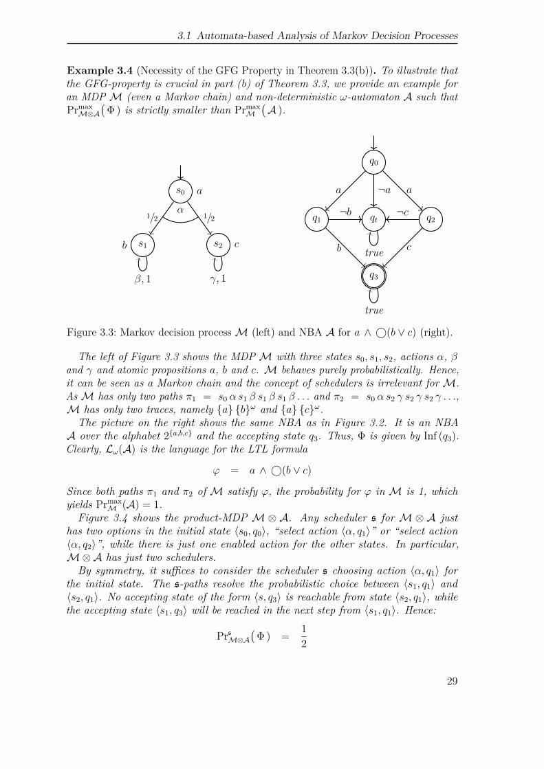
Example 3.4 (Necessity of the GFG Property in Theorem 3.3(b)). To illustrate thatthe GFG-property is crucial in part (b) of Theorem 3.3, we provide an example foran MDPM (even a Markov chain) and non-deterministic ω-automaton A such thatPrmax
M⊗A(Φ ) is strictly smaller than Prmax
M(A ).
s0 a
s1b s2 c
1/2 1/2
β, 1 γ, 1
α
q0
qtq1 q2
q3
a a¬a
b
¬b
c
¬c
true
true
Figure 3.3: Markov decision processM (left) and NBA A for a ∧ ⃝(b ∨ c) (right).
The left of Figure 3.3 shows the MDPM with three states s0, s1, s2, actions α, βand γ and atomic propositions a, b and c. M behaves purely probabilistically. Hence,it can be seen as a Markov chain and the concept of schedulers is irrelevant forM.AsM has only two paths π1 = s0 α s1 β s1 β s1 β . . . and π2 = s0 α s2 γ s2 γ s2 γ . . .,M has only two traces, namely a bω and a cω.The picture on the right shows the same NBA as in Figure 3.2. It is an NBAA over the alphabet 2a,b,c and the accepting state q3. Thus, Φ is given by Inf (q3).Clearly, Lω(A) is the language for the LTL formula
ϕ = a ∧ ⃝(b ∨ c)
Since both paths π1 and π2 of M satisfy ϕ, the probability for ϕ in M is 1, whichyields Prmax
M (A) = 1.Figure 3.4 shows the product-MDP M⊗ A. Any scheduler s for M⊗ A just
has two options in the initial state ⟨s0, q0⟩, “select action ⟨α, q1⟩” or “select action⟨α, q2⟩”, while there is just one enabled action for the other states. In particular,M⊗A has just two schedulers.By symmetry, it suffices to consider the scheduler s choosing action ⟨α, q1⟩ for
the initial state. The s-paths resolve the probabilistic choice between ⟨s1, q1⟩ and⟨s2, q1⟩. No accepting state of the form ⟨s, q3⟩ is reachable from state ⟨s2, q1⟩, whilethe accepting state ⟨s1, q3⟩ will be reached in the next step from ⟨s1, q1⟩. Hence:
PrsM⊗A(Φ ) =
1
2
29
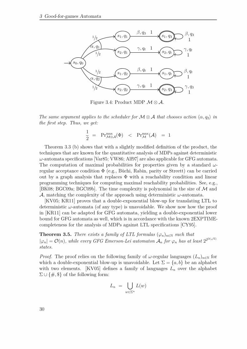
3 Good-for-games Automata
s0, q0
s1, q1
s2, q1
s1, q2
s2, q2
s1, q3
s2, q3
s1, qt
s2, qt
1/2
1/2
1/2
1/2
β, q3 1
γ, qt 1
β, qt 1
γ, qt 1
β, q31
γ, qt1
β, qt1
γ, q31
α, q1
α, q2
Figure 3.4: Product MDPM⊗A.
The same argument applies to the scheduler forM⊗A that chooses action ⟨α, q2⟩ inthe first step. Thus, we get:
1
2= Prmax
M⊗A(Φ) < PrmaxM (A) = 1
Theorem 3.3 (b) shows that with a slightly modified definition of the product, thetechniques that are known for the quantitative analysis of MDPs against deterministicω-automata specifications [Var85; VW86; Alf97] are also applicable for GFG automata.The computation of maximal probabilities for properties given by a standard ω-regular acceptance condition Φ (e.g., Büchi, Rabin, parity or Streett) can be carriedout by a graph analysis that replaces Φ with a reachability condition and linearprogramming techniques for computing maximal reachability probabilities. See, e.g.,[BK08; BGC09a; BGC09b]. The time complexity is polynomial in the size ofM andA, matching the complexity of the approach using deterministic ω-automata.
[KV05; KR11] proves that a double-exponential blow-up for translating LTL todeterministic ω-automata (of any type) is unavoidable. We show now how the proofin [KR11] can be adapted for GFG automata, yielding a double-exponential lowerbound for GFG automata as well, which is in accordance with the known 2EXPTIME-completeness for the analysis of MDPs against LTL specifications [CY95].
Theorem 3.5. There exists a family of LTL formulas (ϕn)n∈N such that|ϕn| = O(n), while every GFG Emerson-Lei automaton An for ϕn has at least 22Ω(
√n)
states.
Proof. The proof relies on the following family of ω-regular languages (Ln)n∈N forwhich a double-exponential blow-up is unavoidable. Let Σ = a, b be an alphabetwith two elements. [KV05] defines a family of languages Ln over the alphabetΣ ∪ #, $ of the following form:
Ln =⋃w∈Σn
L(w)
30
3.1 Automata-based Analysis of Markov Decision Processes
where L(w) is the following ω-regular language:
L(w) =w1 # . . . #wi−1 #w#wi+1 # . . . #wm# $w#ω :
w1, . . . , wi−1, wi+1, . . . , wm ∈ Σ∗, m ∈ N, 0 ⩽ i ⩽ m
The languages Ln are safety languages and can be recognized by a DBA An, which areknown to need at least 22Ω(n) states. Intuitively, this is because An needs to rememberall words of length n that have been seen before $ to check whether one of themmatches the word after $. There exist 2n possible words of length n and therefore 22n
possibilities for which words of length n have occurred before the $-symbol. Thus,intuitively, for checking whether a duplicated word of length n occurs after $, Anneeds at least 22Ω(n) states. The proof from [KV05], that every DBA accepting thelanguage Ln needs at least 22Ω(n) states can be extended to a GFG automata in astraightforward manner.
We will prove the claim that every GFG automaton recognizing Ln has at least22
Ω(n) states by contradiction. We refer to words in Σn as n-blocks. Further weassume a total order on Σn, thereby we can define the n-block wi as the i-th word inΣn. In this proof we will use index sets containing indices ranging from 1 to 2n andcorresponding to the n-blocks that have appeared before the $. We define for everysuch index set
I =i1, i2, . . . , ik
⊆0, 1, . . . , 2n−1
the finite word wI = #wi1#wi2# . . .#wik#$. As An is good-for-games, there existsa GFG-strategy f. Let qI be the state reached in the f-play after consuming thefinite word wI . Since there are 2n different n-blocks, there exist 22
n subsets of0, 1, . . . , 2n−1, but by assumption An has less than 22
n states. Therefore theremust be two distinct sets I = J with qI = qJ . W.l.o.g. let i ∈ I \ J . The wordwI wi#ω belongs to Ln, and hence is accepted by An and the f-play for wI wi#ω isaccepting as well. On the other hand, wJ wi#ω is not in Ln. But as qI = qJ there isan accepting run for the suffix wi#ω and we get wJ wi#ω ∈ Ln. Contradiction.
As other standard acceptance conditions like Rabin, parity or Streett are a particularform of Emerson-Lei, the same argument holds also for GFG Rabin, GFG parity,GFG Streett automata and GFG Emerson-Lei automata. As shown in [KV05], thereis an LTL formula ϕn of size O
(n2)for Ln yielding the double-exponential lower
bound for the transformation from LTL to GFG automata.
Minimal probabilities IfM is an MDP as before and s a scheduler forM then foreach ω-regular language L over the alphabet 2AP :
PrsM(L) = 1− PrsM(L)
where L denotes the complement of L, i.e., L =(2AP)ω \ L. Hence, we get:
PrminM (L) = 1− Prmax
M (L)
As a consequence of Theorem 3.3, we obtain:
31
3 Good-for-games Automata
Corollary 3.6. For each MDPM, LTL formula ϕ and complete GFG-automatonA with acceptance condition Φ for ¬ϕ:
PrminM(ϕ)
= 1− PrmaxM⊗A
(Φ)
Moreover, PrminM(ϕ)≤ 1− Prmax
M⊗A(Φ)for each non-deterministic ω-automaton A
for ¬ϕ.
3.2 From LTL to GFG AutomataIt has previously been shown [KB06; KB07] that it is possible in practice, using thetool ltl2dstar, to obtain deterministic ω-automata for a wide range of LTL formula ϕvia the translation to an NBA and Safra’s determinization construction [Saf88] refinedby various heuristics. Here, we are interested in replacing Safra’s determinizationalgorithm with the HP-algorithm [HP06] to generate a GFG automaton instead of adeterministic automaton. We first provide an outline of the HP-algorithm and thenexplain a few new heuristics.
3.2.1 The HP-algorithmThe HP-algorithm transforms an NBA B = (Q,Σ, δ, q0,Φ) with Φ = Inf (F ) and|Q| = n states into a GFG automaton A with parity acceptance and at most 2n · n2n
states and 2n parity colors (or an NRA with n Rabin pairs), which improves on theupper bound given for Safra’s determinization algorithm.
Like Safra’s construction, the HP-algorithm relies on the simultaneous trackingof multiple subset constructions to determine acceptance or rejection in the NBA.However, while the states of Safra’s DRA organize the subsets in trees, the HP-algorithm uses a simpler, linear arrangement of the subsets. The state space P =(2Q × 2Q)n of the GFG automaton A consists of n pairs of subsets of NBA statesQ, i.e., states of the form p = ⟨(A1, B1), . . . , (An, Bn)⟩ where Bi ⊆ Ai ⊆ Q, plus thefollowing two additional constraints on the state space:
• if Ai = ∅ for i < n, then Ai+1 = ∅, and
• for all i < j, Ai ∩ Aj = ∅ or Aj ⊆ Bi.
The first constraint ensures that an empty Ai implies that all the following Aj areempty as well. The second constraint ensures that each set A is contained in theB-part of some previous pair and disjoint from all sets between the two. Let T ⊆ Pbe the tuples that satisfy the constraints above. Each set Bi serves to mark thosestates in Ai that were reached via some accepting state in F of the NBA. Theinitial state q0,G of A is the tuple ⟨(q0 , q0 ∩ F ), (∅,∅), . . . , (∅,∅)⟩, i.e., whereA1 corresponds to the initial state q0 of the NBA and B1 is non-empty if and only ifq0 is accepting.
32
3.2 From LTL to GFG Automata
The successor state in A for symbol σ is obtained by applying the transitionfunction δ of the NBA to each of the subsets and adding states in F to the Bi
subsets. In crucial difference to Safra’s construction, the HP-algorithm however thenintroduces significant non-determinism by allowing A to discard an arbitrary numberof states in any of the subsets. For p = ⟨. . . (Ai, Bi) . . .⟩, the set A′
i in a σ-successorp′ of A thus does not correspond to A′
i = δ(Ai, σ) but there is a non-deterministicchoice between any A′
i satisfying A′i ⊆ δ(Ai, σ), including the empty set.
For the formal definition of the transition function of the GFG automatonA, we relyon the functions succi(p, σ) : P×Σ→ 2(2
Q×2Q) that provide the possible values for thei-th pair (A′
i, B′i) in the successor state, given a state p = ⟨(A1, B1), . . . , (An, Bn)⟩ ∈ P
in the GFG automaton A and symbol σ. The definition of succi distinguishes threecases. In the first case, where Ai = Bi = ∅ holds, we have
succi(p, σ) = (A′, B′) : A′ ⊆ δ(Ai, σ) andB′ ⊆ (δ(Bi, σ) ∩ A′) ∪ (A′ ∩ F )
This reflects a “standard” step, where the subset construction proceeds as normaland where Bi is updated with newly visited accepting states. In the second case,whenever Ai = Bi = ∅, we have
succi(p, σ) = (A′, B′) : A′ ⊆ δ(Ai, σ) and B′ ⊆ A′ ∩ F
As Ai and Bi are equal, this reflects the situation where all states tracked by Aicould have been reached while visiting some accepting state. The remaining thirdcase arises whenever Ai is empty. Here, succi allows for Ai to be “reset”, starting thesubset construction anew by choosing some subset of states of the first set A1:
succi(p, σ) = (A′, B′) : A′ ⊆ δ(A1, σ) and B′ ⊆ A′
The transition function δG of A is then defined by the application of succi to eachpair, additionally constraining the successor state to those tuples that satisfy theconstraints on the state space by restricting to the states in T :
δG(p, σ) = T ∩n∏i=1
succi(p, σ)
In the acceptance condition of A, the “resets” (whenever Ai = ∅ for some pair i)are reflected as “bad” events for the pair i, as they signify that the previously trackedruns terminated. The “good” events for pair i in the acceptance condition occurwhenever all states in an Ai are marked as having recently visited F , i.e., wheneverAi = Bi = ∅. Infinitely many “good” events for a pair i without “bad” events forthat pair then correspond to the existence of an accepting run in the NBA B. Thiscan be straightforwardly encoded as a Rabin condition with n Rabin pairs or as aparity condition by giving the good and bad events of pair i higher priority than theevents of pair j for j > i.
33
3 Good-for-games Automata
Formally, a parity acceptance condition for A is obtained as follows. For a givenstate p = ⟨(A1, B1), . . . , (An, Bn)⟩, we obtain the left-most “bad” pair via the functionindU(p) and the left-most “good” pair via the function indL(p), defined as follows:
indU(p) = min (k : k ∈ 2, . . . , n ∧ Ak = ∅ ∪ n+ 1)indL(p) = min (k : k ∈ 2, . . . , n ∧ Ak = Bk = ∅ ∪ n+ 1)
The value n+1 signals that none of the pairs were “bad” or “good”, respectively. Thecoloring function for the parity acceptance condition (with colors 0, . . . , 2n− 1) isthen obtained via
col(p) =
⎧⎪⎨⎪⎩0 if A1 = B1 = ∅2i+ 1 if indU(p) = i+ 2 ∧ indL(p) ≥ i+ 2
2i+ 2 if indL(p) = i+ 2 ∧ indU(p) > i+ 2
An equivalent Rabin acceptance can be easily obtained by rewriting the parityacceptance, as usual.
The HP-algorithm relies on the GFG-strategy to resolve the non-determinism inthe constructed automaton A, i.e., which states in the subsets are kept, which aredropped and when to reset. There is a large amount of non-determinism and a lot ofcombinatorial possibilities in the reachable state space of A. This is confirmed by ourexperiments, e.g., applying the construction to the two-state NBA for ♦a alreadyyields a GFG automaton with 16 states, where ltl2dstar generates a two-stateDRA. As stated in [HP06], the HP-algorithm is thus not well-suited for an explicitrepresentation for A, but is intended for a symbolic implementation. In this context,[HP06] briefly discusses the possibility of variants of the transition function in theGFG automaton that either apply more or less strict constraints on the relationshipenforced between the (Ai, Bi) pairs in each state. Especially, [HP06] posits thatintroducing even further non-determinism (and increasing the number of possiblestates) by loosening a disjunctness requirement on the Ai may lead to a smallersymbolic representation. In our experiments, we will consider such a variant ofthe HP-algorithm, where the second constraint on the state space (“for all i < j,Ai ∩ Aj = ∅ or Aj ⊆ Bi”) is removed. We will refer to this variant as the loosevariant.
3.2.2 Iterative approachIn the context of games, [HP06] proposes an iterative approach to the HP-algorithmby successively constructing the automata Am obtained by using only the first mof the n pairs, i.e., by setting Ai = Bi = ∅ for all m < i ≤ n. In the acceptancecondition this reduces the number of required parity colors to 2m and Rabin pairs tom as well. For these automata, Lω(Am) = Lω(A) = Lω(B), but there is no guaranteethat Am for m < n is good-for-games by construction. We start with m = 1 andincrease m until early success or reaching m = n. Our experimental results indeedshow that early termination appears rather often.
34
3.2 From LTL to GFG Automata
We now explain how the iterative approach of [HP06] can be integrated in theGFG-based quantitative analysis of MDPs against LTL specifications. Suppose, e.g.,that the task is to show that Prmax
M(ϕ)≥ θ for some LTL formula ϕ and threshold
θ ∈ ]0, 1]. Let B be an n-state NBA with Lω(B) = L(ϕ) and Am the automatonobtained using only the first m ≤ n pairs in the HP-algorithm applied to B. Let Φm
denote the acceptance condition of Am. By Theorem 3.3 (a):If Prmax
M⊗Am
(Φm)≥ θ for some m ≤ n then Prmax
M(ϕ)≥ θ.
Moreover, PrmaxM⊗Am
(Φm)≤ Prmax
M⊗Am+1
(Φm+1
)form < n, since the paths inM⊗Am
constitute a subset of the paths inM⊗Am+1. These observations suggest an approachthat resembles the classical abstraction-refinement schema: starting with m = 1, wecarry out the quantitative analysis ofM⊗Am against Φm and successively increase muntil Prmax
M⊗Am
(Φm)≥ θ or Am is GFG (which is the case at the latest when m = n).
As an additional heuristic to increase the performance of the linear programmingtechniques that are applied for the quantitative analysis ofM⊗Am against Φm, onecan reuse the results computed forM⊗Am−1 and Φm−1 as initial values.
GFG checking. It remains to explain how to check whether Am has the GFGproperty for m < n, i.e., when it is not clear from the construction itself thatthe GFG property holds. In this aspect, our prototype implementation departsfrom [HP06] and checks whether Am is GFG by solving a Rabin game (itself anNP-complete problem) constructed from Am and a DRA for ¬ϕ constructed withltl2dstar while [HP06] proposes an algorithm based on checking fair simulation.We will use this GFG check in our experimental evaluation to study the impact ofthe iterative approach in terms of the number of required iterations that are actuallyneeded in practice as well as the size of the resulting GFG automata. To obtain theseresults, the particular choice of the GFG test is irrelevant.
We detail here a game-based characterization of the GFG property, which servesas the basis for checking whether a given ω-automaton A is good-for-games in ourimplementation of the iterative approach of the HP-construction. This approach isbased on the game-based approach to determinization of GFG automata presentedin [Bok+13].
Given an NRA A = (Q,Σ, δA, q0,ΦA) then – by definition – A is good-for-gamesif there is a strategy that generates an accepting run for exactly the words w withw ∈ Lω(A). Since the class of ω-regular languages is closed under complementationthere exists a DRA D = (P,Σ, δD, p0,ΦD) with Lω(D) = Σω \ Lω(A). W.l.o.g. weassume transition relations of A and D to be total.
We now construct a turn-based two-player game GA,D with full observation forboth players as follows. The set of game vertices is V = V1 ∪ V0 where the set ofvertices where player 1 moves is V1 = Q×P and where player 0 moves in the verticesin V0 = Q × P × Σ. We set the initial vertex to ⟨q0, p0⟩. The moves in GA,D aredefined by the following two structural operational semantics rules (SOS-rules):
q ∈ Q, p ∈ P, σ ∈ Σ
⟨q, p⟩ −→ ⟨q, p, σ⟩
35
3 Good-for-games Automata
andq′ ∈ δA(q, σ), p′ = δD(p, σ)
⟨q, p, σ⟩ −→ (q′, p′)
Player 1 chooses a symbol σ ∈ Σ and player 0 resolves the non-determinism. As D isdeterministic, the game-structure GA,D can be viewed as a refinement of the monitorgame associated with A. The states in A are simply augmented with the informationon D’s current state and the chosen symbol.
The objective in GA,D is defined such that player 0 wins a play ς , if for every wordw:
• if w ∈ Lω(A), then ς|A is an accepting run in A
• if w /∈ Lω(A), then ς|D is an accepting run in D.
where ς|A denotes the projection of ς to the states A. More precisely, we erase allvertices ⟨q, p, σ⟩ from ς and replace the vertices ⟨q, p⟩ with q. Likewise ς|D arises fromς by taking the projection to the D-components of the vertices ⟨q, p⟩ in ς. Formally,the objective for player 0 in the game GA,D is the Rabin condition resulting from theunion of the acceptances of A and D lifted to the product. That is, if
ΦA =⋁
1≤i≤nFin
(UAi
)∧ Inf
(LAi
)ΦD =
⋁1≤i≤m
Fin(UDi
)∧ Inf
(LDi
)are the Rabin acceptance of A and D, respectively, then we define the objective forplayer 0 in the game GA,D as the Rabin acceptance
Ψ =⋁
1≤i≤n+m
Fin (Ui) ∧ Inf (Li)
where for 1 ≤ i ≤ n and 1 ≤ j ≤ m:
Ui = ⟨q, p⟩ ∈ V0 : q ∈ UAi
Li = ⟨q, p⟩ ∈ V0 : q ∈ LAi
Un+j = ⟨q, p⟩ ∈ V0 : q ∈ UBj
Ln+j = ⟨q, p⟩ ∈ V0 : q ∈ LBj
Lemma 3.7 (Game-based characterization of the GFG property). A is good-for-games iff player 0 has a winning strategy in the Rabin game GA,D.
In what follows, let G = GA,D.
Proof of “⇐=” Assume that player 0 has a winning strategy g : (V1 V0)+ → V1 in
G. To define a GFG-strategy f : (Q× Σ)+ → Q for player 0 in the monitor game forA, we first look at the play fragment q0 σ1 q1 σ2 . . . qn σn+1 and consider the choice ofg in G for the following play fragment in G:
ς = ⟨q0, p0⟩ ⟨q0, p0, σ1⟩ ⟨q1, p1⟩ ⟨q1, p1, σ2⟩ . . . ⟨qn, pn⟩ ⟨qn, pn, σn+1⟩
36
3.2 From LTL to GFG Automata
where pi = δD(p0, σ0 σ1 . . . σi−1) is the unique state in D that is reached from p0 byreading the finite input string σ0 σ1 . . . σi−1. Let ⟨qn+1, pn+1⟩ = g(ς). Then, we define:
f(q0 σ1 q2 σ2 . . . qn σn) = qn+1
Suppose that w = σ0 σ1 σ2 . . . ∈ Lω(A). Since the strategy g is winning, the g-playinduced by w,
ς = ⟨q0, p0⟩ ⟨q0, p0, σ1⟩ ⟨q1, p1⟩ ⟨q1, p1, σ2⟩ . . . ,
in G is winning for player 0, i.e., ς satisfies the Rabin condition Ψ associated with G.We pick some Rabin pair Fin (Ui) ∧ Inf (Li) with 1 ≤ i ≤ n such that ς |= Fin (Ui)and ς |= Inf (Li). There has to exist such a Rabin pair, since ς has to satisfy thewinning objective which means that for an accepted word w ∈ Lω(A) we have tofulfill a Rabin pair stemming from A. By taking the projection of all states inFin (Ui) ∧ Inf (Li) we obtain a Rabin pair Fin
(UAi
)∧ Inf
(LAi
)in A and the f-play
induced by w is q0 σ1 q1 σ2 . . .. Hence, ς|A = q0 q1 . . . is a run for w in A and
ς|A |= Fin(UAi
)and ς|A |= Inf
(LAi
).
Thus, ς meets the Rabin condition of A.
Proof of “=⇒” Assume A is good-for-games. Then, there exists a GFG-strategyf : (Q× Σ)+ → Q for the monitor game for A. We define the strategy g for player 0in G as follows. Given the play fragment
ς = ⟨q0, p0⟩ ⟨q0, p0, σ1⟩ ⟨q1, p1⟩ ⟨q1, p1, σ2⟩ . . . ⟨qn, pn⟩ ⟨qn, pn, σn⟩
in G we define g(ς) as follows:
g(ς) = ⟨f(q0 σ1 q1 σ2 . . . qn σn), δD(pn, σn)⟩
Let w = σ0 σ1 σ2 . . . ∈ Σω be an infinite word.Case 1: w ∈ Lω(A). For the g-play ς = ⟨q0, p0⟩ ⟨q0, p0, σ0⟩ ⟨q1, p1⟩ ⟨q1, p1, σ1⟩ . . .induced by w in G we have:
ς|A = q0 q1 q2 . . . |= Fin(UAi
)∧ Inf
(LAi
)for some i ∈ 1, . . . , n. As G’s objective Ψ contains the corresponding Rabin pair(Ui, Li), we get ς |= Ψ.Case 2: w /∈ Lω(A). Then, w ∈ Lω(D). Let ρ be the unique run for w in D. Then,ρ |= ΦD. Hence, there exists j ∈ 1, . . . ,m with ρ |= Fin
(UDj
)and ρ |= Inf
(LDj
).
Letς = ⟨q0, p0⟩ ⟨q0, p0, σ0⟩ ⟨q1, p1⟩ ⟨q1, p1, σ1⟩ ⟨q2, p2⟩ ⟨q2, p2, σ2⟩ . . .
be the g-play in G if player 1 chooses the symbols σi according to w. Then, ς|D = ρ.Hence, ς |= Fin (Un+j) and ς |= Inf (Ln+j). Thus, ς satisfies the objective Ψ for player0 in G.
37
3 Good-for-games Automata
In practice, when starting from an LTL formula ϕ, we do not construct D fromA via complementation and determinization. As we know that Lω(A) = L(ϕ), weobtain the DRA D by applying standard algorithms for the construction of a DRA forthe negation ¬ϕ, i.e., via the tool ltl2dstar. Even though A and D (and thus thegame as well) have a worst-case double-exponential number of states in the size of theformula, and though solving Rabin games is itself NP-complete, we have been able touse this approach in practice for the smaller automata (see Section 3.3) to determinewhether the intermediate automata in the iterative approach of the HP-constructionare GFG or not.
3.2.3 Union operator for disjunctive formulasFor generating a deterministic automaton from an LTL formula, it has been shownin [KB06] that optionally handling disjunctive LTL formulas of the form ϕ = ϕ1 ∨ ϕ2
by constructing DRA A1 and A2 for the subformulas ϕ1 and ϕ2 and then obtainingthe DRA A1 ∪A2 for the language Lω(A1) ∪ Lω(A2) via a product construction canbe very beneficial in practice. The definition of A1 ∪A2 used in [KB06] can easily beextended to NRA. The GFG property is preserved by the union construction.
Definition 3.8 (Union of two NRA). Let A1 = (Q1,Σ, δ1, q0,1,Φ1) andA2 = (Q2,Σ, δ2, q0,2,Φ2) be two complete NRA over the same alphabet with Φ1 =(Fin (U1,1)∧Inf (L1,1)
)∨. . .∨
(Fin (U1,n)∧Inf (L1,n)
)and Φ2 =
(Fin (U2,1)∧Inf (L2,1)
)∨
. . . ∨(Fin (U2,n) ∧ Inf (L2,n)
). The NRA A1 ∪ A2 = (Q′,Σ, δ′, q′0,Φ
′) is defined asfollows. The state space of A1 ∪A2 is Q′ = Q1×Q2 and q′0 = (q0,1, q0,2) its initialstate. The transition function δ′ is given by:
δ′((q1, q2), σ) =(q′1, q
′2) : q
′1 ∈ δ1(q1, σ), q′2 ∈ δ2(q2, σ)
The Rabin acceptance Φ′ is given by:⋁1≤i≤n
(Fin (U1,i ×Q2) ∧ Inf (L1,i ×Q2)
)∨⋁
1≤j≤m
(Fin (Q1 × U2,j) ∧ Inf (Q1 × L2,j)
)Obviously, Lω(A1 ∪ A2) = Lω(A1) ∪ Lω(A2). Additionally, the union operation
preserves the GFG property.
Lemma 3.9 (Good-for-games for the union operation). Let A1 and A2 be completeNRA. If A1 and A2 are GFG, then A1 ∪ A2 is good-for-games, too.
Proof. Let f1 : (Q1 × Σ)+ → Q1 be a GFG-strategy for A1 and f2 : (Q2 × Σ)+ → Q2
be a GFG-strategy for A2. We define a strategy
f : (Q′ × Σ)+ → Q′
for A1 ∪ A2 and ς = ⟨q0,1, q0,2⟩ σ0 . . . ⟨qi,1, qi,2⟩ σi as follows:
f(ς)def= ⟨ f1(ς
1), f2(ς
2) ⟩
38
3.3 Implementation and Experiments
where ς1= q0,1 σ0 q1,1 . . . qi−1,1σi denotes the projection of the play ς to the first
automaton. ς2is defined analogously.
The goal is to show that f is a GFG-strategy for A1 ∪ A2. Let w = σ0 σ1 σ2 . . . ∈Lω(A1 ∪ A2) = Lω(A1) ∪ Lω(A2) and let
ς = ⟨q0,1, q0,2⟩ σ0 ⟨q1,1, q1,2⟩ σ1 ⟨q2,1, q2,2⟩ σ2 . . .
be the induced f-play in the monitor game for A1∪A2 with ςΣ= w. W.l.o.g. we may
suppose that w ∈ Lω(A1). By the definition of f, the play ς1= q0,1 σ0 q1,1 σ1 q2,1 σ2 . . .
in the monitor game for A1 is f1-conform, and hence q0,1 q1,1 q2,1 . . . is an acceptingrun in A1. Thus, there is a Rabin pair Fin (Uw) ∧ Inf (Lw) in Φ1 with
q0,1 q1,1 . . . |= Fin (Uw) ∧ Inf (Lw)
Hence, for the run ςQ
= ⟨q0,1, q0,2⟩ ⟨q1,1, q1,2⟩ ⟨q2,1, q2,2⟩ . . . in A1 ∪ A2 we have:
ςQ|= Fin (Uw ×Q2) ∧ Inf (Lw ×Q2)
We conclude that ςQis an accepting run for the word w in A1 ∪ A2.
3.3 Implementation and ExperimentsWe have implemented the HP-algorithm in a tool we refer to as ltl2gfg. Based onltl2gfg, we have additionally implemented the GFG-based quantitative analysis ofMDPs in PRISM. After a brief overview of ltl2gfg, we report on our experiments andcomparison with the determinization approach of ltl2dstar. Our implementationand the logs of the experiments are available at [Mül18].
3.3.1 LTL2GFGGiven an LTL formula ϕ, our implementation ltl2gfg constructs a symbolic, BDD-based representation of a GFG-NPA for ϕ. It first converts ϕ into an (explicitlyrepresented) NBA B. In our experiments, we use ltl2ba v1.1 [GO01] for this task.To facilitate an efficient symbolic representation of the various subsets used in theHP-algorithm, B is then converted to a symbolic representation, using a unary en-coding of the |Q| = n states of B, i.e., using one Boolean variable qi per state.1 Thestate space of the GFG-automaton A, i.e., the n pairs (Ai, Bi) is likewise encoded byn2 Boolean variables ai,j and bi,j , i.e., ai,j is true iff NBA state qj ∈ Ai and bi,j is true
1As the states and transition relation of the GFG automaton A have to encode sets of NBA states,such a unary encoding is the most straightforward and natural choice. A similar situation existswhen considering symbolic determinization (e.g., [MS08]). As it is crucial for performance tokeep the number of BDD variables low, this also negates the potential benefits of symbolicLTL-to-NBA translations (e.g., [CGH97; RV10]), as their use would require a very large numberof BDD variables to allow the encoding of sets of NBA states.
39
3 Good-for-games Automata
iff qj ∈ Bi for 1 ≤ i, j ≤ n. To allow the encoding of the transition relations of A andB, each state variable has a primed copy, i.e., q′i, a′i,j and b′i,j and each of the k atomicproposition in ϕ is represented by a Boolean variable li. Using these Boolean variables,the symbolic encoding of the transition relation of the NBA B via a BDD-basedswitching function is straightforwardly obtained by relating the l, q and q′ variablesaccording to the valid choices of successor state. Likewise, the definitions for thetransition relation and acceptance condition of A in the HP-algorithm directly inducethe Boolean BDD operations necessary for building the corresponding switchingfunctions. For the performance of a BDD-based symbolic representation, the orderof the variables is crucial. As is standard for BDD-based automata encodings, thestate variables and their copies are always kept adjacent. The standard variableordering used by ltl2gfg is then an interleaving of the ai,j and bi,j variables withthe qj variables, i.e.,
l1 < . . . < lk < q1 < . . . < qj < a1,j < b1,j < a2,j < b2,j < . . . < qj+1 < . . . .
This ordering ensures that the related parts of the transition relation tend to bein proximity and has fared best in our initial experiments for finding a sensibleordering. As detailed below, we also optionally used dynamic reordering techniquesbased on sifting [Rud93] for the variable order to heuristically reduce the BDD sizeof the symbolic encoding. ltl2gfg uses the JINC C++ BDD library [Oss10] for thesymbolic representation.
Experimental results for the HP-algorithm We report here on a number of ex-periments with ltl2gfg using the benchmark formulas used in the evaluation ofltl2dstar in [KB06; KB07], i.e., 39 LTL formulas from the literature [EH00; SB00]and 55 pattern formulas [DAC99] that represent common specification patterns. Wedenote the generated automata equivalent to formula ϕ by Aϕ. All our experimentswere carried out on a computer with 2 Intel E5-2680 8-core CPUs at 2.70 GHz with384GB of RAM running Linux and with a memory limit of 10 GB and a timeout of30 minutes for each formula.
For every automaton Aϕ, we report on the number of BDD nodes in the encoding ofthe transition function, as this is the most crucial aspect. To allow a fair comparisonwith the explicit determinization in ltl2dstar, we consider symbolic encodings ofthe DRA Aϕ obtained from ltl2dstar 0.5.1, using the same LTL-to-NBA translator,i.e., ltl2ba, as used by ltl2gfg. This encoding uses ⌈log2 n⌉ Boolean variablesto straightforwardly encode the n state indices in Aϕ, which is the same encodingemployed in PRISM for its DRA-based approach to LTL model checking.
Table 3.1 and Table 3.2 present statistics for the construction of DRA withltl2dstar and GFG-NPA/NRA2 with ltl2gfg for the benchmark formulas. Fig-
2The GFG automata obtained directly using the HP-algorithm have parity acceptance, while theautomata obtained by the “union” of multiple GFG automata have Rabin acceptance, as theunion construction does not preserve the special structure of parity acceptance when it considersthe original NPA as NRA in the construction.
40
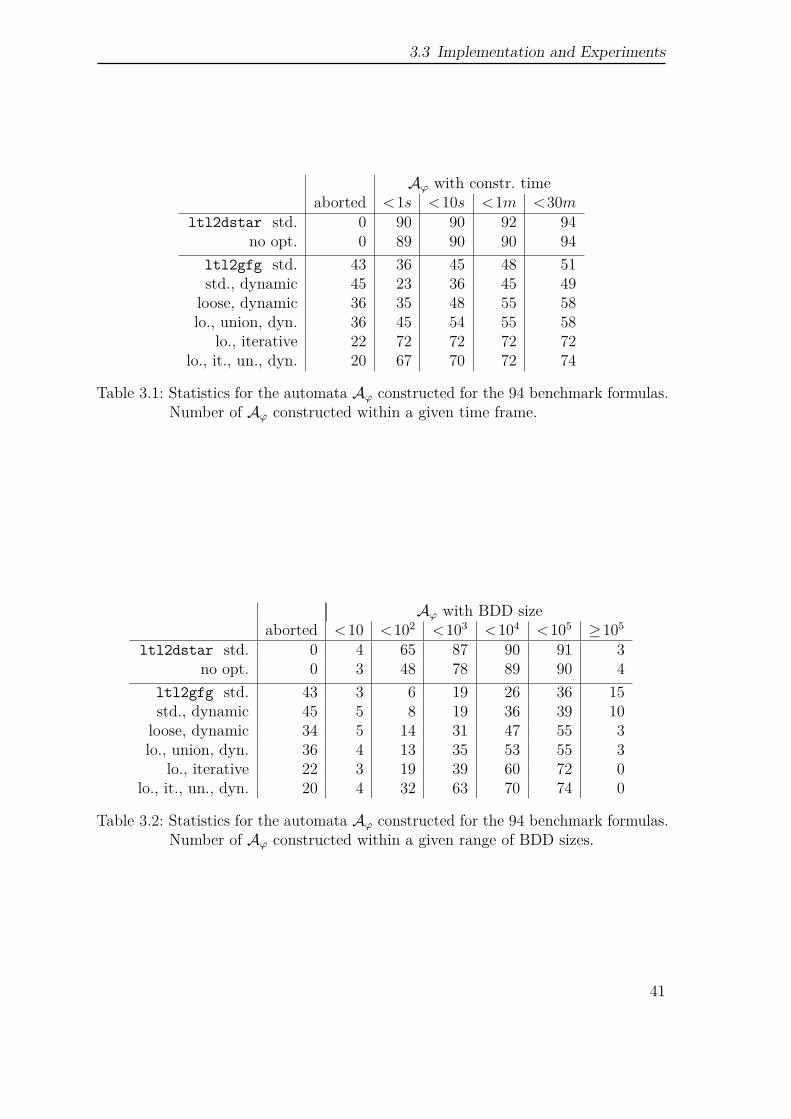
3.3 Implementation and Experiments
Aϕ with constr. timeaborted <1s <10s <1m <30m
ltl2dstar std. 0 90 90 92 94no opt. 0 89 90 90 94
ltl2gfg std. 43 36 45 48 51std., dynamic 45 23 36 45 49
loose, dynamic 36 35 48 55 58lo., union, dyn. 36 45 54 55 58
lo., iterative 22 72 72 72 72lo., it., un., dyn. 20 67 70 72 74
Table 3.1: Statistics for the automata Aϕ constructed for the 94 benchmark formulas.Number of Aϕ constructed within a given time frame.
Aϕ with BDD sizeaborted <10 <102 <103 <104 <105 ≥105
ltl2dstar std. 0 4 65 87 90 91 3no opt. 0 3 48 78 89 90 4
ltl2gfg std. 43 3 6 19 26 36 15std., dynamic 45 5 8 19 36 39 10
loose, dynamic 34 5 14 31 47 55 3lo., union, dyn. 36 4 13 35 53 55 3
lo., iterative 22 3 19 39 60 72 0lo., it., un., dyn. 20 4 32 63 70 74 0
Table 3.2: Statistics for the automata Aϕ constructed for the 94 benchmark formulas.Number of Aϕ constructed within a given range of BDD sizes.
41
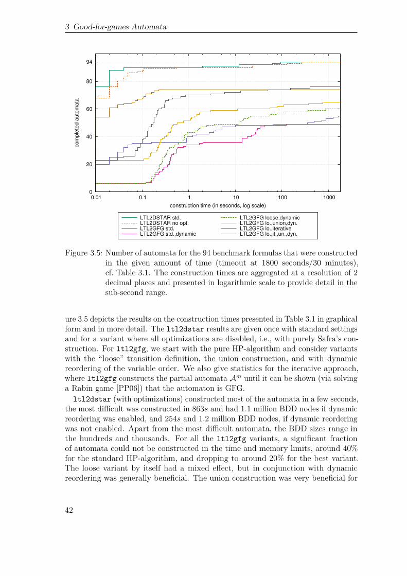
3 Good-for-games Automata
0
20
40
60
80
94
0.01 0.1 1 10 100 1000
com
ple
ted a
uto
mata
construction time (in seconds, log scale)
LTL2DSTAR std.LTL2DSTAR no opt.LTL2GFG std.LTL2GFG std.,dynamic
LTL2GFG loose,dynamicLTL2GFG lo.,union,dyn.LTL2GFG lo.,iterativeLTL2GFG lo.,it.,un.,dyn.
Figure 3.5: Number of automata for the 94 benchmark formulas that were constructedin the given amount of time (timeout at 1800 seconds/30 minutes),cf. Table 3.1. The construction times are aggregated at a resolution of 2decimal places and presented in logarithmic scale to provide detail in thesub-second range.
ure 3.5 depicts the results on the construction times presented in Table 3.1 in graphicalform and in more detail. The ltl2dstar results are given once with standard settingsand for a variant where all optimizations are disabled, i.e., with purely Safra’s con-struction. For ltl2gfg, we start with the pure HP-algorithm and consider variantswith the “loose” transition definition, the union construction, and with dynamicreordering of the variable order. We also give statistics for the iterative approach,where ltl2gfg constructs the partial automata Am until it can be shown (via solvinga Rabin game [PP06]) that the automaton is GFG.
ltl2dstar (with optimizations) constructed most of the automata in a few seconds,the most difficult was constructed in 863s and had 1.1 million BDD nodes if dynamicreordering was enabled, and 254s and 1.2 million BDD nodes, if dynamic reorderingwas not enabled. Apart from the most difficult automata, the BDD sizes range inthe hundreds and thousands. For all the ltl2gfg variants, a significant fractionof automata could not be constructed in the time and memory limits, around 40%for the standard HP-algorithm, and dropping to around 20% for the best variant.The loose variant by itself had a mixed effect, but in conjunction with dynamicreordering was generally beneficial. The union construction was very beneficial for
42
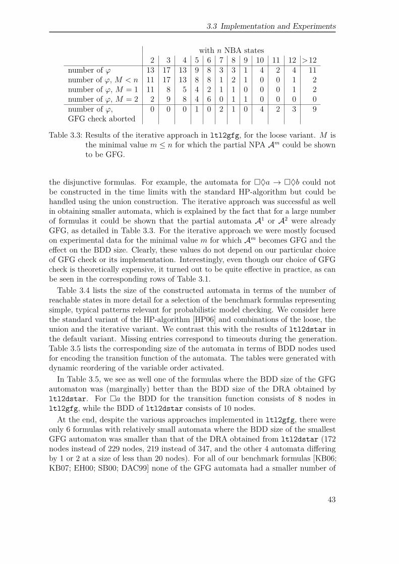
3.3 Implementation and Experiments
with n NBA states2 3 4 5 6 7 8 9 10 11 12 >12
number of ϕ 13 17 13 9 8 3 3 1 4 2 4 11number of ϕ, M < n 11 17 13 8 8 1 2 1 0 0 1 2number of ϕ, M = 1 11 8 5 4 2 1 1 0 0 0 1 2number of ϕ, M = 2 2 9 8 4 6 0 1 1 0 0 0 0number of ϕ,GFG check aborted
0 0 0 1 0 2 1 0 4 2 3 9
Table 3.3: Results of the iterative approach in ltl2gfg, for the loose variant. M isthe minimal value m ≤ n for which the partial NPA Am could be shownto be GFG.
the disjunctive formulas. For example, the automata for ♦a → ♦b could notbe constructed in the time limits with the standard HP-algorithm but could behandled using the union construction. The iterative approach was successful as wellin obtaining smaller automata, which is explained by the fact that for a large numberof formulas it could be shown that the partial automata A1 or A2 were alreadyGFG, as detailed in Table 3.3. For the iterative approach we were mostly focusedon experimental data for the minimal value m for which Am becomes GFG and theeffect on the BDD size. Clearly, these values do not depend on our particular choiceof GFG check or its implementation. Interestingly, even though our choice of GFGcheck is theoretically expensive, it turned out to be quite effective in practice, as canbe seen in the corresponding rows of Table 3.1.
Table 3.4 lists the size of the constructed automata in terms of the number ofreachable states in more detail for a selection of the benchmark formulas representingsimple, typical patterns relevant for probabilistic model checking. We consider herethe standard variant of the HP-algorithm [HP06] and combinations of the loose, theunion and the iterative variant. We contrast this with the results of ltl2dstar inthe default variant. Missing entries correspond to timeouts during the generation.Table 3.5 lists the corresponding size of the automata in terms of BDD nodes usedfor encoding the transition function of the automata. The tables were generated withdynamic reordering of the variable order activated.
In Table 3.5, we see as well one of the formulas where the BDD size of the GFGautomaton was (marginally) better than the BDD size of the DRA obtained byltl2dstar. For a the BDD for the transition function consists of 8 nodes inltl2gfg, while the BDD of ltl2dstar consists of 10 nodes.
At the end, despite the various approaches implemented in ltl2gfg, there wereonly 6 formulas with relatively small automata where the BDD size of the smallestGFG automaton was smaller than that of the DRA obtained from ltl2dstar (172nodes instead of 229 nodes, 219 instead of 347, and the other 4 automata differingby 1 or 2 at a size of less than 20 nodes). For all of our benchmark formulas [KB06;KB07; EH00; SB00; DAC99] none of the GFG automata had a smaller number of
43
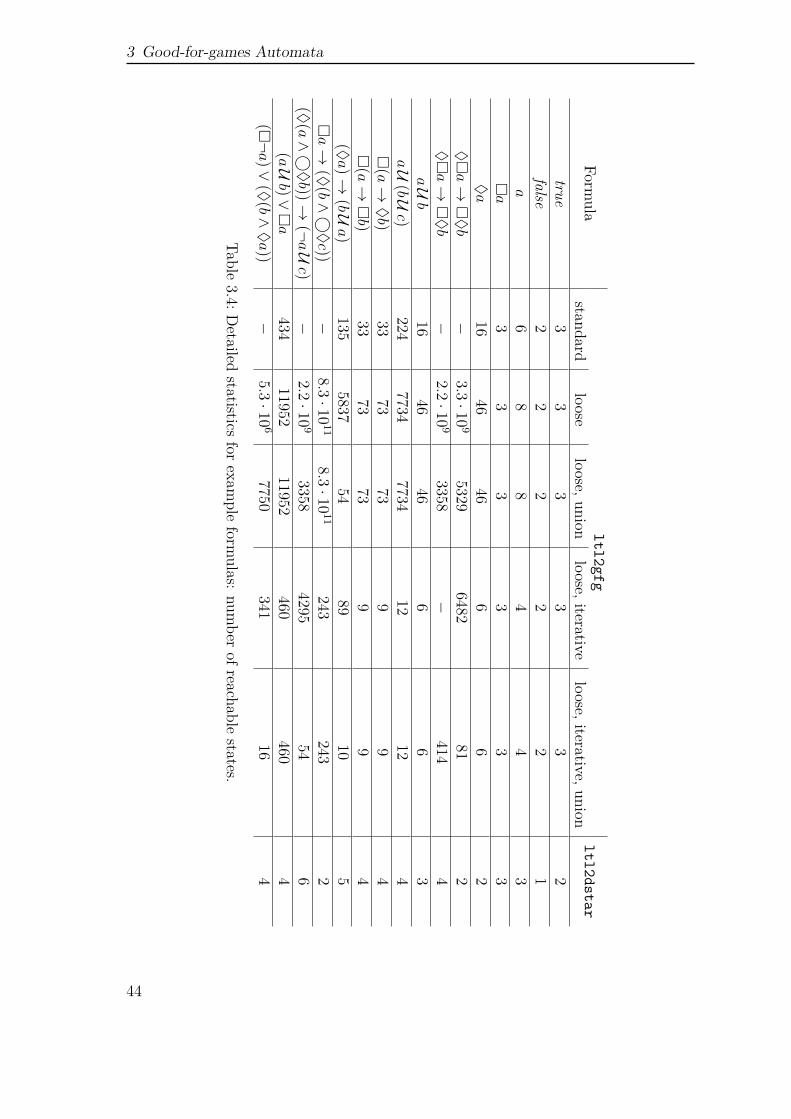
3 Good-for-games Automata
Formula
ltl2gfgltl2dstar
standardloose
loose,unionloose,iterative
loose,iterative,uniontrue
33
33
32
false2
22
22
1a
68
84
43
a
33
33
33
♦a
1646
466
62
♦a→
♦b
−3.3·10
95329
648281
2♦a→
♦b
−2.2·10
93358
−414
4aU
b16
4646
66
3aU
(bUc)
2247734
773412
124
(a→
♦b)
3373
739
94
(a→
b)
3373
739
94
(♦a)→
(bUa)
1355837
5489
105
a→
(♦(b∧⃝
♦c))
−8.3·10
11
8.3·10
11
243243
2(♦
(a∧⃝
♦b))→
(¬aU
c)−
2.2·10
93358
429554
6(aU
b)∨a
43411952
11952460
4604
(¬a)∨
(♦(b∧
♦a))
−5.3·10
67750
34116
4
Table3.4:D
etailedstatistics
forexam
pleform
ulas:num
berofreachable
states.
44
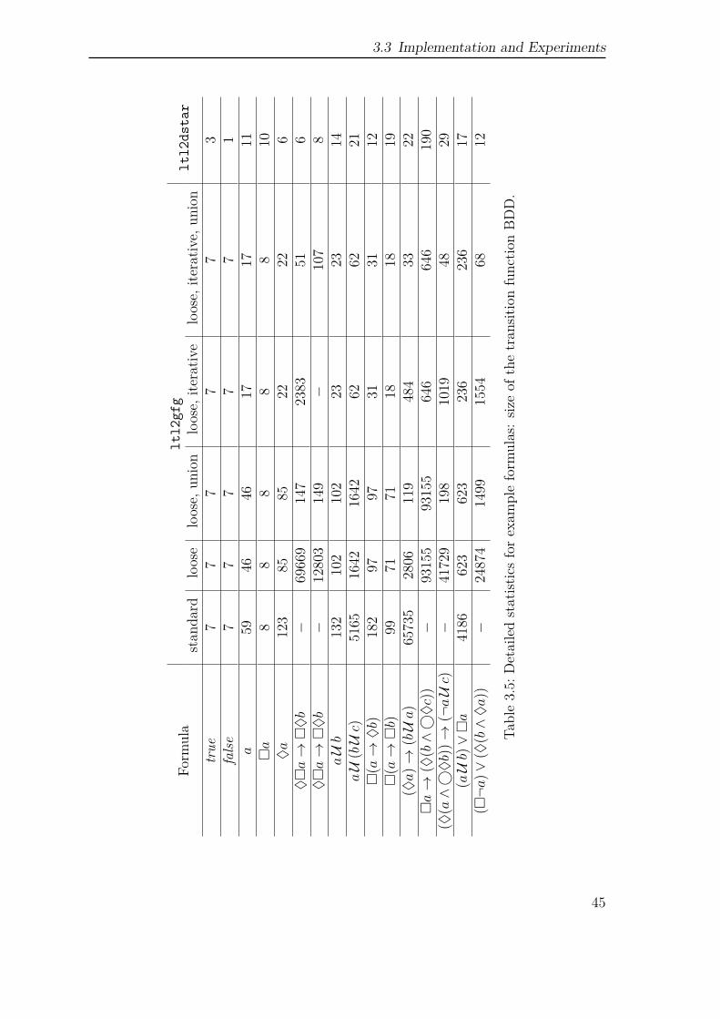
3.3 Implementation and Experiments
Form
ula
ltl2
gfg
ltl2
dsta
rstan
dard
loose
loose,
union
loose,
iterativ
eloose,
iterativ
e,un
ion
true
77
77
73
false
77
77
71
a59
4646
1717
11a
88
88
810
♦a
123
8585
2222
6♦a→
♦b
−69669
147
2383
516
♦a→
♦b
−12803
149
−107
8aUb
132
102
102
2323
14aU(bUc)
5165
1642
1642
6262
21(a→
♦b)
182
9797
3131
12(a→
b)
9971
7118
1819
(♦a)→
(bUa)
65735
2806
119
484
3322
a→
(♦(b∧⃝
♦c))
−93155
93155
646
646
190
(♦(a∧⃝
♦b))→
(¬aUc)
−41729
198
1019
4829
(aUb)∨a
4186
623
623
236
236
17(¬a
)∨(♦
(b∧♦a))
−24874
1499
1554
6812
Table3.5:
Detailedstatist
icsforexam
pleform
ulas:siz
eof
thetran
sitionfunctio
nBDD.
45
3 Good-for-games Automata
states than the DRA generated by ltl2dstar. In particular, the automata obtainedwithout the iterative approach often had millions and more states.
3.3.2 Implementation and experiments in PRISM
Despite the negative results of our experiments in Section 3.3.1, we investigated theuse of good-for-games automata in the context of probabilistic model checking. Itcould be the case that particularities of the symbolic encoding or of the automaton’sstructure turn out to be beneficial in this setting.
We extended the MTBDD-based, symbolic engine of PRISM 4.1 with an implemen-tation of our algorithm for computing Prmax
M (ϕ) using GFG automata for ϕ (andPrmin
M (ϕ) using a GFG automaton for ¬ϕ). We import the BDD of A generatedwith ltl2gfg into PRISM and perform the product withM and analysis inM⊗Asymbolically.
We compare this approach with the standard approach of PRISM, where an explicitDRA is constructed with an integrated version of ltl2dstar, which is then symbol-ically encoded as described before. Additionally, we evaluate our case studies onDelag, our tool for generating deterministic Emerson-Lei automata (see Chapter 5).The analysis is then carried out symbolically by the MTBDD engine for every approach,i.e., where the matrix and the value vector are stored via MTBDDs. Using thehybrid engine, which stores the value vector explicitly, would be obstructive for theGFG approach, since the automata have a large state number, and thus the product.
If PRISM normally handles a formula via a specialized algorithm for simple pathformulas that does not need an automata product construction, we forced the use ofthe general, automata-based approach. We have carried out our experiments withthe different variants for the generation of GFG automata of ltl2gfg. As before, weimpose a 30 minute time and 10GB memory limit.
PRISM case study: IEEE 802.11. For our first experiment, we use a PRISMmodel [KNS02] from the PRISM benchmark suite for parts of the WLAN carrier-sense protocol of IEEE 802.11. For details on the model we refer to http://www.prismmodelchecker.org/casestudies/wlan.php
It models a two-way handshake mechanism of the IEEE 802.11 (WLAN) mediumaccess control scheme with two senders that compete for the medium. As messages getcorrupted when both senders send at the same time (called a collision), a probabilisticback-off mechanism is employed to reduce the likelihood of collisions. The back-offprocedure is the key feature of the protocol, which is started if an error occurredor the sender wants to send a new message after sending a message. The back-offprocedure consists of waiting a randomized amount of time while the channel has tobe free. It ends with retrying to send a message. To define the maximal amount ofwaiting time in the back-off procedure, the model is parametrized by the parameterMAX_BACKOFF. Here, we consider the values MAX_BACKOFF ∈ 1, . . . , 6. Since stationscannot listen to their own transmissions, after having started to transmit a message,they cannot determine for a short amount of time whether another station has started
46
3.3 Implementation and Experiments
to send at the same moment, called the vulnerable section. To reduce the likelihoodof these collisions, a station has to check that the channel is free for a fixed timeperiod. This happens in state Wait_Difs. In the model, a collision counter is usedto record the number of collisions for use in the formulas. For our experiments, weset the maximum number of collisions that can be counted to 4.
For this benchmark we consider the following LTL path properties:
• ϕ1 = ♦(correct1 ∧ correct2)“Eventually station 1 and station 2 have sent their message correctly.”
• ϕ2 = ¬♦(Backoff1 ∨ Wait_Difs1 ∨ Wait_ack1)“Station 1 never gets stuck in the back-off procedure or during one of the waitingprocedures.”
• ϕ3 = (♦Backoff1)→ (♦vuln1)“If station 1 backs off infinitely often, it is also infinitely often in its vulnerablesection.”
• ϕ4 = (col→ ♦msg_1_send)“If a collision occurred on the channel, then station 1 will nevertheless send itsmessage correctly at some point in the future.”
• ϕ5 = (col→ ♦(msg_1_send ∧ #col < 2))“Like ϕ4, but with the additional constraint of no more additional collisions.”
• ϕ6 = ♦(correct1 ∧ correct2) ∧ (# col < 2)“Eventually both stations have sent their messages and the number of collisionsnever exceeds 1.”
We also evaluated the properties we use in Section 5.4.2 (Benchmark for Emerson-Lei acceptance) for the model with MAX_BACKOFF = 3, but the GFG approachperformed so poorly, that an evaluation based on the properties in Section 5.4.2 doesnot make sense. Only the calculation for two properties could be performed withinthe time limit of 30 minutes and memory bound of 10 GB at least for some GFGvariants: Prmin(ϕ1) and Prmin(ϕ2). For Prmin(ϕ1), 9 of the 16 variants were able tocomplete the calculation, mostly variants that contained the iterative computation.The iterative variant with dynamic reordering was the fastest (1120.7 seconds). Thesetting PRISM with Delag (our tool generating Emerson-Lei automata, see Chapter 5)was able to complete the calculation for Prmin(ϕ1) within 10.2 seconds.
47
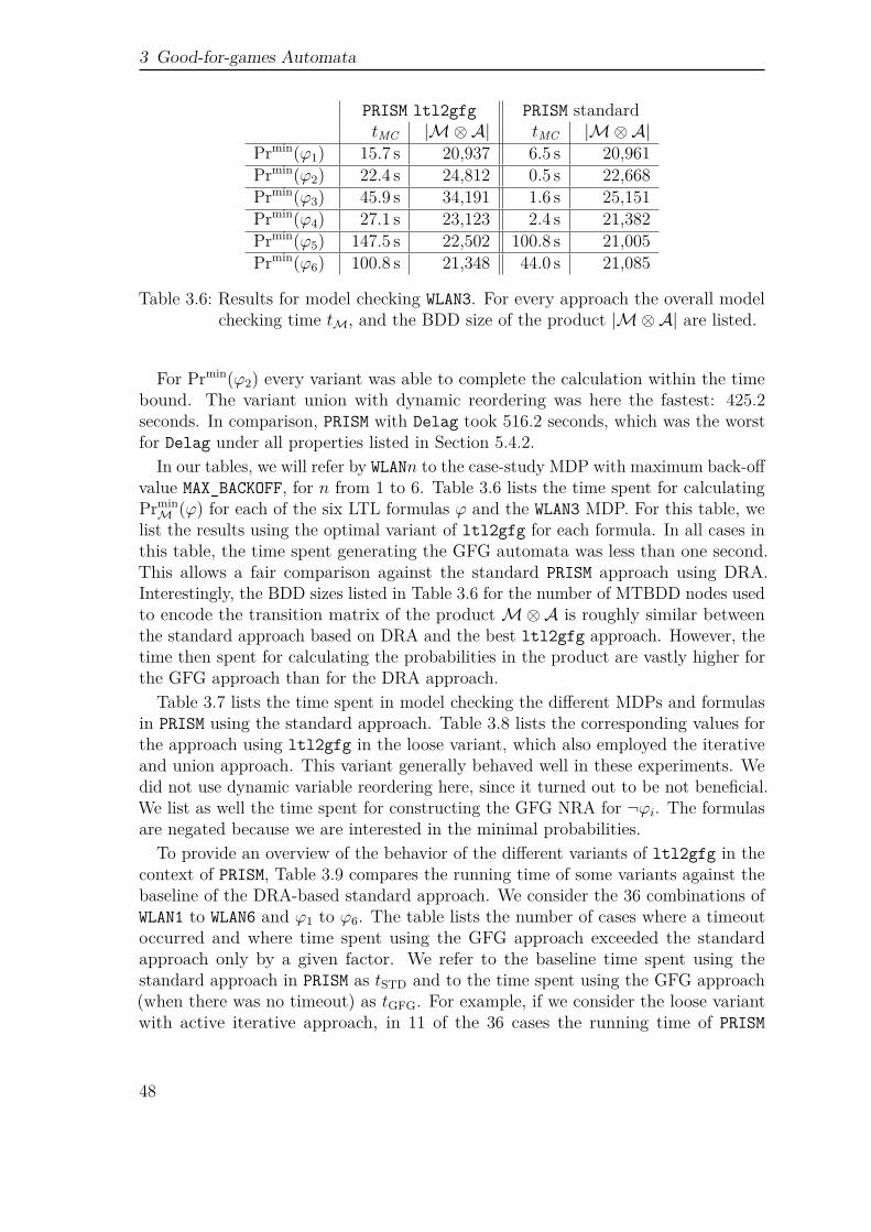
3 Good-for-games Automata
PRISM ltl2gfg PRISM standardtMC |M⊗A| tMC |M⊗A|
Prmin(ϕ1) 15.7 s 20,937 6.5 s 20,961Prmin(ϕ2) 22.4 s 24,812 0.5 s 22,668Prmin(ϕ3) 45.9 s 34,191 1.6 s 25,151Prmin(ϕ4) 27.1 s 23,123 2.4 s 21,382Prmin(ϕ5) 147.5 s 22,502 100.8 s 21,005Prmin(ϕ6) 100.8 s 21,348 44.0 s 21,085
Table 3.6: Results for model checking WLAN3. For every approach the overall modelchecking time tM, and the BDD size of the product |M⊗A| are listed.
For Prmin(ϕ2) every variant was able to complete the calculation within the timebound. The variant union with dynamic reordering was here the fastest: 425.2seconds. In comparison, PRISM with Delag took 516.2 seconds, which was the worstfor Delag under all properties listed in Section 5.4.2.
In our tables, we will refer by WLANn to the case-study MDP with maximum back-offvalue MAX_BACKOFF, for n from 1 to 6. Table 3.6 lists the time spent for calculatingPrmin
M (ϕ) for each of the six LTL formulas ϕ and the WLAN3 MDP. For this table, welist the results using the optimal variant of ltl2gfg for each formula. In all cases inthis table, the time spent generating the GFG automata was less than one second.This allows a fair comparison against the standard PRISM approach using DRA.Interestingly, the BDD sizes listed in Table 3.6 for the number of MTBDD nodes usedto encode the transition matrix of the productM⊗A is roughly similar betweenthe standard approach based on DRA and the best ltl2gfg approach. However, thetime then spent for calculating the probabilities in the product are vastly higher forthe GFG approach than for the DRA approach.
Table 3.7 lists the time spent in model checking the different MDPs and formulasin PRISM using the standard approach. Table 3.8 lists the corresponding values forthe approach using ltl2gfg in the loose variant, which also employed the iterativeand union approach. This variant generally behaved well in these experiments. Wedid not use dynamic variable reordering here, since it turned out to be not beneficial.We list as well the time spent for constructing the GFG NRA for ¬ϕi. The formulasare negated because we are interested in the minimal probabilities.
To provide an overview of the behavior of the different variants of ltl2gfg in thecontext of PRISM, Table 3.9 compares the running time of some variants against thebaseline of the DRA-based standard approach. We consider the 36 combinations ofWLAN1 to WLAN6 and ϕ1 to ϕ6. The table lists the number of cases where a timeoutoccurred and where time spent using the GFG approach exceeded the standardapproach only by a given factor. We refer to the baseline time spent using thestandard approach in PRISM as tSTD and to the time spent using the GFG approach(when there was no timeout) as tGFG. For example, if we consider the loose variantwith active iterative approach, in 11 of the 36 cases the running time of PRISM
48
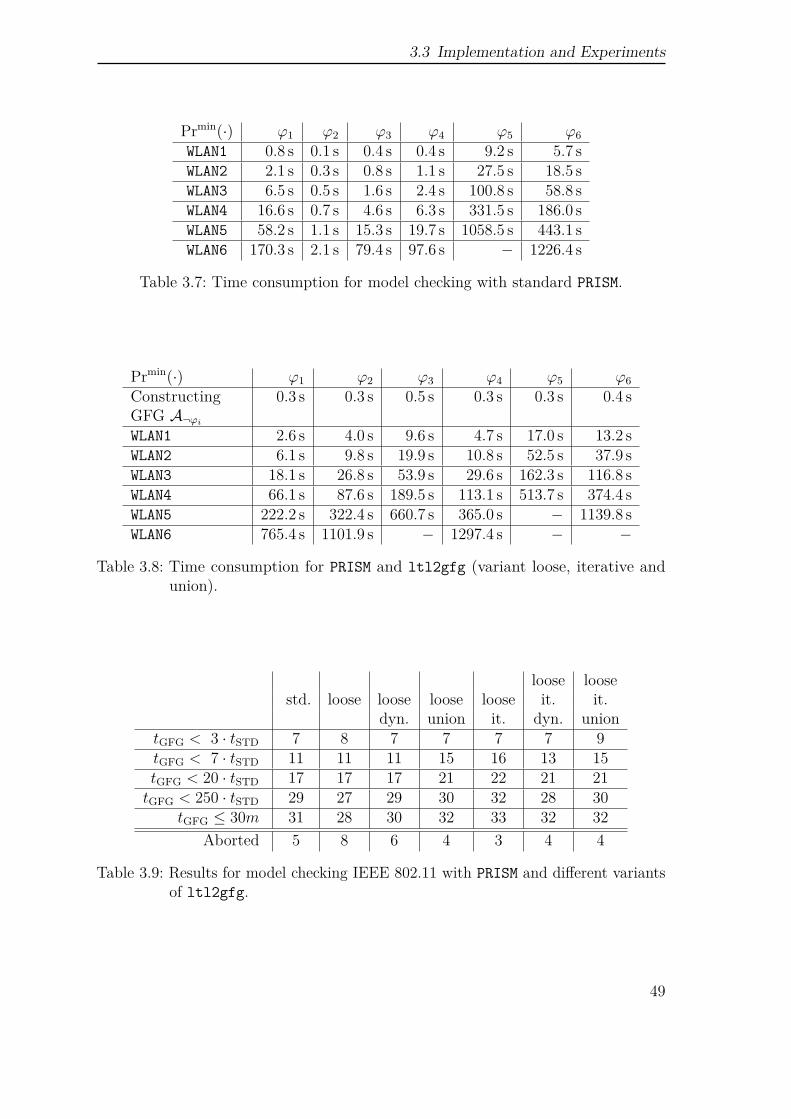
3.3 Implementation and Experiments
Prmin(·) ϕ1 ϕ2 ϕ3 ϕ4 ϕ5 ϕ6
WLAN1 0.8 s 0.1 s 0.4 s 0.4 s 9.2 s 5.7 sWLAN2 2.1 s 0.3 s 0.8 s 1.1 s 27.5 s 18.5 sWLAN3 6.5 s 0.5 s 1.6 s 2.4 s 100.8 s 58.8 sWLAN4 16.6 s 0.7 s 4.6 s 6.3 s 331.5 s 186.0 sWLAN5 58.2 s 1.1 s 15.3 s 19.7 s 1058.5 s 443.1 sWLAN6 170.3 s 2.1 s 79.4 s 97.6 s − 1226.4 s
Table 3.7: Time consumption for model checking with standard PRISM.
Prmin(·) ϕ1 ϕ2 ϕ3 ϕ4 ϕ5 ϕ6
ConstructingGFG A¬ϕi
0.3 s 0.3 s 0.5 s 0.3 s 0.3 s 0.4 s
WLAN1 2.6 s 4.0 s 9.6 s 4.7 s 17.0 s 13.2 sWLAN2 6.1 s 9.8 s 19.9 s 10.8 s 52.5 s 37.9 sWLAN3 18.1 s 26.8 s 53.9 s 29.6 s 162.3 s 116.8 sWLAN4 66.1 s 87.6 s 189.5 s 113.1 s 513.7 s 374.4 sWLAN5 222.2 s 322.4 s 660.7 s 365.0 s − 1139.8 sWLAN6 765.4 s 1101.9 s − 1297.4 s − −
Table 3.8: Time consumption for PRISM and ltl2gfg (variant loose, iterative andunion).
std. looseloose loose
loose loose loose it. it.dyn. union it. dyn. union
tGFG < 3 · tSTD 7 8 7 7 7 7 9tGFG < 7 · tSTD 11 11 11 15 16 13 15tGFG < 20 · tSTD 17 17 17 21 22 21 21tGFG < 250 · tSTD 29 27 29 30 32 28 30
tGFG ≤ 30m 31 28 30 32 33 32 32
Aborted 5 8 6 4 3 4 4
Table 3.9: Results for model checking IEEE 802.11 with PRISM and different variantsof ltl2gfg.
49
3 Good-for-games Automata
with the GFG approach was within the time spent by the standard PRISM approachmultiplied by the factor 7. As can be seen, the loose variant with union and theiterative approach fared well in general. Interestingly, the automata generated withactive dynamic reordering in some cases fared significantly worse than those using theinitial variable ordering. As PRISM does not support a reordering of the variables, theBDD representation of the GFG automaton is optimized by the dynamic reorderingin ltl2gfg for the stand-alone representation. Clearly, this variable ordering mayhowever not be optimal for the product with the MDP. Likewise, the dynamic variablereordering sometimes slowed down the GFG check in the iterative approach.
As it was to be expected given our results on the automata construction, theGFG-based analysis did not improve on the standard approach. Even using theoptimal variant of ltl2gfg for each formula, ignoring the automata constructiontimes, and for cases where the productM⊗A had a comparable BDD size for theGFG- and DRA-based approach, the model checking using the GFG automata tooksignificantly longer.
PRISM case study: Dining philosophers As a second benchmark, we consider thewell-known problem of the dining philosophers. Lehmann and Rabin [LR81] presenteda probabilistic solution to this problem, which was analyzed by Lynch, Saias andSegala [LSS94] for its timing behavior. Our model from the PRISM benchmark suite,see http://www.prismmodelchecker.org/casestudies/phil_lss.php, consists ofthree philosophers, who sit around a table with a fork on the right side of eachphilosopher. Each philosopher either eats or thinks. To eat, the philosopher has tograb both the fork to the left and to the right. The order in which each philosopherwants to grab the forks is determined probabilistically. The PRISM model introducesan additional constant K, which restricts the maximal number of transitions that aphilosopher can be forced to wait if he is currently attempting to grab a fork. Forour benchmark we chose K = 4.
We considered the following LTL properties:
• ϕ1 = (p1 = wait→ ♦p1 = eat)“If philosopher 1 is hungry, he will eat eventually”
• ϕ2 = ♦ (p1 = wait ∨ p2 = wait ∨ p3 = wait)→ ♦ (p1 = eat ∨ p2 = eat ∨ p3 = eat)
“If one philosopher is hungry infinitely often, one philosopher eats infinitelyoften”
• ϕ3 = ¬((p1 = eat∧p2 = eat)∨(p1 = eat∧p3 = eat) ∨ (p2 = eat∧p3 = eat)
“Only one of the philosophers can eat at the same time”
• ϕ4 = ♦(p1 = eat ∨ p2 = eat ∨ p3 = eat)“Eventually at least one philosopher eats”
50
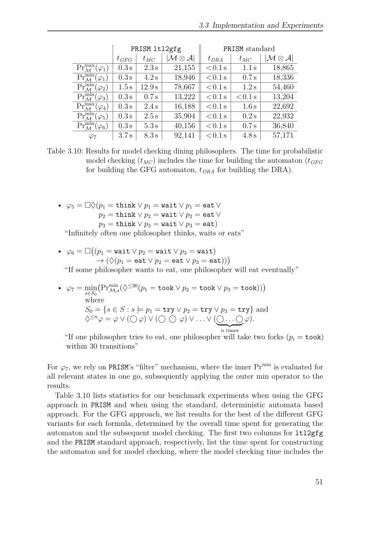
3.3 Implementation and Experiments
PRISM ltl2gfg PRISM standardtGFG tMC |M⊗A| tDRA tMC |M⊗A|
PrmaxM (ϕ1) 0.3 s 2.3 s 21,155 <0.1 s 1.1 s 18,865
PrminM (ϕ1) 0.3 s 4.2 s 18,946 <0.1 s 0.7 s 18,336
PrminM (ϕ2) 1.5 s 12.9 s 78,667 <0.1 s 1.2 s 54,460
PrminM (ϕ3) 0.3 s 0.7 s 13,222 <0.1 s <0.1 s 13,204
PrmaxM (ϕ4) 0.3 s 2.4 s 16,188 <0.1 s 1.6 s 22,692
PrminM (ϕ5) 0.3 s 2.5 s 35,904 <0.1 s 0.2 s 22,932
PrminM (ϕ6) 0.3 s 5.3 s 40,156 <0.1 s 0.7 s 36,840ϕ7 3.7 s 8.3 s 92,141 <0.1 s 4.8 s 57,171
Table 3.10: Results for model checking dining philosophers. The time for probabilisticmodel checking (tMC ) includes the time for building the automaton (tGFGfor building the GFG automaton, tDRA for building the DRA).
• ϕ5 = ♦(p1 = think ∨ p1 = wait ∨ p1 = eat∨p2 = think ∨ p2 = wait ∨ p2 = eat∨p3 = think ∨ p3 = wait ∨ p3 = eat)
“Infinitely often one philosopher thinks, waits or eats”
• ϕ6 = ((p1 = wait ∨ p2 = wait ∨ p3 = wait)→ (♦(p1 = eat ∨ p2 = eat ∨ p3 = eat))
)“If some philosopher wants to eat, one philosopher will eat eventually”
• ϕ7 = mins∈S0
(Prmin
M,s(♦≤30(p1 = took ∨ p2 = took ∨ p3 = took))
)whereS0 = s ∈ S : s |= p1 = try ∨ p2 = try ∨ p3 = try and♦≤nϕ = ϕ ∨ (⃝ϕ) ∨ (⃝ ⃝ ϕ) ∨ . . . ∨ (⃝ . . .⃝⏞ ⏟⏟ ⏞
n times
ϕ).
“If one philosopher tries to eat, one philosopher will take two forks (pi = took)within 30 transitions”
For ϕ7, we rely on PRISM’s “filter” mechanism, where the inner Prmin is evaluated forall relevant states in one go, subsequently applying the outer min operator to theresults.
Table 3.10 lists statistics for our benchmark experiments when using the GFGapproach in PRISM and when using the standard, deterministic automata basedapproach. For the GFG approach, we list results for the best of the different GFGvariants for each formula, determined by the overall time spent for generating theautomaton and the subsequent model checking. The first two columns for ltl2gfgand the PRISM standard approach, respectively, list the time spent for constructingthe automaton and for model checking, where the model checking time includes the
51
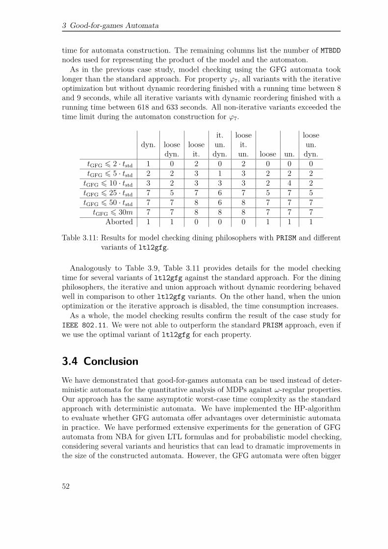
3 Good-for-games Automata
time for automata construction. The remaining columns list the number of MTBDDnodes used for representing the product of the model and the automaton.
As in the previous case study, model checking using the GFG automata tooklonger than the standard approach. For property ϕ7, all variants with the iterativeoptimization but without dynamic reordering finished with a running time between 8and 9 seconds, while all iterative variants with dynamic reordering finished with arunning time between 618 and 633 seconds. All non-iterative variants exceeded thetime limit during the automaton construction for ϕ7.
dyn.it. loose loose
loose loose un. it. un.dyn. it. dyn. un. loose un. dyn.
tGFG ⩽ 2 · tstd 1 0 2 0 2 0 0 0tGFG ⩽ 5 · tstd 2 2 3 1 3 2 2 2tGFG ⩽ 10 · tstd 3 2 3 3 3 2 4 2tGFG ⩽ 25 · tstd 7 5 7 6 7 5 7 5tGFG ⩽ 50 · tstd 7 7 8 6 8 7 7 7tGFG ⩽ 30m 7 7 8 8 8 7 7 7
Aborted 1 1 0 0 0 1 1 1
Table 3.11: Results for model checking dining philosophers with PRISM and differentvariants of ltl2gfg.
Analogously to Table 3.9, Table 3.11 provides details for the model checkingtime for several variants of ltl2gfg against the standard approach. For the diningphilosophers, the iterative and union approach without dynamic reordering behavedwell in comparison to other ltl2gfg variants. On the other hand, when the unionoptimization or the iterative approach is disabled, the time consumption increases.
As a whole, the model checking results confirm the result of the case study forIEEE 802.11. We were not able to outperform the standard PRISM approach, even ifwe use the optimal variant of ltl2gfg for each property.
3.4 ConclusionWe have demonstrated that good-for-games automata can be used instead of deter-ministic automata for the quantitative analysis of MDPs against ω-regular properties.Our approach has the same asymptotic worst-case time complexity as the standardapproach with deterministic automata. We have implemented the HP-algorithmto evaluate whether GFG automata offer advantages over deterministic automatain practice. We have performed extensive experiments for the generation of GFGautomata from NBA for given LTL formulas and for probabilistic model checking,considering several variants and heuristics that can lead to dramatic improvements inthe size of the constructed automata. However, the GFG automata were often bigger
52
3.4 Conclusion
than DRA obtained by the implementation of Safra’s algorithms in ltl2dstar. Thiswas evident not only in the number of states in the generated automata, which is notas crucial for a symbolic encoding, but also in the size of the symbolic BDD-based rep-resentations, in contrast to the expectation that the HP-algorithm could potentiallyconstruct GFG automata with a more efficient symbolic encoding. Our experimentswith the GFG-based approach implemented in probabilistic model checker PRISMthen likewise resulted in a higher time and memory consumption compared to thedeterministic automaton approach.
However, it is still too early to discard the concept of GFG automata for practicalpurposes as our negative results in the experiments might be an artifact of theparticular translation algorithm. Our negative empirical results might be an artifactof the HP-algorithm, which is – to the best of our knowledge – the only implementedalgorithm for the generation of GFG automata that are not deterministic. Therefore,it would be interesting to consider alternative constructions that lead to succinctGFG automata for an explicit or symbolic representation. The recent results on GFGautomata that have fewer states than equivalent deterministic automata [KS15] mightprovide ideas in this direction. It would also be interesting to consider constructionsthat attempt to exploit the potential benefits in succinctness offered by targetingRabin and Streett acceptance conditions directly instead of using parity acceptance.A short while ago, Kuperberg and Majumdar [KM18] designed a new generationalgorithm with non-deterministic co-Büchi automata as starting point. Additionally,they sketched an adaption of Safra’s determinization for achieving the GFG property,but an evaluation of the proposed algorithms remains open.
Likewise, there is an interest in discovering alternative automata types that relyon weaker conditions than the GFG property but can nevertheless be employedfor probabilistic model checking or other settings. One example of such a propertywould be GFG-in-the-limit, but the substantial problem of constructing such succinctautomata remains.
53

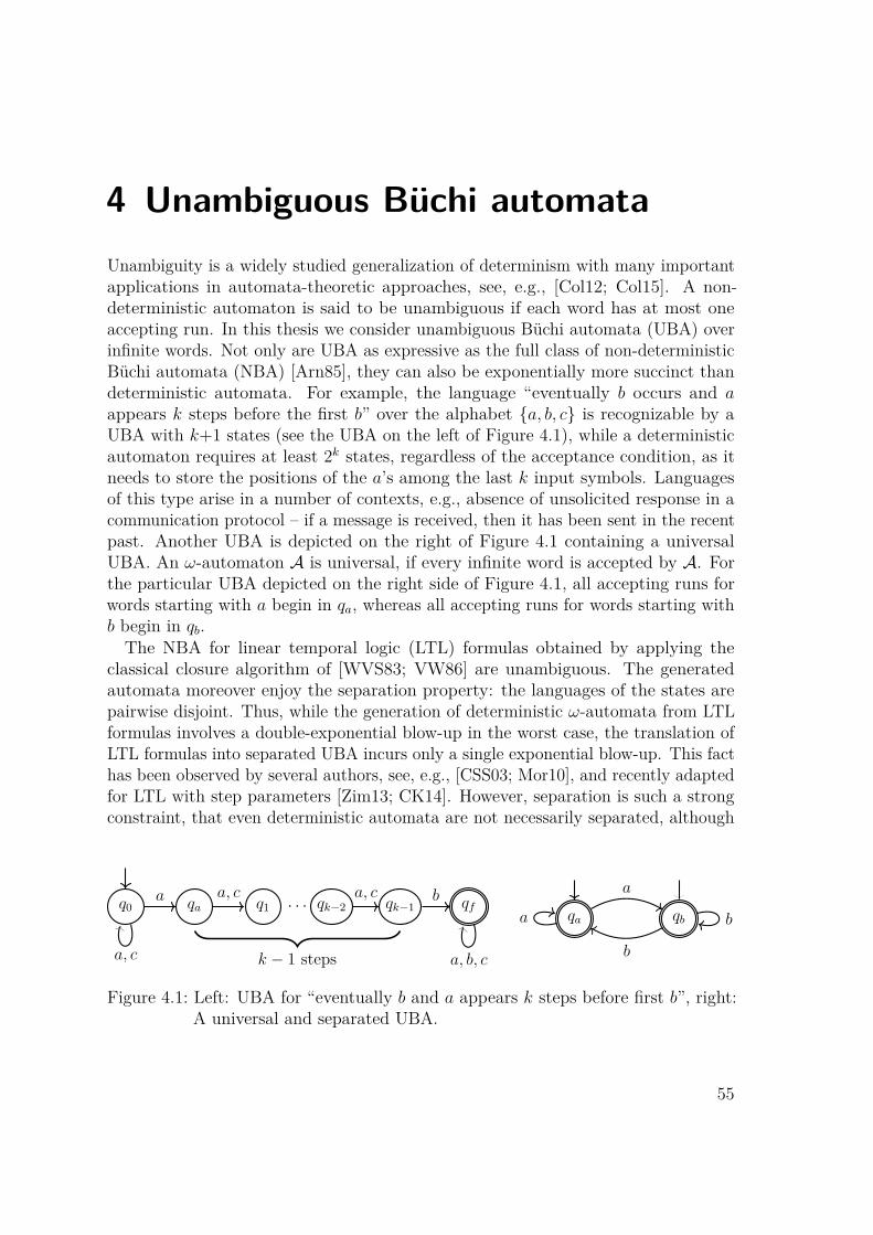
4 Unambiguous Büchi automataUnambiguity is a widely studied generalization of determinism with many importantapplications in automata-theoretic approaches, see, e.g., [Col12; Col15]. A non-deterministic automaton is said to be unambiguous if each word has at most oneaccepting run. In this thesis we consider unambiguous Büchi automata (UBA) overinfinite words. Not only are UBA as expressive as the full class of non-deterministicBüchi automata (NBA) [Arn85], they can also be exponentially more succinct thandeterministic automata. For example, the language “eventually b occurs and aappears k steps before the first b” over the alphabet a, b, c is recognizable by aUBA with k+1 states (see the UBA on the left of Figure 4.1), while a deterministicautomaton requires at least 2k states, regardless of the acceptance condition, as itneeds to store the positions of the a’s among the last k input symbols. Languagesof this type arise in a number of contexts, e.g., absence of unsolicited response in acommunication protocol – if a message is received, then it has been sent in the recentpast. Another UBA is depicted on the right of Figure 4.1 containing a universalUBA. An ω-automaton A is universal, if every infinite word is accepted by A. Forthe particular UBA depicted on the right side of Figure 4.1, all accepting runs forwords starting with a begin in qa, whereas all accepting runs for words starting withb begin in qb.
The NBA for linear temporal logic (LTL) formulas obtained by applying theclassical closure algorithm of [WVS83; VW86] are unambiguous. The generatedautomata moreover enjoy the separation property: the languages of the states arepairwise disjoint. Thus, while the generation of deterministic ω-automata from LTLformulas involves a double-exponential blow-up in the worst case, the translation ofLTL formulas into separated UBA incurs only a single exponential blow-up. This facthas been observed by several authors, see, e.g., [CSS03; Mor10], and recently adaptedfor LTL with step parameters [Zim13; CK14]. However, separation is such a strongconstraint, that even deterministic automata are not necessarily separated, although
q0 qa q1 qk−2· · · qk−1 qf
a, c
a a, c a, c b
a, b, ck − 1 steps
qa qba
a
b
b
Figure 4.1: Left: UBA for “eventually b and a appears k steps before first b”, right:A universal and separated UBA.
55
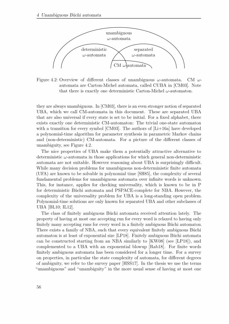
4 Unambiguous Büchi automata
deterministicω-automata
separatedω-automata
unambiguousω-automata
CM ω-automata
Figure 4.2: Overview of different classes of unambiguous ω-automata. CM ω-automata are Carton-Michel automata, called CUBA in [CM03]. Notethat there is exactly one deterministic Carton-Michel ω-automaton.
they are always unambiguous. In [CM03], there is an even stronger notion of separatedUBA, which we call CM-automata in this document. These are separated UBAthat are also universal if every state is set to be initial. For a fixed alphabet, thereexists exactly one deterministic CM-automaton: The trivial one-state automatonwith a transition for every symbol [CM03]. The authors of [Li+16a] have developeda polynomial-time algorithm for parameter synthesis in parametric Markov chainsand (non-deterministic) CM-automata. For a picture of the different classes ofunambiguity, see Figure 4.2.
The nice properties of UBA make them a potentially attractive alternative todeterministic ω-automata in those applications for which general non-deterministicautomata are not suitable. However reasoning about UBA is surprisingly difficult.While many decision problems for unambiguous non-deterministic finite automata(UFA) are known to be solvable in polynomial time [SH85], the complexity of severalfundamental problems for unambiguous automata over infinite words is unknown.This, for instance, applies for checking universality, which is known to be in Pfor deterministic Büchi automata and PSPACE-complete for NBA. However, thecomplexity of the universality problem for UBA is a long-standing open problem.Polynomial-time solutions are only known for separated UBA and other subclasses ofUBA [BL10; IL12].
The class of finitely ambiguous Büchi automata received attention lately. Theproperty of having at most one accepting run for every word is relaxed to having onlyfinitely many accepting runs for every word in a finitely ambiguous Büchi automaton.There exists a family of NBA, such that every equivalent finitely ambiguous Büchiautomaton is at least of exponential size [LP18]. Finitely ambiguous Büchi automatacan be constructed starting from an NBA similarly to [KW08] (see [LP18]), andcomplemented to a UBA with an exponential blowup [Rab18]. For finite wordsfinitely ambiguous automata has been considered for a longer time. For a surveyon properties, in particular the state complexity of automata, for different degreesof ambiguity, we refer to the survey paper [HSS17]. In the thesis we use the terms“unambiguous” and “unambiguity” in the more usual sense of having at most one
56
accepting run for every word, and do not pursue finite ambiguity further.In the context of probabilistic model checking, UFA provide an elegant approach
to compute the probability for a regular safety or cosafety property in finite-stateMarkov chains [BLW14]. The use of separated UBA for a single exponential-timealgorithm that computes the probability for an LTL formula in a Markov chain hasbeen presented in [CSS03]. However, separation is a rather strong condition and non-separated UBA (and even DBA) can be exponentially more succinct than separatedUBA, see [BL10]. This motivates the design of algorithms that operate with generalUBA rather than the subclass of separated UBA. Algorithms for the generation of(possibly non-separated) UBA from LTL formulas that are more compact than theseparated UBA generated by the classical closure-algorithm have been realized in thetool Tulip [Len13b; Len13a] and the automata library SPOT [Dur13].
Contribution. The main theoretical contribution of this chapter is a polynomial-time algorithm to compute the probability measure PrM(Lω(U)) of the set of infinitepaths generated by a finite-state Markov chainM that satisfy an ω-regular propertygiven by a (not necessarily separated) UBA U . The existence of such an algorithmhas previously been claimed in [BLW13b; BLW14; Len13b]. However, these previousworks share a common fundamental error. Specifically they rely on the claim thatif PrM(Lω(U)) > 0, then there exists a state s of the Markov chain M and astate q of the automaton U such that q accepts almost all traces emanating froms (see [BLW13b, Lemma 7.1], [BLW14, Theorem 2]1 , and [Len13b, Section 3.3.1]).While this claim is true in case that U is deterministic [CY95], it needs not to holdwhen U is merely unambiguous. Sections 4.1.1 and 4.1.2 give a more detailed analysisof the issue, describing precisely the nature of the errors in the proofs of [BLW13b;Len13b; BLW14]. To the best of our knowledge these errors are not easily fixable,and we thus take a substantially different approach.
Our algorithm involves a two-phase method that first analyzes the strongly con-nected components (SCCs) of a graph obtained from the product ofM and U , andthen computes the value PrM(Lω(U)) using linear equation systems. The mainchallenge is the treatment of the individual SCCs. For a given SCC, we have anequation system comprising a single variable and equation for each vertex (s, q),with s a state of M and q a state of U . We use results in the spectral theory ofnon-negative matrices to argue that this equation system has a non-zero solutionexactly in case that the SCC makes a non-zero contribution to PrM(Lω(U)). In orderto compute the exact value of PrM(Lω(U)), the key idea is to introduce an additionalnormalization equation. To obtain the latter, we identify a pair (s,R), where s is astate of the Markov chainM and R a set of states of automaton U such that almostall paths starting in s have an accepting run in U when the states in R are declaredto be initial. The crux of establishing a polynomial bound on the running time of ouralgorithm is to find such a pair (s,R) efficiently (in particular, without determinizing
1As the flaw is in the handling of the infinite behavior, the claim and proof of Lemma 1 in [BLW14],dealing with unambiguous automata over finite words, remain unaffected.
57
4 Unambiguous Büchi automata
U) by exploiting structural properties of unambiguous automata.As a consequence of our main result, we obtain that the almost universality problem
for UBA, which can be seen as the probabilistic variant of the universality problemfor UBA and which asks whether a given UBA accepts almost all infinite words, issolvable in polynomial time.
The second contribution in this chapter is an implementation of the new algorithmas an extension of the model checker PRISM, using the automata library SPOT [Dur13]for the generation of UBA from LTL formulas and the COLT library [Hos04] forvarious linear algebra algorithms. We evaluate our approach using the boundedretransmission protocol case study from the PRISM benchmark suite [KNP12] aswell as specific aspects of our algorithm using particularly “challenging” UBA.
4.1 Analysis of Markov chains againstUBA-specifications
The task of the probabilistic model checking problem for a given Markov chainMand NBA A is to compute PrM(Lω(A)). The positive model checking problem forM and A asks whether PrM(Lω(A)) > 0. Likewise, the almost-sure model checkingproblem forM and A denotes the task to check whether PrM(Lω(A)) = 1. Whilethe positive and the almost-sure probabilistic model checking problems for Markovchains and NBA are both known to be PSPACE-complete [Var85; CY95], the analysisof Markov chains against UBA-specification can be carried out efficiently as stated inthe following theorem:
Theorem 4.1. Given a Markov chainM and a UBA U , the value PrM(Lω(U)) iscomputable in time polynomial in the sizes ofM and U .
The statement of Theorem 4.1 has already been presented in [BLW13b] and restated[BLW13a; BLW14] (see also the PhD thesis [Len13b]). However, the presentedalgorithm to compute PrM(Lω(U)) is flawed. This approach, rephrased for thespecial case where the task is to compute Pr(Lω(U)) for a given positive UBA U(which means a UBA where Pr(Lω(U)) > 0) relies on the mistaken belief that thereis at least one state q in U such that Pr(Lω(U [q])) = 1. However, such states neednot exist.
Outline of Section 4.1. At first, we present two counterexamples for [BLW13b] and[BLW14] as well (see also [Len13b]). The remainder of Section 4.1 is devoted to theproof of Theorem 4.1. We first assume that the Markov chainM generates all wordsaccording to a uniform distribution (“uniform Markov chain”) and explain how tocompute the value Pr(Lω(U)) for a given UBA U in polynomial time. For this, we firstaddress the case of strongly connected UBA (Section 4.1.3) and then lift the resultto the general case (Section 4.1.4). The central idea of the algorithm relies on theobservation that each positive, strongly connected UBA has “recurrent sets” of states,
58
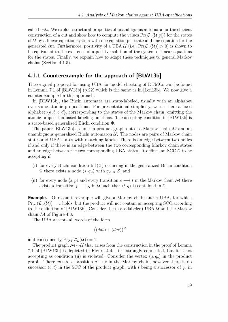
4.1 Analysis of Markov chains against UBA-specifications
called cuts. We exploit structural properties of unambiguous automata for the efficientconstruction of a cut and show how to compute the values Pr(Lω(U [q])) for the statesof U by a linear equation system with one equation per state and one equation for thegenerated cut. Furthermore, positivity of a UBA U (i.e., Pr(Lω(U)) > 0) is shown tobe equivalent to the existence of a positive solution of the system of linear equationsfor the states. Finally, we explain how to adapt these techniques to general Markovchains (Section 4.1.5).
4.1.1 Counterexample for the approach of [BLW13b]The original proposal for using UBA for model checking of DTMCs can be foundin Lemma 7.1 of [BLW13b] (p.22) which is the same as in [Len13b]. We now give acounterexample for this approach.
In [BLW13b], the Büchi automata are state-labeled, usually with an alphabetover some atomic propositions. For presentational simplicity, we use here a fixedalphabet a, b, c, d, corresponding to the states of the Markov chain, omitting theatomic proposition based labeling functions. The accepting condition in [BLW13b] isa state-based generalized Büchi condition Φ.
The paper [BLW13b] assumes a product graph out of a Markov chainM and anunambiguous generalized Büchi automaton U . The nodes are pairs of Markov chainstates and UBA states with matching labels. There is an edge between two nodesif and only if there is an edge between the two corresponding Markov chain statesand an edge between the two corresponding UBA states. It defines an SCC C to beaccepting if
(i) for every Büchi condition Inf (Z) occurring in the generalized Büchi conditionΦ there exists a node ⟨s, qZ⟩ with qZ ∈ Z, and
(ii) for every node ⟨s, p⟩ and every transition s −→ t in the Markov chainM thereexists a transition p −→ q in U such that ⟨t, q⟩ is contained in C.
Example. Our counterexample will give a Markov chain and a UBA, for whichPrM(Lω(U)) = 1 holds, but the product will not contain an accepting SCC accordingto the definition of [BLW13b]. Consider the (state-labeled) UBA U and the MarkovchainM of Figure 4.3.
The UBA accepts all words of the form((dab) + (dac)
)ωand consequently PrM(Lω(U)) = 1.
The product graphM⊗U that arises from the construction in the proof of Lemma7.1 of [BLW13b] is depicted in Figure 4.4. It is strongly connected, but it is notaccepting as condition (ii) is violated: Consider the vertex (a, qa) in the productgraph. There exists a transition a → c in the Markov chain, however there is nosuccessor (c, t) in the SCC of the product graph, with t being a successor of qa in
59
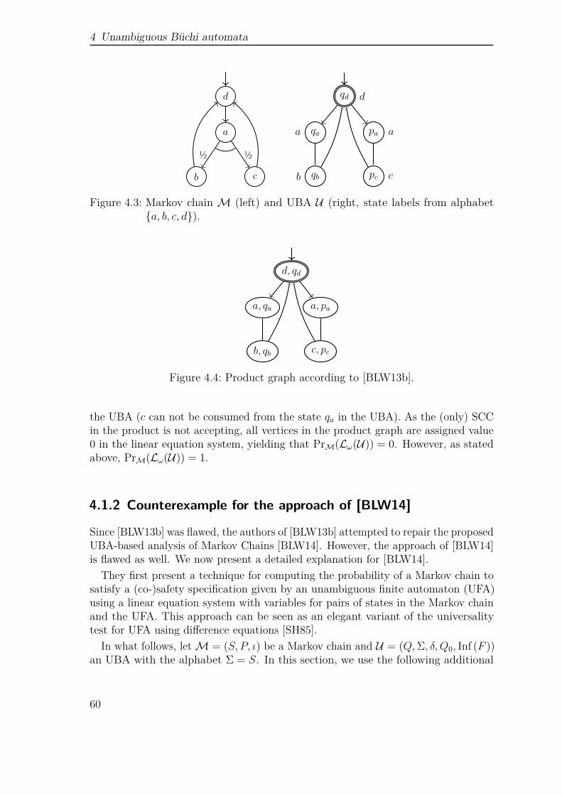
4 Unambiguous Büchi automata
d
a
b c
½ ½
qd d
qaa
qbb
pa a
pc c
Figure 4.3: Markov chain M (left) and UBA U (right, state labels from alphabeta, b, c, d).
d, qd
a, qa
b, qb
a, pa
c, pc
Figure 4.4: Product graph according to [BLW13b].
the UBA (c can not be consumed from the state qa in the UBA). As the (only) SCCin the product is not accepting, all vertices in the product graph are assigned value0 in the linear equation system, yielding that PrM(Lω(U)) = 0. However, as statedabove, PrM(Lω(U)) = 1.
4.1.2 Counterexample for the approach of [BLW14]
Since [BLW13b] was flawed, the authors of [BLW13b] attempted to repair the proposedUBA-based analysis of Markov Chains [BLW14]. However, the approach of [BLW14]is flawed as well. We now present a detailed explanation for [BLW14].
They first present a technique for computing the probability of a Markov chain tosatisfy a (co-)safety specification given by an unambiguous finite automaton (UFA)using a linear equation system with variables for pairs of states in the Markov chainand the UFA. This approach can be seen as an elegant variant of the universalitytest for UFA using difference equations [SH85].
In what follows, letM = (S, P, ι) be a Markov chain and U = (Q,Σ, δ, Q0, Inf (F ))an UBA with the alphabet Σ = S. In this section, we use the following additional
60
4.1 Analysis of Markov chains against UBA-specifications
notations:2Pr#
M[s] =∑t∈S
P (s, t) · PrM[t]
The task addressed in [BLW14] is to compute PrM(Lω(U)). The algorithm proposedin [BLW14] relies on the mistaken belief that if the Markov chainM generates wordsaccepted by the given UBA U with positive probability then the product-graphM⊗U contains recurrent pairs. These are pairs ⟨s, q⟩ consisting of a state s inMand a state q of U such that almost all paths inM starting in a successor of s can bewritten as the infinite concatenation of cycles around s that have a run in U startingand ending in q. (The formal definition of recurrent pairs will be given below.) Thisclaim, however, is wrong as there exist UBA that continuously need a look-ahead forthe paths starting in a fixed state of the Markov chain.
Before presenting a counterexample illustrating this phenomenon and the faultinessof [BLW14], we recall some notations of [BLW14]. Given a state s ∈ S of the MarkovchainM and a state q ∈ Q of the UBA U , the regular languages Gs,q, Hs,q ⊆ S+ aredefined as follows:
Gs,q =s1 s2 . . . sk ∈ S+ : sk = s and p s1 s2... sk−−−−−→ q for some p ∈ Q0
Hs,q =
s1 s2 . . . sk ∈ S+ : sk = s and q s1 s2... sk−−−−−→ q
A pair ⟨s, q⟩ ∈ S × F is called recurrent if Pr#
M[s]
(Hωs,q
)= 1.
The accepted language of U can then be written as:
Lω(U) =⋃
(s,q)∈S×F
Gs,q ·Hωs,q
The idea of [BLW14] is to reduce the task to compute PrM(Lω(U)) to the task ofcomputing the probability forM to generate a finite word accepted by a UFA forthe language given by the UFA resulting from the union of the regular languages Gs,q
where ⟨s, q⟩ is recurrent. To show the correctness of this approach, [BLW14] claimsthat for each pair ⟨s, q⟩ ∈ S ×Q:
Pr#M[s]
(Hωs,q
)∈0, 1
and thus Pr#M[s]
(Hωs,q
)= 0 for the non-recurrent pairs ⟨s, q⟩ ∈ S × F . To prove this
claim, the authors conjecture (in Equation (5) of [BLW14]) that:
Pr#M[s]
((Hs,q)
ω)
= limn→∞
Pr#M[s]
((Hs,q)
n) (∗)
= limn→∞
Pr#M[s]
(Hs,q
)nThe following example shows that equality (∗) is wrong, and recurrent pairs need notexist, even if U is universal.
2We depart here from the notations of [BLW14] where the notation PrM,t has been used as a shortform for Pr#
M[t].
61
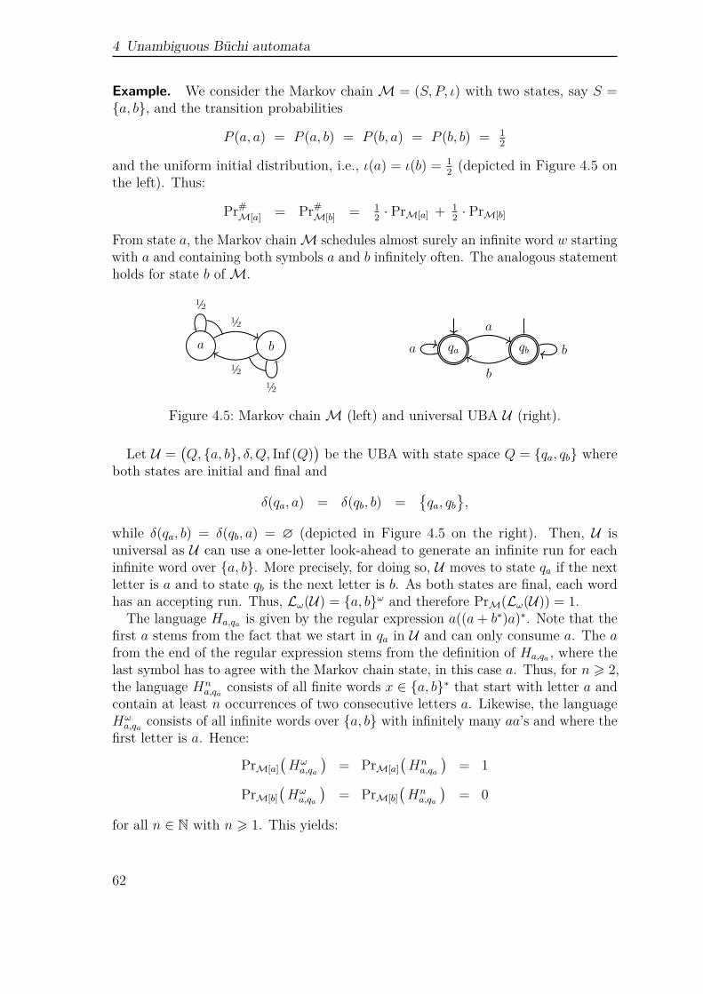
4 Unambiguous Büchi automata
Example. We consider the Markov chainM = (S, P, ι) with two states, say S =a, b, and the transition probabilities
P (a, a) = P (a, b) = P (b, a) = P (b, b) = 12
and the uniform initial distribution, i.e., ι(a) = ι(b) = 12(depicted in Figure 4.5 on
the left). Thus:
Pr#M[a] = Pr#
M[b] = 12· PrM[a] +
12· PrM[b]
From state a, the Markov chainM schedules almost surely an infinite word w startingwith a and containing both symbols a and b infinitely often. The analogous statementholds for state b ofM.
a b
½½
½½
qa qba
a
b
b
Figure 4.5: Markov chainM (left) and universal UBA U (right).
Let U =(Q, a, b, δ, Q, Inf (Q)
)be the UBA with state space Q = qa, qb where
both states are initial and final and
δ(qa, a) = δ(qb, b) =qa, qb
,
while δ(qa, b) = δ(qb, a) = ∅ (depicted in Figure 4.5 on the right). Then, U isuniversal as U can use a one-letter look-ahead to generate an infinite run for eachinfinite word over a, b. More precisely, for doing so, U moves to state qa if the nextletter is a and to state qb is the next letter is b. As both states are final, each wordhas an accepting run. Thus, Lω(U) = a, bω and therefore PrM(Lω(U)) = 1.
The language Ha,qa is given by the regular expression a((a+ b∗)a)∗. Note that thefirst a stems from the fact that we start in qa in U and can only consume a. The afrom the end of the regular expression stems from the definition of Ha,qa , where thelast symbol has to agree with the Markov chain state, in this case a. Thus, for n ⩾ 2,the language Hn
a,qa consists of all finite words x ∈ a, b∗ that start with letter a andcontain at least n occurrences of two consecutive letters a. Likewise, the languageHωa,qa consists of all infinite words over a, b with infinitely many aa’s and where the
first letter is a. Hence:
PrM[a]
(Hωa,qa
)= PrM[a]
(Hna,qa
)= 1
PrM[b]
(Hωa,qa
)= PrM[b]
(Hna,qa
)= 0
for all n ∈ N with n ⩾ 1. This yields:
62
4.1 Analysis of Markov chains against UBA-specifications
Pr#M[a]
(Hωa,qa
)= Pr#
M[a]
(Hna,qa
)= 1
2
for all n ∈ N with n ⩾ 1. On the other hand:
limn→∞
Pr#M[a](Ha,qa )
n = limn→∞
(12
)n= 0
Thus, equality (∗) is wrong. In this example, none of the pairs ⟨a, qa⟩, ⟨a, qb⟩, ⟨b, qa⟩,⟨b, qb⟩ is recurrent. Note that the languages Ha,qb and Hb,qa are empty and that ananalogous calculation yields:
Pr#M[b]
(Hωb,qb
)= Pr#
M[b]
(Hnb,qb
)= 1
2
and limn→∞
Pr#M[b](Hb,qb )
n = 0.
4.1.3 Strongly connected UBAIn Section 4.1.3 we prove Theorem 4.1 in the special case for a uniform Markov chainand a UBA, which is strongly connected. Therefore, we abbreviate PrM(L) by Pr(L)ifM is the uniform Markov chain and L an ω-regular language. We generalize theresults in Section 4.1.4 and Section 4.1.5.
For this we start with a lemma about positive ω-regular languages which we usevery often, in particular in case of strongly connected UBA.
Lemma 4.2. If L ⊆ Σω is ω-regular and Pr(L) > 0, then there exists x ∈ Σ∗ suchthat Pr
(w ∈ Σω : xw ∈ L
)= 1.
Proof. Pick a deterministic ω-automaton D = (Q,Σ, δ, qinit,Φ) for L, for instance,with a Rabin acceptance condition. W.l.o.g. all states are reachable from qinit andD is complete. LetMD = (Q,P ) be the transition-labeled Markov chain resultingfrom D by turning all branchings in D into uniform probabilistic choices, i.e., foreach state q and each letter a, P (q, a, q′) = 1/|Σ| if δ(q, a) = q′ and P (q, a, q′) = 0otherwise. Clearly, the underlying graph of D andMD is the same. If C is a bottomstrongly connected component (BSCC) of D resp. MD, then C is said to satisfyD’s acceptance condition Φ, denoted C |= Φ, iff all infinite paths π with inf (π) = Cmeet the condition imposed by Φ, where inf (π) denotes the set of states that appearinfinitely often in π. For example, if Φ is a Rabin condition, say
Φ =⋁
1⩽i⩽k
(Fin (Ui) ∧ Inf (Li) ) where Ui, Li ⊆ Q,
and C ⊆ Q a BSCC, then C |= Φ iff there is at least one Rabin pair Fin (Ui)∧ Inf (Li)in Φ with C ⊆ Q \ Ui and C ∩ Li = ∅. As almost all paths inMD eventually enter aBSCC and visit all its states infinitely often, we get:
Pr(L) > 0 iff PrMD(Φ) > 0
iff D has at least one BSCC C with C |= Φ
63
4 Unambiguous Büchi automata
In this case and if x is a finite word such that δ(qinit, x) ∩ C = ∅, then Pr(w ∈ Σω :xw ∈ L ) = 1.
We continue with some general observations about strongly connected Büchi au-tomata under probabilistic semantics. For this, we suppose A =
(Q,Σ, δ, Q0, Inf (F )
)is a strongly connected NBA where Q0 and F are non-empty. Note that A might beincomplete.
Fact 4.3. Suppose A is a strongly connected NBA. Then, the following statementsare equivalent:
(1) Pr(Lω(A)) > 0
(2) Pr(Lω(q)) > 0 for some state q
(3) Pr(Lω(p)) > 0 for all states p
Proof. The implications (1) =⇒ (2) and (3) =⇒ (1) are trivial. We now show that(2) =⇒ (3). Since A is strongly connected, there exists a finite word x with p x−→ q,i.e., q ∈ δ(p, x). But then
Pr(Lω(p)) ⩾1
|Σ||x|· Pr(Lω(q)) > 0
Note that 1/|Σ||x| is the probability for (the cylinder set spanned by) the finite wordx.
Moreover, almost all words w ∈ Σω\Lω(A) have a finite prefix x with δ(Q0, x) = ∅:
Lemma 4.4 (Measure of strongly connected NBA). For each strongly connectedNBA A with at least one final state, we have:
Pr(Lω(A)) = 1− Pr(w ∈ Σω : w has a finite prefix x with δ(Q0, x) = ∅
)In particular, A is almost universal if and only if δ(Q0, x) = ∅ for all finite words
x ∈ Σ∗. This observation will be crucial at several places in the soundness proof ofour algorithm for UBA, but can also be used to establish PSPACE-hardness of thepositivity (probabilistic non-emptiness) and almost universality problem for stronglyconnected NBA (see Theorem 4.43).
To prove Lemma 4.4, we accumulate several statements, i.e., Lemma 4.5 untilLemma 4.11 serve as base for a proof. We start with showing that the languageconsisting of all words w ∈ Σω \ Lω(A) such that δ(Q0, x) = ∅ for all x ∈ Pref(w) isa null set. If Lω(A) has positive measure, this statement is a simple consequence ofLemma 4.2 (see Lemma 4.5 below). The general case will be shown in Lemma 4.11using known results for the positive probabilistic model checking problem.
64
4.1 Analysis of Markov chains against UBA-specifications
Lemma 4.5. Suppose A is strongly connected and Pr(Lω(A)) > 0. Let L denotethe set of infinite words w ∈ Σω \ Lω(A) such that δ(Q0, x) = ∅ for all x ∈ Pref(w).Then, Pr(L) = 0.
Proof. Suppose by contradiction that Pr(L) is positive. Obviously, L is ω-regular.Lemma 4.2 yields the existence of a finite word x such that
Pr(
v ∈ Σω : xv ∈ L)
= 1
Let R = δ(Q0, x). Then, R is non-empty and Pr(Lω(A[R]) ) = 0, i.e., Pr(Lω(q) ) = 0for all states q ∈ R. This is impossible by Fact 4.3.
To prove the analogous result for the general case (possibly Pr(Lω(A)) = 0), werely on results by Courcoubetis and Yannakakis [CY95] for the positive probabilisticmodel checking problem. These results rephrased for our purposes yield the following.Let Adet denote the standard powerset construction of A. That is, the states of Adet
are the subsets of Q and the transitions in Adet are given by R a−→ R′ iff R′ = δ(R, a).The initial state of Adet is Q0. Adet is viewed here just as a pointed labeled graphrather than an automaton over words.
Recall that A might be incomplete. Thus, ∅ is a trap state of Adet that is reachedvia the a-transition from any state R ⊆ Q where δ(R, a) is empty. Hence, ∅ is aBSCC of Adet that might or might not be reachable from Q0. We refer to ∅ as thetrap-BSCC of Adet. All other BSCCs of Adet are called non-trap.
A state q ∈ Q of A is said to be recurrent3 if there is some BSCC C of Adet thatcontains a state R ⊆ Q of Adet with q ∈ R and that is reachable from the singletonq viewed as a state of Adet. That is, q is recurrent iff there exists a finite word xsuch that q x−→ q and the set δ(q, x) belongs to a BSCC of Adet.
Fact 4.6 (Proposition 4.1.4 in [CY95]). For each NBA A (not necessarily stronglyconnected):
Pr(Lω(A)
)> 0 iff
there exists a finite word x ∈ Σ∗ such thatδ(Q0, x) ∩ F contains a recurrent state
Example 4.7. We consider the strongly connected NBA shown in Figure 4.6. Then,Adet has two BSCCs, namely the trap-BSCC ∅ and the non-trap BSCC Q.The singletons qa and qb, viewed as states of Adet, can reach Q. Hence, bothstates qa and qb are recurrent. To justify the statement of Fact 4.6, we observe thatPr(Lω(A)) = 1/2 > 0 and δ(qa, a) ∩ F = qb contains a recurrent state.
3The word recurrent has two meanings in this thesis. For the counterexamples of [BLW13b;BLW14] the term is used in the meaning of the according papers, whereas from now on we usethe term recurrent in the sense of a state q of A such that a state R with q ∈ R is reachablefrom q in Adet.
65
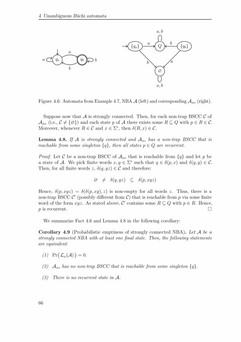
4 Unambiguous Büchi automata
qa qba
a
b
b
qa Q
∅
qba
b
b
a
a, b
a, b
Figure 4.6: Automata from Example 4.7, NBAA (left) and correspondingAdet (right).
Suppose now that A is strongly connected. Then, for each non-trap BSCC C ofAdet (i.e., C = ∅) and each state p of A there exists some R ⊆ Q with p ∈ R ∈ C.Moreover, whenever R ∈ C and x ∈ Σ∗, then δ(R, x) ∈ C.
Lemma 4.8. If A is strongly connected and Adet has a non-trap BSCC that isreachable from some singleton q, then all states p ∈ Q are recurrent.
Proof. Let C be a non-trap BSCC of Adet that is reachable from q and let p bea state of A. We pick finite words x, y ∈ Σ∗ such that q ∈ δ(p, x) and δ(q, y) ∈ C.Then, for all finite words z, δ(q, yz) ∈ C and therefore:
∅ = δ(q, yz) ⊆ δ(p, xyz)
Hence, δ(p, xyz) = δ(δ(p, xy), z) is non-empty for all words z. Thus, there is anon-trap BSCC C ′ (possibly different from C) that is reachable from p via some finiteword of the form xyz. As stated above, C ′ contains some R ⊆ Q with p ∈ R. Hence,p is recurrent.
We summarize Fact 4.6 and Lemma 4.8 in the following corollary:
Corollary 4.9 (Probabilistic emptiness of strongly connected NBA). Let A be astrongly connected NBA with at least one final state. Then, the following statementsare equivalent:
(1) Pr(Lω(A)
)= 0.
(2) Adet has no non-trap BSCC that is reachable from some singleton q.
(3) There is no recurrent state in A.
66
4.1 Analysis of Markov chains against UBA-specifications
q0
p1
p2
c
c c
a, b a, b
c
Q
p1, p2
q0, p1
q0
∅
p2
p1
q0, p2c
a, bc
a, b
c
a, b
a, b
c
c
c
a, b
c
a, ba, b
a, b, c
Figure 4.7: Automata from Example 4.10, NBAA (left) andAdet (right, with BSCCs).
Example 4.10. We consider the strongly connected NBA shown in Figure 4.7. Then,Adet has a non-trap BSCC consisting of the states p1, p2 and Q that is not accessiblefrom any singleton. However, there is another non-trap BSCC in Adet consisting ofthe three states p1, p2 and q0, p2. Indeed, A accepts almost all words startingwith letter c and therefore Pr(Lω(A)) = 1/3.
We are now ready to complete the proof of Lemma 4.4 by proving the followinglemma:
Lemma 4.11. Suppose A is strongly connected with at least one final state. Let L bethe set of infinite words w ∈ Σω \ Lω(A) such that δ(Q0, x) = ∅ for all x ∈ Pref(w).Then, Pr(L) = 0.
Proof. We consider first the case where A has a single initial state, say Q0 = q0.Suppose by contradiction that Pr(L) is positive. Then, there is some finite word zsuch that zv ∈ L for almost all words v ∈ Σω. Let R = δ(q0, z). By definition of L,the set R is non-empty and δ(R, x) = ∅ for all finite words x. Hence, the state ∅ isnot reachable from R in Adet. Therefore, there is a non-trap BSCC of Adet that isreachable from the singleton q0. Hence, Pr(Lω(A)) > 0 by Corollary 4.9. But thenPr(L) = 0 by Lemma 4.5. Contradiction.
The argument for the general case is as follows. Suppose by contradiction that Lhas positive measure. We consider the labeled Markov chainM = (2Q, P,Dirac[Q0])that arises from the deterministic automaton Adet with initial state Q0 by attachinguniform distributions. That is, if R,R′ ⊆ Q and a ∈ Σ, then P (R, a,R′) = 1/|Σ|if R′ = δ(R, a) and P (R, a,R′) = 0 otherwise. For almost all words w in L, thecorresponding path πw inM eventually visits some BSCC C ofM resp. Adet andvisits all its states infinitely often. By assumption C is non-trap.
67
4 Unambiguous Büchi automata
The goal is to show that a non-trap BSCC is accessible from some singleton. LetL′ denote the set of all words w = a1 a2 a3 . . . ∈ L such that πw eventually enterssome BSCC ofM and visits all its states infinitely often. Then, Pr(L′) = Pr(L). Ifw = a1 a2 a3 . . . ∈ L′ and πw = R0R1R2 . . . then R0 = Q0 and Rn = δ(Q0, a1 . . . an).By König’s Lemma (see, e.g., Lemma 8.1.2 of [Die17]) there is an infinite run q0 q1 q2 . . .for w in A such that qi ∈ Ri for all i ∈ N. We write Runs(w) to denote the set ofall these runs. Pick some run ρ = q0 q1 q2 . . . ∈ Runs(w) and define U0 = q0 andUi = δ(q0, a1 a2 . . . ai) = δ(Ui−1, ai) for i ⩾ 1. Clearly, qi ∈ Ui ⊆ Ri for all indices iand πρ = U0 U1 U2 . . . is a path inM and the unique run for w in Adet starting inq0.
Consider the set U of all sets U ⊆ Q such that U ∈ inf (πρ) for some word w ∈ L′
and some ρ ∈ Runs(w). (The notation inf (π) is used to denote the set of elementsthat appear infinitely often in π.) We now show that the subgraph of Adet consistingof the nodes U ∈ U contains a BSCC. For each subset V of U and each state q ∈ Q,let
Lq,V =w ∈ L′ : ∃ρ ∈ Runs(w) s.t. q = first(πρ) ∧ inf (πρ) = V
Then, L′ is the union of all sets Lq,V with (q,V) ∈ Q0 × U. As Pr(L′) = Pr(L) > 0and Q0 × U is finite, there is some pair (q,V) ⊆ Q0 × U with Pr(Lq,V) > 0. Clearly,Lq,V is ω-regular. Hence, there is some finite word z such that
Pr(v ∈ Σω : zv ∈ Lq,V
)= 1.
Let R = δ(q, z). We now regard the fragment of Adet that is reachable from R. LetM[R] be the corresponding Markov chain (i.e., the sub Markov chain of M withinitial state R). Since zv ∈ Lq,V for almost all words v ∈ Σω, inf (π) = V for almostall paths inM[R]. But then V constitutes a non-trap BSCC ofM[R], and thereforeof M and Adet. Since V is reachable from q in Adet, we obtain Pr(Lω(A)) > 0by Corollary 4.9. Lemma 4.5 yields Pr(L) = 0, which contradicts the assumptionPr(L) > 0.
Remark 4.12. Clearly, Pr(Lω(A)) depends on Q0 as there might be state-letterpairs (q, a) where δ(q, a) is empty. However, Lemma 4.4 implies that if A is stronglyconnected with at least one final state, then Pr(Lω(A)) does not depend on F .
For computing Pr(Lω(U)) given a UBA U , it suffices to compute the valuesPr(Lω(q)) for the (initial) states of U as we have
Pr(Lω(U)) =∑q∈Q0
Pr(Lω(q))
The following simple fact will be used at several places:
68
4.1 Analysis of Markov chains against UBA-specifications
Fact 4.13. Let U be a UBA with Lω(q) = ∅ for each state q ∈ Q. Then, for eachstate p ∈ Q, each non-empty subset R of Q of the form R = δ(Q0, y) for some wordy ∈ Σ∗ and each finite word x = a1 a2 . . . an ∈ Σ∗ there exists at most one state q ∈ Rand at most one run
q = q0a1−→ q1
a2−→ . . .an−→ qn = p
for x starting in q and ending in p. In particular, the NFA (Q,Σ, δ, δ(Q0, y),Reach (p))is unambiguous for each y ∈ Σ∗ and each state p ∈ Q.
Proof. If there would be two runs q0y−→ q
x−→ p and q′0y−→ q′
x−→ p where q, q′ ∈ Rand q0, q
′0 ∈ Q0, then each word yxw with w ∈ Lω(p) would have two accepting
runs. This is impossible by the unambiguity of U and the assumption that Lω(p) isnon-empty for all states p ∈ Q.
Fact 4.13 will often be used in form of the statement that, for all states q, p ∈ Qand all finite words x, there is at most one run for x from q to p.
We now suppose that U is a strongly connected UBA. Note that Lω(p) = ∅ andPr(Lω(p)) = 0 is possible. However, in this case Pr(Lω(q)) = 0 for all states q. Thefollowing theorem states that for strongly connected UBA U , the accepting runs ofalmost all words in Lω(U) visit each state of U infinitely often. Although irrelevantfor the soundness of our algorithm, we find that it reveals an interesting structuralproperty of strongly connected UBA.
We use the following notations. For w ∈ Lω(U), we write accrun(w) to denote theunique accepting run for w in U . For q0 q1 q2 . . . ∈ Qω, the set inf (q0 q1 q2 . . .) denotesthe set of all states q ∈ Q such that q = qi for infinitely many indices i. Thus, ifw ∈ Lω(U), then inf (accrun(w)) collects all states q ∈ Q that appear infinitely oftenin the accepting run for w.
Theorem 4.14 (Measure of strongly connected UBA). If U is a strongly connectedUBA with at least one final state, then:
Pr(w ∈ Lω(U) : inf (accrun(w)) = Q
)= Pr
(Lω(U)
)Proof. To prove Theorem 4.14, we can rely on the following facts that hold for allevents (measurable sets) Li, L in each probability space:
• Pr(L1) = Pr(L2) = 1 iff Pr(L1 ∩ L2) = 1
Hence, if L1, . . . , Ln ⊆ L and Pr(L1) = . . . = Pr(Ln) = Pr(L), then Pr(L1∩. . .∩Ln) = Pr(L) as Pr(Li |L) = 1 for all i = 1, . . . , n implies Pr(L1∩ . . .∩Ln |L) =1.
• if (Ln)n∈N is a countable family of measurable sets with L0 ⊇ L1 ⊇ L2 ⊇ . . .,then
Pr(L) = limn→∞
Pr(Ln) where L =⋂n∈N
Ln
as every probability measure is continuous from above.
69
4 Unambiguous Büchi automata
Hence, for the proof of Theorem 4.14 it suffices to show that the accepting runs foralmost all words in Lω(U) contain a fixed state q that appears infinitely often. Thus,the goal is to show:
Pr(w ∈ Lω(U) : q ∈ inf (accrun(w))
)= Pr
(Lω(U)
)The claim is obvious if Pr(Lω(U)) = 0. Suppose now that Pr(Lω(U)) > 0. Hence,Pr(Lω(p)) > 0 for all states p (Fact 4.3). We first show that the accepting runs foralmost all words in Lω(U) eventually visit q.
Claim: Pr(w ∈ Lω(U) : accrun(w) |= ♦q
) = Pr
(Lω(U)
).
Proof of the claim: Suppose by contradiction that there is some state q ∈ Q suchthat the set of words w ∈ Lω(U) whose run does not visit q has positive measure, i.e.,
Prw ∈ Lω(U) : accrun(w) |= ♦q
> 0
Lemma 4.2 yields the existence of a finite word x ∈ Σ∗ such that:
Pr(
w ∈ Σω : xw ∈ Lω(U), accrun(xw) |= ♦q)
= 1
In particular, δ(Q0, x) is non-empty. Pick some state p ∈ δ(Q0, x), say p ∈ δ(q0, x)where q0 ∈ Q0. As U is strongly connected, there is some non-empty finite word ywith q ∈ δ(p, y). Let
L =xyv : v ∈ Lω(q)
and L′ =
yv : v ∈ Lω(q)
.
As Pr(Lω(q)) > 0 and there is exactly one run for xy from Q0 to q, we get:
Pr(L′) ⩾ Pr(L) =1
|Σ|n· Pr(Lω(q)) > 0
where n = |x|+ |y|. The words xyv ∈ L have accepting runs starting with the prefix:
q0x−→ p
y−→ q
In particular:
L′ ⊆w ∈ Σω : xw ∈ Lω(U), accrun(xw) |= ♦q
and therefore:
Pr(
w ∈ Σω : xw ∈ Lω(U), accrun(xw) |= ♦q)
> 0
But then:
Pr(
w ∈ Σω : xw ∈ Lω(U), accrun(xw) |= ♦q)
< 1
Contradiction. This completes the proof of the claim.
70
4.1 Analysis of Markov chains against UBA-specifications
With an analogous argument we get that for each state q ∈ Q, Pr(Lω(U)) = Pr(Ln)where Ln is the set of all infinite words w ∈ Lω(U) such that accrun(w) visits stateq at least n times. It holds, that
Lω(U) = L0 ⊇ L1 ⊇ L2 ⊇ . . . ⊇⋂n∈N
Lndef= L
Then, L is the set of all words w ∈ Lω(U) such that q ∈ inf (accrun(w)). Additionally,we have:
Pr(L) = limn→∞
Pr(Ln) = Pr(Lω(U))
This completes the proof of Theorem 4.14.
Remark 4.15. The only place where the proof of Theorem 4.14 uses the unambiguityof U is in the statement that L agrees with the set of infinite words w such thatq ∈ inf (accrun(w)).
Remark 4.16. With analogous arguments one can show that the accepting runs ofalmost all words in Lω(U) contain each finite path of U infinitely often.
Deciding positivity for strongly connected UBA.
The following lemma provides a criterion to check positivity of a strongly connectedUBA in polynomial time using standard linear algebra techniques.
Lemma 4.17. Let U be a strongly connected UBA with at least one initial and onefinal state, and
(∗) ζq =1
|Σ|·∑σ∈Σ
∑p∈δ(q,σ)
ζp for all q ∈ Q
Then, the following statements are equivalent:
(1) Pr(Lω(U)) > 0,
(2) the linear equation system (*) has a strictly positive solution, i.e., a solution(ζ∗q )q∈Q with ζ∗q > 0 for all q ∈ Q,
(3) the linear equation system (*) has a non-zero solution.
Given the strongly connected UBA U with at least one final state, we define amatrix M ∈ [0, 1]Q×Q by Mp,q =
1|Σ| · |a ∈ Σ : q ∈ δ(p, a)| for all p, q ∈ Q. Since U
is strongly connected, M is irreducible. We write ρ(M) for the spectral radius of M .We will use the following lemma in the proof of Lemma 4.17.
Lemma 4.18. We have ρ(M) ≤ 1. Moreover, ρ(M) = 1 if and only if Pr(Lω(U)) >0.
71
4 Unambiguous Büchi automata
Proof. For p, q ∈ Q and n ∈ N, let Ep,n,q ⊆ Σω denote the event of all wordsw = σ1σ2 . . . such that q ∈ δ(p, σ1σ2 . . . σn). Its probability under the uniformdistribution on Σω is an entry in the n-th power of M :
Pr(Ep,n,q) = (Mn)p,q (4.1)
In particular, Mnp,q ≤ 1 for all n. From the boundedness of Mn it follows (e.g.,
by [HJ13, Corollary 8.1.33]) that ρ(M) ≤ 1. The same result implies that
ρ(M) = 1 ⇐⇒ lim supn→∞
(Mn)p,q > 0 for all p, q ∈ Q
⇐⇒ lim supn→∞
(Mn)p,q > 0 for some p, q ∈ Q(4.2)
For the rest of the proof, fix some state p ∈ Q. By the observations from thebeginning of Section 4.1.3 it suffices to show that Pr(Lω(p)) > 0 if and only ifρ(M) = 1. To this end, consider the event Ep,n :=
⋃q∈QEp,n,q. Notice that (Ep,n)n∈N
forms a decreasing family of sets. We have:
Pr(Lω(p)) = limn→∞
Pr(Ep,n) by Lemma 4.4
= limn→∞
Pr
(⋃q∈Q
Ep,n,q
)by definition of Ep,n
(4.3)
Assuming that ρ(M) = 1, we show that Pr(Lω(p)) > 0. Let q ∈ Q. We have:
Pr(Lω(p)) ≥ lim supn→∞
Pr(Ep,n,q) by (4.3)
= lim supn→∞
(Mn)p,q by (4.1)
> 0 by (4.2)
Conversely, assuming that ρ(M) < 1, we show that Pr(Lω(p)) = 0.
Pr(Lω(p)) = limn→∞
Pr
(⋃q∈Q
Ep,n,q
)by (4.3)
≤ lim supn→∞
∑q∈Q
Pr(Ep,n,q) union bound
= lim supn→∞
∑q∈Q
(Mn)p,q by (4.1)
= 0 by (4.2)
This concludes the proof.
Proof of Lemma 4.17. “(1) =⇒ (2)”: Suppose Pr(Lω(U)) > 0. Define the vector(ζ∗q )q∈Q with ζ∗q = Pr(Lω(q)). It holds that
Lω(q) =⋃σ∈Σ
⋃p∈δ(q,σ)
σw : w ∈ Lω(p)
72
4.1 Analysis of Markov chains against UBA-specifications
Since U is unambiguous, the sets σw : w ∈ Lω(p) are pairwise disjoint. So, thevector (ζ∗q )q∈Q is a solution to the equation system.
As Pr(Lω(U)) > 0 and U is strongly connected, the observation at the beginningof Section 4.1.3 yields that Pr(Lω(q)) > 0 for all states q. Thus, the vector (ζ∗q )q∈Q isstrictly positive.
“(2) =⇒ (3)” holds trivially.“(3) =⇒ (1)”: Suppose ζ∗ is a non-zero solution of the linear equation system.
Then, Mζ∗ = ζ∗. Thus, 1 is an eigenvalue of M . This yields ρ(M) ⩾ 1. But thenρ(M) = 1 and Pr(Lω(U)) > 0 by Lemma 4.18.
Positivity check via rank computation. The first positivity check we present reliessimply on the rank of M − I with M being the matrix from Lemma 4.17. As thesecond positivity check delivers also a possible way to calculate (Pr(Lω(q)) )q∈Q wepostpone its presentation to the end of this section.
Let U be a strongly connected UBA with at least one final state and let M be then × n-matrix from Lemma 4.17, where n = |Q| is the number of states in U . Wecompute rank(M ′) of the matrix M ′ =M − I, where I is the identity matrix. If M ′
has full rank, i.e., rank(M ′) = n, then U is non-positive.IfM ′ does not have full rank, we know that U is positive by the following argument.
As M ′ does not have full rank n, there is a vector v such that (M − I)v is the zerovector; in other words, v is an eigenvector of M with eigenvalue 1. So the spectralradius of M is at least 1. But by Lemma 4.18 the spectral radius of M is at most 1,so it is equal to 1. Since M is irreducible, it follows from the Perron-Frobeniustheorem [BP79, Theorem 2.1.4 (b)] that M has a strictly positive eigenvector v′ witheigenvalue 1, i.e., Mv′ = v′. Lemma 4.17 then yields that U is positive.
Computing pure cuts for positive, strongly connected UBA.
The key observation to compute the values Pr(Lω(q)) for the states q of a positive,strongly connected UBA U is the existence of so-called cuts. These are sets C ofstates with pairwise disjoint languages such that almost all words have an acceptingrun starting in some state q ∈ C. More precisely:
Definition 4.19 ((Pure) cut). Let U be a UBA and C ⊆ Q. C is called a cut for Uif Lω(q)∩Lω(p) = ∅ for all p, q ∈ C with p = q and U [C] is almost universal. A cutis called pure if it has the form δ(q, z) for some state q and some finite word z ∈ Σ∗.
Obviously, U is almost universal iff Q0 is a cut. If q ∈ Q and Kq denotes the set offinite words z ∈ Σ∗ such that δ(q, z) is a cut, then Pr(Lω(q)) equals the probabilitymeasure of the language Lq consisting of all infinite words w ∈ Σω that have a prefixin Kq.
The following concept of cut languages is irrelevant for the soundness proof of ouralgorithm to compute Pr(Lω(U)). However, we find that Lemma 4.21 (see below) isan interesting observation.
73
4 Unambiguous Büchi automata
Definition 4.20 (Cut languages). For each state q in U , let Kq be the set of finitewords x such that δ(q, x) is a cut. We refer to Kq as the cut language for state q.
The cut languages Kq are upward-closed (i.e., if x ∈ Kq, then xy ∈ Kq for all finitewords y) by the first statement of Fact 4.22. The second statement of Fact 4.22 yieldsthat Kq is non-empty if Pr(Lω(q)) is positive. Vice versa, if x ∈ Kq, then almost allinfinite words w with x ∈ Pref(w) belong to Lω(q). Hence, the cut language Kq isnon-empty if and only if Pr(Lω(q)) > 0. Moreover, the cut language Kq is regularsince Kq = Lfin(Udet[q]) where Udet[q] denotes the DFA that results from the powersetconstruction of U by declaring state q to be initial and the states that cannot reachthe trap BSCC to be final (in particular, the states in the non-trap BSCCs are final).The unambiguity of U yields that Kq ∩ Kp = ∅ for all states q, p ∈ Q such thatq, p ⊆ δ(Q0, x) for some finite word x ∈ Σ∗.
We use Pr(Kq) as a short form notation for Pr(L) where L consists of all infinitewords that have some prefix in Kq. Recall that the cut language Kq is empty ifPr(Lω(q)) = 0, in which case Pr(Lω(q)) = Pr(Kq) = 0.
Lemma 4.21. Pr(Lω(q)) = Pr(Kq).
Proof. Obviously, almost all infinite words that have a prefix in Kq belong to Lω(q).This yields Pr(Lω(q)) ⩾ Pr(Kq). Suppose by contradiction that Pr(Lω(q)) > Pr(Kq).Then, the regular language w ∈ Lω(q) : Pref(w) ∩Kq = ∅ is positive. Lemma 4.2yields the existence of some finite word x such that:
Pr(v ∈ Σω : xv ∈ Lω(q), Pref(xv) ∩Kq = ∅
)= 1
In particular, x /∈ Kq and Prv ∈ Σω : xv ∈ Lω(q)
= 1. The latter yields that
δ(q, x) is a cut. But then x ∈ Kq (by definition of Kq). Contradiction.
The following facts are simple, general observations about cuts that will be usedat various places:
Fact 4.22. Suppose U is a UBA (possibly not strongly connected).
• If C is a cut, then so are the sets δ(C, y) for all finite words y ∈ Σ∗.
• If Pr(Lω(U)) > 0, then there exists some finite word x ∈ Σ∗ such that δ(Q0, xy)is a cut for all words y ∈ Σ∗.
Proof. The first statement is obvious. The argument for the second statement is asfollows. Suppose Pr(Lω(U)) > 0. Lemma 4.2 asserts the existence of a finite word xsuch that
Prw ∈ Σω : xw ∈ Lω(U)
= 1
Hence, the δ(Q0, x) is a cut, and so are the sets δ(Q0, xy) = δ(δ(Q0, x), y) for ally ∈ Σ∗ by the first statement.
74
4.1 Analysis of Markov chains against UBA-specifications
Fact 4.22 yields the following characterization of almost universal UBA:
U is almost universal iff Q0 is a cut
iff δ(Q0, x) is a cut for all x ∈ Σ∗
The above characterization holds in any (possibly not strongly connected) UBA. Ananalogous characterization of positivity for strongly connected UBA is obtained usingthe fact that Pr(Lω(U)) > 0 iff Pr(Lω(q)) > 0 for some state q:
U is positive, i.e., Pr(Lω(U)) > 0
iff U has a reachable cut, i.e., a cut of the form δ(Q0, x)
iff U has a pure cut, i.e., a cut of the form δ(q, x)
We now elaborate the notion of cuts in strongly connected UBA.
Fact 4.23. Suppose U is a strongly connected UBA and Pr(Lω(U) ) > 0.
• Let C be a cut and C ′ a subset of Q with Lω(q) ∩ Lω(p) = ∅ for all statesq, p ∈ C ′ with q = p. Then, C ⊆ C ′ implies C = C ′.
• If δ(q, x) is a cut and y ∈ Σ∗ such that q ∈ δ(q, xy), then δ(q, x) = δ(q, xyx).
Proof. The first statement is obvious as Pr(Lω(r)) > 0 for all states r. For the secondstatement we suppose C = δ(q, x) is a cut and r y−→ q for some state r ∈ C. Then:
δ(q, xyx) = δ(C, yx) ⊇ δ(r, yx) = δ( δ(r, y), x) ⊇ δ(q, x) = C
is a cut that subsumes R. Hence, C = δ(q, xyx) by the first statement.
As a consequence of Lemma 4.4, we get that if C ⊆ Q such that Lω(q)∩Lω(p) = ∅for all states q, p ∈ C with q = p then:
C is a cut iff δ(C, y) = ∅ for all y ∈ Σ∗
Corollary 4.24 (Pure cuts in strongly connected UBA; see first part of Lemma 4.27).Let U be a strongly connected UBA with at least one final state. Then for each stateq and each finite word x:
δ(q, x) is a cut iff δ(q, xy) = ∅ for all y ∈ Σ∗
Proof. The languages of the states in δ(q, x) are pairwise disjoint by the unambiguityof U . Hence, δ(q, x) is a (pure) cut if and only if U [δ(q, x)] is almost universal. ByLemma 4.4, this is equivalent to the statement that δ(q, xy) = ∅ for all y ∈ Σ∗.
The following lemma yields that for positive, strongly connected UBA, the purecuts constitute a non-trap BSCC in the deterministic automaton Udet obtained byapplying the standard powerset construction.
75
4 Unambiguous Büchi automata
Lemma 4.25 (See second part of Lemma 4.27). Suppose Pr(Lω(U)) > 0 and U isstrongly connected. Then, for each cut C ⊆ Q the following statements are equivalent:
(1) C is pure, i.e., C = δ(q, x) for some state q ∈ Q and some word x ∈ Σ∗
(2) for each state p ∈ Q there exists a word z ∈ Σ∗ such that C = δ(p, z)
(3) C is reachable from any other cut, i.e., if C ′ is a cut, then there exists a finiteword y with C = δ(C ′, y).
Proof. Obviously, (1) is a consequence of (2). Let us prove the implication (1) =⇒(2). Suppose δ(q, x) is a cut and let p ∈ Q be an arbitrary state. Pick some finiteword y with p
y−→ q. Then, δ(p, yx) ⊇ δ(q, x). We get δ(p, yx) = δ(q, x) by thesecond statement of Fact 4.23.
We now show the implication (2) =⇒ (3). Let C ′ be a cut and p ∈ C ′. Byassumption (2), there is some word z such that C = δ(p, z). Then, δ(C ′, z) is a cutas well and we have:
C = δ(p, z) ⊆ δ(C ′, z)
and therefore C = δ(C ′, z) by the first statement of Fact 4.23.For the implication (3) =⇒ (1) we pick a cut C ′ of the form C ′ = δ(p, z) for some
state p ∈ C and word z. (Such a cut exists by the second statement in Fact 4.22.)By assumption (3) there is a word y with C = δ(C ′, y). But then C = δ(p, yz).
The above lemma shows that if U is positive, then Udet has exactly one non-trapBSCC consisting of the cuts of U that are reachable from some resp. all singleton(s).More precisely, if Pr(Lω(U)) > 0 and U is strongly connected, then the cuts of Uthat are reachable from some singleton constitute a BSCC C of Udet. This is theonly non-trap BSCC of Udet and C is reachable from each cut. Additionally, the trapBSCC ∅ is reachable if there are states q in U with Pr(Lω(q)) < 1.
Remark 4.26. As the results above show: there is no cut C that is reachable fromsome singleton and that is not contained in the non-trap BSCC C. However, theremight be cuts outside C. For example, let U = (Q, a, b, δ, Q0, Inf (F )) where
Q =qa, qb, pa, pb
, Q0 =
qa, pb
, and F =
qa.
The transition function δ is given by:
δ(qa, a) = qa, qbδ(qb, b) = pa, pb
δ(pa, a) = pa, pbδ(pb, b) = qa, qb
and δ(·) = ∅ in all remaining cases. The unambiguity of U is clear since the switchbetween the q- and p-states are deterministic and since
Lω(qa) = Lω(pa) =aw : w ∈ a, bω
,
Lω(qb) = Lω(pb) =bw : w ∈ a, bω
.
76
4.1 Analysis of Markov chains against UBA-specifications
Thus, U is universal. The sets qa, qb, pa, pb constitute the non-trap BSCCconsisting of the cuts that are reachable from the four singletons. The set C = qa, pbis a cut too, but C is not reachable from any singleton. However, δ(C, a) = δ(C, b) =qa, qb.
Corollary 4.24 and Lemma 4.25 are summarized in Lemma 4.27.
Lemma 4.27 (Characterization of pure cuts). Let U be a strongly connected UBA.For all q ∈ Q and z ∈ Σ∗ we have: δ(q, z) is a cut iff δ(q, zy) = ∅ for each wordy ∈ Σ∗. Furthermore, if U is positive, then for each cut C:
C is pure, i.e., C = δ(q, z) for some state-word pair (q, z) ∈ Q× Σ∗
iff for each state q ∈ Q there is some word z ∈ Σ∗ with C = δ(q, z)
iff for each cut C ′ there is some word y ∈ Σ∗ with C = δ(C ′, y)
By Lemma 4.2 and Lemma 4.27 we get:
Corollary 4.28. If U is a strongly connected UBA, then
Pr(Lω(U)) > 0 iff U has a pure cut.
For the rest of Section 4.1.3, we suppose that U is positive and strongly connected.The second part of Lemma 4.27 yields that the pure cuts constitute a bottom stronglyconnected component of the automaton obtained from U using the standard powersetconstruction. The goal is now to design an efficient (polynomially time-bounded)algorithm for the generation of a pure cut. For this, we observe that if q, p ∈ Q,q = p, then q, p ⊆ C for some pure cut C iff there exists a word y such thatq, p ⊆ δ(q, y).
Lemma 4.29. Suppose Pr(Lω(U)) > 0 and U is strongly connected. Let q, p be statesin U with q = p. Then:
q, p ⊆ C for some pure cut C
iff there is some finite word z with q z−→ qz−→ p.
Proof. Let C be a pure cut that contains q and p. By Lemma 4.25 there is a word zwith C = δ(q, z). Then, C = δ(C, z) and δ(p, z) = ∅ by the unambiguity of U (seeFact 4.13). But then q z−→ q
z−→ p. Vice versa, q z−→ qz−→ p implies q, p ⊆ δ(C, z)
for each cut C with q ∈ C.
Remark 4.30. Lemma 4.29 yields that for all states q and p of a strongly connectedUBA U :
• If there is no word z with q z−→ qz−→ p, then there is no cut C with q, p ⊆ C.
• If Pr(Lω(U)) > 0 and q z−→ qz−→ p, then there is a pure cut C that contains q
and p.
77
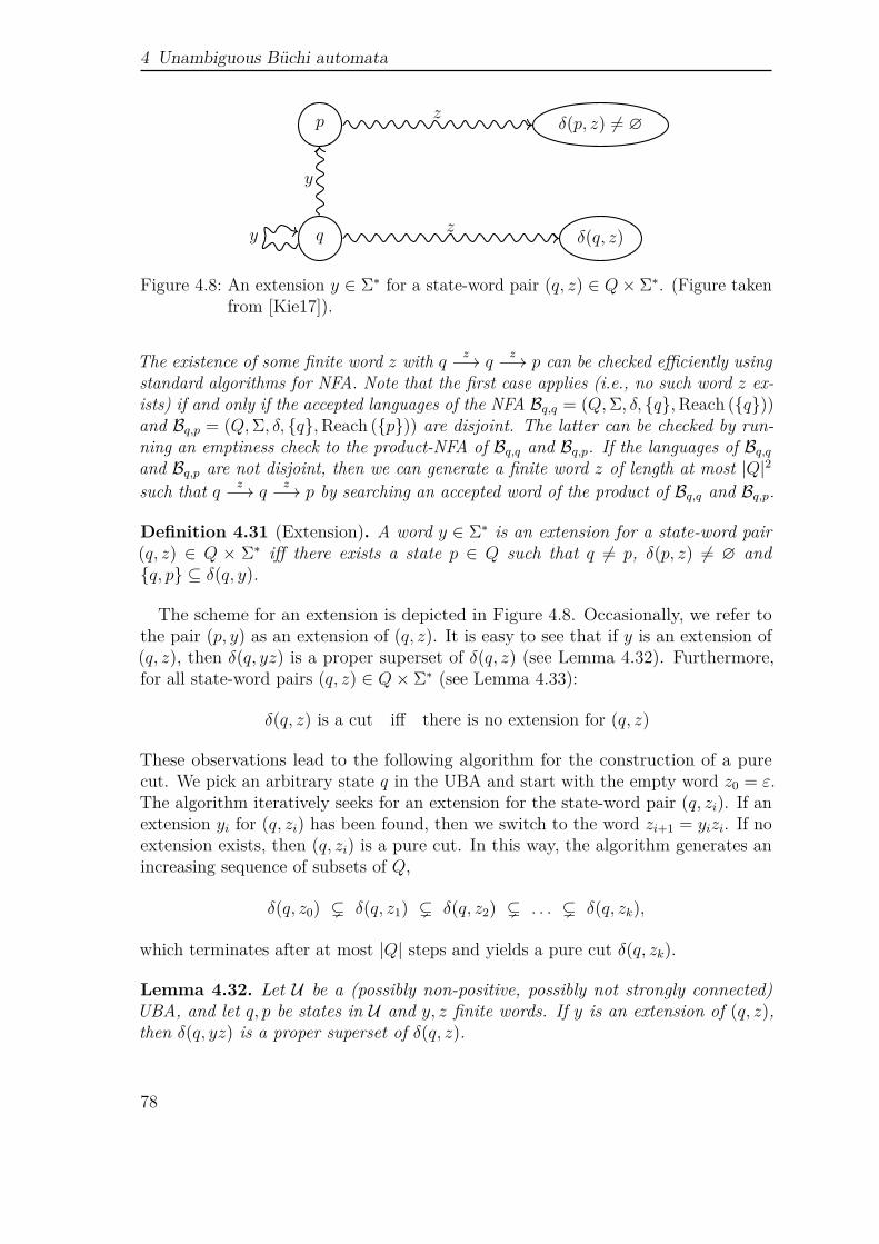
4 Unambiguous Büchi automata
q
p δ(p, z) = ∅
δ(q, z)y
y
z
z
Figure 4.8: An extension y ∈ Σ∗ for a state-word pair (q, z) ∈ Q× Σ∗. (Figure takenfrom [Kie17]).
The existence of some finite word z with q z−→ qz−→ p can be checked efficiently using
standard algorithms for NFA. Note that the first case applies (i.e., no such word z ex-ists) if and only if the accepted languages of the NFA Bq,q = (Q,Σ, δ, q,Reach (q))and Bq,p = (Q,Σ, δ, q,Reach (p)) are disjoint. The latter can be checked by run-ning an emptiness check to the product-NFA of Bq,q and Bq,p. If the languages of Bq,qand Bq,p are not disjoint, then we can generate a finite word z of length at most |Q|2such that q z−→ q
z−→ p by searching an accepted word of the product of Bq,q and Bq,p.
Definition 4.31 (Extension). A word y ∈ Σ∗ is an extension for a state-word pair(q, z) ∈ Q × Σ∗ iff there exists a state p ∈ Q such that q = p, δ(p, z) = ∅ andq, p ⊆ δ(q, y).
The scheme for an extension is depicted in Figure 4.8. Occasionally, we refer tothe pair (p, y) as an extension of (q, z). It is easy to see that if y is an extension of(q, z), then δ(q, yz) is a proper superset of δ(q, z) (see Lemma 4.32). Furthermore,for all state-word pairs (q, z) ∈ Q× Σ∗ (see Lemma 4.33):
δ(q, z) is a cut iff there is no extension for (q, z)
These observations lead to the following algorithm for the construction of a purecut. We pick an arbitrary state q in the UBA and start with the empty word z0 = ε.The algorithm iteratively seeks for an extension for the state-word pair (q, zi). If anextension yi for (q, zi) has been found, then we switch to the word zi+1 = yizi. If noextension exists, then (q, zi) is a pure cut. In this way, the algorithm generates anincreasing sequence of subsets of Q,
δ(q, z0) ⊊ δ(q, z1) ⊊ δ(q, z2) ⊊ . . . ⊊ δ(q, zk),
which terminates after at most |Q| steps and yields a pure cut δ(q, zk).
Lemma 4.32. Let U be a (possibly non-positive, possibly not strongly connected)UBA, and let q, p be states in U and y, z finite words. If y is an extension of (q, z),then δ(q, yz) is a proper superset of δ(q, z).
78
4.1 Analysis of Markov chains against UBA-specifications
Proof. Since q, p ⊆ δ(q, y) we have:
δ(q, z) ⊆ = δ(q, z) ∪ δ(p, z) = δ(q, p, z
)⊆ δ
(δ(q, y), z
)= δ(q, yz)
In particular, δ(q, z) ⊆ δ(q, yz). The set δ(p, z) is non-empty (by the definition ofextensions). Let r be an arbitrary state in δ(p, z). Then, r /∈ δ(q, z), since otherwisethe word yz would have two runs from q to r:
qy−→ q
z−→ r and qy−→ p
z−→ r,
which is impossible by the unambiguity of U (see Fact 4.13).
Lemma 4.33. Let U be a positive, strongly connected UBA. Then for each state-wordpair (q, z) ∈ Q× Σ∗:
δ(q, z) is a cut iff the pair (q, z) has no extension
Proof. “=⇒”: Let δ(q, z) be a cut and suppose by contradiction that there exists anextension y for (q, z). Let p ∈ Q such that q = p, δ(p, z) = ∅ and q, p ⊆ δ(q, y).The set δ(q, yz) \ δ(q, z) is non-empty (Lemma 4.32). As Pr(Lω(r) ) > 0 for all statesr, we get:
Pr(Lω(δ(q, yz))
)= Pr
(Lω(δ(q, z))
)+∑
r ∈ δ(q, yz)r /∈ δ(q, z)
Pr(Lω(r) ) > Pr
(Lω(δ(q, z))
)
Hence, Pr(Lω(δ(q, z)) < 1. But then δ(q, z) cannot be a cut as Pr(Lω(R)) = 1 forall cuts R. Contradiction.
“⇐=”: Suppose now that (q, z) has no extension. We have to show that C = δ(q, z)is a cut.
We first observe that there is some cut R that contains C. For this, we may pickany cut R′ with q ∈ R′. Then, R = δ(R′, z) is a cut with C ⊆ R. For each statep ∈ R \ q, there is some finite word y with q y−→ q
y−→ p (see Lemma 4.29). Sincethere exists no extension for (q, z), we have δ(p, z) = ∅ for all states p ∈ R \C. Thisyields:
C = δ(q, z) = δ(C, z) = δ(R, z)
By Fact 4.22, as R is a cut, δ(R, z) is a cut as well and hence so is C.
It remains to explain an efficient realization of the search for an extension of thestate-word pairs (q, zi). The idea is to store the sets Qi[p] = δ(p, zi) for all states p.The sets Qi[p] can be computed iteratively by:
Q0[p] = p and Qi+1[p] =⋃
r∈δ(p,yi)Qi[r]
79
4 Unambiguous Büchi automata
To check whether (q, zi) has an extension we apply standard techniques for theintersection problem for the languages Hq,q = y ∈ Σ∗ : q ∈ δ(q, y) and Hq,Fi
=y ∈ Σ∗ : δ(q, y) ∩ Fi = ∅ where Fi = p ∈ Q \ q : Qi[p] = ∅. Then, for eachword y ∈ Σ∗ we have: y ∈ Hq,q ∩Hq,Fi
if and only if y is an extension of (q, zi). Thelanguages Hq,q and Hq,Fi
are recognized by the NFA Uq,q = (Q,Σ, δ, q,Reach (q)) andUq,Fi
= (Q,Σ, δ, q,Reach (Fi)). Thus, to check the existence of an extension and tocompute an extension y (if existent) where the word y has length at most |Q|2, wemay run an emptiness check for the product-NFA U [q, q]⊗ U [q, Fi]. We conclude:Corollary 4.34. Given a positive, strongly connected UBA U , a pure cut can becomputed in time polynomial in the word-length of U .
Computing the measure of positive, strongly connected UBA.
We suppose that U =(Q,Σ, δ, Q0, Inf (F )
)is a positive, strongly connected UBA
and C is a cut. (C might be a pure cut that has been computed by the techniquesexplained above. However, in Theorem 4.35 C can be any cut.) Consider the linearequation system of Lemma 4.17 with variables ζq for all states q ∈ Q and add theconstraint that the variables ζq for q ∈ C sum up to 1.Theorem 4.35. Let U be a positive, strongly connected UBA and C a cut. Then,the probability vector (Pr(Lω(q)) )q∈Q is the unique solution of the following linearequation system:
(1) ζq =1
|Σ|·∑σ∈Σ
∑p∈δ(q,σ)
ζp for all states q ∈ Q
(2)∑q∈C
ζq = 1
Proof. Let n = |Q|. Define a matrix M ∈ [0, 1]Q×Q by Mq,p = |σ ∈ Σ : p ∈δ(q, σ)|/|Σ| for all q, p ∈ Q. Then, the n equations (1) can be written as ζ = Mζ,where ζ = (ζq)q∈Q is a vector of n variables. It is easy to see that the valuesζ∗q = Pr(Lω(q)) for q ∈ Q satisfy the equations (1). That is, defining ζ∗ = (ζ∗q )q∈Q wehave ζ∗ =Mζ∗. By the definition of a cut, those values also satisfy equation (2).
It remains to show uniqueness. We employ Perron-Frobenius theory as follows.Since ζ∗ = Mζ∗, the vector ζ∗ is an eigenvector of M with eigenvalue 1. Byζ∗ being strictly positive (i.e., positive in all components), it follows from [BP79,Corollary 2.1.12] that ρ = 1 for the spectral radius ρ of M . Since U is stronglyconnected, matrix M is irreducible. By [BP79, Theorem 2.1.4 (b)] the spectralradius ρ = 1 is a simple eigenvalue of M , i.e., all solutions of ζ = Mζ are scalarmultiples of ζ∗. Among those multiples, only ζ∗ satisfies equation (2). Uniquenessfollows.
Together with the criterion of Lemma 4.17 to check whether a given stronglyconnected UBA is positive, we obtain a polynomially time-bounded computationscheme for the values Pr(Lω(q)) for the states q of a given strongly connected UBA.
80
4.1 Analysis of Markov chains against UBA-specifications
Foundations of the eigenvalue algorithm. The first approach for the positivitycheck (see page 73) was based on a rank computation. Now we give a second approachfor the positivity check and a possible way to calculate the vector (Pr(Lω(q)) )q∈Q aswell. It relies on an iterative approximation of an eigenvector.
Let U be a strongly connected UBA with at least one final state. Let M be thematrix from the proof of Theorem 4.35. Define M = (I +M)/2 where I denotes theQ×Q identity matrix. Denote by 1 = (1)q∈Q the column vector where all componentsare 1. Define 0 similarly. For i ≥ 0 define v(i) =M
i · 1. Our algorithm is as follows.Exploiting the recurrence v(i+ 1) =M · v(i) we compute the sequence v(0), v(1), . . .until we find an i > 0 with either v(i+ 1) < v(i) (by this inequality we mean strictinequality in all components) or v(i+ 1) ≈ v(i). In the first case we conclude thatPr(Lω(U)) = 0. In the second case we compute a cut C and multiply v(i) by a scalarc > 0 so that c ·
∑q∈C v(i)q = 1, and conclude that (Pr(Lω(q)) )q∈Q ≈ c · v(i). This
algorithm is justified by the following two lemmas.Lemma 4.36. We have Pr(Lω(U)) = 0 if and only if there is i ≥ 0 with v(i+1) < v(i).Lemma 4.37. If Pr(Lω(U)) > 0, then v(∞) := limi→∞ v(i) > 0 exists, andMv(∞) = v(∞), and v(∞) is a scalar multiple of (Pr(Lω(q)) )q∈Q.
For the proofs we need the following two auxiliary lemmas:Lemma 4.38. Let ρ > 0 denote the spectral radius of M . Then the matrix limitlimi→∞
(M/ρ
)i exists and is strictly positive in all entries.
Proof. Since M is irreducible, M |Q| is strictly positive (in all entries). Then it followsfrom [HJ13, Theorem 8.2.7] that the matrix limit
limi→∞
(M/ρ
)i= lim
i→∞
((M/ρ
)|Q|)i
exists and is strictly positive.Lemma 4.39. For any v ∈ CQ and any c ∈ C we have Mv = cv if and only ifMv = 1+c
2v. In particular, M and M have the same eigenvectors with eigenvalue 1.
The proof of Lemma 4.39 is obvious. We prove now Lemma 4.36 and 4.37.
Proof of Lemma 4.36. Let i ≥ 0 with v(i+ 1) < v(i). With [BP79, Theorem 2.1.11]it follows that the spectral radius of M is smaller than 1, hence by Lemma 4.39the spectral radius of M is smaller than 1 as well. By Lemma 4.18 it follows thatPr(Lω(U)) = 0.
For the converse, let Pr(Lω(U)) = 0. By Lemma 4.18, the spectral radius of M issmaller than 1. Let ρ denote the spectral radius ofM . By Lemma 4.39, we have ρ < 1.If ρ = 0, then M is the zero matrix and we have v(1) = 0 < 1 = v(0). Let ρ > 0. Itfollows from Lemma 4.38 that there is i ≥ 0 such that ρ
(M/ρ
)i+1<(M/ρ
)i (withthe inequality strict in all components). Hence, M i+1
< Mi and v(i+1) =M
i+1 · 1 <M
i · 1 = v(i).
81
4 Unambiguous Büchi automata
Proof of Lemma 4.37. Let Pr(Lω(U)) > 0. Then, by Lemma 4.18, the spectral radiusof M is 1. So, with Lemma 4.39 the spectral radius of M is 1. By Lemma 4.38 thelimit v(∞) = limi→∞M
i1 exists and is positive. From the definition of v(∞) we have
Mv(∞) = v(∞). By Lemma 4.39 also Mv(∞) = v(∞). So v(∞) solves equation (1)from Theorem 4.35. There is a scalar c > 0 so that cv(∞) satisfies both equations(1) and (2) from Theorem 4.35. By the uniqueness statement of Theorem 4.35 itfollows that cv(∞) = (Pr(Lω(q)) )q∈Q.
The next section shows how to lift these results for arbitrary UBA.
4.1.4 Computing the measure of arbitrary UBAIn what follows, let U = (Q,Σ, δ, Q0, Inf (F )) be a (possibly not strongly connected)UBA and C a strongly connected component (SCC) of U . C is called non-trivial if Cviewed as a direct graph contains at least one edge, i.e., if C is cyclic. Recall that Cis called bottom if δ(q, a) ⊆ C for all q ∈ C and all a ∈ Σ. If C is a non-trivial SCC ofU and p ∈ C, then the sub-NBA
UC,p =
(C,Σ, δ|C, p, Inf (C ∩ F )
)of U with state space C, initial state p and the transition function δ|C given byδ|C(q, a) = δ(q, a)∩C is strongly connected and unambiguous. Let Lp be the acceptedlanguage, i.e., Lp = Lω(U
C,p). The values Pr(Lp), p ∈ C, can be computed using the
techniques for strongly connected UBA presented in Section 4.1.3. A non-trivial SCCC is said to be positive if Pr(Lp) > 0 for all/some state(s) p in C.
We perform the following preprocessing. As before, for any p ∈ Q we write Lω(p)for Lω(U [p] ), and call p zero if Pr(Lω(p)) = 0. First we remove all states that arenot reachable from any initial state. Then we run standard graph algorithms tocompute the directed acyclic graph (DAG) of SCCs of U . By processing the DAGbottom-up we can remove all zero states by running the following loop: If all BSCCsare marked (initially, all SCCs are unmarked), then exit the loop; otherwise pick anunmarked BSCC C.
• If C is trivial or does not contain any final state, then we remove it: moreprecisely, we remove it from the DAG of SCCs, and we modify U by deletingall transitions p σ−→ q where q ∈ C.
• Otherwise, C is a non-trivial BSCC with at least one final state. We checkwhether C is positive by applying the techniques of Section 4.1.3. If it is positive,we mark it; otherwise we remove it as described above.
Note that this loop does not change Pr(Lω(p)) for any state p.Let QBSCC denote the set of states in U that belong to some BSCC. The values
Pr(Lω(p) ) for the states p ∈ QBSCC can be computed using the techniques of
82
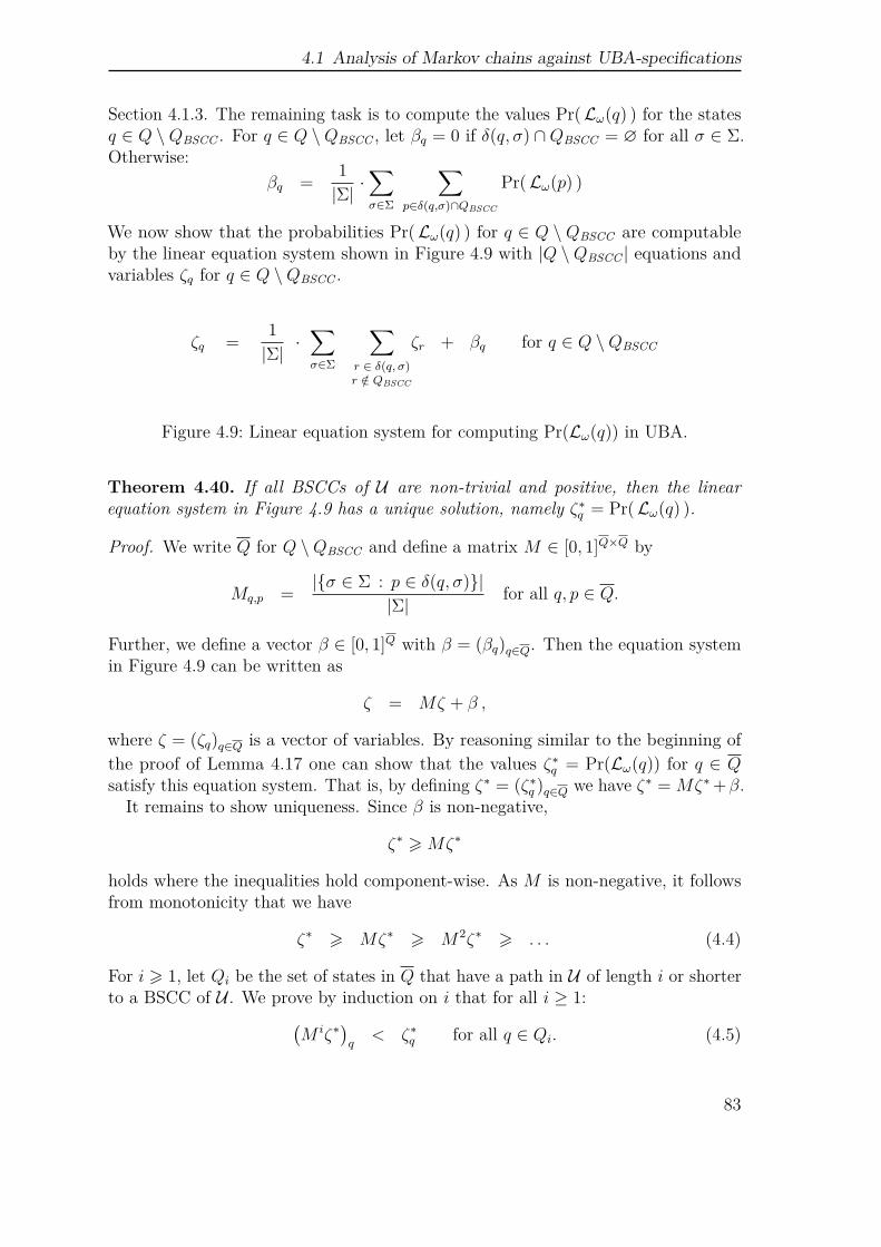
4.1 Analysis of Markov chains against UBA-specifications
Section 4.1.3. The remaining task is to compute the values Pr(Lω(q) ) for the statesq ∈ Q \QBSCC . For q ∈ Q \QBSCC , let βq = 0 if δ(q, σ) ∩QBSCC = ∅ for all σ ∈ Σ.Otherwise:
βq =1
|Σ|·∑σ∈Σ
∑p∈δ(q,σ)∩QBSCC
Pr(Lω(p) )
We now show that the probabilities Pr(Lω(q) ) for q ∈ Q \ QBSCC are computableby the linear equation system shown in Figure 4.9 with |Q \QBSCC | equations andvariables ζq for q ∈ Q \QBSCC .
ζq =1
|Σ|·∑σ∈Σ
∑r ∈ δ(q, σ)r /∈ QBSCC
ζr + βq for q ∈ Q \QBSCC
Figure 4.9: Linear equation system for computing Pr(Lω(q)) in UBA.
Theorem 4.40. If all BSCCs of U are non-trivial and positive, then the linearequation system in Figure 4.9 has a unique solution, namely ζ∗q = Pr(Lω(q) ).
Proof. We write Q for Q \QBSCC and define a matrix M ∈ [0, 1]Q×Q by
Mq,p =|σ ∈ Σ : p ∈ δ(q, σ)|
|Σ|for all q, p ∈ Q.
Further, we define a vector β ∈ [0, 1]Q with β = (βq)q∈Q. Then the equation systemin Figure 4.9 can be written as
ζ = Mζ + β ,
where ζ = (ζq)q∈Q is a vector of variables. By reasoning similar to the beginning ofthe proof of Lemma 4.17 one can show that the values ζ∗q = Pr(Lω(q)) for q ∈ Qsatisfy this equation system. That is, by defining ζ∗ = (ζ∗q )q∈Q we have ζ∗ =Mζ∗+β.
It remains to show uniqueness. Since β is non-negative,
ζ∗ ⩾Mζ∗
holds where the inequalities hold component-wise. As M is non-negative, it followsfrom monotonicity that we have
ζ∗ ⩾ Mζ∗ ⩾ M2ζ∗ ⩾ . . . (4.4)
For i ⩾ 1, let Qi be the set of states in Q that have a path in U of length i or shorterto a BSCC of U . We prove by induction on i that for all i ≥ 1:(
M iζ∗)q
< ζ∗q for all q ∈ Qi. (4.5)
83
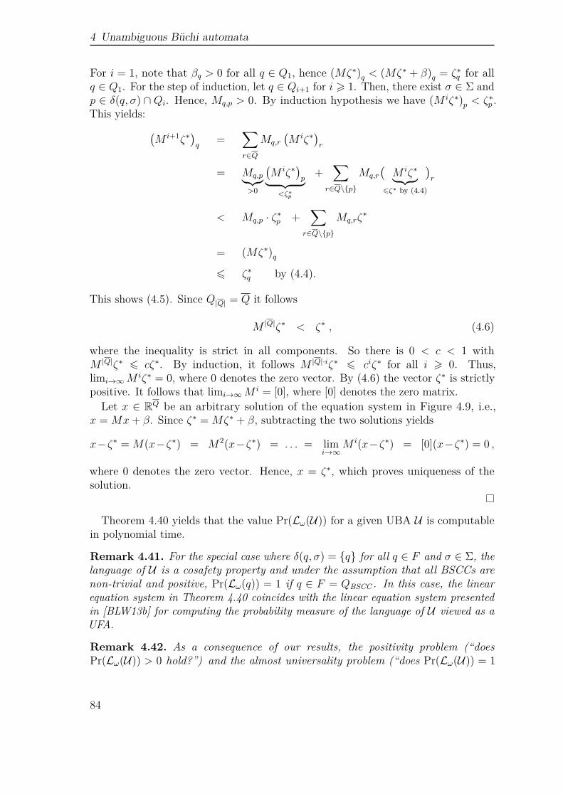
4 Unambiguous Büchi automata
For i = 1, note that βq > 0 for all q ∈ Q1, hence (Mζ∗)q < (Mζ∗ + β)q = ζ∗q for allq ∈ Q1. For the step of induction, let q ∈ Qi+1 for i ⩾ 1. Then, there exist σ ∈ Σ andp ∈ δ(q, σ) ∩ Qi. Hence, Mq,p > 0. By induction hypothesis we have (M iζ∗)p < ζ∗p .This yields: (
M i+1ζ∗)q
=∑r∈Q
Mq,r
(M iζ∗
)r
= Mq,p⏞⏟⏟⏞>0
(M iζ∗
)p⏞ ⏟⏟ ⏞
<ζ∗p
+∑
r∈Q\p
Mq,r
(M iζ∗⏞ ⏟⏟ ⏞
⩽ζ∗ by (4.4)
)r
< Mq,p · ζ∗p +∑
r∈Q\p
Mq,rζ∗
= (Mζ∗)q
⩽ ζ∗q by (4.4).
This shows (4.5). Since Q|Q| = Q it follows
M |Q|ζ∗ < ζ∗ , (4.6)
where the inequality is strict in all components. So there is 0 < c < 1 withM |Q|ζ∗ ⩽ cζ∗. By induction, it follows M |Q|·iζ∗ ⩽ ciζ∗ for all i ⩾ 0. Thus,limi→∞M iζ∗ = 0, where 0 denotes the zero vector. By (4.6) the vector ζ∗ is strictlypositive. It follows that limi→∞M i = [0], where [0] denotes the zero matrix.
Let x ∈ RQ be an arbitrary solution of the equation system in Figure 4.9, i.e.,x =Mx+ β. Since ζ∗ =Mζ∗ + β, subtracting the two solutions yields
x−ζ∗ =M(x−ζ∗) = M2(x−ζ∗) = . . . = limi→∞
M i(x−ζ∗) = [0](x−ζ∗) = 0 ,
where 0 denotes the zero vector. Hence, x = ζ∗, which proves uniqueness of thesolution.
Theorem 4.40 yields that the value Pr(Lω(U)) for a given UBA U is computablein polynomial time.
Remark 4.41. For the special case where δ(q, σ) = q for all q ∈ F and σ ∈ Σ, thelanguage of U is a cosafety property and under the assumption that all BSCCs arenon-trivial and positive, Pr(Lω(q)) = 1 if q ∈ F = QBSCC . In this case, the linearequation system in Theorem 4.40 coincides with the linear equation system presentedin [BLW13b] for computing the probability measure of the language of U viewed as aUFA.
Remark 4.42. As a consequence of our results, the positivity problem (“doesPr(Lω(U)) > 0 hold?”) and the almost universality problem (“does Pr(Lω(U)) = 1
84
4.1 Analysis of Markov chains against UBA-specifications
hold?”) for UBA are solvable in polynomial time. This should be contrasted with thestandard (non-probabilistic) semantics of UBA and the corresponding results for NBA.The non-emptiness problem for UBA is in P (this already holds for NBA), while thecomplexity-theoretic status of the universality problem for UBA is a long-standingopen problem. For standard NBA, it is well-known that the non-emptiness problemis in P and the universality problem is PSPACE-complete. However, the picturechanges when switching to NBA with the probabilistic semantics as both the positivityproblem and the almost universality problem for NBA are PSPACE-complete, evenfor strongly connected NBA.
Theorem 4.43 (see also [Var85; CY95]). The positivity and the almost universalityproblem for strongly connected NBA are PSPACE-complete.
Proof. Membership in PSPACE follows from the results of [Var85; CY95]. PSPACE-hardness of the positivity and almost universality problem for strongly connectedNBA can be established using a polynomial reduction from the universality problemfor non-deterministic finite automata (NFA) where all states are final. The latterproblem is known to be PSPACE-complete [KRS09].
Let B = (Q,Γ, δB, Q0,Reach (Q)) be an NFA. We can safely assume that Q0
is non-empty and all states are reachable from Q0. We define an NBA A =(Q,Σ, δA, Q0, Inf (Q)) over the alphabet Σ = Γ ∪ # as follows. If q ∈ Q anda ∈ Γ, then δA(q, a) = δB(q, a) and δA(q,#) = Q0. Clearly, A is strongly connected.Furthermore, δA(R,#) = Q0 for all non-empty subsets R of Q and δA(q, x#) = Q0
for all states q and all words x ∈ Σ∗ where δA(q, x) is non-empty.B is universal iff Lfin(B) = Γ∗
iff δB(Q0, y) = ∅ for all y ∈ Γ∗
iff δA(Q0, x) = ∅ for all x ∈ Σ∗
By Lemma 4.4 (see Section 4.1.3), B is universal iff Pr(Lω(A)) = 1. This yields thePSPACE-hardness of the almost universality problem for strongly connected NBA.Moreover, all singletons q can reach Q0, and if there is a non-trap BSCC C of Adet,then Q0 ∈ C. Using Corollary 4.9, we obtain:
B is universal iff Q0 is contained in some non-trap BSCC of Adet
iff Pr(Lω(A)) > 0
This yields the PSPACE-hardness of the positivity problem for strongly connectedNBA.
4.1.5 Probabilistic model checking of Markov chains againstUBA
To complete the proof of Theorem 4.1, we show how the results of the previous sectioncan be adapted to compute the value PrM(Lω(U)) for a Markov chainM = (S, P, ι)
85
4 Unambiguous Büchi automata
and a UBA U =(Q,Σ, δ, Q0, Inf (F )
)with alphabet Σ = S.4
For an NBA A over the alphabet S, we write PrM[s](A) for PrM[s](Π) where Πdenotes the set of infinite paths s0 s1 s2 s3 . . . in the Markov chainM such that s0 = sand s1 s2 s3 . . . ∈ Lω(A). Thus, PrM[s](A) = PrM[s](L) where L = sw : w ∈ Lω(A).In contrast, PrM[s](Lω(A)) denotes the probability of the set of infinite paths w inM that start in s and are accepted by A. Thus, PrM[s](Lω(A)) and PrM[s](A) mightbe different.
As a first step, we build a UBA P =M⊗ U that arises from the synchronousproduct of the UBA U with the underlying graph of the Markov chainM. Formally,ifM = (S, P, ι) is a Markov chainM and A =
(Q,S, δ,Q0, Inf (F )
)an NBA with
the alphabet S, then
M⊗A =(S ×Q,S,∆, Q′
0, Inf (S × F ))
whereQ′
0 =⟨s, q⟩ ∈ S ×Q : ι(s) > 0, q ∈ δ(Q0, s)
and for s, t ∈ S with P (s, t) > 0 and q ∈ Q:
∆(⟨s, q⟩, t) =⟨t, p⟩ : p ∈ δ(q, t)
If P (s, t) = 0, then ∆(⟨s, q⟩, t) = ∅. Given that M viewed as an automaton overthe alphabet S behaves deterministically, the NBAM⊗A is unambiguous if A is aUBA.
To adapt the soundness proofs accordingly we need to “relativize” the probabilitiesfor words in S∗ according to the paths inM. That is, we have to switch from theuniform probability measure Pr over the σ-algebra spanned by the cylinder sets ofthe finite words Cyl(x) = xw : w ∈ Σω to the measures PrM[s] induced by thestates ofM.
We now illustrate how the proofs can be adapted by a few central statements.
Lemma 4.44 (cf. Lemma 4.2). Let s ∈ S be a state of M and L ⊆ Sω be anω-regular language with PrM[s](L) > 0. Then, there exists a finite path x ∈ S∗
starting in state s such that almost all extensions of x belong to L according to themeasure PrM[s], i.e.,
PrM[s]
w ∈ L : x ∈ Pref(w)
= PrM[s]
(Cyl(x)
)where Pref(w) denotes the set of finite prefixes of w.
4In practice, e.g., when the UBA is obtained from an LTL formula, the alphabet of the UBAis often defined as Σ = 2AP over a set of atomic propositions AP and the Markov chain isequipped with a labeling function from states to the atomic propositions that hold in each state.Clearly, unambiguity w.r.t. the alphabet 2AP implies unambiguity w.r.t. the alphabet S whenswitching from the original transition function δ : Q × 2AP → 2Q to the transition functionδS : Q×S → 2Q given by δS(q, s) = δ(q, L(s)), where L : S → 2AP denotes the labeling functionof M.
86
4.1 Analysis of Markov chains against UBA-specifications
Proof. The argument is fairly the same as in the proof of Lemma 4.2. We regard adeterministic automaton D for L and consider the product Markov chainM⊗D. Inthis context, we considerM as a transition-labeled Markov chain where all outgoingtransitions of state s are labeled with s. If PrM[s](L) is positive, then there is a finitepath x from s such that the lifting of x from ⟨s, qinit⟩ in the product ends in a statethat belongs to some BSCC where the acceptance condition of D holds. But then,w ∈ L for almost all infinite paths w inM with x ∈ Pref(w).
Lemma 4.45 (Generalization of Lemma 4.4). For each NBA A over the alphabet SwhereM⊗A is strongly connected we have:
PrM(Lω(A)
)= 1− PrM
w ∈ Sω : δ(Q0, x) = ∅ for some x ∈ Pref(w)
In particular, PrM(Lω(A) ) = 1 if and only if δ(Q0, x) = ∅ for all finite wordsx ∈ S+ where x is a finite path inM starting in s.
Proof. The arguments transfers from the proof of Lemma 4.4. Instead of Fact 4.6, wecan rely on the original result of [CY95] for checking whether PrM(Lω(A)) > 0 fora given Markov chainM. Note that the only reference to the probability measureis in the form “almost all words in L enjoy property XY” which simply means “thewords in L not satisfying XY constitute a null set”. At a few places we used 1/|Σ||x|as the measure of (the cylinder set spanned by) the finite word x as label of somepath from state p to q. The value 1/|Σ||x| has to be replaced with Prs(Cyl(x)) for thecorresponding state s inM. Note that if ⟨s, p⟩ x−→ ⟨t, q⟩ inM⊗A, then Prs(Cyl(x))is positive.
Our algorithm relies on the observation that
PrM(Lω(U)) =∑s∈S
ι(s) · PrM[s](U [δ(Q0, s)] )
for a Markov ChainM and UBA U . As the languages of the UBA U [q] for q ∈ δ(Q0, s)are pairwise distinct (by the unambiguity of U), we have PrM[s](U [δ(Q0, s)]) =∑
q∈δ(Q0,s)PrM[s](U [q]). Thus, the task is to compute the values PrM[s](U [q]) for
s ∈ S and q ∈ Q.Let P [s, q] denote the UBA resulting from P by declaring ⟨s, q⟩ to be initial. It
is easy to see that PrM[s](P [s, q] ) = PrM[s](U [q] ) for all states ⟨s, q⟩ of P, as theproduct construction only removes transitions in U that can not occur in the Markovchain. Our goal is thus to compute the values PrM[s](P [s, q]). For this, we removeall states ⟨s, q⟩ from P that can not reach a state in S × F . Then, we determinethe non-trivial SCCs of P and, for each such SCC C, we analyze the sub-UBAPC obtained by restricting to the states in C. An SCC C of P is called positive if
PrM[s](PC[s, q]) > 0 for all/any ⟨s, q⟩ ∈ C. As in Section 4.1.4, we treat the SCCs
in a bottom-up manner, starting with the BSCCs and removing them if they are
87
4 Unambiguous Büchi automata
non-positive. Clearly, if a BSCC C of P does not contain a final state or is trivial, thenC is not positive. Analogously to Lemma 4.17, we can check whether a non-trivialBSCC C in P containing at least one final state is positive by analyzing a linearequation system.
Lemma 4.46 (cf. Lemma 4.17). Let C be a BSCC of P and
(∗) ζs,q =∑
t∈Post(s)
∑p∈δC(q,t)
P (s, t) · ζt,p for all ⟨s, q⟩ ∈ C.
Then, the following statements are equivalent:
(1) C is positive,
(2) the linear equation system (∗) has a positive solution,
(3) the linear equation system (∗) has a non-zero solution.
Proof. The proof of Lemma 4.17 presented in Section 4.1.3 is directly applicable hereas well by considering the |C| × |C|-matrix M with
M⟨s,q⟩,⟨t,p⟩ =
P (s, t) : if p ∈ δ(q, t)0 : otherwise
Note that the matrix M is non-negative and irreducible and the entry in the n-thpower of M for state ⟨s, q⟩ and ⟨t, p⟩ is the probability with respect to PrM[s] of allinfinite paths w = s0 s1 s2 . . . inM with s0 = s such that p ∈ ∆C(q, s1 . . . sn). (Recallthat ∆C denotes the transition relation of P restricted to C.)
We now explain how to adapt the cut-based approach of Section 4.1.3 for computingthe probabilities in a positive BSCC C of P .
For ⟨s, q⟩ ∈ C and t ∈ S, let ∆C(⟨s, q⟩, t) = ∆(⟨s, q⟩, t)∩C. A pure cut in C denotesa set C ⊆ C such that PrM[s](P [C]) = 1 and C = ∆C(⟨s, q⟩, z) for some ⟨s, q⟩ ∈ Cand some finite word z ∈ S∗ such that s z is a cycle inM. (In particular, the lastsymbol of z is s, and therefore C ⊆ ⟨s, p⟩ ∈ C : p ∈ Q.)
Using Lemma 4.45 we can now adapt Corollary 4.24 and obtain:
Corollary 4.47 (Pure cuts in BSCCs of the product; cf. Corollary 4.24). Let C be apositive BSCC of P with at least one final state. Then, for each state ⟨s, q⟩ ∈ C andeach finite word x, the following two statements are equivalent:
(a) ⟨s, p⟩ : p ∈ δC(q, x) is a pure cut.
(b) For each y ∈ S∗, there is some p ∈ δC(q, x) such that ∆C(⟨s, p⟩, y) = ∅.
As before, let C be a positive BSCC of the product-UBA P . Given a state ⟨s, q⟩in C and a word z ∈ S∗, a word y ∈ S∗ is said to be an extension of (⟨s, q⟩, z) if thefollowing two conditions hold:
88
4.1 Analysis of Markov chains against UBA-specifications
(1) s y is a cycle in the Markov chainM
(2) there exists a state p ∈ Q \ q in U such that ∆C(⟨s, p⟩, z) = ∅ and⟨s, q⟩, ⟨s, p⟩ ⊆ ∆C(⟨s, q⟩, y).
Note that (1) implies, if y = t0 t1 . . . tm, then t0 ∈ Post(s) and tm = s. In whatfollows, for s, t ∈ S, q, p ∈ Q and x ∈ S∗, we often write
⟨s, q⟩ x−→C ⟨t, p⟩
to indicate that ⟨t, p⟩ ∈ ∆C(⟨s, q⟩, x).
Lemma 4.48 (cf. Lemma 4.32). If y is an extension of (⟨s, q⟩, z), then ∆C(⟨s, q⟩, yz)is a proper superset of ∆C(⟨s, q⟩, z).
Proof. Let p ∈ Q \ q in U such that ∆C(⟨s, p⟩, z) = ∅ and ⟨s, q⟩, ⟨s, p⟩ ⊆∆C(⟨s, q⟩, y) (see condition (2)).
We first show that ∆C(⟨s, q⟩, z) ⊆ ∆C(⟨s, q⟩, yz). For this, we pick a pair ⟨t, r⟩ ∈∆C(⟨s, q⟩, z). By condition (2) of extensions, we have ⟨s, q⟩ ∈ ∆C(⟨s, q⟩, z). Then:
⟨s, q⟩ y−→C ⟨s, q⟩z−→C ⟨t, r⟩
and therefore ⟨t, r⟩ ∈ ∆C(⟨s, q⟩, yz).To show that the inclusion is strict we prove that ∆C(⟨s, p⟩, z) ∩∆C(⟨s, q⟩, z) = ∅.
We suppose by contradiction that ⟨t, r⟩ ∈ ∆C(⟨s, p⟩, z) ∩∆C(⟨s, q⟩, z). Then:
⟨s, q⟩ y−→C ⟨s, q⟩z−→C ⟨t, r⟩ and ⟨s, q⟩ y−→C ⟨s, p⟩
z−→C ⟨t, r⟩
But then q y−→ qz−→ t and q y−→ p
z−→ t in U . This is impossible by the unambiguityof U .
Lemma 4.49 (cf. Lemma 4.33). As before, let C be a positive BSCC of P. Then foreach ⟨s, q⟩ ∈ C and word z ∈ S+ where the last symbol is s:
∆C(⟨s, q⟩, z) is a pure cut iff the pair (⟨s, q⟩, z) has no extension
Proof. The proof is fairly similar to the proof of Lemma 4.33.“=⇒”: Let C = ∆C(⟨s, q⟩, z) be a pure cut. Suppose by contradiction that there
exists an extension y for (⟨s, q⟩, z). Let p ∈ Q such that q = p, ∆C(⟨s, p⟩, z) = ∅and ⟨s, q⟩, ⟨s, p⟩ ⊆ ∆C(⟨s, q⟩, y). By Lemma 4.48, the set ∆C(⟨s, q⟩, yz) is a propersuperset of ∆(⟨s, q⟩, z). As C is positive, we have PrMu (P [u, r] ) > 0 for all ⟨u, r⟩ ∈ C.With an argument as in the proof of Lemma 4.33 we obtain:
PrM[s]
(P [∆C(⟨s, q⟩, yz)]
)> PrM[s]
(P [∆C(⟨s, q⟩, z)]
)Hence, PrM[s]
(P [∆C(⟨s, q⟩, z)]
)< 1. But then ∆C(⟨s, q⟩, z) cannot be a pure cut.
Contradiction.
89
4 Unambiguous Büchi automata
“⇐=”: Suppose now that (⟨s, q⟩, z) has no extension. To prove that C =∆C(⟨s, q⟩, z) is a cut we rely on the second part of Lemma 4.45. Thus, the taskis to show that ∆C(C, x) = ∅ for all finite words x ∈ S+ where x is a finite path inM starting in s. To prove this, one first shows that C is contained in some pure cutR of the form ∆C(⟨s, r⟩, z) for some state r ∈ Q. As the last symbol of z is s, theelements of R have the form ⟨s, r⟩ for some r ∈ Q. For each state p ∈ Q \ q where⟨s, p⟩ /∈ R, there is some finite word y with
⟨s, q⟩ y−→C ⟨s, q⟩y−→C ⟨s, p⟩
For this we can rely on an adaption of Lemma 4.29. Since there exists no extensionfor (⟨s, q⟩, z), we have ∆C(⟨s, p⟩, z) = ∅ for all states p ∈ Q where ⟨s, p⟩ /∈ C. Thisyields:
C = ∆C(⟨s, q⟩, z) = ∆C(C, z) = ∆C(R, z)
Using that R is a pure cut, we can now apply Lemma 4.45 to obtain the claim.
To compute a pure cut in C, we pick an arbitrary state ⟨s, q⟩ in C and successivelygenerate path fragments z0, z1, . . . , zk ∈ S∗ inM by adding prefixes. More precisely,z0 = ε and zi+1 has the form yzi for some y ∈ S+ such that (1) s y is a cyclein M and (2) there exists a state p ∈ Q \ q in U with ∆C(⟨s, p⟩, zi) = ∅ and⟨s, q⟩, ⟨s, p⟩ ⊆ ∆C(⟨s, q⟩, y). Each such word y is called an extension of (⟨s, q⟩, zi),and ∆C(⟨s, q⟩, zi+1) = ∆C(⟨s, q⟩, yzi) is a proper superset of ∆C(⟨s, q⟩, zi). The setC = ∆C(⟨s, q⟩, z) is a pure cut if and only if (⟨s, q⟩, zi) has no extension. The searchfor an extension can be realized efficiently using a technique similar to the onepresented in Section 4.1.3. Thus, after at most min|C|, |Q| iterations, we obtain apure cut C.
Having computed a pure cut C of C, the values PrMs (P [s, q]) for ⟨s, q⟩ ∈ C arethen computable as the unique solution of the linear equation system consisting ofequations (*) and the additional equation
∑⟨s,q⟩∈C ζs,q = 1.
Theorem 4.50 (cf. Theorem 4.35). Let C be a positive BSCC of P and C a pure cutfor C. Then, the probability vector (PrM[s](Lω(P [s, q]) )⟨s,q⟩∈C is the unique solutionof the following linear equation system:
(1) ζs,q =∑
t∈Post(s)
∑p∈δC(q,t)
P (s, t) · ζt,p for all ⟨s, q⟩ ∈ C
(2)∑
⟨s,q⟩∈C
ζs,q = 1
Proof. It is easy to see that the vector (ζ∗⟨s,q⟩)⟨s,q⟩∈C with
ζ∗⟨s,q⟩ = PrM[s](Lω(P [s, q]) )
90
4.1 Analysis of Markov chains against UBA-specifications
is indeed a solution of (1) and (2). For the uniqueness, we rely on the proofpresented for Theorem 4.35 in Section 4.1.3 with the |C| × |C|-matrix M defined byM⟨s,q⟩,⟨t,p⟩ = P (s, t) if p ∈ δ(q, t) and M⟨s,q⟩,⟨t,p⟩ = 0 otherwise.
Given a non-trivial, non-bottom SCC of P and a state ⟨s, q⟩ ∈ C, we writeC[s, q] to denote the sub-UBA of P that arises when declaring ⟨s, q⟩ as initialstate and restricting the transitions of P to those inside C. That is, C[t, p] =(C, S,∆C, ⟨s, q⟩, Inf (F ∩ C)
). Then, C is positive iff PrM[s](C[s, q]) > 0 for some state
⟨s, q⟩ ∈ C iff PrM[s](C[s, q]) > 0 for all states ⟨s, q⟩ ∈ C.In this way we adapt Theorem 4.35 to obtain the values PrM[s](P [s, q]) for the
states ⟨s, q⟩ belonging to some positive BSCC of P. It remains to explain how toadapt the equation system of Theorem 4.40.
Recall that we assume a preprocessing that treats the SCCs of P in a bottom-upmanner and turns P into a UBA where all BSCCs are non-trivial and positive. QBSCCdenotes the set of states that are contained in some BSCC of P and Q? denotes thestates of (the modified UBA) P not contained in QBSCC . For ⟨s, q⟩ ∈ Q?, let βs,q = 0if ∆(⟨s, q⟩, t) ∩QBSCC = ∅ for all t ∈ S. Otherwise:
βs,q =∑
t∈Post(s)
∑p ∈ δ(q, t) s.t.⟨t, p⟩ ∈ QBSCC
P (s, t) · PrM[t](P [t, p] )
Theorem 4.51 (cf. Theorem 4.40). Notations and assumptions as before. Then, thevector (PrM[s](P [s, q]))⟨s,q⟩∈Q?
is the unique solution of the following linear equationsystem:
ζs,q =∑
t∈Post(s)
∑p ∈ δ(q, t) s.t.⟨t, p⟩ /∈ QBSCC
P (s, t) · ζt,p + βs,q for ⟨s, q⟩ ∈ Q?
Proof. It is easy to see that the vector (PrM[s](P [s, q]))⟨s,q⟩∈Q?indeed solves the linear
equation system. For the uniqueness of the solution, we can apply the same argumentsas in the proof of Theorem 4.40, but now for the |Q?| × |Q?|-matrix M given byM⟨s,q⟩,⟨t,p⟩ = P (s, t) if p ∈ δ(q, t) and M⟨s,q⟩,⟨t,p⟩ = 0 otherwise, where ⟨s, q⟩ and ⟨t, p⟩range over all states in Q?.
Let QBSCC be the set of BSCC states of P and Q? be the states of P not containedin QBSCC . For ⟨s, q⟩ ∈ Q?, let βs,q = 0 if ∆(⟨s, q⟩, t) ∩ QBSCC = ∅ for all t ∈ S.Otherwise:
βs,q =∑
t∈Post(s)
∑p ∈ δ(q, t) s.t.⟨t, p⟩ ∈ QBSCC
P (s, t) · PrM[t](P [t, p] )
91
4 Unambiguous Büchi automata
Then, the vector (PrM[s](P [s, q]))⟨s,q⟩∈Q?is the unique solution of the linear equation
system
ζs,q =∑
t∈Post(s)
∑p ∈ δ(q, t) s.t.⟨t, p⟩ /∈ QBSCC
P (s, t) · ζt,p + βs,q for ⟨s, q⟩ ∈ Q?
This completes the proof of Theorem 4.1.
4.1.6 Separated Büchi automataRecall that an NBA is called separated if the languages of its states are pairwisedisjoint. Obviously, each separated NBA is unambiguous. Although separated Büchiautomata are as powerful as the full class of NBA [CM03] and translations of LTLformulas into separated UBA of (single) exponential time complexity exist [WVS83;CSS03], non-separated UBA and even deterministic automata can be exponentiallymore succinct than separated UBA [BL10].
We now explain in which sense our algorithm for (possibly non-separated) UBAcan be seen as a conservative extension of the approach presented by Couvreur, Saheband Sutre [CSS03]. To keep the presentation simple, we consider the techniques tocompute Pr(Lω(U)). Analogous statements hold for the computation of PrM(Lω(U))for a given Markov chainM.
Given a separated, strongly connected UBA U =(Q,Σ, δ, Q0, Inf (F )
)with at least
one initial and one final state, we have:
Pr(Lω(U)) > 0 iff Q is a reachable cut
Furthermore, Q is a cut iff δ(Q, a) = Q for all a ∈ Σ (Lemma 4.4). Thus, for thespecial case where the given UBA is separated and positive, there is no need for theinductive construction of a cut as outlined in Section 4.1.3. Instead, we can dealwith C = Q. The linear equations in Theorem 4.35 can be derived from the resultspresented in [CSS03]. More precisely, equation (1) corresponds to the equation systemin Proposition 5.1 of [CSS03], while equation (2) can be rephrased to
∑q∈Q ζq = 1,
which corresponds to the equation used in Proposition 5.2 of [CSS03].To check whether Q is a cut for a given (possibly non-positive) separated, strongly
connected UBA, [CSS03] presents a simple criterion that is based on a countingargument. Lemma 4.14 in [CSS03] yields that for separated, strongly connected UBAwe have:
Q is a cut iff |Σ| · |Q| = |δ|
where |δ| is the total number of transitions in U given by∑q∈Q
∑σ∈Σ|δ(q, σ)|.
92
4.2 Implementation and Experiments
4.2 Implementation and ExperimentsWe implemented a probabilistic model checking procedure for Markov chains andUBA specifications using the algorithm detailed in Section 4.1 as an extension to theprobabilistic model checker PRISM [KNP11] version 4.4 beta. All experiments werecarried out on a computer with two Intel E5-2680 8-core CPUs at 2.70 GHz with384GB of RAM running Linux, a time limit of 30 minutes and a memory limit of10GB, if not stated otherwise. Our implementation is based on the explicit engine ofPRISM, where the Markov chain is represented explicitly. Our implementation supportsUBA-based model checking for handling the LTL fragment of PRISM’s PCTL∗-likespecification language as well as direct verification against a path specification givenby a UBA provided in the HOA format [Bab+15]. For LTL formulas, we rely onexternal LTL-to-UBA translators. For the purpose of the benchmarks we employthe ltl2tgba tool from SPOT [Dur14] version 2.5 to generate a UBA for a given LTLformula. The according implementation, as well as the data logs can be found at[Mül18].
For the linear algebra parts of the algorithms, we rely on the COLT library [Hos04].We considered two different variants for the SCC computations. The first variant(see page 73) relies on COLT to perform a QR decomposition of the matrix for the SCCto compute its rank, which allows to decide the positivity of the SCC. The secondapproach (see page 81) relies on a variant of the power iteration method for iterativelycomputing an eigenvector. This method has the benefit that, in addition to decidingthe positivity, the computed eigenvector can be directly used to compute the valuesfor a positive SCC, once a cut has been found. (As the proof of Theorem 4.35 shows:Pr(Lω(q)) = ζ∗q /
∑p∈C ζ
∗p if ζ∗ is an eigenvector of the matrix M for eigenvalue 1.)
We evaluated the performance and scalability of the cut generation algorithm togetherwith both approaches for treating SCCs. For this purpose we selected automataspecifications that are challenging for our UBA-based model checking approach. Asthe power iteration method performed better, our benchmark results presented inthis section are based on power iteration method for the SCC handling.
4.2.1 Evaluation of the rank computationTo assess the scalability of our implementation in the face of particularly difficultUBA, we considered two families of parametrized UBA. Both have an alphabet definedover a single atomic proposition resulting in a two-element alphabet that we use torepresent either a 0 or a 1 bit. The first automaton (“complete automaton”), depictedin Figure 4.10 on the left for k = 2, is a complete automaton, i.e., recognizes Σω. Itconsists of a single, accepting starting state that non-deterministically branches toone of 2k states, each one leading after a further step to a k-state chain that only letsa particular k-bit bitstring pass, subsequently returning to the initial state. As allthe k-bit bitstrings that can occur have a chain, the automaton is complete. Likewise,the automaton is unambiguous as each of the bitstrings can only pass via one of thechains.
93
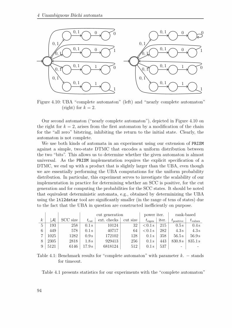
4 Unambiguous Büchi automata
0, 1
0, 1
0, 1
0, 1
0, 1
0, 1
0, 1
0, 1
1
1
0
0 0
1
0
1
0, 1
0, 1
0, 1
0, 1
0, 1
0, 1
0, 1
0, 1
1
1
0
0 0
1
0
1
Figure 4.10: UBA “complete automaton” (left) and “nearly complete automaton”(right) for k = 2.
Our second automaton (“nearly complete automaton”), depicted in Figure 4.10 onthe right for k = 2, arises from the first automaton by a modification of the chainfor the “all zero” bitstring, inhibiting the return to the initial state. Clearly, theautomaton is not complete.
We use both kinds of automata in an experiment using our extension of PRISMagainst a simple, two-state DTMC that encodes a uniform distribution betweenthe two “bits”. This allows us to determine whether the given automaton is almostuniversal. As the PRISM implementation requires the explicit specification of aDTMC, we end up with a product that is slightly larger than the UBA, even thoughwe are essentially performing the UBA computations for the uniform probabilitydistribution. In particular, this experiment serves to investigate the scalability of ourimplementation in practice for determining whether an SCC is positive, for the cutgeneration and for computing the probabilities for the SCC states. It should be notedthat equivalent deterministic automata, e.g., obtained by determinizing the UBAusing the ltl2dstar tool are significantly smaller (in the range of tens of states) dueto the fact that the UBA in question are constructed inefficiently on purpose.
cut generation power iter. rank-basedk |A| SCC size tcut ext. checks cut size teigen iter. tpositive tvalues5 193 258 0.1 s 10124 32 <0.1 s 215 0.5 s 0.4 s6 449 578 0.1 s 40717 64 <0.1 s 282 4.3 s 4.3 s7 1025 1282 0.9 s 172102 128 0.1 s 358 56.5 s 56.9 s8 2305 2818 1.8 s 929413 256 0.1 s 443 830.8 s 835.1 s9 5121 6146 17.9 s 6818124 512 0.1 s 537 - -
Table 4.1: Benchmark results for “complete automaton” with parameter k. − standsfor timeout.
Table 4.1 presents statistics for our experiments with the “complete automaton”
94
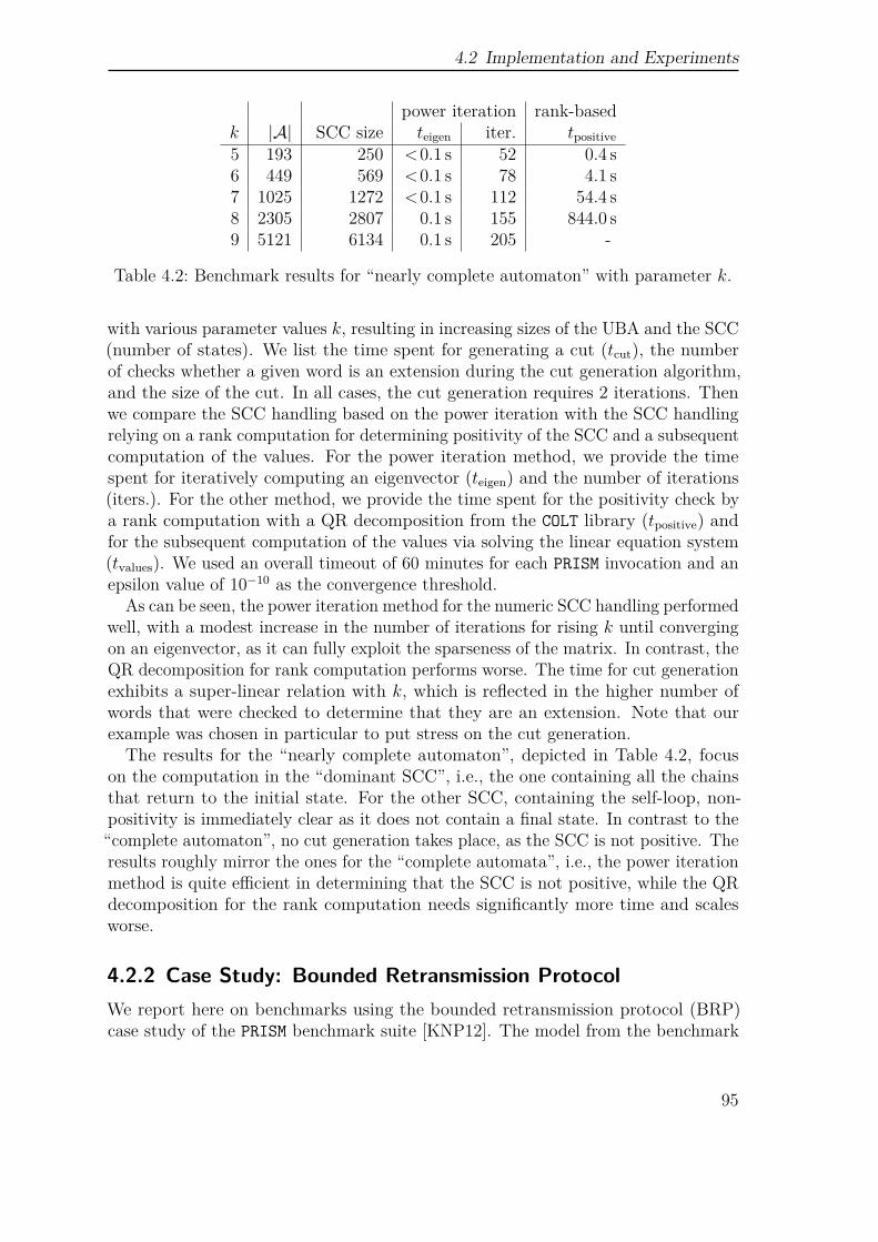
4.2 Implementation and Experiments
power iteration rank-basedk |A| SCC size teigen iter. tpositive5 193 250 <0.1 s 52 0.4 s6 449 569 <0.1 s 78 4.1 s7 1025 1272 <0.1 s 112 54.4 s8 2305 2807 0.1 s 155 844.0 s9 5121 6134 0.1 s 205 -
Table 4.2: Benchmark results for “nearly complete automaton” with parameter k.
with various parameter values k, resulting in increasing sizes of the UBA and the SCC(number of states). We list the time spent for generating a cut (tcut), the numberof checks whether a given word is an extension during the cut generation algorithm,and the size of the cut. In all cases, the cut generation requires 2 iterations. Thenwe compare the SCC handling based on the power iteration with the SCC handlingrelying on a rank computation for determining positivity of the SCC and a subsequentcomputation of the values. For the power iteration method, we provide the timespent for iteratively computing an eigenvector (teigen) and the number of iterations(iters.). For the other method, we provide the time spent for the positivity check bya rank computation with a QR decomposition from the COLT library (tpositive) andfor the subsequent computation of the values via solving the linear equation system(tvalues). We used an overall timeout of 60 minutes for each PRISM invocation and anepsilon value of 10−10 as the convergence threshold.
As can be seen, the power iteration method for the numeric SCC handling performedwell, with a modest increase in the number of iterations for rising k until convergingon an eigenvector, as it can fully exploit the sparseness of the matrix. In contrast, theQR decomposition for rank computation performs worse. The time for cut generationexhibits a super-linear relation with k, which is reflected in the higher number ofwords that were checked to determine that they are an extension. Note that ourexample was chosen in particular to put stress on the cut generation.
The results for the “nearly complete automaton”, depicted in Table 4.2, focuson the computation in the “dominant SCC”, i.e., the one containing all the chainsthat return to the initial state. For the other SCC, containing the self-loop, non-positivity is immediately clear as it does not contain a final state. In contrast to the“complete automaton”, no cut generation takes place, as the SCC is not positive. Theresults roughly mirror the ones for the “complete automata”, i.e., the power iterationmethod is quite efficient in determining that the SCC is not positive, while the QRdecomposition for the rank computation needs significantly more time and scalesworse.
4.2.2 Case Study: Bounded Retransmission ProtocolWe report here on benchmarks using the bounded retransmission protocol (BRP)case study of the PRISM benchmark suite [KNP12]. The model from the benchmark
95
4 Unambiguous Büchi automata
suite covers a single message transmission, retrying for a bounded number of timesin case of an error. We have slightly modified the model to allow the transmissionof an infinite number of messages by restarting the protocol once a message hasbeen successfully delivered or the bound for retransmissions has been reached. Wewill include benchmarks with pre-generated automata, as well as benchmarks withLTL as starting point. For the LTL benchmarks we have implemented the iterativerefinement method presented in [CY95], as it is also a single-exponential approach.We call this implementation PRISM CY95. The benchmarks include also an evaluationfor deterministic Emerson-Lei automata generated by Delag, which we present inChapter 5.
Automata based specifications. We consider the property “the message was re-transmitted k steps before an acknowledgment.” To remove the effect of selectingspecific tools for the LTL-to-automaton translation (ltl2tgba for UBA, the Java-based PRISM reimplementation of ltl2dstar [KB06] to obtain a deterministic Rabinautomaton (DRA) for the standard PRISM approach), we consider directly modelchecking against automata specifications at first. As the language of the propertyis equivalent to the UBA depicted in Figure 4.1 (on the left) when a stands for aretransmission, b for an acknowledgment, and c for no acknowledgment, we use thisautomaton and the minimal DBA for the language (this case is denoted by Ak).We additionally consider the UBA and DBA obtained by replacing the self-loop inthe last state with a switch back to the initial state (denoted by Bk), i.e., roughlyapplying the ω-operator to Ak.
Table 4.3 shows results for selected k (with a timeout of 30 minutes), demonstratingthat for this case study and properties our UBA-based implementation is generallycompetitive with the standard approach of PRISM relying on deterministic automata.For Ak, our implementation detects that the UBA has a special shape where all finalstates have a true-self loop which allows skipping the SCC handling. Without thisoptimization, tPos are in the sub-second range for all considered Ak. At a certainpoint, the implementation of the standard approach in PRISM becomes unsuccessful,due to PRISM size limitations in the product construction of the Markov chain and thedeterministic automaton (Ak/Bk: k ⩾ 16). As can be seen, using the UBA approachwe were able to successfully scale the parameter k beyond 48 when dealing directlywith the automata-based specifications (Ak/Bk) and within reasonable time requiredfor model checking.
LTL based specifications. We consider here two LTL properties: The first one is:
ϕk = (¬ack_received) U(retransmit ∧ (¬ack_received U =k ack_received)
),
where aU =kb stands for a∧¬b∧⃝(a∧¬b)∧ . . .∧⃝k−1(a∧¬b)∧⃝kb. The formulaϕk ensures that k steps before an acknowledgment the message was retransmitted.Hence, it is equivalent to the property described by the automaton Ak. For theLTL-to-automata translation we included the Java-based PRISM reimplementation
96
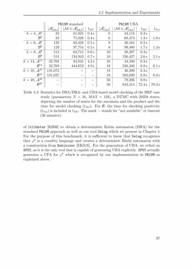
4.2 Implementation and Experiments
PRISM standard PRISM UBA|AkDRA| |M⊗AkDRA| tMC |AkUBA| |M⊗AkUBA| tMC tPos
k = 4, A4 33 61,025 0.4 s 6 34,118 0.3 sB4 33 75,026 0.4 s 6 68,474 1.3 s 1.0 s
k = 6, A6 129 62,428 0.5 s 8 36,164 0.2 sB6 129 97,754 0.5 s 8 99,460 1.7 s 1.3 s
k = 8, A8 513 64,715 0.6 s 10 38,207 0.3 sB8 513 134,943 0.7 s 10 136,427 2.6 s 2.1 s
k = 14, A14 32,769 83,845 4.2 s 16 44,340 0.3 sB14 32,769 444,653 4.9 s 16 246,346 6.8 s 6.1 s
k = 16, A16 131,073 − − 18 46,390 0.3 sB16 131,037 − − 18 282,699 8.9 s 8.0 s
k = 48, A48 − − − 50 79,206 0.8 sB48 − − − 50 843,414 72.4 s 70.3 s
Table 4.3: Statistics for DBA/DRA- and UBA-based model checking of the BRP casestudy (parameters N = 16, MAX = 128), a DTMC with 29358 states,depicting the number of states for the automata and the product and thetime for model checking (tMC). For B, the time for checking positivity(tPos) is included in tMC. The mark − stands for “not available” or timeout(30 minutes).
of ltl2dstar [KB06] to obtain a deterministic Rabin automaton (DRA) for thestandard PRISM approach as well as our tool Delag which we present in Chapter 5.For the purpose of this benchmark, it is sufficient to know that Delag recognizesthat ϕk is a cosafety language and creates a deterministic Büchi automaton witha construction from Rabinizer [EKS16]. For the generation of UBA, we relied onSPOT, as it is the only tool that is capable of generating UBA explicitly. SPOT actuallygenerates a UFA for ϕk which is recognized by our implementation in PRISM asexplained above.
97
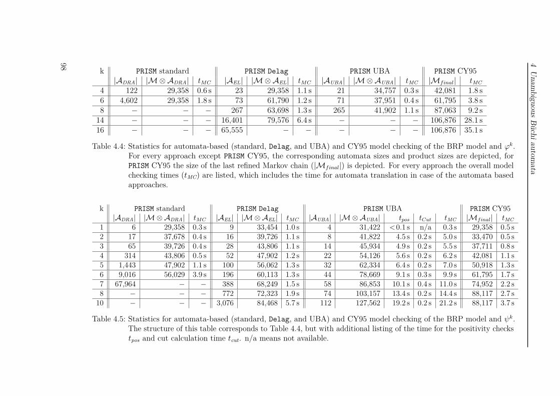
4U
nambiguous
Büchiautom
ata
k PRISM standard PRISM Delag PRISM UBA PRISM CY95|ADRA| |M⊗ADRA| tMC |AEL| |M⊗AEL| tMC |AUBA| |M⊗AUBA| tMC |Mfinal| tMC
4 122 29,358 0.6 s 23 29,358 1.1 s 21 34,757 0.3 s 42,081 1.8 s6 4,602 29,358 1.8 s 73 61,790 1.2 s 71 37,951 0.4 s 61,795 3.8 s8 − − − 267 63,698 1.3 s 265 41,902 1.1 s 87,063 9.2 s14 − − − 16,401 79,576 6.4 s − − − 106,876 28.1 s16 − − − 65,555 − − − − − 106,876 35.1 s
Table 4.4: Statistics for automata-based (standard, Delag, and UBA) and CY95 model checking of the BRP model and ϕk.For every approach except PRISM CY95, the corresponding automata sizes and product sizes are depicted, forPRISM CY95 the size of the last refined Markov chain (|Mfinal|) is depicted. For every approach the overall modelchecking times (tMC) are listed, which includes the time for automata translation in case of the automata basedapproaches.
k PRISM standard PRISM Delag PRISM UBA PRISM CY95|ADRA| |M⊗ADRA| tMC |AEL| |M⊗AEL| tMC |AUBA| |M⊗AUBA| tpos tCut tMC |Mfinal| tMC
1 6 29,358 0.3 s 9 33,454 1.0 s 4 31,422 <0.1 s n/a 0.3 s 29,358 0.5 s2 17 37,678 0.4 s 16 39,726 1.1 s 8 41,822 4.5 s 0.2 s 5.0 s 33,470 0.5 s3 65 39,726 0.4 s 28 43,806 1.1 s 14 45,934 4.9 s 0.2 s 5.5 s 37,711 0.8 s4 314 43,806 0.5 s 52 47,902 1.2 s 22 54,126 5.6 s 0.2 s 6.2 s 42,081 1.1 s5 1,443 47,902 1.1 s 100 56,062 1.3 s 32 62,334 6.4 s 0.2 s 7.0 s 50,918 1.3 s6 9,016 56,029 3.9 s 196 60,113 1.3 s 44 78,669 9.1 s 0.3 s 9.9 s 61,795 1.7 s7 67,964 − − 388 68,249 1.5 s 58 86,853 10.1 s 0.4 s 11.0 s 74,952 2.2 s8 − − − 772 72,323 1.9 s 74 103,157 13.4 s 0.2 s 14.4 s 88,117 2.7 s10 − − − 3,076 84,468 5.7 s 112 127,562 19.2 s 0.2 s 21.2 s 88,117 3.7 s
Table 4.5: Statistics for automata-based (standard, Delag, and UBA) and CY95 model checking of the BRP model and ψk.The structure of this table corresponds to Table 4.4, but with additional listing of the time for the positivity checkstpos and cut calculation time tcut. n/a means not available.
98
4.2 Implementation and Experiments
Table 4.4 lists the results for model checking ϕk. From a certain point on, theimplementation of the standard approach in PRISM is unsuccessful, due to PRISMrestriction in the DRA construction (k ⩾ 8) or a timeout during UBA construction(k ⩾ 13). If PRISM (vs. SPOT or Delag) was able to construct an automaton, thenthe automata-based approaches were faster than PRISM CY95. Delag comes closeto produce deterministic automata with the possible 2k states, but SPOT producesunnecessary large UBA for ϕk. This is reflected in the model checking runtimes wherethe UBA approach is the fastest for k ≤ 8, but this turns for k ≥ 9, where the UBAapproach took 3.1s, and PRISM Delag took 1.3s. For k ≥ 13, SPOT was not able toproduce a UBA within the time bound of 30min.
As second formula we investigate
ψk = (msg_send→ ♦(ack_send ∧ ♦⩽kack_received)),
where ♦⩽ka denotes a ∨⃝(a ∨⃝(. . . ∨⃝a))⏞ ⏟⏟ ⏞k times
. This formula requires that every
request (sending a message and waiting for an acknowledgment) is eventually re-sponded by an answer (the receiver of the message sends an acknowledgment andthis acknowledgment is received within the next k steps).
Table 4.5 summarizes the result of the benchmark for ψk. Here, the PRISM standardapproach with its own implementation of ltl2dstar was able to finish the calculationsuntil k = 6. For k = 7, PRISM standard was able to construct the DRA (with 67,964states and within 27.5 seconds), but not able to construct the product anymore. Incase of Delag, ψk does not belong to the natively supported fragment, and SPOT isused as the fallback solution to generate a deterministic automaton.
In contrast to the deterministic automata, the UBA sizes increase moderately for anincreasing k. The positivity check of the UBA-approach is the most time-consumingpart of the calculation. For k = 1 there is no positive SCC, so the cut calculationis omitted. The model checking process consumes more time in the UBA case incomparison with PRISM standard until k = 6, but for bigger k the performance turnedaround. Even if PRISM standard would have complete the calculation for k = 7 itwould have been slower, as the creation of the DRA took 27.5 seconds.
The other single exponential approach, PRISM CY95, outperforms the other ap-proaches in case of ψk. The final refined Markov chainMfinal are always smaller thanthe size of the product with the UBA. So, besides the case k = 1, the ratio betweentMC for PRISM UBA and tMC for PRISM CY95 amounts between 5 (k = 7) and 10(k = 2).
4.2.3 NBA versus UBATo gain some understanding on the cost of requiring unambiguity for an NBA, wehave compared the sizes of NBA and UBA generated by the ltl2tgba tool of SPOTfor the formulas of [EH00; SB00; DAC99] used for benchmarking, e.g., in [KB06]. Weconsider both the “normal” formulas and their negations, yielding 188 formulas.
99
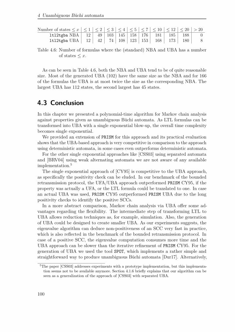
4 Unambiguous Büchi automata
Number of states ≤ x ≤ 1 ≤ 2 ≤ 3 ≤ 4 ≤ 5 ≤ 7 ≤ 10 ≤ 12 ≤ 20 > 20ltl2tgba NBA 12 49 103 145 158 176 181 185 188 0ltl2tgba UBA 12 42 74 108 123 153 168 173 180 8
Table 4.6: Number of formulas where the (standard) NBA and UBA has a numberof states ≤ x.
As can be seen in Table 4.6, both the NBA and UBA tend to be of quite reasonablesize. Most of the generated UBA (102) have the same size as the NBA and for 166of the formulas the UBA is at most twice the size as the corresponding NBA. Thelargest UBA has 112 states, the second largest has 45 states.
4.3 ConclusionIn this chapter we presented a polynomial-time algorithm for Markov chain analysisagainst properties given as unambiguous Büchi automata. As LTL formulas can betransformed into UBA with a single exponential blow-up, the overall time complexitybecomes single exponential.
We provided an extension of PRISM for this approach and its practical evaluationshows that the UBA-based approach is very competitive in comparison to the approachusing deterministic automata, in some cases even outperforms deterministic automata.
For the other single exponential approaches like [CSS03] using separated automataand [BRV04] using weak alternating automata we are not aware of any availableimplementation.5
The single exponential approach of [CY95] is competitive to the UBA approach,as specifically the positivity check can be eluded. In our benchmark of the boundedretransmission protocol, the UFA/UBA approach outperformed PRISM CY95, if theproperty was actually a UFA, or the LTL formula could be translated to one. In casean actual UBA was used, PRISM CY95 outperformed PRISM UBA due to the longpositivity checks to identify the positive SCCs.
In a more abstract comparison, Markov chain analysis via UBA offer some ad-vantages regarding the flexibility. The intermediate step of transforming LTL toUBA allows reduction techniques as, for example, simulation. Also, the generationof UBA could be designed to create smaller UBA. As our experiments suggests, theeigenvalue algorithm can deduce non-positiveness of an SCC very fast in practice,which is also reflected in the benchmark of the bounded retransmission protocol. Incase of a positive SCC, the eigenvalue computation consumes more time and theUBA approach can be slower than the iterative refinement of PRISM CY95. For thegeneration of UBA we used the tool SPOT, which implements a rather simple andstraightforward way to produce unambiguous Büchi automata [Dur17]. Alternatively,
5The paper [CSS03] addresses experiments with a prototype implementation, but this implementa-tion seems not to be available anymore. Section 4.1.6 briefly explains that our algorithm can beseen as a generalization of the approach of [CSS03] with separated UBA.
100
4.3 Conclusion
Tulip contained an LTL-to-UBA translator, but it is not available anymore. Asin case with deterministic automata, the performance of the UBA-based approachdepends strongly on the availability of small UBA. In contrast to non-deterministicor deterministic automata, the generation of small UBA or their simplification hasnot yet been explored thoroughly. Another promising approach would be to modifyknown LTL-to-NBA translations. We see a potential in the compositional approach of[EKS18] by a modification of the translations for the fragments to generate UBA anda disjoint union for the languages in the master theorem of [EKS18]. Alternatively,one would change the longer known translation of [GO01; Bab+12] such that onecreates an unambiguous very weak alternating automaton and applies an adjusted,unambiguity-preserving transformation to NBA. However, for general LTL bench-marks, the difference in the number of states between NBA and UBA is comparablysmall, but as our LTL formulas for the bounded retransmission protocol benchmarksuggest, the look-ahead of UBA has not been fully exploited yet.
101

5 Emerson-Lei acceptanceIn the previous chapters we focused on ω-automata with a restricted form of non-determinism. Now we turn to deterministic ω-automata but delve into the acceptancecondition of ω-automata. It is well-known, that the acceptance condition of anω-automaton has an important influence of the size of the automaton, even in thenon-deterministic case (see for example [Bok17b]). Also for deterministic automata,an exponential blow-up in the state-space may be unavoidable, if one switches froma Rabin acceptance to a Streett acceptance (or the other way around), see [SV89].
We reexamine the Muller acceptance, but due to its large representation, we add acrucial twist by a symbolic representation. A (standard) Muller acceptance is a subsetof the state power set (or transition power set) stating explicitly which inf(ρ) of arun ρ are accepting. More formally, a state-based Muller acceptance of an automatonwith state space Q is a set Z ⊆ 2Q and a run ρ is accepting if and only if inf(ρ) ∈ Z.Thus, the acceptance can be exponentially big in the number of states. This hasled to a representation in a symbolic fashion, as presented in [Bab+15], which wecall Emerson-Lei acceptance (EL for short). For the symbolic representation theatoms Fin (Z) and Inf (Z) with Z ⊆ Q are introduced with the obvious semantics: Arun ρ is accepting for Fin (Z) if and only if Z is visited only finitely often in ρ; ρ isaccepting for Inf (Z) if and only if Z is visited infinitely often in ρ.1
This symbolic Muller acceptance have already been studied by Emerson and Lei.In [EL85] they regard it as a fairness constraint for CTL model checking on Kripkestructures. One problem they consider is to search for a path satisfying a fairnessconstraint (which corresponds to checking non-emptiness for an EL automaton andto positive probability under a maximal scheduler for an MDP). In case of disjunctionof Streett conditions they provide an algorithm with a linear time complexity inthe Kripke structure size and quadratic in the size of the fairness constraint. Theauthors also reduces 3SAT to the general case of finding an accepting path in aKripke structure for a fairness constraint and thus show the NP-hardness of it. TheNP membership of the problem is obtained by a reference to [SC85]. The authorsof [SC85] consider Kripke structures and the LTL fragment LTL(♦,), i.e., thefragment allowing only ♦ and as temporal operators and prove an analogousNP-completeness result for this fragment.
Moving to a compactly expressed acceptance condition allows us to reduce thenumber of states and to use fewer acceptance sets compared to existing translations,although there is a well-known exponential lower bound for the size of deterministic
1Transition-based Muller acceptance and transition-based Emerson-Lei acceptance are definedanalogously.
103

5 Emerson-Lei acceptance
ω-automata starting from a non-deterministic ω-automaton [Mic88; Saf88].The richer acceptance condition complicates typical algorithmic questions, as
deciding positivity for Markov decision processes (does “PrmaxM (L) > 0” hold), or
emptiness for ω-automata.While for Rabin acceptance the solution of the positivity problem for MDPs (and
emptiness for ω-automata) is rather straightforward, the same problems for Streettacceptance triggered a long line of research, see, e.g., [EL85; EL87; BGC09b] wherea repeated generation of SCCs and removal of Fin (·) states is done, until one SCCis found, that contains only Inf (·) states or no SCC is left, which means that theStreett condition is unsatisfiable. This algorithm has been improved by heuristics in[RT96; LH00], and adapted to symbolic computation in [BGS00], parallel computation[ČP03], and on-the-fly-techniques [DPC09].
A lot of research has put into the translation of LTL to deterministic ω-automata(see Section 1.1.3), but to the best of our knowledge all those translations are targetedat a particular acceptance like Rabin, Streett or parity. There exists already theidea of a production construction in [Bab+15] to obtain a complex acceptance: Theformula is split into several subformulas, where the top-most operator in the syntaxtree is a temporal operator, and the subformulas are not nested within the scopeof another temporal operator. These subformulas are converted to deterministicautomata with one of the already known translators. These deterministic automataare composed in a product construction, where the graph is standard product, andthe acceptance of the product automaton where every top-most temporal formula issubstituted by the acceptance of the corresponding deterministic automaton.
Contribution. We present a translation from LTL to deterministic Emerson-Leiautomata that trades a compact state space for a more complex acceptance conditionstructure. Here, we give a direct translation of fragments of LTL without an interme-diate step over non-deterministic automata. We consider special fairness propertiesin particular and give a translation based on buffers. For safety and cosafety LTLformulas we rely on the af function [EKS16; Sic+16] computing the left-derivativedirectly on the formula. Additionally, if we encounter a subformula not containedin our supported fragments for a direct translation, we rely on external tools fortranslation, and compose a deterministic automaton for the overall formula with theproduct construction of [Bab+15]. We improve the product construction and makeuse of the knowledge about the subformulas, if one subformula falls into the fairness orsafety/cosafety fragment. This knowledge helps us to suspend one automaton similarto [Bab+13a], but we work more on the automaton level whereas [Bab+13a] workson the LTL level. A general scheme for our approach is depicted in Figure 5.1, whichwe implemented in our tool Delag (Deterministic Emerson-Lei Automata Generator).
As a second theoretical contribution we consider the complexity of decidingPrmax
M (Φ) > 0 for an MDPM and an Emerson-Lei acceptance Φ. We prove, thatthe positivity problem is NP-complete for a class of Emerson-Lei acceptances if thesatisfiability problem is NP-complete for the corresponding class of Boolean formu-
104
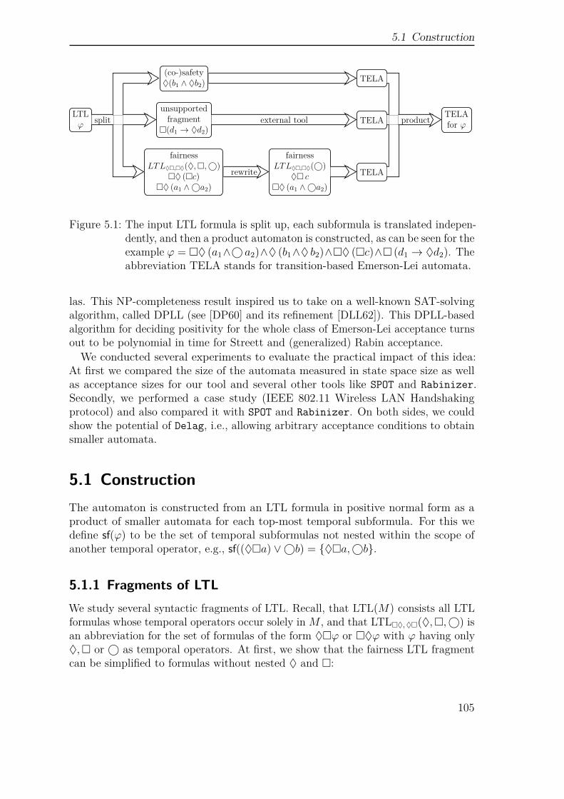
5.1 Construction
LTLϕ
(co-)safety♦(b1 ∧ ♦b2)
TELA
fairnessLTL♦,♦(♦,,⃝)
♦ (c)♦ (a1 ∧⃝a2)
fairnessLTL♦,♦(⃝)
♦ c♦ (a1 ∧⃝a2)
TELA
unsupportedfragment
(d1 → ♦d2)TELA
TELAfor ϕsplit
rewrite
external tool product
Figure 5.1: The input LTL formula is split up, each subformula is translated indepen-dently, and then a product automaton is constructed, as can be seen for theexample ϕ = ♦ (a1∧⃝ a2)∧♦ (b1∧♦ b2)∧♦ (c)∧ (d1 → ♦d2). Theabbreviation TELA stands for transition-based Emerson-Lei automata.
las. This NP-completeness result inspired us to take on a well-known SAT-solvingalgorithm, called DPLL (see [DP60] and its refinement [DLL62]). This DPLL-basedalgorithm for deciding positivity for the whole class of Emerson-Lei acceptance turnsout to be polynomial in time for Streett and (generalized) Rabin acceptance.
We conducted several experiments to evaluate the practical impact of this idea:At first we compared the size of the automata measured in state space size as wellas acceptance sizes for our tool and several other tools like SPOT and Rabinizer.Secondly, we performed a case study (IEEE 802.11 Wireless LAN Handshakingprotocol) and also compared it with SPOT and Rabinizer. On both sides, we couldshow the potential of Delag, i.e., allowing arbitrary acceptance conditions to obtainsmaller automata.
5.1 ConstructionThe automaton is constructed from an LTL formula in positive normal form as aproduct of smaller automata for each top-most temporal subformula. For this wedefine sf(ϕ) to be the set of temporal subformulas not nested within the scope ofanother temporal operator, e.g., sf((♦a) ∨⃝b) = ♦a,⃝b.
5.1.1 Fragments of LTLWe study several syntactic fragments of LTL. Recall, that LTL(M) consists all LTLformulas whose temporal operators occur solely in M , and that LTL♦,♦(♦,,⃝) isan abbreviation for the set of formulas of the form ♦ϕ or ♦ϕ with ϕ having only♦, or ⃝ as temporal operators. At first, we show that the fairness LTL fragmentcan be simplified to formulas without nested ♦ and :
105
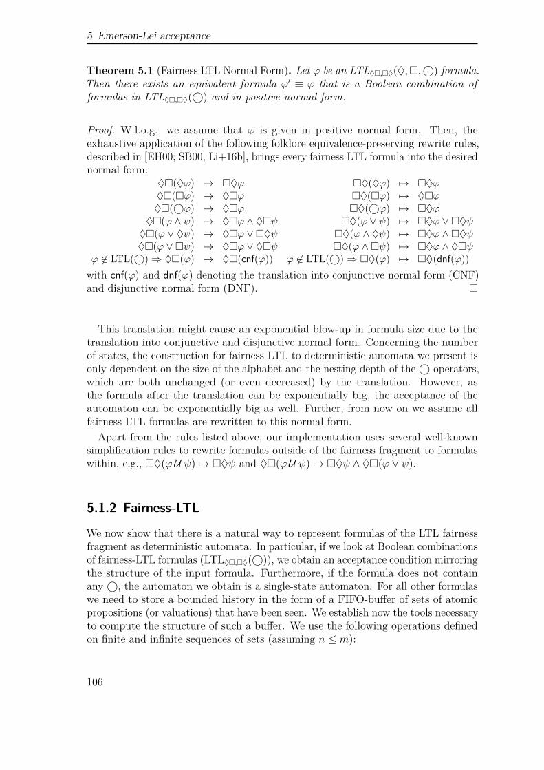
5 Emerson-Lei acceptance
Theorem 5.1 (Fairness LTL Normal Form). Let ϕ be an LTL♦,♦(♦,,⃝) formula.Then there exists an equivalent formula ϕ′ ≡ ϕ that is a Boolean combination offormulas in LTL♦,♦(⃝) and in positive normal form.
Proof. W.l.o.g. we assume that ϕ is given in positive normal form. Then, theexhaustive application of the following folklore equivalence-preserving rewrite rules,described in [EH00; SB00; Li+16b], brings every fairness LTL formula into the desirednormal form:
♦(♦ϕ) ↦→ ♦ϕ ♦(♦ϕ) ↦→ ♦ϕ♦(ϕ) ↦→ ♦ϕ ♦(ϕ) ↦→ ♦ϕ♦(⃝ϕ) ↦→ ♦ϕ ♦(⃝ϕ) ↦→ ♦ϕ
♦(ϕ ∧ ψ) ↦→ ♦ϕ ∧ ♦ψ ♦(ϕ ∨ ψ) ↦→ ♦ϕ ∨♦ψ♦(ϕ ∨ ♦ψ) ↦→ ♦ϕ ∨♦ψ ♦(ϕ ∧ ♦ψ) ↦→ ♦ϕ ∧♦ψ♦(ϕ ∨ψ) ↦→ ♦ϕ ∨ ♦ψ ♦(ϕ ∧ψ) ↦→ ♦ϕ ∧ ♦ψ
ϕ ∈ LTL(⃝)⇒ ♦(ϕ) ↦→ ♦(cnf(ϕ)) ϕ ∈ LTL(⃝)⇒ ♦(ϕ) ↦→ ♦(dnf(ϕ))with cnf(ϕ) and dnf(ϕ) denoting the translation into conjunctive normal form (CNF)and disjunctive normal form (DNF).
This translation might cause an exponential blow-up in formula size due to thetranslation into conjunctive and disjunctive normal form. Concerning the numberof states, the construction for fairness LTL to deterministic automata we present isonly dependent on the size of the alphabet and the nesting depth of the ⃝-operators,which are both unchanged (or even decreased) by the translation. However, asthe formula after the translation can be exponentially big, the acceptance of theautomaton can be exponentially big as well. Further, from now on we assume allfairness LTL formulas are rewritten to this normal form.
Apart from the rules listed above, our implementation uses several well-knownsimplification rules to rewrite formulas outside of the fairness fragment to formulaswithin, e.g., ♦(ϕU ψ) ↦→ ♦ψ and ♦(ϕU ψ) ↦→ ♦ψ ∧ ♦(ϕ ∨ ψ).
5.1.2 Fairness-LTL
We now show that there is a natural way to represent formulas of the LTL fairnessfragment as deterministic automata. In particular, if we look at Boolean combinationsof fairness-LTL formulas (LTL♦,♦(⃝)), we obtain an acceptance condition mirroringthe structure of the input formula. Furthermore, if the formula does not containany ⃝, the automaton we obtain is a single-state automaton. For all other formulaswe need to store a bounded history in the form of a FIFO-buffer of sets of atomicpropositions (or valuations) that have been seen. We establish now the tools necessaryto compute the structure of such a buffer. We use the following operations definedon finite and infinite sequences of sets (assuming n ≤ m):
106
5.1 Construction
Pointwise Intersection: σ0σ1 . . . ⊓ υ0 . . . υm = (σ0 ∩ υ0) . . . (σm ∩ υm)∅ω
Pointwise Union: σ0 . . . σn ⊔ υ0 . . . υm = (σ0 ∪ υ0) . . . (σn ∪ υn) . . . υm
Forward Closure: cl(σ0 . . . σn) = σ0(σ0 ∪ σ1) . . .n⋃k=0
σk
Drop Last Set of Letters: drop(σ0 . . . σnσn+1) = σ0 . . . σn
Relevant History. Let us consider an example formula: ♦(a1 ∧⃝a2). In orderto check whether w |= a1 ∧⃝a2 holds we just need to know whether a1 ∈ w[0] anda2 ∈ w[1] holds. The rest of w can be ignored. The relevant history H(ϕ) for an LTLformula ϕ is a finite word over 2AP and masks all propositions that are irrelevant forevaluating ϕ. We compute the relevant history H recursively from the structure ofthe formula:H : LTL(⃝)→ (2AP)∗ H(true) = ϵ H(false) = ϵ
H(a) = a H(¬a) = aH(ϕ ∧ ψ) = H(ϕ) ⊔ H(ψ) H(ϕ ∨ ψ) = H(ϕ) ⊔ H(ψ)
H(⃝ϕ) = ∅H(ϕ)
Lemma 5.2. Let ϕ be an LTL(⃝) formula and let w = σ0 σ1 . . . be a ω-word. Thenw |= ϕ if and only if w ⊓ H(ϕ) |= ϕ.
Proof. By induction on ϕ. For succinctness we just exhibit two cases and all othercases are analogous.Case ϕ =⃝ψ. Then, w |= ϕ iff w [1 . . .] |= ψ iff w [1 . . .]⊓H(ψ) |= ψ iff ∅(w [1 . . .]⊓H(ψ)) |= ϕ iff w ⊓H(ϕ) |= ϕ.Case ϕ = ψ∧ψ′. Then, w |= ϕ iff w |= ψ∧w |= ψ′ iff w⊓H(ψ) |= ψ∧w⊓H(ψ′) |= ψ′
iff w ⊓ (H(ψ) ⊔H(ψ′)) |= ϕ iff w ⊓H(ϕ) |= ϕ.
The deterministic, transition-based Emerson-Lei automaton we are constructingkeeps a buffer masked by H. Intuitively, the automaton delays the decision whetherϕ holds by n = |H(ϕ)| − 1 steps and then decides whether it holds true, instead ofnon-deterministically guessing the future and verifying this guess as done in standardLTL translations.
Definition 5.3. Let ϕ be an LTL(⃝) formula over AP and let n = max(|H(ϕ)|−1, 0).We then define a transition-based Emerson-Lei automaton for ♦ϕ:
A(♦ϕ) = (Q, 2AP , δ,∅n, Inf (Z))
Q = w ∈ (2AP)n : ∀i. w[i] ⊆ cl(H(ϕ))[i]δ(σw, σ′) = wσ′ ⊓ drop(cl(H(ϕ))) for all σ, σ′ ∈ 2AP and w ∈ (2AP)n−1
Z = (w, σ, w′) ∈ δ : wσ∅ω |= ϕ
107
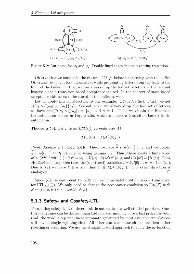
5 Emerson-Lei acceptance
a1
a1
a1
a1a2a1a2
a1a2 a1a2
(a) ψ1 = ♦(a1 ∧⃝a2)
♦(b1 ∧ ♦b2) ♦b2 trueb1b2
b1b2
b1
b2
b2 true
(b) ψ2 = ♦(b1 ∧ ♦b2)
Figure 5.2: Automata for ψ1 and ψ2. Double-lined edges denote accepting transitions.
Observe that we must take the closure of H(ϕ) before intersecting with the buffer.Otherwise, we might lose information while propagating letters from the back to thefront of the buffer. Further, we can always drop the last set of letters of the relevanthistory, since a transition-based acceptance is used. In the context of state-basedacceptance this needs to be stored in the buffer as well.
Let us apply this construction to our example: ♦(a1 ∧ ⃝a2). First, we getH(a1 ∧ ⃝a2) = a1a2. Second, since we always drop the last set of letters,we have drop(H(a1 ∧ ⃝a2)) = a1 and n = 1. Thus, we obtain the Emerson-Lei automaton shown in Figure 5.2a, which is in fact a (transition-based) Büchiautomaton.
Theorem 5.4. Let ϕ be an LTL(⃝) formula over AP.
L(♦ϕ) = L(A(♦ϕ))
Proof. Assume w |= ♦ϕ holds. Thus, we have∞∃ i. w[i . . .] |= ϕ and we obtain
∞∃ i. w[i . . .] ⊓ H(ϕ) |= ϕ by using Lemma 5.2. Thus, there exists a finite wordw′ ∈ (2AP)∗ with (1) w′∅ω = wi ⊓ H(ϕ), (2) w′∅ω |= ϕ, and (3) |w′| = |H(ϕ)|. Thus,A(♦ϕ) infinitely often takes the (shortened) transition t = (w′[0] . . . w′[n−1], w′[n]).Due to (2) we have t ∈ α and thus w ∈ L(A(♦ϕ)). The other direction isanalogous.
Since ♦ϕ is equivalent to ¬♦¬ϕ, we immediately obtain also a translationfor LTL♦(⃝). We only need to change the acceptance condition to Fin (Z) withZ = (w, σ, w′) ∈ δ : wσ∅ω |= ϕ.
5.1.3 Safety- and Cosafety-LTLTranslating safety LTL to deterministic automata is a well-studied problem. Sincethese languages can be defined using bad prefixes, meaning once a bad prefix has beenread, the word is rejected, most automata generated by most available translationswill have a single rejecting sink. All other states and transitions are then eitherrejecting or accepting. We use the straight-forward approach to apply the af -function
108
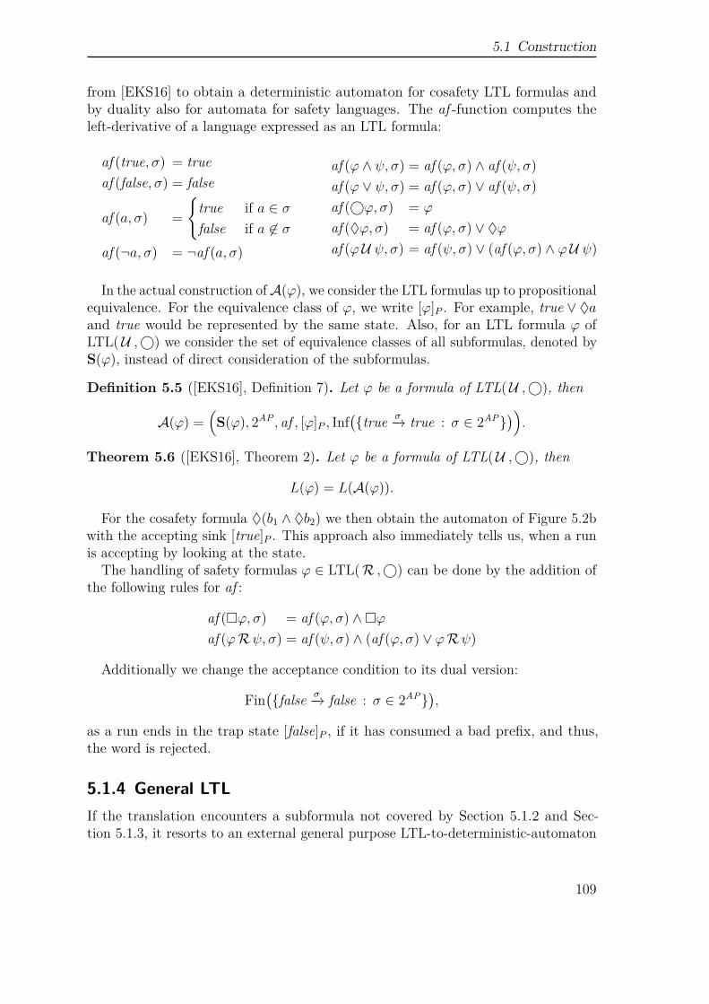
5.1 Construction
from [EKS16] to obtain a deterministic automaton for cosafety LTL formulas andby duality also for automata for safety languages. The af -function computes theleft-derivative of a language expressed as an LTL formula:
af (true, σ) = trueaf (false, σ) = false
af (a, σ) =
true if a ∈ σfalse if a ∈ σ
af (¬a, σ) = ¬af (a, σ)
af (ϕ ∧ ψ, σ) = af (ϕ, σ) ∧ af (ψ, σ)af (ϕ ∨ ψ, σ) = af (ϕ, σ) ∨ af (ψ, σ)af (⃝ϕ, σ) = ϕ
af (♦ϕ, σ) = af (ϕ, σ) ∨ ♦ϕ
af (ϕU ψ, σ) = af (ψ, σ) ∨ (af (ϕ, σ) ∧ ϕU ψ)
In the actual construction ofA(ϕ), we consider the LTL formulas up to propositionalequivalence. For the equivalence class of ϕ, we write [ϕ]P . For example, true ∨ ♦aand true would be represented by the same state. Also, for an LTL formula ϕ ofLTL(U ,⃝) we consider the set of equivalence classes of all subformulas, denoted byS(ϕ), instead of direct consideration of the subformulas.
Definition 5.5 ([EKS16], Definition 7). Let ϕ be a formula of LTL(U ,⃝), then
A(ϕ) =(
S(ϕ), 2AP , af , [ϕ]P , Inf(true σ−→ true : σ ∈ 2AP
)).
Theorem 5.6 ([EKS16], Theorem 2). Let ϕ be a formula of LTL(U ,⃝), then
L(ϕ) = L(A(ϕ)).
For the cosafety formula ♦(b1 ∧ ♦b2) we then obtain the automaton of Figure 5.2bwith the accepting sink [true]P . This approach also immediately tells us, when a runis accepting by looking at the state.
The handling of safety formulas ϕ ∈ LTL(R ,⃝) can be done by the addition ofthe following rules for af :
af (ϕ, σ) = af (ϕ, σ) ∧ϕ
af (ϕRψ, σ) = af (ψ, σ) ∧ (af (ϕ, σ) ∨ ϕRψ)
Additionally we change the acceptance condition to its dual version:
Fin(false σ−→ false : σ ∈ 2AP
),
as a run ends in the trap state [false]P , if it has consumed a bad prefix, and thus,the word is rejected.
5.1.4 General LTLIf the translation encounters a subformula not covered by Section 5.1.2 and Sec-tion 5.1.3, it resorts to an external general purpose LTL-to-deterministic-automaton
109
5 Emerson-Lei acceptance
translation. Here the only restriction on the type of the automaton is that it hasto be transition-based, since the translation for the fragments presented in Sections5.1.2 and 5.1.3 produces transition-based Emerson-Lei automata. Nevertheless, con-verting state-based to transition-based acceptance can be easily achieved by shiftingthe acceptance from every state to its outgoing transitions. Also, every standardacceptance, like Büchi, Rabin, Streett or parity can be interpreted as Emerson-Leiacceptance.
5.1.5 Product constructionIn the previous sections we discussed translations tailored to specific LTL fragments.Now we present a translation for full LTL. We split an LTL formula ϕ into severalsubformulas, that have a temporal operator on the root node in their syntax tree, andare not in the scope of another temporal operator. For all of such subformulas, wetranslate them into a deterministic automaton as described before, or if they do not fallinto one of the supported fragments, we use a general LTL-to-deterministic-automatatranslation. Afterwards, all these deterministic automata yield a deterministicautomaton for ϕ by a product construction. We first introduce the standard productconstruction for Emerson-Lei automata that is similar to the product constructionfor Muller automata and then move on to the enhanced construction.
Consider the following parametric formula: ♦(a1 ∧⃝(a2 ∧ . . .⃝ am)) ∧ ♦(b1 ∧♦(b2∧ . . .♦bn)). We will later demonstrate that the propagation of information allowsus to construct a Büchi automaton of size O(n +m), while SPOT in the standardconfiguration yields automata of size O(n ·m) and only after enabling simulation-based reductions this decreases to sizes comparable to our automata. Let us nowexamine the construction, while we translate the formula ♦(a1∧⃝a2)∧♦(b1∧♦b2).
Standard Construction. For the product construction for an LTL formula ϕ weassume we are given a deterministic Emerson-Lei automaton A(ψ) for every ψ ∈ sf(ϕ).We denote by QA(ψ) the states of A(ψ) and by qA(ψ)
0 the initial state of A(ψ). Everystate of the product automaton is a mapping from sf(ϕ) to
⋃ψ∈sf(ϕ)Q
A(ψ) where everysubformula ψ is mapped to a state in QA(ψ). We denote by s[ψ] = q the current stateof the automaton A(ψ) in the product state s, meaning ψ ↦→ q ∈ s.
Definition 5.7. Let ϕ be a formula and for every ψ ∈ sf(ϕ) let A(ψ) be a deterministicEmerson-Lei automaton recognizing L(ψ). The deterministic Emerson-Lei automatonfor the product is defined as:
A×(ϕ) = (Q, 2AP , δ, q0, A(ϕ))
δ(s, σ) = ψ ↦→ δA(ψ)(s[ψ], σ) : ψ ∈ sf(ϕ) q0 = ψ ↦→ qA(ψ)0 : ψ ∈ sf(ϕ)
Further, Q is defined as the set of all reachable states. The acceptance conditionis recursively computed over the structure of ϕ with ↑ denoting the lifting of theacceptance condition:
110
5.1 Construction
A(true) =true A(ϕ ∧ ψ) =A(ϕ) ∧ A(ψ)A(false) =false A(ϕ ∨ ψ) =A(ϕ) ∨ A(ψ)
α(ψ) = ↑ αA(ψ) for ψ ∈ sf(ϕ)
Since all δA(ψ) are deterministic, δ is also deterministic.
Theorem 5.8. Let ϕ be an LTL formula. Then
L(ϕ) = L(A×(ϕ))
Enhanced Construction. An essential part of the enhanced product construction isthe removal of unnecessary information from the product states. For this we introducethree additional states with special semantics: qacc signalizes that the componentmoved to an accepting sink state, while qrej expresses that the component moved to arejecting sink state. Alternatively, if a component got irrelevant for the acceptancecondition it is also moved to qrej. Lastly, qhold says that the component was put onhold. More specifically, we put the fairness automata on hold, if a “neighboring”automaton still needs to fulfill its goal, such as reaching an accepting trap. To makenotation easier to read we assume that every automaton A(ϕ) contains these statesand all accepting sinks (or traps) have been replaced by qacc and rejecting by qrej.We use the following abbreviations to reason about LTL formulas:
• conj(ϕ) (disj(ϕ)) denotes the set of all conjuncts of a conjunction (disjunctsof a disjunction) outside the scope of a temporal operator, e.g. let ϕ =♦a ∧ (⃝b ∨c), then conj(ϕ) = ♦a,⃝b ∨c and disj(ϕ) = ⃝b,c.
• ϕ[F ← ψ] denotes the substitution of all formulas in the set F with the formulaψ, e.g. (♦a ∧ (⃝b ∨c))[♦a,a ← true] = true ∧ (⃝b ∨c).
• support(ϕ) denotes the support of a formula, where the formula is viewedas a propositional formula, which means that temporal operators are alsoconsidered propositions, e.g., support((⃝a ∧ ♦b) ∨ (♦b)) = ♦b. This meansevery assignment can be restricted to the propositions of the support: S |=P
ϕ⇔ S ∩ support(ϕ) |=P ϕ, where |=P denotes the conventional propositionalsatisfaction relation.
We use the following definitions to manipulate product states:
Definition 5.9 (Product state modifications). An update of a product state tests apredicate P on a formula-state pair (ψ, q) and replaces q with a new value obtainedby the updater U depending on ψ if it holds:
update(s, P, U) = ψ ↦→ (if P (ψ, q) then U(ψ) else q) : ψ ↦→ q ∈ s
111
5 Emerson-Lei acceptance
prune(s) disables automata in s that became irrelevant for the acceptance condition,meaning there are no longer in the support of the original formula after using knowledgefrom other automata. For this let us denote by Facc all ψ ↦→ qacc ∈ s and by Frej allψ ↦→ qrej ∈ s.
prune(s) = update(s, P, U)P (ψ, q) = (q = qacc ∧ ψ ∈ support(ϕ[Facc ← true,Frej ← false]))U(ψ) = qrej
start (s) starts (fairness) automata that are required for the acceptance but have beenput on hold. This is the case, if automata with terminal acceptance for formulasin the same conjunction (start (s)c) have not yet reached qacc or the dual case fordisjunctions:
start (s)c = update(s, Pc, U)start (s)d = update(s, Pd, U)Pc(ψ, q) = (q = qhold ∧ ∃C ∈ conj(ϕ). ψ ∈ C ∧ ∀χ ∈ C ∩ LTL(U ,⃝). s[χ] = qacc)Pd(ψ, q) = (q = qhold ∧ ∃D ∈ disj(ϕ). ψ ∈ D ∧ ∀χ ∈ D ∩ LTL(R ,⃝). s[χ] = qrej)
U(ψ) = qA(ψ)0
Definition 5.10 (Enhanced product automaton). Let ϕ be a formula. The Emerson-Lei automaton for the enhanced product automaton is defined the same way asDefinition 5.7 with the following changes:
A×E(ϕ) = (Q, 2AP , δ, q0, A(ϕ))
δ(s, σ) = start(prune(ψ ↦→ δA(ψ)(s[ψ], σ) : ψ ∈ sf(ϕ))
)q0 = start
(ψ ↦→
qA(ψ)0 if ψ ∈ sf(ϕ) \ LTL♦,♦(⃝)
qhold otherwise
)Theorem 5.11. Let ϕ be a formula.
L(ϕ) = L(A×E(ϕ))
If we apply this construction to ♦(a1∧⃝a2)∧♦(b1∧♦b2), we obtain the automatonshown in Figure 5.3. Observe that ♦(a1 ∧⃝a2) is put on hold until the automatonfor ♦(b1 ∧ ♦b2) reaches qacc.
Further Optimizations
There are two further optimizations we implement: First, we replace the local historiesof each automaton for LTL♦,♦(⃝) with one global history. Second, we piggyback theacceptance of (co-)safety automata on neighboring fairness automata. Let C ∈ conj(ϕ)be a conjunction, ψr ∈ LTL(U ,⃝) ∩ C and ψf ∈ LTL♦(⃝) ∩ C. We then haveαA(ψf ) = Fin (S) and extend S with QA(ψr) \ qacc. The same trick can be appliedto ψf ∈ LTL♦(⃝) and of course to the dual case with ψs ∈ LTL(R ,⃝).
112
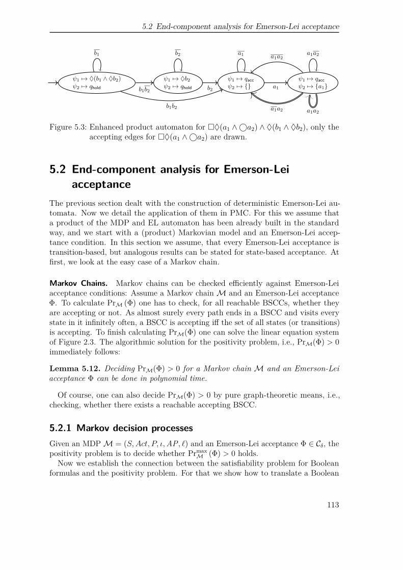
5.2 End-component analysis for Emerson-Lei acceptance
ψ1 ↦→ ♦(b1 ∧ ♦b2)ψ2 ↦→ qhold
ψ1 ↦→ ♦b2ψ2 ↦→ qhold
ψ1 ↦→ qaccψ2 ↦→
ψ1 ↦→ qaccψ2 ↦→ a1b1b2
b1b2
b1
b2
b2
a1
a1 a1a2
a1a2 a1a2
a1a2
Figure 5.3: Enhanced product automaton for ♦(a1 ∧⃝a2) ∧ ♦(b1 ∧ ♦b2), only theaccepting edges for ♦(a1 ∧⃝a2) are drawn.
5.2 End-component analysis for Emerson-Leiacceptance
The previous section dealt with the construction of deterministic Emerson-Lei au-tomata. Now we detail the application of them in PMC. For this we assume thata product of the MDP and EL automaton has been already built in the standardway, and we start with a (product) Markovian model and an Emerson-Lei accep-tance condition. In this section we assume, that every Emerson-Lei acceptance istransition-based, but analogous results can be stated for state-based acceptance. Atfirst, we look at the easy case of a Markov chain.
Markov Chains. Markov chains can be checked efficiently against Emerson-Leiacceptance conditions: Assume a Markov chainM and an Emerson-Lei acceptanceΦ. To calculate PrM (Φ) one has to check, for all reachable BSCCs, whether theyare accepting or not. As almost surely every path ends in a BSCC and visits everystate in it infinitely often, a BSCC is accepting iff the set of all states (or transitions)is accepting. To finish calculating PrM(Φ) one can solve the linear equation systemof Figure 2.3. The algorithmic solution for the positivity problem, i.e., PrM(Φ) > 0immediately follows:
Lemma 5.12. Deciding PrM(Φ) > 0 for a Markov chain M and an Emerson-Leiacceptance Φ can be done in polynomial time.
Of course, one can also decide PrM(Φ) > 0 by pure graph-theoretic means, i.e.,checking, whether there exists a reachable accepting BSCC.
5.2.1 Markov decision processesGiven an MDPM = (S,Act, P, ι,AP, ℓ) and an Emerson-Lei acceptance Φ ∈ Cδ, thepositivity problem is to decide whether Prmax
M (Φ) > 0 holds.Now we establish the connection between the satisfiability problem for Boolean
formulas and the positivity problem. For that we show how to translate a Boolean
113
5 Emerson-Lei acceptance
formula ϕ into an Emerson-Lei acceptance Φ. W.l.o.g. we assume ϕ to be given inpositive normal form. For every atomic proposition x occurring in ϕ we constructan Inf
(s
x−→ s), where s x−→ s is meant as a transition from state s to itself with
action x, and Inf(s
x−→ s)a short form notation for Inf
(s x−→ s
). Analogously, ¬x
is transformed into Fin(s
x−→ s).
With this transformation, the NP-hardness for the satisfiability of a class of Booleanformulas results in the NP-hardness for the corresponding Emerson-Lei acceptanceproblem.
Theorem 5.13. Let C be a class of Boolean formulas and C − SAT the class ofsatisfiable Boolean formulas contained in C. If C − SAT is NP-complete, thendeciding whether the positivity problem for MDPs and C-Emerson-Lei acceptances isNP-complete as well.
Proof. For proving the hardness we provide a polynomial reduction from C − SAT.Let ϕ be a C-formula with atomic propositions X = x1, . . . , xn. We generate aone-state MDP M with an xi action and a transition s
xi,1−−→ s for every atomicproposition xi in ϕ.
For further considerations, we identify a transition by its action, i.e., a transitionsubset Y ⊆ s ×X × 1 × s can be identified by the corresponding labelingsx ∈ X : s
x,1−→ s ∈ Y. The acceptance condition Φ is obtained from ϕ by replacing
every occurrence of xi with Inf (xi) and every occurrence of ¬xi with Fin (xi).Obviously, a transition subset Y ⊆ X (seen as a set of actions) satisfies Φ if and only
if Y |= ϕ. Every model of ϕ can be transformed to a corresponding end-componentof M by visiting Y infinitely often, since there is only one state with a self-loopfor every action x ∈ X. Analogously, every subset of transitions Y satisfying theacceptance condition Φ is also a model for ϕ. Therefore,M is positive for Φ if andonly if ϕ is satisfiable.
To prove that the positivity problem belongs to NP, we assume that we are givenan MDPM and an Emerson-Lei acceptance Φ. One can choose non-deterministicallyan end-component, and check whether the set of transitions in the end-componentsatisfies Φ.
The proof of Theorem 5.13 can be modified to work with state-based acceptance.The key idea is to introduce a state for every atomic proposition in ϕ and to identifythe state space with the atomic propositions.
Clearly, Inf (A) ∨ Inf (B) ≡ Inf (A ∪ B). Hence, each CNF acceptance formula canbe transformed into an equivalent generalized Streett formula of the form
⋀1≤i≤n
Fin (Ai,1)∨. . .∨Fin (Ai,ki)∨Inf (Bi) ≡⋀
1≤i≤n
(Inf(Ai,1)∧. . .∧Inf
(Ai,k
)→ Inf (Bi))
114
5.2 End-component analysis for Emerson-Lei acceptance
Lemma 5.14. Let M be an MDP and Φ a generalized Streett acceptance. Thendeciding whetherM is positive for Φ is NP-complete.
Note, that the class of generalized Streett acceptance corresponds to the classof Horn formulas. So, the reverse direction of Theorem 5.13 does not hold, unlessP = NP . Another prominent example class C of propositional CNF-formulas wherethe satisfiability problem can be solved in polynomial time is 2CNF. The full class of2CNF acceptance for deciding non-emptiness in an automaton is NP-complete, seeLemma 5.15.
Let 2CNF− NEG denote the set of all 2CNF-formulas where only negative literalsoccur, e.g., (¬x1 ∨ ¬x3) ∧ (¬x2 ∨ ¬x3) ∧ (¬x1 ∨ ¬x4). All 2CNF − NEG formulasare satisfiable, since the valuation that assigns false to every atomic proposition isa model for every 2CNF − NEG formula. However, the corresponding problem tocheck whether an MDP is positive for a 2CNF − NEG acceptance is NP-complete.An analogous NP-completeness result for checking emptiness of an automaton witha 2CNF− NEG acceptance has been proven by Emerson and Lei, see [EL87]. Thisproof can be adapted in a straight-forward manner for MDPs.
Lemma 5.15 (see Theorem 4.7 of [EL87]). Deciding non-emptiness for an automatonwith a 2CNF− NEG acceptance condition is NP-complete.
Despite the NP-hardness of 2CNF acceptance, several subclasses of 2CNF ac-ceptance are solvable in polynomial time. So, the positivity problem for Streettacceptance [BGC09b] and clearly Rabin acceptance is decidable in polynomial time(see Section 2.4.1).
In general, deciding positivity ofM (and Φ) can be reduced to the search of somereachable EC satisfying Φ:
By Lemma 2.6 we know that PrmaxM (Φ) > 0 iff there exists some reachable EC
T = (T,A) such that Φ is satisfied by all transitions occurring in T .What remains to explain is how to check whether a particular EC satisfies Φ. For
this, we take the set of transitions of the EC (here we denote it by ∆) and set everyInf (Z) in Φ to true if Z ∩∆ = ∅, otherwise to false. Analogously, we set Fin (Z) totrue if Z ∩ ∆ = ∅, otherwise to false. The overall evaluation of Φ for EC followsimmediately in the standard way.
Algorithm 1 implements a naive positivity check for a given MDPM and Emerson-Lei acceptance Φ. It enumerates all reachable ECs and checks whether there is an ECT = (T,A) satisfying Φ. For the last step we take a function CheckEC for granted,which can be implemented as explained above. As there may be an exponentialnumber of ECs, Algorithm 1 may require exponential time.
5.2.2 Fin (·)-less acceptanceIf the acceptance condition Φ does not use any Fin (·) operator, for any transitionsets T and T ′ with T ⊆ T ′ we have T |= Φ =⇒ T ′ |= Φ, i.e., visiting moretransitions cannot invalidate the acceptance condition. This implies that for checking
115
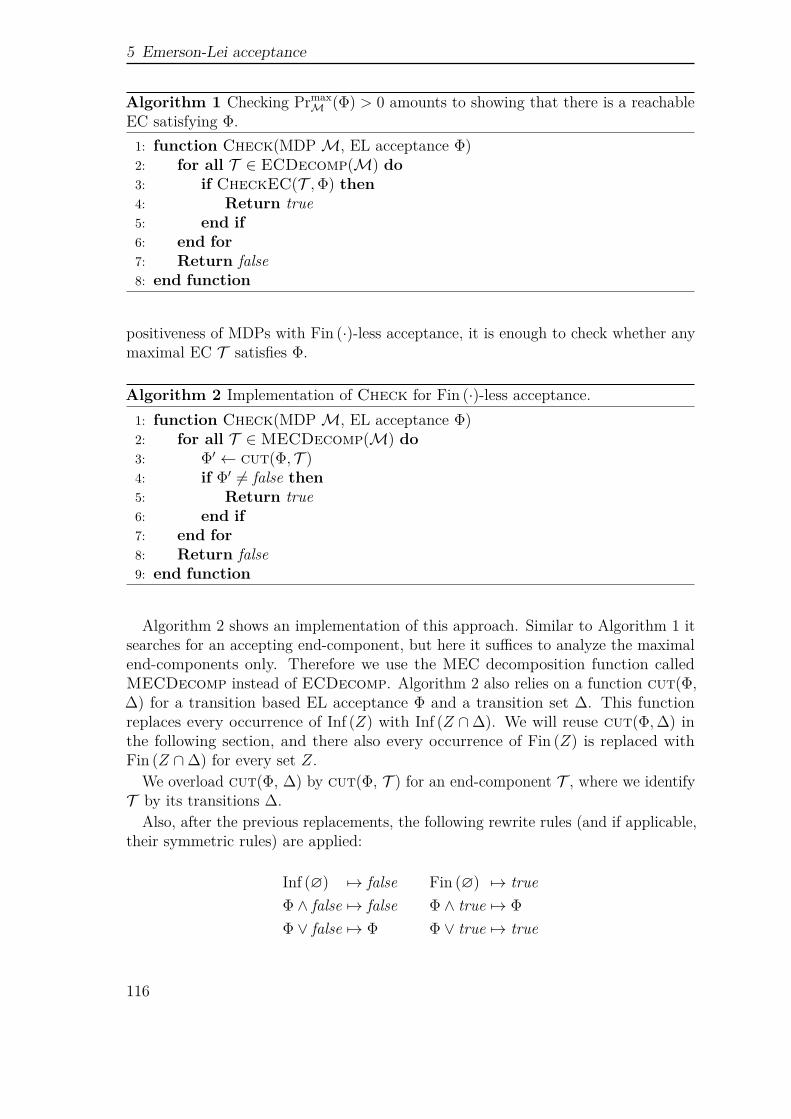
5 Emerson-Lei acceptance
Algorithm 1 Checking PrmaxM (Φ) > 0 amounts to showing that there is a reachable
EC satisfying Φ.1: function Check(MDPM, EL acceptance Φ)2: for all T ∈ ECDecomp(M) do3: if CheckEC(T ,Φ) then4: Return true5: end if6: end for7: Return false8: end function
positiveness of MDPs with Fin (·)-less acceptance, it is enough to check whether anymaximal EC T satisfies Φ.
Algorithm 2 Implementation of Check for Fin (·)-less acceptance.1: function Check(MDPM, EL acceptance Φ)2: for all T ∈MECDecomp(M) do3: Φ′ ← cut(Φ, T )4: if Φ′ = false then5: Return true6: end if7: end for8: Return false9: end function
Algorithm 2 shows an implementation of this approach. Similar to Algorithm 1 itsearches for an accepting end-component, but here it suffices to analyze the maximalend-components only. Therefore we use the MEC decomposition function calledMECDecomp instead of ECDecomp. Algorithm 2 also relies on a function cut(Φ,∆) for a transition based EL acceptance Φ and a transition set ∆. This functionreplaces every occurrence of Inf (Z) with Inf (Z ∩∆). We will reuse cut(Φ,∆) inthe following section, and there also every occurrence of Fin (Z) is replaced withFin (Z ∩∆) for every set Z.
We overload cut(Φ, ∆) by cut(Φ, T ) for an end-component T , where we identifyT by its transitions ∆.
Also, after the previous replacements, the following rewrite rules (and if applicable,their symmetric rules) are applied:
Inf (∅) ↦→ false Fin (∅) ↦→ trueΦ ∧ false ↦→ false Φ ∧ true ↦→ Φ
Φ ∨ false ↦→ Φ Φ ∨ true ↦→ true
116
5.3 A DPLL based positivity check
5.3 A DPLL based positivity checkAs Theorem 5.13 suggests, there is a close connection between Emerson-Lei accep-tances and Boolean formulas. We can see Emerson-Lei acceptances as Booleanformulas in positive normal form with Inf (·) as positive Boolean variables and Fin (·)as negative Boolean variables. One of the most important decision problems inthe context of Boolean formulas is satisfiability, called SAT. Among SAT solvingalgorithms, one of the most prominent ones is the DPLL algorithm, introduced byDavis, Putman, Logemann, and Loveland [DP60; DLL62]. It relies on a split on thetruth values of variables enhanced with heuristics such as unit rule and pure literalrule.
In this section we investigate the connection between Boolean formulas andEmerson-Lei acceptance further and present a DPLL-based Check procedure fordeciding positivity of an MDP.
5.3.1 Tseytin transformation for Emerson-Lei AcceptanceSince the DPLL algorithm presumes conjunctive normal form (CNF) for a propo-sitional formula, we use an adapted Tseytin transformation [Tse68]. Let us firstintroduce some helpful notations. Let Φ be an Emerson-Lei acceptance. We call ΦBoolean if it is of the form Ψ ∧ Γ or Ψ ∨ Γ. The set of the Boolean subformulas of Φis denoted by B(Φ).
For the Tseytin transformation we introduce a slack variable sΨ for every Booleansubformula Ψ ∈ B(Φ). We denote the set of slack variables by V. The functions : Cδ → V ∪ AP maps every Boolean Emerson-Lei acceptance to its correspondingslack variable and preserves atomic propositions:
s(Φ) =
sΦ if Φ is BooleanΦ otherwise
The idea of the Tseytin transformation is to introduce a slack variable for ev-ery Boolean subformula, signaling whether the subformula should be true or not.Therefore, the function t introduces a slack variable for a Boolean subformula andtransforms the subformula into a clause.
t(Φ) =
⎧⎪⎨⎪⎩(¬s (Φ) ∨ s (Ψ)) ∧ (¬s (Φ) ∨ s (Γ)) if Φ = Ψ ∧ Γ
¬s (Φ) ∨ s (Ψ) ∨ s (Γ) if Φ = Ψ ∨ Γ
Φ otherwise
As a whole, we get the following satisfiability-equivalent formula cnf(Φ) in conjunc-tive normal form for an Emerson-Lei acceptance Φ:
cnf(Φ) = s(Φ) ∧⋀
Ψ∈B(Φ)
t(Ψ)
117
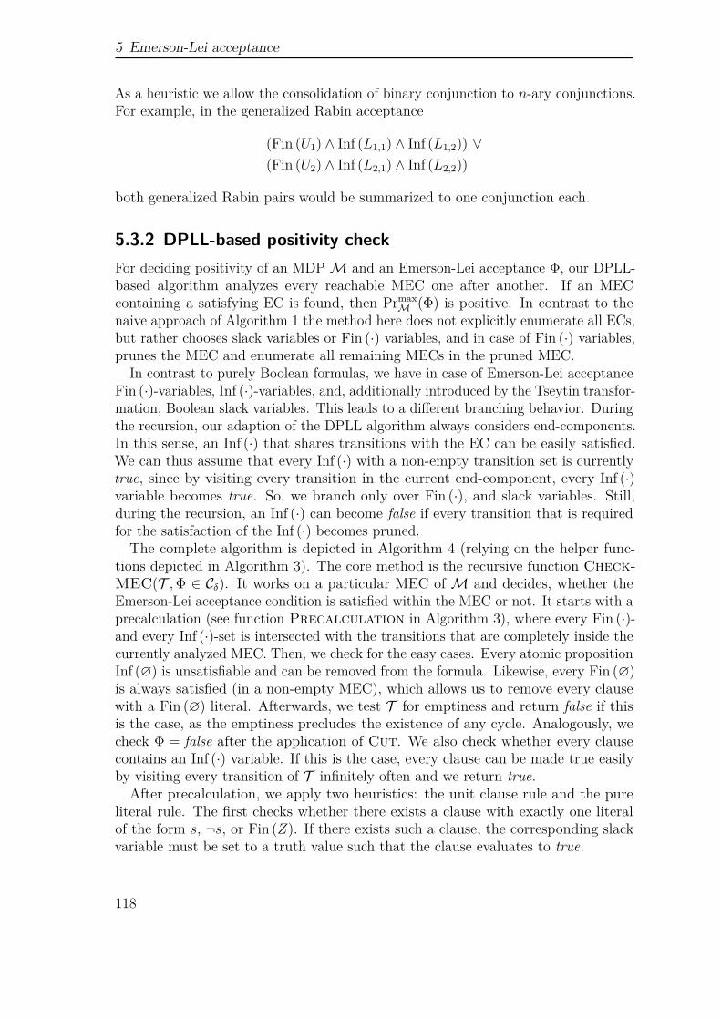
5 Emerson-Lei acceptance
As a heuristic we allow the consolidation of binary conjunction to n-ary conjunctions.For example, in the generalized Rabin acceptance
(Fin (U1) ∧ Inf (L1,1) ∧ Inf (L1,2)) ∨(Fin (U2) ∧ Inf (L2,1) ∧ Inf (L2,2))
both generalized Rabin pairs would be summarized to one conjunction each.
5.3.2 DPLL-based positivity checkFor deciding positivity of an MDPM and an Emerson-Lei acceptance Φ, our DPLL-based algorithm analyzes every reachable MEC one after another. If an MECcontaining a satisfying EC is found, then Prmax
M (Φ) is positive. In contrast to thenaive approach of Algorithm 1 the method here does not explicitly enumerate all ECs,but rather chooses slack variables or Fin (·) variables, and in case of Fin (·) variables,prunes the MEC and enumerate all remaining MECs in the pruned MEC.
In contrast to purely Boolean formulas, we have in case of Emerson-Lei acceptanceFin (·)-variables, Inf (·)-variables, and, additionally introduced by the Tseytin transfor-mation, Boolean slack variables. This leads to a different branching behavior. Duringthe recursion, our adaption of the DPLL algorithm always considers end-components.In this sense, an Inf (·) that shares transitions with the EC can be easily satisfied.We can thus assume that every Inf (·) with a non-empty transition set is currentlytrue, since by visiting every transition in the current end-component, every Inf (·)variable becomes true. So, we branch only over Fin (·), and slack variables. Still,during the recursion, an Inf (·) can become false if every transition that is requiredfor the satisfaction of the Inf (·) becomes pruned.
The complete algorithm is depicted in Algorithm 4 (relying on the helper func-tions depicted in Algorithm 3). The core method is the recursive function Check-MEC(T ,Φ ∈ Cδ). It works on a particular MEC of M and decides, whether theEmerson-Lei acceptance condition is satisfied within the MEC or not. It starts with aprecalculation (see function Precalculation in Algorithm 3), where every Fin (·)-and every Inf (·)-set is intersected with the transitions that are completely inside thecurrently analyzed MEC. Then, we check for the easy cases. Every atomic propositionInf (∅) is unsatisfiable and can be removed from the formula. Likewise, every Fin (∅)is always satisfied (in a non-empty MEC), which allows us to remove every clausewith a Fin (∅) literal. Afterwards, we test T for emptiness and return false if thisis the case, as the emptiness precludes the existence of any cycle. Analogously, wecheck Φ = false after the application of Cut. We also check whether every clausecontains an Inf (·) variable. If this is the case, every clause can be made true easilyby visiting every transition of T infinitely often and we return true.
After precalculation, we apply two heuristics: the unit clause rule and the pureliteral rule. The first checks whether there exists a clause with exactly one literalof the form s, ¬s, or Fin (Z). If there exists such a clause, the corresponding slackvariable must be set to a truth value such that the clause evaluates to true.
118
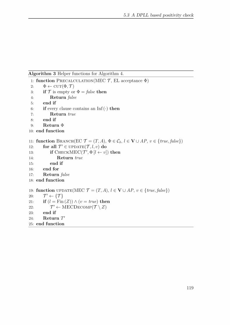
5.3 A DPLL based positivity check
Algorithm 3 Helper functions for Algorithm 4.1: function Precalculation(MEC T , EL acceptance Φ)2: Φ← cut(Φ, T )3: if T is empty or Φ = false then4: Return false5: end if6: if every clause contains an Inf (·) then7: Return true8: end if9: Return Φ
10: end function
11: function Branch(EC T = (T,A), Φ ∈ Cδ, l ∈ V ∪ AP, v ∈ true, false)12: for all T ′ ∈ update(T , l, v) do13: if CheckMEC(T ′,Φ [l ← v]) then14: Return true15: end if16: end for17: Return false18: end function
19: function update(MEC T = (T,A), l ∈ V ∪ AP, v ∈ true, false)20: T ′ ← T 21: if (l = Fin (Z)) ∧ (v = true) then22: T ′ ←MECDecomp(T \ Z)23: end if24: Return T ′
25: end function
119
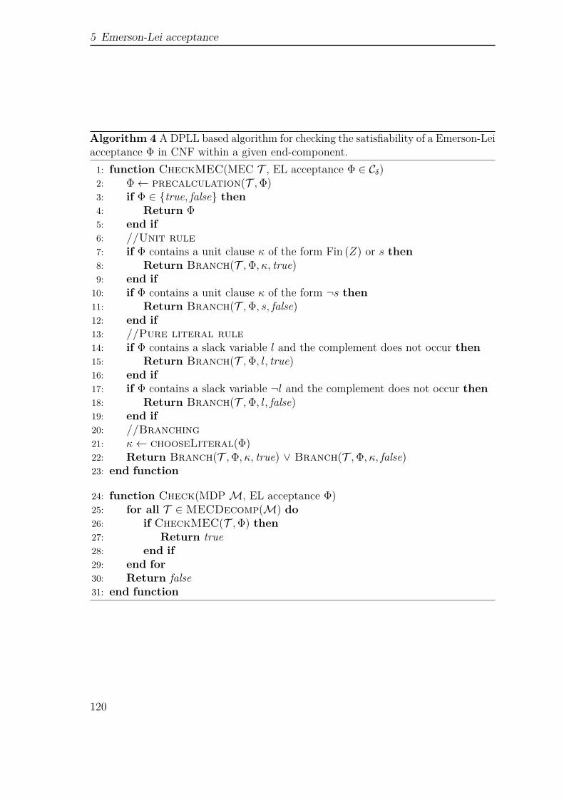
5 Emerson-Lei acceptance
Algorithm 4 A DPLL based algorithm for checking the satisfiability of a Emerson-Leiacceptance Φ in CNF within a given end-component.
1: function CheckMEC(MEC T , EL acceptance Φ ∈ Cδ)2: Φ← precalculation(T ,Φ)3: if Φ ∈ true, false then4: Return Φ5: end if6: //Unit rule7: if Φ contains a unit clause κ of the form Fin (Z) or s then8: Return Branch(T ,Φ, κ, true)9: end if
10: if Φ contains a unit clause κ of the form ¬s then11: Return Branch(T ,Φ, s, false)12: end if13: //Pure literal rule14: if Φ contains a slack variable l and the complement does not occur then15: Return Branch(T ,Φ, l, true)16: end if17: if Φ contains a slack variable ¬l and the complement does not occur then18: Return Branch(T ,Φ, l, false)19: end if20: //Branching21: κ← chooseLiteral(Φ)22: Return Branch(T ,Φ, κ, true) ∨ Branch(T ,Φ, κ, false)23: end function
24: function Check(MDPM, EL acceptance Φ)25: for all T ∈MECDecomp(M) do26: if CheckMEC(T ,Φ) then27: Return true28: end if29: end for30: Return false31: end function
120
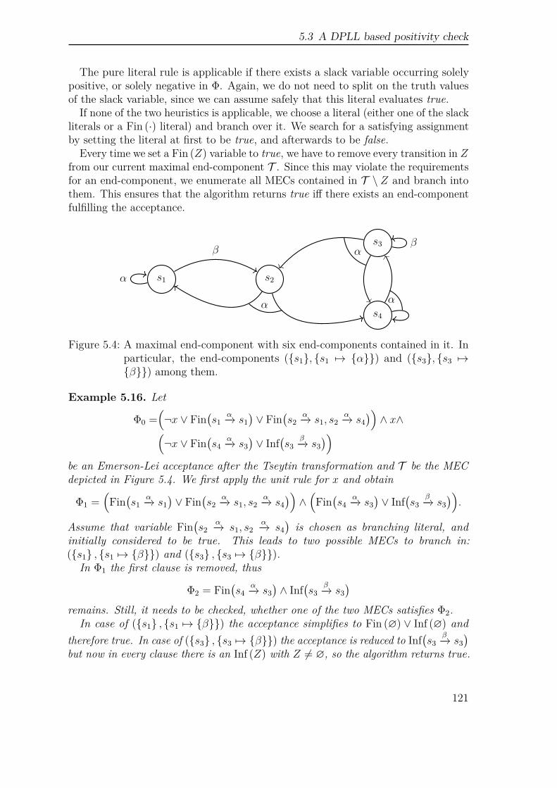
5.3 A DPLL based positivity check
The pure literal rule is applicable if there exists a slack variable occurring solelypositive, or solely negative in Φ. Again, we do not need to split on the truth valuesof the slack variable, since we can assume safely that this literal evaluates true.
If none of the two heuristics is applicable, we choose a literal (either one of the slackliterals or a Fin (·) literal) and branch over it. We search for a satisfying assignmentby setting the literal at first to be true, and afterwards to be false.
Every time we set a Fin (Z) variable to true, we have to remove every transition in Zfrom our current maximal end-component T . Since this may violate the requirementsfor an end-component, we enumerate all MECs contained in T \ Z and branch intothem. This ensures that the algorithm returns true iff there exists an end-componentfulfilling the acceptance.
s1 s2
s3
s4
α
ββ
α
α
α
Figure 5.4: A maximal end-component with six end-components contained in it. Inparticular, the end-components (s1, s1 ↦→ α) and (s3, s3 ↦→β) among them.
Example 5.16. Let
Φ0 =(¬x ∨ Fin
(s1
α−→ s1)∨ Fin
(s2
α−→ s1, s2α−→ s4
))∧ x∧(
¬x ∨ Fin(s4
α−→ s3)∨ Inf
(s3
β−→ s3))
be an Emerson-Lei acceptance after the Tseytin transformation and T be the MECdepicted in Figure 5.4. We first apply the unit rule for x and obtain
Φ1 =(Fin(s1
α−→ s1)∨ Fin
(s2
α−→ s1, s2α−→ s4
))∧(Fin(s4
α−→ s3)∨ Inf
(s3
β−→ s3)).
Assume that variable Fin(s2
α−→ s1, s2α−→ s4
)is chosen as branching literal, and
initially considered to be true. This leads to two possible MECs to branch in:(s1 , s1 ↦→ β) and (s3 , s3 ↦→ β).
In Φ1 the first clause is removed, thus
Φ2 = Fin(s4
α−→ s3)∧ Inf
(s3
β−→ s3)
remains. Still, it needs to be checked, whether one of the two MECs satisfies Φ2.In case of (s1 , s1 ↦→ β) the acceptance simplifies to Fin (∅) ∨ Inf (∅) and
therefore true. In case of (s3 , s3 ↦→ β) the acceptance is reduced to Inf(s3
β−→ s3)
but now in every clause there is an Inf (Z) with Z = ∅, so the algorithm returns true.
121
5 Emerson-Lei acceptance
Emerson-Lei automata. Deciding non-emptiness for automata profits from similartechniques as probabilistic model checking.
We can see an Emerson-Lei automaton as a Markov decision process where everytransition probability equals 1. So, deciding non-emptiness for Emerson-Lei automatareduces to the search for an accepting cycle. Therefore, we analyze every SCC asdescribed in Algorithm 4, but with SCC decomposition instead of MEC decomposition.
To sum up, we can formulate Theorem 5.13 also for Emerson-Lei automata. Sincenon-emptiness and emptiness are dual to each other, we stick to the usual formulationof emptiness checking.
Lemma 5.17 (see Theorem 5.13). Let C − SAT be a class of Boolean formulas, forwhich the satisfiability problem is NP-complete. Then, deciding emptiness Lω(A) = ∅for an Emerson-Lei automaton A with an acceptance condition Φ in C is coNP-complete.
5.3.3 Choosing the branching literalIn Algorithm 4 the function chooseLiteral is left unspecified. In fact, any functionreturning a literal (from the slack or Fin (·) literals) that occurs in Φ leads to acorrect implementation. To achieve a good performance in practice it is interestingto consider several heuristics to select a beneficial literal for the branching step.
One important rule is that we prefer to branch over slack literals if there are anyand only if no slack literal is left we branch over Fin (·) literals. This may lead tofaster pruning of clauses, since every slack variable stands for a whole subformula ofthe original formula. Especially in case of a generalized Rabin acceptance this leadsto a polynomial pair-by-pair check.
5.3.4 Generalized Rabin acceptanceTseytin transformation for generalized Rabin acceptance. The generalized ver-sion of a Rabin condition is a disjunction of conjunctions of a Fin (·) variable andseveral Inf (·) variables:
Φ =(Fin (U1) ∧
⋀j∈J1
Inf (L1,j))∨ . . . ∨
(Fin (Un) ∧
⋀j∈Jn
Inf (Ln,j))
For a depiction of the syntax tree see Figure 5.5. The Tseytin transformationintroduces a slack variable xk for every generalized Rabin pair k. The generalizedRabin pair Fin (Uk)∧ Inf (Lk,1)∧ . . .∧ Inf (Lk,nk
) is represented by the clauses (¬xk ∨Fin (Uk)), (¬xk ∨ Inf (Lk,1)) up to (¬xk ∨ Inf (Lk,nk
)). The choice for Rabin pair kis depends on the clause ¬yk−1 ∨ xk ∨ yk. The clause becomes true if yk−1 becomesfalse, if xk becomes true, or if yk becomes true. Variable yk−1 becomes false only ifat least one Rabin pair with index smaller than k has been satisfied. The variable xkbecomes true only if Rabin pair k is satisfied. Alternatively, also a Rabin pair withindex greater than k can be satisfied, which corresponds to variable yk being true.
122
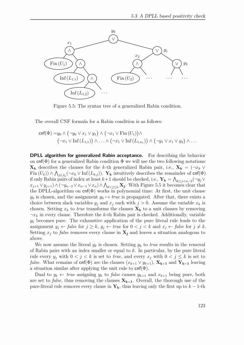
5.3 A DPLL based positivity check
∨
y0
∧x1
Fin (U1) ∧
Inf (L1,1) ∧
Inf (L1,2) · · ·
∨ y1
∧x2
Fin (U2) · · ·
∨ y2
· · · · · ·
Figure 5.5: The syntax tree of a generalized Rabin condition.
The overall CNF formula for a Rabin condition is as follows:
cnf(Φ) =y0 ∧(¬y0 ∨ x1 ∨ y1
)∧(¬x1 ∨ Fin (U1)
)∧(
¬x1 ∨ Inf (L1,1))∧ . . . ∧
(¬x1 ∨ Inf (L1,n1)
)∧(¬y1 ∨ x1 ∨ y2
)∧ . . .
DPLL algorithm for generalized Rabin acceptance. For describing the behavioron cnf(Φ) for a generalized Rabin condition Φ we will use the two following notations:Xk describes the clauses for the k-th generalized Rabin pair, i.e., Xk = (¬xk ∨Fin (Uk)) ∧
⋀j∈Jk(¬xk ∨ Inf (Lk,j)). Yk intuitively describes the remainder of cnf(Φ)
if only Rabin pairs of index at least k+1 should be checked, i.e., Yk =⋀k≤j<n−2(¬yj∨
xj+1∨ yj+1)∧ (¬yn−2∨xn−1∨xn)∧⋀k<j≤n Xj. With Figure 5.5 it becomes clear that
the DPLL-algorithm on cnf(Φ) works in polynomial time: At first, the unit clausey0 is chosen, and the assignment y0 ↦→ true is propagated. After that, there exists achoice between slack variables yj and xj each with j > 0. Assume the variable xk ischosen. Setting xk to true transforms the clauses Xk to a unit clauses by removing¬xk in every clause. Therefore the k-th Rabin pair is checked. Additionally, variableyk becomes pure. The exhaustive application of the pure literal rule leads to theassignment yj ← false for j ≥ k, yj ← true for 0 < j < k and xj ← false for j = k.Setting xj to false removes every clause in Xj and leaves a situation analogous toabove.
We now assume the literal yk is chosen. Setting yk to true results in the removalof Rabin pairs with an index smaller or equal to k. In particular, by the pure literalrule every yj with 0 < j < k is set to true, and every xj with 0 < j ≤ k is set tofalse. What remains of cnf(Φ) are the clauses (xk+1 ∨ yk+1), Xk+1 and Yk+1 leavinga situation similar after applying the unit rule to cnf(Φ).
Dual to yk ← true assigning yk to false causes yk+1 and xk+1 being pure, bothare set to false, thus removing the clauses Xk+1. Overall, the thorough use of thepure-literal rule removes every clause in Yk, thus leaving only the first up to k− 1-th
123
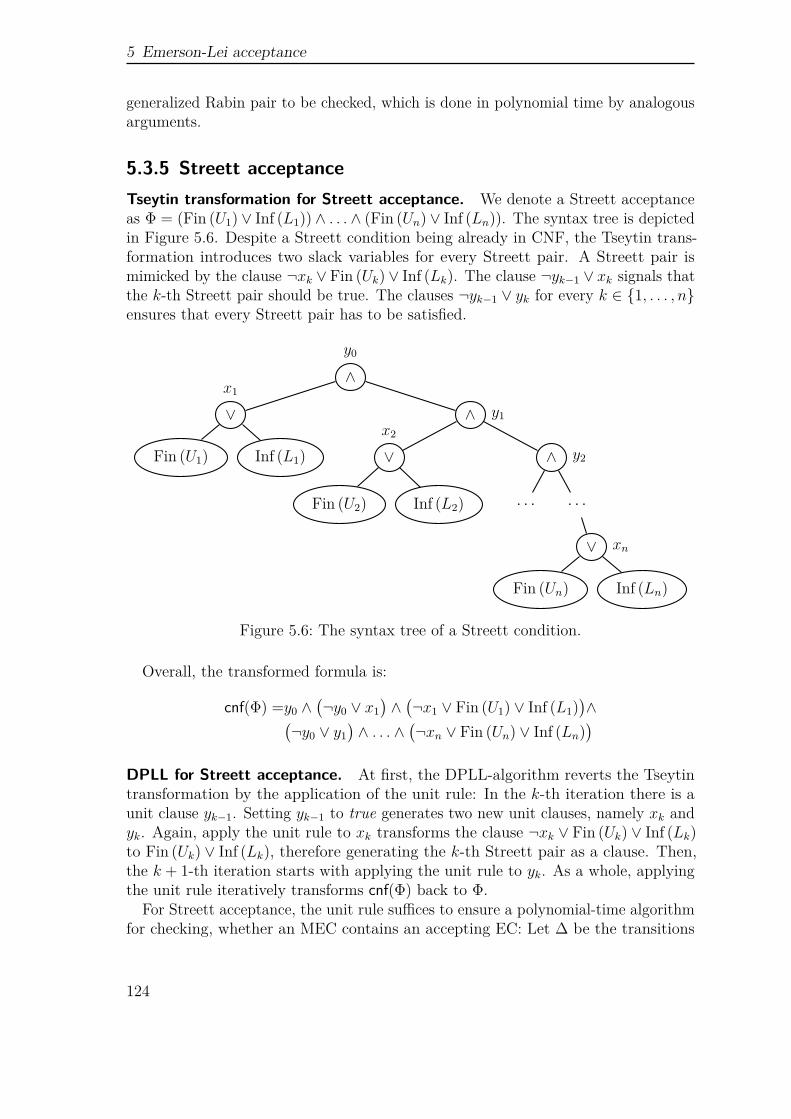
5 Emerson-Lei acceptance
generalized Rabin pair to be checked, which is done in polynomial time by analogousarguments.
5.3.5 Streett acceptanceTseytin transformation for Streett acceptance. We denote a Streett acceptanceas Φ = (Fin (U1) ∨ Inf (L1)) ∧ . . . ∧ (Fin (Un) ∨ Inf (Ln)). The syntax tree is depictedin Figure 5.6. Despite a Streett condition being already in CNF, the Tseytin trans-formation introduces two slack variables for every Streett pair. A Streett pair ismimicked by the clause ¬xk ∨ Fin (Uk) ∨ Inf (Lk). The clause ¬yk−1 ∨ xk signals thatthe k-th Streett pair should be true. The clauses ¬yk−1 ∨ yk for every k ∈ 1, . . . , nensures that every Streett pair has to be satisfied.
∧
y0
∨x1
Fin (U1) Inf (L1)
∧ y1
∨x2
Fin (U2) Inf (L2)
∧ y2
· · · · · ·
∨ xn
Fin (Un) Inf (Ln)
Figure 5.6: The syntax tree of a Streett condition.
Overall, the transformed formula is:
cnf(Φ) =y0 ∧(¬y0 ∨ x1
)∧(¬x1 ∨ Fin (U1) ∨ Inf (L1)
)∧(
¬y0 ∨ y1)∧ . . . ∧
(¬xn ∨ Fin (Un) ∨ Inf (Ln)
)DPLL for Streett acceptance. At first, the DPLL-algorithm reverts the Tseytintransformation by the application of the unit rule: In the k-th iteration there is aunit clause yk−1. Setting yk−1 to true generates two new unit clauses, namely xk andyk. Again, apply the unit rule to xk transforms the clause ¬xk ∨ Fin (Uk) ∨ Inf (Lk)to Fin (Uk) ∨ Inf (Lk), therefore generating the k-th Streett pair as a clause. Then,the k + 1-th iteration starts with applying the unit rule to yk. As a whole, applyingthe unit rule iteratively transforms cnf(Φ) back to Φ.
For Streett acceptance, the unit rule suffices to ensure a polynomial-time algorithmfor checking, whether an MEC contains an accepting EC: Let ∆ be the transitions
124
5.4 Implementation and Experiments
of an MEC which should be checked against a Streett acceptance Φ =(Fin (U1) ∨
Inf (L1))∧ . . . ∧
(Fin (Un) ∨ Inf (Ln)
). First, we intersect all sets with ∆, i.e., we
obtain (Fin (U1 ∩∆) ∨ Inf (L1 ∩∆)
)∧ . . . ∧
(Fin (Un ∩∆) ∧ Inf (Ln ∩∆)
)We remove all literals of the form Inf (∅) (meaning false) and remove all clauses
with Fin (∅) (with the meaning true). Now, if there is in every clause an Inf (·) literal,the formula is fulfilled and therefore satisfiable. If not, then there exists a unit clauseof the form Fin (Fk ∩∆). Applying the unit rule means pruning MEC T . We obtainnew MECs T1, . . . , Tk. Now checking whether Φ is satisfied by an EC in T reducesnow to checking whether there exists MEC Tj ∈ T1, . . . , Tk such that it has anaccepting EC for Φ′.
Complexity. The argument for polynomial time complexity follows [BGC09a]. Asabove, we go through every clause, and either it contains a non-empty Inf (·)-literal(meaning, that at the current moment, it is assumed to be true), or it is a unit literalof the form Fin (Uk). So, the only branching happens on the MDP side, where weprune an MEC, and divide into several new MECs and check them recursively.
Note that the recursion depth is at most min(|Φ|, |T |). Also, after pruning, weobtain at most |T | − 1 new MECs to branch in. With a linear time for finding thenew MECs, we obtain O(|T |2 ·min(|T |, |Φ|)) as overall complexity.
Emerson-Lei automata. Analogously to positivity for MDPs, for emptiness of ELautomata the choice of the branching literal can influence the runtime of Algorithm 4.The presented algorithm works for a generalized Rabin and a Streett acceptance inpolynomial time as well. In particular, the automata-theoretic analog of Algorithm 4works for a Streett acceptance as described in [EL87] and for a generalized Rabinacceptance as the canonical approach.
5.4 Implementation and ExperimentsOur experimental evaluation consists of two parts: At first, we evaluate our translationby comparing the automata sizes and acceptance sizes. The second contribution inour evaluation considers probabilistic model checking with the help of automata. Forevery experiment, we set a time limit of 30 minutes and a memory limit of 10 GBfor every process.2 The according implementations, and data logs can be found at[Mül18].
2All experiments were carried out on a computer with two Intel E5-2680 8-core CPUs at 2.70 GHzwith 384GB of RAM running Linux.
125
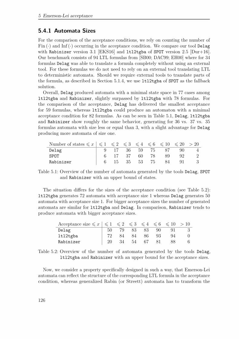
5 Emerson-Lei acceptance
5.4.1 Automata SizesFor the comparison of the acceptance conditions, we rely on counting the number ofFin (·) and Inf (·) occurring in the acceptance condition. We compare our tool Delagwith Rabinizer version 3.1 [EKS16] and ltl2tgba of SPOT version 2.5 [Dur+16].Our benchmark consists of 94 LTL formulas from [SB00; DAC99; EH00] where for 34formulas Delag was able to translate a formula completely without using an externaltool. For these formulas we do not need to rely on an external tool translating LTLto deterministic automata. Should we require external tools to translate parts ofthe formula, as described in Section 5.1.4, we use ltl2tgba of SPOT as the fallbacksolution.
Overall, Delag produced automata with a minimal state space in 77 cases amongltl2tgba and Rabinizer, slightly surpassed by ltl2tgba with 78 formulas. Forthe comparison of the acceptance, Delag has delivered the smallest acceptancefor 59 formulas, whereas ltl2tgba could produce an automaton with a minimalacceptance condition for 82 formulas. As can be seen in Table 5.1, Delag, ltl2tgbaand Rabinizer show roughly the same behavior, generating for 36 vs. 37 vs. 35formulas automata with size less or equal than 3, with a slight advantage for Delagproducing more automata of size one.
Number of states ⩽ x ⩽ 1 ⩽ 2 ⩽ 3 ⩽ 4 ⩽ 6 ⩽ 10 ⩽ 20 > 20Delag 9 17 36 59 75 87 90 4SPOT 6 17 37 60 78 89 92 2Rabinizer 6 15 35 53 75 84 91 3
Table 5.1: Overview of the number of automata generated by the tools Delag, SPOTand Rabinizer with an upper bound of states.
The situation differs for the sizes of the acceptance condition (see Table 5.2):ltl2tgba generates 72 automata with acceptance size 1 whereas Delag generates 50automata with acceptance size 1. For bigger acceptance sizes the number of generatedautomata are similar for ltl2tgba and Delag. In comparison, Rabinizer tends toproduce automata with bigger acceptance sizes.
Acceptance size ⩽ x ⩽ 1 ⩽ 2 ⩽ 3 ⩽ 4 ⩽ 6 ⩽ 10 > 10Delag 50 79 83 83 90 91 3ltl2tgba 72 84 84 86 93 94 0Rabinizer 20 34 54 67 81 88 6
Table 5.2: Overview of the number of automata generated by the tools Delag,ltl2tgba and Rabinizer with an upper bound for the acceptance sizes.
Now, we consider a property specifically designed in such a way, that Emerson-Leiautomata can reflect the structure of the corresponding LTL formula in the acceptancecondition, whereas generalized Rabin (or Streett) automata has to transform the
126
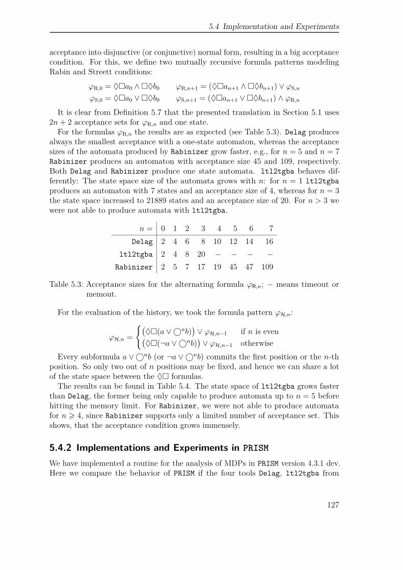
5.4 Implementation and Experiments
acceptance into disjunctive (or conjunctive) normal form, resulting in a big acceptancecondition. For this, we define two mutually recursive formula patterns modelingRabin and Streett conditions:
ϕR,0 = ♦a0 ∧♦b0 ϕR,n+1 = (♦an+1 ∧♦bn+1) ∨ ϕS,n
ϕS,0 = ♦a0 ∨♦b0 ϕS,n+1 = (♦an+1 ∨♦bn+1) ∧ ϕR,n
It is clear from Definition 5.7 that the presented translation in Section 5.1 uses2n+ 2 acceptance sets for ϕR,n and one state.
For the formulas ϕR,n the results are as expected (see Table 5.3). Delag producesalways the smallest acceptance with a one-state automaton, whereas the acceptancesizes of the automata produced by Rabinizer grow faster, e.g., for n = 5 and n = 7Rabinizer produces an automaton with acceptance size 45 and 109, respectively.Both Delag and Rabinizer produce one state automata. ltl2tgba behaves dif-ferently: The state space size of the automata grows with n: for n = 1 ltl2tgbaproduces an automaton with 7 states and an acceptance size of 4, whereas for n = 3the state space increased to 21889 states and an acceptance size of 20. For n > 3 wewere not able to produce automata with ltl2tgba.
n = 0 1 2 3 4 5 6 7
Delag 2 4 6 8 10 12 14 16
ltl2tgba 2 4 8 20 − − − −Rabinizer 2 5 7 17 19 45 47 109
Table 5.3: Acceptance sizes for the alternating formula ϕR,n; − means timeout ormemout.
For the evaluation of the history, we took the formula pattern ϕH,n:
ϕH,n =
(♦(a ∨⃝nb)
)∨ ϕH,n−1 if n is even(
♦(¬a ∨⃝nb))∨ ϕH,n−1 otherwise
Every subformula a ∨⃝nb (or ¬a ∨⃝nb) commits the first position or the n-thposition. So only two out of n positions may be fixed, and hence we can share a lotof the state space between the ♦ formulas.
The results can be found in Table 5.4. The state space of ltl2tgba grows fasterthan Delag, the former being only capable to produce automata up to n = 5 beforehitting the memory limit. For Rabinizer, we were not able to produce automatafor n ⩾ 4, since Rabinizer supports only a limited number of acceptance set. Thisshows, that the acceptance condition grows immensely.
5.4.2 Implementations and Experiments in PRISM
We have implemented a routine for the analysis of MDPs in PRISM version 4.3.1 dev.Here we compare the behavior of PRISM if the four tools Delag, ltl2tgba from
127
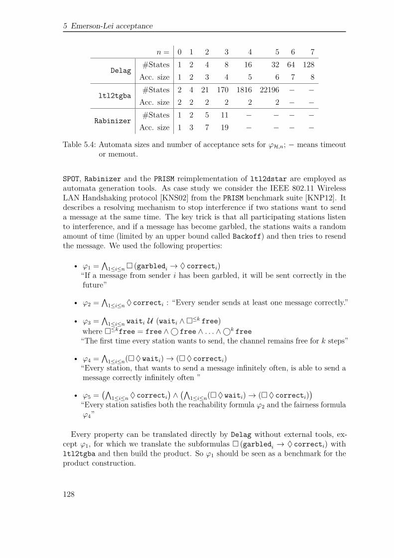
5 Emerson-Lei acceptance
n = 0 1 2 3 4 5 6 7
Delag#States 1 2 4 8 16 32 64 128
Acc. size 1 2 3 4 5 6 7 8
ltl2tgba#States 2 4 21 170 1816 22196 − −Acc. size 2 2 2 2 2 2 − −
Rabinizer#States 1 2 5 11 − − − −Acc. size 1 3 7 19 − − − −
Table 5.4: Automata sizes and number of acceptance sets for ϕH,n; − means timeoutor memout.
SPOT, Rabinizer and the PRISM reimplementation of ltl2dstar are employed asautomata generation tools. As case study we consider the IEEE 802.11 WirelessLAN Handshaking protocol [KNS02] from the PRISM benchmark suite [KNP12]. Itdescribes a resolving mechanism to stop interference if two stations want to senda message at the same time. The key trick is that all participating stations listento interference, and if a message has become garbled, the stations waits a randomamount of time (limited by an upper bound called Backoff) and then tries to resendthe message. We used the following properties:
• ϕ1 =⋀
1≤i≤n (garbledi → ♦ correcti)“If a message from sender i has been garbled, it will be sent correctly in thefuture”
• ϕ2 =⋀
1≤i≤n ♦ correcti : “Every sender sends at least one message correctly.”
• ϕ3 =⋀
1≤i≤n waiti U (waiti ∧≤k free)where ≤kfree = free ∧⃝ free ∧ . . . ∧⃝k free“The first time every station wants to send, the channel remains free for k steps”
• ϕ4 =⋀
1≤i≤n(♦ waiti)→ (♦ correcti)“Every station, that wants to send a message infinitely often, is able to send amessage correctly infinitely often ”
• ϕ5 =(⋀
1≤i≤n ♦ correcti)∧(⋀
1≤i≤n(♦ waiti)→ (♦ correcti))
“Every station satisfies both the reachability formula ϕ2 and the fairness formulaϕ4”
Every property can be translated directly by Delag without external tools, ex-cept ϕ1, for which we translate the subformulas (garbledi → ♦ correcti) withltl2tgba and then build the product. So ϕ1 should be seen as a benchmark for theproduct construction.
128
5.4 Implementation and Experiments
For all properties we asked for the minimal (Prmin (·)) or maximal (Prmax (·)) prob-ability of the IEEE 802.11 handshaking model with two stations and a Backoffof at most 3 to satisfy the property. If a formula has a window length (e.g. ≤k)we uniformly choose k = 6. Table 5.5 lists some measured time values and au-tomata/product sizes. In contrast to the evaluation of the good-for-games approachin Section 3.3, all PRISM experiments in this section were carried out with the hybridengine, an engine that combines symbolic and explicit data structures offering a goodcompromise.
129
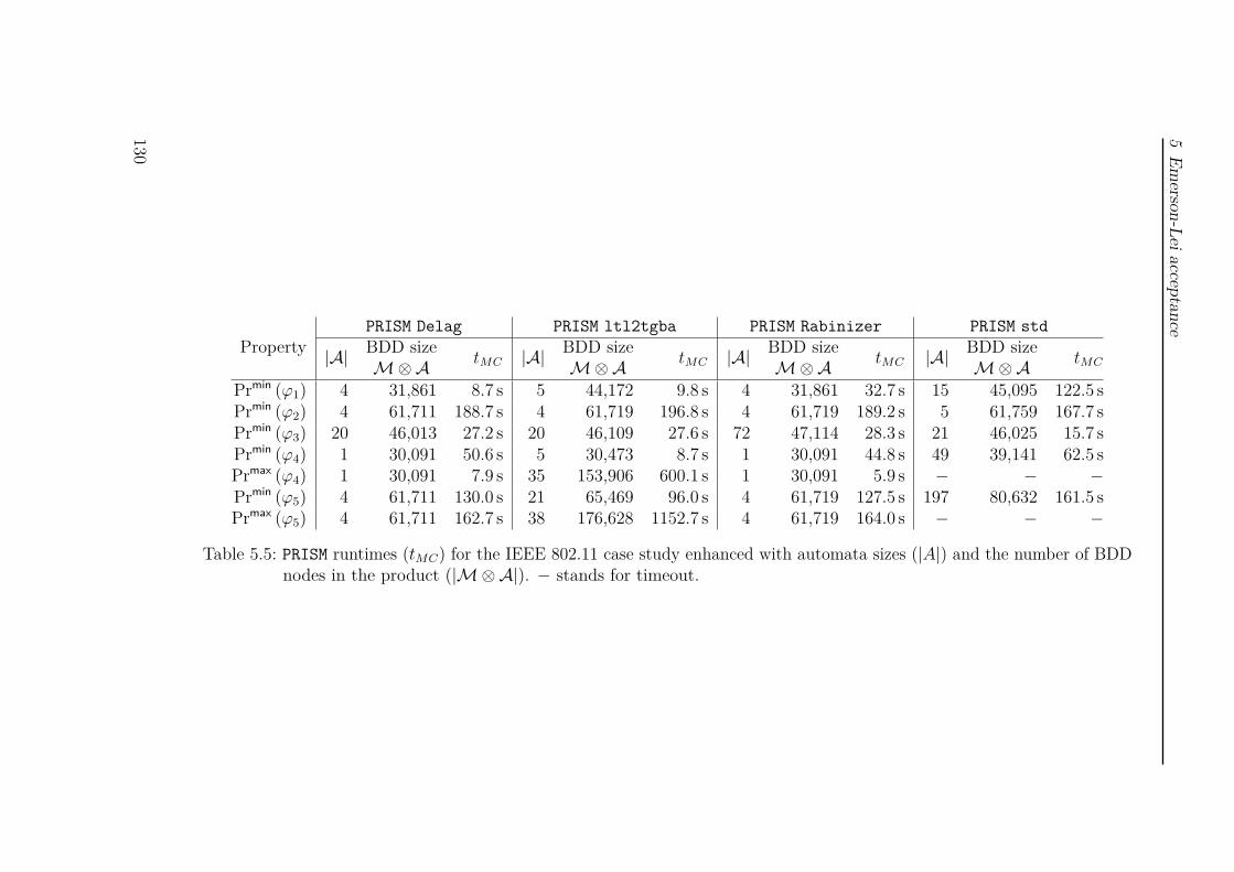
5Em
erson-Leiacceptance
PropertyPRISM Delag PRISM ltl2tgba PRISM Rabinizer PRISM std
|A| BDD sizetMC |A| BDD size
tMC |A| BDD sizetMC |A| BDD size
tMCM⊗A M⊗A M⊗A M⊗APrmin (ϕ1) 4 31,861 8.7 s 5 44,172 9.8 s 4 31,861 32.7 s 15 45,095 122.5 sPrmin (ϕ2) 4 61,711 188.7 s 4 61,719 196.8 s 4 61,719 189.2 s 5 61,759 167.7 sPrmin (ϕ3) 20 46,013 27.2 s 20 46,109 27.6 s 72 47,114 28.3 s 21 46,025 15.7 sPrmin (ϕ4) 1 30,091 50.6 s 5 30,473 8.7 s 1 30,091 44.8 s 49 39,141 62.5 sPrmax (ϕ4) 1 30,091 7.9 s 35 153,906 600.1 s 1 30,091 5.9 s − − −Prmin (ϕ5) 4 61,711 130.0 s 21 65,469 96.0 s 4 61,719 127.5 s 197 80,632 161.5 sPrmax (ϕ5) 4 61,711 162.7 s 38 176,628 1152.7 s 4 61,719 164.0 s − − −
Table 5.5: PRISM runtimes (tMC) for the IEEE 802.11 case study enhanced with automata sizes (|A|) and the number of BDDnodes in the product (|M⊗A|). − stands for timeout.
130
5.5 Conclusion
First, the generation time for every automaton was below 1.0 s, except for Rabinizerat Prmin (ϕ3) where it was 1.8 s and for the ltl2dstar reimplementation in PRISMat Prmax (ϕ4) (3.8 s) as well as at Prmax (ϕ5) (14.1 s). In two cases PRISM Delag wasthe fastest. For Prmin (ϕ4) PRISM ltl2tgba took only 8.7 s in comparison to 50.6 sfor PRISM Delag despite the smaller automaton, as one heuristic applies for PRISMltl2tgba did not apply for PRISM Delag: For the analysis of the MECs we alwayscheck at first, whether the whole MEC satisfies the acceptance condition, and onlyif this is not the case, we look for accepting sub-end-components within the MEC.For PRISM ltl2tgba the whole MEC was accepting, but for PRISM Delag one has tosearch for an accepting sub-end-component. Since in a symbolic representation SCCenumeration is costly, PRISM ltl2tgba was much faster.
In general, one can see, that Delag always produced the smallest automatonresulting in the smallest number of BDD nodes in the product and comparativelysmall model checking times for PRISM Delag.
5.5 ConclusionWe presented a general framework based on the product construction and specializedtranslations for fragments of LTL to build deterministic Emerson-Lei automata. Inparticular, for the important fairness fragment we established an efficient construction,where the state space only depends on the nesting depth of ⃝, and the acceptancecondition reflects the complexity of the formula. The general construction appliesa range of additional optimizations, such as pushing temporal operators down thesyntax tree, piggybacking to reduce the number of acceptance sets and sharing ofequal automata parts. In particular, our history buffer approach reduces the statespace, since the buffer can be shared between automata for different subformulas. Ifa formula does not belong to one of our explicitly supported fragments, we can runan external LTL-to-deterministic-automaton translator and incorporate the resultingautomaton via product construction and lifting.
Benchmarking this approach has shown the potential of our method. Standardbenchmarks highlight the potential of allowing more complex acceptance conditions,our tool produced automata with state numbers comparable to SPOT.
However, the heuristics presented here are not complete, and this approach shouldbe understood as a framework. So, one direction for future work is to add moreexplicitly supported LTL fragments. Another point would be to analyze the subfor-mulas which cannot be translated directly and choose an external tool that behaveswell for these specific subformulas. For example, it is well-known, that obligationLTL formulas can be translated to weak DBA, and then efficiently minimized. Thisis implemented in SPOT. Another direction one could take is a deeper look into isstarting with a non-deterministic Büchi automaton and trying to find small deter-ministic automata with complex acceptance conditions. Of course, general methodsto shrink the state space like bisimulation could be also applied. Also, the particularingredients of our transformation could be optimized further, e.g., the history could
131
5 Emerson-Lei acceptance
be allocated dynamically, and therefore reduce the state space even further withoutincreasing the acceptance condition complexity.
Of course, both approaches could be combined, and intermediate steps over non-deterministic automata are only done, if the LTL formula cannot be dealt with byDelag directly.
For MDP analysis, the Emerson-Lei acceptance adds some difficulty. In fact, ifdeciding satisfiability for a class of Boolean formulas is NP-complete, then decidingpositiveness for MDPs and an Emerson-Lei acceptance of the corresponding Emerson-Lei acceptance class is NP-complete as well. Still, for subclasses like acceptanceswithout any Fin (·) variable, polynomial time checks are possible. For the generalcase the DPLL algorithm for solving the satisfiability of Boolean formula can beadapted to the Emerson-Lei setting. To achieve the required conjunctive normal form,we refined the Tseytin transformation. This transformation introduces slack variableswhich are treated by the consecutive DPLL-algorithm. The slack variables provide aninteresting heuristic for the choice of the branch variable in our DPLL algorithm: Wealways prefer slack variables over Fin (·) variables. This heuristic allows a polynomialtime behavior for Rabin and Streett acceptances similar to already known approaches.
The benchmarks of our approach in the area of PMC show that our DPLL algorithmcauses only a very small overhead, but benefits from the small state space. Thus,the time for the overall model checking process were for 5 out of 7 cases in the sameorder of magnitude as the best time of PRISM Rabinizer and PRISM ltl2tgba.
132
6 ConclusionIn this thesis we presented three new automata-based approaches different from thestandard approach that employs deterministic Rabin automata in order to avoid orcope with the double-exponential blow-up.
Good-for-games automata were a promising candidate for MDP analysis. Weshowed that the GFG strategy of the good-for-games automaton and the maximalscheduler of an MDP share some similarities. The GFG strategy tries to construct anaccepting run for an accepted word depending on the history, whereas the maximizingscheduler tries to maximize the probability depending on the history. Thus, a modifiedproduct construction and a standard MEC and reachability analysis are sufficient forMDP analysis against a GFG automaton specification. The overall approach startingfrom LTL can be done in double-exponential time, thus meeting the lower bound forMDP analysis under LTL specifications. Nonetheless, practical evaluation showedthat good-for-games automata fell behind the standard approach of using [GO01] togenerate a non-deterministic Büchi automaton and Safra’s determinization [Saf88] todeterminize it.
Unambiguous automata on the other hand showed an advantage over deterministicautomata both on a theoretical level and in a practical evaluation. The single-exponential blow-up of the LTL-to-UBA translation gives UBA an edge over deter-ministic automata, but the actual model checking process becomes more complicatedalthough still polynomial. Still, the performance of the overall process heavily dependson efficient LTL-to-UBA translators.
In 2017, Boker, Kupferman and Skrzypczak [BKS17] have proven that everyunambiguous GFG automaton can be transformed to an equivalent deterministicautomaton by removing unnecessary transitions and states. Thus, the combinationof unambiguity and good-for-games is not a promising candidate for performanceimprovements.
The Emerson-Lei acceptance differs from unambiguity and good-for-games, as itworks on the acceptance level, not on the non-determinism of the automaton. Theproduct construction allows a reflection of the Boolean structure of the input LTLformula into the acceptance condition, not into the state space of the automaton. Sinceevery Emerson-Lei automaton is actually a Muller automaton with a symbolicallyrepresented acceptance condition, the double-exponential blow-up from LTL todeterministic automata cannot be avoided by the Emerson-Lei acceptance. Still, inthe automata generation part our tool Delag could compete with other standardautomata tools like Rabinizer and ltl2tgba from SPOT.
In the application for model checking, EL automata are well-suited for the analysisof Markov chains, as checking PrM(Φ) > 0 is still possible in polynomial time. For
133
6 Conclusion
Markov decision processes, the situation becomes more complicated. The positivityproblem relates closely to satisfiability of Boolean formulas, and thus, becomesNP-complete. As solution for checking Prmax
M (Φ) > 0 we took inspiration from theDPLL algorithm. As an advantage, our DPLL-based algorithm works in polynomialtime for the commonly used acceptances generalized Rabin and Streett. As ourpractical evaluation on the WLAN handshaking protocol shows, it is worth to takethe comparably small overhead of solving the NP-complete positivity problem.
Future Work. The bad performance of the good-for-games approach in the bench-marks comes from the GFG automata generation algorithm developed by Henzingerand Piterman. This observation asks for an improved generation algorithm. Veryrecently, [KM18] suggested a modified version of Safra’s determinization algorithmfor translating an NBA to a good-for-games automaton. To the best of our knowl-edge, there is no implementation publicly available and therefore an evaluation oftheir proposal is an open task. If the generation algorithm performs well, the usageof good-for-games automata for probabilistic model checking could turn out morepositive, and if the automaton suits an explicit representation, renders GFG-basedMDP analysis with explicit representation feasible.
The principle that smaller automata likely lead to a more efficient model checkingprocess also holds for our UBA-based approach to Markov chain analysis. Theproblem of UBA generation has not been studied in depth, but is current research byus. Currently, only one LTL-to-UBA translator is available, which uses an adaption of[Cou99], see also [Dur17]. A comparison in a symbolic setting as well as a comparisonwith the other single-exponential approaches of [BRV04] and [CSS03] is also stillopen. Apart from applications in probabilistic model checking, a very intriguing openproblem is universality checking (“Is every infinite word accepted?”) for UBA. Wecan only give a PSPACE upper bound as this problem can be solved in PSPACE forNBA.
Obviously, the single-exponential generation of UBA from LTL forbids a direct usagefor the MDP analysis, as MDP analysis under LTL is 2EXPTIME-complete. However,unambiguous Büchi automata might be a good starting point for deterministic-in-the-limit automata to achieve quantitative MDP analysis similar to [Sic+16].
A natural idea would be to combine unambiguity with Emerson-Lei acceptance.Still, one would have to rewrite the LTL formula on the top-level according to [Dur17],and then apply a product construction for conjunctions and a union of automata fordisjunctions. Nevertheless, as every known translation which produces unambiguous,but not deterministic automata, aims at (generalized) Büchi acceptance, the resultingoverall acceptance would be without any Fin (·) atom.
As we have identified two LTL fragments with a natural translation to deterministicEmerson-Lei automata, the translation of full LTL remains an open question. Areasonable starting point would be NBA and then a modification of a suitabledeterminization algorithm.
For the positivity problem we employed only a rather simple DPLL-based algorithm,
134
known techniques like conflict-driven clause learning could improve the performanceeven further. Not only improving the efficiency of the actual model checking algorithmwould lead to a better overall performance, but also generating smaller deterministicEmerson-Lei automata. However, minimization of Emerson-Lei (or Muller) automatais an unsolved problem, but succinctness results in comparison to Rabin and Streettautomata [Bok17a] demonstrate the potential of Emerson-Lei automata.
135


Bibliography[AD94] Rajeev Alur and David L. Dill. “A Theory of Timed Automata”. In:
Theoretical Computer Science 126.2 (1994), pp. 183–235.[AL04] Rajeev Alur and Salvatore La Torre. “Deterministic Generators and
Games for LTL Fragments”. In: ACM Transactions on ProgrammingLanguages and Systems 5.1 (2004), pp. 1–25.
[Alf97] Luca de Alfaro. “Formal Verification of Probabilistic Systems”. PhDthesis. Stanford University, Department of Computer Science, 1997.
[Arn85] André Arnold. “Deterministic and non ambiguous rational omega-languages”. In: Automata on Infinite Words. Vol. 192. Lecture Notes inComputer Science. Springer, 1985, pp. 18–27.
[Bab+12] Tomás Babiak, Mojmír Křetınský, Vojtěch Řehák, and Jan Strejček.“LTL to Büchi Automata Translation: Fast and More Deterministic”.In: 18th International Conference on Tools and Algorithms for theConstruction and Analysis of Systems (TACAS). Vol. 7214. LectureNotes in Computer Science. Springer, 2012, pp. 95–109.
[Bab+13a] Tomás Babiak, Thomas Badie, Alexandre Duret-Lutz, Mojmır Kretınský,and Jan Strejcek. “Compositional Approach to Suspension and OtherImprovements to LTL Translation”. In: 25th International Symposiumon Model Checking of Software (SPIN). Vol. 7976. Lecture Notes inComputer Science. Springer, 2013, pp. 81–98.
[Bab+13b] Tomáš Babiak, Frantisek Blahoudek, Mojmır Křetınský, and Jan Strejcek.“Effective Translation of LTL to Deterministic Rabin Automata: Beyondthe (F, G)-Fragment”. In: 11th International Symposium on AutomatedTechnology for Verification and Analysis (ATVA). Vol. 8172. LectureNotes in Computer Science. Springer, 2013, pp. 24–39.
[Bab+15] Tomáš Babiak, František Blahoudek, Alexandre Duret-Lutz, JoachimKlein, Jan Křetínský, David Müller, David Parker, and Jan Strejček.“The Hanoi Omega-Automata Format”. In: 27th International Conferenceon Computer Aided Verification (CAV). Vol. 9206. Lecture Notes inComputer Science. Springer, 2015, pp. 479–486.
[Bah+93] R. Iris Bahar, Erica A. Frohm, Charles M. Gaona, Gary D. Hachtel,Enrico Macii, Abelardo Pardo, and Fabio Somenzi. “Algebraic DecisionDiagrams and their Applications”. In: 11th International Conference onComputer-Aided Design (ICCAD). IEEE, 1993, pp. 188–191.
137
Bibliography
[Bai+16] Christel Baier, Stefan Kiefer, Joachim Klein, Sascha Klüppelholz, DavidMüller, and James Worrell. “Markov Chains and Unambiguous BüchiAutomata”. In: 28th International Conference on Computer Aided Veri-fication (CAV) - Part I. Vol. 9779. Lecture Notes in Computer Science.Springer, 2016, pp. 23–42.
[Bai+17] Christel Baier, Joachim Klein, Linda Leuschner, David Parker, andSascha Wunderlich. “Ensuring the Reliability of Your Model Checker:Interval Iteration for Markov Decision Processes”. In: 29th InternationalConference on Computer Aided Verification (CAV). Vol. 10426. LectureNotes in Computer Science. Springer, 2017, pp. 160–180.
[BC04] Yves Bertot and Pierre Castéran. Interactive Theorem Proving andProgram Development. Springer, 2004.
[BD15] Souheib Baarir and Alexandre Duret-Lutz. “SAT-Based Minimizationof Deterministic ω-Automata”. In: 20th International Conference onLogic for Programming, Artificial Intelligence, and Reasoning (LPAR).Vol. 9450. Lecture Notes in Computer Science. Springer, 2015, pp. 79–87.
[BGC09a] Christel Baier, Marcus Größer, and Frank Ciesinski. “Model Check-ing Linear-Time Properties of Probabilistic Systems”. In: Handbookof Weighted Automata. Monographs in Theoretical Computer Science.Springer, 2009. Chap. 13, pp. 519–570.
[BGC09b] Christel Baier, Marcus Größer, and Frank Ciesinski. “QuantitativeAnalysis under Fairness Constraints”. In: 7th International Symposium onAutomated Technology for Verification and Analysis (ATVA). Vol. 5799.Lecture Notes in Computer Science. Springer, 2009, pp. 135–150.
[BGS00] Roderick Bloem, Harold N. Gabow, and Fabio Somenzi. “An Algorithmfor Strongly Connected Component Analysis in n logn Symbolic Steps”.In: Third International Conference on Formal Methods in ComputerAided Design (FMCAD). Lecture Notes in Computer Science 2517.Springer-Verlag, 2000, pp. 37–54.
[Bie+03] Armin Biere, Alessandro Cimatti, Edmund M. Clarke, Ofer Strichman,and Yunshan Zhu. “Bounded Model Checking”. In: Advances in Com-puters 58 (2003), pp. 117–148.
[Bie+99] Armin Biere, Alessandro Cimatti, Edmund M. Clarke, and YunshanZhu. “Symbolic Model Checking without BDDs”. In: Fifth InternationalConference on Tools and Algorithms for Construction and Analysisof Systems (TACAS). Vol. 1579. Lecture Notes in Computer Science.Springer, 1999, pp. 193–207.
[BK08] Christel Baier and Joost-Pieter Katoen. Principles of Model Checking.MIT Press, 2008.
138
Bibliography
[BKS17] Udi Boker, Orna Kupferman, and Michał Skrzypczak. “How Deter-ministic are Good-For-Games Automata?” In: 37th Conference onFoundations of Software Technology and Theoretical Computer Science(FSTTCS). Vol. 93. Leibniz International Proceedings in Informatics.Schloss Dagstuhl - Leibniz-Zentrum für Informatik, 2017, 18:1–18:14.
[BL10] Nicolas Bousquet and Christof Löding. “Equivalence and Inclusion Prob-lem for Strongly Unambiguous Büchi Automata”. In: 4th InternationalConference on Language and Automata Theory and Applications (LATA).Vol. 6031. Lecture Notes in Computer Science. Springer, 2010, pp. 118–129.
[Bla+17] Frantisek Blahoudek, Alexandre Duret-Lutz, Mikulás Klokocka, MojmırKretınský, and Jan Strejcek. “Seminator: A Tool for Semi-Determinizationof Omega-Automata”. In: 21st International Conference on Logic forProgramming, Artificial Intelligence and Reasoning (LPAR). Vol. 46.EPiC Series in Computing. EasyChair Publications, 2017, pp. 356–367.
[BLW13a] Michael Benedikt, Rastislav Lenhardt, and James Worrell. “LTL ModelChecking of Interval Markov Chains”. In: 19th International Conferenceon Tools and Algorithms for the Construction and Analysis of Systems(TACAS). Vol. 7795. Lecture Notes in Computer Science. Springer, 2013,pp. 32–46.
[BLW13b] Michael Benedikt, Rastislav Lenhardt, and James Worrell. “Two Variablevs. Linear Temporal Logic in Model Checking and Games”. In: LogicalMethods in Computer Science 9.2 (2013).
[BLW14] Michael Benedikt, Rastislav Lenhardt, and James Worrell. Model Check-ing Markov Chains Against Unambiguous Büchi Automata. arXiv:1405.4560.2014.
[Bok+13] Udi Boker, Denis Kuperberg, Orna Kupferman, and Michał Skrzypczak.“Nondeterminism in the Presence of a Diverse or Unknown Future”.In: 40th International Conference on Automata, Languages, and Pro-gramming Colloquium (ICALP, Track B). Vol. 7966. Lecture Notes inComputer Science. Springer, 2013, pp. 89–100.
[Bok17a] Udi Boker. “On the (In)Succinctness of Muller Automata”. In: 26thConference on Computer Science Logic (CSL). Vol. 82. Leibniz Interna-tional Proceedings in Informatics. Schloss Dagstuhl - Leibniz-Zentrumfür Informatik, 2017, 12:1–12:16.
[Bok17b] Udi Boker. “Rabin vs. Streett Automata”. In: 37th Conference onFoundations of Software Technology and Theoretical Computer Science(FSTTCS). Vol. 93. Leibniz International Proceedings in Informatics.Schloss Dagstuhl - Leibniz-Zentrum für Informatik, 2017, 17:1–17:15.
[BP79] Abraham Berman and Robert J. Plemmons. Nonnegative Matrices inthe Mathematical Sciences. Academic Press, 1979.
139
Bibliography
[BRV04] Doron Bustan, Sasha Rubin, and Moshe Y. Vardi. “Verifying ω-RegularProperties of Markov Chains”. In: 16th International Conference on Com-puter Aided Verification (CAV). Vol. 3114. Lecture Notes in ComputerScience. Springer, 2004, pp. 189–201.
[Bry86] Randal E. Bryant. “Graph-Based Algorithms for Boolean Function Ma-nipulation”. In: IEEE Transactions on Computers 35.8 (1986), pp. 677–691.
[Büc62] Julius Richard Büchi. “On a Decision Method in restricted Second OrderArithmetic”. In: First International Congress on Logic, Methodologyand Philosophy of Science (CLMPS). Stanford University Press, 1962,pp. 1–11.
[Bur+92] Jerry R. Burch, Edmund M. Clarke, Kenneth L. McMillan, David L.Dill, and L. J. Hwang. “Symbolic Model Checking: 10^20 States andBeyond”. In: Information and Computation 98.2 (1992), pp. 142–170.
[BY04] Johan Bengtsson and Wang Yi. “Timed Automata: Semantics, Algo-rithms and Tools”. In: Lectures on Concurrency and Petri Nets: Advancesin Petri Nets. Vol. 3098. Lecture Notes in Computer Science. Springer,2004, pp. 87–124.
[CE81] Edmund M. Clarke and Ernest A. Emerson. “Design and Synthesisof Synchronization Skeletons Using Branching-Time Temporal Logic”.In: Logics of Programs. Vol. 131. Lecture Notes in Computer Science.Springer, 1981, pp. 52–71.
[CES86] Edmund M. Clarke, Ernest A. Emerson, and A. Prasad Sistla. “Auto-matic Verification of Finite-State Concurrent Systems Using TemporalLogic Specifications”. In: ACM Transactions on Programming Languagesand Systems 8.2 (1986), pp. 244–263.
[CFZ93] Edmund M. Clarke, Masahiro Fujita, and Xudong Zhao. “Multi-TerminalBinary Decision Diagrams and Hybrid Decision Diagrams”. In: ThirdInternational Workshop on Logic & Synthesis (IWLS). 1993, pp. 1–15.
[CGH97] Edmund M. Clarke, Orna Grumberg, and Kiyoharu Hamaguchi. “An-other Look at LTL Model Checking”. In: Formal Methods in SystemDesign 10.1 (1997), pp. 47–71.
[CGK13] Krishnendu Chatterjee, Andreas Gaiser, and Jan Křetınský. “Automatawith Generalized Rabin Pairs for Probabilistic Model Checking andLTL Synthesis”. In: 25th International Conference on Computer AidedVerification (CAV). Lecture Notes in Computer Science. Springer, 2013,pp. 559–575.
140
Bibliography
[Cim+02] Alessandro Cimatti, Edmund M. Clarke, Enrico Giunchiglia, FaustoGiunchiglia, Marco Pistore, Marco Roveri, Roberto Sebastiani, and Ar-mando Tacchella. “NuSMV Version 2: An OpenSource Tool for SymbolicModel Checking”. In: 14th International Conference on Computer-AidedVerification (CAV). Vol. 2404. Lecture Notes in Computer Science.Springer, 2002.
[CK14] Souymodip Chakraborty and Joost-Pieter Katoen. “Parametric LTL onMarkov Chains”. In: 8th IFIP International Conference on TheoreticalComputer Science (TCS). Vol. 8705. Lecture Notes in Computer Science.Springer, 2014, pp. 207–221.
[CM03] Olivier Carton and Max Michel. “Unambiguous Büchi automata”. In:Theoretical Computer Science 297.1–3 (2003), pp. 37–81.
[Col09] Thomas Colcombet. “The Theory of Stabilisation Monoids and Reg-ular Cost Functions”. In: 36 International Colloquium on Automata,Languages and Programming (ICALP). Vol. 5556. Lecture Notes inComputer Science. Springer, 2009, pp. 139–150.
[Col12] Thomas Colcombet. “Forms of Determinism for Automata”. In: 29thInternational Symposium on Theoretical Aspects of Computer Science,(STACS). Vol. 14. Leibniz International Proceedings in Informatics.Schloss Dagstuhl - Leibniz-Zentrum für Informatik, 2012, pp. 1–23.
[Col15] Thomas Colcombet. “Unambiguity in Automata Theory”. In: 17th In-ternational Workshop on Descriptional Complexity of Formal Systems(DCFS). Vol. 9118. Lecture Notes in Computer Science. Springer, 2015,pp. 3–18.
[Cou99] Jean-Michel Couvreur. “On-the-Fly Verification of Linear TemporalLogic”. In: 1st World Congress on Formal Methods in the Developmentof Computing Systems (FM). Vol. 1708. Lecture Notes in ComputerScience. Springer, 1999, pp. 253–271.
[ČP03] Ivana Černá and Radek Pelánek. “Distributed Explicit Fair Cycle Detec-tion (Set Based Approach)”. In: 10th International SPIN Workshop onModel Checking of Software (SPIN). Lecture Notes in Computer Science.Springer, 2003, pp. 49–73.
[CSS03] Jean-Michel Couvreur, Nasser Saheb, and Grégoire Sutre. “An OptimalAutomata Approach to LTL Model Checking of Probabilistic Systems”.In: 10th International Conference on Logic for Programming, Artifi-cial Intelligence, and Reasoning (LPAR). Vol. 2850. Lecture Notes inComputer Science. Springer, 2003, pp. 361–375.
[CY88] Costas Courcoubetis and Mihalis Yannakakis. “Verifying temporal prop-erties of finite-state probabilistic programs”. In: 29th Symposium onFoundations of Computer Science (FOCS). IEEE computer society, 1988,pp. 338–345.
141
Bibliography
[CY95] Costas Courcoubetis and Mihalis Yannakakis. “The Complexity of Prob-abilistic Verification”. In: Journal of the ACM 42.4 (1995), pp. 857–907.
[DAC99] Matthew B. Dwyer, George S. Avrunin, and James C. Corbett. “Patternsin Property Specifications for Finite-State Verification”. In: InternationalConference on Software Engineering (ICSE). ACM, 1999, pp. 411–420.
[Deh+17] Christian Dehnert, Sebastian Junges, Joost-Pieter Katoen, and MatthiasVolk. “A Storm is Coming: A Modern Probabilistic Model Checker”. In:29th International Conference on Computer Aided Verification (CAV).Vol. 10427. Lecture Notes in Computer Science. Springer, 2017, pp. 592–600.
[Die17] Reinhard Diestel. Vol. 173. Graduate Texts in Mathematics. Springer,2017.
[DLL62] Martin Davis, George Logemann, and Donald W. Loveland. “A MachineProgram for Theorem-Proving”. In: Communications of the ACM 5.7(1962), pp. 394–397.
[DP60] Martin Davis and Hilary Putnam. “A Computing Procedure for Quan-tification Theory”. In: Journal of the ACM 7.3 (1960), pp. 201–215.
[DPC09] Alexandre Duret-Lutz, Denis Poitrenaud, and Jean-Michel Couvreur.“On-the-fly Emptiness Check of Transition-based Streett Automata”. In:7th International Symposium on Automated Technology for Verificationand Analysis (ATVA’09). Vol. 5799. Lecture Notes in Computer Science.Springer, 2009, pp. 213–227.
[Dur+16] Alexandre Duret-Lutz, Alexandre Lewkowicz, Amaury Fauchille, ThibaudMichaud, Etienne Renault, and Laurent Xu. “Spot 2.0 - A Frameworkfor LTL and ω-Automata Manipulation”. In: 14th Internation Sympo-sium on Automated Technology for Verification and Analysis (ATVA).Vol. 9938. Lecture Notes in Computer Science. 2016, pp. 122–129.
[Dur13] Alexandre Duret-Lutz. “Manipulating LTL Formulas Using Spot 1.0”. In:11th International Symposium on Automated Technology for Verificationand Analysis (ATVA). Vol. 8172. Lecture Notes in Computer Science.Springer, 2013, pp. 442–445.
[Dur14] Alexandre Duret-Lutz. “LTL translation improvements in Spot 1.0”. In:International Journal of Critical Computer-Based Systems 5.1/2 (2014),pp. 31–54.
[Dur17] Alexandre Duret-Lutz. “Contributions to LTL and ω-Automata forModel Checking”. Habilitation Thesis. Université Pierre et Marie Curie(Paris 6), 2017.
142
Bibliography
[EC80] Ernest A. Emerson and Edmund M. Clarke. “Characterizing CorrectnessProperties of Parallel Programs Using Fixpoints”. In: 7th InternationalConference on Automata, Languages and Programming (ICALP). Vol. 85.Lecture Notes in Computer Science. Springer, 1980, pp. 169–181.
[EH00] Kousha Etessami and Gerard J. Holzmann. “Optimizing Büchi Au-tomata”. In: 11th International Conference on Concurrency Theory(CONCUR). Vol. 1877. Lecture Notes in Computer Science. Springer,2000, pp. 153–167.
[Ehl10] Rüdiger Ehlers. “Minimising Deterministic Büchi Automata PreciselyUsing SAT Solving”. In: 13th International Conference on Theory andApplications of Satisfiability Testing (SAT). Vol. 6175. Lecture Notes inComputer Science. Springer, 2010, pp. 326–332.
[EK14] Javier Esparza and Jan Křetınský. “From LTL to Deterministic Au-tomata: a Safraless Compositional Approach”. In: 26th InternationalConference on Computer Aided Verification (CAV). Vol. 8559. LectureNotes in Computer Science. Springer, 2014, pp. 192–208.
[EKS16] Javier Esparza, Jan Křetınský, and Salomon Sickert. “From LTL toDeterministic Automata - A Safraless Compositional Approach”. In:Formal Methods in System Design 49.3 (2016), pp. 219–271.
[EKS18] Javier Esparza, Jan Křetínský, and Salomon Sickert. “One Theorem toRule Them All: A Unified Translation of LTL into ω-Automata”. In:33th ACM/IEEE Symposium on Logic in Computer Science (LICS). toappear. 2018.
[EL85] Ernest A. Emerson and Chin-Laung Lei. “Modalities for model checking:branching time strikes back”. In: 12th ACM Symposium on Principlesof Programming Languages (POPL). ACM, 1985, pp. 84–96.
[EL87] Ernest A. Emerson and Chin-Laung Lei. “Modalities for Model Check-ing: Branching Time Logic Strikes Back”. In: Science of ComputerProgramming 8.3 (1987), pp. 275–306.
[FL15] Dana Fisman and Yoad Lustig. “A Modular Approach for Büchi Deter-minization”. In: 26th International Conference on Concurrency Theory(CONCUR). Vol. 42. Leibniz International Proceedings in Informatics.Schloss Dagstuhl - Leibniz-Zentrum für Informatik, 2015, pp. 368–382.
[Fog+13] Seth Fogarty, Orna Kupferman, Moshe Y. Vardi, and Thomas Wilke.“Profile Trees for Büchi Word Automata, with Application to Deter-minization”. In: Fourth International Symposium on Games, Automata,Logics and Formal Verification (GandALF). Vol. 119. Electronic Pro-ceedings of Theoretical Computer Science. 2013, pp. 107–121.
[FV96] Jerzy Filar and Koos Vrieze. Competitive Markov Decision Processes.Springer, 1996.
143
Bibliography
[Ger+95] Rob Gerth, Doron Peled, Moshe Y. Vardi, and Pierre Wolper. “Sim-ple On-the-fly Automatic Verification of Linear Temporal Logic”. In:15th IFIP WG6.1 International Symposium on Protocol Specification,Testing and Verification (PSTV). Vol. 38. IFIP Conference Proceedings.Chapman & Hall, 1995, pp. 3–18.
[GO01] Paul Gastin and Denis Oddoux. “Fast LTL to Büchi Automata Transla-tion”. In: 13th International Conference on Computer Aided Verification,(CAV). Vol. 2102. Lecture Notes in Computer Science. Springer, 2001,pp. 53–65.
[GTW02] Erich Grädel, Wolfgang Thomas, and Thomas Wilke, eds. Automata,Logics, and Infinite Games: A Guide to Current Research. Vol. 2500.Lecture Notes in Computer Science. Springer, 2002.
[Hah+14] Ernst Moritz Hahn, Yi Li, Sven Schewe, Andrea Turrini, and LijunZhang. “ISCASMC: A Web-Based Probabilistic Model Checker”. In:19th International Symposium on Formal Methods (FM). Vol. 8442.Lecture Notes in Computer Science. Springer, 2014, pp. 312–317.
[Hah+15] Ernst Moritz Hahn, Guangyuan Li, Sven Schewe, Andrea Turrini, andLijun Zhang. “Lazy Probabilistic Model Checking without Determin-isation”. In: 26th International Conference on Concurrency Theory(CONCUR). Vol. 42. Leibniz International Proceedings in Informatics.Schloss Dagstuhl - Leibniz-Zentrum für Informatik, 2015, pp. 354–367.
[HJ13] Roger A. Horn and Charles R. Johnson. Matrix analysis. 2nd. CambridgeUniversity Press, 2013.
[HJ94] Hans Hansson and Bengt Jonsson. “A Logic for Reasoning about Timeand Reliability”. In: Formal Aspects of Computing 6 (1994), pp. 512–535.
[Hol04] Gerard J. Holzmann. The SPIN Model Checker - Primer and ReferenceManual. Addison-Wesley, 2004. isbn: 978-0-321-22862-8.
[Hos04] Wolfgang Hoschek. The Colt Distribution: Open Source Libraries forHigh Performance Scientific and Technical Computing in Java. 2004.
[HP06] Thomas A. Henzinger and Nir Piterman. “Solving Games WithoutDeterminization”. In: 20th International Workshop on Computer ScienceLogic (CSL). Vol. 4207. Lecture Notes in Computer Science. Springer,2006, pp. 395–410.
[HSP83] Sergiu Hart, Micha Sharir, and Amir Pnueli. “Termination of Probabilis-tic Concurrent Program”. In: Transactions on Programming Languagesand Systems 5.3 (1983), pp. 356–380.
[HSS17] Yo-Sub Han, Arto Salomaa, and Kai Salomaa. “Ambiguity, Nondeter-minism and State Complexity of Finite Automata”. In: Acta Cybernetica23.1 (2017), pp. 141–157.
144
Bibliography
[IL12] Dimitri Isaak and Christof Löding. “Efficient Inclusion Testing for SimpleClasses of Unambiguous ω-Automata”. In: Information Processing Letters112.14-15 (2012), pp. 578–582.
[Kat+11] Joost-Pieter Katoen, Ivan S. Zapreev, Ernst Moritz Hahn, Holger Her-manns, and David N. Jansen. “The Ins and Outs of The ProbabilisticModel Checker MRMC”. In: Performance Evaluation 68.2 (2011), pp. 90–104.
[KB06] Joachim Klein and Christel Baier. “Experiments with deterministic ω-automata for formulas of linear temporal logic”. In: Theoretical ComputerScience 363.2 (2006), pp. 182–195.
[KB07] Joachim Klein and Christel Baier. “On-the-Fly Stuttering in the Con-struction of Deterministic ω-Automata”. In: 12th International Confer-ence on Implementation and Application of Automata (CIAA). Vol. 4783.Lecture Notes in Computer Science. Springer, 2007, pp. 51–61.
[KE12] Jan Křetınský and Javier Esparza. “Deterministic Automata for the(F,G)-fragment of LTL”. In: 24th International Conference on ComputerAided Verification (CAV). Vol. 7358. Lecture Notes in Computer Science.Springer, 2012, pp. 7–22.
[KG13] Jan Kretınský and Ruslán Ledesma Garza. “Rabinizer 2: Small Deter-ministic Automata for LTL\GU”. In: 11th International Symposium onAutomated Technology for Verification and Analysis (ATVA). Vol. 8172.Lecture Notes in Computer Science. Springer, 2013, pp. 446–450.
[Kie17] Stefan Kiefer. Unambiguous Automata: From PSPACE to P. Blog articlefrom Stefan Kiefer. 2017. url: https://stekie.blogspot.de/2017/06/unambiguous-automata-from-pspace-to-p.html.
[Kin17] Dileep Raghunath Kini. “Verification of Linear Time Properties ForFinite Probabilistic Systems”. PhD thesis. University of Illinois, 2017.
[Kle+14] Joachim Klein, David Müller, Christel Baier, and Sascha Klüppelholz.“Are Good-for-Games Automata Good for Probabilistic Model Check-ing?” In: 8th International Conference on Language and AutomataTheory and Applications (LATA). Vol. 8370. Lecture Notes in ComputerScience. Springer, 2014, pp. 453–465.
[Kle+17] Joachim Klein, Christel Baier, Philipp Chrszon, Marcus Daum, ClemensDubslaff, Sascha Klüppelholz, Steffen Märcker, and David Müller. “Ad-vances in probabilistic model checking with PRISM: variable reordering,quantiles and weak deterministic Büchi automata”. In: InternationalJournal on Software Tools for Technology Transfer (STTT) (2017),pp. 1–16.
145
Bibliography
[KM18] Denis Kuperberg and Anirban Majumdar. “Width of Non-deterministicAutomata”. In: 35th International Symposium on Theoretical Aspects ofComputer Science (STACS). Vol. 96. Leibniz International Proceedingsin Informatics. Schloss Dagstuhl - Leibniz-Zentrum für Informatik, 2018.
[KNP04] Marta Zofia Kwiatkowska, Gethin Norman, and David Parker. “Proba-bilistic Symbolic Model Checking with PRISM: A Hybrid Approach”.In: International Journal on Software Tools for Technology Transfer(STTT) 6(2) (2004), pp. 128–142.
[KNP11] Marta Zofia Kwiatkowska, Gethin Norman, and David Parker. “PRISM4.0: Verification of Probabilistic Real-time Systems”. In: 23th Interna-tional Conference on Computer Aided Verification (CAV). Vol. 6806.Lecture Notes in Computer Science. Springer, 2011, pp. 585–591.
[KNP12] Marta Z. Kwiatkowska, Gethin Norman, and David Parker. “The PRISMBenchmark Suite”. In: 9th International Conference on QuantitativeEvaluation of SysTems (QEST). IEEE Computer Society, 2012, pp. 203–204.
[KNS02] Marta Zofia Kwiatkowska, Gethin Norman, and Jeremy Sproston. “Prob-abilistic Model Checking of the IEEE 802.11 Wireless Local Area Net-work Protocol”. In: Second Joint International Workshop on ProcessAlgebra and Probabilistic Methods, Performance Modeling and Veri-fication, (PAPM-PROBMIV). Vol. 2399. Lecture Notes in ComputerScience. Springer, 2002, pp. 169–187.
[KPV06] Orna Kupferman, Nir Piterman, and Moshe Y. Vardi. “Safraless Com-positional Synthesis”. In: 18th International Conference on ComputerAided Verification, (CAV). Vol. 4144. Lecture Notes in Computer Science.Springer, 2006, pp. 31–44.
[KR11] Orna Kupferman and Adin Rosenberg. “The Blow-up in TranslatingLTL to Deterministic Automata”. In: 6th International Workshop onModel Checking and Artificial Intelligence (MoChArt). Vol. 6572. LectureNotes in Computer Science. Springer, 2011, pp. 85–94.
[KRS09] Jui-Yi Kao, Narad Rampersad, and Jeffrey Shallit. “On NFAs whereall states are final, initial, or both”. In: Theoretical Computer Science410.47–49 (2009), pp. 5010–5021.
[KS15] Denis Kuperberg and Michał Skrzypczak. “On Determinisation of Good-for-Games Automata”. In: 42nd International Colloquium on Automata,Languages, and Programming (ICALP). Vol. 9135. Lecture Notes inComputer Science. 2015, pp. 299–310.
[KV05] Orna Kupferman and Moshe Y. Vardi. “From Linear Time to BranchingTime”. In: Transactions on Computational Logic 6.2 (2005), pp. 273–294.
146
Bibliography
[KV15] Dileep Kini and Mahesh Viswanathan. “Limit Deterministic and Prob-abilistic Automata for LTL \G U”. In: 21st International Conferenceon Tools and Algorithms for the Construction and Analysis of Systems(TACAS). Vol. 9035. Lecture Notes in Computer Science. Springer, 2015,pp. 628–642.
[KW08] Detlef Kähler and Thomas Wilke. “Complementation, Disambiguation,and Determinization of Büchi Automata Unified”. In: 35th Interna-tional Colloquium on Automata, Languages and Programming (ICALP).Vol. 5125. Lecture Notes in Computer Science. Springer, 2008, pp. 724–735.
[LDB10] Axel Legay, Benoıt Delahaye, and Saddek Bensalem. “Statistical ModelChecking: An Overview”. In: First International Conference on Run-time Verification (RV). Vol. 6418. Lecture Notes in Computer Science.Springer, 2010, pp. 122–135.
[Len13a] Rastislav Lenhardt. “Tulip: Model Checking Probabilistic Systems UsingExpectation Maximisation Algorithm”. In: 10th International Conferenceon Quantitative Evaluation of Systems (QEST). Vol. 8054. Lecture Notesin Computer Science. Springer, 2013, pp. 155–159.
[Len13b] Rastislav Lenhardt. “Two Variable and Linear Temporal Logic in ModelChecking and Games”. PhD thesis. University of Oxford, 2013.
[LH00] Timo Latvala and Keijo Heljanko. “Coping With Strong Fairness”. In:Fundamenta Informaticae 43.1–4 (2000), pp. 1–19.
[Li+16a] Yong Li, Wanwei Liu, Andrea Turrini, Ernst Moritz Hahn, and LijunZhang. “An Efficient Synthesis Algorithm for Parametric Markov ChainsAgainst Linear Time Properties”. In: Second International Symposiumon Dependable Software Engineering: Theories, Tools, and Applications(SETTA). Vol. 9984. Lecture Notes in Computer Science. Springer, 2016,pp. 280–296.
[Li+16b] Yong Li, Lei Song, Yuan Feng, and Lijun Zhang. “Verify LTL withFairness Assumptions Efficiently”. In: 23rd International Symposiumon Temporal Representation and Reasoning (TIME). IEEE ComputerSociety, 2016, pp. 41–50.
[Löd01] Christof Löding. “Efficient minimization of deterministic weak omega-automata”. In: Information Processing Letters 79.3 (2001), pp. 105–109.
[LP18] Christof Löding and Anton Pirogov. “On Finitely Ambiguous BüchiAutomata”. In: 22nd International Conference on Developments inLanguage Theory (DLT). Vol. 11088. Lecture Notes in Computer Science.Springer, 2018, pp. 503–515.
147
Bibliography
[LP85] Orna Lichtenstein and Amir Pnueli. “Checking That Finite State Concur-rent Programs Satisfy Their Linear Specification”. In: 12th Symposiumon Principles of Programming Languages (POPL). ACM, 1985, pp. 97–107.
[LPY95] Kim G. Larsen, Paul Pettersson, and Wang Yi. “Model-Checking forReal-Time Systems”. In: Fundamentals of Computation Theory. LectureNotes in Computer Science 965. 1995, pp. 62–88.
[LR81] Daniel Lehmann and Michael O. Rabin. “On the Advantages of FreeChoice: A Symmetric and Fully Distributed Solution to the DiningPhilosophers Problem”. In: 8th Symposium on Principles of ProgrammingLanguages (POPL). ACM, 1981, pp. 133–138.
[LSS94] Nancy Lynch, Isaac Saias, and Roberto Segala. “Proving Time Boundsfor Randomized Distributed Algorithms”. In: 13th Symposium on Prin-ciples of Distributed Computing (PODC). ACM, 1994, pp. 314–323.
[LV15] Axel Legay and Mahesh Viswanathan. “Statistical model checking:challenges and perspectives”. In: STTT 17.4 (2015), pp. 369–376.
[McN66] Robert McNaughton. “Testing and Generating Infinite Sequences by aFinite Automaton”. In: Information and Control 9.5 (1966), pp. 521–530.
[MD15] Thibaud Michaud and Alexandre Duret-Lutz. “Practical Stutter-InvarianceChecks for ω-Regular Languages”. In: 22nd International SPIN Sym-posium on Model Checking of Software (SPIN). Vol. 9232. 2015, 2015,pp. 84–101.
[MH84] Satoru Miyano and Takeshi Hayashi. “Alternating Finite Automata onω-Words”. In: Theoretical Computer Science 32 (1984), pp. 321–330.
[Mic88] Max Michel. “Complementation is more difficult with automata oninfinite words”. In: CNET. 1988.
[Mil80] Robin Milner. A Calculus of Communicating Systems. Vol. 92. LectureNotes in Computer Science. Springer, 1980. isbn: 3-540-10235-3.
[Mor10] Andreas Morgenstern. “Symbolic Controller Synthesis for LTL Specifi-cations”. PhD thesis. Technische Universität Kaiserslautern, 2010.
[Mos84] Andrzej W. Mostowski. “Regular expressions for infinite trees and astandard form of automata”. In: Fifth Symposium on ComputationTheory (SCT). Vol. 208. Lecture Notes in Computer Science. Springer,1984, pp. 157–168.
[MS08] Andreas Morgenstern and Klaus Schneider. “From LTL to SymbolicallyRepresented Deterministic Automata”. In: 9th International Conferenceon Verification, Model Checking, and Abstract Interpretation (VMCAI).Vol. 4905. Lecture Notes in Computer Science. Springer, 2008, pp. 279–293.
148
Bibliography
[MS17] David Müller and Salomon Sickert. “LTL to Deterministic Emerson-Lei Automata”. In: 8th International Symposium on Games, Automata,Logics and Formal Verification (GandALF). Vol. 256. Electronic Pro-ceedings of Theoretical Computer Science. Open Publishing Association,2017, pp. 180–194.
[MS95] David E. Muller and Paul E. Schupp. “Simulating Alternating TreeAutomata by Nondeterministic Automata: New Results and New Proofsof the Theorems of Rabin, McNaughton and Safra”. In: TheoreticalComputer Science 141.1&2 (1995), pp. 69–107.
[MT98] Christoph Meinel and Thorsten Theobald. Algorithmen und Datenstruk-turen im VLSI-Design. Springer, 1998.
[Mül18] David Müller. Website with additional material. 2018. url: https://wwwtcs.inf.tu-dresden.de/~david/phd/.
[Mul63] David E. Muller. “Infinite sequences and finite machines”. In: 4th Sym-posium on Switching Circuit Theory and Logical Design. IEEE computersociety, 1963, pp. 3–16.
[NK14] Tobias Nipkow and Gerwin Klein. Concrete Semantics - With Is-abelle/HOL. Springer, 2014. isbn: 978-3-319-10541-3.
[Oss10] Jörn Ossowski. “JINC: A Multi-Threaded Library for Higher-OrderWeighted Decision Diagram Manipulation”. PhD thesis. University ofBonn, 2010.
[Par02] David Parker. “Implementation of Symbolic Model Checking for Proba-bilistic Systems”. PhD thesis. University of Birmingham, 2002.
[Par81] David Park. “Concurrency and automata on infinite sequences”. In:Fifth GI-Conference on Theoretical Computer Science. Springer, 1981,pp. 167–183.
[Pit07] Nir Piterman. “From Nondeterministic Büchi and Streett Automatato Deterministic Parity Automata”. In: Logical Methods in ComputerScience 3(3:5) (2007), pp. 1–21.
[Pnu77] Amir Pnueli. “The Temporal Logic of Programs”. In: 18th Symposiumon Foundations of Computer Science (FOCS). IEEE Computer Society,1977, pp. 46–57.
[PP06] Nir Piterman and Amir Pnueli. “Faster Solutions of Rabin and StreettGames”. In: 21th IEEE Symposium on Logic in Computer Science (LICS).IEEE Computer Society, 2006, pp. 275–284.
[PPS06] Nir Piterman, Amir Pnueli, and Yaniv Sa’ar. “Synthesis of Reactive(1)Designs”. In: 7th International Conference on Verification, Model Check-ing, and Abstract Interpretation (VMCAI). Vol. 3855. Lecture Notes inComputer Science. Springer, 2006, pp. 364–380.
149
Bibliography
[Put94] Martin L. Puterman. Markov Decision Processes: Discrete StochasticDynamic Programming. John Wiley & Sons, Inc., 1994.
[PZ86a] Amir Pnueli and Lenore D. Zuck. “Probabilistic Verification by Tableaux”.In: First Symposium on Logic in Computer Science (LICS). IEEE Com-puter Society, 1986, pp. 322–331.
[PZ86b] Amir Pnueli and Lenore D. Zuck. “Verification of Multiprocess Proba-bilistic Protocols”. In: Distributed Computing 1.1 (1986), pp. 53–72.
[Rab18] Alexander Rabinovich. “Complementation of Finitely Ambiguous BüchiAutomata”. In: 22nd International Conference on Developments inLanguage Theory (DLT). Vol. 11088. Lecture Notes in Computer Science.Springer, 2018, pp. 541–552.
[Rab72] Michael O. Rabin. Automata on Infinite Objects and Church’s Problem.American Mathematical Society, 1972.
[Red12] Roman R. Redziejowski. “An Improved Construction of DeterministicOmega-automaton Using Derivatives”. In: Fundamenta Informaticae119.3-4 (2012), pp. 393–406.
[RS59] Michael O. Rabin and Dana S. Scott. “Finite Automata and TheirDecision Problems”. In: IBM Journal of Research and Development 3.2(1959), pp. 114–125.
[RT96] Monika Rauch Henzinger and Jan Arne Telle. “Faster Algorithms forthe Nonemptiness of Streett Automata and for Communication ProtocolPruning.” In: 5th Scandinavian Workshop on Algorithm Theory (SWAT).Vol. 1097. Lecture Notes in Computer Science. Springer-Verlag, 1996,pp. 16–27.
[Rud93] Richard Rudell. “Dynamic Variable Ordering for Ordered Binary Deci-sion Diagrams”. In: 11th International Conference on Computer-AidedDesign (ICCAD). IEEE, 1993, pp. 42–47.
[RV10] Kristin Y. Rozier and Moshe Y. Vardi. “LTL Satisfiability Checking”.In: International Journal on Software Tools for Technology Transfer(STTT) 12.2 (2010), pp. 123–137.
[Saf88] Shmuel Safra. “On The Complexity of ω-Automata”. In: 29th Symposiumon Foundations of Computer Science (FOCS). IEEE Computer Society,1988, pp. 319–327.
[SB00] Fabio Somenzi and Roderick Bloem. “Efficient Büchi Automata fromLTL Formulae”. In: 12th International Conference on Computer AidedVerification (CAV). Vol. 1855. Lecture Notes in Computer Science.Springer, 2000, pp. 248–263.
[SC85] A. Prasad Sistla and Edmund M. Clarke. “The Complexity of Propo-sitional Linear Temporal Logics”. In: Journal of the ACM 32.3 (1985),pp. 733–749.
150
Bibliography
[Sch09] Sven Schewe. “Tighter Bounds for the Determinisation of Büchi Au-tomata”. In: 12th Conference on Foundations of Software Science andComputational Structures (FOSSACS). Vol. 5504. Lecture Notes inComputer Science. Springer, 2009, pp. 167–181.
[Sch10] Sven Schewe. “Beyond Hyper-Minimisation – Minimising DBAs andDPAs is NP-Complete”. In: 30th Conference on Foundations of SoftwareTechnology and Theoretical Computer Science (FSTTCS). Vol. 8. LeibnizInternational Proceedings in Informatics. Schloss Dagstuhl - Leibniz-Zentrum für Informatik, 2010, pp. 400–411.
[SF07] Sven Schewe and Bernd Finkbeiner. “Bounded Synthesis”. In: Fifth Inter-nation Symposium on Automated Technology for Verification and Anal-ysis (ATVA). Vol. 4762. Lecture Notes in Computer Science. Springer,2007, pp. 474–488.
[SH85] Richard E. Stearns and Harry B. Hunt. “On the equivalence and con-tainment problem for unambiguous regular expressions, grammars, andautomata”. In: SIAM Journal on Computing (1985), pp. 598–611.
[Sic+16] Salomon Sickert, Javier Esparza, Stefan Jaax, and Jan Křetınský. “Limit-Deterministic Büchi Automata for Linear Temporal Logic”. In: 28th In-ternational Conference on Computer Aided Verification (CAV). Vol. 9780.Lecture Notes in Computer Science. Springer, 2016, pp. 312–332.
[SK16] Salomon Sickert and Jan Křetınský. “MoChiBA: Probabilistic LTLModel Checking Using Limit-Deterministic Büchi Automata”. In: 14thInternational Symposium on Automated Technology for Verificationand Analysis (ATVA). Vol. 9938. Lecture Notes in Computer Science.Springer, 2016, pp. 130–137.
[Str82] Robert S. Streett. “Propositional Dynamic Logic of Looping and Con-verse Is Elementarily Decidable”. In: Information and Control 54.1/2(1982), pp. 121–141.
[SV89] Shmuel Safra Safra and Moshe Y. Vardi. “On Ω-automata and TemporalLogic”. In: 21th Symposium on Theory of Computing (STOC). ACM,1989.
[Tho97] Wolfgang Thomas. “Languages, Automata, and Logic”. In: Handbook ofFormal Languages. Vol. 3. Springer, 1997, pp. 389–455.
[Tra62] Boris Avraamovich Trakhtenbrot. “Finite Automata and The Logicof One-Place Predicates”. In: Siberian Mathematical Journal 3 (1962),pp. 103–131.
[Tse68] Gregory S. Tseitin. “On the Complexity of Derivations in the Proposi-tional Calculus”. In: Studies in Mathematics and Mathematical Logic II(1968), pp. 115–125.
151
Bibliography
[Tur17] Andrea Turrini. ePMC is publicly available. Probabilistic Model CheckingTeam @ ISCAS. 2017. url: http://iscasmc.ios.ac.cn/?p=1241(visited on 08/08/2018).
[Var85] Moshe Y. Vardi. “Automatic Verification of Probabilistic ConcurrentFinite-State Programs”. In: 26th IEEE Symposium on Foundations ofComputer Science (FOCS). IEEE Computer Society, 1985, pp. 327–338.
[Var99] Moshe Y. Vardi. “Probabilistic Linear-Time Model Checking: An Overviewof the Automata-Theoretic Approach”. In: Fifth International AMASTWorkshop on Formal Methods for Real-Time and Probabilistic Systems(ARTS). Vol. 1601. Lecture Notes in Computer Science. Springer, 1999,pp. 265–276.
[VW86] Moshe Y. Vardi and Pierre Wolper. “An Automata-Theoretic Approachto Automatic Program Verification”. In: 1st Symposium on Logic inComputer Science (LICS). IEEE Computer Society, 1986, pp. 332–344.
[Weg00] Ingo Wegener. Branching Programs and Binary Decision Diagrams.SIAM, 2000.
[WVS83] Pierre Wolper, Moshe Y. Vardi, and A. Prasad Sistla. “Reasoning aboutInfinite Computation Paths (Extended Abstract)”. In: 24th Symposiumon Foundations of Computer Science (FOCS). IEEE Computer Society,1983, pp. 185–194.
[Zim13] Martin Zimmermann. “Optimal bounds in parametric LTL games”. In:Theoretical Computer Science 493 (2013), pp. 30–45.
152