bayesian palaeoclimate reconstruction
TRANSCRIPT

2006 Royal Statistical Society 0964–1998/06/169395
J. R. Statist. Soc. A (2006)169, Part 3, pp. 395–438
Bayesian palaeoclimate reconstruction
J. Haslett,
Trinity College Dublin, Republic of Ireland
M. Whiley,
Amgen Ltd, Cambridge, UK
S. Bhattacharya,
Duke University Durham, USA
M. Salter-Townshend and Simon P. Wilson,
Trinity College Dublin, Republic of Ireland
J. R. M. Allen and B. Huntley
University of Durham, UK
and F. J. G. Mitchell
Trinity College Dublin, Republic of Ireland
[Read before The Royal Statistical Society on Wednesday, November 23rd, 2005, the President ,Professor D. Holt, in the Chair ]
Summary. We consider the problem of reconstructing prehistoric climates by using fossil datathat have been extracted from lake sediment cores. Such reconstructions promise to provideone of the few ways to validate modern models of climate change. A hierarchical Bayesianmodelling approach is presented and its use, inversely, is demonstrated in a relatively smallbut statistically challenging exercise: the reconstruction of prehistoric climate at Glendalough inIreland from fossil pollen.This computationally intensive method extends current approaches byexplicitly modelling uncertainty and reconstructing entire climate histories.The statistical issuesthat are raised relate to the use of compositional data (pollen) with covariates (climate) whichare available at many modern sites but are missing for the fossil data. The compositional dataarise as mixtures and the missing covariates have a temporal structure. Novel aspects of theanalysis include a spatial process model for compositional data, local modelling of lattice data,the use, as a prior, of a random walk with long-tailed increments, a two-stage implementation ofthe Markov chain Monte Carlo approach and a fast approximate procedure for cross-validationin inverse problems. We present some details, contrasting its reconstructions with those whichhave been generated by a method in use in the palaeoclimatology literature.We suggest that themethod provides a basis for resolving important challenging issues in palaeoclimate research.We draw attention to several challenging statistical issues that need to be overcome.
Keywords: Climatology; Compositional data; Cross-validation; Dirichlet–multinomialdistribution; Inverse problems; Markov chain Monte Carlo methods; Random walk withlong-tailed innovations; Space–time process
Address for correspondence: J. Haslett, Department of Statistics, Trinity College Dublin, Dublin 2, Republicof Ireland.E-mail: [email protected]

396 J. Haslett et al.
1. Introduction
This paper presents a Bayesian approach to quantitative palaeoclimate reconstruction. We illus-trate the methodology by application to a relatively small yet statistically challenging problem:the reconstruction from fossil pollen of aspects of the climate since the last glacial stage at Glen-dalough in Ireland. We feel that the method is sound and capable in principle of forming thebasis for addressing problems that are much more demanding. The methodology is computa-tionally demanding and we make no claim to have overcome all the difficulties. The paper maythus be regarded as a rather detailed ‘proof of concept’ for such problems. Its application to thesmaller Glendalough data set provides many insights into the challenges ahead. Further, it mayserve as a useful vehicle with which to attract the attention of Bayesian and other researchersseeking challenging and useful applications.
Statistically, the simplest version of the problem may be stated as follows. For each of a numberof samples, nm modern and nf fossil, vectors of compositional data pm ={pm
j ; j =1, . . . , nm} andpf ={pf
j; j =1, . . . , nf } are available for study; these are often referred to as ‘pollen assemblages’or ‘pollen spectra’. For the modern sample, vectors of climate data cm ={cm
j ; j =1, . . . , nm} arealso available as covariates; the climate values cf for the fossil sites are missing. The objectiveis to estimate the missing values and thus to reconstruct the prehistoric climate. In Section 3we present a Bayesian model for π.cf |pf , cm, pm/, the distribution of cf given the data; Fig. 1presents this schematically in terms of a graphical model which involves several submodelsand associated parameters. Note that this is an ‘inverse problem’; the ‘forward problem’ wouldinvolve studying π.pf |cf , cm, pm/.
In this study the pf arise from nf =150 samples, corresponding to different depths in a coreextracted from the lake sediment. Here the cj are pairs, being the mean temperature of thecoldest month, MTCO, and the growing degree days above 5 ◦C, GDD5, which is essentially ameasure of the length of the growing season. As depths correspond to dates in times past, ourinterest is thus focused on 150 values of the unobserved bivariate climate cf , here 2×150 values,which describe the varying climate over a period in the past. In this study nm = 7815 and the
r1r2
pf
dStage 1 Stage 2
real climate
taxon
grid climatebQ
k
F
dcf
qf
1
1
1
pf149
pm1
pm2
pm7815
qm7815
qm2qm
1
pf150
qf150qf
149
cf149 cf
150cm
1 cm2 cm
7815
Fig. 1. Graphical model providing schematic representation of the model for palaeoclimate reconstruction(see the text for an explanation of the variables): �, random variables; , variables which play a ‘virtual’ rolein motivating the model; �, known data or fixed values
Palaeoclimate Reconstruction 397
CB
Climate
CA
Pro
pens
ity to
con
trib
ute
polle
n
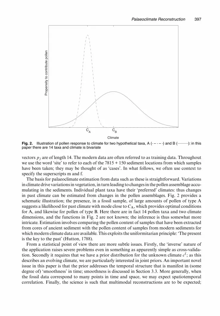
Fig. 2. Illustration of pollen response to climate for two hypothetical taxa, A (� – � – �) and B ( ): in thispaper there are 14 taxa and climate is bivariate
vectors pj are of length 14. The modern data are often referred to as training data. Throughoutwe use the word ‘site’ to refer to each of the 7815 + 150 sediment locations from which sampleshave been taken; they may be thought of as ‘cases’. In what follows, we often use context tospecify the superscripts m and f.
The basis for palaeoclimate estimation from data such as these is straightforward. Variationsin climate drive variations in vegetation, in turn leading to changes in the pollen assemblage accu-mulating in the sediments. Individual plant taxa have their ‘preferred’ climates: thus changesin past climate can be estimated from changes in the pollen assemblages. Fig. 2 provides aschematic illustration; the presence, in a fossil sample, of large amounts of pollen of type Asuggests a likelihood for past climate with mode close to CA, which provides optimal conditionsfor A, and likewise for pollen of type B. Here there are in fact 14 pollen taxa and two climatedimensions, and the functions in Fig. 2 are not known; the inference is thus somewhat moreintricate. Estimation involves comparing the pollen content of samples that have been extractedfrom cores of ancient sediment with the pollen content of samples from modern sediments forwhich modern climate data are available. This exploits the uniformitarian principle: ‘The presentis the key to the past’ (Hutton, 1788).
From a statistical point of view there are more subtle issues. Firstly, the ‘inverse’ nature ofthe application raises severe problems even in something as apparently simple as cross-valida-tion. Secondly it requires that we have a prior distribution for the unknown climate cf ; as thisdescribes an evolving climate, we are particularly interested in joint priors. An important novelissue in this paper is that the prior addresses the temporal structure that is manifest in (somedegree of) ‘smoothness’ in time; smoothness is discussed in Section 3.3. More generally, whenthe fossil data correspond to many points in time and space, we may expect spatiotemporalcorrelation. Finally, the science is such that multimodal reconstructions are to be expected;

398 J. Haslett et al.
see Section 3.1. These all cause particular challenges for the implementation of Markov chainMonte Carlo (MCMC) methods.
1.1. Quantitative palaeoclimate reconstructionQuantitative reconstructions of the palaeoclimate have intrinsic value as a source of insight intothe Earth’s history. Such reconstructions are also an essential basis for evaluating the perfor-mance of the general circulation models (GCMs) that are used to explore the potential futureclimatic consequences of anthropogenic changes to the Earth system. Our focus in this paperis on recent geological history, in particular the period since the onset of rapid deglaciationtowards the end of the last glacial stage, a little less than 15000 calendar years ago. For techni-cal reasons (see Section 1.3) we shall work in ‘radiocarbon years’ (14C years) unless otherwiseexplicitly stated. Our period of interest may thus be stated as that since about 12600 14C yearsbefore present (BP), present being conventionally defined as 1950 for the purposes of the 14Ctimescale; we write this as 12.6 ka BP.
Palaeoclimate reconstructions may be based on a variety of proxy data that provide the basisfor estimates of past climatic conditions. For the terrestrial realm, the most widely availableand most generally useful data are those that are provided by palynology; we use such data inthis paper. We believe, however, that the methodology that is discussed in this paper shouldtransfer to other proxies, including studies utilizing multiple proxies. Palynological data derivefrom counts of pollen, from different types of plant, that have been preserved in sedimentaryrecords.
The value of such reconstructions was demonstrated by the Cooperative Holocene MappingProject (Cooperative Holocene Mapping Project, 1988; Wright et al., 1993). This confronteda series of GCM simulations of climate at intervals of 3000 years since the last glacial maxi-mum, 18 ka BP; reconstructions of the climate at those times were made using various typesof data that can be considered as ‘proxies’ for climate. Subsequently, the Palaeoclimate ModelIntercomparison Project (see for example Farrera et al. (1999) and Joussaume et al. (1999)) hasextended this approach, confronting data-based reconstructions with simulations using a seriesof different GCMs. This allows exploration of the performance of the GCMs when challengedto simulate climates which are markedly different from that of the present.
The GCMs provide simulated climate values on a relatively coarse grid. However, the recon-structions that are used in these data–model comparisons are made with data from many indi-vidual localities (often hundreds), irregularly distributed in geographical space. Glendaloughprovides one such example. Currently climate is reconstructed independently at each such site(and indeed independently for each sample within a site, as we discuss in Section 3.3). See,however, Davis et al. (2003) which proposes the use of four-dimensional smoothing splines fol-lowing pointwise, and independent, determinations of palaeoclimate and age. This paper alsoprovides a good account of the several modelling challenges that are involved, including thevarious sources of uncertainty; it introduces the memorable phrase (page 1705) ‘reconstruc-tion within a haze of uncertainty’. For comparisons, therefore, the reconstructed values arespatially smoothed or aggregated to generate mapped patterns with a spatial resolution that iscomparable with that of the GCM simulations (Prentice et al., 1991).
Despite progress in palaeoclimate reconstruction, several challenging issues remain. As thespatial resolution of GCMs steadily improves, however, what was previously ‘noise’ in the recon-structed values becomes a potential ‘signal’ reflecting finer scale spatial patterns in past climate.A current challenge for reconstruction approaches, therefore, is to use knowledge of the relativespatial locations of sites from which proxy data are available to assist in separating any suchsignal from the noise that is inherent in the proxy data and is generated by non-climatic factors.

Palaeoclimate Reconstruction 399
Another challenge is to provide an entire spatiotemporal reconstruction utilizing all such datasimultaneously. The greatest challenge, however, may be the need to handle uncertainty in ameaningful fashion.
1.2. Statistical approachesVarious estimation methods are currently used; we loosely refer to these as ‘classical’. Theydiffer in detail and use a variety of statistical or other techniques, most especially in the waythat they model the ‘transfer functions’ that are used to describe the response of the plant taxato changes in climate; by response we mean here the propensity to contribute pollen to the sed-imentary record in given climatic conditions, as illustrated in Fig. 2. For methods using pollendata, see for example Bartlein et al. (1984), Klimanov (1984), Bartlein and Webb (1985), Guiot(1985, 1990, 1991), Huntley and Prentice (1988), Prentice et al. (1991), Guiot et al. (1993a,b)and Huntley (1993). See ter Braak (1995) for a recent review. Our method is closest in spiritto a version of the ‘modern analogue’ method: it attributes to a fossil assemblage that modernclimate to which the modern pollen composition is ‘closest’. See Appendix A for more detail andin particular for the version that we have used to generate classical reconstructions in Section 5.
To date, all approaches that are used share some problems, even in their limited application.Perhaps the most important concerns a reliable and realistic modelling of the uncertainty withwhich climatic variables are reconstructed. (Many researchers address uncertainty via cross-validation; indeed we do so in Section 5, but no classical method, to our knowledge, modelsuncertainty.) Closely related to this is the difficulty of combining multiple sources of informa-tion in such reconstructions. These include, for example, the use of multiple proxies, the use ofthe temporal ordering in sediment data, the use of spatial proximity and the due allowance forvariations in quality of data. In a subtle example of data quality issues, tundra and steppevegetation can produce very similar pollen assemblages, yet occur under very different climaticregimes. There can also be difficulties with past types of vegetation that do not occur extensivelyin the present day (Huntley, 1990). The problem of identifying the appropriate modern analoguecan also lead to very noisy reconstructions with apparently large climatic fluctuations betweensamples. We approach uncertainty via the Bayesian paradigm; we exploit mixtures and modelsof correlation to address such difficulties.
We suggest that this formulation is sufficiently flexible to cope with many such generalizationsand difficulties. In this paper we address many of these, but we also side-step several issues. Inparticular, we regard as central to modelling uncertainties the fact that this methodology canbe seen as providing realizations of complete and coherent climate histories. We develop this inSection 3.5. We further expect that the method can provide the basis for reconstructions usingother, and indeed multiple, proxies. If so, this will be an equally important contribution.
One key advance of this paper is the recognition, within the statistical model, of the factthat climate is a stochastic process in space–time. The significance of this is due to the fact thatsome of the above difficulties in part reflect on a further limitation of the classical methodsthat have been applied to date, namely that none of them has taken advantage of the temporaland spatial properties of the data. In these models, climate is reconstructed for each pollensample in isolation; a rare (and undercited) exception is ter Braak et al. (1996). In fact, we havesome knowledge of the temporal and spatial relationships in climate; samples that are close intime (or more generally space–time) might reasonably be expected to have similar climates. Weaddress such temporal and spatial relationships by modelling autocorrelation. Although, in thisapplication, we discuss only the temporal aspect of such autocorrelation, we are mindful of theneed to plan for future work; we return to this in Section 6.
A real strength of the approach that we adopt is that it approaches uncertainty by randomly

400 J. Haslett et al.
generating climates that are consistent with the data. In particular, each realization includes aset of 150 values for the pairs (GDD5, MTCO) corresponding to the fossil samples. These aregenerated jointly; they may be thought of as one sample of an entire climate history. All thehistories so generated are jointly consistent (in a probabilistic sense) with the observed data, i.e.as entire histories rather than as a series of independent reconstructions at different points intime. Some histories, and some details of those histories, recur more frequently than others. Inthis sense, the reconstructions that we propose are qualitatively much richer than those of otherexisting methods, for we have access not only to variability across histories, at given points intime, but also to variability within histories. Although we do not attempt this here, the approachoffers particularly appropriate possibilities for addressing the uncertainties that will arise whencomparisons are made with the output from GCMs.
There is a very small and scattered literature on the use of Bayesian procedures in palaeo-climatology. There are, however, many applications in other areas which are similar from thepoint of view of statistical modelling. In the wider context of environmental modelling, there isof course an abundance of Bayesian work; see, for example, Banerjee et al. (2004).
Possibly the earliest paper on Bayesian palaeoclimatology in the statistics literature is vanDeusen and Reams (1996). They made a tentative foray with an autoregressive AR(2) model butseem to have been discouraged by their results. In the first authoritative attempt, West (1996)provided a very good overview of many of the generic issues in such research. He observed thatthe real interest in such work is concerned with climate change; that being the case, his focus ison the time series analysis of the sediment cores that provide the data for such work. This focusseems to have been largely ignored in the palaeoclimate reconstruction literature (Bayesian orotherwise); however, Dr Andrew Millard has drawn our attention to recent work by Trudinger(2000) and Trudinger et al. (2002a,b). West did not directly address palaeoclimate reconstruc-tion, working instead with a proxy time series. As our procedure can be thought of as randomlygenerating complete climate histories from a posterior distribution, it is very amenable to theanalysis of climate change.
West (1996) drew attention to the fact that proxy series inevitably correspond to randomobservation times and involve temporal (and spatial) aggregation. He identified, for example,the very serious and difficult issues that are associated with uncertainty surrounding observationtimes arising from problems in radiocarbon dating; we have mentioned above that we defer this;see Section 6.
Robertson et al. (1999) introduced the Bayesian approach to climate reconstruction in den-drochronology, an example of an area where there is very little uncertainty about dating. Theyalso provided a very useful introduction to, and discussion of, a whole set of modelling issues,Bayesian and otherwise, in the use of proxies to reconstruct climate. Guiot et al. (2000), usingan MCMC approach, addressed many details associated with palaeoclimate reconstruction via‘inverse vegetation modelling’; their proxy, like ours, is pollen. They introduced the interestingphrase ‘browsing the potential climatic space’ to describe the way in which MCMC samplingexplores the posterior; see Fig. 7 in Section 5. Their model seems, however, to be rather sim-plistic, the sole source of random variation being independent Gaussian noise in the observedproportions. Gachet et al. (2003) discussed quite a different Bayesian approach, which wassimilar to the modern analogue idea above, wherein fossil assemblages are not assigned to asingle ‘closest’ item in a database. Instead each is associated with all the fossil samples via co-occurrence probabilities; Bayes theorem is then used to compute the probability that each samplehas a given palaeoclimate characteristic.
In a series of papers Vasko et al. (2000), Toivonen et al. (2001) and Korhola et al. (2002)appear to be the first to set out a detailed statistical modelling approach to Bayesian cli-

Palaeoclimate Reconstruction 401
mate reconstruction from proxies. Toivonen et al. (2001) discussed not only a specific model—elements of which we adopt below—but they also set the Bayesian approach in the context ofsome of the classical procedures that were covered by Birks (1995) and ter Braak (1995). Itshould be noted that this group used a one-dimensional climate and a rather simple model torelate abundance to climate (essentially that in Fig. 2).
Katz (2002) reviewed wider aspects of uncertainty in climate change and in particular reviewedthe potential for Bayesian methods in assessing this. Research such as in the present paperis important precisely because it contributes to the way that we discuss uncertainty in futurechanges. Hargreaves and Annan (2002) went further, using MCMC methods to integrate (assim-ilate) palaeodata into climate models.
There are of course many studies of data with structures that are similar to ours, i.e. an irregu-lar time series of compositional vectors (here pollen) with unobserved covariates (here climate)and a spatial series of compositional vectors with observed covariates. For example, Grunwaldet al. (1993) dealt with compositional data varying in time, an example being world trade; theyprovided a state space model, using the Dirichlet distribution to provide a basis for the model-ling of the compositional data. Ravishanker et al. (2001) were concerned with a not dissimilarproblem in the analysis of mortality data; they proposed a vector autoregressive moving averagemodel for their compositional data, after transforming them by an additive log-normal ratiotransformation, due to Aitchison (1986). Billheimer et al. (2001) were concerned, as we are,with biological communities and had covariates, as we do. However, their data did not have anexplicitly temporal aspect.
1.3. Issues deferredThere are several issues that we do not address fully at this stage. The first is that by concentrat-ing, as we do here, on temporal reconstruction at a single site we avoid the very considerablechallenge in the spatiotemporal reconstruction of, for example, the European palaeoclimate.The ultimate interest nevertheless lies in spatiotemporal reconstruction.
Even within this limited scope, we have already deferred a second issue by working in radio-carbon years. The relationship between radiocarbon and calendar years is not as simple as wasonce thought. But there is already a literature on this, much of it Bayesian; see, for example,Buck (2003). We defer most of these difficulties by a decision to work here in units of 14C kaBP. Indeed we see that one of the several advantages of this approach is that it is relativelystraightforward to incorporate the relationship between radiocarbon time and calendar timewithin our model. The modular aspect of Bayesian hierarchical modelling facilitates this.
Another concerns the quality of the data and, in particular, the modern data. There are variousaspects to this. One such is that the important scientific information is carried by the compo-sitional vectors .pf , pm/ and it is these that are typically reported in the literature. However,these are themselves derived from count vectors .xf , xm/. Thus for a typical sample (modern orfossil) pij =xij=nj, where
nj =k∑
i=1xij:
The sample sizes contribute information on the quality of the records. Typically the nj are about400. However, for most of the 7815 records in the modern database, the counts are missing.Here we have taken a rather unsatisfactory approach, assigning a total of 400 when the countis missing; for details see Section 3.1. For simplicity we suppress explicit reference to the totalsnj in much of our discussion.
The structure of the paper is as follows. In Section 2 we discuss the data and the science. The

402 J. Haslett et al.
model that we have adopted is presented in detail in Section 3 and some evidence of its validityis given in Section 4. In Section 5 we present some reconstructions. We draw some conclusionsin Section 6 and identify remaining challenges.
The data that are analysed in the paper can be obtained from
http://www.blackwellpublishing.com/rss
2. Data
The primary data on which our reconstructions are based can be considered to have threecomponents: fossil pollen data, pollen surface sample data and climatic data. The last two com-ponents together provide what are often referred to as the training data. In addition, we makelimited use of data that were recovered from an ice core that was obtained from the GreenlandSummit.
2.1. Fossil pollen dataSuch data comprise counts of different pollen taxa in samples that were taken from cores of lakeor mire sediment spanning the time period that is of interest. Pollen samples are taken from anyone sediment sequence at intervals that may be regular or irregular with respect to depth, but ineither case they will be irregular with respect to time because of variations in the rate of accu-mulation of sediment. They typically span 0.5–1.0 cm and reflect the mean pollen input to thelake from various plant taxa over an indeterminate period, typically 5–20 years, the duration ofwhich is dependent on the sample thickness and rate of accumulation of sediment. Radiocarbonage determinations are made on a subseries of samples from the sediment sequence, ages forthe remaining samples being estimated by interpolation. Typically there are at least an order ofmagnitude fewer radiocarbon age determinations than pollen samples for any given sedimentsequence. With such dating uncertainties, the temporal resolution that is allowed by such datais limited. The pollen data also reflect an indeterminate spatial aggregation (Prentice, 1988).
For the present study we use fossil pollen data from a core that was taken at a site in Ireland:the Lower Lake at Glendalough (Irish grid reference T118966; 6◦ 20′ W 53◦ 00′ N). Pollensamples were analysed from 150 different depths in the core. For a brief description of the siteand dating details see Appendix B. For present purposes, these have been expressed in terms ofthe counts for 13 pollen taxa plus ‘other’; the choice of taxa is discussed in Appendix B. Theuse of a category ‘other’ is non-standard; it is introduced here as a somewhat crude device tolimit the size of the data set that is used in this methodological paper; in fact more than 100pollen taxa were recorded.
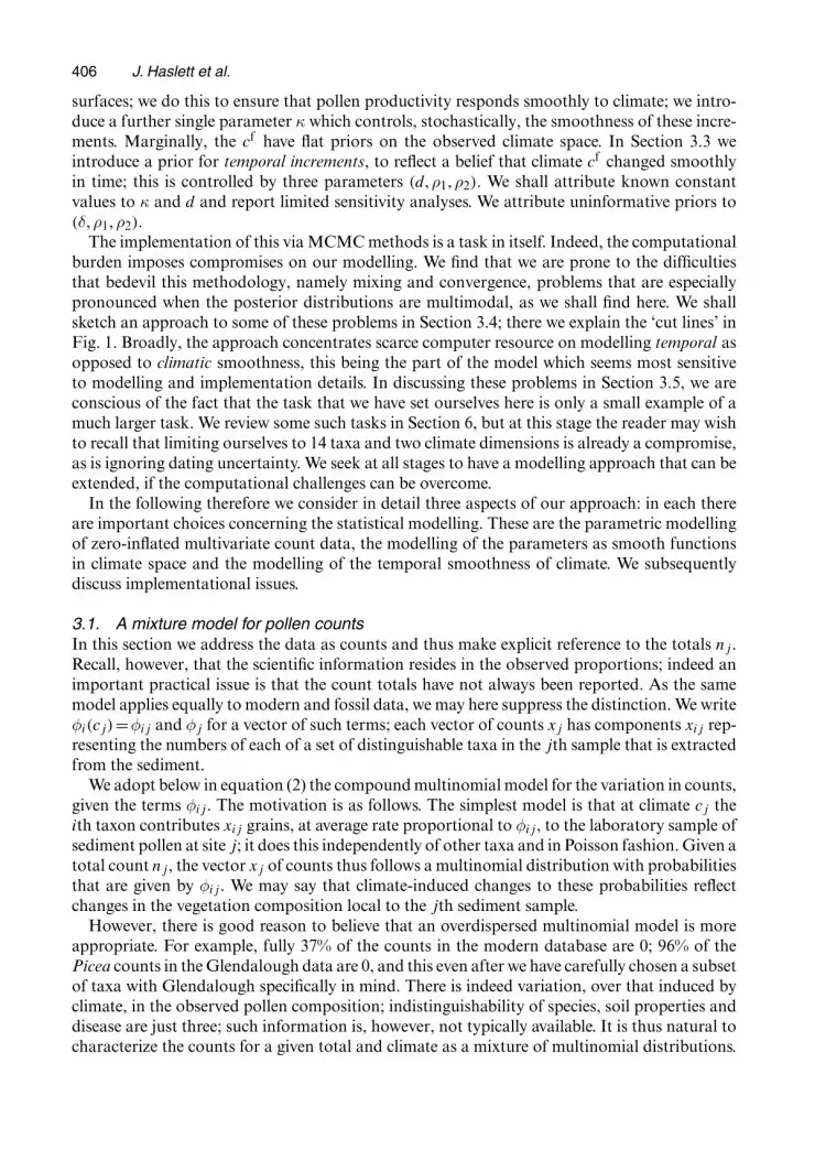
The fossil pollen data from Glendalough are illustrated in the form of a pollen diagram (Fig. 3).The vertical axis of this diagram is age, with the most recent sample at the top. Each individ-ual component graph represents the changing relative abundance of a pollen taxon, sample bysample, expressed here as proportions of the total pollen count for each sample. The diagramclearly shows a very substantial change in the vegetation shortly after about 10 ka BP. Thisrepresents the transition from the late glacial period to the post-glacial (or Holocene) period;it is associated with a shift in dominance from shrubby and herbaceous taxa during the lateglacial to tree taxa in the post-glacial period. Thereafter, the changes during the first half of thepost-glacial period are primarily in the composition of the forests, with a progressive changetowards more open conditions beginning at about 5 ka BP. Note that despite appearances Piceais not completely absent from the record; see Appendix B.
It is important to note a number of distinct sources of sampling variation in such data. Thecounts are based on samples that were taken in the laboratory from sediments at given depths.

Palaeoclimate Reconstruction 403
12
10
8
6
4
2
0
−
−
−
−
−
−
−
−
−
−
−
−
−
−Alnu
sBet
ula
Corylu
s
Pinus D
.
Querc
us D
.
Ulmus
Ericale
s
Junip
erus
Cyper
acea
e
Salix
Gram
ineae
PiceaOth
er
0.3
0.6
0.9
0.4
0.4
0.1
0.4
0.6
0.3
0.3
0.1
0.6
0.1
0.2
Observed Proportion
ka B
P
Fig. 3. Proportions of each of the 14 different categorizations against radiocarbon years BP (vertical axis)at Glendalough: tick marks indicate the sample dates for which we have data; these are irregular in time butregular in depth (depth axis not shown) (Pinus D., Pinus Diploxylon; Quercus D., deciduous Quercus; pollenanalyst, J. Maldonado)
The sampling variation here is relatively well defined. Typically the researcher counts taxa ofdistinguishable type until a total count of about 400 is achieved. However, not all plant speciesare easily distinguishable. The sediments themselves are samples from a region of space and aperiod of time that is less well defined.
2.2. Pollen surface sample dataSuch data are obtained primarily from samples of the uppermost 0.5–1.0 cm of lake sedimentsalthough some are from mires, samples from which comprise the topmost 1–2 cm of the grow-ing surface of the mire, often dominated by Sphagnum moss. Pollen that accumulated in thesecontemporary sediments is extracted and counted by using the same techniques as are used forthe fossil pollen.
For our study we use a data set of 7815 surface samples from the warm and cool temperatezones of the northern hemisphere, including the Arctic. Because this comprises data from manystudies between about 1960 and 1990 important issues arise concerning the quality of these data.Although these samples are derived from a variety of environments, they all provide evidence ofclimatically determined regional vegetation; excluded from the data set are samples that wouldreflect only the vegetation in their immediate vicinity and that would reflect non-local climatefactors. Similarly, although counted by numerous analysts and having variable numbers of pol-len grains identified, the resulting variation in their quality is not necessarily important in thepresent context; this is because we limit our attention to a small number of reliably identified andgenerally more abundant pollen taxa. However, because many of the data were compiled from

404 J. Haslett et al.
the literature, only relative abundances, as opposed to the original pollen counts, are availablein the data set. A subset (61) of samples that were analysed by the authors (BH and JRMA), andfor which pollen count data are available, is employed in Section 4.3 in a limited cross-validation.
2.3. Climatic dataTo complete the training data, climatic data are required for each locality from which a pollensurface sample has been analysed. The sources of such climatic data are the numerous meteoro-logical stations throughout the northern hemisphere. We used a compilation of monthly meandata from these meteorological stations (Leemans and Cramer, 1991) that primarily reflects the‘climatic normal’ period 1931–1960, i.e. for each station the value that is available for Januarytemperature (for example) is the 30-year mean of the monthly mean value in each year of therecord. Estimates of the monthly mean temperatures were interpolated for the locations of thesurface samples by using the method that was developed by Hutchinson (1989). These were thenused to derive MTCO and GDD5, the latter by using the method of Prentice et al. (1992). Weuse RS10rss to refer to the data set comprising these two variables, together with the relativeabundances of the pollen taxa for all the surface samples.
2.4. Ice core dataIn contrast with the relatively poor temporal control and coarse temporal resolution of fossilpollen data, such as those from Glendalough, palaeoclimate proxy data from polar ice coresare available at very high temporal resolution. They can be directly related to a calendar yeartimescale based on annual layering of the ice. We have used the stable oxygen isotope δ18Odata from the ice of the GISP2 core drilled near the summit of the Greenland ice-sheet (see, forexample Stuiver et al. (1995)) to provide a basis for estimating the temporal properties of theclimate system since the end of the last glacial stage. These data principally reflect atmospherictemperature over Greenland; their temporal characteristics can thus be argued to be relevantto our reconstruction of temperature, albeit at a locality some distance from Ireland.
It is clear from Fig. 4 that climate was much more variable during the last glacial stage thanit has been subsequently. It is apparent also that the dramatic rise in temperature about 12000calendar years BP was only one of several such rises during the past 100000 years.
3. Bayesian statistical model and algorithm
To recap, our interest is focused on the palaeoclimate cf at Glendalough, given fossil pollendata pf and modern data .pm, cm/; in the Bayesian sense we study π.cf |pf , cm, pm/, to whichwe refer as π.cf |data/. For simplicity we often suppress, as here, the pollen counts n. Further,when no ambiguity arises, we suppress the distinction (the superscripts (f, m)) between modernand fossil sites. In this section we expand on the model that is sketched in Fig. 1. We approachthe study of
π.cf |data/≡∫
ωπ.cf |ω, data/π.ω/ dω
in the now standard fashion, having unobserved parameters ω which are integrated out viaMCMC methods. We thus write
π.p|c, ω/=∏π.pj|cj, ω/ .1/
for both fossil and modern sites. As indicated in Fig. 1, we assume the conditional indepen-dence of compositional vectors p given climate c and model parameters ω. Within ω lie a high

Palaeoclimate Reconstruction 405
−44−43−42−41−40−39−38−37−36−35−34
Pro
xy fo
r T
emp
0 10 20 30 40 50 60 70 80 90 100−4
−3
−2
−1
0
1
2
3
4
Firs
t Diff
eren
ces
Age (ka BP)
(a)
(b)
Fig. 4. (a) Greenland ice core data and (b) first differences: the ages are given in calendar years BP; theunits of the vertical axis are in relative δ per thousand
dimensional parameter Θ (dimension 10114) and five scalar parameters .κ, d, ρ1, ρ2, δ/; otherparameters, q and β, make only ‘virtual’ appearances in our modelling, motivating details ofour modelling. We develop these below, suppressing parameters where possible.
The probabilistic relationship between climate and pollen composition is described by
π.pf |cf /≡π{pf |Φ.cf /}:
The k-dimensional Φ-function characterizing pollen productivity is discussed below; we adopta parameterization in which expected value E.pf /=Φf . There are of course only k −1=13 setsof scalar functions φi.c/ within Φ.c/ as the constraint∑
i
φi.c/=1
reduces the dimensionality. In simple terms, if the observed pij is high, then we incline, for cj,towards climates c for which φi.c/ is high. Our knowledge of these functions is itself informedby equivalent pairs .cm
j , pmj / at each of j = 1, . . . , 7815 modern sites, for their relationship is
mediated by the same density π{pm|Φ.cm/}. The central statistical tasks in the analysis are themodelling of
(a) the distribution π{p|Φ.c/} and(b) the Φ.c/ function itself.
In Section 3.1 we discuss the likelihood for Φ, given the pollen and climate data, introduc-ing the parameter δ. In Section 3.2 we introduce variables Θ, writing Φ.c/=Φ.c, Θ/. We presenthighly structured distributions for spatial increments (or contrasts) in climate space for such
406 J. Haslett et al.
surfaces; we do this to ensure that pollen productivity responds smoothly to climate; we intro-duce a further single parameter κ which controls, stochastically, the smoothness of these incre-ments. Marginally, the cf have flat priors on the observed climate space. In Section 3.3 weintroduce a prior for temporal increments, to reflect a belief that climate cf changed smoothlyin time; this is controlled by three parameters .d, ρ1, ρ2/. We shall attribute known constantvalues to κ and d and report limited sensitivity analyses. We attribute uninformative priors to.δ, ρ1, ρ2/.
The implementation of this via MCMC methods is a task in itself. Indeed, the computationalburden imposes compromises on our modelling. We find that we are prone to the difficultiesthat bedevil this methodology, namely mixing and convergence, problems that are especiallypronounced when the posterior distributions are multimodal, as we shall find here. We shallsketch an approach to some of these problems in Section 3.4; there we explain the ‘cut lines’ inFig. 1. Broadly, the approach concentrates scarce computer resource on modelling temporal asopposed to climatic smoothness, this being the part of the model which seems most sensitiveto modelling and implementation details. In discussing these problems in Section 3.5, we areconscious of the fact that the task that we have set ourselves here is only a small example of amuch larger task. We review some such tasks in Section 6, but at this stage the reader may wishto recall that limiting ourselves to 14 taxa and two climate dimensions is already a compromise,as is ignoring dating uncertainty. We seek at all stages to have a modelling approach that can beextended, if the computational challenges can be overcome.
In the following therefore we consider in detail three aspects of our approach: in each thereare important choices concerning the statistical modelling. These are the parametric modellingof zero-inflated multivariate count data, the modelling of the parameters as smooth functionsin climate space and the modelling of the temporal smoothness of climate. We subsequentlydiscuss implementational issues.
3.1. A mixture model for pollen countsIn this section we address the data as counts and thus make explicit reference to the totals nj.Recall, however, that the scientific information resides in the observed proportions; indeed animportant practical issue is that the count totals have not always been reported. As the samemodel applies equally to modern and fossil data, we may here suppress the distinction. We writeφi.cj/=φij and φj for a vector of such terms; each vector of counts xj has components xij rep-resenting the numbers of each of a set of distinguishable taxa in the jth sample that is extractedfrom the sediment.
We adopt below in equation (2) the compound multinomial model for the variation in counts,given the terms φij. The motivation is as follows. The simplest model is that at climate cj theith taxon contributes xij grains, at average rate proportional to φij, to the laboratory sample ofsediment pollen at site j; it does this independently of other taxa and in Poisson fashion. Given atotal count nj, the vector xj of counts thus follows a multinomial distribution with probabilitiesthat are given by φij. We may say that climate-induced changes to these probabilities reflectchanges in the vegetation composition local to the jth sediment sample.
However, there is good reason to believe that an overdispersed multinomial model is moreappropriate. For example, fully 37% of the counts in the modern database are 0; 96% of thePicea counts in the Glendalough data are 0, and this even after we have carefully chosen a subsetof taxa with Glendalough specifically in mind. There is indeed variation, over that induced byclimate, in the observed pollen composition; indistinguishability of species, soil properties anddisease are just three; such information is, however, not typically available. It is thus natural tocharacterize the counts for a given total and climate as a mixture of multinomial distributions.

Palaeoclimate Reconstruction 407
We thus model vectors of unobserved latent proportions qj reflecting climate cj and introducea prior for qj to reflect extraclimatic variation; specifically we propose a Dirichlet model for qj,with expected values φj. The Dirichlet model, though restrictive, is very convenient here, beingconjugate to the multinomial; thus we can integrate out the variables qj which now play nofurther role in our modelling; see Fig. 1. This mixture of multinomials has been widely used inmany fields. In palaeoclimatology we here follow Vasko et al. (2000) (noting, however, that theseresearchers did not avail themselves of the conjugacy, as we have done, to simplify the model).The model that we thus adopt for the conditional distribution of xj is thus the compoundmultinomial distribution below; see Dey and Maity (2002).
πx.xj |φj, δ, nj/= nj!Γ.δ/
Γ.nj + δ/
k∏i=1
Γ.xij + δφij/
Γ.δφij/ xij!; .2/
here Σi φij =1 and nj =Σi xij. The reported proportions are pij =xij=nj; to emphasize that thecentral interest lies in the proportions we write
π.pj|φj, δ, nj/=πx.njpj|φj, δ, nj/: .3/
Under this parameterization, E.pij|φij, δ, nj/=φij. Note also that
var.pij|φij, δ, nj/= 1+ δ=nj
1+ δ
φij.1−φij/
nj:
The (common) δ-parameter has a simple interpretation as controlling ‘extramultinomial’ dis-persion. Below, we model Φ.c/ through a smooth function Φ.c, Θ/ of climate c, parameterizedby Θ.
We remark on one source of technical difficulty: that of the multimodal nature of the pos-terior. The essential idea can be seen in a very simple case with just two taxa, say A and B; seeFig. 2. Large counts of A and of B send a very clear signal to the posterior in favour of theirpreferred climates cA and cB; but here, as B is tolerant of many climates, large proportions of Bsend a signal of ‘not cA’; the posterior will be bimodal. With 14 taxa, the signals will be morecomplicated. But multimodal solutions are natural and arise often, as we shall see in Section 5.
We indicate three potential shortcomings to this mixture model; we preface this with theremark that, in our opinion, reconstructions are not overly sensitive to many of the modelling(and implementational) details. Firstly, the Dirichlet mixture is a rather crude option for mixingthe multinomials. The model of Aitchison (1986) provides a much richer approach, includingthe possibility of modelling residual interaction (such as competition) between the taxa, afteraccounting for the response to climate, which is appealing. Unfortunately, however, there is aconsiderable computational overhead in such an approach, for integration cannot be used tomarginalize the distribution. We could in principle retain the latent parameters q; in our casethis would add a further .7815+150/×13=103545 parameters to our model. This would over-whelm it. (However, subtle issues are involved here; retaining the q-terms in the model of Vaskoet al. (2000) leads in fact to better mixing at the MCMC stage, as discussed in Bhattacharya(2005), and thus indirectly to improved speed; but in Bhattacharya (2005) nm =62.)
Secondly, as indicated, only in a minority of cases are counts xij reported for the moderndata. Generally only pij are reported; equivalently many of the nj are missing. Our approach inthese circumstances is to set xij to the nearest integer to 400pij and nj =Σxij; for simplicity werefer to this as setting the sample size to 400. Nevertheless, we are aware that it is not difficultto see Bayesian ways of addressing variation in the quality of the reported data. More generallythere are important other quality issues concerning such data; see Section 6.

408 J. Haslett et al.
Finally, model (3), despite the availability of the parameter δ, does not sit naturally with thescientific explanation, which is that at many sites certain taxa are completely missing; typicallysuch taxa are completely incompatible with the climate, i.e. certain of the qij are exactly 0;however, neither the Dirichlet nor Aitchison’s model give point mass to zero values of qij. Thisis, in fact, the most important of these shortcomings. Note that the multinomial model doesallow observed counts xij, and thus proportions pij, to be 0.
3.2. Response surfacesWe now consider the modelling of the vector-valued response function Φ.c/. This is key bothto the underlying science and to the challenging computations that it implies. We introduce aprior to model components φi.c/ as smooth functions in two-dimensional climate space. Spe-cifically, we develop below a model of the φi.c/ as independent Gaussian processes, truncatedon 0 �φi.c/� 1 and conditioned on Σi φi.c/= 1; this of course introduces dependence. Beforedoing so we briefly consider an apparently natural alternative.
A multivariate log-Gaussian process seems simpler; here we would write φi.c/ ∝ exp{Si.c/}for independent Gaussian processes Si.c/, scaled such that Σi φi.c/=1. This seems at first sightto be more ‘natural’; the range-restricted φ-variables are described in terms of completely unre-stricted Gaussian processes. In the former, they appear to be awkwardly restricted. But thelog-normal model seems much more challenging, at least for our data, in terms of the con-vergence and mixing of the MCMC algorithm. Further, the restrictions are relatively simpleto implement; see Section 3.5. In particular, in the log-Gaussian variant, very small values ofφi.c/ are mapped onto the unrestricted space that is associated with large negative values ofSi.c/. Despite the fact that all such small values of φi.c/ contain effectively the same scientificinformation (i.e. negligible propensity to produce pollen at this climate) this formulation seemsto encourage a very complete, but computationally expensive, stochastic exploration of thisuninformative region. Tierney (1994) has some relevant discussion; see in particular corollary3, which essentially says that bounding the parameter space may improve mixing.
The modelling involves two steps. Firstly we focus on a discretization of climate space by con-sidering in detail only values of φi.c/ on a subset CG ={cg; g∈G} of a regular grid indexed by G
(φig); Fig. 5. For c =∈CG we define φi.c/, for each i, as a weighted average of the φig. Formally, wepropose a stochastic model for φi.c/ only when c∈CG; otherwise we use a deterministic model
φi.c/=∑g
w.c, cg/φig:
The weights w that we use are chosen simply, being inversely proportional to the distance ofthe point c from its surrounding four grid neighbours and being 0 for non-neighbours. (Otherweightings were considered, but the methodology does not seem sensitive to this.) Our discus-sion now focuses on the φig; we regard these as parameters of the function φi.c/. To emphasizethis we introduce the notation Θ={Θi; i=1, . . . , k}, where Θi ={θig; g ∈G}. At grid points wehave φig = θig and, since 0 �φig � 1 and Σi φig = 1, we have 0 � θig � 1 and Σi θig = 1; thus theθig define the φi.c/ surfaces.
At the second step, each of these Θi are themselves modelled as truncated and conditionedGaussian processes, as above, constructed to vary smoothly over CG as detailed below. We saythat Φ.c/ is parameterized as Φ.c, Θ/. Alternatively put, the Gaussian random function Φ.c/ inreal climate space is obtained by applying a filter to a Gaussian process Θ defined on the grid;see Fig. 1. We now expand on the grid and on the Gaussian processes Θi.
The details of the grid are as follows. We focus on a subset CG of 778 points in a 51×51 reg-ular square lattice in climate space; the grid is presented in Fig. 5. Scaling is such that the range

Palaeoclimate Reconstruction 409
0 1000 2000 3000 4000 5000 6000 7000−50
−40
−30
−20
−10
0
10
20
GDD5
MT
CO
Fig. 5. Support lattice for the response surfaces (the modern climate of Glendalough is approximately 1772GDD5 and 4.4 ıC MTCO): �, lattice points which form the support of the response surfaces; �, regular lattice;
, training data set
for each climate variable is 50 units; thus 1 unit= .max −min/=50 for each climate dimension.Formally, for our implementation, the 778 points cg are chosen such that there is at least oneobservation (in the modern data set) in any 2 × 2 square centred at cg (units as above). Thisdefines a region with 740 grid points, with a very irregular boundary and some internal ‘voids’;these voids were manually populated with an additional 38 grid points, giving a total of 778 towhich we refer as CG. There are thus 778 × 14 = 10892 such θig involved in our modelling; ofcourse the constraint means that we need to store only 10114 such. This high dimensionality isa source of much computational burden.
Loosely, the 778 are chosen on the basis that they cover that part of climate space for whichwe have pollen data or onto which we are willing to interpolate. Our MCMC implementation ofthis involves φi.c/ being evaluated only at points lying within squares for which all four latticevertices are defined. Thus the method will not return palaeoclimates that are not close to modernclimates that have actually been observed; such climates have zero prior probability. The edgeof the climate grid raises challenging issues, both scientific and statistical.
This very conservative strategy is a matter of scientific debate and could easily be relaxed.The reasoning is as follows: there are relatively few examples of such extreme climates in themodern surface data; thus reconstructions of such climates are very dependent on a few mod-ern data points and on the details of any smoothing methods. We remark here that much ofthe recent Glendalough climate set lies at about GDD5 = 1600 day ◦C and MTCO = 4 ◦C,which corresponds to the edge of climate space. Even the recent climate at Glendalough isextreme in the sense of Fig. 5. To avoid overreliance on such technicalities, palaeoclimatolo-gists are reluctant to extrapolate beyond the envelope of the climate space that is reflected inthe modern data. A variation of this debate is the ‘no modern analogue’ problem; see Huntley(1990).
We introduce smoothness on CG as follows, introducing a parameter κ; see Fig. 1. We modeleach set of Θi as, a priori, truncated realizations of simply structured and smooth Gaussianrandom functions, stochastic smoothness in climate space being simply controlled by a com-

410 J. Haslett et al.
mon scalar parameter κ as discussed below. Initially these are independent; we subsequentlycondition on them having unit sum. Then, given κ and Σi θig =1, we may write
π.Θ|κ/∝k∏
i=1Nκ.Θi/;
here Nκ.·/ is the relevant multivariate normal density. Truncation with respect to the unit inter-val affects only the normalizing constant. In fact, for our purposes, it is sufficient to specify, ateach cg, only the product over taxa of the relevant full conditionals, i.e. Πk
i=1 nκ.θig|θig′ ; g′ �=g/;here nκ.·/ denotes a univariate normal density. We present below an approximation to each ofthese terms. This approximation simultaneously gives additional flexibility to the modelling andallows us to exploit a parallel processing algorithm.
We first consider a model for each Θi-process that is Gaussian with linear drift and isotro-pic linear variogram, i.e. E.θig − θig′/ =βT.g − g′/ and var.θig − θig′/ =κ|g − g′|. The impliedrandom functions are thus smooth in the sense of mean square continuous in a real climatespace (Stein (1999), section 2.4); here our interest is only on the lattice CG. Given a Gaussianprior on β, the full conditionals are Gaussian. When the variance of the β-prior is indefinitelylarge, the expected value is the best linear unbiased predictor
θig = ∑g′ �=g
λgg′θig′
of θig given the rest; the variance is the associated var.θig − θig/. The β-parameters thus playno further role in our modelling; see Fig. 1. The normal density is thus that of the condi-tional residual eig = θig − θig; see Haslett and Hayes (1998). The λgg′ -terms and the variancevar.θig|θig′ ; g′ �=g/=κσ2
g are simply available from ‘universal kriging’; see, for example, Cressie(1993), page 153. Clearly smaller values of κ define a smoother Θi and thus a smoother functionφi.c, Θi/. Observe that both λgg′ and σ2
g depend only on the geometry of the grid CG and needbe computed only once.
We approximate by working locally, i.e. we specify λgg′ �=0 only for grid locations g′ within alocal neighbourhood of g, which we write as g′ ∼g. Then the local conditional residual is
eig =θig − ∑g′∼g
λgg′θig′
with corresponding local variance κσ2g ; the eig are the spatial increments that were referred to
earlier. Specification via the (local) covariance structure is routine in geostatistics; see Deutschand Wen (1998) for an application that is very similar in spirit to ours. This has two advantages.
Firstly, it contributes flexibility to the model; in fact, the eig may be thought of as residualsfrom a local LOESS smoother, computed, however, via generalized least squares. It is thus aweak prior for the smoothness of the Θi-processes. It is simple, depending only on a singleparameter κ and a neighbourhood system. (Other variogram models with more parameters arepossible, but they do not have the simplicity that λgg′ and σ2
g are parameter free. Here theseterms depend only on the local geometry and may be computed once.)
Secondly, its local structure yields some of the computational advantages of Markov randomfields. (Observe, however, that formally there may not be a unique stochastic process definedon CG having exactly this set of conditional densities.) There are clearly close parallels with the‘intrinsic autoregression’ of Besag and Kooperberg (1995); appendix A.5.3 of Banerjee et al.(2004) has a useful discussion. Here our particular interest is in exploiting a parallel algorithm,with considerable speed advantages; see Whiley and Wilson (2004). Further eig is easy to com-pute for any neighbourhood .g′ ∼ g/ of g, as is σ2
g . In Markov models the neighbourhood is

Palaeoclimate Reconstruction 411
tightly specified and missing points or irregular edges are more difficult to model. In this con-text, we have taken the neighbourhood of a point g as being the 5 × 5 square centred on g; atthe edges, however, this neighbourhood becomes smaller and irregular.
A strength of the modelling approach that is outlined here is that it is simple to see how torelax constraints about working outside the observed climate space or indeed on a differentlystructured grid. Specifically, considerable flexibility has been brought to the modelling of alattice Gaussian process for Θ by specifying it via its covariance structure. There is no particularneed for the lattice to be regular and extending beyond the observed climate space, with dueallowance for the increased uncertainty, is algorithmically straightforward if it is scientificallyacceptable.
In summary, we have imposed smoothness on the response surfaces {Φ.c;Θ/}, via randomfunctions φi.c/, by structuring the prior for Θ, a random variable of dimension 10114. Themodel for Θ is parsimoniously defined via a lattice CG, a single smoothness parameter κ and aneighbourhood system. It is clear that several other variants of this are possible; in particularwe could replace the single κ with taxon-specific κi. Informal experiments suggest that this isnot overrestrictive in this context. Finally, by truncating and conditioning on a unit sum, wehave proposed a computationally attractive spatial process for compositional data.
3.3. Temporal smoothnessThe modern climate values cm are known but the prehistoric climates cf are not. Climate changeexhibits some degree of smoothness in time. Loosely speaking, climate changes can be charac-terized as small, mostly, but occasionally very large. We model this smoothness stochastically,by specifying an appropriate family of priors for cf . In this section the bivariate terms cf
j may bemore readily denoted as {ch.tj/; h= 1, 2}, where the tj are in 14C years BP; here j = 1 denotesthe deepest (oldest) sample; we suppress the superscript f and h = 1 and h = 2 denote GDD5and MTCO respectively.
Light can be shed on the choice of prior for temporal variation by an examination of firstdifferences in the ice core data (Fig. 4); we discuss other possible uses of such data in Sec-tion 7. A probability plot of these increments strongly suggests that the variation is muchlonger tailed than the normal distribution; indeed the td-distribution with d = 8 degrees offreedom seems about right. The lag 1 autocorrelation is about 0.2. This suggests a prior fortemporal smoothness (for both components of climate) as that defined by the random-walkrecursion
ch.tj/= ch.tj−1/+ .|tj − tj−1|1=2ρh/ ".tj/;
here ".tj/ ∼ td , independently. Smoothness is thus characterized via the degrees-of-freedomparameter d, and by the ρh-parameters; the initial (bivariate) climate c.t1/ is taken as uniformon the real climate space as outlined in Section (3.2). We write
πf .c|ρ/=πf1.c|ρ1/πf
2.c|ρ2/
and use the random-walk model to expand each of these terms by writing
πh.c|ρ1, ρ2, d/=150∏j=2
τd{ch.tj/|µh.tj, tj−1/, σh.tj, tj−1/}π{ch.t1/} .4/
for each climate dimension. Here, by τd.u|µ, σ/ we denote the value of the density of a td-distri-bution, evaluated at σ−1.u−µ/. We set µh = ch.tj−1/ and σh =ρh.tj − tj−1/1=2 for each climatedimension. We take π{ch.t1/} to be uniform on the modern climates cm. In this paper we take

412 J. Haslett et al.
d = 8 for our main results. We have, however, conducted smaller studies that were based onthe Cauchy(t1) and normal(t∞) distributions and we report on these below. We have furtherconsidered autoregressive conditional heteroscedasticity type models, in which the varianceterms ρh vary in time; we shall report on these elsewhere.
We have thus specified temporal smoothness by d degrees of freedom and by parameters ρh
for each component of climate. Furthermore, we report below on a model in which there isno constraint of temporal smoothness. In this case, the prior for all terms in cf is independentuniform on climate space.
3.4. Two-stage Markov chain Monte Carlo samplingWe have above provided the means of stating the posterior distribution of all unknowns, i.e.π.cf , Θ, ρ1, ρ2, δ, κ, d|data/; such a statement is of course to within an unknown multiplicativeconstant. Here data = .cm, pm, nm; pf , nf /; below we also refer to the modern data datam =.cm, pm, nm/. As discussed in the next section we attribute known fixed values to .κ, d/ andflat priors for .ρ1, ρ2, δ/. For simplicity of notation, we drop explicit reference to these, exceptwhere required. There are .10417=3+2×150+10114/ random variables in this representation.MCMC sampling provides us with an algorithm with which to sample from this distribution.Our primary interest lies in the marginal posterior distribution π.cf |data/; cf has 2×150=300dimension. From this point of view, the high dimensional Θ is a (costly) nuisance parameter.
We find it computationally advantageous to use an approximation; indeed we feel that thisallows us to make better use of a finite computing resource.
π.cf , Θ, δ, ρ1, ρ2|data/≈π.cf , ρ1, ρ2|pf , nf , Θ, δ, datam/π.Θ, δ|datam/: .5/
The basis for this is that the fossil pollen, on its own, contains very little information on Θ.This approximation allows us to split the problem into two stages. In the first stage we con-
sider the ‘training model’. Effectively this addresses the model as defined in Sections 3.1 and3.2, i.e. that part of the model to the right of the ‘stage 1’ cut line in Fig. 1. The output fromstage 1 is the posterior π.Θ, δ|datam/, which is manifest in a large file of values of .Θ, δ/ thatare consistent with the modern data. This is constructed once. Issues of temporal smoothnessarise at the second stage in the ‘reconstruction model’ π.cf |pf , nf , Θ, δ/; this is that part of Fig. 1to the left of the ‘stage 2’ cut line. A large number of second-stage models are fitted by usingMCMC sampling, each conditioning on a random choice of .Θ, δ/ from the posterior samplefrom stage 1. Hence, for each second-stage MCMC run, .Θ, δ/ are treated as (randomly chosen)known constants, which contribute substantially to mixing overall; see Bhattacharya (2005). Asthe posterior distribution of the reconstruction is our focus, and as it is sensitive to the modellingof temporal smoothness (and to its implementation), this approximation allows us to devotemost of our computing resource to this second stage.
3.5. ImplementationThe foregoing provides the theory for the specification of the posterior distribution π.cf |data/;we explore this distribution by sampling from it via Metropolis–Hastings MCMC methods.We have specified the d = 8 and κ= 0:0005. We report a detailed sensitivity analysis on d byconsidering the Cauchy .d =1/ and the normal (d =∞) models, as well as on a model where notemporal smoothing was employed; this may be thought of as a special case, with large and fixed.ρ1, ρ2/. We also report on an indirect sensitivity analysis for κ. We recall a further importantsimplification; where a count nm
i is unknown, we take it arbitrarily to be 400 (in the sense of

Palaeoclimate Reconstruction 413
Section 3.1); some limited experiments (which are not reported) with values in the range 300–500suggest that the results are not overly sensitive to this.
As well as being computationally demanding, there are difficult technical issues with the algo-rithm. In particular it is necessary to ensure—as best as we can—that the algorithm exploresfully the space of possible realizations, not just of the 300-dimensional climate histories, butalso of the 10117-dimensional space of unknown parameters. Technical issues of mixing andconvergence are problematical with a model that is this large and represent the ‘Achilles heel’of the approach. This is particularly so when the posteriors are naturally multimodal, as in thepresent application. Although there has recently been enormous progress, even the best adviceon many practical aspects of MCMC sampling is still given tentatively.
Our algorithm involves the by now classic Metropolis–Hastings approach, based on a randomwalk within 10117-dimensional space. Updates of the Θ-parameters were implemented in blocksθg (of length 14, although constrained to sum to 1) for each g ∈G. Updates on other variableswere considered singly. Proposals for the former involve a random walk on the simplex imple-mented thus: given θg propose θ′
g ∝θg +u for a vector of uniform random variables u, such that0 � θ′
ig � 1 and Σi θ′ig = 1; it is easy to do this in such a way as to ensure that proposed moves
from θg to θ′g and vice versa have equal probabilities. In fact, to avoid computational problems,
we have found it necessary to impose the somewhat arbitrary constraint θij �10−10.The computational advantage of the two-stage approach comes from the dimensionality of
π.cf , ρ1, ρ2|pf , nf , Θ, δ, datam/. The study of this model by MCMC methods requires explor-ing the space that is spanned by .cf , ρ1, ρ2/; this has 2 × 150 + 2 = 302 dimensions, whereasπ.cf , Θ, δ, ρ1, ρ2|data/ has dimensionality 10417; speed is enormously improved, given that thefirst stage has been completed. Furthermore, random draws from Θ ensure excellent mixingat the second stage, which is a potential source of difficulty. For implementation we first storevalues of .Θ, δ/ from the first-stage training model; the second stage involves randomly drawingseveral .Θ, δ/ from this store and, for each, running the reconstruction model with fixed .Θ, δ/.Note that a burn-in is needed for each randomly sampled .Θ, δ/. But this is an overhead thatis well worth accepting, given the increase in speed. In practical terms, for debugging the codeand testing parts of the model, this has been particularly important.
Specifically, the model was implemented on parallel processing hardware (an eight-processorBeowulf cluster comprising four dual 1 GHz Pentium processors); we used the methods ofWhiley and Wilson (2004) to take maximum advantage of the architecture in the Gaussianmodelling of the Θi. The first stage of the Section 3.4 model is slow, involving a running timeof about 400 central processor unit hours to provide only 86000 realizations after discardingburn-in; these were thinned to 10%. These included several runs, with restarts. We regard this asa very small sample, but adequate we hope for the present purposes. All second-stage runs werebased on the same 300 realizations of Θ and involved, for each MCMC run, a burn-in of 3000following which 20 climate reconstructions were stored, a total of 6000; starting climates wererandomly constant, or sampled from CG for each date, or sampled from previous reconstruc-tions. This second stage took about 30 min of elapsed time. The fact that the same realizationsof Θ were used in all cases increases confidence in the model comparisons in Section 5.
4. Model fit to modern data
In Section 5 we shall compare our reconstructions with those which were achieved by a cus-tomized variant of one of the classic approaches, the so-called response surface model; Huntley(1993). Here we consider model fit from the point of view of the modern data only; for simplicity,the superscript m is implicit in what follows.

414 J. Haslett et al.
4.1. Pollen responseOne method of examining the fit is to contrast the observed vectors pj .j = 1, . . . , 7815/ withthe corresponding distributions π.p|cj, data/. These are obtained from equation (3) by mixingwith respect to the π.Θ, δ|data/.
These distributions are extremely skew; overall they are long tailed with respect to the data.We find that overall only 83% of the 7815 × 14 observed pij-values exceed the corresponding(climate-specific) 95-percentile; 91% exceed the 97-percentile. This disguises some taxa for whichthe model distributions are very long tailed indeed; the corresponding pairs of figures for Cory-lus, Ulmus and Ericales are (38%, 66%), (68%, 82%) and (52%, 68%) respectively. Converselyfor most taxa the model distributions are not sufficiently long tailed. The few large Ericales pro-portions are at the extreme edge of climate space, in fact that edge corresponding to the modernGlendalough climate. So they are simultaneously scientifically important and challenging forstatistical modelling, as discussed in Sections 3.2. Corylus and Ulmus are the only taxa in themodern pollen database which never show high proportions for any of the 7815 modern sites;the maxima are 53% and 56%; the observed (unconditional) distributions are comparativelyshort tailed. It is clear that model (3) is overrestrictive, in the use of one common δ.
4.2. Approximate leave-one-out cross-validationA more focused evaluation of the model’s ability to reconstruct climate lies in leave-one-outcross-validation. By this we mean contrasting each observed climate cj with the correspondingposterior predictive distribution π.c|pj, data.j//; here data.j/ denotes the modern training data,from which case j has been removed. Computationally this is a much more difficult problem thanthat arising in the corresponding forward problem, i.e. the contrast of the pj with π.p|cj, data.j//.We digress briefly, recalling the generic ω that denotes all the unknown parameters.
In the forward problem, interest lies in
π.p|cj, data.j//=∫
π.p|cj, ω/ π.ω|cj, data.j//dω .6/
whereas in the inverse problem we need to study
π.c|pj, data.j//=∫
π.c|pj, ω/ π.ω|pj, data.j//dω: .7/
Two technical differences distinguish these apparently similar tasks. Firstly,
π.ω|cj, data.j//∝π.ω/∏k �=j
π.pk|ck, ω/
(from conditional independence as in equation (1)); thus the functional form of π.ω|cj, data.j//
is available. But the functional form of
π.ω|pj, data.j//=∫
π.ω, c|pj, data.j// dc
is not typically available. Secondly, although the functional form of π.p|cj, ω/ is available(from equation (3)) that for π.c|pj, ω/ is not. Together these preclude analytical integrationin equation (7), for inverse problems generally. See Bhattacharya (2005) and Bhattacharya andHaslett (2005) for more detail. Effectively then the formation of the posterior predictive dis-tributions π.c|pj, data.j// is only available by Monte Carlo integration, i.e. by sampling fromπ.c, ω|pj, data.j//. But this is a variant (for each j) of the ‘training model’ and thus requires

Palaeoclimate Reconstruction 415
7815 implementations of such a model; a crude implementation would require many years ofcomputing. This also cuts off the route to such research as in Marshall and Spiegelhalter (2003)and denies access to the considerable literature on model fit for forward problems.
An approximate implementation involves contrasts with observed climatesπ.c|pj, data/ ratherthan with π.c|pj, data.j//; given the sample size the approximation is excellent. It was imple-mented in the two-stage fashion as in Section 3.5. This takes only a few hours, given the stored.δ, Θ/ values that are already available from the training data. (It may be remarked that anexcellent and fast approximation to π.c|pj, data.j// is available via importance resampling andsubsequent MCMC sampling; see Bhattacharya (2005) and Bhattacharya and Haslett (2005);for a sample that is this large, there is very little difference between the approaches.)
We find that 61% and 63% of GDD5- and MTCO-values lie in the corresponding 50% highestposterior density region (see, for example, chapter 2 of Lee (1997)) of their respective posteriorpredictive distributions; for 95% highest posterior density regions, the figures are 96% and 97%.Further details, and some criticism as being, perhaps, too good, are in Bhattacharya (2005).These provide considerable evidence for the model’s usefulness. We may remark that very manyof the relevant distributions are highly multimodal; consequently many of the highest posteriordensity regions comprise sets of disjoint intervals; see Fig. 6 for examples.
In a sense, these results are better than we might have expected, for the choice of 13 taxa (andin particular the implicit choice of category ‘other’) was made very much with Glendalough inmind; we have little right to expect that these taxa are best suited to the task of climate recon-struction for the very many sites in the modern database that have climates which were quiteunlike that of Glendalough.
4.3. Exact leave-61-out cross-validationA subset of 61 sites was examined in more detail. These sites were selected because the sam-ples were all lake surface mud samples that were collected by BH and JRMA and analysed byJRMA. Thus the original pollen count data were available to us for these sites; more generally,data quality was assured. The 61 sites that were chosen were from lakes in Spain (47 sites), Italy(10 sites), Scotland (three sites) and Norway (one site). Given the choice of taxa, palynologistsmay suggest that these are only suitable for reconstructing the climate in Scotland or Norway;in Italy and Spain they should only be relevant for sites in the more northern, mountainous,regions. Here, for example, in the cooler mountainous samples, other consists mainly of Fagus(beech) and Olea (olive); this is a combination which is very distinctive of higher altitude Italiansites. By comparison, other for the lower altitude site is dominated by Olea and Quercus ilextype (evergreen oak), which is a combination that is much more typical of a warmer, moreMediterranean climate.
These 61 were omitted (en bloc) from the training data and the corresponding predictivedistribution π.c|pj, data.JRMA// (the subscript (JRMA) denoting the exclusion for the trainingdata of these 61 sites) constructed by a full refitting of the (modified) training model; see Fig. 6.Given this, it is striking that the reconstructed climate with the highest probability often matchesthe observed climate quite well.
As expected, the predictions for the climate at the sites in both Scotland and Norway arefairly accurate. The prediction intervals are relatively narrow and all of the 95% predictionintervals contain the true climate values. The Italian and Spanish sites all have multimodalclimate reconstructions which are fairly diffuse, particularly for the Spanish sites. There aresubstantial quantities of other at these sites; this reduces our ability to distinguish accuratelybetween quite different regions of climate space.

416 J. Haslett et al.
0
2000
4000
6000
GD
D5
N Sc I Sp
−40
(a)
(b)
−20
0
20
MT
CO
Fig. 6. Predictions of (a) GDD5 and (b) MTCO for 61 sites for which the true values were known (N, Norway;Sc, Scotland; I, Italy; Sp, Spain; 50%, 90% and 95% prediction intervals are given by the progressively thinnershaded bars): �, observed values
4.4. RemarksThese analyses suggest that the model is imperfect. Section 4.1 suggests that the compoundmultinomial model (3), with a single parameter δ controlling all extramultinomial dispersion,may be inadequate. In contrast the cross-validation exercises suggest that this may not be critical.Indeed, further sensitivity analyses in the next section suggest that the climate reconstructionmay be relatively tolerant to the details of modelling the response surfaces.
5. Results
In what follows we present some of the results of our modelling. To make clear the output of theMCMC algorithm, we provide in Fig. 7 two pairs of reconstructions of GDD5 for each of the t8-and the independence priors. We refer to these as random histories; such histories are consis-tent with the data, under their respective models. We have selected these particular histories

Palaeoclimate Reconstruction 417
010
0020
0030
0040
00
(a)
(b)
0 2 4 6 8 10 12
010
0020
0030
0040
00
Exa
mpl
e G
DD
5 H
isto
ries
ka BP
Fig. 7. Browsing the climate space: two example climate histories of GDD5 with (a) no temporal smoothingand (b) t8 temporal smoothing
to make the point that the t8-reconstructions usually involve one sharp transition from a typi-cal late glacial climate to that of the Holocene, but that occasional brief but dramatic excur-sions to other climates are possible; the independence model constructs much more variablehistories.
Our discussion initially focuses on reconstructions using the t8-model for the temporal struc-ture. Subsequently we examine the effect of choosing other temporal smoothing models. Wereport also on limited sensitivity analysis concerning the modelling of the response surfaces.We conclude by examining the implications of this work for the direct study of climate change.We recall that we have completely avoided issues that are associated with uncertainty in thedating. The tick marks on all plots indicate the approximate radiocarbon dates of the samples.All results are based on the two-stage procedure.
5.1. Climate reconstructionsFig. 8 displays the kernel density estimates of the pointwise marginal posterior distributions ofGDD5 and MTCO using the t8-model of temporal smoothness. The vertical bands represent

418 J. Haslett et al.
(a)
(b)
Fig. 8. Reconstructions as pointwise kernel density estimates of each dimension of climate (a) GDD5 and(b) MTCO with t8 temporal smoothing (the insets are of the kernel density estimates of the marginal posteriorsof GDD5 and MTCO for the 130th historical sample, dated 10.9 ka BP; the lower panels plot the interquartilerange ( ) and the chord distances (see Appendix A) for the RS10rss reconstructions (� – � – �)): · – · – ·,RS10rss reconstructions; , modal values for the reconstructions

Palaeoclimate Reconstruction 419
the marginal posterior for the 150 historical samples, the widths of the bands representing theelapsed radiocarbon times between adjacent observations; we present also the posterior modesand interquartile ranges IQR. The tone is continuous but non-linear and has been chosen toemphasize the minor modes. Overlaid on these are reconstructions from the RS10rss method.It should be recalled that the RS10 reconstructions are just that and should not be treated asthe truth. We thus present also the ‘average chord distance’, a measure of the confidence whichresearchers have in reconstructions using this method; values higher than 0.4 correspond tofossil samples that have no close analogue in the modern vegetation and the reconstructions areto be treated very cautiously. For a critical commentary on these RS10rss reconstructions, seeAppendix A.
In palaeoclimatology the period from 10.8 to 10 ka BP (radiocarbon years) is known as theYounger Dryas; it is very well documented both in its onset and its transition to the stable periodsince 10 ka BP, the Holocene. Although of almost equivalent magnitude, the rapid transitionsout of, and especially into, the Younger Dryas are somewhat masked here; essentially this isbecause of the ‘no modern analogue’ issue in pollen assemblages, which is reflected in the highchord distances of the RS10rss reconstructions. The significance here is that although thesepollen data do not point clearly towards rapid changes of climate—in both directions—thereis evidence from many other sources that exactly this did happen. Reconstructions showingexcursions as dramatic as in Fig. 7 are not necessarily invalid.
The first point of note is that there are two distinct climatic periods, the switch to the Holocenebeing rapid, especially for GDD5. Secondly, we see that there is a broad consistency between ourreconstructions and those of RS10rss, except for the very early records (before about 11.7 ka BP)and, for MTCO in particular, at about 9.4 and 7.8 ka BP. There are specific reasons to distrust theRS10rss MTCO reconstruction at 9.4 ka BP and that of GDD5 at about 9.8 ka BP; see Appen-dix A. Thirdly, there is much more uncertainty, for both procedures, in the very early part ofthe record and at about 9.4 ka BP. Of course, as the temporal smoothing borrows strength fromneighbours there is typically less variation in IQR than there is in chord distance. Next, we notethat our reconstructions show slight evidence of temporal smoothing (relative to RS10rss) at therapid transition to the Holocene; this is more marked for MTCO. This is natural: the RS10rssreconstructions are done independently, which is a point of weakness. We return to this belowwhen discussing the Bayesian reconstructions that involve no temporal smoothing. Finally,although there is very clearly a single dominant mode, many marginal posteriors exhibit minormodes; note that from this point of view RS10rss prefers a minor mode in the very early records.
As a further informal check on the validity of our reconstruction we can compare our recon-struction of climate at −45 14C years BP (i.e. 1995) with observations of current climate atGlendalough. An estimate of present-day GDD5 and MTCO for Glendalough can be derivedby taking readings from a nearby weather-station at Casement Aerodrome in Baldonnel andadjusting them to take into account the fact that the altitude of Glendalough is 33 m higher,giving estimated modern values for Glendalough of 1772 day ◦C and 4.4 ◦C (Fitzgerald, 2003).These modern climate estimates are not inconsistent with our reconstructions and are, in anycase, estimates. We note that under the Bayesian paradigm it would be possible to incorporate,in our model, information on the modern climate at Glendalough; this would require someassessment of uncertainty in our estimates of modern climate so that suitable priors for currentclimate could be constructed.
5.2. Models of temporal smoothness and climate changeAn important novelty of the reconstructions above is a model which includes a prior for thesmoothness of climate change, specified here via a random walk with increments based on a

420 J. Haslett et al.
0
1000
2000
3000
4000
0
1000
2000
3000
4000
0
1000
2000
3000
4000
0
1000
2000
3000
4000
0 2 4 6 8 10 12
−20
−10
0
10
20
−20
−10
0
10
20
−20
−10
0
10
20
−20
−10
0
10
20
ka BP
(a) (b)
(c) (d)
(e) (f)
(g) (h)
0 2 4 6 8 10 12
Fig. 9. Sensitivity to models of temporal smoothness ((e) and (f) are as in Fig. 8 for comparison; (a) and(b) involve no temporal smoothing; (c) and (d) correspond to the Cauchy model; (g) and (h) correspond tothe normal model): (a), (c), (e), (g) GDD5; (b), (d), (f), (h) MTCO
t8-distribution. In what follows we contrast the above with reconstructions that are based onrandom walks with increments that are proportional to normal and Cauchy random variablesand with reconstructions that are based on a prior of independence.
Fig. 9 presents posterior distributions for the three other pairs of reconstructions. It is clearthat the independence model exhibits the greatest variability and the greatest number of minormodes. The RS10rss reconstructions are in general consistent with these. We remark, however,that the interquartile range that is returned by the independence model (which is not shown)suggests that even here we may have very considerable confidence in pointwise reconstructions

Palaeoclimate Reconstruction 421
between about 8.1 and 9 ka BP; in contrast, for RS10rss the chord distances suggest very littleconfidence during this period.
The normal model clearly leads to oversmoothing compared with the t8-model; further it givessome credence to quite a different type of late glacial climate. The Cauchy model, by contrast,draws more attention than the t8-model to several minor modes, especially since about 3 ka BP.It does this by permitting rather more sharp switches between quite different climate regimes(in the sense of Fig. 7) than does the t8-model.
However, all reconstructions share rather similar posterior modes except for MTCO at thecritical transition to the post-Holocene climate and for the very early records. We remark thatother models could be considered. We shall report elsewhere on this, including the use of auto-regressive conditional heteroscedasticity type models.
5.3. Sensitivity analysisThe above analyses are based on a common first-stage model. This involves a grid of 778 pointsand a common smoothing parameter κ set at 0.0005. It is useful to consider the sensitivity tosuch details. However, it is expensive to rerun the first stage and the ‘local’ modelling of theresponse surfaces does not lend itself simply to short cuts such as importance resampling. Weoffer below an alternative approach, based on perturbing the samples of Θ from the first stage,before offering them to the second stage.
One perturbation is to ‘thin’ the arrays of Θ; this relates to the use of a coarser grid at thefirst stage. The Θ-variables at the 778 grid points correspond to a regular ‘unit’ spacing withinthe climate space CG. Adopting a 2 × 2 grid within CG reduces the lattice to 321 points; somead hoc decisions are needed at or close to the edge of CG. By utilizing, at the second stage, only321 of the 778 vectors of θg ={θig; i=1, . . . , k} we emulate, in a sense, the effect of using such acoarser grid. The resulting reconstructions, based on the t8-model, are shown in Figs 10(g) and10(h). It is seen that this adversely impacts MTCO reconstructions of the rapid warming at theend of the glacial period, but it has little effect elsewhere or on GDD5.
An alternative perturbation permits an approximate investigation of the importance ofsmoothing the response surfaces; this is controlled by the value of κ. Now, for each realiza-tion of Θ, we perturb by forming corresponding arrays Θ2 and Θ1=2, supplying these to thesecond stage; by Θr we indicate that each vector θr
g has elements which are proportional to.θig/r, proportionally being such that the elements sum to 1. Thus Θ2 and Θ1=2 represent a‘sharpening’ and a ‘blurring’ of the response surfaces; this emulates the use of smaller andlarger values of κ respectively. The reconstructions in Figs 10(c)–10(f) suggest that varying κwill have little effect, except once more for the MTCO transition to the Holocene.
5.4. Climate changeWe conclude with an example which gives emphasis to the possibilities that this approach offersfor directly analysing climate change; this is after all the ultimate focus of the research. We exploitthe fact that the modelling generates entire climate histories (as in Fig. 7) and thus gives accessto studies of variation within reconstructions; the analyses above primarily concern variationbetween reconstructions.
Fig. 11 plots νh.t/=|tj − tj−1|−1IQR{ch.tj/−ch.tj−1/} for h=1, 2. This is a measure of vari-ability per unit time for GDD5 (h=1) and MTCO (h=2) and is computed ‘within’ each series.νh.t/ is thus a local measure of volatility. We present in Fig. 11 plots of this measure, for all threemodels of smoothness (on a log-scale, for it is apparent that volatility has itself varied, by ordersof magnitude). There is clear evidence of a sharp transition to a more volatile period at about

422 J. Haslett et al.
(a) (b)
(c) (d)
1000
2000
3000
4000
0
0
1000
2000
3000
4000
0
1000
2000
3000
4000
0
1000
2000
3000
4000
0 2 4 6 8 10 12
−20
−10
0
10
20
−20
−10
0
10
20
−20
−10
0
10
20
−20
−10
0
10
20
0 2 4 6 8 10 12
ka BP
(e) (f)
(g) (h)
Fig. 10. Sensitivity analyses via perturbations of Θ ((a) and (b) are as in Fig. 8 for comparison; (c) and (d)are sharpening of the response surface; (e) and (f) are blurring of the response surface; (g) and (h) emulatea coarsening of the climate grid CG ): (a), (c), (e), (g) GDD5; (b), (d), (f), (h) MTCO
5 ka BP. It should be noted that there is no evidence, in Fig. 8, of a rapid warming or coolingat this time. However, a close inspection of Fig. 3 does suggest more variability in pollen.
However, even more caution should be applied than in Section 5.1. For these results may de-pend critically on the fact that radiocarbon dates—for those are what we have used in |tj − tj−1|—provide indirect and uncertain access to calendar dates. Note, however, that, although there is

Palaeoclimate Reconstruction 423
0.1
0.5
2.0
5.0
0 2 4 6 8 10 12
0.00
10.
005
0.02
0
Sca
led
Inte
rqua
rtile
Ran
ge o
f Firs
t Diff
eren
ces
ka BP
(a)
(b)
Fig. 11. Interquartile ranges of pairwise differences of (a) GDD5 and (b) MTCO, scaled by time interval (ona log-scale): � – � – �, Cauchy; , t8; - - - - - - -, normal
considerable uncertainty in the absolute calendar dates computed, for any given sample, fromits radiocarbon date, there is much less uncertainty in the elapsed time between two successivesamples.
The key thing to note is that aspects of the ‘within-history’ variability constitute quite newinformation. We recall that current approaches, with separate reconstructions of each fossilsample, are quite incapable of such analysis. In particular we now have a signal that is quitedifferent from, yet complementary to, the temporal variability in the uncertainty that surroundsthe climate at a point in prehistory; it is this which is plotted in the IQR-values in Fig. 8. Thatpollen, a proxy with relatively poor temporal resolution, can provide any such information mayin fact be a novel finding.
5.5. Climate reconstruction: discussionIt is too early to say anything new, on the basis of this limited analysis, about the prehistoricclimate at Glendalough. There may be some new insight into the fact that the signal for the rapidchange MTCO seems to be weaker than that of GDD5, and thus more sensitive to the choiceof model. The change in variability at 5 ka BP is interesting but should be viewed cautiously.

424 J. Haslett et al.
But, we draw the tentative conclusion that the modelling options on temporal smoothness areof more significance to the results (at least on this timescale) than are the options for imposingsmoothness (in climate space) on the response surfaces.
6. Conclusions
In attempting to draw conclusions about the methodology, it must be re-emphasized that thereconstruction of the climate at Glendalough is only a simple illustrative example of the chal-lenging statistical issues in quantitative palaeoclimate reconstruction. There are several quitedistinct issues to be solved in moving forward.
The paper has presented the possibility for qualitative advance over existing methodologiesin two important areas. These are
(a) the coherent handling of many sources of uncertainty, flowing from the Bayesian para-digm and
(b) the reconstruction of entire climate histories, consequent on modelling the climate as atime series.
We argue that the results above suggest that this is indeed a basis for much richer palaeoclimatereconstruction than is currently available. Yet there remain for discussion several broad statis-tical issues that have not yet been touched on as well as several details of the methodology thatwe have employed.
As one example of a far more challenging exercise, consider the reconstruction of the climateof western Europe over the Holocene in such detail that it may usefully be compared with thedetailed predictions of the GCMs. See, for example, Davis et al. (2003). Additional statisticalaspects of such a research project include
(a) the simultaneous reconstruction of the climate at several hundred locations from multipleproxies, including pollen,
(b) the modelling of climate as a stochastically structured space–time process and(c) the resolution of the uncertainties in radiocarbon and other dating technologies.
These are all interrelated. For example, it is not possible properly to exploit the joint informa-tion, even in two cores using the same proxy but at different locations, until they can be modelledon a common timescale; note here that it is the absolute calendar dates we need. To model threecores jointly requires some information about the differing degrees of intercorrelation; this willbe informed by the spatial aspects of the data. Multiple proxies and multiple cores involve thesame statistical issues. Note that, conditional on climate, there is very little spatial correlationwithin databases such as RS10rss. But, for reconstructions, where climate is unknown, explicitmodelling of spatial smoothness will be important.
On multiple proxies, it will be noted that we have very poorly exploited the information in theGreenland ice core data, by extracting from them only the information that variations in firstdifferences can be crudely described by a t-distribution. It is clear that they carry much moreinformation, most notably about the behaviour of the climate (albeit of Greenland) in the lateglacial and the post-glacial periods; it could better be used as a covariate, for example. However,to exploit fully this information requires that we address the fact that the dating of the two cores(ice from Greenland; sediment from Glendalough) has been done quite separately, draws onquite distinct technologies and is uncertain.
It is not difficult to see how progress may be made within the context of the Bayesian modellingapproach that we have presented. For example, Buck (2003) and collaborators have developed

Palaeoclimate Reconstruction 425
a sophisticated Bayesian approach to issues in radiocarbon dating which will carry into ourmodelling. One of the attractions of the overall methodology is its modular construction: it iseasy to see how to ‘bolt on’ a module dealing with such issues, particularly here given the maturenature of this area of research.
Bayesian approaches to spatial modelling have a long history in MCMC methods, with manyapplications in environmental statistics. Indeed we have pursued one aspect of that in ourapproach to modelling in climate space; so progress here also seems possible. However, cer-tainly the incorporation of these within our algorithms will require a speed-up of at least twoorders of magnitude. Even for relatively simple problems such as reconstructions from a sin-gle core, speed is still likely to be the main impediment to transferring this technology to thepalaeoclimate research community.
Without doubt, one of the main reasons for the slowness of our algorithm is the approachto modelling the response surfaces. Our nonparametric approach involves a two-dimensionalsurface described by 778 parameters θi for each of 13 pollen taxa. Ideally we should use at leastthe 28 taxa that were used by Huntley (1993) and three climate dimensions. This is a clearlydefined technical challenge.
With current computing technology, several ad hoc procedures are available to us within thepresent modelling approach. For a specific study, such as Glendalough, it might be possible touse a much coarser grid in some parts of climate space. It may even be argued that attentioncould be restricted, a priori, to a specific part of climate space. Both would compromise thegenerality of the approach in its application to Western Europe, for example. In any case thereare deeper scientific issues with regard to the exclusion, a priori, of certain types of climate.
It may even be possible to use parametric models. Indeed this was the approach of Vaskoet al. (2000). We have, however, spent a considerable time on generalizations of their approach,involving a mixture of several multivariate Gaussian functions to model the pollen surfaces.Our experience is not encouraging. Fig. 2 helps to make the point. The real interest is in theratios of such response functions and specifically so at the edge of climate space. Simple para-metric functions may fit the data in the body of the data; the implied performance at the edgeis notoriously problematic.
It seems likely that the two-stage procedure in Section 3.4 will be even more important inlarger models. It allows the separation of the research into two discrete tasks: the modellingof the response surfaces and the modelling of the space–time structure of climate change. Theformer will be very demanding, but it can be done once and the results stored for use in otherparts of the model. Indeed, such a store might be made available for researchers elsewhere. Sim-ple palaeoclimate reconstruction (e.g. by using the independence model in Section 3.3) mightbe easier to transfer to the palaeoclimate community via this route; it does require MCMCsampling, even given .Θ, δ/, but is, by contrast, low dimensional and thus fast; classical post hocsmoothing might even suffice. However, the approximation in equation (5) may be more difficultto justify when the fossil data comprise several hundred cores.
If it is possible to overcome the substantial speed issues, it becomes possible to criticize, con-structively, other aspects of the methodology. Thus our analysis of the time series structureremains incomplete in an essential way. For example, do the changes in the uncertainty of ourreconstructions in Section 5.1 reflect changes in climate variability or changes in the powerof reconstruction from pollen? If we can be sure of the latter, then there may be better waysto impose ‘temporal smoothness’, which nevertheless allows (occasional) very rapid changes.Indeed, should spatial smoothness allow for spatial discontinuities?
We have dodged some rather more specific issues in our modelling. One example is the ratherarbitrary assignment of a total of 400 to data with missing counts. But recall that the total is in

426 J. Haslett et al.
fact a quantification of one aspect of quality; there are many other aspects. These include thefacts that pollen samples are aggregates over rather uncertain spatial and temporal regions, inwhich topography plays a large part, climate changes induce differential vegetation changes—it takes a century or two to grow an oak (Quercus) forest but only a decade or so for hazel(Corylus) to establish itself—and ‘climate’ is itself an aggregate and the reporting of data, evenon the ‘modern’ climate, and especially at remote sites, does not always follow a standardizedprocedure. Statistical approaches may be envisaged for all of these, but at a cost. How bestshould we allocate the effort that is implicit in that cost?
One key advance in this paper is the modelling of temporal smoothness. All models yieldqualitatively more satisfying reconstructions than does temporal independence. Furthermoreit seems possible to accommodate very sharp changes within some such models. It seems likelythat spatial smoothness, in European scale reconstructions, will be just as important. Withinthis, modelling spatiotemporal smoothing seems likely to be more fruitful than seeking alterna-tive models of pollen–climate response. However, the computational burden here is such thatfast approximations would be very useful, especially as we move into more dimensions of cli-mate and more pollen taxa. Finally, the use of more climate proxies, most especially those withhigh temporal resolution, seems likely to reduce the reliance on the details of priors. But it willincrease the importance of modelling temporal uncertainty.
In conclusion, we feel that the approach that we have offered here—although very clearly‘work in progress’ and with some warts still ‘on show’—has the potential to provide a basis fora very comprehensive attack on very large problems of great scientific importance. But severalchallenges must be overcome. We have indicated some of them and have suggested, perhapsoptimistically, some paths forward. The authors, and the research area, are very much in themarket for constructive criticism.
Acknowledgements
MW has been supported by the Higher Education Authority ‘Program for research in third levelinstitutes—cycle 1’, Institute for Information Technology and Advanced Computing.
SB, MS-T and JH have been supported variously by Enterprise Ireland grant SC/2001/171and Science Foundation Ireland grant 04/BR/M0049.
JRMA is supported by Natural Environment Research Council grant NER/A/S/2001/01122.BH holds a Royal Society—Wolfson Foundation ‘Research merit award’.MW created most elements of the basic modelling structure that is reported here. We acknow-
ledge the generous advice of Kari Vasko, Andrew Millard and Alan Gelfand.The comments of the Joint Editor and several referees contributed enormously to the improve-
ment over an earlier draft.
Appendix A: Response surface method as used in this paper
The ‘response surface’ method, as it is known in the classical palaeoclimatology literature, is the closestin spirit to our method. It is a version of the modern analogue method. At its simplest, this contraststhe fossil pollen compositional vector that is under study with each of those in the modern database. Itthen attributes, to this vector, that modern climate to which the modern pollen composition is closest;variations include returning the average of the 10 closest modern climates.
The response surface method involves extending, and to a degree smoothing, the modern climate data-base by interpolation onto a regular grid. This latter is referred to as a response surface; searching is nowconducted within this extended data set. The reader is referred to Huntley (1993) for general discussion anddetail. The latest version (of the extended data set) is known as RS10; see Allen et al. (2000). A reduced
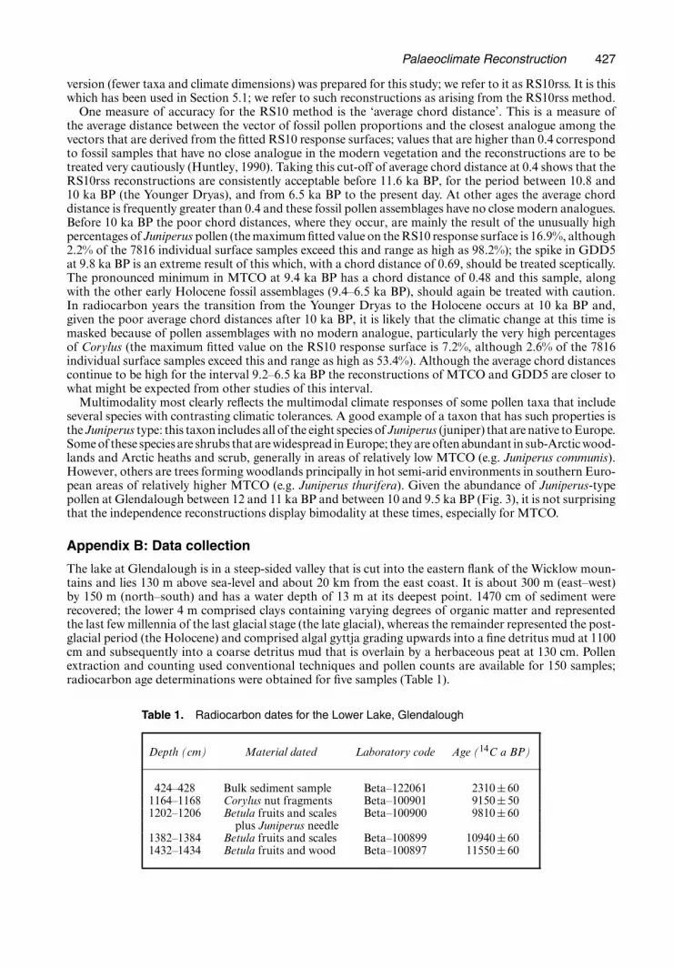
Palaeoclimate Reconstruction 427
version (fewer taxa and climate dimensions) was prepared for this study; we refer to it as RS10rss. It is thiswhich has been used in Section 5.1; we refer to such reconstructions as arising from the RS10rss method.
One measure of accuracy for the RS10 method is the ‘average chord distance’. This is a measure ofthe average distance between the vector of fossil pollen proportions and the closest analogue among thevectors that are derived from the fitted RS10 response surfaces; values that are higher than 0.4 correspondto fossil samples that have no close analogue in the modern vegetation and the reconstructions are to betreated very cautiously (Huntley, 1990). Taking this cut-off of average chord distance at 0.4 shows that theRS10rss reconstructions are consistently acceptable before 11.6 ka BP, for the period between 10.8 and10 ka BP (the Younger Dryas), and from 6.5 ka BP to the present day. At other ages the average chorddistance is frequently greater than 0.4 and these fossil pollen assemblages have no close modern analogues.Before 10 ka BP the poor chord distances, where they occur, are mainly the result of the unusually highpercentages of Juniperus pollen (the maximum fitted value on the RS10 response surface is 16.9%, although2.2% of the 7816 individual surface samples exceed this and range as high as 98.2%); the spike in GDD5at 9.8 ka BP is an extreme result of this which, with a chord distance of 0.69, should be treated sceptically.The pronounced minimum in MTCO at 9.4 ka BP has a chord distance of 0.48 and this sample, alongwith the other early Holocene fossil assemblages (9.4–6.5 ka BP), should again be treated with caution.In radiocarbon years the transition from the Younger Dryas to the Holocene occurs at 10 ka BP and,given the poor average chord distances after 10 ka BP, it is likely that the climatic change at this time ismasked because of pollen assemblages with no modern analogue, particularly the very high percentagesof Corylus (the maximum fitted value on the RS10 response surface is 7.2%, although 2.6% of the 7816individual surface samples exceed this and range as high as 53.4%). Although the average chord distancescontinue to be high for the interval 9.2–6.5 ka BP the reconstructions of MTCO and GDD5 are closer towhat might be expected from other studies of this interval.
Multimodality most clearly reflects the multimodal climate responses of some pollen taxa that includeseveral species with contrasting climatic tolerances. A good example of a taxon that has such properties isthe Juniperus type: this taxon includes all of the eight species of Juniperus (juniper) that are native to Europe.Some of these species are shrubs that are widespread in Europe; they are often abundant in sub-Arctic wood-lands and Arctic heaths and scrub, generally in areas of relatively low MTCO (e.g. Juniperus communis).However, others are trees forming woodlands principally in hot semi-arid environments in southern Euro-pean areas of relatively higher MTCO (e.g. Juniperus thurifera). Given the abundance of Juniperus-typepollen at Glendalough between 12 and 11 ka BP and between 10 and 9.5 ka BP (Fig. 3), it is not surprisingthat the independence reconstructions display bimodality at these times, especially for MTCO.
Appendix B: Data collection
The lake at Glendalough is in a steep-sided valley that is cut into the eastern flank of the Wicklow moun-tains and lies 130 m above sea-level and about 20 km from the east coast. It is about 300 m (east–west)by 150 m (north–south) and has a water depth of 13 m at its deepest point. 1470 cm of sediment wererecovered; the lower 4 m comprised clays containing varying degrees of organic matter and representedthe last few millennia of the last glacial stage (the late glacial), whereas the remainder represented the post-glacial period (the Holocene) and comprised algal gyttja grading upwards into a fine detritus mud at 1100cm and subsequently into a coarse detritus mud that is overlain by a herbaceous peat at 130 cm. Pollenextraction and counting used conventional techniques and pollen counts are available for 150 samples;radiocarbon age determinations were obtained for five samples (Table 1).
Table 1. Radiocarbon dates for the Lower Lake, Glendalough
Depth (cm) Material dated Laboratory code Age (14C a BP)
424–428 Bulk sediment sample Beta–122061 2310±601164–1168 Corylus nut fragments Beta–100901 9150±501202–1206 Betula fruits and scales Beta–100900 9810±60
plus Juniperus needle1382–1384 Betula fruits and scales Beta–100899 10940±601432–1434 Betula fruits and wood Beta–100897 11550±60

428 J. Haslett et al.
The 13 taxa that were used were selected principally on the basis that they were relatively abundantin the fossil pollen data. The exception, Picea (spruce), was selected because of its near absence both inthe fossil pollen data and in surface samples from the nemoral (broad-leaved forest) zone. This contrastswith its presence in surface samples from the boreal (mainly coniferous) zone and allows differentiationbetween pollen spectra from these climatically distinct zones when making reconstructions. Note also thatwe use a composite taxon Artemisia plus Chenopodiaceae—because these taxa, although individually rarein samples from Glendalough, have a similar pattern of occurrence and abundance in relation to climateand thus provide a consistent climatic signal. Amalgamation of the remaining taxa into the category ‘other’also served to ensure differentiation between pollen spectra from climatically distinct regimes. For exam-ple, we wish to distinguish between spectra, with similar relative abundances of the 13 taxa, but differentoverall contribution from these taxa.
References
Aitchison, J. (1986) The Statistical Analysis of Compositional Data. London: Chapman and Hall.Allen, J., Watts, W. and Huntley, B. (2000) Weichselian palynostratigraphy, palaeovegetation and palaeoenviron-
ment: the record from Lago Grande di Monticchio, southern Italy. Quatern. Int., 73, 91–110.Banerjee, S., Carlin, B. and Gelfand, A. (2004) Hierarchical Modeling and Analysis for Spatial Data. New York:
Chapman and Hall.Bartlein, P. and Webb III, T. (1985) Mean July temperature at 6000 yr B.P. in eastern North America: regression
equations for estimates from fossil-pollen data. Syllogeus, 55, 301–342.Bartlein, P., Webb III, T. and Fleri, E. (1984) Holocene climate change in the northern Midwest: pollen-derived
estimates. Quatern. Res., 22, 361–374.Besag, J. and Kooperberg, C. (1995) On conditional and intrinsic autoregression. Biometrika, 82, 733–746.Bhattacharya, S. (2005) Importance resampling MCMC: a methodology for cross-validation in inverse prob-
lems and its application in model assessment. PhD Thesis. Trinity College Dublin, Dublin. (Available fromhttp://www.tcd.ie/Statistics/JHpersonal/thesis.pdf.)
Bhattacharya, S. and Haslett, J. (2005) Importance re-sampling MCMC: for cross validation in inverse problems.Technical Report. Trinity College Dublin, Dublin. (Available from http://www.tcd.ie/Statistics/JHpersonal/irmcmc%20AS%20SUBMITTED%20to%20S&C.pdf.)
Billheimer, D., Guttorp, P. and Fagan, W. F. (2001) Statistical interpretation of species composition. J. Am. Statist.Ass., 96, 1205–1214.
Birks, H. J. B. (1995) Quantitative palaeoenvironmental reconstructions. In Statistical Modelling of QuaternaryScience Data, Technical Guide 5 (eds D. Maddy and J. Brew), pp. 161–254. Cambridge: Quaternary ResearchAssociation.
ter Braak, C. J. F. (1995) Non-linear methods for multivariate statistical calibration and their use in paleoecology:a comparison of inverse and classical approaches. Chemometr. Intell. Lab. Syst., 28, 165–180.
ter Braak, C., van Hobben, H. and di Bella, G. (1996) On inferring past environmental change from species com-position data by non-linear reduced rank models. In Proc. 13th Int. Biometric Conf., pp. 65–70. Chicago:University of Chicago Press.
Buck, C. E. (2003) Bayesian chronological data interpretation: where now? In Tools for Constructing Chronologies:Crossing Disciplinary Boundaries (eds C. E. Buck and A. R. Millard). London: Springer.
Cooperative Holocene Mapping Project (1988) Climatic changes of the last 18,000 years: observations and modelsimulations. Science, 241, 1043–1052.
Cressie, N. A. C. (1993) Statistics for Spatial Data. New York: Wiley.Davis, B., Brewer, S., Stevenson, A., Guiot, J. and data contributors (2003) The temperature of Europe during
the Holocene reconstructed from pollen data. Quatern. Sci. Rev., 22, 1701–1716.van Deusen, P. and Reams, G. (1996) Bayesian procedures for reconstructing past climate. In Tree Rings, Envi-
ronment and Humanity (eds J. Dean, D. Meko and T. Swetnam), pp. 335–339. Tucson: Radiocarbon.Deutsch, C. V. and Wen, X. H. (1998) An improved perturbation mechanism for simulated annealing simulation.
Math. Geol., 30, 801–816.Dey, D. and Maiti, T. (2002) Dirichlet multinominal distribution. In Encyclopedia of Environmetrics (eds A.
El-Shaarawi and W. Piegorsch), pp. 522–523. Stuttgart: Fischer.Farrera, I., Harrison, S. P., Prentice, I. C., Ramstein, G., Guiot, J., Bartlein, P., Bonnefille, R., Bush, M., Cramer,
W., von Grafenstein, U., Holmgren, K., Hooghiemstra, H., Hope, G., Jolly, D., Lauritzen, S. E., Ono, Y., Pinot,S., Stute, M. and Yu, G. (1999) Tropical climates at the last glacial maximum: a new synthesis of terrestrialpalaeoclimate data. 1, Vegetation, lake levels and geochemistry. Clim. Dynam., 15, 823–856.
Fitzgerald, D. (2003) Private communication.Gachet, S., Brewer, S. S., Cheddadi, R., Davis, B., Gritti, E., and Guiot, J. (2003) A probabilistic approach to the
use of pollen indicators for plant attributes and biomes: an application to European vegetation at 0 and 6 ka.Glob. Ecol. Biogeogr., 12, 103–118.

Palaeoclimate Reconstruction 429
Grunwald, G. K., Raftery, A. E. and Guttorp, P. (1993) Times series of continuous proportions. J. R. Statist. Soc.B, 55, 103–116.
Guiot, J. (1985) A method for palaeoclimatic reconstruction in palynology based on multivariate time-seriesanalysis. Geogr. Phys. Quatern., 39, 115–126.
Guiot, J. (1990) Methodology of the last climatic cycle reconstruction in France from pollen data. Palaeogeogr.Palaeoclim. Palaeoecol., 80, 49–69.
Guiot, J. (1991) Structural characteristics of proxy data and methods for quantitative climate reconstructions.In Evaluation of Climate Proxy Data in Relation to the European Holocene (ed. B. Frenzel), pp. 271–284.Stuttgart: Fischer.
Guiot, J., de Beaulieu, J. L., Cheddadi, R., David, F., Ponel, P. and Reille, M. (1993a) The climate in WesternEurope during the last glacial interglacial cycle derived from pollen and insect remains. Palaeogeogr. Palaeoclim.Palaeoecol., 103, 73–93.
Guiot, J., Harrison, S. P. and Prentice, I. C. (1993b) Reconstruction of Holocene precipitation patterns in Europeusing pollen and lake-level data. Quatern. Res., 40, 139–149.
Guiot, J., Torre, F., Jolly, D., Peyron, O., Boreux, J. and Cheddadi, R. (2000) Inverse vegetation modelling byMonte Carlo sampling to reconstruct palaeoclimates under changed precipitation seasonality and CO2 condi-tions: application to glacial climate in the Mediterranean region. Ecol. Modllng, 127, 119–140.
Hargreaves, J. and Annan, J. (2002) Assimilation of paleo-data in a simple earth system model. Clim. Dynam.,19, 371–381.
Haslett, J. and Hayes, K. (1998) Residuals for the linear model with general covariance structure. J. R. Statist.Soc. B, 60, 201–215.
Huntley, B. (1990) Dissimilarity mapping between fossil and contemporary pollen spectra in Europe for the past13,000 years. Quatern. Res., 33, 360–376.
Huntley, B. (1993) The use of climate response surfaces to reconstruct palaeoclimate from quaternary pollen andplant macrofossil data. Phil. Trans. R. Soc. Lond. B, 341, 215–223.
Huntley, B. and Prentice, I. C. (1988) July temperature in Europe from pollen data 6000 years before present.Science, 241, 687–689.
Hutchinson, M. F. (1989) A new objective method for spatial interpolation of meteorological variables fromirregular networks applied to the estimation of monthly mean solar radiation, temperature, precipitationand windrun. Technical Report. Commonwealth Scientific and Industrial Research Organisation, Canberra.
Hutton, J. (1788) An investigation of the laws observable in the composition, dissolution and restoration of theglobe. Trans. R. Soc. Edinb., 1, 209–304.
Joussaume, S., Taylor, K. E., Braconnot, P., Mitchell, J. F. B., Kutzbach, J. E., Harrison, S. P., Prentice, I. C.,Broccoli, A. J., Abe-Ouchi, A., Bartlein, P. J., Bonfils, C., Dong, B., Guiot, J., Herterich, K., Hewitt, C. D., Jolly,D., Kim, J. W., Kislov, A., Kitoh, A., Loutre, M. F., Masson, V., McAvaney, B., McFarlane, N., de Noblet, N.,Peltier, W. R., Peterschmitt, J. Y., Pollard, D., Rind, D., Royer, J. F., Schlesinger, M. E., Syktus, J., Thompson,S., Valdes, P., Vettorett, G., Webb, R. S. and Wyputta, U. (1999) Monsoon changes for 6000 years ago: resultsof 18 simulations from the Paleoclimate Modeling Intercomparison Project (PMIP). Geophys. Res. Lett., 26,859–862.
Katz, R. W. (2002) Techniques for estimating uncertainty in climate change scenarios and impact studies. Clim.Res., 20, 167–185.
Klimanov, V. A. (1984) Paleoclimatic reconstructions based on the information statistical method. In LateQuaternary Environments of the Soviet Union (eds J. H. E. Wright and C. W. Barnosky), pp. 297–303. Lon-don: Longman.
Korhola, A., Vasko, K., Toivonen, H. and Olandor, H. (2002) Holocene temperature changes in northern Fenno-scandia reconstructed from chironomids using Bayesian modelling. Quatern. Sci. Rev., 21, 1841–1860.
Lee, P. M. (1997) Bayesian Statistics, an Introduction, 2nd edn. London: Arnold.Leemans, R. and Cramer, W. (1991) The IIASA database for mean monthly values of temperature, precipita-
tion and cloudiness of a global terrestrial grid. Research Report RR-91-18. International Institute for AppliedSystems Analysis, Laxenburg.
Marshall, E. and Spiegelhalter, D. (2003) Approximate cross-validatory predictive checks in disease-mappingmodels. Statist. Med., 22, 1649–1660.
Prentice, I. C. (1988) Records of vegetation in time and space: the principles of pollen analysis. In VegetationHistory (eds B. Huntley and T. Webb III), pp. 17–42. Dordrecht: Kluwer.
Prentice, I. C., Bartlein, P. J. and Webb III, T. (1991) Vegetation and climate change in eastern North Americasince the last glacial maximum. Ecology, 72, 2038–2056.
Prentice, I. C., Cramer, W., Harrison, S. P., Leemans, R., Monserud, R. A. and Solomon, A. M. (1992) A globalbiome model based on plant physiology and dominance, soil properties and climate. J. Biogeogr., 19, 117–134.
Ravishanker, N., Dey, D. and Iyenger, M. (2001) Compositional time series analysis of mortality proportions.Communs Statist. Theory Meth., 30, 2281–2291.
Robertson, I., Lucy, D., Baxter, L., Pollard, A., Aykroyd, R., Barker, A., Carter, A., Switsur, V. and Waterhouse,J. (1999) A kernel-based Bayesian approach to climatic reconstruction. Holocene, 9, 525–530.
Stein, M. L. (1999) Interpolation of Spatial Data: Some Theory for Kriging. New York: Springer.

430 Discussion on the Paper by Haslett et al.
Stuiver, M., Grootes, P. M. and Braziunas, T. F. (1995) The GISP2 δ18O climate record of the past 16,500 yearsand the role of the sun, ocean, and volcanoes. Quatern. Res., 44, 341–354.
Tierney, L. (1994) Markov chains for exploring posterior distributions (with discussion). Ann. Statist., 22, 1701–1762.
Toivonen, H. T. T., Mannila, H., Korhola, A. and Olander, H. (2001) Applying Bayesian statistics to organism-based environmental reconstruction. Ecol. Appl., 11, 618–630.
Trudinger, C. M. (2000) The carbon cycle over the last 1000 years inferred from inversion of ice core data. PhDThesis. Monash University, Clayton. (Available from http://www.dar.csiro.au/publications/trudinger-2001a0.htm.)
Trudinger, C. M., Enting, I. G. and Rayner, P. J. (2002a) Kalman filter analysis of ice core data: method develop-ment and testing of statistics. J. Geophys. Res., 107, 73–93.
Trudinger, C. M., Enting, I. G., Rayner, P. J. and Francey, R. J. (2002b) Kalman filter analysis of ice core data:double deconvolution of CO2 and δ13C measurements. J. Geophys. Res., 107, 73–93.
Vasko, K., Toivonen, H. T. and Korhola, A. (2000) A Bayesian multinomial Gaussian response model for organ-ism-based environmental reconstruction. J. Paleolimn., 24, 243–250.
West, M. (1996) Some statistical issues in paleoclimatology (with discussion). In Bayesian Statistics 5 (eds J. M.Bernardo, J. Berger, A. P. Dawid and A. F. M. Smith). Oxford: Oxford University Press.
Whiley, M. and Wilson, S. (2004) Parallel algorithms for Markov chain Monte Carlo methods in latent spatialGaussian models. Statist. Comput., 14, 171–179.
Wright, J. H. E., Kutzbach, J. E., Webb III, T., Ruddiman, W. F., Street-Perrott, F. A. and Bartlein, P. J. (1993)Global Climates since the Last Glacial Maximum. Minneapolis: University of Minnesota Press.
Discussion on the paper by Haslett et al.
Caitlin E. Buck (University of Sheffield)The recent palaeoenvironmental literature suggests that, given sufficient data from single environmentalindicators (or proxies) and non-spatial models, we can achieve an understanding of past climate. Haslettand his colleagues make it clear that we shall never obtain reliable palaeoclimate reconstructions unless wesee the problem as multivariate and spatiotemporal with every data source having a unique error structurethat must be carefully delineated and modelled.
This is the first time that I have seen the problems articulated so clearly and I am sure that this paperwill be pivotal in helping data generators to see why they have not been able to make the consistent climatereconstructions that they seek. For that reason I commend the paper and am honoured to have been invitedto propose a vote of thanks on behalf of both those present for the reading of the paper and those in thepalaeoclimate community who are yet to learn about it.
As the authors say, there is much still to do. Put starkly, they tell us that climate is a multivariate,multilocation temporal phenomenon and yet select a case-study that has one spatial location, one climateproxy and temporal uncertainty that they ignore. I fully understand that they make these assumptions tomake progress on implementation but the simplifications lead to serious shortcomings.
In my view, it is the shortcomings in the temporal modelling that must be tackled most urgently, sincein moving from single to multiple sites it will be necessary to utilize more than one chronometric dataset. These will not all be radiocarbon based and will be irreconcilable unless we acknowledge that theamount of radioactive carbon in our atmosphere has changed over time. Calibration is needed to mapfrom the radiocarbon to the calendar scale. For the period of the Glendalough case-study, there is now avery good estimate of the calibration curve (Reimer et al., 2004). Since the curve is not monotonic, wecannot presume that events chronologically ordered on one scale take the same order on the other scale,so calibration must be performed before we impose stratigraphic ordering even at a single site.
Typically we do not have direct dating evidence for every sample. In the Glendalough case-study thereare only five independently dated samples. Each has an associated radiocarbon age and laboratory stan-dard error estimate (here 50 or 60 years). Neither in the paper nor in the data notes are we told how theymoved from the five radiocarbon ages (with laboratory standard errors) to the apparently precise ages thatare associated with the 150 samples in the pollen database. The median differences between their interpo-lated radiocarbon ages of the samples is approximately 50 years. This suggests that laboratory errors ofapproximately the same magnitude are an important source of uncertainty. As a result, I would like to askthe authors what interpolation method they used to obtain the dates that are given in their data file andhow they accounted for the radiocarbon laboratory standard errors.
The authors note the well-established Bayesian framework for radiocarbon calibration. This has recentlybeen supplemented, firstly by models for representing prior information about piecewise linear accumula-tion rates (Blaauw and Christen, 2005), secondly by development of tailored random-walk models that are

Discussion on the Paper by Haslett et al. 431
used to estimate the most recent internationally agreed radiocarbon calibration curves (Buck and Black-well, 2004) and thirdly by development of models for representing the uncertainties that are associatedwith several other choronometric dating methods (Millard, 2003).
Once the authors move from modelling on the radiocarbon to the calibrated scale, various modellingchoices will need re-evaluation but may work more satisfactorily—most obviously the use of changes inδ18O levels in the GISP2 Greenland ice core data to help them to derive a prior for temporal smoothness.The timescale for these data is derived by counting back annually laminated sediments. This timescale hasa monotonic relationship only with calibrated radiocarbon ages. Consequently, the first differences in icecore data are likely to provide a much more reliable prior for chronologies that are built on the calibratedrather than the uncalibrated radiocarbon timescale. Perhaps less obviously, use of the calibration curvecould induce important temporal correlation between sites. Uncertainties on the IntCal04 radiocarboncalibration curve vary between 6 and 163 years (with a median of 16 years) and thus cannot be ignored infuture modelling.
Now my final point: much of the world’s modern climate data are at the edge of known climate space.Expert knowledge might be used to supplement the data. This could prove particularly interesting if expertsare not unified about the behaviour outside the range of modern analogues. Priors based on several differ-ing opinions would allow investigation of the effect that each has on the resultant Bayesian palaeoclimatereconstructions. It seems high time that Bayesian statisticians started show-casing the use of expert opinionin statistical inference and this would make an excellent case-study for so doing.
Cajo J. F. ter Braak (Wageningen University and Research Centre)In this cutting edge research the authors take a modern Bayesian approach to solve the important chal-lenge of reconstructing palaeoclimate from pollen counts. As the causal relationship runs from climate topollen count—typically expressed by response surfaces of pollen with respect to climate—this is an ‘inverseproblem’ also known as multivariate non-linear calibration (a missing keyword). The Bayesian methodallows us
(a) to quantify the uncertainty of a reconstruction and(b) to reduce the uncertainty somewhat by assuming that the fossil climate changes smoothly in time
(Fig. 9).
These are important achievements.The statement ‘our method is closest in spirit to a version of the modern analogue method’ invokes a
historic remark. Frequentists distinguish between classical and inverse approaches to statistical calibra-tion (Osborne, 1991) and for linear models much is known about their relationship in terms of the impliedprior for the unknown climate. The classical approach is based on response surfaces whereas the inverseapproach can do without (ter Braak, 1995). The prototype inverse approach is the ‘modern analogue’method, better known as the k-nearest-neighbour (k-NN) method, which for k =1 estimates the unknownpalaeoclimate by the climate of that particular modern pollen composition that is ‘closest’ to the fossilpollen composition. Here closest is measured by chord distance or some other (dis)similarity measurebetween two pollen compositions. The k-NN method averages climates. The RS10 method is different; itfirst calculates nonparametric response surfaces on a lattice—it averages pollen counts—and then appliesthe 1-NN method with respect to the lattice. The RSl0 method thus can be considered as taking the classicalapproach (with the chord distance taking the role of a likelihood). The Bayesian method proposed is closestin spirit to the ‘classical’ RSl0 method. Stage 1 models the response surfaces and their uncertainty andstage 2 determines, given these, the unknown climate. Even the uniform prior for the initial fossil climatecorresponds to the classical approach. Alternatively, the reconstruction could have been conditioned onthe modern climate at Glendalough.
Palynologists are aware of the no modern analogue problem and the multiple analogue problem. Theno modern analogue problem entails that none of the modern or fitted pollen compositions is similar tothe fossil composition, indicated by a large chord distance. In Fig. 8 the authors plot this distance alongwith the interquartile range of the reconstructed climates. However, the interquartile range is a measureof spread and is not really an inconsistency diagnostic such as the one in linear models (Osborne, 1991;Sundberg, 1994). As the authors took care of modelling the uncertainty of a composition, how would theydefine inconsistency here? The multiple-analogue problem entails that a fossil composition is equally simi-lar to several climatically very different modern ones. This results in multimodality of the posterior, whichis in my view largely confined to stage 2. I found the remark on the multimodal nature of the posterior inSection 3.1 therefore premature. With the two-stage implementation the authors can circumvent the slow

432 Discussion on the Paper by Haslett et al.
mixing of Markov chain Monte Carlo chains on multimodal densities. Temporal and spatial constraintson the reconstructions help to solve both the no analogue and the multiple-analogue problems (ter Braaket al., 1996). Linear constraints were investigated in van Dobben and ter Braak (1998).
In the paper, response surfaces are conceptually modelled via an intrinsic Gaussian random field withlinear variogram and actually calculated on a lattice via an intrinsic Markov random field (Section 3.2).Could the off-putting warning ‘there may not be a unique stochastic process defined’ have been circum-vented by extending the lattice (Rue and Held, 2005)? A Bayesian P-spline approach (Lang and Brezger,2004) might have been more parsimonious. As I have no feeling for the amount of smoothness that isimplied by the abstract formulation, I would welcome some graphs, e.g. the modal and, for comparison,RS10 response curves for the species against GDD5 at MTCO=4 ◦C. Am I right in believing that thesmoothness of the fit is really governed by the balance between κ of the variogram and (δ, nj), which deter-mine the precision of the counts? The data are compositions, so the θg-vectors sum to 1 for each locationg. This is enforced by a Metropolis algorithm with random-walk proposals on the simplex, but I wonderhow? Are all proposals with a θig +ui outside the unit interval simply counted as rejections? Noteworthyhere is also the logistic Gaussian approach to spatial compositional data of Tjelmeland and Lund (2003).
The sharpening and blurring of response surfaces appear very drastic operations to me and I wonderwhy they influence the reconstruction so little. Is it just presence versus absence of taxa that conveys mostof the information?
The authors managed to overcome both the computational burden and the burden of freedom of modelspecification. It is therefore my great pleasure to second the vote of thanks.
The vote of thanks was passed by acclamation.
Andrew R. Millard (Durham University)First I congratulate the authors on what I consider will be a major advance in palaeoclimate modelling. Asnoted by Caitlin Buck, there are issues relating to transferring the modelling from a radiocarbon timescaleto a calendar timescale. However, given the modular approach of the paper I think that this can be donerelatively easily. I wish to comment on other timescale issues.
One of the major advances of this method is the new type of result which allows us to examine within-climate-history variability, as well as the uncertainty (or between-reconstruction variability). However, Ibelieve that the example in Fig. 11 is a methodological artefact. Interquartile ranges are calculated betweenhistories rather than within them. The calculations treat differences between reconstructed histories asdifferences between random walks by dividing by the time difference between samples but in fact they aredifferences between different reconstructions of a single random walk. The differences that are displayedin Fig. 11 derive from uncertainty in the reconstruction, not variability within a reconstruction. Fig. 8shows that the uncertainty of reconstructions is approximately constant over the last 9000 years. There-fore the uncertainty of differences between samples is approximately constant, and when combined withdivision by the time difference we simply see a standard deviation or interquartile range that is inverselyproportional to the square root of the time difference. This is approximately what we see in Fig. 11 wherethe first three segments have time differences between observations in the ratio 1:2:8 and the interquartilerange ratio appears to be approximately 1:
√2:2
√2. However, beyond 9000 years the variability is greater
and may include a genuine signal of change in climate variability.There is within-history information that can be extracted, e.g. variation over a millennium, which could
be calculated for each history together with its uncertainty and compared with other millennia. Care isneeded here, however, as the current method treats each sample as a point in time whereas it is in fact atime average. In periods of slow deposition samples average longer periods and this will reduce apparentvariability; at Glendalough this will be particularly reduced in the 5000–9000-year period compared withthe more recent periods. More sophisticated treatment of time averaging is needed for the reconstructionof some aspects of climate variability.
Overall these are minor points and I think that the authors are to be congratulated on a quantum leapforward in the concepts underlying climate reconstruction.
Jonathan Rougier (Durham University)I congratulate the authors on an impressive study, on the clarity of their exposition and on their frankappraisal. It is possible to take issue with some of their modelling choices, but in my view they are broadly‘fit for purpose’ in this proof of concept; with more at stake, a more careful selection of the various modelcomponents would be required, and I am sure that both the authors and the other discussants will haveplenty of suggestions for alternatives. I would like to address two issues that are more general.

Discussion on the Paper by Haslett et al. 433
First, some missing data: the authors’ stated data are modern climate and pollen, datam, and fossilpollen at Glendalough, pf . But they are missing an important extra piece of information: we also knowthe current climate at Glendalough, c* say. This will surely be useful in reconstructing palaeoclimate atGlendalough, because it tells us where the time series cf.·/ must terminate, and this will be relevant formuch of cf.·/ because it is hypothesized that climate evolves smoothly in time. In fact, it is easy to see howthis information can be incorporated in the analysis. For each step in their sampler, the authors simulatea series cf.tj/, for j =2, 3, . . . going forward in time from a random starting-point cf.t1/ chosen uniformlyon the modern climates. Their stochastic process for cf.·/ is reversible: they choose a random walk withStudent t increments. They could equally well have simulated the series backwards in time, except in thiscase the starting-point would be known, namely cÅ. So to incorporate cÅ in their analysis costs nothing,and it is likely—if cf.·/ is smooth—to lower substantially the rejection rate of their sampler.
Second, I wonder how much we really trust the inferences that we draw from the fully probabilisticanalysis. I suspect that much of the fine scale structure we observe in the results comes from trading off tailprobabilities in the various model components, none of which we really believe. My feeling is that we canonly take a limited amount of information from this exercise, perhaps just the first and second moments ofthe predictand, palaeoclimate. Unfortunately this does not give rise to such exciting graphics, but colouris not required! I am not advocating that the entire inference be attempted in terms of low order moments,but I think that our objective should quite explicitly be to estimate the mean and variance structure of thepredictand that is implied by the data and the probabilistic modelling, rather than to generate a sample ofrealizations.
A. O’Hagan (University of Sheffield)It is a pleasure to join with other speakers in congratulating the authors on such a splendid paper. It ishard to cover large and complex interdisciplinary projects like this in a single paper, and the authors havestruck just the right balance between overview and technical detail. My comments relate to some mattersof detail in the modelling.
First, the use of t-distributions in the modelling of temporal smoothness makes sense, but it needs somethought in view of the unequal time steps between observations. The use of a t8-distribution is justifiedfrom data on annual steps, but whereas a process with independent Gaussian increments retains thatproperty for any time steps this is not true of t-increments. A sum of independent t8 random variables isnot t8 distributed. Because of the central limit theorem it will tend to normality. However, it remains truethat the (extreme) tails of its distribution are like those of a t8 random variable (O’Hagan, 1990). So theauthors’ modelling may be an adequate approximation.
A possibly more important point about the temporal modelling is that there should be correlationbetween GDD5 and MTCO. Correlation should also be modelled between the qj-vectors over time. Someof the variability in pollen counts may be due to climate being more or less conducive, but some will bedue to species abundance. Most tree species in the record are long lived and spread slowly, and this willbe reflected in the qj-vectors changing quite slowly over time.
Finally, I think that the qj-vectors may also be one way to address the excess of 0s in the pollen counts.These parameters in the hierarchy represent a propensity to produce pollen and so could be seen as mea-suring viability. If we imagined that below a certain threshold of viability no pollen would be produced,then this could be modelled to account for excess 0s.
H. John B. Birks (University of Bergen and University College London) and Richard Telford (University ofBergen)Haslett and colleagues provide a bold approach to reconstructing the ‘entire climate history’ for the last12800 years at a site in Ireland by using pollen stratigraphical data and modelling explicitly the history’suncertainty. Other Bayesian approaches to palaeoclimate reconstruction are currently also being devel-oped (e.g. Erasto and Holmstrom (2006) and Kumke et al. (2004)). All climate reconstructions are a majorchallenge as they abound in statistical and biological problems (Birks and Seppa, 2004). We discuss someof these biological problems here.
Haslett and his colleagues use an extensive modern data set of 7815 records and 13 pollen types (plus‘other’) covering Europe, Asia and North America. Given this geographical and palynological range, notsurprisingly the data set exhibits multimodality in the modern pollen–climate responses, thereby creatingmodelling problems. One such problem discussed is the multimodal climatic response of ‘Juniperus’ pollenin Europe. In fact, the 7815 records also include Juniperus and Thuja pollen in North America. The datashow that areas with similar GDD5 and MTCO to Ireland occur in western North America but the pollen

434 Discussion on the Paper by Haslett et al.
assemblages there are very different. Is including North America a help or a hindrance in reconstructingIrish climate?
What advantages do the authors see in using such a geographically extensive and palynologically het-erogeneous data set for reconstructing past climate over the last 12.8 ka in Ireland? Given widespreadhuman impact in much of the northern hemisphere, how do they know that the data ‘all provide evidenceof climatically determined regional vegetation’ (Section 2.2)? We are fascinated by the statement (page 397)that ‘the science is such that multimodal reconstructions are to be expected’. Is this expectation a resultof the reconstruction models, the modern data or the underlying nature of pollen–vegetation–climateresponses?
At Glendalough (Fig. 3), there are striking changes around about 5 ka BP which the authors recognizeas a ‘progressive change towards more open conditions’ (Section 2.1). Interestingly they also demonstrate(Fig. 11) a sharp transition ‘to a more volatile period at about 5 ka BP’ (Section 5.4) and propose thattheir scaled interquartile range values may be ‘a novel finding’ (Section 5.4). What are the likely causes forthese marked changes 5000 years ago?
For the ‘exact’ cross-validation why did they not include some modern pollen spectra from Ireland?Some idea of the model’s abilities to infer climate on ‘home territory’ and not just Glendalough itself(Section 5.1) would be valuable, given that modern Irish climate is at the very edge of modern climatespace.
Richard W. Katz (National Center for Atmospheric Research, Boulder)As one who has long promoted the involvement of statisticians in climate-related research, it is gratify-ing to see the effort of Haslett and his colleagues to bring modern statistical techniques to bear on thechallenging problem of palaeoclimate reconstruction. Although the method that is proposed in the paperis both too computationally complex and not scientifically sufficiently realistic to be routinely applied bypalaeoclimatologists, it should at the least stimulate more extensive collaboration between statisticiansand palaeoclimatologists on this problem.
Better quantification of uncertainty in palaeoclimate reconstruction is paramount to resolving certainpolicy issues concerning greenhouse-gas-induced climate warming, in particular, the extent to which therecent observed warming in global climate is unusual (Osborn and Briffa, 2004). It is noteworthy that theforthcoming UN Fourth Scientific Assessment of the Intergovernmental Panel on Climate Change willdevote an entire chapter to palaeoclimate, including a section on the uncertainty of proxy methods (seehttp://www.ipcc.ch).
The remainder of my contribution focuses on the realism of the treatment of climate and proxy variablesin the paper. It is understandable that interpolation is required to estimate modern climatic conditionsat the locations of the surface pollen data from climate observations that are only available at a differ-ent set of locations. But I find it disconcerting that the growing degree data themselves would require‘reconstruction’, apparently being estimated indirectly from the interpolated monthly mean temperature(Section 2.3).
One of the most novel aspects in the paper is the use of a random walk with heavy-tailed innovations asa prior for the temporal smoothness of climate change, which is consistent with the tail behaviour that isobserved for the Greenland ice core time series (Fig. 4). A heavy-tailed distribution is certainly plausible,especially for a proxy whose modern counterpart has such a feature (e.g. precipitation or related hydrologicvariables such as streamflow). Yet the tail behaviour of proxy time series has only rarely been carefullyexamined. An exception is Katz et al. (2005) in which extreme value theory was applied to examine thetail behaviour of certain proxy variables. For sediment yield recorded in lacustrine varves in the Canadianhigh Arctic, which is a proxy for heavy rain events (Lamoureux, 2000), a heavy upper tail was detected.Still it is curious that Haslett and his colleagues find heavy-tailed behaviour in a temperature proxy, asmodern temperature observations tend to have a light-tailed, or even bounded, distribution.
The following contributions were received in writing after the meeting.
Thomas Brendan Murphy and Isobel Claire Gormley (Trinity College Dublin)We congratulate the authors on an excellent and thought-provoking paper. We would like to discuss oneaspect of the paper.
In the paper, problems of modelling the pollen data are discussed. Particular problems that are mentionedinclude some data as proportions, some as counts and the data have excess 0s. A Dirichlet–multinomialmodel is adopted as the method of conditionally modelling the pollen count xij of pollen type j in sample i.

Discussion on the Paper by Haslett et al. 435
Alternative methods for modelling the pollen data could be employed. One option is that the data couldbe transformed to a binary (presence–absence) format such that
yij ={
1 if pollen j is present in sample i,0 otherwise:
Although this transformation could provide an improved approach to dealing with the excess 0s in thedata, information concerning the relative abundance of the pollen species is lost.
An alternative option is to analyse the pollen abundance in terms of a partial ranking. With this approach,we let rij be the ranking of pollen type j in sample i. Thus the most abundant pollen type has rank rij =1,the second most abundant has rank rij = 2 and so on. If pollen type j is absent from a sample then therank is not observed but is known to be of lower rank than the observed pollen types. With this approach,the issue of the data being available in counts or proportions is avoided and the 0 counts are modelled asbeing less abundant than the observed samples.
Many models exist for partially ranked data (e.g. Marden (1995)). These models could be adapted toallow the distribution of pollen rankings to depend on climate. For example, the exploded logit model (seeTrain (2003), section 7.3) offers one ranking model that includes covariates (e.g. climate), although manyothers could be developed.
This approach to modelling the pollen data could offer a compromise between modelling the pollenabundance values and the presence–absence approach.
S. K. Sahu (University of Southampton) and K. V. Mardia (University of Leeds)This impressive paper presents a novel Bayesian methodology for palaeoclimate reconstruction. The au-thors must be commended because of their efforts in proposing and illustrating a set of very complexmodels to solve a practical problem. Our comments mostly relate to spatiotemporal reconstruction ofpalaeoclimate and difficulties that are associated with such a task.
In modelling the paleoclimate, as the authors state, it is important to account for spatiotemporal varia-tion. The methodology that is presented in the paper only attempts to model temporal variation. Althoughthis is a necessary and desirable feature of the methods, it is not clear that this has been achieved thor-oughly. The authors do not mention the possibility of mixing of pollen over a period of time in the lakebefore deposition. Are they dealing with average time of a pollen sample rather than the absolute time thatwe are led to believe in the paper?
A spatial analysis of fossil pollen data is also fraught with various difficulties. The most notable arisesfrom mixing of pollen from different regions in space; for example, think about a long river collectingpollens on its path and depositing them in the lake. As a result it is very likely that one will encounter theproblem of both spatial and temporal misalignment in the fossil data. Consequently, any statistical-model-based analysis which does not explicitly take account of misalignment is likely to be very inaccurate.
The mixing of pollen data in space and time will have repercussions in modelling the spatiotemporaldependences. Popular separable models of space–time covariance functions are unlikely to work here. Aflexible model for dependence which allows the interchange of correlations in space and time can addressthese concerns and is likely to be more accurate than a separable covariance function. In general, a covari-ance function can be specified as a positive definite function of s − tv of space lag s, time lag t and velocityv. Such a function is worth investigating since it allows a relationship between s and t for a fixed value ofv. Recently, Sahu and Mardia (2005) have mentioned the following possibility for a space–time processw.s, t/ that is based on Taylor’s frozen field hypothesis which states that
cov{w.0, 0/, w.vt, 0/}= cov{w.0, 0/, w.0, t/}for some vector v so that the space vector on the left-hand side leads to the time component on theright-hand side.
E. M. Scott (University of Glasgow)Understanding past climate and its drivers is particularly important as society struggles with the scientificdebate over climate change. This is an activity which until recently has been the focus of often heroicefforts in many scientific disciplines to amass more and better data. The authors have chosen to work on apalaeoclimatic reconstruction based on pollen records, a commonly used proxy climate variable, and havesuccessfully shown how the problem can be posed in a Bayesian statistical framework demonstrating thatequal effort needs to be devoted to modelling the valuable observational data record.

436 Discussion on the Paper by Haslett et al.
To achieve the reconstruction, the authors use many statistical techniques including hierarchical Bayes-ian modelling, modelling uncertainty, compositional data, nonparametric modelling and innovative com-putational techniques. All are required to reflect the complexity of the data structure. The data come froma single Irish site, in the form of a time series (for a single core) with 150 time points (depths which act as asurrogate for time) and where the pollen distribution has been ‘sampled’ at each time point. The timescaleis anchored by five radiocarbon dates. Climate is reconstructed at each of these depths (assuming that thereis a temporal correlation and smooth transition in climate—itself modelled by using ice core data fromGreenland) based on a training set of current climate and pollen records at a large number of sites aroundEurope. Although this reconstruction is for a single site, and there are questions over its robustness, thechallenge will be whether the approach can be extended to reflect the true spatial–temporal nature of theproblem. Spatial–temporal reconstruction is very dependent on the underpinning time axis, which mustbe estimated. Frequently but not exclusively, radiocarbon dating is the method that is used to estimate thetime axis, and the authors have ignored, so far in their approach, the issues in modelling the age–depthrelationship and the calibration of the radiocarbon timescale. This will become even more important whenmultiple chronologies are to be linked and modelling all the uncertainties in a unified manner becomescritical.
There is much to be gained by a greater in-depth study of the methods and results that are presentedin this paper. Future developments must include spatial–temporal modelling over all Europe with devel-opment of a common chronology. There needs also to be improved understanding and modelling of theuncertainties and further computational efficiency gains.
The authors are to be congratulated for this seminal ‘work in progress’ in this important applied area.
The authors replied later, in writing, as follows.
We acknowledge with thanks the constructive contributions of the discussants. There are two recurringthemes touching jointly on the statistics and the science: spatiotemporal aggregation (Katz, Sahu andMardia, and O’Hagan) and the uncertainties of radiocarbon dating (Buck and Scott). A strength of thestatistical approach that was adopted here is that it can in principle be extended to strengthen the modellingin areas such as these. However, some extensions may not lead to meaningful science. Katz is right—themodel may already be too complex. There are several quite specific points of statistical methodology(Rougier, O’Hagan, Millard, Katz, ter Braak, Birks, Murphy and Gormley, and O’Hagan) and someconcerning the science (Birks). We apologize in advance for the fact that for brevity the level of detail ofsome of our responses is reduced.
Aggregation issues arise throughout palaeoclimate reconstruction. Climate itself is an aggregation.From the Web site of the International Panel on Climate Change (http://www.grida.no/climate/ipcc-tar/wgl/518.htm)
‘Climate . . . is usually defined . . . as the statistical description in terms of the mean and variability ofrelevant quantities over a period of time ranging from months to thousands or millions of years. Theclassical period is 30 years, as defined by the World Meteorological Organization (WMO). . .. Climatevariability refers to . . . all temporal and spatial scales beyond that of individual weather events.’
Note the studied imprecision of these statements. Overmodelling, even if possible, may not be meaning-ful.
The temporal aggregation of sediment data is typically of the order of decades. The temporal responseof some pollen is slow—it takes time to establish an oak forest. The spatial aggregation of both pollenand climate is ill defined and depends on both the local topography and the dispersal properties of pollen,which differ with taxa. Some of these difficulties can be avoided by careful choice of lake and of taxa(e.g. excluding the long river of Sahu and Mardia). When we add to this the fact that there is temporaluncertainty in the attributed dates of the samples, it is clear that there is a limit to what can be expected;overinterpretation (of, for example, Fig. 11) is to be avoided. There are ways forward, and the severalproposals are constructive. We agree with Buck that priority must lie with temporal uncertainty.
Katz touches on the tip of another iceberg concerning data quality—even the modern ‘training data’are to be taken cautiously. For example, Rougier suggests that we condition our reconstructions on themodern climate at Glendalough. In fact, however, even the modern climate at Glendalough is not known!What is known is the climate at various Irish synoptic meteorological stations, 50 km or more distant andat different altitudes. Nevertheless Rougier is right: a more informative prior could be developed—possiblyadvantageously—than the flat prior that is implicitly used in the paper. Eliciting a meaningful prior for

Discussion on the Paper by Haslett et al. 437
the entire modern European climate will be a challenge. Birks raises a related data issue: is it a ‘help or ahindrance’ to include North American data in the training set? On the whole it is a help even for the limitedtask that was reported here: a proof-of-concept reconstruction for one site and two climate dimensions.However, the inclusion of the third aspect of climate that is normally involved in climate reconstruction(the availability of moisture) would remove the apparent similarity in most of the cases that he raises.
To answer Birks directly on multimodality, consider, in the context of Fig. 2, the implications for cli-mate reconstruction of a sample with a small proportion of taxon A. The small proportion conveys thestrong message that climate was not cA. As the tolerance of taxon B is consistent with a wide range ofclimates, the posterior is bimodal. With 14 taxa and two climate dimensions such messages become moreconfusing; but multimodality remains and is fundamental to inferences that are based on compositionaldata used inversely. The multimodality of the response surfaces is another question, which is of particularimportance in pollen; see the discussion at the end of Appendix A. Rougier is probably right—it is wise toavoid overinterpretation of the minor modes in, for example, Fig. 8. But multimodality raises challengingissues for algorithms such as Markov chain Monte Carlo algorithms; it is necessary to be aware of it.
ter Braak raises an interesting statistical issue—the no modern analogue problem—bearing directly onthe science. Effectively we may ask whether an observed fossil pollen composition pf
i is inherently unlikely,even when we do not know its climate cf
i . We seek a measure of its distance from an appropriate referencedistribution. What is that distribution? The training data provide empirical information on the joint dis-tribution π.pm, cm/; the chord distance is a particular distance from a marginal distribution π.pm/ whichputs equal mass on all the 7815 elements of pm. Might there be a more appropriate distribution, that isspecific to the (unknown) climate corresponding to ith fossil datum? The marginal prior for the vector cf
is flat, in our treatment. But the remaining fossil pollens, together with the model assumption of temporalsmoothness, do provide access to an informative conditional distribution π.cf
i |pf−i, pm, cm/, and thence to
π.pfi |pf
−i, pm, cm/=∫
π.pfi |cf
i , pf−ip
m, cm/ π.cfi |pf
−i, pm, cm/ dcfi :
Sampling from each is facilitated by the two-stage procedure. Attention thus focuses on sampling fromπ.pf
i |cfi , Θ/ and π.cf
i |pf−i, Θ/; we have dropped the irrelevant pf
−i from the first term. The first term is simple.The second is equivalent to the cross-validation procedure that was discussed in Section 4.2. If this is flat,π.pf
i |cfi , Θ/ collapses to a smoothed version of π.pm/. Thus, if appropriate, such a distance is computable
and might provide a more tailored equivalent to the chord distance.Birks wonders what might be the cause of the apparent change in climate variability? Millard perceptively
remarks that it may in fact be an artefact of our use of the interquartile range to summarize our particularmeasure of variability across climate histories. He is quite correct to suggest that the interquartile rangeis inappropriate. Interestingly, an equivalent plot of the modal variability contains the same message.This does, however, remind us how difficult it is to distinguish variability from uncertainty. Further, theremarks above on temporal uncertainty again caution against overinterpretation. If it is not an artefact, itis possible that this is anthropogenic: the Neolithic culture arrived in Ireland at about this time, with thebeginnings of agriculture and the associated progressive deforestation that has continued to the presentday.
O’Hagan is right to suggest that the t-distribution is unsatisfactory theoretically. The stable family maybe better in principle. The remarks of Katz on long-tailed distributions for such data are constructive.Heavy tails in the GISP data have been remarked on by Wunsch (2003). O’Hagan suggests some correla-tion between the two climate variables in the increments within their respective random walks, This is aconstructive proposal but surprisingly makes little difference to reconstructions here. Zero inflation is aparticular challenge; O’Hagan and others have made some interesting proposals on which we shall reportelsewhere. Also there may be sampling procedures for the Θi that are more efficient than simple randomsampling.
In short, there remain many methodological challenges.
References in the discussion
Birks, H. J. B. and Seppa, H. (2004) Pollen-based reconstructions of the late-Quaternary climate in Europe—progress, problems, and pitfalls. Acta Palaeobot., 44, 317–334.
Blaauw, M. and Christen, J. A. (2005) Radiocarbon peat chronologies and environmental change. Appl. Statist.,54, 805–816.
ter Braak, C. J. F. (1995) Non-linear methods for multivariate statistical calibration and their use in palaeoecology:a comparison of inverse and classical approaches. Chemometr. Intell. Lab. Syst., 28, 165–180.

438 Discussion on the Paper by Haslett et al.
ter Braak, C., van Hobben, H. and di Bella, G. (1996) On inferring past environmental change from speciescomposition data by non-linear reduced rank models. In Proc. 13th Int. Biometric Conf., pp. 65–70. Chicago:University of Chicago Press.
Buck, C. E. and Blackwell, P. G. (2004) Formal statistical models for estimating radiocarbon calibration curves.Radiocarbon, 46, 1093–1102.
van Dobben, H. F. and ter Braak, C. J. F. (1998) Effects of atmospheric NH3 on epiphytic lichens in the Nether-lands: the pitfalls of biological monitoring. Atmos. Environ., 32, 551–557.
Erasto, P. and Holmstrom, L. (2006) Selection of prior probabilities and multiscale analysis in Bayesian temper-ature reconstructions based on fossil assemblages. J. Paleolim., to be published.
Katz, R. W., Brush, G. S. and Parlance, M. B. (2005) Statistics of extremes: modeling ecological disturbances.Ecology, 86, 1124–1134.
Kumke, T., Scholzel, C. and Hense, A. (2004) Transfer functions for paleoclimate reconstructions—theory andmethods. In The Climate in Historical Times (eds H. Fischer, T. Kumke, G. Lohmann, G. Floser, H. Miller, H.van Storch and J. F. W. Negendank), pp. 239–243. Berlin: Springer.
Lamoureux, S. (2000) Five centuries of interannual sediment yield and rainfall-induced erosion in the CanadianHigh Arctic recorded in lacustrine varves. Wat. Resour. Res., 36, 309–318.
Lang, S. and Brezger, A. (2004) Bayesian P-splines. J. Computnl Graph. Statist., 13, 183–212.Marden, J. I. (1995) Analyzing and Modeling Rank Data. London: Chapman and Hall.Millard, A. R. (2003) Taking Bayes beyond radiocarbon: Bayesian approaches to some other chronometric
methods. In Tools for Constructing Chronologies: Crossing Disciplinary Boundaries (eds C. E. Buck and A. R.Millard). London: Springer.
O’Hagan, A. (1990). On outliers and credence for location parameter inference. J. Am. Statist. Ass., 85, 172–176.Osborn, T. J. and Briffa, K. R. (2004) The real color of climate change? Science, 306, 621–622.Osborne, C. (1991) Statistical calibration: a review. Int. Statist. Rev., 59, 309–336.Reimer, P. J., Baillie, M. G. L., Bard, E., Bayliss, A., Beck, J. W., Bertrand, C. J. H., Blackwell, P. G., Buck, C.
E., Burr, G. S., Cutler, K. B., Damon, P. E., Edwards, R. L., Fairbanks, R. G., Friedrich, M., Guilderson,T. P., Hogg, A. G., Hughen, K. A., Kromer, B., McCormac, G., Manning, S., Ramsey, C. B., Reimer, R. W.,Remmele, S., Southon, J. R., Stuiver, M., Talamo, S., Taylor, F. W., van der Plicht, J. and Weyhenmeyer, C. E.(2004) IntCal04—terrestrial radiocarbon age calibration, 0–26 cal kyr BP. Radiocarbon, 46, 1029–1058.
Rue, H. and Held, L. (2005) Gaussian Markov Random Fields. Boca Raton: Chapman and Hall–CRC.Sahu, S. K. and Mardia, K. V. (2005) Recent trends in modeling spatio-temporal data. In Proc. Meet. Statistics
and Environment, Messina, Sept. 21st–23rd, invited papers, pp. 69–83. Messina: Universita di Messina.Sundberg, R. (1994) Most modern calibration is multivariate. In Proc. 17th Int. Biometric Conf., invited papers,
pp. 395–405. Hamilton: Biometric Society.Tjelmeland, H. and Lund, K. V. (2003) Bayesian modelling of spatial compositional data. J. Appl. Statist., 30,
87–100.Train, K. E. (2003) Discrete Choice Methods with Simulation. Cambridge: Cambridge University Press.Wunsch, C. (2003) Greenland–Antarctic phase relations and millennial time-scale climate fluctuations in the
Greenland ice-cores. Quatern. Sci. Rev., 22, 1631–1646.