methodological developments in proteomic analysis
TRANSCRIPT
UNIVERSITÉ DE STRASBOURG
ÉCOLE DOCTORALE DES SCIENCES CHIMIQUES IPHC - UMR 7178
THÈSE présentée par :
Chloé MORITZ
soutenue le : 9 novembre 2021
pour obtenir le grade de : Docteur de l’Université de Strasbourg Discipline/ Spécialité : Chimie analytique
Développements méthodologiques en analyse protéomique : vers une analyse
à haut débit sur des quantités de matériel réduites et de nouvelles
stratégies de quantification
THÈSE dirigée par :
Dr CARAPITO Christine Chargée de recherche, CNRS, Université de Strasbourg Dr SCHAEFFER Christine Ingénieure de recherche, CNRS, Université de Strasbourg
RAPPORTEURS : Prof Dr SCHILLING Oliver Directeur de recherche, Université de Fribourg-en-Brisgau Dr PINEAU Charles Directeur de recherche, INSERM, Université de Rennes

UNIVERSITÉ DE STRASBOURG
ÉCOLE DOCTORALE DES SCIENCES CHIMIQUES IPHC - UMR 7178
THÈSE présentée par :
Chloé MORITZ
soutenue le : 9 Novembre 2021
pour obtenir le grade de : Docteur de l’Université de Strasbourg Discipline/ Spécialité : Chimie analytique
Methodological developments in proteomic analysis: towards high-throughput analysis on reduced quantities of material and new
quantification strategies
THÈSE dirigée par :
Dr CARAPITO Christine Chargée de recherche, CNRS, Université de Strasbourg Dr SCHAEFFER Christine Ingénieure de recherche, CNRS, Université de Strasbourg
RAPPORTEURS : Prof Dr SCHILLING Oliver Directeur de recherche, Université de Fribourg-en-Brisgau Dr PINEAU Charles Directeur de recherche, INSERM, Université de Rennes


To my friends and my family,
« Toute profession s'estime dans son cœur Traite les autres d'ignorantes,
Les qualifie impertinentes, Et semblables discours qui ne nous coûtent rien.
L'amour-propre au rebours, fait qu'au degré suprême On porte ses pareils ; car c'est un bon moyen
De s'élever aussi soi-même. »
Le Lion, le Singe, et les deux Anes, Jean De La Fontaine
REMERCIEMENTS Cette thèse a été réalisée au sein du Laboratoire de Spectrométrie de Masse BioOrganique (LSMBO) de l'Institut Pluridisciplinaire Hubert Curien (IPHC, UMR7178) à Strasbourg. Je tiens à remercier Sarah Cianférani, Christine Carapito et Christine Schaeffer pour m'avoir donné l'opportunité de réaliser ma thèse au sein du laboratoire. Je remercie particulièrement mes directrices de thèse Christine Schaeffer et Christine Carapito pour les leçons qu'elles m'ont apportées tant d'un point de vue scientifique qu'humain. Je remercie également Inoviem en particulier Pierre Eftekhari et Rachel Amouroux pour le financement de cette thèse. Merci également à tous les autres salariés pour les afterworks et les pots de Noël. C’est toujours agréable de pouvoir échanger dans un cadre plus détendu. Je remercie sincèrement Charles Pineau et Oliver Schilling pour avoir accepté et pris le temps d'évaluer mon travail de thèse. Je tiens à remercier les différents collaborateurs avec lesquels j'ai eu la chance de travailler : Can Wang, Marc Graille, Sara Awan, Magalie Lambert, Philippe Boucher, Vincent Mittelheisser, Alexandre Detappe et Torsten Müller qui ont contribué aux travaux présentés dans ce manuscrit. Je tiens également à remercier les différentes personnes de Bruker avec lesquelles j'ai eu l'occasion de travailler, Jean-Michel Billmann, Adeline Mauries, Laure Maret, Andreas Hurbain, Pierre-Olivier Schmit et Manuel Chapelle, qui m'ont aidé à de nombreuses reprises avec la nanoElute et le TimsTOF Pro. Merci pour votre aide et votre patience face à mes interminables questions stupides et parfois mon impatience face à des machines récalcitrantes. Merci d'avoir pris le temps de me montrer le cœur des instruments. C'est quelque chose que je ne connaissais pas du tout avant de venir au laboratoire et grâce à vous j'ai pu découvrir que j'aime comprendre leur fonctionnement et m'en occuper. Toujours à propos d'instruments, je voudrais aussi remercier les personnes d'Agilent avec qui j’ai pu travailler, en particulier Serge Desmoulins, Guillaume Giampaolo et Mauro Cremonini. Merci pour votre aide pour le Bravo et le développement du protocole automatisé SP3. Merci pour votre écoute et votre réactivité face à tous les problèmes auxquels nous avons dû faire face. Je tiens ensuite à remercier tout le LSMBO, les personnes qui sont déjà partis comme ceux qui viennent d'arriver. Je tiens à remercier tout particulièrement Alex et Fabrice V sans qui le monde de l'informatique du laboratoire s'effondrerait. Merci beaucoup Alex pour ta disponibilité, ta patience, et ta gentillesse même après mes dix bêtises de la journée. Le télétravail en ces temps particuliers aurait été très compliqué à mettre en place sans vous deux. Merci également à Magali et François pour votre aide avec les différents logiciels. Magali pour les conseils que tu m'as donnés sur Proline et ProStaR. J'ai beaucoup appris, grâce à ton aide. Je n'oublie pas non plus le grand travail que tu fais dans la gestion des commandes. Sans toi et Martine, nous n'irions pas très loin. Je remercie aussi Martine pour ton aide dans les démarches administratives ou lorsque je perds ma
carte CNRS ou lorsque j'arrive en retard pour m'inscrire aux conférences. Je remercie également Agnès, Hélène, Véronique et Stella pour votre disponibilité et votre contribution à l'ordre et à la qualité du laboratoire. Un grand merci aux "supramolleux", Stéphane, Oscar, Marie L, Evolène et tous les autres pour votre bonne humeur, les bons moments passés ensemble et votre soutien. Un merci particulier à Stéphane pour m'avoir appris à entretenir une des machines les plus importantes du laboratoire, la machine à café, et pour m'avoir conforté dans l'idée de réaliser un certain projet personnel dans le futur. Un grand merci à Marie L et Evolène pour ces longues soirées au labo qui semblaient toujours plus courtes quand vous étiez là. Un grand merci à Jean-Marc et Alfred sans qui le ciel nous tomberait sur la tête. Merci pour toutes vos explications et démonstrations. J'ai adoré en apprendre plus sur toutes les infrastructures qui nous entourent dans le labo, que ce soit les pompes à vide, le générateur d'azote ou la climatisation ! Merci aussi pour vos nécessaires diatribes sur l'ordre et la propreté dans le laboratoire. Merci d'être des MacGyvers et de ne pas hésiter à jeter les étudiants dans l'arène, sur les machines. Ce n'est jamais facile au début, mais je n'aurais jamais pu avoir l'aisance et la confiance que j'ai aujourd'hui sur les machines sans cela. Un merci spécial de la part de mon estomac pour les délicieux beignets, marrons glacés, charlotte au citron vert et barbecue ! Un grand merci à Aurélie et Marie G pour leurs conseils, notamment pour la préparation des échantillons. Je tiens particulièrement à remercier Aurélie, Nicolas et plus récemment Valériane qui se sont toujours démenés pour organiser des sorties au labo, que ce soit du foot, des randonnées ou une soirée jeux de société au labo. Il est dommage que le Covid nous ait empêché de faire plus mais qui sait ce que l'avenir nous réserve. Un grand merci à ceux qui ont déjà pris le large, en particulier Kevin, Joanna, Nicolas, Blandine, Marziyeh, Jessica et tous les autres. Merci pour votre aide et votre compagnie. Un grand merci à mes compagnons du week-end, Marie L, Evolène, Steve, Aurélie et Charlotte. Pour votre soutien et les mini crises cardiaques dans les couloirs sombres en hiver. Merci aux filles du bureau même si la composition a un peu changé au cours de ces trois années. Paola, Justine, Leslie, Marie C et plus récemment Valériane. Un grand merci pour votre écoute, vos conseils, votre soutien, les bonbons/gâteaux et pour les 15 minutes de chansons et de potins. Je tiens également à remercier tous ceux que je n'ai pas encore cités : Fabrice B, Corentin, Rania, Hugo, Jérôme, Delphine et tous les autres. Un merci peut-être un peu atypique à la nanoElute et au TimsTOF Pro. Vous m'en avez fait voir toutes les couleurs. A ce stade, je ne sais pas si c'est l'amour vache ou du syndrome de Stockholm mais, en tout cas, c'est quand il y a des problèmes qu'on apprend le plus. Il est bon de se rappeler que nous ne ferions rien sans nos instruments et qu'il est important de les respecter et de les entretenir correctement. Good luck to Jeewan for your thesis and for taking over the maintenance of these two machines. I am convinced that you will have the opportunity to achieve great things on this coupling.
Je tiens à remercier tout particulièrement Catherine Juste, qui a été mon maître d’alternance pendant mes deux années de BTS il y a déjà 6 ans. Merci de m'avoir fait découvrir le monde de la recherche et de la protéomique. Merci de m'avoir toujours soutenue tant dans mes études que sur le plan personnel. Lorsque nous travaillions ensemble, j'avais l'ambition de poursuivre mes études pour devenir ingénieur. Je n'imaginais pas à l'époque que j'arriverais aujourd'hui à la fin de mon doctorat. Avec le recul, je suis consciente que l'échec qui m'a conduit en BTS et à te rencontrer a finalement été quelque chose d'infiniment positif pour moi tant sur le plan professionnel que personnel. Mon apprentissage avec toi a été un véritable tournant dans ma vie et je ne t’en remercierai jamais assez. Un grand merci à toute ma famille pour son soutien. Merci à Aline, Thierry et tous les cousins de m'avoir hébergé au début de ma thèse alors que je n'avais pas encore de logement. Merci pour votre immense gentillesse, l'année dernière a été compliquée pour se voir mais ce n'est qu'une question de temps avant que nous passions à nouveau des soirées à table à manger plein de bonnes choses et à raconter des bêtises à en pleurer de rire. Un grand merci à ma Mamie Michèle : "Sinon, quand vas-tu trouver un vrai travail avec un salaire décent et des horaires normaux pour pouvoir profiter de tes loisirs ?". Quand on a la tête sous l’eau, il est important d'avoir autour de soi des personnes qui nous aident à relativiser, à remettre les pieds sur terre et à réaliser que le monde ne s'arrêtera pas de tourner si je pars à 16h aujourd'hui ou si je prends trois semaines de vacances à Noël. Mes félicitations aux nouveaux parents Héloïse et Enerick qui ont récemment accueilli la petite Anaïs. J'espère que j'aurai l'occasion de vous rendre visite à nouveau au Kenya et que je prendrais ma revanche sur le Mont Kenya objectif 5000m la prochaine fois ! Merci à mes parents de m'avoir sortie un peu le temps des vacances et des sorties voiles. Une petite pensée pour mes amis de L'A Ty Tud et j'ai hâte de vous retrouver en mer. Les vagues et les embruns me manquent terriblement. Pour finir, je voudrais adresser mes derniers et plus grands remerciements à tous mes amis et à mes colocataires Anne et Joël ! Merci pour votre soutien indéfectible, le repas chaud, la bière fraîche après une dure journée de boulot et les randonnées pour prendre l'air. Je dois avouer que sans votre indéfectible soutien moral, je ne suis pas sûre que j'aurais réussi à terminer cette thèse. Je suis la première de nous trois à passer à la casserole, mais je suis à fond derrière vous pour la fin des vôtres ! Merci aux parents d'Anne qui ont toujours peur que nous nous affamions et qui mettent un point d'honneur à remplir régulièrement notre frigo de plein de bonnes choses. Merci à Anne qui m'a donné la motivation de commencer des projets que j'avais laissés en plan par manque de temps et de courage. Je promets de reprendre les pastels dès que j'en aurai fini avec cette thèse et puis il faudra bien que j'écrive ces livres un jour ! Par contre, je ne sais pas si je dois te remercier de m'avoir donné le virus des plantes vertes, car il commence à y en avoir partout dans la maison ! Merci à Joël de m'avoir motivé à me remettre à la photographie et pourquoi pas, à m'essayer à la vidéo et au montage pour de futurs projets. Je dois avouer que les tournages avec la bande de MadPenguin me manquent. En plus, c'est toujours une bonne occasion pour manger une raclette quelle que soit la saison ! A l'heure où j'écris ces lignes, nous ne sommes pas encore partis mais merci pour ces deux semaines en Islande avec Héloïse et Florent. Merci à Anne et Héloïse pour l'organisation. Je suis désolé de ne pas avoir pu vous aider davantage. En tout cas, je n'ai aucun doute sur le fait que ce voyage va être magnifique, et c'est la meilleure carotte pour écrire ce manuscrit au plus vite et en profiter à 200% avant la dernière ligne droite pour la défense. (Spoiler : C’était trop bien !)


1
Table of contents Table of contents 1 Table of figures 6 Table of tables 14 Abbreviation 16 RÉSUMÉ EN FRANCAIS 20
Partie I : État de l'art de l'analyse protéomique « Bottom-up » par spectrométrie de masse 20 Partie II : Evaluation et optimisation des étapes de préparation des échantillons pour l'analyse protéomique « Bottom-up » à haut débit sur de petites quantités de matériel 24 Partie III : Développement de méthodes d'analyse protéomique quantitative sur un couplage innovant incluant une étape de séparation par mobilité ionique 30 Partie IV : Évaluation d’outils bio-informatiques pour le traitement des données issues d’un couplage nLC-IMS-MS/MS 36 Partie V : Application des développements méthodologiques de la thèse à des projets collaboratifs 45 Conclusion 48
GENERAL INTRODUCTION 51 Part I: State of the art of proteomic analysis by mass spectrometry 55
Chapter 1: Identification of proteins 57 A. Sample preparation methods for bottom-up proteomics 57
1) Cell lysis and protein extraction 57 2) Facultative steps prior to digestion 58 3) Enzymatic digestion 59
a) In-solution digestion 60 b) In-gel digestion 60
i. Sodium Dodecyl Sulphate - Poly Acrylamide Gel Electrophoresis (SDS-PAGE) 60 ii. Tube-Gel 62
c) On-filter digestion 62 iii. Filter Aided Sample Preparation (FASP) 62 iv. In Stage Tip (iST) 63 v. SDS-Trap or Suspension Trap (S-Trap) 64
d) On-beads digestion 65 4) Automated sample preparation for bottom-up proteomics 66
B. Liquid chromatography coupled to tandem mass spectrometry 68 1) Peptide separation by reversed phase liquid chromatography 68 2) Tandem mass spectrometry (MS/MS) coupled to nLC 69
a) Electrospray ionisation (ESI) 70 b) Analyser types 70
i. Time of flight (TOF) 70 ii. Quadrupole 70 iii. Ion Traps 71
c) Tandem analysis and peptide fragmentation 71 d) Data dependent acquisition (DDA) and Data Independent Acquisition (DIA) 72
C. Ion mobility spectrometry (IMS) 73 1) Generalities 73
2
2) Ion mobility spectrometry for bottom-up proteomics 75 a) Field asymmetric waveform ion mobility spectrometry (FAIMS) 75 b) Trapped Ion Mobility Spectrometry (TIMS) 76
D. Data analysis and interpretation 78 1) Protein databases 78 2) Proteomics search engines 80 3) Validation of protein identifications 83
Chapter 2: Different strategies for protein quantification 85 A. Global quantification approaches 85
1) Label-based quantification strategies 86 a) Metabolic and enzymatic labelling 86 b) Chemical labelling 86
2) Label-free quantification strategies 87 a) Spectral counting 87 b) Extracted ion chromatogram (XIC) 88 c) “Absolute” quantification 91
B. Targeted quantitation approaches 92 1) Selected Reaction Monitoring (SRM) 92 2) Parallel Reaction Monitoring (PRM) 92 3) Absolute quantification by targeted approaches 93
C. Data independent acquisition (DIA) 95 1) Developments in full MS range-based strategy 96 2) Developments of isolation windows-based strategies 97
a) Consecutive fixed width windows 97 b) Consecutive variable width windows 98 c) Overlapping windows 98 d) Multiplexed strategies 99
3) DIA Data analysis 99 a) Peptide-centric approach 100
i. Spectral library 100 ii. Targeted spectra extraction 101 iii. Direct spectral matching 102
b) Spectrum-centric approach 102 RESULTS 103 Part II: Optimisation of pre-analytical sample preparation steps for high throughput proteomics analysis on small amounts of material 103
Chapter 1: Evaluation of different digestion methods 103 A. Setup of a volume reduced tube-gel protocol 104
1) Experimental design 104 2) Benchmarking of the stacking gel, tube-gel and volume reduced tube-gel 106
B. Evaluation and optimisation of S-Trap (Suspension or SDS-Trap) digestion 107
1) Evaluation of S-Trap performances 108 a) Experimental design 108 b) Results 108
2) Optimisation of the S-Trap digestion protocol 109 a) Experimental design 110 b) Results 112
C. Optimisation of single-pot, solid-phase-enhanced sample preparation (SP3) 114
3
1) Evaluation of SP3 sample preparation 114 a) Experimental design 114 b) Results 115
D. Benchmarking of SP3 versus S-Trap 118 Chapter 2: Implementation of a high throughput and automated SP3 protocol on a liquid handling robot 119
A. Adjustment and optimisation of the pipetting and shaking steps 121 1) Pipetting settings 121 2) Digestion step 123
B. Analysis of a non-fractionated, non-depleted human plasma 123 1) Evaluation on two amounts of plasma 123 2) Evaluation of repeatability on 3 amounts of plasma 124
C. Analysis of total HeLa cell lysate 127 1) First evaluation on total HeLa cells lysate 127 2) Evaluation of repeatability over a protein range 128 3) Analysis of a HeLa cell lysate protein range prepared in six replicates and with different beads ratio 130
a) Evaluation of the impact of the protein input amount 131 i. Problem linked to the magnet strength and the beads quantity 131 ii. Problem linked to the bead mixing prior pipetting 133 iii. Problem linked to the height of the beads in the well 133 iv. Problem linked to the SPE step and the homogeneity of the recovered volumes 134
b) Evaluation of beads ratios 135 4) Evaluation of two lysis buffers in combination with autoSP3 without evaporation step 136
Part III: Development of quantitative proteomic analysis methods based on an innovative coupling including a mobility step for trapped ions 138
Chapter 1: Optimisation of the nLC-IMS-MS/MS coupling for ddaPASEF 138 A. Optimisation of the liquid chromatography on a nanoElute system 138
1) Optimisation of the analytical flow 139 2) Advantages and drawbacks of trapping columns 140 3) Evaluation of the nLC system robustness 141
B. Optimisation of ddaPASEF acquisition methods 143 1) Optimisation of PASEF parameters 147 2) Evaluation of label-free quantification by extraction of ion current (XIC) from ddaPASEF acquisition on a calibrated range 152 3) Evaluation of the Ion Charge Control (ICC) combined to ddaPASEF for label-free XIC quantification 154
Chapter 2: Optimisation of the nLC-IMS-MS/MS coupling for diaPASEF 158 A. Initial evaluation of label-free quantification in diaPASEF 159 B. Evaluation of diaPASEF after hardware, software, and methods improvements 161
Part IV: Evaluation of nLC-IMS-MS/MS data processing solutions 166 Chapter 1: Evaluation and optimisation of the MaxQuant solution 166
A. Evaluation of the benefits of 4D-match between runs (4D-MBR) 167 1) Gain in reproducibility 168 2) Evaluation of identification performances 170 3) Evaluation of quantification performances 171
B. Evaluation of MaxQuant overall settings 173 1) Evaluation on 10ng of HeLa cell digest 176
4
2) Evaluation on 200ng of HeLa cell digest 177 C. Benefits of MaxQuant LFQ normalisation 179
Chapter 2: Evaluation of alternative software for ddaPASEF and diaPASEF data processing 186
A. ddaPASEF data processing 186 1) Benchmarking of SpectroMine (Biognosys), Proline and MaxQuant on ddaPASEF data 186
a) Protein identification performances 187 b) Label-free XIC-MS1 quantification performances 188
2) Benchmarking of four data treatment software supporting ddaPASEF data for XIC label-free quantification 194
B. diaPASEF data processing 200 1) Spectronaut (Biognosys) 200 2) MaxDIA 204
Part V: Application of methodological developments to answer biological questions 208
Chapter 1: Study of protein-protein interactions by mass spectrometric analysis of immunoprecipitated complexes 208
A. Mass spectrometry analysis of an immunoprecipitated protein complex involved in cholesterol accumulation in late endosomes/liposomes 210
1) Biological context: cholesterol and atherosclerosis 210 2) Project goal and analytical strategy developed 212 3) Study results and discussion 213
B. Analysis in mass spectrometry of an immunoprecipitated protein complex involved in protein translation 215
1) The ribosome and protein translation 215 2) Project goal and analytical strategy developed 216 3) Study results and discussion 217
C. General conclusion about the mass spectrometric analysis of immunoprecipitated complexes 219
Chapter 2: Evaluation of the impact of medically relevant nanoparticles (NPs) on the proteome of three immune cell types 220
A. Nanoparticles and their interest in medicine 220 B. Project goal and analytical strategy 221 C. Preliminary study: stacking gel approach 221 D. Evaluation of SP3 relevancy for a large cohort of samples 226 E. Final cohort’s study results and discussion 227
GENERAL CONCLUSION 231 EXPERIMENTAL SECTION 236
Part II: Optimisation of pre-analytical sample preparation steps for high throughput proteomics analysis on small amounts of material 236 Chapter 1: Evaluation of different digestion methods 236
A. Set-up of a volume reduced tube-gel protocol 236 B. Evaluation and optimisation of S-Trap (Suspension or SDS-Trap) digestion 237 C. Optimisation of Single-pot, solid-phase-enhanced sample preparation (SP3) 238
Chapter 2: Implementation of a high throughput and automated SP3 protocol on a liquid handling robot 239
A. Adjustment and optimisation of the pipetting and shaking steps of the automated SP3 protocol 239
5
B. Analysis of non-fractionated, non-depleted Human plasma and total HeLa cell lysate 241 C. Analysis of non-fractionated, non-depleted Human plasma and a range of total HeLa cell lysate in twelve preparation replicates 241 D. Evaluation of the impact of protein input amount and bead ratios 241 E. Evaluation of the efficiency of two lysis buffers in combination with autoSP3 242
Part II: Development of quantitative proteomic analysis methods based on an innovative coupling including a mobility step for trapped ions 242 Chapter 1: Optimisation of the nLC-IMS-MS/MS coupling for ddaPASEF 242
A. Optimisation of the liquid chromatography on a nanoElute system 243 B. Optimisation of ddaPASEF acquisition methods 243
1) Optimisation of PASEF parameters 243 2) Evaluation of label-free quantification by extraction of ion current (XIC) from ddaPASEF acquisition on a calibrated range and evaluation of the Ion Charge Control (ICC) 244
Chapter 2: Optimisation of the nLC-IMS-MS/MS coupling for diaPASEF 245 A. Initial evaluation of label-free quantification in diaPASEF 245 B. Evaluation of diaPASEF after hardware, software and methods improvements 247
Part IV: Evaluation of nLC-IMS-MS/MS data processing solutions 247 Chapter 1: Evaluation of the optimisation of MaxQuant solution 247
A. Evaluation of the benefits of 4D-match between runs (4D-MBR) 247 B. Evaluation of MaxQuant overall settings 248
Chapter 2: Evaluation of alternative software for ddaPASEF and diaPASEF data processing 248 Part V: Application of methodological developments to answer biological questions 248 Chapter 1: Study of protein-protein interactions by mass spectrometric analysis of immunoprecipitated complexes 248
A. Mass spectrometry analysis of an immunoprecipitated protein complex involved in cholesterol accumulation in late endosomes/liposomes 248 B. Analysis in mass spectrometry of an immunoprecipitated protein complex involved in protein translation 248
Chapter 2: Evaluation of the impact of medically relevant nanoparticles (NPs) on the proteome of three immune cell types 250
A. Preliminary study, stacking gel approach 250 B. Evaluation of SP3 relevancy for a large cohort of sample 251 C. Final cohort’s study results and discussion 252
REFERENCES 253 List of communications 283
Publications 283 Oral presentations 283 Posters 283

6
Table of figures Figure 1: Représentation schématique des trois grandes étapes d’une analyse
protéomique. ......................................................................................................... 20 Figure 2: A. Nombre moyen de protéines identifiées à partir de 200ng théorique de
protéines injectées avec leur écart-type. B. Nombre moyen de protéines quantifiées sans marquage (LFQ) avec leur écart-type. C. Nombre de protéines quantifiées après application du filtre 3/3. D. Nombre de protéines quantifiées après l'application des filtres 3/3 et CV<20%. ..................................................... 25
Figure 3: Nombre moyen de protéines identifiées et quantifiées à partir de 200ng théorique de protéines injectées avec et sans l'application des filtres 3/3 et CV < 20% sur un extrait total de cellules humaines HeLa. ........................................... 26
Figure 4: Comparaison des performances obtenues avec les protocoles S-Trap et SP3 à partir de 200ng théoriques de protéines injectés issus d’une gamme de quantités d’extraits totaux de protéines HeLa. A. Nombre de protéines identifiées. B. Nombre de protéines quantifiées (LFQ). C. Nombre de protéines LFQ après application du filtre 3/3. D. Nombre de protéines LFQ après application du filtre 3/3 ad CV < 20%. .................................................................................................. 28
Figure 5: En jaune, nombres de protéines identifiées à partir de 200ng théorique de protéines injectés obtenus à partir d’une gamme de quantités d’extraits protéiques totaux de cellules HeLa (n=12). En rouge, le nombre moyen de protéines identifiées. ............................................................................................................. 29
Figure 6: En vert, 2 injections réalisées dans des flacons en verre, en bleu 96 injections réalisées dans une plaque 96 puits en polypropylène. A. Nombre de protéines identifiées à partir de 10ng du même échantillon de digest de protéines de cellules HeLa. B. Nombre de protéines quantifiées (LFQ, MaxQuant). ............................ 31
Figure 7: Injections de 200ng théorique de protéines. A. Nombre de protéines UPS identifiées avec et sans match between runs (MBR). B. Nombre de protéines d'Arabidopsis identifiées avec et sans MBR. C. Nombre de protéines UPS quantifiées avec et sans filtres de qualité. D. Nombre de protéines Arabidopsis quantifiées avec et sans filtres de qualité. ............................................................. 32
Figure 8: Courbe de calibration des ratios théoriques et expérimentaux de la gamme UPS1 obtenus à partir de 200ng théorique de protéines injectés A. sans ICC actif B. avec ICC réglé à 130 millions d'ions. ................................................................ 33
Figure 9: Nombre de protéines UPS1 (A) et de peptides (B) quantifiés à partir de 200ng théorique de protéines injectés. Nombre de protéines d'Arabidopsis thaliana (C) et de peptides (D) quantifiés. ................................................................................ 34
Figure 10: Courbes de calibration des ratios théoriques et expérimentaux de la gamme UPS1 au niveau des protéines (A) et des peptides (B) obtenu à partir de 200ng théorique de protéines injectés. ............................................................................ 35
Figure 11: Nombre de protéines UPS1 identifiées à partir d'une gamme dopée dans un fond constant de protéines de levure en injectant 200ng théorique de protéines puis en traitant les données avec MaxQuant en utilisant différentes versions et jeux de paramètres. ............................................................................................... 38
Figure 12: Nombre de protéines de cellules HeLa quantifiées à partir de 200ng injectées sur la base des intensités brutes ou des intensités normalisées (LFQ) en appliquant la normalisation à toutes les analyses, par condition ou sans normalisation mais utilisant un « minimum ratio count » de 2. ......................... 39
7
Figure 13: Gamme UPS1 dopée dans un fond constant de protéines d'Arabidopsis thaliana, 200ng de protéines ont été injectés, analysés puis traités avec différents logiciels. A. Nombre de protéines identifiées. B. Nombre de PSM identifiés. .... 40
Figure 14: Courbes de calibration obtenue à partir de l’injection de 200ng de protéines issues d'une gamme UPS1 dopée dans un fond constant de protéines d'Arabidopsis thaliana traitées avec MaxQuant, SpectroMine et Proline. .......... 41
Figure 15: Identification et quantification sans marquage de protéines de cellules HeLa après injection de 200ng. Le traitement des données a été réalisé avec différents logiciels et en appliquant différents filtres de qualité. ......................................... 42
Figure 16: Nombre de protéines (en A et C) et de peptides (en B et D) UPS1 quantifiés avec une approche centrée sur les peptides pour A et B et une approche centrée sur les spectres pour C et D obtenus à partir de 200ng de protéines injectées. .. 44
Figure 17: Volcano Plot de l'analyse différentielle IP vs contrôle, FDR = 1,36%, seuil de p-value = 1e-04. ...................................................................................................... 47
Figure 18: Illustrations of the life cycle of a batrachian. Photos from the royalty-free Pixabay image bank by Bill Kasmann, Marc Pascual, Aguasas and Gérard G. ..... 51
Figure 19: General scheme of protein in-solution digestion protocol. ........................ 60 Figure 20: General scheme of protein in-gel, SDS-PAGE digestion protocol. ............. 61 Figure 21: General scheme of protein in-gel, tube-gel digestion protocol. ................. 62 Figure 22: General scheme of protein on-filter, FASP digestion protocol. ................. 63 Figure 23: General scheme of protein on-filter, iST digestion protocol. ..................... 63 Figure 24: General scheme of protein on-filter, S-Trap digestion protocol. ............... 64 Figure 25: General scheme of protein on-beads, SP3 digestion protocol. .................. 65 Figure 26: An illustration of traditional and nanoproteomics domains from Yi et al.178.
The nanoproteomics is defined for dealing with samples containing <1μg total protein in starting material. .................................................................................. 67
Figure 27: Biemann nomenclature for peptide fragmentation. The ions a, b and c carry the positive charge at the N-terminus and ions x, y and z carry it at the C-terminus. ............................................................................................................................... 72
Figure 28: General principle of DDA and DIA. ............................................................ 73 Figure 29 : Summary of ion mobility spectrometry devices with their specificities and
vendors. From Dodds and Baker 213...................................................................... 74 Figure 30: FAIMS general principle. The grey arrows represent the gas flow direction.
Adapted from Bonneil et al.219. ............................................................................. 76 Figure 31: a) TIMS components. b) Diagram of the voltage applied during the three
steps of one ion packet separation. c) Illustration of the ions position in the TIMS tunnel. Figure from Michelmann et al. 222. ............................................................ 77
Figure 32 : Number of proteins entries manually reviewed contained in the UniProtKB/Swiss-Prot database. ......................................................................... 78
Figure 33 : Summary of common quantitative mass spectrometry workflows. Boxes in blue and yellow represent two experimental conditions. Horizontal lines indicate when samples are combined. Dashed lines indicate points at which experimental variation and thus quantification errors can occur. From Bantscheff et al.264. ... 85
Figure 34: Three-dimensional peak detection. From Cox et al.11. ............................... 89 Figure 35: Feature detection in 4D data. From Prianichnikov et al.12. ....................... 90 Figure 36: Number of publications per year referenced in PubMed obtained from the
keywords "Data independent acquisition proteomic" the 17/09/2021. .............. 95 Figure 37: Example of overlapping window design in the ion mobility dimension in a
diaPASEF method. The ion precursor density is shown by a colour gradient. From Meier et al.16 supplemental data. .......................................................................... 99
8
Figure 38: Experimental design of the tube-gel, volume reduced tube-gel and stacking gel comparison based on an input protein range of Saccharomyces cerevisiae. ............................................................................................................................. 105
Figure 39: A. Mean numbers of proteins identified with their standard deviation. B. Mean numbers of proteins quantified based on Label-free quantification (LFQ) with their standard deviation. C. Numbers of proteins quantified after application of the 3/3 filter. D. Numbers of proteins quantified after application of the 3/3 and CV<20% filters. Results obtained from 600ng of yeast proteins injected on a Q Exactive Plus. ................................................................................................... 106
Figure 40: Experimental design of the S-Trap benchmark based on an input protein range of human HeLa cell lysate. ........................................................................ 108
Figure 41: Mean numbers of proteins identified, quantified with and without the application of the 3/3 and CV < 20% filters. Results obtained from 200ng of HeLa cell proteins digest injected. ................................................................................ 109
Figure 42: Experimental design of the S-Trap digestion optimisations based on variable enzyme, temperature, and duration combination. ................................ 110
Figure 43: Results obtained from 200ng of HeLa cell protein digest injected. A. Mean numbers of proteins identified and quantified with and without 3/3 and CV < 20% filtering. B. Stacked histogram of the percent of missed cleaved peptides until three missed cleavages and in green, the curve of the mean numbers of peptides with non-specific cleavages. ................................................................................. 112
Figure 44: Experimental design of the SP3 sample preparation evaluation based on an input protein range of human HeLa cell lysate. .................................................. 115
Figure 45: Mean numbers of proteins identified and quantified with and without 3/3 and CV < 20% filtering on triplicate. Results obtained from 200ng of HeLa cell protein digest injected. ......................................................................................... 115
Figure 46: Venn diagram of SP3 preparation replicates for each point of a HeLa cell protein range. A. Proteins identified B. Proteins quantified. ............................. 117
Figure 47: Comparison of performances obtained with S-Trap and SP3 on a HeLa protein range from 200ng of proteins injected. A. Mean numbers of proteins identified with their standard deviation. B. Mean numbers of proteins quantified (LFQ) with their standard deviation. C. Number of proteins LFQ after application of the 3/3 filter. D. Number of proteins LFQ after application of the 3/3 ad CV < 20% filter. ............................................................................................................. 118
Figure 48: AssayMAP Bravo deck configuration for Automated SP3. ....................... 119 Figure 49: VWOrks Bravo software interface dedicated to autoSP3 protocols ......... 120 Figure 50: VWorks Bravo interface for protocol development, example for tips
positioning versus plate for liquid dispensing into the well. ...............................122 Figure 51: In A. the numbers of proteins and in B. the numbers of PSMs identified in
non-depleted, non-fractionated plasma with two different amounts of starting material (n=4). The red lines represent the means. Results obtained from 200ng of proteins injected. ..............................................................................................124
Figure 52: In grey, numbers of proteins and PSMs identified on a non-depleted, non-fractionated plasma range (n=12) from 200ng of proteins injected.1µL of plasma is equivalent to approximately 100µg of proteins, 0.1µL to 10µg and 0.01µL to 1µg. In red, mean numbers of proteins or PSM. ....................................................... 125
Figure 53: A. Plate plan B. Photo of the waste plate and C. Photo of the peptide recovery plate at the end of the AutoSP3 protocol. .............................................126
Figure 54: In A. the numbers of proteins and in B. the numbers of PSMs identified from 20µg of HeLa cells total proteins extracts prepared in AutoSP3 (n=4). Results obtained from 200ng of proteins injected. ......................................................... 128
9
Figure 55: In yellow, numbers of proteins identified on a HeLa cells total proteins range (n=12), in red, mean numbers of proteins identified. Results obtained from 200ng of proteins injected. ................................................................................. 128
Figure 56: In orange, number of PSMs identified on a HeLa cell protein range (n=12), in red, mean numbers of PSMs identified. Results obtained from 200ng of proteins injected. ..................................................................................................129
Figure 57: Plate design for the analysis of a HeLa cell lysate protein range prepared in six replicates and with different beads ratio. ....................................................... 131
Figure 58: Numbers of proteins identified on a range of total HeLa cells proteins with a 1:10 protein: beads ratio. Results obtained from 200ng of proteins injected. . 132
Figure 59: Bead concentration gradient after deposition due to inefficient mixing of beads before pipetting. ......................................................................................... 133
Figure 60: Bead’s height in the wells after the binding step mixing. ......................... 133 Figure 61: Evaluation of the impact of a reduced beads quantity ratio on the number of
proteins obtained with 10µg and 20µg of protein inputs. Results obtained from 200ng of proteins injected. .................................................................................. 135
Figure 62: Comparison of autoSP3 results on HeLa cell pellet lysed with two different lysis buffers. Results obtained from 200ng of proteins injected. .......................136
Figure 63: Number of human proteins identified, quantified, and robustly quantified after application of quality filters with two different analytical flows. Results obtained from 200ng of proteins injected. ..........................................................139
Figure 64: Illustration of the solvent pathway in the nanoElute during the sample loading from the sample loop to the Trap column ............................................. 140
Figure 65: Illustration of the solvent way in the nanoElute when running a gradient with and without using the Trap column ............................................................ 140
Figure 66: Total Ion Chromatogram (TIC) obtained on 10ng of HeLa cell total proteins digest with the same 30 minutes gradient with a Trap column in green and without in red. .................................................................................................................... 141
Figure 67: In green, injections realised in glass vials, in blue injections realised in polypropylene 96 well plates A. Number of proteins identified from 10ng of the same sample of HeLa total proteins digest. B. Number of proteins quantified (MaxQuant’s LFQ)................................................................................................142
Figure 68: Photos of the extraction of the ion mobility cartridge from a TimsTOF Pro. ............................................................................................................................. 144
Figure 69: Principle of the Parallel accumulation in the dual TIMS cell inside a TimsTOF Pro mass spectrometer. Modified from Meier et al, 2015, J Proteome Res. ....................................................................................................................... 145
Figure 70: Principle of the Serial Fragmentation occurring inside a TimsTOF Pro mass spectrometer. From Meier et al10. ....................................................................... 146
Figure 71: General scheme of a ddaPASEF acquisition on a TimsTOF Pro. Adapted from Meier et al.8 .......................................................................................................... 147
Figure 72: Heatmap of the sum of all the ion precursors detected during an entire gradient. The monocharged ions circled in red are excluded from fragmentation thanks to the method exclusion polygon. ........................................................... 148
Figure 73: Evaluation of different parameters of ddaPASEF from 200 ng of HeLa cell protein digest analysis. A. Summary of modified parameters. B. Number of proteins identified and quantified in the first experiment. C. Number of proteins identified and quantified in the second experiment........................................... 149
Figure 74: Scheme of the collision energy as set in OtofControl and TimsControl. . 150 Figure 75: Details of the collision parameters evaluated in OtofControl ................... 151
10
Figure 76: Evaluation of the impact of different MS method parameters on the number of proteins identified and quantified from 10ng of HeLa cell protein digest. .... 151
Figure 77: Experimental design of the UPS1 range spiked in Arabidopsis thaliana protein background. ............................................................................................. 152
Figure 78: A. Number of UPS proteins identified. B. Number of Arabidopsis proteins identified. C. Number of UPS proteins quantified with and without quality filtering. D. Number of Arabidopsis proteins quantified with and without quality filtering. Results obtained from 200ng of proteins injected. .............................. 153
Figure 79: Calibration curve of theoretical (black curve) and experimental fold changes of the UPS1 range. .................................................................................. 154
Figure 80: Number of UPS proteins quantified with and without quality filtering without ICC in A. and with ICC in B. Number of Arabidopsis thaliana proteins quantified with and without quality filtering without ICC without ICC in C. and with ICC in D. Results obtained from 200ng of proteins injected. .................... 156
Figure 81: Calibration curve of theoretical and experimental fold changes of the UPS1 range A. without ICC B. with ICC settled to 130 million of ions. ....................... 156
Figure 82: Principle of diaPASEF. From Meier et al16. ...............................................158 Figure 83: Number of UPS1 proteins (A) and peptides (B) quantified. Number of
Arabidopsis thaliana proteins (C) and peptides (D) quantified. Results obtained from 200ng of proteins injected. ........................................................................ 160
Figure 84: Calibration curves of theoretical and experimental fold changes of the UPS1 range at the level of proteins in A and peptides in B. ......................................... 161
Figure 85: A. Number of UPS1 proteins quantified. B. Number of Arabidopsis thaliana proteins quantified. Results obtained from 400ng of proteins injected. ............163
Figure 86: Calibration curve of theoretical and experimental fold changes of the UPS1 range at the level of proteins. .............................................................................. 164
Figure 87: Match Between Runs principle on TimsTOF Pro data. Modified from Tyanova et al19. ..................................................................................................... 167
Figure 88: Venn diagram of identified HeLa cell proteins for an injection triplicates with MaxQuant versions 1.6.2.10 and 1.6.6.0. Results obtained from 200ng of proteins injected. ................................................................................................. 168
Figure 89: Venn diagram of label-free quantified HeLa cell proteins based on MaxQuant intensities for an injection triplicates with MaxQuant versions 1.6.2.10 and 1.6.6.0. Results obtained from 200ng of proteins injected. ........................ 169
Figure 90: Distribution of the numbers of proteins per intensities’ CV interval obtained with MaxQuant versions 1.6.2.10 and 1.6.6.0 after the application of a 3/3 filter. ............................................................................................................................. 169
Figure 91: Experimental design of the UPS1 protein range spiked in Saccharomyces cerevisiae constant background injected on TimsTOF Pro. The data treatment was realised with MaxQuant 1.6.2.10 and 1.6.6.0 using 4D-MBR. ............................170
Figure 92: Number of UPS1 protein identified from a range spiked in a constant background of yeast with MaxQuant using different versions and set of parameters. Results obtained from 200ng of proteins injected. ........................170
Figure 93: Number of UPS1 proteins quantified based on LFQ intensities in a range spiked in a constant background of yeast. Different versions of MaxQuant were used with and without MBR to generate the results. Then a filtering was applied as followed: A. Number of LFQ without filtering. B. Number of LFQ after 3/3 filtering. C. Number of LFQ after 3/3 and CV < 20% filtering. Results obtained from 200ng of proteins injected. ......................................................................... 172
Figure 94: MaxLFQ principle. Construction of the H(N) function to be minimised to determine the peptides normalisation factors. Modified from Cox et al.13 ....... 180
11
Figure 95: Minimum ratio count principle from Cox et al.13 ...................................... 181 Figure 96: Experimental design, the results of the orange highlighted conditions are
presented in Figure 97. ....................................................................................... 182 Figure 97: Number of proteins quantified based on protein intensities or based on
protein LFQ intensities without LFQ normalisation, with LFQ normalisation across all runs or with LFQ normalisation across a condition. Results obtained from 200ng of proteins injected. ........................................................................ 183
Figure 98: Evaluation of the effect of LFQ normalisation on intensities .................. 184 Figure 99: Arabidopsis thaliana results obtained on a UPS1 range spiked in a constant
background of 200ng. A. Number of proteins identified. B. Number of PSMs identified. ............................................................................................................. 187
Figure 100: UPS1 results obtained on a UPS1 range spiked in a constant background of Arabidopsis thaliana proteins. Results obtained from 200ng of proteins injected. A. Number of proteins identified. B. Number of PSMs identified. ................... 188
Figure 101: Number of Arabidopsis protein quantified without filtering, after application of the 3/3 filter and after application of the 3/3 and CV < 20% filters generated with different software solutions or parameters. In A. using MaxQuant with a min ratio count set to two with the LFQ normalisation, in B. using MaxQuant without the application of a min ratio count cut-off and no LFQ normalisation, in C. using Proline and in D. using SpectroMine. Results obtained from 200ng of proteins injected. ........................................................................ 189
Figure 102: Number of UPS1 protein quantified without filtering, after application of the 3/3 filter and after application of the 3/3 and CV < 20% filters generated with different software solutions or parameters. In A. using MaxQuant with a min ratio count set to two with the LFQ normalisation, in B. using MaxQuant without the application of a min ratio count cut-off and no LFQ normalisation, in C. using Proline and in D. using SpectroMine. Results obtained from 200ng of proteins injected. ................................................................................................................ 191
Figure 103: Calibration curve obtained from a UPS1 range spiked in a constant background of Arabidopsis thaliana proteins treated with MaxQuant from LFQ and Raw intensities, SpectroMine and Proline. ..................................................193
Figure 104: Protein identification and label-free quantification with and without filtering obtained from an input range of HeLa cell proteins processed with different data treatment workflows. Results obtained from 200ng of proteins injected. ................................................................................................................ 195
Figure 105: Number of protein quantified with Proline in Orange and MaxQuant in Blue using different level of normalisation after application of the 3/3 filter and the CV< 20% on the S-Trap evaluation dataset where 200ng were injected. ... 198
Figure 106: Comparison of the quantification accuracy and linearity on a UPS range spiked in a constant background of 200ng of Arabidopsis protein injected. In black, the theoretical curve. In orange, Proline quantification using default parameters. In yellow, Proline quantification using peptide level normalisation. In green, Proline quantification results using protein level normalisation and in Blue, Proline quantification results. .................................................................. 199
Figure 107: Number of Arabidopsis thaliana proteins (in A. and C.) and peptides (in B. and D.) quantified with a peptide-centric approach for A. and B. and a spectrum-centric approach for C. and D. with Spectronaut. Results obtained from 200ng of proteins injected. ................................................................................. 201
Figure 108: Number of UPS1 proteins (in A. and C.) and peptides (in B. and D.) quantified with a peptide-centric approach for A. and B. and a spectrum-centric
12
approach for C. and D. with Spectronaut. Results obtained from 200ng of proteins injected. ............................................................................................................... 202
Figure 109: Calibration curves of UPS1 proteins (in A. and C.) and peptides (in B. and D.) generated with a peptide-centric approach for A. and B. and a spectrum-centric approach for C. and D. with Spectronaut. ............................................. 203
Figure 110: Number of UPS protein, spiked in a constant background of 200ng of Arabidopsis thaliana proteins, quantified using MaxDIA raw intensities in A. and LFQ intensities in B. with and without the application of the 3/3 and CV<20% quality filters. ...................................................................................................... 205
Figure 111: Number of Arabidopsis protein, in a UPS range spiked in a constant background of 200ng of Arabidopsis thaliana proteins, quantified using MaxDIA raw intensities in A. and LFQ intensities in B. with and without the application of the 3/3 and CV<20% quality filters. ................................................................... 206
Figure 112: Calibration curve obtained from a UPS1 range spiked in a constant background of Arabidopsis thaliana proteins acquired in diaPASEF and treated with MaxDIA using raw intensities in A. and LFQ in B. ................................... 206
Figure 113: General principle of Co-immunoprecipitation. From Kerbler et al.392 .. 209 Figure 114: Histogram of the total number of identified PSMs for three biological
replicates for the two target proteins NPC1 and NPC2 and the protein of interest Wnt5a in the IP and their controls. ..................................................................... 213
Figure 115: Wnt5a signalling pathway. Wnt5a promotes cholesterol egress from late endosomes to ER through inhibition of p-mTORC1. In LELs, upon binding to NPC2 and cholesterol, Wnt5a might facilitate cholesterol transfer to NPC1 and to the ER membrane. This suppresses SREBP-2 activity, limits cholesterol accumulation in VSMCs, and protect against atherosclerosis. From the under review publication of Awan et al.404 ....................................................................214
Figure 116: Volcano Plot of the IP vs control differential analysis, FDR = 1.36%, p-value cut-off = 1e-04. ....................................................................................................... 217
Figure 117: Venn diagram of the five replicates of the control and IP samples A. Proteins quantified. B. Peptides quantified. ...................................................... 218
Figure 118: p-value calibration plots obtained from the Tb vs control condition using Benjamini-Hochberg p-value calibration for A., B. and C. In A., we used CA and det quantile imputation for the POV. In B., we do not used CA and we used only det quantile imputation for the POV. In C., we do not used CA and we used only slsa imputation for the POV. The D. plot was obtained from the CNT vs control condition and illustrates what kind of plot can be obtained when many proteins are differentially expressed. ................................................................................ 223
Figure 119: p-value histograms obtained from the Tb vs control condition using Benjamini-Hochberg p-value calibration for A., B. and C. In A., we used CA and det quantile imputation for the POV. In B., we do not used CA and we used det quantile imputation for the POV. In C., we do not used CA and we used slsa imputation for the POV. The D. plot was obtained from the CNT vs control condition and illustrates what kind of plots can be obtained when many proteins are differentially expressed. ................................................................................ 224
Figure 120: Examples of volcano Plots obtained with in A. not very differential conditions (Cont vs Dend) and in opposition in B. very differential conditions (Cont vs CNT). ..................................................................................................... 225
Figure 121: Photo of the samples after the digestion step of the manual SP3 protocol. The magnetic beads are stacked on the tube wall by the magnet and indicated by the arrows. ........................................................................................................... 226
13
Figure 122: Examples of the control sample’s total ion chromatogram prepared in stacking gel (top) and manual SP3 combined with autoSPE (bottom). .......... 227
Figure 123: Gradient 79min used for the analysis of the THUMPD2 IP on a nanoAcquity-Q Exactive + coupling ................................................................... 237
Figure 124: 80min gradient used on a nanoElute-TimsTOF Pro coupling ............... 238 Figure 125: 100min gradient used on a nanoElute-TimsTOF Pro coupling ............. 239 Figure 126: Mascot parameters used to treat TimsTOF Pro data ............................. 240 Figure 127: Proline parameters used to treat TimsTOF Pro data .............................. 240 Figure 128: 62min gradient used on a nanoElute-TimsTOF Pro coupling ................241 Figure 129: Standard SPE settings used on the Bravo excepting the number of columns,
which depends of the replicate number in the experience ................................. 242 Figure 130: 30min gradient used on a nanoElute-TimsTOF Pro coupling ............... 243 Figure 131: Experimental design of the UPS1 range spiked in Arabidopsis thaliana
protein background. ............................................................................................ 244 Figure 132: 80min linear gradient used on a nanoElute-TimsTOF Pro coupling..... 245 Figure 133: Parameters of the isolation windows of the diaPASEF methods used in
OtofControl and published by Meier et al16. ....................................................... 246 Figure 134: Parameters of the isolation widows of Bruker’s long gradient diaPASEF
methods used in TimsControl. ............................................................................ 247 Figure 135: Gradient 79min used for the analysis of the THUMPD2 IP on a
nanoAcquity-Q Exactive HF-X coupling ............................................................ 249 Figure 136: Gradient 79min used on a nanoAcquity-Qexactive HF-X coupling ........ 251
14
Table of tables Table 1: Poids moléculaire et nombre total moyen de PSMs identifiées pour trois
réplicats biologiques pour les deux protéines cibles NPC1 et NPC2 ainsi que la protéine d’intérêt Wnt5a. ...................................................................................... 46
Table 2: Tableau du nombre de protéines différentielles obtenu à partir de 300ng de protéines injectées pour les différentes conditions et lignées cellulaires en comparaison avec le contrôle pour un FDR d’environ 1%.................................... 48
Table 3: Description of the chromatographic systems used in this manuscript. ........ 69 Table 4: MS systems used in this PhD work. ............................................................... 78 Table 5: Summary table of the different search engines for the identification of proteins
by bottom-up approach from 1994 to 2015. Modified from Verheggen et al.250. 81 Table 6: Summary table of the evolution of DIA approaches. Adapted from Zhang et
al.324 and Ludwig et al.321. ..................................................................................... 96 Table 7: Number of proteins and peptides identified in 10ng of injected HeLa cell digest
with different parameters in MaxQuant. The values in the orange boxes do not differ from those obtained with the default settings in bold. .............................. 176
Table 8: Number of proteins quantified in 10ng of injected HeLa cell digest with different parameters in MaxQuant. The values in the orange boxes do not differ from those obtained with the default settings in bold. ........................................ 177
Table 9: Number of proteins and peptides identified in 200ng of injected HeLa cell digest with different parameters in MaxQuant. The values in the orange boxes do not differ from those obtained with the default settings in bold. ........................ 178
Table 10: Number of proteins quantified in 200ng of injected HeLa cell digest with different parameters in MaxQuant. The values in the orange boxes do not differ from those obtained with the default settings in bold. ........................................ 179
Table 11: Number of differential proteins over the total number of proteins with different normalisations ...................................................................................... 185
Table 12: Evaluation of the impact of different abundancy normalisation workflows in Proline. ................................................................................................................. 197
Table 13: Molecular weight and average total number of identified PSMs for three biological replicates for the two target proteins NPC1 and NPC2 and the protein of interest Wnt5a. .....................................................................................................213
Table 14: Numbers of differential proteins for the different conditions in comparison with the control for an FDR around 1%. Results obtained from 330ng of proteins injected. ............................................................................................................... 225
Table 15: Numbers of proteins identified on a control and two conditions prepared in stacking gel and in manual SP3 followed by automated SPE clean up. ............. 227
Table 16: Total amount of proteins (µg) in each sample ........................................... 228 Table 17: Numbers of differential proteins for the different conditions and cell lines in
comparison with the control at an FDR around 1%. Results obtained from 300ng of proteins injected. ............................................................................................. 229
Table 18: MS parameters used on a nanoAcquity-Qexactive + coupling .................. 237 Table 19: MS parameters that have been investigated to improve the TimsTOF Pro’s
MS method between the initial standard method and after optimisation of the method. ................................................................................................................ 244
Table 20: Comparison of diaPASEF methods used ................................................... 246 Table 21: MS parameters used on a nanoAcquity-Q Exactive HF-X coupling .......... 249 Table 22: Sample description for the preliminary study on the impact of nanoparticles
on NK cells ........................................................................................................... 250

15
Table 23: MS parameters used on a nanoAcquity-Qexactive HF-X coupling ............ 251 Table 24: Details of the samples of the upscaled study on the impact of nanoparticles
on immune cells .................................................................................................. 252
16
Abbreviation 1D SDS-PAGE One-Dimensional Sodium Dodecyl Sulfate-PolyAcrylamide Gel
Electrophoresis 2D SDS-PAGE Two- Dimensional Sodium Dodecyl Sulfate-PolyAcrylamide Gel
Electrophoresis 1/K0 Inverse of reduced ion mobility coefficient 2D PAGE Two-Dimensional PolyAcrylamide Gel Electrophoresis 4D-MBR Four-dimension Match Between Runs ACN Acetonitrile ADE-OPI-MS Acoustic Droplet Ejection- Open-Port Interface-Mass
Spectrometer AFSSET French Agency for Environmental and Occupational Health
Safety AGC Automatic Gain Control AQUA Absolute QUAntification AutoSP3 Automated Single-Pot, Solid-Phase-enhanced Sample-
Preparation BiFC Bimolecular Fluorescence Complementation BRNN bi-directional recurrent neural network CCS Collision-Cross Section CE Collision Energy CE-MS Capillary Electrophoresis-Mass Spectrometry CHAPS 3-[(3-Cholamidopropyl)dimethylammonio]-1-propanesulfonate CID Collision-Induced Dissociation CIF (CMMB)-based Isopropanol gradient peptide Fractionation CoFRAC-MS Co-FRACtionation Mass Spectrometry Co-IP Co-Immunoprecipitation COSMIC Catalogue of Somatic Mutations in Cancer COVID Coronavirus Disease CSI Captive Spray Insert CV Coefficient of Variation Da Dalton DDA Data-Dependent Acquisition DDBJ DNA Data Bank of Japan DDIA Data Dependent Independent Acquisition DIA Data-Independent Acquisition DIMS Differential Ion Mobility Spectrometry DMA Differential Mobility Analyser DMS Differential Mobility Spectrometry DNA Deoxyribonucleic acid DTIMS Drift Tube Ion Mobility Spectrometry DTT Dithiothreitol EBI Europe Bioinformatic Institute ESI ElectroSpray Ionisation EMBL European Molecular Biology Laboratory emPAI Exponentially modified Protein Abundance Index ERLIC Electrostatic Repulsion Hydrophilic Interaction
Chromatography ETD Electron Transfer Dissociation
17
EThcD Electron transfer higher energy C-trap dissociation FA Formic acid FACS Fluorescence Activated Cell Sorting FAIMS Field Asymmetric waveform Ion Mobility Spectrometry FASP Filter Aided Sample Preparation FDR False Discovery Rate FFPE Formalin Fixed Paraffin Embedded FLEXIQuant Full-Length EXpressed stable Isotope-labelled proteins for
Quantification FRET Fluorescence Resonance Energy Transfert FT-ARM Fourier Transform-All Reaction Monitoring FTICR Fourier Transform Ion Cyclotron Resonance FWHM Full Width at Half Maximum GC-MS Gas phase Chromatography-Mass Spectrometry gnomAD Genome Aggregation Database GO Gene Ontology GPU Graphics Processing Unit HCD Higher energy C-trap Dissociation HDL High Density Lipoprotein HDMSE High-Definition MSE HeLa Henrietta Lacks HILIC Hydrophilic Interaction LIquid Chromatography HPA Human Protein Atlas HPLC High Performance Liquid Chromatography HRM Hyper Reaction Monitoring IBAQ Intensity-Based Absolute Quantification ICAT Isotope Coded Affinity Tag ICC Ion Charge Control IEF IsoElectric Focusing IEX Ion Exchange Chromatography IMS Ion Mobility Spectrometry IP Immunoprecipitation iRT indexed Retention Time iST In stage tip iTRAQ Isobaric Tag Relative and Absolute Quantification K Ion mobility coefficient K0 Reduced ion mobility coefficient LCM Laser Capture Microdissection LDL Low Density Lipoprotein LEL Late Endosomes/Lysosomes LFQ Label Free Quantification LLOQ Low Limits Of Quantification LOQ Limits Of Quantification LSMBO Laboratoire de Spectométrie de Masse Bio-Organique nLC-IMS-MS/MS Nano Liquid Chromatography coupled to Ion Mobility
Spectrometry and tandem Mass Spectrometry nLC-MS/MS Nano Liquid Chromatography coupled to tandem Mass
Spectrometry MALDI Matrix-Assisted Laser Desorption Ionisation MBR Match Between Runs MCIP Multiple Characteristic Intensity Pattern
18
MEC Missing in an Entire Condition MeOH Methanol Mobi-DIK Ion Mobility DIA Tool-Kit MQ MaxQuant MRM Multiple Reaction Monitoring MS Mass spectrometry MSPLIT Mixture-Spectrum Partitioning using Libraries of Identified
Tandem mass spectra MSX-DIA Multiplexed Data-Independent Acquisition m/z Mass-to-charge ratio nanoPOTS Nanodroplet Processing in One-pot for Trace Samples NCBI National Center for Biotechnology Information NK Natural killer NP Nanoparticle PAC Protein Aggregation Capture PAcIFIC Precursor Acquisition Independent From Ion Count PAI Protein Abundance Index PASEF Parallel Accumulation-SErial Fragmentation PaSER Parallel Database Search Engine PBS Phosphate-Buffered Saline PDB Protein Databank PECAN PEptide-Centric Analysis PEG Polyethylene glycol PFF Peptide Fragmentation Fingerprinting PhD Philosophiæ doctor PIR Protein Information Resource POV Partially Observed Value PrEST Protein Epitope Signature Tag PRF Protein Research Foundation PRIDE PRoteomics IDEntification database PRM Parallel Reaction Monitoring ProFI Proteomics French Infrastructure PSAQ Protein Standard Absolute Quantification PSM Peptide Spectrum Match PTM Post-Translational Modification Q Quadrupole analyser QC Quality Control QconCAT Quantification conCATamer QQQ Triple Quadrupole RF Radio Frequency RNA Ribonucleic acid ROS Reactive Oxygen Species RT Retention Time SDC Sodium Deoxycholate SDS Sodium Dodecyl Sulfate SDS-PAGE Sodium Dodecyl Sulphate-PolyAcrylamide Gel Electrophoresis SEC Steric Exclusion Chromatography SIB Swiss Institute of Bioinformatics SILAC Stable Isotope Labeling by Amino acids in Cell culture SLSA Structured Least Square Adaptative SP3 Single-Pot, Solid-Phase-enhanced Sample-Preparation
19
SPE Solid-Phase Extraction SPEED Sample Preparation by Easy Extraction and Digestion SRIG Stacked Ring Ion Guide SRM Selected Reaction Monitoring S-Trap Suspension Trap or SDS Trap SWATH Sequential Windowed Acquisition of All Theoretical fragment ion
spectra TCA Trichloroacetic acid TEAB Triethylammonium Bicarbonate TFA Trifluoroacetic acid TIMS Trapped Ion Mobility Spectrometry TMT Tandem Mass Tag TOF Time-of-flight analyser TrueSCP True Single-Cell Proteomics TWIMS Traveling Wave Ion Mobility Spectrometry UDMSE Ultra-Definition MSE ULOQ Upper Limit Of Quantification UPLC Ultra Performance Liquid Chromatography UPS1 Universal Proteomics Standard 1 WHO World Health Organisation WiSIM Wide Selected-Ion Monitoring XDIA eXtended Data-Independent Acquisition XIC EXtracted Ion Chromatogram
RÉSUMÉ EN FRANCAIS Partie I : État de l'art de l'analyse protéomique « Bottom-up » par spectrométrie de masse
20
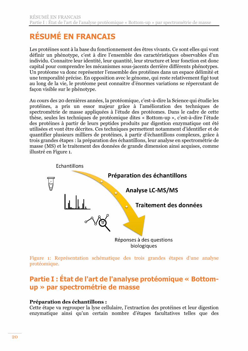
RÉSUMÉ EN FRANCAIS Les protéines sont à la base du fonctionnement des êtres vivants. Ce sont elles qui vont définir un phénotype, c’est à dire l’ensemble des caractéristiques observables d’un individu. Connaitre leur identité, leur quantité, leur structure et leur fonction est donc capital pour comprendre les mécanismes sous-jacents derrière différents phénotypes. Un protéome va donc représenter l’ensemble des protéines dans un espace délimité et une temporalité précise. En opposition avec le génome, qui reste relativement figé tout au long de la vie, le protéome peut connaitre d’énormes variations se répercutant de façon visible sur le phénotype. Au cours des 20 dernières années, la protéomique, c’est-à-dire la Science qui étudie les protéines, a pris un essor majeur grâce à l’amélioration des techniques de spectrométrie de masse appliquées à l’étude des protéomes. Dans le cadre de cette thèse, seules les techniques de protéomique dites « Bottom-up », c’est-à-dire l’étude des protéines à partir de leurs peptides produits par digestion enzymatique ont été utilisées et vont être décrites. Ces techniques permettent notamment d’identifier et de quantifier plusieurs milliers de protéines, à partir d’échantillons complexes, grâce à trois grandes étapes : la préparation des échantillons, leur analyse en spectrométrie de masse (MS) et le traitement des données de grande dimension ainsi acquises, comme illustré en Figure 1.
Figure 1: Représentation schématique des trois grandes étapes d’une analyse protéomique.
Partie I : État de l'art de l'analyse protéomique « Bottom-up » par spectrométrie de masse
Préparation des échantillons : Cette étape va regrouper la lyse cellulaire, l’extraction des protéines et leur digestion enzymatique ainsi qu’un certain nombre d’étapes facultatives telles que des
RÉSUMÉ EN FRANCAIS Partie I : État de l'art de l'analyse protéomique « Bottom-up » par spectrométrie de masse
21
enrichissements pour étudier certaines modifications post-traductionnelles (PTMs), du fractionnement pour augmenter la couverture d’un protéome ou encore du marquage isotopique dans le but de quantifier plus précisément des protéines. Un grand nombre de protocoles de digestion sont apparus depuis 2014. On peut désormais les classifier en quatre catégories : les digestions en solution, les digestions en gel d’acrylamide, les digestions sur filtre et les digestions sur billes, chacune de ces méthodologies possédant ses propres forces et faiblesses.
→ La digestion liquide est rapide mais elle est limitée à des tampons de lyse et d’extraction directement compatibles avec le maintien de l’activité enzymatique et avec l’analyse en MS. Or, ces tampons ne sont pas les plus efficaces. Elle peut être facilement automatisée.
→ La digestion en gel est longue mais elle permet d’utiliser des détergents
normalement non compatibles avec l’analyse en MS, afin d’aider aux étapes de lyse et d’extraction des protéines, notamment des protéines difficiles telles que les protéines membranaires. Certains de ces protocoles peuvent également permettre de fractionner les échantillons mais ils sont difficilement automatisables du fait des risques de perdre des morceaux de gel collant aux cônes.
→ La digestion sur filtre tend à être beaucoup plus rapide notamment avec
l’arrivé de kits commerciaux permettant de réduire l’étape de digestion à quelques heures par rapport à une nuit pour les protocoles plus anciens. Ils sont également compatibles avec de nombreux détergents. Ces protocoles ont également l’avantage d’être automatisables et sont déjà automatisés sur un certain nombre de plateformes de préparation d’échantillons.
→ La digestion sur billes regroupe les mêmes avantages que les digestions sur
filtre avec une efficacité plus élevée sur les petites quantités de matériel et un coût moindre. Des protocoles automatisés ont d’ores et déjà été publiés1,2.
Il est à noter que toutes les étapes de préparation d’échantillon tendent à s’automatiser et pas uniquement l’étape de digestion. Cela a pour but d’être en mesure d’analyser plus rapidement des cohortes d’échantillons variés, de grande taille avec une meilleure répétabilité permettant d’aborder de nouvelles problématiques tout en améliorant la finesse et la robustesse des analyses. Analyse LC-MS/MS : La seconde étape du processus analytique consiste en l’analyse des peptides sur un couplage composé d’une chromatographie liquide et d’un spectromètre de masse (LC-MS). Les peptides issus de la digestion d’un échantillon sont retenus sur la phase stationnaire puis ils sont élués séquentiellement en fonction de leur degré d’hydrophobicité grâce à un gradient croissant de solvant organique. Cela permet de réduire la diversité et la quantité de peptides arrivant en même temps dans la source du spectromètre de masse, dans le but de limiter la compétition à l’ionisation, de réduire la gamme dynamique et ainsi d’augmenter la profondeur d’analyse de l’échantillon pour augmenter la couverture du protéome.
RÉSUMÉ EN FRANCAIS Partie I : État de l'art de l'analyse protéomique « Bottom-up » par spectrométrie de masse
22
Les peptides sont ensuite analysés dans le spectromètre de masse. Il existe trois grands types d’approches :
→ L’approche globale qui est la plus simple et rapide à mettre en œuvre avec des acquisitions en mode « data dependent acquisition » (DDA). Elle permet d’analyser un grand nombre de peptides, de les séquencer individuellement et séquentiellement en fonction de leur abondance, mais souffre d’un manque de reproductibilité lié à la stochasticité de l’acquisition des données. La quantification est réalisée à partir de l’extraction des signaux MS.
→ Les approches ciblées, comme la « Selective Reaction Monitoring » (SRM)
ou la « Parallel Reaction Monitoring » (PRM), sont très lourdes à mettre en œuvre car il s’agit de prédéterminer les peptides signatures les plus pertinents à cibler et d’optimiser l’ensemble des paramètres chromatographiques et d’acquisition MS pour leur détection optimale. Une fois la méthode d’acquisition optimisée, ces méthodes permettent de quantifier très précisément, voire de manière absolue, un nombre limité de peptides grâce à des signaux MS/MS.
→ Finalement, le mode d’acquisition « Data Independent Acquisition » (DIA)
a été introduit plus récemment et promet de combiner le meilleur des deux mondes en permettant de quantifier de façon très précise un grand nombre de protéines grâce aux signaux MS/MS. La mise en œuvre de ces méthodes est d’un niveau de difficulté inférieur aux approches ciblées mais reste pour le moment supérieur à celle des approches globales classiques en DDA, en particulier du fait d’une étape de traitement des données particulièrement complexe et d’outils bio-informatiques dédiés encore en plein développement.
Traitement des données : Le traitement des données s’est encore complexifié ces dernières années, et cela pour toutes les approches, avec l’apparition de nouveaux spectromètres de masse incluant une dimension de séparation supplémentaire avec la séparation des ions en phase gazeuse grâce la spectrométrie de mobilité des ions (IMS). L’association de l’IMS et de la MS n’est pas nouvelle, c’est son application à l’analyse de protéines par des approches « Bottom-up » qui l’est. L’IMS permet de séparer les ions en fonction de leur charge et de leur forme. Elle permet potentiellement de pouvoir accéder à une nouvelle dimension de données grâce aux valeurs de mobilités ioniques normalisées sous forme de « Collision-cross section » (CCS). L’ajout de cette nouvelle dimension de données ouvre de nouvelles portes à la protéomique « Bottom-up » avec par exemple le développement de nouveaux modes d’acquisitions complémentant les approches classiques tels que le PASEF avec ses différentes déclinaisons : ddaPASEF, diaPASEF et prmPASEF. Cela dit, cette nouvelle dimension et le format de données que génèrent ces nouvelles approches complexifient les étapes de traitement de données. Celle-ci vont nécessiter de nombreux développements d’algorithmes et logiciels dans les années à venir afin de tirer le maximum d’informations utiles de ces nouvelles données. Au-delà de l’IMS, le traitement des données reste extrêmement différent selon le type d’acquisitions utilisé et donc le type de données générées utilisant différentes approches et logiciels. Pour des données de DDA, l’identification des peptides dont découle l’identification des protéines, se base sur l’utilisation de moteurs de recherche
RÉSUMÉ EN FRANCAIS Partie I : État de l'art de l'analyse protéomique « Bottom-up » par spectrométrie de masse
23
et de banques de données qui doivent être de qualité et adaptées à la problématique biologique. La banque de séquences protéiques est digérée in silico pour simuler les conditions expérimentales. Les peptides sont identifiés par comparaison des masses théoriques, calculées, à partir de la banque digérée in silico et des données expérimentales obtenues lors de l’analyse de l’échantillon en spectrométrie de masse. Les protéines sont retrouvées par inférence à partir des peptides précédemment identifiés. Les résultats sont validés grâce à des procédés statistiques permettant de limiter le nombre de faux-positifs grâce à l’approche cible-leurre. La quantification sur ce type de données peut être réalisée par différentes approches telles que le comptage de spectres ou l’extraction de courants d’ions. Tandis que pour les données de type DIA, deux approches principales sont utilisées, l’approche peptides-centrée et l’approche spectres-centrée. L'approche centrée sur les peptides utilise des bibliothèques spectrales, préalablement générées, pour effectuer la correspondance spectre-peptide. L’approche centrée sur les spectres ne nécessite pas de générer une librairie spectrale. Elle utilise directement les spectres MS2 multiplexés que des algorithmes vont déconvoluer pour générer des pseudo-spectres MS2. Ces derniers seront soumis à une recherche classique via l'interrogation d'une banque de données digérée in silico. La spécificité du sujet de cette thèse repose sur le fait qu’elle vise à repousser les limites de la protéomique actuelle pour laquelle l’un des grands facteurs limitants reste la quantité d’échantillon accessible. Ce défi doit être levé dans un contexte où la protéomique prétend pouvoir analyser le contenu protéique de cellules uniques, au même titre que la transcriptomique qui comme les autres techniques basées sur les acides nucléiques bénéficie de stratégies d’amplification, en opposition avec les approches basées sur les acides aminés. En parallèle, la quête d’accroitre la couverture du protéome détectable est toujours omniprésente, de même que la mise au point d’approches algorithmiques sophistiquées qui permettront d’extraire un maximum d’informations utiles des données acquises. Dans ce contexte, ces travaux de thèse se sont articulés autour de quatre axes :
→ L’évaluation de protocoles de préparation d’échantillons compatibles avec le sodium dodecyl sulfate (SDS) afin de permettre une extraction efficace des protéines et ainsi être à même de les analyser de façon robuste, rapide, à haut-débit via une automatisation et ceci sur de faibles quantités de matériel de départ.
→ L’implémentation et le développement de nouvelles stratégies de quantification
sans marquage sur un couplage de dernière génération (un nouveau Quadrupole-Temps de Vol (Q-TOF), TimsTOF Pro de Bruker) intégrant une étape de séparation supplémentaire par mobilité ionique (nLC-IMS-MS/MS) opéré en modes d’acquisition ddaPASEF et diaPASEF.
→ L’évaluation et l’optimisation d’outils bio-informatiques pour traiter les données en 4 dimensions (4D) générées grâce à ce nouveau couplage innovant dans le but d’identifier et de quantifier les protéines.
→ Finalement, certains développements analytiques réalisés durant cette thèse ont pu être appliqués pour la résolution de questionnements soulevés par des collaborateurs biologistes.
RÉSUMÉ EN FRANCAIS Partie II : Evaluation et optimisation des étapes de préparation des échantillons pour l'analyse protéomique « Bottom-up » à haut débit sur de petites quantités de matériel
24
Partie II : Evaluation et optimisation des étapes de préparation des échantillons pour l'analyse protéomique « Bottom-up » à haut débit sur de petites quantités de matériel
Un des principaux objectifs de cette thèse a été de développer, d’évaluer et d’optimiser différentes stratégies de préparation d’échantillons, récemment introduites et innovantes, telles que les approches de digestion en gel (tube-gel en volume réduit3,4), de digestion sur filtre (S-Trap5, Protifi) ou sur billes magnétiques (SP36, Single-Pot, Solid-Phase-enhanced Sample Preparation) avec des quantités de matériel allant de 500ng à 50µg selon les approches. Ces différentes stratégies ont été sélectionnées car elles présentent l’avantage de rendre la digestion compatible avec des détergents et chaotropes reconnus pour leur efficacité lors de la lyse cellulaire et l’extraction des protéines tels que le SDS. Ces détergents jouent un rôle majeur pour accéder à des protéines difficiles telles que les protéines membranaires, qui, de par leur localisation jouent souvent un rôle prépondérant dans les mécanismes biologiques. Le gel de concentration (ou gel stacking) a longtemps été la méthode de référence en matière de préparation d’échantillon pour les analyses protéomiques « Bottom-up ». Malheureusement, sa mise en œuvre étant longue et fastidieuse (3-4 jours), notre laboratoire s’est intéressé dès 2016 à de nouveaux protocoles de préparation en gel, notamment dans le cadre de la thèse du Dr Leslie Muller, qui a abouti au développement de l’approche tube-gel4,7. Au cours de ces travaux de thèse, une version miniaturisée du tube-gel a été développée. L’objectif était de réduire le volume de travail afin de limiter la surface de contact entre l’échantillon et les parois du tube, dans le but de diminuer la perte de protéines par adsorption et ainsi améliorer les performances de ce protocole sur des quantités d’échantillons réduites. Une comparaison, a été réalisée sur une gammes de quantités de protéines obtenues à partir d’un lysat total de levure allant de 1 à 50µg préparés en gel stacking, en tube-gel standard et en tube-gel à volume réduit (Figure 2).
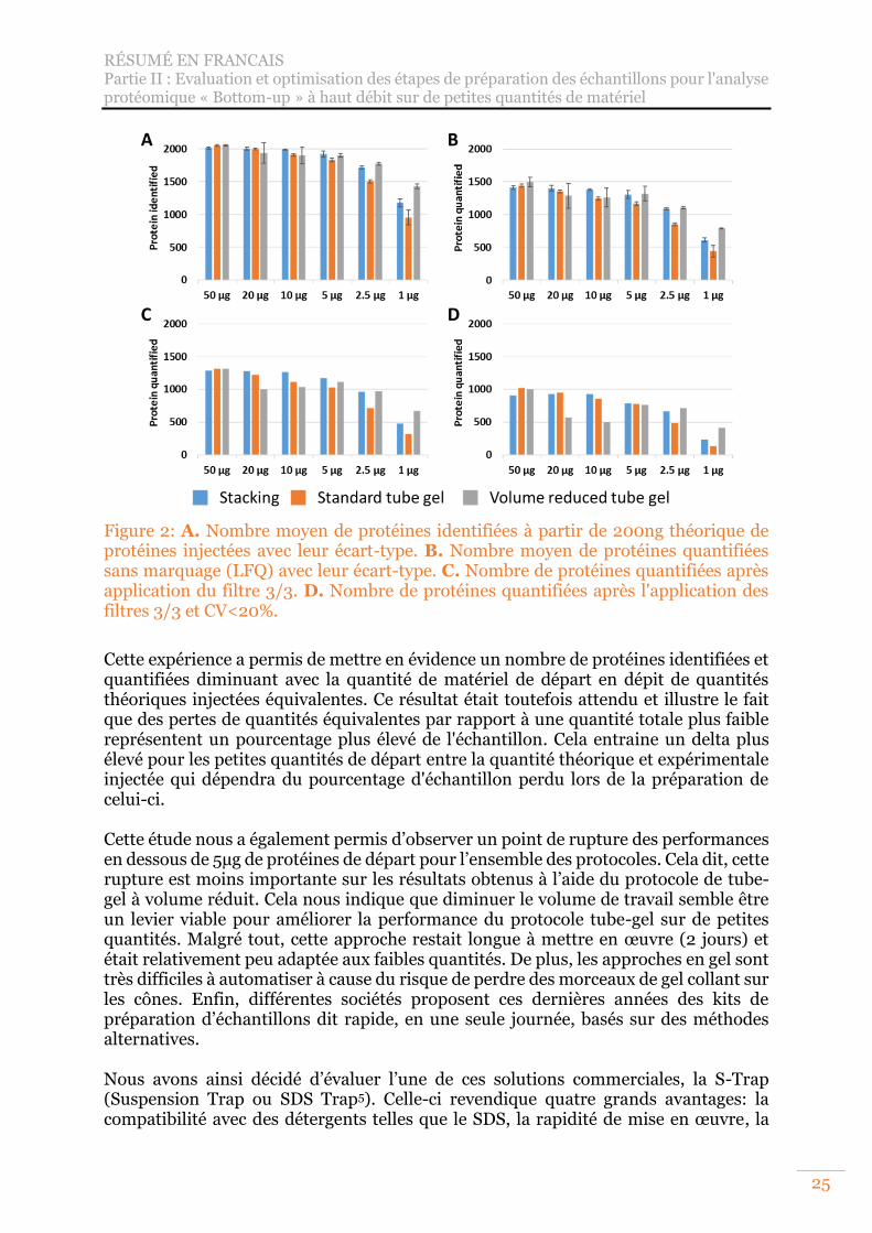
RÉSUMÉ EN FRANCAIS Partie II : Evaluation et optimisation des étapes de préparation des échantillons pour l'analyse protéomique « Bottom-up » à haut débit sur de petites quantités de matériel
25
Figure 2: A. Nombre moyen de protéines identifiées à partir de 200ng théorique de protéines injectées avec leur écart-type. B. Nombre moyen de protéines quantifiées sans marquage (LFQ) avec leur écart-type. C. Nombre de protéines quantifiées après application du filtre 3/3. D. Nombre de protéines quantifiées après l'application des filtres 3/3 et CV<20%.
Cette expérience a permis de mettre en évidence un nombre de protéines identifiées et quantifiées diminuant avec la quantité de matériel de départ en dépit de quantités théoriques injectées équivalentes. Ce résultat était toutefois attendu et illustre le fait que des pertes de quantités équivalentes par rapport à une quantité totale plus faible représentent un pourcentage plus élevé de l'échantillon. Cela entraine un delta plus élevé pour les petites quantités de départ entre la quantité théorique et expérimentale injectée qui dépendra du pourcentage d'échantillon perdu lors de la préparation de celui-ci. Cette étude nous a également permis d’observer un point de rupture des performances en dessous de 5µg de protéines de départ pour l’ensemble des protocoles. Cela dit, cette rupture est moins importante sur les résultats obtenus à l’aide du protocole de tube-gel à volume réduit. Cela nous indique que diminuer le volume de travail semble être un levier viable pour améliorer la performance du protocole tube-gel sur de petites quantités. Malgré tout, cette approche restait longue à mettre en œuvre (2 jours) et était relativement peu adaptée aux faibles quantités. De plus, les approches en gel sont très difficiles à automatiser à cause du risque de perdre des morceaux de gel collant sur les cônes. Enfin, différentes sociétés proposent ces dernières années des kits de préparation d’échantillons dit rapide, en une seule journée, basés sur des méthodes alternatives. Nous avons ainsi décidé d’évaluer l’une de ces solutions commerciales, la S-Trap (Suspension Trap ou SDS Trap5). Celle-ci revendique quatre grands avantages: la compatibilité avec des détergents telles que le SDS, la rapidité de mise en œuvre, la
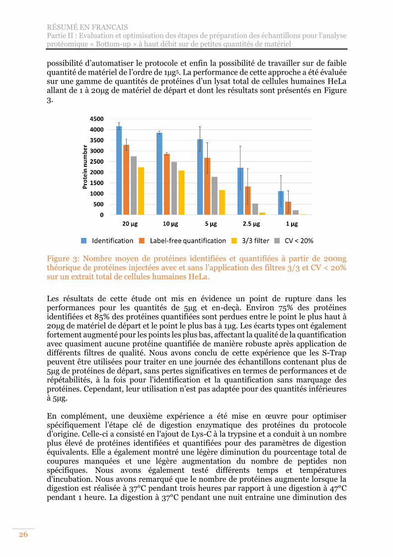
RÉSUMÉ EN FRANCAIS Partie II : Evaluation et optimisation des étapes de préparation des échantillons pour l'analyse protéomique « Bottom-up » à haut débit sur de petites quantités de matériel
26
possibilité d’automatiser le protocole et enfin la possibilité de travailler sur de faible quantité de matériel de l’ordre de 1µg5. La performance de cette approche a été évaluée sur une gamme de quantités de protéines d’un lysat total de cellules humaines HeLa allant de 1 à 20µg de matériel de départ et dont les résultats sont présentés en Figure 3.
Figure 3: Nombre moyen de protéines identifiées et quantifiées à partir de 200ng théorique de protéines injectées avec et sans l'application des filtres 3/3 et CV < 20% sur un extrait total de cellules humaines HeLa.
Les résultats de cette étude ont mis en évidence un point de rupture dans les performances pour les quantités de 5µg et en-deçà. Environ 75% des protéines identifiées et 85% des protéines quantifiées sont perdues entre le point le plus haut à 20µg de matériel de départ et le point le plus bas à 1µg. Les écarts types ont également fortement augmenté pour les points les plus bas, affectant la qualité de la quantification avec quasiment aucune protéine quantifiée de manière robuste après application de différents filtres de qualité. Nous avons conclu de cette expérience que les S-Trap peuvent être utilisées pour traiter en une journée des échantillons contenant plus de 5µg de protéines de départ, sans pertes significatives en termes de performances et de répétabilités, à la fois pour l'identification et la quantification sans marquage des protéines. Cependant, leur utilisation n’est pas adaptée pour des quantités inférieures à 5µg. En complément, une deuxième expérience a été mise en œuvre pour optimiser spécifiquement l’étape clé de digestion enzymatique des protéines du protocole d’origine. Celle-ci a consisté en l'ajout de Lys-C à la trypsine et a conduit à un nombre plus élevé de protéines identifiées et quantifiées pour des paramètres de digestion équivalents. Elle a également montré une légère diminution du pourcentage total de coupures manquées et une légère augmentation du nombre de peptides non spécifiques. Nous avons également testé différents temps et températures d'incubation. Nous avons remarqué que le nombre de protéines augmente lorsque la digestion est réalisée à 37°C pendant trois heures par rapport à une digestion à 47°C pendant 1 heure. La digestion à 37°C pendant une nuit entraine une diminution des
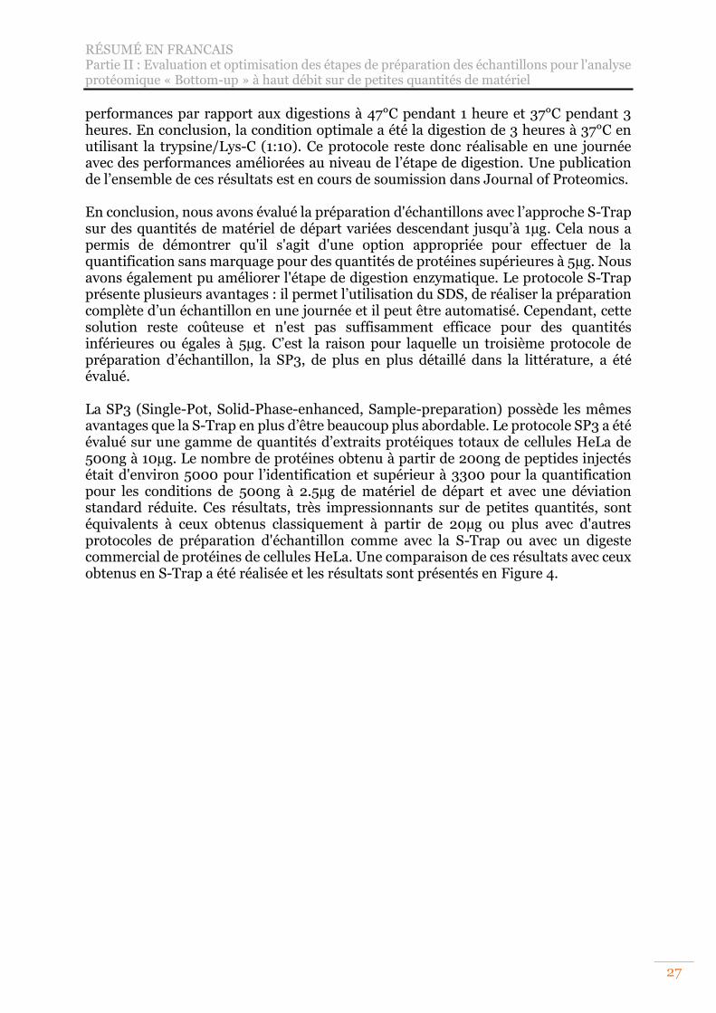
RÉSUMÉ EN FRANCAIS Partie II : Evaluation et optimisation des étapes de préparation des échantillons pour l'analyse protéomique « Bottom-up » à haut débit sur de petites quantités de matériel
27
performances par rapport aux digestions à 47°C pendant 1 heure et 37°C pendant 3 heures. En conclusion, la condition optimale a été la digestion de 3 heures à 37°C en utilisant la trypsine/Lys-C (1:10). Ce protocole reste donc réalisable en une journée avec des performances améliorées au niveau de l’étape de digestion. Une publication de l’ensemble de ces résultats est en cours de soumission dans Journal of Proteomics. En conclusion, nous avons évalué la préparation d'échantillons avec l’approche S-Trap sur des quantités de matériel de départ variées descendant jusqu’à 1µg. Cela nous a permis de démontrer qu'il s'agit d'une option appropriée pour effectuer de la quantification sans marquage pour des quantités de protéines supérieures à 5µg. Nous avons également pu améliorer l'étape de digestion enzymatique. Le protocole S-Trap présente plusieurs avantages : il permet l’utilisation du SDS, de réaliser la préparation complète d’un échantillon en une journée et il peut être automatisé. Cependant, cette solution reste coûteuse et n'est pas suffisamment efficace pour des quantités inférieures ou égales à 5µg. C’est la raison pour laquelle un troisième protocole de préparation d’échantillon, la SP3, de plus en plus détaillé dans la littérature, a été évalué. La SP3 (Single-Pot, Solid-Phase-enhanced, Sample-preparation) possède les mêmes avantages que la S-Trap en plus d’être beaucoup plus abordable. Le protocole SP3 a été évalué sur une gamme de quantités d’extraits protéiques totaux de cellules HeLa de 500ng à 10µg. Le nombre de protéines obtenu à partir de 200ng de peptides injectés était d'environ 5000 pour l’identification et supérieur à 3300 pour la quantification pour les conditions de 500ng à 2.5µg de matériel de départ et avec une déviation standard réduite. Ces résultats, très impressionnants sur de petites quantités, sont équivalents à ceux obtenus classiquement à partir de 20µg ou plus avec d'autres protocoles de préparation d'échantillon comme avec la S-Trap ou avec un digeste commercial de protéines de cellules HeLa. Une comparaison de ces résultats avec ceux obtenus en S-Trap a été réalisée et les résultats sont présentés en Figure 4.
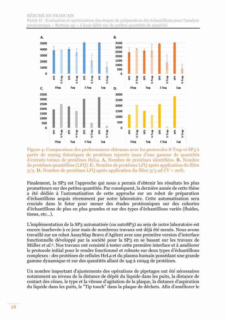
RÉSUMÉ EN FRANCAIS Partie II : Evaluation et optimisation des étapes de préparation des échantillons pour l'analyse protéomique « Bottom-up » à haut débit sur de petites quantités de matériel
28
Figure 4: Comparaison des performances obtenues avec les protocoles S-Trap et SP3 à partir de 200ng théoriques de protéines injectés issus d’une gamme de quantités d’extraits totaux de protéines HeLa. A. Nombre de protéines identifiées. B. Nombre de protéines quantifiées (LFQ). C. Nombre de protéines LFQ après application du filtre 3/3. D. Nombre de protéines LFQ après application du filtre 3/3 ad CV < 20%.
Finalement, la SP3 est l’approche qui nous a permis d’obtenir les résultats les plus prometteurs sur des petites quantités. Par conséquent, la dernière année de cette thèse a été dédiée à l’automatisation de cette approche sur un robot de préparation d’échantillons acquis récemment par notre laboratoire. Cette automatisation sera cruciale dans le futur pour mener des études protéomiques sur des cohortes d’échantillons de plus en plus grandes et sur des types d’échantillons variés (fluides, tissus, etc…). L’implémentation de la SP3 automatisée (ou autoSP3) au sein de notre laboratoire est encore inachevée à ce jour mais de nombreux travaux ont déjà été menés. Nous avons travaillé sur un robot AssayMap Bravo d’Agilent avec une première version d’interface fonctionnelle développé par la société pour la SP3 en se basant sur les travaux de Müller et al.2. Nos travaux ont consisté à tester cette première interface et à améliorer le protocole initial pour le rendre fonctionnel et robuste sur deux types d’échantillons complexes : des protéines de cellules HeLa et du plasma humain possédant une grande gamme dynamique et sur des quantités allant de 1µg à 100µg de protéines. Un nombre important d'ajustements des opérations de pipetages ont été nécessaires notamment au niveau de la distance de dépôt du liquide dans les puits, la distance de contact des cônes, le type et la vitesse d'agitation de la plaque, la distance d'aspiration du liquide dans les puits, le "Tip touch" dans la plaque de déchets. Afin d’améliorer le
RÉSUMÉ EN FRANCAIS Partie II : Evaluation et optimisation des étapes de préparation des échantillons pour l'analyse protéomique « Bottom-up » à haut débit sur de petites quantités de matériel
29
protocole, l’étape d’incubation de la digestion a été implémentée directement sur le robot, ce qui n’était pas le cas dans le protocole autoSP3 publié où la plaque était sortie manuellement et incubé ailleurs. Pour améliorer la conduction et l'homogénéité de la température pendant cette étape, un support de plaque spécial a été ajouté à la station de chauffage. Pour évaluer l’ensemble de ces modifications, des tests ont été menés sur des gammes de quantités de protéines de cellules HeLa et de plasma humain croissantes. De nombreux réplicas d’expériences et techniques (jusqu’à 12 réplicas par condition tel que présenté en Figure 5) ont été réalisés avec l’objectif de tester la robustesse et la répétabilité du protocole.
Figure 5: En jaune, nombres de protéines identifiées à partir de 200ng théorique de protéines injectés obtenus à partir d’une gamme de quantités d’extraits protéiques totaux de cellules HeLa (n=12). En rouge, le nombre moyen de protéines identifiées.
Ces tests ont ainsi pu soulever des problèmes de reproductibilité du protocole mais ont également permis d’apporter des pistes d’améliorations. Parmi les points testés, on peut citer l’ajout d’une étape de SPE à la fin du protocole de SP3 qui a malheureusement créé plus de problèmes qu’elle n’en a résolus. Un premier test a également été réalisé pour évaluer la possibilité de supprimer l’étape d’évaporation et de suspension des peptides avant l’injection en MS avec de premiers résultats
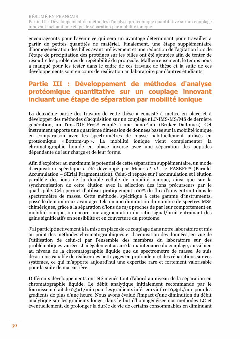
RÉSUMÉ EN FRANCAIS Partie III : Développement de méthodes d'analyse protéomique quantitative sur un couplage innovant incluant une étape de séparation par mobilité ionique
30
encourageants pour l’avenir ce qui sera un avantage déterminant pour travailler à partir de petites quantités de matériel. Finalement, une étape supplémentaire d’homogénéisation des billes avant prélèvement et une réduction de l’agitation lors de l’étape de précipitation des protéines sur les billes ont été ajoutées afin de tenter de résoudre les problèmes de répétabilité du protocole. Malheureusement, le temps nous a manqué pour les tester dans le cadre de ces travaux de thèse et la suite de ces développements sont en cours de réalisation au laboratoire par d’autres étudiants.
Partie III : Développement de méthodes d'analyse protéomique quantitative sur un couplage innovant incluant une étape de séparation par mobilité ionique
La deuxième partie des travaux de cette thèse a consisté à mettre en place et à développer des méthodes d’acquisition sur un couplage nLC-IMS-MS/MS de dernière génération, un TimsTOF Pro8,9 couplé à une nanoElute (Bruker Daltonics). Cet instrument apporte une quatrième dimension de données basée sur la mobilité ionique en comparaison avec les spectromètres de masse habituellement utilisés en protéomique « Bottom-up ». La mobilité ionique vient complémenter la chromatographie liquide en phase inverse avec une séparation des peptides dépendante de leur charge et de leur forme. Afin d’exploiter au maximum le potentiel de cette séparation supplémentaire, un mode d’acquisition spécifique a été développé par Meier et al., le PASEF9,10 (Parallel Accumulation – SErial Fragmentation). Celui-ci repose sur l’accumulation et l’élution parallèle des ions de la double cellule de mobilité ionique, ainsi que sur la synchronisation de cette élution avec la sélection des ions précurseurs par le quadripôle. Cela permet d’utiliser pratiquement 100% du flux d’ions entrant dans le spectromètre de masse. Cette méthode, spécifique à cette gamme d’instruments, possède de nombreux avantages tels qu’une diminution du nombre de spectres MS2 chimériques, grâce à la séparation d’ions de m/z proches de par leur comportement en mobilité ionique, ou encore une augmentation du ratio signal/bruit entrainant des gains significatifs en sensibilité et en couverture du protéome. J’ai participé activement à la mise en place de ce couplage dans notre laboratoire et mis au point des méthodes chromatographiques et d’acquisition des données, en vue de l’utilisation de celui-ci par l'ensemble des membres du laboratoire sur des problématiques variées. J’ai également assuré la maintenance du couplage, aussi bien au niveau de la chromatographie liquide que du spectromètre de masse. Je suis désormais capable de réaliser des nettoyages en profondeur et des réparations sur ces systèmes, ce qui m’apporte aujourd’hui une expertise rare et fortement valorisable pour la suite de ma carrière. Différents développements ont été menés tout d’abord au niveau de la séparation en chromatographie liquide. Le débit analytique initialement recommandé par le fournisseur était de 0,3µL/min pour les gradients inférieurs à 1h et 0,4µL/min pour les gradients de plus d’une heure. Nous avons évalué l’impact d’une diminution du débit analytique sur les gradients longs, dans le but d’homogénéiser nos méthodes LC et éventuellement, de prolonger la durée de vie de certains consommables en diminuant
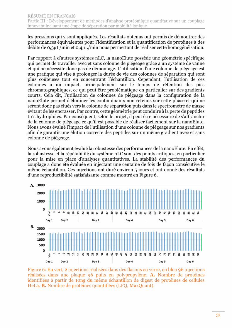
RÉSUMÉ EN FRANCAIS Partie III : Développement de méthodes d'analyse protéomique quantitative sur un couplage innovant incluant une étape de séparation par mobilité ionique
31
les pressions qui y sont appliqués. Les résultats obtenus ont permis de démontrer des performances équivalentes pour l’identification et la quantification de protéines à des débits de 0,3µL/min et 0,4µL/min nous permettant de réaliser cette homogénéisation. Par rapport à d’autres systèmes nLC, la nanoElute possède une géométrie spécifique qui permet de travailler avec et sans colonne de piégeage grâce à un système de vanne et qui ne nécessite donc pas de démontage. L'utilisation d'une colonne de piégeage est une pratique qui vise à prolonger la durée de vie des colonnes de séparation qui sont plus coûteuses tout en concentrant l’échantillon. Cependant, l'utilisation de ces colonnes a un impact, principalement sur le temps de rétention des pics chromatographiques, ce qui peut être problématique en particulier sur des gradients courts. Cela dit, l'utilisation de colonnes de piégeage dans la configuration de la nanoElute permet d’éliminer les contaminants non retenus sur cette phase et qui ne seront donc pas élués vers la colonne de séparation puis dans le spectromètre de masse évitant de les encrasser. Par contre, cette géométrie peut conduire à la perte de peptides très hydrophiles. Par conséquent, selon le projet, il peut être nécessaire de s’affranchir de la colonne de piégeage ce qu’il est possible de réaliser facilement sur la nanoElute. Nous avons évalué l’impact de l’utilisation d’une colonne de piégeage sur nos gradients afin de garantir une élution correcte des peptides sur un même gradient avec et sans colonne de piégeage. Nous avons également évalué la robustesse des performances de la nanoElute. En effet, la robustesse et la répétabilité du système nLC sont des points critiques, en particulier pour la mise en place d’analyses quantitatives. La stabilité des performances du couplage a donc été évaluée en injectant une centaine de fois de façon consécutive le même échantillon. Ces injections ont duré environ 5 jours et ont donné des résultats d’une reproductibilité satisfaisante comme montré en Figure 6.
Figure 6: En vert, 2 injections réalisées dans des flacons en verre, en bleu 96 injections réalisées dans une plaque 96 puits en polypropylène. A. Nombre de protéines identifiées à partir de 10ng du même échantillon de digest de protéines de cellules HeLa. B. Nombre de protéines quantifiées (LFQ, MaxQuant).
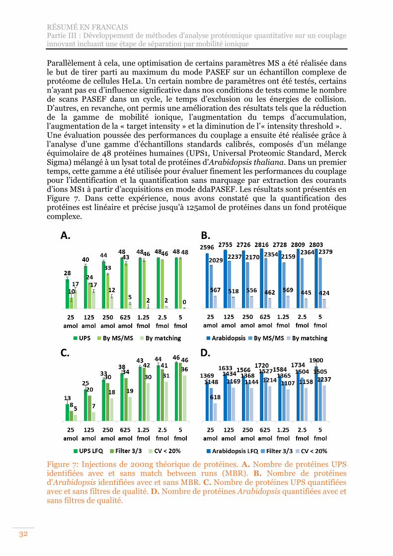
RÉSUMÉ EN FRANCAIS Partie III : Développement de méthodes d'analyse protéomique quantitative sur un couplage innovant incluant une étape de séparation par mobilité ionique
32
Parallèlement à cela, une optimisation de certains paramètres MS a été réalisée dans le but de tirer parti au maximum du mode PASEF sur un échantillon complexe de protéome de cellules HeLa. Un certain nombre de paramètres ont été testés, certains n’ayant pas eu d’influence significative dans nos conditions de tests comme le nombre de scans PASEF dans un cycle, le temps d’exclusion ou les énergies de collision. D’autres, en revanche, ont permis une amélioration des résultats tels que la réduction de la gamme de mobilité ionique, l’augmentation du temps d’accumulation, l’augmentation de la « target intensity » et la diminution de l’« intensity threshold ». Une évaluation poussée des performances du couplage a ensuite été réalisée grâce à l’analyse d’une gamme d’échantillons standards calibrés, composés d’un mélange équimolaire de 48 protéines humaines (UPS1, Universal Proteomic Standard, Merck Sigma) mélangé à un lysat total de protéines d’Arabidopsis thaliana. Dans un premier temps, cette gamme a été utilisée pour évaluer finement les performances du couplage pour l’identification et la quantification sans marquage par extraction des courants d’ions MS1 à partir d’acquisitions en mode ddaPASEF. Les résultats sont présentés en Figure 7. Dans cette expérience, nous avons constaté que la quantification des protéines est linéaire et précise jusqu'à 125amol de protéines dans un fond protéique complexe.
Figure 7: Injections de 200ng théorique de protéines. A. Nombre de protéines UPS identifiées avec et sans match between runs (MBR). B. Nombre de protéines d'Arabidopsis identifiées avec et sans MBR. C. Nombre de protéines UPS quantifiées avec et sans filtres de qualité. D. Nombre de protéines Arabidopsis quantifiées avec et sans filtres de qualité.
RÉSUMÉ EN FRANCAIS Partie III : Développement de méthodes d'analyse protéomique quantitative sur un couplage innovant incluant une étape de séparation par mobilité ionique
33
Nous avons également réalisé des tests sur la fonction d’ICC (Ion Charge Control). Celle-ci permet de contrôler le nombre d’ions entrant dans la cellule de mobilité afin d’éviter les effets d’espace-charge liés à la répulsion des charges de même polarité confinés dans un espace restreint. Nous avons tout d’abord réalisé des tests préliminaires pour déterminer les valeurs optimales d’ICC sur des injections de 10ng et 200ng de HeLa. Une fois ces valeurs obtenues nous avons réinjecté notre gamme UPS1/Arabidopsis afin d’évaluer l’impact de la fonction d’ICC optimisée sur notre quantification. L’utilisation de ce paramètre n’a pas entrainé de changements significatifs au niveau des résultats dans notre configuration comme illustré en Figure 8. Cependant, son intérêt pourrait être plus intéressant sur d’autres types d’échantillons possédant une plus grande gamme dynamique, en injectant davantage de matériel ou avec d’autres modes d’acquisition comme le diaPASEF.
Figure 8: Courbe de calibration des ratios théoriques et expérimentaux de la gamme UPS1 obtenus à partir de 200ng théorique de protéines injectés A. sans ICC actif B. avec ICC réglé à 130 millions d'ions.
Le mode d’acquisition diaPASEF a lui aussi été évalué sur la même gamme UPS1/Arabidopsis. Lors d'une acquisition diaPASEF, les ions entrent dans le spectromètre de masse et sont accumulés dans la première partie de la cellule de mobilité ionique. Ensuite, ils sont séparés et élués séquentiellement dans la seconde. Comme pour le ddaPASEF, l'accumulation et la séparation/élution des ions se font simultanément afin qu'aucun ion ne soit perdu. Lors de la séparation des ions en fonction de leur mobilité ionique, ceux dont la mobilité est la plus faible, généralement les ions ayant le plus grand m/z, seront positionnés près de la sortie de la cellule. Ils seront les premiers à éluer. Pour cette raison, la fenêtre d'isolation m/z du quadripôle commencera par sélectionner des valeurs de m/z élevées et glissera vers des valeurs plus faibles en synchronisation avec l'élution des ions de la cellule de mobilité ionique. Les fenêtres d’isolation des méthodes diaPASEF sont définies dans deux dimensions, la mobilité ionique et le m/z. Les énergies de collision appliquées à ces fenêtres vont également glisser des plus hautes vers les plus basses en synchronisation avec la sélection des ions par le quadripôle. Finalement, les ions sont envoyés à l’analyseur TOF pour obtenir leurs informations de m/z et d'intensité. Les résultats obtenus sont présentés en Figure 9. Le mode d’acquisition diaPASEF a permis de quantifier les 48 protéines UPS entre 5 et 1,25fmol. Une diminution du
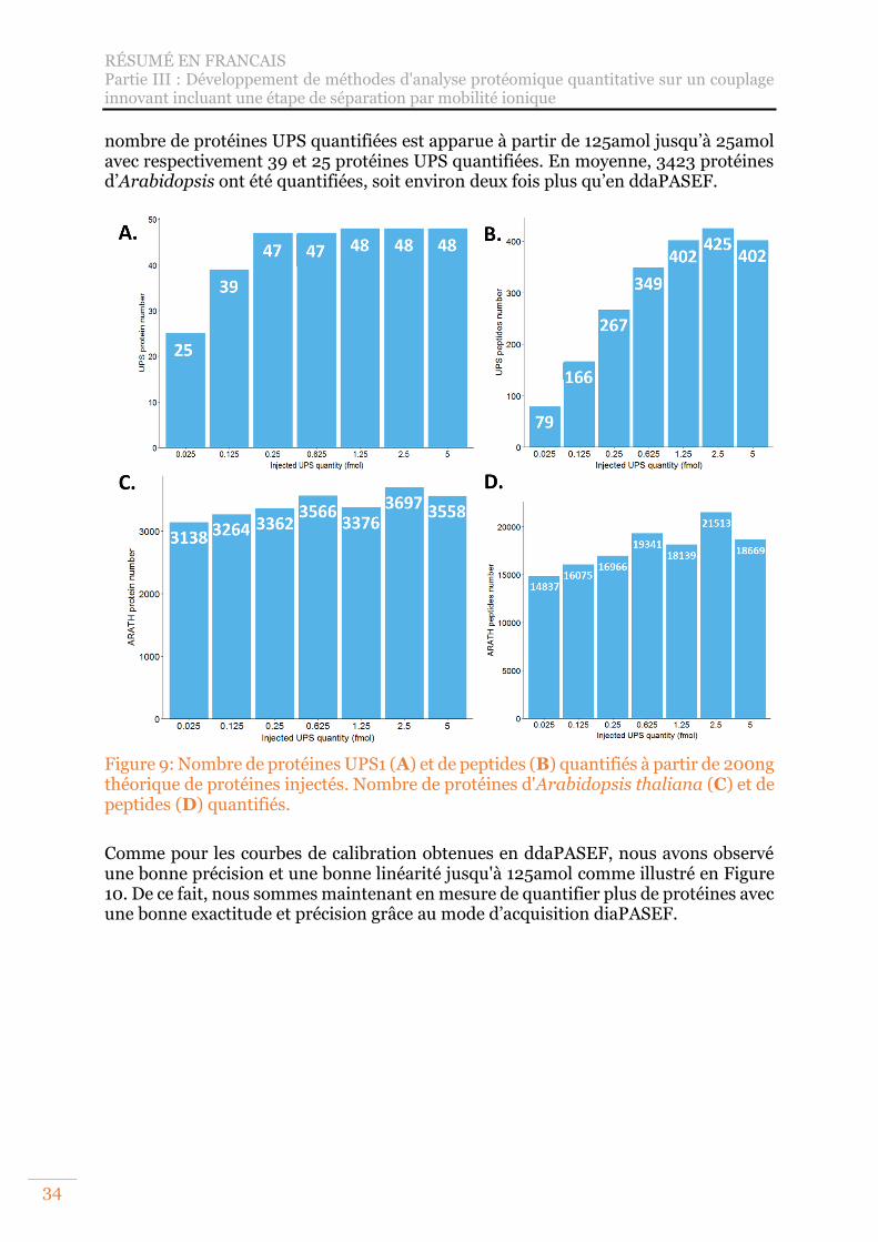
RÉSUMÉ EN FRANCAIS Partie III : Développement de méthodes d'analyse protéomique quantitative sur un couplage innovant incluant une étape de séparation par mobilité ionique
34
nombre de protéines UPS quantifiées est apparue à partir de 125amol jusqu’à 25amol avec respectivement 39 et 25 protéines UPS quantifiées. En moyenne, 3423 protéines d’Arabidopsis ont été quantifiées, soit environ deux fois plus qu’en ddaPASEF.
Figure 9: Nombre de protéines UPS1 (A) et de peptides (B) quantifiés à partir de 200ng théorique de protéines injectés. Nombre de protéines d'Arabidopsis thaliana (C) et de peptides (D) quantifiés.
Comme pour les courbes de calibration obtenues en ddaPASEF, nous avons observé une bonne précision et une bonne linéarité jusqu'à 125amol comme illustré en Figure 10. De ce fait, nous sommes maintenant en mesure de quantifier plus de protéines avec une bonne exactitude et précision grâce au mode d’acquisition diaPASEF.
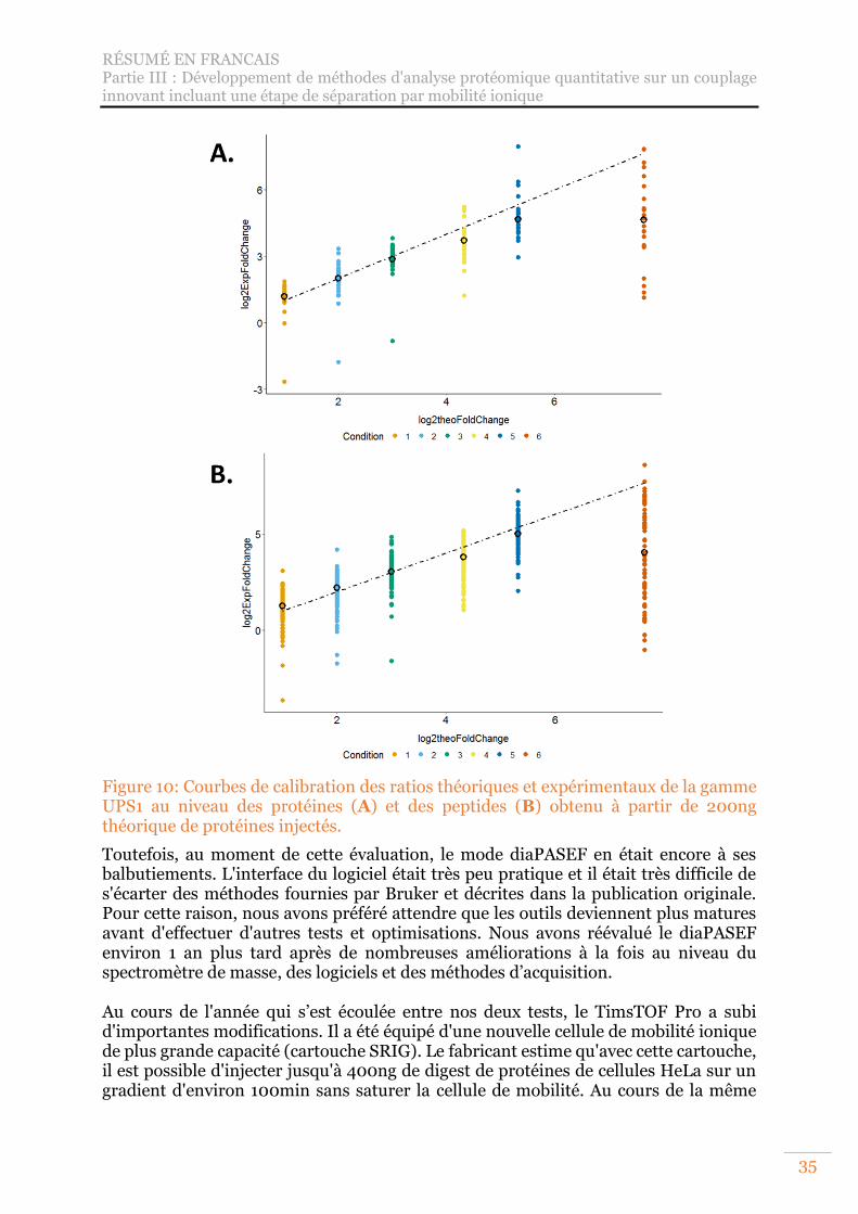
RÉSUMÉ EN FRANCAIS Partie III : Développement de méthodes d'analyse protéomique quantitative sur un couplage innovant incluant une étape de séparation par mobilité ionique
35
Figure 10: Courbes de calibration des ratios théoriques et expérimentaux de la gamme UPS1 au niveau des protéines (A) et des peptides (B) obtenu à partir de 200ng théorique de protéines injectés.
Toutefois, au moment de cette évaluation, le mode diaPASEF en était encore à ses balbutiements. L'interface du logiciel était très peu pratique et il était très difficile de s'écarter des méthodes fournies par Bruker et décrites dans la publication originale. Pour cette raison, nous avons préféré attendre que les outils deviennent plus matures avant d'effectuer d'autres tests et optimisations. Nous avons réévalué le diaPASEF environ 1 an plus tard après de nombreuses améliorations à la fois au niveau du spectromètre de masse, des logiciels et des méthodes d’acquisition. Au cours de l'année qui s’est écoulée entre nos deux tests, le TimsTOF Pro a subi d'importantes modifications. Il a été équipé d'une nouvelle cellule de mobilité ionique de plus grande capacité (cartouche SRIG). Le fabricant estime qu'avec cette cartouche, il est possible d'injecter jusqu'à 400ng de digest de protéines de cellules HeLa sur un gradient d'environ 100min sans saturer la cellule de mobilité. Au cours de la même
RÉSUMÉ EN FRANCAIS Partie IV : Évaluation d’outils bio-informatiques pour le traitement des données issues d’un couplage nLC-IMS-MS/MS
36
période, Bruker a également lancé un nouveau logiciel pour piloter le TimsTOF Pro, appelé TimsControl. Ce logiciel est très récent et même si la création de nouvelles méthodes diaPASEF est grandement facilitée par rapport à OtofControl, certains bogues subsistent. De plus, certaines options telles que le « denoising » des spectres, la génération de méthodes avec des tailles de fenêtres variables ou la génération de schémas de fenêtres d’isolation sur deux « lignes » permettant un recouvrement dans la dimension de la mobilité ionique n’était pas encore accessibles. En conséquence, la méthode diaPASEF que nous avions utilisée précédemment dans OtofControl n'est pas compatible avec TimsControl. De ce fait, nous avons utilisé la méthode standard fournis par Bruker pour la réalisation d’analyses en diaPASEF sur des gradients longs avec la nouvelle cellule de mobilité ionique. Compte tenu de tous ces changements, nous avons décidé de repartir de zéro et de réévaluer complètement le mode diaPASEF. Nous avons utilisé la même gamme que précédemment mais en doublant les quantités injectées pour tirer parti de la plus grande capacité de cette nouvelle cartouche. Le nombre de protéines UPS quantifiées obtenu dans cette configuration est plus faible que lors de notre première expérience pour des quantités équivalentes d’UPS. En moyenne, 3580 protéines d'Arabidopsis ont été quantifiées dans la nouvelle expérience soit un peu plus que les 3423 de la première expérience. Sur la courbe de calibration, la quantification reste linéaire jusqu'à 50amol ce qui est plus bas que sur les courbes de calibrations réalisées précédemment ou la linéarité était perdu en dessous de 125amol. Ces résultats sont cohérents avec les résultats préliminaires que nous avions obtenus en ddaPASEF avec la nouvelle cellule de mobilité en injectant jusqu’à 400ng de protéines. En effet, en DDA comme en DIA, nous n’avons pas observé de gain important suite à l’implémentation de la nouvelle cellule de mobilité ionique et l’augmentation des quantités injectés, contrairement à ce qui était attendu. Nous avons donc émis l’hypothèse que nos méthodes d'acquisition n’étaient pas adaptées à la nouvelle configuration de notre TimsTOF Pro amélioré ou TimsTOF Pro 2-like. Pour cette raison, nous ne sommes pas encore en mesure de tirer le meilleur parti de la nouvelle cartouche SRIG.
Partie IV : Évaluation d’outils bio-informatiques pour le traitement des données issues d’un couplage nLC-IMS-MS/MS
Traitement des données ddaPASEF : Le gain apporté par l'ajout d'une nouvelle dimension de séparation dans le TimsTOF Pro a deux natures complémentaires. La première est purement « hardware » avec le dual-TIMS lui-même et le mode d'acquisition PASEF qui en découle. Cela permet de diminuer la complexité des spectres, d’améliorer la vitesse d’acquisition, d’augmenter le « duty cycle » ainsi que le rapport signal/bruit. Le second gain est lui purement « software » et est lié au traitement des données de la nouvelle dimension de données. Celle-ci a été rendue accessible grâce à la détermination de la CCS, c’est-à-dire une valeur normalisée de la mobilité des ions. Du fait des importantes innovations technologiques du TimsTOF Pro entrainant un format de données spécifique, seuls deux logiciels étaient capables au début de cette thèse de traiter les données générées
RÉSUMÉ EN FRANCAIS Partie IV : Évaluation d’outils bio-informatiques pour le traitement des données issues d’un couplage nLC-IMS-MS/MS
37
pour réaliser une quantification sans marquage : Peaks (Bioinformatics Solutions Inc.) et MaxQuant11–14. Durant ces 3 dernières années, la communauté bioinformatique s’est fortement intéressée à cette nouvelle dimension de données ce qui a conduit à des évolutions régulières des outils existants et au développement de nouveaux algorithmes et logiciels dédiés12,15–18. MaxQuant19 en opposition à Peaks, est un logiciel gratuit et très largement déployé dans le monde de la protéomique. S’agissant du premier logiciel que nous avons utilisé, c’est de fait celui que nous avons le plus exploré. MaxQuant a rapidement commencé à utiliser les informations de la mobilité ionique pour améliorer son traitement de données12 en utilisant par exemple cette donnée additionnelle dans son algorithme de « Match between runs » (MBR) dont j’ai pu évaluer les bénéfices. Ces résultats ont été valorisés par une présentation orale et un poster lors du congrès national des Sociétés Françaises de Spectrométrie de Masse et d’Analyses Protéomiques, SMAP 2019 à Strasbourg. Pour évaluer ce gain, nous avons commencé par traiter des données obtenues à partir de réplicas d’analyses d’extraits protéiques totaux de cellules humaines HeLa. La reproductibilité de l'identification des protéines du TimsTOF Pro a été extrêmement impressionnante avec le 4D-MBR lui permettant d’atteindre 97% de reproductibilité avec plus de 5000 protéines partagées. Nous avons également noté une amélioration du nombre de protéines avec un CV compris entre 1% et 10%. Le 4D-MBR améliore la répétabilité des identités et des intensités des protéines. Cependant, des questions demeurent et notamment : ce gain s'applique-t-il également aux protéines de faible abondance ? Pour l'évaluer, nous avons utilisé les données d’une gamme de protéines UPS1 dopées dans un fond de 200ng de lysat total de Saccharomyces cerevisiae. Les résultats obtenus sont présentés en Figure 11. Nous avons observé une amélioration importante des résultats grâce au 4D-MBR utilisé dans la version 1.6.6.0 de MaxQuant pour l'identification et la quantification des protéines, même sur des protéines présentes à l’état de traces. MaxQuant permet donc une sensibilité impressionnante sur les données de TimsTOF Pro, améliorée par le 4D-MBR, notamment pour des protéines présentes à des quantités inférieures ou égales à 625amol dans un fond complexe.
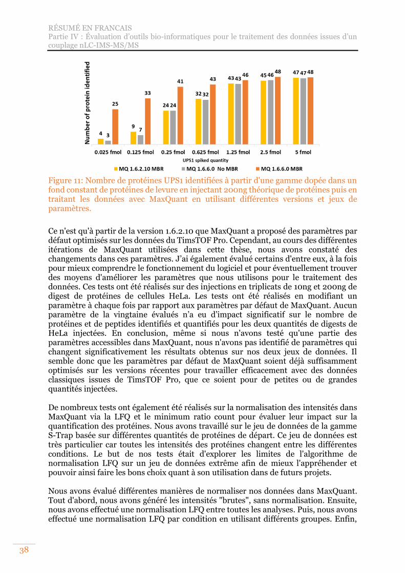
RÉSUMÉ EN FRANCAIS Partie IV : Évaluation d’outils bio-informatiques pour le traitement des données issues d’un couplage nLC-IMS-MS/MS
38
Figure 11: Nombre de protéines UPS1 identifiées à partir d'une gamme dopée dans un fond constant de protéines de levure en injectant 200ng théorique de protéines puis en traitant les données avec MaxQuant en utilisant différentes versions et jeux de paramètres.
Ce n'est qu'à partir de la version 1.6.2.10 que MaxQuant a proposé des paramètres par défaut optimisés sur les données du TimsTOF Pro. Cependant, au cours des différentes itérations de MaxQuant utilisées dans cette thèse, nous avons constaté des changements dans ces paramètres. J’ai également évalué certains d'entre eux, à la fois pour mieux comprendre le fonctionnement du logiciel et pour éventuellement trouver des moyens d'améliorer les paramètres que nous utilisons pour le traitement des données. Ces tests ont été réalisés sur des injections en triplicats de 10ng et 200ng de digest de protéines de cellules HeLa. Les tests ont été réalisés en modifiant un paramètre à chaque fois par rapport aux paramètres par défaut de MaxQuant. Aucun paramètre de la vingtaine évalués n’a eu d’impact significatif sur le nombre de protéines et de peptides identifiés et quantifiés pour les deux quantités de digests de HeLa injectées. En conclusion, même si nous n'avons testé qu'une partie des paramètres accessibles dans MaxQuant, nous n'avons pas identifié de paramètres qui changent significativement les résultats obtenus sur nos deux jeux de données. Il semble donc que les paramètres par défaut de MaxQuant soient déjà suffisamment optimisés sur les versions récentes pour travailler efficacement avec des données classiques issues de TimsTOF Pro, que ce soient pour de petites ou de grandes quantités injectées. De nombreux tests ont également été réalisés sur la normalisation des intensités dans MaxQuant via la LFQ et le minimum ratio count pour évaluer leur impact sur la quantification des protéines. Nous avons travaillé sur le jeu de données de la gamme S-Trap basée sur différentes quantités de protéines de départ. Ce jeu de données est très particulier car toutes les intensités des protéines changent entre les différentes conditions. Le but de nos tests était d'explorer les limites de l'algorithme de normalisation LFQ sur un jeu de données extrême afin de mieux l'appréhender et pouvoir ainsi faire les bons choix quant à son utilisation dans de futurs projets. Nous avons évalué différentes manières de normaliser nos données dans MaxQuant. Tout d'abord, nous avons généré les intensités "brutes", sans normalisation. Ensuite, nous avons effectué une normalisation LFQ entre toutes les analyses. Puis, nous avons effectué une normalisation LFQ par condition en utilisant différents groupes. Enfin,
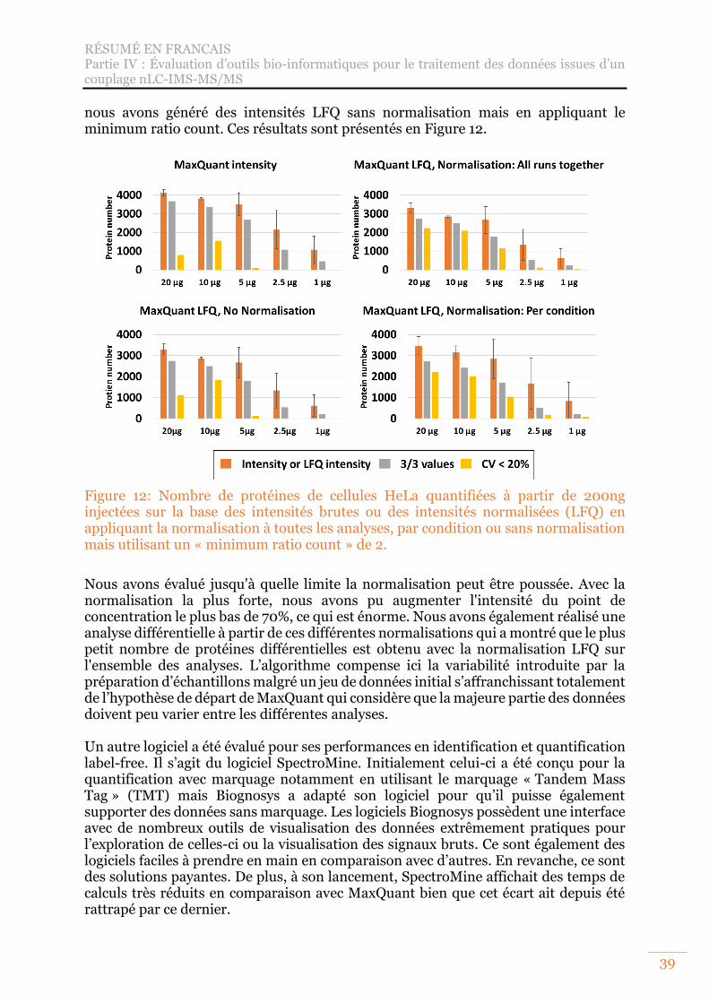
RÉSUMÉ EN FRANCAIS Partie IV : Évaluation d’outils bio-informatiques pour le traitement des données issues d’un couplage nLC-IMS-MS/MS
39
nous avons généré des intensités LFQ sans normalisation mais en appliquant le minimum ratio count. Ces résultats sont présentés en Figure 12.
Figure 12: Nombre de protéines de cellules HeLa quantifiées à partir de 200ng injectées sur la base des intensités brutes ou des intensités normalisées (LFQ) en appliquant la normalisation à toutes les analyses, par condition ou sans normalisation mais utilisant un « minimum ratio count » de 2.
Nous avons évalué jusqu'à quelle limite la normalisation peut être poussée. Avec la normalisation la plus forte, nous avons pu augmenter l'intensité du point de concentration le plus bas de 70%, ce qui est énorme. Nous avons également réalisé une analyse différentielle à partir de ces différentes normalisations qui a montré que le plus petit nombre de protéines différentielles est obtenu avec la normalisation LFQ sur l'ensemble des analyses. L’algorithme compense ici la variabilité introduite par la préparation d’échantillons malgré un jeu de données initial s’affranchissant totalement de l’hypothèse de départ de MaxQuant qui considère que la majeure partie des données doivent peu varier entre les différentes analyses. Un autre logiciel a été évalué pour ses performances en identification et quantification label-free. Il s’agit du logiciel SpectroMine. Initialement celui-ci a été conçu pour la quantification avec marquage notamment en utilisant le marquage « Tandem Mass Tag » (TMT) mais Biognosys a adapté son logiciel pour qu’il puisse également supporter des données sans marquage. Les logiciels Biognosys possèdent une interface avec de nombreux outils de visualisation des données extrêmement pratiques pour l’exploration de celles-ci ou la visualisation des signaux bruts. Ce sont également des logiciels faciles à prendre en main en comparaison avec d’autres. En revanche, ce sont des solutions payantes. De plus, à son lancement, SpectroMine affichait des temps de calculs très réduits en comparaison avec MaxQuant bien que cet écart ait depuis été rattrapé par ce dernier.
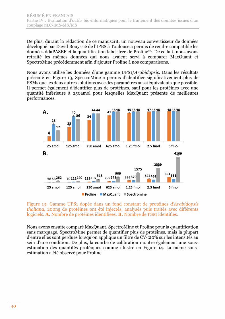
RÉSUMÉ EN FRANCAIS Partie IV : Évaluation d’outils bio-informatiques pour le traitement des données issues d’un couplage nLC-IMS-MS/MS
40
De plus, durant la rédaction de ce manuscrit, un nouveau convertisseur de données développé par David Bouyssié de l’IPBS à Toulouse a permis de rendre compatible les données ddaPASEF et la quantification label-free de Proline20. De ce fait, nous avons retraité les mêmes données qui nous avaient servi à comparer MaxQuant et SpectroMine précédemment afin d’ajouter Proline à nos comparaisons. Nous avons utilisé les données d’une gamme UPS1/Arabidopsis. Dans les résultats présenté en Figure 13, SpectroMine a permis d’identifier significativement plus de PSMs que les deux autres solutions avec des paramètres aussi équivalents que possible. Il permet également d’identifier plus de protéines, sauf pour les protéines avec une quantité inférieure à 250amol pour lesquelles MaxQuant présente de meilleures performances.
Figure 13: Gamme UPS1 dopée dans un fond constant de protéines d'Arabidopsis thaliana, 200ng de protéines ont été injectés, analysés puis traités avec différents logiciels. A. Nombre de protéines identifiées. B. Nombre de PSM identifiés.
Nous avons ensuite comparé MaxQuant, SpectroMine et Proline pour la quantification sans marquage. SpectroMine permet de quantifier plus de protéines, mais la plupart d'entre elles sont perdues lorsqu'on applique un filtre de CV<20% sur les intensités au sein d’une condition. De plus, la courbe de calibration montre également une sous-estimation des quantités protéiques comme illustré en Figure 14. La même sous-estimation a été observé pour Proline.
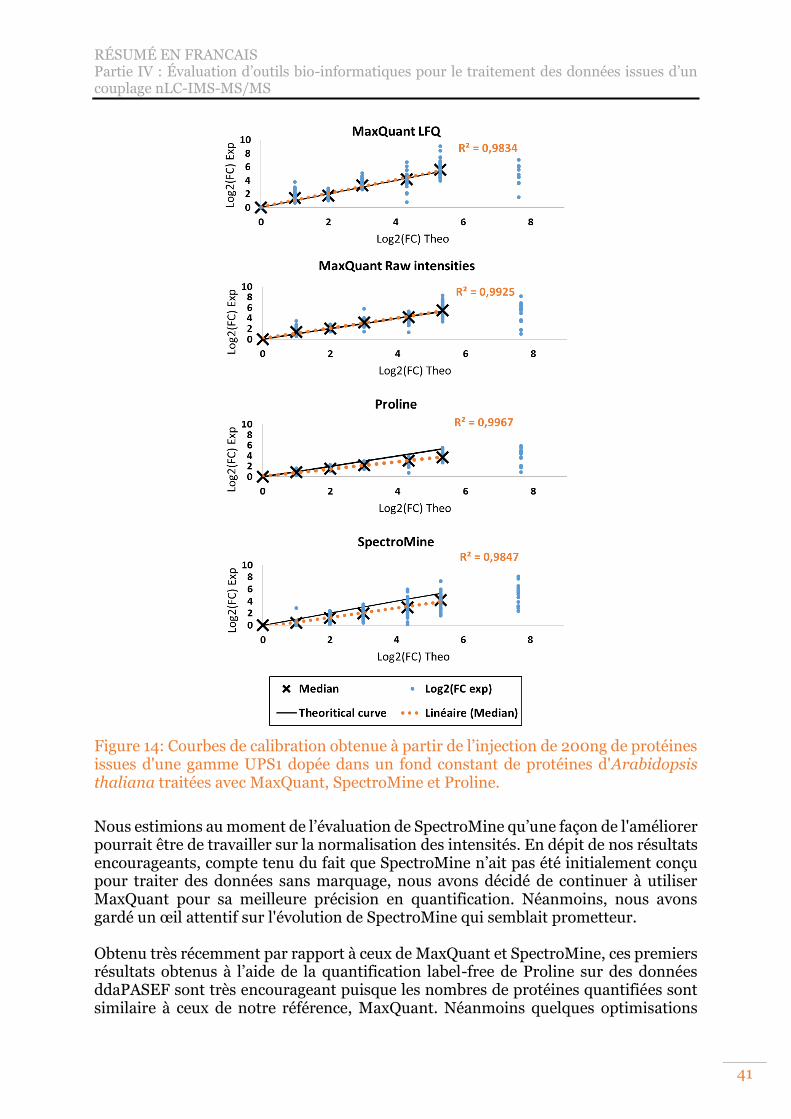
RÉSUMÉ EN FRANCAIS Partie IV : Évaluation d’outils bio-informatiques pour le traitement des données issues d’un couplage nLC-IMS-MS/MS
41
Figure 14: Courbes de calibration obtenue à partir de l’injection de 200ng de protéines issues d'une gamme UPS1 dopée dans un fond constant de protéines d'Arabidopsis thaliana traitées avec MaxQuant, SpectroMine et Proline.
Nous estimions au moment de l’évaluation de SpectroMine qu’une façon de l'améliorer pourrait être de travailler sur la normalisation des intensités. En dépit de nos résultats encourageants, compte tenu du fait que SpectroMine n’ait pas été initialement conçu pour traiter des données sans marquage, nous avons décidé de continuer à utiliser MaxQuant pour sa meilleure précision en quantification. Néanmoins, nous avons gardé un œil attentif sur l'évolution de SpectroMine qui semblait prometteur. Obtenu très récemment par rapport à ceux de MaxQuant et SpectroMine, ces premiers résultats obtenus à l’aide de la quantification label-free de Proline sur des données ddaPASEF sont très encourageant puisque les nombres de protéines quantifiées sont similaire à ceux de notre référence, MaxQuant. Néanmoins quelques optimisations

RÉSUMÉ EN FRANCAIS Partie IV : Évaluation d’outils bio-informatiques pour le traitement des données issues d’un couplage nLC-IMS-MS/MS
42
seront encore nécessaires afin d’améliorer la justesse de la quantification. De même, Proline n’exploite pas à ce jour la dimension de mobilité ionique mais aura tout à y gagner dans le futur. Nous avons par la suite pu mener une nouvelle comparaison des performances de MaxQuant, SpectroMine (Biognosys) et Peaks (Bioinformatics Solutions Inc.) à laquelle nous avons par la suite ajouté Proline. Ces résultats présentés en Figure 15 sont intégrés dans la publication qui sera prochainement soumise à Journal of Proteomics.
Figure 15: Identification et quantification sans marquage de protéines de cellules HeLa après injection de 200ng. Le traitement des données a été réalisé avec différents logiciels et en appliquant différents filtres de qualité.
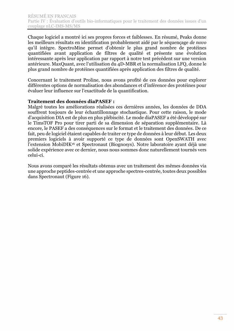
RÉSUMÉ EN FRANCAIS Partie IV : Évaluation d’outils bio-informatiques pour le traitement des données issues d’un couplage nLC-IMS-MS/MS
43
Chaque logiciel a montré ici ses propres forces et faiblesses. En résumé, Peaks donne les meilleurs résultats en identification probablement aidé par le séquençage de novo qu’il intègre. SpectroMine permet d’obtenir le plus grand nombre de protéines quantifiées avant application de filtres de qualité et présente une évolution intéressante après leur application par rapport à notre test précédent sur une version antérieure. MaxQuant, avec l’utilisation du 4D-MBR et la normalisation LFQ, donne le plus grand nombre de protéines quantifiées après application des filtres de qualité. Concernant le traitement Proline, nous avons profité de ces données pour explorer différentes options de normalisation des abondances et d’inférence des protéines pour évaluer leur influence sur l’exactitude de la quantification. Traitement des données diaPASEF : Malgré toutes les améliorations réalisées ces dernières années, les données de DDA souffrent toujours de leur échantillonnage stochastique. Pour cette raison, le mode d’acquisition DIA est de plus en plus plébiscité. Le mode diaPASEF a été développé sur le TimsTOF Pro pour tirer parti de sa dimension de séparation supplémentaire. Là encore, le PASEF a des conséquences sur le format et le traitement des données. De ce fait, peu de logiciel étaient capables de traiter ce type de données à leur début. Les deux premiers logiciels à avoir supporté ce type de données sont OpenSWATH avec l’extension MobiDIK16 et Spectronaut (Biognosys). Notre laboratoire ayant déjà une solide expérience avec ce dernier, nous nous sommes donc naturellement tournés vers celui-ci. Nous avons comparé les résultats obtenus avec un traitement des mêmes données via une approche peptides-centrée et une approche spectres-centrée, toutes deux possibles dans Spectronaut (Figure 16).
RÉSUMÉ EN FRANCAIS Partie IV : Évaluation d’outils bio-informatiques pour le traitement des données issues d’un couplage nLC-IMS-MS/MS
44
Figure 16: Nombre de protéines (en A et C) et de peptides (en B et D) UPS1 quantifiés avec une approche centrée sur les peptides pour A et B et une approche centrée sur les spectres pour C et D obtenus à partir de 200ng de protéines injectées.
L'approche centrée sur les peptides nous a permis de quantifier plus de protéines sur la globalité de l’échantillon alors que l'approche centrée sur les spectres a semblé être plus efficace sur les protéines de faible abondance. Les deux approches montrent une légère sous-estimation des quantités de protéines entre 150 et 250amol avec une chute importante à 25amol. Les deux approches présentent une dispersion des intensités similaire. Les méthodes diaPASEF sont très récentes, et nous pouvons donc espérer de nouvelles améliorations dans le futur à la fois au niveau de l’acquisition et du traitement de ces données. Néanmoins, le logiciel Spectronaut semble être adapté pour le traitement de ce type de données via des approches peptides-centrée et spectres-centrée qui présentent dans notre test des performances similaires. Par ailleurs, Spectronaut est doté comme SpectroMine de nombreux outils de visualisation et d’exploration des données particulièrement attrayant et adaptés. Au même titre que Proline, un autre logiciel a été rendu compatible très récemment avec les données du TimsTOF Pro pour le traitement de donnée diaPASEF. De ce fait, nous avons réalisé une première évaluation de MaxDIA18 implémenté au sein de MaxQuant 2.0 sur le même jeu de donnée que celui utilisé pour l’évaluation de Spectronaut. Bien qu’une comparaison plus complète de ces deux logiciels soit nécessaire pour aller plus loin, nous avons pu constater des performances similaires bien que MaxDIA nous ait permis de quantifier un peu moins de protéines que Spectronaut dans ces tout premiers essais sans optimisation des paramètres.
RÉSUMÉ EN FRANCAIS Partie V : Application des développements méthodologiques de la thèse à des projets collaboratifs
45
Partie V : Application des développements méthodologiques de la thèse à des projets collaboratifs
Finalement, les développements méthodologiques réalisés au cours de cette thèse ont été mis en application dans le cadre de trois collaborations. Les deux premières avaient pour objectif l’analyse de complexes protéiques immunoprécipités (co-IP) dans le but d’identifier et de quantifier des protéines interactantes. La première étude a été réalisée avec l’équipe du Pr Philippe Boucher (CNRS, Unistra, UMR 7021, Strasbourg, France). Elle porte sur l’analyse d’immunoprécipitations de deux protéines cibles d’un complexe impliqué dans l’accumulation du cholestérol dans les endosomes tardifs/liposomes et son lien avec le développement de l’athérosclérose chez la souris. Les résultats obtenus sont venus renforcer les résultats biologiques des collaborateurs et une publication est actuellement en révision dans Circulation Research. Selon l'OMS, en 2019, les deux principales causes de décès dans le monde étaient les cardiopathies ischémiques et les accidents vasculaires cérébraux, qui peuvent tous deux résulter de l'athérosclérose et qui représentent à elles seules 27% des décès dans le monde. Par conséquent, comprendre les mécanismes de l'athérosclérose présente un intérêt majeur pour trouver de nouveaux moyens de diagnostiquer et de guérir ces maladies. Nous avons analysé deux co-IP avec leurs IP contrôles respectifs pour identifier les interactants des protéines lysosomales NPC1 et NPC2 connues pour intervenir dans le métabolisme du cholestérol et qui jouent un rôle important dans la genèse de l'athérosclérose. Les premiers résultats obtenus dans cette étude ont montré une trop grande variabilité entre les réplicats et la présence de protéines non spécifiques liées à la préparation des IPs. Les conditions expérimentales de préparation de ces IPs n’ayant pu être améliorées par le collaborateur, nous avons donc décidé d'analyser ces échantillons sur un couplage plus sensible et de réaliser une étude uniquement qualitative. Nous avons ainsi pu identifier un nombre significatif de peptides issus des protéines d’intérêts NPC1, NPC2 et Wnt5a dans les deux co-IPs comme présenté en Table 1. Malgré l’absence de dimension quantitative, ces résultats ont permis de renforcer les conclusions des autres expériences de biologie présentées dans la publication permettant ainsi d’identifier la protéine Wnt5a comme un interactant de NPC1 et NPC2. Cette étude a permis de révéler une nouvelle fonction de cette protéine qui semble jouer un rôle essentiel dans l'homéostasie du cholestérol in vivo chez la souris et qui pourrait ainsi jouer un rôle important dans le développement de l'athérosclérose.
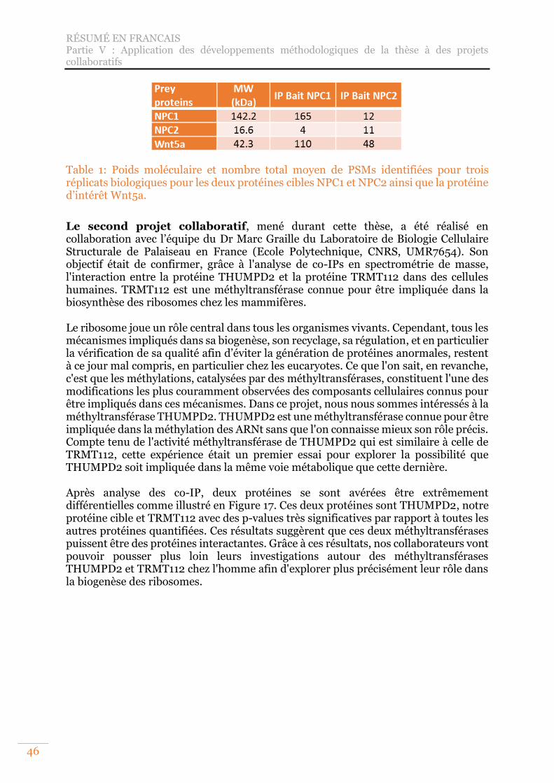
RÉSUMÉ EN FRANCAIS Partie V : Application des développements méthodologiques de la thèse à des projets collaboratifs
46
Table 1: Poids moléculaire et nombre total moyen de PSMs identifiées pour trois réplicats biologiques pour les deux protéines cibles NPC1 et NPC2 ainsi que la protéine d’intérêt Wnt5a.
Le second projet collaboratif, mené durant cette thèse, a été réalisé en collaboration avec l’équipe du Dr Marc Graille du Laboratoire de Biologie Cellulaire Structurale de Palaiseau en France (Ecole Polytechnique, CNRS, UMR7654). Son objectif était de confirmer, grâce à l'analyse de co-IPs en spectrométrie de masse, l'interaction entre la protéine THUMPD2 et la protéine TRMT112 dans des cellules humaines. TRMT112 est une méthyltransférase connue pour être impliquée dans la biosynthèse des ribosomes chez les mammifères. Le ribosome joue un rôle central dans tous les organismes vivants. Cependant, tous les mécanismes impliqués dans sa biogenèse, son recyclage, sa régulation, et en particulier la vérification de sa qualité afin d’éviter la génération de protéines anormales, restent à ce jour mal compris, en particulier chez les eucaryotes. Ce que l'on sait, en revanche, c'est que les méthylations, catalysées par des méthyltransférases, constituent l'une des modifications les plus couramment observées des composants cellulaires connus pour être impliqués dans ces mécanismes. Dans ce projet, nous nous sommes intéressés à la méthyltransférase THUMPD2. THUMPD2 est une méthyltransférase connue pour être impliquée dans la méthylation des ARNt sans que l'on connaisse mieux son rôle précis. Compte tenu de l'activité méthyltransférase de THUMPD2 qui est similaire à celle de TRMT112, cette expérience était un premier essai pour explorer la possibilité que THUMPD2 soit impliquée dans la même voie métabolique que cette dernière. Après analyse des co-IP, deux protéines se sont avérées être extrêmement différentielles comme illustré en Figure 17. Ces deux protéines sont THUMPD2, notre protéine cible et TRMT112 avec des p-values très significatives par rapport à toutes les autres protéines quantifiées. Ces résultats suggèrent que ces deux méthyltransférases puissent être des protéines interactantes. Grâce à ces résultats, nos collaborateurs vont pouvoir pousser plus loin leurs investigations autour des méthyltransférases THUMPD2 et TRMT112 chez l'homme afin d'explorer plus précisément leur rôle dans la biogenèse des ribosomes.
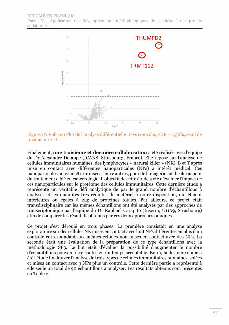
RÉSUMÉ EN FRANCAIS Partie V : Application des développements méthodologiques de la thèse à des projets collaboratifs
47
Figure 17: Volcano Plot de l'analyse différentielle IP vs contrôle, FDR = 1,36%, seuil de p-value = 1e-04.
Finalement, une troisième et dernière collaboration a été réalisée avec l’équipe du Dr Alexandre Detappe (ICANS, Strasbourg, France). Elle repose sur l’analyse de cellules immunitaires humaines, des lymphocytes « natural killer » (NK), B et T après mise en contact avec différentes nanoparticules (NPs) à intérêt médical. Ces nanoparticules peuvent être utilisées, entre autres, pour de l’imagerie médicale ou pour du traitement ciblé en cancérologie. L’objectif de cette étude a été d’évaluer l’impact de ces nanoparticules sur le protéome des cellules immunitaires. Cette dernière étude a représenté un véritable défi analytique de par le grand nombre d’échantillons à analyser et les quantités très réduites de matériel à notre disposition, qui étaient inférieures ou égales à 2µg de protéines totales. Par ailleurs, ce projet était transdisciplinaire car les mêmes échantillons ont été analysés par des approches de transcriptomique par l’équipe du Dr Raphael Carapito (Inserm, U1109, Strasbourg) afin de comparer les résultats obtenus par ces deux approches omiques. Ce projet s'est déroulé en trois phases. La première consistait en une analyse exploratoire sur des cellules NK mises en contact avec huit NPs différentes en plus d’un contrôle correspondant aux mêmes cellules non mises en contact avec des NPs. La seconde était une évaluation de la préparation de ce type échantillons avec la méthodologie SP3. Le but était d'évaluer la possibilité d'augmenter le nombre d'échantillons pouvant être traités en un temps acceptable. Enfin, la dernière étape a été l'étude finale avec l'analyse de trois types de cellules immunitaires humaines isolées et mises en contact avec 9 NPs plus un contrôle. Cette dernière partie a représenté à elle seule un total de 90 échantillons à analyser. Les résultats obtenus sont présentés en Table 2.
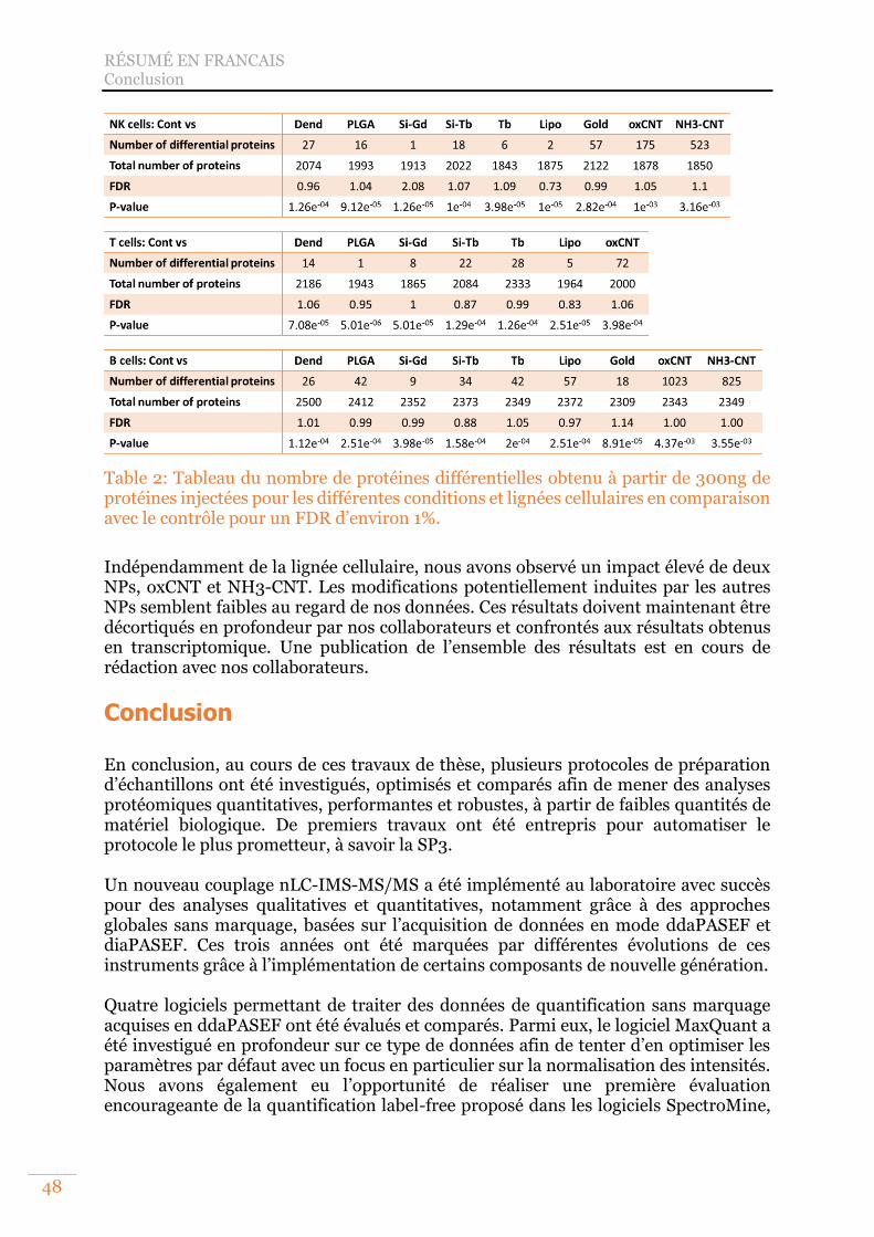
RÉSUMÉ EN FRANCAIS Conclusion
48
Table 2: Tableau du nombre de protéines différentielles obtenu à partir de 300ng de protéines injectées pour les différentes conditions et lignées cellulaires en comparaison avec le contrôle pour un FDR d’environ 1%.
Indépendamment de la lignée cellulaire, nous avons observé un impact élevé de deux NPs, oxCNT et NH3-CNT. Les modifications potentiellement induites par les autres NPs semblent faibles au regard de nos données. Ces résultats doivent maintenant être décortiqués en profondeur par nos collaborateurs et confrontés aux résultats obtenus en transcriptomique. Une publication de l’ensemble des résultats est en cours de rédaction avec nos collaborateurs.
Conclusion
En conclusion, au cours de ces travaux de thèse, plusieurs protocoles de préparation d’échantillons ont été investigués, optimisés et comparés afin de mener des analyses protéomiques quantitatives, performantes et robustes, à partir de faibles quantités de matériel biologique. De premiers travaux ont été entrepris pour automatiser le protocole le plus prometteur, à savoir la SP3. Un nouveau couplage nLC-IMS-MS/MS a été implémenté au laboratoire avec succès pour des analyses qualitatives et quantitatives, notamment grâce à des approches globales sans marquage, basées sur l’acquisition de données en mode ddaPASEF et diaPASEF. Ces trois années ont été marquées par différentes évolutions de ces instruments grâce à l’implémentation de certains composants de nouvelle génération. Quatre logiciels permettant de traiter des données de quantification sans marquage acquises en ddaPASEF ont été évalués et comparés. Parmi eux, le logiciel MaxQuant a été investigué en profondeur sur ce type de données afin de tenter d’en optimiser les paramètres par défaut avec un focus en particulier sur la normalisation des intensités. Nous avons également eu l’opportunité de réaliser une première évaluation encourageante de la quantification label-free proposé dans les logiciels SpectroMine,
RÉSUMÉ EN FRANCAIS Conclusion
49
Peaks et Proline sur des données ddaPASEF. Les logiciels Spectronaut et MaxDIA ont été évalués pour traiter des données de diaPASEF par des approches centrées sur les peptides. Spectronaut a également été évalué en utilisant une approche basée sur les spectres avec directDIA. Finalement, ces travaux de thèse ont pu être mis à contribution dans le cadre de trois collaborations :
→ L’une reposant sur la validation d’un complexe de protéines, impliquées dans l’accumulation du cholestérol entrainant le développement d’athérosclérose chez la souris, qui a permis de confirmer l’implication d’une protéine spécifique.
→ Un deuxième projet a également porté sur l’analyse d’immunoprécipitations
mais cette fois pour étudier des méthyltransférases chez l'homme afin d'explorer leur rôle dans la biogenèse des ribosomes. Ici encore, les résultats sont venus confirmer ceux de nos collaborateurs biologistes et ont permis d’identifier un interactant spécifique.
→ Enfin la dernière étude portait sur l’évaluation des modifications induites sur le
protéome de cellules immunitaires humaines après leur mise en contact avec des nanoparticules d’intérêt médical, notamment pour le développement d’outils de visualisation, de diagnostiques ou de thérapies ciblées en cancérologie. La stratégie analytique que j’ai mise en œuvre a permis l’analyse d’une cohorte de grande taille, en un temps réduit, à partir de quantités de protéines inférieures ou égales à 2µg.
A titre personnel, cette thèse m’a permis d’acquérir un grand nombre de compétences. J’ai eu l’occasion de me former à l’utilisation et à l’optimisation de nombreux protocoles de préparation d’échantillons pour l’analyse protéomique « Bottom-up ». J’ai appris à utiliser un robot de pipetage Bravo AssayMap (Agilent) et j’ai entrepris de premiers travaux pour implémenter un nouveau protocole automatisé me permettant de mettre un premier pied dans l’environnement de développement de méthodes associées à cette plateforme. J’ai acquis une solide expertise en chromatographie liquide et spectrométrie de masse pour le développement de méthodes analytiques sur un instrument incluant une dimension de séparation par mobilité ionique. J’ai appris à gérer l’entretien et les pannes du couplage ainsi que la pression/responsabilité de devoir maintenir et offrir un système fonctionnel et performant à mes collègues et collaborateurs. J’ai également eu l’occasion de me plonger dans le traitement des données de protéomique ainsi que leur analyse statistique et d’acquérir la maitrise profonde d’un certain nombre de logiciels. Cette thèse m’a également permis de développer d’autres compétences via ma thèse en elle-même ou les activités connexes que j’ai pu mener. J’ai pu perfectionner mes compétences en communication de mes résultats, aussi bien à l’oral qu’à l’écrit, auprès d’un public scientifique expert dans mon domaine. J’ai pu développer des qualités de patience, de résilience, de résistance à la pression et à une lourde charge de travail sur une période prolongée. Parmi les activités annexes à cette thèse, j’ai notamment pu participer au concours de vulgarisation scientifique « Ma thèse en 180 secondes » et atteint la finale de la région
RÉSUMÉ EN FRANCAIS Conclusion
50
Alsace, qui n’a malheureusement pas pu avoir lieu à cause des restrictions sanitaires. Cela dit cette expérience m’a permis de grandement améliorer mon aisance à l’oral devant un grand public ou une caméra dans l’exercice, plus difficile qu’il n’y parait, de vulgariser des travaux scientifiques. J’ai également été, pendant deux ans et demi, représentante des doctorants auprès de l’école doctorale de sciences chimique de Strasbourg. Cela m’a permis d’apporter ma petite pierre à l’édifice afin d’améliorer toujours plus la formation doctorale en apportant le point de vue des étudiants aux membres du conseil. Cette expérience a été particulièrement importante et formatrice dans le contexte sanitaire exceptionnel que nous avons connu. Cela m’a également permis de mieux comprendre certains aspects organisationnels et politiques gravitant autour de la formation doctorale auxquels les étudiants ont malheureusement rarement accès. L’ensemble des compétences ainsi développées me seront très profitables pour mon futur parcours professionnel.

GENERAL INTRODUCTION
51
GENERAL INTRODUCTION
From tadpole to frog, from baby to adult, from one cellular type to another, the genome remains globally the same. However, the phenotype, i.e. the set of observable traits of an organism, can vary greatly. This is due to the different expression of the same DNA (deoxyribonucleic acid) to adapt to varying conditions and objectives as illustrated in Figure 18. Indeed, a whole set of different proteins called proteoforms can be derived from the same gene. These proteoforms result, within the same individual, from splicing variants occurring during the transcription of DNA into mRNA (messenger ribonucleic acid). They also result from errors in the translation of mRNA into proteins21. Genomic sequence variants will also be observed between different individuals22.
Figure 18: Illustrations of the life cycle of a batrachian. Photos from the royalty-free Pixabay image bank by Bill Kasmann, Marc Pascual, Aguasas and Gérard G.
The genome, the transcriptome, the proteome, and each other “ome” will then bring an additional level of complexity. For this reason, the different “omics” strategies are complementary and provide different insights into common situations to understand them better. Biological mechanisms occurring at the level of DNA and mRNA already provide a great variety within the protein population, but this is further complicated by post-translational modifications (PTMs). These PTMs, in addition to being extremely varied, will also bring an evolutionary dimension to the proteome because, unlike the
GENERAL INTRODUCTION
52
sequence of a protein which is fixed once it has reached maturity, its modifications may evolve throughout its existence. This will have an impact on its structure and therefore its interactions with other biological components21. In humans, it is estimated that the ~20,300 genes can lead to up to 6 million proteoforms22–24. Indeed, a protein alone is of no interest, what counts are the biological functions. A function will depend on the interaction of tens or even hundreds of proteins and other biological components. The function of a protein will depend on its environment. The same protein at different locations may be involved in different mechanisms. Moreover, proteins are regularly renewed to replace those that are too old to avoid dysfunction or to adapt to constantly changing external conditions. The proteome is therefore complex and constantly changing. However, the tools that are available today do not allow monitoring these flows in real time. The role of the proteomist will therefore consist in taking frozen "photos" of this proteome and attempting to retrace the "film" of the dynamic mechanisms behind it. For those reasons, today’s proteomist described a proteome as confined to a defined space and temporality. Proteins were discovered in 1835 in the Netherlands by the organic chemist Gerardus Johannes Mulder but it is only in 1838 that the word protein was created25. From the 1980s onwards, their analyses were carried out using two-dimensional gel electrophoresis and Edman sequencing to determine the amino acid sequence of their components21,26,27. These are usually twenty in number. Two additional amino acids exist but their presence is limited to certain organisms or precise protein types. Since that time, methods for studying proteins have continued to improve, driven by advances in sample preparation, instrumentation, and computerised data processing, particularly for large datasets. Today, one of the most widely used methods for the study of proteins is based on liquid chromatography coupled to tandem mass spectrometry (LC-MS/MS)28–30. Thanks to these new tools, in addition to being able to identify them, we are also able to quantify several thousands of proteins in a few hours31 and thanks to statistical tools we can evaluate the significance of differences between two proteomes30. Proteomics is therefore a tool that can be used in numerous biological contexts and on various types of samples. This applies equally to fundamental research to understand how living organisms function, to environmental studies for biodiversity monitoring and ecotoxicology, and to the medical field. In this last field, proteomics can notably allow the discovery of new diagnostic means or the search for new therapeutic targets32. Depending on the specificities of each biological question, different approaches have been developed to make the most of each situation. That said, there are still limitations today and it is in this context that my thesis was carried out. My work consisted in exploring, evaluating and implementing in our laboratory the latest technological advances related to protein analysis by bottom-up approaches in mass spectrometry. The final objective was to be able to perform quantitative analyses without labelling using small quantities of starting proteins. This manuscript is therefore structured in seven parts:
GENERAL INTRODUCTION
53
The first part consisted of a summary of my thesis in French since it was carried out within a French doctoral school. The second part will be a state of the art of bottom-up proteomics. It will follow the chronological order of the different steps of a quantitative proteomic analysis in the same logic as the consecutive results parts.
→ The first chapter will present the different steps leading to protein identification.
→ The second chapter will discuss the different steps implicated in protein
quantification. The third part will be the first part of results presenting the work carried out on the preparation of samples from small quantities of proteins. Two chapters compose this part:
→ The first chapter will present the evaluation of different sample preparation protocols adapted to work efficiently with low protein amounts (< 20µg).
→ The second chapter will present trials carried out with the aim of automating
the Single-Pot, Solid-Phase-enhanced Sample Preparation (SP3), the most promising method among the previously presented ones.
The fourth part of this thesis and second part of the results will present the work related to the arrival in our laboratory of a new generation coupling including an additional separation dimension thanks to ion mobility (nLC-IMS-MS/MS strategy) and using a dedicated acquisition mode, the PASEF (Parallel-Accumulation-SErial Fragmentation). This part will also be divided into two chapters based on the data acquisition strategy used:
→ The first chapter will present the data dependent acquisition (DDA).
→ The second chapter will present the data independent acquisition (DIA). The fifth part of this thesis and third part of the results will focus on the processing of the data acquired by the approaches explored in the previous part:
→ The first chapter will present the evaluation and the optimisations of MaxQuant parameters for processing data acquired in ddaPASEF mode.
→ The second chapter will present the benchmark of different other software
allowing to treat ddaPASEF data as well as two possible software for processing diaPASEF data.
The sixth part of this thesis and the fourth and last part of the results will present different collaborative projects integrating some of the developments that will have been highlighted in the previous parts:
GENERAL INTRODUCTION
54
→ The first chapter will present two distinct projects based on the analysis of immunoprecipitations for the study of protein complexes involved in different biological mechanisms. The first project will focus on cholesterol metabolism and its role in the development of atherosclerosis in a mouse model. The second will study specific methyltransferases and their role in ribosome biogenesis in humans.
→ The second chapter will follow the evolution of a project from the exploratory
phase to the study of a cohort of 90 samples requiring advanced optimisations, particularly in terms of sample preparation. In this chapter, we will evaluate the impact of nanoparticles of medical interest, mainly for oncology, on the proteomes of human immune cells.
The seventh and final part will bring together the experimental details of the various works described in this manuscript.
Part I: State of the art of proteomic analysis by mass spectrometry
55
Part I: State of the art of proteomic analysis by mass spectrometry Proteomics is the science that studies the proteome. This term was coined in 1997 by Peter James by deriving the words protein and genome, as was the case for the word proteome derived from protein and genome in 1994 by Mark Wilkins26. Today, this science is particularly interested in the qualitative, quantitative, and functional study of the proteome, through mass spectrometry. The use of mass spectrometry for proteomics was made possible by two inventions made at the same time and having the same goal, the soft ionisation of biological macromolecules. This is the MALDI (Matrix-Assisted Laser Desorption Ionisation) discovered by Koichi Tanaka33 and ESI (ElectroSpray ionisation) discovered by John Fenn34,35. These discoveries earned them a Nobel Prize in Chemistry in 2002. Thanks to these two types of sources, it is now possible to ionise proteins or peptides that are naturally not very volatile and fragile so that they can be analysed by mass spectrometry. Subsequently, the study of proteins has progressed enormously as a result of various developments23,28,36,37. These include methods for separating proteins and peptides upstream of the spectrometer to increase the depth of analysis on complex samples containing many co-eluting elements. Among those techniques, the most widely used is the high-performance liquid chromatography (HPLC). Mass spectrometers have also made great strides in increasing their resolution, sensitivity, accuracy, and acquisition speed. New modes of acquisition have appeared, taking advantage of these improvements, among others, to allow the quantification of peptides and proteins. Finally, computer and statistical tools have also evolved considerably. The advent of new, more powerful and automated software has been made possible by developments in computing with more powerful computers, the use of servers or computing grids. Finally, the improvement of sequenced genome libraries via their completion, annotation and manual verification has improved the quality of the protein databases derived from them and essential for proteomics data processing. The use of LC-MS/MS for the study of proteins has thus allowed the emergence of three major approaches differentiated by the size of the molecules to be analysed:
→ Top-down approaches will allow the analysis of intact proteins. MS1 analysis allows the mass of the protein to be determined while MS2 allows it to be sequenced. This approach is also used for the analysis of PTMs and the characterisation of proteoforms38,39. As with any approach, it has a number of limitations40–42, including delicate sample preparation in order to properly extract and solubilise native proteins. At the analytical level, the ionisation and the fragmentation of proteins require adjustments especially to improve the sequence coverage. The mass spectrometers used must allow a sufficiently fine resolution to enable the separation of isotopic envelope peaks from highly multi-charged fragments. The computer tools must allow the interpretation of complex spectra and their statistical evaluation. However, this approach continues to progress and has enabled the identification of more than a
Part I: State of the art of proteomic analysis by mass spectrometry
56
thousand proteins and several thousand PTMs thanks to its coupling with a multidimensional separation43,44.
→ The middle-down approach is, as its name suggests, in the middle of the top-
down and bottom-up approaches from which it tries to get the best. This approach allows the analysis of large peptides between 3 and 10 kDa generated through partial enzymatic digestion or until 25kDa in specific cases such as mAb characterisation45. The MS1 spectra generated will allow the determination of the mass of the peptide while the MS2 spectra will allow the elucidation of the peptide sequence. This approach will provide similar information to the Top-down approach while reducing its limitations. It will also allow for better protein inference compared to the bottom-up approach by generating fewer and longer peptides that are less likely to co-elute or be shared between multiple proteins. The limitation of this approach is the need to optimise the partial digestion of proteins by perfectly controlling the enzyme used and the digestion conditions, notably time, temperature, and the protein/enzyme ratio.
→ The Bottom-up approach describes the analysis of peptides between 500 Da and
3.000 Da. Enzymes theoretically completely digest the proteins into peptides. Trypsin is classically used alone or coupled with other endoproteases such as Lys-C46–48. Trypsin and Lys-C have the advantage of cutting at specific sites that occur regularly in most proteins. Then, peptides are separated according to their hydrophobicity by high performance liquid chromatography (HPLC/UHPLC) to decrease the number of co-eluting peptides and increase the depth of analysis. The specific enzymatic cuts allow the digestion of proteins to be simulated computationally to compare the m/z obtained experimentally with those generated in silico by digestion of a protein database. This allows the attribution of experimental signals to peptides. The parent proteins can then be determined by inference. However, this process remains tedious because a complex mixture of proteins will have common peptides shared by several proteins. Therefore, rather than identifying proteins, the smallest possible groups of proteins will be identified according to the principle of parsimony49, where the unique representative for each group will be the most likely protein present. It should also be kept in mind that different algorithms exist to do protein inference and each possessed its own way to work releasing thus different results on a same dataset50. This method is best suited for the identification and quantification of proteins in a very complex mixture, which can amount to more than 10,000 proteins identified and quantified in a single run on human tissues in a few hours31.
The bottom-up approach is the one that has been used during this thesis work to be able to identify and quantified as much proteins as possible from small protein amounts. Its different steps will be presented more in detail in the next part. The first chapter will focus on protein identification and the second one on protein quantification.
Part I: State of the art of proteomic analysis by mass spectrometry Chapter 1: Identification of proteins
57
Chapter 1: Identification of proteins The samples analysed in proteomics can have multiple origins and forms. On one hand, they can be “raw” samples such as cell pellets, biological fluids, or tissues. On the other hand, they can be more “refined” such as immunoprecipitations or transfected cell pellets. The classical proteomic analysis scheme will then be divided into three main parts: 1) sample preparation, 2) mass spectrometry analysis and 3) computer-assisted data processing. Depending on the project, two additional steps may exist. A preliminary sample preparation step carried out by a biologist depending on the biological context (i.e the preparation of a protein complex immunoprecipitation) and a final step of statistical data processing, which can be carried out, by the proteomist, a biostatistician or both. Depending on the purpose of the projects, the same samples can also be analysed by other techniques in parallel such as transcriptomics. Proteomics projects are therefore very often multidisciplinary. Focusing on the role of the proteomist, it starts with the preparation of the samples.
A. Sample preparation methods for bottom-up proteomics Sample preparation is a critical step for the quality and repeatability of the results. Poor sample preparation can lead to protein loss or biased quantification, which may result in incorrect biological conclusions. Therefore, this step should be optimised for each sample type, sample origin and project objective. This becomes especially true when working on small quantities (less than 10µg of starting material). In this context, it is important to note that there is still a significant gap in terms of tools between classical proteomic workflows, which process samples down to a low limit around 1µg of protein, and true single-cell proteomics, which requires specific equipment, workflows and analytical pipelines. Single-cell proteomics will be only briefly evocated in the automation part of this manuscript51–54. The first step in sample preparation is the extraction of proteins from the sample.
1) Cell lysis and protein extraction The cell lysis and the extraction of proteins is a key step as if the proteins are not recovered at this step, they are purely lost for the entire analysis thus affecting results quality and repeatability. The aim of that step will be to recover a maximum of proteins without modifying or degrading them. The used methods should be adapted to the sample type, the difficulty to extract certain proteins such as membrane proteins, the protein quantities, the sample volumes and the compatibility with the following intended analytical steps55–58. Cell lysis coupled to protein extraction techniques are divided into two complementary categories, mechanical and chemical approaches59,60: Mechanical approaches include manual grinding with a Potter or automatic grinding using a bead mill. These strategies are usually applied to matrices, tissues, or cells to release the proteins they contain. The final mechanical strategy is sonication or ultra-sonication, usually applied to cells61. Recent development have been made in that field to improve the consistency of this step with for example the Adaptive Focused Acoustics (AFA, Covaris, Brighton, UK) or with Bioruptor62 (Diagenode, Seraing, Belgium). They aim to lyse cells to release their protein content but can also be used to loosen proteins adsorbed on the walls of a container. These methods must be carefully
Part I: State of the art of proteomic analysis by mass spectrometry Chapter 1: Identification of proteins
58
monitored to ensure that they do not raise the temperature of the sample too much or generate free radicals which could alter the sample or even degrade the proteins63. Chemical lysis and extraction of proteins can also be achieved using:
→ Ionic (sodium dodecyl-sulfate, SDS), non-ionic (Triton) or zwitterionic (CHAPS)64 detergents, bile salts (sodium deoxycholate, SDC)65. Some detergents have been specifically developed to be compatible with MS analysis, such as RapiGest, which breaks down in acidic medium into two products, one compatible with MS and the other precipitable by centrifugation66 or the Azo (or 4-hexylphenylazosulfonate), an anionic, photocleavable surfactant that rapidly degrade upon UV exposure67.
→ Chaotropic agents (urea) that denature proteins56.
→ Organic solvents (acetonitrile, ACN or methanol, MeOH)) which facilitate the
denaturation of proteins by changing their conformation. Finally, alternative strategies are emerging with the use of strong acids (trifluoroacetic acid, TFA) for example68. In the end, the most common strategies combine mechanical and chemical approaches to increase their effectiveness56.
2) Facultative steps prior to digestion Additional steps may be introduced after lysis and extraction especially when chemical agents, incompatible with enzymatic digestion or MS analysis, must be removed. This could also be required to remove contaminants from the samples such as lipids, salts, sugars, or nucleic acids. Indeed, those latter may interfere with enzymatic digestion or peptide chromatographic separation. Among these complementary steps, we can mention precipitation with cold organic solvents (glacial acetone), with acids (trichloroacetic acid, TCA), solvent mixture (MeOH/chloroform) or using dialysis or ultrafiltration. However, this type of step is particularly deleterious for samples containing little material because it is an important source of material loss56. Another step that can be necessary depending on the sample type consists in depletion steps. Indeed, depending on the sample type, the dynamic range of the protein abundancies can reach 10 orders of magnitudes23,69–71 whereas LC-MS/MS couplings are able to cover 4 to 5 orders of magnitude at best69,72,73. This results in difficulties to detect low abundant proteins. To solve that problem, the most abundant proteins can be depleted with different technics74,75. However, as for precipitation, this strategy can be risky for samples with low protein quantity75. Another way to proceed those samples is the fractionation allowing decreasing the sample’s complexity and dynamic range. This step can be realised at the level of proteins before digestion or at the level of peptides after digestion76,77. Among the possible approaches, we can cite sodium dodecyl sulphate polyacrylamide gel electrophoresis (SDS-PAGE, molecular weight fractionation), steric exclusion chromatography (SEC, size fractionation), ion exchange chromatography (IEX, isoelectric point fractionation), isoelectric focusing (IEF, isoelectric point
Part I: State of the art of proteomic analysis by mass spectrometry Chapter 1: Identification of proteins
59
fractionation) or reverse phase chromatography (hydrophobicity-based fractionation)56,72,78. Finally, enrichment steps can be added prior to the digestion step such as membrane protein enrichment or after the digestion step at the peptide level to enrich the sample in modified peptides carrying specific PTMs such as phosphorylation or glycosylation among others.
3) Enzymatic digestion The enzymatic digestion step is also a critical step of proteomics sample preparation. Poor digestion results in a high rate of enzymatic missed cleavages decreasing the overall peptides numbers, generating peptides not selected for MS fragmentation or leading to lower quality signals. This will have an impact on the repeatability between replicates and therefore on the performance in protein identification and even more crucially quantification. Protein digestion is usually carried out using trypsin. Indeed, trypsin is an endoprotease that cuts specifically at the C-terminal ends of lysine and arginine residues, except when they are followed by a proline due to steric hindrances47,79. As a result, a positive charge is present after cleavage at the basic C-terminal end of the peptides, which will favour their ionisation and fragmentation during LC-MS/MS analyses. It should also be noted that according to the mobile proton model80,81, fragmentation will also be favoured by the basicity equilibrium between the free amine at the N-terminus of the peptide and the arginine or lysine at the C-terminus. The abundance of lysine and arginine in the general protein population allows the generation of peptides with sizes ranging from 500 to 3000Da, which are therefore suitable for LC-MS/MS analysis. It should also be noted that trypsin is a relatively inexpensive and easy-to-use enzyme. Over time, modified trypsins have also been developed to make them less prone to autolysis, thus avoiding the addition of highly abundant peptides to the samples, which could mask the presence of low abundance proteins. Moreover, trypsin autolysis can also generate pseudo-trypsin, which could play a role in the generation of non-specific cleavages82–84. Finally, the small size of trypsin in its native conformation has been used in the development of in-gel digestion protocols. Trypsin is small enough to slip through the mesh of acrylamide gels to reach and digest the proteins held there in a very efficient way and with a high yield85. However, the widespread use of trypsin also has disadvantages. Although most peptides generated by trypsin are of a size compatible with LC-MS/MS analysis. However, a certain number can be missed such as, peptides carrying specific PTMs, proteoforms or too long or too short peptides. For this reason, various other proteases have been investigated to complement or as an alternative to trypsin, including chymotrypsin, pepsin, LysN, AspN, GluC, Lys-C or ArgC46,47,86,87. This work showed that the combined use of several proteases, in particular the trypsin/Lys-C mixture, contributed to better sequence coverage48,88. The endoproteinase Lys-C is a protease discovered in the bacterium Lysobacter enzymogenes. It cleaves proteins on the C-terminal side of lysine residues, complementing the action of trypsin, especially when this residue is followed by a proline. This enzyme can easily be coupled to trypsin as these commercial forms operate under similar temperature and pH conditions. Moreover, it is resistant to denaturing conditions.
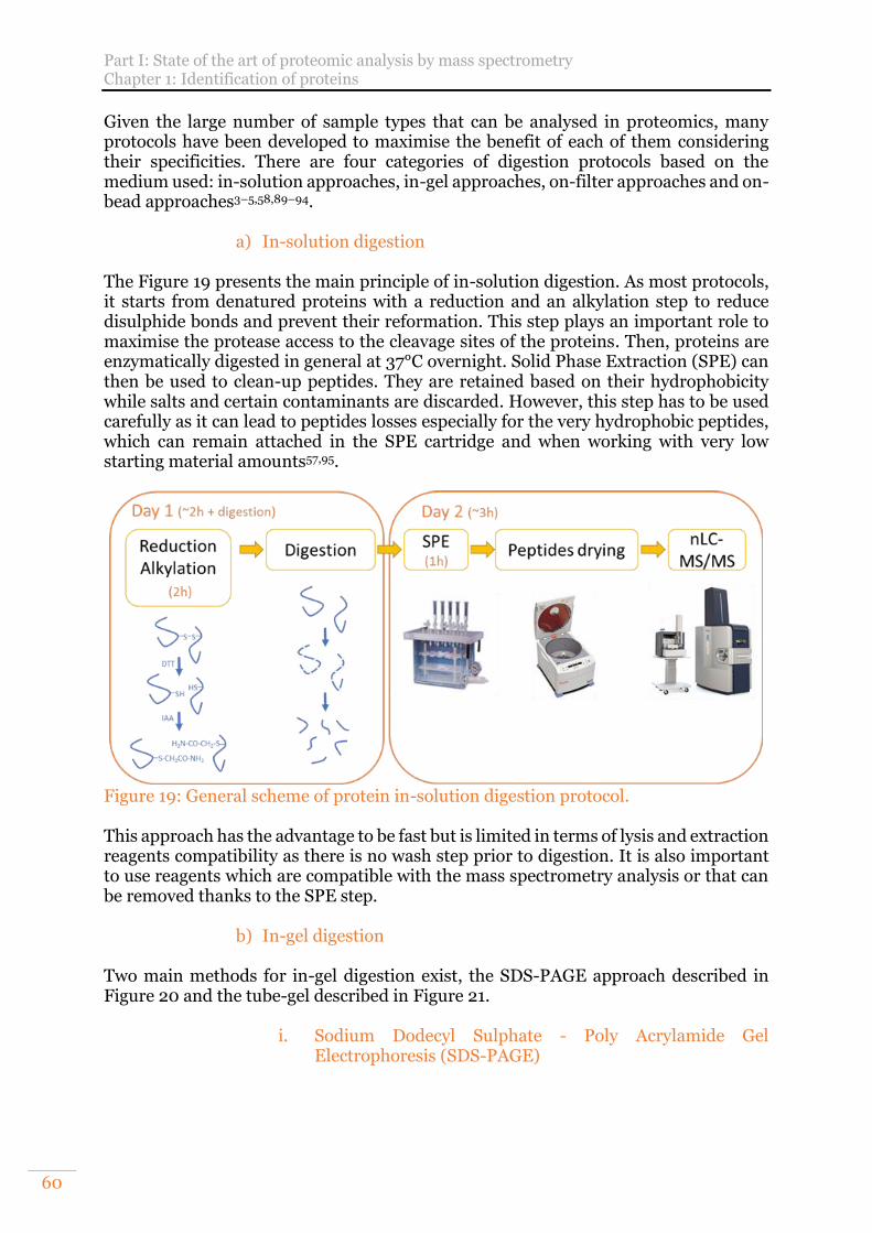
Part I: State of the art of proteomic analysis by mass spectrometry Chapter 1: Identification of proteins
60
Given the large number of sample types that can be analysed in proteomics, many protocols have been developed to maximise the benefit of each of them considering their specificities. There are four categories of digestion protocols based on the medium used: in-solution approaches, in-gel approaches, on-filter approaches and on-bead approaches3–5,58,89–94.
a) In-solution digestion The Figure 19 presents the main principle of in-solution digestion. As most protocols, it starts from denatured proteins with a reduction and an alkylation step to reduce disulphide bonds and prevent their reformation. This step plays an important role to maximise the protease access to the cleavage sites of the proteins. Then, proteins are enzymatically digested in general at 37°C overnight. Solid Phase Extraction (SPE) can then be used to clean-up peptides. They are retained based on their hydrophobicity while salts and certain contaminants are discarded. However, this step has to be used carefully as it can lead to peptides losses especially for the very hydrophobic peptides, which can remain attached in the SPE cartridge and when working with very low starting material amounts57,95.
Figure 19: General scheme of protein in-solution digestion protocol. This approach has the advantage to be fast but is limited in terms of lysis and extraction reagents compatibility as there is no wash step prior to digestion. It is also important to use reagents which are compatible with the mass spectrometry analysis or that can be removed thanks to the SPE step.
b) In-gel digestion Two main methods for in-gel digestion exist, the SDS-PAGE approach described in Figure 20 and the tube-gel described in Figure 21.
i. Sodium Dodecyl Sulphate - Poly Acrylamide Gel Electrophoresis (SDS-PAGE)
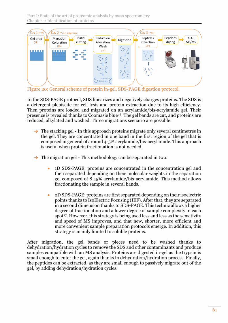
Part I: State of the art of proteomic analysis by mass spectrometry Chapter 1: Identification of proteins
61
Figure 20: General scheme of protein in-gel, SDS-PAGE digestion protocol. In the SDS-PAGE protocol, SDS linearizes and negatively charges proteins. The SDS is a detergent plebiscite for cell lysis and protein extraction due to its high efficiency. Then proteins are loaded and migrated on an acrylamide/bis-acrylamide gel. Their presence is revealed thanks to Coomasie blue96. The gel bands are cut, and proteins are reduced, alkylated and washed. Three migrations scenario are possible:
→ The stacking gel - In this approach proteins migrate only several centimetres in the gel. They are concentrated in one band in the first region of the gel that is composed in general of around 4-5% acrylamide/bis-acrylamide. This approach is useful when protein fractionation is not needed.
→ The migration gel - This methodology can be separated in two:
1D SDS-PAGE: proteins are concentrated in the concentration gel and then separated depending on their molecular weights in the separation gel composed of 8-15% acrylamide/bis-acrylamide. This method allows fractionating the sample in several bands.
2D SDS-PAGE: proteins are first separated depending on their isoelectric points thanks to IsoElectric Focusing (IEF). After that, they are separated in a second dimension thanks to SDS-PAGE. This technic allows a higher degree of fractionation and a lower degree of sample complexity in each spot27. However, this strategy is being used less and less as the sensitivity and speed of MS improves, and that new, shorter, more efficient and more convenient sample preparation protocols emerge. In addition, this strategy is mainly limited to soluble proteins.
After migration, the gel bands or pieces need to be washed thanks to dehydration/hydration cycles to remove the SDS and other contaminants and produce samples compatible with an MS analysis. Proteins are digested in-gel as the trypsin is small enough to enter the gel, again thanks to dehydration/hydration process. Finally, the peptides can be extracted, as they are small enough to passively migrate out of the gel, by adding dehydration/hydration cycles.
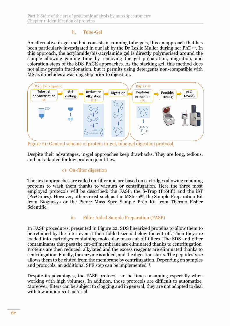
Part I: State of the art of proteomic analysis by mass spectrometry Chapter 1: Identification of proteins
62
ii. Tube-Gel An alternative in-gel method consists in running tube-gels, this an approach that has been particularly investigated in our lab by the Dr Leslie Muller during her PhD4,7. In this approach, the acrylamide/bis-acrylamide gel is directly polymerised around the sample allowing gaining time by removing the gel preparation, migration, and coloration steps of the SDS-PAGE approaches. As the stacking gel, this method does not allow protein fractionation, but it permits using detergents non-compatible with MS as it includes a washing step prior to digestion.
Figure 21: General scheme of protein in-gel, tube-gel digestion protocol. Despite their advantages, in-gel approaches keep drawbacks. They are long, tedious, and not adapted for low protein quantities.
c) On-filter digestion The next approaches are called on-filter and are based on cartridges allowing retaining proteins to wash them thanks to vacuum or centrifugation. Here the three most employed protocols will be described: the FASP, the S-Trap (Protifi) and the iST (PreOmics). However, others exist such as the MStern97, the Sample Preparation Kit from Biognosys or the Pierce Mass Spec Sample Prep Kit from Thermo Fisher Scientific.
iii. Filter Aided Sample Preparation (FASP) In FASP procedures, presented in Figure 22, SDS linearized proteins to allow them to be retained by the filter even if their folded size is below the cut-off. Then they are loaded into cartridges containing molecular mass cut-off filters. The SDS and other contaminants that pass the cut-off membrane are eliminated thanks to centrifugation. Proteins are then reduced, alkylated and the excess reagents are eliminated thanks to centrifugation. Finally, the enzyme is added, and the digestion starts. The peptides’ size allows them to be eluted from the membrane by centrifugation. Depending on samples and protocols, an additional SPE step can be implemented98. Despite its advantages, the FASP protocol can be time consuming especially when working with high volumes. In addition, those protocols are difficult to automatize. Moreover, filters can be subject to clogging and in general, they are not adapted to deal with low amounts of material.
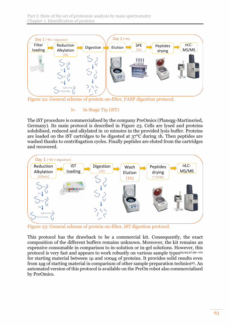
Part I: State of the art of proteomic analysis by mass spectrometry Chapter 1: Identification of proteins
63
Figure 22: General scheme of protein on-filter, FASP digestion protocol.
iv. In Stage Tip (iST) The iST procedure is commercialised by the company PreOmics (Planegg-Martinsried, Germany). Its main protocol is described in Figure 23. Cells are lysed and proteins solubilised, reduced and alkylated in 10 minutes in the provided lysis buffer. Proteins are loaded on the iST cartridges to be digested at 37°C during 1h. Then peptides are washed thanks to centrifugation cycles. Finally peptides are eluted from the cartridges and recovered.
Figure 23: General scheme of protein on-filter, iST digestion protocol. This protocol has the drawback to be a commercial kit. Consequently, the exact composition of the different buffers remains unknown. Moreover, the kit remains an expensive consumable in comparison to in-solution or in-gel solutions. However, this protocol is very fast and appears to work robustly on various sample types93,94,97,99–101 for starting material between 1µ and 100µg of proteins. It provides solid results even from 1µg of starting material in comparison of other sample preparation technics93. An automated version of this protocol is available on the PreOn robot also commercialised by PreOmics.
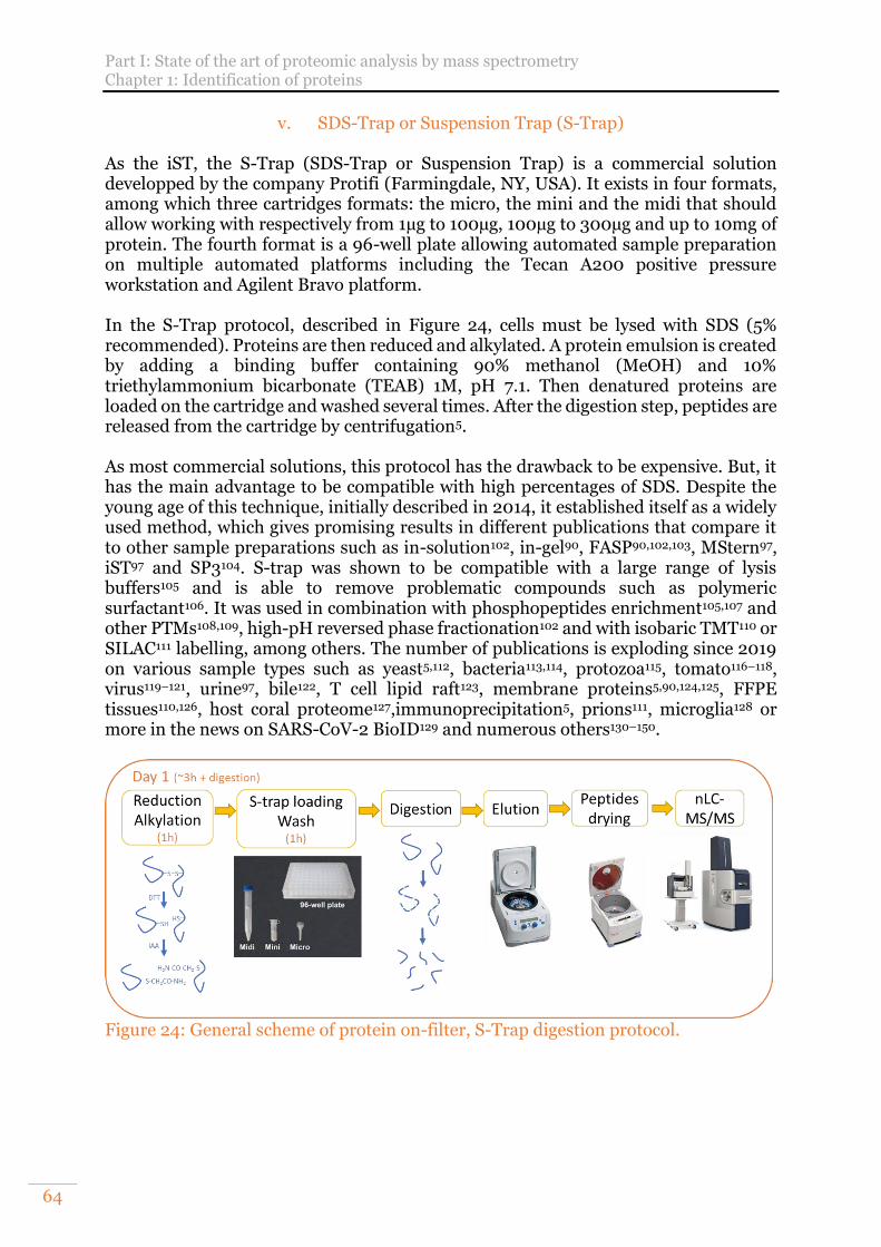
Part I: State of the art of proteomic analysis by mass spectrometry Chapter 1: Identification of proteins
64
v. SDS-Trap or Suspension Trap (S-Trap) As the iST, the S-Trap (SDS-Trap or Suspension Trap) is a commercial solution developped by the company Protifi (Farmingdale, NY, USA). It exists in four formats, among which three cartridges formats: the micro, the mini and the midi that should allow working with respectively from 1µg to 100µg, 100µg to 300µg and up to 10mg of protein. The fourth format is a 96-well plate allowing automated sample preparation on multiple automated platforms including the Tecan A200 positive pressure workstation and Agilent Bravo platform. In the S-Trap protocol, described in Figure 24, cells must be lysed with SDS (5% recommended). Proteins are then reduced and alkylated. A protein emulsion is created by adding a binding buffer containing 90% methanol (MeOH) and 10% triethylammonium bicarbonate (TEAB) 1M, pH 7.1. Then denatured proteins are loaded on the cartridge and washed several times. After the digestion step, peptides are released from the cartridge by centrifugation5. As most commercial solutions, this protocol has the drawback to be expensive. But, it has the main advantage to be compatible with high percentages of SDS. Despite the young age of this technique, initially described in 2014, it established itself as a widely used method, which gives promising results in different publications that compare it to other sample preparations such as in-solution102, in-gel90, FASP90,102,103, MStern97, iST97 and SP3104. S-trap was shown to be compatible with a large range of lysis buffers105 and is able to remove problematic compounds such as polymeric surfactant106. It was used in combination with phosphopeptides enrichment105,107 and other PTMs108,109, high-pH reversed phase fractionation102 and with isobaric TMT110 or SILAC111 labelling, among others. The number of publications is exploding since 2019 on various sample types such as yeast5,112, bacteria113,114, protozoa115, tomato116–118, virus119–121, urine97, bile122, T cell lipid raft123, membrane proteins5,90,124,125, FFPE tissues110,126, host coral proteome127,immunoprecipitation5, prions111, microglia128 or more in the news on SARS-CoV-2 BioID129 and numerous others130–150.
Figure 24: General scheme of protein on-filter, S-Trap digestion protocol.
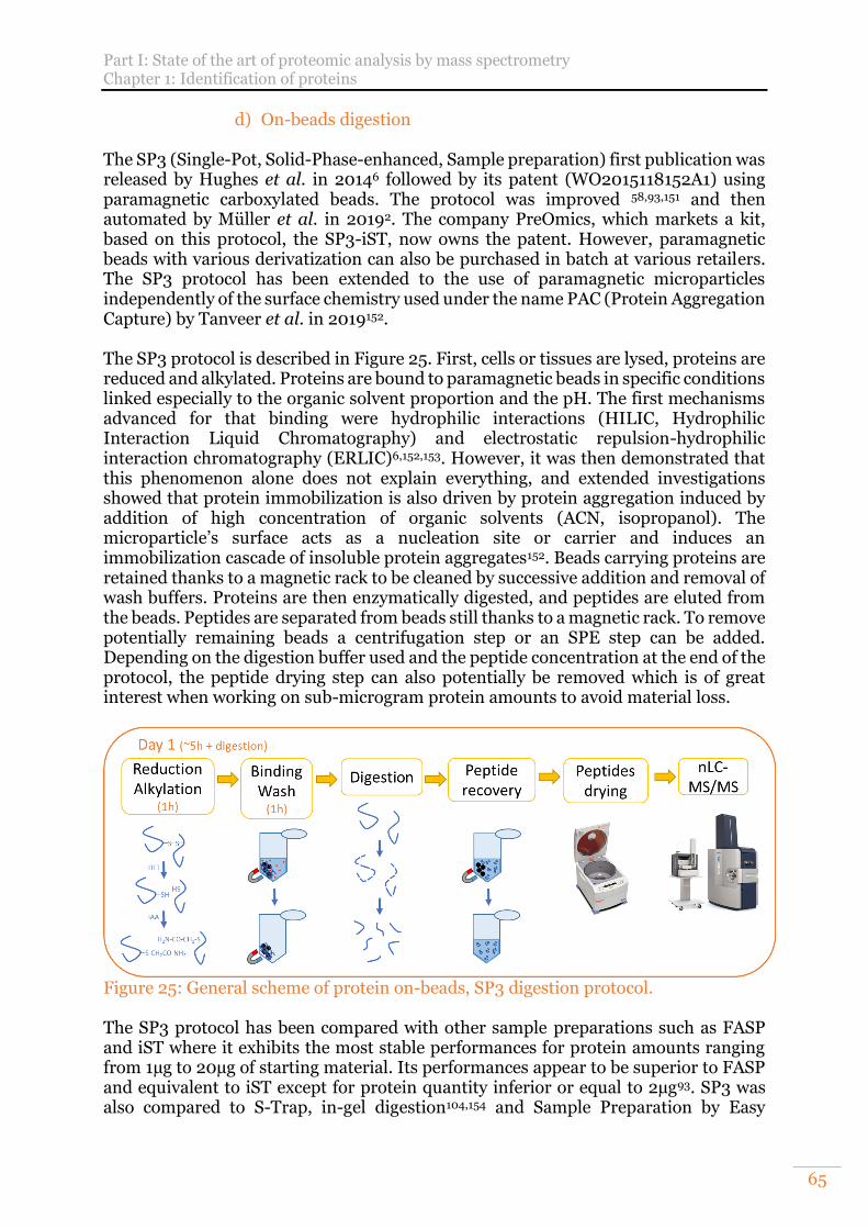
Part I: State of the art of proteomic analysis by mass spectrometry Chapter 1: Identification of proteins
65
d) On-beads digestion The SP3 (Single-Pot, Solid-Phase-enhanced, Sample preparation) first publication was released by Hughes et al. in 20146 followed by its patent (WO2015118152A1) using paramagnetic carboxylated beads. The protocol was improved 58,93,151 and then automated by Müller et al. in 20192. The company PreOmics, which markets a kit, based on this protocol, the SP3-iST, now owns the patent. However, paramagnetic beads with various derivatization can also be purchased in batch at various retailers. The SP3 protocol has been extended to the use of paramagnetic microparticles independently of the surface chemistry used under the name PAC (Protein Aggregation Capture) by Tanveer et al. in 2019152. The SP3 protocol is described in Figure 25. First, cells or tissues are lysed, proteins are reduced and alkylated. Proteins are bound to paramagnetic beads in specific conditions linked especially to the organic solvent proportion and the pH. The first mechanisms advanced for that binding were hydrophilic interactions (HILIC, Hydrophilic Interaction Liquid Chromatography) and electrostatic repulsion-hydrophilic interaction chromatography (ERLIC)6,152,153. However, it was then demonstrated that this phenomenon alone does not explain everything, and extended investigations showed that protein immobilization is also driven by protein aggregation induced by addition of high concentration of organic solvents (ACN, isopropanol). The microparticle’s surface acts as a nucleation site or carrier and induces an immobilization cascade of insoluble protein aggregates152. Beads carrying proteins are retained thanks to a magnetic rack to be cleaned by successive addition and removal of wash buffers. Proteins are then enzymatically digested, and peptides are eluted from the beads. Peptides are separated from beads still thanks to a magnetic rack. To remove potentially remaining beads a centrifugation step or an SPE step can be added. Depending on the digestion buffer used and the peptide concentration at the end of the protocol, the peptide drying step can also potentially be removed which is of great interest when working on sub-microgram protein amounts to avoid material loss.
Figure 25: General scheme of protein on-beads, SP3 digestion protocol. The SP3 protocol has been compared with other sample preparations such as FASP and iST where it exhibits the most stable performances for protein amounts ranging from 1µg to 20µg of starting material. Its performances appear to be superior to FASP and equivalent to iST except for protein quantity inferior or equal to 2µg93. SP3 was also compared to S-Trap, in-gel digestion104,154 and Sample Preparation by Easy

Part I: State of the art of proteomic analysis by mass spectrometry Chapter 1: Identification of proteins
66
Extraction and Digestion (SPEED) protocol, FASP and in-solution digestion68. In this later publication, the SPEED protocol, which is a universal, rapid, and detergent-free protocol, based on acid extraction brings globally the best performances in comparison with other technics. The SP3 protocol was demonstrated to be a viable option for samples containing very low amounts of proteins in the microgram or sub-microgram range93,155 and even for single-cell proteomics156. SP3 is virtually compatible with any kind of samples due to its compatibility with almost all lysis buffers. It is to note that it was shown compatible with high amounts of SDS up to 10%58. It was also shown that PAC and so SP3 enable to decrease the number of missed cleaved peptides in comparison with liquid digestion protocols152. The literature using SP3 protocols is already very extensive and published works applied it to numerous of different sample types such as protozoa154, yeast157,158, human2,159,160, plants161, bacteria155,158,162, FFPE tissue160,163, neurons164, rice165, immunoprecipitation166, skin167 or even paleoproteomics samples168–170. SP3 was combined with TMT and SILAC labelling152,157,164. It can also be used prior to phosphopeptides or glycopeptides enrichment152. A miniaturised version of SP3 sample preparation has been designed to fit on microfluidic chips opening another new field of applications171. SP3 can also be followed by peptide fractionation strategies172 (CIF). SP3 sample preparation is thus not limited to sample preparation for bottom-up proteomics approaches. The paramagnetic beads used for SP3 and PAC, can also be used to purify peptides thanks to specific binding conditions. This procedure was published under the SP2 denomination153. SP3 was also used with success for denaturing top-down proteomics studies.173,174 To conclude, SP3 is an extremely versatile protocol compatible with almost any kind of bottom-up studies, quantitative or not, even on sub-microgram protein amounts or on single-cells. Its main application is already extended to work on peptides or for denaturing top-down studies174. Finally, two independent groups already automate this protocol on an AssayMap Bravo robot 1,2, which will be a great help for studies with hundreds of samples making it an ideal option for high throughput studies.
4) Automated sample preparation for bottom-up proteomics As illustrated in the previous sections, a quantum leap has been made since 2014 in the development and democratisation of new sample preparation protocols. This gap is like the one, which occurred in automated genomic in the 2000’s. These are simpler, faster, more repeatable, and efficient on any type of samples even on small amounts or even on single cell protein extracts. These improvements were intended not only to improve the quality of future projects but also to free up researchers' time so that they could concentrate their efforts on other critical steps such as data acquisition or processing. They can also be hijack of their primary use to adapt to specific situation, as it was the case of numerous AssayMap Bravo, which were converted during the COVID crisis to perform PCR. The other objective is to make the proteomics community capable of routinely analysing large cohorts of hundreds of samples, among which cohorts of clinical samples at high throughput to identify new disease markers or discover new
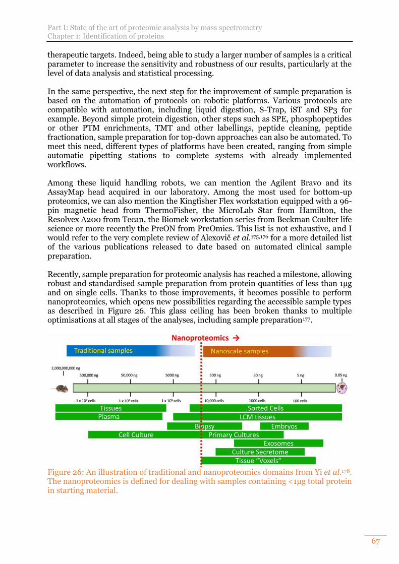
Part I: State of the art of proteomic analysis by mass spectrometry Chapter 1: Identification of proteins
67
therapeutic targets. Indeed, being able to study a larger number of samples is a critical parameter to increase the sensitivity and robustness of our results, particularly at the level of data analysis and statistical processing. In the same perspective, the next step for the improvement of sample preparation is based on the automation of protocols on robotic platforms. Various protocols are compatible with automation, including liquid digestion, S-Trap, iST and SP3 for example. Beyond simple protein digestion, other steps such as SPE, phosphopeptides or other PTM enrichments, TMT and other labellings, peptide cleaning, peptide fractionation, sample preparation for top-down approaches can also be automated. To meet this need, different types of platforms have been created, ranging from simple automatic pipetting stations to complete systems with already implemented workflows. Among these liquid handling robots, we can mention the Agilent Bravo and its AssayMap head acquired in our laboratory. Among the most used for bottom-up proteomics, we can also mention the Kingfisher Flex workstation equipped with a 96-pin magnetic head from ThermoFisher, the MicroLab Star from Hamilton, the Resolvex A200 from Tecan, the Biomek workstation series from Beckman Coulter life science or more recently the PreON from PreOmics. This list is not exhaustive, and I would refer to the very complete review of Alexovič et al.175,176 for a more detailed list of the various publications released to date based on automated clinical sample preparation. Recently, sample preparation for proteomic analysis has reached a milestone, allowing robust and standardised sample preparation from protein quantities of less than 1µg and on single cells. Thanks to those improvements, it becomes possible to perform nanoproteomics, which opens new possibilities regarding the accessible sample types as described in Figure 26. This glass ceiling has been broken thanks to multiple optimisations at all stages of the analyses, including sample preparation177.
Figure 26: An illustration of traditional and nanoproteomics domains from Yi et al.178. The nanoproteomics is defined for dealing with samples containing <1μg total protein in starting material.
Part I: State of the art of proteomic analysis by mass spectrometry Chapter 1: Identification of proteins
68
Recent developments include nested nanoPOTS array (N2) microfluidic chips (nanodroplet Processing in One-pot for Trace Samples) that drastically reduce well volume, allowing a 230% gain in peptide/protein recovery with a median CV of about 16%. These arrays are also compatible with TMT labelling and allow the analysis of 243 single cells on a single chip179. That chip is an improvement of the already published nanoPOTS chip52,180,181. The second recent improvement regarding this technology is its automation via a commercial single cell isolation and picoliter dispenser, the cellenONE from Cellenion (Lyon, France) that includes a direct interfacing with a standard autosampler for LC-MS/MS analysis. This platform allowed to reproducibly yield around 500 protein groups per single HeLa cell and 1,422 protein groups across 30 single cell measurements182. It is interesting to note the development of interfacing possibility between the “sample preparation” and the LC-MS/MS system as it is the case with the cellenONE robot or with the ADE-OPI-MS183 system developed by AB Sciex (Framingham, MA, USA.). This is very important to reduce drastically loss of material, to work on the freshest possible sample and could represent a time saving if an automated online management system supporting every part of the coupling, from sample preparation to MS analysis, is designed. If we have fun digressing towards what could be the future of proteomics, we could imagine a complete online-automated accessible and robust pipeline. This technology could be adapted to perform extensive bioanalysis for personalised medicine in hospitals, as it is already the case for example on microorganisms’ cultures with actual dedicated platforms such as the MALDI-TOF, VitekMS and Vitek 2 from Biomérieux or the Biotyper series from Bruker Daltonics. However, this time it would be with the precision level of the single cell, which could be of highest interest for example to characterise tumour with a high cell heterogeneity to adapt treatments.
B. Liquid chromatography coupled to tandem mass spectrometry
Different kind of separation technics can be coupled to mass spectrometry with different goals, forces, and drawbacks. We can cite the liquid chromatography-mass spectrometry (LC-MS), the capillary electrophoresis-mass spectrometry (CE-MS) or the gas phase chromatography-mass spectrometry (GC-MS) for example. For the separation of peptides prior to mass spectrometry analysis, the LC-MS is the most plebiscite technique.
1) Peptide separation by reversed phase liquid chromatography Enzymatic digestion is the basis of the bottom-up approach in proteomics. However, it also has its weaknesses. One of these is that the samples become more complex as they move from the protein level to the much more numerous peptides23,37. If many peptides co-elute, the signals will suffer from suppression effects. Furthermore, the mass spectrometer will not be able to isolate and fragment all of them or will generate multiplexed fragmentation spectra resulting from multiple precursor ions. To overcome this problem, the peptide mixture is separated by a prior liquid chromatographic step. An efficient separation will increase the sensitivity, selectivity and coverage of the proteome studied77,184.
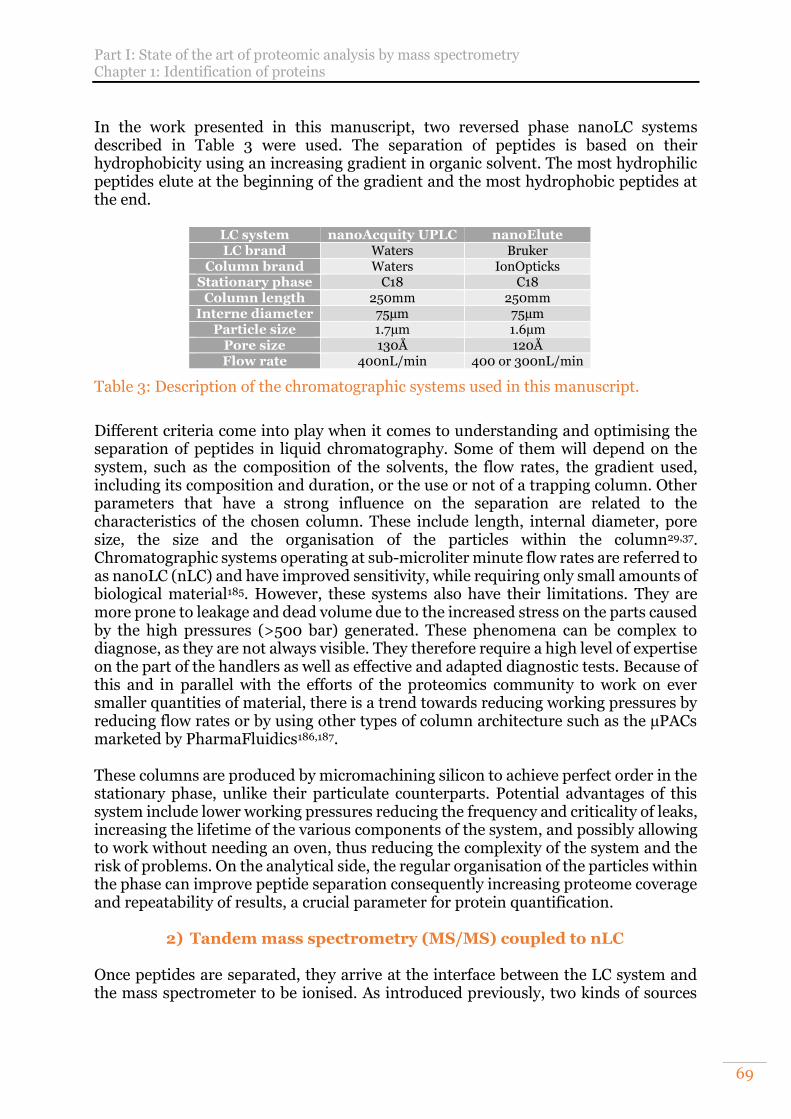
Part I: State of the art of proteomic analysis by mass spectrometry Chapter 1: Identification of proteins
69
In the work presented in this manuscript, two reversed phase nanoLC systems described in Table 3 were used. The separation of peptides is based on their hydrophobicity using an increasing gradient in organic solvent. The most hydrophilic peptides elute at the beginning of the gradient and the most hydrophobic peptides at the end.
LC system nanoAcquity UPLC nanoElute LC brand Waters Bruker
Column brand Waters IonOpticks Stationary phase C18 C18
Column length 250mm 250mm Interne diameter 75µm 75µm
Particle size 1.7µm 1.6µm Pore size 130Å 120Å Flow rate 400nL/min 400 or 300nL/min
Table 3: Description of the chromatographic systems used in this manuscript.
Different criteria come into play when it comes to understanding and optimising the separation of peptides in liquid chromatography. Some of them will depend on the system, such as the composition of the solvents, the flow rates, the gradient used, including its composition and duration, or the use or not of a trapping column. Other parameters that have a strong influence on the separation are related to the characteristics of the chosen column. These include length, internal diameter, pore size, the size and the organisation of the particles within the column29,37. Chromatographic systems operating at sub-microliter minute flow rates are referred to as nanoLC (nLC) and have improved sensitivity, while requiring only small amounts of biological material185. However, these systems also have their limitations. They are more prone to leakage and dead volume due to the increased stress on the parts caused by the high pressures (>500 bar) generated. These phenomena can be complex to diagnose, as they are not always visible. They therefore require a high level of expertise on the part of the handlers as well as effective and adapted diagnostic tests. Because of this and in parallel with the efforts of the proteomics community to work on ever smaller quantities of material, there is a trend towards reducing working pressures by reducing flow rates or by using other types of column architecture such as the µPACs marketed by PharmaFluidics186,187. These columns are produced by micromachining silicon to achieve perfect order in the stationary phase, unlike their particulate counterparts. Potential advantages of this system include lower working pressures reducing the frequency and criticality of leaks, increasing the lifetime of the various components of the system, and possibly allowing to work without needing an oven, thus reducing the complexity of the system and the risk of problems. On the analytical side, the regular organisation of the particles within the phase can improve peptide separation consequently increasing proteome coverage and repeatability of results, a crucial parameter for protein quantification.
2) Tandem mass spectrometry (MS/MS) coupled to nLC Once peptides are separated, they arrive at the interface between the LC system and the mass spectrometer to be ionised. As introduced previously, two kinds of sources
Part I: State of the art of proteomic analysis by mass spectrometry Chapter 1: Identification of proteins
70
can be used to analyse biological macromolecules, the MALDI188,189 and the ESI34,35 but only the last one can be coupled online to the MS instrument (ESI-LC-MS).
a) Electrospray ionisation (ESI) The ESI source is based on the use of a high voltage at a capillary feeding the sample in solution to the spectrometer or directly into it. A spray of charged drops containing the sample is formed by a nebulisation phenomenon. These micro-droplets will evaporate until they contain too many charges of the same polarity confined in a restricted space reaching the Rayleigh limit and causing them to explode. These serial explosions will allow the release of multi-charged molecules free of solvent molecules that will enter the mass spectrometer34,35. At this stage, it is particularly important that the sample does not contain salts that may compete with the peptides for ionisation or may form adducts190.
b) Analyser types After their ionisation, peptides go through the mass spectrometer to be analysed or fragmented and then measured at a detector. Classically, LC-MS couplings allow obtaining three types of information: peptides retention time, peptides and fragments mass/charge ratios and their intensities. Different types of analysers were or are still used today in mass spectrometers dedicated to bottom-up proteomics applications190.
i. Time of flight (TOF) Professor William Stephens first introduced the time-of-flight analyser in 1946. It consists of a tube, usually between 0.5 and 3m long, under a high vacuum in which the ions will fly after being accelerated with equal energies191,192. Their speed through the flight tube will be inversely proportional to their mass. The lightest ions will arrive faster at the detector which will measure the impact of the ions allowing the calculation of their flight time from which their mass to charge ratio (m/z) will be deduced. The intensity is determined from the number of ions that hit the detector. The resolution of a TOF analyser is therefore correlated to the length of the flight tube. To increase the resolution without increasing the size of the analyser, TOFs incorporating an electrostatic mirror, known as a reflectron, have been developed to double the flight distance. These systems also increase the resolution by compensating for small variations in kinetic energy within the population of the same ion. Indeed, the faster ions will penetrate further into the reflectron and have more distance to travel than the slower ions allowing them to arrive at the detector simultaneously190. Among the latest innovations on this type of analyser, this year the manufacturer Waters has unveiled a new mass spectrometer, the select series MRT, and featuring new MRT (Multi Reflecting Time-of-Flight) technology. This technology allows a three-dimensional focusing of the ions through multiple intra-TOF lenses allowing 46 reflections in the TOF and thus a flight path of more than 47 metres with minimal losses providing very high resolution mass spectra (>200,000 FWHM).
ii. Quadrupole
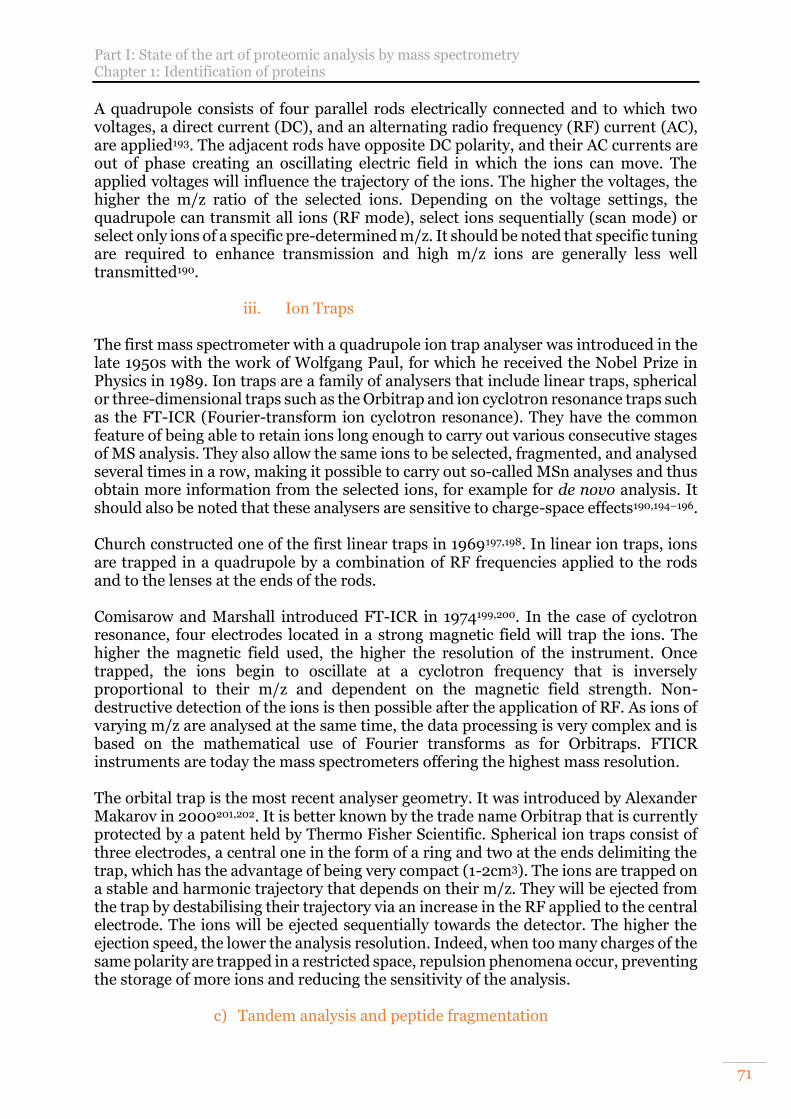
Part I: State of the art of proteomic analysis by mass spectrometry Chapter 1: Identification of proteins
71
A quadrupole consists of four parallel rods electrically connected and to which two voltages, a direct current (DC), and an alternating radio frequency (RF) current (AC), are applied193. The adjacent rods have opposite DC polarity, and their AC currents are out of phase creating an oscillating electric field in which the ions can move. The applied voltages will influence the trajectory of the ions. The higher the voltages, the higher the m/z ratio of the selected ions. Depending on the voltage settings, the quadrupole can transmit all ions (RF mode), select ions sequentially (scan mode) or select only ions of a specific pre-determined m/z. It should be noted that specific tuning are required to enhance transmission and high m/z ions are generally less well transmitted190.
iii. Ion Traps The first mass spectrometer with a quadrupole ion trap analyser was introduced in the late 1950s with the work of Wolfgang Paul, for which he received the Nobel Prize in Physics in 1989. Ion traps are a family of analysers that include linear traps, spherical or three-dimensional traps such as the Orbitrap and ion cyclotron resonance traps such as the FT-ICR (Fourier-transform ion cyclotron resonance). They have the common feature of being able to retain ions long enough to carry out various consecutive stages of MS analysis. They also allow the same ions to be selected, fragmented, and analysed several times in a row, making it possible to carry out so-called MSn analyses and thus obtain more information from the selected ions, for example for de novo analysis. It should also be noted that these analysers are sensitive to charge-space effects190,194–196. Church constructed one of the first linear traps in 1969197,198. In linear ion traps, ions are trapped in a quadrupole by a combination of RF frequencies applied to the rods and to the lenses at the ends of the rods. Comisarow and Marshall introduced FT-ICR in 1974199,200. In the case of cyclotron resonance, four electrodes located in a strong magnetic field will trap the ions. The higher the magnetic field used, the higher the resolution of the instrument. Once trapped, the ions begin to oscillate at a cyclotron frequency that is inversely proportional to their m/z and dependent on the magnetic field strength. Non-destructive detection of the ions is then possible after the application of RF. As ions of varying m/z are analysed at the same time, the data processing is very complex and is based on the mathematical use of Fourier transforms as for Orbitraps. FTICR instruments are today the mass spectrometers offering the highest mass resolution. The orbital trap is the most recent analyser geometry. It was introduced by Alexander Makarov in 2000201,202. It is better known by the trade name Orbitrap that is currently protected by a patent held by Thermo Fisher Scientific. Spherical ion traps consist of three electrodes, a central one in the form of a ring and two at the ends delimiting the trap, which has the advantage of being very compact (1-2cm3). The ions are trapped on a stable and harmonic trajectory that depends on their m/z. They will be ejected from the trap by destabilising their trajectory via an increase in the RF applied to the central electrode. The ions will be ejected sequentially towards the detector. The higher the ejection speed, the lower the analysis resolution. Indeed, when too many charges of the same polarity are trapped in a restricted space, repulsion phenomena occur, preventing the storage of more ions and reducing the sensitivity of the analysis.
c) Tandem analysis and peptide fragmentation
Part I: State of the art of proteomic analysis by mass spectrometry Chapter 1: Identification of proteins
72
The tandem analysis of peptides is based on the analysis of MS1 spectra also called MS providing information at the peptide level and on the analysis of MS2 or MS/MS spectra providing information on the fragments generated from the peptides. Fragmentation can occur at different locations depending on the dissociation method used and the fragments generated are named according to the Biemann nomenclature203 presented in Figure 27.
Figure 27: Biemann nomenclature for peptide fragmentation. The ions a, b and c carry the positive charge at the N-terminus and ions x, y and z carry it at the C-terminus. This fragmentation can be achieved in different ways thanks to collision induced dissociation (CID)204, higher energy C-trap dissociation (HCD)205, electron transfer dissociation (ETD)206, electron capture dissociation (ECD)207 or electron transfer higher energy C-trap dissociation (EThcD)208 that is a mix between ETD and HCD. In bottom-up approaches, CID and HCD are the most used dissociation methods. In both cases, ions are accelerated and collide with neutral gas atoms (argon, helium, nitrogen) in the collision chamber. The kinetic energy is converted in internal energy inducing the peptide bond rupture following the mobile proton model80,81. The only difference of HCD is that prior fragmentation, ions are accumulated in the C-trap then they are sent to the collision cell, fragmented, come back in the C-trap and finally fragments are sent to the analyser. For that reason, HCD fragmentation is specific to Orbitrap instruments. CID and HCD lead especially to the formation of b and y ions in the Biemann nomenclature in opposition to ETD and ECD that generate mostly c and z ions. ETD and ECD can be useful for labile PTM analysis. The different child ions of one precursor are analysed at the same time to generate MS2 spectra.
d) Data dependent acquisition (DDA) and Data Independent Acquisition (DIA)
Peptide analysis by mass spectrometry can be carried out in different ways depending on the objective of the project and the instrumentation available. These different ways of proceeding often rely on different data acquisition strategies. The most used strategy for bottom-up approach is the DDA or data dependent acquisition. In this strategy, a MS1 spectrum of the parent ions is performed and then a Top N, i.e., a number N of the most intense ions seen in the MS1 spectrum is selected and fragmented one by one to generate MS2 spectra as described in Figure 28. This acquisition mode allows the identification and quantification of several thousands of proteins and a good proteome coverage209,210. Unfortunately, this remains a stochastic approach as only the N most intense ions are fragmented resulting in a lack of repeatability despite increasingly sensitive instrumentation due to undersampling of the ions.
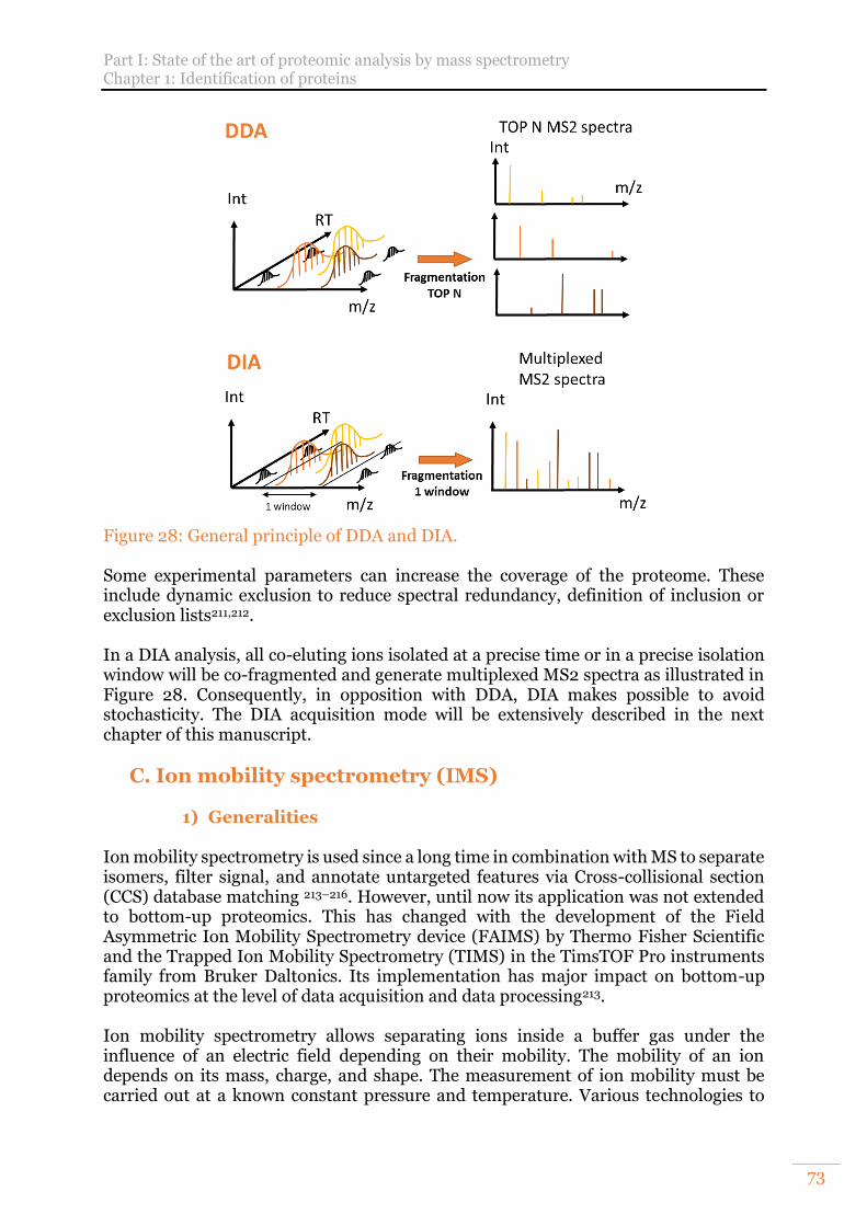
Part I: State of the art of proteomic analysis by mass spectrometry Chapter 1: Identification of proteins
73
Figure 28: General principle of DDA and DIA. Some experimental parameters can increase the coverage of the proteome. These include dynamic exclusion to reduce spectral redundancy, definition of inclusion or exclusion lists211,212. In a DIA analysis, all co-eluting ions isolated at a precise time or in a precise isolation window will be co-fragmented and generate multiplexed MS2 spectra as illustrated in Figure 28. Consequently, in opposition with DDA, DIA makes possible to avoid stochasticity. The DIA acquisition mode will be extensively described in the next chapter of this manuscript.
C. Ion mobility spectrometry (IMS)
1) Generalities Ion mobility spectrometry is used since a long time in combination with MS to separate isomers, filter signal, and annotate untargeted features via Cross-collisional section (CCS) database matching 213–216. However, until now its application was not extended to bottom-up proteomics. This has changed with the development of the Field Asymmetric Ion Mobility Spectrometry device (FAIMS) by Thermo Fisher Scientific and the Trapped Ion Mobility Spectrometry (TIMS) in the TimsTOF Pro instruments family from Bruker Daltonics. Its implementation has major impact on bottom-up proteomics at the level of data acquisition and data processing213. Ion mobility spectrometry allows separating ions inside a buffer gas under the influence of an electric field depending on their mobility. The mobility of an ion depends on its mass, charge, and shape. The measurement of ion mobility must be carried out at a known constant pressure and temperature. Various technologies to
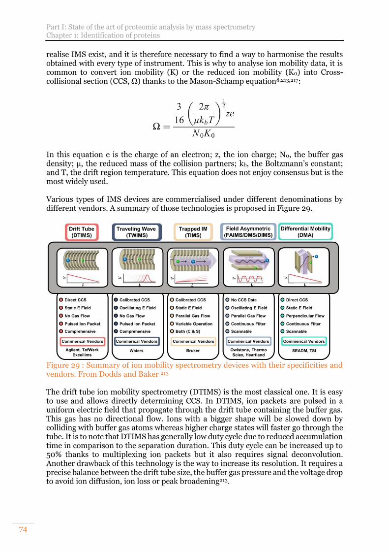
Part I: State of the art of proteomic analysis by mass spectrometry Chapter 1: Identification of proteins
74
realise IMS exist, and it is therefore necessary to find a way to harmonise the results obtained with every type of instrument. This is why to analyse ion mobility data, it is common to convert ion mobility (K) or the reduced ion mobility (K0) into Cross-collisional section (CCS, Ω) thanks to the Mason-Schamp equation8,213,217:
In this equation e is the charge of an electron; z, the ion charge; N0, the buffer gas density; μ, the reduced mass of the collision partners; kb, the Boltzmann’s constant; and T, the drift region temperature. This equation does not enjoy consensus but is the most widely used. Various types of IMS devices are commercialised under different denominations by different vendors. A summary of those technologies is proposed in Figure 29.
Figure 29 : Summary of ion mobility spectrometry devices with their specificities and vendors. From Dodds and Baker 213 The drift tube ion mobility spectrometry (DTIMS) is the most classical one. It is easy to use and allows directly determining CCS. In DTIMS, ion packets are pulsed in a uniform electric field that propagate through the drift tube containing the buffer gas. This gas has no directional flow. Ions with a bigger shape will be slowed down by colliding with buffer gas atoms whereas higher charge states will faster go through the tube. It is to note that DTIMS has generally low duty cycle due to reduced accumulation time in comparison to the separation duration. This duty cycle can be increased up to 50% thanks to multiplexing ion packets but it also requires signal deconvolution. Another drawback of this technology is the way to increase its resolution. It requires a precise balance between the drift tube size, the buffer gas pressure and the voltage drop to avoid ion diffusion, ion loss or peak broadening213.
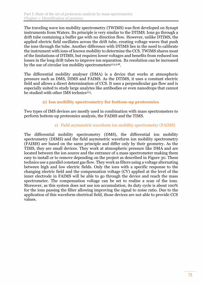
Part I: State of the art of proteomic analysis by mass spectrometry Chapter 1: Identification of proteins
75
The traveling wave ion mobility spectrometry (TWIMS) was first developed on Synapt instruments from Waters. Its principle is very similar to the DTIMS. Ions go through a drift tube containing a buffer gas with no direction flow. However, unlike DTIMS, the applied electric field oscillates across the drift tube, creating voltage waves that push the ions through the tube. Another difference with DTIMS lies in the need to calibrate the instrument with ions of known mobility to determine the CCS. TWIMS shares most of the limitations of DTIMS, but requires lower voltages and benefits from reduced ion losses in the long drift tubes to improve ion separation. Its resolution can be increased by the use of circular ion mobility spectrometers213,218. The differential mobility analyser (DMA) is a device that works at atmospheric pressure such as DMS, DIMS and FAIMS. As the DTIMS, it uses a constant electric field and allows a direct determination of CCS. It uses a perpendicular gas flow and is especially suited to study large analytes like antibodies or even nanodrops that cannot be studied with other IMS technics213.
2) Ion mobility spectrometry for bottom-up proteomics Two types of IMS devices are mostly used in combination with mass spectrometers to perform bottom-up proteomics analysis, the FAIMS and the TIMS.
a) Field asymmetric waveform ion mobility spectrometry (FAIMS) The differential mobility spectrometry (DMS), the differential ion mobility spectrometry (DIMS) and the field asymmetric waveform ion mobility spectrometry (FAIMS) are based on the same principle and differ only by their geometry. As the TIMS, they are small devices. They work at atmospheric pressure like DMA and are located between the ion source and the entrance of a mass spectrometer making them easy to install or to remove depending on the project as described in Figure 30. These technics use a parallel constant gas flow. They work as filters using a voltage alternating between high and low electric fields. Only the ions with a specific response to the changing electric field and the compensation voltage (CV) applied at the level of the inner electrode in FAIMS will be able to go through the device and reach the mass spectrometer. The compensation voltage can be set to realise a scan of the ions. Moreover, as this system does not use ion accumulation, its duty cycle is about 100% for the ions passing the filter allowing improving the signal to noise ratio. Due to the application of this waveform electrical field, those devices are not able to provide CCS values.
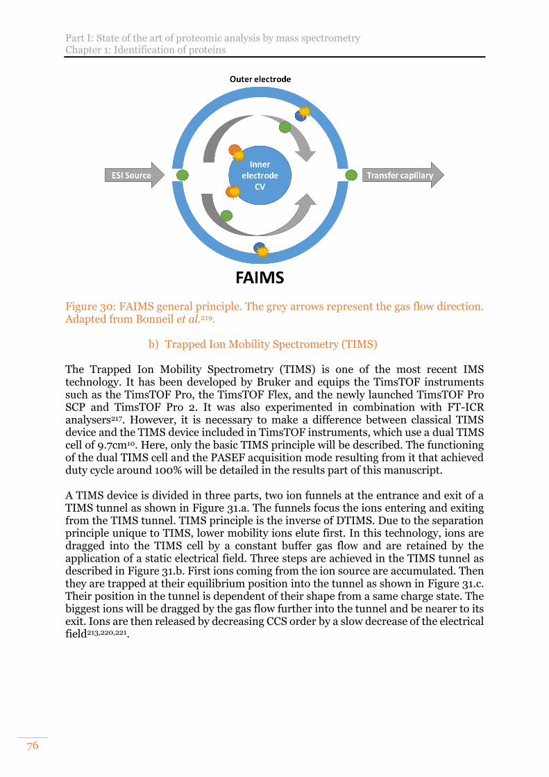
Part I: State of the art of proteomic analysis by mass spectrometry Chapter 1: Identification of proteins
76
Figure 30: FAIMS general principle. The grey arrows represent the gas flow direction. Adapted from Bonneil et al.219.
b) Trapped Ion Mobility Spectrometry (TIMS) The Trapped Ion Mobility Spectrometry (TIMS) is one of the most recent IMS technology. It has been developed by Bruker and equips the TimsTOF instruments such as the TimsTOF Pro, the TimsTOF Flex, and the newly launched TimsTOF Pro SCP and TimsTOF Pro 2. It was also experimented in combination with FT-ICR analysers217. However, it is necessary to make a difference between classical TIMS device and the TIMS device included in TimsTOF instruments, which use a dual TIMS cell of 9.7cm10. Here, only the basic TIMS principle will be described. The functioning of the dual TIMS cell and the PASEF acquisition mode resulting from it that achieved duty cycle around 100% will be detailed in the results part of this manuscript. A TIMS device is divided in three parts, two ion funnels at the entrance and exit of a TIMS tunnel as shown in Figure 31.a. The funnels focus the ions entering and exiting from the TIMS tunnel. TIMS principle is the inverse of DTIMS. Due to the separation principle unique to TIMS, lower mobility ions elute first. In this technology, ions are dragged into the TIMS cell by a constant buffer gas flow and are retained by the application of a static electrical field. Three steps are achieved in the TIMS tunnel as described in Figure 31.b. First ions coming from the ion source are accumulated. Then they are trapped at their equilibrium position into the tunnel as shown in Figure 31.c. Their position in the tunnel is dependent of their shape from a same charge state. The biggest ions will be dragged by the gas flow further into the tunnel and be nearer to its exit. Ions are then released by decreasing CCS order by a slow decrease of the electrical field213,220,221.
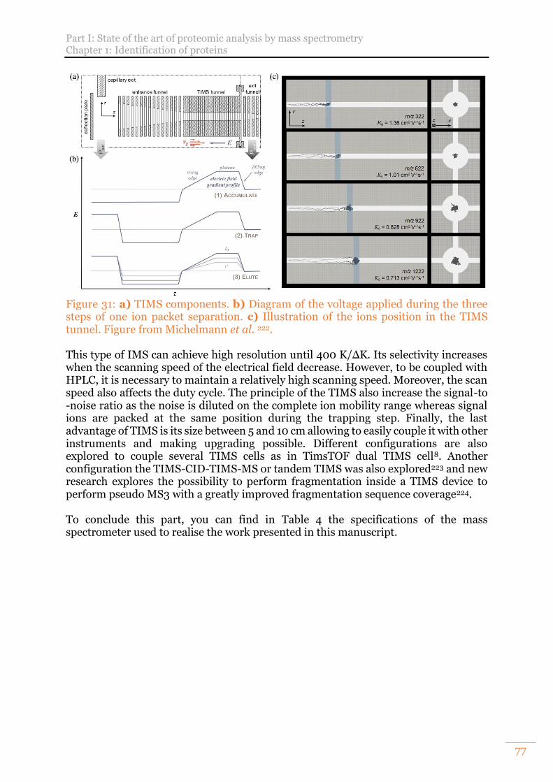
Part I: State of the art of proteomic analysis by mass spectrometry Chapter 1: Identification of proteins
77
Figure 31: a) TIMS components. b) Diagram of the voltage applied during the three steps of one ion packet separation. c) Illustration of the ions position in the TIMS tunnel. Figure from Michelmann et al. 222. This type of IMS can achieve high resolution until 400 K/ΔK. Its selectivity increases when the scanning speed of the electrical field decrease. However, to be coupled with HPLC, it is necessary to maintain a relatively high scanning speed. Moreover, the scan speed also affects the duty cycle. The principle of the TIMS also increase the signal-to -noise ratio as the noise is diluted on the complete ion mobility range whereas signal ions are packed at the same position during the trapping step. Finally, the last advantage of TIMS is its size between 5 and 10 cm allowing to easily couple it with other instruments and making upgrading possible. Different configurations are also explored to couple several TIMS cells as in TimsTOF dual TIMS cell8. Another configuration the TIMS-CID-TIMS-MS or tandem TIMS was also explored223 and new research explores the possibility to perform fragmentation inside a TIMS device to perform pseudo MS3 with a greatly improved fragmentation sequence coverage224. To conclude this part, you can find in Table 4 the specifications of the mass spectrometer used to realise the work presented in this manuscript.
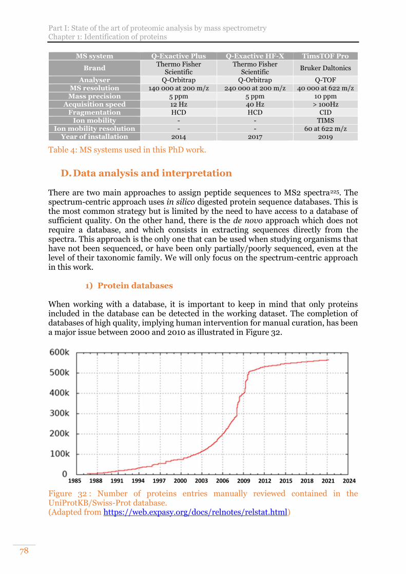
Part I: State of the art of proteomic analysis by mass spectrometry Chapter 1: Identification of proteins
78
MS system Q-Exactive Plus Q-Exactive HF-X TimsTOF Pro
Brand Thermo Fisher
Scientific Thermo Fisher
Scientific Bruker Daltonics
Analyser Q-Orbitrap Q-Orbitrap Q-TOF MS resolution 140 000 at 200 m/z 240 000 at 200 m/z 40 000 at 622 m/z Mass precision 5 ppm 5 ppm 10 ppm
Acquisition speed 12 Hz 40 Hz > 100Hz Fragmentation HCD HCD CID
Ion mobility - - TIMS Ion mobility resolution - - 60 at 622 m/z
Year of installation 2014 2017 2019
Table 4: MS systems used in this PhD work.
D. Data analysis and interpretation There are two main approaches to assign peptide sequences to MS2 spectra225. The spectrum-centric approach uses in silico digested protein sequence databases. This is the most common strategy but is limited by the need to have access to a database of sufficient quality. On the other hand, there is the de novo approach which does not require a database, and which consists in extracting sequences directly from the spectra. This approach is the only one that can be used when studying organisms that have not been sequenced, or have been only partially/poorly sequenced, even at the level of their taxonomic family. We will only focus on the spectrum-centric approach in this work.
1) Protein databases When working with a database, it is important to keep in mind that only proteins included in the database can be detected in the working dataset. The completion of databases of high quality, implying human intervention for manual curation, has been a major issue between 2000 and 2010 as illustrated in Figure 32.
Figure 32 : Number of proteins entries manually reviewed contained in the UniProtKB/Swiss-Prot database. (Adapted from https://web.expasy.org/docs/relnotes/relstat.html)
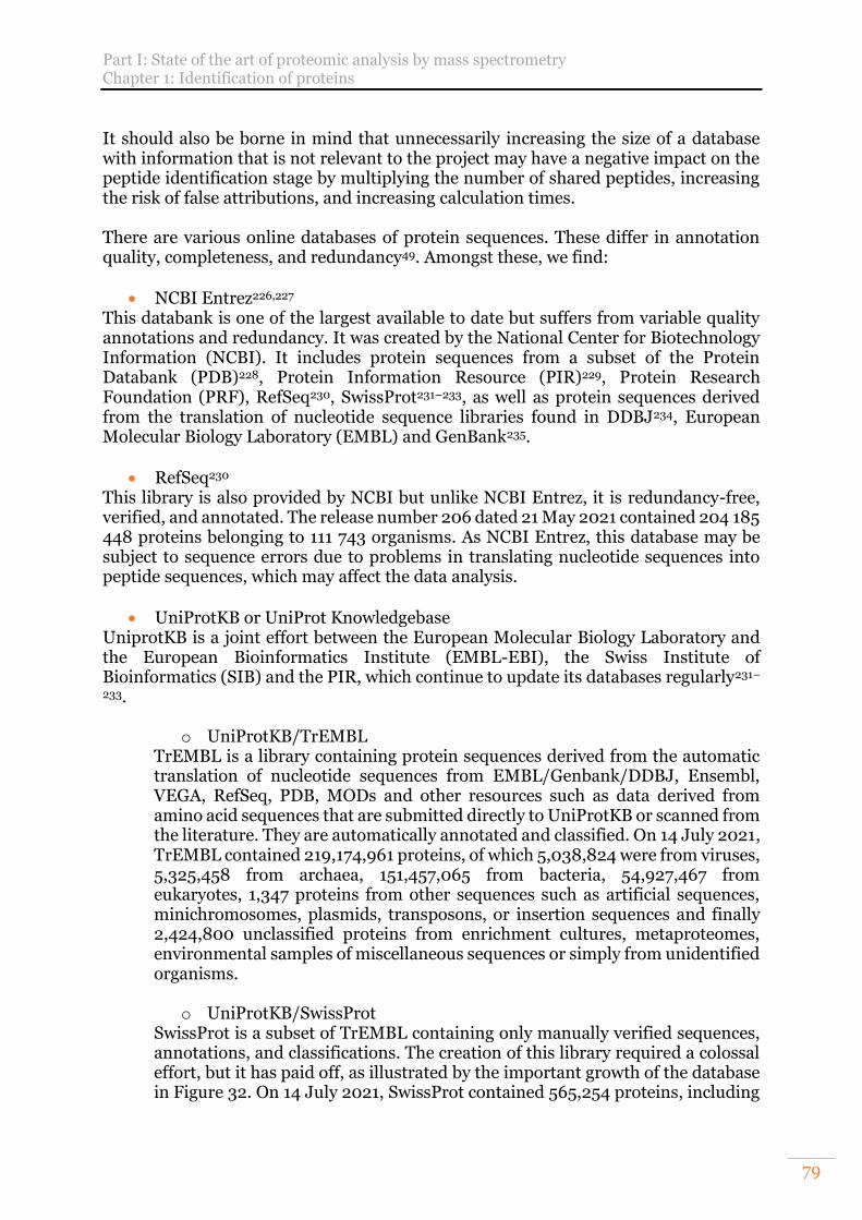
Part I: State of the art of proteomic analysis by mass spectrometry Chapter 1: Identification of proteins
79
It should also be borne in mind that unnecessarily increasing the size of a database with information that is not relevant to the project may have a negative impact on the peptide identification stage by multiplying the number of shared peptides, increasing the risk of false attributions, and increasing calculation times. There are various online databases of protein sequences. These differ in annotation quality, completeness, and redundancy49. Amongst these, we find:
NCBI Entrez226,227 This databank is one of the largest available to date but suffers from variable quality annotations and redundancy. It was created by the National Center for Biotechnology Information (NCBI). It includes protein sequences from a subset of the Protein Databank (PDB)228, Protein Information Resource (PIR)229, Protein Research Foundation (PRF), RefSeq230, SwissProt231–233, as well as protein sequences derived from the translation of nucleotide sequence libraries found in DDBJ234, European Molecular Biology Laboratory (EMBL) and GenBank235.
RefSeq230 This library is also provided by NCBI but unlike NCBI Entrez, it is redundancy-free, verified, and annotated. The release number 206 dated 21 May 2021 contained 204 185 448 proteins belonging to 111 743 organisms. As NCBI Entrez, this database may be subject to sequence errors due to problems in translating nucleotide sequences into peptide sequences, which may affect the data analysis.
UniProtKB or UniProt Knowledgebase UniprotKB is a joint effort between the European Molecular Biology Laboratory and the European Bioinformatics Institute (EMBL-EBI), the Swiss Institute of Bioinformatics (SIB) and the PIR, which continue to update its databases regularly231–
233.
o UniProtKB/TrEMBL TrEMBL is a library containing protein sequences derived from the automatic translation of nucleotide sequences from EMBL/Genbank/DDBJ, Ensembl, VEGA, RefSeq, PDB, MODs and other resources such as data derived from amino acid sequences that are submitted directly to UniProtKB or scanned from the literature. They are automatically annotated and classified. On 14 July 2021, TrEMBL contained 219,174,961 proteins, of which 5,038,824 were from viruses, 5,325,458 from archaea, 151,457,065 from bacteria, 54,927,467 from eukaryotes, 1,347 proteins from other sequences such as artificial sequences, minichromosomes, plasmids, transposons, or insertion sequences and finally 2,424,800 unclassified proteins from enrichment cultures, metaproteomes, environmental samples of miscellaneous sequences or simply from unidentified organisms.
o UniProtKB/SwissProt
SwissProt is a subset of TrEMBL containing only manually verified sequences, annotations, and classifications. The creation of this library required a colossal effort, but it has paid off, as illustrated by the important growth of the database in Figure 32. On 14 July 2021, SwissProt contained 565,254 proteins, including
Part I: State of the art of proteomic analysis by mass spectrometry Chapter 1: Identification of proteins
80
17,014 from viruses, 19,653 from archaea, 335,066 from bacteria and 193,521 from eukaryotes.
NeXtProt236,237 NeXtProt was created by the SIB in 2010 and is limited to the human proteome. It draws data from the Bgee238, COSMIC239,240, Ensembl, ENZYME, GlyConnect, gnomAD241, GO, HPA, IntAct242, InterPro243, MassIVE244,245, MeSH, PeptideAtlas, PROSITE, PubMed, SRMAtlas, UniProt-GOA and UniProtKB/Swiss-Prot databases. In addition to protein sequence information, NeXtProt offers sequence variants, expression, localisation, PTMs, isoforms and experimental information from proteomic experiments. Version 2.35.0 released on 15/02/2021 contained 20379 proteins, 42368 isoforms and 191837 PTMs, among others. The regular updating of sequence libraries following the discovery of new proteins, new variants, or new modifications, among others, is progressively making it possible to identify more and more peptides from MS2 spectra that were previously impossible to assign246. In addition, the cross-referencing of data from different omics disciplines allows for the enrichment of functional annotations, gene prediction algorithms or peptide and protein identification237. This combination is known among others as proteogenomics and is promising but requires complex data integration workflows247–
249. The work presented in this thesis was carried out using sequence databases mainly from UniProtKB/SwissProt and occasionally from UniProtKB/TrEMBL
2) Proteomics search engines On one hand, once the raw data has been acquired, the various information of interest such as m/z, peptide and fragment intensities as well as their linkage and retention time are extracted and compiled into a peaklist. These are our experimental data. On the other hand, we will choose an appropriate database to search the data. This later will be digested in silico with the experimentally used enzyme and will constitute our theoretical data. The identification of the peptides will be done by comparing the experimental and theoretical data. This approach is known as Peptide Fragmentation Fingerprinting (PFF). Once the peptides have been identified, they will be associated with proteins by inference50. Inference is a complex process that is carried out in different ways in the various existing algorithms. Because of shared peptides, it is sometimes impossible to associate strictly a peptide to a protein. The principle of parsimony will then be used to define the smallest possible group of proteins to which a shared peptide could belong to49. As a result, protein identification results are most often groups of proteins presented under different names depending on the software, such as protein group or protein set. There are many search engines, which can realise this work in an automated way. Each possesses its own specificities. Verheggen et al. had compiled a comprehensive list of the different search engines available in 2015250. These results are presented in Table 5 to illustrate the large number of possibilities that exist. However, it should be noted that many of these software packages are no longer updated.
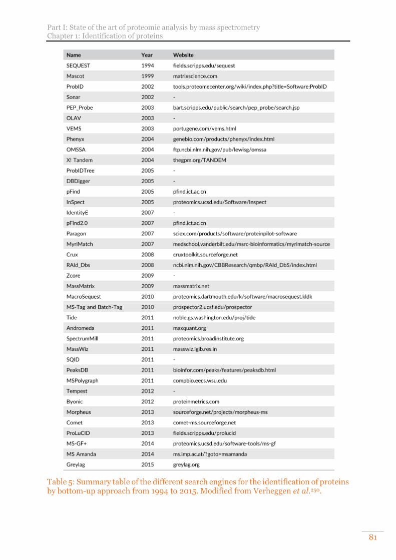
Part I: State of the art of proteomic analysis by mass spectrometry Chapter 1: Identification of proteins
81
Table 5: Summary table of the different search engines for the identification of proteins by bottom-up approach from 1994 to 2015. Modified from Verheggen et al.250.
Part I: State of the art of proteomic analysis by mass spectrometry Chapter 1: Identification of proteins
82
Search engines require setting series of parameters. The number of parameters accessible highly differs from one algorithm to another, which can be both a force and a drawback. Nevertheless, some parameters are necessary for all of them such as:
→ The protein database → The enzyme to use for the database in silico digestion → The maximum number of enzymes missed cleavages allowed → The fragmentation used and the type of fragments awaited → The parent and fragment charges awaited → The amino acid modification systematically or punctualy present → The mass error tolerance at the level of peptides and fragments
As with all stages of the proteomics analysis pipeline, search engines have made great strides since the early 2000s, as evidenced by the raft of new engines released during this period. Search engines have also benefited from advances in instrumental techniques. However, some limitations remain, and it is common to observe that the number of unassigned MS2 spectra in an analysis represents 60 to 75% of the total spectra acquired. There are several reasons for this251:
The quality of low intensity or partially fragmented MS2 spectra252 Some strategies are being developed at the instrumental level to overcome this problem. The TimsTOF Pro has a dedicated process that fragments the same precursor several times within a certain intensity range (not intense enough to be of good quality but too intense to be background) and sums the intensity of the MS2 spectra obtained to increase the overall quality.
The generation of chimeric spectra from the co-fragmentation of several peptides coeluted from the LC and located in a very close m/z window (1-3m/z in general)253. It should be noted that the introduction of ion mobility in bottom-up proteomics analysis via TIMS or FAIMS reduces this problem thanks to a better separation of species with very close m/z and co-eluting from the LC separation thanks to their different mobility coefficients. Beyond the non-attribution of spectra, this point is also problematic for the calculation of the score. Therefore, several search engines have developed workarounds. Andromeda can perform a second search when two species are present on its m/z and retention time maps with such a small m/z delta that it is not possible to select them separately. Since version 2.5, Mascot can also identify multiple peptides within chimeric spectra. (http://www.matrixscience.com/help/june2014.html; and http://www.matrixscience.com/blog/how-many-of-you-are-there-in-there-processing-and-searching-chimeric-msms-spectra-with-mascot-distiller-and-mascot-server.html)
The number of modifications requested is often very limited compared to all known/possible modifications and has to be adapted depending on the sample and the project goal254.
Part I: State of the art of proteomic analysis by mass spectrometry Chapter 1: Identification of proteins
83
This is particularly true for PTMs sought as variable modifications, as this explodes the resource and computational time requirements. The proportion of unassigned spectra due to this limitation is estimated to be around one third of all spectra. However, new and faster search engines, more adapted to searches without enzymes or numerous PTMs, tend to appear, such as MSFragger15,255.
The use of incomplete, error-prone, or unsuitable protein sequence databases as described in the previous section. One way to solve this problem is to use higher quality databases. However, when it is not possible, a hybrid approach using de novo interpretation can be used as it is the case in Peaks with the deep-learning-based model DeepNovo256,257.
Errors in data processing such as incorrect peak extraction, incorrect assignment of the monoisotopic peak or assignment of the wrong charge state.
The work presented in this manuscript was carried out using the following search engines: Andromeda, Mascot, Pulsar and Peaks. Mascot is a commercial search engine from Matrix Science. Its algorithm is not open- source. Each MS2 spectrum allows it to calculate an ion score. The purpose of this is to assess the probability that the match between the spectrum and the in silico digested database is a false positive. The higher the score, the more robust the identification. However, this score only considers the quality of the spectrum and does not evaluate the quality of the database used, which is evaluated using identity and homology thresholds. Andromeda is a free, but non-open-source engine published in 2011 by Jürgen Cox and his team. It is integrated into the MaxQuant software and has a spectra calibration function. This algorithm is based on a probability notation just like Mascot. Although their score scales differ, they offer comparable results. Pulsar is also a commercial, non-open-source algorithm sold by Biognosys (Schlieren, Switzerland). It has been implemented in the Spectronaut and SpectroMine software. It allows the processing of DDA data but also the generation of spectral libraries for the processing of DIA data31,258–260. Finally, the Peaks software includes a search algorithm and is a non-open-source commercial software from Bioinformatics Solutions (Waterloo, Ontario, Canada). It has the particularity of integrating a de novo search in addition to the identification approach by Peptide Fragmentation Fingerprinting via DeepNovo256,257.
3) Validation of protein identifications The search algorithms will look for matches between theoretical and experimental data. They will also assign mostly quality scores to the MS2 spectra. Unfortunately, these scores are not sufficient to rule out the possibility of a bad match. Moreover, the size of the datasets generated nowadays makes it impossible to check each spectrum manually. For this reason, an automated strategy has been introduced, the target-decoy approach261–263.
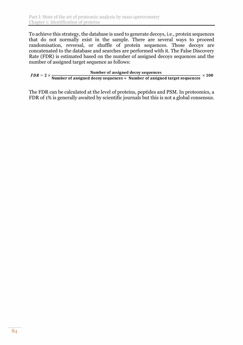
Part I: State of the art of proteomic analysis by mass spectrometry Chapter 1: Identification of proteins
84
To achieve this strategy, the database is used to generate decoys, i.e., protein sequences that do not normally exist in the sample. There are several ways to proceed randomisation, reversal, or shuffle of protein sequences. Those decoys are concatenated to the database and searches are performed with it. The False Discovery Rate (FDR) is estimated based on the number of assigned decoys sequences and the number of assigned target sequence as follows:
The FDR can be calculated at the level of proteins, peptides and PSM. In proteomics, a FDR of 1% is generally awaited by scientific journals but this is not a global consensus.
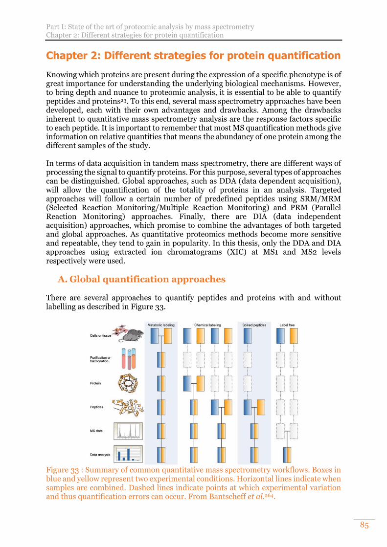
Part I: State of the art of proteomic analysis by mass spectrometry Chapter 2: Different strategies for protein quantification
85
Chapter 2: Different strategies for protein quantification Knowing which proteins are present during the expression of a specific phenotype is of great importance for understanding the underlying biological mechanisms. However, to bring depth and nuance to proteomic analysis, it is essential to be able to quantify peptides and proteins23. To this end, several mass spectrometry approaches have been developed, each with their own advantages and drawbacks. Among the drawbacks inherent to quantitative mass spectrometry analysis are the response factors specific to each peptide. It is important to remember that most MS quantification methods give information on relative quantities that means the abundancy of one protein among the different samples of the study. In terms of data acquisition in tandem mass spectrometry, there are different ways of processing the signal to quantify proteins. For this purpose, several types of approaches can be distinguished. Global approaches, such as DDA (data dependent acquisition), will allow the quantification of the totality of proteins in an analysis. Targeted approaches will follow a certain number of predefined peptides using SRM/MRM (Selected Reaction Monitoring/Multiple Reaction Monitoring) and PRM (Parallel Reaction Monitoring) approaches. Finally, there are DIA (data independent acquisition) approaches, which promise to combine the advantages of both targeted and global approaches. As quantitative proteomics methods become more sensitive and repeatable, they tend to gain in popularity. In this thesis, only the DDA and DIA approaches using extracted ion chromatograms (XIC) at MS1 and MS2 levels respectively were used.
A. Global quantification approaches There are several approaches to quantify peptides and proteins with and without labelling as described in Figure 33.
Figure 33 : Summary of common quantitative mass spectrometry workflows. Boxes in blue and yellow represent two experimental conditions. Horizontal lines indicate when samples are combined. Dashed lines indicate points at which experimental variation and thus quantification errors can occur. From Bantscheff et al.264.
Part I: State of the art of proteomic analysis by mass spectrometry Chapter 2: Different strategies for protein quantification
86
1) Label-based quantification strategies The starting assumption for labelled relative quantification strategies is that isotopically labelled and unlabelled peptides have the same physico-chemical properties. This includes retention time, ease of ionization and fragmentation patterns. Thus, the only criterion differentiating labelled and unlabelled peptides will be their mass, the labelled forms being heavier. The advantage of the labelled approaches is the multiplexing that allows analysing several samples in one analysis, which reduced the constraints of the stability of the analytical coupling and allows comparing the measurements to perform quantification.
a) Metabolic and enzymatic labelling Metabolic labelling consists in using the metabolism of the cells to incorporate stable isotopic markers into their proteins. This labelling is therefore carried out upstream of sample preparation when the cells are cultured in a specific medium. This approach allows labelling all proteins and limits the biases that can be introduced during the different steps of the sample preparation. The most common strategy is SILAC (Stable Isotope Labelling with Amino acids in Cell culture)265. In this, cultures prepared with 13C, 15N labelled Lysine and Arginine are mixed in equivalent amounts prior to sample preparation. After LC-MS/MS analysis, the MS1 signal intensities between labelled and unlabelled peptides are compared to perform the relative quantification. Despite its accuracy, this strategy suffers from being applicable only to cell cultures or SILAC mice266. Moreover, the number of conditions that can be multiplexed is limited to three. Different strategies have therefore been developed to overcome these difficulties. The super-SILAC adds marked internal standards to control the quality of the quantification267. NeuCode (Neutron enCoding) allows increasing the number of multiplexing conditions by using Lysine isotopologues and by combining other labelling strategies268. Another type of metabolic labelling is based on the use of heavy water (H218O) during enzymatic reactions269,270. However, this strategy and all metabolic labelling approaches suffer from poor multiplexing capabilities that can be improved by chemical labelling.
b) Chemical labelling In contrast to metabolic labelling, chemical labelling is performed during sample preparation. Part of them is realised prior to digestion whereas other are realised at peptides level. These strategies modify the reactive groups of certain amino acids, in particular the amine functions of lysine or the thiol functions of cysteine residues with a stable isotopic tag. The first of these strategies is the ICAT (Isotope Coded Affinity Tag)271. This tagging technique uses heavy and light reagents and requires mixing of the samples to be compared, which allows to get rid of the constraint of the reproducibility of the analytical coupling by carrying out the quantification in a single analysis. It uses a reagent divided into three parts, a reactive function that will react with the thiol groups of cysteine-containing proteins, a linker labelled with heavy and light isotopes and a tag, often biotin, to allow an enrichment step in ICAT modified peptides via its affinity for streptavidin. This approach is limited because it is only applicable to cysteine-containing peptides. This concern was subsequently resolved by modifying the linkers to use 13C. Finally, biotin can lead to interference in MS signals.
Part I: State of the art of proteomic analysis by mass spectrometry Chapter 2: Different strategies for protein quantification
87
Here again, developments have been carried out and have led to the creation of cleavable linkers allowing the removal of the biotin tag before MS analysis272. A second category of chemical labelling, which is also the most widely used in recent years, is the use of isobaric labels that react with the reactive functions of amino acid side chains and the N-terminus of peptides. The approaches using amine functions are the most common, but others have been described using cysteine residues and carbonyl groups. The isobaric tags used in these approaches have a peptide-reactive moiety and a cleavable moiety in the CID or HCD mass spectrometry fragmentation step. The different tags used in an experiment to multiplex several conditions will be isobaric to avoid unnecessary complexification of the sample at the peptide level. However, the different fragments also called reporter ions will have different masses. The relative quantification is done by calculating the ratio of the intensity of the MS2 spectra of the reporter ions. Among these approaches, we note the TMT (Tandem Mass Tag, Thermo Fisher Scientific) allowing us to multiplex up to 18 conditions273–276 and the iTRAQ (Isobaric Tag Relative and Absolute Quantification, Sciex) allowing us to multiplex up to 8 samples274,277. However, this type of relative quantification suffers from a compression of the ratios due to interferences272. This can be partially compensated by performing MS3 analysis, which consists in an additional step of isolation and fragmentation of fragments from MS2 analysis.
2) Label-free quantification strategies Label-free quantification has gained in popularity in recent years thanks to the various developments in mass spectrometers and bioinformatics tools. The new generations of instruments allow improved sensitivity278 and a significant increase in their acquisition speed with instruments that can now exceed 100Hz as is the case of the TimsTOF Pro with acquisition modes using PASEF8,10. These strategies are also popular because of their low cost and ease of implementation since they do not require any additional labelling steps. These approaches are not limited in number of conditions since they do not use multiplexing strategies272. However, this point has the disadvantage of making them sensitive to any source of variability during the sample preparation as well as during data acquisition where the stability of the coupling throughout the complete sequence analysis becomes critical279. For that reason, normalisation is commonly performed to compensate that variability. Finally, this type of quantification is applicable to any type of samples. This approach of quantification can be performed from acquisitions in DDA or DIA mode, but the latter will be described in the part specifically dedicated to it.
a) Spectral counting The starting assumption of label-free quantification based on MS2 spectra is as follows: the abundance of a protein is correlated to the number of MS2 spectra acquired on its belonging peptides. One of the advantages of this method is its simplicity, both in terms of sample preparation and data acquisition and processing. Unfortunately, this strategy suffers from the drawbacks inherent to DDA acquisitions, i.e., stochasticity, undersampling and difficulty in identifying and quantifying low abundant peptides in samples with a large dynamic range. This leads to a loss of repeatability of results and increases the number of missing values. For a spectral counting approach, the dynamic exclusion parameter should be removed or minimized. Otherwise, the results will be biased by the limitation of the spectra redundancy. Another limitation is the size of the
Part I: State of the art of proteomic analysis by mass spectrometry Chapter 2: Different strategies for protein quantification
88
proteins studied. The larger a protein is the more peptides it will have and the more likely it is that these peptides will be selected and fragmented. Therefore, the quantification of small proteins (<20kDa) would be more biased and less accurate272. To compensate, normalization methods based on protein length, mass or detection probability of the spectra have been developed. Another problem inherent to all quantification strategies will be the management of peptides shared between several proteins. In the case of spectrum counting, the counting of these peptides is usually weighted by sharing them between the different parent proteins based on the results obtained for single peptides264,280.
b) Extracted ion chromatogram (XIC) The relative quantification without labelling based on the extraction of ion currents from MS1 spectra is based on the following assumption: the abundance of a peptide is linearly correlated to its extracted ion current also called XIC (eXtracted Ion Chromatogram). This type of approach has been democratized with the advent of HR/AM (High-Resolution/Accurate-Mass) mass spectrometers allowing us to correctly separate the different isotopes of the precursor ions. The extraction of an ion current is presented in Figure 34. An algorithm will scan the MS1 spectra for peaks respecting a Gaussian distribution and will assign a centroid mass. A peak can be defined in two cases. First, when the intensity drops to zero or second, when the intensity reaches a local minimum as shown in Figure 34.a and b. Once the peaks and their masses are determined, the spectra are assembled according to their retention time to generate three-dimensional peaks (m/z, intensity, and retention time) as shown in Figure 34.c. This assembly is realized only if the m/z value between two adjacent spectra is close enough. An example of a reconstructed peak visualized in two and three dimensions is shown in Figure 34.d and e. Once the peaks are reconstructed it becomes possible to identify the isotopic clusters and thus to determine the charges of the peptides. In Figure 34.f, eleven peaks are visualized, and form two distinct isotopic clusters also called features11.
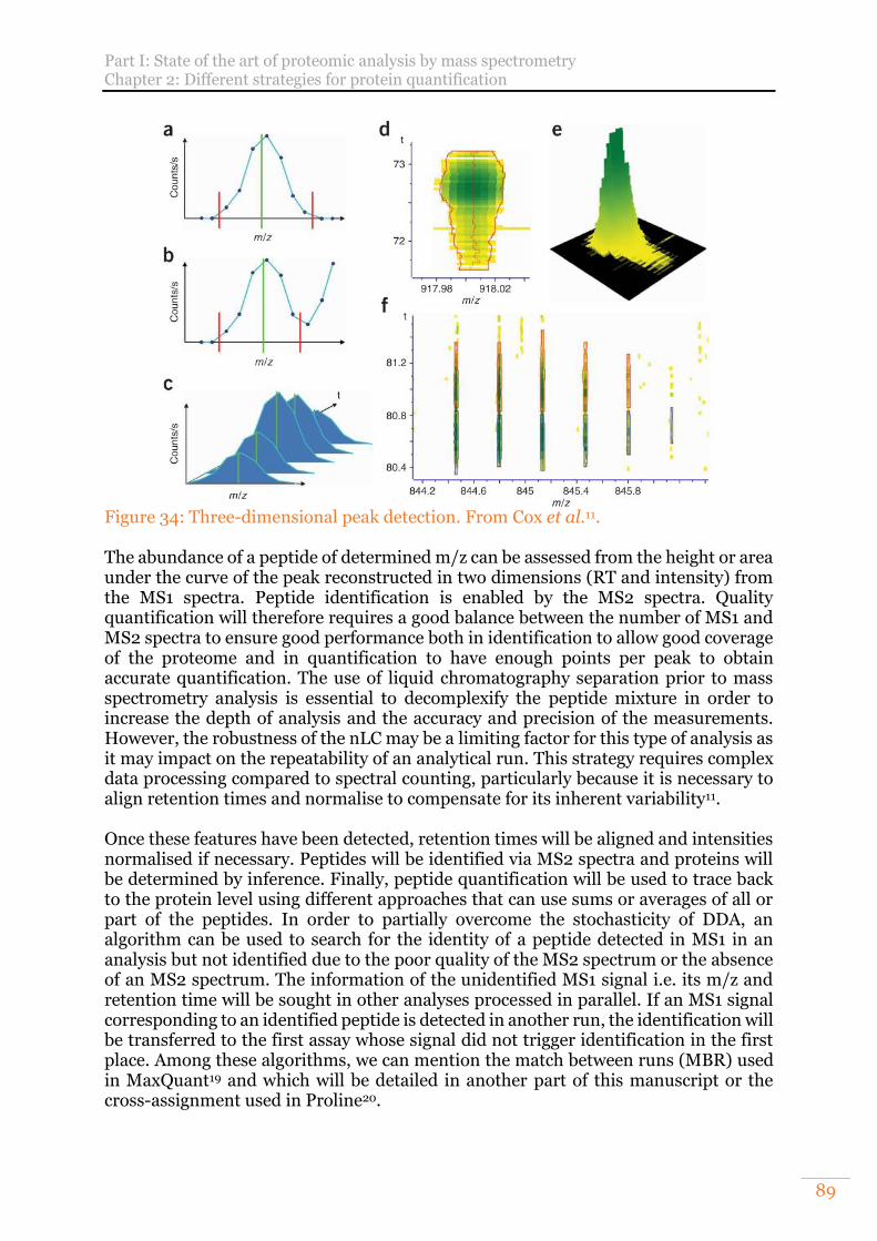
Part I: State of the art of proteomic analysis by mass spectrometry Chapter 2: Different strategies for protein quantification
89
Figure 34: Three-dimensional peak detection. From Cox et al.11. The abundance of a peptide of determined m/z can be assessed from the height or area under the curve of the peak reconstructed in two dimensions (RT and intensity) from the MS1 spectra. Peptide identification is enabled by the MS2 spectra. Quality quantification will therefore requires a good balance between the number of MS1 and MS2 spectra to ensure good performance both in identification to allow good coverage of the proteome and in quantification to have enough points per peak to obtain accurate quantification. The use of liquid chromatography separation prior to mass spectrometry analysis is essential to decomplexify the peptide mixture in order to increase the depth of analysis and the accuracy and precision of the measurements. However, the robustness of the nLC may be a limiting factor for this type of analysis as it may impact on the repeatability of an analytical run. This strategy requires complex data processing compared to spectral counting, particularly because it is necessary to align retention times and normalise to compensate for its inherent variability11. Once these features have been detected, retention times will be aligned and intensities normalised if necessary. Peptides will be identified via MS2 spectra and proteins will be determined by inference. Finally, peptide quantification will be used to trace back to the protein level using different approaches that can use sums or averages of all or part of the peptides. In order to partially overcome the stochasticity of DDA, an algorithm can be used to search for the identity of a peptide detected in MS1 in an analysis but not identified due to the poor quality of the MS2 spectrum or the absence of an MS2 spectrum. The information of the unidentified MS1 signal i.e. its m/z and retention time will be sought in other analyses processed in parallel. If an MS1 signal corresponding to an identified peptide is detected in another run, the identification will be transferred to the first assay whose signal did not trigger identification in the first place. Among these algorithms, we can mention the match between runs (MBR) used in MaxQuant19 and which will be detailed in another part of this manuscript or the cross-assignment used in Proline20.
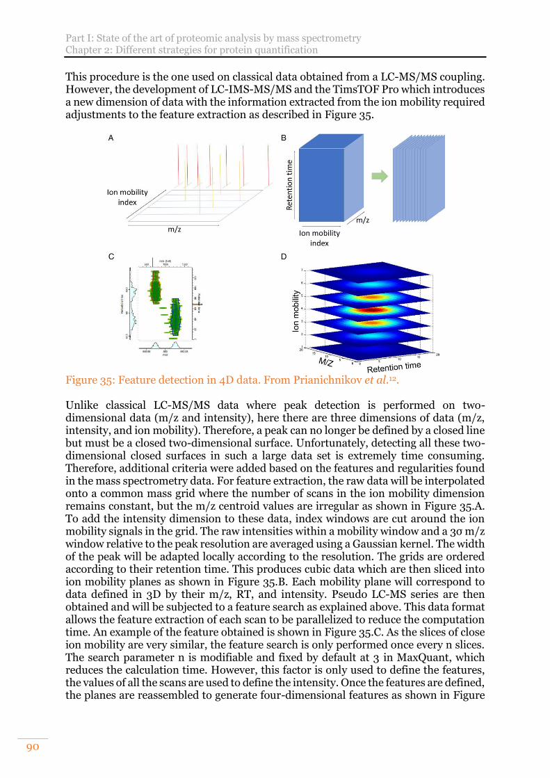
Part I: State of the art of proteomic analysis by mass spectrometry Chapter 2: Different strategies for protein quantification
90
This procedure is the one used on classical data obtained from a LC-MS/MS coupling. However, the development of LC-IMS-MS/MS and the TimsTOF Pro which introduces a new dimension of data with the information extracted from the ion mobility required adjustments to the feature extraction as described in Figure 35.
Figure 35: Feature detection in 4D data. From Prianichnikov et al.12. Unlike classical LC-MS/MS data where peak detection is performed on two-dimensional data (m/z and intensity), here there are three dimensions of data (m/z, intensity, and ion mobility). Therefore, a peak can no longer be defined by a closed line but must be a closed two-dimensional surface. Unfortunately, detecting all these two-dimensional closed surfaces in such a large data set is extremely time consuming. Therefore, additional criteria were added based on the features and regularities found in the mass spectrometry data. For feature extraction, the raw data will be interpolated onto a common mass grid where the number of scans in the ion mobility dimension remains constant, but the m/z centroid values are irregular as shown in Figure 35.A. To add the intensity dimension to these data, index windows are cut around the ion mobility signals in the grid. The raw intensities within a mobility window and a 3σ m/z window relative to the peak resolution are averaged using a Gaussian kernel. The width of the peak will be adapted locally according to the resolution. The grids are ordered according to their retention time. This produces cubic data which are then sliced into ion mobility planes as shown in Figure 35.B. Each mobility plane will correspond to data defined in 3D by their m/z, RT, and intensity. Pseudo LC-MS series are then obtained and will be subjected to a feature search as explained above. This data format allows the feature extraction of each scan to be parallelized to reduce the computation time. An example of the feature obtained is shown in Figure 35.C. As the slices of close ion mobility are very similar, the feature search is only performed once every n slices. The search parameter n is modifiable and fixed by default at 3 in MaxQuant, which reduces the calculation time. However, this factor is only used to define the features, the values of all the scans are used to define the intensity. Once the features are defined, the planes are reassembled to generate four-dimensional features as shown in Figure
Part I: State of the art of proteomic analysis by mass spectrometry Chapter 2: Different strategies for protein quantification
91
35.D. The global intensity of a feature is defined as the integral of the signals in the volume12. There is a plethora of software to process this type of data, among which we can cite those used in this thesis, namely: SpectroMine (Biognosys) and Peaks (Bioinformatics Solutions) which are licensed for a fee. MaxQuant12,14,19 is free but not open source and Proline20 is free, open source and developed by the French proteomics infrastructure ProFI. Each of these software packages has its own features. It should be noted that Proline has only recently been able to support 4D data for label-free quantification and is currently being evaluated. Comparative studies of these different software packages have already been proposed and we ourselves have taken an interest in the issue which will be discussed later in this manuscript20,281,282.
c) “Absolute” quantification In contrast to relative quantification, which gives information in relation to ratios between conditions, absolute quantification will give a quantity value. The absolute term is therefore not representative of the accuracy and precision of a method but simply of the nature of the values provided. Therefore, there will be absolute quantification strategies with and without labelling. Absolute quantification strategies without labelling are interesting because they allow many proteins to be quantified in a simple and inexpensive way272. Unlabelled strategies will aim to estimate the protein quantity but are far from being as accurate and precise as the absolute quantification strategies with labelling which will be presented in the next section. Different strategies exist, firstly emPAI (exponentially modified Protein Abundance Index) which is an extension of PAI (Protein Abundance Index). The relationship between PAI, emPAI and protein content in percentages of mass and molarity is as follows with MW the molecular weight of the protein283:
𝑃𝐴𝐼 =Number of peptides observed
Number of peptides observable
emPAI = 10𝑃𝐴𝐼 − 1
Protein content mol% =𝑒𝑚𝑃𝐴𝐼
𝑒𝑚𝑃𝐴𝐼× 100
Protein content (weight %) =𝑒𝑚𝑃𝐴𝐼 × 𝑀𝑊
𝑒𝑚𝑃𝐴𝐼 × 𝑀𝑊× 100
A second approach is the iBAQ (intensity-Based Absolute Quantification) used in MaxQuant. This is obtained by dividing the sum of the intensities of all peptide peaks by the number of theoretically observed peptides284. This strategy has already been compared with other label-free quantitation strategies285,286. Finally, we can also mention the top 3 strategy287. This uses an unlabelled protein added to the sample in a known quantity to serve as a standard. The abundance of a protein in the sample will be calculated according to its three most intense peptides in comparison with the three most intense peptides of the standard protein. This strategy has already been compared and found equivalent to iBAQ286.
Part I: State of the art of proteomic analysis by mass spectrometry Chapter 2: Different strategies for protein quantification
92
B. Targeted quantitation approaches In contrast to global approaches, targeted approaches allow the quantification of only a small number of peptides but with increased precision and repeatability even on samples with a large dynamic range288. These advantages have made these approaches popular for projects that are interested in only a few specific, pre-defined targets that require high-quality quantification. These approaches have been implemented on various types of instruments. On triple quadrupole mass spectrometers (QQQ), this approach is called SRM (Selected Reaction Monitoring) or MRM (Multiple Reaction Monitoring). On HR/AM instruments such as Q-Orbitrap or Q-TOF, it is called PRM (Parallel Reaction Monitoring)289–291.
1) Selected Reaction Monitoring (SRM) SRM is the reference method for targeted approaches in proteomics272. This method requires extensive preparation prior to the analysis to identify the target peptide and fragments pairs that will then be defined in the MS method as transitions. These transitions are chosen to address a specific biological problem. The peptides usually used for SRM and PRM are proteotypic that means they are peptides that uniquely identify each protein and are consistently observed when a sample mixture is interrogated by a tandem mass spectrometer292,293. SRM analysis is performed on triple-quadrupole instruments. The first and third quadrupoles will operate in ion filter mode at the precursor and fragment levels while the second quadrupole will be used as a collision cell. For each transition, the ion streams will be extracted and grouped by precursor ion. The double selection of a specific precursor ion and fragment ion allows for a very specific and highly sensitive quantification. Finally, the higher the number of transitions monitored, the higher the specificity.
2) Parallel Reaction Monitoring (PRM) The development of high-resolution instruments with high mass accuracy has allowed targeted strategies to be implemented and is now popular under different names such as PRM, MRM-HS (MRM-High Resolution) or Targeted MS/MS. Like SRM, PRM requires the selection of target precursors based on the same criteria, which must address a specific biological problem. To improve the quality of quantification, usually several unique peptides per protein are used in the assay. These must be between 7 and 25 amino acids in size to fall within the mass range of the instrument used. It is recommended that modified peptides or peptides containing an enzymatic cleavage site are not used294. These peptides must have well-defined chromatographic peaks and ionise efficiently. Doubly and triply charged forms are preferred because of their mass range and fragmentation efficiency. The creation of PRM methods is simplified in comparison with SRM as only the m/z and retention time of the precursor ions need to be identified. In addition, HR/AM instruments offer the ability to perform both global and targeted analyses, helping to optimise targeted methods by allowing the transfer of key parameters294. It is to note that SRM and PRM method development also includes steps where the cycle time, the
Part I: State of the art of proteomic analysis by mass spectrometry Chapter 2: Different strategies for protein quantification
93
instrument resolution, the injection time, and the number of selected precursors are optimised to improve the analysis. The resolution is the capacity of an instrument to distinguish ions based on their m/z. Its increase improves the method selectivity295. The injection time can be increased in a certain limit to improve the sensitivity and the dynamic range. On Q-Orbitrap instruments, the AGC target parameter is fixed to limit this number to avoid saturation and to gain time. A similar strategy can be used in the TimsTOF Pro by using the ICC (Ion Charge Control) in prmPASEF acquisition291,296. In a PRM analysis, target ions are selected in the quadrupole and fragmented in the collision cell. All fragment ions are analysed at the same time during MS2 spectrum generation as opposed to SRM where only the fragments specified in a transition are analysed. As a result, PRM methods increase the number of transitions available for data processing, which provides more sensibility and flexibility in the event of interfering transitions288,290. The SRM and PRM methods have been compared in numerous studies and show equivalent reproducibility, accuracy, and quantification precision36,272,289. However, the combination of high resolution and high mass accuracy increases selectivity, signal-to-noise ratio, sensitivity, and dynamic range37,272,289.
3) Absolute quantification by targeted approaches To obtain absolute quantification of peptides and proteins, it is possible to combine targeted approaches with the use of stable isotope labelled peptide or protein standards. These standards will retain the same sequence as the endogenous peptides to preserve their physico-chemical properties. The labelling of arginine and lysine on the C-terminal side of the peptides is preferred in most cases where trypsin is used. This results in mass deltas of 10.01 and 8.01 Da, respectively. The AQUA297 (Absolute QUAntification) strategy is historically one of the first methods created and is still widely used despite its high price (about 300€/peptide). Highly pure labelled synthetic peptides are added to the sample in known quantities and serve as internal standards. A problem with this approach is that it does not reproduce sample preparation biases such as chemical modifications or missed cuts during enzymatic digestion. It should be noted that different levels of quality exist in commercial synthetic peptides. Peptides of medium purity can also be found. These are used for methodological developments or relative quantifications because the quantities added are unknown. They have the advantage of being inexpensive (about 20€/peptide). Another strategy is the QconCAT298 (Quantification conCATamer). In this approach, a synthetic coding DNA is created by genetic engineering approaches and expressed in Escherichia coli bacteria. This strain will be grown in a medium enriched with labelled amino acids. The resulting expressed protein sequence will contain the isotopically labelled peptides of interest. This protein, once purified and quantified, can be added to the sample at the beginning of the preparation protocol to reduce its potential biases. However, this approach does not allow evaluating the bias at the level of the digestion step. The PSAQ299 (Protein Standard Absolute Quantification) strategy is based on the production of proteins and not peptides of interest, unlike the two previous approaches. These labelled proteins are produced in an out-of-cell production system using E. coli machinery. They are purified, quantified, and added to the sample at the beginning of the preparation to minimize preparation bias, including the digestion
Part I: State of the art of proteomic analysis by mass spectrometry Chapter 2: Different strategies for protein quantification
94
step. The final advantage of this approach is that all the peptides in the protein can be used as standards, which can allow additional sample fractionation steps to increase the depth of analysis. However, this technic is extremely expensive which reduces drastically the number of proteins that can be quantified thanks to this approach. The FLEXIQuant300 (Full-Length EXpressed stable Isotope-labelled proteins for Quantification) strategy also uses labelled proteins, but these are produced in vitro from a wheat germ extract and allows the study of post-translational modifications. Finally, the PrEST301 (Protein Epitope Signature Tag) strategy is based on information from the PrEST database developed as part of the Human Protein Atlas project. PrESTs are short regions of 50 to 150 amino acids belonging to proteins of interest contained in the PrEST library. They have been selected for their minimal homology with other proteins. These sequences are fused with solubilisation and purification markers, expressed in E. coli cells grown in a medium enriched in amino acid residues to be isotopically labelled. Finally, they are added to the sample to allow the quantification of many proteins simultaneously. With these approaches, the amount of a peptide is determined from the sum of the areas under the curve of the different isotopic transitions. The ratio of the areas of the endogenous peptide and its labelled form allows determining the amount of endogenous peptide in the sample based on the known amount of synthetic peptide. Absolute quantification from a targeted approach requires the extraction of both endogenous and labelled target ion currents. Various software packages are capable of this but the most widely used is Skyline302 which has many features and data visualisation tools and is free of charge. In targeted approaches, the small number of target peptides makes manual verification of signals possible and desirable to eliminate interfering signals. Different quality criteria are used such as retention time, co-eluting transitions, shape of the chromatographic peak, relative intensities in the different samples and similarity of signals between endogenous and synthetic peptides. This manual verification is time consuming, and tools are being developed to automate this step. Determining the absolute quantity of peptides is an exercise that requires knowledge of the limits of quantification (LOQ) of an analytical pipeline. Indeed, the relationship between the amount of peptide and the area under the chromatographic signal curve is only linear between certain limits290. The lowest amount of a peptide allowing an accurate quantification will be defined as the lower limit of quantification (LLOQ) and the highest amount as the upper limit of quantification (ULOQ). Outside these limits, the relationship between quantity and area is no longer correlated and the assessment of quantity is then distorted. To determine the conditions under which the quantification will be linear, it is necessary to analyse calibration curves, i.e., ranges of labelled peptides, added to a matrix representative of the sample to be analysed later. The data are then processed by applying strict quality criteria such as a CV ≤ 20% between replicates, a difference of less than 20% from the expected value and a coefficient of determination of the curve (R2) greater than 0.99.
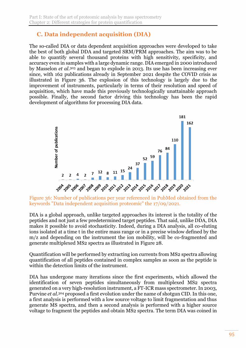
Part I: State of the art of proteomic analysis by mass spectrometry Chapter 2: Different strategies for protein quantification
95
C. Data independent acquisition (DIA) The so-called DIA or data dependent acquisition approaches were developed to take the best of both global DDA and targeted SRM/PRM approaches. The aim was to be able to quantify several thousand proteins with high sensitivity, specificity, and accuracy even in samples with a large dynamic range. DIA emerged in 2000 introduced by Masselon et al.303 and began to explode in 2013. Its use has been increasing ever since, with 162 publications already in September 2021 despite the COVID crisis as illustrated in Figure 36. The explosion of this technology is largely due to the improvement of instruments, particularly in terms of their resolution and speed of acquisition, which have made this previously technologically unattainable approach possible. Finally, the second factor driving this technology has been the rapid development of algorithms for processing DIA data.
Figure 36: Number of publications per year referenced in PubMed obtained from the keywords "Data independent acquisition proteomic" the 17/09/2021. DIA is a global approach, unlike targeted approaches its interest is the totality of the peptides and not just a few predetermined target peptides. That said, unlike DDA, DIA makes it possible to avoid stochasticity. Indeed, during a DIA analysis, all co-eluting ions isolated at a time t in the entire mass range or in a precise window defined by the m/z and depending on the instrument the ion mobility, will be co-fragmented and generate multiplexed MS2 spectra as illustrated in Figure 28. Quantification will be performed by extracting ion currents from MS2 spectra allowing quantification of all peptides contained in complex samples as soon as the peptide is within the detection limits of the instrument. DIA has undergone many iterations since the first experiments, which allowed the identification of seven peptides simultaneously from multiplexed MS2 spectra generated on a very high-resolution instrument, a FT-ICR mass spectrometer. In 2003, Purvine et al.304 proposed a first evolution under the name of shotgun CID. In this one, a first analysis is performed with a low source voltage to limit fragmentation and thus generate MS spectra, and then a second analysis is performed with a higher source voltage to fragment the peptides and obtain MS2 spectra. The term DIA was coined in
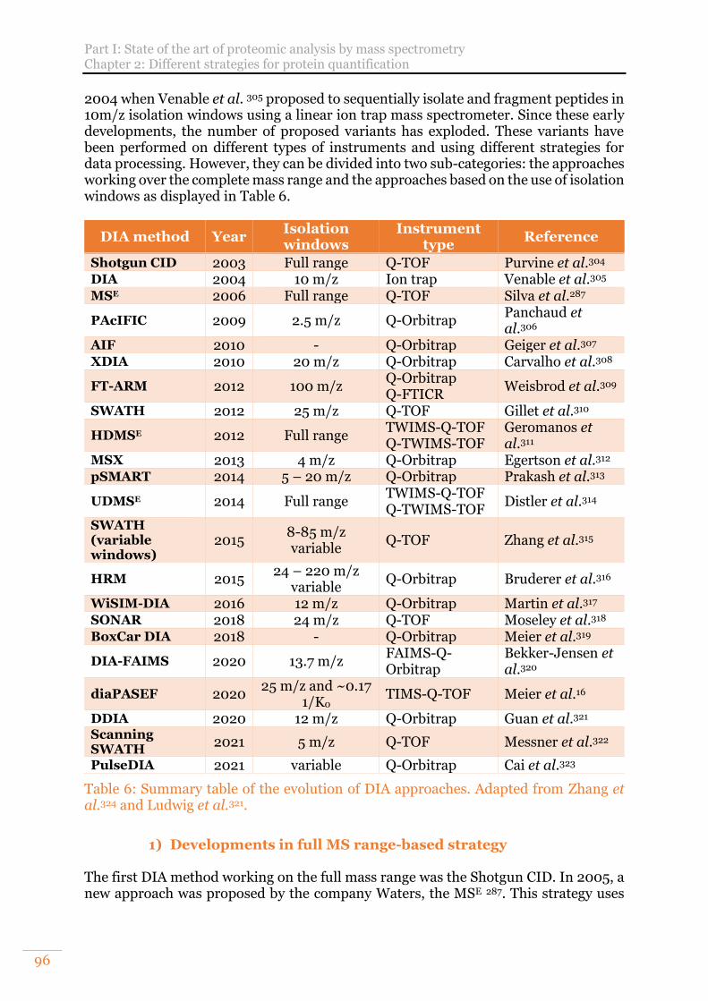
Part I: State of the art of proteomic analysis by mass spectrometry Chapter 2: Different strategies for protein quantification
96
2004 when Venable et al. 305 proposed to sequentially isolate and fragment peptides in 10m/z isolation windows using a linear ion trap mass spectrometer. Since these early developments, the number of proposed variants has exploded. These variants have been performed on different types of instruments and using different strategies for data processing. However, they can be divided into two sub-categories: the approaches working over the complete mass range and the approaches based on the use of isolation windows as displayed in Table 6.
DIA method Year Isolation windows
Instrument type
Reference
Shotgun CID 2003 Full range Q-TOF Purvine et al.304 DIA 2004 10 m/z Ion trap Venable et al.305 MSE 2006 Full range Q-TOF Silva et al.287
PAcIFIC 2009 2.5 m/z Q-Orbitrap Panchaud et al.306
AIF 2010 - Q-Orbitrap Geiger et al.307 XDIA 2010 20 m/z Q-Orbitrap Carvalho et al.308
FT-ARM 2012 100 m/z Q-Orbitrap Q-FTICR
Weisbrod et al.309
SWATH 2012 25 m/z Q-TOF Gillet et al.310
HDMSE 2012 Full range TWIMS-Q-TOF Q-TWIMS-TOF
Geromanos et al.311
MSX 2013 4 m/z Q-Orbitrap Egertson et al.312 pSMART 2014 5 – 20 m/z Q-Orbitrap Prakash et al.313
UDMSE 2014 Full range TWIMS-Q-TOF Q-TWIMS-TOF
Distler et al.314
SWATH (variable windows)
2015 8-85 m/z variable
Q-TOF Zhang et al.315
HRM 2015 24 – 220 m/z
variable Q-Orbitrap Bruderer et al.316
WiSIM-DIA 2016 12 m/z Q-Orbitrap Martin et al.317 SONAR 2018 24 m/z Q-TOF Moseley et al.318 BoxCar DIA 2018 - Q-Orbitrap Meier et al.319
DIA-FAIMS 2020 13.7 m/z FAIMS-Q-Orbitrap
Bekker-Jensen et al.320
diaPASEF 2020 25 m/z and ~0.17
1/K0 TIMS-Q-TOF Meier et al.16
DDIA 2020 12 m/z Q-Orbitrap Guan et al.321 Scanning SWATH
2021 5 m/z Q-TOF Messner et al.322
PulseDIA 2021 variable Q-Orbitrap Cai et al.323
Table 6: Summary table of the evolution of DIA approaches. Adapted from Zhang et al.324 and Ludwig et al.321.
1) Developments in full MS range-based strategy
The first DIA method working on the full mass range was the Shotgun CID. In 2005, a new approach was proposed by the company Waters, the MSE 287. This strategy uses
Part I: State of the art of proteomic analysis by mass spectrometry Chapter 2: Different strategies for protein quantification
97
alternating low and high collision energies to generate MS1 and MS2 spectra and performs quality peptide quantification. In 2010, Thermo Fisher Scientific unveiled a similar approach called AIF307 (All-Ion Fragmentation). Precursor ions and fragments are analysed sequentially. Fragmentation is performed in an HCD collision cell over the entire mass range. In 2012 and 2014, improved versions of the MSE were introduced. The HDMSE (High-Definition MSE) uses additional ion separation via TWIMS ion mobility213 in a SRIG (Stacked Ring Ion Guide) cell325. This separation reduces the complexity of MS2 spectra and increases the signal-to-noise ratio311. The UDMSE (Ultra-Definition MSE), uses variable collision energies and is optimised according to the elution of the ions from the ion mobility cell, which is dependent on their mass314.
2) Developments of isolation windows-based strategies
a) Consecutive fixed width windows The original DIA published in 2004 by Venable et al305 was the first to propose the use of isolation windows for ion fragmentation. Many strategies using fixed size isolation windows have followed. In 2009 Panchaud et al. proposed the PAcIFIC306 (Precursor Acquisition Independent From Ion Count) approach which uses narrow windows to reduce the complexity of MS2 spectra. Unfortunately, with this approach, the analysis of a complex proteome took about 5 days. This time has been greatly reduced by the improvement of the Q-Orbitrap instruments326. The XDIA (eXtended Data-Independent Acquisition) strategy was presented in 2010 by Carvalho et al 308. In this approach, a high-resolution MS1 spectrum is acquired at the beginning of each cycle and then a combination of CID and ETD fragmentation is used. The FT-ARM (Fourier Transform-All Reaction Monitoring) strategy presented in 2012 by Weisbrod et al was used with fixed size windows of 12 m/z and 100 m/z. The SWATH (Sequential Windowed Acquisition of All Theoretical fragment ion spectra) strategy marketed by Sciex was also presented in 2012 by Gillet et al 309. and uses windows of 25m/z. Prakash et al. and Martin et al. proposed respectively the pSMART313 and WiSIM317 (Wide Selected-Ion Monitoring) approaches in 2014 and 2016. In these approaches, high-resolution MS1 spectra are acquired and then MS2 spectra are generated after isolation of precursors in restricted mass windows. The MS1 spectra are used for quantification and the MS2 spectra for identification. In 2020 new DIA strategies using a supplemental ion mobility separation like HDMSE and UDMSE have emerged: DIA-FAIMS320 and diaPASEF. Those devices allow reducing the complexity of MS2 spectra. The diaPASEF16 will be presented in detail in a later part of this manuscript.
Part I: State of the art of proteomic analysis by mass spectrometry Chapter 2: Different strategies for protein quantification
98
Other approaches seem promising such as BoxCar319. This strategy, which can be combined with a DIA acquisition mode, uses the acquisition of MS1 spectra from narrow mass windows, thus increasing the dynamic range of MS1 signals by an order of magnitude or more in the case of biological fluids with a high dynamic range. Since recently, BoxCar data such as diaPASEF data can be easily processed using MaxDIA18. DDIA is a hybrid data acquisition method combining the DDA and DIA approaches321. A cycle is divided into three phases. Analysis of precursor ions for MS1 spectrum generation. The acquisition of MS2 spectra obtained from the selection and sequential fragmentation of the Top N most intense ions by a DDA approach. Finally, the cycle concludes with the acquisition of multiplexed MS2 spectra resulting from the co-fragmentation of ions in isolation windows covering the entire mass range.
b) Consecutive variable width windows The density of tryptic peptides during nLC-MS/MS analysis is variable. This is true for retention times, mass range and ion mobility range when present. In terms of mass range, on a complex proteome the highest density of precursor ions is observed between 400 and 800m/z323. In the ion mobility dimension, the highest density is generally observed between 0.7 and 1.25 1/K0. The higher ion density influences the performance of DIA acquisitions by generating more complex and difficult to interpret multiplexed MS2 spectra. The fact that more ions arrive at the same time also has an impact on the sensitivity and the specificity as the dynamic range within an isolation window will be higher. In order to reduce the complexity of MS2 spectra, it is possible to reduce the size of the windows, but this strategy comes at a cost as it increases the cycle time needed to cover the whole mass range and therefore decreases the coverage of the proteome. To overcome this problem, several approaches have developed DIA methods using variable size isolation windows. In this way, large windows are used in sparse regions and smaller windows in dense regions to reduce the complexity of the spectra while minimising the impact on cycle time. This is the case of the variable windows size SWATH approach315 proposed by Zhang et al. in 2015 also known as SWATH 2.0 which is an evolution of the original 2012 SWATH method using fixed window sizes310. The swath TUNER tool was created to optimise these window sizes according to the complexity of a sample. The HRM (Hyper Reaction Monitoring) approach316 uses the same principle but on Q-Orbitrap instruments and is now owned by the company Biognosys. It should be noted that there is no automated tool for generating these windows. The PulseDIA presented in 2021 by Cai et al.323 is an evolution of the PAcIFIC approach and a gas-phase fractionation – assisted DIA method that uses variable width DIA windows.
c) Overlapping windows Other strategies use significantly overlapping isolation windows. This increases the selectivity of the analysis by helping to de-multiplex MS2 spectra.
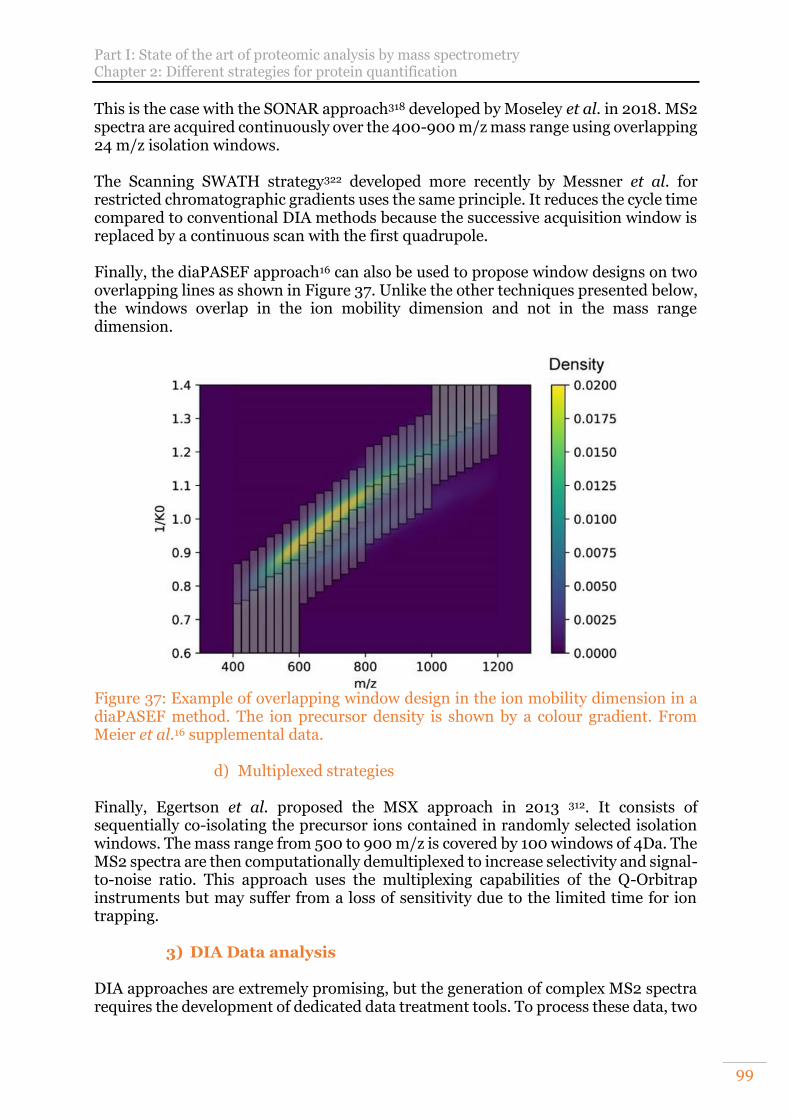
Part I: State of the art of proteomic analysis by mass spectrometry Chapter 2: Different strategies for protein quantification
99
This is the case with the SONAR approach318 developed by Moseley et al. in 2018. MS2 spectra are acquired continuously over the 400-900 m/z mass range using overlapping 24 m/z isolation windows. The Scanning SWATH strategy322 developed more recently by Messner et al. for restricted chromatographic gradients uses the same principle. It reduces the cycle time compared to conventional DIA methods because the successive acquisition window is replaced by a continuous scan with the first quadrupole. Finally, the diaPASEF approach16 can also be used to propose window designs on two overlapping lines as shown in Figure 37. Unlike the other techniques presented below, the windows overlap in the ion mobility dimension and not in the mass range dimension.
Figure 37: Example of overlapping window design in the ion mobility dimension in a diaPASEF method. The ion precursor density is shown by a colour gradient. From Meier et al.16 supplemental data.
d) Multiplexed strategies Finally, Egertson et al. proposed the MSX approach in 2013 312. It consists of sequentially co-isolating the precursor ions contained in randomly selected isolation windows. The mass range from 500 to 900 m/z is covered by 100 windows of 4Da. The MS2 spectra are then computationally demultiplexed to increase selectivity and signal-to-noise ratio. This approach uses the multiplexing capabilities of the Q-Orbitrap instruments but may suffer from a loss of sensitivity due to the limited time for ion trapping.
3) DIA Data analysis DIA approaches are extremely promising, but the generation of complex MS2 spectra requires the development of dedicated data treatment tools. To process these data, two
Part I: State of the art of proteomic analysis by mass spectrometry Chapter 2: Different strategies for protein quantification
100
types of approaches exist to date, peptide-centric and spectrum-centric methods. However, theoretically, the DIA approach allows the collection of MS2 spectra of all peptides in a sample within the instrumental limits. Therefore, the same data set can potentially answer several biological questions, even if these were not considered at the time of the design of the experiment.
a) Peptide-centric approach The peptide centric approach is based on the use of previously generated spectral libraries to perform spectrum-peptide matching. The creation of a spectral library is necessary to process DIA data via a peptide-centric approach.
i. Spectral library These libraries contain MS2 spectra assigned to a peptide sequence with a high level of confidence327,328. These spectra are most often derived from DDA analysis but may also have been extracted from DIA analysis after deconvolution of the MS2 spectra. In a similar way to the processing of DDA data, it will only be possible to assign the signals contained in the library. The completeness of the library is therefore of utmost importance. For this reason, the main approach is to generate these libraries from DDA analyses on fractionated samples to increase the coverage of the proteome and thus the search space. The quality of the library is of strategic importance in data processing. Library generated on the same coupling than DIA analysis remains more adapted to create spectral libraries329,330. If the library includes false positives, generally a 1% FDR is used for its generation, then these false positives will be treated as real identifications and searched in the DIA analysis328,331. Therefore, the quality of the libraries and especially their error rate must be carefully controlled through advanced statistical tests327,332. Unfortunately, the generation of spectral libraries can therefore be time consuming, tedious and expensive329,333. To ensure the presence of peptides of interest in the library, it is possible to use synthetic peptides to generate the library334. Hybrid libraries composed of endogenous and synthetic peptides have already been used335. To compensate for the time-consuming generation of spectral libraries, various platforms such as PeptideAtlas244,336, MassIVE337, PRIDE244 (PRoteomics IDEntification database) or SWATHAtlas333 offer public spectral libraries for the extraction of DIA-SWATH data. Unfortunately, the number of libraries and organisms available is still limited. As of 22/07/2021, seven years after its creation, SWATHAtlas offers only 17 libraries, five of which are human, with very variable proteome coverage ranging from 15 to 99% when it can be estimated. It is perfectly possible to combine the use of several public libraries to increase their comprehensiveness if they contain standard peptides allowing their normalisation. Several studies have shown that MS2 spectra generated on different instruments using CID fragmentation were sufficiently comparable to be used for cross-instrument library generation if the elution order of peptides is the same324,330. Retention times, which can also vary depending on the type and condition of the chromatographic system, can be compensated for by adding standard peptides to the samples used for library generation and DIA analysis. This is the case with the iRTs standard marketed by Biognosys. Other software approaches also allow the comparison of assays and libraries to align retention times against common peptides as is the case with Spectronaut or SpectroMine (Biognosys). Other software such as MaxDIA allow using analysis with different gradient sizes between the
Part I: State of the art of proteomic analysis by mass spectrometry Chapter 2: Different strategies for protein quantification
101
spectral library and DIA runs thanks to non-linear RT mapping between them18. However, this approach also has its limitations as it has already been shown that generating a library from spectra generated on the same coupling as the DIA analyses are more suitable. An approach called MCIP (Multiple Characteristic Intensity Pattern) has been created to better identify spectral variability during library generation331. Currently, the rise of artificial intelligence is reflected in the processing of proteomic data, and particularly in the processing of DIA data. One such tool is DeepMass338, which is able to predict peptide fragmentation patterns using a machine learning algorithm fed by tens of millions of MS2 spectra. Prosit339–342 is a flexible deep neural network architecture capable of predicting retention times, fragmentation and MS2 spectra of peptides. pDeep343 is also capable of predicting peptide fragmentation from different fragmentation modes. It should be noted that the intensity of the predicted spectra is instrument-dependent344. Data processing software such as Spectronaut (Biognosys) or DIA-NN17,345, now use artificial intelligence to improve their processing. The recently released MaxDIA also uses machine learning thanks to DeepMass:Prism338 that uses a bi-directional recurrent neural network346 (BRNN) and XGBoost347. Benchmarking of the different DIA data treatment workflow comparison is currently largely investigated258.
ii. Targeted spectra extraction The spectral libraries contain information at the peptide level such as sequence and normalised retention time, at the precursor level such as m/z, charge state and at the fragment level such as their type, m/z, charge state, and relative intensities. The libraries also contain the parentage between peptide, precursors and fragments that is lost in DIA analysis compared to DDA analysis by co-fragmentation of peptides. Targeted data extraction from a spectral library was initially proposed by Gillet et al. for the processing of SWATH data310. The library information is used to extract XICs from MS2 spectra. Different criteria like those used in the targeted approaches are used to assess the quality of the signals such as the co-elution of fragment ions, the shape of the chromatographic peak, the correlation with the relative intensities of the fragment ions of the spectral library and the retention time. Other criteria can also be added concerning the mass accuracy of the signal such as the co-elution of precursor and fragment ions or the co-elution of different charge states of the same peptide. Those criteria allow improving the quality of the extracted signals. As in DDA, peptide identification is statistically validated using a target-decoy approach to assess the false positive rate (FDR). Then a semi-supervised learning algorithm evaluates the discriminant score, i.e., the combination of weighted individual scores of the identifications, to distinguish the distributions of the scores of target and decoy populations. The candidate peak with the highest discriminant score will be retained and the relevance of the peptide detection will be evaluated by calculating the q-value327,332. This strategy is used in OpenSWATH348, PeakView (AB Sciex), DIA-NN17,345, Skyline302 and Spectronaut (Biognosys). The mProphet349 algorithm is used in the last two solutions. Other algorithms such as TRIC350 (Transfer of Identification Confidence) or DIAlignR351 can also be used to enhance the robustness of identifications by limiting the proportion of false identifications or to normalise retention times between analyses.
Chapter 2: Different strategies for protein quantification
102
Additional software have also been developed to support four-dimensional DIA data, including ion mobility data, to process the data generated by the TimsTOF Pro instruments. This is the case of Mobi-DIK16 which can be used in the OpenSWATH environment, Spectronaut or more recently DIA-NN combined with FragPipe17 and MaxDIA18 implemented within MaxQuant from version 2.0.
iii. Direct spectral matching Another strategy for extracting DIA data is based on a direct comparison of the multiplexed MS2 spectra of an analysis with the assigned spectra contained in a spectral library or database. This type of extraction is therefore not a targeted extraction. The first software using this approach is ProbIDtree352 presented in 2005. For each multiplexed MS2 DIA spectrum, the algorithm identifies all potential precursor ions contained in the corresponding MS1 spectrum that are above a user-defined intensity threshold. From the list of potential precursor ions, a match score is calculated, and a peptide probability tree is constructed. At each iteration, a new MS2 DIA spectrum is generated from the experimental MS2 spectra by deleting the already matched fragments. The MSPLIT-DIA353 software (Mixture-Spectrum Partitioning using Libraries of Identified Tandem mass spectra) deconvolutes the MS2 spectra by evaluating the similarity between them and the MS2 spectra contained in the spectral library. It excludes spectra that are too similar from the targeted extraction and evaluates the quality of the results through retention time scores and statistical validation based on the use of FDR. Finally, the PECAN algorithm354 (PEptide-Centric Analysis) on which EncyclopeDIA355 is based uses a spectral library generated from DIA analyses using very narrow isolation windows (4m/z) drastically reducing the complexity of MS2 spectra.
b) Spectrum-centric approach The spectrum centric approach is based solely on multiplexed MS2 spectra from which algorithms will extract demultiplexed pseudo MS2 spectra which will be subjected to a classical search via interrogation of an in silico digested database. After identification, the assigned spectra are used to generate a spectral library to perform signal extraction for the quantification step. This approach was first used by Purvine et al.304 in 2003. Pseudo DDA spectra were reconstructed from DIA analyses using similar chromatographic characteristics of precursor and fragment ions to identify them manually. Fortunately since then, many algorithms have been developed to perform this task in an automated fashion324,327,356. They are also capable of supporting data from other types of DIA acquisition. These include DIA-Umpire357, which can identify and quantify peptides in a non-targeted manner and can also generate a spectral library for peptide-centric extraction from the initial data. Spectronaut also incorporates the directDIA algorithm for this type of approach to processing DIA data, just like DIA-NN17,345 and MaxDIA discovery mode18.
RESULTS Chapter 1: Evaluation of different digestion methods
103
RESULTS
Part II: Optimisation of pre-analytical sample preparation steps for high throughput proteomics analysis on small amounts of material During the last decade, progress has been done at every stage of the proteomic analysis pipeline. However, some limitations remain, especially for the preparation of samples from small amounts of biological material. This is particularly critical in projects for which samples are difficult to obtain or when working with precious samples such as clinical samples. The COVID-19 crisis was a good example as the samples available for the study of the virus needed to allow as many different analyses as possible358. Low amounts of material requirements for proteomic analysis were in this context a decisive advantage. However, this is also true for every clinical study, cross-discipline or not, where the difficulty to obtain samples and the well-being of donors must be taken into consideration. The second limiting point regarding the sample preparation is the time needed to perform it. Depending on the project and the protocol used, this can need several days. For that reason, the development of shorter and automated protocol is more and more popular. Automation will be in near future a tremendous help for high throughput studies with hundreds of samples such as biomarkers searches. In this context, two main parts of my PhD work consisted in i) the evaluation of new sample preparation protocols adapted for reduced protein amounts and ii) the automation of the most promising of them, in our hands, on a newly sample preparation robot acquired by our laboratory.
Chapter 1: Evaluation of different digestion methods
The terms microproteomics176,359,360 first introduced in 2002 by Krieg et al. and nanoproteomics52,361–364 first introduced in 2004 and by Pasa-Tolić et al. despite their various context-dependent significations are evidences of the long-standing interest of proteomists in reducing the amount of protein required for analyses. To be able to achieve that goal, the complete proteomic analysis pipeline must be screened and adapted. The first step was the development of sample collection technics going down to single cells isolation. This is already possible using techniques such as laser capture microdissection (LCM), fluorescence activated cell sorting (FACS)52 or even exosome isolation technics178. Then comes the protein extraction that must be realised with adapted tools and reagents to reach the highest protein recovery. The digestion must be optimised to reach the best efficiency and allows analysis with improved sensitivity and depth. During all the sample preparation protocols, the quickness, the number of transfers, the contact surface between samples and tubes are especially critical due to proteins and peptides adsorption phenomena on the well walls. In addition to the challenge of reducing the quantity of sample needed, label-free quantification remains also highly challenging especially on low amounts of material. This approach is plebiscite due to its capabilities to quantified thousands of proteins,
Part II: Optimisation of pre-analytical sample preparation steps for high throughput proteomics analysis on small amounts of material Chapter 1: Evaluation of different digestion methods
104
its application easiness, fastness, reduced cost allowing more easily large scale and high-throughput studies. However, in opposition to labelling strategies, it is impossible to multiplex samples365. Consequently, special care must be given for sample preparation and nLC-MS/MS analysis reproducibility to obtain reliable and accurate quantification. At the beginning of my PhD, in our lab, the classical proteins inputs for sample preparation were between 20µg and 100µg for standard bottom-up proteomics analyses. Different approaches were used such as stacking gel, tube-gel, FASP or liquid digestion and some people in the lab also already investigated PreOmics iST kits. In that context, my goal was to investigate new digestion protocols able to deal with 20µg to less than 1µg of proteins, compatible with lysis buffer containing SDS allowing a good extraction of poorly soluble proteins to conduct label-free quantification studies. In this aim, different strategies were investigated:
→ In-gel digestions: a volume-reduced tube-gel was designed, evaluated and compared with other in-gel approaches.
→ On-filter digestions: Suspension-Trap also called SDS-Trap5 (S-Trap, Protifi,
Farmingdale, NY, USA) were evaluated and the protocol optimised.
→ On-beads digestion: Single-pot, solid-phase-enhanced sample preparation58 (SP3) were evaluated, optimised on small protein quantities and compared with S-Trap.
A. Setup of a volume reduced tube-gel protocol This work started from the knowledge and experience already present in the lab. Firstly, an interest was shown in the tube-gel sample preparation developed by the doctor Leslie Muller during her PhD4,7. This protocol consists in polymerising acrylamide gels directly in the tube containing the proteins thus avoiding the long process of 1D-SDS-PAGE gel preparation, loading and migration. Then the tube-gel is cut into pieces with the proteins trapped inside the gel pieces before being washed by successive dehydration/hydration cycles with organic solvent and digested overnight at 37°C. Finally, peptides are extracted from the gel by dehydration thanks to an acidified organic solvent.
1) Experimental design One major problem when working with reduced amount of protein is the loss of proteins and peptides during the sample preparation procedure. Indeed, this lost quantity can represent an important proportion of the total sample that will result in low signals in MS for quantification. To reduce it, different points are known to be critical. The ideal protocol to deal with small amounts should be fast, with a reduced number of steps and ideally in one tube with a small working volume. The aim of all those points is to avoid the adsorption of proteins and peptides on the tube walls that lead to their loss. That the reason why we choose to investigate a volume reduced tube-gel based on the classical tube-gel protocol but using half-reduced volumes. Then, we decided to do a comparison of the three in-gel protocols to confirm if this optimisation
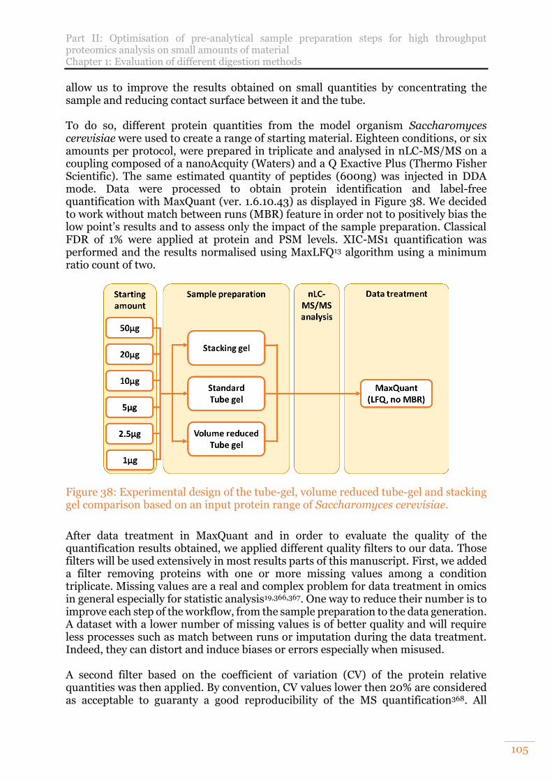
Part II: Optimisation of pre-analytical sample preparation steps for high throughput proteomics analysis on small amounts of material Chapter 1: Evaluation of different digestion methods
105
allow us to improve the results obtained on small quantities by concentrating the sample and reducing contact surface between it and the tube. To do so, different protein quantities from the model organism Saccharomyces cerevisiae were used to create a range of starting material. Eighteen conditions, or six amounts per protocol, were prepared in triplicate and analysed in nLC-MS/MS on a coupling composed of a nanoAcquity (Waters) and a Q Exactive Plus (Thermo Fisher Scientific). The same estimated quantity of peptides (600ng) was injected in DDA mode. Data were processed to obtain protein identification and label-free quantification with MaxQuant (ver. 1.6.10.43) as displayed in Figure 38. We decided to work without match between runs (MBR) feature in order not to positively bias the low point’s results and to assess only the impact of the sample preparation. Classical FDR of 1% were applied at protein and PSM levels. XIC-MS1 quantification was performed and the results normalised using MaxLFQ13 algorithm using a minimum ratio count of two.
Figure 38: Experimental design of the tube-gel, volume reduced tube-gel and stacking gel comparison based on an input protein range of Saccharomyces cerevisiae.
After data treatment in MaxQuant and in order to evaluate the quality of the quantification results obtained, we applied different quality filters to our data. Those filters will be used extensively in most results parts of this manuscript. First, we added a filter removing proteins with one or more missing values among a condition triplicate. Missing values are a real and complex problem for data treatment in omics in general especially for statistic analysis19,366,367. One way to reduce their number is to improve each step of the workflow, from the sample preparation to the data generation. A dataset with a lower number of missing values is of better quality and will require less processes such as match between runs or imputation during the data treatment. Indeed, they can distort and induce biases or errors especially when misused. A second filter based on the coefficient of variation (CV) of the protein relative quantities was then applied. By convention, CV values lower then 20% are considered as acceptable to guaranty a good reproducibility of the MS quantification368. All
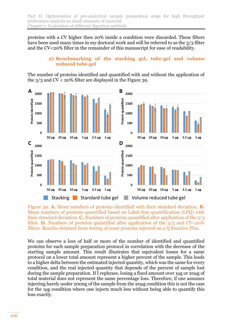
Part II: Optimisation of pre-analytical sample preparation steps for high throughput proteomics analysis on small amounts of material Chapter 1: Evaluation of different digestion methods
106
proteins with a CV higher then 20% inside a condition were discarded. These filters have been used many times in my doctoral work and will be referred to as the 3/3 filter and the CV<20% filter in the remainder of this manuscript for ease of readability.
2) Benchmarking of the stacking gel, tube-gel and volume reduced tube-gel
The number of proteins identified and quantified with and without the application of the 3/3 and CV < 20% filter are displayed in the Figure 39.
Figure 39: A. Mean numbers of proteins identified with their standard deviation. B. Mean numbers of proteins quantified based on Label-free quantification (LFQ) with their standard deviation. C. Numbers of proteins quantified after application of the 3/3 filter. D. Numbers of proteins quantified after application of the 3/3 and CV<20% filters. Results obtained from 600ng of yeast proteins injected on a Q Exactive Plus.
We can observe a loss of half or more of the number of identified and quantified proteins for each sample preparation protocol in correlation with the decrease of the starting sample amount. This result illustrates that equivalent losses for a same protocol on a lower total amount represent a higher percent of the sample. This leads to a higher delta between the estimated injected quantity, which was the same for every condition, and the real injected quantity that depends of the percent of sample lost during the sample preparation. If I rephrase, losing a fixed amount over 1µg or 20µg of total material does not represent the same percentage loss. Therefore, if one assumes injecting barely under 200ng of the sample from the 20µg condition this is not the case for the 1µg condition where one injects much less without being able to quantify this loss exactly.
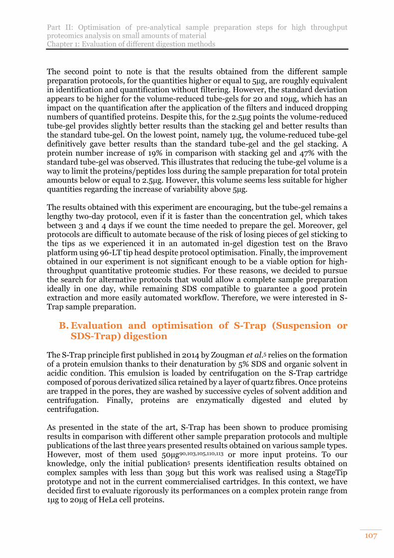
Part II: Optimisation of pre-analytical sample preparation steps for high throughput proteomics analysis on small amounts of material Chapter 1: Evaluation of different digestion methods
107
The second point to note is that the results obtained from the different sample preparation protocols, for the quantities higher or equal to 5µg, are roughly equivalent in identification and quantification without filtering. However, the standard deviation appears to be higher for the volume-reduced tube-gels for 20 and 10µg, which has an impact on the quantification after the application of the filters and induced dropping numbers of quantified proteins. Despite this, for the 2.5µg points the volume-reduced tube-gel provides slightly better results than the stacking gel and better results than the standard tube-gel. On the lowest point, namely 1µg, the volume-reduced tube-gel definitively gave better results than the standard tube-gel and the gel stacking. A protein number increase of 19% in comparison with stacking gel and 47% with the standard tube-gel was observed. This illustrates that reducing the tube-gel volume is a way to limit the proteins/peptides loss during the sample preparation for total protein amounts below or equal to 2.5µg. However, this volume seems less suitable for higher quantities regarding the increase of variability above 5µg. The results obtained with this experiment are encouraging, but the tube-gel remains a lengthy two-day protocol, even if it is faster than the concentration gel, which takes between 3 and 4 days if we count the time needed to prepare the gel. Moreover, gel protocols are difficult to automate because of the risk of losing pieces of gel sticking to the tips as we experienced it in an automated in-gel digestion test on the Bravo platform using 96-LT tip head despite protocol optimisation. Finally, the improvement obtained in our experiment is not significant enough to be a viable option for high-throughput quantitative proteomic studies. For these reasons, we decided to pursue the search for alternative protocols that would allow a complete sample preparation ideally in one day, while remaining SDS compatible to guarantee a good protein extraction and more easily automated workflow. Therefore, we were interested in S-Trap sample preparation.
B. Evaluation and optimisation of S-Trap (Suspension or SDS-Trap) digestion
The S-Trap principle first published in 2014 by Zougman et al.5 relies on the formation of a protein emulsion thanks to their denaturation by 5% SDS and organic solvent in acidic condition. This emulsion is loaded by centrifugation on the S-Trap cartridge composed of porous derivatized silica retained by a layer of quartz fibres. Once proteins are trapped in the pores, they are washed by successive cycles of solvent addition and centrifugation. Finally, proteins are enzymatically digested and eluted by centrifugation. As presented in the state of the art, S-Trap has been shown to produce promising results in comparison with different other sample preparation protocols and multiple publications of the last three years presented results obtained on various sample types. However, most of them used 50µg90,103,105,110,113 or more input proteins. To our knowledge, only the initial publication5 presents identification results obtained on complex samples with less than 30µg but this work was realised using a StageTip prototype and not in the current commercialised cartridges. In this context, we have decided first to evaluate rigorously its performances on a complex protein range from 1µg to 20µg of HeLa cell proteins.
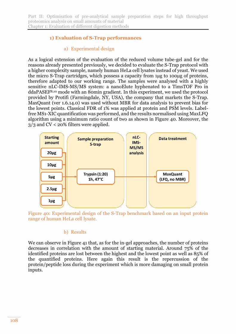
Part II: Optimisation of pre-analytical sample preparation steps for high throughput proteomics analysis on small amounts of material Chapter 1: Evaluation of different digestion methods
108
1) Evaluation of S-Trap performances
a) Experimental design As a logical extension of the evaluation of the reduced volume tube-gel and for the reasons already presented previously, we decided to evaluate the S-Trap protocol with a higher complexity sample, namely human HeLa cell lysates instead of yeast. We used the micro S-Trap cartridges, which possess a capacity from 1µg to 100µg of proteins, therefore adapted to our working range. The samples were analysed with a highly sensitive nLC-IMS-MS/MS system: a nanoElute hyphenated to a TimsTOF Pro in ddaPASEF8,10 mode with an 80min gradient. In this experiment, we used the protocol provided by Protifi (Farmingdale, NY, USA), the company that markets the S-Trap. MaxQuant (ver 1.6.14.0) was used without MBR for data analysis to prevent bias for the lowest points. Classical FDR of 1% was applied at protein and PSM levels. Label-free MS1-XIC quantification was performed, and the results normalised using MaxLFQ algorithm using a minimum ratio count of two as shown in Figure 40. Moreover, the 3/3 and CV < 20% filters were applied.
Figure 40: Experimental design of the S-Trap benchmark based on an input protein range of human HeLa cell lysate.
b) Results
We can observe in Figure 41 that, as for the in-gel approaches, the number of proteins decreases in correlation with the amount of starting material. Around 75% of the identified proteins are lost between the highest and the lowest point as well as 85% of the quantified proteins. Here again this result is the repercussion of the protein/peptide loss during the experiment which is more damaging on small protein inputs.
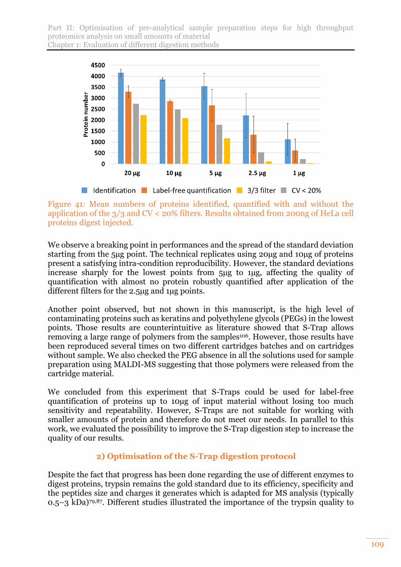
Part II: Optimisation of pre-analytical sample preparation steps for high throughput proteomics analysis on small amounts of material Chapter 1: Evaluation of different digestion methods
109
Figure 41: Mean numbers of proteins identified, quantified with and without the application of the 3/3 and CV < 20% filters. Results obtained from 200ng of HeLa cell proteins digest injected.
We observe a breaking point in performances and the spread of the standard deviation starting from the 5µg point. The technical replicates using 20µg and 10µg of proteins present a satisfying intra-condition reproducibility. However, the standard deviations increase sharply for the lowest points from 5µg to 1µg, affecting the quality of quantification with almost no protein robustly quantified after application of the different filters for the 2.5µg and 1µg points. Another point observed, but not shown in this manuscript, is the high level of contaminating proteins such as keratins and polyethylene glycols (PEGs) in the lowest points. Those results are counterintuitive as literature showed that S-Trap allows removing a large range of polymers from the samples106. However, those results have been reproduced several times on two different cartridges batches and on cartridges without sample. We also checked the PEG absence in all the solutions used for sample preparation using MALDI-MS suggesting that those polymers were released from the cartridge material. We concluded from this experiment that S-Traps could be used for label-free quantification of proteins up to 10µg of input material without losing too much sensitivity and repeatability. However, S-Traps are not suitable for working with smaller amounts of protein and therefore do not meet our needs. In parallel to this work, we evaluated the possibility to improve the S-Trap digestion step to increase the quality of our results.
2) Optimisation of the S-Trap digestion protocol Despite the fact that progress has been done regarding the use of different enzymes to digest proteins, trypsin remains the gold standard due to its efficiency, specificity and the peptides size and charges it generates which is adapted for MS analysis (typically 0.5–3 kDa)79,87. Different studies illustrated the importance of the trypsin quality to
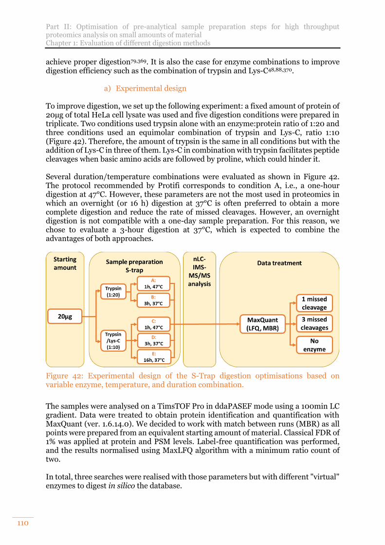
Part II: Optimisation of pre-analytical sample preparation steps for high throughput proteomics analysis on small amounts of material Chapter 1: Evaluation of different digestion methods
110
achieve proper digestion79,369. It is also the case for enzyme combinations to improve digestion efficiency such as the combination of trypsin and Lys-C48,88,370.
a) Experimental design To improve digestion, we set up the following experiment: a fixed amount of protein of 20µg of total HeLa cell lysate was used and five digestion conditions were prepared in triplicate. Two conditions used trypsin alone with an enzyme:protein ratio of 1:20 and three conditions used an equimolar combination of trypsin and Lys-C, ratio 1:10 (Figure 42). Therefore, the amount of trypsin is the same in all conditions but with the addition of Lys-C in three of them. Lys-C in combination with trypsin facilitates peptide cleavages when basic amino acids are followed by proline, which could hinder it. Several duration/temperature combinations were evaluated as shown in Figure 42. The protocol recommended by Protifi corresponds to condition A, i.e., a one-hour digestion at 47°C. However, these parameters are not the most used in proteomics in which an overnight (or 16 h) digestion at 37°C is often preferred to obtain a more complete digestion and reduce the rate of missed cleavages. However, an overnight digestion is not compatible with a one-day sample preparation. For this reason, we chose to evaluate a 3-hour digestion at 37°C, which is expected to combine the advantages of both approaches.
Figure 42: Experimental design of the S-Trap digestion optimisations based on variable enzyme, temperature, and duration combination.
The samples were analysed on a TimsTOF Pro in ddaPASEF mode using a 100min LC gradient. Data were treated to obtain protein identification and quantification with MaxQuant (ver. 1.6.14.0). We decided to work with match between runs (MBR) as all points were prepared from an equivalent starting amount of material. Classical FDR of 1% was applied at protein and PSM levels. Label-free quantification was performed, and the results normalised using MaxLFQ algorithm with a minimum ratio count of two. In total, three searches were realised with those parameters but with different "virtual" enzymes to digest in silico the database.
Part II: Optimisation of pre-analytical sample preparation steps for high throughput proteomics analysis on small amounts of material Chapter 1: Evaluation of different digestion methods
111
→ A first search was performed using trypsin/P as set enzyme and one missed cleavage allowed. Trypsin/P means that the “virtual” enzyme cleaves at carboxyl side of the lysine or arginine amino acids, also if a proline residue follows. Consequently, this parameter is suited to treat dataset from samples digested with trypsin or trypsin/Lys-C. The Figure 43.A was generated from this data treatment, which is representative of the parameters classically used in proteomics.
→ A second search was performed with the same “virtual” enzyme but allowing
three missed cleavages. The goal of that parameter setting was to estimate the proportion of missed cleaved peptides in our sample. Indeed, the probability to have peptides with more than three missed cleavages is very low due to their size most of the time incompatible with MS analysis. Those data were used to generate the stacked histogram in Figure 43.B.
→ Finally, a third search was performed using the parameter “no enzyme”.
Without enzyme specificity specified, all peptides and not only tryptic peptides will be searched. This allows us to recover peptides originated from non-specific cleavages. We were able to generate the curve of the mean numbers of peptides with non-specific cleavages displayed in Figure 43.B from this search. To evaluate those numbers, we subtracted the peptides ending by a lysine or an arginine to the total number of peptides in the same search. However, with this way of proceeding, we are not able to consider the C-terminal tryptic peptide of proteins that does not end with a basic amino acid but is still a tryptic peptide. However, this is not a problem in our case as we can assume that the proportion of C-terminal tryptic peptides is equivalent in each condition. This is not a perfect way to assess the number of non-specific cleavages, but it is sufficient to assess trends and make a comparison between the different digestion conditions.
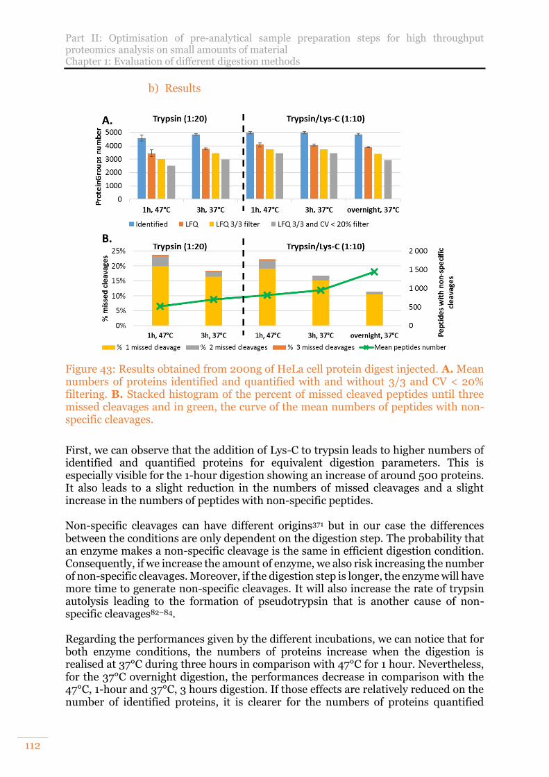
Part II: Optimisation of pre-analytical sample preparation steps for high throughput proteomics analysis on small amounts of material Chapter 1: Evaluation of different digestion methods
112
b) Results
Figure 43: Results obtained from 200ng of HeLa cell protein digest injected. A. Mean numbers of proteins identified and quantified with and without 3/3 and CV < 20% filtering. B. Stacked histogram of the percent of missed cleaved peptides until three missed cleavages and in green, the curve of the mean numbers of peptides with non-specific cleavages.
First, we can observe that the addition of Lys-C to trypsin leads to higher numbers of identified and quantified proteins for equivalent digestion parameters. This is especially visible for the 1-hour digestion showing an increase of around 500 proteins. It also leads to a slight reduction in the numbers of missed cleavages and a slight increase in the numbers of peptides with non-specific peptides. Non-specific cleavages can have different origins371 but in our case the differences between the conditions are only dependent on the digestion step. The probability that an enzyme makes a non-specific cleavage is the same in efficient digestion condition. Consequently, if we increase the amount of enzyme, we also risk increasing the number of non-specific cleavages. Moreover, if the digestion step is longer, the enzyme will have more time to generate non-specific cleavages. It will also increase the rate of trypsin autolysis leading to the formation of pseudotrypsin that is another cause of non-specific cleavages82–84. Regarding the performances given by the different incubations, we can notice that for both enzyme conditions, the numbers of proteins increase when the digestion is realised at 37°C during three hours in comparison with 47°C for 1 hour. Nevertheless, for the 37°C overnight digestion, the performances decrease in comparison with the 47°C, 1-hour and 37°C, 3 hours digestion. If those effects are relatively reduced on the number of identified proteins, it is clearer for the numbers of proteins quantified
Part II: Optimisation of pre-analytical sample preparation steps for high throughput proteomics analysis on small amounts of material Chapter 1: Evaluation of different digestion methods
113
especially after the addition of the 3/3 and CV < 20% filters illustrating a fall in the quality of the signals used for quantification. The conditions raising the highest numbers of proteins are the digestions at 47°C for 1 hour and 37°C for 3 hours using trypsin/Lys-C (1:10). Still, the 37°C 3h digestion presenting a lower percent of missed cleavages, we would recommend this condition. In summary, we have clearly demonstrated that between the initial protocol recommended by Protifi and our optimised parameters, we were able to gain around 500 identified proteins, around 600 quantified proteins and around 900 quantified proteins after application of the 2 levels of quality filtering. Thanks to that improvement, we were able to increase our analysis depth and improve the reproducibility of the quantification. To conclude, we benchmarked the S-Trap sample preparation with protein amounts from 1µg to 20µg and illustrated that it is a suitable option to perform protein analysis and especially label-free MS1-XIC quantification with protein amounts higher than 5µg. We were able to improve the digestion step by using trypsin/Lys-C (1:10) during three hours at 37°C to significantly increase the number of identified and quantified proteins and by reducing the percent of missed cleavage peptides. The S-Trap protocol brings many advantages: the use of SDS for the extraction of membrane proteins, sample preparation in one day and automation. These results will be valorised in a publication currently being written and which should be submitted to the Journal of Proteomics.

Part II: Optimisation of pre-analytical sample preparation steps for high throughput proteomics analysis on small amounts of material Chapter 1: Evaluation of different digestion methods
114
ADD PUBLICATION

Part II: Optimisation of pre-analytical sample preparation steps for high throughput proteomics analysis on small amounts of material Chapter 1: Evaluation of different digestion methods
114
However, this approach remains expensive and is not sufficiently efficient with protein amounts lower or equal to 5µg to realise robust protein label-free quantification. For that reason, we decided to continue to investigate new sample preparation protocols.
C. Optimisation of single-pot, solid-phase-enhanced sample preparation (SP3)
In parallel to my work realised on S-Trap, one engineer, Marziyeh Komeili and one intern, now PhD student in the lab, Marie Gebelin started a preliminary evaluation of a new sample preparation protocol based on on-beads digestion: the single-pot, solid-phase-enhanced, sample preparation or SP3. The SP3 protocol is based on the interaction between proteins and functionalized (carboxyl coated) magnetic beads when they are placed in certain organic solvents. The beads are retained with a magnet to remove the supernatant allowing the proteins to be cleaned by successive washes. Then the beads are suspended in a digestion buffer, endoprotease is added, and the proteins are digested. After digestion and acidification, the peptides are no longer retained on the beads and can be recovered in the supernatant (Figure 25). The SP3 protocol has the advantage to be fast, in one pot, scalable, simple to handle and compatible with high amounts of SDS until 10% recommended and plenty of other detergents, chaotropes and salts58. Consequently, it allows good protein recovery even with limited input material, which makes it compatible with a very wide range of sample types. It is easily adaptable for high-throughput automated sample preparation2 in a flexible manner regarding the number of samples. Given the promising initial results of my colleagues and the many advantages of SP3, especially regarding small amounts of protein, we decided to study this protocol in more detail.
1) Evaluation of SP3 sample preparation
a) Experimental design The SP3 protocol was evaluated on a range of human HeLa cell proteins from 10 to 0.5µg prepared in three replicates. We used the published protocol with slight modifications58 . Briefly, the working volumes were decreased to reduce sample loss, increase digestion efficiency and the digestion was carried out overnight at 37°C. To perform the SP3 experiment and make it easily transferable to a liquid handling robot, we chose to work with different concentrations of reagents between the different conditions while keeping the same working volumes. To realise this experiment, we used a combination of two Sera-Mag carboxylate Speedbeads types (Cytiva) which display slightly different hydrophilic properties. The used protein:beads ratio was 1:10 for each type of beads corresponding to a total of 1:20 ratio of beads. The samples were analysed on a TimsTOF Pro in ddaPASEF mode using an 80min LC gradient as described in Figure 44. MaxQuant (ver 1.6.17.0) without MBR feature was used. Classical FDRs of 1% were applied at proteins and PSM levels. Label-free quantification was performed, and the results normalised using MaxLFQ
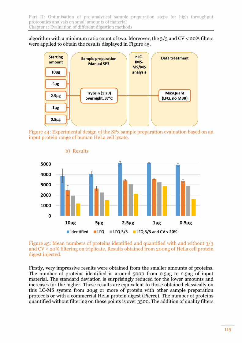
Part II: Optimisation of pre-analytical sample preparation steps for high throughput proteomics analysis on small amounts of material Chapter 1: Evaluation of different digestion methods
115
algorithm with a minimum ratio count of two. Moreover, the 3/3 and CV < 20% filters were applied to obtain the results displayed in Figure 45.
Figure 44: Experimental design of the SP3 sample preparation evaluation based on an input protein range of human HeLa cell lysate.
b) Results
Figure 45: Mean numbers of proteins identified and quantified with and without 3/3 and CV < 20% filtering on triplicate. Results obtained from 200ng of HeLa cell protein digest injected.
Firstly, very impressive results were obtained from the smaller amounts of proteins. The number of proteins identified is around 5000 from 0.5µg to 2.5µg of input material. The standard deviation is surprisingly reduced for the lower amounts and increases for the higher. These results are equivalent to those obtained classically on this LC-MS system from 20µg or more of protein with other sample preparation protocols or with a commercial HeLa protein digest (Pierce). The number of proteins quantified without filtering on those points is over 3300. The addition of quality filters
Part II: Optimisation of pre-analytical sample preparation steps for high throughput proteomics analysis on small amounts of material Chapter 1: Evaluation of different digestion methods
116
shows that the highest number of proteins quantified in a robust way is obtained with 1µg of starting material with around 2800 proteins. One hypothesis, which could explain the decrease in performance for higher amounts, could be that the working volume that we reduced to gain in efficiency on small protein amounts is too low for higher amount of protein, which thus require high amounts of beads. This could hinder the interaction between beads and proteins, possibly due to their aggregation58. In this case, an easy solution would be to keep a larger working volume for experiments with higher amounts of protein. This is not a problem for a manual approach. However, it does mean that automated protocols, which are limited in terms of choice of tanks and plates, may not be able to handle samples with large amounts of proteins due to volume limitations. This is not a problem for classical bottom-up proteomics experiment as we have shown results with virtually no loss with 1µg of input protein, but it could be a hindrance for the study of post-translational modifications or any proteomic workflow including an additional enrichment step which may require important amount of starting material for subsequent efficient MS analysis. Another hypothesis relies on the intact chromatin. For the higher points, the sample is more concentrated. This is true for proteins but also for chromatin, which may not be fully degraded during cell lysis by sonication and is known to interfere with beads and protein binding. In this case, a countermeasure must be taken to degrade the intact chromatin prior to SP3 protocol. An enzymatic option, such as nuclease treatment like with benzonase372, could be considered. However, adding a large amount of protein to a sample is an additional risk of hiding low abundance proteins, although this is more cost effective than the second option. The second option is to use more efficient sonication devices such as Adaptive Focused Acoustics (AFA, Covaris, Brighton, UK) with a focused ultrasonicator or specific conditions with a thermostated water bath sonication solution such as Bioruptor62 (Diagenode, Seraing, Belgium) . Those solutions allow degrading chromatin more efficiently than with conventional sonicators in parallel with the lysis step and without the release of heat that could degrade proteins2. The reproducibility of the proteins identified and quantified among a condition triplicate is shown in Figure 46. The best percentages of proteins and peptides shared among the three replicates of one condition in the Venn diagram are obtained for the same conditions than the best protein numbers between 2.5µg and 0.5µg of proteins with a maximum around 84% for the 1µg condition. The percent of proteins in the three preparations of a condition is conserved between identified and quantified proteins even if the number of proteins decreases. The trends are the same at the peptide level with a minimum value around 34% of the peptides identified and quantified for the 10µg point and a maximum value of 62% for the 1µg point.
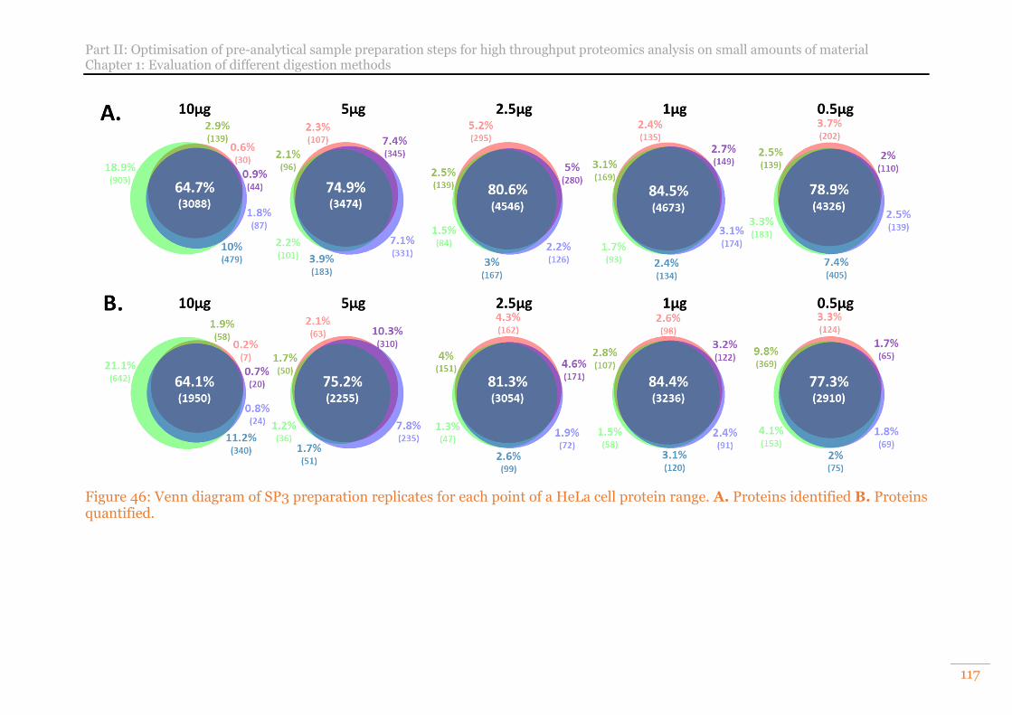
Part II: Optimisation of pre-analytical sample preparation steps for high throughput proteomics analysis on small amounts of material Chapter 1: Evaluation of different digestion methods
117
Figure 46: Venn diagram of SP3 preparation replicates for each point of a HeLa cell protein range. A. Proteins identified B. Proteins quantified.
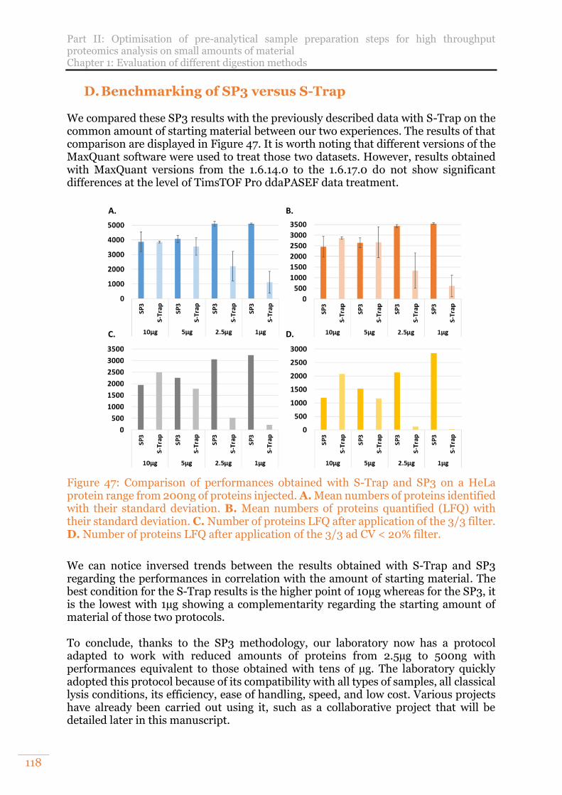
Part II: Optimisation of pre-analytical sample preparation steps for high throughput proteomics analysis on small amounts of material Chapter 1: Evaluation of different digestion methods
118
D. Benchmarking of SP3 versus S-Trap We compared these SP3 results with the previously described data with S-Trap on the common amount of starting material between our two experiences. The results of that comparison are displayed in Figure 47. It is worth noting that different versions of the MaxQuant software were used to treat those two datasets. However, results obtained with MaxQuant versions from the 1.6.14.0 to the 1.6.17.0 do not show significant differences at the level of TimsTOF Pro ddaPASEF data treatment.
Figure 47: Comparison of performances obtained with S-Trap and SP3 on a HeLa protein range from 200ng of proteins injected. A. Mean numbers of proteins identified with their standard deviation. B. Mean numbers of proteins quantified (LFQ) with their standard deviation. C. Number of proteins LFQ after application of the 3/3 filter. D. Number of proteins LFQ after application of the 3/3 ad CV < 20% filter.
We can notice inversed trends between the results obtained with S-Trap and SP3 regarding the performances in correlation with the amount of starting material. The best condition for the S-Trap results is the higher point of 10µg whereas for the SP3, it is the lowest with 1µg showing a complementarity regarding the starting amount of material of those two protocols. To conclude, thanks to the SP3 methodology, our laboratory now has a protocol adapted to work with reduced amounts of proteins from 2.5µg to 500ng with performances equivalent to those obtained with tens of µg. The laboratory quickly adopted this protocol because of its compatibility with all types of samples, all classical lysis conditions, its efficiency, ease of handling, speed, and low cost. Various projects have already been carried out using it, such as a collaborative project that will be detailed later in this manuscript.
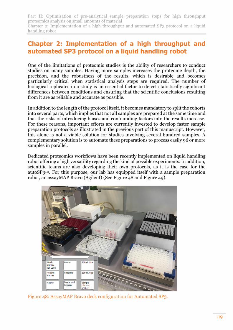
Part II: Optimisation of pre-analytical sample preparation steps for high throughput proteomics analysis on small amounts of material Chapter 2: Implementation of a high throughput and automated SP3 protocol on a liquid handling robot
119
Chapter 2: Implementation of a high throughput and automated SP3 protocol on a liquid handling robot
One of the limitations of proteomic studies is the ability of researchers to conduct studies on many samples. Having more samples increases the proteome depth, the precision, and the robustness of the results, which is desirable and becomes particularly critical when statistical analysis steps are required. The number of biological replicates in a study is an essential factor to detect statistically significant differences between conditions and ensuring that the scientific conclusions resulting from it are as reliable and accurate as possible. In addition to the length of the protocol itself, it becomes mandatory to split the cohorts into several parts, which implies that not all samples are prepared at the same time and that the risks of introducing biases and confounding factors into the results increase. For these reasons, important efforts are currently invested to develop faster sample preparation protocols as illustrated in the previous part of this manuscript. However, this alone is not a viable solution for studies involving several hundred samples. A complementary solution is to automate these preparations to process easily 96 or more samples in parallel. Dedicated proteomics workflows have been recently implemented on liquid handling robot offering a high versatility regarding the kind of possible experiments. In addition, scientific teams are also developing their own protocols, as it is the case for the autoSP31,2. For this purpose, our lab has equipped itself with a sample preparation robot, an assayMAP Bravo (Agilent) (See Figure 48 and Figure 49).
Figure 48: AssayMAP Bravo deck configuration for Automated SP3.
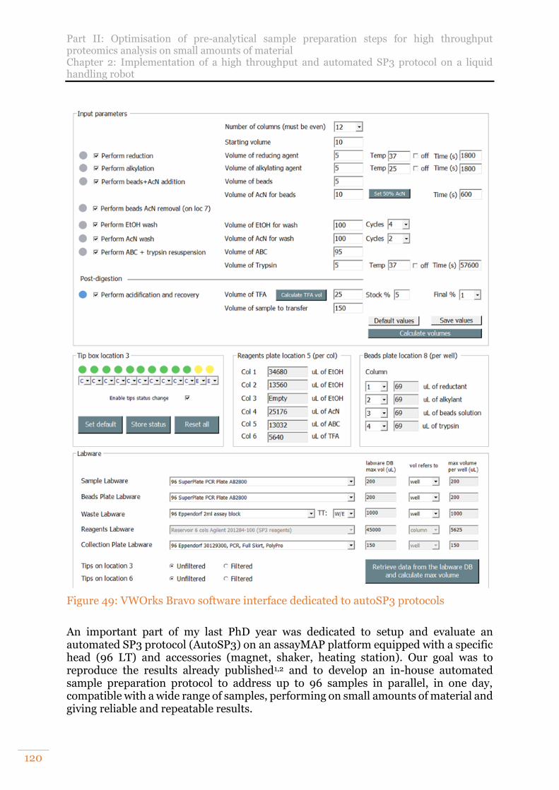
Part II: Optimisation of pre-analytical sample preparation steps for high throughput proteomics analysis on small amounts of material Chapter 2: Implementation of a high throughput and automated SP3 protocol on a liquid handling robot
120
Figure 49: VWOrks Bravo software interface dedicated to autoSP3 protocols
An important part of my last PhD year was dedicated to setup and evaluate an automated SP3 protocol (AutoSP3) on an assayMAP platform equipped with a specific head (96 LT) and accessories (magnet, shaker, heating station). Our goal was to reproduce the results already published1,2 and to develop an in-house automated sample preparation protocol to address up to 96 samples in parallel, in one day, compatible with a wide range of samples, performing on small amounts of material and giving reliable and repeatable results.
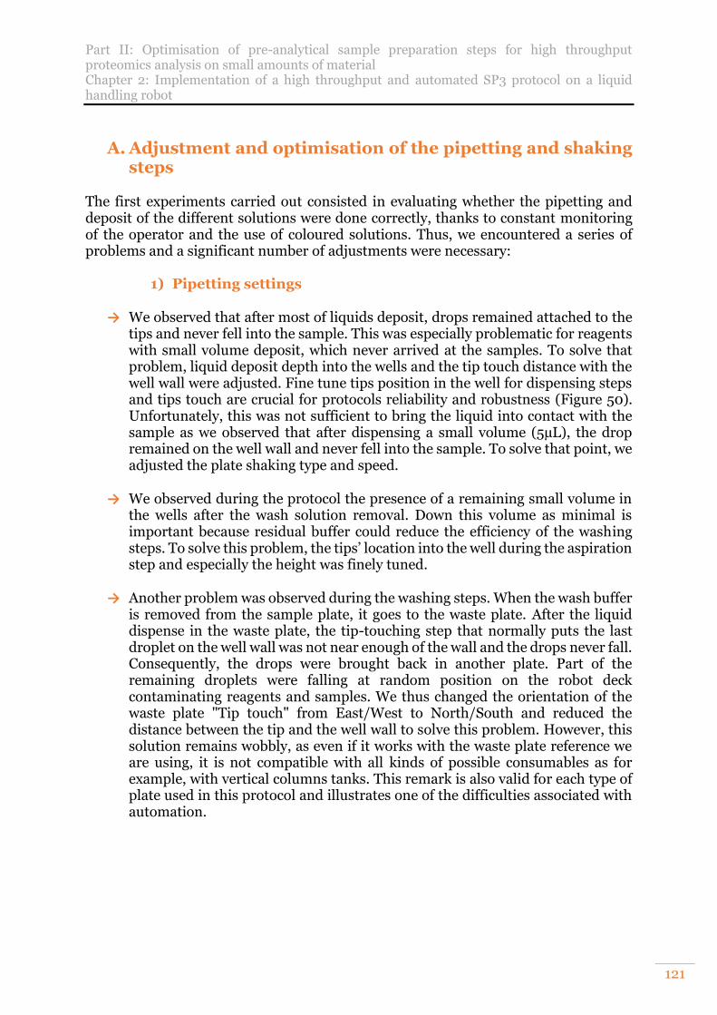
Part II: Optimisation of pre-analytical sample preparation steps for high throughput proteomics analysis on small amounts of material Chapter 2: Implementation of a high throughput and automated SP3 protocol on a liquid handling robot
121
A. Adjustment and optimisation of the pipetting and shaking steps
The first experiments carried out consisted in evaluating whether the pipetting and deposit of the different solutions were done correctly, thanks to constant monitoring of the operator and the use of coloured solutions. Thus, we encountered a series of problems and a significant number of adjustments were necessary:
1) Pipetting settings
→ We observed that after most of liquids deposit, drops remained attached to the tips and never fell into the sample. This was especially problematic for reagents with small volume deposit, which never arrived at the samples. To solve that problem, liquid deposit depth into the wells and the tip touch distance with the well wall were adjusted. Fine tune tips position in the well for dispensing steps and tips touch are crucial for protocols reliability and robustness (Figure 50). Unfortunately, this was not sufficient to bring the liquid into contact with the sample as we observed that after dispensing a small volume (5µL), the drop remained on the well wall and never fell into the sample. To solve that point, we adjusted the plate shaking type and speed.
→ We observed during the protocol the presence of a remaining small volume in
the wells after the wash solution removal. Down this volume as minimal is important because residual buffer could reduce the efficiency of the washing steps. To solve this problem, the tips’ location into the well during the aspiration step and especially the height was finely tuned.
→ Another problem was observed during the washing steps. When the wash buffer
is removed from the sample plate, it goes to the waste plate. After the liquid dispense in the waste plate, the tip-touching step that normally puts the last droplet on the well wall was not near enough of the wall and the drops never fall. Consequently, the drops were brought back in another plate. Part of the remaining droplets were falling at random position on the robot deck contaminating reagents and samples. We thus changed the orientation of the waste plate "Tip touch" from East/West to North/South and reduced the distance between the tip and the well wall to solve this problem. However, this solution remains wobbly, as even if it works with the waste plate reference we are using, it is not compatible with all kinds of possible consumables as for example, with vertical columns tanks. This remark is also valid for each type of plate used in this protocol and illustrates one of the difficulties associated with automation.
Part II: Optimisation of pre-analytical sample preparation steps for high throughput proteomics analysis on small amounts of material Chapter 2: Implementation of a high throughput and automated SP3 protocol on a liquid handling robot
122
Figure 50: VWorks Bravo interface for protocol development, example for tips positioning versus plate for liquid dispensing into the well.
Part II: Optimisation of pre-analytical sample preparation steps for high throughput proteomics analysis on small amounts of material Chapter 2: Implementation of a high throughput and automated SP3 protocol on a liquid handling robot
123
2) Digestion step In opposition with the published autoSP3 protocol, the digestion incubation step was implemented directly in the robot. To improve the temperature conduction and homogeneity during the digestion, a special and dedicated plate support was added on the heating station. This improvement led to the modification of the height of plate deposit by the robot gripper at this specific position on the deck. With this last modification, the sample plate theoretically does not need to be manually moved during the protocol. However, the Bravo does still not support the cover management. Consequently, we interrupt the protocol at the beginning of the digestion incubation to seal the sample plate with a plastic foil to avoid evaporation, which could occur during overnight digestion. However, a sealed plate cover, which should avoid handling the plate, is under investigation by Agilent. Despite the various improvements mentioned above, several problems were observed randomly throughout the various tests we carried out. For example, we found that a smaller volume is added to the last column of the sample plate than to the other columns of the plate. This is particularly noticeable for the steps where organic solvents are added, and which could affect the washing steps. Today, this problem is still not solved. Once those preliminary adjustments were realised, first experiments were carried out on human plasma and HeLa cell lysate proteins.
B. Analysis of a non-fractionated, non-depleted human plasma
1) Evaluation on two amounts of plasma
A first experiment was performed with human plasma. We chose to work with plasma because of its great interest for clinical studies. This type of sample is commercially available and contains a high concentration of proteins. It is obviously a good candidate for the search for biomarkers of disease373. However, the analysis of plasma also represents a great analytical challenge due to its wide dynamic range between low and high abundant proteins and the complexity of its proteome373–375. For this reason, the analysis of this type of sample is often preceded by a depletion of the most abundant proteins such as albumin and/or a fractionation step to improve the depth of the proteome analysis. To perform a fully automated sample preparation on this type of sample, we decided to attempt plasma analysis without these preliminary steps. We worked with 10µg and 100µg of proteins corresponding to approximately 0.1µL and 1µL of human plasma. For both conditions, the samples were prepared in quadruplicate. After autoSP3, the samples were evaporated, suspended, and analysed by nLC-IMS-MS/MS on a nanoElute-TimsTOF Pro coupling in ddaPASEF mode with a 60min gradient. Data were treated using Mascot + Proline studio using a PSM and protein FDR of 1%. The numbers of proteins and PSM identified are shown in Figure 51.
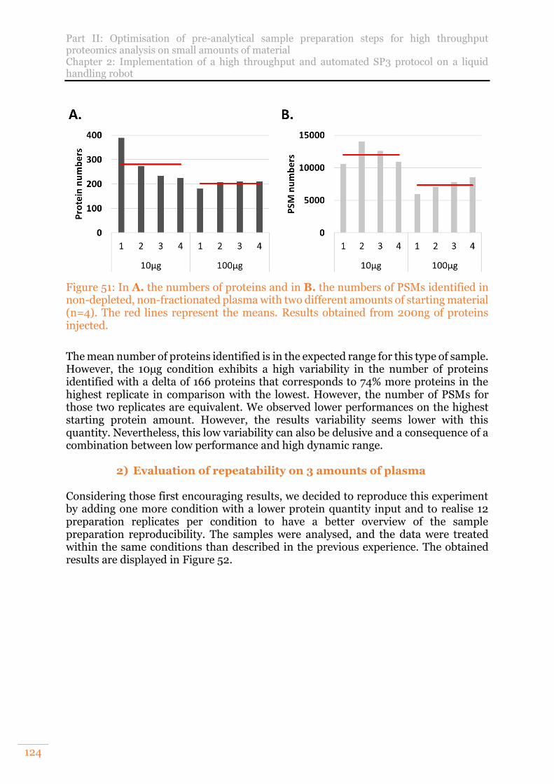
Part II: Optimisation of pre-analytical sample preparation steps for high throughput proteomics analysis on small amounts of material Chapter 2: Implementation of a high throughput and automated SP3 protocol on a liquid handling robot
124
Figure 51: In A. the numbers of proteins and in B. the numbers of PSMs identified in non-depleted, non-fractionated plasma with two different amounts of starting material (n=4). The red lines represent the means. Results obtained from 200ng of proteins injected.
The mean number of proteins identified is in the expected range for this type of sample. However, the 10µg condition exhibits a high variability in the number of proteins identified with a delta of 166 proteins that corresponds to 74% more proteins in the highest replicate in comparison with the lowest. However, the number of PSMs for those two replicates are equivalent. We observed lower performances on the highest starting protein amount. However, the results variability seems lower with this quantity. Nevertheless, this low variability can also be delusive and a consequence of a combination between low performance and high dynamic range.
2) Evaluation of repeatability on 3 amounts of plasma Considering those first encouraging results, we decided to reproduce this experiment by adding one more condition with a lower protein quantity input and to realise 12 preparation replicates per condition to have a better overview of the sample preparation reproducibility. The samples were analysed, and the data were treated within the same conditions than described in the previous experience. The obtained results are displayed in Figure 52.
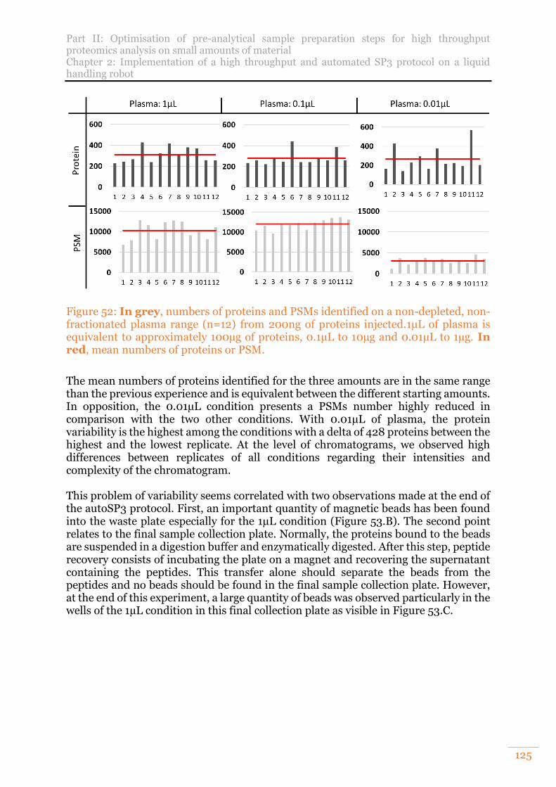
Part II: Optimisation of pre-analytical sample preparation steps for high throughput proteomics analysis on small amounts of material Chapter 2: Implementation of a high throughput and automated SP3 protocol on a liquid handling robot
125
Figure 52: In grey, numbers of proteins and PSMs identified on a non-depleted, non-fractionated plasma range (n=12) from 200ng of proteins injected.1µL of plasma is equivalent to approximately 100µg of proteins, 0.1µL to 10µg and 0.01µL to 1µg. In red, mean numbers of proteins or PSM.
The mean numbers of proteins identified for the three amounts are in the same range than the previous experience and is equivalent between the different starting amounts. In opposition, the 0.01µL condition presents a PSMs number highly reduced in comparison with the two other conditions. With 0.01µL of plasma, the protein variability is the highest among the conditions with a delta of 428 proteins between the highest and the lowest replicate. At the level of chromatograms, we observed high differences between replicates of all conditions regarding their intensities and complexity of the chromatogram. This problem of variability seems correlated with two observations made at the end of the autoSP3 protocol. First, an important quantity of magnetic beads has been found into the waste plate especially for the 1µL condition (Figure 53.B). The second point relates to the final sample collection plate. Normally, the proteins bound to the beads are suspended in a digestion buffer and enzymatically digested. After this step, peptide recovery consists of incubating the plate on a magnet and recovering the supernatant containing the peptides. This transfer alone should separate the beads from the peptides and no beads should be found in the final sample collection plate. However, at the end of this experiment, a large quantity of beads was observed particularly in the wells of the 1µL condition in this final collection plate as visible in Figure 53.C.
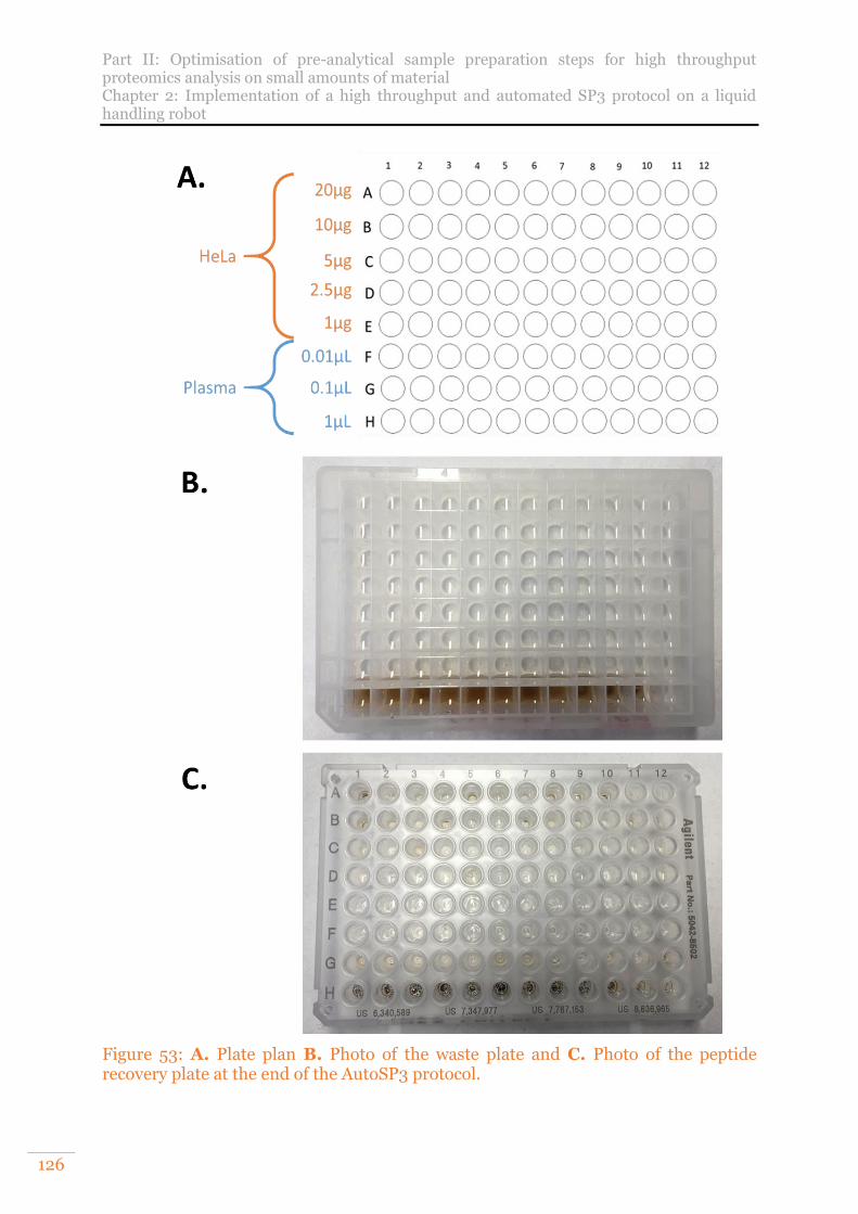
Part II: Optimisation of pre-analytical sample preparation steps for high throughput proteomics analysis on small amounts of material Chapter 2: Implementation of a high throughput and automated SP3 protocol on a liquid handling robot
126
Figure 53: A. Plate plan B. Photo of the waste plate and C. Photo of the peptide recovery plate at the end of the AutoSP3 protocol.
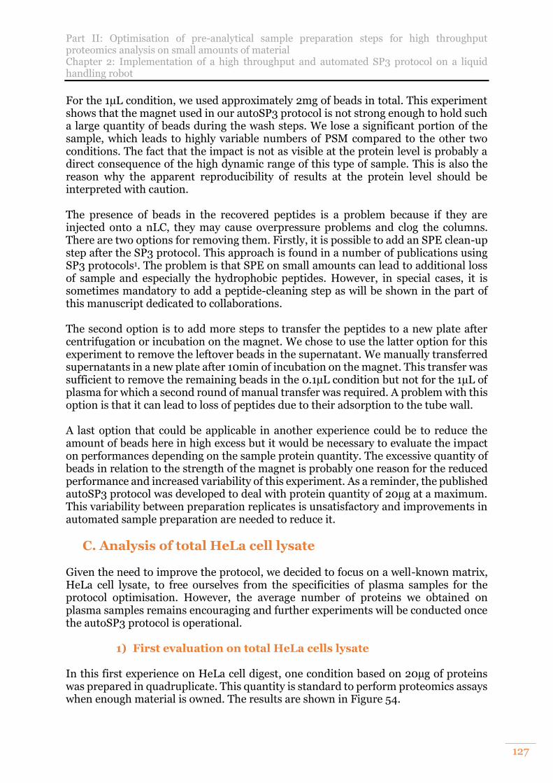
Part II: Optimisation of pre-analytical sample preparation steps for high throughput proteomics analysis on small amounts of material Chapter 2: Implementation of a high throughput and automated SP3 protocol on a liquid handling robot
127
For the 1µL condition, we used approximately 2mg of beads in total. This experiment shows that the magnet used in our autoSP3 protocol is not strong enough to hold such a large quantity of beads during the wash steps. We lose a significant portion of the sample, which leads to highly variable numbers of PSM compared to the other two conditions. The fact that the impact is not as visible at the protein level is probably a direct consequence of the high dynamic range of this type of sample. This is also the reason why the apparent reproducibility of results at the protein level should be interpreted with caution. The presence of beads in the recovered peptides is a problem because if they are injected onto a nLC, they may cause overpressure problems and clog the columns. There are two options for removing them. Firstly, it is possible to add an SPE clean-up step after the SP3 protocol. This approach is found in a number of publications using SP3 protocols1. The problem is that SPE on small amounts can lead to additional loss of sample and especially the hydrophobic peptides. However, in special cases, it is sometimes mandatory to add a peptide-cleaning step as will be shown in the part of this manuscript dedicated to collaborations. The second option is to add more steps to transfer the peptides to a new plate after centrifugation or incubation on the magnet. We chose to use the latter option for this experiment to remove the leftover beads in the supernatant. We manually transferred supernatants in a new plate after 10min of incubation on the magnet. This transfer was sufficient to remove the remaining beads in the 0.1µL condition but not for the 1µL of plasma for which a second round of manual transfer was required. A problem with this option is that it can lead to loss of peptides due to their adsorption to the tube wall. A last option that could be applicable in another experience could be to reduce the amount of beads here in high excess but it would be necessary to evaluate the impact on performances depending on the sample protein quantity. The excessive quantity of beads in relation to the strength of the magnet is probably one reason for the reduced performance and increased variability of this experiment. As a reminder, the published autoSP3 protocol was developed to deal with protein quantity of 20µg at a maximum. This variability between preparation replicates is unsatisfactory and improvements in automated sample preparation are needed to reduce it.
C. Analysis of total HeLa cell lysate Given the need to improve the protocol, we decided to focus on a well-known matrix, HeLa cell lysate, to free ourselves from the specificities of plasma samples for the protocol optimisation. However, the average number of proteins we obtained on plasma samples remains encouraging and further experiments will be conducted once the autoSP3 protocol is operational.
1) First evaluation on total HeLa cells lysate In this first experience on HeLa cell digest, one condition based on 20µg of proteins was prepared in quadruplicate. This quantity is standard to perform proteomics assays when enough material is owned. The results are shown in Figure 54.
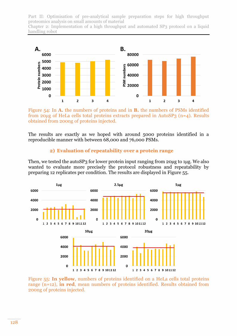
Part II: Optimisation of pre-analytical sample preparation steps for high throughput proteomics analysis on small amounts of material Chapter 2: Implementation of a high throughput and automated SP3 protocol on a liquid handling robot
128
Figure 54: In A. the numbers of proteins and in B. the numbers of PSMs identified from 20µg of HeLa cells total proteins extracts prepared in AutoSP3 (n=4). Results obtained from 200ng of proteins injected.
The results are exactly as we hoped with around 5000 proteins identified in a reproducible manner with between 68,000 and 76,000 PSMs.
2) Evaluation of repeatability over a protein range Then, we tested the autoSP3 for lower protein input ranging from 20µg to 1µg. We also wanted to evaluate more precisely the protocol robustness and repeatability by preparing 12 replicates per condition. The results are displayed in Figure 55.
Figure 55: In yellow, numbers of proteins identified on a HeLa cells total proteins range (n=12), in red, mean numbers of proteins identified. Results obtained from 200ng of proteins injected.
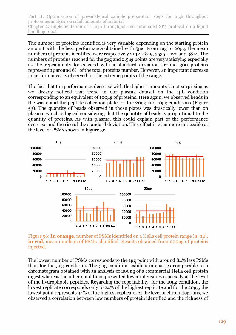
Part II: Optimisation of pre-analytical sample preparation steps for high throughput proteomics analysis on small amounts of material Chapter 2: Implementation of a high throughput and automated SP3 protocol on a liquid handling robot
129
The number of proteins identified is very variable depending on the starting protein amount with the best performance obtained with 5µg. From 1µg to 20µg, the mean numbers of proteins identified were respectively 2142, 4819, 5535, 4122 and 3814. The numbers of proteins reached for the 5µg and 2.5µg points are very satisfying especially as the repeatability looks good with a standard deviation around 300 proteins representing around 6% of the total proteins number. However, an important decrease in performances is observed for the extreme points of the range. The fact that the performances decrease with the highest amounts is not surprising as we already noticed that trend in our plasma dataset on the 1µL condition corresponding to an equivalent of 100µg of proteins. Here again, we observed beads in the waste and the peptide collection plate for the 20µg and 10µg conditions (Figure 53). The quantity of beads observed in those plates was drastically lower than on plasma, which is logical considering that the quantity of beads is proportional to the quantity of proteins. As with plasma, this could explain part of the performance decrease and the rise of the standard deviation. This effect is even more noticeable at the level of PSMs shown in Figure 56.
Figure 56: In orange, number of PSMs identified on a HeLa cell protein range (n=12), in red, mean numbers of PSMs identified. Results obtained from 200ng of proteins injected.
The lowest number of PSMs corresponds to the 1µg point with around 84% less PSMs than for the 5µg condition. The 5µg condition exhibits intensities comparable to a chromatogram obtained with an analysis of 200ng of a commercial HeLa cell protein digest whereas the other conditions presented lower intensities especially at the level of the hydrophobic peptides. Regarding the repeatability, for the 10µg condition, the lowest replicate corresponds only to 24% of the highest replicate and for the 20µg; the lowest point represents 34% of the highest replicate. At the level of chromatograms, we observed a correlation between low numbers of protein identified and the richness of
Part II: Optimisation of pre-analytical sample preparation steps for high throughput proteomics analysis on small amounts of material Chapter 2: Implementation of a high throughput and automated SP3 protocol on a liquid handling robot
130
the chromatogram in terms of peak population especially at the level of hydrophobic peptides but not only. The difference of around 1000 proteins identified between the first and the second experiment on the 20µg condition was very surprising. For this reason, we investigated and discovered that some users misused the shared stock bottle of beads. People did not sufficiently mix the beads before taking them, thus significantly increasing the beads concentration in the stock solutions. When the concentrations of the stock solutions were evaluated, they were respectively of 89µg/µL and 76µg/µL against 50µg/µL waited. Using a protein to bead ratio of 1:10 means that we are already in great excess. Furthermore, for all conditions, we used about 61% more beads than we should have because of the concentration problem of the bead stock solution. Therefore, our first and second experiments are not comparable. The negative impact on the performance is probably related to the loss of beads due to the too low strength of the magnet. On the other hand, a too high concentration of beads leads to their aggregation reducing the efficiency of protein binding and the loss of proteins during the washing steps as observed by Hughes et al.58. Finally, the presence of residual intact chromatin can decrease the binding efficiency. In view of these results, we decided to repeat the experiment with the same concentration of the protein set but with the correct bead ratio.
3) Analysis of a HeLa cell lysate protein range prepared in six replicates and with different beads ratio
Considering the problem of beads remaining in the peptide recovery plate in the previous experiment and various nLC pressure problems, we decided to add an SPE step to clean the peptides before the nLC-MS/MS analysis. This peptide-cleaning step was also performed on the Bravo robot but with the dedicated head for SPE protocol, namely the AssayMap head and RP-C18 cartridges. Each condition in this experiment was prepared in six replicates. Three bead ratios were tested for the 20µg condition and two for the 10µg condition as shown in Figure 57. The goal was to evaluate the possibility to work on important quantity of proteins with a lower quantity of beads without losing in performances and thus limiting the problem linked to the strength of the magnet.
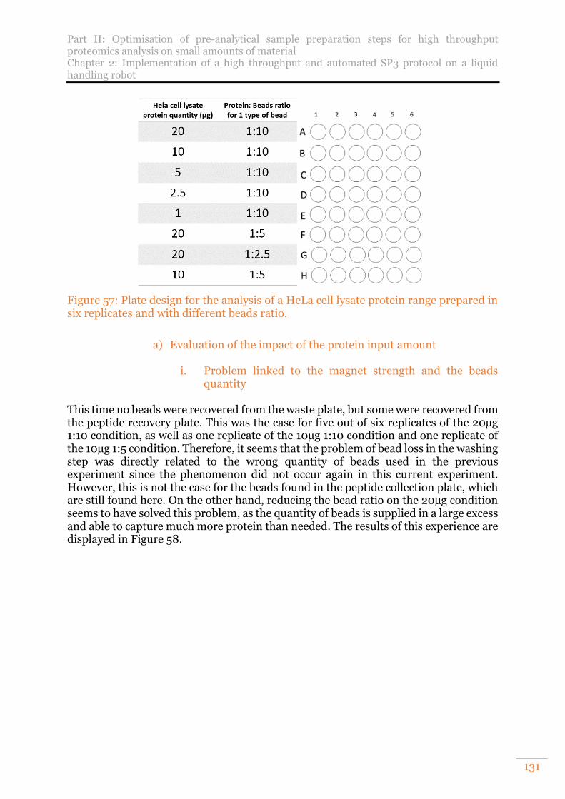
Part II: Optimisation of pre-analytical sample preparation steps for high throughput proteomics analysis on small amounts of material Chapter 2: Implementation of a high throughput and automated SP3 protocol on a liquid handling robot
131
Figure 57: Plate design for the analysis of a HeLa cell lysate protein range prepared in six replicates and with different beads ratio.
a) Evaluation of the impact of the protein input amount
i. Problem linked to the magnet strength and the beads
quantity This time no beads were recovered from the waste plate, but some were recovered from the peptide recovery plate. This was the case for five out of six replicates of the 20µg 1:10 condition, as well as one replicate of the 10µg 1:10 condition and one replicate of the 10µg 1:5 condition. Therefore, it seems that the problem of bead loss in the washing step was directly related to the wrong quantity of beads used in the previous experiment since the phenomenon did not occur again in this current experiment. However, this is not the case for the beads found in the peptide collection plate, which are still found here. On the other hand, reducing the bead ratio on the 20µg condition seems to have solved this problem, as the quantity of beads is supplied in a large excess and able to capture much more protein than needed. The results of this experience are displayed in Figure 58.
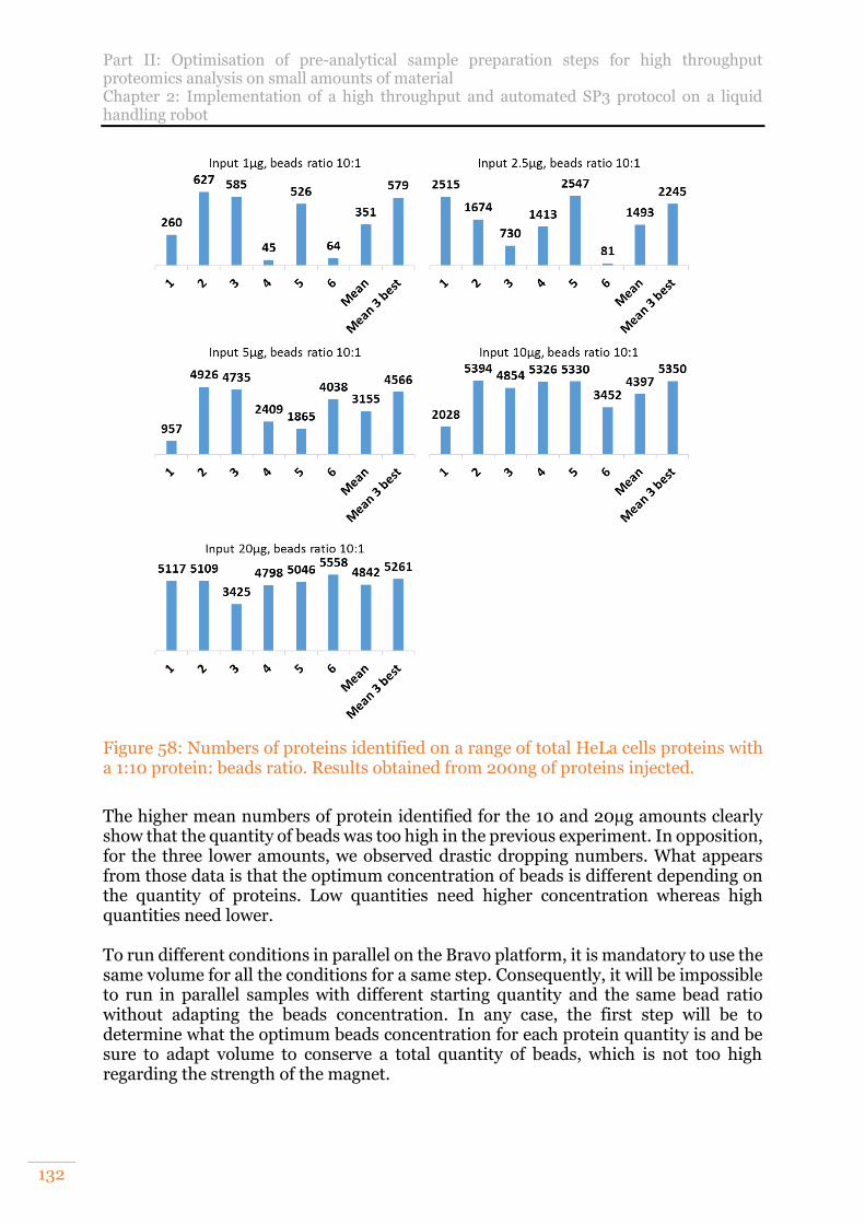
Part II: Optimisation of pre-analytical sample preparation steps for high throughput proteomics analysis on small amounts of material Chapter 2: Implementation of a high throughput and automated SP3 protocol on a liquid handling robot
132
Figure 58: Numbers of proteins identified on a range of total HeLa cells proteins with a 1:10 protein: beads ratio. Results obtained from 200ng of proteins injected.
The higher mean numbers of protein identified for the 10 and 20µg amounts clearly show that the quantity of beads was too high in the previous experiment. In opposition, for the three lower amounts, we observed drastic dropping numbers. What appears from those data is that the optimum concentration of beads is different depending on the quantity of proteins. Low quantities need higher concentration whereas high quantities need lower. To run different conditions in parallel on the Bravo platform, it is mandatory to use the same volume for all the conditions for a same step. Consequently, it will be impossible to run in parallel samples with different starting quantity and the same bead ratio without adapting the beads concentration. In any case, the first step will be to determine what the optimum beads concentration for each protein quantity is and be sure to adapt volume to conserve a total quantity of beads, which is not too high regarding the strength of the magnet.
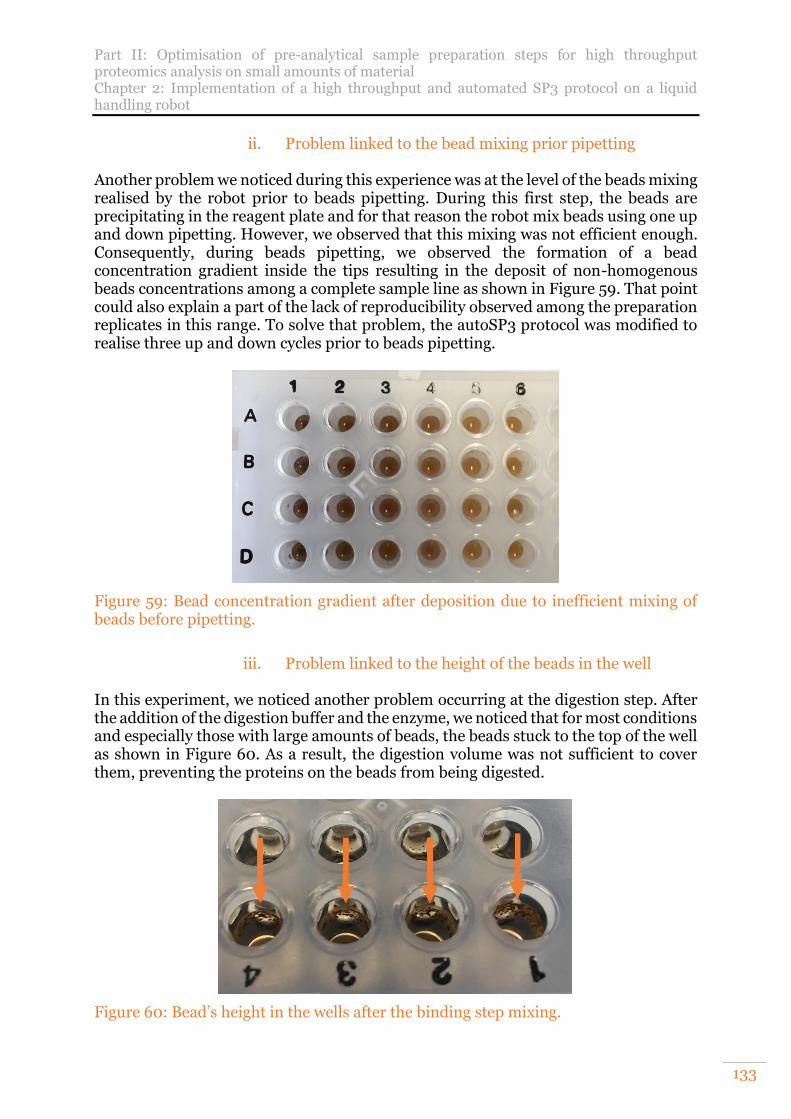
Part II: Optimisation of pre-analytical sample preparation steps for high throughput proteomics analysis on small amounts of material Chapter 2: Implementation of a high throughput and automated SP3 protocol on a liquid handling robot
133
ii. Problem linked to the bead mixing prior pipetting Another problem we noticed during this experience was at the level of the beads mixing realised by the robot prior to beads pipetting. During this first step, the beads are precipitating in the reagent plate and for that reason the robot mix beads using one up and down pipetting. However, we observed that this mixing was not efficient enough. Consequently, during beads pipetting, we observed the formation of a bead concentration gradient inside the tips resulting in the deposit of non-homogenous beads concentrations among a complete sample line as shown in Figure 59. That point could also explain a part of the lack of reproducibility observed among the preparation replicates in this range. To solve that problem, the autoSP3 protocol was modified to realise three up and down cycles prior to beads pipetting.
Figure 59: Bead concentration gradient after deposition due to inefficient mixing of beads before pipetting.
iii. Problem linked to the height of the beads in the well
In this experiment, we noticed another problem occurring at the digestion step. After the addition of the digestion buffer and the enzyme, we noticed that for most conditions and especially those with large amounts of beads, the beads stuck to the top of the well as shown in Figure 60. As a result, the digestion volume was not sufficient to cover them, preventing the proteins on the beads from being digested.
Figure 60: Bead’s height in the wells after the binding step mixing.
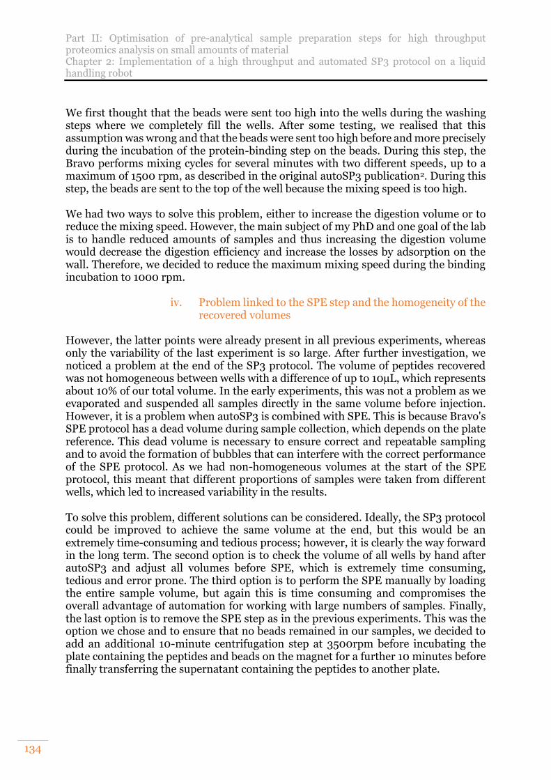
Part II: Optimisation of pre-analytical sample preparation steps for high throughput proteomics analysis on small amounts of material Chapter 2: Implementation of a high throughput and automated SP3 protocol on a liquid handling robot
134
We first thought that the beads were sent too high into the wells during the washing steps where we completely fill the wells. After some testing, we realised that this assumption was wrong and that the beads were sent too high before and more precisely during the incubation of the protein-binding step on the beads. During this step, the Bravo performs mixing cycles for several minutes with two different speeds, up to a maximum of 1500 rpm, as described in the original autoSP3 publication2. During this step, the beads are sent to the top of the well because the mixing speed is too high. We had two ways to solve this problem, either to increase the digestion volume or to reduce the mixing speed. However, the main subject of my PhD and one goal of the lab is to handle reduced amounts of samples and thus increasing the digestion volume would decrease the digestion efficiency and increase the losses by adsorption on the wall. Therefore, we decided to reduce the maximum mixing speed during the binding incubation to 1000 rpm.
iv. Problem linked to the SPE step and the homogeneity of the recovered volumes
However, the latter points were already present in all previous experiments, whereas only the variability of the last experiment is so large. After further investigation, we noticed a problem at the end of the SP3 protocol. The volume of peptides recovered was not homogeneous between wells with a difference of up to 10µL, which represents about 10% of our total volume. In the early experiments, this was not a problem as we evaporated and suspended all samples directly in the same volume before injection. However, it is a problem when autoSP3 is combined with SPE. This is because Bravo's SPE protocol has a dead volume during sample collection, which depends on the plate reference. This dead volume is necessary to ensure correct and repeatable sampling and to avoid the formation of bubbles that can interfere with the correct performance of the SPE protocol. As we had non-homogeneous volumes at the start of the SPE protocol, this meant that different proportions of samples were taken from different wells, which led to increased variability in the results. To solve this problem, different solutions can be considered. Ideally, the SP3 protocol could be improved to achieve the same volume at the end, but this would be an extremely time-consuming and tedious process; however, it is clearly the way forward in the long term. The second option is to check the volume of all wells by hand after autoSP3 and adjust all volumes before SPE, which is extremely time consuming, tedious and error prone. The third option is to perform the SPE manually by loading the entire sample volume, but again this is time consuming and compromises the overall advantage of automation for working with large numbers of samples. Finally, the last option is to remove the SPE step as in the previous experiments. This was the option we chose and to ensure that no beads remained in our samples, we decided to add an additional 10-minute centrifugation step at 3500rpm before incubating the plate containing the peptides and beads on the magnet for a further 10 minutes before finally transferring the supernatant containing the peptides to another plate.
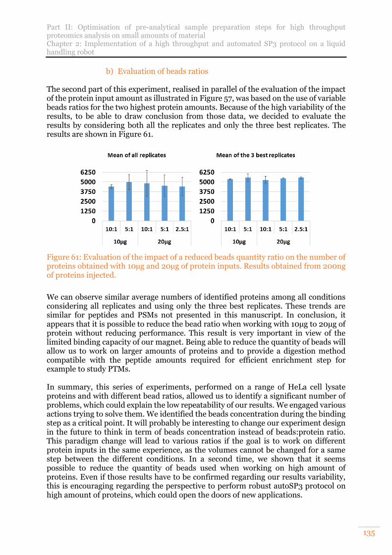
Part II: Optimisation of pre-analytical sample preparation steps for high throughput proteomics analysis on small amounts of material Chapter 2: Implementation of a high throughput and automated SP3 protocol on a liquid handling robot
135
b) Evaluation of beads ratios The second part of this experiment, realised in parallel of the evaluation of the impact of the protein input amount as illustrated in Figure 57, was based on the use of variable beads ratios for the two highest protein amounts. Because of the high variability of the results, to be able to draw conclusion from those data, we decided to evaluate the results by considering both all the replicates and only the three best replicates. The results are shown in Figure 61.
Figure 61: Evaluation of the impact of a reduced beads quantity ratio on the number of proteins obtained with 10µg and 20µg of protein inputs. Results obtained from 200ng of proteins injected.
We can observe similar average numbers of identified proteins among all conditions considering all replicates and using only the three best replicates. These trends are similar for peptides and PSMs not presented in this manuscript. In conclusion, it appears that it is possible to reduce the bead ratio when working with 10µg to 20µg of protein without reducing performance. This result is very important in view of the limited binding capacity of our magnet. Being able to reduce the quantity of beads will allow us to work on larger amounts of proteins and to provide a digestion method compatible with the peptide amounts required for efficient enrichment step for example to study PTMs. In summary, this series of experiments, performed on a range of HeLa cell lysate proteins and with different bead ratios, allowed us to identify a significant number of problems, which could explain the low repeatability of our results. We engaged various actions trying to solve them. We identified the beads concentration during the binding step as a critical point. It will probably be interesting to change our experiment design in the future to think in term of beads concentration instead of beads:protein ratio. This paradigm change will lead to various ratios if the goal is to work on different protein inputs in the same experience, as the volumes cannot be changed for a same step between the different conditions. In a second time, we shown that it seems possible to reduce the quantity of beads used when working on high amount of proteins. Even if those results have to be confirmed regarding our results variability, this is encouraging regarding the perspective to perform robust autoSP3 protocol on high amount of proteins, which could open the doors of new applications.
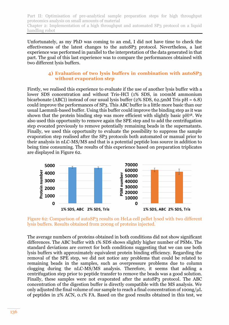
Part II: Optimisation of pre-analytical sample preparation steps for high throughput proteomics analysis on small amounts of material Chapter 2: Implementation of a high throughput and automated SP3 protocol on a liquid handling robot
136
Unfortunately, as my PhD was coming to an end, I did not have time to check the effectiveness of the latest changes to the autoSP3 protocol. Nevertheless, a last experience was performed in parallel to the interpretation of the data generated in that part. The goal of this last experience was to compare the performances obtained with two different lysis buffers.
4) Evaluation of two lysis buffers in combination with autoSP3 without evaporation step
Firstly, we realised this experience to evaluate if the use of another lysis buffer with a lower SDS concentration and without Tris-HCl (1% SDS, in 100mM ammonium bicarbonate (ABC)) instead of our usual lysis buffer (2% SDS, 62.5mM Tris pH = 6.8) could improve the performances of SP3. This ABC buffer is a little more basic than our usual Laemmli-based buffer. Using this buffer could improve the binding step as it was shown that the protein binding step was more efficient with slightly basic pH58. We also used this opportunity to remove again the SPE step and to add the centrifugation step evocated previously to remove potentially remaining beads in the supernatants. Finally, we used this opportunity to evaluate the possibility to suppress the sample evaporation step realised after the SP3 protocols both automated or manual prior to their analysis in nLC-MS/MS and that is a potential peptide loss source in addition to being time consuming. The results of this experience based on preparation triplicates are displayed in Figure 62.
Figure 62: Comparison of autoSP3 results on HeLa cell pellet lysed with two different lysis buffers. Results obtained from 200ng of proteins injected.
The average numbers of proteins obtained in both conditions did not show significant differences. The ABC buffer with 1% SDS shows slightly higher number of PSMs. The standard deviations are correct for both conditions suggesting that we can use both lysis buffers with approximately equivalent protein binding efficiency. Regarding the removal of the SPE step, we did not notice any problems that could be related to remaining beads in the samples, such as overpressure problems due to column clogging during the nLC-MS/MS analysis. Therefore, it seems that adding a centrifugation step prior to peptide transfer to remove the beads was a good solution. Finally, these samples were not evaporated after the autoSP3 protocol. The ABC concentration of the digestion buffer is directly compatible with the MS analysis. We only adjusted the final volume of our sample to reach a final concentration of 100ng/µL of peptides in 2% ACN, 0.1% FA. Based on the good results obtained in this test, we
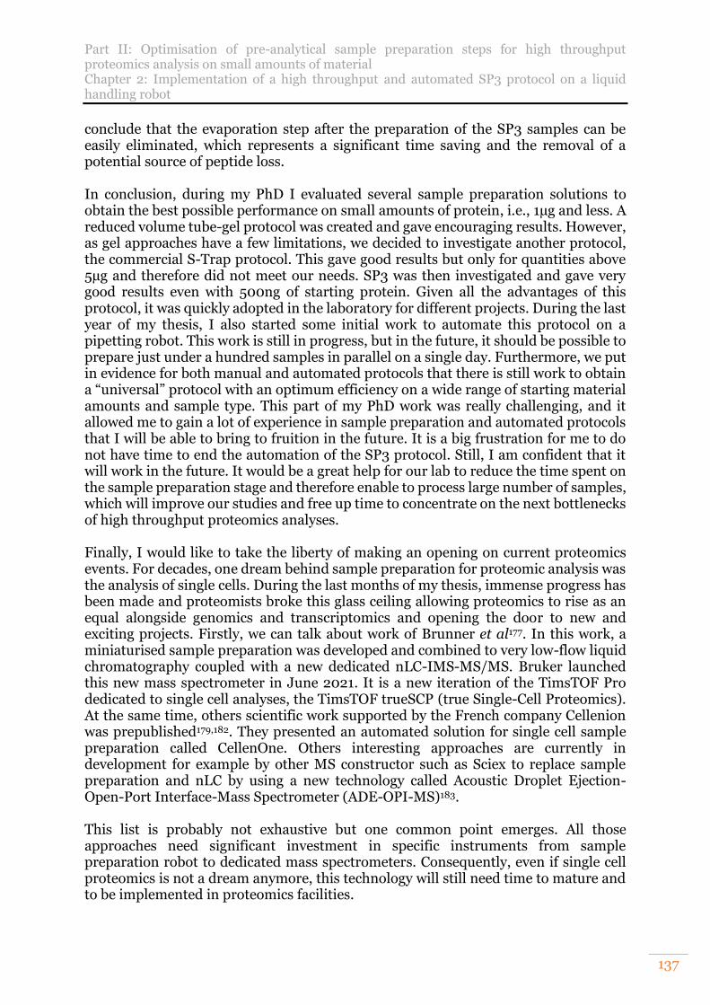
Part II: Optimisation of pre-analytical sample preparation steps for high throughput proteomics analysis on small amounts of material Chapter 2: Implementation of a high throughput and automated SP3 protocol on a liquid handling robot
137
conclude that the evaporation step after the preparation of the SP3 samples can be easily eliminated, which represents a significant time saving and the removal of a potential source of peptide loss. In conclusion, during my PhD I evaluated several sample preparation solutions to obtain the best possible performance on small amounts of protein, i.e., 1µg and less. A reduced volume tube-gel protocol was created and gave encouraging results. However, as gel approaches have a few limitations, we decided to investigate another protocol, the commercial S-Trap protocol. This gave good results but only for quantities above 5µg and therefore did not meet our needs. SP3 was then investigated and gave very good results even with 500ng of starting protein. Given all the advantages of this protocol, it was quickly adopted in the laboratory for different projects. During the last year of my thesis, I also started some initial work to automate this protocol on a pipetting robot. This work is still in progress, but in the future, it should be possible to prepare just under a hundred samples in parallel on a single day. Furthermore, we put in evidence for both manual and automated protocols that there is still work to obtain a “universal” protocol with an optimum efficiency on a wide range of starting material amounts and sample type. This part of my PhD work was really challenging, and it allowed me to gain a lot of experience in sample preparation and automated protocols that I will be able to bring to fruition in the future. It is a big frustration for me to do not have time to end the automation of the SP3 protocol. Still, I am confident that it will work in the future. It would be a great help for our lab to reduce the time spent on the sample preparation stage and therefore enable to process large number of samples, which will improve our studies and free up time to concentrate on the next bottlenecks of high throughput proteomics analyses. Finally, I would like to take the liberty of making an opening on current proteomics events. For decades, one dream behind sample preparation for proteomic analysis was the analysis of single cells. During the last months of my thesis, immense progress has been made and proteomists broke this glass ceiling allowing proteomics to rise as an equal alongside genomics and transcriptomics and opening the door to new and exciting projects. Firstly, we can talk about work of Brunner et al177. In this work, a miniaturised sample preparation was developed and combined to very low-flow liquid chromatography coupled with a new dedicated nLC-IMS-MS/MS. Bruker launched this new mass spectrometer in June 2021. It is a new iteration of the TimsTOF Pro dedicated to single cell analyses, the TimsTOF trueSCP (true Single-Cell Proteomics). At the same time, others scientific work supported by the French company Cellenion was prepublished179,182. They presented an automated solution for single cell sample preparation called CellenOne. Others interesting approaches are currently in development for example by other MS constructor such as Sciex to replace sample preparation and nLC by using a new technology called Acoustic Droplet Ejection- Open-Port Interface-Mass Spectrometer (ADE-OPI-MS)183. This list is probably not exhaustive but one common point emerges. All those approaches need significant investment in specific instruments from sample preparation robot to dedicated mass spectrometers. Consequently, even if single cell proteomics is not a dream anymore, this technology will still need time to mature and to be implemented in proteomics facilities.
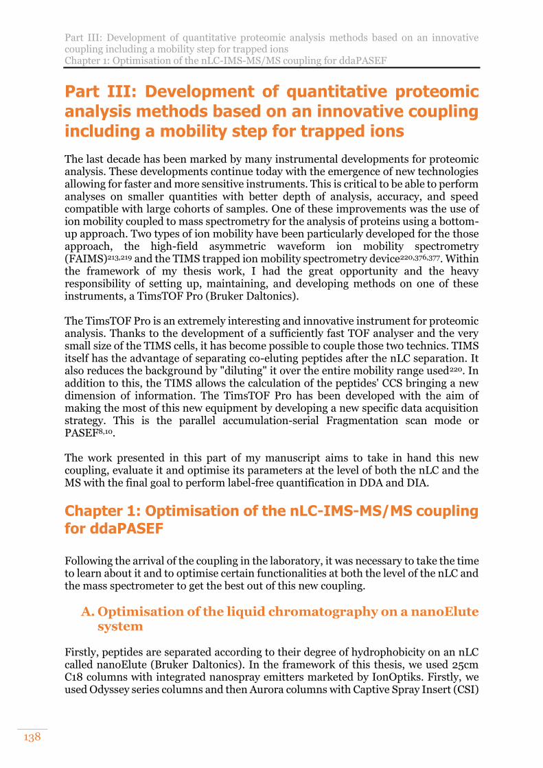
Part III: Development of quantitative proteomic analysis methods based on an innovative coupling including a mobility step for trapped ions Chapter 1: Optimisation of the nLC-IMS-MS/MS coupling for ddaPASEF
138
Part III: Development of quantitative proteomic analysis methods based on an innovative coupling including a mobility step for trapped ions The last decade has been marked by many instrumental developments for proteomic analysis. These developments continue today with the emergence of new technologies allowing for faster and more sensitive instruments. This is critical to be able to perform analyses on smaller quantities with better depth of analysis, accuracy, and speed compatible with large cohorts of samples. One of these improvements was the use of ion mobility coupled to mass spectrometry for the analysis of proteins using a bottom-up approach. Two types of ion mobility have been particularly developed for the those approach, the high-field asymmetric waveform ion mobility spectrometry (FAIMS)213,219 and the TIMS trapped ion mobility spectrometry device220,376,377. Within the framework of my thesis work, I had the great opportunity and the heavy responsibility of setting up, maintaining, and developing methods on one of these instruments, a TimsTOF Pro (Bruker Daltonics). The TimsTOF Pro is an extremely interesting and innovative instrument for proteomic analysis. Thanks to the development of a sufficiently fast TOF analyser and the very small size of the TIMS cells, it has become possible to couple those two technics. TIMS itself has the advantage of separating co-eluting peptides after the nLC separation. It also reduces the background by "diluting" it over the entire mobility range used220. In addition to this, the TIMS allows the calculation of the peptides' CCS bringing a new dimension of information. The TimsTOF Pro has been developed with the aim of making the most of this new equipment by developing a new specific data acquisition strategy. This is the parallel accumulation-serial Fragmentation scan mode or PASEF8,10. The work presented in this part of my manuscript aims to take in hand this new coupling, evaluate it and optimise its parameters at the level of both the nLC and the MS with the final goal to perform label-free quantification in DDA and DIA.
Chapter 1: Optimisation of the nLC-IMS-MS/MS coupling for ddaPASEF
Following the arrival of the coupling in the laboratory, it was necessary to take the time to learn about it and to optimise certain functionalities at both the level of the nLC and the mass spectrometer to get the best out of this new coupling.
A. Optimisation of the liquid chromatography on a nanoElute system
Firstly, peptides are separated according to their degree of hydrophobicity on an nLC called nanoElute (Bruker Daltonics). In the framework of this thesis, we used 25cm C18 columns with integrated nanospray emitters marketed by IonOptiks. Firstly, we used Odyssey series columns and then Aurora columns with Captive Spray Insert (CSI)
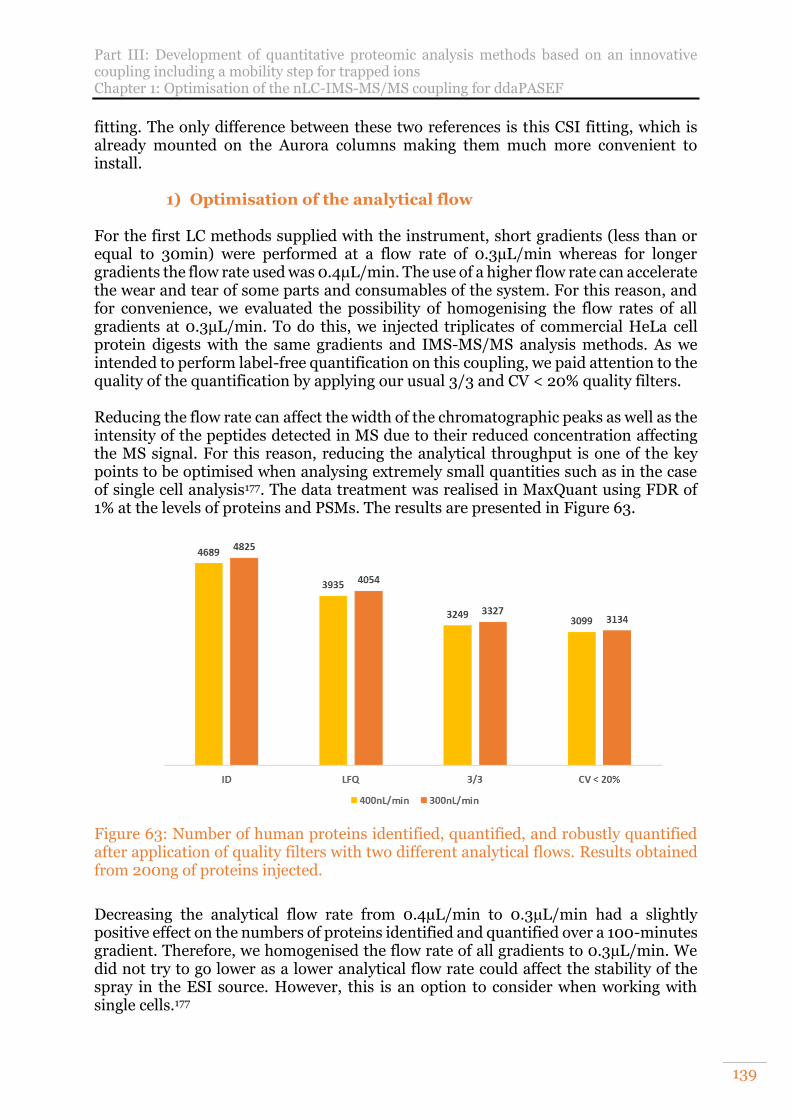
Part III: Development of quantitative proteomic analysis methods based on an innovative coupling including a mobility step for trapped ions Chapter 1: Optimisation of the nLC-IMS-MS/MS coupling for ddaPASEF
139
fitting. The only difference between these two references is this CSI fitting, which is already mounted on the Aurora columns making them much more convenient to install.
1) Optimisation of the analytical flow For the first LC methods supplied with the instrument, short gradients (less than or equal to 30min) were performed at a flow rate of 0.3µL/min whereas for longer gradients the flow rate used was 0.4µL/min. The use of a higher flow rate can accelerate the wear and tear of some parts and consumables of the system. For this reason, and for convenience, we evaluated the possibility of homogenising the flow rates of all gradients at 0.3µL/min. To do this, we injected triplicates of commercial HeLa cell protein digests with the same gradients and IMS-MS/MS analysis methods. As we intended to perform label-free quantification on this coupling, we paid attention to the quality of the quantification by applying our usual 3/3 and CV < 20% quality filters. Reducing the flow rate can affect the width of the chromatographic peaks as well as the intensity of the peptides detected in MS due to their reduced concentration affecting the MS signal. For this reason, reducing the analytical throughput is one of the key points to be optimised when analysing extremely small quantities such as in the case of single cell analysis177. The data treatment was realised in MaxQuant using FDR of 1% at the levels of proteins and PSMs. The results are presented in Figure 63.
Figure 63: Number of human proteins identified, quantified, and robustly quantified after application of quality filters with two different analytical flows. Results obtained from 200ng of proteins injected.
Decreasing the analytical flow rate from 0.4µL/min to 0.3µL/min had a slightly positive effect on the numbers of proteins identified and quantified over a 100-minutes gradient. Therefore, we homogenised the flow rate of all gradients to 0.3µL/min. We did not try to go lower as a lower analytical flow rate could affect the stability of the spray in the ESI source. However, this is an option to consider when working with single cells.177
Part III: Development of quantitative proteomic analysis methods based on an innovative coupling including a mobility step for trapped ions Chapter 1: Optimisation of the nLC-IMS-MS/MS coupling for ddaPASEF
140
2) Advantages and drawbacks of trapping columns Among its advantages, the nanoElute has a backflush configuration with sample loading from the downstream of the trapping column, with the acidified water being sent to the waste bin. Then the trapped peptides are eluted from the trapping column by sending analytical solvent from the upstream of the trapping column to the separation column as shown in Figure 64.
Figure 64: Illustration of the solvent pathway in the nanoElute during the sample loading from the sample loop to the Trap column
The advantage is that the sample loading removes the compounds not retained onto the trapping column and thus potential contaminants that might, in another configuration, be eluted to the separation column and afterwards into the mass spectrometer. Another advantage is that, with a backflush configuration, the peptides are not separated on the C18 trap column but concentrated in the Trap column head allowing to reduce the chromatographic peaks size. The disadvantage is that there is also a potential risk of losing very hydrophilic peptides. Compared to other nLC systems, the nanoElute offers the unique ability to automatically switch from direct injection onto the analytical column to trap column without the need to dismantle or reassemble it as shown in Figure 65.
Figure 65: Illustration of the solvent way in the nanoElute when running a gradient with and without using the Trap column
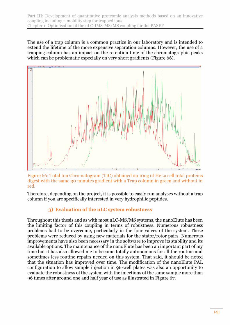
Part III: Development of quantitative proteomic analysis methods based on an innovative coupling including a mobility step for trapped ions Chapter 1: Optimisation of the nLC-IMS-MS/MS coupling for ddaPASEF
141
The use of a trap column is a common practice in our laboratory and is intended to extend the lifetime of the more expensive separation columns. However, the use of a trapping column has an impact on the retention time of the chromatographic peaks which can be problematic especially on very short gradients (Figure 66).
Figure 66: Total Ion Chromatogram (TIC) obtained on 10ng of HeLa cell total proteins digest with the same 30 minutes gradient with a Trap column in green and without in red.
Therefore, depending on the project, it is possible to easily run analyses without a trap column if you are specifically interested in very hydrophilic peptides.
3) Evaluation of the nLC system robustness Throughout this thesis and as with most nLC-MS/MS systems, the nanoElute has been the limiting factor of this coupling in terms of robustness. Numerous robustness problems had to be overcome, particularly in the four valves of the system. These problems were reduced by using new materials for the stator/rotor pairs. Numerous improvements have also been necessary in the software to improve its stability and its available options. The maintenance of the nanoElute has been an important part of my time but it has also allowed me to become totally autonomous for all the routine and sometimes less routine repairs needed on this system. That said, it should be noted that the situation has improved over time. The modification of the nanoElute PAL configuration to allow sample injection in 96-well plates was also an opportunity to evaluate the robustness of the system with the injections of the same sample more than 96 times after around one and half year of use as illustrated in Figure 67.
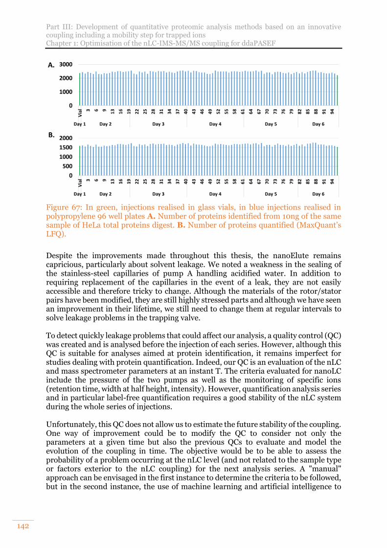
Part III: Development of quantitative proteomic analysis methods based on an innovative coupling including a mobility step for trapped ions Chapter 1: Optimisation of the nLC-IMS-MS/MS coupling for ddaPASEF
142
Figure 67: In green, injections realised in glass vials, in blue injections realised in polypropylene 96 well plates A. Number of proteins identified from 10ng of the same sample of HeLa total proteins digest. B. Number of proteins quantified (MaxQuant’s LFQ).
Despite the improvements made throughout this thesis, the nanoElute remains capricious, particularly about solvent leakage. We noted a weakness in the sealing of the stainless-steel capillaries of pump A handling acidified water. In addition to requiring replacement of the capillaries in the event of a leak, they are not easily accessible and therefore tricky to change. Although the materials of the rotor/stator pairs have been modified, they are still highly stressed parts and although we have seen an improvement in their lifetime, we still need to change them at regular intervals to solve leakage problems in the trapping valve. To detect quickly leakage problems that could affect our analysis, a quality control (QC) was created and is analysed before the injection of each series. However, although this QC is suitable for analyses aimed at protein identification, it remains imperfect for studies dealing with protein quantification. Indeed, our QC is an evaluation of the nLC and mass spectrometer parameters at an instant T. The criteria evaluated for nanoLC include the pressure of the two pumps as well as the monitoring of specific ions (retention time, width at half height, intensity). However, quantification analysis series and in particular label-free quantification requires a good stability of the nLC system during the whole series of injections. Unfortunately, this QC does not allow us to estimate the future stability of the coupling. One way of improvement could be to modify the QC to consider not only the parameters at a given time but also the previous QCs to evaluate and model the evolution of the coupling in time. The objective would be to be able to assess the probability of a problem occurring at the nLC level (and not related to the sample type or factors exterior to the nLC coupling) for the next analysis series. A "manual" approach can be envisaged in the first instance to determine the criteria to be followed, but in the second instance, the use of machine learning and artificial intelligence to
Part III: Development of quantitative proteomic analysis methods based on an innovative coupling including a mobility step for trapped ions Chapter 1: Optimisation of the nLC-IMS-MS/MS coupling for ddaPASEF
143
carry out these tasks in a more refined and automated way would undoubtedly be of great help. Quality control as it is used today also has other limitations. Indeed, today the results are analysed by hand by the users before a series of injection. As a result, it is impractical to run two series of analysis in one night or weekend without wasting time. Similarly, a deterioration in performance during a run is not always possible to see because we are working on samples whose behaviour we do not necessarily know. As a result, a drop in coupling performance during the series can go unnoticed but may have dramatic consequences for a project. To overcome this problem, a system called PaSER (Parallel Database Search Engine) is developed by Bruker. PaSER is a GPU (Graphics Processing Unit) powered real-time database search platform providing parallel computing power and real-time database search results for bottom-up proteomics. It allows the analysis of the data generated by the online coupling to be launched as soon as the acquisitions are completed in an automated manner. This data processing is very fast thanks to the use of cloud-based systems with delocalised computing power. Therefore, PaSER could also allow automated data analysis of QCs and allow automated interruption of acquisitions in case of problems. This would save time in chaining the different series of analyses, avoid the loss of valuable samples and free up the time of the experimenters thanks to automated quality control in real time. To improve its quality control system, Bruker is currently working on different approaches. Another is to come with the new TimsControl acquisition software and its automated real-time calibration of TIMS before each injection. It allows to calibrate the TIMS cell automatically before each acquisition as this calibration can move rapidly unlike the TOF calibration as the TIMS is more sensible to exterior factors such as the gas flow, or the temperature. We had the occasion to made first tests with this feature. However, we observed that it only worked using Bruker's default MS methods at the time of our testing. Moreover, if the system is not able to calibrate correctly the TIMS, there is no possibility to stop automatically the injections to avoid losing precious samples. To conclude, many tools are actually in development at the level of the nLC but also at the level of the MS in order to create more robust and performant systems by allowing easy and automated monitoring of the coupling and in order to reduce the global need in supervision of this kind of instrumentation. Those features will allow us to reduce the risk of losing precious samples and gain in fluidity and so, in time between the sample analysis and the data treatment steps.
B. Optimisation of ddaPASEF acquisition methods In parallel, optimisations were also carried out on the mass spectrometer. Both to optimise the methods and for me personally to gain a deeper understanding of the parameter tunings. As mentioned earlier, the TimsTOF Pro is equipped with an ion mobility dual cell as shown in Figure 68.
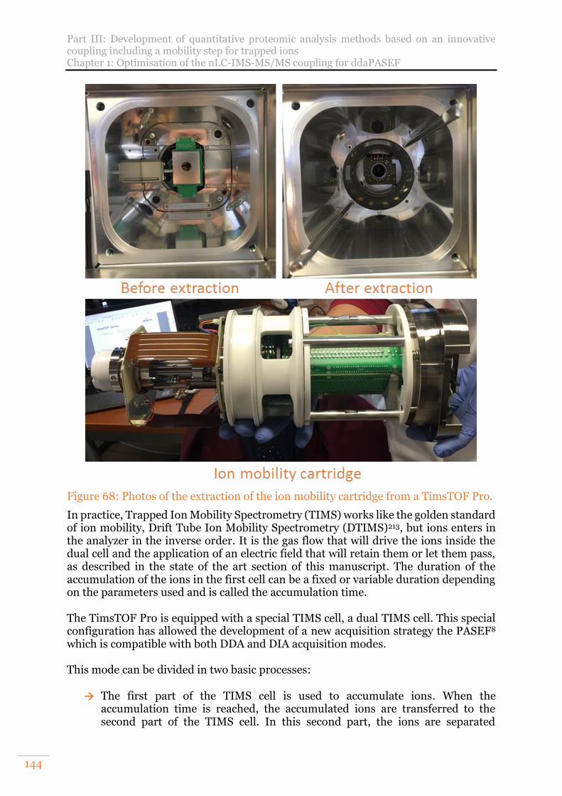
Part III: Development of quantitative proteomic analysis methods based on an innovative coupling including a mobility step for trapped ions Chapter 1: Optimisation of the nLC-IMS-MS/MS coupling for ddaPASEF
144
Figure 68: Photos of the extraction of the ion mobility cartridge from a TimsTOF Pro.
In practice, Trapped Ion Mobility Spectrometry (TIMS) works like the golden standard of ion mobility, Drift Tube Ion Mobility Spectrometry (DTIMS)213, but ions enters in the analyzer in the inverse order. It is the gas flow that will drive the ions inside the dual cell and the application of an electric field that will retain them or let them pass, as described in the state of the art section of this manuscript. The duration of the accumulation of the ions in the first cell can be a fixed or variable duration depending on the parameters used and is called the accumulation time. The TimsTOF Pro is equipped with a special TIMS cell, a dual TIMS cell. This special configuration has allowed the development of a new acquisition strategy the PASEF8 which is compatible with both DDA and DIA acquisition modes. This mode can be divided in two basic processes:
→ The first part of the TIMS cell is used to accumulate ions. When the accumulation time is reached, the accumulated ions are transferred to the second part of the TIMS cell. In this second part, the ions are separated
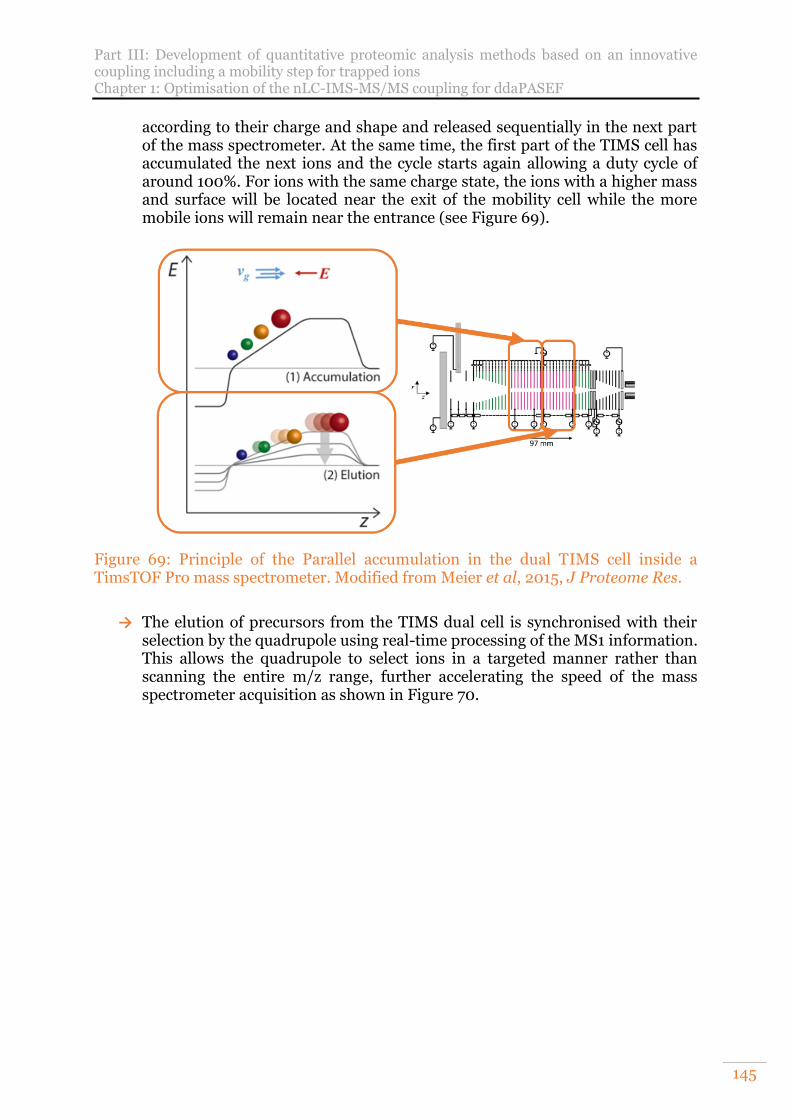
Part III: Development of quantitative proteomic analysis methods based on an innovative coupling including a mobility step for trapped ions Chapter 1: Optimisation of the nLC-IMS-MS/MS coupling for ddaPASEF
145
according to their charge and shape and released sequentially in the next part of the mass spectrometer. At the same time, the first part of the TIMS cell has accumulated the next ions and the cycle starts again allowing a duty cycle of around 100%. For ions with the same charge state, the ions with a higher mass and surface will be located near the exit of the mobility cell while the more mobile ions will remain near the entrance (see Figure 69).
Figure 69: Principle of the Parallel accumulation in the dual TIMS cell inside a TimsTOF Pro mass spectrometer. Modified from Meier et al, 2015, J Proteome Res.
→ The elution of precursors from the TIMS dual cell is synchronised with their
selection by the quadrupole using real-time processing of the MS1 information. This allows the quadrupole to select ions in a targeted manner rather than scanning the entire m/z range, further accelerating the speed of the mass spectrometer acquisition as shown in Figure 70.
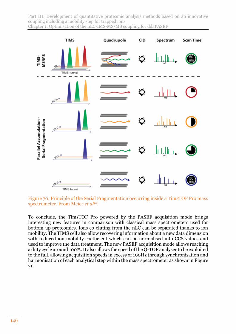
Part III: Development of quantitative proteomic analysis methods based on an innovative coupling including a mobility step for trapped ions Chapter 1: Optimisation of the nLC-IMS-MS/MS coupling for ddaPASEF
146
Figure 70: Principle of the Serial Fragmentation occurring inside a TimsTOF Pro mass spectrometer. From Meier et al10.
To conclude, the TimsTOF Pro powered by the PASEF acquisition mode brings interesting new features in comparison with classical mass spectrometers used for bottom-up proteomics. Ions co-eluting from the nLC can be separated thanks to ion mobility. The TIMS cell also allow recovering information about a new data dimension with reduced ion mobility coefficient which can be normalised into CCS values and used to improve the data treatment. The new PASEF acquisition mode allows reaching a duty cycle around 100%. It also allows the speed of the Q-TOF analyser to be exploited to the full, allowing acquisition speeds in excess of 100Hz through synchronisation and harmonisation of each analytical step within the mass spectrometer as shown in Figure 71.
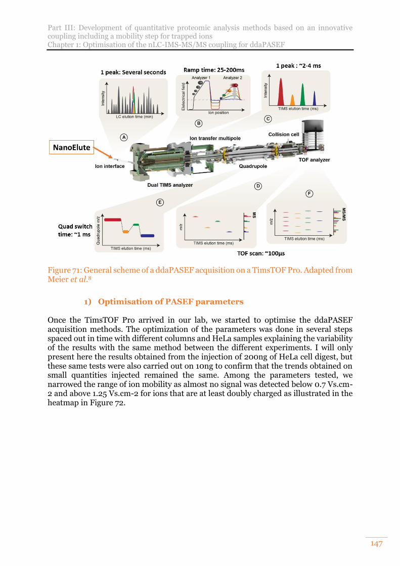
Part III: Development of quantitative proteomic analysis methods based on an innovative coupling including a mobility step for trapped ions Chapter 1: Optimisation of the nLC-IMS-MS/MS coupling for ddaPASEF
147
Figure 71: General scheme of a ddaPASEF acquisition on a TimsTOF Pro. Adapted from Meier et al.8
1) Optimisation of PASEF parameters
Once the TimsTOF Pro arrived in our lab, we started to optimise the ddaPASEF acquisition methods. The optimization of the parameters was done in several steps spaced out in time with different columns and HeLa samples explaining the variability of the results with the same method between the different experiments. I will only present here the results obtained from the injection of 200ng of HeLa cell digest, but these same tests were also carried out on 10ng to confirm that the trends obtained on small quantities injected remained the same. Among the parameters tested, we narrowed the range of ion mobility as almost no signal was detected below 0.7 Vs.cm-2 and above 1.25 Vs.cm-2 for ions that are at least doubly charged as illustrated in the heatmap in Figure 72.
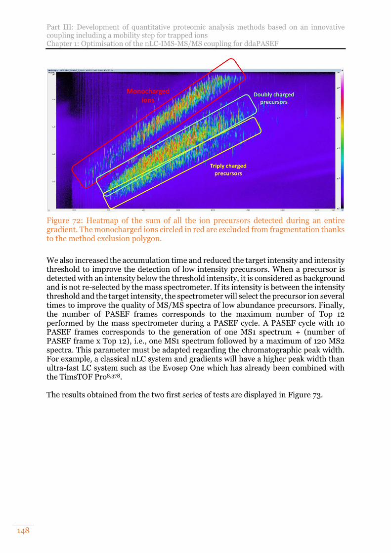
Part III: Development of quantitative proteomic analysis methods based on an innovative coupling including a mobility step for trapped ions Chapter 1: Optimisation of the nLC-IMS-MS/MS coupling for ddaPASEF
148
Figure 72: Heatmap of the sum of all the ion precursors detected during an entire gradient. The monocharged ions circled in red are excluded from fragmentation thanks to the method exclusion polygon.
We also increased the accumulation time and reduced the target intensity and intensity threshold to improve the detection of low intensity precursors. When a precursor is detected with an intensity below the threshold intensity, it is considered as background and is not re-selected by the mass spectrometer. If its intensity is between the intensity threshold and the target intensity, the spectrometer will select the precursor ion several times to improve the quality of MS/MS spectra of low abundance precursors. Finally, the number of PASEF frames corresponds to the maximum number of Top 12 performed by the mass spectrometer during a PASEF cycle. A PASEF cycle with 10 PASEF frames corresponds to the generation of one MS1 spectrum + (number of PASEF frame x Top 12), i.e., one MS1 spectrum followed by a maximum of 120 MS2 spectra. This parameter must be adapted regarding the chromatographic peak width. For example, a classical nLC system and gradients will have a higher peak width than ultra-fast LC system such as the Evosep One which has already been combined with the TimsTOF Pro8,378. The results obtained from the two first series of tests are displayed in Figure 73.
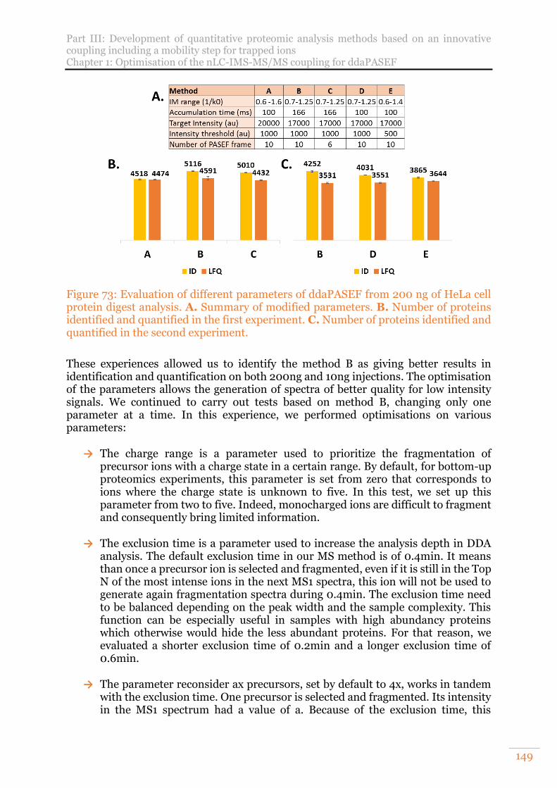
Part III: Development of quantitative proteomic analysis methods based on an innovative coupling including a mobility step for trapped ions Chapter 1: Optimisation of the nLC-IMS-MS/MS coupling for ddaPASEF
149
Figure 73: Evaluation of different parameters of ddaPASEF from 200 ng of HeLa cell protein digest analysis. A. Summary of modified parameters. B. Number of proteins identified and quantified in the first experiment. C. Number of proteins identified and quantified in the second experiment.
These experiences allowed us to identify the method B as giving better results in identification and quantification on both 200ng and 10ng injections. The optimisation of the parameters allows the generation of spectra of better quality for low intensity signals. We continued to carry out tests based on method B, changing only one parameter at a time. In this experience, we performed optimisations on various parameters:
→ The charge range is a parameter used to prioritize the fragmentation of precursor ions with a charge state in a certain range. By default, for bottom-up proteomics experiments, this parameter is set from zero that corresponds to ions where the charge state is unknown to five. In this test, we set up this parameter from two to five. Indeed, monocharged ions are difficult to fragment and consequently bring limited information.
→ The exclusion time is a parameter used to increase the analysis depth in DDA
analysis. The default exclusion time in our MS method is of 0.4min. It means than once a precursor ion is selected and fragmented, even if it is still in the Top N of the most intense ions in the next MS1 spectra, this ion will not be used to generate again fragmentation spectra during 0.4min. The exclusion time need to be balanced depending on the peak width and the sample complexity. This function can be especially useful in samples with high abundancy proteins which otherwise would hide the less abundant proteins. For that reason, we evaluated a shorter exclusion time of 0.2min and a longer exclusion time of 0.6min.
→ The parameter reconsider ax precursors, set by default to 4x, works in tandem
with the exclusion time. One precursor is selected and fragmented. Its intensity in the MS1 spectrum had a value of a. Because of the exclusion time, this
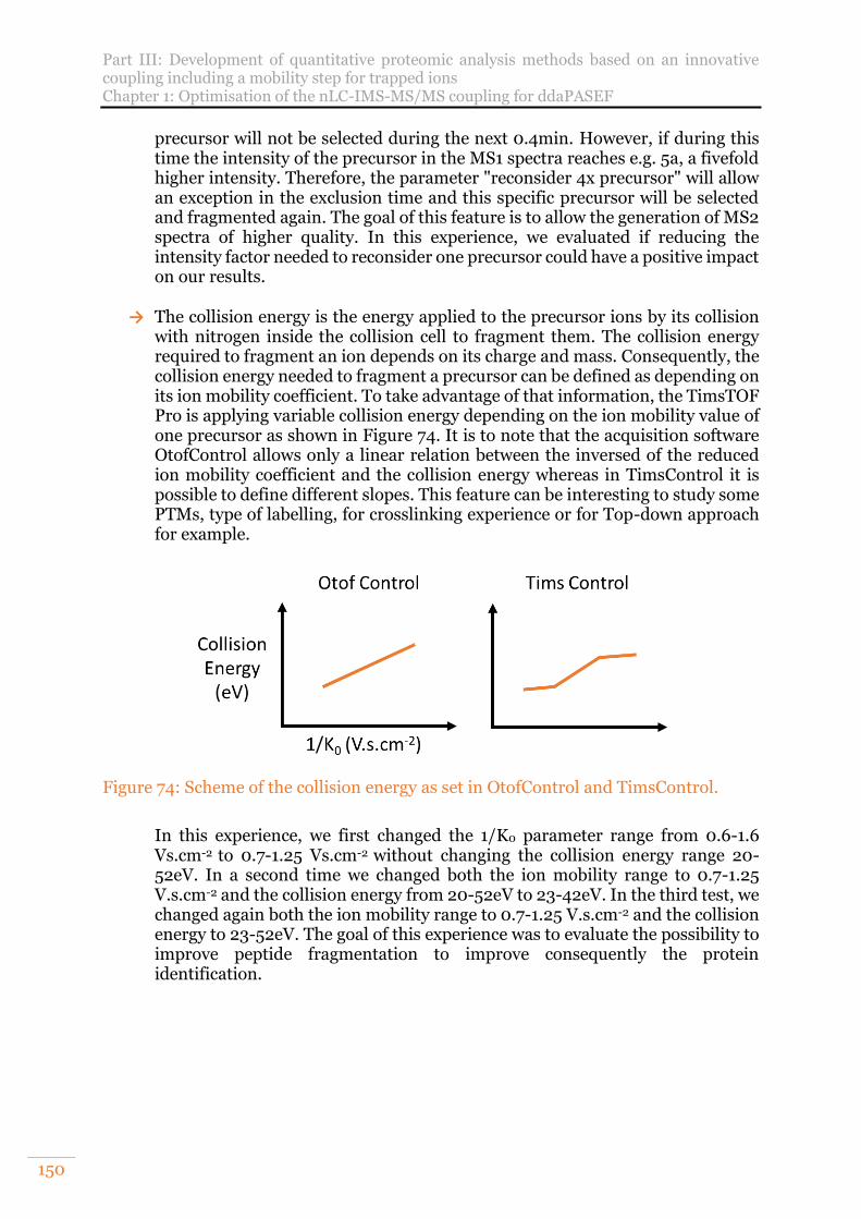
Part III: Development of quantitative proteomic analysis methods based on an innovative coupling including a mobility step for trapped ions Chapter 1: Optimisation of the nLC-IMS-MS/MS coupling for ddaPASEF
150
precursor will not be selected during the next 0.4min. However, if during this time the intensity of the precursor in the MS1 spectra reaches e.g. 5a, a fivefold higher intensity. Therefore, the parameter "reconsider 4x precursor" will allow an exception in the exclusion time and this specific precursor will be selected and fragmented again. The goal of this feature is to allow the generation of MS2 spectra of higher quality. In this experience, we evaluated if reducing the intensity factor needed to reconsider one precursor could have a positive impact on our results.
→ The collision energy is the energy applied to the precursor ions by its collision with nitrogen inside the collision cell to fragment them. The collision energy required to fragment an ion depends on its charge and mass. Consequently, the collision energy needed to fragment a precursor can be defined as depending on its ion mobility coefficient. To take advantage of that information, the TimsTOF Pro is applying variable collision energy depending on the ion mobility value of one precursor as shown in Figure 74. It is to note that the acquisition software OtofControl allows only a linear relation between the inversed of the reduced ion mobility coefficient and the collision energy whereas in TimsControl it is possible to define different slopes. This feature can be interesting to study some PTMs, type of labelling, for crosslinking experience or for Top-down approach for example.
Figure 74: Scheme of the collision energy as set in OtofControl and TimsControl.
In this experience, we first changed the 1/K0 parameter range from 0.6-1.6 Vs.cm-2 to 0.7-1.25 Vs.cm-2 without changing the collision energy range 20-52eV. In a second time we changed both the ion mobility range to 0.7-1.25 V.s.cm-2 and the collision energy from 20-52eV to 23-42eV. In the third test, we changed again both the ion mobility range to 0.7-1.25 V.s.cm-2 and the collision energy to 23-52eV. The goal of this experience was to evaluate the possibility to improve peptide fragmentation to improve consequently the protein identification.
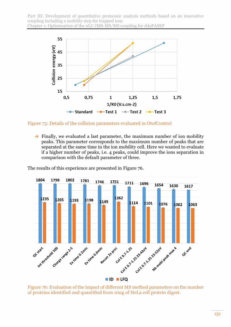
Part III: Development of quantitative proteomic analysis methods based on an innovative coupling including a mobility step for trapped ions Chapter 1: Optimisation of the nLC-IMS-MS/MS coupling for ddaPASEF
151
Figure 75: Details of the collision parameters evaluated in OtofControl
→ Finally, we evaluated a last parameter, the maximum number of ion mobility
peaks. This parameter corresponds to the maximum number of peaks that are separated at the same time in the ion mobility cell. Here we wanted to evaluate if a higher number of peaks, i.e. 4 peaks, could improve the ions separation in comparison with the default parameter of three.
The results of this experience are presented in Figure 76.
Figure 76: Evaluation of the impact of different MS method parameters on the number of proteins identified and quantified from 10ng of HeLa cell protein digest.
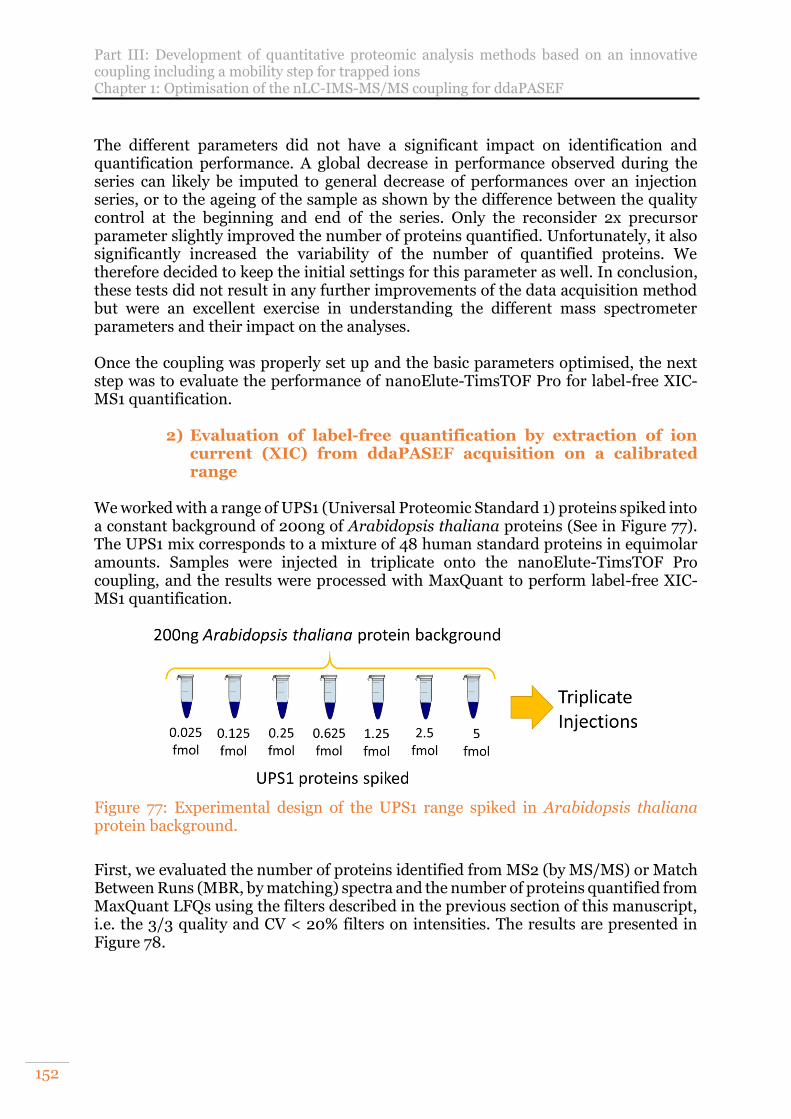
Part III: Development of quantitative proteomic analysis methods based on an innovative coupling including a mobility step for trapped ions Chapter 1: Optimisation of the nLC-IMS-MS/MS coupling for ddaPASEF
152
The different parameters did not have a significant impact on identification and quantification performance. A global decrease in performance observed during the series can likely be imputed to general decrease of performances over an injection series, or to the ageing of the sample as shown by the difference between the quality control at the beginning and end of the series. Only the reconsider 2x precursor parameter slightly improved the number of proteins quantified. Unfortunately, it also significantly increased the variability of the number of quantified proteins. We therefore decided to keep the initial settings for this parameter as well. In conclusion, these tests did not result in any further improvements of the data acquisition method but were an excellent exercise in understanding the different mass spectrometer parameters and their impact on the analyses. Once the coupling was properly set up and the basic parameters optimised, the next step was to evaluate the performance of nanoElute-TimsTOF Pro for label-free XIC-MS1 quantification.
2) Evaluation of label-free quantification by extraction of ion current (XIC) from ddaPASEF acquisition on a calibrated range
We worked with a range of UPS1 (Universal Proteomic Standard 1) proteins spiked into a constant background of 200ng of Arabidopsis thaliana proteins (See in Figure 77). The UPS1 mix corresponds to a mixture of 48 human standard proteins in equimolar amounts. Samples were injected in triplicate onto the nanoElute-TimsTOF Pro coupling, and the results were processed with MaxQuant to perform label-free XIC-MS1 quantification.
Figure 77: Experimental design of the UPS1 range spiked in Arabidopsis thaliana protein background.
First, we evaluated the number of proteins identified from MS2 (by MS/MS) or Match Between Runs (MBR, by matching) spectra and the number of proteins quantified from MaxQuant LFQs using the filters described in the previous section of this manuscript, i.e. the 3/3 quality and CV < 20% filters on intensities. The results are presented in Figure 78.
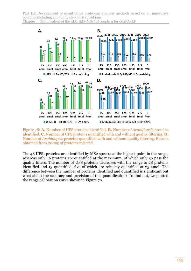
Part III: Development of quantitative proteomic analysis methods based on an innovative coupling including a mobility step for trapped ions Chapter 1: Optimisation of the nLC-IMS-MS/MS coupling for ddaPASEF
153
Figure 78: A. Number of UPS proteins identified. B. Number of Arabidopsis proteins identified. C. Number of UPS proteins quantified with and without quality filtering. D. Number of Arabidopsis proteins quantified with and without quality filtering. Results obtained from 200ng of proteins injected.
The 48 UPS1 proteins are identified by MS2 spectra at the highest point in the range, whereas only 46 proteins are quantified at the maximum, of which only 36 pass the quality filters. The number of UPS proteins decreases with the range to 28 proteins identified and 13 quantified, five of which are robustly quantified at 25 amol. The difference between the number of proteins identified and quantified is significant but what about the accuracy and precision of the quantification? To find out, we plotted the range calibration curve shown in Figure 79.
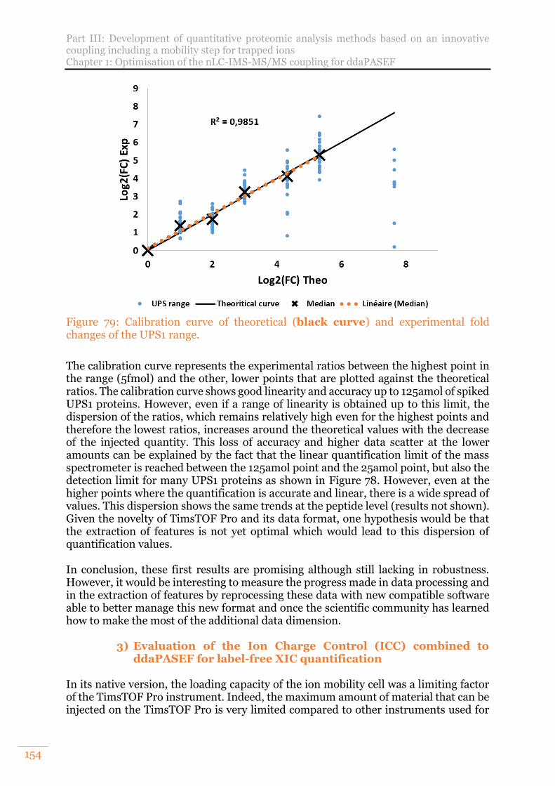
Part III: Development of quantitative proteomic analysis methods based on an innovative coupling including a mobility step for trapped ions Chapter 1: Optimisation of the nLC-IMS-MS/MS coupling for ddaPASEF
154
Figure 79: Calibration curve of theoretical (black curve) and experimental fold changes of the UPS1 range.
The calibration curve represents the experimental ratios between the highest point in the range (5fmol) and the other, lower points that are plotted against the theoretical ratios. The calibration curve shows good linearity and accuracy up to 125amol of spiked UPS1 proteins. However, even if a range of linearity is obtained up to this limit, the dispersion of the ratios, which remains relatively high even for the highest points and therefore the lowest ratios, increases around the theoretical values with the decrease of the injected quantity. This loss of accuracy and higher data scatter at the lower amounts can be explained by the fact that the linear quantification limit of the mass spectrometer is reached between the 125amol point and the 25amol point, but also the detection limit for many UPS1 proteins as shown in Figure 78. However, even at the higher points where the quantification is accurate and linear, there is a wide spread of values. This dispersion shows the same trends at the peptide level (results not shown). Given the novelty of TimsTOF Pro and its data format, one hypothesis would be that the extraction of features is not yet optimal which would lead to this dispersion of quantification values. In conclusion, these first results are promising although still lacking in robustness. However, it would be interesting to measure the progress made in data processing and in the extraction of features by reprocessing these data with new compatible software able to better manage this new format and once the scientific community has learned how to make the most of the additional data dimension.
3) Evaluation of the Ion Charge Control (ICC) combined to ddaPASEF for label-free XIC quantification
In its native version, the loading capacity of the ion mobility cell was a limiting factor of the TimsTOF Pro instrument. Indeed, the maximum amount of material that can be injected on the TimsTOF Pro is very limited compared to other instruments used for
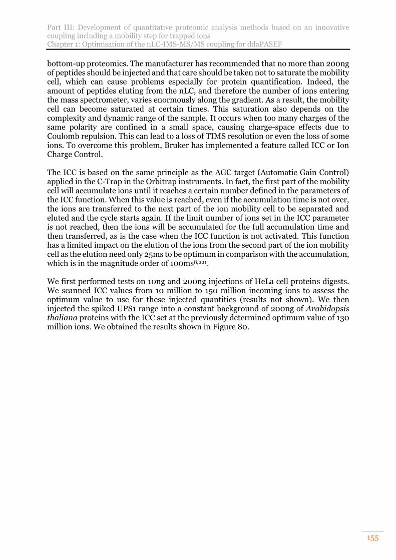
Part III: Development of quantitative proteomic analysis methods based on an innovative coupling including a mobility step for trapped ions Chapter 1: Optimisation of the nLC-IMS-MS/MS coupling for ddaPASEF
155
bottom-up proteomics. The manufacturer has recommended that no more than 200ng of peptides should be injected and that care should be taken not to saturate the mobility cell, which can cause problems especially for protein quantification. Indeed, the amount of peptides eluting from the nLC, and therefore the number of ions entering the mass spectrometer, varies enormously along the gradient. As a result, the mobility cell can become saturated at certain times. This saturation also depends on the complexity and dynamic range of the sample. It occurs when too many charges of the same polarity are confined in a small space, causing charge-space effects due to Coulomb repulsion. This can lead to a loss of TIMS resolution or even the loss of some ions. To overcome this problem, Bruker has implemented a feature called ICC or Ion Charge Control. The ICC is based on the same principle as the AGC target (Automatic Gain Control) applied in the C-Trap in the Orbitrap instruments. In fact, the first part of the mobility cell will accumulate ions until it reaches a certain number defined in the parameters of the ICC function. When this value is reached, even if the accumulation time is not over, the ions are transferred to the next part of the ion mobility cell to be separated and eluted and the cycle starts again. If the limit number of ions set in the ICC parameter is not reached, then the ions will be accumulated for the full accumulation time and then transferred, as is the case when the ICC function is not activated. This function has a limited impact on the elution of the ions from the second part of the ion mobility cell as the elution need only 25ms to be optimum in comparison with the accumulation, which is in the magnitude order of 100ms8,221. We first performed tests on 10ng and 200ng injections of HeLa cell proteins digests. We scanned ICC values from 10 million to 150 million incoming ions to assess the optimum value to use for these injected quantities (results not shown). We then injected the spiked UPS1 range into a constant background of 200ng of Arabidopsis thaliana proteins with the ICC set at the previously determined optimum value of 130 million ions. We obtained the results shown in Figure 80.
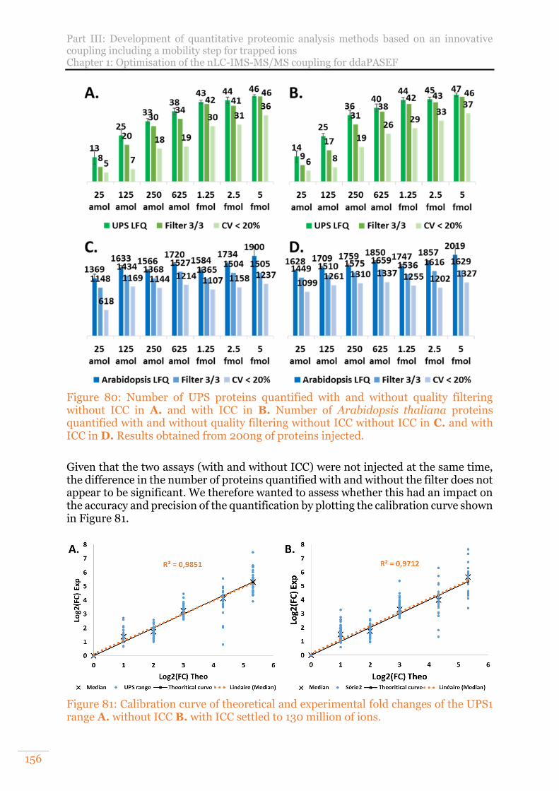
Part III: Development of quantitative proteomic analysis methods based on an innovative coupling including a mobility step for trapped ions Chapter 1: Optimisation of the nLC-IMS-MS/MS coupling for ddaPASEF
156
Figure 80: Number of UPS proteins quantified with and without quality filtering without ICC in A. and with ICC in B. Number of Arabidopsis thaliana proteins quantified with and without quality filtering without ICC without ICC in C. and with ICC in D. Results obtained from 200ng of proteins injected.
Given that the two assays (with and without ICC) were not injected at the same time, the difference in the number of proteins quantified with and without the filter does not appear to be significant. We therefore wanted to assess whether this had an impact on the accuracy and precision of the quantification by plotting the calibration curve shown in Figure 81.
Figure 81: Calibration curve of theoretical and experimental fold changes of the UPS1 range A. without ICC B. with ICC settled to 130 million of ions.
Part III: Development of quantitative proteomic analysis methods based on an innovative coupling including a mobility step for trapped ions Chapter 1: Optimisation of the nLC-IMS-MS/MS coupling for ddaPASEF
157
The experimental curve obtained with the active ICC function is slightly less linear than the one obtained without ICC. Moreover, the scatter of the data seems to be a little larger, although the accuracy of the quantification remains roughly equivalent. In conclusion, in the condition of our tests, the ICC function does not seem to bring any significant gain. This might be the case on other type of samples with a larger dynamic range or on larger quantities of injected material, but the whole evaluation would have to be done again to find the appropriate ICC value and to confirm the positive impact or not of the ICC function. This function could also be interesting to evaluate in the future coupled with another acquisition strategy such as the diaPASEF that will be developed in the following chapter.
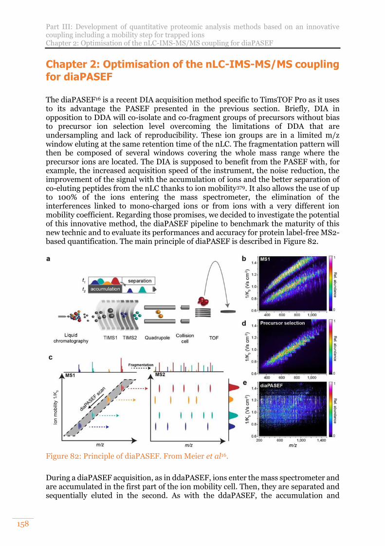
Part III: Development of quantitative proteomic analysis methods based on an innovative coupling including a mobility step for trapped ions Chapter 2: Optimisation of the nLC-IMS-MS/MS coupling for diaPASEF
158
Chapter 2: Optimisation of the nLC-IMS-MS/MS coupling for diaPASEF
The diaPASEF16 is a recent DIA acquisition method specific to TimsTOF Pro as it uses to its advantage the PASEF presented in the previous section. Briefly, DIA in opposition to DDA will co-isolate and co-fragment groups of precursors without bias to precursor ion selection level overcoming the limitations of DDA that are undersampling and lack of reproducibility. These ion groups are in a limited m/z window eluting at the same retention time of the nLC. The fragmentation pattern will then be composed of several windows covering the whole mass range where the precursor ions are located. The DIA is supposed to benefit from the PASEF with, for example, the increased acquisition speed of the instrument, the noise reduction, the improvement of the signal with the accumulation of ions and the better separation of co-eluting peptides from the nLC thanks to ion mobility379. It also allows the use of up to 100% of the ions entering the mass spectrometer, the elimination of the interferences linked to mono-charged ions or from ions with a very different ion mobility coefficient. Regarding those promises, we decided to investigate the potential of this innovative method, the diaPASEF pipeline to benchmark the maturity of this new technic and to evaluate its performances and accuracy for protein label-free MS2-based quantification. The main principle of diaPASEF is described in Figure 82.
Figure 82: Principle of diaPASEF. From Meier et al16.
During a diaPASEF acquisition, as in ddaPASEF, ions enter the mass spectrometer and are accumulated in the first part of the ion mobility cell. Then, they are separated and sequentially eluted in the second. As with the ddaPASEF, the accumulation and
Part III: Development of quantitative proteomic analysis methods based on an innovative coupling including a mobility step for trapped ions Chapter 2: Optimisation of the nLC-IMS-MS/MS coupling for diaPASEF
159
separation/elution of the ions is done simultaneously so that no ions are lost (Figure 82.a). It corresponds to a duty cycle of 100%. When separating ions according to their ion mobility, those with the lower mobility, generally the ions with the higher m/z, are released first followed by ions with higher mobility and lower m/z. Therefore, in diaPASEF, the m/z isolation window of the quadrupole will start from high m/z values and slide down to lower m/z values in synchronization with the elution of the ions from the ion mobility cell to transmit the entire ion cloud as shown in Figure 82.c. The isolation windows for diaPASEF methods are therefore defined in two dimensions, ion mobility and m/z. These windows are designed to cover the majority of doubly and triply charged ions because these are more informative as they fragment more easily. The isolation windows are also located in the most precursor-dense regions as illustrated in Figure 82.b, d and e. Once a window of m/z is selected by the quadrupole, precursor ions are sent to the collision cell in which the collision energy is applied according to the 1/K0 range. Higher energies will be applied for lower ion mobility coefficient and consequently higher m/z as those ions will be more difficult to fragment. The collision energy applied will slide towards lower energies in synchronisation with the ion’s elution from the ion mobility cell. Finally, the ions are sent to the TOF to obtain their m/z and intensity information. Different window schemes were investigated in the initial publication of diaPASEF on complex proteomes16. Based on those data, we decided to test their standard method which consists of 64 windows of 25m/z to cover most of the 2+ and 3+ precursor ions. Those windows are covered in 16 TIMS cycles of 100ms. In other terms, four m/z windows are selected and fragmented in one TIMS elution. The windows overlap in the ion mobility dimension to reduce potential artefacts linked to reduced ion transmission at the edges of the diaPASEF windows. The acquisitions were realised with OtofControl version 6.0. At the time of this work, two software supported diaPASEF data, OpenSWATH thanks to the MobiDIK extension which was used in the initial publication of diaPASEF16 and the commercial Spectronaut (Biognosys). As the lab has already a previous good experience with Spectronaut, we choose to use this software.
A. Initial evaluation of label-free quantification in diaPASEF To evaluate the diaPASEF acquisition and the quality of the quantification achieved, we analysed the same range of UPS1 proteins spiked into a constant background of Arabidopsis thaliana proteins using the diaPASEF method of 64windows and a cycle time ~2s described in the initial publication16. Spectronaut (version 14.0) was used to process these data using a peptide-centric approach using a conventional 1% FDR. A spectral library was generated from an Arabidopsis thaliana sample fractionated into 25 bands by SDS-PAGE. To add the UPS1 proteins to the spectral library, two injections of the highest point of the range were also performed in ddaPASEF. The ddaPASEF method used to generate the spectral library should be as similar as possible to the diaPASEF method. This is mandatory for the collision energy and ion mobility settings to ensure that the information in the spectral library and the analyses performed in diaPASEF are comparable. Otherwise, the data processing software would not be able to analyse the data and to handle the ion mobility dimension correctly. Next, we filtered the results to keep the proteins with at least one q value below 0.005 for one replicate per condition and an intensity CV below 20%. This last part was done after adapting an R script created by Jessica Kurz, a former student in our laboratory.
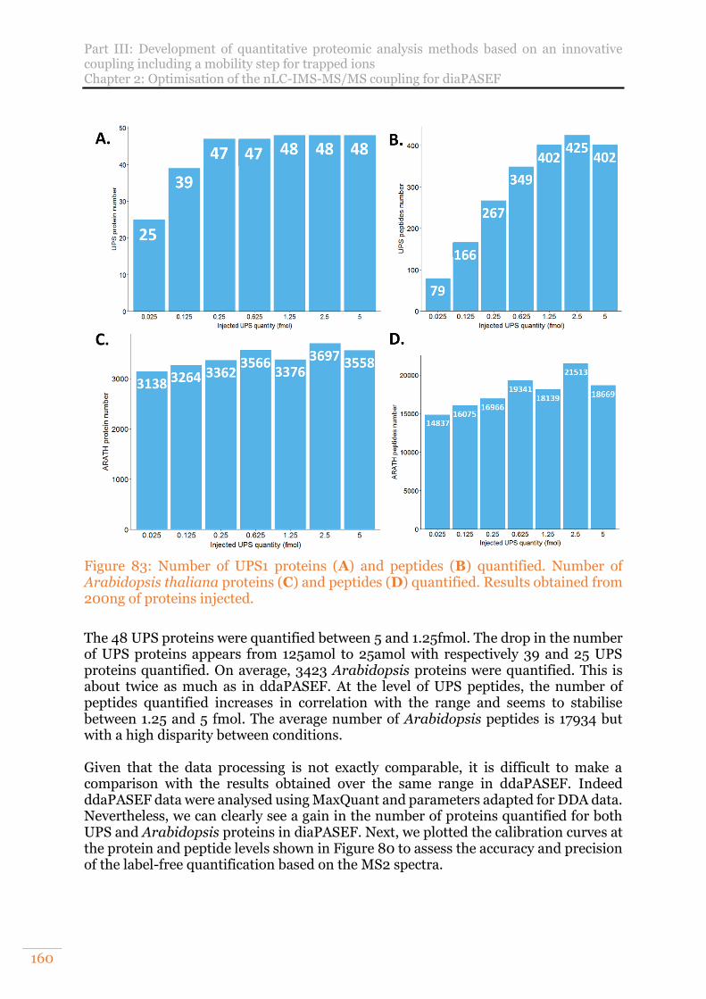
Part III: Development of quantitative proteomic analysis methods based on an innovative coupling including a mobility step for trapped ions Chapter 2: Optimisation of the nLC-IMS-MS/MS coupling for diaPASEF
160
Figure 83: Number of UPS1 proteins (A) and peptides (B) quantified. Number of Arabidopsis thaliana proteins (C) and peptides (D) quantified. Results obtained from 200ng of proteins injected.
The 48 UPS proteins were quantified between 5 and 1.25fmol. The drop in the number of UPS proteins appears from 125amol to 25amol with respectively 39 and 25 UPS proteins quantified. On average, 3423 Arabidopsis proteins were quantified. This is about twice as much as in ddaPASEF. At the level of UPS peptides, the number of peptides quantified increases in correlation with the range and seems to stabilise between 1.25 and 5 fmol. The average number of Arabidopsis peptides is 17934 but with a high disparity between conditions. Given that the data processing is not exactly comparable, it is difficult to make a comparison with the results obtained over the same range in ddaPASEF. Indeed ddaPASEF data were analysed using MaxQuant and parameters adapted for DDA data. Nevertheless, we can clearly see a gain in the number of proteins quantified for both UPS and Arabidopsis proteins in diaPASEF. Next, we plotted the calibration curves at the protein and peptide levels shown in Figure 80 to assess the accuracy and precision of the label-free quantification based on the MS2 spectra.
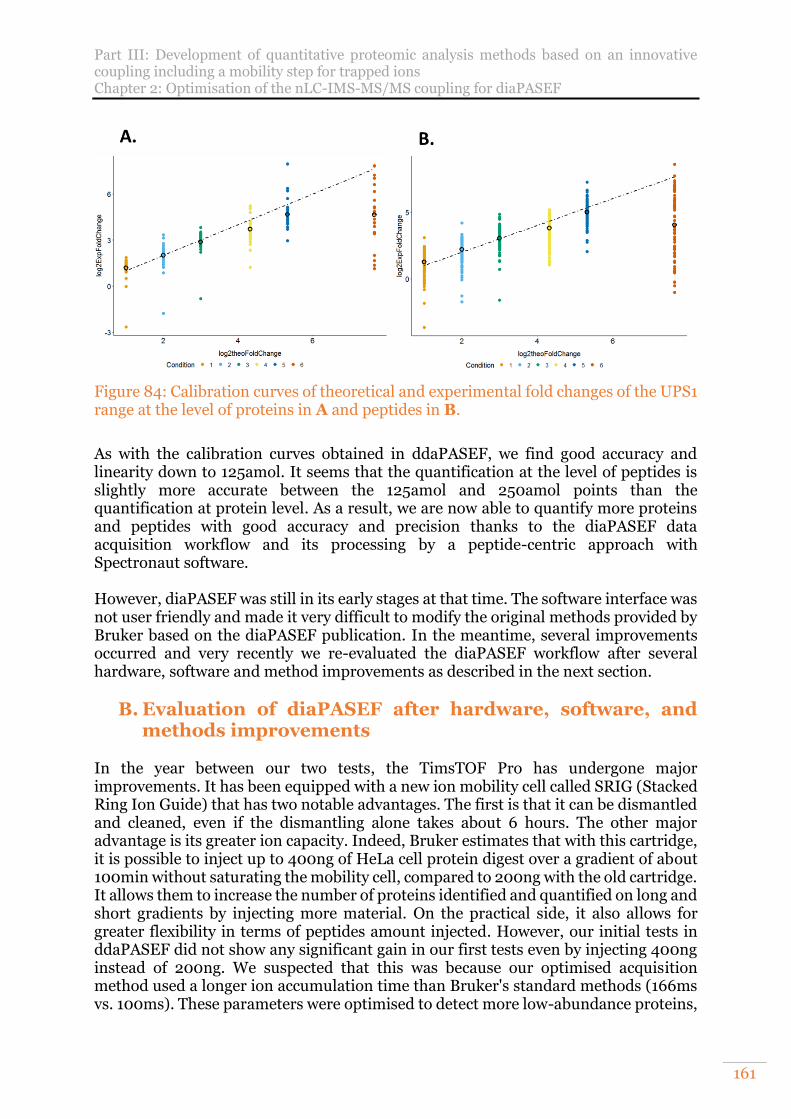
Part III: Development of quantitative proteomic analysis methods based on an innovative coupling including a mobility step for trapped ions Chapter 2: Optimisation of the nLC-IMS-MS/MS coupling for diaPASEF
161
Figure 84: Calibration curves of theoretical and experimental fold changes of the UPS1 range at the level of proteins in A and peptides in B.
As with the calibration curves obtained in ddaPASEF, we find good accuracy and linearity down to 125amol. It seems that the quantification at the level of peptides is slightly more accurate between the 125amol and 250amol points than the quantification at protein level. As a result, we are now able to quantify more proteins and peptides with good accuracy and precision thanks to the diaPASEF data acquisition workflow and its processing by a peptide-centric approach with Spectronaut software. However, diaPASEF was still in its early stages at that time. The software interface was not user friendly and made it very difficult to modify the original methods provided by Bruker based on the diaPASEF publication. In the meantime, several improvements occurred and very recently we re-evaluated the diaPASEF workflow after several hardware, software and method improvements as described in the next section.
B. Evaluation of diaPASEF after hardware, software, and methods improvements
In the year between our two tests, the TimsTOF Pro has undergone major improvements. It has been equipped with a new ion mobility cell called SRIG (Stacked Ring Ion Guide) that has two notable advantages. The first is that it can be dismantled and cleaned, even if the dismantling alone takes about 6 hours. The other major advantage is its greater ion capacity. Indeed, Bruker estimates that with this cartridge, it is possible to inject up to 400ng of HeLa cell protein digest over a gradient of about 100min without saturating the mobility cell, compared to 200ng with the old cartridge. It allows them to increase the number of proteins identified and quantified on long and short gradients by injecting more material. On the practical side, it also allows for greater flexibility in terms of peptides amount injected. However, our initial tests in ddaPASEF did not show any significant gain in our first tests even by injecting 400ng instead of 200ng. We suspected that this was because our optimised acquisition method used a longer ion accumulation time than Bruker's standard methods (166ms vs. 100ms). These parameters were optimised to detect more low-abundance proteins,
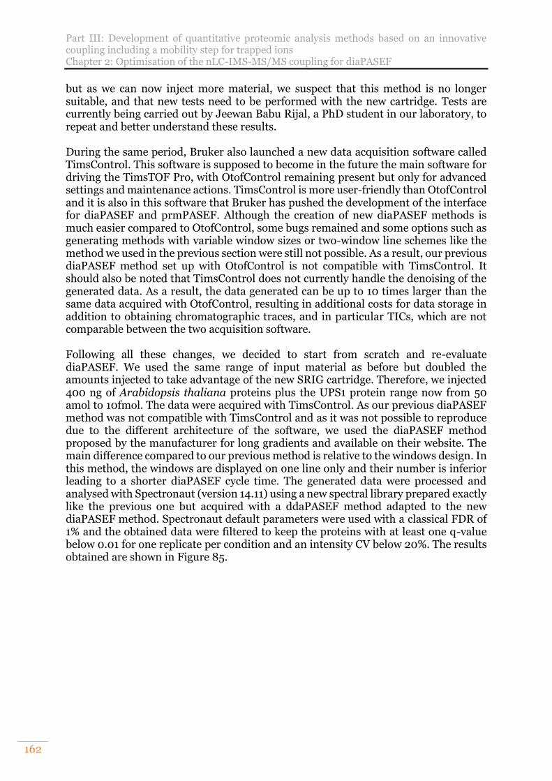
Part III: Development of quantitative proteomic analysis methods based on an innovative coupling including a mobility step for trapped ions Chapter 2: Optimisation of the nLC-IMS-MS/MS coupling for diaPASEF
162
but as we can now inject more material, we suspect that this method is no longer suitable, and that new tests need to be performed with the new cartridge. Tests are currently being carried out by Jeewan Babu Rijal, a PhD student in our laboratory, to repeat and better understand these results. During the same period, Bruker also launched a new data acquisition software called TimsControl. This software is supposed to become in the future the main software for driving the TimsTOF Pro, with OtofControl remaining present but only for advanced settings and maintenance actions. TimsControl is more user-friendly than OtofControl and it is also in this software that Bruker has pushed the development of the interface for diaPASEF and prmPASEF. Although the creation of new diaPASEF methods is much easier compared to OtofControl, some bugs remained and some options such as generating methods with variable window sizes or two-window line schemes like the method we used in the previous section were still not possible. As a result, our previous diaPASEF method set up with OtofControl is not compatible with TimsControl. It should also be noted that TimsControl does not currently handle the denoising of the generated data. As a result, the data generated can be up to 10 times larger than the same data acquired with OtofControl, resulting in additional costs for data storage in addition to obtaining chromatographic traces, and in particular TICs, which are not comparable between the two acquisition software. Following all these changes, we decided to start from scratch and re-evaluate diaPASEF. We used the same range of input material as before but doubled the amounts injected to take advantage of the new SRIG cartridge. Therefore, we injected 400 ng of Arabidopsis thaliana proteins plus the UPS1 protein range now from 50 amol to 10fmol. The data were acquired with TimsControl. As our previous diaPASEF method was not compatible with TimsControl and as it was not possible to reproduce due to the different architecture of the software, we used the diaPASEF method proposed by the manufacturer for long gradients and available on their website. The main difference compared to our previous method is relative to the windows design. In this method, the windows are displayed on one line only and their number is inferior leading to a shorter diaPASEF cycle time. The generated data were processed and analysed with Spectronaut (version 14.11) using a new spectral library prepared exactly like the previous one but acquired with a ddaPASEF method adapted to the new diaPASEF method. Spectronaut default parameters were used with a classical FDR of 1% and the obtained data were filtered to keep the proteins with at least one q-value below 0.01 for one replicate per condition and an intensity CV below 20%. The results obtained are shown in Figure 85.
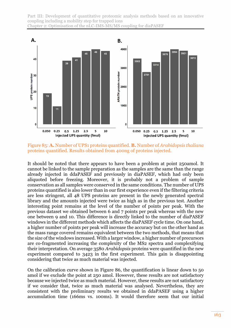
Part III: Development of quantitative proteomic analysis methods based on an innovative coupling including a mobility step for trapped ions Chapter 2: Optimisation of the nLC-IMS-MS/MS coupling for diaPASEF
163
Figure 85: A. Number of UPS1 proteins quantified. B. Number of Arabidopsis thaliana proteins quantified. Results obtained from 400ng of proteins injected.
It should be noted that there appears to have been a problem at point 250amol. It cannot be linked to the sample preparation as the samples are the same than the range already injected in ddaPASEF and previously in diaPASEF, which had only been aliquoted before freezing. Moreover, it is probably not a problem of sample conservation as all samples were conserved in the same conditions. The number of UPS proteins quantified is also lower than in our first experience even if the filtering criteria are less stringent, all 48 UPS proteins are present in the newly generated spectral library and the amounts injected were twice as high as in the previous test. Another interesting point remains at the level of the number of points per peak. With the previous dataset we obtained between 6 and 7 points per peak whereas with the new one between 9 and 10. This difference is directly linked to the number of diaPASEF windows in the different methods which affects the diaPASEF cycle time. On one hand, a higher number of points per peak will increase the accuracy but on the other hand as the mass range covered remains equivalent between the two methods, that means that the size of the windows increased. With a larger window, a higher number of precursors are co-fragmented increasing the complexity of the MS2 spectra and complexifying their interpretation. On average 3580 Arabidopsis proteins were quantified in the new experiment compared to 3423 in the first experiment. This gain is disappointing considering that twice as much material was injected. On the calibration curve shown in Figure 86, the quantification is linear down to 50 amol if we exclude the point at 250 amol. However, these results are not satisfactory because we injected twice as much material. However, these results are not satisfactory if we consider that, twice as much material was analysed. Nevertheless, they are consistent with the preliminary results we obtained in ddaPASEF using a higher accumulation time (166ms vs. 100ms). It would therefore seem that our initial
Part III: Development of quantitative proteomic analysis methods based on an innovative coupling including a mobility step for trapped ions Chapter 2: Optimisation of the nLC-IMS-MS/MS coupling for diaPASEF
164
hypothesis is probably wrong, since despite the use of a method using a reduced accumulation time, we still did not observe any gain from injecting more material.
Figure 86: Calibration curve of theoretical and experimental fold changes of the UPS1 range at the level of proteins.
As these changes have occurred in the last 6 months of my thesis, I have not had time to investigate this further. Having said that, I hypothesised that our current acquisition methods were not suitable for the new configuration of our improved TimsTOF Pro or TimsTOF Pro 2-like. One parameter that we have already tried to optimise to take better advantage of the new cartridge is the detector voltage. Other parameters, which could perhaps be optimised, are the ion transmission and the applied collision energy. For the time being, we are not yet able to make the most of the new SRIG cartridge. Furthermore, the diaPASEF method published by Meier et al. allowed us to achieve similar results as the method provided by Bruker despite the fact that the injection quantity was doubled with the latter. Unfortunately, this first method was created to work with the OtofControl software and was not yet compatible at the time of our test with the new TimsControl software. Finally, TimsControl was not capable of denoising spectra at that time, which meant generating result files up to 10 times larger than with OtofControl. In this situation, I concluded that TimsControl was not at that time mature enough to replace OtofControl for diaPASEF acquisitions, as the compatible methods did not provide significantly better results. However, TimsControl has been improved since then and it is necessary to follow its evolution closely. A sign that supports my feeling is the extremely low number of studies already published using diaPASEF. Excluding the initial publication16 and publications which re-use this first dataset17,379, there is a very reduced number of published studies67,380,381 using it even when including non-reviewed preprints382. Moreover, among those publications, most of them used the first published parameters, or the parameters are not detailed.
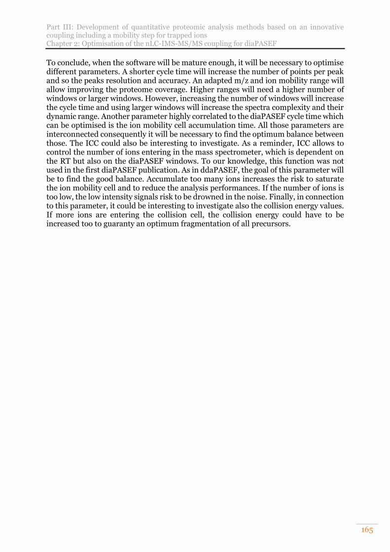
Part III: Development of quantitative proteomic analysis methods based on an innovative coupling including a mobility step for trapped ions Chapter 2: Optimisation of the nLC-IMS-MS/MS coupling for diaPASEF
165
To conclude, when the software will be mature enough, it will be necessary to optimise different parameters. A shorter cycle time will increase the number of points per peak and so the peaks resolution and accuracy. An adapted m/z and ion mobility range will allow improving the proteome coverage. Higher ranges will need a higher number of windows or larger windows. However, increasing the number of windows will increase the cycle time and using larger windows will increase the spectra complexity and their dynamic range. Another parameter highly correlated to the diaPASEF cycle time which can be optimised is the ion mobility cell accumulation time. All those parameters are interconnected consequently it will be necessary to find the optimum balance between those. The ICC could also be interesting to investigate. As a reminder, ICC allows to control the number of ions entering in the mass spectrometer, which is dependent on the RT but also on the diaPASEF windows. To our knowledge, this function was not used in the first diaPASEF publication. As in ddaPASEF, the goal of this parameter will be to find the good balance. Accumulate too many ions increases the risk to saturate the ion mobility cell and to reduce the analysis performances. If the number of ions is too low, the low intensity signals risk to be drowned in the noise. Finally, in connection to this parameter, it could be interesting to investigate also the collision energy values. If more ions are entering the collision cell, the collision energy could have to be increased too to guaranty an optimum fragmentation of all precursors.
Part IV: Evaluation of nLC-IMS-MS/MS data processing solutions Chapter 1: Evaluation and optimisation of the MaxQuant solution
166
Part IV: Evaluation of nLC-IMS-MS/MS data processing solutions The supplemental information dimension, reported as the reduced ion mobility coefficient K0, brought by the TimsTOF Pro changes many things regarding the raw data format. It is a challenge to overcome for data treatment software developers. However, it is worth the effort because it gives access to a completely new data dimension to reinforce the classical triad of the retention time (RT), the intensity and the masse over charge ratio (m/z). Consequently, during the first year of my PhD only a few data treatment workflows supported TimsTOF Pro data and only two were able to do label-free quantification on ddaPASEF data, MaxQuant11,19 and Peaks (Bioinformatics Solutions Inc.). At that time, Bruker had not released diaPASEF. The first workflow I used was for protein identification and validation. I used Mascot search engine (Matrix science) combined to Proline20 for protein validation. Proline is an open-source software suite developed by the national infrastructure in proteomics (ProFI) of which the LSMBO is a part. At the beginning of this thesis and during most of its duration, this workflow was compatible with TimsTOF Pro data but only for protein identification. However, it is very fast in comparison with MaxQuant and Peaks making him ideal for following the nanoElute-TimsTOF Pro coupling performances. However, considering the subject of my PhD work, I was particularly interested in software aiming to treat label-free data for protein quantification. On one hand, Peaks is a commercial software allowing to do protein identification and label-free quantification. It also has the originality to do an additional de novo search. However, the number of accessible parameters is limited. On the other hand, there was MaxQuant, which is one of the most used software for bottom-up proteomic due to the impressive number of accessible parameters and its gratuity. Moreover, MaxQuant has quickly proposed improvements to use more efficiently the ion mobility data. For those reasons, different versions of MaxQuant were used to realise most of the TimsTOF Pro data treatment realised during this PhD.
Chapter 1: Evaluation and optimisation of the MaxQuant solution
MaxQuant is using the Andromeda14 search engine and supported TimsTOF Pro data since MaxQuant version 1.6.2.6. However, it remained numerous problems linked to the default parameters of this version. For this reason, we really started to treat TimsTOF Pro data with the 1.6.2.10 version. At this moment, MaxQuant was not able to use the ion mobility data to reinforce its analysis. However, quickly during the first year of my PhD, MaxQuant released its 1.6.6.0 version. This version was the first one using ion mobility data. The major feature, which allowed that improvement, was and is always the Match Between Runs algorithm (MBR).
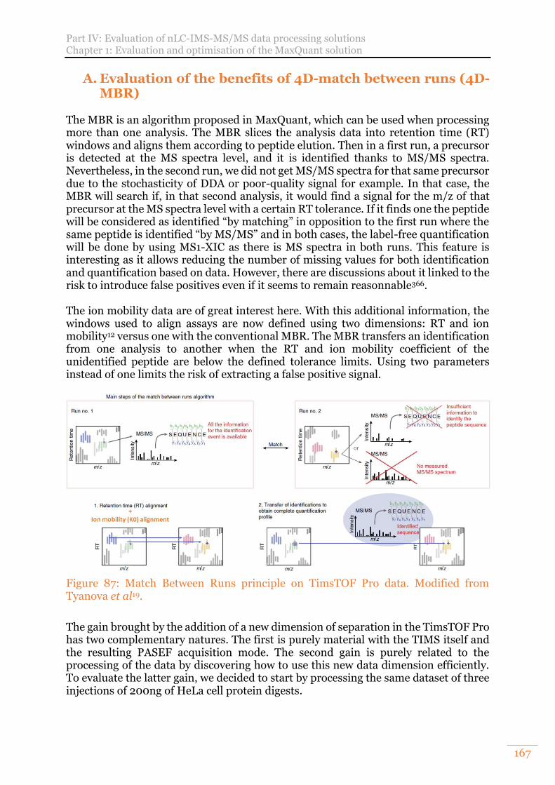
Part IV: Evaluation of nLC-IMS-MS/MS data processing solutions Chapter 1: Evaluation and optimisation of the MaxQuant solution
167
A. Evaluation of the benefits of 4D-match between runs (4D-MBR)
The MBR is an algorithm proposed in MaxQuant, which can be used when processing more than one analysis. The MBR slices the analysis data into retention time (RT) windows and aligns them according to peptide elution. Then in a first run, a precursor is detected at the MS spectra level, and it is identified thanks to MS/MS spectra. Nevertheless, in the second run, we did not get MS/MS spectra for that same precursor due to the stochasticity of DDA or poor-quality signal for example. In that case, the MBR will search if, in that second analysis, it would find a signal for the m/z of that precursor at the MS spectra level with a certain RT tolerance. If it finds one the peptide will be considered as identified “by matching” in opposition to the first run where the same peptide is identified “by MS/MS” and in both cases, the label-free quantification will be done by using MS1-XIC as there is MS spectra in both runs. This feature is interesting as it allows reducing the number of missing values for both identification and quantification based on data. However, there are discussions about it linked to the risk to introduce false positives even if it seems to remain reasonnable366. The ion mobility data are of great interest here. With this additional information, the windows used to align assays are now defined using two dimensions: RT and ion mobility12 versus one with the conventional MBR. The MBR transfers an identification from one analysis to another when the RT and ion mobility coefficient of the unidentified peptide are below the defined tolerance limits. Using two parameters instead of one limits the risk of extracting a false positive signal.
Figure 87: Match Between Runs principle on TimsTOF Pro data. Modified from Tyanova et al19.
The gain brought by the addition of a new dimension of separation in the TimsTOF Pro has two complementary natures. The first is purely material with the TIMS itself and the resulting PASEF acquisition mode. The second gain is purely related to the processing of the data by discovering how to use this new data dimension efficiently. To evaluate the latter gain, we decided to start by processing the same dataset of three injections of 200ng of HeLa cell protein digests.
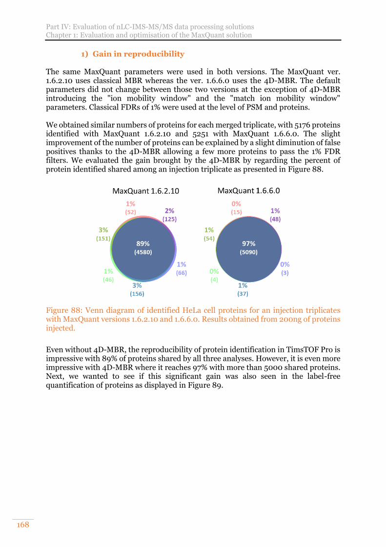
Part IV: Evaluation of nLC-IMS-MS/MS data processing solutions Chapter 1: Evaluation and optimisation of the MaxQuant solution
168
1) Gain in reproducibility The same MaxQuant parameters were used in both versions. The MaxQuant ver. 1.6.2.10 uses classical MBR whereas the ver. 1.6.6.0 uses the 4D-MBR. The default parameters did not change between those two versions at the exception of 4D-MBR introducing the "ion mobility window" and the "match ion mobility window" parameters. Classical FDRs of 1% were used at the level of PSM and proteins. We obtained similar numbers of proteins for each merged triplicate, with 5176 proteins identified with MaxQuant 1.6.2.10 and 5251 with MaxQuant 1.6.6.0. The slight improvement of the number of proteins can be explained by a slight diminution of false positives thanks to the 4D-MBR allowing a few more proteins to pass the 1% FDR filters. We evaluated the gain brought by the 4D-MBR by regarding the percent of protein identified shared among an injection triplicate as presented in Figure 88.
Figure 88: Venn diagram of identified HeLa cell proteins for an injection triplicates with MaxQuant versions 1.6.2.10 and 1.6.6.0. Results obtained from 200ng of proteins injected.
Even without 4D-MBR, the reproducibility of protein identification in TimsTOF Pro is impressive with 89% of proteins shared by all three analyses. However, it is even more impressive with 4D-MBR where it reaches 97% with more than 5000 shared proteins. Next, we wanted to see if this significant gain was also seen in the label-free quantification of proteins as displayed in Figure 89.
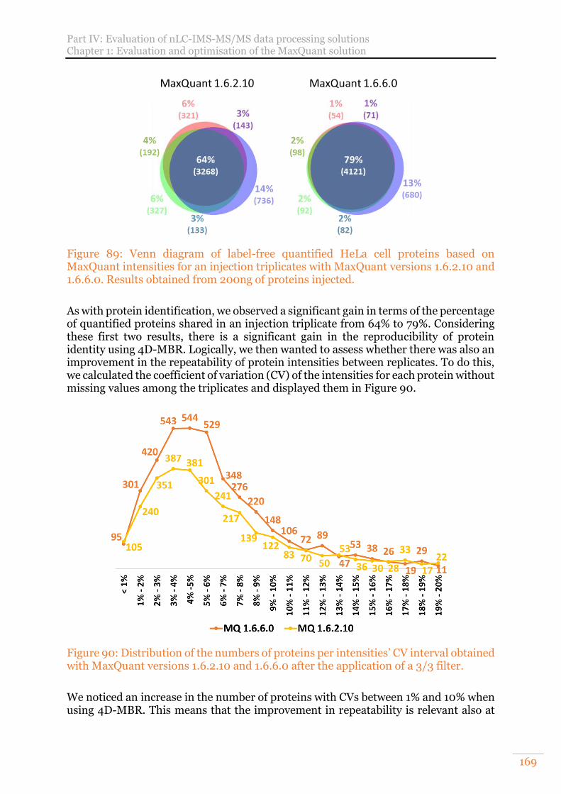
Part IV: Evaluation of nLC-IMS-MS/MS data processing solutions Chapter 1: Evaluation and optimisation of the MaxQuant solution
169
Figure 89: Venn diagram of label-free quantified HeLa cell proteins based on MaxQuant intensities for an injection triplicates with MaxQuant versions 1.6.2.10 and 1.6.6.0. Results obtained from 200ng of proteins injected.
As with protein identification, we observed a significant gain in terms of the percentage of quantified proteins shared in an injection triplicate from 64% to 79%. Considering these first two results, there is a significant gain in the reproducibility of protein identity using 4D-MBR. Logically, we then wanted to assess whether there was also an improvement in the repeatability of protein intensities between replicates. To do this, we calculated the coefficient of variation (CV) of the intensities for each protein without missing values among the triplicates and displayed them in Figure 90.
Figure 90: Distribution of the numbers of proteins per intensities’ CV interval obtained with MaxQuant versions 1.6.2.10 and 1.6.6.0 after the application of a 3/3 filter.
We noticed an increase in the number of proteins with CVs between 1% and 10% when using 4D-MBR. This means that the improvement in repeatability is relevant also at
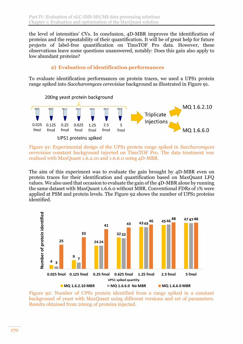
Part IV: Evaluation of nLC-IMS-MS/MS data processing solutions Chapter 1: Evaluation and optimisation of the MaxQuant solution
170
the level of intensities’ CVs. In conclusion, 4D-MBR improves the identification of proteins and the repeatability of their quantification. It will be of great help for future projects of label-free quantification on TimsTOF Pro data. However, these observations leave some questions unanswered, notably: Does this gain also apply to low abundant proteins?
2) Evaluation of identification performances To evaluate identification performances on protein traces, we used a UPS1 protein range spiked into Saccharomyces cerevisiae background as illustrated in Figure 91.
Figure 91: Experimental design of the UPS1 protein range spiked in Saccharomyces cerevisiae constant background injected on TimsTOF Pro. The data treatment was realised with MaxQuant 1.6.2.10 and 1.6.6.0 using 4D-MBR.
The aim of this experiment was to evaluate the gain brought by 4D-MBR even on protein traces for their identification and quantification based on MaxQuant LFQ values. We also used that occasion to evaluate the gain of the 4D-MBR alone by running the same dataset with MaxQuant 1.6.6.0 without MBR. Conventional FDRs of 1% were applied at PSM and protein levels. The Figure 92 shows the number of UPS1 proteins identified.
Figure 92: Number of UPS1 protein identified from a range spiked in a constant background of yeast with MaxQuant using different versions and set of parameters. Results obtained from 200ng of proteins injected.
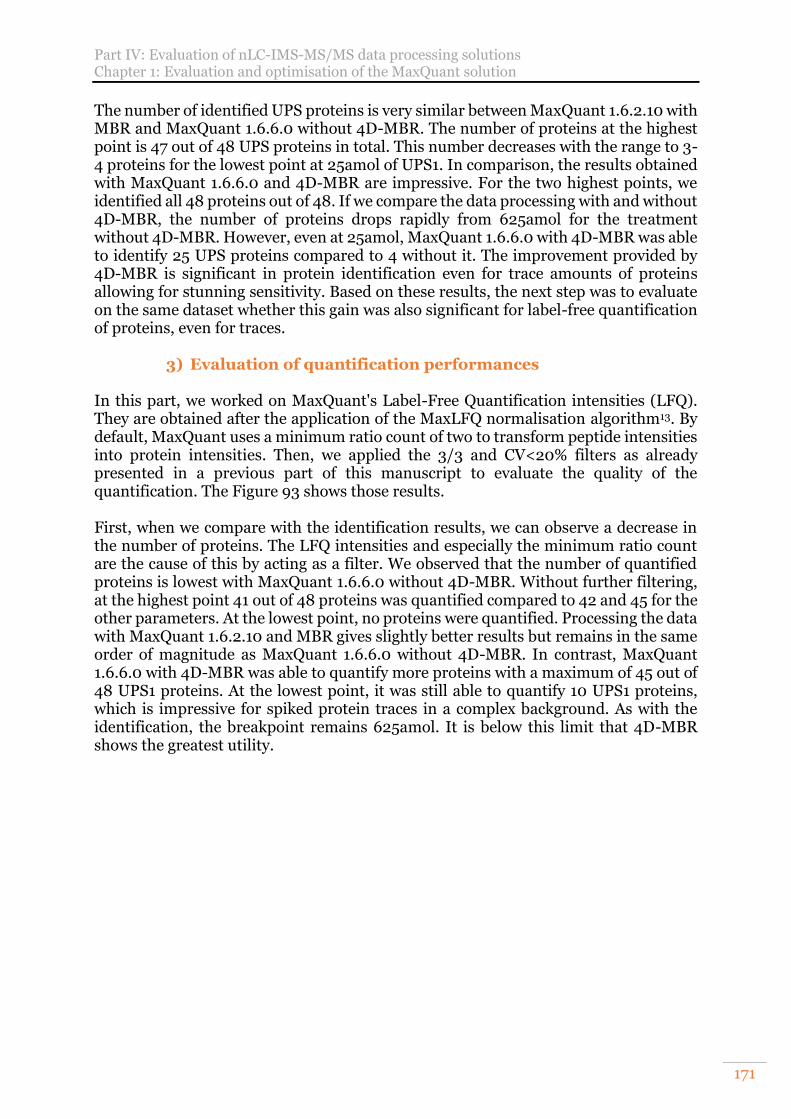
Part IV: Evaluation of nLC-IMS-MS/MS data processing solutions Chapter 1: Evaluation and optimisation of the MaxQuant solution
171
The number of identified UPS proteins is very similar between MaxQuant 1.6.2.10 with MBR and MaxQuant 1.6.6.0 without 4D-MBR. The number of proteins at the highest point is 47 out of 48 UPS proteins in total. This number decreases with the range to 3-4 proteins for the lowest point at 25amol of UPS1. In comparison, the results obtained with MaxQuant 1.6.6.0 and 4D-MBR are impressive. For the two highest points, we identified all 48 proteins out of 48. If we compare the data processing with and without 4D-MBR, the number of proteins drops rapidly from 625amol for the treatment without 4D-MBR. However, even at 25amol, MaxQuant 1.6.6.0 with 4D-MBR was able to identify 25 UPS proteins compared to 4 without it. The improvement provided by 4D-MBR is significant in protein identification even for trace amounts of proteins allowing for stunning sensitivity. Based on these results, the next step was to evaluate on the same dataset whether this gain was also significant for label-free quantification of proteins, even for traces.
3) Evaluation of quantification performances In this part, we worked on MaxQuant's Label-Free Quantification intensities (LFQ). They are obtained after the application of the MaxLFQ normalisation algorithm13. By default, MaxQuant uses a minimum ratio count of two to transform peptide intensities into protein intensities. Then, we applied the 3/3 and CV<20% filters as already presented in a previous part of this manuscript to evaluate the quality of the quantification. The Figure 93 shows those results. First, when we compare with the identification results, we can observe a decrease in the number of proteins. The LFQ intensities and especially the minimum ratio count are the cause of this by acting as a filter. We observed that the number of quantified proteins is lowest with MaxQuant 1.6.6.0 without 4D-MBR. Without further filtering, at the highest point 41 out of 48 proteins was quantified compared to 42 and 45 for the other parameters. At the lowest point, no proteins were quantified. Processing the data with MaxQuant 1.6.2.10 and MBR gives slightly better results but remains in the same order of magnitude as MaxQuant 1.6.6.0 without 4D-MBR. In contrast, MaxQuant 1.6.6.0 with 4D-MBR was able to quantify more proteins with a maximum of 45 out of 48 UPS1 proteins. At the lowest point, it was still able to quantify 10 UPS1 proteins, which is impressive for spiked protein traces in a complex background. As with the identification, the breakpoint remains 625amol. It is below this limit that 4D-MBR shows the greatest utility.
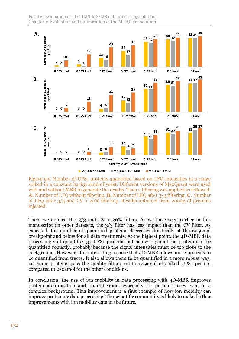
Part IV: Evaluation of nLC-IMS-MS/MS data processing solutions Chapter 1: Evaluation and optimisation of the MaxQuant solution
172
Figure 93: Number of UPS1 proteins quantified based on LFQ intensities in a range spiked in a constant background of yeast. Different versions of MaxQuant were used with and without MBR to generate the results. Then a filtering was applied as followed: A. Number of LFQ without filtering. B. Number of LFQ after 3/3 filtering. C. Number of LFQ after 3/3 and CV < 20% filtering. Results obtained from 200ng of proteins injected.
Then, we applied the 3/3 and CV < 20% filters. As we have seen earlier in this manuscript on other datasets, the 3/3 filter has less impact than the CV filter. As expected, the number of quantified proteins decreases drastically at the 625amol breakpoint and below for all data treatments. At the highest point, the 4D-MBR data processing still quantifies 37 UPS1 proteins but below 125amol, no protein can be quantified robustly, probably because the signal intensities must be too close to the background. However, it is interesting to note that 4D-MBR allows more proteins to be quantified from traces. It also allows them to be quantified in a more robust way, i.e. some proteins pass the quality filters, up to 125amol of spiked UPS1 protein compared to 250amol for the other conditions. In conclusion, the use of ion mobility in data processing with 4D-MBR improves protein identification and quantification, especially for protein traces even in a complex background. This improvement is a first example of how ion mobility can improve proteomic data processing. The scientific community is likely to make further improvements with ion mobility data in the future.
Part IV: Evaluation of nLC-IMS-MS/MS data processing solutions Chapter 1: Evaluation and optimisation of the MaxQuant solution
173
B. Evaluation of MaxQuant overall settings As explained earlier, the format and type of data generated by the TimsTOF instruments unique in many ways. Not only does the ion mobility dimension need to be considered, but also the resulting ddaPASEF acquisition mode. It was not until version 1.6.2.10 that MaxQuant offered effective default settings. However, during the various iterations of MaxQuant used in this thesis, we have seen changes in these parameters. We also evaluated some of them ourselves, both to better understand how the software works and possibly to find ways to improve the parameters we used for our future data processing. To do this, we tested different data processing parameters on triplicate injections of 10ng and 200ng of commercial HeLa cell protein digest. These injections were performed shortly after the installation of the mass spectrometer in our laboratory. It should be noted that at that time, our acquisition methods needed to be improved and the number of proteins in these examples does not reflect what we can achieve now on the coupling after nearly 3 years of improvements. We performed our tests based on a low (10ng) and a high (200ng) injected quantities analysed with adapted gradients to evaluate if the optimal parameters are the same in both ranges. As the advantage of the MBR was already demonstrated in the previous section, we did not evaluate again this parameter. The tests were realised with MaxQuant ver. 1.6.10.43 by changing one parameter at a time in comparison with MaxQuant‘s default parameters using 4D-MBR at some exception which will be explained just below. We evaluated the performances of the different data treatments firstly at the level of protein identification. When the number of proteins differed between one condition and the default parameters, we looked at the number of peptides identified. We realised those tests with 4D-MBR, but the number of proteins and peptides identified "by MS/MS" and "by matching" were evaluated separately. Then we evaluated the changes at the quantification level based on LFQ intensities and after application of the 3/3 and CV<20% filters. Thus, we evaluated more in details about twenty parameters of MaxQuant:
→ The IBAQ with no log fit is a parameter, which allows generating the IBAQ intensities. It is another way to do protein quantification. The IBAQ has been presented more in details in the Part I of this manuscript.
→ We have modified the precursor tolerances for the first and main
searches in MaxQuant. These parameters are by default set to 70ppm each in MaxQuant 1.6.10.43. However, as a matter of routine, we have reduced both to 20ppm. Indeed, these very open tolerances in the default settings were necessary on the very firsts TimsTOF Pro where the instability of a power supply increased the errors. As our TimsTOF Pro had already been modified at the time to correct this problem, we routinely used the value of 20ppm for both tolerances. The reference analysis of this series was therefore carried out with tolerances of 20ppm. In these tests, we evaluated the impact of opening the tolerance of the first search to 30ppm and reducing the tolerance of the main search to 10ppm.
Part IV: Evaluation of nLC-IMS-MS/MS data processing solutions Chapter 1: Evaluation and optimisation of the MaxQuant solution
174
→ We reduced the number of allowed missed cleavages from two by default to one.
→ We increased the minimum ratio count parameter from two to three. This
parameter will be explained more in detail in the next section, which dedicated especially to this parameter. It is a quality filter applied on quantified peptides in order to generate protein LFQ intensities.
→ FastLFQ is an equivalent of the MaxLFQ algorithm, which is used to generate
LFQ intensities. It is automatically used when more than 10 analyses are processed in parallel, in order to reduce the calculation time. Like the minimum count ratio and MaxLFQ, it will be discussed in more detail in the next section.
→ The Skip normalisation parameter is a sub-parameter of the LFQ
normalisation allowing the minimum ratio count filter to be applied without performing the normalisation of peptide intensities.
→ At the time where this test was done, we evaluated the parameter Re-Quantify
because we do not understood what was its function. If this parameter is used, a ratio is calculated for those isotopic patterns, which were not assembled into labelling pair or triplet. The peak shapes of the identified isotope pattern will be translated to the location in the m/z-RT plane where its missing partners are expected and intensities will be integrated over these regions. This is particularly helpful for quantifying proteins with very high ratios. This parameter is not present anymore in the last release of MaxQuant, the version 2.0.3.0.
→ We realised the quantification using unique + razor peptides and all the
peptides in comparison with using only unique peptides in our reference search.
→ We unselected the parameter advanced ratio estimation which is active by default in MaxQuant 1.6.10.43. This parameter is defined in the publication of Tyanova et al. from 201619 as related to MS1-level label-based quantification. “To determine the protein ratios as the median of peptide-feature ratios, keep this option unchecked. Select this option to use a regression model to determine whether there is an intensity dependence of the ratios for a given protein group. A statistically significant correlation between (logarithmic) ratios and intensities would indicate that the protein ratio is too large to be captured within the dynamic range of the less abundant features. In that case, a median of all peptide features would underestimate the features. If the option is checked, the software will automatically decide—on the basis of the goodness of fit—whether the median or the result of the regression is reported.”
→ We reduced the TOF MS/MS match tolerance from 40ppm to 20ppm that
is the tolerance applied to fragments.
→ For each kind of analyser, and in our case the TOF recalibration parameter is unselected by default into MaxQuant global parameters. We did not found more explanation in documentation regarding this precise parameter. Consequently, as MaxQuant performs a calibration of m/z and RT during its
Part IV: Evaluation of nLC-IMS-MS/MS data processing solutions Chapter 1: Evaluation and optimisation of the MaxQuant solution
175
analytical pipeline, we hypothesised that this option could allow repeating the calibration step of the m/z.
→ At the time we realised that test, we did not understood the role of the
Calculate peak properties option. This is why we decided to evaluate it in that test. Now we know that this parameter allows recovering more information at the level of peaks and isotope patterns. The use of this option unselected by default may lead to a substantial increase in computation time.
→ We added a filtering on the number of unique peptide which require at least
one unique peptide for confirm a protein identification. By default, this parameter is set to zero into MaxQuant.
→ When the Second peptides parameters is activated, MaxQuant tried to
identify co-fragmented peptides in all MS/MS spectra14. This parameter is activated by default and we inactivated it in our test.
→ The alignment ion mobility is the parameter defining the size of the ion
mobility windows used to perform the 4D-MBR12 as detailed in the previous section.
→ The parameter stabilise large LFQ ratio plays an important role in the
strength of the LFQ normalisation applied on large ratio as we will illustrate it in the next section of this manuscript even if we do not found any details on how work this parameter.
→ The advanced site intensities option is selected by default in MaxQuant. It
applies to the LFQ of modification sites. “To sum all peptide-feature intensities for a site, switch off this option. Check this option if only one representative peptide type with specific sequence and charge should be used in each sample, to obtain a more consistent quantification profile. If the user has selected this option, MaxQuant uses the combination of peptide sequence and charge that appears in the greatest number of samples. This strategy ensures that same feature types are used for quantification across all samples, leading to more consistent and precise relative quantification”, as described in Tyanova et al. from 201619.
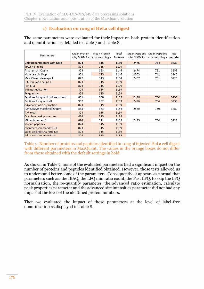
Part IV: Evaluation of nLC-IMS-MS/MS data processing solutions Chapter 1: Evaluation and optimisation of the MaxQuant solution
176
1) Evaluation on 10ng of HeLa cell digest The same parameters were evaluated for their impact on both protein identification and quantification as detailed in Table 7 and Table 8.
Table 7: Number of proteins and peptides identified in 10ng of injected HeLa cell digest with different parameters in MaxQuant. The values in the orange boxes do not differ from those obtained with the default settings in bold.
As shown in Table 7, none of the evaluated parameters had a significant impact on the number of proteins and peptides identified obtained. However, those tests allowed us to understand better some of the parameters. Consequently, it appears as normal that parameters such as: the IBAQ, the LFQ min ratio count, the Fast LFQ, to skip the LFQ normalisation, the re-quantify parameter, the advanced ratio estimation, calculate peak properties parameter and the advanced site intensities parameter did not had any impact at the level of the identified protein numbers. Then we evaluated the impact of those parameters at the level of label-free quantification as displayed in Table 8.
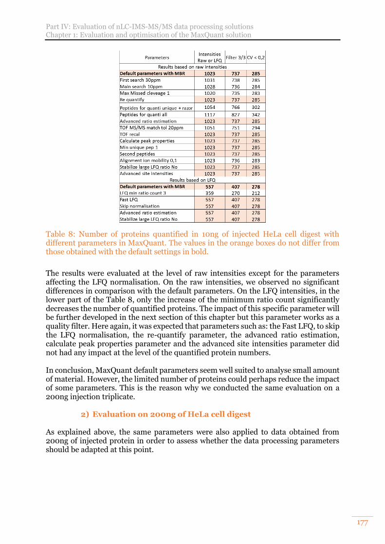
Part IV: Evaluation of nLC-IMS-MS/MS data processing solutions Chapter 1: Evaluation and optimisation of the MaxQuant solution
177
Table 8: Number of proteins quantified in 10ng of injected HeLa cell digest with different parameters in MaxQuant. The values in the orange boxes do not differ from those obtained with the default settings in bold.
The results were evaluated at the level of raw intensities except for the parameters affecting the LFQ normalisation. On the raw intensities, we observed no significant differences in comparison with the default parameters. On the LFQ intensities, in the lower part of the Table 8, only the increase of the minimum ratio count significantly decreases the number of quantified proteins. The impact of this specific parameter will be further developed in the next section of this chapter but this parameter works as a quality filter. Here again, it was expected that parameters such as: the Fast LFQ, to skip the LFQ normalisation, the re-quantify parameter, the advanced ratio estimation, calculate peak properties parameter and the advanced site intensities parameter did not had any impact at the level of the quantified protein numbers. In conclusion, MaxQuant default parameters seem well suited to analyse small amount of material. However, the limited number of proteins could perhaps reduce the impact of some parameters. This is the reason why we conducted the same evaluation on a 200ng injection triplicate.
2) Evaluation on 200ng of HeLa cell digest As explained above, the same parameters were also applied to data obtained from 200ng of injected protein in order to assess whether the data processing parameters should be adapted at this point.
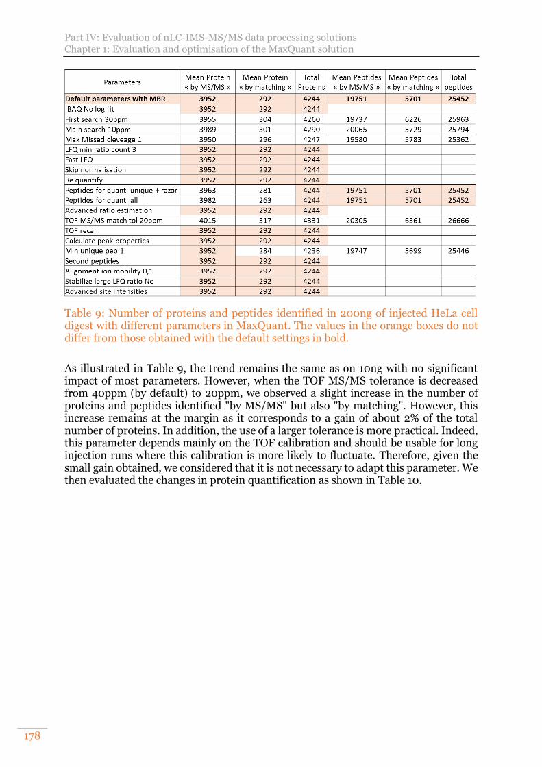
Part IV: Evaluation of nLC-IMS-MS/MS data processing solutions Chapter 1: Evaluation and optimisation of the MaxQuant solution
178
Table 9: Number of proteins and peptides identified in 200ng of injected HeLa cell digest with different parameters in MaxQuant. The values in the orange boxes do not differ from those obtained with the default settings in bold.
As illustrated in Table 9, the trend remains the same as on 10ng with no significant impact of most parameters. However, when the TOF MS/MS tolerance is decreased from 40ppm (by default) to 20ppm, we observed a slight increase in the number of proteins and peptides identified "by MS/MS" but also "by matching". However, this increase remains at the margin as it corresponds to a gain of about 2% of the total number of proteins. In addition, the use of a larger tolerance is more practical. Indeed, this parameter depends mainly on the TOF calibration and should be usable for long injection runs where this calibration is more likely to fluctuate. Therefore, given the small gain obtained, we considered that it is not necessary to adapt this parameter. We then evaluated the changes in protein quantification as shown in Table 10.
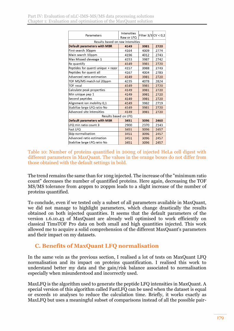
Part IV: Evaluation of nLC-IMS-MS/MS data processing solutions Chapter 1: Evaluation and optimisation of the MaxQuant solution
179
Table 10: Number of proteins quantified in 200ng of injected HeLa cell digest with different parameters in MaxQuant. The values in the orange boxes do not differ from those obtained with the default settings in bold.
The trend remains the same than for 10ng injected. The increase of the "minimum ratio count" decreases the number of quantified proteins. Here again, decreasing the TOF MS/MS tolerance from 40ppm to 20ppm leads to a slight increase of the number of proteins quantified. To conclude, even if we tested only a subset of all parameters available in MaxQuant, we did not manage to highlight parameters, which change drastically the results obtained on both injected quantities. It seems that the default parameters of the version 1.6.10.43 of MaxQuant are already well optimised to work efficiently on classical TimsTOF Pro data on both small and high quantities injected. This work allowed me to acquire a solid comprehension of the different MaxQuant's parameters and their impact on my datasets.
C. Benefits of MaxQuant LFQ normalisation In the same vein as the previous section, I realised a lot of tests on MaxQuant LFQ normalisation and its impact on proteins quantification. I realised this work to understand better my data and the gain/risk balance associated to normalisation especially when misunderstood and incorrectly used. MaxLFQ is the algorithm used to generate the peptide LFQ intensities in MaxQuant. A special version of this algorithm called FastLFQ can be used when the dataset is equal or exceeds 10 analyses to reduce the calculation time. Briefly, it works exactly as MaxLFQ but uses a meaningful subset of comparisons instead of all the possible pair-
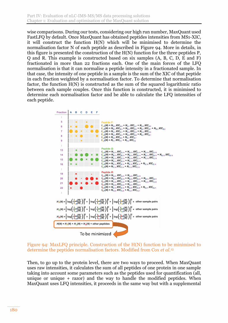
Part IV: Evaluation of nLC-IMS-MS/MS data processing solutions Chapter 1: Evaluation and optimisation of the MaxQuant solution
180
wise comparisons. During our tests, considering our high run number, MaxQuant used FastLFQ by default. Once MaxQuant has obtained peptides intensities from MS1-XIC, it will construct the function H(N) which will be minimised to determine the normalisation factor N of each peptide as described in Figure 94. More in details, in this figure is presented the construction of the H(N) function for the three peptides P, Q and R. This example is constructed based on six samples (A, B, C, D, E and F) fractionated in more than 22 fractions each. One of the main forces of the LFQ normalisation is that it can normalise a peptide intensity in a fractionated sample. In that case, the intensity of one peptide in a sample is the sum of the XIC of that peptide in each fraction weighted by a normalisation factor. To determine that normalisation factor, the function H(N) is constructed as the sum of the squared logarithmic ratio between each sample couples. Once this function is constructed, it is minimised to determine each normalisation factor and be able to calculate the LFQ intensities of each peptide.
Figure 94: MaxLFQ principle. Construction of the H(N) function to be minimised to determine the peptides normalisation factors. Modified from Cox et al.13
Then, to go up to the protein level, there are two ways to proceed. When MaxQuant uses raw intensities, it calculates the sum of all peptides of one protein in one sample taking into account some parameters such as the peptides used for quantification (all, unique or unique + razor) and the way to handle the modified peptides. When MaxQuant uses LFQ intensities, it proceeds in the same way but with a supplemental
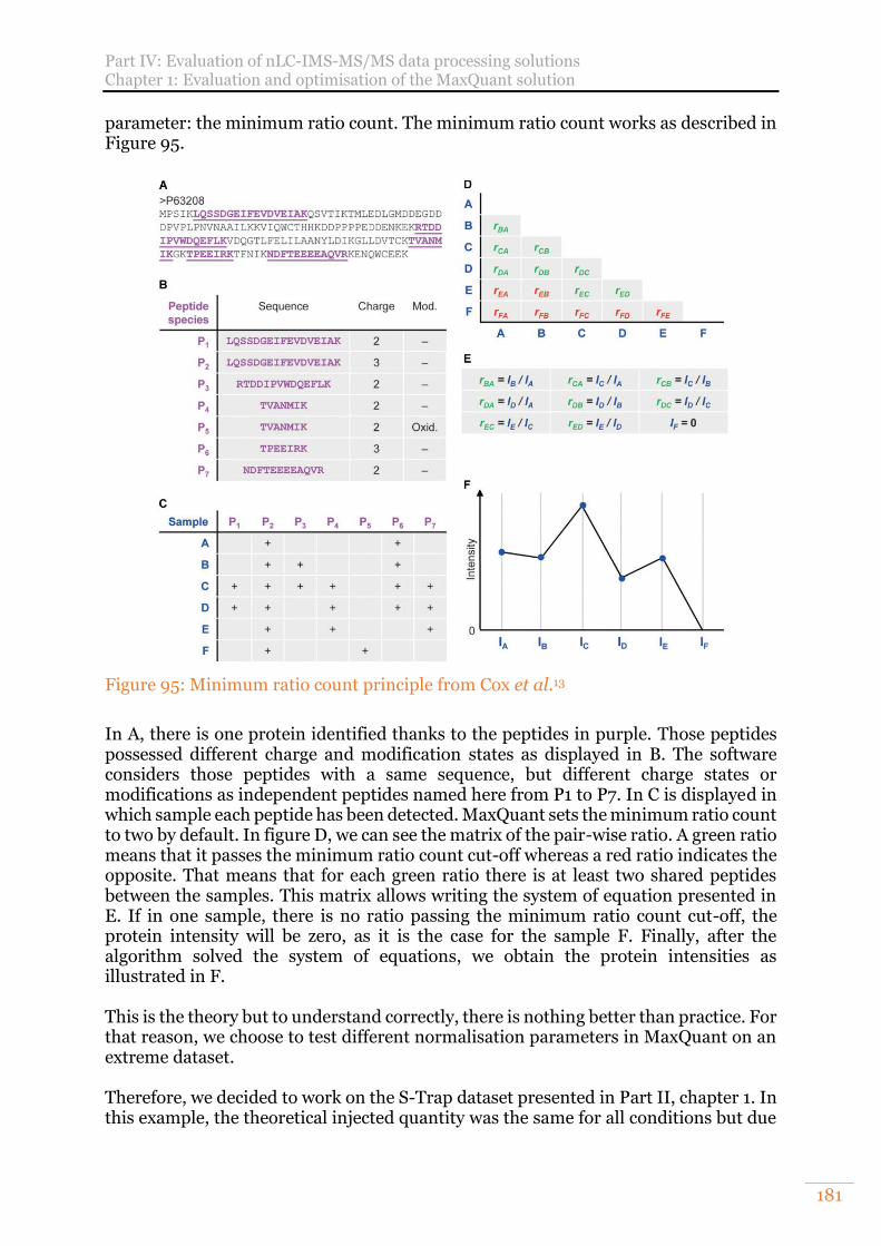
Part IV: Evaluation of nLC-IMS-MS/MS data processing solutions Chapter 1: Evaluation and optimisation of the MaxQuant solution
181
parameter: the minimum ratio count. The minimum ratio count works as described in Figure 95.
Figure 95: Minimum ratio count principle from Cox et al.13
In A, there is one protein identified thanks to the peptides in purple. Those peptides possessed different charge and modification states as displayed in B. The software considers those peptides with a same sequence, but different charge states or modifications as independent peptides named here from P1 to P7. In C is displayed in which sample each peptide has been detected. MaxQuant sets the minimum ratio count to two by default. In figure D, we can see the matrix of the pair-wise ratio. A green ratio means that it passes the minimum ratio count cut-off whereas a red ratio indicates the opposite. That means that for each green ratio there is at least two shared peptides between the samples. This matrix allows writing the system of equation presented in E. If in one sample, there is no ratio passing the minimum ratio count cut-off, the protein intensity will be zero, as it is the case for the sample F. Finally, after the algorithm solved the system of equations, we obtain the protein intensities as illustrated in F. This is the theory but to understand correctly, there is nothing better than practice. For that reason, we choose to test different normalisation parameters in MaxQuant on an extreme dataset. Therefore, we decided to work on the S-Trap dataset presented in Part II, chapter 1. In this example, the theoretical injected quantity was the same for all conditions but due
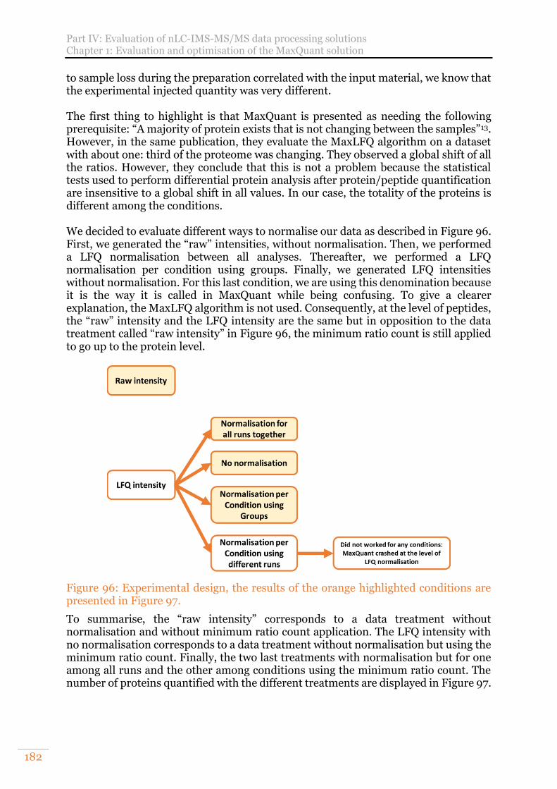
Part IV: Evaluation of nLC-IMS-MS/MS data processing solutions Chapter 1: Evaluation and optimisation of the MaxQuant solution
182
to sample loss during the preparation correlated with the input material, we know that the experimental injected quantity was very different. The first thing to highlight is that MaxQuant is presented as needing the following prerequisite: “A majority of protein exists that is not changing between the samples”13. However, in the same publication, they evaluate the MaxLFQ algorithm on a dataset with about one: third of the proteome was changing. They observed a global shift of all the ratios. However, they conclude that this is not a problem because the statistical tests used to perform differential protein analysis after protein/peptide quantification are insensitive to a global shift in all values. In our case, the totality of the proteins is different among the conditions. We decided to evaluate different ways to normalise our data as described in Figure 96. First, we generated the “raw” intensities, without normalisation. Then, we performed a LFQ normalisation between all analyses. Thereafter, we performed a LFQ normalisation per condition using groups. Finally, we generated LFQ intensities without normalisation. For this last condition, we are using this denomination because it is the way it is called in MaxQuant while being confusing. To give a clearer explanation, the MaxLFQ algorithm is not used. Consequently, at the level of peptides, the “raw” intensity and the LFQ intensity are the same but in opposition to the data treatment called “raw intensity” in Figure 96, the minimum ratio count is still applied to go up to the protein level.
Figure 96: Experimental design, the results of the orange highlighted conditions are presented in Figure 97.
To summarise, the “raw intensity” corresponds to a data treatment without normalisation and without minimum ratio count application. The LFQ intensity with no normalisation corresponds to a data treatment without normalisation but using the minimum ratio count. Finally, the two last treatments with normalisation but for one among all runs and the other among conditions using the minimum ratio count. The number of proteins quantified with the different treatments are displayed in Figure 97.
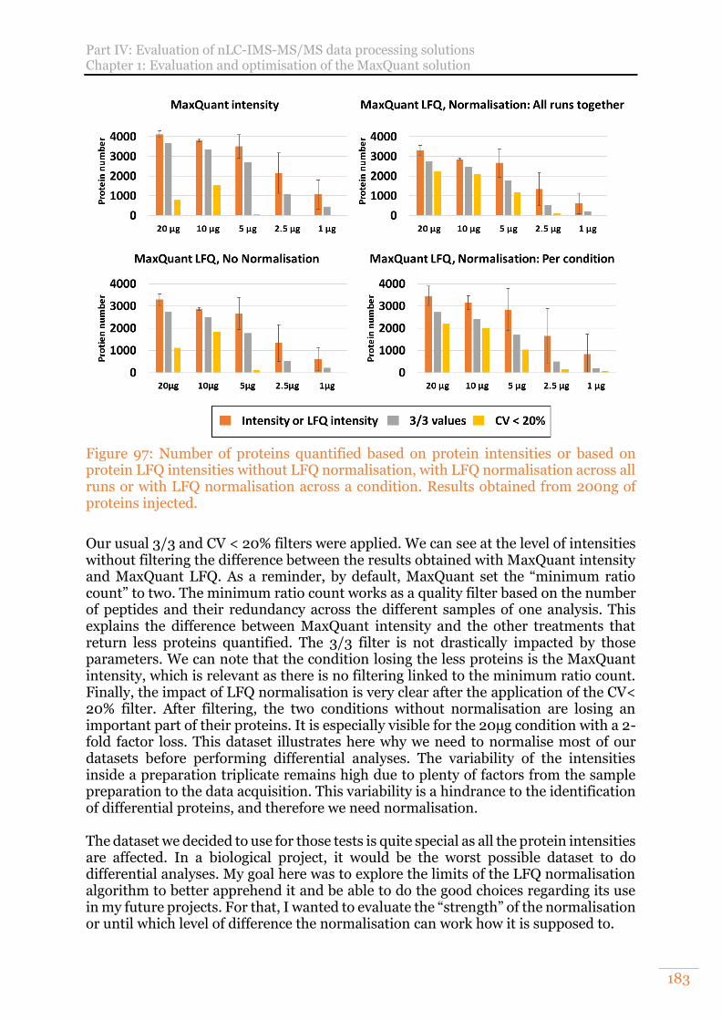
Part IV: Evaluation of nLC-IMS-MS/MS data processing solutions Chapter 1: Evaluation and optimisation of the MaxQuant solution
183
Figure 97: Number of proteins quantified based on protein intensities or based on protein LFQ intensities without LFQ normalisation, with LFQ normalisation across all runs or with LFQ normalisation across a condition. Results obtained from 200ng of proteins injected.
Our usual 3/3 and CV < 20% filters were applied. We can see at the level of intensities without filtering the difference between the results obtained with MaxQuant intensity and MaxQuant LFQ. As a reminder, by default, MaxQuant set the “minimum ratio count” to two. The minimum ratio count works as a quality filter based on the number of peptides and their redundancy across the different samples of one analysis. This explains the difference between MaxQuant intensity and the other treatments that return less proteins quantified. The 3/3 filter is not drastically impacted by those parameters. We can note that the condition losing the less proteins is the MaxQuant intensity, which is relevant as there is no filtering linked to the minimum ratio count. Finally, the impact of LFQ normalisation is very clear after the application of the CV< 20% filter. After filtering, the two conditions without normalisation are losing an important part of their proteins. It is especially visible for the 20µg condition with a 2-fold factor loss. This dataset illustrates here why we need to normalise most of our datasets before performing differential analyses. The variability of the intensities inside a preparation triplicate remains high due to plenty of factors from the sample preparation to the data acquisition. This variability is a hindrance to the identification of differential proteins, and therefore we need normalisation. The dataset we decided to use for those tests is quite special as all the protein intensities are affected. In a biological project, it would be the worst possible dataset to do differential analyses. My goal here was to explore the limits of the LFQ normalisation algorithm to better apprehend it and be able to do the good choices regarding its use in my future projects. For that, I wanted to evaluate the “strength” of the normalisation or until which level of difference the normalisation can work how it is supposed to.
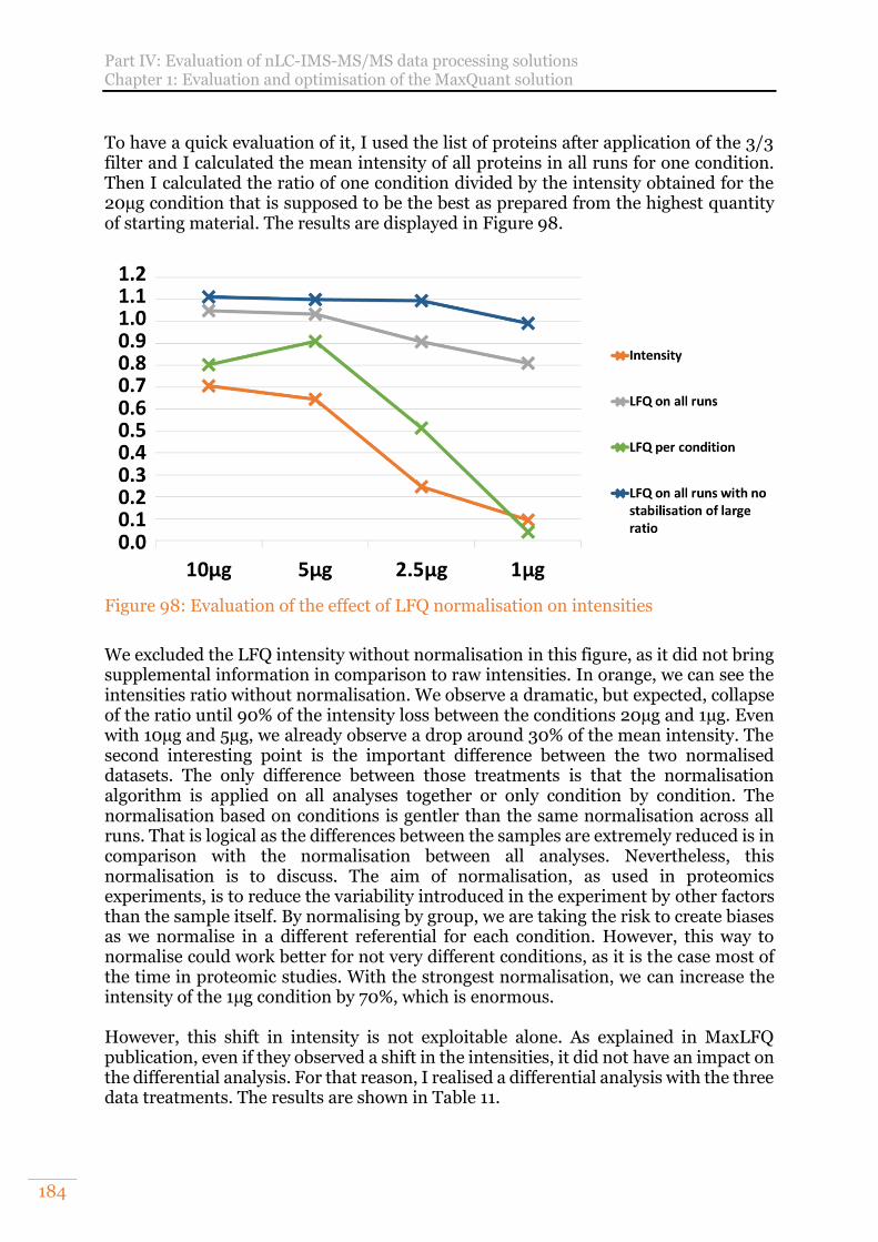
Part IV: Evaluation of nLC-IMS-MS/MS data processing solutions Chapter 1: Evaluation and optimisation of the MaxQuant solution
184
To have a quick evaluation of it, I used the list of proteins after application of the 3/3 filter and I calculated the mean intensity of all proteins in all runs for one condition. Then I calculated the ratio of one condition divided by the intensity obtained for the 20µg condition that is supposed to be the best as prepared from the highest quantity of starting material. The results are displayed in Figure 98.
Figure 98: Evaluation of the effect of LFQ normalisation on intensities
We excluded the LFQ intensity without normalisation in this figure, as it did not bring supplemental information in comparison to raw intensities. In orange, we can see the intensities ratio without normalisation. We observe a dramatic, but expected, collapse of the ratio until 90% of the intensity loss between the conditions 20µg and 1µg. Even with 10µg and 5µg, we already observe a drop around 30% of the mean intensity. The second interesting point is the important difference between the two normalised datasets. The only difference between those treatments is that the normalisation algorithm is applied on all analyses together or only condition by condition. The normalisation based on conditions is gentler than the same normalisation across all runs. That is logical as the differences between the samples are extremely reduced is in comparison with the normalisation between all analyses. Nevertheless, this normalisation is to discuss. The aim of normalisation, as used in proteomics experiments, is to reduce the variability introduced in the experiment by other factors than the sample itself. By normalising by group, we are taking the risk to create biases as we normalise in a different referential for each condition. However, this way to normalise could work better for not very different conditions, as it is the case most of the time in proteomic studies. With the strongest normalisation, we can increase the intensity of the 1µg condition by 70%, which is enormous. However, this shift in intensity is not exploitable alone. As explained in MaxLFQ publication, even if they observed a shift in the intensities, it did not have an impact on the differential analysis. For that reason, I realised a differential analysis with the three data treatments. The results are shown in Table 11.
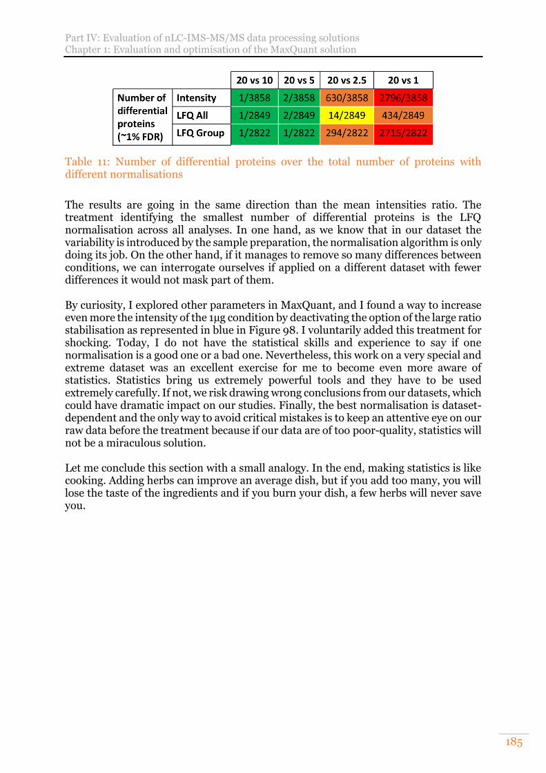
Part IV: Evaluation of nLC-IMS-MS/MS data processing solutions Chapter 1: Evaluation and optimisation of the MaxQuant solution
185
Table 11: Number of differential proteins over the total number of proteins with different normalisations
The results are going in the same direction than the mean intensities ratio. The treatment identifying the smallest number of differential proteins is the LFQ normalisation across all analyses. In one hand, as we know that in our dataset the variability is introduced by the sample preparation, the normalisation algorithm is only doing its job. On the other hand, if it manages to remove so many differences between conditions, we can interrogate ourselves if applied on a different dataset with fewer differences it would not mask part of them. By curiosity, I explored other parameters in MaxQuant, and I found a way to increase even more the intensity of the 1µg condition by deactivating the option of the large ratio stabilisation as represented in blue in Figure 98. I voluntarily added this treatment for shocking. Today, I do not have the statistical skills and experience to say if one normalisation is a good one or a bad one. Nevertheless, this work on a very special and extreme dataset was an excellent exercise for me to become even more aware of statistics. Statistics bring us extremely powerful tools and they have to be used extremely carefully. If not, we risk drawing wrong conclusions from our datasets, which could have dramatic impact on our studies. Finally, the best normalisation is dataset-dependent and the only way to avoid critical mistakes is to keep an attentive eye on our raw data before the treatment because if our data are of too poor-quality, statistics will not be a miraculous solution. Let me conclude this section with a small analogy. In the end, making statistics is like cooking. Adding herbs can improve an average dish, but if you add too many, you will lose the taste of the ingredients and if you burn your dish, a few herbs will never save you.
Part IV: Evaluation of nLC-IMS-MS/MS data processing solutions Chapter 2: Evaluation of alternative software for ddaPASEF and diaPASEF data processing
186
Chapter 2: Evaluation of alternative software for ddaPASEF and diaPASEF data processing
As explained in previous chapters, at the beginning of my PhD, only MaxQuant and Peaks were able to do label-free MS1-XIC quantification on TimsTOF Pro ddaPASEF data. However, an increasing number of software are now becoming available. In this chapter four software allowing to deal with ddaPASEF data have been investigated: MaxQuant13, SpectroMine (Biognosys), Peaks (Bioinformatics Solutions Inc.) and the combination of Mascot (Matrix science) with Proline20 which was available in the last weeks of that manuscript writing. In this part, I also studied the Spectronaut software (Biognosys) to process diaPASEF data with a peptide-centric and spectral approach. Finally, in the last months of this PhD, the MaxDIA18 functionality was integrated into MaxQuant version 2.0. MaxDIA enables MaxQuant to support DIA data, including diaPASEF and BoxCar data. Like Spectronaut, MaxDIA can process DIA data using either a peptide-centric or a spectral approach, known as discovery mode. Only the peptide-centric approach was tested in this work.
A. ddaPASEF data processing Among the software I evaluated, the company Biognosys developed SpectroMine. It was supposed to give better results for protein identification than MaxQuant in a shorter time on ddaPASEF data. At its origin, SpectroMine was created to do protein quantification from TMT labelled samples. We decided to evaluate it when the label-free MS1-XIC quantification feature was released. Finally in the last months of my PhD, Proline20 gains the ability to perform label-free quantification on TimsTOF Pro data thanks to a new data converter developed by David Bouyssié of the IPBS in Toulouse in the framework of ProFI. Indeed, the main limitation of using Proline on TimsTOF Pro’s data was related to peak list format in relationship to the PASEF acquisition mode. In view of these latest developments, I treated again datasets previously used to perform comparison of data treatment solution including Proline.
1) Benchmarking of SpectroMine (Biognosys), Proline and MaxQuant on ddaPASEF data
SpectroMine is similar in its interface to Spectronaut, another software from Biognosys, which is dedicated to treat DIA data and is already well implanted into our lab. Both are using the same search engine, called Pulsar, and possess an impressive number of useful data visualisation and data export tools. As SpectroMine was supposed to give impressive results in identification, we decided first to compare it with MaxQuant, and Mascot (Matrix science) combined with Proline20 for protein identification on a UPS1 range spiked in a constant background of Arabidopsis thaliana acquired in ddaPASEF mode.
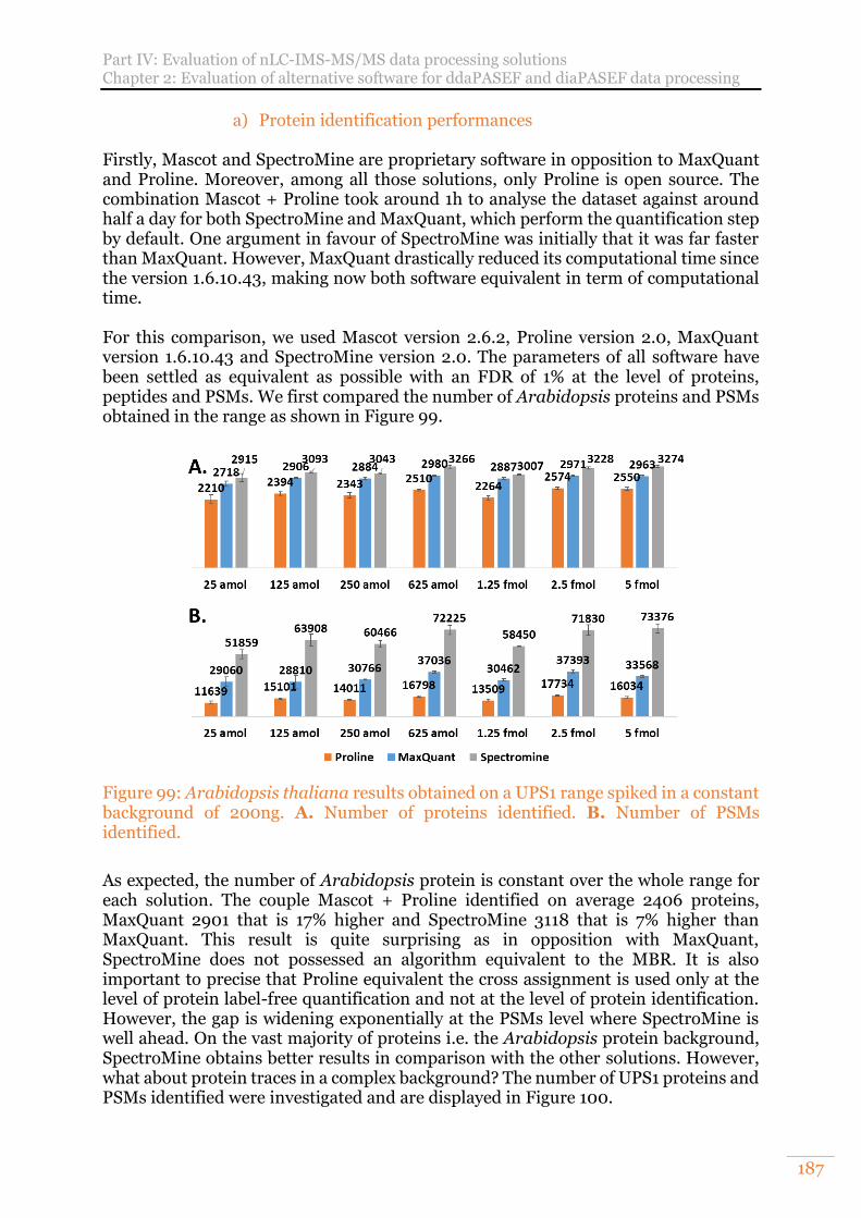
Part IV: Evaluation of nLC-IMS-MS/MS data processing solutions Chapter 2: Evaluation of alternative software for ddaPASEF and diaPASEF data processing
187
a) Protein identification performances Firstly, Mascot and SpectroMine are proprietary software in opposition to MaxQuant and Proline. Moreover, among all those solutions, only Proline is open source. The combination Mascot + Proline took around 1h to analyse the dataset against around half a day for both SpectroMine and MaxQuant, which perform the quantification step by default. One argument in favour of SpectroMine was initially that it was far faster than MaxQuant. However, MaxQuant drastically reduced its computational time since the version 1.6.10.43, making now both software equivalent in term of computational time. For this comparison, we used Mascot version 2.6.2, Proline version 2.0, MaxQuant version 1.6.10.43 and SpectroMine version 2.0. The parameters of all software have been settled as equivalent as possible with an FDR of 1% at the level of proteins, peptides and PSMs. We first compared the number of Arabidopsis proteins and PSMs obtained in the range as shown in Figure 99.
Figure 99: Arabidopsis thaliana results obtained on a UPS1 range spiked in a constant background of 200ng. A. Number of proteins identified. B. Number of PSMs identified.
As expected, the number of Arabidopsis protein is constant over the whole range for each solution. The couple Mascot + Proline identified on average 2406 proteins, MaxQuant 2901 that is 17% higher and SpectroMine 3118 that is 7% higher than MaxQuant. This result is quite surprising as in opposition with MaxQuant, SpectroMine does not possessed an algorithm equivalent to the MBR. It is also important to precise that Proline equivalent the cross assignment is used only at the level of protein label-free quantification and not at the level of protein identification. However, the gap is widening exponentially at the PSMs level where SpectroMine is well ahead. On the vast majority of proteins i.e. the Arabidopsis protein background, SpectroMine obtains better results in comparison with the other solutions. However, what about protein traces in a complex background? The number of UPS1 proteins and PSMs identified were investigated and are displayed in Figure 100.
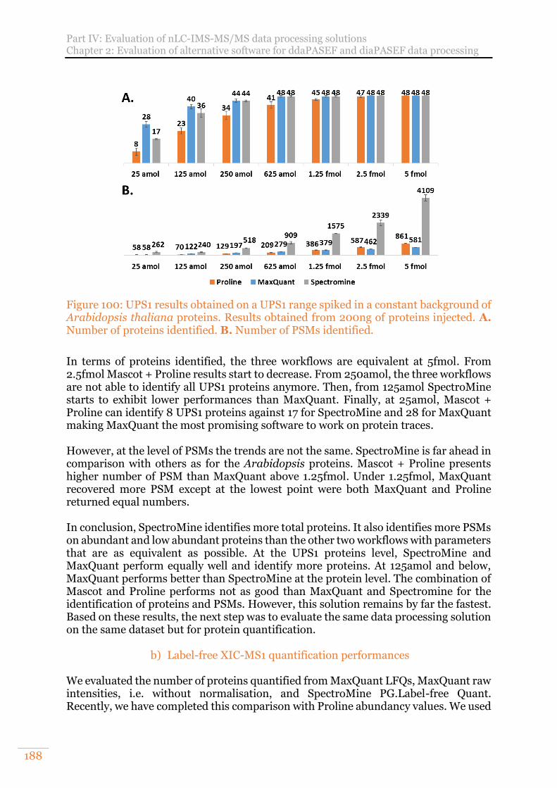
Part IV: Evaluation of nLC-IMS-MS/MS data processing solutions Chapter 2: Evaluation of alternative software for ddaPASEF and diaPASEF data processing
188
Figure 100: UPS1 results obtained on a UPS1 range spiked in a constant background of Arabidopsis thaliana proteins. Results obtained from 200ng of proteins injected. A. Number of proteins identified. B. Number of PSMs identified.
In terms of proteins identified, the three workflows are equivalent at 5fmol. From 2.5fmol Mascot + Proline results start to decrease. From 250amol, the three workflows are not able to identify all UPS1 proteins anymore. Then, from 125amol SpectroMine starts to exhibit lower performances than MaxQuant. Finally, at 25amol, Mascot + Proline can identify 8 UPS1 proteins against 17 for SpectroMine and 28 for MaxQuant making MaxQuant the most promising software to work on protein traces. However, at the level of PSMs the trends are not the same. SpectroMine is far ahead in comparison with others as for the Arabidopsis proteins. Mascot + Proline presents higher number of PSM than MaxQuant above 1.25fmol. Under 1.25fmol, MaxQuant recovered more PSM except at the lowest point were both MaxQuant and Proline returned equal numbers. In conclusion, SpectroMine identifies more total proteins. It also identifies more PSMs on abundant and low abundant proteins than the other two workflows with parameters that are as equivalent as possible. At the UPS1 proteins level, SpectroMine and MaxQuant perform equally well and identify more proteins. At 125amol and below, MaxQuant performs better than SpectroMine at the protein level. The combination of Mascot and Proline performs not as good than MaxQuant and Spectromine for the identification of proteins and PSMs. However, this solution remains by far the fastest. Based on these results, the next step was to evaluate the same data processing solution on the same dataset but for protein quantification.
b) Label-free XIC-MS1 quantification performances We evaluated the number of proteins quantified from MaxQuant LFQs, MaxQuant raw intensities, i.e. without normalisation, and SpectroMine PG.Label-free Quant. Recently, we have completed this comparison with Proline abundancy values. We used
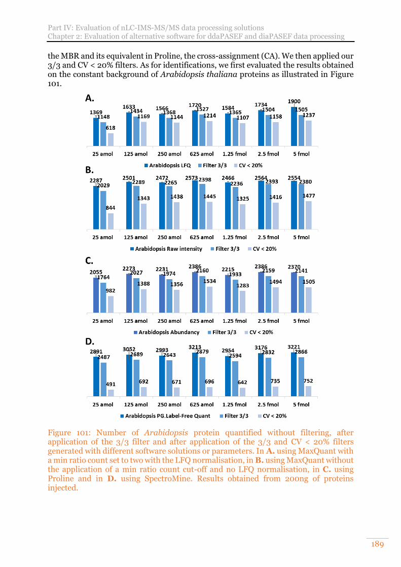
Part IV: Evaluation of nLC-IMS-MS/MS data processing solutions Chapter 2: Evaluation of alternative software for ddaPASEF and diaPASEF data processing
189
the MBR and its equivalent in Proline, the cross-assignment (CA). We then applied our 3/3 and CV < 20% filters. As for identifications, we first evaluated the results obtained on the constant background of Arabidopsis thaliana proteins as illustrated in Figure 101.
Figure 101: Number of Arabidopsis protein quantified without filtering, after application of the 3/3 filter and after application of the 3/3 and CV < 20% filters generated with different software solutions or parameters. In A. using MaxQuant with a min ratio count set to two with the LFQ normalisation, in B. using MaxQuant without the application of a min ratio count cut-off and no LFQ normalisation, in C. using Proline and in D. using SpectroMine. Results obtained from 200ng of proteins injected.
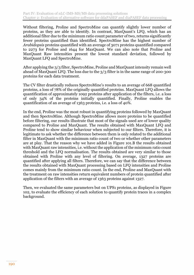
Part IV: Evaluation of nLC-IMS-MS/MS data processing solutions Chapter 2: Evaluation of alternative software for ddaPASEF and diaPASEF data processing
190
Without filtering, Proline and SpectroMine can quantify slightly lower number of proteins, as they are able to identify. In contrast, MaxQuant’s LFQ, which has an additional filter due to the minimum ratio count parameter of two, returns significantly fewer proteins quantified than identified. SpectroMine has the highest number of Arabidopsis proteins quantified with an average of 3071 proteins quantified compared to 2273 for Proline and 1644 for MaxQuant. We can also note that Proline and MaxQuant Raw intensities present the lowest standard deviation, followed by MaxQuant LFQ and SpectroMine. After applying the 3/3 filter, SpectroMine, Proline and MaxQuant intensity remain well ahead of MaxQuant LFQ. The loss due to the 3/3 filter is in the same range of 200-300 proteins for each data treatment. The CV filter drastically reduces SpectroMine's results to an average of 668 quantified proteins, a loss of 78% of the originally quantified proteins. MaxQuant LFQ allows the quantification of approximately 1092 proteins after application of the filters, i.e. a loss of only 34% of the proteins initially quantified. Finally, Proline enables the quantification of an average of 1363 proteins, i.e. a loss of 40%. In the end, Proline was the most robust in quantifying proteins followed by MaxQuant and then SpectroMine. Although SpectroMine allows more proteins to be quantified before filtering, our results illustrate that most of the signals used are of lower quality compared to Proline and MaxQuant. The results obtained with MaxQuant LFQ and Proline tend to show similar behaviour when subjected to our filters. Therefore, it is legitimate to ask whether the difference between them is only related to the additional filter in MaxQuant with the minimum ratio count of two or whether other parameters are at play. That the reason why we have added in Figure 101.B the results obtained with MaxQuant raw intensities, i.e. without the application of the minimum ratio count threshold and the LFQ normalisation. The results obtained are very similar to those obtained with Proline with any level of filtering. On average, 1327 proteins are quantified after applying all filters. Therefore, we can say that the difference between the results obtained with MaxQuant processing based on LFQ intensities and Proline comes mainly from the minimum ratio count. In the end, Proline and MaxQuant with the treatment on raw intensities return equivalent numbers of protein quantified after application of the filters with an average of 1363 proteins against 1327. Then, we evaluated the same parameters but on UPS1 proteins, as displayed in Figure 102, to evaluate the efficiency of each solution to quantify protein traces in a complex background.
Part IV: Evaluation of nLC-IMS-MS/MS data processing solutions Chapter 2: Evaluation of alternative software for ddaPASEF and diaPASEF data processing
191
Figure 102: Number of UPS1 protein quantified without filtering, after application of the 3/3 filter and after application of the 3/3 and CV < 20% filters generated with different software solutions or parameters. In A. using MaxQuant with a min ratio count set to two with the LFQ normalisation, in B. using MaxQuant without the application of a min ratio count cut-off and no LFQ normalisation, in C. using Proline and in D. using SpectroMine. Results obtained from 200ng of proteins injected.
Part IV: Evaluation of nLC-IMS-MS/MS data processing solutions Chapter 2: Evaluation of alternative software for ddaPASEF and diaPASEF data processing
192
We observed the same trends as for the Arabidopsis thaliana protein background with a drastic decrease in SpectroMine performance when applying the CV filter. Even at the highest point, SpectroMine can only robustly quantify 13 UPS proteins, compared to 36 for MaxQuant LFQ, 41 for MaxQuant raw intensities and 45 for Proline. Removing the minimum ratio count threshold in MaxQuant by using raw intensities instead of LFQ intensities increases the number of proteins quantified, making the results at each filter level very similar to those obtained with Proline, except for the points at 250amol and below where MaxQuant's raw intensities return slightly higher numbers than Proline. We now know that SpectroMine quantifies much less protein than MaxQuant, mainly because of the CV filter. Indeed, in the version of SpectroMine used for these data treatments, no normalisation was yet implemented. Following on from these initial findings, we investigated whether the variability of the quantities determined by SpectroMine could affect the accuracy and precision of its quantification. Subsequently, the accuracy and precision of the quantification of Proline was also assessed. To do this, we plotted the calibration curve for UPS1 proteins as shown in the following Figure 103.
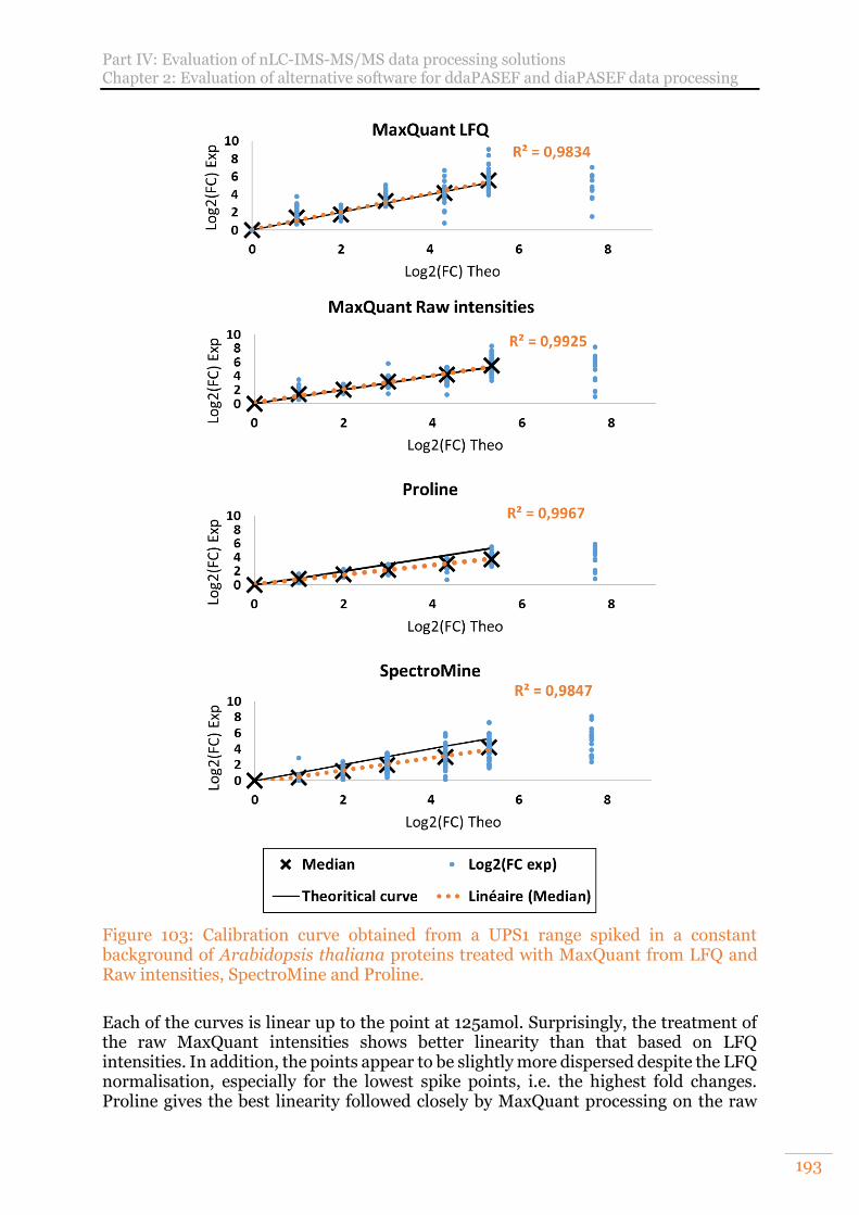
Part IV: Evaluation of nLC-IMS-MS/MS data processing solutions Chapter 2: Evaluation of alternative software for ddaPASEF and diaPASEF data processing
193
Figure 103: Calibration curve obtained from a UPS1 range spiked in a constant background of Arabidopsis thaliana proteins treated with MaxQuant from LFQ and Raw intensities, SpectroMine and Proline.
Each of the curves is linear up to the point at 125amol. Surprisingly, the treatment of the raw MaxQuant intensities shows better linearity than that based on LFQ intensities. In addition, the points appear to be slightly more dispersed despite the LFQ normalisation, especially for the lowest spike points, i.e. the highest fold changes. Proline gives the best linearity followed closely by MaxQuant processing on the raw
Part IV: Evaluation of nLC-IMS-MS/MS data processing solutions Chapter 2: Evaluation of alternative software for ddaPASEF and diaPASEF data processing
194
intensities. However, both SpectroMine and Proline show an underestimation of the protein amounts, which seems to increase as the amount of UPS protein added decreases. For Proline, we repeated the same analysis but without using the cross-assignment, the tendency to underestimate the intensities of low abundant proteins remained although this effect was slightly less pronounced (Results not shown). In conclusion, SpectroMine shows promising results for protein identification. It is also easy to use and has very useful graphical data visualisation tools. In terms of quantification, however, SpectroMine still seems to have room for improvement, especially in terms of reducing the CVs of intensities and improving the accuracy of quantification. One way to improve the software could be to add an algorithm equivalent to MBR, add an intensity normalisation step and use the ion mobility data more efficiently in signal extraction or normalisation. Based on our results, we decided to continue using MaxQuant to process our label-free quantification data during my thesis. Nevertheless, we kept an eye on the evolution of SpectroMine which still gives very promising results in identification and whose interface offers many more options for data visualisation. As a reminder, at the time of the initial comparison between SpectroMine and MaxQuant, Proline was not yet capable of performing label-free quantification on data from TimsTOF Pro. For Proline, the quantification looks promising as it is one of the very first tests using the new TimsTOF Pro data converter. Proline gives satisfactory results for protein identification. For the quantified protein numbers, the first results are very encouraging and equivalent to the MaxQuant treatment on the raw intensities before and after applying the quality filters. However, we observed that like SpectroMine, Proline suffers from an underestimation of the quantity of proteins, particularly on low abundance proteins. Proline gives the best linearity and the lowest point spread of the three evaluated. In addition, Proline remains very fast compared to the other software, both for identification and quantification, making it a tool of choice, for example, for monitoring the daily performance of instruments. In the future, one way to improve the processing of Proline data will be to use information from the additional dimension of ion mobility, which is not yet exploited.
2) Benchmarking of four data treatment software supporting ddaPASEF data for XIC label-free quantification
We did a repeat comparison of MaxQuant and SpectroMine several months later with a different dataset and the addition of Peaks studio software. Recently, as in the previous section, I added the Mascot + Proline workflow for label-free quantification to this comparison. We worked on the dataset we generated for the benchmark of S-Trap cartridges with varying amounts of protein for sample preparation as presented previously. For this comparison, we used MaxQuant version 1.6.14.0, SpectroMine version 2.5, Peaks version 10.6, Mascot version 2.6.2 and Proline Studio version 2.1.2. The parameters of all software were set as equivalent as possible with an FDR of 1% at the protein, peptide and PSM level. We compared the different software for protein identification, label-free quantification with and without the addition of our quality filters. The results are displayed in Figure 104.
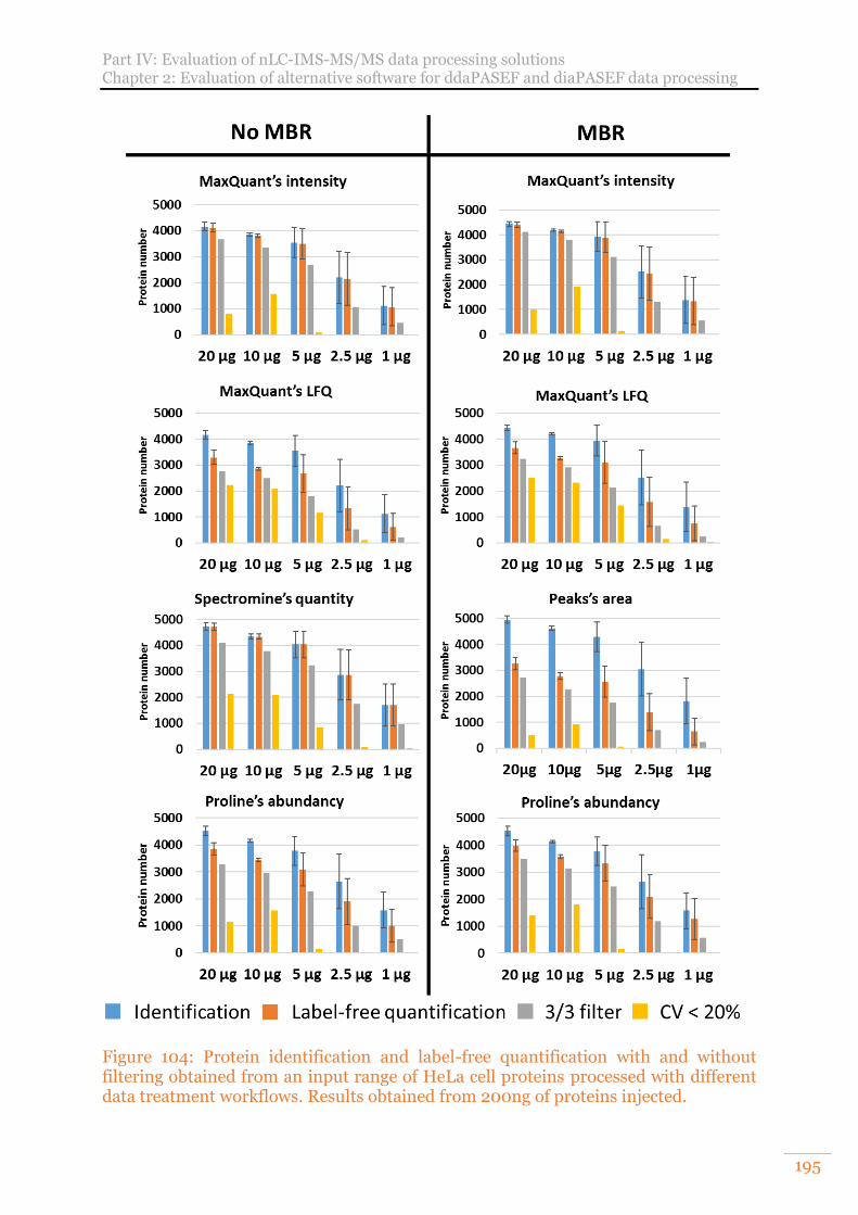
Part IV: Evaluation of nLC-IMS-MS/MS data processing solutions Chapter 2: Evaluation of alternative software for ddaPASEF and diaPASEF data processing
195
Figure 104: Protein identification and label-free quantification with and without filtering obtained from an input range of HeLa cell proteins processed with different data treatment workflows. Results obtained from 200ng of proteins injected.
Part IV: Evaluation of nLC-IMS-MS/MS data processing solutions Chapter 2: Evaluation of alternative software for ddaPASEF and diaPASEF data processing
196
Each software possesses its own specificities, which is the reason why we made different data treatments with MaxQuant and Proline to have the nearest parameters possible to do the comparison between the software as fairly as possible. First, we compared the results obtained with MaxQuant with the different parameter sets on the raw intensities and LFQ data. As expected, MBR slightly increases the number of identified and quantified proteins. In addition, LFQ normalisation has a significant impact on the protein intensity CVs allowing more than 2000 proteins to be quantified after the application of quality filters for the highest points. SpectroMine, Peaks and Proline do not, to our knowledge, use a filter such as the minimum ratio count. SpectroMine does not have an MBR either. However, unlike SpectroMine v2.0 used in the previous section, SpectroMine v2.5 uses intra- and inter-condition intensity normalisations. With regard to protein identification, SpectroMine still outperforms MaxQuant and Proline with and without MBR. However, it is slightly worse than Peaks, which has the original feature of adding a de novo search to the classical search using a protein database. SpectroMine quantifies the largest number of proteins before the application of quality filters. It should be noted that the SpectroMine data processing and MaxQuant raw intensities show a similar number of proteins identified and quantified before the application of the quality filters as seen in the previous section. However, in the previous section, this was also the case for Proline and we can observe that this is less the case on this dataset. After applying the filters, we can see a clear improvement in the SpectroMine results compared to what we obtained in the previous section on the UPS1/Arabidopsis range. In this range, we lost 78% of the quantified proteins with SpectroMine 2.0 but here with version 2.5, on the highest point of the range, we lose only 55% after applying the filters. Furthermore, the distribution of quantified proteins after filtering is similar to that of MaxQuant's LFQs showing here the impact of intensity normalisation. On this dataset, the highest numbers of protein quantified after application of the quality filters are obtained with MaxQuant’s LFQ, but SpectroMine made clear progress and is now only slightly behind. Due to lack of time, we did not retreat the UPS1/Arabidopsis range with the 2.5 version of SpectroMine but it would be very interesting to do so to observe the change between the two versions on a same dataset and to see if the improvement of the intensities normalisation reduced the quantification underestimation we observed with the 2.0 version. Peaks exhibits the best performances for protein identifications. It is probably helped by its MBR equivalent and the fact it is performing an additional de novo search. However, we can observed an important gap between the number of proteins identified and quantified without filtering. This gap is a similar trend with MaxQuant's LFQs linked to the minimum ratio count. However, it seems that their origins differ as the minimum ratio count is acting like a quality filter reducing the losses linked to the 3/3 and CV filters. Nevertheless, in Peaks after the application of the 3/3 and CV quality filters, we again observed a drastic decrease of the number of proteins quantified. Moreover, Peaks does not possess an intensity normalisation algorithm. It is clearly visible after application of the quality filters as Peaks results present the same trends
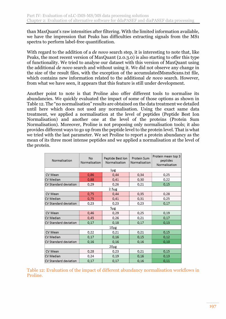
Part IV: Evaluation of nLC-IMS-MS/MS data processing solutions Chapter 2: Evaluation of alternative software for ddaPASEF and diaPASEF data processing
197
than MaxQuant's raw intensities after filtering. With the limited information available, we have the impression that Peaks has difficulties extracting signals from the MS1 spectra to perform label-free quantification. With regard to the addition of a de novo search step, it is interesting to note that, like Peaks, the most recent version of MaxQuant (2.0.3.0) is also starting to offer this type of functionality. We tried to analyse our dataset with this version of MaxQuant using the additional de novo search and without using it. We did not observe any change in the size of the result files, with the exception of the accumulatedMsmsScans.txt file, which contains new information related to the additional de novo search. However, from what we have seen, it appears that this feature is still under development. Another point to note is that Proline also offer different tools to normalise its abundancies. We quickly evaluated the impact of some of those options as shown in Table 12. The “no normalisation” results are obtained on the data treatment we detailed until here which does not used any normalisation. Using the exact same data treatment, we applied a normalisation at the level of peptides (Peptide Best Ion Normalisation) and another one at the level of the proteins (Protein Sum Normalisation). Moreover, Proline is not proposing only normalisation tools; it also provides different ways to go up from the peptide level to the protein level. That is what we tried with the last parameter. We set Proline to report a protein abundancy as the mean of its three most intense peptides and we applied a normalisation at the level of the protein.
Table 12: Evaluation of the impact of different abundancy normalisation workflows in Proline.
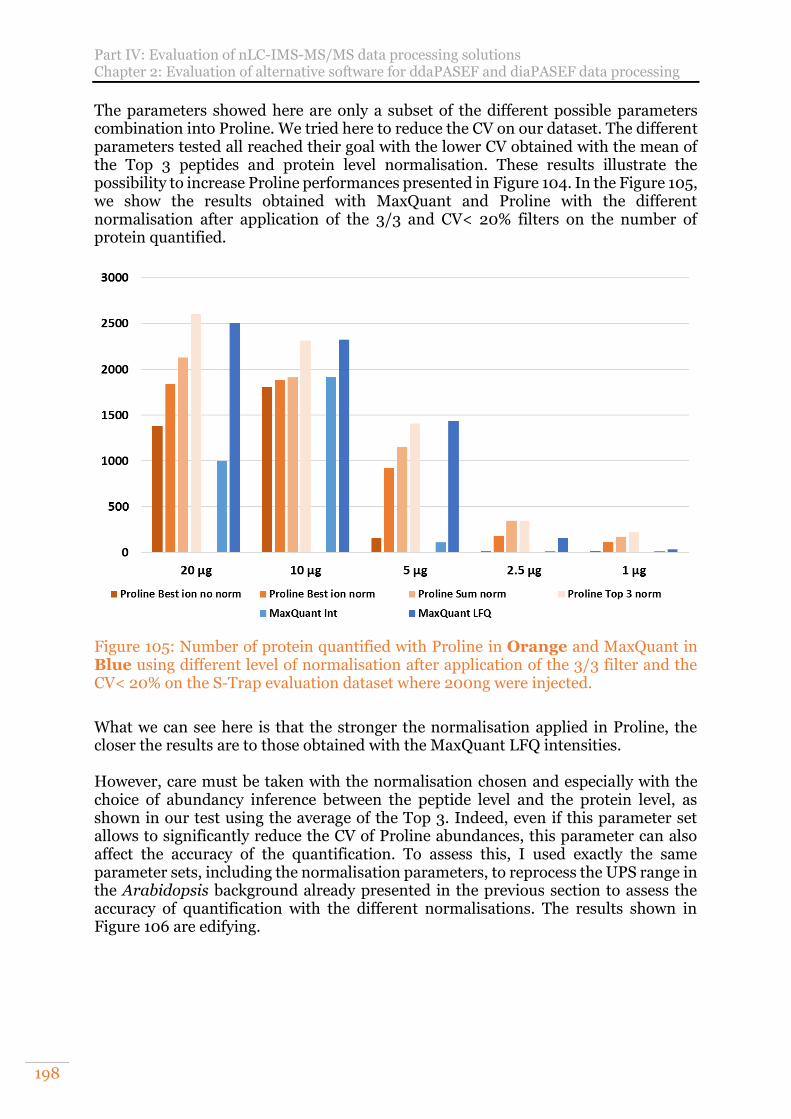
Part IV: Evaluation of nLC-IMS-MS/MS data processing solutions Chapter 2: Evaluation of alternative software for ddaPASEF and diaPASEF data processing
198
The parameters showed here are only a subset of the different possible parameters combination into Proline. We tried here to reduce the CV on our dataset. The different parameters tested all reached their goal with the lower CV obtained with the mean of the Top 3 peptides and protein level normalisation. These results illustrate the possibility to increase Proline performances presented in Figure 104. In the Figure 105, we show the results obtained with MaxQuant and Proline with the different normalisation after application of the 3/3 and CV< 20% filters on the number of protein quantified.
Figure 105: Number of protein quantified with Proline in Orange and MaxQuant in Blue using different level of normalisation after application of the 3/3 filter and the CV< 20% on the S-Trap evaluation dataset where 200ng were injected.
What we can see here is that the stronger the normalisation applied in Proline, the closer the results are to those obtained with the MaxQuant LFQ intensities. However, care must be taken with the normalisation chosen and especially with the choice of abundancy inference between the peptide level and the protein level, as shown in our test using the average of the Top 3. Indeed, even if this parameter set allows to significantly reduce the CV of Proline abundances, this parameter can also affect the accuracy of the quantification. To assess this, I used exactly the same parameter sets, including the normalisation parameters, to reprocess the UPS range in the Arabidopsis background already presented in the previous section to assess the accuracy of quantification with the different normalisations. The results shown in Figure 106 are edifying.
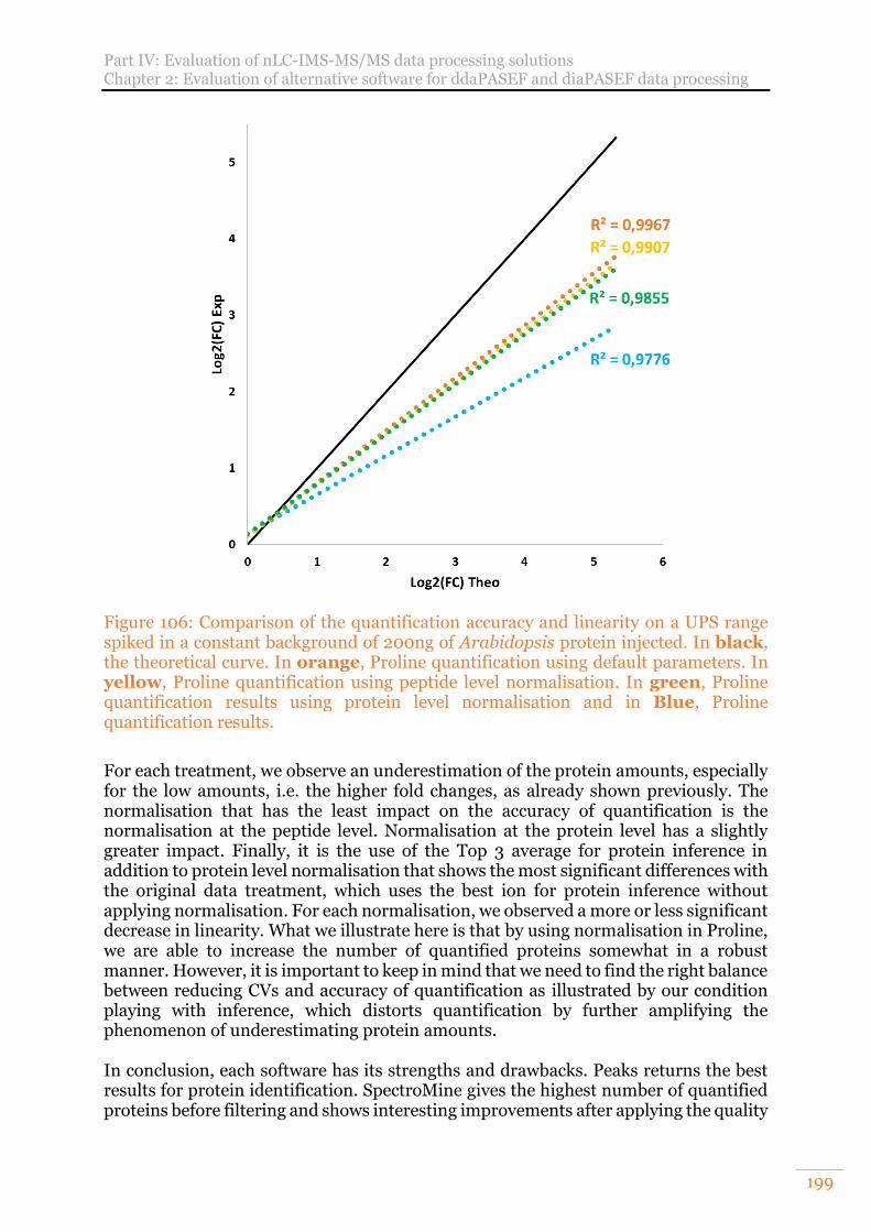
Part IV: Evaluation of nLC-IMS-MS/MS data processing solutions Chapter 2: Evaluation of alternative software for ddaPASEF and diaPASEF data processing
199
Figure 106: Comparison of the quantification accuracy and linearity on a UPS range spiked in a constant background of 200ng of Arabidopsis protein injected. In black, the theoretical curve. In orange, Proline quantification using default parameters. In yellow, Proline quantification using peptide level normalisation. In green, Proline quantification results using protein level normalisation and in Blue, Proline quantification results.
For each treatment, we observe an underestimation of the protein amounts, especially for the low amounts, i.e. the higher fold changes, as already shown previously. The normalisation that has the least impact on the accuracy of quantification is the normalisation at the peptide level. Normalisation at the protein level has a slightly greater impact. Finally, it is the use of the Top 3 average for protein inference in addition to protein level normalisation that shows the most significant differences with the original data treatment, which uses the best ion for protein inference without applying normalisation. For each normalisation, we observed a more or less significant decrease in linearity. What we illustrate here is that by using normalisation in Proline, we are able to increase the number of quantified proteins somewhat in a robust manner. However, it is important to keep in mind that we need to find the right balance between reducing CVs and accuracy of quantification as illustrated by our condition playing with inference, which distorts quantification by further amplifying the phenomenon of underestimating protein amounts. In conclusion, each software has its strengths and drawbacks. Peaks returns the best results for protein identification. SpectroMine gives the highest number of quantified proteins before filtering and shows interesting improvements after applying the quality
Part IV: Evaluation of nLC-IMS-MS/MS data processing solutions Chapter 2: Evaluation of alternative software for ddaPASEF and diaPASEF data processing
200
filters compared to our previous tests on its version 2.0. Finally, MaxQuant using MBR and LFQ gives the highest number of quantified proteins after applying the quality filters. Proline here shows similar trends to MaxQuant allowing the quantification of slightly fewer proteins for each filter level. Some of these results will be used in a publication to be submitted to the Journal of Proteomics. We also used this dataset to make a first assessment of the impact of different levels of normalisation in Proline and the role of protein inference in reducing CVs of abundances and accuracy of quantification. However, at the time of our initial test, all these software packages were only compatible with DDA data and MS1-XIC quantification has its own limitations. It is a stochastic approach to fragmenting only a subset of the ions entering the mass spectrometer. For this reason, new acquisition methods have been developed such as DIA and, for the TimsTOF Pro, diaPASEF. However, the processing of DIA data is completely different from that of DDA data due to their completely different approaches. For this reason, we evaluated the Spectronaut software, which, like SpectroMine, is developed by Biognosys but for processing DIA data. In the last few months of this thesis, version 2.0 of MaxQuant was released. The MaxDIA function has been added to process data from DIA acquisition, including BoxCar and diaPASEF.
B. diaPASEF data processing
1) Spectronaut (Biognosys) Spectronaut was the first software able to treat diaPASEF data. As SpectroMine, it is using the Pulsar search engine. It offers two kinds of approaches to treat DIA data. A peptide-centric approach using spectral libraries generated from DDA analyses to query for the presence of peptides in the data and a spectrum-centric approach called DirectDIA that generates pseudo-MS2 spectra from DIA MS2 spectra. Those pseudo-MS2 spectra can then be submitted for a database search using classical search engines such as Pulsar. Among the big advantages of the spectrum-centric approach is the gain of time brought by the fact that it is not needed to generate a specific spectral library. The data treatment is also not limited anymore by the spectral library size and content. However, the signal extraction from MS2-DIA spectra remains tedious due to the spectra multiplexing and the loss of the link between precursors and fragments. Nevertheless, the TimsTOF Pro has there a card to play, thanks to its speed and as it generates cleaner spectra thanks to the dilution of the noise occurring during the ion mobility separation. Those cleaner spectra could help in reducing the number of false positive spectra possibly coming from that noise. Moreover, Spectronaut is evolving quickly, and many improvements have been made since the last evaluation we have done in the lab and especially the work done by Nicolas Pythoud during his PhD. To evaluate Spectronaut on diaPASEF data, we used a range of UPS1 proteins spiked in a constant background of 200ng of Arabidopsis thaliana proteins with the addition of iRT peptides (Biognosys). We generated a spectral library from an in-gel fractionated sample of Arabidopsis thaliana with the addition of iRT peptides and DDA analysis of the highest point of the range to get the UPS1 proteins in the spectral library. The spectral library was also generated thanks to Spectronaut. We made
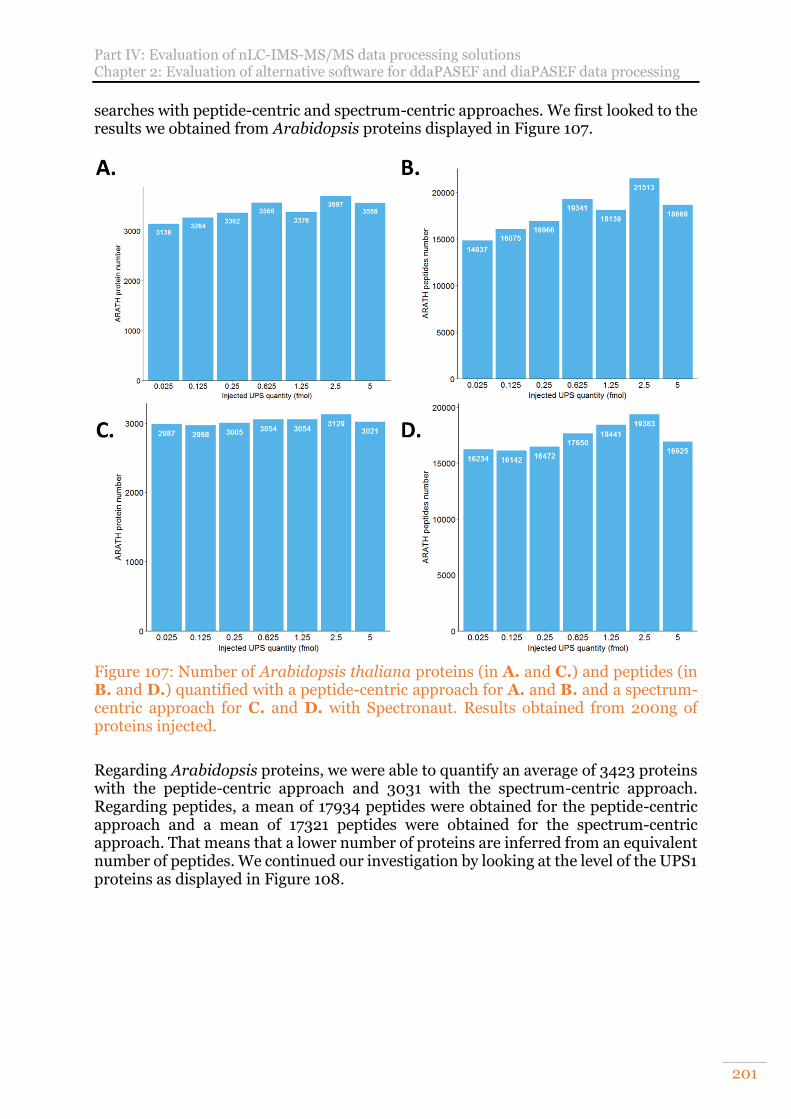
Part IV: Evaluation of nLC-IMS-MS/MS data processing solutions Chapter 2: Evaluation of alternative software for ddaPASEF and diaPASEF data processing
201
searches with peptide-centric and spectrum-centric approaches. We first looked to the results we obtained from Arabidopsis proteins displayed in Figure 107.
Figure 107: Number of Arabidopsis thaliana proteins (in A. and C.) and peptides (in B. and D.) quantified with a peptide-centric approach for A. and B. and a spectrum-centric approach for C. and D. with Spectronaut. Results obtained from 200ng of proteins injected.
Regarding Arabidopsis proteins, we were able to quantify an average of 3423 proteins with the peptide-centric approach and 3031 with the spectrum-centric approach. Regarding peptides, a mean of 17934 peptides were obtained for the peptide-centric approach and a mean of 17321 peptides were obtained for the spectrum-centric approach. That means that a lower number of proteins are inferred from an equivalent number of peptides. We continued our investigation by looking at the level of the UPS1 proteins as displayed in Figure 108.
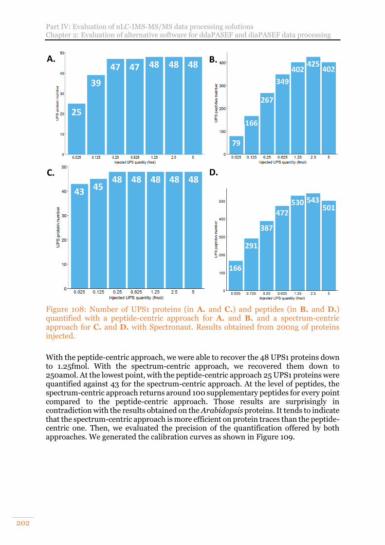
Part IV: Evaluation of nLC-IMS-MS/MS data processing solutions Chapter 2: Evaluation of alternative software for ddaPASEF and diaPASEF data processing
202
Figure 108: Number of UPS1 proteins (in A. and C.) and peptides (in B. and D.) quantified with a peptide-centric approach for A. and B. and a spectrum-centric approach for C. and D. with Spectronaut. Results obtained from 200ng of proteins injected.
With the peptide-centric approach, we were able to recover the 48 UPS1 proteins down to 1.25fmol. With the spectrum-centric approach, we recovered them down to 250amol. At the lowest point, with the peptide-centric approach 25 UPS1 proteins were quantified against 43 for the spectrum-centric approach. At the level of peptides, the spectrum-centric approach returns around 100 supplementary peptides for every point compared to the peptide-centric approach. Those results are surprisingly in contradiction with the results obtained on the Arabidopsis proteins. It tends to indicate that the spectrum-centric approach is more efficient on protein traces than the peptide-centric one. Then, we evaluated the precision of the quantification offered by both approaches. We generated the calibration curves as shown in Figure 109.
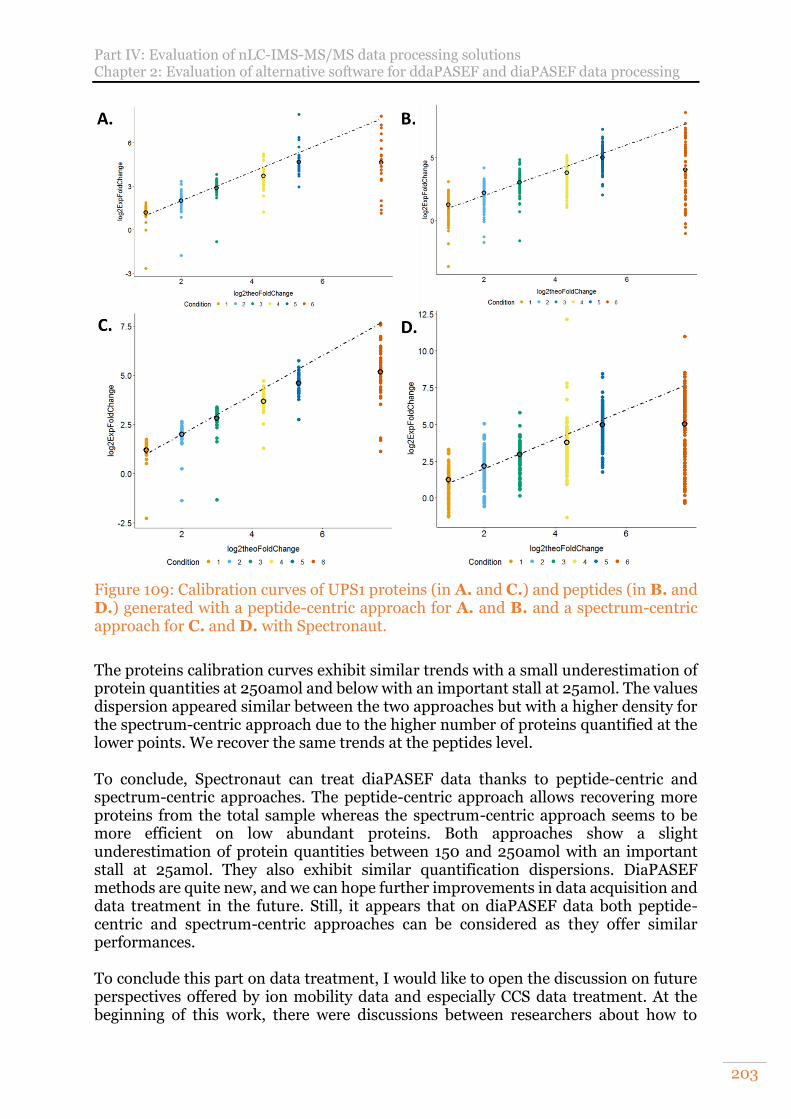
Part IV: Evaluation of nLC-IMS-MS/MS data processing solutions Chapter 2: Evaluation of alternative software for ddaPASEF and diaPASEF data processing
203
Figure 109: Calibration curves of UPS1 proteins (in A. and C.) and peptides (in B. and D.) generated with a peptide-centric approach for A. and B. and a spectrum-centric approach for C. and D. with Spectronaut.
The proteins calibration curves exhibit similar trends with a small underestimation of protein quantities at 250amol and below with an important stall at 25amol. The values dispersion appeared similar between the two approaches but with a higher density for the spectrum-centric approach due to the higher number of proteins quantified at the lower points. We recover the same trends at the peptides level. To conclude, Spectronaut can treat diaPASEF data thanks to peptide-centric and spectrum-centric approaches. The peptide-centric approach allows recovering more proteins from the total sample whereas the spectrum-centric approach seems to be more efficient on low abundant proteins. Both approaches show a slight underestimation of protein quantities between 150 and 250amol with an important stall at 25amol. They also exhibit similar quantification dispersions. DiaPASEF methods are quite new, and we can hope further improvements in data acquisition and data treatment in the future. Still, it appears that on diaPASEF data both peptide-centric and spectrum-centric approaches can be considered as they offer similar performances. To conclude this part on data treatment, I would like to open the discussion on future perspectives offered by ion mobility data and especially CCS data treatment. At the beginning of this work, there were discussions between researchers about how to
Part IV: Evaluation of nLC-IMS-MS/MS data processing solutions Chapter 2: Evaluation of alternative software for ddaPASEF and diaPASEF data processing
204
exploit better the ion mobility dimension and especially the CCS values. At that time, first ways were evocated for lipidomics383 thanks to the generation of CCS libraries and the development of machine learning on those data. Today, those developments are emerging in proteomics allowing the development extensive peptide's CCS databases which could be used to develop machine learning algorithms to predict peptide properties based on their sequences384. This could help for example for diaPASEF MS2 spectra interpretation thanks to spectrum-centric approaches. It could also be useful for databases which do not contain CCS information but from which the CCS values could be predicted to be used for targeted studies on mass spectrometers including an ion mobility dimension. In the long term, these algorithms could make it possible to improve the scores used for searches using databases, for example for biological questions needing large research space like for metaproteomics projects.
2) MaxDIA The initial publication regarding MaxDIA18 was released in July 2021 during the writing of this manuscript. Due to time constraints, only a preliminary evaluation of MaxDIA could be performed on the data of the first UPS-Arabidopsis range injected in diaPASEF with OtofControl and the published diaPASEF method. This same dataset was used for the evaluation of Spectronaut using the spectrum-centric and peptide-centric approach in the previous section. Like Spectronaut, MaxDIA offers a peptide-centric approach and a spectrum-centric approach called "discovery mode". This mode uses libraries generated in silico. A certain number of these libraries have been made available to a dozen reference organisms. Unfortunately, Arabidopsis thaliana is not yet part of this list. Therefore, we limited ourselves to testing the spectral library generation and MaxDIA analysis by peptide-centric approach. We first generated the spectral library through a "classical" analysis of ddaPASEF data in MaxQuant using the same data as used for the generation of the spectral library in Spectronaut. We used two injections of the highest point of the UPS range and the injection of an Arabidopsis thaliana sample split into 25 bands after gel migration. We performed the analysis of the diaPASEF data using the default MaxQuant parameters, except for the following parameters: LFQ intensities were generated, only one maximum missed cleavage was accepted. Only unique peptides were used for protein quantification. Peptides with modifications were not considered for quantification either, except for cysteine carbamidomethylation. The minimum number of unique peptides was set to one and the MBR was not used in this first test. Again, in order to make a first quick evaluation of MaxDIA, we applied our 3/3 and CV filters of intensities < 20% usually used on DDA data.
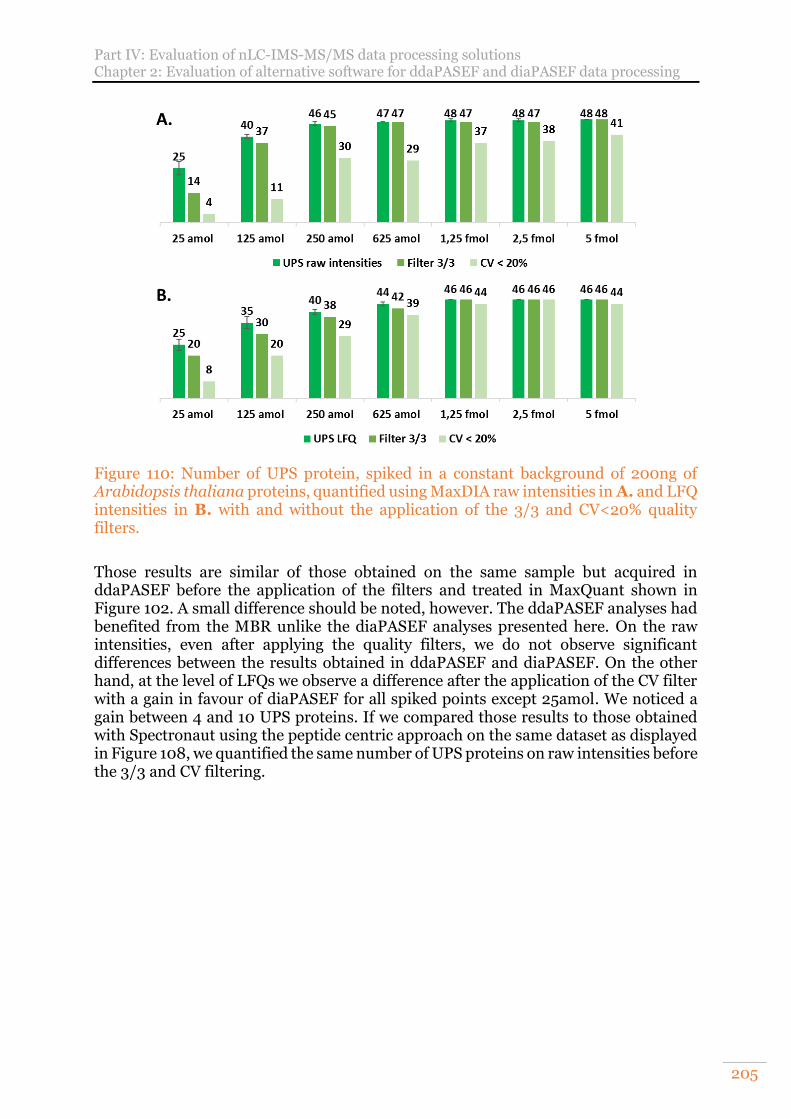
Part IV: Evaluation of nLC-IMS-MS/MS data processing solutions Chapter 2: Evaluation of alternative software for ddaPASEF and diaPASEF data processing
205
Figure 110: Number of UPS protein, spiked in a constant background of 200ng of Arabidopsis thaliana proteins, quantified using MaxDIA raw intensities in A. and LFQ intensities in B. with and without the application of the 3/3 and CV<20% quality filters.
Those results are similar of those obtained on the same sample but acquired in ddaPASEF before the application of the filters and treated in MaxQuant shown in Figure 102. A small difference should be noted, however. The ddaPASEF analyses had benefited from the MBR unlike the diaPASEF analyses presented here. On the raw intensities, even after applying the quality filters, we do not observe significant differences between the results obtained in ddaPASEF and diaPASEF. On the other hand, at the level of LFQs we observe a difference after the application of the CV filter with a gain in favour of diaPASEF for all spiked points except 25amol. We noticed a gain between 4 and 10 UPS proteins. If we compared those results to those obtained with Spectronaut using the peptide centric approach on the same dataset as displayed in Figure 108, we quantified the same number of UPS proteins on raw intensities before the 3/3 and CV filtering.
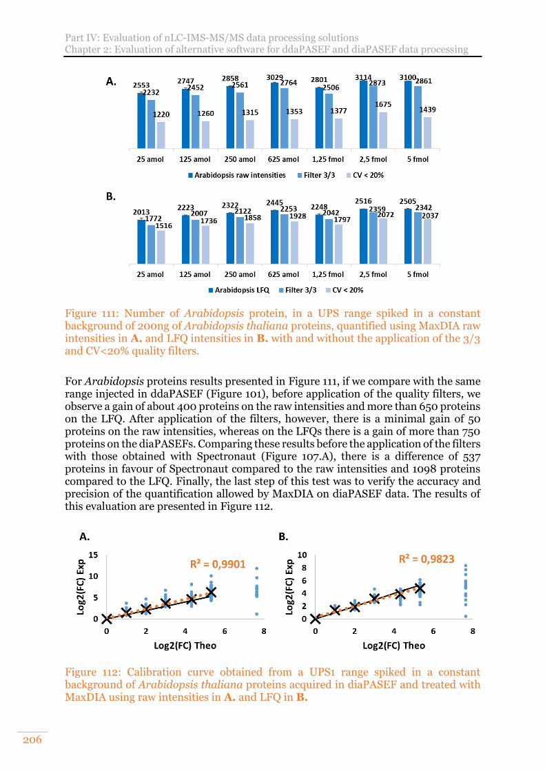
Part IV: Evaluation of nLC-IMS-MS/MS data processing solutions Chapter 2: Evaluation of alternative software for ddaPASEF and diaPASEF data processing
206
Figure 111: Number of Arabidopsis protein, in a UPS range spiked in a constant background of 200ng of Arabidopsis thaliana proteins, quantified using MaxDIA raw intensities in A. and LFQ intensities in B. with and without the application of the 3/3 and CV<20% quality filters.
For Arabidopsis proteins results presented in Figure 111, if we compare with the same range injected in ddaPASEF (Figure 101), before application of the quality filters, we observe a gain of about 400 proteins on the raw intensities and more than 650 proteins on the LFQ. After application of the filters, however, there is a minimal gain of 50 proteins on the raw intensities, whereas on the LFQs there is a gain of more than 750 proteins on the diaPASEFs. Comparing these results before the application of the filters with those obtained with Spectronaut (Figure 107.A), there is a difference of 537 proteins in favour of Spectronaut compared to the raw intensities and 1098 proteins compared to the LFQ. Finally, the last step of this test was to verify the accuracy and precision of the quantification allowed by MaxDIA on diaPASEF data. The results of this evaluation are presented in Figure 112.
Figure 112: Calibration curve obtained from a UPS1 range spiked in a constant background of Arabidopsis thaliana proteins acquired in diaPASEF and treated with MaxDIA using raw intensities in A. and LFQ in B.
Part IV: Evaluation of nLC-IMS-MS/MS data processing solutions Chapter 2: Evaluation of alternative software for ddaPASEF and diaPASEF data processing
207
Firstly, as in DDA, the linearity of the quantification is lost for the lowest point of the range at 25amol. That said the loss of linearity that is not shown here is much less violent than on DDA data, especially on raw intensity. Again, counter-intuitively, we note a slightly better linearity on the raw intensities compared to the LFQ. We also note that the accuracy of the quantification is good on both raw intensities and LFQs. We note a slight overestimation of the protein quantities at the level of the least intense points, i.e. with the highest fold change on the raw intensities. At this stage, we can confirm the gain brought by the diaPASEF acquisition in comparison with the ddaPASEF acquisition after processing all the data in the MaxQuant ecosystem. This confirms the results we already obtained with diaPASEF using Spectronaut, which in our tests allowed us to quantify more proteins than MaxDIA on the same dataset. However, it is important to note that the MaxDIA results presented here were a first attempt; the parameters were not optimised and did not use the MBR. A more in-depth comparison should now be carried out between MaxDIA and Spectronaut using parameters that are as equivalent as possible and using the same spectral library for both analyses. Indeed, it is important to differentiate the potential gain bring by the latter since for each of the analyses presented in this manuscript, it is the spectral library generated from the data treatment software that was used. Furthermore, it would also be interesting to take advantage of this comparison between Spectronaut and MaxDIA to add also DIA-NN, which, like MaxDIA, is free but is also open-source.
Part V: Application of methodological developments to answer biological questions Chapter 1: Study of protein-protein interactions by mass spectrometric analysis of immunoprecipitated complexes
208
Part V: Application of methodological developments to answer biological questions One of the objectives of this thesis was to develop the methodology of each step of the quantitative label-free analysis of proteins using bottom-up proteomic approaches. The medium-term objective is to use these developments in the framework of collaborative projects to provide increasingly precise and reliable answers to biological questions. During this thesis, I had the chance to participate in some of these projects. Two of them were based on the analysis of isolated protein complexes by co-immunoprecipitation (co-IP) to identify or confirm the identity of interacting proteins. The last one aimed at evaluating the impact of nanoparticles (NPs) of medical interest on certain human cell lines based on proteomic and transcriptomic studies.
Chapter 1: Study of protein-protein interactions by mass spectrometric analysis of immunoprecipitated complexes
This first chapter will focus on two projects for which co-IP analyses were carried out. These two projects were very different in their problematics and implementation. Phenotype expression relies among other things on proteins, their nature, their number, their location, their modifications, their interactions, and their regulations. The complexity of protein network at the origin of metabolism is the consequence of the combination of different complexity strata originating from DNA level, RNA level and protein level. It is today well known that one coding gene is not equal to one mRNA that is not equal to one protein385. Moreover, a protein alone has limited interest in biology. It is their interactions leading to functions, which allow us to understand the mechanisms behind phenotypes. This is why the study of protein complexes, or the study of protein-protein interactions is particularly important. There are several ways to study protein-protein interactions between endogenous proteins. Some techniques rely on fluorescence, such as fluorescence resonance energy transfer (FRET) or bimolecular fluorescence complementation (BiFC). These techniques allow the identification of interactions between a small number of interactants in a single experiment, making them low-throughput techniques. On the high-throughput side, yeast two-hybrid screens (Y2H) can now be applied to different cell types, not just yeast. It allows the identification of the interaction between two proteins through genetic engineering. These assays can be multiplexed to achieve high throughput385–388. Other common high-throughput techniques are based on mass spectrometry analyses. MS-based workflows for interactome profiling can be categorised into targeted (AP-MS, proximity tagging) and untargeted (XL-MS, CoFrac-MS, TPP, full proteome co-variation MS) acquisition strategies.387 Co-IP belongs to affinity purification. This type of analysis uses an antibody to capture a target protein (or bait protein) and all the proteins that have a direct or indirect
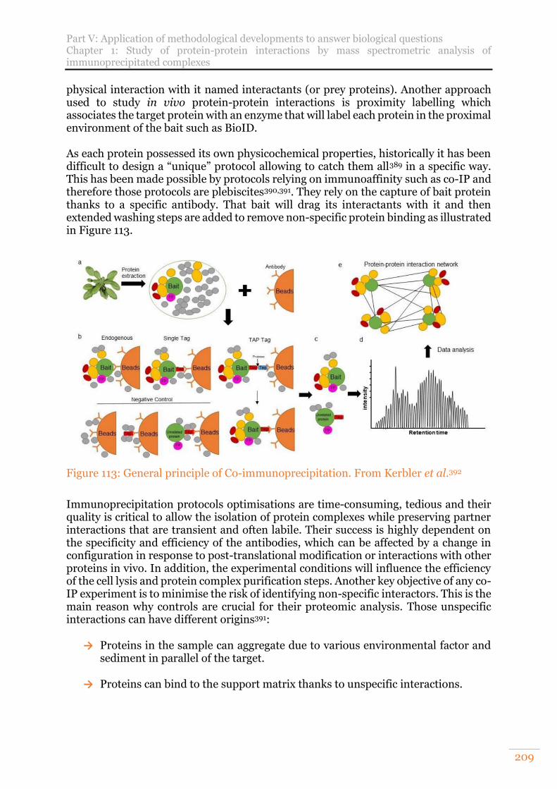
Part V: Application of methodological developments to answer biological questions Chapter 1: Study of protein-protein interactions by mass spectrometric analysis of immunoprecipitated complexes
209
physical interaction with it named interactants (or prey proteins). Another approach used to study in vivo protein-protein interactions is proximity labelling which associates the target protein with an enzyme that will label each protein in the proximal environment of the bait such as BioID. As each protein possessed its own physicochemical properties, historically it has been difficult to design a “unique” protocol allowing to catch them all389 in a specific way. This has been made possible by protocols relying on immunoaffinity such as co-IP and therefore those protocols are plebiscites390,391. They rely on the capture of bait protein thanks to a specific antibody. That bait will drag its interactants with it and then extended washing steps are added to remove non-specific protein binding as illustrated in Figure 113.
Figure 113: General principle of Co-immunoprecipitation. From Kerbler et al.392
Immunoprecipitation protocols optimisations are time-consuming, tedious and their quality is critical to allow the isolation of protein complexes while preserving partner interactions that are transient and often labile. Their success is highly dependent on the specificity and efficiency of the antibodies, which can be affected by a change in configuration in response to post-translational modification or interactions with other proteins in vivo. In addition, the experimental conditions will influence the efficiency of the cell lysis and protein complex purification steps. Another key objective of any co-IP experiment is to minimise the risk of identifying non-specific interactors. This is the main reason why controls are crucial for their proteomic analysis. Those unspecific interactions can have different origins391:
→ Proteins in the sample can aggregate due to various environmental factor and sediment in parallel of the target.
→ Proteins can bind to the support matrix thanks to unspecific interactions.
Part V: Application of methodological developments to answer biological questions Chapter 1: Study of protein-protein interactions by mass spectrometric analysis of immunoprecipitated complexes
210
→ Because of the lysis step, proteins located in different cellular compartment can be released during the cell lysis and can have the capacity to interact.
→ Insufficiently stringent washing conditions can lead to the remaining presence
of abundant proteins.
→ Remaining crude antibody in case of indirect IP.
→ Classical human protein contaminants originated from the manipulator such as keratins contained in skin or hair, or proteins added during the sample preparation such as trypsin211.
When the experience is successful, it will generate a list of candidate proteins, which will need to be validated by the biologist thanks to various biochemical or molecular biology technics.
A. Mass spectrometry analysis of an immunoprecipitated protein complex involved in cholesterol accumulation in late endosomes/liposomes
This project was carried out in collaboration with Dr Philippe Boucher and his students Dr Magalie Lambert and Sara Awan a PhD student, (University of Strasbourg, UMR-S INSERM 1109). The analytical goal was to identify and quantify the interactome of two proteins known to play a role in cholesterol metabolism in mammals and involved in the development of atherosclerosis. According to the WHO, in 2019, the two leading causes of death worldwide were ischemic heart disease and stroke, both of which can result from atherosclerosis. Ischemic heart disease alone accounts for 16% of deaths worldwide while stroke accounts for 11%. Furthermore, ischemic heart disease is the fastest growing cause of death in the last 20 years, with 2 million deaths in the 2000s compared to 8.9 million deaths in 2019. Atherosclerosis is therefore an important public health issue and a better understanding of the mechanisms involved could help to prevent it or develop ways to combat it.
1) Biological context: cholesterol and atherosclerosis Atherosclerosis is an extremely complex disease and part of its mechanisms are still unknown. In the next part, a succinct description will be presented. However, it should be kept in mind that the following part is only a small glimpse of how the disease works to provide a good understanding of the project. This description is simplistic in the face of the complexity and multiple causes associated with this disease. The link between total cholesterol levels and the incidence of cardiovascular disease is known since the 1950’s. The discovery of low-density lipoprotein (LDL) dates from 1955 and the elucidation of LDL receptor role in 1974393 by Michael S. Brown and Joseph L. Goldstein won them the medicine Nobel Prize of 1985.
Part V: Application of methodological developments to answer biological questions Chapter 1: Study of protein-protein interactions by mass spectrometric analysis of immunoprecipitated complexes
211
Atherosclerosis is an inflammatory disease of the arteriosclerosis family, which is characterised by narrowing, hardening and loss of elasticity of the arteries. Some genetic and environmental risk factors are known, such as high blood levels of “bad cholesterol” or LDL, hypertension, diabetes, obesity, age, sex, or smoking. This disease is caused by the formation of atheromatous plaque or atheroma in medium to large arteries394. Atheroma can form when the inner cell layer of an artery, the endothelium, is damaged. LDL particles can then seep in and accumulate between it and the second layer of the artery. Lipoproteins are vesicles formed by a monolayer of phospholipids containing cholesterol and apolipoproteins. Inside these vesicles are hydrophobic molecules such as triglycerides, esterified cholesterol, and hydrophobic vitamins. The function of LDL is to deliver cholesterol to the cells, while the function of the high-density lipoprotein (HDL) or the “good cholesterol” is to deliver this cholesterol to the liver for elimination. A quantity of HDL in the blood, that is higher than the quantity of LDL, therefore has a protective effect against atherosclerosis by preventing the accumulation of cholesterol in arteries395. When the LDLs accumulate under the endothelium, the body will react by sending effector cells of the innate immune system, monocytes that polarise into macrophage to clean up causing inflammation. However, when the quantity of LDL is too high, these immune cells will literally kill themselves at work, releasing cytokines, signal proteins, which will attract other monocytes. This creates a vicious circle causing a mixture of lipids and cellular debris that accumulate in the artery wall forming a cell foam typical structure. This accumulation will cause damage to the endothelium allowing the adhesion of blood platelets normally involved in blood coagulation. This attachment generates the release of growth factor favouring the development of smooth muscle cells, which will multiply between the two layers of the artery. These cells will secrete collagen and elastin fibres as well as calcium, which will crystallise. Normally, these calcium crystals are eliminated by the good cholesterol or high-density lipoprotein (HDL) but in the case of an atherosclerotic plaque, the collagen/elastin fibres and other debris prevent the HDL from accessing the calcium crystals, leading to their accumulation and therefore a stiffening of the artery. From time to time, the damaged endothelium may rupture that will cause a coagulation phenomenon and may lead to the formation of a blood clot. This combination of phenomena can cause various types of damage. These include angina pectoris, myocardial infarction, stroke, the ischaemia i.e., interruption of the blood supply in oxygen, which can lead for example to gangrene or organ failure. An atheromatous plaque can create an aneurysm, i.e., a localized dilation of the wall of an artery leading to the formation of a pocket. The rupture of an aneurysm will cause the release of clots into the bloodstream that will block smaller arteries. This is what is called an embolism and can be fatal. An aneurysm can also cause a decrease in blood affecting the kidneys. This triggers the activation of the renal-angiotensin-aldosterone system, which compensates for this decrease by increasing the blood volume, thus triggering hypertension, which is itself a risk factor for atherosclerosis.
Part V: Application of methodological developments to answer biological questions Chapter 1: Study of protein-protein interactions by mass spectrometric analysis of immunoprecipitated complexes
212
2) Project goal and analytical strategy developed As illustrated in the previous section, cholesterol plays a major role in the development of atherosclerosis. Whereas exogenous cholesterol uptake and endogenous cholesterol biosynthesis have been studied in detail, precise mechanisms of how cholesterol is transported inside the cells are poorly understood. This study focused on the alteration of cholesterol trafficking and especially its exit from lysosomes. We were particularly interested in the Wnt signalling pathway. Indeed, it has been recently reported that it is involved in atherosclerosis396. In mice, it also has been shown that the loss of function of Wnt co-receptor LRP6 causes artery disease397. In Human, mutations of that same protein affect the LDL clearance and internalization that leads to cardiovascular disease associated with hyperlipidaemia, diabetes, osteoporosis, and hypertension398. Finally, still recently, it has been shown that Wnt signalling promote resolution of atherosclerosis in mice and human although the implied mechanisms remain unknown399. In the metabolic point of view, cholesterol uptake begins when LDL-derived cholesteryl esters are endocytosed into late endosomes/lysosomes (LELs) where they are hydrolysed into free cholesterol and fatty acids. Cholesterol export from LELs is thought to require two lysosomal proteins the membrane-bound Niemann–Pick C1 (NPC1) and the soluble Niemann–Pick C2 (NPC2)400–402. NPC1 transferred it to other cellular compartments such as plasma membrane where it plays an important role in membrane fluidity or in the endoplasmic reticulum where the regulation of cholesterol synthesis occurs. It has been shown that mutations of those two proteins, NPC1 and NPC2, lead to a cholesterol accumulation in the LEL which can leads to atherosclerosis403. However, another study suggests that the cholesterol transfer from NPC2 to NPC1 is not direct and that other component are implied401. However, whether other proteins regulate NPC1/NPC2 functions is still unknown. Surprisingly, our collaborators found that Wnt5a specifically co-immunoprecipitates with NPC1 and NPC2. In this context, the role of the proteomic study was to assess whether the proteins NPC1, NPC2 and Wnt5a, which appear to be involved in the same metabolic way, interact and to identify new protein partners of these complexes, proteins that may have a role in the cholesterol accumulation or signalling pathway. To answer this question, our collaborators prepared co-IPs targeted the NPC1 and NPC2 proteins. The initial goal was to perform a differential analysis of the IPs and their respective controls. Unfortunately, we were confronted with a certain number of difficulties. Firstly, the IPs were difficult to prepare due to various problems such as the antibody selectivity, problems in cells transfection, different batches of cells among others. Then, the preparation of the IPs replicates was interrupted by the first confinement linked to the COVID. As a result, the different replicates were prepared several months apart from different cell cultures. Finally, the gels were unfortunately damaged during their transport, causing a strong degradation of two out of the five initially prepared. The five gels received were nevertheless cut as best as possible and the proteins were reduced, alkylated, and digested with trypsin before being analysed in DDA mass spectrometry on a nanoElute-TimsTOF Pro coupling.
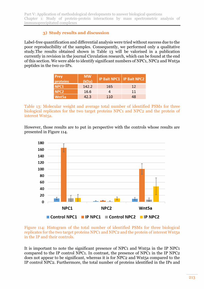
Part V: Application of methodological developments to answer biological questions Chapter 1: Study of protein-protein interactions by mass spectrometric analysis of immunoprecipitated complexes
213
3) Study results and discussion Label-free quantification and differential analysis were tried without success due to the poor reproducibility of the samples. Consequently, we performed only a qualitative study.The results obtained shown in Table 13 will be valorised in a publication currently in revision in the journal Circulation research, which can be found at the end of this section. We were able to identify significant numbers of NPC1, NPC2 and Wnt5a peptides in the two co-IPs.
Table 13: Molecular weight and average total number of identified PSMs for three biological replicates for the two target proteins NPC1 and NPC2 and the protein of interest Wnt5a.
However, those results are to put in perspective with the controls whose results are presented in Figure 114.
Figure 114: Histogram of the total number of identified PSMs for three biological replicates for the two target proteins NPC1 and NPC2 and the protein of interest Wnt5a in the IP and their controls.
It is important to note the significant presence of NPC1 and Wnt5a in the IP NPC1 compared to the IP control NPC1. In contrast, the presence of NPC1 in the IP NPC2 does not appear to be significant, whereas it is for NPC2 and Wnt5a compared to the IP control NPC2. Furthermore, the total number of proteins identified in the IPs and
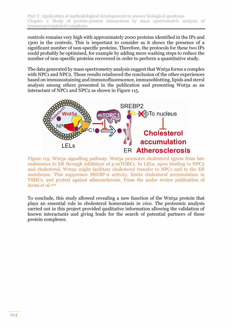
Part V: Application of methodological developments to answer biological questions Chapter 1: Study of protein-protein interactions by mass spectrometric analysis of immunoprecipitated complexes
214
controls remains very high with approximately 2000 proteins identified in the IPs and 1500 in the controls. This is important to consider as it shows the presence of a significant number of non-specific proteins. Therefore, the protocols for these two IPs could probably be optimised, for example by adding more washing steps to reduce the number of non-specific proteins recovered in order to perform a quantitative study. The data generated by mass spectrometry analysis suggest that Wnt5a forms a complex with NPC1 and NPC2. Those results reinforced the conclusion of the other experiences based on immunostaining and immunofluorescence, immunoblotting, lipids and sterol analysis among others presented in the publication and presenting Wnt5a as an interactant of NPC1 and NPC2 as shown in Figure 115.
Figure 115: Wnt5a signalling pathway. Wnt5a promotes cholesterol egress from late endosomes to ER through inhibition of p-mTORC1. In LELs, upon binding to NPC2 and cholesterol, Wnt5a might facilitate cholesterol transfer to NPC1 and to the ER membrane. This suppresses SREBP-2 activity, limits cholesterol accumulation in VSMCs, and protect against atherosclerosis. From the under review publication of Awan et al.404
To conclude, this study allowed revealing a new function of the Wnt5a protein that plays an essential role in cholesterol homeostasis in vivo. The proteomic analysis carried out in this project provided qualitative information allowing the validation of known interactants and giving leads for the search of potential partners of these protein complexes.

Part V: Application of methodological developments to answer biological questions Chapter 1: Study of protein-protein interactions by mass spectrometric analysis of immunoprecipitated complexes
215
Add the publication under review

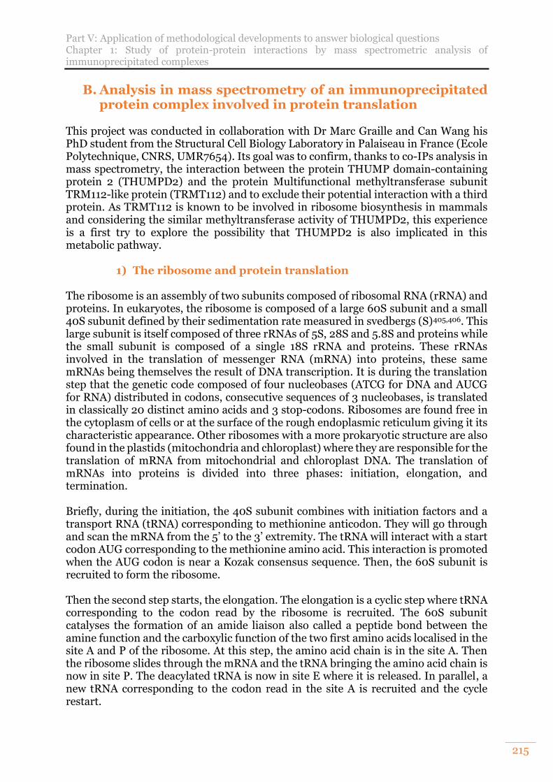
Part V: Application of methodological developments to answer biological questions Chapter 1: Study of protein-protein interactions by mass spectrometric analysis of immunoprecipitated complexes
215
B. Analysis in mass spectrometry of an immunoprecipitated protein complex involved in protein translation
This project was conducted in collaboration with Dr Marc Graille and Can Wang his PhD student from the Structural Cell Biology Laboratory in Palaiseau in France (Ecole Polytechnique, CNRS, UMR7654). Its goal was to confirm, thanks to co-IPs analysis in mass spectrometry, the interaction between the protein THUMP domain-containing protein 2 (THUMPD2) and the protein Multifunctional methyltransferase subunit TRM112-like protein (TRMT112) and to exclude their potential interaction with a third protein. As TRMT112 is known to be involved in ribosome biosynthesis in mammals and considering the similar methyltransferase activity of THUMPD2, this experience is a first try to explore the possibility that THUMPD2 is also implicated in this metabolic pathway.
1) The ribosome and protein translation The ribosome is an assembly of two subunits composed of ribosomal RNA (rRNA) and proteins. In eukaryotes, the ribosome is composed of a large 60S subunit and a small 40S subunit defined by their sedimentation rate measured in svedbergs (S)405,406. This large subunit is itself composed of three rRNAs of 5S, 28S and 5.8S and proteins while the small subunit is composed of a single 18S rRNA and proteins. These rRNAs involved in the translation of messenger RNA (mRNA) into proteins, these same mRNAs being themselves the result of DNA transcription. It is during the translation step that the genetic code composed of four nucleobases (ATCG for DNA and AUCG for RNA) distributed in codons, consecutive sequences of 3 nucleobases, is translated in classically 20 distinct amino acids and 3 stop-codons. Ribosomes are found free in the cytoplasm of cells or at the surface of the rough endoplasmic reticulum giving it its characteristic appearance. Other ribosomes with a more prokaryotic structure are also found in the plastids (mitochondria and chloroplast) where they are responsible for the translation of mRNA from mitochondrial and chloroplast DNA. The translation of mRNAs into proteins is divided into three phases: initiation, elongation, and termination. Briefly, during the initiation, the 40S subunit combines with initiation factors and a transport RNA (tRNA) corresponding to methionine anticodon. They will go through and scan the mRNA from the 5’ to the 3’ extremity. The tRNA will interact with a start codon AUG corresponding to the methionine amino acid. This interaction is promoted when the AUG codon is near a Kozak consensus sequence. Then, the 60S subunit is recruited to form the ribosome. Then the second step starts, the elongation. The elongation is a cyclic step where tRNA corresponding to the codon read by the ribosome is recruited. The 60S subunit catalyses the formation of an amide liaison also called a peptide bond between the amine function and the carboxylic function of the two first amino acids localised in the site A and P of the ribosome. At this step, the amino acid chain is in the site A. Then the ribosome slides through the mRNA and the tRNA bringing the amino acid chain is now in site P. The deacylated tRNA is now in site E where it is released. In parallel, a new tRNA corresponding to the codon read in the site A is recruited and the cycle restart.
Part V: Application of methodological developments to answer biological questions Chapter 1: Study of protein-protein interactions by mass spectrometric analysis of immunoprecipitated complexes
216
When the ribosome arrived at a stop codon, the termination step begins. Different proteins called termination factors are recruited. They are implicated in the dissociation and the recycling of the ribosome as well as in the release of the amino acid chain generated. The ribosome has a central role in all living organisms. However, all the mechanisms involved in its biogenesis, recycling, and regulation, and especially in the verification of its quality to prevent the generation of abnormal proteins, remain only partially understood, particularly in eukaryotes. What is well characterized, however, is that methylations, catalysed by methyltransferases, are one of the most commonly observed modifications of cellular components known to be involved in these mechanisms407–
409. Indeed, many rRNAs, tRNAs, ribosomal proteins and translation factors are methylated410,411. Furthermore, in yeast, several rRNA methyltransferases are known to be involved in ribosome synthesis as well as in translation fidelity411–413. In the frame of this collaboration, our team has been studying these methyltransferases for a long time and previous studies on yeast were conducted by Dr Nicolas Pythoud414. In this project, we were interested in humans and especially the methyltransferase THUMPD2. The THUMPD2 is a methyltransferase known to be involved in tRNA methylation.
2) Project goal and analytical strategy developed The objective of this study was to identify the interactors of the THUMPD2 methyltransferase in human cells. The recombinant protein could be extracted using its FLAG-TAG and magnetic beads carrying anti-FLAG antibodies. The control was generated using a plasmid encoding only FLAG-TAG alone. The samples and controls were prepared in five preparation replicates. When we received the samples, the bait proteins were still attached to the magnetic beads. We therefore decided to proceed in the similar way than for the SP3 protocol to limit the number of sample preparation steps and thus avoid losing material. The beads were washed with ammonium bicarbonate (ABC) and then directly in-solution digested with trypsin/Lys-C. We decided to discard the reduction and alkylation step usually performed to avoid degrading the antibodies and so, limit their tryptic digestion. Indeed, the signals of the antibody’s peptides, which is present in high amount, could hide low abundancy proteins. The beads and peptides were separated using a magnetic rack. Finally, the samples were analysed on a nanoAcquity-Q-Exactive HF-X coupling. The protein identification and quantification were realised in Proline studio using classical FDR of 1%. Cross-assignment was not used. As a reminder, cross-assignment is used to assign an identification, and then to be able to proceed with quantification, of an MS1 signal that was not assigned to a peptide in one analysis because the MS2 signal was absent or of poor quality. In another analysis, processed in parallel, an MS2 signal allowed the identification of this peptide and therefore the identification can be transferred to the first run without a good MS2 signal. This feature is very important as it allows us to decrease the proportion of missing values in a dataset based on experimental data. Indeed, statistical proteomic analyses are not possible when missing values are present. However, cross-assignment does not have many criteria to check the quality of the transferred identification. The signal is transferred if the m/z and RT (and 1/k0
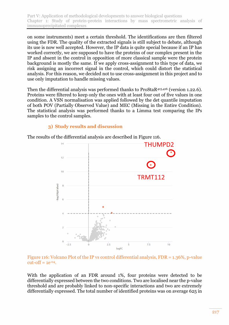
Part V: Application of methodological developments to answer biological questions Chapter 1: Study of protein-protein interactions by mass spectrometric analysis of immunoprecipitated complexes
217
on some instruments) meet a certain threshold. The identifications are then filtered using the FDR. The quality of the extracted signals is still subject to debate, although its use is now well accepted. However, the IP data is quite special because if an IP has worked correctly, we are supposed to have the proteins of our complex present in the IP and absent in the control in opposition of more classical sample were the protein background is mostly the same. If we apply cross-assignment to this type of data, we risk assigning an incorrect signal in the control, which could distort the statistical analysis. For this reason, we decided not to use cross-assignment in this project and to use only imputation to handle missing values. Then the differential analysis was performed thanks to ProStaR415,416 (version 1.22.6). Proteins were filtered to keep only the ones with at least four out of five values in one condition. A VSN normalisation was applied followed by the det quantile imputation of both POV (Partially Observed Value) and MEC (Missing in the Entire Condition). The statistical analysis was performed thanks to a Limma test comparing the IPs samples to the control samples.
3) Study results and discussion The results of the differential analysis are described in Figure 116.
Figure 116: Volcano Plot of the IP vs control differential analysis, FDR = 1.36%, p-value cut-off = 1e-04.
With the application of an FDR around 1%, four proteins were detected to be differentially expressed between the two conditions. Two are localised near the p-value threshold and are probably linked to non-specific interactions and two are extremely differentially expressed. The total number of identified proteins was on average 625 in
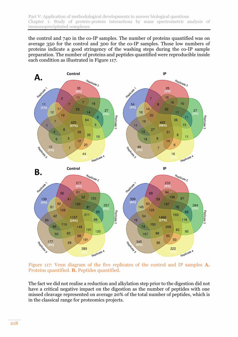
Part V: Application of methodological developments to answer biological questions Chapter 1: Study of protein-protein interactions by mass spectrometric analysis of immunoprecipitated complexes
218
the control and 740 in the co-IP samples. The number of proteins quantified was on average 350 for the control and 300 for the co-IP samples. Those low numbers of proteins indicate a good stringency of the washing steps during the co-IP sample preparation. The number of proteins and peptides quantified were reproducible inside each condition as illustrated in Figure 117.
Figure 117: Venn diagram of the five replicates of the control and IP samples A. Proteins quantified. B. Peptides quantified.
The fact we did not realise a reduction and alkylation step prior to the digestion did not have a critical negative impact on the digestion as the number of peptides with one missed cleavage represented on average 20% of the total number of peptides, which is in the classical range for proteomics projects.
Part V: Application of methodological developments to answer biological questions Chapter 1: Study of protein-protein interactions by mass spectrometric analysis of immunoprecipitated complexes
219
In the end, only two proteins came out to be extremely differentially expressed between co-IP and control samples, namely THUMPD2 our bait and TRMT112 with p-values of respectively 1.75e-13 and 1.14e-11. In view of these results, it seems to be confirmed that these two methyltransferases are true interactors. Moreover, our collaborator confirmed that those results are in line with their own results and seem to indicate strongly that there is no third protein involved in this protein complex. TRMT112 acts as an activator of rRNA, tRNA and protein methyltransferases. It is also involved in the pre-rRNA processing steps leading to small-subunit rRNA production417–421. Thanks to those results, our collaborators will be able to push forward their investigations around the methyltransferases THUMPD2 and TRMT112 in human to explore more precisely their respective roles in ribosome biogenesis.
C. General conclusion about the mass spectrometric analysis of immunoprecipitated complexes
To conclude, we have shown here two examples of proteomic studies based on co-immunoprecipitation samples. The initial goal of both studies was: identifying, quantifying, and conducting a differential analysis of the IP samples versus control samples. However, this kind of studies remains challenging especially at the level of the co-IP preparation. Even if the context was exceptional due to the COVID crisis, we were confronted in the first project to various difficulties leading to low quality results despite our efforts. Among them, we can cite problems of antibody selectivity, problems in cells transfection, the use of different batches of cells and problems of elimination of the proteins interacting in a non-specific way with the beads and antibodies. We also had problems in reproducibility due to the time between the different IP replicates preparation and the degradation of the gels during the transport. Consequently, protein quantification and differential analysis of quality was not achieved in this project. Despite everything, we were able to provide valuable insights based on the identified interactants, which reinforced our collaborators results. On the other hand, the second project illustrates what can bring label-free proteomic analysis. Here, the results were of excellent quality due to a good repeatability between biological replicates of one condition and the reduced number of proteins dragged by non-specific interactions as illustrated in the volcano plot (Figure 116). The difference in p-value and fold change is drastic for the bait and only one other protein shows a similar trend. Moreover, our collaborator obtained results that were very consistent with our own ones, which was overall very encouraging. To conclude, co-IP associated with mass spectrometry is a powerful tool. However, being able to obtain results of quality remains tedious as experimental conditions to isolate protein complexes need to be optimized for each bait. The bead digestion we used to prepare the THUMPD2 co-IP allowed us to prepare the sample more quickly by eliminating the protein concentration step in the SDS-PAGE gel. We also decided to remove the reduction and alkylation steps to avoid the presence of high amounts of antibody peptides in the sample without observing a high proportion of missed cleaved peptides, which could increase the sample dynamic range and hide low abundant proteins. Considering the success of this experience, this way to proceed could be used in the future for other projects.
Part V: Application of methodological developments to answer biological questions Chapter 2: Evaluation of the impact of medically relevant nanoparticles (NPs) on the proteome of three immune cell types
220
Chapter 2: Evaluation of the impact of medically relevant nanoparticles (NPs) on the proteome of three immune cell types
This collaboration was carried out with Dr Alexandre Detappe and his PhD student Vincent Mittelheisser (ICANS, Strasbourg, France). This last project that I will present in this manuscript was undoubtedly the most difficult one that I had to carry out during this thesis. The aim of this project was to evaluate the evolution of the proteome of human immune cells after their contact with nanoparticles (NPs) of medical interest. The first difficulty of this project was the small amounts of starting material that I could obtain to work with (≤ 2µg of proteins) because the number of cells our collaborators could extract by fluorescence activated cell sorting (FACS) from a blood bag was limited and even largely overestimated. The number of biological replicates was also a limiting factor as we got only three biological replicates per condition. Then, during the study, the high number of samples to process has added a second limiting factor.
A. Nanoparticles and their interest in medicine Nanoparticles are defined by their size, which must be between 1 and 100 nm in all three dimensions according to the ISO (International Standard Organisation) TS 80004-2:2015 standard. They are usually composed of different layers with different compositions depending on the desired properties. The nanometric size, the high surface/volume ratio of NPs, their chemical complexity and their nature can give those magnetic properties, mechanical resistance, chemical reactivity, and thermal conductivity among others, which allow numerous applications in very varied fields. We can cite the fields of textiles, cosmetics, food, medical imaging, drug vectorisation, environment, electronics, chemistry, and construction, among others. But they can also be extremely interesting for nanomedicine and especially in oncology422,423:
→ They can drive active substances such as drugs to a specific location such as a tumour in the body to develop targeted treatments.
→ They can also be used in a targeted manner for medical imaging and especially
IRM thanks to their superparamagnetic properties.
→ They can be used as therapeutics especially as a radiosensitising agent for targeted cancer treatment. For example, these nanoparticles will be composed in part of atoms with a high atomic number (Z). In combination with radiotherapy, they will allow a more extensive irradiation of the tumour to destroy it. In the 2000s, clinical studies were carried out on humans using metallic nanoparticles.
However, as for any therapeutic substance, it is necessary to evaluate its impact and notably its possible toxicity for the organism to define its benefit/risk balance. This subject is especially sensible for NPs as they are known to be potentially toxic since the end the 1990s. In France in 2006, the AFSSET (French Agency for Environmental and Occupational Health Safety) released a report about nanomaterial including nanoparticles and their effects on Human health.
Part V: Application of methodological developments to answer biological questions Chapter 2: Evaluation of the impact of medically relevant nanoparticles (NPs) on the proteome of three immune cell types
221
Nanoparticles can enter the body through the lungs, the skin, the intestinal wall and by direct injection in the case of their use in medicine. Environmental nanoparticles are known to affect the cardiac, the respiratory and the reproductive424 systems. Among the mechanisms of toxicity put forward, we can cite toxicity by direct interaction with the DNA or the cellular organelles involved in the cell cycle. NPs can also affect the redox balance leading to the formation of free radicals causing lesions to the DNA or altering its repair mechanisms. Finally, cytotoxicity can be linked to chronic inflammation because of the production of reactive oxygen species (ROS) after internalisation of the NPs in the cells. However, all NPs do not exhibit the same toxicity and some parameters are known to play a role in this such as their size, area, shape, structure that impact their reactive surface but also their numbers, solubility, composition and if they form ROS among others. In this context, we studied several immune cell types, more precisely human lymphocytes, after their exposure to different nanoparticles of medical interest to characterise and quantify whether this exposure led to a significant modification of the proteome of those cell types. These cell types are of primary interest as they are part of the immune system and are involved in the fight against cancer. The fact that the NPs could affect negatively these cells would be a problem as it weakens the natural defences of the human body to fight back. On the other hand, it is also possible that NPs affect positively the immune system, as this last would recognise them as strangers to the organism and generate a stronger immune reaction, which would also fight against the cancer. In parallel to our work, the same samples were analysed to evaluate the impact of the NPs at the level of the transcriptome by the team of Dr Raphael Carapito (UMR-S INSERM 1109, Strasbourg).
B. Project goal and analytical strategy Three phases composed this project. The first one consisted in preliminary study on one cell type with eight NPs and one control, each prepared in biological triplicates. The second was an evaluation of the SP3 sample preparation on this kind of samples to evaluate the possibility to upscale the number of samples that can be processed in a single series. The last step was the final study with the analysis of three different isolated cell types brought into contact with nine NPs plus a control without NP, in biological triplicates. This last part alone represented 90 samples.
C. Preliminary study: stacking gel approach This preliminary study was realised on Lymphocyte Natural Killer (NK) cells isolated by FACS from three donor’s blood. Our collaborators incubated those cells with eight different NPs, then washed them with PBS 1X and pelleted them before bringing them to us. The control consisted in NK cells that had not been incubated with any NP. The samples contained 650,000 cells after FACS. The cells were suspended in 2% SDS, 62.5mM Tris-HCl pH = 6.8 buffer and sonicated in a water bath. It was impossible to use a probe sonication due to the reduced volume of samples (< 100µL). Then, the amount of proteins was evaluated using the DC protein assay from BioRad (Hercules, CAL, USA).
Part V: Application of methodological developments to answer biological questions Chapter 2: Evaluation of the impact of medically relevant nanoparticles (NPs) on the proteome of three immune cell types
222
Regarding the protein assay results and the very low total protein amounts available, we had no choice but to work from 2µg of proteins as the normalized starting material for each sample. Indeed, for some conditions this was the maximum amount of proteins we had. The proteins were reduced, alkylated, and loaded on home-made stacking gels. We choose to use this protocol as we did not have sufficient experience with SP3 at that time. The gels were cut, the gel pieces washed and then proteins were in-gel digested with trypsin and peptides were extracted. The samples were analysed with a nanoAcquity (Waters) and a Q-Exactive HF-X (Thermo Fisher Scientific). The data treatment was realised using Mascot and Proline20 for both the identification and quantification parts using classical FDR of 1% filters. The quantification was done without using the cross assignment (CA). We already explained in a previous part the risk associated with this kind of algorithm regarding the false attribution of signals. In the case of this project, we first tried to use CA, but we recovered aberrant p-value distribution as illustrated in Figure 118.A and Figure 119.A. This differential analysis was realised in ProStaR415,416. After extended investigation, we noticed that this aberrant distribution was only observed on low differential conditions (all conditions except CNT, see Figure 118.D and Figure 119.D) and that it was related to the use of two parameters: the CA and the det quantile imputation of partially observed values (POV). For that reason, we did not used the CA and we used the slsa (Structured Least Square Adaptative) imputation instead of the det quantile imputation for the POV to recover a normal p-value distribution as illustrated in Figure 118 and Figure 119.
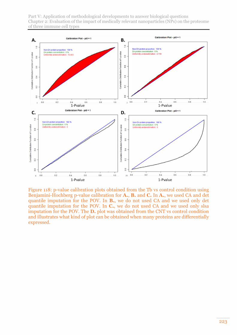
Part V: Application of methodological developments to answer biological questions Chapter 2: Evaluation of the impact of medically relevant nanoparticles (NPs) on the proteome of three immune cell types
223
Figure 118: p-value calibration plots obtained from the Tb vs control condition using Benjamini-Hochberg p-value calibration for A., B. and C. In A., we used CA and det quantile imputation for the POV. In B., we do not used CA and we used only det quantile imputation for the POV. In C., we do not used CA and we used only slsa imputation for the POV. The D. plot was obtained from the CNT vs control condition and illustrates what kind of plot can be obtained when many proteins are differentially expressed.
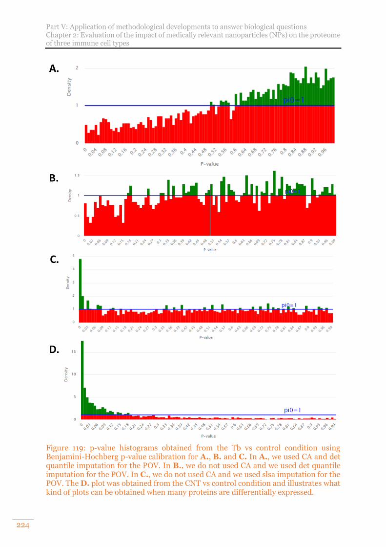
Part V: Application of methodological developments to answer biological questions Chapter 2: Evaluation of the impact of medically relevant nanoparticles (NPs) on the proteome of three immune cell types
224
Figure 119: p-value histograms obtained from the Tb vs control condition using Benjamini-Hochberg p-value calibration for A., B. and C. In A., we used CA and det quantile imputation for the POV. In B., we do not used CA and we used det quantile imputation for the POV. In C., we do not used CA and we used slsa imputation for the POV. The D. plot was obtained from the CNT vs control condition and illustrates what kind of plots can be obtained when many proteins are differentially expressed.
Part V: Application of methodological developments to answer biological questions Chapter 2: Evaluation of the impact of medically relevant nanoparticles (NPs) on the proteome of three immune cell types
225
The det quantile imputation will impute a same value to all the POV and/or MEC (Missing on an Entire Condition) in a dataset. This value is dependant of the entire sample. On the other hand, the slsa imputation is a regression-based imputation method, which accounts for a possible hierarchical design. It uses its nearest peptides to determine the value to impute to one specific POV. Consequently, each missing value will have its own value in opposition with the det quantile imputation. In a way, we can say that the det quantile approach is more deterministic whereas the slsa in more stochastic. After the optimisation of the data treatment, the same parameters were applied for the entire study. For this first experiment, we obtained the Figure 120 and Table 14. In Figure 120, the volcano Plots obtained from the statistical tests realised on one condition which appears to present only slight differences and one that is highly differential compared to the control, are presented. In general, as displayed in Figure 121, most of the conditions appear to be only slightly differential at the exception of the CNT condition for an FDR around 1%.
Figure 120: Examples of volcano Plots obtained with in A. not very differential conditions (Cont vs Dend) and in opposition in B. very differential conditions (Cont vs CNT).
Table 14: Numbers of differential proteins for the different conditions in comparison with the control for an FDR around 1%. Results obtained from 330ng of proteins injected.
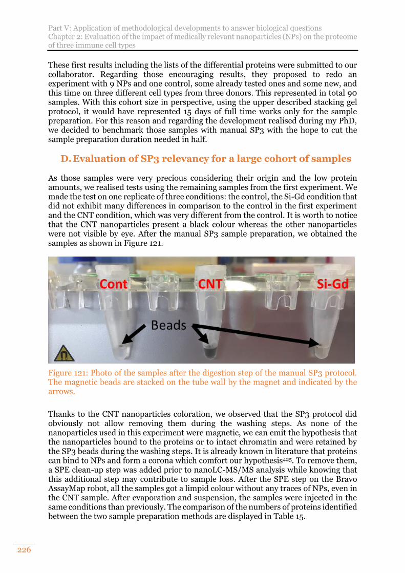
Part V: Application of methodological developments to answer biological questions Chapter 2: Evaluation of the impact of medically relevant nanoparticles (NPs) on the proteome of three immune cell types
226
These first results including the lists of the differential proteins were submitted to our collaborator. Regarding those encouraging results, they proposed to redo an experiment with 9 NPs and one control, some already tested ones and some new, and this time on three different cell types from three donors. This represented in total 90 samples. With this cohort size in perspective, using the upper described stacking gel protocol, it would have represented 15 days of full time works only for the sample preparation. For this reason and regarding the development realised during my PhD, we decided to benchmark those samples with manual SP3 with the hope to cut the sample preparation duration needed in half.
D. Evaluation of SP3 relevancy for a large cohort of samples As those samples were very precious considering their origin and the low protein amounts, we realised tests using the remaining samples from the first experiment. We made the test on one replicate of three conditions: the control, the Si-Gd condition that did not exhibit many differences in comparison to the control in the first experiment and the CNT condition, which was very different from the control. It is worth to notice that the CNT nanoparticles present a black colour whereas the other nanoparticles were not visible by eye. After the manual SP3 sample preparation, we obtained the samples as shown in Figure 121.
Figure 121: Photo of the samples after the digestion step of the manual SP3 protocol. The magnetic beads are stacked on the tube wall by the magnet and indicated by the arrows.
Thanks to the CNT nanoparticles coloration, we observed that the SP3 protocol did obviously not allow removing them during the washing steps. As none of the nanoparticles used in this experiment were magnetic, we can emit the hypothesis that the nanoparticles bound to the proteins or to intact chromatin and were retained by the SP3 beads during the washing steps. It is already known in literature that proteins can bind to NPs and form a corona which comfort our hypothesis425. To remove them, a SPE clean-up step was added prior to nanoLC-MS/MS analysis while knowing that this additional step may contribute to sample loss. After the SPE step on the Bravo AssayMap robot, all the samples got a limpid colour without any traces of NPs, even in the CNT sample. After evaporation and suspension, the samples were injected in the same conditions than previously. The comparison of the numbers of proteins identified between the two sample preparation methods are displayed in Table 15.
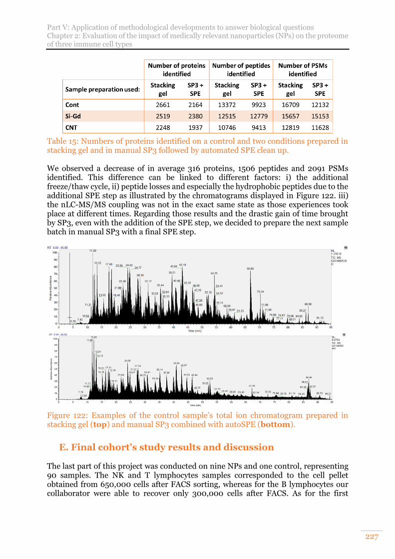
Part V: Application of methodological developments to answer biological questions Chapter 2: Evaluation of the impact of medically relevant nanoparticles (NPs) on the proteome of three immune cell types
227
Table 15: Numbers of proteins identified on a control and two conditions prepared in stacking gel and in manual SP3 followed by automated SPE clean up. We observed a decrease of in average 316 proteins, 1506 peptides and 2091 PSMs identified. This difference can be linked to different factors: i) the additional freeze/thaw cycle, ii) peptide losses and especially the hydrophobic peptides due to the additional SPE step as illustrated by the chromatograms displayed in Figure 122. iii) the nLC-MS/MS coupling was not in the exact same state as those experiences took place at different times. Regarding those results and the drastic gain of time brought by SP3, even with the addition of the SPE step, we decided to prepare the next sample batch in manual SP3 with a final SPE step.
Figure 122: Examples of the control sample’s total ion chromatogram prepared in stacking gel (top) and manual SP3 combined with autoSPE (bottom).
E. Final cohort’s study results and discussion The last part of this project was conducted on nine NPs and one control, representing 90 samples. The NK and T lymphocytes samples corresponded to the cell pellet obtained from 650,000 cells after FACS sorting, whereas for the B lymphocytes our collaborator were able to recover only 300,000 cells after FACS. As for the first
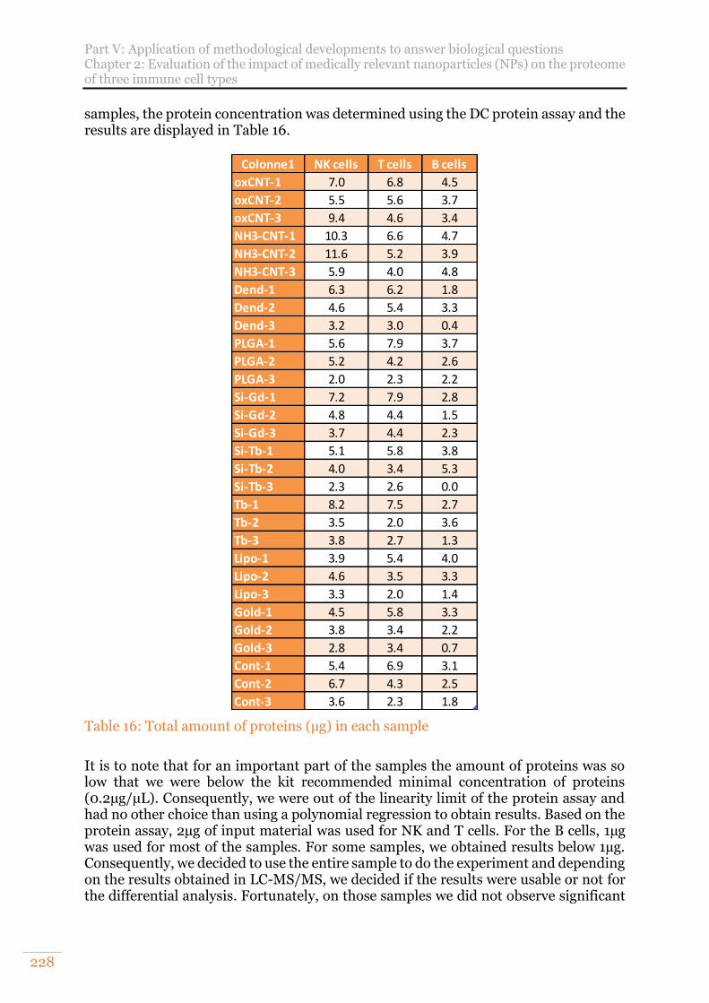
Part V: Application of methodological developments to answer biological questions Chapter 2: Evaluation of the impact of medically relevant nanoparticles (NPs) on the proteome of three immune cell types
228
samples, the protein concentration was determined using the DC protein assay and the results are displayed in Table 16.
Table 16: Total amount of proteins (µg) in each sample
It is to note that for an important part of the samples the amount of proteins was so low that we were below the kit recommended minimal concentration of proteins (0.2µg/µL). Consequently, we were out of the linearity limit of the protein assay and had no other choice than using a polynomial regression to obtain results. Based on the protein assay, 2µg of input material was used for NK and T cells. For the B cells, 1µg was used for most of the samples. For some samples, we obtained results below 1µg. Consequently, we decided to use the entire sample to do the experiment and depending on the results obtained in LC-MS/MS, we decided if the results were usable or not for the differential analysis. Fortunately, on those samples we did not observe significant
Colonne1 NK cells T cells B cells
oxCNT-1 7.0 6.8 4.5
oxCNT-2 5.5 5.6 3.7
oxCNT-3 9.4 4.6 3.4
NH3-CNT-1 10.3 6.6 4.7
NH3-CNT-2 11.6 5.2 3.9
NH3-CNT-3 5.9 4.0 4.8
Dend-1 6.3 6.2 1.8
Dend-2 4.6 5.4 3.3
Dend-3 3.2 3.0 0.4
PLGA-1 5.6 7.9 3.7
PLGA-2 5.2 4.2 2.6
PLGA-3 2.0 2.3 2.2
Si-Gd-1 7.2 7.9 2.8
Si-Gd-2 4.8 4.4 1.5
Si-Gd-3 3.7 4.4 2.3
Si-Tb-1 5.1 5.8 3.8
Si-Tb-2 4.0 3.4 5.3
Si-Tb-3 2.3 2.6 0.0
Tb-1 8.2 7.5 2.7
Tb-2 3.5 2.0 3.6
Tb-3 3.8 2.7 1.3
Lipo-1 3.9 5.4 4.0
Lipo-2 4.6 3.5 3.3
Lipo-3 3.3 2.0 1.4
Gold-1 4.5 5.8 3.3
Gold-2 3.8 3.4 2.2
Gold-3 2.8 3.4 0.7
Cont-1 5.4 6.9 3.1
Cont-2 6.7 4.3 2.5
Cont-3 3.6 2.3 1.8
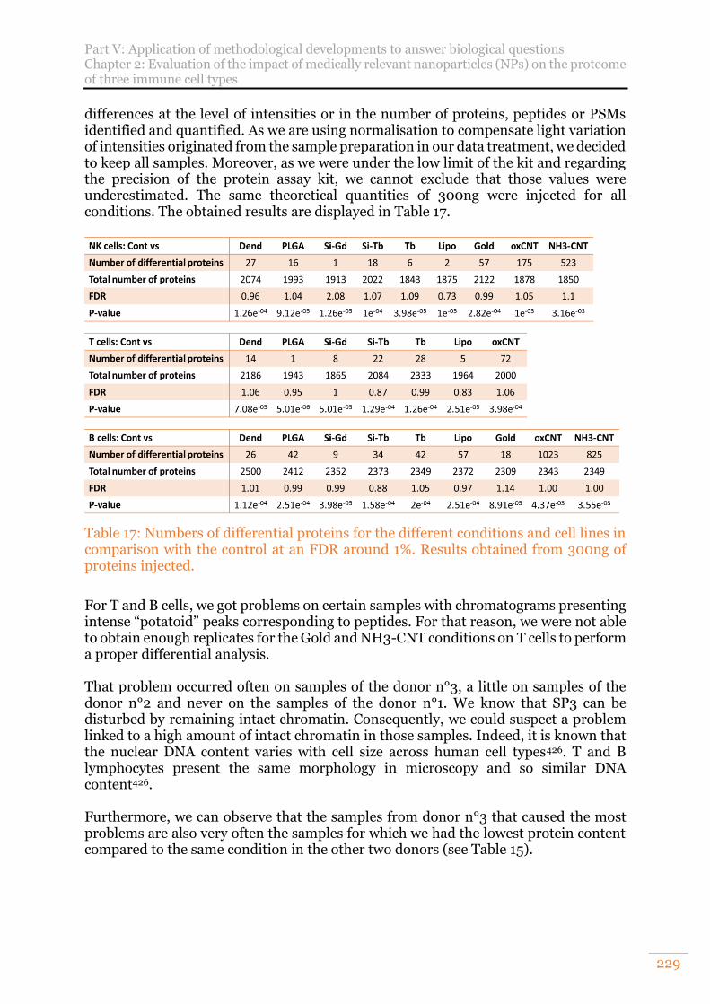
Part V: Application of methodological developments to answer biological questions Chapter 2: Evaluation of the impact of medically relevant nanoparticles (NPs) on the proteome of three immune cell types
229
differences at the level of intensities or in the number of proteins, peptides or PSMs identified and quantified. As we are using normalisation to compensate light variation of intensities originated from the sample preparation in our data treatment, we decided to keep all samples. Moreover, as we were under the low limit of the kit and regarding the precision of the protein assay kit, we cannot exclude that those values were underestimated. The same theoretical quantities of 300ng were injected for all conditions. The obtained results are displayed in Table 17.
Table 17: Numbers of differential proteins for the different conditions and cell lines in comparison with the control at an FDR around 1%. Results obtained from 300ng of proteins injected.
For T and B cells, we got problems on certain samples with chromatograms presenting intense “potatoid” peaks corresponding to peptides. For that reason, we were not able to obtain enough replicates for the Gold and NH3-CNT conditions on T cells to perform a proper differential analysis. That problem occurred often on samples of the donor n°3, a little on samples of the donor n°2 and never on the samples of the donor n°1. We know that SP3 can be disturbed by remaining intact chromatin. Consequently, we could suspect a problem linked to a high amount of intact chromatin in those samples. Indeed, it is known that the nuclear DNA content varies with cell size across human cell types426. T and B lymphocytes present the same morphology in microscopy and so similar DNA content426. Furthermore, we can observe that the samples from donor n°3 that caused the most problems are also very often the samples for which we had the lowest protein content compared to the same condition in the other two donors (see Table 15).
Part V: Application of methodological developments to answer biological questions Chapter 2: Evaluation of the impact of medically relevant nanoparticles (NPs) on the proteome of three immune cell types
230
This may just be normal inter-individual variability, but it is interesting to note. It is well known that certain diseases can induce a higher DNA content in lymphocytes, such as cancers and in particular leukaemia, but to our knowledge the donors were healthy. Another hypothesis could be related to an unknown compound, which contaminated the samples of donors n°2 and n°3. This contamination could affect the protein assay or the protein binding on the SP3 beads. Therefore, this contamination would have to come from a step in the protocol where the samples from the three donors were not prepared in parallel since the samples from donor n°1 are not affected. In any case, the problem is probably due to the steps preceding the enzymatic digestion. Indeed, we checked the percentage of missed cleaved peptides among the different injections and we observed regular values among the chromatograms that show strange profiles and the others with on average respectively 12% and 18% of peptides including missed cleavages. If the amount of proteins was overestimated in the assay or if the binding step was not efficient, the amount of proteins in the digestion step must have been lower than expected, leading to an increase in the experimental trypsin:protein ratio which could have improved digestion and reduced the proportion of peptides with missed cuts. Today, we still do not have a satisfactory answer to this question but if this difficulty is related to intact chromatin, we have already presented different ways to improve the preparation of SP3 samples in the state of the art section and in the chapter of autoSP3 results, with for example the improvement of the sonication step or the use of nucleases. To conclude on the results of this study, independently of the cell type, we observed a high impact of oxCNT and NH3-CNT NPs on the cell proteome. The modifications potentially induced by the other nanoparticles appear to be weak in relation to our data. However, these results need to be confirmed and extended by our collaborators. They will also be compared with the results obtained on the same samples but at the transcriptome level soon. To conclude this applicative part, the optimisations developed during my PhD have been used for collaborative projects. We performed SP3 sample preparation on immune cells incubated with up to nine different NPs and one control. Our two collaborative projects based on IPs allowed me to understand the difficulties of this kind of projects. On one hand, I experienced a project where we encountered many difficulties whereas in the second hand everything went smoothly.
GENERAL CONCLUSION
231
GENERAL CONCLUSION
The subject of my doctorate was methodological developments in proteomic analysis: towards high-throughput analysis on reduced quantities of material and new quantification strategies. Over the last three years, I have had the opportunity to work in parallel on the three main axes that we have chosen to develop from my thesis topic and to apply some of these developments to collaborative projects. Firstly, the sample preparation. Indeed, thanks to the increasingly advanced development of analytical instruments and in particular mass spectrometers, sample preparation has become a limiting stage. These limitations occurred at several levels. First, the amount of material available varies enormously depending on the project. I had the opportunity to demonstrate the impact that less material could have on the depth and repeatability of the analyses by using the preparation methods already implemented in our laboratory, the stacking-gel, and the tube-gel. I tried to improve the performance of the tube-gel and we were able to observe a slight gain. However, it was not significant enough to justify investing so much time in further testing. In addition, gel digestion approaches have another limitation, the time required for sample preparation. Although the Tube-gel has already been a gain, reducing the sample preparation time from 4-5 days to 2-3 days. However, commercial solutions now offer relief from the need to carry out the entire sample preparation process in a single day. These include S-Trap (Protifi), iST (PreOmics) among others. The iST had already been investigated in the laboratory with varying degrees of success on different types of samples. Therefore, we decided to investigate the S-Trap technology. In addition, the S-Trap can overcome another limitation of sample preparation. The extraction of tricky proteins such as membrane proteins, which play important roles in biology due to their localisation, represents a separate analytical challenge. One of the most popular and efficient methods for the extraction of these proteins is the use of extraction buffers containing detergents and SDS. The problem is that SDS is not compatible with mass spectrometry analysis and must be removed before nLC-MS/MS analysis. All the protocols we evaluated were selected in part for their propensity to remove SDS during the protocol. The great advantage of the S-Trap goes beyond simply being SDS compatible. Indeed, it needs a high amount of SDS to work (5%) and was consequently designed to remove it afterwards via washes. We evaluated this preparation for a range of input protein quantities. The S-Trap has been shown to be a good solution for protein amounts greater than or equal to 10µg but presents several problems for lower amounts. There is a loss of depth of analysis, a strong increase in the variability of results both qualitatively and quantitatively. In addition, some contaminants appear when working with very small quantities such as PEG or many keratins and other human contaminants. Therefore, we decided to evaluate a third sample preparation solution, the SP3 based on the use of magnetic beads. The SP3 combines the advantage of being performed in a single tube, in a reduced time that can last one day. It is compatible with SDS even at high percentages and has a high potential for automation. We adapted published protocols to evaluate SP3 on a range of input proteins with the lowest point at 500ng of protein, i.e., a quantity that can be directly injected at once on many nLC-MS/MS
GENERAL CONCLUSION
232
couplings. The results obtained were very impressive on small quantities. However, those experiments also illustrated that the parameters and notably the working volumes used for very small quantities are not optimal for large quantities. To complete this part, I undertook to implement an automated sample preparation protocol in SP3 or autoSP3 on a sample preparation robot acquired by our laboratory. I confronted to numerous problems related to automation. These included problems with pipetting, speed of agitation, and homogenisation of solutions, among others leading to performance and reproducibility problems. Although this work is not yet complete even if many improvements have already been implemented. Once this protocol will be fully operational, it will allow the laboratory to prepare up to 96 samples in parallel, in one day, by using SDS and adapted to small quantities of proteins. This will allow carrying out more ambitious projects in terms of number of samples at high throughput, which will lead also to a gain for data processing, allowing the number of replicas to be increased for statistical analysis. In addition, the automation of the sample preparation stage will also free up time for researchers to focus on other limiting points or to work on a larger number of projects. This part of my project allowed me to develop a great expertise in the preparation of different types of samples for mass spectrometry analysis. Indeed, working on small quantities requires optimization and extreme rigor, to be able to perform quantitative analyses. This also allowed me to acquire a great deal of experience in understanding numerous protein preparation approaches and in carrying them out with a pipette in hand in the laboratory. I also had the opportunity to deepen my knowledge in terms of automation. I became aware of the difficulty of adapting a protocol on a robot. I was also able to start learning how to modify protocols from the constructor interface but also directly by understanding and modifying small java scripts. This part of my subject required a lot of perseverance, patience, and investment. Many experiments ended in failures and even if each failure brings its stone to the edifice, it is something that can be demotivating but that I could learn to manage better. I hope to have the opportunity to continue learning more about automation in general and scripting in Java in the future. The second part of my thesis focused on the implementation of a new and very innovative coupling in the laboratory. I was involved in its installation and was responsible for it for three years. I developed a deep expertise in all kinds of repairs and in nano-plumbing thanks to the redoubtable nanoElute. I can carry out all the common maintenance and repairs of this system and even some fewer common ones. Regarding the mass spectrometer, I can perform a thorough cleaning as well as assess, locate, and solve common problems. That said, it should be noted that these problems have been relatively rare during my thesis, as the TimsTOF Pro has been a model of robustness during these three years. On the other hand, it was not always the case of the various software allowing the management of the coupling, which also knew a great number of evolutions allowing me to discover a whole catalogue of troublesome bugs but also allowing making regularly accessible new functions. This has allowed me to develop great flexibility and adaptability. Overall, I had the opportunity to familiarise myself with the whole environment of an nLC-IMS-MS/MS coupling, which goes far beyond the expertise of a simple user. I have of course acquired experience in nLC systems, ion mobility and TIMS as well as in mass spectrometry. I also mastered innovative acquisition strategies linked to these new technologies with PASEF. I had
GENERAL CONCLUSION
233
the opportunity to develop specific methods for both nLC and MS, taking advantage of the strengths of the TimsTOF Pro, through both DDA and DIA approaches, despite the lack of maturity of the software, which was a real obstacle for the last one. The coupling has evolved enormously over the last three years, both through changes that I would describe as hardware relative to the instruments and in the software. This was both a great opportunity and a great challenge. Indeed, to see many of its landmarks change from one day to the next and to have to adapt as quickly as possible to take advantage of the improvements and to make them available and useful for all users requires a lot of organisation and energy. Beyond that, dealing with the coupling also requires developing planning and communication skills so that the coupling is never idle. Finally, I had the opportunity to accompany and train a certain number of users so that they could discover the specificities of this coupling and become autonomous to launch their analyses. Beyond this coupling, I have also been trained on other instruments, which has allowed me to be comfortable with instruments of different geometries from various suppliers. Even though being responsible for this coupling was a big source of pressure, I loved this experience. I like looking after the machines, maintaining them, figuring out how to solve a problem and sometimes testing original solutions. I also liked having the opportunity to test many parameters to understand better the functioning of the instrument and thus be more comfortable to have eventually ideas of innovative things to test. This is ironically a point that also frustrated me because time is not incompressible, and we don't always have the means to test everything we would like to test especially in the context of a thesis where there are so many other things to learn in parallel. Being able to be responsible for instruments or even to work on their development beyond simply developing methods is something that interests me and that I could consider for my future career. The third part of my thesis focused on the analysis of the generated proteomics data and especially, the TimsTOF Pro data that was very particular compared to most of the couplings used for bottom-up proteomics because of the additional information dimension associated with ion mobility. I had the opportunity to use, evaluate and follow the evolution of different software dedicated to label-free protein identification and quantification. I was able to compare some of them for the analysis of data acquired in DDA. I was also able to process DIA data. Data processing has always been a difficult exercise for me because it is still something abstract in the sense that I find it difficult to visualise exactly what is going on. Therefore, I spent a lot of time doing various tests to understand how the software works and to be able to understand exactly what the parameters associated with the additional data dimension of the TimsTOF Pro could bring to the data processing. In addition, I also had the opportunity to get back to writing R scripts for processing and visualizing the data. Unfortunately, because of the number of things to learn and do during my thesis, I did not manage to allocate as much time as I would have liked, and my mastery of this tool remains superficial. That said, I am aware of its power and the freedom it offers to find the underlying cause of the data, and this is something I want to explore further in the future. Another point that I have taken the time to explore is the statistical processing of data. I was lucky enough to discover and use the ProStaR software which has the advantage of providing its users with many statistical tools and visualisations adapted for the statistical processing of proteomic data. That said, statistics is a whole world to discover, and I am still a newcomer in this field, which I would like to learn more about in the future.
GENERAL CONCLUSION
234
Finally, the last axis of my thesis focused on the application of the developments made during my thesis on collaborative projects applied to biological problems. I had the opportunity to collaborate with several groups of scientists whose work I could discover. This allowed me to discover very diverse and specific research themes. It also gave me the opportunity to work on samples very different from the models used during my thesis. With these projects, I also experienced the pressure of not having a second chance due to the difficulty of obtaining certain samples, some of which represented a real analytical challenge. I have enjoyed these projects and look forward to seeing what our collaborators can learn from our results. I would like to digress to talk about the related activities that I was able to carry out in parallel with my thesis. I was able to participate in various conferences and present my work both orally and through posters. Unfortunately, the Covid was a limiting factor, and I did not have the opportunity to exchange as much as I would have liked with the proteomics community. I also had the opportunity to communicate and specially to popularise my research through my participation in the “Ma thèse en 180 secondes” competition. I was selected among the finalists of the Alsace region. Unfortunately, the public presentation was also cancelled because of Covid. Fortunately, my performance and those of all my comrades could still be filmed and broadcast. They are still available on Youtube (https://www.youtube.com/watch?v=a1kkNe_dO3M). This exercise, as well as all the training I received on this occasion about popularising science and speaking in front of a large audience, was an exhilarating and incredibly enriching experience. I also had the opportunity to meet researchers from all fields, both in the so-called hard sciences and in the politic, economic, and social sciences, and to open to subjects that I would never have suspected existed otherwise. I think on a very personal basis that scientific popularisation, pedagogy, and communication are skills that are not sufficiently valued today within the scientific community. In my humble opinion, this contributes to the cold and arrogant image that the public may have of researchers, with serious consequences that may even put lives at risk, as illustrated by the anti-vaccine movement that is dramatically active in France. I would like to continue to be involved in this type of initiative in the future. I sincerely hope that the crisis we have all been through together will create vocations and that we will learn from it for the future of research and its dissemination to the public. Finally, the last activity related to my thesis that I had the opportunity to carry out was my participation in the council of the doctoral school of Chemical Sciences of the University of Strasbourg as a representative of the doctoral students. I held this position from January 2019 until September 2021. I participated in about ten meetings per year and had the chance to attend the doctoral school competition two years in a row. Once again, being able to attend this competition was a great opportunity for my scientific culture, especially as I originally studied biology and not chemistry before my thesis. I was able to discover a huge number of research fields ranging from synthetic chemistry to chemoinformatic, including other areas of analytical chemistry with subjects from both academia and industry. This allowed me to see behind the scenes and to get a deeper insight into the structure of doctoral research. I was able to see the many organisational, economic, and political constraints to which thesis supervisors and all the people involved in the process are subject. It also allowed me to meet many researchers and to have the opportunity to exchange and find solutions with them. The board of the doctoral school has always been very benevolent and attentive to the

GENERAL CONCLUSION
235
opinions and points of view of the doctoral students, allowing for healthy and constructive exchanges with the aim of improving the doctoral curriculum. In this respect, Covid was once again an exceptional challenge, and I am glad to have been able to be part of the board at that time. I hope that I was able to make a small contribution, but I certainly learned a lot from it. To conclude, the thesis is not an easy challenge to take up both scientifically and humanly and like many PhD students, I almost gave up more than once. However, today I am coming to the end of the writing of this manuscript and looking back on the work I have done over the last three years, I think I can be proud of myself. It is very far from perfect, and I think that is normal since a thesis and even more, so research is first about learning. I have learned a lot in these three years and, as they say in French, only those who do nothing make no mistakes. I think it is a shame that failures are not valued more in the scientific literature because I think we waste a lot of time repeating the mistakes that others have made before us. What I am sure of is that I gave it my best shot. Now I just must look to the future. I do not know yet where my steps will lead me but what is certain is that the thesis is only a stage and that I intend to continue to move forward.
EXPERIMENTAL SECTION Part II: Optimisation of pre-analytical sample preparation steps for high throughput proteomics analysis on small amounts of material
236
EXPERIMENTAL SECTION
Part II: Optimisation of pre-analytical sample preparation steps for high throughput proteomics analysis on small amounts of material
Chapter 1: Evaluation of different digestion methods
All the data generated in this part was treated using recent versions of MaxQuant. The use of MBR is mentioned in the respective results parts. The default parameters were used except for the number of missed cleavages set to one, the minimum number of unique peptides set to one. The quantification was realised using only the unique peptides without modifications except for the carbidomethylation of cysteine residues and using the LFQ normalisation.
A. Set-up of a volume reduced tube-gel protocol Yeast cell pellet was suspended in 2% SDS, 62.5mM Tris-HCl pH = 6.8, 10% glycerol buffer and then lysed using probe sonication. The protein concentration was estimated with the DC kit of Biorad (Hercules, CAL, USA). The following experiments were performed in triplicate with starting protein amounts of 50-20-10-5-2.5-1µg. The tube-gels were prepared following the protocol described by Muller et al4. Enzymatic digestion was performed overnight at 37°C using modified porcine trypsin (Promega) with a trypsin:protein ratio equal to 1:50. Peptides were extracted with 160 μL of a volume mixture of ACN/H2O/FA (60/40/0.1) for 1h and then 160 μL of ACN and FA 0.1% for 1h at room temperature. The reduced tube-gel experiment was performed as the standard tube-gel but by dividing all the volumes for the tube-gel preparation by a factor 2. For the stacking gel, DTT and bromophenol blue was added to reach final concentration of respectively 50mM and 0.05% in each aliquot. After denaturing the proteins at 100°C for 5 min, they were concentrated into a single band via a 4% acrylamide SDS-PAGE gel prepared one day in advance. After a protein fixation step in an EtOH/H2O/acetic acid mixture (50/47/3), the proteins were stained with Coomassie blue. Each strip was finally cut into equal pieces. After four washes with 150 μL of ACN/NH4HCO3 (25 mM) volume mixture (75/25), the pieces were dehydrated with 50 μL of ACN. The proteins were then reduced with 10 mM DTT for 30 min at 60°C and then alkylated with 55 mM IAM for 20 min in the dark at room temperature. After four further washes with 50 μL of ACN/NH4HCO3 (25 mM) volume mixture (75/25), the pieces were dehydrated with 50 μL of ACN prior to enzymatic digestion performed overnight at 37°C with modified porcine trypsin (Promega) via a 1:50 trypsin/protein ratio. Peptides were then extracted with 40 μL of ACN/H2O/FA volume mixture (60/40/0.1) for 1h, followed by 50 μL of ACN for 1h at room temperature.
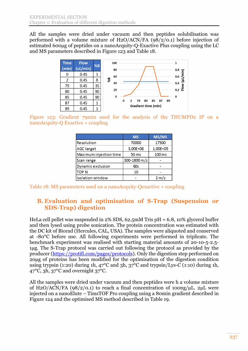
EXPERIMENTAL SECTION Chapter 1: Evaluation of different digestion methods
237
All the samples were dried under vacuum and then peptides solubilisation was performed with a volume mixture of H2O/ACN/FA (98/2/0.1) before injection of estimated 600µg of peptides on a nanoAcquity-Q-Exactive Plus coupling using the LC and MS parameters described in Figure 123 and Table 18.
Figure 123: Gradient 79min used for the analysis of the THUMPD2 IP on a nanoAcquity-Q Exactive + coupling
Table 18: MS parameters used on a nanoAcquity-Qexactive + coupling
B. Evaluation and optimisation of S-Trap (Suspension or SDS-Trap) digestion
HeLa cell pellet was suspended in 2% SDS, 62.5mM Tris pH = 6.8, 10% glycerol buffer and then lysed using probe sonication. The protein concentration was estimated with the DC kit of Biorad (Hercules, CAL, USA). The samples were aliquoted and conserved at -80°C before use. All following experiments were performed in triplicate. The benchmark experiment was realised with starting material amounts of 20-10-5-2.5-1µg. The S-Trap protocol was carried out following the protocol as provided by the producer (https://protifi.com/pages/protocols). Only the digestion step performed on 20µg of proteins has been modified for the optimisation of the digestion condition using trypsin (1:20) during 1h, 47°C and 3h, 37°C and trypsin/Lys-C (1:10) during 1h, 47°C, 3h, 37°C and overnight 37°C. All the samples were dried under vacuum and then peptides were h a volume mixture of H2O/ACN/FA (98/2/0.1) to reach a final concentration of 100ng/µL. 2µL were injected on a nanoElute – TimsTOF Pro coupling using a 80min gradient described in Figure 124 and the optimised MS method described in Table 19.
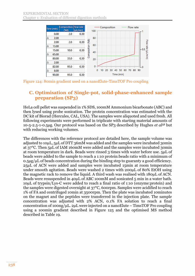
EXPERIMENTAL SECTION Chapter 1: Evaluation of different digestion methods
238
Figure 124: 80min gradient used on a nanoElute-TimsTOF Pro coupling
C. Optimisation of Single-pot, solid-phase-enhanced sample preparation (SP3)
HeLa cell pellet was suspended in 1% SDS, 100mM Ammonium bicarbonate (ABC) and then lysed using probe sonication. The protein concentration was estimated with the DC kit of Biorad (Hercules, CAL, USA). The samples were aliquoted and used fresh. All following experiments were performed in triplicate with starting material amounts of 10-5-2.5-1-0.5µg. Our protocol was based on the SP3 described by Hughes et al58 but with reducing working volumes. The differences with the reference protocol are detailed here, the sample volume was adjusted to 10µL, 5µL of DTT 36mM was added and the samples were incubated 30min at 37°C. Then 5µL of IAM 160mM were added and the samples were incubated 30min at room temperature in dark. Beads were rinsed 3 times with water before use. 5µL of beads were added to the sample to reach a 1:10 protein:beads ratio with a minimum of 0.5µg/µL of beads concentration during the binding step to guaranty a good efficiency. 25µL of ACN were added and samples were incubated 15min at room temperature under smooth agitation. Beads were washed 2 times with 200µL of 80% EtOH using the magnetic rack to remove the liquid. A third wash was realised with 180µL of ACN. Beads were resuspended in 40µL of ABC 100mM and sonicated 5 min in a water bath. 10µL of trypsin/Lys-C were added to reach a final ratio of 1:10 (enzyme:protein) and the samples were digested overnight at 37°C, 600rpm. Samples were acidified to reach 1% of FA and centrifuged 10min at 3500rpm. Then the plate was incubated 10minutes on the magnet and the peptides were transferred in the injection plate. The sample concentration was adjusted with 2% ACN, 0.1% FA solution to reach a final concentration of 100ng/µL. 2µL were injected on a nanoElute – TimsTOF Pro coupling using a 100min gradient described in Figure 125 and the optimised MS method described in Table 19.
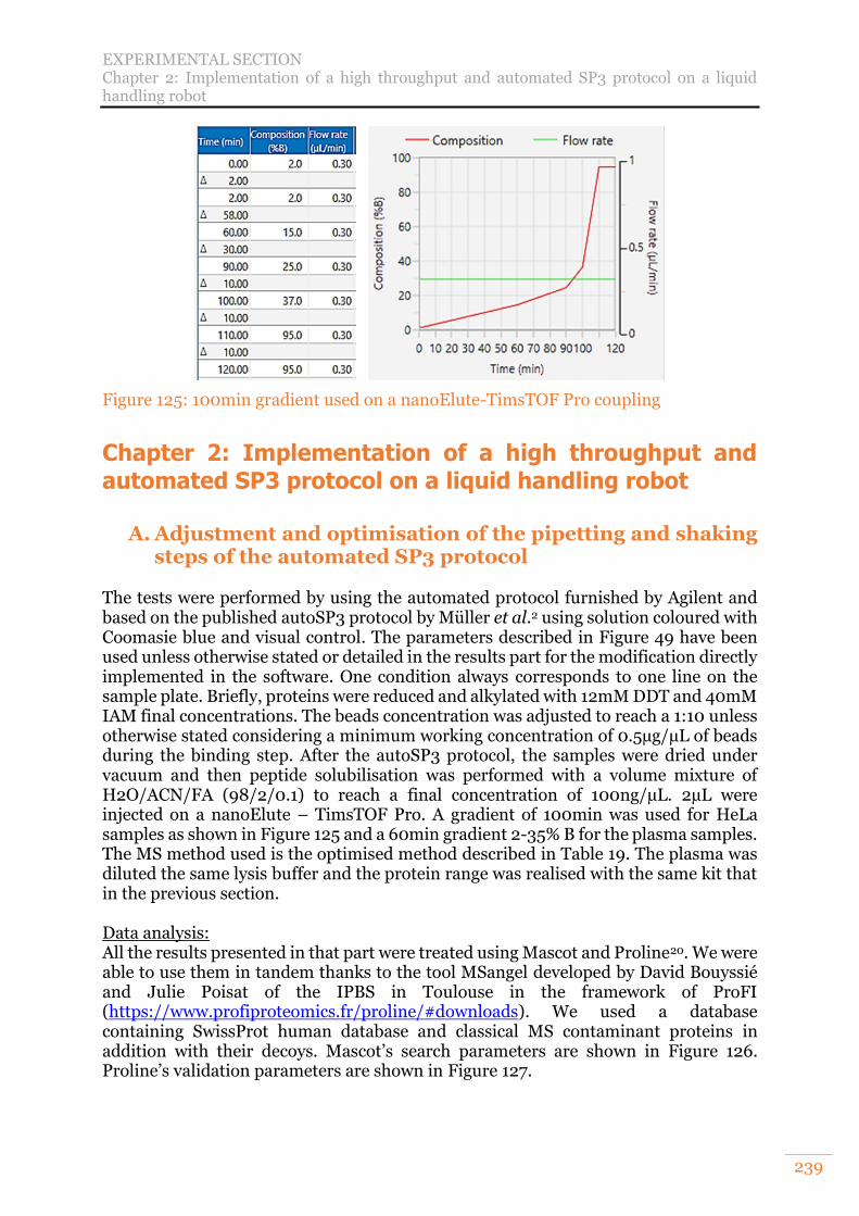
EXPERIMENTAL SECTION Chapter 2: Implementation of a high throughput and automated SP3 protocol on a liquid handling robot
239
Figure 125: 100min gradient used on a nanoElute-TimsTOF Pro coupling
Chapter 2: Implementation of a high throughput and automated SP3 protocol on a liquid handling robot
A. Adjustment and optimisation of the pipetting and shaking steps of the automated SP3 protocol
The tests were performed by using the automated protocol furnished by Agilent and based on the published autoSP3 protocol by Müller et al.2 using solution coloured with Coomasie blue and visual control. The parameters described in Figure 49 have been used unless otherwise stated or detailed in the results part for the modification directly implemented in the software. One condition always corresponds to one line on the sample plate. Briefly, proteins were reduced and alkylated with 12mM DDT and 40mM IAM final concentrations. The beads concentration was adjusted to reach a 1:10 unless otherwise stated considering a minimum working concentration of 0.5µg/µL of beads during the binding step. After the autoSP3 protocol, the samples were dried under vacuum and then peptide solubilisation was performed with a volume mixture of H2O/ACN/FA (98/2/0.1) to reach a final concentration of 100ng/µL. 2µL were injected on a nanoElute – TimsTOF Pro. A gradient of 100min was used for HeLa samples as shown in Figure 125 and a 60min gradient 2-35% B for the plasma samples. The MS method used is the optimised method described in Table 19. The plasma was diluted the same lysis buffer and the protein range was realised with the same kit that in the previous section. Data analysis: All the results presented in that part were treated using Mascot and Proline20. We were able to use them in tandem thanks to the tool MSangel developed by David Bouyssié and Julie Poisat of the IPBS in Toulouse in the framework of ProFI (https://www.profiproteomics.fr/proline/#downloads). We used a database containing SwissProt human database and classical MS contaminant proteins in addition with their decoys. Mascot’s search parameters are shown in Figure 126. Proline’s validation parameters are shown in Figure 127.
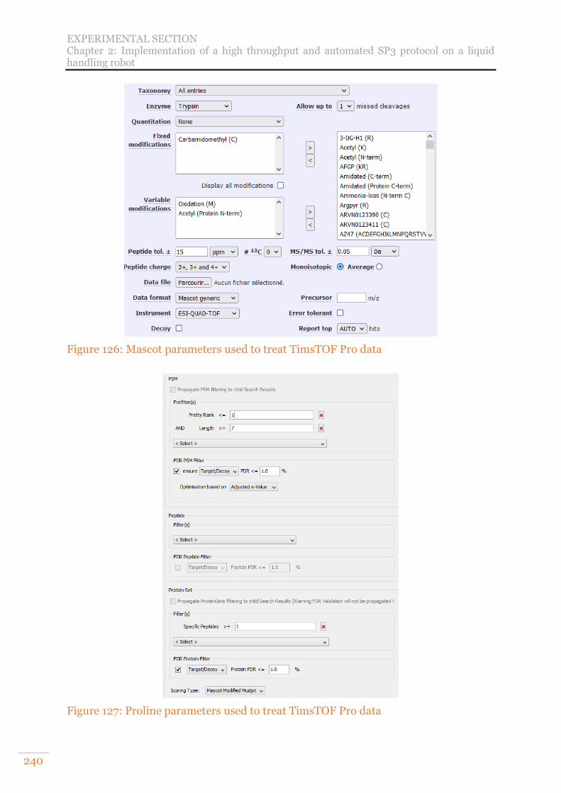
EXPERIMENTAL SECTION Chapter 2: Implementation of a high throughput and automated SP3 protocol on a liquid handling robot
240
Figure 126: Mascot parameters used to treat TimsTOF Pro data
Figure 127: Proline parameters used to treat TimsTOF Pro data
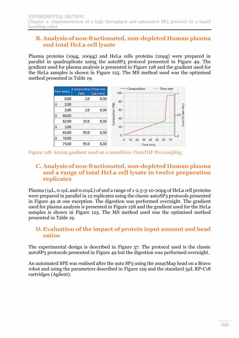
EXPERIMENTAL SECTION Chapter 2: Implementation of a high throughput and automated SP3 protocol on a liquid handling robot
241
B. Analysis of non-fractionated, non-depleted Human plasma and total HeLa cell lysate
Plasma proteins (10µg, 100µg) and HeLa cells proteins (20µg) were prepared in parallel in quadruplicate using the autoSP3 protocol presented in Figure 49. The gradient used for plasma analysis is presented in Figure 128 and the gradient used for the HeLa samples is shown in Figure 125. The MS method used was the optimised method presented in Table 19.
Figure 128: 62min gradient used on a nanoElute-TimsTOF Pro coupling
C. Analysis of non-fractionated, non-depleted Human plasma and a range of total HeLa cell lysate in twelve preparation replicates
Plasma (1µL, 0.1µL and 0.01µL) of and a range of 1-2.5-5-10-20µg of HeLa cell proteins were prepared in parallel in 12 replicates using the classic autoSP3 protocols presented in Figure 49 at one exception. The digestion was performed overnight. The gradient used for plasma analysis is presented in Figure 128 and the gradient used for the HeLa samples is shown in Figure 125. The MS method used was the optimised method presented in Table 19.
D. Evaluation of the impact of protein input amount and bead ratios
The experimental design is described in Figure 57. The protocol used is the classic autoSP3 protocols presented in Figure 49 but the digestion was performed overnight. An automated SPE was realised after the auto SP3 using the assayMap head on a Bravo robot and using the parameters described in Figure 129 and the standard 5µL RP-C18 cartridges (Agilent).
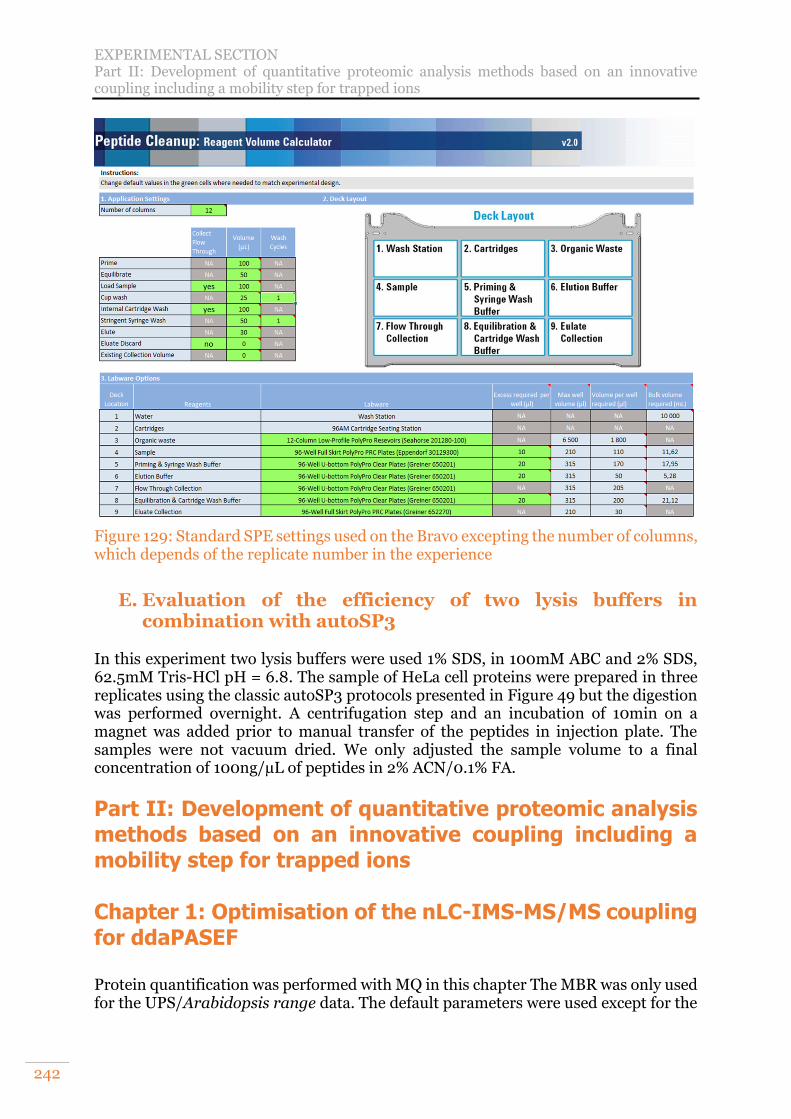
EXPERIMENTAL SECTION Part II: Development of quantitative proteomic analysis methods based on an innovative coupling including a mobility step for trapped ions
242
Figure 129: Standard SPE settings used on the Bravo excepting the number of columns, which depends of the replicate number in the experience
E. Evaluation of the efficiency of two lysis buffers in combination with autoSP3
In this experiment two lysis buffers were used 1% SDS, in 100mM ABC and 2% SDS, 62.5mM Tris-HCl pH = 6.8. The sample of HeLa cell proteins were prepared in three replicates using the classic autoSP3 protocols presented in Figure 49 but the digestion was performed overnight. A centrifugation step and an incubation of 10min on a magnet was added prior to manual transfer of the peptides in injection plate. The samples were not vacuum dried. We only adjusted the sample volume to a final concentration of 100ng/µL of peptides in 2% ACN/0.1% FA.
Part II: Development of quantitative proteomic analysis methods based on an innovative coupling including a mobility step for trapped ions
Chapter 1: Optimisation of the nLC-IMS-MS/MS coupling for ddaPASEF
Protein quantification was performed with MQ in this chapter The MBR was only used for the UPS/Arabidopsis range data. The default parameters were used except for the
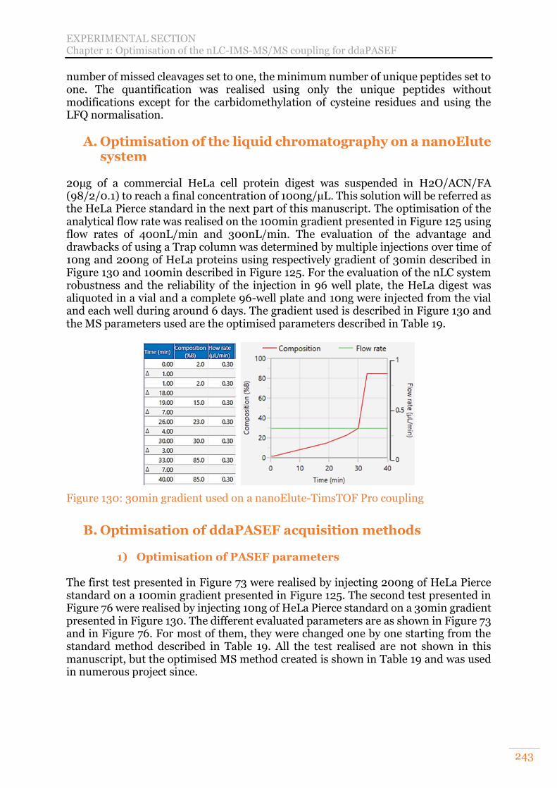
EXPERIMENTAL SECTION Chapter 1: Optimisation of the nLC-IMS-MS/MS coupling for ddaPASEF
243
number of missed cleavages set to one, the minimum number of unique peptides set to one. The quantification was realised using only the unique peptides without modifications except for the carbidomethylation of cysteine residues and using the LFQ normalisation.
A. Optimisation of the liquid chromatography on a nanoElute system
20µg of a commercial HeLa cell protein digest was suspended in H2O/ACN/FA (98/2/0.1) to reach a final concentration of 100ng/µL. This solution will be referred as the HeLa Pierce standard in the next part of this manuscript. The optimisation of the analytical flow rate was realised on the 100min gradient presented in Figure 125 using flow rates of 400nL/min and 300nL/min. The evaluation of the advantage and drawbacks of using a Trap column was determined by multiple injections over time of 10ng and 200ng of HeLa proteins using respectively gradient of 30min described in Figure 130 and 100min described in Figure 125. For the evaluation of the nLC system robustness and the reliability of the injection in 96 well plate, the HeLa digest was aliquoted in a vial and a complete 96-well plate and 10ng were injected from the vial and each well during around 6 days. The gradient used is described in Figure 130 and the MS parameters used are the optimised parameters described in Table 19.
Figure 130: 30min gradient used on a nanoElute-TimsTOF Pro coupling
B. Optimisation of ddaPASEF acquisition methods
1) Optimisation of PASEF parameters The first test presented in Figure 73 were realised by injecting 200ng of HeLa Pierce standard on a 100min gradient presented in Figure 125. The second test presented in Figure 76 were realised by injecting 10ng of HeLa Pierce standard on a 30min gradient presented in Figure 130. The different evaluated parameters are as shown in Figure 73 and in Figure 76. For most of them, they were changed one by one starting from the standard method described in Table 19. All the test realised are not shown in this manuscript, but the optimised MS method created is shown in Table 19 and was used in numerous project since.
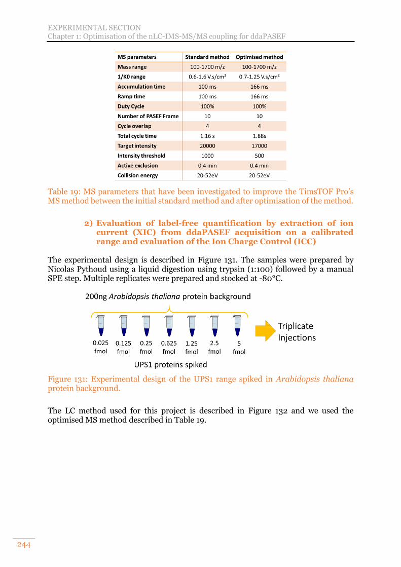
EXPERIMENTAL SECTION Chapter 1: Optimisation of the nLC-IMS-MS/MS coupling for ddaPASEF
244
Table 19: MS parameters that have been investigated to improve the TimsTOF Pro’s MS method between the initial standard method and after optimisation of the method.
2) Evaluation of label-free quantification by extraction of ion
current (XIC) from ddaPASEF acquisition on a calibrated range and evaluation of the Ion Charge Control (ICC)
The experimental design is described in Figure 131. The samples were prepared by Nicolas Pythoud using a liquid digestion using trypsin (1:100) followed by a manual SPE step. Multiple replicates were prepared and stocked at -80°C.
Figure 131: Experimental design of the UPS1 range spiked in Arabidopsis thaliana protein background.
The LC method used for this project is described in Figure 132 and we used the optimised MS method described in Table 19.
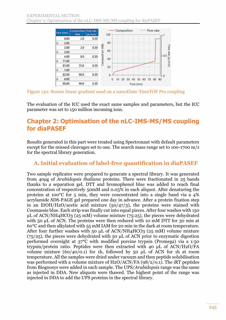
EXPERIMENTAL SECTION Chapter 2: Optimisation of the nLC-IMS-MS/MS coupling for diaPASEF
245
Figure 132: 80min linear gradient used on a nanoElute-TimsTOF Pro coupling
The evaluation of the ICC used the exact same samples and parameters, but the ICC parameter was set to 150 million incoming ions.
Chapter 2: Optimisation of the nLC-IMS-MS/MS coupling for diaPASEF
Results generated in this part were treated using Spectronaut with default parameters except for the missed cleavages set to one. The search mass range set to 100-1700 m/z for the spectral library generation.
A. Initial evaluation of label-free quantification in diaPASEF Two sample replicates were prepared to generate a spectral library. It was generated from 40µg of Arabidopsis thaliana proteins. There were fractionated in 25 bands thanks to a separation gel. DTT and bromophenol blue was added to reach final concentration of respectively 50mM and 0.05% in each aliquot. After denaturing the proteins at 100°C for 5 min, they were concentrated into a single band via a 4% acrylamide SDS-PAGE gel prepared one day in advance. After a protein fixation step in an EtOH/H2O/acetic acid mixture (50/47/3), the proteins were stained with Coomassie blue. Each strip was finally cut into equal pieces. After four washes with 150 μL of ACN/NH4HCO3 (25 mM) volume mixture (75:25), the pieces were dehydrated with 50 μL of ACN. The proteins were then reduced with 10 mM DTT for 30 min at 60°C and then alkylated with 55 mM IAM for 20 min in the dark at room temperature. After four further washes with 50 μL of ACN/NH4HCO3 (25 mM) volume mixture (75/25), the pieces were dehydrated with 50 μL of ACN prior to enzymatic digestion performed overnight at 37°C with modified porcine trypsin (Promega) via a 1:50 trypsin/protein ratio. Peptides were then extracted with 40 μL of ACN/H2O/FA volume mixture (60/40/0.1) for 1h, followed by 50 μL of ACN for 1h at room temperature. All the samples were dried under vacuum and then peptide solubilisation was performed with a volume mixture of H2O/ACN/FA (98/2/0.1). The iRT peptides from Biognosys were added in each sample. The UPS/Arabidopsis range was the same as injected in DDA. New aliquots were thawed. The highest point of the range was injected in DDA to add the UPS proteins in the spectral library.
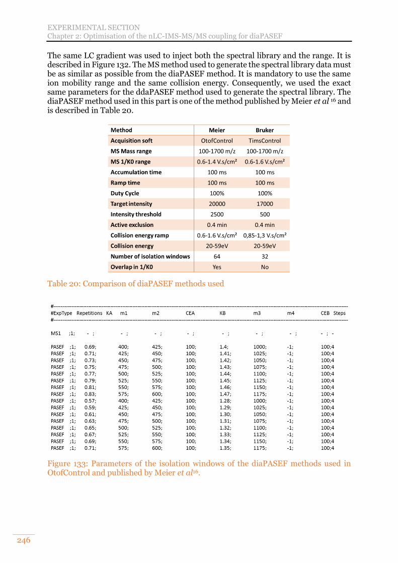
EXPERIMENTAL SECTION Chapter 2: Optimisation of the nLC-IMS-MS/MS coupling for diaPASEF
246
The same LC gradient was used to inject both the spectral library and the range. It is described in Figure 132. The MS method used to generate the spectral library data must be as similar as possible from the diaPASEF method. It is mandatory to use the same ion mobility range and the same collision energy. Consequently, we used the exact same parameters for the ddaPASEF method used to generate the spectral library. The diaPASEF method used in this part is one of the method published by Meier et al 16 and is described in Table 20.
Table 20: Comparison of diaPASEF methods used
Figure 133: Parameters of the isolation windows of the diaPASEF methods used in OtofControl and published by Meier et al16.
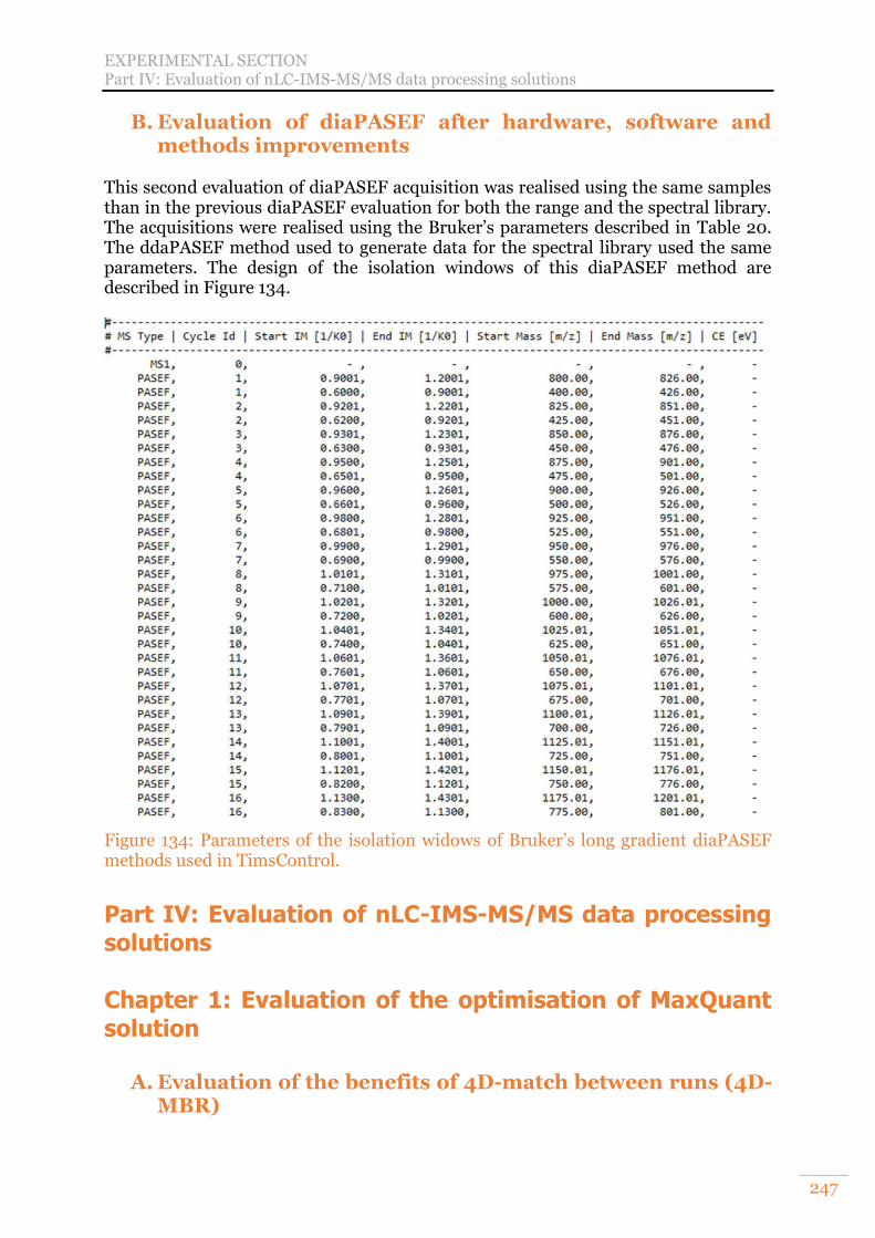
EXPERIMENTAL SECTION Part IV: Evaluation of nLC-IMS-MS/MS data processing solutions
247
B. Evaluation of diaPASEF after hardware, software and methods improvements
This second evaluation of diaPASEF acquisition was realised using the same samples than in the previous diaPASEF evaluation for both the range and the spectral library. The acquisitions were realised using the Bruker’s parameters described in Table 20. The ddaPASEF method used to generate data for the spectral library used the same parameters. The design of the isolation windows of this diaPASEF method are described in Figure 134.
Figure 134: Parameters of the isolation widows of Bruker’s long gradient diaPASEF methods used in TimsControl.
Part IV: Evaluation of nLC-IMS-MS/MS data processing solutions
Chapter 1: Evaluation of the optimisation of MaxQuant solution
A. Evaluation of the benefits of 4D-match between runs (4D-MBR)
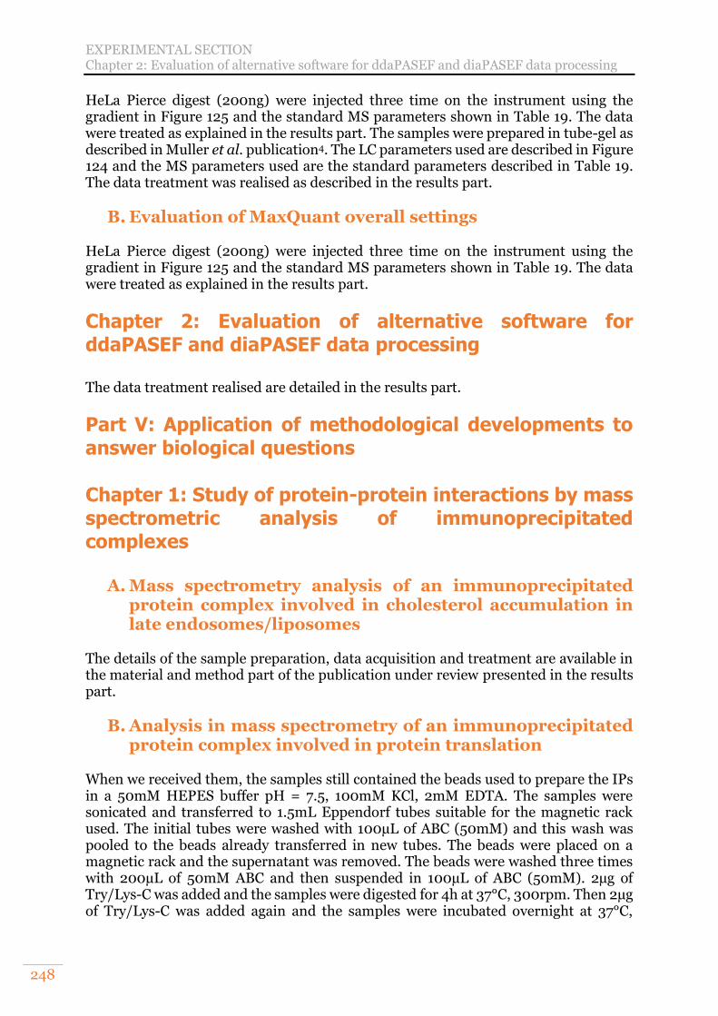
EXPERIMENTAL SECTION Chapter 2: Evaluation of alternative software for ddaPASEF and diaPASEF data processing
248
HeLa Pierce digest (200ng) were injected three time on the instrument using the gradient in Figure 125 and the standard MS parameters shown in Table 19. The data were treated as explained in the results part. The samples were prepared in tube-gel as described in Muller et al. publication4. The LC parameters used are described in Figure 124 and the MS parameters used are the standard parameters described in Table 19. The data treatment was realised as described in the results part.
B. Evaluation of MaxQuant overall settings HeLa Pierce digest (200ng) were injected three time on the instrument using the gradient in Figure 125 and the standard MS parameters shown in Table 19. The data were treated as explained in the results part.
Chapter 2: Evaluation of alternative software for ddaPASEF and diaPASEF data processing
The data treatment realised are detailed in the results part.
Part V: Application of methodological developments to answer biological questions
Chapter 1: Study of protein-protein interactions by mass spectrometric analysis of immunoprecipitated complexes
A. Mass spectrometry analysis of an immunoprecipitated protein complex involved in cholesterol accumulation in late endosomes/liposomes
The details of the sample preparation, data acquisition and treatment are available in the material and method part of the publication under review presented in the results part.
B. Analysis in mass spectrometry of an immunoprecipitated protein complex involved in protein translation
When we received them, the samples still contained the beads used to prepare the IPs in a 50mM HEPES buffer pH = 7.5, 100mM KCl, 2mM EDTA. The samples were sonicated and transferred to 1.5mL Eppendorf tubes suitable for the magnetic rack used. The initial tubes were washed with 100µL of ABC (50mM) and this wash was pooled to the beads already transferred in new tubes. The beads were placed on a magnetic rack and the supernatant was removed. The beads were washed three times with 200µL of 50mM ABC and then suspended in 100µL of ABC (50mM). 2µg of Try/Lys-C was added and the samples were digested for 4h at 37°C, 300rpm. Then 2µg of Try/Lys-C was added again and the samples were incubated overnight at 37°C,
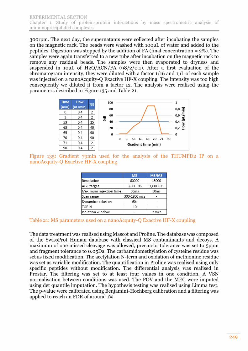
EXPERIMENTAL SECTION Chapter 1: Study of protein-protein interactions by mass spectrometric analysis of immunoprecipitated complexes
249
300rpm. The next day, the supernatants were collected after incubating the samples on the magnetic rack. The beads were washed with 100µL of water and added to the peptides. Digestion was stopped by the addition of FA (final concentration = 2%). The samples were again transferred to a new tube after incubation on the magnetic rack to remove any residual beads. The samples were then evaporated to dryness and suspended in 10µL of H2O/ACN/FA (98/2/0.1). After a first evaluation of the chromatogram intensity, they were diluted with a factor 1/16 and 1µL of each sample was injected on a nanoAcquity-Q Exactive HF-X coupling. The intensity was too high consequently we diluted it from a factor 12. The analysis were realised using the parameters described in Figure 135 and Table 21.
Figure 135: Gradient 79min used for the analysis of the THUMPD2 IP on a nanoAcquity-Q Exactive HF-X coupling
Table 21: MS parameters used on a nanoAcquity-Q Exactive HF-X coupling
The data treatment was realised using Mascot and Proline. The database was composed of the SwissProt Human database with classical MS contaminants and decoys. A maximum of one missed cleavage was allowed, precursor tolerance was set to 5ppm and fragment tolerance to 0.05Da. The carbamidomethylation of cysteine residue was set as fixed modification. The acetylation N-term and oxidation of methionine residue was set as variable modification. The quantification in Proline was realised using only specific peptides without modification. The differential analysis was realised in Prostar. The filtering was set to at least four values in one condition. A VSN normalisation between conditions was used. The POV and the MEC were imputed using det quantile imputation. The hypothesis testing was realised using Limma test. The p-value were calibrated using Benjamini-Hochberg calibration and a filtering was applied to reach an FDR of around 1%.
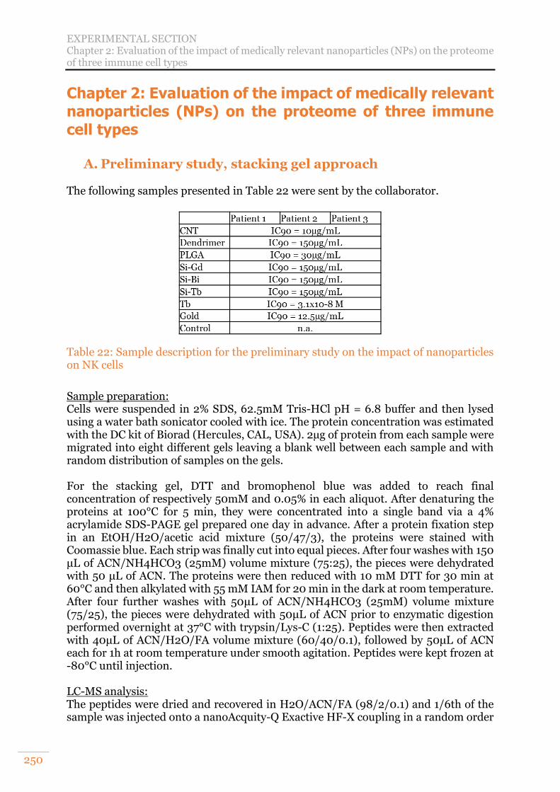
EXPERIMENTAL SECTION Chapter 2: Evaluation of the impact of medically relevant nanoparticles (NPs) on the proteome of three immune cell types
250
Chapter 2: Evaluation of the impact of medically relevant nanoparticles (NPs) on the proteome of three immune cell types
A. Preliminary study, stacking gel approach The following samples presented in Table 22 were sent by the collaborator.
Table 22: Sample description for the preliminary study on the impact of nanoparticles on NK cells
Sample preparation: Cells were suspended in 2% SDS, 62.5mM Tris-HCl pH = 6.8 buffer and then lysed using a water bath sonicator cooled with ice. The protein concentration was estimated with the DC kit of Biorad (Hercules, CAL, USA). 2µg of protein from each sample were migrated into eight different gels leaving a blank well between each sample and with random distribution of samples on the gels. For the stacking gel, DTT and bromophenol blue was added to reach final concentration of respectively 50mM and 0.05% in each aliquot. After denaturing the proteins at 100°C for 5 min, they were concentrated into a single band via a 4% acrylamide SDS-PAGE gel prepared one day in advance. After a protein fixation step in an EtOH/H2O/acetic acid mixture (50/47/3), the proteins were stained with Coomassie blue. Each strip was finally cut into equal pieces. After four washes with 150 μL of ACN/NH4HCO3 (25mM) volume mixture (75:25), the pieces were dehydrated with 50 μL of ACN. The proteins were then reduced with 10 mM DTT for 30 min at 60°C and then alkylated with 55 mM IAM for 20 min in the dark at room temperature. After four further washes with 50μL of ACN/NH4HCO3 (25mM) volume mixture (75/25), the pieces were dehydrated with 50μL of ACN prior to enzymatic digestion performed overnight at 37°C with trypsin/Lys-C (1:25). Peptides were then extracted with 40μL of ACN/H2O/FA volume mixture (60/40/0.1), followed by 50μL of ACN each for 1h at room temperature under smooth agitation. Peptides were kept frozen at -80°C until injection. LC-MS analysis: The peptides were dried and recovered in H2O/ACN/FA (98/2/0.1) and 1/6th of the sample was injected onto a nanoAcquity-Q Exactive HF-X coupling in a random order
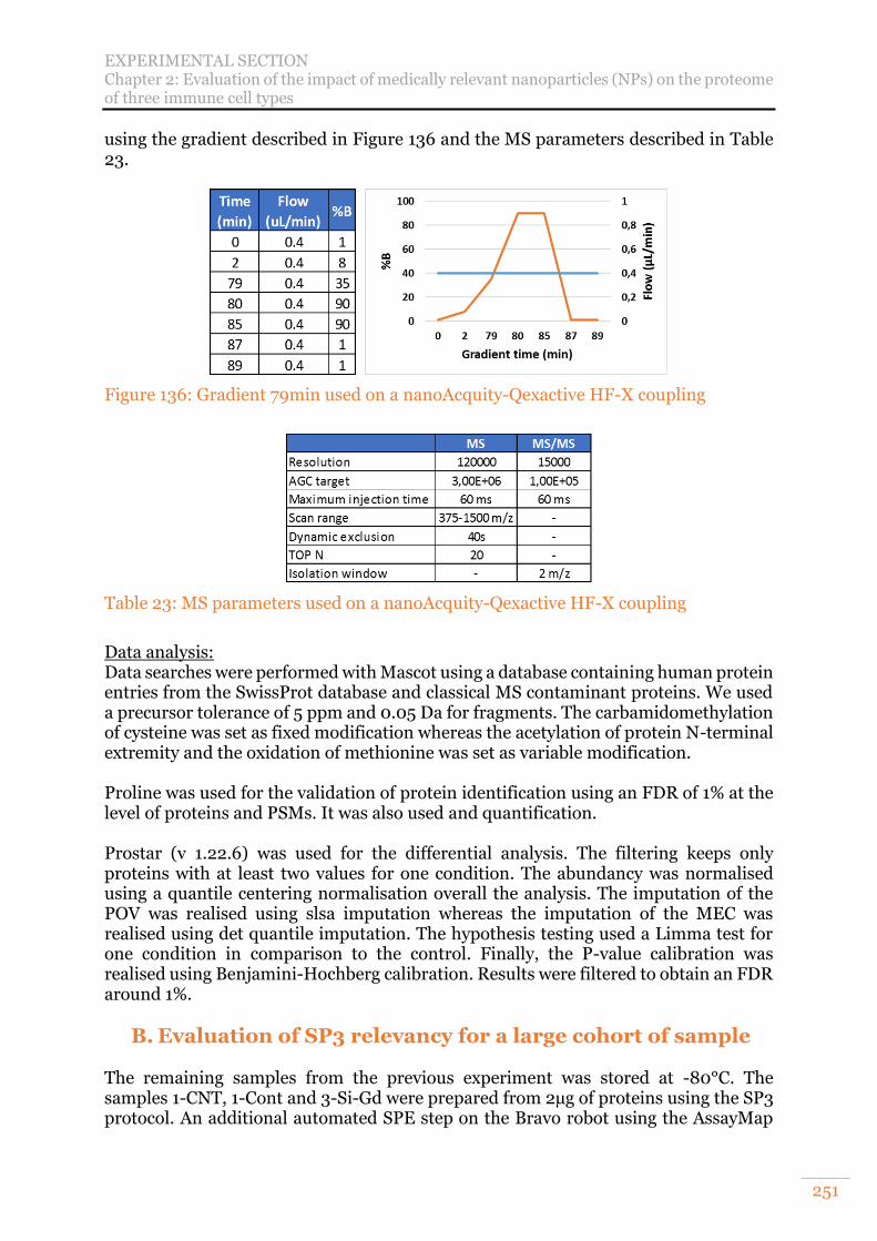
EXPERIMENTAL SECTION Chapter 2: Evaluation of the impact of medically relevant nanoparticles (NPs) on the proteome of three immune cell types
251
using the gradient described in Figure 136 and the MS parameters described in Table 23.
Figure 136: Gradient 79min used on a nanoAcquity-Qexactive HF-X coupling
Table 23: MS parameters used on a nanoAcquity-Qexactive HF-X coupling
Data analysis: Data searches were performed with Mascot using a database containing human protein entries from the SwissProt database and classical MS contaminant proteins. We used a precursor tolerance of 5 ppm and 0.05 Da for fragments. The carbamidomethylation of cysteine was set as fixed modification whereas the acetylation of protein N-terminal extremity and the oxidation of methionine was set as variable modification. Proline was used for the validation of protein identification using an FDR of 1% at the level of proteins and PSMs. It was also used and quantification. Prostar (v 1.22.6) was used for the differential analysis. The filtering keeps only proteins with at least two values for one condition. The abundancy was normalised using a quantile centering normalisation overall the analysis. The imputation of the POV was realised using slsa imputation whereas the imputation of the MEC was realised using det quantile imputation. The hypothesis testing used a Limma test for one condition in comparison to the control. Finally, the P-value calibration was realised using Benjamini-Hochberg calibration. Results were filtered to obtain an FDR around 1%.
B. Evaluation of SP3 relevancy for a large cohort of sample The remaining samples from the previous experiment was stored at -80°C. The samples 1-CNT, 1-Cont and 3-Si-Gd were prepared from 2µg of proteins using the SP3 protocol. An additional automated SPE step on the Bravo robot using the AssayMap
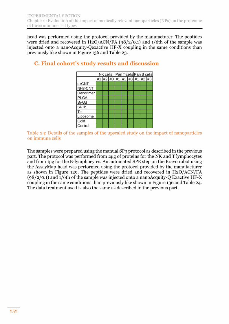
EXPERIMENTAL SECTION Chapter 2: Evaluation of the impact of medically relevant nanoparticles (NPs) on the proteome of three immune cell types
252
head was performed using the protocol provided by the manufacturer. The peptides were dried and recovered in H2O/ACN/FA (98/2/0.1) and 1/6th of the sample was injected onto a nanoAcquity-Qexactive HF-X coupling in the same conditions than previously like shown in Figure 136 and Table 23.
C. Final cohort’s study results and discussion
Table 24: Details of the samples of the upscaled study on the impact of nanoparticles on immune cells
The samples were prepared using the manual SP3 protocol as described in the previous part. The protocol was performed from 2µg of proteins for the NK and T lymphocytes and from 1µg for the B-lymphocytes. An automated SPE step on the Bravo robot using the AssayMap head was performed using the protocol provided by the manufacturer as shown in Figure 129. The peptides were dried and recovered in H2O/ACN/FA (98/2/0.1) and 1/6th of the sample was injected onto a nanoAcquity-Q Exactive HF-X coupling in the same conditions than previously like shown in Figure 136 and Table 24. The data treatment used is also the same as described in the previous part.
#1 #2 #3 #1 #2 #3 #1 #2 #3
oxCNT
NH3-CNT
Dendrimer
PLGA
Si-Gd
Si-Tb
Tb
Liposome
Gold
Control
NK cells Pan T cells Pan B cells
REFERENCES
253
REFERENCES
(1) Zecha, J.; Lee, C. Y.; Bayer, F. P.; Meng, C.; Grass, V.; Zerweck, J.; Schnatbaum, K.; Michler, T.; Pichlmair, A.; Ludwig, C.; Kuster, B. Data, Reagents, Assays and Merits of Proteomics for SARS-CoV-2 Research and Testing. Mol. Cell. Proteomics 2020, 19 (9), 1503–1522. https://doi.org/10.1074/mcp.RA120.002164.
(2) Müller, T.; Kalxdorf, M.; Longuespée, R.; Kazdal, D. N.; Stenzinger, A.; Krijgsveld, J. Automated Sample Preparation with SP 3 for Low‐input Clinical Proteomics . Mol. Syst. Biol. 2020, 16 (1), 1–19. https://doi.org/10.15252/msb.20199111.
(3) Lu, X.; Zhu, H. Tube-Gel Digestion: A Novel Proteomic Approach for High-Throughput Analysis of Membrane Proteins. Mol. Cell. Proteomics 2007, 4 (12), 1948–1958.
(4) Muller, L.; Fornecker, L.; Dorsselaer, A. Van; Cianférani, S.; Carapito, C. Benchmarking Sample Preparation / Digestion Protocols Reveals Tube-Gel Being a Fast and Repeatable Method for Quantitative Proteomics. Proteomics 2016, 16, 2953–2961. https://doi.org/10.1002/pmic.201600288.
(5) Zougman, A.; Selby, P. J.; Banks, R. E. Suspension Trapping (STrap) Sample Preparation Method for Bottom-up Proteomics Analysis. Proteomics 2014, 14 (9), 1006–1000. https://doi.org/10.1002/pmic.201300553.
(6) Hughes, C. S.; Foehr, S.; Garfield, D. A.; Furlong, E. E.; Steinmetz, L. M.; Krijgsveld, J. Ultrasensitive Proteome Analysis Using Paramagnetic Bead Technology. Mol. Syst. Biol. 2014, 10 (10), 757. https://doi.org/10.15252/msb.20145625.
(7) Muller, L.; Fornecker, L.; Chion, M.; Van Dorsselaer, A.; Cianférani, S.; Rabilloud, T.; Carapito, C. Extended Investigation of Tube-Gel Sample Preparation: A Versatile and Simple Choice for High Throughput Quantitative Proteomics. Sci. Rep. 2018, 8 (1), 1–9. https://doi.org/10.1038/s41598-018-26600-4.
(8) Meier, F.; Brunner, A.; Koch, S.; Koch, H.; Lubeck, M.; Krause, M.; Goedecke, N.; Decker, J.; Kosinski, T.; Park, M. A.; Hoerning, O.; Cox, J.; Räther, O.; Mann, M.; Bache, N.; Hoerning, O.; Ra, O.; Mann, M.; Meier, F.; Brunner, A.; Koch, S.; Koch, H.; Lubeck, M.; Krause, M.; Goedecke, N.; Decker, J.; Kosinski, T.; Park, M. A.; Bache, N.; Hoerning, O.; Ra, O.; Mann, M.; Cox, J.; Räther, O.; Mann, M.; Bache, N.; Hoerning, O.; Ra, O.; Mann, M.; Meier, F.; Brunner, A.; Koch, S.; Koch, H.; Lubeck, M.; Krause, M.; Goedecke, N.; Decker, J.; Kosinski, T.; Park, M. A.; Bache, N.; Hoerning, O.; Ra, O.; Mann, M.; Cox, J.; Räther, O.; Mann, M.; Bache, N.; Hoerning, O.; Ra, O.; Mann, M.; Meier, F.; Brunner, A.; Koch, S.; Koch, H.; Lubeck, M.; Krause, M.; Goedecke, N.; Decker, J.; Kosinski, T.; Park, M. A.; Bache, N.; Hoerning, O.; Ra, O.; Mann, M. Online Parallel Accumulation – Serial Fragmentation ( PASEF ) with a Novel Trapped Ion Mobility Mass. Mol. Cell. Proteomics 2018, 17 (12), 2534–2545. https://doi.org/10.1074/mcp.TIR118.000900.
(9) Silveira, J. A.; Ridgeway, M. E.; Laukien, F. H.; Mann, M.; Park, M. A. Parallel Accumulation for 100% Duty Cycle Trapped Ion Mobility-Mass Spectrometry. Int. J. Mass Spectrom. 2017, 413, 168–175. https://doi.org/10.1016/j.ijms.2016.03.004.
(10) Meier, F.; Beck, S.; Grassl, N.; Lubeck, M.; Park, M. A.; Raether, O.; Mann, M. Parallel Accumulation-Serial Fragmentation (PASEF): Multiplying Sequencing Speed and Sensitivity by Synchronized Scans in a Trapped Ion Mobility Device. J. Proteome Res. 2015, 14 (12), 5378–5387. https://doi.org/10.1021/acs.jproteome.5b00932.
(11) Cox, J.; Mann, M. MaxQuant Enables High Peptide Identification Rates, Individualized p.p.b.-Range Mass Accuracies and Proteome-Wide Protein Quantification. Nat. Biotechnol. 2008, 26 (12), 1367–1372. https://doi.org/10.1038/nbt.1511.
(12) Prianichnikov, N.; Koch, H.; Koch, S.; Lubeck, M.; Heilig, R.; Brehmer, S.; Fischer, R.; Cox, J. J. J. J. J. J. J. J. J. J. J. MaxQuant Software for Ion Mobility Enhanced Shotgun Proteomics. Mol. Cell. Proteomics 2020, 19 (6), mcp.TIR119.001720. https://doi.org/10.1074/mcp.tir119.001720.
(13) Cox, J.; Hein, M. Y.; Luber, C. A.; Paron, I.; Nagaraj, N.; Mann, M. Accurate Proteome-Wide Label-Free Quantification by Delayed Normalization and Maximal Peptide Ratio Extraction, Termed MaxLFQ. Mol. Cell. Proteomics 2014, 13 (9), 2513–2526.
REFERENCES
254
https://doi.org/10.1074/mcp.M113.031591. (14) Cox, J.; Neuhauser, N.; Michalski, A.; Scheltema, R. A.; Olsen, J. V.; Mann, M.
Andromeda: A Peptide Search Engine Integrated into the MaxQuant Environment. J. Proteome Res. 2011, 10 (4), 1794–1805. https://doi.org/10.1021/pr101065j.
(15) Yu, F.; Haynes, S. E.; Teo, G. C.; Avtonomov, D. M.; Polasky, D. A.; Nesvizhskii, A. I.; HaynesGuo, S. E.; Teo, C.; Dmitry M. Avtonomov, Daniel A. Polasky1, Alexey I. Nesvizhskii1, 2*. Fast Quantitative Analysis of TimsTOF PASEF Data with MSFragger and IonQuant. Mol. Cell. Proteomics 2020, 19 (9), 1575–1585. https://doi.org/10.1074/mcp.TIR120.002048.
(16) Meier, F.; Brunner, A. D.; Frank, M.; Ha, A.; Bludau, I.; Voytik, E.; Kaspar-Schoenefeld, S.; Lubeck, M.; Raether, O.; Bache, N.; Aebersold, R.; Collins, B. C.; Röst, H. L.; Mann, M. DiaPASEF: Parallel Accumulation–Serial Fragmentation Combined with Data-Independent Acquisition. Nat. Methods 2020, 17 (12), 1229–1236. https://doi.org/10.1038/s41592-020-00998-0.
(17) Demichev, V.; Yu, F.; Teo, G. C.; Szyrwiel, L.; Rosenberger, G. A.; Nesvizhskii, A. I.; Ralser, M. High Sensitivity Dia-PASEF Proteomics with DIA-NN and FragPipe. bioRxiv 2021. https://doi.org/10.1101/2021.03.08.434385.
(18) Sinitcyn, P.; Hamzeiy, H.; Soto, F. S.; Itzhak, D.; Mccarthy, F.; Wichmann, C.; Steger, M.; Ohmayer, U.; Distler, U.; Kaspar-schoenefeld, S.; Prianichnikov, N.; Yılmaz, Ş.; Rudolph, J. D.; Tenzer, S.; Perez-riverol, Y.; Nagaraj, N.; Humphrey, S. J.; Cox, J. MaxDIA Enables Library-Based and Library-Free Data-Independent Acquisition Proteomics. Nat. Biotechnol. 2021. https://doi.org/10.1038/s41587-021-00968-7.
(19) Tyanova, S.; Temu, T.; Cox, J. The MaxQuant Computational Platform for Mass Spectrometry-Based Shotgun Proteomics. Nat. Protoc. 2016, 11 (12), 2301–2319. https://doi.org/10.1038/nprot.2016.136.
(20) Bouyssié, D.; Hesse, A.-M.; Mouton-Barbosa, E.; Rompais, M.; Macron, C.; Carapito, C.; Gonzalez de Peredo, A.; Couté, Y.; Dupierris, V.; Burel, A.; Menetrey, J.-P.; Kalaitzakis, A.; Poisat, J.; Romdhani, A.; Burlet-Schiltz, O.; Cianférani, S.; Garin, J.; Bruley, C. Proline: An Efficient and User-Friendly Software Suite for Large-Scale Proteomics. Bioinformatics 2020, 36 (10), 3148–3155. https://doi.org/10.1093/bioinformatics/btaa118.
(21) Timp, W.; Timp, G. Beyond Mass Spectrometry, the next Step in Proteomics. Sci. Adv. 2020, 6 (2), 1–17. https://doi.org/10.1126/sciadv.aax8978.
(22) Aebersold, R.; Agar, J. N.; Amster, I. J.; Baker, M. S.; Bertozzi, C. R.; Boja, E. S.; Costello, C. E.; Cravatt, B. F.; Fenselau, C.; Garcia, B. A.; Ge, Y.; Gunawardena, J.; Hendrickson, R. C.; Hergenrother, P. J.; Huber, C. G.; Ivanov, A. R.; Jensen, O. N.; Jewett, M. C.; Kelleher, N. L.; Kiessling, L. L.; Krogan, N. J.; Larsen, M. R.; Loo, J. A.; Ogorzalek Loo, R. R.; Lundberg, E.; Maccoss, M. J.; Mallick, P.; Mootha, V. K.; Mrksich, M.; Muir, T. W.; Patrie, S. M.; Pesavento, J. J.; Pitteri, S. J.; Rodriguez, H.; Saghatelian, A.; Sandoval, W.; Schlüter, H.; Sechi, S.; Slavoff, S. A.; Smith, L. M.; Snyder, M. P.; Thomas, P. M.; Uhlén, M.; Van Eyk, J. E.; Vidal, M.; Walt, D. R.; White, F. M.; Williams, E. R.; Wohlschlager, T.; Wysocki, V. H.; Yates, N. A.; Young, N. L.; Zhang, B. How Many Human Proteoforms Are There? Nat. Chem. Biol. 2018, 14 (3), 206–214. https://doi.org/10.1038/nchembio.2576.
(23) Zhang, Y.; Fonslow, B. R.; Shan, B.; Baek, M. C.; Yates, J. R. Protein Analysis by Shotgun/Bottom-up Proteomics. Chem. Rev. 2013, 113 (4), 2343–2394. https://doi.org/10.1021/cr3003533.
(24) Ponomarenko, E. A.; Poverennaya, E. V.; Ilgisonis, E. V.; Pyatnitskiy, M. A.; Kopylov, A. T.; Zgoda, V. G.; Lisitsa, A. V.; Archakov, A. I. The Size of the Human Proteome: The Width and Depth. Int. J. Anal. Chem. 2016, 2016. https://doi.org/10.1155/2016/7436849.
(25) Gerardus Johannes Mulder. Bulletin Des Sciences Physiques et Naturelles En Néerlande; 1838; p 111.
(26) Wilkins, M. R.; Pasquali, C.; Appel, R. D.; Ou, K.; Golaz, O.; Sanchez, J.-C.; Yan, J. X.; Gooley, A. A.; Hughes, G.; Humphery-Smith, I.; Williams, K. L.; Hochstrasser, D. F.
REFERENCES
255
From Proteins to Proteomes: Large Scale Protein Identification by Two-Dimensional Electrophoresis and Amino Acid Analysis. Nat. Biotechnol. 1995, 14, 61–65.
(27) Rabilloud, T.; Lelong, C. Two-Dimensional Gel Electrophoresis in Proteomics: A Tutorial. J. Proteomics 2011, 74 (10), 1829–1841. https://doi.org/10.1016/j.jprot.2011.05.040.
(28) Aebersold, R.; Mann, M. Mass-Spectrometric Exploration of Proteome Structure and Function. Nature 2016, 537 (7620), 347–355. https://doi.org/10.1038/nature19949.
(29) Zhang, Z.; Wu, S.; Stenoien, D. L.; Paša-Tolić, L. High-Throughput Proteomics. Annu. Rev. Anal. Chem. 2014, 7, 427–454. https://doi.org/10.1146/annurev-anchem-071213-020216.
(30) Steen, H.; Mann, M. The ABC’s (and XYZ’s) of Peptide Sequencing. Nat. Rev. Mol. Cell Biol. 2004, 5, 699–711. https://doi.org/10.1038/nmr1468.
(31) Muntel, J.; Gandhi, T.; Verbeke, L.; Bernhardt, O. M.; Treiber, T.; Bruderer, R.; Reiter, L. Surpassing 10 000 Identified and Quantified Proteins in a Single Run by Optimizing Current LC-MS Instrumentation and Data Analysis Strategy. Mol. Omi. 2019, 15 (5), 348–360. https://doi.org/10.1039/c9mo00082h.
(32) Aslam, B.; Basit, M.; Nisar, M. A.; Khurshid, M.; Rasool, M. H. Proteomics: Technologies and Their Applications. J. Chromatogr. Sci. 2017, 55 (2), 182–196. https://doi.org/10.1093/chromsci/bmw167.
(33) Tanaka, K.; Waki, H.; Ido, Y.; Akita, S.; Yoshida, Y.; Yoshida, T.; Matsuo, T. Protein and Polymer Analyses up to m/z 100 000 by Laser Ionization Time‐of‐flight Mass Spectrometry. Rapid Commun. Mass Spectrom. 1988, 2 (8), 151–153. https://doi.org/10.1002/rcm.1290020802.
(34) Fenn, J. B.; Mann, M.; Meng, C. K.; Wong, S. F.; Whitehouse, C. M. Electrospray Ionization for Mass Spectrometry of Large Biomolecules. Science. 1989, pp 64–71. https://doi.org/10.1126/science.2675315.
(35) Fenn, J. B.; Mann, M.; Meng, C. K.; Wong, S. F.; Whitehouse, C. M. Electrospray Ionization–Principles and Practice. Mass Spectrom. Rev. 1990, 9 (1), 37–70. https://doi.org/10.1002/mas.1280090103.
(36) Li, H.; Han, J.; Pan, J.; Liu, T.; Parker, C. E.; Borchers, C. H. Current Trends in Quantitative Proteomics – an Update. J. Mass Spectrom. 2017, 52 (5), 319–341. https://doi.org/10.1002/jms.3932.
(37) Gillet, L. C.; Leitner, A.; Aebersold, R. Mass Spectrometry Applied to Bottom-Up Proteomics: Entering the High-Throughput Era for Hypothesis Testing. Annu. Rev. Anal. Chem. 2016, 9, 449–472. https://doi.org/10.1146/annurev-anchem-071015-041535.
(38) Patrie, S. M. Top-down Mass Spectrometry: Proteomics to Proteoforms. Adv. Exp. Med. Biol. 2016, 919, 171–200. https://doi.org/10.1007/978-3-319-41448-5_8.
(39) Toby, T. K.; Fornelli, L.; Kelleher, N. L.; Bonci, A.; Lupica, C. R.; Morales, M. Progress in Top-Down Proteomics and the Analysis of Proteoforms. Annu Rev Anal Chem 2016, 18 (3), 386–392. https://doi.org/10.1038/nn.3945.Dopaminergic.
(40) Cupp-Sutton, K. A.; Wu, S. High-Throughput Quantitative Top-down Proteomics. Mol. Omi. 2020, 16 (2), 91–99. https://doi.org/10.1039/c9mo00154a.
(41) LeDuc, R. D.; Fellers, R. T.; Early, B. P.; Greer, J. B.; Shams, D. P.; Thomas, P. M.; Kelleher, N. L. Accurate Estimation of Context-Dependent False Discovery Rates in Top-down Proteomics. Mol. Cell. Proteomics 2019, 18 (4), 796–805. https://doi.org/10.1074/mcp.RA118.000993.
(42) Ghezellou, P.; Garikapati, V.; Kazemi, S. M.; Strupat, K.; Ghassempour, A.; Spengler, B. A Perspective View of Top-down Proteomics in Snake Venom Research. Rapid Communications in Mass Spectrometry. 2019, pp 20–27. https://doi.org/10.1002/rcm.8255.
(43) McCool, E. N.; Lubeckyj, R. A.; Shen, X.; Chen, D.; Kou, Q.; Liu, X.; Sun, L. Deep Top-Down Proteomics Using Capillary Zone Electrophoresis-Tandem Mass Spectrometry: Identification of 5700 Proteoforms from the Escherichia Coli Proteome. Anal. Chem. 2018, 90 (9), 5529–5533. https://doi.org/10.1021/acs.analchem.8b00693.

REFERENCES
256
(44) Catherman, A. D.; Durbin, K. R.; Ahl, D. R.; Early, B. P.; Fellers, R. T.; Tran, J. C.; Thomas, P. M.; Kelleher, N. L. Large-Scale Top-down Proteomics of the Human Proteome: Membrane Proteins, Mitochondria, and Senescence. Mol. Cell. Proteomics 2013, 12 (12), 3465–3473. https://doi.org/10.1074/mcp.M113.030114.
(45) Melani, R. D.; Srzentić, K.; Gerbasi, V. R.; McGee, J. P.; Huguet, R.; Fornelli, L.; Kelleher, N. L. Direct Measurement of Light and Heavy Antibody Chains Using Ion Mobility and Middle-down Mass Spectrometry. MAbs 2019, 11 (8), 1351–1357. https://doi.org/10.1080/19420862.2019.1668226.
(46) Swaney, D. L.; Wenger, C. D.; Coon, J. J. Value of Using Multiple Proteases for Large-Scale Mass Spectrometry-Based Proteomics. J. Proteome Res. 2010, 9 (3), 1323–1329. https://doi.org/10.1021/pr900863u.
(47) Giansanti, P.; Tsiatsiani, L.; Low, T. Y.; Heck, A. J. R. Six Alternative Proteases for Mass Spectrometry-Based Proteomics beyond Trypsin. Nat. Protoc. 2016, 11 (5), 993–1006. https://doi.org/10.1038/nprot.2016.057.
(48) Hakobyan, A.; Schneider, M. B.; Liesack, W.; Glatter, T. Efficient Tandem LysC/Trypsin Digestion in Detergent Conditions. Proteomics 2019, 19 (20), 1–6. https://doi.org/10.1002/pmic.201900136.
(49) Nesvizhskii, A. I.; Aebersold, R. Interpretation of Shotgun Proteomic Data. Mol. Cell. Proteomics 2005, 4 (10), 1419–1440. https://doi.org/10.1074/mcp.r500012-mcp200.
(50) Audain, E.; Uszkoreit, J.; Sachsenberg, T.; Pfeuffer, J.; Liang, X.; Hermjakob, H.; Sanchez, A.; Eisenacher, M.; Reinert, K.; Tabb, D. L.; Kohlbacher, O.; Perez-Riverol, Y. In-Depth Analysis of Protein Inference Algorithms Using Multiple Search Engines and Well-Defined Metrics. J. Proteomics 2017, 150, 170–182. https://doi.org/10.1016/j.jprot.2016.08.002.
(51) Huang, E. L.; Piehowski, P. D.; Orton, D. J.; Moore, R. J.; Qian, W. J.; Casey, C. P.; Sun, X.; Dey, S. K.; Burnum-Johnson, K. E.; Smith, R. D. Snapp: Simplified Nanoproteomics Platform for Reproducible Global Proteomic Analysis of Nanogram Protein Quantities. Endocrinology 2016, 157 (3), 1307–1314. https://doi.org/10.1210/en.2015-1821.
(52) Zhu, Y.; Piehowski, P. D.; Kelly, R. T.; Qian, W.-J. J. Nanoproteomics Comes of Age. Expert Rev. Proteomics 2018, 15 (11), 865–871. https://doi.org/10.1080/14789450.2018.1537787.
(53) Kelly, R. T. Single-Cell Proteomics: Progress and Prospects. Mol. Cell. Proteomics 2020, 19 (11), 1739–1748. https://doi.org/10.1074/mcp.R120.002234.
(54) Specht, H.; Slavov, N. Transformative Opportunities for Single-Cell Proteomics. J. Proteome Res. 2018, acs.jproteome.8b00257. https://doi.org/10.1021/acs.jproteome.8b00257.
(55) Bose, U.; Wijffels, G.; Howitt, C. A.; Colgrave, M. L. Proteomics: Tools of the Trade. Adv. Exp. Med. Biol. 2019, 1073, 1–22. https://doi.org/10.1007/978-3-030-12298-0_1.
(56) Feist, P.; Hummon, A. B. Proteomic Challenges: Sample Preparation Techniques for Microgram-Quantity Protein Analysis from Biological Samples. Int. J. Mol. Sci. 2015, 16 (2), 3537–3563. https://doi.org/10.3390/ijms16023537.
(57) Tubaon, R. M.; Haddad, P. R.; Quirino, J. P. Sample Clean-up Strategies for ESI Mass Spectrometry Applications in Bottom-up Proteomics: Trends from 2012 to 2016. Proteomics 2017, 17 (20), 1–27. https://doi.org/10.1002/pmic.201700011.
(58) Hughes, C. S.; Moggridge, S.; Müller, T.; Sorensen, P. H.; Morin, G. B.; Krijgsveld, J. Single-Pot, Solid-Phase-Enhanced Sample Preparation for Proteomics Experiments. Nat. Protoc. 2019, 14 (1), 68–85. https://doi.org/10.1038/s41596-018-0082-x.
(59) Dapic, I.; Uwugiaren, N.; Jansen, P. J.; Corthals, G. L. Fast and Simple Protocols for Mass Spectrometry-Based Proteomics of Small Fresh Frozen Uterine Tissue Sections. Anal. Chem. 2017, 89 (20), 10769–10775. https://doi.org/10.1021/acs.analchem.7b01937.
(60) Shevchenko, G.; Musunuri, S.; Wetterhall, M.; Bergquist, J. Comparison of Extraction Methods for the Comprehensive Analysis of Mouse Brain Proteome Using Shotgun-Based Mass Spectrometry. J. Proteome Res. 2012, 11 (4), 2441–2451. https://doi.org/10.1021/pr201169q.
REFERENCES
257
(61) Islam, M. S.; Aryasomayajula, A.; Selvaganapathy, P. R. A Review on Macroscale and Microscale Cell Lysis Methods. Micromachines 2017, 8 (3). https://doi.org/10.3390/mi8030083.
(62) Pchelintsev, N. A.; Adams, P. D.; Nelson, D. M. Critical Parameters for Efficient Sonication and Improved Chromatin Immunoprecipitation of High Molecular Weight Proteins. PLoS One 2016, 11 (1), 1–11. https://doi.org/10.1371/journal.pone.0148023.
(63) Yusof, N. S. M.; Babgi, B.; Alghamdi, Y.; Aksu, M.; Madhavan, J.; Ashokkumar, M. Physical and Chemical Effects of Acoustic Cavitation in Selected Ultrasonic Cleaning Applications. Ultrason. Sonochem. 2016, 29, 568–576. https://doi.org/10.1016/j.ultsonch.2015.06.013.
(64) Zhang, X. Detergents: Friends Not Foes for High-Performance Membrane Proteomics toward Precision Medicine. Proteomics 2017, 17 (3–4), 3–4. https://doi.org/10.1002/pmic.201600209.
(65) Wang, W. Q.; Jensen, O. N.; Møller, I. M.; Hebelstrup, K. H.; Rogowska-Wrzesinska, A. Evaluation of Sample Preparation Methods for Mass Spectrometry-Based Proteomic Analysis of Barley Leaves. Plant Methods 2018, 14 (1), 1–13. https://doi.org/10.1186/s13007-018-0341-4.
(66) Tanca, A.; Biosa, G.; Pagnozzi, D.; Addis, M. F.; Uzzau, S. Comparison of Detergent-Based Sample Preparation Workflows for LTQ-Orbitrap Analysis of the Escherichia Coli Proteome. Proteomics 2013, 13 (17), 2597–2607. https://doi.org/10.1002/pmic.201200478.
(67) Aballo, T. J.; Roberts, D. S.; Melby, J. A.; Buck, K. M.; Brown, K. A.; Ge, Y. Ultrafast and Reproducible Proteomics from Small Amounts of Heart Tissue Enabled by Azo and TimsTOF Pro. J. Proteome Res. 2021, 20 (8), 4203–4211. https://doi.org/10.1021/acs.jproteome.1c00446.
(68) Doellinger, J.; Schneider, A.; Hoeller, M.; Lasch, P. Sample Preparation by Easy Extraction and Digestion (SPEED) - A Universal, Rapid, and Detergent-Free Protocol for Proteomics Based on Acid Extraction. Mol. Cell. Proteomics 2020, 19 (1), 209–222. https://doi.org/10.1074/mcp.TIR119.001616.
(69) Zubarev, R. A. The Challenge of the Proteome Dynamic Range and Its Implications for In-Depth Proteomics. Proteomics. 2013, pp 723–726. https://doi.org/10.1002/pmic.201200451.
(70) Wu, L.; Han, D. K. Overcoming the Dynamic Range Problem in Mass Spectrometry-Based Shotgun Proteomics. Expert Rev. Proteomics 2006, 3 (6), 611–619. https://doi.org/10.1586/14789450.3.6.611.
(71) Wang, D.; Eraslan, B.; Wieland, T.; Hallström, B.; Hopf, T.; Zolg, D. P.; Zecha, J.; Asplund, A.; Li, L.; Meng, C.; Frejno, M.; Schmidt, T.; Schnatbaum, K.; Wilhelm, M.; Ponten, F.; Uhlen, M.; Gagneur, J.; Hahne, H.; Kuster, B. A Deep Proteome and Transcriptome Abundance Atlas of 29 Healthy Human Tissues. Mol. Syst. Biol. 2019, 15 (2). https://doi.org/10.15252/msb.20188503.
(72) Channaveerappa, D.; Ngounou Wetie, A. G.; Darie, C. C. Bottlenecks in Proteomics: An Update. Adv. Exp. Med. Biol. 2019, 1140, 753–769. https://doi.org/10.1007/978-3-030-15950-4_45.
(73) Gstaiger, M.; Aebersold, R. Applying Mass Spectrometry-Based Proteomics to Genetics, Genomics and Network Biology. Nat. Rev. Genet. 2009, 10 (9), 617–627. https://doi.org/10.1038/nrg2633.
(74) Zougman, A.; Wilson, J. P.; Banks, R. E. A Simple Serum Depletion Method for Proteomics Analysis. Biotechniques 2020, 69 (2), 149–152. https://doi.org/10.2144/BTN-2020-0017.
(75) Gianazza, E.; Miller, I.; Palazzolo, L.; Parravicini, C.; Eberini, I. With or without You - Proteomics with or without Major Plasma/Serum Proteins. J. Proteomics 2016, 140, 62–80. https://doi.org/10.1016/j.jprot.2016.04.002.
(76) Kulak, N. A.; Geyer, P. E.; Mann, M. Loss-Less Nano-Fractionator for High Sensitivity, High Coverage Proteomics. Mol. Cell. Proteomics 2017, 16 (4), 694–705. https://doi.org/10.1074/mcp.O116.065136.
REFERENCES
258
(77) Camerini, S.; Mauri, P. The Role of Protein and Peptide Separation before Mass Spectrometry Analysis in Clinical Proteomics. J. Chromatogr. A 2015, 1381, 1–12. https://doi.org/10.1016/j.chroma.2014.12.035.
(78) Salvato, F.; Gallo de Carvalho, M. C. da C.; Lima Leite, A. de. Strategies for Protein Separation. Integr. Proteomics 2012, No. July 2015. https://doi.org/10.5772/29363.
(79) Burkhart, J. M.; Schumbrutzki, C.; Wortelkamp, S.; Sickmann, A.; Zahedi, R. P. Systematic and Quantitative Comparison of Digest Efficiency and Specificity Reveals the Impact of Trypsin Quality on MS-Based Proteomics. J. Proteomics 2012, 75 (4), 1454–1462. https://doi.org/10.1016/j.jprot.2011.11.016.
(80) Tabb, D. L.; Huang, Y.; Wysocki, V. H.; Yates, J. R. Influence of Basic Residue Content on Fragment Ion Peak Intensities in Low-Energy Collision-Induced Dissociation Spectra of Peptides. Anal. Chem. 2004, 76 (5), 1243–1248. https://doi.org/10.1021/ac0351163.
(81) Wysocki, V. H.; Tsaprailis, G.; Smith, L. L.; Breci, L. A. Mobile and Localized Protons: A Framework for Understanding Peptide Dissociation. J. Mass Spectrom. 2000, 35 (12), 1399–1406. https://doi.org/10.1002/1096-9888(200012)35:12<1399::AID-JMS86>3.0.CO;2-R.
(82) Smith, R. L.; Shaw, E. Pseudotrypsin. J. Biol. Chem. 1969, 244 (17), 4704–4712. https://doi.org/10.1016/s0021-9258(18)93681-1.
(83) Perutka, Z.; Sebela, M. Pseudotrypsin: A Little-Known Trypsin Proteoform. Molecules 2018, 23 (2637), 1–14. https://doi.org/10.3390/molecules23102637.
(84) Niu, B.; Martinelli, M.; Jiao, Y.; Wang, C.; Cao, M.; Wang, J.; Meinke, E. Nonspecific Cleavages Arising from Reconstitution of Trypsin under Mildly Acidic Conditions. PLoS One 2020, 15 (7 July), 1–18. https://doi.org/10.1371/journal.pone.0236740.
(85) Shevchenko, A.; Tomas, H.; Havliš, J.; Olsen, J. V.; Mann, M. In-Gel Digestion for Mass Spectrometric Characterization of Proteins and Proteomes. Nat. Protoc. 2007, 1 (6), 2856–2860. https://doi.org/10.1038/nprot.2006.468.
(86) Morsa, D.; Baiwir, D.; La Rocca, R.; Zimmerman, T. A.; Hanozin, E.; Grifnée, E.; Longuespée, R.; Meuwis, M. A.; Smargiasso, N.; Pauw, E. De; Mazzucchelli, G. Multi-Enzymatic Limited Digestion: The Next-Generation Sequencing for Proteomics? J. Proteome Res. 2019, 18 (6), 2501–2513. https://doi.org/10.1021/acs.jproteome.9b00044.
(87) Tsiatsiani, L.; Heck, A. J. R. Proteomics beyond Trypsin. FEBS J. 2015, 282 (14), 2612–2626. https://doi.org/10.1111/febs.13287.
(88) Glatter, T.; Ludwig, C.; Ahrné, E.; Aebersold, R.; Heck, A. J. R.; Schmidt, A. Large-Scale Quantitative Assessment of Different in-Solution Protein Digestion Protocols Reveals Superior Cleavage Efficiency of Tandem Lys-C/Trypsin Proteolysis over Trypsin Digestion. J. Proteome Res. 2012, 11 (11), 5145–5156. https://doi.org/10.1021/pr300273g.
(89) Wiśniewski, J. R.; Zougman, A.; Nagaraj, N.; Mann, M. Universal Sample Preparation Method for Proteome Analysis. Nat. Methods 2009, 6 (5), 359–362. https://doi.org/10.1038/nmeth.1322.
(90) Yang, Y.; Anderson, E.; Zhang, S. Evaluation of Six Sample Preparation Procedures for Qualitative and Quantitative Proteomics Analysis of Milk Fat Globule Membrane. Electrophoresis 2018, 39 (18), 2332–2339. https://doi.org/10.1002/elps.201800042.
(91) Rogers, J. C.; Bomgarden, R. D. Sample Preparation for Mass Spectrometry-Based Proteomics; from Proteomes to Peptides. Adv. Exp. Med. Biol. 2016, 919, 43–62. https://doi.org/10.1007/978-3-319-41448-5_3.
(92) Medzihradszky, K. F. In-Solution Digestion of Proteins for Mass Spectrometry. Methods Enzymol. 2005, 405 (05), 50–65. https://doi.org/10.1016/S0076-6879(05)05003-2.
(93) Sielaff, M.; Kuharev, J.; Bohn, T.; Hahlbrock, J.; Bopp, T.; Tenzer, S.; Distler, U. Evaluation of FASP, SP3, and IST Protocols for Proteomic Sample Preparation in the Low Microgram Range. J. Proteome Res. 2017, 16 (11), 4060–4072. https://doi.org/10.1021/acs.jproteome.7b00433.
(94) Kulak, N. A.; Pichler, G.; Paron, I.; Nagaraj, N.; Mann, M. Minimal, Encapsulated
REFERENCES
259
Proteomic-Sample Processing Applied to Copy-Number Estimation in Eukaryotic Cells. Nat. Methods 2014, 11 (3), 319–324. https://doi.org/10.1038/nmeth.2834.
(95) Humbert, L. Extraction En Phase Solide (SPE) : Théorie et Applications. Ann. Toxicol. Anal. 2010, 22 (2), 61–68. https://doi.org/10.1051/ata/2010010.
(96) Candiano, G.; Bruschi, M.; Musante, L.; Santucci, L.; Ghiggeri, G. M.; Carnemolla, B.; Orecchia, P.; Zardi, L.; Righetti, P. G. Blue Silver: A Very Sensitive Colloidal Coomassie G-250 Staining for Proteome Analysis. Electrophoresis 2004, 25 (9), 1327–1333. https://doi.org/10.1002/elps.200305844.
(97) Ding, H.; Fazelinia, H.; Spruce, L. A.; Weiss, D. A.; Zderic, S. A.; Seeholzer, S. H. Urine Proteomics: Evaluation of Different Sample Preparation Workflows for Quantitative, Reproducible, and Improved Depth of Analysis. J. Proteome Res. 2020, 19 (4), 1857–1862. https://doi.org/10.1021/acs.jproteome.9b00772.
(98) Wiśniewski, J. R. Filter Aided Sample Preparation – A Tutorial. Anal. Chim. Acta 2019, 1090, 23–30. https://doi.org/10.1016/j.aca.2019.08.032.
(99) Lefeuvre, B.; Cantero, P.; Ehret-Sabatier, L.; Lenormand, C.; Barthel, C.; Po, C.; Parveen, N.; Grillon, A.; Jaulhac, B.; Boulanger, N. Effects of Topical Corticosteroids and Lidocaine on Borrelia Burgdorferi Sensu Lato in Mouse Skin: Potential Impact to Human Clinical Trials. Sci. Rep. 2020, 10 (1), 1–13. https://doi.org/10.1038/s41598-020-67440-5.
(100) Grosche, A.; Hauser, A.; Lepper, M. F.; Mayo, R.; Von Toerne, C.; Merl-Pham, J.; Hauck, S. M. The Proteome of Native Adult Müller Glial Cells from Murine Retina. Mol. Cell. Proteomics 2016, 15 (2), 462–480. https://doi.org/10.1074/mcp.M115.052183.
(101) Zhang, X.; Sadowski, P.; Punyadeera, C. Evaluation of Sample Preparation Methods for Label-Free Quantitative Profiling of Salivary Proteome. J. Proteomics 2020, 210 (September 2019), 103532. https://doi.org/10.1016/j.jprot.2019.103532.
(102) Ludwig, K. R.; Schroll, M. M.; Hummon, A. B. Comparison of In-Solution, FASP, and S-Trap Based Digestion Methods for Bottom-Up Proteomic Studies. J. Proteome Res. 2018, 17 (7), 2480–2490. https://doi.org/10.1021/acs.jproteome.8b00235.
(103) Hailemariam, M.; Eguez, R. V.; Singh, H.; Bekele, S.; Ameni, G.; Pieper, R.; Yu, Y. S-Trap, an Ultrafast Sample-Preparation Approach for Shotgun Proteomics. J. Proteome Res. 2018, 17 (9), 2917–2924. https://doi.org/10.1021/acs.jproteome.8b00505.
(104) Hayoun, K.; Gouveia, D.; Grenga, L.; Pible, O.; Armengaud, J.; Alpha-Bazin, B. Evaluation of Sample Preparation Methods for Fast Proteotyping of Microorganisms by Tandem Mass Spectrometry. Front. Microbiol. 2019, 10, 1–13. https://doi.org/10.3389/fmicb.2019.01985.
(105) Elinger, D.; Gabashvili, A.; Levin, Y. Suspension Trapping (S-Trap) Is Compatible with Typical Protein Extraction Buffers and Detergents for Bottom-Up Proteomics. J. Proteome Res. 2019, 18 (3), 1441–1445. https://doi.org/10.1021/acs.jproteome.8b00891.
(106) Zacchi, L. F.; Recinos, D. R.; Otte, E.; Aitken, C.; Hunt, T.; Sandford, V.; Lee, Y. Y.; Schulz, B. L.; Howard, C. B. S ‐ Trap Eliminates Cell Culture Media Polymeric Surfactants For. J. Proteome Res. 2020, 19, 2149–2158. https://doi.org/10.1021/acs.jproteome.0c00106.
(107) Nguyen, T. T. A.; Li, W.; Park, T. J.; Gong, L. W.; Cologna, S. M. Investigating Phosphorylation Patterns of the Ion Channel TRPM7 Using Multiple Extraction and Enrichment Techniques Reveals New Phosphosites. J. Am. Soc. Mass Spectrom. 2019, 30 (8), 1359–1367. https://doi.org/10.1007/s13361-019-02223-5.
(108) Swearingen, K. E.; Eng, J. K.; Shteynberg, D.; Vigdorovich, V.; Springer, T. A.; Mendoza, L.; Sather, D. N.; Deutsch, E. W.; Kappe, S. H. I.; Moritz, R. L. A Tandem Mass Spectrometry Sequence Database Search Method for Identification of O-Fucosylated Proteins by Mass Spectrometry. J. Proteome Res. 2019, 18 (2), 652–663. https://doi.org/10.1021/acs.jproteome.8b00638.
(109) Bettinger, J. Q.; Welle, K. A.; Hryhorenko, J. R.; Ghaemmaghami, S. Quantitative Analysis of in Vivo Methionine Oxidation of the Human Proteome. J. Proteome Res. 2020, 19 (2), 624–633. https://doi.org/10.1021/acs.jproteome.9b00505.

REFERENCES
260
(110) Kuras, M.; Woldmar, N.; Kim, Y.; Hefner, M.; Malm, J.; Moldvay, J. Proteomic Workflows for High-Quality Quantitative Proteome and Post-Translational Modification Analysis of Clinically Relevant Samples from Formalin-Fixed Paraffin-Embedded Archives. J. Proteome Res. 2021, 20 (1), 1027–1039. https://doi.org/10.1021/acs.jproteome.0c00850.
(111) Hutti, C. R.; Welle, K. A.; Hryhorenko, J. R.; Ghaemmaghami, S. Global Analysis of Protein Degradation in Prion Infected Cells. Sci. Rep. 2020, 10 (1), 1–13. https://doi.org/10.1038/s41598-020-67505-5.
(112) Peng, C.; Andersen, B.; Arshid, S.; Larsen, M. R.; Albergaria, H.; Lametsch, R.; Arneborg, N. Proteomics Insights into the Responses of Saccharomyces Cerevisiae during Mixed-Culture Alcoholic Fermentation with Lachancea Thermotolerans. FEMS Microbiol. Ecol. 2019, 95 (9). https://doi.org/10.1093/femsec/fiz126.
(113) Yu, Y.; O’Rourke, A.; Lin, Y. H.; Singh, H.; Eguez, R. V.; Beyhan, S.; Nelson, K. E. Predictive Signatures of 19 Antibiotic-Induced Escherichia Coli Proteomes. ACS Infect. Dis. 2020, 6 (8), 2120–2129. https://doi.org/10.1021/acsinfecdis.0c00196.
(114) Gibbs, K. D.; Washington, E. J.; Jaslow, S. L.; Bourgeois, J. S.; Foster, M. W.; Guo, R.; Brennan, R. G.; Ko, D. C. The Salmonella Secreted Effector SarA/SteE Mimics Cytokine Receptor Signaling to Activate STAT3. Cell Host Microbe 2020, 27 (1), 129-139.e4. https://doi.org/10.1016/j.chom.2019.11.012.
(115) Arredondo, S. A.; Swearingen, K. E.; Martinson, T.; Steel, R.; Dankwa, D. A.; Harupa, A.; Camargo, N.; Betz, W.; Vigdorovich, V.; Oliver, B. G.; Kangwanrangsan, N.; Ishino, T.; Sather, N.; Mikolajczak, S.; Vaughan, A. M.; Torii, M.; Moritz, R. L.; Kappe, S. H. I. The Micronemal Plasmodium Proteins P36 and P52 Act in Concert to Establish the Replication-Permissive Compartment Within Infected Hepatocytes. Front. Cell. Infect. Microbiol. 2018, 8 (November), 413. https://doi.org/10.3389/fcimb.2018.00413.
(116) Parrine, D.; Wu, B. Sen; Muhammad, B.; Rivera, K.; Pappin, D.; Zhao, X.; Lefsrud, M. Proteome Modifications on Tomato under Extreme High Light Induced-Stress. Proteome Sci. 2018, 16 (1), 1–15. https://doi.org/10.1186/s12953-018-0148-2.
(117) Yang, S.; Li, H.; Bhatti, S.; Zhou, S.; Yang, Y.; Fish, T.; Thannhauser, T. W. The Al-Induced Proteomes of Epidermal and Outer Cortical Cells in Root Apex of Cherry Tomato ‘LA 2710.’ J. Proteomics 2020, 211 (April 2019), 103560. https://doi.org/10.1016/j.jprot.2019.103560.
(118) H, L.; Y, Z.; M, R.; X, W.; S, B.; S, Z.; Y, Y.; T, F.; TW, T. Identification of Heat-Induced Proteomes in Tomato Microspores Using LCM- Proteomics Analysis. Single Cell Biol. 2018, 07 (03). https://doi.org/10.4172/2168-9431.1000173.
(119) Bhagwat, A. R.; Le Sage, V.; Nturibi, E.; Kulej, K.; Jones, J.; Guo, M.; Tae Kim, E.; Garcia, B. A.; Weitzman, M. D.; Shroff, H.; Lakdawala, S. S. Quantitative Live Cell Imaging Reveals Influenza Virus Manipulation of Rab11A Transport through Reduced Dynein Association. Nat. Commun. 2020, 11 (1), 1–14. https://doi.org/10.1038/s41467-019-13838-3.
(120) Lum, K. K.; Howard, T. R.; Pan, C.; Cristeaa, I. M. Charge-Mediated Pyrin Oligomerization Nucleates Antiviral IFI16 Sensing of Herpesvirus DNA. MBio 2019, 10 (4), 1–16.
(121) Naamati, A.; Williamson, J. C.; Greenwood, E. J. D.; Marelli, S.; Lehner, P. J.; Matheson, N. J. Functional Proteomic Atlas of HIV Infection in Primary Human CD4+ T Cells. Elife 2019, 8, 1–27. https://doi.org/10.7554/eLife.41431.
(122) Ciordia, S.; Alvarez-Sola, G.; Rullán, M.; Urman, J. M.; Ávila, M. A.; Corrales, F. J. Digging Deeper into Bile Proteome. J. Proteomics 2021, 230 (103984). https://doi.org/10.1016/j.jprot.2020.103984.
(123) Chhuon, C.; Zhang, S. Y.; Jung, V.; Lewandowski, D.; Lipecka, J.; Pawlak, A.; Sahali, D.; Ollero, M.; Guerrera, I. C. A Sensitive S-Trap-Based Approach to the Analysis of T Cell Lipid Raft Proteome. J. Lipid Res. 2020, 61 (11), 1512–1523. https://doi.org/10.1194/jlr.D120000672.
(124) Christakopoulos, C.; Cehofski, L. J.; Christensen, S. R.; Vorum, H.; Honoré, B. Proteomics Reveals a Set of Highly Enriched Proteins in Epiretinal Membrane
REFERENCES
261
Compared with Inner Limiting Membrane. Exp. Eye Res. 2019, 186 (July), 107722. https://doi.org/10.1016/j.exer.2019.107722.
(125) Antelo-Varela, M.; Bartel, J.; Quesada-Ganuza, A.; Appel, K.; Bernal-Cabas, M.; Sura, T.; Otto, A.; Rasmussen, M.; Van Dijl, J. M.; Nielsen, A.; Maaß, S.; Becher, D. Ariadne’s Thread in the Analytical Labyrinth of Membrane Proteins: Integration of Targeted and Shotgun Proteomics for Global Absolute Quantification of Membrane Proteins. Anal. Chem. 2019, 91 (18), 11972–11980. https://doi.org/10.1021/acs.analchem.9b02869.
(126) Marchione, D. M.; Ilieva, I.; Devins, K.; Sharpe, D.; Pappin, D. J.; Garcia, B. A.; Wilson, J. P.; Wojcik, J. B. HYPERsol: High-Quality Data from Archival FFPE Tissue for Clinical Proteomics. J. Proteome Res. 2020, 19 (2), 973–983. https://doi.org/10.1021/acs.jproteome.9b00686.
(127) Ma, H.; Liao, H.; Dellisanti, W.; Sun, Y.; Chan, L. L.; Zhang, L. Characterizing the Host Coral Proteome of Platygyra Carnosa Using Suspension Trapping ( S-Trap ). J. Proteome Res. 2021, 20 (3), 1783–1791. https://doi.org/10.1021/acs.jproteome.0c00812.
(128) Guergues, J.; Zhang, P.; Liu, B.; Stevens, S. M. Improved Methodology for Sensitive and Rapid Quantitative Proteomic Analysis of Adult-Derived Mouse Microglia: Application to a Novel In Vitro Mouse Microglial Cell Model. Proteomics 2019, 19 (11), 1–5. https://doi.org/10.1002/pmic.201800469.
(129) St-Germain, J. R.; Astori, A.; Raught, B. A SARS-CoV-2 Peptide Spectral Library Enables Rapid, Sensitive Identification of Virus Peptides in Complex Biological Samples. J. Proteome Res. 2021, 20 (5), 2187–2194. https://doi.org/10.1021/acs.jproteome.1c00048.
(130) Sheller-Miller, S.; Radnaa, E.; Arita, Y.; Getahun, D.; Jones, R. J.; Peltier, M. R.; Menon, R. Environmental Pollutant Induced Cellular Injury Is Reflected in Exosomes from Placental Explants. Placenta 2020, 89 (July 2019), 42–49. https://doi.org/10.1016/j.placenta.2019.10.008.
(131) Sheller-Miller, S.; Trivedi, J.; Yellon, S. M.; Menon, R. Exosomes Cause Preterm Birth in Mice: Evidence for Paracrine Signaling in Pregnancy. Sci. Rep. 2019, 9 (1), 1–18. https://doi.org/10.1038/s41598-018-37002-x.
(132) van Oostrum, M.; Müller, M.; Klein, F.; Bruderer, R.; Zhang, H.; Pedrioli, P. G. A.; Reiter, L.; Tsapogas, P.; Rolink, A.; Wollscheid, B. Classification of Mouse B Cell Types Using Surfaceome Proteotype Maps. Nat. Commun. 2019, 10 (1), 1–9. https://doi.org/10.1038/s41467-019-13418-5.
(133) Miyazaki, Y.; Murayama, K.; Fathi, I.; Imura, T.; Yamagata, Y.; Watanabe, K.; Maeda, H.; Inagaki, A.; Igarashi, Y.; Miyagi, S.; Shima, H.; Igarashi, K.; Kamei, T.; Unno, M.; Goto, M. Strategy towards Tailored Donor Tissue-Specific Pancreatic Islet Isolation. PLoS One 2019, 14 (5), 1–14. https://doi.org/10.1371/journal.pone.0216136.
(134) Michailowsky, V.; Li, H.; Mittra, B.; Iyer, S. R.; Mazála, D. A. G.; Corrotte, M.; Wang, Y.; Chin, E. R.; Lovering, R. M.; Andrews, N. W. Defects in Sarcolemma Repair and Skeletal Muscle Function after Injury in a Mouse Model of Niemann-Pick Type A/B Disease. Skelet. Muscle 2019, 9 (1), 1–15. https://doi.org/10.1186/s13395-018-0187-5.
(135) Serebryany, E.; Yu, S.; Trauger, S. A.; Budnik, B.; Shakhnovich, E. I. Dynamic Disulfide Exchange in a Crystallin Protein in the Human Eye Lens Promotes Cataract-Associated Aggregation. J. Biol. Chem. 2018, 293 (46), 17997–18009. https://doi.org/10.1074/jbc.RA118.004551.
(136) Lopez, C. A.; Beavers, W. N.; Weiss, A.; Knippel, R. J.; Zackular, J. P.; Chazin, W. Difficile Metabolism through Zinc Limitation. MBio 2019, No. August, 1–19.
(137) Rezazadeh, S.; Yang, D.; Tombline, G.; Simon, M.; Regan, S. P.; Seluanov, A.; Gorbunova, V. SIRT6 Promotes Transcription of a Subset of NRF2 Targets by Mono-ADP-Ribosylating BAF170. Nucleic Acids Res. 2019, 47 (15), 7914–7928. https://doi.org/10.1093/nar/gkz528.
(138) Anderson, A. P.; Luo, X.; Russell, W.; Yin, Y. W. Oxidative Damage Diminishes Mitochondrial DNA Polymerase Replication Fidelity. Nucleic Acids Res. 2020, 48 (2), 817–829. https://doi.org/10.1093/nar/gkz1018.
REFERENCES
262
(139) Ma, L.; Herren, A. W.; Espinal, G.; Randol, J.; McLaughlin, B.; Martinez-Cerdeño, V.; Pessah, I. N.; Hagerman, R. J.; Hagerman, P. J. Composition of the Intranuclear Inclusions of Fragile X-Associated Tremor/Ataxia Syndrome. Acta Neuropathol. Commun. 2019, 7 (1), 1–26. https://doi.org/10.1186/s40478-019-0796-1.
(140) Agosto, L. M.; Gazzara, M. R.; Radens, C. M.; Sidoli, S.; Baeza, J.; Garcia, B. A.; Lynch, K. W. Deep Profiling and Custom Databases Improve Detection of Proteoforms Generated by Alternative Splicing. Genome Res. 2019, 29 (12), 2046–2055. https://doi.org/10.1101/gr.248435.119.
(141) Carabetta, V. J.; Greco, T. M.; Cristea, I. M.; Dubnau, D. YfmK Is an N e -Lysine Acetyltransferase That Directly Acetylates the Histone-like Protein HBsu in Bacillus Subtilis. Proc. Natl. Acad. Sci. U. S. A. 2019, 116 (9), 3752–3757. https://doi.org/10.1073/pnas.1815511116.
(142) Nkamba, I.; Mulet, C.; Dubey, G. P.; Gorgette, O.; Couesnon, A.; Salles, A.; Moya-Nilges, M.; Jung, V.; Gaboriau-Routhiau, V.; Guerrera, I. C.; Shima, T.; Umesaki, Y.; Nigro, G.; Krijnse-Locker, J.; Bérard, M.; Cerf-Bensussan, N.; Sansonetti, P. J.; Schnupf, P. Intracellular Offspring Released from SFB Filaments Are Flagellated. Nat. Microbiol. 2020, 5 (1), 34–39. https://doi.org/10.1038/s41564-019-0608-1.
(143) Eliash, N.; Thangarajan, S.; Goldenberg, I.; Sela, N.; Kupervaser, M.; Barlev, J.; Altman, Y.; Knyazer, A.; Kamer, Y.; Zaidman, I.; Rafaeli, A.; Soroker, V. Varroa Chemosensory Proteins: Some Are Conserved across Arthropoda but Others Are Arachnid Specific. Insect Mol. Biol. 2019, 28 (3), 321–341. https://doi.org/10.1111/imb.12553.
(144) Cremer, S. E.; Catalfamo, J. L.; Goggs, R.; Seemann, S. E.; Kristensen, A. T.; Brooks, M. B. Proteomic Profiling of the Thrombin-Activated Canine Platelet Secretome (CAPS). PLoS One 2019, 14 (11), 1–22. https://doi.org/10.1371/journal.pone.0224891.
(145) Rojas, A.; Baneth, G. Secretome of the Carcinogenic Helminth Spirocerca Lupi Reveals Specific Parasite Proteins Associated with Its Different Life Stages. Vet. Parasitol. 2019, 275 (September), 108935. https://doi.org/10.1016/j.vetpar.2019.108935.
(146) Dehghan, E.; Goodarzi, M.; Saremi, B.; Lin, R.; Mirzaei, H. Hydralazine Targets CAMP-Dependent Protein Kinase Leading to Sirtuin1/5 Activation and Lifespan Extension in C. Elegans. Nat. Commun. 2019, 10 (1). https://doi.org/10.1038/s41467-019-12425-w.
(147) Johnson, T.; Payne, S.; Grove, R.; McCarthy, S.; Oeltjen, E.; Mach, C.; Adamec, J.; Wilson, M. A.; Cott, K. Van; Blum, P. Methylation Deficiency of Chromatin Proteins Is a Non-Mutational and Epigenetic-like Trait in Evolved Lines of the Archaeon Sulfolobus Solfataricus. J. Biol. Chem. 2019, 294 (19), 7821–7832. https://doi.org/10.1074/jbc.RA118.006469.
(148) Even, A.; Morelli, G.; Broix, L.; Scaramuzzino, C.; Turchetto, S.; Gladwyn-Ng, I.; Le Bail, R.; Shilian, M.; Freeman, S.; Magiera, M. M.; Jijumon, A. S.; Krusy, N.; Malgrange, B.; Brone, B.; Dietrich, P.; Dragatsis, I.; Janke, C.; Saudou, F.; Weil, M.; Nguyen, L. ATAT1-Enriched Vesicles Promote Microtubule Acetylation via Axonal Transport. Sci. Adv. 2019, 5 (12). https://doi.org/10.1126/sciadv.aax2705.
(149) Bosserman, R. E.; Nicholson, K. R.; Champion, M. M.; Champion, P. A. A New ESX-1 Substrate in Mycobacterium Marinum That Is Required for Hemolysis but Not Host Cell Lysis. J. Bacteriol. 2019, 201 (14). https://doi.org/10.1128/JB.00760-18.
(150) Javitt, A.; Barnea, E.; Kramer, M. P.; Wolf-Levy, H.; Levin, Y.; Admon, A.; Merbl, Y. Pro-Inflammatory Cytokines Alter the Immunopeptidome Landscape by Modulation of HLA-B Expression. Front. Immunol. 2019, 10 (FEB), 1–16. https://doi.org/10.3389/fimmu.2019.00141.
(151) Moggridge, S.; Sorensen, P. H.; Morin, G. B.; Hughes, C. S. Extending the Compatibility of the SP3 Paramagnetic Bead Processing Approach for Proteomics. J. Proteome Res. 2018, 17 (4), 1730–1740. https://doi.org/10.1021/acs.jproteome.7b00913.
(152) Batth, T. S.; Tollenaere, M. A. X.; Rüther, P.; Gonzalez-Franquesa, A.; Prabhakar, B. S.; Bekker-Jensen, S.; Deshmukh, A. S.; Olsen, J. V. Protein Aggregation Capture on Microparticles Enables Multipurpose Proteomics Sample Preparation. Mol. Cell. Proteomics 2019, 18 (5), 1027–1035. https://doi.org/10.1074/mcp.TIR118.001270.
(153) Waas, M.; Pereckas, M.; Lipinski, R. A. J.; Ashwood, C.; Gundry, R. L. SP2: Rapid and
REFERENCES
263
Automatable Contaminant Removal from Peptide Samples for Proteomic Analyses. J. Proteome Res. 2019, 18 (4), 1644–1656. https://doi.org/10.1021/acs.jproteome.8b00916.
(154) Balotf, S.; Wilson, R.; Tegg, R. S.; Nichols, D. S.; Wilson, C. R. Optimisation of Sporosori Purification and Protein Extraction Techniques for the Biotrophic Protozoan Plant Pathogen Spongospora Subterranea. Molecules 2020, 25 (14). https://doi.org/10.3390/molecules25143109.
(155) Blankenburg, S.; Hentschker, C.; Nagel, A.; Hildebrandt, P.; Michalik, S.; Dittmar, D.; Surmann, K.; Völker, U. Improving Proteome Coverage for Small Sample Amounts: An Advanced Method for Proteomics Approaches with Low Bacterial Cell Numbers. Proteomics 2019, 19 (23), 1–7. https://doi.org/10.1002/pmic.201900192.
(156) Virant-Klun, I.; Leicht, S.; Hughes, C.; Krijgsveld, J. Identification of Maturation-Specific Proteins by Single-Cell Proteomics of Human Oocytes. Mol. Cell. Proteomics 2016, 15 (8), 2616–2627. https://doi.org/10.1074/mcp.M115.056887.
(157) Paulo, J. A.; Navarrete-Perea, J.; Gygi, S. P. Multiplexed Proteome Profiling of Carbon Source Perturbations in Two Yeast Species with SL-SP3-TMT. J. Proteomics 2020, 210 (July 2019), 103531. https://doi.org/10.1016/j.jprot.2019.103531.
(158) Navarrete-Perea, J.; Gygi, S. P.; Paulo, J. A. Growth Media Selection Alters the Proteome Profiles of Three Model Microorganisms. J. Proteomics 2021, 231 (September 2020), 104006. https://doi.org/10.1016/j.jprot.2020.104006.
(159) Osório, H.; Silva, C.; Ferreira, M.; Gullo, I.; Máximo, V.; Barros, R.; Mendonça, F.; Oliveira, C.; Carneiro, F. Proteomics Analysis of Gastric Cancer Patients with Diabetes Mellitus. J. Clin. Med. 2021, 10 (3), 407. https://doi.org/10.3390/jcm10030407.
(160) Griesser, E.; Wyatt, H.; Have, S. Ten; Stierstorfer, B.; Lenter, M.; Lamond, A. I. Quantitative Profiling of the Human Substantia Nigra Proteome from Laser-Capture Microdissected FFPE Tissue. Mol. Cell. Proteomics 2020, 19 (5), 839–851. https://doi.org/10.1074/mcp.RA119.001889.
(161) Mikulášek, K.; Konečná, H.; Potěšil, D.; Holánková, R.; Havliš, J.; Zdráhal, Z. SP3 Protocol for Proteomic Plant Sample Preparation Prior LC-MS/MS. Front. Plant Sci. 2021, 12 (March). https://doi.org/10.3389/fpls.2021.635550.
(162) Lampaki, D.; Diepold, A.; Glatter, T. A Serial Sample Processing Strategy with Improved Performance for In-Depth Quantitative Analysis of Type III Secretion Events in Pseudomonas Aeruginosa. J. Proteome Res. 2020, 19 (1), 543–553. https://doi.org/10.1021/acs.jproteome.9b00628.
(163) Hughes, C. S.; Mcconechy, M. K.; Cochrane, D. R.; Nazeran, T.; Karnezis, A. N.; Huntsman, D. G.; Morin, G. B. Quantitative Profiling of Single Formalin Fixed Tumour Sections: Proteomics for Translational Research. Sci. Rep. 2016, 6 (June), 1–14. https://doi.org/10.1038/srep34949.
(164) Cagnetta, R.; Frese, C. K.; Shigeoka, T.; Krijgsveld, J.; Holt, C. E. Rapid Cue-Specific Remodeling of the Nascent Axonal Proteome. Neuron 2018, 99 (1), 29-46.e4. https://doi.org/10.1016/j.neuron.2018.06.004.
(165) Chen, H.; Jin, J.; Zhang, H.; Wang, Y.; Li, Q.; Zou, Y.; Huang, X.; Zhou, B.; Zhou, R.; Ding, Y. Comparative Analysis of Proteomics and Transcriptomics during Fertility Transition in a Two-Line Hybrid Rice Line Wuxiang S. Int. J. Mol. Sci. 2019, 20 (18). https://doi.org/10.3390/ijms20184542.
(166) Gonzalez-Lozano, M. A.; Koopmans, F.; Paliukhovich, I.; Smit, A. B.; Li, K. W. A Fast and Economical Sample Preparation Protocol for Interaction Proteomics Analysis. Proteomics 2019, 19 (9), 3–5. https://doi.org/10.1002/pmic.201900027.
(167) Kaleja, P.; Emmert, H.; Gerstel, U.; Weidinger, S.; Tholey, A. Evaluation and Improvement of Protein Extraction Methods for Analysis of Skin Proteome by Noninvasive Tape Stripping. J. Proteomics 2020, 217 (February), 103678. https://doi.org/10.1016/j.jprot.2020.103678.
(168) Cleland, T. P. Human Bone Paleoproteomics Utilizing the Single-Pot, Solid-Phase-Enhanced Sample Preparation Method to Maximize Detected Proteins and Reduce Humics. J. Proteome Res. 2018, 17 (11), 3976–3983.
REFERENCES
264
https://doi.org/10.1021/acs.jproteome.8b00637. (169) Sakalauskaite, J.; Marin, F.; Pergolizzi, B.; Demarchi, B. Shell Palaeoproteomics: First
Application of Peptide Mass Fingerprinting for the Rapid Identification of Mollusc Shells in Archaeology. J. Proteomics 2020, 227 (July), 103920. https://doi.org/10.1016/j.jprot.2020.103920.
(170) Naihui, W.; Samantha, B.; Peter, D.; Sandra, H.; Maxim, K.; Sindy, L.; Oshan, W.; Stefano, G.; Michael, C.; Liora, H. K.; Matthew, S.; Glenn, S.; Michael, S.; Kristine, R. K.; Katerina, D. Testing the Efficacy and Comparability of ZooMS Protocols on Archaeological Bone. J. Proteomics 2021, 233 (December 2020), 104078. https://doi.org/10.1016/j.jprot.2020.104078.
(171) Leipert, J.; Tholey, A. Miniaturized Sample Preparation on a Digital Microfluidics Device for Sensitive Bottom-up Microproteomics of Mammalian Cells Using Magnetic Beads and Mass Spectrometry-Compatible Surfactants. Lab Chip 2019, 19 (20), 3490–3498. https://doi.org/10.1039/c9lc00715f.
(172) Deng, W.; Sha, J.; Plath, K.; Wohlschlegel, J. A. Carboxylate-Modified Magnetic Bead (CMMB)-Based Isopropanol Gradient Peptide Fractionation (CIF) Enables Rapid and Robust Off-Line Peptide Mixture Fractionation in Bottom-Up Proteomics. Mol. Cell. Proteomics 2021, 20, 100039. https://doi.org/10.1074/MCP.RA120.002411.
(173) Dagley, L. F.; Infusini, G.; Larsen, R. H.; Sandow, J. J.; Webb, A. I. Universal Solid-Phase Protein Preparation (USP3) for Bottom-up and Top-down Proteomics. J. Proteome Res. 2019, 18 (7), 2915–2924. https://doi.org/10.1021/acs.jproteome.9b00217.
(174) Yang, Z.; Shen, X.; Chen, D.; Sun, L. Toward a Universal Sample Preparation Method for Denaturing Top-Down Proteomics of Complex Proteomes. J. Proteome Res. 2020, 19 (8), 3315–3325. https://doi.org/10.1021/acs.jproteome.0c00226.
(175) Alexovič, M.; Urban, P. L.; Tabani, H.; Sabo, J. Recent Advances in Robotic Protein Sample Preparation for Clinical Analysis and Other Biomedical Applications. Clin. Chim. Acta 2020, 507 (April), 104–116. https://doi.org/10.1016/j.cca.2020.04.015.
(176) Alexovič, M.; Sabo, J.; Longuespée, R. Microproteomic Sample Preparation. Proteomics 2021, 21 (9), 1–16. https://doi.org/10.1002/pmic.202000318.
(177) Brunner, A.-D. D.; Thielert, M.; Vasilopoulou, C. G.; Ammar, C.; Coscia, F.; Mund, A.; Horning, O. B.; Bache, N.; Apalategui, A.; Lubeck, M.; Raether, O.; Park, M. A.; Richter, S.; Fischer, D. S.; Theis, F. J.; Meier, F.; Mann, M.; Hoerning, O. B.; Bache, N.; Apalategui, A.; Lubeck, M.; Richter, S.; Fischer, D. S.; Raether, O.; Park, M. A.; Meier, F.; Theis, F. J.; Mann, M. Ultra-High Sensitivity Mass Spectrometry Quantifies Single-Cell Proteome Changes upon Perturbation. bioRxiv 2020, 1–32. https://doi.org/10.1101/2020.12.22.423933.
(178) Yi, L.; Piehowski, P. D.; Shi, T.; Smith, R. D.; Qian, W. Advances in Microscale Separations towards Nanoproteomics Applications. J. Chromatogr. A 2017, 1523, 40–48. https://doi.org/10.1016/j.chroma.2017.07.055.Advances.
(179) Woo, J.; Williams, S. M.; Aguilera-vazquez, V.; Sontag, R. L.; Ronald, J.; Markillie, L. M.; Mehta, H. S.; Cantlon, J.; Adkins, J. N.; Smith, R. D.; Clair, G. C.; Pasa-tolic, L.; Zhu, Y.; States, U.; Ag, S.; Sasu, C.; Rockefeller, A.; Bioserra, B. High-Throughput and High-Efficiency Sample Preparation for Single-Cell Proteomics Using a Nested Nanowell Chip Environmental Molecular Sciences Laboratory , Pacific Northwest National Laboratory , Biological Sciences Division , Pacific Northwest National. bioRxiv 2021, 1–29.
(180) Williams, S. M.; Liyu, A. V.; Tsai, C. F.; Moore, R. J.; Orton, D. J.; Chrisler, W. B.; Gaffrey, M. J.; Liu, T.; Smith, R. D.; Kelly, R. T.; Pasa-Tolic, L.; Zhu, Y. Automated Coupling of Nanodroplet Sample Preparation with Liquid Chromatography-Mass Spectrometry for High-Throughput Single-Cell Proteomics. Anal. Chem. 2020, 92 (15), 10588–10596. https://doi.org/10.1021/acs.analchem.0c01551.
(181) Tsai, C. F.; Zhao, R.; Williams, S. M.; Moore, R. J.; Schultz, K.; Chrisler, W. B.; Pasa-Tolic, L.; Rodland, K. D.; Smith, R. D.; Shi, T.; Zhu, Y.; Liu, T. An Improved Boosting to Amplify Signal with Isobaric Labeling (IBASIL) Strategy for Precise Quantitative Single-Cell Proteomics. Mol. Cell. Proteomics 2020, 19 (5), 828–838.
REFERENCES
265
https://doi.org/10.1074/mcp.RA119.001857. (182) Hartlmayr, D.; Ctortecka, C.; Seth, A.; Mendjan, S.; Tourniaire, G.; Mechtler, K.;
Biocenter, V.; Ctortecka, C.; Mechtler, K. An Automated Workflow for Label-Free and Multiplexed Single Cell Proteomics Sample Preparation at Unprecedented Sensitivity. bioRxiv 2021, 1–17.
(183) Zhang, H.; Liu, C.; Hua, W.; Ghislain, L. P.; Liu, J.; Aschenbrenner, L.; Noell, S.; Dirico, K.; Lanyon, L. F.; Steppan, C. M.; Arnold, D. W.; Covey, T. R.; Datwani, S. S.; Troutman, M. D. Acoustic Ejection Mass Spectrometry for High-Throughput Analysis. bioRxiv 2020, No. March, 1–32. https://doi.org/10.1101/2020.01.28.923938.
(184) Fang Xie; Smith, R. D.; Shen, Y. Advanced Proteomic Liquid Chromatography. J. Chromatogr. A 2012, No. 1261, 78–90. https://doi.org/10.1016/j.chroma.2012.06.098.
(185) Bian, Y.; Zheng, R.; Bayer, F. P.; Wong, C.; Chang, Y. C.; Meng, C.; Zolg, D. P.; Reinecke, M.; Zecha, J.; Wiechmann, S.; Heinzlmeir, S.; Scherr, J.; Hemmer, B.; Baynham, M.; Gingras, A. C.; Boychenko, O.; Kuster, B. Robust, Reproducible and Quantitative Analysis of Thousands of Proteomes by Micro-Flow LC–MS/MS. Nat. Commun. 2020, 11 (1), 1–12. https://doi.org/10.1038/s41467-019-13973-x.
(186) Stadlmann, J.; Hudecz, O.; Krššáková, G.; Ctortecka, C.; Van Raemdonck, G.; Op De Beeck, J.; Desmet, G.; Penninger, J. M.; Jacobs, P.; Mechtler, K. Improved Sensitivity in Low-Input Proteomics Using Micropillar Array-Based Chromatography. Anal. Chem. 2019. https://doi.org/10.1021/acs.analchem.9b02899.
(187) Müller, J. B.; Geyer, P. E.; Colaço, A. R.; Treit, P. V.; Strauss, M. T.; Oroshi, M.; Doll, S.; Virreira Winter, S.; Bader, J. M.; Köhler, N.; Theis, F.; Santos, A.; Mann, M. The Proteome Landscape of the Kingdoms of Life. Nature 2020, 582 (7813), 592–596. https://doi.org/10.1038/s41586-020-2402-x.
(188) Karas, M.; Hillenkamp, F. Laser Desorption Ionization of Proteins with Molecular Masses Exceeding 10 000 Daltons. Anal. Chem. 1988, 60 (20), 2299–2301. https://doi.org/10.1021/ac00171a028.
(189) Karas, M.; Bahr, U. Matrix-Assisted Laser Desorption Ionization Mass Spectrometry. Mass Spectrom. Rev. 1992, 835117, 335–357.
(190) Cañas Montalvo, B.; López-Ferrer, D.; Ramos-Fernández, A.; Camafeita, E.; Calvo, E. Mass Spectrometry Technologies for Proteomics. Briefings Funct. Genomics Proteomics 2006, 4 (4), 295–320. https://doi.org/10.1093/bfgp/eli002.
(191) Wolff, M. M.; Stephens, W. E. A Pulsed Mass Spectrometer with Time Dispersion. Rev. Sci. Instrum. 1953, 24 (8), 616–617. https://doi.org/10.1063/1.1770801.
(192) Karas, M. Time-of-Flight Mass Spectrometer with Improved Resolution. J. Mass Spectrom. 1997, 32 (1), 1–11. https://doi.org/10.1002/(SICI)1096-9888(199701)32:1<1::AID-JMS467>3.0.CO;2-6.
(193) Hennequin, J.-F.; Inglebert, R.-L. Transmission d’un Filtre de Masse Quadrupolaire. Rev. Phys. appliquée 1979, 14, 275–287.
(194) J L Mueller, J. C. N. and S. S. D. I. Experimental Evidence for Space-Charge Effects between Ions of the Same Mass-to-Charge in Fourier-Transform Ion Cyclotron Resonance Mass Spectrometry. Int. J. Mass Spectrom. 2007, 265 (2–3), 99–105. https://doi.org/10.1016/j.ijms.2007.01.014.
(195) Ledford, E. B.; Rempel, D. L.; Gross, M. L. Space Charge Effects in Fourier Transform Mass Spectrometry. Mass Calibration. Anal. Chem. 1984, 56 (14), 2744–2748. https://doi.org/10.1021/ac00278a027.
(196) Hohenester, U. M.; Barbier Saint-Hilaire, P.; Fenaille, F.; Cole, R. B. Investigation of Space Charge Effects and Ion Trapping Capacity on Direct Introduction Ultra-High-Resolution Mass Spectrometry Workflows for Metabolomics. J. Mass Spectrom. 2020, 55 (10), 0–3. https://doi.org/10.1002/jms.4613.
(197) Church, D. A. Storage-Ring Ion Trap Derived from the Linear Quadrupole Radio-Frequency Mass Filter. J. Appl. Phys. 1969, 40 (8), 3127–3134. https://doi.org/10.1063/1.1658153.
(198) Douglas, D. J.; Frank, A. J.; Mao, D. Linear Ion Traps in Mass Spectrometry. Mass
REFERENCES
266
Spectrom. Rev. 2005, 24 (1), 1–29. https://doi.org/10.1002/mas.20004. (199) Comisarow, M. B.; Marshall, A. G. Fourier Transform Ion Cyclotron Resonance
Spectroscopy. Chem. Phys. Lett. 1974, 25 (2), 282–283. https://doi.org/10.1016/0009-2614(74)89137-2.
(200) Marshall, A. G.; Hendrickson, C. L.; Jackson, G. S. Fourier Transform Ion Cyclotron Resonance Mass Spectrometry: A Primer. Mass Spectrom. Rev. 1998, 17 (1), 1–35. https://doi.org/10.1002/(SICI)1098-2787(1998)17:1<1::AID-MAS1>3.0.CO;2-K.
(201) Scigelova, M.; Makarov, A. Orbitrap Mass Analyzer - Overview and Applications in Proteomics. Proteomics 2006, 1 (1-2 SUPPL.), 16–21. https://doi.org/10.1002/pmic.200600528.
(202) Makarov, A. Electrostatic Axially Harmonic Orbital Trapping: A High-Performance Technique of Mass Analysis. Anal. Chem. 2000, 72 (6), 1156–1162. https://doi.org/10.1021/ac991131p.
(203) Biemann, K. Nomenclature for Peptide Fragment Ions (Positive Ions). Methods Enzymol. 1990, 193 (C), 886–887. https://doi.org/10.1016/0076-6879(90)93460-3.
(204) Sleno, L.; Volmer, D. A. Ion Activation Methods for Tandem Mass Spectrometry. J. Mass Spectrom. 2004, 39 (10), 1091–1112. https://doi.org/10.1002/jms.703.
(205) Olsen, J. V.; Macek, B.; Lange, O.; Makarov, A.; Horning, S.; Mann, M. Higher-Energy C-Trap Dissociation for Peptide Modification Analysis. Nat. Methods 2007, 4 (9), 709–712. https://doi.org/10.1038/nmeth1060.
(206) Syka, J. E. P.; Coon, J. J.; Schroeder, M. J.; Shabanowitz, J.; Hunt, D. F. Peptide and Protein Sequence Analysis by Electron Transfer Dissociation Mass Spectrometry. Proc. Natl. Acad. Sci. U. S. A. 2004, 101 (26), 9528–9533. https://doi.org/10.1073/pnas.0402700101.
(207) Zubarev, R. A.; Horn, D. M.; Fridriksson, E. K.; Kelleher, N. L.; Kruger, N. A.; Lewis, M. A.; Carpenter, B. K.; Mclafferty, F. W. Electron Capture Dissociation for Structural Characterization of Multiply Charged Protein Cations. Anal. Chem. 2000, 72 (3), 563–573.
(208) Frese, C. K.; Zhou, H.; Taus, T.; Altelaar, A. F. M.; Mechtler, K.; Heck, A. J. R.; Mohammed, S. Unambiguous Phosphosite Localization Using Electron-Transfer/Higher-Energy Collision Dissociation (EThcD). J. Proteome Res. 2013, 12 (3), 1520–1525. https://doi.org/10.1021/pr301130k.
(209) Richards, A. L.; Hebert, A. S.; Ulbrich, A.; Bailey, D. J.; Coughlin, E. E.; Westphall, M. S.; Coon, J. J. One-Hour Proteome Analysis in Yeast. Nat. Protoc. 2015, 10 (5), 701–714. https://doi.org/10.1038/nprot.2015.040.
(210) Michalski, A.; Cox, J.; Mann, M. More than 100,000 Detectable Peptide Species Elute in Single Shotgun Proteomics Runs but the Majority Is Inaccessible to Data-Dependent LC-MS/MS. J. Proteome Res. 2011, 10 (4), 1785–1793. https://doi.org/10.1021/pr101060v.
(211) Hodge, K.; Have, S. Ten; Hutton, L.; Lamond, A. I. Cleaning up the Masses: Exclusion Lists to Reduce Contamination with HPLC-MS/MS. J. Proteomics 2013, 88, 92–103. https://doi.org/10.1016/j.jprot.2013.02.023.
(212) Hecht, E. S.; Eliuk, S.; Scigelova, M.; Makarov, A. Fundamentals and Advances of Orbitrap Mass Spectrometry’ in Encyclopedia of Analytical Chemistry; 2019. https://doi.org/10.1002/9780470027318.a9309.pub2.
(213) Dodds, J. N.; Baker, E. S. Ion Mobility Spectrometry: Fundamental Concepts, Instrumentation, Applications, and the Road Ahead. J. Am. Soc. Mass Spectrom. 2019, 30 (11), 2185–2195. https://doi.org/10.1007/s13361-019-02288-2.
(214) Zhou, Z.; Luo, M.; Chen, X.; Yin, Y.; Xiong, X.; Wang, R.; Zhu, Z. J. Ion Mobility Collision Cross-Section Atlas for Known and Unknown Metabolite Annotation in Untargeted Metabolomics. Nat. Commun. 2020, 11 (1), 1–13. https://doi.org/10.1038/s41467-020-18171-8.
(215) Landreh, M.; Sahin, C.; Gault, J.; Sadeghi, S.; Drum, C. L.; Uzdavinys, P.; Drew, D.; Allison, T. M.; Degiacomi, M. T.; Marklund, E. G. Predicting the Shapes of Protein Complexes through Collision Cross Section Measurements and Database Searches.
REFERENCES
267
Anal. Chem. 2020, 92 (18), 12297–12303. https://doi.org/10.1021/acs.analchem.0c01940.
(216) Stiving, A. Q.; Jones, B. J.; Ujma, J.; Giles, K.; Wysocki, V. H.; Kingdom, U. Protein Complexes : A Database for CCS Calibration. Anal. Chem. 2020, 92 (6), 4475–4483. https://doi.org/10.1021/acs.analchem.9b05519.
(217) Tose, L. V.; Benigni, P.; Leyva, D.; Sundberg, A.; Ramírez, C. E.; Ridgeway, M. E.; Park, M. A.; Romão, W.; Jaffé, R.; Fernandez-Lima, F. Coupling Trapped Ion Mobility Spectrometry to Mass Spectrometry: Trapped Ion Mobility Spectrometry–Time-of-Flight Mass Spectrometry versus Trapped Ion Mobility Spectrometry–Fourier Transform Ion Cyclotron Resonance Mass Spectrometry. Rapid Commun. Mass Spectrom. 2018, 32 (15), 1287–1295. https://doi.org/10.1002/rcm.8165.
(218) Ewing, M. A.; Glover, M. S.; Clemmer, D. E. Hybrid Ion Mobility and Mass Spectrometry as a Separation Tool. J. Chromatogr. A 2016, 1439, 3–25. https://doi.org/10.1016/j.chroma.2015.10.080.
(219) Bonneil, E.; Pfammatter, S.; Thibault, P. Enhancement of Mass Spectrometry Performance for Proteomic Analyses Using High-Field Asymmetric Waveform Ion Mobility Spectrometry (FAIMS). J. Mass Spectrom. 2015, 50 (11), 1181–1195. https://doi.org/10.1002/jms.3646.
(220) Fernandez-Lima, F.; Kaplan, D. A.; Suetering, J.; Park, M. A. Gas-Phase Separation Using a Trapped Ion Mobility Spectrometer. Int. J. Ion Mobil. Spectrom. 2011, 14 (2), 93–98. https://doi.org/10.1007/s12127-011-0067-8.
(221) Fernandez-Lima, F. A.; Kaplan, D. A.; Park, M. A. Note: Integration of Trapped Ion Mobility Spectrometry with Mass Spectrometry. Rev. Sci. Instrum. 2011, 82 (12), 1–3. https://doi.org/10.1063/1.3665933.
(222) Michelmann, K.; Silveira, J. A.; Ridgeway, M. E.; Park, M. A. Fundamentals of Trapped Ion Mobility Spectrometry. J. Am. Soc. Mass Spectrom. 2014, 26 (1), 14–24. https://doi.org/10.1007/s13361-014-0999-4.
(223) Liu, F.; Ridgeway, M.; Park, M.; Bleiholder, C. Tandem Trapped Ion Mobility Spectrometry Journal: Analyst 2018, 143, 2249–2258.
(224) Borotto, N. B.; Graham, K. A. Fragmentation and Mobility Separation of Peptide and Protein Ions in a Trapped-Ion Mobility Device. Anal. Chem. 2021, 93, 9959–9964. https://doi.org/10.1021/acs.analchem.1c01188.
(225) Nesvizhskii, A. I. A Survey of Computational Methods and Error Rate Estimation Procedures for Peptide and Protein Identification in Shotgun Proteomics. J. Proteomics 2010, 73 (11), 2092–2123. https://doi.org/10.1016/j.jprot.2010.08.009.
(226) Agarwala, R.; Barrett, T.; Beck, J.; Benson, D. A.; Bollin, C.; Bolton, E.; Bourexis, D.; Brister, J. R.; Bryant, S. H.; Canese, K.; Cavanaugh, M.; Charowhas, C.; Clark, K.; Dondoshansky, I.; Feolo, M.; Fitzpatrick, L.; Funk, K.; Geer, L. Y.; Gorelenkov, V.; Graeff, A.; Hlavina, W.; Holmes, B.; Johnson, M.; Kattman, B.; Khotomlianski, V.; Kimchi, A.; Kimelman, M.; Kimura, M.; Kitts, P.; Klimke, W.; Kotliarov, A.; Krasnov, S.; Kuznetsov, A.; Landrum, M. J.; Landsman, D.; Lathrop, S.; Lee, J. M.; Leubsdorf, C.; Lu, Z.; Madden, T. L.; Marchler-Bauer, A.; Malheiro, A.; Meric, P.; Karsch-Mizrachi, I.; Mnev, A.; Murphy, T.; Orris, R.; Ostell, J.; O’Sullivan, C.; Palanigobu, V.; Panchenko, A. R.; Phan, L.; Pierov, B.; Pruitt, K. D.; Rodarmer, K.; Sayers, E. W.; Schneider, V.; Schoch, C. L.; Schuler, G. D.; Sherry, S. T.; Siyan, K.; Soboleva, A.; Soussov, V.; Starchenko, G.; Tatusova, T. A.; Thibaud-Nissen, F.; Todorov, K.; Trawick, B. W.; Vakatov, D.; Ward, M.; Yaschenko, E.; Zasypkin, A.; Zbicz, K. Database Resources of the National Center for Biotechnology Information. Nucleic Acids Res. 2018, 46 (D1), D8–D13. https://doi.org/10.1093/nar/gkx1095.
(227) McEntyre, J. Linking up with Entrez. Trends Genet. 1998, 14 (1), 39–40. https://doi.org/10.1016/S0168-9525(97)01325-5.
(228) Berman, H. M.; Battistuz, T.; Bhat, T. N.; Bluhm, W. F.; Bourne, P. E.; Burkhardt, K.; Feng, Z.; Gilliland, G. L.; Iype, L.; Jain, S.; Fagan, P.; Marvin, J.; Padilla, D.; Ravichandran, V.; Schneider, B.; Thanki, N.; Weissig, H.; Westbrook, J. D.; Zardecki, C. The Protein Data Bank. Acta Crystallogr. Sect. D Biol. Crystallogr. 2002, 58 (6 I), 899–
REFERENCES
268
907. https://doi.org/10.1107/S0907444902003451. (229) Wu, C. H.; Yeh, L. S.; Huang, H.; Arminski, L.; Castro-Alvear, J.; Chen, Y.; Hu, Z.;
Kourtesis, P.; Ledley, R. S.; Suzek, B. E.; Vinayaka, C. R.; Zhang, J.; Barker, W. C. The Protein Information Resource. Nucleic Acids Res. 2003, 31 (1), 345–347. https://doi.org/10.1093/nar/gkg040.
(230) O’Leary, N. A.; Wright, M. W.; Brister, J. R.; Ciufo, S.; Haddad, D.; McVeigh, R.; Rajput, B.; Robbertse, B.; Smith-White, B.; Ako-Adjei, D.; Astashyn, A.; Badretdin, A.; Bao, Y.; Blinkova, O.; Brover, V.; Chetvernin, V.; Choi, J.; Cox, E.; Ermolaeva, O.; Farrell, C. M.; Goldfarb, T.; Gupta, T.; Haft, D.; Hatcher, E.; Hlavina, W.; Joardar, V. S.; Kodali, V. K.; Li, W.; Maglott, D.; Masterson, P.; McGarvey, K. M.; Murphy, M. R.; O’Neill, K.; Pujar, S.; Rangwala, S. H.; Rausch, D.; Riddick, L. D.; Schoch, C.; Shkeda, A.; Storz, S. S.; Sun, H.; Thibaud-Nissen, F.; Tolstoy, I.; Tully, R. E.; Vatsan, A. R.; Wallin, C.; Webb, D.; Wu, W.; Landrum, M. J.; Kimchi, A.; Tatusova, T.; DiCuccio, M.; Kitts, P.; Murphy, T. D.; Pruitt, K. D. Reference Sequence (RefSeq) Database at NCBI: Current Status, Taxonomic Expansion, and Functional Annotation. Nucleic Acids Res. 2016, 44 (D1), D733–D745. https://doi.org/10.1093/nar/gkv1189.
(231) Bateman, A. UniProt: A Worldwide Hub of Protein Knowledge. Nucleic Acids Res. 2019, 47 (D1), D506–D515. https://doi.org/10.1093/nar/gky1049.
(232) Apweiler, R.; Junker, V.; Gateau, A.; O’Donovan, C.; Lang, F.; Bairoch, A. New Developments in Linking of Biological Databases and Computer-Generation of Annotation: SWISS-PROT and Its Computer-Annotated Supplement TREMBL. Lect. Notes Comput. Sci. (including Subser. Lect. Notes Artif. Intell. Lect. Notes Bioinformatics) 1997, 1278, 44–51. https://doi.org/10.1007/bfb0033202.
(233) Bairoch, A.; Apweiler, R. The SWISS-PROT Protein Sequence Data Bank and Its Supplement TrEMBL. Nucleic Acids Res. 1997, 25 (1), 31–36. https://doi.org/10.1093/nar/25.1.31.
(234) Kodama, Y.; Mashima, J.; Kosuge, T.; Ogasawara, O. DDBJ Update: The Genomic Expression Archive (GEA) for Functional Genomics Data. Nucleic Acids Res. 2019, 47 (D1), D69–D73. https://doi.org/10.1093/nar/gky1002.
(235) Clark, K.; Karsch-Mizrachi, I.; Lipman, D. J.; Ostell, J.; Sayers, E. W. GenBank. Nucleic Acids Res. 2016, 44 (D1), D67–D72. https://doi.org/10.1093/nar/gkv1276.
(236) Zahn-Zabal, M.; Michel, P. A.; Gateau, A.; Nikitin, F.; Schaeffer, M.; Audot, E.; Gaudet, P.; Duek, P. D.; Teixeira, D.; De Laval, V. R.; Samarasinghe, K.; Bairoch, A.; Lane, L. The NeXtProt Knowledgebase in 2020: Data, Tools and Usability Improvements. Nucleic Acids Res. 2020, 48 (D1), D328–D334. https://doi.org/10.1093/nar/gkz995.
(237) Schaeffer, M.; Gateau, A.; Teixeira, D.; Michel, P. A.; Zahn-Zabal, M.; Lane, L. The NeXtProt Peptide Uniqueness Checker: A Tool for the Proteomics Community. Bioinformatics 2017, 33 (21), 3471–3472. https://doi.org/10.1093/bioinformatics/btx318.
(238) Bastian, F. B.; Roux, J.; Niknejad, A.; Comte, A.; Fonseca Costa, S. S.; Farias, T. M. de; Moretti, S.; Parmentier, G.; Laval, V. R. de; Rosikiewicz, M.; Wollbrett, J.; Echchiki, A.; Escoriza, A.; Gharib, W. H.; Gonzales-Porta, M.; Jarosz, Y.; Laurenczy, B.; Moret, P.; Person, E.; Roelli, P.; Sanjeev, K.; Seppey, M.; Robinson-Rechavi, M. The Bgee Suite : Integrated Curated Expression Atlas and Comparative Transcriptomics in Animals. bioRxiv 2020, 1–21. https://doi.org/10.1101/2020.05.28.119560.
(239) Forbes, S. A.; Beare, D.; Boutselakis, H.; Bamford, S.; Bindal, N.; Tate, J.; Cole, C. G.; Ward, S.; Dawson, E.; Ponting, L.; Stefancsik, R.; Harsha, B.; YinKok, C.; Jia, M.; Jubb, H.; Sondka, Z.; Thompson, S.; De, T.; Campbell, P. J. COSMIC: Somatic Cancer Genetics at High-Resolution. Nucleic Acids Res. 2017, 45 (D1), D777–D783. https://doi.org/10.1093/nar/gkw1121.
(240) Harry C. Jubb; Harpreet K. Saini; Marcel L. Verdonk; Simon A. Forbes. COSMIC-3D Provides Structural Perspectives on Cancer Genetics for Drug Discovery. Nat. Genet. 2018, 50 (September).
(241) Karczewski, K. J.; Francioli, L. C.; Tiao, G.; Cummings, B. B.; Alföldi, J.; Wang, Q.; Collins, R. L.; Laricchia, K. M.; Ganna, A.; Birnbaum, D. P.; Gauthier, L. D.; Brand, H.;
REFERENCES
269
Solomonson, M.; Watts, N. A.; Rhodes, D.; Singer-Berk, M.; England, E. M.; Seaby, E. G.; Kosmicki, J. A.; Walters, R. K.; Tashman, K.; Farjoun, Y.; Banks, E.; Poterba, T.; Wang, A.; Seed, C.; Whiffin, N.; Chong, J. X.; Samocha, K. E.; Pierce-Hoffman, E.; Zappala, Z.; O’Donnell-Luria, A. H.; Minikel, E. V.; Weisburd, B.; Lek, M.; Ware, J. S.; Vittal, C.; Armean, I. M.; Bergelson, L.; Cibulskis, K.; Connolly, K. M.; Covarrubias, M.; Donnelly, S.; Ferriera, S.; Gabriel, S.; Gentry, J.; Gupta, N.; Jeandet, T.; Kaplan, D.; Llanwarne, C.; Munshi, R.; Novod, S.; Petrillo, N.; Roazen, D.; Ruano-Rubio, V.; Saltzman, A.; Schleicher, M.; Soto, J.; Tibbetts, K.; Tolonen, C.; Wade, G.; Talkowski, M. E.; Aguilar Salinas, C. A.; Ahmad, T.; Albert, C. M.; Ardissino, D.; Atzmon, G.; Barnard, J.; Beaugerie, L.; Benjamin, E. J.; Boehnke, M.; Bonnycastle, L. L.; Bottinger, E. P.; Bowden, D. W.; Bown, M. J.; Chambers, J. C.; Chan, J. C.; Chasman, D.; Cho, J.; Chung, M. K.; Cohen, B.; Correa, A.; Dabelea, D.; Daly, M. J.; Darbar, D.; Duggirala, R.; Dupuis, J.; Ellinor, P. T.; Elosua, R.; Erdmann, J.; Esko, T.; Färkkilä, M.; Florez, J.; Franke, A.; Getz, G.; Glaser, B.; Glatt, S. J.; Goldstein, D.; Gonzalez, C.; Groop, L.; Haiman, C.; Hanis, C.; Harms, M.; Hiltunen, M.; Holi, M. M.; Hultman, C. M.; Kallela, M.; Kaprio, J.; Kathiresan, S.; Kim, B. J.; Kim, Y. J.; Kirov, G.; Kooner, J.; Koskinen, S.; Krumholz, H. M.; Kugathasan, S.; Kwak, S. H.; Laakso, M.; Lehtimäki, T.; Loos, R. J. F.; Lubitz, S. A.; Ma, R. C. W.; MacArthur, D. G.; Marrugat, J.; Mattila, K. M.; McCarroll, S.; McCarthy, M. I.; McGovern, D.; McPherson, R.; Meigs, J. B.; Melander, O.; Metspalu, A.; Neale, B. M.; Nilsson, P. M.; O’Donovan, M. C.; Ongur, D.; Orozco, L.; Owen, M. J.; Palmer, C. N. A.; Palotie, A.; Park, K. S.; Pato, C.; Pulver, A. E.; Rahman, N.; Remes, A. M.; Rioux, J. D.; Ripatti, S.; Roden, D. M.; Saleheen, D.; Salomaa, V.; Samani, N. J.; Scharf, J.; Schunkert, H.; Shoemaker, M. B.; Sklar, P.; Soininen, H.; Sokol, H.; Spector, T.; Sullivan, P. F.; Suvisaari, J.; Tai, E. S.; Teo, Y. Y.; Tiinamaija, T.; Tsuang, M.; Turner, D.; Tusie-Luna, T.; Vartiainen, E.; Ware, J. S.; Watkins, H.; Weersma, R. K.; Wessman, M.; Wilson, J. G.; Xavier, R. J.; Neale, B. M.; Daly, M. J.; MacArthur, D. G. The Mutational Constraint Spectrum Quantified from Variation in 141,456 Humans. Nature 2020, 581 (7809), 434–443. https://doi.org/10.1038/s41586-020-2308-7.
(242) Orchard, S.; Ammari, M.; Aranda, B.; Breuza, L.; Briganti, L.; Broackes-Carter, F.; Campbell, N. H.; Chavali, G.; Chen, C.; Del-Toro, N.; Duesbury, M.; Dumousseau, M.; Galeota, E.; Hinz, U.; Iannuccelli, M.; Jagannathan, S.; Jimenez, R.; Khadake, J.; Lagreid, A.; Licata, L.; Lovering, R. C.; Meldal, B.; Melidoni, A. N.; Milagros, M.; Peluso, D.; Perfetto, L.; Porras, P.; Raghunath, A.; Ricard-Blum, S.; Roechert, B.; Stutz, A.; Tognolli, M.; Van Roey, K.; Cesareni, G.; Hermjakob, H. The MIntAct Project - IntAct as a Common Curation Platform for 11 Molecular Interaction Databases. Nucleic Acids Res. 2014, 42 (D1), 358–363. https://doi.org/10.1093/nar/gkt1115.
(243) Blum, M.; Chang, H. Y.; Chuguransky, S.; Grego, T.; Kandasaamy, S.; Mitchell, A.; Nuka, G.; Paysan-Lafosse, T.; Qureshi, M.; Raj, S.; Richardson, L.; Salazar, G. A.; Williams, L.; Bork, P.; Bridge, A.; Gough, J.; Haft, D. H.; Letunic, I.; Marchler-Bauer, A.; Mi, H.; Natale, D. A.; Necci, M.; Orengo, C. A.; Pandurangan, A. P.; Rivoire, C.; Sigrist, C. J. A.; Sillitoe, I.; Thanki, N.; Thomas, P. D.; Tosatto, S. C. E.; Wu, C. H.; Bateman, A.; Finn, R. D. The InterPro Protein Families and Domains Database: 20 Years On. Nucleic Acids Res. 2021, 49 (D1), D344–D354. https://doi.org/10.1093/nar/gkaa977.
(244) Deutsch, E. W.; Csordas, A.; Sun, Z.; Jarnuczak, A.; Perez-Riverol, Y.; Ternent, T.; Campbell, D. S.; Bernal-Llinares, M.; Okuda, S.; Kawano, S.; Moritz, R. L.; Carver, J. J.; Wang, M.; Ishihama, Y.; Bandeira, N.; Hermjakob, H.; Vizcaíno, J. A. The ProteomeXchange Consortium in 2017: Supporting the Cultural Change in Proteomics Public Data Deposition. Nucleic Acids Res. 2017, 45 (D1), D1100–D1106. https://doi.org/10.1093/nar/gkw936.
(245) Wang, M.; Wang, J.; Carver, J.; Pullman, B. S.; Cha, S. W.; Bandeira, N. Assembling the Community-Scale Discoverable Human Proteome. Cell Syst. 2018, 7 (4), 412-421.e5. https://doi.org/10.1016/j.cels.2018.08.004.
(246) Armengaud, J. A Perfect Genome Annotation Is within Reach with the Proteomics and Genomics Alliance. Curr. Opin. Microbiol. 2009, 12 (3), 292–300. https://doi.org/10.1016/j.mib.2009.03.005.
REFERENCES
270
(247) González-Gomariz, J.; Guruceaga, E.; López-Sánchez, M.; Segura, V. Proteogenomics in the Context of the Human Proteome Project (HPP). Expert Rev. Proteomics 2019, 16 (3), 267–275. https://doi.org/10.1080/14789450.2019.1571916.
(248) Nesvizhskii, A. I. Proteogenomics: Concepts, Applications and Computational Strategies. Nat. Methods 2014, 11 (11), 1114–1125. https://doi.org/10.1038/NMETH.3144.
(249) Eicher, T.; Patt, A.; Kautto, E.; Machiraju, R.; Mathé, E.; Zhang, Y. Challenges in Proteogenomics: A Comparison of Analysis Methods with the Case Study of the DREAM Proteogenomics Sub-Challenge. BMC Bioinformatics 2019, 20 (Suppl 24), 1–16. https://doi.org/10.1186/s12859-019-3253-z.
(250) Verheggen, K.; Ræder, H.; Berven, F. S.; Martens, L.; Barsnes, H.; Vaudel, M. Anatomy and Evolution of Database Search Engines—a Central Component of Mass Spectrometry Based Proteomic Workflows. Mass Spectrom. Rev. 2017, 1–15. https://doi.org/10.1002/mas.21543.
(251) Griss, J.; Perez-Riverol, Y.; Lewis, S.; Tabb, D. L.; Dianes, J. A.; Del-Toro, N.; Rurik, M.; Walzer, M.; Kohlbacher, O.; Hermjakob, H.; Wang, R.; Vizcano, J. A. Recognizing Millions of Consistently Unidentified Spectra across Hundreds of Shotgun Proteomics Datasets. Nat. Methods 2016, 13 (8), 651–656. https://doi.org/10.1038/nmeth.3902.
(252) Révész, Á.; Milley, M. G.; Nagy, K.; Szabó, D.; Kalló, G.; Csösz, É.; Vékey, K.; Drahos, L. Tailoring to Search Engines: Bottom-Up Proteomics with Collision Energies Optimized for Identification Confidence. J. Proteome Res. 2021, 20 (1), 474–484. https://doi.org/10.1021/acs.jproteome.0c00518.
(253) Houel, S.; Abernathy, R.; Renganathan, K.; Meyer-Arendt, K.; Ahn, N. G.; Old, W. M. Quantifying the Impact of Chimera MS/MS Spectra on Peptide Identification in Large-Scale Proteomics Studies. J. Proteome Res. 2010, 9 (8), 4152–4160. https://doi.org/10.1021/pr1003856.
(254) Bugyi, F.; Szabó, D.; Szabó, G.; Révész, Á.; Pape, V. F. S.; Soltész-Katona, E.; Tóth, E.; Kovács, O.; Langó, T.; Vékey, K.; Drahos, L. Influence of Post-Translational Modifications on Protein Identification in Database Searches. ACS Omega 2021, 6 (11), 7469–7477. https://doi.org/10.1021/acsomega.0c05997.
(255) Kong, A. T.; Leprevost, F. V.; Avtonomov, D. M.; Mellacheruvu, D.; Nesvizhskii, A. I. MSFragger: Ultrafast and Comprehensive Peptide Identification in Mass Spectrometry-Based Proteomics. Nat. Methods 2017, 14 (5), 513–520. https://doi.org/10.1038/nmeth.4256.
(256) Tran, N. H.; Zhang, X.; Xin, L.; Shan, B.; Li, M. De Novo Peptide Sequencing by Deep Learning. Proc. Natl. Acad. Sci. U. S. A. 2017, 114 (31), 8247–8252. https://doi.org/10.1073/pnas.1705691114.
(257) Tran, N. H.; Qiao, R.; Xin, L.; Chen, X.; Liu, C.; Zhang, X.; Shan, B.; Ghodsi, A.; Li, M. Deep Learning Enables de Novo Peptide Sequencing from Data-Independent-Acquisition Mass Spectrometry. Nat. Methods 2019, 16 (1), 63–66. https://doi.org/10.1038/s41592-018-0260-3.
(258) Gotti, C.; Roux-Dalvai, F.; Joly-Beauparlant, C.; Leclercq, M.; Mangnier, L.; Droit, A. Extensive and Accurate Benchmarking of DIA Acquisition Methods and Software Tools Using a Complex Proteomic Standard. bioRxiv. 2020, p 2020.11.03.365585.
(259) Huang, T.; Bruderer, R.; Muntel, J.; Xuan, Y.; Vitek, O.; Reiter, L. Combining Precursor and Fragment Information for Improved Detection of Differential Abundance in Data Independent Acquisitions. Mol. Cell. Proteomics 2020, 19 (2), 421–430. https://doi.org/10.1074/mcp.RA119.001705.
(260) Bekker-Jensen, D. B.; Bernhardt, O. M.; Hogrebe, A.; Martinez-Val, A.; Verbeke, L.; Gandhi, T.; Kelstrup, C. D.; Reiter, L.; Olsen, J. V. Rapid and Site-Specific Deep Phosphoproteome Profiling by Data-Independent Acquisition without the Need for Spectral Libraries. bioRxiv 2019, 11 (1), 1–12. https://doi.org/10.1101/657858.
(261) Elias, J. E.; Gygi, S. P. Target-Decoy Search Strategy for Increased Confidence in Large-Scale Protein Identifications by Mass Spectrometry. Nat. Methods 2007, 4 (3), 207–214. https://doi.org/10.1038/nmeth1019.
REFERENCES
271
(262) Wang, G.; Wu, W. W.; Zhang, Z.; Masilamani, S.; Shen, R. F. Decoy Methods for Assessing False Positives and False Discovery Rates in Shotgun Proteomics. Anal. Chem. 2009, 81 (1), 146–159. https://doi.org/10.1021/ac801664q.
(263) Navarro, P.; Vazquez, J. A Refined Method to Calculate False Discovery Rates for Peptide Identification Using Decoy Databases. J. Proteome Res. 2009, 8 (4), 1792–1796. https://doi.org/10.1021/pr800362h.
(264) Bantscheff, M.; Lemeer, S.; Savitski, M. M.; Kuster, B. Quantitative Mass Spectrometry in Proteomics: Critical Review Update from 2007 to the Present. Anal. Bioanal. Chem. 2012, 404 (4), 939–965. https://doi.org/10.1007/s00216-012-6203-4.
(265) Ong, S. E.; Blagoev, B.; Kratchmarova, I.; Kristensen, D. B.; Steen, H.; Pandey, A.; Mann, M. Stable Isotope Labeling by Amino Acids in Cell Culture, SILAC, as a Simple and Accurate Approach to Expression Proteomics. Mol. Cell. Proteomics 2002, 1 (5), 376–386. https://doi.org/10.1074/mcp.M200025-MCP200.
(266) Emadali, A.; Gallagher-Gambarelli, M. La Protéomique Quantitative Par La Méthode SILAC: Technique et Perspectives. Medecine/Sciences 2009, 25 (10), 835–842.
(267) Geiger, T.; Cox, J.; Ostasiewicz, P.; Wisniewski, J. R.; Mann, M. Super-SILAC Mix for Quantitative Proteomics of Human Tumor Tissue. Nat. Methods 2010, 7 (5), 383–385. https://doi.org/10.1038/nmeth.1446.
(268) Merrill, A. E.; Hebert, A. S.; MacGilvray, M. E.; Rose, C. M.; Bailey, D. J.; Bradley, J. C.; Wood, W. W.; El Masri, M.; Westphall, M. S.; Gasch, A. P.; Coon, J. J. NeuCode Labels for Relative Protein Quantification. Mol. Cell. Proteomics 2014, 13 (9), 2503–2512. https://doi.org/10.1074/mcp.M114.040287.
(269) Yao, X.; Freas, A.; Ramirez, J.; Demirev, P. A.; Fenselau, C. Erratum: Proteolytic 18O Labeling for Comparative Proteomics: Model Studies with Two Serotypes of Adenovirus (Analytical Chemistry (2001) 73 (2386-2382)). Anal. Chem. 2004, 76 (9), 2675. https://doi.org/10.1021/ac049600x.
(270) Castillo, M. J.; Reynolds, K. J.; Gomesa, A.; Fenselaub, C.; Yao, X. Quantitative Protein Analysis Using Enzymatic [18O] Water Labeling. Curr Protoc Protein Sci 2015. https://doi.org/10.1002/0471140864.ps2304s76.
(271) Gygi, S. P.; Rist, B.; Gerber, S. A.; Turecek, F.; Gelb, M. H.; Aebersold, R. Access Quantitative Analysis of Complex Protein Mixtures Using Isotope-Coded Affinity Tags Nature Biotechnology. Nature 1999, 17 (October), 994–999.
(272) Ankney, J. A.; Muneer, A.; Chen, X. Relative and Absolute Quantitation in Mass Spectrometry-Based Proteomics. Annu. Rev. Anal. Chem. 2018, 11, 49–77. https://doi.org/10.1146/annurev-anchem-061516-045357.
(273) Thompson, A.; Schäfer, J.; Kuhn, K.; Kienle, S.; Schwarz, J.; Schmidt, G.; Neumann, T.; Hamon, C. Tandem Mass Tags: A Novel Quantification Strategy for Comparative Analysis of Complex Protein Mixtures by MS/MS. Anal. Chem. 2003, 75 (8), 1895–1904. https://doi.org/10.1021/ac0262560.
(274) Ross, P. L.; Huang, Y. N.; Marchese, J. N.; Williamson, B.; Parker, K.; Hattan, S.; Khainovski, N.; Pillai, S.; Dey, S.; Daniels, S.; Purkayastha, S.; Juhasz, P.; Martin, S.; Bartlet-Jones, M.; He, F.; Jacobson, A.; Pappin, D. J. Multiplexed Protein Quantitation in Saccharomyces Cerevisiae Using Amine-Reactive Isobaric Tagging Reagents. Mol. Cell. Proteomics 2004, 3 (12), 1154–1169. https://doi.org/10.1074/mcp.M400129-MCP200.
(275) Thompson, A.; Wölmer, N.; Koncarevic, S.; Selzer, S.; Böhm, G.; Legner, H.; Schmid, P.; Kienle, S.; Penning, P.; Höhle, C.; Berfelde, A.; Martinez-Pinna, R.; Farztdinov, V.; Jung, S.; Kuhn, K.; Pike, I. TMTpro: Design, Synthesis, and Initial Evaluation of a Proline-Based Isobaric 16-Plex Tandem Mass Tag Reagent Set. Anal. Chem. 2019, 91 (24), 15941–15950. https://doi.org/10.1021/acs.analchem.9b04474.
(276) Gaun, A.; Lewis Hardell, K. N.; Olsson, N.; O’brien, J. J.; Gollapudi, S.; Smith, M.; Mcalister, G.; Huguet, R.; Keyser, R.; Buffenstein, R.; Mcallister, F. E. Automated 16-Plex Plasma Proteomics with Real-Time Search and Ion Mobility Mass Spectrometry Enables Large-Scale Profiling in Naked Mole-Rats and Mice. J. Proteome Res. 2021, 20 (2), 1280–1295. https://doi.org/10.1021/acs.jproteome.0c00681.
REFERENCES
272
(277) Choe, L.; D’Ascenzo, M.; Relkin, N. R.; Pappin, D.; Ross, P.; Williamson, B.; Guertin, S.; Pribil, P.; Lee, K. H. 8-Plex Quantitation of Changes in Cerebrospinal Fluid Protein Expression in Subjects Undergoing Intravenous Immunoglobulin Treatment for Alzheimer’s Disease. Proteomics 2007, 7 (20), 3651–3660. https://doi.org/10.1002/pmic.200700316.
(278) Schubert, O. T.; Röst, H. L.; Collins, B. C.; Rosenberger, G.; Aebersold, R. Quantitative Proteomics: Challenges and Opportunities in Basic and Applied Research. Nat. Protoc. 2017, 12 (7), 1289–1294. https://doi.org/10.1038/nprot.2017.040.
(279) Ong, S. E.; Mann, M. Mass Spectrometry–Based Proteomics Turns Quantitative. Nat. Chem. Biol. 2005, 1 (5), 252–262. https://doi.org/10.1038/nchembio736.
(280) Blein-Nicolas, M.; Zivy, M. Thousand and One Ways to Quantify and Compare Protein Abundances in Label-Free Bottom-up Proteomics. Biochim. Biophys. Acta - Proteins Proteomics 2016, 1864 (8), 883–895. https://doi.org/10.1016/j.bbapap.2016.02.019.
(281) Ramus, C.; Hovasse, A.; Marcellin, M.; Hesse, A. M.; Mouton-Barbosa, E.; Bouyssié, D.; Vaca, S.; Carapito, C.; Chaoui, K.; Bruley, C.; Garin, J.; Cianférani, S.; Ferro, M.; Van Dorssaeler, A.; Burlet-Schiltz, O.; Schaeffer, C.; Couté, Y.; Gonzalez de Peredo, A. Benchmarking Quantitative Label-Free LC-MS Data Processing Workflows Using a Complex Spiked Proteomic Standard Dataset. J. Proteomics 2016, 132, 51–62. https://doi.org/10.1016/j.jprot.2015.11.011.
(282) Välikangas, T.; Suomi, T.; Elo, L. L. A Comprehensive Evaluation of Popular Proteomics Software Workflows for Label-Free Proteome Quantification and Imputation. Brief. Bioinform. 2017, 19 (6), 1344–1355. https://doi.org/10.1093/bib/bbx054.
(283) Ishihama, Y.; Oda, Y.; Tabata, T.; Sato, T.; Nagasu, T.; Rappsilber, J.; Mann, M. Exponentially Modified Protein Abundance Index (EmPAI) for Estimation of Absolute Protein Amount in Proteomics by the Number of Sequenced Peptides per Protein. Mol. Cell. Proteomics 2005, 4 (9), 1265–1272. https://doi.org/10.1074/mcp.M500061-MCP200.
(284) Schwanhüusser, B.; Busse, D.; Li, N.; Dittmar, G.; Schuchhardt, J.; Wolf, J.; Chen, W.; Selbach, M. Global Quantification of Mammalian Gene Expression Control. Nature 2011, 473 (7347), 337–342. https://doi.org/10.1038/nature10098.
(285) Zhao, L.; Cong, X.; Zhai, L.; Hu, H.; Xu, J. Y.; Zhao, W.; Zhu, M.; Tan, M.; Ye, B. C. Comparative Evaluation of Label-Free Quantification Strategies. J. Proteomics 2020, 215 (August 2019), 103669. https://doi.org/10.1016/j.jprot.2020.103669.
(286) Krey, J. F.; Wilmarth, P. A.; Shin, J.-B.; Klimek, J.; Sherman, N. E.; Jeffery, E. D.; Choi, D.; David, L. L.; Gillespie, P. G. B.-. Accurate Label-Free Protein Quantitation with High- and Low- Resolution Mass Spectrometers. J. Proteome Res. 2014, 13 (2), 1034–1044. https://doi.org/10.1021/pr401017h.
(287) Silva, J. C.; Gorenstein, M. V.; Li, G. Z.; Vissers, J. P. C.; Geromanos, S. J. Absolute Quantification of Proteins by LCMSE: A Virtue of Parallel MS Acquisition. Mol. Cell. Proteomics 2006, 5 (1), 144–156. https://doi.org/10.1074/mcp.M500230-MCP200.
(288) Borràs, E.; Sabidó, E. What Is Targeted Proteomics? A Concise Revision of Targeted Acquisition and Targeted Data Analysis in Mass Spectrometry. Proteomics 2017, 17 (17–18), 1–13. https://doi.org/10.1002/pmic.201700180.
(289) Peterson, A. C.; Russell, J. D.; Bailey, D. J.; Westphall, M. S.; Coon, J. J. Parallel Reaction Monitoring for High Resolution and High Mass Accuracy Quantitative, Targeted Proteomics. Mol. Cell. Proteomics 2012, 11 (11), 1475–1488. https://doi.org/10.1074/mcp.O112.020131.
(290) Vidova, V.; Spacil, Z. A Review on Mass Spectrometry-Based Quantitative Proteomics: Targeted and Data Independent Acquisition. Analytica Chimica Acta. Elsevier Ltd 2017, pp 7–23. https://doi.org/10.1016/j.aca.2017.01.059.
(291) Lesur, A.; Schmit, P. O.; Bernardin, F.; Letellier, E.; Brehmer, S.; Decker, J.; Dittmar, G. Highly Multiplexed Targeted Proteomics Acquisition on a TIMS-QTOF. Anal. Chem. 2021, 93 (3), 1383–1392. https://doi.org/10.1021/acs.analchem.0c03180.
(292) Mallick, P.; Schirle, M.; Chen, S. S.; Flory, M. R.; Lee, H.; Martin, D.; Ranish, J.; Raught, B.; Schmitt, R.; Werner, T.; Kuster, B.; Aebersold, R. Computational Prediction of
REFERENCES
273
Proteotypic Peptides for Quantitative Proteomics. Nat. Biotechnol. 2007, 25 (1), 125–131. https://doi.org/10.1038/nbt1275.
(293) Keerthikumar, S.; Mathivanan, S. Proteotypic Peptides and Their Applications. Methods Mol. Biol. 2017, 1549, 101–107. https://doi.org/10.1007/978-1-4939-6740-7_8.
(294) Rauniyar, N. Parallel Reaction Monitoring: A Targeted Experiment Performed Using High Resolution and High Mass Accuracy Mass Spectrometry. Int. J. Mol. Sci. 2015, 16 (12), 28566–28581. https://doi.org/10.3390/ijms161226120.
(295) Gallien, S.; Duriez, E.; Crone, C.; Kellmann, M.; Moehring, T.; Domon, B. Targeted Proteomic Quantification on Quadrupole-Orbitrap Mass Spectrometer. Mol. Cell. Proteomics 2012, 11 (12), 1709–1723. https://doi.org/10.1074/mcp.O112.019802.
(296) Lesur, A.; Dittmar, G. The Clinical Potential of Prm-PASEF Mass Spectrometry. Expert Rev. Proteomics 2021, 18 (2), 75–82. https://doi.org/10.1080/14789450.2021.1908895.
(297) Gerber, S. A.; Rush, J.; Stemman, O.; Kirschner, M. W.; Gygi, S. P. Absolute Quantification of Proteins and Phosphoproteins from Cell Lysates by Tandem MS. Proc. Natl. Acad. Sci. U. S. A. 2003, 100 (12), 6940–6945. https://doi.org/10.1073/pnas.0832254100.
(298) Beynon, R. J.; Doherty, M. K.; Pratt, J. M.; Gaskell, S. J. Multiplexed Absolute Quantification in Proteomics Using Artificial QCAT Proteins of Concatenated Signature Peptides. Nat. Methods 2005, 2 (8), 587–589. https://doi.org/10.1038/nmeth774.
(299) Brun, V.; Dupuis, A.; Adrait, A.; Marcellin, M.; Thomas, D.; Court, M.; Vandenesch, F.; Garin, J. Isotope-Labeled Protein Standards: Toward Absolute Quantitative Proteomics. Mol. Cell. Proteomics 2007, 6 (12), 2139–2149. https://doi.org/10.1074/mcp.M700163-MCP200.
(300) Singh, S.; Springer, M.; Steen, J.; Kirschner, M. W.; Steen, H. FLEXIQuant: A Novel Tool for the Absolute Quantification of Proteins, and the Simultaneous Identification and Quantification of Potentially Modified Peptides. J. Proteome Res. 2009, 8 (5), 2201–2210. https://doi.org/10.1021/pr800654s.
(301) Zeiler, M.; Straube, W. L.; Lundberg, E.; Uhlen, M.; Mann, M. A Protein Epitope Signature Tag (PrEST) Library Allows SILAC-Based Absolute Quantification and Multiplexed Determination of Protein Copy Numbers in Cell Lines. Mol. Cell. Proteomics 2012, 11 (3), 1–13. https://doi.org/10.1074/mcp.O111.009613.
(302) Pino, L. K.; Searle, B. C.; Bollinger, J. G.; Nunn, B.; Maclean, B.; Maccoss, M. J. The Skyline Ecosystem: Informatics for Quantitative Mass Spectrometry Proteomics. Mass Spectrom. Rev. 2020, 39 (3), 229–244. https://doi.org/10.1002/mas.21540.
(303) Masselon, C.; Anderson, G. A.; Harkewicz, R.; Bruce, J. E.; Pasa-Tolic, L.; Smith, R. D. Accurate Mass Multiplexed Tandem Mass Spectrometry for High-Throughput Polypeptide Identification from Mixtures. Anal. Chem. 2000, 72 (8), 1918–1924. https://doi.org/10.1021/ac991133+.
(304) Purvine, S.; Eppel, J. T.; Yi, E. C.; Goodlett, D. R. Shotgun Collision-Induced Dissociation of Peptides Using a Time of Flight Mass Analyzer. Proteomics 2003, 3 (6), 847–850. https://doi.org/10.1002/pmic.200300362.
(305) Venable, J. D.; Dong, M. Q.; Wohlschlegel, J.; Dillin, A.; Yates, J. R. Automated Approach for Quantitative Analysis of Complex Peptide Mixtures from Tandem Mass Spectra. Nat. Methods 2004, 1 (1), 39–45. https://doi.org/10.1038/nmeth705.
(306) Panchaud, A.; Scherl, A.; Shaffer, S. A.; Von Haller, P. D.; Kulasekara, H. D.; Miller, S. I.; Goodlett, D. R. Precursor Acquisition Independent from Ion Count: How to Dive Deeper into the Proteomics Ocean. Anal. Chem. 2009, 81 (15), 6481–6488. https://doi.org/10.1021/ac900888s.
(307) Geiger, T.; Cox, J.; Mann, M. Proteomics on an Orbitrap Benchtop Mass Spectrometer Using All-Ion Fragmentation. Mol. Cell. Proteomics 2010, 9 (10), 2252–2261. https://doi.org/10.1074/mcp.M110.001537.
(308) Carvalho, P. C.; Han, X.; Xu, T.; Cociorva, D.; da Gloria Carvalho, M.; Barbosa, V. C.; Yates, J. R. XDIA: Improving on the Label-Free Data-Independent Analysis. Bioinformatics 2010, 26 (6), 847–848.
REFERENCES
274
https://doi.org/10.1093/bioinformatics/btq031. (309) Weisbrod, C. R.; Eng, J. K.; Hoopmann, M. R.; Baker, T.; Bruce, J. E. Accurate Peptide
Fragment Mass Analysis: Multiplexed Peptide Identification and Quantification. J. Proteome Res. 2012, 11 (3), 1621–1632. https://doi.org/10.1021/pr2008175.
(310) Gillet, L. C.; Navarro, P.; Tate, S.; Röst, H.; Selevsek, N.; Reiter, L.; Bonner, R.; Aebersold, R. Targeted Data Extraction of the MS/MS Spectra Generated by Data-Independent Acquisition: A New Concept for Consistent and Accurate Proteome Analysis. Mol. Cell. Proteomics 2012, 11 (6), 1–17. https://doi.org/10.1074/mcp.O111.016717.
(311) Geromanos, S. J.; Hughes, C.; Ciavarini, S.; Vissers, J. P. C.; Langridge, J. I. Using Ion Purity Scores for Enhancing Quantitative Accuracy and Precision in Complex Proteomics Samples. Anal. Bioanal. Chem. 2012, 404 (4), 1127–1139. https://doi.org/10.1007/s00216-012-6197-y.
(312) Egertson, J. D.; Kuehn, A.; Merrihew, G. E.; Bateman, N. W.; MacLean, B. X.; Ting, Y. S.; Canterbury, J. D.; Marsh, D. M.; Kellmann, M.; Zabrouskov, V.; Wu, C. C.; MacCoss, M. J. Multiplexed MS/MS for Improved Data-Independent Acquisition. Nat. Methods 2013, 10 (8), 744–746. https://doi.org/10.1038/nmeth.2528.
(313) Prakash, A.; Peterman, S.; Ahmad, S.; Sarracino, D.; Frewen, B.; Vogelsang, M.; Byram, G.; Krastins, B.; Vadali, G.; Lopez, M. Hybrid Data Acquisition and Processing Strategies with Increased Throughput and Selectivity: PSMART Analysis for Global Qualitative and Quantitative Analysis. J. Proteome Res. 2014, 13 (12), 5415–5430. https://doi.org/10.1021/pr5003017.
(314) Distler, U.; Kuharev, J.; Navarro, P.; Levin, Y.; Schild, H.; Tenzer, S. Drift Time-Specific Collision Energies Enable Deep-Coverage Data-Independent Acquisition Proteomics. Nat. Methods 2014, 11 (2), 167–170. https://doi.org/10.1038/nmeth.2767.
(315) Zhang, Y.; Bilbao, A.; Bruderer, T.; Luban, J.; Strambio-De-Castillia, C.; Lisacek, F.; Hopfgartner, G.; Varesio, E. The Use of Variable Q1 Isolation Windows Improves Selectivity in LC-SWATH-MS Acquisition. J. Proteome Res. 2015, 14 (10), 4359–4371. https://doi.org/10.1021/acs.jproteome.5b00543.
(316) Bruderer, R.; Bernhardt, O. M.; Gandhi, T.; Miladinović, S. M.; Cheng, L. Y.; Messner, S.; Ehrenberger, T.; Zanotelli, V.; Butscheid, Y.; Escher, C.; Vitek, O.; Rinner, O.; Reiter, L.; Miladinovic, M.; Cheng, L. Y.; Messner, S.; Ehrenberger, T.; Zanotelli, V.; Butscheid, Y.; Escher, C.; Vitek, O.; Rinner, O.; Reiter, L.; Miladinović, S. M.; Cheng, L. Y.; Messner, S.; Ehrenberger, T.; Zanotelli, V.; Butscheid, Y.; Escher, C.; Vitek, O.; Rinner, O.; Reiter, L.; Miladinovic, M.; Cheng, L. Y.; Messner, S.; Ehrenberger, T.; Zanotelli, V.; Butscheid, Y.; Escher, C.; Vitek, O.; Rinner, O.; Reiter, L. Extending the Limits of Quantitative Proteome Profiling with Data-Independent Acquisition and Application to Acetaminophen-Treated Three-Dimensional Liver Microtissues. Mol. Cell. Proteomics 2015, 14 (5), 1400–1410. https://doi.org/10.1074/mcp.M114.044305.
(317) Martin, L. B. B.; Sherwood, R. W.; Nicklay, J. J.; Yang, Y.; Muratore-Schroeder, T. L.; Anderson, E. T.; Thannhauser, T. W.; Rose, J. K. C.; Zhang, S. Application of Wide Selected-Ion Monitoring Data-Independent Acquisition to Identify Tomato Fruit Proteins Regulated by the CUTIN DEFICIENT2 Transcription Factor. Proteomics 2016, 16 (15–16), 2081–2094. https://doi.org/10.1002/pmic.201500450.
(318) Moseley, M. A.; Hughes, C. J.; Juvvadi, P. R.; Soderblom, E. J.; Lennon, S.; Perkins, S. R.; Thompson, J. W.; Steinbach, W. J.; Geromanos, S. J.; Wildgoose, J.; Langridge, J. I.; Richardson, K.; Vissers, J. P. C. Scanning Quadrupole Data-Independent Acquisition, Part A: Qualitative and Quantitative Characterization. J. Proteome Res. 2018, 17 (2), 770–779. https://doi.org/10.1021/acs.jproteome.7b00464.
(319) Meier, F.; Geyer, P. E.; Virreira Winter, S.; Cox, J.; Mann, M. BoxCar Acquisition Method Enables Single-Shot Proteomics at a Depth of 10,000 Proteins in 100 Minutes. Nat. Methods 2018, 15 (6), 1–9. https://doi.org/10.1038/s41592-018-0003-5.
(320) Bekker-Jensen, D. B.; Martínez-Val, A.; Steigerwald, S.; Rüther, P.; Fort, K. L.; Arrey, T. N.; Harder, A.; Makarov, A.; Olsen, J. V. A Compact Quadrupole-Orbitrap Mass Spectrometer with FAIMS Interface Improves Proteome Coverage in Short LC
REFERENCES
275
Gradients. Mol. Cell. Proteomics 2020, 19 (4), 716–729. https://doi.org/10.1074/mcp.TIR119.001906.
(321) Guan, S.; Taylor, P. P.; Han, Z.; Moran, M. F.; Ma, B. Data Dependent-Independent Acquisition (DDIA) Proteomics. J. Proteome Res. 2020, 19 (8), 3230–3237. https://doi.org/10.1021/acs.jproteome.0c00186.
(322) Messner, C. B.; Demichev, V.; Bloomfield, N.; Yu, J. S. L.; White, M.; Kreidl, M.; Egger, A. S.; Freiwald, A.; Ivosev, G.; Wasim, F.; Zelezniak, A.; Jürgens, L.; Suttorp, N.; Sander, L. E.; Kurth, F.; Lilley, K. S.; Mülleder, M.; Tate, S.; Ralser, M. Ultra-Fast Proteomics with Scanning SWATH. Nat. Biotechnol. 2021, 39 (7), 846–854. https://doi.org/10.1038/s41587-021-00860-4.
(323) Cai, X.; Ge, W.; Yi, X.; Sun, R.; Zhu, J.; Lu, C.; Sun, P.; Zhu, T.; Ruan, G.; Yuan, C.; Liang, S.; Lyu, M.; Huang, S.; Zhu, Y.; Guo, T. PulseDIA: Data-Independent Acquisition Mass Spectrometry Using Multi-Injection Pulsed Gas-Phase Fractionation. J. Proteome Res. 2021, 20 (1), 279–288. https://doi.org/10.1021/acs.jproteome.0c00381.
(324) Zhang, F.; Ge, W.; Ruan, G.; Cai, X.; Guo, T. Data-Independent Acquisition Mass Spectrometry-Based Proteomics and Software Tools: A Glimpse in 2020. Proteomics 2020, 20 (17–18), 1900276. https://doi.org/10.1002/pmic.201900276.
(325) Giles, K.; Pringle, S. D.; Worthington, K. R.; Little, D.; Wildgoose, J. L.; Bateman, R. H. Applications of a Travelling Wave-Based Radio-Frequency-Only Stacked Ring Ion Guide. Rapid Commun. Mass Spectrom. 2004, 18 (20), 2401–2414. https://doi.org/10.1002/rcm.1641.
(326) Panchaud, A.; Jung, S.; Shaffer, S. A.; Aitchison, J. D.; Goodlett, D. R. Faster, Quantitative, and Accurate Precursor Acquisition Independent from Ion Count. Anal. Chem. 2011, 83 (6), 2250–2257. https://doi.org/10.1021/ac103079q.
(327) Ludwig, C.; Gillet, L.; Rosenberger, G.; Amon, S.; Collins, B. C.; Aebersold, R. Data‐independent Acquisition‐based SWATH‐MS for Quantitative Proteomics: A Tutorial. Mol. Syst. Biol. 2018, 14 (8), e8126. https://doi.org/10.15252/msb.20178126.
(328) Schubert, O. T.; Gillet, L. C.; Collins, B. C.; Navarro, P.; Rosenberger, G.; Wolski, W. E.; Lam, H.; Amodei, D.; Mallick, P.; Maclean, B.; Aebersold, R. Building High-Quality Assay Libraries for Targeted Analysis of SWATH MS Data. Nat. Protoc. 2015, 10 (3), 426–441. https://doi.org/10.1038/nprot.2015.015.
(329) Wu, J. X.; Song, X.; Pascovici, D.; Zaw, T.; Care, N.; Krisp, C.; Molloy, M. P. SWATH Mass Spectrometry Performance Using Extended Peptide MS/MS Assay Libraries. Mol. Cell. Proteomics 2016, 15 (7), 2501–2514. https://doi.org/10.1074/mcp.M115.055558.
(330) Bruderer, R.; Bernhardt, O. M.; Gandhi, T.; Xuan, Y.; Sondermann, J.; Schmidt, M.; Gomez-Varela, D.; Reiter, L. Optimization of Experimental Parameters in Data-Independent Mass Spectrometry Significantly Increases Depth and Reproducibility of Results. Mol. Cell. Proteomics 2017, 16 (12), 2296–2309. https://doi.org/10.1074/mcp.RA117.000314.
(331) Ammar, C.; Berchtold, E.; Csaba, G.; Schmidt, A.; Imhof, A.; Zimmer, R. Multi-Reference Spectral Library Yields Almost Complete Coverage of Heterogeneous LC-MS/MS Data Sets. J. Proteome Res. 2019, 18 (4), 1553–1566. https://doi.org/10.1021/acs.jproteome.8b00819.
(332) Rosenberger, G.; Bludau, I.; Schmitt, U.; Heusel, M.; Hunter, C. L.; Liu, Y.; Maccoss, M. J.; Maclean, B. X.; Nesvizhskii, A. I.; Pedrioli, P. G. A.; Reiter, L.; Röst, H. L.; Tate, S.; Ting, Y. S.; Collins, B. C.; Aebersold, R. Statistical Control of Peptide and Protein Error Rates in Large-Scale Targeted Data-Independent Acquisition Analyses. Nat. Methods 2017, 14 (9), 921–927. https://doi.org/10.1038/nmeth.4398.
(333) Rosenberger, G.; Koh, C. C.; Guo, T.; Röst, H. L.; Kouvonen, P.; Collins, B. C.; Heusel, M.; Liu, Y.; Caron, E.; Vichalkovski, A.; Faini, M.; Schubert, O. T.; Faridi, P.; Ebhardt, H. A.; Matondo, M.; Lam, H.; Bader, S. L.; Campbell, D. S.; Deutsch, E. W.; Moritz, R. L.; Tate, S.; Aebersold, R. A Repository of Assays to Quantify 10,000 Human Proteins by SWATH-MS. Sci. Data 2014, 1, 1–15. https://doi.org/10.1038/sdata.2014.31.
(334) Matsumoto, M.; Matsuzaki, F.; Oshikawa, K.; Goshima, N.; Mori, M.; Kawamura, Y.; Ogawa, K.; Fukuda, E.; Nakatsumi, H.; Natsume, T.; Fukui, K.; Horimoto, K.;
REFERENCES
276
Nagashima, T.; Funayama, R.; Nakayama, K.; Nakayama, K. I. A Large-Scale Targeted Proteomics Assay Resource Based on an in Vitro Human Proteome. Nat. Methods 2017, 14 (3), 251–258. https://doi.org/10.1038/nmeth.4116.
(335) Schubert, O. T.; Mouritsen, J.; Ludwig, C.; Röst, H. L.; Rosenberger, G.; Arthur, P. K.; Claassen, M.; Campbell, D. S.; Sun, Z.; Farrah, T.; Gengenbacher, M.; Maiolica, A.; Kaufmann, S. H. E.; Moritz, R. L.; Aebersold, R. The Mtb Proteome Library: A Resource of Assays to Quantify the Complete Proteome of Mycobacterium Tuberculosis. Cell Host Microbe 2013, 13 (5), 602–612. https://doi.org/10.1016/j.chom.2013.04.008.
(336) Desiere, F.; Deutsch, E. W.; King, N. L.; Nesvizhskii, A. I.; Mallick, P.; Eng, J.; Chen, S.; Eddes, J.; Loevenich, S. N.; Aebersold, R. The PeptideAtlas Project. Nucleic Acids Res. 2006, 34 (Database issue), 655–658. https://doi.org/10.1093/nar/gkj040.
(337) M., W. Proteomics Data Reuse with MassIVe-KB. Nat. Res. highlights 2018, 16, 26. (338) Tiwary, S.; Levy, R.; Gutenbrunner, P.; Salinas Soto, F.; Palaniappan, K. K.; Deming, L.;
Berndl, M.; Brant, A.; Cimermancic, P.; Cox, J. High-Quality MS/MS Spectrum Prediction for Data-Dependent and Data-Independent Acquisition Data Analysis. Nat. Methods 2019, 16 (6), 519–525. https://doi.org/10.1038/s41592-019-0427-6.
(339) Gessulat, S.; Schmidt, T.; Zolg, D. P.; Samaras, P.; Schnatbaum, K.; Zerweck, J.; Knaute, T.; Rechenberger, J.; Delanghe, B.; Huhmer, A.; Reimer, U.; Ehrlich, H. C.; Aiche, S.; Kuster, B.; Wilhelm, M. Prosit: Proteome-Wide Prediction of Peptide Tandem Mass Spectra by Deep Learning. Nat. Methods 2019, 16 (6), 509–518. https://doi.org/10.1038/s41592-019-0426-7.
(340) Duarte, H.; Zaini, P. A.; Assis, R. D. A. B.; Saxe, H.; Salemi, M.; Jacobson, A.; Wilmarth, P. A.; Phinney, B. S.; Dandekar, A. M. Deep Learning Neural Network Prediction Method Improves Proteome Profiling of Vascular Sap of Grapevines during Pierce’s Disease Development. Biology (Basel). 2020, 9 (9), 261. https://doi.org/10.3390/biology9090261.
(341) Verbruggen, S.; Gessulat, S.; Gabriels, R.; Matsaroki, A.; Van de Voorde, H.; Kuster, B.; Degroeve, S.; Martens, L.; Van Criekinge, W.; Wilhelm, M.; Menschaert, G. Spectral Prediction Features as a Solution for the Search Space Size Problem in Proteogenomics. Mol. Cell. Proteomics 2021, 20, 100076. https://doi.org/10.1016/j.mcpro.2021.100076.
(342) Wilhelm, M.; Zolg, D. P.; Graber, M.; Gessulat, S.; Schmidt, T.; Schnatbaum, K.; Schwencke-Westphal, C.; Seifert, P.; de Andrade Krätzig, N.; Zerweck, J.; Knaute, T.; Bräunlein, E.; Samaras, P.; Lautenbacher, L.; Klaeger, S.; Wenschuh, H.; Rad, R.; Delanghe, B.; Huhmer, A.; Carr, S. A.; Clauser, K. R.; Krackhardt, A. M.; Reimer, U.; Kuster, B. Deep Learning Boosts Sensitivity of Mass Spectrometry-Based Immunopeptidomics. Nat. Commun. 2021, 12 (1). https://doi.org/10.1038/s41467-021-23713-9.
(343) Zhou, X. X.; Zeng, W. F.; Chi, H.; Luo, C.; Liu, C.; Zhan, J.; He, S. M.; Zhang, Z. PDeep: Predicting MS/MS Spectra of Peptides with Deep Learning. Anal. Chem. 2017, 89 (23), 12690–12697. https://doi.org/10.1021/acs.analchem.7b02566.
(344) Xu, L. L.; Young, A.; Zhou, A.; Röst, H. L. Machine Learning in Mass Spectrometric Analysis of DIA Data. Proteomics 2020, 20 (21–22), 1–4. https://doi.org/10.1002/pmic.201900352.
(345) Demichev, V.; Messner, C. B.; Vernardis, S. I.; Lilley, K. S.; Ralser, M. DIA-NN: Neural Networks and Interference Correction Enable Deep Proteome Coverage in High Throughput. Nat. Methods 2020, 17 (1), 41–44. https://doi.org/10.1038/s41592-019-0638-x.
(346) Graves, A.; Liwicki, M.; Fernández, S.; Bertolami, R.; Bunke, H.; Schmidhuber, J. A Novel Connectionist System for Unconstrained Handwriting Recognition. IEEE Trans. Pattern Anal. Mach. Intell. 2009, 31 (5), 855–868. https://doi.org/10.1109/TPAMI.2008.137.
(347) Chen, T.; Guestrin, C. XGBoost: A Scalable Tree Boosting System. Proc. ACM SIGKDD Int. Conf. Knowl. Discov. Data Min. 2016, 13-17-August-2016, 785–794. https://doi.org/10.1145/2939672.2939785.
REFERENCES
277
(348) Röst, H. L.; Rosenberger, G.; Navarro, P.; Gillet, L.; Miladinoviä, S. M.; Schubert, O. T.; Wolski, W.; Collins, B. C.; Malmström, J.; Malmström, L.; Aebersold, R. OpenSWATH Enables Automated, Targeted Analysis of Data-Independent Acquisition MS Data. Nat. Biotechnol. 2014, 32 (3), 219–223. https://doi.org/10.1038/nbt.2841.
(349) Reiter, L.; Rinner, O.; Picotti, P.; Hüttenhain, R.; Beck, M.; Brusniak, M. Y.; Hengartner, M. O.; Aebersold, R. MProphet: Automated Data Processing and Statistical Validation for Large-Scale SRM Experiments. Nat. Methods 2011, 8 (5), 430–435. https://doi.org/10.1038/nmeth.1584.
(350) Röst, H. L.; Liu, Y.; D’Agostino, G.; Zanella, M.; Navarro, P.; Rosenberger, G.; Collins, B. C.; Gillet, L.; Testa, G.; Malmström, L.; Aebersold, R. TRIC: An Automated Alignment Strategy for Reproducible Protein Quantification in Targeted Proteomics. Nat. Methods 2016, 13 (9), 777–783. https://doi.org/10.1038/nmeth.3954.
(351) Gupta, S.; Ahadi, S.; Zhou, W.; Röst, H. DIAlignR Provides Precise Retention Time Alignment across Distant Runs in DIA and Targeted Proteomics. Mol. Cell. Proteomics 2019, 18 (4), 806–817. https://doi.org/10.1074/mcp.TIR118.001132.
(352) Zhang, N.; Li, X. J.; Ye, M.; Pan, S.; Schwikowski, B.; Aebersold, R. ProbIDtree: An Automated Software Program Capable of Identifying Multiple Peptides from a Single Collision-Induced Dissociation Spectrum Collected by a Tandem Mass Spectrometer. Proteomics 2005, 5 (16), 4096–4106. https://doi.org/10.1002/pmic.200401260.
(353) Wang, J.; Tucholska, M.; Knight, J. D. R.; Lambert, J. P.; Tate, S.; Larsen, B.; Gingras, A. C.; Bandeira, N. MSPLIT-DIA: Sensitive Peptide Identification for Data-Independent Acquisition. Nat. Methods 2015, 12 (12), 1106–1108. https://doi.org/10.1038/nmeth.3655.
(354) Ting, Y. S.; Egertson, J. D.; Bollinger, J. G.; Searle, B. C.; Payne, S. H.; Noble, W. S.; MacCoss, M. J. PECAN: Library-Free Peptide Detection for Data-Independent Acquisition Tandem Mass Spectrometry Data. Nat. Methods 2017, 14 (9), 903–908. https://doi.org/10.1038/nmeth.4390.
(355) Searle, B. C.; Pino, L. K.; Egertson, J. D.; Ting, Y. S.; Lawrence, R. T.; MacLean, B. X.; Villén, J.; MacCoss, M. J. Chromatogram Libraries Improve Peptide Detection and Quantification by Data Independent Acquisition Mass Spectrometry. Nat. Commun. 2018, 9 (1). https://doi.org/10.1038/s41467-018-07454-w.
(356) Wolf-Yadlin, A.; Hu, A.; Noble, W. S. Technical Advances in Proteomics: New Developments in Data-Independent Acquisition. F1000Research 2016, 5, 1–12. https://doi.org/10.12688/f1000research.7042.1.
(357) Tsou, C. C.; Avtonomov, D.; Larsen, B.; Tucholska, M.; Choi, H.; Gingras, A. C.; Nesvizhskii, A. I. DIA-Umpire: Comprehensive Computational Framework for Data-Independent Acquisition Proteomics. Nat. Methods 2015, 12 (3), 258–264. https://doi.org/10.1038/nmeth.3255.
(358) Overmyer, K. A.; Shishkova, E.; Miller, I. J.; Balnis, J.; Bernstein, M. N.; Peters-Clarke, T. M.; Meyer, J. G.; Quan, Q.; Muehlbauer, L. K.; Trujillo, E. A.; He, Y.; Chopra, A.; Chieng, H. C.; Tiwari, A.; Judson, M. A.; Paulson, B.; Brademan, D. R.; Zhu, Y.; Serrano, L. R.; Linke, V.; Drake, L. A.; Adam, A. P.; Schwartz, B. S.; Singer, H. A.; Swanson, S.; Mosher, D. F.; Stewart, R.; Coon, J. J.; Jaitovich, A. Large-Scale Multi-Omic Analysis of COVID-19 Severity. Cell Syst. 2021, 12 (1), 23-40.e7. https://doi.org/10.1016/j.cels.2020.10.003.
(359) Gutstein, H. B.; Morris, J. S.; Annangudi, S. P.; Sweedler, J. V. Microproteomics: Analysis of Protein Diversity in Small Samples. Mass Spectrom. Rev. 2008, 27 (4), 316–330. https://doi.org/10.1002/mas.20161.MICROPROTEOMICS.
(360) Krieg, R. C.; Paweletz, C. P.; Liotta, L. A.; Petricoin, E. F. Clinical Proteomics for Cancer Biomarker Discovery and Therapeutic Targeting. Technol. Cancer Res. Treat. 2002, 1 (4), 263–272. https://doi.org/10.1177/153303460200100407.
(361) Paša-Tolić, L.; Masselon, C.; Barry, R. C.; Shen, Y.; Smith, R. D. Proteomic Analyses Using an Accurate Mass and Time Tag Strategy. Biotechniques 2004, 37 (4), 621–639. https://doi.org/10.2144/04374rv01.
(362) Jia, L.; Lu, Y.; Shao, J.; Liang, X. J.; Xu, Y. Nanoproteomics: A New Sprout from
REFERENCES
278
Emerging Links between Nanotechnology and Proteomics. Trends Biotechnol. 2013, 31 (2), 99–107. https://doi.org/10.1016/j.tibtech.2012.11.010.
(363) Nicolini, C.; Bragazzi, N.; Pechkova, E. Nanoproteomics Enabling Personalized Nanomedicine. Adv. Drug Deliv. Rev. 2012, 64 (13), 1522–1531. https://doi.org/10.1016/j.addr.2012.06.015.
(364) Kobeissy, F. H.; Gulbakan, B.; Alawieh, A.; Karam, P.; Zhang, Z.; Guingab-Cagmat, J. D.; Mondello, S.; Tan, W.; Anagli, J.; Wang, K. Post-Genomics Nanotechnology Is Gaining Momentum: Nanoproteomics and Applications in Life Sciences. Omi. A J. Integr. Biol. 2014, 18 (2), 111–131. https://doi.org/10.1089/omi.2013.0074.
(365) Taverna, D.; Gaspari, M. A Critical Comparison of Three MS-Based Approaches for Quantitative Proteomics Analysis. J. Mass Spectrom. 2021, 56 (1), 0–2. https://doi.org/10.1002/jms.4669.
(366) Lim, M. Y.; Paulo, J. A.; Gygi, S. P. Evaluating False Transfer Rates from the Match-between-Runs Algorithm with a Two-Proteome Model. J. Proteome Res. 2019, 18 (11), 4020–4026. https://doi.org/10.1021/acs.jproteome.9b00492.
(367) Yu, F.; Haynes, S. E.; Nesvizhskii, A. I. IonQuant Enables Accurate and Sensitive Label-Free Quantification with FDR- Controlled Match-between-Runs Department of Pathology , University of Michigan , Ann Arbor , Michigan , USA Michigan , USA Running Title : Match-between-Runs with False Discovery . 2021.
(368) Kaza, M.; Karaźniewicz-Łada, M.; Kosicka, K.; Siemiątkowska, A.; Rudzki, P. J. Bioanalytical Method Validation: New FDA Guidance vs. EMA Guideline. Better or Worse? J. Pharm. Biomed. Anal. 2019, 165, 381–385. https://doi.org/10.1016/j.jpba.2018.12.030.
(369) Zheng, Y. Z.; DeMarco, M. L. Manipulating Trypsin Digestion Conditions to Accelerate Proteolysis and Simplify Digestion Workflows in Development of Protein Mass Spectrometric Assays for the Clinical Laboratory. Clin. Mass Spectrom. 2017, 6 (January), 1–12. https://doi.org/10.1016/j.clinms.2017.10.001.
(370) Li, Q.; Feng, Y.; Tan, M. J.; Zhai, L. H. Evaluation of Endoproteinase Lys-C/Trypsin Sequential Digestion Used in Proteomics Sample Preparation. Chinese J. Anal. Chem. 2017, 45 (3), 316–321. https://doi.org/10.1016/S1872-2040(17)60998-8.
(371) Olsen, J. V.; Ong, S.-E.; Mann, M. Trypsin Cleaves Exclusively C-Terminal to Arginine and Lysine Residues. Mol. Cell. Proteomics 2004, 3 (6), 608–614. https://doi.org/10.1074/mcp.T400003-MCP200.
(372) Potel, C. M.; Lin, M.-H.; Heck, A. J. R.; Lemeer, S. Defeating Major Contaminants in Fe 3+-IMAC Phosphopeptide Enrichment. Mol. Cell. Proteomics 2018, mcp.TIR117.000518. https://doi.org/10.1074/mcp.TIR117.000518.
(373) Geyer, P. E.; Kulak, N. A.; Pichler, G.; Holdt, L. M.; Teupser, D.; Mann, M. Plasma Proteome Profiling to Assess Human Health and Disease. Cell Syst. 2016, 2 (3), 185–195. https://doi.org/10.1016/j.cels.2016.02.015.
(374) Kaur, G.; Poljak, A.; Ali, S. A.; Zhong, L.; Raftery, M. J.; Sachdev, P. Extending the Depth of Human Plasma Proteome Coverage Using Simple Fractionation Techniques. J. Proteome Res. 2021, 20 (2), 1261–1279. https://doi.org/10.1021/acs.jproteome.0c00670.
(375) Beer, L. A.; Liu, P.; Ky, B.; Barnhart, K. T.; Speicher, D. W. Efficient Quantitative Comparisons of Plasma Proteomes Using Label-Free Analysis with MaxQuant Lynn. Methods Mol. Biol. 2017, 1619, 339–352. https://doi.org/10.1007/978-1-4939-7057-5.
(376) Ridgeway, M. E.; Lubeck, M.; Jordens, J.; Mann, M.; Park, M. A. Trapped Ion Mobility Spectrometry: A Short Review. Int. J. Mass Spectrom. 2018, 425, 22–35. https://doi.org/10.1016/j.ijms.2018.01.006.
(377) Jeanne Dit Fouque, K.; Fernandez-Lima, F. Recent Advances in Biological Separations Using Trapped Ion Mobility Spectrometry – Mass Spectrometry. TrAC - Trends Anal. Chem. 2019, 116, 308–315. https://doi.org/10.1016/j.trac.2019.04.010.
(378) Bache, N.; Geyer, P. E.; Bekker-Jensen, D. B.; Hoerning, O.; Falkenby, L.; Treit, P. V.; Doll, S.; Paron, I.; Müller, J. B.; Meier, F.; Olsen, J. V.; Vorm, O.; Mann, M. A Novel LC System Embeds Analytes in Pre-Formed Gradients for Rapid, Ultra-Robust Proteomics.
REFERENCES
279
Mol. Cell. Proteomics 2018, 17 (11), 2284–2296. https://doi.org/10.1074/mcp.TIR118.000853.
(379) Charkow, J.; Röst, H. L. Trapped Ion Mobility Spectrometry Reduces Spectral Complexity in Mass Spectrometry Based Workflow. bioRxiv 2021. https://doi.org/10.1101/2021.04.01.438072.
(380) Alme, E. B.; Stevenson, E.; Krogan, N. J.; Swaney, D. L.; Toczyski, D. P. The Kinase Isr1 Negatively Regulates Hexosamine Biosynthesis in S. Cerevisiae. PLoS Genet. 2020, 16 (6), 1–51. https://doi.org/10.1371/journal.pgen.1008840.
(381) Mun, D.-G.; Vanderboom, P. M.; Madugundu, A. K.; Garapati, K.; Chavan, S.; Peterson, J. A.; Saraswat, M.; Pandey, A. DIA-Based Proteome Profiling of Nasopharyngeal Swabs from COVID-19 Patients. J. Proteome Res. 2021, 20 (8), 4165–4175. https://doi.org/10.1021/acs.jproteome.1c00506.
(382) Le Vasseur, M.; Friedman, J. R.; Jost, M.; Xu, J.; Yamada, J.; Kampmann, M.; Horlbeck, M. A.; Salemi, M. R.; Phinney, B. S.; Weissman, J. S.; Nunnari, J. Genome-Wide CRISPRi Screening Identifies OCIAD1 as a Prohibitin Client and Regulatory Determinant of Mitochondrial Complex III Assembly in Human Cells. Elife 2021, 10. https://doi.org/10.7554/eLife.67624.
(383) Vasilopoulou, C. G.; Sulek, K.; Brunner, A. D.; Meitei, N. S.; Schweiger-Hufnagel, U.; Meyer, S. W.; Barsch, A.; Mann, M.; Meier, F. Trapped Ion Mobility Spectrometry and PASEF Enable In-Depth Lipidomics from Minimal Sample Amounts. Nat. Commun. 2020, 11 (1). https://doi.org/10.1038/s41467-019-14044-x.
(384) Meier, F.; Köhler, N. D.; Brunner, A. D.; Wanka, J. M. H.; Voytik, E.; Strauss, M. T.; Theis, F. J.; Mann, M. Deep Learning the Collisional Cross Sections of the Peptide Universe from a Million Experimental Values. Nat. Commun. 2021, 12 (1). https://doi.org/10.1038/s41467-021-21352-8.
(385) Bludau, I.; Aebersold, R. Proteomic and Interactomic Insights into the Molecular Basis of Cell Functional Diversity. Nat. Rev. Mol. Cell Biol. 2020, 21 (6), 327–340. https://doi.org/10.1038/s41580-020-0231-2.
(386) Salas, D.; Stacey, R. G.; Akinlaja, M.; Foster, L. J. Next-Generation Interactomics: Considerations for the Use of Co-Elution to Measure Protein Interaction Networks. Mol. Cell. Proteomics 2020, 19 (1), 1–10. https://doi.org/10.1074/mcp.R119.001803.
(387) Low, T. Y.; Syafruddin, S. E.; Mohtar, M. A.; Vellaichamy, A.; A Rahman, N. S.; Pung, Y. F.; Tan, C. S. H. Recent Progress in Mass Spectrometry-Based Strategies for Elucidating Protein–Protein Interactions. Cell. Mol. Life Sci. 2021. https://doi.org/10.1007/s00018-021-03856-0.
(388) Iacobucci, I.; Monaco, V.; Cozzolino, F.; Monti, M. From Classical to New Generation Approaches: An Excursus of -Omics Methods for Investigation of Protein-Protein Interaction Networks. J. Proteomics 2021, 230 (September 2020), 103990. https://doi.org/10.1016/j.jprot.2020.103990.
(389) Cuatrecasas, P. Protein Purification by Affinity Chromatography. Derivatizations of Agarose and Polyacrylamide Beads. J. Biol. Chem. 1970, 245 (12), 3059–3065. https://doi.org/10.1016/S0021-9258(18)63022-4.
(390) Hadlock, G. C.; Nelson, C. C.; Baucum, A. J.; Hanson, G. R.; Fleckenstein, A. E. Ex Vivo Identification of Protein-Protein Interactions Involving the Dopamine Transporter. J. Neurosci. Methods 2011, 196 (2), 303–307. https://doi.org/10.1016/j.jneumeth.2011.01.023.
(391) Markham, K.; Bai, Y.; Schmitt-Ulms, G. Co-Immunoprecipitations Revisited: An Update on Experimental Concepts and Their Implementation for Sensitive Interactome Investigations of Endogenous Proteins. Anal. Bioanal. Chem. 2007, 389 (2), 461–473. https://doi.org/10.1007/s00216-007-1385-x.
(392) Kerbler, S. M.; Natale, R.; Fernie, A. R.; Zhang, Y. From Affinity to Proximity Techniques to Investigate Protein Complexes in Plants. Int. J. Mol. Sci. 2021, 22 (13). https://doi.org/10.3390/ijms22137101.
(393) Brown, M. S.; Goldstein, J. L. Familial Hypercholesterolemia: Defective Binding of Lipoproteins to Cultured Fibroblasts Associated with Impaired Regulation of 3 Hydroxy
REFERENCES
280
3 Methylglutaryl Coenzyme A Reductase Activity. Proc. Natl. Acad. Sci. U. S. A. 1974, 71 (3), 788–792. https://doi.org/10.1073/pnas.71.3.788.
(394) Kobiyama, K.; Ley, K. Atherosclerosis: A Chronic Inflammatory Disease with an Autoimmune Component. Circ Res 2018, 123 (10), 1118–1120. https://doi.org/10.1161/CIRCRESAHA.118.313816.
(395) Di Angelantonio, E.; Sarwar, N.; Perry, P.; Kaptoge, S.; Ray, K. K.; Thompson, A.; Wood, A. M.; Lewington, S.; Sattar, N.; Packard, C. J.; Collins, R.; Thompson, S. G.; Danesh, J. Major Lipids, Apolipoproteins, and Risk of Vascular Disease. JAMA - J. Am. Med. Assoc. 2009, 302 (18), 1993–2000. https://doi.org/10.1001/jama.2009.1619.
(396) Badimon, L.; Borrell-Pages, M. Wnt Signaling in the Vessel Wall. Curr. Opin. Hematol. 2017, 24 (3), 230–239. https://doi.org/10.1097/MOH.0000000000000336.
(397) Go, G. W.; Srivastava, R.; Hernandez-Ono, A.; Gang, G.; Smith, S. B.; Booth, C. J.; Ginsberg, H. N.; Mani, A. The Combined Hyperlipidemia Caused by Impaired Wnt-LRP6 Signaling Is Reversed by Wnt3a Rescue. Cell Metab. 2014, 19 (2), 209–220. https://doi.org/10.1016/j.cmet.2013.11.023.
(398) Mani, A. LRP6 Mutation in a Family with Early Coronary Disease and Metabolic Risk Factors (Science (2007) (1278)). Science (80-. ). 2013, 341 (6149), 959. https://doi.org/10.1126/science.341.6149.959-b.
(399) Weinstock, A.; Rahman, K.; Yaacov, O.; Nishi, H.; Menon, P.; Nikain, C. A.; Garabedian, M. L.; Pena, S.; Akbar, N.; Sansbury, B. E.; Heffron, S. P.; Liu, J.; Marecki, G.; Fernandez, D.; Brown, E. J.; Ruggles, K. V.; Ramsey, S. A.; Giannarelli, C.; Spite, M.; Choudhury, R. P.; Loke, P.; Fisher, E. A. Wnt Signaling Enhances Macrophage Responses to IL-4 and Promotes Resolution of Atherosclerosis. Elife 2021, 10, 1–28. https://doi.org/10.7554/eLife.67932.
(400) Maxfield, F. R.; Tabas, I. Role of Cholesterol and Lipid Organization in Disease. Nat. insight Rev. 2005, 438 (1), 612–621.
(401) Infante, R. E.; Wang, M. L.; Radhakrishnan, A.; Hyock, J. K.; Brown, M. S.; Goldstein, J. L. NPC2 Facilitates Bidirectional Transfer of Cholesterol between NPC1 and Lipid Bilayers, a Step in Cholesterol Egress from Lysosomes. Proc. Natl. Acad. Sci. U. S. A. 2008, 105 (40), 15287–15292. https://doi.org/10.1073/pnas.0807328105.
(402) Infante, R. E.; Radhakrishnan, A.; Abi-Mosleh, L.; Kinch, L. N.; Wang, M. L.; Grishin, N. V.; Goldstein, J. L.; Brown, M. S. Purified NPC1 Protein II. Localization of Sterol Binding to a 240-Amino Acid Soluble Luminal Loop. J. Biol. Chem. 2008, 283 (2), 1064–1075. https://doi.org/10.1074/jbc.M707944200.
(403) Zhang, J. R.; Coleman, T.; Langmade, S. J.; Scherrer, D. E.; Lane, L.; Lanier, M. H.; Feng, C.; Sands, M. S.; Schaffer, J. E.; Semenkovich, C. F.; Ory, D. S. Niemann-Pick C1 Protects against Atherosclerosis in Mice via Regulation of Macrophage Intracellular Cholesterol Trafficking. J. Clin. Invest. 2008, 118 (6), 2281–2290. https://doi.org/10.1172/JCI32561.
(404) Sara Awan, Magalie Lambert, Ali Imtiaz, Fabien Alpy, Catherine Tomasetto, Mustapha Oulad-Abdelghani, Christine Schaeffer, Chloé Moritz, Diane Julien-David, Souad Najib, Laurent Martinez, Rachel L. Matz, Xavier Collet, Roberto Silva-Rojas, Johann Böhm, Joa, and P. B. WNT5A PROMOTES LYSOSOMAL CHOLESTEROL EGRESS AND PROTECTS AGAINST ATHEROSCLEROSIS. J. Circ. Res.
(405) Fromont-Racine, M.; Senger, B.; Saveanu, C.; Fasiolo, F. Ribosome Assembly in Eukaryotes. Gene 2003, 313 (1–2), 17–42. https://doi.org/10.1016/S0378-1119(03)00629-2.
(406) Henras, A. K.; Soudet, J.; Gérus, M.; Lebaron, S.; Caizergues-Ferrer, M.; Mougin, A.; Henry, Y. The Post-Transcriptional Steps of Eukaryotic Ribosome Biogenesis. Cell. Mol. Life Sci. 2008, 65 (15), 2334–2359. https://doi.org/10.1007/s00018-008-8027-0.
(407) Al-Hadid, Q.; White, J.; Clarke, S. Ribosomal Protein Methyltransferases in the Yeast Saccharomyces Cerevisiae: Roles in Ribosome Biogenesis and Translation. Biochem. Biophys. Res. Commun. 2016, 470 (3), 552–557. https://doi.org/10.1016/j.bbrc.2016.01.107.
(408) Polevoda, B.; Sherman, F. Methylation of Proteins Involved in Translation. Molecular
REFERENCES
281
Microbiology. 2007, pp 590–606. https://doi.org/10.1111/j.1365-2958.2007.05831.x. (409) Decatur, W. A.; Fournier, M. J. RRNA Modifications and Ribosome Function. Trends
Biochem. Sci. 2002, 27 (7), 344–351. https://doi.org/10.1016/S0968-0004(02)02109-6.
(410) Johansson, M. J. O.; Esberg, A.; Huang, B.; Björk, G. R.; Byström, A. S. Eukaryotic Wobble Uridine Modifications Promote a Functionally Redundant Decoding System. Mol. Cell. Biol. 2008, 28 (10), 3301–3312. https://doi.org/10.1128/mcb.01542-07.
(411) Bokar, J. A. The Biosynthesis and Functional Roles of Methylated Nucleosides in Eukaryotic MRNA. 2005, 12 (January), 141–177. https://doi.org/10.1007/b106365.
(412) Zengel, J. M.; Lindahl, L. Diverse Mechanisms for Regulating Ribosomal Escherichia Coli. In Progress in nucleic acid research and molecular biology; 1994; pp 331–370. https://doi.org/10.1016/S0079-6603(08)60256-1.
(413) Baudin-baillieu, A.; Fabret, C.; Liang, X. H.; Piekna-Przybylska, D.; Fournier, M. J.; Rousset, J. P. Nucleotide Modifications in Three Functionally Important Regions of the Saccharomyces Cerevisiae Ribosome Affect Translation Accuracy. Nucleic Acids Res. 2009, 37 (22), 7665–7677. https://doi.org/10.1093/nar/gkp816.
(414) Lacoux, C.; Wacheul, L.; Saraf, K.; Pythoud, N.; Huvelle, E.; Figaro, S.; Graille, M.; Carapito, C.; Lafontaine, D. L. J.; Heurgué-Hamard, V. The Catalytic Activity of the Translation Termination Factor Methyltransferase Mtq2-Trm112 Complex Is Required for Large Ribosomal Subunit Biogenesis. Nucleic Acids Res. 2021, 48 (21), 12310–12325. https://doi.org/10.1093/nar/gkaa972.
(415) Wieczorek, S.; Giai Gianetto, Q.; Burger, T. Five Simple yet Essential Steps to Correctly Estimate the Rate of False Differentially Abundant Proteins in Mass Spectrometry Analyses. J. Proteomics 2019, 207 (June), 103441. https://doi.org/10.1016/j.jprot.2019.103441.
(416) Wieczorek, S.; Combes, F.; Lazar, C.; Gianetto, Q. G.; Gatto, L.; Dorffer, A.; Hesse, A. M.; Couté, Y.; Ferro, M.; Bruley, C.; Burger, T. DAPAR & ProStaR: Software to Perform Statistical Analyses in Quantitative Discovery Proteomics. Bioinformatics 2017, 33 (1), 135–136. https://doi.org/10.1093/bioinformatics/btw580.
(417) Zorbas, C.; Nicolas, E.; Wacheul, L.; Huvelle, E.; Heurgué-Hamard, V.; Lafontaine, D. L. J. The Human 18S RRNA Base Methyltransferases DIMT1L and WBSCR22-TRMT112 but Not RRNA Modification Are Required for Ribosome Biogenesis. Mol. Biol. Cell 2015, 26 (11), 2080–2095. https://doi.org/10.1091/mbc.E15-02-0073.
(418) Figaro, S.; Scrima, N.; Buckingham, R. H.; Heurgué-Hamard, V. HemK2 Protein, Encoded on Human Chromosome 21, Methylates Translation Termination Factor ERF1. FEBS Lett. 2008, 582 (16), 2352–2356. https://doi.org/10.1016/j.febslet.2008.05.045.
(419) Fu, D.; Brophy, J. A. N.; Chan, C. T. Y.; Atmore, K. A.; Begley, U.; Paules, R. S.; Dedon, P. C.; Begley, T. J.; Samson, L. D. Human AlkB Homolog ABH8 Is a TRNA Methyltransferase Required for Wobble Uridine Modification and DNA Damage Survival. Mol. Cell. Biol. 2010, 30 (10), 2449–2459. https://doi.org/10.1128/mcb.01604-09.
(420) Van Tran, N.; Ernst, F. G. M.; Hawley, B. R.; Zorbas, C.; Ulryck, N.; Hackert, P.; Bohnsack, K. E.; Bohnsack, M. T.; Jaffrey, S. R.; Graille, M.; Lafontaine, D. L. J. The Human 18S RRNA M6A Methyltransferase METTL5 Is Stabilized by TRMT112. Nucleic Acids Res. 2019, 47 (15), 7719–7733. https://doi.org/10.1093/nar/gkz619.
(421) Li, W.; Shi, Y.; Zhang, T.; Ye, J.; Ding, J. Structural Insight into Human N6amt1–Trm112 Complex Functioning as a Protein Methyltransferase. Cell Discov. 2019, 5 (1), 1–13. https://doi.org/10.1038/s41421-019-0121-y.
(422) Calugaru, V.; Magné, N.; Hérault, J.; Bonvalot, S.; Le Tourneau, C.; Thariat, J. Nanoparticles and Radiation Therapy. Bull. Cancer 2015, 102 (1), 105–112. https://doi.org/10.1016/j.bulcan.2014.10.002.
(423) Verry, C.; Porcel, E.; Chargari, C.; Rodriguez-Lafrasse, C.; Balosso, J. Utilisation de Nanoparticules Comme Agent Radiosensibilisant En Radiothérapie : Où En Est-On ? Cancer/Radiothérapie. 2019, pp 917–921. https://doi.org/10.1016/j.canrad.2019.07.134.

REFERENCES
282
(424) Greco, F.; Courbière, B.; Rose, J.; Orsière, T.; Sari-Minodier, I.; Bottero, J. Y.; Auffan, M.; Perrin, J. Toxicity of Nanoparticles on Reproduction. Gynecol. Obstet. Fertil. 2015, 43 (1), 49–55. https://doi.org/10.1016/j.gyobfe.2014.11.014.
(425) Blume, J. E.; Manning, W. C.; Troiano, G.; Hornburg, D.; Figa, M.; Hesterberg, L.; Platt, T. L.; Zhao, X.; Cuaresma, R. A.; Everley, P. A.; Ko, M.; Liou, H.; Mahoney, M.; Ferdosi, S.; Elgierari, E. M.; Stolarczyk, C.; Tangeysh, B.; Xia, H.; Benz, R.; Siddiqui, A.; Carr, S. A.; Ma, P.; Langer, R.; Farias, V.; Farokhzad, O. C. Rapid, Deep and Precise Profiling of the Plasma Proteome with Multi-Nanoparticle Protein Corona. Nat. Commun. 2020, 11 (1), 1–14. https://doi.org/10.1038/s41467-020-17033-7.
(426) Gillooly, J. F.; Hein, A.; Damiani, R. Nuclear DNA Content Varies with Cell Size across Human Cell Types. Cold Spring Harb. Perspect. Biol. 2015, 7 (7), 1–27. https://doi.org/10.1101/cshperspect.a019091.
283
List of communications
Publications
Under review : Sara Awan, Magalie Lambert, Ali Imtiaz, Fabien Alpy, Catherine Tomasetto, Mustapha Oulad-Abdelghani, Christine Schaeffer, Chloé Moritz, Diane Julien-David, Souad Najib, Laurent Martinez, Rachel L. Matz, Xavier Collet, Roberto Silva-Rojas, Johann Böhm, Joachim Herz, Jérôme Terrand, and Philippe Boucher. Wnt5a promotes lysosomal cholesterol egress and protects against atherosclerosis. Cir Res 2021. Currently being submitted : Chloé Moritz, Christine Schaeffer, Christine Carapito. Input matters: S-trap sample preparation for protein label-free quantification. J. Proteomics 2021. A publication on the analysis of the impact of nanoparticles of medical interest on the proteome of immune cells is also being written with our collaborators.
Oral presentations
Chloé MORITZ, Jean-Marc STRUB, Christine CARAPITO, Christine SCHAEFFER: Use of ion mobility on a TimsTOF Pro instrument to improve proteomics analysis performances - SMAP Congress (Mass Spectrometry and Proteomic Analysis Congress) - 16-19 September 2019, Strasbourg, France. Chloé MORITZ, Christine CARAPITO, Christine SCHAEFFER : Evaluation of a diaPASEF strategy to improve proteome analysis by nLC-IMS-MS/MS - Back to School Day of the Strasbourg Doctoral School of Chemical Sciences - 12 November 2020, Strasbourg, France This presentation was awarded the prize for the best presentation of the ED 222 PhD students' day in 2020.
Posters
Chloé MORITZ, Jean-Marc STRUB, Christine CARAPITO, Christine SCHAEFFER: Use of ion mobility on a TimsTOF Pro instrument to improve proteomics analysis performances - SMAP Congress (Mass Spectrometry and Proteomic Analysis Congress) - 16-19 September 2019, Strasbourg, France. Chloé MORITZ, Christine CARAPITO, Christine SCHAEFFER: Comparison of three data processing workflows for label-free XIC quantification on TimsTOF Pro data – Online Congress JFSM 2021 (Journées Françaises de Spectrométrie de Masse 2021) - 14-24/06/2021

Chloé MORITZ
Développements méthodologiques en analyse protéomique : vers une analyse à haut débit sur des quantités de matériel réduites et
de nouvelles stratégies de quantification.
Résumé Ce travail de thèse porte sur l’étude des protéines à partir d’échantillons en contenant jusqu’à moins d’un microgramme. Il est axé sur l’évaluation de nouveaux protocoles de préparation d’échantillons et l’automatisation de l’un d’entre eux, la SP3. Des méthodes d’acquisitions en ddaPASEF et diaPASEF ont été évaluées grâce à un spectromètre de masse innovant possédant une dimension de séparation en mobilité ionique. Des outils bio-informatiques dédiés à la protéomique quantitative permettant de traiter ces données au format atypique ont été évaluées. Enfin, différentes stratégies analytiques ont été développées pour étudier les interactions protéine-protéine, afin de mieux appréhender les mécanismes d’accumulation du cholestérol et son rôle dans l’athérosclérose ainsi que d’étudier la biogénèse du ribosome et la régulation des ARNm. Enfin un dernier projet a permis d’évaluer l’impact de nanoparticules d’intérêt médical sur des cellules immunitaires humaines.
Mots-clés : Protéomique quantitative, nanoProtéomique, nLC-IMS-MS/MS
Summary This thesis focuses on the study of proteins from samples containing less than one microgram. It concentrates on the evaluation of new sample preparation protocols and the automation of one of them, the SP3. Acquisition methods in ddaPASEF and diaPASEF were evaluated using an innovative mass spectrometer with an ion mobility separation dimension. Bioinformatics tools dedicated to quantitative proteomics allowing to process these data with an atypical format were evaluated. Finally, different analytical strategies were developed to study protein-protein interactions, to better understand the mechanisms of cholesterol accumulation and its role in atherosclerosis as well as to study ribosome biogenesis and mRNA regulation. Finally, a last project allowed us to evaluate the impact of nanoparticles of medical interest on human immune cells.
Keywords : Quantitative proteomics, nanoproteomics, nLC-IMS-MS/MS