measurements of nox in remote & polluted environments
TRANSCRIPT
Measurements of NOX in Remote
& Polluted Environments
Amy Foulds MChem (Hons)
Master of Science by Research
University of York
Chemistry
October 2015
2
ABSTRACT
A laser induced fluorescence instrument was tested for NOx measurements. Laboratory tests
at the University of York indicated that the instrument could be efficiently used for NO2
measurements in a polluted atmosphere, with the installation of a gas phase titration system
also showing promising results for NO characterisation. However, deployment at the Cape
Verde Atmospheric Observatory for measurements in the remote marine boundary layer
resulted in a significant over-estimation of NO2 mixing ratios. The LIF instrument measured
NO2 levels that were around 8 times higher than those measured by a standard
chemiluminescence analyser. The measurement inaccuracy was concluded to be a result of
some kind of leak within the instrument. This meant that NO2 in the laboratory would also
have been detected, resulting in greatly enhanced mixing ratios than would have been
expected. This led to the conclusion that, in its current configuration, the instrument would
not be suitable for long-term NO2 measurements in the remote boundary layer. This, along
with consumable restrictions meant that the laser induced fluorescence was not used for NO
measurements at the Cape Verde Atmospheric Observatory.
A photolytic chemiluminescence analyser was used to measure NOx emissions from oil and
gas rigs in the North Sea as part of the airborne “Oil and Gas” campaign in the summer of
2015. Substantial NOx enhancements were observed during the campaign, with numerous
exceedances of 10,000 pptv (10 ppbv). The direct integration method was used to derive NOx
emissions coming from a specific set of rigs in the North Sea. These were then scaled up to
evaluate the NAEI estimates for the whole North Sea drilling region. This study found that
the NOx emissions from oil and gas rigs in the North Sea are poorly represented by the NAEI,
with over 40,000 tons per year being unaccounted for. Such a substantial discrepancy
highlights the need for regular assessment of inventory estimates, as these provide a basis
for air quality directives and legislation, which in turn, are put in place to protect and improve
local and regional air quality.
3
TABLE OF CONTENTS
ABSTRACT .......................................................................................................................................... 2
TABLE OF CONTENTS……………………………………………………………………………………………………………………3
LIST OF FIGURES ................................................................................................................................ 5
LIST OF TABLES .................................................................................................................................. 9
LIST OF EQUATIONS ........................................................................................................................ 10
ACKNOWLEDGEMENTS ................................................................................................................... 11
AUTHOR'S DECLARATION……………………………………………..…………………………………………………………...12
CHAPTER 1: INTRODUCTION ........................................................................................................... 13
1.1 Motivation for this Study ................................................................................................ 13
1.2 Global Distribution of NOx .............................................................................................. 15
1.3 Instrumental Techniques for the Measurement of NOx ................................................. 16
1.3.1 NO2 Measurement Techniques………………………………………………………………………...16
1.3.2 NO Measurement Techniques…………………………………………………………………………..19
1.4 Aims and Objectives of the Study ................................................................................... 21
CHAPTER 2: EXPERIMENTAL ........................................................................................................... 23
2.1 Introduction to the TD-LIF Instrument ............................................................................ 23
2.1.1 Instrument Components ......................................................................................... 23
2.1.2 Instrument Parameters ........................................................................................... 29
2.1.3 Detection of Organic Nitrates and Nitric Acid ........................................................ 34
2.1.4 Error Analysis .......................................................................................................... 35
2.1.5 General Laboratory Testing of the LIF ..................................................................... 36
2.1.6 Characterisation for NO Measurements ................................................................. 41
2.2 Introduction to the Airborne P-CL Instrument ............................................................... 49
2.2.1 Instrument Components ......................................................................................... 50
2.2.2 Instrument Parameters ........................................................................................... 56
2.2.3 Error Analysis .......................................................................................................... 59
4
2.2.4 Laboratory Testing of the Airborne P-CL Instrument .............................................. 64
CHAPTER 3: MEASUREMENT OF NOx IN THE REMOTE ATMOSPHERE – TD-LIF DEPLOYMENT AT THE CAPE VERDE ATMOSPHERIC OBSERVATORY ........................................................................... 66
3.1 NOx Measurements in the Remote Atmosphere ............................................................ 66
3.2 Site Description ............................................................................................................... 67
3.3 Objectives of Deployment .............................................................................................. 67
3.4 NO-NO2-O3 Photo-stationary state .................................................................................. 68
3.5 Results and Discussion .................................................................................................... 72
3.5.1 NO2 Measurements at CVAO: January 2015 ........................................................... 72
3.5.2 Instrument Performance ......................................................................................... 73
CHAPTER 4: AIRBORNE NOx MEASUREMENTS IN A POLLUTED ATMOSPHERE – THE “OIL & GAS” CAMPAIGN (SUMMER 2015)........................................................................................................... 76
4.1 Atmospheric Emissions from Oil and Gas Rigs ........................................................ 76
4.1.1 Oil and Gas Emissions in the North Sea .................................................................. 78
4.2 Oil and Gas Rig Emissions in the North Sea: the “Oil and Gas” Campaign ..................... 79
4.2.1 Flight Tracks ............................................................................................................ 82
4.2.2 NOx Emissions from North Sea Rigs……………………………………………………………………..87
4.3 Background NOx Mixing Ratios ..................................................................................... 111
4.4 Evaluation of NAEI Estimates for Oil & Gas NOx Emissions in the North Sea: The Direct Integration Method .................................................................................................................. 128
4.4.1 Background to the NAEI ........................................................................................ 128
4.4.2 Calculation of Emissions: Direct Integration Method ........................................... 128
4.4.3 Using the Direct Integration Method to Calculate NOx Emissions from the Forties and Nelson Rigs in the North Sea .......................................................................................... 133
CONCLUSION ................................................................................................................................. 143
LIST OF ABBREVIATIONS ............................................................................................................... 146
REFERENCES…………………………………………………………………………………………………………………………….148
5
LIST OF FIGURES
Figure 2.1: Absorption cross-section of NO2 at 300 K and 760 Torr………………………………….25
Figure 2.2: Schematic of a LIF detection cell…………………………………………………………………….26
Figure 2.3: The time-gating detection method used for LIF detection of NO2…………………..28
Figure 2.4: Simplified schematic of the LIF instrument…………………………………………………....34
Figure 2.5: Evaluation of zero air supplies for the LIF instrument…………………………………….38
Figure 2.6: LIF and P-CL measurements of NO2 in Heslington………………………………………..…38
Figure 2.7: LIF measurements of NO2 in Heslington between 15th and 16th October
2014…………………………………………………………………………………………………………………………………39
Figure 2.8: NO2 measurements in Fishergate and Heslington between 15th and 16th October
2014………………………………………………………………………………………………………………………………...40
Figure 2.9: Schematic of the LIF configuration for NO characterisation…………………………….42
Figure 2.10: Determination of the O3 mixing ratio required for gas phase titration…………..43
Figure 2.11: Assessing the effect of changing NO mixing ratios on the conversion efficiency
of the LIF instrument…………………………………………………………………………………………………………44
Figure 2.12: Evaluating the effect of increased reaction volume at different NO mixing
ratios……………………………………………………………………………………………………………………………..….46
Figure 2.13: Box schematic of the P-CL instrument……………………………………………………………50
Figure 2.14: Flow diagram of the P-CL instrument…………………………………………………………….51
Figure 2.15: Flow diagram of the P-CL inlet box…………………………………………………………………52
Figure 2.16: Emission spectra of 18 W Nichia and Hamamatsu converters centred at 365 nm
and a BLC centred at 395 nm…………………………………………………………………………………………….55
Figure 2.17: Sample artefact data from the P-CL instrument……………………………………………..60
Figure 2.18: Monitoring the conversion efficiency of the P-CL instrument with respect to
pressure…………………………………………………………………………………………………………………………….64
Figure 2.19: Variation of the inlet pressure of the P-CL instrument with changes in
altitude………………………………………………………………………………………………………………………………65
Figure 3.1: LIF and CL measurements of NO2 at CVAO in January 2015……………………………..72
Figure 4.1: Map of the operational oil and gas platforms around the UK…………………………..78
6
Figure 4.2: Route flown during flight B907…………………………………………………………………………82
Figure 4.3: Route flown during flight B908…………………………………………………………………………83
Figure 4.4: Route flown during flight B910…………………………………………………………………………83
Figure 4.5: Route flown during flight B912…………………………………………………………………………84
Figure 4.6: Route flown during flight B913…………………………………………………………………………85
Figure 4.7: Route flown during flight B918…………………………………………………………………………86
Figure 4.8: Location of the Forties and Nelson rigs…………………………………………………………….86
Figure 4.9: B907 NOx mixing ratios during flight legs conducted at 152 metres………………...88
Figure 4.10: B907 NOx mixing ratios during flight legs conducted at 305 metres…………….…89
Figure 4.11: B907 surface layer NOx mixing ratios and flight altitudes…………………………….…89
Figure 4.12: B908 NOx mixing ratios during flight legs conducted at 152 metres……………….91
Figure 4.13: B908 NOx mixing ratios during flight legs conducted at 305 metres……………….91
Figure 4.14: B908 surface layer NOx mixing ratios and flight altitudes…………………………….…92
Figure 4.15: B910 NOx mixing ratios during flight legs conducted at 152 metres……………….93
Figure 4.16: B910 NOx mixing ratios during flight legs conducted at 305 metres……………….93
Figure 4.17: B910 surface layer NOx mixing ratios and flight altitudes……………………………….94
Figure 4.18: B912 NOx mixing ratios during flight legs conducted at 152 metres……………….95
Figure 4.19: B912 NOx mixing ratios during flight legs conducted at 305 metres……………….96
Figure 4.20: B912 surface layer NOx mixing ratios and flight altitudes……………………………….96
Figure 4.21: B913 NOx mixing ratios during flight legs conducted at 152 metres……………….98
Figure 4.22: B913 NOx mixing ratios during flight legs conducted at 305 metres……………….99
Figure 4.23: B913 surface layer NOx mixing ratios and flight altitudes……………………………….99
Figure 4.24: B918 surface layer NOx mixing ratios and flight altitudes……………………………..100
Figure 4.25: B918 NOx mixing ratios upwind of the Forties and Nelson rigs……………………..101
Figure 4.26: B918 NOx mixing ratios on Run 3 (31 metres, 5 nautical miles downwind of the
Forties and Nelson rigs)……………………………………………………………………………………………………102
7
Figure 4.27: B918 NOx mixing ratios on Run 4 (76 metres, 5 nautical miles downwind of the
Forties and Nelson rigs)……………………………………………………………………………………………………102
Figure 4.28: B918 NOx mixing ratios on Run 5 (152 metres, 5 nautical miles downwind of the
Forties and Nelson rigs)……………………………………………………………………………………………………103
Figure 4.29: B918 NOx mixing ratios on Run 6 (305 metres, 5 nautical miles downwind of the
Forties and Nelson rigs)……………………………………………………………………………………………………103
Figure 4.30: B918 NOx mixing ratios on Run 7 (305 metres, 10 nautical miles downwind of
the Forties and Nelson rigs)…………………………………………………………………………………………….104
Figure 4.31: B918 NOx mixing ratios on Run 8 (152 metres, 10 nautical miles downwind of
the Forties and Nelson rigs)…………………………………………………………………………………………….104
Figure 4.32: B918 NOx mixing ratios on Run 9 (76 metres, 10 nautical miles downwind of the
Forties and Nelson rigs)………………………………………………………………………………………………..…105
Figure 4.33: B918 NOx mixing ratios on Run 12 (305 metres, 15 nautical miles downwind of
the Forties and Nelson rigs)………………………………………………………………………………………….…105
Figure 4.34: B918 NOx mixing ratios on Run 13 (229 metres, 15 nautical miles downwind of
the Forties and Nelson rigs)………………………………………………………………………………………….…106
Figure 4.35: B918 NOx mixing ratios on Run 14 (152 metres, 15 nautical miles downwind of
the Forties and Nelson rigs)…………………………………………………………………………………………….106
Figure 4.36: B918 NOx mixing ratios on Run 15 (152 metres, 20 nautical miles downwind of
the Forties and Nelson rigs)…………………………………………………………………………………………….107
Figure 4.37: B918 NOx mixing ratios on Run 16 (229 metres, 20 nautical miles downwind of
the Forties and Nelson rigs)…………………………………………………………………………………………….107
Figure 4.38: B918 NOx mixing ratios on Run 17 (305 metres, 20 nautical miles downwind of
the Forties and Nelson rigs)………………………………………………………………………………………….…108
Figure 4.39: B918 NOx mixing ratios on Run 19 (91 metres, 1 nautical mile downwind of the
Forties and Nelson rigs)…………………………………………………………………………………………………..108
Figure 4.40: B918 NOx mixing ratios on Run 20 (61 metres, 1 nautical mile downwind of the
Forties and Nelson rigs)…………………………………………………………………………………………………..109
Figure 4.41: Histogram showing the distribution of NOx data from flight B907………………..112
Figure 4.42: 5-day back trajectories for flight B907………………………………………………………….113
Figure 4.43: Histogram showing the distribution of NOx data from flight B908………………..114
Figure 4.44: 5-day back trajectories for flight B908………………………………………………………….115
8
Figure 4.45: Histogram showing the distribution of NOx data from flight B910………………..116
Figure 4.46: 5-day back trajectories for flight B910………………………………………………………….117
Figure 4.47: Histogram showing the distribution of NOx data from flight B912………………..118
Figure 4.48: 5-day back trajectories for flight B912……………………………………………………….…119
Figure 4.49: Histogram showing the distribution of NOx data from flight B913………………..120
Figure 4.50: 5-day back trajectories for flight B913………………………………………………………….121
Figure 4.51: Histogram showing the distribution of NOx data from flight B918………………..122
Figure 4.52: 5-day back trajectories for flight B918……………………………………………………….…124
Figure 4.53: Potential temperature vertical profile for flight B918…………………………………..130
Figure 4.54: Total water specific humidity vertical profile for flight B918………………………..132
Figure 4.55: Dew point temperature vertical profile for flight B918………………………………..132
Figure 4.56: NOx plume peaks measured during flight B918…………………………………………….135
Figure 4.57: Comparison of estimated and measured NOx emissions from the Forties and
Nelson rigs………………………………………………………………………………………………………………………137
Figure 4.58: NAEI map of total NOx emissions from the south of the UK in 2012……………..141
9
LIST OF TABLES
Table 2.1: LIF sensitivity and background counts…………………………………………………………….…36
Table 2.2: The effect of increasing the reaction volume using ½ inch tubing……………………..45
Table 2.3: Testing the mercury lamp at various NO mixing ratios………………………………………47
Table 2.4: Testing the mercury lamp with various reaction tube lengths…………………………..48
Table 2.5: Total error associated with the 1 Hz NO data on the P-CL instrument……………….62
Table 2.6: Total error associated with the 1 Hz NO2 data on the P-CL instrument…………..…62
Table 2.7: Total error associated with the 10 second NO data on the P-CL
instrument………………………………………………………………………………………………………………………..63
Table 2.8: Total error associated with the 10 second NO2 data on the P-CL
instrument………………………………………………………………………………………………………………………..63
Table 2.9: Monitoring the conversion efficiency of the P-CL instrument with respect to
pressure changes………………………………………………………………………………………………………………64
Table 3.1: Average NO2 mixing ratios measured at CVAO in January 2007 and January
2015………………………………………………………………………………………………………………………………….73
Table 4.1: Gases emitted by oil and gas platforms…………………………………………………………….76
Table 4.2: Instruments and measurements made on the BAe-146 (FAAM) aircraft during the
“Oil and Gas” campaign…………………………………………………………………………………………………….81
Table 4.3: Summary of NOx plume mixing ratios measured during the “Oil and Gas”
campaign………………………………………………………………………………………………………………………...110
Table 4.4: Summary of background NOx mixing ratios and back trajectories for all “Oil and
Gas” flights………………………………………………………………………………………………………………………126
Table 4.5: Flight runs and integrated plume peak areas measured during flight
B918………………………………………………………………………………………………………………………………..134
Table 4.6: Comparison of estimated and measured NOx emissions from the Forties and
Nelson rigs………………………………………………………………………………………………………………………136
10
LIST OF EQUATIONS
Equation 2.1: The energy of the laser pulse in the LIF instrument……………………………………..23
Equation 2.2: LIF sensitivity……………………………………………………………………………………………….29
Equation 2.3: LIF background…………………………………………………………………………………………….31
Equation 2.4: LIF signal to noise ratio………..………………………………………………………………………32
Equation 2.5: LIF fluorescence signal…………………………………………………………………………………32
Equation 2.6: LIF detection limit………………………………………………………………………………………..32
Equation 2.7: LIF calibration mixing ratio…………………………………………………………………………..33
Equation 2.8: LIF NO2 mixing ratio……………………………………………………………………………………..34
Equation 2.9: LIF channel uncertainties……………………………………………………………………………..35
Equation 2.10: LIF NO2 dilution mixing ratio………………………………………………………………………43
Equation 2.11: P-CL NO mixing ratio………………………………………………………………………………….56
Equation 2.12: P-CL NO channel sensitivity……………………………………………………………………….57
Equation 2.13: P-CL NO2 mixing ratio…………………………………………………………………………………57
Equation 2.14: P-CL NO2 channel sensitivity………………………………………………………………………58
Equation 3.1: NO-NO2-O3 photo-stationary state………………………………………………………………69
Equation 3.2: NO-NO2-O3 photo-stationary state in terms of NO2 mixing ratio………………….69
Equation 3.3: NO-NO2-O3 photo-stationary state in terms of NO2 mixing ratio with
substituted parameters……………………………………………………………………………………………………..69
Equation 3.4: Ideal gas equation……………………………………………………………………………………….70
Equation 3.5: Ideal gas equation in terms of the number of molecules (“N”)…………………….70
Equation 3.6: Calculation of the steady state mixing ratio of NO2………………………………………70
Equation 4.1: The direct integration equation for emissions calculations………………………..128
Equation 4.2: Calculation of potential temperature…………………………………………………………130

11
ACKNOWLEDGEMENTS
I would like to thank my supervisor, Dr James Lee, for his continued guidance and
encouragement throughout this project, and for taking the time to read several drafts of this
thesis and giving me constructive feedback.
In addition, I would also like to thank Dr Piero di Carlo for putting his faith in me to look after
his beloved LIF instrument both in York and in Cape Verde, whilst always replying promptly
to my emails when the instrument decided to misbehave.
Many thanks also go to Dr Stéphanne Bauguitte, without whom I would not have felt
confident enough to operate the BAe-146 NOx instrument solo during the “Oil and Gas” flight
campaign.
I would also like to thank everyone at the Wolfson Atmospheric Chemistry Laboratories –
your constant humour and our regular Friday night pub sessions kept me positive throughout
this project. I will miss you all greatly when I continue my research career in Bristol.
Thanks also go to all of my friends, particularly Emma and Meghan, who have been a great
source of support and positivity to me. Finally, many thanks go to my Mum and Dad, without
whose unwavering emotional support (and copious amounts of tea), this thesis would not
have been possible. Thank you for being there.

12
AUTHOR’S DECLARATION
I, the candidate, hereby declare that all work presented here is my own, except where
otherwise acknowledged, and has not been submitted in full or part for any other degree.
13
CHAPTER 1: INTRODUCTION
1.1 Motivation for this Study
Nitrogen oxides (NOx = NO + NO2) are trace species which have a central role in atmospheric
chemistry. They are predominantly emitted via fossil fuel combustion processes, with one of
the most significant sources being the road transport sector. Natural sources of NOx include
lightning and soil, though these are minimal in comparison.
NOx emissions play a role in the formation of photochemical smog1,2 and affect the oxidative
capacity of the atmosphere, through their involvement in photochemical cycles which result
in the formation of tropospheric ozone (O3).3,4,5 When photolysed, O3 is a major source of the
hydroxyl radical (OH), which controls the lifetime of many other atmospheric species, such
as methane and carbon monoxide, through its ability as a powerful oxidising agent. Methane
is a potent greenhouse gas, thus meaning that NOx mixing ratios also have an indirect effect
on the earth’s radiative forcing. Nitrogen dioxide (NO2) itself reacts with the OH radical,
providing a sink for NOx and having an additional impact on the polluted atmosphere.6 This
reaction also reduces the radical mixing ratios, therefore causing elevated mixing ratios of
gases which would have ordinarily been removed from the atmosphere.
It is the rapid interconversion between nitric oxide (NO) and NO2 which results in their direct
part in the formation of tropospheric O3, should their ambient mixing ratios be sufficiently
high. Unperturbed, the interconversion of O3, NO and NO2 establish a photo-stationary state
equilibrium whereby no net O3 production or destruction occurs.7 This equilibrium is
represented by reactions (1) and (2) below, where NO reacts with O3 to form NO2. This is
then photolysed back to NO by sunlight.
O3 + NO → NO2 + O2 (1)
NO2 + hν → NO + O( P)3 (λ < 420 nm) (2)
O( P) + O2 + M → O3 + M3 (3)
Reactions (1-3) result in no net formation of O3, should there be no other species which could
cause additional NO to NO2 transformations. This is rarely the case, with peroxy radicals (RO2)
catalysing the interconversion between NO and NO2.
14
RO2 are predominantly found in clean or moderately polluted conditions, and are formed
during the OH-initiated oxidation of hydrocarbons (R refers to any organic group):
RH + OH ( +O2) → RO2 + H2O (4)
The RO2 radical then reacts with NO, producing an organic oxy radical (RO) and NO2:
RO2 + NO → RO + NO2 (5)
The NO2 is then photolysed, ultimately leading to the production of O3. If the mixing ratios of
NOx are extremely low, the RO2 radicals undergo recombination reactions, rather than
reacting with NO. This consequently terminates the radical chain, meaning that O3
destruction dominates under these conditions. However, at higher NOx mixing ratios, the RO2
radicals oxidise NO to NO2. This then leads to net O3 production, which has impacts on human
health, as well as natural vegetation and crop yields.8,9 The critical NOx level at which this
change from an O3 destroying regime to an O3 producing regime occurs is known as the O3
compensation point, and typically lies between 5 and 100 pptv.10
The main daytime sink of NOx is the formation of nitric acid (HNO3), through the reaction of
gaseous NO2 and the OH radical. The nocturnal atmospheric chemistry of NOx is dominated
by an accumulation of the nitrate radical (NO3) and its reservoir species, dinitrogen pentoxide
(N2O5),11 which results from reactions (6) and (7), shown below. With no photolysis occurring
at night, NO2 instead reacts with O3 to generate the NO3 radical. Reaction of NO3 with NO2
results in a chemical equilibrium with N2O5. The N2O5 can result in further acid deposition,
through its subsequent reaction with atmospheric water vapour to form HNO3.
NO2 + O3 → NO3 + O2 (6)
NO3 + NO2 ↔ N2O5 (7)
The HNO3 is scavenged by precipitation in the lower troposphere, resulting in wet
deposition.11 The NO, NO2 and HNO3 can also be taken up as gases or solid particles by plants
and surfaces (dry deposition). It is by this deposition process that NOx has detrimental effects
on the environment, through the resultant acidification and eutrophication of ecosystems.12
This cycle is completed through the recycling of HNO3 back to NOx. This can occur through
the reaction of HNO3 with the OH radical or by photolysis.
15
As well as having detrimental impacts on the environment, NOx emissions are known to have
significant effects on human health.4 NO2 in particular causes respiratory problems on both
short and long-term scales. High mixing ratios of the species can cause inflammation of the
airway, while long-term exposure may reduce lung capacity and cause enhanced
susceptibility to allergens13,14
1.2 Global Distribution of NOx
As discussed previously, the dominant source of NOx emissions in the troposphere is the
combustion of fossil fuels, with a high proportion coming from the road transport sector. NOx
mixing ratios are therefore highly variable across the globe, on both temporal and spatial
scales, as a result of the non-uniform distribution of sources and sinks.15
The lifetime of NOx in the lower troposphere is extremely short, in the order of a few
hours.16,17 This means that the highest mixing ratios are often observed in close proximity to
the emissions sources, such as large cities with extensive road networks. NOx mixing ratios
measured in the boundary layer above such an area are typically on the scale of several tens
ppbv.4 For example, a study by Aruffo et al. (2014)18 measured the mixing ratios of various
species over the metropolitan area of London, with maximum NOx mixing ratios of around
30 ppbv being detected downwind of the city.
In contrast, in the upper troposphere, NOx emissions persist for several days.16,17 Here, it can
be transported to remote regions (where there are minimal local sources of NOx) by reservoir
species such as peroxyacetyl nitrate (PAN).19 This species thermally decomposes at altitudes
below 7 km, which subsequently releases NOx into the remote troposphere. 19,20 Due to their
location away from large emission sources, NOx mixing ratios in remote regions are several
orders of magnitude smaller than those measured in industrialised areas, rarely exceeding
200 pptv.4 A good representation of the remote atmosphere is the Cape Verde Atmospheric
Observatory (CVAO), which is used for long-term measurements of atmospheric species,
such as NOx and O3. Various studies have taken place at this site, with typical mixing ratios of
NOx being well below 30 pptv.10
16
1.3 Instrumental Techniques for the Measurement of NOx
The measurement of NOx is extremely challenging for a number of reasons. The first of which
is the fact that there is a large dynamic range of mixing ratios which are spread non-uniformly
around the earth, as discussed in section 1.2. NOx mixing ratios also change on a timescale
of hours, with any primary emissions being converted into other species extremely quickly.1
This highlights another challenge associated with NOx measurements: selective detection.
Species such as HNO3 and PAN can easily decompose into NO2, thus meaning that
interferences from these species are often detected.
1.3.1 NO2 Measurement Techniques
Differential Optical Absorption Spectroscopy (DOAS)
Many spectroscopic methods have been developed for the measurement of NO2, which
exploit the broad absorbance spectrum of NO2 in the ultraviolet and visible regions of the
electromagnetic spectrum.21 An example of such a technique for NO2 measurements is
DOAS22, which is based on the use of a beam of white light of a specific wavelength which is
“folded” by an array of retro-reflectors. The absorption bands associated with the returning
light beam are used to determine which molecules are present at any point in the beam path.
The amount of the absorber (i.e. the amount of a particular species) along the light path is
then determined through the application of Lambert’s law, which relates the amount of light
absorbed to the distance it travels through an absorbing medium (for example, air).
Cavity Enhanced Absorption Spectroscopy (CEAS)
Another technique which has also been applied to NO2 measurements is CEAS.23,24 Where
DOAS is applied to smaller molecules through tuning to narrow lines of the absorption
spectra, CEAS is more applicable to larger molecules with broader spectra through the use of
a broadband source. This means that it can be used to observe several species
simultaneously. CEAS is therefore essentially a multi-pass variant of the DOAS technique.
17
Cavity Ring Down Spectroscopy (CRDS)
This is another spectroscopic technique which has been widely used for NO2
measurements.25,26 This method works by “trapping” a single frequency laser in a cavity
which is defined by several high reflectivity mirrors, thus causing the intensity of laser light
to build up. The laser light is tuned across very narrow individual lines of a spectra. This makes
it possible to measure a particular molecule, by selecting a laser frequency which is tuned to
specific absorption lines associated with that molecule. When the laser is turned off, the light
pulse decays, undergoing thousands of reflections between the mirrors. This then eventually
emerges through one of the mirrors, with the instrument measuring how long it takes for the
light to decay to 1/e of its original intensity (also known as the “ring-down time”). The ring-
down time decreases when the absorbing species is introduced into the cavity and can
therefore be used to determine the mixing ratio of said species in the air sample.
Cavity Attenuated Phase Shift Spectroscopy (CAPS)
This also works in a similar way to CRDS in that photons are injected into and “trapped” in a
mirror-defined cavity. The photons are then reflected between the mirrors and slowly leak
out of the cavity, travelling to the detector. The wave form resulting from the coupling of the
square or sine wave modulated light source and the cavity is slightly shifted from the original
waveform, and it is this which is measured by the detector. The technique is used to measure
the mixing ratio of a molecule which absorbs in the same wavelength band as the light within
the cavity. For example, Kebabian et al. (2005)27 used a 430 nm light emitting diode (LED); a
light source with an absorption wavelength specific to NO2. Absorbance of the light by the
molecule in question (for example, NO2), adds another loss term into the instrument, causing
a phase shift that is proportional to its mixing ratio.
Tunable Diode Laser Absorption Spectroscopy (TDLAS)
The TDLAS technique uses a laser diode which is tuned to a wavelength for the measurement
of a specific species and has been used for the measurement of tropospheric NO2 on various
occasions.28,29 As with other spectroscopic techniques, TDLAS uses the Beer-Lambert law to
directly relate the absorption of light by a chemical species to its mixing ratio. The method
18
works by passing laser light though the gas in the sample cell, towards the detector. The light
is absorbed if the species in question is present. The size of the absorption peak can be
accurately measured and subsequently used to determine the mixing ratio of a species in the
air sample. As with CRDS, TDLAS is particularly useful for gaseous molecules with narrow,
strong and distinct absorption bands. These molecules are quantified by tuning the laser
diode over a small wavelength range, thus making it possible to identify the absorption bands
and attribute them to a particular species.
Laser Induced Fluorescence (LIF)
Although all of the spectroscopic techniques discussed can be specific to NO2, the LIF
technique combines this with a much higher sensitivity, as well as providing a direct, in-situ,
fast response technique for NO2 detection.21 A variant of this technique, fluorescence assay
by gas expansion (FAGE) was used for NO2 quantification by George and O’Brien (1991)30,
using a frequency doubled Nd:YAG laser. This resulted in a detection limit of 500 pptv
averaged over one minute at an SNR (signal to noise ratio) of one. Fong and Brune (1997)31
found that this detection limit could be improved to 300 pptv through the use of a tunable
dye laser and multi-pass alignment. More recent developments of the technique have shown
consistently high levels of sensitivity. Thornton et al. (2000)22 for example, used a two-
wavelength excitation instrument, resulting in a detection limit of 15 pptv averaged over ten
seconds at an SNR of two. A YAG Q-switched inter-cavity doubled laser was used for NO2
quantification by Dari-Salisburgo et al. (2009).32 This instrument had an extremely low
detection limit of 10 pptv averaged over one minute, and was used in a number of ground-
based and aircraft campaigns,33,34,35,36 thus giving assurance that this technique could
accurately quantify NO2 mixing ratios in a range of atmospheric environments. The LIF
technique itself works by selectively exciting NO2 molecules through one of their molecular
transitions, using a narrow-band laser. In most cases, the transition used in LIF is between
the ground 2A1 electronic state and the excited 2B2 electronic state of NO2. When NO2 absorbs
a photon in the visible region for this transition, it becomes electronically excited, becoming
NO2*. On relaxation back to its ground state, NO2* emits red-shifted fluorescence, which is
proportional to the mixing ratio of NO2 in the air sample.
19
Thermal Dissociation-Laser Induced Fluorescence (TD-LIF)
The LIF technique has been developed further for in-situ measurements of other reactive
nitrogen (NOy) species, namely alkyl nitrates (hereafter referred to as “ANs”), peroxy nitrates
(hereafter referred to as “PNs”) and HNO3. This has been done by combining two analytical
techniques, thermal dissociation and laser induced fluorescence.37 Most NOy species
thermally dissociate to produce NO2 and a radical species (x):
XNO2 + heat → x + NO2 (8)
The NO2 is measured directly by laser induced fluorescence, as discussed previously. The
organic nitrates and HNO3 channels of the instrument are heated to their respective
dissociation temperatures to form NO2, which is then measured by laser induced
fluorescence. The temperatures required for complete dissociation of PNs, ANs and HNO3
are 200°C, 400°C and 650°C, respectively. A similar instrument was used by Di Carlo et al.
(2013)38 for simultaneous NO2, PN, AN and HNO3 measurements. The instrument was found
to be sensitive and fast enough with a time resolution of 0.1 seconds) to provide accurate
NO2 and organic nitrate measurements, with detection limits of 9.8, 18.4, 28.1 and 49.7 pptv
for NO2 detection by the NO2 cell, PN cell, AN cell and HNO3 cell, respectively.
1.3.2 NO Measurement Techniques
Chemiluminescence
Aside from spectroscopic methods, the most widely-used and commercially available
technique for NOx detection is based on the gas-phase chemiluminescent reaction of NO and
O3.39,40
NO + O3 → NO2∗ + O2 (9)
NO2∗ → NO2 + hν (10)
NO reacts with O3 to produce the electronically excited NO2* molecule (reaction (9)). The
excited NO2 molecule fluoresces at wavelengths in the visible and near-infrared regions of
the electromagnetic spectrum (i.e. wavelengths longer than 600 nm).41 A cooled
20
photomuliplier tube (PMT) detects the photons released during fluorescence. The sample is
kept under low pressure in order to maximise the fluorescence lifetime of the NO2*. The
intensity of the signal is proportional to the mixing ratio of NO, when the O3 is in excess, thus
meaning that this technique provides a direct measurement of NO. This method can also be
applied to indirect NO2 measurements, by converting it to NO prior to chemiluminescence
detection. This signal then represents the mixing ratio of total NOx in the air sample.
Generally, instruments which use the O3 chemiluminescence technique therefore have two
operating modes, one which measures NO directly, and one which measures total NOx. The
difference between these two signals can then be reported as the ambient mixing ratio of
NO2.
NO2 Converters
Many commercial instruments use a heated molybdenum (Mo) catalyst to reduce the NO2
to NO.40,42 Although this method has proved to be highly successful in terms of NO2 to NO
conversion efficiencies (often converting around 90% of the NO2 to NO),41 one of its biggest
downfalls is the fact that the conversion is not specific to NO2. Other reactive nitrogen
species, such as PAN and HNO3 may also decompose to produce NO on contact with the
heated Mo catalyst. 40,43,44,45 This consequently means that, rather than solely being due to
NO2, it is more likely that the subtraction of the NO signal from the total NOx signal will be
representative of the summed mixing ratio of all nitrogen species which have been reduced
to NO.
A variation of this instrumentation involves a photolytic, rather than a catalytic converter.
This method exploits the fact that, in the presence of UV radiation (at wavelengths shorter
than 420 nm), NO2 readily photo-dissociates to form NO.10 Photolytic converters can
therefore be used to convert NO2 to NO specifically, over a narrow wavelength band (thus
minimising interferences from species like PAN and HNO3). A number of different types of
photolytic converters have been tested for NO2 quantification, including metal halide and
high pressure xenon lamps. Although these have shown conversion efficiencies of up to
70%,46,47 they required a huge amount of power for continuous operation, meaning there
was scope to improve the conversion efficiencies and to develop a photolytic converter
which was more economical to use. Such converters came in the form of LEDs (light-emitting
diodes). These have longer lifetimes and lower power requirements compared to the metal
21
halide and xenon lamps,42 and provide consistently high conversion efficiencies of around
90%41 (compared to 70% using metal halide or xenon lamps).The use of LEDs in the near-UV
region, which produce radiation of wavelengths 385 to 405 nm, are known to be particularly
efficient at specifically converting NO2.10 with recent work demonstrating a particularly high
affinity for NO2 conversion using 395 nm “blue light” LEDs (also known as blue light
converters, or “BLCs”).48 LEDs have proved to be invaluable in chemiluminescence-based NOx
measurements, and are now widely used in both ground-based and airborne research
campaigns.10,18,38,49 However, they are not without interferences. The wavelength of many of
these converters coincides with the photolysis wavelength of other ambient nitrogen-
containing species, such as chlorine nitrate (ClONO2), bromine nitrate (BrONO2) and nitrous
acid (HONO).48 There are also many atmospheric species which thermally decompose to
produce NO2 at the operating temperatures of the converters. A recent study reported a
significant interference from the thermal decomposition of PAN in a BLC-equipped
chemiluminescence analyser.50 This study also used model estimates to postulate that the
decomposition of other NO2-containing species (such as peroxynitric acid (HO2NO2)) may also
be leading to the over-reporting of NO2 mixing ratios by chemiluminescence analysers, via
positive interferences in the BLC.
Although the specificity problem has been substantially minimised through the use of
photolytic converters in chemiluminescence instruments, the main downfall of the technique
is its inability to directly measure NO2. The only way that the NO2 can be observed is if it is
first converted into NO, as discussed earlier in the chapter. This means that the apparent NO2
signal is still likely to suffer from interferences, thus affecting the accuracy of the
measurements. This is where direct NO2 measurement techniques, such as laser induced
fluorescence, have a big advantage over the chemiluminescence method. These two
techniques will be discussed in greater detail in chapter 2.
1.4 Aims and Objectives of the Study
One of the main aims of the study was to assess a TD-LIF instrument for NO measurements
in a remote atmospheric environment. The instrument was first tested for ambient NO2
measurements alongside a P instrument in York, with further experiments being undertaken
to characterise the instrument for NOx measurements. On completion of these experiments,
the LIF was deployed at the CVAO in order to assess its ability to measure the low NO2 mixing

22
ratios observed at this remote site, which is widely representative of the marine boundary
layer. Observations from the laboratory tests in York would then be used to configure the LIF
for NO measurements at the observatory.
Another objective of the study was to measure NOx in a polluted environment, through
participation in the UK-based airborne “Oil and Gas” aircraft campaign, in collaboration with
the Facility for Airborne Atmospheric Measurements (FAAM) in Cranfield. The survey flights
of the campaign took place over the active oil and gas drilling areas of the North Sea, with a
view to measuring the atmospheric emissions from the rigs. As a point source of NOx in the
National Atmospheric Emissions Inventory (NAEI – this will be described in detail in chapter
4), it was hoped that observations regarding oil and gas rig emissions could be used to assess
the accuracy of inventory estimates. This could then also have long-term impacts, particularly
in terms of air quality legislation in the UK.
23
CHAPTER 2: EXPERIMENTAL
2.1 Introduction to the TD-LIF Instrument
The TD-LIF instrument used during this research project was originally developed at the
CETEMPS Department of Physical and Chemical Sciences at the University of L’Aquila for
ground-based measurements of NO2.32 It was a very similar instrument to that initially
developed by Day et al. in 2002.37 The instrument has four channels, which enables direct
measurement of NO2 via laser induced fluorescence. The remaining three channels are
heated for the simultaneous detection of the sum of total peroxy nitrates (ΣPNs), the sum of
total alkyl nitrates (ΣANs) and HNO3, via thermal dissociation.
2.1.1 Instrument Components
Light Source
Although similar to the original TD-LIF instrument, one key difference is the light source used.
The instrument used in this work uses a Q-switched, pulsed Nd:YAG laser, which emits light
at 532 nm. The laser has a maximum power of 3.8 W, with a 15 kHz repetition rate and a
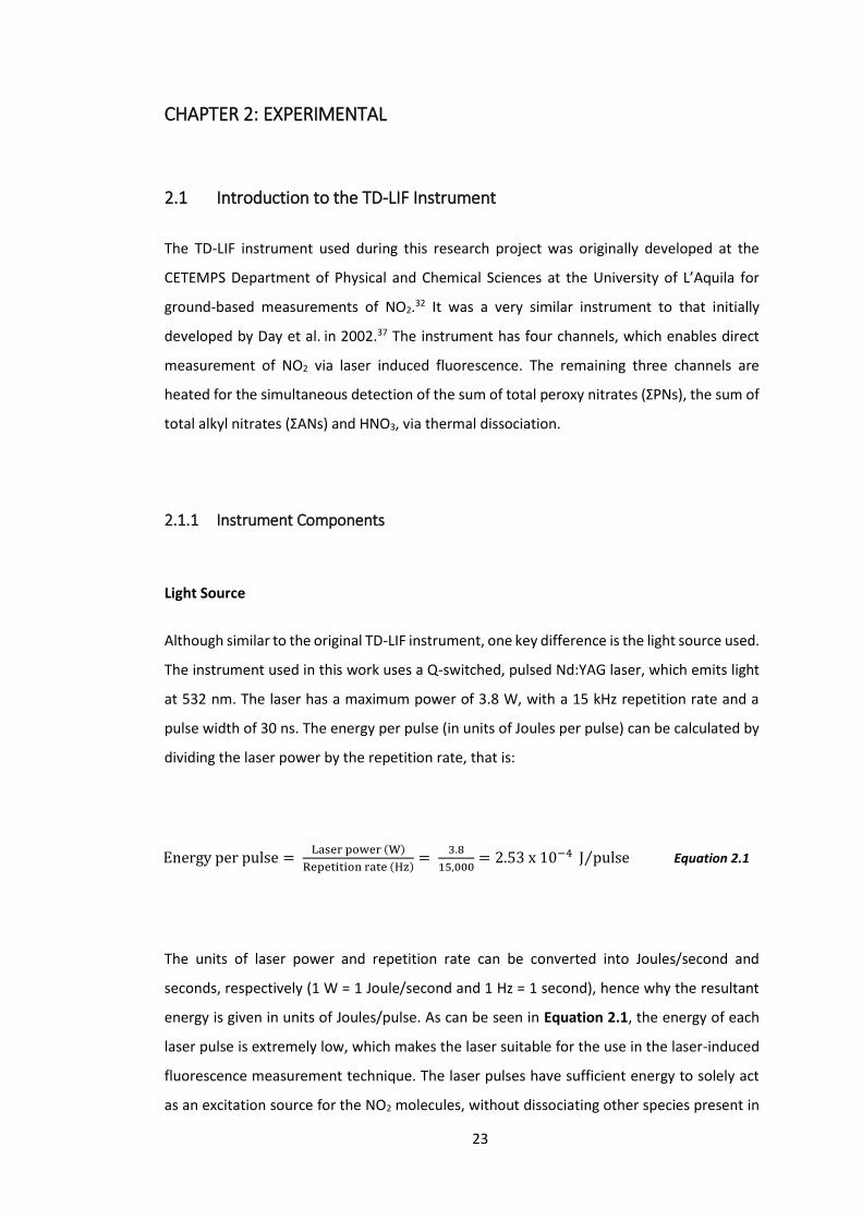
pulse width of 30 ns. The energy per pulse (in units of Joules per pulse) can be calculated by
dividing the laser power by the repetition rate, that is:
Energy per pulse = Laser power (W)
Repetition rate (Hz)=
3.8
15,000= 2.53 x 10⁻⁴ J pulse⁄ Equation 2.1
The units of laser power and repetition rate can be converted into Joules/second and
seconds, respectively (1 W = 1 Joule/second and 1 Hz = 1 second), hence why the resultant
energy is given in units of Joules/pulse. As can be seen in Equation 2.1, the energy of each
laser pulse is extremely low, which makes the laser suitable for the use in the laser-induced
fluorescence measurement technique. The laser pulses have sufficient energy to solely act
as an excitation source for the NO2 molecules, without dissociating other species present in
24
the sampled ambient air. This could affect the accuracy of the NO2 data, producing molecules
which are able to quench the fluorescence, thus meaning that it is essential to minimise the
dissociation through the use of a low powered laser.
High reflectivity mirrors are also installed between each cell, which direct the laser beam
towards the next detection cell. The laser must be well aligned, ensuring that as much of the
laser light passes through each of the detection cells. This will mean that the maximum
number of fluorescence photons are detected, thus resulting in as accurate a measurement
as possible. To monitor the laser power during calibrations and measurements, photodiodes
are located before the entrance of each detection cell.
NO2 Spectroscopy
Spectroscopic techniques such as laser-induced fluorescence are used for NO2
measurements, due to the nature of the absorption cross-section of NO2 itself.
The majority of the cross-section lies in the visible region, with a maximum observed at
approximately 420 nm.25 The reason behind this lies in the interaction between the ground
state and first excited state of NO2. The upper vibrational levels of the ground state
configuration of NO2 (X 2A1) are strongly coupled to the first excited state configuration (A
2B2) via Herzberg-Teller interactions.51 As a result, there are an extremely high number of
energy levels in the ultraviolet-visible region of the electromagnetic spectrum, thus also
meaning that the transitions between these energy levels are optically active. It is these
interactions which provide a basis for the nature of the absorption cross-section of NO2.
25
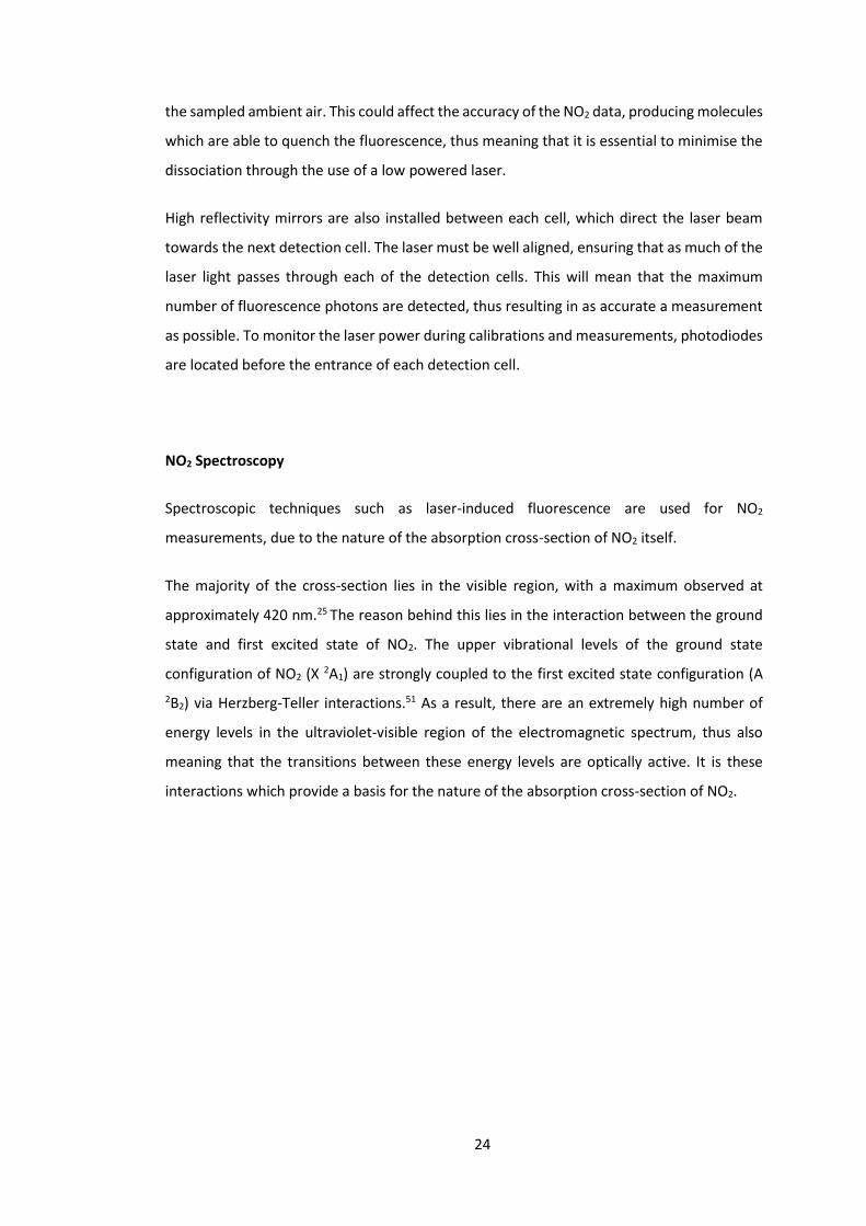
As the majority of the cross-section is in the visible region (400 to 700 nm), it means that the
radiation wavelength used to excite the NO2 molecule can be chosen based on the particular
instrument in question, some of which are shown in Figure 2.1. In order to understand why
these wavelengths were selected, it is first necessary to get a clear idea as to what an
absorption cross-section actually is. The definition of an absorption cross-section is “the
effective area of the molecule that a photon needs to traverse in order to be absorbed. The
larger the absorption cross-section, the easier it is to photo-excite the molecule.” As can be
seen in Figure 2.1, the corresponding absorption cross-sections at the excitation wavelengths
used are large, thus increasing the likelihood of absorption of the radiation. As previously
mentioned, the light source in the instrument used during this project is an Nd:YAG laser
which emits UV radiation at 532 nm. This wavelength corresponds to the second harmonic
of the Nd:YAG laser and, as can be seen on Figure 2.1, has been used in other instruments
for the detection of NO2, 21,30 due to the absorption cross-section of NO2 being relatively large
at this wavelength. Another benefit of using 532 nm is that there are no other gas-phase
absorbers at this wavelength, aside from O3.54,55 The Rayleigh scattering cross-section of air
is also modest at this wavelength,56,57 which assists in reducing the background signal of the
instrument. A single pass configuration is used in the instrument. This is similar to that used
by Matsumoto et al.,21 whose study found that using such a configuration can dramatically
reduce the instrument’s limit of detection. Using a single pass configuration and a single
wavelength, powerful laser consequently means that the laser would be simpler to align,
Figure 2.1: Absorption cross section of NO2 at 300K and 760 Torr. Letters (a) to (f) represent the excitation wavelength used in various LIF instruments. (a) Bradshaw et al. (1999)52, (b) Matsumi et al. (2001)33, (c) Matsumoto et al. (2003)21, (d) George and O’Brien (1991)30 and this thesis, (e) Fong and Brune (1997)31 and (f) Perkins et al. (1999)53
26
whilst also providing laser light powerful enough to supply all 4 detection cells for the in-situ
measurement of NO2, PNs, ANs and HNO3.
Excitation of NO2 at 532 nm results in fluorescence at wavelengths longer than 630 nm,
allowing for optical filtering of the laser radiation. This was also observed by Matsumoto et
al.,21 who used an Nd:YAG laser with the same excitation wavelength. This feature of the laser
also means that it possible to deduce that the only origin of the fluorescence is the NO2
present, Although O3 also absorbs UV radiation at 532 nm, it does not fluoresce at
wavelengths longer than 630 nm, thus meaning it is impossible for the fluorescence signal to
be due to O3.
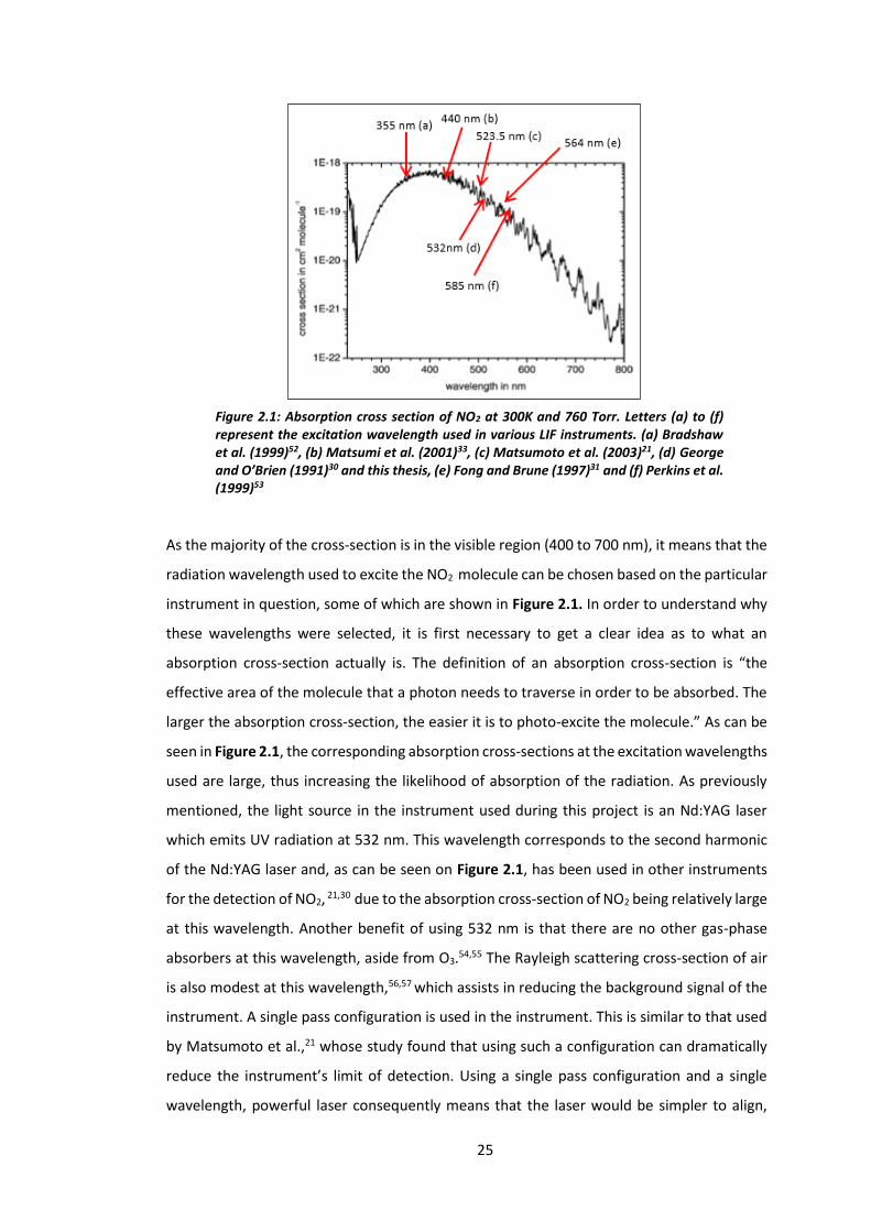
Detection Cells
The four detection cells in the instrument comprise of a central cubic structure, with two
cylindrical arms on opposite faces of said cube. The internal assembly of the cells has many
features which are in place to reduce the background signal. These arms hold a sequence of
baffles, which reduce scattering of the laser light inside the cell, whilst also minimising the
amount of external solar light that reaches the central cubic part of the detection cell. A
schematic illustrating the assembly of one of these detection cells is shown in Figure 2.2.
Figure 2.2: Schematic of a LIF detection cell
27
The walls of the cell, along with the arms and baffles are coated with a low fluorescent optical
black paint, which also acts to minimise any scattering within the cell. The cells are also
designed to maximise the fluorescence signal measured.
An aluminium-coated concave mirror is mounted below the centre of each detection cell,
which directs the laser beam towards the PMT detector. This, along with two lenses, which
are placed before the PMT, act to maximise the photon collection efficiency of the
instrument. In order to minimise the amount of Raman or Rayleigh scattering, there are a
number of low fluorescence optical filters. These work by separating the fluorescent and
non-fluorescent photons (which can be thought of as the “background” – see later). These
filters are non-fluorescent and are specifically chosen, as they need to transmit over the
range of wavelengths at which NO2 fluoresces. As a result, the fact that the filters are non-
fluorescent means it is possible to deduce that there is no fluorescence coming from the
filters, solely the NO2 molecules. There are two long-pass filters, which cut out wavelengths
of 620 and 640 nm (to reject any Raman-scattered radiation), whilst transmitting more than
85% above 640 nm. In addition to these, there are also two filters which reject any Rayleigh-
scattered radiation at 532 nm, also demonstrating a very high transmission (>95% above 640
nm). These lenses and filters are therefore in place to optimize the fluorescence detection
and minimise any non-fluorescent photons that reach the detector.
Sampling and Inlet System
The common inlet consists of a PFA tube, which samples ambient air at a flow rate of
approximately 8.5 L/min. Once the air reaches the instrument, the flow is split into four
channels. The first of these channels is another PFA tube, which is kept at ambient
temperature to measure ambient mixing ratios of NO2 in the detection cell in closest
proximity to the light source (i.e. the NO2 cell). The other three channels comprise of U-
shaped quartz tubes, which are heated to different temperatures using a heated 132 W wire,
and connect the inlets to the respective detection cells. The temperatures are specifically
chosen to correspond to the thermal dissociation temperatures of RO2NO2 species (200°C),
RONO2 species (400°C) and HNO3 (550°C). At the exit of each of these quartz tube, there is a
pinhole which acts to dramatically reduce the pressure from ambient to around 50 Torr. This
means that the residence time of the sample air in the tubes is reduced, minimising any
recombination reactions which could occur. The sample air then travels through another PFA
28
tube to a stainless steel tube in the centre of the detection cell, bringing with it another
pressure drop, this time to around 4 Torr.
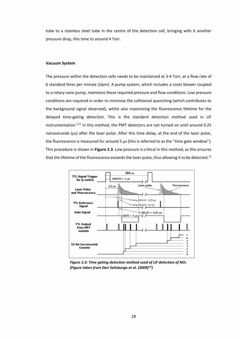
Vacuum System
The pressure within the detection cells needs to be maintained at 3-4 Torr, at a flow rate of
6 standard litres per minute (slpm). A pump system, which includes a roots blower coupled
to a rotary vane pump, maintains these required pressure and flow conditions. Low pressure
conditions are required in order to minimise the collisional quenching (which contributes to
the background signal observed), whilst also maximising the fluorescence lifetime for the
delayed time-gating detection. This is the standard detection method used in LIF
instrumentation.5,21 In this method, the PMT detectors are not turned on until around 0.25
nanoseconds (μs) after the laser pulse. After this time delay, at the end of the laser pulse,
the fluorescence is measured for around 5 μs (this is referred to as the “time gate window”).
This procedure is shown in Figure 2.3. Low pressure is critical in this method, as this ensures
that the lifetime of the fluorescence exceeds the laser pulse, thus allowing it to be detected.32
Figure 2.3: Time gating detection method used of LIF detection of NO2
(Figure taken from Dari Salisburgo et al. (2009)ref)

29
2.1.2 Instrument Parameters
Sensitivity
The instrument sensitivity has a great influence on the quality of the data, meaning it is
therefore important to discuss the factors which affect it.58 The overall equation which gives
the sensitivity of LIF (α), in units of counts per second per ppbv, is given below.
α =SFC
nNO2= lCF
σ(ν)P(ν)
aq ∫ Ω (ν, VF) T(ν) η(ν) ε(ν) ∂ν Equation 2.2
Where:
- ν = frequency of incident radiation (photon s-1)
- SF = fluorescence signal (photons s-1)
- C = collection efficiency
- nNO2 = mixing ratio of NO2 (ppbv)
- lCF = effective path length where fluorescence takes place (cm)
- σ(ν) = absorption cross section (cm2 molecule-1)
- P(ν) = photons flux (photons s-1)
- aq = quenching factor (cm3)
- VF = volume of fluorescence (cm3)
- Ω (ν, VF) = fraction of photons emitted into volume of fluorescence
- η(ν) = quantum efficiency of PMT
- ε(ν) = normalized fluorescence spectrum of the molecule

30
During work with the instrument, the sensitivities of the NO2, PN, AN and HNO3 channels
were found to be stable at 173, 83, 46 and 18 counts per second per ppbv (c/s/ppbv). This
decline in sensitivity from the NO2 to the HNO3 cell can be explained using Equation 2.2, with
a gradual decrease in laser power playing a key role in this. However, it should be noted that
it is not possible to quantify all terms in this equation, hence illustrating a need for an actual
calibration. The sensitivity of the instrument is a function of the collection efficiency and the
fluorescence photons. The collection efficiency is dependent on the quality of the optics
which are used to collect the fluorescence signal, along with the quality of the PMT, which is
used to detect the fluorescence photons.
The amount of fluorescence photons that reach the detector (i.e. the degree of fluorescence
observed) is affected by a number of competitive processes. Another way that the excited
NO2 molecules can lose energy is through collisional quenching with other molecules, namely
nitrogen and oxygen molecules. The sensitivity of the instrument is therefore improved in a
number of ways. The first is to increase the number of fluorescence photons by reducing the
instrument background. Methods of reducing the background signal were discussed in
section 2.1.1, with low pressure operation and the use of baffles and optical filters being
some of the key examples. Increasing the laser power also increases the amount of
fluorescence photons. Referring back to the decline in sensitivity observed from the NO2 to
the HNO3 cell, this can be put down to the laser power gradually weakening at it travels
through the instrument. As the sensitivity is a function of fluorescence photons, which
depend partly on the power of the laser, the more powerful the laser, the higher the
sensitivity will be (in conjunction with other factors discussed above).
31
Background signal
The background signal can have significant impacts on instrumental performance,
particularly through its contribution to the instrumental sensitivity (see later). In order to
keep the background down to a minimum, it is important to consider where the signal
actually comes from.
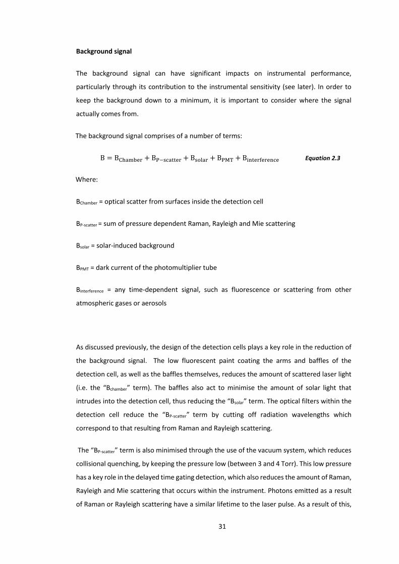
The background signal comprises of a number of terms:
B = BChamber + BP−scatter + Bsolar + BPMT + Binterference Equation 2.3
Where:
BChamber = optical scatter from surfaces inside the detection cell
BP-scatter = sum of pressure dependent Raman, Rayleigh and Mie scattering
Bsolar = solar-induced background
BPMT = dark current of the photomultiplier tube
Binterference = any time-dependent signal, such as fluorescence or scattering from other
atmospheric gases or aerosols
As discussed previously, the design of the detection cells plays a key role in the reduction of
the background signal. The low fluorescent paint coating the arms and baffles of the
detection cell, as well as the baffles themselves, reduces the amount of scattered laser light
(i.e. the “Bchamber” term). The baffles also act to minimise the amount of solar light that
intrudes into the detection cell, thus reducing the “Bsolar” term. The optical filters within the
detection cell reduce the “BP-scatter” term by cutting off radiation wavelengths which
correspond to that resulting from Raman and Rayleigh scattering.
The “BP-scatter” term is also minimised through the use of the vacuum system, which reduces
collisional quenching, by keeping the pressure low (between 3 and 4 Torr). This low pressure
has a key role in the delayed time gating detection, which also reduces the amount of Raman,
Rayleigh and Mie scattering that occurs within the instrument. Photons emitted as a result
of Raman or Rayleigh scattering have a similar lifetime to the laser pulse. As a result of this,
32
these photons are not detected when using the time-gating method, so do not affect the
fluorescence counts.
Limit of Detection
The limit of detection of the LIF instrument is dictated by the signal to noise ratio (SNR),
which in turn, is dependent on both the sensitivity (α, which is calculated using Equation 2.2)
and the background (B, which is calculated using Equation 2.3).
The mixing ratio is then determined through the division of the fluorescence signal by the
calibration factor (see Equation 2.8).
It is assumed that the statistics of the photon counts is Poissonian and that the same amount
of time is spent on measuring the background as is spent on measuring the fluorescence
signal. With these assumed conditions, the SNR can be calculated using Equation 2.4, where
“Xt” refers to the fluorescence signal detected at time “t” and “Bt” refers to the background
signal.
SNR = Xt
√Xt+2Bt Equation 2.4
At the limit of detection, the fluorescence signal, Xmin, is considered to be much lower than
the background signal, B. As a result of this, Equation 2.4 is then rearranged to become:
Xmin = SNR √2B
t Equation 2.5
The detection limit is then calculated using Equation 2.6:
nNO2min =
SNR
α √
2B
t Equation 2.6
The detection limits (1s, SNR = 2) for NO2, PNs, ANs and HNO3 are 9.8, 18.5, 28.1 and 49.7
pptv, respectively.38 It should be noted however, that these limits of detection correspond
to calibrations which were carried out in a laboratory, thus sampling laboratory air.
Therefore, for calibrations and measurements in remote atmospheric environments, such as
Cape Verde, it is vital that any interferences and leaks within the instrument are minimised,
as these could cause significant interferences.

33
Calibration and Background Procedures
LIF is not an absolute technique, and the instrument used in this work does not have an
automated calibration or background measurement system in place.
Calibrations of the instrument are done by first overflowing the lines and detection cells with
zero air by opening the zero air valve. This is done in order to ensure that the instrument is
no longer measuring ambient air, thus providing a background measurement. The
background signal has a number of sources, which are given in Equation 2.3. In this work,
the zero air was supplied from a BTCA-172 cylinder containing synthetic air (5 ppmv, certified
by BOC for less than 1 ppmv NOx), filtered with a Sofnafil/activated charcoal trap.
The instrument is then calibrated by standard addition of a known mixing ratio of NO2 from
a standard cylinder (5 ppmv, NIST traceable), which is diluted in zero air. The flows of both
the NO2 and the zero air are controlled using internal mass flow controllers (0 – 20 standard
cubic centimetres per minute (sccm) and 0 – 20,000 sccm, respectively). Both of these flows
are manually selected in order to give a calibration mixing ratio of NO2. Flows generally used
for calibrations during this work were 50 sccm NO2 in 8000 sccm zero air. This gives a
calibration NO2 mixing ratio of approximately 35.8 ppbv. This calibration mixing ratio is
calculated by multiplying the mixing ratio in the cylinder by the dilution factor (i.e. the
dilution of NO2 within the total gas flow), that is:
NO2 (ppbv) = (5.00 𝑥 10−6) 𝑝𝑝𝑚𝑣 𝑥 ξNO2
ξzero+ ξNO2 Equation 2.7
Where:
ξNO2 = NO2 flow (sccm)
ξ zero = zero air flow (sccm)
The instrument software works by taking a known amount of NO2 (i.e. the calibration mixing
ratio) and dividing this by the counts observed during the calibration. This then gives the
instrument sensitivity.
The mixing ratio observed is then determined through the division of the fluorescence signal,
X (counts per second) by the calibration factor, α (counts per second per ppbv):
34
nNO2obs =
X
α Equation 2.8
The NOy channels of the instrument were not calibrated during this work, as these were done
by Di Carlo et al. in 2013, prior to the airborne “Role of Night-time Chemistry in Controlling
the Oxidising Capacity of the Atmosphere” (RONOCO) campaign.38
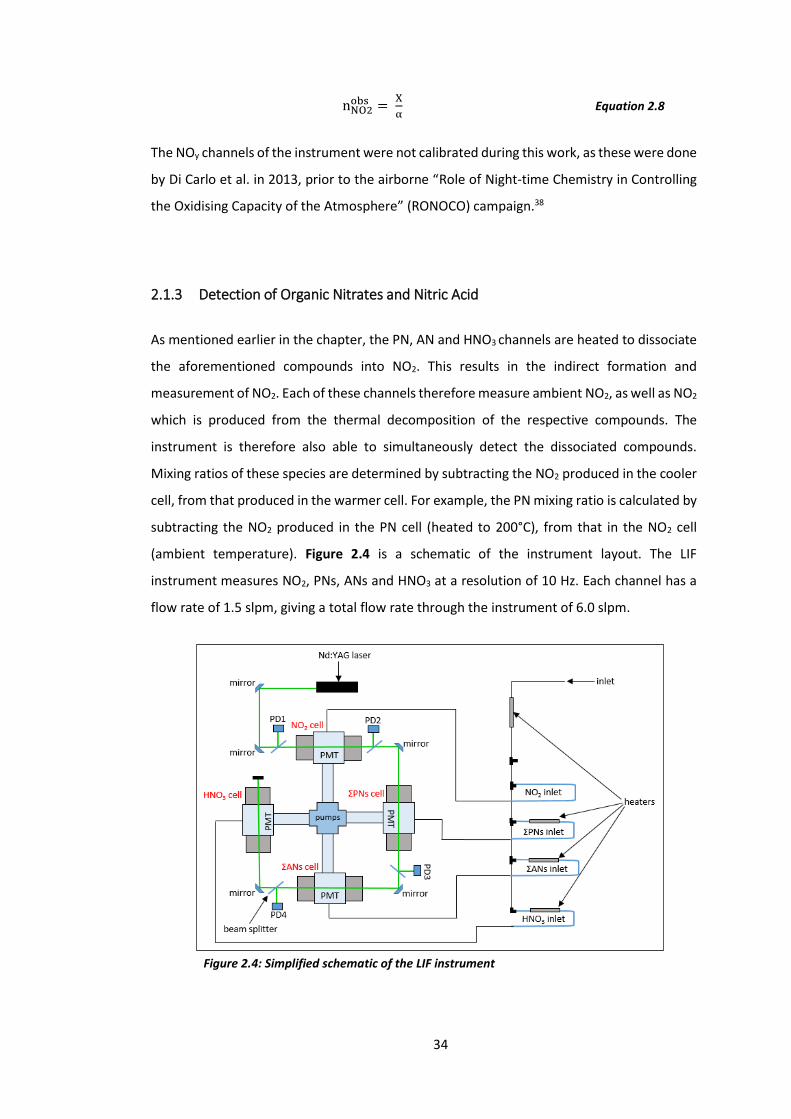
2.1.3 Detection of Organic Nitrates and Nitric Acid
As mentioned earlier in the chapter, the PN, AN and HNO3 channels are heated to dissociate
the aforementioned compounds into NO2. This results in the indirect formation and
measurement of NO2. Each of these channels therefore measure ambient NO2, as well as NO2
which is produced from the thermal decomposition of the respective compounds. The
instrument is therefore also able to simultaneously detect the dissociated compounds.
Mixing ratios of these species are determined by subtracting the NO2 produced in the cooler
cell, from that produced in the warmer cell. For example, the PN mixing ratio is calculated by
subtracting the NO2 produced in the PN cell (heated to 200°C), from that in the NO2 cell
(ambient temperature). Figure 2.4 is a schematic of the instrument layout. The LIF
instrument measures NO2, PNs, ANs and HNO3 at a resolution of 10 Hz. Each channel has a
flow rate of 1.5 slpm, giving a total flow rate through the instrument of 6.0 slpm.
Figure 2.4: Simplified schematic of the LIF instrument
35
2.1.4 Error Analysis
It is important to ensure that the data obtained from the instrument is as accurate and
reliable as possible. This therefore means that the uncertainties and errors associated with
the instrument and the data need to be considered.
As the calibration of the instrument determines the sensitivities of each of the instrument
channels, the procedure needs to be done as accurately as possible. The accuracy is
dependent on the uncertainty associated with the mixing ratio of NO2 in the standard
cylinder. Cylinders of between 2 and 10 ppmv NO2 are typically used (the cylinder used during
this research project was certified to contain 5 ppmv NO2) and have an uncertainty of
between 1 and 3%.
The accuracy of the calibration also depends on the uncertainty of the mass flow controllers
used for the air and NO2 flows. This uncertainty therefore depends on the flow rate of the air
and NO2. The mass flow controller used for the air flow has uncertainties of between 3.4 and
1%, when the flow rate is 1500 and 5,000 sccm, respectively. The mass flow controller used
for the NO2 calibration gas has uncertainties of between 100 and 1%, when the flow rate is
0.2 and 20 sccm, respectively. It should also be noted that there is a relative error in the
sensitivity itself, of approximately 3%. In its current configuration, the accuracy of the
channels of the LIF instrument is considered to be 10, 22, 34 and 46% for the NO2, PN, AN
and HNO3 channels, respectively.38
As discussed previously, the total mixing ratios of PNs, ANs and HNO3 are determined through
the subtraction of the NO2 produced in the cooler cell, from that produced in the warmer
cell. This means that the limit of detection of each of the channels depends on the signal,
along with the uncertainties associated with the channels in question. This is expressed in
Equation 2.9 below, referring to signals from adjacent channels “A” and “B” and their
associated uncertainties.
(B − A) ± (σA2 + σB
2 ) Equation 2.9
There are also some potential interferences which have errors, although are very small and
easily quantifiable, associated with them. These interferences include the reduction of NO2
by O3 at higher temperatures and the complexation of NO2 to produce PNs or HNO3. The total
error associated with all three of these interferences summed together, is less than 5%. The
36
most likely interference, however, is the heterogeneous conversion of NO2-containing
compounds (e.g. N2O5) to NO2 in the sample lines or the oxidation of NO to NO2. However,
this interference is minimised by simply increasing the sample flow rate.
2.1.5 General Laboratory Testing of the LIF
General Instrumental Operation
Once the instrument was turned on, parameters needed to be set before it could be used for
laboratory testing. The laser power of the instrument was gradually dialled up to full power,
at a wavelength of 532 nm, thus providing a suitably long time period for the diodes and
thus, the laser, to heat up and reach full power. This is an extremely important factor for
optimal instrumental performance, due to the spectroscopic nature of the technique.
On stabilisation of the laser at full power, the instrument was calibrated using the procedure
given in section 2.1.2. Flows used for the calibrations in the lab were 50 sccm NO2 in 8000
sccm zero air, which resulted in a calibration mixing ratio of 35.8 ppbv. Background checks
were also conducted, using the method described in section 2.1.2. After conducting several
calibrations and background checks, the sensitivities and zero signals were found to be stable
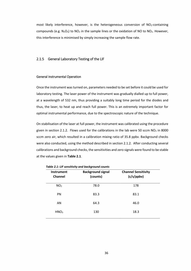
at the values given in Table 2.1.
Table 2.1: LIF sensitivity and background counts
Instrument
Channel
Background signal
(counts)
Channel Sensitivity
(c/s/ppbv)
NO2 78.0 178
PN 83.3 83.1
AN 64.3 46.0
HNO3 130 18.3
37
These calibrations and background were conducted on a regular basis, in order to monitor
any changes in sensitivities of the individual channels. If the values deviated too much from
the values given above, the likely cause was misalignment of the laser. In such cases, the
laser power was reduced to 30%, meaning it was then safe to open the instrument and adjust
the mirrors on the relevant detection cells, in order to re-align the laser.
Zero Air Supply Testing
It is important to have a good source of zero NOx, as this makes it possible to assess
interferences on both the LIF and other instruments used for NOx measurements. The
instrument was therefore used to evaluate the quality of different zero air supplies in the
laboratory (i.e. rather than to test the performance of the instrument itself). The first
potential source of zero air tested was a pure air generator (with a Sofnafil/activated charcoal
trap), which was used for all background air measurements required by the various
instruments in the laboratories. The second supply was a BTCA cylinder (5 ppmv, certified by
BOC). The air coming from this cylinder was also scrubbed with a Sofnafil/activated charcoal
trap (as with the pure air generator). These supplies were connected to the zero air inlet on
the LIF, with the instrument then left running for a period of approximately 10 minutes in
order to monitor the background counts on the NO2 channel.
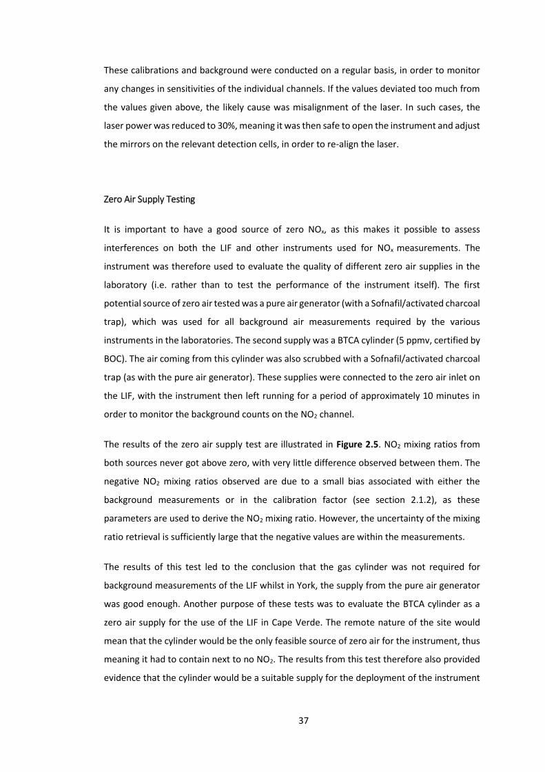
The results of the zero air supply test are illustrated in Figure 2.5. NO2 mixing ratios from
both sources never got above zero, with very little difference observed between them. The
negative NO2 mixing ratios observed are due to a small bias associated with either the
background measurements or in the calibration factor (see section 2.1.2), as these
parameters are used to derive the NO2 mixing ratio. However, the uncertainty of the mixing
ratio retrieval is sufficiently large that the negative values are within the measurements.
The results of this test led to the conclusion that the gas cylinder was not required for
background measurements of the LIF whilst in York, the supply from the pure air generator
was good enough. Another purpose of these tests was to evaluate the BTCA cylinder as a
zero air supply for the use of the LIF in Cape Verde. The remote nature of the site would
mean that the cylinder would be the only feasible source of zero air for the instrument, thus
meaning it had to contain next to no NO2. The results from this test therefore also provided
evidence that the cylinder would be a suitable supply for the deployment of the instrument
38
in Cape Verde. With extremely low mixing ratios of NO2 being expected at the site, this
background mixing ratio should not have a significant effect on the instrument sensitivity.
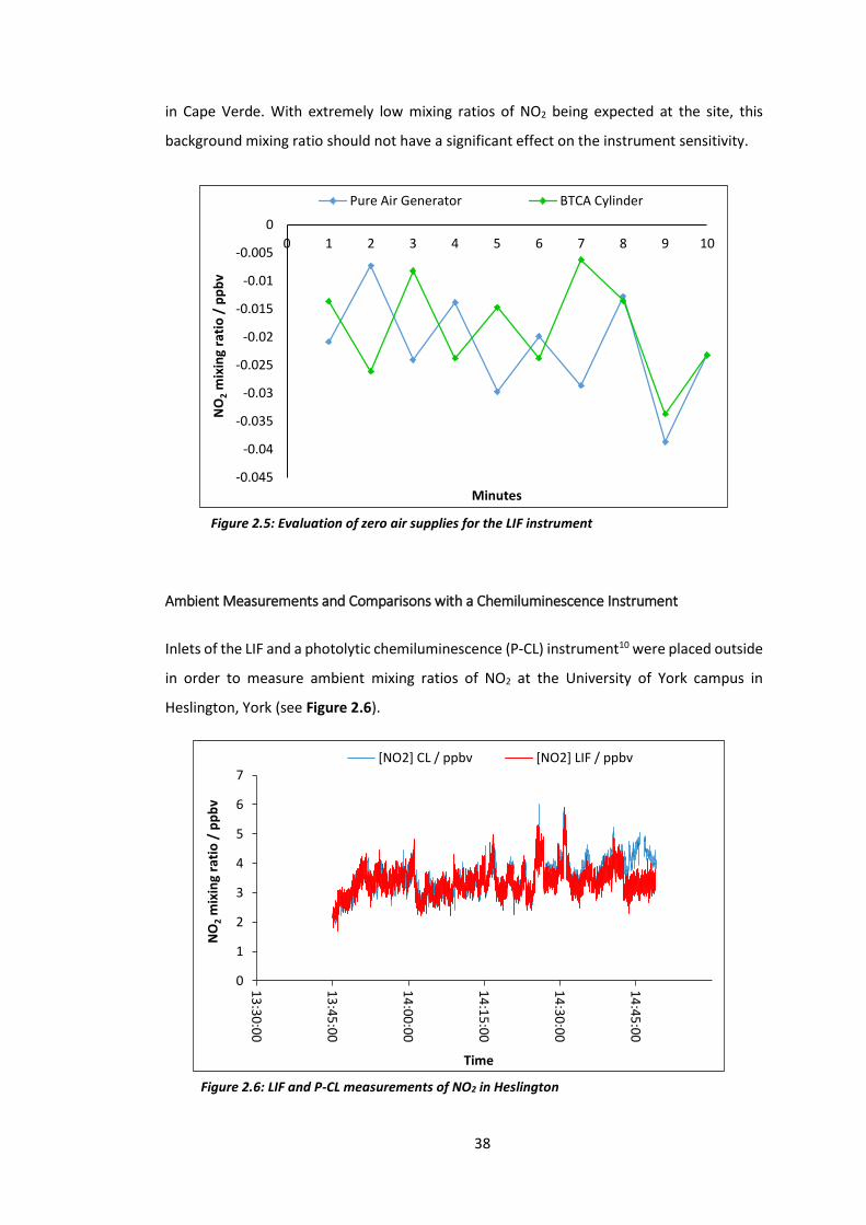
Ambient Measurements and Comparisons with a Chemiluminescence Instrument
Inlets of the LIF and a photolytic chemiluminescence (P-CL) instrument10 were placed outside
in order to measure ambient mixing ratios of NO2 at the University of York campus in
Heslington, York (see Figure 2.6).
Figure 2.5: Evaluation of zero air supplies for the LIF instrument
-0.045
-0.04
-0.035
-0.03
-0.025
-0.02
-0.015
-0.01
-0.005
0
0 1 2 3 4 5 6 7 8 9 10
NO
2m
ixin
g ra
tio
/ p
pb
v
Minutes
Pure Air Generator BTCA Cylinder
0
1
2
3
4
5
6
7
13
:30
:00
13
:45
:00
14
:00
:00
14
:15
:00
14
:30
:00
14
:45
:00
NO
2m
ixin
g ra
tio
/ p
pb
v
Time
[NO2] CL / ppbv [NO2] LIF / ppbv
Figure 2.6: LIF and P-CL measurements of NO2 in Heslington
39
A direct comparison between the two instruments would also give an indication as to how
reliable their measurements are. As can be seen in Figure 2.6, both instruments measured
very similar NO2 mixing ratios over the time period studied. Chemiluminescence is a standard
technique for atmospheric NOx measurements. It has been used in a number of ground-
based and airborne studies to provide reliable data.59,60,61 Therefore, the comparability of the
LIF and P-CL data provided some assurance that the NO2 mixing ratios measured by the LIF
could be trusted to be an accurate representation of the surrounding atmosphere.
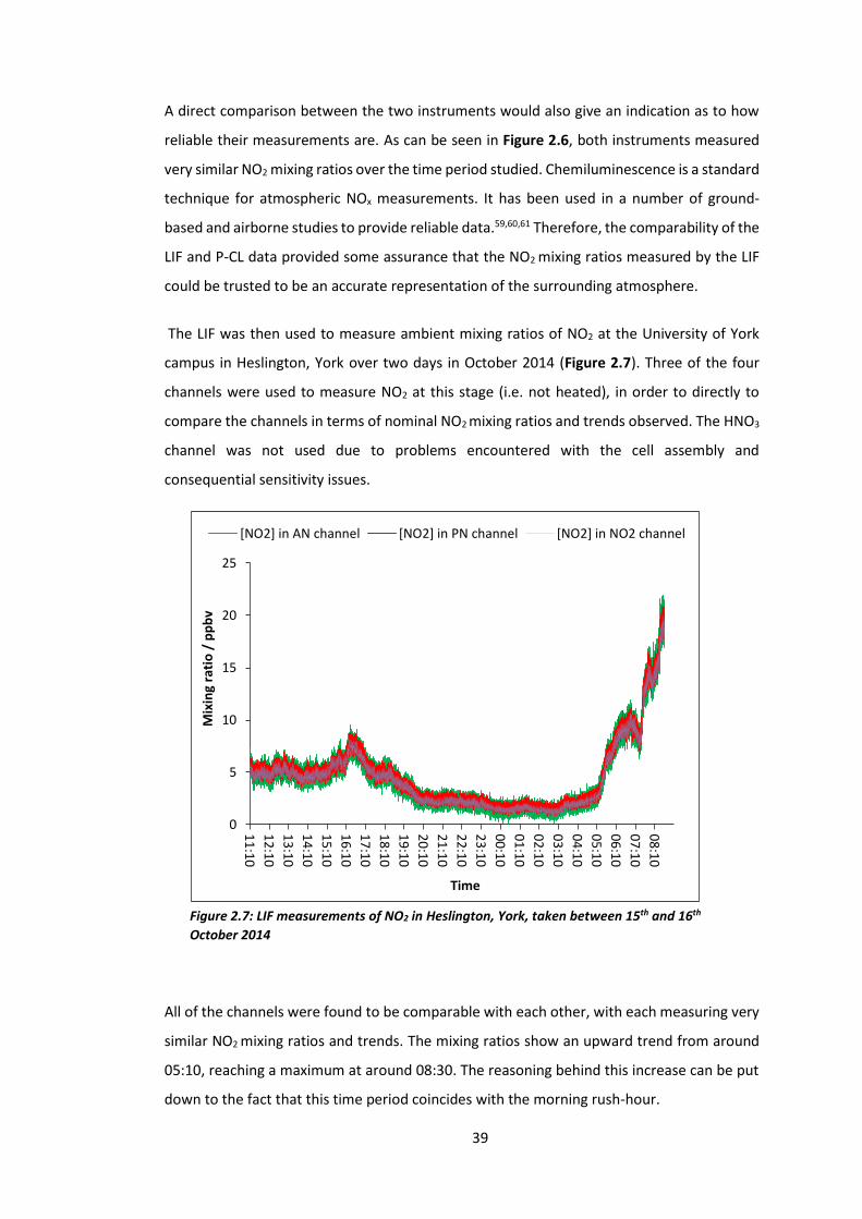
The LIF was then used to measure ambient mixing ratios of NO2 at the University of York
campus in Heslington, York over two days in October 2014 (Figure 2.7). Three of the four
channels were used to measure NO2 at this stage (i.e. not heated), in order to directly to
compare the channels in terms of nominal NO2 mixing ratios and trends observed. The HNO3
channel was not used due to problems encountered with the cell assembly and
consequential sensitivity issues.
All of the channels were found to be comparable with each other, with each measuring very
similar NO2 mixing ratios and trends. The mixing ratios show an upward trend from around
05:10, reaching a maximum at around 08:30. The reasoning behind this increase can be put
down to the fact that this time period coincides with the morning rush-hour.
0
5
10
15
20
25
11
:10
12
:10
13
:10
14
:10
15
:10
16
:10
17
:10
18
:10
19
:10
20
:10
21
:10
22
:10
23
:10
00
:10
01
:10
02
:10
03
:10
04
:10
05
:10
06
:10
07
:10
08
:10
Mix
ing
rati
o /
pp
bv
Time
[NO2] in AN channel [NO2] in PN channel [NO2] in NO2 channel
Figure 2.7: LIF measurements of NO2 in Heslington, York, taken between 15th and 16th
October 2014
40
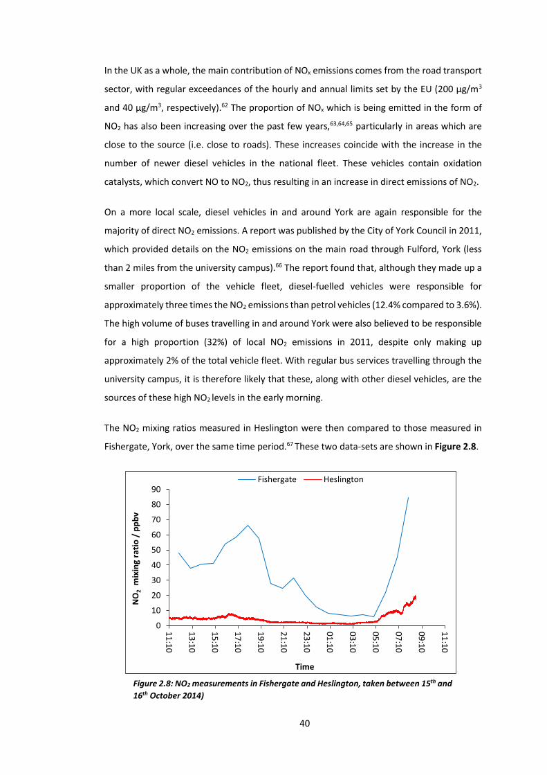
In the UK as a whole, the main contribution of NOx emissions comes from the road transport
sector, with regular exceedances of the hourly and annual limits set by the EU (200 μg/m3
and 40 μg/m3, respectively).62 The proportion of NOx which is being emitted in the form of
NO2 has also been increasing over the past few years,63,64,65 particularly in areas which are
close to the source (i.e. close to roads). These increases coincide with the increase in the
number of newer diesel vehicles in the national fleet. These vehicles contain oxidation
catalysts, which convert NO to NO2, thus resulting in an increase in direct emissions of NO2.
On a more local scale, diesel vehicles in and around York are again responsible for the
majority of direct NO2 emissions. A report was published by the City of York Council in 2011,
which provided details on the NO2 emissions on the main road through Fulford, York (less
than 2 miles from the university campus).66 The report found that, although they made up a
smaller proportion of the vehicle fleet, diesel-fuelled vehicles were responsible for
approximately three times the NO2 emissions than petrol vehicles (12.4% compared to 3.6%).
The high volume of buses travelling in and around York were also believed to be responsible
for a high proportion (32%) of local NO2 emissions in 2011, despite only making up
approximately 2% of the total vehicle fleet. With regular bus services travelling through the
university campus, it is therefore likely that these, along with other diesel vehicles, are the
sources of these high NO2 levels in the early morning.
The NO2 mixing ratios measured in Heslington were then compared to those measured in
Fishergate, York, over the same time period.67 These two data-sets are shown in Figure 2.8.
Figure 2.8: NO2 measurements in Fishergate and Heslington, taken between 15th and
16th October 2014)
0
10
20
30
40
50
60
70
80
90
11
:10
13
:10
15
:10
17
:10
19
:10
21
:10
23
:10
01
:10
03
:10
05
:10
07
:10
09
:10
11
:10
NO
2m
ixin
g ra
tio
/ p
pb
v
Time
Fishergate Heslington
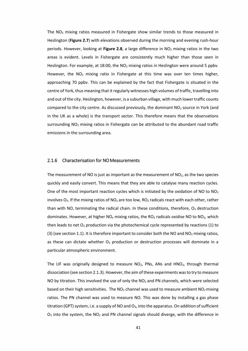
41
The NO2 mixing ratios measured in Fishergate show similar trends to those measured in
Heslington (Figure 2.7) with elevations observed during the morning and evening rush-hour
periods. However, looking at Figure 2.8, a large difference in NO2 mixing ratios in the two
areas is evident. Levels in Fishergate are consistently much higher than those seen in
Heslington. For example, at 18:00, the NO2 mixing ratios in Heslington were around 5 ppbv.
However, the NO2 mixing ratio in Fishergate at this time was over ten times higher,
approaching 70 ppbv. This can be explained by the fact that Fishergate is situated in the
centre of York, thus meaning that it regularly witnesses high volumes of traffic, travelling into
and out of the city. Heslington, however, is a suburban village, with much lower traffic counts
compared to the city centre. As discussed previously, the dominant NO2 source in York (and
in the UK as a whole) is the transport sector. This therefore means that the observations
surrounding NO2 mixing ratios in Fishergate can be attributed to the abundant road traffic
emissions in the surrounding area.
2.1.6 Characterisation for NO Measurements
The measurement of NO is just as important as the measurement of NO2, as the two species
quickly and easily convert. This means that they are able to catalyse many reaction cycles.
One of the most important reaction cycles which is initiated by the oxidation of NO to NO2
involves O3. If the mixing ratios of NOx are too low, RO2 radicals react with each other, rather
than with NO, terminating the radical chain. In these conditions, therefore, O3 destruction
dominates. However, at higher NOx mixing ratios, the RO2 radicals oxidise NO to NO2, which
then leads to net O3 production via the photochemical cycle represented by reactions (1) to
(3) (see section 1.1). It is therefore important to consider both the NO and NO2 mixing ratios,
as these can dictate whether O3 production or destruction processes will dominate in a
particular atmospheric environment.
The LIF was originally designed to measure NO2, PNs, ANs and HNO3, through thermal
dissociation (see section 2.1.3). However, the aim of these experiments was to try to measure
NO by titration. This involved the use of only the NO2 and PN channels, which were selected
based on their high sensitivities. The NO2 channel was used to measure ambient NO2 mixing
ratios. The PN channel was used to measure NO. This was done by installing a gas phase
titration (GPT) system, i.e. a supply of NO and O3, into the apparatus. On addition of sufficient
O3 into the system, the NO2 and PN channel signals should diverge, with the difference in
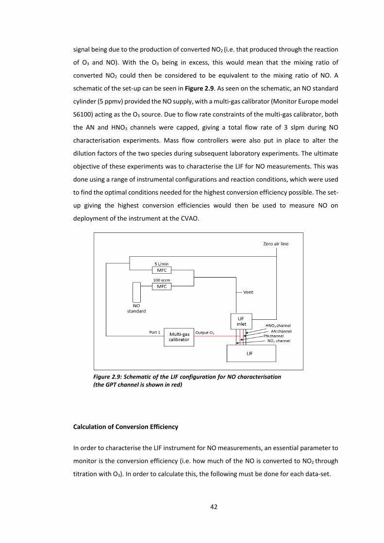
42
signal being due to the production of converted NO2 (i.e. that produced through the reaction
of O3 and NO). With the O3 being in excess, this would mean that the mixing ratio of
converted NO2 could then be considered to be equivalent to the mixing ratio of NO. A
schematic of the set-up can be seen in Figure 2.9. As seen on the schematic, an NO standard
cylinder (5 ppmv) provided the NO supply, with a multi-gas calibrator (Monitor Europe model
S6100) acting as the O3 source. Due to flow rate constraints of the multi-gas calibrator, both
the AN and HNO3 channels were capped, giving a total flow rate of 3 slpm during NO
characterisation experiments. Mass flow controllers were also put in place to alter the
dilution factors of the two species during subsequent laboratory experiments. The ultimate
objective of these experiments was to characterise the LIF for NO measurements. This was
done using a range of instrumental configurations and reaction conditions, which were used
to find the optimal conditions needed for the highest conversion efficiency possible. The set-
up giving the highest conversion efficiencies would then be used to measure NO on
deployment of the instrument at the CVAO.
Calculation of Conversion Efficiency
In order to characterise the LIF instrument for NO measurements, an essential parameter to
monitor is the conversion efficiency (i.e. how much of the NO is converted to NO2 through
titration with O3). In order to calculate this, the following must be done for each data-set.
Figure 2.9: Schematic of the LIF configuration for NO characterisation (the GPT channel is shown in red)
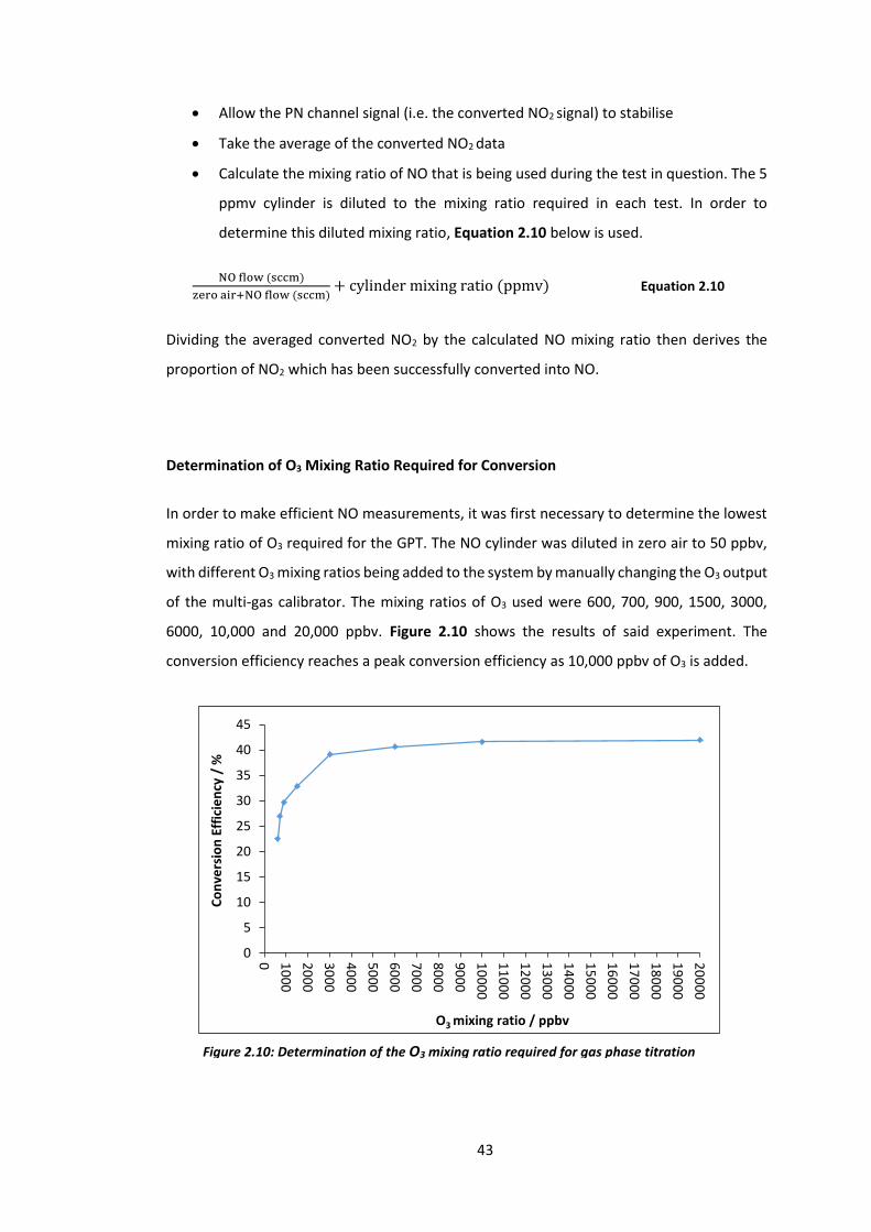
43
Allow the PN channel signal (i.e. the converted NO2 signal) to stabilise
Take the average of the converted NO2 data
Calculate the mixing ratio of NO that is being used during the test in question. The 5
ppmv cylinder is diluted to the mixing ratio required in each test. In order to
determine this diluted mixing ratio, Equation 2.10 below is used.
NO flow (sccm)
zero air+NO flow (sccm)+ cylinder mixing ratio (ppmv) Equation 2.10
Dividing the averaged converted NO2 by the calculated NO mixing ratio then derives the
proportion of NO2 which has been successfully converted into NO.
Determination of O3 Mixing Ratio Required for Conversion
In order to make efficient NO measurements, it was first necessary to determine the lowest
mixing ratio of O3 required for the GPT. The NO cylinder was diluted in zero air to 50 ppbv,
with different O3 mixing ratios being added to the system by manually changing the O3 output
of the multi-gas calibrator. The mixing ratios of O3 used were 600, 700, 900, 1500, 3000,
6000, 10,000 and 20,000 ppbv. Figure 2.10 shows the results of said experiment. The
conversion efficiency reaches a peak conversion efficiency as 10,000 ppbv of O3 is added.
Figure 2.10: Determination of the O3 mixing ratio required for gas phase titration
0
5
10
15
20
25
30
35
40
45
0 10
00
20
00
30
00
40
00
50
00
60
00
70
00
80
00
90
00
10
00
0
11
00
0
12
00
0
13
00
0
14
00
0
15
00
0
16
00
0
17
00
0
18
00
0
19
00
0
20
00
0
Co
nve
rsio
n E
ffic
ien
cy /
%
O3 mixing ratio / ppbv
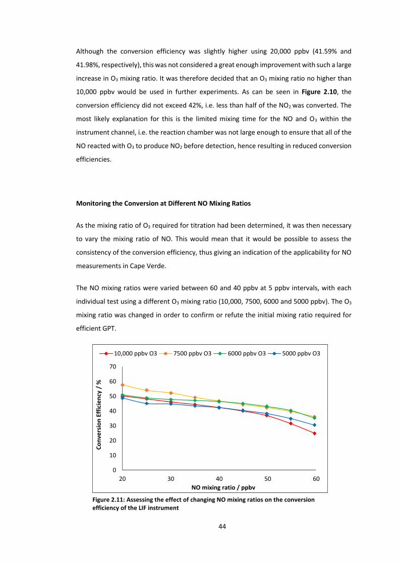
44
Although the conversion efficiency was slightly higher using 20,000 ppbv (41.59% and
41.98%, respectively), this was not considered a great enough improvement with such a large
increase in O3 mixing ratio. It was therefore decided that an O3 mixing ratio no higher than
10,000 ppbv would be used in further experiments. As can be seen in Figure 2.10, the
conversion efficiency did not exceed 42%, i.e. less than half of the NO2 was converted. The
most likely explanation for this is the limited mixing time for the NO and O3 within the
instrument channel, i.e. the reaction chamber was not large enough to ensure that all of the
NO reacted with O3 to produce NO2 before detection, hence resulting in reduced conversion
efficiencies.
Monitoring the Conversion at Different NO Mixing Ratios
As the mixing ratio of O3 required for titration had been determined, it was then necessary
to vary the mixing ratio of NO. This would mean that it would be possible to assess the
consistency of the conversion efficiency, thus giving an indication of the applicability for NO
measurements in Cape Verde.
The NO mixing ratios were varied between 60 and 40 ppbv at 5 ppbv intervals, with each
individual test using a different O3 mixing ratio (10,000, 7500, 6000 and 5000 ppbv). The O3
mixing ratio was changed in order to confirm or refute the initial mixing ratio required for
efficient GPT.
0
10
20
30
40
50
60
70
20 30 40 50 60
Co
nve
rsio
n E
ffic
ien
cy /
%
NO mixing ratio / ppbv
10,000 ppbv O3 7500 ppbv O3 6000 ppbv O3 5000 ppbv O3
Figure 2.11: Assessing the effect of changing NO mixing ratios on the conversion efficiency of the LIF instrument
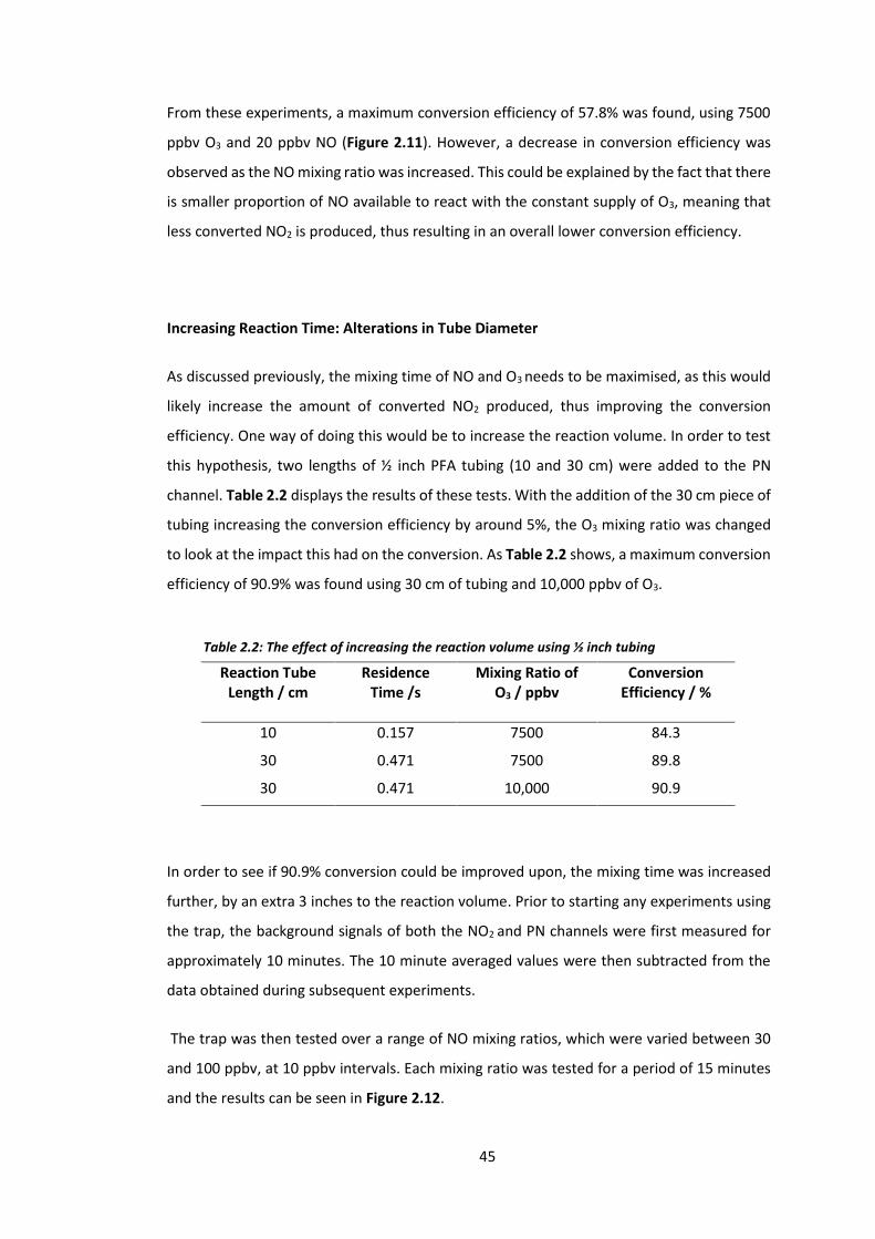
45
From these experiments, a maximum conversion efficiency of 57.8% was found, using 7500
ppbv O3 and 20 ppbv NO (Figure 2.11). However, a decrease in conversion efficiency was
observed as the NO mixing ratio was increased. This could be explained by the fact that there
is smaller proportion of NO available to react with the constant supply of O3, meaning that
less converted NO2 is produced, thus resulting in an overall lower conversion efficiency.
Increasing Reaction Time: Alterations in Tube Diameter
As discussed previously, the mixing time of NO and O3 needs to be maximised, as this would
likely increase the amount of converted NO2 produced, thus improving the conversion
efficiency. One way of doing this would be to increase the reaction volume. In order to test
this hypothesis, two lengths of ½ inch PFA tubing (10 and 30 cm) were added to the PN
channel. Table 2.2 displays the results of these tests. With the addition of the 30 cm piece of
tubing increasing the conversion efficiency by around 5%, the O3 mixing ratio was changed
to look at the impact this had on the conversion. As Table 2.2 shows, a maximum conversion
efficiency of 90.9% was found using 30 cm of tubing and 10,000 ppbv of O3.
In order to see if 90.9% conversion could be improved upon, the mixing time was increased
further, by an extra 3 inches to the reaction volume. Prior to starting any experiments using
the trap, the background signals of both the NO2 and PN channels were first measured for
approximately 10 minutes. The 10 minute averaged values were then subtracted from the
data obtained during subsequent experiments.
The trap was then tested over a range of NO mixing ratios, which were varied between 30
and 100 ppbv, at 10 ppbv intervals. Each mixing ratio was tested for a period of 15 minutes
and the results can be seen in Figure 2.12.
Reaction Tube Length / cm
Residence Time /s
Mixing Ratio of O3 / ppbv
Conversion Efficiency / %
10 0.157 7500 84.3
30 0.471 7500 89.8
30 0.471 10,000 90.9
Table 2.2: The effect of increasing the reaction volume using ½ inch tubing
46
The results from these experiments confirmed the adding the 3 inch diameter reaction
volume improved the conversion efficiency greatly, thus emphasising the key role that the
NO and O3 mixing time has on the performance of the LIF for NO characterisation.
Alteration of O3 Source: Mercury Lamp
A spectral calibration lamp (model 6035, manufactured by “Oriel Instruments”, a “Newport
Corporation” brand), was tested as an alternative O3 source for NO characterisation of the
LIF. The lamp works by producing narrow, intense lines from the excitation of argon gas and
mercury vapour, operating at 13 to 23 milliamps (mA). This would be a more practical option
than the multi-gas calibrator, due to the much reduced space and weight requirements,
particularly for transportation and deployment in Cape Verde. The lamp in question emitted
UV light at a wavelength which leads to photolysis of molecular oxygen (185 nm). The oxygen
molecules then react with the dissociated oxygen atoms, thus producing O3. The lamp was
inserted into an empty reaction vessel, which was then covered in a layer of black insulation,
to minimise exposure to the harmful UV radiation. Due to the fact that the lamp was in the
preliminary stages of testing, its suitability as an O3 source was as yet unknown. The seal of
the lamp was therefore only temporary.
Figure 2.12: Evaluating the effect of increased reaction volume at different NO mixing ratios
60
70
80
90
100
110
120
30 40 50 60 70 80 90 100
Co
nve
rsio
n E
ffic
ien
cy /
%
NO mixing ratio / ppbv
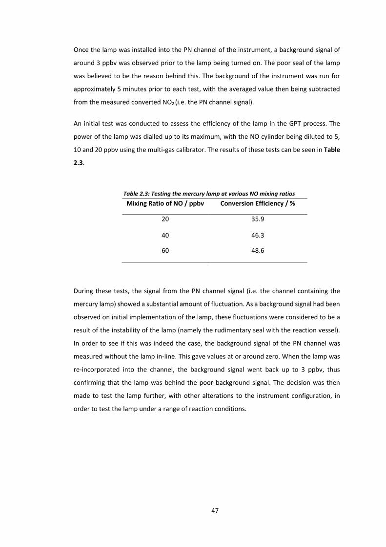
47
Once the lamp was installed into the PN channel of the instrument, a background signal of
around 3 ppbv was observed prior to the lamp being turned on. The poor seal of the lamp
was believed to be the reason behind this. The background of the instrument was run for
approximately 5 minutes prior to each test, with the averaged value then being subtracted
from the measured converted NO2 (i.e. the PN channel signal).
An initial test was conducted to assess the efficiency of the lamp in the GPT process. The
power of the lamp was dialled up to its maximum, with the NO cylinder being diluted to 5,
10 and 20 ppbv using the multi-gas calibrator. The results of these tests can be seen in Table
2.3.
During these tests, the signal from the PN channel signal (i.e. the channel containing the
mercury lamp) showed a substantial amount of fluctuation. As a background signal had been
observed on initial implementation of the lamp, these fluctuations were considered to be a
result of the instability of the lamp (namely the rudimentary seal with the reaction vessel).
In order to see if this was indeed the case, the background signal of the PN channel was
measured without the lamp in-line. This gave values at or around zero. When the lamp was
re-incorporated into the channel, the background signal went back up to 3 ppbv, thus
confirming that the lamp was behind the poor background signal. The decision was then
made to test the lamp further, with other alterations to the instrument configuration, in
order to test the lamp under a range of reaction conditions.
Mixing Ratio of NO / ppbv Conversion Efficiency / %
20 35.9
40 46.3
60 48.6
Table 2.3: Testing the mercury lamp at various NO mixing ratios
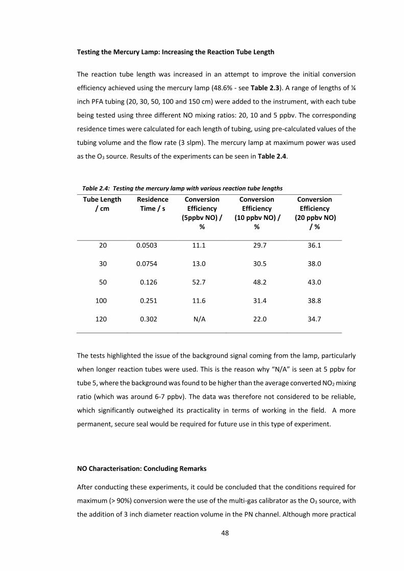
48
Testing the Mercury Lamp: Increasing the Reaction Tube Length
The reaction tube length was increased in an attempt to improve the initial conversion
efficiency achieved using the mercury lamp (48.6% - see Table 2.3). A range of lengths of ¼
inch PFA tubing (20, 30, 50, 100 and 150 cm) were added to the instrument, with each tube
being tested using three different NO mixing ratios: 20, 10 and 5 ppbv. The corresponding
residence times were calculated for each length of tubing, using pre-calculated values of the
tubing volume and the flow rate (3 slpm). The mercury lamp at maximum power was used
as the O3 source. Results of the experiments can be seen in Table 2.4.
The tests highlighted the issue of the background signal coming from the lamp, particularly
when longer reaction tubes were used. This is the reason why “N/A” is seen at 5 ppbv for
tube 5, where the background was found to be higher than the average converted NO2 mixing
ratio (which was around 6-7 ppbv). The data was therefore not considered to be reliable,
which significantly outweighed its practicality in terms of working in the field. A more
permanent, secure seal would be required for future use in this type of experiment.
NO Characterisation: Concluding Remarks
After conducting these experiments, it could be concluded that the conditions required for
maximum (> 90%) conversion were the use of the multi-gas calibrator as the O3 source, with
the addition of 3 inch diameter reaction volume in the PN channel. Although more practical
Tube Length / cm
Residence Time / s
Conversion Efficiency
(5ppbv NO) / %
Conversion Efficiency
(10 ppbv NO) / %
Conversion Efficiency
(20 ppbv NO) / %
20 0.0503 11.1 29.7 36.1
30 0.0754 13.0 30.5 38.0
50 0.126 52.7 48.2 43.0
100 0.251 11.6 31.4 38.8
120 0.302 N/A 22.0 34.7
Table 2.4: Testing the mercury lamp with various reaction tube lengths
49
in terms of field work, the mercury lamp was not deemed suitable for NO characterisation in
its current configuration. The lowest O3 mixing ratio required for efficient conversion was
found to be 10,000 ppbv, thus meaning that this, along with the aforementioned apparatus,
would be used to measure NO in Cape Verde.
2.2 Introduction to the Airborne P-CL Instrument
The instrument used for airborne NOx measurements during the 2015 “Oil and Gas”
campaign is a P-CL instrument designed by “Air Quality Design Inc.” (Colorado USA). The
instrument detects NO directly from the chemiluminescence resulting from the reaction of
NO and O3. NO2 is then quantified using the same instrument, by first photolytically
converting NO2 to NO using blue light LED diodes centred at 385 nm10 followed by
chemiluminescence.
The instrument is fitted into a rack, which can then be installed in the BAe-146-301 research
aircraft used for the airborne measurements. It is then possible to sample and measure air
in-situ during flights around a particular area of interest. Typically, the aircraft flights at a
speed of 200 knots (100 m/s), thus meaning that it is possible to obtain measurements with
high spatial resolution, if the both the sampling and analysis of the air are conducted using a
sufficiently high time resolution (typically 1 Hz).
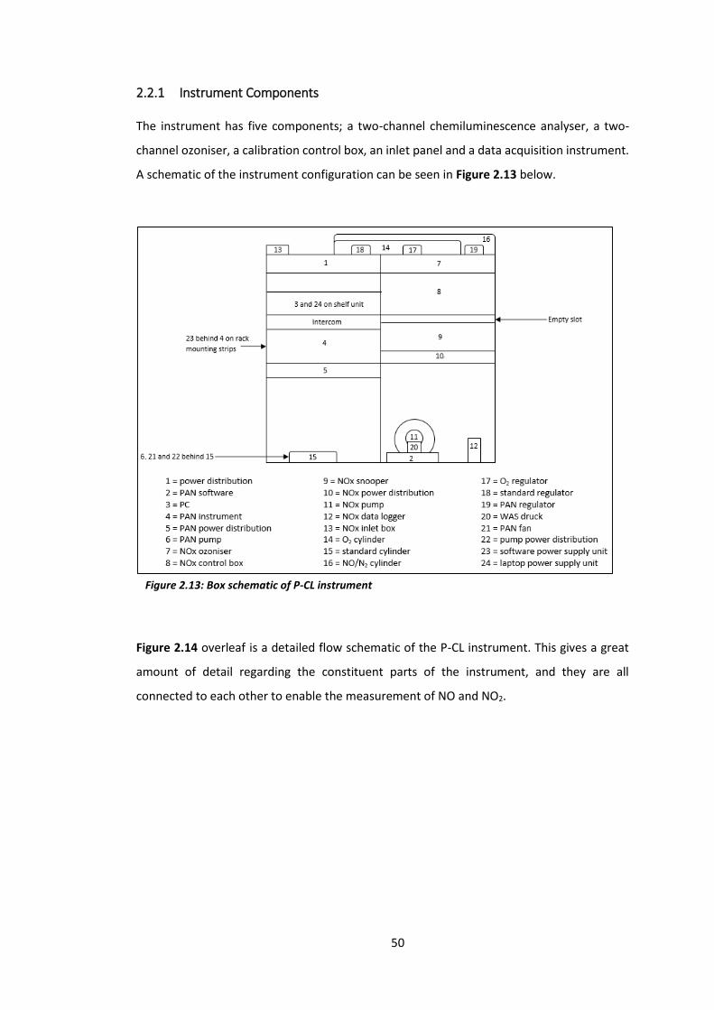
50
2.2.1 Instrument Components
The instrument has five components; a two-channel chemiluminescence analyser, a two-
channel ozoniser, a calibration control box, an inlet panel and a data acquisition instrument.
A schematic of the instrument configuration can be seen in Figure 2.13 below.
Figure 2.14 overleaf is a detailed flow schematic of the P-CL instrument. This gives a great
amount of detail regarding the constituent parts of the instrument, and they are all
connected to each other to enable the measurement of NO and NO2.
Figure 2.13: Box schematic of P-CL instrument
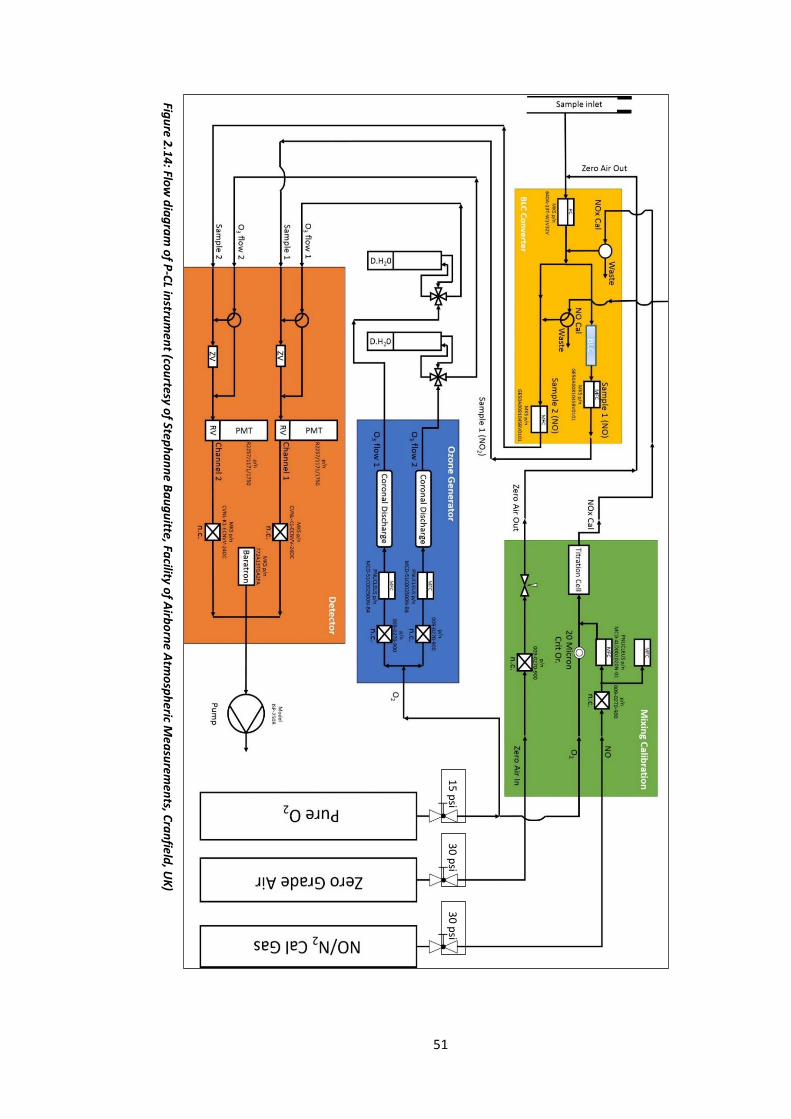
51
15
psi
30
psi
30
psi
Figu
re 2.1
4: Flo
w d
iag
ram
of P
-CL in
strum
ent (co
urtesy o
f Steph
an
ne B
au
gu
itte, Facility o
f Airb
orn
e Atm
osp
heric M
ea
surem
ents, C
ran
field
, UK
)
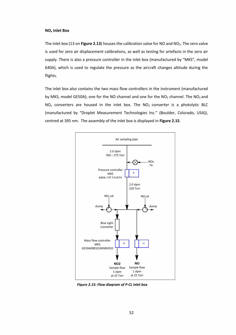
52
NOx Inlet Box
The inlet box (13 on Figure 2.13) houses the calibration valve for NO and NO2. The zero valve
is used for zero air displacement calibrations, as well as testing for artefacts in the zero air
supply. There is also a pressure controller in the inlet box (manufactured by “MKS”, model
640A), which is used to regulate the pressure as the aircraft changes altitude during the
flights.
The inlet box also contains the two mass flow controllers in the instrument (manufactured
by MKS, model GE50A); one for the NO channel and one for the NO2 channel. The NO2 and
NOy converters are housed in the inlet box. The NO2 converter is a photolytic BLC
(manufactured by “Droplet Measurement Technologies Inc.” (Boulder, Colorado, USA)),
centred at 395 nm. The assembly of the inlet box is displayed in Figure 2.15.
2.0 slpm 760 – 275 Torr
NOx ZA
Pressure controller MKS
640A-13T-S1V62V
2.0 slpm 220 Torr
NO2 cal NO cal
dump dump
Blue Light Converter
Mass flow controller MKS
GE50A00810104SBV010
NO2 Sample flow
1 slpm at 25 Torr
NO Sample flow
1 slpm at 25 Torr
Air sampling pipe
Figure 2.15: Flow diagram of P-CL inlet box
53
NOx Calibration Box and Calibration Procedure
This part of the aircraft rack (8 on Figure 2.13), contains the mass flow controller for the NO
calibration gas. One of the main components situated in the control box is the GPT cell. The
cell comprises of an aluminium block containing a Teflon tube. A small amount of air and
calibration gas then flows through this cell and, when illuminated by a pen-ray lamp (which
is also situated within the aluminium block), the NO calibration gas is titrated with the O3
(see “Ozoniser” section for more information) to produce NO2. The lamp itself is turned on,
thus starting the NO2 channel calibrations (it is left off for the NO channel calibrations).
The instrument is calibrated using the method of standard addition, whereby a small flow of
the NO calibration gas (5 sccm) is added to the flow of ambient sample gas (1000 sccm) in
both instrument channels. The mixing ratio of the NO calibration gas used is 5 ppmv.
However, the cylinder mixing ratio is diluted at the inlet. This mixing ratio of NO at the inlet
is calculated by multiplying the mixing ratio in the cylinder by the flow dilution (i.e. 5/1000).
On doing this, the inlet mixing ratio was calculated to be 25,000 pptv (25 ppbv). The
calibration procedure consists of two cycles. The first cycle calibrates for the sensitivity of
the NO channel, by flowing NO gas in nitrogen. The second and final cycle calibrates the
sensitivity of the NO2 channel, using the NO calibration gas with the added O3. This then gives
a known mixing ratio of NO2. The instrument measured the background signal using a duty
cycle of a 15 second long zero measurement, every two minutes. However, the zeros could
be manually paused for a certain time period, if necessary.
This standard addition calibration method requires a low and stable background of NO and
NO2. As a result, pre- and post-flight calibrations required a NOx trap to be connected to the
inlet. These calibrations were done around 90 and 30 minutes before take-off, and repeated
prior to instrument shut-down. If the calibrations results were outside 15% of the nominal
sensitivities, these were changed to the calibration results. It was important to do this, as it
was these numbers which were then used to calculate the flight data. The trap was then
removed and the inlet line attached to the instrument. This also meant that any in-flight
calibrations could only be done on a straight run above the boundary layer (typically between
8,000 and 10,000 ft). If only a “quick” calibration (i.e. only the NO sensitivities of both
channels) was done, a straight and level run was not required. It did, however, require a
stable background, so was typically done above the boundary layer.
54
NO Detector
This contains the cooling housing for the PMT detectors (9 on Figure 2.13). The PMTs are
cooled to -25°C using a thermoelectric refrigerated chamber. This chamber leads to a
reduction in the anode dark current through the cooling of the photocathode. This improves
the SNR of the instrument. The pre-reaction and reaction volume are also located in this part
of the instrument. The pre-chamber system involves the addition of O3 upstream of the main
reactor, and this provides the instrument’s zero (or background) reading. This is discussed
further in section 2.2.2.
Also housed in this box are the pulse amplifier/discriminator, as well as the pressure sensor
and power supplies for the snooper instrument. This part of the instrument also controls the
high voltage applied to the PMT detectors, the zero and vacuum valves, through the use of
switches, which have three settings: on, off and automatic.
Ozoniser
The ozoniser, which is housed in the control box, generates O3 using a corona discharge tube
(manufactured by “Ozone Services”). This piece of apparatus operates by splitting oxygen
molecules into two oxygen atoms using an electric discharge. These unstable oxygen
molecules then react with other oxygen molecules, thus forming O3.
Data Acquisition System
This part of the instrument consists of a USB port accessible data acquisition board (LabJack),
a connection panel that contains the instrument connections, and a laptop computer.
“DaqFactory” software is used for the running of the instrument, with the LabJack data
acquisition card also being controlled by said software.
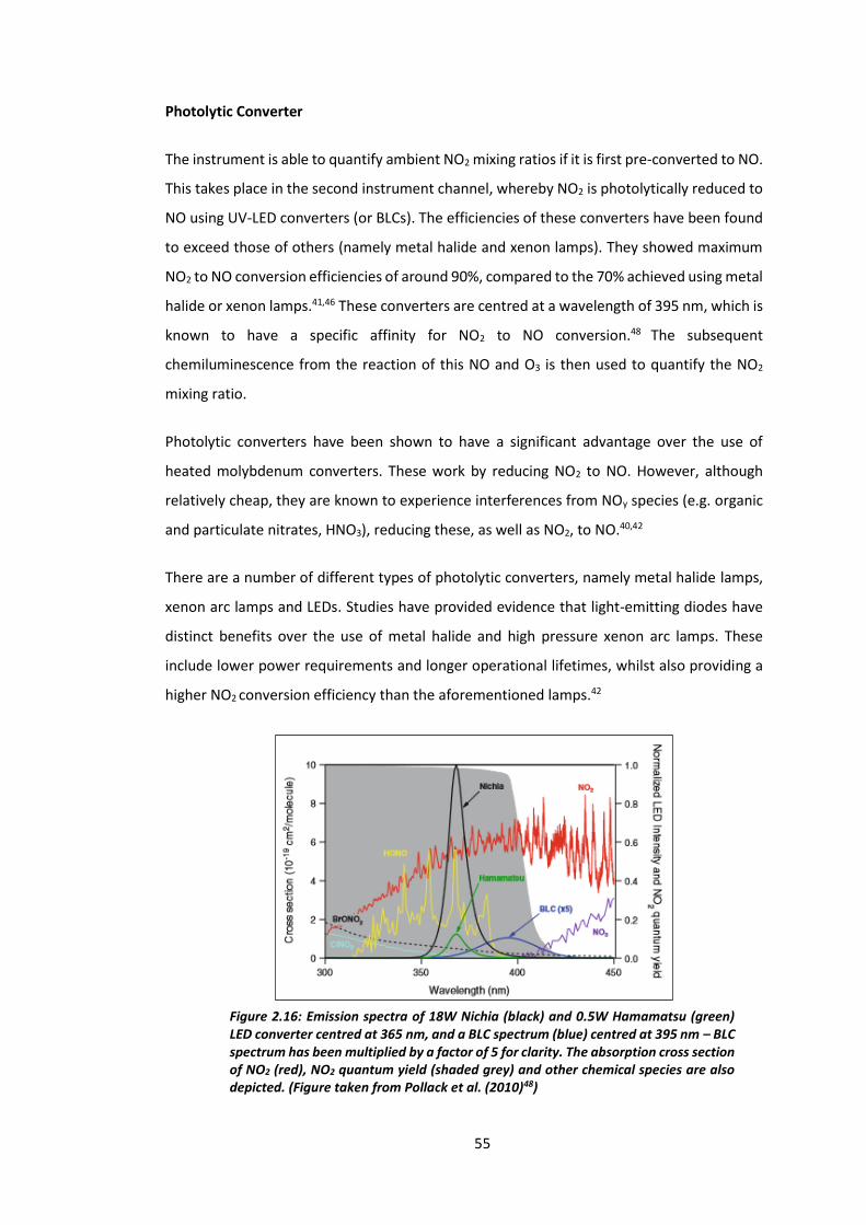
55
Photolytic Converter
The instrument is able to quantify ambient NO2 mixing ratios if it is first pre-converted to NO.
This takes place in the second instrument channel, whereby NO2 is photolytically reduced to
NO using UV-LED converters (or BLCs). The efficiencies of these converters have been found
to exceed those of others (namely metal halide and xenon lamps). They showed maximum
NO2 to NO conversion efficiencies of around 90%, compared to the 70% achieved using metal
halide or xenon lamps.41,46 These converters are centred at a wavelength of 395 nm, which is
known to have a specific affinity for NO2 to NO conversion.48 The subsequent
chemiluminescence from the reaction of this NO and O3 is then used to quantify the NO2
mixing ratio.
Photolytic converters have been shown to have a significant advantage over the use of
heated molybdenum converters. These work by reducing NO2 to NO. However, although
relatively cheap, they are known to experience interferences from NOy species (e.g. organic
and particulate nitrates, HNO3), reducing these, as well as NO2, to NO.40,42
There are a number of different types of photolytic converters, namely metal halide lamps,
xenon arc lamps and LEDs. Studies have provided evidence that light-emitting diodes have
distinct benefits over the use of metal halide and high pressure xenon arc lamps. These
include lower power requirements and longer operational lifetimes, whilst also providing a
higher NO2 conversion efficiency than the aforementioned lamps.42
Figure 2.16: Emission spectra of 18W Nichia (black) and 0.5W Hamamatsu (green) LED converter centred at 365 nm, and a BLC spectrum (blue) centred at 395 nm – BLC spectrum has been multiplied by a factor of 5 for clarity. The absorption cross section of NO2 (red), NO2 quantum yield (shaded grey) and other chemical species are also depicted. (Figure taken from Pollack et al. (2010)48)
56
The BLC in the instrument used during this research project is similar to that used in a study
by Pollack et al.,48 which compared three different types of LED. The BLC used by Pollack et
al. consisted of two 395 nm LED modules at each end of the photolysis, thus producing
emission in the same wavelength interval as the BLC used in this thesis. As seen in Figure
2.15, the BLC, centred at 395 nm, has a distinct advantage. As well as showing good overlap
with the NO2 absorption cross section, the wavelength emitted from the BLC exhibits a very
poor amount of overlap with the absorption cross section of HONO. The affinity of 395 nm
for NO2 photolytic conversion to HNO3 thus provides a great amount of analyte selectivity
within the channel, due to the low probability of other species, such as HONO, being
photolyzed. This provides the reasoning behind the use of a BLC in the airborne
chemiluminescence instrument.
The total NOx is therefore quantified simply through addition of the direct NO measurement
from the first channel, and the indirect NO2 measurement in the second instrument channel.
NO and NOx measurements are therefore synchronous, as a result of the dual channel
configuration. This is a key requirement for the instrument, particularly in terms its use for
airborne measurements, which require it to measure at a resolution of 1 Hz.
2.2.2 Instrument Parameters
NO Mixing Ratios and Sensitivities
The measurement of the NO mixing ratio is direct, as this corresponds to the signal observed
when the LEDs in the BLC are turned off. It is calculated using Equation 2.11:
[NO] =(NOmeas−NOzeroint)
NO_NOsensint Equation 2.11
Where:
NOmeas = counts recorded by PMT while in measure mode
NOzeroint = interpolated value of averaged counts recorded while in pre-chamber mode
NOsensint = interpolated value of the sensitivity

57
The sensitivity of the NO channel is determined using Equation 2.12:
NO_NOsensint =(NO−NOmeasint)
NO_NOcalconc Equation 2.12
Where:
NOmeasint = interpolated value of the measure-mode counts
NOcalconc = mixing ratio of the NO calibration
NO2 Mixing Ratios and Sensitivities
The mixing ratio of NO2 is calculated in a similar way to NO, using Equation 2.13:
[NO2] =(NO2meas − NO2zeroint)
NO2_NO2sensint Equation 2.13
Where:
NO2meas = counts recorded by PMT while in measure mode
NO2zeroint = interpolated value of average counts measured in the zero mode
NO2_NO2sensint = interpolated NO2 sensitivity for the instrument
58
The NO2 channel sensitivity is calculated using Equation 2.14:
NO2NO2sens=
(NO2cal−NO2measint)
NO2_NO2calconc Equation 2.14
Where:
NO2cal = average of counts from the instrument in calibration mode
NO2measint = interpolated value of the measure-mode counts
NO2_NO2calconc = mixing ratio of the NO2 calibration
“Zero” Instrument Modes
The instrument has two “zero” modes. The first mode uses the pre-chamber to react the O3
with NO before reaching the PMT detector. This means that all chemiluminescence occurs
here and a background signal of the PMT is measured. The signal resulting from the addition
of O3 in the prechamber accounts for any interferences (namely, the reaction of O3 with
hydrocarbons and the reaction chamber walls),41 thus giving the instrument’s zero (or
background) reading. This is a result of the reaction of NO and O3 being faster than most of
these interference reactions. Then, during measure mode, the O3 is added to the main
reaction chamber. The difference in signal between said measure mode and the zero mode
(when O3 is added to the pre-reaction volume) corresponds to the NO mixing ratio in the
sample air. It is the chemiluminescence resulting from the gas-phase titration (i.e. the
reaction of NO and O3) which is then observed by the PMT.
The other zero mode is when zero air is added to the sample lines, thus giving an indication
of the artefact associated with each instrument channel. This mode is particularly important
when looking at the errors associated with the instrument, and is discussed further in section
2.2.3.
59
2.2.3 Error Analysis
It is important to carry out error analysis associated with the instrument, as this allows
assessment of the reliability of the data obtained during the flights. This involves looking at
both the accuracy and precision of the data.
Accuracy
The accuracy of the observations is affected by a number of uncertainties. The first of which
is in the calibration procedure. The total accuracy of the calibration depends on the errors
associated with three instrumental features; the sample and calibration gas MFCs, the mixing
ratio of the NO standard and the NO2 conversion efficiency.
It is vital that during calibrations, the mixing ratio of NO standard gas that is added to the
system is measured with as high an accuracy as possible. This consequently depends on the
accuracy of the sample and calibration gas mass flow controllers. These have an associated
accuracy of 1% each, and are calibrated before, during and after any research campaign using
a digital flow meter. This ensures that they are measuring flows as accurately as possible,
thus minimising the error associated with the mass flow controllers. It is also important to
check the mixing ratio of the reference gas against the manufacturer’s stated mixing ratio.
This is done using the ACTRIS protocols (see http://www.actris.eu/ for details).
The mixing ratio of the NO standard is known to an accuracy of ±1% (British Oxygen Company
(BOC), certified to the UK National Physical Laboratory). The NO/N2 mix should be stable for
5 years (certified by BOC). The oxygen cylinder has a high purity level of N2.6. This means
that it has a guaranteed minimum purity of 99.6% and maximum impurity level of 0.4%,
certified by BOC.
There is also an error associated with the NO2 conversion efficiency that the instrument
measures. This is particularly important for the NO2 mixing ratios that are measured during
the calibration. This error is only small, at 1%, but must be considered as an important
component in the determination of the instrument’s total error (see later).
As a very efficient quencher of both the excited state of NO2 and reactions that produce the
background signal, water vapour can significantly affect the sensitivity of the instrument
through alterations of the background signal. During the flights, changing altitudes leads to
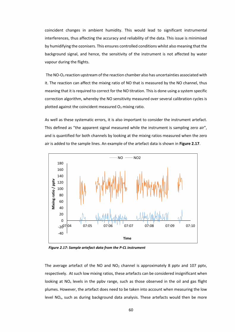
60
coincident changes in ambient humidity. This would lead to significant instrumental
interferences, thus affecting the accuracy and reliability of the data. This issue is minimised
by humidifying the ozonisers. This ensures controlled conditions whilst also meaning that the
background signal, and hence, the sensitivity of the instrument is not affected by water
vapour during the flights.
The NO-O3 reaction upstream of the reaction chamber also has uncertainties associated with
it. The reaction can affect the mixing ratio of NO that is measured by the NO channel, thus
meaning that it is required to correct for the NO titration. This is done using a system specific
correction algorithm, whereby the NO sensitivity measured over several calibration cycles is
plotted against the coincident measured O3 mixing ratio.
As well as these systematic errors, it is also important to consider the instrument artefact.
This defined as “the apparent signal measured while the instrument is sampling zero air”,
and is quantified for both channels by looking at the mixing ratios measured when the zero
air is added to the sample lines. An example of the artefact data is shown in Figure 2.17.
The average artefact of the NO and NO2 channel is approximately 8 pptv and 107 pptv,
respectively. At such low mixing ratios, these artefacts can be considered insignificant when
looking at NOx levels in the ppbv range, such as those observed in the oil and gas flight
plumes. However, the artefact does need to be taken into account when measuring the low
level NOx, such as during background data analysis. These artefacts would then be more
Figure 2.17: Sample artefact data from the P-CL instrument
-40
-20
0
20
40
60
80
100
120
140
160
180
07:04 07:05 07:06 07:07 07:08 07:09 07:10
Mix
ing
rati
o /
pp
tv
Time
NO NO2
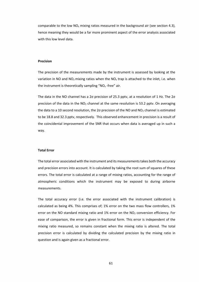
61
comparable to the low NOx mixing ratios measured in the background air (see section 4.3),
hence meaning they would be a far more prominent aspect of the error analysis associated
with this low level data.
Precision
The precision of the measurements made by the instrument is assessed by looking at the
variation in NO and NO2 mixing ratios when the NOx trap is attached to the inlet, i.e. when
the instrument is theoretically sampling “NOx -free” air.
The data in the NO channel has a 2σ precision of 25.3 pptv, at a resolution of 1 Hz. The 2σ
precision of the data in the NO2 channel at the same resolution is 53.2 pptv. On averaging
the data to a 10 second resolution, the 2σ precision of the NO and NO2 channel is estimated
to be 18.8 and 32.3 pptv, respectively. This observed enhancement in precision is a result of
the coincidental improvement of the SNR that occurs when data is averaged up in such a
way.
Total Error
The total error associated with the instrument and its measurements takes both the accuracy
and precision errors into account. It is calculated by taking the root sum of squares of these
errors. The total error is calculated at a range of mixing ratios, accounting for the range of
atmospheric conditions which the instrument may be exposed to during airborne
measurements.
The total accuracy error (i.e. the error associated with the instrument calibration) is
calculated as being 4%. This comprises of; 1% error on the two mass flow controllers, 1%
error on the NO standard mixing ratio and 1% error on the NO2 conversion efficiency. For
ease of comparison, the error is given in fractional form. This error is independent of the
mixing ratio measured, so remains constant when the mixing ratio is altered. The total
precision error is calculated by dividing the calculated precision by the mixing ratio in
question and is again given as a fractional error.
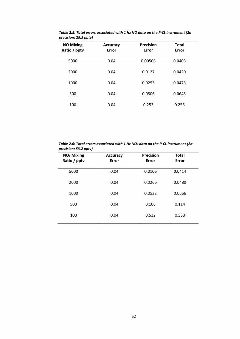
62
NO Mixing Ratio / pptv
Accuracy Error
Precision Error
Total Error
5000 0.04 0.00506 0.0403
2000 0.04 0.0127 0.0420
1000 0.04 0.0253 0.0473
500 0.04 0.0506 0.0645
100 0.04 0.253 0.256
NO2 Mixing Ratio / pptv
Accuracy Error
Precision Error
Total Error
5000 0.04 0.0106 0.0414
2000 0.04 0.0266 0.0480
1000 0.04 0.0532 0.0666
500 0.04 0.106 0.114
100 0.04 0.532 0.533
Table 2.5: Total errors associated with 1 Hz NO data on the P-CL instrument (2σ precision: 25.3 pptv)
Table 2.6: Total errors associated with 1 Hz NO2 data on the P-CL instrument (2σ precision: 53.2 pptv)
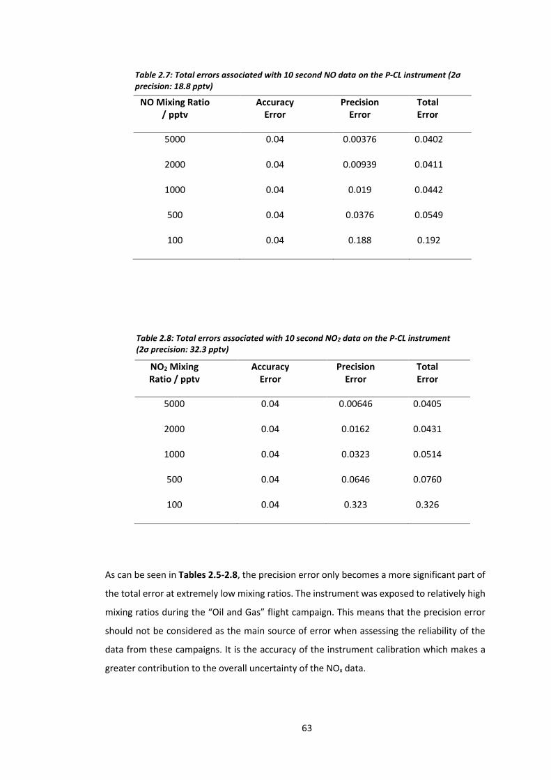
63
As can be seen in Tables 2.5-2.8, the precision error only becomes a more significant part of
the total error at extremely low mixing ratios. The instrument was exposed to relatively high
mixing ratios during the “Oil and Gas” flight campaign. This means that the precision error
should not be considered as the main source of error when assessing the reliability of the
data from these campaigns. It is the accuracy of the instrument calibration which makes a
greater contribution to the overall uncertainty of the NOx data.
NO Mixing Ratio / pptv
Accuracy Error
Precision Error
Total Error
5000 0.04 0.00376 0.0402
2000 0.04 0.00939 0.0411
1000 0.04 0.019 0.0442
500 0.04 0.0376 0.0549
100 0.04 0.188 0.192
NO2 Mixing Ratio / pptv
Accuracy Error
Precision Error
Total Error
5000 0.04 0.00646 0.0405
2000 0.04 0.0162 0.0431
1000 0.04 0.0323 0.0514
500 0.04 0.0646 0.0760
100 0.04 0.323 0.326
Table 2.7: Total errors associated with 10 second NO data on the P-CL instrument (2σ precision: 18.8 pptv)
Table 2.8: Total errors associated with 10 second NO2 data on the P-CL instrument (2σ precision: 32.3 pptv)
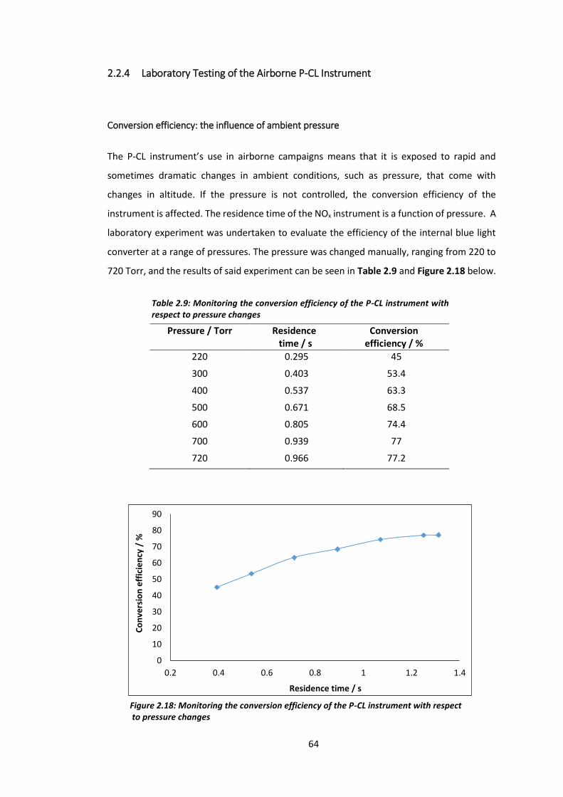
64
2.2.4 Laboratory Testing of the Airborne P-CL Instrument
Conversion efficiency: the influence of ambient pressure
The P-CL instrument’s use in airborne campaigns means that it is exposed to rapid and
sometimes dramatic changes in ambient conditions, such as pressure, that come with
changes in altitude. If the pressure is not controlled, the conversion efficiency of the
instrument is affected. The residence time of the NOx instrument is a function of pressure. A
laboratory experiment was undertaken to evaluate the efficiency of the internal blue light
converter at a range of pressures. The pressure was changed manually, ranging from 220 to
720 Torr, and the results of said experiment can be seen in Table 2.9 and Figure 2.18 below.
Pressure / Torr Residence time / s
Conversion efficiency / %
220 0.295 45
300 0.403 53.4
400 0.537 63.3
500 0.671 68.5
600 0.805 74.4
700 0.939 77
720 0.966 77.2
Figure 2.18: Monitoring the conversion efficiency of the P-CL instrument with respect to pressure changes
0
10
20
30
40
50
60
70
80
90
0.2 0.4 0.6 0.8 1 1.2 1.4
Co
nve
rsio
n e
ffic
ien
cy /
%
Residence time / s
Table 2.9: Monitoring the conversion efficiency of the P-CL instrument with respect to pressure changes
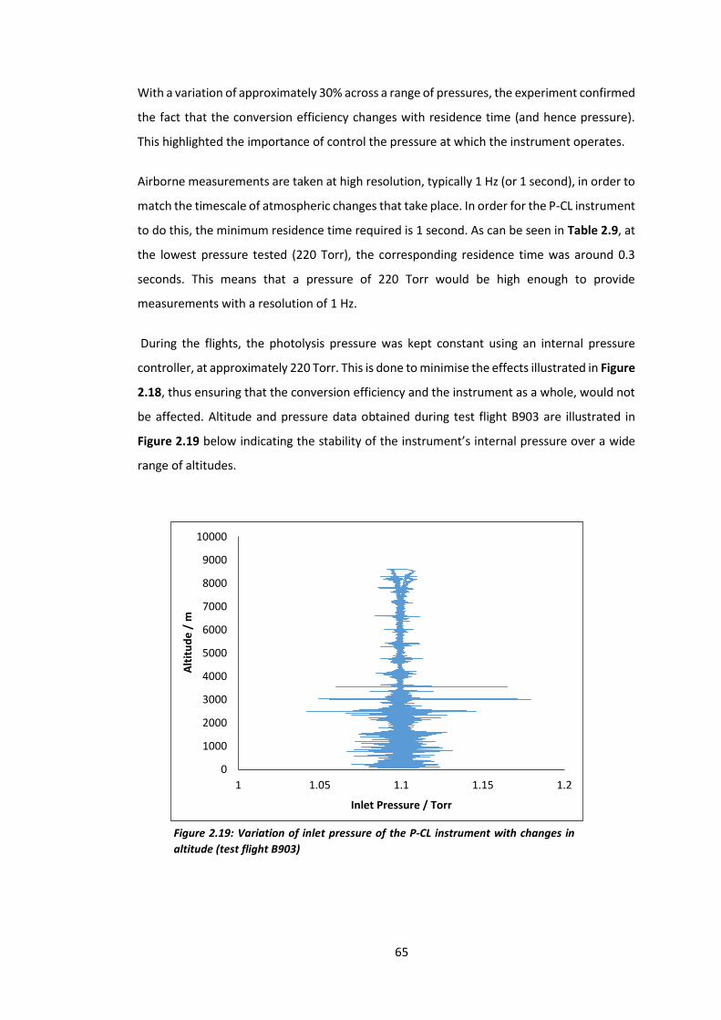
65
With a variation of approximately 30% across a range of pressures, the experiment confirmed
the fact that the conversion efficiency changes with residence time (and hence pressure).
This highlighted the importance of control the pressure at which the instrument operates.
Airborne measurements are taken at high resolution, typically 1 Hz (or 1 second), in order to
match the timescale of atmospheric changes that take place. In order for the P-CL instrument
to do this, the minimum residence time required is 1 second. As can be seen in Table 2.9, at
the lowest pressure tested (220 Torr), the corresponding residence time was around 0.3
seconds. This means that a pressure of 220 Torr would be high enough to provide
measurements with a resolution of 1 Hz.
During the flights, the photolysis pressure was kept constant using an internal pressure
controller, at approximately 220 Torr. This is done to minimise the effects illustrated in Figure
2.18, thus ensuring that the conversion efficiency and the instrument as a whole, would not
be affected. Altitude and pressure data obtained during test flight B903 are illustrated in
Figure 2.19 below indicating the stability of the instrument’s internal pressure over a wide
range of altitudes.
Figure 2.19: Variation of inlet pressure of the P-CL instrument with changes in
altitude (test flight B903)
0
1000
2000
3000
4000
5000
6000
7000
8000
9000
10000
1 1.05 1.1 1.15 1.2
Alt
itu
de
/ m
Inlet Pressure / Torr
66
CHAPTER 3: MEASUREMENT OF NOx IN THE REMOTE ATMOSPHERE –
TD-LIF DEPLOYMENT AT THE CVAO
3.1 NOx Measurements in the Remote Atmosphere
NOx emissions in the remote boundary layer, such as the North Atlantic Ocean are very low,
due to their location away from large emission sources (e.g. vehicular combustion and
biomass burning). This consequently means that there are very few local emissions of NOx in
these areas.
The amount of NOx directly transported to remote regions is also very low. Any primary NOx
is reacted away on a timescale of a few hours. This occurs through the oxidation of NO2 by
the hydroxyl radical, and the hydrolysis of N2O5 onto aerosol surfaces.68,69 Instead, it is
produced via the thermal decomposition of compounds such as PAN. PAN is a secondary
pollutant which is produced in regions of high NOx and volatile organic compound (VOC)
mixing ratios. Its stability in the mid-troposphere means that it is capable of long-range
transport, acting as a NOx reservoir in the process. However, PAN thermally decomposes at
altitudes below 7 km, releasing NOx into the remote atmosphere.19,20
Regions such Cape Verde are extremely sensitive to any slight changes in atmospheric
conditions, particularly in terms of O3 production. This is a result of the measured mixing
ratios of NOx often being extremely close to what is known as the O3 compensation point.
This is the level of NOx at which there is a switch from net destruction to net production of
O3. It is widely believed that this is found between 5 and 100 pptv NOx,10 with the actual
compensation point depending on the time of year, the location in the troposphere and the
mixing ratios of tropospheric O3 and water vapour. The measurement of NOx at the CVAO is
well documented, with consistent of NOx mixing ratios which lie within this crucial NOx
range.10,70 As a result of this, only minimal increases in NOx mixing ratios in remote areas like
Cape Verde could lead to a significant amount of O3 production in the marine boundary layer,
and in turn, have wide-reaching impacts on the global background atmosphere.71
67
3.2 Site Description
The CVAO is located on the island of São Vicente in the Cape Verde archipelago, off the west
coast of Africa. The site is part of the World Meteorological Organisation Global Atmosphere
Watch (WMO-GAW) long-term monitoring network, which measures a comprehensive range
of atmospheric species across the globe. (See
http://www.wmo.int/pages/prog/arep/gaw/gaw_home_en.html for more information.)
The main objective of the measurements at the site is to improve understanding of the
interactions which take place between the ocean and the air, through the monitoring of
trends of important atmospheric species. The CVAO is situated in the North Atlantic Ocean,
meaning that the majority of air masses observed at the site are well-processed within the
marine boundary layer, with minimal influence from local pollution sources. The location of
the site also means that a number of air masses of various origins are observed, with the
atmospheric chemistry taking place in the surrounding marine atmosphere being
significantly influenced by long-range transport.70 There are four main areas of air mass
origin: the Atlantic Ocean, continental Africa, coastal Africa and Europe. The influence of
these air masses varies depending on the time of year, with continental Africa being the most
dominant air mass in winter months and air masses of Atlantic or coastal African origin having
the most influence during the spring and summer months.10
3.3 Objectives of Deployment
As discussed in chapter 1, existing standard NO2 measurement techniques only measure NO2
indirectly, by first converting it to NO. A common way of doing this is to use heated
molybdenum catalysts, which reduce NO2 to NO. However, there have been noted
interferences from other NOy species, which also thermally decompose to produce NO2.40,44
Photolytic converters have been shown to minimise these interferences, using narrow
wavelength bands of radiation to specifically convert NO2 to NO.10,41,48 However, Reed et al.
(2015)50 recently investigated interferences in photolytic NO2 measurements, using a BLC-
equipped chemiluminescence instrument. A notable increase in NO2 mixing ratio was
reported in the photolysis cell in the presence of PAN, thus indicating that the decomposition
of PAN could also be a potentially significant source of interference for photolytic
68
chemiluminescence instruments. Earlier studies had also noted an interference from PAN
with photolytic converters.42,72
These interferences are likely to lead to an over-estimation of NO2 mixing ratios, with the
apparent “NO2” signal actually representing a range of other reactive nitrogen species in the
surrounding atmosphere. The use of direct NO2 measurement techniques alleviates this
issue, by exploiting spectroscopic features which are specific to NO2. The laser induced
fluorescence technique for example, is now a well-documented method for direct NO2
quantification32,34,37,38 and has been developed to ensure minimal interferences from other
atmospheric species are observed. (See sections 1.3 and 2.1)
The TD-LIF instrument used in this study has provided reliable NO2 measurements in a
number of field campaigns.18,32,38 However, prior to this study, the instrument had not been
used to measure NO2 in the remote boundary layer. A key requirement of the
instrumentation used for atmospheric measurements is that it is able to perform just as well
in remote locations, as well as in regions which experience high pollutant mixing ratios. The
TD-LIF instrument was deployed at the CVAO in January 2015, in order to assess the
performance of the instrument in terms of remote NO2 measurements. The NO2 data from
the TD-LIF would then be compared to the steady state NO2 mixing ratio, along with data
from a chemiluminescence instrument, which takes long-term measurements of NO2 (and
NO) at the observatory. A detailed description of this instrument can be found in a paper by
Lee et al. (2009).10 This instrument measures higher NO2 mixing ratios than expected at the
CVAO. This means that there is scope for improving the reliability and accuracy of long-term
measurements at the site, with the deployment of the TD-LIF being an attempt to do so.
Configuration of the TD-LIF for NO measurements also took place, using the experimental
set-up and reaction conditions that gave the maximum conversion efficiency in laboratory
tests conducted in York.
3.4 NO-NO2-O3 Photo-stationary state
As discussed in chapter 1, the cycle involving NO, NO2 and O3 generally results in no net
chemistry occurring, with the three species reaching a photo-stationary state after only a few
minutes.7 It is possible to predict the photo-stationary state mixing ratios of any one of these
three species by using Equation 3.1.
69
[NO] x [O3]
[NO2]=
J2
k1 Equation 3.1
Where:
J2 = rate of NO2 photolysis (1 x 10⁻² s-1)*
k1 = rate coefficient for the reaction of NO with O3 (1.90 x 10⁻⁴ molecules cm-3 s-1)73
[NO] = number density of NO (molecules cm-3)
[O3] = number density of O3 (molecules cm-3)
[NO2] = number density of NO2 (molecules cm-3)
*measured by a spectral radiometer74
At the CVAO, there is a chemiluminescence NOx analyser which is used to take long-term
measurements of NO and NO2. A steady state calculation can be done to determine the
mixing ratio of NO2 expected at the CVAO, which will give an indication as to how accurately
the chemiluminescence analyser is measuring NO2. This is done by looking at Equation 3.1 in
more detail.
The photo-stationary state equation is rearranged in terms of the NO2 mixing ratio.
[NO2] = k1 x [O3]x [NO]
J2 Equation 3.2
The mixing ratios of NO and O3 used in subsequent calculations refer to those measured at
CVAO in January 2007, at 33.4 and 4.5 pptv, with respect to O3 and NO.10
The NO and O3 mixing ratios were converted to number densities, and could be substituted
into Equation 3.2, along with the kinetic constants, to derive the NO2 number density.
[NO2] = (1.90 x 10⁻¹⁴ molecules cm−3s−1) x (8.23 x 1011 molecules cm−3) x (1.11 x 108 molecules cm−3)
1 x 10⁻² s−1
= 1.74 x 10⁸ molecules cm−3
Equation 3.3
70
In order to convert the NO2 number density back into a mixing ratio (for direct comparisons
with 2015 measurements of the same units), the number of air molecules in 1 cm3 of air must
be calculated. This is done using a form of the ideal gas equation.
PV = NkBT Equation 3.4
Where:
P = pressure (Pa)
V = volume (m3)
N = number of molecules
kB = Boltzmann constant (1.381 x 10⁻²³ J K-1)
T = temperature (K)
Equation 3.4 is then rearranged in terms of the number of molecules (i.e. “N”).
N =PV
kBT=
(105 Pa) x (10−6 m3)
(1.381 x 10⁻²³ J K−1)x (298 K)= 2.43 x 10¹⁹ air molecules Equation 3.5
In order to calculate an NO2 mixing ratio, in pptv, the number density of NO2 is divided by the
number of air molecules in 1 cm3 of air and multiplied by 1 trillion (1 x 10¹²).
NO2 mixing ratio = 1.74 x 10⁸ molecules cm−3 NO2
2.43 x 10¹⁹ molecules cm−3 air x (1 x 1012)
= 7.16 pptv Equation 3.6
This means that the theoretical average daytime NO2 mixing ratio at the CVAO in January
2007 is 7.6 pptv. The mean daytime NO2 mixing ratio measured by the chemiluminescence
instrument, however, is approximately 6 times higher than this, at 42.4 pptv.10 This finding
in itself is unsurprising, as several studies have reported a significant imbalance between the
measured NO2 and that expected from steady state calculations, particularly in low- NOx
environments.75,76,77
71
This has led to a number of hypotheses regarding the cause of this “gap” between theoretical
and measured NO2 mixing ratios in the remote environment. One suggestion is that there is
some sort of “mystery”, unmeasured oxidant which is reacting with NO to create NO2.78
Hosaynali Beygi et al. (2001)76 found that the NO2/NO ratio in the southern Atlantic Ocean
was around a factor of seven higher that what would be predicted by the Leighton
relationship (i.e. the steady state calculation).
The supporting measurements of other atmospheric species such as O3, carbon monoxide
and RO2 radicals, proved to by typical of the surrounding atmosphere. The authors therefore
attributed the discrepancy to an unknown oxidant, which selectively converts NO to NO2.
Another postulation surrounding the over-estimation of NO2 measurements in remote
environments is that there are species in the atmosphere which, although only being present
in trace quantities, are reacting with NO to produce NO2. Several studies have suggested that
the species in question are halogen oxides.79 For example, Bauguitte et al. (2012),75 reported
a significant discrepancy between observed and calculated NO2/NO ratios. However, the
reaction of the halogen oxides with NO was shown to have an impact on the NO2/NO ratios.
When the halogen oxides were included in the steady state calculations, the agreement with
the observations vastly improved. This suggested that the halogen oxides were reacting with
NO to produce NO2, thus resulting in increased the NO2/NO ratios that were previously
unaccounted for in the steady state calculation.
The LIF instrument was deployed at the CVAO to provide a direct, interference free method
of NO2 detection in order to confirm the high NO2 observed with the chemluminescence
instrument. This would also provide an insight into its suitability for NO2 measurements in a
remote atmospheric environment.
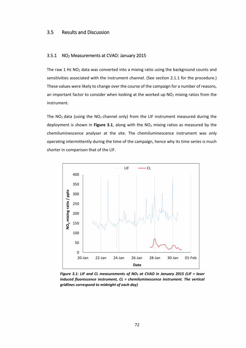
72
3.5 Results and Discussion
3.5.1 NO2 Measurements at CVAO: January 2015
The raw 1 Hz NO2 data was converted into a mixing ratio using the background counts and
sensitivities associated with the instrument channel. (See section 2.1.1 for the procedure.)
These values were likely to change over the course of the campaign for a number of reasons,
an important factor to consider when looking at the worked up NO2 mixing ratios from the
instrument.
The NO2 data (using the NO2 channel only) from the LIF instrument measured during the
deployment is shown in Figure 3.1, along with the NO2 mixing ratios as measured by the
chemiluminescence analyser at the site. The chemiluminescence instrument was only
operating intermittently during the time of the campaign, hence why its time series is much
shorter in comparison that of the LIF.
Figure 3.1: LIF and CL measurements of NO2 at CVAO in January 2015 (LIF = laser
induced fluorescence instrument, CL = chemiluminescence instrument. The vertical
gridlines correspond to midnight of each day)
0
50
100
150
200
250
300
350
400
20-Jan 22-Jan 24-Jan 26-Jan 28-Jan 30-Jan 01-Feb
NO
2m
ixin
g ra
tio
/ p
ptv
Date
LIF CL
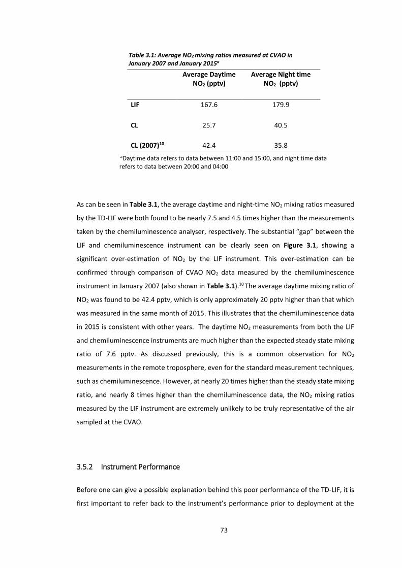
73
As can be seen in Table 3.1, the average daytime and night-time NO2 mixing ratios measured
by the TD-LIF were both found to be nearly 7.5 and 4.5 times higher than the measurements
taken by the chemiluminescence analyser, respectively. The substantial “gap” between the
LIF and chemiluminescence instrument can be clearly seen on Figure 3.1, showing a
significant over-estimation of NO2 by the LIF instrument. This over-estimation can be
confirmed through comparison of CVAO NO2 data measured by the chemiluminescence
instrument in January 2007 (also shown in Table 3.1).10 The average daytime mixing ratio of
NO2 was found to be 42.4 pptv, which is only approximately 20 pptv higher than that which
was measured in the same month of 2015. This illustrates that the chemiluminescence data
in 2015 is consistent with other years. The daytime NO2 measurements from both the LIF
and chemiluminescence instruments are much higher than the expected steady state mixing
ratio of 7.6 pptv. As discussed previously, this is a common observation for NO2
measurements in the remote troposphere, even for the standard measurement techniques,
such as chemiluminescence. However, at nearly 20 times higher than the steady state mixing
ratio, and nearly 8 times higher than the chemiluminescence data, the NO2 mixing ratios
measured by the LIF instrument are extremely unlikely to be truly representative of the air
sampled at the CVAO.
3.5.2 Instrument Performance
Before one can give a possible explanation behind this poor performance of the TD-LIF, it is
first important to refer back to the instrument’s performance prior to deployment at the
Average Daytime NO2 (pptv)
Average Night time NO2 (pptv)
LIF 167.6 179.9
CL 25.7 40.5
CL (2007)10 42.4 35.8
Table 3.1: Average NO2 mixing ratios measured at CVAO in January 2007 and January 2015a
aDaytime data refers to data between 11:00 and 15:00, and night time data refers to data between 20:00 and 04:00
74
CVAO. The instrument was run in the laboratory at the University of York in order to run
various experiments, and to assess the performance of the instrument in a polluted
atmospheric environment. Whilst there, several calibrations per day were conducted, in
order to get a stable background and sensitivity for all of the instrument channels. The
sensitivity of the NO2 channel stabilised at approximately 180 c/s/ppbv (the sensitivities of
the other three instrument channels can be seen in section 2.1.5) Confidence in the
instrument’s data was provided by the comparison to the AQD chemiluminescence NOx
analyser in the same laboratory, which showed very similar mixing ratios that were
representative of the surrounding area. (see section 2.1.5).
The TD-LIF was then deployed at the CVAO and the calibrations were conducted in exactly
the same manner as in York, running several per day to ensure stable calibration data.
However, a clear decline in the NO2 channel sensitivity was observed, dropping from by 80
c/s/ppbv from 180 down to 100 c/s/ppbv. Looking at Figure 3.1 and Table 3.1, one can see
that the chemiuminescence analyser and the TD-LIF data are not comparable, with the only
noticeable difference being the sensitivity of the instrument. However, the sensitivity is
dependent on a number of factors, meaning that it is not sufficient to directly link it to the
poor performance of the instrument. As discussed in section 2.1.2 the sensitivity is a function
of the collection efficiency. This depends on both the quality of the optics in the instrument
and on the quality of the PMT detector. The optics play a crucial role as these collect the
fluorescence photons, i.e. the fluorescence signal. The laser alignment therefore has to be as
good as possible, as this determines how much of the laser light passes through each
detection cell. However, such a large over-estimation of the NO2 mixing ratios by the LIF are
unlikely to be due solely to the mis-alignment of the laser, particularly due to the fact that
the data measured came from the first detection cell of the instrument (i.e. the NO2 cell). As
described and illustrated in section 2.1.1, this cell is in the closest proximity to the light
source, with only two reflective mirrors between the two instrument components, thus
meaning the laser power entering the would have been near-optimal. Therefore, slight mis-
alignment of the laser would only be likely to result in a minimal over-estimation of NO2 by
the detection cell.
The high mixing ratios of NO2 observed by the LIF must have therefore been due to a leak
within the system. Looking at the configuration of the instrument, the components most
likely to be prone to leaks would be the connection between the inlet line and the inlet box
and the connection between the NO2 inlet and the LIF instrument itself. Should either of
75
these experience leaks, the NO2 detected by the instrument would be representative of not
only the ambient air, but also the air within the laboratory. Although such leaks could not be
found during the deployment, these could provide an explanation as to why such elevated
NO2 mixing ratios were measured by the instrument.
NO Measurements
The LIF instrument was set up for NO measurements at the CVAO using the GPT configuration
described in section 2.1.6. A standard synthetic air cylinder (BTCA cylinder, 5 ppmv, certified
by BOC) was used as a constant supply of air for the O3 source, i.e. the multi-gas calibrator.
Although only running at a pressure of around 2 bar for the NO measurements, the cylinder
was also used as the zero air supply for the instrument calibrations. These calibrations were
critical to the operation of the instrument and required zero air at a pressure of 4 bar, in
order to completely flush all instrument channels. As discussed earlier in the chapter, the
comparison of NO2 data from the LIF and the chemiluminescence instrument indicated a
substantial over-estimation of NO2 mixing ratios by the LIF, which was believed to be due to
some kind of leak within the instrument. This would have impacted on any other
measurements made by the instrument. Therefore, for the sake of conserving the synthetic
air cylinder for the instrument calibrations, it was considered more viable to use the
instrument solely for NO2 measurements, whilst the cause of the instrument’s poor
sensitivity was determined.
Concluding Remarks
The TD-LIF instrument showed promising results when used to measure NO2 levels in a
polluted atmospheric environment (i.e. at the University of York). However, over-estimation
of NO2 levels at the remote monitoring site of the CVAO was observed, with average mixing
ratios being orders of magnitude higher than both the chemiluminescence analyser and the
expected steady state mixing ratio. This has led to the conclusion that the sensitivity of the
instrument is likely to have been over-estimated. It is thought that there may have been
some disruption to the instrument’s configuration, or leaks within the system, which has
caused the decline in sensitivity. This means that it would not be a viable instrument for long-
term NO2 measurements at the CVAO in its current configuration.
76
CHAPTER 4: AIRBORNE NOx MEASUREMENTS IN A POLLUTED
ATMOSPHERE – THE “OIL & GAS” CAMPAIGN (SUMMER 2015)
4.1 Atmospheric Emissions from Oil and Gas Rigs
The oil and gas industry supplies the UK with more than 70% of its total primary energy, with
oil meeting 97% of the country’s transport sector demand and gas being a key fuel for heating
and electricity generation.80 The industry also has substantial economic benefits, supporting
over 400,000 jobs and being the country’s largest industrial investor, paying around £4.7
billion in production tax in 2013/14.80
However, the processes involved in the industry, namely extraction, stabilisation and export
of hydrocarbons have substantial atmospheric emissions associated with them. The
continued operation of the offshore oil and gas platforms also release gases through
activities such as combustion, gas flaring and tank loading. The gases emitted by these
processes are given in Table 4.1.
Processes Gases released
Fuel combustion and gas flaring
Carbon dioxide (CO2)
Carbon monoxide (CO)
Methane (CH4)
Nitrogen oxides (NOx)
Sulphur oxides (SOx)
Nitrous oxide (N2O)
Tank loading Volatile organic compounds (VOCs)
Methane (CH4) Refrigeration and firefighting Chlorofluorocarbons (CFCs)
As can be seen in Table 4.1, the oil and gas platforms release a range of gases into the
surrounding atmosphere. According to Oil and Gas UK, the largest emission from the
platforms in the UK is CO2, with a 2014 document by the industry reporting the production
of around 14 million tonnes of CO2 in 2013.81
Table 4.1: Gases emitted by oil and gas platforms
77
Many oil and gas platforms, particularly in the North Sea, are often manned, hence meaning
that they require a large amount of power generation through fuel combustion. As Table 4.1
shows, this process leads to the production and subsequent release of a number of gases,
including NOx. In order to allow them to operate continuously, these rigs often require
support vessels which also produce NOx through fuel combustion. As result, although the NOx
produced by the platforms is relatively small when compared to CO2 (45,000 tonnes
produced in 2013)81, their operation involves continuous processes that can potentially emit
substantial amounts of NOx into an environment which is otherwise relatively clean.
Although the oil and gas industry is known to have many benefits in terms of meeting the
UK’s energy demands and economy, these substantial atmospheric emissions could have a
number of impacts on the environment on a regional, even global scale. The emission of
potent greenhouse gases, such as CO2 and CH4 through fuel combustion contributes to global
warming, due to their stability in the atmosphere and subsequent long atmospheric lifetimes
(5-200 and 12 years, respectively).82 The reaction between VOCs and NOx also has
implications for tropospheric O3 formation. This has knock-on effects for the oxidative
capacity of the atmosphere through the role of O3 as a precursor for OH radical formation,8
and as a strong oxidising agent in itself. The OH radical is one of the most powerful oxidising
agent in the atmosphere, controlling the lifetime of many potent greenhouse gases such as
methane,83,84 meaning that tropospheric O3 also has an indirect impact on the earth’s
radiative balance. As well as the atmosphere, tropospheric O3 also has adverse impacts on
human health, vegetation and crop yield through oxidative damage it causes.9 The acidic
gases, NOx and SOx, can also cause damage to ecosystems through acidification and
eutrophication.11,12
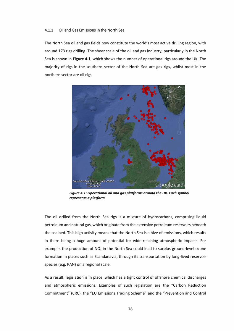
78
4.1.1 Oil and Gas Emissions in the North Sea
The North Sea oil and gas fields now constitute the world’s most active drilling region, with
around 173 rigs drilling. The sheer scale of the oil and gas industry, particularly in the North
Sea is shown in Figure 4.1, which shows the number of operational rigs around the UK. The
majority of rigs in the southern sector of the North Sea are gas rigs, whilst most in the
northern sector are oil rigs.
The oil drilled from the North Sea rigs is a mixture of hydrocarbons, comprising liquid
petroleum and natural gas, which originate from the extensive petroleum reservoirs beneath
the sea bed. This high activity means that the North Sea is a hive of emissions, which results
in there being a huge amount of potential for wide-reaching atmospheric impacts. For
example, the production of NOx in the North Sea could lead to surplus ground-level ozone
formation in places such as Scandanavia, through its transportation by long-lived reservoir
species (e.g. PAN) on a regional scale.
As a result, legislation is in place, which has a tight control of offshore chemical discharges
and atmospheric emissions. Examples of such legislation are the “Carbon Reduction
Commitment” (CRC), the “EU Emissions Trading Scheme” and the “Prevention and Control
Figure 4.1: Operational oil and gas platforms around the UK. Each symbol represents a platform
79
of Pollution” (PPC). It is therefore essential that emissions inventories are as accurate as
possible, as these provide estimates for current and likely future emissions from particular
sources.
4.2 Oil and Gas Rig Emissions in the North Sea: the “Oil and Gas” Campaign
During the summer of 2015, a series of survey flights took place over operational oil and gas
fields in the North Sea, on the UK’s FAAM BAe-146 research aircraft. A range of
measurements were made during the campaign, which are listed in Table 4.2. The airborne
photolytic chemiluminescence analyser, described in section 2.2, was used to measure NOx
emissions during the flights. The aim of the campaign was to fly downwind of active oil fields,
taking measurements in the plumes from oil and gas rigs. The direct integration method
would then be used for one of these flights, which would target specific rigs and calculate
the average emissions produced by each rig, in tons per year, which would then be compared
to the respective estimates from the NAEI.
The NAEI comprises the Greenhouse Gas Inventory (GHGI) and the Air Quality Pollutant
Inventory (AQPI). The inventory is maintained by Ricardo-AEA and is funded by Department
of Energy and Climate Change (DECC), the Department for Environment, Food and Rural
Affairs (DEFRA), the Scottish and Welsh governments, along with the Department of
Environment in Northern Ireland. The NAEI estimates annual emissions of a number of air
pollutants, most of which date back to 1970. In order to compile these inventories,
information from a wide range of sources is collected. These sources can range in scale, from
individual point sources such as power plants, to national energy statistics. Inventory data is
used in a number of applications which rely on them being as accurate as possible. The
estimates provide information about the sources and trends in emissions of greenhouse
gases and other air pollutants, which can have adverse effects on human health and the
natural environment. This, in turn means that the appropriate air quality reduction policies
can be implemented. The data can be used to track the UK’s progress towards international
legislation targets for both regional air pollution and climate change. This would then bring
the importance of improving the local, national and global environment to light.

80
Although several species were measured during the campaign, this thesis chapter will focus
solely on NOx emissions from the rigs, as these are point sources within the NAEI, thus
meaning that the measurements taken in plumes from individual rigs can be used to assess
the accuracy of these estimates.
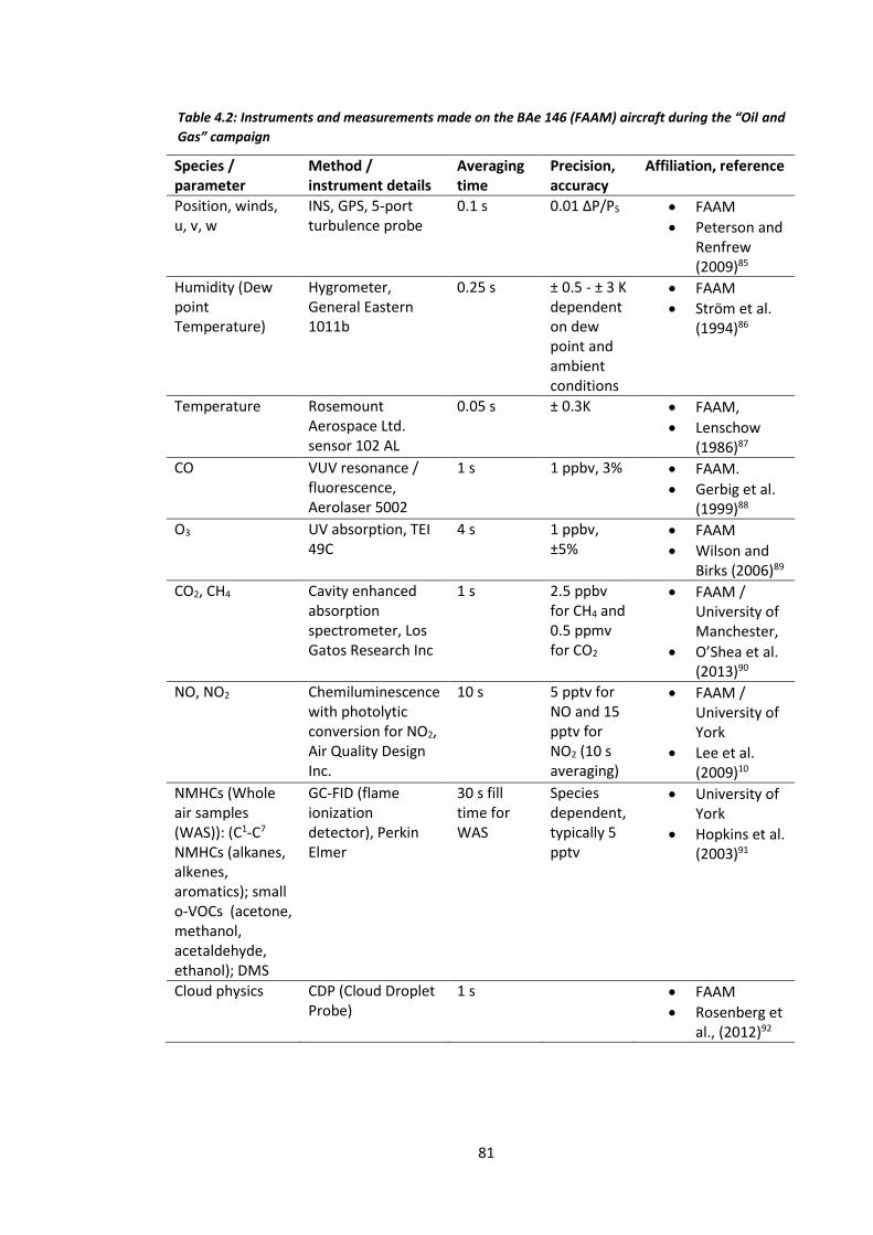
81
Species / parameter
Method / instrument details
Averaging time
Precision, accuracy
Affiliation, reference
Position, winds, u, v, w
INS, GPS, 5-port turbulence probe
0.1 s 0.01 ΔP/PS FAAM
Peterson and Renfrew (2009)85
Humidity (Dew point Temperature)
Hygrometer, General Eastern 1011b
0.25 s ± 0.5 - ± 3 K dependent on dew point and ambient conditions
FAAM
Ström et al. (1994)86
Temperature Rosemount Aerospace Ltd. sensor 102 AL
0.05 s ± 0.3K FAAM,
Lenschow (1986)87
CO
VUV resonance / fluorescence, Aerolaser 5002
1 s 1 ppbv, 3% FAAM.
Gerbig et al. (1999)88
O3
UV absorption, TEI 49C
4 s 1 ppbv, ±5%
FAAM
Wilson and Birks (2006)89
CO2, CH4
Cavity enhanced absorption spectrometer, Los Gatos Research Inc
1 s 2.5 ppbv for CH4 and 0.5 ppmv for CO2
FAAM / University of Manchester,
O’Shea et al. (2013)90
NO, NO2
Chemiluminescence with photolytic conversion for NO2, Air Quality Design Inc.
10 s 5 pptv for NO and 15 pptv for NO2 (10 s averaging)
FAAM / University of York
Lee et al. (2009)10
NMHCs (Whole air samples (WAS)): (C1-C7 NMHCs (alkanes, alkenes, aromatics); small o-VOCs (acetone, methanol, acetaldehyde, ethanol); DMS
GC-FID (flame ionization detector), Perkin Elmer
30 s fill time for WAS
Species dependent, typically 5 pptv
University of York
Hopkins et al. (2003)91
Cloud physics CDP (Cloud Droplet Probe)
1 s FAAM
Rosenberg et al., (2012)92
Table 4.2: Instruments and measurements made on the BAe 146 (FAAM) aircraft during the “Oil and
Gas” campaign
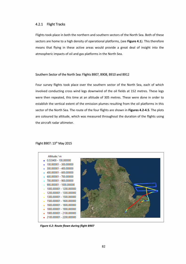
82
4.2.1 Flight Tracks
Flights took place in both the northern and southern sectors of the North Sea. Both of these
sectors are home to a high density of operational platforms, (see Figure 4.1). This therefore
means that flying in these active areas would provide a great deal of insight into the
atmospheric impacts of oil and gas platforms in the North Sea.
Southern Sector of the North Sea: Flights B907, B908, B910 and B912
Four survey flights took place over the southern sector of the North Sea, each of which
involved conducting cross wind legs downwind of the oil fields at 152 metres. These legs
were then repeated, this time at an altitude of 305 metres. These were done in order to
establish the vertical extent of the emission plumes resulting from the oil platforms in this
sector of the North Sea. The route of the four flights are shown in Figures 4.2-4.5. The plots
are coloured by altitude, which was measured throughout the duration of the flights using
the aircraft radar altimeter.
Flight B907: 13th May 2015
Figure 4.2: Route flown during flight B907
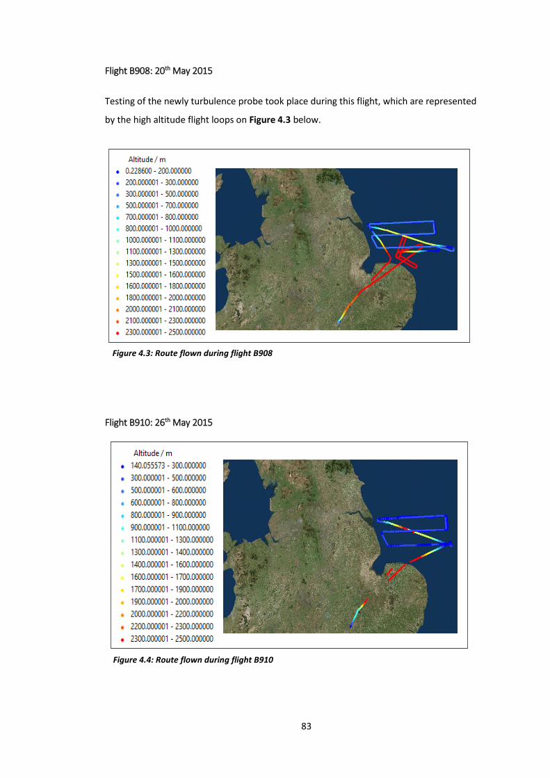
83
Flight B908: 20th May 2015
Testing of the newly turbulence probe took place during this flight, which are represented
by the high altitude flight loops on Figure 4.3 below.
Flight B910: 26th May 2015
Figure 4.3: Route flown during flight B908
Figure 4.4: Route flown during flight B910
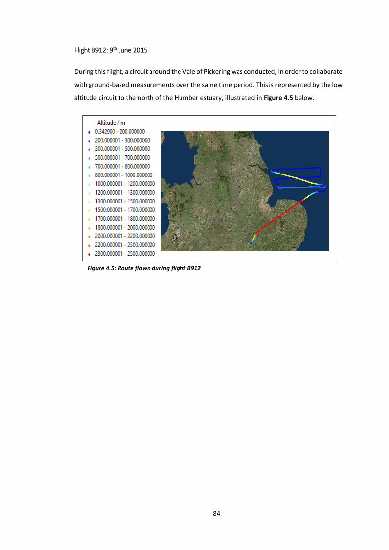
84
Flight B912: 9th June 2015
During this flight, a circuit around the Vale of Pickering was conducted, in order to collaborate
with ground-based measurements over the same time period. This is represented by the low
altitude circuit to the north of the Humber estuary, illustrated in Figure 4.5 below.
Figure 4.5: Route flown during flight B912
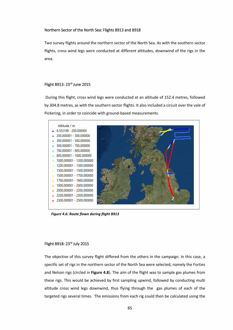
85
Northern Sector of the North Sea: Flights B913 and B918
Two survey flights around the northern sector of the North Sea. As with the southern sector
flights, cross wind legs were conducted at different altitudes, downwind of the rigs in the
area.
Flight B913: 23rd June 2015
During this flight, cross wind legs were conducted at an altitude of 152.4 metres, followed
by 304.8 metres, as with the southern sector flights. It also included a circuit over the vale of
Pickering, in order to coincide with ground-based measurements.
Flight B918: 23rd July 2015
The objective of this survey flight differed from the others in the campaign. In this case, a
specific set of rigs in the northern sector of the North Sea were selected, namely the Forties
and Nelson rigs (circled in Figure 4.8). The aim of the flight was to sample gas plumes from
these rigs. This would be achieved by first sampling upwind, followed by conducting multi
altitude cross wind legs downwind, thus flying through the gas plumes of each of the
targeted rigs several times. The emissions from each rig could then be calculated using the
Figure 4.6: Route flown during flight B913
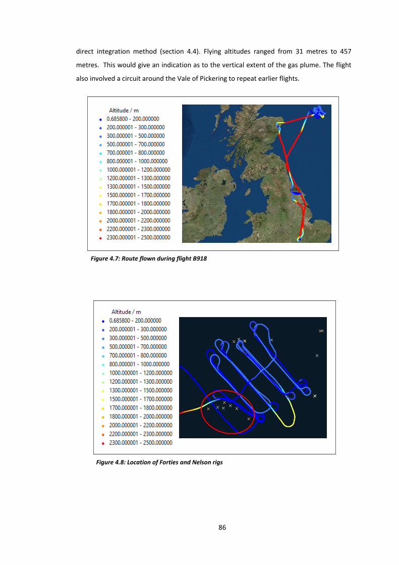
86
direct integration method (section 4.4). Flying altitudes ranged from 31 metres to 457
metres. This would give an indication as to the vertical extent of the gas plume. The flight
also involved a circuit around the Vale of Pickering to repeat earlier flights.
Figure 4.7: Route flown during flight B918
Figure 4.8: Location of Forties and Nelson rigs
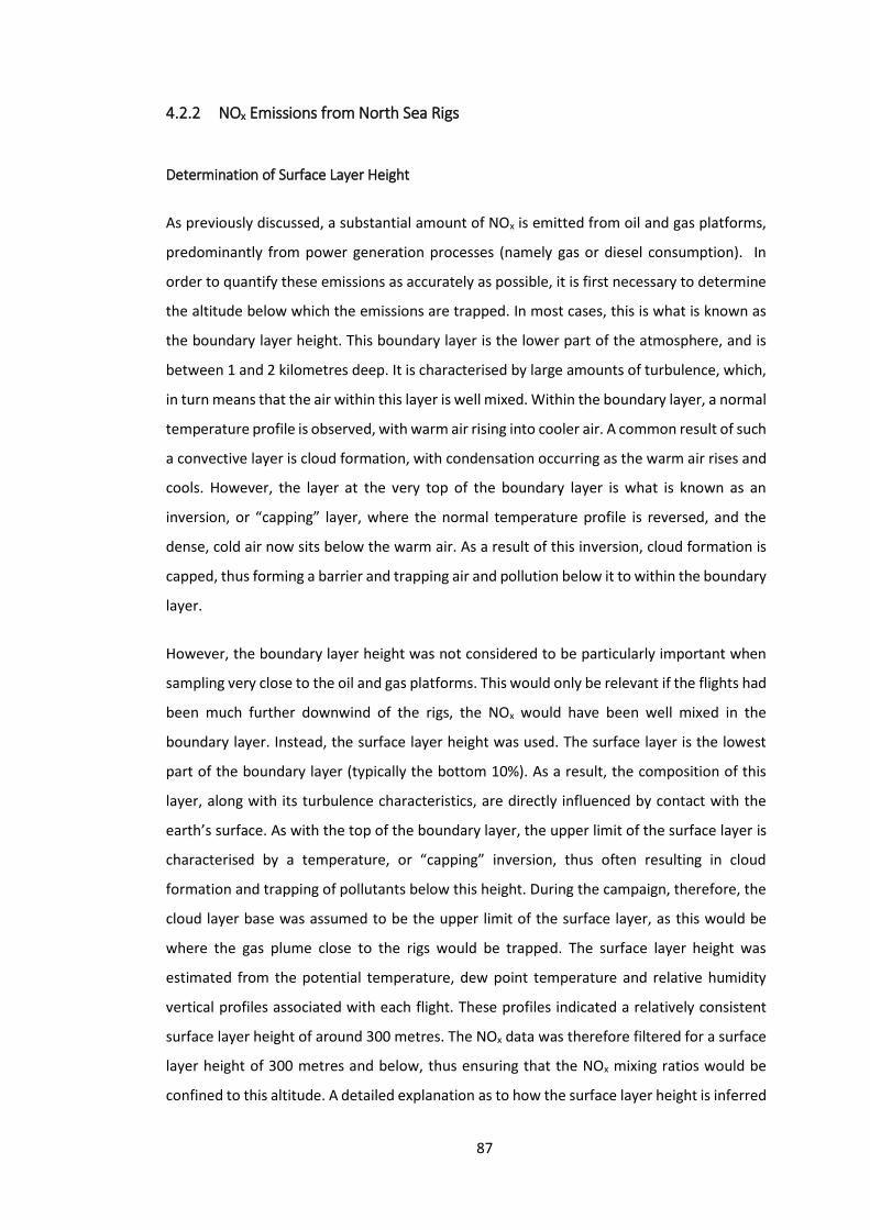
87
4.2.2 NOx Emissions from North Sea Rigs
Determination of Surface Layer Height
As previously discussed, a substantial amount of NOx is emitted from oil and gas platforms,
predominantly from power generation processes (namely gas or diesel consumption). In
order to quantify these emissions as accurately as possible, it is first necessary to determine
the altitude below which the emissions are trapped. In most cases, this is what is known as
the boundary layer height. This boundary layer is the lower part of the atmosphere, and is
between 1 and 2 kilometres deep. It is characterised by large amounts of turbulence, which,
in turn means that the air within this layer is well mixed. Within the boundary layer, a normal
temperature profile is observed, with warm air rising into cooler air. A common result of such
a convective layer is cloud formation, with condensation occurring as the warm air rises and
cools. However, the layer at the very top of the boundary layer is what is known as an
inversion, or “capping” layer, where the normal temperature profile is reversed, and the
dense, cold air now sits below the warm air. As a result of this inversion, cloud formation is
capped, thus forming a barrier and trapping air and pollution below it to within the boundary
layer.
However, the boundary layer height was not considered to be particularly important when
sampling very close to the oil and gas platforms. This would only be relevant if the flights had
been much further downwind of the rigs, the NOx would have been well mixed in the
boundary layer. Instead, the surface layer height was used. The surface layer is the lowest
part of the boundary layer (typically the bottom 10%). As a result, the composition of this
layer, along with its turbulence characteristics, are directly influenced by contact with the
earth’s surface. As with the top of the boundary layer, the upper limit of the surface layer is
characterised by a temperature, or “capping” inversion, thus often resulting in cloud
formation and trapping of pollutants below this height. During the campaign, therefore, the
cloud layer base was assumed to be the upper limit of the surface layer, as this would be
where the gas plume close to the rigs would be trapped. The surface layer height was
estimated from the potential temperature, dew point temperature and relative humidity
vertical profiles associated with each flight. These profiles indicated a relatively consistent
surface layer height of around 300 metres. The NOx data was therefore filtered for a surface
layer height of 300 metres and below, thus ensuring that the NOx mixing ratios would be
confined to this altitude. A detailed explanation as to how the surface layer height is inferred
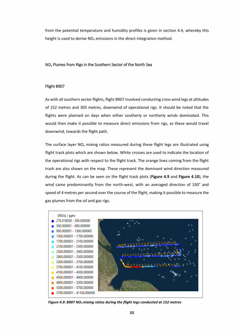
88
from the potential temperature and humidity profiles is given in section 4.4, whereby this
height is used to derive NOx emissions in the direct integration method.
NOx Plumes from Rigs in the Southern Sector of the North Sea
Flight B907
As with all southern sector flights, flight B907 involved conducting cross wind legs at altitudes
of 152 metres and 305 metres, downwind of operational rigs. It should be noted that the
flights were planned on days when either southerly or northerly winds dominated. This
would then make it possible to measure direct emissions from rigs, as these would travel
downwind, towards the flight path.
The surface layer NOx mixing ratios measured during these flight legs are illustrated using
flight track plots which are shown below. White crosses are used to indicate the location of
the operational rigs with respect to the flight track. The orange lines coming from the flight
track are also shown on the map. These represent the dominant wind direction measured
during the flight. As can be seen on the flight track plots (Figure 4.9 and Figure 4.10), the
wind came predominantly from the north-west, with an averaged direction of 330° and
speed of 4 metres per second over the course of the flight, making it possible to measure the
gas plumes from the oil and gas rigs.
Figure 4.9: B907 NOx mixing ratios during the flight legs conducted at 152 metres
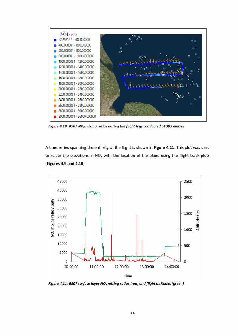
89
A time series spanning the entirety of the flight is shown in Figure 4.11. This plot was used
to relate the elevations in NOx with the location of the plane using the flight track plots
(Figures 4.9 and 4.10).
Figure 4.10: B907 NOx mixing ratios during the flight legs conducted at 305 metres
Figure 4.11: B907 surface layer NOx mixing ratios (red) and flight altitudes (green)
0
500
1000
1500
2000
2500
0
5000
10000
15000
20000
25000
30000
35000
40000
45000
10:00:00 11:00:00 12:00:00 13:00:00 14:00:00
Alt
itu
de
/ m
NO
xm
ixin
g ra
tio
/ p
ptv
Time
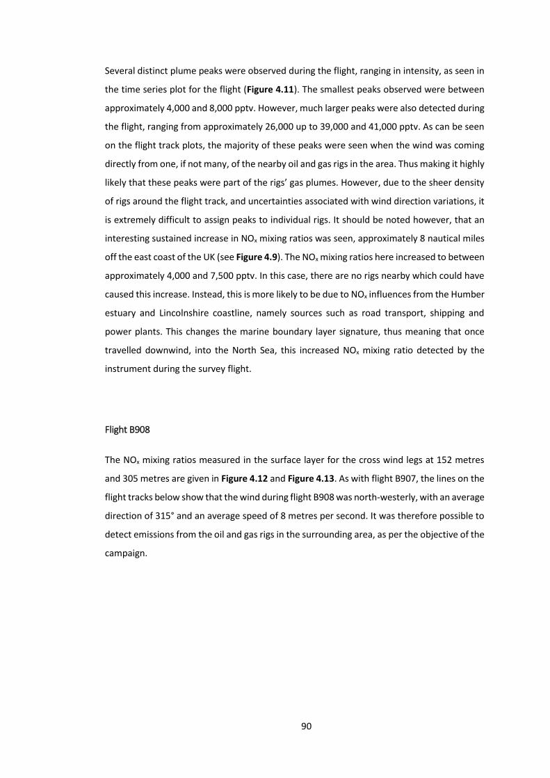
90
Several distinct plume peaks were observed during the flight, ranging in intensity, as seen in
the time series plot for the flight (Figure 4.11). The smallest peaks observed were between
approximately 4,000 and 8,000 pptv. However, much larger peaks were also detected during
the flight, ranging from approximately 26,000 up to 39,000 and 41,000 pptv. As can be seen
on the flight track plots, the majority of these peaks were seen when the wind was coming
directly from one, if not many, of the nearby oil and gas rigs in the area. Thus making it highly
likely that these peaks were part of the rigs’ gas plumes. However, due to the sheer density
of rigs around the flight track, and uncertainties associated with wind direction variations, it
is extremely difficult to assign peaks to individual rigs. It should be noted however, that an
interesting sustained increase in NOx mixing ratios was seen, approximately 8 nautical miles
off the east coast of the UK (see Figure 4.9). The NOx mixing ratios here increased to between
approximately 4,000 and 7,500 pptv. In this case, there are no rigs nearby which could have
caused this increase. Instead, this is more likely to be due to NOx influences from the Humber
estuary and Lincolnshire coastline, namely sources such as road transport, shipping and
power plants. This changes the marine boundary layer signature, thus meaning that once
travelled downwind, into the North Sea, this increased NOx mixing ratio detected by the
instrument during the survey flight.
Flight B908
The NOx mixing ratios measured in the surface layer for the cross wind legs at 152 metres
and 305 metres are given in Figure 4.12 and Figure 4.13. As with flight B907, the lines on the
flight tracks below show that the wind during flight B908 was north-westerly, with an average
direction of 315° and an average speed of 8 metres per second. It was therefore possible to
detect emissions from the oil and gas rigs in the surrounding area, as per the objective of the
campaign.
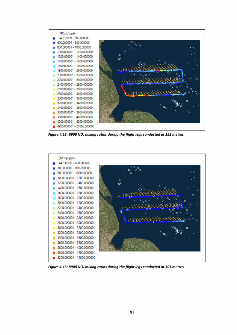
91
Figure 4.13: B908 NOx mixing ratios during the flight legs conducted at 305 metres
Figure 4.12: B908 NOx mixing ratios during the flight legs conducted at 152 metres
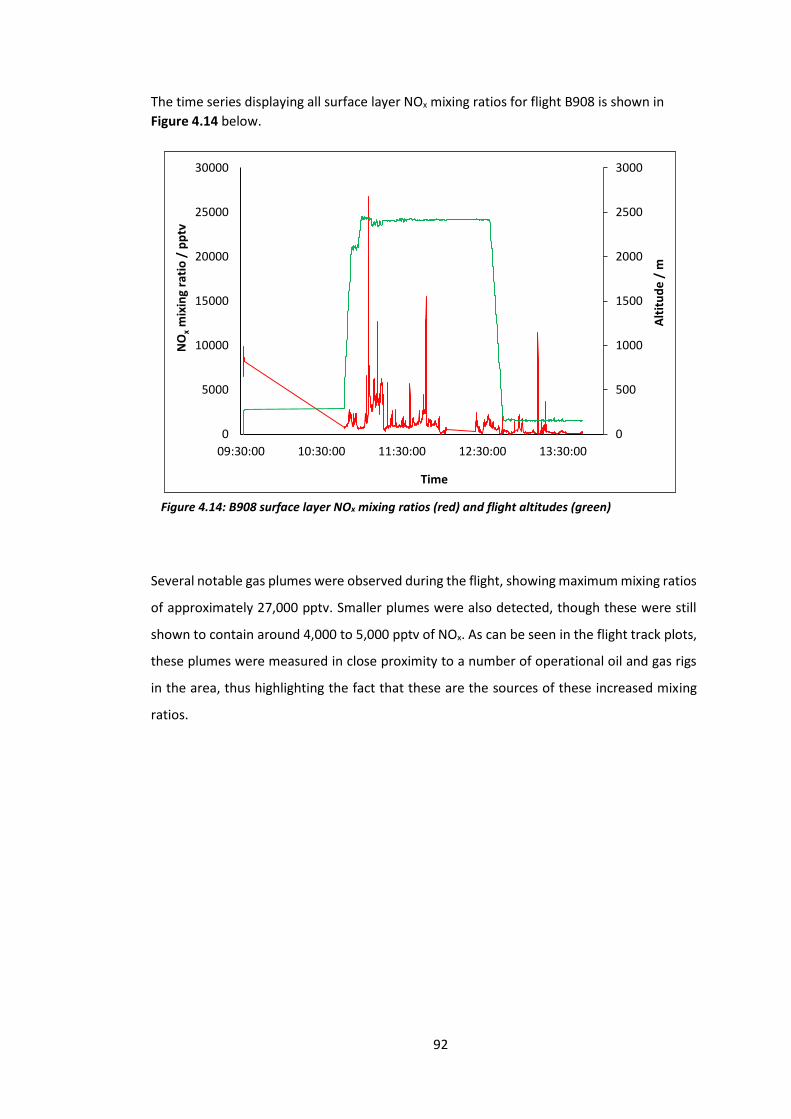
92
The time series displaying all surface layer NOx mixing ratios for flight B908 is shown in
Figure 4.14 below.
Several notable gas plumes were observed during the flight, showing maximum mixing ratios
of approximately 27,000 pptv. Smaller plumes were also detected, though these were still
shown to contain around 4,000 to 5,000 pptv of NOx. As can be seen in the flight track plots,
these plumes were measured in close proximity to a number of operational oil and gas rigs
in the area, thus highlighting the fact that these are the sources of these increased mixing
ratios.
0
500
1000
1500
2000
2500
3000
0
5000
10000
15000
20000
25000
30000
09:30:00 10:30:00 11:30:00 12:30:00 13:30:00
Alt
itu
de
/ m
NO
xm
ixin
g ra
tio
/ p
ptv
Time
Figure 4.14: B908 surface layer NOx mixing ratios (red) and flight altitudes (green)
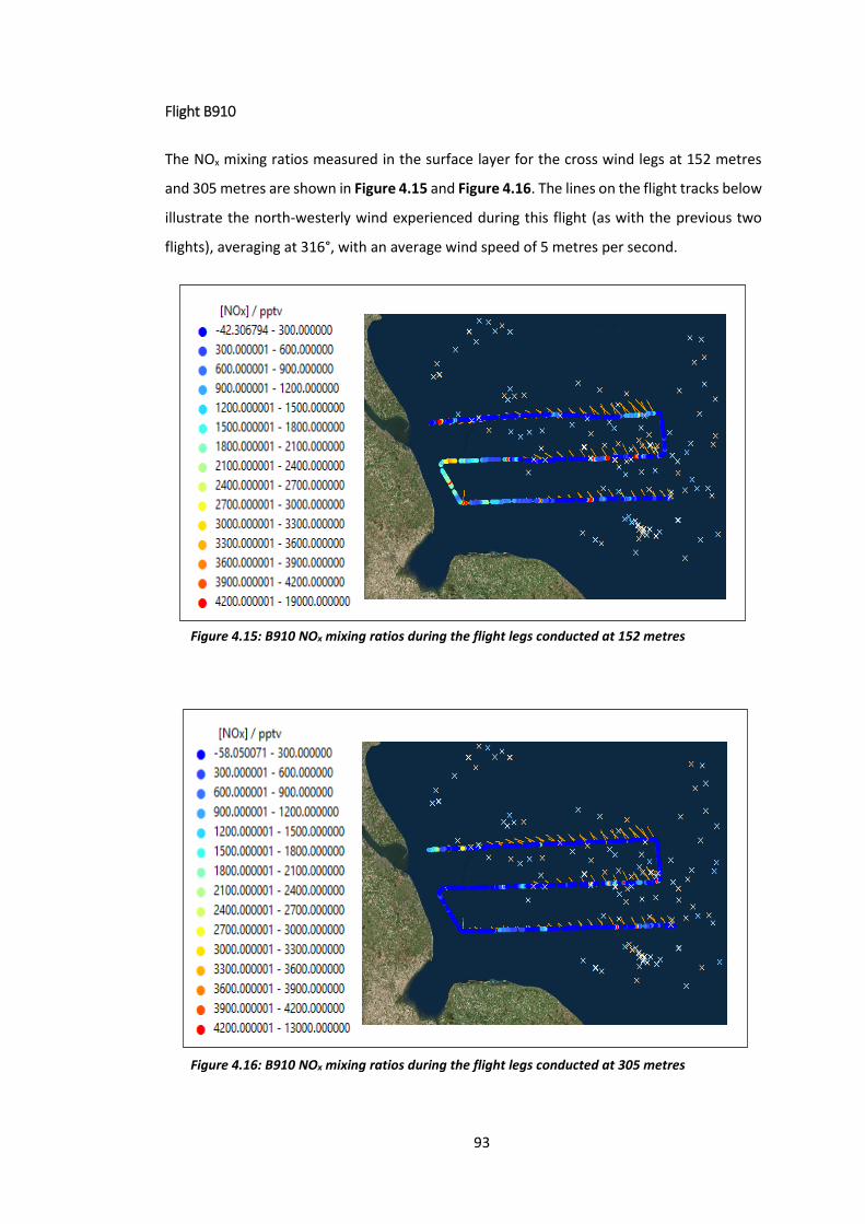
93
Flight B910
The NOx mixing ratios measured in the surface layer for the cross wind legs at 152 metres
and 305 metres are shown in Figure 4.15 and Figure 4.16. The lines on the flight tracks below
illustrate the north-westerly wind experienced during this flight (as with the previous two
flights), averaging at 316°, with an average wind speed of 5 metres per second.
Figure 4.15: B910 NOx mixing ratios during the flight legs conducted at 152 metres
Figure 4.16: B910 NOx mixing ratios during the flight legs conducted at 305 metres
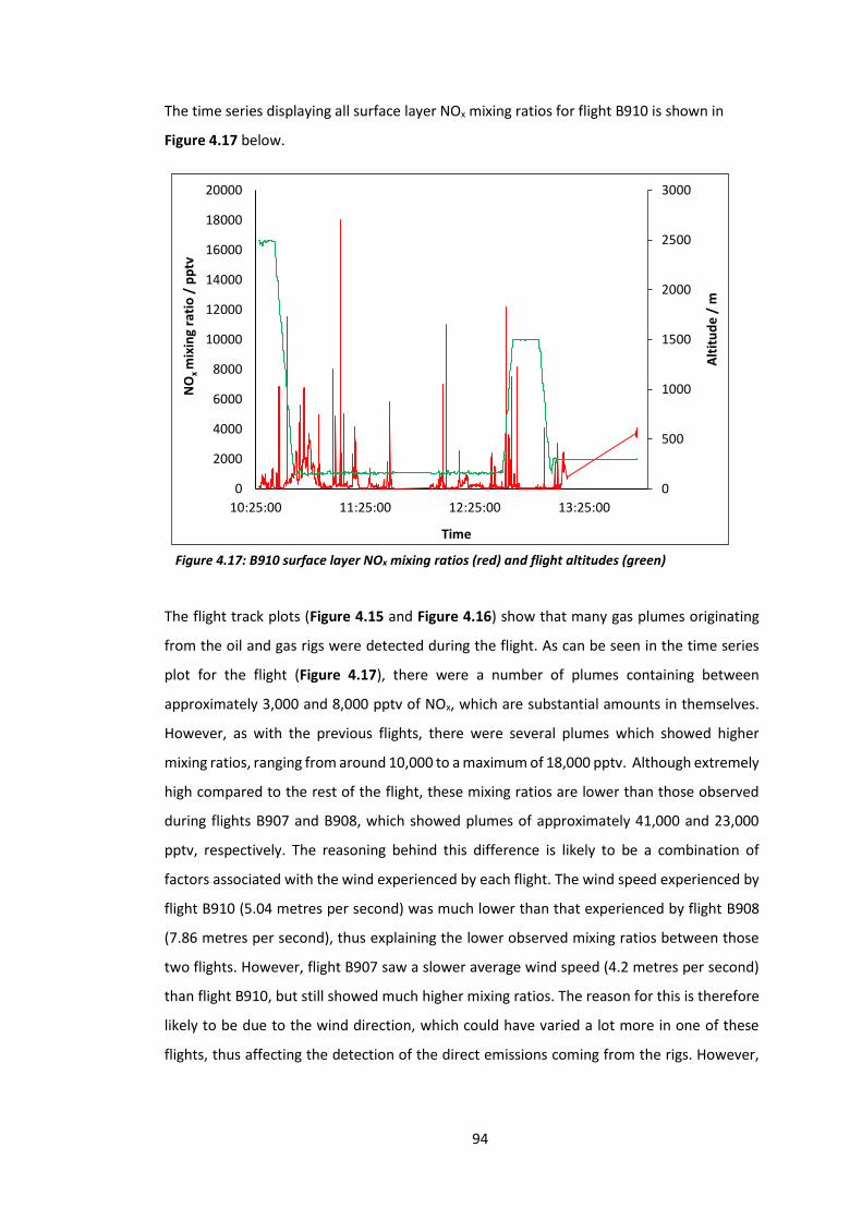
94
The time series displaying all surface layer NOx mixing ratios for flight B910 is shown in
Figure 4.17 below.
The flight track plots (Figure 4.15 and Figure 4.16) show that many gas plumes originating
from the oil and gas rigs were detected during the flight. As can be seen in the time series
plot for the flight (Figure 4.17), there were a number of plumes containing between
approximately 3,000 and 8,000 pptv of NOx, which are substantial amounts in themselves.
However, as with the previous flights, there were several plumes which showed higher
mixing ratios, ranging from around 10,000 to a maximum of 18,000 pptv. Although extremely
high compared to the rest of the flight, these mixing ratios are lower than those observed
during flights B907 and B908, which showed plumes of approximately 41,000 and 23,000
pptv, respectively. The reasoning behind this difference is likely to be a combination of
factors associated with the wind experienced by each flight. The wind speed experienced by
flight B910 (5.04 metres per second) was much lower than that experienced by flight B908
(7.86 metres per second), thus explaining the lower observed mixing ratios between those
two flights. However, flight B907 saw a slower average wind speed (4.2 metres per second)
than flight B910, but still showed much higher mixing ratios. The reason for this is therefore
likely to be due to the wind direction, which could have varied a lot more in one of these
flights, thus affecting the detection of the direct emissions coming from the rigs. However,
0
500
1000
1500
2000
2500
3000
0
2000
4000
6000
8000
10000
12000
14000
16000
18000
20000
10:25:00 11:25:00 12:25:00 13:25:00
Alt
itu
de
/ m
NO
x m
ixin
g ra
tio
/ p
ptv
Time
Figure 4.17: B910 surface layer NOx mixing ratios (red) and flight altitudes (green)
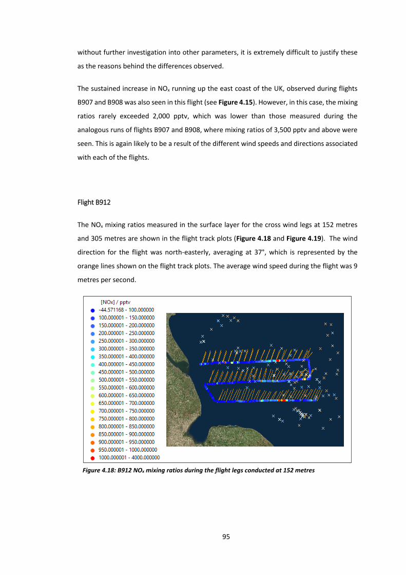
95
without further investigation into other parameters, it is extremely difficult to justify these
as the reasons behind the differences observed.
The sustained increase in NOx running up the east coast of the UK, observed during flights
B907 and B908 was also seen in this flight (see Figure 4.15). However, in this case, the mixing
ratios rarely exceeded 2,000 pptv, which was lower than those measured during the
analogous runs of flights B907 and B908, where mixing ratios of 3,500 pptv and above were
seen. This is again likely to be a result of the different wind speeds and directions associated
with each of the flights.
Flight B912
The NOx mixing ratios measured in the surface layer for the cross wind legs at 152 metres
and 305 metres are shown in the flight track plots (Figure 4.18 and Figure 4.19). The wind
direction for the flight was north-easterly, averaging at 37°, which is represented by the
orange lines shown on the flight track plots. The average wind speed during the flight was 9
metres per second.
Figure 4.18: B912 NOx mixing ratios during the flight legs conducted at 152 metres
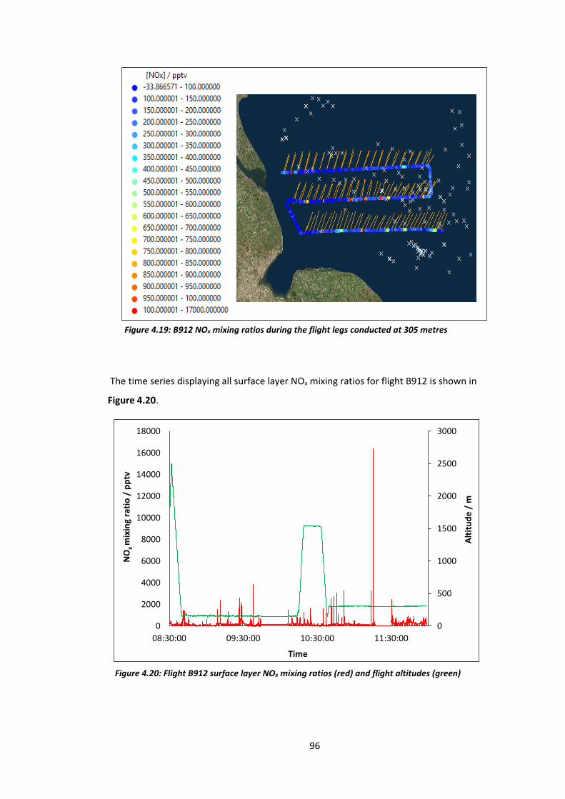
96
The time series displaying all surface layer NOx mixing ratios for flight B912 is shown in
Figure 4.20.
Figure 4.19: B912 NOx mixing ratios during the flight legs conducted at 305 metres
0
500
1000
1500
2000
2500
3000
0
2000
4000
6000
8000
10000
12000
14000
16000
18000
08:30:00 09:30:00 10:30:00 11:30:00
Alt
itu
de
/ m
NO
x m
ixin
g ra
tio
/ p
ptv
Time
Figure 4.20: Flight B912 surface layer NOx mixing ratios (red) and flight altitudes (green)

97
The gas plumes from the many oil and gas rigs in the surrounding area of the North Sea were
detected during the flight. It is possible to deduce this by looking at the flight track plots,
which show the average wind direction of 37° (Figure 4.18 and Figure 4.19). These show that
the elevated NOx mixing ratios were often observed when the plane was directly downwind
of one, or several of the rigs.
Compared to the other flights in the southern sector of the North Sea, the majority of gas
plumes observed in flight B912 were a lot smaller, ranging from around 1,000 to 4,000 pptv,
as can be seen on the time series plot for the flight (Figure 4.20). However, the largest gas
plume detected during this flight contained approximately 16,000 pptv of NOx. The reasons
for the lower mixing ratios in flight B912 compared to other flights are as yet unclear. One
possible reason could be the fact the wind, rather coming from a NNW direction (as in flights
B907, B908 and B910), instead comes from a NNE direction. This therefore could have meant
that plumes from particular rigs that were detected by the earlier three flights, were not seen
during B912, as the wind was coming from a slightly different direction. However, as
discussed earlier, it is very difficult to link plume peaks to particular rigs, so it is hard to say
whether this is, in fact, the reason behind the lower plume mixing ratios.
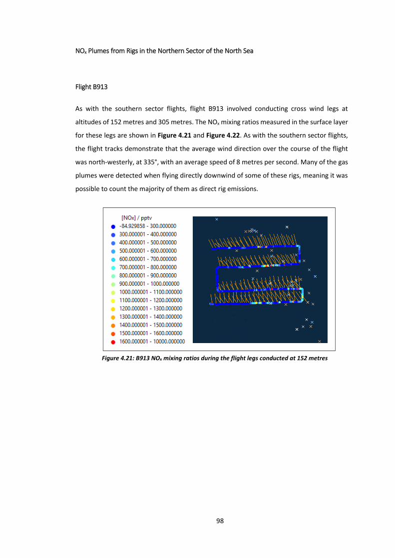
98
NOx Plumes from Rigs in the Northern Sector of the North Sea
Flight B913
As with the southern sector flights, flight B913 involved conducting cross wind legs at
altitudes of 152 metres and 305 metres. The NOx mixing ratios measured in the surface layer
for these legs are shown in Figure 4.21 and Figure 4.22. As with the southern sector flights,
the flight tracks demonstrate that the average wind direction over the course of the flight
was north-westerly, at 335°, with an average speed of 8 metres per second. Many of the gas
plumes were detected when flying directly downwind of some of these rigs, meaning it was
possible to count the majority of them as direct rig emissions.
Figure 4.21: B913 NOx mixing ratios during the flight legs conducted at 152 metres
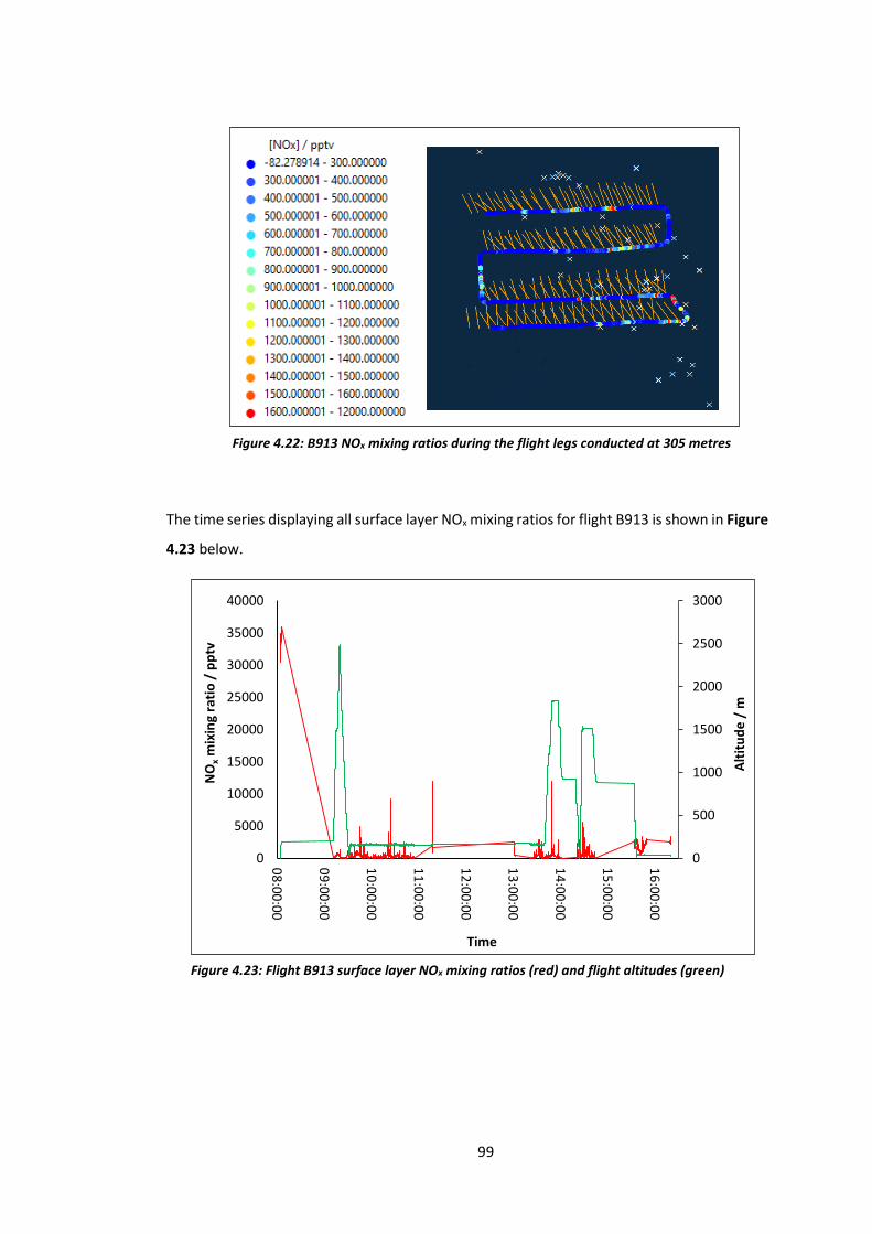
99
The time series displaying all surface layer NOx mixing ratios for flight B913 is shown in Figure
4.23 below.
Figure 4.22: B913 NOx mixing ratios during the flight legs conducted at 305 metres
0
500
1000
1500
2000
2500
3000
0
5000
10000
15000
20000
25000
30000
35000
400000
8:0
0:0
0
09
:00
:00
10
:00
:00
11
:00
:00
12
:00
:00
13
:00
:00
14
:00
:00
15
:00
:00
16
:00
:00
Alt
itu
de
/ m
NO
xm
ixin
g ra
tio
/ p
ptv
Time
Figure 4.23: Flight B913 surface layer NOx mixing ratios (red) and flight altitudes (green)
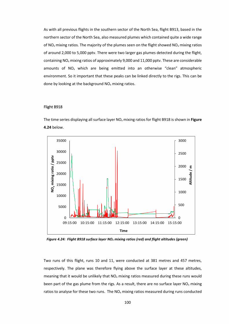
100
As with all previous flights in the southern sector of the North Sea, flight B913, based in the
northern sector of the North Sea, also measured plumes which contained quite a wide range
of NOx mixing ratios. The majority of the plumes seen on the flight showed NOx mixing ratios
of around 2,000 to 5,000 pptv. There were two larger gas plumes detected during the flight,
containing NOx mixing ratios of approximately 9,000 and 11,000 pptv. These are considerable
amounts of NOx which are being emitted into an otherwise “clean” atmospheric
environment. So it important that these peaks can be linked directly to the rigs. This can be
done by looking at the background NOx mixing ratios.
Flight B918
The time series displaying all surface layer NOx mixing ratios for flight B918 is shown in Figure
4.24 below.
Two runs of this flight, runs 10 and 11, were conducted at 381 metres and 457 metres,
respectively. The plane was therefore flying above the surface layer at these altitudes,
meaning that it would be unlikely that NOx mixing ratios measured during these runs would
been part of the gas plume from the rigs. As a result, there are no surface layer NOx mixing
ratios to analyse for these two runs. The NOx mixing ratios measured during runs conducted
0
500
1000
1500
2000
2500
3000
0
5000
10000
15000
20000
25000
30000
35000
09:15:00 10:15:00 11:15:00 12:15:00 13:15:00 14:15:00 15:15:00
Alt
itu
de
/ m
NO
xm
ixin
g ra
tio
/ p
ptv
Time
Figure 4.24: Flight B918 surface layer NOx mixing ratios (red) and flight altitudes (green)
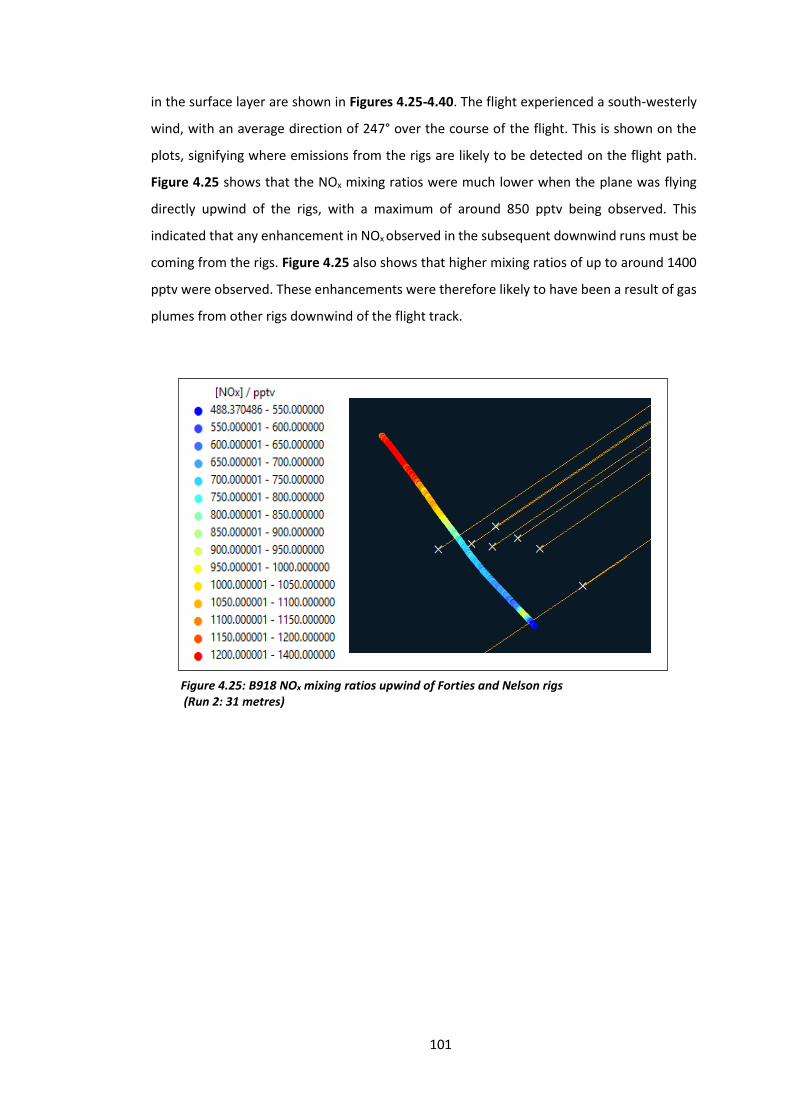
101
in the surface layer are shown in Figures 4.25-4.40. The flight experienced a south-westerly
wind, with an average direction of 247° over the course of the flight. This is shown on the
plots, signifying where emissions from the rigs are likely to be detected on the flight path.
Figure 4.25 shows that the NOx mixing ratios were much lower when the plane was flying
directly upwind of the rigs, with a maximum of around 850 pptv being observed. This
indicated that any enhancement in NOx observed in the subsequent downwind runs must be
coming from the rigs. Figure 4.25 also shows that higher mixing ratios of up to around 1400
pptv were observed. These enhancements were therefore likely to have been a result of gas
plumes from other rigs downwind of the flight track.
Figure 4.25: B918 NOx mixing ratios upwind of Forties and Nelson rigs (Run 2: 31 metres)
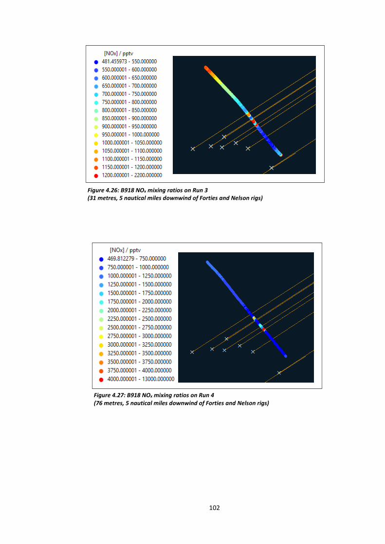
102
Figure 4.26: B918 NOx mixing ratios on Run 3 (31 metres, 5 nautical miles downwind of Forties and Nelson rigs)
Figure 4.27: B918 NOx mixing ratios on Run 4 (76 metres, 5 nautical miles downwind of Forties and Nelson rigs)
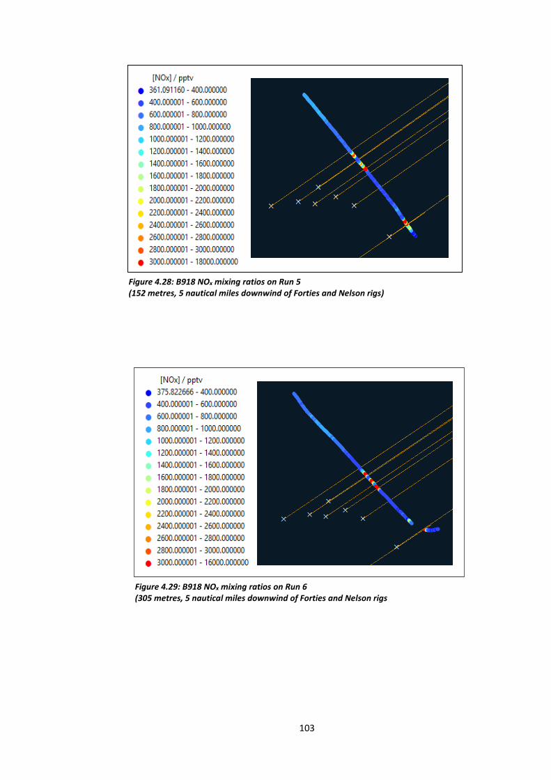
103
Figure 4.28: B918 NOx mixing ratios on Run 5 (152 metres, 5 nautical miles downwind of Forties and Nelson rigs)
Figure 4.29: B918 NOx mixing ratios on Run 6 (305 metres, 5 nautical miles downwind of Forties and Nelson rigs
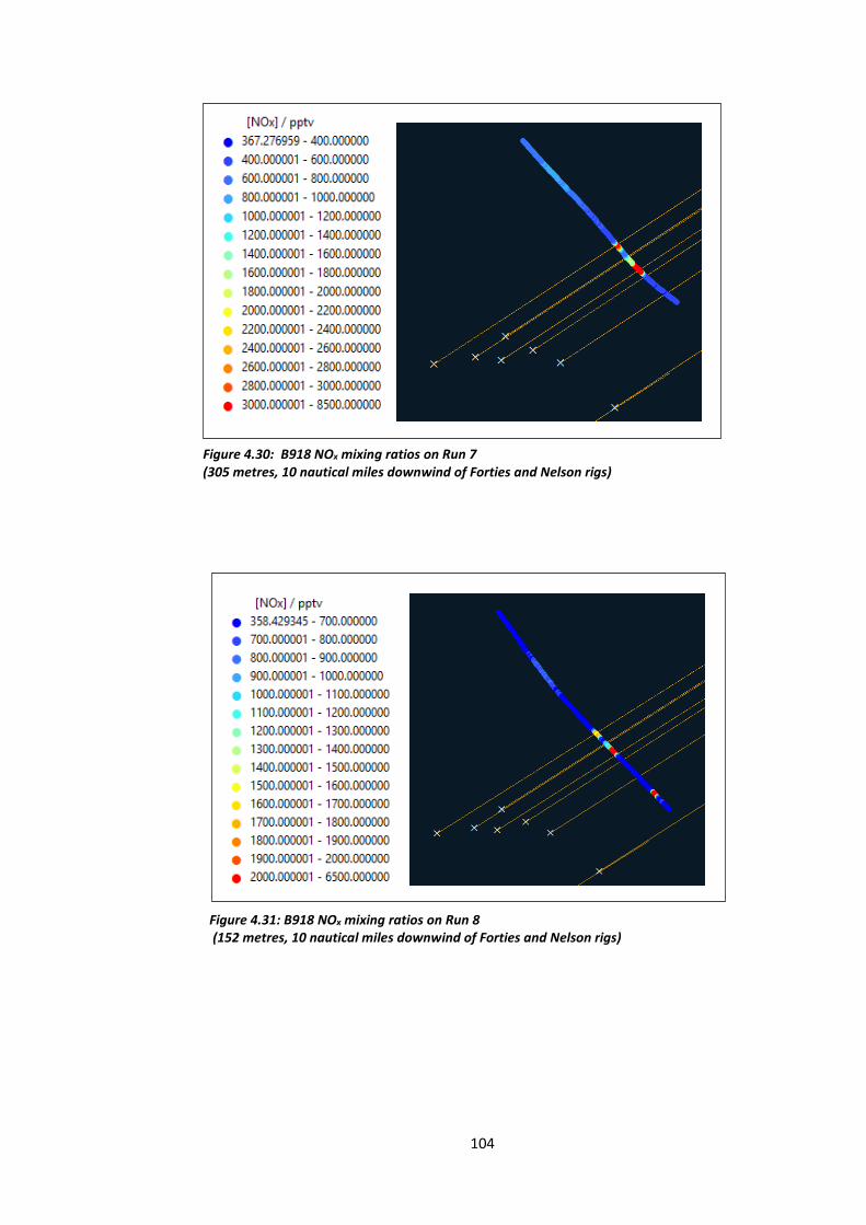
104
Figure 4.30: B918 NOx mixing ratios on Run 7 (305 metres, 10 nautical miles downwind of Forties and Nelson rigs)
Figure 4.31: B918 NOx mixing ratios on Run 8 (152 metres, 10 nautical miles downwind of Forties and Nelson rigs)
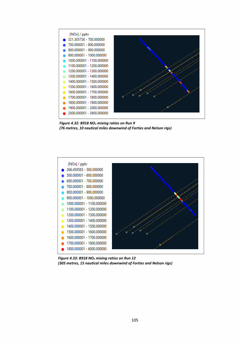
105
Figure 4.32: B918 NOx mixing ratios on Run 9 (76 metres, 10 nautical miles downwind of Forties and Nelson rigs)
Figure 4.33: B918 NOx mixing ratios on Run 12 (305 metres, 15 nautical miles downwind of Forties and Nelson rigs)
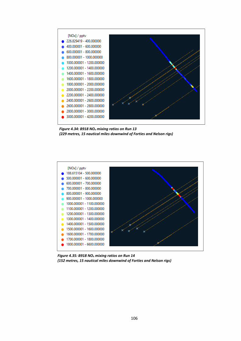
106
Figure 4.34: B918 NOx mixing ratios on Run 13 (229 metres, 15 nautical miles downwind of Forties and Nelson rigs)
Figure 4.35: B918 NOx mixing ratios on Run 14 (152 metres, 15 nautical miles downwind of Forties and Nelson rigs)
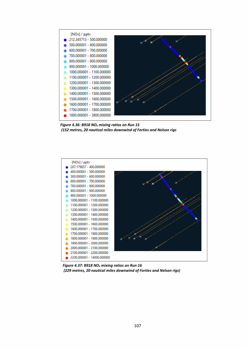
107
Figure 4.36: B918 NOx mixing ratios on Run 15 (152 metres, 20 nautical miles downwind of Forties and Nelson rigs
Figure 4.37: B918 NOx mixing ratios on Run 16 (229 metres, 20 nautical miles downwind of Forties and Nelson rigs)
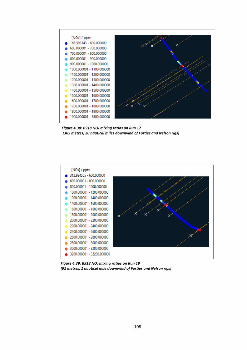
108
Figure 4.38: B918 NOx mixing ratios on Run 17 (305 metres, 20 nautical miles downwind of Forties and Nelson rigs)
Figure 4.39: B918 NOx mixing ratios on Run 19 (91 metres, 1 nautical mile downwind of Forties and Nelson rigs)
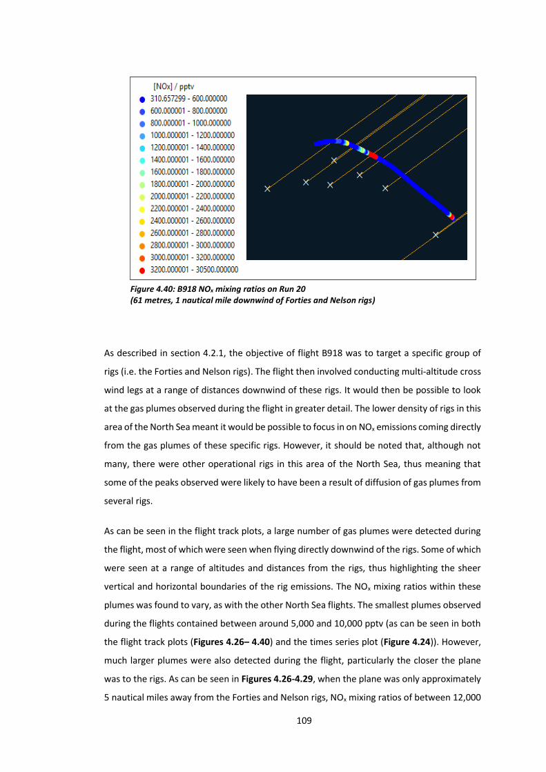
109
As described in section 4.2.1, the objective of flight B918 was to target a specific group of
rigs (i.e. the Forties and Nelson rigs). The flight then involved conducting multi-altitude cross
wind legs at a range of distances downwind of these rigs. It would then be possible to look
at the gas plumes observed during the flight in greater detail. The lower density of rigs in this
area of the North Sea meant it would be possible to focus in on NOx emissions coming directly
from the gas plumes of these specific rigs. However, it should be noted that, although not
many, there were other operational rigs in this area of the North Sea, thus meaning that
some of the peaks observed were likely to have been a result of diffusion of gas plumes from
several rigs.
As can be seen in the flight track plots, a large number of gas plumes were detected during
the flight, most of which were seen when flying directly downwind of the rigs. Some of which
were seen at a range of altitudes and distances from the rigs, thus highlighting the sheer
vertical and horizontal boundaries of the rig emissions. The NOx mixing ratios within these
plumes was found to vary, as with the other North Sea flights. The smallest plumes observed
during the flights contained between around 5,000 and 10,000 pptv (as can be seen in both
the flight track plots (Figures 4.26– 4.40) and the times series plot (Figure 4.24)). However,
much larger plumes were also detected during the flight, particularly the closer the plane
was to the rigs. As can be seen in Figures 4.26-4.29, when the plane was only approximately
5 nautical miles away from the Forties and Nelson rigs, NOx mixing ratios of between 12,000
Figure 4.40: B918 NOx mixing ratios on Run 20 (61 metres, 1 nautical mile downwind of Forties and Nelson rigs)
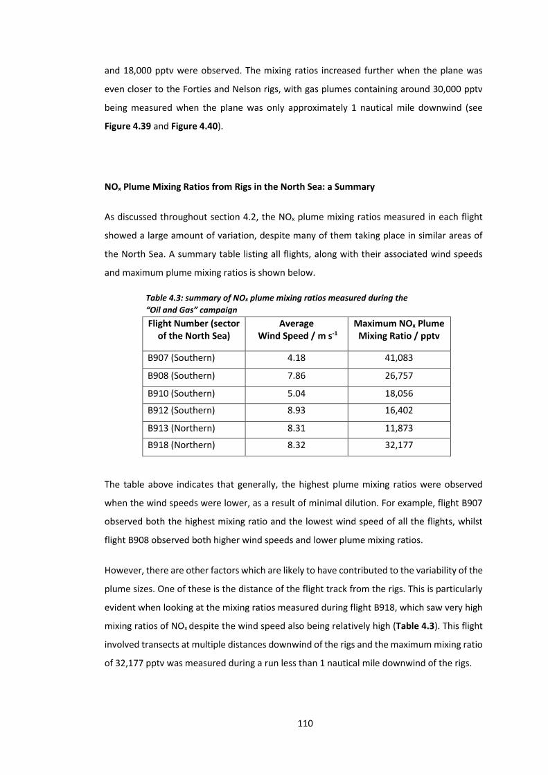
110
and 18,000 pptv were observed. The mixing ratios increased further when the plane was
even closer to the Forties and Nelson rigs, with gas plumes containing around 30,000 pptv
being measured when the plane was only approximately 1 nautical mile downwind (see
Figure 4.39 and Figure 4.40).
NOx Plume Mixing Ratios from Rigs in the North Sea: a Summary
As discussed throughout section 4.2, the NOx plume mixing ratios measured in each flight
showed a large amount of variation, despite many of them taking place in similar areas of
the North Sea. A summary table listing all flights, along with their associated wind speeds
and maximum plume mixing ratios is shown below.
The table above indicates that generally, the highest plume mixing ratios were observed
when the wind speeds were lower, as a result of minimal dilution. For example, flight B907
observed both the highest mixing ratio and the lowest wind speed of all the flights, whilst
flight B908 observed both higher wind speeds and lower plume mixing ratios.
However, there are other factors which are likely to have contributed to the variability of the
plume sizes. One of these is the distance of the flight track from the rigs. This is particularly
evident when looking at the mixing ratios measured during flight B918, which saw very high
mixing ratios of NOx despite the wind speed also being relatively high (Table 4.3). This flight
involved transects at multiple distances downwind of the rigs and the maximum mixing ratio
of 32,177 pptv was measured during a run less than 1 nautical mile downwind of the rigs.
Flight Number (sector of the North Sea)
Average Wind Speed / m s-1
Maximum NOx Plume Mixing Ratio / pptv
B907 (Southern) 4.18 41,083
B908 (Southern) 7.86 26,757
B910 (Southern) 5.04 18,056
B912 (Southern) 8.93 16,402
B913 (Northern) 8.31 11,873
B918 (Northern) 8.32 32,177
Table 4.3: summary of NOx plume mixing ratios measured during the
“Oil and Gas” campaign
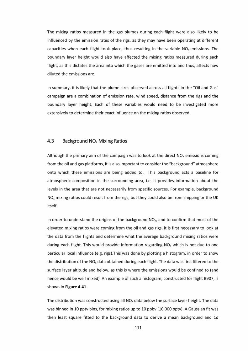
111
The mixing ratios measured in the gas plumes during each flight were also likely to be
influenced by the emission rates of the rigs, as they may have been operating at different
capacities when each flight took place, thus resulting in the variable NOx emissions. The
boundary layer height would also have affected the mixing ratios measured during each
flight, as this dictates the area into which the gases are emitted into and thus, affects how
diluted the emissions are.
In summary, it is likely that the plume sizes observed across all flights in the “Oil and Gas”
campaign are a combination of emission rate, wind speed, distance from the rigs and the
boundary layer height. Each of these variables would need to be investigated more
extensively to determine their exact influence on the mixing ratios observed.
4.3 Background NOx Mixing Ratios
Although the primary aim of the campaign was to look at the direct NOx emissions coming
from the oil and gas platforms, it is also important to consider the “background” atmosphere
onto which these emissions are being added to. This background acts a baseline for
atmospheric composition in the surrounding area, i.e. it provides information about the
levels in the area that are not necessarily from specific sources. For example, background
NOx mixing ratios could result from the rigs, but they could also be from shipping or the UK
itself.
In order to understand the origins of the background NOx, and to confirm that most of the
elevated mixing ratios were coming from the oil and gas rigs, it is first necessary to look at
the data from the flights and determine what the average background mixing ratios were
during each flight. This would provide information regarding NOx which is not due to one
particular local influence (e.g. rigs).This was done by plotting a histogram, in order to show
the distribution of the NOx data obtained during each flight. The data was first filtered to the
surface layer altitude and below, as this is where the emissions would be confined to (and
hence would be well mixed). An example of such a histogram, constructed for flight B907, is
shown in Figure 4.41.
The distribution was constructed using all NOx data below the surface layer height. The data
was binned in 10 pptv bins, for mixing ratios up to 10 ppbv (10,000 pptv). A Gaussian fit was
then least square fitted to the background data to derive a mean background and 1σ
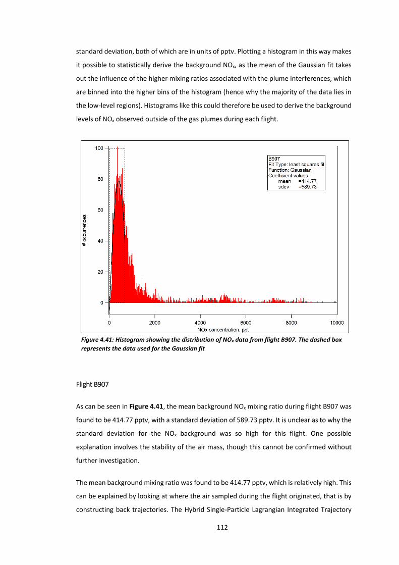
112
standard deviation, both of which are in units of pptv. Plotting a histogram in this way makes
it possible to statistically derive the background NOx, as the mean of the Gaussian fit takes
out the influence of the higher mixing ratios associated with the plume interferences, which
are binned into the higher bins of the histogram (hence why the majority of the data lies in
the low-level regions). Histograms like this could therefore be used to derive the background
levels of NOx observed outside of the gas plumes during each flight.
Flight B907
As can be seen in Figure 4.41, the mean background NOx mixing ratio during flight B907 was
found to be 414.77 pptv, with a standard deviation of 589.73 pptv. It is unclear as to why the
standard deviation for the NOx background was so high for this flight. One possible
explanation involves the stability of the air mass, though this cannot be confirmed without
further investigation.
The mean background mixing ratio was found to be 414.77 pptv, which is relatively high. This
can be explained by looking at where the air sampled during the flight originated, that is by
constructing back trajectories. The Hybrid Single-Particle Lagrangian Integrated Trajectory
Figure 4.41: Histogram showing the distribution of NOx data from flight B907. The dashed box
represents the data used for the Gaussian fit
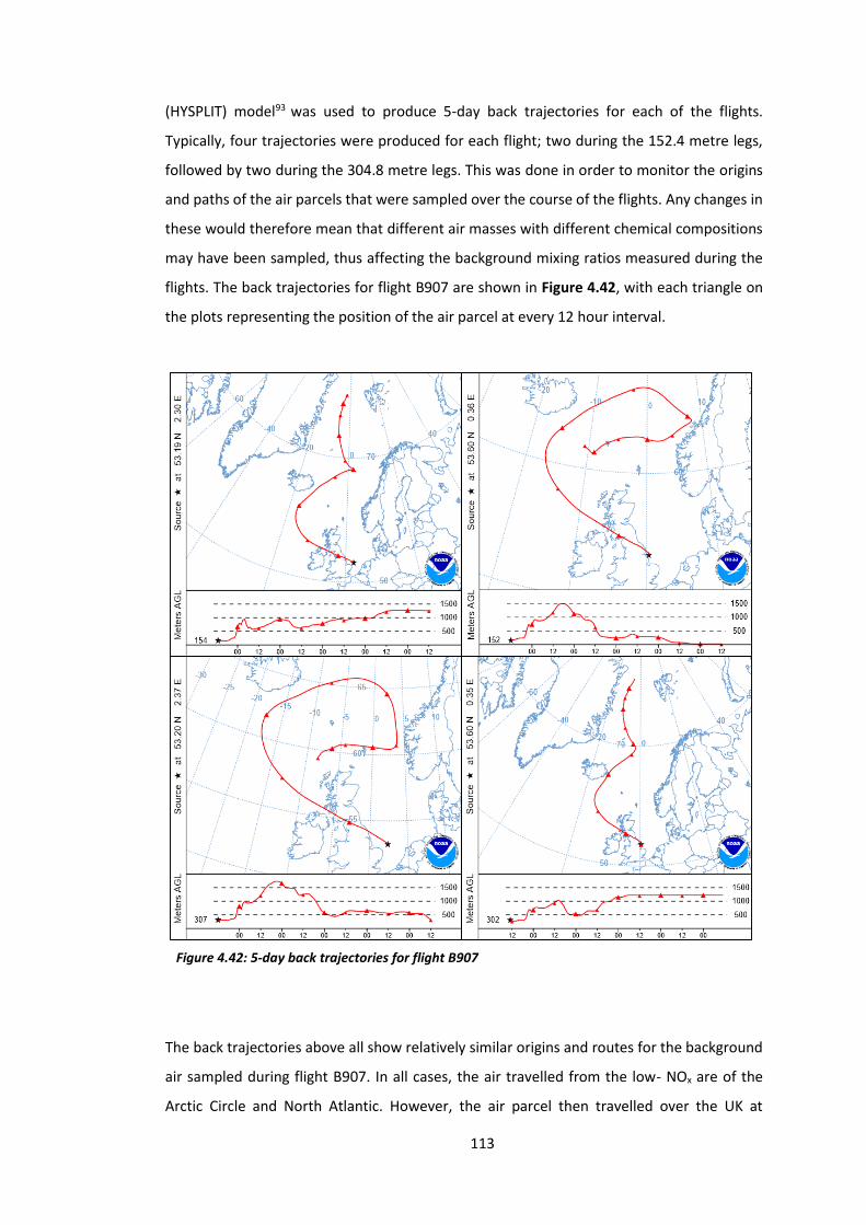
113
(HYSPLIT) model93 was used to produce 5-day back trajectories for each of the flights.
Typically, four trajectories were produced for each flight; two during the 152.4 metre legs,
followed by two during the 304.8 metre legs. This was done in order to monitor the origins
and paths of the air parcels that were sampled over the course of the flights. Any changes in
these would therefore mean that different air masses with different chemical compositions
may have been sampled, thus affecting the background mixing ratios measured during the
flights. The back trajectories for flight B907 are shown in Figure 4.42, with each triangle on
the plots representing the position of the air parcel at every 12 hour interval.
The back trajectories above all show relatively similar origins and routes for the background
air sampled during flight B907. In all cases, the air travelled from the low- NOx are of the
Arctic Circle and North Atlantic. However, the air parcel then travelled over the UK at
Figure 4.42: 5-day back trajectories for flight B907
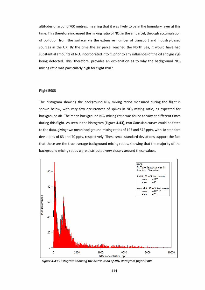
114
altitudes of around 700 metres, meaning that it was likely to be in the boundary layer at this
time. This therefore increased the mixing ratio of NOx in the air parcel, through accumulation
of pollution from the surface, via the extensive number of transport and industry-based
sources in the UK. By the time the air parcel reached the North Sea, it would have had
substantial amounts of NOx incorporated into it, prior to any influences of the oil and gas rigs
being detected. This, therefore, provides an explanation as to why the background NOx
mixing ratio was particularly high for flight B907.
Flight B908
The histogram showing the background NOx mixing ratios measured during the flight is
shown below, with very few occurrences of spikes in NOx mixing ratio, as expected for
background air. The mean background NOx mixing ratio was found to vary at different times
during this flight. As seen in the histogram (Figure 4.43), two Gaussian curves could be fitted
to the data, giving two mean background mixing ratios of 127 and 872 pptv, with 1σ standard
deviations of 83 and 70 pptv, respectively. These small standard deviations support the fact
that these are the true average background mixing ratios, showing that the majority of the
background mixing ratios were distributed very closely around these values.
Figure 4.43: Histogram showing the distribution of NOx data from flight B908
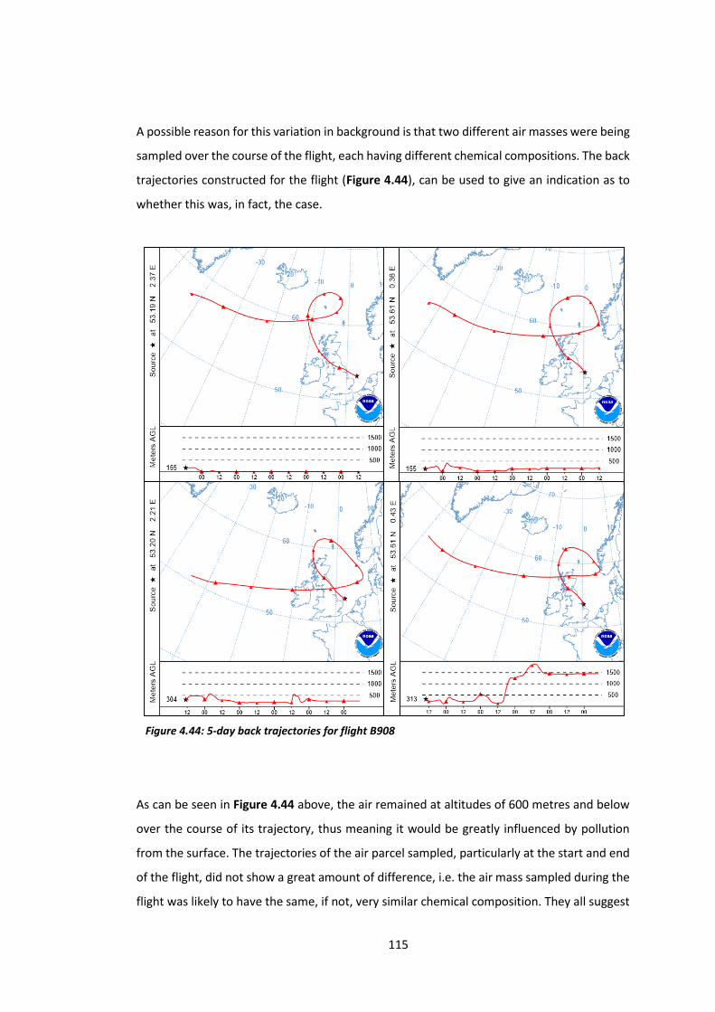
115
A possible reason for this variation in background is that two different air masses were being
sampled over the course of the flight, each having different chemical compositions. The back
trajectories constructed for the flight (Figure 4.44), can be used to give an indication as to
whether this was, in fact, the case.
As can be seen in Figure 4.44 above, the air remained at altitudes of 600 metres and below
over the course of its trajectory, thus meaning it would be greatly influenced by pollution
from the surface. The trajectories of the air parcel sampled, particularly at the start and end
of the flight, did not show a great amount of difference, i.e. the air mass sampled during the
flight was likely to have the same, if not, very similar chemical composition. They all suggest
Figure 4.44: 5-day back trajectories for flight B908
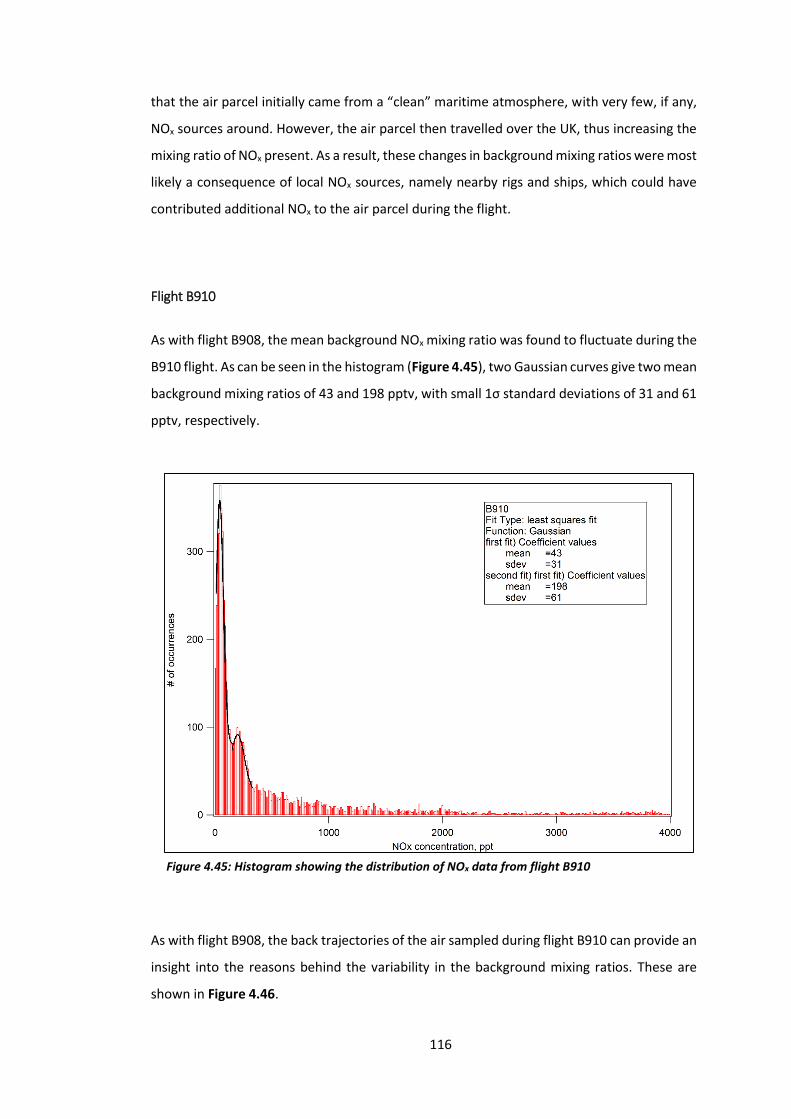
116
that the air parcel initially came from a “clean” maritime atmosphere, with very few, if any,
NOx sources around. However, the air parcel then travelled over the UK, thus increasing the
mixing ratio of NOx present. As a result, these changes in background mixing ratios were most
likely a consequence of local NOx sources, namely nearby rigs and ships, which could have
contributed additional NOx to the air parcel during the flight.
Flight B910
As with flight B908, the mean background NOx mixing ratio was found to fluctuate during the
B910 flight. As can be seen in the histogram (Figure 4.45), two Gaussian curves give two mean
background mixing ratios of 43 and 198 pptv, with small 1σ standard deviations of 31 and 61
pptv, respectively.
As with flight B908, the back trajectories of the air sampled during flight B910 can provide an
insight into the reasons behind the variability in the background mixing ratios. These are
shown in Figure 4.46.
Figure 4.45: Histogram showing the distribution of NOx data from flight B910
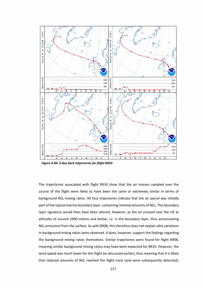
117
The trajectories associated with flight B910 show that the air masses sampled over the
course of the flight were likely to have been the same or extremely similar in terms of
background NOx mixing ratios. All four trajectories indicate that the air parcel was initially
part of the typical marine boundary layer, containing minimal amounts of NOx. This boundary
layer signature would then have been altered, however, as the air crossed over the UK at
altitudes of around 1000 metres and below, i.e. in the boundary layer, thus accumulating
NOx emissions from the surface. As with B908, this therefore does not explain why variations
in background mixing ratios were observed. It does, however, support the findings regarding
the background mixing ratios themselves. Similar trajectories were found for flight B908,
meaning similar background mixing ratios may have been expected for B910. However, the
wind speed was much lower for this flight (as discussed earlier), thus meaning that it is likely
that reduced amounts of NOx reached the flight track (and were subsequently detected),
Figure 4.46: 5-day back trajectories for flight B910
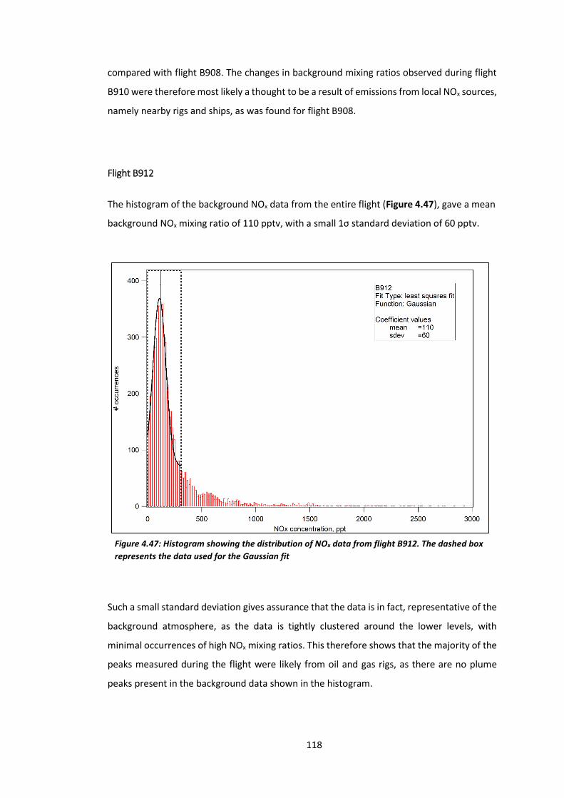
118
compared with flight B908. The changes in background mixing ratios observed during flight
B910 were therefore most likely a thought to be a result of emissions from local NOx sources,
namely nearby rigs and ships, as was found for flight B908.
Flight B912
The histogram of the background NOx data from the entire flight (Figure 4.47), gave a mean
background NOx mixing ratio of 110 pptv, with a small 1σ standard deviation of 60 pptv.
Such a small standard deviation gives assurance that the data is in fact, representative of the
background atmosphere, as the data is tightly clustered around the lower levels, with
minimal occurrences of high NOx mixing ratios. This therefore shows that the majority of the
peaks measured during the flight were likely from oil and gas rigs, as there are no plume
peaks present in the background data shown in the histogram.
Figure 4.47: Histogram showing the distribution of NOx data from flight B912. The dashed box
represents the data used for the Gaussian fit
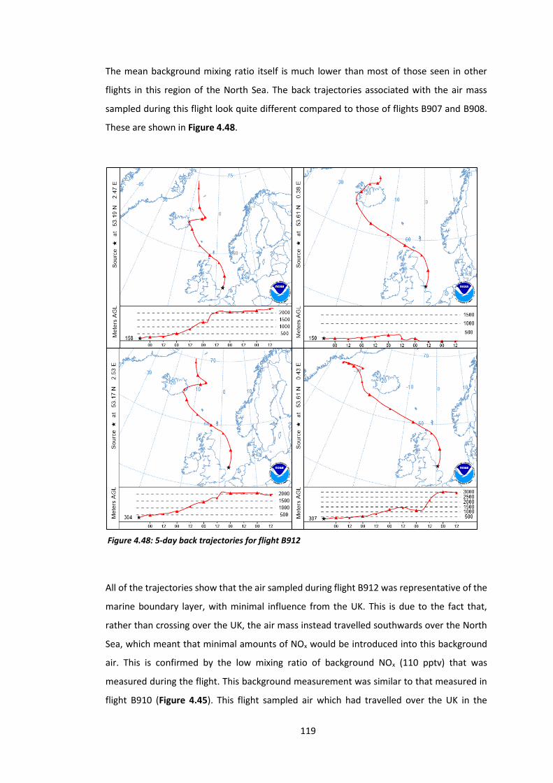
119
The mean background mixing ratio itself is much lower than most of those seen in other
flights in this region of the North Sea. The back trajectories associated with the air mass
sampled during this flight look quite different compared to those of flights B907 and B908.
These are shown in Figure 4.48.
All of the trajectories show that the air sampled during flight B912 was representative of the
marine boundary layer, with minimal influence from the UK. This is due to the fact that,
rather than crossing over the UK, the air mass instead travelled southwards over the North
Sea, which meant that minimal amounts of NOx would be introduced into this background
air. This is confirmed by the low mixing ratio of background NOx (110 pptv) that was
measured during the flight. This background measurement was similar to that measured in
flight B910 (Figure 4.45). This flight sampled air which had travelled over the UK in the
Figure 4.48: 5-day back trajectories for flight B912
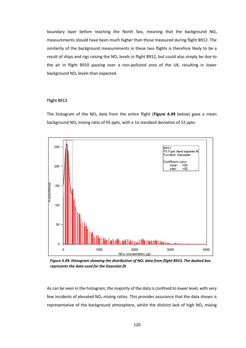
120
boundary layer before reaching the North Sea, meaning that the background NOx
measurements should have been much higher than those measured during flight B912. The
similarity of the background measurements in these two flights is therefore likely to be a
result of ships and rigs raising the NOx levels in flight B912, but could also simply be due to
the air in flight B910 passing over a non-polluted area of the UK, resulting in lower
background NOx levels than expected.
Flight B913
The histogram of the NOx data from the entire flight (Figure 4.49 below) gave a mean
background NOx mixing ratio of 95 pptv, with a 1σ standard deviation of 52 pptv.
As can be seen in the histogram, the majority of the data is confined to lower level, with very
few incidents of elevated NOx mixing ratios. This provides assurance that the data shown is
representative of the background atmosphere, whilst the distinct lack of high NOx mixing
Figure 4.49: Histogram showing the distribution of NOx data from flight B913. The dashed box
represents the data used for the Gaussian fit
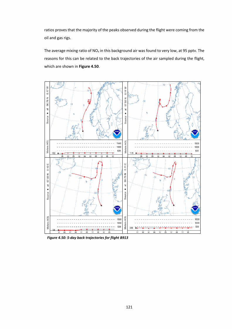
121
ratios proves that the majority of the peaks observed during the flight were coming from the
oil and gas rigs.
The average mixing ratio of NOx in this background air was found to very low, at 95 pptv. The
reasons for this can be related to the back trajectories of the air sampled during the flight,
which are shown in Figure 4.50.
Figure 4.50: 5-day back trajectories for flight B913
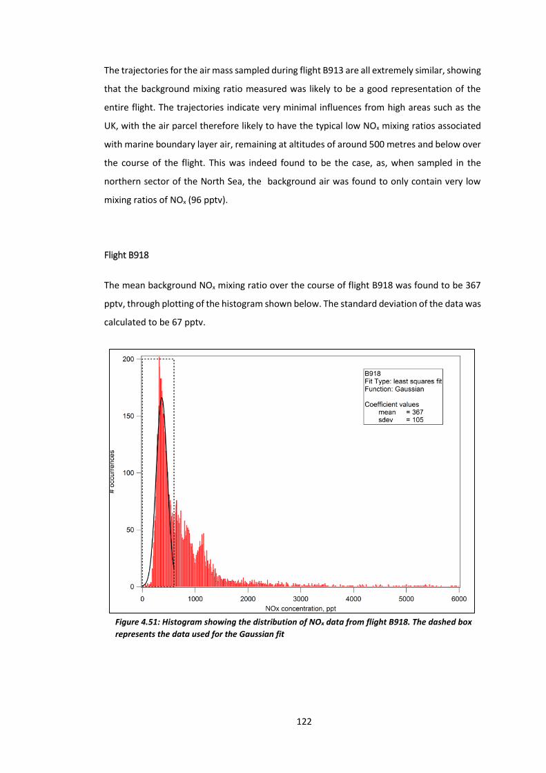
122
The trajectories for the air mass sampled during flight B913 are all extremely similar, showing
that the background mixing ratio measured was likely to be a good representation of the
entire flight. The trajectories indicate very minimal influences from high areas such as the
UK, with the air parcel therefore likely to have the typical low NOx mixing ratios associated
with marine boundary layer air, remaining at altitudes of around 500 metres and below over
the course of the flight. This was indeed found to be the case, as, when sampled in the
northern sector of the North Sea, the background air was found to only contain very low
mixing ratios of NOx (96 pptv).
Flight B918
The mean background NOx mixing ratio over the course of flight B918 was found to be 367
pptv, through plotting of the histogram shown below. The standard deviation of the data was
calculated to be 67 pptv.
Figure 4.51: Histogram showing the distribution of NOx data from flight B918. The dashed box
represents the data used for the Gaussian fit

123
Although in a very similar location to flight B913, in the northern sector of the North Sea, the
background NOx mixing ratios measured in the two flights are considerably different. Flight
B913 saw an average background mixing ratio of 95 pptv, whereas, for flight B918, this was
found to be almost 300 pptv higher, at 367 pptv. This may be a result of different air masses
sampled in the two flights, this being a consequence of the back trajectories. The trajectories
associated with the air mass sampled during flight B918 can be seen in Figure 4.52.
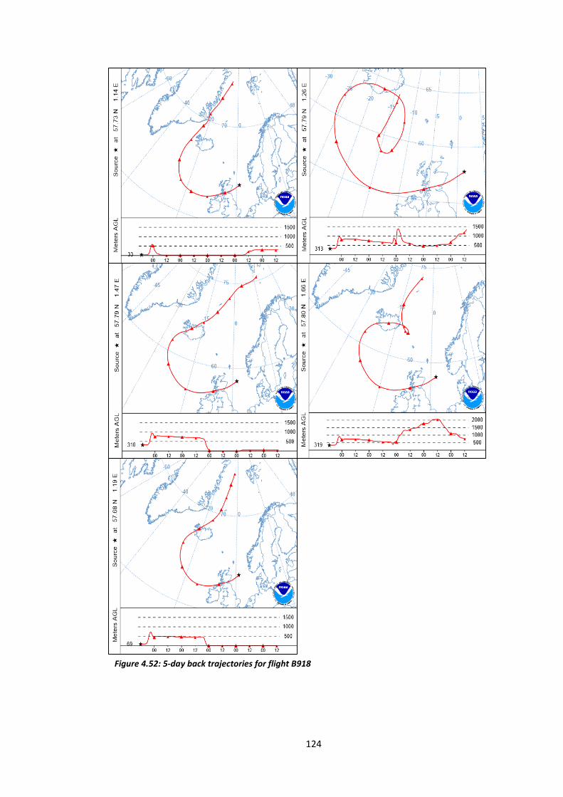
124
Figure 4.52: 5-day back trajectories for flight B918

125
The trajectory plots associated with flight B918 show a distinct difference to those
constructed for flight B913 (Figure 4.50). Both air masses begin in the North Atlantic Ocean,
in low- NOx conditions which are typical of the marine boundary layer. However, the key
difference is that the air sampled during flight B918 passes over the northern UK at altitudes
of between 500 and 1,000 metres (i.e. within the boundary layer), thus accumulating NOx
emissions from UK-based sources such as road transport and industry. This consequently
means that this additional NOx is then transported in the forward trajectory of the air parcel,
thus resulting in the observed higher background NOx mixing ratios by the time it reaches the
North Sea.
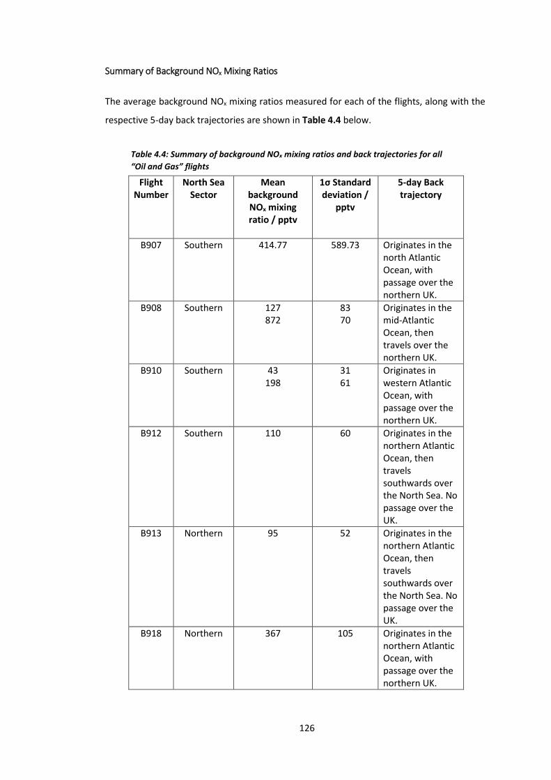
126
Summary of Background NOx Mixing Ratios
The average background NOx mixing ratios measured for each of the flights, along with the
respective 5-day back trajectories are shown in Table 4.4 below.
Flight Number
North Sea Sector
Mean background NOx mixing ratio / pptv
1σ Standard deviation /
pptv
5-day Back trajectory
B907 Southern 414.77 589.73 Originates in the north Atlantic Ocean, with passage over the northern UK.
B908 Southern 127 872
83 70
Originates in the mid-Atlantic Ocean, then travels over the northern UK.
B910 Southern 43 198
31 61
Originates in western Atlantic Ocean, with passage over the northern UK.
B912 Southern 110 60 Originates in the northern Atlantic Ocean, then travels southwards over the North Sea. No passage over the UK.
B913 Northern 95 52 Originates in the northern Atlantic Ocean, then travels southwards over the North Sea. No passage over the UK.
B918 Northern 367 105 Originates in the northern Atlantic Ocean, with passage over the northern UK.
Table 4.4: Summary of background NOx mixing ratios and back trajectories for all
“Oil and Gas” flights

127
The background NOx mixing ratios measured over the course of the “Oil and Gas” campaign
could generally be explained by their respective back trajectories. The lowest mixing ratios
were observed for the two survey flights in which the air mass sampled had not been
influenced by UK-based NOx emissions. These two flights were B912 and B913 and, as seen
in Table 4.4, although the flights took place in different sectors of the North Sea, both
showed very similar, low background NOx mixing ratios as a result of their similar back
trajectories.
Higher background mixing ratios were measured during the remaining survey flights, all of
which measured in air masses which had experienced some influence from the UK. For
example, the average background NOx mixing ratio measured in flight B908 was 872 pptv.
The air sampled during this flight had travelled over the UK before reaching the North Sea.
This explains why the average background mixing ratio was over 700 pptv higher than flight
B912, despite both flights taking place in the same sector of the North Sea.
These background mixing ratio measurements were necessary as they show a lot of variation
depending on the back trajectory of the air mass. Measuring the background mixing ratios
was also needed in order to measure any NOx enhancements coming from the rigs.
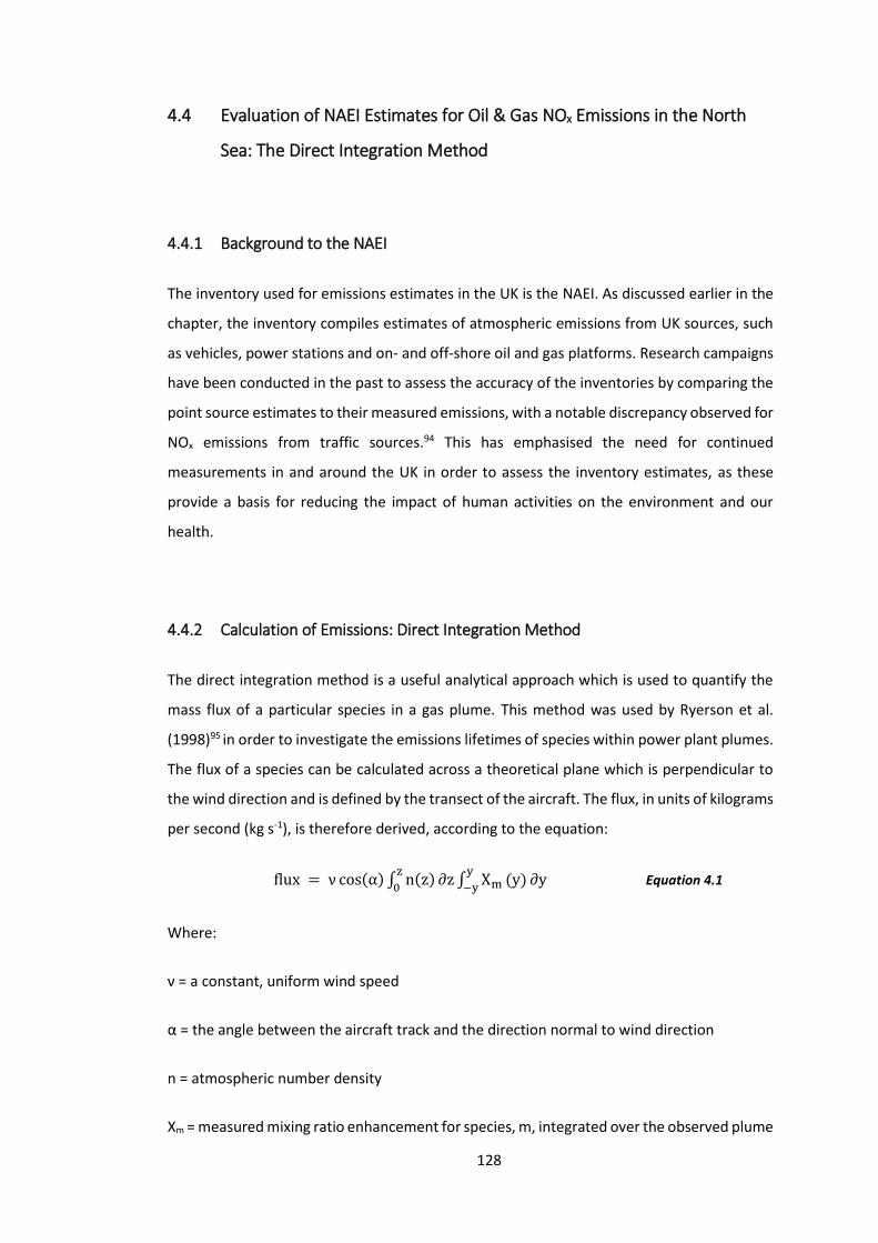
128
4.4 Evaluation of NAEI Estimates for Oil & Gas NOx Emissions in the North
Sea: The Direct Integration Method
4.4.1 Background to the NAEI
The inventory used for emissions estimates in the UK is the NAEI. As discussed earlier in the
chapter, the inventory compiles estimates of atmospheric emissions from UK sources, such
as vehicles, power stations and on- and off-shore oil and gas platforms. Research campaigns
have been conducted in the past to assess the accuracy of the inventories by comparing the
point source estimates to their measured emissions, with a notable discrepancy observed for
NOx emissions from traffic sources.94 This has emphasised the need for continued
measurements in and around the UK in order to assess the inventory estimates, as these
provide a basis for reducing the impact of human activities on the environment and our
health.
4.4.2 Calculation of Emissions: Direct Integration Method
The direct integration method is a useful analytical approach which is used to quantify the
mass flux of a particular species in a gas plume. This method was used by Ryerson et al.
(1998)95 in order to investigate the emissions lifetimes of species within power plant plumes.
The flux of a species can be calculated across a theoretical plane which is perpendicular to
the wind direction and is defined by the transect of the aircraft. The flux, in units of kilograms
per second (kg s-1), is therefore derived, according to the equation:
flux = ν cos(α) ∫ n(z) ∂z ∫ Xmy
−y(y) ∂y
z
0 Equation 4.1
Where:
ν = a constant, uniform wind speed
α = the angle between the aircraft track and the direction normal to wind direction
n = atmospheric number density
Xm = measured mixing ratio enhancement for species, m, integrated over the observed plume
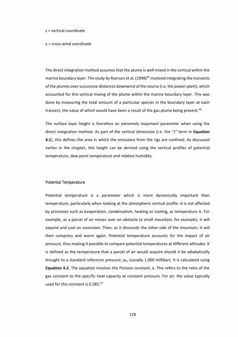
129
z = vertical coordinate
y = cross-wind coordinate
The direct integration method assumes that the plume is well mixed in the vertical within the
marine boundary layer. The study by Ryerson et al. (1998)95 involved integrating the transects
of the plumes over successive distances downwind of the source (i.e. the power plant), which
accounted for this vertical mixing of the plume within the marine boundary layer. This was
done by measuring the total amount of a particular species in the boundary layer at each
transect, the value of which would have been a result of the gas plume being present.96
The surface layer height is therefore an extremely important parameter when using the
direct integration method. As part of the vertical dimension (i.e. the “z” term in Equation
4.1), this defines the area in which the emissions from the rigs are confined. As discussed
earlier in the chapter, this height can be derived using the vertical profiles of potential
temperature, dew point temperature and relative humidity.
Potential Temperature
Potential temperature is a parameter which is more dynamically important than
temperature, particularly when looking at the atmospheric vertical profile. It is not affected
by processes such as evaporation, condensation, heating or cooling, as temperature is. For
example, as a parcel of air moves over an obstacle (a small mountain, for example), it will
expand and cool on ascension. Then, as it descends the other side of the mountain, it will
then compress and warm again. Potential temperature accounts for the impact of air
pressure, thus making it possible to compare potential temperatures at different altitudes. It
is defined as the temperature that a parcel of air would acquire should it be adiabatically
brought to a standard reference pressure, p0, (usually 1,000 millibar). It is calculated using
Equation 4.2. The equation involves the Poisson constant, κ. This refers to the ratio of the
gas constant to the specific heat capacity at constant pressure. For air, the value typically
used for this constant is 0.285.97
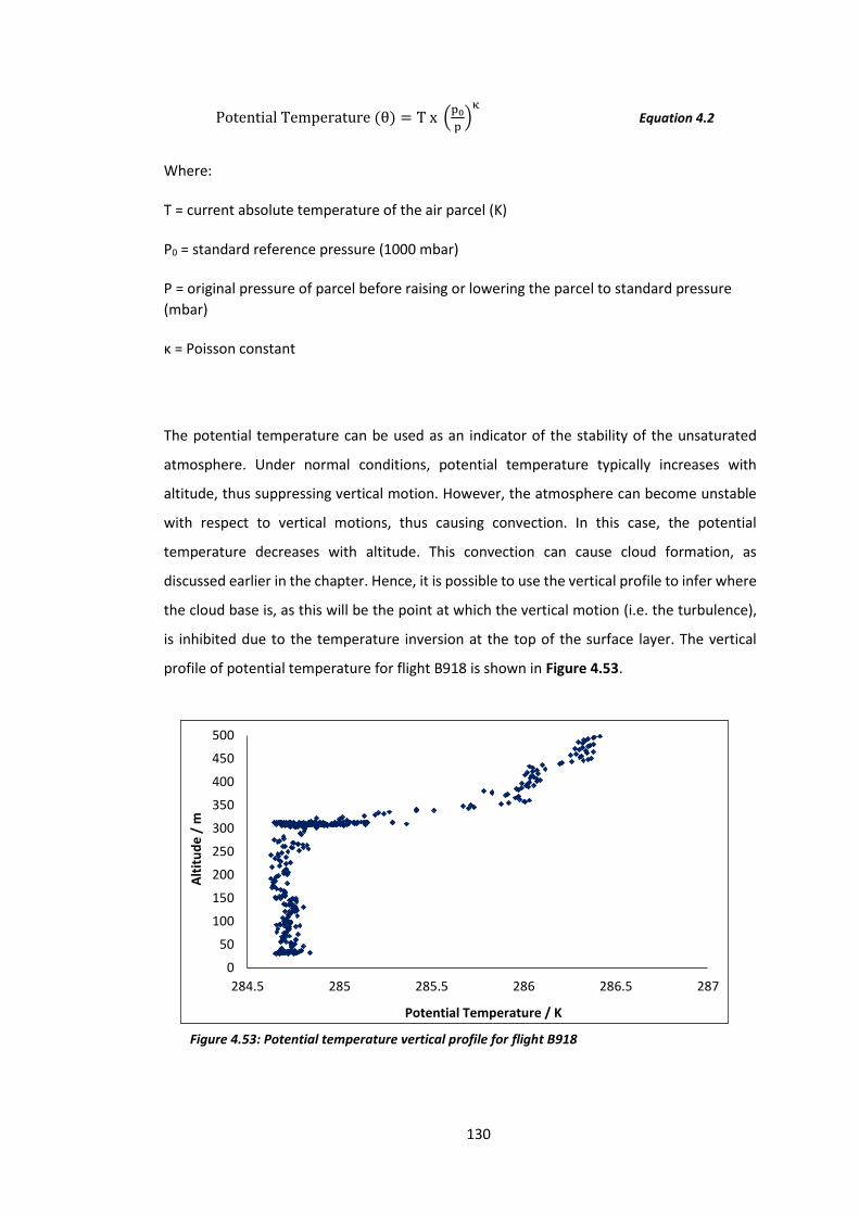
130
Potential Temperature (θ) = T x (p0
p)
κ Equation 4.2
Where:
T = current absolute temperature of the air parcel (K)
P0 = standard reference pressure (1000 mbar)
P = original pressure of parcel before raising or lowering the parcel to standard pressure
(mbar)
κ = Poisson constant
The potential temperature can be used as an indicator of the stability of the unsaturated
atmosphere. Under normal conditions, potential temperature typically increases with
altitude, thus suppressing vertical motion. However, the atmosphere can become unstable
with respect to vertical motions, thus causing convection. In this case, the potential
temperature decreases with altitude. This convection can cause cloud formation, as
discussed earlier in the chapter. Hence, it is possible to use the vertical profile to infer where
the cloud base is, as this will be the point at which the vertical motion (i.e. the turbulence),
is inhibited due to the temperature inversion at the top of the surface layer. The vertical
profile of potential temperature for flight B918 is shown in Figure 4.53.
Figure 4.53: Potential temperature vertical profile for flight B918
0
50
100
150
200
250
300
350
400
450
500
284.5 285 285.5 286 286.5 287
Alt
itu
de
/ m
Potential Temperature / K
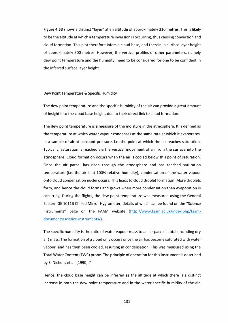
131
Figure 4.53 shows a distinct “layer” at an altitude of approximately 310 metres. This is likely
to be the altitude at which a temperature inversion is occurring, thus causing convection and
cloud formation. This plot therefore infers a cloud base, and therein, a surface layer height
of approximately 300 metres. However, the vertical profiles of other parameters, namely
dew point temperature and the humidity, need to be considered for one to be confident in
the inferred surface layer height.
Dew Point Temperature & Specific Humidity
The dew point temperature and the specific humidity of the air can provide a great amount
of insight into the cloud base height, due to their direct link to cloud formation.
The dew point temperature is a measure of the moisture in the atmosphere. It is defined as
the temperature at which water vapour condenses at the same rate at which it evaporates,
in a sample of air at constant pressure, i.e. the point at which the air reaches saturation.
Typically, saturation is reached via the vertical movement of air from the surface into the
atmosphere. Cloud formation occurs when the air is cooled below this point of saturation.
Once the air parcel has risen through the atmosphere and has reached saturation
temperature (i.e. the air is at 100% relative humidity), condensation of the water vapour
onto cloud condensation nuclei occurs. This leads to cloud droplet formation. More droplets
form, and hence the cloud forms and grows when more condensation than evaporation is
occurring. During the flights, the dew point temperature was measured using the General
Eastern GE 1011B Chilled Mirror Hygrometer, details of which can be found on the “Science
Instruments” page on the FAAM website (http://www.faam.ac.uk/index.php/faam-
documents/science-instruments/).
The specific humidity is the ratio of water vapour mass to an air parcel’s total (including dry
air) mass. The formation of a cloud only occurs once the air has become saturated with water
vapour, and has then been cooled, resulting in condensation. This was measured using the
Total Water Content (TWC) probe. The principle of operation for this instrument is described
by S. Nicholls et al. (1990).98
Hence, the cloud base height can be inferred as the altitude at which there is a distinct
increase in both the dew point temperature and in the water specific humidity of the air.
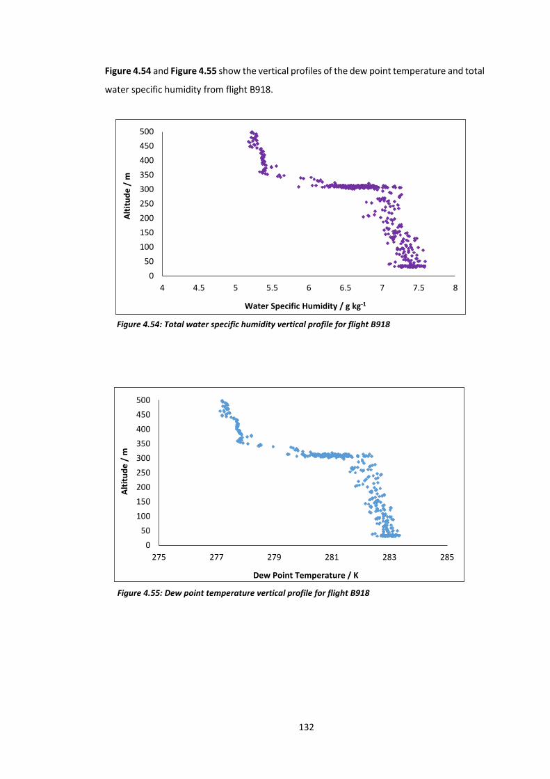
132
Figure 4.54 and Figure 4.55 show the vertical profiles of the dew point temperature and total
water specific humidity from flight B918.
Figure 4.55: Dew point temperature vertical profile for flight B918
0
50
100
150
200
250
300
350
400
450
500
4 4.5 5 5.5 6 6.5 7 7.5 8
Alt
itu
de
/ m
Water Specific Humidity / g kg-1
Figure 4.54: Total water specific humidity vertical profile for flight B918
0
50
100
150
200
250
300
350
400
450
500
275 277 279 281 283 285
Alt
itu
de
/ m
Dew Point Temperature / K
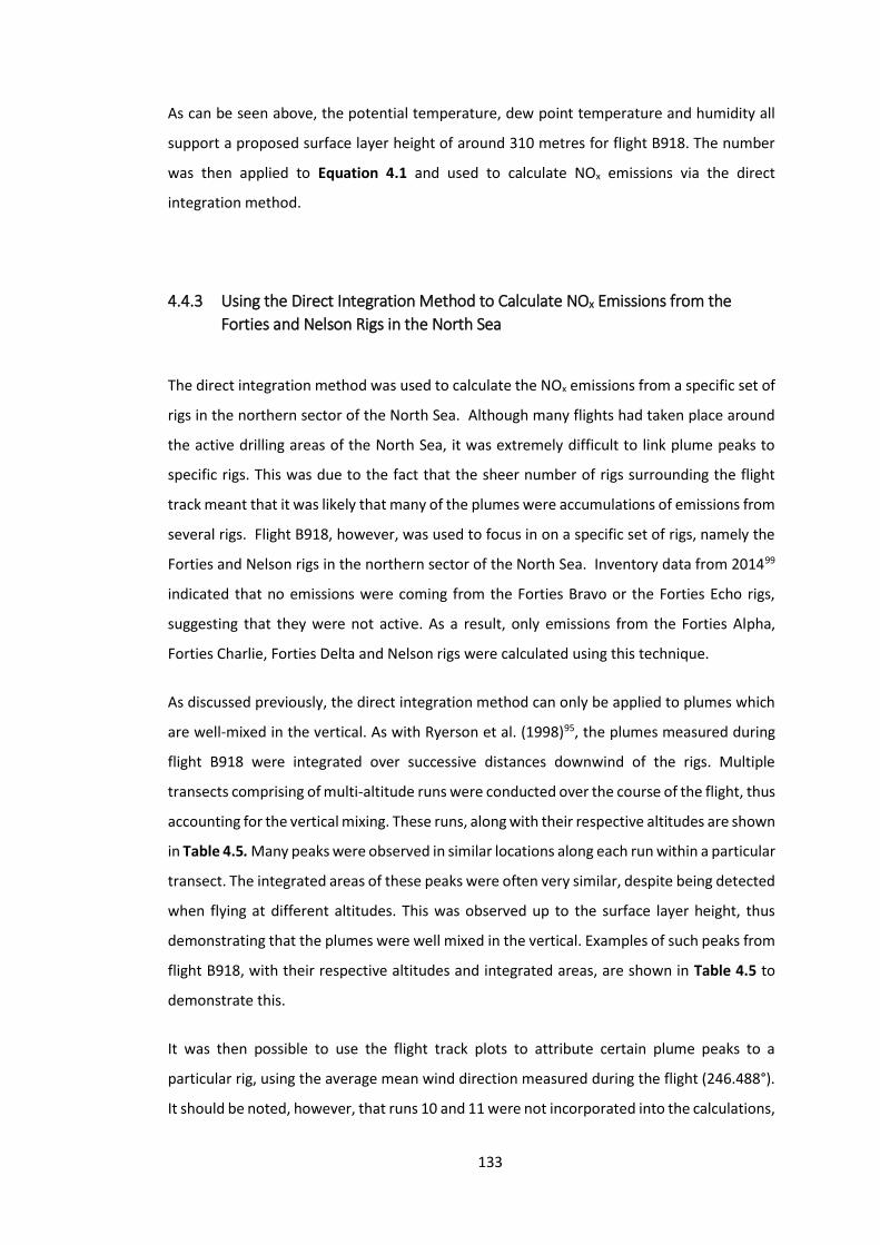
133
As can be seen above, the potential temperature, dew point temperature and humidity all
support a proposed surface layer height of around 310 metres for flight B918. The number
was then applied to Equation 4.1 and used to calculate NOx emissions via the direct
integration method.
4.4.3 Using the Direct Integration Method to Calculate NOx Emissions from the
Forties and Nelson Rigs in the North Sea
The direct integration method was used to calculate the NOx emissions from a specific set of
rigs in the northern sector of the North Sea. Although many flights had taken place around
the active drilling areas of the North Sea, it was extremely difficult to link plume peaks to
specific rigs. This was due to the fact that the sheer number of rigs surrounding the flight
track meant that it was likely that many of the plumes were accumulations of emissions from
several rigs. Flight B918, however, was used to focus in on a specific set of rigs, namely the
Forties and Nelson rigs in the northern sector of the North Sea. Inventory data from 201499
indicated that no emissions were coming from the Forties Bravo or the Forties Echo rigs,
suggesting that they were not active. As a result, only emissions from the Forties Alpha,
Forties Charlie, Forties Delta and Nelson rigs were calculated using this technique.
As discussed previously, the direct integration method can only be applied to plumes which
are well-mixed in the vertical. As with Ryerson et al. (1998)95, the plumes measured during
flight B918 were integrated over successive distances downwind of the rigs. Multiple
transects comprising of multi-altitude runs were conducted over the course of the flight, thus
accounting for the vertical mixing. These runs, along with their respective altitudes are shown
in Table 4.5. Many peaks were observed in similar locations along each run within a particular
transect. The integrated areas of these peaks were often very similar, despite being detected
when flying at different altitudes. This was observed up to the surface layer height, thus
demonstrating that the plumes were well mixed in the vertical. Examples of such peaks from
flight B918, with their respective altitudes and integrated areas, are shown in Table 4.5 to
demonstrate this.
It was then possible to use the flight track plots to attribute certain plume peaks to a
particular rig, using the average mean wind direction measured during the flight (246.488°).
It should be noted, however, that runs 10 and 11 were not incorporated into the calculations,
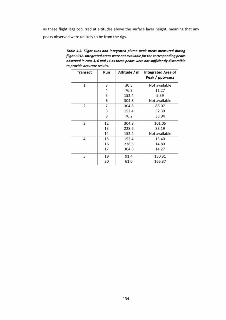
134
as these flight legs occurred at altitudes above the surface layer height, meaning that any
peaks observed were unlikely to be from the rigs.
Transect Run Altitude / m Integrated Area of Peak / pptv-secs
1 3 4 5 6
30.5 76.2
152.4 304.8
Not available 11.27 9.39
Not available
2 7 8 9
304.8 152.4 76.2
88.07 52.39 33.94
3 12 13 14
304.8 228.6 152.4
101.05 83.19
Not available
4 15 16 17
152.4 228.6 304.8
13.40 14.80 14.27
5 19 20
91.4 61.0
150.31 166.37
Table 4.5: Flight runs and integrated plume peak areas measured during
flight B918. Integrated areas were not available for the corresponding peaks
observed in runs 3, 6 and 14 as these peaks were not sufficiently discernible
to provide accurate results.
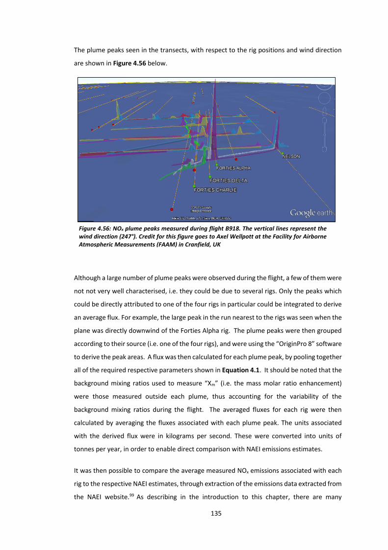
135
The plume peaks seen in the transects, with respect to the rig positions and wind direction
are shown in Figure 4.56 below.
Although a large number of plume peaks were observed during the flight, a few of them were
not not very well characterised, i.e. they could be due to several rigs. Only the peaks which
could be directly attributed to one of the four rigs in particular could be integrated to derive
an average flux. For example, the large peak in the run nearest to the rigs was seen when the
plane was directly downwind of the Forties Alpha rig. The plume peaks were then grouped
according to their source (i.e. one of the four rigs), and were using the “OriginPro 8” software
to derive the peak areas. A flux was then calculated for each plume peak, by pooling together
all of the required respective parameters shown in Equation 4.1. It should be noted that the
background mixing ratios used to measure “Xm” (i.e. the mass molar ratio enhancement)
were those measured outside each plume, thus accounting for the variability of the
background mixing ratios during the flight. The averaged fluxes for each rig were then
calculated by averaging the fluxes associated with each plume peak. The units associated
with the derived flux were in kilograms per second. These were converted into units of
tonnes per year, in order to enable direct comparison with NAEI emissions estimates.
It was then possible to compare the average measured NOx emissions associated with each
rig to the respective NAEI estimates, through extraction of the emissions data extracted from
the NAEI website.99 As describing in the introduction to this chapter, there are many
Figure 4.56: NOx plume peaks measured during flight B918. The vertical lines represent the wind direction (247°). Credit for this figure goes to Axel Wellpott at the Facility for Airborne Atmospheric Measurements (FAAM) in Cranfield, UK
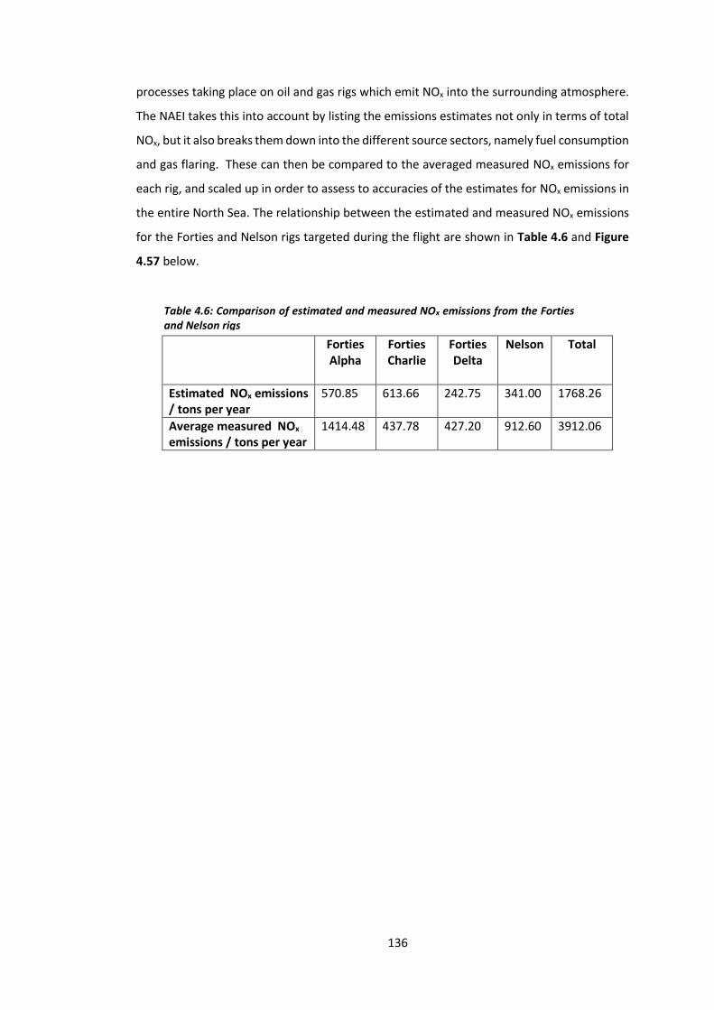
136
processes taking place on oil and gas rigs which emit NOx into the surrounding atmosphere.
The NAEI takes this into account by listing the emissions estimates not only in terms of total
NOx, but it also breaks them down into the different source sectors, namely fuel consumption
and gas flaring. These can then be compared to the averaged measured NOx emissions for
each rig, and scaled up in order to assess to accuracies of the estimates for NOx emissions in
the entire North Sea. The relationship between the estimated and measured NOx emissions
for the Forties and Nelson rigs targeted during the flight are shown in Table 4.6 and Figure
4.57 below.
Forties Alpha
Forties Charlie
Forties Delta
Nelson Total
Estimated NOx emissions / tons per year
570.85 613.66 242.75 341.00 1768.26
Average measured NOx
emissions / tons per year 1414.48 437.78 427.20 912.60 3912.06
Table 4.6: Comparison of estimated and measured NOx emissions from the Forties and Nelson rigs
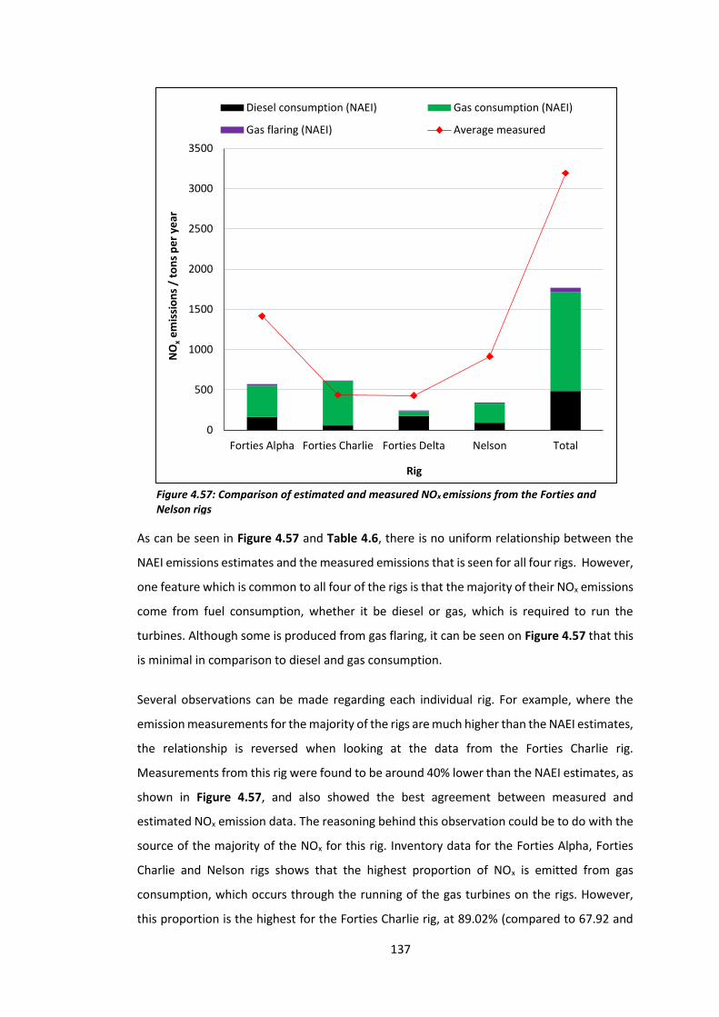
137
As can be seen in Figure 4.57 and Table 4.6, there is no uniform relationship between the
NAEI emissions estimates and the measured emissions that is seen for all four rigs. However,
one feature which is common to all four of the rigs is that the majority of their NOx emissions
come from fuel consumption, whether it be diesel or gas, which is required to run the
turbines. Although some is produced from gas flaring, it can be seen on Figure 4.57 that this
is minimal in comparison to diesel and gas consumption.
Several observations can be made regarding each individual rig. For example, where the
emission measurements for the majority of the rigs are much higher than the NAEI estimates,
the relationship is reversed when looking at the data from the Forties Charlie rig.
Measurements from this rig were found to be around 40% lower than the NAEI estimates, as
shown in Figure 4.57, and also showed the best agreement between measured and
estimated NOx emission data. The reasoning behind this observation could be to do with the
source of the majority of the NOx for this rig. Inventory data for the Forties Alpha, Forties
Charlie and Nelson rigs shows that the highest proportion of NOx is emitted from gas
consumption, which occurs through the running of the gas turbines on the rigs. However,
this proportion is the highest for the Forties Charlie rig, at 89.02% (compared to 67.92 and
0
500
1000
1500
2000
2500
3000
3500
Forties Alpha Forties Charlie Forties Delta Nelson Total
NO
xe
mis
sio
ns
/ to
ns
pe
r ye
ar
Rig
Diesel consumption (NAEI) Gas consumption (NAEI)
Gas flaring (NAEI) Average measured
Figure 4.57: Comparison of estimated and measured NOx emissions from the Forties and Nelson rigs
138
69.53% for the Forties Alpha and Nelson rigs, respectively). This is also significant when
looking at the Forties Alpha and Nelson rig measurements, and their comparisons to NAEI
estimates. The source contributions of these two rigs are relatively similar, each
predominantly emitting NOx through the operation of gas turbines. Another similarity
between the Forties Alpha and Nelson rigs is that their average measured NOx emissions both
greatly exceed the inventory estimates, being 2.5 and 2.7 times higher, respectively.
All of these observations regarding the Forties Alpha, Forties Charlie and Nelson rigs appear
to be under-pinned by the proportion of NOx emitted through the operation of gas turbines.
As can be seen in Figure and Table, all of the rigs except Forties Charlie have underestimated
the NOx emissions. This could be because this rigs has a larger proportion of its NOx coming
from gas turbines, compared to the Forties Alpha and Nelson rigs, which also run on gas
turbines. This may be due to these turbines being better represented by the NAEI, thus
resulting in a better agreement between measured and inventory data. It also suggests that
there may be some differences in the operation of these turbines on each of these rigs, i.e.
there may be more turbines, or they may be running at higher power on this rig, compared
to the other two.
The Forties Delta rig, according to the NAEI data, should emit the least amount of NOx out of
the four rigs used for this study (see Figure 4.57). This inventory prediction was corroborated
by the average emissions measured during the flight. The operation of this rig appears to be
slightly different, compared to the other three, particularly in the type of turbines used.
According to the inventory data, the majority of the NOx emitted by the Forties Delta rig
comes from diesel consumption through the operation of the turbines, whereas, on the other
three rigs, the turbines are predominantly powered by gas. The lower total NOx emissions
from the Forties Delta rig can therefore be attributed to the use of diesel, as opposed to gas
turbines. This could therefore lead to further speculation surrounding oil and gas rigs in
general, suggesting that NOx emissions from these sources could be reduced through
alteration of the rig infrastructure. However, the type of turbine does not make a difference
when comparing the inventory estimates to the average measured emissions from the
Forties Delta rig. As with the Forties Alpha and Nelson rigs, the measured NOx emissions
greatly exceeded the inventory estimates, being approximately 1.8 times higher.
In summary, although a relatively good relationship was observed for the Forties Charlie rig,
the majority of the data obtained suggest that the NAEI is severely under-estimating the NOx
emissions from the Forties and Nelson rigs in the North Sea. Both Figure 4.57 and Table 4.6
139
show a large difference between the summed inventory estimates and measured data for
the four rigs. The total measured data suggests that 1,423 tons of extra NOx is being emitted
into the atmosphere by these four rigs alone, compared to what the NAEI is predicting.
Limitations of the Study
There are errors and limitations with this type of study which must be considered. This study
only involved analysis of data from a single flight, meaning that diurnal or seasonal changes
in emissions were not taken into account. For example, the increased amount of fuel burning
in colder winter months would mean that the demand for oil and gas would be higher, thus
requiring an increase in activity (and subsequent increase in emissions) by the rigs compared
to the milder times of year. It was also assumed that not only were all rigs in the North Sea
operational, but that they were operating 365 days a year. This means that it is highly likely
that the majority of rigs were misrepresented in the study, i.e. it was assumed that NOx
emissions are uniform across all North Sea rigs. Not all rigs in the North Sea operate in exactly
the same manner as each other, meaning that their NOx emissions are likely to differ.
In order to get a better understanding of emissions from North Sea rigs in the future, this
direct integration method could be applied, by conducting regular, year-round survey flights
around all oil and gas fields in the active drilling regions. Ensuring that all criteria for the
direct integration are met (for example, the air being well mixed in the vertical), the method
could then be used to calculate average emissions of all species by the rigs, and investigated
further in terms of their seasonal variations and comparison to NAEI estimates. As discussed
previously, the NAEI breaks down the emissions estimates into different source sectors.
Comparison of the measured and estimated emissions could then be used to investigate how
well each source sector is being represented by the NAEI. This, in turn, would help to improve
the understanding of the reasons behind any discrepancies between measured and
estimated rig emissions in the North Sea, whilst also giving a more accurate representation
of emissions coming from North Sea rigs.
140
4.3.4 NOx Emissions from North Sea Oil and Gas Platforms: A Wider Perspective
As discussed previously, the North Sea is now considered one of the world’s most active
drilling areas. Therefore, these findings must be scaled up and applied to all of the
operational rigs in the North Sea, in order to fully understand the extent and potential
impacts of NOx emissions from oil and gas platforms.
One way of doing this is to take the percentage extra NOx produced according to the
measured Forties and Nelson rig data and apply it to the rest of the operational rigs in the
North Sea. This percentage is calculated by dividing the total measured NOx emissions by the
total NOx emissions according to the inventory. Doing so shows that the measured NOx
emissions from the Forties and Nelson rigs are 1.805 times higher than the respective NAEI
estimates. The most recent NAEI data99 indicates that there are 272 rigs emitting NOx in the
North Sea, with total annual emissions of 52,705 tons, according to the inventory. Assuming
the extra NOx measured from the Forties and Nelson rigs is duplicated across all rigs in the
North Sea, an extra 42,438 tons of NOx, is being emitted, which is not being accounted for
by the NAEI.
Using the NAEI mapping tool,100 it was found that this surplus NOx from the oil and gas rigs
in the North Sea (42,438 tons per year) is roughly equivalent to the annual NOx emissions
coming from a circle of 50 km diameter around London (45,851 tons per year). London is an
extremely large, industrialised city, with a population of approximately 8.6 million. This urban
environment brings with it high NOx mixing ratios, due to the large number of vehicles
travelling in and around the city and all hours of the day. This can be seen on Figure 4.58,
whereby the large density of high NOx areas, predominantly roads, can be easily
distinguished. The fact that the North Sea oil and gas rigs could possibly be emitting around
the same amount of NOx as a busy city like London is a good indication that the rigs are a
significant point source of NOx, and that the inventory data is severly underestimating their
contribution to the UK’s NOx budget.
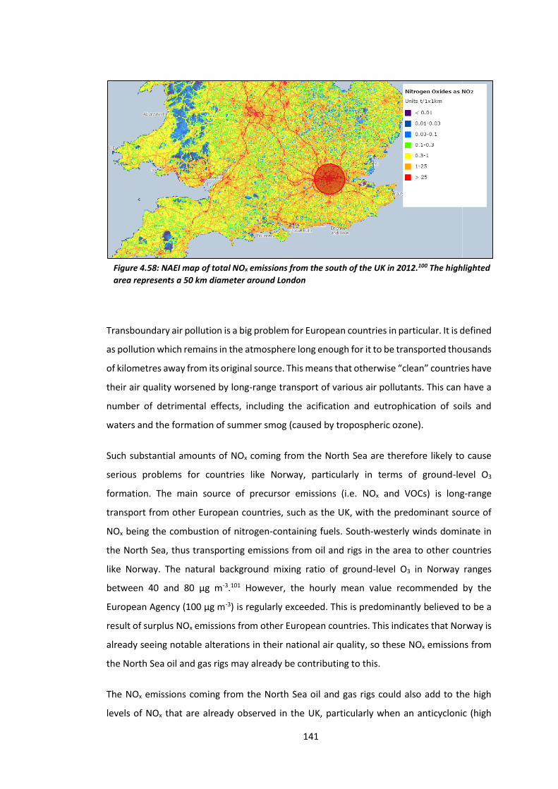
141
Transboundary air pollution is a big problem for European countries in particular. It is defined
as pollution which remains in the atmosphere long enough for it to be transported thousands
of kilometres away from its original source. This means that otherwise “clean” countries have
their air quality worsened by long-range transport of various air pollutants. This can have a
number of detrimental effects, including the acification and eutrophication of soils and
waters and the formation of summer smog (caused by tropospheric ozone).
Such substantial amounts of NOx coming from the North Sea are therefore likely to cause
serious problems for countries like Norway, particularly in terms of ground-level O3
formation. The main source of precursor emissions (i.e. NOx and VOCs) is long-range
transport from other European countries, such as the UK, with the predominant source of
NOx being the combustion of nitrogen-containing fuels. South-westerly winds dominate in
the North Sea, thus transporting emissions from oil and rigs in the area to other countries
like Norway. The natural background mixing ratio of ground-level O3 in Norway ranges
between 40 and 80 μg m-3.101 However, the hourly mean value recommended by the
European Agency (100 μg m-3) is regularly exceeded. This is predominantly believed to be a
result of surplus NOx emissions from other European countries. This indicates that Norway is
already seeing notable alterations in their national air quality, so these NOx emissions from
the North Sea oil and gas rigs may already be contributing to this.
The NOx emissions coming from the North Sea oil and gas rigs could also add to the high
levels of NOx that are already observed in the UK, particularly when an anticyclonic (high
Figure 4.58: NAEI map of total NOx emissions from the south of the UK in 2012.100 The highlighted
area represents a 50 km diameter around London
142
pressure) system is dominating the regional meteorology. These systems have small pressure
gradients, which bring about gentle winds. These winds generally blow from an easterly
direction, thus bringing air from the North Sea to the UK. Such high pressure systems
therefore result in the accumulation of high pollutant mixing ratios, brought about by limited
mixing and dilution. A consequence of this “trapping” of pollutants, such as NOx and VOCs,
can result in increased amounts of ground-level O3. This was observed during the “heat
wave” over Western Europe in 2003, whereby a persistent anticyclone resulted in regular
exceedances of 30°C in the UK. This high pressure system also caused significantly enhanced
levels of pollutants such as NOx and tropospheric O3. A study by Lee et al. (2006)102 suggested
that these increased levels were likely to be a result of both local atmospheric processes and
regional transport. Derwent and Jenkin (1991)103 also emphasised the contribution that
atmospheric transport makes to high O3 events in the UK. Therefore, these additional NOx
emissions from the oil and gas rigs in the North Sea would only exacerbate the tropospheric
O3 production under these conditions. High mixing ratios of ground-level, or tropospheric O3
can cause a range of health problems, including eye irritation and exacerbation of respiratory
illnesses. It can also affect vegetation, reducing crops yields by slowing down processes like
photosynthesis and growth, hence why it is of utmost important that its mixing ratios are
minimised.
The road transport sector (predominantly diesel-fuelled vehicles), is a key NOx source in the
UK and is believed to be at least in part, the reason behind the UK not meeting EU standards
for NO2. Breaching these limits means that the UK would be fined by the EU. As well as these
economic costs, NO2 causes detrimental effects to human health, particular in terms of
respiratory disease, whilst also being an element of tropospheric O3 formation. It is therefore
in the best interests of the UK to keep NOx mixing ratios as low as possible, meaning any
additional emissions from oil and gas platforms are only likely to make this a more difficult
process.
143
CONCLUSION
A LIF instrument was evaluated as a direct method for tropospheric NO2 quantification. The
instrument was initially tested for NO2 measurements in a polluted atmosphere at the
University of York campus in the suburban village of Heslington, York. Ambient
measurements of NO2 made by the LIF instrument were directly compared with a standard
P-CL analyser in the laboratory. The mixing ratios measured by both instruments compared
well with each other, both measuring NO2 levels that were consistent with the surrounding
atmospheric environment (between around 3 and 6 ppbv). NO2 data from an urban
monitoring site in the centre of York was compared with the data measured in Heslington.
The NO2 mixing ratios from the city centre were significantly higher, peaking at
approximately 66 ppbv, which could be attributed to the higher road traffic volume in the
area. This provided a great amount of assurance as to the reliability of the NO2
measurements made by the LIF instrument in Heslington. The LIF instrument was also
characterised for NO measurements, through the installation an efficient GPT system, similar
to those used in commercial chemiluminescence instruments. This involved the
manipulation of various experimental conditions, to ultimately yield the highest conversion
efficiency possible. A conversion efficiency of over 90% was achieved through the
incorporation of an additional reaction volume, thus emphasising the importance of mixing
time for efficient NO measurements.
However, the instrument proved not to perform as well for remote marine boundary layer
measurements. Deployment at the CVAO saw the instrument significantly over-estimating
the ambient NO2 mixing ratios. The cause of such an over-estimation was deduced to be a
result of a leak within the instrument, which meant that the instrument was sampling
laboratory air, as well as the marine boundary layer air. Consumable restrictions meant that
it was deemed unviable to use the LIF for NO measurements at the CVAO. Deployment at the
observatory led to the conclusion that, although performing well in the polluted boundary
layer, the instrument would not be suitable for long-term NO2 measurements in the remote
boundary layer in its current configuration.
Although the LIF technique has the distinct advantage over chemiluminescence instruments
in terms of direct NO2 measurements, this study has found that, for this instrument in
particular, there is still scope to improve it. As discussed in section 2.1, there are a great
number of factors which can influence of the sensitivity of LIF instruments, and it is these
144
factors in particular which must be taken into account to maximise the capability of the LIF
technique in tropospheric measurements.
Oil and gas rigs are a point source of NOx within the NAEI, though it has been as yet unclear
as to how well the inventory represents these NOx emissions. The operation of these rigs is
also known to release vast amounts of other atmospheric species, such as CO2 and CH4 into
the surrounding atmosphere every year, would could lead to dramatic impacts on the
environment. The “Oil and Gas” campaign took place in summer 2015, with the objective of
assessing the extent of these emissions coming from North Sea rigs (a highly active drilling
region), whilst also using the direct integration method to assess the accuracy of NOx
estimates in the NAEI.
Survey flights took place around the active oil and gas fields in the southern and northern
sectors of the North Sea. Substantial NOx enhancements were regularly observed when flying
directly downwind of the rigs, with the largest gas plumes containing between around 20,000
and 40,000 pptv. Analysis of the background mixing ratios, along with back trajectories were
used to confirm that the majority of the plume mixing ratios observed were coming from the
rigs. However, in some flights, there was a notable influence from UK-based NOx sources,
namely the Humberside and Lincolnshire coastline, which also contributed to some of the
high level NOx detected.
The nature of these survey flights, i.e. the high density of rigs in the surrounding area meant
that it was very difficult to attribute each NOx plume peak to a specific rig. Flight B918 was
used to derive NOx emissions coming from individual rigs using the direct integration method.
The Forties and Nelson rigs in the North Sea were targeted and multiple-altitude transects
were conducted at various distances downwind of them. Doing so would mean that it would
be possible to ascertain which plume peaks were coming from which rig. Once this was done,
the emissions coming from each of the rigs could be ascertained using the direct integration
method. Averaging the measured emissions from the Forties and Nelson rigs and comparing
them to the respective NAEI estimate indicated a significant discrepancy, with the NAEI
under-estimating the annual NOx emissions by around 2,000 tons. Further analysis of the
NAEI data indicated that some source sectors were better represented than others,
particularly in terms of the fuel used to operate the turbines. These findings were then scaled
up to evaluate the NAEI estimates for the whole North Sea drilling region, showing that this
poor representation of NOx emissions from oil and gas rigs was leading to a (theoretical)
under-estimation of around 40,000 tons per year. Such a substantial amount of surplus NOx

145
in the atmosphere could have detrimental impacts on a large scale, highlighting the
importance of the NAEI for accurate NOx measurements.
However, there are errors and limitations with this type of study, meaning that important
factors such as diurnal and seasonal variations were not taken into account. In order to get
a more representative picture of NOx emissions from North Sea rigs, it would therefore be
necessary to conduct year-round survey flights around the operational drilling areas and use
the direct integration method to compare their emissions with the respective inventory data.
This would also provide more information as to how well the rigs are represented as point
sources in the NAEI.

146
LIST OF ABBREVIATIONS
AN alkyl nitrate
BLC blue light converter
BOC British Oxygen Company
c/s/ppbv counts per second per ppbv
CAPS cavity attenuated phase shift spectroscopy
CEAS cavity enhanced absorption spectroscopy
CRDS cavity ring down spectroscopy
CVAO Cape Verde Atmospheric Observatory
DOAS differential optical absorption spectroscopy
FAAM Facility for Airborne Atmospheric Measurements
FAGE fluorescence assay by gas expansion
GPT gas phase titration
LED light emitting diode
LIF laser induced fluorescence
MFC mass flow controller
NAEI National Atmospheric Emissions Inventory
Nd:YAG neodymium-doped yttrium aluminium garnet (crystal used as a lasing
medium)
nm nanometres
P-CL photolytic chemiluminescence

147
PMT photomultiplier tube
PN peroxy nitrate
ppbv parts per billion by volume (10-9)
pptv parts per trillion by volume (10-12)
sccm standard cubic centimetres
slpm standard litres per minute
SNR signal to noise ratio
TDLAS tunable diode laser absorption spectroscopy
TD-LIF thermal dissociation-laser induced fluorescence
μg/m3 micrograms per cubic metre
ppmv parts per million by volume (10-6)
148
REFERENCES
1 R. Atkinson, Atmos. Environ., 2000, 34, 2063-2101
2 G. –J. Roelofs and J. Lelieveld., Tellus B, 1997, 49, 38-55
3 J. A. Logan et al., J. Geophys. Res., 1981, 86, 7210-7254
4 G. J. M. Velders et al., J. Geophys. Res., 2001, 106, 12643-12660
5 J. A. Thornton et al., Anal. Chem., 2000, 72, 528-539
6 G. Villena et al., Atmos. Meas. Tech., 2011, 4, 1663–1676
7 K. Mannschreck et al., Atmos. Chem. Phys., 2004, 4, 1265–1277
8 O. R. Cooper et al., Elem. Sci. Anth., 2014, 2, doi: 10.12952/journal.elementa.000029
9 R. Van Dingenen et al., Atmos. Environ., 2009, 43, 604-618
10 J. D. Lee et al., J. Geophys. Res., 2009, 14, D21302
11 H. Fuchs et al., Atmos. Meas. Tech., 2010, 3, 21-37
12 S. E. Schwartz, Science, 1989, 243, 753-763
13 W. S. Tunnicliffe et al., Lancet, 1994, 344, 1733-1736
14 V. Strand et al., Euro. Respir. J., 1998, 12, 6-12
15 L. K. Emmons et al., Atmos. Environ., 1997, 31, 1851-1904
16 X. Tie et al., J. Geophys. Res., 2001, 106, 3167–3178.
17 X. Tie et al., J. Atmos. Chem., 2002, 43, 61–74
18 E. Aruffo et al., Atmos. Environ., 2014, 94, 479-488
19 E. V. Fischer et al., Atmos. Chem. Phys., 2014, 14, 2679–2698
20 R. K. Talukdar et al., J. Geophys. Res., 1995, 100, 14163-14173
21 J. Matsumoto and Y. Kajii, Atmos. Environ., 2003, 37, 4847-4851
22 J. A. Thornton et al., J. Geophys. Res., 2003, 108, D4496
23 T. Gherman et al., Environ. Sci. Technol., 2008, 42, 890-895
24 T. Wu et al., Appl. Phys. B, 2009, 94, 85-94
25 H. D. Osthoff et al., J. Geophys. Res., 2006, 111, D12305
26 H. Fuchs et al., Environ. Sci. Technol., 2009, 43, 7831-7836
27 P. L. Kebabian et al., Anal. Chem., 2005, 77, 724-728
28 Y. Q. Li et al., J. Geophys. Res., 2004, 109, D16S08
29 G. L. Gregory et al., J. Geophys. Res., 1990, 95, 10103-10127
30 L. A. George and R. J. O’Brien, J. Atmos. Chem., 1991, 12, 195-209
31 C. Fong and W. H. Brune, Rev. Sci. Instrum., 1997, 68, 4253-4262
32 C. Dari-Salisburgo et al., Atmos. Environ., 2009, 43, 970-977

149
33 Y. Matsumi et al., Anal. Chem., 2001, 73, 5485-5493
34 P. A. Cleary et al., Appl. Opt., 2002, 41, 6950-6956
35 J. G. Murphy et al., Atmos. Chem. Phys., 2004, 4, 377-384
36 F. Taketani et al., Appl. Opt., 2007, 46, 907-915
37 D. A. Day et al., J. Geophys. Res., 2002, 107, D64046
38 P. Di Carlo et al., Atmos. Meas. Tech., 2013, 6, 971-980
39 B. J. Finlayson-Pitts and J. N. Pitts, Jr., Chemistry of the Upper and Lower Atmosphere,
Academic Press, San Diego, 2000
40 E. J. Dunlea et al., Atmos. Chem. Phys., 2007, 7, 2691-2704
41 R. R. Dickerson et al., Rev. Sci. Instrum., 1984, 55, 1995-1998
42 Y. Sadanaga et al., Anal. Chem., 2010, 82, 9234-9239
43 D. Grosjean and J. Harrison, Environ. Sci. Technol., 1985, 19, 862-865
44 A. M. Winer et al, Environ. Sci. Technol., 1974, 8, 1118-1121
45 N. A. Marley et al., Rev. Sci. Instrum., 2004, 75, 4595-460
46 D. D. Parrish et al., J. Geophys. Res., 1990, 95, 1817-1836
47 T. B. Ryerson et al., J. Geophys. Res., 2000, 105, 26447-2646
48 I. B. Pollack et al., J. Atmos. Chem., 2010, 65, 111-125
49 M.D. Shaw et al., Atmos. Chem. Phys., 2015, 15, 5083-5097
50 C. Reed et al., Atmos. Chem. Phys. Discuss., submitted 2015
51 C. A. Biesheuvel et al., J. Chem. Phys., 1998, 109, 9701-9712
52 J. Bradshaw et al., Geophys. Res. Lett., 1999, 26, 471
53 K. K. Perkins et al., J. Geophys. Res., 1999, 104, 26687
54 J. B. Burkholder and R. K. Talukdar, Geophys. Res. Lett., 1994, 21, 581
55 L. S. Rothman et al., J. Quant. Spectrosc. Radiat. Transfer, 2005, 96, 1394
56 B. A. Bodhaine et al., J. Atmos. Oceanic Technol., 1999, 16, 1854
57 A. Bucholtz, Appl. Opt., 1995, 34, 2765
58 C. D. Salisburgo, PhD Thesis, University of L’Aquila, 2006-2007
59 J. Drummond et al., J. Atmos. Chem., 1985, 2, 287–306
60 M. C. Peterson and R. E. Honrath, J. Geophys. Res., 1999, 104, 11,695–11,707
61 M. Val Martin et al., J. Geophys. Res., 2008, 113, D17307
62 http://www.theicct.org/sites/default/files/ICCT_PEMS-study_diesel-
cars_2014_factsheet_EN.pdf (accessed 4/8/15)
63 D. C. Carslaw., Atmos. Environ., 2005, 39, 4793
64 P. Anttila and J.-P. Tuovinen, Atmos. Environ., 2010, 44, 30

150
65 R. Alvarez et al., Atmos. Environ., 2008, 42, 4699
66http://www.jorair.co.uk/reports/Further/Further%20Assessment%20for%20Fulford%20Main%
20Street%20-%20April%202011.pdf (accessed 4/8/15)
67 http://uk-air.defra.gov.uk/data/ (accessed 13/10/15)
68 S. S. Brown et al., J. Geophys. Res. Lett., 2004, 31, doi:10.1029/2004GL019412
69 N. Riemer et al., J. Geophys. Res., 2003, 108, 1-21
70 L. J. Carpenter et al., J. Atmos. Chem., 2010, 67, 87–140
71 P. J. Crutzen et al., Tellus A, 1999, 51, 123–146
72 B. A. Ridley et al., J. Geophys. Res., 1988, 93, 15803–15811
73 P. C. Moonen et al., J. Atmos. Chem., 1998, 29, 299-314
74 G. D. Edwards and P. S. Monks, J. Geophys. Res., 2003, 108, doi:10.1029/2002JD002844
75 S. J. B. Bauguitte et al., Atmos. Chem. Phys., 2012, 12, 989–1002
76 Z. Hosaynali Beygi et al., Atmos. Chem. Phys., 2011, 11, 8497–8513
77 M. M. Frey et al., Atmos. Chem. Phys., 2013, 13, 3045–3062
78 M. M. Frey et al., Atmos. Chem. Phys., 2015, 15, 7859–7875
79 C. A. Cantrell et al., J. Geophys. Res., 2003, 108, doi:10.1029/2002JD002198
80 http://oilandgasuk.co.uk/key-facts/energy-provider.cfm (accessed 12/09/15)
81 http://oilandgasuk.co.uk/environment-report.cfm (accessed 12/09/15)
82 http://cdiac.esd.ornl.gov/pns/current_ghg.html (accessed 12/09/15)
83I. S. A. Isaksen et al., Atmos., 2014, 5, 518-535
84G. L. Vaghjiani and A. R. Ravishankara, Nature, 1991, 350, 406-409
85 G. N. Petersen and I. A. Renfrew, Q. J. R. Meteorol. Soc., 2009, 135, 2030–2045
86 J. R. Ström et al., J. Atmos. Tech., 1994, 11, 1392–1399
87 Probing the Atmospheric Boundary Layer, ed. D. H. Lenschow, Americ. Met. Soc., Boston,
Massachusetts, 1986
88 C. Gerbig et al., J. Geophys. Res., 1999, 104, 1699–1704
89 K. L. Wilson and J. W. Birks, Env. Sci. Tech., 2006, 40, 6361-6367
90 S. J. O'Shea, et al., Atmos. Meas. Tech., 2013, 6, 1095-1109
91 J. R. Hopkins et al., J. Environ. Monit., 2003, 5, 8-13
92 P. D. Rosenberg et al., Atmos. Meas. Tech., 2012, 5, 1147-1163
93 https://ready.arl.noaa.gov/HYSPLIT_traj.php (accessed 29/09/15 and 30/09/15)
94 J. D. Lee et al., Environ. Sci. Technol., 2015, 49, 1025−1034
95 T. B. Ryerson et al., J. Geophys. Res., 1998, 103, 22569-22583
96 W. H. White et al., Science, 1976, 194, 187-189

151
97 http://glossary.ametsoc.org/wiki/Poisson_constant (accessed 25/9/15)
98 S. Nicholls, J. Leighton and R. Barker, J. Atmos. Ocean. Tech., 1990, 7, 706-718
99 http://naei.defra.gov.uk/ (accessed 21/9/15)
100http://naei.defra.gov.uk/data/gis-mapping (accessed 5/10/15)
101 http://www.environment.no/Topics/Air-pollution/Ground-level-ozone-/ (accessed 5/10/15)
102 J.D. Lee et al., Atmos. Environ., 2006, 40, 7598–7613
103 R. G. Derwent and M. E. Jenkin., Atmos. Environ. Part A, 1991, 25, 1661-1678