mathematical modelling of problems related to image
TRANSCRIPT
HAL Id: tel-01270213https://tel.archives-ouvertes.fr/tel-01270213
Submitted on 5 Feb 2016
HAL is a multi-disciplinary open accessarchive for the deposit and dissemination of sci-entific research documents, whether they are pub-lished or not. The documents may come fromteaching and research institutions in France orabroad, or from public or private research centers.
L’archive ouverte pluridisciplinaire HAL, estdestinée au dépôt et à la diffusion de documentsscientifiques de niveau recherche, publiés ou non,émanant des établissements d’enseignement et derecherche français ou étrangers, des laboratoirespublics ou privés.
Mathematical modelling of problems related to imageregistration
Solène Ozeré
To cite this version:Solène Ozeré. Mathematical modelling of problems related to image registration. Analysis of PDEs[math.AP]. INSA de Rouen, 2015. English. NNT : 2015ISAM0010. tel-01270213

THESEprésentée à
par Solène OZERÉ
MODÉLISATION MATHÉMATIQUE
DE PROBLÈMES RELATIFS
Devant le jury composé de
6 novembre 2015
Après avis de :


A mon grand-pere.

REMERCIEMENTS
Au terme de ces trois annees de these, je souhaiterais remercier toutes les personnes qui m’ontaidees, qui ont cru en moi, et qui m’ont permis d’arriver au bout de cette these.
En premier lieu, j’adresse un immense merci a mes directeurs de these Christian Goutet Carole Le Guyader. Merci de m’avoir fait confiance et de m’avoir donne l’opportunite derealiser cette these avec eux, ce fut un plaisir de travailler sous leur direction. Je remercieChristian pour son soutien, ses conseils, sa gentillesse, la confiance qu’il m’a accordee et sabonne humeur. Je remercie Carole pour sa disponibilite, sa patience, nos nombreuses dis-cussions et ses precieux conseils. J’ai beaucoup appris grace a elle, de par sa grande culturescientifique, sa rigueur mathematique mais aussi ses qualites humaines. J’espere avoir etedigne de la confiance qu’ils m’ont accordee et que ce travail est finalement a la hauteur deleurs esperances.
Je remercie tres sincerement Madame Stephanie Allassonniere, Monsieur Simon Masnouet Madame Carola Schonlieb qui ont accepte d’etre rapporteurs de cette these. Je les remerciepour l’interet qu’ils ont porte a ce travail et pour l’honneur qu’ils m’ont fait en participantau jury.Je remercie egalement Monsieur Olivier Ley, Madame Caroline Petitjean et Monsieur GabrielPeyre pour l’honneur qu’ils m’ont fait de participer au jury de these.
Je remercie egalement Monsieur Herve Le Dret pour les reponses et l’aide qu’il nous aapportees au cours de ce travail.
Je tiens egalement a remercier l’ensemble des membres du Laboratoire de Mathematiquesde l’INSA. Merci a Brigitte Diarra pour sa gentillesse et son efficacite, a Nicolas Forcadel a lafois pour son humour et pour son aide. Je remercie tout particulierement les doctorants, Flo-rentina Nicolau et Zacharie Ales pour leur gentillesse et leurs conseils et d’avoir partage avecmoi le bureau, pour l’une, et les groupes de TD pour l’autre. Merci a Theophile Chaumont-Frelet pour sa bonne humeur, nos fous rires, et sa presence ponctuelle dans le bureau !Merci a Wilfredo Salazar sans qui ces deux dernieres annees n’auraient pas ete aussi agreables.Merci d’avoir partage toutes ces pauses-cafe et tous ces repas avec moi, merci de m’avoirecoutee et conseillee.
Je voudrais egalement remercier le departement du premier cycle de l’INSA qui m’a ac-cueillie dans le cadre de ma mission enseignement, en particulier Jean-Marc Cabanial et CaroleLe Guyader pour la confiance qu’ils m’ont accordee. Ce fut une experience tres interessanteet enrichissante.
Je voudrais maintenant remercier d’autres personnes qui m’ont aidee, peut-etre sans lesavoir, ma famille. Merci a mes parents pour leur soutien inconditionnel et leurs encourage-ments. Merci egalement a mon frere et mon pere pour leurs avis et leur aide en matiere degraphismes et d’esthetique pour mon manuscrit !Enfin, merci a celui qui m’a aidee plus qu’il ne le realise sans doute, Sebastien. Merci d’unepart pour m’avoir aidee grace a tes talents d’informaticien, a debugger mes codes et ameliorerma facon de proceder. Mais surtout, merci d’avoir toujours ete la, de m’avoir encouragee, dem’avoir fait voir le bon cote des choses quand il le fallait. Merci de tout ce que tu m’apportes.
Contents
1 Introduction generale 1
1.1 Traitement d’images et cadre mathematique . . . . . . . . . . . . . . . . . . . 1
1.2 Le recalage d’images . . . . . . . . . . . . . . . . . . . . . . . . . . . . . . . . 2
1.2.1 Interpolation et approximation des images . . . . . . . . . . . . . . . . 4
1.2.2 La mesure de similarite . . . . . . . . . . . . . . . . . . . . . . . . . . 6
1.2.3 Le modele de deformation . . . . . . . . . . . . . . . . . . . . . . . . . 10
1.2.4 La preservation de la topologie . . . . . . . . . . . . . . . . . . . . . . 12
1.3 Contribution . . . . . . . . . . . . . . . . . . . . . . . . . . . . . . . . . . . . 13
1.3.1 Preservation de la topologie du champ de deformation associe au re-calage d’images . . . . . . . . . . . . . . . . . . . . . . . . . . . . . . . 13
1.3.2 Modele conjoint de segmentation et recalage fonde sur la variation totaleponderee et l’elasticite non lineaire . . . . . . . . . . . . . . . . . . . . 16
1.3.3 Modele conjoint de segmentation et recalage non local . . . . . . . . . 17
1.4 Organisation de la these . . . . . . . . . . . . . . . . . . . . . . . . . . . . . . 18
2 Mathematical preliminaries 25
2.1 Lp Spaces . . . . . . . . . . . . . . . . . . . . . . . . . . . . . . . . . . . . . . 25
2.2 Sobolev spaces . . . . . . . . . . . . . . . . . . . . . . . . . . . . . . . . . . . 28
2.3 Functions of bounded variation . . . . . . . . . . . . . . . . . . . . . . . . . . 33
2.4 Direct methods in the calculus of variations . . . . . . . . . . . . . . . . . . . 34
2.4.1 Quasiconvexity, Polyconvexity and Rank one convexity . . . . . . . . . 35
2.5 Tridimensional elasticity . . . . . . . . . . . . . . . . . . . . . . . . . . . . . . 36
3 Topology preservation 41
3.1 Correction of the deformation . . . . . . . . . . . . . . . . . . . . . . . . . . . 46
3.2 Deformation reconstruction . . . . . . . . . . . . . . . . . . . . . . . . . . . . 49
3.2.1 Functional to be minimized . . . . . . . . . . . . . . . . . . . . . . . . 50
3.2.2 Characterization of the solution . . . . . . . . . . . . . . . . . . . . . . 55
3.2.3 Lagrange multipliers . . . . . . . . . . . . . . . . . . . . . . . . . . . . 56
3.2.4 Theoretical convergence result . . . . . . . . . . . . . . . . . . . . . . 57
3.2.5 Discretization . . . . . . . . . . . . . . . . . . . . . . . . . . . . . . . . 62
3.3 Numerical experiments . . . . . . . . . . . . . . . . . . . . . . . . . . . . . . . 66
3.3.1 First example : a slice of the brain . . . . . . . . . . . . . . . . . . . . 67
3.3.2 Second example : brain mapping . . . . . . . . . . . . . . . . . . . . . 70
3.3.3 Third example: the disks . . . . . . . . . . . . . . . . . . . . . . . . . 71
i
ii CONTENTS
4 Joint segmentation/registration model by shape alignment 77
4.1 Mathematical Modelling . . . . . . . . . . . . . . . . . . . . . . . . . . . . . . 79
4.1.1 General mathematical background . . . . . . . . . . . . . . . . . . . . 79
4.1.2 Depiction of the original model . . . . . . . . . . . . . . . . . . . . . . 80
4.1.3 Mathematical obstacle and derivation of a relaxed problem . . . . . . 83
4.1.4 Theoretical results . . . . . . . . . . . . . . . . . . . . . . . . . . . . . 84
4.2 Numerical method of resolution . . . . . . . . . . . . . . . . . . . . . . . . . . 90
4.2.1 Description and Analysis of the Proposed Numerical Method . . . . . 90
4.2.2 Numerical Scheme . . . . . . . . . . . . . . . . . . . . . . . . . . . . . 96
4.3 Numerical experiments . . . . . . . . . . . . . . . . . . . . . . . . . . . . . . . 99
4.3.1 Regridding technique, choice of the parameters and registration accuracy 99
4.3.2 Letter C . . . . . . . . . . . . . . . . . . . . . . . . . . . . . . . . . . . 101
4.3.3 Noisy triangle . . . . . . . . . . . . . . . . . . . . . . . . . . . . . . . . 103
4.3.4 Mouse brain gene expression data . . . . . . . . . . . . . . . . . . . . 104
4.3.5 Slices of the brain . . . . . . . . . . . . . . . . . . . . . . . . . . . . . 109
4.3.6 MRI images of cardiac cycle . . . . . . . . . . . . . . . . . . . . . . . . 110
4.3.7 Comparisons with prior related works . . . . . . . . . . . . . . . . . . 113
5 Nonlocal Joint Segmentation Registration Model 121
5.1 Mathematical Modelling . . . . . . . . . . . . . . . . . . . . . . . . . . . . . . 122
5.2 Theoretical results . . . . . . . . . . . . . . . . . . . . . . . . . . . . . . . . . 125
5.2.1 Existence of minimizers and relaxation theorem . . . . . . . . . . . . . 125
5.2.2 Well-definedness of Φ . . . . . . . . . . . . . . . . . . . . . . . . . . . 126
5.3 Numerical Method of Resolution . . . . . . . . . . . . . . . . . . . . . . . . . 132
5.4 Discretization and Implementation . . . . . . . . . . . . . . . . . . . . . . . . 136
5.4.1 Introduction of an AOS scheme for the evolution problem . . . . . . . 136
5.4.2 Thomas algorithm . . . . . . . . . . . . . . . . . . . . . . . . . . . . . 140
5.4.3 Euler-Lagrange equations for functional Iγ . . . . . . . . . . . . . . . . 141
5.5 Numerical results . . . . . . . . . . . . . . . . . . . . . . . . . . . . . . . . . . 141
5.5.1 Letter C . . . . . . . . . . . . . . . . . . . . . . . . . . . . . . . . . . . 142
5.5.2 Triangle . . . . . . . . . . . . . . . . . . . . . . . . . . . . . . . . . . . 143
5.5.3 Mouse brain gene expression . . . . . . . . . . . . . . . . . . . . . . . 144
5.5.4 Slices of brain . . . . . . . . . . . . . . . . . . . . . . . . . . . . . . . . 145
6 Nonlinear elasticity and geometric constraints 151
6.1 Mathematical modelling . . . . . . . . . . . . . . . . . . . . . . . . . . . . . . 152
6.1.1 Preliminaries . . . . . . . . . . . . . . . . . . . . . . . . . . . . . . . . 152
6.1.2 Depiction of the model . . . . . . . . . . . . . . . . . . . . . . . . . . . 153
6.1.3 Mathematical obstacle and relaxed problem . . . . . . . . . . . . . . . 155
6.1.4 Theoretical results . . . . . . . . . . . . . . . . . . . . . . . . . . . . . 163
6.1.5 Relaxation theorem . . . . . . . . . . . . . . . . . . . . . . . . . . . . 168
6.2 A convergence result . . . . . . . . . . . . . . . . . . . . . . . . . . . . . . . . 168
6.3 Discretization and Implementation . . . . . . . . . . . . . . . . . . . . . . . . 171
6.3.1 Augmented Lagrangian . . . . . . . . . . . . . . . . . . . . . . . . . . 171
6.3.2 Implementation details . . . . . . . . . . . . . . . . . . . . . . . . . . . 174
6.4 Numerical experiments . . . . . . . . . . . . . . . . . . . . . . . . . . . . . . . 175
CONTENTS iii
7 Registration based on Gradient Comparison 1837.1 Mathematical modelling . . . . . . . . . . . . . . . . . . . . . . . . . . . . . . 1857.2 Existence minimizers for the initial problem . . . . . . . . . . . . . . . . . . . 1867.3 Introduction of an auxiliary variable . . . . . . . . . . . . . . . . . . . . . . . 188
7.3.1 Existence of minimizers for the decoupled problem . . . . . . . . . . . 1907.4 Approximation method of the total variation of T ϕ . . . . . . . . . . . . . 193
7.4.1 Existence of minimizers for the Problem with approximation of the totalvariation . . . . . . . . . . . . . . . . . . . . . . . . . . . . . . . . . . . 194
7.4.2 Study of limn→∞
ϕn and Γ-convergence . . . . . . . . . . . . . . . . . . . 196
7.4.3 Euler-Lagrange equation . . . . . . . . . . . . . . . . . . . . . . . . . . 2057.5 Implementation details . . . . . . . . . . . . . . . . . . . . . . . . . . . . . . . 206
7.5.1 Experiments on a restoration problem . . . . . . . . . . . . . . . . . . 2077.6 Implementation of the registration problem . . . . . . . . . . . . . . . . . . . 214
7.6.1 Scheme for the auxiliary variable method . . . . . . . . . . . . . . . . 2147.6.2 Scheme for the approximation method . . . . . . . . . . . . . . . . . . 2147.6.3 Numerical results . . . . . . . . . . . . . . . . . . . . . . . . . . . . . . 215

CHAPTER 1
INTRODUCTION GENERALE
1.1 Traitement d’images et cadre mathematique
L’imagerie est un domaine qui ne cesse de se developper et dont les applications sont nom-breuses, telles
• la photographie, avec l’argentique depuis les annees 1800 et la photographie numerique,
• l’imagerie medicale depuis le premier echographe en 1960, puis l’echographie numeriquedans les annees 1990,
• la biometrie, avec la reconnaissance d’empreintes depuis les annees 1970,
• l’imagerie satellitaire, avec les premiers satellites numeriques en 1976,
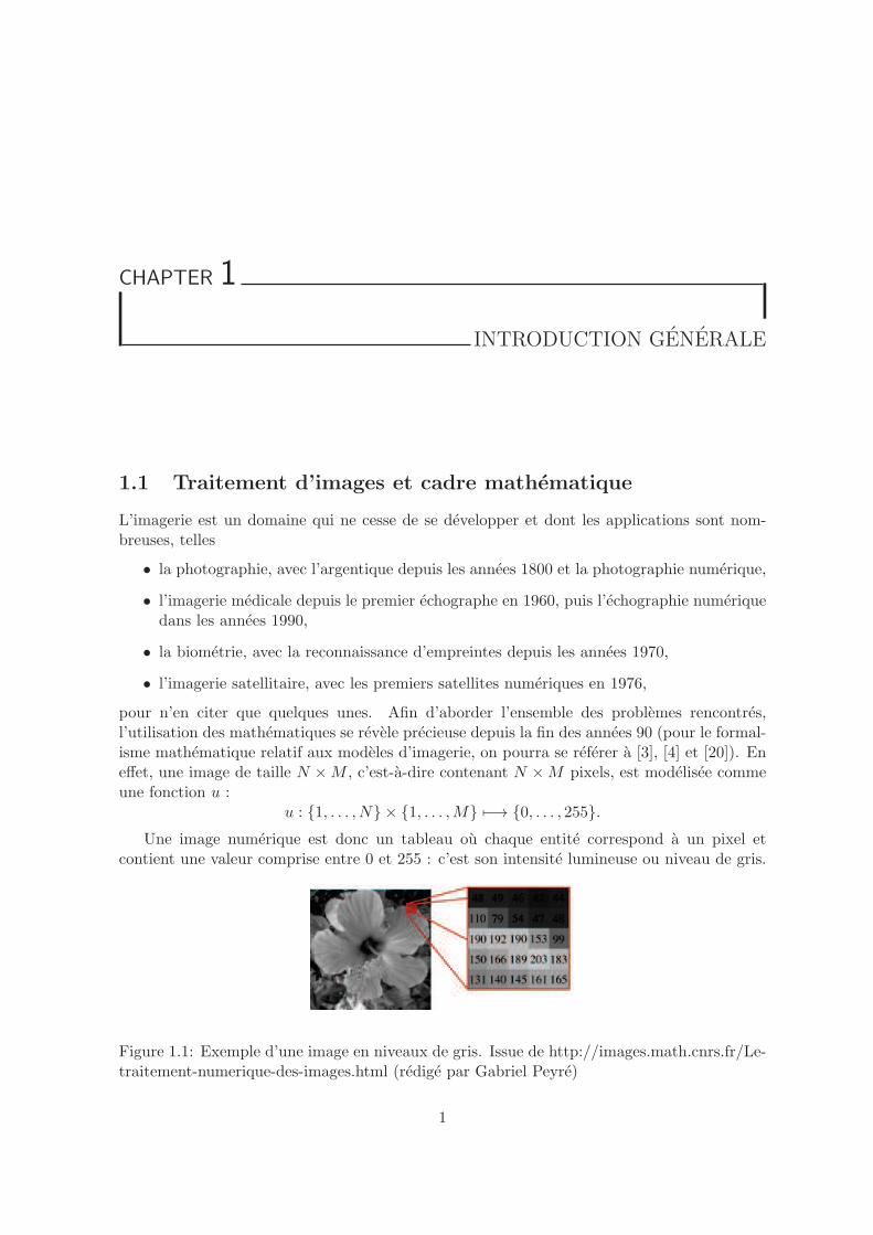
pour n’en citer que quelques unes. Afin d’aborder l’ensemble des problemes rencontres,l’utilisation des mathematiques se revele precieuse depuis la fin des annees 90 (pour le formal-isme mathematique relatif aux modeles d’imagerie, on pourra se referer a [3], [4] et [20]). Eneffet, une image de taille N ×M , c’est-a-dire contenant N ×M pixels, est modelisee commeune fonction u :
u : 1, . . . , N × 1, . . . ,M 7−→ 0, . . . , 255.Une image numerique est donc un tableau ou chaque entite correspond a un pixel et
contient une valeur comprise entre 0 et 255 : c’est son intensite lumineuse ou niveau de gris.
Figure 1.1: Exemple d’une image en niveaux de gris. Issue de http://images.math.cnrs.fr/Le-traitement-numerique-des-images.html (redige par Gabriel Peyre)
1
2 CHAPTER 1. INTRODUCTION GENERALE
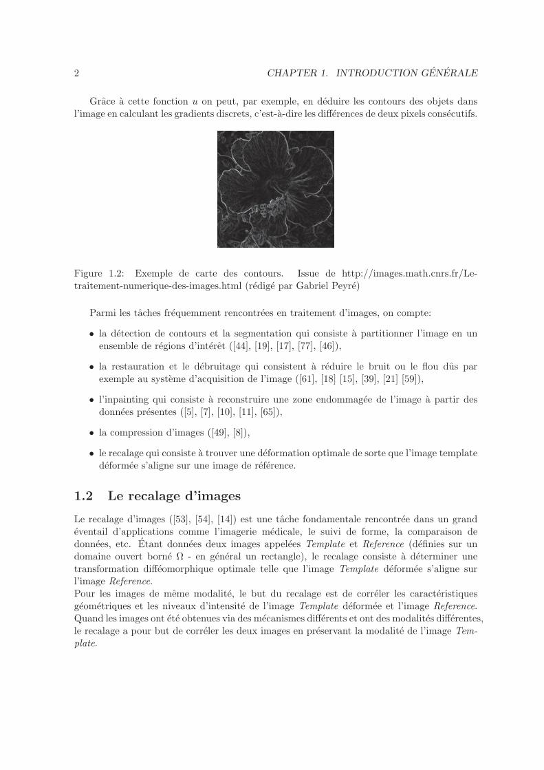
Grace a cette fonction u on peut, par exemple, en deduire les contours des objets dansl’image en calculant les gradients discrets, c’est-a-dire les differences de deux pixels consecutifs.
Figure 1.2: Exemple de carte des contours. Issue de http://images.math.cnrs.fr/Le-traitement-numerique-des-images.html (redige par Gabriel Peyre)
Parmi les taches frequemment rencontrees en traitement d’images, on compte:
• la detection de contours et la segmentation qui consiste a partitionner l’image en unensemble de regions d’interet ([44], [19], [17], [77], [46]),
• la restauration et le debruitage qui consistent a reduire le bruit ou le flou dus parexemple au systeme d’acquisition de l’image ([61], [18] [15], [39], [21] [59]),
• l’inpainting qui consiste a reconstruire une zone endommagee de l’image a partir desdonnees presentes ([5], [7], [10], [11], [65]),
• la compression d’images ([49], [8]),
• le recalage qui consiste a trouver une deformation optimale de sorte que l’image templatedeformee s’aligne sur une image de reference.
1.2 Le recalage d’images
Le recalage d’images ([53], [54], [14]) est une tache fondamentale rencontree dans un grandeventail d’applications comme l’imagerie medicale, le suivi de forme, la comparaison dedonnees, etc. Etant donnees deux images appelees Template et Reference (definies sur undomaine ouvert borne Ω - en general un rectangle), le recalage consiste a determiner unetransformation diffeomorphique optimale telle que l’image Template deformee s’aligne surl’image Reference.Pour les images de meme modalite, le but du recalage est de correler les caracteristiquesgeometriques et les niveaux d’intensite de l’image Template deformee et l’image Reference.Quand les images ont ete obtenues via des mecanismes differents et ont des modalites differentes,le recalage a pour but de correler les deux images en preservant la modalite de l’image Tem-plate.
1.2. LE RECALAGE D’IMAGES 3
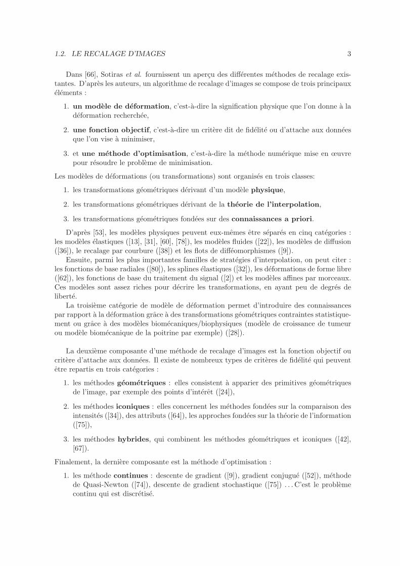
Dans [66], Sotiras et al. fournissent un apercu des differentes methodes de recalage exis-tantes. D’apres les auteurs, un algorithme de recalage d’images se compose de trois principauxelements :
1. un modele de deformation, c’est-a-dire la signification physique que l’on donne a ladeformation recherchee,
2. une fonction objectif, c’est-a-dire un critere dit de fidelite ou d’attache aux donneesque l’on vise a minimiser,
3. et une methode d’optimisation, c’est-a-dire la methode numerique mise en œuvrepour resoudre le probleme de minimisation.
Les modeles de deformations (ou transformations) sont organises en trois classes:
1. les transformations geometriques derivant d’un modele physique,
2. les transformations geometriques derivant de la theorie de l’interpolation,
3. les transformations geometriques fondees sur des connaissances a priori.
D’apres [53], les modeles physiques peuvent eux-memes etre separes en cinq categories :les modeles elastiques ([13], [31], [60], [78]), les modeles fluides ([22]), les modeles de diffusion([36]), le recalage par courbure ([38]) et les flots de diffeomorphismes ([9]).
Ensuite, parmi les plus importantes familles de strategies d’interpolation, on peut citer :les fonctions de base radiales ([80]), les splines elastiques ([32]), les deformations de forme libre([62]), les fonctions de base du traitement du signal ([2]) et les modeles affines par morceaux.Ces modeles sont assez riches pour decrire les transformations, en ayant peu de degres deliberte.
La troisieme categorie de modele de deformation permet d’introduire des connaissancespar rapport a la deformation grace a des transformations geometriques contraintes statistique-ment ou grace a des modeles biomecaniques/biophysiques (modele de croissance de tumeurou modele biomecanique de la poitrine par exemple) ([28]).
La deuxieme composante d’une methode de recalage d’images est la fonction objectif oucritere d’attache aux donnees. Il existe de nombreux types de criteres de fidelite qui peuventetre repartis en trois categories :
1. les methodes geometriques : elles consistent a apparier des primitives geometriquesde l’image, par exemple des points d’interet ([24]),
2. les methodes iconiques : elles concernent les methodes fondees sur la comparaison desintensites ([34]), des attributs ([64]), les approches fondees sur la theorie de l’information([75]),
3. les methodes hybrides, qui combinent les methodes geometriques et iconiques ([42],[67]).
Finalement, la derniere composante est la methode d’optimisation :
1. les methode continues : descente de gradient ([9]), gradient conjugue ([52]), methodede Quasi-Newton ([74]), descente de gradient stochastique ([75]) . . . C’est le problemecontinu qui est discretise.
4 CHAPTER 1. INTRODUCTION GENERALE
2. les methodes discretes : methodes fondees sur la theorie des graphes ([68]), beliefpropagation, methodes de programmation lineaire,
3. les algorithmes gloutons et evolutionnistes.
Dans [54], Modersitzki fournit egalement un apercu des methodes de recalage parametriqueset non parametriques (incluant les methodes geometriques avec appariement de points d’interet,les methodes iconiques avec la dissimilarite fondee sur la norme L2 par exemple, les modelesd’elasticite lineaire, la diffusion lineaire, les modeles fluides, . . . ).
Dans le cas des methodes parametriques, un ensemble de caracteristiques de l’image Tem-plate est defini et le but est de trouver une deformation appariant ces caracteristiques avecleur homologue dans l’image Reference. De plus, l’ensemble des transformations admissiblesest restreint a une certaine classe d’applications (applications polynomiales, splines, etc. . . )en exprimant la transformation a l’aide de fonctions de base.
Dans le cas des methodes non parametriques (notre cadre), la transformation n’est pasrestreinte a un ensemble parametrisable et le probleme est formule en termes de minimi-sation de fonctionnelle (avec le champ de deformation inconnu ϕ) comprenant un criterede mesure de distance et un regularisateur portant sur le champ de deformation afin que leprobleme soit bien pose. Le plus souvent, des arguments physiques motivent la construction duregularisateur. Des regularisateurs classiques comme ceux fondes sur la theorie de l’elasticitelineaire ne sont pas adaptes a des problemes impliquant de grandes deformations (notre casd’etude) puisqu’ils supposent de petites deformations et la validite de la loi de Hooke. Cette loide comportement enoncee par Robert Hooke en les termes latins ”ut tensio sic vis” traduit larelation de proportionnalite entre la force exercee sur un solide et l’allongement qui en resulte.
Dans la suite, les problematiques relatives a la mise en œuvre pratique des methodes derecalage sont examinees, la question de l’interpolation des images (en effet, si ϕ designe ladeformation recherchee, il nous faut evaluer T ϕ), la conception du critere d’attache auxdonnees (les criteres classiques et les criteres plus evolues fondes sur des modeles combinesde segmentation et recalage) et la construction de regularisateur portant sur la deformation.
1.2.1 Interpolation et approximation des images
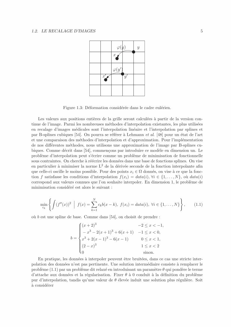
Au cours de l’algorithme mis en œuvre dans le cadre du recalage, il faut calculer l’imagedeformee T ϕ. Un point y ∈ Ω fixe de l’image Template deformee (de coordonnees entieres enpratique) est lie au point x = ϕ(y) (de coordonnees non necessairement entieres) et l’intensitelumineuse de l’image deformee en y, T = T ϕ(y) est donnee par : T ϕ(y) = T (x). Le pointx n’etant pas necessairement situe a un nœud de la grille discrete, il est alors necessaire demettre en œuvre une methode d’interpolation (on pourra se referer a [40] pour plus de detailssur les cadres eulerien et lagrangien).
1.2. LE RECALAGE D’IMAGES 5
ϕ(y′)
ϕ(y) y
x
x′
y′
Figure 1.3: Deformation consideree dans le cadre eulerien.
Les valeurs aux positions entieres de la grille seront calculees a partir de la version con-tinue de l’image. Parmi les nombreuses methodes d’interpolation existantes, les plus utiliseesen recalage d’images medicales sont l’interpolation lineaire et l’interpolation par splines etpar B-splines cubiques [54]. On pourra se referer a Lehmann et al. [48] pour un etat de l’artet une comparaison des methodes d’interpolation et d’approximation. Pour l’implementationde nos differentes methodes, nous utilisons une approximation de l’image par B-splines cu-biques. Comme decrit dans [54], commencons par introduire ce modele en dimension un. Leprobleme d’interpolation peut s’ecrire comme un probleme de minimisation de fonctionnellesous contraintes. On cherche a reecrire les donnees dans une base de fonctions splines. On viseen particulier a minimiser la norme L2 de la derivee seconde de la fonction interpolante afinque celle-ci oscille le moins possible. Pour des points xi ∈ Ω donnes, on vise a ce que la fonc-tion f satisfasse les conditions d’interpolation f(xi) = data(i), ∀i ∈ 1, . . . , N, ou data(i)correspond aux valeurs connues que l’on souhaite interpoler. En dimension 1, le probleme deminimisation considere est alors le suivant :
minck
∫(f ′′(x))2
∣∣∣ f(x) =N∑
k=1
ckb(x− k), f(xi) = data(i), ∀i ∈ 1, . . . , N, (1.1)
ou b est une spline de base. Comme dans [54], on choisit de prendre :
b =
(x+ 2)3 −2 ≤ x < −1,
− x3 − 2(x+ 1)3 + 6(x+ 1) −1 ≤ x < 0,
x3 + 2(x− 1)3 − 6(x− 1) 0 ≤ x < 1,
(2− x)3 1 ≤ x < 2
0 sinon.
En pratique, les donnees a interpoler peuvent etre bruitees, dans ce cas une stricte inter-polation des donnees n’est pas pertinente. Une solution intermediaire consiste a remplacer leprobleme (1.1) par un probleme dit relaxe en introduisant un parametre θ qui pondere le termed’attache aux donnees et la regularisation. Fixer θ a 0 conduit a la definition du problemepur d’interpolation, tandis qu’une valeur de θ elevee induit une solution plus reguliere. Soita considerer
6 CHAPTER 1. INTRODUCTION GENERALE
minck
‖f − data‖2
RN + θ
∫
Ω(f ′′)2
∣∣∣ f(x) =N∑
k=1
ckb(x− k)
(1.2)
ou ‖f − data‖2RN =
N∑
i=1
(f(xi)− data(i))2.
La resolution de ce probleme conduit a resoudre un systeme lineaire que l’on peut ecrire sousla forme suivante :
(BTB + θM)c = BT data
avec B =(bk(xi) = b(xi − k)
)1≤i≤N1≤k≤N
, c =(ck)1≤k≤N et Mjk =
∫Ω(bj)
′′(bk)′′dx.
Une approche plus generale consiste a remplacerM par une matrice arbitraire symetriquesemi-definie positiveW . Le choixW =M est theoriquement bien justifie puisque l’optimisationest realisee dans l’espace de splines. Cependant, d’autres regularisations sont possibles :W = I appelee regularisation de Tychonoff ou W = DTD appelee regularisation de Ty-
chonoff–Phillips avec D =
−1 1
. . .. . .
−1 1
∈ R
N−1,N .
Pour des images en dimension deux, l’interpolation bicubique est utilisee et l’extension aucas bidimensionnel est immediat. La formulation matricielle du probleme permet de simplifierles ecritures. Pour d’avantage de details, on renvoie le lecteur a l’ouvrage [54], Chapitre 3,section 3.6.1.
1.2.2 La mesure de similarite
Comparaison des intensites
La norme L2 (ou SSD pour Sum of Squared Distance) correspond a la somme des erreurs aucarre pixel par pixel. On la calcule grace a la formule suivante :
DSSD(R, T ϕ) = 1
2‖R− T ϕ‖2L2(Ω) =
1
2
∫
Ω(R(x)− T ϕ(x))2 dx,
ou R correspond a l’image Reference et T ϕ correspond a l’image Template deformee.Ce critere est le critere le plus utilise pour recaler des images de meme modalite bien qu’ilsoit assez sensible aux valeurs aberrantes.
Coefficient de correlation lineaire
Il est parfois necessaire de remettre a l’echelle les valeurs des images considerees, par exem-ple dans le cas ou elles ont ete obtenues par des instruments de mesure differents. Cetteremise a l’echelle se fait au moyen d’une relation affine entre les intensites des deux images.Pour evaluer l’existence de cette relation affine entre deux images, on utilise le coefficient decorrelation lineaire :
σ2(R, T ϕ) = cov(R, T ϕ)var(R)var(T ϕ) ,
ou var et cov representent respectivement la variance et la covariance des intensites. Si lecoefficient de correlation est nul, cela signifie qu’il n’existe pas de relation affine entre les deux
1.2. LE RECALAGE D’IMAGES 7
images et donc que les deux images sont des realisations aleatoires non correlees. Le but estalors de determiner ϕ maximisant ce terme.
Information mutuelle
L’information mutuelle est un critere qui provient de la theorie de l’information et quis’applique couramment au recalage multi-modal (dans le cas ou les images sont de modalitesdifferentes) depuis 1995 (Wells [75], Collignon [29]).Ce critere est utilise pour le recalage multi-modal puisqu’il ne necessite aucune connaissancea priori sur les intensites et il ne suppose pas de relation affine entre les images. L’idee est demaximiser l’information mutuelle des images par rapport a la transformation.
Definition 1.2.1
Soit q ∈ N et ρ une densite sur Rq, ie, ρ : Rq → R, ρ(x) ≥ 0,
∫
Rq
ρ(x)dx = 1.
L’entropie (differentielle) de la densite est definie par
H(ρ) = −Eρ[log ρ] = −∫
Rq
ρ log ρ dx
L’entropie se mesure donc a partir de l’histogramme des niveaux de gris. Si l’image est larealisation d’une variable aleatoire ne privilegiant aucune valeur de pixel alors l’histogrammede l’amplitude sera relativement plat et l’entropie maximale.L’information mutuelle est alors definie par :
MI(R, T ) = H(ρR) +H(ρT )−H(ρR,T )
ou ρR, ρT et ρR,T representent les densites des niveaux de gris de R, T et la densite conjointedes niveaux de gris. L’information mutuelle correspond alors a la reduction d’entropie ap-portee par leur apparitions communes.En imagerie medicale, l’information mutuelle est un critere particulierement adapte auximages n’ayant pas les memes modalites. Cependant, cette mesure possede certains in-convenients : elle est couteuse en temps de calcul, elle est non convexe et possede un nombreimportant de minima locaux. Sa complexite en termes de cout de calcul vient du fait quel’information mutuelle necessite d’evaluer les probabilites conjointes pour chaque niveau degris sur l’ensemble de l’image. Mais malgre ces limites, elle reste tres utilisee pour le recalagemulti-modal.
Champ de gradients
Il est aussi possible de comparer les champs de gradients des deux images. C’est ce qui a etefait par Haber et Modersitzki ([41]) et par Droske et Rumpf ([35]). Dans [41], Haber et al.utilisent les champs de gradients pour comparer deux images, en s’appuyant sur l’idee quedeux images sont similaires si les changements d’intensite ont lieu a la meme position. Pourcela, ils apparient les champs de gradients normalises des deux images.
Le champ de gradients normalises est defini comme suit :
nε(I, x) =∇I(x)√
∇I(x)T∇I(x) + ε2,
8 CHAPTER 1. INTRODUCTION GENERALE
avec ε une constante strictement positive. La mesure de similarite entre les deux images estalors evaluee comme suit :
Dc(T,R) =1
2
∫
Ω‖nε(R, x)× nε(T ϕ, x)‖2dx,
ou × represente le produit vectoriel.
Lignes de niveau
Dans [35], Droske et Rumpf proposent un critere fonde sur la notion de morphologie mathematique([63]). La morphologie mathematique d’une image est definie comme la collection des courbesde niveau :
M [I] =MI
c
∣∣∣ c ∈ R
, MI
c =x ∈ Ω
∣∣∣ I(x) = c.
On peut definir de maniere equivalente le vecteur normal a une courbe de niveauquelconque :
NI : Ω −→ Rd; x 7−→ ∇I
‖∇I‖ .
On cherche alors une deformation telle que M [T ϕ] = M [R]. Cette mesure a l’avantaged’etre invariante par une reparametrisation des niveaux de gris, ce qui la rend adaptee aurecalage multi-modal.
Modeles conjoints de segmentation et de recalage
Le recalage d’images peut egalement etre realise simultanement avec la segmentation. Yezziet al. [79] proposent une approche variationnelle conjointe de segmentation et de recalage.Les deux images Template et Reference sont supposees contenir un objet commun visualiseavant et apres avoir ete soumis a une deformation que l’on cherche a apparier et a segmenter.L’objectif est de definir une courbe fermee C capturant les bords de l’objet dans l’image Ref-erence et une courbe C capturant son homologue dans l’image Template, telles que C = g(C),ou g est un element d’un groupe de dimension finie par exemple l’ensemble des deformationsrigides. Il y a alors deux inconnues : la courbe C et la deformation g.Les auteurs formulent le probleme comme la minimisation d’une fonctionnelle d’energie dontla construction est fondee sur le modele des contours actifs sans bord de Chan et Vese [19] :
E(g, C) = E1(C) + E2(g(C))
=
∫
Cin(R− u)2dx+
∫
Cout(R− v)2dx+
∫
Cin(T − u)2dx+
∫
Cout(T − v)2dx,
=
∫
Cinfindx+
∫
Coutfoutdx+
∫
Cinfindx+
∫
Coutfoutdx,
avec Cin et Cout les regions a l’interieur et a l’exterieur de C, u et v la moyenne des valeursde R dans Cin et Cout, Cin et Cout les regions a l’interieur et a l’exterieur de C, et u et v lamoyenne des valeurs de T dans Cin et Cout.Comme C = g(C), on peut reecrire la fonctionnelle de la facon suivante, en exprimant lesintegrales seulement sur l’ouvert Ω sur lequel est defini l’image Reference R :
E(g, C) =∫
Cin(fin(x) + fin(g(x))|g′(x)|)dx+
∫
Cout(fout(x) + fout(g(x))|g′(x)|)dx.
1.2. LE RECALAGE D’IMAGES 9
Ce modele a ete etendu aux deformations non rigides dans [70], [73] et [76].
Dans [71], [72], Vemuri et al. proposent un modele d’equations aux derivees partielles pourrealiser conjointement la segmentation et le recalage. Dans la premiere EDP, les level sets del’image source evoluent selon leur normale avec une vitesse definie comme la difference entrel’image cible et l’image source deformee. La deuxieme EDP permet de retrouver explicitementle champ de vecteurs deplacement. Le modele est fonde sur la minimisation de la fonctionnellesuivante inspiree du modele de segmentation propose par Chan et Vese dans [19] et integrantun a priori de forme :
E(φ, u+, u−, µ,R, T ) =α
∫
Ω|u+ − I|2H(φ)dx+ α
∫
Ω|u− − I|2(1−H(φ))dx
+ β
∫
Ω|∇u+|2H(φ)dx+ β
∫
Ω|∇u−|2(1−H(φ))dx
+
∫
Ωd2(µRx+ T )δ(φ)|∇φ|dx,
ou I est l’image a segmenter, φ la fonction level set inconnue, d la fonction distance a un apriori de forme, µ un parametre d’echelle, R et T une matrice de rotation et un vecteur detranslation.
Dans [50], Lord et al. traitent le probleme de quantification de la difference de deuxformes. Leur travail s’inscrit dans le contexte de l’analyse de forme de l’hippocampe et estmotive par le fait que la classification de maladies est facilitee par la comparaison d’asymetries.Pour effectuer ces analyses comparatives, les auteurs proposent une methode traitant simul-tanement le processus de segmentation et de recalage en introduisant deux inconnues : lechamp de deformation et la courbe realisant la segmentation. La segmentation est guideepar la deformation, et le critere d’attache aux donnees, contrairement aux methodes clas-siques de recalage, s’appuie sur la comparaison des structures metriques des deux surfaces etplus precisement sur la minimisation de la deviation par rapport a une isometrie. Le critered’attache aux donnees est base sur la comparaison des structures metriques des surfaces, plusprecisement sur leur premiere forme fondamentale (FFF) et sur une contrainte d’homogeneitede type Chan-Vese.
Dans [47], Le Guyader et Vese proposent un modele de recalage et de segmentation si-multanes. Les auteurs proposent de joindre le modele des contours actifs sans bord de Chanet Vese [19] a un recalage d’images dont le terme de regularisation est fonde sur la theoriede l’elasticite non lineaire. Les formes a apparier sont assimilees a des materiaux homogenes,isotropes, hyperelastiques de type Ciarlet-Geymonat. Le probleme est formule comme la min-imisation d’une fonctionnelle composee d’un terme lie a la segmentation et d’un second termelie au modele de deformation :
E(c1, c2, u) =Ed(c1, c2, u) + Ereg(u),
=ν1
∫
Ω|R(x)− c1|2H(Φ0(x− u(x)))dx
+ ν2
∫
Ω|R(x)− c2|2 (1−H(Φ0(x− u(x)))) dx+ Ereg(u),
10 CHAPTER 1. INTRODUCTION GENERALE
ou Φ0 est une level set fixee dont le niveau zero est une courbe segmentant l’image TemplateT , c1 et c2 sont respectivement la moyenne des niveaux de gris a l’interieur et a l’exterieur dela courbe, u = ϕ− Id est le vecteur deplacement.
1.2.3 Le modele de deformation
Le modele de deformation ou regularisateur est generalement motive par des argumentsphysiques et definit l’espace fonctionnel dans lequel evolue la deformation ϕ.
Modele elastique lineaire
Le modele elastique a ete introduit par Broit [13], puis developpe par Bajcsy [6]. Les imagessont apprehendees comme les observations d’un meme corps elastique, l’une avant et l’autreapres avoir ete soumis a une deformation. Le terme de regularisation est le potentiel elastiquelineaire du deplacement u:
P(u) =
∫
Ω
µ
4
d∑
j,k=1
(∂xjuk + ∂xkuj)2 +
λ
2(div u)2dx,
ou µ et λ sont les constantes de Lame. L’utilisation de l’elasticite lineaire presente deuxinconvenients : la topologie n’est pas necessairement preservee, et le modele est restreint aucas de petites deformations.
Modele fluide
Dans [22], Christensen et al. proposent un modele fluide visqueux sous forme non vari-ationnelle. Les objets a apparier sont assimiles a des fluides evoluant selon les equationsde Navier-Stokes. Si le modele elastique est caracterise par une regularisation spatiale dudeplacement, le modele fluide, lui, est caracterise par une regularisation de la vitesse :
µ∆v + (λ+ µ) div v + F = 0,
avec v = ∂tu et F , la mesure de similarite choisie. Avec le temps, u = ϕ − Id devientstationnaire et de larges deformations sont theoriquement possibles.
Modele de diffusion
Dans [69], Thirion et al. proposent d’assimiler le recalage non rigide a un modele de diffusionqui est un cas particulier des methodes de flot optique utilisees en traitement d’images pourevaluer le mouvement. Il introduit de nouvelles entites appelees demons qui sont en fait deseffecteurs poussant localement l’image. Les contours des objets presents dans l’image sontapprehendes comme des membranes semi-permeables pouvant se mouvoir sous l’action dedemons. Cet algorithme montre des resultats tres satisfaisants avec des temps de calcul reduitset il permet d’avoir de larges deformations. Cependant, le comportement de cet algorithmen’est pas encore bien compris (voir [58] et [37] pour plus de details). Dans [37], Fischer etModersitzki introduisent un nouveau modele de diffusion dans lequel le regularisateur s’ecrit:
S[u] = 1
2
d∑
l=1
∫
Ω‖∇ul‖2dx.
1.2. LE RECALAGE D’IMAGES 11
Dans cette methode aussi, les transformations sont restreintes a de petites deformations,mais le modele peut etre combine avec l’idee precedente de fluide pour generer de plus largesdeformations.
Modele par courbure
Dans [38], Fischer et Modersitzki introduisent un modele de recalage fonde sur la courbure.Le regularisateur est defini par :
S[u] = 1
2
d∑
l=1
∫
Ω(∆ul)
2 dx,
(∆ul)2 pouvant etre apprehende comme une approximation de la courbure. Ainsi l’idee du
regularisateur est de minimiser la courbure des composantes de la deformation.Encore une fois, les transformations sont restreintes a de petites deformations, et ce modelepeut etre combine avec l’idee precedente de fluide pour generer de plus larges deformations.
Modeles elastiques non lineaires
Afin d’obtenir de larges deformations, l’utilisation de l’elasticite non lineaire se revele necessaire(voir [27] et [26] pour plus de details). En effet, la theorie de l’elasticite lineaire n’est pasadaptee a des problemes impliquant de grandes deformations puisque cette theorie suppose depetites deformations et la validite de la loi de Hooke. On peut remarquer que le caoutchouc,les tissus biologiques, les elastomeres sont frequemment modelises par des materiaux hy-perelastiques. En elasticite, on introduit souvent le tenseur de deformation de Green-SaintVenant :
E(u) =1
2(∇u+∇uT ) + 1
2∇uT∇u,
qui constitue une mesure de la deviation de la deformation associee ϕ = Id+u par rapport aune deformation rigide. La partie lineaire du tenseur de Green-Saint Venant :
e(u) =1
2(∇u+∇uT ),
est ce que l’on appelle le tenseur de deformation linearise que l’on retrouve dans le cadre dela theorie de l’elasticite lineaire.
Dans le cadre du recalage d’images fonde sur des principes d’elasticite non lineaire, Droskeet Rumpf [35] traitent le probleme du recalage non rigide d’images multi-modales. Le criterede similarite inclut les derivees du premier ordre de la deformation et est complete par uneregularisation elastique non lineaire basee sur une densite d’energie polyconvexe. Dans [47],Le Guyader et Vese introduisent un modele couple de segmentation et recalage dans lequelles objets a apparier sont assimiles a des materiaux de type Ciarlet-Geymonat. On peutegalement mentionner [51] et [9] pour une methode variationnelle de recalage dans le casde grandes deformations (Large Deformation Diffeomorphic Metric Mapping - LDDMM),ainsi que [60] qui presente egalement une methode utilisant une regularisation elastique nonlineaire.
Plus recemment, dans [16], les auteurs construisent une densite d’energie hyperelastiquepenalisant les variations de longueur et d’aire, et ajoutent une penalisation sur le jacobien dela deformation de telle sorte que l’energie tende vers l’infini quand le jacobien tend vers zero.
12 CHAPTER 1. INTRODUCTION GENERALE
1.2.4 La preservation de la topologie
Il est egalement possible d’ajouter certaines contraintes sur la deformation recherchee. Une desplus importantes proprietes qu’un algorithme de recalage doit satisfaire est la preservation dela topologie ou de l’orientation. La preservation de la topologie est equivalente a l’inversibilitedu champ de deformation. Le jacobien de la deformation contient l’information concernantles proprietes locales du champ de deformation. En effet, si le jacobien de la deformationdevient negatif alors la deformation perd son caractere injectif et cela traduit physiquementune interpenetration de la matiere.
Afin d’eviter des singularites dans le champ de deformation, Christensen et al. [22] pro-posent de controler les valeurs du jacobien au fur et a mesure de l’algorithme. Lorsquesa valeur est inferieure a un seuil predefini, une image deformee intermediaire est creee etl’algorithme de recalage est reinitialise.Une autre facon de preserver la topologie est d’inclure des contraintes, c’est-a-dire d’ajouterdans la fonction objectif un terme controlant le jacobien. Dans [23], Christensen and Johnsonajoutent un terme a la fonction objectif qui penalise les petites et les grandes valeurs dujacobien.
1.3. CONTRIBUTION 13
1.3 Contribution
Cette these se divise en trois parties dont les resultats ont ete exposes dans les articles [56],[57] et [55].Dans [56], on s’interesse a la construction d’une methode de correction du champ de deformationassocie a un algorithme de recalage d’images afin que celui-ci preserve la topologie ou l’orientation.La violation de cette contrainte de preservation de la topologie se manifeste, numeriquement,par la presence de chevauchements ou de plis sur la grille de deformation (cf Figure 3.1 page42). La methode se compose de deux etapes : la premiere consiste a detecter et corriger leszones ou le jacobien discret est negatif. La deuxieme consiste a reconstruire la deformation apartir des valeurs de ses gradients discrets. Le probleme est formule comme la minimisationd’une fonctionnelle sous contraintes de type interpolation de Lagrange.Dans [57], on introduit un modele conjoint de segmentation et de recalage fonde sur l’elasticitenon lineaire. On construit une mesure de similarite basee sur la variation totale ponderee et unregularisateur faisant intervenir la densite d’energie d’un materiau de Saint Venant-Kirchhoff.Le fait d’ajouter le terme de variation totale ponderee permet d’aligner les bords des objetsmeme si les modalites sont differentes.Dans [55], on construit egalement un modele conjoint de segmentation et de recalage. Danscette partie, les objets a apparier sont modelises par des fonctions level sets et evoluent defacon a minimiser une fonctionnelle contenant un regularisateur fonde sur l’elasticite nonlineaire et un critere de similarite base sur des resultats intermediaires de segmentation.
Dans ce qui suit, on donne un resume de chacune de ces contributions qui seront developpeesrespectivement dans les chapitres 3, 4 et 5.
1.3.1 Preservation de la topologie du champ de deformation associe au
recalage d’images
Cette methode visant a obtenir un champ de deformation preservant la topologie se divise endeux etapes : la premiere consiste a localiser les chevauchements de la grille de deformation eta appliquer un parametre de correction aux jacobiens discrets de la deformation. La deuxiemeetape consiste a reconstruire la deformation a partir des gradients discrets corriges.
Correction du jacobien
La premiere etape est fondee sur cette proposition de Karacali et Davatzikos :
Proposition 1.3.1 (De Karacali et Davatzikos [43])
Soit C la classe de deformations h = (f, g) definies sur un rectangle discret Ω = [0, 1, . . . ,M1]×[0, 1, . . . , N1] ⊂ N
2 pour lesquelles Jff , Jfb, Jbf , Jbb sont positifs pour tout (x, y) ∈ Ω.Soit h = (f, g) une deformation appartenant a C. Alors son equivalent continu determinepar l’interpolation de h sur le domaine ΩC = [0,M1]×[0, N1] ⊂ R
2 en utilisant l’interpolantΦ donne par Φ(x, y) = Ψ(x)Ψ(y) avec
Ψ :
1 + t si − 1 ≤ t ≤ 01− t si 0 ≤ t ≤ 10 sinon
preserve la topologie avec le schema backward et forward de differences finies fbx, ffx , fby, f
fy
14 CHAPTER 1. INTRODUCTION GENERALE
pour approximer les derivees partielles de f (de meme pour g) et :
Jff = ffx (p1)gfy (p1)− ffy (p1)g
fx(p1)
Jbf = fbx(p2)gfy (p2)− ffy (p2)g
bx(p2)
Jfb = ffx (p3)gby(p3)− fby(p3)g
fx(p3)
Jbb = fbx(p4)gby(p4)− fby(p4)g
bx(p4).
On rappelle :
ffx (x, y) = f(x+ 1, y)− f(x, y)
fbx(x, y) = f(x, y)− f(x− 1, y)
ffy (x, y) = f(x, y + 1)− f(x, y)
fby(x, y) = f(x, y)− f(x, y − 1).
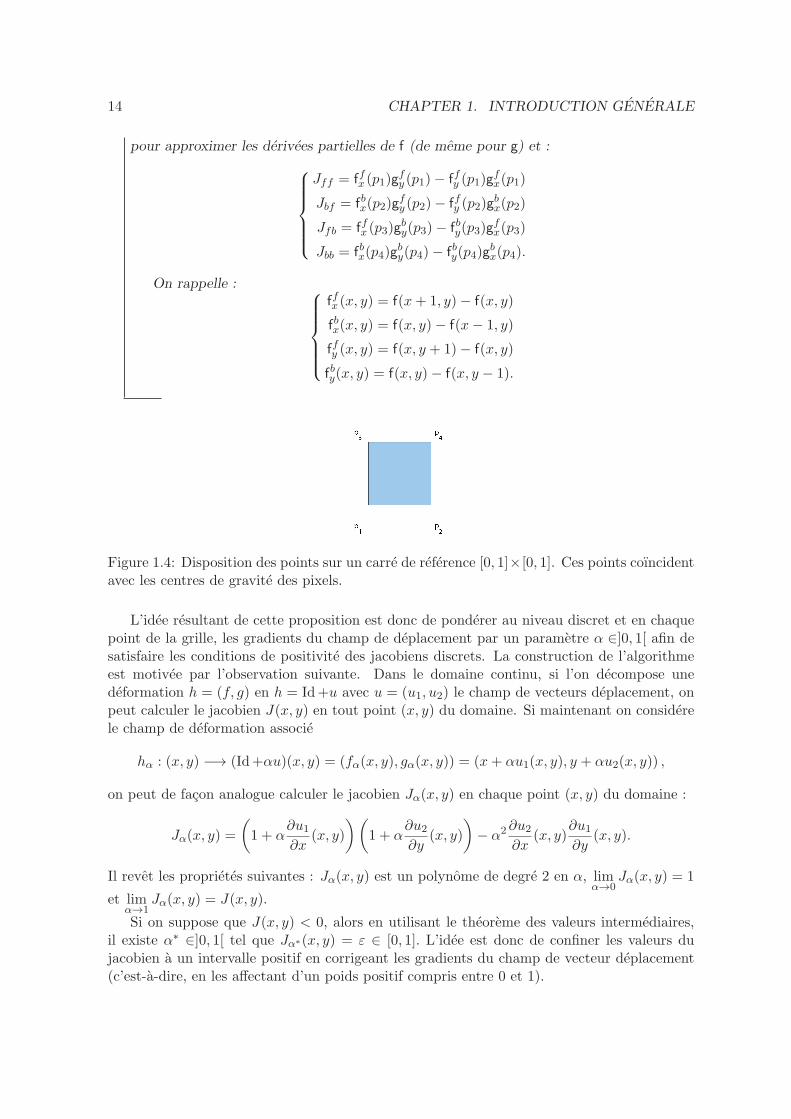
Figure 1.4: Disposition des points sur un carre de reference [0, 1]×[0, 1]. Ces points coıncidentavec les centres de gravite des pixels.
L’idee resultant de cette proposition est donc de ponderer au niveau discret et en chaquepoint de la grille, les gradients du champ de deplacement par un parametre α ∈]0, 1[ afin desatisfaire les conditions de positivite des jacobiens discrets. La construction de l’algorithmeest motivee par l’observation suivante. Dans le domaine continu, si l’on decompose unedeformation h = (f, g) en h = Id+u avec u = (u1, u2) le champ de vecteurs deplacement, onpeut calculer le jacobien J(x, y) en tout point (x, y) du domaine. Si maintenant on considerele champ de deformation associe
hα : (x, y) −→ (Id+αu)(x, y) = (fα(x, y), gα(x, y)) = (x+ αu1(x, y), y + αu2(x, y)) ,
on peut de facon analogue calculer le jacobien Jα(x, y) en chaque point (x, y) du domaine :
Jα(x, y) =
(1 + α
∂u1∂x
(x, y)
)(1 + α
∂u2∂y
(x, y)
)− α2∂u2
∂x(x, y)
∂u1∂y
(x, y).
Il revet les proprietes suivantes : Jα(x, y) est un polynome de degre 2 en α, limα→0
Jα(x, y) = 1
et limα→1
Jα(x, y) = J(x, y).
Si on suppose que J(x, y) < 0, alors en utilisant le theoreme des valeurs intermediaires,il existe α∗ ∈]0, 1[ tel que Jα∗(x, y) = ε ∈ [0, 1]. L’idee est donc de confiner les valeurs dujacobien a un intervalle positif en corrigeant les gradients du champ de vecteur deplacement(c’est-a-dire, en les affectant d’un poids positif compris entre 0 et 1).
1.3. CONTRIBUTION 15
Grace a ce parametre α, on peut calculer les matrices jacobiennes corrigees (quand cela estnecessaire) en chaque point de la grille discrete. Le resultat de cette premiere etape del’algorithme est donc l’ensemble discret des matrices jacobiennes eventuellement corrigeesnotees ωi dans la suite.
Reconstruction de la deformation
Pour la seconde etape, on suppose que l’on a identifie (manuellement pour le moment) Nsous-espaces connexes non vides Ωi de Ω, i ∈ 1, . . . ,N sur lesquels la preservation del’orientation n’est pas satisfaite. Nous introduisons ensuite notre modele mathematique dereconstruction, valide pour chaque sous-domaine Ωi, i ∈ 1, . . . ,N. Une approche Dm-splineest retenue (voir [1] pour plus de details).
Soient A = aii=1,··· ,N un ensemble de N points de Ων contenant un sous-ensemble P1-unisolvant. Dans notre cas, l’ensemble A contient les coordonnees des pixels de l’image inclusdans Ων .Soient ωii=1,··· ,N l’ensemble des N matrices jacobiennes de la deformation donnees auxpoints aii=1,··· ,N . Cet ensemble contient les gradients corriges de la deformation obtenus al’etape de correction de l’algorithme.Enfin, soient bii=1,··· ,l l points de Ων ou les gradients sont restes inchanges. En pra-tique, ces points appartiennent a la frontiere du domaine Ων , ∂Ων . On fixe des contraintesd’interpolation de Lagrange en ces points. Cela signifie que si h represente la deformationnon alteree et v la deformation inconnue du probleme de minimisation, on doit avoir
∀i ∈ 1, . . . , l, v(bi) = h(bi).
Soit K l’ensemble defini par K = v ∈ H3(Ων ,R2), β(v) = η, avec β l’application :
β :
∣∣∣∣∣H3(Ων ,R
2) → R2l
v 7→ β(v) =(v(b1), · · · , v(bl)
)T
et η =(h(b1), · · · , h(bl)
)T.
On definit egalement :
ρ :
∣∣∣∣∣H2(Ων ,R
2×2) → (R2×2)N
v 7→ ρ(v) =(v(a1), v(a2), · · · , v(aN )
)T . (1.3)
Le probleme, formule au moyen de la fonctionnelle Jǫ (| · |3,Ων ,R2 designant la semi-norme surH3(Ων ,R
2)),
Jǫ :∣∣∣∣H3(Ων ,R
2) → R
v 7→ 〈ρ(Dv)− w〉2N + ǫ |v|23,Ων ,R2 ,
est defini par : Trouver σǫ ∈ K telle que
∀v ∈ K,Jǫ(σǫ) ≤ Jǫ(v).(1.4)
On peut egalement definir un probleme equivalent au moyen des multiplicateurs de Lagrange.Si σǫ est l’unique solution du probleme (1.4), on demontre que σǫ est aussi la solution du
16 CHAPTER 1. INTRODUCTION GENERALE
probleme suivant avec multiplicateurs de Lagrange :
Trouver (σǫ, λ) ∈ K × R
2l,
∀v ∈ H3(Ων ,R2), a(σǫ, v)− L(v) + 〈λ, β(v)〉2l = 0,
(1.5)
avec a la forme bilineaire symetrique definie par :
a :
∣∣∣∣H3(Ων ,R
2)×H3(Ων ,R2) → R
(u, v) 7→ 〈ρ(Du), ρ(Dv)〉N + ǫ (u, v)3,Ων ,R2 ,
et L la forme lineaire definie par :
L :
∣∣∣∣H3(Ων ,R
2) → R
v 7→ 〈ρ(Dv), ω〉N .
Il faut ensuite discretiser le probleme (1.5). Pour ce faire, nous utilisons la theorie deselements finis (voir [1] et [25]).
1.3.2 Modele conjoint de segmentation et recalage fonde sur la variation
totale ponderee et l’elasticite non lineaire
Dans cette methode, le modele de deformation choisi est un modele elastique non lineaire.Plus particulierement, les objets a apparier sont assimiles a des materiaux de type SaintVenant-Kirchhoff. On introduit egalement un terme d’attache aux donnees fonde sur la vari-ation totale ponderee afin d’apparier les bords des objets contenus dans les images.
On note ϕ : Ω → R2 la deformation recherchee, et T et R les images Template et Refer-
ence.La densite d’energie d’un materiau de type Saint Venant-Kirchhoff est definie par :
WSV K(F ) = W (E) =λ
2(trE)2 + µ trE2.
Pour s’assurer que le jacobien de la deformation ne presente pas de trop grandes expansionsou contractions, on ajoute a cette densite le terme µ (detF − 1)2 controlant que le jacobienreste proche de 1.Le terme de regularisation de notre fonctionnelle s’ecrit donc :
W (F ) =WSV K(F ) + µ (detF − 1)2.
De meme, le critere de similarite s’ecrit :
Wfid(ϕ) = varg T ϕ+ν
2
∫
Ω(T ϕ−R)2 dx, (1.6)
avec
varg(u) = sup
∫
Ωu div(ϕ) dx : |ϕ| ≤ g partout, ϕ ∈ Lip0(Ω,R
2)
<∞, (1.7)
1.3. CONTRIBUTION 17
g est une fonction edge detector et Lip0(Ω,R2) est l’espace des fonctions lipschitziennes a
support compact. Le probleme de minimisation (P ) s’ecrit :
infϕ∈Id+W1,4
0 (Ω,R2)
I(ϕ) = varg T ϕ+
∫
Ωf(x, ϕ(x),∇ϕ(x)) dx
= varg T ϕ+
∫
Ω
[ν2(T (ϕ)−R)2 +W (∇ϕ(x))
]dx
.
(P)
Cependant f n’est pas quasiconvexe (voir [30] Chapitre 9 pour plus de details sur cettenotion) ce qui pose un probleme de nature theorique puisqu’on ne peut etablir la semi-continuite inferieure faible de la fonctionnelle et subsequemment l’existence de minimiseurs.Pour pallier ce probleme, nous avons defini un probleme relaxe associe au probleme initial enremplacant f par son enveloppe quasiconvexe.
Cette enveloppe quasiconvexe Qf de f est definie par Qf(x, ϕ, ξ) =ν
2(T (ϕ)−R)2 +QW (ξ)
avec QW (ξ) =
W (ξ) si ‖ξ‖2 ≥ 2λ+ µ
λ+ 2µ,
Ψ(det ξ) si ‖ξ‖2 < 2λ+ µ
λ+ 2µ,
et Ψ, l’application convexe telle que Ψ : t 7→ −µ2t2 + µ (t− 1)2 +
µ(λ+ µ)
2(λ+ 2µ).
Le probleme relaxe (QP ) introduit est alors defini par :
inf
I(ϕ) = varg T ϕ+
∫
ΩQf(x, ϕ(x),∇ϕ(x)) dx
, (QP)
avec ϕ ∈ Id +W 1,40 (Ω,R2).
On peut, entre autres, etablir un resultat d’existence de minimiseurs de ce probleme relaxe,et avec une hypothese de convergence L1 supplementaire, on peut montrer que les solutionsdu probleme relaxe sont des solutions dites generalisees du probleme initial.
1.3.3 Modele conjoint de segmentation et recalage non local
Dans ce chapitre, on utilise le meme modele de deformation que dans le chapitre precedent, asavoir un modele elastique non lineaire. En ce qui concerne le terme d’attache aux donnees,sa construction est liee a une equation d’evolution issue d’un probleme de segmentation souscontraintes topologiques. Plus precisement, on definit Φ0 une fonction level set dont le niveauzero represente le bord des objets contenus dans l’image Template.On se propose d’etudier le probleme de minimisation suivant :
inf
I(ϕ) =
∫
Ωf(x, ϕ(x),∇ϕ(x)) dx : ϕ ∈ Id +W 1,4
0 (Ω,R2)
, (1.8)
18 CHAPTER 1. INTRODUCTION GENERALE
avec f(x, ϕ, ξ) =ν
2‖Φ0ϕ−Φ(·, T )‖2+QW (ξ), ou Φ est une solution de l’equation d’evolution
provenant du modele de segmentation preservant la topologie de Le Guyader et Vese ([46])
∂Φ
∂t= |∇Φ|
[div
(g(|∇R|) ∇Φ
|∇Φ|
)]+ 4
µ′
d2H(Φ(x) + l)H(l − Φ(x))
∫
Ω
[〈x− y,∇Φ(y)〉 e−‖x−y‖22/d2H(Φ(y) + l)H(l − Φ(y))
]dy ,
Φ(x, 0) = Φ0(x) ,
∂Φ
∂~ν= 0, on ∂Ω .
(E)
La fonction g est un fonction edge detector classique.On peut etablir un resultat d’existence de solutions pour ce probleme de minimisation.On etudie ensuite le caractere bien pose de Φ. Pour cela, le cadre de la theorie des solutions deviscosite est un cadre approprie du fait de la non linearite due au terme de courbure pondereeet de la singularite en ∇Φ = 0.
1.4 Organisation de la these
Dans le chapitre 2, nous presentons les outils mathematiques necessaires a l’introduction eta l’etude des modeles proposes. Ces rappels concernent les espaces fonctionnels de Lebesgueet de Sobolev, les fonctions a variation bornee, l’analyse convexe, ainsi que la theorie del’elasticite en suivant principalement [12], [30], [33] et [45].
Dans le chapitre 3, nous presentons la methode de correction de champ de deformationpreservant la topologie developpee dans [56].
Dans le chapitre 4, nous etudions un modele conjoint de segmentation et recalage fondesur la variation totale ponderee et sur l’elasticite non lineaire suivant [57].
Dans le chapitre 5, nous introduisons un modele conjoint de segmentation et recalage nonlocal avec une regularisation elastique non lineaire comme presente dans [55].
Les chapitres 6 et 7 constituent des pistes de recherche qui n’ont ete que partiellementabouties a ce jour et qui feront l’objet d’etudes ulterieures. Le chapitre 6 presente l’ajout decontraintes geometriques au critere de similarite L2 classique. Dans le chapitre 7, nous avonstente de construire un critere de similarite base sur la comparaison des gradients normalisesdes images en nous inspirant du modele d’inpainting introduit par Ballester et al. [7].
BIBLIOGRAPHY
[1] R. Arcangeli, M. C. Lopez de Silanes, and J. J. Torrens, Multidimensionalminimizing splines. Theory and applications, Grenoble Sciences, Kluwer Academic Pub-lishers, Boston, MA, 2004.
[2] J. Ashburner and K. J. Friston, Nonlinear spatial normalization using basis func-tions, Human brain mapping, 7 (1999), pp. 254–266.
[3] G. Aubert and P. Kornprobst, Mathematical problems in image processing, volume147 of applied mathematical sciences, 2002.
[4] , Mathematical problems in image processing: partial differential equations and thecalculus of variations, vol. 147, Springer Science & Business Media, 2006.
[5] J.-F. Aujol, S. Ladjal, and S. Masnou, Exemplar-based inpainting from a varia-tional point of view, SIAM Journal on Mathematical Analysis, 42 (2010), pp. 1246–1285.
[6] R. Bajcsy and S. Kovacic, Multiresolution elastic matching, Computer Vision, Graph-ics, and Image Processing, 46 (1989), pp. 1–21.
[7] C. Ballester, M. Bertalmio, V. Caselles, G. Sapiro, and J. Verdera, Filling-in by joint interpolation of vector fields and gray levels, Image Processing, IEEE Trans-actions on, 10 (2001), pp. 1200–1211.
[8] M. F. Barnsley and L. P. Hurd, Fractal image compression, AK Peters, Ldt., 1993.
[9] M. Beg, M. Miller, A. Trouve, and L. Younes, Computing Large DeformationMetric Mappings via Geodesic Flows of Diffeomorphisms, International Journal of Com-puter Vision, 61 (2005), pp. 139–157.
[10] M. Bertalmio, A. L. Bertozzi, and G. Sapiro, Navier-stokes, fluid dynamics, andimage and video inpainting, in Computer Vision and Pattern Recognition, 2001. CVPR2001. Proceedings of the 2001 IEEE Computer Society Conference on, vol. 1, IEEE, 2001,pp. I–355.
[11] M. Bertalmio, L. Vese, G. Sapiro, and S. Osher, Simultaneous structure andtexture image inpainting, Image Processing, IEEE Transactions on, 12 (2003), pp. 882–889.
19
20 BIBLIOGRAPHY
[12] H. Brezis, Analyse fonctionelle. Theorie et Applications, Dunod, Paris, 2005.
[13] C. Broit, Optimal Registration of Deformed Images, PhD thesis, Computer and Infor-mation Science, University of Pennsylvania, 1981.
[14] L. G. Brown, A survey of image registration techniques, ACM computing surveys(CSUR), 24 (1992), pp. 325–376.
[15] A. Buades, B. Coll, and J.-M. Morel, A review of image denoising algorithms,with a new one, Multiscale Modeling & Simulation, 4 (2005), pp. 490–530.
[16] M. Burger, J. Modersitzki, and L. Ruthotto, A hyperelastic regularization energyfor image registration, SIAM Journal on Scientific Computing, 35 (2013), pp. B132–B148.
[17] V. Caselles, R. Kimmel, and G. Sapiro, Geodesic active contours, Internationaljournal of computer vision, 22 (1997), pp. 61–79.
[18] A. Chambolle and P.-L. Lions, Image recovery via total variation minimization andrelated problems, Numerische Mathematik, 76 (1997), pp. 167–188.
[19] T. Chan and L. Vese, An active contour model without edges, Lecture Notes in Com-puter Science, 1682 (1999), pp. 141–151.
[20] T. F. Chan and J. J. Shen, Image processing and analysis: variational, PDE, wavelet,and stochastic methods, Siam, 2005.
[21] T. F. Chan and C.-K. Wong, Total variation blind deconvolution, Image Processing,IEEE Transactions on, 7 (1998), pp. 370–375.
[22] G. Christensen, R. Rabbitt, and M. Miller, Deformable Templates Using LargeDeformation Kinematics, IEEE Trans. Image Process., 5 (1996), pp. 1435–1447.
[23] G. E. Christensen and H. J. Johnson, Consistent image registration, Medical Imag-ing, IEEE Transactions on, 20 (2001), pp. 568–582.
[24] H. Chui and A. Rangarajan, A new point matching algorithm for non-rigid registra-tion, Computer Vision and Image Understanding, 89 (2003), pp. 114–141.
[25] P. Ciarlet, The Finite Element Method for Elliptic Problems, North Holland, Amster-dam, The Netherlands, 1978.
[26] , Elasticite Tridimensionnelle, Masson, 1985.
[27] , Mathematical Elasticity, Volume I: Three-dimensional elasticity, Amsterdam etc.,North-Holland, 1988.
[28] O. Clatz, M. Sermesant, P.-Y. Bondiau, H. Delingette, S. K. Warfield,
G. Malandain, and N. Ayache, Realistic simulation of the 3-D growth of brain tumorsin MR images coupling diffusion with biomechanical deformation, Medical Imaging, IEEETransactions on, 24 (2005), pp. 1334–1346.
[29] A. Collignon, F. Maes, D. Delaere, D. Vandermeulen, P. Suetens, and
G. Marchal, Automated multi-modality Image Registration based on information the-ory, 3 (1995).
BIBLIOGRAPHY 21
[30] B. Dacorogna, Direct Methods in the Calculus of Variations, Second Edition, Springer,2008.
[31] C. Davatzikos, Spatial transformation and registration of brain images using elasticallydeformable models, Computer Vision and Image Understanding, 66 (1997), pp. 207–222.
[32] M. H. Davis, A. Khotanzad, D. P. Flamig, and S. E. Harms, A physics-basedcoordinate transformation for 3-D image matching, Medical Imaging, IEEE Transactionson, 16 (1997), pp. 317–328.
[33] F. Demengel and G. Demengel, Functional Spaces for the Theory of Elliptic PartialDifferential Equations, Springer, 2012.
[34] R. Derfoul and C. Le Guyader, A relaxed problem of registration based on the SaintVenant-Kirchhoff material stored energy for the mapping of mouse brain gene expressiondata to a neuroanatomical mouse atlas, SIAM Journal on Imaging Sciences, 7 (2014),pp. 2175–2195.
[35] M. Droske and M. Rumpf, A Variational Approach to Non-Rigid Morphological Reg-istration, SIAM J. Appl. Math., 64 (2004), pp. 668–687.
[36] B. Fischer and J. Modersitzki, Fast diffusion registration, AMS ContemporaryMathematics, Inverse Problems, Image Analysis, and Medical Imaging, 313 (2002),pp. 11–129.
[37] , Fast diffusion registration, AMS Contemporary Mathematics, Inverse Problems,Image Analysis, and Medical Imaging, 313 (2002), pp. 117–129.
[38] , Curvature based image registration, J. Math. Imaging Vis., 18 (2003), pp. 81–85.
[39] G. Gilboa and S. Osher, Nonlocal operators with applications to image processing,Multiscale Modeling & Simulation, 7 (2008), pp. 1005–1028.
[40] E. Haber, S. Heldmann, and J. Modersitzki, A computational framework forimage-based constrained registration, Linear Algebra and its Applications, 431 (2009),pp. 459–470. Special Issue in honor of Henk van der Vorst.
[41] E. Haber and J. Modersitzki, Intensity gradient based registration and fusion ofmulti-modal images, in Medical Image Computing and Computer-Assisted Intervention–MICCAI 2006, Springer, 2006, pp. 726–733.
[42] P. Hellier and C. Barillot, Coupling dense and landmark-based approaches fornonrigid registration, Medical Imaging, IEEE Transactions on, 22 (2003), pp. 217–227.
[43] B. Karacali and C. Davatzikos, Estimating topology preserving and smooth displace-ment fields, IEEE Trans. Med. Imag., 23 (2004), pp. 868–880.
[44] M. Kass, A. Witkin, and D. Terzopoulos, Snakes: Active contour models, Inter-national journal of computer vision, 1 (1988), pp. 321–331.
[45] H. Le Dret, Notes de Cours de DEA. Methodes mathematiques en elasticit e, (2003-2004).
22 BIBLIOGRAPHY
[46] C. Le Guyader and L. Vese, Self-repelling snakes for topology-preserving segmenta-tion models, Image Processing, IEEE Transactions on, 17 (2008), pp. 767–779.
[47] C. Le Guyader and L. Vese, A combined segmentation and registration frameworkwith a nonlinear elasticity smoother, Computer Vision and Image Understanding, 115(2011), pp. 1689–1709.
[48] T. M. Lehmann, C. Gonner, and K. Spitzer, Survey: Interpolation methods inmedical image processing, Medical Imaging, IEEE Transactions on, 18 (1999), pp. 1049–1075.
[49] A. S. Lewis and G. Knowles, Image compression using the 2-d wavelet transform,Image Processing, IEEE Transactions on, 1 (1992), pp. 244–250.
[50] N. Lord, J. Ho, B. Vemuri, and S. Eisenschenk, Simultaneous registration and par-cellation of bilateral hippocampal surface pairs for local asymmetry quantification, IEEETrans Med Imaging., 26 (2007), pp. 471–478.
[51] M. Miller, A. Trouve, and L. Younes, On the metrics and Euler-Lagrange equa-tions of computational anatomy, Annual Review of Biomedical Engineering, 4 (2002),pp. 375–405.
[52] M. I. Miller and L. Younes, Group actions, homeomorphisms, and matching: Ageneral framework, International Journal of Computer Vision, 41 (2001), pp. 61–84.
[53] J. Modersitzki, Numerical Methods for Image Registration, Oxford University Press,2004.
[54] , FAIR: Flexible Algorithms for Image Registration, Society for Industrial and Ap-plied Mathematics (SIAM), 2009.
[55] S. Ozere and C. Le Guyader, Nonlocal joint segmentation registration model, in ScaleSpace and Variational Methods in Computer Vision, Springer, 2015, pp. 348–359.
[56] S. Ozere and C. Le Guyader, Topology preservation for image-registration-relateddeformation fields, Communications in Mathematical Sciences, 13 (2015), pp. 1135–1161.
[57] S. Ozere and C. Le Guyader, Joint segmentation/registration model by shape align-ment via weighted total variation minimization and nonlinear elasticity, accepted forpublication in SIIMS, (July 2015).
[58] X. Pennec, P. Cachier, and N. Ayache, Understanding the “demon’s algorithm”: 3dnon-rigid registration by gradient descent, in Medical Image Computing and Computer-Assisted Intervention–MICCAI’99, Springer, 1999, pp. 597–605.
[59] G. Peyre, Image processing with nonlocal spectral bases, Multiscale Modeling & Simu-lation, 7 (2008), pp. 703–730.
[60] R. Rabbitt, J. Weiss, G. Christensen, and M. Miller, Mapping of HyperelasticDeformable Templates Using the Finite Element Method, in Proceedings SPIE, vol. 2573,SPIE, 1995, pp. 252–265.
BIBLIOGRAPHY 23
[61] L. I. Rudin, S. Osher, and E. Fatemi, Nonlinear total variation based noise removalalgorithms, Physica D: Nonlinear Phenomena, 60 (1992), pp. 259–268.
[62] T. Sederberg and S. Parry, Free-form Deformation of Solid Geometric Models, SIG-GRAPH Comput. Graph., 20 (1986), pp. 151–160.
[63] J. Serra, Image analysis and mathematical morphology, Academic Press, Inc., 1983.
[64] D. Shen and C. Davatzikos, HAMMER: hierarchical attribute matching mechanismfor elastic registration, Medical Imaging, IEEE Transactions on, 21 (2002), pp. 1421–1439.
[65] J. Shen, S. H. Kang, and T. F. Chan, Euler’s elastica and curvature-based inpainting,SIAM Journal on Applied Mathematics, 63 (2003), pp. 564–592.
[66] A. Sotiras, C. Davatzikos, and N. Paragios, Deformable medical image registra-tion: A survey, Medical Imaging, IEEE Transactions on, 32 (2013), pp. 1153–1190.
[67] A. Sotiras, Y. Ou, B. Glocker, C. Davatzikos, and N. Paragios, Simultane-ous geometric-iconic registration, in Medical Image Computing and Computer-AssistedIntervention–MICCAI 2010, Springer, 2010, pp. 676–683.
[68] T. W. Tang and A. C. Chung, Non-rigid image registration using graph-cuts, inMedical Image Computing and Computer-Assisted Intervention–MICCAI 2007, Springer,2007, pp. 916–924.
[69] J.-P. Thirion, Image matching as a diffusion process: an analogy with Maxwell’sdemons, Medical Image Analysis, 2 (1998), pp. 243 – 260.
[70] G. Unal and G. Slabaugh, Coupled PDEs for non-rigid registration and segmentation,in Computer Vision and Pattern Recognition, 2005. CVPR 2005. IEEE Computer SocietyConference on, vol. 1, 2005, pp. 168–175.
[71] B. Vemuri and Y. Chen, Joint Image Registration and Segmentation, in GeometricLevel Set Methods in Imaging, Vision, and Graphics, Springer New York, 2003, pp. 251–269.
[72] B. Vemuri, J. Ye, Y. Chen, and C. Leonard, Image registration via level-set motion:Applications to atlas-based segmentation, Medical Image Analysis, 7 (2003), pp. 1 – 20.
[73] F. Wang and B. Vemuri, Simultaneous Registration and Segmentation of AnatomicalStructures from Brain MRI, in Medical Image Computing and Computer-Assisted Inter-vention – MICCAI 2005, J. Duncan and G. Gerig, eds., vol. 3749 of Lecture Notes inComputer Science, Springer Berlin Heidelberg, 2005, pp. 17–25.
[74] F. Wang, B. C. Vemuri, A. Rangarajan, and S. J. Eisenschenk, Simultaneousnonrigid registration of multiple point sets and atlas construction, Pattern Analysis andMachine Intelligence, IEEE Transactions on, 30 (2008), pp. 2011–2022.
[75] W. M. Wells, P. Viola, H. Atsumi, S. Nakajima, and R. Kikinis, Multi-modalvolume registration by maximization of mutual information, Medical image analysis, 1(1996), pp. 35–51.
24 BIBLIOGRAPHY
[76] C. Xiaohua, M. Brady, and D. Rueckert, Simultaneous Segmentation and Regis-tration for Medical Image, in Medical Image Computing and Computer-Assisted Inter-vention – MICCAI 2004, C. Barillot, D. Haynor, and P. Hellier, eds., vol. 3216 of LectureNotes in Computer Science, Springer Berlin Heidelberg, 2004, pp. 663–670.
[77] C. Xu and J. L. Prince, Snakes, shapes, and gradient vector flow, Image Processing,IEEE Transactions on, 7 (1998), pp. 359–369.
[78] I. Yanovsky, C. Le Guyader, A. Leow, A. Toga, P. Thompson, and L. Vese,Unbiased volumetric registration via nonlinear elastic regularization, in 2nd MICCAIWorkshop on Mathematical Foundations of Computational Anatomy, 2008.
[79] A. Yezzi, L. Zollei, and T. Kapur, A variational framework for joint segmenta-tion and registration, in Mathematical Methods in Biomedical Image Analysis, IEEE-MMBIA, 2001, pp. 44–51.
[80] L. Zagorchev and A. Goshtasby, A comparative study of transformation functionsfor nonrigid image registration, Image Processing, IEEE Transactions on, 15 (2006),pp. 529–538.
CHAPTER 2
MATHEMATICAL PRELIMINARIES
In this chapter, we provide definitions and theorems that are needed to introduce our prob-lems and prove the existence of solutions. First, we make a brief reminder about functionalspaces, in particular Sobolev spaces and the space of bounded variation functions. Next, wesummarize some relevant facts in the theory of calculus of variations. At last, we give a briefexposition of elasticity and hyperelasticity theory.
2.1 Lp Spaces
In a first time, we introduce Lp space. Definitions and theorems of this section are extractedfrom [3].
In the sequel, we denote by Ω an open set of RN endowed with the Lebesgue measure dx.
Definition 2.1.1 (Lp Space)
Let p ∈ R with 1 ≤ p <∞. We set
Lp(Ω) =f : Ω → R, f measurable and |f |p ∈ L1(Ω)
.
We denote by
‖f‖Lp(Ω) =
(∫
Ω|f(x)|p dx
)1/p
.
Definition 2.1.2 (L∞ Space)
We set
L∞(Ω) = f : Ω → R, f measurable and ∃ a constant C such that |f(x)| ≤ C a.e. on Ω .
We denote by‖f‖L∞(Ω) = inf C, |f(x)| ≤ C a.e. on Ω .
25
26 CHAPTER 2. MATHEMATICAL PRELIMINARIES
Theorem 2.1.3
Lp(Ω) is a vector space and ‖.‖Lp(Ω) is a norm for all 1 ≤ p ≤ ∞.
We start with important integration results.
Theorem 2.1.4 (Monotone Convergence Theorem of Beppo-Levi)
Let (fn) be an increasing sequence of functions in L1(Ω) such that supn
∫
Ωfn < ∞. Then
fn(x) converges a.e. on Ω to a finite limit denoted by f(x).Moreover, f ∈ L1(Ω) and ‖fn − f‖L1(Ω) −→ 0.
Theorem 2.1.5 (Lebesgue Dominated Convergence Theorem)
Let (fn) be a sequence of functions in L1(Ω). We assume that
1. fn(x) −→ f(x) a.e. on Ω,
2. there exists a function g ∈ L1(Ω) such that for every n, |fn(x)| ≤ g(x) a.e. on Ω.Then f ∈ L1(Ω) and ‖fn − f‖L1(Ω) −→ 0.
Lemma 2.1.6 (Fatou Lemma)
Let (fn) be a sequence of functions in L1(Ω) such that
1. for every n, fn(x) ≥ 0 a.e. on Ω,
2. supn
∫fn <∞.
For every x ∈ Ω we set f(x) = lim infn→+∞
f(x). Then f ∈ L1(Ω) and
∫f ≤ lim inf
n→+∞
∫fn.
Theorem 2.1.7 (Holder inequality)
Let f ∈ Lp(Ω) and g ∈ Lq(Ω) with 1 ≤ p ≤ ∞ and q be the conjugate exponent of p, i.e.,1
p+
1
q= 1.
Then fg ∈ L1(Ω) and ∫
Ω|fg| ≤ ‖f‖Lp(Ω)‖g‖Lq(Ω).
2.1. LP SPACES 27
Theorem 2.1.8 (Generalized Holder inequality)
Let 1 ≤ r ≤ ∞ and 1 ≤ pj ≤ ∞ with
n∑
j=1
1
pj=
1
r≤ 1. Let fj ∈ Lpj (Ω) for j = 1 . . . n.
Then
n∏
j=1
fj ∈ Lr(Ω) and
‖n∏
j=1
fj‖Lr(Ω) ≤n∏
j=1
‖fj‖Lpj (Ω).
Theorem 2.1.9 (Young inequality)
Assume that 1 < p <∞ and q is the conjugate exponent of p, then
ab ≤ 1
pap +
1
qbq, ∀a ≥ 0, ∀b ≥ 0.
Theorem 2.1.10 (Young inequality with ε)
Assume that 1 < p <∞ and q is the conjugate exponent of p, then
ab ≤ εap + C(ε)bq, for C(ε) = (εp)−q/pq−1.
Theorem 2.1.11
Let (fn) be a sequence of Lp and f ∈ Lp, such that ‖fn − f‖Lp → 0. Then there exists asubsequence (fnk
) such that
1. fnk(x) → f(x) a.e. on Ω
2. |fnk(x)| ≤ h(x) ∀k and a.e. on Ω, with h ∈ Lp.
Theorem 2.1.12 (Fisher-Riesz )
Lp is a Banach space for 1 ≤ p ≤ ∞.
Theorem 2.1.13
Lp is a reflexive space for 1 < p <∞.
Theorem 2.1.14
Lp is a separable space for 1 ≤ p <∞.
28 CHAPTER 2. MATHEMATICAL PRELIMINARIES
Theorem 2.1.15 (Compactness properties)
(i) Let X be a reflexive Banach space and let C > 0 be a positive real constant. Letalso (un) be a sequence of X such that ‖un‖X ≤ C. Then there exists u ∈ X and a
subsequence (unk) of (un) such that unk
X− u when k → +∞.
(ii) Let X be a separable Banach space and let C > 0 be a positive real constant. Letalso (ln) be a sequence of X ′ such that ‖ln‖X′ ≤ C. Then there exists l ∈ X ′ and a
subsequence (lnk) of (ln) such that lnk
∗−X
l when k → +∞.
2.2 Sobolev spaces
Definition 2.2.1
The Sobolev space W1,p(Ω) is defined by
W1,p(Ω) =
u ∈ Lp(Ω)
∣∣∣∣∣∣
∃g1, . . . gN ∈ Lp(Ω) such that∫
Ωu∂ϕ
∂xi= −
∫
Ωgiϕ, ∀ϕ ∈ C∞
c (Ω), ∀i = 1, 2, . . . , N
.
We setH1(Ω) = W1,2(Ω).
For u ∈ W1,p(Ω), we denote by
∂u
∂xi= gi and ∇u =
(∂u
∂x1,∂u
∂x2, . . . ,
∂u
∂xN
).
The space W1,p(Ω) is equipped with the norm
‖u‖W1,p(Ω) = ‖u‖Lp(Ω) +N∑
i=1
‖ ∂u∂xi
‖Lp(Ω),
or sometimes with the equivalent norm
(‖u‖pLp(Ω) +
N∑
i=1
‖ ∂u∂xi
‖pLp(Ω)
)1/p
(if 1 ≤ p <∞).
In particular, H1(Ω) is equipped with the inner product
(u, v)H1(Ω) = (u, v)L2(Ω) +
N∑
i=1
(∂u
∂xi,∂v
∂xi
)
L2(Ω)
and the associated norm ‖u‖H1(Ω) =
(‖u‖2L2(Ω) +
N∑
i=1
‖ ∂u∂xi
‖2L2(Ω)
)1/2
is equivalent to the
norm of W1,2(Ω).Unless mentioned otherwise, W1,p will denote W1,p(Ω).
2.2. SOBOLEV SPACES 29
Proposition 2.2.1
The space W1,p is a Banach space for 1 ≤ p ≤ ∞.It is a reflexive space for 1 < p <∞ and a separable space for 1 ≤ p <∞.The space H1 is a separable Hilbert space, that is a vector space endowed with an innerproduct (u, v) complete for the induced norm (u, u)1/2.
Definition 2.2.2
(i) C0(Ω) = C(Ω) is the set of continuous functions u : Ω −→ R.
(ii) C0(Ω) = C(Ω) is the set of continuous functions u : Ω −→ R, which can be continu-ously extended to Ω. The norm over C(Ω) is given by
‖u‖C0 = supx∈Ω
|u(x)|.
(iii) The support of a function u : Ω −→ R is defined as
supp u := x ∈ Ω : u(x) 6= 0.
(iv) Cc(Ω) = u ∈ C(Ω) : supp u ⊂ Ω is compact .
(iv) For all k ∈ N, we denote by Ck(Ω) the space of continuous functions whose all partialderivatives up to order order k are continuous.
(vi) Ck(Ω) is the set of Ck(Ω) functions whose derivatives up to order k can be extendedcontinuously to Ω. It is equipped with the following norm
‖u‖Ck = max0≤α≤k
supx∈Ω
|Dαu(x)|.
Theorem 2.2.3
Assume that 1 ≤ p <∞.
(i) (Product Rule) If u, v ∈ W1,p(Ω) ∩ L∞(Ω), then uv ∈ W1,p(Ω) ∩ L∞(Ω) and
∂(uv)
∂xi=
∂u
∂xiv + u
∂v
∂xi, i = 1, 2, . . . N.
(ii) (Chain Rule) Let G ∈ C1(R) such that G(0) = 0 and |G′(s)| ≤ M ∀s ∈ R. Letu ∈ W1,p(Ω), then
G u ∈ W1,p(Ω) and∂
∂xi(G u) = (G′ u) ∂u
∂xi.
30 CHAPTER 2. MATHEMATICAL PRELIMINARIES
Theorem 2.2.4 (Trace Theorem)
Assume that Ω is bounded and of class C1, and 1 ≤ p <∞. There exists a bounded linearoperator T : W1,p(Ω) → Lp(∂Ω) such that Tu = u on ∂Ω for all u ∈ W1,p(Ω) ∩ C(Ω).Furthermore, for all φ ∈ C∞
c (RN ,RN ) and u ∈ W1,p(Ω),
∫
Ωu div φ dx = −
∫
Ω∇u · φ dx+
∫
∂Ω(φ · ν)Tu dHN−1,
ν denoting the unit outer normal to ∂Ω.
Theorem 2.2.5 (Generalized Poincare inequality, [6])
Let Ω be a Lipschitz bounded domain in RN . Let p ∈ [1,∞) and let N be a continuous
seminorm on W1,p(Ω), that is, a norm on the constant functions. Then there exists aconstant C > 0 that depends only on Ω, N, p, such that
‖u‖W1,p(Ω) ≤ C
((∫
Ω|∇u|p dx
)1/p
+N (u)
).
We apply this result to N (u) =
∫
∂Ω|u(x)| dx.
Theorem 2.2.6 (Friedrichs)
Let u ∈ W1,p(Ω) with 1 ≤ p < ∞. Then there exists a sequence (un) of C∞c (RN ) such
that
1. un|Ω −→ u in Lp(Ω)
2. ∇un|ω −→ ∇u|ω in Lp(ω)N for all ω ⊂⊂ Ω
(the notation ω ⊂⊂ Ω means that ω is an open such that ω ⊂ Ω and ω is a compact set).
Theorem 2.2.7 (Density)
We assume Ω to be of class C1. Let u ∈ W1,p(Ω) with 1 ≤ p < ∞. Then there exists asequence (un) ∈ C∞
c (RN ) such that un|Ω −→ u in W1,p(Ω). In other words, the restrictions
to Ω of the functions of C∞c (RN ) are dense in W1,p(Ω).
2.2. SOBOLEV SPACES 31
Theorem 2.2.8
We assume Ω to be of class C1, with ∂Ω bounded (or Ω = RN+ ). Then there exists a linear
extension operatorP : W1,p(Ω) −→ W1,p(RN ),
such that ∀u ∈ W1,p(Ω)
(i) Pu|Ω = u,
(ii) ‖Pu‖Lp(RN ) ≤ C‖u‖Lp(Ω),
(iii) ‖Pu‖W1,p(RN ) ≤ C‖u‖W1,p(Ω),
where C depends only on Ω.
Theorem 2.2.9 (Sobolev, Gagliardo, Nirenberg)
Let 1 ≤ p < N , then
W1,p(RN ) ⊂ Lp∗(RN ) where p∗ is given by
1
p∗=
1
p− 1
N, (2.1)
and there exists a constant C = C(p,N) such that
‖u‖Lp∗ ≤ C‖∇u‖Lp ∀u ∈ W1,p(RN ).
Corollary 2.2.2
Let 1 ≤ p < N . ThenW1,p(RN ) ⊂ Lq(RN ) ∀q ∈ [p, p∗]
with continuous embedding.
Corollary 2.2.3
In the case of p = N , we have
W1,N (RN ) ⊂ Lq(RN ) ∀q ∈ [N,+∞[
with continuous embedding.
Theorem 2.2.10 (Morrey)
Let p > N , thenW1,p(RN ) ⊂ L∞(RN )
with continuous embedding.Moreover, for all u ∈ W1,p(RN ), we have
|u(x)− u(y)| ≤ C|x− y|α‖∇u‖Lp a.e. x, y ∈ RN
with α = 1− Np and C is a constant (depending only on p and N).
32 CHAPTER 2. MATHEMATICAL PRELIMINARIES
Corollary 2.2.4
Let m ≥ 1 be an integer and 1 ≤ p <∞. We have
if1
p− m
N> 0, then Wm,p(RN ) ⊂ Lq(RN ) where
1
q=
1
p− m
N,
if1
p− m
N= 0, then Wm,p(RN ) ⊂ Lq(RN ) where ∀q ∈ [p,∞[,
if1
p− m
N< 0, then Wm,p(RN ) ⊂ L∞(RN ),
with continuous embeddings.
Moreover, if m− N
p> 0 is not an integer, we set
k =
[m− N
p
]and θ = m− N
p− k (0 < θ < 1).
We have, for all u ∈ W1,p(RN ),
‖Dαu‖L∞ ≤ C‖u‖Wm,p ∀α with |α| ≤ k
and
|Dαu(x)− dαu(y)| ≤ C‖u‖Wm,p |x− y|θ ae. x, y ∈ RN , ∀α, |α| = k.
In particular, Wm,p(RN ) ⊂ Ck(RN ).
In what follows, we assume that Ω is an open space of class C1, with bounded boundary∂Ω, or Ω = R
N+ .
Corollary 2.2.5
Let 1 ≤ p ≤ ∞. We have
• if 1 ≤ p < N , then W1,p(Ω) ⊂ Lp∗(RN ) where
1
p∗=
1
p− 1
N,
• if p = N , then W1,p(Ω) ⊂ Lq(RN ) where ∀q ∈ [p,∞[,
• if p > N , then W1,p(Ω) ⊂ L∞(Ω),
with continuous embeddings.Moreover, if p > N we have for all u ∈ W1,p(Ω)
|u(x)− u(y)| ≤ C‖u‖W1,p |x− y|α ae.x, y ∈ Ω,
with α = 1− N
pand C depends only on Ω, p, and N .
In particular, W1,p(Ω) ⊂ C(Ω).
Corollary 2.2.6
The conclusion of Corollary 2.2.4 remains true if we replace RN by Ω.
2.3. FUNCTIONS OF BOUNDED VARIATION 33
Theorem 2.2.11 (Rellich-Kondrachov)
Assume that Ω is an open bounded space of class C1. We have
• if p < N , then W1,p(Ω) ⊂ Lq(Ω), ∀q ∈ [1, p∗[ where1
p∗=
1
p− 1
N,
• if p = N , then W1,p(Ω) ⊂ Lq(Ω), ∀q ∈ [1,+∞[,
• if p > N , then W1,p(Ω) ⊂ C(Ω),
with compact embeddings.
2.3 Functions of bounded variation
As stressed in [1], the discontinuities in the images are significant and important features.However, classical Sobolev spaces are not suitable spaces to take into account this phe-nomenon. When u is discontinuous, the gradient of u has to be understood as a measureand the space BV (Ω) of functions of bounded variation is well adapted to this purpose. Def-initions and theorems of this section are extracted from [6] and [7].
Definition 2.3.1 (BV (Ω) space)
We define u ∈ BV (Ω) as the set of u in L1(Ω) such that
‖Du‖(Ω) = |u|BV (Ω) := sup∫
Ωu div φ dx, φ ∈ C1
c (Ω,RN ), |φ(x)| ≤ 1 <∞.
‖Du‖(Ω) is called the total variation of u in Ω.
Definition 2.3.2 (Weak-∗ convergence in BV (Ω))
Let u ∈ BV (Ω), (un)n∈N ⊆ BV (Ω). We say that the sequence (un) converges weakly-∗to u in BV (Ω) if (un) converges to u in L1(Ω) and (Dun) converges to Du weakly-∗ inM(Ω) (space of Radon measures), i.e.,
limn→+∞
‖un − u‖L1(Ω) and limn→+∞
∫
ΩvDun =
∫
ΩvDu, ∀v ∈ Cc(Ω,R2).
Theorem 2.3.3 (Lower Semicontinuity of Total Variation)
Suppose un ∈ BV (Ω) (n = 1, 2, . . . ) and un −→ u in L1(Ω). Then
‖Du‖(Ω) ≤ lim infn→+∞
‖Dun‖(Ω).
34 CHAPTER 2. MATHEMATICAL PRELIMINARIES
Theorem 2.3.4 (Compactness)
Let Ω ⊂ RN be an open bounded set, with Lipschitz boundary ∂Ω. Assume un∞n=1 is a
sequence in BV (Ω) satisfyingsupn
‖un‖BV (Ω) <∞.
Then there exists a subsequence unj∞j=1 and a function u ∈ BV (Ω) such that
unj
j→+∞−−−−→ u in L1(Ω).
Theorem 2.3.5 (Embedding Theorem)
Let Ω ⊂ RN be an open and bounded set, with a Lipschitz boundary ∂Ω.
Then the embedding BV (Ω) −→ LN/(N−1)(Ω) is continuous and BV (Ω) −→ Lp(Ω) iscompact for all 1 ≤ p < N
N−1 .
2.4 Direct methods in the calculus of variations
This section is based on the book of B. Dacorogna [5].The calculus of variation is the set of the methods designed to find extrema of functionals ofthe form:
I(u) =
∫
Ωf(x, u(x),∇u(x)) dx
where
• Ω ⊂ RN , N ≥ 1, is an open bounded set and a point in Ω is denoted by x =
(x1, x2, . . . , xN );
• u : Ω → RM , M ≥ 1, and hence
∇u =
(∂uj
∂xi
)1≤j≤M
1≤i≤N∈ R
M×N ;
• f : Ω× RM × R
M×N → R, f = f(x, u, ξ), is a given function.
Associated with the functional I is the minimization problem
m := infI(u) : u ∈ X, (P)
meaning that we wish to find u ∈ X such that
m = I(u) ≤ I(u) for every u ∈ X.
Here, X is the space of admissible functions, in most parts, it is the Sobolev space u0 +W1,p
0 (Ω,RM ), where u0 is a given function. We say that the problem under consideration isscalar if M = 1 or N = 1; otherwise we speak of the vectorial case.
As reminded in [1], proving the existence of a solution is usually achieved by the followingsteps, which constitute the direct method of the calculus of variations:
2.4. DIRECT METHODS IN THE CALCULUS OF VARIATIONS 35
1. One constructs a minimizing sequence un ∈ X, i.e., a sequence satisfying
limn→+∞
I(un) = infx∈X
I(u).
2. One obtains a uniform bound on ‖un‖X by deriving a coercivity inequality. Indeed, if Iis coercive, meaning that lim
‖u‖X→+∞I(u) = +∞, this uniform bound is straightforwardly
extracted. (Arguing by contradiction, let us assume that ∀C > 0, ∃n ∈ N, ‖un‖X > C.We prove, by construction that there exists a subsequence (unk
) of (un) such thatlim
k→+∞I(unk
) = +∞ owing to the coercivity of I, which contradicts the fact that
limk→+∞
I(unk) = inf
u∈XI(u)).
If I is reflexive, then by Theorem 2.1.15, one can thus find u ∈ X and a subsequence
(unk) of (un) such that unk
X− u when k −→ +∞.
3. To prove that x is a minimizer of F it suffices to have the inequality
I(u) ≤ lim infk→+∞
I(unk).
The latter property is called weak lower semi-continuity.
Definition 2.4.1 (Sequential weak lower semi-continuity)
Let p ≥ 1 and Ω, u, f be as above. We say that I is sequentially weakly lower semi-
continuous in W1,p(Ω) if for every sequence unW1,p(Ω)−−−−− u, then
I(u) ≤ lim infn→+∞
I(un).
If p = ∞, we say that I is sequentially weak-∗ lower semi-continuous in W1,∞(Ω) is the
same inequality holds for every sequence un∗−−−−−−
W1,∞(Ω)u
2.4.1 Quasiconvexity, Polyconvexity and Rank one convexity
We turn our attention to the vectorial case. The convexity of ξ −→ f(x, u, ξ) plays a centralrole in the scalar case (M = 1 or N = 1). In the vectorial case, it is still a sufficient conditionto ensure weak lower semi-continuity of I, however, it is not a necessary one. Such a conditionis the so-called quasiconvexity introduces by Morrey.
f quasiconvex ⇔ I weakly lower semi-continuous.
But the quasiconvexity is difficult to characterize, therefore one is led to introduce a slightlyweaker condition, known as rank one convexity. We also introduce a stronger condition, calledpolyconvexity.
Definition 2.4.2 (Rank one convex function, [5])
A function f : RM×N → R ∪ +∞ is said to be rank one convex if
f(λξ + (1− λ)η) ≤ λf(ξ) + (1− λ)f(η)
for every λ ∈ [0, 1], ξ, η ∈ RM×N with rank(ξ − η) ≤ 1.
36 CHAPTER 2. MATHEMATICAL PRELIMINARIES
Definition 2.4.3 (Quasiconvex function, [5])
A Borel measurable and locally bounded function f : RM×N → R is said to be quasi-convex if
f(ξ) ≤ 1
measD
∫
Df(ξ +∇ϕ(x)) dx
for every open bounded setD ⊂ RN , for every ξ ∈ R
M×N and for every ϕ ∈ W1,∞0 (D,RM ).
Definition 2.4.4 (Polyconvex function, [5])
A function f : RM×N → R ∪ +∞ is said to be polyconvex if there existsF : Rτ(N,M) → R ∪ +∞ convex such that
f(ξ) = F (T (ξ)),
where T : RM×N → Rτ(N,M) is such that
T (ξ) := (ξ, adj2 ξ, . . . , adjN∧M ξ) .
We recall that adjs ξ stands for the matrix of all s × s minors of ξ ∈ RM×N , 2 ≤ s ≤
N ∧M = min(N,M) and
τ(N,M) =
N∧M∑
s=1
σ(s), where σ(s) :=
(M
s
)(N
s
)=
M !N !
(s!)2(M − s)!(N − s)!.
In the case N =M = 2, T (ξ) = (ξ, det ξ).
Proposition 2.4.1
Let f : RM×N −→ R. Then
f convex =⇒ f polyconvex =⇒ f quasiconvex =⇒ f rank one convex.
Definition 2.4.5 (Quasiconvex Envelope)
The quasiconvex envelope of f denoted by Qf is the quasiconvex function:
Qf = supgg ≤ f, g quasiconvex.
2.5 Tridimensional elasticity
In this section, we recall some definitions of the theory of tri-dimensional elasticity extractedfrom [8] and [4].
Let Ω be an open bounded connected space of R3. We consider that the points x ∈ Ωrepresent the points of a material. Ω is said to be the reference configuration of the material.The map ϕ : Ω −→ R
3 is a deformation. We also introduce the displacement u = ϕ− Id.The matrix (∇ϕ)ij = ∂jϕi is called the gradient of the deformation.
2.5. TRIDIMENSIONAL ELASTICITY 37
Remark 2.5.1
The preservation of the orientation corresponds to the condition
detϕ(x) > 0, x ∈ Ω.
Definition 2.5.1
(i) The deformation tensor or right Cauchy-Green tensor associated with the deforma-tion ϕ is defined by:
C = ∇ϕT∇ϕ.It can be interpreted as a quantifier of the square of local change in distances dueto deformation.
(ii) The Green-Saint Venant tensor is defined by:
E =1
2(C − I) =
1
2(∇u+∇uT ) + 1
2∇uT∇u.
It is a measure of the deviation between ϕ and a rigid deformation.
Definition 2.5.2
A deformation ϕ is said to be rigid if it can be written
ϕ(x) = a+Qx,
where a ∈ R3 and Q ∈ SO(3) are respectively a given vector and a rotation matrix.
Definition 2.5.3
Let Tϕ : ϕ(Ω) −→M3 be a tensor field on the deformed configuration ϕ(Ω). We defineits Piola transform by
T (x) = [Tϕ ϕ(x)]cof∇ϕ(x).
Definition 2.5.4
An application tϕ : ϕ(Ω) × S2 → R3 is called the Cauchy strain vector (where S2 is
the unit sphere of R3).
38 CHAPTER 2. MATHEMATICAL PRELIMINARIES
Theorem 2.5.5 (Cauchy’s theorem)
Assume that the applied body force density fϕ : ϕ(Ω) → R3 is continuous and that the
Cauchy stress vector field
tϕ : (y, n) ∈ ϕ(Ω)× S2 −→ tϕ(y, n) ∈ R3
is C1 with respect to y and continuous with respect to n. The Cauchy’s axiome impliesthat there exists a continuously differentiable tensor field Tϕ : ϕ(Ω) →M3 such that
∀y, n, tϕ(y, n) = Tϕ(y)n,
and such thatTϕ(y) = Tϕ(y)T .
Moreover, Tϕ is of class C1 and satisfies
− divy Tϕ = fϕ.
The tensor Tϕ is called the Cauchy stress tensor.
Definition 2.5.6
The behavior law of a material is defined by:
T : Ω× deformations −→ S3,
where S3 is the space of 3× 3 symmetric matrices, such that for every deformation ϕ andevery point x ∈ Ω, we have:
Tϕ(y) = T (x, ϕ) for y = ϕ(x).
Definition 2.5.7
(i) A material is said to be elastic if its behavior law can be written:
T : Ω×M+3 −→ S3
withTϕ(y) = T (x,∇ϕ(x)).
In other words, a material is said to be elastic if its behavior law depends only onthe gradient of the deformation.
(ii) A material is said to be isotropic if it has the same mechanical properties in everydirection.
(iii) A material is said to be homogeneous if its behavior law does not depend on x.
BIBLIOGRAPHY
[1] G. Aubert and P. Kornprobst, Mathematical problems in image processing: partialdifferential equations and the calculus of variations, vol. 147, Springer Science & BusinessMedia, 2006.
[2] S. Benzoni-Gavage, Methodes directes en calcul des variations, quasiconvexite, Journalde maths des eleves, 1 (1995), pp. 121–128.
[3] H. Brezis, Analyse Fonctionnelle, Theorie et Applications. 1999, Dunod, Paris, 1999.
[4] P. G. Ciarlet, Elasticite tridimensionnelle, vol. 1, Masson, 1986.
[5] B. Dacorogna, Direct methods in the calculus of variations, vol. 78, Springer, 2007.
[6] F. Demengel, G. Demengel, and R. Erne, Functional spaces for the theory of ellipticpartial differential equations, Springer, 2012.
[7] L. C. Evans and R. F. Gariepy, Measure theory and fine properties of functions, vol. 5,CRC press, 1991.
[8] H. Le Dret, Notes de Cours de DEA. Methodes mathematiques en elasticit e, (2003-2004).
39

CHAPTER 3
TOPOLOGY PRESERVATION FORIMAGE-REGISTRATION-RELATED DEFORMATION FIELDS
In this chapter, we address the issue of designing a theoretically well-motivated and com-putationally efficient method ensuring topology preservation on image-registration-relateddeformation fields. The model is motivated by a mathematical characterization of topologypreservation for a deformation field mapping two subsets of Z2, namely, positivity of the fourapproximations to the Jacobian determinant of the deformation on a square patch. The firststep of the proposed algorithm thus consists in correcting the gradient vector field of thedeformation (that does not comply with the topology preservation criteria) at the discretelevel in order to fulfill this positivity condition. Once this step is achieved, it thus remainsto reconstruct the deformation field, given its full set of discrete gradient vectors. A func-tional minimization problem under Lagrange interpolation constraints is introduced and itswell-posedness is studied.
The remainder of the chapter is organized as follows. In section 3.1, the first step ofthe method is recalled. Section 3.2 is dedicated to the modelling of the reconstruction step.Theoretical results are established such that the result of existence/uniqueness of the solu-tion of the involved minimization problem, the characterization of the solution, a result ofconvergence as well as the discretization of the problem. Section 3.3 is devoted to numericalsimulations demonstrating the ability of the model to handle large deformations and the in-terest of having decomposed the problem into independent smaller ones from a computationalviewpoint.
Introduction
Given two images called Template and Reference, image registration consists in determiningan optimal diffeomorphic transformation ϕ such that the deformed Template image is alignedwith the Reference. This technique is encountered in a wide range of fields, such as medicalimaging, when comparing data to a common Reference frame, when fusing images that havenot necessarily been acquired through similar sensors, or when tracking shapes. For imagesof the same modality, the goal of registration is to correlate the geometrical features and the
41
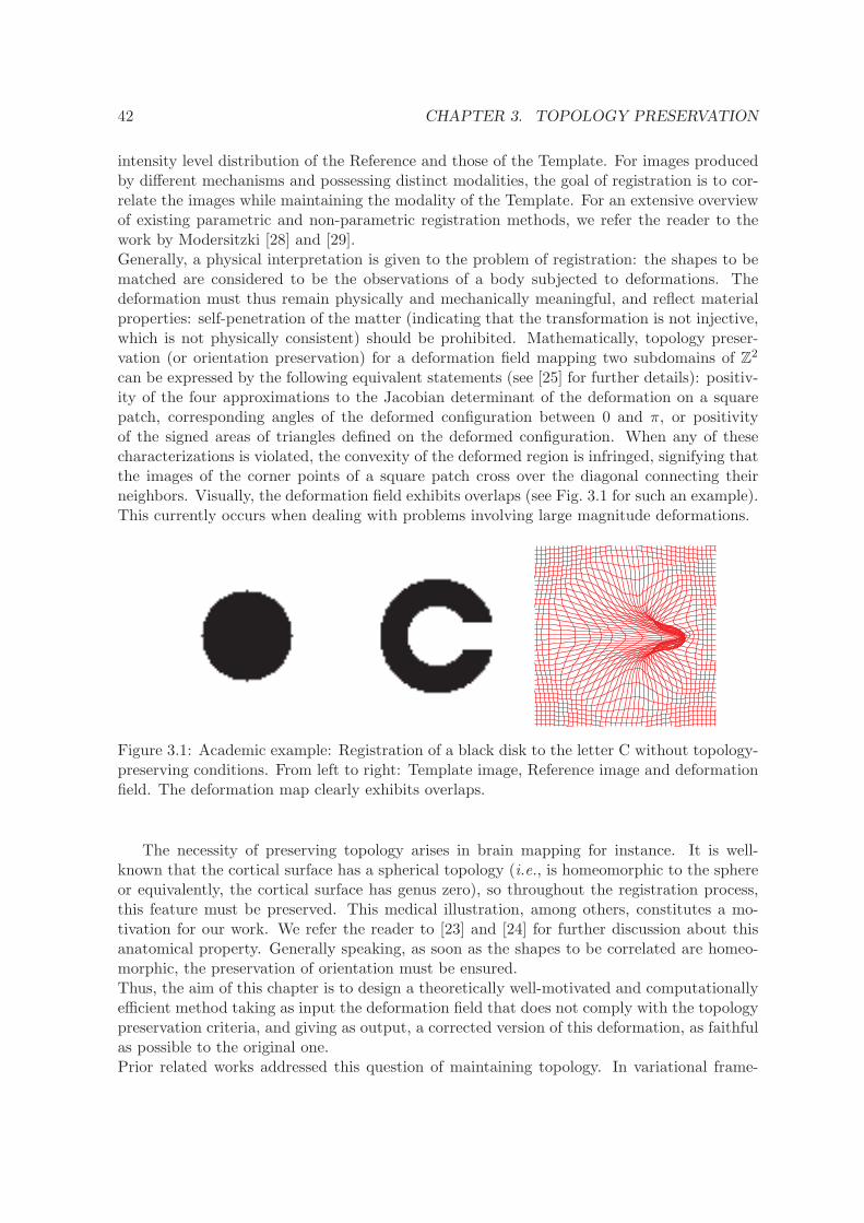
42 CHAPTER 3. TOPOLOGY PRESERVATION
intensity level distribution of the Reference and those of the Template. For images producedby different mechanisms and possessing distinct modalities, the goal of registration is to cor-relate the images while maintaining the modality of the Template. For an extensive overviewof existing parametric and non-parametric registration methods, we refer the reader to thework by Modersitzki [28] and [29].Generally, a physical interpretation is given to the problem of registration: the shapes to bematched are considered to be the observations of a body subjected to deformations. Thedeformation must thus remain physically and mechanically meaningful, and reflect materialproperties: self-penetration of the matter (indicating that the transformation is not injective,which is not physically consistent) should be prohibited. Mathematically, topology preser-vation (or orientation preservation) for a deformation field mapping two subdomains of Z2
can be expressed by the following equivalent statements (see [25] for further details): positiv-ity of the four approximations to the Jacobian determinant of the deformation on a squarepatch, corresponding angles of the deformed configuration between 0 and π, or positivityof the signed areas of triangles defined on the deformed configuration. When any of thesecharacterizations is violated, the convexity of the deformed region is infringed, signifying thatthe images of the corner points of a square patch cross over the diagonal connecting theirneighbors. Visually, the deformation field exhibits overlaps (see Fig. 3.1 for such an example).This currently occurs when dealing with problems involving large magnitude deformations.
Figure 3.1: Academic example: Registration of a black disk to the letter C without topology-preserving conditions. From left to right: Template image, Reference image and deformationfield. The deformation map clearly exhibits overlaps.
The necessity of preserving topology arises in brain mapping for instance. It is well-known that the cortical surface has a spherical topology (i.e., is homeomorphic to the sphereor equivalently, the cortical surface has genus zero), so throughout the registration process,this feature must be preserved. This medical illustration, among others, constitutes a mo-tivation for our work. We refer the reader to [23] and [24] for further discussion about thisanatomical property. Generally speaking, as soon as the shapes to be correlated are homeo-morphic, the preservation of orientation must be ensured.Thus, the aim of this chapter is to design a theoretically well-motivated and computationallyefficient method taking as input the deformation field that does not comply with the topologypreservation criteria, and giving as output, a corrected version of this deformation, as faithfulas possible to the original one.Prior related works addressed this question of maintaining topology. In variational frame-
43
works, the main idea is to control the Jacobian determinant of the deformation, propermeasure for the local volume transformation under the considered deformation. We wouldlike to mention the work by Ashburner et al. (see [7], [5] and [6]) and the work by Musse etal. (see [30]). In [30], the deformation map is modeled as a hierarchical displacement fielddecomposed on a multiresolution B-splines basis. Topology preservation is enforced by con-trolling the Jacobian of the transformation. The problem amounts to solving a constrainedoptimization problem: the residual energy between the target and the deformed source imageis minimized under constraints on the Jacobian. This paper is then extended to the 3D caseby Noblet et al. (see [32]). The main difference with the proposed approach is that, in ourcase, the set of feasible transformations is not restricted to a certain class of mappings.In [14] (work dedicated to registration under nonlinear elasticity principles), Droske andRumpf address the issue of non-rigid registration of multi-modal image data. A suitable de-formation is determined via the minimization of a morphological matching functional whichlocally measures the defect of the normal fields of the set of level lines of the Template imageand the deformed Reference image. The matching criterion includes first order derivativesof the deformation and is complemented by a nonlinear elastic regularization of the form∫
ΩW (DΦ,CofDΦ, detDΦ) dx, where W : R3×3 × R
3×3 × R → R is supposed to be convex,
DΦ is the Jacobian matrix of the deformation Φ, CofDΦ, the cofactor matrix of DΦ anddetDΦ, the Jacobian determinant.In [27], Le Guyader and Vese introduce a non-parametric combined segmentation/registrationmodel in which the shapes to be matched are viewed as Ciarlet-Geymonat materials. Thestored energy function of such a material is built so that it becomes infinite when the Jaco-bian determinant of the deformation tends to 0+. In [21], Haber and Modersitzki address theissue of non-parametric image registration under volume-preserving constraints. They pro-pose to restrict the set of feasible mappings by adding a volume-preserving constraint whichforces the Jacobian of the deformation to be equal to 1. In [22], the authors pursue in thesame direction: they propose to keep the Jacobian determinant bounded, which leads to aninequality-constrained minimization problem.An information-theoretic-based approach is proposed in [34] to generate diffeomorphic map-pings and to monitor the statistical distribution of the Jacobian determinant. The authorspropose to quantify the magnitude of the deformation by means of the Kullback-Leiblerdistance between the probability density function associated with the deformation and theidentity mapping.Although theoretically well-motivated, the above mentioned models are hard to handle nu-merically, requiring for instance, the use of optimization techniques such as logarithmic barriermethods or special discretization schemes (see [33] or [29]). This observation led us to dis-connect the registration problem from the topology-preserving question.An alternative to the straight penalization of the Jacobian of the deformation was proposedby Christensen and collaborators. In [11], they introduce a viscous fluid registration modelin which objects are viewed as fluids evolving in accordance with the fluid dynamics Navier-Stokes equations. This model is complemented by a regridding technique ensuring positivityof the Jacobian determinant. The method consists in monitoring the values of the Jacobiandeterminant of the deformation. If the values drop below a defined threshold, the processis reinitialized taking as initialization the last computed deformed Template. However, forproblems involving large deformations, numerous regridding steps might be required, which ismemory-consuming since one needs to store the last computed deformation field before each
44 CHAPTER 3. TOPOLOGY PRESERVATION
reinitialization. Numerically, the resulting deformation field (computed as the composite ofintermediate deformations) may not fulfill the topology-preserving conditions, even if the in-termediate ones do.In this chapter, we propose a theoretically well-motivated algorithm that falls within theframework of a previous work by Le Guyader ([26]). In this preliminary work, the authors,inspired by [25], design a two-step-algorithm enforcing topology preservation, independentlyof the registration technique used. The algorithm is thus independent of the selected regis-tration model. It can be applied at intermediate steps of the registration process or at theend.The first step consists in correcting the gradient vector field of the deformation (that doesnot comply with the topology preservation criteria) at the discrete level in order to fulfilla set of conditions ensuring topology preservation in the continuous domain after bilinearinterpolation (see also [25]). Basically, it consists in balancing the gradient vectors of thedisplacement field u (related to the deformation field ϕ by the relation ϕ = Id+u) by a pa-rameter α belonging to ]0, 1[. The proposed algorithm provides a unique optimal parameter αat each node of the grid. Once the correction stage is achieved, it remains to reconstruct thedeformation field, given its full set of discrete gradient vectors. The problem is phrased as aregularized least-squares problem but as is, one would fail to get the uniqueness of the solution(the solutions would be defined up to a constant). It is thus complemented by a constrainton the mean of the deformation field, thus ensuring uniqueness of the solution. The algo-rithm is shown to be efficient and has demonstrated its ability to handle large deformations.Also, it has been compared with Christensen et al.’s regridding technique on complex slicesof brain data in the case of brain mapping to a disk. In many cases, the proposed algorithmoutperforms the regridding technique. Nevertheless, some criticisms can be raised:
• First of all, the computations are carried out on the whole image domain, even thoughthe regions exhibiting overlaps are generally very few and localized on the image do-main, which leads to superfluous calculations and strays us from real-time computationrequirements. In practice, the deformation components are recomputed over the wholedomain, altering somewhat the physics of the problem.
• Besides, the constraint that complements the approximation problem (being about themean of the deformation) is rather artificial and cannot be physically interpreted. It isglobal and may not render well the complexity of variations of the deformation compo-nents.
We thus propose in this chapter to decompose the original reconstruction problem into inde-pendent problems of smaller dimensions, yielding a natural parallelization of the computa-tions. We localize the regions exhibiting overlaps, and formulate for each domain a functionalminimization problem equipped with interpolation constraints on the boundary, reproducingmore accurately the physics of the problem. The algorithm acts locally (the deformationis left unaltered where the topology-preserving criterion is fulfilled) and the obtained resultthus remains more consistent with the physics of the problem (due also to the Lagrange in-terpolation constraints stemming from the unaltered deformation field). One could objectthat when applied at the end of the process, the obtained deformation field is no longer asolution of the optimization process. This is indeed true, but as previously mentioned, theproposed algorithm acts locally and the minimization problems are constrained with Lagrangeinterpolation constraints stemming from the unaltered deformation. Besides, the proposed
45
algorithm is applied when the registration process produces a deformation field that is itselfmechanically and physically meaningless (a minimization problem in registration can be well-posed with the guarantee of existence of minimizers -for instance in the nonlinear elasticityframework-, but may numerically generate overlaps). It thus makes sense to correct the ob-tained deformation field. At last, the algorithm acts on the magnitude of the displacementvectors, not on their direction.One could also claim that registration models involving controls on the Jacobian determinantare more relevant than the proposed modelling. We answer first, that for many of thosemethods, no theoretical result of existence of minimizers is provided (or theoretical resultsare given but the theoretical model is not the one that is implemented in practice). It thusmeans that the numerical scheme, at best, makes the energy decrease to the infimum, butthe optimization problem does not necessarily admit a minimizer. Besides, some numericalartifices are often used. For instance, for the fluid registration model by Christensen et al., adetailed algorithm is provided in [28]. In the main loop, the displacement vector field is up-
dated in the following way: ~U (k+1) = ~U (k)+δt(k)δ~U (k) with
δu
(k)max = ||δ~U (k)||V ,
δt(k) = min(1, tolu/δu
(k)max
) .
It means that this procedure has the same effect as the method we propose: the directionof the obtained displacement vector field is preserved while the magnitude can be modified.This strategy of rescaling is further discussed p. 183 of [28] for variational non parametricregistration methods.The implementation of such methods (without heavy numerical artifices) does not guaranteeeither that the obtained deformation field is topology-preserving and fails to correctly alignthe shapes when the deformations are too large. That is why we took the side of decouplingthe registration process from the topology-preserving question. When applied at intermedi-ate steps of the registration process, the corrected deformation field can be interpreted asa new initial condition of the problem. At last, one could also argue that decomposing theoriginal problem into smaller dimension independent ones may destroy the global coupling.For the reasons stated above, we believe that this decoupling does not affect the result. Inparticular, the proposed results are qualitatively comparable to those presented in [26], whenno decomposition into subproblems is considered.The novelty of the chapter thus rests upon:
• the decomposition of the original problem into independent problems of smaller dimen-sions, enabling us to reduce significantly the computational time (up to a factor 80 forsome critical applications),
• the proof of the existence/uniqueness of the solution of the introduced functional mini-mization problem on each subdomain,
• a theoretical result of convergence when the size of the data to approximate increasesto infinity, ensuring the well-posedness of the problem,
• a result of convergence of the method in the discrete setting,
• a precise depiction of the discretization of the problem: generic finite element, basisfunctions, properties of the systems to be solved, and in particular a result of nonsin-gularity of the symmetric indefinite matrix involved in the linear systems.
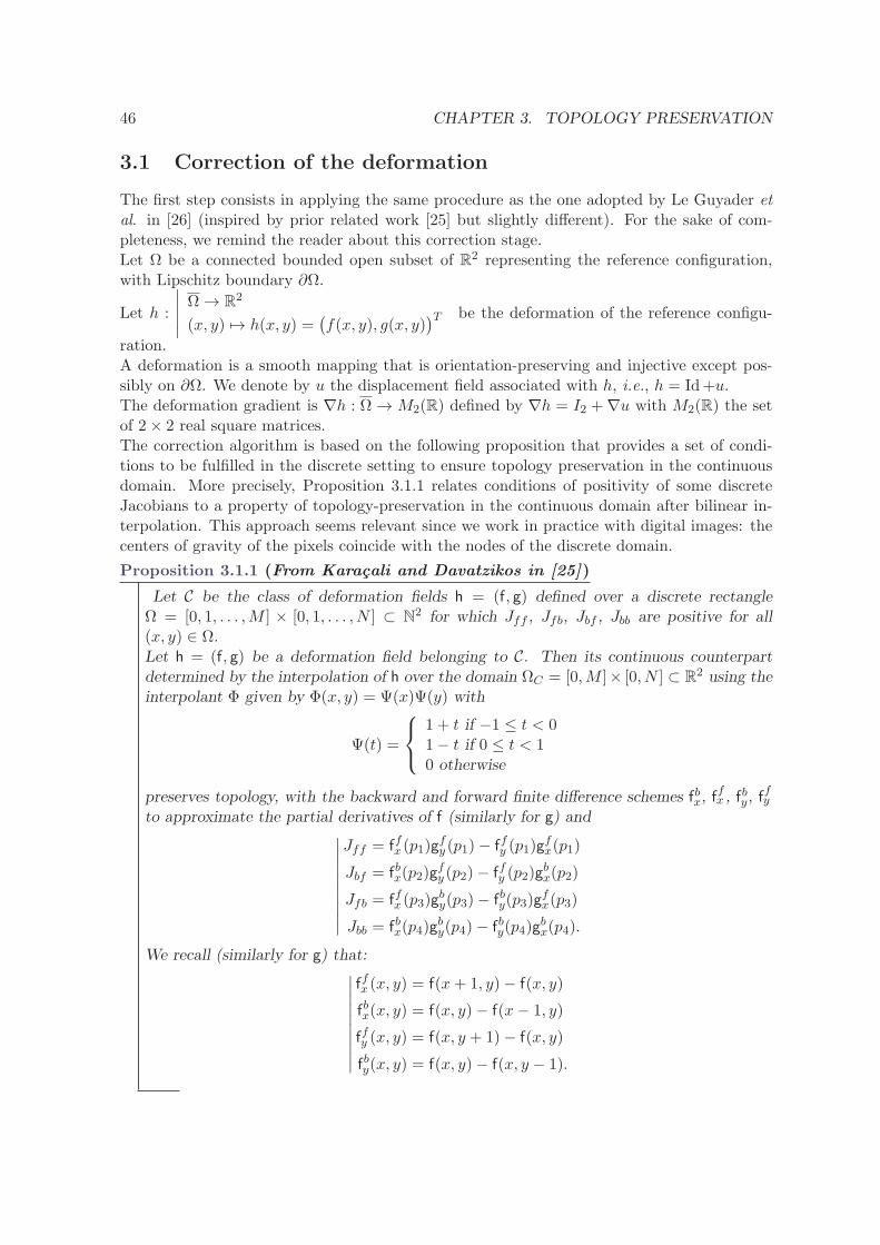
46 CHAPTER 3. TOPOLOGY PRESERVATION
3.1 Correction of the deformation
The first step consists in applying the same procedure as the one adopted by Le Guyader etal. in [26] (inspired by prior related work [25] but slightly different). For the sake of com-pleteness, we remind the reader about this correction stage.Let Ω be a connected bounded open subset of R2 representing the reference configuration,with Lipschitz boundary ∂Ω.
Let h :
∣∣∣∣∣Ω → R
2
(x, y) 7→ h(x, y) =(f(x, y), g(x, y)
)T be the deformation of the reference configu-
ration.A deformation is a smooth mapping that is orientation-preserving and injective except pos-sibly on ∂Ω. We denote by u the displacement field associated with h, i.e., h = Id+u.The deformation gradient is ∇h : Ω → M2(R) defined by ∇h = I2 +∇u with M2(R) the setof 2× 2 real square matrices.The correction algorithm is based on the following proposition that provides a set of condi-tions to be fulfilled in the discrete setting to ensure topology preservation in the continuousdomain. More precisely, Proposition 3.1.1 relates conditions of positivity of some discreteJacobians to a property of topology-preservation in the continuous domain after bilinear in-terpolation. This approach seems relevant since we work in practice with digital images: thecenters of gravity of the pixels coincide with the nodes of the discrete domain.
Proposition 3.1.1 (From Karacali and Davatzikos in [25])
Let C be the class of deformation fields h = (f, g) defined over a discrete rectangleΩ = [0, 1, . . . ,M ] × [0, 1, . . . , N ] ⊂ N
2 for which Jff , Jfb, Jbf , Jbb are positive for all(x, y) ∈ Ω.Let h = (f, g) be a deformation field belonging to C. Then its continuous counterpartdetermined by the interpolation of h over the domain ΩC = [0,M ]× [0, N ] ⊂ R
2 using theinterpolant Φ given by Φ(x, y) = Ψ(x)Ψ(y) with
Ψ(t) =
1 + t if −1 ≤ t < 01− t if 0 ≤ t < 10 otherwise
preserves topology, with the backward and forward finite difference schemes fbx, ffx , fby, f
fy
to approximate the partial derivatives of f (similarly for g) and∣∣∣∣∣∣∣∣∣∣
Jff = ffx (p1)gfy (p1)− ffy (p1)g
fx(p1)
Jbf = fbx(p2)gfy (p2)− ffy (p2)g
bx(p2)
Jfb = ffx (p3)gby(p3)− fby(p3)g
fx(p3)
Jbb = fbx(p4)gby(p4)− fby(p4)g
bx(p4).
We recall (similarly for g) that:∣∣∣∣∣∣∣∣∣∣
ffx (x, y) = f(x+ 1, y)− f(x, y)
fbx(x, y) = f(x, y)− f(x− 1, y)
ffy (x, y) = f(x, y + 1)− f(x, y)
fby(x, y) = f(x, y)− f(x, y − 1).
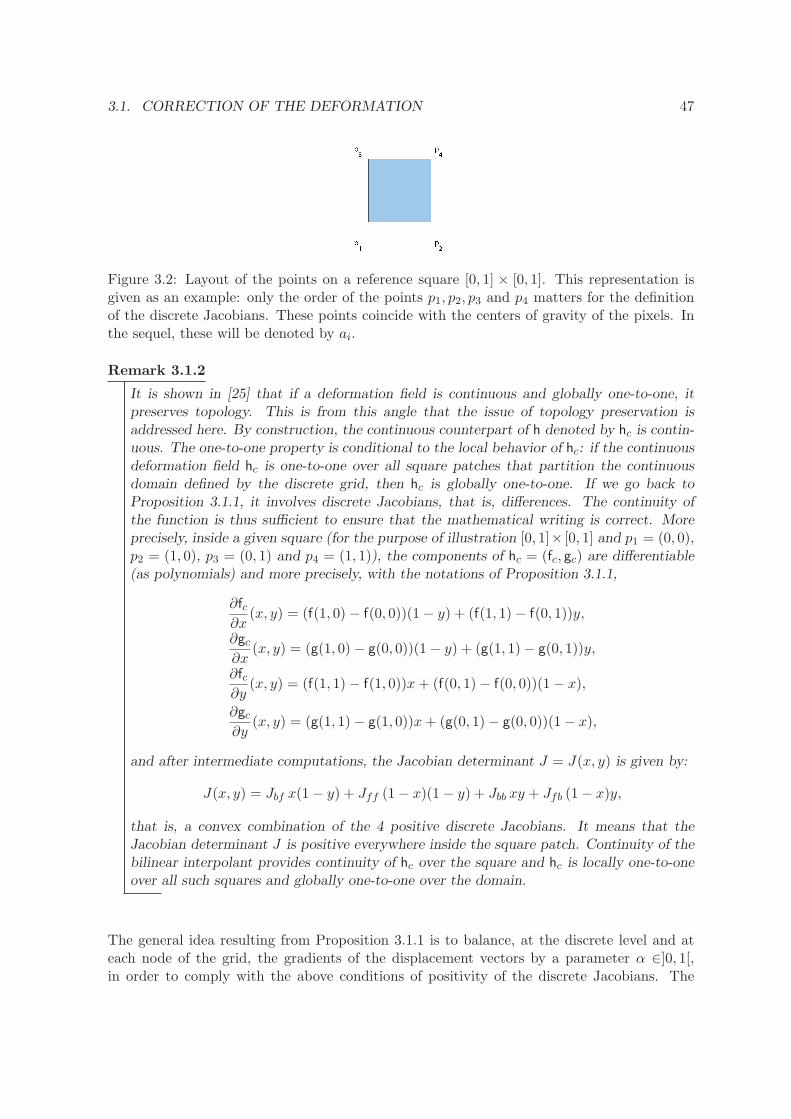
3.1. CORRECTION OF THE DEFORMATION 47
Figure 3.2: Layout of the points on a reference square [0, 1] × [0, 1]. This representation isgiven as an example: only the order of the points p1, p2, p3 and p4 matters for the definitionof the discrete Jacobians. These points coincide with the centers of gravity of the pixels. Inthe sequel, these will be denoted by ai.
Remark 3.1.2
It is shown in [25] that if a deformation field is continuous and globally one-to-one, itpreserves topology. This is from this angle that the issue of topology preservation isaddressed here. By construction, the continuous counterpart of h denoted by hc is contin-uous. The one-to-one property is conditional to the local behavior of hc: if the continuousdeformation field hc is one-to-one over all square patches that partition the continuousdomain defined by the discrete grid, then hc is globally one-to-one. If we go back toProposition 3.1.1, it involves discrete Jacobians, that is, differences. The continuity ofthe function is thus sufficient to ensure that the mathematical writing is correct. Moreprecisely, inside a given square (for the purpose of illustration [0, 1]× [0, 1] and p1 = (0, 0),p2 = (1, 0), p3 = (0, 1) and p4 = (1, 1)), the components of hc = (fc, gc) are differentiable(as polynomials) and more precisely, with the notations of Proposition 3.1.1,
∂fc∂x
(x, y) = (f(1, 0)− f(0, 0))(1− y) + (f(1, 1)− f(0, 1))y,
∂gc∂x
(x, y) = (g(1, 0)− g(0, 0))(1− y) + (g(1, 1)− g(0, 1))y,
∂fc∂y
(x, y) = (f(1, 1)− f(1, 0))x+ (f(0, 1)− f(0, 0))(1− x),
∂gc∂y
(x, y) = (g(1, 1)− g(1, 0))x+ (g(0, 1)− g(0, 0))(1− x),
and after intermediate computations, the Jacobian determinant J = J(x, y) is given by:
J(x, y) = Jbf x(1− y) + Jff (1− x)(1− y) + Jbb xy + Jfb (1− x)y,
that is, a convex combination of the 4 positive discrete Jacobians. It means that theJacobian determinant J is positive everywhere inside the square patch. Continuity of thebilinear interpolant provides continuity of hc over the square and hc is locally one-to-oneover all such squares and globally one-to-one over the domain.
The general idea resulting from Proposition 3.1.1 is to balance, at the discrete level and ateach node of the grid, the gradients of the displacement vectors by a parameter α ∈]0, 1[,in order to comply with the above conditions of positivity of the discrete Jacobians. The
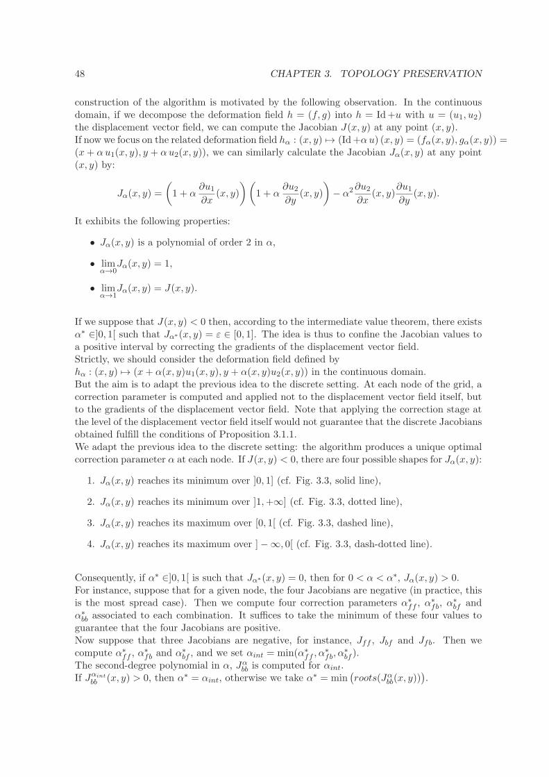
48 CHAPTER 3. TOPOLOGY PRESERVATION
construction of the algorithm is motivated by the following observation. In the continuousdomain, if we decompose the deformation field h = (f, g) into h = Id+u with u = (u1, u2)the displacement vector field, we can compute the Jacobian J(x, y) at any point (x, y).If now we focus on the related deformation field hα : (x, y) 7→ (Id+αu) (x, y) = (fα(x, y), gα(x, y)) =(x+ αu1(x, y), y + αu2(x, y)), we can similarly calculate the Jacobian Jα(x, y) at any point(x, y) by:
Jα(x, y) =
(1 + α
∂u1∂x
(x, y)
)(1 + α
∂u2∂y
(x, y)
)− α2∂u2
∂x(x, y)
∂u1∂y
(x, y).
It exhibits the following properties:
• Jα(x, y) is a polynomial of order 2 in α,
• limα→0
Jα(x, y) = 1,
• limα→1
Jα(x, y) = J(x, y).
If we suppose that J(x, y) < 0 then, according to the intermediate value theorem, there existsα∗ ∈]0, 1[ such that Jα∗(x, y) = ε ∈ [0, 1]. The idea is thus to confine the Jacobian values toa positive interval by correcting the gradients of the displacement vector field.Strictly, we should consider the deformation field defined byhα : (x, y) 7→ (x+ α(x, y)u1(x, y), y + α(x, y)u2(x, y)) in the continuous domain.But the aim is to adapt the previous idea to the discrete setting. At each node of the grid, acorrection parameter is computed and applied not to the displacement vector field itself, butto the gradients of the displacement vector field. Note that applying the correction stage atthe level of the displacement vector field itself would not guarantee that the discrete Jacobiansobtained fulfill the conditions of Proposition 3.1.1.We adapt the previous idea to the discrete setting: the algorithm produces a unique optimalcorrection parameter α at each node. If J(x, y) < 0, there are four possible shapes for Jα(x, y):
1. Jα(x, y) reaches its minimum over ]0, 1] (cf. Fig. 3.3, solid line),
2. Jα(x, y) reaches its minimum over ]1,+∞] (cf. Fig. 3.3, dotted line),
3. Jα(x, y) reaches its maximum over [0, 1[ (cf. Fig. 3.3, dashed line),
4. Jα(x, y) reaches its maximum over ]−∞, 0[ (cf. Fig. 3.3, dash-dotted line).
Consequently, if α∗ ∈]0, 1[ is such that Jα∗(x, y) = 0, then for 0 < α < α∗, Jα(x, y) > 0.For instance, suppose that for a given node, the four Jacobians are negative (in practice, thisis the most spread case). Then we compute four correction parameters α∗
ff , α∗fb, α
∗bf and
α∗bb associated to each combination. It suffices to take the minimum of these four values to
guarantee that the four Jacobians are positive.Now suppose that three Jacobians are negative, for instance, Jff , Jbf and Jfb. Then wecompute α∗
ff , α∗fb and α
∗bf , and we set αint = min(α∗
ff , α∗fb, α
∗bf ).
The second-degree polynomial in α, Jαbb is computed for αint.If Jαint
bb (x, y) > 0, then α∗ = αint, otherwise we take α∗ = min(roots(Jαbb(x, y))
).
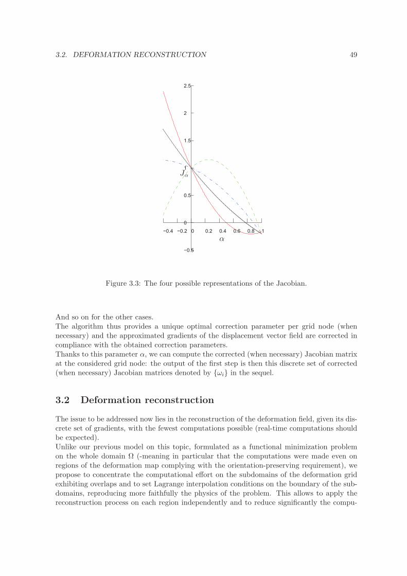
3.2. DEFORMATION RECONSTRUCTION 49
−0.4 −0.2 0 0.2 0.4 0.6 0.8 1
−0.5
0
0.5
1
1.5
2
2.5
α
Jα
Figure 3.3: The four possible representations of the Jacobian.
And so on for the other cases.The algorithm thus provides a unique optimal correction parameter per grid node (whennecessary) and the approximated gradients of the displacement vector field are corrected incompliance with the obtained correction parameters.Thanks to this parameter α, we can compute the corrected (when necessary) Jacobian matrixat the considered grid node: the output of the first step is then this discrete set of corrected(when necessary) Jacobian matrices denoted by ωi in the sequel.
3.2 Deformation reconstruction
The issue to be addressed now lies in the reconstruction of the deformation field, given its dis-crete set of gradients, with the fewest computations possible (real-time computations shouldbe expected).Unlike our previous model on this topic, formulated as a functional minimization problemon the whole domain Ω (-meaning in particular that the computations were made even onregions of the deformation map complying with the orientation-preserving requirement), wepropose to concentrate the computational effort on the subdomains of the deformation gridexhibiting overlaps and to set Lagrange interpolation conditions on the boundary of the sub-domains, reproducing more faithfully the physics of the problem. This allows to apply thereconstruction process on each region independently and to reduce significantly the compu-
50 CHAPTER 3. TOPOLOGY PRESERVATION
tational cost. In the sequel, we assume that we have identified (manually for the moment) Nnonempty connected bounded open subsets Ωi of Ω with Lipschitz boundary, i ∈ 1, · · · ,Non which orientation preservation is violated. ∀i ∈ 1, · · · ,N, Ωi ⊂ Ω and Ωi ∩ Ωj = ∅ fori 6= j. We then introduce our mathematical model of reconstruction, valid for each subdo-main Ωi, i ∈ 1, · · · ,N. A Dm-spline approach is retained (cf. [2]). Generally speaking, theDm-splines over an open subset of Rn are multidimensional minimizing splines, i.e., functionsdefined on Ω subjected to interpolation or smoothing conditions and that minimize an energyfunctional involving derivatives of order m. This choice of methodology is guided by theauthors’ experience in the field of approximation. This technique proves to be very satisfac-tory both in terms of theory (convergence results validate the approach) and applications: itprovides accurate results. Here again we refer the reader to [2] for more details. Of course,other strategies could have been considered.
3.2.1 Functional to be minimized
We remind the reader that ∀i ∈ 1, · · · ,N, Ωi is a nonempty connected bounded open subsetof Ω ⊂ R
2 with Lipschitz boundary. Let ν be an integer such that ν ∈ 1, · · · ,N. Inspiredby the Dm-spline approach, we introduce a regularized least-squares problem defined on aspace of vector-valued functions, in order to fit the discrete set of corrected gradient vectorsof the deformation and to satisfy Lagrange interpolation constraints. More precisely, theproblem is phrased as a constrained functional minimization problem on a convex subspaceof the Hilbert space H3(Ων ,R
2) so that the Sobolev’s embedding H3(Ων ,R2) C1(Ων ,R
2)holds (it means that the inclusion of H3(Ων ,R
2) into C1(Ων ,R2) is continuous, that is to
say : H3(Ων ,R2) ⊂ C1(Ων ,R
2) and there exists C > 0, depending only on Ων , such that∀u ∈ H3(Ων ,R
2), ‖u‖C1(Ων ,R2) ≤ C‖u‖H3(Ων ,R2), see [1] or [8]). It guarantees, in particular,that the pointwise fitting term dealing with the derivatives of the unknown is well-defined.We thus rebuild a smoother-than-required deformation field (by smoother, we mean moreregular) but retain only the values of the deformation components obtained at the grid nodes(centers of gravity of the pixels). Before depicting our model, we introduce some fundamentalmathematical notions that will be useful to state the functional minimization problem.
For any γ = (γ1, γ2) ∈ N2, we write |γ| = γ1+γ2 and ∂γ =
∂|γ|
∂xγ11 ∂xγ22. We recall the standard
inner product and the induced norm on H3(Ων ,R2):
((u, v))H3(Ων ,R2) =∑
|γ|≤3
∫
Ων
〈∂γu, ∂γv〉2 dx1 dx2 and ‖v‖2H3(Ων ,R2) = ((v, v))H3(Ων ,R2),
and the semi-inner product and the semi-norm:
(u, v)3,Ων ,R2 =∑
|γ|=3
∫
Ων
〈∂γu, ∂γv〉2 dx1 dx2 and |v|23,Ων ,R2 = (v, v)3,Ων ,R2 ,
where 〈·, ·〉2 denotes the Euclidean scalar product in R2. For the sake of clarity, we recall the
general definition of a P -unisolvent set.
3.2. DEFORMATION RECONSTRUCTION 51
Definition 3.2.1 (see [2])
For any l ∈ N, we denote by Pl the space of polynomial functions defined over Rn ofdegree ≤ l with respect to the set of variables, and for any l ∈ N and for any nonemptyconnected open subset Ω in R
n, by Pl(Ω) the space of restrictions to Ω of the functionsin Pl. A set A = a1, · · · , aN of N points of Rn is Pl-unisolvent if ∀ α1, · · · , αN ⊂ R,∃!Ψ ∈ Pl, ∀i ∈ 1, · · · , N, Ψ(ai) = αi.In particular, ∃!Ψ ∈ Pl, ∀i ∈ 1, · · · , N, Ψ(ai) = 0 (Ψ ≡ 0). It is clear that a necessarycondition for the set A to be Pl-unisolvent is that N = dimPl.
Let A = aii=1,··· ,N be a set of N points of Ων containing a P1-unisolvent subset (As the setA contains a P1-unisolvent subset, we can only infer that N ≥ dim P1). In our application,the set A is made of the coordinates of the image pixels included in Ων .Let also ωii=1,··· ,N be the set ofN Jacobian matrices of the deformation given at aii=1,··· ,N .This set is made of the corrected gradient vectors of the deformation obtained at the correctionstep of the algorithm. At last, let bii=1,··· ,l be l points of Ων where the discrete gradientvectors of the deformation have been unaltered (so the deformation is unchanged). In allour applications, these points will belong to the boundary ∂Ων of Ων . We set Lagrangeinterpolation constraints at these points (see Fig. 3.4). It means that if h denotes the unaltereddeformation and v denotes the unknown deformation of the minimization problem, we musthave:
∀i ∈ 1, · · · , l , v(bi) = h(bi).
Figure 3.4: Example of a subdomain (white zone) Ω1 ⊂ Ω on the boundary of which, inter-polation conditions are prescribed (black dots representing the bi, i ∈ 1, · · · , l).
Let K be the set defined by K = v ∈ H3(Ων ,R2), β(v) = η, with β the mapping:
β :
∣∣∣∣∣H3(Ων ,R
2) → R2l
v 7→ β(v) =(v(b1), · · · , v(bl)
)T
52 CHAPTER 3. TOPOLOGY PRESERVATION
and η =(h(b1), · · · , h(bl)
)T. The convex set K is closed as the reciprocal image of a closed
set by a continuous mapping (see [8]). The approximation problem can be stated as follows:given the set of N Jacobian matrices defined at aii=1,··· ,N , search for v sufficiently smoothsuch that ∀i ∈ 1, · · · , N, the Jacobian matrix Dv evaluated at ai is close to wi and such that∀i ∈ 1, · · · , l, v(bi) = h(bi). In this purpose, we need the following additional notations.We denote by ρ the operator defined by:
ρ :
∣∣∣∣∣H2(Ων ,R
2×2) → (R2×2)N
v 7→ ρ(v) =(v(a1), v(a2), · · · , v(aN )
)T . (3.1)
The problem is then cast as an optimization one by means of functional Jǫ defined by:
Jǫ :∣∣∣∣H3(Ων ,R
2) → R
v 7→ 〈ρ(Dv)− w〉2N + ǫ |v|23,Ων ,R2 ,
with ǫ > 0 a tuning parameter and with w =(w1, w2, · · · , wN
)T ∈(R2×2
)N. The opera-
tor 〈·, ·〉N is defined as follows: ∀ξ ∈(R2×2
)N, ∀η ∈
(R2×2
)N, 〈ξ, η〉N =
N∑
i=1
4∑
j=1
ξijηij and
〈ξ〉N = 〈ξ, ξ〉12N . The first term of functional Jǫ ensures closeness to the data while the second
component is a regularizing component. We consider the following minimization problem :
Search for σǫ ∈ K such that
∀v ∈ K,Jǫ(σǫ) ≤ Jǫ(v).(3.2)
We can notice that minimizing Jǫ with respect to v is equivalent to minimizing:
〈ρ(Dv)〉2N − 2〈ρ(Dv), ω〉N + ǫ |v|23,Ων ,R2 .
From now on, we thus denote by Jǫ the new functional:
Jǫ :∣∣∣∣H3(Ων ,R
2) → R
v 7→ 〈ρ(Dv)〉2N − 2〈ρ(Dv), ω〉N + ǫ |v|23,Ων ,R2 .
Our goal being to prove the existence/uniqueness of the solution of the introduced functionalminimization problem, we rephrase functional Jǫ in terms of the bilinear form a and the linearform L defined hereafter. Let a be the symmetric bilinear form such that:
a :
∣∣∣∣H3(Ων ,R
2)×H3(Ων ,R2) → R
(u, v) 7→ 〈ρ(Du), ρ(Dv)〉N + ǫ (u, v)3,Ων ,R2 .
Let also L be the linear form defined by:
L :
∣∣∣∣H3(Ων ,R
2) → R
v 7→ 〈ρ(Dv), ω〉N .
The minimization problem thus becomes:
Search for σǫ ∈ K such that
∀v ∈ K, a(σǫ, σǫ)− 2L(σǫ) ≤ a(v, v)− 2L(v).(3.3)
3.2. DEFORMATION RECONSTRUCTION 53
The mappings a and L are continuous, but the trouble is that the bilinear form a is notH3(Ων ,R
2)-elliptic, which prevents us from applying Stampacchia’s theorem ([8]) straightfor-wardly. To circumvent this issue, we introduce an artificial term in the minimization problemformulation as follows:
Search for σǫ ∈ K such that
∀v ∈ K, a(σǫ, σǫ)− 2L(σǫ) + ‖β(σǫ)‖22l ≤ a(v, v)− 2L(v) + ‖β(v)‖22l.(3.4)
This new phrasing involves the bilinear form denoted by a defined by
a :
∣∣∣∣H3(Ων ,R
2)×H3(Ων ,R2) → R
(u, v) 7→ a(u, v) + 〈β(u), β(v)〉2land the following propositions hold.
Proposition 3.2.1
The mapping ‖.‖ defined on H3(Ων ,R2) by
‖.‖ :
∣∣∣∣H3(Ων ,R
2) → R
v 7→√a(v, v)
is a Hilbertian norm.
Proof : The proof is based on the argument of connectedness of Ων and the property ofP1-unisolvence of the set A.
• It is obvious that ‖λv‖ = |λ|‖v‖, ∀λ ∈ R according to the definition of a.
• The triangle inequality is also obvious as a result of the definition of a and theinner product.
• Let us prove that ‖v‖ = 0 ⇒ v ≡ 0.Let v ∈ H3(Ων ,R
2) be such that ‖v‖ = 0.It implies that:
X |v|3,Ων ,R2 = 0 and as Ων is connected, it yields v ∈ P2(Ων ,R2).
X Also, 〈ρ(Dv)〉N = 0. As v ∈ P2(Ων ,R2), it follows that Dv ∈ P1(Ων ,R
2×2)and from the unisolvence property we conclude that Dv = 0R2×2 . The map-
ping v can thus be written as v =
(c1c2
)where c1 and c2 are constants.
X At last, 〈β(v)〉2R2l = 0 ⇔ β(v) = 0R2l and so c1 = c2 = 0.
It yields v ≡ 0.
Proposition 3.2.2
The norm ‖.‖ is equivalent to the norm ‖.‖H3(Ων ,R2) on H3(Ων ,R2).
54 CHAPTER 3. TOPOLOGY PRESERVATION
Proof : The proof is based on a theorem of equivalence of norms by Necas (Theorem 7.1.,[31]) and on the continuity of the bilinear form a on H3(Ων ,R
2)×H3(Ων ,R2).
Theorem 3.2.2 (Necas [31, Theorem 7.1])
Let Ω ∈ N(0) (with a continuous boundary), fi functionals satisfying
l∑
i=1
|fiv|p = 0 ⇔ v ≡ 0.
Let p ≥ 1, and k ≥ 1 an integer. We have the inequality:
c1‖u‖Wk,p(Ω) ≤[ ∑
|α|=k‖Dαu‖pLp(Ω) +
l∑
i=1
|fiu|p] 1
p ≤ c2‖u‖Wk,p(Ω).
The continuity of the bilinear form a results from the continuity of a and the followinginequality: ∀(u, v) ∈ H3(Ων ,R
2)×H3(Ων ,R2),
|〈β(u), β(v)〉R2l | ≤ |β(u)|R2l |β(v)|R2l (Cauchy-Schwarz inequality)
with |β(u)|R2l =
√l∑
i=1〈u(bi)〉22.
But 〈u(bi)〉2 ≤ ‖u‖C0(Ων ,R2) with ‖u‖C0(Ων ,R2) = supx∈Ων
〈u(x)〉2and using the Sobolev’s embedding theorem, we have: 〈u(bi)〉2 ≤ C‖u‖H3(Ων ,R2).
Therefore, |β(u)|R2l ≤√lC‖u‖H3(Ων ,R2) and
|〈β(u), β(v)〉R2l | ≤ lC2‖u‖H3(Ων ,R2)‖v‖H3(Ων ,R2).
The bilinear form a being continuous on H3(Ων ,R2)× H3(Ων ,R
2), there exists a con-stant c > 0 such that ∀v ∈ H3(Ων ,R
2):
a(v, v) = ‖v‖2 ≤ c‖v‖2H3(Ων ,R2).
For the second part of the inequality, we use Necas’ theorem with k = 3 and p = 2. We
take f1 : v 7→ 1√ǫρ(Dv) and f2 : v 7→ 1√
ǫβ(v). ∀v ∈ P2(Ων ,R
2),2∑i=1
|fiv|2 = 0 ⇔ v ≡ 0
from the unisolvence property of the set A. From Necas’ theorem, we then get thatthere exists a constant c1 > 0 such that:c21‖v‖2H3(Ων ,R2) ≤ |v|23,Ων ,R2 +
1ǫ 〈ρ(Dv)〉2N + 1
ǫ‖β(v)‖2R2l
⇔ ǫ c21‖v‖2H3(Ων ,R2) ≤ ǫ |v|23,Ων ,R2 + 〈ρ(Dv)〉2N + ‖β(v)‖2R2l
⇔ ‖v‖2H3(Ων ,R2) ≤ 1ǫc21
‖v‖2
It results in the following theorem.
3.2. DEFORMATION RECONSTRUCTION 55
Theorem 3.2.3
Problem (3.2) admits a unique solution σǫ ∈ K. This solution is characterized by thevariational inequality: ∀v ∈ K, a(σǫ, v − σǫ) ≥ L(v − σǫ).
Proof : The proof is based on Stampacchia’s theorem ([8]).
3.2.2 Characterization of the solution
Let K0 be the vector subspace of H3(Ων ,R2) defined by
K0 = v ∈ H3(Ων ,R2) | β(v) = 0R2l.
Let S be the set defined by
S = u ∈ H3(Ων ,R2) | ∀v ∈ K0, a(u, v) = L(v).
Then the following proposition holds.
Proposition 3.2.4
The unique solution σǫ of problem (3.2) is characterized by:
σǫ = K ∩ S.
This is mainly an abstract result that will be useful to prove Theorem 3.2.3.
Proof : First, let us prove that σǫ ⊂ K ∩ S.From Stampacchia’s theorem, we have ∀v ∈ K:
a(σǫ, v − σǫ) ≥ L(v − σǫ).
But v − σǫ ∈ K0 so a(σǫ, v − σǫ) = a(σǫ, v − σǫ) ≥ L(v − σǫ).Moreover, −(v − σǫ) ∈ K0 since K0 is a vector space, so ∀v ∈ K:
a(σǫ,−(v − σǫ)) ≥ L(−(v − σǫ)) ⇐⇒ a(σǫ, v − σǫ) ≤ L(v − σǫ).
By gathering the two above results, it yields a(σǫ, v − σǫ) = L(v − σǫ), which meansthat ∀v0 ∈ K0, a(σǫ, v0) = L(v0).Therefore σǫ ∈ K ∩ S.Now, let us prove that K ∩ S ⊂ σǫ.Let w ∈ K ∩ S. So w ∈ K and ∀v0 ∈ K0, a(w, v0) = L(v0).∀v ∈ K, v − w ∈ K0 so:
a(w, v − w) = a(w, v − w) = L(v − w) ≥ L(v − w).
Therefore, w is a solution of Problem (3.2) and by uniqueness of the solution, w = σǫ.It yields K ∩ S ⊂ σǫ.
56 CHAPTER 3. TOPOLOGY PRESERVATION
3.2.3 Lagrange multipliers
We now introduce Lagrange multipliers, which enables us to define the variational formulationof problem (3.2) on the whole space H3(Ων ,R
2) and to obtain a variational equality (efficientlytractable in the context of the Finite Element Method) instead of a variational inequality.Let K⊥
0 be the orthogonal complement of K0 in H3(Ων ,R2) for the scalar product a(·, ·):
K⊥0 = u ∈ H3(Ων ,R
2) | a(u, v) = 0, ∀v ∈ K0.
The space H3(Ων ,R2) can be written as the direct sum H3(Ων ,R
2) = K⊥0 ⊕K0.
Let us denote by β|K⊥0
the restriction of β to K⊥0 . Then β|K⊥
0is a topological isomorphism
(in particular, it is obvious that kerβ|K⊥0= K0 ∩K⊥
0 = 0. Moreover, β|K⊥0
is onto since K
is non-empty). The main theorem is stated as follows.
Theorem 3.2.3
If σǫ is the unique solution of problem (3.2), then σǫ is also the solution of the followingproblem with Lagrange multipliers:
Search for (σǫ, λ) ∈ K × R
2l,
∀v ∈ H3(Ων ,R2), a(σǫ, v)− L(v) + 〈λ, β(v)〉2l = 0.
(3.5)
Proof : Assume that (u, λ) ∈ K × R2l is a solution of problem (3.5). Then ∀v ∈ K0, we
have:a(u, v)− L(v) = 0,
since β(v) = 0R2l . Thus u ∈ K ∩ S and from Proposition 3.2.4, u = σǫ.Conversely, from Proposition 3.2.4, σǫ = K ∩ S so ∀v0 ∈ K0, a(σǫ, v0) = L(v0).Let us consider the linear form defined ∀w ∈ K⊥
0 by:
L :
∣∣∣∣K⊥
0 → R
w 7→ −a(σǫ, w) + L(w).
We remind the reader that, denoting by E and F two normed vector spaces and by Aa continuous linear mapping from E to F , the adjoint operator At : F ′ → E′ is definedby:
∀v ∈ E, ∀w ∈ F ′, 〈Atw, v〉EE = 〈w,Av〉F ′F ,
〈·, ·〉G′G denoting the dual pairing.The mapping β|K⊥
0: K⊥
0 → R2l is a topological isomorphism and consequently so is
the mapping βt|K⊥0: R2l → (K⊥
0 )′.
As L ∈ (K⊥0 )′, there exists a unique λ ∈ R
2l such that βt|K⊥0(λ) = L. It means that:
L(w) = −a(σǫ, w) + L(w) = 〈βt|K⊥0(λ), w〉(K⊥
0 )′K⊥0,
⇐⇒ a(σǫ, w)− L(w) + 〈βt|K⊥0(λ), w〉(K⊥
0 )′K⊥0= 0,
⇐⇒ a(σǫ, w)− L(w) + 〈λ, β|K⊥0(w)〉(R2l)′R2l = 0.
3.2. DEFORMATION RECONSTRUCTION 57
Let v ∈ H3(Ων ,R2). Since H3(Ων ,R
2) = K⊥0 ⊕K0, ∃!(v0, w) ∈ K⊥
0 ×K0, v = v0 + w.From the last equality, it yields ∃!λ ∈ R
2l, such that ∀v ∈ H3(Ων ,R2):
a(σǫ, v)− L(v)− a(σǫ, v0) + L(v0) + 〈λ, β(w)〉(R2l)′R2l = 0,
⇐⇒a(σǫ, v)− L(v) + 〈λ, β(w)〉(R2l)′R2l = 0,
since v0 ∈ K0, and a(σǫ, v0) = L(v0) from Proposition 3.2.4.To conclude, β(w) = β(v − v0) = β(v) since β(v0) = 0R2l .Finally,
∃!λ ∈ R2l, ∀v ∈ H3(Ων ,R
2), a(σǫ, v)− L(v) + 〈λ, β(v)〉(R2l)′R2l = 0
3.2.4 Theoretical convergence result
We now provide a theoretical convergence result that is an abstract result highlighting thewell-posedness of the modelling.Let D be a subset of ]0,+∞[ admitting 0 as accumulation point (this implies that 0 ∈ D).For each d ∈ D, let Ad be a set of N = N(d) distinct points of Ων containing a P1-unisolventsubset (we cannot say much on N except that N ≥ dimP1 and as d tends to 0, N(d) increasesto +∞).We suppose that
supx∈Ων
δ(x,Ad) = d, (3.6)
where δ is the Euclidean distance in R2. Let us observe that the left-hand side of (3.6) is just
the Hausdorff distance between Ad and Ων . Consequently, it implies that D is bounded andthat this distance tends to 0 as d does. Thus d is the radius of the largest sphere includedin Ων that contains no point from Ad (Hausdorff distance). Let us remark the ambiguity inthe meaning of d defined first as an index and next, independently, in (3.6). This situation isanalogous to that found in the Finite Element theory (see [2] and [12]).We point out that the hypotheses 0 ∈ D and (3.6) imply the weaker condition
limd→0
supx∈Ων
δ(x,Ad) = 0. (3.7)
For all d ∈ D, we denote by ρd the mapping defined by:
ρd :
∣∣∣∣∣H2(Ων ,R
2×2) → (R2×2)N(d)
v 7→ ρd(v) =((v(a))a∈Ad
)T .
Then we introduce the norm ‖·‖d equivalent to the norm ‖ · ‖H3(Ων ,R2) on H3(Ων ,R2) defined
by: ∀v ∈ H3(Ων ,R2),
‖v‖d =[〈ρd(Dv)〉2N(d) + ǫ |v|23,Ων ,R2 + ‖β(v)‖22l
] 12.
(It is possible to check that ‖·‖d is a norm by applying similar arguments to those in Propo-sition 3.2.1). The following lemma holds and allows to state Theorem 3.2.5.
58 CHAPTER 3. TOPOLOGY PRESERVATION
Lemma 3.2.4
Suppose that (3.7) holds. Let A0 = b01, . . . , b0ℵ be a fixed P1-unisolvent subset of Ων(in this case ℵ = dimP1).
∀j = 1, . . . ,ℵ, ∃(ad0j
)d∈D,
(∀d ∈ D, ad0j ∈ Ad
)and
(b0j = lim
d→0ad0j
). (3.8)
For all d ∈ D, let Ad0 be the set ad01, . . . , ad0ℵ and ‖.‖Ad0be the mapping defined by:
∀v ∈ H3(Ων ,R2),
‖v‖Ad0=
ℵ∑
j=1
〈Dv(ad0j)〉24 + ǫ |v|23,Ων ,R2 + ‖β(v)‖22l
12
,
(where 〈ξ, η〉4 =4∑j=1
ξjηj ,with ξ, η ∈ R2×2).
Then, there exists µ > 0 such that for all d ≤ µ, the set Ad0 is P1-unisolvent and ‖ · ‖Ad0is
a norm on H3(Ων ,R2) uniformly equivalent on D∩]0, µ] to the norm ‖ · ‖H3(Ων ,R2).
Proof : According to the Sobolev embedding:
∃C1 > 0, ∀d ∈ D, ∀v ∈ H3(Ων ,R2), ‖v‖Ad
0≤ C1‖v‖H3(Ων ,R2)
Constant C1 does not depend on d, it only depends on ℵ, l and ǫ.Now, it suffices to find a constant C2 > 0 independent of d such that ‖v‖H3(Ω,R2) ≤C2‖v‖Ad
0.
For v ∈ H3(Ων ,R2),
1
2
ℵ∑
j=1
〈Dv(b0j)〉24 =1
2
ℵ∑
j=1
〈Dv(b0j)−Dv(ad0j) +Dv(ad0j)〉24
≤ℵ∑
j=1
〈Dv(b0j)−Dv(ad0j)〉24 +ℵ∑
j=1
〈Dv(ad0j)〉24. (3.9)
Also, the Holder inclusion gives:
∃λ ∈]0, 1],H3(Ων ,R2) C1,λ(Ων ,R
2).
Thus v ∈ C1,λ(Ων ,R2) and ∃C > 0, ∀j = 1, . . . ,ℵ, ∀d ∈ D,
〈Dv(b0j)−Dv(ad0j)〉24 ≤ ‖v‖2C1,λ(Ων ,R2)
〈b0j − ad0j〉2λ2 ≤ C2‖v‖2H3(Ων ,R2)〈b0j − ad0j〉2λ2 .(3.10)
Moreover, by (3.8), it comes: ∀j = 1, . . . ,ℵ,
∀γj > 0, ∃µγj , ∀d ∈ D,(d ≤ µγj ⇒ 〈ad0j − b0j〉2 ≤ γj
).
3.2. DEFORMATION RECONSTRUCTION 59
Then
∀γj > 0, ∃µγj , ∀d ∈ D,(d ≤ µγj ⇒ 〈Dv(b0j)−Dv(ad0j)〉24 ≤ C2γ2λj ‖v‖2H3(Ων ,R2)
).
Let γ > 0 and taking γj = γ, ∀j = 1, . . . ,ℵ and µ = min(µγ1 , . . . , µγℵ) then
∀d ∈ D,
d ≤ µ⇒
ℵ∑
j=1
〈Dv(b0j)−Dv(ad0j)〉24 ≤ C2ℵγ2λ‖v‖2H3(Ων ,R2)
.
Finally,∀γ > 0, ∃µ > 0, ∀d ∈ D, ∀v ∈ H3(Ων ,R
2),d ≤ µ⇒
ℵ∑
j=1
〈Dv(b0j)−Dv(ad0j)〉24 ≤ C2γ2λℵ‖v‖2H3(Ων ,R2)
Using (3.9), we obtain:
∀γ > 0, ∃µ > 0, ∀d ∈ D, ∀v ∈ H3(Ων ,R2),
d ≤ µ⇒ 1
2
ℵ∑
j=1
〈Dv(b0j)〉24 + ǫ|v|23,Ων ,R2 + ‖β(v)‖2R2l ≤ ‖v‖2
Ad0+ C2γ2λℵ‖v‖2H3(Ων ,R2)
,
d ≤ µ⇒ 1
2
ℵ∑
j=1
〈Dv(b0j)〉24 + ǫ|v|23,Ων ,R2 + ‖β(v)‖2R2l − C2γ2λℵ‖v‖2H3(Ων ,R2) ≤ ‖v‖2
Ad0
.
The map v ∈ H3(Ων ,R2) 7→
[1
2
ℵ∑j=1
〈Dv(b0j)〉24 + ǫ|v|23,Ων ,R2 + ‖β(v)‖2R2l
] 12
is an equiv-
alent norm on H3(Ων ,R2) to the norm ‖.‖H3(Ων ,R2), then:
∀γ > 0, ∃µ > 0, ∀d ∈ D, ∀v ∈ H3(Ων ,R2),
(d ≤ µ⇒ (C ′2 − C2γ2λℵ)‖v‖2H3(Ων ,R2) ≤ ‖v‖2
Ad0
).
It suffices to choose a right γ to obtain the equivalence of norms. We notice that ‖·‖Ad0
is clearly a semi-norm. Thanks to the double inequality obtained, this is a norm onH3(Ων ,R
2) since ‖v‖Ad0= 0 ⇒ v = 0.
Theorem 3.2.5
Suppose that there exists a function f ∈ K such that for all d ∈ D: ρd(Df) = ω, andǫ = ǫ(d) ∈]0, ǫ0], ǫ0 > 0.For all d ∈ D, we denote by udǫ the unique solution of problem (3.2), then under the aboveassumptions we have:
limd→0
‖udǫ − f‖H3(Ων ,R2) = 0.
60 CHAPTER 3. TOPOLOGY PRESERVATION
Proof : The proof is divided into four steps.
First step
We start by proving that the sequence(udǫ
)d∈D∩]0,µ]ǫ∈]0,ǫ0]
is bounded in H3(Ων ,R2) inde-
pendently of d. By taking v = f in problem (3.2), we obtain :
〈ρ(Dudǫ −Df
)〉2N(d) + ǫ|udǫ |23,Ων ,R2 + ‖β(udǫ )‖2R2l ≤ ǫ|f |23,Ων ,R2 + ‖β(f)‖2
R2l .
We deduce that:
|udǫ |3,Ων ,R2 ≤ |f |3,Ων ,R2 ,
〈ρ(Dudǫ −Df
)〉2N(d) ≤ ǫ0|f |23,Ων ,R2 .
As Ad0 ⊂ Ad then:
∑
a∈Ad0
〈Dudǫ (a)−Df(a)〉24 ≤∑
a∈Ad
〈Dudǫ (a)−Df(a)〉24 = 〈ρd(Dudǫ −Df
)〉2N(d) ≤ ǫ0|f |23,Ων ,R2 .
Moreover,∑
a∈Ad0
〈Dudǫ (a)〉24 =∑
a∈Ad0
〈Dudǫ (a)−Df(a) +Df(a)〉24,
≤∑
a∈Ad0
〈Dudǫ (a)−Df(a)〉24 +∑
a∈Ad0
〈Df(a)〉24,
≤ ǫ0|f |23,Ων ,R2 + 2ℵ‖f‖2C1(Ων ,R2),
and using the equivalence of norm given in Lemma 3.2.4, we establish that:
∃ν > 0, ∀d ∈ D, ∀ǫ ∈]0, ǫ0],(d ≤ µ⇒ ‖udǫ‖H3(Ων ,R2) ≤ ν
).
The sequence(udǫ
)d∈D∩]0,µ]ǫ∈]0,ǫ0]
is bounded in H3(Ων ,R2), so one can extract a subsequence
(udlǫl
)l∈N with lim
l→∞dl = 0 (since 0 is an accumulation point of D) and ǫl ∈]0, ǫ0], ∀l ∈ N
(-we assume that ǫ = ǫ(d)-) that weakly converges to an element of H3(Ων ,R2) denoted
by f∗.
Second step
In this step, we argue by contradiction and prove that Df∗ = Df using compact-ness arguments (Sobolev’s embeddings in Holder’s spaces and Rellich-Kondrachov’stheorem, see [8]). Finally, the Lagrange interpolation constraints give us that f∗ = f .
We start by proving that Df = Df∗.We argue by contradiction. We assume that Df 6= Df∗, then there exists an open setω non empty included in Ω and a positive number α such that:
∀x ∈ ω, 〈Df(x)−Df∗(x)〉4 > α.
3.2. DEFORMATION RECONSTRUCTION 61
Let ξ = 1 + E
[ǫ0|f |3,Ων ,R2
α2
]where E[.] represents the integer part.
Let B0 = p01, . . . , p0ξ a subset of ξ points of ω, we have:
∀i = 1, . . . , ξ, ∃(pd0i)d∈D,(∀d ∈ D, pd0i ∈ Ad
)and
(p0i = lim
d→0pd0i
)
For all d ∈ D, let Bd0 be the set pd01, . . . , pd0ξ.
As previously shown and knowing that Bd0 ⊂ Ad, we have
ξ∑
i=1
〈Dudlǫ (pdl0i)−Df(pdl0i)〉24 ≤ ǫ0|f |23,Ων ,R2 . (3.11)
Moreover, ∀i = 1, . . . , ξ,
〈Dudlǫ (pdl0i)−Df∗(p0i)〉4 = 〈Dudlǫ (pdl0i)−Dudlǫ (p0i) +Dudlǫ (p0i)−Df∗(p0i)〉4≤ 〈Dudlǫ (pdl0i)−Dudlǫ (p0i)〉4 + 〈Dudlǫ (p0i)−Df∗(p0i)〉4.
As ∃λ ∈]0, 1],H3(Ων ,R2) C1,λ(Ων ,R
2), there exists a constant C3 such that:
(‖udlǫl ‖C1,λ(Ων ,R2) ≤ C3‖udlǫl ‖H3(Ων ,R2)
).
Consequently,〈Dudlǫl (p
dl0i)−Dudlǫl (p0i)〉4 ≤ C3〈pdl0i − p0i〉λ2 .
But liml→∞
dl = 0 and p0i = liml→∞
pdl0i, we deduce that:
liml→∞
〈Dudlǫl (pdl0i)−Dudlǫl (p0i)〉4 = 0.
By Rellich-Kondrachov theorem, H3(Ων ,R2)
c⊂ C1(Ων ,R2), then
liml→∞
〈Dudlǫl (p0i)−Df∗(p0i)〉4 = 0. Therefore liml→∞
〈Dudlǫl (pdl0i)−Df∗(p0i)〉4 = 0.
Soliml→∞
Dudlǫl (pdl0i) = Df∗(p0i).
Letting l −→ ∞ in equation (3.11), yields to:
ξ∑
i=1
〈Df∗(p0i)−Df(p0i)〉24 ≤ ǫ0|f |23,Ων ,R2
and then,ξα2 ≤ ǫ0|f |23,Ων ,R2
This inequality is in contradiction with the choice of ξ. Thus Df∗ = Df .To conclude, ∀i ∈ 1, . . . , l, f∗(bi) = f(bi) = ηi hence f
∗ = f .
62 CHAPTER 3. TOPOLOGY PRESERVATION
Third step
The aim is to prove that(udlǫl
)l∈N strongly converges to f in H3(Ων ,R
2).
Thanks to Rellich-Kondrachov’s compact embedding theorem, we obtain that(udlǫl
)l∈N
strongly converges to f in H2(Ων ,R2). Since
‖udlǫl − f‖2H3(Ων ,R2) = ‖udlǫl − f‖2H2(Ων ,R2) + |udlǫl − f |23,Ων ,R2 ,
we just need to prove that liml→∞
|udlǫl − f |3,Ων ,R2 = 0. We have:
|udlǫl − f |23,Ων ,R2 = |udlǫl |23,Ων ,R2 + |f |23,Ων ,R2 − 2(udlǫl , f)3,Ων ,R2 .
But |udlǫl |3,Ων ,R2 ≤ |f |3,Ων ,R2 , so
|udlǫl − f |23,Ων ,R2 ≤ 2|f |23,Ων ,R2 − 2(udlǫl , f)3,Ων ,R2 .
Moreover, udlǫlH3(Ων ,R2)−−−−−− f , consequently
∀ϕ ∈ L2(Ων ,R2), (∂αudlǫl , ϕ)L2(Ων ,R2) −→
l→+∞(∂αf , ϕ)L2(Ων ,R2), ∀α ∈ N, |α| = 3. Taking
ϕ = ∂αf with |α| = 3, yields to:(∂αudlǫl , ∂
αf)L2(Ων ,R2) −→l→+∞
||∂αf ||2L2(Ων ,R2) and (udlǫl , f)3,Ων ,R2 −→ |f |3,Ων ,R2 when l
tends to +∞.It follows from the previous inequality that lim
l→∞‖udlǫl − f‖H3(Ων ,R2) = 0.
Fourth Step
Assume that ‖udǫ − f‖H3(Ων ,R2) does not tend to 0 when d tends to 0.It means that there exist a real number α > 0 and two sequences (dk)k∈N and (ǫk)k∈Nsuch that dk −→
k→+∞0 and ǫk = ǫ(dk), and ∀k ∈ N,
‖udkǫk − f‖H3(Ων ,R2) > α. (3.12)
Following the same steps as previously done, there exists a subsequence of(udkǫk
)k∈N
that strongly converges to f in H3(Ων ,R2), which is in contradiction with (3.12).
3.2.5 Discretization
We now discretize the variational problem (3.5). To do so, we will use classical notations usedin the Finite Element theory (similar to those in [2] and [12]). Let H be an open boundedsubset of ]0,+∞[ admitting 0 as accumulation point. Let us recall that the elements of classCk
′can be used for the computation of discreteDm-splines (in our casem = 3) withm ≤ k′+1
(where k′ is an integer). Consequently, (k′,m) = (2, 3) is a satisfactory combination. We alsorecall that for all n ∈ N and for all subset E of R2, Ql(E) denotes the space of the restrictionsto E of the polynomial functions over R2 of degree ≤ l with respect to each variable. ∀h ∈ H,let (Vh)
2 be the subspace of H3(Ων ,R2) of finite dimension with (Vh)
2 C1(Ων ,R2). The
reference finite element is the Bogner-Fox-Schmit C2 rectangle (cf. [12]). It is defined as thefollowing triplet (K,PK ,ΣK):
3.2. DEFORMATION RECONSTRUCTION 63
• Let b00 =(b100, b
200
)∈ R
2, h1, h2 > 0. K ⊂ Ων is the rectangle with vertices bγ =b00 + γ1 h1 ~e1 + γ2 h2 ~e2 with γ = (γ1, γ2) ∈ N
2 such that 0 ≤ γ1 ≤ 1 and 0 ≤ γ2 ≤ 1, and(~e1, ~e2) the canonical basis of R2.
• PK = Q5(K).
• The set of linear mappings ΣK is defined by: ΣK = v 7→ ∂αv(bγ) | |α|∞ ≤ 2, where,if α = (α1, α2), |α|∞ = max (α1, α2).
The number of degrees of freedom of the Bogner-Fox-Schmit rectangle of class C2 is thus equalto 36.
The basis functions are defined by pγα(x1, x2) = hα11 hα2
2 qγ1α1
(x1 − b100h1
)qγ2α2
(x2 − b200h2
)with:
q00(t) = (1− t)3(6t2 + 3t+ 1), q01(t) = t(1− t)3(3t+ 1), q02(t) =1
2t2(1− t)3
q10(t) = t3(6t2 − 15t+ 10), q11(t) = t3(1− t)(3t− 4), q12(t) =1
2t3(t− 1)2.
We can prove that problem (3.5) is decoupled with respect to each component. Let (vq)q=1,2
be the components of v ∈ H3(Ων ,R2), ((ωiq)
T )q=1,2 the qth row of ωi, ∀i ∈ 1, . . . , N, andλ = (λq)q=1,2 with λq ∈ R
l.Problem (3.5) can therefore be stated as:
Search for (σǫ = (σqǫ )q=1,2, λ = (λq)q=1,2) ∈ H3(Ων ,R2)× R
2l such that
σǫ ∈ K,
∀v = (vq)q=1,2 ∈ H3(Ων ,R2),
∀q ∈ 1, 2 ,N∑
i=1
〈∇σqǫ (ai),∇vq(ai)〉2 + ǫ (σqǫ , vq)3,Ων ,R +
l∑
i=1
λqi vq(bi) =
N∑
i=1
〈∇vq(ai), ωiq〉2.
(3.13)
We solve (3.13) in Vh for q = 1, 2. Let Mh be the dimension of Vh and P hj j=1,...,Mhbe basis
functions (for the sake of clarity, from now on, we use this notation for the basis functions).
We denote by (σh,qǫ )q=1,2 the approximate solution of (3.13) in (Vh)2; σh,qǫ is decomposed into
the basis P hj j=1,...,Mhas follows:
∀q = 1, 2,
∃(αqj)j=1,...,Mh∈ R such that
σh,qǫ =
Mh∑
j=1
αqjPhj .
(3.14)
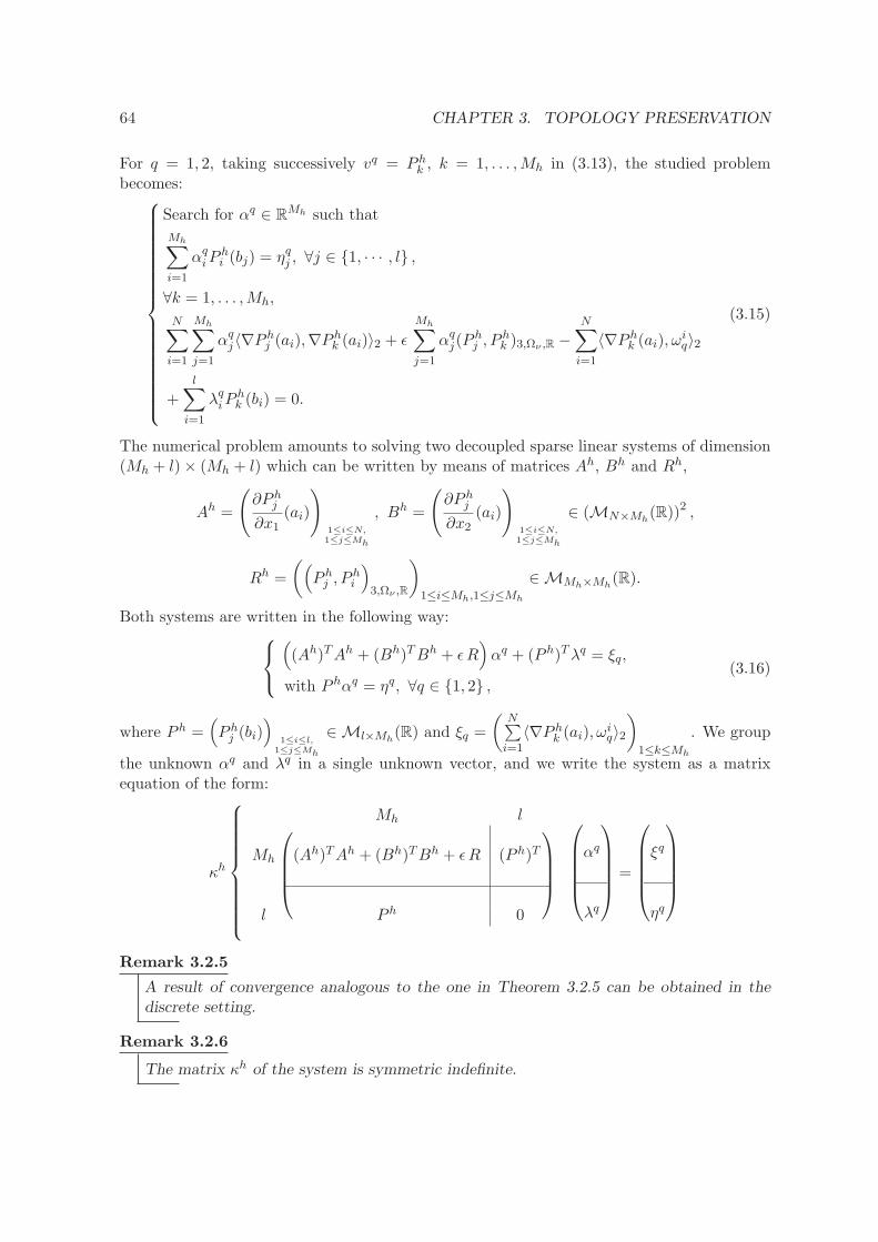
64 CHAPTER 3. TOPOLOGY PRESERVATION
For q = 1, 2, taking successively vq = P hk , k = 1, . . . ,Mh in (3.13), the studied problembecomes:
Search for αq ∈ RMh such that
Mh∑
i=1
αqiPhi (bj) = ηqj , ∀j ∈ 1, · · · , l ,
∀k = 1, . . . ,Mh,
N∑
i=1
Mh∑
j=1
αqj〈∇P hj (ai),∇P hk (ai)〉2 + ǫ
Mh∑
j=1
αqj(Phj , P
hk )3,Ων ,R −
N∑
i=1
〈∇P hk (ai), ωiq〉2
+l∑
i=1
λqiPhk (bi) = 0.
(3.15)
The numerical problem amounts to solving two decoupled sparse linear systems of dimension(Mh + l)× (Mh + l) which can be written by means of matrices Ah, Bh and Rh,
Ah =
(∂P hj∂x1
(ai)
)
1≤i≤N,1≤j≤Mh
, Bh =
(∂P hj∂x2
(ai)
)
1≤i≤N,1≤j≤Mh
∈ (MN×Mh(R))2 ,
Rh =
((P hj , P
hi
)3,Ων ,R
)
1≤i≤Mh,1≤j≤Mh
∈ MMh×Mh(R).
Both systems are written in the following way:
((Ah)TAh + (Bh)TBh + ǫR
)αq + (P h)Tλq = ξq,
with P hαq = ηq, ∀q ∈ 1, 2 ,(3.16)
where P h =(P hj (bi)
)1≤i≤l,
1≤j≤Mh
∈ Ml×Mh(R) and ξq =
(N∑i=1
〈∇P hk (ai), ωiq〉2)
1≤k≤Mh
. We group
the unknown αq and λq in a single unknown vector, and we write the system as a matrixequation of the form:
κh
Mh l
Mh (Ah)TAh + (Bh)TBh + ǫR (P h)T
l P h 0
αq
λq
=
ξq
ηq
Remark 3.2.5
A result of convergence analogous to the one in Theorem 3.2.5 can be obtained in thediscrete setting.
Remark 3.2.6
The matrix κh of the system is symmetric indefinite.
3.2. DEFORMATION RECONSTRUCTION 65
Remark 3.2.7
In practice, the interpolation conditions are set on the boundary nodes of the finite elementmesh. In this case, we have the following result:
Proposition 3.2.8
Matrix κh is nonsingular.
Proof : For the sake of clarity, we denote by Ch the matrix Ch = (Ah)TAh+(Bh)TBh+ǫR. The proof is based on Lemma 16.1 of [33] that states that if Z is a basis for the
null space of P h and if the reduced Hessian ZTChZ is positive definite and(P h
)Thas
full rank, then κh is nonsingular.As the interpolation conditions are set on the boundary of the finite element mesh,
the columns of(P h
)Tare made of l independent vectors of the canonical basis of
RMh , so
(P h
)Thas full rank. More precisely, if the column of index p of
(P h
)Tde-
noted by(P h
)Tpis related to node q(p) of the finite element mesh, one has:
(P h
)Tj,p
=∣∣∣∣1 if j = 9(q − 1) + 1,0 otherwise
, j ∈ 1, · · · ,Mh.The columns (Z1, · · · , ZMh−l) of Z are thus made of the Mh− l (independent) vectors
of the canonical basis of RMh orthogonal to the columns of(P h
)T.
The matrix Ch is semi-positive definite. Indeed, ∀α ∈ RMh , αT Ch α = a(vh, vh) ≥ 0
with vh =
Mh∑
j=1
αj Phj . From what was previously done, the quantity a(vh, vh) van-
ishes when vh is a constant c1, which corresponds to α = (αj)Mh
j=1 such that αj =∣∣∣∣∣c1 if j = 1 + 9s, s ∈
0, · · · , Mh
9 − 1,
0 otherwise. In particular, the vector ξ ∈ R
Mh defined
by ξj =
∣∣∣∣∣1 if j = 1 + 9s, s ∈
0, · · · , Mh
9 − 1,
0 otherwiseis not spanned by (Z1, · · · , ZMh−l).
Let us now takeX ∈ RMh−l\
0RMh−l
. It is clear that ZX /∈ span (ξ) soXTZTChZX >
0, which achieves the proof.
A large variety of methods can be found in the literature to solve the considered linear sys-tems: null-space methods ([17], [3]), direct solvers ([9]), the classical Uzawa algorithm ([4]),the inexact Uzawa algorithm ([16]), splitting schemes ([15]), augmented Lagrangian approach([18]). In our application, we use the diagonal pivoting method due to Bunch and Parlett([9]) which computes a permutation P such that PAP T = LDLT - when solving a linearsystem whose symmetric definite matrix is A-, where D is a direct sum of 1 by 1 and 2 by2 pivot blocks and L is unit lower triangular (see also [19]). P is chosen so that the entries
in the unit lower triangular L satisfy |lij | ≤ 1. This factorization involves n3
3 flops and oncecomputed can be used to solve Ax = b with O(n2) work.
66 CHAPTER 3. TOPOLOGY PRESERVATION
Remark 3.2.9
Extension of the algorithm to the 3D caseThe main brake to the straight extension of the model to 3D is the phase of identificationof subdomains (in practice small cubes) where the computations need to be done. (In2D, visual inspection suffices to determine these regions). The semi-automation of thisprocess, based on segmentation techniques, is a project in progress. The idea is to workwith the 3D images of the discrete Jacobians and to partition the images into two smoothregions: a region for which the discrete Jacobians are greater than a defined threshold anda region for which they are lower (region that thus needs to be processed). This binarypartition of the data can be performed using a Chan-Vese like ([10]) segmentation criterionin a level set framework. This step is done for each discrete Jacobian. The regions to beprocessed are thus localized and are embedded in cubes. The derivation of the topology-preserving conditions in the 3D case is quite analogous to the 2D case. We impose thatthe 8 corner Jacobians are positive (see [25] for justifications). The Jacobian Jα(x, y, z) isnow a polynomial of degree 3 in α but the method, as in the 2D case, amounts to studyingthe roots of polynomials, here of degree 3. The theoretical results in the reconstructionstage hold in three dimensions. The numerical problem consists in solving three decoupledsparse linear systems of dimension (Mh + l) × (Mh + l) but this time there are 33 basisfunctions per node so Mh = dimVh = 33 × number of mesh nodes. The basis functionsare still obtained by tensor product from the 1D case and the system matrix structure isthe same, except that the block (1,1) is of the form (Ah)TAh+(Bh)TBh+(Ch)TCh+ ǫR,
with Ch =
(∂P hj∂x3
(ai)
)
1≤i≤N,1≤j≤Mh
. The optimization computational tools are the same as the
ones in Section 3.3. Some very preliminary experiments have been made on cubes of size36× 36× 36 and the computational time decreases to 23 seconds.
3.3 Numerical experiments
In the sequel, we provide numerical simulations. Classically, in the Dm-spline setting, param-eter ǫ balancing the semi-norm is set to 10−6. (There also exist methods for an automaticchoice of ǫ mainly based on statistical considerations as the generalized cross-validation andthe generalized maximum likelihood methods (see [13] and [20])). From our experience, wehave realized that it suffices to fix the value ǫ in a neighborhood of 10−6 to produce satisfactoryresults. Besides, the method proves to be not too sensitive to the choice of this parameter.That is why we did not resort to the generalized cross-validation method to set parameter ǫ.Owing to the fact that the proposed algorithm calls basic linear algebra functions such thattransposing matrices, summing matrices, multiplying matrices or solving linear systems, itappeared relevant to use LAPACK and Basic Linear Algebra Subprogram routines (officialwebsites: http://www.netlib.org/blas/ and http://www.netlib.org/lapack/). BLASis a corpus of routines that provides standard building blocks for performing basic vectorand matrix operations. LAPACK (designed at the outset to exploit BLAS routines) pro-vides routines for solving systems of linear equations among others. For each subdomain Ων ,ν ∈ 1, · · · ,N, we obtain two disconnected linear systems to be solved with the same matrix.Our resorting to BLAS/LAPACK thus seems apposite. We particularly focused on the dsysvfunction provided by the software package LAPACK which computes the solution of a real
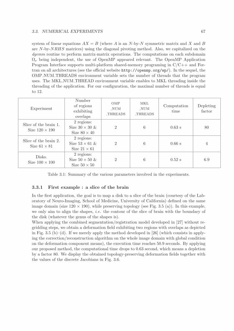
3.3. NUMERICAL EXPERIMENTS 67
system of linear equations AX = B (where A is an N -by-N symmetric matrix and X and Bare N -by-NRHS matrices) using the diagonal pivoting method. Also, we capitalized on thedgemm routine to perform matrix-matrix operations. The computations on each subdomainΩν being independent, the use of OpenMP appeared relevant. The OpenMP ApplicationProgram Interface supports multi-platform shared-memory programing in C/C++ and For-tran on all architectures (see the official website http://openmp.org/wp/). In the sequel, theOMP NUM THREADS environment variable sets the number of threads that the programuses. The MKL NUM THREAD environment variable enables to MKL threading inside thethreading of the application. For our configuration, the maximal number of threads is equalto 12.
Experiment
Numberof regionsexhibitingoverlaps
OMP
NUM
THREADS
MKL
NUM
THREADS
Computationtime
Depletingfactor
Slice of the brain 1.Size 120× 190
2 regions:Size 30× 30 &Size 80× 40
2 6 0.63 s 80
Slice of the brain 2.Size 61× 81
2 regions:Size 53× 61 &Size 21× 61
2 6 0.66 s 4
Disks.Size 100× 100
2 regions:Size 50× 50 &Size 50× 50
2 6 0.52 s 6.9
Table 3.1: Summary of the various parameters involved in the experiments.
3.3.1 First example : a slice of the brain
In the first application, the goal is to map a disk to a slice of the brain (courtesy of the Lab-oratory of Neuro-Imaging, School of Medicine, University of California) defined on the sameimage domain (size 120 × 190), while preserving topology (see Fig. 3.5 (a)). In this example,we only aim to align the shapes, i.e. the contour of the slice of brain with the boundary ofthe disk (whatever the genus of the shapes is).When applying the combined segmentation/registration model developed in [27] without re-gridding steps, we obtain a deformation field exhibiting two regions with overlaps as depictedin Fig. 3.5 (b)–(d). If we merely apply the method developed in [26] (which consists in apply-ing the correction/reconstruction algorithm on the whole image domain with global conditionon the deformation component means), the execution time reaches 50.9 seconds. By applyingour proposed method, the computational time drops to 0.63 second, which means a depletionby a factor 80. We display the obtained topology-preserving deformation fields together withthe values of the discrete Jacobians in Fig. 3.6.
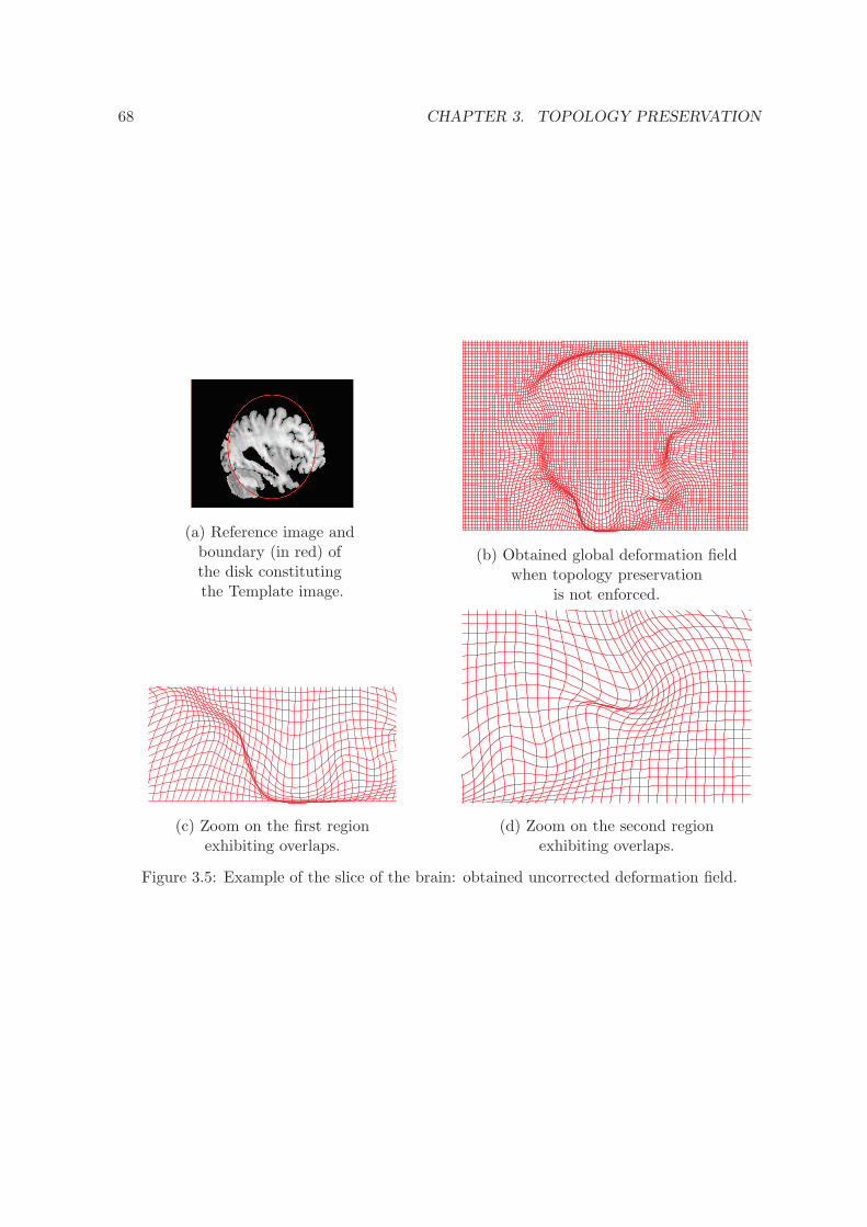
68 CHAPTER 3. TOPOLOGY PRESERVATION
(a) Reference image andboundary (in red) ofthe disk constitutingthe Template image.
(b) Obtained global deformation fieldwhen topology preservation
is not enforced.
(c) Zoom on the first regionexhibiting overlaps.
(d) Zoom on the second regionexhibiting overlaps.
Figure 3.5: Example of the slice of the brain: obtained uncorrected deformation field.
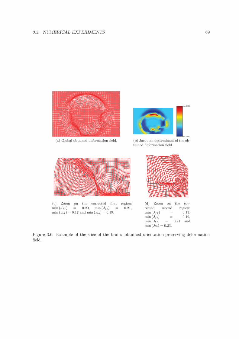
3.3. NUMERICAL EXPERIMENTS 69
(a) Global obtained deformation field.
min:0.045
max:3.002
(b) Jacobian determinant of the ob-tained deformation field.
(c) Zoom on the corrected first region:min (Jff ) = 0.20, min (Jfb) = 0.21,min (Jbf ) = 0.17 and min (Jbb) = 0.19.
(d) Zoom on the cor-rected second region:min (Jff ) = 0.13,min (Jfb) = 0.19,min (Jbf ) = 0.21 andmin (Jbb) = 0.23.
Figure 3.6: Example of the slice of the brain: obtained orientation-preserving deformationfield.
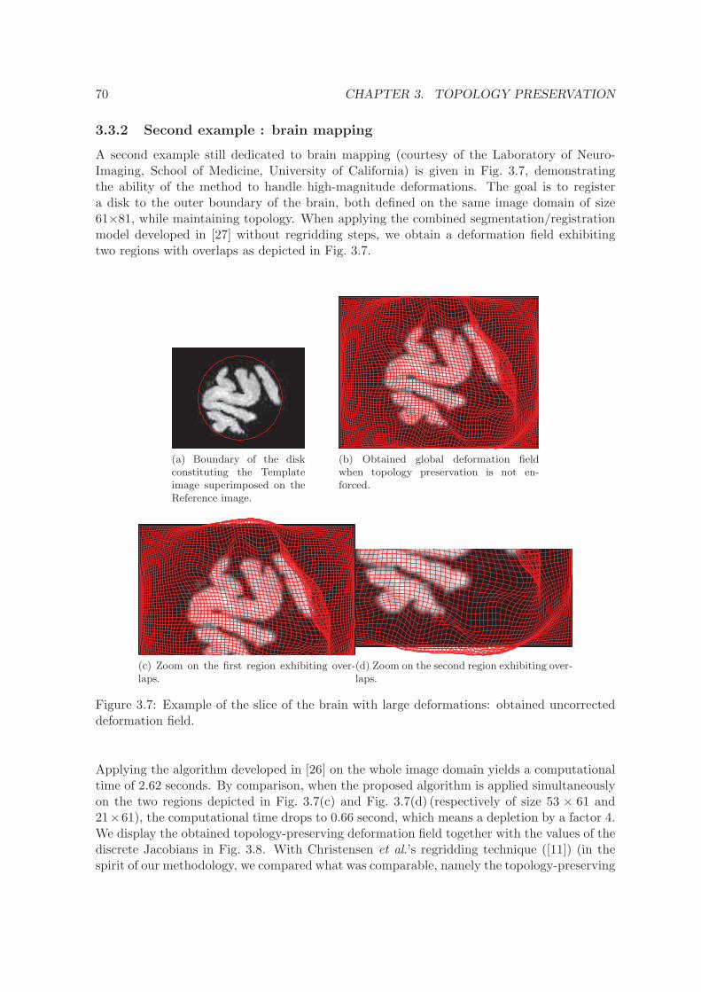
70 CHAPTER 3. TOPOLOGY PRESERVATION
3.3.2 Second example : brain mapping
A second example still dedicated to brain mapping (courtesy of the Laboratory of Neuro-Imaging, School of Medicine, University of California) is given in Fig. 3.7, demonstratingthe ability of the method to handle high-magnitude deformations. The goal is to registera disk to the outer boundary of the brain, both defined on the same image domain of size61×81, while maintaining topology. When applying the combined segmentation/registrationmodel developed in [27] without regridding steps, we obtain a deformation field exhibitingtwo regions with overlaps as depicted in Fig. 3.7.
(a) Boundary of the diskconstituting the Templateimage superimposed on theReference image.
(b) Obtained global deformation fieldwhen topology preservation is not en-forced.
(c) Zoom on the first region exhibiting over-laps.
(d) Zoom on the second region exhibiting over-laps.
Figure 3.7: Example of the slice of the brain with large deformations: obtained uncorrecteddeformation field.
Applying the algorithm developed in [26] on the whole image domain yields a computationaltime of 2.62 seconds. By comparison, when the proposed algorithm is applied simultaneouslyon the two regions depicted in Fig. 3.7(c) and Fig. 3.7(d) (respectively of size 53 × 61 and21×61), the computational time drops to 0.66 second, which means a depletion by a factor 4.We display the obtained topology-preserving deformation field together with the values of thediscrete Jacobians in Fig. 3.8. With Christensen et al.’s regridding technique ([11]) (in thespirit of our methodology, we compared what was comparable, namely the topology-preserving
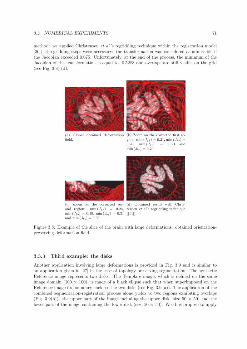
3.3. NUMERICAL EXPERIMENTS 71
method: we applied Christensen et al.’s regridding technique within the registration model[26]), 3 regridding steps were necessary: the transformation was considered as admissible ifthe Jacobian exceeded 0.075. Unfortunately, at the end of the process, the minimum of theJacobian of the transformation is equal to -0.5288 and overlaps are still visible on the grid(see Fig. 3.8) (d).
(a) Global obtained deformationfield.
(b) Zoom on the corrected first re-gion: min (Jff ) = 0.21, min (Jfb) =0.20, min (Jbf ) = 0.21 andmin (Jbb) = 0.20.
(c) Zoom on the corrected sec-ond region: min (Jff ) = 0.24,min (Jfb) = 0.19, min (Jbf ) = 0.31and min (Jbb) = 0.30.
(d) Obtained result with Chris-tensen et al ’s regridding technique([11])
Figure 3.8: Example of the slice of the brain with large deformations: obtained orientation-preserving deformation field.
3.3.3 Third example: the disks
Another application involving large deformations is provided in Fig. 3.9 and is similar toan application given in [27] in the case of topology-preserving segmentation. The syntheticReference image represents two disks. The Template image, which is defined on the sameimage domain (100 × 100), is made of a black ellipse such that when superimposed on theReference image its boundary encloses the two disks (see Fig. 3.9 (a)). The application of thecombined segmentation-registration process alone yields to two regions exhibiting overlaps(Fig. 3.9(b)): the upper part of the image including the upper disk (size 50 × 50) and thelower part of the image containing the lower disk (size 50 × 50). We thus propose to apply
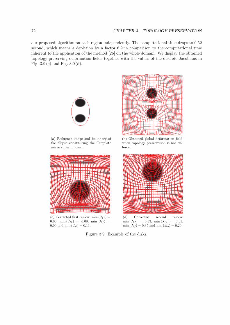
72 CHAPTER 3. TOPOLOGY PRESERVATION
our proposed algorithm on each region independently. The computational time drops to 0.52second, which means a depletion by a factor 6.9 in comparison to the computational timeinherent to the application of the method [26] on the whole domain. We display the obtainedtopology-preserving deformation fields together with the values of the discrete Jacobians inFig. 3.9 (c) and Fig. 3.9 (d).
(a) Reference image and boundary ofthe ellipse constituting the Templateimage superimposed.
(b) Obtained global deformation fieldwhen topology preservation is not en-forced.
(c) Corrected first region: min (Jff ) =0.06, min (Jfb) = 0.08, min (Jbf ) =0.09 and min (Jbb) = 0.11.
(d) Corrected second region:min (Jff ) = 0.33, min (Jfb) = 0.31,min (Jbf ) = 0.35 and min (Jbb) = 0.29.
Figure 3.9: Example of the disks.
BIBLIOGRAPHY
[1] R. A. Adams, Sobolev Spaces, Academic, Boston, MA, 1975.
[2] R. Arcangeli, M. C. Lopez de Silanes, and J. J. Torrens, Multidimensionalminimizing splines. Theory and applications, Grenoble Sciences, Kluwer Academic Pub-lishers, Boston, MA, 2004.
[3] M. Arioli and L. Baldini, A backward error analysis of a null space algorithm insparse quadratic programming, SIAM J. Matrix Anal. Appl., 23 (2001), pp. 425–442.
[4] K. Arrow, L. Hurwicz, and H. Uzawa, Studies in Nonlinear Programming, StanfordUniversity Press, Stanford, 1958.
[5] J. Ashburner, J. L. R. Andersson, and K. J. Friston, High-dimensional imageregistration using symmetric priors, Neuroimage, 9 (1999), pp. 619–628.
[6] J. Ashburner and K. J. Friston, Voxel-based morphometry: the methods, Neuroim-age, 11 (2000), pp. 805–821.
[7] J. Ashburner, P. Neelin, D. L. Collins, A. Evans, and K. J. Firston, Incorpo-rating prior knowledge into image registration, Neuroimage, 6 (1997), pp. 344–352.
[8] H. Brezis, Analyse fonctionelle. Theorie et Applications, Dunod, Paris, 2005.
[9] J. R. Bunch and B. N. Parlett, Direct methods for solving symmetric indefinitesystems of linear equations, SIAM J. Numer. Anal., 8 (1971), pp. 639–655.
[10] T. Chan and L. Vese, Active Contours Without Edges, IEEE Trans. Image Process.,10 (2001), pp. 266–277.
[11] G. E. Christensen, R. D. Rabitt, and M. I. Miller, Deformable templates usinglarge deformation kinematics, IEEE Trans. Imag. Process., 10 (1996), pp. 1435–1447.
[12] P. G. Ciarlet, The Finite Element Method for Elliptic Problems, North Holland, Am-sterdam, The Netherlands, 1978.
[13] P. Craven and G. Wahba, Smoothing noisy data with spline functions, Numer. Math.,31 (1979), pp. 377–403.
73
74 BIBLIOGRAPHY
[14] M. Droske and M. Rumpf, A Variational Approach to Non-Rigid Morphological Reg-istration, SIAM J. Appl. Math., 64 (2004), pp. 668–687.
[15] N. Dyn and W. E. Ferguson, The numerical solution of equality-constrained quadraticprogramming problems, Math. Comp., 41 (1983), pp. 165–170.
[16] H. C. Elman and G. H. Golub, Inexact and preconditioned Uzawa algorithms forsaddle point problems, SIAM J. Numer. Anal., 31 (1994), pp. 1645–1661.
[17] R. Fletcher and T. Johnson, On the Stability of Null-Space Methods for KKT Sys-tems, tech. rep., University of Dundee, Department of Mathematics and Computer Sci-ence, Dundee, UK, 1995.
[18] G. H. Golub and C. Greif, On solving block-structured indefinite linear systems,SIAM J. Sci. Comput., 24 (2003), pp. 2076–2092.
[19] G. H. Golub and C. F. Van Loan, Matrix Computations, 4th edition, Johns HopkinsUniversity Press, Baltimore, 2013.
[20] C. Gu and G. Wahba, Minimizing GCV/GML scores with multiple smoothing param-eters via the newton method, SIAM J. Sci. Stat. Comp., 12 (1991), pp. 383–398.
[21] E. Haber and J. Modersitzki, Numerical methods for volume preserving image reg-istration, Inverse Probl., 20 (2004), pp. 1621–1638.
[22] , Image registration method with guaranteed displacement regularity, Int. J. Comput.Vision, 71 (2007), pp. 361–372.
[23] X. Han, C. Xu, U. Braga-Neto, and J. L. Prince, Topology correction in braincortex segmentation using a multiscale, graph-based algorithm, IEEE Trans. Med. Imag.,21 (2002), pp. 109–121.
[24] , A topology preserving geometric deformable model and its application in braincortical surface reconstruction, in Geometric Level Set Methods in Imaging, Vis., Graph.,Stanley Osher and Nikos Paragios, Eds., New York: Springer-Verlag, 2003.
[25] B. Karacali and C. Davatzikos, Estimating topology preserving and smooth displace-ment fields, IEEE Trans. Med. Imag., 23 (2004), pp. 868–880.
[26] C. Le Guyader, D. Apprato, and C. Gout, On the construction of topology-preserving deformation fields, IEEE Transactions on Image Processing, 21 (2012),pp. 1587–1599.
[27] C. Le Guyader and L. Vese, A combined segmentation and registration frameworkwith a nonlinear elasticity smoother, Computer Vision and Image Understanding, 115(2011), pp. 1689–1709.
[28] J. Modersitzki, Numerical Methods for Image Registration, Oxford University Press,2004.
[29] , FAIR: Flexible Algorithms for Image Registration, Society for Industrial and Ap-plied Mathematics (SIAM), 2009.
BIBLIOGRAPHY 75
[30] O. Musse, F. Heitz, and J.-P. Armspach, Topology preserving deformable imagematching using constrained hierarchical parametric models, IEEE Trans. Image Process.,10 (2001), pp. 1081–1093.
[31] J. Necas, Les methodes directes en theorie des equations elliptiques, Masson, Paris,1967.
[32] V. Noblet, C. Heinrich, F. Heitz, and J.-P. Armspach, 3-D deformable imageregistration: a topology preservation scheme based on hierarchical deformation modelsand interval analysis optimization, IEEE Trans. Image Process., 14 (2005), pp. 553–566.
[33] J. Nocedal and S. J. Wright, Numerical Optimization, Springer, New York, 1999.
[34] I. Yanovsky, P. M. Thompson, S. Osher, and A. D. Leow, Topology preservinglog-unbiased nonlinear image registration: Theory and implementation, in Proc. IEEEConf. Comput. Vis. Pattern Recognit., 2007, pp. 1–8.

CHAPTER 4
JOINT SEGMENTATION/REGISTRATION MODEL BY SHAPEALIGNMENT VIA WEIGHTED TOTAL VARIATION
MINIMIZATION AND NONLINEAR ELASTICITY
This work falls within the scope of joint segmentation-registration using nonlinear elasticityprinciples. We introduce a variational model combining a measure of dissimilarity based onweighted total variation and a regularizer based on the stored energy function of a SaintVenant-Kirchhoff material. Adding a weighted total variation based criterion enables us toalign the edges of the objects even if the modalities are different.We derive a relaxed problem associated to the initial one for which we are able to providea result of existence of minimizers. A description and analysis of a numerical method ofresolution based on a decoupling principle is then provided including a theoretical result ofΓ-convergence. Applications on academic and biological images are provided.
Introduction
In [40], Sotiras et al. provide an overview of the different existing registration methods.According to the authors, an image registration algorithm consists of three main components:
1. a deformation model,
• geometric transformations derived from physical models,
• geometric transformations derived from interpolation theory,
• and knowledge-based geometric transformations,
2. an objective function,
• geometric methods: the criterion takes into account landmark information ([14]),
• iconic methods: it concerns intensity-based methods ([19]), attribute-based meth-ods ([39]), information-theoretic approaches ([44]),
• and hybrid methods.
3. and an optimization method,
77
78CHAPTER 4. JOINT SEGMENTATION/REGISTRATIONMODEL BY SHAPE ALIGNMENT
• continuous methods: gradient descent ([3]), conjugate gradient ([31]), Quasi-Newton([43]), stochastic gradient descent methods ([44])...
• discrete methods: graph-based ([41]), belief propagation, linear programming meth-ods,
• greedy approaches and evolutionary algorithms.
Our method falls within the scope of geometric transformations derived from physicalmodels in particular from nonlinear elasticity based regularization and the iconic methodssince we introduce an intensity-based criterion as well as a shape-based criterion. The chosenoptimization method is incorporated within the framework of the continuous model since weuse a gradient descent method.The scope of the proposed work is first to devise a theoretically well-motivated registrationmodel in a variational formulation, authorizing large and smooth deformations. In addition,to handle a large class of images, we propose defining a geometric dissimilarity measure basedon shape comparisons. This work follows on from that of Derfoul and Le Guyader in [19]in which basic similarity measures are incorporated and a Saint Venant-Kirchhoff like storedenergy function is considered. It enriches [19] by treating simultaneously the question ofsegmentation and registration, by involving new mathematical tools and by broadening theclass of considered images. The mathematical treatment proposed in this work introduces theweighted total variation, entailing substantial modifications in the mathematical proofs andin the design of the algorithm. In [19], theoretical results such as the explicit expression ofthe quasiconvex envelop of this modified Saint Venant-Kirchhoff stored energy function areestablished as well as a Γ-convergence result.
Thus in addition to devising a theoretically well-motivated registration model, we alsodesign an original dissimilarity measure based on segmentation principles (more precisely,on the weighted total variation stemming from Bresson et al.’s unified active contour model([6])), unlike classical measures such as intensity-based measures or mutual-information-basedtechniques. Registration is thus jointly performed with segmentation, which means that thealgorithm produces both a smooth mapping between the two shapes, and the segmentationof the object contained in the Reference image. Prior related works (different from theproposed approach) suggest to jointly treat segmentation and registration: [45] in which acurve evolution approach is retained, formulated in a level set framework, [42] in which theauthors propose a coupled PDE model to perform both segmentation and registration byevolving the level sets of the source image, [27] in which the model combines a matchingcriterion founded on the active contours without edges ([11]) and a nonlinear elasticity-basedregularizer, [29], model based on metric structure comparisons, or more recently [23].To summarize, the novelty of the proposed work rests upon:
(i) an original modelling based on the stored energy function of a Saint Venant-Kirchhoffmaterial (isotropic, homogeneous, hyperelastic material) and on the weighted total vari-ation. Note that rubber, filled elastomers, biological tissues are often modeled withinthe hyperelastic material, which motivates our modelling,
(ii) the introduction of a relaxed problem for which we can provide theoretical results,
(iii) the introduction of an original numerical method of resolution based on the dual for-mulation of the weighted total variation and on a decoupling principle with a result ofΓ-convergence.
4.1. MATHEMATICAL MODELLING 79
4.1 Mathematical Modelling
4.1.1 General mathematical background
Let us denote by
• Ω a connected bounded open subset of R2 with boundary ∂Ω of class C1,
• R : Ω −→ R, the Reference image,
• T : Ω −→ R, the Template image assumed to be compactly supported and Lipschitzcontinuous (we denote by kT the Lipschitz constant),
• ϕ : Ω −→ R2 the sought deformation with prescribed values on the boundary: ϕ = Id
on ∂Ω.
There are forward and backward transformations: the former is done in the Lagrangian frame-work where a forward transformation ψ is sought and grid points x with intensity values T (x)are moved and arrive at non-grid points y = ψ(x) with intensity values T (x) = T (ψ−1(y)). Inthe Eulerian framework (considered here), we find a backward transformation ϕ = ψ−1 suchthat grid points y in the deformed image originate from non-grid points x = ϕ(y) = ψ−1(y)and are assigned intensity values T (ϕ(y)) = T (ψ−1(y)) = T (x). We thus compare a point(y,R(y)) with
(y, T (ψ−1(y)) = T (ϕ(y))
). We refer the reader to [24] in which both frame-
works are clearly stated.
For theoretical and numerical purposes, we assume that T is compactly supported on Ωto ensure that T ϕ is always defined and we assume that T is Lipschitz continuous. It canthus be considered as an element of W1,∞(R2,R). Also, R is supposed to be smooth enough.The expression smooth enough is a convenient way of saying that in a given definition, thesmoothness of the involved variables or data is such that all arguments make sense.We recall that, in the general case, if U is an open subset of RN , for 1 ≤ p ≤ +∞, the Sobolevspace denoted by W1,p(U) consists of the functions in Lp(U) whose partial derivatives up toorder 1, in the sense of distributions, can be identified with functions in Lp(U). In theconsidered case, N = 2, U = R
2 and p = ∞ so that one has the following Sobolev embeddingtheorem (see [18, Theorem 2.31]):
0 < λ ≤ 1 ⇒ W1,∞(R2) := W1,∞(R2,R) C0,λb (R2),
with C0,λb (R2) the functional space that consists of functions in
C0b (R
2) =u ∈ C0(R2) | ∃K, ‖u‖∞ ≤ K
such that
∃Cλ, ∀x, y ∈ R2, |u(x)− u(y)| ≤ Cλ |x− y|λ.
Let ϕ : Ω → R2 be the sought transformation. (Of course, in practice, the sought trans-
formation ϕ should be with values in Ω but from a mathematical point of view, if we workwith such spaces of functions we loose the structure of vector space). A deformation is asmooth enough mapping that is orientation-preserving and injective, except possibly on ∂Ω.As stressed by Ciarlet ([16, p. 26]), the reason a deformation may loose its injectivity on

80CHAPTER 4. JOINT SEGMENTATION/REGISTRATIONMODEL BY SHAPE ALIGNMENT
the boundary of Ω is that self-contact must be allowed. We also denote by u the associateddisplacement such that ϕ = Id+ u. The deformation gradient is ∇ϕ = I +∇u : Ω →M2(R),the set M2(R) being the set of all real square matrices of order 2 identified to R
4. Thus theidea is to find a smooth deformation field ϕ such that the deformed Template matches theReference.
4.1.2 Depiction of the original model
The model is phrased as a functional minimization problem whose unknown is ϕ. It combinesa regularizer on the deformation field and a distance measure criterion. To allow large defor-mations, we introduce a nonlinear-elasticity-based smoother (see [16], [15] for further details),the theory of linear elasticity being unsuitable in this case since assuming small strains andthe validity of Hooke’s law. We propose viewing the shapes to be warped as isotropic, homo-geneous, hyperelastic materials and more precisely as Saint Venant-Kirchhoff materials. Notethat rubber, filled elastomers, biological tissues are often modeled within the hyperelasticframework, which motivates our modelling.For the sake of completeness, we would like to refer the reader to previous works related toregistration based on nonlinear elasticity principles. In [21], Droske and Rumpf address theissue of non-rigid registration of multi-modal image data. The matching criterion includesfirst order derivatives of the deformation and is complemented by a nonlinear elastic regular-ization based on a polyconvex stored energy function, which is different from our proposedapproach. We also mention the combined segmentation/registration model introduced by LeGuyader and Vese ([27]) in which the shapes to be matched are viewed as Ciarlet-Geymonatmaterials, the works [3] and [30] for a variational registration method for large deformations(Large Deformation Diffeomorphic Metric Mapping - LDDMM), and refer to [36] for a muchrelated work that also uses nonlinear elasticity regularization but implemented by the finiteelement method.In [7], the authors design an hyperelastic regularizer. More precisely, they build an hyper-elastic stored energy function penalizing variations of lengths and areas, and add a penaltyterm on the Jacobian determinant such that the energy tends to infinity as det∇ϕ tends to0 and such that shrinkage and growth have the same price. The numerical implementation isbased on a discretize-then-optimize strategy and the authors use a generalized Gauss-Newtonscheme to compute a numerical minimizer. In our case, we add a penalty term to the SaintVenant-Kirchhoff stored energy function but we have chosen to force the Jacobian to remainclose to 1.
Before depicting the mathematical material, we review some fundamental concepts andnotations (see [16] for further details). We recall that the right Cauchy-Green strain tensoris defined by
C = ∇ϕT∇ϕ = F TF ∈ S2
with S2 =A ∈M2(R), A = AT
, set of all real symmetric matrices of order 2. Physically,
the right Cauchy-Green tensor can be interpreted as a quantifier of the square of local changein distances due to deformation. The Green- Saint Venant strain tensor is defined by
E =1
2
(∇u+∇uT +∇uT∇u
).
Associated with a given deformation ϕ, it is a measure of the deviation between ϕ and a rigiddeformation. We also need the following notations: A : B = trATB the matrix inner product
4.1. MATHEMATICAL MODELLING 81
and ‖A‖ =√A : A, the related matrix norm (Frobenius norm). The stored energy function
of an isotropic, homogeneous, hyperelastic material, if the reference configuration is a naturalstate, is of the form:
W (F ) = W (E) =λ
2(trE)2 + µ trE2 + o
(‖E‖2
), F TF = I + 2E, (4.1)
with I the identity matrix. The stored energy function of a Saint Venant-Kirchhoff materialis the simplest one that agrees with expansion (4.1). It is defined by
WSV K(F ) = W (E) =λ
2(trE)2 + µ trE2.
To ensure that the distribution of the deformation Jacobian determinants does not exhibitcontractions or expansions that are too large, we complement the stored energy functionWSV K(F ) by the term µ (detF − 1)2 controlling that the Jacobian determinant remainsclose to 1. The weighting of the determinant component by parameter µ is justified in theproof of Proposition 4.1.3. Therefore, the regularization can be written as:
W (F ) =WSV K(F ) + µ (detF − 1)2.
The regularizer on the deformation ϕ is complemented by a dissimilarity measure based onthe unified active contour model developed by Bresson et al. ([6] - designed to overcomethe limitation of local minima and to deal with global minimum-) and more precisely, onthe unification of the Rudin-Osher-Fatemi model for image restoration ([38]) and the activecontour model ([8]).To this purpose, let g : R+ → R
+ be an edge detector function satisfying
• g(0) = 1,
• g strictly decreasing,
• and limr→+∞
g(r) = 0.
We apply the edge detector function to the norm of the Reference image gradient: g(|∇R|)with |∇R| : Ω → R
+. From now on, for the sake of conciseness, we set g := g(|∇R|) sothat g : Ω → R
+, and for theoretical purposes, we assume that ∃c > 0 such that 0 < c < gand that g is Lipschitz continuous. We then use the generalization of the notion of functionof bounded variation to the setting of BV -spaces associated with a Muckenhoupt’s weightfunction depicted in [2]. We follow Baldi’s arguments and notations to define the weightedBV -space related to weight g. As noticed by Baldi, the following definition coincides withthe BV functions defined in [4].For a general weight w, some hypotheses are required. More precisely, Ω0 being a neighbor-hood of Ω, the positive weight w ∈ L1
loc(Ω0) is assumed to belong to the global Muckenhoupt’sA1 = A1(Ω) class of weight functions, i.e., w satisfies the condition:
C w(x) ≥ 1
|B(x, r)|
∫
B(x,r)w(y) dy a.e. (4.2)
in any ball B(x, r) ⊂ Ω0. Now, denoting by A∗1 the class of weight w ∈ A1, w lower semi-
continuous (lsc) and that satisfy condition (4.2) pointwise, the definition of the weightedBV -space related to weight w is given by:
82CHAPTER 4. JOINT SEGMENTATION/REGISTRATIONMODEL BY SHAPE ALIGNMENT
Definition 4.1.1 ([2, Definition 2])
Let w be a weight function in the class A∗1. We denote by BV (Ω, w) the set of functions
u ∈ L1(Ω, w) (set of functions that are integrable with respect to the measure w(x) dx)such that:
sup
∫
Ωu div(ϕ) dx : |ϕ| ≤ w everywhere, ϕ ∈ Lip0(Ω,R
2)
<∞, (4.3)
with Lip0(Ω,R2) the space of Lipschitz continuous functions with compact support. We
denote by varw u the quantity (4.3).
Due to the properties of function g (it is obviously L1, continuous and it suffices to set
C =1
cto satisfy (4.2) pointwise) that enable us to define the weighted BV -space, BV (Ω, g),
and equipped with the above notations, we propose introducing as dissimilarity measure thefollowing functional:
Wfid(ϕ) = varg T ϕ+ν
2
∫
Ω(T ϕ−R)2 dx. (4.4)
(We justify in the sequel that the function T ϕ belongs to BV (Ω, g)).Adding the term varg T ϕ enables us to consider a larger class of images and to compareshapes (alignment of level curves) rather than intensities. We recall that if v is a characteristicfunction, 1ΩC
, of a closed set ΩC ⊂ Ω with C the boundary of ΩC ,
varg (v = 1ΩC) =
∫
Cg ds.
The term
∫
Cg ds is a new definition of the curve length with a metric that depends on the
Reference image content. We thus aim to locate the curve C where g is close to zero, thatis, on the boundary of the shape contained in the Reference image. In the end, the globalminimization problem (P ) is stated by:
inf
I(ϕ) = varg T ϕ+
∫
Ωf(x, ϕ(x),∇ϕ(x)) dx
= varg T ϕ+
∫
Ω
[ν2(T (ϕ)−R)2 +W (∇ϕ(x))
]dx
,
(P)
with ϕ ∈ Id + W1,40 (Ω,R2) and f(x, ϕ, ξ) =
ν
2(T (ϕ)−R)2 + WSV K(ξ) + µ (det ξ − 1)2 =
ν
2(T (ϕ)−R)2 + W (ξ). Also, ϕ ∈ Id + W1,4
0 (Ω,R2) means that ϕ = Id on ∂Ω and ϕ ∈W 1,4(Ω,R2). W1,4(Ω,R2) denotes the Sobolev space of functions ϕ ∈ L4(Ω,R2) with distri-butional derivatives up to order 1 which also belong to L4(Ω). Note that from generalizedHolder’s inequality, if ϕ ∈ W1,4(Ω,R2), then det∇ϕ ∈ L2(Ω). It is clear later that W1,4(Ω,R2)is a suitable functional space for the considered problem. Now we justify that varg T ϕ iswell-defined. In [1], Ambrosio and Dal Maso prove a general chain rule for the distributionderivatives of the composite function v(x) = f(u(x)), where u : Rn → R
m has bounded varia-tion and f : Rm → R
k is Lipschitz continuous. A simpler result is given when u ∈ W1,p(Ω,Rm)for some p, 1 ≤ p ≤ +∞ as follows:
4.1. MATHEMATICAL MODELLING 83
Corollary 4.1.1 ([1, Corollary 3.2])
Let p ∈ [1,+∞], u ∈ W1,p(Ω,Rm) (open set Ω ⊂ Rn) and let f : Rm → R
k be a Lipschitzcontinuous function such that f(0) = 0. Then v = f(u) belongs to W1,p(Ω,Rk), for almostevery x ∈ Ω the restriction of f to the affine space
T ux = y ∈ Rm : y = u(x) + 〈∇u(x), z〉 for some z ∈ R
nis differentiable at u(x) and,
∇v = ∇(f|Tux)(u)∇u a.e. in Ω.
Assuming T (0) = 0, it follows that T ϕ ∈ W1,4(Ω) := W1,4(Ω,R) ⊂ BV (Ω). As g ≤ w∗ withw∗ = 1, BV (Ω) ⊂ BV (Ω, g) and T ϕ ∈ BV (Ω, g).
4.1.3 Mathematical obstacle and derivation of a relaxed problem
We start by expressing the main technical difficulty related to this problem that led us tointroduce a relaxed problem related to (P ). It is this relaxed problem that is then studiedthroughout the chapter.
Proposition 4.1.2
Function f is not quasiconvex (see [17, Chapter 9] for a complete review of this notion).
Proof : The proof is based on the argument that the stored energy function W is notrank-1 convex and consequently neither quasiconvex, nor polyconvex. To prove thisstatement, a technique similar to the one applied by Raoult in [37] to demonstrate thatthe stored energy function of a Saint Venant-Kirchhoff material is not rank-1 convexis employed. The Saint Venant-Kirchhoff stored energy function reads equivalently
WSV K(ξ) =λ
8
(‖ξ‖2 − 2
)2+µ
4‖ξT ξ − I‖2.
The characteristic polynomial of ξT ξ is defined by
χξT ξ(X) = X2 − tr(ξT ξ
)X + det ξT ξ
and using Cayley-Hamilton theorem, it can be proved that
(det ξ)2 =1
2‖ξ‖4 − 1
2‖ξT ξ‖2.
After some intermediate computations, one then has:
W (ξ) =λ+ 2µ
8‖ξ‖4 − λ+ µ
2‖ξ‖2 +Φ(det ξ) +
λ+ µ
2
with Φ the convex mapping defined by Φ : s 7→ µ
2s2 − 2µ s + µ. For the sake of
simplicity, we set: W (ξ) = a1 ‖ξ‖4 + a2 ‖ξ‖2 + Φ(det ξ) +λ+ µ
2with a1 > 0 and
a2 < 0.We argue by contradiction and assume that W is rank-one convex. Let us set ξ = ε Iand ξ′ = ε diag (1, 3) with ε > 0. Obviously, rank (ξ − ξ′) = 1 and according to the
84CHAPTER 4. JOINT SEGMENTATION/REGISTRATIONMODEL BY SHAPE ALIGNMENT
hypothesis of rank-1 convexity, one should have:
W
(ξ + ξ′
2
)≤ 1
2W (ξ) +
1
2W (ξ′). (4.5)
Standard computations give that
W (ξ) = 4a1 ε4 + 2a2 ε
2 +Φ(ε2) +λ+ µ
2,
W (ξ′) = 100a1 ε4 + 10a2 ε
2 +Φ(3ε2) +λ+ µ
2,
W
(ξ + ξ′
2
)= 25a1 ε
4 + 5a2 ε2 +Φ(2ε2) +
λ+ µ
2.
Inequality (4.5) thus amounts to:(27a1 +
µ
2
)ε2 + a2 ≥ 0,
which raises a contradiction for ε small enough.Then by definition (see [17, Chapitre 9, p. 432]), for almost every x ∈ Ω and forevery (ϕ, ξ) ∈ R
2×R4, the quasiconvex envelope of f with respect to the last variable,
denoted by Qf , is defined by:
Qf(x, ϕ, ξ) = inf
1
meas(D)
∫
Df(x, ϕ, ξ +∇Φ(y)) dy : Φ ∈ W1,∞
0 (D,R2)
,
D ⊂ R2 being a bounded open set. Consequently, in our case,
Qf(x, ϕ, ξ) =ν
2(T (ϕ)−R)2 +QW (ξ).
It ensues that Qf 6= f and f is not quasiconvex.
Proposition 4.1.2 raises a drawback of a theoretical nature since we cannot obtain the weaklower semicontinuity of the introduced functional. The idea is thus to replace the originalproblem (P ) by a relaxed one denoted by (QP ) formulated in terms of the quasiconvexenvelope Qf of f . We draw the reader’s attention on the fact that the introduced problem(QP ) is not the relaxed problem associated to (P ) in the sense of Dacorogna ([17, chapter 9],definition that applies to problems phrased in the form of integral).As stressed in [25], the derivation of the relaxed problem associated to a given problem in thesense of Dacorogna entails the computation of the quasiconvex envelope of a function definedon a space of matrices, which is generally an hopeless task. We dwell on this point at theend of subsection 4.1.4 and the proposed relaxation technique is justified. In any case, onehas inf (QP ) ≤ inf (P ). The infimum of (QP ) is reached and with additional hypotheses theequality inf (QP ) = inf (P ) can hold.
4.1.4 Theoretical results
In what follows, we start by establishing the explicit expression of the quasiconvex envelopeof f and derive the considered relaxed problem.
4.1. MATHEMATICAL MODELLING 85
Proposition 4.1.3
The quasiconvex envelope Qf of f is defined by Qf(x, ϕ, ξ) =ν
2(T (ϕ)−R)2 + QW (ξ)
with QW (ξ) =
W (ξ) if ‖ξ‖2 ≥ 2λ+ µ
λ+ 2µ,
Ψ(det ξ) if ‖ξ‖2 < 2λ+ µ
λ+ 2µ,
and Ψ, the convex mapping such that
Ψ : t 7→ −µ2t2 + µ (t− 1)2 +
µ(λ+ µ)
2(λ+ 2µ).
The relaxed problem (QP ) is chosen to be:
inf
I(ϕ) = varg T ϕ+
∫
ΩQf(x, ϕ(x),∇ϕ(x)) dx
, (QP)
with ϕ ∈ Id+W1,40 (Ω,R2).
Proof : As previously shown, Qf(x, ϕ, ξ) =ν
2(T (ϕ)−R)2 +QW (ξ).
After some intermediate computations, one has
W (ξ) = β(‖ξ‖2 − α
)2+ ψ(det ξ)
with α = 2λ+ µ
λ+ 2µand β =
λ+ 2µ
8.
Let us denote by W1 : ξ 7→ β(‖ξ‖2 − α
)2and by g : ξ 7→ ψ(det ξ). It is well-known
that QW1(ξ) =W1(ξ) if ‖ξ‖2 ≥ α and QW1(ξ) = 0 if ‖ξ‖2 < α. Also, it is not difficultto see that QW1 + g ≤ QW . Indeed, QW1 = Q (W − g) and for any D ⊂ R
2 boundedopen set,
1
meas(D)
∫
Dg(ξ +∇Φ(y)) dy =
1
meas(D)
∫
DΨ(det (ξ +∇Φ(y))) dy,
≥ Ψ
(1
meas(D)
∫
Ddet (ξ +∇Φ(y)) dy
),
from Jensen’s inequality. In addition, from [17, lemma 5.5, p. 160],1
meas(D)
∫
Ddet (ξ +∇Φ(y)) dy = det ξ, so:
1
meas(D)
∫
Dg(ξ +∇Φ(y)) dy ≥ ψ(det ξ).
Consequently, according to the definition of the quasiconvex envelope of a function, itfollows that QW1 + g ≤ QW .The most difficult part of the proof lies in the derivation of the inequality QW ≤QW1+ g when ‖ξ‖2 < α, the case ‖ξ‖2 ≥ α being obvious. As the following inequalityholds, QW ≤ RW ≤ W with RW the rank one convex envelope of W , it suffices toprove that RW ≤ QW1 + g. Let us consider ξ ∈ R
4 such that 0 < ‖ξ‖2 < α. In [5,lemma 3.2], Bousselsal proves that one can always decompose ξ into ξ = λ ξ1+(1−λ) ξ2with λ ∈]0, 1[ and such that rank(ξ1−ξ2) ≤ 1, ‖ξ1‖2 = ‖ξ2‖2 = α and det ξ1 = det ξ2 =det ξ. With this decomposition it is now easy to conclude. By definition of the rank-oneconvexity,
RW (ξ) ≤ λW (ξ1) + (1− λ)W (ξ2) = ψ(det(ξ)) = QW1(ξ) + g(ξ).
We provide a detailed review of the quasiconvex envelop of W in Chapter 6.
86CHAPTER 4. JOINT SEGMENTATION/REGISTRATIONMODEL BY SHAPE ALIGNMENT
Remark 4.1.4
This judicious rewriting of W (ξ) into W (ξ) = β(‖ξ‖2 − α
)2+ψ(det ξ) allows to see that
W 1,4(Ω,R2) is a suitable functional space for ϕ. Indeed, it can easily be proved that
β(‖ξ‖2 − α
)2 ≤ β ‖ξ‖4 + β α2,
ψ(det ξ) ≤ µ (det ξ)2 + 3µ+µ (λ+ µ)
2(λ+ 2µ),
so that if ϕ ∈ W1,4(Ω,R2),
∫
Ωf(x, ϕ(x),∇ϕ(x)) dx < ∞. Recall that from generalized
Holder’s inequality, if ϕ ∈ W1,4(Ω,R2), then det∇ϕ ∈ L2(Ω).
Remark 4.1.5
In fact, we can prove a stronger result, namely, that the polyconvex envelope of W , PW ,coincides with the quasiconvex envelope of W : PW = QW .
Remark 4.1.6
We understand better through this proof, the choice of the weighting parameter balancingthe component (det ξ − 1)2; it has been chosen in order that the mapping ψ is convex.
Remark 4.1.7
We emphasize that the extension of the model to the 3D case is not straightforward.Indeed, in three dimensions, the expression of WSV K(ξ) involves the cofactor matrixdenoted by Cof ξ as follows:
WSV K(ξ) =λ
8
(‖ξ‖2 −
(3 +
2µ
λ
))2
+µ
4
(‖ξ‖4 − 2 ‖Cof ξ‖2
)− µ
4λ(2µ+ 3λ) ,
and it is not clear that one can derive the explicit expression of the quasiconvex envelopeQW of W .
We now prove that the infimum of (QP ) is attained. Note that one always has inf(QP ) ≤inf(P ).
Theorem 4.1.2
Assume that there exists ϕ ∈ Id+W1,40 (Ω,R2) such that I(ϕ) < +∞. Then the infimum
of (QP ) is attained.
Before giving the sketch of the proof, we introduce a useful lemma.
4.1. MATHEMATICAL MODELLING 87
Lemma 4.1.3 (Generalized Poincare’s inequality, taken from [18, p. 106 –107] )
Let Ω be a Lipschitz bounded domain in RN . Let p ∈ [1,+∞[ and let N be a continuous
semi-norm on W1,p(Ω); that is, a norm on the constant functions. Then there exists aconstant C > 0 depending only on Ω, N and p such that:
‖u‖W 1,p(Ω) ≤ C
((∫
Ω|∇u(x)|p dx
) 1p
+N (u)
).
In practice, we will take N (u) =
∫
∂Ω|u(x)| dσ, (Ω being of class C1).
Proof of Theorem 4.1.2 :We assume that there exists ϕ ∈ Id+W1,4
0 (Ω,R2) such that I(ϕ) < +∞.The first step rests upon the derivation of the following coerciveness inequality:
Qf(x, ϕ, ξ) ≥ µ
4(det ξ)2 +
β
2‖ξ‖4 − βα2 − 3µ+
µ(λ+ µ)
2(λ+ 2µ), (4.6)
ensuring that the infimum is finite.Then we introduce a minimizing sequence (ϕk) ∈ Id + W1,4
0 (Ω,R2). We can alwaysassume that I(ϕk) ≤ 1 + I(ϕ). From estimation (4.6) and the generalized Poincare’sinequality, it follows that ϕk is bounded in W1,4(Ω,R2) and det (∇ϕk) is bounded inL2(Ω). We can thus extract a subsequence, still denoted by (ϕk), such that:
ϕk ϕ in W1,4(Ω,R2),det (∇ϕk) δ in L2(Ω).
From Theorem 1.14, p. 16 of [17], if ϕk ϕ in W1,4(Ω,R2), then det (∇ϕk) det (∇ϕ) in L2(Ω), yielding to δ = det (∇ϕ) by uniqueness of the weak limit in L2(Ω).The last step consists in letting k tend to +∞.
The mapping F 7→ h(F ) =
∣∣∣∣β
(‖F‖2 − α
)2if ‖F‖2 ≥ α
0 if ‖F‖2 < αis continuous and convex
on M2(R) ∼ R4.
Let (Ψk) be a given sequence that strongly converges to Ψ in W1,4(Ω,R2) (so ∇Ψk →∇Ψ in L4(Ω,M2(R)). One can always extract a subsequence still denoted by (Ψk)such that ∇Ψk → ∇Ψ almost everywhere. According to the continuity of h, it followsthat:
h(∇Ψk(x)) → h(∇Ψ(x))
and Fatou’s lemma ensures that:
lim infk→+∞
∫
Ωh(∇Ψk(x)) dx ≥
∫
Ωh(∇Ψ(x)) dx.
By employing this technique, one proves that functional J defined on
W1,4(Ω,R2)× L2(Ω) by J(Φ, δ) =
∫
ΩW
∗(∇Φ, δ) dx with
W∗(∇Φ, δ) =
∣∣∣∣β
(‖∇Φ‖2 − α
)2+ ψ(δ) if ‖∇Φ‖2 ≥ α
ψ(δ) if ‖∇Φ‖2 < αis convex (thanks to the ar-
gument of polyconvexity) and strongly sequentially lower semicontinuous since W∗ is
convex and continuous. It is thus weakly lower semicontinuous and
J(ϕ, det (∇ϕ)) ≤ lim infk→+∞
J(ϕk, det (∇ϕk)).
88CHAPTER 4. JOINT SEGMENTATION/REGISTRATIONMODEL BY SHAPE ALIGNMENT
The Rellich-Kondrachov embedding theorem gives that W1,4(Ω,R2) cC0(Ω,R2) with
compact injection, so (ϕk) uniformly converges to ϕ and of course in L1(Ω,R2). Dueto the hypothesis of Lipschitz continuity of T , T ϕk strongly converges to T ϕ inL1(Ω) and finally in L1(Ω, g). The semicontinuity theorem ([2, Theorem 3.2]) enablesus to conclude that:
varg T ϕ ≤ lim infk→+∞
varg T ϕk,
and Lebesgue’s dominated convergence theorem that
limk→+∞
‖T ϕk −R‖2L2(Ω) = ‖T ϕ−R‖2L2(Ω),
and conclusively,
I(ϕ) ≤ lim infk→+∞
I(ϕk).
It remains to prove that ϕ ∈ Id+W1,40 (Ω,R2), which is guaranteed due to the continuity
of the trace map.
We now concentrate upon the relation between inf(QP )(= min(QP )) and inf(P ) when addi-tional hypotheses are assumed. In this prospect, we investigate the auxiliary problem (4.7)studied in [19] and defined by:
inf
F(ϕ) =
∫
Ωf(x, ϕ(x),∇ϕ(x)) dx : ϕ ∈ Id +W1,4
0 (Ω,R2)
, (4.7)
with f given in (P). The following results can be established successively (see [19]):
Proposition 4.1.8
The relaxed problem in the sense of Dacorogna associated to (4.7) is defined by:
inf
F(ϕ) =
∫
ΩQf(x, ϕ(x),∇ϕ(x)) dx : ϕ ∈ Id+W1,4
0 (Ω,R2)
, (4.8)
with Qf given in Proposition (4.1.3).
Theorem 4.1.4
The infimum of (4.8) is attained. Let then ϕ∗ ∈ W1,4(Ω,R2) be a minimizer of therelaxed problem (4.8). Then there exists a sequence ϕν∞ν=1 ⊂ ϕ∗ + W1,4
0 (Ω,R2) suchthat ϕν → ϕ∗ in L4(Ω,R2) as ν → +∞ and F(ϕν) → F(ϕ∗) as ν → +∞, yielding tomin(4.8) = inf(4.7).Moreover, the following holds: ϕν ϕ∗ in W1,4(Ω,R2) as ν → +∞.
4.1. MATHEMATICAL MODELLING 89
Remark 4.1.9
In fact, the result is even stronger and can be stated as follows (see [17, Theorem 9.8]).Let 4 ≤ q ≤ ∞ and u ∈ W1,q(Ω,R2). Then there exists a sequence uν∞ν=1 ⊂ u +
W1,q0 (Ω,R2) such that:
uν → u in Lq(Ω,R2) as ν → ∞,∫
Ωf(x, uν(x),∇uν(x)) dx→
∫
ΩQf(x, u(x),∇u(x)) dx,
as ν → +∞. In addition to the above conclusions, the following holds:
uν u in W1,4(Ω,R2) as ν → +∞.
With these elements in hand, we now provide a result relating inf(QP )(= min(QP )) andinf(P ) when additional hypotheses are assumed.
Proposition 4.1.10
Let us assume that T ∈ W2,∞(R2,R), ∇T being Lipschitz continuous with Lipschitzconstant κ′.Let ϕ ∈ Id + W1,4
0 (Ω,R2) be a minimizer of the relaxed problem (QP ). Due to Re-
mark 4.1.9, there exists a sequence ϕν∞ν=1 ⊂ ϕ+W1,40 (Ω,R2) such that
ϕν ϕ in W1,4(Ω,R2) as ν → ∞and ∫
Ωf(x, ϕν(x),∇ϕν(x)) dx→
∫
ΩQf(x, ϕ(x),∇ϕ(x)) dx.
If moreover ∇ϕν strongly converges to ∇ϕ in L1(Ω,M2(R)), then one has I(ϕν) → I(ϕ)as ν → ∞ and therefore inf(QP ) = min(QP ) = inf(P ).
Proof : The mapping T ϕ belongs to W1,4(Ω) := W1,4(Ω,R) and since T has continuousfirst order partial derivatives, the chain rule holds almost everywhere on Ω. Also, asT ϕ ∈ W1,1(Ω), Ω being bounded, it also belongs to W1,1(Ω, g) and the norms on
BV (Ω, g) and W1,1(Ω, g) are equivalent, i.e., varg T ϕ =
∫
Ω|∇(T ϕ)|g(x) dx. We
now aim to estimate:
|varg T ϕν − varg T ϕ| =∣∣∣∣∫
Ω|∇(T ϕν)|g(x) dx−
∫
Ω|∇(T ϕ)|g(x) dx
∣∣∣∣ .
We denote by x = (x1, x2). Then
|varg T ϕν − varg T ϕ| ≤∫
Ω|∇(T ϕν)−∇(T ϕ)| g(x) dx,
≤∫
Ω
(∣∣∣∣∇T (ϕν)∂ϕν∂x1
−∇T (ϕ) ∂ϕ∂x1
∣∣∣∣+∣∣∣∣∇T (ϕν)
∂ϕν∂x2
−∇T (ϕ) ∂ϕ∂x2
∣∣∣∣)dx.
90CHAPTER 4. JOINT SEGMENTATION/REGISTRATIONMODEL BY SHAPE ALIGNMENT
We focus on the former component, the reasoning being the same for the latter one.∫
Ω
∣∣∣∣∇T (ϕν)∂ϕν∂x1
−∇T (ϕ) ∂ϕ∂x1
∣∣∣∣ dx ≤∫
Ω
∣∣∣∣∇T (ϕν)(∂ϕν∂x1
− ∂ϕ
∂x1
)∣∣∣∣ dx
+
∫
Ω|∇T (ϕ)−∇T (ϕν)|
∣∣∣∣∂ϕ
∂x1
∣∣∣∣ dx,
≤ ‖∇T‖L∞(R2,R2)‖∂ϕν∂x1
− ∂ϕ
∂x1‖L1(Ω,R2)
+ κ′ ‖ϕ− ϕν‖L4(Ω,R2)‖∂ϕ
∂x1‖L
43 (Ω,R2)
,
from Holder’s inequality and owing to the hypotheses on T . The conclusion is straight-forward.
We now propose a numerical method for the resolution of the relaxed problem. It is motivatedby a prior related work by Negron Marrero ([34]).
4.2 Numerical method of resolution
4.2.1 Description and Analysis of the Proposed Numerical Method
In [34], Negron Marrero describes and analyzes a numerical method that detects singularminimizers and avoids the Lavrentiev phenomenon for three dimensional problems in non-linear elasticity. This method consists in decoupling the function ϕ from its gradient and informulating a related decoupled problem under inequality constraints. With this in mind, weintroduce two auxiliary variables: T simulating the deformed Template T ϕ and V simulat-ing the Jacobian deformation field ∇ϕ (-the underlying idea being to remove the nonlinearityin the derivatives of the deformation-) and derive a functional minimization problem phrasedin terms of the variables ϕ, V and T . Nevertheless, our approach is different from that in [34]in several points: first, we do not formulate a minimization problem under constraints butincorporate Lp-type penalizations (p = 1 or 2 - the choice of the L1-penalization is discussedin Subsection 4.2.2) in the functional to be minimized. In [34], the author focuses on the de-coupled discretized problem (discretized with the finite element method - the paper providesneither numerical applications, nor details of the implementation) for which the existenceof minimizers is guaranteed, while we consider the continuous problem. Also, the author as-sumes that the finite element approximations satisfy some convergence hypotheses. Moreover,in our case, (as we work in two dimensions) less regularity is required for the formulation ofthe penalization (see in particular Remark 4.2.1).
The decoupled problem is thus defined by means of the following functional:
Iγ(ϕ, V, T ) =varg T +ν
2‖T (ϕ)−R‖2L2(Ω) +
∫
ΩQW (V ) dx
+γ
2‖V −∇ϕ‖2L2(Ω,M2)
+ γ ‖T − T ϕ‖L1(Ω). (4.9)
We set W = Id+W1,20 (Ω,R2) and χ =
V ∈ L4(Ω,M2(R))
. The decoupled problem consists
in minimizing (4.9) on W × χ×BV (Ω, g). Then the following theorem holds.
4.2. NUMERICAL METHOD OF RESOLUTION 91
Theorem 4.2.1
Let (γj) be an increasing sequence of positive real numbers such that limj→+∞
γj = +∞.
Let also(ϕk(γj), Vk(γj), Tk(γj)
)be a minimizing sequence of the decoupled problem with
γ = γj . Then there exist a subsequence denoted by(ϕN(γζ(j))(γζ(j)), VN(γζ(j))(γζ(j)), TN(γζ(j))(γζ(j))
)of
(ϕk(γj), Vk(γj), Tk(γj)
)and a mini-
mizer ϕ of I (ϕ ∈ Id+W1,40 (Ω,R2)) such that:
limj→+∞
Iγζ(j)
(ϕN(γζ(j))(γζ(j)), VN(γζ(j))(γζ(j)), TN(γζ(j))(γζ(j))
)= I(ϕ).
Proof : Let ǫ > 0 be given, ǫ ∈]0, ǫ0], ǫ0 > 0 fixed. Without loss of generality, we assumethat meas(Ω) = 1. There exists ϕǫ ∈ W = Id +W1,4
0 (Ω,R2) such that:
inf(ϕ,V,T )∈W×χ×BV (Ω,g)
Iγ(ϕ, V, T ) ≤ Iγ(ϕǫ,∇ϕǫ, T ϕǫ) = I(ϕǫ),
< infϕ∈W
I(ϕ) + ǫ ≤ infϕ∈W
I(ϕ) + ǫ0.
Consequently,
inf(ϕ,V,T )∈W×χ×BV (Ω,g)
Iγ(ϕ, V, T ) ≤ infϕ∈W
I(ϕ) + ǫ. (4.10)
The second part of the proof consists in taking an increasing sequence (γj) of positivereal numbers such that lim
j→+∞γj = +∞. We then consider a minimizing sequence
denoted by(ϕk(γj), Vk(γj), Tk(γj)
)for the decoupled problem with γ = γj , that is:
limk→+∞
Iγj
(ϕk(γj), Vk(γj), Tk(γj)
)= inf
(ϕ,V,T )∈W×χ×BV (Ω,g)Iγj (ϕ, V, T ).
In particular, ∀ǫ > 0, ∃N(ǫ, γj) ∈ N, ∀k ∈ N,(k ≥ N(ǫ, γj) =⇒ Iγj
(ϕk(γj), Vk(γj), Tk(γj)
)≤ inf
(ϕ,V,T )∈W×χ×BV (Ω,g)Iγj (ϕ, V, T ) + ǫ
).
Let us take in particular ǫ = 1γj. There exists N(γj) ∈ N such that ∀k ∈ N,
(k ≥ N(γj) =⇒ Iγj
(ϕk(γj), Vk(γj), Tk(γj)
)≤ inf
(ϕ,V,T )∈W×χ×BV (Ω,g)Iγj (ϕ, V, T ) +
1
γj
).
We then set k = N(γj) and we obtain:
Iγj
(ϕN(γj)(γj), VN(γj)(γj), TN(γj)(γj)
)≤ inf
(ϕ,V,T )∈W×χ×BV (Ω,g)Iγj (ϕ, V, T ) +
1
γj,
≤ infϕ∈W
I(ϕ) +2
γj≤ inf
ϕ∈WI(ϕ) +
2
γ0< +∞,
(4.11)
92CHAPTER 4. JOINT SEGMENTATION/REGISTRATIONMODEL BY SHAPE ALIGNMENT
from (5.10).Similarly to the coercivity inequality obtained in the proof of Theorem 4.1.2, thefollowing inequality holds:
µ
4(det (V ))2 +
β
2‖V ‖4 − β α2 − 3µ+
µ(λ+ µ)
2(λ+ 2µ)≤ QW (V ).
As a consequence,VN(γj)(γj) is uniformly bounded in L4(Ω,M2) (so in L2(Ω,M2) with M2 =M2(R) ∼ R
4) and
det(VN(γj)(γj)) is uniformly bounded in L2(Ω).
We can thus extract a subsequence denoted by(VN(γΨ(j))(γΨ(j))
)such that:
VN(γΨ(j))(γΨ(j)) j→+∞
V in L4(Ω,M2),
det(VN(γΨ(j))(γΨ(j))) j→+∞
δ in L2(Ω).
In addition,
γΨ(j)
2‖VN(γΨ(j))(γΨ(j))−∇ϕN(γΨ(j))(γΨ(j))‖2L2(Ω,M2)
≤ βα2 + 3µ− µ(λ+ µ)
2(λ+ 2µ)+ infϕ∈W
I(ϕ) +2
γ0,
so,
‖VN(γΨ(j))(γΨ(j))−∇ϕN(γΨ(j))(γΨ(j))‖2L2(Ω,M2)≤ 2
γ0
(βα2 + 3µ− µ(λ+ µ)
2(λ+ 2µ)+ infϕ∈W
I(ϕ) +2
γ0
),
and
| ‖∇ϕN(γΨ(j))(γΨ(j))‖L2(Ω,M2) − ‖VN(γΨ(j))(γΨ(j))‖L2(Ω,M2) |≤ ‖VN(γΨ(j))(γΨ(j))−∇ϕN(γΨ(j))(γΨ(j))‖L2(Ω,M2),
≤(
2
γ0
(βα2 + 3µ− µ(λ+ µ)
2(λ+ 2µ)+ infϕ∈W
I(ϕ) +2
γ0
)) 12
.
The sequence(ϕN(γΨ(j))(γΨ(j))
)is thus uniformly bounded in W1,2(Ω,R2) according
to the generalized Poincare inequality. (Recall that ϕN(γΨ(j))(γΨ(j)) = Id on ∂Ω). We
can therefore extract a subsequence denoted by(ϕN(γΨg(j))(γΨg(j))
)such that:
ϕN(γΨg(j))(γΨg(j)) j→+∞
ϕ in W1,2(Ω,R2).
Similarly, varg TN(γΨg(j))(γΨg(j)) is bounded independently of j as well as ‖TN(γΨg(j))(γΨg(j))‖L1(Ω).For the latter case, the uniform bound is obtained remarking that
‖T ϕN(γΨg(j))(γΨg(j))‖L1(Ω) ≤ κ ‖ϕN(γΨg(j))(γΨg(j))‖L1(Ω,R2).
As function g satisfies g ≤ 1, it follows that TN(γΨg(j))(γΨg(j)) is uniformly bounded
in L1(Ω, g) and consequently in BV (Ω, g) (- this space being equipped with the norm‖ · ‖BV (Ω,g) = ‖ · ‖L1(Ω,g) + varg · -).We now need the following theorem from [2].
4.2. NUMERICAL METHOD OF RESOLUTION 93
Theorem 4.2.2 (Theorem 3.4 of [2])
Let Ω be an open set in Rn. Suppose w ∈ Lip(Ω), w ∈ A1 is a weight function. Let
u ∈ BV (Ω, w), then there exists a sequence uk ⊂ C∞(Ω) ∩BV (Ω, w) such that:
(i) ‖uk − u‖L1(Ω,w) → 0 as k → +∞.
(ii) varw uk → varw u as k → +∞.
From Theorem 4.2.2, for each j, there exists gj such that gj ∈ C∞(Ω) and
∫
Ωg |TN(γΨg(j))(γΨg(j))− gj | dx ≤ 1
j,
supj
∫
Ωg |∇gj | dx <∞.
As function g satisfies 0 < c ≤ g, it follows that:
∫
Ω|TN(γΨg(j))(γΨg(j))− gj | dx ≤ 1
cj,
supj
∫
Ω|∇gj | dx <∞.
Consequently, there exist ¯T ∈ BV (Ω) ⊂ BV (Ω, g) and a subsequence of gj stilldenoted by gj such that:
gj → ¯T in L1(Ω), so in L1(Ω, g).
But,
‖TN(γΨg(j))(γΨg(j))− ¯T‖L1(Ω,g) ≤ ‖TN(γΨg(j))(γΨg(j))− gj‖L1(Ω,g) + ‖gj − ¯T‖L1(Ω,g),
so it implies that TN(γΨg(j))(γΨg(j)) → ¯T in L1(Ω, g). We have proved that there exists
a subsequence of TN(γΨg(j))(γΨg(j)) denoted by TN(γζ(j))(γζ(j)) := TN(γΨgh(j))(γΨgh(j))
and a function ¯T in BV (Ω, g) such that TN(γζ(j))(γζ(j)) →¯T in L1(Ω, g) and so in L1(Ω).
Let us now set xj = TN(γζ(j))(γζ(j))− T ϕN(γζ(j))(γζ(j)). Since,
‖TN(γζ(j))(γζ(j))− T ϕN(γζ(j))(γζ(j))‖L1(Ω)
≤ 1
γζ(j)
(βα2 + 3µ− µ(λ+ µ)
2(λ+ 2µ)+ infϕ∈W
I(ϕ) +2
γ0
),
it implies that xj →j→+∞
0 in L1(Ω) and consequently, TN(γζ(j))(γζ(j)) → T ϕ in L1(Ω)
as
‖TN(γζ(j))(γζ(j))− T ϕ‖L1(Ω) ≤ ‖TN(γζ(j))(γζ(j))− T ϕN(γζ(j))(γζ(j))‖L1(Ω)
+ ‖T ϕN(γζ(j))(γζ(j))− T ϕ‖L1(Ω),
≤ ‖TN(γζ(j))(γζ(j))− T ϕN(γζ(j))(γζ(j))‖L1(Ω)
+ κ ‖ϕN(γζ(j))(γζ(j))− ϕ‖L1(Ω,R2),
and ϕN(γζ(j))(γζ(j)) strongly converges to ϕ in L1(Ω,R2). By uniqueness of the limit,
it yields to ¯T = T ϕ. Also, as TN(γζ(j))(γζ(j)) ∈ BV (Ω, g) and TN(γζ(j))(γζ(j)) → T ϕ
94CHAPTER 4. JOINT SEGMENTATION/REGISTRATIONMODEL BY SHAPE ALIGNMENT
in L1(Ω, g) as j → +∞, varg T ϕ ≤ lim infj→+∞
varg TN(γζ(j))(γζ(j)).
To summarize at this stage,
VN(γζ(j))(γζ(j)) j→+∞
V in L4(Ω,M2),
det(VN(γζ(j))(γζ(j))) j→+∞
δ in L2(Ω),
ϕN(γζ(j))(γζ(j)) j→+∞
ϕ in W1,2(Ω,R2),
and TN(γζ(j))(γζ(j)) →j→+∞
T ϕ in L1(Ω).
Let us now set zj = ∇ϕN(γζ(j))(γζ(j))− VN(γζ(j))(γζ(j)). Since
‖VN(γζ(j))(γζ(j))−∇ϕN(γζ(j))(γζ(j))‖2L2(Ω,M2)
≤2
γζ(j)
(βα2 + 3µ− µ(λ+ µ)
2(λ+ 2µ)+ infϕ∈W
I(ϕ) +2
γ0
),
it implies that zj →j→+∞
0 in L2(Ω,M2) and consequently,
∇ϕN(γζ(j))(γζ(j)) j→+∞
V in L2(Ω,M2).
Indeed, ∀Φ ∈ L2(Ω,M2),
∫
Ωzj : Φ dx →
j→+∞0. So,
∫
Ω
(∇ϕN(γζ(j))(γζ(j))− VN(γζ(j))(γζ(j))
): Φ dx →
j→+∞0.
But VN(γζ(j))(γζ(j)) j→+∞
V in L4(Ω,M2) so in L2(Ω,M2) and ∀Φ ∈ L2(Ω,M2),
∫
Ω∇ϕN(γζ(j))(γζ(j)) : Φ dx →
j→+∞
∫
ΩV : Φ dx.
In addition, ∇ϕN(γζ(j))(γζ(j)) j→+∞
∇ϕ in L2(Ω,M2), and by uniqueness of the weak
limit in L2(Ω,M2), ∇ϕ = V ∈ L4(Ω,M2).As previously mentioned, VN(γζ(j))(γζ(j)) = ∇ϕN(γζ(j))(γζ(j)) − zj with zj →
j→+∞0 in
L2(Ω,M2). Consequently,
det(VN(γζ(j))(γζ(j))) = det(∇ϕN(γζ(j))(γζ(j))) + dj ,
with
dj =(zj)11(zj)22 − (zj)21(zj)12 − (zj)22∂ϕ1
N(γζ(j))(γζ(j))
∂x
− (zj)11∂ϕ2
N(γζ(j))(γζ(j))
∂y+ (zj)21
∂ϕ1N(γζ(j))
(γζ(j))
∂y
+ (zj)12∂ϕ2
N(γζ(j))(γζ(j))
∂x,
((zj)kl denoting the element of the kth row and the lth column of the matrix zj and with
ϕN(γζ(j))(γζ(j)) =(ϕ1N(γζ(j))
(γζ(j)), ϕ2N(γζ(j))
(γζ(j)))). The following inequality holds:
∫
Ω|dj | dx ≤ 1
2‖zj‖2L2(Ω,M2)
+ ‖zj‖L2(Ω,M2)‖∇ϕN(γζ(j))(γζ(j))‖L2(Ω,M2),
4.2. NUMERICAL METHOD OF RESOLUTION 95
‖∇ϕN(γζ(j))(γζ(j))‖L2(Ω,M2) being bounded independently of j. As a consequence,
dj →j→+∞
0 in L1(Ω). Let us now gather all the previous results:
det(VN(γζ(j))(γζ(j))) j→+∞
δ in L2(Ω),
ϕN(γζ(j))(γζ(j)) j→+∞
ϕ in W1,2(Ω,R2),
and det(VN(γζ(j))(γζ(j))) = det(∇ϕN(γζ(j))(γζ(j))) + dj with dj →j→+∞
0 in L1(Ω).
From Theorem 1.14 from [17], if ϕN(γζ(j))(γζ(j)) j→+∞
ϕ in W1,2(Ω,R2), then
det(∇ϕN(γζ(j))(γζ(j))) j→+∞
det(∇ϕ) in the sense of distributions.
Also, ∀Φ ∈ D(Ω),∫
Ωdet(VN(γζ(j))(γζ(j))) Φ dx →
j→+∞
∫
ΩδΦ dx,
since det(VN(γζ(j))(γζ(j))) weakly converges to δ in L2(Ω).In addition:∫
Ωdet(VN(γζ(j))(γζ(j))) Φ dx =
∫
Ωdet(∇ϕN(γζ(j))(γζ(j))) Φ dx+
∫
Ωdj Φ dx,
and
∫
Ωdet(∇ϕN(γζ(j))(γζ(j))) Φ dx →
j→+∞
∫
Ωdet(∇ϕ) Φ dx,
∣∣∣∣∫
Ωdj Φ dx
∣∣∣∣ ≤ ‖dj‖L1(Ω) ‖Φ‖C0(Ω) →j→+∞
0 from Holder’s inequality.
Consequently, ∀Φ ∈ D(Ω),∫
ΩδΦ dx =
∫
Ωdet(∇ϕ) Φ dx
and det(∇ϕ) = δ in the sense of distributions. As det(∇ϕ) ∈ L2(Ω) (since ϕ ∈W1,4(Ω,R2) -recall that if Φn weakly converges to Φ in W1,p and Φn = Id on ∂Ω, thenΦ = Id on ∂Ω - ) and as δ ∈ L2(Ω), it results in det(∇ϕ) = δ almost everywhere.
The mapping J(V, δ) =
∫
ΩW
∗(V, δ) dx with
W∗(V, δ) =
∣∣∣∣β
(‖V ‖2 − α
)2+Ψ(δ) if ‖V ‖2 ≥ α
Ψ(δ) if ‖V ‖2 < αis defined on L4(Ω,M2) × L2(Ω).
It is convex and strongly sequentially lower semi-continuous since W∗ is convex and
continuous. It is thus weakly sequentially lower semi-continuous.The Rellich-Kondrachov compact embedding theorem gives thatW1,2(Ω,R2)
cLq(Ω,R2), ∀q ∈ [1,+∞[. In particular, ϕN(γζ(j))(γζ(j)) strongly con-
verges to ϕ in L2(Ω,R2). As T is assumed to be Lipschitz continuous with Lipschitzconstant κ, it can be proved that:
limj→+∞
∫
Ω
(T(ϕN(γζ(j))(γζ(j))
)−R
)2dx =
∫
Ω(T (ϕ)−R)2 dx.
By passing to the limit when j goes to +∞, it yields to:
infϕ∈W
I(ϕ) ≤ I(ϕ) ≤ lim infj→+∞
Iγζ(j)
(ϕN(γζ(j))(γζ(j)), VN(γζ(j))(γζ(j)), TN(γζ(j))(γζ(j))
),
96CHAPTER 4. JOINT SEGMENTATION/REGISTRATIONMODEL BY SHAPE ALIGNMENT
since
varg TN(γζ(j))(γζ(j))) +ν
2‖T (ϕN(γζ(j))(γζ(j)))−R‖2L2(Ω) +
∫
ΩQW (VN(γζ(j))(γζ(j))) dx
≤ Iγζ(j)
(ϕN(γζ(j))(γζ(j)), VN(γζ(j))(γζ(j)), TN(γζ(j))(γζ(j))
).
In conclusion, we have obtained the two following inequalities:
infϕ∈W
I(ϕ) ≤ I(ϕ) ≤ lim infj→+∞
Iγζ(j)
(ϕN(γζ(j))(γζ(j)), VN(γζ(j))(γζ(j)), TN(γζ(j))(γζ(j))
)and
Iγζ(j)
(ϕN(γζ(j))(γζ(j)), VN(γζ(j))(γζ(j)), TN(γζ(j))(γζ(j))
)≤ inf
ϕ∈WI(ϕ) +
2
γζ(j)
,
that is,
lim supj→+∞
Iγζ(j)
(ϕN(γζ(j))(γζ(j)), VN(γζ(j))(γζ(j)), TN(γζ(j))(γζ(j))
)≤ inf
ϕ∈WI(ϕ),
and finally:
limj→+∞
Iγζ(j)
(ϕN(γζ(j))(γζ(j)), VN(γζ(j))(γζ(j)), TN(γζ(j))(γζ(j))
)= I(ϕ) = inf
ϕ∈WI(ϕ).
Remark 4.2.1
We remark that we gain some regularity: indeed, ϕN(γζ(j))(γζ(j)) is only W1,2(Ω,R2) and
TN(γζ(j))(γζ(j)) ∈ BV (Ω, g) but when passing to the limit when j → +∞, we prove that
ϕN(γζ(j))(ǫζ(j)) ϕ in W1,2(Ω,R2) with ϕ ∈ W1,4(Ω,R2) and TN(γζ(j))(γζ(j)) → T ϕ in
L1(Ω) with T ϕ ∈ W1,4(Ω).
Inspired by this theoretical result, we now turn to the discretization of the considered problem.
4.2.2 Numerical Scheme
The algorithm requires the evaluation of the Template T at ϕ(x). We thus assume that Tis a smooth mapping that has been obtained by interpolating the image data provided onthe grid. As an additional convention, T is supposed to vanish outside the domain, i.e.,T (x) = 0 if x /∈ Ω. As suggested by Modersitzki in [33], Chapter 3, subsection 3.6.1, for theinterpolation stage we apply a multiscale interpolation technique which includes a weightingparameter controlling smoothness versus data proximity. Also, for the sake of optimization,a multilevel representation of the data is adopted (see Chapter 3, section 3.7 of [33]).We first solve inf
TE(T ) = varg T + γ ‖T − T ϕ‖L1(Ω), for fixed ϕ, the minimization being
based on a convex regularization as done in [6], on the dual formulation of the weighted totalvariation and on Chambolle’s projection algorithm ([9]). An important result (see again [10]and [6]) is that if T ϕ is a characteristic function, if T is a minimizer of E then for almostevery µ0 ∈ [0, 1], one has that the characteristic function 1x | T (x)>µ0 is a global minimizer
of E.
4.2. NUMERICAL METHOD OF RESOLUTION 97
Then we solve (for fixed T ): infϕ,V
Jǫ(ϕ, V ) +γ
2‖∇ϕ− V ‖2L2(Ω,M2(R))
+ γ ‖T − T ϕ‖L1(Ω), with
Jǫ(ϕ, V ) =
∫
ΩW (V )Hǫ
(‖V ‖2 − α
)dx
+
∫
ΩΨ(det V )Hǫ
(α− ‖V ‖2
)dx+
ν
2
∫
Ω(T (ϕ)−R)2 dx,
where γ is a positive constant big enough to ensure that V and ∇ϕ, respectively, T andT ϕ are sufficiently close in the sense of the L2-norm, respectively the L1-norm. Hǫ is theregularized one-dimensional Heaviside function defined by Hǫ : z 7→ 1
2
(1 + 2
π Arctan zǫ). The
edge detector function g is defined by
g(s) =1
1 + as2where a is a positive constant.
These schemes are easy to implement and very fast compared with usual ones.Fixing ϕ and V , we minimize the following functional with respect to T :
infT
vargT + γ‖T − T ϕ‖L1(Ω)
. (4.12)
Following the same strategy as Bresson et al.’s one in [6], we introduce an auxiliary variablef (different from the f in section 4.1) such that the problem amounts to minimizing:
infT ,f
vargT + γ‖f‖L1(Ω) +
1
2θ‖T − T ϕ+ f‖2L2(Ω)
,
problem decoupled into the two following subproblems:
infT
vargT +
1
2θ‖T − T ϕ+ f‖2L2(Ω)
,
inff
γ‖f‖L1(Ω) +
1
2θ‖T − T ϕ+ f‖2L2(Ω)
.
(4.13)
(4.14)
Proposition 4.2.2
The solution of (4.13) is given by
T = T ϕ− f −ΠθK (T ϕ− f) ,
where Π represents the orthogonal projection, and K is the closure ofdiv ξ : ξ ∈ C1
c (Ω,R2), |ξ(x)| ≤ g(x), ∀x ∈ Ω
, | · | being the Euclidean norm in R
2.
Proof : The proof is inspired by [22]. Writing the associated Euler-Lagrange equation, Tis solution of (4.13) is equivalent to :
0 ∈ ∂varg(T ) +1
θ(T − T ϕ+ f),
where ∂varg is the sub-differential of varg.Equivalently,
− 1
θ(T − T ϕ+ f) ∈ ∂varg(T )
⇐⇒ T ∈ ∂var∗g
(− T − T ϕ+ f
θ
),
where var∗g is the Legendre-Fenchel transform of varg.
98CHAPTER 4. JOINT SEGMENTATION/REGISTRATIONMODEL BY SHAPE ALIGNMENT
Therefore,
0 ∈ −T + ∂var∗g
(T ϕ− T − f
θ
)
⇐⇒ 0 ∈ T ϕ− T − f
θ− T ϕ− f
θ+
1
θ∂var∗g
(T ϕ− T − f
θ
).
We get that w =T ϕ− T − f
θis a minimizer of
1
2
∥∥∥∥w −(T ϕ− f
θ
)∥∥∥∥2
L2(Ω)
+1
θvar∗g(w).
According to general convex analysis results, the Legendre-Fenchel transform of aconvex and one-homogeneous functional is the characteristic function of a closed convexset K:
var∗g(v) = χK(v) =
0 if v ∈ K
+∞ otherwise.
Then w = ΠK
(T ϕ− f
θ
)=
1
θΠθK (T ϕ− f), where ΠK represents the orthogonal
projection on K, and K is the closure ofdiv ξ : ξ ∈ C1
c (Ω,R2), |ξ(x)| ≤ g(x), ∀x ∈ Ω
.
Hence the solution is given by
T = T ϕ− f −ΠθK (T ϕ− f) .
Proposition 4.2.3
The solution of (4.14) is given by
f =
T ϕ− T − θγ if T ϕ− T ≥ θγ,
T ϕ− T + θγ if T ϕ− T ≤ −θγ,0 otherwise .
Remark 4.2.4
Numerically, computing ΠθK (T ϕ− f) amounts to solving:
min‖θ div p− (T ϕ− f)‖2L2(Ω) : |p(x)|2 − g(x)2 ≤ 0.The Karush-Kuhn-Tucker conditions yield to the following equation satisfied by p:
g(x)∇(θ div p− (T ϕ− f))− |∇(θ div p− (T ϕ− f))|p = 0.
The previous equation can be solved by a fixed point method:
p0 = 0,
pn+1 =pn + τ∇(div pn − (T ϕ− f)/θ)
1 + τg(x) |∇(div pn − (T ϕ− f)/θ)| .
4.3. NUMERICAL EXPERIMENTS 99
The Euler-Lagrange equation for ϕ is defined by:
0 = ν(T ϕ−R)∇T (ϕ)− γ∆ϕ+ γ
(div V1div V2
)− 1
θ(f − T ϕ+ T )∇T (ϕ),
and the system of equations for V is:
0 = 2βc0V11 (2Hε(c0) + c0δε(c0)) + µV22(detV − 2) + γ(V11 −∂ϕ1
∂x),
0 = 2βc0V12 (2Hε(c0) + c0δε(c0))− µV21(detV − 2) + γ(V12 −∂ϕ1
∂y),
0 = 2βc0V21 (2Hε(c0) + c0δε(c0))− µV12(detV − 2) + γ(V21 −∂ϕ2
∂x),
0 = 2βc0V22 (2Hε(c0) + c0δε(c0)) + µV11(detV − 2) + γ(V22 −∂ϕ2
∂y),
where c0 = (‖V ‖2 − α), Vi denotes the ith row of V and V = (Vij)1≤i,j≤2.
These equations are solved by a gradient descent method using an implicit scheme of finitedifferences for ϕ and a semi-implicit scheme for V .
Remark 4.2.5
In practice, we take two different parameters γ:
infϕ,V
Jǫ(ϕ, V ) + γ1 ‖T − T ϕ‖L1(Ω) +γ22
‖∇ϕ− V ‖2L2(Ω,M2(R)).
4.3 Numerical experiments
We now present some results. Prior to this, we introduce the regridding technique employed,comment on the choice of the tuning parameters and propose an assessment of the registrationaccuracy.
4.3.1 Regridding technique, choice of the parameters and registration ac-
curacy
The deformation must remain physically and mechanically meaningful, and reflect materialproperties: self-penetration of the matter (indicating that the transformation is not injective)should be prohibited. The penalty term (det∇ϕ− 1)2 does not guarantee that the Jacobiandeterminant remains positive. That is the reason why we have implemented the regriddingalgorithm proposed by Christensen and his collaborators in [12] to ensure the positivity ofthe Jacobian. Indeed, we have chosen the regridding method described in [12] because theimplementation is quite simple and is performed simultaneously with the resolution. Themethod consists in monitoring the values of the Jacobian at each step of the descent gradient.If the Jacobian drops below a defined threshold, then the process is reinitialized taking asnew Template the previous computed deformed Template.
100CHAPTER 4. JOINT SEGMENTATION/REGISTRATIONMODEL BY SHAPE ALIGNMENT
Algorithm 1 Regridding method.
1. Initialization: V 0 = I, ϕ0 = Id, regrid count=0.
2. For k = 0, 1, . . .
(ϕk+1, V k+1) = argminϕ,V
Jε(ϕ, V ) +γ
2‖∇ϕ− V ‖2L2(Ω,M2(R))
+ γ ‖T − T ϕ‖L1(Ω)
if det∇ϕk+1 < tol
• regrid count=regrid count+1
• T = T ϕk
• save tab ϕ(regrid count) = ϕk, ϕk+1 = Id, V k+1 = I
3. If regrid count>0ϕfinal = tab ϕ(1) · · · tab ϕ(regrid count)
An alternative method would consist in applying a correction step when the Jacobian isnot positive as done by Ozere and Le Guyader in [35].For each pair, we provide the Reference and the Template images, the deformed Template,that is to say T ϕ, the deformed grid associated with ϕ (Reference to Template, straightfor-wardly given by ϕ), the deformed grid associated with ϕ−1 (Template to Reference, computedusing interpolation techniques) and the distortion map drawing the displacement vectors at-tached to the grid points of the Reference image and pointing towards non-grid points afterregistration. We also display the segmentation of the Reference image obtained thanks to T .For applications not requiring regridding steps (see Figs. 4.4 and 4.6), we display the com-
ponents V11, V12, V21, and V22 versus∂ϕ1
∂x,∂ϕ1
∂y,∂ϕ2
∂x, and
∂ϕ2
∂yrespectively.
For all applications, the ranges of the parameters are the same. Parameter ν balancing theintensity L2 distance is between 0.5 and 1, the Lame coefficient λ is set to 10. The physicalmeaning of Lame’s parameter λ is not straightforward: Lame’s parameter λ is related to thebulk modulus which measures the substance resistance to uniform compression. This numer-ical value of λ is not physically inconsistent. The Lame coefficient µ is between 1000 and3500. It is the shear modulus, that is to say that µ measures the resistance of the material.From our experience, the parameter that proves to be the most sensitive is the Lame param-eter µ. It can be seen as a measure of rigidity. The greater parameter µ is, the more rigid thedeformation is (which can be relevant if we aim to obtain a smooth and topology-preservingdeformation map). The issue is thus to find a proper trade-off between accurate image align-ment (which means authorizing large deformations) and topology or orientation preservation(which means monitoring the Jacobian determinant by limiting shrinkage and growth). Toget a clearer picture of the range of the different parameters, a table summarizes the selectedvalues.
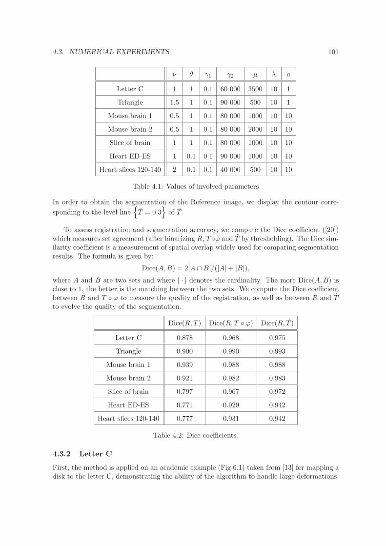
4.3. NUMERICAL EXPERIMENTS 101
ν θ γ1 γ2 µ λ a
Letter C 1 1 0.1 60 000 3500 10 1
Triangle 1.5 1 0.1 90 000 500 10 1
Mouse brain 1 0.5 1 0.1 80 000 1000 10 10
Mouse brain 2 0.5 1 0.1 80 000 2000 10 10
Slice of brain 1 1 0.1 80 000 1000 10 10
Heart ED-ES 1 0.1 0.1 90 000 1000 10 10
Heart slices 120-140 2 0.1 0.1 40 000 500 10 10
Table 4.1: Values of involved parameters
In order to obtain the segmentation of the Reference image, we display the contour corre-
sponding to the level lineT = 0.3
of T .
To assess registration and segmentation accuracy, we compute the Dice coefficient ([20])which measures set agreement (after binarizing R, T ϕ and T by thresholding). The Dice sim-ilarity coefficient is a measurement of spatial overlap widely used for comparing segmentationresults. The formula is given by:
Dice(A,B) = 2|A ∩B|/(|A|+ |B|),where A and B are two sets and where | · | denotes the cardinality. The more Dice(A,B) isclose to 1, the better is the matching between the two sets. We compute the Dice coefficientbetween R and T ϕ to measure the quality of the registration, as well as between R and Tto evolve the quality of the segmentation.
Dice(R, T ) Dice(R, T ϕ) Dice(R, T )
Letter C 0.878 0.968 0.975
Triangle 0.900 0.990 0.993
Mouse brain 1 0.939 0.988 0.988
Mouse brain 2 0.921 0.982 0.983
Slice of brain 0.797 0.967 0.972
Heart ED-ES 0.771 0.929 0.942
Heart slices 120-140 0.777 0.931 0.942
Table 4.2: Dice coefficients.
4.3.2 Letter C
First, the method is applied on an academic example (Fig 6.1) taken from [13] for mapping adisk to the letter C, demonstrating the ability of the algorithm to handle large deformations.
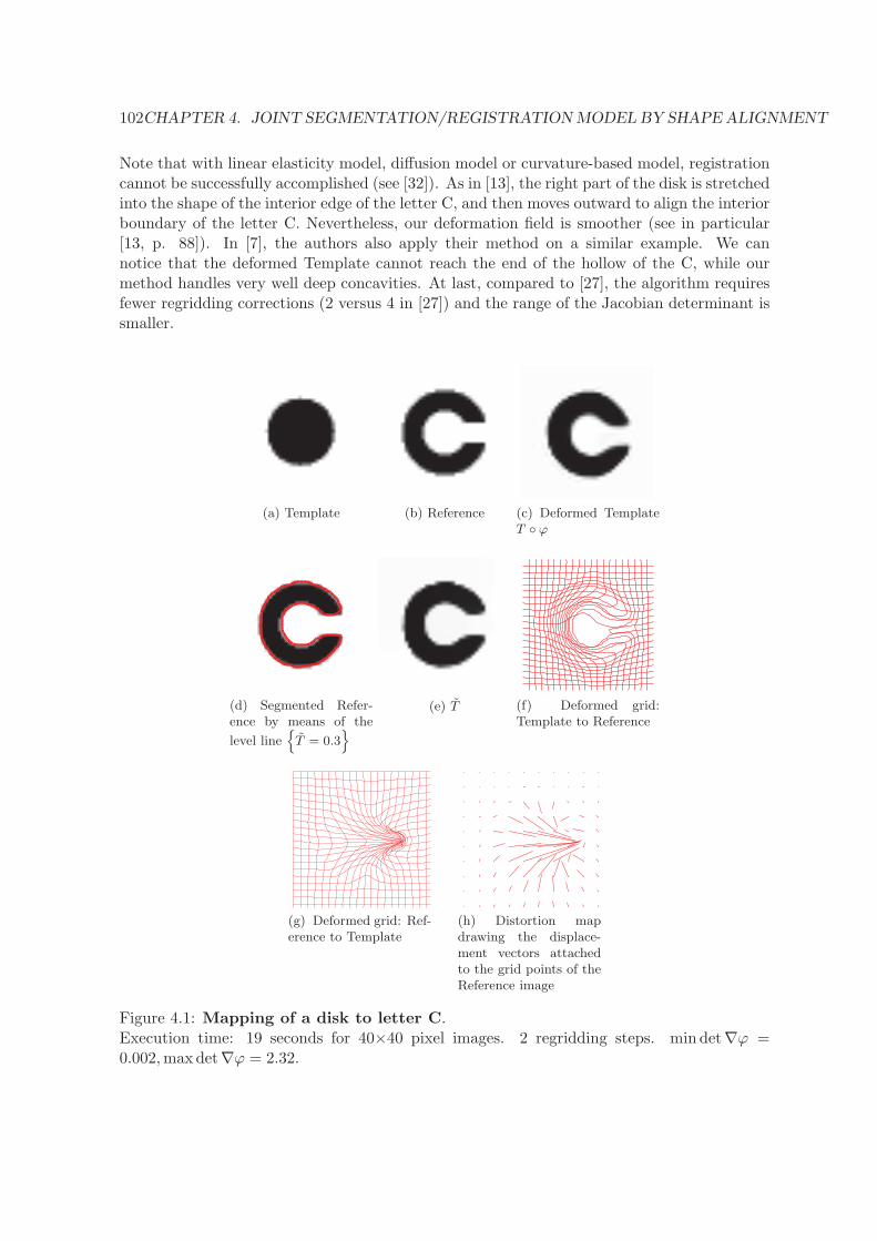
102CHAPTER 4. JOINT SEGMENTATION/REGISTRATIONMODEL BY SHAPE ALIGNMENT
Note that with linear elasticity model, diffusion model or curvature-based model, registrationcannot be successfully accomplished (see [32]). As in [13], the right part of the disk is stretchedinto the shape of the interior edge of the letter C, and then moves outward to align the interiorboundary of the letter C. Nevertheless, our deformation field is smoother (see in particular[13, p. 88]). In [7], the authors also apply their method on a similar example. We cannotice that the deformed Template cannot reach the end of the hollow of the C, while ourmethod handles very well deep concavities. At last, compared to [27], the algorithm requiresfewer regridding corrections (2 versus 4 in [27]) and the range of the Jacobian determinant issmaller.
(a) Template (b) Reference (c) Deformed TemplateT ϕ
(d) Segmented Refer-ence by means of the
level line
T = 0.3
(e) T (f) Deformed grid:Template to Reference
(g) Deformed grid: Ref-erence to Template
(h) Distortion mapdrawing the displace-ment vectors attachedto the grid points of theReference image
Figure 4.1: Mapping of a disk to letter C.Execution time: 19 seconds for 40×40 pixel images. 2 regridding steps. min det∇ϕ =0.002,maxdet∇ϕ = 2.32.
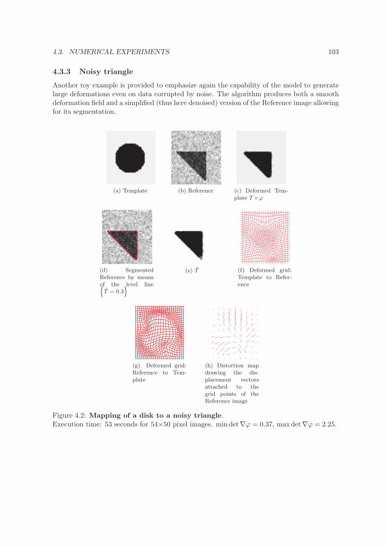
4.3. NUMERICAL EXPERIMENTS 103
4.3.3 Noisy triangle
Another toy example is provided to emphasize again the capability of the model to generatelarge deformations even on data corrupted by noise. The algorithm produces both a smoothdeformation field and a simplified (thus here denoised) version of the Reference image allowingfor its segmentation.
(a) Template (b) Reference (c) Deformed Tem-plate T ϕ
(d) SegmentedReference by meansof the level line
T = 0.3
(e) T (f) Deformed grid:Template to Refer-ence
(g) Deformed grid:Reference to Tem-plate
(h) Distortion mapdrawing the dis-placement vectorsattached to thegrid points of theReference image
Figure 4.2: Mapping of a disk to a noisy triangle.Execution time: 53 seconds for 54×50 pixel images. min det∇ϕ = 0.37, max det∇ϕ = 2.25.
104CHAPTER 4. JOINT SEGMENTATION/REGISTRATIONMODEL BY SHAPE ALIGNMENT
4.3.4 Mouse brain gene expression data
Then the method was applied on medical images (Figs 6.3, 6.4) with the goal to map a2D slice of mouse brain gene expression data (Template T) to its corresponding 2D slice ofthe mouse brain atlas, in order to facilitate the integration of anatomic, genetic and physi-ologic observations from multiple subjects in a common space. Since genetic mutations andknock-out strains of mice provide critical models for a variety of human diseases, such linkagebetween genetic information and anatomical structure is important. The data are providedby the Center for Computational Biology, UCLA. The mouse atlas acquired from the LONIdatabase was pre-segmented. The gene expression data were segmented manually to facilitatedata processing in other applications. Some algorithms have been developed to automaticallysegment the brain area of gene expression data. The non-brain regions have been removed toproduce better matching. Our method qualitatively performs as the one in [28] and producesa smooth deformation field but also provides both a simplified version of the Reference imageand its segmentation. In order to assess the closeness of V and ∇ϕ and to underline thatwe have indeed a good match between these two variables, we display their components inFig. 4.4 and Fig. 4.6. Compared to the results obtained in [27], [28] or [19], the deformationgrid is more regular and does not exhibit shrinkage or growth. For Fig. 6.3, the Jacobiandeterminants mass around the value 1 (range [0.63,1.28]) versus [0.28,2.09] in [27], [0.15,2.40]in [28] or [0.09,2.47] in [19]. The same remark can be done for Fig. 6.4: the Jacobian deter-minants remain close to 1 (range [0.68, 1.42]) versus [0.03,3.48] in [27], [0.18,3.23] in [28] or[0.01,2.18] in [19]. At last, contrary to [27], no regridding correction is required.

4.3. NUMERICAL EXPERIMENTS 105
(a) Template (b) Reference (c) Deformed Template T ϕ
(d) Segmented Referenceby means of the level line
T = 0.3
(e) T
(f) Deformed grid : Templateto Reference
(g) Deformed grid: Referenceto Template
(h) Distortion map drawingthe displacement vectors at-tached to the grid points ofthe Reference image
Figure 4.3: Mapping of a 2D slice of mouse brain gene expression data to itscounterpart in an atlas.Execution time: 5 minutes for 200×200 pixel images. min det∇ϕ = 0.63, max det∇ϕ = 1.28.
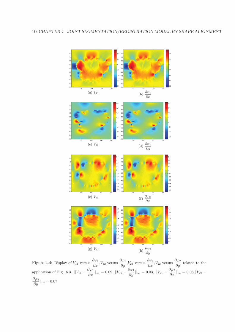
106CHAPTER 4. JOINT SEGMENTATION/REGISTRATIONMODEL BY SHAPE ALIGNMENT
(a) V11 (b)∂ϕ1
∂x
(c) V12 (d)∂ϕ1
∂y
(e) V21 (f)∂ϕ2
∂x
(g) V22 (h)∂ϕ2
∂y
Figure 4.4: Display of V11 versus∂ϕ1
∂x,V12 versus
∂ϕ1
∂y,V21 versus
∂ϕ2
∂x,V22 versus
∂ϕ2
∂yrelated to the
application of Fig. 6.3. ‖V11 −∂ϕ1
∂x‖∞ = 0.09, ‖V12 −
∂ϕ1
∂y‖∞ = 0.03, ‖V21 −
∂ϕ2
∂x‖∞ = 0.06,‖V22 −
∂ϕ2
∂y‖∞ = 0.07
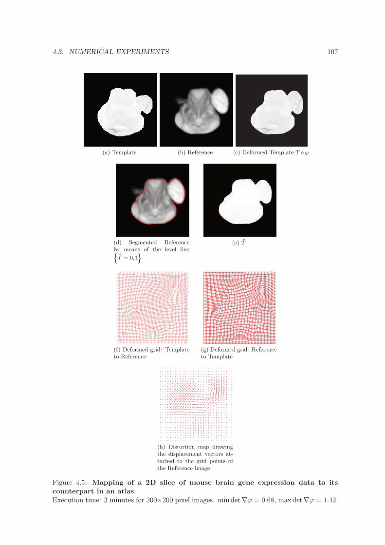
4.3. NUMERICAL EXPERIMENTS 107
(a) Template (b) Reference (c) Deformed Template T ϕ
(d) Segmented Referenceby means of the level line
T = 0.3
(e) T
(f) Deformed grid: Templateto Reference
(g) Deformed grid: Referenceto Template
(h) Distortion map drawingthe displacement vectors at-tached to the grid points ofthe Reference image
Figure 4.5: Mapping of a 2D slice of mouse brain gene expression data to itscounterpart in an atlas.Execution time: 3 minutes for 200×200 pixel images. min det∇ϕ = 0.68, max det∇ϕ = 1.42.
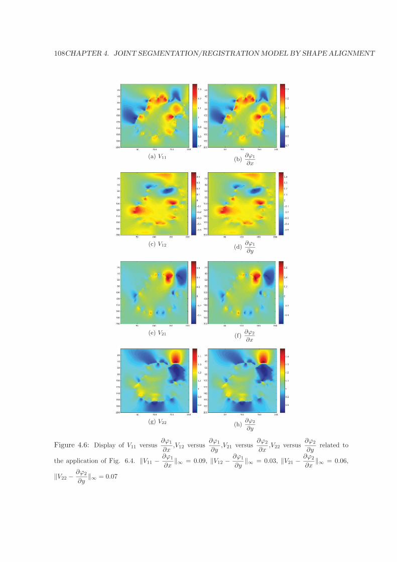
108CHAPTER 4. JOINT SEGMENTATION/REGISTRATIONMODEL BY SHAPE ALIGNMENT
(a) V11 (b)∂ϕ1
∂x
(c) V12 (d)∂ϕ1
∂y
(e) V21 (f)∂ϕ2
∂x
(g) V22 (h)∂ϕ2
∂y
Figure 4.6: Display of V11 versus∂ϕ1
∂x,V12 versus
∂ϕ1
∂y,V21 versus
∂ϕ2
∂x,V22 versus
∂ϕ2
∂yrelated to
the application of Fig. 6.4. ‖V11 − ∂ϕ1
∂x‖∞ = 0.09, ‖V12 − ∂ϕ1
∂y‖∞ = 0.03, ‖V21 − ∂ϕ2
∂x‖∞ = 0.06,
‖V22 −∂ϕ2
∂y‖∞ = 0.07
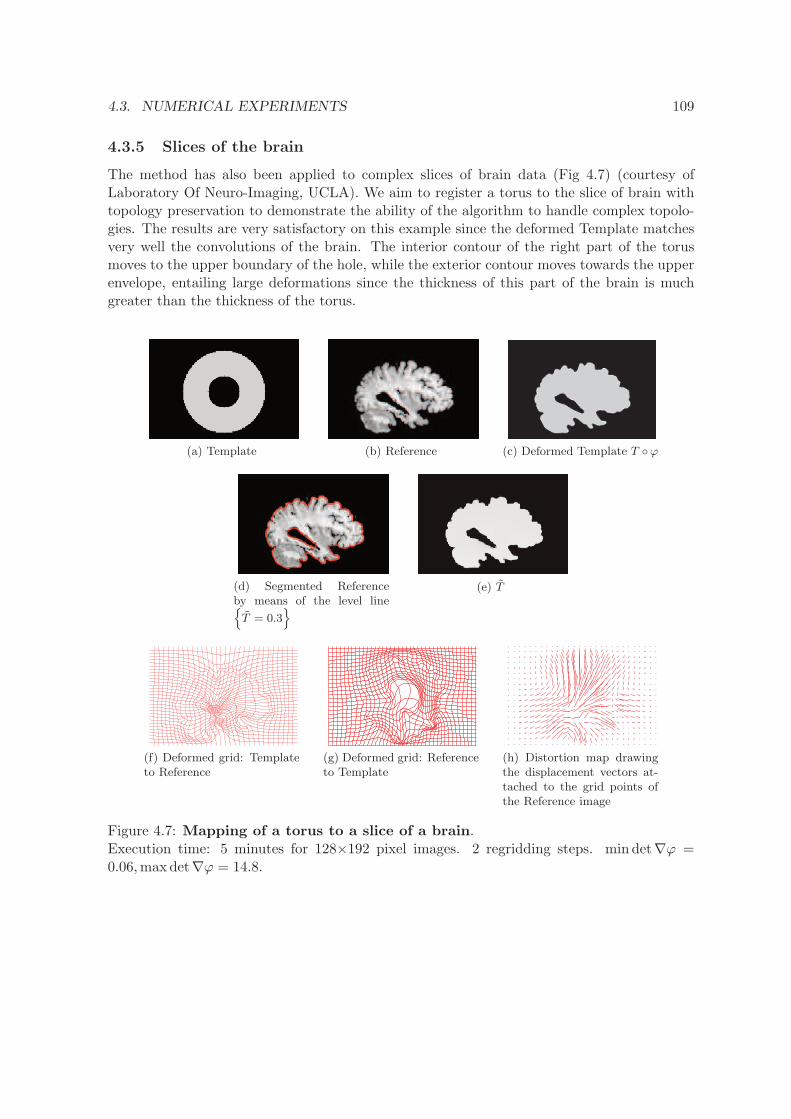
4.3. NUMERICAL EXPERIMENTS 109
4.3.5 Slices of the brain
The method has also been applied to complex slices of brain data (Fig 4.7) (courtesy ofLaboratory Of Neuro-Imaging, UCLA). We aim to register a torus to the slice of brain withtopology preservation to demonstrate the ability of the algorithm to handle complex topolo-gies. The results are very satisfactory on this example since the deformed Template matchesvery well the convolutions of the brain. The interior contour of the right part of the torusmoves to the upper boundary of the hole, while the exterior contour moves towards the upperenvelope, entailing large deformations since the thickness of this part of the brain is muchgreater than the thickness of the torus.
(a) Template (b) Reference (c) Deformed Template T ϕ
(d) Segmented Referenceby means of the level line
T = 0.3
(e) T
(f) Deformed grid: Templateto Reference
(g) Deformed grid: Referenceto Template
(h) Distortion map drawingthe displacement vectors at-tached to the grid points ofthe Reference image
Figure 4.7: Mapping of a torus to a slice of a brain.Execution time: 5 minutes for 128×192 pixel images. 2 regridding steps. min det∇ϕ =0.06,maxdet∇ϕ = 14.8.
110CHAPTER 4. JOINT SEGMENTATION/REGISTRATIONMODEL BY SHAPE ALIGNMENT
4.3.6 MRI images of cardiac cycle
Finally, numerical simulations on MRI images of a patient cardiac cycle have been carried out.We were supplied with a whole cardiac MRI examination of a patient (courtesy of the LITIS,University of Rouen, France). It is made of 280 images divided into 14 levels of slice and20 images per cardiac cycle. The numbering of the images goes from 0 to 279, and includesboth the slice number and the time index. The image 0 is set at the upper part of the heartand the sequence from image 0 to image 19 contains the whole cardiac cycle for this slice.The sequence from images 20 to 39 contains the whole cardiac cycle for the slice underneaththe previous one and so on. A cardiac cycle is composed of a contraction phase (40% of thecycle duration), followed by a dilation phase (60% of the cycle duration). The first image ofthe sequence (frames 0, 20, 40, etc.) is when the heart is most dilated (end diastole - ED)and the 8th of the sequence (end systole - ES) is when the heart is most contracted. It thusseemed relevant, in order to assess the accuracy of the proposed algorithm in handling largedeformations, to register a pair of the type: Reference corresponding to end diastole (ED),that is the first image of a sequence, and Template corresponding to end systole (ES), thatis the 8th frame of the same sequence. Besides, due to the patient’s breathing, images from aslice to another are not stackable (whereas they should be) so we also registered pairs of theform 120-140, that thus correspond to two images taken when the heart is most dilated butat different levels of slice.We provide extra numerical results on the webpage http://lmi.insa-rouen.fr/31.html
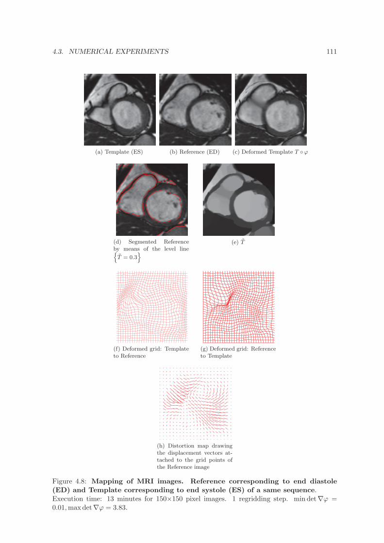
4.3. NUMERICAL EXPERIMENTS 111
(a) Template (ES) (b) Reference (ED) (c) Deformed Template T ϕ
(d) Segmented Referenceby means of the level line
T = 0.3
(e) T
(f) Deformed grid: Templateto Reference
(g) Deformed grid: Referenceto Template
(h) Distortion map drawingthe displacement vectors at-tached to the grid points ofthe Reference image
Figure 4.8: Mapping of MRI images. Reference corresponding to end diastole(ED) and Template corresponding to end systole (ES) of a same sequence.Execution time: 13 minutes for 150×150 pixel images. 1 regridding step. min det∇ϕ =0.01,maxdet∇ϕ = 3.83.
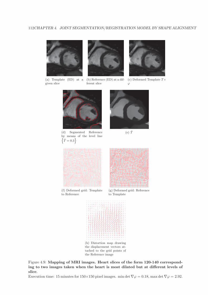
112CHAPTER 4. JOINT SEGMENTATION/REGISTRATIONMODEL BY SHAPE ALIGNMENT
(a) Template (ED) at agiven slice
(b) Reference (ED) at a dif-ferent slice
(c) Deformed Template T
ϕ
(d) Segmented Referenceby means of the level line
T = 0.3
(e) T
(f) Deformed grid: Templateto Reference
(g) Deformed grid: Referenceto Template
(h) Distortion map drawingthe displacement vectors at-tached to the grid points ofthe Reference image
Figure 4.9: Mapping of MRI images. Heart slices of the form 120-140 correspond-ing to two images taken when the heart is most dilated but at different levels ofslice.Execution time: 15 minutes for 150×150 pixel images. min det∇ϕ = 0.18, max det∇ϕ = 2.92.
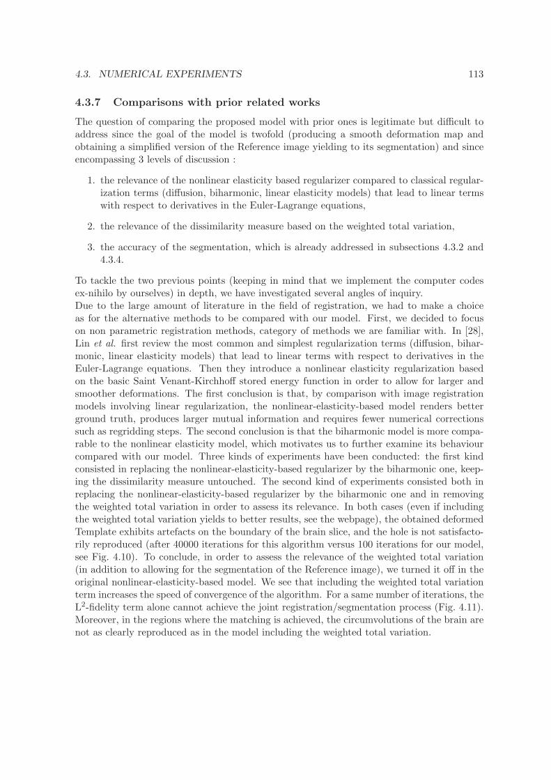
4.3. NUMERICAL EXPERIMENTS 113
4.3.7 Comparisons with prior related works
The question of comparing the proposed model with prior ones is legitimate but difficult toaddress since the goal of the model is twofold (producing a smooth deformation map andobtaining a simplified version of the Reference image yielding to its segmentation) and sinceencompassing 3 levels of discussion :
1. the relevance of the nonlinear elasticity based regularizer compared to classical regular-ization terms (diffusion, biharmonic, linear elasticity models) that lead to linear termswith respect to derivatives in the Euler-Lagrange equations,
2. the relevance of the dissimilarity measure based on the weighted total variation,
3. the accuracy of the segmentation, which is already addressed in subsections 4.3.2 and4.3.4.
To tackle the two previous points (keeping in mind that we implement the computer codesex-nihilo by ourselves) in depth, we have investigated several angles of inquiry.Due to the large amount of literature in the field of registration, we had to make a choiceas for the alternative methods to be compared with our model. First, we decided to focuson non parametric registration methods, category of methods we are familiar with. In [28],Lin et al. first review the most common and simplest regularization terms (diffusion, bihar-monic, linear elasticity models) that lead to linear terms with respect to derivatives in theEuler-Lagrange equations. Then they introduce a nonlinear elasticity regularization basedon the basic Saint Venant-Kirchhoff stored energy function in order to allow for larger andsmoother deformations. The first conclusion is that, by comparison with image registrationmodels involving linear regularization, the nonlinear-elasticity-based model renders betterground truth, produces larger mutual information and requires fewer numerical correctionssuch as regridding steps. The second conclusion is that the biharmonic model is more compa-rable to the nonlinear elasticity model, which motivates us to further examine its behaviourcompared with our model. Three kinds of experiments have been conducted: the first kindconsisted in replacing the nonlinear-elasticity-based regularizer by the biharmonic one, keep-ing the dissimilarity measure untouched. The second kind of experiments consisted both inreplacing the nonlinear-elasticity-based regularizer by the biharmonic one and in removingthe weighted total variation in order to assess its relevance. In both cases (even if includingthe weighted total variation yields to better results, see the webpage), the obtained deformedTemplate exhibits artefacts on the boundary of the brain slice, and the hole is not satisfacto-rily reproduced (after 40000 iterations for this algorithm versus 100 iterations for our model,see Fig. 4.10). To conclude, in order to assess the relevance of the weighted total variation(in addition to allowing for the segmentation of the Reference image), we turned it off in theoriginal nonlinear-elasticity-based model. We see that including the weighted total variationterm increases the speed of convergence of the algorithm. For a same number of iterations, theL2-fidelity term alone cannot achieve the joint registration/segmentation process (Fig. 4.11).Moreover, in the regions where the matching is achieved, the circumvolutions of the brain arenot as clearly reproduced as in the model including the weighted total variation.
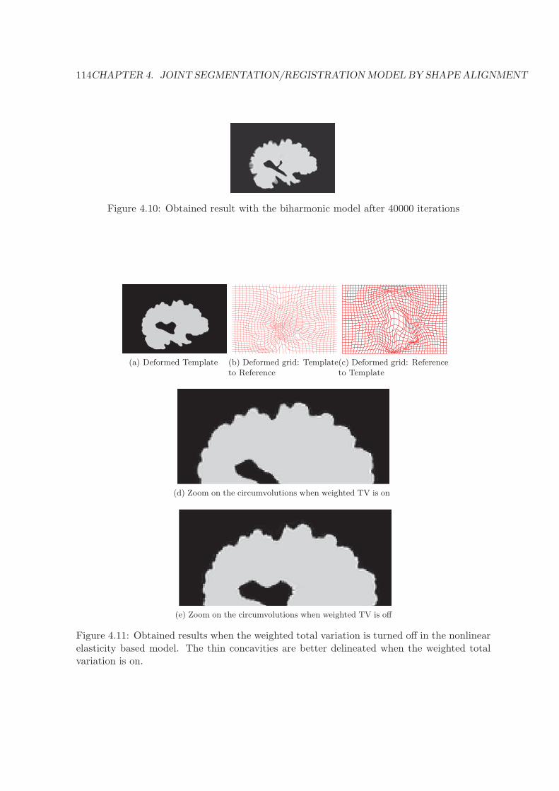
114CHAPTER 4. JOINT SEGMENTATION/REGISTRATIONMODEL BY SHAPE ALIGNMENT
Figure 4.10: Obtained result with the biharmonic model after 40000 iterations
(a) Deformed Template (b) Deformed grid: Templateto Reference
(c) Deformed grid: Referenceto Template
(d) Zoom on the circumvolutions when weighted TV is on
(e) Zoom on the circumvolutions when weighted TV is off
Figure 4.11: Obtained results when the weighted total variation is turned off in the nonlinearelasticity based model. The thin concavities are better delineated when the weighted totalvariation is on.
4.3. NUMERICAL EXPERIMENTS 115
Remark 4.3.1
Two alternative models have been experimented and give similar results. These are anal-ogously built on Bresson et al.’s ones in [6]. The first one consists in minimizing thefollowing functional :
G(T , V ) = ν
∫
Ω|T −R|dx+ varg(T ) +
∫
ΩQW (V )dx
subjected to ‖T − T ϕ‖2L2(Ω) ≤ ε,
‖∇ϕ− V ‖2L2(Ω,M2)≤ ε,
(4.15)
(4.16)
with the idea to let ε tend to 0. The second one, also based on [6], employs Chan-Vesesegmentation principles:
H(T , V ) = ν
∫
Ω
((c1 −R)2 − (c2 −R)2
)T dx+ varg(T ) +
∫
ΩQW (V )dx
subjected to ‖T − T ϕ‖L1(Ω) ≤ ε,
‖∇ϕ− V ‖2L2(Ω,M2)≤ ε,
where c1 =
∫ΩR(x)H(T )∫
ΩH(T )and c2 =
∫ΩR(x)(1−H(T ))∫
Ω(1−H(T )).
(4.17)
(4.18)
This is still a work in progress.
Conclusion
We therefore have designed functionals for image joint registration/segmentation problem,not only based on intensity differences but also on weighted total variation in order to favorshape alignment rather than intensity matching. Moreover, we overcome the obstacle ofnon quasiconvexity of the stored energy function of Saint Venant-Kirchhoff using a relaxedproblem associated with the original one. Then we provide theoretical results as existence ofminimizers for the relaxed problem and equality of the two infima under certain conditions.Also a Γ-convergence result for the decoupled problem is established.Our future work consists in extending the problem to the 3D case, using the formulation ofthe Saint Venant-Kirchhoff stored function in terms of the singular values of ∇ϕ and a finiteelement approach for the numerical discretization as done by Le Dret in [26].
Acknowledgment: We would like to thank Dr. Caroline Petitjean (LITIS, Universite deRouen, France) for providing us with the cardiac cycle MRI images. Her help has been muchappreciated and has been decisive.

BIBLIOGRAPHY
[1] L. Ambrosio and G. Dal Maso, A general chain rule for distributional derivatives,Proceedings of the American Mathematical Society, 108 (1990), pp. 691–702.
[2] A. Baldi, Weighted BV functions, Houston Journal of Mathematics, 27 (2001), pp. 683–705.
[3] M. Beg, M. Miller, A. Trouve, and L. Younes, Computing Large DeformationMetric Mappings via Geodesic Flows of Diffeomorphisms, International Journal of Com-puter Vision, 61 (2005), pp. 139–157.
[4] G. Bellettini, G. Bouchitte, and I. Fragala, Bv functions with respect to a mea-sure and relaxation of metric integral functionals, Journal of convex analysis, 6 (1999),pp. 349–366.
[5] M. Bousselsal, Etude de Quelques Problemes de Calcul des Variations Lies a laMecanique, PhD thesis, University of Metz, France, 1993.
[6] X. Bresson, S. Esedoglu, P. Vandergheynst, J.-P. Thiran, and S. Osher,Fast Global Minimization of the Active Contour/Snake Model, J. Math. Imaging Vis., 68(2007), pp. 151–167.
[7] M. Burger, J. Modersitzki, and L. Ruthotto, A hyperelastic regularization energyfor image registration, SIAM Journal on Scientific Computing, 35 (2013), pp. B132–B148.
[8] V. Caselles, R. Kimmel, and G. Sapiro, Geodesic Active Contours, Int. J. Comput.Vis., 22 (1993), pp. 61–87.
[9] A. Chambolle, An algorithm for total variation minimization and applications, J.Math. Imaging Vis., 20 (2004), pp. 89–97.
[10] T. Chan, S. Esedoglu, and M. Nikolova, Algorithms for finding global minimizersof image segmentation and denoising models, SIAM J. Appl. Math., 66 (2006), pp. 1632–1648.
[11] T. Chan and L. Vese, Active Contours Without Edges, IEEE Trans. Image Process.,10 (2001), pp. 266–277.
117
118 BIBLIOGRAPHY
[12] G. Christensen, R. Rabbitt, and M. Miller, Deformable Templates Using LargeDeformation Kinematics, IEEE Trans. Image Process., 5 (1996), pp. 1435–1447.
[13] G. E. Christensen, Deformable shape models for anatomy, PhD thesis, WashingtonUniversity, Sever Institute of technology, USA, 1994.
[14] H. Chui and A. Rangarajan, A new point matching algorithm for non-rigid registra-tion, Computer Vision and Image Understanding, 89 (2003), pp. 114–141.
[15] P. Ciarlet, Elasticite Tridimensionnelle, Masson, 1985.
[16] , Mathematical Elasticity, Volume I: Three-dimensional elasticity, Amsterdam etc.,North-Holland, 1988.
[17] B. Dacorogna, Direct Methods in the Calculus of Variations, Second Edition, Springer,2008.
[18] F. Demengel and G. Demengel, Functional Spaces for the Theory of Elliptic PartialDifferential Equations, Springer, 2012.
[19] R. Derfoul and C. Le Guyader, A relaxed problem of registration based on the SaintVenant-Kirchhoff material stored energy for the mapping of mouse brain gene expressiondata to a neuroanatomical mouse atlas, SIAM Journal on Imaging Sciences, 7 (2014),pp. 2175–2195.
[20] L. R. Dice, Measures of the Amount of Ecologic Association Between Species, Ecology,26 (1945), pp. 297–302.
[21] M. Droske and M. Rumpf, A Variational Approach to Non-Rigid Morphological Reg-istration, SIAM J. Appl. Math., 64 (2004), pp. 668–687.
[22] J. Duran, B. Coll, and C. Sbert, Chambolle’s projection algorithm for total variationdenoising, Image Processing On Line, 2013 (2013), pp. 311–331.
[23] A. Gooya, K. Pohl, M. Bilello, L. Cirillo, G. Biros, E. Melhem, and C. Da-
vatzikos, GLISTR: Glioma Image Segmentation and Registration, Medical Imaging,IEEE Transactions on, 31 (2012), pp. 1941–1954.
[24] E. Haber, S. Heldmann, and J. Modersitzki, A computational framework forimage-based constrained registration, Linear Algebra and its Applications, 431 (2009),pp. 459–470. Special Issue in honor of Henk van der Vorst.
[25] N. Kerdid, H. Le Dret, and A. Saıdi, Numerical approximation for a non-linearmembrane problem, International Journal of Non-Linear Mechanics, 43 (2008), pp. 908–914.
[26] H. Le Dret and A. Raoult, The quasi-convex envelope of the Saint Venant-Kirchhoffstored energy function., Proceedings of the Royal Society of Edinburgh: Section A Math-ematics, 125 (1995), pp. 1179–1192.
[27] C. Le Guyader and L. Vese, A combined segmentation and registration frameworkwith a nonlinear elasticity smoother, Computer Vision and Image Understanding, 115(2011), pp. 1689–1709.
BIBLIOGRAPHY 119
[28] T. Lin, C. Le Guyader, I. Dinov, P. Thompson, A. Toga, and L. Vese, GeneExpression Data to Mouse Atlas Registration Using a Nonlinear Elasticity Smoother andLandmark Points Constraints, J. Sci. Comput., 50 (2012), pp. 586–609.
[29] N. Lord, J. Ho, B. Vemuri, and S. Eisenschenk, Simultaneous Registration andParcellation of Bilateral Hippocampal Surface Pairs for Local Asymmetry Quantification,IEEE Trans. Med. Imaging, 26 (2007), pp. 471–478.
[30] M. Miller, A. Trouve, and L. Younes, On the Metrics and Euler-Lagrange Equa-tions of Computational Anatomy, Annu. Rev. B. Eng., 4 (2002), pp. 375–405.
[31] M. I. Miller and L. Younes, Group actions, homeomorphisms, and matching: Ageneral framework, International Journal of Computer Vision, 41 (2001), pp. 61–84.
[32] J. Modersitzki, Numerical Methods for Image Registration, Oxford University Press,2004.
[33] , FAIR: Flexible Algorithms for Image Registration, Society for Industrial and Ap-plied Mathematics (SIAM), 2009.
[34] P. Negron Marrero, A numerical method for detecting singular minimizers of multidi-mensional problems in nonlinear elasticity, Numerische Mathematik, 58 (1990), pp. 135–144.
[35] S. Ozere and C. Le Guyader, Topology preservation for image-registration-relateddeformation fields, Communications in Mathematical Sciences, 13 (2015), pp. 1135–1161.
[36] R. Rabbitt, J. Weiss, G. Christensen, and M. Miller, Mapping of HyperelasticDeformable Templates Using the Finite Element Method, in Proceedings SPIE, vol. 2573,SPIE, 1995, pp. 252–265.
[37] A. Raoult, Non-polyconvexity of the stored energy function of a Saint Venant-Kirchhoffmaterial, Aplikace Matematiky, 31 (1986), pp. 417–419.
[38] L. Rudin, S. Osher, and E. Fatemi, Nonlinear Total Variation Based Noise RemovalAlgorithms, Phys. D, 60 (1992), pp. 259–268.
[39] D. Shen and C. Davatzikos, HAMMER: hierarchical attribute matching mechanismfor elastic registration, Medical Imaging, IEEE Transactions on, 21 (2002), pp. 1421–1439.
[40] A. Sotiras, C. Davatzikos, and N. Paragios, Deformable medical image registra-tion: A survey, Medical Imaging, IEEE Transactions on, 32 (2013), pp. 1153–1190.
[41] T. W. Tang and A. C. Chung, Non-rigid image registration using graph-cuts, inMedical Image Computing and Computer-Assisted Intervention–MICCAI 2007, Springer,2007, pp. 916–924.
[42] B. Vemuri, J. Ye, Y. Chen, and C. Leonard, Image Registration via level-setmotion: Applications to atlas-based segmentation, Medical Image Analysis, 7 (2003),pp. 1–20.

120 BIBLIOGRAPHY
[43] F. Wang, B. C. Vemuri, A. Rangarajan, and S. J. Eisenschenk, Simultaneousnonrigid registration of multiple point sets and atlas construction, Pattern Analysis andMachine Intelligence, IEEE Transactions on, 30 (2008), pp. 2011–2022.
[44] W. M. Wells, P. Viola, H. Atsumi, S. Nakajima, and R. Kikinis, Multi-modalvolume registration by maximization of mutual information, Medical image analysis, 1(1996), pp. 35–51.
[45] A. Yezzi, L. Zollei, and T. Kapur, A variational framework for joint segmenta-tion and registration, in Mathematical Methods in Biomedical Image Analysis, IEEE-MMBIA, 2001, pp. 44–51.
CHAPTER 5
NONLOCAL JOINT SEGMENTATION REGISTRATION MODEL
In this chapter, we address the issue of designing a theoretically well-motivated joint segmentation-registration method capable of handling large deformations. The shapes to be matched areimplicitly modeled by level set functions and are evolved in order to minimize a functionalcontaining both a nonlinear-elasticity-based regularizer and a criterion that forces the evolv-ing shape to match intermediate topology-preserving segmentation results.
The chapter is organized as follows. First, we present the mathematical modelling and weintroduce the nonlinear-elasticity-based regularizer. Then we are concerned with the designof the fidelity term inspired by a topology-preserving segmentation model. Next, we proceedwith the study of theoretical results encompassing existence of minimizers, a Γ-convergenceresult and the existence of a weak viscosity solution of the related evolution problem. Finally,we provide a discretization method and implementation details as well as some numericalresults.
Introduction
Image segmentation aims to partition a given image into meaningful constituents or to findboundaries delineating such objects (see [1, Chapter 4] for instance, for a relevant analysis ofthis problem), while registration, given two images called Template and Reference, consistsin determining a smooth deformation field ϕ such that the deformed Template is aligned withthe Reference. According to the modalities of the involved images, the goal of registrationmight differ: for images of the same modality, the purpose of registration is to match thegeometrical features, the shapes and the intensity level distribution of the Reference withthose of the Template. When the images have been acquired through different mechanismsand have different modalities, registration aims to correlate both images in terms of shapesand salient components, while preserving the modality of the Template image. In this paper,instead of considering these two tasks, segmentation and registration, as independent ones,we propose to jointly treat them: the segmentation result obtained at intermediate steps willserve as a target to reach in the registration process and will guide it. The scope of theproposed work is thus first to devise a theoretically well-motivated registration model in avariational formulation, authorizing large and smooth deformations. In particular, classical
121
122 CHAPTER 5. NONLOCAL JOINT SEGMENTATION REGISTRATION MODEL
regularizers such as linear elasticity (see [6]) are not suitable for this kind of problems involvinglarge deformations since assuming small strains and the validity of Hooke’s law. In addition,to handle a large class of images, we propose defining a geometric dissimilarity measure basedon shape comparisons thanks to successive segmentation results that will serve as inputsin our registration model. Thus the algorithm produces both a smooth mapping betweenthe two shapes as well as a segmentation of the Reference image. The idea of combiningsegmentation and registration is not new. Prior related works suggest to take advantage ofboth processes: in [28], a curve evolution approach is used and phrased in terms of level setfunctions. In [26], Vemuri et al. propose a coupled PDE model to perform both segmentationand registration. In the first PDE, the level sets of the source image are evolved along theirnormals with a speed defined as the difference between the target and the evolving sourceimage. In [18], the model combines a matching criterion based on the active contours withoutedges ([9]) and a nonlinear-elasticity-based regularizer. In [19], Lord et al. propose a unifiedmethod that simultaneously treats segmentation and registration based on metric structurecomparisons. In [15], Droske et al. aim to match the edges and the normals of the twoimages by applying a Mumford-Shah type free discontinuity problem. More recently, Ozereet al. ([22]) have introduced a variational joint segmentation/registration model combininga measure of dissimilarity based on weighted total variation and a regularizer based on thestored energy function of a Saint Venant-Kirchhoff material.
5.1 Mathematical Modelling
Making the same assumptions as those in the previous chapters, let us denote by:
• Ω a connected bounded open subset of R2 with Lipschitz boundary ∂Ω,
• R : Ω −→ R, representing the Reference image,
• T : Ω −→ R, the Template image assumed to be compactly supported and Lipschitzcontinuous (we denote by kT the Lipschitz constant),
• ϕ : Ω −→ R2 the sought deformation with prescribed values on the boundary: ϕ = Id
on ∂Ω.
The shape contained in the Template image is supposed to be modeled by a Lipschitz con-tinuous function Φ0 whose zero level line is the shape boundary. Denoting by C the zero levelset of Φ0 and by w ⊂ Ω the open set it delineates, Φ0 is chosen such that
C = x ∈ Ω |Φ0(x) = 0 ,w = x ∈ Ω |Φ0(x) > 0 ,Ω \ w = x ∈ Ω |Φ0(x) < 0 .
For theoretical and numerical purposes, we may consider a linear extension operator (see [5,p. 158]) P : W1,∞(Ω) → W1,∞(R2) such that for all Φ ∈ W1,∞(Ω),
(i) PΦ|Ω = Φ,
(ii) ‖PΦ‖L∞(R2) ≤ C ‖Φ‖L∞(Ω),
(iii) ‖PΦ‖W1,∞(R2) ≤ C ‖Φ‖W1,∞(Ω), with C depending only on Ω.
5.1. MATHEMATICAL MODELLING 123
By this extension process, we consider then that Φ0 ∈ W1,∞(R2) to ensure that Φ0 ϕ – withϕ introduced later – is always defined.Let ϕ : Ω → R
2 be the sought deformation. A deformation is a smooth mapping that isorientation-preserving and injective, except possibly on ∂Ω. We also denote by u the associ-ated displacement such that ϕ = Id+u, Id denoting the identity mapping. The deformationgradient is ∇ϕ = I+∇u, Ω →M2(R), the set M2(R) being the set of all real square matricesof order 2 identified to R
4.The idea is thus to find a smooth deformation field ϕ such that the zero level line of Φ0ϕ givesa relevant partition of the Reference image R, relating then segmentation and registration.The model is phrased as a functional minimization problem with unknown ϕ; it combines asmoother on the deformation field, and a distance measure criterion between Φ0 ϕ and aninput resulting from the topology-preserving segmentation process of Le Guyader and Vese([17]).
In many applications, such as medical imaging, topology preservation is a desirable prop-erty: when the shape to be detected has a known topology (e.g. spherical topology for thebrain), or when the resulting shape must be homeomorphic to the initial one. In other words,an initial contour should be deformed without change of topology as merging or breaking.We expect this property to be inherited by the registration process. This measure constitutesan alternative to classical intensity-based/information-theoretic-based matching measures,mutual information – suitable when dealing with images that have been acquired throughdifferent sensors –, measures based on the comparison of gradient vector fields of both im-ages, metric structure comparisons, mass-preserving measures, etc. The proposed matchingcriterion is complemented by a nonlinear-elasticity-based regularizer on the deformation fieldϕ. To allow large and nonlinear deformations, we propose to view the shapes to be warped asisotropic, homogeneous, hyperelastic materials and more precisely as Saint Venant-Kirchhoffmaterials (see [11] for further details and [7] for an alternative hyperelastic model). A moti-vation for this choice is that the stored energy function of such materials is the simplest onethat agrees with the generic expression of the stored energy of an isotropic, homogeneous,hyperelastic material. To ensure that the distribution of the deformation Jacobian determi-nants does not exhibit shrinkages or growths, we propose complementing the model by a termcontrolling that the Jacobian determinant remains close to 1. At this stage, the consideredregularizer would be, setting F = ∇ϕ
W (F ) =WSV K(F ) + µ (detF − 1)2 ,
with WSV K(F ) =λ
2(trE)2 +µ trE2, the stored energy function of a Saint Venant-Kirchhoff
material, λ and µ the Lame coefficients, E =(F TF − I
)/2 the Green-Saint Venant stress
tensor measuring the deviation between ϕ and a rigid deformation, and with the followingnotation A : B = trATB, the matrix inner product and ‖A‖ =
√A : A the related matrix
norm (Frobenius norm).Nevertheless, the stored energy function W written as is exhibits undesirable properties:it is not rank-1 convex (as the density WSV K), and consequently neither quasiconvex, norpolyconvex, which raises a drawback of theoretical nature since we cannot obtain the weaklower semicontinuity of the introduced functional. The idea is thus to replace W by itsquasiconvex envelope QW (see [13] for a deeper presentation of these notions). In general,deriving the explicit expression of this envelope is an hopeless task, but in this case, using
124 CHAPTER 5. NONLOCAL JOINT SEGMENTATION REGISTRATION MODEL
Jensen’s inequality and a decomposition result by Bousselsal ([4]), one can establish that
QW (F ) =
∣∣∣∣W (F ) = β
(‖F‖2 − α
)2+ ψ(detF ) if ‖F‖2 ≥ α ,
ψ(detF ) if ‖F‖2 < α ,
with α = 2λ+ µ
λ+ 2µ, β =
λ+ 2µ
8and ψ the convex mapping defined by
ψ : t 7→ −µ2t2 + µ (t− 1)2 +
µ (λ+ µ)
2(λ+ 2µ).
Remark 5.1.1
In fact, we can prove a stronger result, namely, that the polyconvex envelope of W , PW ,coincides with the quasiconvex envelope of W : PW = QW .
Ultimately, we propose to consider the following minimization problem, with T > 0 fixed
inf
I(ϕ) =
∫
Ωf(x, ϕ(x),∇ϕ(x)) dx : ϕ ∈ Id +W1,4
0 (Ω,R2)
, (5.1)
with f(x, ϕ, ξ) =ν
2‖Φ0 ϕ − Φ(·, T )‖2 +QW (ξ) and Φ a solution of the evolution equation
stemming from the topology-preserving segmentation model by Le Guyader and Vese ([17])
∂Φ
∂t= |∇Φ|
[div
(g(|∇R|) ∇Φ
|∇Φ|
)]+ 4
µ′
d2H(Φ(x) + l)H(l − Φ(x))
∫
Ω
[〈x− y,∇Φ(y)〉 e−‖x−y‖22/d2H(Φ(y) + l)H(l − Φ(y))
]dy ,
Φ(x, 0) = Φ0(x) ,
∂Φ
∂~ν= 0, on ∂Ω .
(E)
Function g is an edge-detector function satisfying
(i) g(0) = 1,
(ii) g strictly decreasing,
(iii) limr→+∞
g(r) = 0.
This evolution equation results from the minimization of functional J(Φ) + µ′L(Φ) (µ′ > 0,
tuning parameter), combination of J(Φ) =
∫
Ωg(|∇R|)|DH(Φ)| coming from the classical
geodesic active contour model ([8]) (H being the one-dimensional Heaviside function) and L,related to the topological constraint:
L(Φ) = −∫
Ω
∫
Ω
[exp
(−‖x− y‖22
d2
)〈∇Φ(x),∇Φ(y)〉 H(Φ(x) + l)H(l − Φ(x))
H(Φ(y) + l)H(l − Φ(y))]dx dy. (5.2)
The Euclidean scalar product in R2 is denoted by 〈·, ·〉 and ‖ · ‖2 is the associated norm.
A geometrical observation motivates the introduction of L. Indeed, in the case when Φ is a
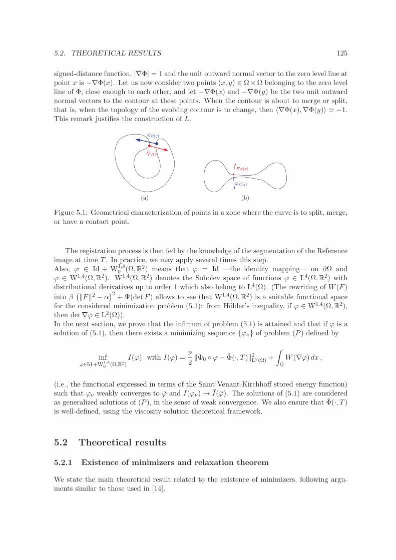
5.2. THEORETICAL RESULTS 125
signed-distance function, |∇Φ| = 1 and the unit outward normal vector to the zero level line atpoint x is −∇Φ(x). Let us now consider two points (x, y) ∈ Ω×Ω belonging to the zero levelline of Φ, close enough to each other, and let −∇Φ(x) and −∇Φ(y) be the two unit outwardnormal vectors to the contour at these points. When the contour is about to merge or split,that is, when the topology of the evolving contour is to change, then 〈∇Φ(x),∇Φ(y)〉 ≃ −1.This remark justifies the construction of L.
-
-
(a)
-
-
(b)
Figure 5.1: Geometrical characterization of points in a zone where the curve is to split, merge,or have a contact point.
The registration process is then fed by the knowledge of the segmentation of the Referenceimage at time T . In practice, we may apply several times this step.Also, ϕ ∈ Id + W1,4
0 (Ω,R2) means that ϕ = Id —the identity mapping— on ∂Ω andϕ ∈ W1,4(Ω,R2). W1,4(Ω,R2) denotes the Sobolev space of functions ϕ ∈ L4(Ω,R2) withdistributional derivatives up to order 1 which also belong to L4(Ω). (The rewriting of W (F )
into β(‖F‖2 − α
)2+ Ψ(detF ) allows to see that W1,4(Ω,R2) is a suitable functional space
for the considered minimization problem (5.1): from Holder’s inequality, if ϕ ∈ W1,4(Ω,R2),then det∇ϕ ∈ L2(Ω)).In the next section, we prove that the infimum of problem (5.1) is attained and that if ϕ is asolution of (5.1), then there exists a minimizing sequence ϕν of problem (P ) defined by
infϕ∈Id+W1,4
0 (Ω,R2)I(ϕ) with I(ϕ) =
ν
2‖Φ0 ϕ− Φ(·, T )‖2L2(Ω) +
∫
ΩW (∇ϕ) dx ,
(i.e., the functional expressed in terms of the Saint Venant-Kirchhoff stored energy function)such that ϕν weakly converges to ϕ and I(ϕν) → I(ϕ). The solutions of (5.1) are consideredas generalized solutions of (P ), in the sense of weak convergence. We also ensure that Φ(·, T )is well-defined, using the viscosity solution theoretical framework.
5.2 Theoretical results
5.2.1 Existence of minimizers and relaxation theorem
We state the main theoretical result related to the existence of minimizers, following argu-ments similar to those used in [14].
126 CHAPTER 5. NONLOCAL JOINT SEGMENTATION REGISTRATION MODEL
Theorem 5.2.1
The infimum of (5.1) is attained. Let then ϕ ∈ W1,4(Ω,R2) be a minimizer of therelaxed problem (5.1). Then there exists a sequence ϕν∞ν=1 ⊂ ϕ+W1,4
0 (Ω,R2) such thatϕν → ϕ in L4(Ω,R2) as ν → ∞ and I(ϕν) → I(ϕ) as ν → ∞. Moreover, the followingholds: ϕν ϕ in W1,4(Ω,R2) as ν → ∞.It means in particular that inf
ϕ∈Id+W1,40 (Ω,R2)
I(ϕ) = minϕ∈Id+W1,4
0 (Ω,R2)I(ϕ),
as QW ≤ W . The solutions of (5.1) are considered as generalized solutions of problem(P).
Proof : The proof is similar to the one of Theorem 6.1.8 in Chapter 6.
We now investigate the well-definedness of Φ(·, T ).
5.2.2 Well-definedness of Φ
Problem (E) is hard to handle from a theoretical point of view. A suitable setting would be theone of the viscosity solution theory ([12]) (owing to the nonlinearity induced by the modifiedmean curvature term), but the dependency of the nonlocal term on the gradient ∇Φ(y)and the failure to fulfill the monotony property in Φ make it difficult. For this reason, forthe theoretical part, we consider a slightly modified problem: we assume that the topologicalconstraint is only applied to the zero level line. Assuming that Φ is a signed-distance function,the topological constraint L is then rephrased as
L(Φ) = −∫
Ω
∫
Ω
[exp
(−‖x− y‖22
d2
)〈∇Φ(x),∇Φ(y)〉δ(Φ(x))δ(Φ(y))dx dy ,
with δ the Dirac measure.The evolution equation coming from the Euler-Lagrange equation associated to J(Φ)+µL(Φ)is computed. It can be formally obtained as follows: let us denote by Γ(ν) = J (ν) + µL(ν)with J (ν) = J(Φ + νΨ) and L(ν) = L(Φ + νΨ), ν being a small parameter and Ψ a functionlike Φ. A minimizer Φ will satisfy Γ′(0) = J ′(0) + µL′(0) = 0 for all functions Ψ.
We set G(x − y) = exp
(−‖x− y‖22
d2
)and h(∇Φ(x),∇Φ(y)) = −〈∇Φ(x),∇Φ(y)〉. We will
use the following notations h = h(z1, z2, z3, z4) and we will denote by ∇z1z2h = (hz1 , hz2)T
and ∇z3z4h = (hz3 , hz4)T .
L(ν) =∫
Ω
∫
ΩG(x− y)h
(∇Φ(x) + ν∇Ψ(x),∇Φ(y) + ν∇Ψ(y)
)
δ(Φ(x) + νΨ(x))δ(Φ(y) + νΨ(y)) dx dy.
5.2. THEORETICAL RESULTS 127
One has,
L′(0) =∫
Ω
∫
ΩG(x− y)h
(∇Φ(x),∇Φ(y)
)
(δ′(Φ(x))δ(Φ(y))Ψ(x) + δ′(Φ(y))δ(Φ(x))Ψ(y)
)dx dy
+
∫
Ω
∫
ΩG(x− y)δ(Φ(x))δ(Φ(y))
(〈∇z1z2h(∇Φ(x),∇Φ(y)),∇Ψ(x)〉+ 〈∇z3z4h(∇Φ(x),∇Φ(y)),∇Ψ(y)〉
)dx dy.
Switching x and y and assuming we can interchange the order of integration, we obtain
L′(0) =2
∫
Ω
∫
Ω
[G(x− y)h(∇Φ(x),∇Φ(y))δ′(Φ(x))δ(Φ(y))
]dy
Ψ(x) dx
+ 2
∫
Ω
∫
ΩG(x− y)δ(Φ(x))δ(Φ(y))〈∇z1z2h(∇Φ(x),∇Φ(y)),∇Ψ(x)〉 dx dy,
and integrating by parts and setting the necessary boundary conditions to zero,
L′(0) =2
∫
Ω
∫
Ω
[G(x− y)h(∇Φ(x),∇Φ(y))δ′(Φ(x))δ(Φ(y))
]dy
Ψ(x)dx
− 2
∫
Ω
∫
Ωdiv
(G(x− y)δ(Φ(x))δ(Φ(y))∇z1z2h(∇Φ(x),∇Φ(y))
)dy
Ψ(x)dx.
Finally, we obtain the following Euler-Lagrange equation
−δ(Φ(x)) div(g(|∇R|) ∇Φ
|∇Φ|
)− 4µ
d2δ(Φ(x))
∫
Ω
(〈x− y,∇Φ(y)〉e
−‖x−y‖22d2 δ(Φ(y))
)dy = 0.
Then applying an integration by parts, a gradient descent method and a rescaling by re-placing δ(Φ) by |∇Φ|, yields to the evolution problem (defined on R
2 for the space coordinatesfor the sake of simplicity)
∂Φ
∂t= |∇Φ|
div
(g(|∇R|) ∇Φ
|∇Φ|
)+ c0 ∗
[Φ(·, t)
], (5.3)
with[Φ(·, t)
]the characteristic function of the set
Φ(·, t) ≥ 0
and
c0 :
R2 → R
x 7→ 4µ
d2
(2− 2
d2‖x‖22
)exp
(−‖x‖22
d2
). (5.4)
Remark 5.2.1
A sample of experiments shows that this simplified model qualitatively performs in asimilar way to [17] (see [16] in particular).
128 CHAPTER 5. NONLOCAL JOINT SEGMENTATION REGISTRATION MODEL
We now describe the general framework our equation falls within, recall the definition ofweak solutions in this context, give the general existence theorem (in the unbounded case)introduced by Barles et al. ([2]) and check whether it applies to the considered problem (5.3).Note that the proposed result, which is a result of existence of weak solutions to problem(5.3)– with no restriction on time T – is different from the one obtained in [16], which is ashort-time existence/uniqueness result in the classical sense.
General framework
We follow the notations of [2]. Let us consider the class of nonlocal and nonlinear parabolicequations which can be rewritten as
ut = H[1u≥0]
(x, t, u,Du,D2u
)in R
N × (0, T ) ,
u(·, 0) = u0 in RN ,
(5.5)
where ut, Du and D2u stand respectively for the time derivative, gradient and Hessian matrixwith respect to the space variable x of u : RN×[0, T ] → R, and where 1A denotes the indicatorfunction of a set A. The initial datum u0 is a bounded and Lipschitz continuous function onRN .
For any indicator function χ : RN × [0, T ] → R, or more generally for any χ ∈ L∞(RN ×[0, T ]; [0, 1]), H[χ] denotes a function of (x, t, r, p, A) ∈ R
N × [0, T ]×R×RN \0×SN where
SN is the set of real, N ×N symmetric matrices.For almost any t ∈ [0, T ], (x, r, p, A) 7→ H[χ](x, t, r, p, A) is a continuous function on R
N×R×RN \ 0 × SN with a possible singularity at p = 0, while t 7→ H[χ](x, t, r, p, A) is a bounded
measurable function for all (x, r, p, A) ∈ RN × R× R
N \ 0 × SN .The equation is said to be degenerate elliptic if, for any χ ∈ L∞(RN × [0, T ]; [0, 1]), for any(x, r, p) ∈ R
N × R× RN \ 0, for almost every t ∈ [0, T ] and for all A,B ∈ SN , one has:
H[χ](x, t, r, p, A) ≤ H[χ](x, t, r, p, B) if A ≤ B ,
with ≤ the usual partial ordering for symmetric matrices.The notion of viscosity solutions for equations with a measurable dependence in time (calledL1-viscosity solution) is needed to define weak solutions. For a complete presentation of thetheory, the reader may refer to [3]. The following definition of weak solutions is introducedin [2].
Definition 5.2.2 (Taken from [2])
Let u : RN × [0, T ] → R be a continuous function. u is said to be a weak solution of (5.5)if there exists χ ∈ L∞(RN × [0, T ]; [0, 1]) such that:
i) u is a L1-viscosity solution of
ut(x, t) = H[χ](x, t, u,Du,D2u) in R
N × (0, T ) ,u(·, 0) = u0 in R
N .(5.6)
ii) For almost all t ∈ [0, T ],
1u(·,t)>0 ≤ χ(·, t) ≤ 1u(·,t)≥0 a.e. in RN . (5.7)
5.2. THEORETICAL RESULTS 129
Moreover, we say that u is a classical solution of (5.5) if in addition, for almost everyt ∈ [0, T ],
1u(·,t)>0 = 1u(·,t)≥0 a.e in RN .
We now state some assumptions (still following [2]) that are needed to establish the result ofexistence of at least one weak solution to general problem (5.5).
[A1] i) For any χ ∈ X ⊂ L∞(RN × [0, T ]; [0, 1]), equation (5.6) has a bounded uniformlycontinuous L1-viscosity solution u. Moreover, there exists a constant L > 0 inde-pendent of χ ∈ X such that |u|∞ ≤ L.
ii) For any fixed χ ∈ X, a comparison principle holds for equation (5.6): if u is abounded, upper semi-continuous L1-viscosity subsolution of (5.6) in R
N × (0, T )and v is a bounded, lower semi-continuous L1-viscosity supersolution of (5.6) inRN × (0, T ) with u(·, 0) ≤ v(·, 0) in R
N , then u ≤ v in RN × (0, T ).
[A2] i) For any compact subset K ⊂ RN × R × R
N \ 0 × SN , there exists a (locallybounded) modulus of continuity mK : [0, T ] × R
+ → R+ such that mK(·, ε) → 0
in L1(0, T ) as ε→ 0, and
|H[χ](x1, t, r1, p1, A1)−H[χ](x2, t, r2, p2, A2)| ≤mK(t, |x1 − x2|+ |r1 − r2|+ |p1 − p2|+ |A1 −A2|) ,
for any χ ∈ X, for almost all t ∈ [0, T ] and all (x1, r1, p1, A1),(x2, r2, p2, A2) ∈ K.
ii) There exists a bounded function h(x, t, r), which is continuous in x and r foralmost every t and measurable in t, such that: for any neighborhood V of (0, 0) inRN \ 0 × SN and any compact subset K ⊂ R
N × R, there exists a modulus ofcontinuity mK,V : [0, T ]×R
+ → R+ such that mK,V (·, ε) → 0 in L1(0, T ) as ε→ 0,
and|H[χ](x, t, r, p, A)− h(x, t, r)| ≤ mK,V (t, |p|+ |A|) ,
for any χ ∈ X, for almost all t ∈ [0, T ], all (x, r) ∈ K and (p,A) ∈ V .
iii) If χn χ weakly-∗ in L∞(RN × [0, T ]; [0, 1]) with χn, χ ∈ X for all n, then for all(x, t, r, p, A) ∈ R
N × [0, T ]× R× RN \ 0 × SN ,
∫ 1
0H[χn](x, s, r, p, A) ds →
n→+∞
∫ 1
0H[χ](x, s, r, p, A) ds ,
locally uniformly for t ∈ [0, T ]
[A3] For any χ ∈ X, for almost every t ∈ [0, T ], for all (x, p,A) ∈ RN × R
N \ 0 × SN , andfor any r1 ≤ r2,
H[χ](x, t, r1, p, A) ≥ H[χ](x, t, r2, p, A) .
The general existence theorem proposed by Barles et al. ([2]) is then:
Theorem 5.2.3 (General existence theorem by Barles et al. [2])
Assume that [A1], [A2] and [A3] hold. Then there exists at least a weak solution to (5.5).
130 CHAPTER 5. NONLOCAL JOINT SEGMENTATION REGISTRATION MODEL
Existence of weak solutions of the considered evolution problem
Equipped with these theoretical elements, we now state the main theoretical result regardingthe existence of at least one weak solution to problem (5.3).
Theorem 5.2.4
Assuming that g := g(|∇R|), g 12 and ∇g are bounded and Lipschitz continuous on R
2,problem (5.3) admits at least one weak solution.
Proof : First, one can easily check that setting C(p) := (I − p⊗p
|p|2 ),
H[χ](x, t, p, A) =g(x)tr (C(p)A) + 〈∇g(x), p〉+ |p|∫
R2
c0(x− y)χ(y, t) dy .
We give the sketch of the proof by mainly checking that the assumptions of Theorem5.2.3 are fulfilled.
For assumption [A1], we have both to prove the existence of a L1-viscosity solutionand a comparison principle (following the Perron method). This result is obtained bycombining the results of Bourgoing in [3] and Nunziante in [21].
Let us now focus on assumption [A2] i).M > 0 denotes a positive constant that may change line to line and that may dependon K, g, ∇g, ‖c0‖L1(R2) or ‖∇c0‖L1(R2). Recall that (xi, pi, Ai) belongs to the compactsubset K. One then has
|〈∇g(x1), p1〉 − 〈∇g(x2), p2〉| =|〈∇g(x1)−∇g(x2), p1〉+ 〈∇g(x2), p1 − p2〉|≤M (|x1 − x2|+ |p1 − p2|) ,
due to the properties of ∇g. Also,
∣∣∣∣|p1|∫
R2
c0(x1 − y)χ(y, t) dy − |p2|∫
R2
c0(x2 − y)χ(y, t) dy
∣∣∣∣
≤ ||p1| − |p2||∣∣∣∣∫
R2
c0(x1 − y)χ(y, t) dy
∣∣∣∣
+ |p2|∣∣∣∣∫
R2
(c0(x1 − y)− c0(x2 − y))χ(y, t) dy
∣∣∣∣ ,
≤ |p1 − p2| ‖c0‖L1(R2)‖χ‖L∞(R2×[0,T ])
+ |p2|∣∣∣∣∫
R2
(∫ 1
0〈∇c0((x2 − y) + s(x1 − x2)), x1 − x2〉 ds
)χ(y, t) dy
∣∣∣∣ .
5.2. THEORETICAL RESULTS 131
A change of variable in the integral allows to conclude that
∣∣∣∣|p1|∫
R2
c0(x1 − y)χ(y, t) dy − |p2|∫
R2
c0(x2 − y)χ(y, t) dy
∣∣∣∣≤ |p1 − p2| ‖c0‖L1(R2)‖χ‖L∞(R2×[0,T ])
+ |p2| |x1 − x2| ‖χ‖L∞(R2×[0,T ]) ‖∇c0‖L1(R2) ,
≤M (|p1 − p2|+ |x1 − x2|) .
It remains to estimate |g(x1)tr (C(p1)A1)− g(x2)tr (C(p2)A2)|. One has
|g(x1)tr (C(p1)A1)− g(x2)tr (C(p2)A2)| ≤ |g(x1)− g(x2)| |tr (C(p1)A1)|+ g(x2) |tr (C(p1)A1)− tr (C(p2)A2)| ,≤M |x1 − x2| ‖C(p1)‖F ‖A1‖F + g(x2) |tr ((C(p1)− C(p2))A1)
+ tr (C(p2) (A1 −A2))| ,
‖ · ‖F denoting the Frobenius norm. Remarking that ‖C(p1)‖F = 1 and that one has‖A1‖F ≤
√2‖A1‖2 =
√2|A1|, it yields to
|g(x1)tr (C(p1)A1)− g(x2)tr (C(p2)A2)| ≤M (|x1 − x2|+ |A1 −A2|)+ g(x2) |tr ((C(p1)− C(p2))A1)| . (5.8)
One can notice that C(p) = σ(p)σ(p)T with σ(p) =
(p02|p| 0
−p01|p| 0
), p = (p01, p02)
T 6= 0.
Consequently,
g(x2) |tr ((C(p1)− C(p2))A1)| ≤M
∣∣tr((σ(p1)− σ(p2))σ(p1)
TA1
)+ tr
(σ(p2)
(σ(p1)
T − σ(p2)T)A1
)∣∣ .
Focusing on the first term of the right part of the inequality, the result being similarfor the second component, one obtains
∣∣tr((σ(p1)− σ(p2))σ(p1)
TA1
)∣∣ ≤ ‖A1‖F ‖σ(p1)− σ(p2)‖F ‖σ(p1)T ‖F ,
≤M
∣∣∣∣p1|p1|
− p2|p2|
∣∣∣∣ ≤|p1 − p2|
min (|p1|, |p2|),
so ∣∣tr((σ(p1)− σ(p2))σ(p1)
TA1
)∣∣ ≤M |p1 − p2| .Including this result in equation (5.8) yields to the desired estimation.
The two remaining assumptions are checked using the same arguments as above andtaking h the null function for assumption [A2] ii) and by definition of the L∞-weak ∗convergence for assumption [A2] iii).
Assumption [A3] is obviously fulfilled, H[χ] being independent of r in the consideredproblem.
132 CHAPTER 5. NONLOCAL JOINT SEGMENTATION REGISTRATION MODEL
5.3 Numerical Method of Resolution
In [20], Negron Marrero describes and analyzes a numerical method that detects singularminimizers and avoids the Lavrentiev phenomenon for three dimensional problems in non-linear elasticity. This method consists in decoupling the function ϕ from its gradient andin formulating a related decoupled problem under inequality constraint. In the same spirit,we introduce an auxiliary variable V simulating the Jacobian deformation field ∇ϕ (–theunderlying idea being to remove the nonlinearity in the derivatives of the deformation–) andderive a functional minimization problem phrased in terms of the two variables ϕ and V . Thedecoupled problem is thus defined by means of the following functional:
Iγ(ϕ, V ) =ν
2‖Φ0 ϕ− Φ(·, T )‖2L2(Ω) +
∫
ΩQW (V ) dx+
γ
2‖V −∇ϕ‖2L2(Ω,M2)
, (5.9)
the idea being to let γ tend to +∞. Let us now denote by W the functional space defined byW = Id +W1,2
0 (Ω,R2) and by χ, the functional space χ =V ∈ L4(Ω,M2)
. The decoupled
problem consists in minimizing (5.9) on W × χ. Then the following theorem holds.
Theorem 5.3.1
Let (γj) be an increasing sequence of positive real numbers such that limj→+∞
γj = +∞.
Let also (ϕk(γj), Vk(γj)) be a minimizing sequence of the decoupled problem with γ = γj .Then there exist a subsequence denoted by(ϕN(γΨζ(j))(γΨζ(j)), VN(γΨζ(j))(γΨζ(j))
)of (ϕk(γj), Vk(γj)) and a minimizer ϕ of I (ϕ ∈
Id+W1,40 (Ω,R2)) such that:
limj→+∞
IγΨζ(j)
(ϕN(γΨζ(j))(γΨζ(j)), VN(γΨζ(j))(γΨζ(j))
)= I(ϕ).
Proof : Let ǫ > 0 be given, ǫ ∈]0, ǫ0], ǫ0 > 0 fixed. There exists ϕǫ ∈ W = Id+W1,40 (Ω,R2)
such that:inf
(ϕ,V )∈W×χIγ(ϕ, V ) ≤ Iγ(ϕǫ,∇ϕǫ) = I(ϕǫ)
< infϕ∈W
I(ϕ) + ǫ ≤ infϕ∈W
I(ϕ) + ǫ0.
Consequently,
inf(ϕ,V )∈W×χ
Iγ(ϕ, V ) ≤ infϕ∈W
I(ϕ) + ǫ. (5.10)
The second part of the proof consists in taking an increasing sequence (γj) of positivereal numbers such that lim
j→+∞γj = +∞. We then consider a minimizing sequence
denoted by (ϕk(γj), Vk(γj)) for the decoupled problem with γ = γj , that is:
limk→+∞
Iγj (ϕk(γj), Vk(γj), ) = inf(ϕ,V )∈W×χ
Iγj (ϕ, V ).
In particular, ∀ǫ > 0, ∃N(ǫ, γj) ∈ N, ∀k ∈ N,(k ≥ N(ǫ, γj) =⇒ Iγj (ϕk(γj), Vk(γj)) ≤ inf
(ϕ,V )∈W×χIγj (ϕ, V ) + ǫ
).
5.3. NUMERICAL METHOD OF RESOLUTION 133
Let us take in particular ǫ = 1γj. There exists N(γj) ∈ N such that ∀k ∈ N,
(k ≥ N(γj) =⇒ Iγj (ϕk(γj), Vk(γj)) ≤ inf
(ϕ,V )∈W×χIγj (ϕ, V ) +
1
γj
).
We then set k = N(γj) and we obtain:
Iγj
(ϕN(γj)(γj), VN(γj)(γj)
)≤ inf
(ϕ,V )∈W×χIγj (ϕ, V ) +
1
γj,
≤ infϕ∈W
I(ϕ) +2
γj≤ inf
ϕ∈WI(ϕ) +
2
γ0< +∞, (5.11)
from (5.10).Similarly to the coercivity inequality obtained in the proof of Theorem 5.2.1, thefollowing inequality holds:
µ
4(det (V ))2 +
β
2‖V ‖4 − β α2 − 3µ+
µ(λ+ µ)
2(λ+ 2µ)≤ QW (V ).
As a consequence,
VN(γj)(γj) is uniformly bounded in L4(Ω,M2) (so in L2(Ω,M2) with M2 =M2(R) ∼ R
4) and
det(VN(γj)(γj)) is uniformly bounded in L2(Ω).
We can thus extract a subsequence denoted by(VN(γΨ(j))(γΨ(j))
)such that:
VN(γΨ(j))(γΨ(j)) −−−−j→+∞
V in L4(Ω,M2),
det(VN(γΨ(j))(γΨ(j))) −−−−j→+∞
δ in L2(Ω).
In addition,
γΨ(j)
2‖VN(γΨ(j))(γΨ(j))−∇ϕN(γΨ(j))(γΨ(j))‖2L2(Ω,M2)
≤(βα2 + 3µ− µ(λ+ µ)
2(λ+ 2µ)
)meas(Ω)
+ infϕ∈W
I(ϕ) +2
γ0,
so,
‖VN(γΨ(j))(γΨ(j))−∇ϕN(γΨ(j))(γΨ(j))‖2L2(Ω,M2)≤ 2
γ0
((βα2 + 3µ− µ(λ+ µ)
2(λ+ 2µ)
)meas(Ω)
+ infϕ∈W
I(ϕ) +2
γ0
)
and
| ‖∇ϕN(γΨ(j))(γΨ(j))‖L2(Ω,M2) − ‖VN(γΨ(j))(γΨ(j))‖L2(Ω,M2) |≤ ‖VN(γΨ(j))(γΨ(j))−∇ϕN(γΨ(j))(γΨ(j))‖L2(Ω,M2)
≤(
2
γ0
((βα2 + 3µ− µ(λ+ µ)
2(λ+ 2µ)
)meas(Ω) + inf
ϕ∈WI(ϕ) +
2
γ0
)) 12
.
134 CHAPTER 5. NONLOCAL JOINT SEGMENTATION REGISTRATION MODEL
The sequence(ϕN(γΨ(j))(γΨ(j))
)is thus uniformly bounded in W1,2(Ω,R2) according
to the generalized Poincare inequality. (Recall that ϕN(γΨ(j))(γΨ(j)) = Id on ∂Ω). We
can therefore extract a subsequence denoted by(ϕN(γΨζ(j))(γΨζ(j))
)such that:
ϕN(γΨζ(j))(γΨζ(j)) −−−−j→+∞
ϕ in W1,2(Ω,R2).
To summarize at this stage,
VN(γΨζ(j))(γΨζ(j)) −−−−j→+∞
V in L4(Ω,M2),
det(VN(γΨζ(j))(γΨζ(j))) −−−−j→+∞
δ in L2(Ω),
ϕN(γΨζ(j))(γΨζ(j)) −−−−j→+∞
ϕ in W1,2(Ω,R2).
For the sake of clarity, we denote by h(j) := Ψ ζ(j).Let us now set zj = ∇ϕN(γh(j))(γh(j))− VN(γh(j))(γh(j)).Since
‖VN(γh(j))(γζ(j))−∇ϕN(γh(j))(γh(j))‖L2(Ω,M2) ≤1
γh(j)
((βα2 + 3µ− µ(λ+ µ)
2(λ+ 2µ)
)meas(Ω)
+ infϕ∈W
I(ϕ) +2
γ0
),
it implies that zj →j→+∞
0 in L2(Ω,M2) and consequently,
∇ϕN(γh(j))(γh(j)) −−−−j→+∞V in L2(Ω,M2).
Indeed, ∀Φ ∈ L2(Ω,M2),
∫
Ωzj : Φ dx −→
j→+∞0. So,
∫
Ω
(∇ϕN(γh(j))(γh(j))− VN(γh(j))(γh(j))
): Φ dx −→
j→+∞0.
But VN(γh(j))(γh(j)) j→+∞
V in L4(Ω,M2) so in L2(Ω,M2) and ∀Φ ∈ L2(Ω,M2),
∫
Ω∇ϕN(γh(j))(γh(j)) : Φ dx −→
j→+∞
∫
ΩV : Φ dx.
In addition, ∇ϕN(γh(j))(γh(j)) −−−−j→+∞∇ϕ in L2(Ω,M2), and by uniqueness of the weak
limit in L2(Ω,M2), ∇ϕ = V ∈ L4(Ω,M2).As previously mentioned, VN(γh(j))(γh(j)) = ∇ϕN(γh(j))(γh(j)) − zj with zj −→
j→+∞0 in
L2(Ω,M2). Consequently,
det(VN(γh(j))(γh(j))) = det(∇ϕN(γh(j))(γh(j))) + dj ,
with
dj =(zj)11(zj)22 − (zj)21(zj)12 − (zj)22∂ϕ1
N(γh(j))(γh(j))
∂x
− (zj)11∂ϕ2
N(γh(j))(γh(j))
∂y+ (zj)21
∂ϕ1N(γh(j))
(γh(j))
∂y
+ (zj)12∂ϕ2
N(γh(j))(γh(j))
∂x,
5.3. NUMERICAL METHOD OF RESOLUTION 135
((zj)kl denoting the element of the kth row and the lth column of the matrix zj and
with ϕN(γh(j))(γh(j)) =(ϕ1N(γh(j))
(γh(j)), ϕ2N(γh(j))
(γh(j)))). The following inequality
holds:∫
Ω|dj | dx ≤ 1
2‖zj‖2L2(Ω,M2)
+ ‖zj‖L2(Ω,M2)‖∇ϕN(γh(j))(γh(j))‖L2(Ω,M2),
‖∇ϕN(γh(j))(γh(j))‖L2(Ω,M2) being bounded independently of j. As a consequence,
dj −→j→+∞
0 in L1(Ω). Let us now gather all the previous results:
det(VN(γh(j))(γh(j))) −−−−j→+∞δ in L2(Ω),
ϕN(γh(j))(γh(j)) −−−−j→+∞ϕ in W1,2(Ω,R2),
and det(VN(γh(j))(γh(j))) = det(∇ϕN(γh(j))(γh(j))) + dj with dj −→j→+∞
0 in L1(Ω).
From Theorem 1.14 from [13], if ϕN(γh(j))(γh(j)) −−−−j→+∞ϕ in W1,2(Ω,R2), then
det(∇ϕN(γh(j))(γh(j))) −−−−j→+∞det(∇ϕ) in the sense of distributions.
Also, ∀Φ ∈ D(Ω),
∫
Ωdet(VN(γh(j))(γh(j))) Φ dx −→
j→+∞
∫
ΩδΦ dx,
since det(VN(γh(j))(γh(j))) weakly converges to δ in L2(Ω).In addition:
∫
Ωdet(VN(γh(j))(γh(j))) Φ dx =
∫
Ωdet(∇ϕN(γh(j))(γh(j))) Φ dx+
∫
Ωdj Φ dx
and
∫
Ωdet(∇ϕN(γh(j))(γh(j))) Φ dx −→
j→+∞
∫
Ωdet(∇ϕ) Φ dx,
∣∣∣∣∫
Ωdj Φ dx
∣∣∣∣ ≤ ‖dj‖L1(Ω) ‖Φ‖C0(Ω) −→j→+∞
0 from Holder’s inequality.
Consequently, ∀Φ ∈ D(Ω),
∫
ΩδΦ dx =
∫
Ωdet(∇ϕ) Φ dx
and det(∇ϕ) = δ in the sense of distributions. As det(∇ϕ) ∈ L2(Ω) (since ϕ ∈W1,4(Ω,R2) -recall that if Φn weakly converges to Φ in W1,p and Φn = Id on ∂Ω, thenΦ = Id on ∂Ω - ) and as δ ∈ L2(Ω), it results in det(∇ϕ) = δ almost everywhere.
The mapping J(V, δ) =
∫
ΩW
∗(V, δ) dx with
W∗(V, δ) =
∣∣∣∣β
(‖V ‖2 − α
)2+Ψ(δ) if ‖V ‖2 ≥ α
Ψ(δ) if ‖V ‖2 < αis defined on L4(Ω,M2) × L2(Ω).
It is convex and strongly sequentially lower semi-continuous since W∗ is convex and
continuous. It is thus weakly sequentially lower semi-continuous.
136 CHAPTER 5. NONLOCAL JOINT SEGMENTATION REGISTRATION MODEL
The Rellich-Kondrachov compact embedding theorem gives thatW1,2(Ω,R2)
cLq(Ω,R2), ∀q ∈ [1,+∞[. In particular, ϕN(γh(j))(γh(j)) strongly con-
verges to ϕ in L2(Ω,R2). As Φ0 is assumed to be Lipschitz continuous, it can be provedthat:
limj→+∞
∫
Ω
(Φ0
(ϕN(γh(j))(γh(j))
)− Φ(., T )
)2dx =
∫
Ω
(Φ0(ϕ)− Φ(., T )
)2dx.
By passing to the limit when j goes to +∞, it yields to:
infϕ∈W
I(ϕ) ≤ I(ϕ) ≤ lim infj→+∞
Iγh(j)
(ϕN(γh(j))(γh(j)), VN(γh(j))(γh(j))
),
since
ν
2‖Φ0(ϕN(γh(j))(γh(j)))− Φ(., T )‖2L2(Ω) +
∫
ΩQW (VN(γh(j))(γh(j))) dx
≤ Iγh(j)
(ϕN(γh(j))(γh(j)), VN(γh(j))(γh(j))
).
In conclusion, we have obtained the two following inequalities:
infϕ∈W
I(ϕ) ≤ I(ϕ) ≤ lim infj→+∞
Iγh(j)
(ϕN(γh(j))(γh(j)), VN(γh(j))(γh(j))
)and
Iγh(j)
(ϕN(γh(j))(γh(j)), VN(γh(j))(γh(j))
)≤ inf
ϕ∈WI(ϕ) +
2
γh(j),
that is,
lim supj→+∞
Iγh(j)
(ϕN(γh(j))(γh(j)), VN(γh(j))(γh(j))
)≤ inf
ϕ∈WI(ϕ),
and finally:
limj→+∞
Iγh(j)
(ϕN(γh(j))(γh(j)), VN(γh(j))(γh(j))
)= I(ϕ) = inf
ϕ∈WI(ϕ).
5.4 Discretization and Implementation
5.4.1 Introduction of an AOS scheme for the evolution problem
For the discretization of the evolution problem (E), an Additive Operator Splitting (AOS)scheme is implemented (see the seminal work [27] and [17]), requiring a linear computationalcost at each step. The matrices involved in the sub-problems are monotone and their inversematrices are such that the sum of the coefficients of each row is equal to 1. The scheme isthus unconditionally stable for the L∞-norm.
First of all, we recall the classical scheme of discretization of div (c∇Φ)
div (c∇Φ) ≃ ∂x
(ci,j
Φi+ 12,j − Φi− 1
2,j
h
)+ ∂y
(ci,j
Φi,j+ 12− Φi,j− 1
2
h
)
≃ ci+ 12,j
Φi+1,j − Φi,jh2
− ci− 12,j
Φi,j − Φi−1,j
h2
+ ci,j+ 12
Φi,j+1 − Φi,jh2
− ci,j− 12
Φi,j − Φi,j−1
h2,
5.4. DISCRETIZATION AND IMPLEMENTATION 137
where ci± 12,j and ci,j± 1
2are determined by bilinear interpolation. We use a vectorial repre-
sentation of our function Φ by concatenation of the rows. Now we denote by Φ ∈ RM×N ,
where M is the number of rows and N is the number of columns. Thus Φni corresponds to anapproximation of Φ(xi, tn).We apply a semi-implicit finite differences scheme and using the previous discretization of
div (c∇Φ) with c(x) =g(|∇R(x)|)|∇Φ(x)|
, we obtain the following discretization:
Φn+1i =Φni + τ |∇Φ|ni
∑
j∈Λ(i)
(g
|∇Φ|
)ni+
(g
|∇Φ|
)nj
2
Φn+1j − Φn+1
i
h2
+4µ′τd2
Hε(Φni + l)Hε(l − Φni )
∫
Ω〈x− y,∇Φn(y)〉e−‖x−y‖22/d2
Hε(Φn(y) + l)Hε(l − Φn(y)) dy,
where τ is the time step, Λ(i) corresponds to the neighbours of i and Hε is a C∞-regularizationof the Heaviside function:
Hε(x) =1
2
(1 +
2
πarctan(
x
ε)
).
If we directly implement this scheme, the term |∇Φ| can be a problem in particular when|∇Φ| = 0. That is the reason why Weickert et al. in [27] propose to replace the arithmeticmean by the harmonic mean. Thus we obtain:
Φn+1i =Φni + τ |∇Φ|ni
∑
j∈Λ(i)
2(|∇Φ|g
)ni+
(|∇Φ|g
)nj
Φn+1j − Φn+1
i
h2
+4µ′τd2
Hε(Φni + l)Hε(l − Φni )
∫
Ω〈x− y,∇Φn(y)〉e−‖x−y‖22/d2
Hε(Φn(y) + l)Hε(l − Φn(y)) dy.
If |∇Φ|ni = 0 or gi = 0, we set Φn+1i = Φni . The previous equation can be rewritten as
follows:Φn+1 = Φn + τ
∑
l∈x,yAl(Φ
n)Φn+1
+4µ′τd2
Hε(Φn + l)Hε(l − Φn)
∫
Ω〈x− y,∇Φn(y)〉e−‖x−y‖22/d2
Hε(Φn(y) + l)Hε(l − Φn(y)) dy
with
aijx(Φn)
|∇Φ|ni2(
|∇Φ|g
)ni+
(|∇Φ|g
)nj
, j ∈ Λx(i),
− |∇Φ|ni∑
m∈Λx(i)
2(|∇Φ|g
)ni+
(|∇Φ|g
)nm
, i = j,
0 otherwise.
138 CHAPTER 5. NONLOCAL JOINT SEGMENTATION REGISTRATION MODEL
Λx(i) is the set of neighbors of i in the direction x. Matrix Ay(Φn) is determined in the same
way. For the sake of conciseness, we denote by Gtopo(Φn), the term corresponding to the
topological constraint:
Gtopo(Φn) =
4µ′τd2
Hε(Φn + l)Hε(l − Φn)
∫
Ω〈x− y,∇Φn(y)〉e−‖x−y‖22/d2
Hε(Φn(y) + l)Hε(l − Φn(y)) dy.
Therefore, we have to solve the following linear system:I − τ
∑
l∈x,yAl(Φ
n)
Φn+1 = Φn +Gtopo(Φ
n). (5.12)
Let us consider the matrix
I − τ
∑
l∈x,yAl(Φ
n)
, where I is the identity matrix. This ma-
trix is strictly diagonally dominant, pentadiagonal, tridiagonal per block (and so invertible).However, due to the structure of the matrix, the computation cost remains high: the matrixis sparse by bands with at most 5 non zero coefficients per row. The resolution requires theuse of iterative methods whose convergence is slow owing to the condition number of thematrix that increases when τ increases. That is the reason why Weickert et al. ([27]) proposeto apply an AOS (Additive Operator Splitting) scheme. Instead of applying the followingscheme:
Φn+1 =
I − τ
∑
l∈x,yAl(Φ
n)
−1 (Φn +Gtopo(Φ
n)),
Weickert et al. consider the following AOS scheme:
Φn+1 =1
2
∑
l∈x,y
(I − 2τAl(Φ
n))−1 (
Φn +Gtopo(Φn)), (5.13)
Let us set Bl(Φn) = I − 2τAl(Φ
n). We obtain two disconnected linear systems that are bothtridiagonal if one reorders the nodes of the mesh in a different way for the second system.Matrix Bl(Φ
n) is strictly diagonally dominant and monotone. Therefore, we can solve thesystems computing by means of Thomas algorithm with a linear complexity. The algorithmcan be summarized as follows:
Algorithm 2 Algorithm for the AOS scheme.
1. Solve(I − 2τAx(Φ
n))vn+1 = Φn +Gtopo(Φ
n)
2. Solve(I − 2τAy(Φ
n))wn+1 = Φn +Gtopo(Φ
n)
3. Φn+1 =1
2(vn+1 + wn+1).
We observe that the AOS schemes separate the treatment of the axis x and y, and areadditive. Moreover, these schemes are unconditionally stable.
5.4. DISCRETIZATION AND IMPLEMENTATION 139
Remark 5.4.1
In practice, we also add a balloon force term: kg(|∇R|)|∇Φ| in order to increase the speedof convergence. A classical discretization of the gradient can lead to the creation of loops.The condition of entropy of Sethian [24] prevents the curve from propagating where it hasalready been and thus avoids loop formation. The hyperbolic conservation laws enable toobtain the discretization of the gradient:
(|∇Φ|ni
)2≃
[max(D−xΦni , 0)
2 +min(D+xΦni , 0)2
+max(D−yΦni , 0)2 +min(D+yΦni , 0)
2], if k < 0
≃[max(D+xΦni , 0)
2 +min(D−xΦni , 0)2
+max(D+yΦni , 0)2 +min(D−yΦni , 0)
2], if k > 0.
Lastly, we have assumed that Φ is a signed distance function. Thus we need to periodicallyapply a reinitialization process. We have used the scheme obtained by Russo and Smereka in[23], defined by:
Φn+1i,j =
Φni,j −∆t
∆x
(sign(Φ0
i,j)|Φni,j | −Di,j
)if Φ0
i,jΦ0i−1,j < 0 or Φ0
i,jΦ0i+1,j < 0
or Φ0i,jΦ
0i,j−1 < 0 or Φ0
i,jΦ0i,j+1 < 0,
Φni,j −∆t sign(Φ0i,j)G(Φ)i,j otherwise,
with Dij , the distance of node (i, j) from the interface and where, if Φ0i,j > 0,
G(Φ)i,j =
(max
((max(D−
x Φi,j , 0))2, (min(D+
x Φi,j , 0))2
)
+max
((max(D−
y Φi,j , 0))2, (min(D+
y Φi,j , 0))2
)− 1
) 12
,
and if Φ0i,j < 0,
G(Φ)i,j =
(max
((min(D−
x Φi,j , 0))2, (max(D+
x Φi,j , 0))2
)
+max
((min(D−
y Φi,j , 0))2, (max(D+
y Φi,j , 0))2
)− 1
) 12
.
140 CHAPTER 5. NONLOCAL JOINT SEGMENTATION REGISTRATION MODEL
5.4.2 Thomas algorithm
We provide a brief description of the algorithm. Let us consider the following linear system:
Bu = d, with B ∈MN (R) defined by:
B =
α1 β1γ1 α2 β2
γ2 α3 β3. . .
. . .. . .
γN−2 αN−1 βN−1
γN−1 αN
The first step consists in obtaining the LR decomposition of B, where L is a lower bidiagonalmatrix and R is a upper bidiagonal matrix:
L =
1l1 1
. . .. . .
lN−1 1
, R =
m1 r1m2 r2
. . .. . .
mN−1 rN−1
mN
Then we have: ∀k ∈ 1, . . . , N − 1, rk = βk,
m1 = α1.
∀k ∈ 1, . . . , N − 1, lk =γkmk
,
mk+1 = αk+1 − βklk.
The second step consists in solving:Ly = d.
It yields to: y1 = d1
∀k ∈ 2, . . . , N, yk = dk − yk−1lk−1.
Thirdly, we solve:Ru = y.
We obtain:
uN =yNmN
∀k ∈ 1, . . . , N − 1, uN−k =yN−k − βN−kuN−k+1
mN−k.
If we have a look at the computational cost, we observe that:
• for the decomposition LR: 2(N − 1) divisions/multiplications and N − 1 subtractionsare required,
• for the resolution of Ly = d: (N−1) multiplications and N−1 subtractions are required,
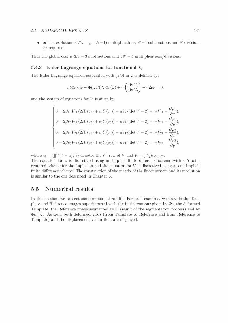
5.5. NUMERICAL RESULTS 141
• for the resolution of Ru = y: (N−1) multiplications, N−1 subtractions and N divisionsare required.
Thus the global cost is 3N − 3 subtractions and 5N − 4 multiplications/divisions.
5.4.3 Euler-Lagrange equations for functional Iγ
The Euler-Lagrange equation associated with (5.9) in ϕ is defined by:
ν(Φ0 ϕ− Φ(., T ))∇Φ0(ϕ) + γ
(div V1div V2
)− γ∆ϕ = 0,
and the system of equations for V is given by:
0 = 2βc0V11 (2Hε(c0) + c0δε(c0)) + µV22(detV − 2) + γ(V11 −∂ϕ1
∂x),
0 = 2βc0V12 (2Hε(c0) + c0δε(c0))− µV21(detV − 2) + γ(V12 −∂ϕ1
∂y),
0 = 2βc0V21 (2Hε(c0) + c0δε(c0))− µV12(detV − 2) + γ(V21 −∂ϕ2
∂x),
0 = 2βc0V22 (2Hε(c0) + c0δε(c0)) + µV11(detV − 2) + γ(V22 −∂ϕ2
∂y),
where c0 = (‖V ‖2 − α), Vi denotes the ith row of V and V = (Vij)1≤i,j≤2.
The equation for ϕ is discretized using an implicit finite difference scheme with a 5 pointcentered scheme for the Laplacian and the equation for V is discretized using a semi-implicitfinite difference scheme. The construction of the matrix of the linear system and its resolutionis similar to the one described in Chapter 6.
5.5 Numerical results
In this section, we present some numerical results. For each example, we provide the Tem-plate and Reference images superimposed with the initial contour given by Φ0, the deformedTemplate, the Reference image segmented by Φ (result of the segmentation process) and byΦ0 ϕ. As well, both deformed grids (from Template to Reference and from Reference toTemplate) and the displacement vector field are displayed.
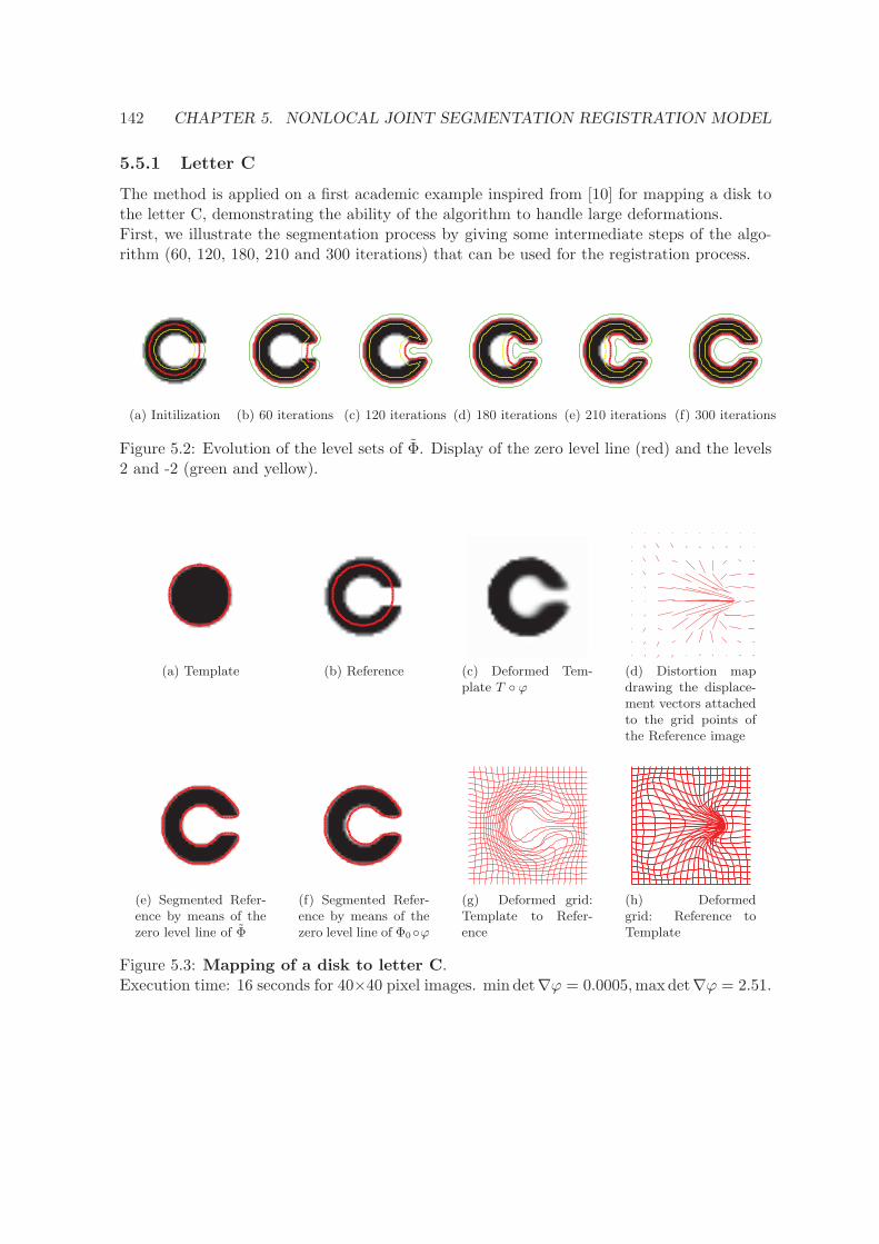
142 CHAPTER 5. NONLOCAL JOINT SEGMENTATION REGISTRATION MODEL
5.5.1 Letter C
The method is applied on a first academic example inspired from [10] for mapping a disk tothe letter C, demonstrating the ability of the algorithm to handle large deformations.First, we illustrate the segmentation process by giving some intermediate steps of the algo-rithm (60, 120, 180, 210 and 300 iterations) that can be used for the registration process.
(a) Initilization (b) 60 iterations (c) 120 iterations (d) 180 iterations (e) 210 iterations (f) 300 iterations
Figure 5.2: Evolution of the level sets of Φ. Display of the zero level line (red) and the levels2 and -2 (green and yellow).
(a) Template (b) Reference (c) Deformed Tem-plate T ϕ
(d) Distortion mapdrawing the displace-ment vectors attachedto the grid points ofthe Reference image
(e) Segmented Refer-ence by means of thezero level line of Φ
(f) Segmented Refer-ence by means of thezero level line of Φ0ϕ
(g) Deformed grid:Template to Refer-ence
(h) Deformedgrid: Reference toTemplate
Figure 5.3: Mapping of a disk to letter C.Execution time: 16 seconds for 40×40 pixel images. min det∇ϕ = 0.0005,maxdet∇ϕ = 2.51.
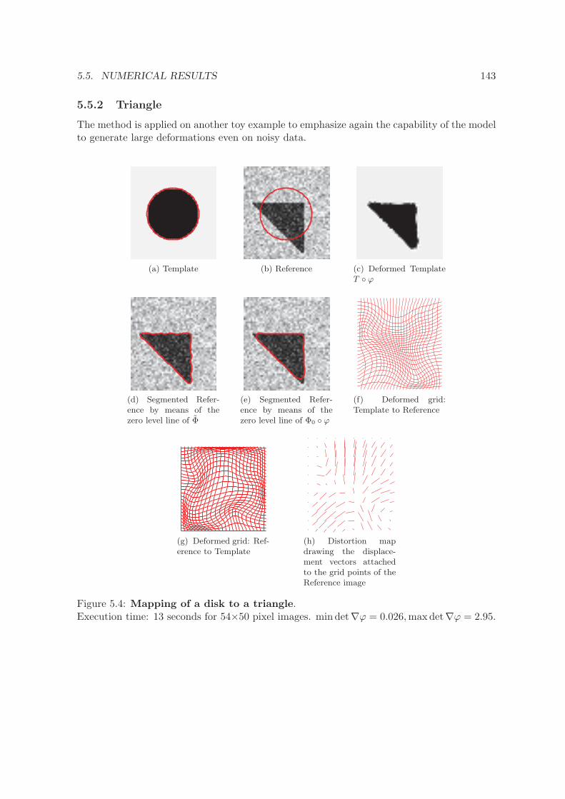
5.5. NUMERICAL RESULTS 143
5.5.2 Triangle
The method is applied on another toy example to emphasize again the capability of the modelto generate large deformations even on noisy data.
(a) Template (b) Reference (c) Deformed TemplateT ϕ
(d) Segmented Refer-ence by means of thezero level line of Φ
(e) Segmented Refer-ence by means of thezero level line of Φ0 ϕ
(f) Deformed grid:Template to Reference
(g) Deformed grid: Ref-erence to Template
(h) Distortion mapdrawing the displace-ment vectors attachedto the grid points of theReference image
Figure 5.4: Mapping of a disk to a triangle.Execution time: 13 seconds for 54×50 pixel images. min det∇ϕ = 0.026,maxdet∇ϕ = 2.95.
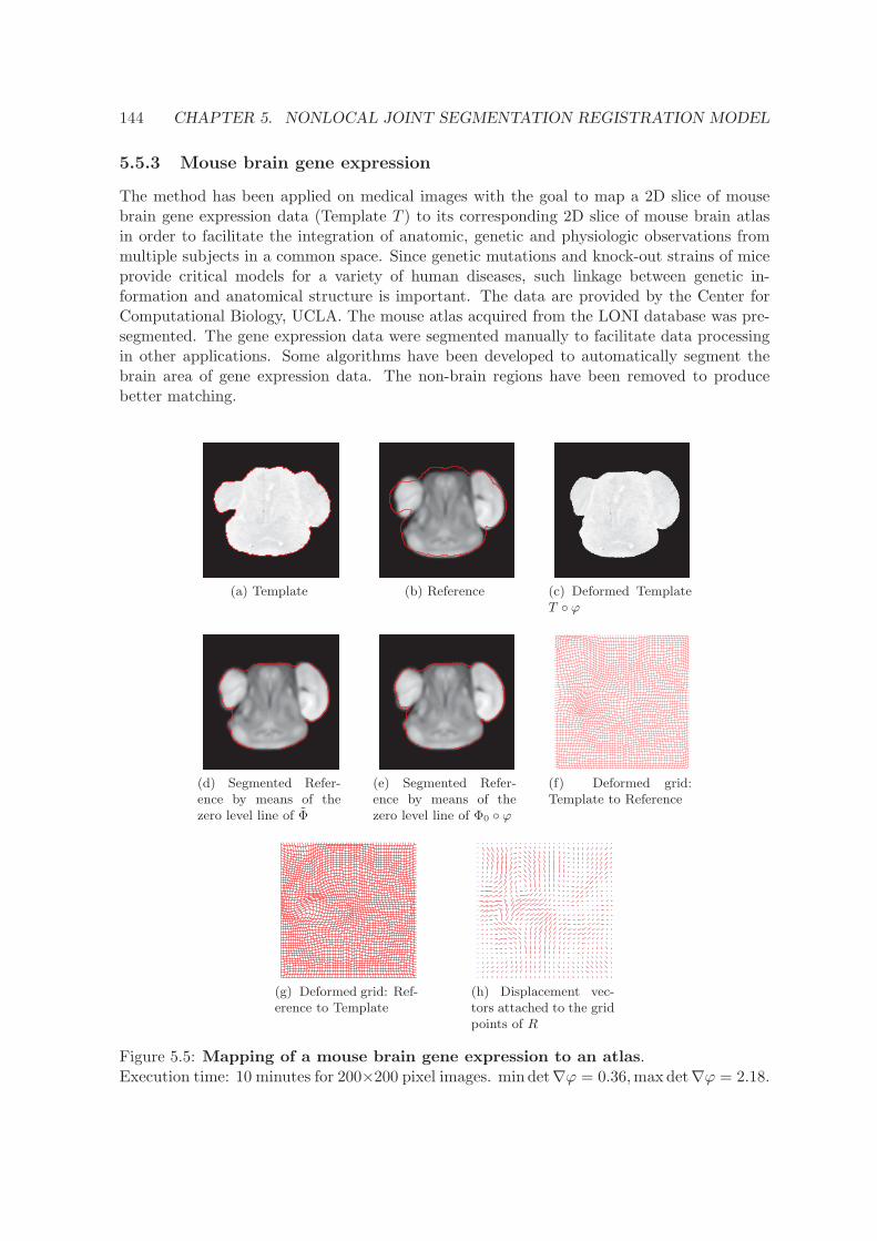
144 CHAPTER 5. NONLOCAL JOINT SEGMENTATION REGISTRATION MODEL
5.5.3 Mouse brain gene expression
The method has been applied on medical images with the goal to map a 2D slice of mousebrain gene expression data (Template T ) to its corresponding 2D slice of mouse brain atlasin order to facilitate the integration of anatomic, genetic and physiologic observations frommultiple subjects in a common space. Since genetic mutations and knock-out strains of miceprovide critical models for a variety of human diseases, such linkage between genetic in-formation and anatomical structure is important. The data are provided by the Center forComputational Biology, UCLA. The mouse atlas acquired from the LONI database was pre-segmented. The gene expression data were segmented manually to facilitate data processingin other applications. Some algorithms have been developed to automatically segment thebrain area of gene expression data. The non-brain regions have been removed to producebetter matching.
(a) Template (b) Reference (c) Deformed TemplateT ϕ
(d) Segmented Refer-ence by means of thezero level line of Φ
(e) Segmented Refer-ence by means of thezero level line of Φ0 ϕ
(f) Deformed grid:Template to Reference
(g) Deformed grid: Ref-erence to Template
(h) Displacement vec-tors attached to the gridpoints of R
Figure 5.5: Mapping of a mouse brain gene expression to an atlas.Execution time: 10 minutes for 200×200 pixel images. min det∇ϕ = 0.36,maxdet∇ϕ = 2.18.
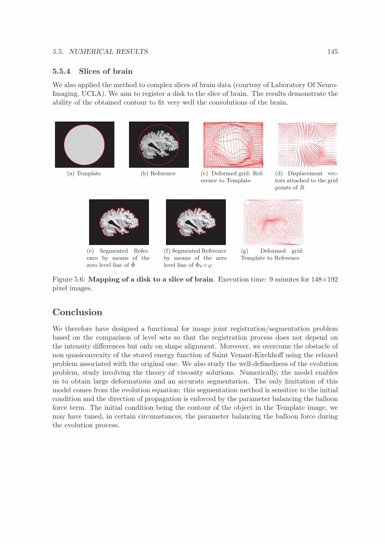
5.5. NUMERICAL RESULTS 145
5.5.4 Slices of brain
We also applied the method to complex slices of brain data (courtesy of Laboratory Of Neuro-Imaging, UCLA). We aim to register a disk to the slice of brain. The results demonstrate theability of the obtained contour to fit very well the convolutions of the brain.
(a) Template (b) Reference (c) Deformed grid: Ref-erence to Template
(d) Displacement vec-tors attached to the gridpoints of R
(e) Segmented Refer-ence by means of thezero level line of Φ
(f) Segmented Referenceby means of the zerolevel line of Φ0 ϕ
(g) Deformed grid:Template to Reference
Figure 5.6: Mapping of a disk to a slice of brain. Execution time: 9 minutes for 148×192pixel images.
Conclusion
We therefore have designed a functional for image joint registration/segmentation problembased on the comparison of level sets so that the registration process does not depend onthe intensity differences but only on shape alignment. Moreover, we overcome the obstacle ofnon quasiconvexity of the stored energy function of Saint Venant-Kirchhoff using the relaxedproblem associated with the original one. We also study the well-definedness of the evolutionproblem, study involving the theory of viscosity solutions. Numerically, the model enablesus to obtain large deformations and an accurate segmentation. The only limitation of thismodel comes from the evolution equation: this segmentation method is sensitive to the initialcondition and the direction of propagation is enforced by the parameter balancing the balloonforce term. The initial condition being the contour of the object in the Template image, wemay have tuned, in certain circumstances, the parameter balancing the balloon force duringthe evolution process.

BIBLIOGRAPHY
[1] G. Aubert and P. Kornprobst, Mathematical Problems in Image processing: PartialDifferential Equations and the Calculus of Variations, vol. 147 of Applied MathematicalSciences, Springer-Verlag, 2001.
[2] G. Barles, P. Cardaliaguet, O. Ley, and A. Monteillet, Existence of weaksolutions for general nonlocal and nonlinear second-order parabolic equations, NonlinearAnalysis: Theory, Methods & Applications, 71 (2009), pp. 2801–2810.
[3] M. Bourgoing, Viscosity solutions of fully nonlinear second order parabolic equationswith L1 dependence in time and neumann boundary conditions, Discrete Contin. Dyn.Syst, 21 (2008), pp. 763–800.
[4] M. Bousselsal, Etude de quelques problemes de calcul des variations lies a lamecanique, PhD thesis, Universite de Metz, 1993.
[5] H. Brezis, Analyse Fonctionnelle, Theorie et Applications, Dunod, Paris, 2005.
[6] C. Broit, Registration of Deformed Images, PhD thesis, Universite de Pennsylvania,USA, 1981.
[7] M. Burger, J. Modersitzki, and L. Ruthotto, A hyperelastic regularization energyfor image registration, SIAM Journal on Scientific Computing, 35 (2013), pp. B132–B148.
[8] V. Caselles, R. Kimmel, and G. Sapiro, Geodesic active contours, Internationaljournal of computer vision, 22 (1997), pp. 61–79.
[9] T. F. Chan and L. Vese, Active contours without edges, IEEE T. Image Processing,10 (2001), pp. 266–277.
[10] G. E. Christensen, Deformable shape models for anatomy, PhD thesis, WashingtonUniversity, Sever Institute of technology, USA, 1994.
[11] P. G. Ciarlet, Elasticite tridimensionnelle, Masson, 1985.
[12] M. G. Crandall, H. Ishii, and P.-L. Lions, User’s guide to viscosity solutions of sec-ond order partial differential equations, Bulletin of the American Mathematical Society,27 (1992), pp. 1–67.
147
148 BIBLIOGRAPHY
[13] B. Dacorogna, Direct methods in the calculus of variations, vol. 78 of Applied Math-ematical Sciences, Springer, 2008.
[14] R. Derfoul and C. Le Guyader, A Relaxed Problem of Registration Based on theSaint Venant–Kirchhoff Material Stored Energy for the Mapping of Mouse Brain GeneExpression Data to a Neuroanatomical Mouse Atlas, SIAM Journal on Imaging Sciences,7 (2014), pp. 2175–2195.
[15] M. Droske and M. Rumpf, Multiscale joint segmentation and registration of imagemorphology, Pattern Analysis and Machine Intelligence, IEEE Transactions on, 29 (2007),pp. 2181–2194.
[16] N. Forcadel and C. Le Guyader, A short time existence/uniqueness result for anonlocal topology-preserving segmentation model, Journal of Differential Equations, 253(2012), pp. 977–995.
[17] C. Le Guyader and L. Vese, Self-repelling snakes for topology-preserving segmenta-tion models, Image Processing, IEEE Transactions on, 17 (2008), pp. 767–779.
[18] C. Le Guyader and L. A. Vese, A combined segmentation and registration frameworkwith a nonlinear elasticity smoother, Computer Vision and Image Understanding, 115(2011), pp. 1689–1709.
[19] N. Lord, J. Ho, B. C. Vemuri, S. Eisenschenk, et al., Simultaneous registrationand parcellation of bilateral hippocampal surface pairs for local asymmetry quantification,Medical Imaging, IEEE Transactions on, 26 (2007), pp. 471–478.
[20] P. V. N. Marrero, A numerical method for detecting singular minimizers of multidi-mensional problems in nonlinear elasticity, Numerische Mathematik, 58 (1990), pp. 135–144.
[21] D. Nunziante, Existence and uniqueness of unbounded viscosity solutions of parabolicequations with discontinuous time-dependence, Nonlinear Analysis: Theory, Methods &Applications, 18 (1992), pp. 1033–1062.
[22] S. Ozere, C. Gout, and C. Le Guyader, Joint segmentation/registration modelby shape alignment via weighted total variation minimization and nonlinear elasticity,Accepted for publication in Siam Imaging Sciences, (July 2015).
[23] G. Russo and P. Smereka, A Remark on Computing Distance Functions, Journal ofComputational Physics, 163 (2000), pp. 51 – 67.
[24] J. A. Sethian, Level set methods and fast marching methods: evolving interfaces incomputational geometry, fluid mechanics, computer vision, and materials science, vol. 3,Cambridge university press, 1999.
[25] A. Sotiras, C. Davatzikos, and N. Paragios, Deformable medical image registra-tion: A survey, Medical Imaging, IEEE Transactions on, 32 (2013), pp. 1153–1190.
[26] B. C. Vemuri, J. Ye, Y. Chen, and C. M. Leonard, Image registration via level-set motion: Applications to atlas-based segmentation, Medical image analysis, 7 (2003),pp. 1–20.

BIBLIOGRAPHY 149
[27] J. Weickert and G. Kuhne, Fast methods for implicit active contour models, Springer,2003.
[28] A. Yezzi, L. Zollei, and T. Kapur, A variational framework for joint segmentationand registration, in Mathematical Methods in Biomedical Image Analysis, 2001. MMBIA2001. IEEE Workshop on, IEEE, 2001, pp. 44–51.

CHAPTER 6
REGISTRATION PROBLEM BASED ON GEOMETRICCONSTRAINTS AND SAINT VENANT-KIRCHHOFF MATERIAL
In this chapter, we introduce a registration model under constraints based on nonlinear elas-ticity theory. In particular, we choose to view the shapes to be matched as hyperelastic,isotropic and homogeneous materials. The choice of a hyperelastic material can be explainedby two reasons: on the one hand, this kind of regularizer enables us to handle large and non-linear deformations, on the other hand, in the literature, biological tissues are often modelledas hyperelastic materials.Moreover, we introduce geometrical constraints, that is to say that we seek to match pairs ofcontrol points on the Reference image and the Template image.
The chapter is organized as follows. In a first section, we present the mathematicalmodelling of our method based on the stored energy function of the Saint Venant-Kirchhoffmaterial. We formulate our problem as a functional minimization problem. Next, we establishtheoretical results such as the existence of so-called generalized solutions (solutions of anassociated relaxed problem). We also establish a convergence result when the number ofcontrol points increases to infinity. Finally, we are concerned with the discretization and theimplementation of the model, and we conclude the chapter with some numerical experiments.
Introduction
Image registration is a fundamental task encountered in a large range of applications such asmedical imaging, when comparing an image to an atlas or when fusing two images. Giventwo images, registration consists in determining an optimal diffeomorphic transformation ϕsuch that the deformed Template image is aligned with the Reference. For images of the samemodality, the goal of registration is to correlate the geometrical features and the intensity leveldistribution of the Reference and those of the deformed Template. When the images havebeen acquired through different mechanisms and have different modalities, registration aimsto correlate both images while preserving the modality of the Template image. Sometimes, inmedical image registration, geometrical constraints such as landmark points can complementthe image data. In this case, relevant points on the Reference image are manually selected and
151
152 CHAPTER 6. NONLINEAR ELASTICITY AND GEOMETRIC CONSTRAINTS
their counterparts on the Template are identified by an expert (see [19] for details and [17]for applications to registration of mouse brain gene expression data to an atlas). This priorknowledge allows, in particular, to increase the reliability of the obtained results. The qualityof the obtained deformation can thus be measured by comparing the position of the landmarkpoints on the Template and the position of the associated deformed landmark points. In thischapter, we propose a nonlinear elasticity based registration method including geometricalconstraints manually selected on the images. The energy to be minimized consists of threeterms: the L2 distance of the grey levels, the elasticity-based regularizer and the geometricalconstraint term (denoted respectively by Fid,Reg, Const). The minimization problem canbe written in the form
infϕ
Fid(ϕ) +Reg(ϕ) + Const(ϕ) .
To allow large deformations, we introduce a nonlinear-elasticity-based smoother (see [8],[9] for further details), the theory of linear elasticity being unsuitable in this case since as-suming small strains and the validity of Hooke’s law. We propose viewing the shapes to bewarped as isotropic, homogeneous, hyperelastic materials and more precisely as Saint Venant-Kirchhoff materials. Note that rubber, filled elastomers, biological tissues are often modeledwithin the hyperelastic framework, which motivates our modelling.For the sake of completeness, we would like to refer the reader to previous works related toregistration based on nonlinear elasticity principles. In [13], Droske and Rumpf address theissue of non-rigid registration of multi-modal image data. The matching criterion includesfirst order derivatives of the deformation and is complemented by a nonlinear elastic regular-ization based on a polyconvex stored energy function, which is different from our proposedapproach. We also mention the combined segmentation/registration model introduced by LeGuyader and Vese ([16]) in which the shapes to be matched are viewed as Ciarlet-Geymonatmaterials, the works [2] and [18] for a variational registration method for large deformations(Large Deformation Diffeomorphic Metric Mapping - LDDMM), and refer to [22] for a muchrelated work that also uses nonlinear elasticity regularization but implemented by the finiteelement method.In [5], the authors design an hyperelastic regularizer. More precisely, they build an hyper-elastic stored energy function penalizing variations of lengths and areas, and add a penaltyterm on the Jacobian determinant such that the energy tends to infinity as det∇ϕ tends to0 and such that shrinkage and growth have the same price. The numerical implementation isbased on a discretize-then-optimize strategy and the authors use a generalized Gauss-Newtonscheme to compute a numerical minimizer.
6.1 Mathematical modelling
6.1.1 Preliminaries
Before introducing the model, let us make a short reminder on nonlinear elasticity and onthe Saint Venant-Kirchhoff material. Denoting by ϕ a deformation, we recall that the rightCauchy-Green strain tensor is defined by
C = ∇ϕT∇ϕ = F TF ∈ S2
with S2 =A ∈M2(R), A = AT
, set of all real symmetric matrices of order 2. Physically,
the right Cauchy-Green tensor can be interpreted as a quantifier of the square of local change
6.1. MATHEMATICAL MODELLING 153
in distances due to deformation. The Green-Saint Venant strain tensor is defined by
E =1
2(∇u+∇uT +∇uT∇u).
Associated with a given deformation ϕ = Id+u, it is a measure of the deviation between ϕand a rigid deformation. We also provide the following notations:
• A : B = trATB the matrix inner product
• ‖A‖ =√A : A, the related matrix norm (Frobenius norm).
The stored energy function of an isotropic, homogeneous, hyperelastic material, if the refer-ence configuration is a natural state, is of the form:
W (F ) = W (E) =λ
2(trE)2 + µ trE2 + o
(‖E‖2
), F TF = I + 2E, (6.1)
with I the identity matrix. The Saint Venant-Kirchhoff material is the simplest homogeneous,isotropic, hyperelastic material with a natural reference configuration complying with theprevious expansion (6.1). The stored energy function is defined by
WSV K(F ) = WSV K(E) =λ
2(trE)2 + µ tr(E2).
The coefficients λ and µ are the Lame constants. The first Lame parameter λ has no straight-forward physical interpretation, but is related to the bulk modulus. The second Lame pa-rameter µ is the shear modulus. That is to say that µ measures the resistance of a material:the greater µ, the stronger the applied force to obtain the same deformation. If a materialhad a null shear modulus, it would not be stable.
6.1.2 Depiction of the model
We focus on a registration problem based on the L2-norm of the difference between the Tem-plate and the Reference images. Concerning the regularizer, we choose a nonlinear elasticregularizer, in particular, the stored energy function of a Saint Venant-Kirchhoff material.Moreover, from a numerical viewpoint, this choice of regularizer enables us to deal with high-magnitude deformations. Also, we add a penalty term to force the Jacobian to be close to 1in order to obtain a homogeneous deformation that is to say to prevent the deformation mapfrom exhibiting contractions and expansions that are too large.Moreover, we propose to include geometrical constraints to match some interest points. In-deed, we manually choose a finite number of points on the Template image and on the Refer-ence image and we want every point on the Reference image to be mapped to its counterparton the Template image.
Let us denote by:
• Ω a connected bounded open subset of R2 with Lipschitz boundary ∂Ω,
• R : Ω −→ R, the Reference image,
• T : Ω −→ R, a Lipschitz continuous function (we denote by kT the Lipschitz constant)with compact support, representing the Template image,
• ϕ : Ω −→ R2 the sought deformation with ϕ = Id on ∂Ω.
154 CHAPTER 6. NONLINEAR ELASTICITY AND GEOMETRIC CONSTRAINTS
Geometrical constraints
The geometrical constraints correspond to selected landmark points on R and their corre-sponding counterpart on T . We denote by ω = (ω1, . . . , ωN ) ∈ (R2)N , the landmark pointson R and ω = (ω1, . . . , ωN ) ∈ (R2)N their counterparts on T .We define the linear mapping ρ by:
ρ : W1,4(Ω,R2) −→ (R2)N
ϕ 7−→ (ϕ(ω1), . . . , ϕ(ωN ))T .
We justify the choice of the functional space W1,4(Ω,R2) in the sequel. The mapping ρ iswell defined since we have the continuous embedding W1,4(Ω,R2) → C0(Ω,R2). The purposeis to minimize
〈ρ(ϕ)− ω〉22N ,with respect to ϕ where 〈.〉2N is the Euclidean norm in R
2N and N is the number of con-straints.In fact, we aim to minimize the distance between ϕ(ωi) and ωi, i = 1 . . . N , ie, we search forthe deformation such that the points in the Reference image are mapped to the points of theTemplate image though this smooth deformation. We can notice that minimizing 〈ρ(ϕ)−ω〉22Nwith respect to ϕ is equivalent to minimizing 〈ρ(ϕ)〉22N − 2〈ρ(ϕ), ω〉2N .
Elastic regularization
As already mentioned, we choose to view the shapes to be matched as Saint Venant-Kirchhoffmaterials. In addition, we complement the stored energy function WSV K by the termµ(det∇ϕ− 1)2 controlling that the Jacobian remains close to 1. The weighting of the deter-minant component by parameter µ is justified in the proof of 6.1.1.We set W (∇ϕ) =WSV K(∇ϕ)+µ(det∇ϕ− 1)2 where WSV K is the stored energy function ofa Saint Venant-Kirchhoff material, defined by
WSV K(F ) = WSV K(E) =λ
2(trE)2 + µ tr(E2), with E =
1
2(F TF − I).
We first rewrite WSV K(∇ϕ) in a more simplified way. In two dimensions, we have:
WSV K(F ) =λ
2(trE)2 + µ tr(E2),
=λ
8(‖F‖2 − 2)2 +
µ
4(‖F TF‖2 − 2‖F‖2 + 2),
= −λ+ µ
2︸ ︷︷ ︸a1<0
‖F‖2 + λ+ 2µ
8︸ ︷︷ ︸a2
‖F‖4 − µ
2(detF )2 +
λ+ µ
2.
(6.2)
Indeed, considering the characteristic polynomial χFTF of F TF , we have:
χFTF (X) = X2 − tr(F TF )X + det(F TF )I.
Moreover, according to Cayley-Hamilton theorem, χFTF (FTF ) = 0, then
(F TF )2 − tr(F TF )F TF + det(F TF )I = 0.
6.1. MATHEMATICAL MODELLING 155
Passing to the trace we obtain: ‖F TF‖2 − ‖F‖4 + 2(detF )2 = 0. Replacing ‖F TF‖2 by‖F‖4 − 2(detF )2, we obtain the desired expression of WSV K .
Therefore,
W (F ) = a1‖F‖2 + a2‖F‖4 +λ+ µ
2+ φ(detF ),
with φ : s 7−→ −µ2s2 + µ(s− 1)2.
Functional to be minimized
Finally, we aim to minimize the following functional:
infϕ∈W
I(ϕ) =
ν
2
∫
Ω(T ϕ−R)2 dx+
∫
ΩW (∇ϕ)dx+ η〈ρ(ϕ)〉22N − 2η〈ρ(ϕ), ω〉2N
(P)
with W =ϕ ∈ Id+W1,4
0 (Ω,R2), where ν, η are positive parameters. ϕ ∈ Id+W1,4
0 (Ω,R2)
means that ϕ = Id on ∂Ω and ϕ ∈ W1,4(Ω,R2), W1,4(Ω,R2) denoting the Sobolev space offunctions ϕ ∈ L4(Ω,R2) with distributional derivatives up to order 1 which also belong toL2(Ω).
The functional is well defined for ϕ ∈ W1,4(Ω,R2). Indeed, we have the continuousembedding W1,4(Ω,R2) → C0(Ω,R2) ensuring that the geometrical term makes sense and thegeneralized Holder inequality ([4]) guarantees that det∇ϕ ∈ L2(Ω).
6.1.3 Mathematical obstacle and relaxed problem
We are faced with a theoretical problem with problem (P).
Proposition 6.1.1
W is not rank 1-convex.
Proof : The proof is based on the same technique as the one applied by A. Raoult in [23].
Let ε > 0. We set F = εI and F ′ = ε diag(1, 3). Then F − F ′ =
(0 00 −2ε
)and we
have rank(F − F ′) = 1.We have detF = ε2, detF ′ = 3ε2, ‖F‖2 = 2ε2, ‖F ′‖2 = 10ε2, det(F+F ′
2 ) = 2ε2, ‖F+F ′
2 ‖2 =5ε2.We argue by contradiction and assume that W is rank 1-convex, then
W
(F + F ′
2
)≤ 1
2
(W (F ) +W (F ′)
),
156 CHAPTER 6. NONLINEAR ELASTICITY AND GEOMETRIC CONSTRAINTS
⇐⇒ 5a1ε2 + 25a2ε
4 − 2µε4 + µ(2ε2 − 1)2 ≤ 1
2
(2a1ε
2 + 4a2ε4 − µ
2ε4 + µ(ε2 − 1)2
+10a1ε2 + 100a2ε
4 − 9
2µε4 + µ(3ε2 − 1)2
),
⇐⇒ ε2(5a1 − 4µ) + ε4(25a2 + 2µ) ≤ 1
2
(ε2(12a1 − 8µ) + ε4(104a2 + 5µ)
),
⇐⇒ a1ε2 + 27a2ε
4 +1
2µε4 ≥ 0,
⇐⇒ a1︸︷︷︸<0
+ε2(27a2 +1
2µ) ≥ 0.
which raises a contradiction for ε small enough.
The stored energy function W is not rank 1-convex so it is not quasiconvex, which raises adrawback of theoretical nature since we cannot obtain the weak sequential lower semicon-tinuity of the functional (quasiconvexity is a necessary and sufficient condition to get weaklower semicontinuity). This prevents us from applying the direct method. As stressed byDacorogna ([10, page 17]), the general rule is that in this case the considered problem has nominimizers.
Proposition 6.1.2
The stored energy function W (F ) can be written as follows:
W (F ) = β(‖F‖2 − α)2 + ψ(detF ),
with β > 0, α > 0, and where ψ is a convex function.
Proof :
W (F ) = a2‖F‖4 + a1‖F‖2 + φ(detF ) +λ+ µ
2,
= a2
(‖F‖2 − (− a1
2a2)
)2
− a2
(a12a2
)2
+λ+ µ
2+ φ(detF ),
= β(‖F‖2 − α
)2+ ψ(detF ),
with β = a2 =λ+ 2µ
8, α = − a1
2a2= 2
λ+ µ
λ+ 2µ
and ψ : s 7−→ −µ2s2 + µ(s− 1)2 +
µ(λ+ µ)
2(λ+ 2µ)︸ ︷︷ ︸γ
convex.
6.1. MATHEMATICAL MODELLING 157
Theorem 6.1.1 (Bousselsal [3, Theorem 3.1])
Let W : Rn×n −→ R. Let ψ : R −→ R be a convex function such that
W (F ) = β(‖F‖2 − α)2 + ψ(detF ), α, β ∈ R∗+.
Then
PW (F ) = QW (F ) = RW (F ) =
W (F ) if ‖F‖2 ≥ α
ψ(detF ) if ‖F‖2 < α.
Before proving Theorem 6.1.1, we give the following lemmas:
Lemma 6.1.2 (Bousselsal [3, Lemma 3.1])
Let f : Rn×n −→ R and ψ : R −→ R such that
f(F ) = ψ(detF ).
Then
f polyconvex ⇐⇒ f quasiconvex ⇐⇒ f rank-1 convex ⇐⇒ ψ convex.
Proof (taken from [3]) : By definition, we have f polyconvex ⇐⇒ ψ convex.Moreover, we know that f polyconvex =⇒ f quasiconvex =⇒ f rank-1 convex.Thus we just need to prove that f rank-1 convex=⇒ ψ convex.Let A and B ∈ R
n×n be such that rank(A−B) ≤ 1.We suppose that f is rank 1-convex then for λ ∈ [0, 1]:
f(λA+ (1− λ)B) ≤ λf(A) + (1− λ)f(B)
⇐⇒ ψ(det(λA+ (1− λ)B)) ≤ λψ(detA) + (1− λ)ψ(detB)
We use the following lemma.
Lemma 6.1.3 (Dacorogna [10, Lemma 5.5])
Let ξ ∈ RN×n and T : RN×n −→ R
τ(n,N) is such that T (ξ) = (ξ, adj2 ξ, . . . , adjn∧N )
with τ(n,N) =n∧N∑s=1
σ(s) where σ(s) =(Ns
)(ns
).
For every ξ, η ∈ RN×n with rank(ξ− η) ≤ 1 and for every λ ∈ [0, 1], the following identity
holds:T (λξ + (1− λ)η) = λT (ξ) + (1− λ)T (η).
Then we obtain that det(λA+ (1− λ)B) = λ detA+ (1− λ) detB. Therefore
ψ(λ detA+ (1− λ) detB) ≤ λψ(detA) + (1− λ)ψ(detB).
Then ψ is convex.
158 CHAPTER 6. NONLINEAR ELASTICITY AND GEOMETRIC CONSTRAINTS
Lemma 6.1.4 (Bousselsal [3, Lemma 3.2])
Let F ∈ Rn×n be such that 0 ≤ ‖F‖2 < α. Then there exist B,C ∈ R
n×n, λ ∈]0, 1[ suchthat
F = λB + (1− λ)C,
rank(B − C) ≤ 1,
‖B‖2 = ‖C‖2 = α,
detF = detB = detC.
Proof (taken from [3]) :
If rank(F ) = 1, the result is immediate taking B = −√αF
‖F‖ , C =√αF
‖F‖and λ =
1
2(1− ‖F‖√
α).
If rank(F ) = 0, which means that F is the null matrix, it suffices to take for example
B = (B1, 0, . . . , 0) with B1 =√α(1, 0, . . . , 0)T , C = −B, and λ =
1
2.
If rank(F ) 6= 1, we denote by Fj the jth column of F . Then there exists j0 such that
Fj0 6= 0. We can suppose that F2 6= 0 without loss of generality, then we set E = aGwith G = (F2, 0, . . . , 0) ∈ R
n×n, a 6= 0.We choose
B = F − (1− λ)E,
C = F + λE.
Matrix E has rank equal to 1, and we have F = λB+ (1− λ)C and rank(B−C) ≤ 1.Moreover, detF = detB = detC.It remains to prove that ‖B‖2 = ‖C‖2 = α, which is equivalent to
‖F‖2 − 2(1− λ)(F,E) + (1− λ)2‖E‖2 = α
‖F‖2 + 2λ(F,E) + λ2‖E‖2 = α,
⇐⇒‖F‖2 − 2(1− λ)a(F,G) + (1− λ)2a2‖G‖2 = α
‖F‖2 + 2λa(F,G) + λ2a2‖G‖2 = α.
(6.3)
(6.4)
We set Σ = 2(F,G), (·, ·) denoting the inner product.The last step consists in finding λ ∈]0, 1[ and a such that (6.3) and (6.4) are satisfied.We can notice that if λ and λ− 1 are solutions of (6.4), then (6.3) is satisfied. This isthe case if
λ+ λ− 1 =−aΣa2‖G‖2 ,
⇐⇒λ =1
2(1− aΣ
a2‖G‖2 ).
The equations are satisfied if
λ(λ− 1) =‖F‖2 − α
a2‖G‖2 ,
⇐⇒(
aΣ
a2‖G‖2)2
+4(α− ‖F‖2)a2‖G‖2 = 1.
6.1. MATHEMATICAL MODELLING 159
We assume that we can find an a ∈ R such that
(aΣ
a2‖G‖2)2
+4(α− ‖F‖2)a2‖G‖2 = 1 (6.5)
then
−1 ≤ aΣ
a2‖G‖2 ≤ 1
and so λ ∈]0, 1[. It remains to be proved that there exists a ∈ R such that (6.5) holds.To do so, we notice that
• if a −→ 0 the left member of (6.5) tends to +∞,
• if a −→ +∞ the left member of (6.5) tends to 0.
By continuity, there exists a value of a such that (6.5) is satisfied. Therefore, we obtainthe desired result.
Theorem 6.1.5 (Bousselsal [3, Theorem 3.2])
We assume that g is a non-negative function such that g = 0 on ‖F‖2 = α, and g isconvex outside Bα = F : ‖F‖2 ≤ α.Then
Cg = Pg = Qg = Rg =
g outside Bα
0 inside Bα.
Proof : We denote by
g =
g outside Bα
0 inside Bα.
By construction, we have g ≤ g.We begin by proving that the function g is convex.On the one hand, if λF1 + (1− λ)F2 ∈ Bα, λ ∈ [0, 1], and since g ≥ 0, we have
0 = g(λF1 + (1− λ)F2) ≤ λg(F1) + (1− λ)g(F2).
On the other hand, we focus on the outside of Bα.Function g is convex outside Bα and non-negative so if there exists a convex functiong such that g = g outside Bα, necessarily by convexity of g, g ≤ 0 on Bα.If λF1 + (1− λ)F2 /∈ Bα, we have
g(λF1 + (1− λ)F2) = g(λF1 + (1− λ)F2)
and
g(λF1 + (1− λ)F2) ≤ λg(F1) + (1− λ)g(F2) ≤ λg(F1) + (1− λ)g(F2).
Therefore, we have proved that
g(λF1 + (1− λ)F2) ≤ λg(F1) + (1− λ)g(F2)
160 CHAPTER 6. NONLINEAR ELASTICITY AND GEOMETRIC CONSTRAINTS
for all F1, F2 ∈ Rn×n, λ ∈ [0, 1], then g is convex.
Next, if h is a convex function such that h ≤ g, by convexity, we also have h ≤ g andby definition of the convex envelop Cg = g. Since Cg ≤ Pg ≤ Qg ≤ Rg ≤ g and g = goutside Bα, then
Cg = Pg = Qg = Rg = g outside Bα.
Inside Bα, we have Cg = g = 0. Moreover, according to lemma 6.1.4, for F ∈ Bα,there exist B,C ∈ (Rn×n)2 and λ ∈]0, 1[ such that F = λB+(1−λ)C, rank(B−C) ≤ 1and ‖B‖2 = ‖C‖2 = α.Therefore,
Rg(F ) = Rg(λB + (1− λ)C) ≤ λRg(B) + (1− λ)Rg(C) ≤ λg(B) + (1− λ)g(C).
But, g(C) = g(B) = 0, since ‖B‖2 = ‖C‖2 = α, so Rg(F ) ≤ 0. We obtain
0 = Cg ≤ Rg ≤ 0 inside Bα.
In conclusion,Cg = Pg = Qg = Rg = g.
Proof of Theorem 6.1.1 (from [3]) :Let f(F ) = ψ(detF ) and g(F ) = β(‖F‖2 − α)2 then W (F ) = f(F ) + g(F ). Thefunction ψ being convex, f is polyconvex. According to Theorem 6.1.5, we can deducethat
Cg(F ) = Pg(F ) = Qg(F ) = Rg(F ) =
g(F ) if ‖F‖2 ≥ α
0 if ‖F‖2 < α.
Moreover, g = W − f ≥ Cg = Pg and f is polyconvex so f + Pg is polyconvex andW ≥ f + Pg = f + Cg then by definition of the polyconvex envelop, we obtain:
PW (F ) ≥ (f + Cg)(F ) =
W (F ) if ‖F‖2 ≥ α
f(F ) if ‖F‖2 < α.
In particular we have
PW (F ) = RW (F ) =W (F ) if ‖F‖2 ≥ α
andf(F ) ≤ PW (F ) ≤ QW (F ) ≤ RW (F ) if ‖F‖2 < α.
It remains to prove the inequality RW (F ) ≤ f(F ) in the case ‖F‖2 < α.According to lemma 6.1.4, there exist B,C ∈ R
n×n and λ ∈]0, 1[ such that F =λB + (1− λ)C, rank(B − C) ≤ 1, detB = detC = detF , and ‖B‖2 = ‖C‖2 = α. Bydefinition, RW (F ) is rank-one convex, we obtain:
RW (F ) ≤ λRW (B)+(1−λ)RW (C) ≤ λW (B)+(1−λ)W (C) = λf(B)+(1−λ)f(C) = ψ(detF )
According to the two previous inequalities, we can conclude that RW (F ) = f(F ) if‖F‖2 < α. Therefore,
PW (F ) = QW (F ) = RW (F ) =
W (F ) if ‖F‖2 ≥ α
ψ(detF ) if ‖F‖2 < α.
6.1. MATHEMATICAL MODELLING 161
Remark 6.1.3
We can show the same result using Dacorogna’s arguments.
Alternative proof : The proof is based on a property of invariance of the consideredstored energy function. We first recall a few definitions.
Definition 6.1.6 (Dacorogna [10])
• The set of orthogonal matrices is denoted by O(n). It is the set of matrices R ∈Mn(R) such that
RRt = I.
• The set of special orthogonal matrices, denoted by SO(n), is the subset of O(n) suchthat the matrices satisfy
detR = 1.
• Let ξ ∈Mn(R). The singular values of ξ, denoted by
0 ≤ λ1 ≤ · · · ≤ λn,
are defined to be the square root of the eigenvalues of the symmetric positive semidef-inite matrix ξξt ∈Mn(R).
• The signed singular values of ξ, denoted by
0 ≤ |µ1(ξ)| ≤ µ2(ξ) ≤ · · · ≤ µn(ξ),
are defined by
µ1(ξ) = λ1(ξ) sign(det ξ) and µj(ξ) = λj(ξ), ∀j = 2, . . . , n.
• A function f :Mn(R) → [−∞,+∞] is said to be SO(n)× SO(n) invariant if:
∀ξ ∈Mn(R), ∀Q,R ∈ SO(n)× SO(n), f(QξR) = f(ξ).
According to the singular value theorem (Theorem 13.3 in [10]), for all ξ ∈Mn(R), wecan findQ andR in SO(n) such that ξ = QΛR where Λ = diag(sign(det ξ)λ1, λ2, . . . , λn).In terms of singular values, function W can be rewritten
W (ξ) = β(λ21 + λ22 − α)2 + ψ(sign(det ξ)λ1λ2) = β(λ21 + λ22 − α)2 + ψ(µ1µ2).
Let
g(ξ) =
W (ξ) if ‖ξ‖2 ≥ α
ψ(ξ) if ‖ξ‖2 < α.
In view of the general results, we have:
PW ≤ QW ≤ RW ≤W.
Therefore, we only need to prove that
RW (ξ) = PW (ξ) = g(ξ), ∀ξ ∈Mn(R).
162 CHAPTER 6. NONLINEAR ELASTICITY AND GEOMETRIC CONSTRAINTS
The stored energy function W (ξ) is SO(2)× SO(2) invariant as function of the traceand the determinant. Indeed,
‖ξ‖2 = tr(ξT ξ),
‖QξR‖2 = tr(RT ξTQTQξR) = tr(RT ξT ξR) = tr(ξT ξRRT ) = ‖ξ‖2,det(QξR) = det(ξ).
Hence, according to Theorem 6.20 in [10], PW , QW and RW are SO(2) × SO(2)invariant. Therefore, we can restrict ourselves to the case of matrices of the form:
ξ =
(x 00 y
)where |x| ≤ y.
Then we have: det ξ = xy and ‖ξ‖2 = x2 + y2.Before proceeding further, it is convenient to introduce the two following functionsdefined on R
2 by
χ(x, y) = β(x2 + y2 − α)2 + µ(xy − 1)2 − µ
2x2y2 + γ
φ(x, y) = β[x2 + y2 − α]2+ + µ(xy − 1)2 − µ
2x2y2 + γ
with [z]2+ =
z2 if z ≥ 0
0 otherwise.
A simple calculation leads toW
(x 00 y
)= χ(x, y) and g
(x 00 y
)= φ(x, y). According
to Definition 5.42 of [10], φ is polyconvex, then g is polyconvex ([10, Theorem 5.43]).Since g(ξ) ≤W (ξ) and PW = suph ≤W,h polyconvex , we have
g(ξ) ≤ PW (ξ).
Case 1: ‖ξ‖2 < α.
Let us set
ξ1 =
x 0
−√α− (x2 + y2) y
, ξ2 =
x 0
√α− (x2 + y2) y
Then
ξ =1
2ξ1 +
1
2ξ2,
‖ξ1‖2 = ‖ξ2‖2 = α,
and rank(ξ1 − ξ2) = 1.
This implies that
g(ξ) ≤ PW (ξ) ≤ RW (ξ) ≤ 1
2RW (ξ1) +
1
2RW (ξ2) ≤
1
2W (ξ1) +
1
2W (ξ2) = g(ξ).
6.1. MATHEMATICAL MODELLING 163
Case 2: ‖ξ‖2 ≥ α.
W (ξ) = g(ξ) ≤ PW (ξ) ≤ QW (ξ) ≤ RW (ξ) ≤W (ξ),
which concludes the proof.
As established in Proposition 6.1.1, the functional to be minimized is not quasiconvex,therefore we cannot prove the existence of minimizers of the functional using the directmethod. Indeed, quasiconvexity is a necessary and sufficient condition to get (sequentially)weak lower semicontinuity. To overcome this issue, we propose to deal with a relaxed problemassociated with the original problem obtained by taking the quasiconvex envelop of W . Inthe sequel, we prove that the initial and this relaxed problem both admit the same infimum.
6.1.4 Theoretical results
Definition 6.1.7 (Dacorogna [10])
Given the problem
inf
I(u) =
∫
Ωf(x, u(x),∇u(x))dx : u ∈ u0 +W1,p(Ω,RN )
, (P)
where
• Ω ⊂ Rn, n ≥ 1, is a bounded open set,
• u : Ω → RN , N ≥ 1 and u0 ∈ W1,p(Ω,RN ) is a given function,
• f : Ω× RN × R
N×n, f = f(x, u, ξ), is a given non-quasiconvex function.
There is a way of defining generalized solutions of (P) via the so-called relaxed problem
inf
I(u) =
∫
ΩQf(x, u(x),∇u(x))dx : u ∈ u0 +W1,p(Ω,RN )
, (QP)
where Qf is the quasiconvex envelop of f with respect to the last variable.
Applying this definition to our problem, we can define a relaxed problem (not exactly therelaxed problem in the sense of Dacorogna since our functional cannot be written in integralform). Therefore, we define our relaxed problem.
164 CHAPTER 6. NONLINEAR ELASTICITY AND GEOMETRIC CONSTRAINTS
Proposition 6.1.4
The relaxed problem associated to (P) we consider hereafter is defined by:
infϕ∈W
I(ϕ) =
ν
2
∫
Ω(T ϕ(x)−R(x))2 dx+
∫
ΩQW (∇ϕ) dx+ η〈ρ(ϕ)〉22N − 2η〈ρ(ϕ), ω〉2N
(QP)
where W =ϕ ∈ Id+W1,4
0 (Ω,R2), and QW is the quasiconvex envelop of W given by:
QW (F ) =
β(‖F‖2 − α)2 + ψ(detF ) if ‖F‖2 ≥ α,
ψ(detF ) if ‖F‖2 < α,
with ψ : s 7−→ −µ2s2 + µ(s− 1)2 + γ convex.
Theorem 6.1.8
Assume that I is proper. Then functional I admits minimizers in W.
Proof : The proof is divided into three steps.
Coercivity inequality
In the first step, we demonstrate that the infimum is finite by establishing a coercivityinequality.First, we have
β(‖∇ϕ‖2 − α)2 ≥ β
2‖∇ϕ‖4 − βα2.
It could be recalled that ψ(s) = −µ2s2 + µ(s− 1)2 + γ =
µ
4s2 +
µ
4s2 − 2µs+ µ+ γ ≥
µ
4s2 − 3µ+ γ. Consequently,
QW (∇ϕ) ≥ β
2‖∇ϕ‖4 − βα2 +
µ
4(det∇ϕ)2 − 3µ+ γ. (6.6)
We know that W1,4(Ω,R2) is continuously embedded in C0(Ω,R2) endowed with thenorm ‖ϕ‖C0(Ω,R2) = sup
x∈Ω〈ϕ(x)〉2.
That is to say that there exists a constant C depending only on Ω such that
∀ϕ ∈ W1,4(Ω,R2), ‖ϕ‖C0(Ω,R2) ≤ C‖ϕ‖W1,4(Ω,R2).
6.1. MATHEMATICAL MODELLING 165
Since the term 〈ρ(ϕ)〉22N is positive, we just have to bound from below the term−2η〈ρ(ϕ), ω〉2N . Indeed,
〈ρ(ϕ), ω〉2N ≤ 〈ρ(ϕ)〉2N 〈ω〉2N (by Cauchy-Schwartz)
≤√N〈ω〉2N‖ϕ‖C0(Ω,R2)
≤ C1(N,Ω)‖ϕ‖W1,4(Ω,R2).
Hence,
I(ϕ) ≥ C2‖∇ϕ‖4L4(Ω,M2)− C1‖ϕ‖W1,4(Ω,R2) +
µ
4‖ det∇ϕ‖2L2(Ω) +K,
where C2 =β2 , and K ∈ R. The constant K may change line to line.
We use the generalized Poincare inequality ([15]):
‖ϕ‖4L4(Ω,R2) ≤ c
(‖∇ϕ‖4L4(Ω,M2)
+
∣∣∣∣∫
∂Ωϕdσ
∣∣∣∣4).
Since ϕ is known on ∂Ω,
‖ϕ‖4W1,4(Ω,R2) ≤ (c+ 1)‖∇ϕ‖4L4(Ω,M2)+ k,
which implies that
I(ϕ) ≥ C2
c+ 1
(‖ϕ‖4W1,4(Ω,R2) − C ′
1‖ϕ‖W1,4(Ω,R2) +µ(c+ 1)
4C2‖ det∇ϕ‖2L2(Ω)
)+K.
Using Young inequality, ab ≤ ap
p+bq
q, taking a = ‖ϕ‖W1,4(Ω,R2), b = C ′
1, p = 4,
q = 43 , we obtain
C ′1‖ϕ‖W1,4(Ω,R2) ≤
1
4‖ϕ‖4W1,4(Ω,R2) + Cq.
To conclude,
I(ϕ) ≥ C3
(‖ϕ‖4W1,4(Ω,R2) + ‖ det∇ϕ‖2L2(Ω)
)+K. (6.7)
Therefore, the infimum of I is finite.
Convergence of a minimizing sequence in W
Let (ϕk) ∈ W be a minimizing sequence of the problem, that is:
I(ϕk) −→ infΨ∈W
I(Ψ) when k −→ +∞.
We have assumed that I is proper so ∃ϕ ∈ W such that I(ϕ) < +∞. For k largeenough: I(ϕk) ≤ I(ϕ) + 1. Thanks to the coercivity inequality,
C3
(‖ϕk‖4W1,4(Ω,R2) + ‖ det∇ϕk‖2L2(Ω)
)+K ≤ I(ϕk) ≤ I(ϕ) + 1,
166 CHAPTER 6. NONLINEAR ELASTICITY AND GEOMETRIC CONSTRAINTS
and we can deduce thatϕk is bounded in W1,4(Ω,R2) independently of k,
det(∇ϕk) is bounded in L2(Ω) independently of k.(6.8)
Therefore, we can extract a subsequence of ϕk (still denoted by ϕk) such that:
ϕk ϕ in W1,4(Ω,R2),
det(∇ϕk) δ in L2(Ω).(6.9)
We have the following theorem:
Theorem 6.1.9 ([10, Theorem 8.20])
Let Ω be a bounded open set, 1 < p <∞, and let
uν u in W1,p(Ω,RN ).
• Let N = n = 2 and p ≥ 2. Then
det∇uν det∇u in D′(Ω),
and if p > 2, thendet∇uν det∇u in Lp/2(Ω).
• Let N = n = 3. If p ≥ 2 then
adj2∇uν adj2∇u in D′(Ω,R9),
and if p > 2, thenadj2∇uν adj2∇u in Lp/2(Ω,R9).
If p ≥ 3, thendet∇uν det∇u in D′(Ω),
and if p > 3, thendet∇uν det∇u in Lp/3(Ω).
• Let N = n and p ≥ n. Then
det∇uν det∇u in D′(Ω),
and if p > n, thendet∇uν det∇u in Lp/n(Ω).
• Let N, n ≥ 2, 2 ≤ s ≤ n ∧N = min(n,N) and p ≥ s. Then
adjs∇uν adjs∇u in D′(Ω,Rσ(s)),
where σ(s) =(Ns
)(ns
)= N !n!
(s!)2(N−s)!(n−s)! .Furthermore, if p > s, then
adjs∇uν adjs∇u in Lp/s(Ω,Rσ(s)),
6.1. MATHEMATICAL MODELLING 167
• Let N, n ≥ 2, 2 ≤ s ≤ n ∧N and assume that
adjs−1∇uν adjs−1∇u in Lr(Ω,Rσ(s−1)),
where r > 1 with 1p +
1r ≤ 1. Then
adjs∇uν adjs∇u in D′(Ω,Rσ(s)).
Hence, by uniqueness of the weak limit in L2(Ω), we can conclude that δ = det(∇ϕ).
Lower semicontinuity of I
Let J(Ψ, δ) be the functional defined by
J(Ψ, δ) =
∫
ΩW ∗(∇Ψ(x), δ(x)) dx
with W ∗(∇Ψ, δ) =
β(‖∇Ψ‖2 − α)2 + ψ(δ) if ‖∇Ψ‖2 ≥ α,
ψ(δ) otherwise.
J is defined on W1,4(Ω,R2)× L2(Ω) with values in R.It is convex and strongly sequentially lower semi-continuous since W ∗ is convex andcontinuous.
Thus it is weakly lower semicontinuous and
J(ϕ, det∇ϕ) ≤ lim infk→+∞
J(ϕk, det∇ϕk).
We recall that W1,4(Ω,R2) → C0(Ω,R2) with compact embedding so (ϕk) stronglyconverges to ϕ in C0(Ω,R2), therefore, ϕk uniformly converges to ϕ and we have:
|〈ρ(ϕk)− ρ(ϕ), w〉2N | ≤ 〈ρ(ϕk)− ρ(ϕ)〉2N︸ ︷︷ ︸k→+∞
0
〈w〉2N and 〈ρ(ϕk)〉22N −→ 〈ρ(ϕ)〉22N .
According to Fatou’s Lemma:
∫
Ω(T ϕ−R)2 dx ≤ lim inf
k→+∞
∫
Ω(T ϕk −R)2 dx.
Finally,I(ϕ) ≤ lim inf
k→+∞I(ϕk).
The space W is a closed affine subspace of W1,4(Ω,R2) by continuity of the trace on∂Ω, then W is a strongly closed convex subspace. According to Theorem III.7 in [4],W is a weakly closed convex subspace. Therefore, we obtain that ϕ ∈ W, that is tosay that: ϕ = Id on ∂Ω.To conclude, the relaxed problem admits at least one solution ϕ ∈ W.
168 CHAPTER 6. NONLINEAR ELASTICITY AND GEOMETRIC CONSTRAINTS
6.1.5 Relaxation theorem
Theorem 6.1.10
Let ϕ ∈ W1,4(Ω,R2) be a minimizer of the relaxed problem (QP). Then there exists asequence
ϕk∞k=1 ⊂ ϕ+W1,40 (Ω,R2) such that ϕk
k→∞−→ ϕ in L4(Ω,R2)
andI(ϕk) −→ I(ϕ).
Moreover, the following holds:
ϕk ϕ in W1,4(Ω,R2).
Solutions of problem (QP) are said to be generalized solutions of problem (P).
Proof : The proof is based on Theorem 9.8 in [10] and on the compact embedding ofW1,4(Ω,R2) in C0(Ω,R2) for the geometric constraints.
6.2 A convergence result
In this section, we establish a result of convergence when the number of geometrical con-straints increases to infinity. The proof is based on prior related works developed in [1]dedicated to applications of Dm-splines in the theory of approximation.
Let D be a subset of ]0,+∞[ admitting 0 as accumulation point (this implies that 0 ∈ D).For each d ∈ D, let Ad be a set of N = N(d) distinct points of Ω.We assume that
supx∈Ω
δ(x,Ad) = d, (6.10)
where δ is the Euclidean distance in R2. Let us observe that the left-hand side of (6.10) is
just the Hausdorff distance between Ad and Ω. Consequently, it implies that D is boundedand that this distance tends to 0 as d does. Thus d is the radius of the largest sphere includedin Ω that contains no point from Ad (Hausdorff distance).
For all d ∈ D, we denote by ρd the mapping defined by:
ρd :
∣∣∣∣∣W1,4(Ω,R2) → (R2)N(d)
ϕ 7→ ρd(ϕ) =((ϕ(a))a∈Ad
)T .
We denote by ωd = (ω1, . . . , ωN(d)) the corresponding landmark points on the Templateimage T .
6.2. A CONVERGENCE RESULT 169
Theorem 6.2.1
Assume that there exists ϕ ∈ W1,4(Ω,R2) such that for any d ∈ D, ρd(ϕ) = ωd, ϕ = Idon ∂Ω. For any d ∈ D, let us denote by ϕd a minimizer of (QP). Under the aboveassumptions, we have:
limd→0
‖ϕd − ϕ‖C0(Ω,R2) = 0.
Proof : The proof is divided into three steps.
First step: We start by proving that the sequence(ϕd
)d∈D∩]0,η′] (η
′ fixed) is bounded
in W1,4(Ω,R2) independently of d. By definition of a minimizer, we have:
ν
2
∫
Ω(T ϕd −R)2dx+
∫
ΩQW (∇ϕd)dx+ η〈ρd(ϕd)− ωd〉22N(d) ≤
ν
2
∫
Ω(T ϕ−R)2dx
+
∫
ΩQW (∇ϕ)dx
Using the coercivity inequality previously established (∀V ∈ L4(Ω,M2),QW (V ) ≥ −µ+ γ < 0), we obtain that
ϕd is bounded in W1,4(Ω,R2) independently of d,
det∇ϕd is bounded in L2(Ω) independently of d.
Therefore, we can extract a subsequence (ϕdl) that weakly converges to ϕ∗ inW1,4(Ω,R2):
(ϕdl) ϕ∗ in W1,4(Ω,R2), with liml→+∞
dl = 0.
Second step: The second step consists in proving that ϕ∗ = ϕ.We argue by contradiction, by assuming that ϕ∗ 6= ϕ. It means that there exists anon-empty open subset of Ω denoted by ℵ and a positive real α > 0 such that
∀x ∈ ℵ, 〈ϕ(x)− ϕ∗(x)〉2 > α.
Let us set
ξ = 1 + E
[1
ηα2
(ν
2
∫
Ω(T ϕ−R)2dx+
∫
ΩQW (∇ϕ)dx+ µ− γ
)],
where E denotes the integer part.Let B0 = p01, . . . , p0ξ be a subset of ξ distinct points of ℵ, we have:
∀i = 1, . . . , ξ, ∃(pd0i
)d∈D
(∀d ∈ D, pd0i ∈ Ad
)and
(p0i = lim
d→0pd0i
)
170 CHAPTER 6. NONLINEAR ELASTICITY AND GEOMETRIC CONSTRAINTS
For all d ∈ D, let Bd0 be the set pd01, . . . , pd0ξ. As Bd
0 ⊂ Ad, we have:
η
ξ∑
i=1
〈ϕdl(pdl0i)− ϕ(pdl0i)〉22 ≤ν
2
∫
Ω(T ϕ−R)2dx+
∫
ΩQW (∇ϕ)dx+ µ− γ. (6.11)
Moreover,
〈ϕdl(pdl0i)− ϕ∗(p0i)〉2 = 〈ϕdl(pdl0i)− ϕdl(p0i) + ϕdl(p0i)− ϕ∗(p0i)〉2,≤ 〈ϕdl(pdl0i)− ϕdl(p0i)〉2 + 〈ϕdl(p0i)− ϕ∗(p0i)〉2.
On the one hand, according to the compact embedding W1,4(Ω,R2) C0, 12 (Ω,R2),
there exists a constant k2 such that
〈ϕdl(pdl0i)− ϕdl(p0i)〉2 ≤ k2〈pdl0i − p0i〉122 .
But liml→+∞
dl = 0 and p0i = limd→0
pd0i, then
liml→+∞
〈ϕdl(pdl0i)− ϕdl(p0i)〉2 = 0.
On the other hand, according to Rellich-Kondrachov Theorem, we have the compactembedding W1,4(Ω,R2) C0(Ω,R2). Therefore, weak convergence in W1,4(Ω,R2)implies uniform convergence:
liml→+∞
〈ϕdl(p0i)− ϕ∗(p0i)〉2 = 0.
Hence,
liml→+∞
〈ϕdl(pdl0i)− ϕ∗(p0i)〉2 = 0,
That is to say
liml→+∞
ϕdl(pdl0i) = ϕ∗(p0i).
Letting l → +∞ in (6.11), we conclude that
η
ξ∑
i=1
〈ϕ∗(p0i)− ϕ(p0i)〉22 ≤ν
2
∫
Ω(T ϕ−R)2dx+
∫
ΩQW (∇ϕ)dx+ µ− γ,
and then
ηα2ξ ≤ ν
2
∫
Ω(T ϕ−R)2dx+
∫
ΩQW (∇ϕ)dx+ µ− γ,
which is in contradiction with the definition of ξ.Therefore, ϕ∗ = ϕ and
(ϕdl
)weakly converges to ϕ in W1,4(Ω,R2) and uniformly as
a result.
6.3. DISCRETIZATION AND IMPLEMENTATION 171
Third step: We now prove that(ϕd
)d∈D∩]0,η′] uniformly converges to ϕ arguing by
contradiction.We suppose that ‖ϕd − ϕ‖C0(Ω,R2) does not tend to 0 when d→ 0, that is to say, thatthere exists a constant α > 0 and a sequence (dk)k∈N such that lim
k→+∞dk = 0 and
∀k ∈ N, ‖ϕdk − ϕ‖C0(Ω,R2) > α. (6.12)
Following the same previous steps, we build a subsequence of (ϕdk) uniformly converg-ing to ϕ, which is in contradiction with the hypothesis (6.12).
6.3 Discretization and Implementation
6.3.1 Augmented Lagrangian
The computation of the Euler-Lagrange equations satisfied by u (we recall that ϕ = Id+u)turns out to be cumbersome. That is the reason why we introduce an auxiliary variable V ,such that V = ∇ϕ. Therefore, we consider the following constrained optimization problem
minϕ,V
Jε(ϕ, V )
such that V = ∇ϕ,(6.13)
with
Jε(ϕ, V ) =ν
2
∫
Ω(T ϕ(x)−R(x))2 dx+
∫
Ωβ(‖V ‖2 − α)2Hε(‖V ‖2 − α) + ψ(detV ) dx
+η〈ρ(ϕ)− ω〉22N .The function Hε is the regularized one-dimensional Heaviside function, defined by
Hε : z 7−→1
2(1 +
2
πArctan
z
ε) and we denote by δε the regularized Dirac defined by
δε : z 7−→ε/π
z2 + ε2.
We propose to solve (6.13) by an augmented Lagrangian method which aims to solve:
minϕ,V
maxβ
Lα,ε(ϕ, V, β) = Jε(ϕ, V ) +α
2
∫
Ω‖V −∇ϕ‖2 dx+
∫
Ωβ : (V −∇ϕ) dx,
where β ∈ M2(R) is the Lagrangian multiplier (we think that there is confusion with thepreviously introduced coefficient β) and α is a positive constant.The goal is thus to search for a saddle point of Lα,ε. We can summarize the algorithm asfollows:
Algorithm 3 Augmented Lagrangian Method.
1. Initialization: β0 = 0, V 0 = I, ϕ0 = Id.
2. For k = 0, 1, . . .
(ϕk+1, V k+1) = argminϕ,V
Lα,ε(ϕ, V, βk) (6.14)
Update βk+1 = βk + α(V k+1 −∇ϕk+1).
172 CHAPTER 6. NONLINEAR ELASTICITY AND GEOMETRIC CONSTRAINTS
To solve (6.14), the problem is divided into two subproblems:
minV
∫
ΩQW (V ) dx+
α
2‖V −∇ϕ‖2 +
∫
Ωβ : V dx, (6.15)
for fixed ϕ, and then
minϕ
ν
2
∫
Ω(T ϕ(x)−R(x))2 dx+
α
2‖V −∇ϕ‖2 −
∫
Ωβ : ∇ϕdx+ η〈ρ(ϕ)− ω〉22N , (6.16)
for fixed V .
Numerically, the Euler-Lagrange equations in V and ϕ are alternatively solved using agradient descent method, parameterizing the descent direction by an artificial time t ≥ 0. We
set V =
(V11 V12V21 V22
)and β =
(β11 β12β21 β22
).
The Euler-Lagrange equations for problem (6.15) are given by:
∂Lα,ε∂V11
=µV22(detV − 2) + 4β(‖V ‖2 − α)V11Hε(‖V ‖2 − α)+
2β(‖V ‖2 − α)2V11δε(‖V ‖2 − α) + β11 + α(V11 −∂ϕ1
∂x) = 0,
∂Lα,ε∂V12
=− µV21(detV − 2) + 4β(‖V ‖2 − α)V12Hε(‖V ‖2 − α)
+ 2β(‖V ‖2 − α)2V12δε(‖V ‖2 − α) + β12 + α(V12 −∂ϕ1
∂y) = 0,
∂Lα,ε∂V21
=− µV12(detV − 2) + 4β(‖V ‖2 − α)V21Hε(‖V ‖2 − α)
+ 2β(‖V ‖2 − α)2V21δε(‖V ‖2 − α) + β21 + α(V21 −∂ϕ2
∂x) = 0,
∂Lα,ε∂V22
=µV11(detV − 2) + 4β(‖V ‖2 − α)V22Hε(‖V ‖2 − α)
+ 2β(‖V ‖2 − α)2V22δε(‖V ‖2 − α) + β22 + α(V22 −∂ϕ2
∂y) = 0.
The descent gradient method gives:
∂V11∂t
= −∂Lα,ε∂V11
,
∂V12∂t
= −∂Lα,ε∂V12
,
∂V21∂t
= −∂Lα,ε∂V21
,
∂V22∂t
= −∂Lα,ε∂V22
,
and using semi-implicit finite difference schemes with a time step dt, we obtain the followingdiscretized equations for V :
6.3. DISCRETIZATION AND IMPLEMENTATION 173
(1 + αdt)V k+111 =V k
11 − dt
[µV k
22(detVk − 2) + 4β(‖V k‖2 − α)V k
11Hε(‖V k‖2 − α)
+2β(‖V k‖2 − α)2V k11δε(‖V k‖2 − α) + β11 − α
∂ϕ1
∂x
],
(1 + αdt)V k+112 =V k
12 − dt
[− µV k
21(detVk − 2) + 4β(‖V k‖2 − α)V k
12Hε(‖V k‖2 − α)
+2β(‖V k‖2 − α)2V k12δε(‖V k‖2 − α) + β12 − α
∂ϕ1
∂y
],
(1 + αdt)V k+121 =V k
21 − dt
[− µV k
12(detVk − 2) + 4β(‖V k‖2 − α)V k
21Hε(‖V k‖2 − α)
+2β(‖V k‖2 − α)2V k21δε(‖V k‖2 − α) + β21 − α
∂ϕ2
∂x
],
(1 + αdt)V k+122 =V k
22 − dt
[µV k
11(detVk − 2) + 4β(‖V k‖2 − α)V k
22Hε(‖V k‖2 − α)
+2β(‖V k‖2 − α)2(V k22δε(‖V k‖2 − α) + β22 − α
∂ϕ2
∂y
].
The Euler-Lagrange equations for (6.16) are given by
ν(T ϕ−R)∇T (ϕ) + 2η
N∑
i=1
(ϕ(ωi)− ωi)δωi+ α
(div V1div V2
)− α∆ϕ+
(div β1div β2
)= 0,
where V1 and V2 are respectively the first row and the second row of V , and β1 and β2 arethe first row and the second row of β.The equations are discretized using an implicit finite difference scheme with a 5 point schemefor the Laplacian (in practice, we search for u instead of ϕ). That is to say that we have tosolve a linear system of the form:
AUk+1l = B(Ukl ),
with A ∈ M(M−2)×(N−2)(R), Uk+1l , Ukl , B ∈ R
(M−2)×(N−2), l = 1, 2. We denote by M,N
the dimensions of the grid which correspond to the image size. We only solve Ukl for i =2 . . .M − 1, j = 2 . . . N − 1 since the displacement is supposed to be null on the boundary.
Ukl =
ukl,2,2ukl,3,2...
ukl,i,2...
ukl,i−1,j
ukl,i,jukl,i+1,j
...ukl,M−1,N−1
, Uk+1l =
uk+1l,2,2
uk+1l,3,2...
uk+1l,i,2...
uk+1l,i−1,j
uk+1l,i,j
uk+1l,i+1,j...
uk+1l,M−1,N−1
174 CHAPTER 6. NONLINEAR ELASTICITY AND GEOMETRIC CONSTRAINTS
B(Ukl ) = Ukl + dt
(−ν(T ϕk −R)
∂T
∂xl(ϕk)− α div Vl − div βl − 2η
N∑
i=1
(ϕk(ωi)− ωi
)lδωi
)
Matrix A is a symmetric block tridiagonal matrix:
A =
D −γIM−2 0M−2 . . . 0M−2
−γIM−2 D −γIM−2 0M−2...
0M−2 −γIM−2. . .
. . . 0M−2
... 0M−2. . . D −γIM−2
0M−2 . . . 0M−2 −γIM−2 D
(N − 2)
with
D =
d −γ 0 0
−γ d. . . 0
0. . .
. . . −γ0 0 −γ d
∈M(M−2)(R).
Also d = 1 + 4αdt
h2, γ =
αdt
h2where h is the spatial step and IM−2 is the identity matrix
and 0M−2 the zero matrix of order M − 2 .
6.3.2 Implementation details
The algorithm requires the evaluation of the Template T at ϕ(x). We thus assume that Tis a smooth mapping that has been obtained by interpolating the image data provided onthe grid. As an additional convention, T is supposed to vanish outside the domain, i.e.,T (x) = 0 if x /∈ Ω. As suggested by Modersitzki in [20], Chapter 3, subsection 3.6.1, for theinterpolation stage we apply a multiscale interpolation technique which includes a weightingparameter controlling smoothness versus data proximity. Also, for the sake of optimization,a multilevel representation of the data is adopted (see Chapter 3, section 3.7 of [20]).
Concerning the resolution of the linear system, the matrix being sparse we choose to keepin memory only non-zero elements. Indeed, if we store the whole matrix in the case of a200 × 200 pixel image, the matrix will be composed of (198 × 198)2 elements. The data weuse are double precision, then there are coded on 8 bytes. The necessary memory to storethe whole matrix is then more than 12 Gigabytes. That is the reason why we have chosena method enabling us to store only non-zero elements. The necessary memory to store non-zero element is about 1 Megabyte. The library MUMPS enables us to store only non-zeroelements and in the case of a symmetric matrix, only the upper or lower triangular part. Wealso store the corresponding coordinates of the non-zero elements in integer tables. Moreover,the library MUMPS uses MPI to parallelize the computations during the resolution of thelinear system.
6.4. NUMERICAL EXPERIMENTS 175
6.4 Numerical experiments
First, we have experimented our method on an academic example which consists in mappinga disk to the letter C, this example being inspired from [7]. We compute for each example,the average distance between the landmarks:
LD =1
N〈ρ(ϕ)− ω〉2N .
In each case, we display the Template image with the control points in blue diamonds, theReference image with the control points in green squares, and the deformed Template T ϕ.Then, on the Template image, we display the deformed control points ρ(ϕ) in red circles. Thegreen points move to red spots and these red spots should be as close as possible to the bluespots. We also provide the deformation from Template to Reference and the deformation fromReference to Template, as well as the displacement vector field, and the difference between Rand T ϕ.Concerning the parameters, the Lame coefficients are fixed to µ = 3000 and λ = 10, the timestep is dt = 0.01 and the space step is h = 1. Finally, the weight of the geometrical term isbetween 20000 and 60000 and ν = 1.
For this example, we also estimate the contribution of the geometrical constraints bycomparing the mutual information with and without the geometrical term. In informationtheory, the mutual information (MI) between two random variables is a measure of thevariable mutual dependence and is defined as follows:
MIX,Y =
∫
Y
∫
Xp(x, y) log
(p(x, y)
p(x)p(y)
)dx dy,
where p(x, y) is the joint probability density function of X and Y , and p(x) and p(y) are themarginal probability density functions ofX and Y respectively. Mutual information quantifiesthe dependence between X and Y , that is, in our case, the intensity maps of R and T ϕ.Larger mutual information indicates better registration.
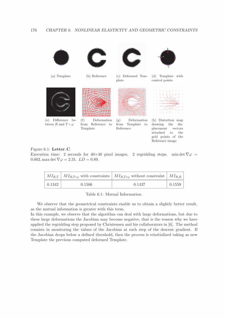
176 CHAPTER 6. NONLINEAR ELASTICITY AND GEOMETRIC CONSTRAINTS
(a) Template (b) Reference (c) Deformed Tem-plate
(d) Template withcontrol points
(e) Difference be-tween R and T ϕ
(f) Deformationfrom Reference toTemplate
(g) Deformationfrom Template toReference
(h) Distortion mapdrawing the dis-placement vectorsattached to thegrid points of theReference image
Figure 6.1: Letter C.Execution time: 2 seconds for 40×40 pixel images. 2 regridding steps. min det∇ϕ =0.002,maxdet∇ϕ = 2.31. LD = 0.89.
MIR,T MIR,Tϕ with constraints MIR,Tϕ without constraint MIR,R
0.1342 0.1506 0.1437 0.1559
Table 6.1: Mutual Information.
We observe that the geometrical constraints enable us to obtain a slightly better result,as the mutual information is greater with this term.In this example, we observe that the algorithm can deal with large deformations, but due tothese large deformations the Jacobian may become negative, that is the reason why we haveapplied the regridding step proposed by Christensen and his collaborators in [6]. The methodconsists in monitoring the values of the Jacobian at each step of the descent gradient. Ifthe Jacobian drops below a defined threshold, then the process is reinitialized taking as newTemplate the previous computed deformed Template.
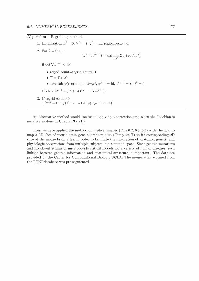
6.4. NUMERICAL EXPERIMENTS 177
Algorithm 4 Regridding method.
1. Initialization:β0 = 0, V 0 = I, ϕ0 = Id, regrid count=0.
2. For k = 0, 1, . . .(ϕk+1, V k+1) = argmin
ϕ,VLα,ε(ϕ, V, βk)
if det∇ϕk+1 < tol
• regrid count=regrid count+1
• T = T ϕk
• save tab ϕ(regrid count)=ϕk, ϕk+1 = Id, V k+1 = I, βk = 0.
Update βk+1 = βk + α(V k+1 −∇ϕk+1).
3. If regrid count>0ϕfinal = tab ϕ(1) · · · tab ϕ(regrid count)
An alternative method would consist in applying a correction step when the Jacobian isnegative as done in Chapter 3 ([21]).
Then we have applied the method on medical images (Figs 6.2, 6.3, 6.4) with the goal tomap a 2D slice of mouse brain gene expression data (Template T) to its corresponding 2Dslice of the mouse brain atlas, in order to facilitate the integration of anatomic, genetic andphysiologic observations from multiple subjects in a common space. Since genetic mutationsand knock-out strains of mice provide critical models for a variety of human diseases, suchlinkage between genetic information and anatomical structure is important. The data areprovided by the Center for Computational Biology, UCLA. The mouse atlas acquired fromthe LONI database was pre-segmented.
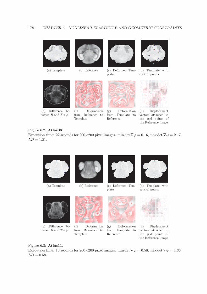
178 CHAPTER 6. NONLINEAR ELASTICITY AND GEOMETRIC CONSTRAINTS
(a) Template (b) Reference (c) Deformed Tem-plate
(d) Template withcontrol points
(e) Difference be-tween R and T ϕ
(f) Deformationfrom Reference toTemplate
(g) Deformationfrom Template toReference
(h) Displacementvectors attached tothe grid points ofthe Reference image
Figure 6.2: Atlas08.Execution time: 22 seconds for 200×200 pixel images. min det∇ϕ = 0.16,maxdet∇ϕ = 2.17.LD = 1.21.
(a) Template (b) Reference (c) Deformed Tem-plate
(d) Template withcontrol points
(e) Difference be-tween R and T ϕ
(f) Deformationfrom Reference toTemplate
(g) Deformationfrom Template toReference
(h) Displacementvectors attached tothe grid points ofthe Reference image
Figure 6.3: Atlas11.Execution time: 16 seconds for 200×200 pixel images. min det∇ϕ = 0.58,maxdet∇ϕ = 1.36.LD = 0.58.
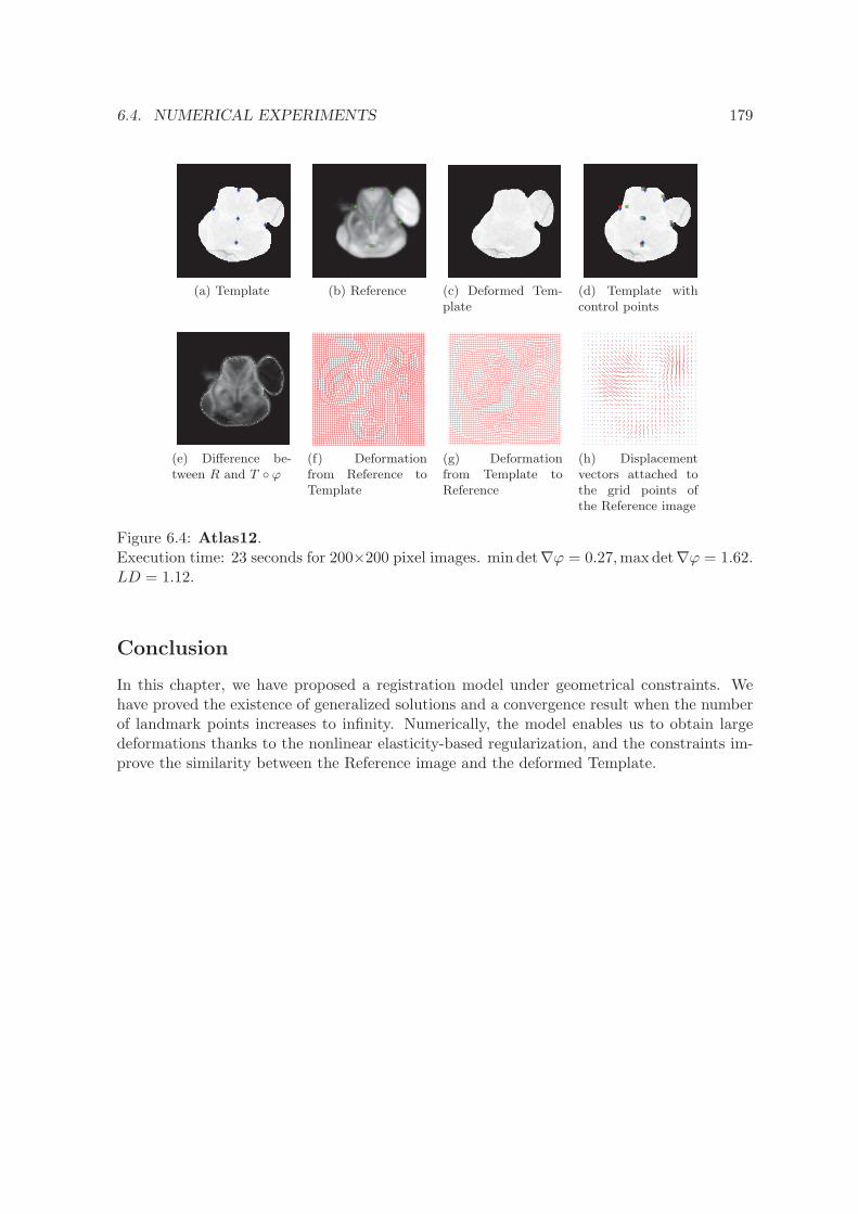
6.4. NUMERICAL EXPERIMENTS 179
(a) Template (b) Reference (c) Deformed Tem-plate
(d) Template withcontrol points
(e) Difference be-tween R and T ϕ
(f) Deformationfrom Reference toTemplate
(g) Deformationfrom Template toReference
(h) Displacementvectors attached tothe grid points ofthe Reference image
Figure 6.4: Atlas12.Execution time: 23 seconds for 200×200 pixel images. min det∇ϕ = 0.27,maxdet∇ϕ = 1.62.LD = 1.12.
Conclusion
In this chapter, we have proposed a registration model under geometrical constraints. Wehave proved the existence of generalized solutions and a convergence result when the numberof landmark points increases to infinity. Numerically, the model enables us to obtain largedeformations thanks to the nonlinear elasticity-based regularization, and the constraints im-prove the similarity between the Reference image and the deformed Template.

BIBLIOGRAPHY
[1] R. Arcangeli, M. C. L. de Silanes, and J. J. Torrens, An extension of a bound forfunctions in sobolev spaces, with applications to (m, s)-spline interpolation and smooth-ing, Numerische Mathematik, 107 (2007), pp. 181–211.
[2] M. Beg, M. Miller, A. Trouve, and L. Younes, Computing Large DeformationMetric Mappings via Geodesic Flows of Diffeomorphisms, International Journal of Com-puter Vision, 61 (2005), pp. 139–157.
[3] M. Bousselsal, Etude de quelques problemes de calcul des variations lies a lamecanique, PhD thesis, Universite de Metz, 1993.
[4] H. Brezis, Analyse Fonctionnelle, Theorie et Applications. 1999, Dunod, Paris, 1999.
[5] M. Burger, J. Modersitzki, and L. Ruthotto, A hyperelastic regularization energyfor image registration, SIAM Journal on Scientific Computing, 35 (2013), pp. B132–B148.
[6] G. Christensen, R. Rabbitt, and M. Miller, Deformable Templates Using LargeDeformation Kinematics, IEEE Trans. Image Process., 5 (1996), pp. 1435–1447.
[7] G. E. Christensen, Deformable shape models for anatomy, PhD thesis, WashingtonUniversity, Sever Institute of technology, USA, 1994.
[8] P. Ciarlet, Elasticite tridimensionnelle, Recherches en mathematiques appliquees,Masson, 1986.
[9] , Mathematical Elasticity: Three-dimensional elasticity, vol. 1, North-Holland, 1993.
[10] B. Dacorogna, Direct methods in the calculus of variations, vol. 78, Springer, 2007.
[11] R. Derfoul and C. Le Guyader, A constrained registration problem based on Ciarlet-Geymonat stored energy, in SPIE Medical Imaging, International Society for Optics andPhotonics, 2014, pp. 90343Q–90343Q.
[12] R. Derfoul and C. Le Guyader, A relaxed problem of registration based on the SaintVenant-Kirchhoff material stored energy for the mapping of mouse brain gene expressiondata to a neuroanatomical mouse atlas, SIAM Journal on Imaging Sciences, 7 (2014),pp. 2175–2195.
181
182 BIBLIOGRAPHY
[13] M. Droske and M. Rumpf, A Variational Approach to Non-Rigid Morphological Reg-istration, SIAM J. Appl. Math., 64 (2004), pp. 668–687.
[14] N. Kerdid, H. Le Dret, and A. Saıdi, Numerical approximation for a non-linearmembrane problem, International Journal of Non-Linear Mechanics, 43 (2008), pp. 908–914.
[15] H. Le Dret, Notes de Cours de DEA. Methodes mathematiques en elasticite, (2003-2004).
[16] C. Le Guyader and L. Vese, A combined segmentation and registration frameworkwith a nonlinear elasticity smoother, Computer Vision and Image Understanding, 115(2011), pp. 1689–1709.
[17] T. Lin, E.-F. Lee, I. Dinov, C. Le Guyader, P. Thompson, A. Toga, and
L. Vese, A landmark-based nonlinear elasticity model for mouse atlas registration, inBiomedical Imaging: From Nano to Macro, 2008. ISBI 2008. 5th IEEE InternationalSymposium on, 2008, pp. 788–791.
[18] M. Miller, A. Trouve, and L. Younes, On the Metrics and Euler-Lagrange Equa-tions of Computational Anatomy, Annu. Rev. B. Eng., 4 (2002), pp. 375–405.
[19] J. Modersitzki, Numerical Methods for Image Registration, Oxford University Press,2004.
[20] , FAIR: Flexible Algorithms for Image Registration, Society for Industrial and Ap-plied Mathematics (SIAM), 2009.
[21] S. Ozere and C. Le Guyader, Topology preservation for image-registration-relateddeformation fields, Communications in Mathematical Sciences, 13 (2015), pp. 1135–1161.
[22] R. Rabbitt, J. Weiss, G. Christensen, and M. Miller, Mapping of HyperelasticDeformable Templates Using the Finite Element Method, in Proceedings SPIE, vol. 2573,SPIE, 1995, pp. 252–265.
[23] A. Raoult, Non-polyconvexity of the stored energy function of a Saint Venant-Kirchhoffmaterial, Aplikace matematiky, 31 (1986), pp. 417–419.
CHAPTER 7
REGISTRATION BASED ON GRADIENT COMPARISON
In this chapter, we introduce a registration model based on the comparison of the gradientsof the involved images. Indeed, in the case of multi-modal images, we would like to matchthe edges of the objects regardless of intensity levels.
The chapter is organized as follows. In a first section, we present the proposed model.Then we establish the existence of minimizers for this problem. Due to computational issues,we have to find an alternative method to minimize the functional. To do so, we proposetwo methods: the first one consists in introducing an auxiliary variable and in this case, wedemonstrate the existence of solutions for this decoupled problem. The second one consistsin approximating the term that raises issues using a sequence of integral operators involvinga differential quotient and a suitable sequence of radial mollifiers, and we also demonstrateexistence results as well as a result of Γ-convergence.
This chapter provides a complete theoretical study of the method, however, no satisfactorynumerical result has been obtained for the moment. This study could constitute the beginningof future lines of research and perspectives.
Introduction
We plan to compare the gradients of the images instead of the gray levels, which would enableus to compare images with different modalities. Indeed, an important challenge is to comparemultiple images obtained with different devices for example in medical imaging. In particular,this idea has been investigated by Haber and Modersitzki in [12] and by Droske and Rumpf in[10]. In [12], Haber et al. use derivatives to characterize similarity between two images. Theybase their work on the following observation: ”Two images are considered similar, if intensitychanges occur at the same location”. To do so, they aim to match the normalized gradientvector fields of the two considered images. They define the normalized gradient vector fieldas follows:
n(I, x) =
∇I(x)‖∇I(x)‖ if ∇I(x) 6= 0,
0 otherwise.
The purpose is to align n(T ϕ, x) and n(R, x). The angle between the two vectors is denotedby θ(x). The distance measure is then based on the angle θ(x): it is equivalent to minimizing
183
184 CHAPTER 7. REGISTRATION BASED ON GRADIENT COMPARISON
sin2 θ(x) or maximizing cos2 θ(x) to align the two vector fields. This observation comes fromthe definition of the inner product or the cross product. Therefore, they define the followingdistance measures:
Dc(T,R) =1
2
∫
Ω‖n(R, x)× n(T ϕ, x)‖2dx,
Dd(T,R) = −1
2
∫
Ω〈n(R, x), n(T ϕ, x)〉2dx.
In [10], Droske et al. develop a similar idea but use the notion of morphologies. Themorphology of an image I is the collection of the level sets of the image:
M [I] =MI
c |c ∈ R, MI
c =x ∈ Ω ⊂ R
d|I(x) = c.
They also use the normal field NI on MIc defined by:
NI : Ω −→ Rd; x 7−→ ∇I
‖∇I‖ .
They search for a deformation ϕ such that M [T ϕ] =M [R], that is to say that they try toalign the normal fields. The energy functional to be minimized can be written as follows:
Em[ϕ] =
∫
Ωg(NT ϕ,NR,Cof∇ϕ)dµ,
with g(v, w,A) =(v − Aw
‖Aw‖
), which corresponds to the energy
∫
Ω‖NT ϕ−Nϕ
R‖2,
whereNϕR is the transformed normal of the reference image on Tϕ(x)ϕ(MR
R(x)) at position ϕ(x).
In order to build our functional based on gradient vector field comparison of the images,we have been inspired by [4]. In [4], Ballester et al. are interested in an inpainting problem.They consider an image u0 containing a hole of missing data, Ω, that they aim to fill-in. Theenergy functional they propose is minimized with respect to two variables: a vector field θwhich represents the directions of the level lines of u, and the grey level u. Moreover, θ shouldsatisfy |θ| ≤ 1 on Ω and should be related to u by trying to impose θ · ∇u = |∇u|.They thus propose to minimize a functional of the form
∫
Ω| div θ|p(a+ b|∇k ∗ u|dx
+α
∫
Ω(|∇u| − θ · ∇u) dx,
where a, b and α are positive constants and k is a smoothing kernel.Inspired by this model, we have tried to adapt the second term of this functional to ourregistration problem. We would like to match ∇(T ϕ) and ∇R. Following [4], T ϕ is asubstitute for u, the unknown corresponding to the grey level and ∇R
|∇R| a substitute for θ,normalized vector field. Then we propose the following distance measure:
∫
Ω
(|∇(T ϕ)| − 〈 ∇R
|∇R| ,∇(T ϕ)〉).
7.1. MATHEMATICAL MODELLING 185
7.1 Mathematical modelling
We make the same hypotheses as previously done. Let:
• Ω be a connected bounded open subset of R2 of class C1,
• R : Ω −→ R, be the Reference image,
• T : Ω −→ R, be a Lipschitz continuous function compactly supported, defining theTemplate image,
• ϕ : Ω −→ R2 the sought deformation with ϕ = Id on ∂Ω.
As mentioned above, the data fidelity term will be written as follows:
∫
Ω|∇(T ϕ)| − 〈∇(T ϕ), ∇R
|∇R| 〉.
As Ballester et al. in [4], we introduce θ a vector field with values in R2 satisfying
θ(x) · ∇R(x) = |R(x)| and |θ(x)| ≤ 1.
The vector field of normal θ can be defined as the Radon-Nikodyn derivative of the measure∇R with respect to |∇R|. We assume that θ ∈ L∞(Ω,R2) and div θ ∈ L2(Ω) for theoreticalpurposes.
For the regularizer term, we can choose for instance: ‖∇ϕ‖2L2(Ω,M2). Indeed, in this section,
we focus primarily on the dissimilarity measure based on the gradient vector fields.The problem is then phrased as follows:
infϕ∈Id+W1,2
0 (Ω,R2)
E(ϕ) =
∫
Ω|∇(T ϕ)| − 〈∇(T ϕ), θ〉+ α
2
∫
Ω‖∇ϕ‖2
. (7.1)
According to the following corollary:
Corollary 7.1.1 (Ambrosio [1])
Let Ω ⊂ Rn. Let p ∈ [1,+∞], u ∈ W1,p(Ω,Rm), and let f : Rm → R
k be a Lipschitzcontinuous function such that f(0) = 0. Then v = f(u) belongs to W1,p(Ω,Rk), for almostevery x ∈ Ω the restriction of the function f to the affine space
T ux = y ∈ Rm : y = u(x) + 〈∇u(x), z〉 for some z ∈ R
n
is differentiable at u(x), and
∇v = ∇(f|Tux)(u)∇u a.e in Ω.
Then T ϕ ∈ W1,2(Ω) and so T ϕ ∈ BV (Ω) since W1,2(Ω) ⊂ BV (Ω) and our functionalis well defined.We start by proving the existence of minimizers for the initial problem (7.1).
186 CHAPTER 7. REGISTRATION BASED ON GRADIENT COMPARISON
7.2 Existence minimizers for the initial problem
Theorem 7.2.1
Assuming that E is proper, the functional
E(ϕ) =
∫
Ω|∇(T ϕ)| − 〈∇(T ϕ), θ〉+ α
2
∫
Ω‖∇ϕ‖2
admits minimizers on Id+W1,20 (Ω,R2).
Proof :
Coercivity inequalityFirst, ∫
Ω|∇(T ϕ)| − 〈∇(T ϕ), θ〉 ≥ 0.
Using the generalized Poincare inequality: ‖ϕ‖2L2(Ω,R2) ≤ c
(‖∇ϕ‖2L2(Ω,M2)
+
∣∣∣∣∫
∂Ωϕdσ
∣∣∣∣2),
so ‖ϕ‖2W1,2(Ω,R2) ≤ (c+ 1)‖∇ϕ‖2L2(Ω,M2)+ k, then we obtain:
E(ϕ) ≥ c‖ϕ‖2W1,2(Ω,R2) + k, k ∈ R,
c denoting a constant depending on Ω that may change line to line.Therefore, E being proper, the infimum denoted by d is finite.
Convergence of a minimizing sequenceLet (ϕn) be a minimizing sequence of E, that is a sequence such that
E(ϕn)n→∞−→ inf
ψ∈Id+W1,20 (Ω,R2)
E(ψ).
Since E is assumed to be proper, there exists ϕ ∈ Id+W1,2(Ω,R2) such that E(ϕ) <+∞. From the previous coercivity inequality, we can deduce that, for n large enough,
c‖ϕn‖2W1,2(Ω,R2) + k ≤ E(ϕn) ≤ E(ϕ) + 1,
which means that ϕn is uniformly bounded in W1,2(Ω,R2).Therefore, since W1,2(Ω,R2) is a reflexive space, we can extract a subsequence of ϕn(still denoted by ϕn) such that:
ϕn ϕ in W1,2(Ω,R2).
It remains to prove that E is sequentially lower semi-continuous to conclude to theexistence of minimizers.
7.2. EXISTENCE MINIMIZERS FOR THE INITIAL PROBLEM 187
Lower semicontinuity of EThe L2-norm is convex, lower semi-continuous for the weak topology in L2, since
strongly sequentially continuous.Since ϕn ϕ in W1,2(Ω,R2), using Rellich-Kondrachov Theorem we obtain thatϕn −→ ϕ in L2(Ω,R2) and then
ϕn −→ ϕ in L1(Ω,R2),
since Ω is a bounded subset.Moreover, T is a Lipschitz continuous function (of Lipschitz constant kT ) so
∫
Ω|T ϕn − T ϕ| ≤
∫
ΩkT |ϕn − ϕ| =⇒ T ϕn −→ T ϕ in L1(Ω).
According to Corollary 7.1.1, T ϕ ∈ W1,2(Ω) and so it belongs to the space ofbounded variation functions BV(Ω). The strong convergence of T ϕn to T ϕ inL1(Ω) enables us to conclude that
∫
Ω|∇(T ϕ)| ≤ lim inf
n→+∞
∫
Ω|∇(T ϕn)|. (7.2)
The proof of (7.2) is rather classical.
Proof : Let φ ∈ C1c (Ω,R
2) and |φ(x)| ≤ 1 everywhere, then∫
ΩT ϕ(x) div φ(x) dx = lim
k→∞
∫
ΩT ϕk(x) div φ(x) dx.
Consequently, ∀ε > 0, ∃N(ε, φ), ∀k ∈ N,(k ≥ N =⇒
∣∣∣∣∫
ΩT ϕk(x) div φ(x) dx−
∫
ΩT ϕ(x) div φ(x) dx
∣∣∣∣ ≤ ε,
=⇒∫
ΩT ϕ(x) div φ(x) dx− ε ≤
∫
ΩT ϕk(x) div φ(x) dx ≤
∫
ΩT ϕ(x) div φ(x) dx+ ε
).
Since
∫
Ω|∇u| = sup
∫
Ωu div φ, |φ(x)| ≤ 1 e., φ ∈ C1
c (Ω,R2)
, we have
∫
ΩT ϕk(x) div φ(x) dx ≤
∫
Ω|∇(T ϕk)|.
Then ∀k ≥ N(ε, φ),∫
ΩT ϕ(x) div φ(x) dx− ε ≤
∫
Ω|∇(T ϕk)|,
which implies that∫
ΩT ϕ(x) div φ(x) dx ≤ lim inf
k→∞
∫
Ω|∇(T ϕk)|.
Taking the supremum over all φ ∈ C1c (Ω,R
2), we conclude that∫
Ω|∇(T ϕ)| ≤ lim inf
k→∞
∫
Ω|∇(T ϕk)|.
188 CHAPTER 7. REGISTRATION BASED ON GRADIENT COMPARISON
Finally, we can apply the following theorem from [2]:
Theorem 7.2.2 (Anzellotti [2, Theorem 1.9])
Let Ω ∈ RN with N ≥ 2 be a bounded open set with Lipschitz boundary. Let us
denote by ν the outward unit normal to ∂Ω. If one of these conditions is satisfied :
1. u ∈ BV(Ω) ∩ Lq(Ω), ψ ∈ ξ ∈ L∞(Ω,RN ), div ξ ∈ Lp(Ω), 1 < p ≤ N, 1p +1q = 1,
2. u ∈ BV(Ω) ∩ L∞(Ω), ψ ∈ ξ ∈ L∞(Ω,RN ), div ξ ∈ L1(Ω),3. u ∈ BV(Ω)∩L∞(Ω)∩C0(Ω), ψ ∈ ξ ∈ L∞(Ω,RN ), div ξ is a bounded measure in Ω,
then one has ∫
Ωu divψ +
∫
Ω(∇u, ψ) =
∫
∂Ω[ψ.ν]udHN−1.
Therefore, we obtain:
∫
Ω〈∇(T ϕn), θ〉 = −
∫
ΩT ϕn div θ +
∫
∂Ω[θ, ν]T ϕn dH1
︸ ︷︷ ︸known on ∂Ω and
independent of n sinceϕn|∂Ω = Id.
,
and we know that limn→∞
∫
ΩT ϕn div θ =
∫
ΩT ϕ div θ since T ϕn strongly converges
to T ϕ in L2(Ω) and div θ ∈ L2(Ω). Gathering all this results, we obtain that E issequentially lower semi-continuous.Moreover, Id+W1,2
0 (Ω,R2) is a closed convex subspace of W1,2(Ω,R2) by continuityof the trace, thus it is a weakly closed convex space according to Theorem III.7 in [6].We obtain that ϕ ∈ Id+W1,2
0 (Ω,R2) and finally ϕ = Id on ∂Ω. This completes the
proof showing that E admits minimizers on Id+W1,20 (Ω,R2).
Numerically, the total variation of T ϕ may turn out to be complicated to compute, that isthe reason why we have to find a suitable way to compute this term efficiently. To do so, wehave investigated two methods.
7.3 Introduction of an auxiliary variable
Firstly, we propose to introduce an auxiliary variable to handle the term in T ϕ.
infW×X
Eγ(ϕ, T ) =
∫
Ω|∇T | − 〈∇T , θ〉+ α
2
∫
Ω‖∇ϕ‖2 dx+ γ‖T ϕ− T‖L1(Ω)
(7.3)
with W = ϕ ∈ Id+W1,20 (Ω,R2), X = T ∈ BV (Ω) with T = T on ∂Ω .
However, the trace of BV functions is not continuous for the BV weak-∗ topology, which is anobstacle to prove that a minimizing sequence converges in W×X . Indeed, as seen previously,the weak and strong topology are equivalent on a closed convex subspace but this property
7.3. INTRODUCTION OF AN AUXILIARY VARIABLE 189
does not hold for the weak-∗ topology.That is the reason why, inspired by [9], we define two equivalent problems. Before, we use the
formula introduced in Theorem 7.2.2, namely:
∫
Ω〈∇T , θ〉 = −
∫
ΩT div θ +
∫
∂Ω[θ, ν] T dH1
︸ ︷︷ ︸known on ∂Ω
.
Therefore, problem (7.3) is equivalent to:
infW×BV0(Ω)
Eγ(ϕ, T ) =
∫
Ω|∇T |+
∫
ΩT div θ +
α
2
∫
Ω‖∇ϕ‖2 dx+ γ‖T ϕ− T‖L1(Ω)
(7.4)
(recalling the T is compactly supported and ϕ|∂Ω = Id), and we define an associated relaxedproblem:
infW×BV (Ω)
Eγ(ϕ, T ) =
∫
Ω|∇T |+
∫
ΩT div θ+
∫
∂Ω|T | dH1
+α
2
∫
Ω‖∇ϕ‖2 dx+ γ‖T ϕ− T‖L1(Ω)
.
(7.5)
We aim to prove in a first step that
infW×BV0(Ω)
Eγ(ϕ, T ) = inf(7.4)= infW×BV (Ω)
Eγ(ϕ, T ) = inf(7.5).
In this prospect, we need the following density result:
Theorem 7.3.1 (Demengel [9, Theorem 6.70, Chapter 6, page 322])
Let Ω be an open subset of RN of class C1 and let u ∈ BV (Ω). Then there exists asequence un of functions in C∞
c (Ω) such that
‖un − u‖L1(Ω)n→+∞−→ 0 and
∫
Ω|∇un| n→+∞−→
∫
Ω|∇u|+
∫
∂Ω|u|.
First, as W ×BV0(Ω) is included in W ×BV (Ω) it is clear that
inf (7.5)≤ inf (7.4).
Let us denote by (ϕ, ¯T ) a minimizing pair of problem (7.5) (we prove further that such aminimizing pair exists). According to Theorem 7.3.1, there exists a sequence (Tn) ∈ C∞
c (Ω)such that:
Tn −→ ¯T in L1(Ω),∫
Ω|∇Tn| −→
∫
Ω|∇ ¯T |+
∫
∂Ω| ¯T | dH1.
(7.6)
Also, there exists (ϕn) ∈ W1,2(Ω,R2)∩C∞c (Ω,R2) (as Ω is bounded, of class C1, [6, Corollary
IX.8]), such that
ϕnn→+∞−→ ϕ in W1,2(Ω,R2).
190 CHAPTER 7. REGISTRATION BASED ON GRADIENT COMPARISON
As Tn is uniformly bounded in BV (Ω) and thus in L2(Ω) (due to the continuous embeddingof BV (Ω) in L2(Ω) - recall that Ω ⊂ R
2), we can extract a subsequence of Tn, still denoted
by Tn, such that Tn converges to T ∗ in L2(Ω). It is not difficult to prove that T ∗ = ¯T .Consequently,
∫
Ω|∇Tn|+
∫
ΩTn div θ +
α
2
∫
Ω‖∇ϕn‖2 + γ‖T ϕn − Tn‖L1(Ω)
n→+∞−→∫
Ω|∇ ¯T |+
∫
∂Ω| ¯T | dH1 +
∫
Ω
¯T div θ +α
2
∫
Ω‖∇ϕ‖2 dx+ γ‖T ϕ− ¯T‖L1(Ω).
In conclusion,
inf (7.4) = inf (7.5).
7.3.1 Existence of minimizers for the decoupled problem
Theorem 7.3.2
Assuming that Eγ is proper. The decoupled problem
infϕ∈Id+W1,2
0 (Ω,R2)
T∈BV(Ω)
Eγ(ϕ, T ) =
∫
Ω|∇T |+
∫
ΩT div θ +
∫
∂Ω|T | dH1
+α
2
∫
Ω‖∇ϕ‖2 dx+ γ‖T ϕ− T‖L1(Ω)
,
admits at least one solution.
Remark 7.3.1
We can check that the problem is well defined since as Ω ⊂ R2 is bounded with Lipschitz
boundary, we have BV(Ω) ⊂ L2(Ω).
Proof :Coercivity inequality
M is a positive constant that may change line to line and that may depend on γ(here, γ is fixed).
As
∣∣∣∣∫
ΩT div θ
∣∣∣∣ ≤ ‖T‖L2(Ω)‖ div θ‖L2(Ω), then
∫
ΩT div θ ≥ −‖T‖L2(Ω)‖ div θ‖L2(Ω) ≥ −κ‖ div θ‖L2(Ω)‖T‖BV (Ω),
κ > 0, still due to the continuous embedding BV (Ω) ⊂ L2(Ω). It follows that
Eγ(ϕ, T ) ≥∫
Ω|∇T | − κ‖T‖BV (Ω)‖ div θ‖L2(Ω) + γ‖T‖L1(Ω) − γ‖T ϕ‖L1(Ω) +
α
2‖∇ϕ‖2L2(Ω,M2)
,
≥(min(1, γ)− κ‖ div θ‖L2(Ω)
)‖T‖BV (Ω) − γ‖T ϕ‖L1(Ω) +
α
2‖∇ϕ‖2L2(Ω,M2)
.
T is assumed to be Lipschitz continuous and compactly supported. For theoreticaland numerical purposes, we may consider a linear extension operator ([6, TheoremIX.7, page 158]) P : W1,∞(Ω) −→ W1,∞(R2) such that
7.3. INTRODUCTION OF AN AUXILIARY VARIABLE 191
(i) PT|Ω = T ,
(ii) ‖PT‖L∞(R2) ≤ C‖T‖L∞(Ω) and
(iii) ‖PT‖W1,∞(R2) ≤ C‖T‖W1,∞(Ω) with C depending only on Ω.
Thus
Eγ(ϕ, T ) ≥(min(1, γ)− κ‖ div θ‖L2(Ω)
)‖T‖BV (Ω)−γ|Ω|‖PT‖L∞(R2)+
α
2‖∇ϕ‖2L2(Ω,M2)
.
Finally, using the generalized Poincare inequality:
Eγ(ϕ, T ) ≥(min(1, γ)− κ‖ div θ‖L2(Ω)
)‖T‖BV (Ω) − γ|Ω|‖PT‖L∞(R2) +A‖ϕ‖2W1,2(Ω,R2) −K
with A > 0,K ∈ R and if ‖ div θ‖L2(Ω) <min(1, γ)
κ, the infimum is finite.
Convergence of a minimizing sequence
Let (ϕn, Tn) be a minimizing sequence of Eγ(ϕ, T ). Since Eγ is proper, for n largeenough,(min(1, γ)− κ‖ div θ‖L2(Ω)
)‖T‖BV (Ω)+A‖ϕ‖2W1,2(Ω,R2)−K ≤ Eγ(ϕn, Tn) ≤M , which
implies that (ϕn) is uniformly bounded in W1,2(Ω,R2). We can thus extract a subse-quence, still denoted by ϕn, such that
ϕn ϕγ in W1,2(Ω,R2).
Also, Tn is uniformly bounded in BV (Ω) (thus in L2(Ω)) and we can extract a subse-quence, still denoted by Tn, of Tn such that:
Tn Tγ in L2(Ω)
and
Tn∗ Tγ in BV (Ω),
which means, for the weak-∗ convergence in BV (Ω), that Tn converges strongly inL1(Ω) to Tγ and for all φ in (C0(Ω))2,
∫
Ωφ∇Tn −→
∫
Ωφ∇Tγ .
In summary, working with a common extraction mapping (we do not change thenotations for the common extraction mappings),
ϕn ϕγ in W1,2(Ω,R2)
Tn∗ Tγ in BV (Ω).
Rellich-Kondrachov embedding theorem gives that ϕn strongly converges to ϕγ inL2(Ω,R2) (and thus in L1(Ω,R2)).
192 CHAPTER 7. REGISTRATION BASED ON GRADIENT COMPARISON
Lower semicontinuity of Eγ
By lower semicontinuity of the total variation,∫
Ω|∇Tγ | ≤ lim inf
n→∞
∫
Ω|∇Tn|.
The L2-norm being convex and strongly sequentially lower semi-continuous, it is lowersemi-continuous and ∫
Ω‖∇ϕγ‖2 ≤ lim inf
n→+∞
∫
Ω‖∇ϕn‖2.
As div θ is assumed to belong to L2(Ω) and Tn weakly converges to Tγ in L2(Ω),
limn→+∞
∫
ΩTn div θ =
∫
ΩTγ div θ.
At last,
‖T ϕn − Tn − (T ϕγ − Tγ)‖L1(Ω) ≤ ‖T ϕn − T ϕγ‖L1(Ω) + ‖Tn − Tγ‖L1(Ω),
≤ kT ‖ϕn − ϕγ‖L1(Ω) + ‖Tn − Tγ‖L1(Ω),
which implies that limn→+∞
‖T ϕn − Tn‖L1(Ω) = ‖T ϕγ − Tγ‖L1(Ω).
Now, denoting by Tn an extension of Tn by 0 outside of Ω, we have, according to theextension theorem ([11, Theorem 1, page 183]), that Tn ∈ BV (R2) and
∫
R2
|∇Tn| =∫
Ω|∇Tn|+
∫
∂Ω|Tn| dH1.
If Tn converges weakly-∗ to Tγ in BV (Ω), then Tn converges weakly-∗ to an elementu of BV (R2). We must have u = 0 in the complement of Ω and u = Tγ in Ω. Inparticular, ∫
R2
|∇u| =∫
Ω|∇Tγ |+
∫
∂Ω|Tγ | dH1.
By the weak lower semicontinuity property,∫
R2
|∇u| ≤ lim infn→+∞
∫
R2
|∇Tn|,
that is ∫
Ω|∇Tγ |+
∫
∂Ω|Tγ | dH1 ≤ lim inf
n→+∞
∫
R2
Tn +
∫
∂Ω|Tn|dH1.
In conclusion,∫
Ω|∇Tγ |+
∫
∂Ω|Tγ | dH1 +
∫
ΩTγ div θ
+α
2
∫
Ω‖∇ϕγ‖2 + γ‖T ϕγ − Tγ‖L1(Ω)
≤ lim infn→+∞
(∫
Ω|∇Tn|+
∫
ΩTn div θ +
∫
∂Ω|Tn| dH1
+α
2
∫
Ω‖∇ϕn‖2 + γ‖T ϕn − Tn‖L1(Ω)
),
which implies that (ϕγ , Tγ) is a minimizing pair of problem (7.5).
7.4. APPROXIMATION METHOD OF THE TOTAL VARIATION OF T ϕ 193
7.4 Approximation method of the total variation of T ϕWe now come to the second method to overcome the difficulties revealed by the total variationof T ϕ.
As described in [3], Aubert and Kornprobst use an approximation of the semi-norm on
W1,p(Ω): |u|pW1,p =
∫
Ω|∇u|p, ∀p. They propose an alternative method based on a character-
ization of the Sobolev spaces by Bourgain et al. in [5] and extended by Ponce in [13]. Beforeproviding approximation results, we introduce a sequence (ρn) of radial mollifiers, i.e.,
ρn(x) = ρn(|x|),
ρn ≥ 0,
∫
RN
ρn(x)dx = 1,
and for every δ > 0, we assume that limn→∞
∫ ∞
δρn(r)r
N−1dr = 0 (Ω ⊂ RN ).
(7.7)
In [5], the authors provide the following theorem:
Theorem 7.4.1 ([5, Theorem 2])
Assume u ∈ Lp(Ω), 1 < p <∞. Then
limn→∞
∫
Ω
∫
Ω
|u(x)− u(y)|p|x− y|p ρn(x− y) dx dy = Kp,N
∫
Ω|∇u|p dx = Kp,N |u|pW1,p (7.8)
with the convention that |u|W1,p = ∞ if u /∈ W1,p(Ω). Here Kp,N depends only on p andN .
In [13], Ponce provides a follow-up to [5], replacing |.|p with a continuous function w andusing functions ρn that are no longer assumed to be radial. He also focuses on the BV -caseand provides the following corollary:
Corollary 7.4.1 ([13, Corollary 1])
Suppose that ρn is radial for each n > 0. If u ∈ W1,p(Ω), p > 1 or if u ∈ BV (Ω) andp = 1, then
limn→∞
∫
Ω
∫
Ω
|u(x)− u(y)|p|x− y|p ρn(x− y) dx dy = Kp,N
∫
Ω|Du|p,
where Kp,N = −∫
SN−1
|e · σ|p dHN−1.
In our work, we use this characterization to approximate the total variation.Then we propose minimizing the following functional:
infϕ∈W
En(ϕ) =
1
K1,N
∫
Ω
∫
Ω
|T ϕ(x)− T ϕ(y)||x− y| ρn(x− y) dx dy −
∫
Ω〈∇(T ϕ), θ〉 dx
+α
2
∫
Ω‖∇ϕ‖2 dx
,
(7.9)
194 CHAPTER 7. REGISTRATION BASED ON GRADIENT COMPARISON
with W =Id+W1,2
0 (Ω,R2).
Functional En is well defined for ϕ ∈ W1,2(Ω), since T is Lipschitz continuous, T ϕ ∈ W1,2(Ω)according to Theorem 7.1.1, and then T ϕ ∈ BV (Ω).
For the sake of clarity, we denote by Fn(u) the approximation:
Fn(u) =
∫
Ω
∫
Ω
|u(x)− u(y)||x− y| ρn(x− y) dx dy.
7.4.1 Existence of minimizers for the Problem with approximation of the
total variation
Theorem 7.4.2
Assuming En is proper, for n large enough, Problem (7.9) admits at least one solution.
Proof :
Coercivity inequalityLet us fix ε = 1. According to Corollary 7.4.1,
∃n0 ∈ N, ∀n ∈ N,(n ≥ n0 =⇒
∣∣∣∣Fn(T ϕ)−K1,N
∫
Ω|∇(T ϕ)|
∣∣∣∣ ≤ 1
)
so
(n ≥ n0 =⇒
∫
Ω|∇(T ϕ)| − 1
K1,N≤ 1
K1,NFn(T ϕ) ≤
∫
Ω|∇(T ϕ)|+ 1
K1,N
).
Therefore, we obtain
1
K1,NFn(T ϕ)−
∫
Ω〈∇(T ϕ), θ〉 dx ≥
∫
Ω|∇(T ϕ)| −
∫
Ω〈∇(T ϕ), θ〉 dx− 1
K1,N,
for n large enough.
Since
∫
Ω|∇(T ϕ)| −
∫
Ω〈∇(T ϕ), θ〉 dx ≥ 0, it yields to
En(ϕ) ≥α
2‖∇ϕ‖2L2(Ω,M2)
− 1
K1,N.
At last, using the generalized Poincare inequality, we obtain:
En(ϕ) ≥ c‖ϕ‖2W1,2(Ω,R2) + κ , κ ∈ R. (7.10)
Therefore, En being proper, the infimum of En is finite.
Convergence of a minimizing sequenceLet (ϕkn) ∈ Id+W1,2
0 (Ω,R2) be a minimizing sequence of En(ϕ).
En(ϕkn)
k→∞−→ infΨ∈Id+W1,2
0 (Ω,R2)En(Ψ).
7.4. APPROXIMATION METHOD OF THE TOTAL VARIATION OF T ϕ 195
We have assumed that En is proper that is to say that there exists ϕn such thatEn(ϕn) < ∞, then for k large enough we have En(ϕ
kn) ≤ En(ϕn) + 1. So, from
the coercivity inequality, (ϕkn) is bounded in W1,2(Ω,R2), we can therefore extract asubsequence still denoted by (ϕkn) such that:
(ϕkn)k ϕn in W1,2(Ω,R2).
And by continuity of the trace: ϕn = Id on ∂Ω.
Lower semicontinuityAccording to Rellich-Kondrachov theorem, we also have ϕkn −→ ϕn in L2(Ω,R2) and
so in L1(Ω,R2).T being a Lipschitz continuous function: T ϕkn −→ T ϕn in L2(Ω). So T ϕkn weaklyconverges to T ϕn in L2(Ω). Consequently, since it is assumed that div θ ∈ L2(Ω),
∫
Ω
(T ϕkn
)div θ dx
k→+∞−→∫
Ω(T ϕn) div θ dx.
Recalling that
∫
Ω〈∇
(T ϕkn
), θ〉 dx = −
∫
ΩT ϕkn div θ dx+
∫
∂Ω[θ, n]T ϕkn dH1, we
obtain that
∫
Ω〈∇
(T ϕkn
), θ〉 dx k→+∞−→
∫
Ω〈∇ (T ϕn) , θ〉 dx,
since again ϕkn = Id on ∂Ω and T is assumed to be compactly supported.Thanks to Theorem 2.1.11 ([6, Theorem IV.9]), we also have the convergence almost ev-
erywhere of a subsequence of T ϕkn to T ϕn. Therefore|T ϕkn(x)− T ϕkn(y)|
|x− y| ρn(x−
y) converges to|T ϕn(x)− T ϕn(y)|
|x− y| ρn(x−y) almost everywhere. Moreover, we use
the following proposition:
Proposition 7.4.2 ([3, Proposition 2.1])
Assume 1 ≤ p ≤ ∞ and u ∈ W1,p(Ω) and let ρ ∈ L1(RN ), ρ > 0. Then
∫
Ω
∫
Ω
|u(x)− u(y)|p|x− y|p ρ(x− y) dx dy ≤ C|u|p
W1,p‖ρ‖L1(RN ),
where |u|pW1,p denote the semi-norm defined by |u|p
W1,p =
∫
Ω|∇u|p dx and C depends only
on p and Ω.
196 CHAPTER 7. REGISTRATION BASED ON GRADIENT COMPARISON
Thus,
∫
Ω
∫
Ω
|T ϕkn(x)− T ϕkn(y)||x− y| ρn(x− y) dx dy
≤kT∫
Ω
∫
Ω
|ϕkn(x)− ϕkn(y)||x− y| ρn(x− y) dx dy
≤kT∫
Ω
∫
Ω
|(ϕkn
)1(x)−
(ϕkn
)1(y)|
|x− y| ρn(x− y) dx dy
+ kT
∫
Ω
∫
Ω
|(ϕkn
)2(x)−
(ϕkn
)2(y)|
|x− y| ρn(x− y) dx dy,
≤kTC(‖(ϕkn
)1‖W1,2(Ω,R2) + ‖
(ϕkn
)2‖W1,2(Ω,R2)
),
which is bounded independently of k ((ϕkn)1 and (ϕkn)
2 denoting the components ofϕkn).Then according to the dominated convergence theorem:
∫
Ω
∫
Ω
|T ϕn(x)− T ϕn(y)||x− y| ρn(x− y) dx dy
= limk→+∞
∫
Ω
∫
Ω
|T ϕkn(x)− T ϕkn(y)||x− y| ρn(x− y) dx dy.
To conclude, the functional is weakly sequentially lower semicontinuous and
En(ϕn) ≤ lim infk→∞
En(ϕkn).
Therefore, there exists at least one minimizer of En on Id+W1,20 (Ω,R2).
7.4.2 Study of limn→∞
ϕn and Γ-convergence
According to Theorem 3 in [5]:
Theorem 7.4.3 ([5, Theorem 3])
Assume f ∈ W1,1(Ω), Ω ⊂ RN . Then
limj→∞
∫
Ω
∫
Ω
|f(x)− f(y)||x− y| ρεj (x− y) dx dy = K1,N |f |W1,1(Ω) .
K1,N only depends on N .
Proof (inspired of [5]) : As N = 2 in practice, we restrict ourselves to this case in theproof.For f ∈ W1,1(Ω), let
Fn(x, y) =|f(x)− f(y)|
|x− y| ρn(x− y).
7.4. APPROXIMATION METHOD OF THE TOTAL VARIATION OF T ϕ 197
We have to prove that
limn→∞
‖Fn‖L1(Ω×Ω) = K1,N |f |W1,1(Ω).
Theorem 7.4.4 ([5, Theorem 1])
Assume f ∈ W1,p(Ω), 1 ≤ p <∞, and let ρ ∈ L1(RN ), ρ ≥ 0. Then
∫
Ω
∫
Ω
|f(x)− f(y)|p|x− y|p ρ(x− y) dx dy ≤ C |f |p
W1,p ‖ρ‖L1 ,
where C depends only on p and Ω.
The proof of Theorem 7.4.4 relies on Proposition IX.3 in [6].By Theorem 7.4.4 and using the fact that ρn is radial, we have for any n and f, g ∈W1,1(Ω),
∣∣‖Fn‖L1(Ω×Ω) − ‖Gn‖L1(Ω×Ω)
∣∣ ≤ ‖Fn −Gn‖L1(Ω×Ω) ≤ C |f − g|W1,1(Ω) ,
with C being independent of f, g and n thanks to the properties of radial functions.Therefore, it suffices to establish the result for f ∈ C2(Ω) and by density, it will besatisfied for f ∈ W1,1(Ω). Indeed, ∀f ∈ W1,1(Ω), there exists a sequence (fk) ∈ C2(Ω)such that
fkk→+∞−→ f in W1,1(Ω).
Then |f − fk|W1,1(Ω)k→+∞−→ 0 implies
∣∣‖Fn‖L1(Ω×Ω) − ‖Fk,n‖L1(Ω×Ω)
∣∣ k→+∞−→ 0, which
yields to the validity of the result for f ∈ W1,1(Ω) if the result holds for f ∈ C2(Ω).
Fix some f ∈ C2(Ω), then
|f(x)− f(y)||x− y| =
∣∣∣∣(∇f)(x) ·x− y
|x− y|
∣∣∣∣+O(|x− y|).
For each fixed x ∈ Ω, let us set R = dist(x, ∂Ω). Denoting by B(x,R) the open ballwith center x and radius R,
∫
Ω
|f(x)− f(y)||x− y| ρn(x− y) dy =
∫
B(x,R)
|f(x)− f(y)||x− y| ρn(x− y) dy
+
∫
Ω\B(x,R)
|f(x)− f(y)||x− y| ρn(x− y) dy.
∫
Ω\B(x,R)
|f(x)− f(y)||x− y| ρn(x− y) dy ≤
2‖f‖C0(Ω)
R
∫
Ω\B(x,R)ρn(x− y) dy,
≤2‖f‖C0(Ω)
R|S1|
∫ +∞
Rrρn(r) dr,
which tends to 0 as n −→ ∞, as a result of the properties of ρn. Let us now make the
expression of
∫
B(x,R)
|f(x)− f(y)||x− y| ρn(x− y) dy explicit. Denoting by y = (y1, y2) and
198 CHAPTER 7. REGISTRATION BASED ON GRADIENT COMPARISON
x = (x1, x2), we make the change of variables
y1 = x1 + r cos θ
y2 = x2 + r sin θ, with θ ∈ [0, 2π] and r ∈ [0, R].
Then
∫
B(x,R)
|f(x)− f(y)||x− y| ρn(x− y) dy =
∫
B(x,R)
(∣∣∣∣(∇f)(x) ·x− y
|x− y|
∣∣∣∣
+O(|x− y|))ρn(x− y) dy,
=
∫ R
0rρn(r)
∫ 2π
0
(∣∣∣∣(∇f)(x) ·(cos θ
sin θ
)∣∣∣∣)dθ dr
+ |S1|O(∫ R
0r2ρn(r) dr
).
Then setting ∇f(x) = |∇f(x)|e with e a unit vector (here e depends on x), it yieldsto:
∫
B(x,R)
|f(x)− f(y)||x− y| ρn(x− y) dy = |∇f(x)|
∫ R
0rρn(r)
∫ 2π
0
(|e ·
(cos θ
sin θ
)|)dθ dr,
+ |S1|O(∫ R
0r2ρn(r) dr
),
First of all,
∫ 2π
0
(|e ·
(cos θ
sin θ
)|)dθ is independent of the unit vector e.
Secondly,
|S1|∫ R
0rρn(r) dr = |S1|
∫ +∞
0rρn(r) dr
︸ ︷︷ ︸= 1
according to the
hypotheses
on ρn
− |S1|∫ +∞
Rrρn(r) dr.
︸ ︷︷ ︸n→+∞
0
Thirdly, as proved by Spector in his PhD manuscript ([15, page 58]), if E ⊂ RN is
bounded and measurable, then
limn→+∞
∫
E|x|ρn(x) dx = 0.
In our case, taking E = B(0, R) and making the change of variables
x1 = r cos θx2 = r sin θ,
we get ∫
B(0,R)|x|ρn(x) dx = |S1|
∫ R
0r2ρn(r) dr,
7.4. APPROXIMATION METHOD OF THE TOTAL VARIATION OF T ϕ 199
which tends to 0 when n tends to +∞.In conclusion,
∫
B(x,R)
|f(x)− f(y)||x− y| ρn(x− y) dy =
|∇f(x)||S1|
(∫ 2π
0
(|e ·
(cos θ
sin θ
)|)dθ
)∫ R
0|S1|rρn(r) dr,
+ |S1|O(∫ R
0r2ρn(r) dr
),
and with the material above,
limn→+∞
∫
B(x,R)
|f(x)− f(y)||x− y| ρn(x− y) dy = K1,2|∇f(x)|, (7.11)
with K1,2 =1
|S1|
∫ 2π
0|e ·
(cos θ
sin θ
)| dθ and e any unit vector of R2.
Since f ∈ C2(Ω), there exists L such that |f(x)− f(y)| ≤ L|x− y|, ∀x, y ∈ Ω, then
∫
Ω
|f(x)− f(y)||x− y| ρn(x− y) dy ≤ L, ∀x ∈ Ω, (7.12)
(one assume that Ω is connected, which is the case in practice).Using the dominated convergence theorem, with (7.11) and (7.12), we conclude thatfor f ∈ C2(Ω), lim
n→∞‖Fn‖L1(Ω×Ω) = K1,N |f |W1,1(Ω). That is to say
limn→∞
∫
Ω
∫
Ω
|f(x)− f(y)||x− y| ρn(x− y) dx dy = K1,N |f |W1,1(Ω) .
We complete the proof thanks to the density of C2(Ω) in W1,1(Ω) (corollary IX.8 in[6]).
We have provided the proof in the case of f ∈ W1,1(Ω), which is sufficient in our case sinceT ϕ ∈ W1,2(Ω) so T ϕ ∈ W1,1(Ω). However, in [8], Davila provides the proof for the BVcase:
Theorem 7.4.5 ([8, Theorem 1])
Let Ω ⊂ RN be open bounded with a Lipschitz boundary and let f ∈ BV (Ω). Consider a
sequence ρn satisfying (7.7). Then
limn→∞
∫
Ω
∫
Ω
|f(x)− f(y)||x− y| ρn(x− y) dx dy = K1,N |f |BV (Ω)
with |f |BV (Ω) =
∫
Ωf divϕ ∈ C1
c (Ω,RN ), |ϕ| ≤ 1 in Ω
.
For n fixed, we have proved the existence of a solution ϕn in Id+W1,2(Ω,R2) to problem(7.9) for n large enough.
∀v ∈ Id+W1,20 (Ω), En(ϕn) ≤ En(v).
200 CHAPTER 7. REGISTRATION BASED ON GRADIENT COMPARISON
From this inequality and the coercivity inequality, ϕn is bounded independently of n then,up to a subsequence, ϕn weakly converges to ϕ in W1,2(Ω,R2).We would like to prove that En(ϕn) converges to E(ϕ) when n tends to +∞.By definition of ϕn, one has En(ϕn) ≤ En(ϕ), thus by passing to the upper limit when ntends to +∞,
lim supn→+∞
En(ϕn) ≤ lim supn→+∞
En(ϕ)
= limn→+∞
1
K1,2
∫
Ω
∫
Ω
|T ϕ(x)− T ϕ(y)||x− y| ρn(x− y) dx dy
+
∫
ΩT ϕ div θ dx+
α
2
∫
Ω‖∇ϕ‖2 dx,
=
∫
Ω|∇(T ϕ)|+
∫
ΩT ϕ div θ dx+
α
2
∫
Ω‖∇ϕ‖2 dx,
= E(ϕ).
Thus,
lim supn→+∞
En(ϕn) ≤ E(ϕ).
It remains to prove thatE(ϕ) ≤ lim inf
n→+∞En(ϕn).
Due to compactness properties, it suffices to prove that∫
Ω|∇(T ϕ)| ≤ lim inf
n→+∞Fn(T ϕn).
In that purpose, let us introduce some notations.For r > 0, we define the two following sets:
Ωr = x ∈ Ω : dist(x, ∂Ω) > r,
Ωr = x ∈ R2 : dist(x,Ω) < r.
Let η ∈ C∞0 (R2) be a nonnegative radial function such that
∫
Ωη = 1, Supp η ⊂ B(0, 1), and
let us define
fδ(x) =1
δ2
∫
Ωf(y) η(
x− y
δ) dy, ∀x ∈ Ωδ,
where fδ is a regularization of f .For the sake of clarity, we set f = T ϕ, and due to the properties of T , fn = T ϕn stronglyconverges to f = T ϕ in L1(Ω).From Lemma 4 in [13], for each r > 0:
Fn(fn) ≥∫
Ωr
∫
Ωr
|fn,δ(x)− fn,δ(y)||x− y| ρn(x− y) dx dy, ∀δ ∈ (0, r).
We first aim to prove that
limn→+∞
∫
Ωr
∫
Ωr
|fn,δ(x)− fn,δ(y)||x− y| ρn(x− y) dy dx = lim
n→+∞
∫
Ωr
∫
Ωr
∣∣∣∣∇fδ(x) ·x− y
|x− y|
∣∣∣∣ ρn(x− y) dy dx
= K1,2
∫
Ωr
|∇fδ|.
7.4. APPROXIMATION METHOD OF THE TOTAL VARIATION OF T ϕ 201
We start by proving that
limn→+∞
∣∣∣∣∫
Ωr
∫
Ωr
( |fn,δ(x)− fn,δ(y)||x− y| − ∇fδ(x) ·
x− y
|x− y|
)ρn(x− y) dy dx
∣∣∣∣ = 0.
It is easily seen that
∣∣∣∣∫
Ωr
∫
Ωr
( |fn,δ(x)− fn,δ(y)||x− y| −
∣∣∣∣∇fδ(x) ·x− y
|x− y|
∣∣∣∣)ρn(x− y) dy dx
∣∣∣∣
≤∫
Ωr
∫
Ωr
∣∣∣∣|fn,δ(x)− fn,δ(y)|
|x− y| −∣∣∣∣∇fδ(x) ·
x− y
|x− y|
∣∣∣∣∣∣∣∣ ρn(x− y) dy dx,
≤∫
Ωr
∫
Ωr
|fn,δ(x)− fn,δ(y)−∇fδ(x) · (x− y)||x− y| ρn(x− y) dy dx.
Let us take η such that η ∈ (0, r − δ). Then if x ∈ Ωr and y ∈ (Ωr)η, if |x − y| < η, the
segment of endpoints x and y is contained in (Ωr)η so that, fn,δ being sufficiently smooth,from Taylor’s expansion:
fn,δ(y)− fn,δ(x) =
∫ 1
0(y − x) · ∇fn,δ(x+ s(y − x)) ds,
then,
fn,δ(x)− fn,δ(y)−∇fδ(x) · (x− y) =
∫ 1
0(x− y) · (∇fn,δ(x+ s(y − x))−∇fδ(x)) ds,
and
|fn,δ(x)− fn,δ(y)−∇fδ(x) · (x− y)| ≤ |x− y|∫ 1
0|∇fn,δ(x+ s(y − x))−∇fδ(x)| ds,
≤ |x− y|∫ 1
0|∇fn,δ(x+ s(y − x))−∇fδ(x+ s(y − x))
+∇fδ(x+ s(y − x))−∇fδ(x)| ds.
We know that fn,δ converges to fδ in C2(Ωr), then
|fn,δ(x)− fn,δ(y)−∇fδ(x) · (x− y)| ≤ |x− y|‖∇fn,δ −∇fδ‖L∞((Ωn)η)
+ |x− y|∫ 1
0|∇fδ(x+ s(y − x))−∇fδ(x)| ds,
≤ |x− y|‖∇fn,δ −∇fδ‖L∞((Ωn)η)+
1
2|x− y|2‖∇2fδ‖L∞((Ωn)η)
.
Thus,
|fn,δ(x)− fn,δ(y)−∇fδ(x) · (x− y)||x− y| ≤ ‖∇fn,δ −∇fδ‖L∞((Ωn)η)
+1
2|x− y|‖∇2fδ‖L∞((Ωn)η)
.

202 CHAPTER 7. REGISTRATION BASED ON GRADIENT COMPARISON
Now,
∫
Ωr
∫
Ωr
|fn,δ(x)− fn,δ(y)−∇fδ(x) · (x− y)||x− y| ρn(x− y) dy dx
≤∫
Ωr
∫
(Ωr)η
|fn,δ(x)− fn,δ(y)−∇fδ(x) · (x− y)||x− y| ρn(x− y) dy dx,
≤∫
Ωr
∫
(Ωr)η∩|x−y|<η
|fn,δ(x)− fn,δ(y)−∇fδ(x) · (x− y)||x− y| ρn(x− y) dy dx
+
∫
Ωr
∫
(Ωr)η∩|x−y|≥η
|fn,δ(x)− fn,δ(y)−∇fδ(x) · (x− y)||x− y| ρn(x− y) dy dx.
We consider each component of the right-hand side of the inequality.
∫
Ωr
∫
(Ωr)η∩|x−y|<η
|fn,δ(x)− fn,δ(y)−∇fδ(x) · (x− y)||x− y| ρn(x− y) dy dx
≤∫
Ωr
∫
(Ωr)η∩|x−y|<η
(‖∇fn,δ −∇fδ‖L∞((Ωr)η)
+1
2|x− y|‖∇2fδ‖L∞((Ωr)η)
)ρn(x− y) dy dx,
≤ |Ωr| ‖∇fn,δ −∇fδ‖L∞((Ωr)η)︸ ︷︷ ︸n→+∞
+|Ωr|2
‖∇2fδ‖L∞((Ωr)η)
∫
|h|≤η|h|ρn(h) dh
︸ ︷︷ ︸.
n→+∞
0 0
since fn,δ converges due to the result by D. Spector[15]to fδ in C2((Ωr)η)
7.4. APPROXIMATION METHOD OF THE TOTAL VARIATION OF T ϕ 203
∫
Ωr
∫
(Ωr)η∩|x−y|≥η
|fn,δ(x)− fn,δ(y)−∇fδ(x) · (x− y)||x− y| ρn(x− y) dy dx
≤1
η
∫
Ωr
∫
(Ωr)η∩|x−y|≥η|fn,δ(x)− fn,δ(y)| ρn(x− y) dy dx
+
∫
Ωr
∫
(Ωr)η∩|x−y|≥η
∣∣∣∣∇fδ(x) ·(x− y)
|x− y|
∣∣∣∣ ρn(x− y) dy dx,
≤1
η
∫
Ωr
∫
(Ωr)η∩|x−y|≥η
(|fn,δ(x)− fδ(x)|+ |fδ(x)− fδ(y)|
+ |fδ(y)− fn,δ(y)|)ρn(x− y) dy dx
+ ‖∇fδ‖L∞((Ωr)η)
∫
Ωr
∫
(Ωr)η∩|x−y|≥ηρn(x− y) dy dx,
≤ 2
η‖fn,δ − fδ‖L∞((Ωr)η)
|Ωr|∫
|h|≥ηρn(h) dh
+2
η‖fδ‖L∞((Ωr)η)
|Ωr|∫
|h|≥ηρn(h) dh
+ ‖∇fδ‖L∞((Ωr)η)|Ωr|
∫
|h|≥ηρn(h) dh.
We thus have proved that
limn→+∞
∣∣∣∣∫
Ωr
∫
Ωr
|fn,δ(x)− fn,δ(y)||x− y| ρn(x− y) dy dx
−∫
Ωr
∫
Ωr
∣∣∣∣∇fδ(x) ·x− y
|x− y|
∣∣∣∣ ρn(x− y) dy dx
∣∣∣∣ = 0.
Now it suffices to prove that the limit of
∫
Ωr
∫
Ωr
∣∣∣∣∇fδ(x) ·x− y
|x− y|
∣∣∣∣ ρn(x − y) dy dx when n
tends to +∞ exists and compute it.
∫
Ωr
∫
R2
∣∣∣∣∇fδ(x) ·x− y
|x− y|
∣∣∣∣ ρn(x− y) dy dx =
∫
Ωr
∫
Ωr
∣∣∣∣∇fδ(x) ·x− y
|x− y|
∣∣∣∣ ρn(x− y) dy dx
+
∫
Ωr
∫
R2\Ωr
∣∣∣∣∇fδ(x) ·x− y
|x− y|
∣∣∣∣ ρn(x− y) dy dx.
204 CHAPTER 7. REGISTRATION BASED ON GRADIENT COMPARISON
Fixing λ > 0,
∫
Ωr
∫
R2\Ωr
∣∣∣∣∇fδ(x) ·x− y
|x− y|
∣∣∣∣ ρn(x− y) dy dx
≤|Ωr|‖∇fδ‖L∞(Ωr)
∫
|h|>λρn(h) dh
+ ‖∇fδ‖L∞(Ωr)
∫
Ωr\Ωr+λ
∫
|x−y|≤λρn(x− y) dy dx,
≤|Ωr|‖∇fδ‖L∞(Ωr)
∫
|h|>λρn(h) dh
+ |Ωr \ Ωr+λ|‖∇fδ‖L∞(Ωr)
∫
|h|≤λρn(h) dh.
By letting n tend to +∞, and then λ tend to 0, it follows that:
limn→+∞
∫
Ωr
∫
R2\Ωr
∣∣∣∣∇fδ(x) ·x− y
|x− y|
∣∣∣∣ ρn(x− y) dy dx = 0,
(using again the properties of ρn).Now,
∫
Ωr
∫
R2
∣∣∣∣∇fδ(x) ·x− y
|x− y|
∣∣∣∣ ρn(x− y) dy dx =
∫
Ωr
∫ 2π
0
∫ +∞
0
∣∣∣∣∇fδ(x) ·(cos θ
sin θ
)∣∣∣∣ ρn(r)r dr dθ dx,
with the change of variables
y1 = x1 + r cos θy2 = x2 + r sin θ, θ ∈ [0, 2π] and r ∈ [0,+∞[.
That is, ∫
Ωr
|∇fδ(x)|∫ +∞
0
[∫ 2π
0|e ·
(cos θ
sin θ
)| dθ
]rρn(r) dr dx,
with e any unit vector in R2.
In the end,
limn→+∞
∫
Ωr
∫
R2
∣∣∣∣∇fδ(x) ·x− y
|x− y|
∣∣∣∣ ρn(x− y) dy dx =1
|S1|
∫ 2π
0|e ·
(cos θ
sin θ
)| dθ
∫
Ωr
|∇fδ(x)| dx,
= K1,2
∫
Ωr
|∇fδ(x)| dx.
In particular,
K1,2
∫
Ωr
|∇fδ| dx = lim infn→+∞
∫
Ωr
∫
Ωr
|fn,δ(x)− fn,δ(y)||x− y| ρn(x− y) dx dy ≤ lim inf
n→+∞Fn(fn).
Using the fact that fδ strongly converges to f in L1(Ωr) when δ −→ 0+,
K1,2
∫
Ωr
|∇(T ϕ)| ≤ K1,2 lim infδ→0+
∫
Ωr
|∇fδ|
≤ lim infn→+∞
Fn(fn).
7.4. APPROXIMATION METHOD OF THE TOTAL VARIATION OF T ϕ 205
Following Ponce [13], we obtain that supA⊂⊂Ω
∫
A|∇f | =
∫
Ω|∇f |, then
lim infn→∞
Fn(ϕn) ≥ K1,2
∫
Ω|∇(T ϕ)|.
Combining the two previous results allows to conclude that
limn→+∞
En(ϕn) = E(ϕ).
7.4.3 Euler-Lagrange equation
Let us assume that ϕn minimizes Fn. Consequently, Gn defined below is minimum for ε = 0.We define the functional Gn(ε) by
Gn(ε) = Fn(ϕn + εφ) =
∫
Ω
∫
Ω
|T (ϕn + εφ)(x)− T (ϕn + εφ)(y)||x− y| ρn(x− y) dx dy,
∀φ ∈ W1,2(Ω,R2). So necessarily,∂Gn∂ε
∣∣∣∣ε=0
= 0.
To do so, we have to establish a chain rule for T ϕn. We need further regularity on T thanLipschitz continuity.
Theorem 7.4.6
We assume that T ∈ W2,∞(Ω,R2), T is compactly supported and T (0) = 0. Let ϕ ∈W1,p(Ω,R2), then
T ϕ ∈ W1,p and
∂(T ϕ)∂x
=∂T
∂x(ϕ)
∂ϕ1
∂x+∂T
∂y(ϕ)
∂ϕ2
∂x,
∂(T ϕ)∂y
=∂T
∂x(ϕ)
∂ϕ1
∂y+∂T
∂y(ϕ)
∂ϕ2
∂y.
Proof : For ϕ ∈ W1,p(Ω,R2), T ϕ ∈ W1,p(Ω) and∂T
∂xi
∂ϕj
∂xk∈ Lp(Ω).
Let (ϕk) be a sequence of C∞c (R2,R2) such that
ϕk −→ ϕ in Lp(Ω,R2),
∇ϕk −→ ∇ϕ in Lp(ω,R2), ∀ω ⊂⊂ Ω,
according to Theorem IX.2 in [6]. (For a subsequence, ϕk and ∇ϕk converge almosteverywhere to ϕ and ∇ϕ).We have ∀φ ∈ C1
c (Ω),
∫
ΩT ϕk
∂φ
∂xdx = −
∫
Ω
[∂T
∂x(ϕk)
∂ϕ1k
∂x+∂T
∂y(ϕk)
∂ϕ2k
∂x
]φ dx.
206 CHAPTER 7. REGISTRATION BASED ON GRADIENT COMPARISON
But T ϕk k→+∞−→ T ϕ in Lp(Ω) then
∫
ΩT ϕk
∂φ
∂x
k→+∞−→∫
ΩT ϕ∂φ
∂x, ∀φ ∈ C1
c (Ω),
and∂T
∂x(ϕk)
∂ϕ1k
∂x
k→+∞−→ ∂T
∂x(ϕ)
∂ϕ1
∂xin Lp(ω) by dominated convergence.
Therefore,∫
ΩT ϕ∂φ
∂xdx = −
∫
Ω
[∂T
∂x(ϕ)
∂ϕ1
∂x+∂T
∂y(ϕ)
∂ϕ2
∂x
]φ dx.
Now we can compute the Euler-Lagrange equation:
∂Gn∂ε
∣∣∣∣ε=0
= limε→0
Fn(ϕn + εφ)− Fn(ϕn)
ε,
∂Gn∂ε
∣∣∣∣ε=0
=
∫
Ω
∫
Ω
T ϕn(x)− T ϕn(y)|T ϕn(x)− T ϕn(y)|
(∇T (ϕn(x))φ(x)−∇T (ϕn(y))φ(y)
)ρn(x− y)
|x− y| dx dy,
=
∫
Ω
∫
Ω
T ϕn(x)− T ϕn(y)|T ϕn(x)− T ϕn(y)|
∇T (ϕn(x))φ(x)ρn(x− y)
|x− y| dx dy
−∫
Ω
∫
Ω
T ϕn(x)− T ϕn(y)|T ϕn(x)− T ϕn(y)|
∇T (ϕn(y))φ(y)ρn(x− y)
|x− y| dx dy.
We exchange x and y in the second integral, and assuming that the order of integration doesnot matter,
∂Gn∂ε
∣∣∣∣ε=0
=
∫
Ω
∫
Ω
T ϕn(x)− T ϕn(y)|T ϕn(x)− T ϕn(y)|
∇T (ϕn(x))φ(x)ρn(x− y)
|x− y| dx dy
−∫
Ω
∫
Ω
T ϕn(y)− T ϕn(x)|T ϕn(y)− T ϕn(x)|
∇T (ϕn(x))φ(x)ρn(y − x)
|y − x| dy dx
=2
∫
Ω
∫
Ω
T ϕn(x)− T ϕn(y)|T ϕn(x)− T ϕn(y)|
∇T (ϕn(x))φ(x)ρn(x− y)
|x− y| dx dy.
If ϕn is a minimizer, necessarily:
2
K1,2∇T (ϕn(x))
∫
Ωsign (T ϕn(x)− T ϕn(y))
ρn(x− y)
|x− y| dy +∇T (ϕn) div (θ)− α∆ϕ = 0.
7.5 Implementation details
In this section, implementation details are provided to compute numerically the Euler-Lagrangeequation obtained in the previous section. Indeed, a nonlocal term whose discretization re-quires special care appears in the Euler-Lagrange equation, making the implementation dif-ficult.To do so, we take a simple example stemming from a restoration problem and then, we applythe method to our problem.
7.5. IMPLEMENTATION DETAILS 207
7.5.1 Experiments on a restoration problem
Problem
As Aubert and Kornprobst in [3], we have implemented a classical model for image restorationproblem to understand the approximation method and its performances.Let u : Ω ⊂ R
2 −→ R be an original image describing a real scene, and let u0 be the observedimage of the same scene. We assume that the degradation model reads as
u0 = Ru+ η,
where η stands for a white additive Gaussian noise and where R is a linear operator repre-senting the blur. Given u0, the problem is then to reconstruct u. The following minimizationproblem is proposed :
infu
∫
Ω|u0 −Ru|2 dx+ λ
∫
Ω|∇u|p dx. (7.13)
The idea developed by Aubert and Kornprobst is to replace the smoothing term
∫
Ω|∇u|p dx
by the considered sequence of integral operators. Without loss of generality, the operator Ris supposed to be the identity operator.We have implemented the model introduced by Rudin, Osher and Fatemi in [14] for p = 1.
Implementation
The Euler-Lagrange equation of (7.13) is defined by:
2pλ
∫
Ω
|u(x)− u(y)|p−2
|x− y|p (u(x)− u(y)) ρn(x− y)dy − 2(u0 − u) = 0. (7.14)
Using a gradient descent method, we obtain:
uk+1(x)− uk(x)
dt= −2pλIuk(x) + 2(u0(x)− uk(x)),
u0(x) = u0(x). (7.15)
with
Iuk(x) =
∫
Ω
|uk(x)− uk(y)|p−2
|x− y|p(uk(x)− uk(y)
)ρn(x− y) dy,
and dt is the discrete time step.
The problem is to discretize in space the integral Iuk which has a singular kernel, notdefined when x = y. The authors introduce the function Juk(x, y) such that:
Iuk(x) =
∫
Ω
Juk(x, y)
|x− y| dy, (7.16)
with
Juk(x, y) =|uk(x)− uk(y)|p−2
(uk(x)− uk(y)
)ρn(x− y)
|x− y|p−1.
Because of the singularity, the schemes using finite differences and integral approximationswill not lead to a suitable numerical solution. That is the reason why, the method proposedby the authors in [3] is the following:
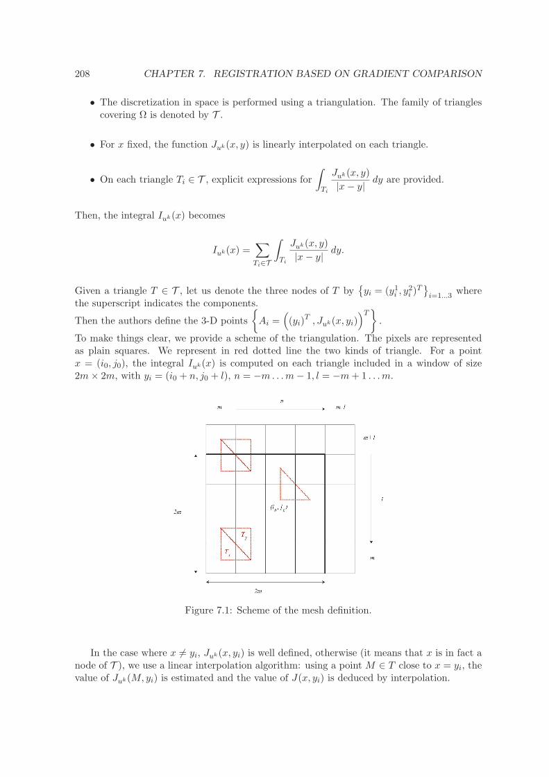
208 CHAPTER 7. REGISTRATION BASED ON GRADIENT COMPARISON
• The discretization in space is performed using a triangulation. The family of trianglescovering Ω is denoted by T .
• For x fixed, the function Juk(x, y) is linearly interpolated on each triangle.
• On each triangle Ti ∈ T , explicit expressions for
∫
Ti
Juk(x, y)
|x− y| dy are provided.
Then, the integral Iuk(x) becomes
Iuk(x) =∑
Ti∈T
∫
Ti
Juk(x, y)
|x− y| dy.
Given a triangle T ∈ T , let us denote the three nodes of T byyi = (y1i , y
2i )Ti=1...3
wherethe superscript indicates the components.
Then the authors define the 3-D points
Ai =
((yi)
T , Juk(x, yi))T
.
To make things clear, we provide a scheme of the triangulation. The pixels are representedas plain squares. We represent in red dotted line the two kinds of triangle. For a pointx = (i0, j0), the integral Iuk(x) is computed on each triangle included in a window of size2m× 2m, with yi = (i0 + n, j0 + l), n = −m. . .m− 1, l = −m+ 1 . . .m.
Figure 7.1: Scheme of the mesh definition.
In the case where x 6= yi, Juk(x, yi) is well defined, otherwise (it means that x is in fact anode of T ), we use a linear interpolation algorithm: using a point M ∈ T close to x = yi, thevalue of Juk(M,yi) is estimated and the value of J(x, yi) is deduced by interpolation.
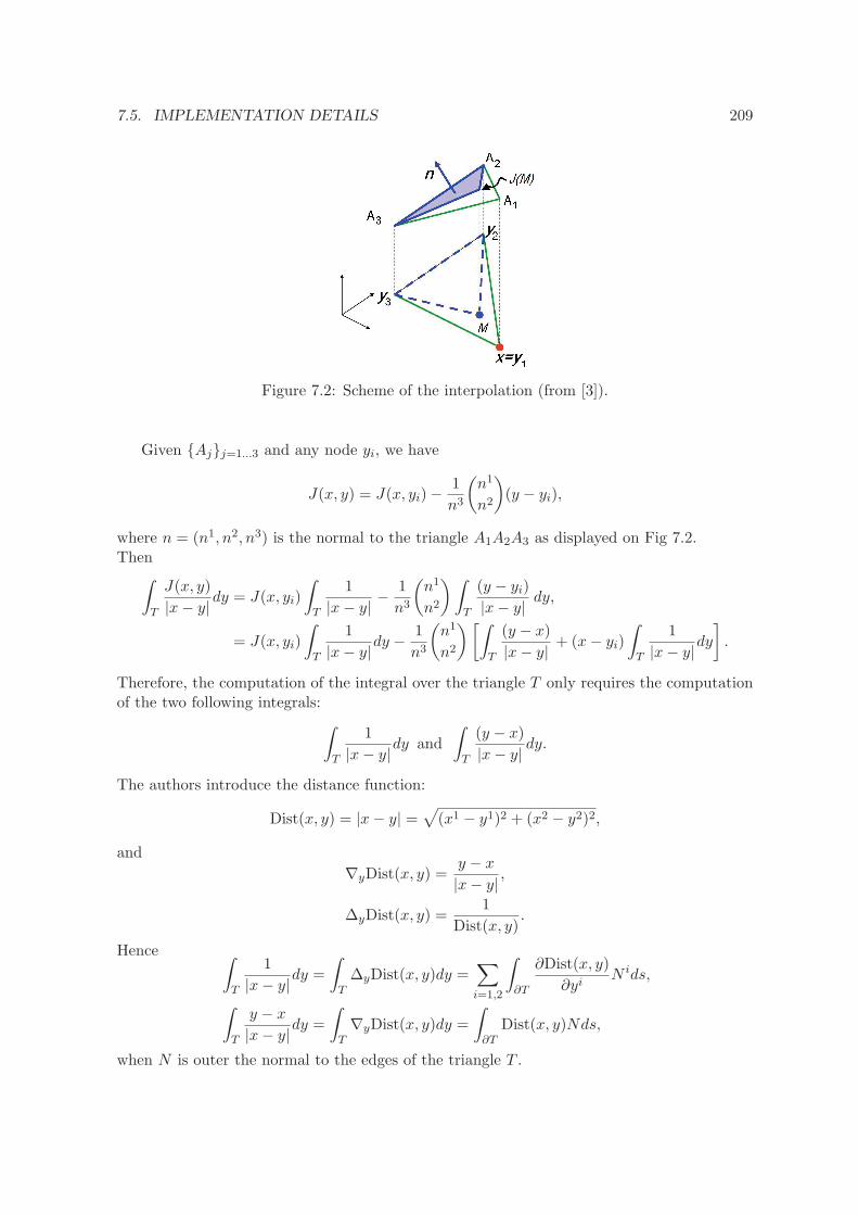
7.5. IMPLEMENTATION DETAILS 209
Figure 7.2: Scheme of the interpolation (from [3]).
Given Ajj=1...3 and any node yi, we have
J(x, y) = J(x, yi)−1
n3
(n1
n2
)(y − yi),
where n = (n1, n2, n3) is the normal to the triangle A1A2A3 as displayed on Fig 7.2.Then
∫
T
J(x, y)
|x− y| dy = J(x, yi)
∫
T
1
|x− y| −1
n3
(n1
n2
)∫
T
(y − yi)
|x− y| dy,
= J(x, yi)
∫
T
1
|x− y|dy −1
n3
(n1
n2
)[∫
T
(y − x)
|x− y| + (x− yi)
∫
T
1
|x− y|dy].
Therefore, the computation of the integral over the triangle T only requires the computationof the two following integrals:
∫
T
1
|x− y|dy and
∫
T
(y − x)
|x− y| dy.
The authors introduce the distance function:
Dist(x, y) = |x− y| =√(x1 − y1)2 + (x2 − y2)2,
and
∇yDist(x, y) =y − x
|x− y| ,
∆yDist(x, y) =1
Dist(x, y).
Hence ∫
T
1
|x− y|dy =
∫
T∆yDist(x, y)dy =
∑
i=1,2
∫
∂T
∂Dist(x, y)
∂yiN ids,
∫
T
y − x
|x− y|dy =
∫
T∇yDist(x, y)dy =
∫
∂TDist(x, y)Nds,
when N is outer the normal to the edges of the triangle T .
210 CHAPTER 7. REGISTRATION BASED ON GRADIENT COMPARISON
Lemma 7.5.1
Let us consider a segment S = (α, β) of extremities α = (α1, α2), β = (β1, β2), N thenormal to this segment, and x a given point. Let us define:
a = |αβ|, δ = a2b2 − c2, l1 = c/√δ,
b = |xα|, d = ~xα.N, l2 = (a2 + c)/√δ,
c = ~xα. ~αβ.
We have
I1 =∑
i=1,2
∫
S
∂Dist(x, y)
∂yiN ids =
0 if x is aligned with S,d(asinh(l2)− asinh(l1)) otherwise,
(7.17)
and
I2 =
∫
SDist(x, y)ds =
a2/2 if x = α or x = β,
a2/2 + c if c = ab (x aligned with ~αβ and c > 0),
− a2/2− c if c = −ab (x aligned with ~αβ and c < 0),
δ
2a2(l2
√1 + l22 + asinh(l2)− l1
√1 + l21 − asinh(l1)) otherwise,
(7.18)
Proof : First, let us parametrize the segment S so that:
S =
y(t) = t
(β1
β2
)+ (1− t)
(α1
α2
): t ∈ [0, 1]
.
The unit normal to the segment S can be written as follows: N =1
a
(β2 − α2
−(β1 − α1)
)
and the distance function can be expressed with respect to t :
Dist(x, y(t)) =
√(tβ1 + (1− t)α1 − x1)2 + (tβ2 + (1− t)α2 − x2)2,
=√a2t2 + 2ct+ b2,
=
√a2(t+
c
a2)2 − c2
a2+ b2,
=
√δ
a
√a4
δ(t+
c
a2)2 + 1, if δ 6= 0.
7.5. IMPLEMENTATION DETAILS 211
• To start with, let us prove the result for I1.
– In the case where x is not aligned with S.
I1 =1
a
∫ 1
0
((tβ1 + (1− t)α1 − x1)(β2 − α2)− (tβ2 + (1− t)α2 − x2)(β1 − α1)
Dist(x, y(t))
)a dt,
=1
a
∫ 1
0
((β2 − α2)(α1 − x1)− (β1 − α1)(α2 − x2)
Dist(x, y(t))
)a dt,
= ~αβ · ~xα⊥∫ 1
0
1
Dist(x, y(t))dt,
= ~αβ · ~xα⊥∫ 1
0
1√δa
√a4
δ (t+ca2)2 + 1
dt,
and using the change of variable z =a2√δ(t+
c
a2) it yields to:
I1 =~αβ ~xα⊥
a
∫ l2
l1
dz√z2 + 1
,
=~xαN
a
∫ l2
l1
dz√z2 + 1
,
= d(asinh(l2)− asinh(l1)).
– In the case where x is aligned with S, then ~xα and N are orthogonal and~xα.N = 0 =⇒ I1 = 0.
• We now prove the result for I2.
I2 =
∫
SDist(x, y)ds =
∫ 1
0aDist(x, y(t)) dt.
– If x = α,
b = 0
c = 0
δ = 0
=⇒ Dist(x, y(t)) = at.
Then
I2 =
∫ 1
0a2tdt =
a2
2.
– If x = β
b = a
c = −a2 = −b2δ = 0
=⇒ Dist(x, y(t)) = −a(t− 1).
Then
I2 =
∫ 1
0−a(t− 1)dt =
a2
2.
212 CHAPTER 7. REGISTRATION BASED ON GRADIENT COMPARISON
– If c = −ab (it means that x is aligned with S but ~xα and ~αβ have oppositedirection)
So b ≥ a and Dist(x, y(t)) = −at+ b.
Then
I2 =
∫ 1
0a(−at+ b)dt = −a
2
2− c.
– If c = ab (it means that x is aligned with S but ~xα and ~αβ have the samedirection)
Dist(x, y(t)) = at+ b.
Then
I2 =
∫ 1
0a(at+ b)dt =
a2
2+ c.
– Otherwise,
I2 =
∫ 1
0
√δ
√a4
δ(t+
c
a2)2 + 1 dt, using the change of variable z =
a2√δ(t+
c
a2),
=
∫ l2
l1
√δ
√δ
a2
√z2 + 1dz
=
∫ l2
l1
δ
a2
√z2 + 1dz, using the change of variable z = sinh(u),
=δ
a2
∫ asinh(l2)
asinh(l1)cosh(u)2du =
δ
a2
∫ asinh(l2)
asinh(l1)
1
2(1 + cosh(2u))du
=δ
2a2
[u+
1
2sinh(2u)
]asinh(l2)
asinh(l1)
,
=δ
2a2(l2
√1 + l22 + asinh(l2)− l1
√1 + l21 − asinh(l1)).
To summarize, we recall that
Iuk(x) =∑
Ti∈T
∫
Ti
Juk(x, y)
|x− y| dy,
with T is a family of triangles, and
Juk(x, y) =|uk(x)− uk(y)|p−2
(uk(x)− uk(y)
)ρn(x− y)
|x− y|p−1.
We can simplify the previous expression as follows:
∫
T
J(x, y)
|x− y| dy = J(x, yi)I1 −1
n3
(n1
n2
)[I2 + I1(x− yi)] ,
with T ∈ T ,and I1 and I2 explicitly given in the previous proposition.
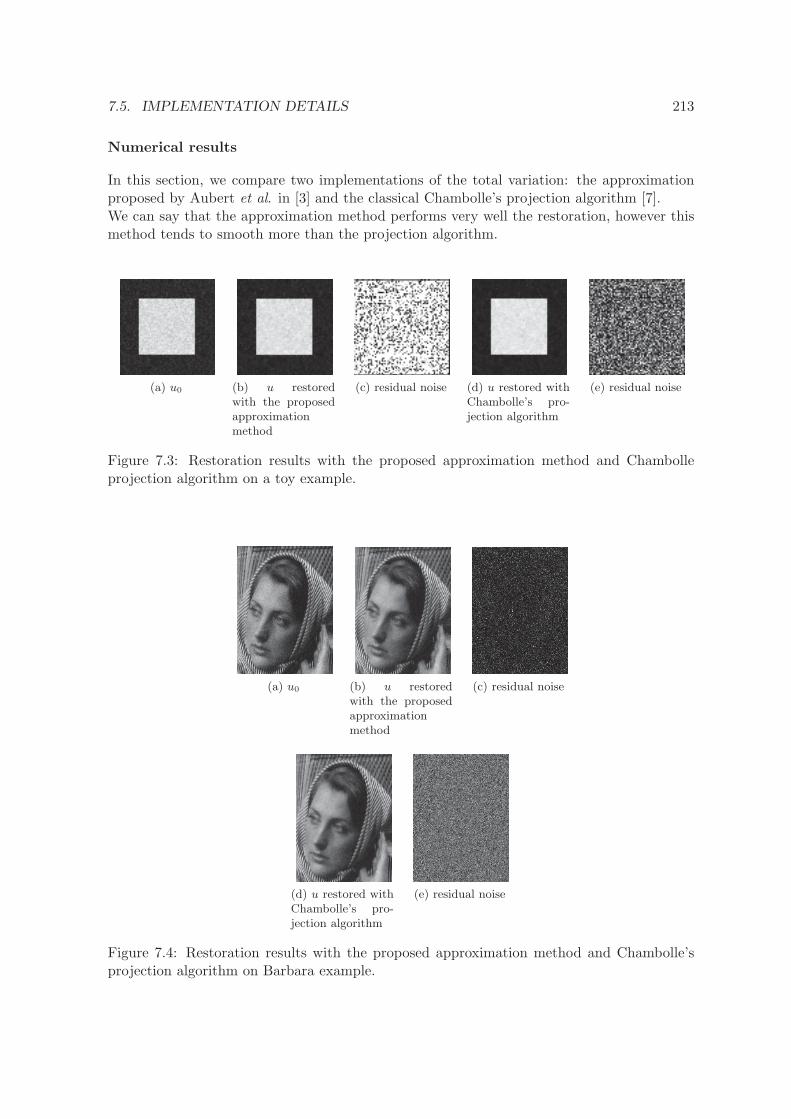
7.5. IMPLEMENTATION DETAILS 213
Numerical results
In this section, we compare two implementations of the total variation: the approximationproposed by Aubert et al. in [3] and the classical Chambolle’s projection algorithm [7].We can say that the approximation method performs very well the restoration, however thismethod tends to smooth more than the projection algorithm.
(a) u0 (b) u restoredwith the proposedapproximationmethod
(c) residual noise (d) u restored withChambolle’s pro-jection algorithm
(e) residual noise
Figure 7.3: Restoration results with the proposed approximation method and Chambolleprojection algorithm on a toy example.
(a) u0 (b) u restoredwith the proposedapproximationmethod
(c) residual noise
(d) u restored withChambolle’s pro-jection algorithm
(e) residual noise
Figure 7.4: Restoration results with the proposed approximation method and Chambolle’sprojection algorithm on Barbara example.
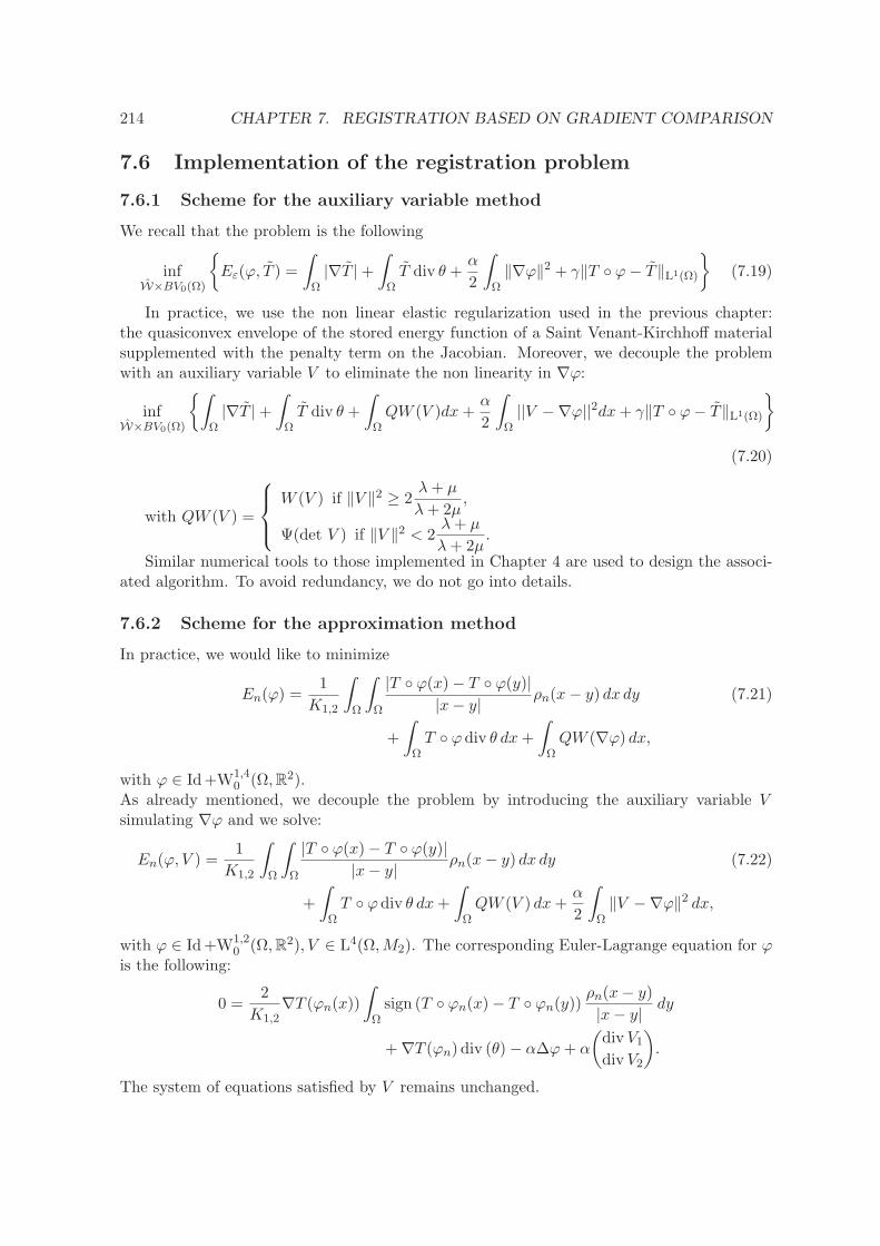
214 CHAPTER 7. REGISTRATION BASED ON GRADIENT COMPARISON
7.6 Implementation of the registration problem
7.6.1 Scheme for the auxiliary variable method
We recall that the problem is the following
infW×BV0(Ω)
Eε(ϕ, T ) =
∫
Ω|∇T |+
∫
ΩT div θ +
α
2
∫
Ω‖∇ϕ‖2 + γ‖T ϕ− T‖L1(Ω)
(7.19)
In practice, we use the non linear elastic regularization used in the previous chapter:the quasiconvex envelope of the stored energy function of a Saint Venant-Kirchhoff materialsupplemented with the penalty term on the Jacobian. Moreover, we decouple the problemwith an auxiliary variable V to eliminate the non linearity in ∇ϕ:
infW×BV0(Ω)
∫
Ω|∇T |+
∫
ΩT div θ +
∫
ΩQW (V )dx+
α
2
∫
Ω||V −∇ϕ||2dx+ γ‖T ϕ− T‖L1(Ω)
(7.20)
with QW (V ) =
W (V ) if ‖V ‖2 ≥ 2λ+ µ
λ+ 2µ,
Ψ(det V ) if ‖V ‖2 < 2λ+ µ
λ+ 2µ.
Similar numerical tools to those implemented in Chapter 4 are used to design the associ-ated algorithm. To avoid redundancy, we do not go into details.
7.6.2 Scheme for the approximation method
In practice, we would like to minimize
En(ϕ) =1
K1,2
∫
Ω
∫
Ω
|T ϕ(x)− T ϕ(y)||x− y| ρn(x− y) dx dy
+
∫
ΩT ϕ div θ dx+
∫
ΩQW (∇ϕ) dx,
(7.21)
with ϕ ∈ Id+W1,40 (Ω,R2).
As already mentioned, we decouple the problem by introducing the auxiliary variable Vsimulating ∇ϕ and we solve:
En(ϕ, V ) =1
K1,2
∫
Ω
∫
Ω
|T ϕ(x)− T ϕ(y)||x− y| ρn(x− y) dx dy
+
∫
ΩT ϕ div θ dx+
∫
ΩQW (V ) dx+
α
2
∫
Ω‖V −∇ϕ‖2 dx,
(7.22)
with ϕ ∈ Id+W1,20 (Ω,R2), V ∈ L4(Ω,M2). The corresponding Euler-Lagrange equation for ϕ
is the following:
0 =2
K1,2∇T (ϕn(x))
∫
Ωsign (T ϕn(x)− T ϕn(y))
ρn(x− y)
|x− y| dy
+∇T (ϕn) div (θ)− α∆ϕ+ α
(div V1div V2
).
The system of equations satisfied by V remains unchanged.
7.6. IMPLEMENTATION OF THE REGISTRATION PROBLEM 215
7.6.3 Numerical results
We have implemented both methods for our problem, that is to say, the decoupled problemwith an auxiliary variable and the approximation method of the total variation by the sequenceof integral operators.Unfortunately, we have not been able to obtain satisfactory results. This could partly beexplained by the fact that the gradient information is meaningful in texture regions and closeto 0 in homogeneous areas, then there is not enough information to match.
Conclusion
To conclude this chapter, we have designed a theoretically well-motivated method, and provedseveral interesting theoretical results. This model is inspired by other works which are notregistration models but inpainting ones and we have tried to apply these methods to ourproblem. We have also proposed two alternative solutions which have been theoreticallyjustified. However, we have been unable to obtain satisfactory numerical results although thecomputing codes are consistent with the theory.

BIBLIOGRAPHY
[1] L. Ambrosio and G. Dal Maso, A general chain rule for distributional derivatives,Proceedings of the American Mathematical Society, 108 (1990), pp. 691–702.
[2] G. Anzellotti, Pairings between measures and bounded functions and compensatedcompactness, Annali di Matematica Pura ed Applicata, 135 (1983), pp. 293–318.
[3] G. Aubert and P. Kornprobst, Can the nonlocal characterization of Sobolev spacesby Bourgain et al. be useful for solving variational problems?, SIAM Journal on NumericalAnalysis, 47 (2009), pp. 844–860.
[4] C. Ballester, M. Bertalmio, V. Caselles, G. Sapiro, and J. Verdera, Filling-in by joint interpolation of vector fields and gray levels, Image Processing, IEEE Trans-actions on, 10 (2001), pp. 1200–1211.
[5] J. Bourgain, H. Brezis, and P. Mironescu, Another look at sobolev spaces, IOSPress, (2001), pp. 439–455.
[6] H. Brezis, Analyse Fonctionnelle, Theorie et Applications. 1999, Dunod, Paris, 1999.
[7] A. Chambolle, An algorithm for total variation minimization and applications, J.Math. Imaging Vis., 20 (2004), pp. 89–97.
[8] J. Davila, On an open question about functions of bounded variation, Calculus of Vari-ations and Partial Differential Equations, 15 (2002), pp. 519–527.
[9] F. Demengel, G. Demengel, and R. Erne, Functional spaces for the theory of ellipticpartial differential equations, Springer, 2012.
[10] M. Droske and M. Rumpf, A variational approach to nonrigid morphological imageregistration, SIAM Journal on Applied Mathematics, 64 (2004), pp. 668–687.
[11] L. C. Evans and R. F. Gariepy, Measure theory and fine properties of functions,vol. 5, CRC press, 1991.
[12] E. Haber and J. Modersitzki, Intensity gradient based registration and fusion ofmulti-modal images, in Medical Image Computing and Computer-Assisted Intervention–MICCAI 2006, Springer, 2006, pp. 726–733.
217

218 BIBLIOGRAPHY
[13] A. C. Ponce, A new approach to Sobolev spaces and connections to Gamma-convergence,Calculus of Variations and Partial Differential Equations, 19 (2004), pp. 229–255.
[14] L. I. Rudin, S. Osher, and E. Fatemi, Nonlinear total variation based noise removalalgorithms, Physica D: Nonlinear Phenomena, 60 (1992), pp. 259–268.
[15] D. Spector, Characterization of Sobolev and BV Spaces, PhD thesis, Carnegie MellonUniversity, 2011.