dealing with edge effects in least-squares image deconvolution problems

Astronomy & Astrophysics manuscript no. ”Dealing with edge effects in least-squares image deconvolution problems”July 21, 2005(DOI: will be inserted by hand later)

Dealing with edge effects inleast-squares image deconvolution problems ?

R. Vio1 J. Bardsley2, M. Donatelli3, and W. Wamsteker4

1 Chip Computers Consulting s.r.l., Viale Don L. Sturzo 82, S.Liberale di Marcon, 30020 Venice, Italye-mail: [email protected]

2 Department of Mathematical Sciences, The University of Montana, Missoula, MT 59812-0864, USA.e-mail: [email protected]

3 Dipartimento di Fisica e Matematica, Universita dell’Insubria, via Valleggio 11, 22100 Como, Italy.e-mail: [email protected]

4 INTA/LAEFF, Apartado 50727, 28080 Madrid, Spaine-mail: [email protected]

Received .............; accepted ................

Abstract. It is well-known that when an astronomical image is collected by a telescope, the measured intensitiesat pixels near the edge of the image may depend on the intensity of the object outside of the field of view (FOV)of the instrument. This makes the deconvolution of astronomical images troublesome. Standard approaches forsolving this problem artificially extend the object outside the FOV via the imposition of boundary conditions(BCs). Unfortunately, in many instances the artificially extended object has little in common with the object itselfoutside of the FOV. This is most pronounced in the case of objects close to the boundary of the image and/orextended objects not completely contained in the image domain. In such cases, an inaccurate extension of theimage outside of the FOV can introduce non-physical edge effects near the boundary that can degrade the qualityof the reconstruction. For example, if the BCs used result in an extended image that is discontinuous at theboundary, these edge effects take the form of ripples (Gibbs oscillations). In this paper, we extend to least-squares(LS) algorithms a method recently proposed by Bertero & Boccacci (2005) in the context of the Richardson-Lucy(RL) algorithm for the restoration of images contaminated by Poissonian noise. The most important characteristicof the proposed approach is that it does not impose any kind of artificial BCs and is therefore free from edgeeffects. For this reason it can be considered the natural method for the restoration of images via LS algorithms.

Key words. Methods: data analysis – Methods: statistical – Techniques: Image processing

1. Introduction

When a two-dimensional object f(x, y) in outer-space isviewed through a telescope, the observed image g(x, y) isrelated to f via the integral equation

g(x, y) =

+∞∫

−∞

+∞∫

−∞h(x, y, x′, y′)f(x′, y′) dx′ dy′, (1)

where h(x, y, x′, y′) is called the point-spread function(PSF) and characterizes the blurring effects of the imagingsystem of interest. For example, in the case of a ground-based telescope, h characterizes both the diffractive blur-ring effects of the finite aperture of the telescope and the

Send offprint requests to: R. Vio? This is a preprint of an article accepted for publication in

Astron. Astrophys.

refractive blurring effects of turbulence in the earth’s at-mosphere. Model (1) allows the PSF to vary with positionin both the (x, y) and (x′, y′) variables. In this case, wesay that h is a spatially-varying PSF. Often, it is possi-ble to simplify this model by assuming that the PSF isindependent of position. In this case, we say that h isa spatially-invariant PSF, and (1) takes the convolutionform

g(x, y) =

+∞∫

−∞

+∞∫

−∞h(x− x′, y − y′)f(x′, y′) dx′ dy′. (2)

Models (1) and (2) are only theoretical. In practicalapplications, we only have discrete noisy observations ofthe image g(x, y), which we model as a discrete linearsystem

g = Af + z. (3)

2 R. Vio J. Bardsley et al.: Dealing with edge effects in least-squares image deconvolution problems

Here g = vec(G) and f = vec(F ) are one-dimensionalcolumn arrays containing, respectively, the observed im-age G and the object F in stacked order, z is an arraycontaining the noise contribution (assumed to be of addi-tive Gaussian type), and A is a matrix that represents thediscretized blurring operator corresponding to the PSF H.

The image deblurring, or deconvolution, problem is toobtain an approximate solution of the linear system (3). Avery common approach is the least-squares (LS) method,where the restored image is obtained by approximatelysolving

fLS = argminf

( ‖Af − g ‖22). (4)

For astronomical imaging problems, solving (4) is nontriv-ial because the matrix A is typically highly ill-conditionedand the number of unknowns is usually extremely large.A vast literature exists that is devoted to the problem ofsolving large-scale least squares problems, and a plethoraof algorithms have been developed with different restora-tion capabilities (e.g., see Bjorck 1996; Starck et al, 2002).Nonetheless, for image deblurring problems, there is an is-sue that has not been satisfactorily addressed, and arisesfrom the fact that collected images are available only in afinite region, causing measured intensities near the bound-ary to be affected by data outside the field of view (FOV).Formally this means that, in the case of an Np ×Np PSFH and of an N × N observed image G (for simplicity,we assume square images), f is an M2 × 1 array withM = N + Np. In other words, problem (4) is under-determined. As a consequence A is a rectangular-matrix(its size is N2 × M2) and this prevents the use of algo-rithms based on the discrete Fourier transform (DFT).Hence, the huge storage and computational advantagesgained by using fast implementations of the DFT are lost.

The standard approach that is used to avoid this prob-lem is to impose a priori boundary conditions (BCs) onF . The BCs that are most often used force a functionaldependency between the elements of f external to theFOV and those internal to this area. This has the ef-fect of extending F outside of the FOV without addingany unknowns to the associated image deblurring prob-lem. Because of this, problem (4) can be reformulated interms of an N2× 1 unknown array F , and A can be writ-ten as an N2 ×N2 square matrix whose structure can beexploited by fast algorithms.

2. The most popular boundary conditions

The following BCs and associated extensions of F are byfar the most common choices in image processing:

• Zero boundary conditions (Z-BCs) assume that the ob-ject is zero outside of the FOV. That is, one assumesthat F has been extracted from a larger array of theform

0 0 00 F 00 0 0

• Periodic boundary conditions (P-BCs) assume that theobject repeats in all directions. That is, one assumesthat F has been extracted from a larger array of theform

F F FF F FF F F

• Reflective boundary conditions (R-BCs) assume thatoutside the FOV the object is a mirror image of F .That is, one assumes that F has been extracted froma larger array of the form

F rc F r F rc

F c F F c

F rc F r F rc

where F c is obtained by “flipping” the columns of F ,F r is obtained by “flipping” the rows of F , and F rc

is obtained by “flipping” the rows and columns of F .• AntiReflective boundary conditions (AR-BCs) have a

more elaborate definition, but have a simple moti-vation: where R-BCs result in an extension that isC0 continuous at the boundary of the FOV, AR-BCsyield an extension that is C1 continuous (see Serra-Capizzano 2003). They are given by

F (1− i, j) = 2F (1, j)− F (i + 1, j)1 ≤ i ≤ Np, 1 ≤ j ≤ N ;

F (i, 1− j) = 2F (i, 1)− F (i, j + 1)1 ≤ i ≤ N, 1 ≤ j ≤ Np;

F (N + i, j) = 2F (N, j)− F (N − i, j)1 ≤ i ≤ Np, 1 ≤ j ≤ N ;

F (i,N + j) = 2F (i,N)− F (i,N − j)1 ≤ i ≤ N, 1 ≤ j ≤ Np;

for the edges, while for the corners the more compu-tationally attractive choice is to antireflect first in onedirection and then the other. This yields

F (1− i, 1− j) = 4F (1, 1)− 2F (1, j + 1)− 2F (i + 1, 1) + F (i + 1, j + 1);

F (1− i,N + j) = 4F (1, N)− 2F (1, N − j)− 2F (i + 1, N) + F (i + 1, N − j);

F (N + i, 1− j) = 4F (N, 1)− 2F (N, j + 1)− 2F (N − i, 1) + F (N − i, j + 1);

F (N + i,N + j) = 4F (N, N)− 2F (N, N − j)− 2F (N − i,N) + F (N − i,N − j);

for 1 ≤ i, j ≤ Np. Another natural choice for thecorners is to antireflect with respect to the vertices.For instance around the corner (1, 1) we obtain F (1−i, 1− j) = 2F (1, 1)− F (i + 1, j + 1) (for more details,see Donatelli et al. 2003). Despite the fact that thetwo strategies provide restored images of comparablequality, the latter spoils the structure of the coeffi-cient matrix more, with a correction of rank at mostO(N2

p ), and therefore in the numerical experiments wewill adopt the first strategy.

R. Vio J. Bardsley et al.: Dealing with edge effects in least-squares image deconvolution problems 3

For a spatially invariant PSF, each of these choices im-poses a particular kind of structure on the matrix A thatcan be exploited to develop computationally efficient al-gorithms (e.g., see Jain 1989; Ng et al. 1999; Serra-Capizzano 2003, and the references therein). It is im-portant to emphasize, though, that the extensions of Fobtained using the above BCs are artificial. Consequently,the reconstructed images obtained in the correspondingdeblurring problems may contain artifacts due to the in-accuracy of such extensions. In practical applications ithas been found that, in general, Z-BCs and P-BCs pro-vide the worst results. This is due to the fact that Z-BCsand P-BCs extensions can be discontinuous at the bound-ary of the FOV, which is incompatible with model (3).When discontinuities are present in the extension, ripples,or Gibbs oscillations, form in the restored images. Thisphenomenon is much less prevalent when R-BCs are usedsince the resulting extension of F preserves the continu-ity of the image; and is even less prevalent for AR-BCswhich, in addition, preserve the continuity of the gradi-ent of the image. Not surprisingly, of the above choices,AR-BCs yield the most accurate image reconstructions.Nonetheless, even with AR-BCs, there is no guarantee ofthe quality of the final result.

3. A natural solution

Formally, the minimum norm solution of problem (4) isgiven by

fLS = A†g, (5)

where A† denotes the pseudo-inverse of A and has theform A† = (AT A)−1AT provided the matrix A has fullcolumn rank N . Here, as was noted above, the fact thatthis matrix is not square prevents the use of the fast DFT.To combat this difficulty, one can zero-pad and shift Hso that it becomes an M ×M array Hp. A periodic ex-tension of Hp of period M yields an M2 × M2 blurringmatrix A that is block circulant with circulant blocks, andhence, the fast DFT can be used. G is also zero extendedto become an M ×M array that we will denote Gp. Wenote the very useful fact that zero padding G in this waynegates the nonphysical effects that can arise in the asso-ciated deblurred images due to the assumption that Hp

is periodic.The benefit of the approach set forth in the previous

paragraph is that it allows for the use of the fast DFT.Unfortunately it does not, by itself, work well. The rea-son is that the matrix A in (3) maps M ×M arrays intoN × N arrays, whereas AT works in the opposite direc-tion. However, because of the zero-padding operation, thematrices A and AT are artificially forced to map M ×Marrays into M ×M arrays. Thus, one might expect thatif the zero-extended model is modified in such a way thatthe domains in which A and AT operate are preserved,things should work. This simple observation was recentlymade by Bertero & Boccacci (2005) in the context of therestoration of images contaminated by Poissonian noise,

and led to the development of a modified version of theRichardson-Lucy (RL) algorithm that has proved to pro-vide superb results 1.

The extension of the arguments of Bertero & Boccacci(2005) to the LS case leads us to rewrite problem (4) inthe equivalent form

fLS = argminf

( ‖WAf − gp ‖22). (6)

Here, W = diag[W ], where W is the M2 × 1 vector ob-tained by column-stacking the M×M mask-matrix havingentries set to 1 in correspondence to the pixels containingthe original image G and 0 otherwise.

Problem (6) can be rewritten in the revealing form

fLS = argminf

( ‖W ¯Af − gp ‖22), (7)

where symbol “¯” means element-wise multiplication. Itis evident that the role of the mask W (and hence ofmatrix W ) is to force the comparison between gp andAf only in correspondence to the pixels in the originalimage G without the imposition of any a priori BCs. Thesolutions of (4) and (6) coincide (from an algebraic pointof view the expressions of the two functionals in (4) and(6) are exactly the same), and yet this simple modificationpermits us to develop algorithms that can exploit the fastDFT preserving all the information present in the originalproblem (4).

4. A modified Landweber algorithm

The prototypical iterative regularization algorithm forleast squares problems is the Landweber method (LW).This is a gradient descent algorithm for solving prob-lem (4). In particular, it creates a sequence of iteratesthat, provided A has full column rank, converges to thesolution in Eq. (5) (see Engl et al. 1996). Because of itsslow convergence, it is not frequently used in practical ap-plications. However, because of its simplicity, it is oftenutilized in the theoretical analysis of the potential perfor-mance of the LS approach.

If f0 is the starting image, then the iterations take theform

fk = fk−1 + ωAT [g −Afk−1], (8)

where, k = 1, 2, . . ., and ω is a real positive parametersatisfying 0 < ω < 2/‖A‖22. The value of ω determines,in part, the convergence of the iteration. If f0 = 0, thisequation can be rewritten in the form

fk = ω

k−1∑

l=0

(I − ωAT A)lAT g. (9)

1 It is probable that in White (1993) and Stobie et al.(1994) a similar algorithm, implemented in the STSDAS soft-ware package, is proposed. However, not many technical detailsare provided for a complete comparison.


Applying LW to the problem of solving (6) yields themodified Landweber iteration

fk = fk−1 + ω(WA)T [gp − (WA)fk−1]. (10)

We note that due to the equivalence of (4) and (6), thesequences generated by (8) and (10) will be the same.Moreover, as was already observed, this sequence con-verges to the solution in Eq. (5). Thus, since the se-quence generated by (10) converges to (WA)†gp, we have(WA)†gp = A†g.

For the sake of clarity and completeness, we now pro-vide a detailed analysis of the convergence of (10). Theanalogue of Eq. (9) in this case is

fk = ω

k−1∑

l=0

(I − ω(WA)T (WA))l(WA)T gp. (11)

Now, if the SVD of WA is given by WA = UΛV T ,where Λ = diag(s1, . . . , sM2), replacing WA in Eq. (11)by its SVD yields

fk = V ΛkUT gp, (12)

where the matrix Λk is diagonal with diagonal elements

[Λk]ii = ωsi

k−1∑

l=0

(1− ωs2i )

l

={

(1− (1− ωs2i )

k)s−1i si > 0,

0 si = 0.(13)

A geometric series identity was used to obtain the secondequality for si > 0. It is evident from Eq. (13) that Λk =ΛkΛ†, where

[Λk]ii = 1− (1− ωs2i )

k, (14)

and

[Λ†]ii ={

s−1i si > 0,0 si = 0.

(15)

Thus Eq. (12) can be rewritten as

fk = (V ΛkV T )(V Λ†UT )gp (16)

=[I − (I − ωAT WA)k

](WA)†gp. (17)

Now, provided 0 < ω < 2/‖WA‖22, we have (I −ωAT WA)k −→ 0 as k →∞, and hence,

limk→∞

fk = (WA)†gp. (18)

Eventually, since (WA)†gp = A†g and ‖WA‖2 = ‖A‖2,we conclude from Eq. (18) that limk→∞ fk = A†g when0 < ω < 2/‖A‖22.

A DFT-based coding of the modified LW is trivial. Infact, since Wgp = gp, W 2 = W , and W T = W , it isnot difficult to see that the iterate (10) can be rewrittenin the form

fk = fk−1 + ωAT [gp −W ¯Afk−1]. (19)

Iteration (19) can be efficiently computed via a two-stepprocedure. In particular,

1. the term in the square brackets on the rhs is evaluatedfirst via the equation

r(i, j) = gp(i, j)−W (i, j)(Hp ⊗ fk−1)(i, j);

2. then the updated iterate is computed using

fk(i, j) = fk−1(i, j) + ω(HTp ⊗ r)(i, j).

Here symbol “⊗” denotes the convolution operator. Asis well known, in the case of two-dimensional arrays(x ⊗ y)(i, j) = IDFT2[x(i, j)y(i, j)] and (xT ⊗ y)(i, j) =IDFT2[x∗(i, j)y(i, j)], where x(i, j) = DFT2[x(i, j)],y(i, j) = DFT2[y(i, j)], with DFT2[.], IDFT2[.] and “ ∗ ”indicating the two-dimensonal discrete Fourier transform,the two-dimensional inverse discrete Fourier transformand the complex-conjugate matrix, respectively.

For each iteration this procedure requires the compu-tation of four M ×M DFTs, versus the two N ×N DFTsrequired by the classic algorithm based on P-BCs.

5. Some numerical experiments

We now present some numerical experiments in which theperformance of the modified LW algorithm is comparedwith the performance of classical LW when R-BCs andAR-BCs are imposed. Actually, we have used a projectedversion of LW that constrains the solution to be nonnega-tive. We do this because in the experiments we have usedas a benchmark the modified RL algorithm as proposedby Bertero & Boccacci (2005) which also imposes a non-negativity constraint on the solution.

In all of the experiments, the adopted PSF is aGaussian with circular symmetry and dispersion set to 6pixels. We have deliberately chosen non-astronomical ob-jects. In fact, because of the more important contributionof the high frequency components, objects with sharp out-line are much more difficult to restore than those typicalof astronomical observations. Hence, we have considered arectangular function and a very sharply structured object.For each object we have considered three different situa-tions concerning noise, i.e., no-noise, Gaussian noise andPoissonian noise. In the last two cases an SNR = 20 dBand a peak SNR = 30 dB 2, respectively, have beenadopted. This is to ensure that the performance of themodified LW does not depend on the particular kind ofnoise that contaminates the images. In order to avoid pix-els with zero values, a sky-background has been addedwhose intensity, in the blurred image, is set to 1% of themaximum value of the image. Figures 1-10 clearly indicatethe supremacy of the modified LW over classical LW withboth R-BCs and AR-BCs.

As shown by Figs. 11-13, this result does not changewhen an experiment based on a typical astronomical ob-ject is considered. Apart from the fact that the noise is

2 For Gaussian noise SRN = 20 log(σI/σz) dB, where σI andσz are the standard deviation of the noise-free blurred imageand of the noise respectively. For Poissonian noise, SRN =20 log(bmax/b

1/2max) dB, where bmax is the maximum value in

the noise-free blurred image.


Poissonian with a peak SNR = 60 dB, the other condi-tions of the experiment are identical to those in the previ-ous cases. The only point worth noting is that AR-BC isable to provide a reconstruction whose quality is similarto that of the modified LW and RL algorithms. This isa consequence of the fact that in the object the contri-bution of the high frequency components (i.e., those thatdetermine the edge effects) is negligible.

6. Conclusions

The theoretical arguments and numerical experimentspresented above lead one to conclude that in the case ofobjects close to the boundaries of an image and/or ex-tended objects not completely contained in the image do-main, the imposition of artificial BCs is not, in general,the optimal approach. This is due to the fact that impos-ing BCs can alter the original problem in a way that is notcompatible with physical reality. Much better results areobtained by solving the under-determined LS problem (6).

Three more points have to be stressed. The first one isthat there are indications that the solution of problem (6)permits one to obtain remarkably good restorations evenin the case of Poissonian noise, where model (3) no longerholds. Given the limited number of experiments carriedout in this paper, we cannot justifiably make the claimthat this will hold in general. However, in a recent work,Vio et al. (2005) have shown that the LS deblurring al-gorithms are remarkably insensitive to the nature of thenoise. Hence, it can be safely expected that modified LSalgorithms will also work well in the case of non-Gaussiannoises.

A second point to note is the fact that, in spite of infe-rior performance in terms of reconstruction quality whencompared to the approach that we advocate in this paper,AR-BCs work surprisingly well. This could be useful inthe case of very large images. In fact, when the PSF isdoubly symmetric, the deblurring algorithms can be im-plemented using the discrete sine transform (DST-I). Inthis case, LW requires two (N−2)×(N−2) DST-Is and afew computations of lower order for the edges (Donatelli &Serra-Capizzano 2005), whereas with an asymmetric PSF,it requires two DFTs of size M ×M (extending the imagewith an antireflective padding). Therefore, in the case ofa generic PSF, one LW iteration with AR-BCs shows acomputational cost about one half of modified LW.

As a final comment, we note that although we haveconsidered only the Landweber algorithm, all of the LSalgorithms that make use of the matrices A and AT canbe similarly modified.

References

Bertero, M., & Boccacci, P. 2005, A&A preprintdoi:10.1051/0004-6361:20052717

Bjorck, A. 1996, Numerical Methods for Least SquaresProblems, SIAM.

Donatelli, M., Estatico, C., Nagy, J., Perrone, L., & Serra-Capizzano, S. 2003, SPIE’s 48th Annual Meeting, SanDiego, CA USA, F. Luk Ed, Vol. 5205 pp. 380-389.

Donatelli, M., & Serra-Capizzano, S. 2005, InverseProblems, 21, 169.

Engl, H.W., Hanke, M. & Neubauer, A. 1996,Regularization of Inverse Problems, (Kluwer AcamedicPublishers).

Jain, A.K. 1989, Fundamentals of Digital ImageProcessing, (Prentice-Hall, New York)

Ng, M.K., Chan, R.H., & Tang, W.C. 1999,SIAM J. Sci. Comput., 21, 851

Serra-Capizzano, S. 2003, SIAM J. Sci. Comput., 25, 1307.Starck, J.L, Pantin, E. & Murthag, F. 2002, PASP, 114,

1051Stobie, E.B., Hanisch, R.J., & White, R.L. 1994,

Astronomical Data Analysis Software and Systems III,ASP Conference Series, Vol. 61, 296

Vio, R., Bardsley, J., & Wamsteker, W. 2005, A&Apreprint doi:10.1051/0004-6361:20041997

Vogel, C. R. 2002, Computational Methods for InverseProblems, SIAM

White, R.L. 1993, Newsletter of STScI’s ImagesRestoration Project, 1, 11


Object

20 40 60 80 100 120

20

40

60

80

100

120

Image

20 40 60 80 100 120

20

40

60

80

100

120

Object in the FOV

10 20 30 40 50 60

10

20

30

40

50

60

Image in the FOV

10 20 30 40 50 60

10

20

30

40

50

60

Fig. 1. Rectangular function used in the first experiment. Nonoise has been added. The delimited area corresponds to theimage used in the deblurring operation.

500 1000 1500 2000 2500 3000 3500 4000 4500 5000

0.25

0.3

0.35

0.4

0.45

0.5

Number of iterations

RR

E

Noise−free image

LW + Reflec.LW + AntiRefl.Mod. LWMod. RL

Fig. 2. Relative restoration error (RRE) ‖fk − f‖/‖f‖ vs.the number of iterations for the experiment with the objectin Fig. 1.

LW + Reflective − RRE = 0.39071

10 20 30 40 50 60

10

20

30

40

50

60

LW + AntiReflective − RRE = 0.28859

10 20 30 40 50 60

10

20

30

40

50

60

Modified LW − RRE = 0.24091

10 20 30 40 50 60

10

20

30

40

50

60

Modified RL − RRE = 0.26102

10 20 30 40 50 60

10

20

30

40

50

60

Fig. 3. Results obtained from deblurring for the experimentwith the object in Fig. 1. The displayed RREs correspond tothe best value obtained during the iterations.


500 1000 1500 2000 2500 3000 3500 4000 4500 5000

0.25

0.3

0.35

0.4

0.45

0.5


RR

EGaussian noise


Fig. 4. As in Fig. 2 but in the case of Gaussian noise withSNR = 20 dB.

500 1000 1500 2000 2500 3000 3500 4000 4500 5000

0.25

0.3

0.35

0.4

0.45

0.5


RR

E

Poissonian noise


Fig. 5. As in Fig. 2 but in the case of Poissonian noise withpeak SNR = 30 dB.


Object

100 200 300 400 500

100

200

300

400

500

Image

100 200 300 400 500

100

200

300

400

500

Object in the FOV

50 100 150 200 250

50

100

150

200

250

Image in the FOV

50 100 150 200 250

50

100

150

200

250

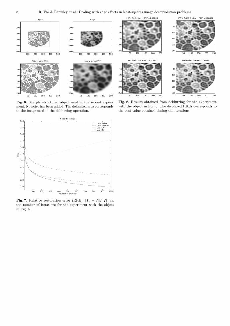
Fig. 6. Sharply structured object used in the second experi-ment. No noise has been added. The delimited area correspondsto the image used in the deblurring operation.

100 200 300 400 500 600 700 800 900 1000

0.38

0.39

0.4

0.41

0.42

0.43

0.44

0.45

0.46

0.47

0.48


RR

E

Noise−free image


Fig. 7. Relative restoration error (RRE) ‖fk − f‖/‖f‖ vs.the number of iterations for the experiment with the objectin Fig. 6.


50 100 150 200 250

50

100

150

200

250


50 100 150 200 250

50

100

150

200

250


50 100 150 200 250

50

100

150

200

250


50 100 150 200 250

50

100

150

200

250

Fig. 8. Results obtained from deblurring for the experimentwith the object in Fig. 6. The displayed RREs corresponds tothe best value obtained during the iterations.


100 200 300 400 500 600 700 800 900 1000

0.38

0.39

0.4

0.41

0.42

0.43

0.44

0.45

0.46

0.47

0.48


RR

EGaussian noise


Fig. 9. As in Fig. 7 but in the case of Gaussian noise withSNR = 20 dB.

100 200 300 400 500 600 700 800 900 1000

0.38

0.39

0.4

0.41

0.42

0.43

0.44

0.45

0.46

0.47

0.48


RR

E

Poissonian noise


Fig. 10. As in Fig. 7 but in the case of Poissonian noise withpeak SNR = 30 dB.


Object

50 100 150 200 250

50

100

150

200

250

Image

50 100 150 200 250

50

100

150

200

250

Object in the FOV

20 40 60 80 100 120

20

40

60

80

100

120

Image in the FOV

20 40 60 80 100 120

20

40

60

80

100

120

Fig. 11. Rectangular function used in the third experiment.Noise is Poissonian with peak SNR = 60 dB. The delimitedarea corresponds to the image used in the deblurring operation.

50 100 150 200 250 300 350 400 450 500

0.03

0.04

0.05

0.06

0.07

0.08

0.09

0.1


RR

E

Poissonian noise


Fig. 12. Relative restoration error (RRE) ‖fk − f‖/‖f‖ vs.the number of iterations for the experiment with the object inFig. 11.


20 40 60 80 100 120

20

40

60

80

100

120


20 40 60 80 100 120

20

40

60

80

100

120


20 40 60 80 100 120

20

40

60

80

100

120


20 40 60 80 100 120

20

40

60

80

100

120

Fig. 13. Results obtained from deblurring for the experimentwith the object in Fig. 11. The displayed RREs corresponds tothe best value obtained during the iterations.

dealing with edge effects in least-squares image deconvolution problems

Documents