using partial least squares regression for

Statistica Applicata - Italian Journal of Applied Statistics Vol. 32 (1) 67

USING PARTIAL LEAST SQUARES REGRESSIONFOR CONJOINT ANALYSIS

Giorgio Russolillo, Gilbert Saporta1

Department of Mathematics and Statistics, CNAM, Paris, France

Abstract. After a presentation of the classical methodology of conjoint analysis we advocatethe use of PLS regression instead of classical regression in order to obtain a better accuracyin the estimation of utilities. PLS regression provides also interesting graphicalrepresentations allowing quick and easy interpretation of the relations among preferences,attributes and profiles.

Keywords: Conjoint analysis, Consumer choice, Data visualization, Partial Least Squares,Optimal Scaling.

1. INTRODUCTION

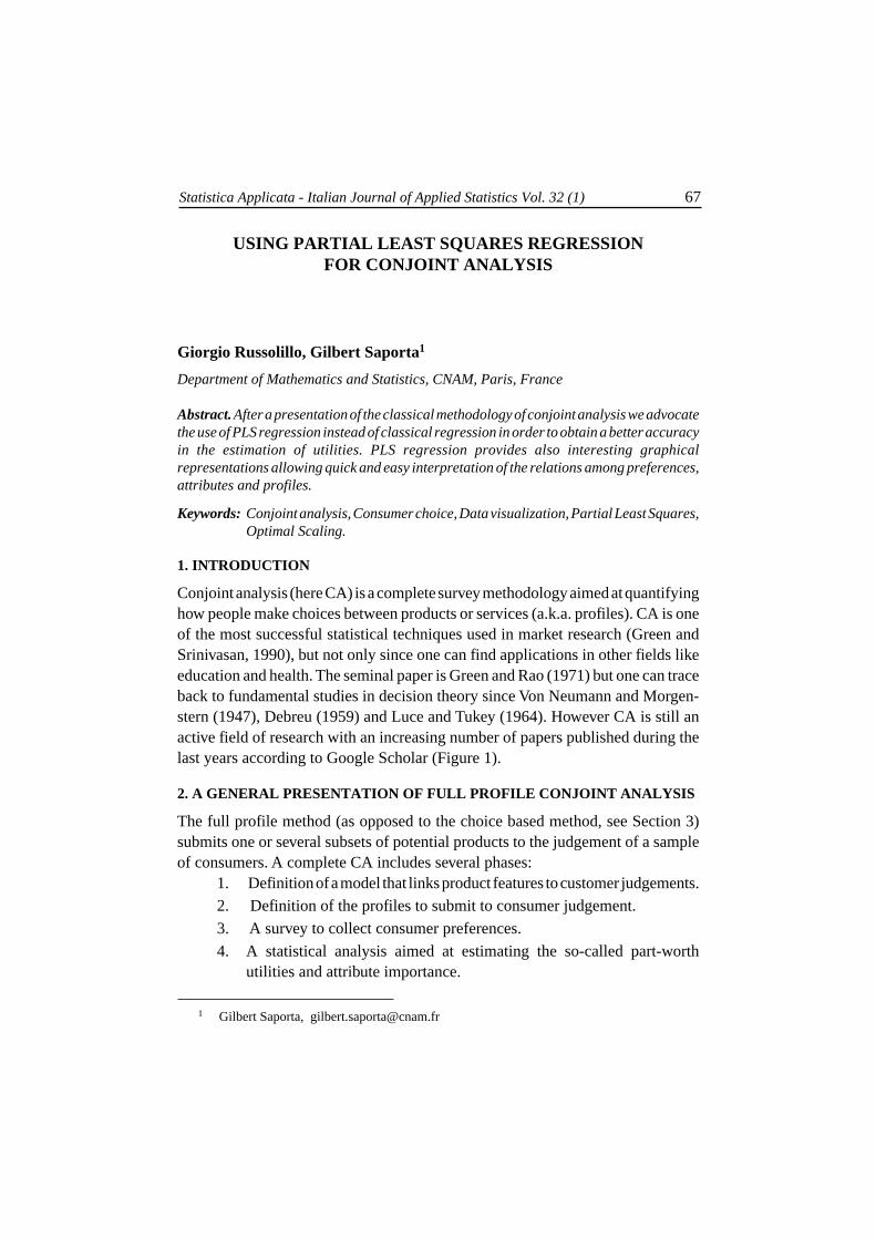
Conjoint analysis (here CA) is a complete survey methodology aimed at quantifyinghow people make choices between products or services (a.k.a. profiles). CA is oneof the most successful statistical techniques used in market research (Green andSrinivasan, 1990), but not only since one can find applications in other fields likeeducation and health. The seminal paper is Green and Rao (1971) but one can traceback to fundamental studies in decision theory since Von Neumann and Morgen-stern (1947), Debreu (1959) and Luce and Tukey (1964). However CA is still anactive field of research with an increasing number of papers published during thelast years according to Google Scholar (Figure 1).

2. A GENERAL PRESENTATION OF FULL PROFILE CONJOINT ANALYSIS

The full profile method (as opposed to the choice based method, see Section 3)submits one or several subsets of potential products to the judgement of a sampleof consumers. A complete CA includes several phases:

1. Definition of a model that links product features to customer judgements.

2. Definition of the profiles to submit to consumer judgement.

3. A survey to collect consumer preferences.

4. A statistical analysis aimed at estimating the so-called part-worthutilities and attribute importance.

1 Gilbert Saporta, [email protected]

rosariaromano

Casella di testo

doi.org/10.26398/IJAS.0032-005

68 Russolillo G., Saporta G.

2.2. THE CHOICE OF THE PROFILES

Each profile is defined by a combination of a (generally small) number P of at-

tributes with m1, . . . ,mP categories. Most of the time, attributes are qualitative

variables with few ordered or non-ordered categories, but may be also discretized

continuous variables (e.g. price) with few levels. Proposed profiles should not

include the ‘perfect’ product (e.g. a car with high speed, high comfort, high se-

curity and low price), since it would be trivially chosen by all consumers. On the

contrary, CA assumes that each consumer makes a trade off between attributes by

putting into balance advantages and inconveniences.

2.1 THE MODEL

CA differs from classical choice models: it is not a collective model but anindividual one. Consumer preferences are decomposed according to an additiveutility model, specific to each respondent. This is a very important feature of CA:there is no average or typical consumer, but different consumers who have differentways of weighting attributes and their categories.Suppose that a product is defined by a combination of levels (i, j,k,...) of P attributes:its global utility for a customer is equal to ai + bj + ck + ..., a sum of part-worthutilities. The previous model is an additive model without interaction, which is aclear limitation: one can easily think of examples where interactions are present(e.g. the influence of the price could depend on the brand). However, introducinginteractions generates more parameters which in turn necessitates more products toevaluate, and this is not generally feasible since it is commonly accepted that arespondent cannot rank more than N = 16 products.

5. A simulation phase where market shares for submitted and new profilesmay be estimated.

Fig. 1: Number of papers per year mentioning conjoint analysis.

Using Partial Least Squares Regression for Conjoint Analysis 69

2 When all attributes have 2 levels, practitioners frequently use factorial fractional designs orPlackett & Burman designs up to 12 attributes. For more than two levels, Latin and andgraeco-latin squares may be used for attributes with the same number of levels.

2.3 COLLECTING CONSUMER PREFERENCES

The basic experience consists in asking Q consumers to fully rank the fictitiousproducts. Sorting products is a rather difficult task when there are many products torank. So why not to rate products by giving scores to each of them? Rating products ismuch easier but has severe drawbacks: there are no comparison between products,

Since the total number of productsP∏

p=1mp to be compared is generally large,

the subsets have to be carefully chosen in such a way that the estimation of the

part-worth utilities should be obtained with a minimal variance and attributes ef-

fects estimated without confounding. This is usually achieved through orthog-

onal designs, which have optimal properties. In a balanced orthogonal design,

all combinations of levels of each pair of attributes should be observed the same

number of times. This implies that the number of profiles proposed to the con-

sumers N should be equal or proportional to the least common multiple of all

pairs mpmp′∀p � p′ while being larger than the number of independent parame-

tersP∑

p=1mp−P 1.

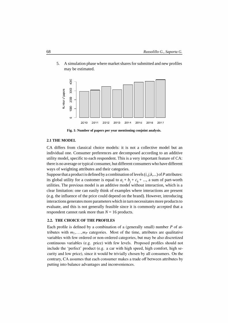
Let us take as an illustration the Frozen Diet Entrées example (Kuhfeld, 2010).

There are three attributes (Ingredients, Fat quantity and Price) with 3 categories

and one attribute (Calories) with 2 categories, which generates a total amount ofP∏

p=1mp = 54 profiles. The least common multiple of 3× 3 and 3× 2 is 18, which

leads to the orthogonal design in Table 1 (note that there are several equivalent

designs which could be obtained by permutations of the labels of the categories

of each attribute).

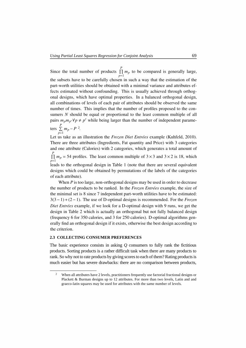
When P is too large, non-orthogonal designs may be used in order to decrease

the number of products to be ranked. In the Frozen Entrées example, the size of

the minimal set is 8 since 7 independent part-worth utilities have to be estimated:

3(3−1)+ (2−1). The use of D-optimal designs is recommended. For the FrozenDiet Entrées example, if we look for a D-optimal design with 9 runs, we get the

design in Table 2 which is actually an orthogonal but not fully balanced design

(frequency 6 for 350 calories, and 3 for 250 calories). D-optimal algorithms gen-

erally find an orthogonal design if it exists, otherwise the best design according to

the criterion.

2


2.4. ESTIMATION OF PART-WORTH UTILITIES AND ATTRIBUTE IMPOR-TANCE

Let X be the binary design matrix with N rows andP∑

p=1mp + 1 columns (one for

the intercept). The Q ranks defined by consumer preferences are juxtaposed in

Tab. 1: (33×2)/3 orthogonal design

Obs. Ingredients Fat Price Calories1 Turkey 5 Grams $1.99 3502 Turkey 8 Grams $2.29 3503 Chicken 8 Grams $1.99 3504 Turkey 2 Grams $2.59 2505 Beef 8 Grams $2.59 3506 Beef 2 Grams $1.99 3507 Beef 5 Grams $2.29 3508 Beef 5 Grams $2.29 2509 Chicken 2 Grams $2.29 350

10 Beef 8 Grams $2.59 25011 Turkey 8 Grams $2.29 25012 Chicken 5 Grams $2.59 35013 Chicken 5 Grams $2.59 25014 Chicken 2 Grams $2.29 25015 Turkey 5 Grams $1.99 25016 Turkey 2 Grams $2.59 35017 Beef 2 Grams $1.99 25018 Chicken 8 Grams $1.99 250

Tab. 2: An optimal design in 9 runs

Obs Ingredients Fat Price Calories1 Turkey 8 grams $1.99 3502 Turkey 5 grams $2.29 2503 Turkey 2 grams $2.59 3504 Chicken 8 grams $2.59 2505 Chicken 5 grams $1.99 3506 Chicken 2 grams $2.29 3507 Beef 8 grams $2.29 3508 Beef 5 grams $2.59 3509 Beef 2 grams $1.99 250

scales across respondents may not be comparable, the risk of ties becomes important.Rankings are thus usually preferred since the implication of respondents if higher.It frequently happens that respondents are unable to give a complete order, but areable to rank only their ‘best’ products, the other products becoming ex aequo. Thisis not a behavior to be encouraged but simulation studies tends to prove that rankinghalf of the profiles is enough to estimate utilities (Benammou et al., 2003).


the response matrix Y . Practitioners use reversed ranks, in a way that low ranks

mean highly preferred products. Ordinary Least Squares (OLS) regression of Yon X is commonly used for estimating coefficients assigned to categories, which

are interpreted as part-worth utilities. Since the matrix X is not of full rank we

need constraints for the utilities. The usual constraints (unlike in the general lin-

ear model) are that the sum of part-worth utilities for each attribute is equal to zero.

The OLS approach forgets about the ordinal nature of the ranks. Many researchers

recommend to use monotonous regression which comes down to look for the

monotonous transformation T (Y) which is best fitted by a linear combination of

the categories indicators according to the least squares criterion:

minT,y‖T (Y)−Xb‖

This is solved by an iterative algorithm, alternating Kruskal monotonic regression

for finding T when b is known and OLS regression to find b when T is known

(Kruskal, 1964).

OLS and monotonous regressions may lead to severe overfitting: in practical ap-

plications the degrees of freedom N −(

P∑p=1

mp−P)

of standard linear model is

usually low; moreover, transforming the ranks decreases the degrees of freedom

even more. We will see later in this paper that PLS regression provides an elegant

solution to the overfitting risk and other issues.

Part-worth utilities refer to attribute levels, while analysts are also interested in

evaluating the impact of an attribute on the preferences as a whole. The impor-

tance of an attribute for a consumer is usually calculated as the normalized range

of the part-worth coefficients of the attribute levels on the consumer’s ranking.

Clustering respondents according to their revealed utilities is very useful in real

life applications to target classes of consumers.

2.5. SIMULATION AND MARKET SHARE ESTIMATION

Since for any respondent q (q = 1 . . .Q), we know the m1 + · · ·+mP part-worth

utilities, it is possible to:

• Simulate new profiles: Model estimates allow us to compute the total utility

of combinations of attribute levels which have not been considered in the

design by simply adding the part-worth utilities. For discretized continuous

attributes, like price, it is also possible to consider new levels: the part-

worth utility of such a level being estimated by interpolation.


• Estimate market shares: Suppose that we want to estimate the market shares

of 3 competing products. If the 3 utilities are U1q ,U

2q ,U

3q , a simple rule

should be that respondent i chooses the product with the maximal utility.

But when products have close utilities, a probabilistic choice is more real-

istic. There are two popular methods: the Bradley-Terry-Luce rule which

assumes that the probabilities of choice are proportional to U1q , U2

q ,U3q and

the logit rule where probabilities are proportional to exp(U1

q

), exp

(U2

q

),

exp(U3

q

). It is easy to obtain the market shares of the 3 products by averag-

ing the probabilities of choice over the Q respondents.

• Study consumer real purchase intents: Simulating market shares, as ex-

plained before, might not be realistic since some products are unlikely to be

bought when they do not belong to the universe of choice of some respon-

dents. The value of the utility is not enough and often practitioners add a

‘will buy’ question for each submitted product. This allows to derive an in-

tent of purchase function which will revise the utilities in the market shares

models

3. ALTERNATIVE METHODS TO FULL PROFILE CONJOINT ANALY-SIS

The full profile method is not well adapted to cases where the number of attributes

and (or) the number of categories is large. For this reason choice based CA and

(or) adaptive designs are often preferred to full profile designs.

Adaptive conjoint analysis (ACA) (Johnson, 1987), was very popular with the de-

velopment of CAPI and CAWI systems. The core of the method consists in a set

of paired comparisons involving an increasing number of attributes, depending

on the previous answers, until parameters (part-worth utilities) are estimated with

enough precision, in a bayesian style. Prior importance and category ordering are

estimated through introductory questions.

In discrete choice models, also known as Choice Base Conjoint (CBC) (Huber

et al., 1992), instead of rating or ranking product concepts, respondents are shown

several sets of products and asked to indicate which one they would choose. The

sets of choice questions is obtained by design of experiments techniques.

Utilities are estimated by the multinomial logit model which assumes that the

probability that an individual will choose one of the N alternatives, ci, from choice


set C is:

P(ci/C) =exp(U(ci))

N∑j=1

exp(U(c j)

) = exp(xiβ)N∑

j=1exp

(x jβ

)

where xi is a vector of coded attributes and β is a vector of unknown attribute

parameters (part-worth utilities) . U(ci) = xiβ is the utility for alternative ci, which

is a linear function of the attributes.

Choice based conjoint designs may accommodate easily an additional choice: the

‘none’ alternative, which allows a customer to refuse all the products in a set.

However it is not easy to use this possibility in the estimation phase of part-worth

utilities. Elrod et al. (1992) specified the no choice as another alternative with

attributes levels set to zero and determine the choice between the products and the

option ‘zero’ by comparing their utilities. But this technique is highly arguable

since the no-choice alternative is of a different kind. Ohannessian and Saporta

(2008) proposed an other approach distinguishing two cases where a respondent

does not choose any product. In the first case, no product have a utility larger than

some minimum value and the whole submitted set of products is rejected. In the

second case the ‘no choice’ results from what they call a conflict: it occurs when

the respondent cannot decide between products when the differences between util-

ities are too small.

Some authors consider that CBC is not conjoint analysis (Louviere et al., 2010);

our opinion is that any technique providing individual part-worth utilities belongs

to CA in a broad sense.

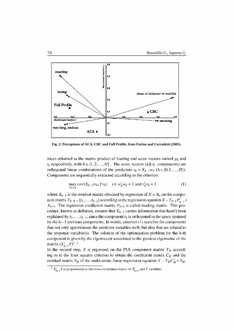
Furlan and Corradetti (2005) made a comparison between several kinds of CA

from the point of view of the respondents; they concluded that choice tasks are

simpler than full profiles rankings and closer to real situations (see Figure 2 from

their publication).

4. PARTIAL LEAST SQUARES REGRESSION

Partial Least Square Regression (PLSR) (Tenenhaus, 1998) is a component-based

regression method that aims at predicting a set of response variables Y =[y1, . . . ,yQ

]from a set of predictor variables X = [x1, . . . , xP]. In PLSR changing the relative

scale of the responses and/or the predictors changes the predictive model. This

ambiguity is usually solved by standardizing all the variables before the analysis

is performed. For this reason hereinafter we assume without loss of generality

that both predictor and response variables are standardized. PLSR involves two

steps: In the first step, the X-matrix is approximated by a sum of H rank-1 ma-


Fig. 2: Perceptions of ACA, CBC and Full Profile, from Furlan and Corradetti (2005).

3

3


Since the component matrix can be re-expressed as TH = XWH(P′HWH)−1, where

WH = [w1, . . . ,wH], the PLS regression equation can be written as a linear combi-

nation of X:

Y = XBH +YH , where BH =WH(P′HWH)−1C′H (2)

When the response is univariate, the PLS (a.k.a. PLS1) estimator variability has

been shown to increase as the number of components increases (De Jong, 1995).

For this reason PLS1 is typically used to replace the OLS estimator when esti-

mate variability and prediction accuracy are inflated by predictor multicollinear-

ity. Moreover, PLS regression can handle flat predictor matrices, that is it yields a

solution even if the number of the predictor variables is bigger than the number of

the observed units. In this framework the number of components, usually chosen

by cross-validation, is used as a regularization parameter H ∈ {1, . . . ,rank(X)}. In

the simplest, one-dimensional model, covariances between predictors are not at all

considered in the coefficient estimation process. In the full, rank(X)-dimensional

model the X-matrix is perfectly recomposed and PLSR provides the minimum

length least square solution of the regression of Y on X (De Jong, 1995). This

property holds even when the response is multivariate.

Multivariate response PLSR (a.k.a. PLS2) estimator variability does not increase

systematically as the number of components increases. For this reason PLS2

regression is mostly used as a visualization tool for exploratory purposes. Ob-

servations and variables are projected onto the factorial subspaces spanned by

PLS components and loadings to investigate the variable correlation structure and

observation similarities through their visualization in two or three dimensional

spaces. Moreover, biplots can be drawn to represent observations and variables at

the same time.

4.1. NON-METRIC PLS REGRESSION

Non-metric PLS (NM-PLS) regression (Russolillo, 2012) is an extension of PLSR

that handles both quantitative and qualitative (non-metric) predictor and response

variables.

According to the principles of the Optimal Scaling (OS), each distinct level of a

qualitative variable is replaced by a numerical (scaling) value. This is equivalent

to assign to the qualitative variable a new metric that quantifies the (relative) dis-

tances between each pair of levels. The new metric is typically required to hold

some or all of the properties of the original measurement scale. So, for example,

if the original variable is an ordinal variable then scaling values may be required


to reflect the intrinsic ordinality of its modalities.

NM-PLSR is powered by an enhanced PLS algorithm who works also as an OS

algorithm. Since NM-PLSR takes into account the type of measurement scale on

which the qualitative variable has been observed, it ensures a proper treatment

for ordinal and nominal variables. NM-PLSR algorithm returns both the PLSR

parameter estimates and the metrics (that is the scaling parameter estimates) that

1. maximize criterion 1 for h = 1

2. respect the constraints defined by the properties of the original measurement

scale that the analyst wants to keep in the transformation.

5. USING PARTIAL LEAST SQUARES REGRESSION FOR CONJOINTANALYSIS

Using Least Squares for estimating part-worth utilities has some limitations. First

of all, the number of products must be greater that the number of part-worth utili-

ties to be estimated, as estimation procedure demands at least one degree of free-

dom for the error term. Moreover, the number of products must be not too large,

as respondents are not able to build long rankings. As a result, most of regres-

sion models for conjoint analysis have one or few error degrees of freedom. As

already discussed in Section 2.4, these models tend to overfit data, that is they

fit almost perfectly in-sample profiles but they are expected not to fit well new

(out-of-sample) profiles. The risk of overfitting is even higher when non-metric

part-worth utilities are estimated.

Replacing OLS by PLS estimation allows overcoming these drawbacks. PLS in-

creases the flexibility when building the design matrix, since it yields a solution

independently on the number of attributes and the one of their levels. Moreover,

as a shrinkage technique, PLSR provides more efficient estimations of the utilities

of new products.

While PLS1 regression can be used as a predictive tool, PLS2 regression allows

enriching CA by means of graphical tools for exploring sample data, as proposed

by Russolillo (2009). Preference maps (Lauro et al., 1998) can be built, in which

products, judges and attribute levels are visualized as points or vectors on PLS

factorial plans. Finally non-metric PLS regression introduces even more flexibil-

ity for the exploratory analysis. Non-metric part-worth utilities can be obtained

when judge rankings (the Y-variables) are handled as ordinal variables exactly as

monotonic regression (Young et al., 1976) is used instead of standard OLS regres-


sion in monotonic CA. Finally non-metric PLSR can provide every X-variable -

attribute with a new metric, transforming it into an interval-scaled variable. This

strategy allows estimating a unique part worth coefficient, weight and loading for

each attribute. This makes the visualization clearer and the interpretation of the

graphics easier.

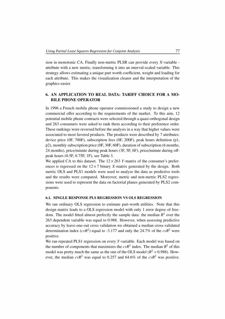
6. AN APPLICATION TO REAL DATA: TARIFF CHOICE FOR A MO-BILE PHONE OPERATOR

In 1996 a French mobile phone operator commissioned a study to design a new

commercial offer according to the requirements of the market. To this aim, 12

potential mobile phone contracts were selected through a quasi-orthogonal design

and 263 consumers were asked to rank them according to their preference order.

These rankings were reversed before the analysis in a way that higher values were

associated to most favored products. The products were described by 7 attributes:

device price (0F, 700F), subscription fees (0F, 200F), peak hours definition (p1,

p2), monthly subscription price (0F, 30F, 60F), duration of subscription (6 months,

24 months), price/minute during peak hours (3F, 5F, 6F), price/minute during off-

peak hours (0.5F, 0.75F, 1F), see Table 3.

We applied CA to this dataset. The 12× 263 Y-matrix of the consumer’s prefer-

ences is regressed on the 12× 7 binary X-matrix generated by the design. Both

metric OLS and PLS1 models were used to analyse the data as predictive tools

and the results were compared. Moreover, metric and non-metric PLS2 regres-

sions were used to represent the data on factorial planes generated by PLS2 com-

ponents.

6.1. SINGLE RESPONSE PLS REGRESSION VS OLS REGRESSION

We ran ordinary OLS regression to estimate part-worth utilities. Note that this

design matrix leads to a OLS regression model with only 1 error degree of free-

dom. The model fitted almost perfectly the sample data: the median R2 over the

263 dependent variable was equal to 0.988. However, when assessing predictive

accuracy by leave-one-out cross validation we obtained a median cross-validated

determination index (cvR2) equal to -3.177 and only the 24.7% of the cvR2 were

positive.

We ran repeated PLS1 regression on every Y-variable. Each model was based on

the number of components that maximizes the cvR2 index. The median R2 of this

model was pretty much the same as the one of the OLS model (R2 = 0.988). How-

ever, the median cvR2 was equal to 0.257 and 64.6% of the cvR2 was positive.


Tab. 3: Mobile Phone Data

Attributes ConsumersContr. Device Subscr. Min. Peak Month PH Off-PH

Price Fee Dur. Hours Price Pr/Min Pr/Min 1 ... 2631 700F 200F 24m p2 60F 3F 0.50F 11 ... 12 700F 200F 6m p1 60F 6F 0.75F 8 ... 23 700F 200F 6m p1 0F 5F 1F 7 ... 44 700F 0F 24m p2 0F 5F 0.75F 6 ... 35 700F 0F 24m p1 30F 3F 1F 9 ... 66 700F 0F 6m p2 30F 6F 0.50F 5 ... 87 0F 200F 24m p2 0F 6F 1F 4 ... 58 0F 200F 24m p1 30F 5F 0.50F 3 ... 79 0F 200F 6m p2 30F 3F 0.75F 10 ... 10

10 0F 0F 24m p1 60F 6F 0.75F 2 ... 911 0F 0F 6m p2 60F 5F 1F 1 ... 1112 0F 0F 6m p1 0F 3F 0.50F 12 ... 12

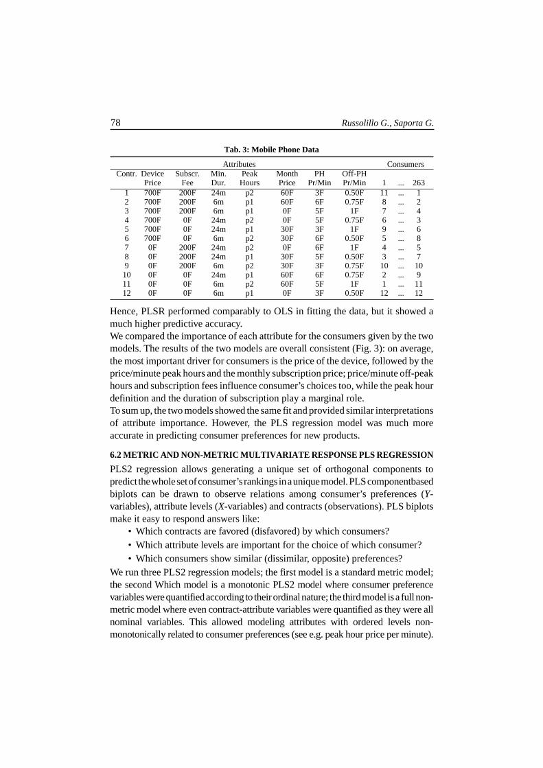
Hence, PLSR performed comparably to OLS in fitting the data, but it showed amuch higher predictive accuracy.We compared the importance of each attribute for the consumers given by the twomodels. The results of the two models are overall consistent (Fig. 3): on average,the most important driver for consumers is the price of the device, followed by theprice/minute peak hours and the monthly subscription price; price/minute off-peakhours and subscription fees influence consumer’s choices too, while the peak hourdefinition and the duration of subscription play a marginal role.To sum up, the two models showed the same fit and provided similar interpretationsof attribute importance. However, the PLS regression model was much moreaccurate in predicting consumer preferences for new products.

6.2 METRIC AND NON-METRIC MULTIVARIATE RESPONSE PLS REGRESSION

PLS2 regression allows generating a unique set of orthogonal components topredict the whole set of consumer’s rankings in a unique model. PLS componentbasedbiplots can be drawn to observe relations among consumer’s preferences (Y-variables), attribute levels (X-variables) and contracts (observations). PLS biplotsmake it easy to respond answers like:

• Which contracts are favored (disfavored) by which consumers?• Which attribute levels are important for the choice of which consumer?• Which consumers show similar (dissimilar, opposite) preferences?

We run three PLS2 regression models; the first model is a standard metric model;the second Which model is a monotonic PLS2 model where consumer preferencevariables were quantified according to their ordinal nature; the third model is a full non-metric model where even contract-attribute variables were quantified as they were allnominal variables. This allowed modeling attributes with ordered levels non-monotonically related to consumer preferences (see e.g. peak hour price per minute).


Fig. 3: Each pair of bars represents the mean importance of an attribute given by the OLSand the PLS regression models. For each attribute, the correlation between the

distributions of the importances in the two models is shown over the correspondentpair of bars.

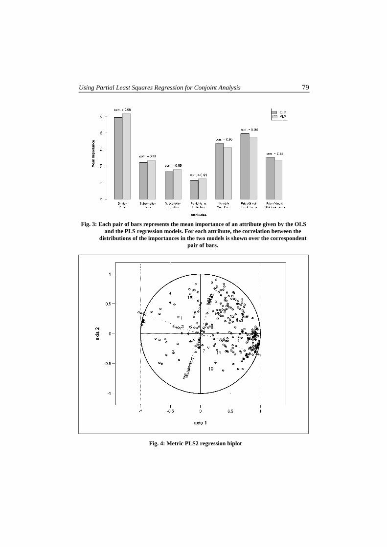
Fig. 4: Metric PLS2 regression biplot


Figure 4 shows the biplot from two-component metric PLS2 regression. Dashedlines represents attribute levels, points represent customer preferences and numeralsrepresent contracts. PLS criterion (1) is a compromise between the quality ofrepresentation of within-set correlations of X and Y variables and the quality ofrepresentation of correlation among X and Y variables. Since the X-matrix isgenerated by a quasi-orthogonal design, the criterion tends to explain mainly the Y-variables and their correlations with the X-variables. That’s why the Y-variables areexplained better than X-variables (R2

Y = 0.59, R2X = 0.24). Starting from these

considerations, to the extent that components fit the data well, the biplot can beinterpreted according to the following rules:• Virtual vectors joining the origin to the points that point the same (opposite)

direction correspond to consumers that have similar (opposite) preferences.• Dashed segments that point in the same direction correspond to attribute levels

that are favored by the same consumers• Numerals that are close together correspond to contracts that are favored by the

same consumers• The length of the dashed line is proportional to the quality of representation of

the attribute level.• The distance of a point from the origin is proportional to the quality of

representation of the corresponding consumer’s preferences• The distance of a numeral from the origin is proportional to the quality of

representation of the corresponding contract.The best represented attribute levels are the most important drivers for consumerpreferences: consistently with the previous analysis, they are price levels of thedevice (labeled as Dev700F and Dev0F), but also price/minute levels during peakhours (labeled as PH3F and PH6F) and the level 60F of the attribute Monthlysubscription price.Going from left to right we find less and less expensive contracts. The first axis ishighly correlated to price levels of the device and to subscription fees: it representsfixed costs. The second axis is highly correlated to peak and off-peak hours prices/minute and to monthly subscription price: it represents variable costs.The best represented contracts are 10, 12 and 2. The contract 10, which is positionedon the lower right of the plot, is characterized by low fixed cost and high variablecosts. Contracts 12 and 2 are positioned opposite each other: they are the cheapestand the most expensive contract in terms of both fixed and variable costs. Most ofconsumers are on the upper right, so they prefer cheaper contracts like contract 12.However, there is a minority that prefers more expensive contracts, probablybecause higher prices are associated to a better quality and/or a higher social status.


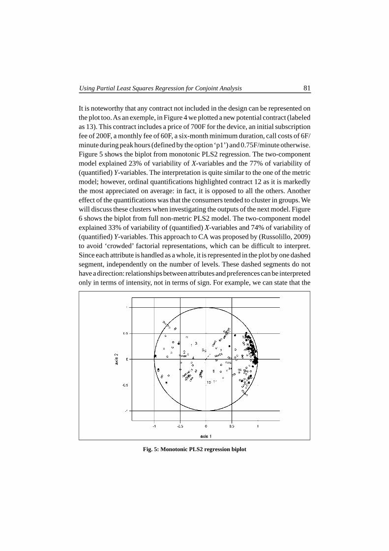
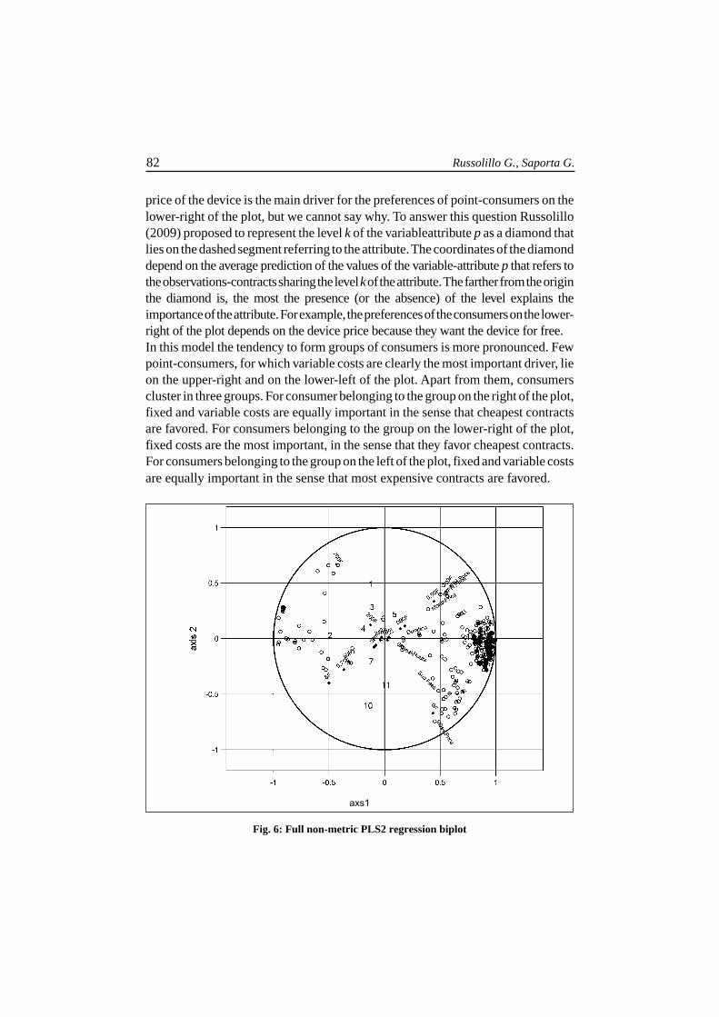
It is noteworthy that any contract not included in the design can be represented onthe plot too. As an exemple, in Figure 4 we plotted a new potential contract (labeledas 13). This contract includes a price of 700F for the device, an initial subscriptionfee of 200F, a monthly fee of 60F, a six-month minimum duration, call costs of 6F/minute during peak hours (defined by the option ‘p1’) and 0.75F/minute otherwise.Figure 5 shows the biplot from monotonic PLS2 regression. The two-componentmodel explained 23% of variability of X-variables and the 77% of variability of(quantified) Y-variables. The interpretation is quite similar to the one of the metricmodel; however, ordinal quantifications highlighted contract 12 as it is markedlythe most appreciated on average: in fact, it is opposed to all the others. Anothereffect of the quantifications was that the consumers tended to cluster in groups. Wewill discuss these clusters when investigating the outputs of the next model. Figure6 shows the biplot from full non-metric PLS2 model. The two-component modelexplained 33% of variability of (quantified) X-variables and 74% of variability of(quantified) Y-variables. This approach to CA was proposed by (Russolillo, 2009)to avoid ‘crowded’ factorial representations, which can be difficult to interpret.Since each attribute is handled as a whole, it is represented in the plot by one dashedsegment, independently on the number of levels. These dashed segments do nothave a direction: relationships between attributes and preferences can be interpretedonly in terms of intensity, not in terms of sign. For example, we can state that the

Fig. 5: Monotonic PLS2 regression biplot


price of the device is the main driver for the preferences of point-consumers on thelower-right of the plot, but we cannot say why. To answer this question Russolillo(2009) proposed to represent the level k of the variableattribute p as a diamond thatlies on the dashed segment referring to the attribute. The coordinates of the diamonddepend on the average prediction of the values of the variable-attribute p that refers tothe observations-contracts sharing the level k of the attribute. The farther from the originthe diamond is, the most the presence (or the absence) of the level explains theimportance of the attribute. For example, the preferences of the consumers on the lower-right of the plot depends on the device price because they want the device for free.In this model the tendency to form groups of consumers is more pronounced. Fewpoint-consumers, for which variable costs are clearly the most important driver, lieon the upper-right and on the lower-left of the plot. Apart from them, consumerscluster in three groups. For consumer belonging to the group on the right of the plot,fixed and variable costs are equally important in the sense that cheapest contractsare favored. For consumers belonging to the group on the lower-right of the plot,fixed costs are the most important, in the sense that they favor cheapest contracts.For consumers belonging to the group on the left of the plot, fixed and variable costsare equally important in the sense that most expensive contracts are favored.

Fig. 6: Full non-metric PLS2 regression biplot

axs1


CONCLUSION

Even if since almost fifty years CA is a well established methodology in marketingresearch, the application of this technique is not trivial. Practical implementationsof CA require a lot of attention so as not to incur errors that could falsify theconclusions. In most of cases, CA is not a reliable tool to predict part worth utilitiesfor out-of-sample profiles when it is implemented by OLS regression. Thisdrawback is due to the lack of degrees of freedom which typically affects the model.We showed on real data that replacing OLS by PLS estimates sensibly improves CAprediction accuracy. Moreover, we showed how to use PLS2 regression graphicalrepresentations to quickly and easily interpret relations among preferences, attributesand profiles. A further advantage of using PLS to run CA is its flexibility: non-metric PLS regression can be used to transform preference and/or attributevariables to take into account their non-quantitative nature.

REFERENCES

Benammou, S., Harbi, S. and Saporta, G. (2003). Sur l’utilisation de l’analyse conjointe en cas deréponses incomplètes ou de non réponses. In Revue de Statistique Appliquée, 51 (4): 31–55.URL http://www.numdam.org/item/ RSA_2003__51_4_31_0.

De Jong, S. (1995). Pls shrinks. In Journal of Chemometrics, 9 (4): 323–326. doi:10.1002/cem.1180090406. URL https://onlinelibrary.wiley.com/ doi/abs/10.1002/cem.1180090406.

Debreu, G. (1959). Cardinal utility for even-chance mixtures of pairs of sure prospects*. In

The Review of Economic Studies, 26 (3): 174–177. doi:10.2307/ 2295745. URL http://dx.doi.org/10.2307/2295745.

Elrod, T., Louviere, J.J. and Davey, K.S. (1992). An empirical comparison of ratings-based andchoice-based conjoint models. In Journal of Marketing Research, 29 (3): 368–377. URL http://www.jstor.org/stable/3172746.

Furlan, R. and Corradetti, R. (2005). An empirical comparison of conjoint analysis models on a samesample. In Rivista di Statistica Applicata, 17 (2): 141 – 158. URL http://sa-ijas.stat.unipd.it/sites/sa-ijas.stat. unipd.it/files/Furlan\%20141-158.pdf.

Green, P.E. and Rao, V.R. (1971). Conjoint measurement for quantifying judgmental data. In Journalof Marketing Research, 8 (3): 355–363. URL http://www.jstor.org/stable/3149575.

Green, P.E. and Srinivasan, V. (1990). Conjoint analysis in marketing: New developments withimplications for research and practice. In Journal of Marketing, 54 (4): 3–19. URL http://www.jstor.org/stable/1251756.

Huber, J., Wittink, D.R., Johnson, R.M. and Miller, R. (1992). Learning effects in preference tasks:Choice-based versus standard conjoint. In Sawtooth Software Conference Proceedings. SunValley, ID.

Johnson, R.M. (1987). Adaptive conjoint analysis. In Sawtooth Software Conference Proceedings.Ketchum, ID.

Kruskal, J. (1964). Nonmetric multidimensional scaling: A numerical method. In Psychometrika, 29(2): 115–129. doi:https://doi.org/10.1007/BF02289694.


Kuhfeld, W. (2010). Marketing research methods in SAS - SAS9.2 Edition. SAS Institute Inc., Cary,NC, USA.

Lauro, C.N., Giordano, G. and Verde, R. (1998). A multidimensional approach to conjoint analysis.In Applied Stochastic Models and Data Analysis, 14 (4): 265–274. doi:10.1002/(SICI)1099-0747(199812)14:4<265:: AID-ASM362>3.0.CO;2-W. URL http://dx.doi.org/10.1002/(SICI)1099-0747(199812)14:4<265::AID-ASM362>3.0.CO;2-W.

Louviere, J.J., Flynn, T.N. and Carson, R.T. (2010). Discrete choice experiments are not conjointanalysis. In Journal of Choice Modelling, 3 (3): 57 – 72. doi:https://doi.org/10.1016/S1755-5345(13)70014-9. URL http://www.

sciencedirect.com/science/article/pii/S1755534513700149.

Luce, R. and Tukey, J.W. (1964). Simultaneous conjoint measurement: A new type of fundamentalmeasurement. In Journal of Mathematical Psychology, 1 (1): 1 – 27. doi:https://doi.org/10.1016/0022-2496(64) 90015-X. URL http://www.sciencedirect.com/science/article/ pii/002224966490015X.

Ohannessian, S. and Saporta, G. (2008). ‘Zero option’ in conjoint analysis: a new specification of theindecision and the refusal. In Atti della 44esima riunione scientifica della SIS. Universitá dellaCalabria, Arcavacata di Rende, Italy.

Russolillo, G. (2009). Partial Least Squares Methods for Non-Metric Data. Ph.D. thesis, Dipartimen-to di Matematica e Statistica, Universitá degli Studi di Napoli ‘Federico II’, Napoli, Italy.

Russolillo, G. (2012). Non-metric partial least squares. In Electron. J. Statist., 6: 1641–1669.doi:10.1214/12-EJS724. URL https://doi.org/10.1214/ 12-EJS724.

Tenenhaus, M. (1998). La Régression PLS: théorie et pratique. Technip, Paris.

Von Neumann, J. and Morgenstern, O. (1947). Theory of games and economic behavior (2nd rev. ed.).Princeton University Press, Princeton, NJ.

Young, F.W., J., D.L. and Takane, Y. (1976). Regression with qualitative and quantitative variables:an alternating least squares approach with optimal scaling features. In Psychometrika, 41: 505–529. doi:10.1214/12-EJS724.

using partial least squares regression for

Documents