J. Sci. FoodAgric. 1983,34,715-124

Preference of Cauliflower Related to Sensory Descriptive Variables by Partial Least Squares (PLS) Regression

Magni Martens, Harald Martens and Svante Wolda

Norwegian Food Research Institute, P.O. Box 50, N-1432 Aas-NLH, Norway and aUmed University, S-90187 Urned, Sweden

(Manuscript received 27 April 1982)

Two new multivariate techniques for comparing two blocks of variables were tested on sensory data from cauliflower. The techniques are based on Partial Least Squares (PLS) regression on latent variables. The method of PLS2 was used for relating four different preference variables simultaneously to 1 1 descriptive variables by regression on common factors. The method of PLSl was subsequently used to relate individual preference variables to the 11 descriptive variables. Two factors were in each case found to be statistically significant by cross-validation. The first, dominating PLS2 factor was a general quality factor showing that all the descriptive variables were more or less related to all the preference variables. This quality factor agreed well with the producers quality classification of the batches upon harvesting. A second, minor factor dis- tinguished between texture and flavour descriptor’s relationships to the preferences. PLSl regressions showed that texture preference was best predicted by texture descrip- to1 s, especially crispness, and flavour preference was best predicted by flavour descrip- tors, especially fruitiness. Some benefits of the PLS methods over the conventional alternatives of stepwise regression and principle component analysis are discussed.

1. Introduction

It is difficult to interpret many experimental variables simultaneously. A new approach to multi- variate data analysis is presently tested by modelling sensory data.

Sensory data are usually collected in order to get a quality assessment of a food product. Since human perception of quality is complex and therefore difficult to measure by only one sensory variable, it is customary to characterise food samples by means of multiple sensory variables. Such sensory variables are primarily of two different types: (a) preference variables which express a subjective opinion about a product and (b) descriptive variables which have status closer to instru- mental (objective) variables, and which describe a product in an analytical way. Preference data should be collected from a large, representative group of people (consumer panel), while descriptive data are usually collected from a smaller group of trained persons (laboratory panel). However, in the present methodology study, both preference and descriptive data were for simplicity obtained from a laboratory panel.

Multivariate data analysis of sensory data, comprising multivariate sensory observations on a number of related food samples, can be done with different objectives. One is often interested in the relationships between different types of sensory variables, for instance in order to predict one type from another. One may also want to find out how the sensory quality varies between the objects investigated. In addition, classification criteria on the basis of the sensory variables are often sought. However, data tables in quality research are usually large and therefore difficult to interpret visually or by univariate statistics. Even studies of correlations between pairs of vari- ables are unsatisfactory when the number of variables are high, since the number of such variable pairs creates ‘mental overflow’ as well as the danger of spurious correlations erroneously appearing as significant. By multivariate statistics the interpretation of large data tables may become faster,

715

716 M. Martens et al.

more reliable and more complete. Multivariate pattern recognition may be used to obtain clear criteria for classification of samples into quality classes. Multivariate regression methods may be used to summarise relationships between many different measurement variables. Powers1 reviewed various methods for finding relations between sensory and instrumental data sets.

In both pattern recognition and regression analysis a number of different statistical methods are available. One group of methods, the latent variable methods, is used in order to ‘focus’ the information of large data tables into a few underlying phenomena (called latent variables or factors) leaving most of the measurement noise behind as residuals. In other words, each object is regarded as a ‘mixture’ of a few underlying phenomena and the aim is to identify and quantify these phenom- ena with minimal effects of measurement noise.

In the present paper a new multivariate regression technique, Partial Least Squares (PLS) re- gression on latent variables, is tested on sensory data from cauliflower. The method corresponds well to the type of noise and redundance commonly found in experimental data. Its mathematical basis has been described previously2 and the algorithms have been published3,* ; they are described conceptually in Section 2.3. Two different versions of PLS regression are used. First, the relation- ships between several descriptive variables and several preference variables are explored in a causal model with the former used as independent (X) and the latter as dependent variables ( Y ) . Secondly, the PLS technique is used in order to relate individual preference variables to the descrip- tive ones.

2. Experimental 2.1. Material In order to get a representative agronomical variation in the material, 12 batches of fresh cauliflower (Brussicu nupus var. nupobrussicu L.) from different origins (different varieties, soil types and stages of development) were collected in September 1980. The samples were analysed within 10 days after harvesting. Storage conditions during these days were 0°C and 95 % relative humidity. Heads (15 from each batch) were cut into four pieces, mixed and randomly prepared as a sample for the sensory evaluation. One whole head from each batch was also included for colour and appearance assessments.

2.2. Sensory evaluation A well trained laboratory panel of 11 judges evaluated 36 samples (12 batches x 3 replicates). The samples were randomised within each replicate and served in a different sequence for different judges. Six samples were evaluated at each session. A category scale (points 0-9) was used for the 11 sensory variables judged in the following sequence : 1, total impression of colour (‘colour preference’, CP) ; 2, total impression of appearance, colour excluded (‘appearance preference’, AP) ; 3, crisp- ness (cr); 4, chewing resistance (ch); 5, juiciness (ju); 6, total impression of texture (‘texture prefer- ence’, TP); 7, sweet taste (sw); 8, fruity taste (fr); 9, bitter taste (bi); 10, total flavour strength (fl). 11, total impression of flavour (‘flavour preference’, FP).

Concerning the four preference variables (upper-case letters in the abbreviations) the judges were instructed to give their own opinion of the samples along a scale from very bad to very good (quality scales). As for the seven descriptive variables (lower-case letters), the strength of the different properties was to be judged (intensity scales). Although we are aware that the 11 judges are not representative for a consumer group, the preference variables were used to simulate consumer preference data in order to illustrate the statistical methods.

2.3. Data analytical method 2.3.1. The PLSl method When used to explore the mathematical relationships between one dependent variable (one preference regressand, y ) and a block of independent variables, (many descriptive regressors, X = (xI,x~, . . .) ) the PLS regression resembles stepwise multiple linear regression, but in contrast to the latter

Cauliflower preference 717

it is applicable even if the regressors are strongly intercorrelated (multicolinear regressors) and contain significant noise, and even if the number of regressors is higher than the number of observa- tions. All regressors are included in the final solution; no variables have to be discarded as in stepwise multiple linear regression. In these respects it is similar to principal component regression,S which consists of multiple linear regression on the largest of the principal components of the regres- sor matrix. But the PLSl method is more efficient, since it extracts from the regressor matrix only those factors that are relevant to the prediction of the regressand, y. This PLS algorithm is termed PLSl and can be described as follows :

A latent variable (factor 1) representing a linear combination of all the regressors, is esti- mated so that the regressand is predicted optimally (least squares residuals). Both regressand and regressors are then projected on to this latent variable. A second latent variable (factor2) representing a linear combination of the residuals of the regressors after the first projection, is then estimated. This factor is orthogonal to the first one and optimally predicts the residual of the regressand after the first projection. The regressands’ residuals and regressors’residuals are then projected on to this second factor, whereupon a third factor is similarly estimated from the new regressor residuals in order to predict the new regressands’ residuals, etc.

Each factor is characterised in terms of loadings for the regressand (here: one preference variable) and for all the regressors (here: the seven descriptive variables), and in terms of its factor scores for each object (here: each cauliflower batch).

The result is a small set of factors, that from the regressors predict the regressand optimally in terms of least squares residuals.

2.3.2. The PLS2 Method When used to explore the relationships between a block of several regressands Y = ( y l , y ~ , . . .) and a block of several regressors X = ( X I , X Z , . . .) the PLS algorithm is slightly different and is termed PLS2. For each factor this is now an iterative procedure. The algorithm resembles canonical correlation betwen the two matrices, but in contrast to the latter, PLS2 works even if there are

Figure 1. Relationship between joint Principal Component Analysis (PCA) (left) of two blocks of variables X and Y, and PLSZ regression on latent

Conceptually, PCA picks up, as latent variables, all the systematic variation in both X and Y while PLS2 primarily seeks those latent variables that are common to both X and Y. PLSZ thus, in principle, leaves out factors in Y irrelevant to Xand factors in Xirrelevant to Y, and focuses only on interrelation- ships between X and Y. In joint PCA these interrela- tionships may be intermingled with factors unique to

variables (right) for the same two blocks X and Y. X X

X or unique to Y, and therefore less easily seen. Joint PCA PLS2

more variables than observations in both matrices, and even if both X and Y have high noise and multicollinear redundancy. It may now be compared to a joint Principal Component Analysis (PCA) of two matrices X and Y, but, in contrast to the joint PCA the PLS2 primarily extracts the interrelating factors, leaving out the factors unique to only X or only Y (Figure 1). The PLS2 algorithm can be described as follows:

A latent variable (factor 1) representing a linear combination of all the regressors, is iteratively estimated so that all the regressands are predicted optimally (in terms of least sum of squares in residuals for all the regressands together). All regressors and regressands are then projected onto this latent variable. A second latent variable (factor 2), representing a linear combina- tion of the regressor residuals after the first projection, is then estimated iteratively. This

718 M. Martens et al.

second factor, which is orthogonal to the first one, optimally predicts the residuals of all the regressors. All the regressands’ residuals and the regressors’ residuals are then projected on to this second factor, and a third factor is similarly estimated from the new regressor residuals in order to predict all the new regressand residuals, etc.

Each factor is characterised in terms of loadings for all the regressands (here: the four preference variables) and for all the regressors (here: the seven descriptive variables), and in terms of its factor scores for each object (here: each cauliflower batch).

The result is a small set of factors, that from the regressors predict optimally all the regressands at the same time in terms of total least squares residuals.

Ideally, statistical results should be tested on independent data, in order to check their true signifi- cance. Like PCA, factor analysis and other latent variables methods, the PLS methods are dependent on a correct choice of number of factors in order to avoid overfitting of the data. In the present case, independent data for prediction testing were not available. Instead, the technique of cross- validation6 was used to determine the maximum number of significant PLS factors. In the cross- validation each factor was here estimated four times, each time keeping one quarter of the samples out from the estimation, using these samples instead for prediction. In this way every sample served for independent testing of the factor’s predictive ability. Thus the possibility of mistaken interpre- tation of factors caused by trivial, random measurement errors was greatly reduced.

Like other least squares techniques, PLSl and PLS2 are somewhat sensitive to the relative scaling of the different variables and observations. Each sensory variable was here standardised to zero mean, unit variance, prior to the PLS analysis, in order to ensure that no variable overshadowed the others in the least squares procedures. Other weightings of the variables were also tested, but their effects were negligible. All samples were given the same weight, since we assume the same analytical precision for each cauliflower batch.

2.4. Computations The PLS calculations were done in the microcomputer programs CPLSl and CPLS2 in BASIC language,‘ run in part on an ABC-80 microcomputer and in part on a NORD-1OS minicomputer.

Univariate analysis-of-variance (ANOVA) was performd in FORTRAN on a NORD-10s minicomputer.

3. Results and discussion

3.1. Input data Table 1 gives the input for the multivariate PLS estimations, the values for the 11 variables for the 12 cauliflower batches, averaged over three replicates and 11 judges. The table also gives the total mean and the total standard deviation (stat) for each variable over the 12 batches. Univariate 3-way analysis-of-variance (ANOVA of batch x replicate x judge) was performed on each variable separately, in order to get an indication of the signal/noise ratios of the variables. All variables showed statistically significant variation between batches. Colour preference and appearance preference showed exceptionally good signal/noise ratios. Among the descriptive texture variables juiciness showed the best ratio, and among the descriptive flavour variables fruitiness showed the best one. Sweetness showed much lower signal/noise ratio than the other variables, as can be seen from the F-values in the last column. The absolute noise level was about the same for all 11 sensory variables, as shown by the residual standard deviations (serr) from the univariate ANOVA.

The ANOVA showed small, but significant interactions for judges x batches for all variables, except the colour preference. Thus, when we for simplicity use data averaged over the 11 judges, we loose some information about the individual judges’ cauliflower preferences and perception of the scales, but this should not affect our present conclusions.

Each of the 12 cauliflower batches had been graded subjectively by the farmer into class I (eight

Cauliflower preference 719

Table 1. Input data for the PLS analyses. Mean of three replicates and 11 judges for each of the sensory variables. Farmers’ prior quality classification is given in the bottom column. The total standard deviation is given as stat and the univariate error standard deviation as selr. The signal/noise ratio (univariate F-test for between-batches

differences) is given in the last column

Sensory variables

Preference CP AP TP FP

Descriptive cr ch ju

fr bi fl

SW

Class

Batch No. Total

1 2 3 4 5 6 7 8 9 10 11 12 mean stOt

6.83 8.03 8.25 7.67 8.53 8.61 8.47 7.53 2.17 1.92 2.92 5.11 6.34 2.60 0.15 6.97 8.14 7.61 7.33 7.97 7.78 7.75 7.61 2.56 3.08 4.25 5.17 6.35 2.03 0.18 7.69 7.58 7.89 7.97 7.83 8.14 8.06 7.61 3.47 4.06 5.08 5.97 6.78 1.69 0.17 7.17 7.67 7.39 8.08 7.50 7.69 7.39 7.44 2.58 3.81 4.17 5.42 6.36 1.86 0.22

7.50 7.56 7.61 7.50 7.78 8.00 7.97 7.78 3.86 4.58 5.28 6.17 6.80 1.45 0.19 2.64 2.81 2.56 2.44 2.53 2.19 2.31 2.61 5.67 5.42 4.69 3.64 3.29 1.26 0.16 7.17 6.72 7.00 7.39 7.08 7.28 7.22 6.78 3.56 3.97 4.92 5.61 6.23 1.37 0.16 3.06 2.50 2.81 3.00 2.61 2.78 2.92 2.72 1.64 2.08 1.94 2.36 2.54 0.45 0.17 6.81 6.78 7.11 7.42 6.16 7.03 6.92 6.64 2.58 3.64 4.33 5.31 5.93 1.59 0.19 1.47 1.97 2.06 1.06 1.61 2.31 2.22 1.03 4.44 4.00 3.61 2.50 2.36 1.12 0.22 6.75 6.92 6.89 7.06 6.53 6.97 6.89 6.19 3.17 4.61 4.75 5.64 6.03 1.24 0.22

I I I I I I I I I I I I I I I I

F*

264*** 123*** 99*** 63***

54*** 62*** 73***

3** 51*** 17*** 34***

a serr is estimated as z/SSem/(nl/nz), where SSerr represents the sum-of-squares from all interactions, nl represent the number of degrees of freedom for this error (=372) and n2 is the number of observations behind each input data (33).

The F-values were compared to the F-distribution with I 1 and 372 degrees of freedom. *** p<0.001; **0.001 <P<O.Ol. For explanation of abbreviations see Section 2.2.

batches) or class I1 (four batches), according to Norwegian Standard.8 This prior classification is given in the bottom column in Table I .

3.2. Relationships between the block of preference data and the block of descriptive data (PLSZ) The essential relationships between the four preference and seven descriptive variables were ex- tracted by PLS2, using the former as regressands and the latter as regressors. One major and one minor factor were found to be statistically significant in the sense of improving cross-validation predictability for the preference variables of samples excluded from the actual estimation. The PLS2 solution is described in Table 2 and Figures 2 and 3.

Table 2 gives the variance described by the first two factors and the residual variances. The first factor (column 1) was strongly correlated to all the variables; it described about 95 % of the total variance of both the preference variables (block Y ) and the descriptive variables (block X ) . Some of the variables (e.g. texture preference and flavour preference, chewing resistance, juiciness and fruitiness) were more or less completely described by this first factor. The second factor (column 2) explained only 3% of the total variance for the preference variables (block Y ) and 1 % of the descriptive variables (block X ) . In the preference block it was mainly correlated to colour and appearance preference, and in the descriptive block to sweetness, bitterness and crispness.

The residual variances in X and Y after two PLS2 factors are shown in column 3. On average, 95.1% of the total variance in the descriptive variables was explained by the first two factors, leaving only 4.9 % residual variance. Correspondingly, 97.8 % of the four preference variables’ total variance was described by the two factors, leaving on average only 2.2% residual variance, This means that 97.8 % of the total variance of the four preference variables was described by the

720 M. Martens et al.

Table 2. PLS2 regression of all four preference variables versus the seven descriptive variables

Column

Regressands, Y CP AP TP FP

Y, all 4 pref. variables

Regressors, X cr ch ju

fr bi fl

sw

X, all 7 descriptive variables

1 2 3 4 5

%Explained by Residual Residual variance variance Residual

Factor 1 Factor 2 PLS2( %) ANOVA( %) s.d. ~

91 93 98 98

94.9

97 98 99 91 99 86 95

94.1

5 5 1 0

2.9

2 I 0 6 0 2 0

1.0

4 2 0 .3 2

2.2

1 1 1 3 1

12 5

4 .9

0 .3 1 1 1

0.9

2 2 1

14 1 4 3

3 .9

0.53 0.31 0.10 0.26

0.15 0.13 0.14 0.08 0.16 0.38 0.28

For explanation of abbreviations see Section 2.2. Explained variances and residual variances for the two statistically significant factors are given in percent of total variance, stotZ. ANOVA residual variance percentages are calculated from Table 1. Residual s.d. gives absolute residual standard deviations after two PLSZ factors.

Factor 2

CP AP cr

TP -ch

bi

I

-!I ch

-2 L -b i

SW

Figure 2. PLSZ loadings for the four preference variables (upper-case letters) and the seven descriptive variables (lower-case letters) for the two significant factors. CP, AP, TP and FP represent colour, appearance, texture and flavour preferences, respectively; cr = crisp- ness; ch=chewing resistance; ju= juiciness; sw=sweetness; fr =fruiti- ness; bi=bitterness; fl=flavour strength. The variables ju, FP, fl and fr appear in the same cluster.

seven descriptive variables. The residuals in column 3 correspond well with the noise levels (the residual variances in column 4) after the univariate ANOVA except for sweetness and bitter- ness. This can also be seen when the residual standard deviation (column 5, Table 2) is compared to the ANOVA standard deviation (serr) in Table 1.

Sweetness is possibly somewhat overfitted by factor 2, although lower weighting of sweetness also

Cauliflower preference

r Factor *

721

Figure 3. PLS2 scores for the 12 cauliflower batches plotted for the two significant factors. The number repre- sent batch numbers. Each score vector is scaled so that its variance equals the vari- ance it accounted for in the regressor block (the seven descriptive variables).

-9

6 71 , I

1 4

2 Factor I

gave the same general solution. Bitterness apparently has some unique variance that is irrelevant to the preference variables and hence left out from the PLS2 solution.

The loadings of the variables for the two first factors of the standardised PLS2 solution are given in Figure 2. Factor 1 is a general quality factor, with all preference and descriptive variables except bitterness and chewing resistance responding similarly. Bitterness and chewing resistance showed loadings approximately opposite to the other variables. Multiplying these two ‘bad’ variables by - 1 to make them ‘good’ (‘lack of-bitterness’, -bi, and ‘lack-of-chewing resistance’, -ch) made them more easily comparable with the other sensory variables; now all variables showed factor 1 loadings near 1.0.

Factor 2 is quantitatively much less important than factor 1, as can be seen from the lower explained variance (column 2, Table 2), and also less certain. It represents an additional small tendency of colour and appearance preferences being positively related to the texture variables crispness and lack-of-chewing resistance, and negatively to the flavour variables sweetness and lack- of-bitterness. The variables fruitiness, flavour strength, flavour preference and juiciness were more or less uncorrelated with factor 2.

3.3. Classification and characterisation of the material based on factor scores (PLS2) Figure 3 shows the batch factor scores of factor 2 plotted against the batch factor scores of factor 1 from the PLS2 solution. Batches number 9, 10, 11 and 12 obtained much lower scores than the others along the general quality factor (factor l), meaning that they are of inferior general quality. The same batches were graded by the farmers as class I1 as seen in Table 1. Thus there is a good agreement between the farmers’ classification of the batches and the characterisation given by the sensory panel.

The PLS two-factor solution can be interpreted as follows : In general the class I batches scored higher than the class I1 batches in both preference and descriptive variables (except chewing resis- tance and bitterness). This type of variability dominated the systematic variation in the data and hence the total variation, since the random noise level was very low in the data. It is described by factor 1 and may be understood by comparing for instance batches 7 and 9: Table 1 shows that batch 7 was judged much higher than batch 9 in all variables except chewing resistance and bitterness, the two variables that obtained negative factor 1 loadings (Figura 2). The quality differences between batches 7 and 9 are reflected by their difference in factor 1 scores (Figure 3).

The less important factor 2 may likewise be understood by comparing some extreme batches. Table 1 shows that for instance batch 6 was less sweet and more bitter than batch 1. But, on the other hand batch 6 scored higher than batch 1 in, for example, e.g. colour and appearance preferences contrary to what swaetness and bitterness would imply. Factor 2 picks up this new type of vari- ability (Figure 2) and gives batch 6 high score and batch 1 low score (Figure 3). Batch 7 lies between batches 6 and 1 in the sensory data, and received intermediate factor 2 score.

3.4. Detailed study of individual preference variables (PLSl) In order to obtain more detailed information on how the individual preference variables relate to the descriptive ones, PLSl was used in analogy to a multiple linear regression.

48

122 M. Martens el al.

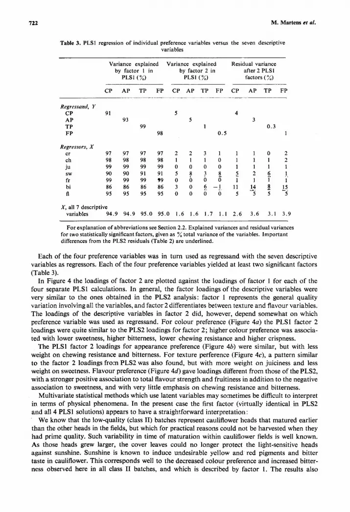
Table 3. PLSl regression of individual preference variables versus the seven descriptive variables

Variance explained Variance explained Residual variance by factor 1 in by factor 2 in after 2 PLSl

PLSl(%) PLSl(%) factors (z) CP AP TP FP CP AP TP FP CP AP TP FP

Regressand, Y CP 91 5 4 AP 93 5 3 TP 99 1 0.3 FP 98 0 .5 1

Regressors, cr ch ju

fr bi fl

sw

X 9 7 9 7 9 7 9 7 2 2 3 1 1 1 0 2 9 8 9 8 9 8 9 8 1 1 1 0 1 1 1 2 9 9 9 9 9 9 9 9 0 0 0 0 1 1 1 1 9 0 9 0 9 1 9 1 5 8 3 8 - 5 2 6 1 9 9 9 9 9 9 9 9 0 6 0 0 1 1 1 1 86 86 86 86 3 0 6 -! 11 14 8 l5 9 5 9 5 9 5 9 5 0 0 0 0 5 5 5 5

X, all 7 descriptive variables 94.9 94.9 95.0 95.0 1.6 1.6 1.7 1.1 2.6 3.6 3.1 3.9

For explanation of abbreviations see Section 2.2. Explained variances and residual variances for two statistically significant factors, given as % total variance of the variables. Important differences from the PLS2 residuals (Table 2) are underlined.

Each of the four preference variables was in turn used as regressand with the seven descriptive variables as regressors. Each of the four preference variables yielded at least two significant factors (Table 3).

In Figure 4 the loadings of factor 2 are plotted against the loadings of factor 1 for each of the four separate PLSl calculations. In general, the factor loadings of the descriptive variables were very similar to the ones obtained in the PLS2 analysis: factor 1 represents the general quality variation involving all the variables, and factor 2 differentiates between texture and flavour variables. The loadings of the descriptive variables in factor 2 did, however, depend somewhat on which preference variable was used as regressand. For colour preference (Figure 4a) the PLSl factor 2 loadings were quite similar to the PLS2 loadings for factor 2; higher colour preference was associa- ted with lower sweetness, higher bitterness, lower chewing resistance and higher crispness.

The PLSl factor 2 loadings for appearance preference (Figure 46) were similar, but with less weight on chewing resistance and bitterness. For texture perference (Figure 4c), a pattern similar to the factor 2 loadings from PLS2 was also found, but with more weight on juiciness and less weight on sweetness. Flavour preference (Figure 4 4 gave loadings different from those of thePLS2, with a stronger positive association to total flavour strength and fruitiness in addition to the negative association to sweetness, and with very little emphasis on chewing resistance and bitterness.

Multivariate statistical methods which use latent variables may sometimes be difficult to interpret in terms of physical phenomena. In the present case the first factor (virtually identical in PLS2 and all 4 PLSl solutions) appears to have a straightforward interpretation:

We know that the low-quality (class 11) batches represent cauliflower heads that matured earlier than the other heads in the fields, but which for practical reasons could not be harvested when they had prime quality. Such variability in time of maturation within cauliflower fields is well known. As those heads grew larger, the cover leaves could no longer protect the light-sensitive heads against sunshine. Sunshine is known to induce undesirable yellow and red pigments and bitter taste in cauliflower. This corresponds well to the decreased colour preference and increased bitter- ness observed here in all class I1 batches, and which is described by factor 1. The results also

Cauliflower preference 723

C

bi

b d

Figure 4 a-d. PLSl loadings for the PLSl solution obtained when using individual preference variables as regres- sands and the seven descriptive variables as regressors, given for the two first factors (See figure 2 for explanation of abbreviations).

indicate that the increased maturity of the class I1 heads leads to increased chewing resistance and decreases in all the remaining observed variables.

A physical interpretation of the second factor is not equally obvious. It seems that some batches (e.g. batches 11, 2, 5 and 6) have lower sweetness and higher bitterness than expected from the other descriptive variables, and that this was associated with increased preference. The opposite is apparently the case in, for example, batches 10, 1 and 4.

This effect was observed within both class I and class I1 cauliflower. It may indicate that the perception of sweetness and bitterness are complex processes.

4. Conclusions

A new multivariate approach to data analysis of two blocks of observed variables on the same objects has been tested on sensory quality data of cauliflower. The joint covariance between four

724 M. Martens et al.

sensory preference variables, on one hand, and seven descriptive variables, on the other, was extracted in a single two-factor-solution by a method termed PLS2, leaving residuals that were similar to the estimated univariate noise levels in the data. A related method (PLSl), representing a new multivariate approach to multiple linear regression, was then used to study the dependency of individual preference variable to the descriptive ones. By comparing the PLSl solutions obtained for each of the four preference variables, the results from the PLS2 analysis were verified and studied in more detail.

The new algorithms, PLS2 and PLSl, behaved very satisfactorily when used with cross-validation for the determination of correct number of significant factors. The algorithms apparently combine useful aspects of PCA and traditional multiple linear regression techniques. They allow multiple regressions to be performed without discarding variables, even when both regressors and regressands have noise and the number of objects is low. PLS2 even allows simultaneous examination of several regressands.

Bearing in mind that the present data were obtained from a laboratory panel, on a limited number of cauliflower batches, the PLS results showed that good quality (class I) was associated with high crispness, high juiciness and low chewing resistance, as well as strong total flavour, strong fruitiness, strong sweetness and little bitterness. This dominated the observed perception of cauliflower quality (factor l), and was interpreted in terms of maturity of the heads. However, too much sweetness, together with too low bitterness, was associated with some decrease in preference (factor 2).

After two factors the four preference variables could most precisely be explained by the des- criptors juiciness, lack-of-chewing resistance, crispness and fruitiness. Texture and flavour prefer- ences were more completely explained than colour and appearance preferences.

Even if the present methodology study was performed on a small number of batches, the PLS methods appeared suitable for exploring relationships between two different types of variables. Other sensory PLS applications have recently been published. 931O

Acknowledgements The authors thank S. Hurv for technical assistance, U. Haugdahl for typing the original manuscript, H. J. Rosenfeld for discussions concerning agronomical factors and P. Lea for statistical assistance.

References 1. Powers, J. J. Perception and analysis: A perspective view of attempts to find causal relations between sensory

and objective data sets. In Flavour '81 (Schreier, P., Ed.), Walter de Gruyter & Co, Berlin, New York,1981,

2. Wold, H. Soft modelling: The basic design and some extensions. In Systems Under Indirect ObSerYUtioJl

3. Wold, S.; Martens, H.; Wold, H. The multivariate calibration problem in chemistry solved by the PLS method.

4.Martens, H.; Jensen, S. hi. Two-stage PLS regression on latent variables: A new approach for NIR calibration.

5 . Mandel, J. Use of the singular value decomposition in regression analysis. The American Statistician 1982,

6. Wold, S. Cross-validatory estimation of the number of components in factor and principal components

7 . Wold, S. SIMCA-3B Manual Umeft Univ., Sweden, 1981. 8. Norsk Standard for grennsaker og matpoteter NS2820, Norges Standardiserings-forbund, Oslo, 1976,3rd edn. 9. Martens, M.; Fieldsenden, B.; Russwurm, Jr., H.; Martens, H. Relationship between sensory and chemical

quality criteria for carrots studied by multivariate data analysis. In Sensory Quality in Foods and Beverages (Williams, A. A.; Atkin, R. K., Eds), Society of Chemical Industry and Ellis Horwood Ltd. Chichester, England, 1983.

10. Martens, M.; Lea, P.; Martens, H. Predicting human response to food quality by analytical measurements: The PLS regFessson method. In Nordic Symposium on Applied Statistics (Christie, 0. H. J., Ed.), Rogaland Research Institute, Stavanger, 1983.

pp. 103-131.

(Joreskog, K. G. ; Wold, H., Eds), North-Holland, Amsterdam, 1981.

In Matrix Pencils. Lecture Notes in Mathematics Springer Verlag, Heidelberg, 1982, in press.

Proc. 7th World Cereal and Bread Congress Praha, 1982, Elsevier, Amsterdam, in press.

36,lS-24.

models. Technomefrics 1978, 20, 397-405.