the successive projections algorithm for interval selection in pls
TRANSCRIPT

Microchemical Journal 110 (2013) 202–208
Contents lists available at SciVerse ScienceDirect
Microchemical Journal
j ourna l homepage: www.e lsev ie r .com/ locate /mic roc
The successive projections algorithm for interval selection in PLS☆
Adriano de Araújo Gomes a, Roberto Kawakami Harrop Galvão b, Mário Cesar Ugulino de Araújo a,Germano Véras c,1, Edvan Cirino da Silva a,⁎a Universidade Federal da Paraíba, CCEN, Departamento de Química, Caixa Postal 5093, CEP 58051-970, João Pessoa, PB, Brazilb Instituto Tecnológico de Aeronáutica, Divisão de Engenharia Eletrônica, CEP 12228-900, São José dos Campos, SP, Brazilc Universidade Estadual da Paraíba, CCT, Departamento de Química, 58.429-500, Campina Grande, PB, Brazil
☆ Paper presented at 5th Ibero-American Congress of⁎ Corresponding author. Tel.: +55 83 3216 7438; fax
E-mail address: [email protected] (E.C. da Silv1 Tel.: +55 83 3315 3356.
0026-265X/$ – see front matter © 2013 Elsevier B.V. Alhttp://dx.doi.org/10.1016/j.microc.2013.03.015
a b s t r a c t
a r t i c l e i n f oArticle history:Received 27 November 2012Received in revised form 4 March 2013Accepted 17 March 2013Available online 1 April 2013
Keywords:Variable selectioniPLSSuccessive projections algorithmPartial Least SquaresNIR spectrometry
The successive projections algorithm (SPA) is aimed at selecting a subset of variables with small multi-collinearity and suitable prediction power for use in Multiple Linear Regression (MLR). The resultingSPA–MLR models have advantages in terms of simplicity and ease of interpretation as compared tolatent-variable models, such as Partial-Least-Squares (PLS). However, PLS tends to be less sensitive to instru-mental noise. The present paper proposes an extension of SPA to combine the noise-reduction properties ofPLS with the possibility of discarding non-informative variables in SPA. For this purpose, SPA is modified inorder to select intervals of variables for use in PLS. The proposed iSPA–PLS algorithm is evaluated in twocase studies involving near-infrared spectrometric analysis of wheat and beer extract samples. As comparedto full-spectrum PLS, the resulting iSPA–PLS models exhibited better performance in terms of bothcross-validation and external prediction. On the other hand, iSPA–PLS and SPA–MLR presented similarcross-validation performance, but the iSPA–PLS models clearly outperformed SPA–MLR in the external pre-diction. Such results indicate that iSPA–PLSmay bemore robust with respect to differences between the ex-ternal prediction set and the calibration set used in the cross-validation procedure.
© 2013 Elsevier B.V. All rights reserved.
1. Introduction
Modern analytical instruments have the ability of providing alarge amount of measured variables per analyzed sample within ashort time. However, in many cases not all of these variables are ofvalue to build a multivariate calibration model that relates the analyt-ical signal with the parameter of interest. Within this scope, selectiontechniques can be used to find a suitable subset of informative vari-ables and thus obtain simpler models without compromising the pre-diction ability [1–5]. Although this topic has been the subject ofextensive investigations, it is still a matter of much research in the lit-erature [6,7].
Variable selection can be regarded as a combinatorial optimiza-tion problem involving the minimization of a cost function relatedto the analytical goal. In this sense, a variable selection strategy can
Analytical Chemistry 2012.: +55 83 3216 7437.a).
l rights reserved.
be characterized by the type of cost function, the constraints im-posed on the combinations of variables, and the optimization algo-rithm itself [8]. Different options for these three features have beeninvestigated in the literature, giving rise to several selection strate-gies [9–12]. However this topic is still a matter of much research inChemometrics and related fields.
Within the scope of multivariate calibration, Araújo and collabo-rators have proposed the Successive Projection Algorithm (SPA) forselection of variables in Multiple Linear Regression (MLR) modeling[13,14]. This algorithm is aimed at selecting a subset of variableswith small multi-collinearity and suitable prediction power. Thegood results obtained by SPA–MLR in different analytical prob-lems [15] motivated the extension of the algorithm to other fieldsof Chemometrics, such as calibration transfer [16], classificationproblem [17–19] and sample selection [20].
As compared to multivariate calibration methods based on latentvariables, such as Partial-Least-Squares (PLS), SPA–MLR modelshave advantages in terms of simplicity and ease of interpretation.Moreover, in some reported cases, SPA–MLR provided better predic-tion results compared to PLS, which may be ascribed to the removalof uninformative variables from the modeling process [21–23]. How-ever, PLS models tend to be less sensitive to instrumental noisebecause of the averaging process involved in the calculation of latentvariables from several redundant variables in the original domain

203A. de Araújo Gomes et al. / Microchemical Journal 110 (2013) 202–208
[24]. Therefore, it could be of value to develop an extension of SPAfor use with PLS modeling instead of MLR.
The present paper proposes a modification of SPA for the se-lection of intervals of variables to be used in a PLS model. Theproposed algorithm, termed iSPA–PLS, combines the noise-reduction properties of PLS with the possibility of discardingnon-informative variables in SPA. Therefore, the resulting iSPA–PLS model is expected to provide better predictions as comparedto either PLS or SPA–MLR. This investigation is in line with previ-ous works that have reported improvements in PLS through theuse of variable selection strategies, such as Genetic Algorithms(GA-PLS) [25], Backward Variable Selection for PLS [26], IterativePredictor Weighting PLS [27], Elimination of Uninformative Vari-ables (UVE-PLS) [28], ant colony PLS [29], Tabu Search PLS [30],interval PLS and its variants [31,32], and ordered predictor selec-tion (OPS-PLS) [33].
The performance of iSPA–PLS is evaluated in two case studies in-volving near-infrared (NIR) spectrometric analysis of wheat andbeer extract samples. The results are compared to those obtained byfull-spectrum PLS and SPA–MLR.
2. Background and theory
2.1. Notation
In what follows, matrices, vectors and scalars will be denoted bybold capital letters, bold lowercase letters and italic characters, re-spectively. The T superscript indicates the transpose of a vector ormatrix.
2.2. The successive projection algorithm
SPA–MLR can be divided into three phases [8,15,34,35]. In Phase 1,the instrumental responses of the calibration samples are disposed ina mean-centered matrix Xcal of dimensions (Ncal × K) such that thekth variable xk is associated to the kth column vector xk ∈ RNcal .These column vectors are subjected to a sequence of projection oper-ations that result in the creation of K chains of M variables, whereM = min (Ncal − 1, K) is the maximum number of variables thatcan be included in an MLR model with mean-centered data. The kthchain is initialized with variable xk and is progressively augmentedwith variables that display the least collinearity with the previousones, according to the procedure described below. At the end ofPhase 1, these chains are stored in a matrix SEL (M × K) such thatSEL(1, k), SEL(2, k), …, SEL(M, k) correspond to the indexes of the Mvariables in the kth chain.
Step 1: (Initialization): Letz1 = xk (vector that defines the initial projection operations)xj1 = xj, j = 1, …, KSEL(1, k) = ki = 1 (iteration counter).Step 2: Calculate the matrix Pi of projection onto the subspace
orthogonal to zi as
Pi ¼ I−zi zi� �
T
zi� �Tzi ð1Þ
where I is a (Ncal × Ncal) identity matrix.Step 3: Calculate the projected vectors xji + 1 as
xiþ1j ¼ Pixi
j ð2Þ
for all j = 1, …, K.Step 4: Determine the index j* of the largest projected vector and
store this index in element (i + 1, k) of the SEL matrix:
j� ¼ arg maxj¼1;…;K
jjxjiþ1jj ð3Þ
SEL iþ 1; kð Þ ¼ j � : ð4Þ
Step 5: Let zi + 1 = xj *i + 1 (vector that defines the projection opera-tions for the next iteration).
Step 6: Let i = i + 1. If i b M return to Step 2.
Phase 2 consists of evaluating candidate subsets of variablesextracted from the chains stored in matrix SEL. The candidate subsetof m variables starting from xk is defined by the index set {SEL(1, k),SEL(2, k), …, SEL(m, k)}. Since m ranges from 1 to M and k rangesfrom 1 to K and, a total of M × K subsets of variables are to be evalu-ated. The best subset of variables is selected on the basis of a costfunction related to the prediction ability of the resulting MLR model.Usually, this cost function is calculated as the root-mean-squareerror obtained by using either cross-validation or a separate valida-tion set [36].
Phase 3 consists of a backward elimination procedure aimed atimproving the parsimony of the model. More details concerning thisfinal phase are provided elsewhere [35].
2.3. Proposed modification of SPA for interval selection in PLS
In the proposed iSPA–PLS algorithm, it is assumed that the K var-iables x1, x2, …, xK have been divided into w non-overlapping inter-vals of lengths F1, F2, …, Fw. In general, the intervals will have thesame length, but this is not a requirement. If K is not divisible byw, the remainder of the division can be distributed among the inter-vals so that
F1 þ F2 þ ⋯þ Fw ¼ K:
The iSPA–PLS algorithm can be divided into two phases, whichinvolve modifications to Phases 1 and 2 of SPA–MLR. In Phase 1,the columns of Xcal are partitioned according to the intervals ofvariables previously defined. The column with the largest normwithin each of the w intervals is taken as a representative ele-ment of that interval. The w representative columns thus obtainedare stored in a matrix Wcal (Ncal × w). The projection operationsdescribed in Section 2.2 are then carried out by using the columnsof Wcal instead of Xcal. Therefore, at the end of Phase 1, the index-es in the resulting matrix SEL will correspond to the intervalsunder consideration, rather than individual variables as in SPA–MLR.
In Phase 2, PLS is employed to build models for each combina-tion of intervals associated to the indexes stored in matrix SEL.The combination of m intervals starting from the kth interval is de-fined by the index set {SEL(1, k), SEL(2, k), …, SEL(m, k)}. In thiscase, k ranges from 1 to w and m ranges from 1 to (w − 1).Cross-validation is employed to determine an appropriate numberof latent variables in each PLS model. The best combination of in-tervals is then chosen on the basis of the smallest root-mean-square error of cross-validation.
It should be noted that setting m = w corresponds to the use of allintervals. Therefore such an option leads to a standard PLS model(i.e. a PLS model using all available variables), rather than a iSPA–PLS model. This is the reason why m is varied from 1 to (w − 1) inthe above procedure.

204 A. de Araújo Gomes et al. / Microchemical Journal 110 (2013) 202–208
3. Experimental
3.1. Data sets
Two publicly available data sets were employed in this study.The first data set (http://www.idrc-chambersburg.org/shootout.html) involves 107 wheat samples, with NIR spectra acquired inthe range 1100–2500 nm using a resolution of 2 nm. The parameterof interest consists of protein content, which ranges from 9.7 to14.4% (w/w). The second data set (http://www.models.kvl.dk/go?filename=ItoolsGUI1_01.zip) comprises 60 samples of beer extract,with NIR spectra acquired in the range 1100–2250 nm using a reso-lution of 2 nm. The parameter of interest is a measure of extractconcentration, ranging from 4.2 to 18.8 mg L−1. As described else-where [37], extract is an important quality parameter in thebrewing industry indicating the potential of the beer to fermentalcohol.
3.2. Chemometrics procedure and software
In order to remove baseline features, the NIR spectra wereprocessed by using the first derivative Savitzky–Golay filter, as in pre-vious works involving applications of SPA [15,34,38]. A window of 17points and a second-order polynomial were adopted. The resultingderivative spectra were used throughout the work.
The performance of the multivariate calibration models wasevaluated in terms of the prediction error for a set of sampleswhich were not employed in the model-building process. Hence-forth such a set will be termed “external prediction set”. The beer
Fig. 1. (a) Original and (b) derivative NIR spectra of the 107 wheat samples.
extract data set is already provided with a separation between cali-bration (40 samples) and external prediction (20 samples). In thecase of the wheat data set, the SPXY algorithm [39] was applied tothe 107 derivative NIR spectra in order to form calibration and ex-ternal prediction sets with 67 and 40 samples, respectively.
Savitzky–Golay and full-spectrum PLS calculations were carriedout by using The Unscrambler® 9.7 (CAMO AS). SPXY, SPA–MLRand iSPA–PLS calculations were carried out in Matlab® 2010b(Mathworks). The proposed iSPA–PLS algorithm was tested by divid-ing the spectrum into 10 intervals (10-iSPA–PLS) and also 20 inter-vals (20-iSPA–PLS). Cross-validation was employed to optimize thenumber of PLS factors and to guide the selection process in SPA–MLR and iSPA–PLS.
The results are expressed in terms of the root-mean-square errorin the external prediction set (RMSEP), as well as the coefficient ofdetermination (R2
(pred)). In addition, the root-mean-square error ofcross-validation (RMSECV) and the associated coefficient of determi-nation (R2
(cv)) are also presented for comparison.
4. Results
4.1. Wheat data set
Fig. 1a and b present the original and derivative NIR spectra of the107 wheat samples, respectively. As can be seen, the original spectra
Fig. 2. Mean NIR spectrum of the wheat samples with indication of the interval selec-tion results using (a) 10-iSPA–PLS and (b) 20-iSPA–PLS. In both graphs, the whitecircle markers indicate the variables selected by SPA–MLR.

Table 1Prediction results for protein content in the wheat samples.
Model RMSECV(% w/w)
R2(cv) biascv (t)
(tcrit = 1.668)RMSEP (% w/w) R2
(pred) biaspred (t)(tcrit = 1.685)
Number of variablesa
PLS 0.29 0.971 0.001 (0.020) 0.25 0.967 0.022 (0.545) 6SPA–MLR 0.22 0.984 0.001 (0.032) 0.26 0.965 0.042 (1.044) 410-iSPA–PLS 0.21 0.983 −0.003 (0.076) 0.20 0.977 −0.012 (0.479) 720-iSPA–PLS 0.20 0.985 −0.001 (0.099) 0.21 0.998 −0.009 (0.266) 6
a Latent variables in PLS/iSPA–PLS and spectral variables in SPA–MLR.
205A. de Araújo Gomes et al. / Microchemical Journal 110 (2013) 202–208
exhibited systematic baseline features, which were removed by theSavitzky–Golay derivative procedure.
Fig. 2a and b present the spectral intervals selected by using10-iSPA–PLS and 20-iSPA–PLS, respectively. For comparison, the vari-ables selected by SPA–MLR are indicated by white circle markers inboth graphs. As can be seen, these variables are located within the in-tervals selected by iSPA–PLS, both in Fig. 2a and b. The selected inter-vals are associated to the second CH overtone, first overtone of CHcombination bands, and first NH overtone [40], which are related tothe protein content of the samples.
Table 1 summarizes the cross-validation and external predic-tion results obtained with SPA–MLR, 10-iSPA–PLS and 20-iSPA–PLS. For comparison, the results obtained by using full-spectrumPLS are also presented. As can be seen, the iSPA–PLS models
Fig. 3. Predicted versus reference values of protein content for cross-validation (●) and exte(d) 20-interval iSPA–PLS. The ideal result (predicted = reference) is indicated by a straigh
outperform full-spectrum PLS in terms of both cross-validationand external prediction (smaller RMSECV/RMSEP and largerR2
(cv)/R2(pred)). Interestingly, iSPA–PLS and SPA–MLR present sim-
ilar cross-validation performance, but the iSPA–PLS models clearlyoutperform SPA–MLR in the external prediction. It is worth notingthat the selection of variables in SPA–MLR and intervals in iSPA–PLS are both guided by the cross-validation error in the calibrationset. Therefore, it can be argued that iSPA–PLS is more robust with re-spect to differences between the calibration set and the external pre-diction set.
These results are corroborated by the graphs of predicted versusreference values in Fig. 3. It is worth noting that the samples arerandomly distributed on both sides of the bisecting line, which indi-cates the absence of systematic error. Such a finding was confirmed
rnal prediction (○): (a) full-spectrum PLS, (b) SPA–MLR, (c) 10-interval iSPA–PLS, andt line, which corresponds to the bisecting line of the plot.

206 A. de Araújo Gomes et al. / Microchemical Journal 110 (2013) 202–208
by a t-test with significance α = 0.05 (Table 1), as recommended byASTM [41].
4.2. Beer extract data set
Fig. 4a and b present the original and derivative NIR spectra ofthe 60 beer extract samples, respectively. As can be seen, thespectra present poor signal-to-noise ratio above 1800 nm. Thisregion was retained in order to investigate the ability of iSPA–PLS to automatically exclude non-informative parts of thespectrum.
A single interval was selected by using either 10-iSPA–PLS or20-iSPA–PLS, as shown in Fig. 5a and b, respectively. The interval inboth cases encompasses the single variable selected by SPA–MLR. Asexpected, the region with low signal-to-noise ratio above 1800 nmwas not included in the selection outcome.
Table 2 summarizes the cross-validation and external predic-tion results obtained with the SPA–MLR, full-spectrum PLS,10-iSPA–PLS and 20-iSPA–PLS models. As with the wheat dataset, the iSPA–PLS models outperform full-spectrum PLS in termsof both cross-validation and external prediction. Again, iSPA–PLSand SPA–MLR present similar cross-validation performance, butiSPA–PLS is noticeably superior in terms of external prediction.Such results once more point towards a better robustness ofiSPA–PLS with respect to differences between the calibration setand the external prediction set. These results are corroborated bythe graphs of predicted versus reference values in Fig. 6. Again,the samples are randomly distributed on both sides of thebisecting line, which indicates the absence of systematic error.
Fig. 4. (a) Original and (b) derivative NIR spectra of the 60 beer extract samples.
Fig. 5. Mean NIR spectrum of the beer extract samples with indication of the intervalsselected by using (a) 10-iSPA–PLS and (b) 20-iSPA–PLS. In both graphs, the white circlemarker indicates the variable selected by SPA–MLR.
Such a finding was confirmed by a t-test (Table 2), as recommendedby ASTM [41].
Finally, Table 3 summarizes the comparison between the iSPA–PLS, MLR-SPA and PLS models in terms of the results of an F-test ap-plied to the RMSEP values [42,43]. As can be seen, most of thep-values are smaller than or close to the significance level of 0.05usually employed in the literature. Moreover, in all but one case,the p-values are smaller than 0.10. Therefore, it can be concludedthat the proposed iSPA–PLS modeling technique generally providessignificantly better prediction results as compared to MLR–SPA andPLS.
5. Conclusion
This paper proposed an extension of SPA to select intervalsof variables for use in PLS modeling. The proposed iSPA–PLS al-gorithm combines the noise-reduction properties of PLS withthe possibility of discarding non-informative variables in SPA.Two case studies involving near-infrared (NIR) spectrometricanalysis of wheat and beer extract samples were presented. Ascompared to full-spectrum PLS, the resulting iSPA–PLS modelsexhibited better performance in terms of both cross-validationand external prediction. On the other hand, iSPA–PLS andSPA–MLR presented similar cross-validation performance, butthe iSPA–PLS models clearly outperformed SPA–MLR in the ex-ternal prediction. Such results indicate that iSPA–PLS may bemore robust with respect to differences between the external
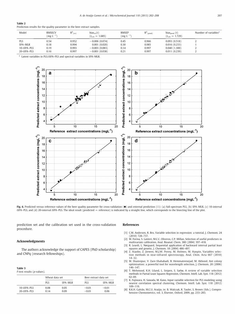
Fig. 6. Predicted versus reference values of the beer quality parameter for cross-validation (●) and external prediction (○): (a) full-spectrum PLS, (b) SPA–MLR, (c) 10-intervaliSPA–PLS, and (d) 20-interval iSPA–PLS. The ideal result (predicted = reference) is indicated by a straight line, which corresponds to the bisecting line of the plot.
Table 2Prediction results for the quality parameter in the beer extract samples.
Model RMSECV(mg L−1)
R2(cv) biascv(t)
(tcrit = 1.685)RMSEP(mg L−1)
R2(pred) biaspred (t)
(tcrit = 1.729)Number of variablesa
PLS 0.54 0.952 −0.006 (0.074) 0.45 0.966 0.093 (0.518) 2SPA–MLR 0.18 0.994 0.001 (0.020) 0.30 0.985 0.016 (0.233) 110-iSPA–PLS 0.19 0.993 −0.003 (0.083) 0.14 0.997 0.040 (1.300) 220-iSPA–PLS 0.16 0.997 −0.001 (0.038) 0.21 0.997 0.011 (0.239) 2
a Latent variables in PLS/iSPA–PLS and spectral variables in SPA–MLR.
207A. de Araújo Gomes et al. / Microchemical Journal 110 (2013) 202–208
prediction set and the calibration set used in the cross-validationprocedure.
Acknowledgments
The authors acknowledge the support of CAPES (PhD scholarship)and CNPq (research fellowships).
Table 3F-test results (p-values).
Wheat data set Beer extract data set
PLS SPA–MLR PLS SPA–MLR
10-iSPA–PLS 0.08 0.05 b0.01 b0.0120-iSPA–PLS 0.14 0.09 b0.01 0.06
References
[1] C.M. Andersen, R. Bro, Variable selection in regression: a tutorial, J. Chemom. 24(2010) 728–737.
[2] M. Forina, S. Lanteri, M.C.C. Oliveros, C.P. Millan, Selection of useful predictors inmultivariate calibration, Anal. Bioanal. Chem. 380 (2004) 397–418.
[3] R. Leardi, L. Nørgaard, Sequential application of backward interval partial leastsquares and genetic, J. Chemom. 18 (2004) 486–497.
[4] Z. Xiaobo, Z. Jiewen, M.J.W. Povey, M. Holmes, M. Hanpin, Variables selec-tion methods in near-infrared spectroscopy, Anal. Chim. Acta 667 (2010)14–32.
[5] M. Shamsipur, V. Zare-Shahabadi, B. Hemmateenejad, M. Akhond, Ant colonyoptimisation: a powerful tool for wavelength selection, J. Chemom. 20 (2006)146–147.
[6] T. Mehmood, K.H. Liland, L. Snipen, S. Sæbø, A review of variable selectionmethods in Partial Least Squares Regression, Chemom. Intell. Lab. Syst. 118 (2012)62–69.
[7] K. Fujiwara, H. Sawada, M. Kano, Input variable selection for PLS modeling usingnearest correlation spectral clustering, Chemom. Intell. Lab. Syst. 118 (2012)109–119.
[8] R.K.H. Galvão, M.C.U. Araújo, in: B. Walczak, R. Tauler, S. Brown (Eds.), Compre-hensive Chemometrics, vol. 3, Elsevier, Oxford, 2009, pp. 233–283.

208 A. de Araújo Gomes et al. / Microchemical Journal 110 (2013) 202–208
[9] H. Martens, M. Martens, Modified Jack-knife estimation of parameter uncertaintyin bilinear modelling by partial least squares regression (PLSR), Food Qual. Prefer.11 (2000) 5–16.
[10] R.M. Balabin, S.V. Smirnov, Variable selection in near-infrared spectroscopy:benchmarking of feature selection methods on biodiesel data, Anal. Chim. Acta692 (2011) 63–72.
[11] Y. Liao, Y. Fan, F. Cheng, On-line prediction of pH values in fresh pork usingvisible/near-infrared spectroscopy with wavelet de-noising and variable selec-tion methods, J. Food Eng. 109 (2012) 668–675.
[12] N. Goudarzi, M. Goodarzi, Application of successive projections algorithm (SPA)as a variable selection in a QSPR study to predict the octanol/water partition co-efficients (Kow) of some halogenated organic compounds, Anal. Methods 2(2010) 758–764.
[13] M.C.U. Araújo, T.C.B. Saldanha, R.K.H. Galvão, T. Yoneyama, H.C. Chame, V. Visani,The successive projections algorithm for variable selection in spectroscopicmulticomponent analysis, Chemom. Intell. Lab. Syst. 57 (2001) 65–73.
[14] R.K.H. Galvão, M.F. Pimentel, M.C.U. Araújo, T. Yoneyama, V. Visani, Aspects of thesuccessive projections algorithm for variable selection in multivariate calibrationapplied to plasma emission spectrometry, Anal. Chim. Acta 443 (2001) 107–115.
[15] S.F.C. Soares, A.A. Gomes, A.R. Galvão Filho, R.K.H. Galvão, M.C.U. Araújo, The suc-cessive projections algorithm, Trends Anal. Chem. 42 (2013) 84–98.
[16] F.A. Honorato, R.K.H. Galvão, M.F. Pimentel, B. Barros Neto, M.C.U. Araújo, F.R.Carvalho, Robust modeling for multivariate calibration transfer by the SuccessiveProjections Algorithm, Chemom. Intell. Lab. Syst. 76 (2005) 65–72.
[17] M.J.C. Pontes, R.K.H. Galvão, M.C.U. Araújo, P.N.T. Moreira, O.D. Pessoa Neto, G.E.José, T.C.B. Saldanha, The successive projections algorithm for spectral variableselection in classification problems, Chemom. Intell. Lab. Syst. 78 (2005) 11–18.
[18] E.D. Moreira, M.J.C. Pontes, R.K.H. Galvão, M.C.U. Araújo, Near infrared reflectancespectrometry classification of cigarettes using the successive projections algo-rithm for variable selection, Talanta 79 (2009) 1260–1264.
[19] M. Ghasemi-Varnamkhasti, S.S. Mohtasebi, M.L. Rodriguez-Mendez, A.A. Gomes,M.C.U. Araújo, R.K.H. Galvão, Screening analysis of beer ageing using near infraredspectroscopy and the Successive Projections Algorithm for variable selection,Talanta 89 (2012) 286–291.
[20] H.A. Dantas Filho, R.K.H. Galvão, M.C.U. Araújo, E.C. Silva, T.C.B. Saldanha, G.E.José, C. Pasquini, I.M. Raimundo Jr., J.J.R. Rohwedder, A strategy for selecting cal-ibration samples for multivariate modelling, Chemom. Intell. Lab. Syst. 72 (2004)83–91.
[21] M.S. Di Nezio, M.F. Pistonesi, W.D. Fragoso, M.J.C. Pontes, H.C. Goicoechea, M.C.U.Araujo, B.S.F. Band, Successive projections algorithm improving the multivariatesimultaneous direct spectrophotometric determination of five phenolic com-pounds in sea water, Microchem. J. 85 (2007) 194–200.
[22] M.C. Breitkreitz, I.M. Raimundo Jr., J.J.R. Rohwedder, C. Pasquini, H.A. Dantas Filho,G.E. José, M.C.U. Araújo, Determination of total sulfur in diesel fuel employing NIRspectroscopy and multivariate calibration, Analyst 128 (2003) 1204–1207.
[23] L.F.B. Lira, M.S. Albuquerque, J.G.A. Pacheco, T.M. Fonseca, E.H.S. Cavalcanti, L.Stragevitch, M.F. Pimentel, Infrared spectroscopy and multivariate calibration tomonitor stability quality parameters of biodiesel, Microchem. J. 96 (2010) 126–131.
[24] R.G. Brereton, Introduction to multivariate calibration in analytical Chemistry,Analyst 15 (2000) 2125–2154.
[25] R.J. Leardi, Application of genetic algorithm-PLS for feature selection in spectraldata sets, J. Chemom. 14 (2000) 643–655.
[26] J.A.F. Pierna, O. Abbas, V. Baeten, P. Dardenne, A Backward Variable Selectionmethod for PLS regression (BVSPLS), Anal. Chim. Acta 642 (2009) 89–93.
[27] M. Forina, C. Casolino, C.P.Millan, Iterativepredictorweighting (IPW) PLS: a techniquefor the elimination of useless predictors in regression problems, J. Chemom. 13 (1999)165–184.
[28] V. Centner, D.L. Massart, O.E. Noord, S. Jong, B.M. Vandeginste, C. Sterna, Eliminationof uninformative variables for multivariate calibration, Anal. Chem. 68 (1996)3851–3858.
[29] F. Allegrini, A.C. Olivieri, A new and efficient variable selection algorithm based onant colony optimization. Applications to near infrared spectroscopy/partialleast-squares analysis, Anal. Chim. Acta 699 (2011) 18–25.
[30] J.A. Hageman, M. Streppel, R. Wehrens, L.M.C. Buydens, Wavelength selectionwith Tabu Search, J. Chemom. 17 (2003) 427–437.
[31] Y.P. Du, Y.Z. Liang, J.H. Jiang, R.J. Berry, Y. Ozaki, Spectral regions selection to im-prove prediction ability of PLS models by changeable size moving window partialleast squares and searching combination moving window partial least squares,Anal. Chim. Acta 501 (2004) 183–191.
[32] A.L.H. Müller, E.M.M. Flores, E.I. Müller, F.E.B. Silva, M.F. Ferrão, Attenuated total re-flectancewith Fourier transform infrared spectroscopy (ATR/FTIR) and different PLSalgorithms for simultaneous determination of clavulanic acid and amoxicillin inpowder pharmaceutical formulation, J. Braz. Chem. Soc. 22 (2011) 1903–1912.
[33] R.F. Teófilo, J.P.A. Martins, M.M.C. Ferreira, Sorting variables by using informativevectors as a strategy for feature selection in multivariate regression, J. Chemom.23 (2009) 32–48.
[34] H.M. Paiva, S.F.C. Soares, R.K.H. Galvão, M.C.U. Araújo, A graphical user interfacefor variable selection employing the Successive Projections Algorithm, Chemom.Intell. Lab. Syst. 118 (2012) 260–266.
[35] R.K.H. Galvão, M.C.U. Araújo, W.D. Fragoso, E.C. Silva, G.E. José, S.F.C. Soares, H.M.Paiva, A variable elimination method to improve the parsimony of MLR modelsusing the successive projections algorithm, Chemom. Intell. Lab. Syst. 92 (2008)83–91.
[36] R.K.H. Galvão, M.C.U. Araújo, E.C. Silva, G.E. José, S.F.C. Soares, H.M. Paiva,Cross-validation for the selection of spectral variables using the successive pro-jections algorithm, J. Braz. Chem. Soc. 18 (2007) 1580–1584.
[37] F. Westad, H. Martens, Variable selection in near infrared spectroscopy based onsignificance testing in partial least squares regression, J. Near Infrared Spectrosc.8 (2000) 117–124.
[38] D.D.S. Fernandes, A.A. Gomes, G.B. Costa, G.W.B. Silva, G. Véras, Determination ofbiodiesel content in biodiesel/diesel blends using NIR and visible spectroscopywith variable selection, Talanta 87 (2011) 30–34.
[39] R.K.H. Galvão, M.C.U. Araújo, G.E. José, M.J.C. Pontes, E.C. Silva, T.C.B. Saldanha, Amethod for calibration and validation subset partitioning, Talanta 67 (2005)736–740.
[40] S.A. Tsuchikawa, A review of recent near infrared research for wood and paper,Appl. Spectrosc. Rev. 42 (2007) 42–71.
[41] Annual Book of ASTM Standards, Standards Practices for Infrared, Multivariate,Quantitative Analysis, E1655, vol. 03.06, ASTM International, West Conshohocken,Pennsylvania, USA, 2012.
[42] Ba. Li, D.Wang, C. Xu, Z. Zhang, Flow-injection simultaneous chemiluminescence de-termination of ascorbic acid and L-cysteine with partial least squares calibration,Microchim. Acta 149 (2005) 205–212.
[43] D.M. Haaland, E.V. Thomas, Partial least-squares methods for spectral analyses. 1.Relation to other quantitative calibration methods and the extraction of qualita-tive information, Anal. Chem. 60 (1988) 1193–1202.