the equivalence between successive approximations ... - mdpi
TRANSCRIPT
applied sciences
Article
The Equivalence between Successive Approximations andMatricial Load Flow Formulations
María Camila Herrera-Briñez 1,* , Oscar Danilo Montoya 2,3 and Lazaro Alvarado-Barrios 4
and Harold R. Chamorro 5
�����������������
Citation: Herrera-Briñez, M.C.;
Montoya, O.D.; Chamorro, H.R.;
Alvarado-Barrios, L. The Equivalence
between Successive Approximations
and Matricial Load Flow Formulations.
Appl. Sci. 2021, 11, 2905. https://
doi.org/10.3390/app11072905
Academic Editor: Pierluigi Siano
Received: 24 February 2021
Accepted: 22 March 2021
Published: 24 March 2021
Publisher’s Note: MDPI stays neutral
with regard to jurisdictional claims in
published maps and institutional affil-
iations.
Copyright: © 2021 by the authors.
Licensee MDPI, Basel, Switzerland.
This article is an open access article
distributed under the terms and
conditions of the Creative Commons
Attribution (CC BY) license (https://
creativecommons.org/licenses/by/
4.0/).
1 Estudiante de Ingeniería Eléctrica, Universidad Distrital Francisco José de Caldas, Bogotá 11021, Colombia2 Facultad de Ingeniería, Universidad Distrital Francisco José de Caldas, Bogotá 11021, Colombia;
[email protected] Laboratorio Inteligente de Energía, Universidad Tecnológica de Bolívar, Cartagena 131001, Colombia4 Department of Engineering, Universidad Loyola Andalucía, 41704 Sevilla, Spain; [email protected] Department of Electrical Engineering at KTH, Royal Institute of Technology, SE-44 100 Stockholm, Sweden;
[email protected]* Correspondence: [email protected]
Abstract: This paper shows the equivalence of the matricial form of the classical backward/forwardload flow formulation for distribution networks with the recently developed successive approxima-tions (SA) load flow approach. Both formulations allow solving the load flow problem in meshedand radial distribution grids even if these are operated with alternating current (AC) or direct current(DC) technologies. Both load flow methods are completely described in this research to make a faircomparison between them and demonstrate their equivalence. Numerical comparisons in the 33- and69-bus test feeder with radial topology show that both methods have the same number of iterationsto find the solution with a convergence error defined as 1× 10⁻¹⁰.
Keywords: successive approximations method; matricial backward/forward method; load flowanalysis; electrical distribution networks; equivalent formulations
1. Introduction
Load flow is one of the most recognized studies in electrical networks from high-to low-voltage levels [1,2]. This problem relates voltages, currents, and powers understeady state conditions, which produce a set of nonlinear non-convex equations that neednumerical methods to be resolved [3]. In the case of power systems, the Newton–Raphson(NR) and the Gauss–Seidel (GS) methods are the most classical approaches, the formerbeing the most used method in commercial applications such as DigSILENT [4] andETAP [5], as it converges speedily to the solution of the problem using the informationof the derivatives in the Jacobian matrix [6,7]. However, for the analyses of electricaldistribution networks in load flow studies, there are multiple approaches in the literaturethat take advantage of the grid structure to propose alternative formulations that can workdirectly in the complex domain, such as Gauss–Seidel derived methods. These methodsare classical backward/forward and its matricial equivalent [8,9], the triangular-basedload flow method [3], the hyperbolic and product-derived Taylor methods [10,11], thesuccessive approximations (SA) method [12], and linear approximations based on thelogarithmic transformation of the voltage variables [13], and the Laurent series expansionapproach [14], among others. Based on the multiple possibilities for efficiently solvingthe load flow problem in electrical networks, typically the preferred methods avoid theuse of derivatives in their formulation due to the sparsity nature of electrical distributiongrids [15]. The two most recommended methods are the recently developed SA [12] andthe matricial backward/forward (MBF) methods [8,9], as they can work with mesh andradial distribution grid topologies.
Appl. Sci. 2021, 11, 2905. https://doi.org/10.3390/app11072905 https://www.mdpi.com/journal/applsci
Appl. Sci. 2021, 11, 2905 2 of 10
From a simplistic point of view, these methods look different, as SA is a compactrepresentation of the Gauss–Seidel method using a matricial representation derived fromthe admittance matrix representation, while the MBF load flow method is derived usingthe topology of the network based on the incidence matrix [9], however, it is possibleto demonstrate that the recursive formulas derived for these methods are completelyequivalent, i.e., both methodologies are exactly equal. The aim of this study is to provethat these methods are exactly the same but derived from two different points of view.
One of the most important advantages of these load flow representations is that theconvergence of both approaches can be demonstrated using the Banach fixed-point theoremas was demonstrated in [8,9] for the the MBF method and in [12] for the SA approach. Tovalidate the proposed comparative study, we employ two classical distribution networkscomposed of 33 and 69 nodes with radial topologies in medium voltage levels [16] tocompare it with other literature approaches. The radial configuration is selected to thetests, as this configuration produces worsens operative conditions when compared withmeshed topologies.
The remaining sections of this brief are organized as follows: Section 2 describes thecomplete formulation of the SA load flow approach, while Section 3 presents the completederivation of the MBF load flow approach. Section 4 demonstrates via incidence matrixrepresentation that both methodologies are equal based on the definition of the nodaladmittance matrix. Section 5 presents the configuration of the test feeders employed tocompare the two methodologies. Section 6 shows the computational validations, includingcomparisons with other classical load flow methods applicable to distribution networks.Finally, Section 7 presents the main concluding remarks of this study.
2. SA Load Flow
The complex load flow formulation of electrical distribution grids is developed byapplying the conventional nodal voltage method to all buses of the system under steady-state operative conditions [11]. The main complication of the load flow problem is that it isnonlinear non-convex because of the hyperbolic relation between voltages and currents,which is due to the presence of constant power loads. The basis of the load flow problemformulation is presented below [12,17].
I = YV, (1)
S = diag(V)I? ⇔ S? = diag(V?)I, (2)
where V ∈ Cn and I ∈ Cn are column vectors with the nodal voltages and injected currents,respectively. Y ∈ Cn×n is the bus admittance matrix of the distribution grid; diag(V) beinga diagonal matrix that has invertible properties, such that diagii(·) = Vi, i = 1, 2, ..., nand diagij(·) = 0, i 6= j. In addition, S ∈ Cn is a column vector that has apparent powerinjections in all the buses of the grid, and n is the total nodes of the distribution system.
If Expressions (1) and (2) are combined, the classical load flow representation in thedomain of the complex number is found to be formulated as in (3):
S? = diag(V?)YV, (3)
Remark 1. Note that the main interest in the solution of the load flow formulation defined in (3)corresponds to the determination of the unknown voltage variables associated with all the demandnodes, as in the slack node, this variable is perfectly known.
Taking this into account, Expression (3) can be split as presented below.
S?g = diag
(V?
g
)[YggVg +YgdVd
], (4)
−S?d = diag(V?
d)[YdgVg +YddVd
], (5)
Appl. Sci. 2021, 11, 2905 3 of 10
where Sd ∈ Cn−s and Sg ∈ Cs represent the complex power consumed in all load busesand the apparent power generation of voltage controlled buses, respectively; Vg ∈ Cs
corresponds to the voltage outputs in the slack buses, while Vd ∈ Cn−s represents theunknowable voltages of all the load buses of the grid. Observe that diagg
(Vg)∈ Cs×s and
diagd(Vd) ∈ C(n−s)×(n−s) can be interpreted in the same form that diag(V). In addition,note that s defines the number of ideal voltage-controlled sources (e.g., slack nodes), whichentails that s ≥ 1. In addition,
Y =
[Ygg YgdYdg Ydd
],
where we know that Ydg = YTgd due to the properties of symmetry of the admittance matrix.
Remark 2. Note that in the load flow formulation given by (4) and (5), the expression associatedwith the slack nodes, i.e., Equation (4), is linear, as Vg is perfectly known in magnitude and angle,and the variables Vd and Sg have a linear relation. Nonetheless, the set of Equations in (5) remaina nonlinear set of expressions in the complex domain due to the presence of the product betweenvoltages in the demand nodes.
The solution of Equation (5) is known and can be reached with the SA load flowapproach, as demonstrated in [12], by rewriting it as follows:
Vd = −Y−1dd
[diag−1(V?
d)S?d +YdgVg
]. (6)
Note that if an iterative counter t is added to the contraction map defined by (6) bystarting it with t = 0 and the initial voltages Vd = 1∠0◦, i.e., plane voltages, then, thefollowing recursive formula can be found:
Vt+1d = −Y−1
dd
[diag−1
(Vt,?
d
)S?
d +YdgVg
]. (7)
The iterative procedure using the recursive formula (7) is made until the convergenceerror is reached, i.e., maxd
{∣∣∣∣∣∣Vt+1d
∣∣∣− ∣∣Vtd
∣∣∣∣∣} ≤ ε, where ε is known as the convergence
error, which is typically defined in the literature as 1× 10⁻¹⁰ [12].
Remark 3. The convergence of the recursive formula (7) can be demonstrated with the Banachfixed-point theorem, as presented in [9], due to this the formula defines a contraction map with theform Vd = f (Vd).
3. MBF Load Flow
The MBF load flow formulation is a compact generalization of the classical iterativesweep load flow, where the incidence matrix is employed. To obtain this compact load flowformulation, the incidence matrix is defined as follows [8,9]:
Definition 1 (Incidence matrix A). An electrical distribution network can be represented by aconnected graph composed of n vertices and b branches using a rectangular matrixA ∈ Rb×n calledthe incidence matrix. To construct this matrix, arbitrary directions associated with the current flowsare assumed in all the branches as follows:
• Ai,j = 1 when branch i connects bus j and its current is leaving bus i;• Ai,j = −1 when branch i connects bus j and its current is arriving bus j;• Ai,j = 0 when branch i has no connection with bus j.
For an electrical distribution network, the incidence matrix, can be split into twosubmatrices that contain information of the slack and demand nodes and their relations
Appl. Sci. 2021, 11, 2905 4 of 10
with all the branches as follows (for the sake of simplicity, we assume that the slack node islocated at bus 1):
A =[Ag Ad
], (8)
where Ag represents the first column of the matrix A (i.e., voltage-controlled source),and Ad is the remaining columns of the matrix A, i.e., columns associated with all theload buses.
Now, we define the voltage drop at branch i as Ei and the voltages on its sending andreceiving nodes Vj. Then, the following result is achieved:
E = AgVg +AdVd, (9)
where E is a vector that has all the voltage drops in all the links of the distribution network.In addition, to determine the relation between the branch’s currents and their volt-
age drops, the Omh’s law is applied to each one of them, which allows the finding ofthe following:
E = ZpJ, (10)
where Zp corresponds to the diagonal invertible matrix that holds in all the branch’impedances, i.e., Z = diag(Z1 Z2 , ..., Zb ).
Now, to define the mathematical relation between the nodal currents (i.e., I) and allthe lines’ currents, we apply the second Kirchhoff’s law on each bus, which produces, in acompact form, the following result, split for the slack and demand nodes:
Ig = ATg J, (11)
Id = ATd J. (12)
Observe that if Expressions (9), (10), and (12) are combined, considering that Yp = Z−1,then the result is as follows:
Id = ATdYpAgVg +AT
dYpAdVd. (13)
To determine the relationship between the nodal currents and the net powers, fromthe Tellegen’s theorem defined in (2), we can obtain the following:
Ig = diag−1(
V?g
)S?
g, (14)
Id = −diag−1(V?d)S
?d . (15)
Now, if Equations (1) and (15) are mixed to attain Vd, then, the next result yields:
Vd = −Zdd
[diag−1(V?
d)S?d +A
TdYpAgVg
], (16)
being Zdd defined as[AT
dYpAd]−1.
Remark 4. The solution of Equation (16) is found in the same form as described for Equation (7)by adding an iterative counter and starting with plane voltages. In this sense, the general MBFformula is defined below:
Vt+1d = −Zdd
[diag−1
(Vt,?
d
)S?
d +ATdYpAgVg
], (17)
where its convergence can also be proved with the Banach fixed-point theorem, as presented in [8].
Appl. Sci. 2021, 11, 2905 5 of 10
Note that the evaluation of the recursive formula (17) for the MBF load flow methodis made until the convergence criterion meets as explained for the SA method.
4. Demonstration of the Equivalence
To demonstrate that the SA and MBF methods with the recursive formulas (7) and (17)are equivalent (i.e., equal) formulations for the load flow problem, we present the generalstructure of the nodal admittance matrix using the incidence matrix. To make this com-parison, let us again take Expression (1) where the matricial relation between currents andvoltages are defined with the admittance matrix, i.e., Y. In addition, from Equation (10),we know the following:
J = YpE, (18)
where Yp is known as the primitive admittance matrix. Now, if we compact the relationbetween the voltage drops in branches with nodal voltages in Equation (9), we havethe following:
E =[Ag Ad
][VgVd
]. (19)
In addition, if we also compact Expressions (11) and (12), we achieve the following result:[IgId
]=
[AT
gAT
d
]J. (20)
Now, observe that Expressions (19) and (20) can be substituted in (18), which producesthe following result: [
IgId
]=
[AT
gAT
d
]Yp[Ag Ad
][VgVd
], (21)
where we know that the admittance matrix can be defined as follows:
Y =
[AT
gAT
d
]Yp[Ag Ad
]. (22)
Note that Expression (22) can be split as follows by formulating its matricial operations:
Y =
[AT
gYpAg ATgYpAd
ATdYpAg AT
dYpAd
]=
[Ygg YgdYdg Ydd
]. (23)
Remark 5. From the results of (23), it is possible to observe that Ydg = ATdYpAg and
Ydd = ATdYpAd, which confirms that when recursive load flow formulas (7) and (17) are com-
pared with Zdd = Y−1dd , these turn out to be the equal, i.e., the SA and the MBF load flows are
completely equivalent.
It is worth highlighting that the SA and MBF approaches are exactly equivalent in thecontext of DC distribution networks, as to transform the AC load flow problem into a DCone, it is necessary to take zero as the values of the reactive power consumption in all thenodes and the reactances of all the branches, which have previously been demonstratedin [18,19], respectively.
5. Test Systems and Comparative Methods
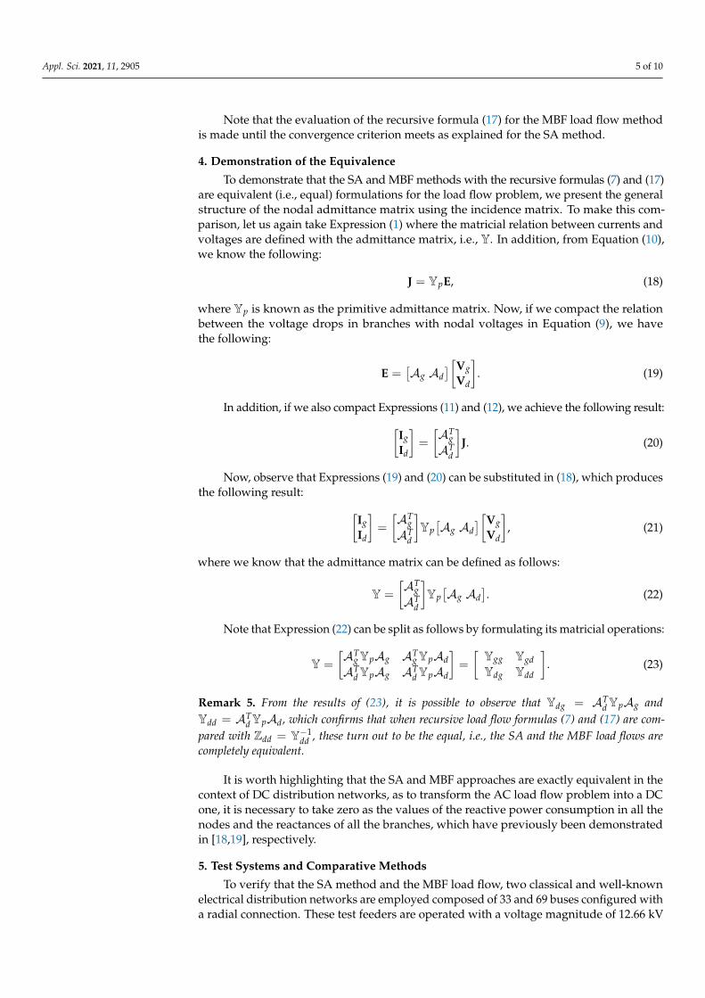
To verify that the SA method and the MBF load flow, two classical and well-knownelectrical distribution networks are employed composed of 33 and 69 buses configured witha radial connection. These test feeders are operated with a voltage magnitude of 12.66 kV
Appl. Sci. 2021, 11, 2905 6 of 10
at the slack source, which is positioned at bus 1 for both test feeders as depicted in Figure 1.Note that these systems were selected to evaluate the equivalence between the studiedpower flow approaches, as in the specialized literature, these systems are currently selectedto implement different optimization strategies for distribution systems, such as the optimallocation of distributed generators [16,20], optimal location of capacitor banks and staticdistribution compensators [21–23], and grid reconfiguration studies [24,25], among others.
slack
1 2
3 4 5
67 8 9 10 11 12 13 14 15 16 17 18
232425
19202122
26 27 28 29 30 31 32 33
(a)
slack
1 2 3 4 5 6 7 8 9 10 11 12 13 14 15 16 17 18 19 20 21 22 23 24 25 26 27
36 37 38 39 40 41 42 43 44 45 46
47 48 49 50 53 54 55 56 57 58 59 60 61 62 63 64 65
5152
6667
6869
28 29 30 31 32 33 34 35
(b)
Figure 1. Electrical configuration of the test feeders: (a) 33-node test system and (b) 69-nodetest system.
The complete information regarding these test systems can be found in [16].On the other hand, to verify that both methods are equivalent for load flow calculations
in AC networks, we implement different load flow methods available in the scientificliterature for distribution systems. These are the GS [6], the accelerate version of theGauss–Seidel (AG) [7], the NR [26], and the Levenberg–Marquardt (LM) methods [27].
6. Numerical Validation
The numerical validations are implemented using a personal computer with an IN-TEL(R) Core(TM) i7− 7700 processor at 3.60 GHz, 8 GB RAM, running a 64-bits Windows10 operative system. The simulation software used is MATLAB 2020b. In addition, theprocessing time presented in this research are the average values after 10,000 repetitionsfor the studied and comparative methods. Besides, to determine the effectiveness of eachof the studied and comparative methods, we evaluate the amount of active power losseson the distribution network (see Equation (24)). Note that we consider ε = 1× 10⁻¹⁰ as theconvergence error between two consecutive iterations of voltage variables:
ploss = real{|J|TZp|J|
}= real
{VTY?V?
}. (24)
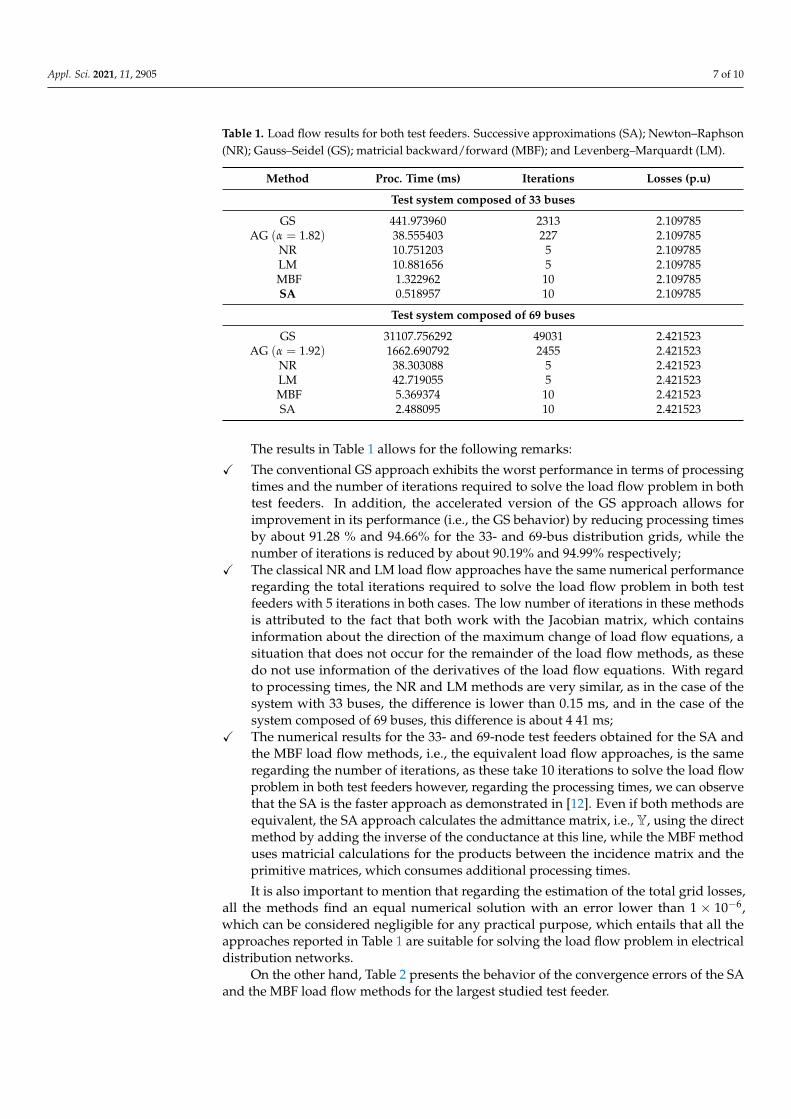
Table 1 reports the numerical results of the studied load flow methods, i.e., the SA andthe MBF load flow approaches as well as the results of the comparative methods.
Appl. Sci. 2021, 11, 2905 7 of 10
Table 1. Load flow results for both test feeders. Successive approximations (SA); Newton–Raphson(NR); Gauss–Seidel (GS); matricial backward/forward (MBF); and Levenberg–Marquardt (LM).
Method Proc. Time (ms) Iterations Losses (p.u)
Test system composed of 33 buses
GS 441.973960 2313 2.109785AG (α = 1.82) 38.555403 227 2.109785
NR 10.751203 5 2.109785LM 10.881656 5 2.109785MBF 1.322962 10 2.109785SA 0.518957 10 2.109785
Test system composed of 69 buses
GS 31107.756292 49031 2.421523AG (α = 1.92) 1662.690792 2455 2.421523
NR 38.303088 5 2.421523LM 42.719055 5 2.421523MBF 5.369374 10 2.421523SA 2.488095 10 2.421523
The results in Table 1 allows for the following remarks:
X The conventional GS approach exhibits the worst performance in terms of processingtimes and the number of iterations required to solve the load flow problem in bothtest feeders. In addition, the accelerated version of the GS approach allows forimprovement in its performance (i.e., the GS behavior) by reducing processing timesby about 91.28 % and 94.66% for the 33- and 69-bus distribution grids, while thenumber of iterations is reduced by about 90.19% and 94.99% respectively;
X The classical NR and LM load flow approaches have the same numerical performanceregarding the total iterations required to solve the load flow problem in both testfeeders with 5 iterations in both cases. The low number of iterations in these methodsis attributed to the fact that both work with the Jacobian matrix, which containsinformation about the direction of the maximum change of load flow equations, asituation that does not occur for the remainder of the load flow methods, as thesedo not use information of the derivatives of the load flow equations. With regardto processing times, the NR and LM methods are very similar, as in the case of thesystem with 33 buses, the difference is lower than 0.15 ms, and in the case of thesystem composed of 69 buses, this difference is about 4 41 ms;
X The numerical results for the 33- and 69-node test feeders obtained for the SA andthe MBF load flow methods, i.e., the equivalent load flow approaches, is the sameregarding the number of iterations, as these take 10 iterations to solve the load flowproblem in both test feeders however, regarding the processing times, we can observethat the SA is the faster approach as demonstrated in [12]. Even if both methods areequivalent, the SA approach calculates the admittance matrix, i.e., Y, using the directmethod by adding the inverse of the conductance at this line, while the MBF methoduses matricial calculations for the products between the incidence matrix and theprimitive matrices, which consumes additional processing times.
It is also important to mention that regarding the estimation of the total grid losses,all the methods find an equal numerical solution with an error lower than 1 × 10⁻⁶,which can be considered negligible for any practical purpose, which entails that all theapproaches reported in Table 1 are suitable for solving the load flow problem in electricaldistribution networks.
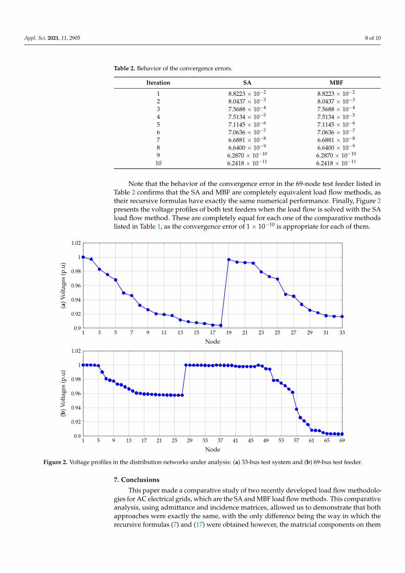
On the other hand, Table 2 presents the behavior of the convergence errors of the SAand the MBF load flow methods for the largest studied test feeder.
Appl. Sci. 2021, 11, 2905 8 of 10
Table 2. Behavior of the convergence errors.
Iteration SA MBF
1 8.8223 × 10⁻² 8.8223 × 10⁻²
2 8.0437 × 10⁻³ 8.0437 × 10⁻³
3 7.5688 × 10⁻⁴ 7.5688 × 10⁻⁴
4 7.5134 × 10⁻⁵ 7.5134 × 10⁻⁵
5 7.1145 × 10⁻⁶ 7.1145 × 10⁻⁶
6 7.0636 × 10⁻⁷ 7.0636 × 10⁻⁷
7 6.6881 × 10⁻⁸ 6.6881 × 10⁻⁸
8 6.6400 × 10⁻⁹ 6.6400 × 10⁻⁹
9 6.2870 × 10⁻¹⁰ 6.2870 × 10⁻¹⁰
10 6.2418 × 10⁻¹¹ 6.2418 × 10⁻¹¹
Note that the behavior of the convergence error in the 69-node test feeder listed inTable 2 confirms that the SA and MBF are completely equivalent load flow methods, astheir recursive formulas have exactly the same numerical performance. Finally, Figure 2presents the voltage profiles of both test feeders when the load flow is solved with the SAload flow method. These are completely equal for each one of the comparative methodslisted in Table 1, as the convergence error of 1× 10⁻¹⁰ is appropriate for each of them.
1 3 5 7 9 11 13 15 17 19 21 23 25 27 29 31 330.9
0.92
0.94
0.96
0.98
1
1.02
Node
(a)V
olta
ges
(p.u
)
1 5 9 13 17 21 25 29 33 37 41 45 49 53 57 61 65 690.9
0.92
0.94
0.96
0.98
1
1.02
Node
(b)V
olta
ges
(p.u
)
Figure 2. Voltage profiles in the distribution networks under analysis: (a) 33-bus test system and (b) 69-bus test feeder.
7. Conclusions
This paper made a comparative study of two recently developed load flow methodolo-gies for AC electrical grids, which are the SA and MBF load flow methods. This comparativeanalysis, using admittance and incidence matrices, allowed us to demonstrate that bothapproaches were exactly the same, with the only difference being the way in which therecursive formulas (7) and (17) were obtained however, the matricial components on them
Appl. Sci. 2021, 11, 2905 9 of 10
were equal. Numerical simulations using two radial test feeders composed of 33 and69 buses demonstrated that the number of iterations taken by the SA and MBF was thesame, as the convergence error was exactly equal, which also confirmed that both loadflow methodologies were completely equivalent. With regard to processing times, theSA approach had a small advantage, as the required number of calculations to obtain theadmittance matrix was lower in comparison to the MBF, which clearly affected the finalprocessing times of the second one.
Author Contributions: Conceptualization, methodology, software, and writing—review and editing,M.C.H.-B., O.D.M., H.R.C. and L.A.-B. All authors have read and agreed to the published version ofthe manuscript.
Funding: This work was supported in part by the Laboratorio de Simulación Hardware-in-the-looppara Sistemas Ciberfísicos under Grant TEC2016-80242-P (AEI/FEDER) and in part by the SpanishMinistry of Economy and Competitiveness under Grant DPI2016-75294-C2-2-R.
Institutional Review Board Statement: Not applicable.
Informed Consent Statement: Not applicable.
Data Availability Statement: No new data were created or analyzed in this study. Data sharing isnot applicable to this article.
Acknowledgments: This work has been derived from the undergraduate project: “Formulación ycomparación de cinco métodos para el análisis de flujo de potencia en sistemas de distribución ACen el software MATLAB®” presented by the student María Camila Herrera-Briñez to the ElectricalEngineering Program of the Engineering Faculty at Universidad Distrital Francisco José de Caldas asa partial requirement for the Bachelor in Electrical Engineering.
Conflicts of Interest: The authors declare no conflict of interest.
References1. Abdi, H.; Beigvand, S.D.; Scala, M.L. A review of optimal power flow studies applied to smart grids and microgrids. Renew.
Sustain. Energy Rev. 2017, 71, 742–766. [CrossRef]2. Lavaei, J.; Low, S.H. Zero Duality Gap in Optimal Power Flow Problem. IEEE Trans. Power Syst. 2012, 27, 92–107. [CrossRef]3. Marini, A.; Mortazavi, S.; Piegari, L.; Ghazizadeh, M.S. An efficient graph-based power flow algorithm for electrical distribution
systems with a comprehensive modeling of distributed generations. Electr. Power Syst. Res. 2019, 170, 229–243. [CrossRef]4. Phongtrakul, T.; Kongjeen, Y.; Bhumkittipich, K. Analysis of Power Load Flow for Power Distribution System based on
PyPSA Toolbox. In Proceedings of the 2018 15th International Conference on Electrical Engineering/Electronics, Computer,Telecommunications and Information Technology (ECTI-CON), Chiang Rai, Thailand, 18–21 July 2018. [CrossRef]
5. Prabhu, J.A.X.; Sharma, S.; Nataraj, M.; Tripathi, D.P. Design of electrical system based on load flow analysis using ETAP for IECprojects. In Proceedings of the 2016 IEEE 6th International Conference on Power Systems (ICPS), New Delhi, India, 4–6 March2016. [CrossRef]
6. Grainger, J.J.; Stevenson, W.D. Power System Analysis; McGraw-Hill series in electrical and computer engineering: Power andenergy; McGraw-Hill: New York, NY, USA, 2003.
7. Gönen, T. Modern Power System Analysis; CRC Press: Boca Raton, FL, USA, 2016.8. Montoya, O.D.; Gil-González, W.; Giral, D.A. On the Matricial Formulation of Iterative Sweep Power Flow for Radial and Meshed
Distribution Networks with Guarantee of Convergence. Appl. Sci. 2020, 10, 5802. [CrossRef]9. Shen, T.; Li, Y.; Xiang, J. A Graph-Based Power Flow Method for Balanced Distribution Systems. Energies 2018, 11, 511. [CrossRef]10. Garces, A. A Linear Three-Phase Load Flow for Power Distribution Systems. IEEE Trans. Power Syst. 2016, 31, 827–828. [CrossRef]11. Bocanegra, S.Y.; Gil-Gonzalez, W.; Montoya, O.D. A New Iterative Power Flow Method for AC Distribution Grids with Radial
and Mesh Topologies. In Proceedings of the 2020 IEEE International Autumn Meeting on Power, Electronics and Computing(ROPEC), Ixtapa, Mexico, 4–6 November 2020. [CrossRef]
12. Montoya, O.D.; Gil-González, W. On the numerical analysis based on successive approximations for power flow problems in ACdistribution systems. Electr. Power Syst. Res. 2020, 187, 106454. [CrossRef]
13. Li, Z.; Yu, J.; Wu, Q.H. Approximate Linear Power Flow Using Logarithmic Transform of Voltage Magnitudes With ReactivePower and Transmission Loss Consideration. IEEE Trans. Power Syst. 2018, 33, 4593–4603. [CrossRef]
14. Montoya, O.D. On Linear Analysis of the Power Flow Equations for DC and AC Grids With CPLs. IEEE Trans. Circuits Syst. IIExpress Briefs 2019, 66, 2032–2036. [CrossRef]
15. Molzahn, D.K.; Hiskens, I.A. Sparsity-Exploiting Moment-Based Relaxations of the Optimal Power Flow Problem. IEEE Trans.Power Syst. 2015, 30, 3168–3180. [CrossRef]
Appl. Sci. 2021, 11, 2905 10 of 10
16. Grisales-Noreña, L.; Montoya, D.G.; Ramos-Paja, C. Optimal Sizing and Location of Distributed Generators Based on PBIL andPSO Techniques. Energies 2018, 11, 1018. [CrossRef]
17. Simpson-Porco, J.W.; Dorfler, F.; Bullo, F. On Resistive Networks of Constant-Power Devices. IEEE Trans. Circuits Syst. II ExpressBriefs 2015, 62, 811–815. [CrossRef]
18. Montoya, O.D.; Garrido, V.M.; Gil-Gonzalez, W.; Grisales-Norena, L.F. Power Flow Analysis in DC Grids: Two AlternativeNumerical Methods. IEEE Trans. Circuits Syst. II Express Briefs 2019, 66, 1865–1869. [CrossRef]
19. Montoya, O.D. On the Existence of the Power Flow Solution in DC Grids With CPLs Through a Graph-Based Method. IEEETrans. Circuits Syst. II Express Briefs 2020, 67, 1434–1438. [CrossRef]
20. Kaur, S.; Kumbhar, G.; Sharma, J. A MINLP technique for optimal placement of multiple DG units in distribution systems. Int. J.Electr. Power Energy Syst. 2014, 63, 609–617. [CrossRef]
21. Gil-González, W.; Montoya, O.D.; Rajagopalan, A.; Grisales-Noreña, L.F.; Hernández, J.C. Optimal Selection and Location ofFixed-Step Capacitor Banks in Distribution Networks Using a Discrete Version of the Vortex Search Algorithm. Energies 2020,13, 4914. [CrossRef]
22. Riaño, F.E.; Cruz, J.F.; Montoya, O.D.; Chamorro, H.R.; Alvarado-Barrios, L. Reduction of Losses and Operating Costs inDistribution Networks Using a Genetic Algorithm and Mathematical Optimization. Electronics 2021, 10, 419. [CrossRef]
23. Montoya, O.D.; Gil-González, W.; Hernández, J.C. Efficient Operative Cost Reduction in Distribution Grids Considering theOptimal Placement and Sizing of D-STATCOMs Using a Discrete-Continuous VSA. Appl. Sci. 2021, 11, 2175. [CrossRef]
24. Taher, S.A.; Karimi, M.H. Optimal reconfiguration and DG allocation in balanced and unbalanced distribution systems. AinShams Eng. J. 2014, 5, 735–749. [CrossRef]
25. Priyadarshini, R.; Prakash, R.; C.B, S. Network Reconfiguration of radial distribution network using Cuckoo Search Algorithm.In Proceedings of the 2015 Annual IEEE India Conference (INDICON), New Delhi, India, 17–20 December 2015. [CrossRef]
26. Lagace, P.J.; Vuong, M.H.; Kamwa, I. Improving power flow convergence by Newton Raphson with a Levenberg-Marquardtmethod. In Proceedings of the 2008 IEEE Power and Energy Society General Meeting—Conversion and Delivery of ElectricalEnergy in the 21st Century, Pittsburgh, PA, USA, 20–24 July 2008, pp. 1–6.
27. Milano, F. Analogy and Convergence of Levenberg’s and Lyapunov-Based Methods for Power Flow Analysis. IEEE Trans. PowerSyst. 2016, 31, 1663–1664.. [CrossRef]