adaptive martingale approximations

Adaptive MartingaleApproximations

Pedro J. Catuogno, Sebastian E. Ferrando, andAlfredo L. Gonzalez

ABSTRACT. H-systems are those orthonormal systems which allow com-putation of conditionals expectations via a Fourier expansion. These systemsprovide natural approximations to continuous stochastic processes and we indi-cate how they could be used to perform lossy compression on a set of given sig-nals. More specifically, we show how to construct, for a given random variable,an adaptive martingale approximation by means of generalized Haar functions.We also indicate how the construction can be extended to a given random vec-tor. A generalized multiresolution analysis algorithm is also described andnumerical examples are provided.

1. Introduction

Consider a probability space (Ω,A, P ) and the associated Hilbert spaceL2(Ω,A, P ). An orthonormal system of functions ukk≥0 defined on Ωis called an H-system if and only if for any X ∈ L2(Ω,A, P )

XAn ≡ E(X|u0, u1, . . . , un) =n∑

k=0

〈X, uk〉uk, for all n ≥ 0, (1.1)

formal details are provided in Definition 2.1.This paper studies this class of orthonormal systems and their potentialto perform lossy compression. From a theoretical point of view they areinteresting as the sequence of approximations is a martingale; moreover,for a given collection of random variables X = X1, . . . , Xd, we show howto construct the system uk adaptively to obtain efficient approximations.

Math Subject Classifications. 41A46, 60G42, 42C40.Keywords and Phrases. Conditional expectations, H-systems, martingales, pointwiseconvergence.The research of P. J. Catuogno is supported in part by a FAPESP grant. Theresearch of S.E. Ferrando is supported in part by an NSERC grant.

c© 2004 Birkhauser Boston. All rights reservedISSN 1069-5869

2 Pedro J. Catuogno, Sebastian E. Ferrando, and Alfredo L. Gonzalez

Notice that the word adapted is used with two meanings. Firstly, the systemuk will be constructed, in an optimal way, using the set X (and henceadapted to X ) and, secondly, the functions uk are simple functions which areadapted (according to measure theory) to the sigma algebras σ(u0, . . . , un)which form a natural filtration in the sense that the filtration generatesσ(X ).

The main contribution of the paper is in the construction, via thegreedy splitting algorithm, of H-systems adapted to a collection of randomvariables and in showing the usefulness of these approximations in a concretesetting. The main step in our construction is explained next and at the sametime we take the opportunity to introduce some simple notions from non-linear approximation theory. Consider the dictionary of (generalized) Haarfunctions (see Definition 2),

D ≡ ψ = a 1A + b 1B, a, b ∈ R, A ∩B = ∅, A, B ∈ A

we also require that each ψ ∈ D satisfies∫

Ωψ(ω) dP (ω) = 0,

∫

Ωψ2(ω) dP (ω) = 1.

Under appropriate conditions on a random variable X we show how to con-struct ψ0 = a 1A1,0 + b 1A1,1 ∈ D such that

〈X,ψ0〉 = supψ∈D

〈X, ψ〉. (1.2)

The above result represents the main step to set up a greedy algorithm (see[17]), also called a pursuit algorithm (see [14]), on an overcomplete dictionarylike D. Equation (1.2) can be iterated by replacing X above by the residualRX ≡ X−〈X,ψ0〉ψ0. More generally, we set Rn+1X ≡ RnX−〈RnX, ψn〉ψn

where ψn is the Haar function chosen at iteration n and, of course, R0X ≡ X.If the resulting approximation is to be used to perform a (lossy) com-

pression of the information contained in X, a main problem to address is thecost to encode the approximation. The cost of this encoding can be substan-tially reduced by performing a restricted nonlinear approximation ([4], [3])which in our case will imply to impose a tree structure on the supports of theHaar functions ψn. For example, in the first iteration, this restriction entailsto apply (1.2) to (1A1,iRX), i = 1, 2, alternately. Even when restricting theapproximation to have a tree structure, the cost of storing a single H-systemfor each given input X could be too high for a compression application. Weapproach this problem by extending the main step, given by (1.2), to a vec-tor setting. More precisely, we will deal with vector valued Haar functionsψ = a 1A + b 1B where now a, b ∈ Rd and X = (X1, . . . , Xd) ∈ L2(Ω,A,Rd).We will then show how to find ψ0 so that it maximizes the inner product [, ]

Adaptive Martingale Approximations 3

in L2(Ω,A,Rd), namely:

[X,ψ0] ≡∫

Ω〈X(w), ψ0〉 dP (w) = sup

ψ∈D[X, ψ], (1.3)

where, in this instance, we have used D to denote the dictionary of vectorvalued Haar functions.

Let us comment, using an intuitive explanation, on why we expect ourapproximations to be of very good quality. In the case when we restrict ourconstruction to a single random variable, X = X, our algorithm finds anefficient approximation using natural events, namely events A ∈ A whichare generators of σ(X). The construction behaves anologously in the vectorcase where X = X1, . . . , Xd. Our approach is natural in the sense thatwe expect, a priori, to obtain good quality approximations if there is aneffective way to approximate the joint σ-algebra of the random variablesX1, . . . , Xd. Intuitively, this should be possible if the random variables Xi

share some commonality at the level of the σ-algebras σ(Xi).Our approach could be compared with the one from [8] where uncon-

ditional basis are constructed for a given sequence of partitions. In contrastto their work, we provide effective ways for constructing the sequence ofpartitions. Some of the material in [6] can also be related to our mainconstruction. In that paper, some upper bounds for nonlinear approxima-tion errors are proven for dictionaries of functions (actually vectors in theirsetting) that take only three values, this is analogous to our dictionary D.Moreover, a close inspection of the construction used in [6], the one usedto prove their l2 theorem, reveals a close connection to our main construc-tion. Two main differences, between our approach and the one in [6], is thatwe emphasize martingale approximations which are tree-structured as op-posed to a direct application of the greedy algorithm, moreover, we providevector approximations. Finally, we remark that our results, in the vectorsetting, are independent of analogous vector versions of greedy algorithmsas analized in [13] and [11].

The remaining of the paper is organized as follows, Section 2 introducesformally the notion of H-systems and establishes some basic properties. Sec-tion 3 illustrates how H-systems can be used to approximate continuousstochastic processes. Section 4 provides some formulae and indicates, as-suming an H-system is given, how to organize the needed computations viathe multiresolution analysis algorithm in our setting. Section 5 is the mainsection of the paper, it provides the details and properties of optimized con-structions of H-systems adapted to a given random variable. Section 6 showshow to generalize the construction from a single random variable to a vectorof random variables. Section 7 provides some numerical output from a soft-ware implementation. Section 8 draws some conclusions and indicates futurework. Finally, Appendix A presents the multiresolution analysis algorithm


2. H-Systems

Let (Ω,A, P ) denote an arbitrary probability space. The notation || ||2 =〈, 〉 stands for the inner product on L2(Ω,A, P ). The following definition,taken from Gundy’s [9], is motivated by the classical Haar system definedon L2([0, 1]).

Definition 1. An orthonormal system of functions ukk≥0 defined on Ωis called an H-system if and only if for any X ∈ L2(Ω,A, P )

XAn ≡ E(X|u0, u1, . . . , un) =n∑

k=0

〈X, uk〉uk, for all n ≥ 0, (2.1)

where An = σ(u0, . . . , un). The intended meaning of k ≥ 0 in the abovedefinition is to allow the system ukk≥0 to be finite or infinite. We alsouse the notation A∞ = σ(∪n≥0An). In applications we will make use of thepointwise convergence of (2.1) which holds due to the martingale conver-gence theorem [15]. Moreover, if p ∈ [1,∞) is a given real number then, forevery X ∈ Lp, the sequence XAn = E(X|An) converges a.e. and in Lp toX∞ = E(X|A∞).The following proposition, which is proven in [9], gives an alternative char-acterization of H-systems equivalent to Definition 1.

Proposition 1. An orthonormal system ukk≥0 defined on Ω is an H-system if and only if the following three conditions hold:

1. Each uk assumes at most two nonzero values with positive probability.2. The σ-algebra An consists exactly of n + 1 atoms.3. E(uk+1|u0, u1, . . . , uk) = 0; k ≥ 0. So the functions uk are martin-

gale differences.

Corollary 1. Assume ukk≥0 is an H-system. Then, u0 = 1Ω and foreach n ≥ 0, un+1 takes two nonzero values (one positive and the other neg-ative) only on one atom of An (hence this atom becomes its support). Con-sequently, An+1 consists of n atoms from An and two more atoms obtainedby splitting the remaining atom from An.

In view of the above proposition and its corollary, the functions in an H-system are natural generalizations of classic Haar functions, as the nextdefinition states.

Definition 2. Given A ∈ A, P (A) > 0, a function ψ is called a (general-ized) Haar function on A if there exist Ai ∈ A, A0 ∩ A1 = ∅, A = A0 ∪ A1,ψ = a 1A0 + b 1A1 and

∫

Ωψ(ω) dP (ω) = 0,

∫

Ωψ2(ω) dP (ω) = 1.


2.1 Basic Properties of H-Systems

This section introduces some elementary properties of H-systems and par-titions. It should be clear, from Corollary 1, that an H-system naturallydefines a binary tree of partitions, these are formally introduced in the nextdefinition.

Definition 3. A sequence of partitions of Ω, Q := Qjj≥0, is called abinary sequence of partitions if for j ≥ 0, the members of Qj have positiveprobability, Q0 = Ω, and for j ≥ 1, A ∈ Qj if and only if it is also amember of Qj−1 or there exists another member A′ of Qj such that A∪A′ ∈Qj−1.We set A0,0 := Ω, hence Q0 = A0,0. For j ≥ 1, if A ∈ Qj and A = Ak,i ∈Qj−1 then A preserves its index. Otherwise (i.e. A /∈ Qj−1, and not yetindexed) then there exists Ak,i ∈ Qj−1 and A′ ∈ Qj such that

Ak,i = A ∪A′, (2.2)

then set Ak+1,2i := A and Ak+1,2i+1 := A′.

The index j in Aj,i will be called the scale parameter (we will also call it thelevel), it indicates the number of times A0,0 has been split to obtain Aj,i.Notice that Qj can have at most 2j members, and if Ak,i ∈ Qj then k ≤ jand 0 ≤ i ≤ 2k − 1. The name scale is borrowed from wavelet theory whereit indicates the extent of the localization (or resolution) of the wavelet.The information about the splitting of atoms is stored in the indexation,it allows to rearrange a given binary sequence of partitions so as to collectall atoms with the same scale parameter j. Atoms at lower levels, whichcomplete a partition and will not be further split, are also included. Thiswill be formalized in the next definition.

Definition 4. A binary sequence of partitions R = Rj will be calleda mutiresolution sequence (of partitions) if each Ak,i belonging to Rj , withj > k, also belongs to Rj′ for all j′ ≥ j.

Observe that if R is a multiresolution sequence of partitions and Ak,i ∈ Rj

with k < j, Ak,i has not been split since level k and will not be further split,while if k = j, Aj,i comes from the splitting of an atom of Rj−1. To thistype of partitions we will associate a Multiresolution Analysis Algorithm(MRA) in complete analogy with wavelet theory and, in particular, allowsthe computation of inner products and the corresponding approximationsto be organized by the scale parameter.The following sets of indexes will be used throughout the paper, consider


j ≥ 0 and let

Ij ≡ i : Aj,i ∈ Rj and Aj,i = Aj+1,2i ∪Aj+1,2i+1, and

Kj ≡ (k, i) : Ak,i ∈ Rj .(2.3)

Theorem 1. Every H-system induces naturally a multiresolution sequenceof partitions and reciprocally.

Proof. Let ukk≥0 be an H-system and A0,0 = Ω. We define recursivelythe following sequence of partitions.

R0 = A0,0.

Assuming Rj has been defined, we will generate Rj+1. Consider a genericatom Ak,i ∈ Rj , by Corollary 1 it is enough to consider the following cases:• If k < j we add Ak,i to Rj+1.• If k = j and Aj,i is not the support of any ur, we add Aj,i to Rj+1.• If k = j and Aj,i = supp ur for some ur. Then we add

Aj+1,2i = u−1r ((−∞, 0)) and Aj+1,2i+1 = u−1

r ((0,∞))

to Rj+1.

Clearly this is a multiresolution sequence of partitions.Reciprocally, letR be a multiresolution sequence of partitions, we will definea family of Haar functions ψj,i, associated with R. For each Aj,i ∈ Rj

such that Aj,i = Aj+1,2i ∪Aj+1,2i+1, let ψj,i be defined on Ω by

ψj,i(ω) =

aj,i if ω ∈ Aj+1,2i,bj,i if ω ∈ Aj+1,2i+1 and,0 if ω /∈ Aj,i.

(2.4)

Where aj,i and bj,i are chosen requiring that ψj,i is a Haar function. Theabove equations define (up to a sign) ψj,i(ω) for all ω ∈ Ω, indeed we choose

aj,i =

√P (Aj+1,2i+1)

P (Aj+1,2i)P (Aj,i)(2.5)

and

bj,i = −√

P (Aj+1,2i)P (Aj+1,2i+1)P (Aj,i)

. (2.6)

Give the natural order to the set N = 2j + i : j ≥ 0, i ∈ Ij and let π bean order preserving isomorphism from N to an integer interval [1, N ] or N.Defining

vπ(2j+i) = u2j+i ≡ ψj,i


and v0 ≡ φ0,0(ω) ≡ 1Ω(ω), the resulting sequence vll≥0 is orthonormal andtrivially verifies (1), (2) and (3) of Proposition 1, thus, it is an H-system.

Remark 1. If R is a multiresolution sequence induced by an H-systemvkk≥0, then the H-system built in Theorem 1 is a rearrangement vπkk≥0

of vkk≥0.

3. Approximation of Stochastic Processes

Let (Ω,A, P ) be a complete probability space and S = (St : 0 ≤ t ≤ T )be a continuous stochastic process defined on this probability space. LetF = Ft : 0 ≤ t ≤ T be the filtration where Ft is the completion ofσ(Sr : 0 ≤ r ≤ t). In Theorem 2 we will associate, in a natural way, asequence of H-systems with a continuous time skeleton approximation ofthe stochastic process S.Following W. Willinger [18], we introduce the notion of skeleton-approachfor stochastic processes.

Definition 5. A continuous-time skeleton approach of S is a triple (Iξ,Fξ, ξ),consisting of a index-set Iξ, a filtration Fξ = Fξ

t : 0 ≤ t ≤ T, the skeletonfiltration, and a Fξ-adapted process ξ = (ξ : 0 ≤ t ≤ T ) such that:

1. Iξ = 0 = t(ξ, 0) < ... < t(ξ,Nξ) = T, where Nξ < ∞.

2. For each t, Fξt is a finitely generated sub σ-algebra of Ft, with atoms

Pξt .

3. For t ∈ [0, T ] − Iξ, we set Fξt = Fξ

t(ξ,k) if t ∈ [t(ξ, k), t(ξ, k + 1))forsome 0 ≤ k < Nξ.

4. For each 0 ≤ t ≤ T , ξt = E(St | Fξt ).

Definition 6. A sequence (I(n),F (n), ξ(n)) of continuous time skeletonsof S will be called a continuous-time skeleton approximation of S if thefollowing three properties hold.

1. The sequence I(n) of index satisfies

limn→∞ |(I

(n)| = 0

where |(I(n)| ≡ max|t(ξ(n), k)− t(ξ(n), k − 1)| : 1 ≤ k ≤ N (n), andI ≡ ∪nI(n) is a dense subset of [0, T ].

2. For each 0 ≤ t ≤ T , F (n)t ↑ Ft.

3. P (ω ∈ Ω : limn→∞ sup0≤t≤T |St(ω)− ξ(n)t (ω)| = 0) = 1.

The fundamental result of W. Willinger ([18] pp. 52, Lemma 4.3.1) is statednext, it guarantees the existence of continuous-time skeleton approximations


for continuous processes. These discrete pathwise approximations are finitein space and time.

Lemma 1. There exist a continuous-time skeleton approximation for S.

Each continuous time skeleton (I(ξ),Fξ, ξ) of S determines a sequence ofnested finite partitions Pξ

tm. Clearly, there exists a multiresolution se-quence of partitions Rξ

jj≥0 such that Rjm = Pξtm for 0 = j0 < j1 < ... <

jN . Now, we can construct a finite family of H-systems associated to thecontinuous time skeleton (I(ξ),Fξ, ξ) of S applying Theorem 1 to the mul-tiresolution sequences of partitions Rjj≥0. Obviously, these H-systemsare adapted to the filtration Fξ

tm , that is ψj,i ∈ Fξtm for j ≤ jm.

Theorem 2. Let (Ω,A, P ) be a complete probability space and S = (St :0 ≤ t ≤ T ) be a continuous stochastic process defined on this probabilityspace. Let F = Ft : 0 ≤ t ≤ T be the filtration where Ft is the completionof σ(Sr : 0 ≤ r ≤ t). Then there exist a sequence of finite H-systems (H(n) =ψn

j,i) and two sequences of finite index (I(n) = 0 = tn0 < ... < tnNn= T)

and (J (n) = 0 = jn0 < ... < jn

Mn) such that

1. ψnj,i ∈ Ftnm for j ≤ jn

m.2. For each 0 ≤ t ≤ T ,

limn→∞ sup|St − ξ

(n)t | : 0 ≤ t ≤ T = 0 a.e.

where ξ(n)t =

∑j≤jn

m〈St, ψ

nj,i〉 ψn

j,i for t ∈ [tnm, tnm+1).

Proof. Let (I(n),F (n), ξ(n)) be a continuous-time skeleton approximationof S. We construct for each n an H-system (H(n) = ψn

j,i) associated

to the sequence of partitions R(n)j j≥0, as we explain above. In order to

conclude the proof it is sufficient to observe that ξ(n)t = E(St | F (n)

t ) =∑j≤jn

m〈St, ψ

nj,i〉 ψn

j,i for t ∈ [tnm, tnm+1).

It is possible to construct interesting examples of H-systems in a financialcontext, we refer the reader to [2].

4. Multiresolution Analysis

We begin introducing the notation and algebraic relationships needed to setup computations with the multiresolution algorithm.Let R := Rjj≥0 be a sequence of multiresolution partitions of Ω. We willnow introduce the natural orthonormal basis of characteristic functions at


level j. For each Ak,i ∈ Rj , let

φk,i ≡1Ak,i√P (Ak,i)

.

Given a random variable X, our next aim is to study the relationship be-tween the coefficients in this basis, which are proportional to samples atlevel j, with the coefficients in the H-system φ0,0, ψj,i associated with Rin Theorem 1.Recalling the notation from (2.3), for each j ≥ 0, φk,i(k,i)∈Kj

there isan orthonormal basis of the subspace Vj of piecewise constant functions onthe atoms of Rj . The φk,i correspond, in our setting, to the scaled andtranslated scale functions from wavelet theory and the ψj,i correspond tothe wavelets. We have the relations:

φj,i =

√pj+1[2i]

pj [i]φj+1,2i +

√pj+1[2i + 1]

pj [i]φj+1,2i+1 (4.1)

and

ψj,i = aj,i1Aj+1,2i + bj,i1Aj+1,2i+1

= aj,i

√pj+1[2i]φj+1,2i + bj,i

√pj+1[2i + 1]φj+1,2i+1

(4.2)

where aj,i and bj,i were calculated in (2.5) and (2.6) respectively, and wehave used the array notation

pj [i] ≡ P (Aj,i). (4.3)

Observe that since√

pj+1[2i + 1]pj [i]

aj,i

√pj+1[2i]−

√pj+1[2i]

pj [i]bj,i

√pj+1[2i + 1] = 1 6= 0,

ψj,i, φj,i and φj+1,2i, φj+1,2i+1 span the same 2-dimensional subspace.Thus φ0,0 ∪ ψk,i0≤k≤j−1,i∈Ik

is a basis of L2(Ω, σ(Rj), P ) = Vj , andmoreover it is also orthonormal as is the basis φk,i(k,i)∈Kj

.For a given X ∈ L2(Ω) and fixed j ≥ 0, we will write Xj ≡ XRj ≡E(X|σ(Rj)) for notational simplicity. Then we have the following expan-sions

Xj(ω) = c0[0] φ0,0(ω) +j−1∑

k=0

∑

i∈Ik

dk[i] ψk,i(ω) =∑

(k,i)∈Kj

ck[i] φk,i(ω) (4.4)

where ck[i] = 〈Xj , φk,i〉 and dk[i] = 〈Xj , ψk,i〉.


Given that the conditional expectation Xj of X is constant on eachAk,i, we have that

ck[i] = 〈Xj , φk,i〉 =1√pk[i]

∫

Ak,i

XjdP =1√pk[i]

∫

Ak,i

XdP = 〈X,φk,i〉.(4.5)

Analogously, we have that dk[i] = 〈X,ψk,i〉. Moreover we can state thefollowing proposition.

Proposition 2. Given X ∈ L2(Ω,A, P ) and a sequence of multiresolutionpartitions R = RjJ

j=0. Then for each j′ < j ≤ J , the following holds

Xj = Xj′ +j−1∑

k=j′

∑

i∈Ik

dk[i]ψk,i (4.6)

and∑

(k,i)∈Kj

c2k[i] =

∑

(k,i)∈Kj′

c2k[i] +

j−1∑

k=j′

∑

i∈Ik

d2k[i]. (4.7)

Proof. For each j < J we have that Vj = span φk,i : (k, i) ∈ Kj, letWj ≡ span ψj,i : i ∈ Ij. It is clear that Xj ∈ Vj and Vj−1 ⊂ Vj .By definition ψj−1,i ∈ Vj∩V ⊥

j−1, also as we have noted before, ψj−1,i, φj−1,iand φj,2i, φj,2i+1 span the same subspace, thus Vj = Vj−1⊕Wj−1. This isone reason we have used the classical wavelet notation.Since E(X|σ(Rj)) and E(X|σ(Rj−1)) are the orthogonal projections of Xonto Vj and Vj−1 respectively, we see that E(X|σ(Rj)) − E(X|σ(Rj−1)) isthe orthogonal projection of X onto Wj−1 and then we have the expansion

Xj = Xj−1 +∑

i∈Ij−1

dj−1[i]ψj−1,i,

from which (4.6) follows inductively. Equation (4.7) is a direct consequenceof (4.4) and (4.6).

The precedent proposition, with the aid of (4.1) and (4.2), also gives arelation between the coefficients cj [i] and dj [i], which permit us to have ex-pansions on all coarser “levels j”, starting from the one corresponding toφk,i(k,i)∈KJ

on a finer level J . These are the fundamentals of the mul-tiresolution algorithm for H-systems, it is an adaptation of the well knownalgorithm for wavelet theory, introduced by S. Mallat [10], to our setting.This algorithm produces a relation between the samples of X, namely,

xk[i] = Xj(ω), ω ∈ Ak,i, for (k, i) ∈ Kj , (4.8)

and the coefficients dk[i]. This algorithm is described in Appendix A.


5. Construction: The Greedy Splitting Algorithm

As outlined in the Introduction, a main goal is to use H-systems to obtainefficient approximations. Namely, for a given error level we seek to minimizethe number of Haar functions needed to achieve such an error. In this sectionwe present a procedure to construct a “good” H-system in the above sense.This procedure will be called Greedy Splitting Algorithm (GSA).In this section we consider a single random variable X and will define theH-system implicitly by describing a binary sequence (of partitions) Q =Qjj≥0. Start by setting Q0 = A0,0 = Ω and assume, inductively, thatQk, k ≤ j, has been constructed. We need some intermediate definitions inorder to define Qj+1. For a given measurable set A define

CA = ψ : such that ψ is a Haar function on A, (see Definition 2).(5.1)

Under appropriate conditions on a given random variable X, we will showthat there exists ψm

A = a1Am0

+ b1Am1∈ CA (we will say that Am

0 and Am1 are

the best split of A, for the given X) satisfying

|〈X, ψmA 〉| = supψ∈CA

|〈X − 1P (A)

∫

AX, ψ〉| = supψ∈CA

|〈X, ψ〉|. (5.2)

Select now A ∈ Qj which satisfies

|〈X, ψmA〉| ≥ |〈X,ψm

A 〉| for all A ∈ Qj . (5.3)

According to the indexing of partitions previously introduced in the paper(Definition 3), A = Ak,i for some index (k, i), k ≤ j, now define Ak+1,2i =Am

0 and Ak+1,2i+1 = Am1 . Finally, set Qj+1 = Qj\A∪Aj+1,2i, Aj+1,2i+1.

Therefore, we have |Qj+1| = |Qj |+ 1 (where |S| denotes cardinality of a setS) unless E(X|Qj) = X in which case the algorithm terminates.

First we mention some notation to be used in the remaining of thissection, let AA ≡ B ∩ A : B ∈ A; XA ≡ X|A (the restriction of X toA) and PA ≡ 1

P (A)P . It is clear that XA ∈ L2(A,AA, PA) and FXA(t) =

PA(XA ≤ t) = 1P (A)P (X ≤ t ∩ A), where FX denotes the cumulative

distribution function of X. F−1X denotes the right continuous inverse of FX .

The norm ||Y ||2A = 〈Y, Y 〉A denotes the inner product in L2(A,AA, PA).Expectation on (A,AA, PA) will be denoted with EA. In order to evaluatethe supremum in (5.2) we observe that any ψ ∈ CA can be written, in theform

ψ = a 1A0 + b 1A1 (5.4)

for some A0 ⊂ A with PA(A0) = u ∈ (0, 1), and A1 = A\A0. With thisnotation

〈X,ψ〉 = (a−b)〈X, 1A0〉+b〈X, 1A〉 = b P (A)(EA(XA)− 1

u〈XA, 1A0〉A

).

(5.5)


Noticing that b = ±√

uP (A) (1−u) , in order to calculate the supremum in (5.2)

we define

λA(u) ≡ supA0∈AA: PA(A0)=u

√P (A) u

(1− u)

(EA(XA)− 1

u〈XA,1A0〉A

). (5.6)

It is clear that if ψ ∈ CA then ψ ∈ CA,u ≡ ψ ∈ CA : P (A0) = u for someu ∈ (0, 1). Therefore for a given random variable X,

supψ∈CA

|〈X,ψ〉| = supu∈(0,1)

supψ∈CA,u

|〈X, ψ〉| = supu∈(0,1)

|λA(u)|. (5.7)

Under appropriate conditions we will prove

supψ∈CA

|〈X, ψ〉| = λA(u?) = 〈X, ψu?〉,

for some u? ∈ (0, 1) and ψu? ∈ CA,u? . We will need a series of intermediateresults, in particular, we borrow the following Bathtub Principle from [12].

Theorem 3. For a given number G > 0 and f(x), a real valued measurablefunction, defined on Ω, set:

D = g : 0 ≤ g(x) ≤ 1 for all x and∫

Ωg(x) dP (x) = G. (5.8)

Then the minimization problem

I = infg∈D

∫

Ωf(x) g(x) dP (x),

is solved byg(x) = χf<s(x) + c χf=s(x),

andI =

∫

f<sf(x) dP (x) + c s P (f = s).

Wheres = supt : P (f < t) ≤ G,c P (f = s) = G− P (f < s).

Lemma 2. Assume X ∈ L2(Ω,A, P ) and A ∈ A. Then the fuction λA, in(5.6), is well defined for all u ∈ (0, 1) and in fact

|λA(u)| ≤√

P (A)‖X‖A. (5.9)

Moreover, assuming FX to be continuous, the Haar function ψu defined by

ψu = −√

P (A) (1− u)u

1XA≤F−1XA

(u) +

√P (A) u

1− u1XA≥F−1

XA(u) (5.10)


satisfiesλA(u) = 〈X, ψu〉.

Proof.∣∣EA(XA)− 1

u〈XA,1A0〉A∣∣ =

∣∣∫A X(1A − 1

u1A0)dPA

∣∣ ≤ ‖XA‖A‖1A − 1u1A0‖A

= ‖XA‖A(‖1A1‖2A + ‖(1− 1

u)1A0‖2A)1/2

= ‖XA‖A

√(1−u)

u .

Consequently (5.9) holds. For the last assertion consider

λA(u) = supA0:P (A0)=u√

P (A) u(1−u)

(EA(XA)− 1

u〈XA,1A0〉A)

=

=√

P (A) u(1−u)

(EA(XA)− 1

u infA0:P (A0)=u 〈XA,1A0〉A).

In order to find the minimizer of 〈XA,1A0〉A, for fixed u, we apply the bath-tub principle to the probability space (A,BA, PA) and remark that continuityof FX implies continuity of FXA

. The application of this principle and thecontinuity of FXA

immediately gives A0 = XA ≤ F−1XA

(u) and PA(A0) = u.This proves (5.10) and concludes the proof.

The following result gives sufficient conditions under which λA(u) is contin-uous on [0, 1] and also for its supremum to be realized for some u? ∈ (0, 1).

Lemma 3. Assume FX to be continuous then λA(u) is continuous on(0, 1). Furthermore, if X ∈ L∞ then λA(u) is continuous on [0, 1] and

limu→0+

λA(u) = limu→1−

λA(u) = 0. (5.11)

Proof. According to Lemma 2, we have

λA(u) =

√P (A) u

(1− u)

(EA(XA)− 1

u〈XA,1A0〉A

),

where A0 = XA ≤ F−1XA

(u). Notice that∫A0

XA(ω)dPA(ω) =∫FXA

(XA)≤uXA(ω)dPA(ω) is continuous for u ∈ (0, 1),this proves continuity of λA(u) on (0, 1). Notice that PA(A0) = u, hence

−||XA||∞√

u ≤√

u

u

∫

A0

X(ω)dPA(ω) ≤ √uF−1

XA(u), (5.12)

both left and right sides of the above equation converge to 0 because XA isa bounded function, therefore, λA(0+) = 0.In order to evaluate λA(1−) define A1 = A\A0 and write

λA(u) =

√(1− u)P (A)u

(1

(1− u)

∫

A1

X(ω)dP (ω)−∫

A(X(ω)dP (ω)

). (5.13)


Observe that PA(A1) = 1− u, hence

√1− u F−1

XA(u) ≤

√1− u

1− u

∫

A1

X(ω)dPA(ω) ≤ ||XA||∞√

1− u, (5.14)

both left and right sides of the above equation converge to 0 because XA is abounded function. It follows from (5.13) that we have stablished λA(1−) = 0.

Proposition 3. Assume X ∈ L2(Ω,A, P ) and that the hypothesis inLemma 3 are satisfied. Then there exist u∗ ∈ (0, 1) such that ψm

A ≡ ψu∗ ∈CA,u?, where ψu∗ is given by (5.10) and verifies

〈X, ψmA 〉 = sup

ψ∈CA

|〈X,ψ〉|. (5.15)

Proof. Since λA is continuous, by Lemma 3, let u∗ be its maximizer andψm

A ≡ ψu∗ . Consider now ψ ∈ CA, we know that

ψ = b√

P (A)(−(1− u)

u1A0 + 1A1

),

with b ≡ ±√

u(1−u) . If b < 0

ψ =√

P (A) (1−u)u 1A0 −

√P (A) u(1−u) 1A1

=√

P (A) u′(1−u′)

(− (1−u′)

u′ 1A′0 + 1A′1

),

where u′ = 1−u, A′0 = A1 and A′1 = A0, thus ψ ∈ CA,u′ with b′ =√

u′(1−u′) >

0. Thus, ψ belongs to some CA,u with b > 0. Consequently

−〈X,ψmA 〉 ≤ 〈X,ψ〉 ≤ 〈X,ψm

A 〉.

We remark that we have provided sufficient conditions, via the greedy split-ting algorithm, for the existence of H-systems. In what follows, for the sakeof generality, we will only need to assume that an H-system is given.

Theorem 4. Assume X satisfies: X ∈ L∞(Ω,A, P ). Then A∞ = σ(X ).

Under the same Hypothesis as in Theorem 4 we also obtain the followingtheorem.

Theorem 5. The H-system constructed by the above greedy splitting algo-rithm is an unconditional basis for each Lp(Ω,A∞, P ) for 1 < p < ∞. Inparticular, X = limn→∞

∑ni=1 〈X, ui〉 ui a.e.

Proof. It follows trivially from the above theorem, properties of H-systems and the increasing martingale theorem ( see [16] Theorem 8.10).


5.1 Proof of Theorem 4

We observe that the partition Qn verifies σ(Qn) = σ(u0, . . . , un). In order toprove the convergence of the GSA we are going to show that

∨Qn = σ(X).

We need the following lemmas.

Lemma 4. The atoms of Qn have the form ω : a ≤ X(ω) < b.Proof. It is clear from our description of Qn in the GSA.

We enumerate the n + 1 atoms of the partition Qn by Ani = ω : an

i ≤X(ω) < an

i+1 where ani < an

i+1. For each ω ∈ Ω we denote by Aniω

theunique atom of Qn such that ω ∈ An

iωand by Q(ω) the set

⋂n An

iω.

Lemma 5. For each ω ∈ Ω the restriction of X to Q(ω) is constant a.e.

Proof. In the case of P (Q(ω)) = 0 the lemma is trivial. We suppose thatP (Q(ω)) > 0 and X is not constant in Q(ω). We set

K = sup|〈X, φ〉| : φ ∈ CQ(ω).

We observe that K > 0. We claim there exists n0 ∈ N such that for alln ≥ n0,

sup|〈X, φ〉| : φ ∈ CAniω >

K

2.

In fact, we have that there exist φ ≡ a1A + b1B ∈ CQ(ω) such that |〈X,φ〉| >K2 . Let Cn = An

iω− CQ(ω) we define φn ≡ an1A∪Cn + bn1B ∈ CAn

iωwhere

an =

√P (A) + P (Cn)

P (B)(P (A) + P (B) + P (Cn))

and

bn = −√

P (B)(P (A) + P (Cn)(P (A) + P (B) + P (Cn))

.

The monotone convergence theorem implies that limn→∞ P (Cn) = 0, hencelimn→∞ φn = φ a.e. Now, applying the dominated convergence theorem,we conclude that limn→∞ |〈X,φn〉| = |〈X, φ〉|. This show that there existn0 such that for n > n0, sup|〈X, φ〉| : φ ∈ CAn

iω ≥ |〈X, φn〉| > K

2 . But|〈X,un〉| = sup|〈X, φ〉| : φ ∈ CAn

iω, then we have that |〈X, un〉| > K

2 for alln > n0, which is impossible.

Lemma 6.∨

n Qn = σ(X) a.e.

Proof. We need to prove that X is∨

n Qn-measurable. Let a ∈ R, weclaim that the set ω : X(ω) ≤ a is in

∨n Qn. In fact, by the previous

lemmas is clear that X = a ⊂ Q(ω) a.e. for all ω ∈ X = a. Weconsider two cases.


1) P (Q(ω)) = 0. We have that given ε > 0 there exist n0 such that forn > n0, P (An

iω) < ε, then we take An =

⋃i≤iω

Ani . Obviously, An ∈ ∨

n Qn

and P (An − X ≤ a) < ε.2) P (Q(ω)) > 0. We know that the restriction of X to Q(ω) is a constant ba.e. Let ε > 0 there exist n0 such that for n > n0, P (An

iω−Q(ω)) < ε. If b ≤ a

we take An =⋃

i≤iωAn

i . Obviously, An ∈ ∨n Qn and P (An−X ≤ a) < ε.

In the other case a ≤ b we take An =⋃

i<iωAn

i . Obviously, An ∈ ∨n Qn

and P (X ≤ a −An) < ε.

6. Vector Greedy Splitting Algorithm

This section considers the case where a collection X = X1, . . . , Xd ofd input signals is given, they are collected into a vector valued functionX = (X1, . . . , Xd), which we assume belongs to L2(Ω,A,Rd). This spaceconsists of vector valued random variables Y = (Y1, . . . , Yd) and it is endowedwith the following inner product

[Z, Y ] ≡∫

Ω〈Z(ω), Y (ω)〉 dP (ω), (6.1)

where 〈 , 〉 is the Euclidean inner product in Rd, namely,

〈Z(ω), Y (ω)〉 =d∑

i=1

Zi(ω) Yi(ω). (6.2)

We will use ‖ ‖2 for the squared of the norm for the two different innerproducts, namely ‖Z‖2 = [Z,Z] and ‖a‖2 = 〈a, a〉. The reader should beable to distinguish the scalar case from the vector case from the context.

Definition 7. Given A ∈ A, P (A) > 0, ψ will be called a vector Haarfunction on A if A = A0 ∪A1, is a disjoint union of nonempty sets in A and

ψ = a 1A0 + b 1A1 ,

a, b ∈ Rd with ∫Ω ψ(ω) dP (ω) = 0,

||ψ||2 =∫Ω ‖ψ(ω)‖2 dP (ω) = 1.

(6.3)

Notice that 1A is still the scalar characteristic function of the set A. We willalso use the notation D to denote now the collection of vector valued Haarfuntions.The above equations give a relation between a and b which will be usedlater,

a =− b P (A1)

P (A0)and ‖b‖2 =

P (A0)P (A1) P (A)

. (6.4)


It will be useful to normalize b, hence if b′ ≡ b/‖b‖, we then obtain

b = b′√

P (A0)P (A1) P (A)

. (6.5)

We describe next how the scalar construction described in the previous sec-tion can be extended to the present vector setting. The presentation iskept informal, in particular we do not make explicit some of the neededhypothesis on X , and keep the discussion oriented towards the algorithmiccontent.The general form of the algorithm is the same as in the scalar case, the onlydifference is how we perform each split for a given atom A. Accordingly weonly need to explain that step.Consider A ∈ A with 0 < P (A) < 1, the idea is to find ψA = a 1A0

+ b 1A1,

a vector valued Haar function on A, satisfying

[X, ψA] ≥ [X,ψ] for any vector valued Haar function ψ on A. (6.6)

Let ψ = a 1A0 + b 1A1 as in Definition 7. Set u ≡ P (A0) with 0 < u < P (A)and b′ = b/‖b‖, so b′ ∈ Sd, where Sd denotes the unit sphere in Rd. One cancheck that

[X,ψ] =

√P (A) u

P (A)− u(

1P (A)

∫

A〈X(ω), b′〉 dP (ω)− (6.7)

1P (A0)

∫

A0

〈X(ω), b′〉 dP (ω)).

Recall we intend to evaluate supψ∈D[X,ψ]; under appropriate conditions thiscan be written as follows (notice that we are not normalizing the measureof A0 with respect to A)

supψ∈D

[X, ψ] = supu∈(0,P (A))

supb′∈Sd

supA0⊆A, P (A0)=u

[X, ψ], (6.8)

In order to maximize (6.8) there are three quantities to be optimized, namelyu, b′ and A0. To address these computations, for fixed b′ ∈ Sd, introducethe scalar random variable

X[b′](ω) ≡ 〈X(ω), b′〉. (6.9)

Then for fixed u, with 0 < u < P (A), and fixed b′ ∈ Sd we can optimizeA0. This is so because the problem becomes one dimensional and it hasbeen solved in the previous section. More explicitly, we need to solve thefollowing minimization problem

infA0⊆A,P (A0)=u

∫

A0

〈X(ω), b′〉 dP (ω), (6.10)


for a fixed b′.Lets introduce some more notation, namely the cumulative distribution func-tion for X[b′]

FX[b′](x) ≡ P (ω : X[b′](ω) ≤ x). (6.11)

Under appropriate conditions on X , the solution to (6.10) is given by

A0 = Au,b′ ≡ ω ∈ A : FX[b]

(〈X(w), b′〉) ≤ u = (6.12)

ω ∈ A : 〈X(w), b〉 ≤ F−1X[b′](u).

If we use this solution set, namely Au,b′ , in (6.7) and using P (Au,b′) =u we obtain that equation (6.7) gives the following functional defined in(0, P (A))× Sd (where ψ = a1Au,b′ + b 1A−Au,b′ )

[X,ψ] = λ(u, b′) = (6.13)

√P (A) u

P (A)− u

(1

P (A)

∫

A〈X(ω), b′〉 dP (ω)− 1

u

∫

Au,b′〈X(ω), b′〉 dP (ω)

).

Therefore, our original optimization problem (i.e. the maximization of (6.7)over all ψ, ψ a vector Haar function on A) can be re-written as follows

sup0<u<P (A), b′∈Sd

λ(u, b′). (6.14)

Once u and b′ solving (6.14) are obtained, we have that the best split of A isgiven by A0 = A(u, b′), from (6.12) and A1 = A \ A0. Moreover using (6.4)and (6.5) we obtain a and b as follows

b = b′√

P (A0)P (A1) P (A)

and a = −bP (A1))P (A0)

(6.15)

FinallyψA = a 1A0

+ b 1A1(6.16)

The above computational steps can be implemented by an algorithm whichwe will call the Vector Greedy Splitting (VGS) Algorithm. At this momentwe only remark that the algorithm can be implemented very efficiently andruns in realtime. It is important to emphasize, that the VGS constructionprovides a binary tree of partitions and hence a natural H-system. This H-system is common to all the signals, i.e. X1, . . . , Xd, and hence the storagecost for this orthonormal system is offset using moderately large values ofd. This is a crucial property in compression applications.


7. Numerical Examples

We present some results and illustrations for the adaptive VGS algorithm.For the first set of examples, we have built five different input vectors, eachwith d = 4, the components of these vectors are 1-dimensional signals. Forthese examples we present some comparisons with the standard Haar trans-form; these results are taken from [7]. Another example presents an inputvector where the components are 2-dimensional signals (images), in this cased = 9. This example is taken from [1], in the case of images we report thePSNR (a metric standard in image processing). Even though the resultsare interesting an encouraging, the intention is to illustrate the algorithmand we do not intent to pursue here a full application or perform thoroughcomparisons, nor we discuss practical aspects of the algorithm. These topicswill be dealt with elsewhere.All 1-dimensional signals have 512 samples and their values are normalizedto be in the segment [−1, 1].

0 512−1

−0.50

0.51

Input vector 1, all input signals in one graph

0 512

−0.50

0.51

Input signal 1

0 512−1

−0.50

0.51

Input signal 2

0 512−1

−0.50

0.51

Input signal 3

0 512−1

−0.50

0.51

Input signal 4

Samples

FIGURE 1 Input vector I.

Figure 1 displays input vector I. We see five subplots, the upper one presentsall the components for vector I in one graph; the 4 bottom subplots illustrate


each of the input signals separately.The components of the input vector I are signals described by the formulaXi(t) = sin(2πfit). In words, input vector I contains tones of differentfrequencies with the same amplitude.

0 512−1

−0.50

0.51


0 512

−0.50

0.51

Input signal 1

0 512−1

−0.50

0.51

Input signal 2

0 512−1

−0.50

0.51

Input signal 3

0 512−1

−0.50

0.51

Input signal 4

Samples

FIGURE 2 Input vector II.

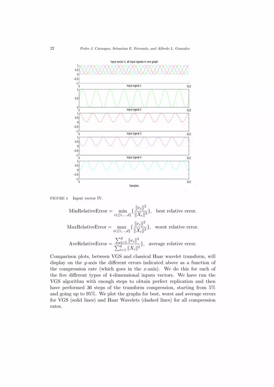
Figure 2 displays input vector II. The input components are described bythe formula Xi(t) = Ai sin(2πf1t) + Bi cos(2πf2t). Therefore, all signalsof the input vector II are in-phase, i.e. they oscillate with the same phasecharacteristic.Figure 3 displays input vector III which contains rather arbitrary, indepen-dent components.Figure 4 displays input vector IV its components represent the same tonebut with different initial phase, spaced by π/2.Figure 5 displays input vector V its components contain frequency-modulatedsignals.Set e = X − X where X = (X1, . . . , Xd) is the input vector and X =(X1, . . . , Xd) a constructed approximating vector (which may be given byour algorithm or the classical Haar wavelet transform). It is important to


]

0 512−1

−0.50

0.51


0 512

0

x 10−3 Input signal 1

0 512−1

−0.50

0.51

Input signal 2

0 512−1

−0.50

0.51

Input signal 3

0 512−1

−0.50

0.51

Input signal 4

Samples

FIGURE 3 Input vector III.

emphasize how the approximations are obtained; once the binary tree ofpartitions, constructed by the VGS algorithm, is available, each componentof the vector is expanded on the corresponding H-system. Then, a nonlinearapproximation (which we will also call transform compression) is performed.The classical Haar wavelet transform is treated in a similar way. The nonlin-ear approximation step refers to the following generic operations: we expanda given scalar signal in an orthonormal basis and keep a given percentageof the largest inner products in the expansion. This percentage of largestinner products will be called the (transform) compression rate, therefore, ifwe say we are using a 5% compression rate it means we keep, in our finalapproximation, only the 5% largest coefficients.We report a variety of errors, these are:

RelativeError =‖e‖2

‖X‖2, for total vector of signals.

RelativeErrori =‖ei‖2

‖Xi‖2, for each component i ∈ 1, . . . , d.


0 512−1

−0.50

0.51


0 5120

0.5

1Input signal 1

0 512−1

−0.50

0.51

Input signal 2

0 512−1

−0.50

0.51

Input signal 3

0 512−1

−0.50

0.51

Input signal 4

Samples

FIGURE 4 Input vector IV.

MinRelativeError = mini∈1,...,d

‖ei‖2

‖Xi‖2, best relative error.

MaxRelativeError = maxi∈1,...,d

‖ei‖2

‖Xi‖2, worst relative error.

AveRelativeError =∑d

i=1 ‖ei‖2

∑di=1 ‖Xi‖2

, average relative error.

Comparison plots, between VGS and classical Haar wavelet transform, willdisplay on the y-axis the different errors indicated above as a function ofthe compression rate (which goes in the x-axis). We do this for each ofthe five different types of 4-dimensional inputs vectors. We have run theVGS algorithm with enough steps to obtain perfect replication and thenhave performed 36 steps of the transform compression, starting from 5%and going up to 95%. We plot the graphs for best, worst and average errorsfor VGS (solid lines) and Haar Wavelets (dashed lines) for all compressionrates.


0 512−1

−0.50

0.51


0 512

−0.50

0.5

Input signal 1

0 512−1

−0.50

0.51

Input signal 2

0 512−1

−0.50

0.51

Input signal 3

0 512−1

−0.50

0.51

Input signal 4

Samples

FIGURE 5 Input vector V.

The next example is a vector X with d = 9, i.e. the input vector con-tains nine components, each of these components is an image of grid size128x128. The information displayed for this example is of a different natureto the one in the previous example. Figure 11 presents the original inputvector which consists of nine images. Figure 12 shows the nine approxima-tions obtained by performing a nonlinear approximation using the H-systemobtained through the VGS binary tree and keeping the largest 100 innerproducts (i.e. at 0.6% transform compression rate). Figure 13 and Figure14 shows similar approximations but keeping the largest 500 and 100 innerproducts respectively (i.e. at 3% and 6.1% transform compression rates re-spectively). Finally, Figure 15 presents the value of the PSNR metric (seeformula below) on the y-axis as a function of number of best components(displayed in the x-axis).Let V be the number of gray values in an image, V = 255 in our case,

PSNR ≡ 10 log10(V 2

MSE),

where MSE stands for the mean square error between the digital image


100 90 80 70 60 50 40 30 20 10 00

10

20

30

40

50

60

70

Relative errors of VGS and Haar wavelet algorithms

Compression rate, %

Re

lative

Err

or

of

Syn

the

sis

, %

VGS best relative error VGS average relative error VGS worst relative error Haar best relative error Haar average relative errorHaar worst relative error

FIGURE 6 Relative error for VGS and Haar wavelets for input vector I

I(x, y) and the approximating digital image I(x, y), explicitly,

MSE =1

MN

M−1∑

x=0

N−1∑

y=0

[I(x, y)− I(x, y)]2.


100 90 80 70 60 50 40 30 20 10 00

10

20

30

40

50

60

70

80


Compression rate, %

Re

lative

Err

or

of

Syn

the

sis

, %


FIGURE 7 Relative error for VGS and Haar wavelets for input vector II

8. Conclusions and Future Work

In the setting of H-systems, we have introduced an algorithm that allows foran optimized construction, this construction is adapted to a given collectionX of random variables defined on an arbitrary domain Ω. The resultingapproximating Haar functions are measurable with respect to events thatgenerate the sigma algebra σ(X ). It is expected that this last propertyis essential to explain the good approximating properties observed in thenumerical examples.

An analysis of mathematical properties of the construction is providedfor the scalar case. A description of a natural extension to the vector caseis also provided, this gives the vector greedy splitting (VGS) algorithm.We believe this last extension is crucial for the algorithm to be successfully


100 90 80 70 60 50 40 30 20 10 00

10

20

30

40

50

60

70

80


Compression rate, %

Re

lative

Err

or

of

Syn

the

sis

, %


FIGURE 8 Relative error for VGS and Haar wavelets for input vector III

deployed in applications. A direct implementation of the VGS algorithmgives encouraging results and it is possible, with more effort, to improveseveral aspects of the algorithm to obtain enhanced performance.

In later work, we expect to carry a similar mathematical investigationfor the vector version of the construction. We also plan to study the speedof convergence of the algorithm in relation to the class X . Moreover anexhaustive numerical study needs to be done to evaluate the usefulness ofthe algorithm in practical situations.

A. Multiresolution Analysis Algorithm


100 90 80 70 60 50 40 30 20 10 00

5

10

15

20

25

30


Compression rate, %

Re

lativ

e E

rro

r o

f S

ynth

esi

s, %


FIGURE 9 Relative error for VGS and Haar wavelets for input vector IV

A.1 Analysis

Assume we have an input signal X : Ω → R, we will describe how to com-pute, using the notation introduced in Section 4, its expansion in the asso-ciated H-system

XRJ(ω) = c0[0] φ0,0(ω) +

J−1∑

j=0

∑

i∈Ij

dj [i] ψj,i(ω) (A.1)

These computations are called the analysis part of the algorithm, it involvescomputing all the inner products dj [i] = 〈X,ψj,i〉 ≡ dAj,i and computingthe values of XRJ

(ω) on the atoms of RJ . Notice XRJis a simple function

constant on each of the atoms of RJ . The inputs to the analysis formulasare the numbers

P (A) and1

P (A)

∫

AX(w)dP (w) = XRJ

(ω) for all A ∈ RJ , ω ∈ A. (A.2)

Therefore, our finest approximation is just the discretization, of X(ω), givenby averaging X over the finest atoms, namely the elements ofRJ . As in clas-


100 90 80 70 60 50 40 30 20 10 00

10

20

30

40

50

60

70

80

90


Compression rate, %

Re

lative

Err

or

of

Syn

the

sis

, %


FIGURE 10 Relative error for VGS and Haar wavelets for input vector V

sic Multi-resolution analysis, we will compute the inner products 〈X, ψj−1,i〉from 〈X,ψj,i〉. To define the formulas we need intermediate node variables,labelled x, d and p, their simple meaning is explained below. Here are therecursive formulas (bottom up recursion, i.e., we start at the leafs)

pfather = pLchildren + pRchildren, (A.3)

xfather =1

pfather(pLchildren xLchildren + pRchildren xRchildren) (A.4)

dfather =√

pLchildren pRchildrenpfather

(xLchildren − xRchildren). (A.5)

To be able to run this recursive formula we just need to initialize the x and


FIGURE 11 Original

FIGURE 12 100 Components, PSNR = 5.47


FIGURE 13 Best 500 Components, average PSNR = 15.86

FIGURE 14 Best 1000 Components, average PSNR = 22.01


FIGURE 15 PSNR vs. number of best components

p variables at the terminal nodes, this is done by using the inputs,

pleaf = P(A), where the atom A ∈ RJ is associated to the given leaf,(A.6)

xleaf = XRJ(ω), where ω ∈ A ∈ RJ is the atom associated to the given leaf.(A.7)

It is easy to see that the meaning of the intermediate variable x at nodeA ∈ ∪J

j=0Rj is

xA =1

P (A)

∫

AX(w)dP (w) =

√P (A) cA, (A.8)

where cAk,i≡ ck[i]. The meaning of the variable d at node A ∈ ∪k=0,...,n−1Qk

is: dA = 〈X, ψA〉 and pnodeA = P (A). The above recursion gives 〈X,ψ0,0〉 =1

P (Ω)

∫Ω X(w)dP (w) =

∫Ω X(w)dP (w) = xroot.

Therefore, analysis gives us the inner products and, if we are interested,it gives coarser approximations (“zoom-outs”) to X given by the values ofthe x intermediate variables. To be more precise at each level j, 0 ≤ j ≤ J ,of the tree we have the approximations

XRj (ω) = xA =1

P (A)

∫

AX(w)dP (w) where ω ∈ A ∈ Rj , (A.9)

so, the simple function XRj is the coarser approximation associated to thepartition Rj , completely analogous to the wavelet approximations at differ-ent scales.

Synthesis: The input to synthesis is the analysis tree of X containingthe dA values (which are equal to the inner product at node A or zero) where


A is a non-terminal node. Also the pA (i.e. the probability at node A) valuesare needed for all nodes A. We also need as input xA0,0 ; the output will be xAfor all nodes A (including the leafs). Here are the reconstruction formulas(top-down recursion, i.e. we start at the top)

xLchildren = xfather +√

pRchildrenpfather pLchildren

dfather (A.10)

xRchildren = xLchidren −√

pfatherpLchidren pRchildren

dfather. (A.11)

References[1] Ariel J. Bernal, Implementation of the vector greedy algorithm for images. Available

at http://www.math.ryerson.ca, 2007.

[2] Pedro J. Catuogno, Sebastian E. Ferrando and Alfredo L. Gonzalez (2007), H-systemsfor efficient hedging and approximation of derivatives. Proceedings of the Third Brazil-ian Conference on Statistical Modelling in Insurance and Finance. Maresias, March25-30, 108-113.

[3] A. Cohen, R.A. DeVore and R. Hochmuth (2000), Restricted nonlinear approximation,Constructive Approx. 16, 85–113.

[4] A. Cohen, W. Dahmen, I. Daubechies and R. DeVore (2001), Tree approximation andoptimal encoding. Appl. Comput. Harmon. Anal. 11(2), pp. 192–226.

[5] Ronald A. DeVore (Summer 1998), Nonlinear approximation. Acta Numerica, 1-99.

[6] Ronald A. DeVore and Vladimir Temlyakov (1997), Nonlinear approximation in finitedimensional spaces. Journal of Complexity, 13, 489–508.

[7] Evgeny Klavir and S.E. Ferrando, A C++ implementation for the vector greedysplitting algorithm, one dimensional case. Available at http://www.math.ryerson.ca,2007.

[8] M. Girardi and W. Sweldens (1997), A new class of unbalanced Haar wavelets thatform an unconditional basis for Lp on general measure spaces. The Journal of FourierAnalysis and Applications, 3, 457–474.

[9] Richard F. Gundy (1966), Martingale theory and pointwise convergence of certainorthogonal systems. Trans. Amer. Math. Soc., 124, 228–248.

[10] A. Jensen and A. la Cour-Harbo (2001): Ripples in Mathematics. The DiscreteWavelet Transform. Springer.

[11] D. Leviatan and V.N. Temlyakov (2003). Simultaneous approximation by greedy al-gorithms. IMI-Preprint 02, 1–17.

[12] Elliott H. Lieb and Michael Loss (2001). Analysis. Second Edition. Graduate Studiesin Mathematics, Volumen 14, American mathematical Society.

[13] A. Lutoborski and V.N. Temlyakov (2002). Vector greedy algorithms. IMI-Preprint10, 1–16.

[14] S. Mallat and Z. Zhang (1993). Matching pursuits with time-frequency dictionaries.IEEE Transactions of Signal Processing, Vol. 41, 3397–3415.

[15] J. Neveu (1975). Discrete-Parameter Martingales, North-Holland.

[16] M. Pollicott and M. Yuri (1998). Dynamical Systems and Ergodic Theory, LondonMathematical Society. Student Texts 40.

[17] V.N. Temlyakov (1999), Greedy algorithms and m-term approximation with regardto redundant dictionaries. J.Approx. Theory, 98, 117–145.


[18] W. Willinger (1987). Pathwise Stochastic Integration and Almost-Sure Aproximationof Stochastic Processes., Thesis, Cornell University.

P.J. Catuogno: Departamento de Matematica. Universidade Estadual de Campinas13.081-97-Campinas, SP, Brazil

e-mail: [email protected]

S.E.Ferrando: Department of Mathematics, Ryerson University350 Victoria St., Toronto, Ontario M5B 2K3, Canadae-mail: [email protected]

A.L. Gonzalez: Departamento de Matematica FCEyN. Universidad Nacional de Mar del Plata. Funes 3350Mar del Plata 7600, Argentinae-mail: [email protected]

adaptive martingale approximations

Documents