mathematical modeling of renal autoregulation
TRANSCRIPT

Mathematical Modeling of Renal
Autoregulation
Nicole C. Kleinstreuer
A thesis
submitted in partial fulfilment
of the requirements for the degree of
Doctor of Philosophy
in
Bioengineering
University of Canterbury
Centre for Bioengineering
Department of Mechanical Engineering
2009

Acknowledgements
This work would not have been possible without the support, encouragement, and assistance of many
people. I would like firstly to thank my supervisors, Prof. Tim David, Dr. Mike Plank, and Prof. Zoltan
Endre for academic guidance, financial assistance, discussion, and feedback over the last several years. I am
greatly indebted to Scott Graybill, who was extremely helpful with writing MATLAB code and provided an
excellent sounding board for ideas. I would like to thank Dr. Harold Layton for inviting me to the workshop
on the kidney at the Mathematical Biosciences Institute, Ohio State University, during the first year of
my PhD where I was able to meet the foremost renal modelling experts in the world and participate in
many amazing discussions that influenced the course of my study. Dr. Jonathan Hill provided me with the
experimental data analyzed in Ch. 5, and has always been available for technical assistance and scintillating
debates. I am especially grateful to Dr. David Nordsletten for the micro-CT images and data that made
this model possible, and to Dr. Brian Carlson, Dr. Niels-Henrik Holstein-Rathlou, and the members of the
Otago Renal Theme for their correspondence and advice.
On a personal note, my network of friends has been invaluable, and I would specifically like to thank Dora
Teglasy, Julie Stafford, and Johnny Humphries for the countless number of occasions that they have helped
me and reminded me what it means to truly love and care for one another. Lastly, and most importantly, I
would like to express my sincere gratitude to my family. My parents, Christin and Clement, and my brother,
Joshua, have always been amazing sources of unconditional love and support, and I thank them from the
bottom of my heart.
ii

To my father,
Professor Clement Kleinstreuer,
whose contributions to my academic and personal successes are immeasurable.
iii

iv

Contents
1 Introduction 1
2 Anatomy of the Kidney 5
2.1 Gross Anatomy . . . . . . . . . . . . . . . . . . . . . . . . . . . . . . . . . . . . . . . . . . . . 5
2.2 Blood Supply . . . . . . . . . . . . . . . . . . . . . . . . . . . . . . . . . . . . . . . . . . . . . 7
2.3 Arterial Structure . . . . . . . . . . . . . . . . . . . . . . . . . . . . . . . . . . . . . . . . . . 9
2.4 Nephrons . . . . . . . . . . . . . . . . . . . . . . . . . . . . . . . . . . . . . . . . . . . . . . . 10
2.4.1 The Renal Corpuscle . . . . . . . . . . . . . . . . . . . . . . . . . . . . . . . . . . . . . 11
2.4.2 The Proximal Tubule . . . . . . . . . . . . . . . . . . . . . . . . . . . . . . . . . . . . 14
2.4.3 The Loop of Henle . . . . . . . . . . . . . . . . . . . . . . . . . . . . . . . . . . . . . . 14
2.4.4 The Juxtaglomerular Apparatus . . . . . . . . . . . . . . . . . . . . . . . . . . . . . . 15
2.4.5 The Distal Tubule and Collecting Duct . . . . . . . . . . . . . . . . . . . . . . . . . . 16
3 Renal Physiology 19
3.1 Autoregulation . . . . . . . . . . . . . . . . . . . . . . . . . . . . . . . . . . . . . . . . . . . . 20
3.2 Tubular Reabsorption . . . . . . . . . . . . . . . . . . . . . . . . . . . . . . . . . . . . . . . . 22
3.2.1 Passive Transport . . . . . . . . . . . . . . . . . . . . . . . . . . . . . . . . . . . . . . 22
3.2.2 Active Transport . . . . . . . . . . . . . . . . . . . . . . . . . . . . . . . . . . . . . . . 24
3.2.3 Transport by Segment . . . . . . . . . . . . . . . . . . . . . . . . . . . . . . . . . . . . 27
3.3 Glomerular Filtration . . . . . . . . . . . . . . . . . . . . . . . . . . . . . . . . . . . . . . . . 28
4 Literature Review of Renal Autoregulatory Models 31
4.1 Modeling the Myogenic Response . . . . . . . . . . . . . . . . . . . . . . . . . . . . . . . . . . 32
4.2 Modeling at the level of the Nephron . . . . . . . . . . . . . . . . . . . . . . . . . . . . . . . . 34
v
5 Experimental Analysis 41
5.1 Isolated Perfused Rat Kidney Data Analysis . . . . . . . . . . . . . . . . . . . . . . . . . . . . 41
5.2 Results and Discussion . . . . . . . . . . . . . . . . . . . . . . . . . . . . . . . . . . . . . . . . 48
6 Mathematical Model of the Renal Myogenic Response 51
6.1 Introduction . . . . . . . . . . . . . . . . . . . . . . . . . . . . . . . . . . . . . . . . . . . . . . 51
6.2 Model Development . . . . . . . . . . . . . . . . . . . . . . . . . . . . . . . . . . . . . . . . . 53
6.2.1 Arterial Tree Representation . . . . . . . . . . . . . . . . . . . . . . . . . . . . . . . . 53
6.2.2 Vessel Model . . . . . . . . . . . . . . . . . . . . . . . . . . . . . . . . . . . . . . . . . 58
6.2.3 Effect of NO . . . . . . . . . . . . . . . . . . . . . . . . . . . . . . . . . . . . . . . . . 59
6.2.4 VSM activation . . . . . . . . . . . . . . . . . . . . . . . . . . . . . . . . . . . . . . . . 60
6.3 Parameter Determination . . . . . . . . . . . . . . . . . . . . . . . . . . . . . . . . . . . . . . 63
6.4 Numerical Methods . . . . . . . . . . . . . . . . . . . . . . . . . . . . . . . . . . . . . . . . . . 65
7 Renal Myogenic Model Results 67
7.1 Model Parameters . . . . . . . . . . . . . . . . . . . . . . . . . . . . . . . . . . . . . . . . . . 67
7.2 Active Response . . . . . . . . . . . . . . . . . . . . . . . . . . . . . . . . . . . . . . . . . . . 70
7.3 Steady-State Whole-Organ Response . . . . . . . . . . . . . . . . . . . . . . . . . . . . . . . . 73
7.4 Inclusion of NO . . . . . . . . . . . . . . . . . . . . . . . . . . . . . . . . . . . . . . . . . . . . 74
7.5 Discussion of Myogenic Model Results . . . . . . . . . . . . . . . . . . . . . . . . . . . . . . . 75
7.5.1 Dynamic Response . . . . . . . . . . . . . . . . . . . . . . . . . . . . . . . . . . . . . . 75
7.5.2 Whole-Organ Autoregulation . . . . . . . . . . . . . . . . . . . . . . . . . . . . . . . . 77
7.5.3 Myogenic Model Summary . . . . . . . . . . . . . . . . . . . . . . . . . . . . . . . . . 77
8 Incorporating a Mathematical Model of the TGF Mechanism 79
8.1 Introduction . . . . . . . . . . . . . . . . . . . . . . . . . . . . . . . . . . . . . . . . . . . . . . 79
8.2 Glomerular Model . . . . . . . . . . . . . . . . . . . . . . . . . . . . . . . . . . . . . . . . . . 80
8.3 Tubular Model . . . . . . . . . . . . . . . . . . . . . . . . . . . . . . . . . . . . . . . . . . . . 81
8.4 TGF model . . . . . . . . . . . . . . . . . . . . . . . . . . . . . . . . . . . . . . . . . . . . . . 84
8.5 Numerical Methods . . . . . . . . . . . . . . . . . . . . . . . . . . . . . . . . . . . . . . . . . . 85
9 Combined Renal Autoregulation Model Results 87
9.1 Model Parameters . . . . . . . . . . . . . . . . . . . . . . . . . . . . . . . . . . . . . . . . . . 87
vi
9.2 Autoregulatory Response . . . . . . . . . . . . . . . . . . . . . . . . . . . . . . . . . . . . . . 88
9.3 Pulsatile Pressure Input . . . . . . . . . . . . . . . . . . . . . . . . . . . . . . . . . . . . . . . 92
9.4 Experimental Comparison . . . . . . . . . . . . . . . . . . . . . . . . . . . . . . . . . . . . . . 93
9.5 Discussion of Combined Model Results . . . . . . . . . . . . . . . . . . . . . . . . . . . . . . . 94
9.5.1 Dynamic Response . . . . . . . . . . . . . . . . . . . . . . . . . . . . . . . . . . . . . . 94
9.5.2 Whole-Organ Autoregulation . . . . . . . . . . . . . . . . . . . . . . . . . . . . . . . . 95
9.5.3 Model Validation . . . . . . . . . . . . . . . . . . . . . . . . . . . . . . . . . . . . . . . 96
9.5.4 Combined Model Summary . . . . . . . . . . . . . . . . . . . . . . . . . . . . . . . . . 97
10 Modeling Pathological Conditions 99
10.1 Hypertension . . . . . . . . . . . . . . . . . . . . . . . . . . . . . . . . . . . . . . . . . . . . . 100
10.2 Diabetes . . . . . . . . . . . . . . . . . . . . . . . . . . . . . . . . . . . . . . . . . . . . . . . . 105
11 Conclusions, Limitations, and Future Work 111
11.1 Model Summary and Conclusions . . . . . . . . . . . . . . . . . . . . . . . . . . . . . . . . . . 111
11.2 Model Limitations . . . . . . . . . . . . . . . . . . . . . . . . . . . . . . . . . . . . . . . . . . 112
11.3 Future Work . . . . . . . . . . . . . . . . . . . . . . . . . . . . . . . . . . . . . . . . . . . . . 113
vii

viii

List of Figures
2.1 Diagram of the location of the kidneys, reprinted from [115] . . . . . . . . . . . . . . . . . . . 6
2.2 Diagram of the layers protecting the kidneys, reprinted from [115] . . . . . . . . . . . . . . . 7
2.3 Division of the anatomical structure of the kidneys . . . . . . . . . . . . . . . . . . . . . . . . 7
2.4 Lumen of the ureter . . . . . . . . . . . . . . . . . . . . . . . . . . . . . . . . . . . . . . . . . 8
2.5 Light microscope image of the arteries of the rat kidney using silicon cast. (Large white arrow:
arcuate artery, small white arrow:interlobular artery, empty arrow: afferent arteriole, white
line: 1 mm) Reprinted from [96]. . . . . . . . . . . . . . . . . . . . . . . . . . . . . . . . . . . 9
2.6 Structure of resistance vessels, reprinted from [35] . . . . . . . . . . . . . . . . . . . . . . . . . 10
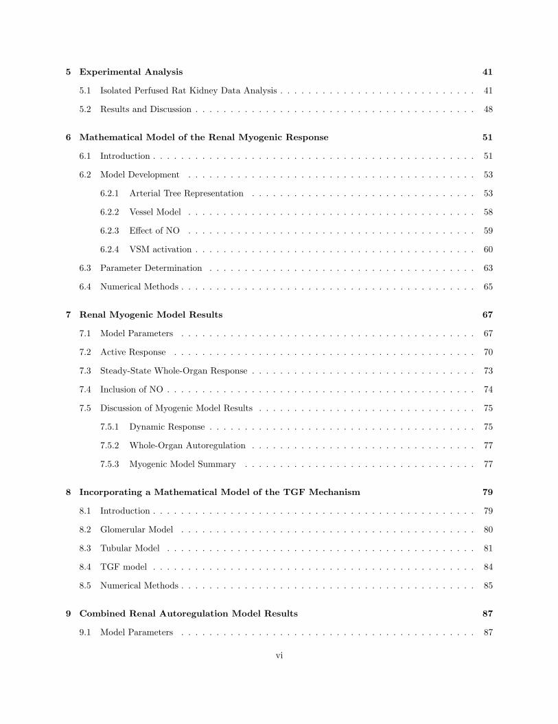
2.7 Cross-section of the kidney showing nephron types, adapted from [24]. . . . . . . . . . . . . . 12
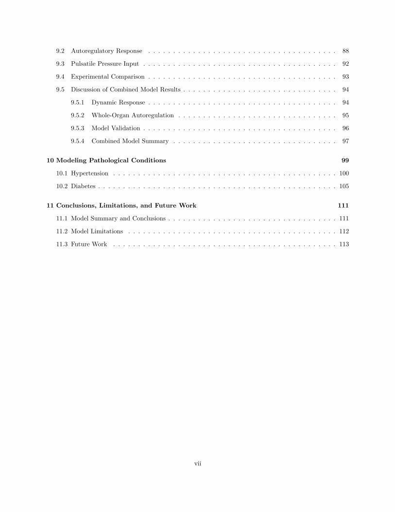
2.8 (a) The glomerulus and Bowman’s Capsule: magnified sections showing filtration barrier,
adapted from [24]. (b) Scanning electron micrograph of the glomerulus, Reprinted from [115]. 13
2.9 Lumen of the proximal tubule . . . . . . . . . . . . . . . . . . . . . . . . . . . . . . . . . . . . 14
2.10 The Loop of Henle . . . . . . . . . . . . . . . . . . . . . . . . . . . . . . . . . . . . . . . . . . 15
2.11 (a) The juxtaglomerular apparatus (JGA) (b) Scanning electron micrograph of the JGA, both
adapted from [122]. AA: Afferent Arteriole, DT or DCT: Distal Tubule, MD: Macula Densa,
EA: Efferent Arteriole, BC: Bowmans Capsule, BS: Bowmans Space, Glom: Glomerulus, PT:
Proximal Tubule . . . . . . . . . . . . . . . . . . . . . . . . . . . . . . . . . . . . . . . . . . . 16
2.12 Tubular cell types; a: Proximal Tubule, b: Thin limb loop of Henle, c: Thick ascending limb
loop of Henle and distal tubule, d: Collecting duct . . . . . . . . . . . . . . . . . . . . . . . . 17
3.1 Perfect autoregulation . . . . . . . . . . . . . . . . . . . . . . . . . . . . . . . . . . . . . . . . 21
3.2 Osmotic diffusion of water molecules, reprinted from [24] . . . . . . . . . . . . . . . . . . . . . 23
3.3 The Na-K-ATPase, or sodium pump, reprinted from [24] . . . . . . . . . . . . . . . . . . . . . 25
3.4 Secondary and tertiary active transport, reprinted from [24] . . . . . . . . . . . . . . . . . . . 26
ix

3.5 Nephron transport of sodium and water by segment; PT is proximal tubule, DL is descending
limb of loop of Henle, AL is ascending limb of loop of henle . . . . . . . . . . . . . . . . . . . 27
3.6 Forces affecting ultrafiltration in the glomerulus, adapted from [35] . . . . . . . . . . . . . . . 29
4.1 (a) The sigmoidal relationship relationship between stretch and active tension development
estimated from Thurau’s data and (b) theoretical pressure-flow relationships with and without
(TA = 0) the participation of active tension in the model, both reprinted from [73]. . . . . . . 34
4.2 Vessel wall tension as a function of circumferential length, reprinted from [9]. Solid curves
are labelled, where maximally active tension assumes full vascular smooth muscle (VSM)
activation. Dashed curves show active and total tension at 50% VSM activation. Dotted
curve shows typical observed behavior during contractile response, as activation increases
with increasing tension. . . . . . . . . . . . . . . . . . . . . . . . . . . . . . . . . . . . . . . . 35
4.3 Idealised glomerular capillary bed, reprinted from [22] . . . . . . . . . . . . . . . . . . . . . . 36
4.4 Proximal tubule fluid reabsorption rate as a function of distance, parameters from [43] . . . . 37
5.1 Isolated Perfused Rat Kidney (IPRK) experimental set-up . . . . . . . . . . . . . . . . . . . . 43
5.2 Close-up of the ex vivo kidney preparation, still protected by the renal fascia . . . . . . . . . 44
5.3 SD Rats: in all plots solid line represents control ramp, dashed line represents AngII ramp,
and dotted line represents papaverine ramp. Blue is normal and red is diabetic. . . . . . . . . 45
5.4 Ren2 Rats: in all plots solid line represents control ramp, dashed line represents AngII ramp,
and dotted line represents papaverine ramp. Blue is normal and red is diabetic. . . . . . . . . 46
5.5 Solid line represents experimental data (4 month old normal Ren2 rats, AngII ramp), dashed
line is logistic curve fit via Nonlinear Least Squares Method. Data is normalized to flow value
at upper limit of autoregulation. . . . . . . . . . . . . . . . . . . . . . . . . . . . . . . . . . . 47
6.1 Potential pathways involved in the development of myogenic tone, reprinted from [39] . . . . 52
6.2 Strahler ordering, reprinted from [79] . . . . . . . . . . . . . . . . . . . . . . . . . . . . . . . . 54
6.3 Rat renal vasculature color-coded by Strahler order, reprinted from [79] . . . . . . . . . . . . 55
6.4 Distally dominant resistance distribution: rat renal vasculature at MAP of 100 mmHg. . . . . 57
6.5 Blood pressure and shear stress are mechanical stimuli acting on smooth muscle (SMC) and
endothelial cells (EC) respectively to achieve basal tone in resistance arteries. Reprinted from
[39] . . . . . . . . . . . . . . . . . . . . . . . . . . . . . . . . . . . . . . . . . . . . . . . . . . . 60
6.6 Effect of NO activation on relationship between φMRss and Ttot. (Legend: “NO” is φNO) . . 61
x

6.7 Schematic representation of renal myogenic autoregulation system. . . . . . . . . . . . . . . . 62
7.1 Passive tension data [7] and model results, i = 4 (d0=172 µm) . . . . . . . . . . . . . . . . . . 68
7.2 NO activation: dependence on shear stress for vascular orders: i = 2 (d0=385 µm), i = 5
(d0=108 µm) and i = 9 (d0=40 µm). . . . . . . . . . . . . . . . . . . . . . . . . . . . . . . . . 69
7.3 (a) Length-tension curves: Strahler order i = 5 (d0 = 108µm). Model results for passive (. . .),
maximally active (- · -), and maximally active total tension (-). Also shown is active response
to two pressure step increases (5 → 85 → 165 mmHg.) (b) Diameter response of isolated
vessel, i = 5 (d0 = 108µm), to same pressure step increase. Location of pressure steps is
circled on (a) and (b). . . . . . . . . . . . . . . . . . . . . . . . . . . . . . . . . . . . . . . . . 70
7.4 (a) Dynamic myogenic response, model prediction. (b) Steady-state myogenic response of
intermediate interlobular artery (i = 8, d0 = 60µm) to pressure step increase (80 → 120 →
160 mmHg.), model prediction and data [106]. . . . . . . . . . . . . . . . . . . . . . . . . . . . 71
7.5 (a) Renal blood flow response exhibiting partial autoregulation (inset: mean arterial pressure
step increases) (b) Changes in VSM activation (c) Diameter response to pressure steps (i =
1..4) (d) Diameter response to pressure steps (i = 5..11). Note: In (b),(c), (d), i increases
from top to bottom . . . . . . . . . . . . . . . . . . . . . . . . . . . . . . . . . . . . . . . . . 72
7.6 (a) Idealized autoregulatory curve: complete renal autoregulation (b) Myogenic renal autoreg-
ulatory response: comparison of model results with experimental data from [87]. . . . . . . . 73
7.7 Effect of NO release in mathematical model: (a) Including NO: diameter response, i = 4, d0 =
172µm, to multiple pressure step increases (b)Inhibiting NO: diameter response, i = 4, d0 =
172µm, to multiple pressure step increases (40 → 60 → 80 → 100 mmHg.) . . . . . . . . . . . 75
8.1 Schematic representation of renal autoregulation system. . . . . . . . . . . . . . . . . . . . . . 86
9.1 Autoregulation of renal blood flow in response to multiple step increases in pressure. Note
the presence of damped oscillations within the autoregulatory range. . . . . . . . . . . . . . . 89
9.2 Response to multiple pressure steps from 60 to 180 mmHg: (a) Changes in VSM activation,
(i = 1..4) (b) Changes in VSM activation, (i = 5..11) (c) Diameter response (i = 1..4) (d)
Diameter response (i = 5..11) . . . . . . . . . . . . . . . . . . . . . . . . . . . . . . . . . . . . 90
9.3 Pressure dependence of TGF activation (a) and Macula Densa NaCl concentration (b) . . . . 91
9.4 Comparison of steady state renal blood flow over range of arterial pressure: results shown for
passive response, myogenic response, and combined renal autoregulation . . . . . . . . . . . . 91
xi

9.5 Pulsatile pressure input, step increase from 130/110mmHg to 150/130mmHg: (a) Flow re-
sponse (b)Diameter responses (i = 5..11) . . . . . . . . . . . . . . . . . . . . . . . . . . . . . 92
9.6 Autoregulation of renal tubular flow in response to multiple step increases in perfusion pres-
sure. Note the presence of damped oscillations within the autoregulatory range. . . . . . . . . 97
10.1 Renal blood flow autoregulation, under control conditions and impaired basal and vascular
NO production. MAP was increased from 60 to 190 mmHg in 5 mmHg steps . . . . . . . . . 101
10.2 Model results: arterial pressure forcings and blood flow for normotensive (top) and hyperten-
sive (bottom) rats . . . . . . . . . . . . . . . . . . . . . . . . . . . . . . . . . . . . . . . . . . 103
10.3 Typical arterial pressure and blood flow data from SDR and SHR, reprinted from [12] . . . . 103
10.4 Distal diameter responses (i = 8, ..., 11) to multiple pressure steps (P=60 → 190mmHg,
5mmHg steps) for normotensive case (colored lines) and hypertensive case produced by in-
hibiting NO (dashed black lines) . . . . . . . . . . . . . . . . . . . . . . . . . . . . . . . . . . 104
10.5 Renal blood flow autoregulation: under control conditions and increased NO production.
MAP was increased from 60 to 190 mmHg in 5 mmHg steps . . . . . . . . . . . . . . . . . . . 106
10.6 Renal blood flow autoregulation: under control conditions, increased NO production, and
increased NO + increased proximal tubular reabsorption. MAP was increased from 60 to 190
mmHg in 5 mmHg steps . . . . . . . . . . . . . . . . . . . . . . . . . . . . . . . . . . . . . . . 108
10.7 Autoregulation of flow entering the proximal tubule: under control conditions, increased NO
production, and increased NO + increased proximal tubular reabsorption. MAP was increased
from 60 to 190 mmHg in 5 mmHg steps . . . . . . . . . . . . . . . . . . . . . . . . . . . . . . 109
1 Schematic diagram of glomerular filtration . . . . . . . . . . . . . . . . . . . . . . . . . . . . . 117
xii

List of Tables
1 Nomenclature . . . . . . . . . . . . . . . . . . . . . . . . . . . . . . . . . . . . . . . . . . . . . xiv
5.1 Estimation of the lower limit of autoregulation by manual and mathematical method, cor-
relation coefficients for logistic curve fitting also shown. SD: Sprague-Dawley, R2: Ren2; n:
normal, d: diabetic; 0,2,4: months; c: control ramp, a: AngII ramp . . . . . . . . . . . . . . . 48
5.2 Autoregulatory Data for IPRK Experimental Preparation. SD: Sprague-Dawley, R2: Ren2;
n: normal, d: diabetic; 0,2,4: months; c: control ramp, a: AngII ramp . . . . . . . . . . . . . 49
6.1 Renal arterial tree measurements [79]. . . . . . . . . . . . . . . . . . . . . . . . . . . . . . . . 56
7.1 Model parameters for rat renal vasculature . . . . . . . . . . . . . . . . . . . . . . . . . . . . 67
9.1 Model parameters for nephron: ∗, †, or ‡ taken from [43], [58], or [123] respectively . . . . . . 88
9.2 Comparison of Model Simulations with Experimental Data: Autoregulatory Index (ARI) rep-
resents change in flow relative to change in pressure . . . . . . . . . . . . . . . . . . . . . . . 93
10.1 Mean Pressure and Flow Values for Experimental Comparison with [12] . . . . . . . . . . . . 104
xiii

Nomenclature
Table 1: NomenclatureSymbol Units Description
Independent variablest s Timex m Glomerular distancez m Tubular distance
Dependent variablesd(t) m DiameterQ(t) m3.s−1 Volumetric flow rateR(t) Pa.s.m−3 ResistanceP (t) Pa Local pressureC(t, z) mol.m−3 NaCl concentrationP (t, z) Pa Tubular fluid pressureQ(t, z) m3.s−1 Tubular volume flow rate
Auxiliary variablesη Pa.s Dynamic viscosityTtot N.m−1 Total tensionTpass N.m−1 Passive tensionTact N.m−1 Active tensionφV SM VSM activationφMR Myogenic activationφTGF TGF activationφNO eNOS activationJs kg.s−1.m−1 NaCl reabsorptionJv m.s−2 Fluid volume reabsorption
Subscriptsi Strahler Ordera Afferent arteriolee Efferent arterioleg Glomerulusb Bowman’s capsule
xiv

Abstract
Renal autoregulation is unique and critically important in maintaining homeostasis in the body via con-
trol of renal blood flow and filtration. The myogenic reflex responds directly to pressure variation and is
present throughout the vasculature in varying degrees, while the tubuloglomerular feedback (TGF) mecha-
nism adjusts microvascular resistance and glomerular filtration rate (GFR) to maintain distal tubular NaCl
delivery. No simple models are available which allow the independent contributions of the myogenic and TGF
responses to be compared and which include control over multiple metabolic and physiological parameters.
Independently developed mathematical models of myogenic autoregulation and TGF control of GFR have
been combined to produce a comprehensive model for the rat kidney which is responsive to multiple small
step changes in mean arterial pressure. The system encompasses every level of the renal vasculature and
the tubular system of the nephrons while simultaneously incorporating the modulatory effects of changes
in viscosity and shear stress-induced nitric oxide (NO) production. The vasculature of the rat kidney has
previously been divided via a Strahler ordering scheme using morphological data derived from micro-CT
imaging. This data, combined with an extensive literature review of the relevant experimental data, led to
the development of order-specific parameter sets for each of the eleven vascular levels. The model of the
myogenic response depends primarily on circumferential wall tension, corresponding to a distally dominant
resistance distribution with the highest contributions localized to the afferent arterioles and interlobular ar-
teries. The constrictive response is tempered by the vasodilatory influence of flow-induced NO. Experimental
comparison with data from groups that inhibited the TGF mechanism showed that the model was able to
accurately reproduce the characteristics of renal myogenic autoregulation. This myogenic model was coupled
with a system of equations that represented both spatial and temporal changes in concentration of the filtrate
in the tubular system of the nephrons and the corresponding resistance changes of the afferent arteriole via
the TGF mechanism. Computer simulation results of the system response to pressure perturbations were
examined, as well as the interaction between mechanisms and the modulatory influences of metabolic and
hemodynamic factors on the steady state and transient characteristics of whole-organ renal autoregulation.
The responses of the model were consistent with experimental observations and showed that the frequency
of the myogenic reflex was approximately 0.4 Hz while that of TGF was 0.06 Hz, corresponding to a 2-3
sec response time for myogenic contraction and 16.7 sec for TGF. Within the autoregulatory range step in-
creases in pressure induced damped oscillations in tubular flow, macula densa NaCl concentration, arteriolar
diameter, and renal blood flow. The model demonstrated that these oscillations were triggered by TGF and
xv

confined to vessels less than 100 micrometer in diameter. The pressure response in larger vessels remained
important in characterizing total autoregulatory efficacy. Examination of the steady-state and transient
characteristics of the model results demonstrates the necessity of considering the whole organ response in
studies of renal autoregulation. A comprehensive model of autoregulation also allows for the examination of
pathological states, such as the altered NO production in hypertension or the excess tubular reabsorption
of water seen in diabetes. The model was able to reproduce experimental results when simulating diseased
states, enabling the analysis of impaired autoregulation as well as the identification of key factors affecting
the autoregulatory response.
xvi

Chapter 1
Introduction
Of all the organs in the body, the kidney is the most essential component in maintaining the delicate
homeostasis required for cells to function properly on a day-to-day basis. Via a variety of mechanisms
and functions, the kidney controls the balance of extracellular fluid, acids and bases, blood volume, and
concentration of sodium and other important ions in the body. The complex and highly specialized anatomy
of the kidney works to create a stable environment for tissue and cell metabolism by conserving nutrients,
excreting waste products, balancing water and solute transport, and regulating blood pressure. None of
these physiological processes could be maintained without the protection of renal autoregulation, which
functions to stabilize renal blood flow and glomerular filtration despite large fluctuations in arterial pressure.
Concurrently, a breakdown in autoregulation is a hallmark of renal disease, as well as a catalyst for the
further progression of renal injury and dysfunction. Although the major mechanisms responsible for renal
autoregulation have been identified, there are still many questions to be answered regarding autoregulatory
function in both healthy and pathological settings.
Mathematical modeling of biological systems is an approach that has been recognized and refined over the
last century as an extremely powerful tool for gaining understanding of complicated physiological processes.
The construction of a mathematical model begins by incorporating the available scientific evidence into a
system that is as accurate as possible while still remaining computationally solvable. It is essential to preserve
a balance between necessary simplifying assumptions and the crucial variables involved in a biological system,
in this case renal autoregulation. The objective of forming a holistic model of autoregulation in the kidney
is not only to facilitate a deeper understanding of this important process, but to attempt to elucidate the
roles and contributions of key factors, such as the varying myogenic response throughout the vasculature,
1

shear stress-induced nitric oxide production, changes in plasma NaCl concentration, the strength of the
tubuloglomerular feedback response, and others. The impact that each of these variables has on the system
cannot be expected to remain static when progressing from a healthy environment to a pathological setting.
The goal is therefore to build a mathematical model which can reproduce qualitative flow regulation results in
both normal and diseased states, with the aim of providing insight into the inner workings of autoregulation,
areas in which to focus potential future treatments, and inspiration for further experimental work.
In the following sections detailing the renal anatomy and physiology, several of the figures pertain to
human kidneys, and it should be emphasized that the mathematical model presented in this thesis applies
to autoregulation in the rat kidney. However, when examining renal function on a macroscopic level the
differences between the human and the rat kidney are relatively minor, and are largely a question of scale.
The rat is the most widely used animal model to experimentally represent human renal function and disease,
and while the conclusions reached by studying and modeling the rat kidney cannot be applied explicitly to
humans, there are distinct parallels that can be made to help provide direction in the ongoing battle against
kidney disease.
The mathematical model in this thesis builds on previous models for myogenic flow regulation [9], glomeru-
lar filtration [58], and nephron tubular reabsorption [43]. These models have been expanded upon and inte-
grated with micro-CT data on the anatomical structure of the renal vasculature [79] to form an original and
unique whole-organ model of autoregulation in the rat kidney. This model was subjected to various pressure
perturbations, and the respective contributions of both autoregulatory mechanisms and roles of metabolic
factors were examined and compared with experimental results. Other original work presented here includes
data analysis performed on experimental work investigating autoregulation in diabetic kidneys, and model
simulations of key aspects of hypertension and diabetes mellitus. A list of conference presentations and
publications follows:
Publications:
Kleinstreuer, N., T. David, M. Plank, and Z. Endre (2008). Dynamic myogenic autoregulation in the rat
kidney: a whole-organ model. American Journal of Physiology: Renal 294, F1453-F1464.
Kleinstreuer, N., T. David, M. Plank, and Z. Endre (2007). Myogenic autoregulation in the rat kidney:
a whole-organ mathematical model. Journal of Biomechanical Science and Engineering Vol. 2, S.1, S59
Proposed Publications:
Kleinstreuer, N., T. David, S. Graybill, M. Plank, and Z. Endre (2009). A Mathematical Analysis of Dy-
namic Whole Organ Renal Autoregulation. American Journal of Physiology: Renal or Kidney International
2

Kleinstreuer, N., T. David, M. Plank, and Z. Endre (2009). Effects of Diminished Nitric Oxide Production
in Hypertension on Renal Blood Flow and Autoregulation Represented via a Whole-Organ Mathematical
Model. Circulation Research or Hypertension
Kleinstreuer, N., T. David, M. Plank, and Z. Endre (2009). Inhibited Proximal Tubular Reabsorption
and Over-Production of Nitric Oxide in Early Stages of Diabetes Mellitus Simulated with a Mathematical
Model of Whole Organ Renal Autoregulation. Circulation Research or Diabetes
Selected Conference Presentations:
“Modeling Autoregulation in the Rat Kidney”, 7th joint Australia-New Zealand Mathematics Convention,
December 2008 (Australian Mathematical Society B. H. Neumann Prize 2008)
“A Mathematical Analysis of Renal Autoregulation” New Zealand Mathematics and Statistics Postgrad-
uate Conference, November 2008
“A Whole Organ Mathematical Model Of Dynamic Autoregulation in the Rat Kidney” 18th annual
Queenstown Molecular Biology Meeting, September 2008
“Dynamic Autoregulation in the Rat Kidney: A Whole-Organ Model”, Mathematical Biosciences Insti-
tute Workshop on the Kidney, Ohio State University, USA, February 2007
3

4

Chapter 2
Anatomy of the Kidney
2.1 Gross Anatomy
The kidneys are bean shaped organs that lie outside the peritoneal cavity, close to the posterior abdominal
wall. The rounded surface faces outward and the medial indented surface, the hilum, is penetrated by the
renal artery, renal vein, nerves, and ureter. There is one kidney on each side of the vertebral column, located
between the level of the twelfth thoracic and third lumbar vertebrae. The right kidney sits slightly lower
than the left because of displacement by the liver, while the left kidney is slightly longer and is closer to the
midline, adjacent to the spleen and below the diaphragm, as shown in Figure 2.1 [26].
Above each kidney lies the adrenal, or suprarenal gland. The kidneys and their respective glands are
very effectively protected from trauma by their placement between the abdominal organs and the muscles
of the back, as well as by three highly specialized layers of tissues (Fig 2.2). The outer layer, called the
renal fascia or fibrous membrane, is primarily composed of connective tissue that shields the kidneys from
trauma. The next layer, known as the pararenal and perirenal fat, connects the kidneys to the abdominal
wall and is made up of adipose tissue, layers of fatty tissue forming a protective cushion around the organ.
The innermost layer, the renal capsule, is a fibrous sac that also protects it from trauma and infection.
The kidney can be divided into two regions, the outer cortex and the inner medulla, which have distinct
structural and functional properties. However, their working tissue mass is the same in that both are
composed of a tightly intertwined system of tubules and blood vessels, though they are arranged differently
in each section. The organization of the renal tissue is so economical that the interstitium, containing
primarily fibroblast cells that synthesize an extracellular matrix of collagen, proteoglycans, and glycoproteins,
5

Figure 2.1: Diagram of the location of the kidneys, reprinted from [115]
comprises less than ten percent of the total renal volume. The medulla can be further divided into an inner
and an outer portion, the outer medulla being adjacent to the cortex. The medulla consists of wedges of
renal tissue called the renal pyramids. Renal columns extend from the cortex between the renal pyramids,
and each pyramid together with the associated overlying cortex forms a renal lobe. The tip of the pyramid,
the papilla, is found in the inner medulla and opens into the renal calyces, first the minor, then the major.
The calyces perform the function of collecting the urine formed by the renal tissue in the pyramids. The
major calyces join to form the renal pelvis, a funnel-like extension of the upper end of the ureter. Figure 2.3
shows a cross-section of the kidney, with the major anatomical structures labelled.
The ureters are tubes that extend from the kidneys to the bladder, and measure approximately 1 to 5
mm in diameter and 27 to 30 cm in length. They transport urine from the kidney pelvis to the bladder
via peristaltic contractions, aided by the unique star-shaped structure of the lumen (Fig 2.4) and the strong
muscular layers. The bladder is a reservoir for urine before it leaves the body, located behind the symphysis
6

Figure 2.2: Diagram of the layers protecting the kidneys, reprinted from [115]
Figure 2.3: Division of the anatomical structure of the kidneys
pubis. There are two openings in the bladder where urine enters from the ureters and one where urine exits
into the urethra [118].
2.2 Blood Supply
Though the kidneys make up only 0.5% of the total body weight they are highly vascular organs, and receive
over 20% of total cardiac output, equivalent to approximately 1200 mL of blood per minute. This is due to
7

Figure 2.4: Lumen of the ureter
the demands of the constant cycle of filtration and reabsorption occurring at the level of the nephron. The
average filtration rate of the kidney is 125ml/min, which equates to 180 L/day. With a total of approximately
8 L of blood in the human body, this means the entire blood volume gets filtered approximately 25 times
per day.
The blood supply for the kidneys is the renal artery, which originates as the fifth branch of the abdominal
aorta. The renal arteries subdivide numerous times, forming a vascular tree responsible for maintaining the
extremely high perfusion required by the kidney. These branches are commonly known as (in descending
order): segmental arteries, lobar arteries, interlobar arteries, arcuate arteries, interlobular arteries, and
afferent arterioles. A light microscope image of a silicon cast of a distal segment of the rat renal vasculature
is shown in Figure 2.5. The vasculature of the rat kidney is quite similar to that of the human kidney,
though humans have approximately one million nephrons, while rats have approximately thirty-five thousand
[26, 96]. The afferent arterioles further subdivide into capillary networks known as glomeruli, which form the
beginning of the tubular system of the nephrons. Elsewhere in the body capillaries signify the start of the
venous system, however the renal structure is unique in that another arteriole continues from the glomerular
capillary ball, known as the efferent arteriole. The efferent arterioles give rise to another capillary network,
the peritubular capillaries that supply blood to the cortex and the vasa recta that extend deep into the
medulla. The kidney is the only place in the body where an arteriole connects two capillary beds [118].
The vasa recta are bundles of parallel vessels that supply blood to the medulla. The descending vasa recta
8

Figure 2.5: Light microscope image of the arteries of the rat kidney using silicon cast. (Large white arrow:arcuate artery, small white arrow:interlobular artery, empty arrow: afferent arteriole, white line: 1 mm)Reprinted from [96].
initially have a structure that is similar to arterioles, with smooth muscle cells in their walls, but become
more akin to capillaries as they progress deeper into the medulla. They are closely paralleled by ascending
vasa recta that carry blood back to the venous system. The ascending vasa recta have a similar wall structure
to glomerular capillaries, containing fenestrated endothelium that enable the exchange of water and solutes
between plasma and the interstitium. This attribute, combined with their close proximity to the tubular
system of the nephrons and the arrangement of descending and ascending flow in parallel, is essential for
the reabsorption of key plasma constituents and concentration of urine achieved by the kidney. The venous
system follows a similar path to the arteries in reverse; blood flows back through the interlobular veins,
arcuate veins, interlobar veins, renal vein, and ultimately the inferior vena cava.
2.3 Arterial Structure
The arteries that make up the renal vasculature are known as resistance vessels, due to their ability to
change their diameter and therefore alter peripheral resistance. This attribute is especially crucial in blood
9

pressure/flow regulation. The capacity for resistance change is greatest in the small arterioles; this is known
as a distally dominant resistance distribution. The larger arteries, while not capable of actively constricting,
maintain a level of basal tone that provides an important contribution to the overall resistance. The most
vasoactive vessels are found in the cerebral and renal vasculature, with varying levels of size and thickness of
the smooth muscle cell layer that facilitates contraction or dilation. A diagram of the arterial wall structure
is shown in Fig 2.6.
Figure 2.6: Structure of resistance vessels, reprinted from [35]
The lumen of the artery has a layer of endothelial cells as the boundary between the blood and the vessel
itself. The endothelium layer rests upon a basement membrane, connective tissue, and an internal elastic
membrane, together referred to as the tunica intima. This is encompassed by the smooth muscle cell layer,
which is the largest component of the vascular wall. The smooth muscle cells determine the radius of the
vessel by their state of contraction. The formation of myosin-actin cross bridges and resulting constriction
of the smooth muscle is determined by the change in intracellular calcium concentration, where a rise in
calcium initiates a contraction and a decrease promotes relaxation.
2.4 Nephrons
The blood carried by the afferent arterioles is delivered to the nephrons, where approximately 20% of the
plasma is filtered through the glomerulus. Erythrocytes and large plasma proteins such as albumin are too
10

large to pass through the glomerular filtration barrier. Each nephron consists of the glomerular capillary
tuft, its protective capsule, and the tubular system. The glomerulus is a compact ball of interconnected
capillary loops surrounded by the fluid filled sac known as Bowman’s Capsule; together they are referred to
as the renal corpuscle. The filtrate exiting the glomerulus enters the proximal convoluted tubule, then the
loop of Henle, passing first through the descending limb and then the ascending limb. The next segment
is the distal convoluted tubule, which empties into the collecting ducts, which eventually join to form the
ureter [118]. All of these segments are heterogeneous, with varying transport properties and cell types, which
will be examined in detail further on.
The glomeruli of all nephrons are located in the cortical region of the kidney, with the loops of Henle
descending into the medulla. However, there are two distinct kinds of nephrons: cortical and juxtamedullary,
both of which are classified according to the location of their associated renal corpuscle. Figure 2.7 shows
both kinds of nephrons, with their respective segments labelled, and their placement within the kidney.
Cortical nephrons make up 85% of all nephrons in humans, and have their renal corpuscle in the superficial
renal cortex. The renal corpuscles of juxtamedullary nephrons, the other 15% in humans, are located near
the boundary of the renal medulla. Cortical nephrons primarily perform excretory and regulatory functions,
while juxtamedullary nephrons are responsible for the concentration and dilution of urine. The current work
is concerned with examining autoregulation, and will therefore focus exclusively on cortical nephrons. There
are small aspects of biochemical and functional heterogeneity among these nephrons, mainly arising from
the varying lengths of the loops of Henle, but they are generally considered to be negligible [26].
2.4.1 The Renal Corpuscle
The renal corpuscle of the nephron consists of two parts: the glomerular capillary tuft and the surrounding
Bowman’s capsule, shown in Figures 2.8(a) and 2.8(b). Blood enters and exits the glomerulus via the afferent
and efferent arterioles respectively, both of which penetrate the surface at the vascular pole. The filtrate
exiting the glomerular capillaries passes through the lumen of the capsule, known as Bowman’s space, and
exits at the opposite end of the vascular pole (known as the urinary pole) to enter the tubular system. The
glomerulus contains three major cell types: endothelial, mesangial, and epithelial cells. Endothelial cells are
situated on the surface of the lumen, have large fenestrae, and are not covered by diaphragms, rendering them
permeable to all components of blood except platelets and erythrocytes. The following layer is called the
glomerular basement membrane, and is a sponge-like network of proteoglycans and glycoproteins. Mesangial
cells are modified smooth muscle cells that lie between the capillaries and the capsule which act as phagocytes
11
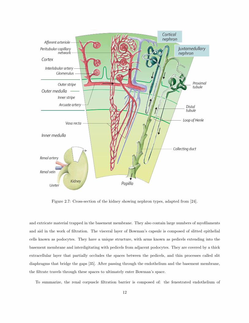
Figure 2.7: Cross-section of the kidney showing nephron types, adapted from [24].
and extricate material trapped in the basement membrane. They also contain large numbers of myofilaments
and aid in the work of filtration. The visceral layer of Bowman’s capsule is composed of slitted epithelial
cells known as podocytes. They have a unique structure, with arms known as pedicels extending into the
basement membrane and interdigitating with pedicels from adjacent podocytes. They are covered by a thick
extracellular layer that partially occludes the spaces between the pedicels, and thin processes called slit
diaphragms that bridge the gaps [35]. After passing through the endothelium and the basement membrane,
the filtrate travels through these spaces to ultimately enter Bowman’s space.
To summarize, the renal corpuscle filtration barrier is composed of: the fenestrated endothelium of
12
(a)
(b)
Figure 2.8: (a) The glomerulus and Bowman’s Capsule: magnified sections showing filtration barrier, adaptedfrom [24]. (b) Scanning electron micrograph of the glomerulus, Reprinted from [115].
glomerular capillaries, the glomerular basement membrane, the fused basal lamina of endothelial cells and
podocytes, and the filtration slits of the podocytes. This barrier permits the passage of water, ions (e.g.
sodium, potassium, chloride), glucose, and other small molecules from the bloodstream into Bowman’s space.
Large and/or negatively charged proteins such as globulins are not freely filtered, thereby retaining these
13

proteins in the circulation.
2.4.2 The Proximal Tubule
The filtrate exiting Bowman’s capsule drains into the proximal tubule, which has a convoluted segment
followed by a straight segment. The entire tubular system of the nephron consists of epithelial cells resting
on a basement membrane, though the structure and function of the cells varies significantly among the
segments. The epithelial cells found in the proximal tubule are columnar to cuboidal, with large luminal
surface areas due to extensive microvillous brush borders (Fig 2.9). Earlier parts of the tubule, specifically the
convoluted portion, have higher numbers of mitochondria facilitating active transport and allowing for more
rapid reabsorption. About 80% of the filtrate is reabsorbed in the proximal tubule [35]. Smaller molecules
like amino acids pass directly through the cell membranes and larger molecules like proteins and polypeptides
are reabsorbed by endocytosis. Sodium is actively pumped into the extracellular space, followed by water
and chloride ions. The cells contain deep folds in their basolateral membrane, known as basal labyrinth,
that are in close contact with the intracellular mitochondria that produce the ATP needed to pump sodium
across the cell wall [24].
Figure 2.9: Lumen of the proximal tubule
2.4.3 The Loop of Henle
The loop of Henle, shown in Figure 2.10, consists of three parts. The first part of the descending limb
is a continuation from the proximal tubule in which the cells become exclusively cuboidal and loose their
microvillous border. The descending limb reaches deep into the medulla, and has low permeability to ions
14
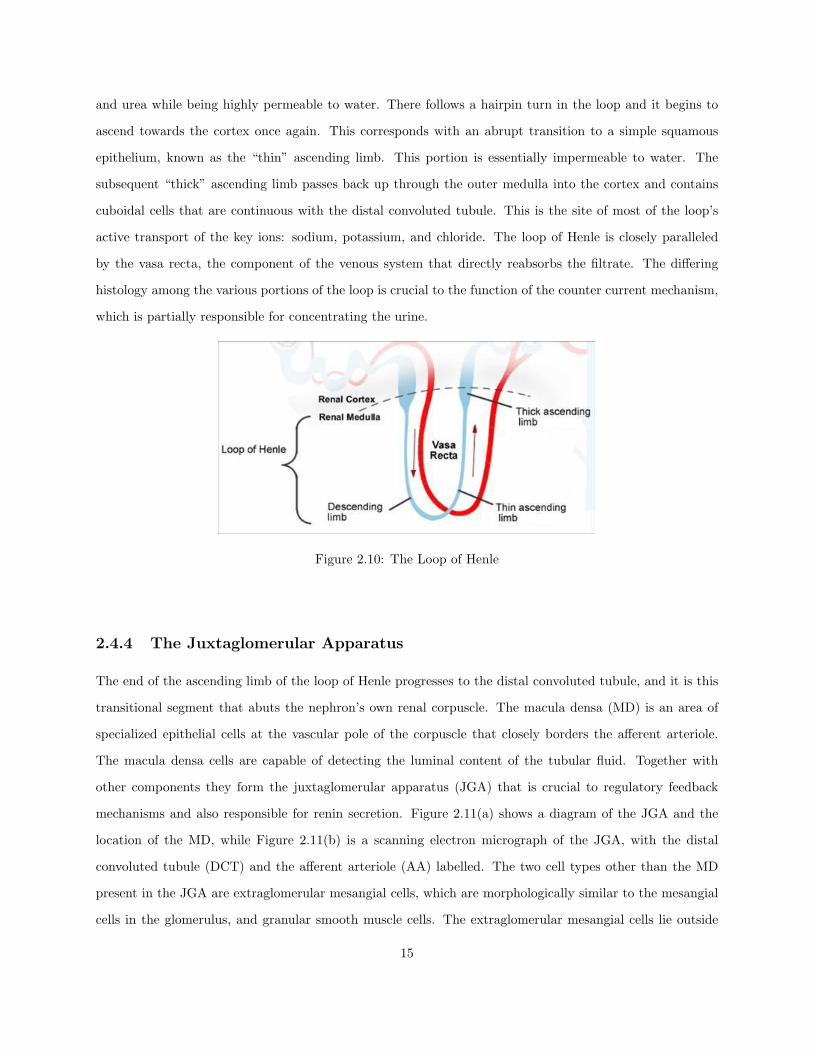
and urea while being highly permeable to water. There follows a hairpin turn in the loop and it begins to
ascend towards the cortex once again. This corresponds with an abrupt transition to a simple squamous
epithelium, known as the “thin” ascending limb. This portion is essentially impermeable to water. The
subsequent “thick” ascending limb passes back up through the outer medulla into the cortex and contains
cuboidal cells that are continuous with the distal convoluted tubule. This is the site of most of the loop’s
active transport of the key ions: sodium, potassium, and chloride. The loop of Henle is closely paralleled
by the vasa recta, the component of the venous system that directly reabsorbs the filtrate. The differing
histology among the various portions of the loop is crucial to the function of the counter current mechanism,
which is partially responsible for concentrating the urine.
Figure 2.10: The Loop of Henle
2.4.4 The Juxtaglomerular Apparatus
The end of the ascending limb of the loop of Henle progresses to the distal convoluted tubule, and it is this
transitional segment that abuts the nephron’s own renal corpuscle. The macula densa (MD) is an area of
specialized epithelial cells at the vascular pole of the corpuscle that closely borders the afferent arteriole.
The macula densa cells are capable of detecting the luminal content of the tubular fluid. Together with
other components they form the juxtaglomerular apparatus (JGA) that is crucial to regulatory feedback
mechanisms and also responsible for renin secretion. Figure 2.11(a) shows a diagram of the JGA and the
location of the MD, while Figure 2.11(b) is a scanning electron micrograph of the JGA, with the distal
convoluted tubule (DCT) and the afferent arteriole (AA) labelled. The two cell types other than the MD
present in the JGA are extraglomerular mesangial cells, which are morphologically similar to the mesangial
cells in the glomerulus, and granular smooth muscle cells. The extraglomerular mesangial cells lie outside
15

of Bowman’s Capsule and represent the transitional region between the tubule and the afferent arteriole,
receiving signals from the macula densa and passing them on to the granular smooth muscle cells of the
arteriole.
(a) (b)
Figure 2.11: (a) The juxtaglomerular apparatus (JGA) (b) Scanning electron micrograph of the JGA, bothadapted from [122]. AA: Afferent Arteriole, DT or DCT: Distal Tubule, MD: Macula Densa, EA: EfferentArteriole, BC: Bowmans Capsule, BS: Bowmans Space, Glom: Glomerulus, PT: Proximal Tubule
2.4.5 The Distal Tubule and Collecting Duct
The cells of the distal tubule are small and densely packed cuboidal cells with extensive basal and lateral
invaginations. The collecting tubule has the same cell type and continues on from the distal convoluted
tubule to drain into the collecting ducts. Here water is absorbed, promoted by the presence or absence of
anti-diuretic hormone (ADH). ADH has an influence on the collecting duct’s permeability to water, therefore
increasing reabsorption to concentrate the urine or decreasing it to dilute the urine. The differing epithelial
cell types along the tubular segments are shown in Fig 2.12.
16

Figure 2.12: Tubular cell types; a: Proximal Tubule, b: Thin limb loop of Henle, c: Thick ascending limbloop of Henle and distal tubule, d: Collecting duct
17

18

Chapter 3
Renal Physiology
The kidney performs an array of crucial functions, which will be very briefly outlined. Here the focus is
upon modeling the kidney’s ability to stabilize blood flow despite fluctuations in arterial pressure, hence the
physiology behind autoregulation will be most closely examined. For a more in-depth review of the other
important renal functions, the reader is referred to Vander’s Renal Physiology [26].
The kidney is responsible for both the intermediate and the long-term control of blood pressure. In
conjunction with the sympathetic nervous system, the renin-angiotensin mechanism responds to sustained
deviations in blood pressure with the release of vasoactive substances that have a stabilizing effect. On
a larger time scale blood pressure is directly dependent upon blood volume, or extracellular fluid volume.
When blood volume is low, the kidneys secrete renin which stimulates the production of angiotensin, causing
constriction of blood vessels and resulting in increased blood pressure. Angiotensin also stimulates the
secretion of the hormone aldosterone from the adrenal cortex, which changes the permeability of the collecting
duct and results in the retention of sodium and water. This increases the volume of fluid in the body, which
also increases blood pressure. Therefore, the kidney controls blood volume and sets long term blood pressure
via the maintenance of salt and water balance. This was demonstrated experimentally by Guyton and others
by effectively denervating the kidneys of dogs, which resulted in a more variable arterial pressure but the
same average value [35].
Regulation of water and electrolyte balance is a related function, playing an important role in blood
pressure control and autoregulation. The kidney is extremely effective at balancing the input and output
of various substances, despite the highly variable daily intake of minerals such as sodium, magnesium,
potassium, and others. Water consumption is the most extreme example, varying to a degree that can be far
19

below or far in excess of the body’s needs. The kidney is able to concentrate or dilute the urine accordingly
to ensure the amount of water present in the body remains in an appropriate balance. Other than water,
the urine is primarily composed of metabolic waste products such as creatinine, uric acid, and urea. These
end products of metabolic processes are often harmful in high concentrations and must be excreted, along
with hormones and other foreign substances such as drugs. The processes of metabolic excretion and tubular
secretion are directly connected to pH regulation. For example, excess hydrogen ions (H+) are combined
with ammonia (NH3) to form ammonium ions (NH4+) and transported to the cells of the collecting ducts,
where the NH4+ dissociates back into ammonia and H+. Both are then secreted into the tubular fluid by
active transport mechanisms, and are responsible for maintaining control of the pH of the blood. When
the pH of the blood becomes too low, more hydrogen ions are secreted, whereas if the blood becomes too
alkaline, secretion of H+ is reduced. In maintaining the pH of the blood within its normal limits of 7.37.4,
the kidney can produce a urine with a pH as low as 4.5 or as high as 8.5 [26].
The kidney also produces the active form of vitamin D and erythropoietin, a peptide hormone that
stimulates the bone marrow to increase red blood cell production. A substantial fraction of gluconeogenesis,
the production of new glucose, occurs in the kidneys. The kidneys also produce calcitrol, which encourages
reabsorption of calcium and phosphate, and prostaglandins, which control platelet aggregation, cell growth,
hormone regulation, etc [26].
All of the aforementioned processes and functions are almost entirely dependent on the transport of water
and solutes between the blood and the tubular lumina of the nephrons. The most important constituents
freely filtered into the tubular system are water, sodium, and chloride, substances whose intake and excretion
rates can vary immensely from day to day and between individuals. The kidney is extremely capable of
altering tubular reabsorption, secretion, and excretion, achieving a remarkably wide urinary concentration
range. The rate of renal blood flow, and subsequently glomerular filtration rate, is the crucial determinant
in this system, and must be held in an appropriate balance by autoregulation so as not to overwhelm the
cellular transport mechanisms.
3.1 Autoregulation
The phenomenon of autoregulation, the stabilization of local blood flow despite large changes in arterial
pressure, exists throughout the body though it is strongest in the cerebral and renal vasculature. There
are two major renal autoregulatory mechanisms, the myogenic response and the tubuloglomerular feedback
(TGF), that function cooperatively to allow only slight changes in renal blood flow and glomerular filtration
20

rate within a systemic blood pressure range of approximately 80 to 180mmHg [24]. When the mean blood
pressure changes within this range, the resistances of the distal renal vessels, primarily the interlobular
arteries and the afferent arterioles, adjust accordingly by actively constricting or dilating. This results in a
pressure/flow curve with a small gradient within the physiological range, and much higher gradient above
and below, as shown in Fig 3.1.
Figure 3.1: Perfect autoregulation
The myogenic response is a direct response of the vascular smooth muscle (VSM) to a variation in
pressure and the corresponding change in circumferential wall tension. All VSM cells respond to stretch by
constricting and to relaxation by dilating, providing an extremely fast negative feedback mechanism that
works on the order of a few seconds. The strength of the myogenic response varies depending on the size of
the vessel and the number of force-generating smooth muscle cells. The VSM cells of the renal vasculature
have a particularly responsive myogenic reflex. The second mechanism of renal autoregulation is specific to
the kidney, and utilizes the salt sensitivity of the macula densa cells in the juxtaglomerular apparatus to
produce a phenomenon known as the TGF response. High levels of Na+ flowing past the macula densa, at
the distal end of Henle’s loop, signify that an excessive amount has escaped reabsorption in the proximal
tubule and the loop of Henle and the rate of filtration must be lowered. Conversely low levels of Na+
detected by the macula densa produce a feedback signal to increase the filtration rate. The effector site of
this mechanism is the distal afferent arteriole, and the constrictor or dilatory signals operate on a slower
time scale than that of the myogenic response, on the order of 15− 25 seconds [26].
21

The detailed physiology behind the myogenic response and TGF is not fully understood; however there
is a large body of experimental and theoretical work dedicated to elucidating the finer points of these renal
autoregulatory mechanisms. Both are modelled as part of the current work, and will be explained in more
depth in Chapters 6 and 8. As mentioned previously, the cellular transport mechanisms of the nephron
are simultaneously protected by renal autoregulation via the maintenance of steady flow, and influence the
autoregulatory response by altering the plasma composition that determines tubuloglomerular feedback.
These important pathways, both passive and active, are explained in detail in the following sections.
3.2 Tubular Reabsorption
The two routes that a molecule can travel when passing through the wall of the renal tubule are via transcel-
lular or paracellular pathways. Transcellular transport requires that a substance cross both the luminal and
the basolateral membrane of the tubular cells, and is achieved via a variety of passive and active transporters
that will be explored in detail. Paracellular transport involves water and small solutes travelling around the
cells and passing through the matrix of tight junctions that bind the tubular epithelial cells together. The
ease of paracellular transport is determined by the “tightness” of these junctions and osmolality on either
side of the tubule. The term diffusion is often applied to paracellular transport though it can refer to some
substances travelling a transcellular route as well, such as the blood gases which can diffuse directly through
the lipid bilayer [26]. Osmolality is defined as the ratio of the concentration of a solute to the mass of solvent,
and in this case the primary solute under examination is Na+ and the solvent is water.
3.2.1 Passive Transport
A substance suspended in a solution undergoes Brownian, or random, motion but net diffusion across a
barrier is related to the net movement of molecules in one direction or another. The driving force behind
passive diffusion is an electrochemical gradient, or a greater concentration of solutes on one side of a barrier
than on the other. The tighter the junctions between the tubular cells, the greater the concentration gradient
that can be attained [24]. Molecules transported by transcellular diffusion travel through channels, proteins
that contain structural pathways specific to water or certain solutes, such as sodium or potassium. Ion
channels require a concentration gradient to transport substances, and can exist in an open or closed state
thereby controlling the passage of the molecules. The proteins that selectively transport water molecules are
known as aquaporins. Osmosis is the force that drives water through aquaporins from areas of high water
22

(or low solute) concentration to areas of low water (or high solute) concentration, as seen in Fig 3.2.
Osmotic flow is the product of the hydraulic conductivity (Kf ) and the osmotic pressure difference
(∆π), which is directly dependent on the difference between the particle concentrations on either side of the
membrane. The higher concentration, Cbosm in Figure 3.2, attracts the water, signifying that water flows
against the concentration gradient of the solute particles. Osmosis cannot occur unless the membrane is less
permeable to the solutes than to water.
Figure 3.2: Osmotic diffusion of water molecules, reprinted from [24]
Many molecules are passively reabsorbed by the peritubular capillaries back into the bloodstream along
with the flow of water by a process known as solvent drag. The inertial movement of the water carries along
with it small molecules such as sodium, while larger molecules like urea and calcium that are resistant to
the drag force become more concentrated in the tubular fluid, and are able to be passively reabsorbed along
their concentration gradient [24]. The passive transport processes are intimately bound to active transport
processes, as it is the active reabsorption (namely of sodium and glucose) that causes the osmotic gradient
leading to the passive reabsorption of water. Another form of diffusion driven by the existence of a gradient
is facilitated diffusion, or movement through a uniporter. While channels are pores that freely permit the
movement of solutes, uniporters such as the GLUT family of proteins transporting glucose through the
proximal tubule epithelial cells require that that the solute bind to a specific binding site on either side of
the basolateral membrane to travel into the interstitium [26].
23

3.2.2 Active Transport
There are two major types of transport requiring energy that can move a substance against its electrochemical
gradient: primary and secondary active transport processes. All transport requires energy, however in the
case of uniporters or channels, that energy is inherently present due to the electrochemical gradient. Similar
to channels, transporters are proteins that allow for the transmembrane flux of a specific solute. Because
the solute must bind strongly to the transport protein, the specificity of transporters is higher than that of
channels and the rate of movement is slower [35].
In the case of primary active transport, the hydrolysis of adenosine triphosphate (ATP) provides the
energy needed for the transporters to move solutes across the cellular membrane, leading to the names
ATPases or ion pumps. There are many types of ATPases, such as the Ca2+ATPase found in the endoplasmic
reticulum or the H+ATPase found in lysosomes, but the most pertinent and widespread type is the Na+-
K+ATPase, also called the sodium pump. An isoform of this ATPase is present in every cell in the body
[26]. As the vast majority of all reabsorption in the nephron is dependent on sodium, either directly by
sharing a transport mechanism, or indirectly by the formation of an osmotic gradient, the sodium pump will
be the only ATPase closely examined here.
The cycle of the sodium pump (Fig 3.3) is as follows. Initially, 3 Na+ ions are pumped out of the cell and
2 K+ ions are pumped into the cell, and 1 ATP molecule phosphorylates the carrier protein. Phosphorylation
produces a conformational change of the protein and alters the affinities of the Na+ and K+ binding sites by
moving them to the opposite side of the membrane. This is the key step in the transport process, carrying
Na+ across the membrane to be discharged and exchanged for K+ ions. Dephosphorylation produces another
conformational change that restores the pump to its original state. The pumping rate increases when either
the extracellular K+ rises or the cytosolic Na+ concentration rises. [24] The basolateral membrane of the
renal tubular epithelial cells is extremely permeable to K+, and almost as soon as they are pumped into the
cell K+ ions diffuse back into the interstitium. The net result is the formation of a low sodium concentration
within the cell, promoting the influx of Na+ ions across the luminal membrane and out of the tubular fluid,
by both passive and facilitated diffusion enabled by the large number of sodium carrier proteins, specifically
in the proximal tubule [35]. Chloride reabsorption also follows both the passive paracellular route and the
active transcellular pathway, and is virtually always in parallel with sodium reabsorption, such that when
referring to Na+ reabsorption, Cl reabsorption is implied [26]. The process of secondary active transport
can be further differentiated into co-transport and counter transport. Co-transport is achieved by proteins
known as symporters that move two or more species of solutes in the same direction across a membrane,
24

Figure 3.3: The Na-K-ATPase, or sodium pump, reprinted from [24]
while counter transport via antiporters moves different types of solutes in opposite directions. Examples of
these varying transport pathways are shown in Fig 3.4. An important symporter in the nephron is that which
25

Figure 3.4: Secondary and tertiary active transport, reprinted from [24]
moves sodium and glucose together into the cell, known as SGLT1 or SGLT2 depending on the number of
Na+ ions (two or one respectively) used to transport one glucose ion. Glucose is transported uphill against
its’ gradient by utilizing the energy created by moving sodium along the downhill gradient into the cell.
Another symporter found in the thick ascending limb of the loop of Henle is the Na-K-2Cl protein, which
maintains electroneutrality by moving two positively charged solutes (sodium and potassium) alongside two
ions of a negatively charged solute (chloride). An example of an antiporter, where the compound and the
driving ion are being transported in different directions, is the exchange of one H+ ion (moving out of
the cell) for one Na+ ion (moving into the cell). This is also an example of an electroneutral transport
process, where the charge remains balanced throughout. The SGLT symporters referred to previously, as
well as the sodium-amino acid symporter, are examples of electrogenic transport. The sole driving force for
electroneutral transport is the chemical Na+ gradient, while the negative membrane potential provides an
additional driving force for electrogenic cotransport [24]. Whether directly or indirectly, tubular transport
26

of all solutes is almost entirely dependent on sodium.
3.2.3 Transport by Segment
A simple diagram of the passive and active transport mechanisms that dominate each section of the nephron is
shown in Figure 3.5. Under average salt intake conditions, the proximal tubule reabsorbs 65% of both filtered
sodium and water, primarily due to the activity and large ATP consumption of the Na-K-ATPase pumps.
Volume reabsorption in the proximal tubule is iso-osmotic due to the high water permeability of the proximal
tubule cells, allowing for very small differences in osmolality caused by solute reabsorption (1− 2mOsm/L)
to inspire a large reabsorption of water. Within this segment of the nephron the kidney retains most of the
crucial organic substances required for the body to function: 90% of the filtered bicarbonate and over 99%
of amino acids, glucose, and lactate. The secretion of H+ ions by counter transport with Na+ across the
luminal membrane is required for the reabsorption of bicarbonate [26].
Figure 3.5: Nephron transport of sodium and water by segment; PT is proximal tubule, DL is descendinglimb of loop of Henle, AL is ascending limb of loop of henle
27

The loop of Henle is the first site of urinary concentration, usually absorbing approximately 25% of the
filtered sodium load compared with 10% of the water. The descending limb marks an abrupt transition to a
thin layer of epithelial cells, with no brush border and very few mitochondria, highlighting its function as a
site primarily for diffusion. The permeability to water is high, promoting diffusion out of the tubule as the
loop descends into the medulla and the interstitium becomes more concentrated, while very little sodium
and chloride is reabsorbed [35]. In contrast, the ascending limb (both the thin and the thick portion) is
impermeable to water but transports sodium both passively and actively. The significant water reabsorption
in the descending limb creates a concentrated luminal fluid and favorable conditions for the passive para-
cellular reabsorption of sodium in the early ascending limb. Further along the ascending limb the transport
properties of the epithelium change and the active processes begin to dominate, primarily the Na-K-2Cl
symporter and the Na-H antiporter, described in the previous section and located in the luminal membrane,
and of course the ubiquitous Na-K-ATPase in the basolateral membrane. The paracellular conductance for
sodium is also still high in this section, which when combined with the positive luminal potential provides a
driving force for cations and significant reabsorption of both potassium and calcium as well [26].
Similar to the ascending limb of Henle’s loop, the water permeability of the distal tubule is low, while
solutes are still reabsorbed through epithelial sodium channels. Therefore, the tubular fluid becomes even
more hypo-osmotic as it is diluted even further in this section. In contrast, the collecting duct exhibits a wide
range of water permeability that is solely dependent on the presence or absence of anti-diuretic hormone
(ADH). Without ADH, there is very little cortical reabsorption and the urine is dilute, a phenomenon
known as water diuresis. In the presence of ADH, the kidney can produce a very concentrated urine and
retain most of the fluid within the body. ADH effects permeability control by catalyzing or preventing the
migration of intracellular vesicles containing aquaporins to the luminal membrane of the epithelial cells [26].
3.3 Glomerular Filtration
According to the principle of mass balance, the mass excreted in the urine must be equal to the mass filtered
through the glomeruli into the nephrons, minus the mass reabsorbed into the renal venous system across
the tubular epithelia, plus the mass secreted into the tubular luminal fluid. The filtration barrier of the
glomerulus is both charge and size-selective, retaining large and negatively charged macromolecules within
the circulation. The endothelium, the basement membrane, and the podocytes all contain fixed polyanions
on their surfaces, ensuring that macromolecules with a negative charge, such as all plasma proteins, cannot
leave the blood stream. All molecules below 7,000 daltons (molecular weight) are freely filtered, and all
28

those above 70,000 daltons are excluded. Within this range the amount of any molecule present in the
filtrate progressively decreases with increasing size. Often the composition of the filtrate is an indicator of
disease; the presence of large proteins signifies a breakdown in the negative charge of the glomerular capillary
membrane, while an over-abundance of small proteins such as myoglobin and hemoglobin points to damaged
muscles or erythrocytes respectively.
The kidney filters blood at an astonishing rate of 125 mL/min, signifying that the entire blood volume is
filtered over 25 times per day. This ultrafiltration occurs due to Starling forces, or hydrostatic and oncotic
forces, that drive fluid from the lumen of glomerular capillaries across the filtration barriers into Bowman’s
space. Hydrostatic pressure is the pressure that exists due to fluid forces, while oncotic pressure is a form of
osmotic pressure exerted by proteins in blood plasma that usually tends to pull water into the circulatory
system because the plasma proteins are too large to cross the capillary wall. The net filtration pressure is a
balance of four contributing pressures, and is significantly higher than the pressure in other capillary beds
throughout the body.
Figure 3.6: Forces affecting ultrafiltration in the glomerulus, adapted from [35]
Those forces driving filtration are the glomerular capillary hydrostatic pressure (PGC) and the Bowman’s
capsule oncotic pressure (πBS), while the glomerular capillary oncotic pressure (πGC) and Bowman’s capsule
hydrostatic pressure (PBS) oppose it. However, due to the absence of filtered proteins oncotic pressure in
Bowman’s Capsule is negligible. The glomerular filtration rate (GFR) is equal to the product of the net
filtration pressure and the ultrafiltration coefficient, Kf, which depends on both the intrinsic permeability
of the glomerular capillaries and the glomerular surface available for filtration [35]. Equation 3.1 shows this
29

calculation. Typical values in humans are PGC = 60mmHg, PBS = 15mmHg, πGC = 29mmHg, and πBS = 0,
leading to a net filtration pressure of 16mmHg and a GFR of 125ml/min.
GFR = Kf ∗ {[PGC − PBS ]− [πGC − πBS ]} (3.1)
An increase in renal arterial pressure transiently elevates glomerular capillary pressure, thus enhancing
GFR. Similarly a decrease in pressure inhibits GFR. Each of these effects can be offset by a corresponding
change in arteriolar resistance to stabilize GFR and tubular flow. This is a major consequence of au-
toregulation, along with stabilizing renal blood flow and protecting the glomeruli from damaging pressure
fluctuations.
30
Chapter 4
Literature Review of Renal
Autoregulatory Models
Autoregulation was first characterized in 1902 by Bayliss, who noted the tendency of the renal vasculature
to exhibit a powerful vasoconstrictive response when the kidney was subjected to heightened pressure. In
this landmark paper he observed, “In the case of the kidney vessels this reaction to increased tension is very
marked....The peripheral powers of reaction possessed by the arteries is of such a nature as to provide as far
as possible for the maintenance of a constant flow of blood through the tissues supplied by them, whatever
may be the height of the general blood-pressure...” [3]. This was the first known characterization of the
myogenic response, one of the two major renal autoregulatory mechanisms and the most easily identifiable
as it is an inherent property of arterial smooth muscle present in vascular beds throughout the body. The
concept of tubuloglomerular feedback as the other key renal autoregulatory mechanism was significantly more
elusive, although the distal afferent arteriole was already identified in 1937 by Goormaghtigh as a potential
regulatory site due to the unique anatomical relationship between the vascular pole of the glomerulus and the
early part of the distal tubule [72]. Subsequent experiments throughout the following two decades elucidated
the phenomenon that alterations in both the composition and flow rate of the distal tubule fluid affected
the glomerular filtration rate of the corresponding nephron, leading to the hypothesis presented by Guyton
in 1963, that there existed a regulatory mechanism unique to the kidney where increased distal delivery
produced preglomerular vasoconstriction. This was one of the first identifications of the important concept
of organ-specific vascular regulation working in conjunction with a general myogenic response to address the
differing metabolic and physiological requirements of various tissues [35].
31

After the basic identification of the primary mechanisms, the role of mathematical modeling began to
develop as a useful tool for understanding the relative contributions and importance of each. Mathemati-
cal models based on known physiological principles were developed and compared with experimental data
from scenarios designed to test autoregulation, usually utilizing significant changes in pressure, infusion of
vasoactive drugs, or interruption of distal tubular flow. It was this combined approach by several groups
[43, 78, 81] that confirmed the theory that both the myogenic and TGF mechanisms are necessary for normal
autoregulation, although the strength of their relative contributions remains controversial and appears to
vary based on the experimental conditions. Another point of controversy is the underlying purpose of renal
autoregulation; whether it exists to protect the delicate capillary structure of the glomerulus from damaging
pressure fluctuations, to control GFR and insulate cellular transport mechanisms and therefore sodium and
volume regulation, to protect the renal vasculature from the detrimental effects of hypertension, or what
is most likely: a combination of all of these. This section will discuss the mathematical models that have
significantly advanced the current understanding of renal autoregulation, although no attempt is made to
be exhaustive and for other excellent reviews on the subject the reader is referred to [72] and [108].
4.1 Modeling the Myogenic Response
The local myogenic response of vascular beds, specifically that of the kidney and the brain, was formally
recognized as crucially important in protecting against hypertensive injury in 1972, following a series of
pioneering experiments. In both the cerebral and renal vasculature several groups showed the development
of hypertensive encephalopathy and vascular injury after blood pressure was maintained at an excessive
level which overwhelmed the myogenic capacity [72]. Furthermore, although the hypothesis was originally
proposed with respect to severe hypertension, impaired autoregulatory function in the form of increased
glomerular capillary pressure, lack of preglomerular response to stimuli, and progressive glomerulosclero-
sis has been noted by many groups even in cases of moderate hypertension [2]. For example, models of
chronic kidney disease [2, 44] exhibit both impaired renal autoregulation and extremely heightened glomeru-
lar susceptibility to hypertensive injury, providing a potential causal link and motivation for developing a
comprehensive model of the myogenic response.
In 1980, in the Cardiovascular Handbook, Johnson described the myogenic response in resistance vessels
as a series-coupled network of independent units capable of responding to changes in wall tension by con-
stricting or dilating accordingly [53]. Aukland and Oien combined this in 1983 with their characterization
of the relationship between vessel radius and wall tension as being dependent on a gain factor to create a
32

mathematical model of the myogenic response specific to the renal vasculature. Their model represented
the renal vessels as one unbranched tube, where the lengths of vessel segments were scaled according to
their resistance contributions (shortest for the renal artery, longest for the afferent arterioles). Each vessel
segment was assumed to possess muscle tone responsive to changes in wall tension, regulated by a simple
closed loop gain factor, G (Eqn 4.1), defined as the ratio between tension reduction upon vessel constriction
and initial tension elevation upon pressure increase [81]:
G =P (r − rc)(Pc − P )rc
, (4.1)
where Pc refers to control pressure and P to altered pressure, and rc and r the respective radii in each case.
As in the vast majority of modeling papers concerning resistance vessels, the Hagen-Poiseuille representation
was used where resistance, and therefore flow, at a given pressure is proportional to the inverse fourth power
of the arteriolar radius. Although this model upheld the concept of descending autoregulation, where the
constriction of proximal vessels aided in inhibiting the transmission of pressure increases to the smaller
vessels, and represented the basic pressure/flow relationship adequately, it was lacking in complexity and
a physiologically realistic characterization of wall tension regulation. Further development of the sensor-
effector coupling from a “black-box” gain factor to a mathematically described process came about in Lush
and Fray’s paper the following year, which focused exclusively upon myogenic autoregulation in the renal
afferent arteriole [73]. Their myogenic model was based on the concept that the distending and contracting
forces acting on a vessel must be equal to produce steady state flow, the distensive force being Laplacian
tension and the contractile force consisting of two components, one passive and one active. The development
of active tension was modeled as a sigmoidal dependence on intracellular calcium concentration, where an
increase in Ca+ would cause a contraction. The “calcium permeability” of the vascular smooth muscles cells
also had a sigmoidal relationship with stretch levels; these models were based on data from Thurau shown
in Fig 4.1(a). Mathematically, the use of sigmoidal relationships produced a smooth autoregulatory curve
between pressure and flow that could better approximate a physiologically realistic relationship (Fig 4.1(b)),
though the contribution of the myogenic response to “perfect” autoregulation was greatly overestimated, as
was the upper limit of the autoregulatory pressure range.
These models and ones similar were elaborated upon to include other components such as metabolic
factors and coupled with models of the tubuloglomerular feedback mechanism, but for many years no further
modeling progress was made on myogenic autoregulation. More recent work in 2005 on the myogenic response
by Carlson and Secomb focused upon expanding the concept of passive and active components in the vessel.
33

(a) (b)
Figure 4.1: (a) The sigmoidal relationship relationship between stretch and active tension developmentestimated from Thurau’s data and (b) theoretical pressure-flow relationships with and without (TA = 0) theparticipation of active tension in the model, both reprinted from [73].
Their model was “designed to be used as part of more comprehensive models of blood flow regulation in
vascular networks” [9], and provides the inspiration for the renal myogenic model presented in detail in
Chapter 6. In brief, their work provided a description of the differing responses among resistance vessels
of varying sizes. The nonlinear passive component of the vessel developed tension at an exponential rate
with increasing circumferential length, while the active contractile component was modeled as a Gaussian
dependence between circumference and tension, signifying maximal active tension at a specific diameter. An
example of the passive and active length-tension relationships as well as typical observed behavior during an
active contractile response is shown in Fig 4.2.
The diameter-dependent parameter determination was based on empirical data fitting of a wide range
of data from numerous studies concerning the active and passive length-tension characteristics of vascular
smooth muscle. None of the vessels considered in their modeling study were from the kidney, however they
were of comparable size and vasoactivity to renal arterioles, and the same concepts readily applied to the
appropriate data.
4.2 Modeling at the level of the Nephron
The first models to focus on the microvascular filtration unit of the kidney were seen in the 1970s, and
attempted to describe transport of macromolecules across the glomerular capillary wall. Several important
papers [22, 25, 77] utilized hydrodynamic theories of solute transport through porous membranes, with
34

Figure 4.2: Vessel wall tension as a function of circumferential length, reprinted from [9]. Solid curves arelabelled, where maximally active tension assumes full vascular smooth muscle (VSM) activation. Dashedcurves show active and total tension at 50% VSM activation. Dotted curve shows typical observed behaviorduring contractile response, as activation increases with increasing tension.
emphasis on their application to macromolecule movement across capillary walls. These models treated
permeating solutes as hard spheres and the capillary wall as a barrier containing uniform cylindrical pores,
while also considering the influences of various hemodynamic perturbations on solute transport. They were
successful in describing the charge and size-selectivity of the glomerulus as well as characterizing glomerular
intracapillary and transcapillary pressures. Via this analysis of the factors involved in determining glomerular
filtration, the maintenance of single nephron glomerular filtration rate (SNGFR) was officially identified as a
protective target for autoregulation. Of the early glomerular models, Deen’s [22] has been most widely used,
where the glomerular capillary bed was represented as a single tube of equivalent surface area and of length
L with axial distance coordinate x as is shown in Fig 4.3. The SNGFR was defined as the product of the
membrane hydraulic permeability, the available surface area, and the ultrafiltration pressure PUF (Eqn 4.2).
The permeability and surface area were combined into one filtration coefficient term, Kf , whose computation
was based on experimental measurements of SNGFR and PUF. The net pressure driving filtration results
from the imbalance of transmembrane hydrostatic and osmotic pressures, also shown in Eqn 4.2, where the
subscripts GC and BS stand for glomerular capillaries and Bowman’s space respectively.
35

Figure 4.3: Idealised glomerular capillary bed, reprinted from [22]
SNGFR = Kf ∗ PUF = Kf ∗ [(PGC − PBS)− (πGC − πBS)] (4.2)
The model of Keener and Sneyd published in 1998 used similar principles to Deen’s model, but represented
the glomerulus as two parallel tubules, one representing the glomerular capillaries and the other representing
Bowman’s capsule [58]. Similar to Eqn 4.2, the rate of change of glomerular flow was represented as the
product of the capillary filtration rate and the ultrafiltration pressure. The expansion and integration of
this equation along the total length of the glomerulus yields an implicit relationship between the influx
(flow in the afferent arteriole), the efflux (flow in the efferent arteriole), and the pressure in Bowman’s space
(entering the proximal tubule). This relationship forms part of the glomerular model detailed in Chapter
8. Keener and Sneyd also used a simple feedback expression directly dependent on the rate of filtration to
incorporate resistance changes of the arterioles. They accurately noted that a more realistic model would
allow the resistance to alter as a function of the Na+ concentration at the distal end of the loop of Henle [58].
Accomplishing this task necessitated the development of a model relating flow rate to Na+ concentration,
stated another way, a model of the TGF mechanism.
Mathematical models of the TGF mechanism tend to focus on the portions of the tubular system of the
nephron most relevant to autoregulatory function; the proximal tubule and the loop of Henle. While the distal
tubule and the collecting duct are key elements in urinary concentrating ability and blood pressure/volume
regulation, they are distal to the macula densa cells and are assumed to not have any significant effect on
renal autoregulation. Experimental data has also shown that the majority of solute reabsorption occurs in
the proximal tubule, which has amplified the modeling focus upon it. Weinstein’s review of proximal tubule
models goes into great detail regarding the current knowledge on proximal tubule reabsorption, cellular
pathways, and remaining uncertainties [119]. However, it is clear that when considering autoregulation
36

certain simplifying assumptions can be made concerning proximal tubule reabsorption, as it follows the same
trend across the physiological pressure range. Shown in Fig 4.4, the behaviour observed experimentally by
Jacobson in 1979 [51] and many others since is that early segments of the proximal tubule reabsorb fluid
more rapidly and in higher volume than later portions.
Figure 4.4: Proximal tubule fluid reabsorption rate as a function of distance, parameters from [43]
There are two major groups responsible for the majority of nephron, tubular, and TGF modeling in the
last twenty years; that of Holstein-Rathlou, Marsh, Young, and colleagues [42, 43, 74, 75, 76, 123] and that
of Layton, Moore, Pitman, and colleagues [68, 69, 78, 103, 108]. Their models differ primarily with respect
to the handling of the tubular system, while the components representing feedback and afferent arteriolar
response are very similar. In the work of Layton et al, the proximal tubule and the descending limb were
not represented explicitly, such that fluid flow into the ascending limb of the loop of Henle was a specified
function of single nephron glomerular filtration rate. The initial model [69] was entirely focused on active
chloride transport, backleak, and diffusion in the ascending limb, and its direct effect on SNGFR. In later
work [67] the actions of the afferent arteriole and the glomerulus were also represented by phenomenological
relations and inter-nephron coupling incorporated and was found to increase the spectral complexity of
the system. Their methods of investigating the model behaviour have traditionally been mathematically
37

based, by analysis of the model’s characteristic equation and direct computation of numerical solutions
of the model equations [67]. Another recently published form of their model characterized the delay in
the tubuloglomerular feedback by three first-order coupled differential equations, and the movement of the
afferent arteriole as a second-order linear differential equation, of the form shown in Eqn 4.3,
d2r
dt2+ k
dr
dt=
Pav − Peq
ω, (4.3)
where r is the arteriole radius, k is a characteristic time constant describing the damping, and ω is a pa-
rameter that controls the natural frequency of the oscillations. This representation was chosen in response
to the widely observed experimental phenomenon that arterioles tend to perform damped, oscillatory con-
tractions in response to external stimuli. In addition to the delay equations for the TGF, Equation 4.3
produces a mathematical system that is inherently oscillatory. This method is equivalent to that used by
Holstein-Rathlou’s group, where the resistance of the afferent arteriole was modeled by a second-order linear
differential equation with characteristic time frequency chosen by them to be equivalent to that of the TGF,
between 15-30 seconds [43]. In both cases, the activation of the feedback response was sigmoidally dependent
on the solute concentration at the macula densa. The model of [43] was more spatially comprehensive, using
the reduced form of the Navier-Stokes equations to describe the variation in flow and pressure in the tubular
system from the glomerulus to the macula densa. These equations, shown below in Eqns 4.4 and 4.5, were
derived for a noncompressible Newtonian fluid in a compliant, reabsorbing tubule at low Reynold’s number
by Young and Marsh [123]. They were further simplified to produce the tubular model described in Chapter
8, and the derivation is outlined in Appendix C.
∂PT
∂z= − ρ
πr2
∂QT
∂t− 8η
πr4QT , (4.4)
∂QT
∂z= −2πr
∂r
∂PT
∂PT
∂t− Jv, (4.5)
Another commonality between the two models, as well as the work presented here, is the use of a par-
tial differential equation to represent the change in solute concentration over time and space. In [43] the
transtubular solute flux took the form of a piecewise function representing the various transport mechanisms
in the three heterogeneous portions of the nephron, while in [69] reabsorption in the thick ascending limb
was modeled as a combination of passive diffusion and active Michaelis-Menten transport terms. The con-
centration equation used by Holstein-Rathlou [43] formed the basis for part of the system presented here,
38

and will be further elaborated on when discussing the current TGF model.
Until recently, a renal autoregulatory model that encompassed the entire kidney was not possible due to
the lack of anatomical data on the vasculature. Nordsletten’s paper in 2006 [79] used microCT measurements
to provid length, radial, and connectivity data for the rat kidney, and found that the vasculature could be
distinctly divided via a Strahler ordering scheme. A multitude of experimental work over the last 100
years combined with the ability to determine order-specific parameters based on this recent data opened the
door for the project presented here, which endeavours to incorporate and elaborate upon the existing renal
modelling body of knowledge to create a whole-organ model of autoregulation.
39

40

Chapter 5
Experimental Analysis
To provide a more in-depth understanding of the kidney and insight into the practical side of renal mod-
elling, several additional projects involving collaboration with experimentalists were undertaken as part of
this thesis. One of these projects focused on data analysis from the isolated perfused rat kidney (IPRK)
experimental preparation to examine autoregulatory function in normal and diabetic rats of different geno-
types. This chapter will constitute a slight departure from the autoregulatory modelling focus of the rest of
the thesis; however the experience of working directly with nephrologists and experimentalists contributed
greatly to my understanding of renal autoregulation and deserves to be elaborated upon. Additionally,
the collaboration with Prof. Endre’s group has led to data used for experimental comparison with the
mathematical model.
5.1 Isolated Perfused Rat Kidney Data Analysis
Diabetes mellitus is a widespread disease that produces many vascular changes, among them glomerular
kidney disease, ischaemic heart conditions, and peripheral vascular disease. The precursor to vascular dis-
ease has been identified as endothelial dysfunction, clinically assessed as impaired endothelium-dependent
vasomotion. The varying roles of the endothelium include protecting the arterial wall, controlling vascular
hemodynamics and thrombogenic processes, and vessel remodelling. All of these intact functions are crucial
to vascular health. Endothelial dysfunction is implied in the progression of vascular disease and is defini-
tively seen in subjects with established cardiovascular disease in the coronary circulation or in the peripheral
arterial vasculature. It is a key marker for atherogenesis, and is also associated with other risk factors for
41

atherosclerosis such as smoking and hypertension [84].
Concurrently, a large volume of evidence has been amassed recently that implicates oxidative stress in
the pathogenesis of disorders ranging from diabetes to neurodegenerative diseases, aging, and atherosclerosis.
Oxidative stress occurs when the relative rates of oxidant generation differ from the levels of antioxidants
that scavenge or metabolize them, resulting in increased levels of oxidized biomolecules and associated tis-
sue damage. In the kidney it is known that diabetic renal disease is accelerated by Angiotensin II (AngII)
facilitated increases in superoxide production, which leads to oxidative stress [97]. This stress, combined
with hyperglycaemia, elicits a vicious cycle by increasing AngII receptor expression and amplifying the ef-
fects of hypertension on the endothelium, as well as increasing apoptosis in mesangial and proximal tubule
cells [94]. Oxidative stress also modulates signal transduction to the smooth muscle cells which control
vascular tone. Therefore, a clear indication of oxidation and impaired endothelial function can be found by
examining changes in autoregulatory behavior of the renal vascular smooth muscle, fulfilling an identified
need for mechanism-based markers to determine the role of oxidative stress in endothelial dysfunction and
atherosclerosis [84]. Additionally, analysis of altered gene expression and tissue markers of oxidative stress
further facilitates this understanding. The central hypothesis of the study undertaken by Prof. Zoltan En-
dre’s group is that oxidative stress and hyperglycaemia induce endothelial dysfunction in diabetes, producing
progressive renal and cardiovascular disease; the aim is to identify new targets for preventative treatment of
diabetic kidney disease.
The control group in this study was the normal Sprague-Dawley (SD) rats, and the Ren2 (R2) rats made
up the diseased group. The R2 rats exhibit hypertension and augmented plasma prorenin and enhanced
tissue renin-angiotensin products which are precursors of oxidative stress and diabetic damage; following
streptozotocin (STZ) infusion, microscopic changes occur consistent with those seen in human diabetic
disease [59]. These microscopic changes are not typically seen in wild-type animals with STZ-induced diabetes
mellitus, though there is evidence of renal cellular injury [82]. The IPRK experimental preparation has been
developed and refined by Prof. Endre over many years, and is a unique ex vivo method that allows for the
observation and integration of vascular and cellular changes in the absence of neurohumoral and homeostatic
compensation. The surgical procedure and perfusion protocol are described in detail in [34], and an image
of the experimental set-up is seen in Figure 5.1. The next image (Figure 5.2) is a zoomed in shot of the
isolated rat kidney suspension.
Here the kidney was perfused with increasing pressure steps to test renal autoregulation and consequently
integrated renal vascular endothelial function. Sequential ramps were performed, first under control condi-
42

Figure 5.1: Isolated Perfused Rat Kidney (IPRK) experimental set-up
tions, then during infusion of AngII, and finally papaverine. Papaverine is an antagonist of autoregulation,
a phosphodiesterase inhibitor producing complete vasodilation. Between the AngII and papaverine ramps,
dose response curves were performed by co-infusion of methacholine. Angiotensin II is a required facilitator
of autoregulation, while methacholine stimulates the release of endothelial nitric oxide, prostaglandins, and
endothelium derived hyperpolarizing factor (EDHF). Assessment of autoregulation is based on the flow-
pressure curve, plotted for each pressure range, under each condition.
The raw flow and pressure data were collected on Mac AcqKnowledge software (OS 9), converted to PC
AcqKnowledge format, then exported into txt files which were handed over for analysis. The txt files were
imported into MATLAB, converted into data files, and averaged to determine the mean and standard error
over the sample size for each group of rats and every ramp experiment. The rats were of two genotypes, the
Sprague-Dawley rats (SD) shown in Fig 5.3 and the heterozygote transgenic Ren2 rats (R2) shown in Fig 5.4.
Within a subsample of each of these groups diabetes was induced by intravenous injection of streptozocin
(STZ) at the age of six weeks. Rats were sacrificed and the kidneys perfused for ramp experiments at 2 and
43

Figure 5.2: Close-up of the ex vivo kidney preparation, still protected by the renal fascia
4 months, as well as 0 months in the non-diabetic SD group (data not shown).
The autoregulatory index (ARI) is defined over the physiological range within the inflection points of
the curve, or the area within which flow increases less markedly with respect to pressure. In almost every
instance papaverine provided complete inhibition of autoregulation and unrestricted increases in flow with
respect to pressure, therefore the ARI’s for these curves are trivial and will not be reported. The one case
in which flow still appears to be regulated during the papaverine ramp is the Ren2 4 month old diabetic
rats, although perfusion tended to be generally low in this group, resulting in less of a noticeable difference
between curves for the three ramps (Fig 5.4).
In many papers analyzing experimental autoregulatory curves, the lower limit of autoregulation is de-
termined manually by drawing intersecting straight lines to correspond with the different portions of the
curve. This method leaves much to be desired, as it is highly subjective to interobserver error. The method
proposed recently in [110] is mathematically based and consistent among data sets that exhibit at least
partial autoregulation. The data was normalized to represent percent change in flow and a logistic curve
44

Figure 5.3: SD Rats: in all plots solid line represents control ramp, dashed line represents AngII ramp, anddotted line represents papaverine ramp. Blue is normal and red is diabetic.
was fitted of the form:
y =1
1 + ea(x−b), (5.1)
where the x-variable is perfusion pressure and the y-variable is renal blood flow, and a and b are coefficients
determining the shape of the curve. The upper limit of autoregulation was manually determined on all curves
and found to be 175 mmHg for the SD rat kidneys and 190 mmHg for the R2 rat kidneys, values that are
consistent with those published in the literature. The data was normalized to the flow value corresponding
45

Figure 5.4: Ren2 Rats: in all plots solid line represents control ramp, dashed line represents AngII ramp,and dotted line represents papaverine ramp. Blue is normal and red is diabetic.
to this upper limit and only those values below it were used, to allow for logistic curve fitting as shown in
Fig 5.5.
The curve was fit by the Nonlinear Least Squares method in MATLAB and the coefficients estimated
to within 95% confidence bounds. The lower limit of autoregulation was then determined as the perfusion
pressure at which the third derivative of the curve was zero [110]. Referring to the coefficients a and b in
Eqn 5.1, the point at which the third derivative is zero corresponds to an x-value of:
46

Figure 5.5: Solid line represents experimental data (4 month old normal Ren2 rats, AngII ramp), dashedline is logistic curve fit via Nonlinear Least Squares Method. Data is normalized to flow value at upper limitof autoregulation.
x =ln(2±
√3) + ab
a(5.2)
The derivation of this formula is shown in Appendix A. The inflection point was calculated both by the
above method and manually, and the results compared in Table 5.1. When the correlation coefficient (r2
value) was above 0.9, the experimental pressure closest to the calculated value was used as the lower limit
of autoregulation (PLL). Otherwise the manual method was relied upon to determine the value for PLL.
Correlation coefficients for the curve fitting were all above 0.9, except in certain cases where a logistic
curve could not be fit, five in total. All but one of these cases were during infusion of AngII, where in some
instances flow was over-regulated and the lower limit of autoregulation was distinct and easily computed via
the manual method. The other category included that of the control and AngII ramps for the 4 month old
normal SD rats, where blood flow is partially regulated as a linear dependence with a more gradual slope
than that of the unregulated papaverine ramp. In those instances the lower limit was assumed to be 85
47

Table 5.1: Estimation of the lower limit of autoregulation by manual and mathematical method, correlationcoefficients for logistic curve fitting also shown. SD: Sprague-Dawley, R2: Ren2; n: normal, d: diabetic;0,2,4: months; c: control ramp, a: AngII ramp
GROUP Manual Mathematical r2
SDn0c 115 122 0.99SDn0a 70 73 0.90SDn2c 100 105 0.98SDn2a 70 55 -0.32SDn4c 85 68 -0.16SDn4a 85 60 -0.6SDd2c 100 104 0.97SDd2a 85 77 0.75SDd4c 85 100 0.98SDd4a 70 67 0.90R2n2c 100 106 0.99R2n2a 100 90 0.99R2n4c 100 104 0.99R2n4a 85 88 0.99R2d2c 85 95 0.98R2d2a 70 70 0.99R2d4c 85 84 0.98R2d4a 70 53 0.63
mmHg. The ARI was then computed from examining the actual Flow/g kidney values at the corresponding
pressures (Eqn 5.3). RBFUL, RBFLL, PUL, and PLL stand for renal blood flow and renal perfusion pressure
at the upper and lower limits of autoregulation respectively.
ARI =(RBFUL−RBFLL)
RBFLL
(PUL−PLL)PLL
(5.3)
5.2 Results and Discussion
The ARI values for the control and AngII ramps are shown for each group in Table 5.2, as well as the
pressures corresponding to the upper and lower limits of autoregulation and their respective renal blood flow
values. All of the MATLAB code written for use in curve fitting and calculations is shown in Appendix E.
Examining the ARI’s across all rats, it is first immediately clear that autoregulation was more efficient
under infusion of AngII than during the control ramp in every case. However, the magnitude by which AngII
improved autoregulatory function varied significantly among the groups. For example, when examining the
two month old normal non-diabetic rats, AngII had far less of an effect on the Ren2 group (R2n2c ARI=0.338,
R2n2a ARI=0.274), than the SD group (SDn2c ARI=0.313, SDn2a ARI=0.082). This is consistent with
48

Table 5.2: Autoregulatory Data for IPRK Experimental Preparation. SD: Sprague-Dawley, R2: Ren2; n:normal, d: diabetic; 0,2,4: months; c: control ramp, a: AngII ramp
GROUP PLL RBFLL PUL RBFUL ARI(mmHg) (mL/min/g) (mmHg) (mL/min/g)
SDn0c 115 15.53 175 19.60 0.502SDn0a 70 11.70 175 15.07 0.192SDn2c 100 17.22 175 21.26 0.313SDn2a 70 14.41 175 16.19 0.082SDn4c 85 20.02 175 25.82 0.274SDn4a 85 19.82 175 24.75 0.235SDd2c 100 16.94 175 20.83 0.306SDd2a 85 16.36 175 18.39 0.117SDd4c 100 18.50 175 22.20 0.267SDd4a 70 14.75 175 17.29 0.115R2n2c 100 16.69 190 21.76 0.338R2n2a 85 14.54 190 19.41 0.271R2n4c 100 18.49 190 23.59 0.306R2n4a 85 16.41 190 21.18 0.235R2d2c 100 16.02 190 19.26 0.225R2d2a 70 12.45 190 15.60 0.148R2d4c 85 13.21 190 16.40 0.195R2d4a 70 11.74 190 13.70 0.097
the known over-production of tissue renin-angiotensin products in the Ren2 rat, as the endothelium may be
damaged or saturated and unable to respond to further increases in angiotensin. The four month old normal
SD rats were also less responsive to AngII infusion than the two month old group (SDn4c ARI=0.274, SDn4a
ARI=0.235). The diabetic SD rats were responsive to AngII to a degree that essentially did not vary with
age between the two and four month cases. Interestingly, the diabetic Ren2 dats exhibited more effective
autoregulation than the normal Ren2 rats, and this difference seems to become more pronounced in the
four month old group. However, the R2d4 group also had the lowest overall renal blood flow and least
responsiveness to all drugs, papaverine included.
Turning the focus now to quantitative values of renal blood flow (RBF), reported in mL/min/g kidney
weight to allow for comparison, there are several trends worth noting in the data. Comparing the normal
Ren2 groups between two and four months, the RBF increased in every ramp with age, while the converse
was true for the diabetic Ren2 groups, where RBF was lower for all ramps in the four month group than in
the two month group. The normal SD rats saw a general increase in blood flow in all ramps as age increased
from zero to two to four months, while the diabetic SD rats followed a different pattern. In the control
ramps the RBF increased but only slightly, and in the AngII ramps the RBF decreased. Throughout every
group, when comparing rats of the same age and genotype, the RBF was higher in the normal categories
49

than in the diabetics. As mentioned previously, the lowest blood flow across all ramps was seen in the R2d4
group and there was very little change among the ramps, suggesting significant endothelial dysfunction and
a decreased ability to respond to stimulus by AngII, methacholine, or papaverine.
The pathogenesis of reactive oxygen species (ROS) generation and oxidative stress is extremely complex;
however, it is largely determined by the bioavailability of NO and its role in maintaining endothelial function.
Vascular health is dependent on the balance between NO and ROS, where a shift to ROS signaling represents
distinct characteristics of cardiovascular disease [98]. The results presented and analyzed here demonstrate
a significant reduction in NO-mediated vasodilatory activity in the Ren2 diabetic rats. This was most
noticeable in the 4-month old Ren2 diabetics, where excessive vasoconstriction was exhibited under all
infusions, and was further induced by the presence of AngII. This could be due to AngII facilitated production
of ROS, combined with low basal levels of bioavailable NO. This is consistent with the findings of [107] in
the two-kidney-one-clip model of hypertension, where it was shown that AngII-induced ROS is important
for vasoconstriction.
There are obvious limitations to any experimental preparation that is not in vivo, however this ex vivo
approach attempts to minimize those discrepancies and test autoregulatory function in contrasting models
of diabetes in wild-type animals and in transgenic animals with essential hypertension. Certain groups
have questioned the use of STZ-induced diabetic Ren2 rats as a model for progressive diabetic nephropathy,
suggesting instead that the long-term course of this animal model strongly resembles severe hypertensive
nephrosclerosis [38]. While the results from the R2d4 group showing enhanced vasoconstriction are consistent
with those seen in hypertension, there is a significant difference between the normal Ren2 rats of the same
age and the diabetic rats. The diabetic Ren2 rats exhibit marked decreases in overall renal blood flow
and autoregulatory results indicative of pronounced endothelial dysfunction that are not seen in the non-
diabetic Ren2 rats. In conclusion, the results presented here support a potential role for oxidative stress and
hyperglycaemia induced endothelial dysfunction in the progression of diabetic renal injury.
50

Chapter 6
Mathematical Model of the Renal
Myogenic Response
6.1 Introduction
The myogenic response, a pressure-induced constriction or dilation of the vasculature first discovered 100
years ago by Bayliss and now known to exist throughout the body [53], is crucial in establishing basal arterial
tone and maintaining a relatively constant blood supply to major organs. This phenomenon of the myogenic
reflex [20] exists to varying degrees throughout the renal vasculature, and accounts for at least 50% of renal
autoregulation. When combined with tubuloglomerular feedback (TGF), addressed in detail in Chapter
8, these two key regulatory mechanisms are thought to provide over 90% of renal autoregulatory capacity
[55, 56, 71]. Other possible mechanisms, with less impact and longer time courses, could be attributed to
metabolic catalysts, sympathetic stimulation, or various other causes.
The myogenic response features predominantly in the small arteries and arterioles which make up the
majority of peripheral resistance in the vasculature [53]; this adjusts the vascular smooth muscle (VSM) tone
and hence diameter, to provide dynamic regulation of blood flow. The cellular mechanisms by which the
myogenic response operates have been extensively studied [20, 39, 48, 95, 100]. There is general agreement
that an alteration in circumferential wall tension is the catalyst for change in VSM tone, mediated by an influx
of extracellular calcium through voltage-gated ion channels and to a lesser extent by integrin recruitment of
calcium from intracellular storage spaces. A diagram of the current understanding of the pathways involved
in myogenic tone development is shown in Figure 6.1.
51
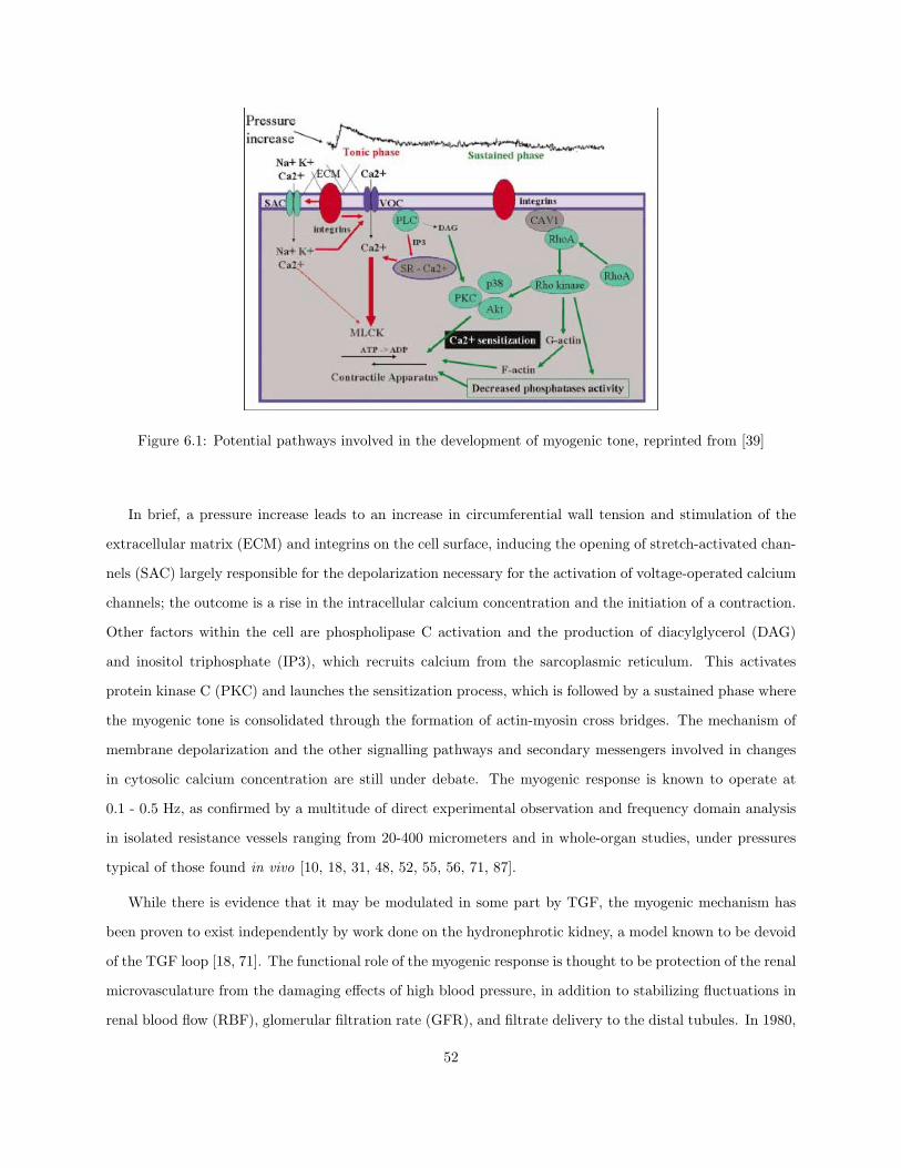
Figure 6.1: Potential pathways involved in the development of myogenic tone, reprinted from [39]
In brief, a pressure increase leads to an increase in circumferential wall tension and stimulation of the
extracellular matrix (ECM) and integrins on the cell surface, inducing the opening of stretch-activated chan-
nels (SAC) largely responsible for the depolarization necessary for the activation of voltage-operated calcium
channels; the outcome is a rise in the intracellular calcium concentration and the initiation of a contraction.
Other factors within the cell are phospholipase C activation and the production of diacylglycerol (DAG)
and inositol triphosphate (IP3), which recruits calcium from the sarcoplasmic reticulum. This activates
protein kinase C (PKC) and launches the sensitization process, which is followed by a sustained phase where
the myogenic tone is consolidated through the formation of actin-myosin cross bridges. The mechanism of
membrane depolarization and the other signalling pathways and secondary messengers involved in changes
in cytosolic calcium concentration are still under debate. The myogenic response is known to operate at
0.1 - 0.5 Hz, as confirmed by a multitude of direct experimental observation and frequency domain analysis
in isolated resistance vessels ranging from 20-400 micrometers and in whole-organ studies, under pressures
typical of those found in vivo [10, 18, 31, 48, 52, 55, 56, 71, 87].
While there is evidence that it may be modulated in some part by TGF, the myogenic mechanism has
been proven to exist independently by work done on the hydronephrotic kidney, a model known to be devoid
of the TGF loop [18, 71]. The functional role of the myogenic response is thought to be protection of the renal
microvasculature from the damaging effects of high blood pressure, in addition to stabilizing fluctuations in
renal blood flow (RBF), glomerular filtration rate (GFR), and filtrate delivery to the distal tubules. In 1980,
52
Johnson was the first to argue the possibility that myogenic constriction in proximal vessels of a vascular bed
could limit the pressure elevations transmitted downstream to the smaller, distal vessels [53]. Although the
resistance of the renal vasculature is known to be predominantly distal in nature, it is not confined simply to
the afferent arterioles, the feed vessels for the nephrons, as is evidenced by the large body of aforementioned
work showing active myogenic constriction in vessels up to 400 µm in diameter. Therefore, the hypothesis
presented here is that myogenic activation, via the maintenance of basal tone in larger arteries as well as
active constriction in smaller arterioles, exerts its influence throughout the arterial structure of the kidney
to facilitate autoregulation.
There are numerous mathematical and dynamical models of the myogenic response [15, 16, 70, 71, 73, 81],
but this is the first that has attempted to encompass the entire renal vasculature. In vivo, the myogenic
mechanism does not act in isolation, but rather interacts in a complex way with several other processes, such
as TGF and cardiac and respiratory oscillations. However, in order to facilitate a clear modelling focus on
the myogenic response, these confounding factors are, at this stage, neglected and a constant mean arterial
pressure is used as the relevant input variable. Only when the myogenic model has been fully investigated
and validated can the effects of including these other factors be systematically addressed. The recently
published model for isolated vessels by Carlson and Secomb in 2005 [9] uses circumferential wall tension as
the variable determining the level of VSM tone, and this provides the basic framework for the expanded
model presented in the current study. Other factors included in the system are the effects of flow-induced
dilation via nitric oxide (NO) production, viscosity variation in the microvasculature, and the series coupling
of different levels of the renal vasculature.
6.2 Model Development
6.2.1 Arterial Tree Representation
The rat renal vasculature is modeled as twelve compartments in series, where the first eleven represent
the renal artery through to the distal afferent arteriole, each with unique myogenic and flow-dependent
properties. The compartment model of the arterial tree is similar in structure to that used for the coronary
circulation by Cornelissen et al [15, 16]. The resistances of the venules and capillaries are assumed to be
constant and are lumped together in the final compartment. The recently published morphological data of
Nordsletten et al [79] employ information from micro-computer tomography (CT) scans to divide the arterial
structure via a Strahler ordering scheme [104], an algorithm originally developed for stream ordering and
53

found to be highly applicable to vascular branching. An example of Strahler ordering is shown in Figure
6.2; this method is particularly suited for the kidney due to the complete lack of anastomotic connections
between vessels.
Figure 6.2: Strahler ordering, reprinted from [79]
Initially a 20 µm voxel resolution image was used to segment the arterial and venous trees, identifying
vessels down to 30 µm in radius, followed by the division of a renal subtree using a higher resolution 4 µm
voxel image. An iterative scheme was developed to integrate the two bodies of information and map the
entire topology of the renal vascular tree. A color-coded representation of the rat renal vasculature is shown
in Figure 6.3, divided by Strahler order. For further information regarding the reconstruction process and
its robustness quantification via error analysis, the reader is referred to [79].
The relevant radial, length, and connectivity data are shown in Table 1 with order 1 designated as the
renal artery and orders 10 and 11 the proximal and distal afferent arteriole respectively. Because this model
does not include the TGF system, the influence of the TGF on the distal afferent arteriole [96] is neglected
at present. Additionally, it has been shown that there exist interactions and coupling phenomena among
nephrons due to the TGF [74, 75], which have also been omitted to facilitate a clear focus on modeling and
an understanding of the myogenic response.
54

Figure 6.3: Rat renal vasculature color-coded by Strahler order, reprinted from [79]
Each compartment of the vasculature (i = 1, 2, ..., 11) is assumed to represent Ni vessels in parallel, with
average length Li and diameter di, with the constant resistance of the venous and capillary system lumped in
the eleventh compartment. Assumptions about bifurcational structure of the vascular tree are not necessary
in the sense that the number of vessels of order i+1 that originate from a given single vessel of order i
is unspecified; the important parameter is simply the total number of vessels in each order. The efferent
arteriole is also assumed to be part of the postglomerular vasculature in the most distal compartment. The
diameter values in Table 6.1 represent the anatomical diameters (d0i), defined as the passive value at a mean
arterial pressure (MAP) of 100 mmHg. Because of the existence of myogenic tone, and the ability of the
smaller vessels to constrict, the typical diameter values in vivo will be less than the anatomical diameters, and
55

Table 6.1: Renal arterial tree measurements [79].
Order Anatomical Diameter Std Dev Vessel Length Std Dev No. of Elements Std Devµm µm mm mm
1 432.20 4.74 0.185 − 1 −2 384.84 17.79 1.440 0.647 3 −3 279.66 20.11 8.975 1.331 6 −4 172.30 24.06 2.516 2.053 24 15 107.74 12.51 1.031 0.674 90 66 88.46 9.81 0.511 0.000 247 237 78.58 1.08 1.001 0.216 578 718 59.74 0.35 0.656 0.286 1,245 1989 40.12 6.90 0.404 0.390 4,373 66410 27.80 3.80 0.423 0.283 13,070 2,29311 20.16 0.14 0.312 0.285 29,566 5,965
are dependent on the hemodynamic properties of flow and pressure in the vessel. The Poiseuille relationship
between pressure, flow, and resistance is applied throughout the renal vasculature, leading to the expression:
Ri =128ηiLi
Niπd4i
(6.1)
The subscript i refers to the vascular order, and ηi is the viscosity of the perfusate, which varies throughout
the vasculature and exhibits diameter dependence. In accordance with the Fahraeus-Lindqvist effect, effective
viscosity decreases with decreasing vessel diameter to a certain point. However, in the microvasculature,
consisting of vessel diameters below 30 µm, the effective viscosity begins to increase again, providing a
profound impact on the magnitude of resistance changes due to constriction. The work of Pries et al.
[90, 91] in the rat mesentery vasculature observed this effect and produced an expression for in vivo viscosity
variation, shown in Eqn 6.2.
ηi =
[1 +
(6e−0.085di + 2.2− 2.44e−0.06d0.645
i
)( di
di − 1.1
)2](
di
di − 1.1
)2
(6.2)
Here ηi is the viscosity, with units of cP, and di is the diameter in micrometers. This equation assumes an
invariant systemic hematocrit of 45% and was developed using an approach combining novel experimental
methods for the measurement of hematocrit and flow velocity in vessel segments of large microvascular
networks and theoretical blood flow simulations through these networks based on experimentally determined
architecture. For further details the reader is referred to [91]. The resistance of each unit varies as a function
of the diameter and the viscosity, which is diameter-dependent itself. The local pressure Pi within each vessel
order is taken to be the mean of the inlet (Pin,i) and outlet (Pin,i+1) pressures, where the outlet pressure
56

of the twelfth compartment is kept at the constant venous pressure (Pven) of 5 mmHg. It is assumed that
the local pressure is steady (with the input pressure to Strahler order 1 being determined by MAP), with
pressure variations arising from the cardiac cycle being ignored. The volumetric flow rate Qi through each
compartment is dependent on the pressure and resistance. We thus have the following,
Pi = Pin,i+Pin,i+12 for i = 1, 2, ..., 11 (6.3)
Qi = Pin,i−Pin,i+1Ri
for i = 1, 2, ..., 11 (6.4)
Q11 = Pin,11−Pven
R11. (6.5)
The representation of the pre-glomerular arterial tree corresponds to a distally dominant resistance
distribution, with the highest active contributions localized to the arterioles, as shown in Figure 6.4. The
resistance of the most distal compartment, representing the capillaries and veins, is determined by applying
a normal glomerular pressure of 60 mmHg in the rat at a typical MAP of 120 mmHg [30], and is not subject
to variation. Given the inlet and outlet values, local pressures for each Strahler order can be easily calculated
from the condition that the flow in all orders must be the same.
Figure 6.4: Distally dominant resistance distribution: rat renal vasculature at MAP of 100 mmHg.
57

6.2.2 Vessel Model
Autoregulation is achieved by virtue of the capacity for change of resistance vessels, with the strongest
responses localized to small arterioles, but with a measurable contribution provided by the more proximal
large arterioles and small arteries [14, 19, 30, 66]. This occurs via dilation or constriction in response to
alterations in blood pressure, which incite changes in circumferential wall tension. The active myogenic
response closely follows an initial passive distension, as has been observed in a multitude of experimental
studies [10, 18, 31, 48, 52, 55, 56, 71, 87, 106, 116, 121].
The vessel wall can therefore be treated as a nonlinear spring and contractile unit in parallel as was
done in [9], representing the passive and active components of the myogenic response respectively (see also
[21, 71, 81, 95, 100]). Passive tension, Tpass, is dependent on inherent properties of the vessel wall, primarily
distensibility, while active tension only develops due to the activation of the VSM cells, and is represented
as the maximal active tension, Tmaxact , that can possibly be generated at a given circumference multiplied by
φMR, the degree of VSM activation, also referred to as myogenic tone. This leads to an expression for total
wall tension, Ttot,
Ttoti = Tpassi + φMRiTmaxacti
. (6.6)
Throughout the system, the subscript i refers to the particular Strahler order (i = 1, 2, ..., 11) of the
vascular tree, as all the parameters are unique for each level. As has been demonstrated in experimental
length-tension studies, passive tension increases nonlinearly and quite rapidly at high levels of circumferential
stretch [9, 20, 65, 66, 70], leading to the following exponential form,
Tpassi= Cpi
eC′
pi(
did0i
−1), (6.7)
where the diameter di is normalized with respect to the anatomical diameter d0i, Cpi
is the passive
tension at d0i and C ′pi
is a parameter determining the slope of the exponential curve. Total maximal tension
is quantified in length-tension studies by bathing vessels in maximally activating physiological salt solutions
[21]. The maximally active component of tension is found by subtracting the passive component from the
total, and has been shown to follow a Gaussian shaped curve [9] of the form
Tmaxacti
= Caie−
did0i
−C′ai
C′′ai
2
, (6.8)
58

where Cai is the peak magnitude of maximal active tension, C ′ai
is the relative peak location, and C ′′ai
is
the relative curve width. The Gaussian distribution signifies that active tension is at a maximum at a certain
circumferential length, and decreases symmetrically due to an increase or decrease in diameter. Equation 6.8
assumes full VSM activation, and is directly related to the size of the vessel (via Cai), as the wall thickness
and hence the number and/or size of force-generating smooth muscle cells increases with increasing diameter.
The dependence on the diameter di dictates where along the Gaussian curve the maximally active tension
value lies at that moment, while the contribution to the system is determined by the level of VSM tone,
φMRi. C ′
aiand C ′′
aiare dimensionless parameters that were found to not vary significantly over a wide range
of vessel diameters [9], and therefore for our purposes were assumed to be the same for all i. Determination
of all other parameters was dependent on the Strahler order to which they apply, and is addressed in detail
further on.
6.2.3 Effect of NO
While blood pressure is the primary myogenic stimulus, flow-induced dilation modulated by shear stress and
endothelial nitric oxide synthase (eNOS) production has been shown to attenuate increases in VSM tone
[39, 54, 57, 65, 66, 89, 120]. Furthermore, basal arterial tone is the result of a balance between myogenic
activation and continuously synthesized nitric oxide (NO) released from the endothelium, thought to be
particularly crucial in large resistance vessels [27, 88, 112]. Figure 6.5 shows the hypothesized relationship
between the vasodilatory effects of NO and myogenic vasconstriction to achieve an equilibrium diameter.
A crucial stimulus of NO release is haemodynamic shear stress on the endothelium [54, 65, 66, 112] causing
direct phosphorylation leading to mechanical eNOS activation, and more long-term production via eNOS
gene transcription. Shear stress for each compartment per unit vessel was calculated using the following
equation [6, 63]:
τi =32Qiηi
πNid3i
. (6.9)
As shown in Fig 6.5, NO activates guanylate cyclase in VSM cells to synthesize cyclic guanosine-3,5-
monophosphate (cGMP) which results in several biological effects [29, 112], in this case the most relevant
being a reduction in vascular tone via dilation. The activation factor, φNO, of this potent vasodilator has a
sigmoidal dependence on shear stress [11], ranging from 0, inactive, to 1, fully active eNOS production:
59

Figure 6.5: Blood pressure and shear stress are mechanical stimuli acting on smooth muscle (SMC) andendothelial cells (EC) respectively to achieve basal tone in resistance arteries. Reprinted from [39]
φNOi=
11 + e−(CNOτi−C′
NO). (6.10)
This phenomenological expression for eNOS, and subsequently NO, activation cannot be directly phys-
iologically quantified. However, it provides a tool for representing the effect of nitric oxide on the VSM
cells. CNO and C ′NO are parameters which determine the characteristics of the shear stress dependence for
each vascular level. Smith, Moore, and Layton [103] used a similar approach to model the effects of NO on
myogenic reactivity, via a sigmoidal relationship between concentration and percentage relaxation.
6.2.4 VSM activation
An analogous expression for the level of VSM activation, or myogenic tone, allows for the incorporation of
NO-mediated dilatory effects into the system. Experimental data on renal vessels have shown the major
effect of NO to be a decrease in sensitivity of the contractile mechanism [88, 111]. Therefore, while the steady
state myogenic activation factor for each vessel order, φMRssi, has a sigmoidal dependence on circumferential
wall tension [9, 116], the slope of this curve, and hence the sensitivity of the dependence, is directly affected
by the level of NO activation:
φMRssi=
1
1 + e−(
CtiTtoti
1+giφNOi−C′
ti). (6.11)
60

An example of the effect of eNOS activation on the relationship between φMRss and wall tension for vessel
order i = 6 (danat=88 µm) is shown in Figure 6.6. As φNO ranges from virtually inactive (0.01) to partially
active (0.5) to fully active (1), the rightward shift of the curve and decrease in slope represent a marked
reduction in sensitivity of the contractile apparatus; stated a different way, a significantly greater increase
in circumferential wall tension is required to elicit a corresponding change in VSM activation and vascular
tone. The parameter gi is also order-specific, ranges from 0.2 to 1, and represents the relative influence of
eNOS activation, a direct consequence of the varying responsiveness to flow throughout the arterial tree. A
g value of 1 allows for a potential halving in sensitivity of the contractile mechanism, as is the case in Figure
6.6.
Figure 6.6: Effect of NO activation on relationship between φMRss and Ttot. (Legend: “NO” is φNO)
At a given arterial pressure, the diameter at each level of the renal vasculature adjusts to achieve a
balance between actual tension, as determined by the law of Laplace, and the summation of the passive and
active components (Eqn 6.6), leading to the following expression:
TLap =Pidi
2= Cpi
eC′
pi(
did0i
−1)+ φMRi
Caie−
did0i
−C′ai
C′′ai
2
. (6.12)
This diameter response depends on the viscosity and inertia of the blood, the vessel wall, and the
surrounding tissue, and is taken to be instantaneous, as the time constant has been shown to be negligible
compared to that involved in the development of active tension in the VSM cells [21]. To model the dynamic
61

behaviour of the network, the actual VSM activation is treated as a time-dependent variable and satisfies
the first order dynamic equation:
dφMRi
dt=
1tai
(φMRssi − φMRi). (6.13)
This equation represents the physiological phenomenon of a reverting system, where the relationship
between wall tension and φMRssihas been well-characterized experimentally, and the rate of change of VSM
activation depends upon the time constant tai , which varies throughout the vasculature based on the size
of the vessel and the number of force-generating smooth muscle cells. This system functions such that wall
tension is controlled by a negative feedback mechanism [53]. An increase in tension due to a pressure jump
elicits an increase in tone and a reduction in diameter, which in turn causes a decrease in wall tension by the
law of Laplace. In addition, due to the pressure increase, flow increases, resulting in greater shear stress and
eNOS activation, which modulates the diameter response. The reverse holds true in response to a decrease
in mean arterial pressure, effecting a delicate balance between myogenic and dilatory responses. A control
diagram of the mathematical system is shown in Figure 6.7.
Figure 6.7: Schematic representation of renal myogenic autoregulation system.
There are several simplifying assumptions and mathematical modeling choices that have been made
in this system. Laplace’s law is applicable to thin-walled cylinders only, and is an oversimplification of the
mechanics involved in arterioles that actively constrict and dilate. Future work could include a more detailed
analytic solution for the wall stress. Additionally for the VSM sigmoidal response, a decrease in sensitivity
62

due to NO activation can also be expressed by simply shifting the curve to the right. However the current
method was chosen as the most physiologically realistic way of representing the presence of NO in the system,
based on work done by [113] showing that the TGF response curve becomes less steep as NO concentration
increases.
6.3 Parameter Determination
For the eleven Strahler orders that represent the renal arterial tree to the distal afferent arteriole, the
parameters that determine the passive and active vessel responses to stimuli such as pressure, flow, wall
tension, and shear stress are: Cpi , C′pi
, Cai , C′ai
, C ′′ai
, Cti , C′ti
, CNOi , C′NOi
, gi, and tai . A literature review of
the relevant experimental papers from the last 50 years provided pressure response data on renal vessels
ranging in diameter from 15 µm to 500 µm [10, 28, 31, 37, 48, 52, 54, 55, 56, 57, 71, 87, 91, 95, 106, 121],
which were used to estimate the corresponding parameters for each vascular level. When possible, preferential
consideration was given to data obtained in vivo as opposed to in vitro, from rats rather than dogs, rabbits,
or other animals, and from untreated vessels under free-flow conditions. This is because the anatomical
data upon which the model is based is from a rat kidney, and the model attempts to simulate the healthy
autoregulatory function of the rat kidney in vivo. Data used in the parameter estimation process are shown
in Appendix B.
For each vascular order (i = 1, 2, ..., 11) passive tension at di = d0i, evaluated at 100 mmHg using
Laplace’s law, yields Cpi . Mean arterial pressure was applied to the system at the level of the renal artery,
and the subsequent pressure drops over each vascular order calculated to yield the corresponding values for
Cpi. The parameter characterizing the exponential relationship between diameter and passive tension, C ′
pi,
was estimated based on the work of Liao and Kuo [65, 70] and Cornelissen et al [15, 16] in the coronary
vasculature. Their passive pressure-diameter relationship, shown below, was based on empirical data from
arteries that fall into the range of d0 = 70 − 200µm, encompassing intermediate and large arterioles and
small arteries:
dpassi = d0i
(0.705 + 0.363
Pi
22.7 + Pi
). (6.14)
Tension was computed via Laplace’s law and plotted against the ratio of the passive and anatomical
diameters. They found that the distribution of data points fits an exponential curve with a value of 14.87
for the coefficient in the argument of the exponential [65, 70]. Referring to Eqn 6.7, this value for C ′pi
63

was applied to the Strahler orders within that range of diameters: i = 4, 5, 6, 7. This representation of the
steepness of the passive response curve, which provides an indication of the distensibility of the vessel, has
been shown to exhibit a negative trend in response to increasing diameter [9]. For this reason, a slightly
smaller value was assigned to the first three orders, representing the feeding renal and interlobar arteries,
and similarly, increasing values assigned to the smaller arterioles. These passive parameter values showed
good agreement to pressure-diameter data obtained from wire myograph studies.
The active parameters, Cai, C ′
ai, C ′′
ai, Cti
, and C ′ti
were determined for best fit to the available active
pressure data as follows. The parameters for peak location, C ′ai
, and range, C ′′ai
, of force generation were
found not to exhibit significant dependence on reference diameter, and were thus taken to be the same for
all vessel orders [9]. However, Caiexhibited significant variation over the orders due to the wide range of
tension values throughout the vasculature. This peak value was defined as the tension present at the upper
limit of autoregulation, when φMR = 1, di = C ′ai
d0i, and P = 180 mmHg, found by computing the total
tension and subtracting the passive component. Various studies [18, 19, 20, 121] have shown that this mean
arterial pressure value approximates the upper bound of the autoregulatory range, and therefore corresponds
to the maximum active tension possible. In contrast to the parameter determination for the passive behavior,
this maximum pressure was applied uniformly at each Strahler order, rather than the renal artery, as this
more accurately represents the experimental scenarios where the vessel is bathed in a maximally activating
solution and forced to contract, providing active tension data.
The active data from [10, 31, 37, 48, 52, 54, 121] were subsequently examined to determine the shape
and position of the sigmoidal dependence between tension and VSM activation, providing values for Ctiand
C ′ti
. An iterative bisection method was used for each Strahler order to determine the sigmoidal relationships
between φMRssand Ttot that, when incorporated into the mathematical system, minimized the error in
vessel diameter responses between the model predictions and the experimental results. These active data
also produced values for the time constant of VSM activation, tai , which shows a positive trend in response
to increasing diameter. This means that the larger the artery, and hence the thicker the wall, the longer
the delay in development of active tension. In addition, the parameter data from the model of Carlson and
Secomb [9] provided guidelines and a more comprehensive overview of the varying smooth muscle response
in vessels of differing sizes and species.
The same procedure was followed using the available data on flow-dependent dilation [6, 27, 40, 54, 57, 63,
65, 66, 70, 88, 89, 120] to determine the relationship between flow, shear stress, and eNOS activation, φNOi.
The parameters CNOi and C ′NOi
were estimated for the optimal fit to the data, by firstly determining the
64
range of shear stress values experienced by each vessel, and that value which would correspond to φNOi = 0.5.
Again, an iterative method was used to adjust CNOiand C ′
NOito obtain the sigmoidal dependencies between
shear stress and eNOS activation for each vascular order that minimized the deviation between simulated and
experimental diameter responses. The parameters were also evaluated in accordance with the observation
that, for the majority of vascular levels, the magnitude of flow-induced dilation is usually highest at resting
levels of vascular tone [88], highlighting the important contribution of this mechanism to the balance that
maintains resting diameter. This influence of φNOi on the sensitivity of the contractile mechanism is governed
by the gain gi, which varies between 0 and 1 and is assigned based on the relative responsiveness to flow of
arteries and arterioles of differing diameters [65, 66, 102].
6.4 Numerical Methods
The system encompassed by Equations 6.1−6.5 and 6.9−6.13 was solved using the math software package
MATLAB. A user-written first-order temporal finite differencing scheme with step size of 0.01 s was used,
combined with inner iterations to fulfill convergence criteria. For each Strahler order at every time step, the
instantaneous diameter response was evaluated using Eqn 6.12 within an inner while loop for a given level
of VSM activation, φMRi. The time dynamics are incorporated via Eqns 6.11 and 6.13, as the activation
for each order adjusts over varying time scales to the steady-state value for a given circumferential tension,
Ttoti, and eNOS activation level, φNOi
. Finally, in the outermost loop, the resistance values are adjusted
based on the changes in diameter and subsequent compartmental pressures are calculated, as well as the
overall renal blood flow.
To determine the steady-state response of the system, the procedure described above was allowed to
reach a steady-state renal blood flow value for a wide range of arterial pressures. Convergence criteria were
firstly based on achieving a balance between Laplacian and actual circumferential wall tension, and secondly
on the flow in all compartments being equal, both with a tolerance of 10−6. This convergence was typically
achieved in less than 10, 000 iterations for each pressure input. The numerical simulations were performed
on a desktop PC with a 2.2 GHz AMD Athlon 64 processor, and were completed in under 2 minutes per
simulation. The MATLAB script is contained in Appendix F.
65

66

Chapter 7
Renal Myogenic Model Results
The mathematical model of the myogenic mechanism in the rat kidney was developed to include order-
specific parameters that mimic the response of each level of the arterial tree. The system was subjected
to computer simulations of pressure perturbations in the form of step increases. The dynamic response is
examined, as well as the steady state flow-pressure relationship over the physiological pressure range.
7.1 Model Parameters
The values for the eleven parameters that govern the system, specific to each of the eleven Strahler orders,
are shown in Table 7.1.
Table 7.1: Model parameters for rat renal vasculatureOrder Anatomical Diameter Cp C ′
p Ca C ′a C ′′
a Ct C ′t CNO C ′
NO g taµm N/m N/m m/N m2/N s
1 432.20 2.88 10 3.55 0.91 0.374 1.06 1.33 0.95 16.20 0.2 452 384.84 2.53 10 3.14 0.91 0.374 1.95 2.16 0.87 5.48 0.45 403 279.66 1.77 10 2.34 0.91 0.374 5.40 3.49 0.71 6.25 0.7 354 172.30 1.02 14.87 1.61 0.91 0.374 15.74 4.72 0.43 4.90 1.0 305 107.74 0.62 14.87 1.02 0.91 0.374 26.94 4.71 0.34 4.87 1.0 256 88.46 0.49 14.87 0.83 0.91 0.374 31.87 4.78 0.47 3.89 1.0 207 78.58 0.43 14.87 0.74 0.91 0.374 32.93 4.68 0.72 3.26 0.9 158 59.74 0.33 18.5 0.59 0.91 0.374 35.28 4.03 0.81 3.21 0.75 109 40.12 0.21 21 0.40 0.91 0.374 38.15 3.34 0.89 4.05 0.6 510 27.80 0.15 25 0.29 0.91 0.374 54.56 2.64 0.92 6.41 0.5 211 20.16 0.10 28 0.21 0.91 0.374 67.92 2.91 0.93 7.57 0.4 1.8
The passive tension at a MAP of 100 mmHg was calculated according to the law of Laplace, beginning
67

in the renal artery. The baseline resistance of the branching structure of the pre-afferent arteriole renal
vasculature (i = 1, 2, ..., 9) was calculated using Equation 6.1 and the reported anatomical diameters for each
order. At a MAP of 100 mmHg, the first nine Strahler orders account for a pressure drop of 19.1 mmHg,
corresponding to an inlet pressure of 80.9 mmHg at the proximal afferent arteriole in this passive state. The
parameters Cp and C ′p show acceptable agreement with passive data for various arterial sizes [7, 65, 66, 70].
An example is shown in Fig 7.1, where data were obtained from Bund et al [7] on femoral arterioles with
passive diameters equivalent to renal vascular order i = 4 (d0=172 µm). The minor discrepancies between
the model predictions and the data for smaller diameter values is likely due to the experimental protocol,
where passive conditions were simulated using a Ca2+-free solution. Here, the VSM activation is taken to be
zero, representing solely the passive component of wall tension. However, although the extracellular calcium
has been abolished, the contribution to VSM activation from intracellular calcium sources is neglected.
Therefore, the experimental values of passive tension at small diameters are slightly overestimated and most
likely represent a small active contribution as well.
Figure 7.1: Passive tension data [7] and model results, i = 4 (d0=172 µm)
An optimization procedure to determine best fit with active pressure data [10, 31, 37, 48, 52, 54, 121]
provided values for Cai , Cti , and C ′ti
. The peak magnitude of maximally active tension, Cai , was found
to exhibit a strong positive correlation with increasing diameter, due to the increased wall thickness and
therefore increased number of force-generating smooth muscle cells. The values of C ′ai
and C ′′ai
were deter-
mined by Carlson and Secomb [9] to be the averages obtained from length-tension experiments performed
on vessels from 50 µm to 300 µm in diameter, signifying that maximum active tension is reached at around
91% of the passive anatomical diameter. The parameter Cti , characterizing the dependence of vascular tone
68

on circumferential wall tension, showed an inverse relationship with diameter, exhibiting a strong increase
in smaller arterioles, while C ′ti
did not exhibit significant diameter dependence.
The vessels experiencing the most variable shear stresses were also the orders known to be most responsive
to flow, resulting in smaller CNOivalues for the small arteries and large arterioles. The sigmoidal dependence
on shear stress for each of the intermediate Strahler orders had a more gradual slope, and φNOi is capable of
changing over a larger range of shear stress values, as shown in Figure 7.2. The parameter C ′NOi
determines
the midpoint of the curve, and did not show significant correlation with diameter, depending instead on the
typical shear stress values for each level.
Figure 7.2: NO activation: dependence on shear stress for vascular orders: i = 2 (d0=385 µm), i = 5 (d0=108µm) and i = 9 (d0=40 µm).
The relationship between shear stress and φNOiis also determined by gi which varies from 1, allowing
for a halving in sensitivity of the contractile apparatus in the case of full eNOS activation, to 0.2, which only
permits up to a 16.7% decrease in sensitivity. The large arterioles most sensitive to changes in flow have
higher gi values, while those with diameters above and below this range have lower values. The parameter
determining the time constant of VSM activation, ta, has a positive correlation with diameter, also due to
the increase in wall thickness and variation in size and number of smooth muscle cells. The fastest responses
are seen in the higher Strahler orders corresponding to the interlobular arteries and afferent arterioles,
contributing to the distally dominant nature of the autoregulatory response.
Parameter sensitivity analysis was performed by varying each of the parameters individually within a
reasonable range and observing the change in outcome of the simulation. Those that could not be directly
calculated, and were therefore estimated based on the available data, were subject to the most variability and
69

exhibited the highest sensitivity. Specifically, changes in Cti , C′ti
, CNOi , and C ′NOi
had the greatest impact
on the system response.
7.2 Active Response
An example of the length-tension relationships for passive tension, maximally active tension, and total tension
are shown in Figure 7.3(a), as well as the active diameter response to step increases in pressure, for vascular
order i = 5 (d0=108 µm). The hysteresis behaviour is evident as the diameter initially behaves passively,
then readjusts as the VSM activation increases and causes constriction, resulting in a restabilization of blood
flow and a decrease in wall tension. As the pressure exceeds the autoregulatory range for the vessel and
VSM activation achieves a maximum value of 1, the diameter response follows the curve for total tension
with maximum activation. Under pressure of such magnitude, the isolated vessel is already fully activated
and begins to distend (Figure 7.3(b)).
(a) (b)
Figure 7.3: (a) Length-tension curves: Strahler order i = 5 (d0 = 108µm). Model results for passive (. . .),maximally active (- · -), and maximally active total tension (-). Also shown is active response to two pressurestep increases (5 → 85 → 165 mmHg.) (b) Diameter response of isolated vessel, i = 5 (d0 = 108µm), tosame pressure step increase. Location of pressure steps is circled on (a) and (b).
Extensive comparison with experimental data is difficult, as this system mimics the functioning of the
myogenic response in a fully intact kidney in vivo, without the influence of the TGF, a scenario that is
challenging to reproduce in the laboratory. Most available renal data are obtained in vitro or under sedation,
both factors that have a large influence on the dynamics and magnitude of the response. In addition, data
are often unattainable throughout the vasculature of the kidney, due to the difficulties that arise when
attempting to measure the response of intermediate vessels that are embedded in the tissue and are not
70

readily accessible. However, the limited data available show good preliminary agreement with the model
results, especially concerning the qualitative trends of the myogenic response. To obtain results that lend
themselves to comparison, the full model simulations were run and the diameter values recorded for one
particular Strahler order. In Figure 7.4, both the dynamic and the steady-state behavior of a single vessel
order in response to multiple pressure step increases are shown, and the steady-state values compared to
data from Takenaka et al [106]. This group examined the steady-state myogenic response of rat interlobular
arteries in the hydronephrotic kidney, a preparation known to be devoid of the TGF. Following the method
used by the experimentalists, the diameter values presented here were normalized with respect to the diameter
at a local pressure of 80 mmHg. To prevent bias, these and all other data used for experimental comparison
were not used in the parameter determination procedure.
Figure 7.4: (a) Dynamic myogenic response, model prediction. (b) Steady-state myogenic response of inter-mediate interlobular artery (i = 8, d0 = 60µm) to pressure step increase (80 → 120 → 160 mmHg.), modelprediction and data [106].
The time-dependent diameter responses of every level in the series organization of the renal vasculature
are shown in Figures 7.5(c) and 7.5(d), as well as the myogenic activation, shown in Figure 7.5(b), in
response to pressure step increases from 80 to 120 to 160 mmHg (inset, Fig 7.5(a)). Also shown is the partial
autoregulation of renal blood flow (Fig 7.5(a)), which initially spikes due to the step increase in pressure and
is restabilized via the myogenic response of the renal vasculature. Here the larger vessels, while maintaining
a certain level of tone, dilate in response to increases in pressure. The varying time scales are evident in the
graph, as larger vessels require more time for activation than the smaller arterioles. The passive distensive
response is taken to be instantaneous for all Strahler orders. Here it is assumed that the efferent arteriole is
part of the postglomerular vasculature in the most distal compartment containing the capillaries and veins
71

(a) (b)
(c) (d)
Figure 7.5: (a) Renal blood flow response exhibiting partial autoregulation (inset: mean arterial pressure stepincreases) (b) Changes in VSM activation (c) Diameter response to pressure steps (i = 1..4) (d) Diameterresponse to pressure steps (i = 5..11). Note: In (b),(c), (d), i increases from top to bottom
as well. The resistance of this compartment is determined by applying a normal glomerular pressure of 60
mmHg in the rat at a typical MAP of 120 mmHg [30], and is not subject to variation. There is a great
deal of controversy concerning the relative contribution of the efferent arteriole to overall resistance change,
and it is generally accepted that the afferent arteriole has a significantly greater impact in flow regulation
[26]. However, it has been shown recently that the efferent arteriole receives a TGF signal as well that
is complementary to that received by the afferent arteriole [93], meaning that when the afferent arteriole
constricts the efferent arteriole dilates, and vice versa. This is an effect that could be incorporated in future
work on this model.
72

7.3 Steady-State Whole-Organ Response
A significant result of the model simulations is the overall renal autoregulation curve, demonstrating the
ability of the kidney to stabilize renal blood flow under a wide range of mean arterial pressures. A fully
functioning, healthy, intact kidney would produce a waveform similar to the idealised curve shown in Figure
7.6(a). However, one would expect less than perfect autoregulation from a system that solely exhibits a
myogenic response, as shown in Figure 7.6(b). Pires et al [87] performed experiments to determine sponta-
neous renal blood flow autoregulation curves in conscious sinoaortic baroreceptor-denervated rats, inhibit-
ing the TGF with furosemide. This is known to cause near-complete suppression of the TGF response
[55, 57, 87, 101, 103, 120].
(a) (b)
Figure 7.6: (a) Idealized autoregulatory curve: complete renal autoregulation (b) Myogenic renal autoregu-latory response: comparison of model results with experimental data from [87].
The reported flow data for both the experimental and the model results have been normalized with
respect to the flow value at a MAP of 70 mmHg to facilitate comparison. Both curves show a non-zero
gradient within the autoregulatory range that is qualitatively similar. The percentage difference between
model predictions and experimental data ranges from 0.38% at 100 mmHg, to 4.06% at 120 mmHg, with
data for all other pressure values falling within this range of deviation. These differences fall well within
the reported bounds of experimental error, and the simulated model results are therefore judged to be in
close agreement with these experimental data, which are a representation of the autoregulatory mechanism
resulting from a uniquely myogenic response.
73

7.4 Inclusion of NO
Pressure induced increases in VSM tone are attenuated by flow-induced dilation, which is modulated by shear
stress and eNOS production of nitric oxide, as has been shown by many experimental groups [39, 54, 57, 65,
66, 89, 120]. In addition, the basal tone of the vessels is the result of a balance between myogenic activation
and continuously synthesized NO released from the endothelium, an effect which is thought to be particularly
crucial in large resistance vessels [27, 88, 112]. NO signalling activates guanylate cyclase in VSM cells to
synthesize cyclic guanosine-3,5-monophosphate (cGMP) which results in a reduction in vascular tone via
dilation [29, 112]. It is also important to note that shear stress has been shown to cause the release of other
prostaglandins via the endothelium, which have a similar dilatory effect on the vessels [45, 105]. Therefore,
in this system it can be assumed that the parameter for NO activation, φNO, effectively encompasses all
endothelium derived dilatory factors whose production is induced by shear stress.
The necessity of including the effects of nitric oxide is demonstrated by the diameter response of an
isolated vessel, i = 4, d0 = 172µm, shown with (Fig 7.7(a)) and without (Fig 7.7(b)) the inclusion of shear
stress induced eNOS production and subsequent NO-mediated dilation, via Eqns 6.9 - 6.11. Pressure was
increased in 20 mmHg increments from 40 mmHg to 100 mmHg. Holding the parameter φNO to zero
mimics the suppression of eNOS activation; in an experimental scenario this is achieved with an inhibitor of
nitric oxide synthase such as N(G)-nitro-L-arginine methyl ester (L-NAME). Strahler order 4 was chosen for
illustrative purposes as it is within the range of vessels that exhibit the greatest responsiveness to changes
in shear stress [65, 66, 70]. The qualitative nature of the differing response between eNOS activation and
suppression is representative of that for all orders, though the quantitative difference is smaller for other
orders.
When nitric oxide synthase was inhibited, the baseline diameter of the vessel showed a marked decrease,
indicating a significant contribution of NO to resting vascular tone. Additionally, in response to increases
in mean arterial pressure the artery exhibited sustained tone and constriction until the VSM cells were fully
active and the vessel was forced to dilate in response to continued pressure increases. In contrast, the complete
system including the effects of NO behaved as one would expect for this portion of the physiological range of
blood pressure. Examining the steady-state values, the vessel initially dilated by 2.9% as MAP approaches
typical resting values and finally constricted by 4.1% as pressure continues to rise.
74

(a) (b)
Figure 7.7: Effect of NO release in mathematical model: (a) Including NO: diameter response, i = 4, d0 =172µm, to multiple pressure step increases (b)Inhibiting NO: diameter response, i = 4, d0 = 172µm, tomultiple pressure step increases (40 → 60 → 80 → 100 mmHg.)
7.5 Discussion of Myogenic Model Results
Modeling the myogenic response throughout the kidney demonstrates the necessity of considering the entire
vasculature when examining renal autoregulation. Although the capacity for resistance change, and therefore
impact on blood flow stabilization, is greatest in the small vessels, it is not solely confined to the afferent
arterioles as many models assume [71, 81, 95]. The lower-order vessels with larger diameters are not capable
of constriction, however they maintain a level of vascular tone which is required in a comprehensive renal
model. Ultimately a representation of whole-organ autoregulation will allow for extrapolation from normal
baseline conditions to pathological scenarios, as is discussed in Chapter 10.
7.5.1 Dynamic Response
The theoretical model for the myogenic response in an isolated vessel based on length-tension characteristics
of vascular smooth muscle presented by Carlson and Secomb in 2005 [9] was designed to provide a foundation
upon which to build a more comprehensive model of autoregulation, such as the current whole-organ renal
model. The close fit of experimental data to our model supports the hypothesis that circumferential wall
tension is the primary factor governing VSM activation, and expands upon this to account for modulation by
nitric oxide and viscosity variation in the microvasculature. Furthermore, the results are consistent with the
well-established proposal that flow, and subsequently shear stress, are important variables that cause eNOS
activation and NO production, resulting in indirect dilation via a reduction in sensitivity of the contractile
75

apparatus.
The passive behavior of the vessels is well represented by the mathematical model, as shown in Figure
7.1, when taking into account the slight overestimation of the experimental values of passive tension at small
diameters due to the intracellular calcium contribution. The development of active tension in the VSM cells
follows a different time course for each Strahler order. At normal physiological values, the lower orders are
already significantly active and exist in a state of partial constriction [20, 41]. In response to an increase
in pressure these larger vessels cannot change as drastically or as quickly as the smaller vessels, represented
by the higher Strahler orders. Examining the diameter response to step increases in pressure throughout
the vasculature reveals that the larger arteries are ultimately only capable of dilating, and thus decreasing
resistance, in response to increased pressure, while the smaller arterioles exhibit active myogenic constriction
and are responsible for partially stabilizing renal blood flow. However, all the vessels exhibit varying degrees
of myogenic reactivity via the maintenance of vascular tone, without which the diameter response would be
a purely passive distension.
Model results for inhibition of NO in an isolated vessel presented in Figure 7.7(b) demonstrate the
exaggerated constrictor response of the vessel that is also seen experimentally [29, 57, 111]. The response
was examined, and contrasted to one which includes nitric oxide, over the lower part of the physiological
pressure range (40 → 100 mmHg), as this is where nitric oxide concentration will vary most due to the large
dependence of shear stress on diameter. The diameter changes most significantly over this segment of the
pressure spectrum, producing the most variable shear stress and eNOS production.
The sigmoidal dependence between wall tension and VSM activation, and additionally between shear
stress and eNOS activation, is at the heart of the behaviour of the resistance vessels, and provides a phys-
iologically based model of the autoregulatory response. The nature of the chemical cascade occurring in
vascular smooth muscle is such that there exist lower and upper bounds of myogenic activation, between
which there is a smooth transition whose characteristics depend on the physical attributes of the vessel and
the availability of calcium, nitric oxide, and other ions. The present model shows that a sigmoidal variation
in myogenic tone as a function of wall tension is consistent with the myogenic responses of a wide range of
vessels observed experimentally. Similarly, fluid shear stress is known to be one of the most important stimuli
with regard to nitric oxide production. The relationship between eNOS activation and shear stress follows
the same sort of sigmoidal curve, as has been shown previously [1, 63]. This negative feedback mechanism
to induce dilation reduces shear stress levels, preventing additional energy expenditure and work for the
cardiovascular system.
76

7.5.2 Whole-Organ Autoregulation
The system exhibits partial autoregulation over a wide range of pressures (Fig 7.6(b)), with a nonzero gradient
of flow with respect to pressure in the autoregulatory range due to the omission of TGF and other potentially
influential factors from the model. This result corresponds well to data from the experimental scenario that
most closely simulates the condition of purely myogenic renal autoregulation [87]. To prevent bias, this data
set was not used to determine the parameters used in the mathematical system. The range of autoregulation
was from 70 to 150 mmHg for the model results; the experimental data appears to follow the same trend,
although this observation is limited by the lack of data for pressures greater than 120 mmHg. The closeness
of fit between experimental observations and model predictions suggests that nitric oxide may be one of the
most important metabolites to consider when examining renal autoregulation. Another possibility is that
the term φNO, taken here to be eNOS activation, actually encompasses the effects of prostaglandins and
endothelium-derived hyperpolarizing factor as well. Both have been shown to be stimulated and released
by changes in flow and shear stress [63], the key variables in Eqns 6.9 and 6.10, and both influence renal
autoregulation in the intact rat kidney in vitro [34]. Renal nitric oxide production is also known to be
severely affected in the early stages of diabetes mellitus and diabetic nephropathy [60, 61], as well as acute
renal failure [33]. Hence, a comprehensive model of autoregulation capable of representing diseased states
requires this crucial component.
The autoregulatory range exhibited by the model appears to be shifted toward the lower end of that seen
in perfect autoregulation. Additionally, the active higher order vessels exhibit over-constriction following
the passive distensive response(Fig 7.5(d)), in contrast to the lower order arteries with larger diameters.
This trend corresponds well with experimental observation [56, 57, 101, 120, 121], and the dynamics of
the response will also become more complex with the inclusion of oscillations induced by the cardiac and
respiratory cycles and by the TGF. The existing behavior is due to interaction between flow-induced dilation,
pressure-induced constriction, and (to a lesser extent) resistance change due to viscosity variation.
7.5.3 Myogenic Model Summary
The complexity of vascular regulation necessitates that the principal mechanisms be identified and modelled
to a level that will facilitate a more holistic approach. In this initial part of the model, the focus lies on the
pressure-induced myogenic response via VSM activation and the flow-induced dilation via eNOS activation.
The model results demonstrate good agreement with available experimental data, and provides a valuable tool
for examining the whole-organ myogenic response in the rat kidney. Pressure-induced myogenic activation
77

functions in conjunction with changes in viscosity and flow-induced dilation to partially autoregulate renal
blood flow. Differential myogenic and shear stress responsiveness throughout the renal circulation allow the
mathematical model to accurately mimic the pressure and flow-induced changes in the vasculature responsible
for maintaining a relatively constant level of blood flow to the kidney. The obvious extension to the model
is now the inclusion of the major autoregulatory mechanism unique to the kidney, the tubuloglomerular
feedback mechanism, addressed in detail in the following chapters.
78

Chapter 8
Incorporating a Mathematical Model
of the TGF Mechanism
8.1 Introduction
Autoregulation in the kidney is unique because both blood flow and glomerular filtration rate (GFR) are
simultaneously regulated by at least two inputs, the tubuloglomerular feedback (TGF) loop which monitors
sodium chloride (NaCl) delivery and filtration rate and adjusts afferent arteriolar resistance accordingly, and
the pressure-induced myogenic response which is present to varying degrees of strength throughout the renal
vasculature and has been modelled as such. The entire autoregulatory process of sensation, transduction, and
actuation is localized within the kidney, independent of any central neural or hormonal control [17]. Together,
these two mechanisms account for over 90% percent of steady state renal autoregulation, with approximately
equal contributions attributed to the myogenic and TGF components [55, 56, 71], highlighting the necessity
of including them both in a holistic model of regulation in the kidney.
TGF depends on the unique tubular structure of the nephrons and the ability of specialized macula densa
cells to sense changes in the Na+ and Cl− concentrations in the distal loops of Henle. The juxtaglomerular
apparatus (JGA) is the site of close physical proximity between the macula densa, located at the distal thick
ascending limb of the loop of Henle, and the vascular pole of the corresponding glomerulus. Changes in
tubular fluid flux of these specific ions through the Na+-K+/2Cl− (NKCC2) cotransporter on the luminal
surface of the macula densa cells elicit alterations in vascular tone of the afferent arteriole that produce
reciprocal changes in glomerular filtration rate. This stabilizes distal fluid and electrolyte delivery and
79
maintains the balance between GFR and tubular reabsorption [26]. Due to the tubular transit time and the
delay associated with signaling through the JGA, the TGF mechanism is much slower than the myogenic
response and operates within the frequency range of 0.03-0.06 Hz [42, 43, 69, 113]. The TGF model of
autoregulation presented here consists of three coupled sub-models: the glomerular model, the tubular
model, and the TGF activation model. The glomerular model is based primarily on [58] and the tubular
model on [43], while the feedback response and the coupling to the myogenic system via the VSM activation
of the proximal and distal afferent arterioles have been developed independently.
The inclusion of a mathematical representation of TGF serves to further develop the myogenic model and
aims to create a model of renal autoregulation that encompasses the renal vasculature and incorporates both
major mechanisms and their interactions at the primary effector site, the afferent arteriole. By maintaining
basal tone in larger arteries and producing active constriction in smaller arterioles, myogenic activation
exerts its influence throughout the renal arterial tree to facilitate autoregulation; this was coupled to TGF
via the change in resistance of the afferent arteriole. In order to facilitate a clear delineation of the two
major autoregulatory mechanisms, constant mean arterial pressure was initially used as the relevant input
variable. Additional modulatory factors included in this system were the effects of flow-induced dilation via
nitric oxide (NO) production, viscosity variation as a function of arteriolar diameter, and a series coupling
of different levels of the renal vasculature. The model was then tested under various pressure perturbations
and confounding factors such as the influence of cardiac oscillations. Once the model of healthy renal
autoregulation was established, the basis upon which to mimic pathological conditions was formed and is
addressed in Chapter 10.
8.2 Glomerular Model
The afferent arterioles are the terminal vessels of the renal resistance vasculature and the feed vessels for
the functional units of the kidney, the nephrons. Blood delivered via the afferent arteriole is driven from
the lumen of the glomerular capillaries by the hydrostatic and colloid osmotic pressure difference through
the size- and charge-selective walls into Bowman’s space, forming an ultrafiltrate that is iso-osmotic to
plasma NaCl concentration, but contains no large proteins. This flows into the renal tubule where the
composition is dramatically altered by the process of reabsorption and secretion through various cellular
transport mechanisms.
Glomerular filtration is treated as a spatial, one-dimensional diffusion model that relates the pressure
difference to the flow across the glomerular wall and was based on the work of Keener and Sneyd [58] and
80

Deen et al [22]. The capillary bed was modelled using simple diffusion and represented as two parallel,
one-dimensional tubules [58]. The glomerular system of equations was assumed to be in a pseudo-steady
state as the transit time through the capillaries is an order of magnitude smaller than other time dynamics
considered in the TGF model, such as the tubular transit time [43]. The pressure in the glomerulus, Pg,
and in Bowman’s capsule, Pb, were allowed to vary as the input pressure varies, but were assumed to be
spatially uniform as the change in pressure in each is small compared to the pressure drop in the afferent
arteriole [58]. The change in glomerular volume flow, or filtration across the capillary wall, is proportional
to the sum of the hydrostatic and oncotic pressure differences, leading to an expression relating the volume
flows through the afferent arteriole, Qa, and the efferent arteriole, Qe [58],
Qe
Qa+
πa
Pg − Pbln
( Qe
Qa− πa
Pg−Pb
1− πa
Pg−Pb
)= 1−Kf
Pg − Pb
Qa, (8.1)
where πa is the inlet osmotic pressure and Kf is the permeability of the glomerular capillary wall. This
equation is derived in Appendix C. Applying continuity of flow through the glomerulus and the fluid dynamic
equivalent of Ohm’s law across the afferent arteriole respectively gives,
Qt = Qa −Qe, (8.2)
QaRa = Pa − Pg, (8.3)
where Ra is the resistance of the afferent arteriole, Pa is the pressure upstream of the afferent arteriole, and
Qt is the flow entering the proximal tubule. The myogenic model produces the inputs Ra, Qa, and Pa for the
glomerular pseudo-steady state system, and the outputs Qt and Pb are the inputs to the tubular model. While
there are small anatomical and physiological variations among nephrons, the amount of computational power
required to individually model each is prohibitive. For the sake of simplicity homogeneity among nephrons
has been assumed.
8.3 Tubular Model
The heterogeneous tubular system of the nephron is divided into the proximal tubule, descending limb, and
ascending limb of the loop of Henle, each section with unique physiological properties [26]. The specialized
macula densa cells capable of detecting the NaCl concentration of the fluid and effecting corresponding
resistance changes in the afferent arteriole lie at the end of the ascending limb of Henle’s loop, therefore the
81

model ignores tubular segments distal to the macula densa since they do not affect the TGF mechanism.
The work of Holstein-Rathlou [42, 43] provided the basis for the tubular model and many of the parameters
used in the system. Young’s work [123] showed that tubular flow equilibrates much more rapidly than
pressure and NaCl concentration and can be assumed to be in a pseudo-steady state. In the present model
rigid tubular walls are assumed, since although compliance would slightly delay the propagation of flow
disturbances through the tubule, it has (as far as we are aware) no other significant effect on nephron
autoregulatory function [68, 69]. Vascular compliance has a larger impact on flow regulation, and its effect
is incorporated through the passive tension response of the arterioles. In this case, with the conditions
of laminar non-pulsatile flow in a non-compliant, reabsorbing, cylindrical tubule, the Navier-Stokes and
continuity equations become respectively,
dP
dz= − 8µ
πr4Q, (8.4)
dQ
dz= −Jv, (8.5)
where z is the distance along the tubule from the glomerulus, r is the radius of the tubule, µ is the dynamic
tubular fluid viscosity, and Jv is the rate of fluid volume reabsorption per unit time per unit distance. The
derivation of this reduced form is shown in Appendix D. Numerically Eqn 8.4 is solved by taking the definite
integral of the flow over the length of the tubule, which provides an expression for the pressure difference
between the proximal end, Pb, and the distal end, Pd. Volume reabsorption, Jv, is modelled as a piece-
wise continuous function to represent the distinct tubular segments and their varying transport properties.
Proximal tubule cells have large numbers of mitochondria to allow for rapid active transport and early
portions of the proximal tubule reabsorb the most vigorously, corresponding well to a decaying exponential
model [43]. The strength of volume reabsorption is also governed by the normalized tubular flow, Qt = Qt
Qref,
rather than applying a constant reabsorption term which is specific to one set of conditions as has been done
previously in [43]. This is especially relevant at lower pressures, where a fixed reabsorption rate which is
unrealistically high will cause the model to diverge. Utilizing the dependence on the inlet flow rate ensures
that the exponential decay of proximal tubule reabsorption rate is still relative to the actual tubular flow
value. In the descending limb of the loop of Henle, reabsorption is governed primarily by osmotic forces, and
is therefore proportional to the difference in concentration between the interstitium and the tubular lumen.
82

The ascending limb is impermeable to water, hence the volume reabsorption in this segment is zero:
Jv(z, C) =
κ(1− e−Qt)e−θz 0 ≤ z < zp (proximal tubule)
Lv (C − CI(z)) zp ≤ z < zd (descending limb)
0 zd ≤ z < L (ascending limb).
(8.6)
Here zp and zd are the tubular positions at the end of the proximal tubule and descending limb respectively,
C is the luminal NaCl concentration, L is tubule length, κ and θ are constants governing volume reabsorption
in the proximal tubule, and Lv is the water permeability of the tubular wall. The NaCl concentration in
the interstitium, CI(z), is represented as a piecewise linear function of z, corresponding to a low concentra-
tion (150mM) at the top of the loop, the site of the proximal tubule and macula densa cells, and a high
concentration (300mM) at the bottom of the loop, the ascending/descending limb boundary [43]. This is a
simplification of the interstitial gradient to aid the modeling process. Conservation of solute mass gives,
A∂(C)∂t
= −∂(QC)∂z
− Js, (8.7)
where Js is the rate of NaCl reabsorption per unit time per unit distance and A is the cross-sectional area of
the tubule. To ensure that the NaCl concentration remains constant over the length of the proximal tubule
as is observed experimentally, in the proximal tubule NaCl reabsorption is assumed to be proportional to
volume reabsorption (Eqn 8.6). In the descending limb NaCl reabsorption is proportional to the concentration
difference across the wall, and in the ascending limb it is a combination of passive transport, as in the
descending limb, and an active Na+-K+/2Cl− cotransporter, which pumps NaCl out of the tubule and is
modelled by Michaelis–Menten kinetics [43]. The solute reabsorption in the tubule is therefore represented
as:
Js(z, C) =
Cinκ(1− e−Qt)e−θz 0 ≤ z < zp (proximal tubule)
Lsns (C − CI(z)) zp ≤ z < zd (descending limb)
Lsns (C − CI(z)) + VmaxCKm+C zd ≤ z < L (ascending limb),
(8.8)
where Ls is the NaCl permeability of the tubule, ns is the number of osmoles per mole of solute, Cin is
the NaCl concentration at the tubule inlet (z = 0), and Vmax and Km are the Michaelis–Menten constants
that characterize the active transport of NaCl in the ascending limb. The inlet boundary conditions for
tubular flow and pressure were determined by the glomerular model such that P (t, 0) = Pb and Q(t, 0) = Qt.
83

The inlet NaCl concentration is the concentration in the blood (Cin = 150mM) and the outlet boundary
condition for pressure is constant and comes from the glomerular model, such that P (t, L) = Pd.
8.4 TGF model
In previous models [43, 69] the feedback from the macula densa solute concentration was coupled with a
second order linear differential equation for the change in resistance/radius of the afferent arteriole. Like
all second-order linear differential equations, this has a characteristic frequency ω, chosen by [43] and [69]
to be the same as the known frequency of the TGF mechanism, 0.03 − 0.05 Hz. Rather than choosing an
inherently oscillatory mathematical expression, here the change in VSM activation φMR (from Chapter 6)
is represented as a more physiologically realistic first order differential equation with a time scale derived
from experimental observation, and the action of the renal vessels is based on recorded passive/active length
tension relationships.
Tubuloglomerular feedback is represented by a phenomenological activation factor similar to φMR and
φNO, also introduced in Chapter 6. The stimulus for TGF activation is the change in NaCl concentration
at the macula densa cells (CMD), influenced by both flow and reabsorption along the nephron. The TGF
activation, φTGF , is a time-dependent variable, satisfying a first-order dynamic equation to reach a steady
state activation level, φTGFss, which directly determines the change in resistance of the afferent arteriole,
shown experimentally to have a sigmoidal dependence on macula densa NaCl concentration [42, 43, 68, 69]:
dφTGF
dt=
1tTGF
(φTGFss − φTGF ), (8.9)
φTGFss=
1
1 + e−(
CT GF CMD1+g11φNO11
−C′T GF )
. (8.10)
Here tTGF is the characteristic timescale of the rate of change of VSM activation due to macula densa
(MD) signalling and CTGF and C ′TGF are parameters which determine the range, and midpoint of the
sigmoidal dependence upon concentration. Similar to the expression for φMRss , the sensitivity of φTGFss
is also tempered by the level of NO present in the distal afferent arteriole. In addition to the vascular NO
induced by shear stress in the vessels, renal expression of neuronal NO synthase (nNOS) at the macula
densa cells suggests a role for NO in TGF [113]. Experimentally, NO has been shown to modulate the TGF
mechanism by tonically attenuating the vasoconstrictive response and subsequent reduction of GFR. Studies
using pharmacological NO inhibitors and nNOS knock-out animal models have both shown an enhanced
84

TGF response to a given change in NaCl concentration due to the inhibition or deficiency of macula densa
NO [99, 113].
For the first nine Strahler orders, the activation of VSM cells is entirely pressure-dependent and devoid
of the effects of the TGF response, whose contribution to resistance changes is confined almost exclusively
to the afferent arteriole [96]. There is evidence of a calcium wave travelling up the afferent arteriole [86] and
causing nephron interaction via TGF coupling; this is small compared to the local effects and was assumed to
be negligible. Hence, for i = 1, 2, ..., 9 the total activation φV SMi is identical to φMRi , myogenic activation.
The proximal, i = 10, and distal, i = 11, portions of the afferent arteriole incorporate the effects of TGF via
a weighted activation sum,
φV SMi =
φMRi i = 1, 2, ..., 9
αiφMRi + (1− αi)φTGF i = 10, 11,
(8.11)
where αi represents the contributions of the TGF to activation of the vascular smooth muscle, and
is assigned to produce an even balance in the distal afferent arteriole (αi=11 = 0.5) and a lesser TGF
contribution in the proximal portion (αi=10 = 0.8).
To summarize the combined model, vessel wall tension and NaCl concentration are controlled by negative
feedback mechanisms. An increase in tension due to a pressure jump elicits an increase in tone and a
reduction in diameter, which in turn causes a decrease in wall tension by the law of Laplace. Due to the
pressure increase, flow also increases, resulting in increased NaCl delivery at the MD cells, TGF activation,
and a (delayed) constriction signal to the afferent arteriole. An increase in flow also causes greater shear
stress and eNOS activation, which modulates the diameter response for both the myogenic reflex and TGF.
The reverse holds true in response to a decrease in mean arterial pressure, effecting a delicate balance between
constrictive and dilatory responses. The discrepancy in time scales between the two coupled mechanisms
adds a degree of complexity not seen in the solely myogenic model response [62]. A control diagram of the
mathematical system is shown in Figure 8.1.
8.5 Numerical Methods
Numerical simulations, with temporal resolution of 0.01 sec, were run in MATLAB on a desktop PC with a
2.2 GHz AMD Athlon 64 processor; each simulation lasted between 4 - 12 hours. The myogenic portion of
the model was solved as is detailed in Chapter 6, where the coupling of the TGF system was achieved via
85

Figure 8.1: Schematic representation of renal autoregulation system.
the weighted VSM activation sum for the proximal and distal afferent arterioles. The pseudo-steady state
representation for tubular volume flow was discretised and integrated using Simpson’s rule, and was solved
in conjunction with the glomerular model equations using a multidimensional Newton’s method at each time
step. The solver used was ’mmfsolve’, written by D.C. Hanselmann, which can be found as Algorithm D6.1.3
in [23]. The partial differential equation for NaCl concentration was solved using user-written temporal and
spatial explicit forward finite differencing. The tubular pressure and flow profiles, TGF activation, VSM
activation, and eNOS activation are then solved using temporal explicit forward finite differencing. The
temporal step size was an order of magnitude smaller than the spatial step size to ensure numerical stability.
The code for the combined model is contained in Appendix G.
86

Chapter 9
Combined Renal Autoregulation
Model Results
9.1 Model Parameters
All parameter values for the glomerular, tubular, and TGF portions of the model are shown in Table 9.1.
The parameter αi is held to a value of one for the first nine Strahler orders to represent the solely myogenic
contribution to VSM activation and for i = 10, 11 is assigned to represent an even autoregulatory balance in
the distal afferent arteriole, and a smaller but measurable TGF effect in the proximal afferent arteriole. The
time constant for TGF activation of the VSM cells, tTGF, is assumed to be the sum of ta11 , the myogenic
activation time constant in the distal afferent arteriole from Ch. 6, and the JGA delay in signal transduction,
known to be approximately 3 seconds. Mean arterial pressure, Pin, is a predetermined waveform set by the
modeler/experimentalist. All other parameters were taken from [43], [58], or [123] respectively.
Parameter sensitivity analysis was performed by varying each of the parameters individually within a
reasonable range and observing the change in outcome of the simulation. Those that could not be directly
calculated, and were therefore estimated based on the available data, were subject to the most variability
and exhibited the highest sensitivity. Specifically, from the myogenic portion of the model, changes in
Cti, C ′
ti, CNOi
, and C ′NOi
, and from the TGF portion, CTGF, C ′TGF,tTGF, tai
, and αi had the greatest
impact on the system response.
87

Table 9.1: Model parameters for nephron: ∗, †, or ‡ taken from [43], [58], or [123] respectively
Symbol Value Units DescriptionPin 60− 190 mmHg Mean arterial pressureKf 3.1×10⁻¹⁶ m3.s−1.Pa−1∗ Glomerular wall filtration fractionπi 3.3×10³ Pa† Input osmotic pressurePe 2.4×10³ Pa† Efferent arteriole pressurePd 1.9-2.4×10³ Pa† Macula densa pressureCTGF 0.4 m3.mol−1∗ Sensitivity of the TGF responseC ′
TGF 44 mol.m−3∗ Inflection point of the TGF curveCin 150 mol.m−3∗ Inlet NaCl concentrationκ 5.60×10⁻¹¹ m2.s−1∗ Proximal volume reabsorption constantθ 1.3×10² m−1∗ Proximal volume reabsorption constantLv 1×10⁻¹² m5.mol−1.s−1∗ Descending limb water permeabilityLs 3.4×10⁻¹¹ m2.s−1∗ Ascending limb NaCl permeabilityVmax 6.5×10⁻⁹ mol.m−1.s−1∗ Michaelis-Menten constantKm 20 mol.m−3∗ Michaelis-Menten constantµ 7.2×10⁻⁴ Pa.s‡ Dynamic tubular viscosityzp 1.0×10⁻² m∗ Distance to end of proximal tubulezd 1.3×10⁻² m∗ Distance bend of loop of HenleL 1.8×10⁻² m∗ Tubule lengthΛ 3.3 ∗ Efferent blood viscosity constantns 2 ∗ Number of osmoles per mole of NaClr0 1.1×10⁻⁵ m∗ Tubule radiusQref 3.3×10⁻¹³ m3.s−1‡ Tubular volume flow reference valuetref 11.73 s∗ Tubular time reference valueαi 0.8,0.5 i = 10, 11 Weighted TGF effect constanttTGF 4.8 s TGF activation time constant
9.2 Autoregulatory Response
The renal vascular-tubular model was subjected to multiple pressure step increases to test the autoregulatory
response over a mean arterial pressure range of 60 to 190 mmHg, as shown in Fig 9.1(a). Effective renal
autoregulation is demonstrated by the stabilization of blood flow within the autoregulatory range, resulting
in a much smaller mean gradient in the middle of the curve than at either end (Fig 9.1(b)). At the lower
end of the pressure range, the vascular smooth muscle is less active and flow rate increases until it reaches
a physiological level and autoregulation begins to take effect. As the pressure approaches 170 mmHg,
autoregulation is overwhelmed and the flow begins to markedly increase once again. The effects of the
TGF are most noticeable within the autoregulatory range, causing damped oscillations in the flow which
are not present above and below these pressure values. Notably, these oscillations are not present in an
autoregulatory model that focuses exclusively upon the myogenic response [62].
The curves for the changes in vascular smooth muscle activation and diameters in response to pressure
step increases are divided into the first four Strahler orders (di > 100µm), shown in Figures 9.2(a) and
88

(a) (b)
Figure 9.1: Autoregulation of renal blood flow in response to multiple step increases in pressure. Note thepresence of damped oscillations within the autoregulatory range.
9.2(c), and the last seven Strahler orders (di < 100µm), shown in Figures 9.2(b) and 9.2(d). Larger arteries
maintain basal tone, but dilate in response to increases in pressure. The hysteresis behaviour of the system
is particularly evident in the response of the smaller arterioles where the diameters initially dilate passively,
then readjust as the VSM activation increases and causes constriction, resulting in a restabilization of blood
flow and NaCl delivery and a decrease in wall tension. Damped oscillations were seen predominantly in the
highest Strahler orders, corresponding to the smallest vessels; these are not present in a purely myogenic
model [62]. These oscillations are strongest at the level of the afferent arteriole (i = 10, 11) and exist in a
highly damped fashion through the preceding levels of the vasculature.
The changes in TGF activation and macula densa NaCl concentration, are shown in Figures 9.3(a) and
9.3(b). The activation of the TGF mechanism ranges from 0, inactive, at lower pressures, to 1, fully active,
at the upper end of the autoregulatory range. The change in NaCl concentration exhibits a similar trend
to renal blood flow in response to pressure increases; it is well-regulated within the physiological range due
to the presence of an fully functioning TGF mechanism, and changes significantly above or below those
pressure values. To confirm that the damped oscillatory behaviour originates from the presence of the TGF,
frequency analysis via Fourier transform was performed on the flow waveform directly following a pressure
step and the subsequent initial passive distension. The frequency of the damped oscillations was 0.06 Hz,
corresponding to the known operating frequency of the TGF mechanism with a period of approximately 17
seconds, a result consistent with experimental observation [42, 43]. The diameter response (on which flow
89

(a) (b)
(c) (d)
Figure 9.2: Response to multiple pressure steps from 60 to 180 mmHg: (a) Changes in VSM activation,(i = 1..4) (b) Changes in VSM activation, (i = 5..11) (c) Diameter response (i = 1..4) (d) Diameter response(i = 5..11)
depends) exhibited an immediate passive distension followed by a myogenic contraction 2-3 seconds later,
corresponding to a frequency of approximately 0.4 Hz. Coupling with TGF provides more effective renal
autoregulation than the solely myogenic system, as shown in Figure 9.4.
The purely passive response of the system was achieved by disabling the TGF portion and setting φV SM
to zero, so that circumferential wall tension was determined entirely by the passive contribution. All vessels
in the system continued to dilate in response to increasing mean arterial pressure, resulting in an unregulated,
linear increase in flow, as shown in Fig 9.4. The myogenic model [62] produced lower values for blood flow
across the pressure range due to the existence of basal myogenic tone in the arteries, and a lower gradient due
to active myogenic constriction in the arterioles. The complete model, including an active TGF mechanism,
produces a pressure/flow curve that was more similar to an idealised autoregulatory curve [26] with steady
90

(a) (b)
Figure 9.3: Pressure dependence of TGF activation (a) and Macula Densa NaCl concentration (b)
Figure 9.4: Comparison of steady state renal blood flow over range of arterial pressure: results shown forpassive response, myogenic response, and combined renal autoregulation
91

state flow changing less over the autoregulatory range (approx. 90−160 mmHg) and increasing or decreasing
markedly for pressure values above or below this range. Examining the changes within the well-regulated
portion of the curve, the increase in flow rate between pressures of 95 mmHg and 150 mmHg for the passive
model was 12.5 ml/min, for the myogenic model 5.9 ml/min, and for the complete model 2.8 ml/min. These
values correspond with postulated estimates of autoregulatory balance [55, 56, 71].
9.3 Pulsatile Pressure Input
The model was also subjected to a pulsatile pressure input at a frequency of 2 Hz, close to the heart rate
of the rat as has been done previously in an experimental setting [71], with an added step increase in the
mean value. The amplitude of the pressure sine wave was 10 mmHg, mimicking a change in systolic/diastolic
range from 130/110mmHg to 150/130mmHg. The response of the flow, shown in Fig 9.5(a), exhibits two
distinct oscillations, the fast forcing frequency, and the much slower damped TGF oscillation also seen in
the simulation results using a mean arterial pressure input. The renal vessels display vasomotion at the 2
Hz frequency as well as the damped TGF oscillation seen in the flow response.
(a) (b)
Figure 9.5: Pulsatile pressure input, step increase from 130/110mmHg to 150/130mmHg: (a) Flow response(b)Diameter responses (i = 5..11)
It is interesting to note that at the time corresponding to the step increase in pressure and the immediate
passive distension of the arterioles, the amplitude of the vasomotion increases, most markedly in the smaller
vessels shown in Fig 9.5(b). As myogenic contraction occurs, the oscillatory amplitude decreases below that
92

of the steady state value. The distal afferent arteriole initially oscillates between 10.35 and 12.65µm, a peak
to peak range of 2.3µm; directly after a pressure step that range increases to 5.8µm, decreasing to 1.5µm
during overconstriction, and finally settling to a range of 1.8µm. The vasomotion amplitude of the larger
vessels, such as the renal artery, does not change significantly in response to a step change in pressure.
9.4 Experimental Comparison
Model simulations were run over a range of pressure step sizes and values to enable comparison with
experimental data. The Autoregulatory Index (ARI) was calculated via the commonly used method as
[(Q2 − Q1)/Q1]/[(P2 − P1)/P1] [34], where the subscripts 1 and 2 refer to the bounds of the range within
which the ARI is being examined. The ARI’s for each group in Table 9.2 are taken directly from published
results. In the cases [32, 34] where the ARI was reported in the publication it is reprinted here, when blood
flow and pressure values were given [117] it was calculated using the aforementioned formula, and when
Autoregulatory Efficiency was reported the ARI was back-calculated from that [56]. Model simulations were
designed to closely match experimental conditions by using the same pressure inputs and inhibiting either
the TGF or both mechanisms simultaneously when appropriate.
Table 9.2: Comparison of Model Simulations with Experimental Data: Autoregulatory Index (ARI) repre-sents change in flow relative to change in pressureExperimental Conditions Pressure (mmHg) Experimental ARI Model ARI
In vivo anesthetized rats [56]Control Conditions, n = 12 95 → 115 0.07± 0.04 0.332Furosemide (inhibition of TGF), n = 8 95 → 115 0.43± 0.09 0.72Dilitiazem (passive response), n = 5 95 → 115 1.16± 0.09 1.21
In vitro perfused juxtamedullary nephron preparation [117]Control Conditions, n = 8 100 → 148 0.297 0.436Interruption of distal tubular flow (no TGF), n = 8 100 → 148 0.735 0.872
In vitro perfused rat kidney preparation [32]Control Conditions, n = 8 100 → 120 → 140 0.1± 0.05 0.36
Isolated perfused rat kidney preparation (IPRK) [34]Control Conditions, n = 18 80 → 90 → 100 → 110 0.59± 0.06 0.42Infusion of 50pM AngII, n = 6 80 → 90 → 100 → 110 0.4± 0.11 0.42
Isolated perfused rat kidney preparation (IPRK), unpublished data from Endre et al.Control Conditions, n = 7 100 → 115 → 130 → 145 0.332 0.428
The model underestimates autoregulation of renal blood flow under control conditions when compared
with some experimental preparations; however it is qualitatively similar in that much more efficient autoreg-
ulation is observed with both major mechanisms present than with one inhibited, and with one present than
93

with both inhibited. When comparing the dynamic response of the system to a pressure step, the behaviour
of the simulated flow curve matches experimental results. For example, the initial passive distension when
pressure was increased from 100 mmHg to 148 mmHg was 190% of the baseline flow value, compared to 170%
experimentally [117]. The decaying exponential behaviour and time course to reach a new steady state value
were also similar, around 14s experimentally and 16s for the model. The diameter of the afferent arteriole
decreased by 16% in the simulated case, and by approximately 18% in the experimental recording [117].
9.5 Discussion of Combined Model Results
The results obtained by modeling both the myogenic response throughout the renal vasculature and the
TGF response at the level of the nephron demonstrate the necessity of considering the entire vasculature
when examining renal autoregulation. A physiologically accurate model of complete autoregulatory function
requires that both of the two major mechanisms be present in the system. Although the small vessels have
a more significant impact on blood flow stabilization due to their greater capacity for resistance change, the
lower-order vessels with larger diameters maintain a level of vascular tone which is required in a compre-
hensive renal model. It was shown that a model which represents an exclusively myogenic response only
provides partial autoregulation [62] and does not exhibit the type of oscillatory behaviour seen experimen-
tally in organs with intact autoregulatory function [56, 57, 101, 120, 121]. Thus a TGF model is required to
adequately model a fully-functioning kidney. Ultimately this will allow extrapolation from normal baseline
conditions to pathological scenarios ranging from manageable, such as diabetes or hypertension, to extreme,
such as acute renal failure or chronic kidney disease.
9.5.1 Dynamic Response
Subjecting the model to numerous pressure step increases over a wide range of arterial pressures elucidates
both the dynamics of the response and the steady state autoregulatory behaviour. Examining Figures 9.2(a)
and 9.2(b) reveals that the development of active tension in the VSM cells follows a different time course
for each Strahler order. At normal physiological pressure values, the larger vessels are already significantly
active and exist in a state of partial constriction [20, 41]. In response to an increase in pressure these lower
orders cannot change their diameter as drastically or as quickly as the smaller resistance vessels, represented
by the higher Strahler orders. As pressure increases the larger arteries are ultimately only capable of dilating
in response to increased pressure (Fig 9.2(c)), while the smaller arterioles exhibit active constriction due to
94
the influence of both the myogenic and the TGF mechanisms (Fig 9.2(d)), and are primarily responsible for
stabilizing renal blood flow. However, all the vessels exhibit varying degrees of myogenic reactivity via the
maintenance of vascular tone; without which the diameter response would be a purely passive distension.
The characteristic frequencies of both the myogenic and the TGF response have been shown experimen-
tally to be 0.2 − 0.4Hz and 0.04 − 0.06Hz respectively [18, 42, 57, 69, 71, 113] corresponding well to the
two frequency peaks present in the simulation response of the system (0.4Hz and 0.06Hz). The influence of
the TGF is seen in the over-constriction and damped oscillations exhibited most strongly in the diameter
response of the afferent arteriole, and mirrored in the overall renal blood flow waveform (Fig 9.1(b)). Sim-
ilar to the results seen by Marsh et al [74], at lower arterial pressures there is no TGF oscillation present
and as pressure increases the TGF oscillations emerges and the interaction between the two mechanisms is
more pronounced. The activation of the TGF (Fig 9.3(a)) also displays damped oscillatory behaviour that
becomes active within the autoregulatory range, as does the concentration of NaCl at the macula densa cells
(Fig 9.3(b)). The efficacy of the TGF mechanism can also be observed in the stabilization of MD NaCl
concentration within the physiological range.
9.5.2 Whole-Organ Autoregulation
The steady state flow/pressure distributions of three forms of the renal autoregulatory model (passive, myo-
genic, and complete) are displayed in Figure 9.4. The passive model displays a purely distensive response,
the myogenic model provides partial autoregulation, and the complete model shows effective autoregulation
within a distinct autoregulatory range. This result parallels that seen by Moore when interrupting tubular
flow to inhibit the TGF in single nephrons [78], as well as in numerous experimental scenarios employ-
ing furosemide preparations [55, 57, 87, 101, 103, 120]. The renal blood flow values are lower across the
entire physiological range when both mechanisms are present, supporting the role of TGF in augmenting
autoregulation. Examination of the pressure/flow curves supports the concept that the bulk of autoregula-
tion is performed by the myogenic response, while TGF acts as a fine-tuning mechanism to further enhance
autoregulatory efficacy.
The two most significant variables in the system are NaCl concentration at the macula densa, and renal
blood flow, both of which follow a typical regulatory curve as the pressure increases and display minimal
change within the physiological range. NaCl is extremely well regulated, with a gradient close to zero within
the pressure range where the TGF mechanism is active, as shown in Fig 9.3(b). The sigmoidal dependencies
between wall tension and VSM activation as well as macula densa NaCl concentration and TGF activation are
95

at the heart of this regulatory behaviour, and provide a mathematical model that can accurately reproduce
many physiologically realistic attributes of the renal response.
The model response to a pulsatile pressure input upholds the prevailing hypothesis that renal autoreg-
ulation acts as a high-pass filter, allowing the high frequency cardiac oscillations to be transmitted while
low-frequency changes in pressure initiate a corresponding change in VSM activation and renal vascular
resistance [17]. The mean value of the pulsatile flow in the steady state is equivalent to the non-pulsatile
case, supporting the use of mean arterial pressure as the input to the autoregulatory model. The amplitude
of the steady state arteriolar oscillations was lower at higher pressure values, potentially supporting a role
for hypertension in arterial stiffness and vascular susceptibility to injury.
9.5.3 Model Validation
Model simulation results are compared with a range of experimental data from different groups in Table
9.2. Under control conditions the model most closely simulates the in vitro preparations and underestimates
autoregulatory efficacy in vivo. This is not surprising, as the majority of experimental results available when
determining the model parameters were in vitro data. When TGF is inhibited in the in vivo case the increase
in ARI predicted by the model is very similar to that seen experimentally (a difference of 0.39 as compared
to 0.36 respectively), and the passive response is the same, suggesting that the myogenic contractile strength
is underestimated in the system. The in vitro perfused rat kidney data [32] also showing almost perfect
autoregulation under control conditions was from a whole-animal preparation, while the other perfused
whole kidney data [34] was from an isolated organ, in which case the data showed a weaker autoregulatory
response than the simulation. The model under simulated control conditions most resembled the response
of the isolated perfused rat kidney when infused with 50pM Ang II to augment the contractile strength of
the vasculature and facilitate autoregulation. However, it is worthwhile to note that the autoregulation of
flow entering the proximal tubule, which is equivalent to single nephron glomerular filtration rate (snGFR),
is significantly more effective than that of blood flow, as shown in Figure 9.6.
The ARI for tubular flow within the physiological pressure range was 0.2, which is closer to the autoreg-
ulation exhibited in vivo where steady state flow changes very little or not at all with respect to pressure
variation. This observation is consistent with the conjecture posed by experimentalists, that one of the
primary functions of renal autoregulation is to control snGFR and therefore protect the cellular transport
mechanisms of the tubular system.
Some of the discrepancy between the strength of autoregulation in vivo and the model results can be
96

Figure 9.6: Autoregulation of renal tubular flow in response to multiple step increases in perfusion pressure.Note the presence of damped oscillations within the autoregulatory range.
attributed to the underestimation of parameters governing the vascular smooth muscle activation, the lack of
a renin-angiotensin mechanism or sympathetic nervous system, and other simplifying assumptions detailed
in the last section of the thesis. However, the existence of a third mechanism, with a slower time course and
unknown origin, has recently been postulated by Just and others [55] and could also account for some of the
additional autoregulatory capacity not captured by the model.
9.5.4 Combined Model Summary
Trends observed in the available experimental data demonstrate good agreement with model simulations,
and the system constitutes a valuable tool for examining the whole-organ autoregulatory response in the
rat kidney. Pressure-induced myogenic activation functions in conjunction with tubuloglomerular feedback
and changes in viscosity and flow-induced dilation to stabilize renal blood flow. Differential myogenic and
shear stress responsiveness throughout the renal circulation coupled with the TGF operating on a distinctly
different time scale produces a mathematical model that can replicate the pressure and flow-induced changes
in the vasculature responsible for renal autoregulation. The model is consistent with experimental results
for a range of preparations and conditions.
97

98

Chapter 10
Modeling Pathological Conditions
In healthy, normal kidneys autoregulation is an extremely effective process that is sensitive to alterations
in mean blood pressure over a wide range. However, it becomes significantly less efficient in pathological
settings such as hypertension and diabetes [50]. Under conditions of autoregulatory impairment, the ability
of the arterioles to actively constrict or dilate and change peripheral resistance to match pressure variations
is altered, as is control of overall renal blood flow. This results in changes in the autoregulatory range and
an increase in the potential for damaging pressure fluctuations to reach the glomeruli. Additionally, renal
flow must remain at a sufficient level to drive glomerular filtration and tubular reabsorption to maintain
homeostasis in the body; conversely it cannot increase beyond a certain value or the cellular transport
mechanisms will be overwhelmed, resulting in the loss of key plasma constituents that would normally be
reabsorbed. If reabsorption itself is altered, as in many diseases, there is also a significant impact on renal
health.
Chronic kidney disease (CKD) is brought on by conditions that damage the kidneys and decrease their
ability to maintain homeostasis in the body, and results in progressive renal injury over months and years,
with early stages often appearing asymptomatic and therefore difficult to detect. In over 75% of cases,
CKD is caused by diabetes, high blood pressure, or glomerulonephritis (inflammation of the glomeruli), all
of which exhibit impaired renal autoregulation [44, 50]. During the initial onset of kidney disease, waste
products can rise to high levels in the blood and cause illness and complications like high blood pressure,
anemia, weak bones, poor nutritional health, and nerve damage. Kidney disease also greatly increases the
risk of developing cardiovascular disease and long-term deterioration of the blood vessels. When renal disease
progresses, it may eventually lead to kidney failure, which requires dialysis or an organ transplant to survive.
99
Therefore, great emphasis placed on the understanding of factors that increase the risk of kidney disease
and how blood is distributed and autoregulated throughout the kidney, enabling proper filtration. The
mathematical model comprises a useful tool to examine the effects of altering specific variables, such as
nitric oxide (NO) production and tubular reabsorption, to mimic certain pathological conditions and their
effects on renal autoregulation.
10.1 Hypertension
The condition of chronically elevated blood pressure, or hypertension, is a wide-spread problem whose causal
factors are poorly understood, and often results in progressive renal injury. The determinants of blood
pressure are cardiac output and peripheral resistance; hence the development of hypertension is intimately
tied to these variables, specifically the latter. In established hypertensives, both the catalyst and the outcome
of the disease consist of a significant increase in peripheral resistance [13]. It has been hypothesized that
alterations in both vascular structure and function are at the heart of this elevated resistance, under the
influence of locally active factors produced by the endothelium and changing response characteristics of
key renal autoregulatory mechanisms. Glomerular stress, compensation, injury, and failure have all been
attributed in part to loss of autoregulatory efficiency [50]. A small impairment in autoregulation is sufficient
to facilitate the transmission of increased arterial pressure and cause elevated glomerular capillary pressure
and subsequent glomerular injury, suggesting that autoregulatory behavior need not be eliminated, simply
altered, to result in glomerular stress. Impaired renal autoregulation is seen experimentally in many animal
models of hypertension [47, 49, 85, 92], resulting in renal injury representative of that seen in human
hypertensives.
The role of NO in hypertension has come under scrutiny as a possible functional pressor influence leading
to an increase in renal vascular resistance (RVR) [13]. The activity of this potent vasodilator in animal and
human hypertensive populations has been studied experimentally by many groups, under the hypothesis
that attenuated vascular NO activity could result in the relative increase in peripheral resistance seen in
established hypertensives. It has been shown that mice with targeted disruption of the eNOS gene are
hypertensive [46]. Studies in human hypertensive populations have revealed impaired endothelial function
via a decrease in stimulated vascular NO release, as well as diminished basal NO production, assessed by
quantifying the vasoconstrictive response to NO synthase inhibitors [8, 83]. Findings such as these provided
the basis for partially inhibiting NO in the mathematical model to mimic a key aspect of hypertension
and examine its effect on autoregulation. Figure 10.1 shows a comparison between the fully functioning
100
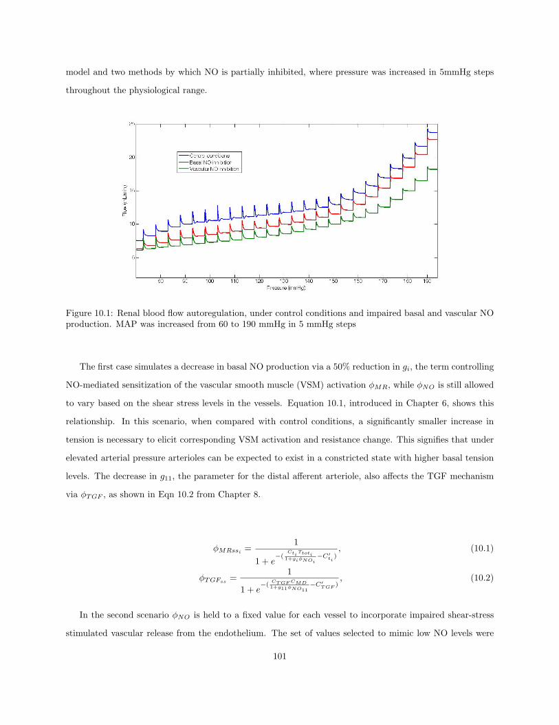
model and two methods by which NO is partially inhibited, where pressure was increased in 5mmHg steps
throughout the physiological range.
Figure 10.1: Renal blood flow autoregulation, under control conditions and impaired basal and vascular NOproduction. MAP was increased from 60 to 190 mmHg in 5 mmHg steps
The first case simulates a decrease in basal NO production via a 50% reduction in gi, the term controlling
NO-mediated sensitization of the vascular smooth muscle (VSM) activation φMR, while φNO is still allowed
to vary based on the shear stress levels in the vessels. Equation 10.1, introduced in Chapter 6, shows this
relationship. In this scenario, when compared with control conditions, a significantly smaller increase in
tension is necessary to elicit corresponding VSM activation and resistance change. This signifies that under
elevated arterial pressure arterioles can be expected to exist in a constricted state with higher basal tension
levels. The decrease in g11, the parameter for the distal afferent arteriole, also affects the TGF mechanism
via φTGF , as shown in Eqn 10.2 from Chapter 8.
φMRssi=
1
1 + e−(
CtiTtoti
1+giφNOi−C′
ti), (10.1)
φTGFss=
1
1 + e−(
CT GF CMD1+g11φNO11
−C′T GF )
, (10.2)
In the second scenario φNO is held to a fixed value for each vessel to incorporate impaired shear-stress
stimulated vascular release from the endothelium. The set of values selected to mimic low NO levels were
101

chosen by running the model under control conditions at a pressure of 60 mmHg, with correspondingly
low flow and shear stresses, and recording the steady state φNO values. Impaired autoregulation at higher
pressures and decreased renal blood flow (RBF) across the entire range is seen in both cases, where at a
pressure of 120mmHg steady state RBF decreased by 33% under conditions simulating basal NO inhibition
(11.33 mL/min to 9.42 mL/min), and by a further 12% (to 8.06 mL/min) when φNO is fixed to simulate
impaired vascular NO release as well.
Increasing arterial pressure generally causes increasing wall shear stress, and the resultant vasodilation
would be expected to weaken autoregulation. Therefore, inhibiting the NO response would be expected to
strengthen autoregulation, which is not immediately evident from the results. However, examination of Fig
10.1 reveals that flow regulation under NO inhibition is indeed slightly stronger within the autoregulatory
range. Due to the over-constricted state of the arterioles and the higher basal tension levels, autoregu-
lation appears to be shifted so that the autoregulatory response begins at a lower pressure value, and is
overwhelmed sooner as the pressure increases. This creates a paradox that is well known in hypertensives:
increased peripheral resistance entails correspondingly strong autoregulation at lower blood pressures, but
when coupled with a constantly elevated mean arterial pressure results in autoregulatory impairment.
A decrease in the lower limit of autoregulation is apparent when NO is inhibited, paralleling the result
seen experimentally by [110] when examining impaired renal blood flow autoregulation in two-kidney, one-clip
hypertensive rats and by [64] in anesthetized animals under acute NO synthesis blockade. In the hypertensive
kidneys, [110] found that NO-inhibitor (L-NNA) infusion resulted in a decrease in RBF and a further increase
in MAP and RVR, as well as a significant decrease in the lower limit of autoregulation from 85± 3 to 72± 5
mmHg (P < 0.05), where the model simulations performed here showed a change from 90 ± 5 to 75 ± 5
mmHg. Autoregulatory resetting under acute inhibition of NO was also observed by [64] as a decrease of
15mmHg in the lower limit, in addition to attenuated RBF across the pressure range. It is notable that the
damped oscillations seen in the control model attributed to the TGF mechanism are not discernible when
NO is inhibited, suggesting an interaction between between normal, variable NO (from both the endothelium
and the macula densa) and TGF that promotes the damped oscillatory behavior typically seen in response
to a pressure step. To demonstrate that the inhibition of NO adequately represents a key component of
hypertension, the model was subjected to more physiologically realistic pressure forcings (Fig 10.2) and
compared with experimental results (Fig 10.3).
The objective of the study performed by [12] was to produce broadband excitation of the arterial blood
pressure while measuring arterial blood pressure and renal blood flow at a sufficiently high frequency. Blood
102

Figure 10.2: Model results: arterial pressure forcings and blood flow for normotensive (top) and hypertensive(bottom) rats
Figure 10.3: Typical arterial pressure and blood flow data from SDR and SHR, reprinted from [12]
pressure was measured in the superior mesenteric artery with a standard pressure amplifier, and renal blood
flow was measured in the left renal artery with an electromagnetic flow probe at a sampling rate of 2 Hz. To
closely simulate these experimental conditions, the renal arterial pressure input to the mathematical model
was a 2 Hz sine wave, with added stochastic variation of maximum magnitude 2mmHg, centered around a
mean pressure of 120mmHg for the normotensive case and 140mmHg for the hypertensive case. The mean
arterial pressure and renal blood flow values are reported in Table 10.1.
103

Table 10.1: Mean Pressure and Flow Values for Experimental Comparison with [12]
Normotensive (SDR)MAP (mmHg) RBF (mL/min)
Exp 117.0± 6.3 12.6± 1.1Model 120± 5.0 11.1± 1.0
Hypertensive (SHR)Exp 145.6± 14.1 10.3± 2.8Model 140± 5.0 9.6± 1.0
The model results (Fig 10.2) are similar to the arterial pressure and blood flow data for normotensive
Sprague-Dawley rats (SDR) and spontaneously hypertensive rats (SHR), where the blood flow values are
lower for the hypertensive animals despite the higher arterial pressure (Fig 10.3). This result suggests that
the inhibition of NO may be one of the most important aspects of simulating hypertension. It is worth
noting, however, that the decrease in blood flow in the experimental case (2.3 mL/min) is higher than that
seen in the model simulation (1.5 mL/min), confirming that while NO is a crucial factor in the decreased
RBF seen in this pathological condition, it is not solely responsible for the change.
The diameter values in response to pressure increases for the last four Strahler orders are displayed in
Figure 10.4, where NO inhibition is modeled via a reduction in g, as in the first case (basal NO inhibition)
in Figure 10.1. This method for representing attenuated NO was deemed the more physiologically realistic
of the two because shear stress remains a factor in the model, albeit with diminished influence.
Figure 10.4: Distal diameter responses (i = 8, ..., 11) to multiple pressure steps (P=60 → 190mmHg, 5mmHgsteps) for normotensive case (colored lines) and hypertensive case produced by inhibiting NO (dashed blacklines)
104

The focus is upon these vascular levels because they contribute the most to peripheral resistance change;
the response of the other Strahler orders is qualitatively similar. In the hypertensive model, the overconstric-
tion of the vessels is apparent, especially at lower pressure values, and represents the lack of vasodilatory NO
activity in the system. The constrictive response is particularly enhanced in the hypertensive vessel orders
i = 8, 9, corresponding to the interlobular arteries. Experimentally, it has been shown that in SHR the
exaggerated contractile response to arginine vasopressin (AVP), which increases intracellular free Ca2+ sen-
sitivity, is mainly mediated through interlobular arterial vasoconstriction, rather than in the afferent arteriole
[36]. Their group noted that under AVP stimulation in control animals, the diameter of both interlobular
and afferent arterioles was reduced by 20% on average, while in hypertensive animals the afferent arteriolar
diameter decreased by only 10% and the interlobular diameter decreased by approximately 40% [36]. In
addition, they found that the resting diameters of SHR were significantly smaller than the normotensive
rats, as is the case in the current model simulation results. As can be seen in Figure 10.4, at higher pressures
the distal afferent arteriole does not provide a measurable difference in resistance contribution between the
control and hypertensive models, in contrast to the overconstriction of the proximal afferent arteriole and
most notably the interlobular arteries. There is also less variation in the vessel diameter before settling
to a steady state value; in the control model the passive dilatory response is larger, as is the constrictive
overshoot and damped oscillatory behavior. This result is consistent with the increased stiffness of arterioles
seen in hypertensives, and highlights the importance of NO in maintaining vascular health.
10.2 Diabetes
Diabetes mellitus type 1, a leading cause of end-stage renal disease [113], is consistently characterized by
increased renal blood flow (RBF) and glomerular filtration rate (GFR). The mechanisms by which renal vas-
cular resistance changes in the early stages of the disease to produce these increases are not fully understood.
Many groups have provided evidence that increases in glomerular hydrostatic pressure and hyperfiltration
may cause the progression of diabetic nephropathy, a direct result of the impaired efficacy of both renal
autoregulatory mechanisms [5, 113]. Elucidating the mechanism for renal vasodilation early in diabetes is a
crucial step towards preventing the transmission of elevated pressure into the glomerulus and the associated
hemodynamic-mediated renal injury [80].
A very recent series of experimental studies showed that continuously recorded renal blood flow, measured
18 hr/day using a Transonic flow probe, increases uniformly in rats with streptozotocin-induced diabetes and
is accompanied by an increase in GFR [4, 5]. They further showed that this increase can be prevented by
105

chronic blockade of NO synthesis. Their data strongly suggest that NO plays an important role in causing
renal vasodilation and increased RBF in diabetes. In addition, transfer function analysis of the response
of the diabetic rats revealed impairment of both autoregulatory mechanisms and dynamic autoregulation
overall, a change which was also prevented by chronic inhibition of NO. This result lends significant support
to the hypothesis that the mechanism for diabetes-induced renal vasodilation may involve attenuation of RBF
autoregulation by NO [4]. To simulate the conditions of early diabetic over-production of NO (Fig 10.5), the
parameter gi controlling NO-mediated sensitization of the vascular smooth muscle (VSM) activation φMR,
was doubled (Eqn 10.1) while φNO was still allowed to vary based on the shear stress levels in the vessels.
In this scenario, when compared to control conditions, a significantly larger increase in tension is necessary
to elicit corresponding VSM activation and resistance change, signifying that the arterioles exist in a more
dilated state.
Figure 10.5: Renal blood flow autoregulation: under control conditions and increased NO production. MAPwas increased from 60 to 190 mmHg in 5 mmHg steps
The model simulation results for increased NO in the system exhibit impaired autoregulation, especially
in the higher end of the pressure range, as well as increased renal blood flow across all pressures examined.
106

The lower limit of autoregulation is slightly shifted towards lower pressures, with the TGF mechanism
becoming active earlier due to the increased flow and therefore increased distal delivery to the macula densa.
The activation of the TGF is evident by the presence of damped oscillations in the flow, which appear more
pronounced within the autoregulatory range of the diabetic response, potentially due to the interaction
with excess NO. Flow regulation is overwhelmed in the diabetic scenario as the pressure increases beyond
120mmHg, mirroring the vasodilatory effect of endothelial produced NO as well as concurrent effects of
neuronal NO from the MD. Macula Densa over-activity of nNOS is modeled via an increase in g11 and
resulting decrease in sensitivity of φTGF (Eqn 10.2). At the site of the juxtaglomerular apparatus, NO is
thought to inhibit salt entry into the MD cells, blunting the sensory mechanism of the TGF system and
thereby impacting glomerular hemodynamics [109].
Other experimental groups that have focused on the pathophysiological importance of TGF in diabetes
mellitus have revealed a different aspect of the breakdown in this autoregulatory mechanism via a change in
tubular reabsorption. Micropuncture experiments performed in nephrons of streptozotocin-induced diabetic
rats showed that an increase in Na+/glucose cotransport upstream of the MD reduces the TGF signal
and contributes to the increase in GFR seen in early diabetes [114]. Further evidence has since been
presented that shows a primary increase of fluid and electrolyte reabsorption in the proximal tubule both in
experimental models of diabetic rats and early insulin-dependent diabetes mellitus in humans [109, 113]. The
primary increase, so named because it exists independently of glomerular hyperfiltration, is the combined
result of enhanced expression of the Na+/glucose cotransporter SGLT, a hyperglycemia-induced rise in
filtered glucose, and to a certain extent an increase in tubular length [113]. The result is a decrease in
NaCl concentration at the MD, which inspires a TGF-dependent increase in flow to restore the fluid and
electrolyte delivery to the distal tubule. This effect is reproduced by the mathematical model of diabetes
when the constant governing the rate of volume reabsorption in the proximal tubule, κ, is increased by 20%,
as in Figure 10.6.
The increase in κ of 20% was chosen to reflect the experimental result found by [114], that diabetic rats
exhibited a 20 to 28% reduction in ambient early distal tubular concentrations of Na+, Cl−, and K+. Above
and below the range of the active TGF, RBF at any given pressure is the same as in the first simulated
diabetic case, with only increased NO, implying that the impact of increased proximal tubular reabsorption
is confined to the TGF mechanism. This is manifested within the autoregulatory range as an increase in
flow, and is even more evident when examining the single nephron GFR (snGFR), or the flow entering the
proximal tubule, seen in Figure 10.7.
107

Figure 10.6: Renal blood flow autoregulation: under control conditions, increased NO production, andincreased NO + increased proximal tubular reabsorption. MAP was increased from 60 to 190 mmHg in 5mmHg steps
In the first case where NO is over-produced, snGFR does not vary significantly from control values
within the range where flow is still effectively autoregulated. However, the upper limit is approximately
25mmHg less and autoregulation is much more easily overwhelmed as pressure increases. With the addition
of increased proximal tubular reabsorption into the system there appears a consistent increase in snGFR of
approximately 13% (compared to control values) within the physiological range corresponding to the active
TGF mechanism. This parallels the result seen experimentally by [114], where at resting blood pressure
(123mmHg in control and 111mmHg in diabetic rats) the snGFR was 27% greater in the diabetic case.
Although the results are qualitatively similar, the model underestimates the quantitative increase in flow;
this is likely due to the relatively small (20%) increase in κ applied to the system. The discrepancy in resting
arterial pressure seen experimentally is also consistent with the simulation results of the current diabetic
model, where the autoregulatory range is shifted toward lower pressures by approximately 10−15mmHg. The
presence of damped oscillations with the characteristic frequency of the TGF (approx. 0.06Hz) parallels that
seen in the renal blood flow results shown in Figure 10.5. The oscillatory behavior is even more noticeable
108

Figure 10.7: Autoregulation of flow entering the proximal tubule: under control conditions, increased NOproduction, and increased NO + increased proximal tubular reabsorption. MAP was increased from 60 to190 mmHg in 5 mmHg steps
when examining flow entering the proximal tubule (Fig 10.7), suggesting an interaction between TGF and
the excess NO present in the system. The model results simulating the early stages of diabetes mellitus
type 1 exhibit the observed dual effect of diabetes on TGF, in the form of impaired TGF-mediated dynamic
autoregulation and TGF-mediated steady-state glomerular hyperfiltration [113]. The impaired myogenic
response of every level of the vasculature reflects the vasodilatory effects of excess NO, and remains important
in characterizing the increase in overall RBF.
In summary, the importance of including the arterial structure of the kidney in a more comprehensive
model of renal autoregulation becomes evident when simulating pathological scenarios. Vasoactive sub-
stances such as NO exert their influence throughout the arterial tree, necessitating a anatomically based
framework within which to examine the autoregulatory response. By varying parameters which control the
production and effect of NO in the system and simulating changes in tubular reabsorption, the model was
able to reproduce experimental trends of altered RBF and snGFR and impaired autoregulation, isolating
these variables as important contributors to the mechanisms behind hemodynamic-mediated renal injury in
109

hypertension and diabetes.
110

Chapter 11
Conclusions, Limitations, and Future
Work
11.1 Model Summary and Conclusions
In the context of the existing body of knowledge concerning renal autoregulation, the multi-scale mathe-
matical model presented in this dissertation utilizes a novel whole-organ approach to understanding how the
kidney effectively stabilizes renal blood flow and glomerular filtration in healthy scenarios, and furthermore
how this protective mechanism begins to break down in pathological scenarios. The complexity of vascular
regulation necessitates that the principal mechanisms be identified and modelled to a level that facilitates a
holistic approach.
The initial part of the model focused on the response of the renal vasculature, from the renal artery to
the distal afferent arteriole. The pressure-induced myogenic reflex was modeled via the activation of the
vascular smooth muscle in response to changes in circumferential wall tension. The constrictive response of
the vessels was modulated by flow-induced dilation via the activation of eNOS and the production of nitric
oxide, and to a lesser extent by viscosity variation in the microvasculature. The partial autoregulation of renal
blood flow exhibited by the myogenic model demonstrated good agreement with available experimental data,
and the inclusion of differential myogenic and shear stress responsiveness throughout the renal circulation
provided a valuable tool for examining the autoregulatory response on distinct levels of the vasculature.
The coupling with the tubuloglomerular feedback response increased the efficacy of autoregulation in the
model, and produced damped oscillations in flow consistent with experimental observations. The added
111

complexities attained by modeling the glomerular/tubular systems of the nephrons, in conjunction with
the influence of both mechanisms operating on distinctly different time scales, produced a mathematical
model that can replicate, with greater physiological accuracy, the pressure and flow-induced changes in the
vasculature responsible for renal autoregulation.
The necessity of including both the arterial structure of the kidney and the reabsorbing tubular system
of the nephrons in a holistic model of renal autoregulation became even more apparent when simulating
pathological scenarios. The impact of NO in the system is significant, as was observed by inhibiting NO
production to model hypertension, and by overproducing NO to model one aspect of early diabetes mellitus,
and would not be effectively represented without an anatomically based framework within which to examine
the response. The model was able to simulate these diseased states and reproduce experimental observations
of altered RBF and snGFR and impaired autoregulation. Although there are undoubtedly a myriad of other
factors affecting the progression of renal injury and disease, the model was able to isolate the variables of NO
availability and tubular reabsorption as important contributors to the pathways of hemodynamic-mediated
renal injury in hypertension and diabetes.
11.2 Model Limitations
The phenomenon of blood pressure regulation is omitted from the model due to the high level of influence the
clinician or experimentalist has over mean arterial pressure in a controlled setting. The series representation
of the arterial structure assumes homogeneity of length, diameter, and wall thickness among vessels of
the same order, an obvious simplification. However, this assumption is necessary for mathematical modeling
purposes and is particularly suitable for the kidney as this organ has no anastomoses between vessels and can
be accurately divided by the Strahler ordering scheme used by [79]. Due to the incomplete understanding
of the cellular cascades involved in certain signalling processes, this model and ones similar [9, 15, 16,
19, 43, 69, 70, 73, 95] contain empirical elements to describe steady-state or reference properties, such
as those that determine the shape of the sigmoidal dependence between circumferential wall tension and
VSM activation, shear stress and eNOS activation, or macula densa concentration and TGF activation.
These variables constitute modeling assumptions as activation factors that do not represent quantitative
physiological entities, but rather qualitative effects. Here, the focus lies on the two major autoregulatory
mechanisms: the pressure-induced myogenic response and the NaCl concentration-dependent TGF response.
There are other crucial factors at work in the kidney, such as the renin-angiotensin system, baroreceptors, and
the sympathetic nervous system, which affect vascular resistance and form feedback loops to regulate blood
112
pressure. There is also the recently postulated existence of a third autoregulatory mechanism whose pathways
are uncertain, though it has been found to be independent of the TGF and to contribute approximately
12−15% to perfect autoregulation [12, 55, 57]. The interaction between neighboring nephrons has also been
omitted, and if considered in the system would add further complexity to the oscillatory dynamics of the
autoregulatory response [75, 76].
11.3 Future Work
There are many ways in which the current model of renal autoregulation can be expanded upon and improved;
two of which are presented here. As seen in Ch. 9, the model underestimates autoregulatory efficacy in vivo,
which could be due to the lack of the third autoregulatory mechanism. Its existence, though controversial, has
recently been corroborated by several experimental groups who have put forth several possibilities including
adenosine triphosphate signalling to P2X1 receptors, the influence of Angiotensin II, or a slow component
of the myogenic response [57]. A multi-disciplinary approach to answering this question would include both
experimental testing and mathematical modeling of the potential pathways, with the aim of incorporating
the third mechanism into the model.
The experimental analysis work done in Ch. 5 on the diabetic Ren2-transgenic rats, combined with the
modeling of diseased states in Ch. 10, has emphasized the important role of nitric oxide in this biological
system. A recent study showed that endothelial function, which is intimately tied to autoregulation and
cardiovascular disease, is dependent on bioavailability of NO, controlled largely by the presence or absence
of reactive oxygen species (ROS) such as superoxide which scavenge NO [98]. In the presented model, shear
stress induces eNOS activation, which is taken to be synonymous with nitric oxide production. The reality
of the situation is more complex, as eNOS can produce both NO, via its oxygenase function, and superoxide,
via its reductase function, the latter dependent on nicotinamide adenine dinucleotide (NADPH) oxidase.
NADPH oxidase quenches NO as well as being responsible for the uncoupling of eNOS and contributing
to oxidative stress in the vascular wall. A detailed mathematical model of NO production and scavenging
would be extremely useful, and may provide insight into the mechanisms by which the balance is tipped in
favor of ROS signaling and subsequent endothelial dysfunction. Coupling such a model with the existing
model of renal autoregulation could help achieve a deeper understanding of the autoregulatory impairment
and vascular injury seen in kidney disease.
113

Appendix A: Derivation of Inflection-Point Determination Method
Adapted from [110]. Assume that k(x) is a function for which k(x) = 1f(x) . In the general case, the first
three derivatives of k(x) are
k′(x) = − f ′(x)f(x)2
,
k′′(x) = −f ′′(x)f(x)2
+2f ′(x)2
f(x)3,
k′′′(x) = −f ′′′(x)f(x)2
+6f ′′(x)f ′(x)
f(x)3− 6f ′(x)3
f(x)4.
In the case that f(x) is the sigmoidal curve f(x) = 1 + eb(x−c), we get
f ′(x) = beb(x−c),
f ′′(x) = b2eb(x−c),
f ′′′(x) = b3eb(x−c),
and
f(x)2 =(1 + eb(x−c)
)2
,
f(x)3 =(1 + eb(x−c)
)3
,
f(x)4 =(1 + eb(x−c)
)4
.
Substituting these into the derivatives of k(x), and setting y = eb(x−c), yields
k′′′(x) = − yb3
(1 + y)2+
6y2b3
(1 + y)3− 6y3b3
(1 + y)4
=−yb3(y2 − 4y + 1)
(1 + y)4.
Solving y2 − 4y + 1 = 0 gives y = 2±√
3, from which k′′′(x) = 0 if and only if
x =ln (2±
√3) + bc
b.
114

Appendix B: Experimental Data Used in Determining Order-Specific Parameters, Divided
by Vessel Size
Afferent Arterioles
Group Pressure (mm Hg) Diameter (µm)
Gebremedhin (1990) [31] 80 27 28
120 25 27
160 24 26
Carmines (1990) [10] 100 20.4
160 12.0
Inscho (1997) [48] 100 20
130 18
160 15.3
Juncos (1994) [54] 30 18.8
60 19.3
90 18.2
120 16.7
Loutzenhiser (2002) [71] 80 17.4
100 14.4
120 12.5
140 11
160 10.4
Interlobular
115

Group Pressure (mm Hg) Diameter (µm)
Takenaka (1998) [106] 80 28.5 49.6 75.4
120 26.3 46.9 75.3
160 23.5 44.4 72.0
Carmines (1990) [10] 100 35.7
160 27.9
Gebremedhin (1990) [31] 80 68
120 78
160 85
Arcuate/Interlobar
Group Pressure (mm Hg) Diameter (µm)
Carmines (1990) [10] 100 68.6
160 59.6
Jernigan (2006) [52] 100 58
125 65
150 70
Harder (1987) [37] 60 127
80 115
100 109
120 105
Gebremehdin (1990) [31] 80 430
120 514
160 581
116

Appendix C: Derivation of Implicit Relationship for Glomerular Flow
Assume that the glomerular capillaries and Bowman’s Capsule can each be effectively represented by a
one-dimensional tubule, as shown below, where x = 0 represents the afferent arteriolar entrance to the
glomerulus and x = L is the exit via the efferent arteriole. As explained in Chapter 3, the flow, q, through
-%' -
Qa q Qe
Qt
x = 0 x = L
Figure 1: Schematic diagram of glomerular filtration
the glomerulus is proportional to the pressure difference across the capillary wall. This gives an expression
for the rate of change of flow within the glomerulus:
dq
dx= −Kf (Pg − Pb − πc) , (1)
where Pb and Pg are the hydrostatic pressures in Bowman’s Capsule and the glomerulus respectively, πc is
the osmotic pressure of the suspended proteins, and Kf is the ultrafiltration coefficient. For filtration to
occur, dqdx must be negative, where the pressures opposing filtration are Pb and πc, and the pressure favoring
filtration is Pg. Pb and Pg are assumed to be spatially constant, since the hydrostatic pressure drop across
the glomerulus is negligible compared to that in the arterioles. Because filtration is occurring along the entire
length of the glomerulus, πc changes with respect to x as the solution becomes more concentrated. Large
proteins completely bypass the capillary filter due to size and charge selectivity, therefore the conservation
law gives
πaQa = πcq. (2)
This provides an expression for πc in terms of q, πa, and Qa, where πa is the input osmotic pressure, more
easily measured experimentally, and Qa is the distal afferent arteriolar flow input provided by the myogenic
117

model. Substituting back into Equation 1 yields
dq
dx= −Kf
(Pg − Pb − πa
Qa
q
). (3)
This first order differential equation for q can be solved analytically by integrating along the length of the
glomerulus, from x = 0 to x = L, as shown below:
∫ L
0
q
(Pg − Pb)q − πaQadq =
∫ L
0
−Kfdx. (4)
Setting α = πa
Pg−Pbgives, ∫ L
0
q(
απa
)q − αQa
dq =∫ L
0
−Kfdx. (5)
This can be divided into an expression that is easily integrable:
α
πa
∫ L
0
(1 +
αQa
q − αQa
)dq =
∫ L
0
−Kfdx. (6)
Integrating yieldsα
πa[q + αQa ln(q − αQa)]L0 = −KfL. (7)
Because q(0) = Qa and q(L) = Qe, we have
Qe −Qa + αQa [ln(Qe − αQa)− ln(Qa − αQa)] =−KfLπa
α. (8)
Dividing both sides by Qa and simplifying gives
Qe
Qa+ α ln
(Qe
Qa− α
1− α
)= 1− KfLπa
αQa. (9)
Substituting πa
Pg−Pbback in for α yields
Qe
Qa+
πa
Pg − Pbln
( Qe
Qa− πa
Pg−Pb
1− πa
Pg−Pb
)= 1−Kf
Pg − Pb
Qa. (10)
118

Appendix D: Pressure-flow Relationship in the Nephron Model
Momentum Equation
Adapted from [123]. Assuming laminar flow of a homogeneous fluid at low Reynolds number in a cylindrical
tubule that is not compliant, the radial velocity component (Vr) will be very small compared to the axial
component (Vz). In this case the Navier-Stokes (N-S) equations can be reduced to represent fluid motion in
only the axial direction, as
∂Vz
∂t+(
Vr∂Vz
∂r+ Vz
∂Vz
∂z
)= −1
ρ
∂P
∂z+
µ
ρr
∂
∂r
(r∂Vz
∂r
). (11)
The conditions of fully developed tubular flow signify that flow is unidirectional, therefore Vr can be assumed
to be zero, and by the continuity equation (Equation 27) this means that ∂Vz
∂z can also be assumed to be
zero. Thereby eliminating the last two terms on the left-hand side of Equation 11), and integrating over the
cross-sectional area of the tubule, A, yields
∫ 2π
0
∫ R
0
∂Vz
∂trdrdθ = −1
ρ
∫ 2π
0
∫ R
0
∂P
∂zrdrdθ +
∫ 2π
0
∫ R
0
µ
ρr
∂
∂r
(r∂Vz
∂r
)rdrdθ, (12)
The integration of each term is outlined below.
∫ 2π
0
∫ R
0
∂(Vz)∂t
rdrdθ =∂
∂t
(∫ 2π
0
∫ R
0
Vzrdrdθ
)(13)
=∂(AVz
∂t, (14)
−1ρ
∫ 2π
0
∫ R
0
∂P
∂zrdrdθ = −1
ρ
∫ 2π
0
∫ R
0
rdrdθ∂P
∂z(15)
= −πR2
ρ
∂P
∂z, (16)
∫ 2π
0
∫ R
0
µ
ρr
∂
∂r
(r∂Vz
∂r
)rdrdθ =
µ
ρ
∫ 2π
0
∫ R
0
∂
∂r
(r∂Vz
∂r
)drdθ (17)
=µ
ρ
∫ 2π
0
(r∂Vz
∂r
)|r=Rdθ (18)
= 2πµ
ρ
(r∂Vz
∂r
)|r=R, (19)
119

Equation 12 then becomes∂(AVz)
∂t= −πR2
ρ
∂P
∂z+ 2π
µ
ρ
(r∂Vz
∂r
)|r=R, (20)
where R is the radius of the tubule and Vz is the axial velocity averaged over the cross-sectional area, defined
below.
Vz =∫ 2π
0
∫ R
0
Vzrdrdθ. (21)
The volume flow rate Q is defined as Q = AVz. The N-S equation has been solved analytically for a
reabsorbing tubule with steady flow and a parabolic axial velocity profile holds for several different patterns
of reabsorption [123]:
Vz = 2Vz
(1− r2
R2
). (22)
Substituting Equation 22 into Equation 20, incorporating the expression for Q, and simplifying, yields,
∂Q
∂t= −πR2
ρ
∂P
∂z− 8µ
ρR2Q. (23)
To establish the relative orders of magnitude of each term in this equation, the variables are first non-
dimensionalized as follows:
Q(z, t) =Q(z, t)Qref
,
R(z, t) =R(z, t)Rref
,
P (z, t) =P (z, t)Pref
,
t =tQref
πR2refL
,
z =z
L.
Inserting these dimensionless variables into Equation 23 yields,
Q2ref
πR2refL
∂Q
∂t= −
R2ref R2Pref
ρL
∂P
∂z− 8µQref Q
ρR2ref R
. (24)
Here, L is the length of the proximal tubule, and Qref = 20nL/min, Pref = 10mmHg, and Rref = 10µm
120

are reference values from [123]. Converting these to SI units and substituting back into Equation 24 gives,
7.96× 10⁻⁸ ∂Q
∂t= −4.2× 10⁻² ∂P
∂z− 4.0× 10⁻² Q
R. (25)
The term on the left-hand side of Equation 25 is many orders of magnitude smaller than the terms on the
right-hand side, and can be neglected. The momentum equation can therefore be approximated as:
∂P
∂z= − 8µ
πr4Q. (26)
Continuity Equation
The continuity equation for flow in a cylindrical tubule is defined as
1r
∂
∂r(Vrr) +
∂Vz
∂z= 0. (27)
Under the conditions of fully developed, unidirectional tubular flow Vr can be assumed to be zero. Integrating
over the cross-sectional area of the tubule and adding a leakage term to account for reabsorption yields,
∂AVz
∂z= −Jv, (28)
where Jv is the volume flux due to reabsorption of tubular fluid. This yields an expression for the change in
volume flow rate, Q,∂Q
∂z= −Jv. (29)
121

Appendix E: MATLAB Code Used in Experimental Analysis
Data is first imported in MATLAB using the Import Data option under the File menu, and each file saved
according to the group from which it came. The data for each pressure step series under control conditions,
papaverine infusion, and AngiotensinII infusion is extracted and saved.
Data Extraction ’dataextract.m’
Author: N.C. Kleinstreuer
SDnorm0control=SDnorm0(1:11,1:2);
SDnorm0angii=SDnorm0(12:22,1:2);
SDnorm0pap=SDnorm0(23:33,1:2);
SDnorm2control=SDnorm2(1:11,1:2);
SDnorm2angii=SDnorm2(12:22,1:2);
SDnorm2pap=SDnorm2(23:33,1:2);
SDnorm4control=SDnorm4(1:11,1:2);
SDnorm4angii=SDnorm4(12:22,1:2);
SDnorm4pap=SDnorm4(23:33,1:2);
SDdiab2control=SDdiab2(1:11,1:2);
SDdiab2angii=SDdiab2(12:22,1:2);
SDdiab2pap=SDdiab2(23:33,1:2);
SDdiab4control=SDdiab4(1:11,1:2);
SDdiab4angii=SDdiab4(12:22,1:2);
SDdiab4pap=SDdiab4(23:33,1:2);
R2norm2control=R2norm2(1:11,1:2);
R2norm2angii=R2norm2(12:22,1:2);
R2norm2pap=R2norm2(23:33,1:2);
122

R2norm4control=R2norm4(1:11,1:2);
R2norm4angii=R2norm4(12:22,1:2);
R2norm4pap=R2norm4(23:33,1:2);
R2diab2control=R2diab2(1:11,1:2);
R2diab2angii=R2diab2(12:22,1:2);
R2diab2pap=R2diab2(23:33,1:2);
R2diab4control=R2diab4(1:11,1:2);
R2diab4angii=R2diab4(12:22,1:2);
R2diab4pap=R2diab4(23:33,1:2);
% normalize the data to enable curve fitting
% Upper limit of autoregulation is manually identified on the curves
% as 190 mmHg, this is confirmed in the literature - this is set to 1
nSDnorm0control=SDnorm0control(:,1)./(SDnorm0control(8,1));
nSDnorm0angii=SDnorm0angii(:,1)./(SDnorm0angii(8,1));
nSDnorm0pap=SDnorm0pap(:,1)./(SDnorm0pap(8,1));
nSDnorm2control=SDnorm2control(:,1)./(SDnorm2control(8,1));
nSDnorm2angii=SDnorm2angii(:,1)./(SDnorm2angii(8,1));
nSDnorm2pap=SDnorm2pap(:,1)./(SDnorm2pap(8,1));
nSDnorm4control=SDnorm4control(:,1)./(SDnorm0control(8,1));
nSDnorm4angii=SDnorm4angii(:,1)./(SDnorm0angii(8,1));
nSDnorm4pap=SDnorm4pap(:,1)./(SDnorm0pap(8,1));
nSDdiab2control=SDdiab2control(:,1)./(SDdiab2control(8,1));
nSDdiab2angii=SDdiab2angii(:,1)./(SDdiab2angii(8,1));
123

nSDdiab2pap=SDdiab2pap(:,1)./(SDdiab2pap(8,1));
nSDdiab4control=SDdiab4control(:,1)./(SDdiab4control(8,1));
nSDdiab4angii=SDdiab4angii(:,1)./(SDdiab4angii(8,1));
nSDdiab4pap=SDdiab4pap(:,1)./(SDdiab4pap(8,1));
nR2norm2control=R2norm2control(:,1)./(R2norm2control(9,1));
nR2norm2angii=R2norm2angii(:,1)./(R2norm2angii(9,1));
nR2norm2pap=R2norm2pap(:,1)./(R2norm2pap(9,1));
nR2norm4control=R2norm4control(:,1)./(R2norm4control(9,1));
nR2norm4angii=R2norm4angii(:,1)./(R2norm4angii(9,1));
nR2norm4pap=R2norm4pap(:,1)./(R2norm4pap(9,1));
nR2diab2control=R2diab2control(:,1)./(R2diab2control(9,1));
nR2diab2angii=R2diab2angii(:,1)./(R2diab2angii(9,1));
nR2diab2pap=R2diab2pap(:,1)./(R2diab2pap(9,1));
nR2diab4control=R2diab4control(:,1)./(R2diab4control(9,1));
nR2diab4angii=R2diab4angii(:,1)./(R2diab4angii(9,1));
nR2diab4pap=R2diab4pap(:,1)./(R2diab4pap(9,1));
Experimental Curve Fitting ’expcurvefit.m’
Author: N.C. Kleinstreuer
% plot experimental data for SD & R2 rats for all 3 ramps
Pressure=[70 85 100 115 130 145 160 175 190 205 220]’;
ShortPressure=[70 85 100 115 130 145 160 175 190]’;
figure(’Name’,’SD Rats Normal, 0 months’);
hold on;
124

errorbar(Pressure,SDnorm0control(:,1),SDnorm0control(:,2),’LineWidth’,2);
errorbar(Pressure,SDnorm0angii(:,1),SDnorm0angii(:,2),’--’,’LineWidth’,2);
errorbar(Pressure,SDnorm0pap(:,1),SDnorm0pap(:,2),’:’,’LineWidth’,2);
xlabel(’Pressure (mmHg)’,’FontSize’,16);
ylabel(’Percent Change in Flow’,’FontSize’,16);
figure(’Name’,’SD Rats Normal, 2 months’);
hold on;
errorbar(Pressure,SDnorm2control(:,1),SDnorm2control(:,2),’LineWidth’,2);
errorbar(Pressure,SDnorm2angii(:,1),SDnorm2angii(:,2),’--’,’LineWidth’,2);
errorbar(Pressure,SDnorm2pap(:,1),SDnorm2pap(:,2),’:’,’LineWidth’,2);
xlabel(’Pressure (mmHg)’,’FontSize’,16);
ylabel(’Percent Change in Flow’,’FontSize’,16);
figure(’Name’,’SD Rats Diabetic, 2 months’);
hold on;
errorbar(Pressure,SDdiab2control(:,1),SDdiab2control(:,2),’r’,’LineWidth’,2);
errorbar(Pressure,SDdiab2angii(:,1),SDdiab2angii(:,2),’--r’,’LineWidth’,2);
errorbar(Pressure,SDdiab2pap(:,1),SDdiab2pap(:,2),’:r’,’LineWidth’,2);
xlabel(’Pressure (mmHg)’,’FontSize’,16); ylabel(’Percent Change in Flow’,’FontSize’,16);
figure(’Name’,’SD Rats Normal, 4 months’);
hold on;
errorbar(Pressure,SDnorm4control(:,1),SDnorm4control(:,2),’LineWidth’,2);
errorbar(Pressure,SDnorm4angii(:,1),SDnorm4angii(:,2),’--’,’LineWidth’,2);
errorbar(Pressure,SDnorm4pap(:,1),SDnorm4pap(:,2),’:’,’LineWidth’,2);
xlabel(’Pressure (mmHg)’,’FontSize’,16); ylabel(’Percent Change in Flow’,’FontSize’,16);
figure(’Name’,’SD Rats Diabetic, 4 months’);
hold on;
125

errorbar(Pressure,SDdiab4control(:,1),SDdiab4control(:,2),’r’,’LineWidth’,2);
errorbar(Pressure,SDdiab4angii(:,1),SDdiab4angii(:,2),’--r’,’LineWidth’,2);
errorbar(Pressure,SDdiab4pap(:,1),SDdiab4pap(:,2),’:r’,’LineWidth’,2);
xlabel(’Pressure (mmHg)’,’FontSize’,16); ylabel(’Percent Change in Flow’,’FontSize’,16);
figure(’Name’,’Ren2 Rats Normal, 2 months’);
hold on;
errorbar(Pressure,R2norm2control(:,1),R2norm2control(:,2),’LineWidth’,2);
errorbar(Pressure,R2norm2angii(:,1),R2norm2angii(:,2),’--’,’LineWidth’,2);
errorbar(Pressure,R2norm2pap(:,1),R2norm2pap(:,2),’:’,’LineWidth’,2);
xlabel(’Pressure (mmHg)’,’FontSize’,16); ylabel(’Percent Change in Flow’,’FontSize’,16);
figure(’Name’,’Ren2 Rats Diabetic, 2 months’);
hold on;
errorbar(Pressure,R2diab2control(:,1),R2diab2control(:,2),’r’,’LineWidth’,2);
errorbar(Pressure,R2diab2angii(:,1),R2diab2angii(:,2),’--r’,’LineWidth’,2);
errorbar(Pressure,R2diab2pap(:,1),R2diab2pap(:,2),’:r’,’LineWidth’,2);
xlabel(’Pressure (mmHg)’,’FontSize’,16); ylabel(’Percent Change in Flow’,’FontSize’,16);
figure(’Name’,’Ren2 Rats Normal, 4 months’);
hold on;
errorbar(Pressure,R2norm4control(:,1),R2norm4control(:,2),’LineWidth’,2);
errorbar(Pressure,R2norm4angii(:,1),R2norm4angii(:,2),’--’,’LineWidth’,2);
errorbar(Pressure,R2norm4pap(:,1),R2norm4pap(:,2),’:’,’LineWidth’,2);
xlabel(’Pressure (mmHg)’,’FontSize’,16); ylabel(’Percent Change in Flow’,’FontSize’,16);
figure(’Name’,’Ren2 Rats Diabetic, 4 months’);
hold on;
errorbar(ShortPressure,R2diab4control(:,1),R2diab4control(:,2),’r’,’LineWidth’,2);
errorbar(ShortPressure,R2diab4angii(:,1),R2diab4angii(:,2),’--r’,’LineWidth’,2);
errorbar(ShortPressure,R2diab4pap(:,1),R2diab4pap(:,2),’:r’,’LineWidth’,2);
126

xlabel(’Pressure (mmHg)’,’FontSize’,16); ylabel(’Percent Change in Flow’,’FontSize’,16);
% fit logistic curve to data to determine inflection points and ARI
s = fitoptions(’Method’,’NonlinearLeastSquares’,...
’Lower’,[0,0],...
’Upper’,[Inf,1e6],...
’Startpoint’,[0.1 50]);
f = fittype(’1/(1+exp(-a*(x-b)))’,’options’,s);
Pressure=[70 85 100 115 130 145 160 175 190]’;
PressureA=[70 85 100 115 130 145 160 175]’;
% Store coefficients and goodness of fit for each group
[SDn0c,gofSDn0c]=fit(PressureA,nSDnorm0control(1:8,1),f);
[SDn0a,gofSDn0a]=fit(PressureA,nSDnorm0angii(1:8,1),f);
[SDn0p,gofSDn0p]=fit(PressureA,nSDnorm0pap(1:8,1),f);
[SDn2c,gofSDn2c]=fit(PressureA,nSDnorm2control(1:8,1),f);
[SDn2a,gofSDn2a]=fit(PressureA,nSDnorm2angii(1:8,1),f);
[SDn2p,gofSDn2p]=fit(PressureA,nSDnorm2pap(1:8,1),f);
[SDn4c,gofSDn4c]=fit(PressureA,nSDnorm4control(1:8,1),f);
[SDn4a,gofSDn4a]=fit(PressureA,nSDnorm4angii(1:8,1),f);
[SDn4p,gofSDn4p]=fit(PressureA,nSDnorm4pap(1:8,1),f);
[SDd2c,gofSDd2c]=fit(PressureA,nSDdiab2control(1:8,1),f);
[SDd2a,gofSDd2a]=fit(PressureA,nSDdiab2angii(1:8,1),f);
[SDd2p,gofSDd2p]=fit(PressureA,nSDdiab2pap(1:8,1),f);
127

[SDd4c,gofSDd4c]=fit(PressureA,nSDdiab4control(1:8,1),f);
[SDd4a,gofSDd4a]=fit(PressureA,nSDdiab4angii(1:8,1),f);
[SDd4p,gofSDd4p]=fit(PressureA,nSDdiab4pap(1:8,1),f);
[R2n2c,gofR2n2c]=fit(Pressure,nR2norm2control(1:9,1),f);
[R2n2a,gofR2n2a]=fit(Pressure,nR2norm2angii(1:9,1),f);
[R2n2p,gofR2n2p]=fit(Pressure,nR2norm2pap(1:9,1),f);
[R2n4c,gofR2n4c]=fit(Pressure,nR2norm4control(1:9,1),f);
[R2n4a,gofR2n4a]=fit(Pressure,nR2norm4angii(1:9,1),f);
[R2n4p,gofR2n4p]=fit(Pressure,nR2norm4pap(1:9,1),f);
[R2d2c,gofR2d2c]=fit(Pressure,nR2diab2control(1:9,1),f);
[R2d2a,gofR2d2a]=fit(Pressure,nR2diab2angii(1:9,1),f);
[R2d2p,gofR2d2p]=fit(Pressure,nR2diab2pap(1:9,1),f);
[R2d4c,gofR2d4c]=fit(ShortPressure,nR2diab4control(1:9,1),f);
[R2d4a,gofR2d4a]=fit(ShortPressure,nR2diab4angii(1:9,1),f);
[R2d4p,gofR2d4p]=fit(ShortPressure,nR2diab4pap(1:9,1),f);
128

Appendix F: MATLAB Code Used in Model of Renal Myogenic Autoregulation
Myogenic Model Time-dependent Response ’Myomodel.m’
Author: N.C. Kleinstreuer
% Myogenic Model applied to Rat Renal Vasculature from renal artery to distal afferent arteriole
clear all
close all
clc
% Morphological Data from Nordsletten et al
Dp = [432 382 280 172 108 88 78 60 40 28 20]; %passive diameter (micrometer) at 100mmHg
N = [1 3 6 24 90 247 578 1245 4373 13070 29566]; %number of vessels
L = [185 1440 8975 2516 1031 511 1001 656 604 423 312]; %avg length micrometer
% Model Parameters
Cp = [2.8770 2.5313 1.7693 1.0165 0.6155 0.4914 0.4297 0.3257 0.2136 0.1464 0.1045]; %Cpass N/m,
%passsive tension at Lo
Cpp = [10 10 10 14.87 14.87 14.87 14.87 18.5 21 25 28]; %Cpass prime, steepness of exp curve
Ca = [3.5473 3.1419 2.3380 1.6115 1.0178 0.8320 0.7390 0.5935 0.4045 0.2903 0.2104]; %Cact N/m,
%peak magnitude of Gaussian dist.
Cap = [0.91 0.91 0.91 0.91 0.91 0.91 0.91 0.91 0.91 0.91 0.91]; %Cact prime, relative peak location
Capp= [0.374 0.374 0.374 0.374 0.374 0.374 0.374 0.374 0.374 0.374 0.374]; %Cact dbl prime,
%relative curve width
% g = [1 1 1 1 1 1 1 1 1 1];
g = [0.2 0.45 0.7 1 1 1 0.9 0.75 0.6 0.5 0.4];
Ct = (1+g).*[0.8859 1.3482 3.1759 7.8679 13.4691 15.9331 17.3293 20.1579 23.8455 36.3745 48.5126];
%Ct params to match recorded exp behaviour
T50 = [1.5 1.6 1.1 0.6 0.35 0.3 0.27 0.2 0.14 0.1 0.06];
tau50 = [12.05 5.3 6.8 11.4 14.33 8.27 4.33 3.96 3.55 3.97 8.14];
Cno = [0.95 0.87 0.71 0.53 0.44 0.57 0.72 0.81 0.89 0.92 0.93];
129

Cnop= tau50.*Cno;
Ctp = T50.*Ct./(1+g); %Ctone prime, determines tension at 50% max act.
ta = [1/45 1/40 1/35 1/30 1/25 1/20 1/15 1/10 1/5 1/2 1/1.8]; %time constant activation change
td = 1; %time constant diameter change
Pout= 5; % venous pressure
% Simulation Time Parameters
TimeStepSize = 0.01; % s
StepSize = 0.01;
TimeLength = 300;
ActivationTime = 50;
ActivationTime2 = 100;
ActivationTime3 = 150;
Time = TimeStepSize:TimeStepSize:TimeLength;
TimeSize = size(Time);
Tol = 1e-6;
num = 12;
Converge = 0;
% Initialize State Variables
Ttot = zeros(num-1,TimeSize(2));
T = zeros(num-1,TimeSize(2));
Tpass = zeros(num-1,TimeSize(2));
Tact = zeros(num-1,TimeSize(2));
Ass = zeros(num-1,TimeSize(2));
A = zeros(num-1,TimeSize(2));
v = zeros(num-1,TimeSize(2));
Pin = zeros(TimeSize(1),num); %inlet pressure at each level
Pinlet = zeros(TimeSize(1),TimeSize(2)); %overall inlet pressure
P = zeros(num-1,TimeSize(2)); %local pressure at each level
130
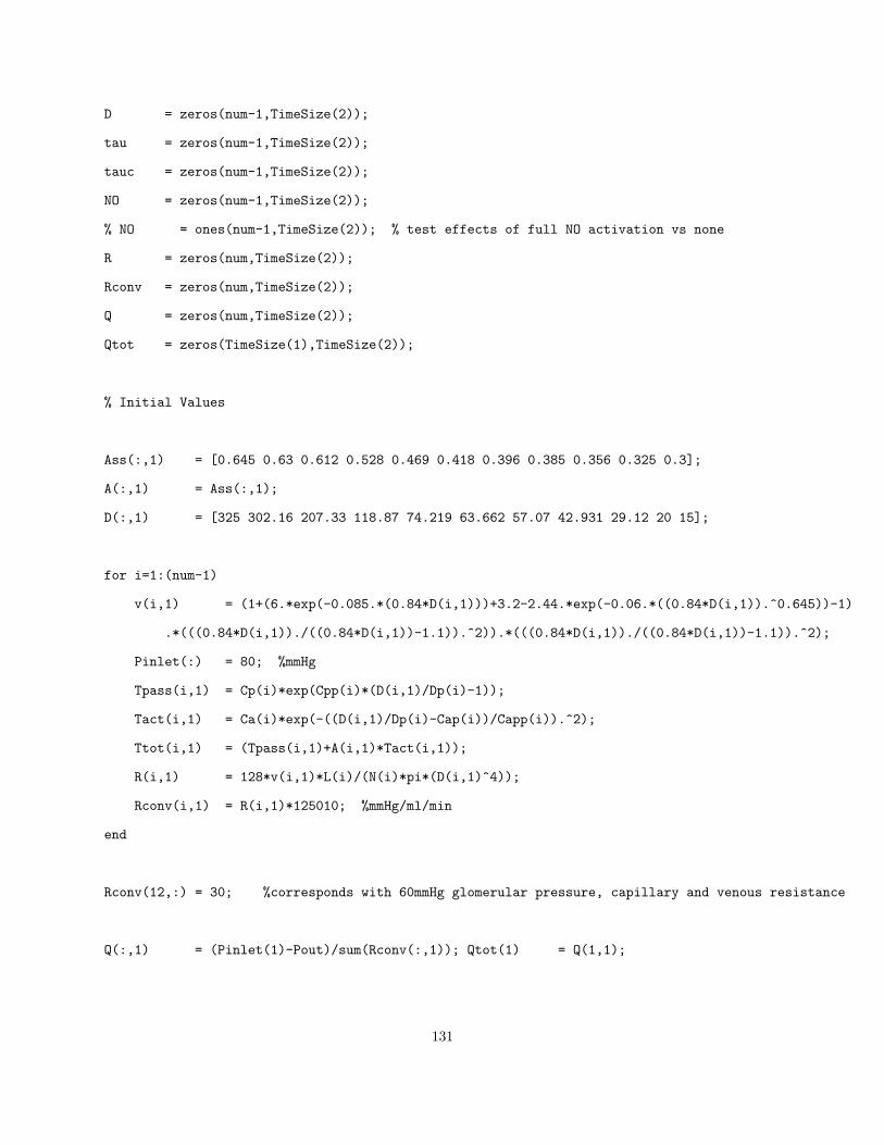
D = zeros(num-1,TimeSize(2));
tau = zeros(num-1,TimeSize(2));
tauc = zeros(num-1,TimeSize(2));
NO = zeros(num-1,TimeSize(2));
% NO = ones(num-1,TimeSize(2)); % test effects of full NO activation vs none
R = zeros(num,TimeSize(2));
Rconv = zeros(num,TimeSize(2));
Q = zeros(num,TimeSize(2));
Qtot = zeros(TimeSize(1),TimeSize(2));
% Initial Values
Ass(:,1) = [0.645 0.63 0.612 0.528 0.469 0.418 0.396 0.385 0.356 0.325 0.3];
A(:,1) = Ass(:,1);
D(:,1) = [325 302.16 207.33 118.87 74.219 63.662 57.07 42.931 29.12 20 15];
for i=1:(num-1)
v(i,1) = (1+(6.*exp(-0.085.*(0.84*D(i,1)))+3.2-2.44.*exp(-0.06.*((0.84*D(i,1)).^0.645))-1)
.*(((0.84*D(i,1))./((0.84*D(i,1))-1.1)).^2)).*(((0.84*D(i,1))./((0.84*D(i,1))-1.1)).^2);
Pinlet(:) = 80; %mmHg
Tpass(i,1) = Cp(i)*exp(Cpp(i)*(D(i,1)/Dp(i)-1));
Tact(i,1) = Ca(i)*exp(-((D(i,1)/Dp(i)-Cap(i))/Capp(i)).^2);
Ttot(i,1) = (Tpass(i,1)+A(i,1)*Tact(i,1));
R(i,1) = 128*v(i,1)*L(i)/(N(i)*pi*(D(i,1)^4));
Rconv(i,1) = R(i,1)*125010; %mmHg/ml/min
end
Rconv(12,:) = 30; %corresponds with 60mmHg glomerular pressure, capillary and venous resistance
Q(:,1) = (Pinlet(1)-Pout)/sum(Rconv(:,1)); Qtot(1) = Q(1,1);
131
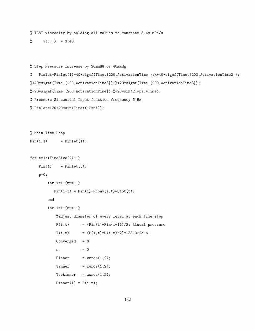
% TEST viscosity by holding all values to constant 3.48 mPa/s
% v(:,:) = 3.48;
% Step Pressure Increase by 20mmHG or 40mmHg
% Pinlet=Pinlet(1)+40*sigmf(Time,[200,ActivationTime]);%+40*sigmf(Time,[200,ActivationTime2]);
%+40*sigmf(Time,[200,ActivationTime3]);%+20*sigmf(Time,[200,ActivationTime3]);
%-20*sigmf(Time,[200,ActivationTime]);%+20*sin(2.*pi.*Time);
% Pressure Sinusoidal Input function frequency 6 Hz
% Pinlet=120+20*sin(Time*(12*pi));
% Main Time Loop
Pin(1,1) = Pinlet(1);
for t=1:(TimeSize(2)-1)
Pin(1) = Pinlet(t);
p=0;
for i=1:(num-1)
Pin(i+1) = Pin(i)-Rconv(i,t)*Qtot(t);
end
for i=1:(num-1)
%adjust diameter of every level at each time step
P(i,t) = (Pin(i)+Pin(i+1))/2; %local pressure
T(i,t) = (P(i,t)*D(i,t)/2)*133.322e-6;
Converged = 0;
n = 0;
Dinner = zeros(1,2);
Tinner = zeros(1,2);
Ttotinner = zeros(1,2);
Dinner(1) = D(i,t);
132

Tinner(1) = T(i,t);
Ttotinner(1)= Ttot(i,t);
while ~Converged & n < 100000
n = n+1;
Dinner(2) = Dinner(1)-(StepSize*(Dp(i)/td)*(Ttotinner(1)-Tinner(1)));
Tinner(2) = (P(i,t)*Dinner(2)/2)*133.322e-6;
Ttotinner(2) = (Cp(i)*exp(Cpp(i)*(Dinner(2)/Dp(i)-1))+A(i,t)*Ca(i)*
exp(-((Dinner(2)/Dp(i)-Cap(i))/Capp(i)).^2));
if abs(Ttotinner(2)-Tinner(2))<Tol
D(i,t+1) = Dinner(2);
Converged = 1;
end
Dinner(1) = Dinner(2);
Tinner(1) = Tinner(2);
Ttotinner(1)= Ttotinner(2);
end
A(i,t+1) = A(i,t)-(TimeStepSize*ta(i)*(A(i,t)-Ass(i,t)));
Tpass(i,t+1) = Cp(i)*exp(Cpp(i)*(D(i,t+1)/Dp(i)-1));
Tact(i,t+1) = Ca(i)*exp(-((D(i,t+1)/Dp(i)-Cap(i))/Capp(i)).^2);
Ttot(i,t+1) = (Tpass(i,t+1)+A(i,t+1)*Tact(i,t+1));
v(i,t+1) = (1+(6.*exp(-0.085.*(0.84*D(i,t+1)))+3.2-2.44
.*exp(-0.06.*((0.84*D(i,t+1)).^0.645))-1).*(((0.84*D(i,t+1))./((0.84*D(i,t+1))-1.1)).^2))
.*(((0.84*D(i,t+1))./((0.84*D(i,t+1))-1.1)).^2);
R(i,t+1) = 128*v(i,t+1)*L(i)/(N(i)*pi*(D(i,t+1))^4); %cP/micron^3
Rconv(i,t+1) = R(i,t+1)*125010; %resistance units mmHg/ml/min
Q(i,t+1) = (Pin(i)-Pin(i+1))/(Rconv(i,t+1));
tau(i,t+1) = 32*Q(i,t+1)*v(i,t+1)/(N(i)*pi*(D(i,t+1)^3)); %cP*ml/min(micron^3)
tauc(i,t+1) = tau(i,t+1)*1.667e7; %Pa
NO(i,t+1) = 1/(1+exp(-Cno(i)*tauc(i,t+1)+Cnop(i)));
Ass(i,t+1) = 1/(1+exp(-Ct(i)*Ttot(i,t+1)/(1+g(i)*NO(i,t+1))+Ctp(i)));
133

end
Q(num,t+1)= (Pin(num)-Pout)/Rconv(num,t+1);
Qtot(t+1) = (Pin(1)-Pout)/sum(Rconv(:,t+1));
err=sum(abs(Qtot(t)-Q(:,t)))/Qtot(t);
end
% % hold on; grid on;
figure;
% % subplot(2,2,1);
plot(Time, Pinlet);
xlabel(’Time(s)’);ylabel(’Pressure(mmHg)’);
xlim([10 250]);ylim([60 160]);
% % subplot(2,2,2);
figure; plot(Time, Qtot);
xlim([10 250]);ylim([1 5]);
xlabel(’Time(s)’);ylabel(’Flow mL/min’);
% % subplot(2,2,3);
figure; plot(Time, A);
xlim([10 250]);ylim([0.2 1]);
xlabel(’Time(s)’);ylabel(’Myogenic Activation’);
% % subplot(2,2,4);
figure; plot(Time, D);
xlim([10 120]);ylim([0 400]);
xlabel(’Time(s)’);ylabel(’Diameter(m)’);
Myogenic Model Steady State Flow-Pressure Curve ’Myosteadystate.m’
Author: N.C. Kleinstreuer
% Steady State Pressure Flow Curve for Myogenic Model
% Time-dependent convergence to steady state achieved for each pressure value
clear all
134

close all
clc
% Morphological Data from Nordsletten et al
Dp = [432 382 280 172 108 88 78 60 40 28 20]; %passive diameter (micrometer) at 100mmHg
N = [1 3 6 24 90 247 578 1245 4373 13070 29566]; %number of vessels
L = [185 1440 8975 2516 1031 511 1001 656 604 423 312]; %avg length micrometer
% Model Parameters
%Passive
Cp = [2.8770 2.5313 1.7693 1.0165 0.6155 0.4914 0.4297 0.3257 0.2136 0.1464 0.1045];
%Cpass N/m, passsive tension at Lo
Cpp = [10 10 10 14.87 14.87 14.87 14.87 18.5 21 25 28]; %Cpass prime, steepness of exp curve
%Active
Ca = [3.5473 3.1419 2.3380 1.6115 1.0178 0.8320 0.7390 0.5935 0.4045 0.2903 0.2104];
%Cact N/m, peak magnitude of Gaussian dist.
Cap = [0.91 0.91 0.91 0.91 0.91 0.91 0.91 0.91 0.91 0.91 0.91]; %Cact prime, relative peak location
Capp= [0.374 0.374 0.374 0.374 0.374 0.374 0.374 0.374 0.374 0.374 0.374];
%Cact dbl prime, relative curve width
tau50 = [12.05 5.3 6.8 11.4 14.33 8.27 4.33 3.96 3.55 3.97 8.14];
Cno = [0.95 0.87 0.71 0.53 0.44 0.57 0.72 0.81 0.89 0.92 0.93];
Cnop= tau50.*Cno;
g = [0.2 0.45 0.7 1 1 1 0.9 0.75 0.6 0.5 0.4];
Ct = (1+g).*[0.8859 1.3482 3.1759 7.8679 13.4691 15.9331 17.3293 22.1579 28.8455 36.3745 48.5126];
%Ctone m/N, sigmoidal activation curve steepness
T50 = [1.5 1.6 1.1 0.6 0.35 0.3 0.27 0.2 0.14 0.1 0.06];
Ctp = T50.*Ct./(1+g); %Ctone prime, determines tension at 50% max act.
ta = [1/45 1/40 1/35 1/30 1/25 1/20 1/15 1/10 1/5 1/2 1/1.8]; %time constant activation change
td = 1; %time constant diameter change
Pout= 5; % venous pressure
135

% Simulation Time Parameters
TimeStepSize = 0.1; % s
StepSize = 0.05;
TimeLength = 100;
% ActivationTime = 40;
% ActivationTime2 = 80;
% ActivationTime3 = 90;
Time = TimeStepSize:TimeStepSize:TimeLength*NumberOfPressureSteps;
TimeSize = size(Time);
Tol = 1e-6;
num = 12;
Converge = 0;
% Initialize State Variables
Ttot = zeros(num-1,TimeSize(2));
T = zeros(num-1,TimeSize(2));
Tpass = zeros(num-1,TimeSize(2));
Tact = zeros(num-1,TimeSize(2));
Ass = zeros(num-1,TimeSize(2));
A = zeros(num-1,TimeSize(2));
v = zeros(num-1,TimeSize(2));
Pin = zeros(TimeSize(1),num); %inlet pressure at each level
Pinlet = zeros(TimeSize(1),TimeSize(2)); %overall inlet pressure
P = zeros(num-1,TimeSize(2)); %local pressure at each level
D = zeros(num-1,TimeSize(2));
tau = zeros(num-1,TimeSize(2));
tauc = zeros(num-1,TimeSize(2));
W = zeros(num-1,TimeSize(2));
NO = zeros(num-1,TimeSize(2));
R = zeros(num,TimeSize(2));
136

Rconv = zeros(num,TimeSize(2));
Q = zeros(num,TimeSize(2));
Qtot = zeros(TimeSize(1),TimeSize(2));
% Initial Values
Ass(:,1) = [0.645 0.63 0.612 0.528 0.469 0.418 0.396 0.385 0.356 0.325 0.3];
A(:,1) = Ass(:,1);
D(:,1) = [325 302.16 207.33 118.87 74.219 63.662 57.07 42.931 29.12 20 15];
% Ass(:,1) = [0.01 0.01 0.01 0.01 0.01 0.01 0.01 0.01 0.01 0.01 0.01];
% A(:,1) = Ass(:,1);
% D(:,1) = 0.2*Dp;
for i=1:(num-1)
v(i,1) = (1+(6.*exp(-0.085.*(0.84*D(i,1)))+3.2-2.44.*exp(-0.06.*((0.84*D(i,1)).^0.645))-1)
.*(((0.84*D(i,1))./((0.84*D(i,1))-1.1)).^2)).*(((0.84*D(i,1))./((0.84*D(i,1))-1.1)).^2);
Tpass(i,1) = Cp(i)*exp(Cpp(i)*(D(i,1)/Dp(i)-1));
Tact(i,1) = Ca(i)*exp(-((D(i,1)/Dp(i)-Cap(i))/Capp(i)).^2);
Ttot(i,1) = (Tpass(i,1)+A(i,1)*Tact(i,1));
R(i,1) = 128*v(i,1)*L(i)/(N(i)*pi*(D(i,1)^4));
Rconv(i,1) = R(i,1)*125010; %mmHg/ml/min
end
Rconv(12,:) = 30; %corresponds with 60mmHg, capillary and venous resistance
%Simulation Pressure Range
PressureStepSize = 5;
PressureStart = 80;
137
PressureLength = 190;
Pressure = PressureStart:PressureStepSize:PressureLength;
PressureSize = size(Pressure);
Q(:,1) = PressureStart/sum(Rconv(:,1));
Qtot(1) = Q(1,1);
Rout = zeros(num-1,PressureSize(2));
Qout = zeros(PressureSize(1),PressureSize(2));
Pinlet = zeros(PressureSize(1),PressureSize(2));
Pinlet(1) = PressureStart; %mmHg
%NO Test
% NO(:,:)=1;
% Main Time Loop
Pin(1) = Pinlet(1);
for p=1:PressureStepSize:(PressureSize(2)-1)
for t=1:(TimeSize(2)-1)
Pin(1) = Pinlet(p);
for i=1:(num-1)
Pin(i+1) = Pin(i)-Rconv(i,t)*Qtot(t);
end
for i=1:(num-1)
%adjust diameter of every level at each time step
P(i,t) = (Pin(i)+Pin(i+1))/2; %local pressure
T(i,t) = (P(i,t)*D(i,t)/2)*133.322e-6;
Converged = 0;
n = 0;
Dinner = zeros(1,2);
Tinner = zeros(1,2);
138

Ttotinner = zeros(1,2);
Dinner(1) = D(i,t);
Tinner(1) = T(i,t);
Ttotinner(1)= Ttot(i,t);
while ~Converged & n < 100000
n = n+1;
Dinner(2) = Dinner(1)-(StepSize*(Dp(i)/td)*(Ttotinner(1)-Tinner(1)));
Tinner(2) = (P(i,t)*Dinner(2)/2)*133.322e-6;
Ttotinner(2) = (Cp(i)*exp(Cpp(i)*(Dinner(2)/Dp(i)-1))+A(i,t)*Ca(i)
*exp(-((Dinner(2)/Dp(i)-Cap(i))/Capp(i)).^2));
if abs(Ttotinner(2)-Tinner(2))<Tol
D(i,t+1) = Dinner(2);
Converged = 1;
end
Dinner(1) = Dinner(2);
Tinner(1) = Tinner(2);
Ttotinner(1)= Ttotinner(2);
end
A(i,t+1) = A(i,t)-(TimeStepSize*ta(i)*(A(i,t)-Ass(i,t)));
Tpass(i,t+1) = Cp(i)*exp(Cpp(i)*(D(i,t+1)/Dp(i)-1));
Tact(i,t+1) = Ca(i)*exp(-((D(i,t+1)/Dp(i)-Cap(i))/Capp(i)).^2);
Ttot(i,t+1) = (Tpass(i,t+1)+A(i,t+1)*Tact(i,t+1));
v(i,t+1) = (1+(6.*exp(-0.085.*(0.84*D(i,t+1)))+3.2-2.44.*exp(-0.06
.*((0.84*D(i,t+1)).^0.645))-1).*(((0.84*D(i,t+1))./((0.84*D(i,t+1))-1.1)).^2))
.*(((0.84*D(i,t+1))./((0.84*D(i,t+1))-1.1)).^2);
R(i,t+1) = 128*v(i,t+1)*L(i)/(N(i)*pi*(D(i,t+1))^4); %cP/micron^3
Rconv(i,t+1) = R(i,t+1)*125010; %resistance units mmHg/ml/min
Q(i,t+1) = (Pin(i)-Pin(i+1))/(Rconv(i,t+1));
tau(i,t+1) = 32*Q(i,t+1)*v(i,t+1)/(N(i)*pi*(D(i,t+1)^3)); %cP*ml/min(micron^3)
tauc(i,t+1) = tau(i,t+1)*1.667e7; %Pa
139

NO(i,t+1) = 1/(1+exp(-Cno(i)*tauc(i,t+1)+Cnop(i)));
Ass(i,t+1) = 1/(1+exp(-Ct(i)*Ttot(i,t+1)/(1+g(i)*NO(i,t+1))+Ctp(i)));
end
Q(num,t+1)= Pin(num)/Rconv(num,t+1);
Qtot(t+1) = Pin(1)/sum(Rconv(:,t+1));
err=sum(abs(Qtot(t)-Q(:,t)))/Qtot(t);
end
Qout(p) = Qtot(t+1);
Pinlet(p+1) = Pinlet(p)+PressureStepSize;
end
figure; plot(Pinlet, Qout);
140

Appendix G: MATLAB Code Used in Combined Model of Renal Autoregulation: Myogenic
and TGF
Combined Model Time-dependent Response ’CompleteModel.m’
Author: N.C. Kleinstreuer
% Autoregulation Model applied to Rat Renal Vasculature from renal artery to distal afferent arteriole
clear all
close all
clc
% Morphological Data from Nordsletten et al
Dp = [432 382 280 172 108 88 78 60 40 28 20]; %passive diameter (micrometer) at 100mmHg
N = [1 3 6 24 90 247 578 1245 4373 13070 29566]; %number of vessels
L = [185 1440 8975 2516 1031 511 1001 656 604 423 312]; %avg length micrometer
% Model Parameters
Cp = [2.8770 2.5313 1.7693 1.0165 0.6155 0.4914 0.4297 0.3257 0.2136 0.1464 0.1045];
%Cpass N/m, passsive tension at Lo
Cpp = [10 10 10 14.87 14.87 14.87 14.87 18.5 21 25 28]; %Cpass prime, steepness of exp curve
Ca = [3.5473 3.1419 2.3380 1.6115 1.0178 0.8320 0.7390 0.5935 0.4045 0.2903 0.2104];
%Cact N/m, peak magnitude of Gaussian dist.
Cap = [0.91 0.91 0.91 0.91 0.91 0.91 0.91 0.91 0.91 0.91 0.91];
%Cact prime, relative peak location
Capp= [0.374 0.374 0.374 0.374 0.374 0.374 0.374 0.374 0.374 0.374 0.374];
%Cact dbl prime, relative curve width
g = [0.2 0.45 0.7 1 1 1 0.9 0.75 0.6 0.5 0.4]; %gain for effect of NO
tau50 = [12.05 5.3 6.8 11.4 14.33 8.27 4.33 3.96 3.55 3.97 8.14];
%Shear stress values matching 50% NO activation
Cno = [0.95 0.87 0.71 0.53 0.44 0.57 0.72 0.81 0.89 0.92 0.93];
%Sensitivity of NO activation - middle orders smaller b/c under more variable ss
141

Cnop= tau50.*Cno; %CNO prime, determines shear stress at 50% max act.
Ct = (1+g).*[0.8859 1.3482 3.1759 7.8679 13.4691 15.9331 17.3293 20.1579 23.8455 36.3745 48.5126];
%Ctone m/N, sigmoidal activation curve steepness
T50 = [1.5 1.6 1.1 0.6 0.35 0.3 0.27 0.2 0.14 0.1 0.06]; %Tension values matching 50% VSM activation
Ctp = T50.*Ct./(1+g); %Ctone prime, determines tension at 50% max act.
ta = [1/45 1/40 1/35 1/30 1/25 1/20 1/15 1/10 1/5 1/2 1/1.8]; %time constant activation change
ttgf= 1/4.8;
alpha = [1 1 1 1 1 1 1 1 1 0.8 0.5]; %weighted myogenic/TGF contribution
Pout= 5; % efferent & venous pressure
% Simulation Time Parameters
TimeStepSize = 0.01; % s
StepSize = 0.01;
TimeLength = 80;
Time = TimeStepSize:TimeStepSize:TimeLength;
TimeSize = size(Time);
Tol = 1e-6;
num = 12;
Converge = 0;
ActivationTime = 40;
ActivationTime2 = 70;
ActivationTime3 = 100;
ActivationTime4 = 200;
ActivationTime5 = 300;
ActivationTime6 = 400;
ActivationTime7 = 500;
ActivationTime8 = 600;
ActivationTime9 = 700;
ActivationTime10 = 800;
142

ActivationTime11 = 900;
ActivationTime12 = 1000;
ActivationTime13 = 1100;
ActivationTime14 = 1200;
ActivationTime15 = 1300;
ActivationTime16 = 1400;
ActivationTime17 = 1500;
ActivationTime18 = 1600;
ActivationTime19 = 1700;
ActivationTime20 = 1800;
ActivationTime21 = 1900;
ActivationTime22 = 2000;
ActivationTime23 = 2100;
ActivationTime24 = 2200;
ActivationTime25 = 2300;
ActivationTime26 = 2400;
ActivationTime27 = 2500;
ActivationTime28 = 2600;
% ActivationTime29 = 1450;
% ActivationTime30 = 1500;
% ActivationTime31 = 1550;
% ActivationTime32 = 1600;
% Initialize State Variables
Ttot = zeros(num-1,TimeSize(2));
T = zeros(num-1,TimeSize(2));
Tpass = zeros(num-1,TimeSize(2));
Tact = zeros(num-1,TimeSize(2));
Ass = zeros(num-1,TimeSize(2));
Avsm = zeros(num-1,TimeSize(2));
143

A = zeros(num-1,TimeSize(2));
v = zeros(num-1,TimeSize(2));
Pin = zeros(TimeSize(1),num); %inlet pressure at each level
Pinlet = zeros(TimeSize(1),TimeSize(2)); %overall inlet pressure
P = zeros(num-1,TimeSize(2)); %local pressure at each level
D = zeros(num-1,TimeSize(2));
tau = zeros(num-1,TimeSize(2));
tauc = zeros(num-1,TimeSize(2));
NO = zeros(num-1,TimeSize(2));
R = zeros(num,TimeSize(2));
Rconv = zeros(num,TimeSize(2));
Q = zeros(num,TimeSize(2));
Qtot = zeros(TimeSize(1),TimeSize(2));
Qactual = zeros(TimeSize(1),TimeSize(2));
%*************************test effects of inhibiting vascular NO in the system
% NO(:,:) = 0.3;
% NO(1,:) = 0.4361;
% NO(2,:) = 0.4361;
% NO(3,:) = 0.4326;
% NO(4,:) = 0.2283;
% NO(5,:) = 0.1426;
% NO(6,:) = 0.1678;
% NO(7,:) = 0.2323;
% NO(8,:) = 0.2832;
% NO(9,:) = 0.3647;
% NO(10,:)= 0.2748;
% NO(11,:)= 0.3669;
%**************************test effects of full NO activation
144

% NO = ones(num-1,TimeSize(2));
%%%%%%%%%%%%%%%%%%%%%%%%%%%%%%%%%%%%%%%%%%%%%%%%%%%%%%%%%%%%%%%%%%%%%%%%%%%%%%%%%%%%%%%%%%%%%%%%%%%%%%%%
% Initial Diameter and Activation values
% For starting MAP 120 mmHg
% Ass(:,1) = [0.7461 0.7474 0.7608 0.7048 0.6541 0.5711 0.5283 0.4790 0.4196 0.3665 0.3453];
% A(:,1) = Ass(:,1);
% Avsm(:,1) = Ass(:,1);
% D(:,1) = [339.8907 298.3438 200.3056 111.3332 67.7117 57.2859 51.8158 40.2181 28.0178 20.3831 13.2398];
%control conditions, works for start of 100 mmHg
% Ass(:,1) = [0.6445 0.6252 0.6108 0.5668 0.5350 0.4618 0.4217 0.3822 0.3378 0.2904 0.2654];
% A(:,1) = Ass(:,1);
% Avsm(:,1) = Ass(:,1);
% D(:,1) = [325.8537 292.0819 202.6257 113.5242 68.1799 58.0267 52.9809 41.3347 28.8004 22.0908 16.9582];
%Very low pressure start MAP=60
D(:,1) = [376.8765 332.8373 240.5695 152.8504 95.0088 76.8871 67.7948 53.3195 35.8727 25.4205 18.1691];
Ass(:,1) = 0.2;
A(:,1) = Ass(:,1);
Avsm(:,1) = A(:,1);
% For starting MAP 160 mmHg
% Ass(:,1) = [0.8483 0.8785 0.9227 0.9271 0.9159 0.8822 0.8528 0.7893 0.6586 0.4988 0.4950];
% A(:,1) = Ass(:,1);
% Avsm(:,1) = [0.8560 0.8868 0.9308 0.9347 0.9217 0.8830 0.8543 0.7996 0.6803 0.5740 0.5000];
% D(:,1) = [392.1287 339.0935 225.6871 119.0308 70.3940 56.5068 49.5402 37.3063 25.9537 18.7671 12.7406];
%%%%%%%%%%%%%%%%%%%%%%%%%%%%%%%%%%%%%%%%%%%%%%%%%%%%%%%%%%%%%%%%%%%%%%%%%%%%%%%%%%%%%%%%%%%%%%%
145

%***********************************test viscosity by holding all values to constant 3.48 mPa/s
% v(:,:) = 3.48;
%%%%%%%%%%%%%%%%%%%%%%%%%%%%%%%%%%%%%%%%%%%%%%%%%%%%%%%%%%%%%%%%%%%%%%%%%%%%%%%%%%
% TGF addition - define reference values; constants in separate mfile -
%spatial discretization
nz=41; %HR
%nz=101; %finer spatial discretization - same result, increased sim time
conversions
constantsTGF
% set tubular step sizes
hz=Lt/nz; % spatial step size
hzhat=hz/Lt;
hthat=TimeStepSize/tref;
% initialise conc and flow matrices
zhat=linspace(0,1,nz)’;
Qhat=zeros(nz,TimeSize(2));
Chat=zeros(nz,TimeSize(2));
Phat=zeros(nz,TimeSize(2));
Rahat=zeros(1,TimeSize(2));
Qahat=zeros(1,TimeSize(2));
Pahat=zeros(1,TimeSize(2));
Pghat=zeros(1,TimeSize(2));
Pbhat=zeros(1,TimeSize(2));
Qehat=zeros(1,TimeSize(2));
Raa=zeros(1,TimeSize(2));
Atgfss=zeros(1,TimeSize(2));
146

Atgf=zeros(1,TimeSize(2));
%*******************if necessary***************
Ctgf=zeros(1,TimeSize(2));
%***********************************************
Dtgf=zeros(1,TimeSize(2));
dC=zeros(nz-1,1);
Qhatin=1;
Phatin=1;
% pack up constants into structuring array
packupconstants
consts.nz=nz;
reltf=0.5;
consts.reltf=reltf;
% set initial conditions based on steady state solver
C0=extCI(zhat,zdhat,zphat,1)/cref;
C0(find(C0==0))=1;
% Ra0=0.1; %for low pressure start, normal NO
% Ra0=0.7; % for NO inhibition
Ra0=0.4;
X0=[ones(nz,1); C0(2:end); [0.6 0.2 5 2]’; Ra0];
Options=mmfsolve(’default’);
Options=mmfsolve(Options,’Jacobian’,’finite’,’MaxIter’,100);
[xf,fval,exitflag,iters]=mmfsolve(@(xvec) steadystate(xvec,consts),X0,Options);
exitflag
iters
Qhatss=xf(1:nz);
147

auxvarsss=xf([1:nz (2*nz):(end-1)]);
Chatss=[Chatin; xf((nz+1):(2*nz-1))];
Qehatss=xf(2*nz+1)
Actss=0.17;
ssD=D(:,1);
rehat=restructhat*exp(lambda*hcta);
Rconv(12,:)=rehat*260000/N(num-1);
Ctgfp=Chalfhat*gain; %TGF sigmoidal midpoint
%**************to incorporate stochastic fluctuation, use:
% gain = (0.45+0.03*randn(size(Time)))*cref;
%**************Normally use:
Ctgf=1.4*gain; %TGF gain, incorporate shear stress by factor 1+NO(11)
for i=1:(num-1)
Pinlet(:) = 70; %mmHg
Pin(1) = Pinlet(1);
v(i,1) = (1+(6.*exp(-0.085.*(0.84*D(i,1)))+3.2-2.44.*exp(-0.06.*((0.84*D(i,1)).^0.645))-1)
.*(((0.84*D(i,1))./((0.84*D(i,1))-1.1)).^2)).*(((0.84*D(i,1))./((0.84*D(i,1))-1.1)).^2);
R(i,1) = 128*v(i,1)*L(i)/(N(i)*pi*(D(i,1)^4));
Rconv(i,1) = R(i,1)*125010; %mmHg/ml/min
Q(i,1) = (Pinlet(1)-Pout)/sum(Rconv(:,1));
Qtot(1) = Q(1,1);
Pin(i+1) = Pin(i)-Rconv(i,1)*Qtot(1);
P(i,1) = (Pin(i)+Pin(i+1))/2;
T(i,1) = (P(i,1)*D(i,1)/2)*133.322e-6;
Tpass(i,1) = Cp(i)*exp(Cpp(i)*(D(i,1)/Dp(i)-1));
Tact(i,1) = Ca(i)*exp(-((D(i,1)/Dp(i)-Cap(i))/Capp(i)).^2);
148

Avsm(i,1) = (T(i,1)-Tpass(i,1))/Tact(i,1);
% Ttot(i,1) =T(i,1);
end
Qehat(1)=Qehatss;
Qhat(:,1)=Qhatss; % flow initial condition
Phat(:,1)=Phatin*ones(nz,1); % flow initial condition
Chat(:,1)=Chatss; % conc initial condition
Atgfss(1)=Actss;
Atgf(1)=Atgfss(1);
Chat(1,:)=Chatin*ones(1,TimeSize(2)); % conc boundary condition
%%%%%%%%%%%%%%%%%%%%%%%%%%%%%%%%%%%%%%%%%%%%%%%%%%%%%%%%%%%%%%%%%%%%%%%%%%%%%%%%%%%%%
%Pressure Inputs
% Step Pressure Increase by 20mmHG P = 1./(1 + exp(-2*(x-10)));
% Pinlet=Pinlet(1)-5*sigmf(Time,[10,ActivationTime])-5*sigmf(Time,[10,ActivationTime2])
%+5*sigmf(Time,[10,ActivationTime3])+5*sigmf(Time,[10,ActivationTime4])
%+5*sigmf(Time,[10,ActivationTime5])+5*sigmf(Time,[10,ActivationTime6])
%+5*sigmf(Time,[10,ActivationTime7])+5*sigmf(Time,[10,ActivationTime8])
%+5*sigmf(Time,[500,ActivationTime9])+5*sigmf(Time,[10,ActivationTime10])
%+5*sigmf(Time,[10,ActivationTime11])+5*sigmf(Time,[10,ActivationTime12])
%+5*sigmf(Time,[10,ActivationTime13])+5*sigmf(Time,[10,ActivationTime14])
%+5*sigmf(Time,[10,ActivationTime15])+5*sigmf(Time,[10,ActivationTime16])
%+5*sigmf(Time,[10,ActivationTime17])+5*sigmf(Time,[10,ActivationTime18])
%+5*sigmf(Time,[10,ActivationTime19])+5*sigmf(Time,[10,ActivationTime20])
%+5*sigmf(Time,[10,ActivationTime21])+5*sigmf(Time,[10,ActivationTime22])
%+5*sigmf(Time,[10,ActivationTime23])+5*sigmf(Time,[10,ActivationTime24])
149
%+5*sigmf(Time,[10,ActivationTime25])+5*sigmf(Time,[10,ActivationTime26])%+20*sin(2.*pi.*Time);
Pinlet=Pinlet(1)+20*sigmf(Time,[10,ActivationTime]);%+10*sigmf(Time,[10,ActivationTime2])
%+10*sigmf(Time,[10,ActivationTime3])+10*sigmf(Time,[10,ActivationTime4])
%+10*sigmf(Time,[10,ActivationTime5])+10*sigmf(Time,[10,ActivationTime6]);
%Pinlet=Pinlet(1)-5*sigmf(Time,[10,ActivationTime])-5*sigmf(Time,[10,ActivationTime2])
%-5*sigmf(Time,[10,ActivationTime3])
% Pinlet(51000:end)=120;
% Pressure Sinusoidal Input function frequency 6 Hz
% Pinlet=Pinlet(1)+10*sin(Time*(4*pi))+20*sigmf(Time,[10,ActivationTime]);
%+20*sigmf(Time,[10,ActivationTime2])+20*sigmf(Time,[10,ActivationTime3]);
% Pinlet=120+20*sin(Time*(12*pi));
% Pressure Ramp function
% Pinlet=Pinlet(1)+Time/2;
%%%%%%%%%%%%%%%%%%%%%%%%%%%%%%%%%%%%%%%%%%%%%%%%%%%%%%%%%%%%%%%%%%%%%%%%%%%%%%%%%%%%%%
%*************************test changing the effects of NO via g
% g = g.*2;
% g = g.*0.5;
% Main Time Loop
Pin(1,1) = Pinlet(1);
for t=1:(TimeSize(2)-1)
Pin(1) = Pinlet(t);
150

% MYOGENIC response for each level, RA to distal AA
for i=1:(num-1)
Pin(i+1) = Pin(i)-Rconv(i,t)*Qtot(t);
end
for i=1:(num-1)
%adjust diameter of every level at each time step
P(i,t) = (Pin(i)+Pin(i+1))/2; %local pressure
T(i,t) = (P(i,t)*D(i,t)/2)*133.322e-6;
Converged = 0;
n = 0;
Dinner = zeros(1,2);
Tinner = zeros(1,2);
Ttotinner = zeros(1,2);
Dinner(1) = D(i,t);
Tinner(1) = T(i,t);
Ttotinner(1)= Ttot(i,t);
while ~Converged & n < 100000
n = n+1;
Dinner(2) = Dinner(1)-(StepSize*(Dp(i))*(Ttotinner(1)-Tinner(1)));
Tinner(2) = (P(i,t)*Dinner(2)/2)*133.322e-6;
Ttotinner(2) = (Cp(i)*exp(Cpp(i)*(Dinner(2)/Dp(i)-1))+Avsm(i,t)*Ca(i)
*exp(-((Dinner(2)/Dp(i)-Cap(i))/Capp(i)).^2));
if abs(Ttotinner(2)-Tinner(2))<Tol
D(i,t+1) = Dinner(2);
T(i,t+1) = Tinner(2);
Converged = 1;
end
Dinner(1) = Dinner(2);
Tinner(1) = Tinner(2);
Ttotinner(1)= Ttotinner(2);
151

end
Tpass(i,t+1) = Cp(i)*exp(Cpp(i)*(D(i,t+1)/Dp(i)-1));
Tact(i,t+1) = Ca(i)*exp(-((D(i,t+1)/Dp(i)-Cap(i))/Capp(i)).^2);
v(i,t+1) = (1+(6.*exp(-0.085.*(0.84*D(i,t+1)))+3.2-2.44.*exp(-0.06.*((0.84
*D(i,t+1)).^0.645))-1).*(((0.84*D(i,t+1))./((0.84*D(i,t+1))-1.1)).^2))
.*(((0.84*D(i,t+1))./((0.84*D(i,t+1))-1.1)).^2);
R(i,t+1) = 128*v(i,t+1)*L(i)/(N(i)*pi*(D(i,t+1))^4); %cP/micron^3
Rconv(i,t+1) = R(i,t+1)*125010; %resistance units mmHg/ml/min
Q(i,t+1) = (Pin(i)-Pin(i+1))/(Rconv(i,t+1));
% %*********Comment out next 3 lines to mimic inhibition of NO
tau(i,t+1) = 32*Q(i,t+1)*v(i,t+1)/(N(i)*pi*(D(i,t+1)^3)); %cP*ml/min(micron^3)
tauc(i,t+1) = tau(i,t+1)*1.667e7; %Pa
NO(i,t+1) = 1/(1+exp(-Cno(i)*tauc(i,t+1)+Cnop(i)));
Ass(i,t+1) = 1/(1+exp(-Ct(i)*T(i,t+1)/(1+g(i)*NO(i,t+1))+Ctp(i)));
A(i,t+1) = A(i,t)-(TimeStepSize*ta(i)*(A(i,t)-Ass(i,t)));
end
% TGF response for proximal and distal AA
Rahat(t)=(Rconv(num-2,t)*N(num-2)+Rconv(num-1,t)*N(num-1))/260000;
%nondimensionalize from mmHgmin/mL and incorporate parallel vessels
Qahat(t)=Q(num-2,t)*(mL2m3/min2sec)/(qref*(N(num-1)+N(num-2)));
Pahat(t)=Pin(num-2)*mmHg2Pa/pref; %Glomerular pressure input to TGF model
reltf=abs(1-exp(-Qhat(1,t)));
consts.reltf=reltf;
Jscurr=Jshat(zhat,Chat(:,t),consts); % solute flux at current time step
Jvcurr=Jvhat(zhat,Chat(:,t),consts); % volume flux at current time step
X0=[Qhat(:,t); Qehat(t); Phat(1,t)];
sol=mmfsolve(@(xvec) auxequations(xvec,consts,Chat(:,t),Pahat(t),Qahat(t),
Rahat(t)),X0,Options);
Qtub=sol(1:nz);
152

Qehat(t)=sol(nz+1);
Phat(1,t+1)=sol(nz+2);
Qdhat=Qtub(1);
Qhat(1,t+1)=Qdhat;
% compute flow inlet BC pass into spatial loop as Qhat(1,j+1)
for z=2:nz % spatial loop
% Qhat(i,j)=Qhat(i-1,j)+hzhat*(-Lt*J0/qref*Jvcurr(i)); % flow at next time step
dC(z-1)=-2*((Qhat(z,t)*Chat(z,t)-Qhat(z-1,t)*Chat(z-1,t))/hzhat+Ls*Lt/qref*Jscurr(z));
% conc at next time step
Chat(z,t+1) = Chat(z,t)-hthat*((Qhat(z,t)*Chat(z,t)-Qhat(z-1,t)*Chat(z-1,t))
/hzhat+Ls*Lt/qref*Jscurr(z)); % conc at next time step
Qhat(z,t+1) = Qhat(z-1,t+1)+hzhat*(-Lt*J0/qref*Jvcurr(z)); % flow at next time step
Phat(z,t+1) = Phat(z-1,t+1)+hzhat*((-8*eta*Lt*qref/(pi*r0p^4*pref))*Qhat(z,t+1));
% pressure at next time step
end
%********* Use in stochastic gain simulations
% Atgfss(t+1) = 1/(1+exp(-Ctgf(t)*Chat(end,t)/(1+g(11)*NO(11,t))+Ctgfp));
% Otherwise
Atgfss(t+1) = 1/(1+exp(-Ctgf*Chat(end,t)/(1+g(11)*NO(11,t))+Ctgfp));
Atgf(t+1) = Atgf(t)-(TimeStepSize*ttgf*(Atgf(t)-Atgfss(t)));
% Activation for AA is weighted sum of myogenic and tgf activation
for i=1:num-1
Avsm(i,t+1)=alpha(i)*A(i,t+1)+(1-alpha(i))*Atgf(t+1);
Ttot(i,t+1) = (Tpass(i,t+1)+Avsm(i,t+1)*Tact(i,t+1));
end
%to add in RVR change
Q(num,t+1) = (Pin(num)-Pout)/Rconv(num,t+1);
Qtot(t+1) = (Pin(1)-Pout)/sum(Rconv(:,t+1));
Qactual(t+1)= Qtot(t+1)*10; % for exp comparison factor 10 mL/min
err=sum(abs(Qtot(t)-Q(:,t)))/Qtot(t);
153

end
%%%%%%%%%%%%%%%%%%%%%%%%%%%%%%%%%%%%%%%%%%%%%%%%%%%%%%%%%%%%%%%%%%%%%%%%%%%
%Plotting Options
% % hold on; grid on;
figure;
% % subplot(2,2,1);
plot(Time, Pinlet);
xlabel(’Time(s)’);ylabel(’Pressure(mmHg)’);
xlim([10 1650]);ylim([80 180]);
% % subplot(2,2,2);
figure;
plot(Time, Qactual);
xlim([10 1650]);ylim([0 25]);
xlabel(’Time(s)’);ylabel(’Flow mL/min’);
% % subplot(2,2,3);
figure;
plot(Time, Avsm);
xlim([10 1650]);ylim([0 1]);
xlabel(’Time(s)’);ylabel(’VSM Activation’);
% % subplot(2,2,4);
figure;
plot(Time, D);
xlim([10 1650]);ylim([0 450]);
xlabel(’Time(s)’);ylabel(’Diameter(micron)’);
figure;
plot(Time, Atgf);
xlim([10 1650]);ylim([0 1]);
154

xlabel(’Time(s)’);ylabel(’TGF Activation’);
figure;
plot(Time, Qhat(1,:));
xlim([10 1650]);ylim([0 1]);
xlabel(’Time(s)’);ylabel(’Tubular Flow’);
figure;
plot(Time, Chat(end,:));
xlim([10 1650]);ylim([0 1]);
xlabel(’Time(s)’);ylabel(’MD Na+ Concentration’);
Supplementary Files
Defining Constants ’ConstantsTGF.m’
Author: N.C. Kleinstreuer
%Conversions
mmHg2Pa=101325/760;
nL2m3=1e-12;
min2sec=60;
cm2m=0.01;
L2m3=1e-3;
mL2m3=1e-6;
mmol2mol=1e-3;
psi2mmHg=51.7149;
microm2m=1e-6;
Pa2mmHg=1/mmHg2Pa;
m32nL=1/nL2m3;
sec2min=1/min2sec;
155

m2cm=1/cm2m;
m32L=1/L2m3;
m32mL=1/mL2m3;
mol2mmol=1/mmol2mol;
mmHg2psi=1/psi2mmHg;
m2microm=1/microm2m;
%Reference values
pref=10*mmHg2Pa; % young81
qref=35*nL2m3/min2sec; % HR90
rgref=0.26*mmHg2Pa*min2sec/nL2m3; % value of Ra in HR87
cref=150; % HR90
%Constants
re=0.19*mmHg2Pa*min2sec/nL2m3; % HR87
restruct=0.19*mmHg2Pa*min2sec/nL2m3; % 0.298 HR87
Chatin=150/cref; % HR90
Kf=2.5*nL2m3/min2sec/mmHg2Pa; % HR90 2.5
kappa=33.6*nL2m3/min2sec/cm2m; % HR90
%kappa=50.4*nL2m3/min2sec/cm2m; %**********test higher values
theta=1.3/cm2m; % HR90
Lt=1.8*cm2m; % HR90 %vary and investigate results
r0p=11e-4*cm2m; % HR90
eta=7.2e-4; % young81
J0=22.4*nL2m3/min2sec/cm2m; % HR90
Ls=3.4e-7*cm2m^2; % HR90
Lv=2e-5*cm2m^2*L2m3; % HR90 osmol^(-1) cancels with osmol from ns
%Michaelis-Menten flux parameters
Vmax=0.65e-7*mmol2mol/cm2m; % HR90 [0.65, 1.0]
ns=2; % HR90
156

Km=20; % HR90
zp=1*cm2m; % HR90
zd=1.3*cm2m; % HR90
tref=pi*r0p^2*Lt/qref; % young81
k=0.4*L2m3/mmol2mol; % HR90 [0.0 0.4]
psi=0.02*mmHg2Pa*min2sec/nL2m3; % HR90
zimax=0.057*mmHg2Pa*min2sec/nL2m3; % HR90 0.057
omega=0.2; % HR90 [0.2 0.25]
zeta=0.9; % HR90 [0.9 1.2]
trref=tref;
lambda=3.3; % HR90
hcta=0.5; % HR90
pa=65*mmHg2Pa; % HR90 108.5 far too high
rahat=0.6;
reltf=1;
%large effect on the system
pii=15*mmHg2Pa; % sneyd 25
gain=0.3*cref; % HR90 [0.0 0.4]
% gain=0.5*cref; % Higher gain to increase rate of activation
% gain=0.35*cref; % Lower gain to decrease rate of activation
%small effect on the system
Chalf=44; % HR90 [44 or 56]
pd=6*mmHg2Pa; % sneyd [6-10] HR [6.8-8]
pe=5*mmHg2Pa; % sneyd [0-18] HR [4 8]
% Nondimenisonalized variables for tubular system
zphat=zp/Lt;
zdhat=zd/Lt;
157

pahat=pa/pref;
pdhat=pd/pref;
pehat=pe/pref;
rehat=re/rgref;
restructhat=restruct/rgref;
piihat=pii/pref;
Chalfhat=Chalf/cref;
Initial Steady State Values for Tubular PDE System ’steadystate.m’
Authors: N.C. Kleinstreuer, S. Graybill
function fvec=steadystate(xvec,consts)
% Computes the steady state initial values for Conc & Tub flow
hzhat=consts.hzhat;
nz=consts.nz;
fvec=zeros(2*nz+4,1);
J0=consts.J0;
Lt=consts.Lt;
qref=consts.qref;
Ls=consts.Ls;
eta=consts.eta;
r0p=consts.r0p;
piihat=consts.piihat;
k=consts.k;
Kf=consts.Kf;
cref=consts.cref;
Chalfhat=consts.Chalfhat;
lambda=consts.lambda;
hcta=consts.hcta;
psi=consts.psi;
158

Chatin=consts.Chatin;
pahat=consts.pahat;
pehat=consts.pehat;
pdhat=consts.pdhat;
rgref=consts.rgref;
pref=consts.pref;
restructhat=consts.restructhat;
zimax=consts.zimax;
%%%%%%%%%%%%%%%%%%%%%%%%%%%%%%%%%%%%%%%%%%%%%%%%%%%%%%%%%%%%%%%%%%%%%%%%%%%
% tubular equations
%%%%%%%%%%%%%%%%%%%%%%%%%%%%%%%%%%%%%%%%%%%%%%%%%%%%%%%%%%%%%%%%%%%%%%%%%%%
z=linspace(0,1,nz)’;
qdhat=xvec(1);
q=xvec(2:nz);
c=xvec((nz+1):(2*nz-1));
qihat=xvec(2*nz);
qehat=xvec(2*nz+1);
p1hat=xvec(2*nz+2);
p2hat=xvec(2*nz+3);
rahat=xvec(2*nz+4);
Mq=diag(ones(1,nz-1))-diag(ones(1,nz-2),-1);
M=blkdiag(Mq,Mq);
a=zeros(2*nz-2,1);
a(1:(nz-1))=J0*Lt/qref*Jvhat(z(2:nz),c(1:end),consts);
a(nz:(2*nz-2))=Ls*Lt/qref*Jshat(z(2:nz),c(1:end),consts);
b=zeros(2*nz-2,1);
159

b(1)=qdhat;
b(nz)=qdhat*Chatin;
fvec(1:(2*nz-2))=M*[q; c.*q]+hzhat*a-b;
%%%%%%%%%%%%%%%%%%%%%%%%%%%%%%%%%%%%%%%%%%%%%%%%%%%%%%%%%%%%%%%%%%%%%%%%%%%
% glomerular equations
%%%%%%%%%%%%%%%%%%%%%%%%%%%%%%%%%%%%%%%%%%%%%%%%%%%%%%%%%%%%%%%%%%%%%%%%%%%
% calculate p1hat and qihat
I=simprulefuncvals([qdhat; q],hzhat);
rehat=restructhat*exp(lambda*hcta);
fvec(2*nz-1)=qihat-qehat-qdhat;
fvec(2*nz)=pahat-p1hat-rgref*qref/pref*rahat*qihat/(1-hcta);
fvec(2*nz+1)=p1hat-pehat-rgref*qref/pref*rehat*qehat/(1-hcta);
fvec(2*nz+2)=p2hat-pdhat-8*eta*Lt*qref/(r0p^4*pi*pref)*I;
fvec(2*nz+3)=-(qihat*(p2hat-p1hat)+piihat*qihat)*exp(-(Kf*pref*(p2hat-p1hat)^2/qref+(qihat-qehat)
*(p2hat-p1hat))/(piihat*qihat))+qehat*(p2hat-p1hat)+piihat*qihat;
fvec(2*nz+4)=exp(lambda*hcta)/rgref*(zimax-psi/(1+exp(k*cref*(c(end)-Chalfhat))))-rahat;
Solute Flux ’Jshat.m’
Author: N.C. Kleinstreuer
function output=Jshat(zhat,Chatvec,consts)
constsunpack;
output=(Chatin*reltf*kappa/Ls*exp(-theta*Lt*zhat)).*(zhat<=zphat)+(Chatvec-extCI(zhat,zdhat,zphat,1)
/cref+Vmax*Chatvec./(Ls*(Km+cref*Chatvec))).*(zdhat<=zhat & zhat<=1);
Volume Flux ’Jvhat.m’
Author: N.C. Kleinstreuer
160

function output=Jvhat(zhat,Chatvec,consts)
constsunpack;
output=(reltf*kappa/J0*exp(-theta*Lt*zhat)).*(zhat<=zphat)+(Lv*ns*cref/J0*(extCI(zhat,zdhat,zphat,1)
/cref-Chatvec)).*(zphat<zhat & zhat<=zdhat);
External Concentration Profile ’extCI.m’
Author: N.C. Kleinstreuer
function CI=extCI(z,zd,zp,L)
%Continuous linear piece-wise approximation to Interstitial Concentration HR90
CI=(150+150/(zd-zp)*(z-zp)).*(zp<=z & z<zd)+(300-150/(L-zd)*(z-zd)).*(zd<=z);
Simpson’s Rule Integral Approximation ’simprulefuncvals.m’
Authors: N.C. Kleinstreuer, S. Graybill
function int=simprulefuncvals(evalfunc,h)
% calculates the simpson’s approximation to the integral.
% evalfunc are the function values evaluated at evenly spaced steps with
% step length h.
n=length(evalfunc)-1;
if mod(n,2)~=0
error(’n must be divisible by 2’);
end
sumodd=sum(evalfunc(2:2:n)); sumeven=sum(evalfunc(3:2:(n-1))); int=h*(evalfunc(1)+4*sumodd
+2*sumeven+evalfunc(end))/3;
Auxiliary Equations for Glomerular/Tubular System ’auxequations.m’
Authors: N.C. Kleinstreuer, S. Graybill
function fvec=auxequations(xvec,consts,c,pahat,qahat,rahat)
161

nz=consts.nz;
fvec=zeros(nz+2,1);
hzhat=consts.hzhat;
Lt=consts.Lt;
J0=consts.J0;
qref=consts.qref;
pref=consts.pref;
rgref=consts.rgref;
pdhat=consts.pdhat;
pehat=consts.pehat;
restructhat=consts.restructhat;
Lt=consts.Lt;
r0p=consts.r0p;
eta=consts.eta;
piihat=consts.piihat;
Kf=consts.Kf;
hcta=consts.hcta;
lambda=consts.lambda;
z=linspace(0,1,nz)’;
qdhat=xvec(1); %input to tubular flow
q=xvec(2:nz); %tubular flow
qehat=xvec(nz+1);
pbhat=xvec(nz+2);
rehat=restructhat*exp(lambda*hcta);
pghat=pahat-(qref*rgref/(pref*(1-hcta)))*qahat*rahat;
fvec(1)=qdhat-qahat+qehat;
162

Mq=diag(ones(1,nz-1))-diag(ones(1,nz-2),-1);
a=J0*Lt/qref*Jvhat(z(2:nz),c(2:nz),consts);
b=zeros(nz-1,1);
b(1)=qdhat;
fvec(2:nz)=Mq*q+hzhat*a-b;
fvec(nz+1)=-(qahat*(pbhat-pghat)+piihat*qahat)*exp(-(Kf*pref*(pbhat-pghat)^2/qref+(qahat-qehat)
*(pbhat-pghat))/(piihat*qahat))+qehat*(pbhat-pghat)+piihat*qahat;
I=simprulefuncvals([qdhat; q],hzhat); %integrate flow over length of tubule to get pressure diff
fvec(nz+2)=pbhat-pdhat+8*eta*Lt*qref/(r0p^4*pi*pref)*I;
163

164
Bibliography
[1] Bagi, Z., J. A. Frangos, J. C. Yeh, C. R. White, G. Kaley, and A. Koller (2005). PECAM-1 mediates
NO-dependent dilation of arterioles to high temporal gradients of shear stress. Arteriosclerosis Thrombosis
and Vascular Biology 25 (8), 1590–1595.
[2] Baldwin, D. and J. Neugarten (1987). Hypertension and renal diseases. American Journal of Kidney
Disease 10 (3), 186–191.
[3] Bayliss, W. (1902). On the local reaction of the arterial wall to changes in intraluminal pressure. Journal
of Physiology 28, 220–231.
[4] Bell, T., G. DiBona, R. Biemiller, and M. Brands (2008). Continuously measured renal blood flow
does not increase in diabetes if nitric oxide synthase is blocked. American Journal of Physiology - Renal
Physiology 295, F1449–F1456.
[5] Bell, T., G. DiBona, Y. Wang, and M. Brands (2006). Mechanisms for renal blood flow control early in
diabetes as revealed by chronic flow measurement and transfer function analysis. Journal of the American
Society of Nephrology 17, 2184–2192.
[6] Bryan, R. M., S. P. Marrelli, M. L. Steenberg, L. A. Schildmeyer, and T. D. Johnson (2001). Effects
of luminal shear stress on cerebral arteries and arterioles. American Journal of Physiology - Heart and
Circulatory Physiology 280 (5), H2011–H2022.
[7] Bund, S. J. (2001). Spontaneously hypertensive rat resistance artery structure related to myogenic and
mechanical properties. Clinical Science 101 (4), 385–393.
[8] Calver, A., J. Collier, S. Moncada, and P. Vallance (1992). Effect of local intra-arterial NG-monomethyl-
L-arginine in patients with hypertension: the nitric oxide dilator mechanism appears abnormal. Journal
of Hypertension 10, 1025–1031.
165

[9] Carlson, B. E. and T. W. Secomb (2005). A theoretical model for the myogenic response based on the
length-tension characteristics of vascular smooth muscle. Microcirculation 12, 327–338.
[10] Carmines, P. K., E. W. Inscho, and R. C. Gensure (1990). Arterial-pressure effects on preglomerular
microvasculature of juxtamedullary nephrons. American Journal of Physiology 258 (1), F94–F102.
[11] Cheng, C., R. van Haperen, M. de Waard, L. C. A. van Damme, D. Tempel, L. Hanemaaijer, G. W. A.
van Cappellen, J. Bos, C. J. Slager, D. J. Duncker, A. F. W. van der Steen, R. de Crom, and R. Krams
(2005). Shear stress affects the intracellular distribution of eNOS: direct demonstration by a novel in vivo
technique. Blood 106 (12), 3691–3698.
[12] Chon, K., Y. Chen, N. Holstein-Rathlou, and V. Marmarelis (1998). Nonlinear system analysis of
renal autoregulation in normotensive and hypertensive rats. IEEE Transactions on Biomedical Engineer-
ing 45 (3), 342–353.
[13] Chowdhary, S. and J. Townend (2001). Nitric oxide and hypertension: not just an endothelium derived
relaxing factor. Journal of Human Hypertension 15, 219–227.
[14] Christensen, K. L. and M. J. Mulvany (2001). Location of resistance arteries. Journal of Vascular
Research 38 (1), 1–12.
[15] Cornelissen, A. J., J. Dankelman, H. G. Stassen, and J. A. Spaan (2000). Myogenic reactivity and
resistance distribution in the coronary arterial tree: a model study. American Journal of Physiology -
Heart and Circulatory Physiology 278, H1490–H1499.
[16] Cornelissen, A. J., J. Dankelman, E. VanBavel, and J. A. Spaan (2002). Balance between myogenic,
flow-dependent, and metabolic flow control in coronary arterial tree: a model study. American Journal of
Physiology - Heart and Circulatory Physiology 282, 2224–2237.
[17] Cupples, W. and B. Braam (2007). Assessment of renal autoregulation. American Journal of Physiology
- Renal Physiology 292, F1105–F1123.
[18] Cupples, W. and R. Loutzenhiser (1998). Dynamic autoregulation in the in vitro perfused hy-
dronephrotic rat kidney. American Journal of Physiology - Renal Physiology 275, F126–F130.
[19] Davis, M. J. (1993). Myogenic response gradient in an arteriolar network. American Journal of Physi-
ology - Heart and Circulatory Physiology 264 (6), H2168–H2179.
166

[20] Davis, M. J. and M. A. Hill (1999). Signaling mechanisms underlying the vascular myogenic response.
Physiological Reviews 79 (2), 387–423.
[21] Davis, M. J. and P. Sikes (1990). Myogenic responses of isolated arterioles - test for a rate-sensitive
mechanism. American Journal of Physiology 259 (6), H1890–H1900.
[22] Deen, W., C. Robertson, and B. Brenner (1972). A model of glomerular ultrafiltration in the rat.
American Journal of Physiology 223 (5), 1178–1183.
[23] Dennis, J. and R. Schnabel (1996). Numerical Methods for Unconstrained Optimization and Nonlinear
Equations. SIAM Books.
[24] Despopoulos, A. and S. Silbernagl (2003). Color Atlas of Physiology, Fifth ed. Thieme Medical Pub-
lishers.
[25] Dubois, R., J. Decoodt, A. Gassee, and P. Lambert (1975). Determination of glomerular intracapillary
and transcapillary pressure gradients from sieving data: a mathematical model. Pflugers Archive 356 (4),
299–316.
[26] Eaton, D. C. and J. P. Pooler (2004). Vander’s Renal Physiology, Sixth ed. Lange Medical
Books/McGraw-Hill.
[27] Eskinder, H., D. R. Harder, and J. H. Lombard (1990). Role of the vascular endothelium in regulating the
response of small arteries of the dog kidney to transmural pressure elevation and reduced po-2. Circulation
Research 66 (5), 1427–1435.
[28] Fellner, S. K. and W. J. Arendhorst (1999). Capacitative calcium entry in smooth muscle cells from
preglomerular vessels. American Journal of Physiology - Renal Physiology 277, F533–F542.
[29] Feng, M. G. and L. G. Navar (2006). Nitric oxide synthase inhibition activates L- and T- type Ca2+
channels in afferent and efferent arterioles. American Journal of Physiology - Renal Physiology 290 (4),
F873–F879.
[30] Fenger-Gron, J., M. J. Mulvany, and K. L. Christensen (1995). Mesenteric blood-pressure profile of
conscious, freely moving rats. Journal of Physiology - London 488 (3), 753–760.
[31] Gebremedhin, D., F. J. Fenoy, D. R. Harder, and R. J. Roman (1990). Enhanced vascular tone in the
renal vasculature of spontaneously hypertensive rats. Hypertension 16 (6), 648–654.
167

[32] Griffin, K. A., R. Hacioglu, I. Abu-Amarah, R. Loutzenhiser, G. A. Williamson, and A. K. Bidani
(2004). Effects of calcium channel blockers on “dynamic” and “steady-state step” renal autoregulation.
American Journal of Physiology - Renal Physiology 286, F1136–F1143.
[33] Guan, Z., G. Gobe, D. A. Willgoss, and Z. H. Endre (2006). Renal endothelial dysfunction and impaired
autoregulation after ischemia-reperfusion injury result from excess nitric oxide. American Journal of
Physiology - Renal Physiology 291 (3), F619–F628.
[34] Guan, Z., D. A. Willgoss, A. Matthias, S. W. Manley, S. Crozier, G. Gobe, and Z. H. Endre (2003).
Facilitation of renal autoregulation by angiotensin II is mediated through modulation of nitric oxide. Acta
Physiologica Scandinavica 179 (2), 189–201.
[35] Guyton, A. (1991). Textbook of Medical Physiology, Eighth ed. W.B. Saunders Company.
[36] Hansen, F., B. Oyvind, and B. Iversen (2005). Enhanced response to AVP in the interlobular artery
from the spontaneously hypertensive rat. American Journal of Physiology - Renal Physiology 288, F1023–
F1031.
[37] Harder, D. R., R. Gilbert, and J. H. Lombard (1987). Vascular muscle-cell depolarization and activation
in renal-arteries on elevation of transmural pressure. American Journal of Physiology 253 (4), F778–F781.
[38] Hartner, A., N. Cordasic, B. Klanke, M. Wittman, R. Veelken, and K. Hilgers (2007). Renal injury
in streptozotocin-diabetic Ren2-transgenic rats is mainly dependent on hypertension, not on diabetes.
American Journal of Physiology - Renal Physiology 292, F820–F827.
[39] Henrion, D. (2005). Pressure and flow-dependent tone in resistance arteries - role of myogenic tone.
Archives Des Maladies Du Coeur Et Des Vaisseaux 98 (9), 913–921.
[40] Henrion, D., M. Iglarz, and B. I. Levy (1999). Chronic endothelin-1 improves nitric oxide-dependent
flow-induced dilation in resistance arteries from normotensive and hypertensive rats. Arteriosclerosis
Thrombosis and Vascular Biology 19 (9), 2148–2153.
[41] Hill, M. A., M. J. Davis, G. A. Meininger, S. J. Potocnik, and T. V. Murphy (2006). Arteriolar
myogenic signalling mechanisms: Implications for local vascular function. Clinical Hemorheology and
Microcirculation 34 (1-2), 67–79.
[42] Holstein-Rathlou, N., A. Wagner, and D. Marsh (1991). Tubloglomerular feedback dynamics and renal
blood flow autoregulation in rats. American Journal of Physiology - Renal Physiology 260, F53–F68.
168

[43] Holstein-Rathlou, N. H. and D. J. Marsh (1990). A dynamic model of the tubuloglomerular feedback
mechanism. American Journal of Physiology - Renal Physiology 258 (5), F1448–1459.
[44] Hostetter, T. (2004). Chronic kidney disease predicts cardiovascular disease. New England Journal of
Medicine 351 (13), 1344–6.
[45] Huang, A., D. Sun, and A. Koller (2000). Shear stress induced release of prostaglandin H2 in arterioles
of hypertensive rats. Hypertension 35, 925–930.
[46] Huang, P. e. a. (1995). Hypertension in mice lacking the gene for endothelial nitric oxide synthase.
Nature 377, 239–242.
[47] Inscho, E., P. Carmines, A. Cook, and L. Navar (1990). Afferent arteriolar responsiveness to altered
perfusion pressure in renal hypertension. Hypertension 15, 748–752.
[48] Inscho, E., A. Cook, V. Mui, and J. Imig (1998). Calcium mobilization contributes to pressure-mediated
afferent arteriolar vasoconstriction. Hypertension 31 (1), 421–428.
[49] Inscho, E., A. Cook, J. Murzynowski, and J. Imig (2004). Elevated arterial pressure impairs autoregu-
lation independently of AT1 receptors. Journal of Hypertension 22, 811–818.
[50] Inscho, E. W. (2009). Mysteries of renal autoregulation. Hypertension 53, 299–306.
[51] Jacobson, H. and H. Baer (1979). Characteristics of volume reabsorption in rabbit superficial and
juxtamedullary proximal convoluted tubules. American Journal of Physiology - Renal Physiology 63 (3),
410–418.
[52] Jernigan, N. L. and H. A. Drummond (2005). Vascular ENaC proteins are required for renal myogenic
constriction. Journal of Clinical Investigation 289 (4), F891–F901.
[53] Johnson, P. (1980). The Myogenic Response, Volume II. Bethesda, MD: American Physiological Society.
[54] Juncos, L. A., J. Garvin, O. A. Carretero, and S. Ito (1995). Flow modulates myogenic responses in
isolated microperfused rabbit afferent arterioles via endothelium-derived nitric-oxide. Journal of Clinical
Investigation 95 (6), 2741–2748.
[55] Just, A. (2007). Mechanisms of renal blood flow autoregulation: dynamics and contributions. American
Journal of Physiology - Regulatory Integrative and Comparative Physiology 292 (1), R1–R17.
169

[56] Just, A. and W. J. Arendshorst (2003). Dynamics and contribution of mechanisms mediating renal
blood flow autoregulation. American Journal of Physiology - Regulatory Integrative and Comparative
Physiology 285 (3), R619–R631.
[57] Just, A. and W. J. Arendshorst (2005). Nitric oxide blunts myogenic autoregulation in rat renal but
not skeletal muscle circulation via tubuloglomerular feedback. Journal of Physiology - London 569 (3),
959–974.
[58] Keener, J. and J. Sneyd (1998). Mathematical Physiology. Springer.
[59] Kelly, D., Y. Zhang, and C. Hepper (2003). Protein kinase C beta inhibition attenuates the progression
of experimental diabetic nephropathy in the presence of continued hypertension. Diabetes 52 (2), 512–518.
[60] Keynan, S., B. Hirshberg, N. Levin-Iaina, I. D. Wexler, R. Dahan, E. Reinhartz, H. Ovadia, Y. Wollman,
T. Chernihovskey, A. Iaina, and I. Raz (2000). Renal nitric oxide production during the early phase of
experimental diabetes mellitus. Kidney International 58 (2), 740–747.
[61] Khamaisi, M., S. Keynan, M. Bursztyn, R. Dahan, E. Reinhartz, H. Ovadia, and I. Raz (2006). Role
of renal nitric oxide synthase in diabetic kidney disease during the chronic phase of diabetes. Nephron
Physiology 102 (3-4), 72–80.
[62] Kleinstreuer, N., T. David, M. Plank, and Z. Endre (2008). Dynamic myogenic autoregulation in the
rat kidney: a whole-organ model. American Journal of Physiology - Renal Physiology 294, F1453–F1464.
[63] Koller, A., D. Sun, and G. Kaley (1993). Role of shear-stress and endothelial prostaglandins in flow-
induced and viscosity-induced dilation of arterioles invitro. Circulation Research 72 (6), 1276–1284.
[64] Kramp, R., P. Fourmanoir, L. L., E. Joly, C. Gerbaux, A. El Hajjam, and N. Caron (2001). Endothelin
resets renal blood flow autoregulatory efficiency during acute blockade of NO in the rat. American Journal
of Physiology - Renal Physiology 281, F1132–F1140.
[65] Kuo, L., M. J. Davis, and W. M. Chilian (1990). Endothelium-dependent, flow-induced dilation of
isolated coronary arterioles. American Journal of Physiology 259 (4), H1063–H1070.
[66] Kuo, L., M. J. Davis, and W. M. Chilian (1992). Endothelial modulation of arteriolar tone. News in
Physiological Sciences 7, 5–9.
170

[67] Layton, A., L. Moore, and H. Layton (2006). Multistability in tubuloglomerular feedback and spectral
complexity in spontaneously hypertensive rats. American Journal of Physiology - Renal Physiology 291,
F79–F97.
[68] Layton, H., E. Pitman, and L. Moore (1995). Instantaneous and steady-state gains in the tubuloglomeru-
lar feedback system. American Journal of Physiology - Renal Physiology 268, F163–F174.
[69] Layton, H. E., E. B. Pitman, and L. C. Moore (1991). Bifurcation analysis of TGF-mediated oscillations
in SNGFR. American Journal of Physiology - Renal Physiology 261 (5), F904–919.
[70] Liao, J. C. and L. Kuo (1997). Interaction between adenosine and flow-induced dilation in coronary
microvascular network. American Journal of Physiology - Heart and Circulatory Physiology 41 (4), H1571–
H1581.
[71] Loutzenhiser, R., A. Bidani, and L. Chilton (2002). Renal myogenic response: Kinetic attributes and
physiological role. Circulation Research 90, 1316–1324.
[72] Loutzenhiser, R., K. Griffin, G. Williamson, and A. Bidani (2006). Renal autoregulation: new perspec-
tives regarding the protective and regulatory roles of the underlying mechanisms. American Journal of
Physiology - Regulatory, Integrative and Computational Physiology 290, 1156–1167.
[73] Lush, D. J. and J. C. Fray (1984). Steady-state autoregulation of renal blood flow: a myogenic model.
American Journal of Physiology - Regulatory, Integrative and Computational Physiology 247, R89–R99.
[74] Marsh, D., O. Sosnovtseva, K. Chon, and N. Holstein-Rathlou (2005). Nonlinear interactions in re-
nal blood blow regulation. American Journal of Physiology - Regulatory, Integrative and Comparative
Physiology 288, R1143–R1159.
[75] Marsh, D., O. Sosnovtseva, E. Mosekilde, and N. Holstein-Rathlou (2007). Vascular coupling induces
synchronization, quasiperiodicity, and chaos in a nephron tree. Chaos 17, 015114.
[76] Marsh, D., O. Sosnovtseva, A. Pavlov, K. Yip, and N. Holstein-Rathlou (2005). Frequency encoding in
renal blood blow regulation. American Journal of Physiology - Regulatory, Integrative and Comparative
Physiology 288, R1160–R1167.
[77] Marshall, E. and E. Trowbridge (1974). A mathematical model of the ultrafiltration process in a single
glomerular capillary. Journal of Theoretical Biology 48, 389–412.
171
[78] Moore, L. (1984). Tubuloglomerular feedback and SNGFR autoregulation in the rat. American Journal
of Physiology - Renal Physiology 247 (2), F267–276.
[79] Nordsletten, D. A., S. Blackett, M. D. Bentley, E. L. Ritman, and N. P. Smith (2006). Structural mor-
phology of renal vasculature. American Journal of Physiology - Heart and Circulatory Physiology 291 (1),
H296–H309.
[80] O’Bryan, G. and T. Hostetter (1997). The renal hemodynamic basis of diabetic nephropathy. Seminars
in Nephrology 17, 93–100.
[81] Oien, A. H. and K. Aukland (1983). A mathematical-analysis of the myogenic hypothesis with special
reference to auto-regulation of renal blood-flow. Circulation Research 52 (3), 241–252.
[82] Onozato, M., A. Tojo, A. Goto, T. Fujita, and C. Wilcox (2002). Oxidative stress and nitric oxide
synthase in rat diabetic nephrophathy: effects of ACEI and ARB. Kidney International 61, 186–194.
[83] Panza, J., P. Casino, C. Kilcoyne, and A. Quyyumi (1993). Role of endothelium-derived nitric ox-
ide in the abnormal endothelium-dependent vascular relaxation of patients with essential hypertension.
Circulation 87, 1468–1474.
[84] Pennathur, S. and J. Heinecke (2007). Oxidative stress and endothelial dysfunction in vascular disease.
Current Diabetes Reports 7, 257–264.
[85] Persson, P. (2002). Renal blood flow autoregulation in blood pressure control. Current Opinions in
Nephrology and Hypertension 11, 67–72.
[86] Peti-Peterdi, J. (2006). Calcium wave of tubuloglomerular feedback. American Journal of Physiology -
Renal Physiology 291, F473–F480.
[87] Pires, S. L. S., C. Julien, B. Chapuis, J. Sassard, and C. Barres (2002). Spontaneous renal blood
flow autoregulation curves in conscious sinoaortic baroreceptor-denervated rats. American Journal of
Physiology - Renal Physiology 282 (1), F51–F58.
[88] Pohl, U. and C. de Wit (1999). A unique role of NO in the control of blood flow. News in Physiological
Sciences 14, 74–80.
[89] Pohl, U., K. Herlan, A. Huang, and E. Bassenge (1991). Edrf-mediated shear-induced dilation opposes
myogenic vasoconstriction in small rabbit arteries. American Journal of Physiology 261 (6), H2016–H2023.
172

[90] Pries, A. R. and T. W. Secomb (2005). Microvascular blood viscosity in vivo and the endothelial surface
layer. American Journal of Physiology - Heart and Circulatory Physiology 289 (6), H2657–H2664.
[91] Pries, A. R., T. W. Secomb, T. Gessner, M. B. Sperandio, J. F. Gross, and P. Gaehtgens (1994).
Resistance to blood-flow in microvessels in-vivo. Circulation Research 75 (5), 904–915.
[92] Racasan, S., J. Joles, P. Boer, H. Koomans, and B. Braam (2003). NO dependency of RBF and autoreg-
ulation in the spontaneously hypertensive rat. American Journal of Physiology - Renal Physiology 285,
F105–F112.
[93] Ren, Y., J. Garvin, and O. Carretero (2001). Efferent arteriole tubuloglomerular feedback in the renal
nephron. Kidney International 59, 222–229.
[94] Ritz, E. and V. Haxsen (2003). Angiotensin II and oxidative stress: an unholy alliance. Journal of the
American Society of Nephrology 14, 2985–2987.
[95] Roman, R. J. and D. R. Harder (1993). Cellular and ionic signal-transduction mechanisms for the me-
chanical activation of renal arterial vascular smooth-muscle. Journal of the American Society of Nephrol-
ogy 4 (4), 986–996.
[96] Rosivall, L. and E. Kiss (2003). Nephrology. Medintel Press.
[97] Sachse, A. and G. Wolf (2007). Angiotensin II-induced reactive oxygen species and the kidney. Journal
of the American Society of Nephrology 18, 2439–2446.
[98] Schiffrin, E. (2008). Oxidative stress, nitric oxide synthase, and superoxide dismutase: A matter of
imbalance underlies endothelial dysfunction in the human coronary circulation. Hypertension 51, 31–32.
[99] Schnermann, J. and D. Levine (2003). Paracrine factors in tubuloglomerular feedback: adenosine, ATP,
and nitric oxide. Annual Review of Physiology 65, 501–529.
[100] Schubert, R. and M. J. Mulvany (1999). The myogenic response: established facts and attractive
hypotheses. Clinical Science 96, 313–326.
[101] Shi, Y., X. M. Wang, K. H. Chon, and W. A. Cupples (2006). Tubuloglomerular feedback-dependent
modulation of renal myogenic autoregulation by nitric oxide. American Journal of Physiology - Regulatory,
Integrative and Comparative Physiology 290 (4), R982–R991.
173

[102] Smiesko, V., D. J. Lang, and P. C. Johnson (1989). Dilator response of rat mesenteric arcading
arterioles to increased blood-flow velocity. American Journal of Physiology 257 (6), H1958–H1965.
[103] Smith, K. M., L. C. Moore, and H. E. Layton (2003). Advective transport of nitric oxide in a math-
ematical model of the afferent arteriole. American Journal of Physiology - Renal Physiology 284 (5),
F1080–F1096.
[104] Strahler, A. (1952). Hypsometric (area altitude) analysis of erosional topology. Bulletin of the Geolog-
ical Society of America 63, 117–142.
[105] Sun, D., A. Huang, C. Smith, C. Stackpole, J. Connetta, E. Shesely, A. Koller, and G. Kaley (1999).
Enhanced release of prostaglandins contributes to flow-induced arteriolar dilation in enos knockout mice.
Circulation Research 85, 288–293.
[106] Takenaka, T., H. Suzuki, H. Okada, K. Hayashi, Y. Ozawa, and T. Saruta (1998). Biophysical signals
underlying myogenic responses in rat interlobular artery. Hypertension 32 (6), 1060–1065.
[107] Taniyama, Y. and K. Griendling (2003). Reactive oxygen species in the vasculature: Molecular and
cellular mechanisms. Hypertension 42, 1075–1081.
[108] Thomas, S., A. Layton, H. Layton, and L. Moore (2006). Kidney modeling: Status and perspectives.
Proceedings of the IEEE 94 (4), 740–752.
[109] Thomson, S., A. Deng, N. Komin, J. Hammes, R. Blantz, and F. Gabbai (2004). Early diabetes as
a model for testing the regulation of juxtaglomerular NOS I. American Journal of Physiology - Renal
Physiology 287, F732–F738.
[110] Turkstra, E., B. Braam, and H. Koomans (2000). Impaired renal blood flow autoregulation in two-
kidney, one-clip hypertensive rats is caused by enhanced activity of nitric oxide. Journal of the American
Society of Nephrology 11, 847–855.
[111] Uhrenholt, T., J. Schjerning, P. Vanhoutte, B. Jensen, and O. Skott (2007). Intercellular calcium
signalling and nitric oxide feedback during constriction of rabbit renal afferent arterioles. American Journal
of Physiology - Renal Physiology 292, F1124–F1131.
[112] Vallance, P. and N. Chan (2001). Endothelial function and nitric oxide: clinical relevance. Heart 85 (3),
342–350.
174

[113] Vallon, V. (2003). Tubuloglomerular feedback and the control of glomerular filtration rate. News in
Physiological Sciences 18, 169–174.
[114] Vallon, V., K. Richter, R. Blantz, S. Thomson, and H. Osswald (1999). Glomerular hyperfiltration in
experimental diabetes mellitus: potential role of tubular reabsorption. Journal of the American Society
of Nephrology 10, 2569–2576.
[115] Van De Graaff, A. (2001). Human Anatomy, Sixth ed. McGraw-Hill.
[116] Vanbavel, E. and M. J. Mulvany (1994). Role of wall tension in the vasoconstrictor response of
cannulated rat mesenteric small arteries. Journal of Physiology - London 477 (1), 103–115.
[117] Walker, M., L. Harrison-Bernard, A. Cook, and L. Navar (2000). Dynamic interaction between myo-
genic and TGF mechanisms in afferent arteriolar blood flow autoregulation. American Journal of Physi-
ology - Renal Physiology 279, F858–F865.
[118] Wallace, M. (1998). Anatomy and physiology of the kidney. AORN Journal 68, 803–816.
[119] Weinstein, A. M. (2003). Mathematical models of renal fluid and electrolyte transport: acknowledging
our uncertainty. American Journal of Physiology - Renal Physiology 284, 871–884.
[120] Wronski, T., E. Seeliger, P. B. Persson, C. Forner, C. Fichtner, J. Scheller, and B. Flemming (2003).
The step response: a method to characterize mechanisms of renal blood flow autoregulation. American
Journal of Physiology - Renal Physiology 285 (4), F758–F764.
[121] Yip, K.-P. and D. J. Marsh (1996). [Ca2+]i in rat afferent arteriole during constriction measured with
confocal flourescence microscopy. American Journal of Physiology - Renal Physiology 271, F1004–F1011.
[122] Young, B. and J. Heath (2000). Wheater’s Functional Histology, Fourth ed. Chruchill Livingstone.
[123] Young, D. K. and D. J. Marsh (1981). Pulse-wave propagation in rat renal tubules - implications for
GFR auto-regulation. American Journal of Physiology - Renal Physiology 240 (5), F446–F458.
175