managerial economics & business strategy chapter 2 market forces: demand and supply

Michael R. Baye, Managerial Economics and Business Strategy, 5e. Copyright © 2006 by The McGraw-Hill Companies, Inc. All rights reserved.

Managerial Economics & Business Strategy

Chapter 2 Market Forces: Demand and Supply

Hakan TASCI Elon University Department of Economics Spring 2007


Overview

III. Market Equilibrium

IV. Price Restrictions

V. Comparative Statics

II. Market Supply Curve� The Supply Function

� Supply Shifters

� Producer Surplus

I. Market Demand Curve� The Demand Function

� Determinants of Demand

� Consumer Surplus



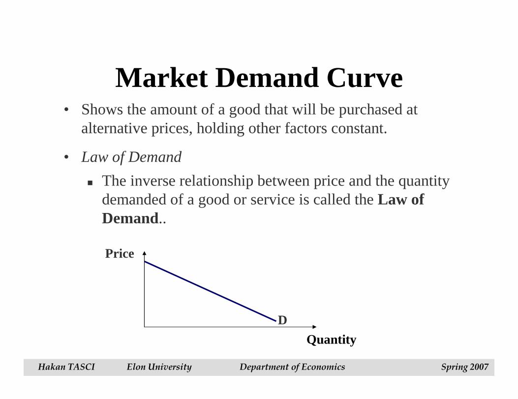
Market Demand Curve• Shows the amount of a good that will be purchased at

alternative prices, holding other factors constant.

• Law of Demand

� The inverse relationship between price and the quantity demanded of a good or service is called the Law of Demand..

Quantity

D

Price



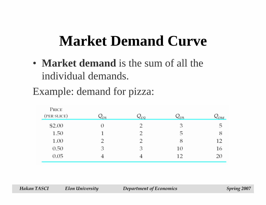
Market Demand Curve• Market demand is the sum of all the

individual demands.

Example: demand for pizza:



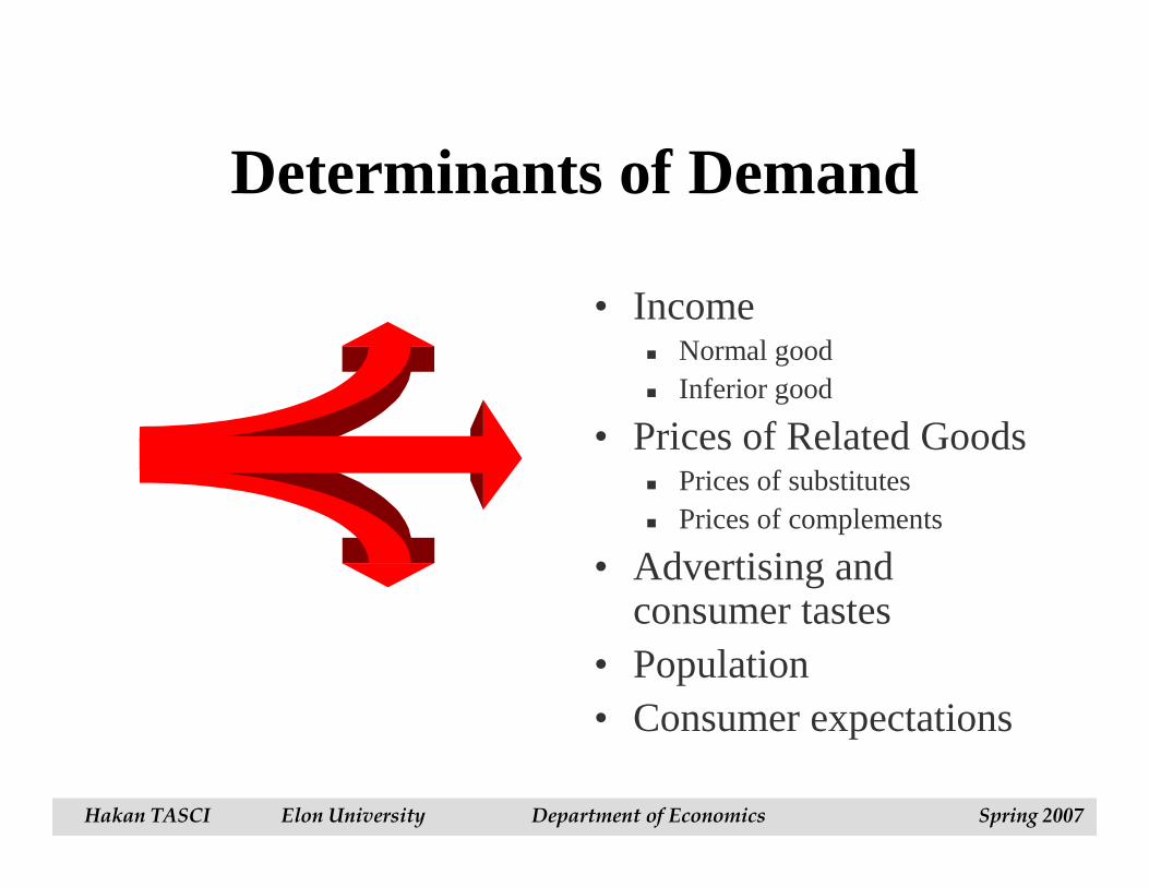
Determinants of Demand

• Income� Normal good� Inferior good

• Prices of Related Goods� Prices of substitutes � Prices of complements

• Advertising and consumer tastes

• Population• Consumer expectations



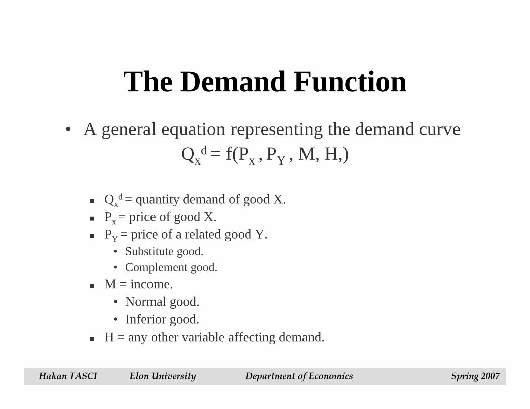
The Demand Function

• A general equation representing the demand curveQx

d = f(Px , PY , M, H,)

� Qxd = quantity demand of good X.

� Px = price of good X.� PY = price of a related good Y.

• Substitute good.• Complement good.

� M = income.• Normal good.• Inferior good.

� H = any other variable affecting demand.



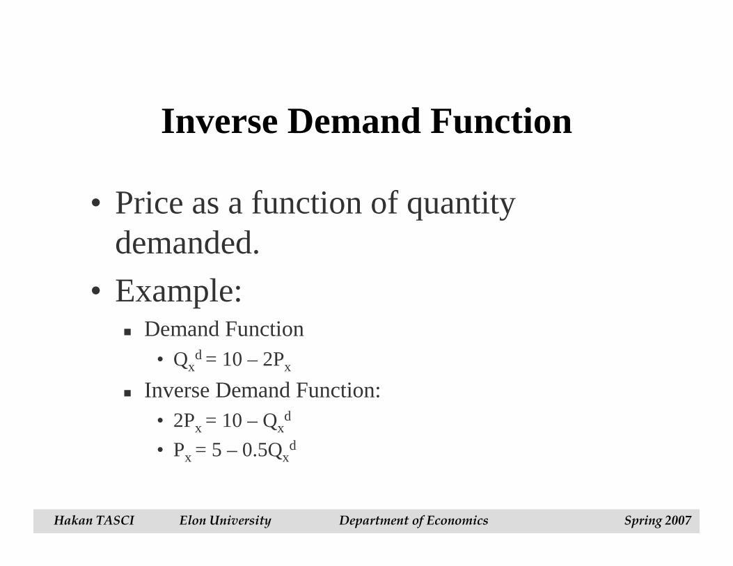
Inverse Demand Function

• Price as a function of quantity demanded.

• Example:� Demand Function

• Qxd = 10 – 2Px

� Inverse Demand Function:• 2Px = 10 – Qx

d

• Px = 5 – 0.5Qxd



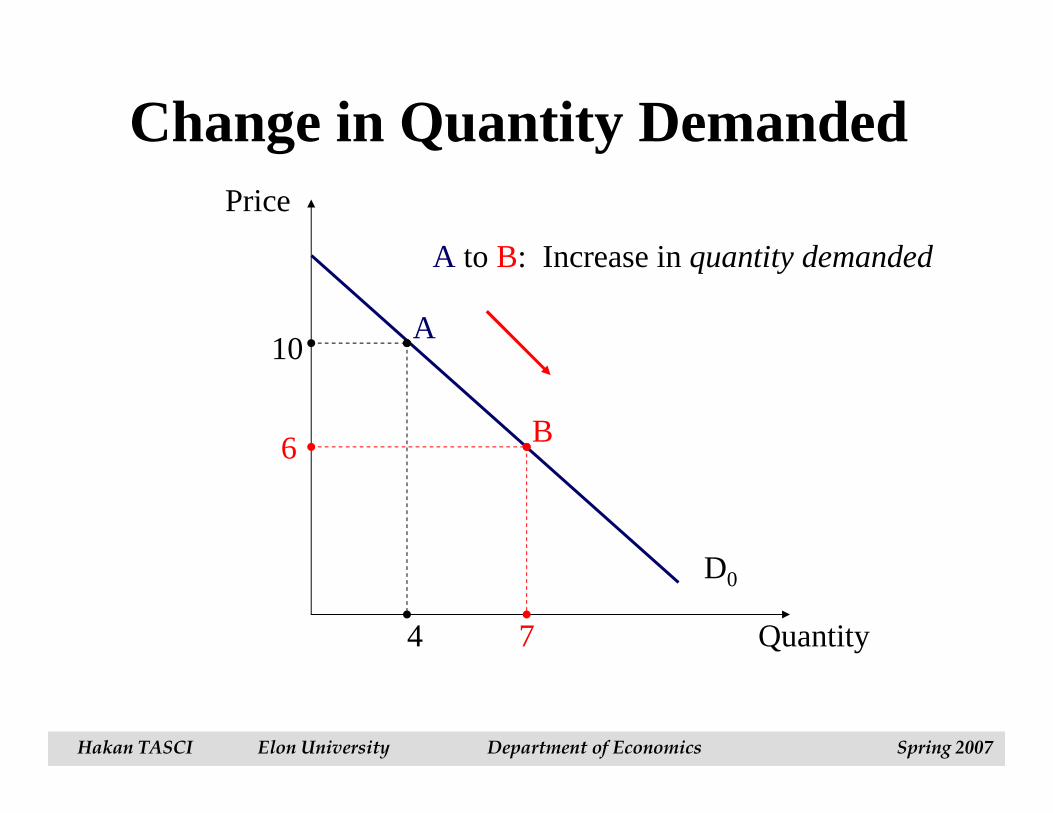
Change in Quantity DemandedPrice

Quantity

D0

4 7

6

A to B: Increase in quantity demanded

B

10A



Price

Quantity

D0

D1

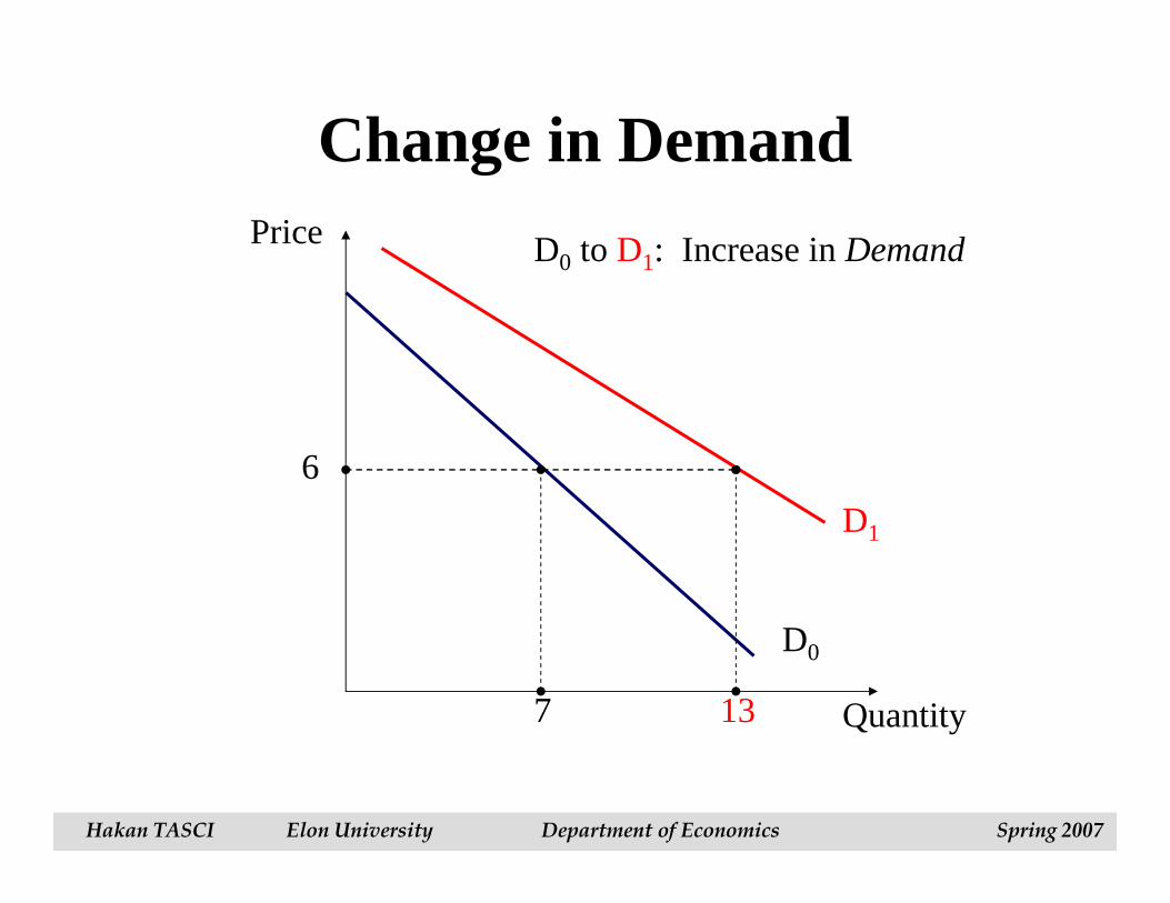
6

7

D0 to D1: Increase in Demand

Change in Demand

13



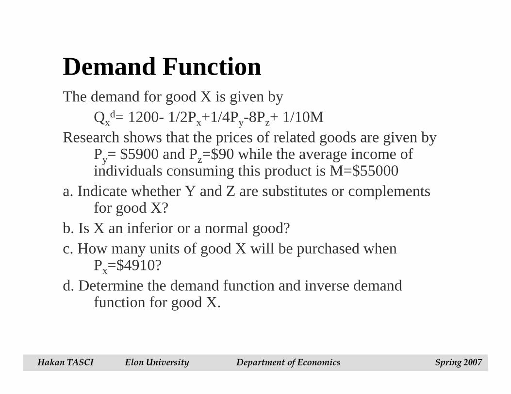
Demand FunctionThe demand for good X is given by

Qxd= 1200- 1/2Px+1/4Py-8Pz+ 1/10M

Research shows that the prices of related goods are given by Py= $5900 and Pz=$90 while the average income of individuals consuming this product is M=$55000

a. Indicate whether Y and Z are substitutes or complements for good X?

b. Is X an inferior or a normal good?c. How many units of good X will be purchased when

Px=$4910?d. Determine the demand function and inverse demand

function for good X.



Consumer Surplus:

• The value consumers get from a good but do not have to pay for.



Price

Quantity

D

10

8

6

4

2

1 2 3 4 5

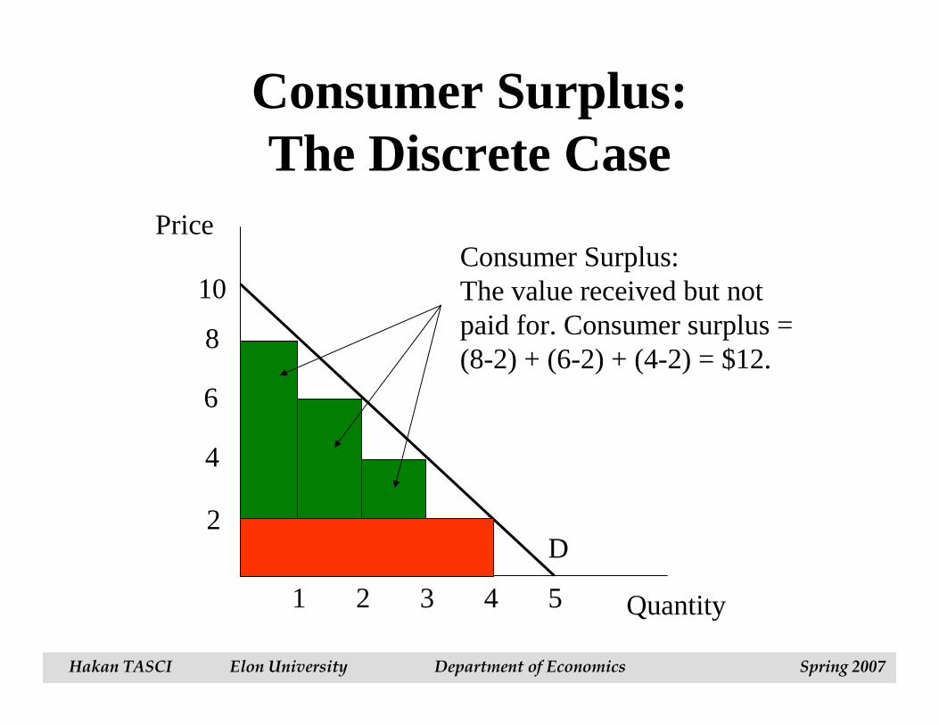
Consumer Surplus:The value received but notpaid for. Consumer surplus =(8-2) + (6-2) + (4-2) = $12.

Consumer Surplus: The Discrete Case



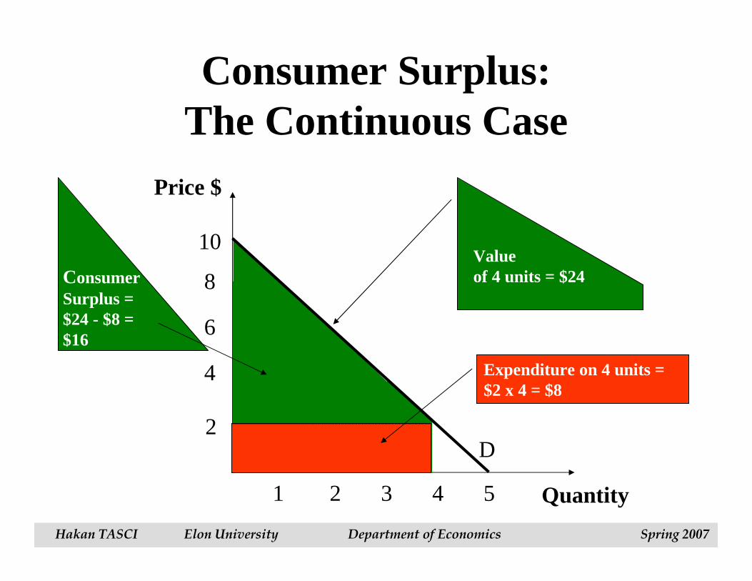
Consumer Surplus:The Continuous Case

Price $

Quantity

D

10

8

6

4

2

1 2 3 4 5

Valueof 4 units = $24Consumer

Surplus = $24 - $8 = $16

Expenditure on 4 units = $2 x 4 = $8



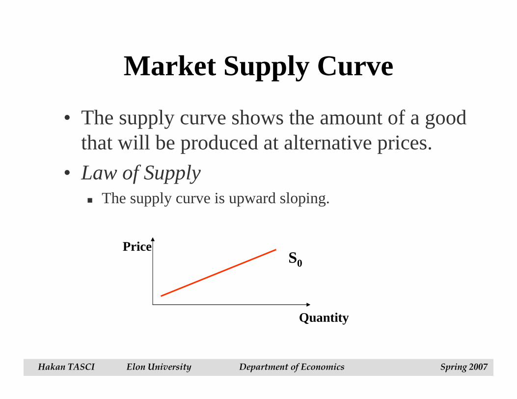
Market Supply Curve

• The supply curve shows the amount of a good that will be produced at alternative prices.

• Law of Supply� The supply curve is upward sloping.

Price

Quantity

S0



Supply Shifters

• Input prices

• Technology or government regulations

• Number of firms� Entry

� Exit

• Substitutes in production

• Taxes� Excise tax

� Ad valorem tax

• Producer expectations



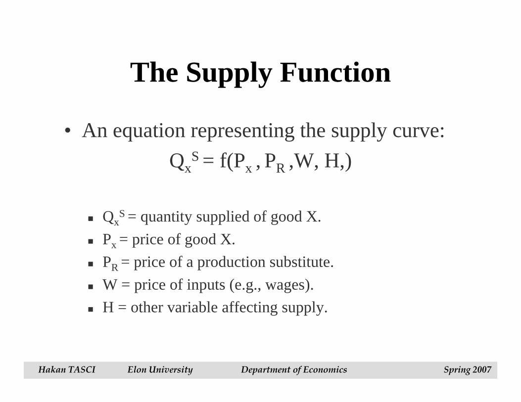
The Supply Function

• An equation representing the supply curve:

QxS = f(Px , PR ,W, H,)

� QxS = quantity supplied of good X.

� Px = price of good X.

� PR = price of a production substitute.

� W = price of inputs (e.g., wages).

� H = other variable affecting supply.



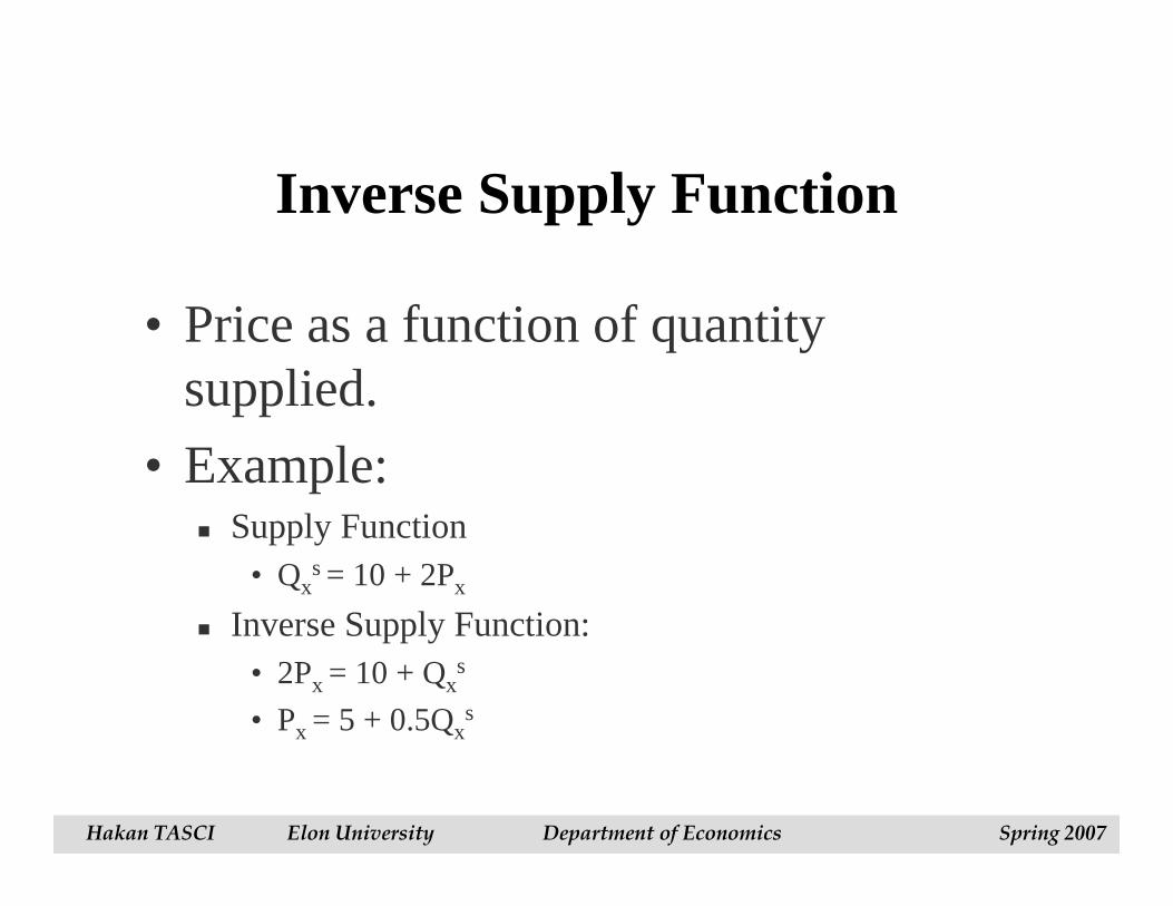
Inverse Supply Function

• Price as a function of quantity supplied.

• Example:� Supply Function

• Qxs= 10 + 2Px

� Inverse Supply Function:• 2Px = 10 + Qx

s

• Px = 5 + 0.5Qxs



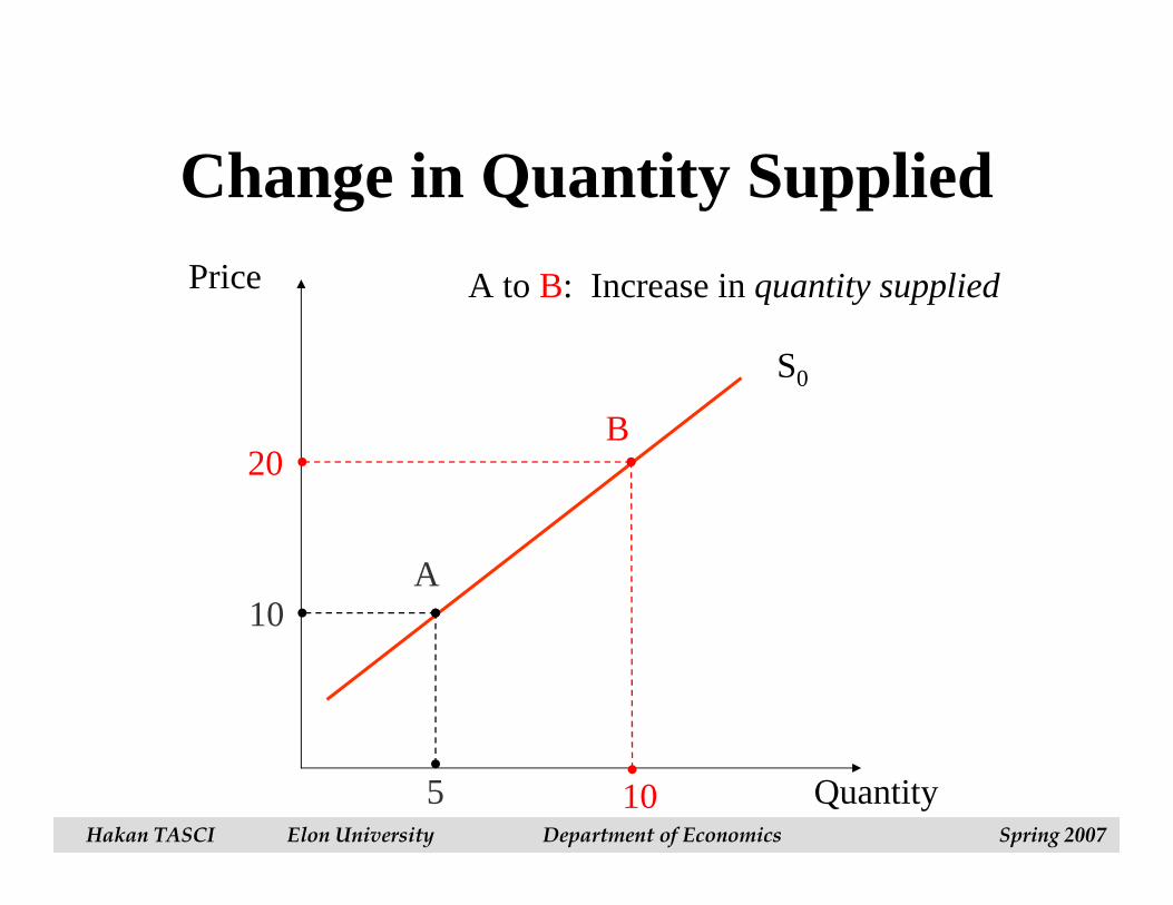
Change in Quantity SuppliedPrice

Quantity

S0

20

10

B

A

5 10

A to B: Increase in quantity supplied



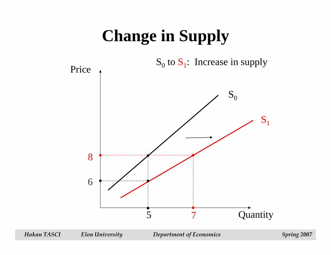
Price

Quantity

S0

S1

8

75

S0 to S1: Increase in supply

Change in Supply

6



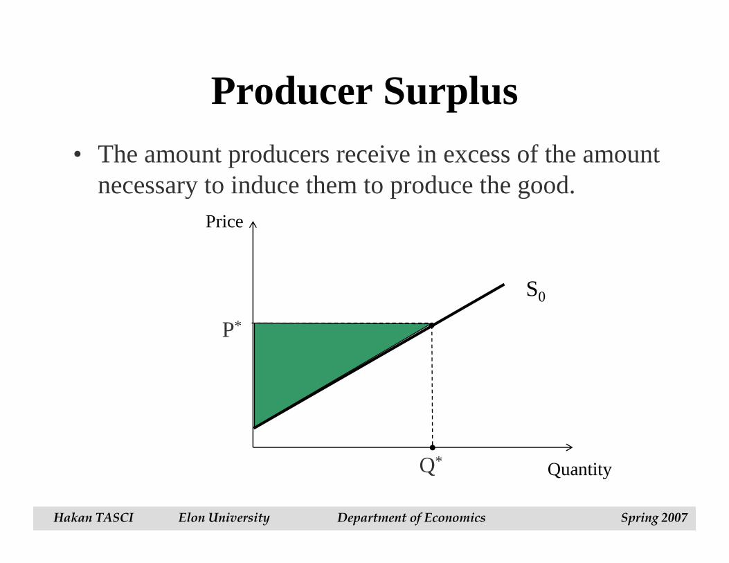
Producer Surplus• The amount producers receive in excess of the amount

necessary to induce them to produce the good.Price

Quantity

S0

Q*

P*



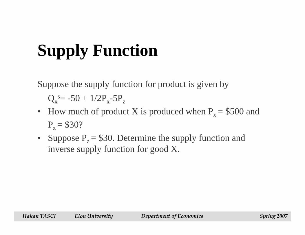
Supply Function

Suppose the supply function for product is given by

Qxs= -50 + 1/2Px-5Pz

• How much of product X is produced when Px = $500 and

Pz = $30?

• Suppose Pz = $30. Determine the supply function and inverse supply function for good X.



Market Equilibrium

• Balancing supply and demand

� QxS = Qx

d

• Steady-state



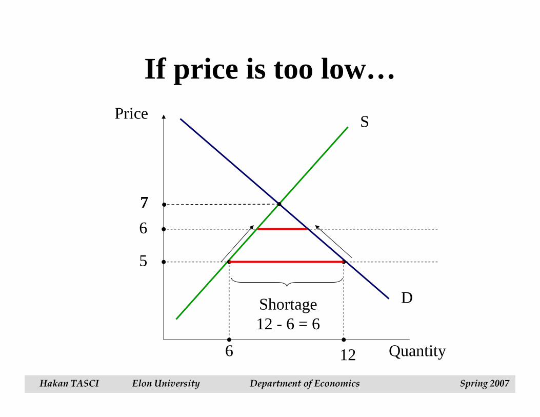
Price

Quantity

S

D

5

6 12

Shortage12 - 6 = 6

6

If price is too low…

7



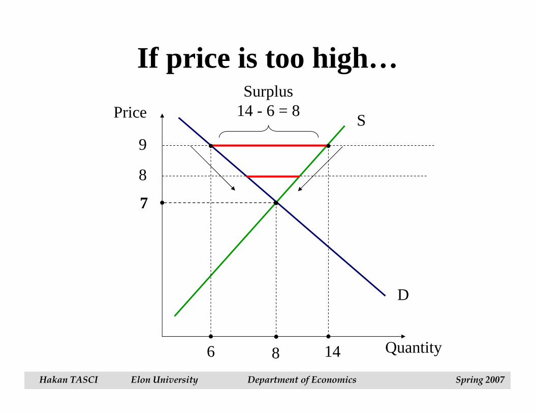
Price

Quantity

S

D

9

14

Surplus14 - 6 = 8

6

8

8

If price is too high…

7



Price Restrictions

• Price Ceilings� The maximum legal price that can be charged.� Examples:

• Gasoline prices in the 1970s.

• Housing in New York City.

• Proposed restrictions on ATM fees.

• Price Floors� The minimum legal price that can be charged.

� Examples:• Minimum wage.

• Agricultural price supports.



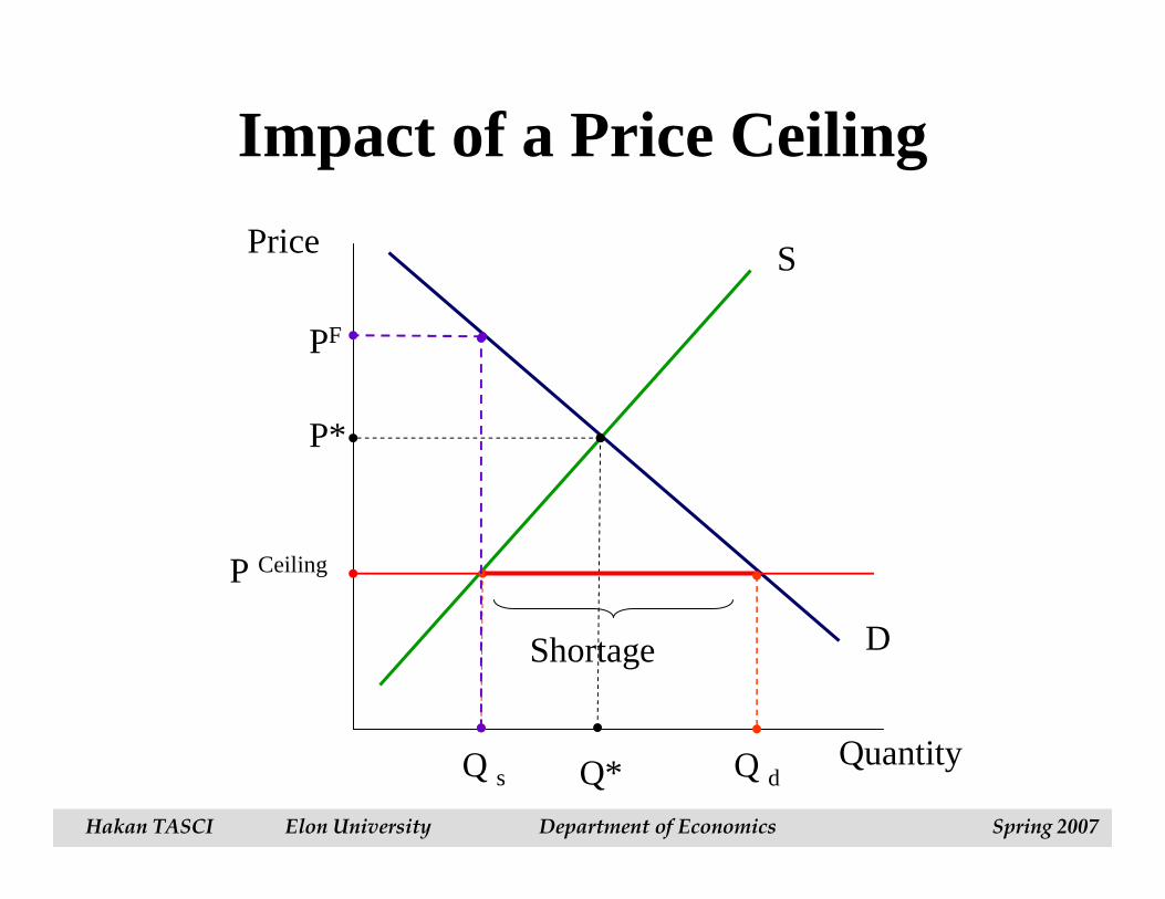
Price

Quantity

S

D

P*

Q*

P Ceiling

Q s

PF

Impact of a Price Ceiling

Shortage

Q dHakan TASCI Elon University Department of Economics Spring 2007


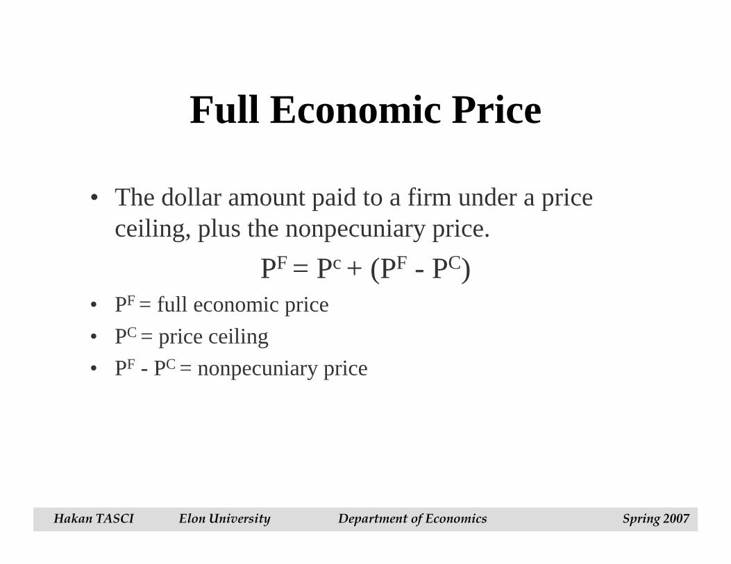
Full Economic Price

• The dollar amount paid to a firm under a price ceiling, plus the nonpecuniary price.

PF = Pc + (PF - PC) • PF = full economic price

• PC = price ceiling

• PF - PC = nonpecuniary price



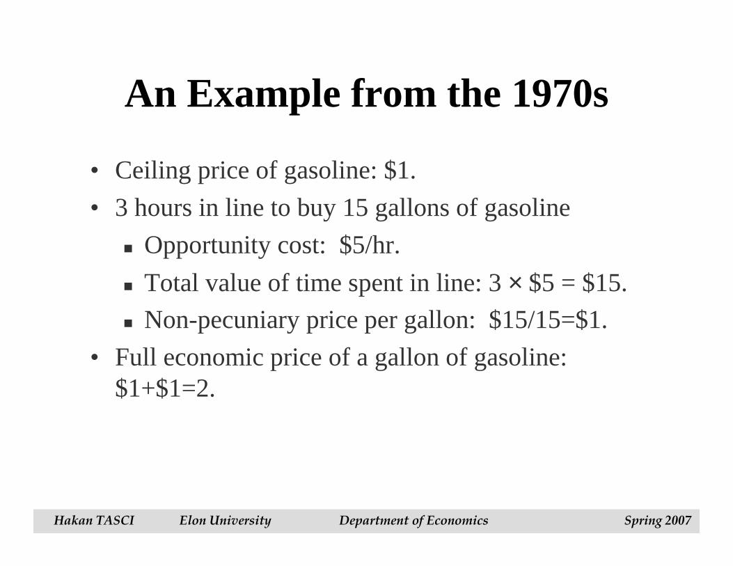
An Example from the 1970s

• Ceiling price of gasoline: $1.

• 3 hours in line to buy 15 gallons of gasoline

� Opportunity cost: $5/hr.

� Total value of time spent in line: 3 × $5 = $15.

� Non-pecuniary price per gallon: $15/15=$1.

• Full economic price of a gallon of gasoline: $1+$1=2.



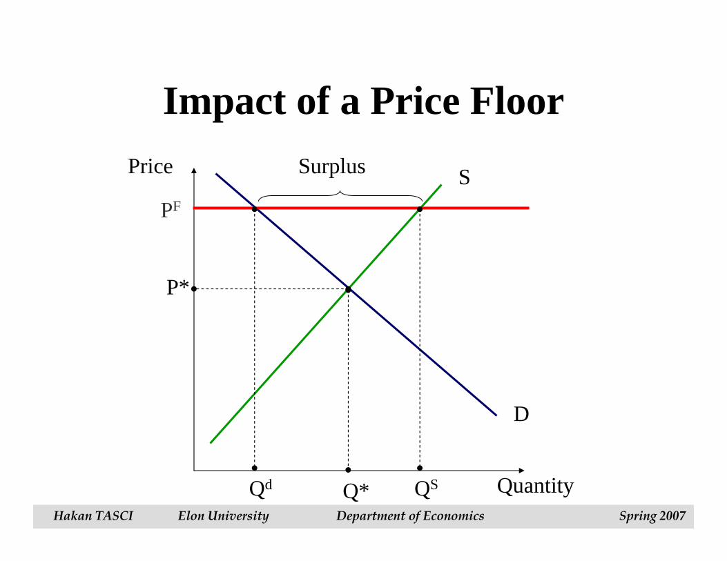
Impact of a Price Floor

Price

Quantity

S

D

P*

Q*

Surplus

PF

Qd QS



Comparative Static Analysis

• How do the equilibrium price and quantity change when a determinant of supply and/or demand change?



Applications of Demand and Supply Analysis

• Event: The WSJ reports that the prices of PC components are expected to fall by 5-8 percent over the next six months.

• Scenario 1: You manage a small firm that manufactures PCs.

• Scenario 2: You manage a small software company.



Use Comparative Static Analysis to see the Big Picture!

• Comparative static analysis shows how the equilibrium price and quantity will change when a determinant of supply or demand changes.



Scenario 1: Implications for a Small PC Maker

• Step 1: Look for the “Big Picture.”

• Step 2: Organize an action plan (worry about details).



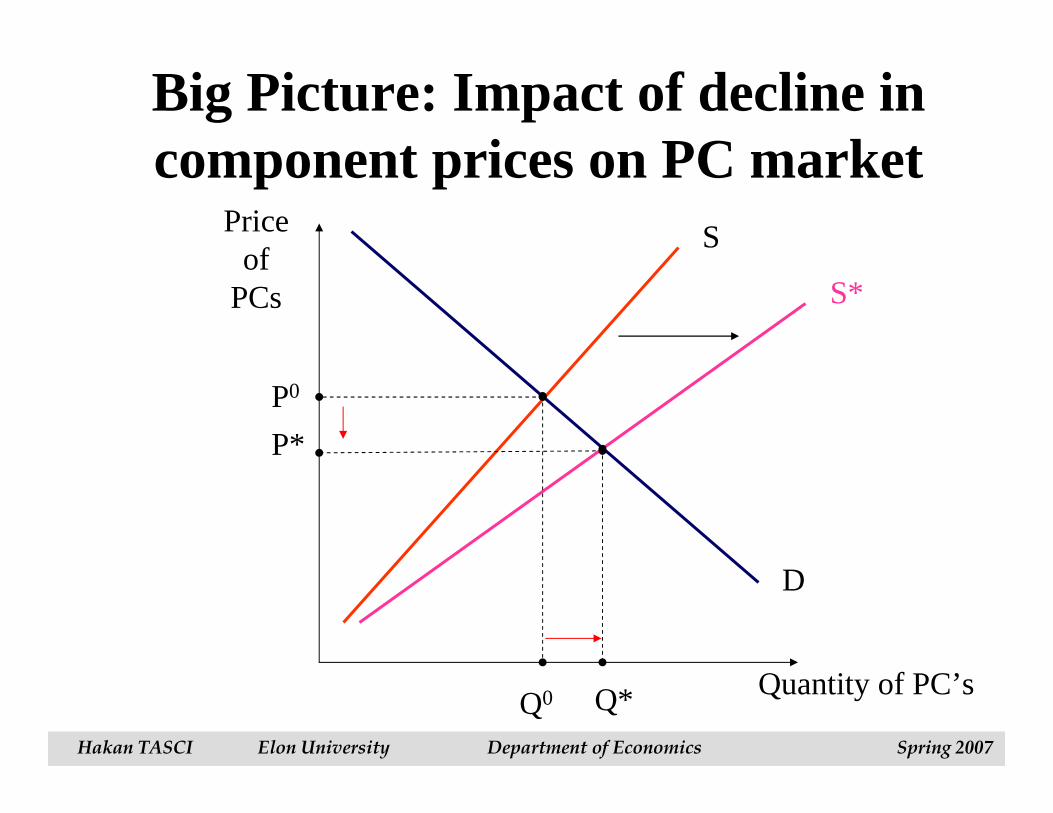
Priceof

PCs

Quantity of PC’s

S

D

S*

P0

P*

Q0 Q*

Big Picture: Impact of decline in component prices on PC market



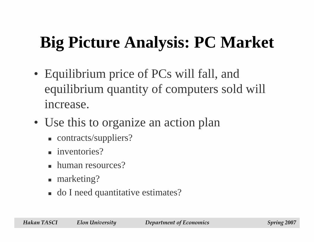
• Equilibrium price of PCs will fall, and equilibrium quantity of computers sold will increase.

• Use this to organize an action plan� contracts/suppliers?

� inventories?

� human resources?

� marketing?

� do I need quantitative estimates?

Big Picture Analysis: PC Market



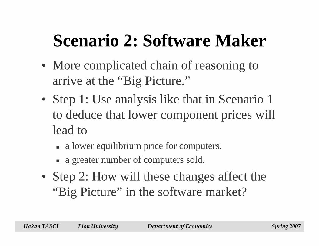
Scenario 2: Software Maker• More complicated chain of reasoning to

arrive at the “Big Picture.”

• Step 1: Use analysis like that in Scenario 1 to deduce that lower component prices will lead to� a lower equilibrium price for computers.

� a greater number of computers sold.

• Step 2: How will these changes affect the “Big Picture” in the software market?



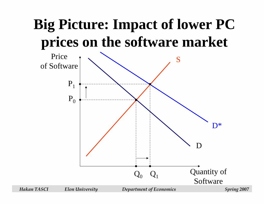
Priceof Software

Quantity ofSoftware

S

D

Q0

D*

P1

Q1

Big Picture: Impact of lower PC prices on the software market

P0



• Software prices are likely to rise, and more software will be sold.

• Use this to organize an action plan.

Big Picture Analysis: Software Market



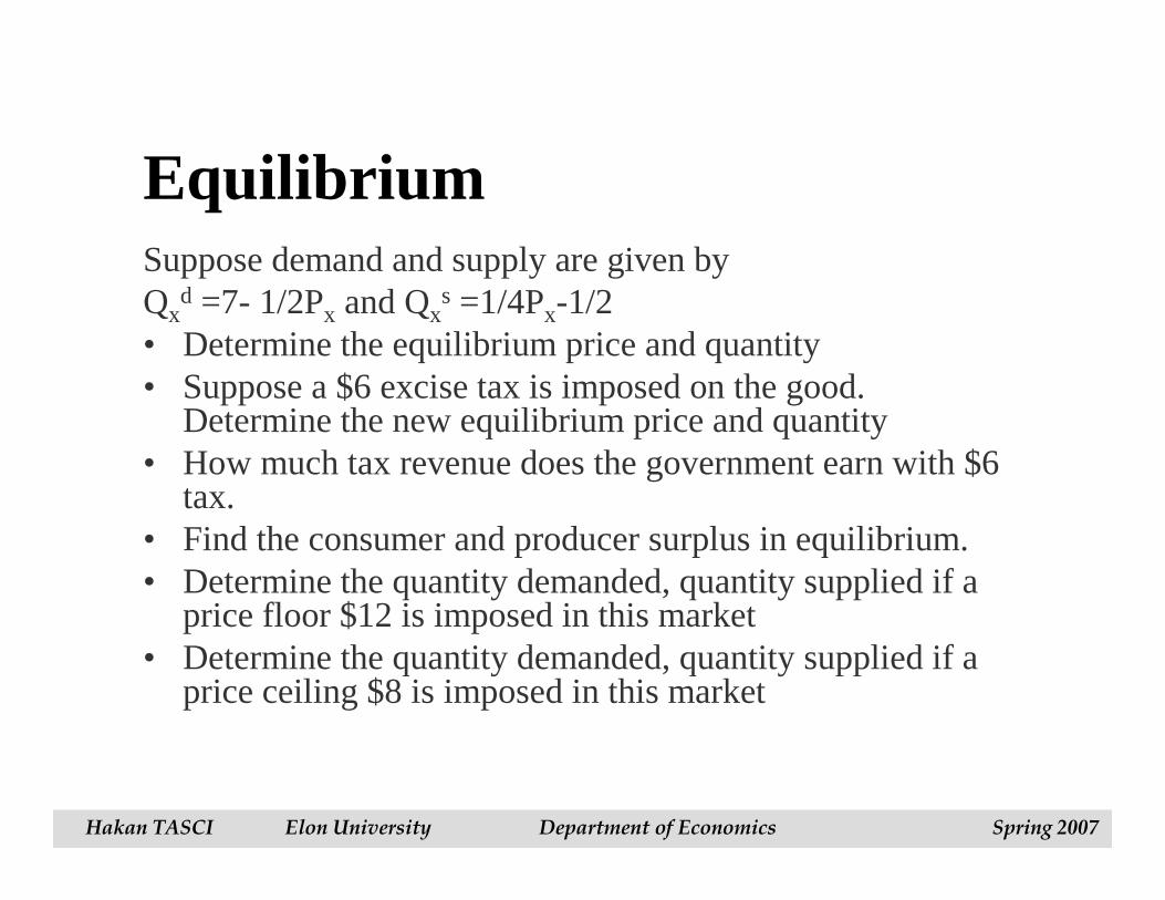
EquilibriumSuppose demand and supply are given by Qx

d =7- 1/2Px and Qxs =1/4Px-1/2

• Determine the equilibrium price and quantity• Suppose a $6 excise tax is imposed on the good.

Determine the new equilibrium price and quantity• How much tax revenue does the government earn with $6

tax.• Find the consumer and producer surplus in equilibrium.• Determine the quantity demanded, quantity supplied if a

price floor $12 is imposed in this market • Determine the quantity demanded, quantity supplied if a

price ceiling $8 is imposed in this market



Conclusion

• Use supply and demand analysis to� clarify the “big picture” (the general impact of a current

event on equilibrium prices and quantities).

� organize an action plan (needed changes in production, inventories, raw materials, human resources, marketing plans, etc.).



Additional Review• Baye’s Text, pages 66-71

Question #5, 6, 8, 9, 12, 14, 16, 18, 19• Chapter 2

Demonstration Problem 2- 3, 4, 5, 6• Math Review

Graphical AnalysisArea finding. Area of a triangleSimple Algebra


managerial economics & business strategy chapter 2 market forces: demand and supply

Documents