magnetic detection of microstructural change in power plant
TRANSCRIPT

Magnetic Detection of
Microstructural Change in
Power Plant Steels
Victoria Anne Yardley
Emmanuel College
This dissertation is submittedfor the degree of Doctor of Philosophy
at the University of Cambridge
PREFACE
This dissertation is submitted for the degree of Doctor of Philosophy at the
University of Cambridge. The research described herein was conducted un-
der the supervision of Professor H. K. D. H. Bhadeshia and Dr M. G. Blamire
in the Department of Materials Science and Metallurgy, University of Cam-
bridge, between October 1999 and April 2003.
Except where acknowledgement and reference are made to previous work,
this work is, to the best of my knowledge, original. This dissertation is
the result of my own work and includes nothing which is the outcome of
work done in collaboration except where specifically indicated in the text.
Neither this, nor any substantially similar dissertation has been, or is being,
submitted for any other degree, diploma, or other qualification at any other
university. This dissertation does not exceed 60,000 words in length.
Victoria Anne Yardley
May 2003
– i –
ACKNOWLEDGEMENTS
I am grateful to Professor Alan Windle and Professor Derek Fray for
the provision of laboratory facilities in the Department of Materials Science
and Metallurgy at the University of Cambridge. I would like to thank my
supervisors, Professor Harry Bhadeshia and Dr Mark Blamire, for their help,
enthusiasm and support.
I would like to express my gratitude to EPSRC, CORUS and the Isaac
Newton Trust for their financial support, and to my industrial supervisor,
Dr Peter Morris, and his colleagues for useful discussions and for the provision
of samples and data.
Much of the work in this thesis would have been impossible without the
generosity of Dr V. Moorthy, Dr Brian Shaw and Mr Mohamed Blaow of
Newcastle University in allowing me to use their Barkhausen noise measure-
ment apparatus and to benefit from their expertise. I am also grateful to
Dr Matthias Gester, Professor Brian Tanner, the late Dr Patrick Squire,
Dr Philippe Baudouin and his colleagues at the University of Ghent, and
Dr Shin-ichi Yamaura for useful discussions, and to Dr Carlos Capdevila
Montes for information on ODS alloys.
I am indebted to the Ironmongers’ Company for their generous bur-
sary enabling me to study for a month at Tohoku University, to Professor
Tadao Watanabe and his colleagues for the warm welcome they extended
to me, and to all the people who, by their friendship, hospitality and kind-
ness, made my stay in Japan so enjoyable. In particular, I would like to
thank Mr Takashi Matsuzaki for supervising my use of the ‘denshikenbikyo’,
Dr Toshihiro Tsuchiyama and his colleagues and family for the invitation to
visit Fukuoka and give a talk at Kyushu University, and Professor Yoshiyuki
Saito for his invitation to visit Waseda University.
I am very grateful to Professor and Mrs Watanabe for their ongoing en-
couragement of, and interest in, me and my work. I would also like to thank
Dr Koichi Kawahara for his help, friendship and encouragement over the past
year, and for many fascinating discussions during which I learned a lot about
domain walls, grain boundaries and Japanese life and culture.
– ii –

It is my pleasure to acknowledge all the PT-members, past and present,
for their kindness, help and friendship and for many enjoyable times, in par-
ticular Daniel Gaude-Fugarolas, Ananth Marimuthu, Dominique Carrouge,
Philippe Opdenacker, Yann de Carlan, Chang Hoon Lee, Professor Yanhong
Wei, Carlos Garcıa Mateo, Thomas Sourmail, Mathew Peet, Gareth Hopkin,
Miguel Yescas-Gonzalez, Pedro Rivera, Franck Tancret and Hiroshi Mat-
suda. My especial thanks go to Shingo, Michiko and Hiroki Yamasaki, for
their warm friendship and hospitality, Japanese lessons and okonomiyaki.
Finally, I would like to thank my parents and friends for their love and
support during the past three years.
– iii –

In loving memory ofEdward and Mary Yardley
– iv –
Contents
Nomenclature vi
Abbreviations vi
Abstract xii
1 Introduction 1
2 Microstructural Evolution in Power Plant Steels 3
2.1 Power plant operation . . . . . . . . . . . . . . . . . . . . . . 3
2.2 Creep mechanism . . . . . . . . . . . . . . . . . . . . . . . . . 5
2.3 Creep-resistant steels . . . . . . . . . . . . . . . . . . . . . . . 6
2.3.1 Characteristics of martensitic steels . . . . . . . . . . . 7
2.3.2 Martensite morphology . . . . . . . . . . . . . . . . . . 8
2.3.3 Tempering of plain-carbon martensitic steels . . . . . . 9
2.3.4 Precipitation Sequences . . . . . . . . . . . . . . . . . 11
2.4 Differences in bainitic microstructures . . . . . . . . . . . . . . 16
2.5 Changes during service . . . . . . . . . . . . . . . . . . . . . . 17
2.5.1 Lath coarsening, recovery and recrystallisation . . . . . 18
2.5.2 Cavitation and final failure . . . . . . . . . . . . . . . . 19
2.6 Design life and remanent life estimation . . . . . . . . . . . . . 19
2.7 Scope for magnetic methods . . . . . . . . . . . . . . . . . . . 20
3 Magnetic Domains 21
3.1 Ferromagnetism and domain theory . . . . . . . . . . . . . . . 21
3.1.1 Atomic origin of ferromagnetism . . . . . . . . . . . . . 21
– v –
3.1.2 Weiss domain theory . . . . . . . . . . . . . . . . . . . 22
3.1.3 Ideal domain structure . . . . . . . . . . . . . . . . . . 23
3.1.4 Energy and width of domain walls . . . . . . . . . . . . 27
3.1.5 Determination of the equilibrium domain structure . . 29
3.2 Evolution of domain structure on application of a magnetic field 29
3.2.1 Ideal magnetisation and demagnetisation . . . . . . . . 29
3.2.2 Magnetic hysteresis . . . . . . . . . . . . . . . . . . . . 30
3.3 Theories of domain wall-defect interactions . . . . . . . . . . . 31
3.3.1 Inclusions . . . . . . . . . . . . . . . . . . . . . . . . . 31
3.3.2 Stress inhomogeneities . . . . . . . . . . . . . . . . . . 33
3.3.3 Grain boundaries . . . . . . . . . . . . . . . . . . . . . 35
3.3.4 Models of domain wall dynamics . . . . . . . . . . . . 35
3.3.5 Correlated domain wall motion and avalanche effects . 38
3.3.6 Mechanism of magnetisation reversal . . . . . . . . . . 39
3.4 Direct observation of domains and domain walls . . . . . . . . 40
3.4.1 Surface domain structures . . . . . . . . . . . . . . . . 42
3.4.2 Magnetisation process in a single crystal . . . . . . . . 43
3.4.3 Domain wall behaviour at grain boundaries . . . . . . 43
3.4.4 Effect of grain boundary misorientations . . . . . . . . 46
3.4.5 Effect of grain size . . . . . . . . . . . . . . . . . . . . 49
3.4.6 Effect of deformation . . . . . . . . . . . . . . . . . . . 50
3.4.7 Second-phase particles and microstructural differences . 51
3.5 Conclusions . . . . . . . . . . . . . . . . . . . . . . . . . . . . 52
4 Magnetic Properties in Nondestructive Testing 54
4.1 Hysteresis properties . . . . . . . . . . . . . . . . . . . . . . . 54
4.1.1 The hysteresis loop . . . . . . . . . . . . . . . . . . . . 54
4.1.2 Alternative terminology . . . . . . . . . . . . . . . . . 56
4.2 Magnetic noise . . . . . . . . . . . . . . . . . . . . . . . . . . 56
4.2.1 Barkhausen effect . . . . . . . . . . . . . . . . . . . . . 56
4.2.2 Magnetoacoustic effect . . . . . . . . . . . . . . . . . . 57
4.2.3 Magnetic noise measurement . . . . . . . . . . . . . . . 57
4.2.4 Data analysis . . . . . . . . . . . . . . . . . . . . . . . 57
– vi –
4.3 Applications of magnetic NDT . . . . . . . . . . . . . . . . . . 59
4.3.1 Microstructural type determination . . . . . . . . . . . 59
4.3.2 Empirical correlations . . . . . . . . . . . . . . . . . . 60
4.4 Grain boundaries . . . . . . . . . . . . . . . . . . . . . . . . . 60
4.4.1 Grain size effects . . . . . . . . . . . . . . . . . . . . . 60
4.4.2 Grain boundary misorientation . . . . . . . . . . . . . 63
4.4.3 Grain size influence on BN frequency . . . . . . . . . . 64
4.4.4 Summary . . . . . . . . . . . . . . . . . . . . . . . . . 65
4.5 Dislocations and plastic strain . . . . . . . . . . . . . . . . . . 66
4.5.1 Deformation . . . . . . . . . . . . . . . . . . . . . . . . 66
4.5.2 Annealing of deformed materials . . . . . . . . . . . . . 67
4.5.3 Deformation and saturation effects . . . . . . . . . . . 69
4.5.4 Summary . . . . . . . . . . . . . . . . . . . . . . . . . 71
4.6 Second-phase particles . . . . . . . . . . . . . . . . . . . . . . 71
4.6.1 Ideal systems . . . . . . . . . . . . . . . . . . . . . . . 71
4.6.2 Effect of carbon on hysteresis properties . . . . . . . . 73
4.6.3 Effect of carbon on BN and MAE . . . . . . . . . . . . 76
4.6.4 Summary . . . . . . . . . . . . . . . . . . . . . . . . . 77
4.7 Magnetic properties of tempered steels . . . . . . . . . . . . . 78
4.7.1 Changes in hysteresis properties on tempering . . . . . 78
4.7.2 Effect of tempering on magnetic noise . . . . . . . . . . 81
4.7.3 Changes in BN with tempering time . . . . . . . . . . 83
4.7.4 Summary . . . . . . . . . . . . . . . . . . . . . . . . . 87
4.8 Are the results inconsistent? . . . . . . . . . . . . . . . . . . . 88
4.9 Effects of magnetising parameters . . . . . . . . . . . . . . . . 89
4.9.1 Surface condition . . . . . . . . . . . . . . . . . . . . . 89
4.9.2 Magnetising field waveform . . . . . . . . . . . . . . . 90
4.9.3 Magnetising frequency . . . . . . . . . . . . . . . . . . 90
4.9.4 Magnetising field amplitude . . . . . . . . . . . . . . . 91
4.9.5 Demagnetising and stray fields . . . . . . . . . . . . . . 91
4.9.6 Stress . . . . . . . . . . . . . . . . . . . . . . . . . . . 92
4.9.7 Temperature . . . . . . . . . . . . . . . . . . . . . . . . 93
4.9.8 Magnetic history . . . . . . . . . . . . . . . . . . . . . 93
– vii –
4.9.9 Solute segregation . . . . . . . . . . . . . . . . . . . . . 93
4.10 Summary and conclusions . . . . . . . . . . . . . . . . . . . . 94
5 Barkhausen Noise Modelling 95
5.1 Existing models of hysteresis and Barkhausen noise . . . . . . 95
5.1.1 Jiles-Atherton model . . . . . . . . . . . . . . . . . . . 95
5.1.2 Preisach model . . . . . . . . . . . . . . . . . . . . . . 97
5.1.3 Equivalence of models and relationship to microstructure 98
5.1.4 Alessandro, Beatrice, Bertotti and Montorsi
(ABBM) model . . . . . . . . . . . . . . . . . . . . . . 98
5.1.5 Extensions to ABBM . . . . . . . . . . . . . . . . . . . 100
5.1.6 Relationships between ABBM parameters and real data 102
5.1.7 Microstructure-based modelling . . . . . . . . . . . . . 103
5.1.8 Models for power plant steels . . . . . . . . . . . . . . 105
5.1.9 Summary . . . . . . . . . . . . . . . . . . . . . . . . . 106
5.2 A new model for BN in power plant steels . . . . . . . . . . . 108
5.3 Assumptions . . . . . . . . . . . . . . . . . . . . . . . . . . . . 108
5.4 Origin of the noise . . . . . . . . . . . . . . . . . . . . . . . . 110
5.5 Construction of the statistical model . . . . . . . . . . . . . . 111
5.5.1 Distribution of pinning sites . . . . . . . . . . . . . . . 111
5.5.2 Impediments to domain wall motion . . . . . . . . . . 111
5.5.3 Mean free path of domain walls . . . . . . . . . . . . . 112
5.5.4 Number of Barkhausen events occurring . . . . . . . . 112
5.5.5 Barkhausen amplitude . . . . . . . . . . . . . . . . . . 112
5.5.6 Multiple distributions of pinning points . . . . . . . . . 113
5.6 Log-normal model . . . . . . . . . . . . . . . . . . . . . . . . . 114
5.7 Summary of model equations . . . . . . . . . . . . . . . . . . 115
5.8 Comparison with experimental data . . . . . . . . . . . . . . . 115
5.9 Relationship between fitting parameters and metallographic
data . . . . . . . . . . . . . . . . . . . . . . . . . . . . . . . . 121
5.9.1 Pinning strength relationships to grain and carbide sizes121
5.9.2 Fitting of model to microstructural data . . . . . . . . 122
5.9.3 Tests of the model on other data sets . . . . . . . . . . 122
– viii –
5.10 Discussion . . . . . . . . . . . . . . . . . . . . . . . . . . . . . 129
5.11 Conclusion . . . . . . . . . . . . . . . . . . . . . . . . . . . . . 129
6 Sample Preparation and Characterisation 130
6.1 Sample preparation . . . . . . . . . . . . . . . . . . . . . . . . 130
6.2 Optical microscopy . . . . . . . . . . . . . . . . . . . . . . . . 132
6.2.1 As-quenched sample . . . . . . . . . . . . . . . . . . . 132
6.2.2 Tempering at 500◦C . . . . . . . . . . . . . . . . . . . 133
6.2.3 Tempering at 600◦C . . . . . . . . . . . . . . . . . . . 133
6.2.4 Tempering at 700◦C . . . . . . . . . . . . . . . . . . . 133
6.2.5 Long-term specimens . . . . . . . . . . . . . . . . . . . 146
6.3 Scanning electron microscopy . . . . . . . . . . . . . . . . . . 146
6.4 Feature size measurements . . . . . . . . . . . . . . . . . . . . 147
6.4.1 Coarsening in 700◦C tempered steel . . . . . . . . . . . 148
6.4.2 Carbide phases . . . . . . . . . . . . . . . . . . . . . . 149
6.5 Hardness . . . . . . . . . . . . . . . . . . . . . . . . . . . . . . 149
6.6 Magnetic hysteresis measurements . . . . . . . . . . . . . . . . 151
6.7 Conclusion . . . . . . . . . . . . . . . . . . . . . . . . . . . . . 153
7 Orientation Imaging Microscopy and Grain Boundary Anal-
ysis in Tempered Power Plant Steel 154
7.1 Grain orientation . . . . . . . . . . . . . . . . . . . . . . . . . 155
7.1.1 Pole figures and inverse pole figures . . . . . . . . . . . 155
7.1.2 Euler angles . . . . . . . . . . . . . . . . . . . . . . . . 156
7.1.3 Angle-axis pairs . . . . . . . . . . . . . . . . . . . . . . 156
7.2 Grain boundary geometry . . . . . . . . . . . . . . . . . . . . 157
7.2.1 The coincidence site lattice model . . . . . . . . . . . . 158
7.2.2 Estimation of grain boundary energy . . . . . . . . . . 159
7.3 Electron Backscatter Diffraction . . . . . . . . . . . . . . . . . 160
7.3.1 Formation of Kikuchi patterns . . . . . . . . . . . . . . 160
7.3.2 Indexing Kikuchi patterns . . . . . . . . . . . . . . . . 161
7.3.3 Diffraction geometry in the SEM . . . . . . . . . . . . 163
– ix –
7.4 Automated Orientation Imaging
Microscopy . . . . . . . . . . . . . . . . . . . . . . . . . . . . 164
7.4.1 Representation of data . . . . . . . . . . . . . . . . . . 164
7.4.2 Image Quality . . . . . . . . . . . . . . . . . . . . . . . 165
7.5 OIM observations of martensitic steels . . . . . . . . . . . . . 166
7.5.1 Crystallographic relationships . . . . . . . . . . . . . . 166
7.5.2 Creep-deformed martensitic steels . . . . . . . . . . . . 167
7.6 Experimental technique . . . . . . . . . . . . . . . . . . . . . . 168
7.6.1 Sample Preparation . . . . . . . . . . . . . . . . . . . . 168
7.6.2 Orientation Imaging Microscopy . . . . . . . . . . . . . 168
7.7 Results . . . . . . . . . . . . . . . . . . . . . . . . . . . . . . . 169
7.7.1 As-quenched data . . . . . . . . . . . . . . . . . . . . . 191
7.7.2 Indeterminate points . . . . . . . . . . . . . . . . . . . 193
7.7.3 600◦C, 4 hours tempering . . . . . . . . . . . . . . . . 193
7.7.4 600◦C, 16 hours tempering . . . . . . . . . . . . . . . . 194
7.7.5 600◦C, 64 hours tempering . . . . . . . . . . . . . . . . 195
7.7.6 600◦C, 128 hours tempering . . . . . . . . . . . . . . . 195
7.7.7 600◦C, 256 hours tempering . . . . . . . . . . . . . . . 196
7.7.8 Summary . . . . . . . . . . . . . . . . . . . . . . . . . 197
7.8 Statistical analysis . . . . . . . . . . . . . . . . . . . . . . . . 197
7.8.1 Grain boundary misorientations . . . . . . . . . . . . . 197
7.8.2 Coincidence boundaries . . . . . . . . . . . . . . . . . . 198
7.8.3 Statistics of indeterminate points . . . . . . . . . . . . 198
7.8.4 Image quality statistics . . . . . . . . . . . . . . . . . . 202
7.9 Orientation relationships . . . . . . . . . . . . . . . . . . . . . 204
7.9.1 256 hour sample . . . . . . . . . . . . . . . . . . . . . . 206
7.9.2 AQ sample . . . . . . . . . . . . . . . . . . . . . . . . 207
7.10 Relationship to magnetic properties . . . . . . . . . . . . . . . 208
7.11 Conclusions . . . . . . . . . . . . . . . . . . . . . . . . . . . . 209
8 Barkhausen Noise Experiments on Power Plant Steels 211
8.1 Experimental Method . . . . . . . . . . . . . . . . . . . . . . . 211
8.1.1 Sample Preparation . . . . . . . . . . . . . . . . . . . . 211
– x –
8.1.2 Instrumentation . . . . . . . . . . . . . . . . . . . . . . 211
8.1.3 Operating Conditions . . . . . . . . . . . . . . . . . . . 212
8.2 Results . . . . . . . . . . . . . . . . . . . . . . . . . . . . . . . 217
8.2.1 Peak height, width and position . . . . . . . . . . . . . 218
8.2.2 Comparison with results of Moorthy et al. . . . . . . . 226
8.2.3 Experiments on tempered plain-carbon steel . . . . . . 227
8.3 Frequency analysis . . . . . . . . . . . . . . . . . . . . . . . . 229
8.3.1 Checks on validity of results . . . . . . . . . . . . . . . 235
8.4 Discussion . . . . . . . . . . . . . . . . . . . . . . . . . . . . . 237
8.4.1 Tempered 214Cr1Mo steels . . . . . . . . . . . . . . . . 237
8.4.2 11Cr1Mo steels . . . . . . . . . . . . . . . . . . . . . . 238
8.5 Conclusions . . . . . . . . . . . . . . . . . . . . . . . . . . . . 238
9 Model Fitting to Power-Plant Steel Data 240
9.1 Data and fitting procedure . . . . . . . . . . . . . . . . . . . . 240
9.2 Results . . . . . . . . . . . . . . . . . . . . . . . . . . . . . . . 240
9.3 Fitting parameters . . . . . . . . . . . . . . . . . . . . . . . . 244
9.3.1 Comparison of Model 1 and Model 2 . . . . . . . . . . 244
9.3.2 Model 2 parameter variations with Larson-Miller pa-
rameter . . . . . . . . . . . . . . . . . . . . . . . . . . 248
9.4 Discussion . . . . . . . . . . . . . . . . . . . . . . . . . . . . . 252
9.4.1 Relationship of fitting parameters to microstructure . . 252
9.5 Conclusion . . . . . . . . . . . . . . . . . . . . . . . . . . . . . 253
10 Barkhausen Noise in PM2000 Oxide Dispersion Strength-
ened Alloy 254
10.1 Oxide dispersion strengthened alloys . . . . . . . . . . . . . . 254
10.2 Relevance of PM2000 to magnetic property studies . . . . . . 255
10.3 Experimental Method . . . . . . . . . . . . . . . . . . . . . . . 256
10.3.1 Sample preparation . . . . . . . . . . . . . . . . . . . . 256
10.3.2 BN measurement . . . . . . . . . . . . . . . . . . . . . 257
10.4 Microstructures . . . . . . . . . . . . . . . . . . . . . . . . . . 258
10.4.1 Naked-eye observations . . . . . . . . . . . . . . . . . . 258
– xi –
10.4.2 Optical micrographs . . . . . . . . . . . . . . . . . . . 258
10.4.3 TEM observation . . . . . . . . . . . . . . . . . . . . . 258
10.4.4 Melted (oxide-free) sample . . . . . . . . . . . . . . . . 261
10.5 Hardness measurements . . . . . . . . . . . . . . . . . . . . . 261
10.6 Comparison between unrecrystallised,
melted and recrystallised PM2000 . . . . . . . . . . . . . . . . 265
10.6.1 Hysteresis . . . . . . . . . . . . . . . . . . . . . . . . . 265
10.6.2 Barkhausen noise . . . . . . . . . . . . . . . . . . . . . 266
10.6.3 Conclusion . . . . . . . . . . . . . . . . . . . . . . . . . 267
10.7 BN across a grain boundary . . . . . . . . . . . . . . . . . . . 267
10.8 Recrystallisation sequences . . . . . . . . . . . . . . . . . . . . 267
10.8.1 Unrecrystallised sample . . . . . . . . . . . . . . . . . 268
10.8.2 Effect of heat treatment . . . . . . . . . . . . . . . . . 268
10.9 Tests on unprepared samples . . . . . . . . . . . . . . . . . . . 277
10.10Conclusions . . . . . . . . . . . . . . . . . . . . . . . . . . . . 280
11 Summary, Conclusions and Suggestions for Further Work 281
11.1 Summary and conclusions . . . . . . . . . . . . . . . . . . . . 281
11.2 Future work . . . . . . . . . . . . . . . . . . . . . . . . . . . . 284
11.2.1 Experimental work . . . . . . . . . . . . . . . . . . . . 284
11.2.2 Modelling . . . . . . . . . . . . . . . . . . . . . . . . . 285
Bibliography 286
Appendix: Modelling Program 308
– xii –

ABBREVIATIONS
b.c.c. Body-centred cubic
ppm Parts per million
ABBM Alessandro, Beatrice, Bertotti and Montorsi model
AQ As-quenched
BN Barkhausen noise
CSL Coincidence site lattice
EBSD Electron backscatter diffraction
FEG Field emission gun
FWHM Full width half maximum
IQ Image quality
MAE Magnetoacoustic Emission
NDT Nondestructive testing
ODS Oxide-dispersion strengthened
OIM Orientation imaging microscopy
PHD Pulse height distribution
RMS Root-mean-square
SEM Scanning electron microscope
TEM Transmission electron microscope
VSM Vibrating sample magnetometer
– xiii –

NOMENCLATURE
Note: Two SI systems for magnetics nomenclature exist, but the Sommerfeld
system has been used throughout; equations not conforming to this system
have been converted. A comparison table including the two SI systems and
the cgs system can be found in Jiles (1998).
General
d Grain diameter
E Efficiency
M Magnification
Mf Martensite-finish temperature
Ms Martensite-start temperature
P Larson-Miller parameter
t Time
T Absolute temperature
T1 Absolute heat source temperature
T2 Absolute heat sink temperature
TM Absolute melting temperature
Magnetics
B Magnetic induction
BS Saturation induction
BR Remanent induction
Ea Anisotropy energy
– xiv –

Earea Area reduction energy (Kersten model)
Ed Demagnetising energy
Edemag Inclusion demagnetising energy (Neel model)
Eex Exchange energy
Em Magnetostatic energy
Epin Energy dissipated against pinning
Esupp Energy supplied
H Magnetic field
HC Coercive field
Hd Demagnetising field
He Weiss mean field
Hmax Maximum applied field
HS Field at which M = MS
K1 Anisotropy constant
M Magnetisation
m Magnetic moment
MR Remanent magnetisation
MS Saturation magnetisation
Nd Demagnetising constant
P Barkhausen noise power
TC Curie temperature
V Voltage
– xv –

WH Hysteresis energy loss
α Mean field constant
β Term characterising nearest-neighbour interactions
γ Domain wall energy
δ Domain wall thickness
λUV W Magnetostrictive strain along < UV W >
λsi Ideal magnetostrictive strain
µ0 Permeability of free space
µ′ Differential permeability
µ′max Maximum differential permeability
σ Electrical conductivity
χ′in Initial differential susceptibility
χ′max Maximum differential susceptibility
Φ Magnetic flux
ω∗ Surface pole density
J Term characterising nearest-neighbour interactions
Modelling: existing models
A, B Amplitude of fluctuations in ABBM
k pinning parameter
Man Anhysteretic magnetisation
MJS BN jump sum
– xvi –

Mrev Reversible magnetisation
< Mdisc > Average BN event size
v domain wall velocity
W noise term in ABBM
< επ > Pinning energy for 180◦ wall
< εpin > Pinning enrgy for wall at arbitrary angle
ξ Correlation length
Modelling: new model
Ai Total number pinning points of ith type per unit volume
Aw Wall surface area
C Constant
E Fitting error
E0 Electric field amplitude
lw Wall jump distance
l{H} Distance between pinning sites at field H
< l > {H} Domain wall mean free path
N{H} Number of pinning sites of strength ≥ H
n{S} Number pinning sites of strength S
S Pinning site field strength
Sb Field at which unpinning first occurs
< S >i Mean value of S for ith type of pinning site
– xvii –

V {H} BN voltage at field H
Vr{H} Real V {H}
Vp{H} Predicted V {H}
< x > Mean value of ln{S} for log-normal distribution
β Parameter depending on angle between adjacent domains
∆Si Standard deviation of S for ith type of pinning site
∆x Standard deviation of ln{S} for log-normal distribution
Orientation Imaging Microscopy
cc Crystal coordinate system
cs Sample coordinate system
d Planar spacing
G Rotation matrix
M Misorientation matrix
< UV W > Misorientation axis
ν0 Brandon ratio proportionality constant
νm Maximum allowable deviation from ideal coincidence
λ Radiation wavelength
θ Misorientation angle
θB Bragg angle
– xviii –
ABSTRACT
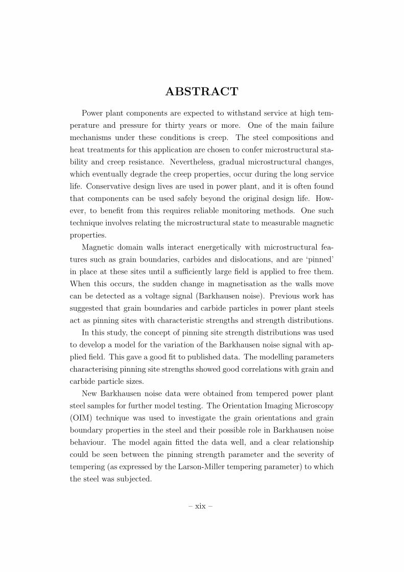
Power plant components are expected to withstand service at high tem-
perature and pressure for thirty years or more. One of the main failure
mechanisms under these conditions is creep. The steel compositions and
heat treatments for this application are chosen to confer microstructural sta-
bility and creep resistance. Nevertheless, gradual microstructural changes,
which eventually degrade the creep properties, occur during the long service
life. Conservative design lives are used in power plant, and it is often found
that components can be used safely beyond the original design life. How-
ever, to benefit from this requires reliable monitoring methods. One such
technique involves relating the microstructural state to measurable magnetic
properties.
Magnetic domain walls interact energetically with microstructural fea-
tures such as grain boundaries, carbides and dislocations, and are ‘pinned’
in place at these sites until a sufficiently large field is applied to free them.
When this occurs, the sudden change in magnetisation as the walls move
can be detected as a voltage signal (Barkhausen noise). Previous work has
suggested that grain boundaries and carbide particles in power plant steels
act as pinning sites with characteristic strengths and strength distributions.
In this study, the concept of pinning site strength distributions was used
to develop a model for the variation of the Barkhausen noise signal with ap-
plied field. This gave a good fit to published data. The modelling parameters
characterising pinning site strengths showed good correlations with grain and
carbide particle sizes.
New Barkhausen noise data were obtained from tempered power plant
steel samples for further model testing. The Orientation Imaging Microscopy
(OIM) technique was used to investigate the grain orientations and grain
boundary properties in the steel and their possible role in Barkhausen noise
behaviour. The model again fitted the data well, and a clear relationship
could be seen between the pinning strength parameter and the severity of
tempering (as expressed by the Larson-Miller tempering parameter) to which
the steel was subjected.
– xix –
The experimental results suggest that the Barkhausen noise characteris-
tics of the steels investigated depend strongly on the strain at grain bound-
aries. As tempering progresses and the grain boundary dislocation density
falls, the pinning strength of the grain boundaries also decreases. A clear
difference in Barkhausen noise response could be seen between a 214Cr1Mo
traditional power-plant steel and an 11Cr1Mo steel designed for superior heat
resistance.
A study of an oxide dispersion strengthened ferrous alloy, in which the mi-
crostructure undergoes dramatic coarsening on recrystallisation, was used to
investigate further the effects of grain boundaries and particles on Barkhausen
noise. The findings from these experiments supported the conclusion that
grain boundary strain reduction gave large changes in the observed Barkhausen
noise.
– xx –

Chapter 1
Introduction
The aim of this work was to investigate the use of magnetic property mea-
surements as a nondestructive tool for microstructural evaluation in power
plant steels. A survey of the existing literature pointed to Barkhausen noise
as a suitable property for investigation. A new model for Barkhausen noise
from power plant steels was proposed and tested using previous published
data. New data for further model testing were generated from 214Cr1Mo
and 11Cr1Mo (wt. %) power plant steel samples. Detailed characterisation
of the grain structures in these steels was carried out to study the role of
grain boundaries in Barkhausen noise. Experiments on an oxide dispersion
strengthened alloy, in which the grain size and oxide particle distribution
could be varied separately, were used to give further clarification of this.
Power plant conditions and the physical metallurgy of power plant steels
are discussed in Chapter 2, which also reviews some of the existing methods
of nondestructive microstructural evaluation.
The concept of magnetic domains is essential for understanding the mi-
crostructural dependence of magnetic properties. The theory of domains is
given in the first half of Chapter 3. Observations of the interactions between
the domain structure and microstructural features appear in the second half.
Chapter 4 introduces the magnetic properties commonly used in mi-
crostructural characterisation, including magnetic hysteresis and Barkhausen
noise. Previous work on the relationships between microstructural features
and magnetic properties is reviewed, with particular emphasis on studies of
– 1 –
Chapter 1 Introduction
Barkhausen noise in tempered martensitic steels.
Insights from one of these studies were used as the basis for a new model of
the microstructural dependence of the Barkhausen signal in tempered steels.
Chapter 5 summarises existing models of hysteresis and Barkhausen noise,
describes the derivation of the new model and gives details of model testing
using published data from the literature.
Chapter 6 describes the preparation of power plant steel samples. Opti-
cal micrographs, hardness and coercive field data and estimates of the mi-
crostructural feature sizes are given in this chapter. A subset of the samples
were selected for more detailed characterisation using the technique of Ori-
entation Imaging Microscopy in the scanning electron microscope. Chapter 7
explains the basis of this technique and presents micrographs and analysis.
Barkhausen noise experiments on the power plant steel samples are de-
scribed in Chapter 8. The data generated were used to fit the new model;
the results are given in Chapter 9.
Chapter 10 gives details of experiments performed on an oxide dispersion
strengthened alloy with the aim of understanding the role of grain boundaries
and particle dispersions in hysteresis and Barkhausen noise.
Chapter 11 summarises the findings of this study and gives suggestions
for future directions in which this work can be taken. The code of the model
fitting program and a description of its operation are given in the Appendix.
– 2 –

Chapter 2
Microstructural Evolution inPower Plant Steels
2.1 Power plant operation
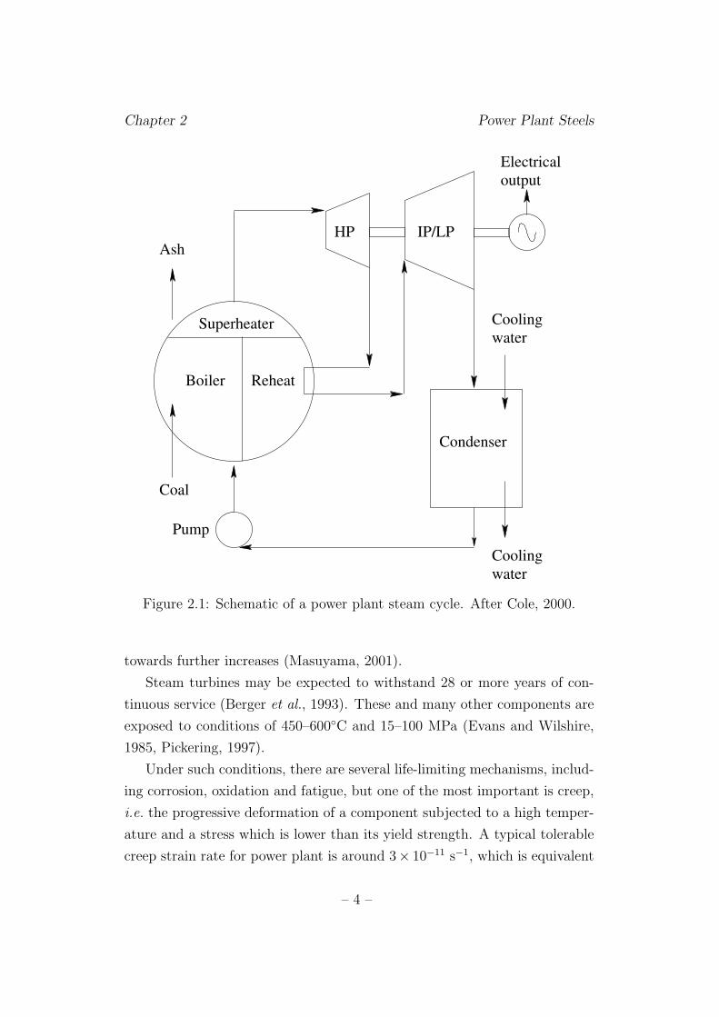
In power plant, heat energy from fuel combustion or nuclear fission is used
to produce jets of steam. The kinetic energy of the steam is converted to
electrical energy by a system of turbines and a generator. Figure 2.1 shows
the route followed by the steam and water. Water is pumped into the boiler
and converted to steam, then superheated. It is injected through nozzles
onto the blades of the high pressure (HP) turbines. Following this, it is
reheated and sent to the intermediate pressure (IP) turbines and then to the
low pressure (LP) turbines. The rotary motion of the turbines is used to
drive the generator to produce electrical power, and the exhaust steam is
condensed and recirculated.
The Carnot efficiency E of such a cycle is given by:
E =T1 − T2
T1
(2.1)
where T1 and T2 are the absolute temperatures of the heat source and heat
sink respectively. It is therefore desirable from both economic and environ-
mental points of view to use as high an operating temperature as possible.
Progress in power-plant alloy design has allowed T1 to be increased from
370◦C in the 1920s to a current level of 600◦C or higher, and there is a drive
– 3 –
Chapter 2 Power Plant Steels
Pump
Cooling
water
Cooling
water
Electrical
output
Condenser
Reheat
Coal
Boiler
Superheater
AshHP IP/LP
Figure 2.1: Schematic of a power plant steam cycle. After Cole, 2000.
towards further increases (Masuyama, 2001).
Steam turbines may be expected to withstand 28 or more years of con-
tinuous service (Berger et al., 1993). These and many other components are
exposed to conditions of 450–600◦C and 15–100 MPa (Evans and Wilshire,
1985, Pickering, 1997).
Under such conditions, there are several life-limiting mechanisms, includ-
ing corrosion, oxidation and fatigue, but one of the most important is creep,
i.e. the progressive deformation of a component subjected to a high temper-
ature and a stress which is lower than its yield strength. A typical tolerable
creep strain rate for power plant is around 3× 10⁻¹¹ s−1, which is equivalent
– 4 –
Chapter 2 Power Plant Steels
to 2% elongation over 30 years (Bhadeshia et al., 1998).
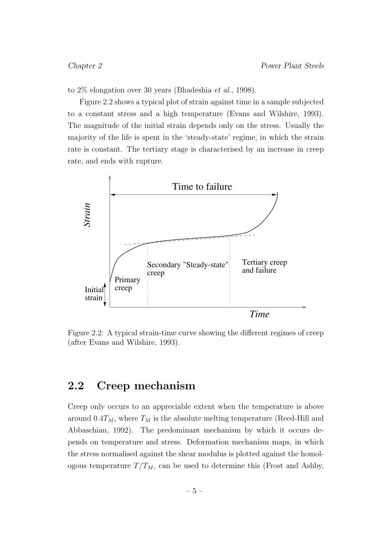
Figure 2.2 shows a typical plot of strain against time in a sample subjected
to a constant stress and a high temperature (Evans and Wilshire, 1993).
The magnitude of the initial strain depends only on the stress. Usually the
majority of the life is spent in the ‘steady-state’ regime, in which the strain
rate is constant. The tertiary stage is characterised by an increase in creep
rate, and ends with rupture.
Primarycreep
Time to failure
Time
Str
ain
Initialstrain
Tertiary creepand failurecreep
Secondary "Steady-state"
Figure 2.2: A typical strain-time curve showing the different regimes of creep(after Evans and Wilshire, 1993).
2.2 Creep mechanism
Creep only occurs to an appreciable extent when the temperature is above
around 0.4TM , where TM is the absolute melting temperature (Reed-Hill and
Abbaschian, 1992). The predominant mechanism by which it occurs de-
pends on temperature and stress. Deformation mechanism maps, in which
the stress normalised against the shear modulus is plotted against the homol-
ogous temperature T/TM , can be used to determine this (Frost and Ashby,
– 5 –
Chapter 2 Power Plant Steels
1982; Ashby and Jones, 1989). It is found that under typical power plant
operating conditions, creep occurs by dislocation glide and climb, rather than
by bulk diffusion.
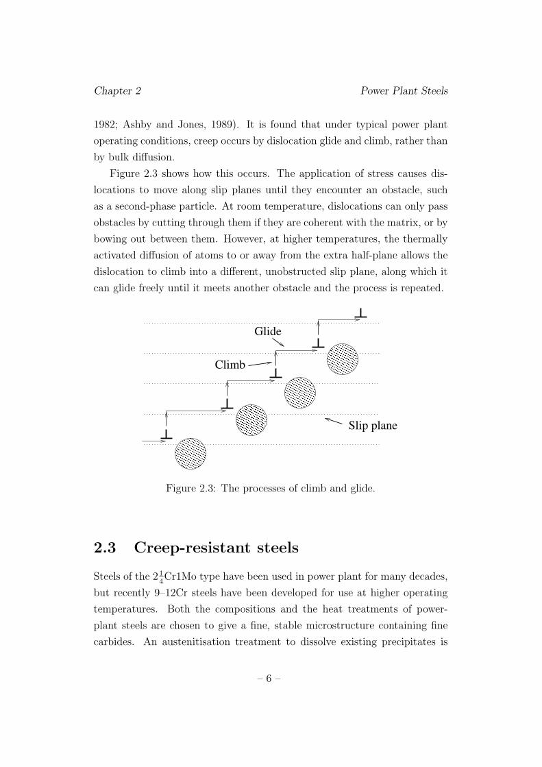
Figure 2.3 shows how this occurs. The application of stress causes dis-
locations to move along slip planes until they encounter an obstacle, such
as a second-phase particle. At room temperature, dislocations can only pass
obstacles by cutting through them if they are coherent with the matrix, or by
bowing out between them. However, at higher temperatures, the thermally
activated diffusion of atoms to or away from the extra half-plane allows the
dislocation to climb into a different, unobstructed slip plane, along which it
can glide freely until it meets another obstacle and the process is repeated.
�������������������������������������������������
������������������������������������������������� �������������������������������������������������
������������������������������������������������� �������������������������������������������������
������������������������������������������������� �������������������������������������������������
���������������������
Climb
Slip plane
Glide
Figure 2.3: The processes of climb and glide.
2.3 Creep-resistant steels
Steels of the 214Cr1Mo type have been used in power plant for many decades,
but recently 9–12Cr steels have been developed for use at higher operating
temperatures. Both the compositions and the heat treatments of power-
plant steels are chosen to give a fine, stable microstructure containing fine
carbides. An austenitisation treatment to dissolve existing precipitates is
– 6 –
Chapter 2 Power Plant Steels
carried out above 1000◦C, the exact temperature depending on the steel com-
position. The steel is then air-cooled. In 214Cr1Mo, this results in a predom-
inantly bainitic microstructure, but 9–12 Cr steels are fully air-hardenable,
and martensite is formed.
Tempering is then carried out, typically at around 700◦C, to produce fine
carbides and reduce the stored energy in the microstructure so that there
is only a very small driving force for microstructural change during service.
Bhadeshia et al. (1998) have calculated the stored energy of a power plant
alloy in martensitic form is 1214 J mol−1 greater than that in its equilibrium
state, whereas the post-tempering microstructure is only 63 J mol−1 above
equilibrium.
Lower tempering temperatures give high creep rupture strength in the
short term, but this decreases rapidly; tempering at a higher temperature
gives better long-term creep properties (Yoshikawa et al., 1986, Masuyama,
2001). This is believed to occur because the change from martensite to ferrite
is complete after high-temperature tempering, but will occur during service
if the tempering temperature is low.
2.3.1 Characteristics of martensitic steels
The transformation from austenite to martensite is diffusionless, occurring
as a deformation of the parent lattice. On cooling sufficiently rapidly to
suppress the diffusional ferrite and pearlite reactions and the intermediate
bainite reaction, martensite formation begins at the martensite-start tem-
perature Ms. The transformation is rapid and athermal. The Mf temper-
ature marks the point at which transformation should be complete, but in
practice, some retained austenite often remains. In plain carbon steels with
<0.5 wt. % C, very little austenite is retained (2% or less) but higher carbon
contents increase this proportion. Because the transformation from austen-
ite is diffusionless, the martensite is supersaturated in carbon, and has a
tetragonal crystal structure if the carbon content is sufficiently high.
– 7 –
Chapter 2 Power Plant Steels
2.3.2 Martensite morphology
Martensite forms in thin plates or laths on specific habit planes within the
prior austenite grains. In order to accommodate the shape deformation of the
transformation while maintaining a planar interface between the transformed
and untransformed phases, the martensite slips or twins on a fine scale.
The dislocation density of ferrous martensites is of the order of 1011–
1012 cm−2, similar to that achieved by severe cold work. In lower-carbon
martensites (<0.5 wt. % C), only dislocations are usually present, but higher-
carbon martensites also exhibit twinning, which is favoured by a higher yield
stress.
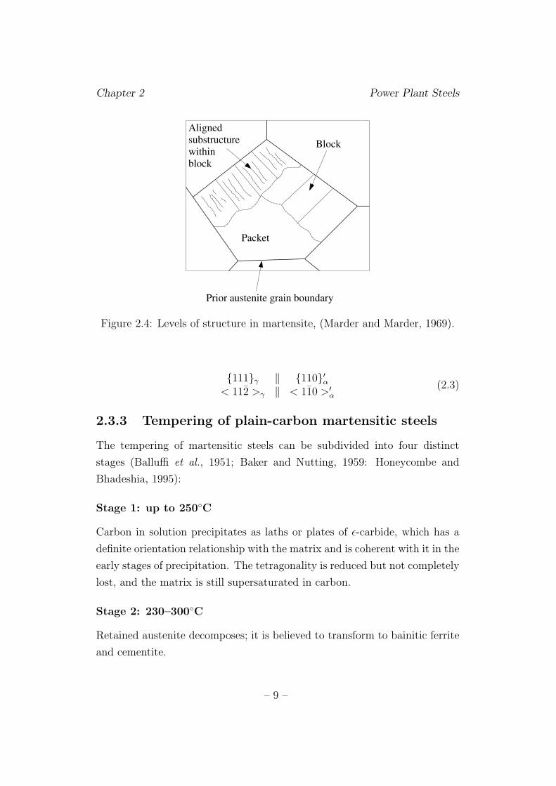
Figure 2.4 illustrates schematically the structural levels in martensitic mi-
crostructures (Marder and Marder, 1969). The prior austenite grain bound-
ary structure is preserved, and laths forming within the grains stop at these
boundaries because the austenite grains do not, in general, have any special
orientation relationship to one another. A packet is a region of laths with
the same habit plane, and blocks are subunits of packets, in which the lath
orientation is also the same. The combination of habit plane and orientation
is known as a variant.
The sizes of both blocks and packets increased with increasing prior
austenite grain size (Maki et al., 1980). However, the clear block and packet
structure in Figure 2.4 was only observed for carbon contents less than
0.5 wt. % in plain-carbon steels. Higher carbon contents gave a microstruc-
ture of irrationally arranged laths throughout the prior austenite grain.
In low-carbon martensitic steels (<0.5 wt. %C), the habit plane is {111}γ,
and the orientation relationship between the austenite γ and martensite α′
is due to Kurdjumov and Sachs (1930):
{111}γ ‖ {110}′α< 110 >γ ‖ < 111 >′
α
(2.2)
Intermediate carbon contents give rise to a habit plane close to {225}γ
and the same Kurdjumov-Sachs relationship, but in high-carbon martensites
(>1.4 wt. %) the habit plane is close to {229}γ and the orientation relation
changes to Nishiyama-Wasserman (Wassermann, 1933; Nishiyama, 1934):
– 8 –
Chapter 2 Power Plant Steels
Prior austenite grain boundary
substructure
within
block
Block
Packet
Aligned
Figure 2.4: Levels of structure in martensite, (Marder and Marder, 1969).
{111}γ ‖ {110}′α< 112 >γ ‖ < 110 >′
α
(2.3)
2.3.3 Tempering of plain-carbon martensitic steels
The tempering of martensitic steels can be subdivided into four distinct
stages (Balluffi et al., 1951; Baker and Nutting, 1959: Honeycombe and
Bhadeshia, 1995):
Stage 1: up to 250◦C
Carbon in solution precipitates as laths or plates of ε-carbide, which has a
definite orientation relationship with the matrix and is coherent with it in the
early stages of precipitation. The tetragonality is reduced but not completely
lost, and the matrix is still supersaturated in carbon.
Stage 2: 230–300◦C
Retained austenite decomposes; it is believed to transform to bainitic ferrite
and cementite.
– 9 –
Chapter 2 Power Plant Steels
Stage 3: 100–300◦C
This overlaps with Stage 2. Cementite, Fe3C, is precipitated as plates with a
Widmanstatten distribution. It nucleates on ε-matrix interfaces or on twin,
martensitic lath and prior austenite grain boundaries. The ε-carbides gradu-
ally dissolve as the cementite forms. Occurring concurrently with this is the
loss of tetragonality of the martensite, which relaxes to ferrite as it loses its
supersaturation.
Stage 4: 300–700◦C (plain-carbon steels)
In plain-carbon steels, the final stage of tempering is the spheroidisation
and coarsening of cementite particles. Coarsening begins between 300 and
400◦C, but spheroidisation tends to occur at higher temperatures, up to
700◦C. The driving force for these processes is the reduction in surface area,
and hence in surface energy, of precipitates. Particles on lath boundaries or
prior austenite grain boundaries are favoured for growth over those in the
matrix since boundary sites allow easier diffusion and a source of vacancies
to accommodate the less dense cementite. Recovery occurs between 300 and
600◦C. Dislocations rearrange to form subgrains within the laths. Above
600◦C, recrystallisation occurs, and equi-axed ferrite grains form at the ex-
pense of the original laths. Carbide particles retard grain growth by pinning
grain boundaries, but eventually a microstructure of equi-axed grains and
spheroidal carbides is produced. Further tempering causes a gradual coars-
ening of this structure.
Stage 4 in alloy steels
Chromium, molybdenum, vanadium, tungsten and titanium all form carbides
which are thermodynamically more stable than cementite. Alloy carbide
formation requires substitutional diffusion and therefore occurs more slowly
than cementite precipitation, for which only interstitial carbon diffusion is
necessary. Stages 1–3 occur in the same way as for a plain-carbon steel, and
the cementite begins to grow, but it subsequently dissolves to be replaced
by alloy carbide phases. Often, the new carbide is part of a precipitation
– 10 –
Chapter 2 Power Plant Steels
sequence of many phases, beginning with the most kinetically favoured and
ending with the equilibrium phase. These changes may take place extremely
slowly.
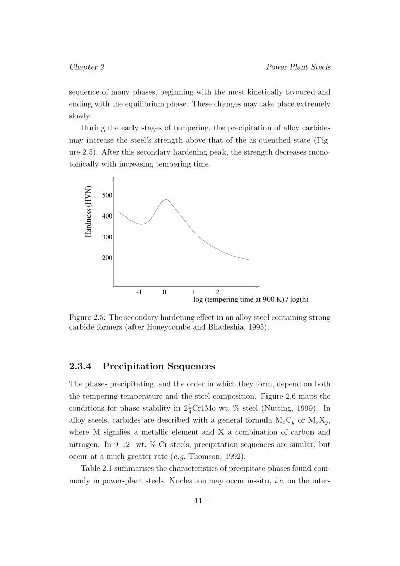
During the early stages of tempering, the precipitation of alloy carbides
may increase the steel’s strength above that of the as-quenched state (Fig-
ure 2.5). After this secondary hardening peak, the strength decreases mono-
tonically with increasing tempering time.
log (tempering time at 900 K) / log(h)
Har
dnes
s (H
VN
)
300
400
200
500
0-1 1 2
Figure 2.5: The secondary hardening effect in an alloy steel containing strongcarbide formers (after Honeycombe and Bhadeshia, 1995).
2.3.4 Precipitation Sequences
The phases precipitating, and the order in which they form, depend on both
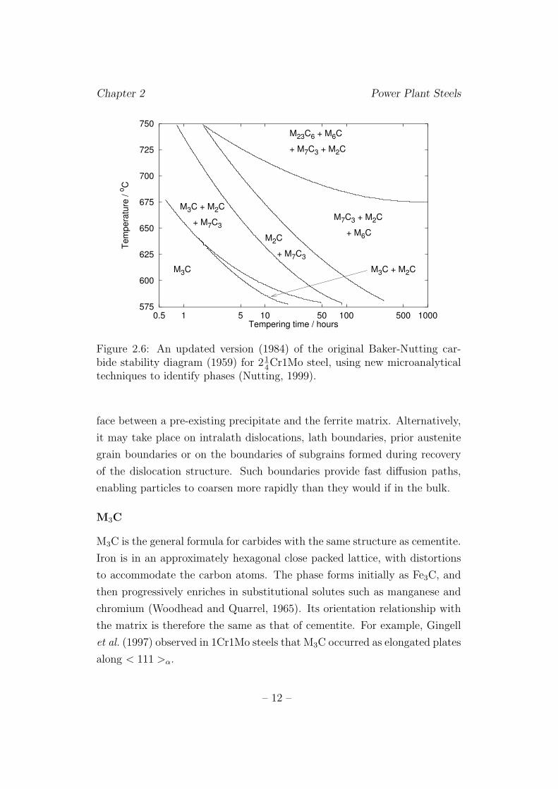
the tempering temperature and the steel composition. Figure 2.6 maps the
conditions for phase stability in 214Cr1Mo wt. % steel (Nutting, 1999). In
alloy steels, carbides are described with a general formula MxCy or MxXy,
where M signifies a metallic element and X a combination of carbon and
nitrogen. In 9–12 wt. % Cr steels, precipitation sequences are similar, but
occur at a much greater rate (e.g. Thomson, 1992).
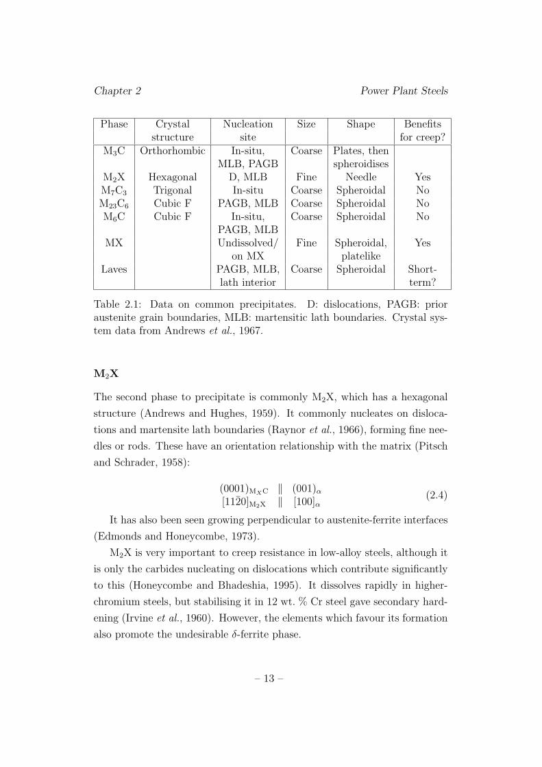
Table 2.1 summarises the characteristics of precipitate phases found com-
monly in power-plant steels. Nucleation may occur in-situ, i.e. on the inter-
– 11 –
Chapter 2 Power Plant Steels
575
600
625
650
675
700
725
750
0.5 1 5 10 50 100 500 1000
Tem
pera
ture
/ o
C
Tempering time / hours
M3C
M3C + M2C
+ M7C3
M2C
+ M7C3
M7C3 + M2C
+ M6C
M23C6 + M6C
+ M7C3 + M2C
M3C + M2C
Figure 2.6: An updated version (1984) of the original Baker-Nutting car-bide stability diagram (1959) for 21
4Cr1Mo steel, using new microanalytical
techniques to identify phases (Nutting, 1999).
face between a pre-existing precipitate and the ferrite matrix. Alternatively,
it may take place on intralath dislocations, lath boundaries, prior austenite
grain boundaries or on the boundaries of subgrains formed during recovery
of the dislocation structure. Such boundaries provide fast diffusion paths,
enabling particles to coarsen more rapidly than they would if in the bulk.
M3C
M3C is the general formula for carbides with the same structure as cementite.
Iron is in an approximately hexagonal close packed lattice, with distortions
to accommodate the carbon atoms. The phase forms initially as Fe3C, and
then progressively enriches in substitutional solutes such as manganese and
chromium (Woodhead and Quarrel, 1965). Its orientation relationship with
the matrix is therefore the same as that of cementite. For example, Gingell
et al. (1997) observed in 1Cr1Mo steels that M3C occurred as elongated plates
along < 111 >α.
– 12 –
Chapter 2 Power Plant Steels
Phase Crystal Nucleation Size Shape Benefitsstructure site for creep?
M3C Orthorhombic In-situ, Coarse Plates, thenMLB, PAGB spheroidises
M2X Hexagonal D, MLB Fine Needle YesM7C3 Trigonal In-situ Coarse Spheroidal NoM23C6 Cubic F PAGB, MLB Coarse Spheroidal NoM6C Cubic F In-situ, Coarse Spheroidal No
PAGB, MLBMX Undissolved/ Fine Spheroidal, Yes
on MX platelikeLaves PAGB, MLB, Coarse Spheroidal Short-
lath interior term?
Table 2.1: Data on common precipitates. D: dislocations, PAGB: prioraustenite grain boundaries, MLB: martensitic lath boundaries. Crystal sys-tem data from Andrews et al., 1967.
M2X
The second phase to precipitate is commonly M2X, which has a hexagonal
structure (Andrews and Hughes, 1959). It commonly nucleates on disloca-
tions and martensite lath boundaries (Raynor et al., 1966), forming fine nee-
dles or rods. These have an orientation relationship with the matrix (Pitsch
and Schrader, 1958):
(0001)MXC ‖ (001)α
[1120]M2X ‖ [100]α(2.4)
It has also been seen growing perpendicular to austenite-ferrite interfaces
(Edmonds and Honeycombe, 1973).
M2X is very important to creep resistance in low-alloy steels, although it
is only the carbides nucleating on dislocations which contribute significantly
to this (Honeycombe and Bhadeshia, 1995). It dissolves rapidly in higher-
chromium steels, but stabilising it in 12 wt. % Cr steel gave secondary hard-
ening (Irvine et al., 1960). However, the elements which favour its formation
also promote the undesirable δ-ferrite phase.
– 13 –
Chapter 2 Power Plant Steels
M7C3
M7C3 only appears if the chromium content is sufficiently high compared to
that of other alloying elements (Woodhead and Quarrell, 1965). If molybde-
num is present, M23C6 may form instead. If M7C3 is observed, it forms after
M2X (Baker and Nutting, 1959) or after M3C without the intermediate M2X
stage (Janovec et al., 1994). It nucleates close to cementite, possibly at the
cementite-ferrite interface (Kuo, 1953; Baker and Nutting, 1959). Darbyshire
and Barford (1966) state that the nucleation can be in-situ or on fresh sites.
This phase coarsens rapidly (Sakuma et al., 1981; Yong Wey et al., 1981)
and is not thought to be beneficial for creep resistance.
M23C6
This is rich in chromium (Woodhead and Quarrell, 1965) and is often an
equilibrium phase in chromium-rich steels. It nucleates on prior austenite
grain and martensite lath boundaries (Senior, 1989) and has also been iden-
tified adjacent to M7C3 (Nutting, 1999). It forms after either M7C3 or M2X.
The particles are large, and do not contribute to creep strength, but Bjarbo
(1994) has suggested that it may retard microstructural coarsening by sta-
bilising martensitic lath boundaries.
M6C
M6C is an equilibrium phase in molybdenum-rich, relatively chromium-poor
steels (Edmonds and Honeycombe, 1973; Tillman and Edmonds, 1974). It
can nucleate on prior austenite grain boundaries and martensitic lath bound-
aries. Kurdzylowski and Zielinski (1984) report that it also nucleates in-situ
on M2X- or M23C6-ferrite interfaces, but Nutting (1999) has suggested that
it instead forms by diffusion. Its rapid coarsening rate, greater than that of
M23C6, make it a particularly undesirable phase (Vodarek and Strang, 1997),
especially since it forms at the expense of finer carbides.
– 14 –
Chapter 2 Power Plant Steels
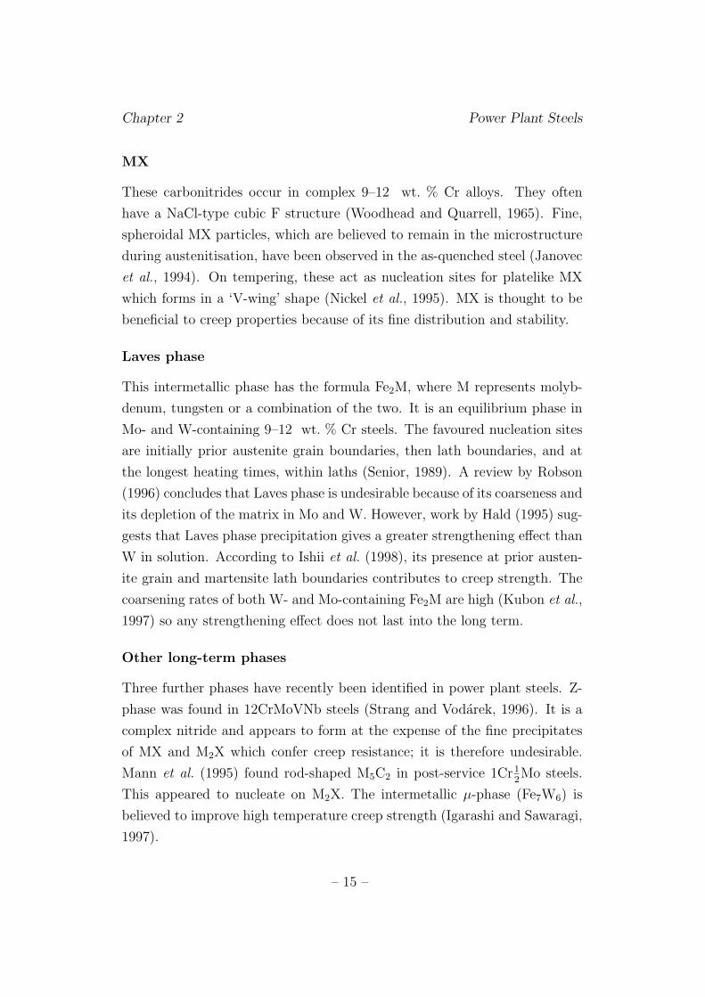
MX
These carbonitrides occur in complex 9–12 wt. % Cr alloys. They often
have a NaCl-type cubic F structure (Woodhead and Quarrell, 1965). Fine,
spheroidal MX particles, which are believed to remain in the microstructure
during austenitisation, have been observed in the as-quenched steel (Janovec
et al., 1994). On tempering, these act as nucleation sites for platelike MX
which forms in a ‘V-wing’ shape (Nickel et al., 1995). MX is thought to be
beneficial to creep properties because of its fine distribution and stability.
Laves phase
This intermetallic phase has the formula Fe2M, where M represents molyb-
denum, tungsten or a combination of the two. It is an equilibrium phase in
Mo- and W-containing 9–12 wt. % Cr steels. The favoured nucleation sites
are initially prior austenite grain boundaries, then lath boundaries, and at
the longest heating times, within laths (Senior, 1989). A review by Robson
(1996) concludes that Laves phase is undesirable because of its coarseness and
its depletion of the matrix in Mo and W. However, work by Hald (1995) sug-
gests that Laves phase precipitation gives a greater strengthening effect than
W in solution. According to Ishii et al. (1998), its presence at prior austen-
ite grain and martensite lath boundaries contributes to creep strength. The
coarsening rates of both W- and Mo-containing Fe2M are high (Kubon et al.,
1997) so any strengthening effect does not last into the long term.
Other long-term phases
Three further phases have recently been identified in power plant steels. Z-
phase was found in 12CrMoVNb steels (Strang and Vodarek, 1996). It is a
complex nitride and appears to form at the expense of the fine precipitates
of MX and M2X which confer creep resistance; it is therefore undesirable.
Mann et al. (1995) found rod-shaped M5C2 in post-service 1Cr12Mo steels.
This appeared to nucleate on M2X. The intermetallic µ-phase (Fe7W6) is
believed to improve high temperature creep strength (Igarashi and Sawaragi,
1997).
– 15 –
Chapter 2 Power Plant Steels
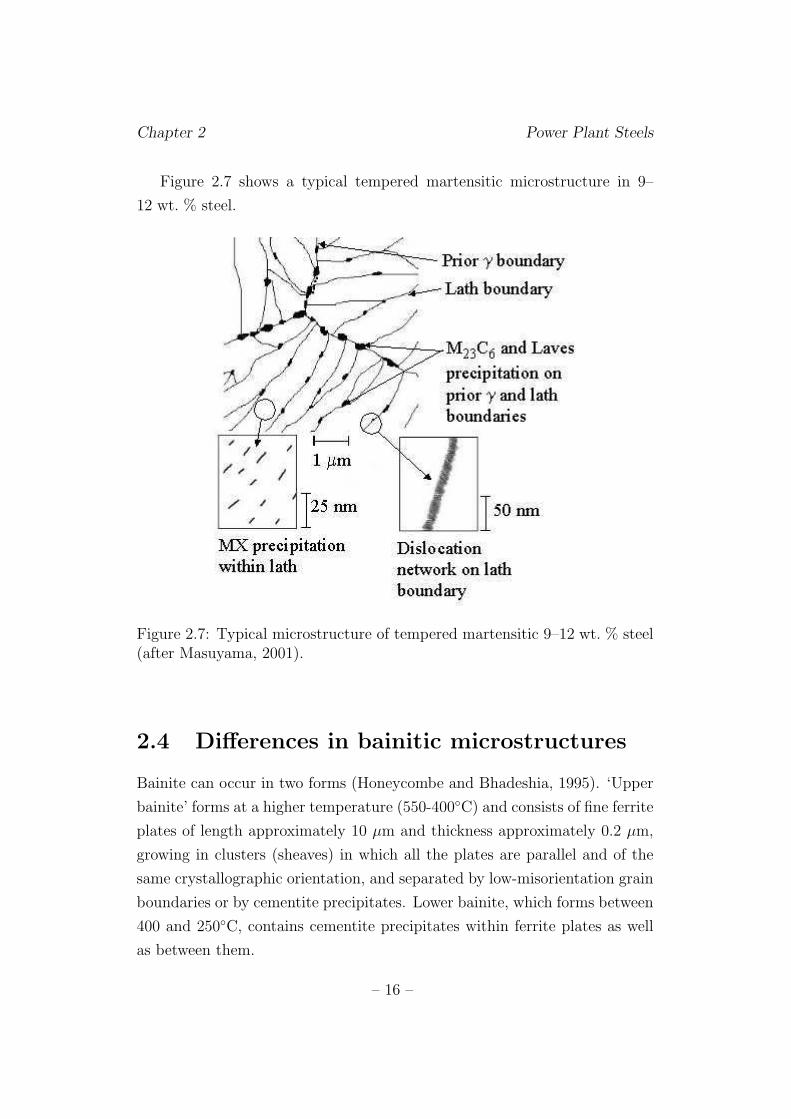
Figure 2.7 shows a typical tempered martensitic microstructure in 9–
12 wt. % steel.
Figure 2.7: Typical microstructure of tempered martensitic 9–12 wt. % steel(after Masuyama, 2001).
2.4 Differences in bainitic microstructures
Bainite can occur in two forms (Honeycombe and Bhadeshia, 1995). ‘Upper
bainite’ forms at a higher temperature (550-400◦C) and consists of fine ferrite
plates of length approximately 10 µm and thickness approximately 0.2 µm,
growing in clusters (sheaves) in which all the plates are parallel and of the
same crystallographic orientation, and separated by low-misorientation grain
boundaries or by cementite precipitates. Lower bainite, which forms between
400 and 250◦C, contains cementite precipitates within ferrite plates as well
as between them.
– 16 –
Chapter 2 Power Plant Steels
Bainite is closer to equilibrium than martensite, being only slightly su-
persaturated in carbon. Cementite particles are already present and these
tend to be larger than the cementite formed on tempering of martensite. The
dislocation content is also smaller than that of martensite. In plain-carbon
bainite, short-term tempering gives little change in microstructure, but a
significant drop in strength is seen when the plate-like ferrite and cementite
spheroidise to an equiaxed structure. The effect of alloying with carbide-
forming elements is the same as for tempered martensite, but alloy carbides
form on a longer timescale.
Baker and Nutting (1959) investigated the effect on tempering kinet-
ics of using a martensitic rather than bainitic starting microstructure in
214Cr1Mo steel. Differences were observed, but they were very small, be-
cause the defect densities of the two starting microstructures were very sim-
ilar. Bhadeshia (2000) raised the question of why the higher-Cr steel was
martensitic, and concluded that this was a by-product of alloying to increase
oxidation and corrosion resistance. However, he suggested that the fine plate-
like microstructure in martensite may contribute to creep resistance by im-
peding dislocation motion. Yamada et al. (2002) found that in 9Cr3W3Co
steels, water-quenching instead of air-cooling gave longer creep rupture lives.
Quenching gave a better distribution of MX particles, suppressing complex
MX phases and accelerating the formation of more beneficial VC.
2.5 Changes during service
In 214Cr1Mo steels, M2X provides long-term creep resistance, but this phase
dissolves rapidly when the chromium content is higher. A review of strength-
ening mechanisms in tempered high-Cr creep resistant steels by Maruyama
et al. (2001) concludes that dislocations, solutes, intragranular particles (MX)
and particles on boundaries all contribute to creep strength, but not in a sim-
ple additive manner.
During creep deformation, the dislocation substructure of the tempered
steel, which is stable with respect to temperatures up to 650◦C in the ab-
sence of stress, undergoes recovery into a subgrain structure (Nickel, 1995;
– 17 –
Chapter 2 Power Plant Steels
Iwanaga et al., 1998; Cerjak et al., 2000). The growth of these subgrains
is accompanied by a reduction in dislocation density, and reduces the creep
resistance.
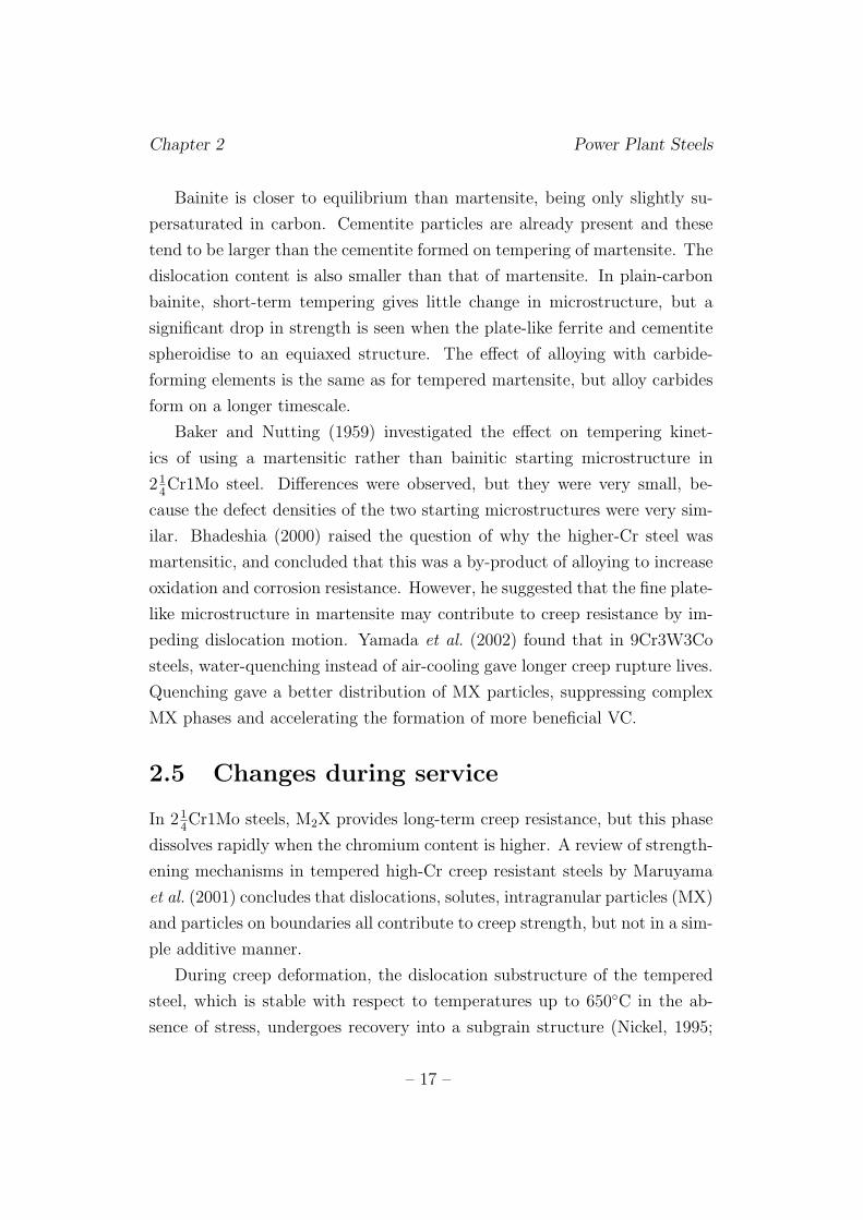
2.5.1 Lath coarsening, recovery and recrystallisation
Martensite laths in 9Cr-W steels subjected to creep were found to coarsen
concurrently with M23C6 particles (Abe, 1999). An increase in the tungsten
content retarded the coarsening of both the M23C6 and the laths, while caus-
ing the precipitation of Laves phase. It was concluded from this that M23C6
particles are more effective than Laves phase for pinning lath boundaries.
The lath coarsening observed by Abe occurred by lath boundary triple point
migration (Figure 2.8).
Triple
point
(a) (b)
Carbide particle
Figure 2.8: Lath coalescence: Triple points migrate and lath boundariescoalesce (a) to give a coarser structure (b). After Abe, 1999.
– 18 –
Chapter 2 Power Plant Steels
2.5.2 Cavitation and final failure
Creep rupture may occur in a more brittle or more ductile manner; cavi-
ties occur at smaller strains when the ductility is low (Beech et al., 1984).
Second-phase particles on grain boundaries can act as nucleation sites for
voids (Martin, 1980). Grain boundary triple points also concentrate stress
during grain boundary sliding in creep, resulting in cavitation (Watanabe,
1983).
In power-plant steels, failure can be promoted by preferential recovery
at prior austenite grain boundaries (Kushima et al., 1999; Abe, 2000). The
large, rapidly coarsening particles on grain boundaries deplete the local ma-
trix of solutes and fine particles, and the resulting recovered region acts as a
strain concentrator and is able to crack easily.
2.6 Design life and remanent life estimation
Conservative component design lives are used to accommodate the effects of
microstructural heterogeneity and variation in service conditions. The work-
ing stress is set at around 0.8 times the value of the lower bound of creep
rupture stress at the intended life (Halmshaw, 1991). It has often been found
that components reaching the end of their design lives are still in a safe con-
dition for several more years of use. Bhadeshia et al. (1998) have reviewed
the techniques available for the estimation of the remanent lives of such com-
ponents. These subdivide into methods based on mechanical properties such
as hardness and impact toughness, those involving microstructural observa-
tion, and those in which other properties, such as resistivity or density, are
measured and used to infer the component condition. However, Bhadeshia
et al. concluded that none of these techniques gave a sufficiently compre-
hensive characterisation to be used in isolation. Also, implementation often
requires a plant shutdown, the expense of which contributes a great deal to
the cost of life extension as opposed to component replacement at the end of
the design life.
– 19 –

Chapter 2 Power Plant Steels
2.7 Scope for magnetic methods
It is clear that there is a need for additional microstructural monitoring tech-
niques, especially those which can be used in-situ with minimal preparation,
and which give a comprehensive characterisation of the component state.
Ferritic power plant steels are ferromagnetic, allowing the use of mag-
netic monitoring methods. Magnetic techniques are routinely in use for crack
detection in ferromagnetic components, and appear promising for the mea-
surement of stress effects. For example, a programme for the evaluation of
structural materials in nuclear power plant after tensile and fatigue load-
ing, which includes the measurement of several magnetic properties, is under
development in Japan (Uesaka et al., 2001).
The aim of this study is to investigate their usefulness as a method of
microstructural evaluation for the purpose of remanent life estimation in
power plant steels. This requires an understanding of the relationships be-
tween magnetic properties and the characteristics of microstructural features
such as grain boundaries and carbides. Chapter 3 and Chapter 4 discuss the
progress made so far in understanding these.
– 20 –

Chapter 3
Magnetic Domains
3.1 Ferromagnetism and domain theory
3.1.1 Atomic origin of ferromagnetism
Bulk magnetic behaviour arises from the magnetic moments of individual
atoms. There are two contributions to the atomic magnetic moment from
the momentum of electrons. Firstly, each electron has an intrinsic magnetic
moment and an intrinsic angular momentum (spin). Secondly, electrons may
also have a magnetic moment and an angular momentum as a result of their
orbital motion in atoms.
The Pauli exclusion principle permits only one electron in an atom to
have a particular combination of the four quantum numbers n, l, ml and
ms. The first three numbers specify the electron energy state. The spin
quantum number, ms, can only take the values ±1/2. Each energy state
may therefore contain up to two electrons. If only one electron is present, its
spin moment contributes to the overall spin moment of the atom. A second
electron is required to have an antiparallel spin to the first, and the two
spins will cancel out, giving no net moment. Strong magnetic properties are
associated with elements which have a large number of unpaired spins.
In solid materials, the orbital moments are strongly coupled to the crystal
lattice and are therefore unable to change direction when a magnetic field is
applied. Because of this ‘orbital quenching’, the magnetic moments in solids
can be considered as due to the spins only. An atom with uncompensated
– 21 –
Chapter 3 Magnetic Domains
spins has a net magnetic moment in the absence of an applied field; solids
composed of such atoms are termed ‘paramagnetic’. In general, the atomic
magnetic moments in paramagnets are randomly aligned when no field is
present, and the magnetisation process consists of aligning them into the
field direction. However, some paramagnetic materials undergo a transition
on cooling to an ordered state in which there is local alignment of atomic
moments. The ordered state is ‘ferromagnetic’ if adjacent atomic moments
are aligned parallel to one another, and ‘ferrimagnetic’ if they are antiparallel
but of different magnitude such that there is a local net magnetisation.
The temperature of the order/disorder transition is known as the Curie
temperature (TC) in ferromagnets. The degree of ordering increases with
decreasing temperature. Iron in its body-centred cubic (b.c.c.) ferrite form
is strongly ferromagnetic, as are many widely used steels. In the ferritic
power plant steels discussed in Chapter 2, the austenitisation treatment takes
the steel above its Curie temperature, and it becomes paramagnetic. Air-
cooling or quenching to give bainite or martensite gives a b.c.c. or body-
centred tetragonal structure which is ferromagnetic, and the ferromagnetism
is retained on tempering.
3.1.2 Weiss domain theory
Weiss (1906, 1907) postulated that atoms in ferromagnetic materials had
permanent magnetic moments which were aligned parallel to one another
over extensive regions of a sample. This was later refined into a theory
of ‘domains’ of parallel moments (Weiss, 1926). The overall magnetisation
(magnetic moment per unit volume) of a block of material is the vector sum
of the domain magnetisations. In the demagnetised state, this is zero. As
a field is applied, changes in the domain configuration, for example in the
relative widths of domains, allow a net magnetisation in the field direction.
Weiss’ hypothesis was later confirmed by direct observation (Bitter, 1931),
and the concept of magnetostatic energy, which explained the formation of
domains, was proposed by Landau and Lifshitz (1935).
– 22 –
Chapter 3 Magnetic Domains
3.1.3 Ideal domain structure
In a homogeneous, defect-free, single-crystal ferromagnet with cubic symme-
try, the domain structure can be explained by a balance between four energy
terms: exchange, magnetostatic, anisotropy and magnetoelastic (Kittel and
Galt, 1956).
Exchange energy
Weiss extended an existing statistical thermodynamic theory for paramag-
netism (Langevin, 1905), to describe the alignment of the atomic magnetic
moments within domains. The Weiss ‘mean field’ He in the original theory
was given by:
He = αM (3.1)
where M is the magnetisation, and α is the ‘mean field constant’. The mean
field approximation requires that all magnetic moments interact equally with
all others. Although this is obviously a simplification of the true situation,
it is nevertheless a useful concept for consideration of the atoms within do-
mains, which usually extend over 1012 to 1018 atoms. The origin of the in-
teraction was later identified by Heisenberg (1928) as a quantum-mechanical
exchange effect due to overlapping wavefunctions of neighbouring atoms. If
only nearest neighbours are considered, the exchange energy Eex per unit
volume associated with this interaction is:
Eex = −2β∑
i
∑
j
mi · mj (3.2)
where β is a term characterising the strength of the interaction, and the
summation is over all nearest-neighbour pairs i and j in a unit of volume.
In ferromagnetic materials, β is positive, giving a minimum exchange energy
when moments lie parallel. Complete alignment of all atomic moments in
the sample (magnetic saturation) is therefore favoured by this term. An
explanation is therefore needed of how the demagnetised state can arise; this
is given by the magnetostatic energy term.
– 23 –
Chapter 3 Magnetic Domains
Magnetostatic energy
A body of magnetisation M in a magnetic field H has a magnetostatic energy
Em arising from the interaction of M with H:
Em = −µ0
∫
H · ∂M (3.3)
where µ0 is the permeability of free space. At any internal or external
surface of a uniformly magnetised body, there is a discontinuous change in
the component of M normal to the surface, which can be envisaged as a
source of ‘free poles’. These are magnetic (north or south) poles which are not
compensated by poles of the opposite kind in the immediate vicinity. They
produce a demagnetising field, which favours a change in the arrangement
of magnetic moments such that the poles disappear. A finite body has free
poles on its outer surfaces, resulting in a demagnetising field Hd antiparallel
to the magnetisation M; this tends to turn M so that it points parallel to
the surfaces. This field is given by:
Hd = NdM (3.4)
where Nd is the demagnetising factor, which depends only on sample geom-
etry. For a sample with magnetisation M but no applied field, the magneto-
static energy depends only on M and Nd, and can be obtained by substituting
Equation 3.4 into Equation 3.3 to give:
Ed =µ0
2NdM
2 (3.5)
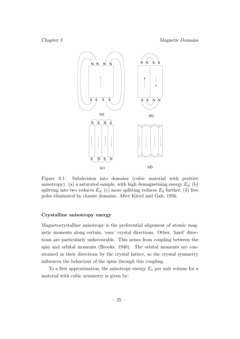
In the absence of an applied field, the magnetostatic energy is therefore
a minimum when the magnetisation is zero, and subdivision into domains
is favoured (Figure 3.1 (a), (b)). Reducing the domain width decreases the
spatial extent of the field and hence the energy (c). If domains magnetised
at 90◦ to the main domains can form, external free poles can be eliminated
entirely, reducing the magnetostatic energy to zero (Figure 3.1 (d)).
Demagnetising factors can be determined exactly for ellipsoids of revolu-
tion only, but approximate values have been calculated for commonly used
sample shapes, such as cylinders (Chen et al., 1991).
– 24 –
Chapter 3 Magnetic Domains
N N S S
S S N N
N NSS
N S N S
N NNN
S SS S
(a) (b)
(c) (d)
Figure 3.1: Subdivision into domains (cubic material with positiveanisotropy). (a) a saturated sample, with high demagnetising energy Ed; (b)splitting into two reduces Ed; (c) more splitting reduces Ed further; (d) freepoles eliminated by closure domains. After Kittel and Galt, 1956.
Crystalline anisotropy energy
Magnetocrystalline anisotropy is the preferential alignment of atomic mag-
netic moments along certain, ‘easy’ crystal directions. Other, ‘hard’ direc-
tions are particularly unfavourable. This arises from coupling between the
spin and orbital moments (Brooks, 1940). The orbital moments are con-
strained in their directions by the crystal lattice, so the crystal symmetry
influences the behaviour of the spins through this coupling.
To a first approximation, the anisotropy energy Ea per unit volume for a
material with cubic symmetry is given by:
– 25 –
Chapter 3 Magnetic Domains
Ea = K1(α21α
22 + α2
2α23 + α2
3α21) (3.6)
where K1 is a constant of proportionality known as the anisotropy constant,
and α1, α2 and α3 are the cosines of the angles made by magnetisation vector
with the crystal axes x, y and z. In b.c.c. iron, K1 is positive, and the cube
edges < 100 > are the easy directions (Honda and Kaya, 1926). Antiparal-
lel magnetisation directions are crystallographically equivalent, giving three
distinct easy directions for positive-K1 materials. This allows the formation
of closure domains oriented at 90◦ to the main domains (Figure 3.1 (d)).
Magnetoelastic energy
If a cubic single crystal is magnetised to saturation in a direction defined
by the direction cosines α1, α2 and α3 with respect to the crystal axes x, y
and z, a magnetostrictive strain λsi is induced in a direction defined by the
cosines β1, β2 and β3:
λsi = λ100
(
α21β
21α
22β
22α
23β
23 −
1
3
)
+ 3λ111(α1α2β1β2 + α2α3β2β3 + α3α1β3β1)
(3.7)
where λ100 and λ111 are the magnetostriction constants along < 100 > and
< 111 > respectively. λsi is the ‘ideal’ magnetic field-induced magnetostric-
tion. This is defined by Cullity (1971) as the strain induced when a specimen
is brought to technical saturation (§ 3.2.1) from the ideal demagnetised state,
i.e. the state in which all of the domain orientations allowed by symmetry
are present in equal volumes.
If magnetostriction is isotropic, i.e. λ100 = λ111 = λsi, then Equation 3.7
may be simplified to:
λθ =3
2λsi
(
cos2 θ − 1
3
)
(3.8)
where λ is the magnetostriction measured at an angle θ to the magnetisation
and the field.
In practice, however, the magnetostriction is not ideal, but depends on
the magnetic history of the material and the thermomechanical treatment
– 26 –
Chapter 3 Magnetic Domains
to which it has been subjected. It is possible, for example, to produce a
preferred orientation of magnetic domains by annealing in a magnetic field
(e.g. review by Watanabe et al., 2000).
If a domain is constrained by its neighbours, magnetostriction manifests
itself as a strain energy rather than a dimensional change. Maintaining co-
herence between the closure domains and the main domains in Figure 3.1 (d)
requires a strain energy proportional to the volume of the closure domains.
This can be reduced, while maintaining the closure effect, by increasing the
number both of closure domains and main domains. However, this requires
more domain walls to be created; since, as will be discussed below, domain
walls have a higher energy than the bulk, the equilibrium configuration is
determined by a balance between domain wall and magnetoelastic energy
contributions.
In polycrystals with no preferred orientation, the magnetostriction con-
stant λsi will be an average of the values of all the crystal orientations. To
obtain an estimate for this average, assumptions must be made about the
grain size and the transfer of stress or strain between grains. The expres-
sions obtained depend on these assumptions unless the grains are elastically
isotropic (Cullity, 1971).
3.1.4 Energy and width of domain walls
The transition region between domains magnetised in different directions was
first studied by Bloch (1932). The change from one direction to the other is
not discontinuous but occurs over a width determined by a balance between
exchange and anisotropy energy. The energy and thickness of various types
of domain walls have been calculated (Kittel and Galt, 1956).
The mean field approximation breaks down at domain walls, but the
exchange energy per moment, Eex, can be calculated by considering only
nearest-neighbour interactions and neglecting others. For neighbouring mo-
ments mi and mj, Eex is given by:
Eex = −µ0zJmi · mj (3.9)
– 27 –
Chapter 3 Magnetic Domains
where J is a term characterising nearest-neighbour interactions and z is the
number of nearest neighbours1. If the angle between mi and mj is φ,
Eex = −µ0zJm2 cos φ (3.10)
For a linear chain of moments, each has two nearest neighbours. Substituting
the small-angle approximation cos φ = 1 − φ2/2 gives:
Eex = µ0Jm2(φ2 − 2) (3.11)
A wall separating domains magnetised at 180◦ to one another, and extending
across n lattice parameters of size a, has an exchange energy per unit areaEex
a2 :
Eex
a2=
µ0Jm2φ2π2
na2(3.12)
Eex is therefore lowest when n is large, favouring wide walls.
The anisotropy energy of the pth moment in a wall can be approximated
as:
Ea = (K1/4) sin2 2pφ (3.13)
where K1 is the anisotropy constant. Summing this over the domain wall
width gives an anisotropy energy per unit area:
Ea = K1na (3.14)
where a is the lattice spacing and n the number of layers of atoms in the
domain wall. Ea increases with n, favouring a narrow wall. The total wall
energy per unit area γ = Eex+Ea is minimised by differentiating with respect
to the wall width δ = na and setting the derivative to zero.
∂γ
∂δ=
−µ0Jm2π2
δ2a+ K1 = 0 (3.15)
Hence,
1This is of a similar form to Equation 3.2 but in this case is expressed per moment.
– 28 –
Chapter 3 Magnetic Domains
δ =
√
µ0Jm2π2
K1a(3.16)
Using these expressions, Jiles (1998) has estimated the width of a wall
separating antiparallel domains in iron as 40 nm, or 138 lattice parameters,
and its energy as 3 x 10⁻³ J m−2.
3.1.5 Determination of the equilibrium domain struc-ture
To obtain the minimum-energy configuration of an assembly of domains so
that the equilibrium structure can be found, a set of differential equations
must be solved. These micromagnetics equations (Brown, 1963) assume con-
tinuously varying atomic moments, and are therefore difficult to solve for
large-scale arrays of domains. In practice, a less complex ‘domain theory’
is applied, which treats each domain as uniformly magnetised to saturation,
with variations in direction occurring only within domain walls (Hubert and
Schafer, 2000). It is assumed throughout the rest of this discussion that,
far from domain walls, the domain magnetisation is MS, which is known as
‘saturation’ or ‘spontaneous’ magnetisation.
3.2 Evolution of domain structure on appli-
cation of a magnetic field
3.2.1 Ideal magnetisation and demagnetisation
When a magnetic field H is applied to a sample with no net magnetic mo-
ment, the energy balance previously existing is upset by the additional mag-
netostatic energy due to the field. The domain structure rearranges itself in
order to minimise the energy under the new conditions.
In simple terms, at low H this occurs by the enlargement of domains with
MS oriented approximately parallel to H at the expense of those oriented
antiparallel (Kittel and Galt, 1956). As H increases, domain walls are swept
out. Rotations of domain magnetisation vectors into easy directions near
– 29 –
Chapter 3 Magnetic Domains
that of H may also occur at intermediate fields. The resulting single domain
has MS parallel to the easy direction nearest the direction of H. At high
field, MS is rotated against the anisotropy to lie exactly parallel to H. This
state is known as technical saturation. Further increases in the field give
small increases in the magnetisation. Atomic moments deviate slightly from
the applied field direction due to thermal activation,but higher applied fields
reduce this deviation.
On reducing H, the domain magnetisation rotates into an easy direction,
and the single domain subdivides by the nucleation of domains magnetised
in the opposite direction to M (‘reverse domains’).
The balance between the energy terms varies from one material to an-
other, and this influences the exact details of magnetisation and demagneti-
sation. Ferritic iron has a high anisotropy constant K1, so rotation out of
the easy directions is difficult, and all low-field magnetisation changes can be
attributed to domain wall motion (Shilling and Houze, 1974).
3.2.2 Magnetic hysteresis
In real materials, the magnetisation behaviour is influenced by microstruc-
tural defects and inhomogeneities, such as grain boundaries, dislocations,
solutes, precipitates, inclusions, voids and cracks. Cycling between nega-
tive and positive applied field directions gives a hysteresis loop, in which M
takes different values depending on whether H is increasing or decreasing.
Magnetic hysteresis, which was first noted in iron by Warburg (1881) and
described and named by Ewing (1900), results from energy losses incurred in
magnetisation and demagnetisation. These are due in part to energetic in-
teractions between domain walls and defects, and in part to rotation against
the anisotropy.
– 30 –
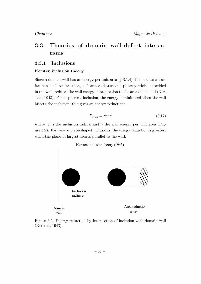
Chapter 3 Magnetic Domains
3.3 Theories of domain wall-defect interac-
tions
3.3.1 Inclusions
Kersten inclusion theory
Since a domain wall has an energy per unit area (§ 3.1.4), this acts as a ‘sur-
face tension’. An inclusion, such as a void or second-phase particle, embedded
in the wall, reduces the wall energy in proportion to the area embedded (Ker-
sten, 1943). For a spherical inclusion, the energy is minimised when the wall
bisects the inclusion; this gives an energy reduction:
Earea = πr2γ (3.17)
where r is the inclusion radius, and γ the wall energy per unit area (Fig-
ure 3.2). For rod- or plate-shaped inclusions, the energy reduction is greatest
when the plane of largest area is parallel to the wall.
Domain
wall r
Area reduction
= π2
Inclusion
radius r
������������������������������������������������������������
������������������������������������������������������������
Kersten inclusion theory (1943)
Figure 3.2: Energy reduction by intersection of inclusion with domain wall(Kersten, 1943).
– 31 –
Chapter 3 Magnetic Domains
Neel inclusion theory
Neel (1944) demonstrated that energetic interactions between domain walls
and inclusions also arise from internal demagnetising fields. In general, an
inclusion has different magnetic properties from the bulk. If the normal
component of magnetisation is discontinuous across the inclusion/matrix in-
terface, a distribution of free poles will be present, giving a demagnetising
field (Figure 3.3 (a)).
For a spherical, nonmagnetic inclusion of radius r, the associated magne-
tostatic energy is:
Edemag =8π2M2
Sr3
9(3.18)
where MS is the saturation magnetisation of the matrix. Positioning the
domain wall so that it bisects the inclusion redistributes the free poles, ap-
proximately halving the demagnetising energy (Figure 3.3 (b)). It is not
necessary that inclusions be nonmagnetic to cause demagnetising effects; for
example, Fe3C is ferromagnetic at room temperature, but has a pronounced
effect on the magnetic properties of ferritic iron (Dykstra, 1969). It still
behaves as a magnetic inhomogeneity in ferritic steel because its magnetic
properties are different from those of the bulk (Jiles, 1998).
The Neel demagnetising effect scales with r3 (Equation 3.18), and there-
fore increases more rapidly than the Kersten area-reduction effect (Equa-
tion 3.17). However, for sufficiently large inclusions, it is energetically favour-
able to reduce the demagnetising energy of the inclusion by forming sub-
sidiary domains around it, despite the additional domain wall energy in-
volved. These thin, triangular ‘spike’ domains were predicted theoretically
by Neel (1944) and subsequently observed by Williams (1947).
If an inclusion is bisected by a domain wall, closure domains can form, re-
ducing the magnetostatic energy to zero (Cullity, 1972; Figure 3.4 (a)). When
the main domain wall moves away from the inclusion under the action of an
applied field, the subsidiary domain structure is drawn with it Figure 3.4 (b))
before becoming irreversibly detached and forming spike domains (c).
Craik and Tebble (1965) calculated that inclusions whose diameter was
– 32 –
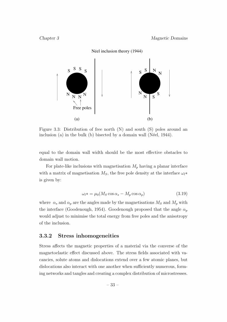
Chapter 3 Magnetic Domains
SS S
S
NN N
N
SS
SSN
N
NN
Neel inclusion theory (1944)
Free poles
(a) (b)
Figure 3.3: Distribution of free north (N) and south (S) poles around aninclusion (a) in the bulk (b) bisected by a domain wall (Neel, 1944).
equal to the domain wall width should be the most effective obstacles to
domain wall motion.
For plate-like inclusions with magnetisation Mp having a planar interface
with a matrix of magnetisation MS, the free pole density at the interface ωl∗is given by:
ωl∗ = µ0(MS cos αs − Mp cos αp) (3.19)
where αs and αp are the angles made by the magnetisations MS and Mp with
the interface (Goodenough, 1954). Goodenough proposed that the angle αp
would adjust to minimise the total energy from free poles and the anisotropy
of the inclusion.
3.3.2 Stress inhomogeneities
Stress affects the magnetic properties of a material via the converse of the
magnetoelastic effect discussed above. The stress fields associated with va-
cancies, solute atoms and dislocations extend over a few atomic planes, but
dislocations also interact with one another when sufficiently numerous, form-
ing networks and tangles and creating a complex distribution of microstresses.
– 33 –
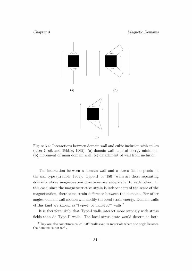
Chapter 3 Magnetic Domains
���������������������������������������������������������������������������������
���������������������������������������������������������������������������������
���������������������������������������������������������������������������������
���������������������������������������������������������������������������������
(a)
(c)
(b)
Figure 3.4: Interactions between domain wall and cubic inclusion with spikes(after Craik and Tebble, 1965): (a) domain wall at local energy minimum,(b) movement of main domain wall, (c) detachment of wall from inclusion.
The interaction between a domain wall and a stress field depends on
the wall type (Trauble, 1969). ‘Type-II’ or ‘180◦’ walls are those separating
domains whose magnetisation directions are antiparallel to each other. In
this case, since the magnetostrictive strain is independent of the sense of the
magnetisation, there is no strain difference between the domains. For other
angles, domain wall motion will modify the local strain energy. Domain walls
of this kind are known as ‘Type-I’ or ‘non-180◦’ walls.2
It is therefore likely that Type-I walls interact more strongly with stress
fields than do Type-II walls. The local stress state would determine both
2They are also sometimes called ‘90◦’ walls even in materials where the angle between
the domains is not 90◦ .
– 34 –
Chapter 3 Magnetic Domains
the position and the energy of a Type-I wall, but the position of a Type-II
wall would remain unchanged (Cullity, 1972). The longer-range interactions
of Type-I walls with stress fields should make them less mobile, requiring
a higher applied field before they will move (Trauble, 1969). As a result,
magnetisation change at low applied fields is expected to occur predominantly
by Type-II wall motion.
Calculations of the interaction force between domain walls and disloca-
tions were made for several ideal cases by Trauble (1969). Scherpereel et al.
(1970) calculated the energy of interaction of many different types of disloca-
tions with Type-II and Type-I walls. On average, this was found to be higher
for Type-II walls than for Type-I walls in iron, while the reverse was observed
for nickel. This finding does not agree well with the model of Trauble. How-
ever, an experimental observation on an iron-based alloy appeared to support
the Trauble interpretation (§ 3.4.2).
3.3.3 Grain boundaries
In general, two grains meeting at a grain boundary are at an arbitrary crystal-
lographic orientation to one another, and their easy magnetisation directions
are not parallel (Goodenough, 1954). If the applied field is not sufficient
to rotate the grain magnetisations out of their easy directions, there will be
a discontinuity in the component of the magnetisation normal to the grain
boundary, and free poles will be present. If the angles made by the magneti-
sations MS of the two grains with the normal to the grain boundary are θ1
and θ2, the surface pole density at the grain boundary is:
ω∗ = µ0MS(cos θ1 − cos θ2) (3.20)
Subsidiary domains may form at the boundary if the magnetostatic energy
reduction achieved by this is larger than the domain wall energy required.
3.3.4 Models of domain wall dynamics
Two models of the ‘pinning’ of domain walls by microstructural defects have
been proposed. The rigid-wall model considers an inflexible wall whose mo-
– 35 –
Chapter 3 Magnetic Domains
tion is retarded by statistical fluctuations in the density of defects, which
modify the local potential energy. If defects are uniformly distributed on
either side of the wall, the forces on it sum to zero, but otherwise a net force
tends to move the wall to a more energetically favourable position.
The bowing-wall model, by contrast, allows the wall to bulge outwards
between pinning points when a field is applied, before becoming detached
when the wall area is too great. For some time, it was a subject of debate
which of these models was correct (Hilzinger and Kronmuller, 1976).
Potential energy model
Kittel and Galt (1956) proposed that rigid-wall motion could be modelled by
considering fluctuations of potential energy with position. This model has
been widely used as a qualitative description of wall energetics and dynamics
(e.g. Craik and Tebble, 1965; Astie et al., 1982; Pardavi-Horvath, 1999).
Defects, such as inclusions and dislocations, locally modify the ‘constants’
characterising the exchange interaction and magnetocrystalline anisotropy.
The resulting potential energy wells act as pinning sites, holding the walls in
place until sufficient energy is supplied to free them.
Using such a model, it is possible to estimate the magnetic properties of
a material by making assumptions about its defect distribution (e.g. Jiles,
1998). Also, since the derivative of potential energy with respect to dis-
tance, ∂E/∂x, is proportional to the magnetic field required to move the
domain wall, the defect distribution can be related to the external applied
field (Pardavi-Horvath, 1999; Figure 3.5). However, because of the demag-
netising effect, the applied field necessary for unpinning is greater than the
unpinning field value calculated from this model (Kawahara, personal com-
munication). Also, the critical unpinning field depends on the magnetisation
state of the surrounding domains as well as the properties of individual de-
fects (Pardavi-Horvath, 1999).
A potential energy model should characterise the energy of the ‘system’,
i.e. the wall and its surroundings, rather than the wall alone (Cullity, 1972).
For example, the interaction between a domain wall and an inclusion involves
reduction of the wall energy by decreasing its area, and reduction of the local
– 36 –
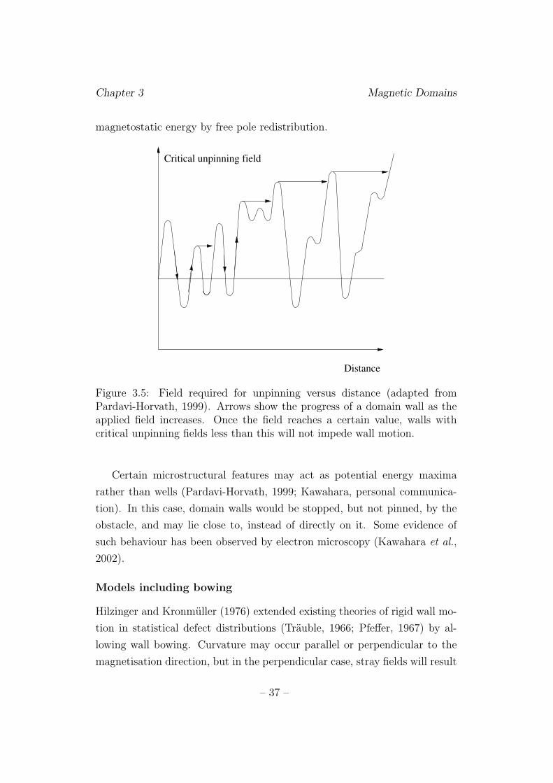
Chapter 3 Magnetic Domains
magnetostatic energy by free pole redistribution.
Critical unpinning field
Distance
Figure 3.5: Field required for unpinning versus distance (adapted fromPardavi-Horvath, 1999). Arrows show the progress of a domain wall as theapplied field increases. Once the field reaches a certain value, walls withcritical unpinning fields less than this will not impede wall motion.
Certain microstructural features may act as potential energy maxima
rather than wells (Pardavi-Horvath, 1999; Kawahara, personal communica-
tion). In this case, domain walls would be stopped, but not pinned, by the
obstacle, and may lie close to, instead of directly on it. Some evidence of
such behaviour has been observed by electron microscopy (Kawahara et al.,
2002).
Models including bowing
Hilzinger and Kronmuller (1976) extended existing theories of rigid wall mo-
tion in statistical defect distributions (Trauble, 1966; Pfeffer, 1967) by al-
lowing wall bowing. Curvature may occur parallel or perpendicular to the
magnetisation direction, but in the perpendicular case, stray fields will result
– 37 –
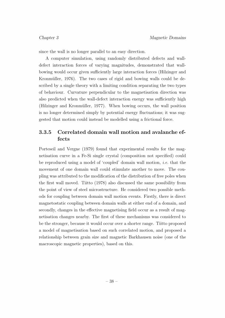
Chapter 3 Magnetic Domains
since the wall is no longer parallel to an easy direction.
A computer simulation, using randomly distributed defects and wall-
defect interaction forces of varying magnitudes, demonstrated that wall-
bowing would occur given sufficiently large interaction forces (Hilzinger and
Kronmuller, 1976). The two cases of rigid and bowing walls could be de-
scribed by a single theory with a limiting condition separating the two types
of behaviour. Curvature perpendicular to the magnetisation direction was
also predicted when the wall-defect interaction energy was sufficiently high
(Hilzinger and Kronmuller, 1977). When bowing occurs, the wall position
is no longer determined simply by potential energy fluctuations; it was sug-
gested that motion could instead be modelled using a frictional force.
3.3.5 Correlated domain wall motion and avalanche ef-fects
Porteseil and Vergne (1979) found that experimental results for the mag-
netisation curve in a Fe-Si single crystal (composition not specified) could
be reproduced using a model of ‘coupled’ domain wall motion, i.e. that the
movement of one domain wall could stimulate another to move. The cou-
pling was attributed to the modification of the distribution of free poles when
the first wall moved. Tiitto (1978) also discussed the same possibility from
the point of view of steel microstructure. He considered two possible meth-
ods for coupling between domain wall motion events. Firstly, there is direct
magnetostatic coupling between domain walls at either end of a domain, and
secondly, changes in the effective magnetising field occur as a result of mag-
netisation changes nearby. The first of these mechanisms was considered to
be the stronger, because it would occur over a shorter range. Tiitto proposed
a model of magnetisation based on such correlated motion, and proposed a
relationship between grain size and magnetic Barkhausen noise (one of the
macroscopic magnetic properties), based on this.
– 38 –
Chapter 3 Magnetic Domains
3.3.6 Mechanism of magnetisation reversal
Goodenough (1954) assessed the possible mechanisms of reverse domain nu-
cleation. Inclusions and grain boundaries, at which subsidiary domain struc-
tures are known to occur in non-saturated samples, were proposed as nu-
cleation sites. If the spike domains on large spheroidal inclusions are to
contribute to magnetisation reversal, their magnetisation must be rotated
against the anisotropy energy to become antiparallel to the bulk magneti-
sation. Goodenough showed that, in materials with cubic symmetry, the
applied field required to accomplish this is too large for it to be a viable
reversal mechanism. Even in uniaxial materials, in which the energy of re-
verse domain formation is lower, a very large field is required to detach the
domains so formed from their nucleating particles. Goodenough therefore
considered that spike structures of this kind did not contribute to magneti-
sation reversal.
At grain boundaries or planar inclusions, by contrast, Goodenough cal-
culated the reverse domain formation energy to be much lower. Reverse
domains were modelled as prolate ellipsoids and assumed to be continuous
across the grain boundary. Figure 3.6 is a schematic of such a layout, based
on the description by Goodenough.
A further site for domain nucleation suggested by Goodenough is the
material surface. Unless parallel to an easy direction, this has free poles,
which may be compensated by domain formation.
– 39 –
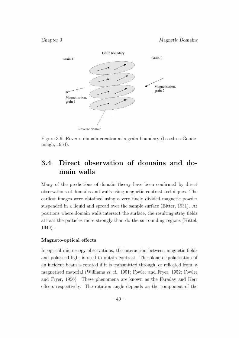
Chapter 3 Magnetic Domains
Magnetisation,
grain 1
Magnetisation,
grain 2
Grain boundary
Reverse domain
Grain 1 Grain 2
Figure 3.6: Reverse domain creation at a grain boundary (based on Goode-nough, 1954).
3.4 Direct observation of domains and do-
main walls
Many of the predictions of domain theory have been confirmed by direct
observations of domains and walls using magnetic contrast techniques. The
earliest images were obtained using a very finely divided magnetic powder
suspended in a liquid and spread over the sample surface (Bitter, 1931). At
positions where domain walls intersect the surface, the resulting stray fields
attract the particles more strongly than do the surrounding regions (Kittel,
1949).
Magneto-optical effects
In optical microscopy observations, the interaction between magnetic fields
and polarised light is used to obtain contrast. The plane of polarisation of
an incident beam is rotated if it is transmitted through, or reflected from, a
magnetised material (Williams et al., 1951; Fowler and Fryer, 1952; Fowler
and Fryer, 1956). These phenomena are known as the Faraday and Kerr
effects respectively. The rotation angle depends on the component of the
– 40 –
Chapter 3 Magnetic Domains
magnetisation in the direction of the incident beam, which depends in turn
on the magnetisation direction of the domain on which the beam impinges.
Domain contrast is obtained by setting an analyser in the extinction position
for one of the sets of domains. The Faraday effect is of limited use for
domain imaging since it requires an optically transparent medium, but Kerr
microscopy is used extensively.
Electron microscopy
An electron beam incident on a magnetic domain is deflected in a direc-
tion determined by the domain magnetisation direction. In a transmission
electron microscope (TEM), this can be used for magnetic contrast imag-
ing (‘Lorentz microscopy’). The beam deflection is extremely small, so no
contrast is obtained using bright-field conditions, but by displacing the ob-
jective aperture so that only electrons deflected by certain sets of domains
are allowed through, an image can be obtained in which some domains ap-
pear bright and others dark (Boersch and Raith, 1959). This is known as the
Foucault method. Another technique, the Fresnel method, is used to observe
domain walls. By going from an underfocused to an overfocused condition,
domain walls change from bright to dark or vice versa. This enables domain
walls to be distinguished from other features, such as dislocations, which do
not show this behaviour (Hale et al., 1959).
Scanning electron microscopy (SEM) techniques have also been devel-
oped. In highly anisotropic materials, in which the magnetisation has a
component perpendicular to the surface, secondary electrons arising from a
beam normally incident to the surface will be deflected in opposite directions
by antiparallel domains. This gives rise to alternating light and dark bands
in the secondary electron image (Type I contrast, Banbury and Nixon, 1969).
A method suitable for less anisotropic materials relies on the deflection
of electrons after they enter the specimen (Type II contrast, Fathers et al.,
1973). The domain magnetisation direction governs whether deflection oc-
curs towards or away from the surface, and hence determines the number
of backscattered electrons emitted from that domain. This method requires
a tilted specimen and a precise combination of electron beam parameters,
– 41 –
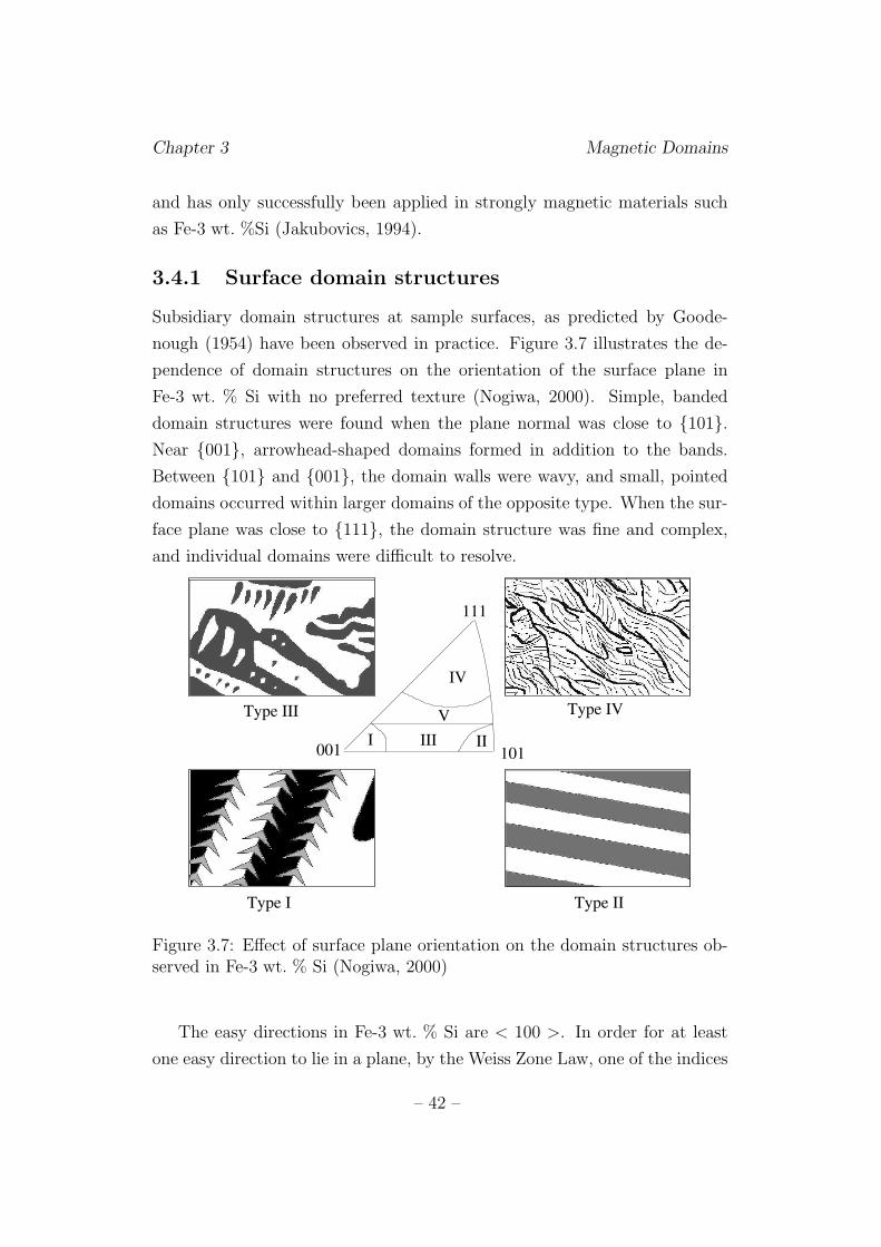
Chapter 3 Magnetic Domains
and has only successfully been applied in strongly magnetic materials such
as Fe-3 wt. %Si (Jakubovics, 1994).
3.4.1 Surface domain structures
Subsidiary domain structures at sample surfaces, as predicted by Goode-
nough (1954) have been observed in practice. Figure 3.7 illustrates the de-
pendence of domain structures on the orientation of the surface plane in
Fe-3 wt. % Si with no preferred texture (Nogiwa, 2000). Simple, banded
domain structures were found when the plane normal was close to {101}.Near {001}, arrowhead-shaped domains formed in addition to the bands.
Between {101} and {001}, the domain walls were wavy, and small, pointed
domains occurred within larger domains of the opposite type. When the sur-
face plane was close to {111}, the domain structure was fine and complex,
and individual domains were difficult to resolve.
001I
101
111
IIIII
V
IV
Type I
Type III Type IV
Type II
Figure 3.7: Effect of surface plane orientation on the domain structures ob-served in Fe-3 wt. % Si (Nogiwa, 2000)
The easy directions in Fe-3 wt. % Si are < 100 >. In order for at least
one easy direction to lie in a plane, by the Weiss Zone Law, one of the indices
– 42 –
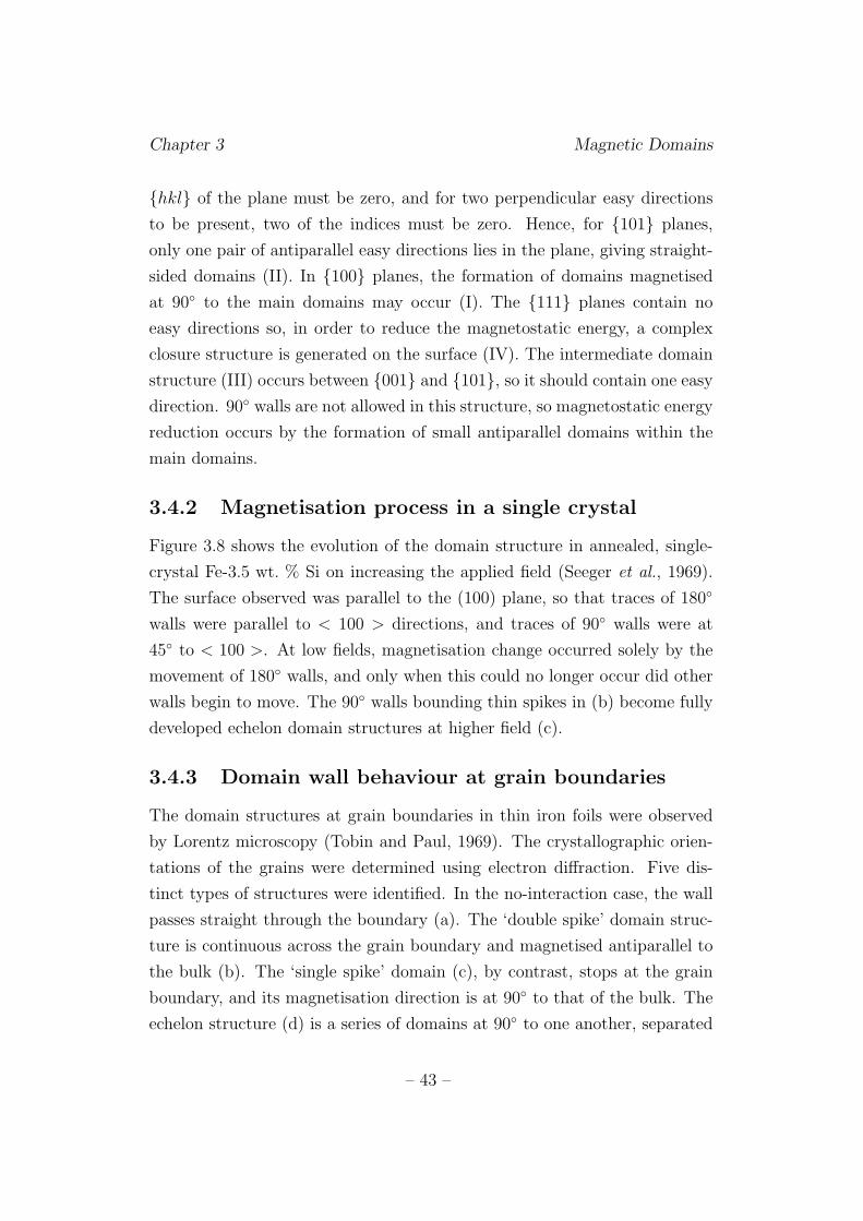
Chapter 3 Magnetic Domains
{hkl} of the plane must be zero, and for two perpendicular easy directions
to be present, two of the indices must be zero. Hence, for {101} planes,
only one pair of antiparallel easy directions lies in the plane, giving straight-
sided domains (II). In {100} planes, the formation of domains magnetised
at 90◦ to the main domains may occur (I). The {111} planes contain no
easy directions so, in order to reduce the magnetostatic energy, a complex
closure structure is generated on the surface (IV). The intermediate domain
structure (III) occurs between {001} and {101}, so it should contain one easy
direction. 90◦ walls are not allowed in this structure, so magnetostatic energy
reduction occurs by the formation of small antiparallel domains within the
main domains.
3.4.2 Magnetisation process in a single crystal
Figure 3.8 shows the evolution of the domain structure in annealed, single-
crystal Fe-3.5 wt. % Si on increasing the applied field (Seeger et al., 1969).
The surface observed was parallel to the (100) plane, so that traces of 180◦
walls were parallel to < 100 > directions, and traces of 90◦ walls were at
45◦ to < 100 >. At low fields, magnetisation change occurred solely by the
movement of 180◦ walls, and only when this could no longer occur did other
walls begin to move. The 90◦ walls bounding thin spikes in (b) become fully
developed echelon domain structures at higher field (c).
3.4.3 Domain wall behaviour at grain boundaries
The domain structures at grain boundaries in thin iron foils were observed
by Lorentz microscopy (Tobin and Paul, 1969). The crystallographic orien-
tations of the grains were determined using electron diffraction. Five dis-
tinct types of structures were identified. In the no-interaction case, the wall
passes straight through the boundary (a). The ‘double spike’ domain struc-
ture is continuous across the grain boundary and magnetised antiparallel to
the bulk (b). The ‘single spike’ domain (c), by contrast, stops at the grain
boundary, and its magnetisation direction is at 90◦ to that of the bulk. The
echelon structure (d) is a series of domains at 90◦ to one another, separated
– 43 –
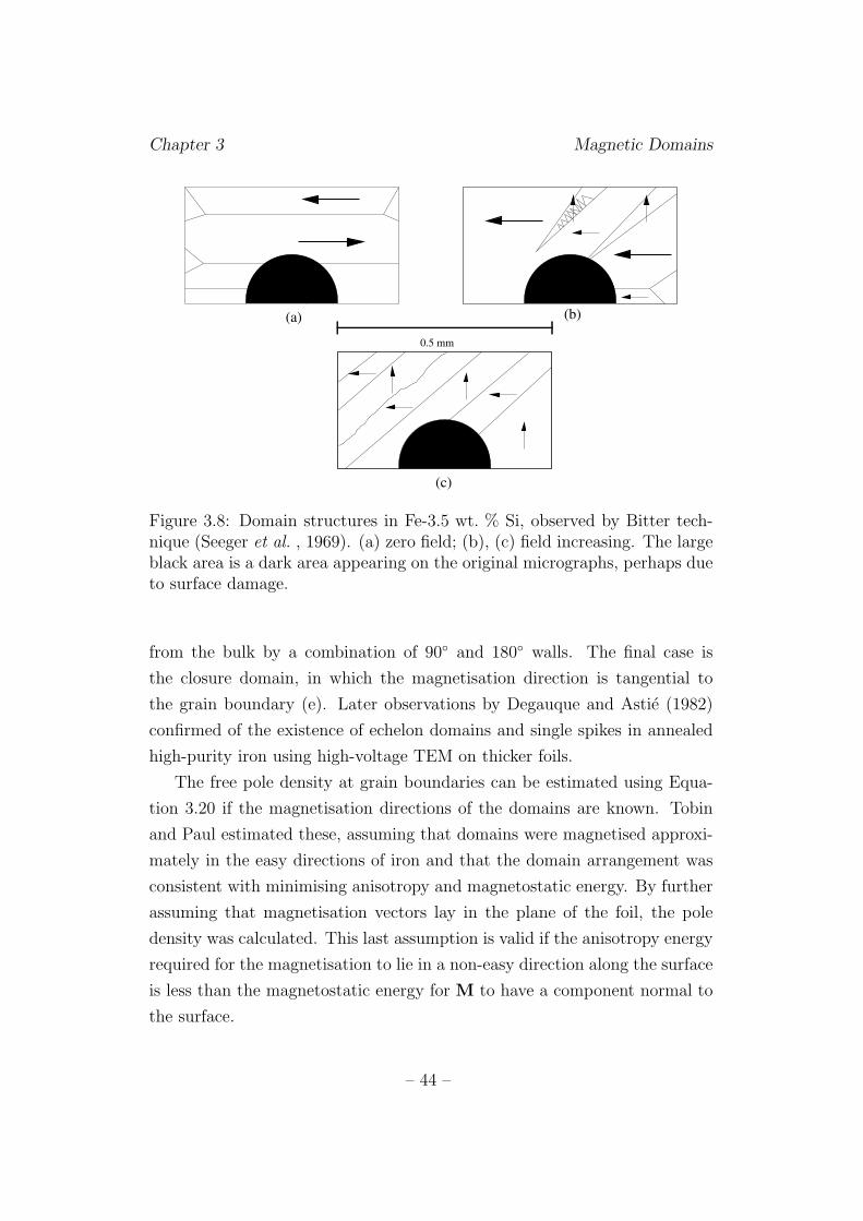
Chapter 3 Magnetic Domains
0.5 mm
(a) (b)
(c)
Figure 3.8: Domain structures in Fe-3.5 wt. % Si, observed by Bitter tech-nique (Seeger et al. , 1969). (a) zero field; (b), (c) field increasing. The largeblack area is a dark area appearing on the original micrographs, perhaps dueto surface damage.
from the bulk by a combination of 90◦ and 180◦ walls. The final case is
the closure domain, in which the magnetisation direction is tangential to
the grain boundary (e). Later observations by Degauque and Astie (1982)
confirmed of the existence of echelon domains and single spikes in annealed
high-purity iron using high-voltage TEM on thicker foils.
The free pole density at grain boundaries can be estimated using Equa-
tion 3.20 if the magnetisation directions of the domains are known. Tobin
and Paul estimated these, assuming that domains were magnetised approxi-
mately in the easy directions of iron and that the domain arrangement was
consistent with minimising anisotropy and magnetostatic energy. By further
assuming that magnetisation vectors lay in the plane of the foil, the pole
density was calculated. This last assumption is valid if the anisotropy energy
required for the magnetisation to lie in a non-easy direction along the surface
is less than the magnetostatic energy for M to have a component normal to
the surface.
– 44 –

Chapter 3 Magnetic Domains
(311)
(111)
(111)
(211)
(111)
(110)
(111)
(100)
(311)
(a) No interaction (b) Double spike (c) Single spike
(e) Closure(d) Echelon
(311)
Figure 3.9: The five types of interaction between grain boundaries and do-main walls, shown in order of increasing magnetic pole density at the grainboundary (Tobin and Paul, 1969).
The no-interaction and double-spike configurations were found to have
the lowest pole densities, and closure domains the highest, with single-spike
and echelon structures in the low-to-intermediate range. It is notable that
90◦ walls do not occur at low pole densities.
The observations of double spike domains are consistent with the theo-
retical analysis of Goodenough (1954), but he did not predict the existence
of 90◦ closure walls at grain boundaries. It appears that if an easy direction
occurs parallel to the wall, it is favourable to form such a closure domain.
These domains, unlike the 180◦ reverse spike domains, are not expected to
contribute to magnetisation reversal according to the arguments of Goode-
nough.
Lorentz microscopy observations of domain walls and grain boundaries
during the magnetisation of spinel ferrites showed that if a domain wall
was parallel to a grain boundary, the wall was stopped completely by the
– 45 –
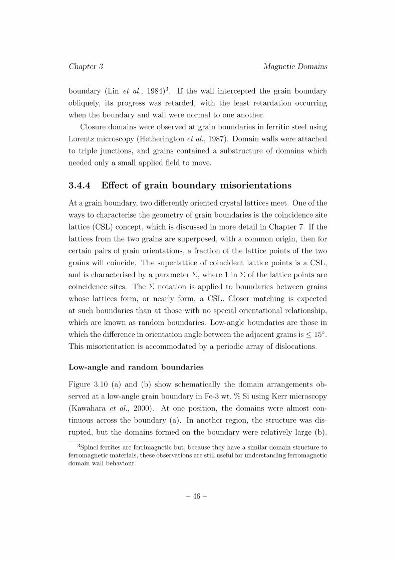
Chapter 3 Magnetic Domains
boundary (Lin et al., 1984)3. If the wall intercepted the grain boundary
obliquely, its progress was retarded, with the least retardation occurring
when the boundary and wall were normal to one another.
Closure domains were observed at grain boundaries in ferritic steel using
Lorentz microscopy (Hetherington et al., 1987). Domain walls were attached
to triple junctions, and grains contained a substructure of domains which
needed only a small applied field to move.
3.4.4 Effect of grain boundary misorientations
At a grain boundary, two differently oriented crystal lattices meet. One of the
ways to characterise the geometry of grain boundaries is the coincidence site
lattice (CSL) concept, which is discussed in more detail in Chapter 7. If the
lattices from the two grains are superposed, with a common origin, then for
certain pairs of grain orientations, a fraction of the lattice points of the two
grains will coincide. The superlattice of coincident lattice points is a CSL,
and is characterised by a parameter Σ, where 1 in Σ of the lattice points are
coincidence sites. The Σ notation is applied to boundaries between grains
whose lattices form, or nearly form, a CSL. Closer matching is expected
at such boundaries than at those with no special orientational relationship,
which are known as random boundaries. Low-angle boundaries are those in
which the difference in orientation angle between the adjacent grains is ≤ 15◦.
This misorientation is accommodated by a periodic array of dislocations.
Low-angle and random boundaries
Figure 3.10 (a) and (b) show schematically the domain arrangements ob-
served at a low-angle grain boundary in Fe-3 wt. % Si using Kerr microscopy
(Kawahara et al., 2000). At one position, the domains were almost con-
tinuous across the boundary (a). In another region, the structure was dis-
rupted, but the domains formed on the boundary were relatively large (b).
3Spinel ferrites are ferrimagnetic but, because they have a similar domain structure to
ferromagnetic materials, these observations are still useful for understanding ferromagnetic
domain wall behaviour.
– 46 –
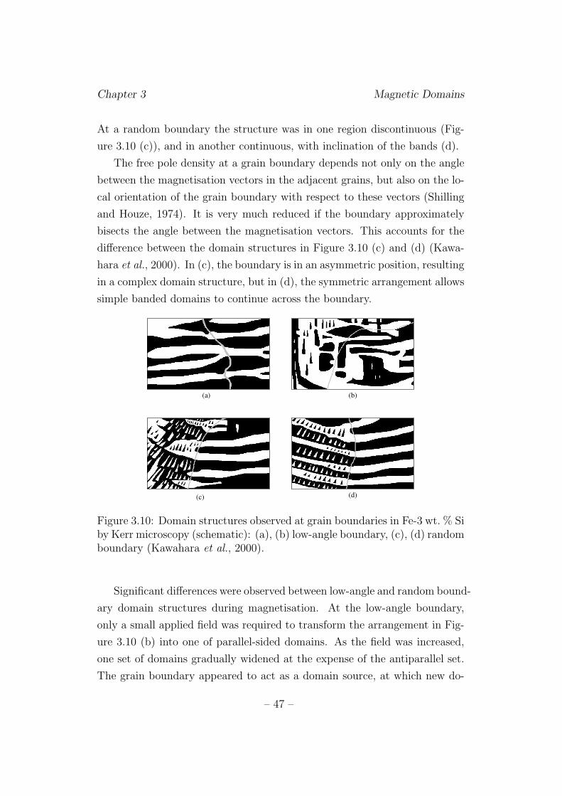
Chapter 3 Magnetic Domains
At a random boundary the structure was in one region discontinuous (Fig-
ure 3.10 (c)), and in another continuous, with inclination of the bands (d).
The free pole density at a grain boundary depends not only on the angle
between the magnetisation vectors in the adjacent grains, but also on the lo-
cal orientation of the grain boundary with respect to these vectors (Shilling
and Houze, 1974). It is very much reduced if the boundary approximately
bisects the angle between the magnetisation vectors. This accounts for the
difference between the domain structures in Figure 3.10 (c) and (d) (Kawa-
hara et al., 2000). In (c), the boundary is in an asymmetric position, resulting
in a complex domain structure, but in (d), the symmetric arrangement allows
simple banded domains to continue across the boundary.
(b)
(c)
(a)
(d)
Figure 3.10: Domain structures observed at grain boundaries in Fe-3 wt. % Siby Kerr microscopy (schematic): (a), (b) low-angle boundary, (c), (d) randomboundary (Kawahara et al., 2000).
Significant differences were observed between low-angle and random bound-
ary domain structures during magnetisation. At the low-angle boundary,
only a small applied field was required to transform the arrangement in Fig-
ure 3.10 (b) into one of parallel-sided domains. As the field was increased,
one set of domains gradually widened at the expense of the antiparallel set.
The grain boundary appeared to act as a domain source, at which new do-
– 47 –
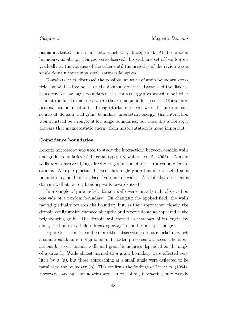
Chapter 3 Magnetic Domains
mains nucleated, and a sink into which they disappeared. At the random
boundary, no abrupt changes were observed. Instead, one set of bands grew
gradually at the expense of the other until the majority of the region was a
single domain containing small antiparallel spikes.
Kawahara et al. discussed the possible influence of grain boundary stress
fields, as well as free poles, on the domain structure. Because of the disloca-
tion arrays at low-angle boundaries, the strain energy is expected to be higher
than at random boundaries, where there is no periodic structure (Kawahara,
personal communication). If magnetoelastic effects were the predominant
source of domain wall-grain boundary interaction energy, this interaction
would instead be stronger at low-angle boundaries, but since this is not so, it
appears that magnetostatic energy from misorientation is more important.
Coincidence boundaries
Lorentz microscopy was used to study the interactions between domain walls
and grain boundaries of different types (Kawahara et al., 2002). Domain
walls were observed lying directly on grain boundaries, in a ceramic ferrite
sample. A triple junction between low-angle grain boundaries acted as a
pinning site, holding in place five domain walls. A void also acted as a
domain wall attractor, bending walls towards itself.
In a sample of pure nickel, domain walls were initially only observed on
one side of a random boundary. On changing the applied field, the walls
moved gradually towards the boundary but, as they approached closely, the
domain configuration changed abruptly, and reverse domains appeared in the
neighbouring grain. The domain wall moved so that part of its length lay
along the boundary, before breaking away in another abrupt change.
Figure 3.11 is a schematic of another observation on pure nickel in which
a similar combination of gradual and sudden processes was seen. The inter-
actions between domain walls and grain boundaries depended on the angle
of approach. Walls almost normal to a grain boundary were affected very
little by it (a), but those approaching at a small angle were deflected to lie
parallel to the boundary (b). This confirms the findings of Lin et al. (1984).
However, low-angle boundaries were an exception, interacting only weakly
– 48 –
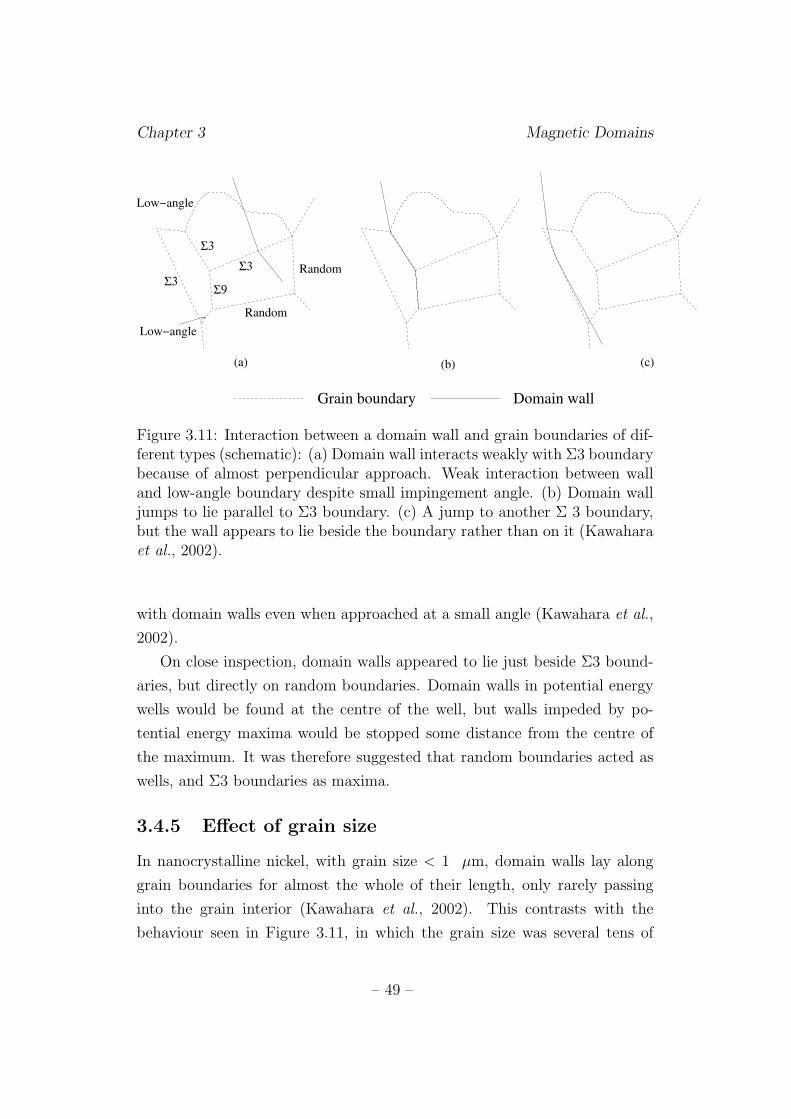
Chapter 3 Magnetic Domains
Grain boundary Domain wall
Random
Low−angle
Σ3
Σ3
Low−angle
Random
Σ3
Σ9
(a) (b) (c)
Figure 3.11: Interaction between a domain wall and grain boundaries of dif-ferent types (schematic): (a) Domain wall interacts weakly with Σ3 boundarybecause of almost perpendicular approach. Weak interaction between walland low-angle boundary despite small impingement angle. (b) Domain walljumps to lie parallel to Σ3 boundary. (c) A jump to another Σ 3 boundary,but the wall appears to lie beside the boundary rather than on it (Kawaharaet al., 2002).
with domain walls even when approached at a small angle (Kawahara et al.,
2002).
On close inspection, domain walls appeared to lie just beside Σ3 bound-
aries, but directly on random boundaries. Domain walls in potential energy
wells would be found at the centre of the well, but walls impeded by po-
tential energy maxima would be stopped some distance from the centre of
the maximum. It was therefore suggested that random boundaries acted as
wells, and Σ3 boundaries as maxima.
3.4.5 Effect of grain size
In nanocrystalline nickel, with grain size < 1 µm, domain walls lay along
grain boundaries for almost the whole of their length, only rarely passing
into the grain interior (Kawahara et al., 2002). This contrasts with the
behaviour seen in Figure 3.11, in which the grain size was several tens of
– 49 –
Chapter 3 Magnetic Domains
µm. The greater concentration of grain boundaries in the nanocrystalline
sample allows domain walls to lie on grain boundaries without significant
deviation.
The domain width in Fe-3 wt. % Si increased with increasing grain size
(Shilling and Houze, 1974). A grain boundary is more likely to be in an
approximately symmetrical position between the magnetisation directions in
adjacent grains when the misorientation angle between the grains is small.
This becomes less likely with decreasing grain size. Larger demagnetising
fields, and the consequent development of a finer domain structure, is there-
fore likely in finer-grained materials.
3.4.6 Effect of deformation
Heavy deformation of a Fe-3.5 wt. % Si single crystal produced a domain
structure in which only one pair of antiparallel magnetisation directions was
represented, even though directions perpendicular to these were permitted
by symmetry (Seeger et al., 1969). Deformation is believed to favour 180◦
over 90◦ wall motion because 90◦ walls interact more strongly with stress
fields, becoming immobilised in a highly dislocated structure.
In-situ magnetising experiments on annealed, lightly deformed and heav-
ily worked samples of pure iron demonstrated the pinning effect of disloca-
tions on domain walls (Degauque and Astie, 1982a). The annealed material
contained a few small tangles of dislocations, which acted as strong pin-
ning sites, retarding the movement of the domain walls to which they were
attached while other, unpinned domains moved more freely. Mixed disloca-
tions in the lightly strained sample and long screw dislocations in the heavily
worked sample also pinned domain walls. Work on macroscopic magnetic
properties suggested that domain wall motion was more strongly pinned in
the heavily worked sample (Astie et al., 1981), but such differences were
difficult to discern using TEM.
– 50 –
Chapter 3 Magnetic Domains
3.4.7 Second-phase particles and microstructural dif-ferences
Lath microstructures
Domain structures in bainitic and martensitic forms of the same carbon-
manganese steel composition were compared (Beale et al., 1992). In speci-
mens with long, parallel laths, a regular structure of 180◦ walls, branching
into 90◦ walls, was observed. In a sample in which only part of the struc-
ture contained laths, the domain walls were found to stretch across the laths,
and to move parallel to them when the field was applied. Apart from this
one study, domain arrangements in lath microstructures do not seem to have
been studied extensively.
Ferritic-pearlitic steels
Hetherington et al. (1987) concluded that the domain wall arrangement in
pearlitic steels depended on the orientation of the walls with respect to the
cementite lamellae. If a wall lies parallel to a lamella, it is strongly pinned,
whereas if it is perpendicular, it moves easily until it meets another grain in
which the lamellae are oriented differently.
It is also believed that the lamellar spacing plays an important role in
the domain layout (Lo et al., 1997a). Small spacings gave small domains
which were mainly bounded by Type-II walls following the ferrite/cementite
interface. When the spacing was larger, domains extended across several
lamellae, and Type-I walls were observed. Dynamic magnetisation experi-
ments showed that in the finer pearlite, the nucleation and growth of reverse
domains required a higher applied field, and individual domain wall jumps
were smaller.
In both fully pearlitic and fully ferritic microstructures, domains of reverse
magnetisation nucleated when the field was reduced from saturation, but the
growth of domain walls across the grain occurred more rapidly in the ferritic
sample (Lo and Scruby, 1999). In the pearlitic sample, it did not occur until
the applied field direction had been reversed. These findings demonstrate
the pinning strength of pearlite lamellae.
– 51 –
Chapter 3 Magnetic Domains
Lamellar and spheroidal cementite
The pinning effect of lamellar and spheroidised pearlitic microstructures were
compared (Lo et al., 1997b). In both cases, the cementite particles acted
as domain wall pinning sites, but coarser domains were observed when the
carbides were spheroidal. On reduction of the field from saturation, domain
wall motion required a larger reverse field in lamellar than in spheroidised
pearlite. Closure domains were observed on the carbide particles in the
spheroidal microstructure, and these interacted with the 180◦ walls as they
moved.
The results from experiments on pearlite show that lamellar particles are
a more effective impediment to domain wall motion than spheroidal particles.
This may be due to the flat, continuous nature of the particles, or to their
parallel, regularly spaced arrangement, or to a combination of both. It does
not appear that any observations have been made on needle- or plate-shaped
particles such as M2X in tempered steels. If the flat, elongated shape is the
more important factor in pinning, these particles, too, would act as strong
pinning sites. However, if parallelism is more important, then M2X may only
pin weakly since it tends to be small.
3.5 Conclusions
Experimental observations of domain structures in ferromagnetic materials
show a remarkable agreement with the theory which, in some cases, pre-dated
them by several decades. It has been shown that domains interact with grain
boundaries, inclusions and dislocations. Some of the main findings from these
studies are as follows:
• Cubic or spheroidal inclusions interact with domain walls by wall area
reduction and by setting up demagnetising fields. Inclusions larger than
a critical size have subsidiary spike domains.
• Lamellar precipitates in steel have a stronger pinning effect on domain
walls than do spheroidal precipitates.
– 52 –
Chapter 3 Magnetic Domains
• Specimen surfaces nucleate fine domains to reduce magnetostatic en-
ergy if they are not parallel to crystallographic planes containing easy
directions.
• It has been observed that at low values of applied field, magnetisation
change occurs preferentially by 180◦ wall motion.
• Domain walls tend to be attracted towards voids and grain boundary
triple (or multiple) junctions.
• The domain structure at grain boundaries depends on the misorienta-
tion between the adjacent grains, and on the angle made by the grain
boundary plane with the grain magnetisations.
• The dynamic interaction between grain boundaries and domain walls
depends on the angle at which the domain wall intercepts the grain
boundary, and also on the grain boundary character. Low-angle bound-
aries exert a weaker pinning effect than boundaries of other types.
• The width of domains has been observed to increase with increasing
grain size.
• In a material with finer grains, domain walls were observed to lie along
grain boundaries for far more of their length than in coarser-grained
material.
• It is predicted that reverse domains should nucleate on grain bound-
aries, surfaces and planar inclusions, but not on cubic or spheroidal
inclusions.
– 53 –

Chapter 4
Magnetic Properties inNondestructive Testing
It has been known for many years that the magnetic properties of steels de-
pend on their composition and heat treatment. Mechanically harder steels
have superior properties as permanent magnets than softer steels, hence the
terminology of ‘hard’ and ‘soft’ magnetic materials. Curie (1898) found a
relationship between magnetic behaviour and carbon content in permanent
magnet steels, and Evershed (1925) observed a deterioration of magnet steel
properties over time, which he related to slow metallurgical changes. Such re-
lationships suggested that magnetic measurements could be used as a nonde-
structive testing (NDT) method to determine materials properties. In recent
decades, many investigations have been carried out to develop such tech-
niques; progress has been reviewed by Blitz (1991), Swartzendruber (1992),
Devine (1992), Sipahi (1994), Sablik and Augustyniak (1999) and Ara (2002).
4.1 Hysteresis properties
4.1.1 The hysteresis loop
Figure 4.1 is a plot of magnetisation M against applied field H. On applica-
tion of a field to a demagnetised sample, M increases with H, reaching the
saturation magnetisation MS if a sufficiently large field is applied. When H
is reduced, and subsequently cycled between positive and negative directions,
– 54 –
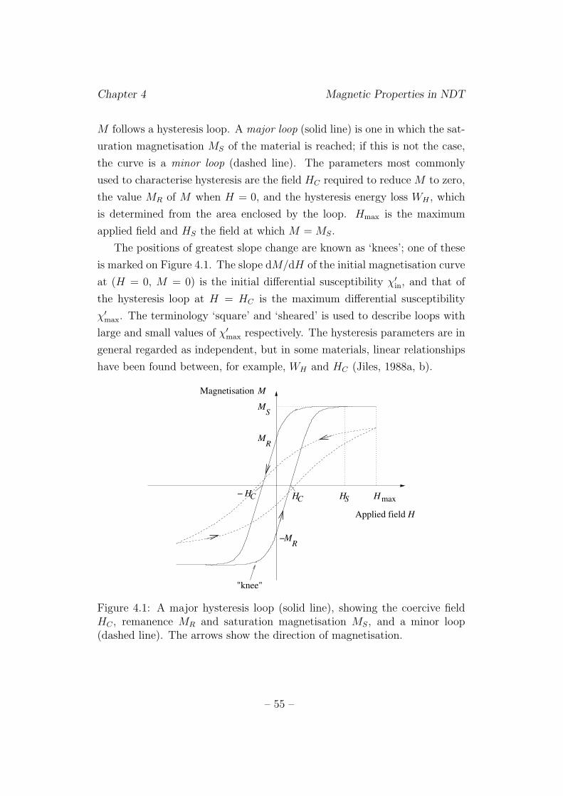
Chapter 4 Magnetic Properties in NDT
M follows a hysteresis loop. A major loop (solid line) is one in which the sat-
uration magnetisation MS of the material is reached; if this is not the case,
the curve is a minor loop (dashed line). The parameters most commonly
used to characterise hysteresis are the field HC required to reduce M to zero,
the value MR of M when H = 0, and the hysteresis energy loss WH , which
is determined from the area enclosed by the loop. Hmax is the maximum
applied field and HS the field at which M = MS.
The positions of greatest slope change are known as ‘knees’; one of these
is marked on Figure 4.1. The slope dM/dH of the initial magnetisation curve
at (H = 0, M = 0) is the initial differential susceptibility χ′in, and that of
the hysteresis loop at H = HC is the maximum differential susceptibility
χ′max. The terminology ‘square’ and ‘sheared’ is used to describe loops with
large and small values of χ′max respectively. The hysteresis parameters are in
general regarded as independent, but in some materials, linear relationships
have been found between, for example, WH and HC (Jiles, 1988a, b).
HApplied field
HS Hmax
−
−
MS
MMagnetisation
H
"knee"
C
MR
HC
MR
Figure 4.1: A major hysteresis loop (solid line), showing the coercive fieldHC , remanence MR and saturation magnetisation MS, and a minor loop(dashed line). The arrows show the direction of magnetisation.
– 55 –
Chapter 4 Magnetic Properties in NDT
4.1.2 Alternative terminology
The magnetic induction B = µ0(H + M) is sometimes used instead of M.
B-H and M -H loops contain the same information but different terminology
is used: BS and BR instead of MS and MR, respectively. The slope of a B-H
loop, dB/dH, is the differential permeability, µ′; the maximum value of this
usually occurs at H = HC and is denoted µ′max. The magnetic flux Φ is the
product of B and the sample cross-sectional area.
HC is usually referred to as the coercive field, and BR and MR as the re-
manent induction and remanent magnetisation respectively. The alternative
terms ‘coercivity’ and ‘remanence’ are also used, but an emerging convention
(noted by Jiles, 1998) is to reserve these last two terms for major loops only1.
Hysteresis experiments for use in NDT usually involve measurement of
the M −H or B−H loop and extraction of a selection of the above parame-
ters. An alternative approach, developed by Davis (1971) and Willcock and
Tanner (1983a, b), is to express the loop in terms of Fourier coefficients. This
method is used in industry for stress monitoring using magnetic hysteresis
(Tanner, personal communication), and has the advantage that the entire
data set is used, but it has not so far been adopted for microstructure-based
investigations.
4.2 Magnetic noise
4.2.1 Barkhausen effect
Barkhausen (1919) discovered that, during the magnetisation of an iron bar,
many short-lived voltage pulses were induced in a coil wound around the bar.
These were detected as audible clicks in a loudspeaker. By electromagnetic
induction, the voltage depends on the rate of change of magnetisation with
time; discrete pulses imply abrupt changes in magnetisation. Even when
care was taken to change the magnetising field smoothly, the discontinuities
persisted, demonstrating that magnetisation was an intrinsically discrete pro-
1A distinction also exists between the coercivity, at which B = 0, and the intrinsic
coercivity, at which M = 0, but this can be neglected for steels, in which HC is small.
– 56 –
Chapter 4 Magnetic Properties in NDT
cess. Barkhausen used this observation to support the hypothesis of magnetic
domains predicted theoretically by Weiss (1906, 1907). The characteristics
of the Barkhausen noise (BN) signal depend on several factors, including
microstructure.
4.2.2 Magnetoacoustic effect
The abrupt motion of Type-I domain walls is accompanied by a change in
the magnetostrictive strain. This causes an acoustic wave, which travels
through the material and can be picked up on the surface by a piezoelectric
transducer (Lord, 1975). Since such magnetoacoustic emission (MAE) arises
only from Type-I wall motion, but BN can be produced by any sudden change
in the magnetisation state, measuring both properties gives complementary
information.
4.2.3 Magnetic noise measurement
The basis of a BN measurement system is an electromagnetic yoke to pro-
duce an alternating field and a pickup coil to detect the noise pulses, but
two variations exist. The sample may be positioned within the yoke, with
the pickup coil surrounding the sample (Figure 4.2 (a)). This restricts the
sample size and shape, and is therefore inconvenient for NDT. The alter-
native method uses a yoke placed onto a flat sample, and a pickup coil on
or near the surface (Figure 4.2 (b)). MAE measurements are made using
an arrangement similar to (b), but with a piezoelectric transducer bonded
directly to the sample surface instead of a pickup coil.
Comparisons of magnetic noise literature reveal considerable differences
in yoke geometry, experimental conditions and signal processing. In some
cases, the influences of these factors on the signal have been investigated
(§ 4.9), but such characterisations are not comprehensive.
4.2.4 Data analysis
The raw magnetic noise data are a series of voltage pulses, and their asso-
ciated applied field values, obtained as a function of time (Figure 4.3 (a)).
– 57 –
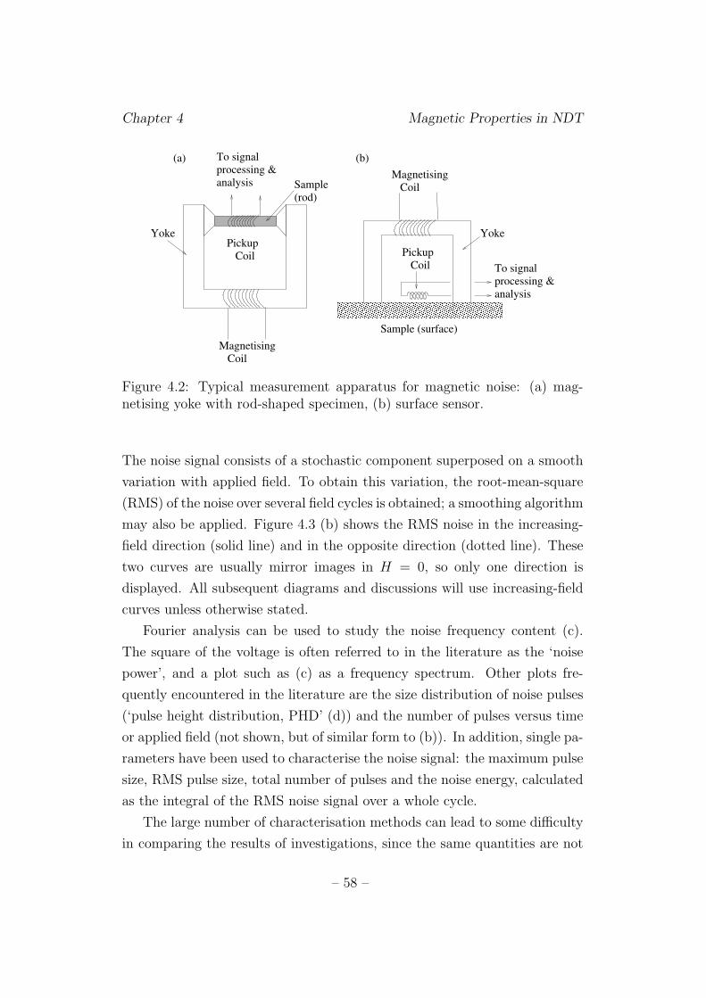
Chapter 4 Magnetic Properties in NDT
Magnetising
Coil
Pickup
Coil To signal
processing &
analysis
Pickup
Coil
To signal
processing &
analysisMagnetising
Coil
������������������������������������������������������������������������������������������������������������������������������������������������������������
������������������������������������������������������������������������������������������������������������������������������������������������������������
Sample (surface)
Sample
(rod)
YokeYoke
(a) (b)
Figure 4.2: Typical measurement apparatus for magnetic noise: (a) mag-netising yoke with rod-shaped specimen, (b) surface sensor.
The noise signal consists of a stochastic component superposed on a smooth
variation with applied field. To obtain this variation, the root-mean-square
(RMS) of the noise over several field cycles is obtained; a smoothing algorithm
may also be applied. Figure 4.3 (b) shows the RMS noise in the increasing-
field direction (solid line) and in the opposite direction (dotted line). These
two curves are usually mirror images in H = 0, so only one direction is
displayed. All subsequent diagrams and discussions will use increasing-field
curves unless otherwise stated.
Fourier analysis can be used to study the noise frequency content (c).
The square of the voltage is often referred to in the literature as the ‘noise
power’, and a plot such as (c) as a frequency spectrum. Other plots fre-
quently encountered in the literature are the size distribution of noise pulses
(‘pulse height distribution, PHD’ (d)) and the number of pulses versus time
or applied field (not shown, but of similar form to (b)). In addition, single pa-
rameters have been used to characterise the noise signal: the maximum pulse
size, RMS pulse size, total number of pulses and the noise energy, calculated
as the integral of the RMS noise signal over a whole cycle.
The large number of characterisation methods can lead to some difficulty
in comparing the results of investigations, since the same quantities are not
– 58 –
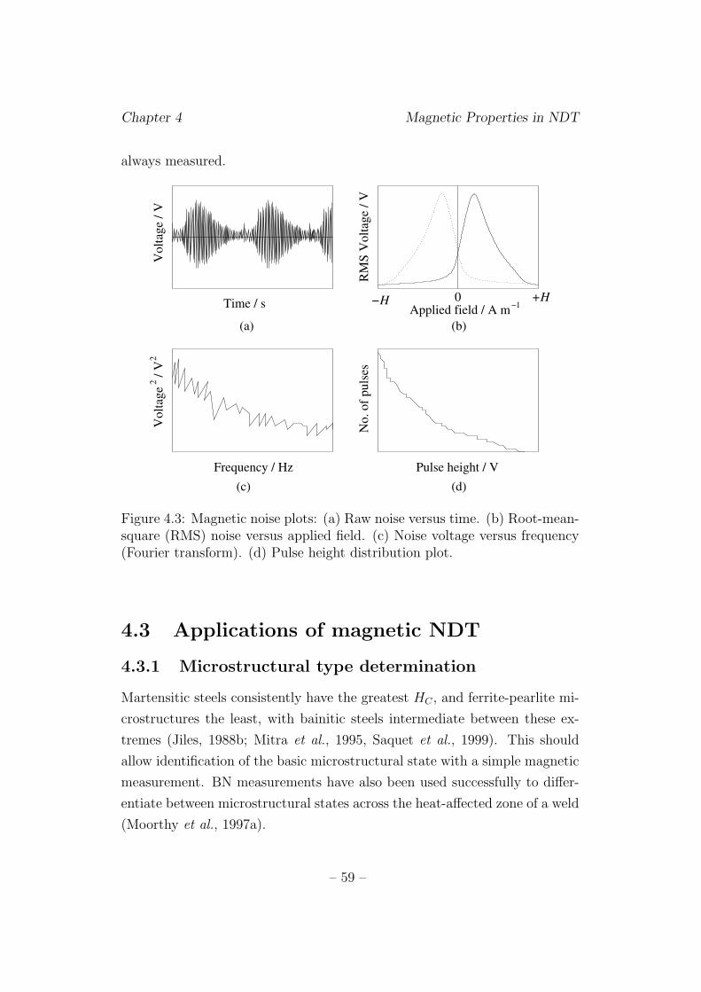
Chapter 4 Magnetic Properties in NDT
always measured.
−1Applied field / A m−H +HTime / s
Vol
tage
/ V
RM
S V
olta
ge /
V
0
(d)(c)Pulse height / VFrequency / Hz
No.
of p
ulse
s
2V
olta
ge
/ V
(a)
2
(b)
Figure 4.3: Magnetic noise plots: (a) Raw noise versus time. (b) Root-mean-square (RMS) noise versus applied field. (c) Noise voltage versus frequency(Fourier transform). (d) Pulse height distribution plot.
4.3 Applications of magnetic NDT
4.3.1 Microstructural type determination
Martensitic steels consistently have the greatest HC , and ferrite-pearlite mi-
crostructures the least, with bainitic steels intermediate between these ex-
tremes (Jiles, 1988b; Mitra et al., 1995, Saquet et al., 1999). This should
allow identification of the basic microstructural state with a simple magnetic
measurement. BN measurements have also been used successfully to differ-
entiate between microstructural states across the heat-affected zone of a weld
(Moorthy et al., 1997a).
– 59 –
Chapter 4 Magnetic Properties in NDT
4.3.2 Empirical correlations
Correlations for the determination of mechanical or microstructural proper-
ties using magnetic measurements have been found in many materials. Ex-
amples include extensive work in the former Soviet Union on monitoring the
quality of heat-treatment and hardening in a variety of steels (Mikheev et al.,
1978; Kuznetsov et al., 1982, Zatsepin et al., 1983; Mikheev, 1983). Devine
(1992) describes many more such results.
The important consideration for NDT is that there is a monotonic change
in the magnetic property within the range of interest, as pointed out by
Halmshaw (1991). Correlations are specific to particular microstructures
and ranges of composition and temperature, and are liable to fail outside
these limits. For example, in a pearlitic rail steel, the correlation between
coercive field and hardness was poor at room temperature, but good at high
temperatures (Bussiere et al., 1987). The suggested reason for this was that
at high temperatures, the Fe3C particles were above their Curie temperature
TC , and so acted as nonferromagnetic inhomogeneities.
Findings such as these have led to investigations of the effects of indi-
vidual microstructural features, such as grain boundaries, dislocations and
inclusions, on the magnetic properties.
4.4 Grain boundaries
4.4.1 Grain size effects
High-purity materials
Two distinct theoretical models predict that HC should be proportional to
1/d, where d is the average grain diameter, in materials where grain bound-
aries are the dominant obstacle to domain wall motion (Goodenough, 1954;
Globus and Guyot, 1972). Degauque et al. (1982) found that this relation-
ship was valid for annealed high-purity iron, although d−1/2 also fitted the
data satisfactorily. In commercial-purity nickel, too, the coercive field de-
creased with increasing grain size over a wide range from nanocrystalline to
∼ 102 µm (Kawahara et al., 2002).
– 60 –
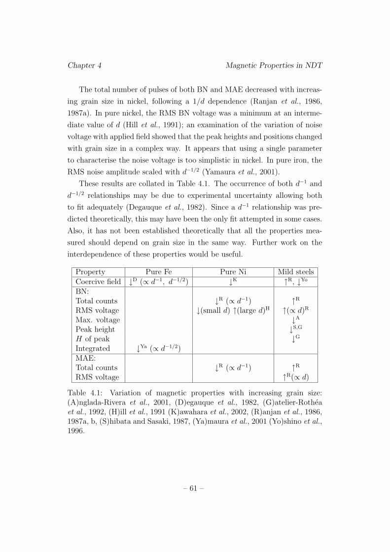
Chapter 4 Magnetic Properties in NDT
The total number of pulses of both BN and MAE decreased with increas-
ing grain size in nickel, following a 1/d dependence (Ranjan et al., 1986,
1987a). In pure nickel, the RMS BN voltage was a minimum at an interme-
diate value of d (Hill et al., 1991); an examination of the variation of noise
voltage with applied field showed that the peak heights and positions changed
with grain size in a complex way. It appears that using a single parameter
to characterise the noise voltage is too simplistic in nickel. In pure iron, the
RMS noise amplitude scaled with d−1/2 (Yamaura et al., 2001).
These results are collated in Table 4.1. The occurrence of both d−1 and
d−1/2 relationships may be due to experimental uncertainty allowing both
to fit adequately (Degauque et al., 1982). Since a d−1 relationship was pre-
dicted theoretically, this may have been the only fit attempted in some cases.
Also, it has not been established theoretically that all the properties mea-
sured should depend on grain size in the same way. Further work on the
interdependence of these properties would be useful.
Property Pure Fe Pure Ni Mild steels
Coercive field ↓D (∝ d−1, d−1/2) ↓K ↑R, ↓Yo
BN:Total counts ↓R (∝ d−1) ↑R
RMS voltage ↓(small d) ↑(large d)H ↑(∝ d)R
Max. voltage ↓A
Peak height ↓S,G
H of peak ↓G
Integrated ↓Ya (∝ d−1/2)MAE:Total counts ↓R (∝ d−1) ↑R
RMS voltage ↑R(∝ d)
Table 4.1: Variation of magnetic properties with increasing grain size:(A)nglada-Rivera et al., 2001, (D)egauque et al., 1982, (G)atelier-Rotheaet al., 1992, (H)ill et al., 1991 (K)awahara et al., 2002, (R)anjan et al., 1986,1987a, b, (S)hibata and Sasaki, 1987, (Ya)maura et al., 2001 (Yo)shino et al.,1996.
– 61 –
Chapter 4 Magnetic Properties in NDT
Mild steels
The final column of Table 4.1 displays results from mild steels. In decar-
burised steel, all the properties show opposite trends to those in the purer
metals; for example, the RMS noise voltages are directly proportional to d
(Ranjan et al., 1986, 1987a). This was explained by the presence of impurities
– MnS particles within the grains and phosphorus on the grain boundaries
– whose presence overwhelmed the intrinsic grain size effect (Ranjan et al.,
1987b). However, Yoshino et al. (1996) reported that in steels containing
only ferrite, HC was inversely proportional to the grain size.
The average BN amplitude in low carbon steel (composition not specified)
varied as ln d/dC , where dC is the extrapolated grain size for which the BN
amplitude is zero, for small grain size d, and saturated at a critical value of
d (Tiitto, 1978).
The variation of BN and MAE voltage with position in the magnetisation
cycle for 0.1 wt. % C steel showed two peaks (Shibata and Sasaki, 1987). For
BN, the first of these decreased in height with increasing grain size, while the
second showed little variation. The first MAE peak occurred at a stronger
applied field than the first BN peak, but the second peaks coincided. It was
concluded that the first peak was due to domain wall motion, which occurred
at a lower field for Type-II than for Type-I walls, while the second peak was
attributed to discontinuous rotation of domains.
In Fe-0.013 wt. % C, a single BN peak, whose height decreased with in-
creasing grain size, was seen (Gatelier-Rothea et al., 1992). Similarly, in
0.4 wt. % C steel, the maximum BN amplitude was largest in a fine-grained
and smallest in a coarse-grained sample (Anglada-Rivera et al., 2001). In
both cases, these results were explained as due to a larger number of do-
main walls within fine-grained samples. The domain size was reported by
Degauque et al. (1982) as proportional to the square root of grain size for
grain diameters between 0.05 and 10 mm. Hence, both the the number of
domain walls and the number of pinning sites per unit volume is greatest for
small grains.
The BN peaks observed by Gatelier-Rothea et al. (1992) were situated
– 62 –
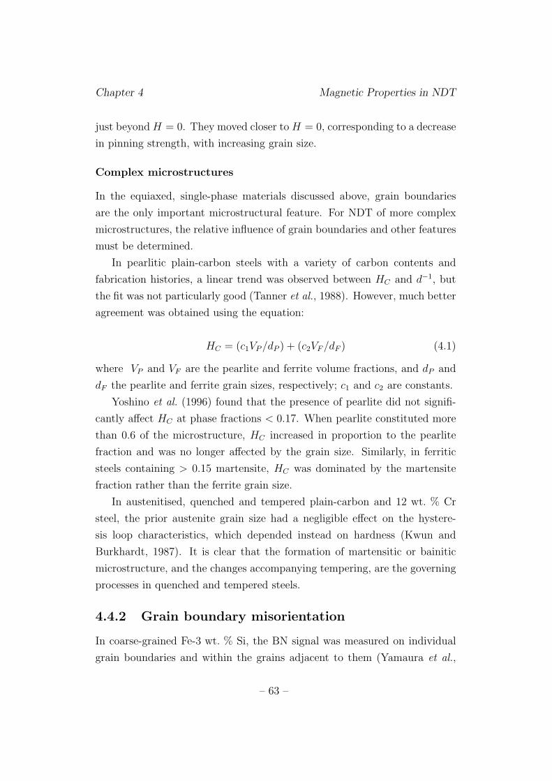
Chapter 4 Magnetic Properties in NDT
just beyond H = 0. They moved closer to H = 0, corresponding to a decrease
in pinning strength, with increasing grain size.
Complex microstructures
In the equiaxed, single-phase materials discussed above, grain boundaries
are the only important microstructural feature. For NDT of more complex
microstructures, the relative influence of grain boundaries and other features
must be determined.
In pearlitic plain-carbon steels with a variety of carbon contents and
fabrication histories, a linear trend was observed between HC and d−1, but
the fit was not particularly good (Tanner et al., 1988). However, much better
agreement was obtained using the equation:
HC = (c1VP /dP ) + (c2VF /dF ) (4.1)
where VP and VF are the pearlite and ferrite volume fractions, and dP and
dF the pearlite and ferrite grain sizes, respectively; c1 and c2 are constants.
Yoshino et al. (1996) found that the presence of pearlite did not signifi-
cantly affect HC at phase fractions < 0.17. When pearlite constituted more
than 0.6 of the microstructure, HC increased in proportion to the pearlite
fraction and was no longer affected by the grain size. Similarly, in ferritic
steels containing > 0.15 martensite, HC was dominated by the martensite
fraction rather than the ferrite grain size.
In austenitised, quenched and tempered plain-carbon and 12 wt. % Cr
steel, the prior austenite grain size had a negligible effect on the hystere-
sis loop characteristics, which depended instead on hardness (Kwun and
Burkhardt, 1987). It is clear that the formation of martensitic or bainitic
microstructure, and the changes accompanying tempering, are the governing
processes in quenched and tempered steels.
4.4.2 Grain boundary misorientation
In coarse-grained Fe-3 wt. % Si, the BN signal was measured on individual
grain boundaries and within the grains adjacent to them (Yamaura et al.,
– 63 –
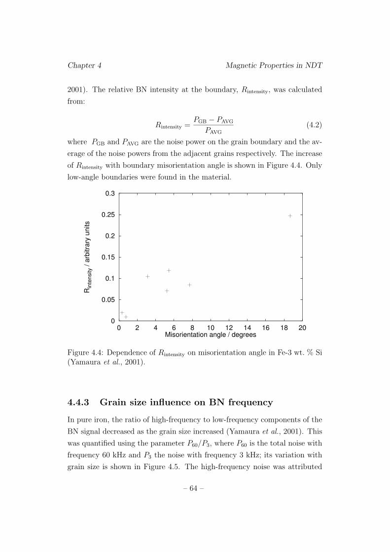
Chapter 4 Magnetic Properties in NDT
2001). The relative BN intensity at the boundary, Rintensity, was calculated
from:
Rintensity =PGB − PAVG
PAVG
(4.2)
where PGB and PAVG are the noise power on the grain boundary and the av-
erage of the noise powers from the adjacent grains respectively. The increase
of Rintensity with boundary misorientation angle is shown in Figure 4.4. Only
low-angle boundaries were found in the material.
0
0.05
0.1
0.15
0.2
0.25
0.3
0 2 4 6 8 10 12 14 16 18 20
Rin
ten
sity / a
rbitra
ry u
nits
Misorientation angle / degrees
Figure 4.4: Dependence of Rintensity on misorientation angle in Fe-3 wt. % Si(Yamaura et al., 2001).
4.4.3 Grain size influence on BN frequency
In pure iron, the ratio of high-frequency to low-frequency components of the
BN signal decreased as the grain size increased (Yamaura et al., 2001). This
was quantified using the parameter P60/P3, where P60 is the total noise with
frequency 60 kHz and P3 the noise with frequency 3 kHz; its variation with
grain size is shown in Figure 4.5. The high-frequency noise was attributed
– 64 –
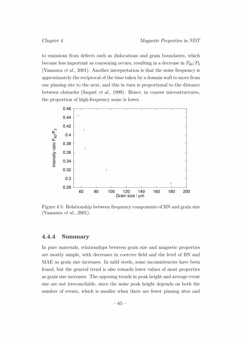
Chapter 4 Magnetic Properties in NDT
to emissions from defects such as dislocations and grain boundaries, which
become less important as coarsening occurs, resulting in a decrease in P60/P3
(Yamaura et al., 2001). Another interpretation is that the noise frequency is
approximately the reciprocal of the time taken by a domain wall to move from
one pinning site to the next, and this in turn is proportional to the distance
between obstacles (Saquet et al., 1999). Hence, in coarser microstructures,
the proportion of high-frequency noise is lower.
0.28
0.3
0.32
0.34
0.36
0.38
0.4
0.42
0.44
0.46
60 80 100 120 140 160 180 200
Inte
nsity r
atio
P6
0/P
3
Grain size / µm
Figure 4.5: Relationship between frequency components of BN and grain size(Yamaura et al., 2001).
4.4.4 Summary
In pure materials, relationships between grain size and magnetic properties
are mostly simple, with decreases in coercive field and the level of BN and
MAE as grain size increases. In mild steels, some inconsistencies have been
found, but the general trend is also towards lower values of most properties
as grain size increases. The opposing trends in peak height and average event
size are not irreconcilable, since the noise peak height depends on both the
number of events, which is smaller when there are fewer pinning sites and
– 65 –
Chapter 4 Magnetic Properties in NDT
moving walls, and the average event size, which is large when a domain wall
can move a long distance without being pinned.
The pinning strength of grain boundaries was slightly greater for smaller
grains. Finer-grained iron also gave a greater proportion of high-frequency
noise; this can be related to a shorter domain wall time-of-flight between
obstacles. At individual low-angle grain boundaries in Fe-3 wt. % Si, the ratio
of the noise measured across the boundary to the noise from the adjacent
grains increased with misorientation angle.
In steels with a second microstructural constituent, this tended to dom-
inate magnetic behaviour when it was present in sufficient quantities. Simi-
larly, in austenitised, quenched and tempered steels, the prior austenite grain
size had no significant effect on hysteresis properties.
4.5 Dislocations and plastic strain
4.5.1 Deformation
At a low level of deformation in pure iron, isolated, homogeneously dis-
tributed dislocations appeared, but caused very little change in HC compared
to the undeformed state (Astie et al., 1981). Further deformation produced
dislocation tangles and a rapid increase in HC with stress. At even higher
strain, dislocations formed subgrain boundaries and the intragranular dis-
location density decreased. HC still increased with stress, but the rate of
increase was smaller.
Jiles (1998b) investigated the effect of plastic compressive deformation on
a high-chromium steel in three microstructural conditions: ferrite/pearlite,
ferrite/bainite and tempered martensite. The coercive field was propor-
tional to the hardness irrespective of the microstructure. However, some mi-
crostructural differences were evident. In ferrite/pearlite and ferrite/bainite,
WH and HC increased with increasing plastic strain; this was attributed to
the additional obstacles to domain wall motion provided by a greater dis-
location density. In martensite, by contrast, HC and WH decreased with
increasing plastic strain. It was suggested that this, in the same way as the
– 66 –
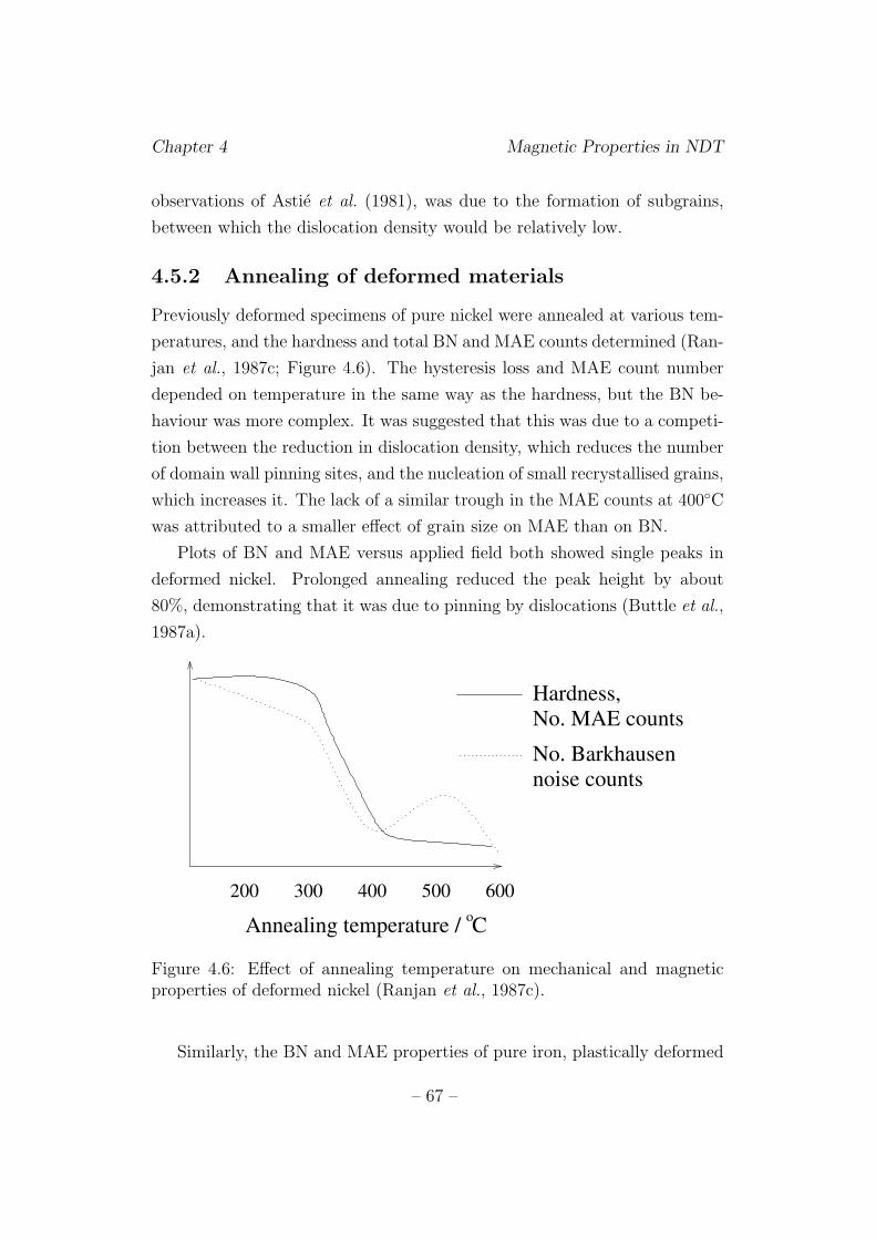
Chapter 4 Magnetic Properties in NDT
observations of Astie et al. (1981), was due to the formation of subgrains,
between which the dislocation density would be relatively low.
4.5.2 Annealing of deformed materials
Previously deformed specimens of pure nickel were annealed at various tem-
peratures, and the hardness and total BN and MAE counts determined (Ran-
jan et al., 1987c; Figure 4.6). The hysteresis loss and MAE count number
depended on temperature in the same way as the hardness, but the BN be-
haviour was more complex. It was suggested that this was due to a competi-
tion between the reduction in dislocation density, which reduces the number
of domain wall pinning sites, and the nucleation of small recrystallised grains,
which increases it. The lack of a similar trough in the MAE counts at 400◦C
was attributed to a smaller effect of grain size on MAE than on BN.
Plots of BN and MAE versus applied field both showed single peaks in
deformed nickel. Prolonged annealing reduced the peak height by about
80%, demonstrating that it was due to pinning by dislocations (Buttle et al.,
1987a).
No. Barkhausen
noise counts
Hardness,
No. MAE counts
600500400300200
Annealing temperature / Co
Figure 4.6: Effect of annealing temperature on mechanical and magneticproperties of deformed nickel (Ranjan et al., 1987c).
Similarly, the BN and MAE properties of pure iron, plastically deformed
– 67 –
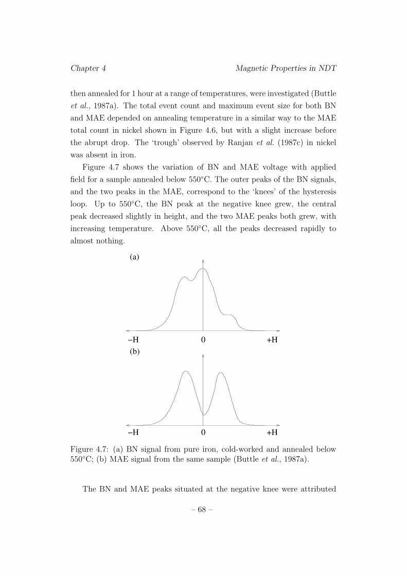
Chapter 4 Magnetic Properties in NDT
then annealed for 1 hour at a range of temperatures, were investigated (Buttle
et al., 1987a). The total event count and maximum event size for both BN
and MAE depended on annealing temperature in a similar way to the MAE
total count in nickel shown in Figure 4.6, but with a slight increase before
the abrupt drop. The ‘trough’ observed by Ranjan et al. (1987c) in nickel
was absent in iron.
Figure 4.7 shows the variation of BN and MAE voltage with applied
field for a sample annealed below 550◦C. The outer peaks of the BN signals,
and the two peaks in the MAE, correspond to the ‘knees’ of the hysteresis
loop. Up to 550◦C, the BN peak at the negative knee grew, the central
peak decreased slightly in height, and the two MAE peaks both grew, with
increasing temperature. Above 550◦C, all the peaks decreased rapidly to
almost nothing.
(b)+H0
(a)
−H +H0
−H
Figure 4.7: (a) BN signal from pure iron, cold-worked and annealed below550◦C; (b) MAE signal from the same sample (Buttle et al., 1987a).
The BN and MAE peaks situated at the negative knee were attributed
– 68 –
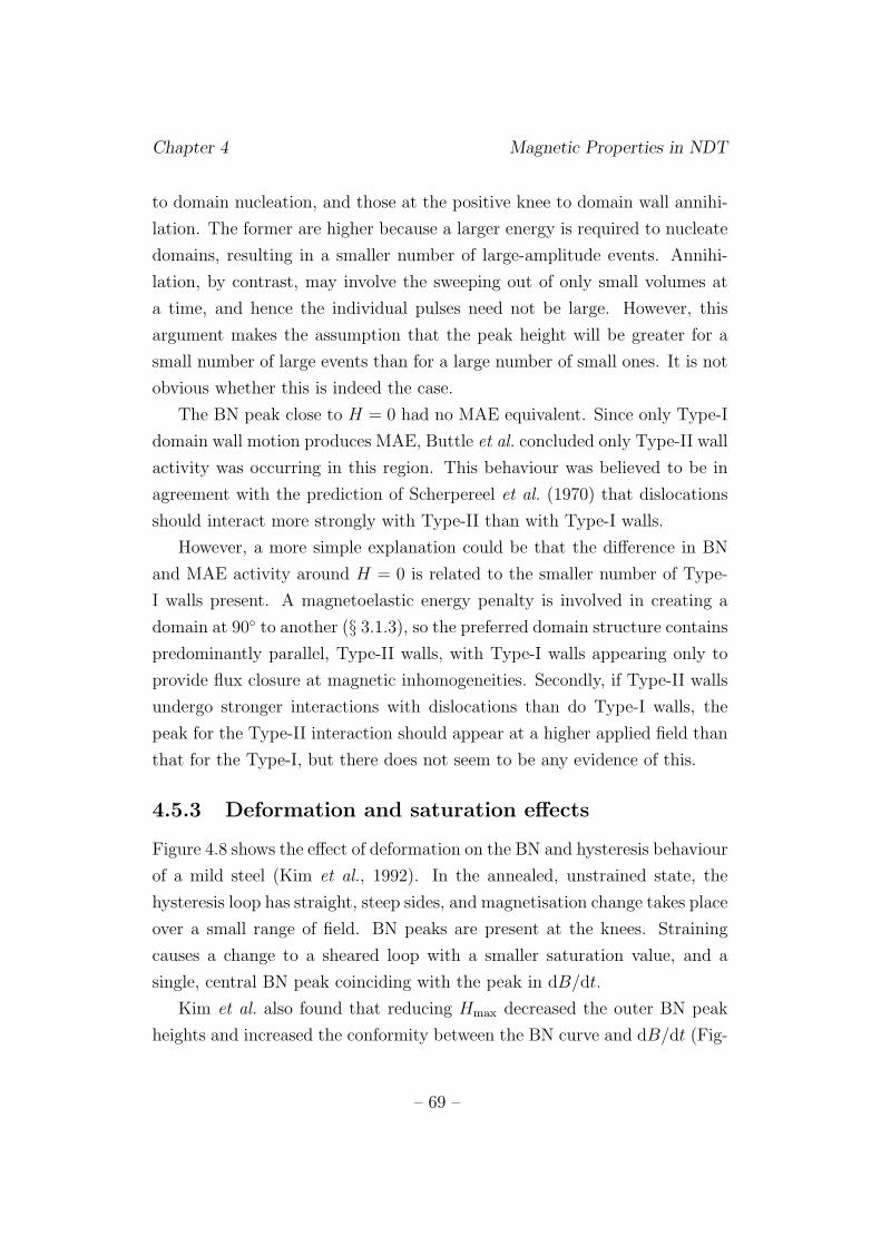
Chapter 4 Magnetic Properties in NDT
to domain nucleation, and those at the positive knee to domain wall annihi-
lation. The former are higher because a larger energy is required to nucleate
domains, resulting in a smaller number of large-amplitude events. Annihi-
lation, by contrast, may involve the sweeping out of only small volumes at
a time, and hence the individual pulses need not be large. However, this
argument makes the assumption that the peak height will be greater for a
small number of large events than for a large number of small ones. It is not
obvious whether this is indeed the case.
The BN peak close to H = 0 had no MAE equivalent. Since only Type-I
domain wall motion produces MAE, Buttle et al. concluded only Type-II wall
activity was occurring in this region. This behaviour was believed to be in
agreement with the prediction of Scherpereel et al. (1970) that dislocations
should interact more strongly with Type-II than with Type-I walls.
However, a more simple explanation could be that the difference in BN
and MAE activity around H = 0 is related to the smaller number of Type-
I walls present. A magnetoelastic energy penalty is involved in creating a
domain at 90◦ to another (§ 3.1.3), so the preferred domain structure contains
predominantly parallel, Type-II walls, with Type-I walls appearing only to
provide flux closure at magnetic inhomogeneities. Secondly, if Type-II walls
undergo stronger interactions with dislocations than do Type-I walls, the
peak for the Type-II interaction should appear at a higher applied field than
that for the Type-I, but there does not seem to be any evidence of this.
4.5.3 Deformation and saturation effects
Figure 4.8 shows the effect of deformation on the BN and hysteresis behaviour
of a mild steel (Kim et al., 1992). In the annealed, unstrained state, the
hysteresis loop has straight, steep sides, and magnetisation change takes place
over a small range of field. BN peaks are present at the knees. Straining
causes a change to a sheared loop with a smaller saturation value, and a
single, central BN peak coinciding with the peak in dB/dt.
Kim et al. also found that reducing Hmax decreased the outer BN peak
heights and increased the conformity between the BN curve and dB/dt (Fig-
– 69 –
Chapter 4 Magnetic Properties in NDT
+ 1.6−1.6 0Current / A
0
5
Am
plitu
de /
V(a) Annealed, undeformed
0
5
Current / A+ 0.8−0.8 0
Am
plitu
de /
V
(c) Annealed, undeformedSmaller applied field range
Barkhausen noise
HysteresisdB / dt
+ 1.6−1.6 0Current / A
0
5(b) 35.5% strain
Figure 4.8: Effect of straining and changing the applied current range (andhence Hmax) on BN, hysteresis and dB/dt curves (Kim et al., 1992).
ure 4.8 (c)). The ability of both deformation and reduction of Hmax to
suppress the outer peaks led to the conclusion that domain nucleation and
annihilation did not take place in many of the domains in the deformed ma-
terial. The dramatic reduction in the value of M at Hmax supports this; it is
unlikely that the true MS (which is generally viewed as a structure-insensitive
property) could be changed to this extent by deformation. Instead, it seems
that the highly dislocated material does not become fully saturated. The
BN activity around zero field increases on deformation. It appears that in a
relatively strain-free sample, it is easy for the structure to ‘switch’ from one
state of near-saturation to another, but when many dislocations are present,
domain walls must overcome these, with an associated emission of BN around
– 70 –
Chapter 4 Magnetic Properties in NDT
H = 0.
4.5.4 Summary
In many cases, there is a simple linear correlation between hardness and HC ,
but when the dislocation density is very high, this relationship is altered by
the formation of subgrain boundaries.
In pure iron and nickel, magnetic noise levels are high after deformation,
but decrease to almost nothing after high-temperature annealing. By con-
trast, in mild steel, the large BN signal from annealed material was reduced
by deformation. This was accompanied by a change from three peaks to
only one. The outer peaks have been attributed to domain nucleation and
annihilation and the central region to pinned domain wall motion. Heavy de-
formation increases the number of pinning sites and increases the difficulty
of saturation so that the outer two peaks disappear.
4.6 Second-phase particles
4.6.1 Ideal systems
The study of particle effects on magnetic properties in steels is complicated
by the inhomogeneous distribution of some precipitates, which nucleate pref-
erentially on grain boundaries (§ 2.3.4) and by the ferromagnetic nature of
Fe3C and some other carbides below their Curie temperatures. To determine
the essential features of particle effects, ‘ideal’ systems, which avoid these
complexities, have been studied.
Magnetic precipitation hardening is an increase in HC due to the forma-
tion of a precipitate phase on ageing. Shilling and Soffa (1978) found that
this effect was linked to a periodic array of fine particles coherent with the
matrix. Within this regime, HC could be increased by increasing the volume
fraction or size of particles. Overageing, i.e. reduction in HC , was associated
with a loss of periodicity. In the periodic alloy, the Kersten pinning theory
(§ 3.3.1) was adequate for describing changes in HC .
‘Incoloy 904’ nickel-based superalloy (33.8 Ni, 51.0 Fe, 14.0 Co,
– 71 –
Chapter 4 Magnetic Properties in NDT
1.2 Ti wt. %) was selected as an ideal system because the second phase
is nonferromagnetic, nucleates homogeneously, is distributed evenly in the
matrix and grows as spheres on ageing (Buttle et al., 1987b). A monotonic
increase in HC with ageing time was observed, but the total BN event count
showed a maximum at an intermediate time.
Domain wall-particle interactions were observed using Fresnel and Fou-
cault microscopy (§ 3.4). Small particles deflected the walls slightly. As the
applied field was increased, small wall displacements occurred in a quasi-
continuous manner, passing through several inclusions at a time, up to a
critical field at which a long-range domain wall jump occurred. When the
particles were large, domain wall motion occurred in discrete jumps. The
inclusions were surrounded by closure domains, which grew as the particles
coarsened, to form an interacting network. This limited the domain wall
jump size, since the wall was pinned by the networks rather than individual
particles.
The maximum Barkhausen event size increased with ageing time in single-
crystal Incoloy 904, but remained approximately constant in polycrystalline
samples. This was attributed to the limitation of jump distances by grain
boundaries. The maximum volume swept out in a single jump was calculated
using BN data and found to be of similar magnitude to the grain size as
observed by scanning electron microscopy.
As in the dislocation study (Buttle et al., 1987a; § 4.5.2) the BN and MAE
profiles both had peaks at the hysteresis loop knees, and an additional central
peak was present in the BN signal. The BN peak heights increased up to an
annealing time of 520 h, at which stage the inclusion diameter was about the
same as the wall width, then decreased again after longer annealing. Buttle
et al. (1987b) again attributed the outer peaks to domain nucleation and
annihilation, and the central peak to domain wall motion, predominantly of
Type-II walls. Very little noise activity occurred around H = 0 in unaged
specimens; this was explained by the ease of domain wall motion in a matrix
with few pinning points.
Buttle et al. suggested that the closure domains on large inclusions may
persist at high fields, and regrow when the field is reduced, avoiding the
– 72 –

Chapter 4 Magnetic Properties in NDT
necessity for additional nucleation. This may explain why the outer BN
peaks decrease in height after long ageing times.
4.6.2 Effect of carbon on hysteresis properties
On the basis of the Neel theory (§ 3.3.1), a maximum in HC was predicted
at the Curie temperature of Fe3C in plain-carbon steels (Figure 4.9). This
was sought unsuccessfully by Dijkstra and Wert (1950) and others, so it was
concluded that Fe3C behaved ‘as if nonmagnetic’. However, English (1967)
found such maxima in pearlitic Fe-0.8 wt. % C and 2Cr-1C wt. % steel. The
temperatures at which they occurred were different for the two steels, and this
was attributed to the modification of the carbide composition, and therefore
its magnetic behaviour, by the presence of chromium in the carbide.
In coarse spheroidised pearlitic microstructures, no HC anomaly was
found. English suggested that this may have been due to interparticle inter-
actions, such as the formation of a network of spike domains, which did not
allow the particles to be considered in isolation.
Coe
rciv
e fi
eld
of Fe C3
oMeasurement temperature / C
0 100 200 300−100
Curie temp.
Figure 4.9: Anomaly in the coercive field predicted at the Curie temperatureof Fe3C (English, 1967).
In plain-carbon steels, HC increased with carbon content in both pearlitic
and spheroidal microstructures; this was a much stronger influence on HC
than that of grain size (Ranjan et al., 1986, 1987; Jiles, 1988a). Monotonic
– 73 –
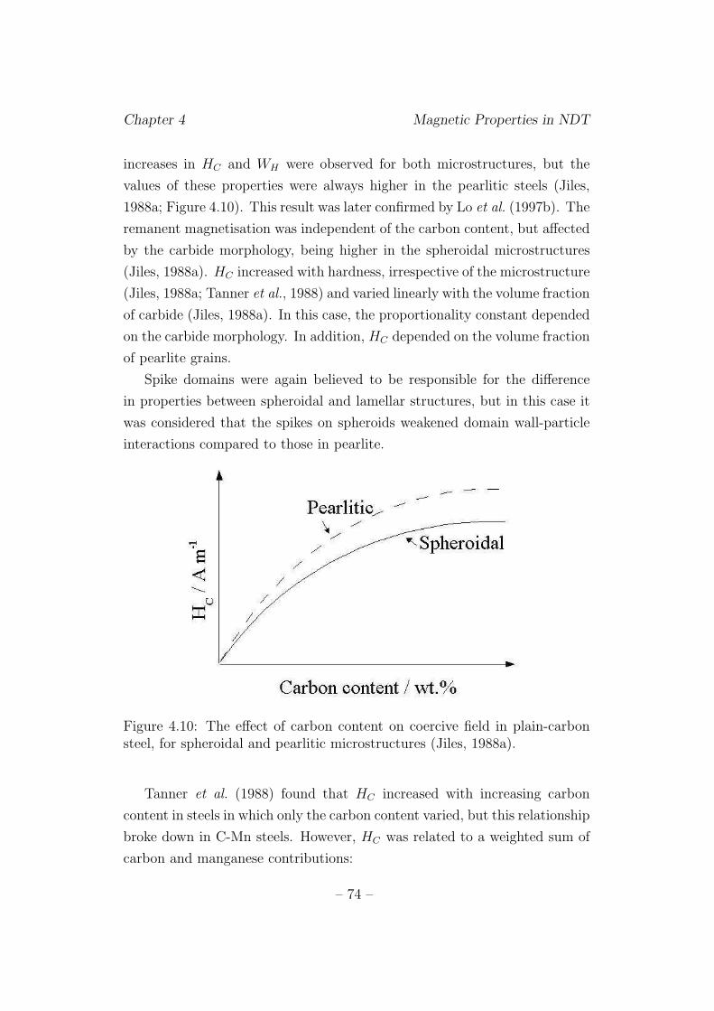
Chapter 4 Magnetic Properties in NDT
increases in HC and WH were observed for both microstructures, but the
values of these properties were always higher in the pearlitic steels (Jiles,
1988a; Figure 4.10). This result was later confirmed by Lo et al. (1997b). The
remanent magnetisation was independent of the carbon content, but affected
by the carbide morphology, being higher in the spheroidal microstructures
(Jiles, 1988a). HC increased with hardness, irrespective of the microstructure
(Jiles, 1988a; Tanner et al., 1988) and varied linearly with the volume fraction
of carbide (Jiles, 1988a). In this case, the proportionality constant depended
on the carbide morphology. In addition, HC depended on the volume fraction
of pearlite grains.
Spike domains were again believed to be responsible for the difference
in properties between spheroidal and lamellar structures, but in this case it
was considered that the spikes on spheroids weakened domain wall-particle
interactions compared to those in pearlite.
Figure 4.10: The effect of carbon content on coercive field in plain-carbonsteel, for spheroidal and pearlitic microstructures (Jiles, 1988a).
Tanner et al. (1988) found that HC increased with increasing carbon
content in steels in which only the carbon content varied, but this relationship
broke down in C-Mn steels. However, HC was related to a weighted sum of
carbon and manganese contributions:
– 74 –
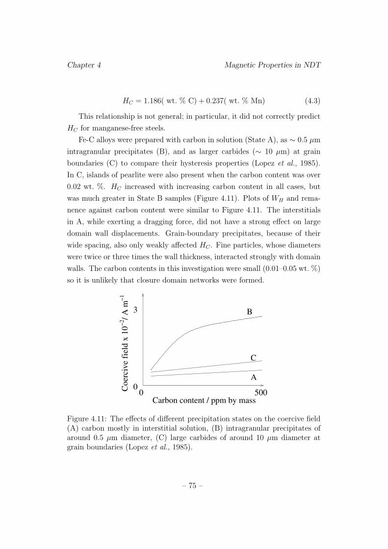
Chapter 4 Magnetic Properties in NDT
HC = 1.186( wt. % C) + 0.237( wt. % Mn) (4.3)
This relationship is not general; in particular, it did not correctly predict
HC for manganese-free steels.
Fe-C alloys were prepared with carbon in solution (State A), as ∼ 0.5 µm
intragranular precipitates (B), and as larger carbides (∼ 10 µm) at grain
boundaries (C) to compare their hysteresis properties (Lopez et al., 1985).
In C, islands of pearlite were also present when the carbon content was over
0.02 wt. %. HC increased with increasing carbon content in all cases, but
was much greater in State B samples (Figure 4.11). Plots of WH and rema-
nence against carbon content were similar to Figure 4.11. The interstitials
in A, while exerting a dragging force, did not have a strong effect on large
domain wall displacements. Grain-boundary precipitates, because of their
wide spacing, also only weakly affected HC . Fine particles, whose diameters
were twice or three times the wall thickness, interacted strongly with domain
walls. The carbon contents in this investigation were small (0.01–0.05 wt. %)
so it is unlikely that closure domain networks were formed.
Coe
rciv
e fi
eld
x 10
/ A
m−2
−1
0 5000
3
Carbon content / ppm by mass
B
C
A
Figure 4.11: The effects of different precipitation states on the coercive field(A) carbon mostly in interstitial solution, (B) intragranular precipitates ofaround 0.5 µm diameter, (C) large carbides of around 10 µm diameter atgrain boundaries (Lopez et al., 1985).
– 75 –
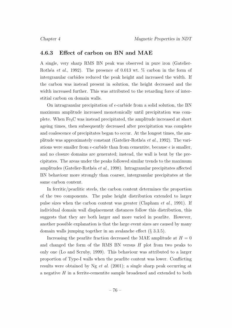
Chapter 4 Magnetic Properties in NDT
4.6.3 Effect of carbon on BN and MAE
A single, very sharp RMS BN peak was observed in pure iron (Gatelier-
Rothea et al., 1992). The presence of 0.013 wt. % carbon in the form of
intergranular carbides reduced the peak height and increased the width. If
the carbon was instead present in solution, the height decreased and the
width increased further. This was attributed to the retarding force of inter-
stitial carbon on domain walls.
On intragranular precipitation of ε-carbide from a solid solution, the BN
maximum amplitude increased monotonically until precipitation was com-
plete. When Fe3C was instead precipitated, the amplitude increased at short
ageing times, then subsequently decreased after precipitation was complete
and coalescence of precipitates began to occur. At the longest times, the am-
plitude was approximately constant (Gatelier-Rothea et al., 1992). The vari-
ations were smaller from ε-carbide than from cementite, because ε is smaller,
and no closure domains are generated; instead, the wall is bent by the pre-
cipitates. The areas under the peaks followed similar trends to the maximum
amplitudes (Gatelier-Rothea et al., 1998). Intragranular precipitates affected
BN behaviour more strongly than coarser, intergranular precipitates at the
same carbon content.
In ferritic/pearlitic steels, the carbon content determines the proportion
of the two components. The pulse height distribution extended to larger
pulse sizes when the carbon content was greater (Clapham et al., 1991). If
individual domain wall displacement distances follow this distribution, this
suggests that they are both larger and more varied in pearlite. However,
another possible explanation is that the large event sizes are caused by many
domain walls jumping together in an avalanche effect (§ 3.3.5).
Increasing the pearlite fraction decreased the MAE amplitude at H = 0
and changed the form of the RMS BN versus H plot from two peaks to
only one (Lo and Scruby, 1999). This behaviour was attributed to a larger
proportion of Type-I walls when the pearlite content was lower. Conflicting
results were obtained by Ng et al. (2001); a single sharp peak occurring at
a negative H in a ferrite-cementite sample broadened and extended to both
– 76 –
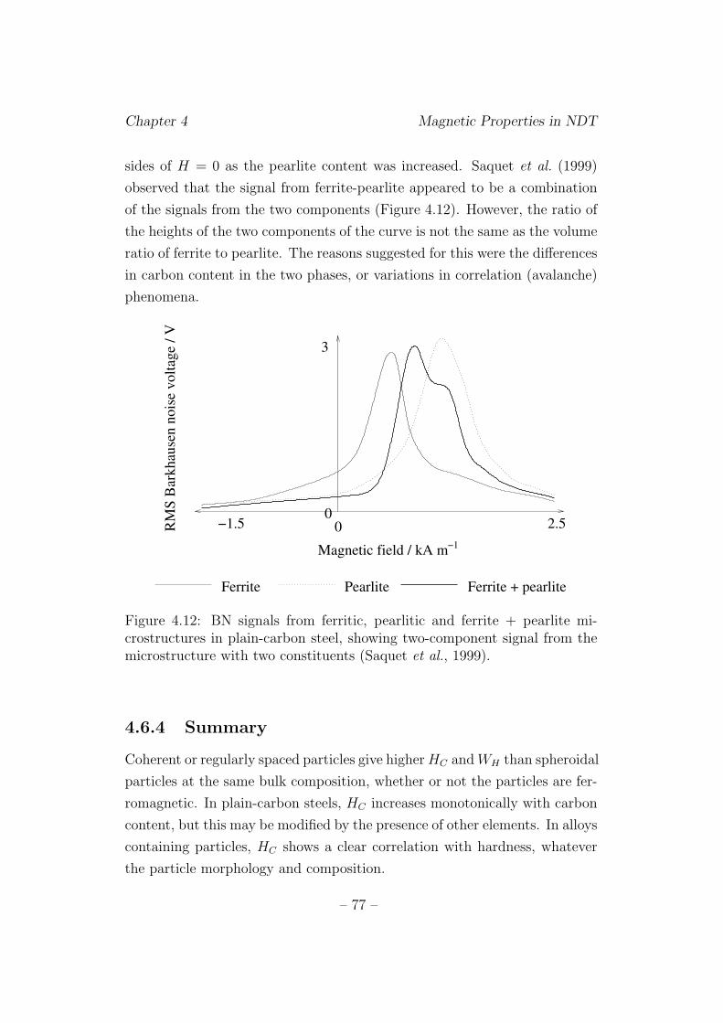
Chapter 4 Magnetic Properties in NDT
sides of H = 0 as the pearlite content was increased. Saquet et al. (1999)
observed that the signal from ferrite-pearlite appeared to be a combination
of the signals from the two components (Figure 4.12). However, the ratio of
the heights of the two components of the curve is not the same as the volume
ratio of ferrite to pearlite. The reasons suggested for this were the differences
in carbon content in the two phases, or variations in correlation (avalanche)
phenomena.
−1Magnetic field / kA m
3
0−1.5 0R
MS
Bar
khau
sen
nois
e vo
ltage
/ V
2.5
Ferrite Pearlite Ferrite + pearlite
Figure 4.12: BN signals from ferritic, pearlitic and ferrite + pearlite mi-crostructures in plain-carbon steel, showing two-component signal from themicrostructure with two constituents (Saquet et al., 1999).
4.6.4 Summary
Coherent or regularly spaced particles give higher HC and WH than spheroidal
particles at the same bulk composition, whether or not the particles are fer-
romagnetic. In plain-carbon steels, HC increases monotonically with carbon
content, but this may be modified by the presence of other elements. In alloys
containing particles, HC shows a clear correlation with hardness, whatever
the particle morphology and composition.
– 77 –
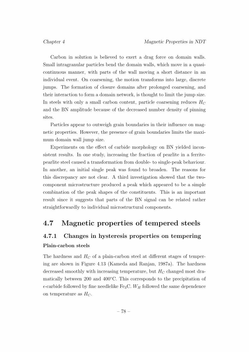
Chapter 4 Magnetic Properties in NDT
Carbon in solution is believed to exert a drag force on domain walls.
Small intragranular particles bend the domain walls, which move in a quasi-
continuous manner, with parts of the wall moving a short distance in an
individual event. On coarsening, the motion transforms into large, discrete
jumps. The formation of closure domains after prolonged coarsening, and
their interaction to form a domain network, is thought to limit the jump size.
In steels with only a small carbon content, particle coarsening reduces HC
and the BN amplitude because of the decreased number density of pinning
sites.
Particles appear to outweigh grain boundaries in their influence on mag-
netic properties. However, the presence of grain boundaries limits the maxi-
mum domain wall jump size.
Experiments on the effect of carbide morphology on BN yielded incon-
sistent results. In one study, increasing the fraction of pearlite in a ferrite-
pearlite steel caused a transformation from double- to single-peak behaviour.
In another, an initial single peak was found to broaden. The reasons for
this discrepancy are not clear. A third investigation showed that the two-
component microstructure produced a peak which appeared to be a simple
combination of the peak shapes of the constituents. This is an important
result since it suggests that parts of the BN signal can be related rather
straightforwardly to individual microstructural components.
4.7 Magnetic properties of tempered steels
4.7.1 Changes in hysteresis properties on tempering
Plain-carbon steels
The hardness and HC of a plain-carbon steel at different stages of temper-
ing are shown in Figure 4.13 (Kameda and Ranjan, 1987a). The hardness
decreased smoothly with increasing temperature, but HC changed most dra-
matically between 200 and 400◦C. This corresponds to the precipitation of
ε-carbide followed by fine needlelike Fe3C. WH followed the same dependence
on temperature as HC .
– 78 –
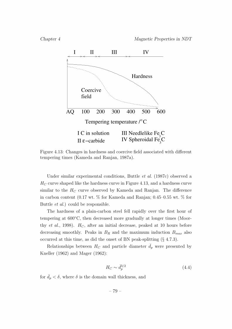
Chapter 4 Magnetic Properties in NDT
3
Coercive
100 200 300 400 500 600AQ
I II IVIII
Tempering temperature / Co
II −carbideε
I C in solution
Hardness
III Needlelike Fe CIV Spheroidal Fe C
3
field
Figure 4.13: Changes in hardness and coercive field associated with differenttempering times (Kameda and Ranjan, 1987a).
Under similar experimental conditions, Buttle et al. (1987c) observed a
HC curve shaped like the hardness curve in Figure 4.13, and a hardness curve
similar to the HC curve observed by Kameda and Ranjan. The difference
in carbon content (0.17 wt. % for Kameda and Ranjan; 0.45–0.55 wt. % for
Buttle et al.) could be responsible.
The hardness of a plain-carbon steel fell rapidly over the first hour of
tempering at 600◦C, then decreased more gradually at longer times (Moor-
thy et al., 1998). HC , after an initial decrease, peaked at 10 hours before
decreasing smoothly. Peaks in BR and the maximum induction Bmax also
occurred at this time, as did the onset of BN peak-splitting (§ 4.7.3).
Relationships between HC and particle diameter dp were presented by
Kneller (1962) and Mager (1962):
HC ∼ d3/2p (4.4)
for dp < δ, where δ is the domain wall thickness, and
– 79 –
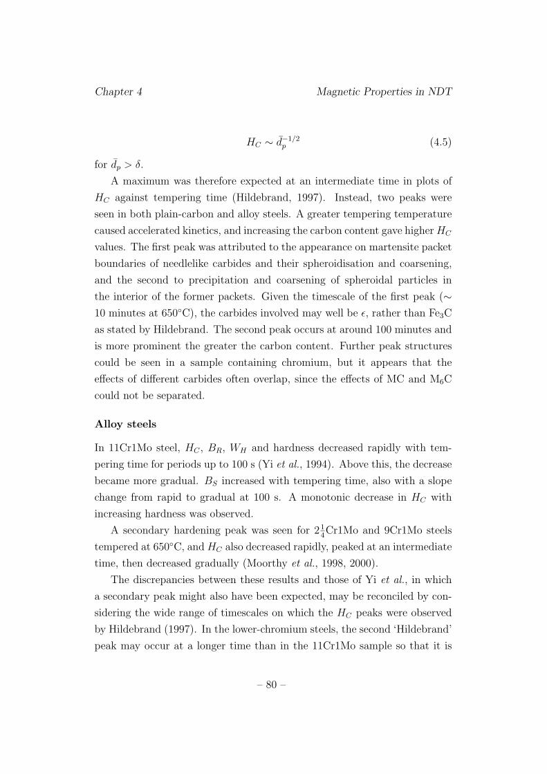
Chapter 4 Magnetic Properties in NDT
HC ∼ d−1/2p (4.5)
for dp > δ.
A maximum was therefore expected at an intermediate time in plots of
HC against tempering time (Hildebrand, 1997). Instead, two peaks were
seen in both plain-carbon and alloy steels. A greater tempering temperature
caused accelerated kinetics, and increasing the carbon content gave higher HC
values. The first peak was attributed to the appearance on martensite packet
boundaries of needlelike carbides and their spheroidisation and coarsening,
and the second to precipitation and coarsening of spheroidal particles in
the interior of the former packets. Given the timescale of the first peak (∼10 minutes at 650◦C), the carbides involved may well be ε, rather than Fe3C
as stated by Hildebrand. The second peak occurs at around 100 minutes and
is more prominent the greater the carbon content. Further peak structures
could be seen in a sample containing chromium, but it appears that the
effects of different carbides often overlap, since the effects of MC and M6C
could not be separated.
Alloy steels
In 11Cr1Mo steel, HC , BR, WH and hardness decreased rapidly with tem-
pering time for periods up to 100 s (Yi et al., 1994). Above this, the decrease
became more gradual. BS increased with tempering time, also with a slope
change from rapid to gradual at 100 s. A monotonic decrease in HC with
increasing hardness was observed.
A secondary hardening peak was seen for 214Cr1Mo and 9Cr1Mo steels
tempered at 650◦C, and HC also decreased rapidly, peaked at an intermediate
time, then decreased gradually (Moorthy et al., 1998, 2000).
The discrepancies between these results and those of Yi et al., in which
a secondary peak might also have been expected, may be reconciled by con-
sidering the wide range of timescales on which the HC peaks were observed
by Hildebrand (1997). In the lower-chromium steels, the second ‘Hildebrand’
peak may occur at a longer time than in the 11Cr1Mo sample so that it is
– 80 –
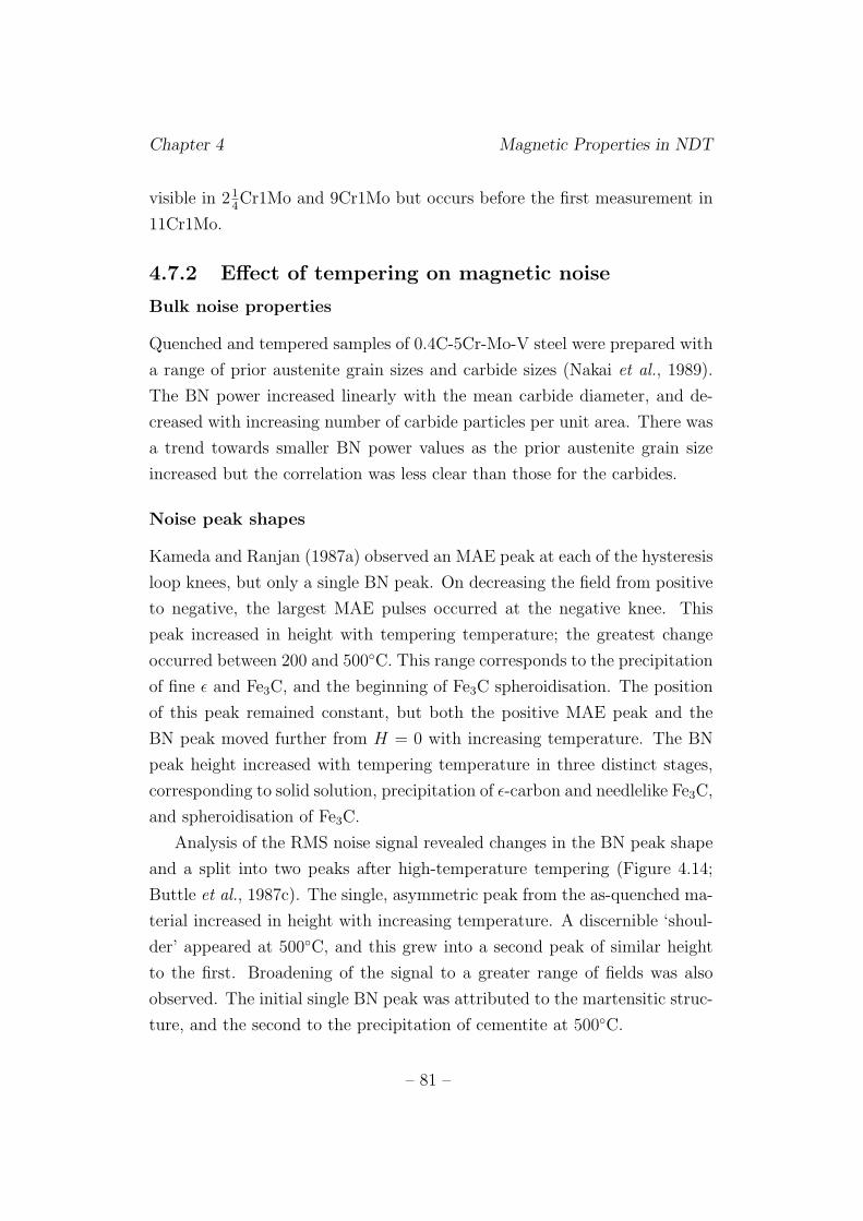
Chapter 4 Magnetic Properties in NDT
visible in 214Cr1Mo and 9Cr1Mo but occurs before the first measurement in
11Cr1Mo.
4.7.2 Effect of tempering on magnetic noise
Bulk noise properties
Quenched and tempered samples of 0.4C-5Cr-Mo-V steel were prepared with
a range of prior austenite grain sizes and carbide sizes (Nakai et al., 1989).
The BN power increased linearly with the mean carbide diameter, and de-
creased with increasing number of carbide particles per unit area. There was
a trend towards smaller BN power values as the prior austenite grain size
increased but the correlation was less clear than those for the carbides.
Noise peak shapes
Kameda and Ranjan (1987a) observed an MAE peak at each of the hysteresis
loop knees, but only a single BN peak. On decreasing the field from positive
to negative, the largest MAE pulses occurred at the negative knee. This
peak increased in height with tempering temperature; the greatest change
occurred between 200 and 500◦C. This range corresponds to the precipitation
of fine ε and Fe3C, and the beginning of Fe3C spheroidisation. The position
of this peak remained constant, but both the positive MAE peak and the
BN peak moved further from H = 0 with increasing temperature. The BN
peak height increased with tempering temperature in three distinct stages,
corresponding to solid solution, precipitation of ε-carbon and needlelike Fe3C,
and spheroidisation of Fe3C.
Analysis of the RMS noise signal revealed changes in the BN peak shape
and a split into two peaks after high-temperature tempering (Figure 4.14;
Buttle et al., 1987c). The single, asymmetric peak from the as-quenched ma-
terial increased in height with increasing temperature. A discernible ‘shoul-
der’ appeared at 500◦C, and this grew into a second peak of similar height
to the first. Broadening of the signal to a greater range of fields was also
observed. The initial single BN peak was attributed to the martensitic struc-
ture, and the second to the precipitation of cementite at 500◦C.
– 81 –
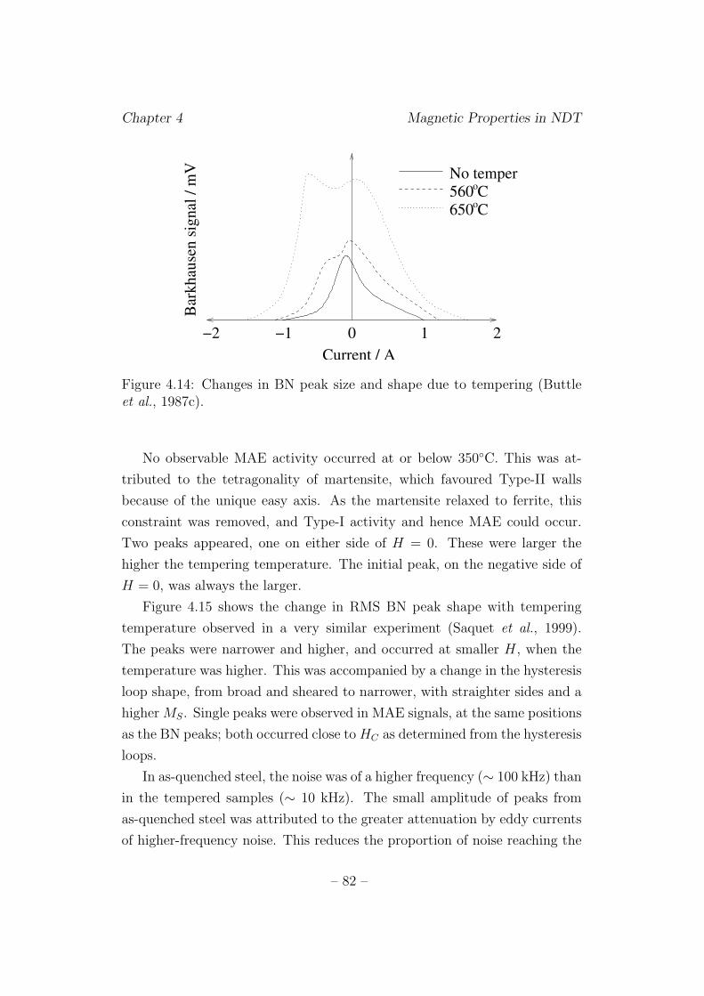
Chapter 4 Magnetic Properties in NDT
Current / A0−1−2 1 2
No tempero560 C
650 CoB
arkh
ause
n si
gnal
/ m
V
Figure 4.14: Changes in BN peak size and shape due to tempering (Buttleet al., 1987c).
No observable MAE activity occurred at or below 350◦C. This was at-
tributed to the tetragonality of martensite, which favoured Type-II walls
because of the unique easy axis. As the martensite relaxed to ferrite, this
constraint was removed, and Type-I activity and hence MAE could occur.
Two peaks appeared, one on either side of H = 0. These were larger the
higher the tempering temperature. The initial peak, on the negative side of
H = 0, was always the larger.
Figure 4.15 shows the change in RMS BN peak shape with tempering
temperature observed in a very similar experiment (Saquet et al., 1999).
The peaks were narrower and higher, and occurred at smaller H, when the
temperature was higher. This was accompanied by a change in the hysteresis
loop shape, from broad and sheared to narrower, with straighter sides and a
higher MS. Single peaks were observed in MAE signals, at the same positions
as the BN peaks; both occurred close to HC as determined from the hysteresis
loops.
In as-quenched steel, the noise was of a higher frequency (∼ 100 kHz) than
in the tempered samples (∼ 10 kHz). The small amplitude of peaks from
as-quenched steel was attributed to the greater attenuation by eddy currents
of higher-frequency noise. This reduces the proportion of noise reaching the
– 82 –
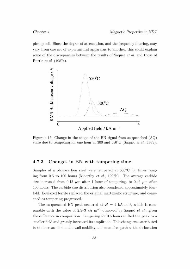
Chapter 4 Magnetic Properties in NDT
pickup coil. Since the degree of attenuation, and the frequency filtering, may
vary from one set of experimental apparatus to another, this could explain
some of the discrepancies between the results of Saquet et al. and those of
Buttle et al. (1987c).
AQ
−1
o300 C
o550 C
0 4
RM
S B
arkh
ause
n vo
ltage
/ V
Applied field / kA m
Figure 4.15: Change in the shape of the BN signal from as-quenched (AQ)state due to tempering for one hour at 300 and 550◦C (Saquet et al., 1999).
4.7.3 Changes in BN with tempering time
Samples of a plain-carbon steel were tempered at 600◦C for times rang-
ing from 0.5 to 100 hours (Moorthy et al., 1997b). The average carbide
size increased from 0.13 µm after 1 hour of tempering, to 0.46 µm after
100 hours. The carbide size distribution also broadened approximately four-
fold. Equiaxed ferrite replaced the original martensitic structure, and coars-
ened as tempering progressed.
The as-quenched BN peak occurred at H = 4 kA m−1, which is com-
parable with the value of 2.5–3 kA m−1 observed by Saquet et al., given
the difference in composition. Tempering for 0.5 hours shifted the peak to a
smaller field and greatly increased its amplitude. This change was attributed
to the increase in domain wall mobility and mean free path as the dislocation
– 83 –
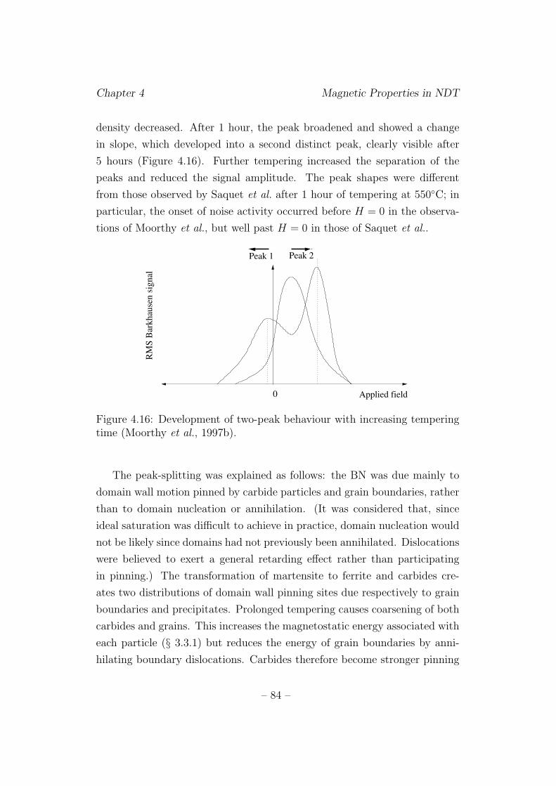
Chapter 4 Magnetic Properties in NDT
density decreased. After 1 hour, the peak broadened and showed a change
in slope, which developed into a second distinct peak, clearly visible after
5 hours (Figure 4.16). Further tempering increased the separation of the
peaks and reduced the signal amplitude. The peak shapes were different
from those observed by Saquet et al. after 1 hour of tempering at 550◦C; in
particular, the onset of noise activity occurred before H = 0 in the observa-
tions of Moorthy et al., but well past H = 0 in those of Saquet et al..
0
RM
S B
ark
hau
sen
sig
nal
Applied field
Peak 2Peak 1
Figure 4.16: Development of two-peak behaviour with increasing temperingtime (Moorthy et al., 1997b).
The peak-splitting was explained as follows: the BN was due mainly to
domain wall motion pinned by carbide particles and grain boundaries, rather
than to domain nucleation or annihilation. (It was considered that, since
ideal saturation was difficult to achieve in practice, domain nucleation would
not be likely since domains had not previously been annihilated. Dislocations
were believed to exert a general retarding effect rather than participating
in pinning.) The transformation of martensite to ferrite and carbides cre-
ates two distributions of domain wall pinning sites due respectively to grain
boundaries and precipitates. Prolonged tempering causes coarsening of both
carbides and grains. This increases the magnetostatic energy associated with
each particle (§ 3.3.1) but reduces the energy of grain boundaries by anni-
hilating boundary dislocations. Carbides therefore become stronger pinning
– 84 –
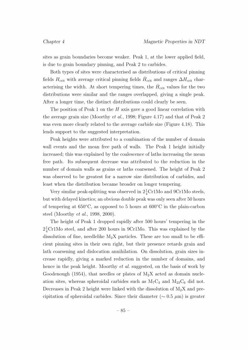
Chapter 4 Magnetic Properties in NDT
sites as grain boundaries become weaker. Peak 1, at the lower applied field,
is due to grain boundary pinning, and Peak 2 to carbides.
Both types of sites were characterised as distributions of critical pinning
fields Hcrit with average critical pinning fields Hcrit and ranges ∆Hcrit char-
acterising the width. At short tempering times, the Hcrit values for the two
distributions were similar and the ranges overlapped, giving a single peak.
After a longer time, the distinct distributions could clearly be seen.
The position of Peak 1 on the H axis gave a good linear correlation with
the average grain size (Moorthy et al., 1998; Figure 4.17) and that of Peak 2
was even more clearly related to the average carbide size (Figure 4.18). This
lends support to the suggested interpretation.
Peak heights were attributed to a combination of the number of domain
wall events and the mean free path of walls. The Peak 1 height initially
increased; this was explained by the coalescence of laths increasing the mean
free path. Its subsequent decrease was attributed to the reduction in the
number of domain walls as grains or laths coarsened. The height of Peak 2
was observed to be greatest for a narrow size distribution of carbides, and
least when the distribution became broader on longer tempering.
Very similar peak-splitting was observed in 214Cr1Mo and 9Cr1Mo steels,
but with delayed kinetics; an obvious double peak was only seen after 50 hours
of tempering at 650◦C, as opposed to 5 hours at 600◦C in the plain-carbon
steel (Moorthy et al., 1998, 2000).
The height of Peak 1 dropped rapidly after 500 hours’ tempering in the
214Cr1Mo steel, and after 200 hours in 9Cr1Mo. This was explained by the
dissolution of fine, needlelike M2X particles. These are too small to be effi-
cient pinning sites in their own right, but their presence retards grain and
lath coarsening and dislocation annihilation. On dissolution, grain sizes in-
crease rapidly, giving a marked reduction in the number of domains, and
hence in the peak height. Moorthy et al. suggested, on the basis of work by
Goodenough (1954), that needles or plates of M2X acted as domain nucle-
ation sites, whereas spheroidal carbides such as M7C3 and M23C6 did not.
Decreases in Peak 2 height were linked with the dissolution of M2X and pre-
cipitation of spheroidal carbides. Since their diameter (∼ 0.5 µm) is greater
– 85 –
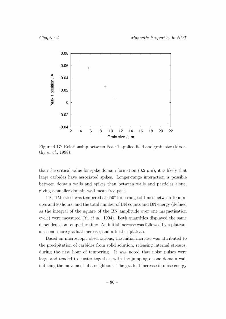
Chapter 4 Magnetic Properties in NDT
-0.04
-0.02
0
0.02
0.04
0.06
0.08
2 4 6 8 10 12 14 16 18 20 22
Peak 1
positio
n / A
Grain size / µm
Figure 4.17: Relationship between Peak 1 applied field and grain size (Moor-thy et al., 1998).
than the critical value for spike domain formation (0.2 µm), it is likely that
large carbides have associated spikes. Longer-range interaction is possible
between domain walls and spikes than between walls and particles alone,
giving a smaller domain wall mean free path.
11Cr1Mo steel was tempered at 650◦ for a range of times between 10 min-
utes and 80 hours, and the total number of BN counts and BN energy (defined
as the integral of the square of the BN amplitude over one magnetisation
cycle) were measured (Yi et al., 1994). Both quantities displayed the same
dependence on tempering time. An initial increase was followed by a plateau,
a second more gradual increase, and a further plateau.
Based on microscopic observations, the initial increase was attributed to
the precipitation of carbides from solid solution, releasing internal stresses,
during the first hour of tempering. It was noted that noise pulses were
large and tended to cluster together, with the jumping of one domain wall
inducing the movement of a neighbour. The gradual increase in noise energy
– 86 –
Chapter 4 Magnetic Properties in NDT
0.29
0.3
0.31
0.32
0.33
0.34
0.35
0.1 0.15 0.2 0.25 0.3 0.35 0.4 0.45 0.5
Peak 2
positio
n / A
Carbide size / µm
Figure 4.18: Relationship between Peak 2 applied field and carbide size(Moorthy et al., 1998).
between 1 and 20 hours was attributed to the coarsening and reduction in
number density of M23C6 particles; this increases the interparticle distance
and hence the size of individual Barkhausen events. In the final stage, the
observed abrupt change in noise energy was found to occur concurrently with
a rapid decrease in dislocation density.
The measurements were made using a small range of applied field, such
that only pinned domain wall motion should occur and nucleation and anni-
hilation should be avoided. Within this regime, both the BN energy and the
number of counts were linearly related to the hardness.
4.7.4 Summary
The most pronounced change in HC on tempering in plain-carbon steel was
associated with the precipitation of needlelike carbides from solution. During
prolonged tempering at 600–650◦C, maxima in hardness and HC appeared
in some cases but not in others. Measurements of HC at very short tem-
– 87 –
Chapter 4 Magnetic Properties in NDT
pering times revealed two distinct peaks, the first of which occurred within
∼ 10 minutes of the start of tempering. The timescale of the second varied;
this may be the reason for the discrepancies seen in other studies. The simple
relationships between HC and hardness observed in other materials do not
always hold in tempered steels.
In as-quenched samples, little or no MAE activity was seen, but peaks
appeared at the ‘knees’ of the hysteresis curve after tempering, and grew in
height with increasing tempering temperature. Although the precise char-
acteristics of the BN peak shapes vary considerably from one experimental
study to another, there is a trend towards higher peaks at lower H, signi-
fying weaker pinning, with increasing tempering temperature. Prolonged,
high-temperature tempering causes the peak to split into two parts, which
separate and decrease in height with tempering time. Moorthy et al. (1997b,
1998, 2000) explained the peak shapes in terms of distributions of pinning
sites from carbides and grain boundaries, and supported the interpretation
with linear relationships between peak positions and microstructural feature
dimensions.
4.8 Are the results inconsistent?
Concerns have been raised over discrepancies between magnetic noise results,
for example variations in the number and shape of BN peaks in different
studies on very similar materials (Moorthy et al., 1997b; Saquet et al., 1999,
Sablik and Augustyniak, 1999). It has been suggested that inconsistencies
in experimental apparatus and conditions are the cause.
It is true that conditions vary widely. As an illustration, Table 4.2 demon-
strates the differences in applied field range, frequency and filtering used in
experiments on tempered steels. It has been shown that changes in these
parameters can alter the BN characteristics (§ 4.9.3, § 4.9.4) and even the
number of peaks (Kim et al., 1992). However, taking this into account, some
conclusions can still be drawn (§ 4.10).
– 88 –
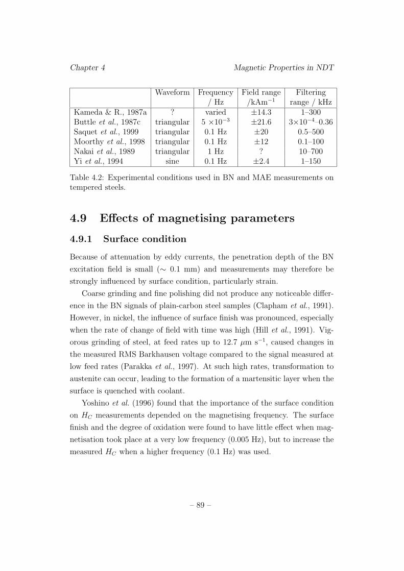
Chapter 4 Magnetic Properties in NDT
Waveform Frequency Field range Filtering/ Hz /kAm−1 range / kHz
Kameda & R., 1987a ? varied ±14.3 1–300Buttle et al., 1987c triangular 5 ×10⁻³ ±21.6 3×10⁻⁴–0.36Saquet et al., 1999 triangular 0.1 Hz ±20 0.5–500Moorthy et al., 1998 triangular 0.1 Hz ±12 0.1–100Nakai et al., 1989 triangular 1 Hz ? 10–700Yi et al., 1994 sine 0.1 Hz ±2.4 1–150
Table 4.2: Experimental conditions used in BN and MAE measurements ontempered steels.
4.9 Effects of magnetising parameters
4.9.1 Surface condition
Because of attenuation by eddy currents, the penetration depth of the BN
excitation field is small (∼ 0.1 mm) and measurements may therefore be
strongly influenced by surface condition, particularly strain.
Coarse grinding and fine polishing did not produce any noticeable differ-
ence in the BN signals of plain-carbon steel samples (Clapham et al., 1991).
However, in nickel, the influence of surface finish was pronounced, especially
when the rate of change of field with time was high (Hill et al., 1991). Vig-
orous grinding of steel, at feed rates up to 12.7 µm s−1, caused changes in
the measured RMS Barkhausen voltage compared to the signal measured at
low feed rates (Parakka et al., 1997). At such high rates, transformation to
austenite can occur, leading to the formation of a martensitic layer when the
surface is quenched with coolant.
Yoshino et al. (1996) found that the importance of the surface condition
on HC measurements depended on the magnetising frequency. The surface
finish and the degree of oxidation were found to have little effect when mag-
netisation took place at a very low frequency (0.005 Hz), but to increase the
measured HC when a higher frequency (0.1 Hz) was used.
– 89 –
Chapter 4 Magnetic Properties in NDT
4.9.2 Magnetising field waveform
A number of different waveforms have been used for the alternating excita-
tion field to obtain BN signals. The most common of these are triangular
and sinusoidal, but square waves are also occasionally used. Sipahi et al.
(1993) found that the noise frequency content was similar when obtained
with the triangular or sinusoidal waveform, but was significantly altered by
using a square wave. Square waves were more likely to introduce spurious
data than either sinusoidal or triangular waves. It was therefore considered
that sinusoidal or triangular waveforms should be preferred for BN studies.
4.9.3 Magnetising frequency
In a plain-carbon steel, the RMS BN voltage was higher, and larger peaks
were observed, at higher magnetising frequencies (Dhar and Atherton, 1992).
This result was true for a variety of applied field amplitudes. The suggested
reason was that a greater number of domain walls participated in magnetisa-
tion at higher frequencies. However, it was admitted that the precise effect
of frequency was difficult to determine.
Similarly, the maximum amplitude of both BN and MAE increased with
frequency in a quenched and tempered plain-carbon steel (Kameda and Ran-
jan, 1987a).
In MAE, the integrated signal was found to be linearly related to mag-
netising frequency at higher frequencies, but to deviate from linearity at
lower values, in both mild steel and nickel (Ng et al., 1996). A model was
suggested to explain this behaviour: the observed signal was attributed to a
component from domain wall motion and a component from nucleation and
annihilation. The different dependences of these on frequency were used to
account for the shape of the curve.
A wide variety of magnetising frequency settings are found in the litera-
ture (e.g. Table 4.2). Work by Moorthy et al. (2001) has demonstrated, in
addition, that variations in both the frequency and the filtering range can
significantly affect the shape of a BN voltage peak, and even the number of
peaks visible. It would therefore be advisable to introduce more consistency
– 90 –
Chapter 4 Magnetic Properties in NDT
into experimental design to ensure repeatability.
4.9.4 Magnetising field amplitude
It has been seen that modification of Hmax can affect the number of BN peaks
observed (Kim et al., 1992; § 4.5.3).
In a plain-carbon steel, the RMS BN voltage increased smoothly to a
maximum at an intermediate Hmax value, then decreased at higher Hmax
(Dhar and Atherton, 1992). The increase was attributed to the greater ca-
pacity for overcoming pinning obstacles when the applied field was larger,
and the decrease to the predominance of domain rotation over domain wall
motion at very high fields. The same form of dependence of RMS voltage on
Hmax was seen for all frequencies investigated.
The dependence of RMS BN voltage on Hmax is shown in Figure 4.19
for three microstructures with the same composition: bainitic, pearlitic and
spheroidised pearlite (Mitra et al., 1995). There is clearly a complex inter-
dependence between magnetising frequency, Hmax and microstructural state,
and this may account for the discrepancies seen in BN results. It would be
useful to conduct a systematic investigation of the dependence of peak shapes,
RMS voltages, etc. for a wide range of compositions and microstructures to
give a deeper understanding of these issues.
4.9.5 Demagnetising and stray fields
The demagnetising effect (§ 3.1.3) reduces the actual field experienced when
a given field is applied. HC should be independent of the demagnetising field
(Swartzendruber, 1992) but in practice can have some shape-dependence
(Blamire, personal communication). Other properties, including BN and
MAE characteristics, are subject to demagnetising fields.
Stray fields are those which result from incomplete magnetic circuits, for
example at air gaps between a magnetic yoke and a sample surface. In MAE
experiments, nonmagnetic spacers are customarily used between the yoke and
the surface to minimise extraneous noise. However, these spacers introduce
demagnetising and stray fields. Ng et al. (1994) found that varying the spacer
– 91 –
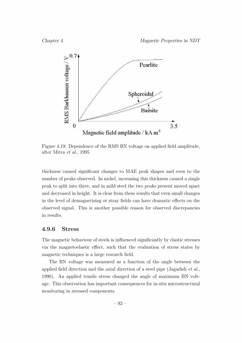
Chapter 4 Magnetic Properties in NDT
Figure 4.19: Dependence of the RMS BN voltage on applied field amplitude,after Mitra et al., 1995
thickness caused significant changes to MAE peak shapes and even to the
number of peaks observed. In nickel, increasing this thickness caused a single
peak to split into three, and in mild steel the two peaks present moved apart
and decreased in height. It is clear from these results that even small changes
in the level of demagnetising or stray fields can have dramatic effects on the
observed signal. This is another possible reason for observed discrepancies
in results.
4.9.6 Stress
The magnetic behaviour of steels is influenced significantly by elastic stresses
via the magnetoelastic effect, such that the evaluation of stress states by
magnetic techniques is a large research field.
The BN voltage was measured as a function of the angle between the
applied field direction and the axial direction of a steel pipe (Jagadish et al.,
1990). An applied tensile stress changed the angle of maximum BN volt-
age. This observation has important consequences for in-situ microstructural
monitoring in stressed components.
– 92 –
Chapter 4 Magnetic Properties in NDT
4.9.7 Temperature
The transition between ferromagnetic and paramagnetic behaviour at the
Curie temperatures of certain carbides can produce an anomaly in the mea-
sured HC (English, 1967). From the two examples given by English, it ap-
pears that TC can vary by at least 200◦C depending on composition. Anoma-
lies could cause confusing results if the temperature during NDT is close to
TC for any of the carbides present. However, it may also be possible, after a
systematic study, to make use of the phenomenon for identification of phases
and monitoring of their compositions.
A further temperature effect is thermal activation, which allows domain
walls to overcome pinning sites more easily (Pardavi-Horvath, 1999) but this
does not seem to have been investigated extensively.
4.9.8 Magnetic history
On repetition of an earlier measurement on a steel pipe, it was found that
the direction in which the greatest BN voltage was observed had changed by
30◦ (Jagadish et al., 1990). It appeared that the repeated magnetisation and
demagnetisation during experiments had altered the magnetic properties of
the sample. This effect does not appear to have been documented elsewhere,
but it may present difficulties for NDT applications.
4.9.9 Solute segregation
Segregation of solutes, although it did not affect the hysteresis properties,
was detectable by both BN and MAE measurement (Kameda and Ranjan,
1987b). For constant carbide morphology and hardness, the RMS and max-
imum MAE voltages increased as a greater proportion of solute segregated
to grain boundaries. The maximum BN voltage was a minimum for an in-
termediate level of segregation. The results were the same for Sn, Sb and P
dopants; this means that magnetic noise is not useful for monitoring grain
boundary embrittlement, the degree of which depends on the chemistry of
the segregant.
– 93 –
Chapter 4 Magnetic Properties in NDT
4.10 Summary and conclusions
Magnetic hysteresis and noise properties have been investigated for use in
microstructural testing. Clear relationships between HC and microstructural
feature sizes, carbon content or hardness have often been found in simple
systems such as equiaxed ferrite. However, these do not always hold in more
complicated microstructures such as tempered martensite.
BN and magnetoacoustic emission signals can be difficult to interpret,
and the discrepancies in results are well documented. Nonetheless, general
results have emerged from this review. Magnetically hard materials, contain-
ing strong pinning sites, tend to produce a single BN peak, which can be at-
tributed to pinned wall motion. Fine structure is sometimes seen on this peak
if microstructural constituents have sufficiently different pinning strengths.
In softer materials, by contrast, two peaks positioned at the ‘knees’ of the
hysteresis curve are present in addition to, or in place of, the single peak.
These, because of their position, are believed to arise from domain nucle-
ation and annihilation. Reducing the applied field range in these samples, so
that the material is only cycled through a minor loop, suppresses the outer
peaks. It is suggested that increasing the level of pinning has a similar effect,
preventing domain nucleation and annihilation.
Single-value BN or MAE parameters such as the total number of counts
or maximum noise amplitude can be related to microstructural data in simple
systems, but may not always be useful when more than one microstructural
feature is changing. Analyses of the entire signal contain more information
and, in particular, allow the variation in pinning field strength to be followed.
Experimental conditions, such as the magnetising frequency and Hmax,
can significantly affect the measured noise signals. Because of this, it would
be advisable to adopt a standard set of experimental practices, or to conduct
systematic studies of the effects of magnetising conditions on the material of
interest before using magnetic methods for NDT.
– 94 –
Chapter 5
Barkhausen Noise Modelling
5.1 Existing models of hysteresis and Barkhausen
noise
5.1.1 Jiles-Atherton model
Jiles and Atherton (1983) used an energy balance to model magnetic hystere-
sis. The energy supplied to the material by a change in applied field can be
dissipated either as a change in magnetostatic energy, or as hysteresis loss.
In the absence of hysteresis, all the energy supplied would go toward
modifying the magnetostatic energy. In such a case, the magnetisation would
be a reversible, single-valued function of the applied field. This anhysteretic
magnetisation Man can be modelled as:
Man = MSf{He} (5.1)
where MS is the saturation magnetisation, He = H +αM is the Weiss mean
field (Equation 3.1) and f is an arbitrary function with the properties:
f = 0 when He = 0f → 1 when He → ∞ (5.2)
A modified Langevin expression (Langevin, 1905) was used to model Man:
Man{He} = MS
[
coth{
He
a
}
−(
a
He
)]
(5.3)
where a is a parameter with units of field.
– 95 –
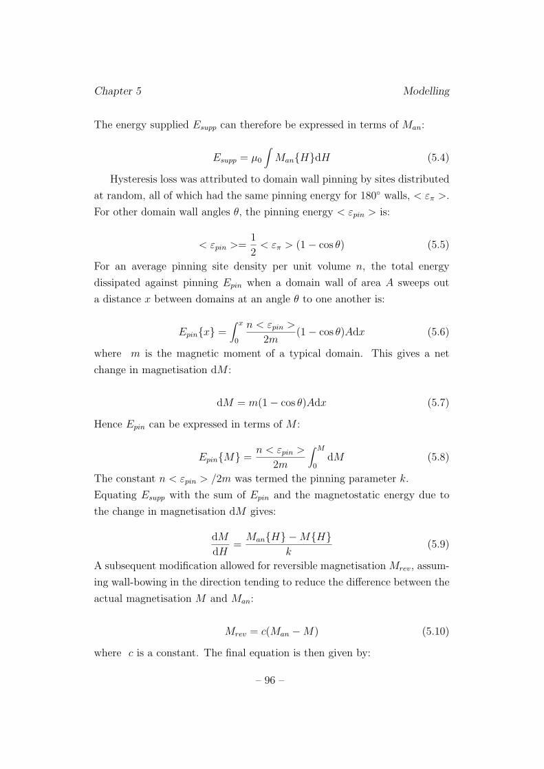
Chapter 5 Modelling
The energy supplied Esupp can therefore be expressed in terms of Man:
Esupp = µ0
∫
Man{H}dH (5.4)
Hysteresis loss was attributed to domain wall pinning by sites distributed
at random, all of which had the same pinning energy for 180◦ walls, < επ >.
For other domain wall angles θ, the pinning energy < εpin > is:
< εpin >=1
2< επ > (1 − cos θ) (5.5)
For an average pinning site density per unit volume n, the total energy
dissipated against pinning Epin when a domain wall of area A sweeps out
a distance x between domains at an angle θ to one another is:
Epin{x} =∫ x
0
n < εpin >
2m(1 − cos θ)Adx (5.6)
where m is the magnetic moment of a typical domain. This gives a net
change in magnetisation dM :
dM = m(1 − cos θ)Adx (5.7)
Hence Epin can be expressed in terms of M :
Epin{M} =n < εpin >
2m
∫ M
0dM (5.8)
The constant n < εpin > /2m was termed the pinning parameter k.
Equating Esupp with the sum of Epin and the magnetostatic energy due to
the change in magnetisation dM gives:
dM
dH=
Man{H} − M{H}k
(5.9)
A subsequent modification allowed for reversible magnetisation Mrev, assum-
ing wall-bowing in the direction tending to reduce the difference between the
actual magnetisation M and Man:
Mrev = c(Man − M) (5.10)
where c is a constant. The final equation is then given by:
– 96 –
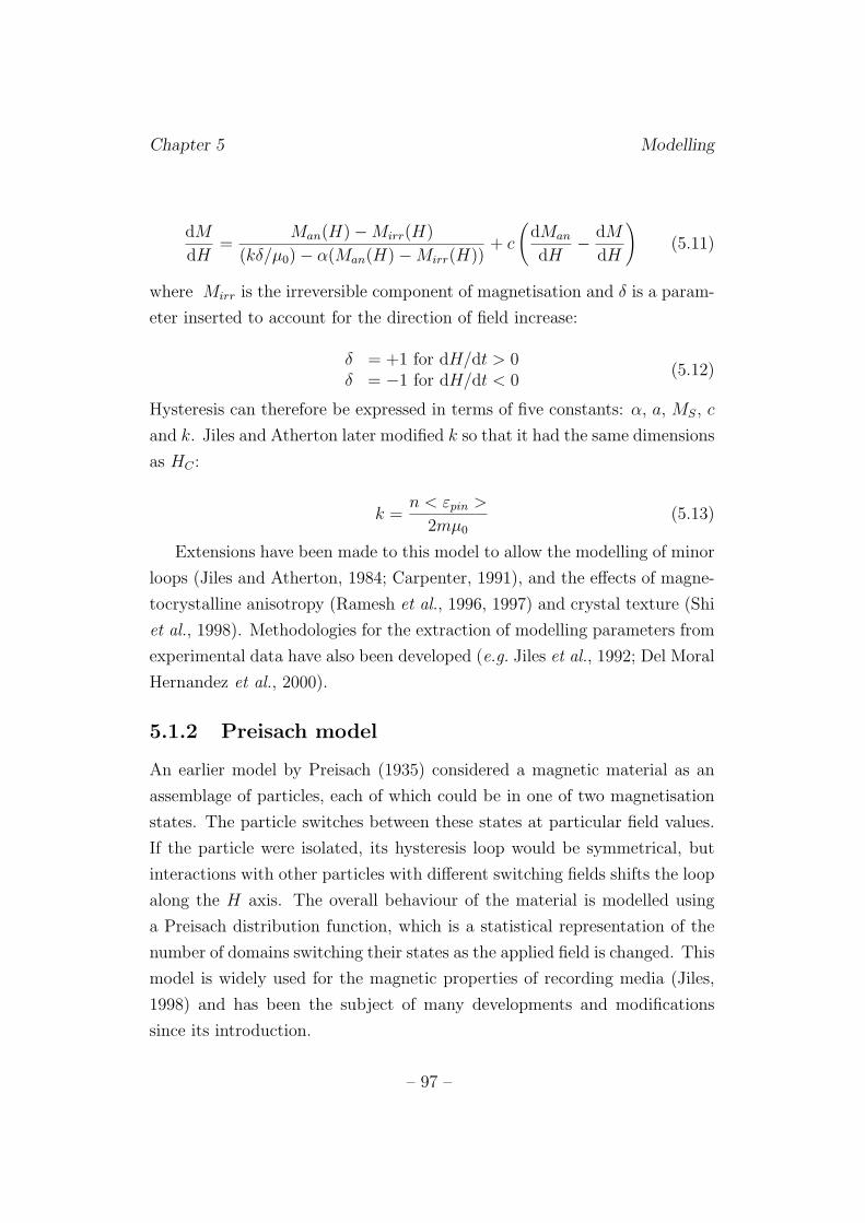
Chapter 5 Modelling
dM
dH=
Man(H) − Mirr(H)
(kδ/µ0) − α(Man(H) − Mirr(H))+ c
(
dMan
dH− dM
dH
)
(5.11)
where Mirr is the irreversible component of magnetisation and δ is a param-
eter inserted to account for the direction of field increase:
δ = +1 for dH/dt > 0δ = −1 for dH/dt < 0
(5.12)
Hysteresis can therefore be expressed in terms of five constants: α, a, MS, c
and k. Jiles and Atherton later modified k so that it had the same dimensions
as HC :
k =n < εpin >
2mµ0
(5.13)
Extensions have been made to this model to allow the modelling of minor
loops (Jiles and Atherton, 1984; Carpenter, 1991), and the effects of magne-
tocrystalline anisotropy (Ramesh et al., 1996, 1997) and crystal texture (Shi
et al., 1998). Methodologies for the extraction of modelling parameters from
experimental data have also been developed (e.g. Jiles et al., 1992; Del Moral
Hernandez et al., 2000).
5.1.2 Preisach model
An earlier model by Preisach (1935) considered a magnetic material as an
assemblage of particles, each of which could be in one of two magnetisation
states. The particle switches between these states at particular field values.
If the particle were isolated, its hysteresis loop would be symmetrical, but
interactions with other particles with different switching fields shifts the loop
along the H axis. The overall behaviour of the material is modelled using
a Preisach distribution function, which is a statistical representation of the
number of domains switching their states as the applied field is changed. This
model is widely used for the magnetic properties of recording media (Jiles,
1998) and has been the subject of many developments and modifications
since its introduction.
– 97 –
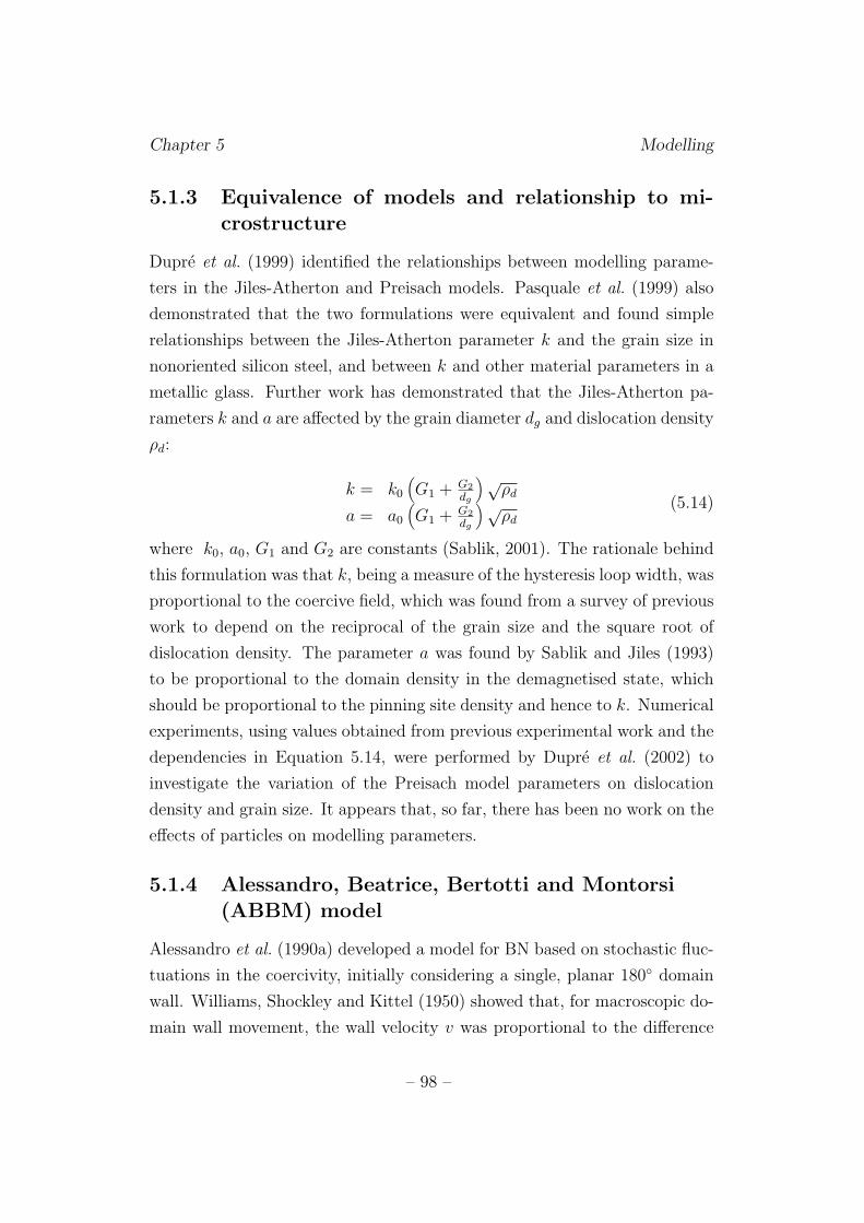
Chapter 5 Modelling
5.1.3 Equivalence of models and relationship to mi-crostructure
Dupre et al. (1999) identified the relationships between modelling parame-
ters in the Jiles-Atherton and Preisach models. Pasquale et al. (1999) also
demonstrated that the two formulations were equivalent and found simple
relationships between the Jiles-Atherton parameter k and the grain size in
nonoriented silicon steel, and between k and other material parameters in a
metallic glass. Further work has demonstrated that the Jiles-Atherton pa-
rameters k and a are affected by the grain diameter dg and dislocation density
ρd:
k = k0
(
G1 + G2
dg
)√ρd
a = a0
(
G1 + G2
dg
)√ρd
(5.14)
where k0, a0, G1 and G2 are constants (Sablik, 2001). The rationale behind
this formulation was that k, being a measure of the hysteresis loop width, was
proportional to the coercive field, which was found from a survey of previous
work to depend on the reciprocal of the grain size and the square root of
dislocation density. The parameter a was found by Sablik and Jiles (1993)
to be proportional to the domain density in the demagnetised state, which
should be proportional to the pinning site density and hence to k. Numerical
experiments, using values obtained from previous experimental work and the
dependencies in Equation 5.14, were performed by Dupre et al. (2002) to
investigate the variation of the Preisach model parameters on dislocation
density and grain size. It appears that, so far, there has been no work on the
effects of particles on modelling parameters.
5.1.4 Alessandro, Beatrice, Bertotti and Montorsi(ABBM) model
Alessandro et al. (1990a) developed a model for BN based on stochastic fluc-
tuations in the coercivity, initially considering a single, planar 180◦ domain
wall. Williams, Shockley and Kittel (1950) showed that, for macroscopic do-
main wall movement, the wall velocity v was proportional to the difference
– 98 –
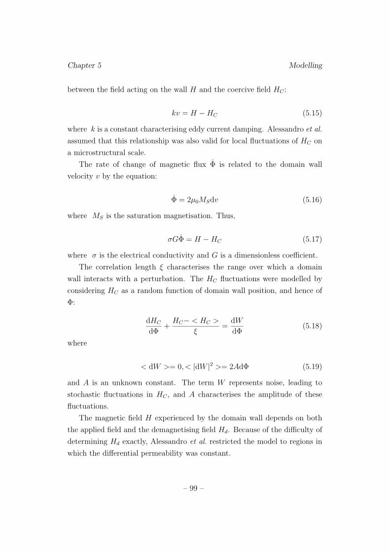
Chapter 5 Modelling
between the field acting on the wall H and the coercive field HC :
kv = H − HC (5.15)
where k is a constant characterising eddy current damping. Alessandro et al.
assumed that this relationship was also valid for local fluctuations of HC on
a microstructural scale.
The rate of change of magnetic flux Φ is related to the domain wall
velocity v by the equation:
Φ = 2µ0MSdv (5.16)
where MS is the saturation magnetisation. Thus,
σGΦ = H − HC (5.17)
where σ is the electrical conductivity and G is a dimensionless coefficient.
The correlation length ξ characterises the range over which a domain
wall interacts with a perturbation. The HC fluctuations were modelled by
considering HC as a random function of domain wall position, and hence of
Φ:
dHC
dΦ+
HC− < HC >
ξ=
dW
dΦ(5.18)
where
< dW >= 0, < |dW |2 >= 2AdΦ (5.19)
and A is an unknown constant. The term W represents noise, leading to
stochastic fluctuations in HC , and A characterises the amplitude of these
fluctuations.
The magnetic field H experienced by the domain wall depends on both
the applied field and the demagnetising field Hd. Because of the difficulty of
determining Hd exactly, Alessandro et al. restricted the model to regions in
which the differential permeability was constant.
– 99 –
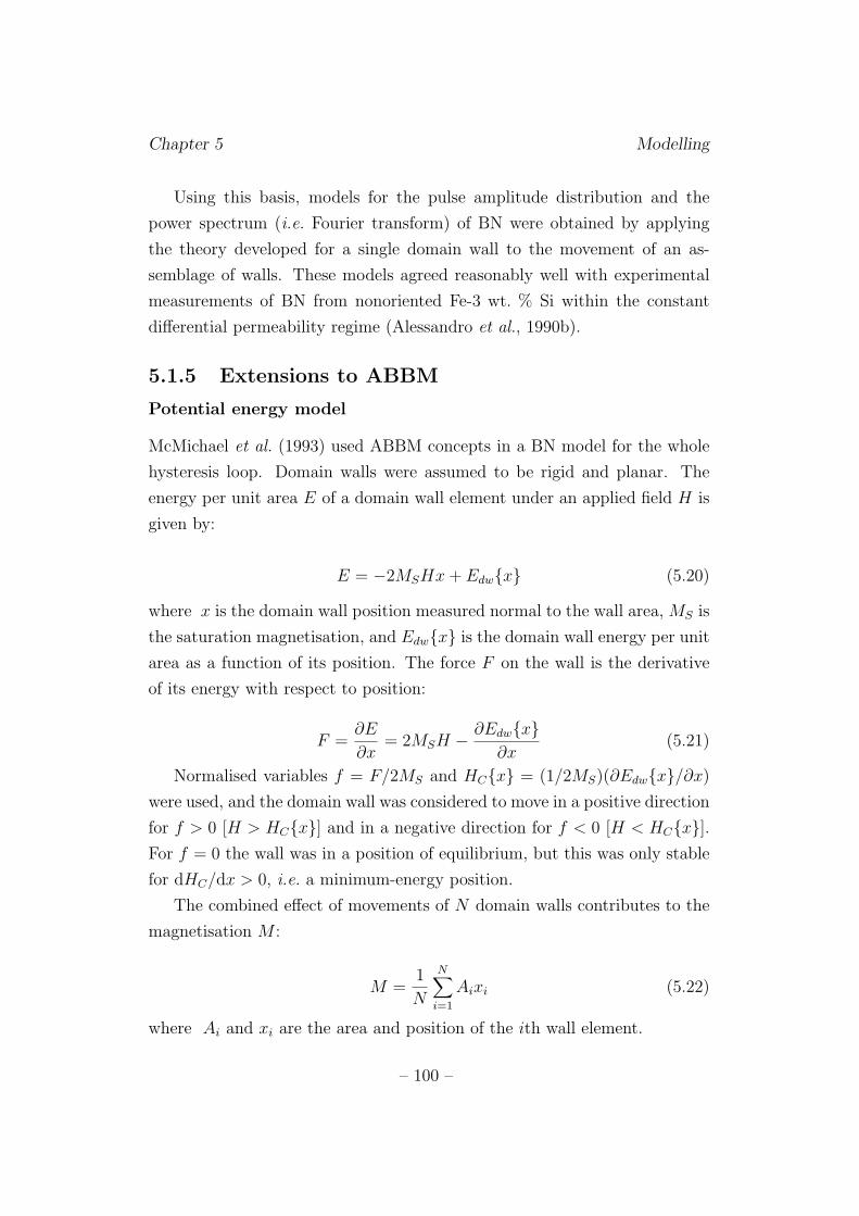
Chapter 5 Modelling
Using this basis, models for the pulse amplitude distribution and the
power spectrum (i.e. Fourier transform) of BN were obtained by applying
the theory developed for a single domain wall to the movement of an as-
semblage of walls. These models agreed reasonably well with experimental
measurements of BN from nonoriented Fe-3 wt. % Si within the constant
differential permeability regime (Alessandro et al., 1990b).
5.1.5 Extensions to ABBM
Potential energy model
McMichael et al. (1993) used ABBM concepts in a BN model for the whole
hysteresis loop. Domain walls were assumed to be rigid and planar. The
energy per unit area E of a domain wall element under an applied field H is
given by:
E = −2MSHx + Edw{x} (5.20)
where x is the domain wall position measured normal to the wall area, MS is
the saturation magnetisation, and Edw{x} is the domain wall energy per unit
area as a function of its position. The force F on the wall is the derivative
of its energy with respect to position:
F =∂E
∂x= 2MSH − ∂Edw{x}
∂x(5.21)
Normalised variables f = F/2MS and HC{x} = (1/2MS)(∂Edw{x}/∂x)
were used, and the domain wall was considered to move in a positive direction
for f > 0 [H > HC{x}] and in a negative direction for f < 0 [H < HC{x}].For f = 0 the wall was in a position of equilibrium, but this was only stable
for dHC/dx > 0, i.e. a minimum-energy position.
The combined effect of movements of N domain walls contributes to the
magnetisation M :
M =1
N
N∑
i=1
Aixi (5.22)
where Ai and xi are the area and position of the ith wall element.
– 100 –
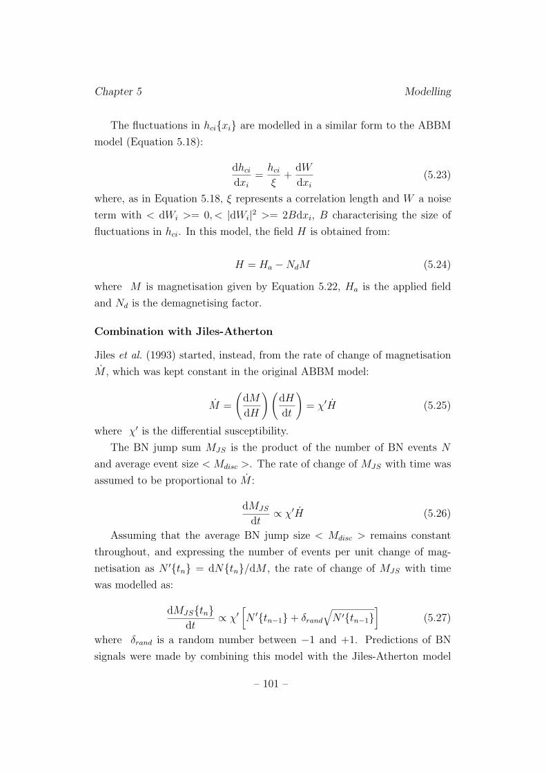
Chapter 5 Modelling
The fluctuations in hci{xi} are modelled in a similar form to the ABBM
model (Equation 5.18):
dhci
dxi
=hci
ξ+
dW
dxi
(5.23)
where, as in Equation 5.18, ξ represents a correlation length and W a noise
term with < dWi >= 0, < |dWi|2 >= 2Bdxi, B characterising the size of
fluctuations in hci. In this model, the field H is obtained from:
H = Ha − NdM (5.24)
where M is magnetisation given by Equation 5.22, Ha is the applied field
and Nd is the demagnetising factor.
Combination with Jiles-Atherton
Jiles et al. (1993) started, instead, from the rate of change of magnetisation
M , which was kept constant in the original ABBM model:
M =
(
dM
dH
)(
dH
dt
)
= χ′H (5.25)
where χ′ is the differential susceptibility.
The BN jump sum MJS is the product of the number of BN events N
and average event size < Mdisc >. The rate of change of MJS with time was
assumed to be proportional to M :
dMJS
dt∝ χ′H (5.26)
Assuming that the average BN jump size < Mdisc > remains constant
throughout, and expressing the number of events per unit change of mag-
netisation as N ′{tn} = dN{tn}/dM , the rate of change of MJS with time
was modelled as:
dMJS{tn}dt
∝ χ′[
N ′{tn−1} + δrand
√
N ′{tn−1}]
(5.27)
where δrand is a random number between −1 and +1. Predictions of BN
signals were made by combining this model with the Jiles-Atherton model
– 101 –
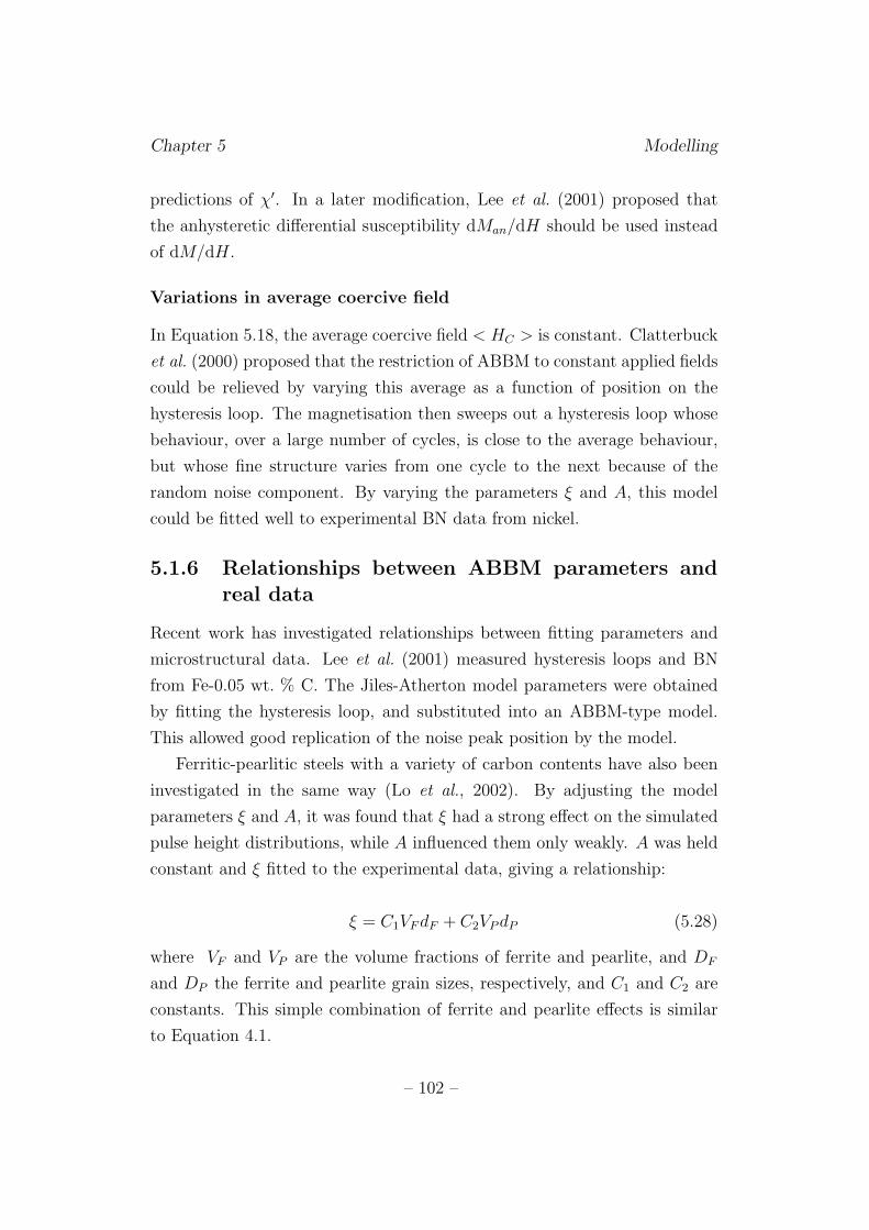
Chapter 5 Modelling
predictions of χ′. In a later modification, Lee et al. (2001) proposed that
the anhysteretic differential susceptibility dMan/dH should be used instead
of dM/dH.
Variations in average coercive field
In Equation 5.18, the average coercive field < HC > is constant. Clatterbuck
et al. (2000) proposed that the restriction of ABBM to constant applied fields
could be relieved by varying this average as a function of position on the
hysteresis loop. The magnetisation then sweeps out a hysteresis loop whose
behaviour, over a large number of cycles, is close to the average behaviour,
but whose fine structure varies from one cycle to the next because of the
random noise component. By varying the parameters ξ and A, this model
could be fitted well to experimental BN data from nickel.
5.1.6 Relationships between ABBM parameters andreal data
Recent work has investigated relationships between fitting parameters and
microstructural data. Lee et al. (2001) measured hysteresis loops and BN
from Fe-0.05 wt. % C. The Jiles-Atherton model parameters were obtained
by fitting the hysteresis loop, and substituted into an ABBM-type model.
This allowed good replication of the noise peak position by the model.
Ferritic-pearlitic steels with a variety of carbon contents have also been
investigated in the same way (Lo et al., 2002). By adjusting the model
parameters ξ and A, it was found that ξ had a strong effect on the simulated
pulse height distributions, while A influenced them only weakly. A was held
constant and ξ fitted to the experimental data, giving a relationship:
ξ = C1VF dF + C2VP dP (5.28)
where VF and VP are the volume fractions of ferrite and pearlite, and DF
and DP the ferrite and pearlite grain sizes, respectively, and C1 and C2 are
constants. This simple combination of ferrite and pearlite effects is similar
to Equation 4.1.
– 102 –
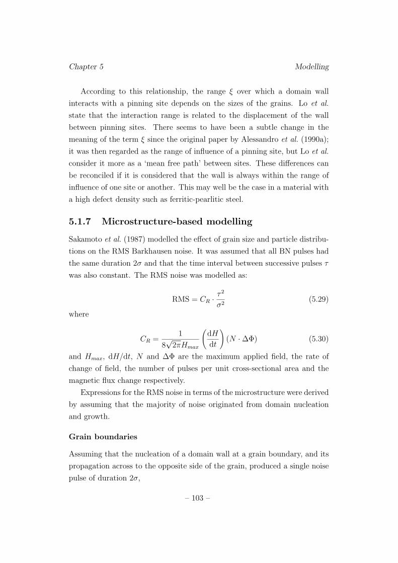
Chapter 5 Modelling
According to this relationship, the range ξ over which a domain wall
interacts with a pinning site depends on the sizes of the grains. Lo et al.
state that the interaction range is related to the displacement of the wall
between pinning sites. There seems to have been a subtle change in the
meaning of the term ξ since the original paper by Alessandro et al. (1990a);
it was then regarded as the range of influence of a pinning site, but Lo et al.
consider it more as a ‘mean free path’ between sites. These differences can
be reconciled if it is considered that the wall is always within the range of
influence of one site or another. This may well be the case in a material with
a high defect density such as ferritic-pearlitic steel.
5.1.7 Microstructure-based modelling
Sakamoto et al. (1987) modelled the effect of grain size and particle distribu-
tions on the RMS Barkhausen noise. It was assumed that all BN pulses had
the same duration 2σ and that the time interval between successive pulses τ
was also constant. The RMS noise was modelled as:
RMS = CR · τ 2
σ2(5.29)
where
CR =1
8√
2πHmax
(
dH
dt
)
(N · ∆Φ) (5.30)
and Hmax, dH/dt, N and ∆Φ are the maximum applied field, the rate of
change of field, the number of pulses per unit cross-sectional area and the
magnetic flux change respectively.
Expressions for the RMS noise in terms of the microstructure were derived
by assuming that the majority of noise originated from domain nucleation
and growth.
Grain boundaries
Assuming that the nucleation of a domain wall at a grain boundary, and its
propagation across to the opposite side of the grain, produced a single noise
pulse of duration 2σ,
– 103 –
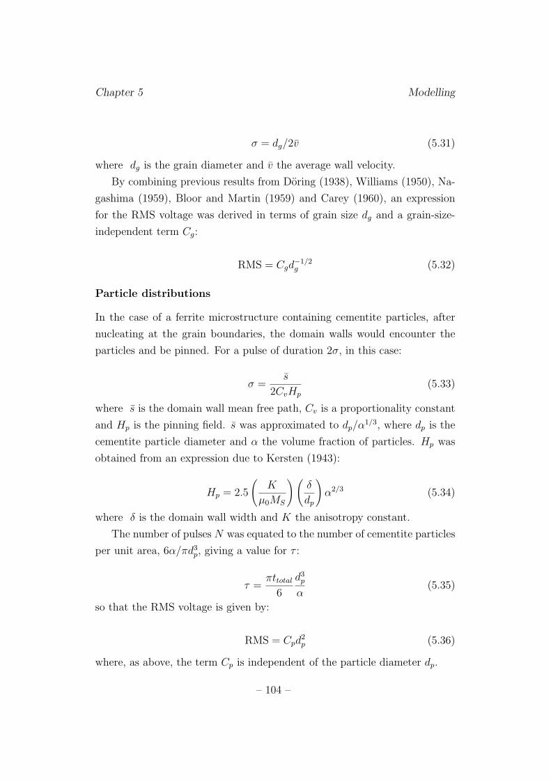
Chapter 5 Modelling
σ = dg/2v (5.31)
where dg is the grain diameter and v the average wall velocity.
By combining previous results from Doring (1938), Williams (1950), Na-
gashima (1959), Bloor and Martin (1959) and Carey (1960), an expression
for the RMS voltage was derived in terms of grain size dg and a grain-size-
independent term Cg:
RMS = Cgd−1/2g (5.32)
Particle distributions
In the case of a ferrite microstructure containing cementite particles, after
nucleating at the grain boundaries, the domain walls would encounter the
particles and be pinned. For a pulse of duration 2σ, in this case:
σ =s
2CvHp
(5.33)
where s is the domain wall mean free path, Cv is a proportionality constant
and Hp is the pinning field. s was approximated to dp/α1/3, where dp is the
cementite particle diameter and α the volume fraction of particles. Hp was
obtained from an expression due to Kersten (1943):
Hp = 2.5
(
K
µ0MS
)(
δ
dp
)
α2/3 (5.34)
where δ is the domain wall width and K the anisotropy constant.
The number of pulses N was equated to the number of cementite particles
per unit area, 6α/πd3p, giving a value for τ :
τ =πttotal
6
d3p
α(5.35)
so that the RMS voltage is given by:
RMS = Cpd2p (5.36)
where, as above, the term Cp is independent of the particle diameter dp.
– 104 –
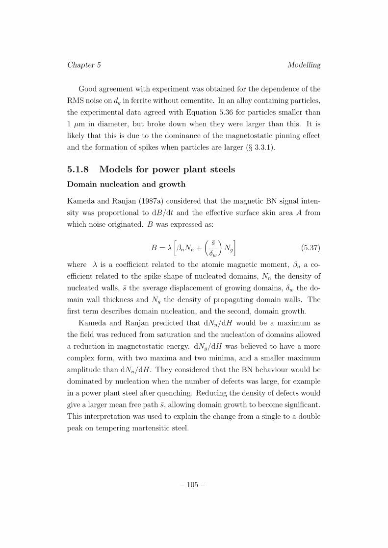
Chapter 5 Modelling
Good agreement with experiment was obtained for the dependence of the
RMS noise on dg in ferrite without cementite. In an alloy containing particles,
the experimental data agreed with Equation 5.36 for particles smaller than
1 µm in diameter, but broke down when they were larger than this. It is
likely that this is due to the dominance of the magnetostatic pinning effect
and the formation of spikes when particles are larger (§ 3.3.1).
5.1.8 Models for power plant steels
Domain nucleation and growth
Kameda and Ranjan (1987a) considered that the magnetic BN signal inten-
sity was proportional to dB/dt and the effective surface skin area A from
which noise originated. B was expressed as:
B = λ[
βnNn +(
s
δw
)
Ng
]
(5.37)
where λ is a coefficient related to the atomic magnetic moment, βn a co-
efficient related to the spike shape of nucleated domains, Nn the density of
nucleated walls, s the average displacement of growing domains, δw the do-
main wall thickness and Ng the density of propagating domain walls. The
first term describes domain nucleation, and the second, domain growth.
Kameda and Ranjan predicted that dNn/dH would be a maximum as
the field was reduced from saturation and the nucleation of domains allowed
a reduction in magnetostatic energy. dNg/dH was believed to have a more
complex form, with two maxima and two minima, and a smaller maximum
amplitude than dNn/dH. They considered that the BN behaviour would be
dominated by nucleation when the number of defects was large, for example
in a power plant steel after quenching. Reducing the density of defects would
give a larger mean free path s, allowing domain growth to become significant.
This interpretation was used to explain the change from a single to a double
peak on tempering martensitic steel.
– 105 –

Chapter 5 Modelling
Moorthy et al. interpretation
The alternative interpretation of power plant steel BN data, by Moorthy
et al. (1997b, 1998, 2000) was introduced in § 4.7.3. Pinning sites due to
grain boundaries were considered to have a distribution of strengths with a
width ∆Hgb and average value Hgb, and pinning sites due to carbide particles
could likewise be described by ∆Hcp and Hcp. Magnetisation was described
as a two-stage process: firstly, the domain walls nucleated at, and became
unpinned from, the grain boundaries and were pinned by the carbides, and
secondly, they were unpinned from the carbides. The two sets of unpinning
events were each associated with a peak in BN emission.
5.1.9 Summary
It has been seen that there are several modelling strategies for magnetic
hysteresis and BN:
1. Use of an energy balance to model hysteresis, with a single parameter
to characterise pinning strength.
2. Preisach-type models using distributions of subunits, each of which can
adopt one of two states.
3. Models based on stochastic fluctuations in local coercive field, charac-
terised by their amplitude and interaction range.
4. Quantitative microstructural interpretations based on the effect of fea-
ture spacing on jump sizes.
5. Considerations of the probability of domain nucleation and growth.
6. Qualitative microstructural interpretations based on distributions of
pinning site strengths due to grain boundaries and carbides.
If, as is suggested by Moorthy et al., both grain boundary and carbide
particle pinning sites play a part in the overall BN behaviour, it is possible
that models of types 1 and 3 will not be able to accommodate the complexity
– 106 –

Chapter 5 Modelling
of the problem without the introduction of, for example, a second k parameter
in the Jiles-Atherton model or two distributions of HC fluctuations in ABBM-
type models. The Sakamoto et al. model (4) considers both kinds of sites,
but these were used to model the overall RMS noise rather than the variation
of the BN voltage with H. Kameda and Ranjan (5) considered the effect of
pinning site densities on mean free path, and Moorthy et al. (6) introduced
the idea of distributions of pinning site strengths. These two concepts were
used to develop a new model of the dependence of BN voltage on H in a
steel containing two types of pinning sites.
– 107 –
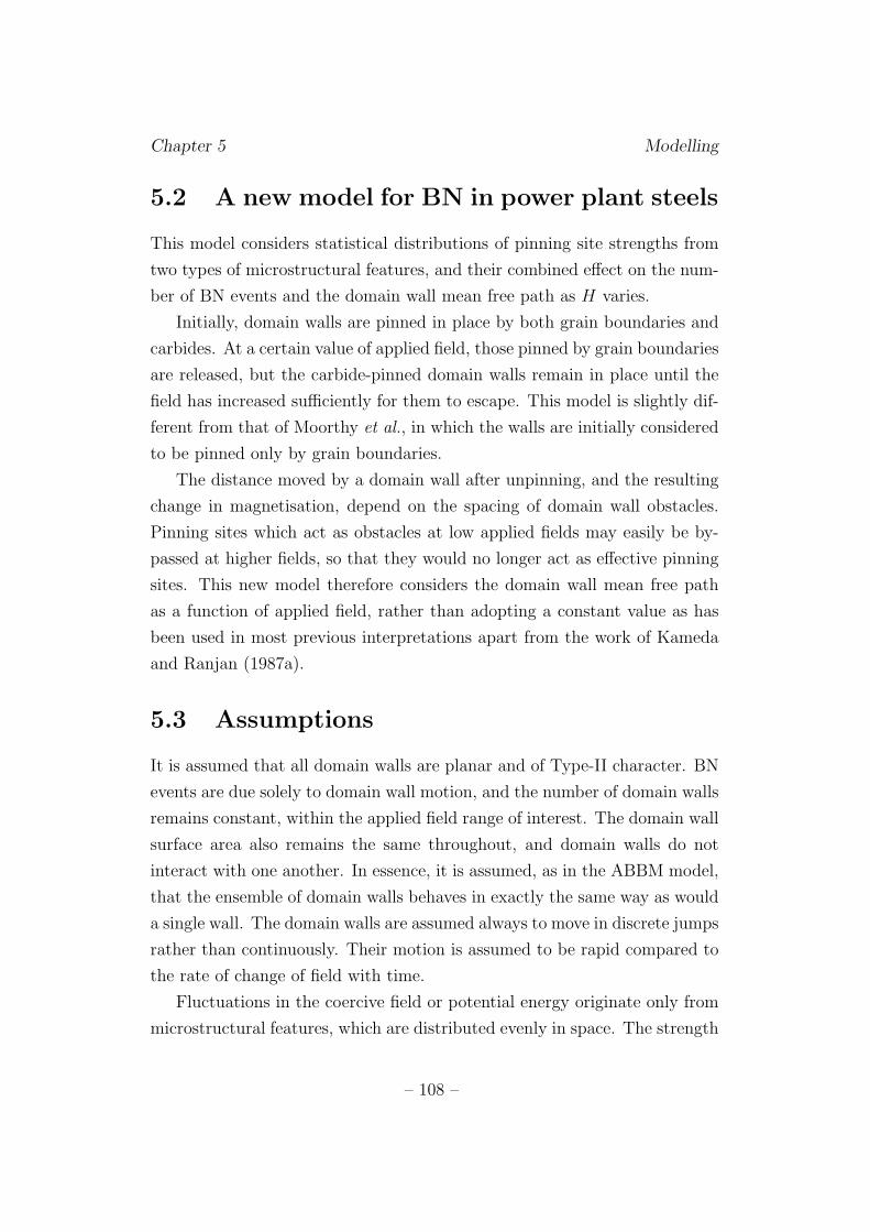
Chapter 5 Modelling
5.2 A new model for BN in power plant steels
This model considers statistical distributions of pinning site strengths from
two types of microstructural features, and their combined effect on the num-
ber of BN events and the domain wall mean free path as H varies.
Initially, domain walls are pinned in place by both grain boundaries and
carbides. At a certain value of applied field, those pinned by grain boundaries
are released, but the carbide-pinned domain walls remain in place until the
field has increased sufficiently for them to escape. This model is slightly dif-
ferent from that of Moorthy et al., in which the walls are initially considered
to be pinned only by grain boundaries.
The distance moved by a domain wall after unpinning, and the resulting
change in magnetisation, depend on the spacing of domain wall obstacles.
Pinning sites which act as obstacles at low applied fields may easily be by-
passed at higher fields, so that they would no longer act as effective pinning
sites. This new model therefore considers the domain wall mean free path
as a function of applied field, rather than adopting a constant value as has
been used in most previous interpretations apart from the work of Kameda
and Ranjan (1987a).
5.3 Assumptions
It is assumed that all domain walls are planar and of Type-II character. BN
events are due solely to domain wall motion, and the number of domain walls
remains constant, within the applied field range of interest. The domain wall
surface area also remains the same throughout, and domain walls do not
interact with one another. In essence, it is assumed, as in the ABBM model,
that the ensemble of domain walls behaves in exactly the same way as would
a single wall. The domain walls are assumed always to move in discrete jumps
rather than continuously. Their motion is assumed to be rapid compared to
the rate of change of field with time.
Fluctuations in the coercive field or potential energy originate only from
microstructural features, which are distributed evenly in space. The strength
– 108 –
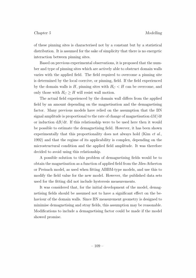
Chapter 5 Modelling
of these pinning sites is characterised not by a constant but by a statistical
distribution. It is assumed for the sake of simplicity that there is no energetic
interaction between pinning sites.
Based on previous experimental observations, it is proposed that the num-
ber and type of pinning sites which are actively able to obstruct domain walls
varies with the applied field. The field required to overcome a pinning site
is determined by the local coercive, or pinning, field. If the field experienced
by the domain walls is H, pinning sites with HC < H can be overcome, and
only those with HC ≥ H will resist wall motion.
The actual field experienced by the domain wall differs from the applied
field by an amount depending on the magnetisation and the demagnetising
factor. Many previous models have relied on the assumption that the BN
signal amplitude is proportional to the rate of change of magnetisation dM/dt
or induction dB/dt. If this relationship were to be used here then it would
be possible to estimate the demagnetising field. However, it has been shown
experimentally that this proportionality does not always hold (Kim et al.,
1992) and that the regime of its applicability is complex, depending on the
microstructural condition and the applied field amplitude. It was therefore
decided to avoid using this relationship.
A possible solution to this problem of demagnetising fields would be to
obtain the magnetisation as a function of applied field from the Jiles-Atherton
or Preisach model, as used when fitting ABBM-type models, and use this to
modify the field value for the new model. However, the published data sets
used for the fitting did not include hysteresis measurements.
It was considered that, for the initial development of the model, demag-
netising fields should be assumed not to have a significant effect on the be-
haviour of the domain walls. Since BN measurement geometry is designed to
minimise demagnetising and stray fields, this assumption may be reasonable.
Modifications to include a demagnetising factor could be made if the model
showed promise.
– 109 –
Chapter 5 Modelling
5.4 Origin of the noise
A domain wall of surface area Aw, moving a distance lw
and sweeping out a
volume (Aw.δlw), causes a change in magnetisation δm:
δm = β(Aw.δlw) (5.38)
where β depends on the angle between the magnetisation of adjacent do-
mains and the atomic magnetic moment (Saquet et al., 1999). If it is assumed
that the domain walls always move in a direction parallel to the normal of
the domain wall plane, then the expression (S.δl) reduces to S · δl. The total
change in magnetisation δM{H} at a certain field H is given by the product
of the number of domain wall movement events at field H, N{H} and the
vector sum of all the individual changes δm. Assuming that all the domain
walls involved are Type-II (180◦), β is constant, and Equation 5.38 reduces
to:
δM{H} ∝ N{H} < l > {H} (5.39)
where < l > {H} is the average domain wall displacement (mean free path)
at field H.
The electric field amplitude E0 induced by this change in magnetisation
is given by the rate of change of magnetisation with time. For a discrete
change in magnetisation, this is given by:
E0 =δM
δt(5.40)
where δt is the time interval over which the change occurs. As mentioned
above, it is assumed that the domain walls move rapidly enough that the
change in magnetisation δM{H} occurs immediately the field is changed,
and does not depend on the rate of change of field.
The noise voltage V measured by the pickup coil depends on the noise
frequency, with higher-frequency noise experiencing more signal attenuation
(Saquet et al., 1999). However, for low-frequency noise, the measured voltage
can be considered to be proportional to E0. For simplicity, therefore, it is
– 110 –
Chapter 5 Modelling
assumed that the frequency f is low enough to avoid attenuation and to
allow a simple proportionality between the change of magnetisation and the
measured pulse size:
V ∝ N{H} < l > {H} (5.41)
This is the simple relationship ‘Noise amplitude = number of events ×mean free path’ which is sometimes used to interpret BN signals in the lit-
erature, but it is only truly valid in a limited range of circumstances.
5.5 Construction of the statistical model
5.5.1 Distribution of pinning sites
Initially, it was assumed that the number of pinning sites per unit volume
with pinning strength S, n{S}, follows a normal distribution with mean value
< S > and standard deviation ∆S. The total number of pinning points per
unit volume was A. Thus:
n{S} =A
∆S√
2π· exp
{
−1
2
(
S− < S >
∆S
)2}
(5.42)
5.5.2 Impediments to domain wall motion
When the material experiences a magnetic field H, pinning sites with pinning
strength S ≥ H are able to impede domain wall motion. These sites will be
referred to as ‘active sites’.
The number of active sites per unit volume N{H} is given by the integral
of n{S} with respect to S from H to infinity:
N{H} =∫ ∞
Hn{S}dS (5.43)
Thus:
N{H} =A
2erfc
{
H− < S >
∆S√
2
}
(5.44)
– 111 –
Chapter 5 Modelling
5.5.3 Mean free path of domain walls
In order to estimate the mean free path, it is necessary to make an assumption
about the arrangement of the active pinning sites. A suitably basic first
approximation is to consider all the pinning sites as points arranged in a
simple cubic lattice, with one site per cube of side l, where l = l{H}:
l{H} =
(
1
N{H}
)1
3
(5.45)
The mean free path of domain walls travelling through the material can
be approximated to l{H}:
< l > {H} = l{H} (5.46)
The assumptions made to derive this expression are crude, taking no
account of the planar nature of grain boundaries, variations in carbide diam-
eter, or phenomena such as the preferential nucleation of carbides at grain
boundaries, but subsequent refinements could be made if the model showed
promise.
5.5.4 Number of Barkhausen events occurring
Assuming for simplicity that there are no demagnetising fields, the field H
experienced by the material is equal to the applied field. The number of
Barkhausen events occurring due to domain wall unpinning at applied field
H is equal to the number of pinning sites of strength S = H.
This is obtained from Equation 5.42:
n{H} =A
∆S√
2π· exp
{
−1
2
(
H− < S >
∆S
)2}
(5.47)
5.5.5 Barkhausen amplitude
Adopting the assumption that the RMS voltage V {H} at field H is propor-
tional to the number of Barkhausen events n{H} multiplied by the mean
free path < l > {H}:
– 112 –
Chapter 5 Modelling
V {H} = C · n{H}· < l > {H} (5.48)
where C is a constant, gives:
V {H} = C · A
∆S√
2π· exp
{
−1
2
(
H− < S >
∆S
)2}
·[
A
2erfc
{
H− < S >
∆S√
2
}]− 1
3
(5.49)
5.5.6 Multiple distributions of pinning points
Different types of pinning site can be modelled by introducing more than one
distribution, with different constant terms for each:
ni{S} = Ai · exp
−(
S− < S >i
(∆S)i
)2
(5.50)
The overall number of pinning sites with a pinning strength greater than
H is now given by:
N{H} =m∑
i=1
∫ ∞
Hni{S}dS (5.51)
where m is the total number of pinning site distributions.
Thus:
N{H} =m∑
i=1
Ai
√π
2(∆S)i
· erfc{
H− < S >i
(∆S)i
}
(5.52)
The relation V {H} = C · n{H}· < l > {H} (Equation 5.48) should still
apply as long as there are no preferential orientations of particular types of
sites; hence:
V {H} = C ·m∑
i=1
Ai
√π
2(∆S)i
· erfc{
H− < S >i
(∆S)i
}
(5.53)
Plots of this function for m = 2 were able to replicate single-peak, shoul-
der and double-peak behaviour when appropriate values of the parameters
Ai, < S >i and ∆Si were selected. An example is shown in Figure 5.1. This
– 113 –
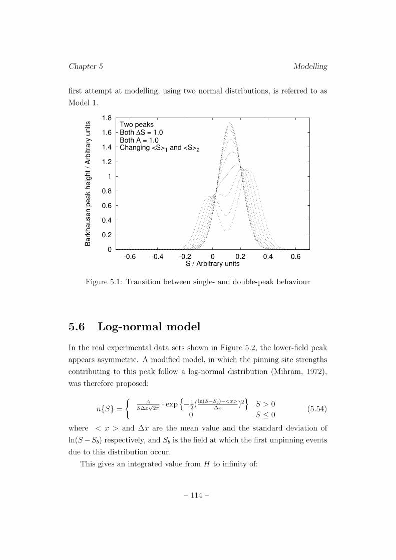
Chapter 5 Modelling
first attempt at modelling, using two normal distributions, is referred to as
Model 1.
0
0.2
0.4
0.6
0.8
1
1.2
1.4
1.6
1.8
-0.6 -0.4 -0.2 0 0.2 0.4 0.6
Bark
hausen p
eak h
eig
ht / A
rbitra
ry u
nits
S / Arbitrary units
Two peaksBoth ∆S = 1.0Both A = 1.0Changing <S>1 and <S>2
Figure 5.1: Transition between single- and double-peak behaviour
5.6 Log-normal model
In the real experimental data sets shown in Figure 5.2, the lower-field peak
appears asymmetric. A modified model, in which the pinning site strengths
contributing to this peak follow a log-normal distribution (Mihram, 1972),
was therefore proposed:
n{S} =
{
AS∆x
√2π
· exp{
−12( ln(S−Sb)−<x>
∆x)2}
S > 0
0 S ≤ 0(5.54)
where < x > and ∆x are the mean value and the standard deviation of
ln(S−Sb) respectively, and Sb is the field at which the first unpinning events
due to this distribution occur.
This gives an integrated value from H to infinity of:
– 114 –
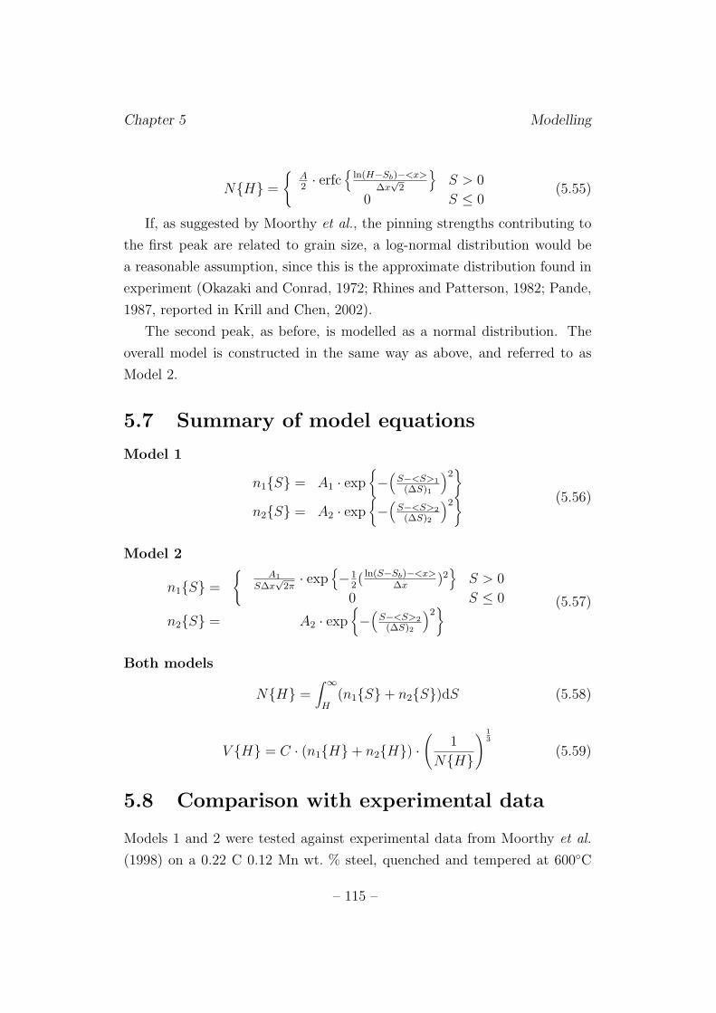
Chapter 5 Modelling
N{H} =
{
A2· erfc
{
ln(H−Sb)−<x>
∆x√
2
}
S > 0
0 S ≤ 0(5.55)
If, as suggested by Moorthy et al., the pinning strengths contributing to
the first peak are related to grain size, a log-normal distribution would be
a reasonable assumption, since this is the approximate distribution found in
experiment (Okazaki and Conrad, 1972; Rhines and Patterson, 1982; Pande,
1987, reported in Krill and Chen, 2002).
The second peak, as before, is modelled as a normal distribution. The
overall model is constructed in the same way as above, and referred to as
Model 2.
5.7 Summary of model equations
Model 1
n1{S} = A1 · exp{
−(
S−<S>1
(∆S)1
)2}
n2{S} = A2 · exp{
−(
S−<S>2
(∆S)2
)2} (5.56)
Model 2
n1{S} =
{
A1
S∆x√
2π· exp
{
−12( ln(S−Sb)−<x>
∆x)2}
S > 0
0 S ≤ 0
n2{S} = A2 · exp{
−(
S−<S>2
(∆S)2
)2}
(5.57)
Both models
N{H} =∫ ∞
H(n1{S} + n2{S})dS (5.58)
V {H} = C · (n1{H} + n2{H}) ·(
1
N{H}
)1
3
(5.59)
5.8 Comparison with experimental data
Models 1 and 2 were tested against experimental data from Moorthy et al.
(1998) on a 0.22 C 0.12 Mn wt. % steel, quenched and tempered at 600◦C
– 115 –
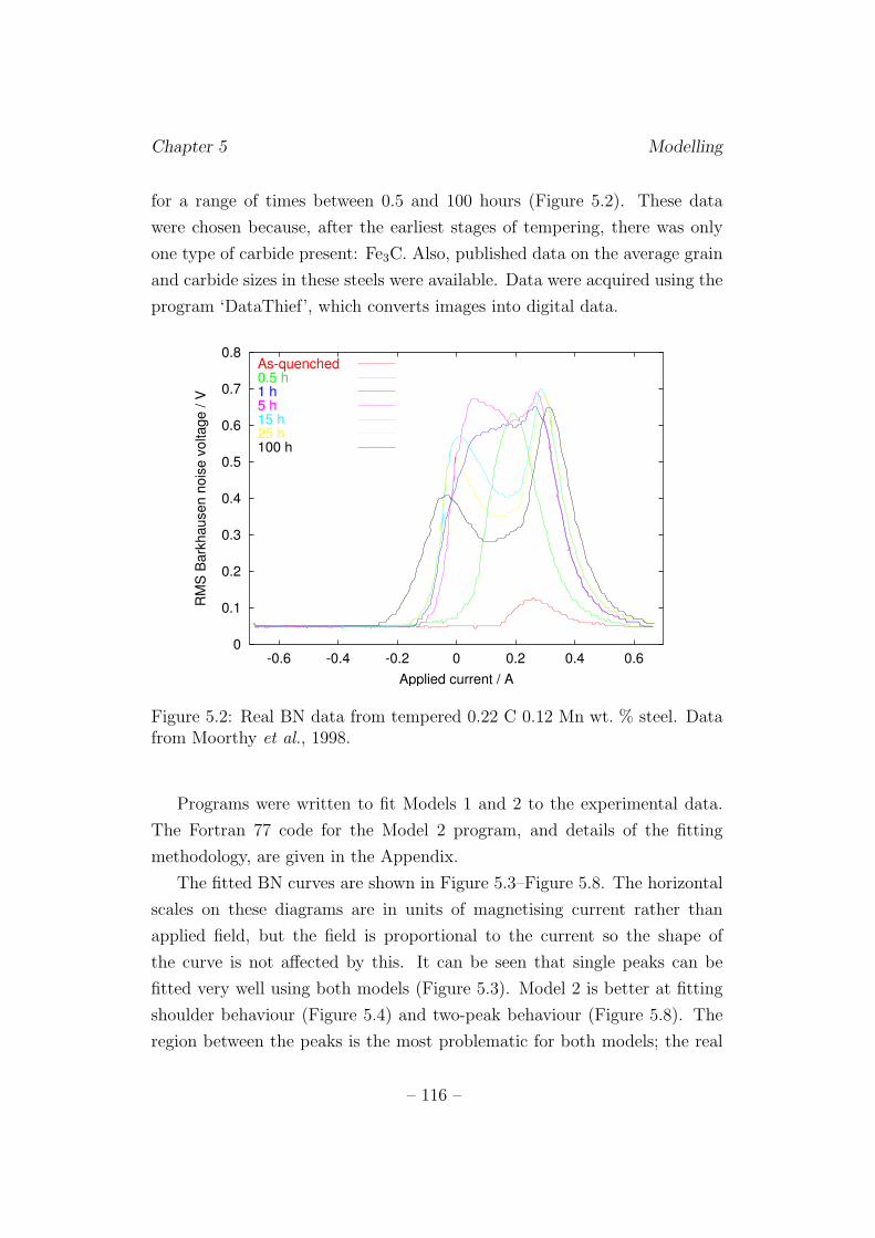
Chapter 5 Modelling
for a range of times between 0.5 and 100 hours (Figure 5.2). These data
were chosen because, after the earliest stages of tempering, there was only
one type of carbide present: Fe3C. Also, published data on the average grain
and carbide sizes in these steels were available. Data were acquired using the
program ‘DataThief’, which converts images into digital data.
0
0.1
0.2
0.3
0.4
0.5
0.6
0.7
0.8
-0.6 -0.4 -0.2 0 0.2 0.4 0.6
RM
S B
ark
hausen n
ois
e v
oltage / V
Applied current / A
As-quenched0.5 h1 h5 h15 h25 h100 h
Figure 5.2: Real BN data from tempered 0.22 C 0.12 Mn wt. % steel. Datafrom Moorthy et al., 1998.
Programs were written to fit Models 1 and 2 to the experimental data.
The Fortran 77 code for the Model 2 program, and details of the fitting
methodology, are given in the Appendix.
The fitted BN curves are shown in Figure 5.3–Figure 5.8. The horizontal
scales on these diagrams are in units of magnetising current rather than
applied field, but the field is proportional to the current so the shape of
the curve is not affected by this. It can be seen that single peaks can be
fitted very well using both models (Figure 5.3). Model 2 is better at fitting
shoulder behaviour (Figure 5.4) and two-peak behaviour (Figure 5.8). The
region between the peaks is the most problematic for both models; the real
– 116 –
Chapter 5 Modelling
V value is higher than the modelled value, causing the fitted peaks to move
closer together than the real peaks. The noise in this central area may be
due to pinning by intragranular dislocations, which have not been considered
in either model.
The ‘error’ figure quoted to quantify the goodness of fit is calculated
using:
E =
[
∑
(Vr{H} − Vp{H})2
∑
(Vr{H})2
]− 1
2
· 100% (5.60)
where Vr{H} is the real value and Vp{H} the predicted value of the RMS
Barkhausen voltage V at field H.
Barkhausen two-peak data may also be analysed by fitting a normal dis-
tribution to each peak. The total amplitude is given by the sum of two ex-
pressions of the form of n1 and n2 in Equation 5.56 (but since Equation 5.58
and Equation 5.59 are not considered, the parameters in the normal distribu-
tion expressions have different meanings from those in Equation 5.56). The
error due to fitting using this method was compared with the errors due to
the two models. The results in Table 5.1 show that, while the peak-fitting
method sometimes produces a fit comparable with that of Model 1, Model 2
performs consistently better, especially at longer tempering times when the
double-peak behaviour is well developed.
– 117 –
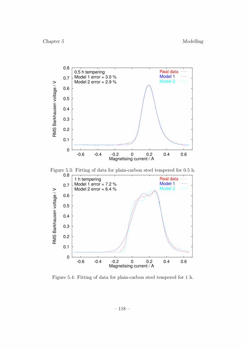
Chapter 5 Modelling
0
0.1
0.2
0.3
0.4
0.5
0.6
0.7
0.8
-0.6 -0.4 -0.2 0 0.2 0.4 0.6
RM
S B
ark
hausen v
oltage / V
Magnetising current / A
0.5 h temperingModel 1 error = 3.0 %Model 2 error = 2.9 %
Real dataModel 1Model 2
Figure 5.3: Fitting of data for plain-carbon steel tempered for 0.5 h.
0
0.1
0.2
0.3
0.4
0.5
0.6
0.7
0.8
-0.6 -0.4 -0.2 0 0.2 0.4 0.6
RM
S B
ark
hausen v
oltage / V
Magnetising current / A
1 h temperingModel 1 error = 7.2 %Model 2 error = 6.4 %
Real dataModel 1Model 2
Figure 5.4: Fitting of data for plain-carbon steel tempered for 1 h.
– 118 –
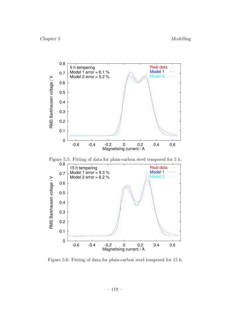
Chapter 5 Modelling
0
0.1
0.2
0.3
0.4
0.5
0.6
0.7
0.8
-0.6 -0.4 -0.2 0 0.2 0.4 0.6
RM
S B
ark
hausen v
oltage / V
Magnetising current / A
5 h temperingModel 1 error = 6.1 %Model 2 error = 5.2 %
Real dataModel 1Model 2
Figure 5.5: Fitting of data for plain-carbon steel tempered for 5 h.
0
0.1
0.2
0.3
0.4
0.5
0.6
0.7
0.8
-0.6 -0.4 -0.2 0 0.2 0.4 0.6
RM
S B
ark
hausen v
oltage / V
Magnetising current / A
15 h temperingModel 1 error = 9.3 %Model 2 error = 6.2 %
Real dataModel 1Model 2
Figure 5.6: Fitting of data for plain-carbon steel tempered for 15 h.
– 119 –
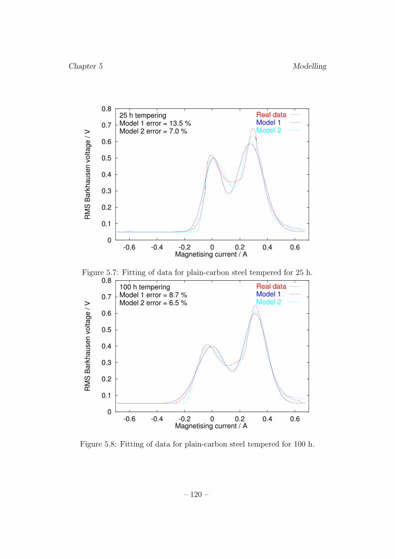
Chapter 5 Modelling
0
0.1
0.2
0.3
0.4
0.5
0.6
0.7
0.8
-0.6 -0.4 -0.2 0 0.2 0.4 0.6
RM
S B
ark
hausen v
oltage / V
Magnetising current / A
25 h temperingModel 1 error = 13.5 %Model 2 error = 7.0 %
Real dataModel 1Model 2
Figure 5.7: Fitting of data for plain-carbon steel tempered for 25 h.
0
0.1
0.2
0.3
0.4
0.5
0.6
0.7
0.8
-0.6 -0.4 -0.2 0 0.2 0.4 0.6
RM
S B
ark
hausen v
oltage / V
Magnetising current / A
100 h temperingModel 1 error = 8.7 %Model 2 error = 6.5 %
Real dataModel 1Model 2
Figure 5.8: Fitting of data for plain-carbon steel tempered for 100 h.
– 120 –
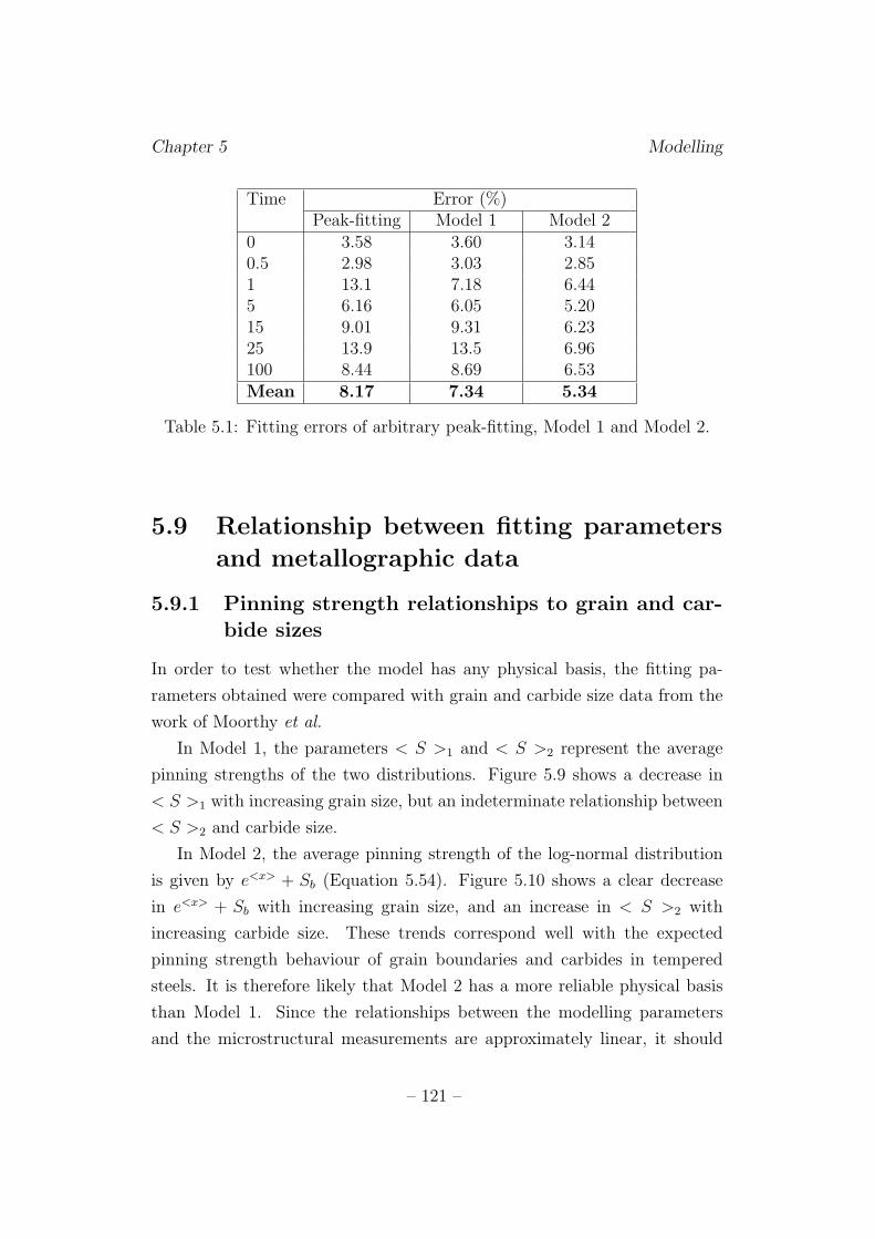
Chapter 5 Modelling
Time Error (%)Peak-fitting Model 1 Model 2
0 3.58 3.60 3.140.5 2.98 3.03 2.851 13.1 7.18 6.445 6.16 6.05 5.2015 9.01 9.31 6.2325 13.9 13.5 6.96100 8.44 8.69 6.53Mean 8.17 7.34 5.34
Table 5.1: Fitting errors of arbitrary peak-fitting, Model 1 and Model 2.
5.9 Relationship between fitting parameters
and metallographic data
5.9.1 Pinning strength relationships to grain and car-bide sizes
In order to test whether the model has any physical basis, the fitting pa-
rameters obtained were compared with grain and carbide size data from the
work of Moorthy et al.
In Model 1, the parameters < S >1 and < S >2 represent the average
pinning strengths of the two distributions. Figure 5.9 shows a decrease in
< S >1 with increasing grain size, but an indeterminate relationship between
< S >2 and carbide size.
In Model 2, the average pinning strength of the log-normal distribution
is given by e<x> + Sb (Equation 5.54). Figure 5.10 shows a clear decrease
in e<x> + Sb with increasing grain size, and an increase in < S >2 with
increasing carbide size. These trends correspond well with the expected
pinning strength behaviour of grain boundaries and carbides in tempered
steels. It is therefore likely that Model 2 has a more reliable physical basis
than Model 1. Since the relationships between the modelling parameters
and the microstructural measurements are approximately linear, it should
– 121 –
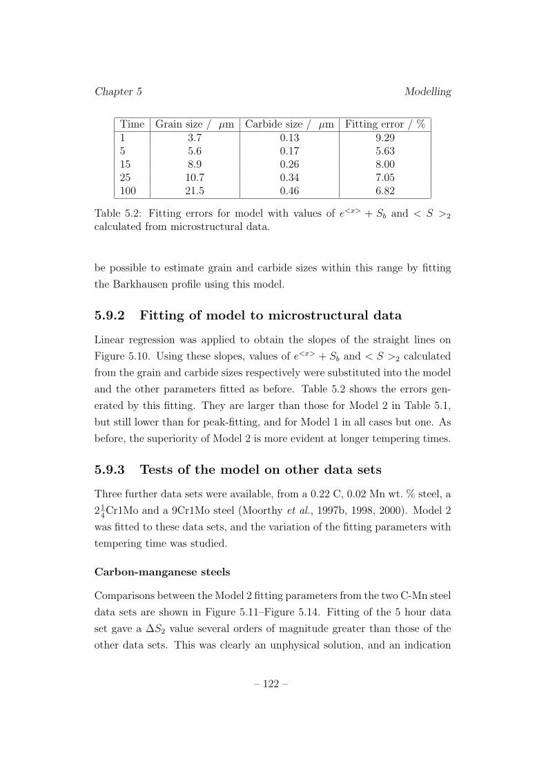
Chapter 5 Modelling
Time Grain size / µm Carbide size / µm Fitting error / %1 3.7 0.13 9.295 5.6 0.17 5.6315 8.9 0.26 8.0025 10.7 0.34 7.05100 21.5 0.46 6.82
Table 5.2: Fitting errors for model with values of e<x> + Sb and < S >2
calculated from microstructural data.
be possible to estimate grain and carbide sizes within this range by fitting
the Barkhausen profile using this model.
5.9.2 Fitting of model to microstructural data
Linear regression was applied to obtain the slopes of the straight lines on
Figure 5.10. Using these slopes, values of e<x> + Sb and < S >2 calculated
from the grain and carbide sizes respectively were substituted into the model
and the other parameters fitted as before. Table 5.2 shows the errors gen-
erated by this fitting. They are larger than those for Model 2 in Table 5.1,
but still lower than for peak-fitting, and for Model 1 in all cases but one. As
before, the superiority of Model 2 is more evident at longer tempering times.
5.9.3 Tests of the model on other data sets
Three further data sets were available, from a 0.22 C, 0.02 Mn wt. % steel, a
214Cr1Mo and a 9Cr1Mo steel (Moorthy et al., 1997b, 1998, 2000). Model 2
was fitted to these data sets, and the variation of the fitting parameters with
tempering time was studied.
Carbon-manganese steels
Comparisons between the Model 2 fitting parameters from the two C-Mn steel
data sets are shown in Figure 5.11–Figure 5.14. Fitting of the 5 hour data
set gave a ∆S2 value several orders of magnitude greater than those of the
other data sets. This was clearly an unphysical solution, and an indication
– 122 –
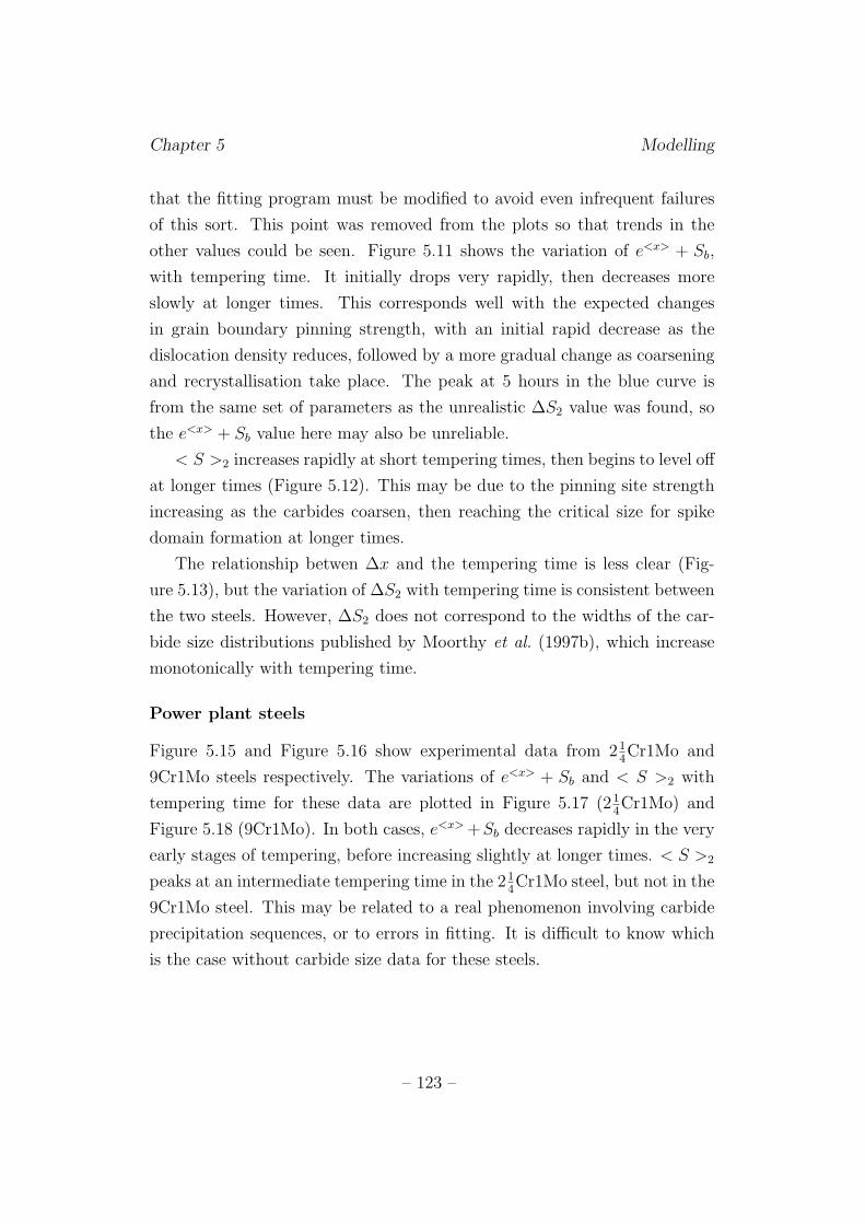
Chapter 5 Modelling
that the fitting program must be modified to avoid even infrequent failures
of this sort. This point was removed from the plots so that trends in the
other values could be seen. Figure 5.11 shows the variation of e<x> + Sb,
with tempering time. It initially drops very rapidly, then decreases more
slowly at longer times. This corresponds well with the expected changes
in grain boundary pinning strength, with an initial rapid decrease as the
dislocation density reduces, followed by a more gradual change as coarsening
and recrystallisation take place. The peak at 5 hours in the blue curve is
from the same set of parameters as the unrealistic ∆S2 value was found, so
the e<x> + Sb value here may also be unreliable.
< S >2 increases rapidly at short tempering times, then begins to level off
at longer times (Figure 5.12). This may be due to the pinning site strength
increasing as the carbides coarsen, then reaching the critical size for spike
domain formation at longer times.
The relationship betwen ∆x and the tempering time is less clear (Fig-
ure 5.13), but the variation of ∆S2 with tempering time is consistent between
the two steels. However, ∆S2 does not correspond to the widths of the car-
bide size distributions published by Moorthy et al. (1997b), which increase
monotonically with tempering time.
Power plant steels
Figure 5.15 and Figure 5.16 show experimental data from 214Cr1Mo and
9Cr1Mo steels respectively. The variations of e<x> + Sb and < S >2 with
tempering time for these data are plotted in Figure 5.17 (214Cr1Mo) and
Figure 5.18 (9Cr1Mo). In both cases, e<x> +Sb decreases rapidly in the very
early stages of tempering, before increasing slightly at longer times. < S >2
peaks at an intermediate tempering time in the 214Cr1Mo steel, but not in the
9Cr1Mo steel. This may be related to a real phenomenon involving carbide
precipitation sequences, or to errors in fitting. It is difficult to know which
is the case without carbide size data for these steels.
– 123 –
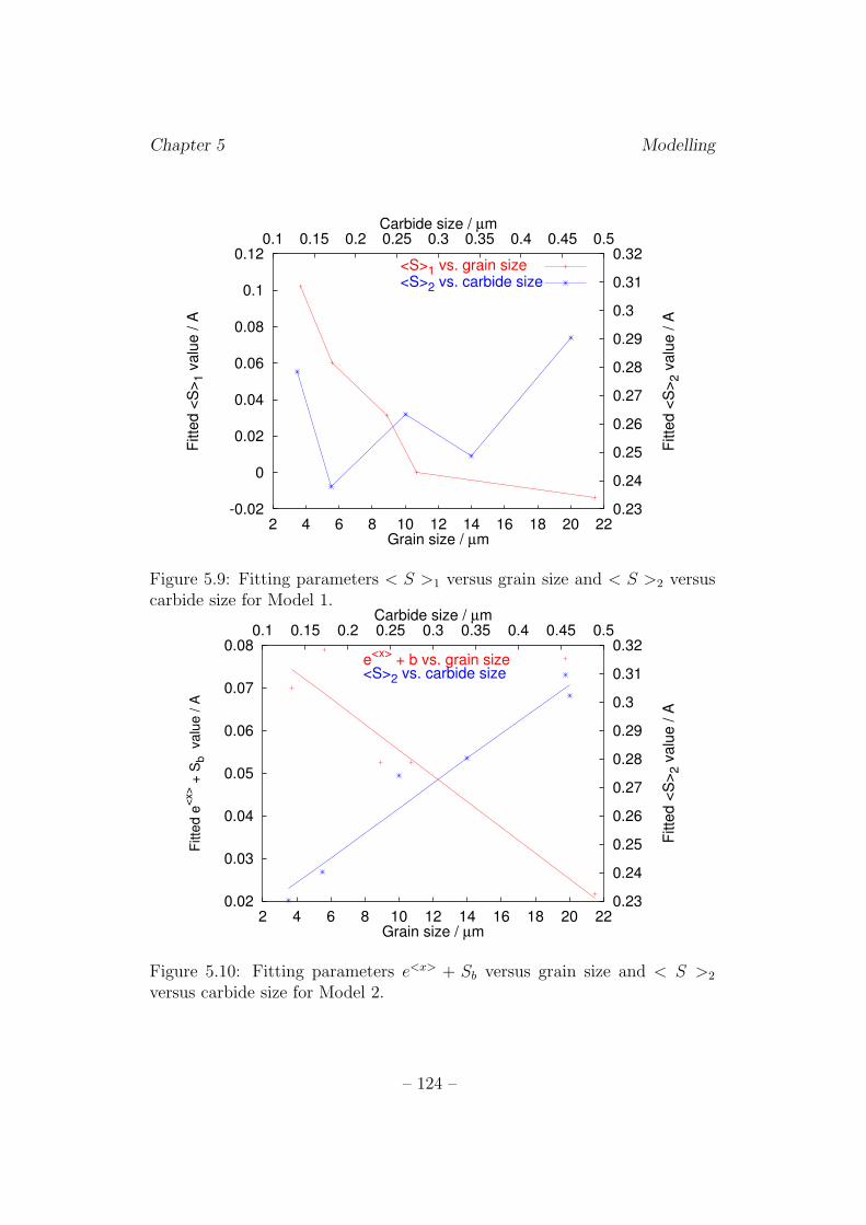
Chapter 5 Modelling
-0.02
0
0.02
0.04
0.06
0.08
0.1
0.12
2 4 6 8 10 12 14 16 18 20 220.23
0.24
0.25
0.26
0.27
0.28
0.29
0.3
0.31
0.320.1 0.15 0.2 0.25 0.3 0.35 0.4 0.45 0.5
Fitte
d <
S>
1 v
alu
e / A
Fitte
d <
S>
2 v
alu
e / A
Grain size / µm
Carbide size / µm
<S>1 vs. grain size<S>2 vs. carbide size
Figure 5.9: Fitting parameters < S >1 versus grain size and < S >2 versuscarbide size for Model 1.
0.02
0.03
0.04
0.05
0.06
0.07
0.08
2 4 6 8 10 12 14 16 18 20 220.23
0.24
0.25
0.26
0.27
0.28
0.29
0.3
0.31
0.320.1 0.15 0.2 0.25 0.3 0.35 0.4 0.45 0.5
Fitte
d e
<x> +
Sb valu
e / A
Fitte
d <
S>
2 v
alu
e / A
Grain size / µm
Carbide size / µm
e<x>
+ b vs. grain size<S>2 vs. carbide size
Figure 5.10: Fitting parameters e<x> + Sb versus grain size and < S >2
versus carbide size for Model 2.
– 124 –
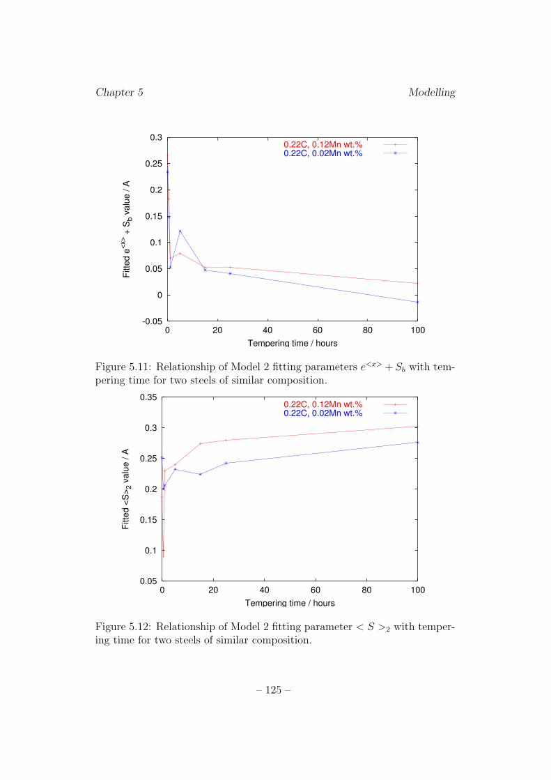
Chapter 5 Modelling
-0.05
0
0.05
0.1
0.15
0.2
0.25
0.3
0 20 40 60 80 100
Fitte
d e
<x> +
Sb v
alu
e / A
Tempering time / hours
0.22C, 0.12Mn wt.%0.22C, 0.02Mn wt.%
Figure 5.11: Relationship of Model 2 fitting parameters e<x> + Sb with tem-pering time for two steels of similar composition.
0.05
0.1
0.15
0.2
0.25
0.3
0.35
0 20 40 60 80 100
Fitte
d <
S>
2 v
alu
e / A
Tempering time / hours
0.22C, 0.12Mn wt.%0.22C, 0.02Mn wt.%
Figure 5.12: Relationship of Model 2 fitting parameter < S >2 with temper-ing time for two steels of similar composition.
– 125 –
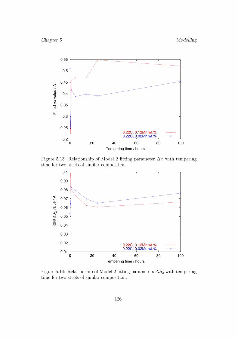
Chapter 5 Modelling
0.2
0.25
0.3
0.35
0.4
0.45
0.5
0.55
0 20 40 60 80 100
Fitte
d ∆
x v
alu
e / A
Tempering time / hours
0.22C, 0.12Mn wt.%0.22C, 0.02Mn wt.%
Figure 5.13: Relationship of Model 2 fitting parameter ∆x with temperingtime for two steels of similar composition.
0.01
0.02
0.03
0.04
0.05
0.06
0.07
0.08
0.09
0.1
0 20 40 60 80 100
Fitte
d ∆
S2 v
alu
e / A
Tempering time / hours
0.22C, 0.12Mn wt.%0.22C, 0.02Mn wt.%
Figure 5.14: Relationship of Model 2 fitting parameters ∆S2 with temperingtime for two steels of similar composition.
– 126 –
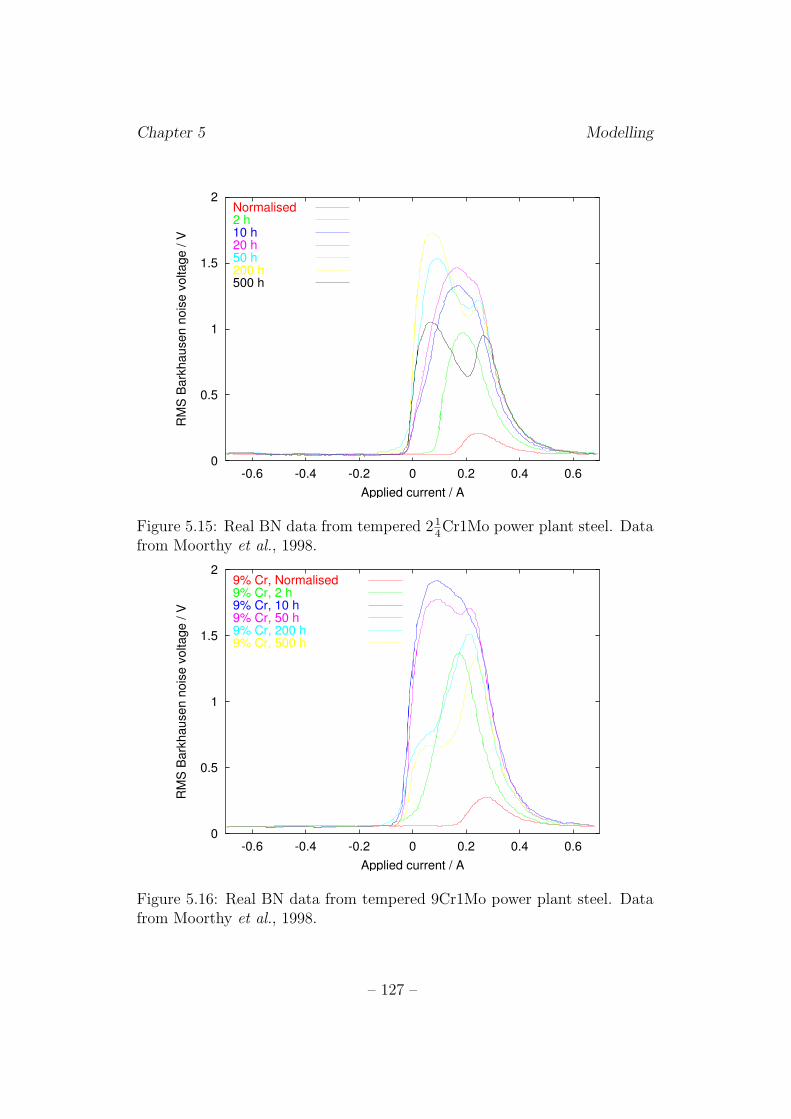
Chapter 5 Modelling
0
0.5
1
1.5
2
-0.6 -0.4 -0.2 0 0.2 0.4 0.6
RM
S B
ark
hausen n
ois
e v
oltage / V
Applied current / A
Normalised2 h10 h20 h50 h200 h500 h
Figure 5.15: Real BN data from tempered 214Cr1Mo power plant steel. Data
from Moorthy et al., 1998.
0
0.5
1
1.5
2
-0.6 -0.4 -0.2 0 0.2 0.4 0.6
RM
S B
ark
hausen n
ois
e v
oltage / V
Applied current / A
9% Cr, Normalised9% Cr, 2 h9% Cr, 10 h9% Cr, 50 h9% Cr, 200 h9% Cr, 500 h
Figure 5.16: Real BN data from tempered 9Cr1Mo power plant steel. Datafrom Moorthy et al., 1998.
– 127 –
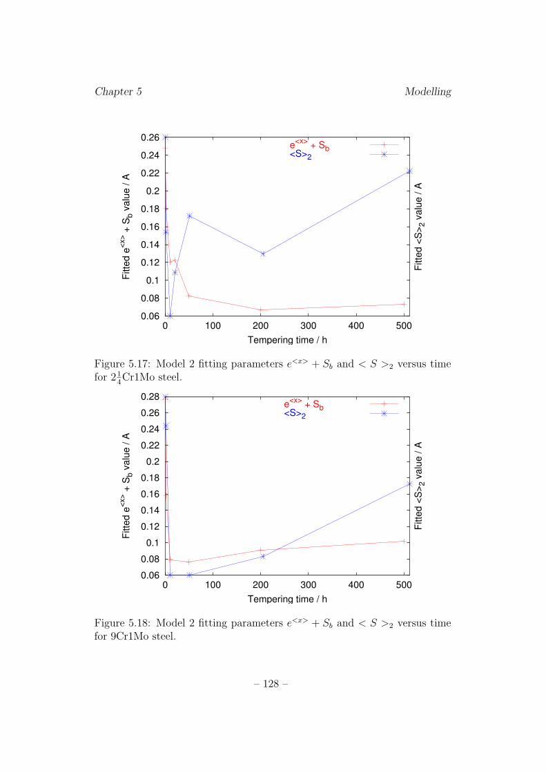
Chapter 5 Modelling
0.06
0.08
0.1
0.12
0.14
0.16
0.18
0.2
0.22
0.24
0.26
0 100 200 300 400 500
Fitte
d e
<x> +
Sb v
alu
e / A
Fitte
d <
S>
2 v
alu
e / A
Tempering time / h
e<x>
+ Sb<S>2
Figure 5.17: Model 2 fitting parameters e<x> + Sb and < S >2 versus timefor 21
4Cr1Mo steel.
0.06
0.08
0.1
0.12
0.14
0.16
0.18
0.2
0.22
0.24
0.26
0.28
0 100 200 300 400 500
Fitte
d e
<x> +
Sb v
alu
e / A
Fitte
d <
S>
2 v
alu
e / A
Tempering time / h
e<x>
+ Sb <S>2
Figure 5.18: Model 2 fitting parameters e<x> + Sb and < S >2 versus timefor 9Cr1Mo steel.
– 128 –
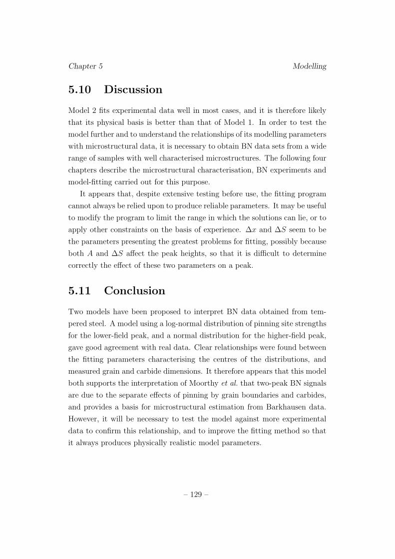
Chapter 5 Modelling
5.10 Discussion
Model 2 fits experimental data well in most cases, and it is therefore likely
that its physical basis is better than that of Model 1. In order to test the
model further and to understand the relationships of its modelling parameters
with microstructural data, it is necessary to obtain BN data sets from a wide
range of samples with well characterised microstructures. The following four
chapters describe the microstructural characterisation, BN experiments and
model-fitting carried out for this purpose.
It appears that, despite extensive testing before use, the fitting program
cannot always be relied upon to produce reliable parameters. It may be useful
to modify the program to limit the range in which the solutions can lie, or to
apply other constraints on the basis of experience. ∆x and ∆S seem to be
the parameters presenting the greatest problems for fitting, possibly because
both A and ∆S affect the peak heights, so that it is difficult to determine
correctly the effect of these two parameters on a peak.
5.11 Conclusion
Two models have been proposed to interpret BN data obtained from tem-
pered steel. A model using a log-normal distribution of pinning site strengths
for the lower-field peak, and a normal distribution for the higher-field peak,
gave good agreement with real data. Clear relationships were found between
the fitting parameters characterising the centres of the distributions, and
measured grain and carbide dimensions. It therefore appears that this model
both supports the interpretation of Moorthy et al. that two-peak BN signals
are due to the separate effects of pinning by grain boundaries and carbides,
and provides a basis for microstructural estimation from Barkhausen data.
However, it will be necessary to test the model against more experimental
data to confirm this relationship, and to improve the fitting method so that
it always produces physically realistic model parameters.
– 129 –

Chapter 6
Sample Preparation andCharacterisation
6.1 Sample preparation
214Cr1Mo steel
A section of a 214Cr1Mo power plant steel from Drax Power Station was
supplied by National Power plc. The composition is given in Table 6.1.
A piece of this steel of approximate dimensions 100 × 100 × 12 mm was
placed in a furnace at 500◦C. The temperature was increased to 1000◦C and
held for 30 minutes to transform the steel to austenite. The sample was then
quenched directly into water. During quenching, it was agitated to prevent
the buildup of a layer of bubbles which would provide insulation and reduce
the cooling rate.
Using a spark-cutter, square plates of the material of side 10 mm and ap-
proximate depth 1 mm were cut from the large piece, taking care to discard
C Si Mn P S Cr Mo Ni Al As0.12 0.29 0.51 0.021 0.021 2.22 0.97 0.21 0.008 0.030Co Cu Nb Pb Sn Ti V W Sb
0.027 0.23 <0.005 0.009 0.022 <0.005 0.017 0.019 0.015
Table 6.1: Composition of 214Cr1Mo steel; all quantities in wt. %. Data
supplied by Bodycote Materials Testing Ltd., Bridgwater, Somerset.
– 130 –
Chapter 6 Sample Preparation & Characterisation
the decarburised layer on the outside. The thickness of this layer was esti-
mated at 0.05 mm using the constant-concentration solution to Fick’s second
law, but 2 mm was cut from each edge to be sure of excluding decarburised
material.
In order to prevent decarburisation and oxidation during tempering, the
square plates were sealed into silica tubes which were evacuated and back-
filled with a small partial pressure of argon to provide an inert atmosphere.
Two plates were placed into each tube so that the samples for Barkhausen
analysis and for electron microscopy would receive exactly the same heat
treatment.
The samples were subjected to tempering heat treatments of between
1 hour and 512 hours at 500◦C and at 600◦C, and between 1 hour and
8 hours at 700◦C. This last series was intended to replicate the microstruc-
tural changes during the pre-service tempering treatment of power-plant
steels (Morris, personal communication). As-quenched (AQ) samples were
retained for comparison with the tempered steels.
After tempering, the samples were allowed to air-cool while remaining
within the silica tubes. The tubes were then broken, and the samples were
hot-mounted in Bakelite, ground using 2500 grit silicon carbide paper and
polished to 1 µm using diamond paste. Finally, the surfaces were etched
using 2% nital to remove the strained layer and reveal the microstructure for
observation using an optical microscope and a Hitachi S-4200 Field Emission
Gun SEM.
Long-term specimens
Specimens of 11Cr1Mo wt. % steel which had been heated for several thou-
sands of hours at 550◦C were supplied by Corus RD&T. These were from
creep tests, and comprised a screw-thread, which was used to hold the speci-
men in place, and a gauge length tapering to a fracture surface (Figure 6.1).
In order to study only the effects of prolonged exposure to high tempera-
ture, samples for BN testing and microscopy were cut from the threaded
area, which was not subjected to stress, using a Struers Accutom lubricated
rotary cutter.
– 131 –
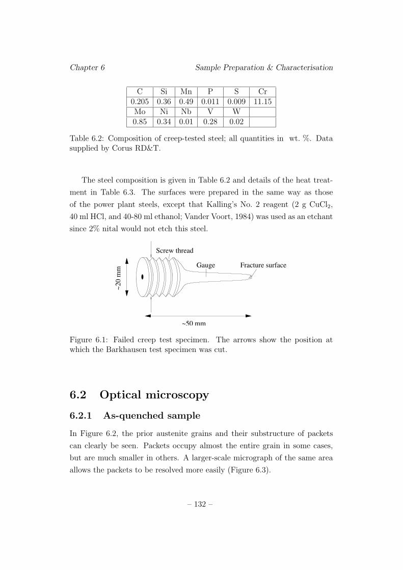
Chapter 6 Sample Preparation & Characterisation
C Si Mn P S Cr0.205 0.36 0.49 0.011 0.009 11.15Mo Ni Nb V W0.85 0.34 0.01 0.28 0.02
Table 6.2: Composition of creep-tested steel; all quantities in wt. %. Datasupplied by Corus RD&T.
The steel composition is given in Table 6.2 and details of the heat treat-
ment in Table 6.3. The surfaces were prepared in the same way as those
of the power plant steels, except that Kalling’s No. 2 reagent (2 g CuCl2,
40 ml HCl, and 40-80 ml ethanol; Vander Voort, 1984) was used as an etchant
since 2% nital would not etch this steel.
~20 m
m
~50 mm
Fracture surface
Screw thread
Gauge
Figure 6.1: Failed creep test specimen. The arrows show the position atwhich the Barkhausen test specimen was cut.
6.2 Optical microscopy
6.2.1 As-quenched sample
In Figure 6.2, the prior austenite grains and their substructure of packets
can clearly be seen. Packets occupy almost the entire grain in some cases,
but are much smaller in others. A larger-scale micrograph of the same area
allows the packets to be resolved more easily (Figure 6.3).
– 132 –
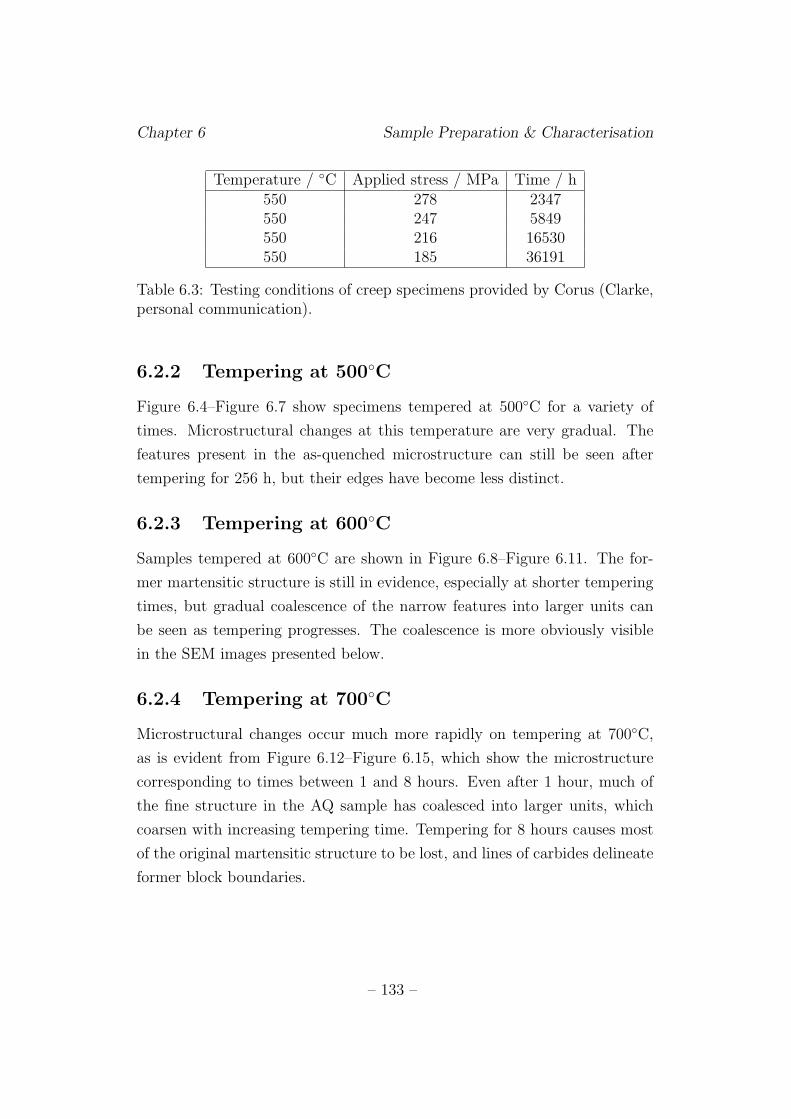
Chapter 6 Sample Preparation & Characterisation
Temperature / ◦C Applied stress / MPa Time / h550 278 2347550 247 5849550 216 16530550 185 36191
Table 6.3: Testing conditions of creep specimens provided by Corus (Clarke,personal communication).
6.2.2 Tempering at 500◦C
Figure 6.4–Figure 6.7 show specimens tempered at 500◦C for a variety of
times. Microstructural changes at this temperature are very gradual. The
features present in the as-quenched microstructure can still be seen after
tempering for 256 h, but their edges have become less distinct.
6.2.3 Tempering at 600◦C
Samples tempered at 600◦C are shown in Figure 6.8–Figure 6.11. The for-
mer martensitic structure is still in evidence, especially at shorter tempering
times, but gradual coalescence of the narrow features into larger units can
be seen as tempering progresses. The coalescence is more obviously visible
in the SEM images presented below.
6.2.4 Tempering at 700◦C
Microstructural changes occur much more rapidly on tempering at 700◦C,
as is evident from Figure 6.12–Figure 6.15, which show the microstructure
corresponding to times between 1 and 8 hours. Even after 1 hour, much of
the fine structure in the AQ sample has coalesced into larger units, which
coarsen with increasing tempering time. Tempering for 8 hours causes most
of the original martensitic structure to be lost, and lines of carbides delineate
former block boundaries.
– 133 –
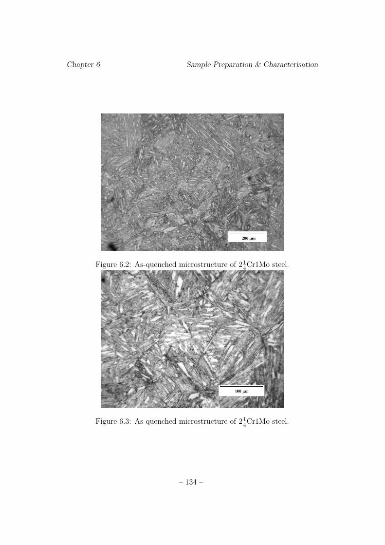
Chapter 6 Sample Preparation & Characterisation
Figure 6.2: As-quenched microstructure of 214Cr1Mo steel.
Figure 6.3: As-quenched microstructure of 214Cr1Mo steel.
– 134 –
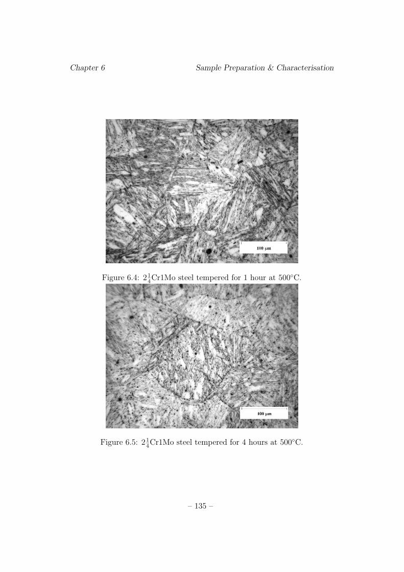
Chapter 6 Sample Preparation & Characterisation
Figure 6.4: 214Cr1Mo steel tempered for 1 hour at 500◦C.
Figure 6.5: 214Cr1Mo steel tempered for 4 hours at 500◦C.
– 135 –
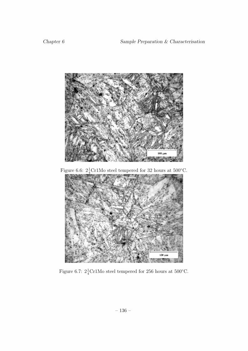
Chapter 6 Sample Preparation & Characterisation
Figure 6.6: 214Cr1Mo steel tempered for 32 hours at 500◦C.
Figure 6.7: 214Cr1Mo steel tempered for 256 hours at 500◦C.
– 136 –
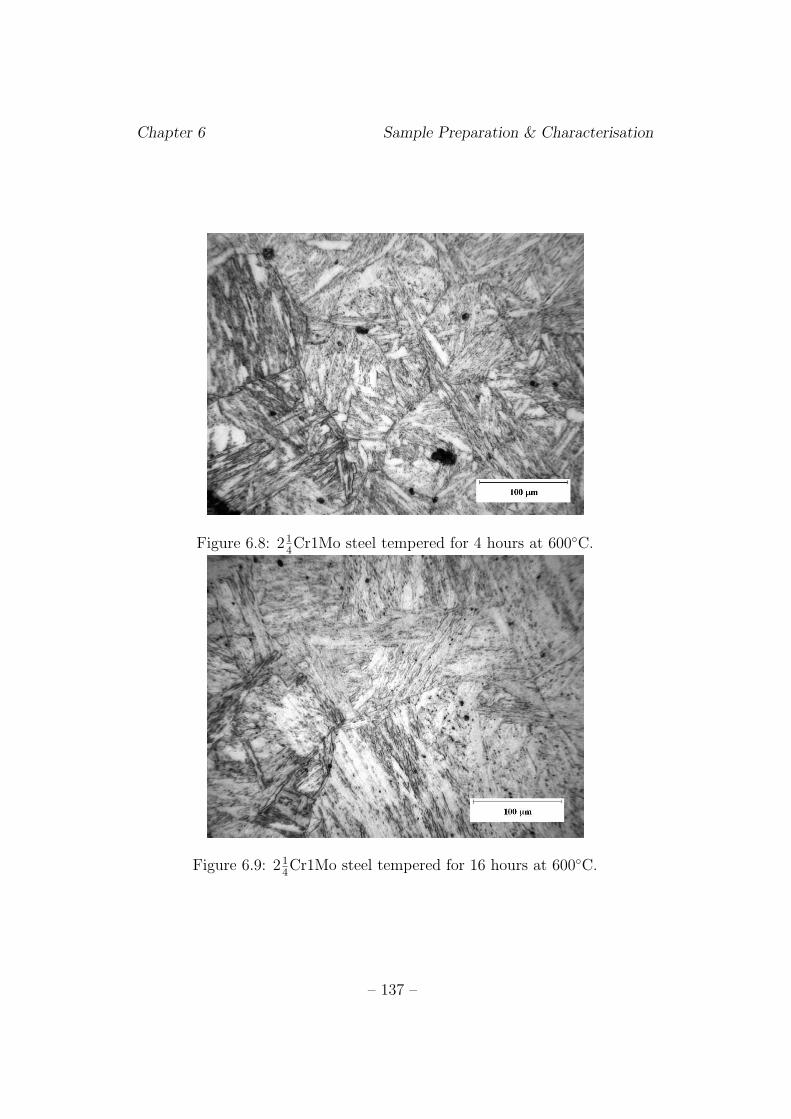
Chapter 6 Sample Preparation & Characterisation
Figure 6.8: 214Cr1Mo steel tempered for 4 hours at 600◦C.
Figure 6.9: 214Cr1Mo steel tempered for 16 hours at 600◦C.
– 137 –
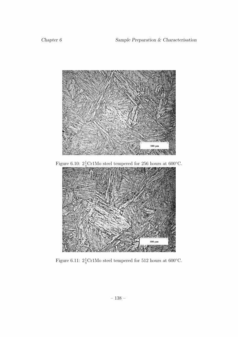
Chapter 6 Sample Preparation & Characterisation
Figure 6.10: 214Cr1Mo steel tempered for 256 hours at 600◦C.
Figure 6.11: 214Cr1Mo steel tempered for 512 hours at 600◦C.
– 138 –
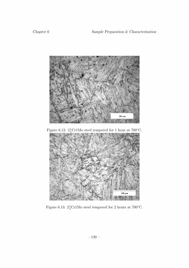
Chapter 6 Sample Preparation & Characterisation
Figure 6.12: 214Cr1Mo steel tempered for 1 hour at 700◦C.
Figure 6.13: 214Cr1Mo steel tempered for 2 hours at 700◦C.
– 139 –
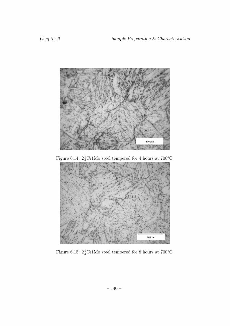
Chapter 6 Sample Preparation & Characterisation
Figure 6.14: 214Cr1Mo steel tempered for 4 hours at 700◦C.
Figure 6.15: 214Cr1Mo steel tempered for 8 hours at 700◦C.
– 140 –
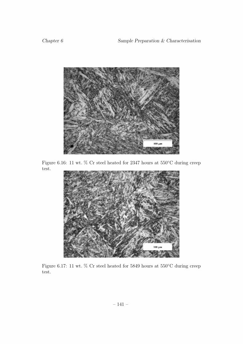
Chapter 6 Sample Preparation & Characterisation
Figure 6.16: 11 wt. % Cr steel heated for 2347 hours at 550◦C during creeptest.
Figure 6.17: 11 wt. % Cr steel heated for 5849 hours at 550◦C during creeptest.
– 141 –
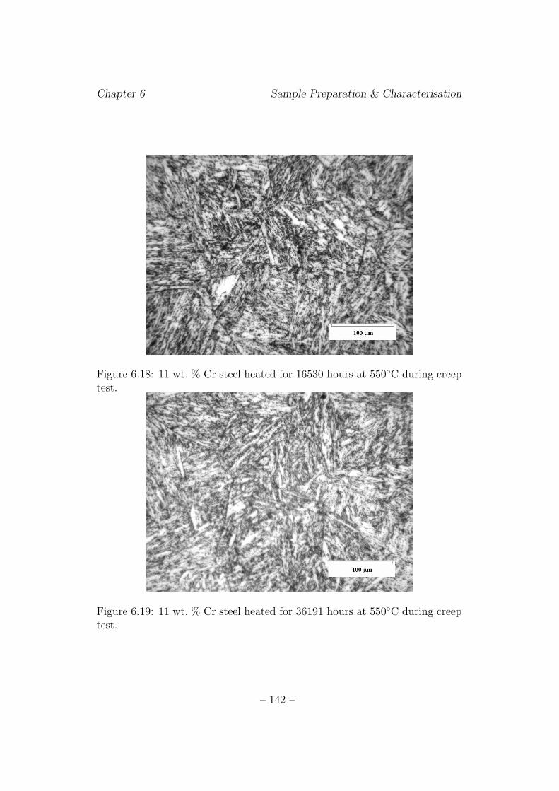
Chapter 6 Sample Preparation & Characterisation
Figure 6.18: 11 wt. % Cr steel heated for 16530 hours at 550◦C during creeptest.
Figure 6.19: 11 wt. % Cr steel heated for 36191 hours at 550◦C during creeptest.
– 142 –
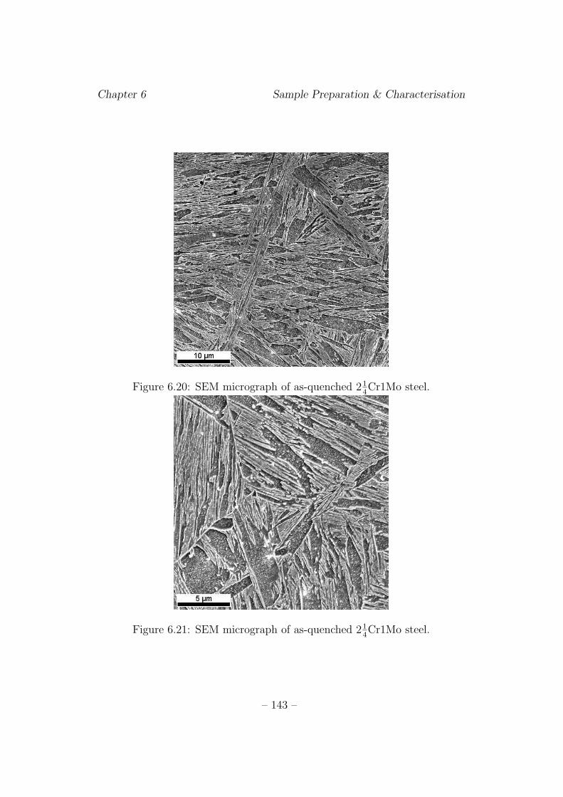
Chapter 6 Sample Preparation & Characterisation
Figure 6.20: SEM micrograph of as-quenched 214Cr1Mo steel.
Figure 6.21: SEM micrograph of as-quenched 214Cr1Mo steel.
– 143 –
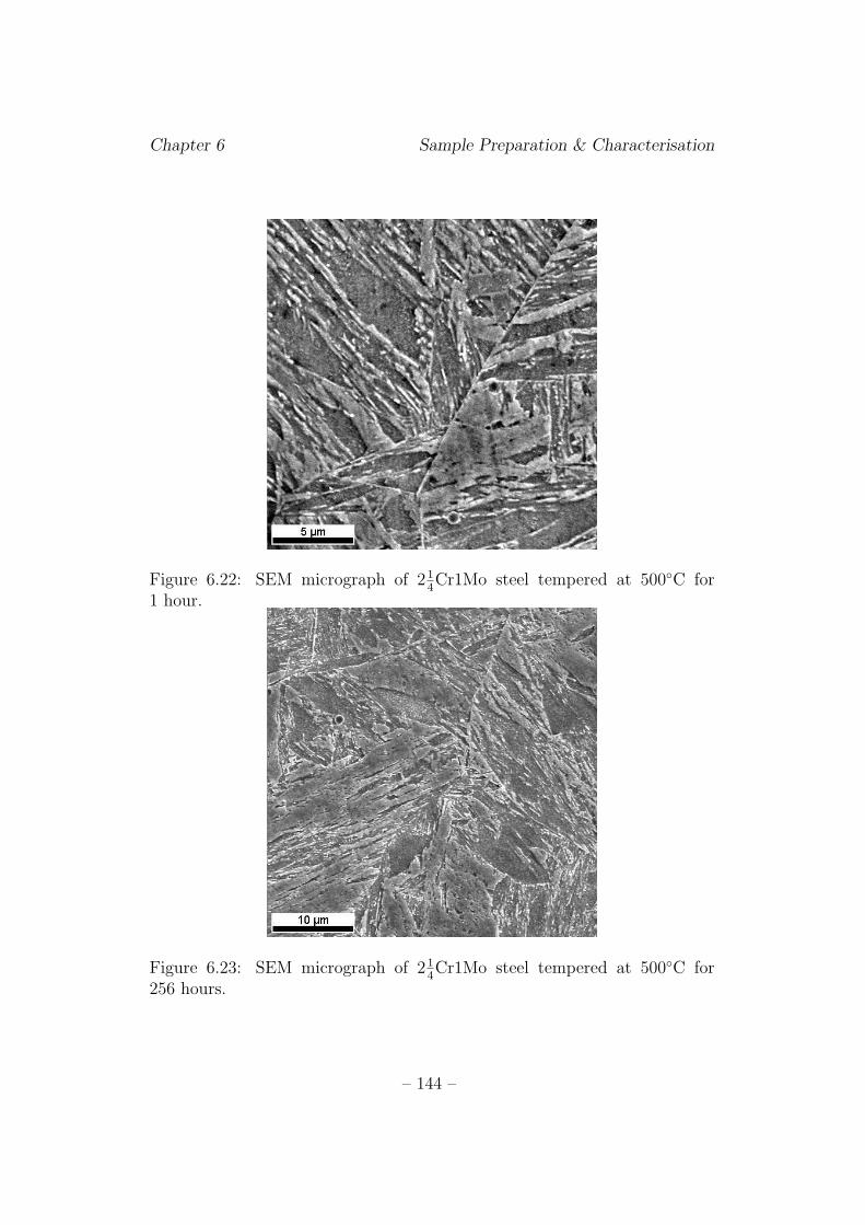
Chapter 6 Sample Preparation & Characterisation
Figure 6.22: SEM micrograph of 214Cr1Mo steel tempered at 500◦C for
1 hour.
Figure 6.23: SEM micrograph of 214Cr1Mo steel tempered at 500◦C for
256 hours.
– 144 –
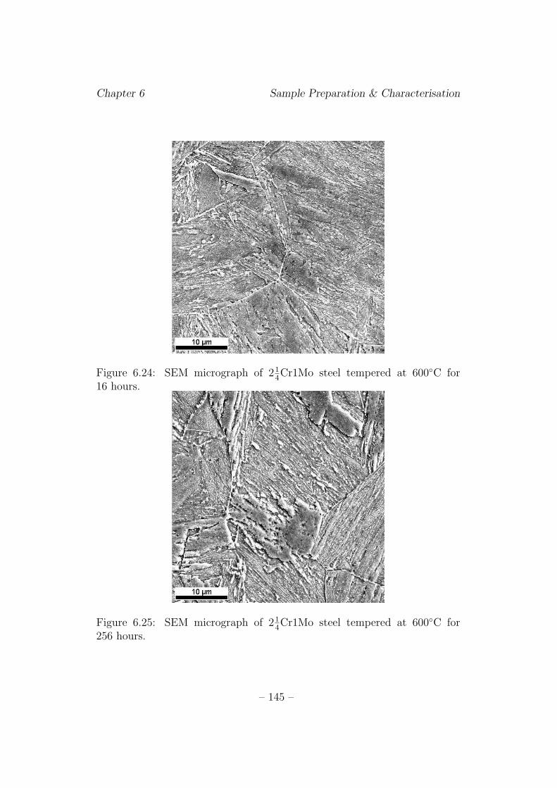
Chapter 6 Sample Preparation & Characterisation
Figure 6.24: SEM micrograph of 214Cr1Mo steel tempered at 600◦C for
16 hours.
Figure 6.25: SEM micrograph of 214Cr1Mo steel tempered at 600◦C for
256 hours.
– 145 –
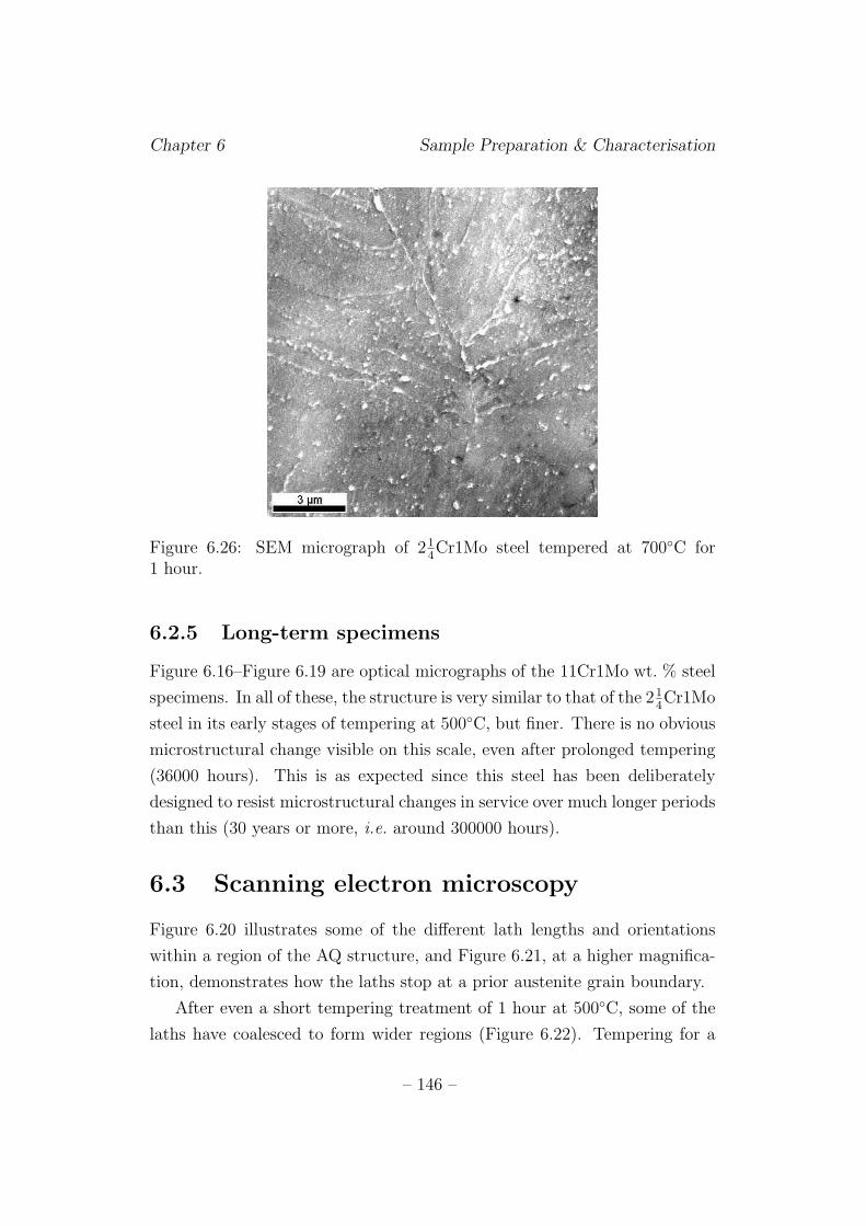
Chapter 6 Sample Preparation & Characterisation
Figure 6.26: SEM micrograph of 214Cr1Mo steel tempered at 700◦C for
1 hour.
6.2.5 Long-term specimens
Figure 6.16–Figure 6.19 are optical micrographs of the 11Cr1Mo wt. % steel
specimens. In all of these, the structure is very similar to that of the 214Cr1Mo
steel in its early stages of tempering at 500◦C, but finer. There is no obvious
microstructural change visible on this scale, even after prolonged tempering
(36000 hours). This is as expected since this steel has been deliberately
designed to resist microstructural changes in service over much longer periods
than this (30 years or more, i.e. around 300000 hours).
6.3 Scanning electron microscopy
Figure 6.20 illustrates some of the different lath lengths and orientations
within a region of the AQ structure, and Figure 6.21, at a higher magnifica-
tion, demonstrates how the laths stop at a prior austenite grain boundary.
After even a short tempering treatment of 1 hour at 500◦C, some of the
laths have coalesced to form wider regions (Figure 6.22). Tempering for a
– 146 –
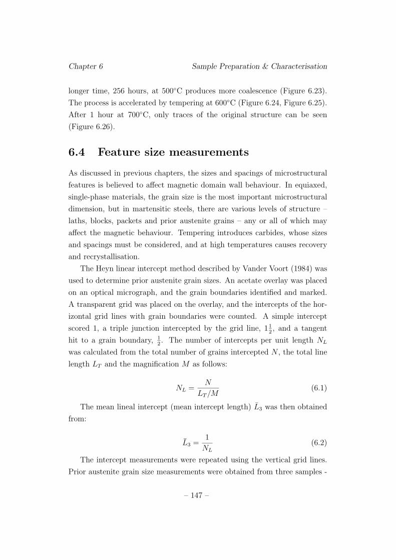
Chapter 6 Sample Preparation & Characterisation
longer time, 256 hours, at 500◦C produces more coalescence (Figure 6.23).
The process is accelerated by tempering at 600◦C (Figure 6.24, Figure 6.25).
After 1 hour at 700◦C, only traces of the original structure can be seen
(Figure 6.26).
6.4 Feature size measurements
As discussed in previous chapters, the sizes and spacings of microstructural
features is believed to affect magnetic domain wall behaviour. In equiaxed,
single-phase materials, the grain size is the most important microstructural
dimension, but in martensitic steels, there are various levels of structure –
laths, blocks, packets and prior austenite grains – any or all of which may
affect the magnetic behaviour. Tempering introduces carbides, whose sizes
and spacings must be considered, and at high temperatures causes recovery
and recrystallisation.
The Heyn linear intercept method described by Vander Voort (1984) was
used to determine prior austenite grain sizes. An acetate overlay was placed
on an optical micrograph, and the grain boundaries identified and marked.
A transparent grid was placed on the overlay, and the intercepts of the hor-
izontal grid lines with grain boundaries were counted. A simple intercept
scored 1, a triple junction intercepted by the grid line, 112, and a tangent
hit to a grain boundary, 12. The number of intercepts per unit length NL
was calculated from the total number of grains intercepted N , the total line
length LT and the magnification M as follows:
NL =N
LT /M(6.1)
The mean lineal intercept (mean intercept length) L3 was then obtained
from:
L3 =1
NL
(6.2)
The intercept measurements were repeated using the vertical grid lines.
Prior austenite grain size measurements were obtained from three samples -
– 147 –
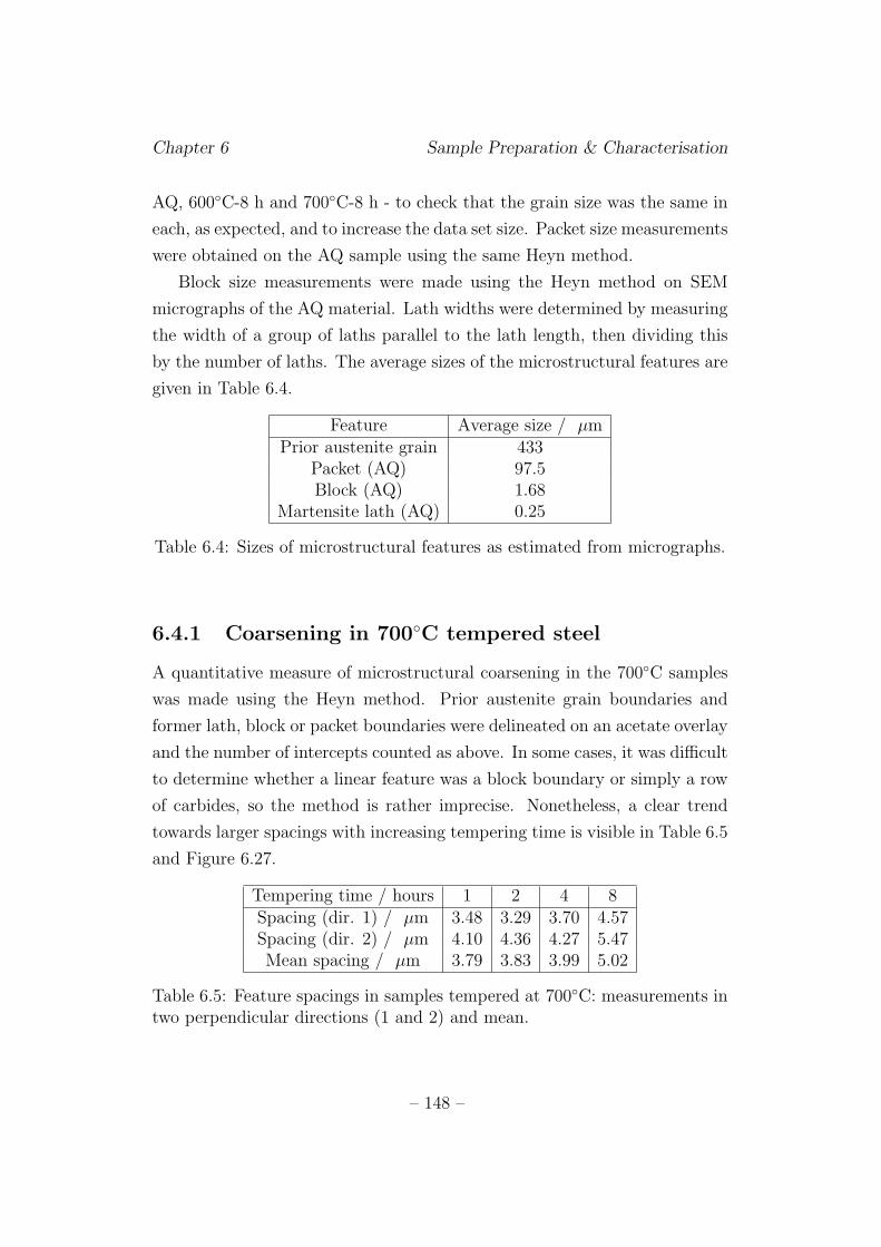
Chapter 6 Sample Preparation & Characterisation
AQ, 600◦C-8 h and 700◦C-8 h - to check that the grain size was the same in
each, as expected, and to increase the data set size. Packet size measurements
were obtained on the AQ sample using the same Heyn method.
Block size measurements were made using the Heyn method on SEM
micrographs of the AQ material. Lath widths were determined by measuring
the width of a group of laths parallel to the lath length, then dividing this
by the number of laths. The average sizes of the microstructural features are
given in Table 6.4.
Feature Average size / µmPrior austenite grain 433
Packet (AQ) 97.5Block (AQ) 1.68
Martensite lath (AQ) 0.25
Table 6.4: Sizes of microstructural features as estimated from micrographs.
6.4.1 Coarsening in 700◦C tempered steel
A quantitative measure of microstructural coarsening in the 700◦C samples
was made using the Heyn method. Prior austenite grain boundaries and
former lath, block or packet boundaries were delineated on an acetate overlay
and the number of intercepts counted as above. In some cases, it was difficult
to determine whether a linear feature was a block boundary or simply a row
of carbides, so the method is rather imprecise. Nonetheless, a clear trend
towards larger spacings with increasing tempering time is visible in Table 6.5
and Figure 6.27.
Tempering time / hours 1 2 4 8Spacing (dir. 1) / µm 3.48 3.29 3.70 4.57Spacing (dir. 2) / µm 4.10 4.36 4.27 5.47Mean spacing / µm 3.79 3.83 3.99 5.02
Table 6.5: Feature spacings in samples tempered at 700◦C: measurements intwo perpendicular directions (1 and 2) and mean.
– 148 –
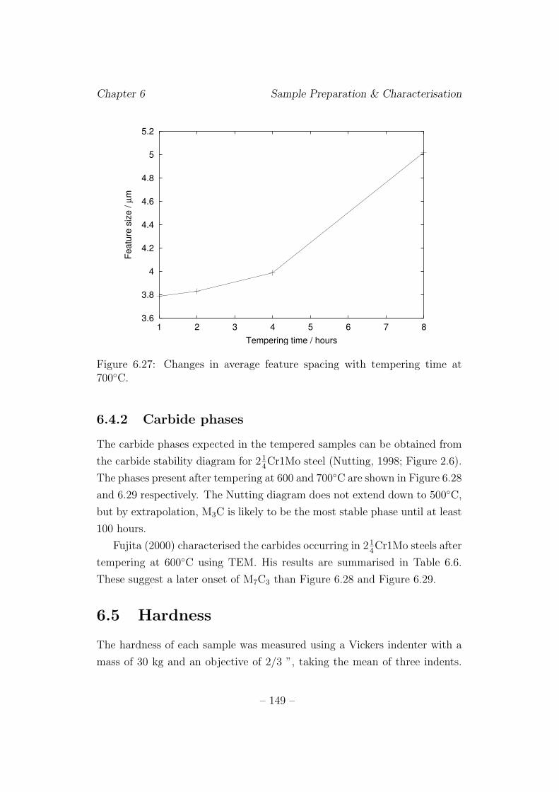
Chapter 6 Sample Preparation & Characterisation
3.6
3.8
4
4.2
4.4
4.6
4.8
5
5.2
1 2 3 4 5 6 7 8
Featu
re s
ize / µ
m
Tempering time / hours
Figure 6.27: Changes in average feature spacing with tempering time at700◦C.
6.4.2 Carbide phases
The carbide phases expected in the tempered samples can be obtained from
the carbide stability diagram for 214Cr1Mo steel (Nutting, 1998; Figure 2.6).
The phases present after tempering at 600 and 700◦C are shown in Figure 6.28
and 6.29 respectively. The Nutting diagram does not extend down to 500◦C,
but by extrapolation, M3C is likely to be the most stable phase until at least
100 hours.
Fujita (2000) characterised the carbides occurring in 214Cr1Mo steels after
tempering at 600◦C using TEM. His results are summarised in Table 6.6.
These suggest a later onset of M7C3 than Figure 6.28 and Figure 6.29.
6.5 Hardness
The hardness of each sample was measured using a Vickers indenter with a
mass of 30 kg and an objective of 2/3 ”, taking the mean of three indents.
– 149 –
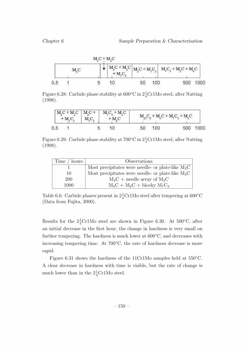
Chapter 6 Sample Preparation & Characterisation
Figure 6.28: Carbide phase stability at 600◦C in 214Cr1Mo steel, after Nutting
(1998).
Figure 6.29: Carbide phase stability at 700◦C in 214Cr1Mo steel, after Nutting
(1998).
Time / hours Observations1 Most precipitates were needle- or plate-like M3C10 Most precipitates were needle- or plate-like M3C200 M3C + needle array of M2C1000 M3C + M2C + blocky M7C3
Table 6.6: Carbide phases present in 214Cr1Mo steel after tempering at 600◦C
(Data from Fujita, 2000).
Results for the 214Cr1Mo steel are shown in Figure 6.30. At 500◦C, after
an initial decrease in the first hour, the change in hardness is very small on
further tempering. The hardness is much lower at 600◦C, and decreases with
increasing tempering time. At 700◦C, the rate of hardness decrease is more
rapid.
Figure 6.31 shows the hardness of the 11Cr1Mo samples held at 550◦C.
A clear decrease in hardness with time is visible, but the rate of change is
much lower than in the 214Cr1Mo steel.
– 150 –
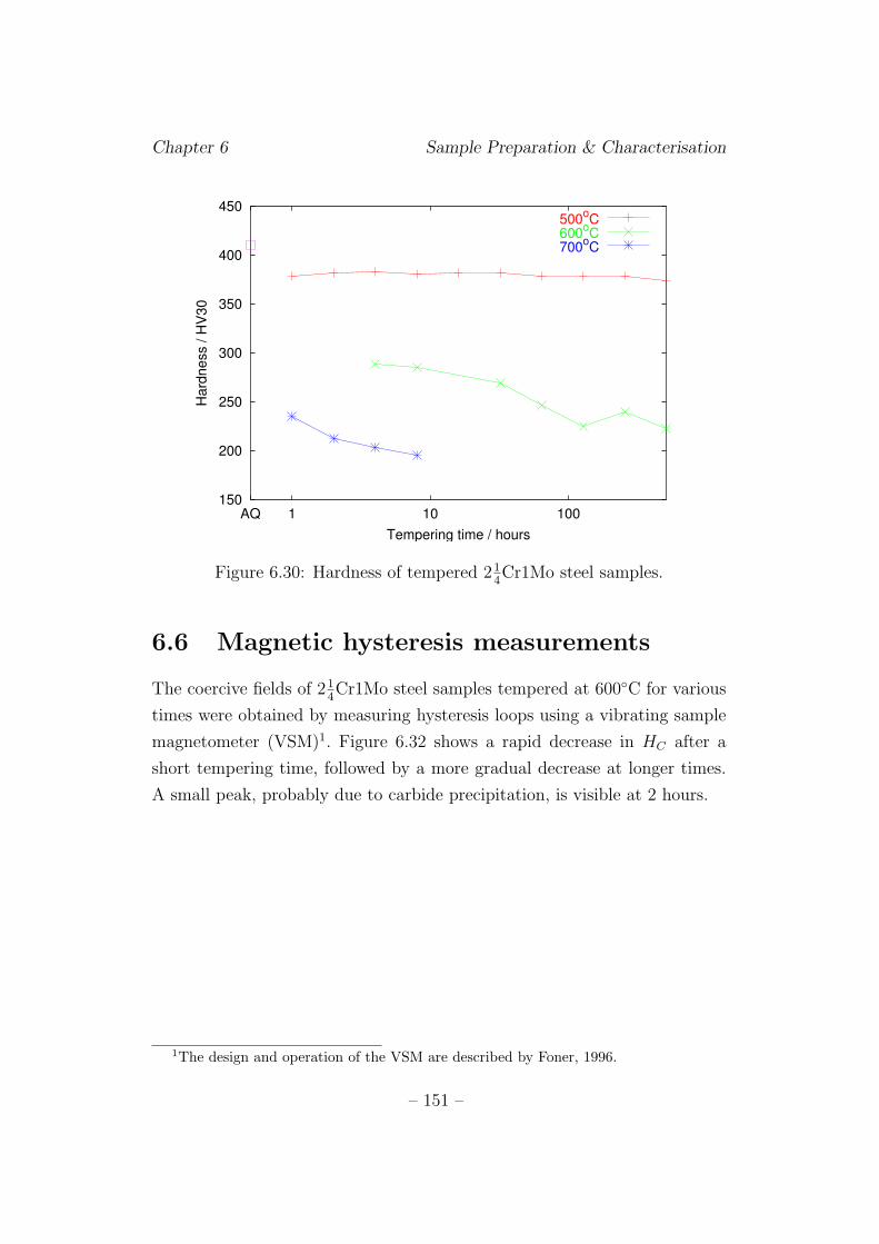
Chapter 6 Sample Preparation & Characterisation
150
200
250
300
350
400
450
AQ 1 10 100
Hard
ness / H
V30
Tempering time / hours
500oC
600oC
700oC
Figure 6.30: Hardness of tempered 214Cr1Mo steel samples.
6.6 Magnetic hysteresis measurements
The coercive fields of 214Cr1Mo steel samples tempered at 600◦C for various
times were obtained by measuring hysteresis loops using a vibrating sample
magnetometer (VSM)1. Figure 6.32 shows a rapid decrease in HC after a
short tempering time, followed by a more gradual decrease at longer times.
A small peak, probably due to carbide precipitation, is visible at 2 hours.
1The design and operation of the VSM are described by Foner, 1996.
– 151 –
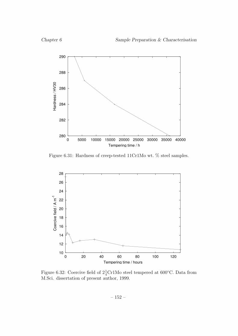
Chapter 6 Sample Preparation & Characterisation
280
282
284
286
288
290
0 5000 10000 15000 20000 25000 30000 35000 40000
Hard
ness / H
V30
Tempering time / h
Figure 6.31: Hardness of creep-tested 11Cr1Mo wt. % steel samples.
10
12
14
16
18
20
22
24
26
28
0 20 40 60 80 100 120
Coerc
ive fie
ld / A
m-1
Tempering time / hours
Figure 6.32: Coercive field of 214Cr1Mo steel tempered at 600◦C. Data from
M.Sci. dissertation of present author, 1999.
– 152 –
Chapter 6 Sample Preparation & Characterisation
6.7 Conclusion
Changes in microstructure and hardness were very small for 214Cr1Mo sam-
ples tempered at 500◦C, although martensite lath coalescence could be seen
using SEM. At 600◦C, the change in hardness was more pronounced, lath coa-
lescence was observed, but the changes visible in the optical microscope were
subtle and gradual. The coercive field decreased rapidly at short tempering
times, and more gradually at longer times. Tempering at 700◦C caused a
rapid reduction in hardness and microstructural coarsening. On tempering
at 600◦C, needlelike M2C is expected to form after a few hours of tempering,
and spheroidal carbides to appear later. The samples tempered at 700◦C
should have both M2C and M7C3 in the microstructure, as well as M3C, at
the tempering times used in this study.
In the 11Cr1Mo wt. % samples held at 550◦C, there were no visible mi-
crostructural changes and a very gradual decrease in hardness with time.
– 153 –
Chapter 7
Orientation ImagingMicroscopy and GrainBoundary Analysis inTempered Power Plant Steel
Over the past decade, the rapid, automated acquisition of large numbers of
grain orientation data in the SEM has become possible. The sampling volume
for each measurement is sufficiently small that many measurements can be
made within a single grain, enabling point-by-point ‘maps’ of orientation
data to be obtained and related directly to microstructure. By comparing
data from adjacent points, it is also possible to determine the positions and
characteristics of grain boundaries.
Using this technique, grain orientations and grain boundaries in 214Cr1Mo
steels in the as-quenched and tempered states were investigated, giving a
more complete microstructural characterisation than would be possible by
conventional optical microscopy and SEM. The purpose of the study was to
obtain insight into the likely microstructural origins of the changes in the
Barkhausen noise signal with tempering.
– 154 –

Chapter 7 Orientation Imaging Microscopy
7.1 Grain orientation
The specification of grain orientations requires the definition of a crystal
coordinate system cc, which is usually chosen with reference to the crystal
symmetry, and a sample system cs. This may be based on rolling, transverse
and normal directions if these exist, but is otherwise defined arbitrarily. The
crystal orientation is defined by the rotation matrix G which brings the
crystal system into coincidence with the sample system.
cc = G · cs (7.1)
The elements of G are given by:
G =
cos α1 cos β1 cosγ1
cos α2 cos β2 cosγ2
cos α3 cos β3 cosγ3
(7.2)
where α1, β1 and γ1 are the angles between the crystal axis [100] and the
specimen axes X, Y and Z respectively and the second and third rows of
cosines correspond to the [010] and [001] axes referred to the same sample
axes.
Only three independent variables are required to specify a crystal orien-
tation, so the matrix format contains a certain amount of redundant infor-
mation. A variety of methods have been developed to represent orientation
information more succinctly. These include pole figures, inverse pole figures,
Euler angles and angle-axis pairs.
7.1.1 Pole figures and inverse pole figures
If a crystal is envisaged at the centre of a sphere, a crystal axis can be
described by the point, or pole, at which it intersects the sphere surface. In
two dimensions, the stereographic projection of the sphere and the poles,
projected with reference to specified sample axes, form a pole figure. An
indication of the sample texture can be obtained by plotting the poles of
selected crystal axes from a large number of crystals.
– 155 –
Chapter 7 Orientation Imaging Microscopy
If, instead, directions in the sample coordinate system are projected onto
the crystal coordinates, the result is an inverse pole figure. Because of crystal
symmetry, a single stereographic triangle contains all necessary information.
In materials with cubic symmetry, the triangle containing < 100 >, < 110 >
and < 111 > is used.
7.1.2 Euler angles
The three Euler angles are the angles of rotations which are applied sequen-
tially to bring the sample coordinate system into coincidence with the crystal
system. Several alternative conventions for these exist but the Bunge system
(Bunge, 1965, 1985) is the most commonly used, and is the system used by
the automated orientation analysis software described below.
7.1.3 Angle-axis pairs
Orientations can be described as a single rotation performed about a speci-
fied axis to map the crystal coordinates onto the sample coordinates. This
notation can be used to describe differences in orientation between adjacent
grains (misorientations) as well as the orientations of individual crystals.
The matrix of misorientation M between grains of orientations G1 and
G2 is calculated from:
M12 = G−11 G2 (7.3)
where one of the grains is arbitrarily designated as the reference grain, with
orientation G1. The misorientation angle-axis pair, θ< UV W >, where
U2 + V 2 + W 2 = 1, and θ is measured in a right-handed sense, is obtained
from M using the equations:
cos θ = (M11 + M22 + M33 − 1)/2 (7.4)
U = M23 − M32
V = M31 − M13
W = M12 − M21
(7.5)
– 156 –
Chapter 7 Orientation Imaging Microscopy
(Santoro and Mighell, 1973).
The angle-axis pair description is commonly used to describe grain mis-
orientations because it can be related to the geometry of the grain boundary
separating adjacent grains.
7.2 Grain boundary geometry
A grain boundary is the plane where two crystals of different orientations
meet. Figure 7.1 shows an imaginary extension of the lattices of two crystals
so that they interpenetrate with a common origin. The misorientation angle-
axis pair θ< UV W > describes the rotation which must be performed to
bring Lattice 1 into coincidence with Lattice 2. A possible grain boundary
plane is marked on the left-hand diagram, but the position of this is not
defined by θ< UV W >. A parameter characterising the grain boundary
plane normal is required for a complete macroscopic characterisation of the
boundary.
The left-hand diagram is a special case of grain boundary in which
< UV W > lies in the grain boundary plane. This is known as a tilt boundary.
A general boundary consists of a tilt component and also a twist component
(a component of < UV W > perpendicular to the boundary plane); an ex-
ample of such a boundary is shown in the right-hand diagram.
The imaginary interpenetrating region in Figure 7.1 contains lattice points
from both crystal lattices. Certain rotations θ< UV W > will cause some
of the lattice points from Lattice 1 to come into coincidence with Lattice 2
points, giving a superlattice of coincident points. This is known as a coinci-
dence site lattice (CSL) and has already been mentioned briefly in Chapter 3.
CSLs are characterised by a parameter Σ, which is the reciprocal of the ratio
[ number of lattice points in coincidence: total number of lattice points]. A
Σ3 CSL is thus one in which 1 in 3 lattice points are coincident sites.
7.2.1 The coincidence site lattice model
The CSL is a fictitious concept, since the two lattices do not really interpen-
etrate, but it has relevance at the grain boundary, where they meet. A CSL
– 157 –
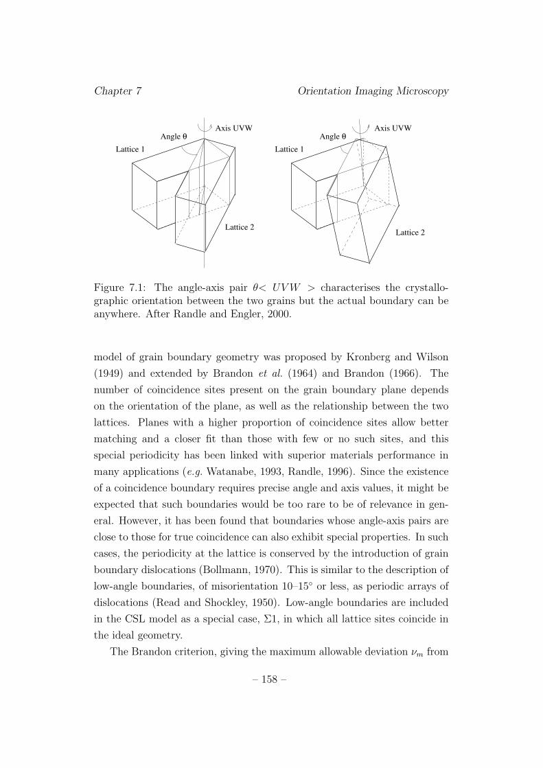
Chapter 7 Orientation Imaging Microscopy
Angle θAxis UVW
Lattice 2
Lattice 1
Angle θAxis UVW
Lattice 1
Lattice 2
Figure 7.1: The angle-axis pair θ< UV W > characterises the crystallo-graphic orientation between the two grains but the actual boundary can beanywhere. After Randle and Engler, 2000.
model of grain boundary geometry was proposed by Kronberg and Wilson
(1949) and extended by Brandon et al. (1964) and Brandon (1966). The
number of coincidence sites present on the grain boundary plane depends
on the orientation of the plane, as well as the relationship between the two
lattices. Planes with a higher proportion of coincidence sites allow better
matching and a closer fit than those with few or no such sites, and this
special periodicity has been linked with superior materials performance in
many applications (e.g. Watanabe, 1993, Randle, 1996). Since the existence
of a coincidence boundary requires precise angle and axis values, it might be
expected that such boundaries would be too rare to be of relevance in gen-
eral. However, it has been found that boundaries whose angle-axis pairs are
close to those for true coincidence can also exhibit special properties. In such
cases, the periodicity at the lattice is conserved by the introduction of grain
boundary dislocations (Bollmann, 1970). This is similar to the description of
low-angle boundaries, of misorientation 10–15◦ or less, as periodic arrays of
dislocations (Read and Shockley, 1950). Low-angle boundaries are included
in the CSL model as a special case, Σ1, in which all lattice sites coincide in
the ideal geometry.
The Brandon criterion, giving the maximum allowable deviation νm from
– 158 –
Chapter 7 Orientation Imaging Microscopy
ideal coincidence for a Σ coincidence boundary, is:
νm = ν0Σ−1/2 (7.6)
where ν0 is a constant of proportionality set to 15◦, the maximum allowable
deviation for a low-angle (Σ1) boundary. Thus, boundaries with smaller Σ
accommodate a greater possible deviation. This criterion is almost univer-
sally used for the categorisation of grain boundaries (Randle, 1993). The
Brandon ratio, characterising the deviation from coincidence, is the actual
misorientation normalised by νm for that value of Σ. When assessing grain
boundary types, the Σ for which the Brandon ratio is smallest is chosen.
Boundaries which do not fulfil the criterion for any CSL are designated as
random.
The 60◦ < 111 >, Σ3 boundary type is of particular interest. If the
boundary plane is either {111} or {211} as referred to the crystal lattice, this
is a twin boundary, in which all the sites in the plane are coincidence sites.
Most other low-Σ CSL boundaries also exhibit twinning on certain planes,
but it is the 60◦ < 111 > orientation which is most commonly referred to as
a ‘twin’ orientation in the literature (Randle, 1993).
7.2.2 Estimation of grain boundary energy
Grain boundaries have an intrinsic energy over and above that of the crystal
lattice. As reported by Randle (1996), grain boundary energies tend usu-
ally to correlate with the free volume at the boundary. The periodicity in
CSL arrangements reduces the free volume compared to random boundaries
and thus a lower energy is expected. Determination of the misorientation
dependence of boundary energies, by calculation or experiment, have mainly
been performed on high-symmetry boundaries in pure metals (e.g. Tsurekawa
et al., 1994; Nakashima and Takeuchi, 2000). General boundaries in alloys
are likely to have much higher energy (Randle, 1996). Extrinsic influences
on grain boundary energy include precipitates, lattice dislocations, vacancies
and impurity atoms, all of which tend to segregate to boundaries because
of the increased free volume. It is not, therefore, possible to estimate grain
– 159 –
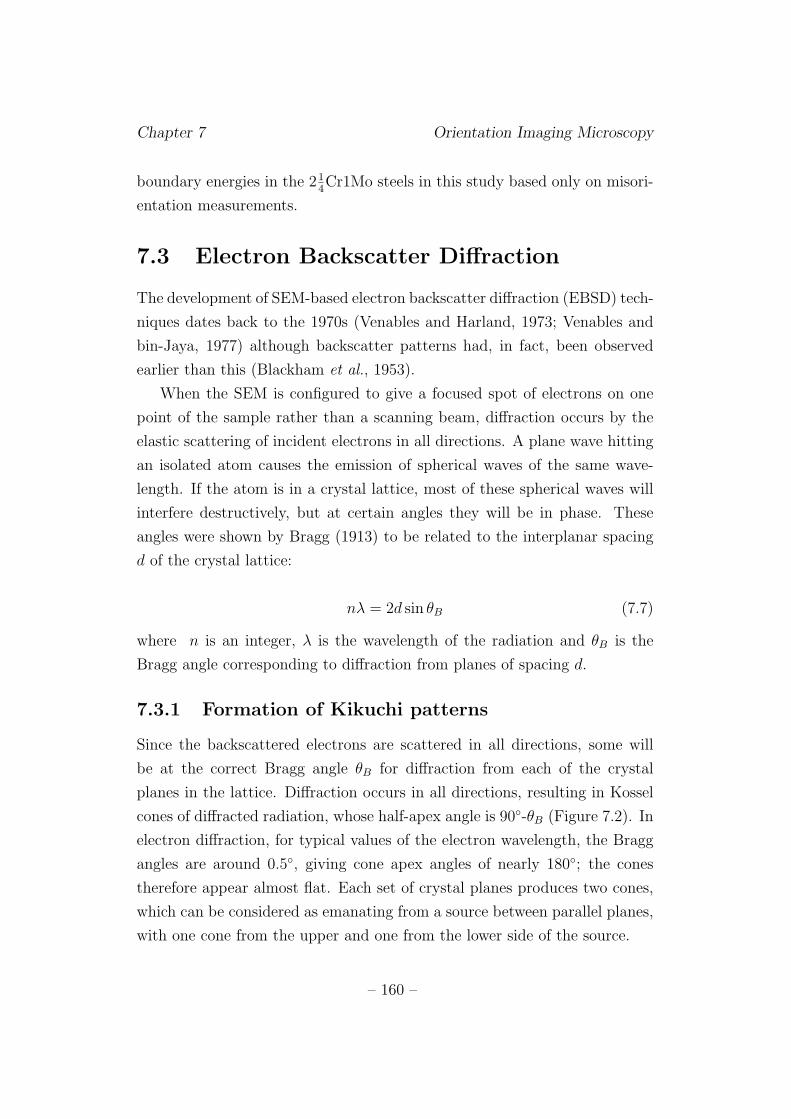
Chapter 7 Orientation Imaging Microscopy
boundary energies in the 214Cr1Mo steels in this study based only on misori-
entation measurements.
7.3 Electron Backscatter Diffraction
The development of SEM-based electron backscatter diffraction (EBSD) tech-
niques dates back to the 1970s (Venables and Harland, 1973; Venables and
bin-Jaya, 1977) although backscatter patterns had, in fact, been observed
earlier than this (Blackham et al., 1953).
When the SEM is configured to give a focused spot of electrons on one
point of the sample rather than a scanning beam, diffraction occurs by the
elastic scattering of incident electrons in all directions. A plane wave hitting
an isolated atom causes the emission of spherical waves of the same wave-
length. If the atom is in a crystal lattice, most of these spherical waves will
interfere destructively, but at certain angles they will be in phase. These
angles were shown by Bragg (1913) to be related to the interplanar spacing
d of the crystal lattice:
nλ = 2d sin θB (7.7)
where n is an integer, λ is the wavelength of the radiation and θB is the
Bragg angle corresponding to diffraction from planes of spacing d.
7.3.1 Formation of Kikuchi patterns
Since the backscattered electrons are scattered in all directions, some will
be at the correct Bragg angle θB for diffraction from each of the crystal
planes in the lattice. Diffraction occurs in all directions, resulting in Kossel
cones of diffracted radiation, whose half-apex angle is 90◦-θB (Figure 7.2). In
electron diffraction, for typical values of the electron wavelength, the Bragg
angles are around 0.5◦, giving cone apex angles of nearly 180◦; the cones
therefore appear almost flat. Each set of crystal planes produces two cones,
which can be considered as emanating from a source between parallel planes,
with one cone from the upper and one from the lower side of the source.
– 160 –
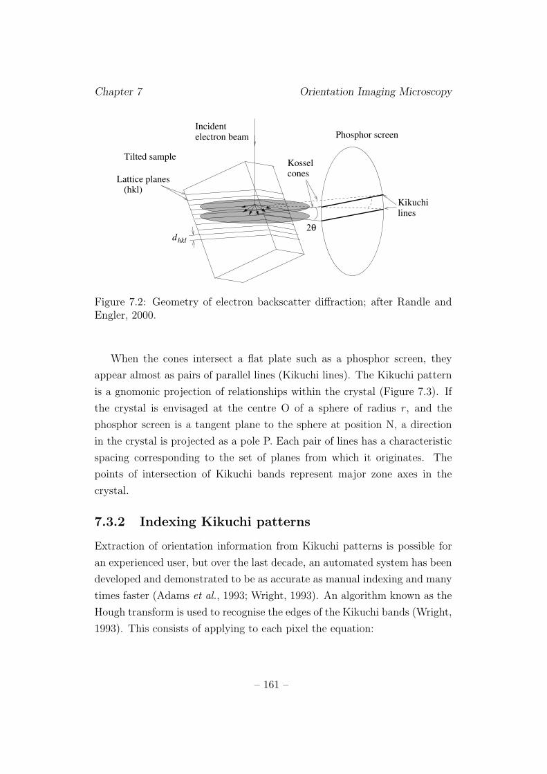
Chapter 7 Orientation Imaging Microscopy
dhkl
Incident electron beam
Kosselcones
linesKikuchi
Lattice planes (hkl)
Phosphor screen
2θ
Tilted sample
Figure 7.2: Geometry of electron backscatter diffraction; after Randle andEngler, 2000.
When the cones intersect a flat plate such as a phosphor screen, they
appear almost as pairs of parallel lines (Kikuchi lines). The Kikuchi pattern
is a gnomonic projection of relationships within the crystal (Figure 7.3). If
the crystal is envisaged at the centre O of a sphere of radius r, and the
phosphor screen is a tangent plane to the sphere at position N, a direction
in the crystal is projected as a pole P. Each pair of lines has a characteristic
spacing corresponding to the set of planes from which it originates. The
points of intersection of Kikuchi bands represent major zone axes in the
crystal.
7.3.2 Indexing Kikuchi patterns
Extraction of orientation information from Kikuchi patterns is possible for
an experienced user, but over the last decade, an automated system has been
developed and demonstrated to be as accurate as manual indexing and many
times faster (Adams et al., 1993; Wright, 1993). An algorithm known as the
Hough transform is used to recognise the edges of the Kikuchi bands (Wright,
1993). This consists of applying to each pixel the equation:
– 161 –
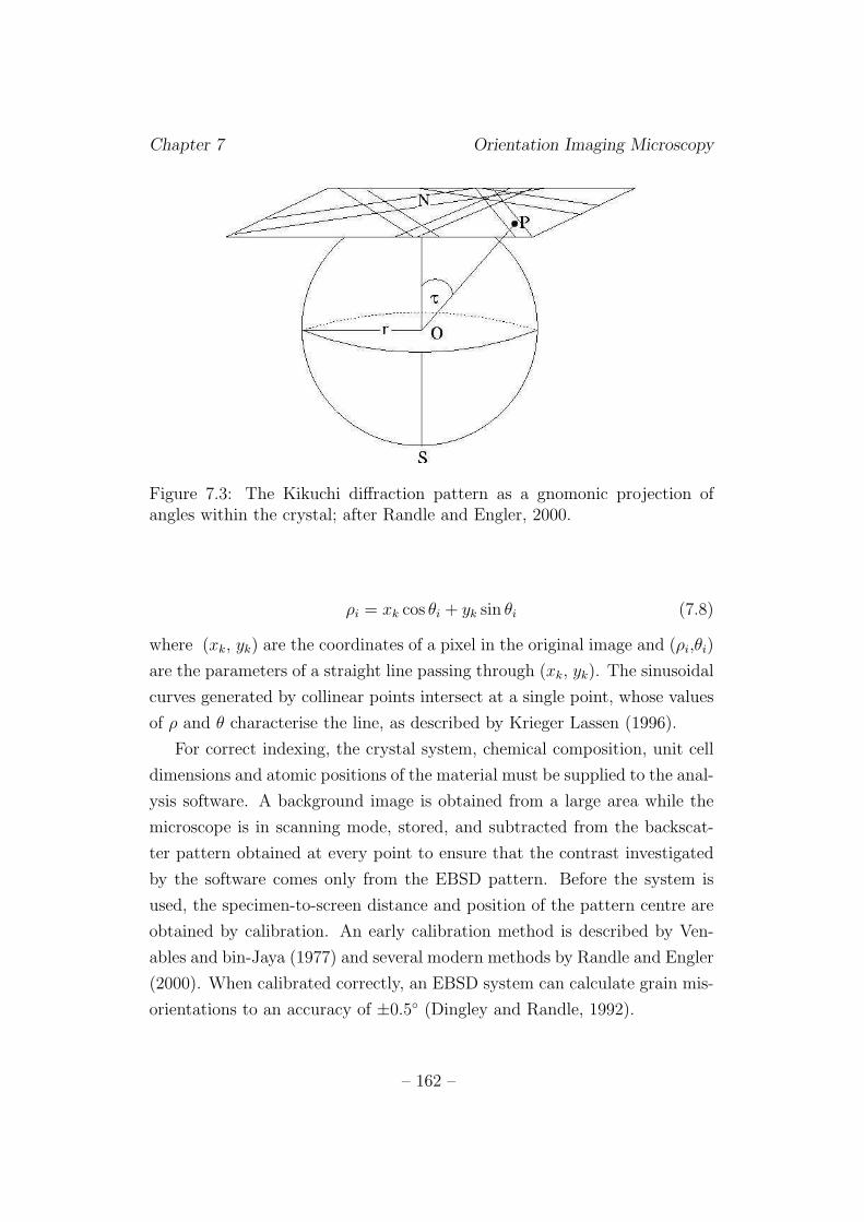
Chapter 7 Orientation Imaging Microscopy
Figure 7.3: The Kikuchi diffraction pattern as a gnomonic projection ofangles within the crystal; after Randle and Engler, 2000.
ρi = xk cos θi + yk sin θi (7.8)
where (xk, yk) are the coordinates of a pixel in the original image and (ρi,θi)
are the parameters of a straight line passing through (xk, yk). The sinusoidal
curves generated by collinear points intersect at a single point, whose values
of ρ and θ characterise the line, as described by Krieger Lassen (1996).
For correct indexing, the crystal system, chemical composition, unit cell
dimensions and atomic positions of the material must be supplied to the anal-
ysis software. A background image is obtained from a large area while the
microscope is in scanning mode, stored, and subtracted from the backscat-
ter pattern obtained at every point to ensure that the contrast investigated
by the software comes only from the EBSD pattern. Before the system is
used, the specimen-to-screen distance and position of the pattern centre are
obtained by calibration. An early calibration method is described by Ven-
ables and bin-Jaya (1977) and several modern methods by Randle and Engler
(2000). When calibrated correctly, an EBSD system can calculate grain mis-
orientations to an accuracy of ±0.5◦ (Dingley and Randle, 1992).
– 162 –
Chapter 7 Orientation Imaging Microscopy
7.3.3 Diffraction geometry in the SEM
Figure 7.4 shows the arrangement of the hardware for automated electron
backscatter diffraction. The sample is tilted through an angle of 70◦ to
the horizontal to reduce the path length of backscattered electrons and allow
more electrons to escape from the surface and be detected (Venables and Har-
land, 1973). It lies in the eucentric plane, enabling it to remain in focus when
the stage is moved in the surface plane, and is mounted on a piezoelectric
stage capable of motions of 0.1 µm. Modern systems use a forward-mounted
backscatter detector (the phosphor screen in Figure 7.4) and a camera to
record diffraction patterns (Randle and Engler, 2000).
Figure 7.4: Experimental setup for SEM-based EBSD at Tohoku University.Diagram by K. Kawahara; used with permission.
7.4 Automated Orientation Imaging
Microscopy
The development of automated Kikuchi pattern indexing led to the new
technique of Orientation Imaging Microscopy (OIM). Television-based sys-
tems for capturing backscatter patterns and computer systems able both to
– 163 –
Chapter 7 Orientation Imaging Microscopy
control the stage or electron beam position and to index patterns with min-
imal or no human intervention were developed (Adams et al., 1993; Wright
et al., 1993). This allows the rapid acquisition of a large number of orienta-
tion data. Current systems are able to solve a Kikuchi pattern in less than
one second using a standard PC (Randle and Engler, 2000).
The user typically programs in an array of positions from which orien-
tation data should be acquired by specifying the spatial range and step size
of sampling points. A hexagonal or square grid can be chosen but hexag-
onal tends to be preferred since each hexagon has six nearest neighbours,
while in a square grid, four nearest and four next-nearest neighbours must
be considered (Randle and Engler, 2000). A single data point is obtained
as follows: the stage is moved to a specified point, the camera captures the
Kikuchi pattern, and this is analysed and the Euler angles, stage position
and image quality (§ 7.4.2) are recorded (Wright, 1993).
7.4.1 Representation of data
Orientation mapping
Automated OIM allows maps of the spatial dependence of orientation data
to be plotted and related directly to microstructural features. Colour can
be used to represent particular orientations or texture components (Wright,
1993). OIM observations have demonstrated that variations in orientation
can occur within a single grain, making the definition of concepts such as
grain size less definite than was previously believed (Adams et al., 1993). In
addition, boundaries were apparent which could not be seen on a conventional
SEM image of the same area.
At grain boundaries, the Kikuchi patterns from neighbouring grains may
overlap, producing a complex pattern which cannot be solved correctly by
the indexing system (Adams et al., 1993). Various ‘clean-up’ algorithms
are available in the computer software to assign orientation values to such
indeterminate points. The criteria used for this operation by the algorithms
are described in detail in the software documentation, supplied by Tex-SEM
Ltd. The clean-up process does alter the data set and should not be used
– 164 –
Chapter 7 Orientation Imaging Microscopy
carelessly since it may introduce spurious features.
Grain boundary properties
Using the orientation data from neighbouring points, it is possible to deter-
mine the positions and misorientation angles of grain boundaries (Wright,
1993). Currently available software can identify coincidence boundaries and
produce a colour-coded map according to Σ. Adams et al. (1993) noted
that some of the boundaries identified appeared to terminate in grain inte-
riors. Since this is topographically impossible, it was attributed to differ-
ences in orientation along the boundaries which, in some positions, cause the
measured misorientation to fall below the arbitrarily designated minimum
misorientation required to identify a grain boundary. OIM analysis is only
two-dimensional and does not give information on the grain boundary plane
orientation, but serial sectioning techniques have been developed to study
this (Wall et al., 2001).
Statistical approaches
The large numbers of data acquired using OIM allow statistical analyses
of, for example, the distribution of misorientation angles θ between pairs
of sampling points (Wright, 1993). This can be compared with theoreti-
cal predictions assuming a random distribution or a particular orientation
relationship.
7.4.2 Image Quality
The image quality (IQ) of Kikuchi patterns, as represented by the sharp-
ness of the lines, has been quantified and related to the level of deformation
present in specimens (Quested et al., 1988; Wilkinson and Dingley, 1991).
The quantification method in current use was proposed by Krieger Lassen
et al. (1994) and gives IQ values between 0 and 1, where 0 represents the
worst image quality (no definition at all) and 1 the best. Since the devel-
opment of automated OIM, image quality measurements can be obtained at
every sampling point and displayed as a map. Minimum-quality points were
– 165 –
Chapter 7 Orientation Imaging Microscopy
found to coincide with grain boundaries (Adams et al., 1993; Wright, 1993)
but could also be present in certain areas within grain interiors. This was
attributed to high dislocation density. Image qualities were higher in certain
grains than in others.
As well as the deformation state, IQ depends on the accelerating voltage,
beam current, the state of the vacuum, the filament quality and alignment,
and the specimen preparation (Randle and Engler, 2000). It may also depend
on orientation but this has not yet been investigated fully. IQ measurements
are not, therefore, fully quantitative, but semi-quantitative comparisons can
be made within a single scan, enabling heavily deformed regions to be iden-
tified.
7.5 OIM observations of martensitic steels
7.5.1 Crystallographic relationships
A martensitic packet identified by optical microscopy or conventional SEM as
a region of parallel laths is designated a ‘morphological’ packet. By contrast,
a ‘crystallographic’ packet is a region of uniform orientation as determined by
EBSD. Gourgues et al. (2000) studied the relationship between the two packet
types in a low-alloy steel. Crystallographic packets were found to be much
smaller than morphological packets, and to correspond to the ‘blocks’ in Fig-
ure 2.4. Between neighbouring blocks of the same morphological packet, the
misorientation angle-axis pairs were mostly 60◦ < 111 > but occasionally 55◦
< 110 >. This suggests that the blocks within a packet have a close-packed
plane parallel to the same prior austenite prior austenite {111} plane and are
mostly twin related. The misorientation angle distribution had a peak for
θ = 60◦. This was compared with theoretical distributions for Kurdjumov-
Sachs and Nishiyama-Wasserman relationships, and it was concluded that
Kurdjumov-Sachs corresponded more closely to the real data.
Previous TEM work had shown that each individal martensitic lath could
nucleate with one of the six possible crystallographic variants from the same
austenite < 111 > (Chilton et al., 1970; Sarikaya et al., 1986). However,
– 166 –
Chapter 7 Orientation Imaging Microscopy
Gourgues et al. instead found that martensite formed blocks of many laths
with the same orientation.
Low-angle boundaries were found within crystallographic packets (blocks).
The internal structure of a packet consists of several slightly misoriented
groups of laths. The misorientations are present because of the high disloca-
tion density associated with the shear strain of transformation from austenite
to martensite.
In a 9 wt. % Cr steel subjected to a short tempering treatment after
quenching, crystallographic packet sizes increased slightly with increasing
prior austenite grain size (Barcelo et al., 2002). The pole figures of the
< 200 > axis from single prior austenite grains did not correspond directly
to either the Kurdjumov-Sachs or the Nishiyama-Wasserman relationship al-
though it showed some similarities to both. In small prior austenite grains
(∼15 µm), only a subset of the possible variants predicted by either relation-
ship were observed, but larger grains (> 40 µm) contained all the possible
variants.
7.5.2 Creep-deformed martensitic steels
In martensitic 9Cr1Mo, 9Cr3Co and 9Cr3W3Co (wt. %) steels, the mi-
crostructure was very inhomogeneous, with some blocks extending to 10 µm
and others as small as 1 µm (Nakashima et al., 2000, 2001; Yoshida et al.,
2002). Areas of indeterminate orientation were present, but these were elimi-
nated by creep deformation. They were attributed to high dislocation density,
which is reduced by dynamic recovery during creep.
The misorientation angle distribution for boundaries with common axis
< 110 > was determined. In the 9Cr1Mo steel, peaks were found at low an-
gles and in the regions around 60 and 80◦ . This agreed reasonably well with
the values of 10◦, 50.5◦ and 70.5◦ predicted from the Kurdjumov-Sachs rela-
tionship. Peaks at similar positions were found in the 9Cr3Co and 9Cr3W3Co
steels. Creep deformation of the 9Cr1Mo steel decreased the number of grain
boundaries with a specific orientation relationship and increased the number
of random boundaries.
– 167 –
Chapter 7 Orientation Imaging Microscopy
7.6 Experimental technique
7.6.1 Sample Preparation
An AQ sample and samples tempered at 600◦C for 4, 16, 64, 128 and
256 hours were selected for observation. They were prepared as described in
§ 6.1, but instead of the final polishing stage described there, they were pol-
ished to 6 µm using diamond paste, and to 0.1 µm using alumina slurry. They
were then electropolished using a mixture of 164 cm3 acetic acid, 18 cm3 per-
chloric acid and 18 cm3 methanol which was cooled in iced water and stirred
during polishing. The polishing conditions were 20–30 V for 3–5 minutes,
with adjustments made depending on the appearances of the surfaces.
7.6.2 Orientation Imaging Microscopy
A Hitachi S-4200 Field Emission Gun Scanning Electron Microscope (FEG-
SEM), belonging to the Materials Design and Interface Engineering Labora-
tory at Tohoku University, was used for the observations. The OIM system
is shown schematically in Figure 7.4.
The accelerating voltage was 30 kV, the beam current 50 pA, and the
beam penetration depth several tens of nanometres. A large spot size was
used to maximise the backscattered signal. Operation of the OIM system
was controlled using purpose-designed software by Tex-SEM Ltd. The step
size was set to 0.1 µm, and the magnification to 6000×, to allow investigation
on the lath scale.
Before acquisition of each data set, EBSD patterns were obtained from
points on the sample surface to check the image quality. If this was adequate,
a 14 x 15 µm area on the surface was selected and imaged using conventional
SEM. After changing to backscatter mode, the scan was begun and left to
run automatically. A complete scan took between two and three hours using
this system.
Three scans were obtained from each of the steel samples at different
positions on the surface. However, since the working distance between the
pole piece and surface should be kept at approximately 15 mm for EBSD,
– 168 –
Chapter 7 Orientation Imaging Microscopy
this only gave a limited range of regions for sampling.
7.7 Results
OIM maps and micrographs are presented in Figure 7.7–Figure 7.24. On each
page, the top two diagrams are colour-coded maps of the orientation of the
sample normal axis with respect to the crystal axes of the lattice. The colour
key is given in Figure 7.5. The maps do not give comprehensive information,
since there is a degree of freedom in rotation perpendicular to this direction,
but it is possible to identify both gradual and abrupt orientation changes by
their differences in colour.
The top left-hand diagram contains the raw orientation data, including
indeterminate points, and the right-hand diagram is the result of a ‘clean-
up’ algorithm, Grain Dilation. This takes an indeterminate point bordered
by points belonging to grains, and assigns an orientation to it based on the
orientations of its neighbours. (Full details of its operation are given in
the software documentation.) The algorithm is iterative and operates until
all points have been assigned to grains. The user is prompted to supply the
minimum number of points which must be in a cluster if it is to be considered
a grain; in this study, this was set at 4.
Beneath the raw data map is a grey-scale map of image quality. The
lighter the colour, the higher the IQ. To the right of this is a grain boundary
map calculated from the cleaned orientation data. These were used in pref-
erence to the raw data because most of the indeterminate points occurred at
grain boundaries, obscuring the true orientation relationships between the
grains. Figure 7.6 is the colour key for this map: red represents a low-angle
boundary (2 ≤ θ < 15◦), light green is Σ3, black is random, and other colours
are used to represent boundaries with different Σ values, as determined by
the Brandon criterion. Misorientations of < 2◦ between adjacent points are
not considered to be grain boundaries.
The lowest image is a conventional SEM micrograph of the same area.
The electropolishing removes much of the surface relief, so some of these
images are of poor quality.
– 169 –
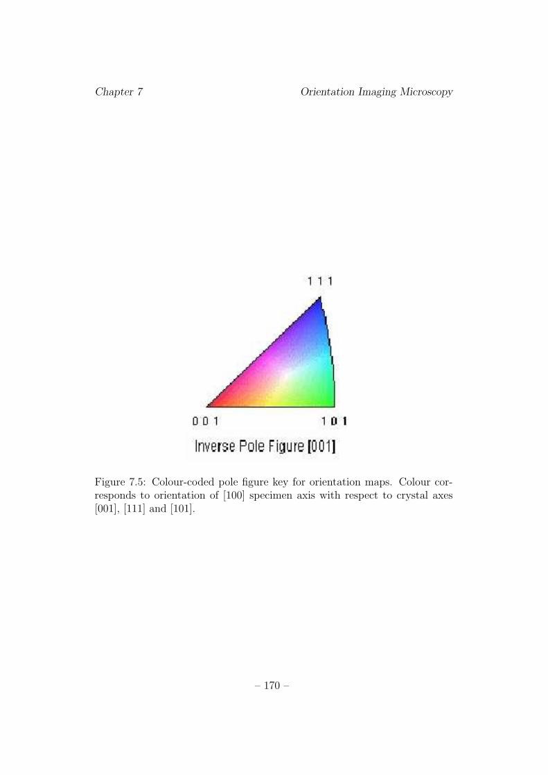
Chapter 7 Orientation Imaging Microscopy
Figure 7.5: Colour-coded pole figure key for orientation maps. Colour cor-responds to orientation of [100] specimen axis with respect to crystal axes[001], [111] and [101].
– 170 –
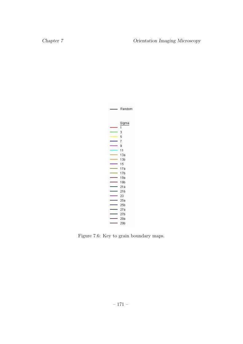
Chapter 7 Orientation Imaging Microscopy
Figure 7.6: Key to grain boundary maps.
– 171 –
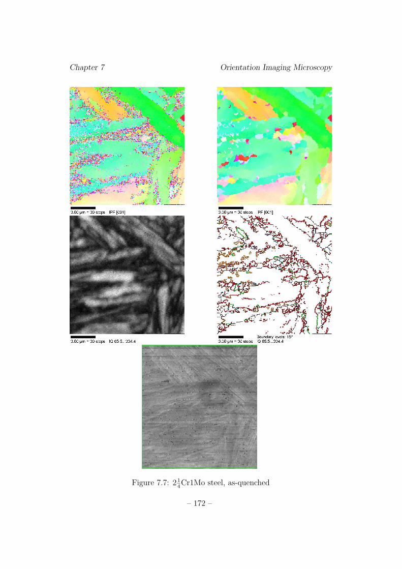
Chapter 7 Orientation Imaging Microscopy
Figure 7.7: 214Cr1Mo steel, as-quenched
– 172 –
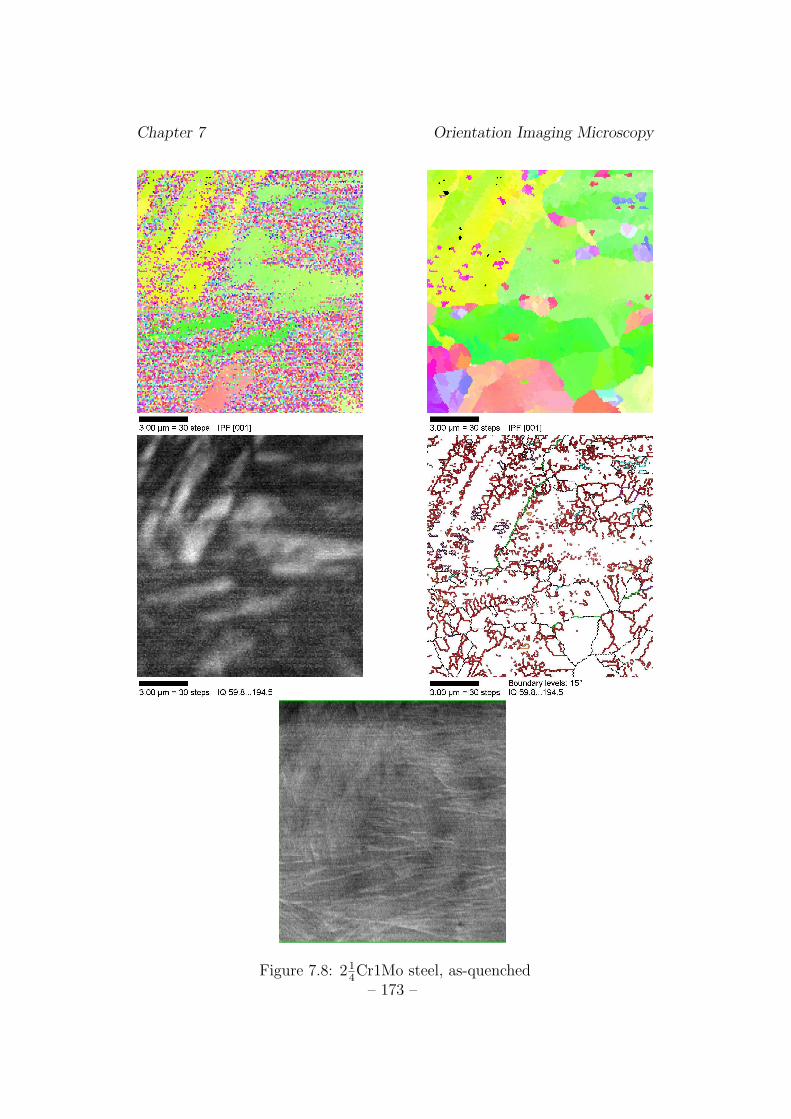
Chapter 7 Orientation Imaging Microscopy
Figure 7.8: 214Cr1Mo steel, as-quenched
– 173 –
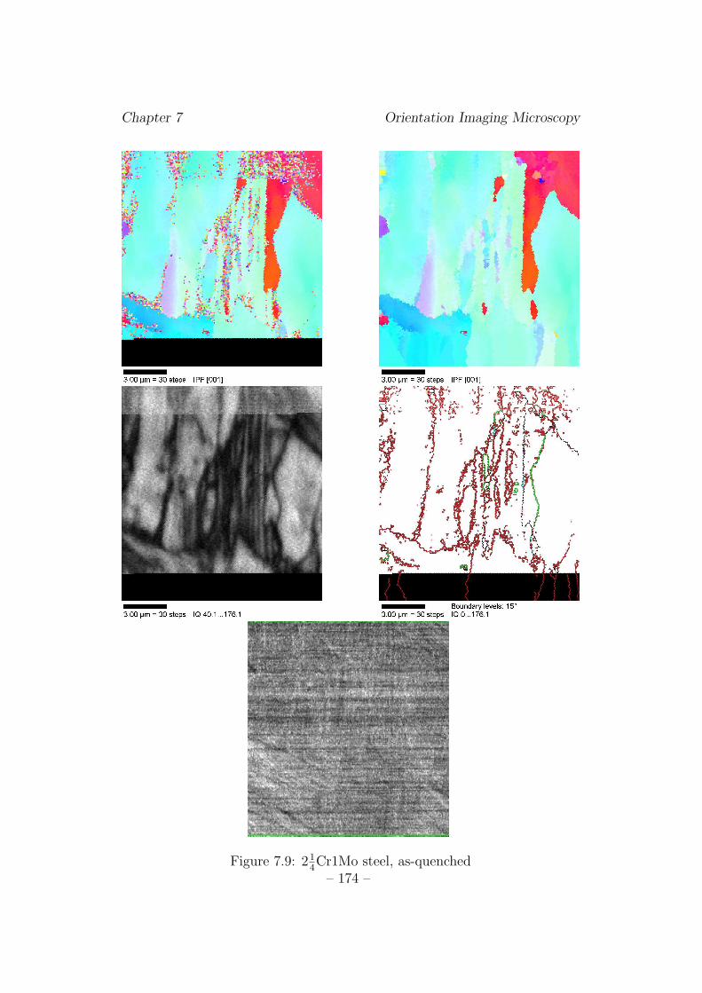
Chapter 7 Orientation Imaging Microscopy
Figure 7.9: 214Cr1Mo steel, as-quenched
– 174 –

Chapter 7 Orientation Imaging Microscopy
Figure 7.10: 214Cr1Mo steel, 600 ◦C, 4 hours tempering
– 175 –
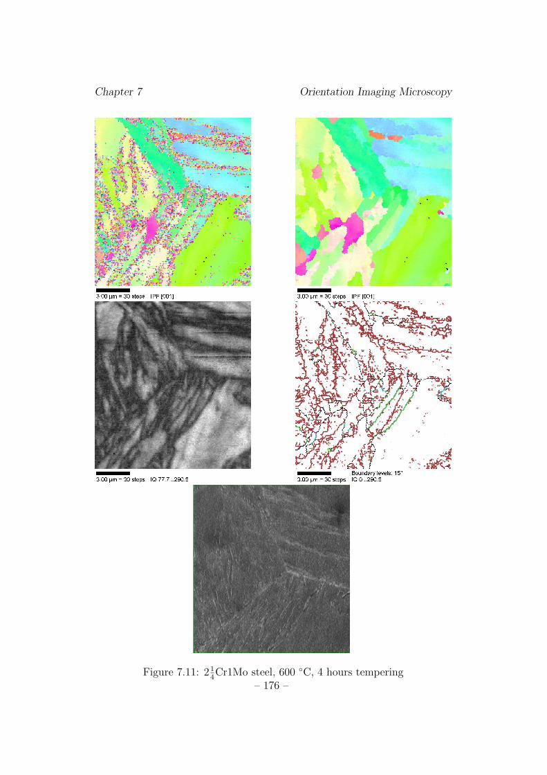
Chapter 7 Orientation Imaging Microscopy
Figure 7.11: 214Cr1Mo steel, 600 ◦C, 4 hours tempering
– 176 –
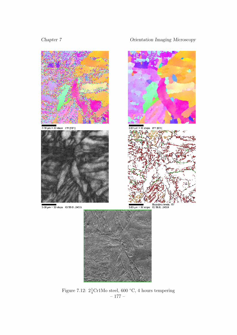
Chapter 7 Orientation Imaging Microscopy
Figure 7.12: 214Cr1Mo steel, 600 ◦C, 4 hours tempering
– 177 –
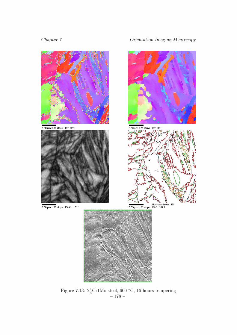
Chapter 7 Orientation Imaging Microscopy
Figure 7.13: 214Cr1Mo steel, 600 ◦C, 16 hours tempering
– 178 –
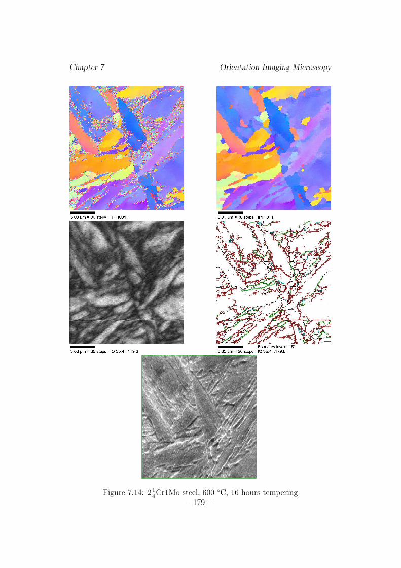
Chapter 7 Orientation Imaging Microscopy
Figure 7.14: 214Cr1Mo steel, 600 ◦C, 16 hours tempering
– 179 –
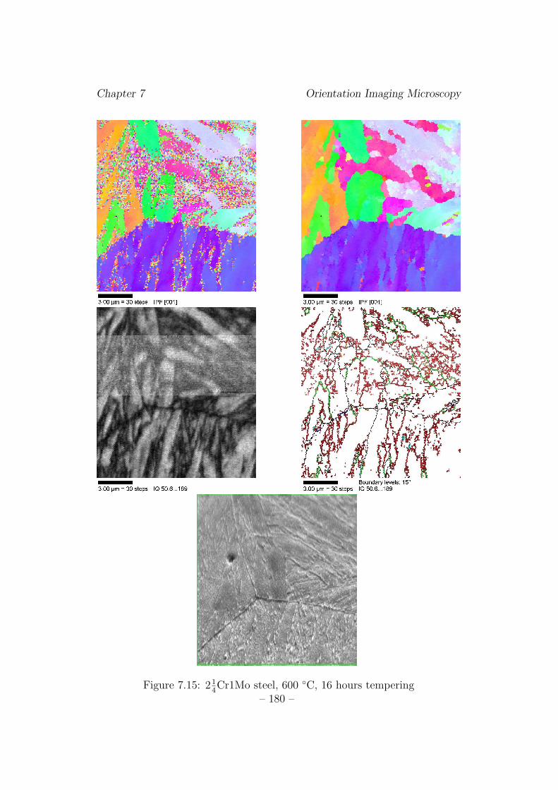
Chapter 7 Orientation Imaging Microscopy
Figure 7.15: 214Cr1Mo steel, 600 ◦C, 16 hours tempering
– 180 –
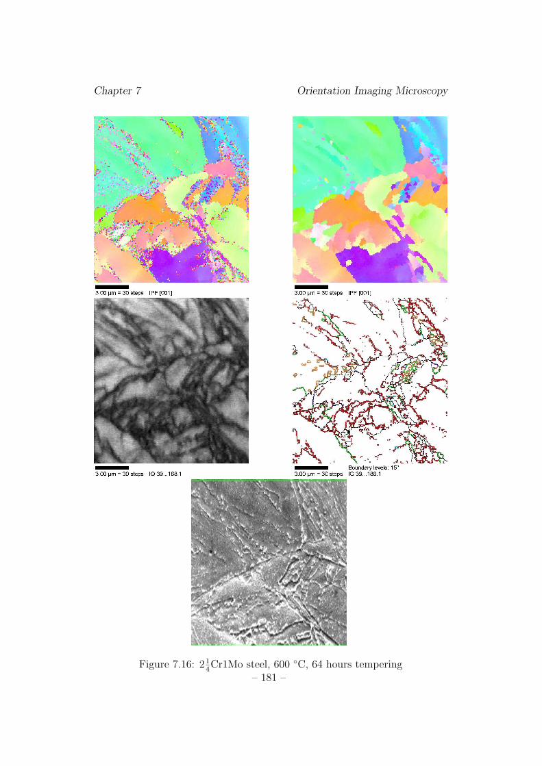
Chapter 7 Orientation Imaging Microscopy
Figure 7.16: 214Cr1Mo steel, 600 ◦C, 64 hours tempering
– 181 –
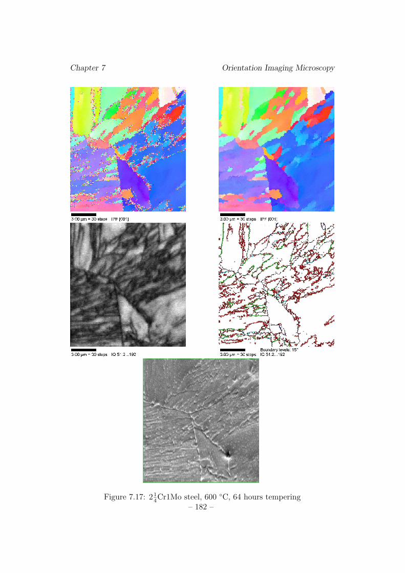
Chapter 7 Orientation Imaging Microscopy
Figure 7.17: 214Cr1Mo steel, 600 ◦C, 64 hours tempering
– 182 –
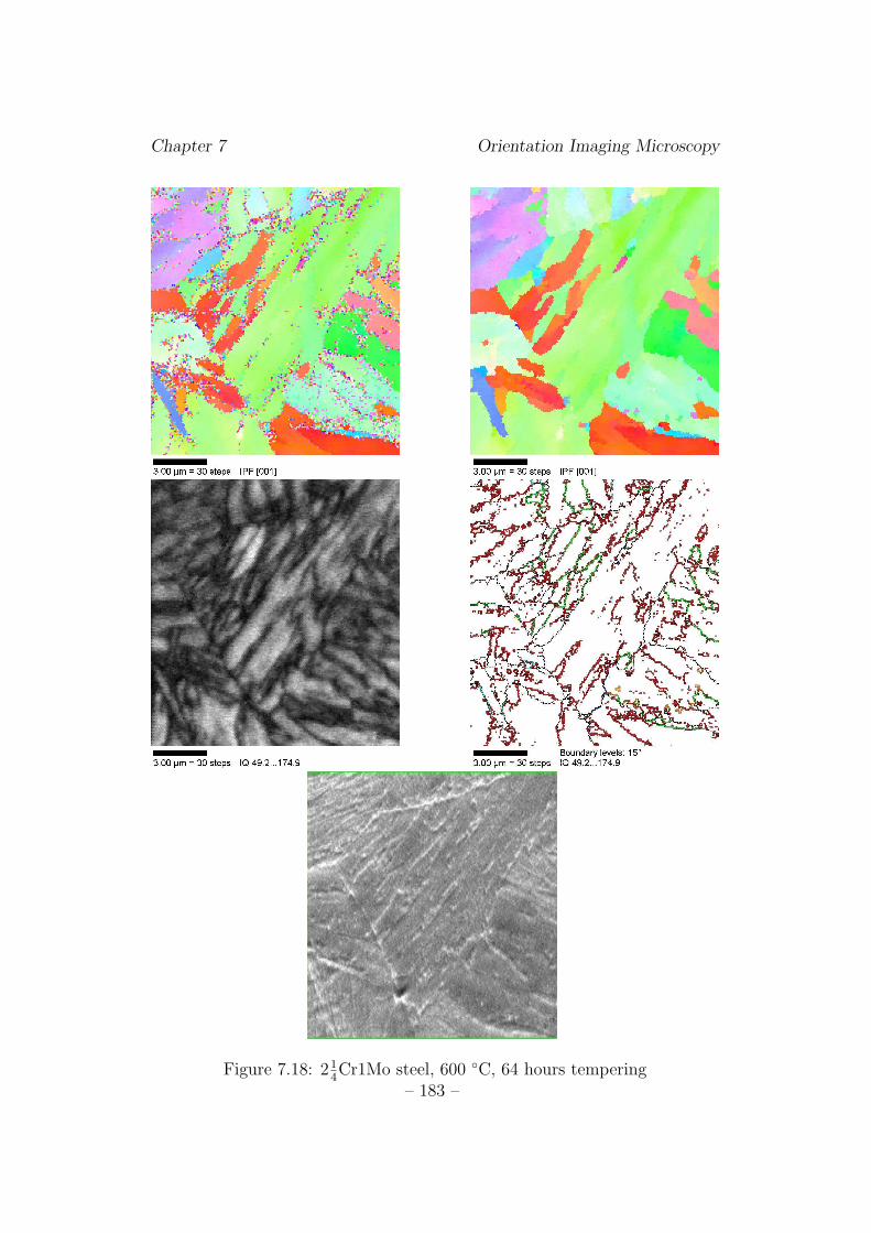
Chapter 7 Orientation Imaging Microscopy
Figure 7.18: 214Cr1Mo steel, 600 ◦C, 64 hours tempering
– 183 –
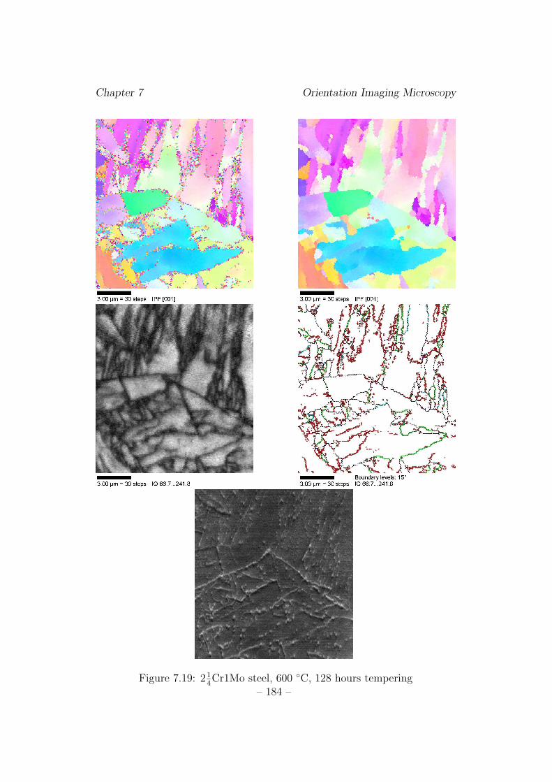
Chapter 7 Orientation Imaging Microscopy
Figure 7.19: 214Cr1Mo steel, 600 ◦C, 128 hours tempering
– 184 –
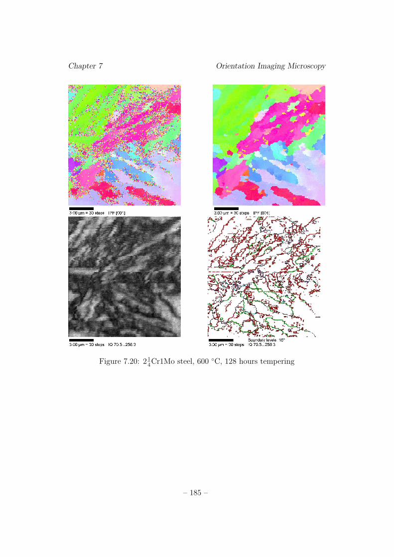
Chapter 7 Orientation Imaging Microscopy
Figure 7.20: 214Cr1Mo steel, 600 ◦C, 128 hours tempering
– 185 –
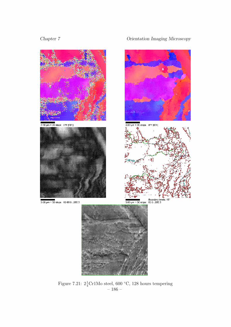
Chapter 7 Orientation Imaging Microscopy
Figure 7.21: 214Cr1Mo steel, 600 ◦C, 128 hours tempering
– 186 –
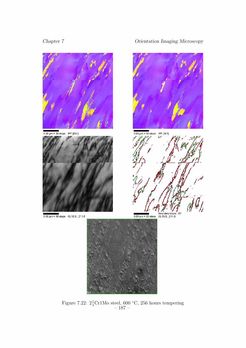
Chapter 7 Orientation Imaging Microscopy
Figure 7.22: 214Cr1Mo steel, 600 ◦C, 256 hours tempering
– 187 –
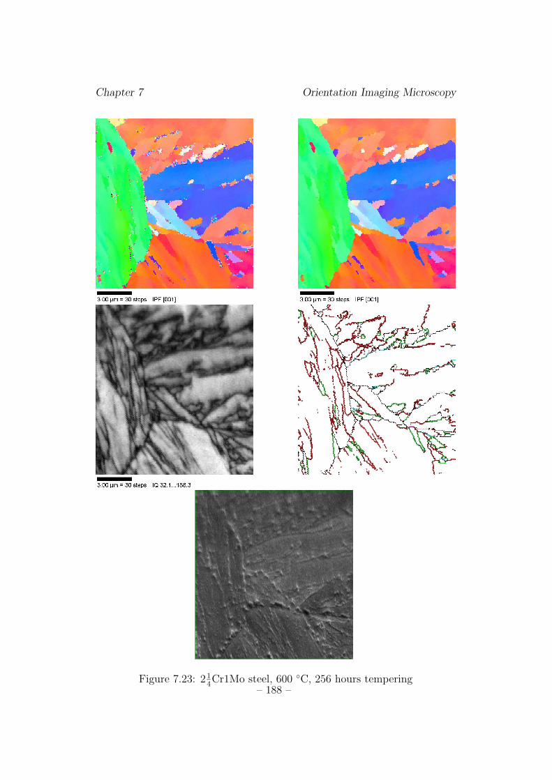
Chapter 7 Orientation Imaging Microscopy
Figure 7.23: 214Cr1Mo steel, 600 ◦C, 256 hours tempering
– 188 –
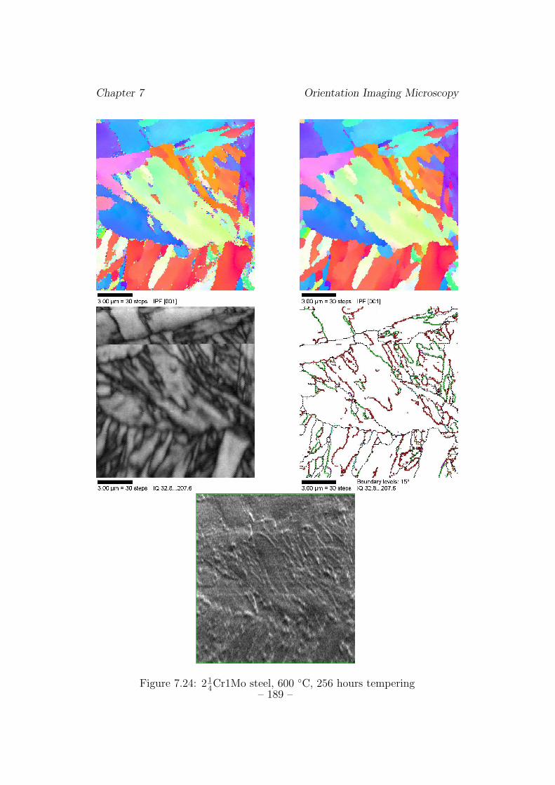
Chapter 7 Orientation Imaging Microscopy
Figure 7.24: 214Cr1Mo steel, 600 ◦C, 256 hours tempering
– 189 –
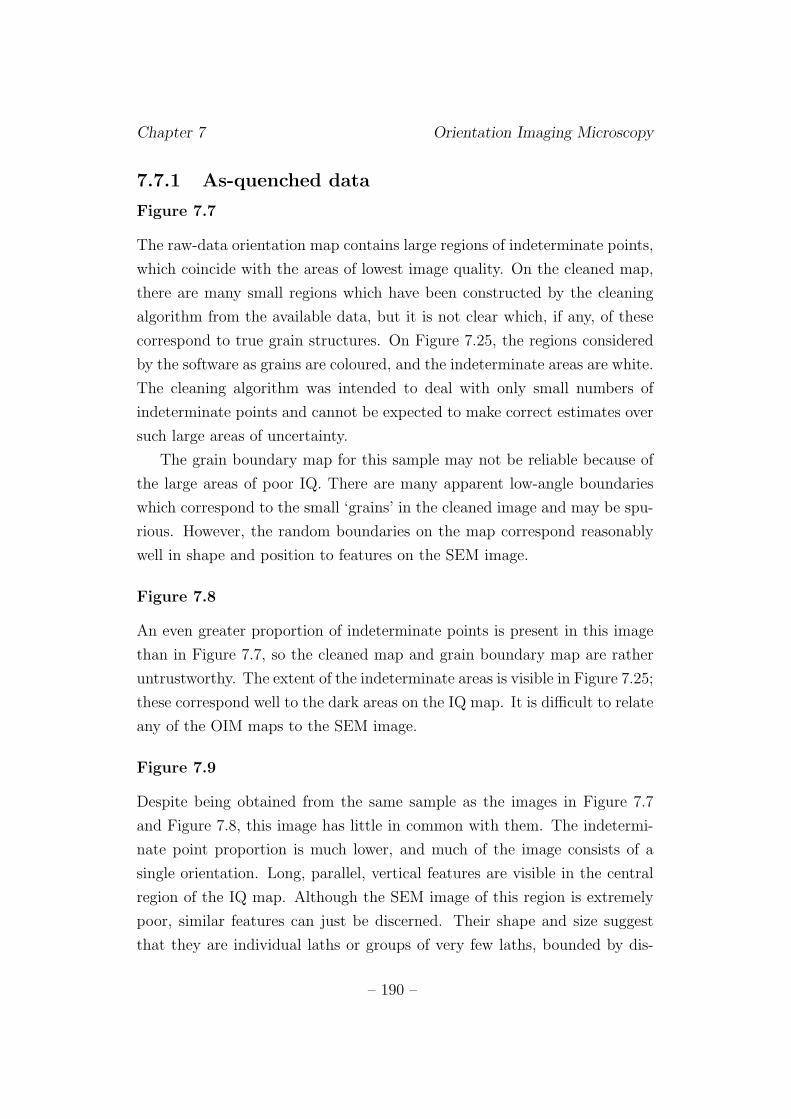
Chapter 7 Orientation Imaging Microscopy
7.7.1 As-quenched data
Figure 7.7
The raw-data orientation map contains large regions of indeterminate points,
which coincide with the areas of lowest image quality. On the cleaned map,
there are many small regions which have been constructed by the cleaning
algorithm from the available data, but it is not clear which, if any, of these
correspond to true grain structures. On Figure 7.25, the regions considered
by the software as grains are coloured, and the indeterminate areas are white.
The cleaning algorithm was intended to deal with only small numbers of
indeterminate points and cannot be expected to make correct estimates over
such large areas of uncertainty.
The grain boundary map for this sample may not be reliable because of
the large areas of poor IQ. There are many apparent low-angle boundaries
which correspond to the small ‘grains’ in the cleaned image and may be spu-
rious. However, the random boundaries on the map correspond reasonably
well in shape and position to features on the SEM image.
Figure 7.8
An even greater proportion of indeterminate points is present in this image
than in Figure 7.7, so the cleaned map and grain boundary map are rather
untrustworthy. The extent of the indeterminate areas is visible in Figure 7.25;
these correspond well to the dark areas on the IQ map. It is difficult to relate
any of the OIM maps to the SEM image.
Figure 7.9
Despite being obtained from the same sample as the images in Figure 7.7
and Figure 7.8, this image has little in common with them. The indetermi-
nate point proportion is much lower, and much of the image consists of a
single orientation. Long, parallel, vertical features are visible in the central
region of the IQ map. Although the SEM image of this region is extremely
poor, similar features can just be discerned. Their shape and size suggest
that they are individual laths or groups of very few laths, bounded by dis-
– 190 –
Chapter 7 Orientation Imaging Microscopy
As-quenched; Figure 7.7 As-quenched; Figure 7.8
As-quenched; Figure 7.9600◦C, 256 hour tempered; Fig-ure 7.23
Figure 7.25: Maps with regions identified as unique grains marked in colour,and indeterminate regions in white.
– 191 –
Chapter 7 Orientation Imaging Microscopy
located regions. Their misorientation angle is very small; since the grain
boundary map shows discontinuous low-angle boundaries in this region, it
must be around 2◦. In other parts of the image, there are gradual orienta-
tion variations without any clearly visible lath boundaries. The red region
towards the right-hand side is partly bounded by a Σ3 boundary and may
be a twin-related variant of the light-blue orientation.
7.7.2 Indeterminate points
The presence of indeterminate points may be due to retained austenite or to
martensite tetragonality. The data supplied to the software assumed a body-
centred structure, so if other crystal structures were present, their Kikuchi
lines would be incorrectly indexed. This would give rise to problems in orien-
tation determination where these phases were prevalent. OIM software can
index multiphase microstructures if the correct lattice constants are provided
for each, so it is possible to repeat the experiments on these samples to check
for other phases. However, another possible origin of the indexing problem
is low Kikuchi pattern image quality. This results from high strain and does
not depend on the assumed crystal structure. Since regions of low IQ con-
sistently coincide with indeterminate point regions, it is suggested that high
strain, rather than incorrect crystal structure data, is the main cause.
7.7.3 600◦C, 4 hours tempering
Figure 7.10
Many indeterminate points are still present after four hours of tempering, but
they are more evenly distributed. Laths or groups of laths can be identified
by their edges on the image quality map and by small changes at their edges
on the orientation map. The grain boundary map contains many, probably
spurious, discontinuous boundaries but also some more clearly defined low-
angle boundaries with equivalents on the other maps.
– 192 –
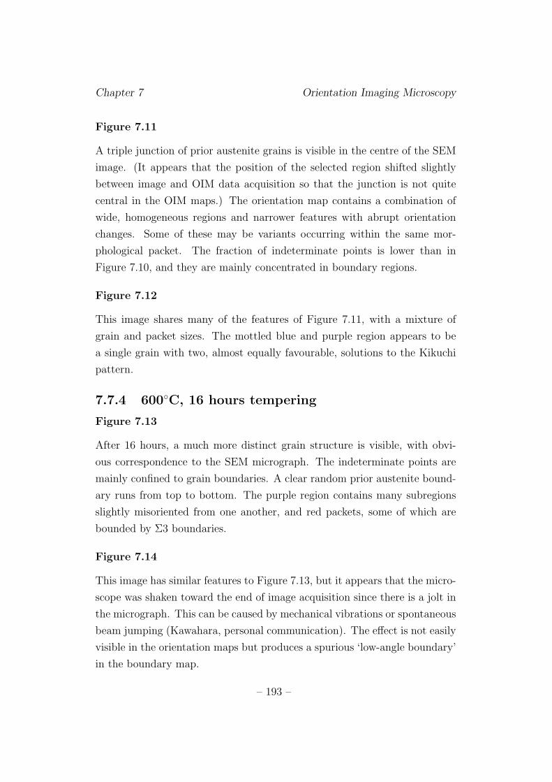
Chapter 7 Orientation Imaging Microscopy
Figure 7.11
A triple junction of prior austenite grains is visible in the centre of the SEM
image. (It appears that the position of the selected region shifted slightly
between image and OIM data acquisition so that the junction is not quite
central in the OIM maps.) The orientation map contains a combination of
wide, homogeneous regions and narrower features with abrupt orientation
changes. Some of these may be variants occurring within the same mor-
phological packet. The fraction of indeterminate points is lower than in
Figure 7.10, and they are mainly concentrated in boundary regions.
Figure 7.12
This image shares many of the features of Figure 7.11, with a mixture of
grain and packet sizes. The mottled blue and purple region appears to be
a single grain with two, almost equally favourable, solutions to the Kikuchi
pattern.
7.7.4 600◦C, 16 hours tempering
Figure 7.13
After 16 hours, a much more distinct grain structure is visible, with obvi-
ous correspondence to the SEM micrograph. The indeterminate points are
mainly confined to grain boundaries. A clear random prior austenite bound-
ary runs from top to bottom. The purple region contains many subregions
slightly misoriented from one another, and red packets, some of which are
bounded by Σ3 boundaries.
Figure 7.14
This image has similar features to Figure 7.13, but it appears that the micro-
scope was shaken toward the end of image acquisition since there is a jolt in
the micrograph. This can be caused by mechanical vibrations or spontaneous
beam jumping (Kawahara, personal communication). The effect is not easily
visible in the orientation maps but produces a spurious ‘low-angle boundary’
in the boundary map.
– 193 –
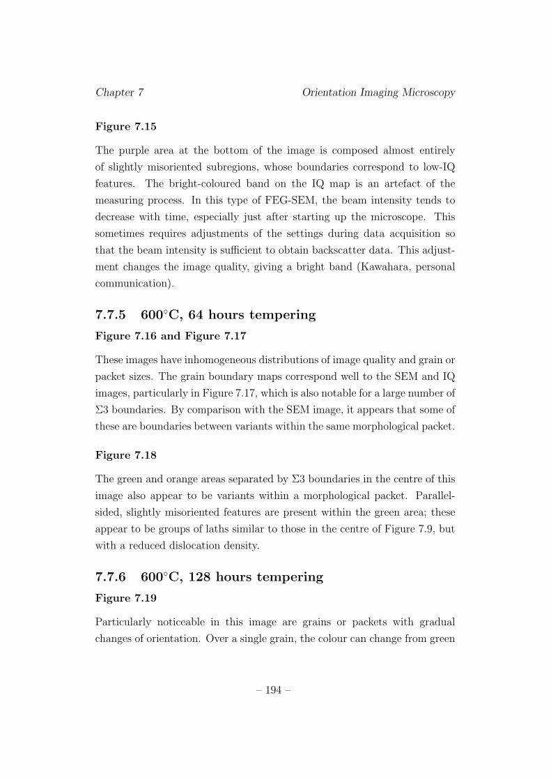
Chapter 7 Orientation Imaging Microscopy
Figure 7.15
The purple area at the bottom of the image is composed almost entirely
of slightly misoriented subregions, whose boundaries correspond to low-IQ
features. The bright-coloured band on the IQ map is an artefact of the
measuring process. In this type of FEG-SEM, the beam intensity tends to
decrease with time, especially just after starting up the microscope. This
sometimes requires adjustments of the settings during data acquisition so
that the beam intensity is sufficient to obtain backscatter data. This adjust-
ment changes the image quality, giving a bright band (Kawahara, personal
communication).
7.7.5 600◦C, 64 hours tempering
Figure 7.16 and Figure 7.17
These images have inhomogeneous distributions of image quality and grain or
packet sizes. The grain boundary maps correspond well to the SEM and IQ
images, particularly in Figure 7.17, which is also notable for a large number of
Σ3 boundaries. By comparison with the SEM image, it appears that some of
these are boundaries between variants within the same morphological packet.
Figure 7.18
The green and orange areas separated by Σ3 boundaries in the centre of this
image also appear to be variants within a morphological packet. Parallel-
sided, slightly misoriented features are present within the green area; these
appear to be groups of laths similar to those in the centre of Figure 7.9, but
with a reduced dislocation density.
7.7.6 600◦C, 128 hours tempering
Figure 7.19
Particularly noticeable in this image are grains or packets with gradual
changes of orientation. Over a single grain, the colour can change from green
– 194 –
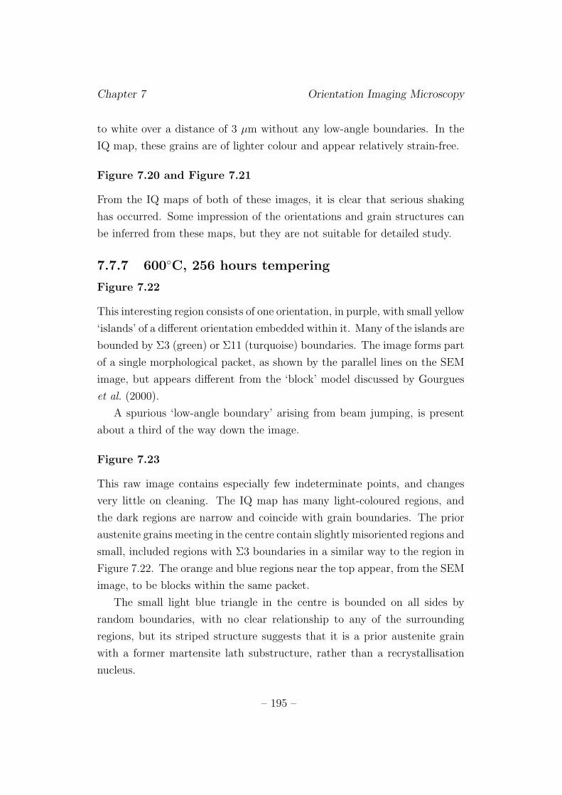
Chapter 7 Orientation Imaging Microscopy
to white over a distance of 3 µm without any low-angle boundaries. In the
IQ map, these grains are of lighter colour and appear relatively strain-free.
Figure 7.20 and Figure 7.21
From the IQ maps of both of these images, it is clear that serious shaking
has occurred. Some impression of the orientations and grain structures can
be inferred from these maps, but they are not suitable for detailed study.
7.7.7 600◦C, 256 hours tempering
Figure 7.22
This interesting region consists of one orientation, in purple, with small yellow
‘islands’ of a different orientation embedded within it. Many of the islands are
bounded by Σ3 (green) or Σ11 (turquoise) boundaries. The image forms part
of a single morphological packet, as shown by the parallel lines on the SEM
image, but appears different from the ‘block’ model discussed by Gourgues
et al. (2000).
A spurious ‘low-angle boundary’ arising from beam jumping, is present
about a third of the way down the image.
Figure 7.23
This raw image contains especially few indeterminate points, and changes
very little on cleaning. The IQ map has many light-coloured regions, and
the dark regions are narrow and coincide with grain boundaries. The prior
austenite grains meeting in the centre contain slightly misoriented regions and
small, included regions with Σ3 boundaries in a similar way to the region in
Figure 7.22. The orange and blue regions near the top appear, from the SEM
image, to be blocks within the same packet.
The small light blue triangle in the centre is bounded on all sides by
random boundaries, with no clear relationship to any of the surrounding
regions, but its striped structure suggests that it is a prior austenite grain
with a former martensite lath substructure, rather than a recrystallisation
nucleus.
– 195 –
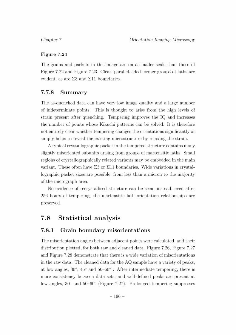
Chapter 7 Orientation Imaging Microscopy
Figure 7.24
The grains and packets in this image are on a smaller scale than those of
Figure 7.22 and Figure 7.23. Clear, parallel-sided former groups of laths are
evident, as are Σ3 and Σ11 boundaries.
7.7.8 Summary
The as-quenched data can have very low image quality and a large number
of indeterminate points. This is thought to arise from the high levels of
strain present after quenching. Tempering improves the IQ and increases
the number of points whose Kikuchi patterns can be solved. It is therefore
not entirely clear whether tempering changes the orientations significantly or
simply helps to reveal the existing microstructure by relaxing the strain.
A typical crystallographic packet in the tempered structure contains many
slightly misoriented subunits arising from groups of martensitic laths. Small
regions of crystallographically related variants may be embedded in the main
variant. These often have Σ3 or Σ11 boundaries. Wide variations in crystal-
lographic packet sizes are possible, from less than a micron to the majority
of the micrograph area.
No evidence of recrystallised structure can be seen; instead, even after
256 hours of tempering, the martensitic lath orientation relationships are
preserved.
7.8 Statistical analysis
7.8.1 Grain boundary misorientations
The misorientation angles between adjacent points were calculated, and their
distribution plotted, for both raw and cleaned data. Figure 7.26, Figure 7.27
and Figure 7.28 demonstrate that there is a wide variation of misorientations
in the raw data. The cleaned data for the AQ sample have a variety of peaks,
at low angles, 30◦, 45◦ and 50–60◦ . After intermediate tempering, there is
more consistency between data sets, and well-defined peaks are present at
low angles, 30◦ and 50–60◦ (Figure 7.27). Prolonged tempering suppresses
– 196 –
Chapter 7 Orientation Imaging Microscopy
the 30◦ peak (Figure 7.28). In the raw data, the indeterminate points con-
tribute to the statistics of misorientations, and it is only by removing them
that real relationships can be revealed. However, as discussed above, the
cleaning algorithm is not infallible, especially when there are many indeter-
minate points, so the data from longer tempering times are probably more
trustworthy than those from the AQ and 4 hour samples.
These observations agree well with those of Gourgues et al., who also
detected a peak at 60◦.
7.8.2 Coincidence boundaries
Figure 7.29 shows the variation in the fraction of low-angle, Σ3 and random
boundaries, as obtained from the cleaned data, with tempering time. In all of
these specimens, the fraction of boundaries of any other type than these three
is extremely small. Only one set of data was included for 128 hours because
of the image shaking problem affecting the other sets. A decrease in the
low-angle boundary fraction and an increase in Σ3 and random boundaries
occurs during tempering. This may be a real phenomenon, or simply the
result of the disappearance of spurious low-angle boundaries arising from
indeterminate points and cleaning.
Low-angle and random boundaries are the predominant types, with a
significant minority of Σ3. It can be seen by inspection of grain boundary
maps that prior austenite boundaries are always random, and the internal
structure of prior austenite grains contains many low-angle boundaries, some
Σ3 and some random boundaries.
7.8.3 Statistics of indeterminate points
The number of indeterminate points in each image was quantified by gener-
ating an image similar to those in Figure 7.25 and converting it to a black-
and-white image as shown in Figure 7.30. An image analysis program, ‘Im-
ageTool’, was then used to determine the fraction of the image occupied by
black points.
Figure 7.31 shows the relationship between the indeterminate point frac-
– 197 –
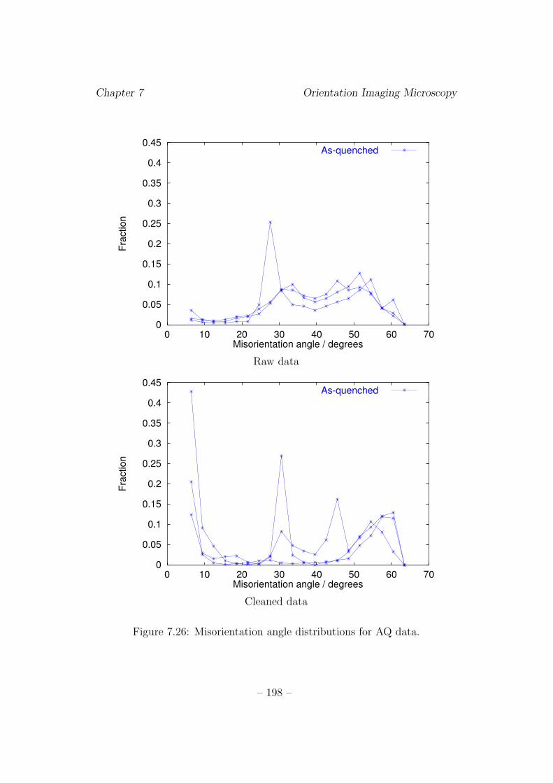
Chapter 7 Orientation Imaging Microscopy
0
0.05
0.1
0.15
0.2
0.25
0.3
0.35
0.4
0.45
0 10 20 30 40 50 60 70
Fra
ction
Misorientation angle / degrees
As-quenched
Raw data
0
0.05
0.1
0.15
0.2
0.25
0.3
0.35
0.4
0.45
0 10 20 30 40 50 60 70
Fra
ction
Misorientation angle / degrees
As-quenched
Cleaned data
Figure 7.26: Misorientation angle distributions for AQ data.
– 198 –
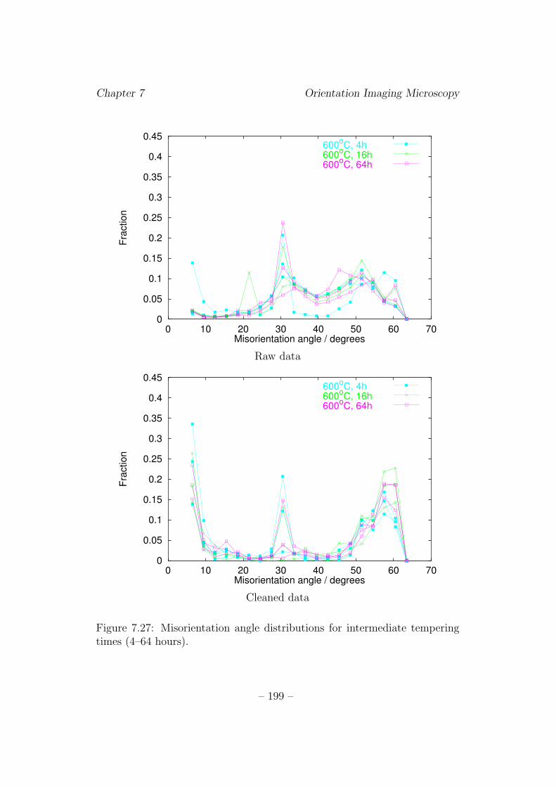
Chapter 7 Orientation Imaging Microscopy
0
0.05
0.1
0.15
0.2
0.25
0.3
0.35
0.4
0.45
0 10 20 30 40 50 60 70
Fra
ction
Misorientation angle / degrees
600oC, 4h
600oC, 16h
600oC, 64h
Raw data
0
0.05
0.1
0.15
0.2
0.25
0.3
0.35
0.4
0.45
0 10 20 30 40 50 60 70
Fra
ction
Misorientation angle / degrees
600oC, 4h
600oC, 16h
600oC, 64h
Cleaned data
Figure 7.27: Misorientation angle distributions for intermediate temperingtimes (4–64 hours).
– 199 –
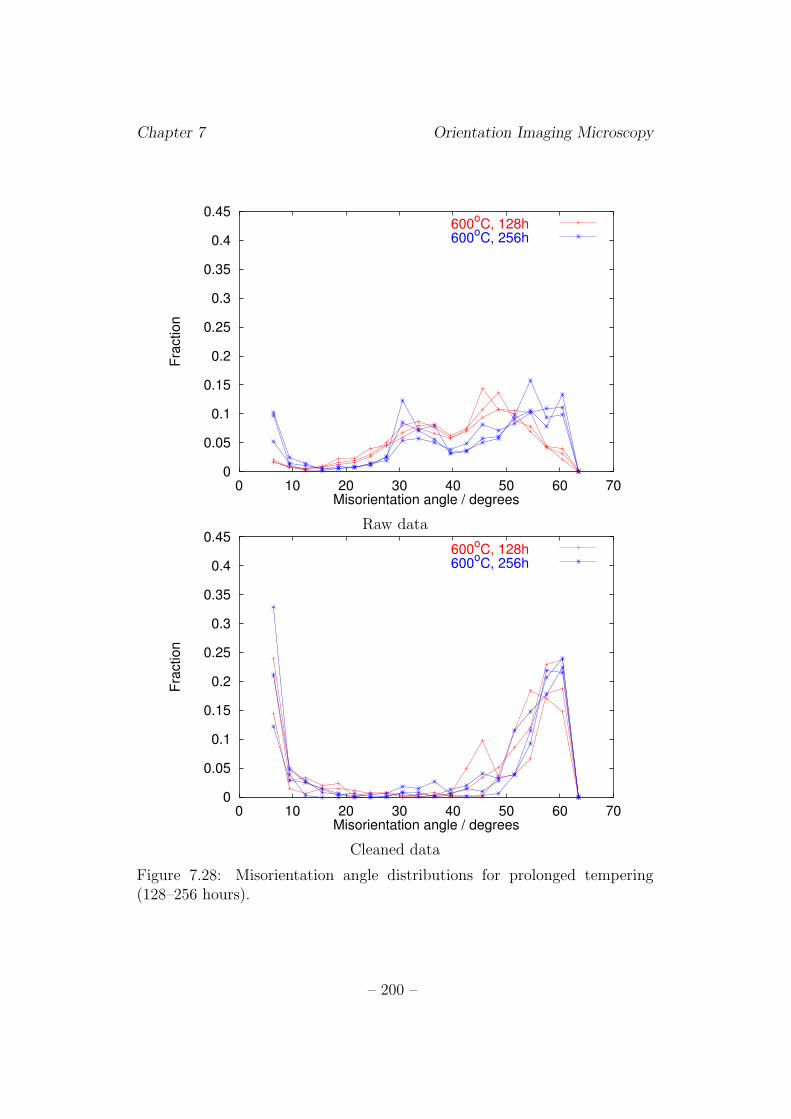
Chapter 7 Orientation Imaging Microscopy
0
0.05
0.1
0.15
0.2
0.25
0.3
0.35
0.4
0.45
0 10 20 30 40 50 60 70
Fra
ction
Misorientation angle / degrees
600oC, 128h
600oC, 256h
Raw data
0
0.05
0.1
0.15
0.2
0.25
0.3
0.35
0.4
0.45
0 10 20 30 40 50 60 70
Fra
ction
Misorientation angle / degrees
600oC, 128h
600oC, 256h
Cleaned data
Figure 7.28: Misorientation angle distributions for prolonged tempering(128–256 hours).
– 200 –
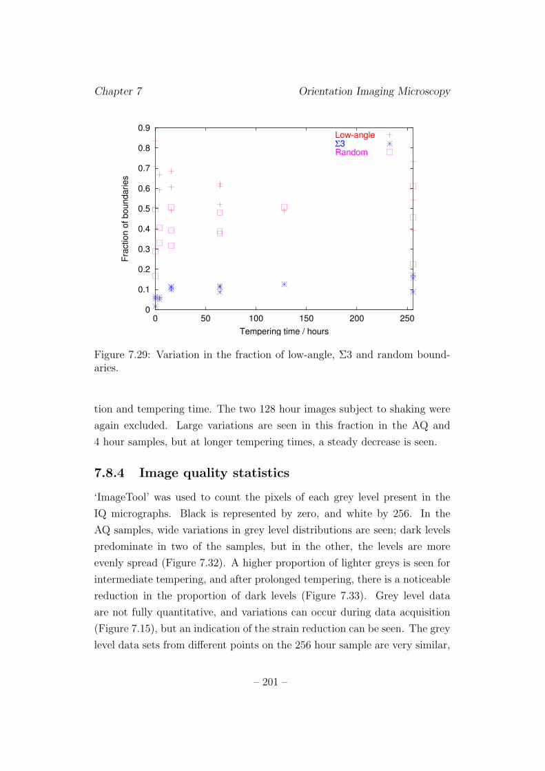
Chapter 7 Orientation Imaging Microscopy
0
0.1
0.2
0.3
0.4
0.5
0.6
0.7
0.8
0.9
0 50 100 150 200 250
Fra
ction o
f boundaries
Tempering time / hours
Low-angleΣ3Random
Figure 7.29: Variation in the fraction of low-angle, Σ3 and random bound-aries.
tion and tempering time. The two 128 hour images subject to shaking were
again excluded. Large variations are seen in this fraction in the AQ and
4 hour samples, but at longer tempering times, a steady decrease is seen.
7.8.4 Image quality statistics
‘ImageTool’ was used to count the pixels of each grey level present in the
IQ micrographs. Black is represented by zero, and white by 256. In the
AQ samples, wide variations in grey level distributions are seen; dark levels
predominate in two of the samples, but in the other, the levels are more
evenly spread (Figure 7.32). A higher proportion of lighter greys is seen for
intermediate tempering, and after prolonged tempering, there is a noticeable
reduction in the proportion of dark levels (Figure 7.33). Grey level data
are not fully quantitative, and variations can occur during data acquisition
(Figure 7.15), but an indication of the strain reduction can be seen. The grey
level data sets from different points on the 256 hour sample are very similar,
– 201 –
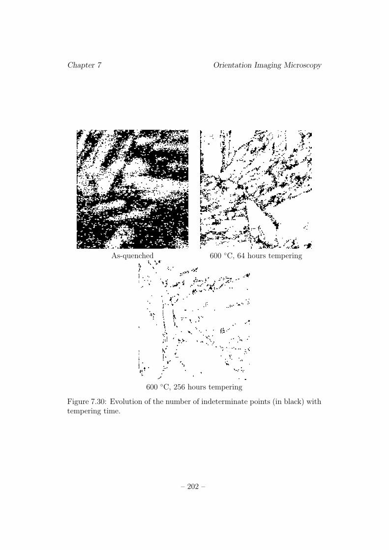
Chapter 7 Orientation Imaging Microscopy
As-quenched 600 ◦C, 64 hours tempering
600 ◦C, 256 hours tempering
Figure 7.30: Evolution of the number of indeterminate points (in black) withtempering time.
– 202 –
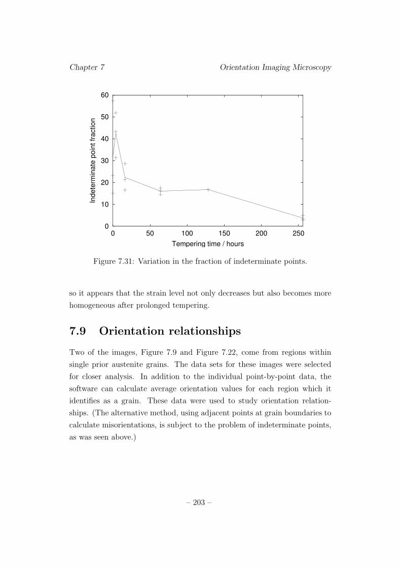
Chapter 7 Orientation Imaging Microscopy
0
10
20
30
40
50
60
0 50 100 150 200 250
Indete
rmin
ate
poin
t fr
action
Tempering time / hours
Figure 7.31: Variation in the fraction of indeterminate points.
so it appears that the strain level not only decreases but also becomes more
homogeneous after prolonged tempering.
7.9 Orientation relationships
Two of the images, Figure 7.9 and Figure 7.22, come from regions within
single prior austenite grains. The data sets for these images were selected
for closer analysis. In addition to the individual point-by-point data, the
software can calculate average orientation values for each region which it
identifies as a grain. These data were used to study orientation relation-
ships. (The alternative method, using adjacent points at grain boundaries to
calculate misorientations, is subject to the problem of indeterminate points,
as was seen above.)
– 203 –
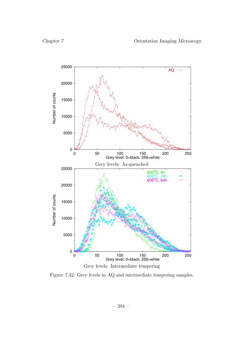
Chapter 7 Orientation Imaging Microscopy
0
5000
10000
15000
20000
25000
0 50 100 150 200 250
Num
ber
of counts
Grey level: 0=black, 256=white
AQ
Grey levels: As-quenched
0
5000
10000
15000
20000
25000
0 50 100 150 200 250
Num
ber
of counts
Grey level: 0=black, 256=white
600oC, 4h
600oC, 16h
600oC, 64h
Grey levels: Intermediate tempering
Figure 7.32: Grey levels in AQ and intermediate tempering samples.
– 204 –
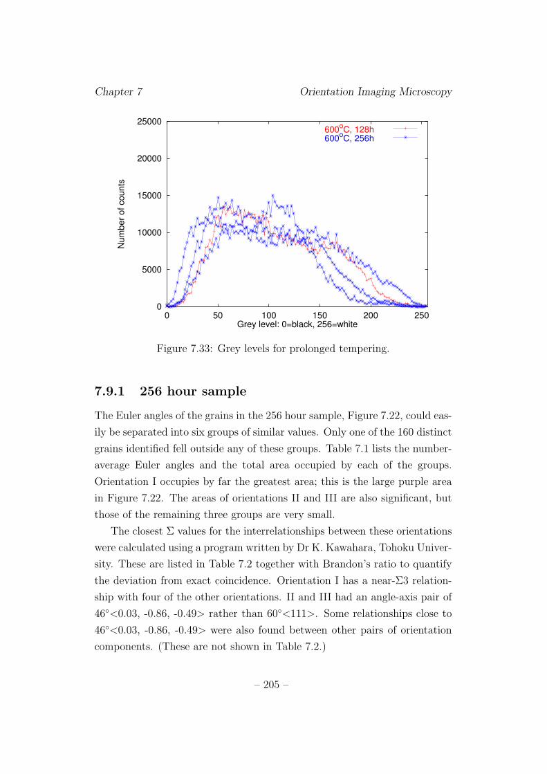
Chapter 7 Orientation Imaging Microscopy
0
5000
10000
15000
20000
25000
0 50 100 150 200 250
Num
ber
of counts
Grey level: 0=black, 256=white
600oC, 128h
600oC, 256h
Figure 7.33: Grey levels for prolonged tempering.
7.9.1 256 hour sample
The Euler angles of the grains in the 256 hour sample, Figure 7.22, could eas-
ily be separated into six groups of similar values. Only one of the 160 distinct
grains identified fell outside any of these groups. Table 7.1 lists the number-
average Euler angles and the total area occupied by each of the groups.
Orientation I occupies by far the greatest area; this is the large purple area
in Figure 7.22. The areas of orientations II and III are also significant, but
those of the remaining three groups are very small.
The closest Σ values for the interrelationships between these orientations
were calculated using a program written by Dr K. Kawahara, Tohoku Univer-
sity. These are listed in Table 7.2 together with Brandon’s ratio to quantify
the deviation from exact coincidence. Orientation I has a near-Σ3 relation-
ship with four of the other orientations. II and III had an angle-axis pair of
46◦<0.03, -0.86, -0.49> rather than 60◦<111>. Some relationships close to
46◦<0.03, -0.86, -0.49> were also found between other pairs of orientation
components. (These are not shown in Table 7.2.)
– 205 –
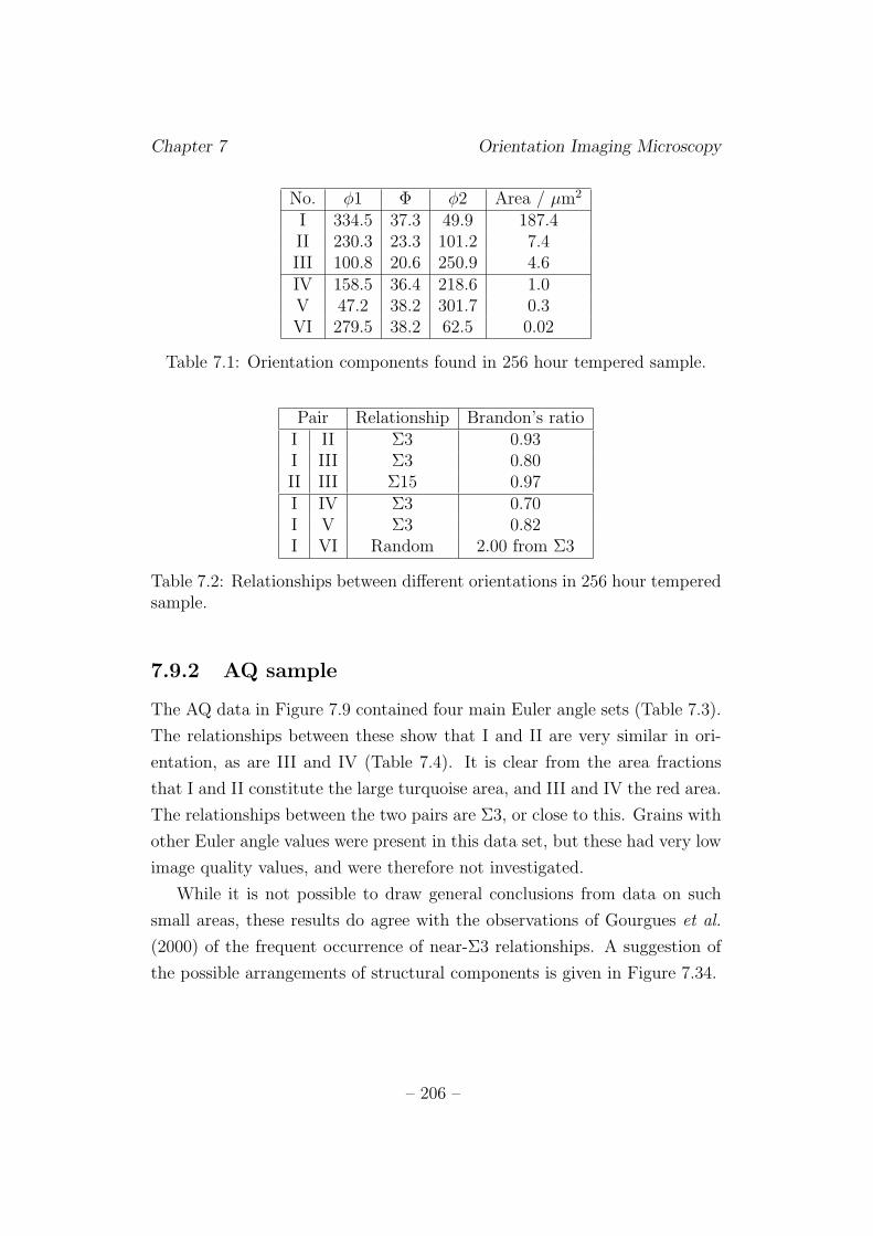
Chapter 7 Orientation Imaging Microscopy
No. φ1 Φ φ2 Area / µm2
I 334.5 37.3 49.9 187.4II 230.3 23.3 101.2 7.4III 100.8 20.6 250.9 4.6IV 158.5 36.4 218.6 1.0V 47.2 38.2 301.7 0.3VI 279.5 38.2 62.5 0.02
Table 7.1: Orientation components found in 256 hour tempered sample.
Pair Relationship Brandon’s ratioI II Σ3 0.93I III Σ3 0.80II III Σ15 0.97I IV Σ3 0.70I V Σ3 0.82I VI Random 2.00 from Σ3
Table 7.2: Relationships between different orientations in 256 hour temperedsample.
7.9.2 AQ sample
The AQ data in Figure 7.9 contained four main Euler angle sets (Table 7.3).
The relationships between these show that I and II are very similar in ori-
entation, as are III and IV (Table 7.4). It is clear from the area fractions
that I and II constitute the large turquoise area, and III and IV the red area.
The relationships between the two pairs are Σ3, or close to this. Grains with
other Euler angle values were present in this data set, but these had very low
image quality values, and were therefore not investigated.
While it is not possible to draw general conclusions from data on such
small areas, these results do agree with the observations of Gourgues et al.
(2000) of the frequent occurrence of near-Σ3 relationships. A suggestion of
the possible arrangements of structural components is given in Figure 7.34.
– 206 –
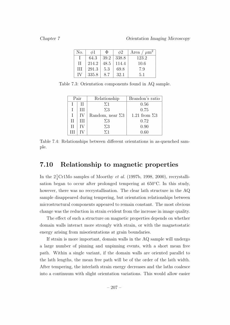
Chapter 7 Orientation Imaging Microscopy
No. φ1 Φ φ2 Area / µm2
I 64.3 39.2 338.8 123.2II 214.2 48.5 114.4 10.6III 291.3 5.3 69.8 7.9IV 335.8 8.7 32.1 5.1
Table 7.3: Orientation components found in AQ sample.
Pair Relationship Brandon’s ratioI II Σ1 0.56I III Σ3 0.75I IV Random, near Σ3 1.21 from Σ3II III Σ3 0.72II IV Σ3 0.90III IV Σ1 0.60
Table 7.4: Relationships between different orientations in as-quenched sam-ple.
7.10 Relationship to magnetic properties
In the 214Cr1Mo samples of Moorthy et al. (1997b, 1998, 2000), recrystalli-
sation began to occur after prolonged tempering at 650◦C. In this study,
however, there was no recrystallisation. The clear lath structure in the AQ
sample disappeared during tempering, but orientation relationships between
microstructural components appeared to remain constant. The most obvious
change was the reduction in strain evident from the increase in image quality.
The effect of such a structure on magnetic properties depends on whether
domain walls interact more strongly with strain, or with the magnetostatic
energy arising from misorientations at grain boundaries.
If strain is more important, domain walls in the AQ sample will undergo
a large number of pinning and unpinning events, with a short mean free
path. Within a single variant, if the domain walls are oriented parallel to
the lath lengths, the mean free path will be of the order of the lath width.
After tempering, the interlath strain energy decreases and the laths coalesce
into a continuum with slight orientation variations. This would allow easier
– 207 –
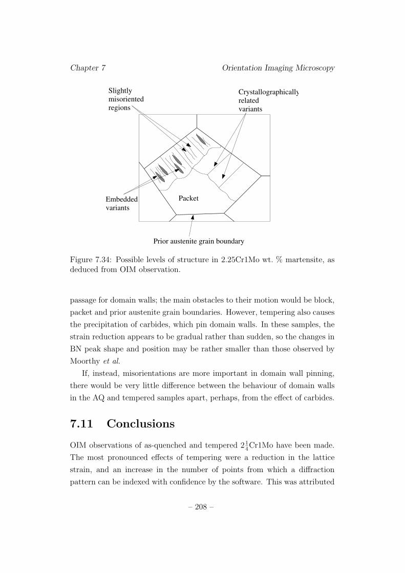
Chapter 7 Orientation Imaging Microscopy
Prior austenite grain boundary
related
variants
CrystallographicallySlightly
misoriented
regions
variants
Embedded Packet
Figure 7.34: Possible levels of structure in 2.25Cr1Mo wt. % martensite, asdeduced from OIM observation.
passage for domain walls; the main obstacles to their motion would be block,
packet and prior austenite grain boundaries. However, tempering also causes
the precipitation of carbides, which pin domain walls. In these samples, the
strain reduction appears to be gradual rather than sudden, so the changes in
BN peak shape and position may be rather smaller than those observed by
Moorthy et al.
If, instead, misorientations are more important in domain wall pinning,
there would be very little difference between the behaviour of domain walls
in the AQ and tempered samples apart, perhaps, from the effect of carbides.
7.11 Conclusions
OIM observations of as-quenched and tempered 214Cr1Mo have been made.
The most pronounced effects of tempering were a reduction in the lattice
strain, and an increase in the number of points from which a diffraction
pattern can be indexed with confidence by the software. This was attributed
– 208 –

Chapter 7 Orientation Imaging Microscopy
to a decrease in strain due to a reduction in dislocation density at grain and
lath boundaries.
Prior austenite grain boundaries were always random, and within the
prior austenite grains a combination of low-angle, Σ3 and random bound-
aries occurred. Individual crystallographic packets contained many slightly
misoriented groups of laths. Variants related by Σ3 were found; in some cases
one variant was found in small regions embedded in large areas of another
variant.
An estimation of the likely effect of these tempered mirostructures on BN
has been made, and will be tested in Chapter 8.
– 209 –
Chapter 8
Barkhausen Noise Experimentson Power Plant Steels
8.1 Experimental Method
8.1.1 Sample Preparation
The samples for BN testing were prepared as described in § 6.1. A 2% nital
etch was used for the 214Cr1Mo steel samples, and a Kalling’s No. 2 etch for
the 11Cr1Mo samples.
8.1.2 Instrumentation
The BN measurements were taken at the University of Newcastle Design
Unit under the supervision of Dr V. Moorthy, using a commercially avail-
able ‘µSCAN 500’ testing machine manufactured by Stresstech Oy - AST
(Figure 8.1). Such instruments are used routinely in industry for a variety
of nondestructive testing applications, such as detecting residual stresses at
surfaces (Stresstech, WWW site). Figure 8.2 is a schematic diagram of the
measurement system. The BN unit generates a sinusoidally varying current
which, after amplification and filtration, is supplied to a coil wound around
a yoke made of a ceramic ferrite material. The yoke is placed directly onto
the sample, taking care to ensure good contact between the sensor and the
surface. A pickup coil, wound around a core of the same ceramic ferrite,
acquires the BN voltage signal, which is amplified and filtered. The unit is
– 210 –
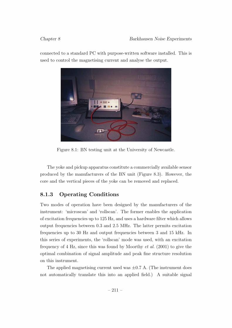
Chapter 8 Barkhausen Noise Experiments
connected to a standard PC with purpose-written software installed. This is
used to control the magnetising current and analyse the output.
Figure 8.1: BN testing unit at the University of Newcastle.
The yoke and pickup apparatus constitute a commercially available sensor
produced by the manufacturers of the BN unit (Figure 8.3). However, the
core and the vertical pieces of the yoke can be removed and replaced.
8.1.3 Operating Conditions
Two modes of operation have been designed by the manufacturers of the
instrument: ‘microscan’ and ‘rollscan’. The former enables the application
of excitation frequencies up to 125 Hz, and uses a hardware filter which allows
output frequencies between 0.3 and 2.5 MHz. The latter permits excitation
frequencies up to 30 Hz and output frequencies between 3 and 15 kHz. In
this series of experiments, the ‘rollscan’ mode was used, with an excitation
frequency of 4 Hz, since this was found by Moorthy et al. (2001) to give the
optimal combination of signal amplitude and peak fine structure resolution
on this instrument.
The applied magnetising current used was ±0.7 A. (The instrument does
not automatically translate this into an applied field.) A suitable signal
– 211 –
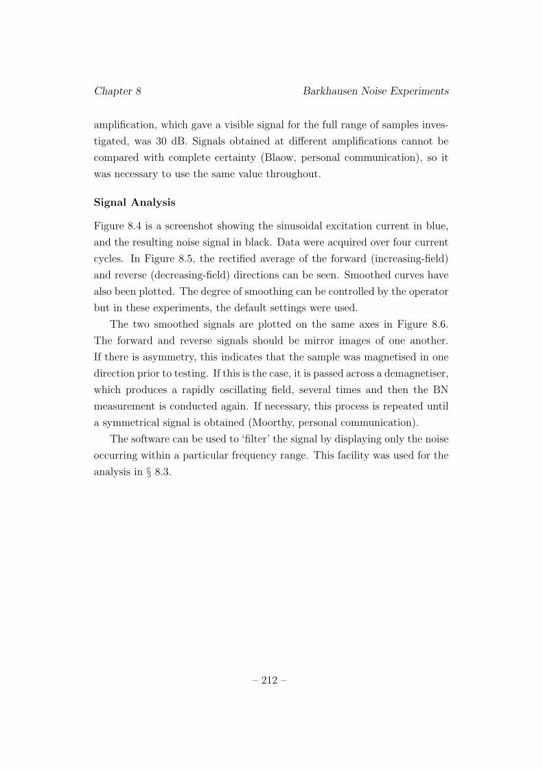
Chapter 8 Barkhausen Noise Experiments
amplification, which gave a visible signal for the full range of samples inves-
tigated, was 30 dB. Signals obtained at different amplifications cannot be
compared with complete certainty (Blaow, personal communication), so it
was necessary to use the same value throughout.
Signal Analysis
Figure 8.4 is a screenshot showing the sinusoidal excitation current in blue,
and the resulting noise signal in black. Data were acquired over four current
cycles. In Figure 8.5, the rectified average of the forward (increasing-field)
and reverse (decreasing-field) directions can be seen. Smoothed curves have
also been plotted. The degree of smoothing can be controlled by the operator
but in these experiments, the default settings were used.
The two smoothed signals are plotted on the same axes in Figure 8.6.
The forward and reverse signals should be mirror images of one another.
If there is asymmetry, this indicates that the sample was magnetised in one
direction prior to testing. If this is the case, it is passed across a demagnetiser,
which produces a rapidly oscillating field, several times and then the BN
measurement is conducted again. If necessary, this process is repeated until
a symmetrical signal is obtained (Moorthy, personal communication).
The software can be used to ‘filter’ the signal by displaying only the noise
occurring within a particular frequency range. This facility was used for the
analysis in § 8.3.
– 212 –
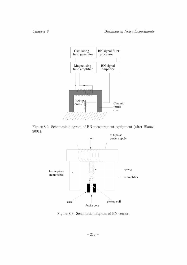
Chapter 8 Barkhausen Noise Experiments
Ceramicferritecore
Oscillatingprocessor
Magnetising
BN signal filterfield generator
field amplifierBN signalamplifier
Pickupcoil
Figure 8.2: Schematic diagram of BN measurement equipment (after Blaow,2001).
to bipolarpower supplycoil
ferrite piece(removable)
ferrite core
pickup coilcase
to amplifier
spring
Figure 8.3: Schematic diagram of BN sensor.
– 213 –
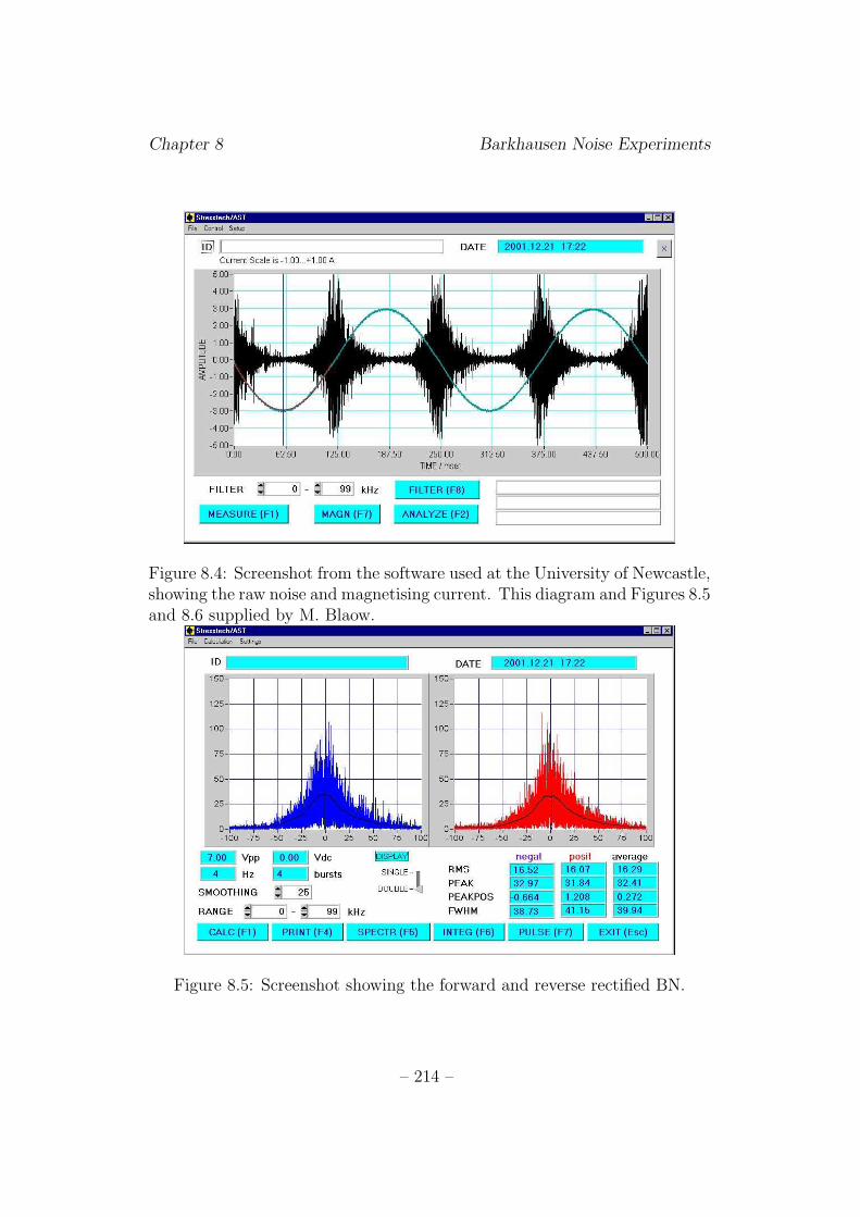
Chapter 8 Barkhausen Noise Experiments
Figure 8.4: Screenshot from the software used at the University of Newcastle,showing the raw noise and magnetising current. This diagram and Figures 8.5and 8.6 supplied by M. Blaow.
Figure 8.5: Screenshot showing the forward and reverse rectified BN.
– 214 –
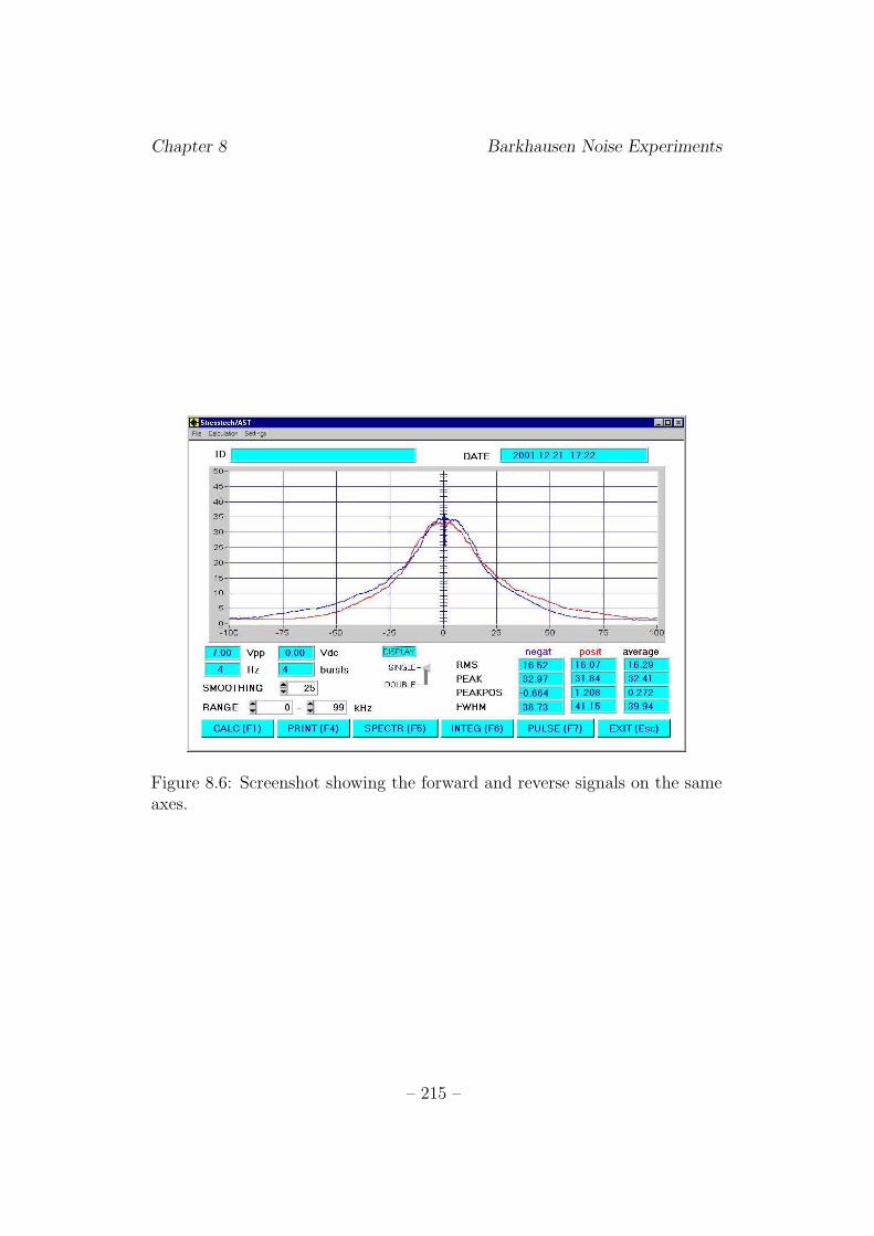
Chapter 8 Barkhausen Noise Experiments
Figure 8.6: Screenshot showing the forward and reverse signals on the sameaxes.
– 215 –
Chapter 8 Barkhausen Noise Experiments
8.2 Results
The rectified and smoothed BN signals were plotted against magnetising
current for each of the samples tested. In each case, only the forward direction
has been shown, since the reverse signal is almost identical. The scale on the
horizontal axis is the applied magnetising current, and the vertical scale,
quantifying the noise voltage, is given as a percentage of 5 V. These scales
tend to be regarded as rather arbitrary, and not to be compared with the
output from testing equipment with different geometries (Moorthy, personal
communication).
500◦C tempering
Figure 8.7 and Figure 8.8 show the BN signals for samples tempered at 500◦C.
On both graphs, the as-quenched (AQ) peak is shown for comparison.
For all the tempered specimens, the peaks are higher than for AQ. There
appears to be a trend towards higher, narrower peaks with higher tempering
time, but there is some scatter in this. The dramatic peak height increase
between AQ specimens and those tempered even for a short time agrees well
with the behaviour observed by Moorthy et al. in their tempering experi-
ments. The onset of Barkhausen activity occurs at a lower current in the
tempered sample than in the as-quenched sample in all cases.
Samples tempered for longer times (Figure 8.8) show much less varia-
tion in BN peak shape and position than those tempered for shorter times
(Figure 8.7). In all the 500◦C samples, an approximately symmetrical peak
centred at a current of around 0.1 A is followed by a change in slope near
0.2 A, giving a gradual decrease of noise at high current.
600◦C tempering
Figure 8.9 and Figure 8.10 show the noise signals from samples tempered at
600◦C, with the AQ signal for reference. The maximum peak height observed
in this series is larger than in the 500◦C series.
The peak heights do not show much variation, apart from the peak at
256 hours, which is significantly higher than the others. The shape of the
– 216 –
Chapter 8 Barkhausen Noise Experiments
32 hour peak seems anomalous.
The onset of noise occurs at a lower current in this set of samples than
in the 500◦C samples. The 600◦C peaks are rather broader than the 500◦C
peaks, and enclose a larger area. However, the curve shapes may still be
interpreted as an initial peak followed by a slope change to a less steep slope.
700◦C tempering
Peaks from samples tempered at 700◦C (Figure 8.11) are significantly broader
than those from lower tempering temperatures; more activity occurs both at
currents below zero and at high currents. There is no obvious trend between
peak height and tempering time, or between peak position and tempering
time.
Long-term 11Cr1Mo wt. % samples
The peak occurs at a noticeably higher current for the 11Cr1Mo samples
(Figure 8.12) than for the tempered 214Cr1Mo steels, as illustrated by com-
parison with the 214Cr1Mo AQ peak. The peak heights are mostly smaller
than those for tempered 214Cr1Mo steel, but there is no obvious systematic
variation of height with tempering time.
8.2.1 Peak height, width and position
For each data set, the maximum height, the full width half maximum (FWHM),
and the position on the applied current axis of the maximum height, were
determined and plotted against tempering time (Figure 8.13, Figure 8.15 and
Figure 8.17).
The Larson-Miller parameter P can be used to relate tempering time and
temperature conditions on the same scale:
P = T (C + log t) (8.1)
where T is the absolute temperature (in K), t is the time in hours, and C is
a constant with a value around 20.
– 217 –
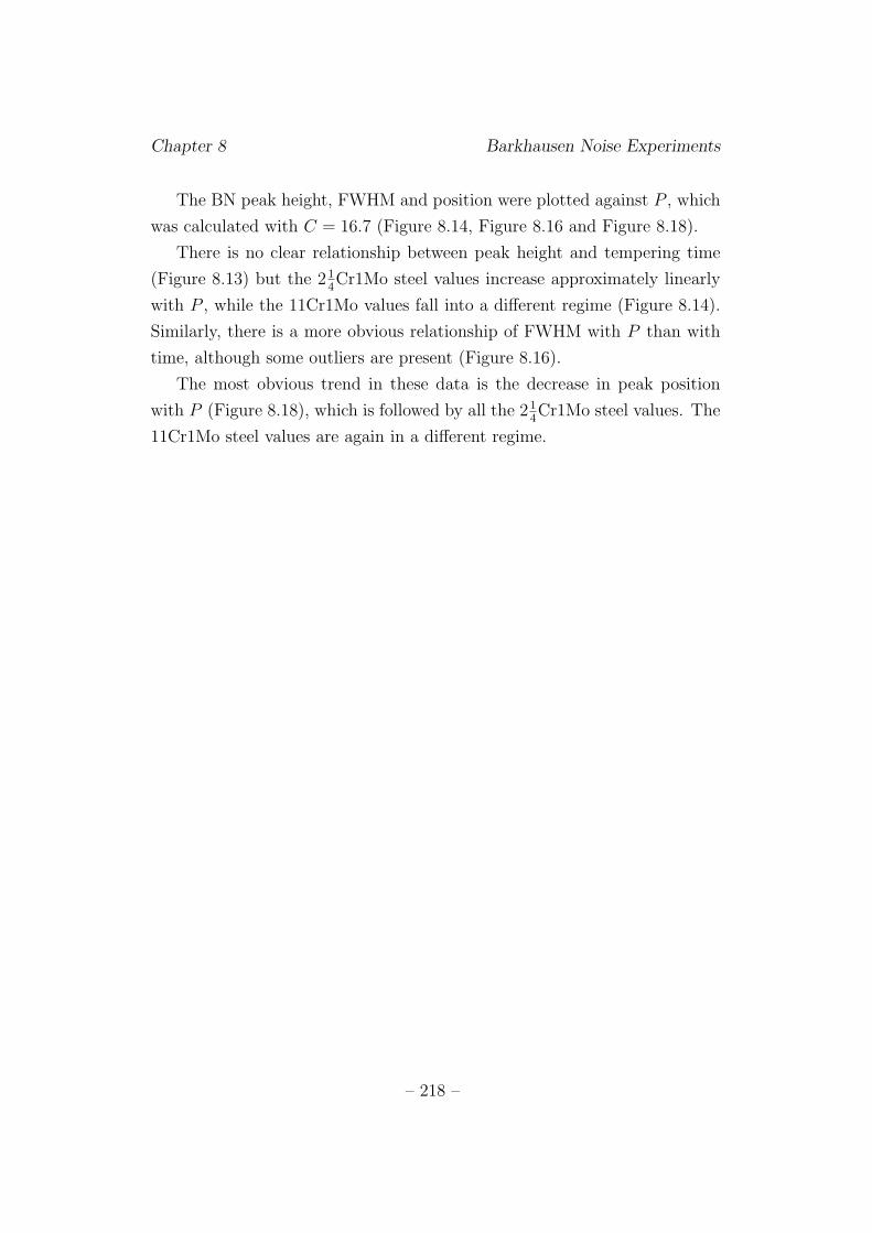
Chapter 8 Barkhausen Noise Experiments
The BN peak height, FWHM and position were plotted against P , which
was calculated with C = 16.7 (Figure 8.14, Figure 8.16 and Figure 8.18).
There is no clear relationship between peak height and tempering time
(Figure 8.13) but the 214Cr1Mo steel values increase approximately linearly
with P , while the 11Cr1Mo values fall into a different regime (Figure 8.14).
Similarly, there is a more obvious relationship of FWHM with P than with
time, although some outliers are present (Figure 8.16).
The most obvious trend in these data is the decrease in peak position
with P (Figure 8.18), which is followed by all the 214Cr1Mo steel values. The
11Cr1Mo steel values are again in a different regime.
– 218 –
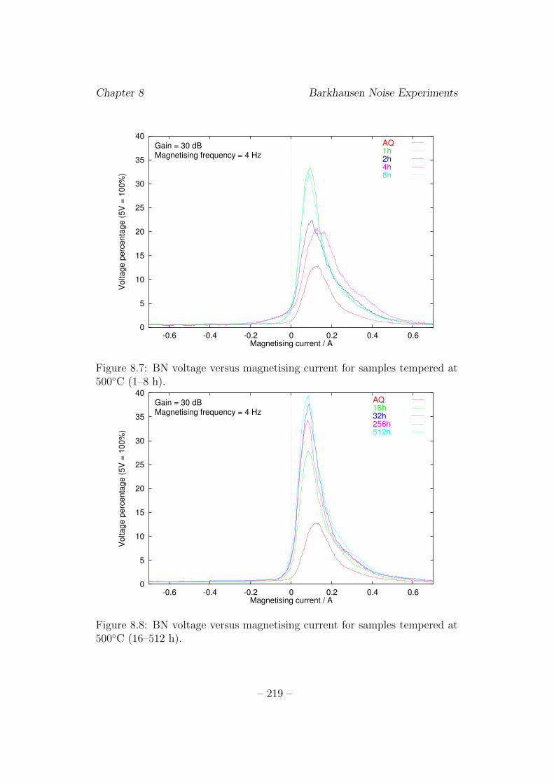
Chapter 8 Barkhausen Noise Experiments
0
5
10
15
20
25
30
35
40
-0.6 -0.4 -0.2 0 0.2 0.4 0.6
Vo
lta
ge
pe
rce
nta
ge
(5
V =
10
0%
)
Magnetising current / A
Gain = 30 dBMagnetising frequency = 4 Hz
AQ1h2h4h8h
Figure 8.7: BN voltage versus magnetising current for samples tempered at500◦C (1–8 h).
0
5
10
15
20
25
30
35
40
-0.6 -0.4 -0.2 0 0.2 0.4 0.6
Vo
lta
ge
pe
rce
nta
ge
(5
V =
10
0%
)
Magnetising current / A
Gain = 30 dBMagnetising frequency = 4 Hz
AQ16h32h256h512h
Figure 8.8: BN voltage versus magnetising current for samples tempered at500◦C (16–512 h).
– 219 –
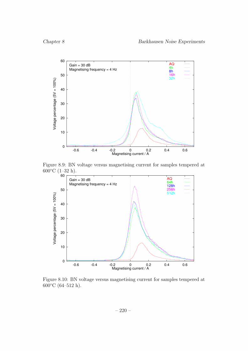
Chapter 8 Barkhausen Noise Experiments
0
10
20
30
40
50
60
-0.6 -0.4 -0.2 0 0.2 0.4 0.6
Vo
lta
ge
pe
rce
nta
ge
(5
V =
10
0%
)
Magnetising current / A
Gain = 30 dBMagnetising frequency = 4 Hz
AQ4h8h16h32h
Figure 8.9: BN voltage versus magnetising current for samples tempered at600◦C (1–32 h).
0
10
20
30
40
50
60
-0.6 -0.4 -0.2 0 0.2 0.4 0.6
Vo
lta
ge
pe
rce
nta
ge
(5
V =
10
0%
)
Magnetising current / A
Gain = 30 dBMagnetising frequency = 4 Hz
AQ64h128h256h512h
Figure 8.10: BN voltage versus magnetising current for samples tempered at600◦C (64–512 h).
– 220 –
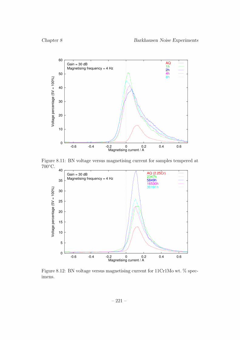
Chapter 8 Barkhausen Noise Experiments
0
10
20
30
40
50
60
-0.6 -0.4 -0.2 0 0.2 0.4 0.6
Vo
lta
ge
pe
rce
nta
ge
(5
V =
10
0%
)
Magnetising current / A
Gain = 30 dBMagnetising frequency = 4 Hz
AQ1h2h4h8h
Figure 8.11: BN voltage versus magnetising current for samples tempered at700◦C.
0
5
10
15
20
25
30
35
40
-0.6 -0.4 -0.2 0 0.2 0.4 0.6
Vo
lta
ge
pe
rce
nta
ge
(5
V =
10
0%
)
Magnetising current / A
Gain = 30 dBMagnetising frequency = 4 Hz
AQ (2.25Cr)2347h5849h16530h36191h
Figure 8.12: BN voltage versus magnetising current for 11Cr1Mo wt. % spec-imens.
– 221 –
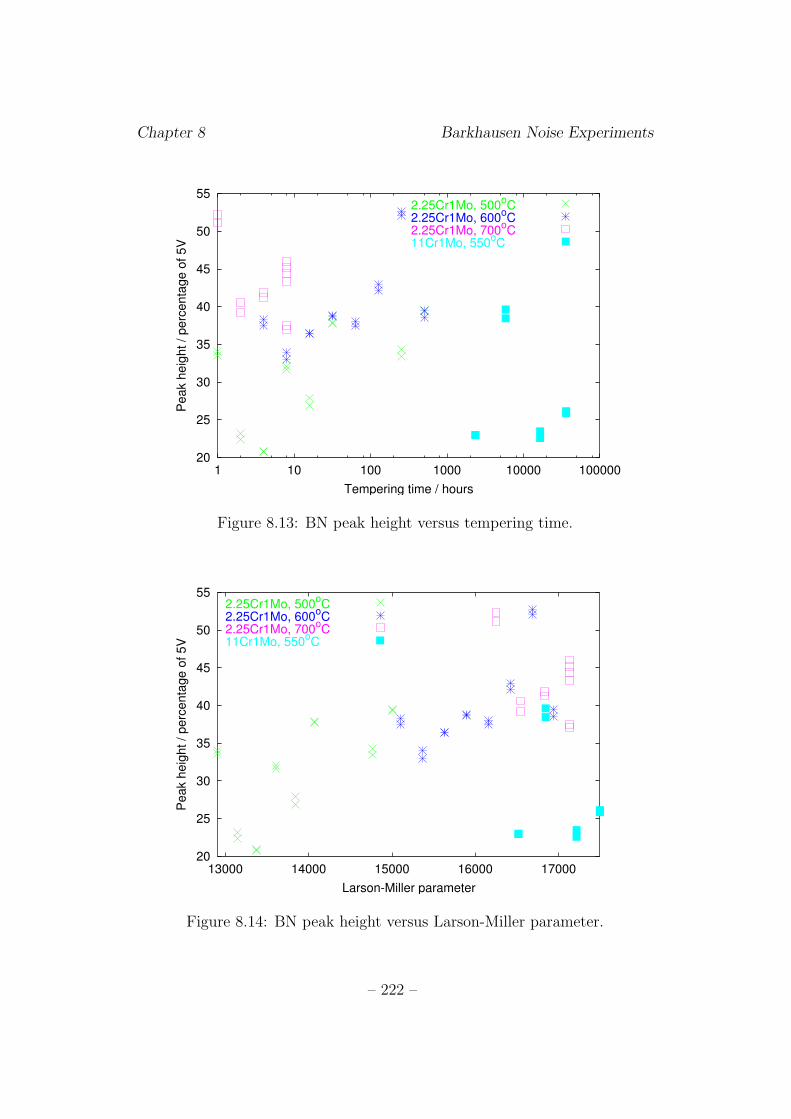
Chapter 8 Barkhausen Noise Experiments
20
25
30
35
40
45
50
55
1 10 100 1000 10000 100000
Peak h
eig
ht / perc
enta
ge o
f 5V
Tempering time / hours
2.25Cr1Mo, 500oC
2.25Cr1Mo, 600oC
2.25Cr1Mo, 700oC
11Cr1Mo, 550oC
Figure 8.13: BN peak height versus tempering time.
20
25
30
35
40
45
50
55
13000 14000 15000 16000 17000
Peak h
eig
ht / perc
enta
ge o
f 5V
Larson-Miller parameter
2.25Cr1Mo, 500oC
2.25Cr1Mo, 600oC
2.25Cr1Mo, 700oC
11Cr1Mo, 550oC
Figure 8.14: BN peak height versus Larson-Miller parameter.
– 222 –
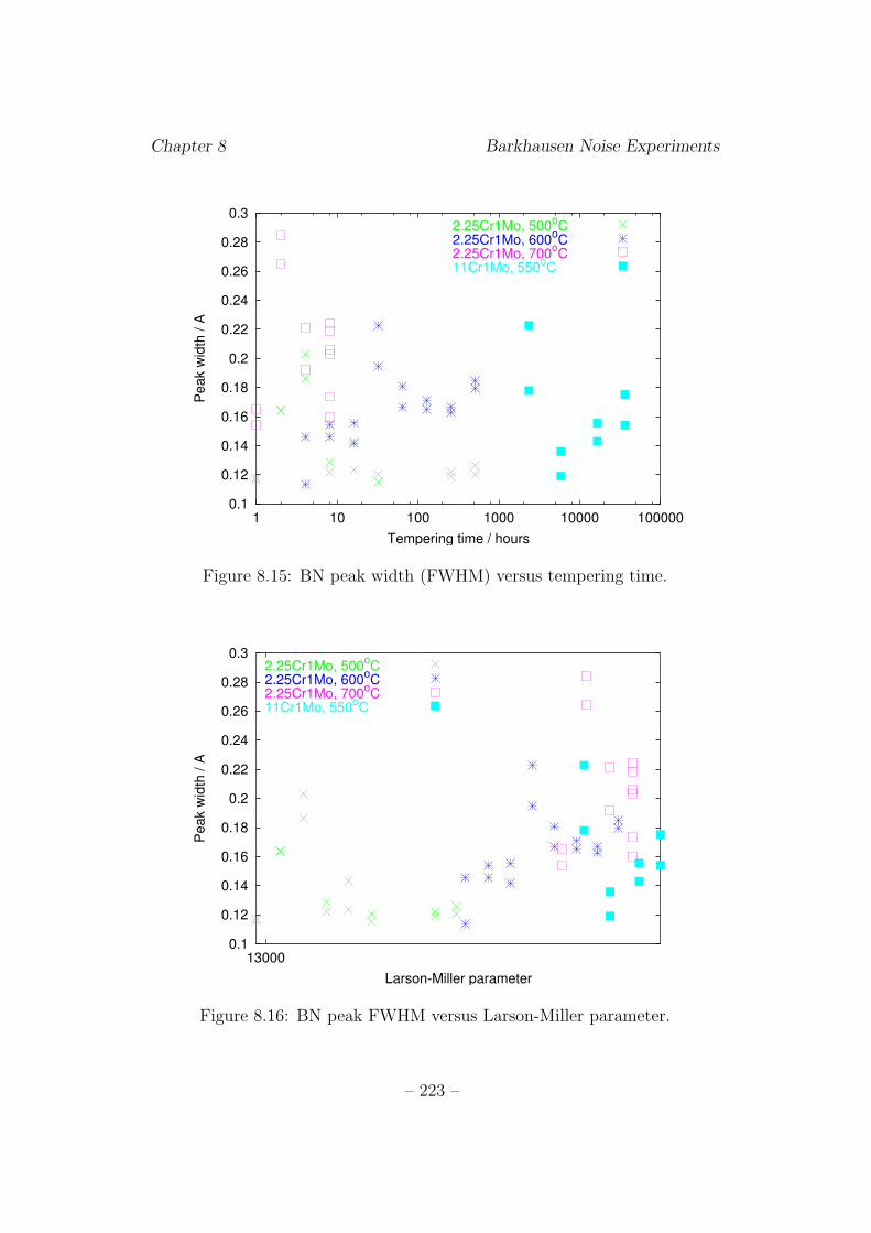
Chapter 8 Barkhausen Noise Experiments
0.1
0.12
0.14
0.16
0.18
0.2
0.22
0.24
0.26
0.28
0.3
1 10 100 1000 10000 100000
Peak w
idth
/ A
Tempering time / hours
2.25Cr1Mo, 500oC
2.25Cr1Mo, 600oC
2.25Cr1Mo, 700oC
11Cr1Mo, 550oC
Figure 8.15: BN peak width (FWHM) versus tempering time.
0.1
0.12
0.14
0.16
0.18
0.2
0.22
0.24
0.26
0.28
0.3
13000
Peak w
idth
/ A
Larson-Miller parameter
2.25Cr1Mo, 500oC
2.25Cr1Mo, 600oC
2.25Cr1Mo, 700oC
11Cr1Mo, 550oC
Figure 8.16: BN peak FWHM versus Larson-Miller parameter.
– 223 –
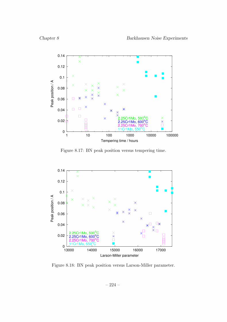
Chapter 8 Barkhausen Noise Experiments
0
0.02
0.04
0.06
0.08
0.1
0.12
0.14
1 10 100 1000 10000 100000
Peak p
ositio
n / A
Tempering time / hours
2.25Cr1Mo, 500oC
2.25Cr1Mo, 600oC
2.25Cr1Mo, 700oC
11Cr1Mo, 550oC
Figure 8.17: BN peak position versus tempering time.
0
0.02
0.04
0.06
0.08
0.1
0.12
0.14
13000 14000 15000 16000 17000
Peak p
ositio
n / A
Larson-Miller parameter
2.25Cr1Mo, 500oC
2.25Cr1Mo, 600oC
2.25Cr1Mo, 700oC
11Cr1Mo, 550oC
Figure 8.18: BN peak position versus Larson-Miller parameter.
– 224 –
Chapter 8 Barkhausen Noise Experiments
8.2.2 Comparison with results of Moorthy et al.
Figure 8.19 shows a selection of the results obtained here together with some
results on a 214Cr1Mo steel obtained by Moorthy et al. (1998, 2000) using
apparatus of type (a) in Figure 4.2; the University of Newcastle apparatus is
of type (b). The tempering temperatures are not the same in the two cases
because the present work was intended to be complementary to those of
Moorthy et al. rather than repeats of the same experiments. Also, Moorthy
et al. did not quench their samples. The actual amplitudes of the noise
signals measured depend on such factors as experimental geometry and signal
amplification, so it is not possible to compare the values directly, and they
are plotted on different vertical axes. However, the range of values on the
horizontal axis should be the same since the current varies within the same
range.
In the results of Moorthy et al., the noise peaks occur at higher currents.
The two sets of results are consistent in that the peak becomes higher, and
moves to a lower current, after tempering. The change in height on temper-
ing is more pronounced in the results of Moorthy et al. than in this study.
The AQ peak from this study and the normalised peak of Moorthy et al.
are similar in shape, but the tempered sample peak shapes in the present
study are much less symmetrical than the Moorthy et al. peaks. The peak
height changes seen by Moorthy et al. are much more dramatic than those
in Figure 8.9, Figure 8.10 and Figure 8.11. Some of these differences can
be accounted for by the greater severity of tempering in the Moorthy et al.
experiment1. However, the comparative positions of the AQ and normalised
peaks suggest that there is also some influence from the apparatus configu-
ration.
The double-peak behaviour observed by Moorthy et al. at long tempering
times is completely absent in all the measurements made in this study. This
may be because 600◦C is too low a temperature to produce this behaviour
even at long tempering times, while the tempering at 700◦C was carried out
1The highest Larson-Miller parameter value in the Moorthy et al. study was just under
18000, whereas the highest value in the present study was 17000.
– 225 –
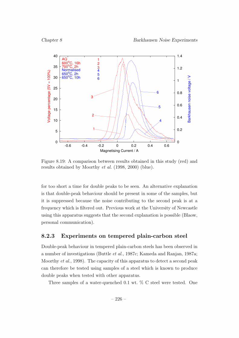
Chapter 8 Barkhausen Noise Experiments
0
5
10
15
20
25
30
35
40
-0.6 -0.4 -0.2 0 0.2 0.4 0.60
0.2
0.4
0.6
0.8
1
1.2
1.4
Vo
lta
ge
pe
rce
nta
ge
(5
V =
10
0%
)
Ba
rkh
au
se
n n
ois
e v
olta
ge
/ V
Magnetising current / A
AQ600
oC, 16h
700oC, 2h
Normalised650
oC, 2h
650oC, 10h
Vo
lta
ge
pe
rce
nta
ge
(5
V =
10
0%
)
Magnetising Current / A
Ba
rkh
au
se
n n
ois
e v
olta
ge
/ V
123456
4
5
6
1
2
3
Figure 8.19: A comparison between results obtained in this study (red) andresults obtained by Moorthy et al. (1998, 2000) (blue).
for too short a time for double peaks to be seen. An alternative explanation
is that double-peak behaviour should be present in some of the samples, but
it is suppressed because the noise contributing to the second peak is at a
frequency which is filtered out. Previous work at the University of Newcastle
using this apparatus suggests that the second explanation is possible (Blaow,
personal communication).
8.2.3 Experiments on tempered plain-carbon steel
Double-peak behaviour in tempered plain-carbon steels has been observed in
a number of investigations (Buttle et al., 1987c; Kameda and Ranjan, 1987a;
Moorthy et al., 1998). The capacity of this apparatus to detect a second peak
can therefore be tested using samples of a steel which is known to produce
double peaks when tested with other apparatus.
Three samples of a water-quenched 0.1 wt. % C steel were tested. One
– 226 –
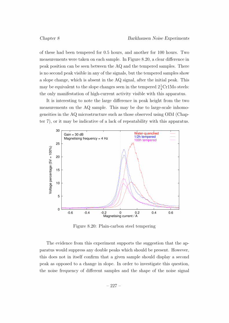
Chapter 8 Barkhausen Noise Experiments
of these had been tempered for 0.5 hours, and another for 100 hours. Two
measurements were taken on each sample. In Figure 8.20, a clear difference in
peak position can be seen between the AQ and the tempered samples. There
is no second peak visible in any of the signals, but the tempered samples show
a slope change, which is absent in the AQ signal, after the initial peak. This
may be equivalent to the slope changes seen in the tempered 214Cr1Mo steels:
the only manifestation of high-current activity visible with this apparatus.
It is interesting to note the large difference in peak height from the two
measurements on the AQ sample. This may be due to large-scale inhomo-
geneities in the AQ microstructure such as those observed using OIM (Chap-
ter 7), or it may be indicative of a lack of repeatability with this apparatus.
0
5
10
15
20
25
30
-0.6 -0.4 -0.2 0 0.2 0.4 0.6
Vo
lta
ge
pe
rce
nta
ge
(5
V =
10
0%
)
Magnetising current / A
Gain = 30 dBMagnetising frequency = 4 Hz
Water-quenched1/2h tempered100h tempered
Figure 8.20: Plain-carbon steel tempering
The evidence from this experiment supports the suggestion that the ap-
paratus would suppress any double peaks which should be present. However,
this does not in itself confirm that a given sample should display a second
peak as opposed to a change in slope. In order to investigate this question,
the noise frequency of different samples and the shape of the noise signal
– 227 –
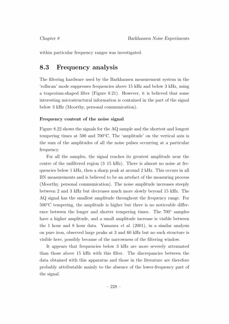
Chapter 8 Barkhausen Noise Experiments
within particular frequency ranges was investigated.
8.3 Frequency analysis
The filtering hardware used by the Barkhausen measurement system in the
‘rollscan’ mode suppresses frequencies above 15 kHz and below 3 kHz, using
a trapezium-shaped filter (Figure 8.21). However, it is believed that some
interesting microstructural information is contained in the part of the signal
below 3 kHz (Moorthy, personal communication).
Frequency content of the noise signal
Figure 8.22 shows the signals for the AQ sample and the shortest and longest
tempering times at 500 and 700◦C. The ‘amplitude’ on the vertical axis is
the sum of the amplitudes of all the noise pulses occurring at a particular
frequency.
For all the samples, the signal reaches its greatest amplitude near the
centre of the unfiltered region (3–15 kHz). There is almost no noise at fre-
quencies below 1 kHz, then a sharp peak at around 2 kHz. This occurs in all
BN measurements and is believed to be an artefact of the measuring process
(Moorthy, personal communication). The noise amplitude increases steeply
between 2 and 3 kHz but decreases much more slowly beyond 15 kHz. The
AQ signal has the smallest amplitude throughout the frequency range. For
500◦C tempering, the amplitude is higher but there is no noticeable differ-
ence between the longer and shorter tempering times. The 700◦ samples
have a higher amplitude, and a small amplitude increase is visible between
the 1 hour and 8 hour data. Yamaura et al. (2001), in a similar analysis
on pure iron, observed large peaks at 3 and 60 kHz but no such structure is
visible here, possibly because of the narrowness of the filtering window.
It appears that frequencies below 3 kHz are more severely attenuated
than those above 15 kHz with this filter. The discrepancies between the
data obtained with this apparatus and those in the literature are therefore
probably attributable mainly to the absence of the lower-frequency part of
the signal.
– 228 –
Chapter 8 Barkhausen Noise Experiments
Fraction
of signal
allowed
through
3 15
Frequency / kHz
Unfilteredregion
0 20
Figure 8.21: Frequency filter in ‘rollscan’ mode (Blaow, personal communi-cation).
Signal analysis in narrow frequency ranges
Moorthy et al. (2001) noted the lack of the expected second peak in quenched
and tempered 0.1 wt. % C steel using this apparatus, and analysed the signal
within narrow frequency ranges to study the low-frequency noise. A clear
second peak was visible in the tempered steel in the range 4–5 kHz, while
only a single peak was seen in the AQ sample at all frequencies.
The signals from the 600◦C 214Cr1Mo steel samples were analysed in a
similar way to test whether a second peak was visible at low frequencies. The
first analysis considered noise with frequencies between 0 and 3 kHz. The
signal amplitude was low, owing to filtering, so the highest available ampli-
fication, 99 dB, was applied. Figure 8.23 shows some evidence of a second
peak centred around a current between 0.3 and 0.4 A; this is particularly
prominent in the 256 h signal. However, some evidence of activity at 0.4 A
is also visible in the AQ sample, which should have only a single peak. The
large peak, although at a similar position to the peaks in Figure 8.9 and
Figure 8.10, is narrower and more symmetrical.
Setting the upper frequency limit to 5 kHz (Figure 8.24) gives peaks which
more closely resemble those in Figure 8.9 and Figure 8.10. However, there
– 229 –
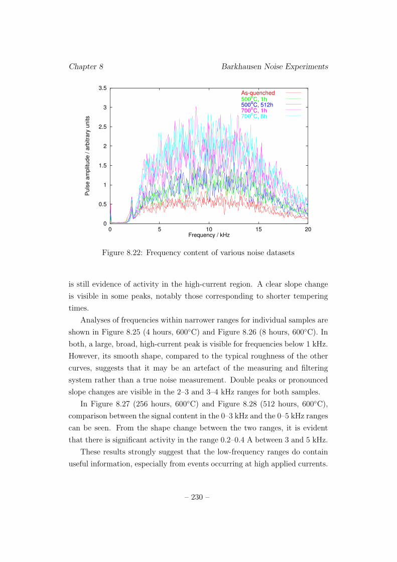
Chapter 8 Barkhausen Noise Experiments
0
0.5
1
1.5
2
2.5
3
3.5
0 5 10 15 20
Pu
lse
am
plit
ud
e /
arb
itra
ry u
nits
Frequency / kHz
As-quenched500
oC, 1h
500oC, 512h
700oC, 1h
700oC, 8h
Figure 8.22: Frequency content of various noise datasets
is still evidence of activity in the high-current region. A clear slope change
is visible in some peaks, notably those corresponding to shorter tempering
times.
Analyses of frequencies within narrower ranges for individual samples are
shown in Figure 8.25 (4 hours, 600◦C) and Figure 8.26 (8 hours, 600◦C). In
both, a large, broad, high-current peak is visible for frequencies below 1 kHz.
However, its smooth shape, compared to the typical roughness of the other
curves, suggests that it may be an artefact of the measuring and filtering
system rather than a true noise measurement. Double peaks or pronounced
slope changes are visible in the 2–3 and 3–4 kHz ranges for both samples.
In Figure 8.27 (256 hours, 600◦C) and Figure 8.28 (512 hours, 600◦C),
comparison between the signal content in the 0–3 kHz and the 0–5 kHz ranges
can be seen. From the shape change between the two ranges, it is evident
that there is significant activity in the range 0.2–0.4 A between 3 and 5 kHz.
These results strongly suggest that the low-frequency ranges do contain
useful information, especially from events occurring at high applied currents.
– 230 –
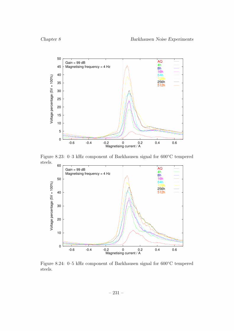
Chapter 8 Barkhausen Noise Experiments
0
5
10
15
20
25
30
35
40
45
50
-0.6 -0.4 -0.2 0 0.2 0.4 0.6
Vo
lta
ge
pe
rce
nta
ge
(5
V =
10
0%
)
Magnetising current / A
Gain = 99 dBMagnetising frequency = 4 Hz
AQ4h8h16h64h128h256h512h
Figure 8.23: 0–3 kHz component of Barkhausen signal for 600◦C temperedsteels.
0
10
20
30
40
50
60
-0.6 -0.4 -0.2 0 0.2 0.4 0.6
Vo
lta
ge
pe
rce
nta
ge
(5
V =
10
0%
)
Magnetising current / A
Gain = 99 dBMagnetising frequency = 4 Hz
AQ4h8h16h64h128h256h512h
Figure 8.24: 0–5 kHz component of Barkhausen signal for 600◦C temperedsteels.
– 231 –
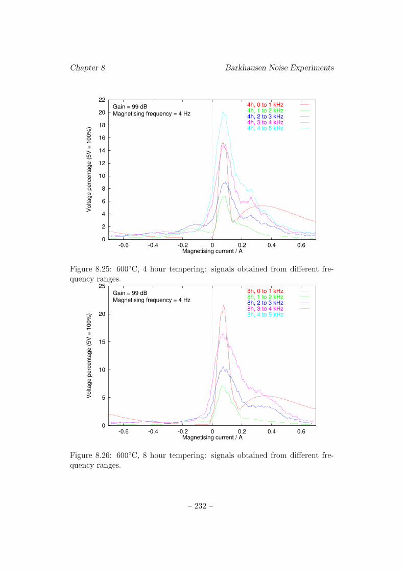
Chapter 8 Barkhausen Noise Experiments
0
2
4
6
8
10
12
14
16
18
20
22
-0.6 -0.4 -0.2 0 0.2 0.4 0.6
Vo
lta
ge
pe
rce
nta
ge
(5
V =
10
0%
)
Magnetising current / A
Gain = 99 dBMagnetising frequency = 4 Hz
4h, 0 to 1 kHz4h, 1 to 2 kHz4h, 2 to 3 kHz4h, 3 to 4 kHz4h, 4 to 5 kHz
Figure 8.25: 600◦C, 4 hour tempering: signals obtained from different fre-quency ranges.
0
5
10
15
20
25
-0.6 -0.4 -0.2 0 0.2 0.4 0.6
Vo
lta
ge
pe
rce
nta
ge
(5
V =
10
0%
)
Magnetising current / A
Gain = 99 dBMagnetising frequency = 4 Hz
8h, 0 to 1 kHz8h, 1 to 2 kHz8h, 2 to 3 kHz8h, 3 to 4 kHz8h, 4 to 5 kHz
Figure 8.26: 600◦C, 8 hour tempering: signals obtained from different fre-quency ranges.
– 232 –
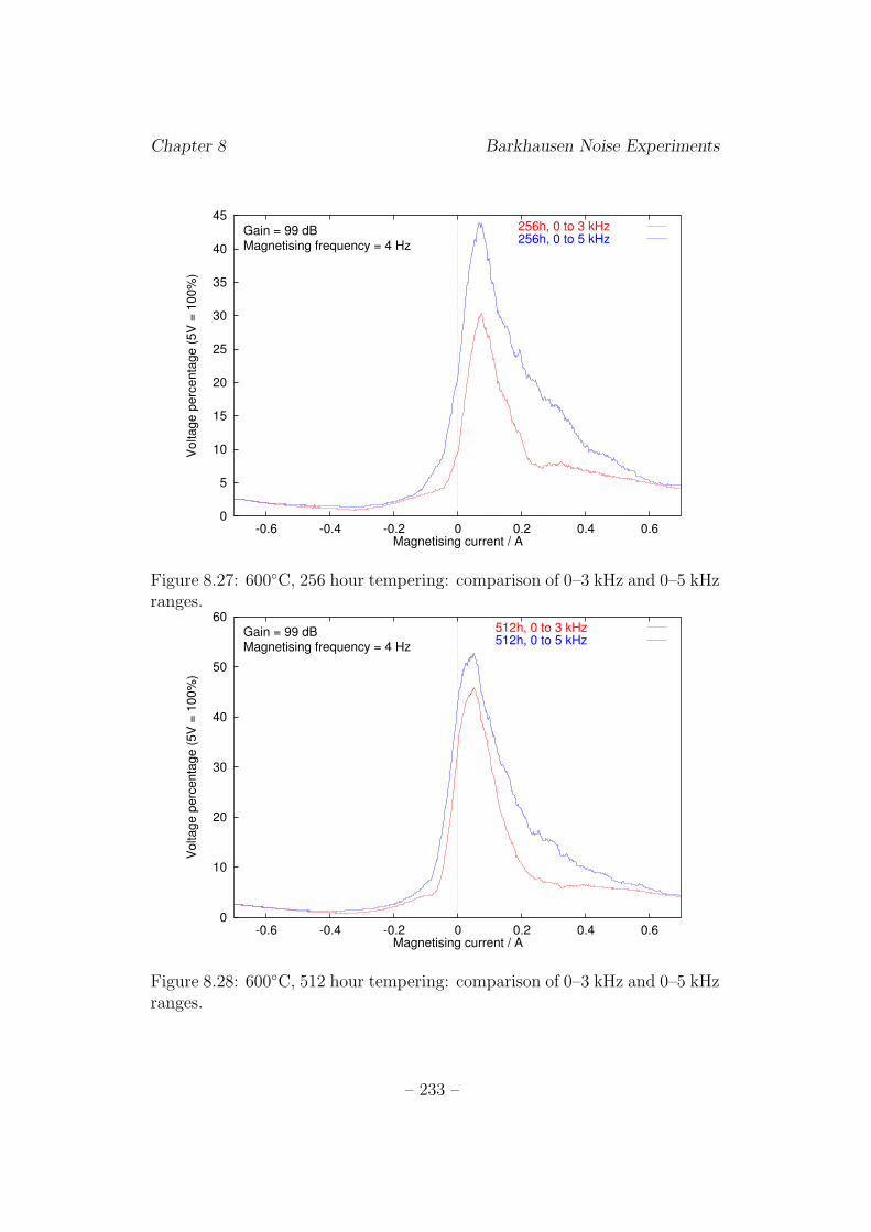
Chapter 8 Barkhausen Noise Experiments
0
5
10
15
20
25
30
35
40
45
-0.6 -0.4 -0.2 0 0.2 0.4 0.6
Vo
lta
ge
pe
rce
nta
ge
(5
V =
10
0%
)
Magnetising current / A
Gain = 99 dBMagnetising frequency = 4 Hz
256h, 0 to 3 kHz256h, 0 to 5 kHz
Figure 8.27: 600◦C, 256 hour tempering: comparison of 0–3 kHz and 0–5 kHzranges.
0
10
20
30
40
50
60
-0.6 -0.4 -0.2 0 0.2 0.4 0.6
Vo
lta
ge
pe
rce
nta
ge
(5
V =
10
0%
)
Magnetising current / A
Gain = 99 dBMagnetising frequency = 4 Hz
512h, 0 to 3 kHz512h, 0 to 5 kHz
Figure 8.28: 600◦C, 512 hour tempering: comparison of 0–3 kHz and 0–5 kHzranges.
– 233 –
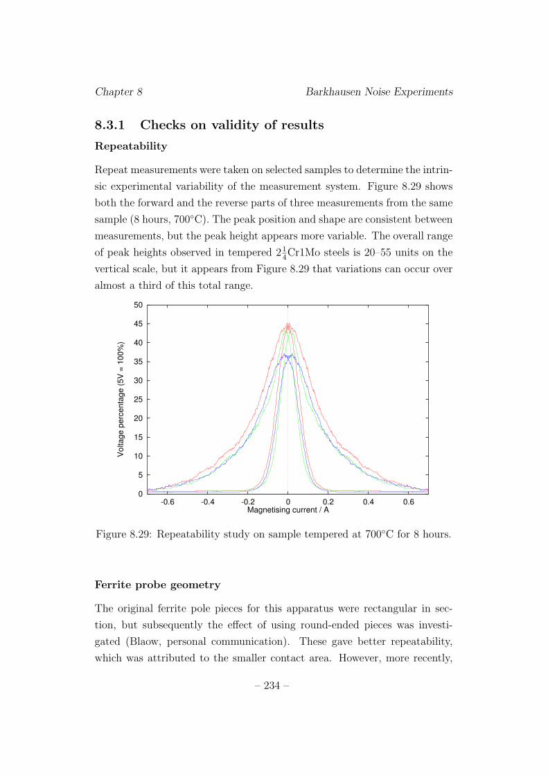
Chapter 8 Barkhausen Noise Experiments
8.3.1 Checks on validity of results
Repeatability
Repeat measurements were taken on selected samples to determine the intrin-
sic experimental variability of the measurement system. Figure 8.29 shows
both the forward and the reverse parts of three measurements from the same
sample (8 hours, 700◦C). The peak position and shape are consistent between
measurements, but the peak height appears more variable. The overall range
of peak heights observed in tempered 214Cr1Mo steels is 20–55 units on the
vertical scale, but it appears from Figure 8.29 that variations can occur over
almost a third of this total range.
0
5
10
15
20
25
30
35
40
45
50
-0.6 -0.4 -0.2 0 0.2 0.4 0.6
Vo
lta
ge
pe
rce
nta
ge
(5
V =
10
0%
)
Magnetising current / A
Figure 8.29: Repeatability study on sample tempered at 700◦C for 8 hours.
Ferrite probe geometry
The original ferrite pole pieces for this apparatus were rectangular in sec-
tion, but subsequently the effect of using round-ended pieces was investi-
gated (Blaow, personal communication). These gave better repeatability,
which was attributed to the smaller contact area. However, more recently,
– 234 –
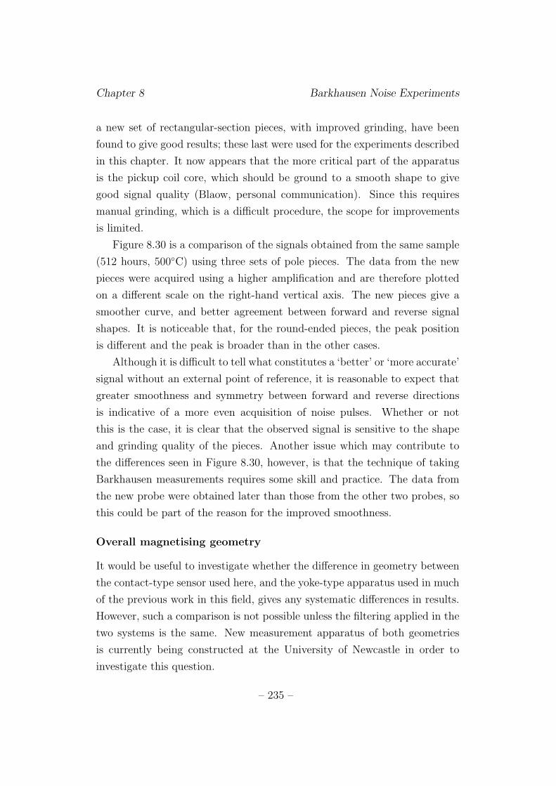
Chapter 8 Barkhausen Noise Experiments
a new set of rectangular-section pieces, with improved grinding, have been
found to give good results; these last were used for the experiments described
in this chapter. It now appears that the more critical part of the apparatus
is the pickup coil core, which should be ground to a smooth shape to give
good signal quality (Blaow, personal communication). Since this requires
manual grinding, which is a difficult procedure, the scope for improvements
is limited.
Figure 8.30 is a comparison of the signals obtained from the same sample
(512 hours, 500◦C) using three sets of pole pieces. The data from the new
pieces were acquired using a higher amplification and are therefore plotted
on a different scale on the right-hand vertical axis. The new pieces give a
smoother curve, and better agreement between forward and reverse signal
shapes. It is noticeable that, for the round-ended pieces, the peak position
is different and the peak is broader than in the other cases.
Although it is difficult to tell what constitutes a ‘better’ or ‘more accurate’
signal without an external point of reference, it is reasonable to expect that
greater smoothness and symmetry between forward and reverse directions
is indicative of a more even acquisition of noise pulses. Whether or not
this is the case, it is clear that the observed signal is sensitive to the shape
and grinding quality of the pieces. Another issue which may contribute to
the differences seen in Figure 8.30, however, is that the technique of taking
Barkhausen measurements requires some skill and practice. The data from
the new probe were obtained later than those from the other two probes, so
this could be part of the reason for the improved smoothness.
Overall magnetising geometry
It would be useful to investigate whether the difference in geometry between
the contact-type sensor used here, and the yoke-type apparatus used in much
of the previous work in this field, gives any systematic differences in results.
However, such a comparison is not possible unless the filtering applied in the
two systems is the same. New measurement apparatus of both geometries
is currently being constructed at the University of Newcastle in order to
investigate this question.
– 235 –
Chapter 8 Barkhausen Noise Experiments
0
5
10
15
20
25
-0.6 -0.4 -0.2 0 0.2 0.4 0.60
5
10
15
20
25
30
35
40V
olta
ge
pe
rce
nta
ge
(5
V =
10
0%
)
Vo
lta
ge
pe
rce
nta
ge
(5
V =
10
0%
)
Magnetising current / A
Round-endedFlat-endedNew
Figure 8.30: Effect of different pole-piece shapes on the 500◦C, 512 hourssignal.
8.4 Discussion
8.4.1 Tempered 214Cr1Mo steels
If the BN activity at higher currents corresponds to the second peak seen
by Moorthy et al. (1997b) and attributed by them to unpinning of domain
walls by carbides, then it appears that this activity is predominantly low-
frequency noise. The other peak, occurring at a lower current and associated
with unpinning from grain boundaries, is prominent at all frequencies. If the
frequency is approximately the reciprocal of the ‘time of flight’ of the domain
wall between pinning sites (Saquet et al., 1999), then more closely spaced
sites will produce noise of higher frequencies. When the applied current is
small, the domain walls will be pinned by both weak and strong pinning sites,
and the time interval between pinning events will be small. Increasing the
current allows domain walls to bypass weaker pinning sites and move longer
distances between events. If it is assumed that the domain wall velocity
is approximately constant, then this would give noise of lower frequencies.
– 236 –
Chapter 8 Barkhausen Noise Experiments
(Equation 5.15, however, gives the domain wall velocity as proportional to
the difference between the applied field and HC , so that walls would move
faster at higher currents. Since this would tend to increase the frequency
of events occurring at high currents, it appears that the jump size effect is
dominant over the wall velocity effect in the system under investigation.)
Since it is believed that there is important information missing in these
data sets as a result of filtering, it is not possible to interpret the signal
shapes for the tempered steels with a great deal of confidence. However, the
broadening of the peaks at higher temperatures and longer tempering times
are indicative of a wider distribution of pinning site strengths, and the shift of
the noise onset to a lower applied current after longer tempering corresponds
to the appearance of weaker pinning sites.
8.4.2 11Cr1Mo steels
Steels designed for creep resistance contain, after tempering, a high con-
centration of fine alloy carbide particles to confer long-term microstructural
stability. The high currents at which the peaks occur in this steel, and their
similarity in shape to the AQ peak (Figure 8.12), suggest that little or no
microstructural coarsening has taken place. This is borne out by an exami-
nation of the optical micrographs (Figure 6.16–6.19), which closely resemble
the 214Cr1Mo steel in the very early stages of its tempering at 500 or 600◦C.
Coarsening, with its associated loss of creep resistance, may be detectable
in this steel by a shift of the noise onset to a lower current.
8.5 Conclusions
BN measurements were carried out on 214Cr1Mo and 11Cr1Mo steels tem-
pered in a wide variety of conditions. In the 214Cr1Mo samples, some of the
characteristics observed in previous work by Moorthy et al. could be seen;
between the as-quenched and the tempered states the peak height increased,
and its position moved to a lower current. Evidence of a second peak at
higher current was present, but much suppressed by the hardware filtering,
because it is composed primarily of noise with frequencies below the filtering
– 237 –
Chapter 8 Barkhausen Noise Experiments
range of the system. Because of the difficulties in observing this second peak,
detailed analysis of its relationship to tempering conditions and carbide sizes
could not be carried out.
In the 214Cr1Mo samples, the maximum BN voltage occurs at a lower ap-
plied current with increasing Larson-Miller parameter. The 11Cr1Mo wt. %
steel samples displayed peaks at a high current even after long-term heat
treatment. It is believed that this is due to the coarsening resistance con-
ferred by fine alloy carbides.
Measured BN data are very sensitive to experimental conditions such as
frequency filtering and the shape and surface roughness of the yoke contact
points and pickup coil core. This sensitivity may go some way towards ex-
plaining the discrepancies between results in the literature. Taking this into
account, it would be advisable to develop a standard instrument and tech-
nique if BN measurements are to be used for safety-critical NDT applications.
Chapter 9 discusses the fitting of the model developed in Chapter 5 to
these data sets.
– 238 –
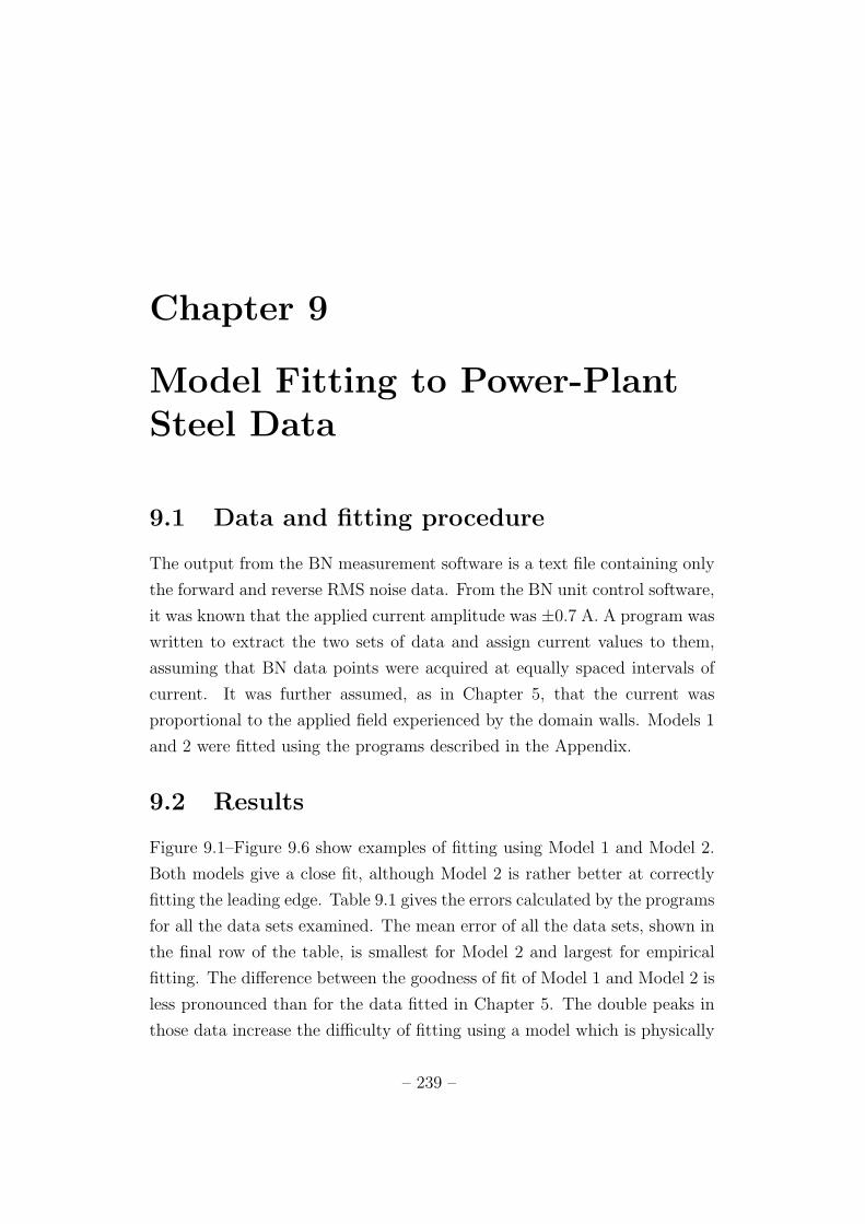
Chapter 9
Model Fitting to Power-PlantSteel Data
9.1 Data and fitting procedure
The output from the BN measurement software is a text file containing only
the forward and reverse RMS noise data. From the BN unit control software,
it was known that the applied current amplitude was ±0.7 A. A program was
written to extract the two sets of data and assign current values to them,
assuming that BN data points were acquired at equally spaced intervals of
current. It was further assumed, as in Chapter 5, that the current was
proportional to the applied field experienced by the domain walls. Models 1
and 2 were fitted using the programs described in the Appendix.
9.2 Results
Figure 9.1–Figure 9.6 show examples of fitting using Model 1 and Model 2.
Both models give a close fit, although Model 2 is rather better at correctly
fitting the leading edge. Table 9.1 gives the errors calculated by the programs
for all the data sets examined. The mean error of all the data sets, shown in
the final row of the table, is smallest for Model 2 and largest for empirical
fitting. The difference between the goodness of fit of Model 1 and Model 2 is
less pronounced than for the data fitted in Chapter 5. The double peaks in
those data increase the difficulty of fitting using a model which is physically
– 239 –
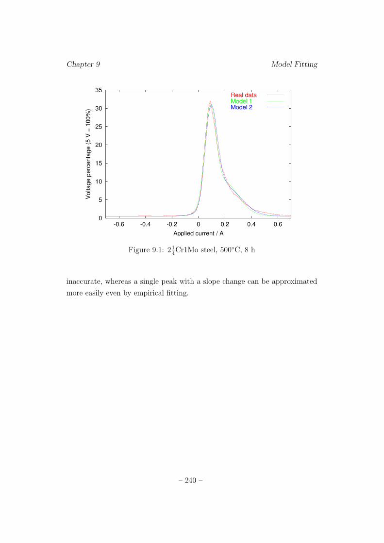
Chapter 9 Model Fitting
0
5
10
15
20
25
30
35
-0.6 -0.4 -0.2 0 0.2 0.4 0.6
Voltage p
erc
enta
ge (
5 V
= 1
00%
)
Applied current / A
Real dataModel 1Model 2
Figure 9.1: 214Cr1Mo steel, 500◦C, 8 h
inaccurate, whereas a single peak with a slope change can be approximated
more easily even by empirical fitting.
– 240 –
Chapter 9 Model Fitting
0
5
10
15
20
25
30
35
-0.6 -0.4 -0.2 0 0.2 0.4 0.6
Voltage p
erc
enta
ge (
5 V
= 1
00%
)
Applied current / A
Real dataModel 1Model 2
Figure 9.2: 214Cr1Mo steel, 600◦C, 8 h
0
5
10
15
20
25
30
35
40
45
50
-0.6 -0.4 -0.2 0 0.2 0.4 0.6
Voltage p
erc
enta
ge (
5 V
= 1
00%
)
Applied current / A
Real dataModel 1Model 2
Figure 9.3: 214Cr1Mo steel, 700◦C, 8 h
– 241 –
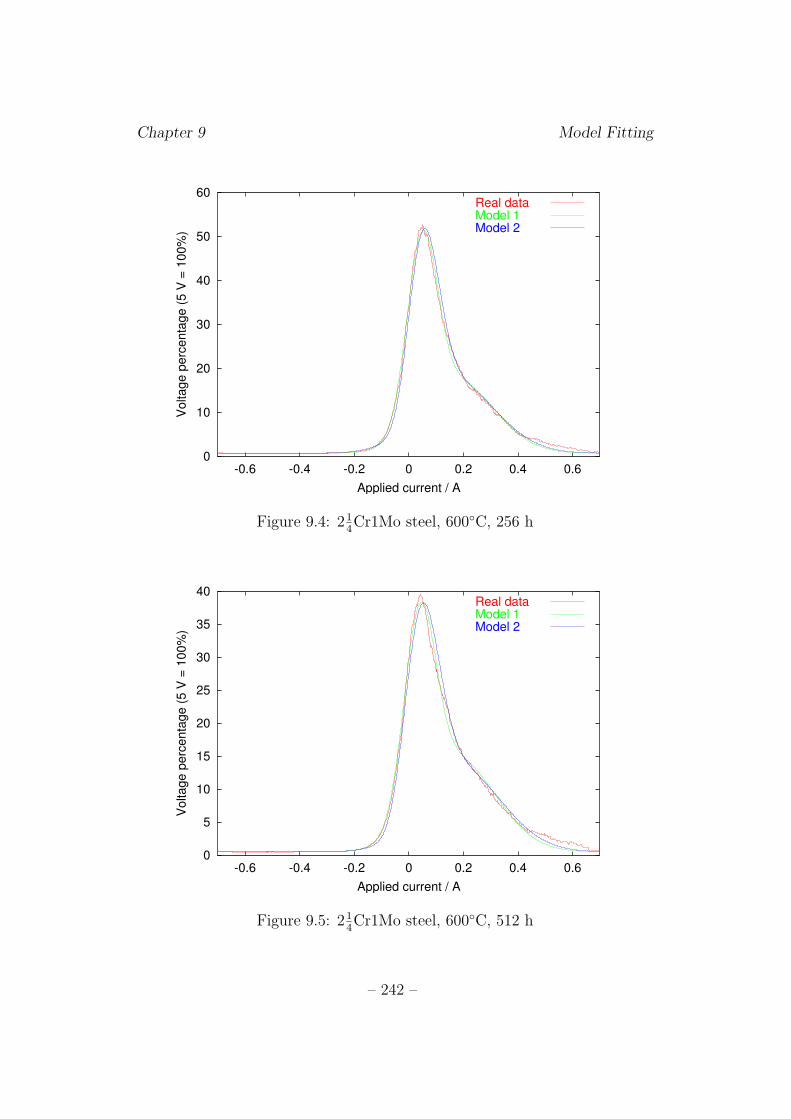
Chapter 9 Model Fitting
0
10
20
30
40
50
60
-0.6 -0.4 -0.2 0 0.2 0.4 0.6
Voltage p
erc
enta
ge (
5 V
= 1
00%
)
Applied current / A
Real dataModel 1Model 2
Figure 9.4: 214Cr1Mo steel, 600◦C, 256 h
0
5
10
15
20
25
30
35
40
-0.6 -0.4 -0.2 0 0.2 0.4 0.6
Voltage p
erc
enta
ge (
5 V
= 1
00%
)
Applied current / A
Real dataModel 1Model 2
Figure 9.5: 214Cr1Mo steel, 600◦C, 512 h
– 242 –
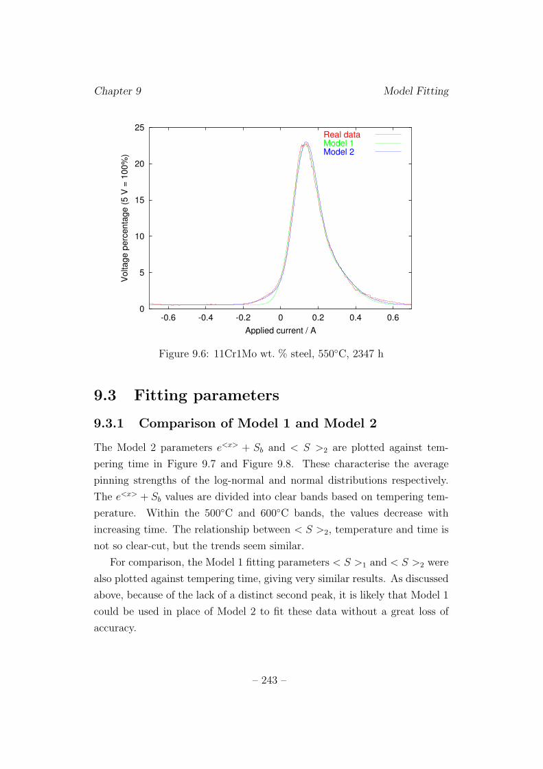
Chapter 9 Model Fitting
0
5
10
15
20
25
-0.6 -0.4 -0.2 0 0.2 0.4 0.6
Voltage p
erc
enta
ge (
5 V
= 1
00%
)
Applied current / A
Real dataModel 1Model 2
Figure 9.6: 11Cr1Mo wt. % steel, 550◦C, 2347 h
9.3 Fitting parameters
9.3.1 Comparison of Model 1 and Model 2
The Model 2 parameters e<x> + Sb and < S >2 are plotted against tem-
pering time in Figure 9.7 and Figure 9.8. These characterise the average
pinning strengths of the log-normal and normal distributions respectively.
The e<x> + Sb values are divided into clear bands based on tempering tem-
perature. Within the 500◦C and 600◦C bands, the values decrease with
increasing time. The relationship between < S >2, temperature and time is
not so clear-cut, but the trends seem similar.
For comparison, the Model 1 fitting parameters < S >1 and < S >2 were
also plotted against tempering time, giving very similar results. As discussed
above, because of the lack of a distinct second peak, it is likely that Model 1
could be used in place of Model 2 to fit these data without a great loss of
accuracy.
– 243 –
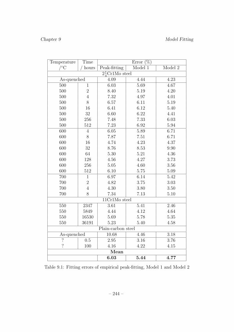
Chapter 9 Model Fitting
Temperature Time Error (%)/◦C / hours Peak-fitting Model 1 Model 2
214Cr1Mo steel
As-quenched 4.09 4.44 4.23500 1 6.03 5.69 4.67500 2 8.40 5.19 4.20500 4 7.32 4.97 4.01500 8 6.57 6.11 5.19500 16 6.41 6.12 5.40500 32 6.60 6.22 4.41500 256 7.48 7.33 6.03500 512 7.23 6.92 5.94600 4 6.05 5.89 6.71600 8 7.87 7.51 6.71600 16 4.74 4.23 4.37600 32 8.76 8.53 9.90600 64 5.30 5.21 4.36600 128 4.56 4.27 3.73600 256 5.05 4.60 3.56600 512 6.10 5.75 5.09700 1 6.97 6.14 5.42700 2 4.82 3.75 3.03700 4 4.30 3.80 3.50700 8 7.34 7.13 5.10
11Cr1Mo steel550 2347 3.61 5.41 2.46550 5849 4.44 4.12 4.64550 16530 5.69 5.78 5.35550 36191 5.23 5.40 4.58
Plain-carbon steelAs-quenched 10.68 4.46 3.18? 0.5 2.95 3.16 3.76? 100 4.16 4.22 4.15
Mean6.03 5.44 4.77
Table 9.1: Fitting errors of empirical peak-fitting, Model 1 and Model 2
– 244 –
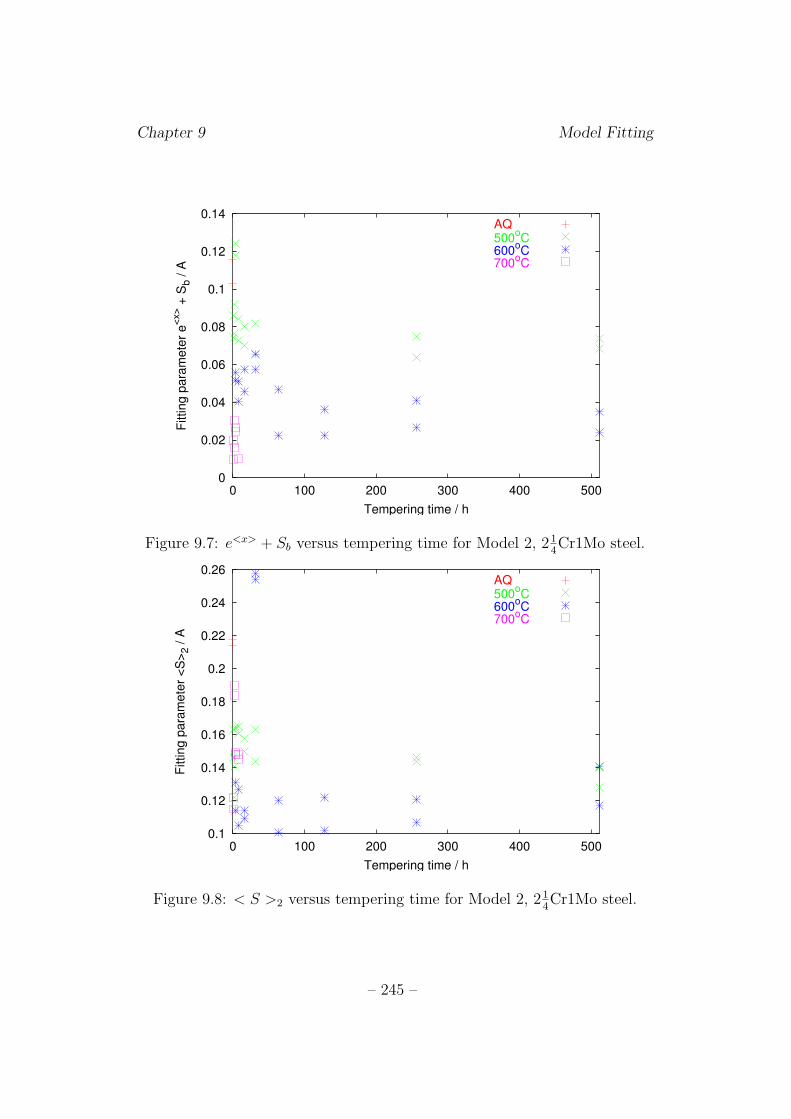
Chapter 9 Model Fitting
0
0.02
0.04
0.06
0.08
0.1
0.12
0.14
0 100 200 300 400 500
Fitting p
ara
mete
r e
<x> +
Sb / A
Tempering time / h
AQ500
oC
600oC
700oC
Figure 9.7: e<x> + Sb versus tempering time for Model 2, 214Cr1Mo steel.
0.1
0.12
0.14
0.16
0.18
0.2
0.22
0.24
0.26
0 100 200 300 400 500
Fitting p
ara
mete
r <
S>
2 / A
Tempering time / h
AQ500
oC
600oC
700oC
Figure 9.8: < S >2 versus tempering time for Model 2, 214Cr1Mo steel.
– 245 –
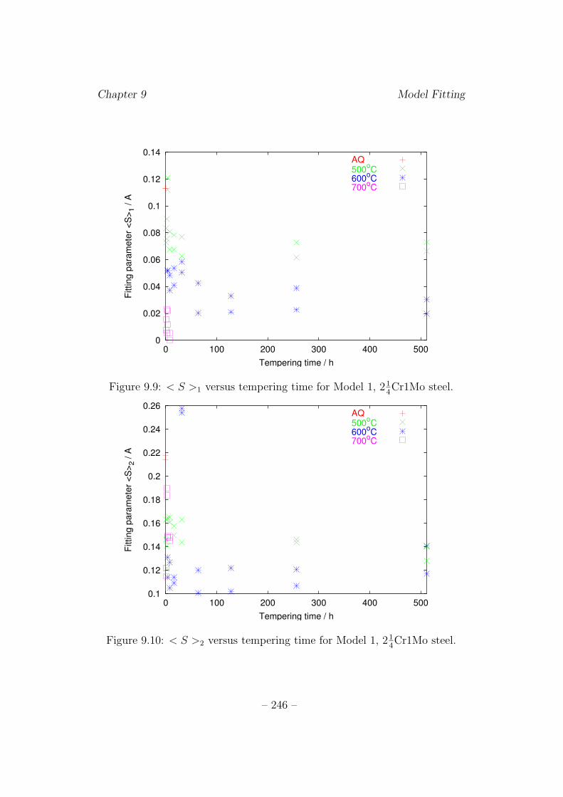
Chapter 9 Model Fitting
0
0.02
0.04
0.06
0.08
0.1
0.12
0.14
0 100 200 300 400 500
Fitting p
ara
mete
r <
S>
1 / A
Tempering time / h
AQ500
oC
600oC
700oC
Figure 9.9: < S >1 versus tempering time for Model 1, 214Cr1Mo steel.
0.1
0.12
0.14
0.16
0.18
0.2
0.22
0.24
0.26
0 100 200 300 400 500
Fitting p
ara
mete
r <
S>
2 / A
Tempering time / h
AQ500
oC
600oC
700oC
Figure 9.10: < S >2 versus tempering time for Model 1, 214Cr1Mo steel.
– 246 –

Chapter 9 Model Fitting
9.3.2 Model 2 parameter variations with Larson-Millerparameter
The combination e<x> + Sb is plotted against the Larson-Miller parameter
P in Figure 9.11. This is very similar in appearance to Figure 8.18, with
a monotonic decrease in e<x> + Sb with P for all the 214Cr1Mo samples.
The 11Cr1Mo samples have higher e<x> + Sb values than the 214Cr1Mo.
< S >2 decreases with P at short times, then increases again at longer times
(Figure 9.12).
A1 and A2 both increase monotonically with increasing P in the 214Cr1Mo
steel samples. The 11Cr1Mo values fall below these curves. A2 has around
half the value of A1.
The distribution widths ∆x and ∆S2, shown in Figure 9.15 and Fig-
ure 9.16 respectively, tend to higher values at higher P , but there is more
scatter than for A1, A2 and e<x> + Sb.
– 247 –
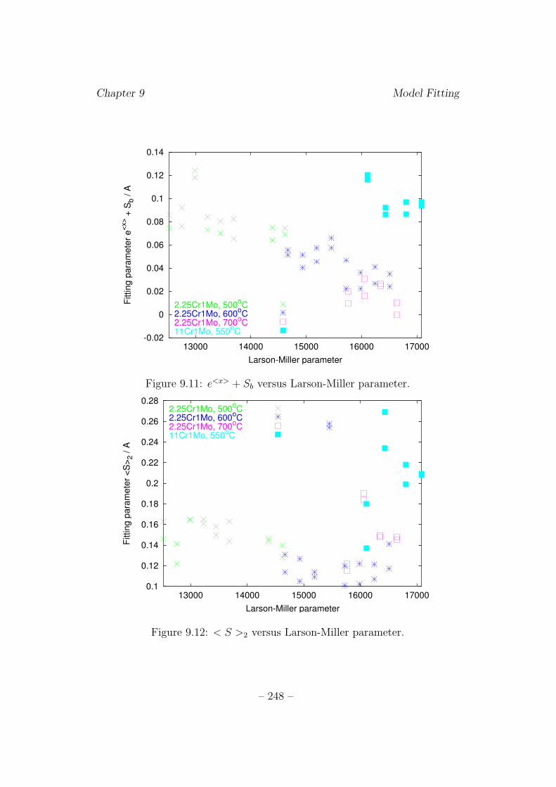
Chapter 9 Model Fitting
-0.02
0
0.02
0.04
0.06
0.08
0.1
0.12
0.14
13000 14000 15000 16000 17000
Fitting p
ara
mete
r e
<x> +
Sb / A
Larson-Miller parameter
2.25Cr1Mo, 500oC
2.25Cr1Mo, 600oC
2.25Cr1Mo, 700oC
11Cr1Mo, 550oC
Figure 9.11: e<x> + Sb versus Larson-Miller parameter.
0.1
0.12
0.14
0.16
0.18
0.2
0.22
0.24
0.26
0.28
13000 14000 15000 16000 17000
Fitting p
ara
mete
r <
S>
2 / A
Larson-Miller parameter
2.25Cr1Mo, 500oC
2.25Cr1Mo, 600oC
2.25Cr1Mo, 700oC
11Cr1Mo, 550oC
Figure 9.12: < S >2 versus Larson-Miller parameter.
– 248 –
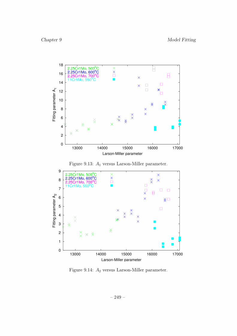
Chapter 9 Model Fitting
0
2
4
6
8
10
12
14
16
18
13000 14000 15000 16000 17000
Fitting p
ara
mete
r A
1
Larson-Miller parameter
2.25Cr1Mo, 500oC
2.25Cr1Mo, 600oC
2.25Cr1Mo, 700oC
11Cr1Mo, 550oC
Figure 9.13: A1 versus Larson-Miller parameter.
0
1
2
3
4
5
6
7
8
9
13000 14000 15000 16000 17000
Fitting p
ara
mete
r A
2
Larson-Miller parameter
2.25Cr1Mo, 500oC
2.25Cr1Mo, 600oC
2.25Cr1Mo, 700oC
11Cr1Mo, 550oC
Figure 9.14: A2 versus Larson-Miller parameter.
– 249 –
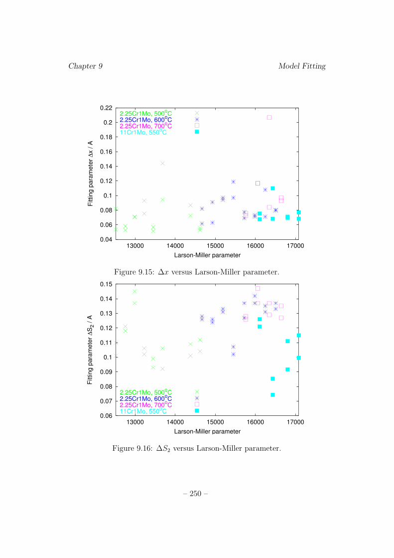
Chapter 9 Model Fitting
0.04
0.06
0.08
0.1
0.12
0.14
0.16
0.18
0.2
0.22
13000 14000 15000 16000 17000
Fitting p
ara
mete
r ∆
x / A
Larson-Miller parameter
2.25Cr1Mo, 500oC
2.25Cr1Mo, 600oC
2.25Cr1Mo, 700oC
11Cr1Mo, 550oC
Figure 9.15: ∆x versus Larson-Miller parameter.
0.06
0.07
0.08
0.09
0.1
0.11
0.12
0.13
0.14
0.15
13000 14000 15000 16000 17000
Fitting p
ara
mete
r ∆
S2 / A
Larson-Miller parameter
2.25Cr1Mo, 500oC
2.25Cr1Mo, 600oC
2.25Cr1Mo, 700oC
11Cr1Mo, 550oC
Figure 9.16: ∆S2 versus Larson-Miller parameter.
– 250 –
Chapter 9 Model Fitting
9.4 Discussion
9.4.1 Relationship of fitting parameters to microstruc-ture
It was seen in Chapter 6 that 214Cr1Mo steel samples tempered at 700◦C
underwent rapid microstructural coarsening and softening, but at 500 and
600◦C, changes were much more gradual. Despite these differences, if the
Larson-Miller parameter is used to combine temperature and time condi-
tions, it can be seen that the BN model parameters from this steel fall into
the same regime of behaviour. In particular, there is a very clear relation-
ship between e<x> + Sb and the Larson-Miller parameter; this accurately
replicates the relationship between peak position and P seen in Chapter 8.
This large peak is believed to correspond to the lower-field peak observed
by Moorthy et al. and attributed to interactions between domain walls and
grain boundaries. If this is so, the results of Chapter 7 suggest that the
gradual reduction of strain at grain boundaries during tempering reduces
the strength of their interactions with domain walls. The lack of any clear
changes in grain boundary character distribution during tempering at 600◦C
leads to the conclusion that the main changes are in magnetoelastic rather
than magnetostatic energy, and are associated with changes in the dislocation
density at grain boundaries. In as-quenched steel, adjacent martensitic laths
within the same packet are separated by a highly strained boundary, but
the misorientation between the laths is very small. Tempering reduces the
dislocation density, and this decreases the strength and density of obstacles
to domain wall motion.
No recrystallisation has been observed in any of the samples in this study.
If the temperature and time were increased sufficiently to allow this, a dif-
ferent regime of BN behaviour, in which magnetostatic energy changes are
important, may result.
The initial decrease of < S >2 with tempering time may be related to the
dissolution of M3C and its replacement with fine, needlelike M2X carbides,
giving a reduction in pinning strength. The subsequent appearance and rapid
growth of spheroidal M7C3 carbides and other coarse phases at longer times
– 251 –
Chapter 9 Model Fitting
increases < S >2 again. It would be useful to repeat these experiments
using BN apparatus which is capable of detecting double-peak behaviour to
investigate the high-field region more fully.
The A parameters characterising the number of pinning sites show an
unexpected monotonic increase with tempering time. It would be expected
that the number of pinning sites from grain boundaries would fall as coars-
ening occurs, and the number of carbides may vary in a complex way during
the precipitation sequence. The observed behaviour of A suggests that the
model is not currently physically accurate in this respect. The width ∆S2
does follow the expected behaviour of a carbide size distribution, increasing
with tempering time as the carbide sizes become more varied, but ∆x is more
difficult to interpret.
The 11Cr1Mo steel BN parameters do not follow the same relationships
as those of the 214Cr1Mo steel, although there is a suggestion in Figure 9.11
that its e<x> + Sb values may lie on a parallel line to the 214Cr1Mo steel
values. However, more data, with a larger range of tempering conditions,
would be needed to test this.
9.5 Conclusion
Model 2 fits these experimental data well, but almost as good a fit can be
obtained using Model 1, possibly because the lack of a distinct second peak
makes fitting easier. Clear relationships between the microstructural charac-
teristics and the Model 2 parameters have been observed. From a comparison
between microscopy, orientation measurements and modelling results, it has
been concluded that the principal influence on magnetic behaviour in these
samples is the reduction of the high levels of strain initially present in the
quenched microstructure. However, it would be advisable to repeat the ex-
periments using more suitable apparatus to check these conclusions.
– 252 –
Chapter 10
Barkhausen Noise in PM2000Oxide Dispersion StrengthenedAlloy
10.1 Oxide dispersion strengthened alloys
PM2000 is an oxide dispersion strengthened (ODS) alloy of composition
20 Cr, 0.5 Ti, 0.5 Y2O3, 5.5 Al, balance Fe (wt. %), manufactured by
mechanically alloying the metallic components with fine particles of Y2O3
(Krautwasser et al., 1994). It has been proposed as a suitable material for
biomass-based power plant with an operating temperature of around 1100◦C
and a pressure of 15–30 bar (Capdevila et al., 2001). A material for this ap-
plication must have good oxidation resistance, which in PM2000 is provided
by the aluminium, and good creep performance. At such a high temperature,
this is only achieved using a very coarse grain size in combination with an
oxide dispersion.
Powders of the components are severely deformed by ball milling to pro-
duce a mixture with a uniform distribution of oxide particles. This is con-
solidated by hot isostatic pressing, then extruded into tubular form. The
microstructure of the material at this stage consists of very fine equiaxed
grains (Sporer et al., 1993). These are less than 1 µm wide and heavily
strained because of the cold deformation.
Recrystallisation, to give a coarse microstructure for creep resistance, re-
– 253 –
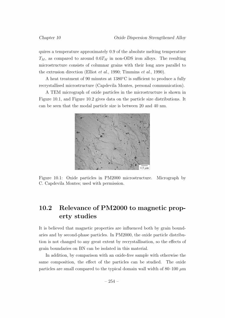
Chapter 10 Oxide Dispersion Strengthened Alloy
quires a temperature approximately 0.9 of the absolute melting temperature
TM , as compared to around 0.6TM in non-ODS iron alloys. The resulting
microstructure consists of columnar grains with their long axes parallel to
the extrusion direction (Elliot et al., 1990; Timmins et al., 1990).
A heat treatment of 90 minutes at 1380◦C is sufficient to produce a fully
recrystallised microstructure (Capdevila Montes, personal communication).
A TEM micrograph of oxide particles in the microstructure is shown in
Figure 10.1, and Figure 10.2 gives data on the particle size distributions. It
can be seen that the modal particle size is between 20 and 40 nm.
Figure 10.1: Oxide particles in PM2000 microstructure. Micrograph byC. Capdevila Montes; used with permission.
10.2 Relevance of PM2000 to magnetic prop-
erty studies
It is believed that magnetic properties are influenced both by grain bound-
aries and by second-phase particles. In PM2000, the oxide particle distribu-
tion is not changed to any great extent by recrystallisation, so the effects of
grain boundaries on BN can be isolated in this material.
In addition, by comparison with an oxide-free sample with otherwise the
same composition, the effect of the particles can be studied. The oxide
particles are small compared to the typical domain wall width of 80–100 µm
– 254 –
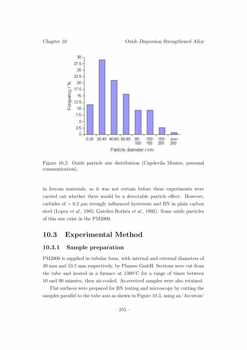
Chapter 10 Oxide Dispersion Strengthened Alloy
Figure 10.2: Oxide particle size distribution (Capdevila Montes, personalcommunication).
in ferrous materials, so it was not certain before these experiments were
carried out whether there would be a detectable particle effect. However,
carbides of ∼ 0.2 µm strongly influenced hysteresis and BN in plain carbon
steel (Lopez et al., 1985; Gatelier-Rothea et al., 1992). Some oxide particles
of this size exist in the PM2000.
10.3 Experimental Method
10.3.1 Sample preparation
PM2000 is supplied in tubular form, with internal and external diameters of
49 mm and 53.5 mm respectively, by Plansee GmbH. Sections were cut from
the tube and heated in a furnace at 1380◦C for a range of times between
10 and 90 minutes, then air-cooled. As-received samples were also retained.
Flat surfaces were prepared for BN testing and microscopy by cutting the
samples parallel to the tube axis as shown in Figure 10.3, using an ‘Accutom’
– 255 –
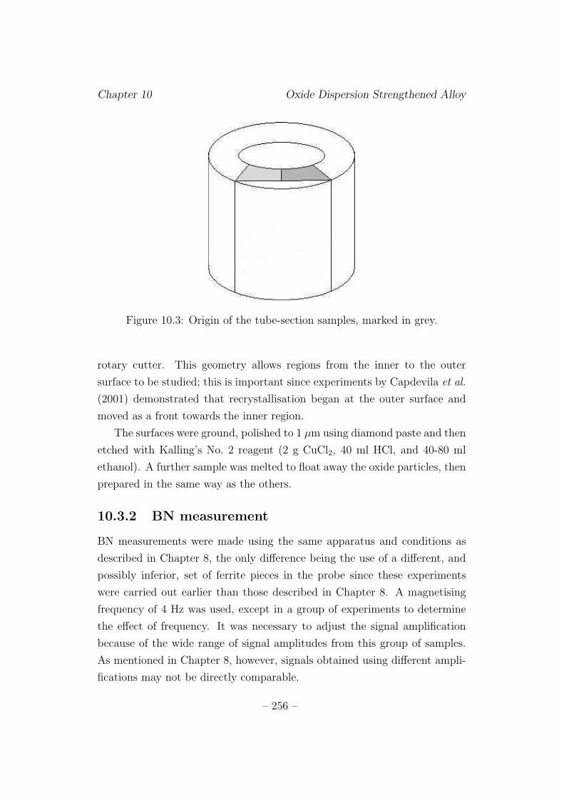
Chapter 10 Oxide Dispersion Strengthened Alloy
Figure 10.3: Origin of the tube-section samples, marked in grey.
rotary cutter. This geometry allows regions from the inner to the outer
surface to be studied; this is important since experiments by Capdevila et al.
(2001) demonstrated that recrystallisation began at the outer surface and
moved as a front towards the inner region.
The surfaces were ground, polished to 1 µm using diamond paste and then
etched with Kalling’s No. 2 reagent (2 g CuCl2, 40 ml HCl, and 40-80 ml
ethanol). A further sample was melted to float away the oxide particles, then
prepared in the same way as the others.
10.3.2 BN measurement
BN measurements were made using the same apparatus and conditions as
described in Chapter 8, the only difference being the use of a different, and
possibly inferior, set of ferrite pieces in the probe since these experiments
were carried out earlier than those described in Chapter 8. A magnetising
frequency of 4 Hz was used, except in a group of experiments to determine
the effect of frequency. It was necessary to adjust the signal amplification
because of the wide range of signal amplitudes from this group of samples.
As mentioned in Chapter 8, however, signals obtained using different ampli-
fications may not be directly comparable.
– 256 –
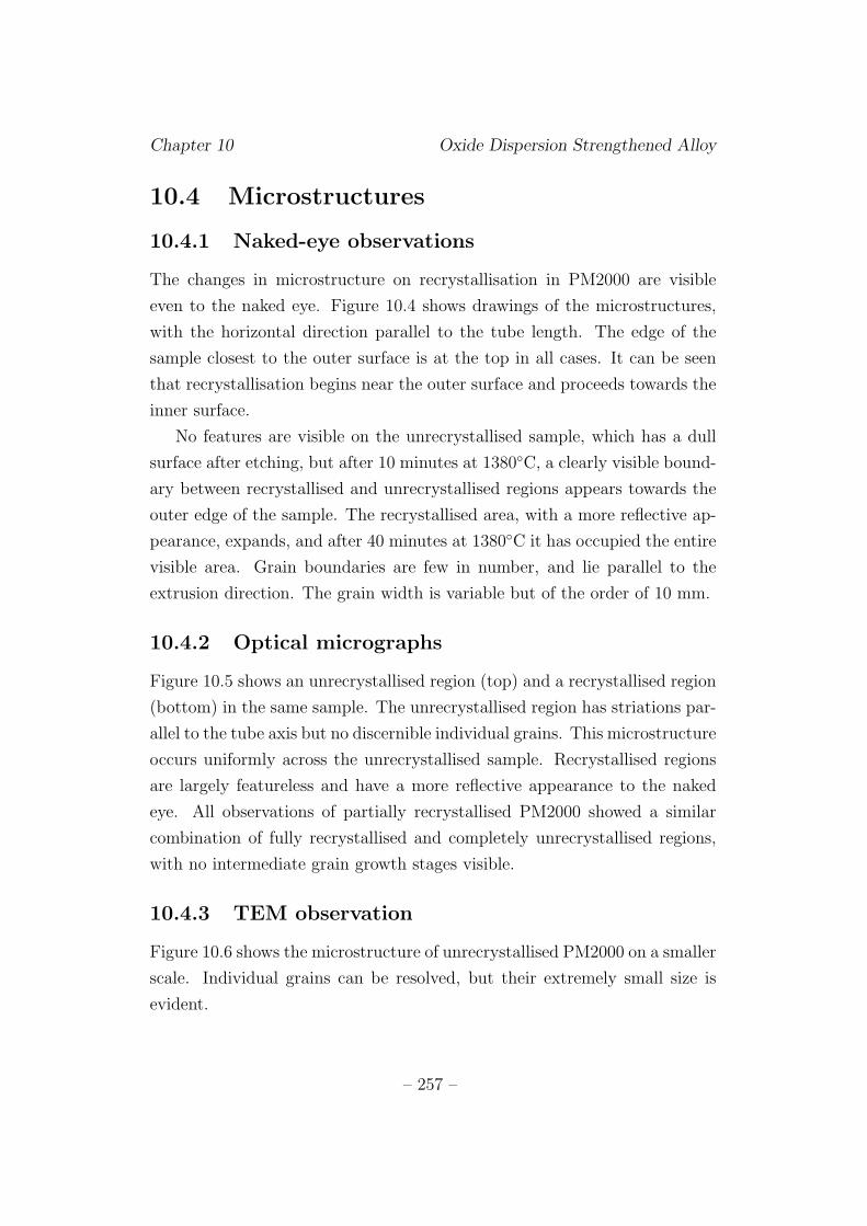
Chapter 10 Oxide Dispersion Strengthened Alloy
10.4 Microstructures
10.4.1 Naked-eye observations
The changes in microstructure on recrystallisation in PM2000 are visible
even to the naked eye. Figure 10.4 shows drawings of the microstructures,
with the horizontal direction parallel to the tube length. The edge of the
sample closest to the outer surface is at the top in all cases. It can be seen
that recrystallisation begins near the outer surface and proceeds towards the
inner surface.
No features are visible on the unrecrystallised sample, which has a dull
surface after etching, but after 10 minutes at 1380◦C, a clearly visible bound-
ary between recrystallised and unrecrystallised regions appears towards the
outer edge of the sample. The recrystallised area, with a more reflective ap-
pearance, expands, and after 40 minutes at 1380◦C it has occupied the entire
visible area. Grain boundaries are few in number, and lie parallel to the
extrusion direction. The grain width is variable but of the order of 10 mm.
10.4.2 Optical micrographs
Figure 10.5 shows an unrecrystallised region (top) and a recrystallised region
(bottom) in the same sample. The unrecrystallised region has striations par-
allel to the tube axis but no discernible individual grains. This microstructure
occurs uniformly across the unrecrystallised sample. Recrystallised regions
are largely featureless and have a more reflective appearance to the naked
eye. All observations of partially recrystallised PM2000 showed a similar
combination of fully recrystallised and completely unrecrystallised regions,
with no intermediate grain growth stages visible.
10.4.3 TEM observation
Figure 10.6 shows the microstructure of unrecrystallised PM2000 on a smaller
scale. Individual grains can be resolved, but their extremely small size is
evident.
– 257 –
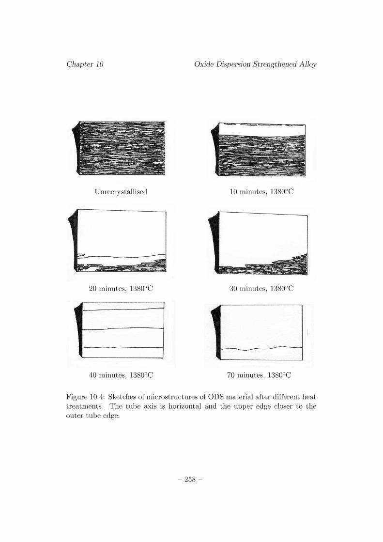
Chapter 10 Oxide Dispersion Strengthened Alloy
Unrecrystallised 10 minutes, 1380◦C
20 minutes, 1380◦C 30 minutes, 1380◦C
40 minutes, 1380◦C 70 minutes, 1380◦C
Figure 10.4: Sketches of microstructures of ODS material after different heattreatments. The tube axis is horizontal and the upper edge closer to theouter tube edge.
– 258 –
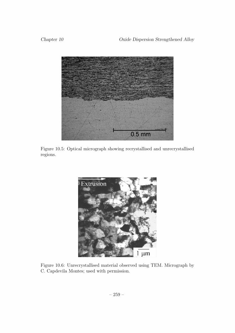
Chapter 10 Oxide Dispersion Strengthened Alloy
Figure 10.5: Optical micrograph showing recrystallised and unrecrystallisedregions.
Figure 10.6: Unrecrystallised material observed using TEM. Micrograph byC. Capdevila Montes; used with permission.
– 259 –
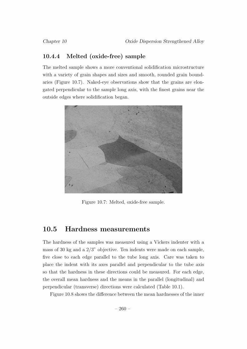
Chapter 10 Oxide Dispersion Strengthened Alloy
10.4.4 Melted (oxide-free) sample
The melted sample shows a more conventional solidification microstructure
with a variety of grain shapes and sizes and smooth, rounded grain bound-
aries (Figure 10.7). Naked-eye observations show that the grains are elon-
gated perpendicular to the sample long axis, with the finest grains near the
outside edges where solidification began.
Figure 10.7: Melted, oxide-free sample.
10.5 Hardness measurements
The hardness of the samples was measured using a Vickers indenter with a
mass of 30 kg and a 2/3” objective. Ten indents were made on each sample,
five close to each edge parallel to the tube long axis. Care was taken to
place the indent with its axes parallel and perpendicular to the tube axis
so that the hardness in these directions could be measured. For each edge,
the overall mean hardness and the means in the parallel (longitudinal) and
perpendicular (transverse) directions were calculated (Table 10.1).
Figure 10.8 shows the difference between the mean hardnesses of the inner
– 260 –
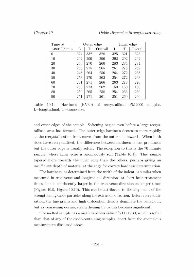
Chapter 10 Oxide Dispersion Strengthened Alloy
Time at Outer edge Inner edge1380◦C/ min L T Overall L T Overall0 324 332 328 325 321 32310 292 299 296 292 292 29220 250 270 260 283 284 28430 255 275 265 261 276 26940 248 264 256 264 272 26850 253 270 262 254 272 26360 261 271 266 263 278 27070 250 273 262 150 150 15080 250 265 258 254 266 26090 251 271 261 251 269 260
Table 10.1: Hardness (HV30) of recrystallised PM2000 samples.L=longitudinal, T=transverse.
and outer edges of the sample. Softening begins even before a large recrys-
tallised area has formed. The outer edge hardness decreases more rapidly
as the recrystallisation front moves from the outer side inwards. When both
sides have recrystallised, the difference between hardness is less prominent
but the outer edge is usually softer. The exception to this is the 70 minute
sample, whose inner edge is anomalously soft (Table 10.1). This sample
tapered more towards the inner edge than the others, perhaps giving an
insufficient depth of material at the edge for correct hardness determination.
The hardness, as determined from the width of the indent, is similar when
measured in transverse and longitudinal directions at short heat treatment
times, but is consistently larger in the transverse direction at longer times
(Figure 10.9, Figure 10.10). This can be attributed to the alignment of the
strengthening oxide particles along the extrusion direction. Before recrystalli-
sation, the fine grains and high dislocation density dominate the behaviour,
but as coarsening occurs, strengthening by oxides becomes significant.
The melted sample has a mean hardness value of 211 HV30, which is softer
than that of any of the oxide-containing samples, apart from the anomalous
measurement discussed above.
– 261 –
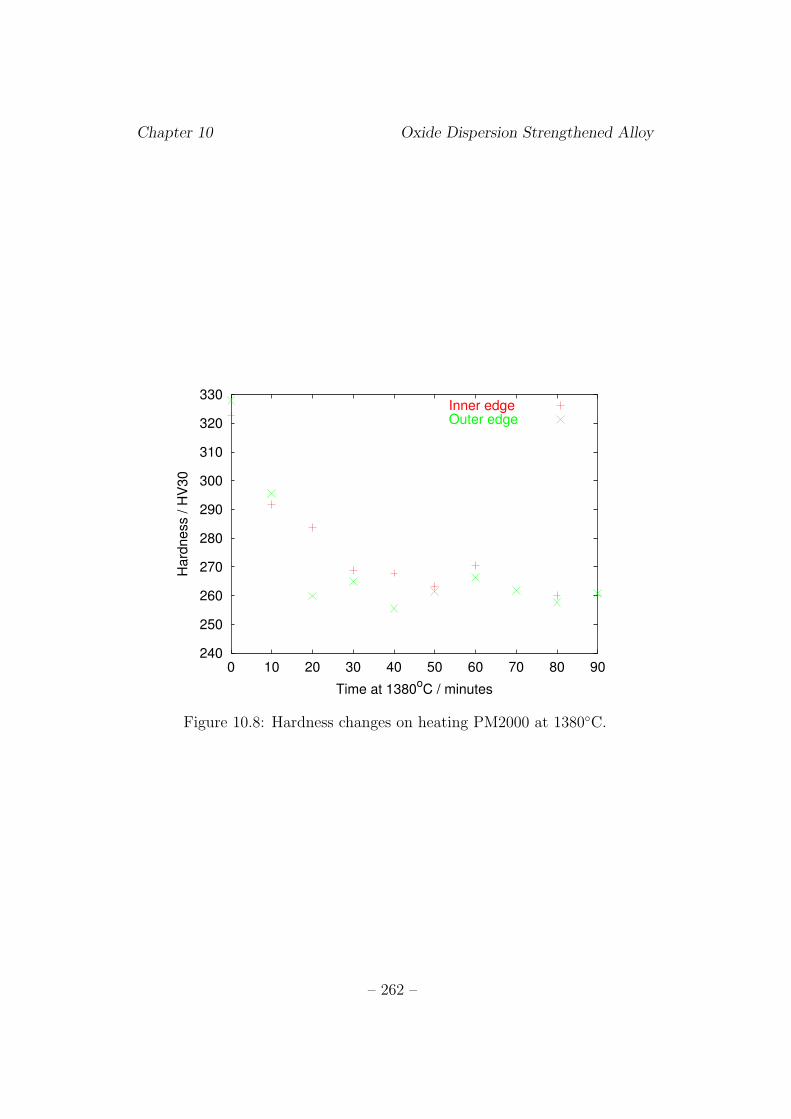
Chapter 10 Oxide Dispersion Strengthened Alloy
240
250
260
270
280
290
300
310
320
330
0 10 20 30 40 50 60 70 80 90
Hard
ness / H
V30
Time at 1380oC / minutes
Inner edgeOuter edge
Figure 10.8: Hardness changes on heating PM2000 at 1380◦C.
– 262 –
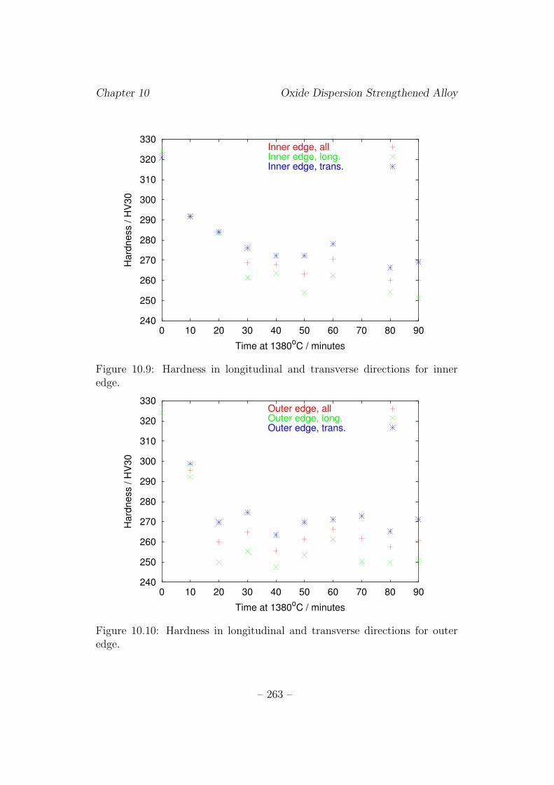
Chapter 10 Oxide Dispersion Strengthened Alloy
240
250
260
270
280
290
300
310
320
330
0 10 20 30 40 50 60 70 80 90
Hard
ness / H
V30
Time at 1380oC / minutes
Inner edge, allInner edge, long.Inner edge, trans.
Figure 10.9: Hardness in longitudinal and transverse directions for inneredge.
240
250
260
270
280
290
300
310
320
330
0 10 20 30 40 50 60 70 80 90
Hard
ness / H
V30
Time at 1380oC / minutes
Outer edge, allOuter edge, long.Outer edge, trans.
Figure 10.10: Hardness in longitudinal and transverse directions for outeredge.
– 263 –
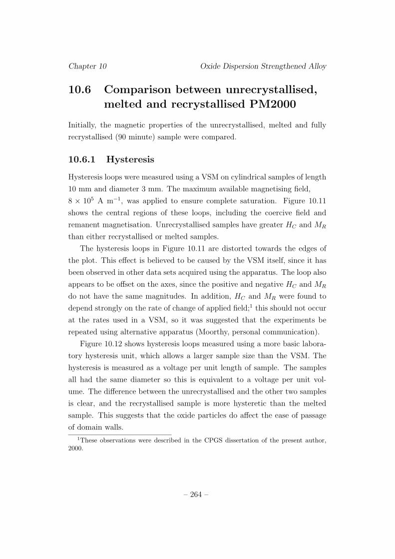
Chapter 10 Oxide Dispersion Strengthened Alloy
10.6 Comparison between unrecrystallised,
melted and recrystallised PM2000
Initially, the magnetic properties of the unrecrystallised, melted and fully
recrystallised (90 minute) sample were compared.
10.6.1 Hysteresis
Hysteresis loops were measured using a VSM on cylindrical samples of length
10 mm and diameter 3 mm. The maximum available magnetising field,
8 × 10⁵ A m−1, was applied to ensure complete saturation. Figure 10.11
shows the central regions of these loops, including the coercive field and
remanent magnetisation. Unrecrystallised samples have greater HC and MR
than either recrystallised or melted samples.
The hysteresis loops in Figure 10.11 are distorted towards the edges of
the plot. This effect is believed to be caused by the VSM itself, since it has
been observed in other data sets acquired using the apparatus. The loop also
appears to be offset on the axes, since the positive and negative HC and MR
do not have the same magnitudes. In addition, HC and MR were found to
depend strongly on the rate of change of applied field;1 this should not occur
at the rates used in a VSM, so it was suggested that the experiments be
repeated using alternative apparatus (Moorthy, personal communication).
Figure 10.12 shows hysteresis loops measured using a more basic labora-
tory hysteresis unit, which allows a larger sample size than the VSM. The
hysteresis is measured as a voltage per unit length of sample. The samples
all had the same diameter so this is equivalent to a voltage per unit vol-
ume. The difference between the unrecrystallised and the other two samples
is clear, and the recrystallised sample is more hysteretic than the melted
sample. This suggests that the oxide particles do affect the ease of passage
of domain walls.
1These observations were described in the CPGS dissertation of the present author,
2000.
– 264 –
Chapter 10 Oxide Dispersion Strengthened Alloy
10.6.2 Barkhausen noise
BN data were obtained with the magnetising field in longitudinal (L) and
transverse (T) directions on the unrecrystallised and recrystallised samples,
and in two arbitrary perpendicular directions on the melted sample. Fig-
ure 10.13 shows the RMS noise envelope for these samples from magnetisa-
tion at 4 Hz. In the melted and recrystallised samples, the peaks are close
to H = 0. The unrecrystallised material has a large peak at around 0.3 A
in the longitudinal direction, and much smaller peak at around 0.1 A in the
transverse direction. The peak positions indicate that domain wall pinning is
stronger in the unrecrystallised sample than the others, as would be expected
given the high level of strain in the microstructure.
If the magnetising frequency is decreased from 4 to 2 Hz, the comparative
heights of the BN peaks are changed (Figure 10.14). The unrecrystallised
longitudinal peak shrinks, but the melted and recrystallised sample peaks
remain in approximately the same proportion.
The change in frequency causes large differences in the frequency spectra
from the unrecrystallised and recrystallised samples, but little difference for
the melted material (Figure 10.15, Figure 10.16). As discussed in Chapter 8,
the filter allows through frequencies between 3 and 15 kHz, and a part of the
signal immediately below and above this. The melted sample noise level is
approximately constant across this window, but both the recrystallised and
unrecrystallised samples have a higher level of activity towards the higher-
frequency end. Noise frequency is considered to be related to domain wall
obstacle spacing (Saquet et al., 1999); this would imply here that the spacing
is very similar in recrystallised and unrecrystallised material. This, in turn,
leads to the conclusion that oxide particles do act as pinning sites, since the
difference in grain boundary spacing between these two samples is several
orders of magnitude. However, as discussed in Chapter 8, the filtering window
is narrow, and it is believed to exclude frequencies of interest, so it may be
that this observation does not give a complete characterisation of the BN
behaviour of this material.
– 265 –
Chapter 10 Oxide Dispersion Strengthened Alloy
10.6.3 Conclusion
This comparison demonstrates that both grain boundaries and oxide parti-
cles play a role in the magnetic behaviour of PM2000. Oxide particles affect
the hysteresis properties. The inter-particle spacing, rather than the grain
size, appears to be the factor controlling the noise frequency. The pinning
strength is much greater when the sample is unrecrystallised, owing to the
presence of high-energy grain boundaries, dislocations or both. In addition,
in this sample, there is a large difference in signal amplitude when magnetis-
ing perpendicular and parallel to the tube axis. This may be due to the
elongation of the grains along the extrusion direction, which gives a larger
spacing between obstacles and a larger possible domain wall jump size in this
direction.
10.7 BN across a grain boundary
The coarse grain structure of the recrystallised material allows a comparison
of noise signals from the grain interior and across a boundary. Figure 10.17
shows the positions at which measurements were taken, and Figure 10.18 the
resulting signals. The peak height is lower when the noise is measured across
the grain boundary than along it or in the bulk.
10.8 Recrystallisation sequences
The BN behaviour of intermediate stages between unrecrystallised and fully
recrystallised material were studied. In these experiments, a different set of
ferrite pieces was used from in the experiment described above, giving some
differences in the results. Measurements were made at several positions on
each sample to test the influence of grain boundaries and recrystallised and
unrecrystallised regions on the BN signal.
– 266 –
Chapter 10 Oxide Dispersion Strengthened Alloy
10.8.1 Unrecrystallised sample
This sample required an amplification of 70 dB to obtain a visible signal; this
is in contrast to the previous set of experiments in which peaks could be seen
at a much lower amplification. The reason for this may be the differences in
ferrite pole piece geometry.
In Figure 10.19, two types of behaviour are observed: a smaller peak
closer to zero current, and a larger peak in the higher-current range. All
the transverse measurements show the former type of behaviour, but in the
longitudinal direction, examples of both types can be seen. It appears that
BN behaviour depends very much on position in this sample.
10.8.2 Effect of heat treatment
Figure 10.20 shows a comparison between noise signals in the unrecrystallised
region and on the boundary between recrystallised and unrecrystallised ma-
terial in the transverse direction. The gain used in this measurement is still
70 dB but the boundary region gives larger, more uniform, lower-field signals
than the unrecrystallised area. In the longitudinal direction, too, there is a
clear difference between these regions but in this case, the signals are much
larger, requiring only a gain of 40 dB (Figure 10.21).
After 20 minutes of heat treatment, the gain could again be reduced, to
5 dB. The difference between longitudinal and transverse behaviour decreased
(Figure 10.22). Despite the presence of a small unrecrystallised region, the
positions of the peaks were much more uniform than in the samples described
previously.
The longest heating time for which an unrecrystallised region was present
was 30 minutes. When the signal was measured in the longitudinal direc-
tion, there was a clear difference in peak position from the recrystallised and
unrecrystallised regions and the boundary (Figure 10.23).
In the samples heated for longer times than this, measurements were
made within grains and across grain boundaries to test whether the presence
of a boundary always affected the signal in the same way as found previously
(§ 10.7). However, no consistent relationship could be found between peak
– 267 –
Chapter 10 Oxide Dispersion Strengthened Alloy
amplitudes or positions and the presence of grain boundaries in the longi-
tudinal direction. Peaks measured along grain boundaries in the transverse
direction tended to be slightly larger than those measured elsewhere. This
is illustrated in Figure 10.24 for a 70 minute heat treatment, but was not
observed in all the samples.
In general, the repeatability between measurements can be very poor,
with large differences in peak height and position arising from neighbouring
regions on the same grain. It may be that variations in oxide particle content
are responsible, but this is unlikely since the volume sampled by the BN
probe is very large relative to the particle volume and spacing. Much more
likely is that the variations arose from the measurement technique. As noted
in Chapter 8, using the equipment requires a certain amount of skill and
experience, and the results are affected by the quality of grinding of the
ferrite pieces. The measurements discussed here were made earlier than those
discussed in Chapter 8, using an older, less well ground set of ferrite pieces,
so this may have caused the lack of repeatability.
– 268 –
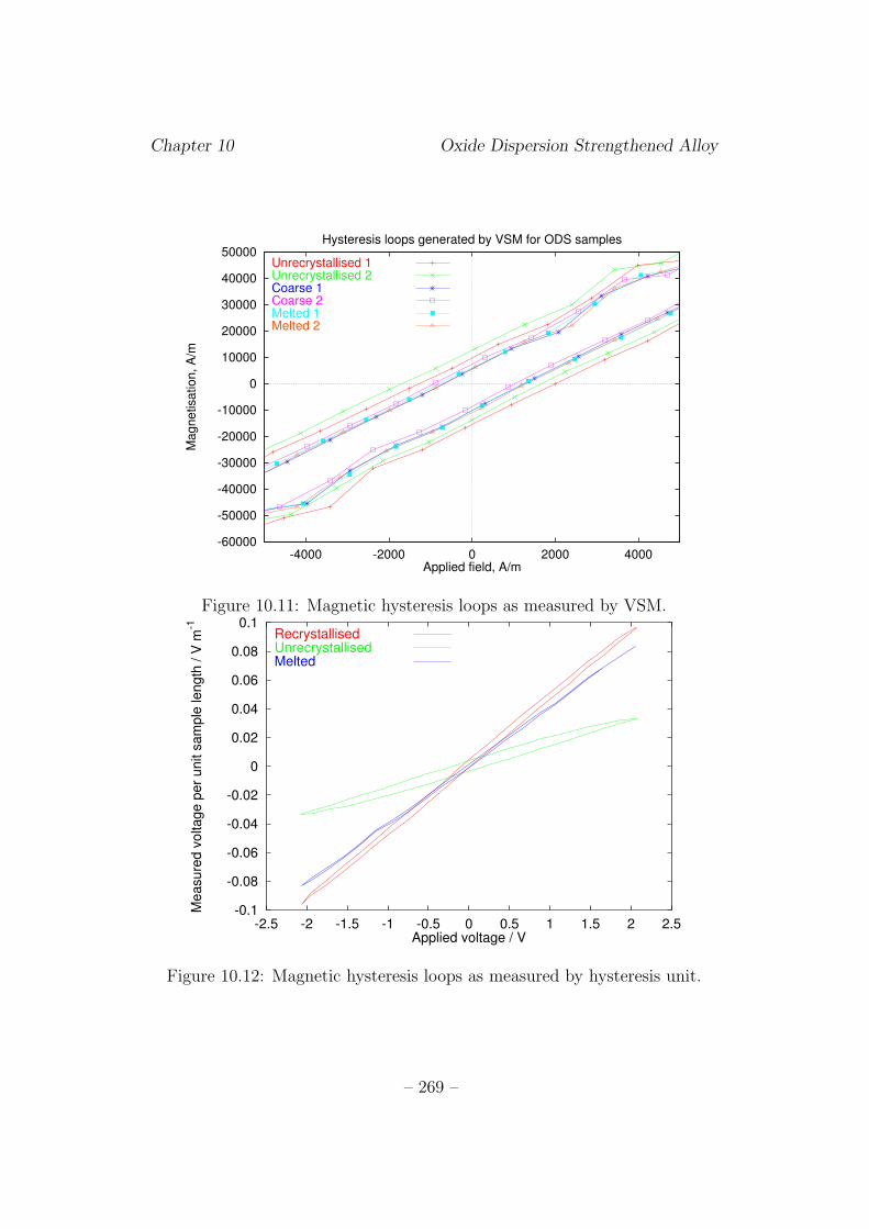
Chapter 10 Oxide Dispersion Strengthened Alloy
-60000
-50000
-40000
-30000
-20000
-10000
0
10000
20000
30000
40000
50000
-4000 -2000 0 2000 4000
Ma
gn
etisa
tio
n,
A/m
Applied field, A/m
Hysteresis loops generated by VSM for ODS samples
Unrecrystallised 1Unrecrystallised 2Coarse 1Coarse 2Melted 1Melted 2
Figure 10.11: Magnetic hysteresis loops as measured by VSM.
-0.1
-0.08
-0.06
-0.04
-0.02
0
0.02
0.04
0.06
0.08
0.1
-2.5 -2 -1.5 -1 -0.5 0 0.5 1 1.5 2 2.5
Me
asu
red
vo
lta
ge
pe
r u
nit s
am
ple
le
ng
th /
V m
-1
Applied voltage / V
RecrystallisedUnrecrystallisedMelted
Figure 10.12: Magnetic hysteresis loops as measured by hysteresis unit.
– 269 –
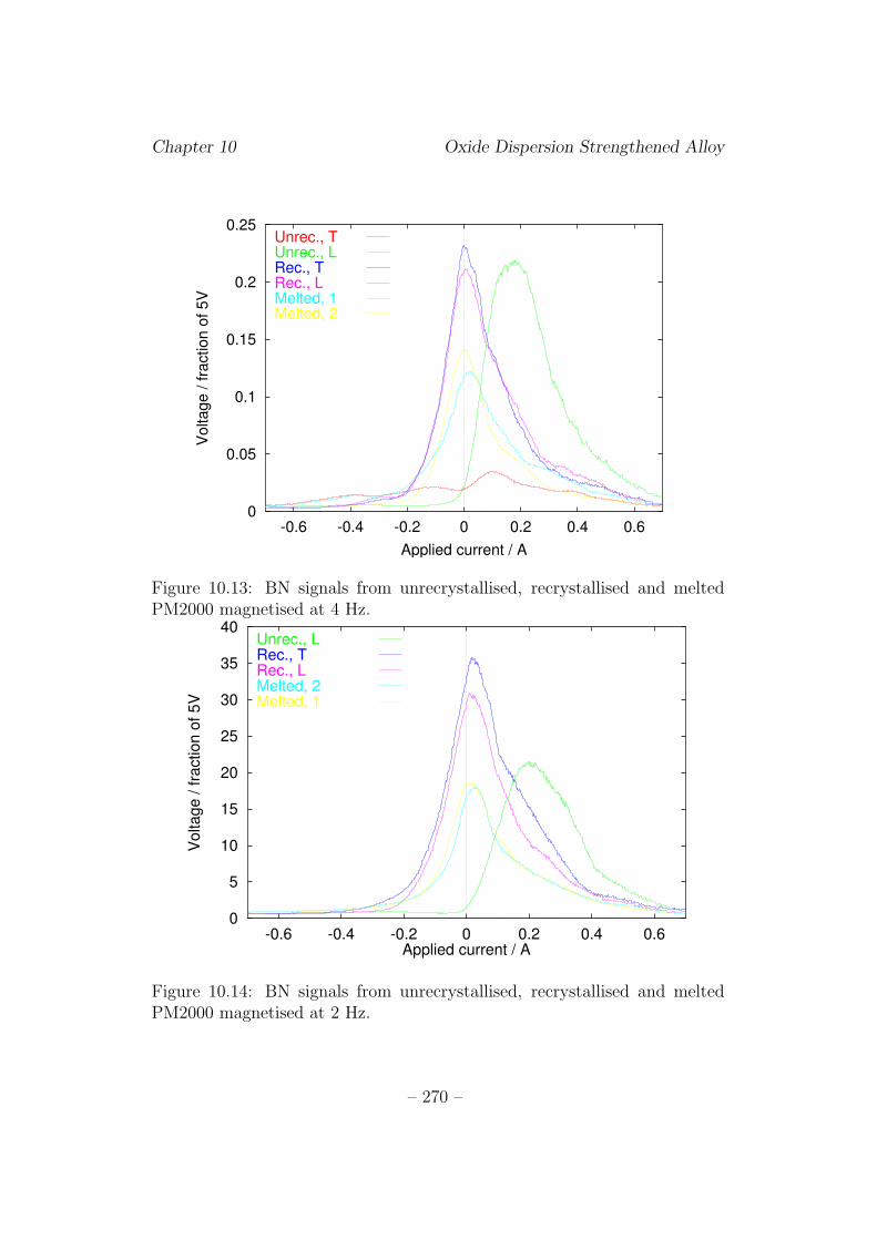
Chapter 10 Oxide Dispersion Strengthened Alloy
0
0.05
0.1
0.15
0.2
0.25
-0.6 -0.4 -0.2 0 0.2 0.4 0.6
Voltage / fra
ction o
f 5V
Applied current / A
Unrec., TUnrec., LRec., TRec., LMelted, 1Melted, 2
Figure 10.13: BN signals from unrecrystallised, recrystallised and meltedPM2000 magnetised at 4 Hz.
0
5
10
15
20
25
30
35
40
-0.6 -0.4 -0.2 0 0.2 0.4 0.6
Voltage / fra
ction o
f 5V
Applied current / A
Unrec., LRec., TRec., LMelted, 2Melted, 1
Figure 10.14: BN signals from unrecrystallised, recrystallised and meltedPM2000 magnetised at 2 Hz.
– 270 –
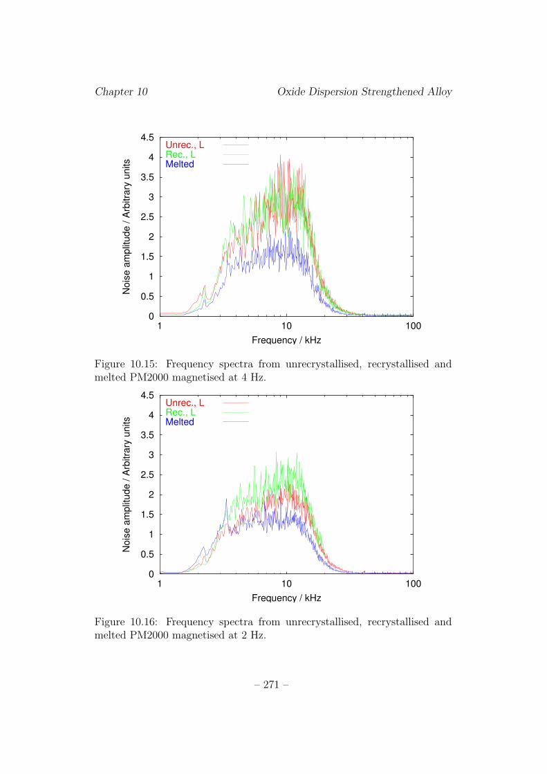
Chapter 10 Oxide Dispersion Strengthened Alloy
0
0.5
1
1.5
2
2.5
3
3.5
4
4.5
1 10 100
Nois
e a
mplit
ude / A
rbitra
ry u
nits
Frequency / kHz
Unrec., LRec., LMelted
Figure 10.15: Frequency spectra from unrecrystallised, recrystallised andmelted PM2000 magnetised at 4 Hz.
0
0.5
1
1.5
2
2.5
3
3.5
4
4.5
1 10 100
Nois
e a
mplit
ude / A
rbitra
ry u
nits
Frequency / kHz
Unrec., LRec., LMelted
Figure 10.16: Frequency spectra from unrecrystallised, recrystallised andmelted PM2000 magnetised at 2 Hz.
– 271 –
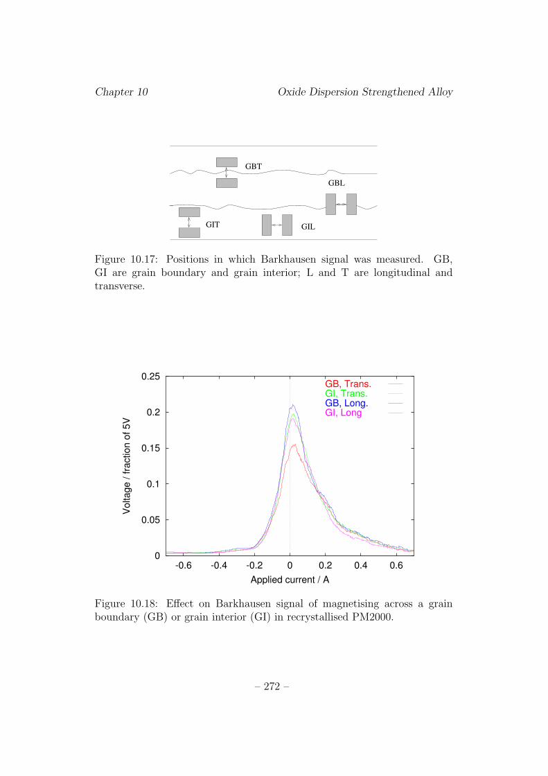
Chapter 10 Oxide Dispersion Strengthened Alloy
GBT
GBL
GILGIT
Figure 10.17: Positions in which Barkhausen signal was measured. GB,GI are grain boundary and grain interior; L and T are longitudinal andtransverse.
0
0.05
0.1
0.15
0.2
0.25
-0.6 -0.4 -0.2 0 0.2 0.4 0.6
Voltage / fra
ction o
f 5V
Applied current / A
GB, Trans.GI, Trans.GB, Long.GI, Long
Figure 10.18: Effect on Barkhausen signal of magnetising across a grainboundary (GB) or grain interior (GI) in recrystallised PM2000.
– 272 –
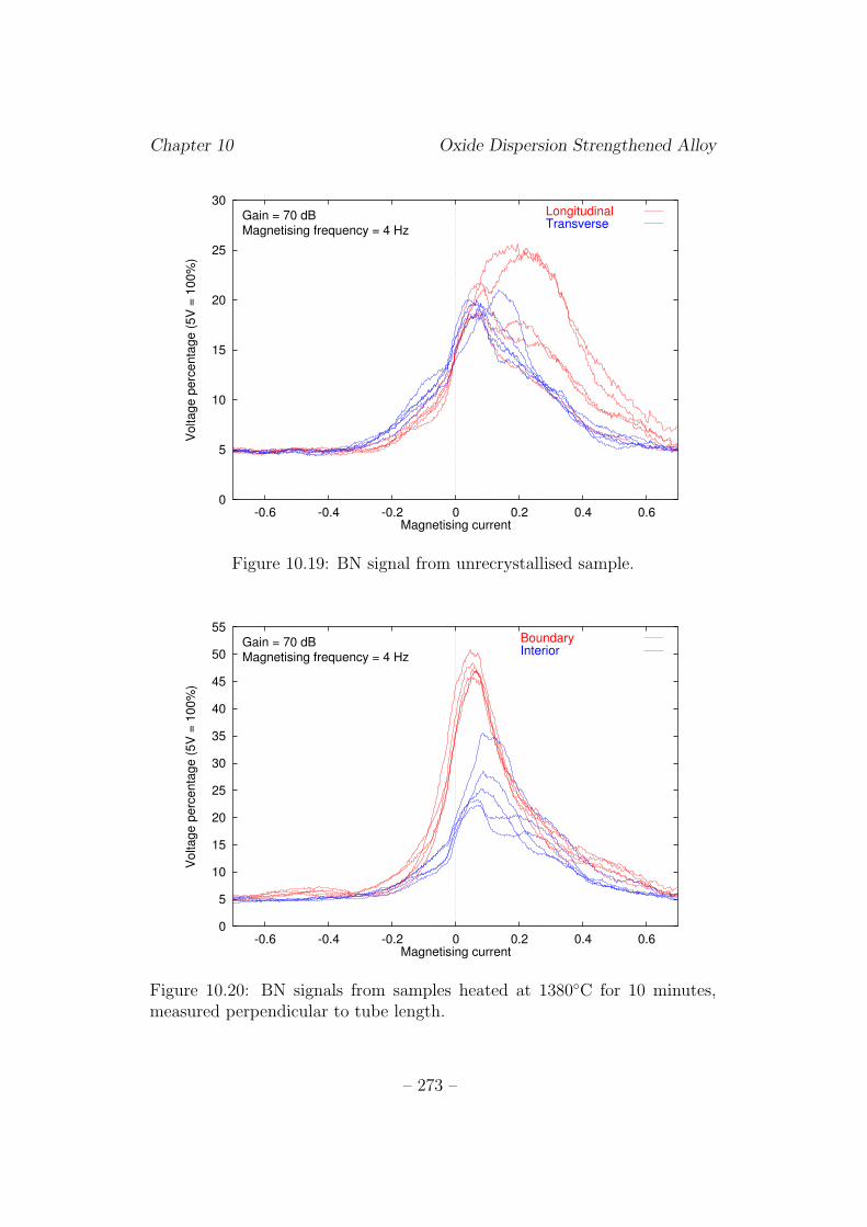
Chapter 10 Oxide Dispersion Strengthened Alloy
0
5
10
15
20
25
30
-0.6 -0.4 -0.2 0 0.2 0.4 0.6
Vo
lta
ge
pe
rce
nta
ge
(5
V =
10
0%
)
Magnetising current
Gain = 70 dBMagnetising frequency = 4 Hz
LongitudinalTransverse
Figure 10.19: BN signal from unrecrystallised sample.
0
5
10
15
20
25
30
35
40
45
50
55
-0.6 -0.4 -0.2 0 0.2 0.4 0.6
Vo
lta
ge
pe
rce
nta
ge
(5
V =
10
0%
)
Magnetising current
Gain = 70 dBMagnetising frequency = 4 Hz
Boundary Interior
Figure 10.20: BN signals from samples heated at 1380◦C for 10 minutes,measured perpendicular to tube length.
– 273 –
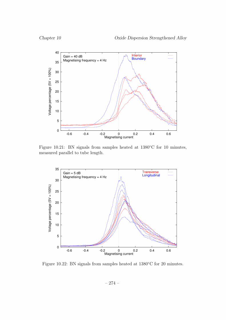
Chapter 10 Oxide Dispersion Strengthened Alloy
0
5
10
15
20
25
30
35
40
-0.6 -0.4 -0.2 0 0.2 0.4 0.6
Vo
lta
ge
pe
rce
nta
ge
(5
V =
10
0%
)
Magnetising current
Gain = 40 dBMagnetising frequency = 4 Hz
Interior Boundary
Figure 10.21: BN signals from samples heated at 1380◦C for 10 minutes,measured parallel to tube length.
0
5
10
15
20
25
30
35
-0.6 -0.4 -0.2 0 0.2 0.4 0.6
Vo
lta
ge
pe
rce
nta
ge
(5
V =
10
0%
)
Magnetising current
Gain = 5 dBMagnetising frequency = 4 Hz
TransverseLongitudinal
Figure 10.22: BN signals from samples heated at 1380◦C for 20 minutes.
– 274 –
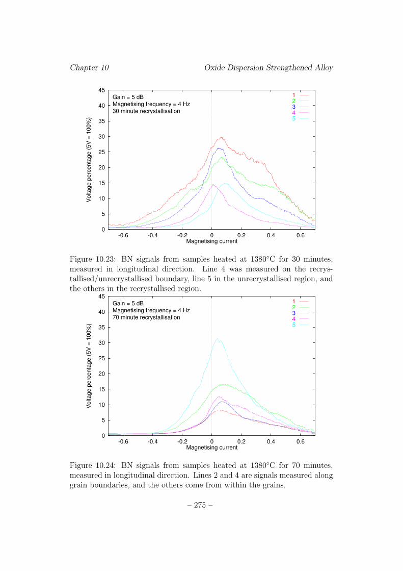
Chapter 10 Oxide Dispersion Strengthened Alloy
0
5
10
15
20
25
30
35
40
45
-0.6 -0.4 -0.2 0 0.2 0.4 0.6
Vo
lta
ge
pe
rce
nta
ge
(5
V =
10
0%
)
Magnetising current
Gain = 5 dBMagnetising frequency = 4 Hz30 minute recrystallisation
12345
Figure 10.23: BN signals from samples heated at 1380◦C for 30 minutes,measured in longitudinal direction. Line 4 was measured on the recrys-tallised/unrecrystallised boundary, line 5 in the unrecrystallised region, andthe others in the recrystallised region.
0
5
10
15
20
25
30
35
40
45
-0.6 -0.4 -0.2 0 0.2 0.4 0.6
Vo
lta
ge
pe
rce
nta
ge
(5
V =
10
0%
)
Magnetising current
Gain = 5 dBMagnetising frequency = 4 Hz70 minute recrystallisation
12345
Figure 10.24: BN signals from samples heated at 1380◦C for 70 minutes,measured in longitudinal direction. Lines 2 and 4 are signals measured alonggrain boundaries, and the others come from within the grains.
– 275 –
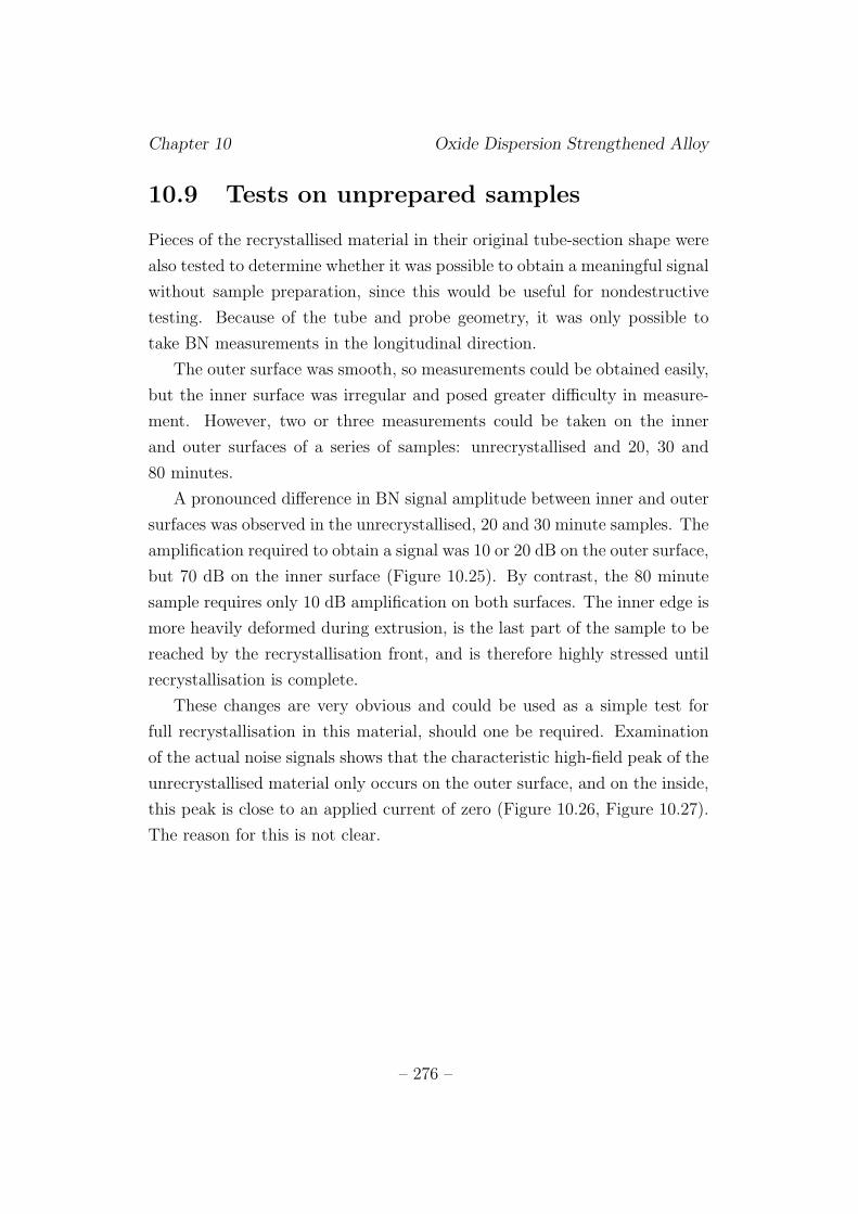
Chapter 10 Oxide Dispersion Strengthened Alloy
10.9 Tests on unprepared samples
Pieces of the recrystallised material in their original tube-section shape were
also tested to determine whether it was possible to obtain a meaningful signal
without sample preparation, since this would be useful for nondestructive
testing. Because of the tube and probe geometry, it was only possible to
take BN measurements in the longitudinal direction.
The outer surface was smooth, so measurements could be obtained easily,
but the inner surface was irregular and posed greater difficulty in measure-
ment. However, two or three measurements could be taken on the inner
and outer surfaces of a series of samples: unrecrystallised and 20, 30 and
80 minutes.
A pronounced difference in BN signal amplitude between inner and outer
surfaces was observed in the unrecrystallised, 20 and 30 minute samples. The
amplification required to obtain a signal was 10 or 20 dB on the outer surface,
but 70 dB on the inner surface (Figure 10.25). By contrast, the 80 minute
sample requires only 10 dB amplification on both surfaces. The inner edge is
more heavily deformed during extrusion, is the last part of the sample to be
reached by the recrystallisation front, and is therefore highly stressed until
recrystallisation is complete.
These changes are very obvious and could be used as a simple test for
full recrystallisation in this material, should one be required. Examination
of the actual noise signals shows that the characteristic high-field peak of the
unrecrystallised material only occurs on the outer surface, and on the inside,
this peak is close to an applied current of zero (Figure 10.26, Figure 10.27).
The reason for this is not clear.
– 276 –
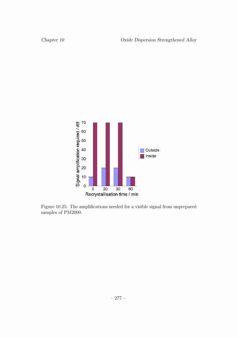
Chapter 10 Oxide Dispersion Strengthened Alloy
Figure 10.25: The amplifications needed for a visible signal from unpreparedsamples of PM2000.
– 277 –
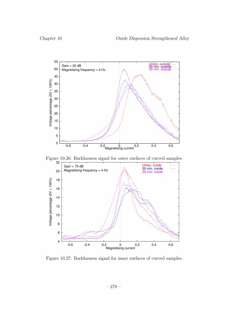
Chapter 10 Oxide Dispersion Strengthened Alloy
0
5
10
15
20
25
30
35
40
45
50
55
-0.6 -0.4 -0.2 0 0.2 0.4 0.6
Voltage p
erc
enta
ge (
5V
= 1
00%
)
Magnetising current
Gain = 20 dB
Magnetising frequency = 4 Hz
Unrec. outside20 min. outside30 min. outside
Figure 10.26: Barkhausen signal for outer surfaces of curved samples.
4
6
8
10
12
14
16
18
20
22
-0.6 -0.4 -0.2 0 0.2 0.4 0.6
Vo
lta
ge
pe
rce
nta
ge
(5
V =
10
0%
)
Magnetising current
Gain = 70 dBMagnetising frequency = 4 Hz
Unrec. inside20 min. inside30 min. inside
Figure 10.27: Barkhausen signal for inner surfaces of curved samples.
– 278 –
Chapter 10 Oxide Dispersion Strengthened Alloy
10.10 Conclusions
The transformation from a fine- to a coarse-grained microstructure gives a
clear change in BN behaviour, even on unprepared, curved tube sections.
The oxide particles in the microstructure also have an effect on magnetic
properties, although this is more obviously visible in hysteresis than in BN
measurements. Recrystallised and unrecrystallised regions within the same
sample could also easily be discerned on the basis of their BN behaviour.
A large difference between longitudinal and transverse noise signals was ob-
served in unrecrystallised material, but this decreased on recrystallisation.
The changes in BN are not directly related to the hardness, because the
oxide particles influence the hardness strongly, but the BN only weakly.
The effect of grain boundaries in recrystallised PM2000 has not been clar-
ified. Initial studies gave a clear difference between noise amplitude when
measured across a grain boundary and within the bulk, but attempts to
reproduce this result on other samples did not succeed. Overall, the repeata-
bility seemed rather poor.
As mentioned in Chapter 8, the frequency filtering range used in these
measurements is narrow and there is the possibility of important information
going unrecorded. If possible, these experiments should be repeated using
apparatus with a larger frequency range to check the conclusions.
– 279 –
Chapter 11
Summary, Conclusions andSuggestions for Further Work
11.1 Summary and conclusions
The existing literature on the dependence of magnetic properties on mi-
crostructure has been reviewed. The consensus from this is that particles,
dislocations and grain boundaries all affect the domain wall behaviour. The
effect of particles depends on their size and is most pronounced when they
are evenly spaced. Dislocations interact with domain walls and appear to
suppress domain nucleation and annihilation, making a deformed sample
more difficult to saturate than an annealed sample of the same material.
Grain boundaries appear to exert a weaker pinning effect than carbides or
dislocations, but they can nonetheless limit domain wall jump sizes.
In as-quenched or normalised and air-cooled ferritic steel, the RMS Bark-
hausen noise signal is a small peak at a high applied field. On tempering, this
increases in height and moves to a lower field. Prolonged tempering causes
splitting into two peaks. This was attributed to separate distributions of
pinning strengths from grain boundaries and carbides. On tempering, the
pinning strength of grain boundaries decreases, and that of carbides increases.
Using this interpretation, a model has been developed based on two sta-
tistical distributions of pinning site strengths. The first attempt at modelling
treated these both as normal distributions, and the second (Model 2) used
a log-normal distribution for the weaker sites. Both models fitted published
– 280 –
Chapter 11 Conclusions
data well, but linear relationships were observed between Model 2 fitting
parameters and the dimensions of microstructural features.
Samples of austenitised, quenched and tempered 214Cr1Mo power plant
steel were prepared. Changes in microstructure and hardness were slow
at lower tempering temperatures, but accelerated at higher temperature.
11Cr1Mo steel samples, which had been heated for several thousands of
hours, showed a very gradual change in hardness and no discernible mi-
crostructural coarsening. Orientation imaging microscopy observations on
214Cr1Mo samples tempered at 600◦C revealed that the main change occur-
ring was a strain reduction, which appeared as an increase in image qual-
ity. Even after tempering for over 250 hours, the relationships from the
martensitic structure were preserved. Blocks, consisting of slightly misori-
ented groups of laths, often had Σ3 relationships with their neighbours within
a packet. It is expected that, as the dislocation density reduces during tem-
pering, it will become progressively easier for a domain wall to move through
the structure.
The BN peaks obtained from these samples were different in shape from
those observed previously on tempered 214Cr1Mo steel. Peak-splitting had
been expected after prolonged tempering in the 214Cr1Mo samples, but it
was not observed; neither could it be seen in tempered plain-carbon steel
samples which were known to give a double peak using other apparatus. It
was suspected that the filtering in the apparatus used in this study excluded
important low-frequency information. Analysing only low-frequency noise
gave evidence of a second peak at high current values.
The BN peak moves toward lower currents with larger Larson-Miller pa-
rameter P in the 214Cr1Mo samples. In the 11Cr1Mo steel, the peak remains
at a position close to that of the as-quenched 214Cr1Mo samples, even af-
ter prolonged tempering. This agrees well with the lack of microstructural
change and the very small hardness change in this sample.
Model 2 was fitted to the new experimental data, and in all cases, a good
fit was obtained. The model parameter characterising the pinning strength of
the weaker pinning points decreased with P , following the same curve shape
as the peak positions, in the 214Cr1Mo steel. This weaker distribution is
– 281 –
Chapter 11 Conclusions
believed to arise from pinning by grain boundaries. Taking into account the
optical and OIM measurements, it can be concluded that the pinning strength
of this distribution is related to the degree of strain in the microstructure,
and in particular the dislocation density at lath and grain boundaries. As
this is decreased by tempering, domain wall motion becomes easier. The
pinning strength of the distribution attributed to carbides had a minimum
at an intermediate value of P . This may be associated with the dissolution
of Fe3C and the precipitation of fine particles of more stable carbides, since it
occurs at an appropriate value of P as determined from the carbide stability
diagram.
The modelling parameter values also suggested that the number of grain-
or lath-boundary pinning sites increased with greater severity of tempering.
In reality, the opposite is likely, since lath boundaries become less well defined
on tempering. The initial assumptions made when developing the model
were very simple, so it may be necessary to modify some of these to obtain
a physically meaningful model of the number of sites.
The fitting parameters for the 11Cr1Mo steel lay in a different regime
from those of the 214Cr1Mo steel, and their variations with P could not be
determined because all the points had very similar P values. More data,
from a wide range of tempering conditions, are needed to study this.
In the ODS alloy, it was possible to isolate the effects of grain bound-
aries and particles, and to demonstrate that both influence magnetic prop-
erties. However, possibly because of the small size of the particles in this
material, grain boundaries dominated the Barkhausen noise behaviour. The
Barkhausen peak moves from a higher to a lower applied current on re-
crystallisation from a fine-grained, heavily strained microstructure to coarse
columnar grains. This is comparable to the change in peak position occurring
on tempering of 214Cr1Mo steel, and lends support to the interpretation that
the 214Cr1Mo steel BN behaviour is mainly due to effects at grain boundaries.
In summary, the large Barkhausen noise peak observed in these steels is
believed, on the basis of experiment and modelling, to originate from domain
wall interactions with grain and lath boundaries. During tempering, the dis-
location density at these boundaries decreases, and this reduces their pinning
– 282 –
Chapter 11 Conclusions
strength. The peak therefore shifts to a lower field. The peak position, and
the modelling parameter based on this, decrease smoothly with increasing
severity of tempering, as characterised by the Larson-Miller parameter.
11.2 Future work
11.2.1 Experimental work
Since there is a clear relationship between BN peak position and P in the
214Cr1Mo steel, it would be interesting to investigate whether similar re-
lationships exist in other steel compositions, including an extension of the
existing work on 11Cr1Mo. Comparisons with samples which are in an unsat-
isfactory microstructural condition, both overcoarsened and creep-deformed,
should be obtained so that criteria for a safe condition can be determined.
Two new sets of BN measuring apparatus, of types (a) and (b) in Fig-
ure 4.2, are being built at the University of Newcastle. The filtering ranges
of these will be set to allow analysis of low-frequency noise. Repeating the
experiments in this study using the new apparatus should enable high-field,
low-frequency peaks to be detected where these exist. Careful characterisa-
tion of the effects of changing experimental conditions should be carried out
to enable repeatability between results. Once this has been achieved, a wide
variety of samples can be tested to verify existing interpretations of the role
of microstructure in Barkhausen noise, and to gain new insights.
Time limitations prevented a detailed investigation of the carbides in the
214Cr1Mo steel in this study. Carbon replica measurements can be used
to measure particle shapes and sizes, and the identity of the species deter-
mined using electron diffraction in the TEM. These can be compared with
BN signals obtained from a full frequency range. As Moorthy et al. (1998)
suggested, it may be possible to relate changes in the BN behaviour to the
dissolution of the fine needles of M2X which are beneficial to creep proper-
ties, and the precipitation of spheroidal carbides in their place. This would be
extremely useful for estimation of the creep resistance of the microstructure.
Finally, magnetic domain imaging, using the techniques described in § 3.4,
– 283 –
Chapter 11 Conclusions
could be used to give a more complete understanding of the interaction pro-
cesses between domain walls and microstructural features in these steels.
11.2.2 Modelling
The Model 2 average pinning site strength values have clear relationships
with microstructural or tempering parameters, but the other parameters,
characterising the number of sites and the distribution widths, are less ob-
viously related to microstructure. This may well be due to the assumptions
used in the model, so it would be useful to test modifications to these, to
attempt to produce a more physically reasonable model. For example, it may
be necessary to introduce a demagnetising field, a variable number of domain
walls, or a more complex arrangement of pinning sites.
Modification of the model fitting program is also necessary to eliminate
unphysical solutions. This could take the form of constraints on allowable fit-
ting parameter values. A further suggested alteration to the fitting procedure
is discussed in the Appendix.
– 284 –
� ��� ������� ��� ���
�����������������! #"%$'&)(+*,$-�."-*#/0$'1��!*�/�243��!*657�."-�8*#9.�:�!*<;=�.98"?>A@?$'/�2B2�1B@'/C$'1B��*D/0*#E<;=�.2B/0$'�8EF &#�8*#�!GH�.*�/I��JK&I�ML!/�N#/�*O(+*#@?$-1�$' 6$'�P��5RQS�8$'/�2B@8�UTWV!V!VI��X�Y!V[ZIX0V�\
�������K���]� F "-�A9.�.�8E#1B*I^!@_��5a`b2]$'"-/Cc%dA$-�.�82eX�f�f!fI�=g�/C$'1B��*�/�2b;h�8@-�i/0"-9j&k(+*#@?$-1�$' 6$'�l57�!"QS�m$j/�2�@.��JK@? #no #��/I�pL!/�N�/0*q��X�f!f!f6�qT!TWV[ZrT[X�V
��E�/�GH@.�As��ot��]�,u)"?1B^!&,$i�Ad��A(j�ovxwP I*#y.�0�Iwz�]��{}|m~��������6�������-�����#�?���I�.�A�m~����C�I���P�6�#���� TWV!V!�,����YITWVWZ6Y!�IT
��2B�8@-@-/�*#E#"?�#�qs��]�Us��./0$'"?1B98����3����Us��."?$-��$-$-1��q���p/�*#E�Q��!*,$'�!"?@-1��p���]�����C�A�m�������¡ ¢��£�¤£�����|-¥�¦�§A¨W�m���j�m��©rª¬«-©� � TWV!V!f!�m�rX�V�fITmZIX�V�f,®
��2B�8@-@-/�*#E#"?�#�As����6s��./0$'"?1B9.�0�A3����6s��8"?$'�0$-$'1��o�z�ov¯QS�!*,$'��"-@-1��o���]�r���C�A�������U�¡ ���£,£�����|-¥¦�§A¨W�m���j�m�r©rª¬«-©� � TWV!V!f,���rX�V!f�Y[ZIX�VITW°
��*#E#"?�8±=@8��wz�Iu²�rv´³b #^!&I�.@.��³µ���q�I¶U·m�'�C�l¸r~+|j|m��·m�I�m~�¶B�U¹Aºr» � TWV,°�V,�����!f�\[Z6�IT!T
��*#E#"?�8±=@8�Rwz�Uu²����¼�>6@?�!*q�¬¼M��LI�¬v½wP�8�W±=*q�Rd���;P�]��¾¿(+*o$-�."?N#"-�m$j/0$-1B�!*D��5À�82B�.9m$'"?�!*E#1]Á�"-/�98$-1B�!*ÂN#/0$-$-�."-*I@.Ã]�r³b1B2�^!�."À/�*#EOu</0$?$'@8�rtÄ��*#E#�!* � TiV!Å,®!�
��*#^!2B/�E�/Cc+;h1]Æ!�8"'/I��LI��� F /�E#�WÆ!�8@-�0��t���;P�Rv�3À/�N=Ç�Cc%dI/�*I9j&#�.y0��LI���K���C�A�m�����=�¡ H{È�W��¤��|m~��B�mÉ����¥H{È�W����|m~����e{È��~+|m�m�����Ê�m���r»U¹ � X�f!fIT[����X�V�V[Z6�!f!Å
��"'/6�rw��]�U¾ÌËRÆ0/�2� �/0$'1��!*Â��5�57�."-"?�! #@=GÍ/0$'�8"-1Î/02qN#"-��Np�8"?$'1��.@= #@?1B*#^ÍsÀ/�"?nA&#/� #@-�8*l*#��1B@-�0Ã��(%d6(%L dANp�89.1Î/02edA>AGHNp��@-1B IG ¾Ì¼e�mÆ!�.2��!N#GH�.*,$_�05¢*#�!*#EI�.@?$-"- #9m$'1]Æ!�Ï�mÆ�/02B �/0$-1B�!*GH�8$-&#�6EI@h I@-1B*I^HGÍ/�^!*I�8$'1�9eN#"?�!Np�8"?$-1B�.@8Ã���QS/�"-9j&lX�f!f,X
ZÂX�Y,°µZ
Ð�Ñ+Ò0Ó�Ñ�ÔWÕ,Ö'×.Ø�Ù�Ú
��@-&o�,>!�qQD�����rvÛL��!*I�.@.��¼M�r;P�r³a�]�U¾ÌË�*#^!1�*#�.�8"-1�*#^_QS/0$'�8"-1Î/02B@¢T!Ü4��*�(+*,$'"-�AE# #9m$'1��!*$-��$-&#�.1�" F "-�!N��."%$'1B�8@h/�*#E���N#N#2�1B9./0$'1��!*#@.Ã]� F �."?^,/�GH�!* � TWV!Y�V,�
��@?$-1mÇ�0�6sb���6¼e�.^,/0 #Ýo #���6LI�]� F �!"?$-�.@-�81B2��ALI�6t��AvßÞ��8"-^!*#�0�I;P�]�I·'à�à4à´�#�?���I�.�A�m~����C�I�¢�C�{È�W����|m~����j�m�#áâ�_ã:äi¹Iåq«'©p � TWV!YITW�m�rX�V!X�V[ZIX�V��IT
��@?$-1mÇ�0�#s��]�#¼e�8^,/� #Ýo #�0��LI�]� F �!"?$-�.@-�81B2��#LI�It��6væÞ��."?^!*#���I;µ�]�p���C�A�������Ä�¡ h{��W����|m~��B�mÉ����¥�{È�W����|m~����¢{���~+|m�������Ê�m����ª � TWV�Y,X!�m��Ti\,V[Z�TW°��
sÀ/�n��8".�K;P�K�z��vçgh I$-$-1B*#^#��LI�]�P���C�A�������P�¡ �~�§�|O·��j�C�x����¥)¸r~¡|j|m��·m�I�m~���~��6~+|m�µ¹6ºr�� TWV,°�V,���rX!°!®iZIX�Y!Å
sÀ/�2B2� Iè���;µ��u²�]�=3��!&#�8*q�KQD��vé�bÆ��."?��/�9j&q��s���t��]�:�#�?���I�:��ÉH¶b¸q�W�.¶h{}|m~ê¶B�K�p»� TWV,°6T[���#\,V,®iZI°!X�Å
sÀ/�*o�# #"%>!�pLI�r;µ�#vëgb1íìI��*q�Iu²��3��]�q�#¶�¸q�m��¶�·m�I�m~�¶B�#�r� � TWV�Å!V,�m�IY!Y!V[ZAY!V,X
sÀ/�"-98�.2��#��������s�"'/�9j&I�8$i�RLI��3���v½E#�Â3À/�"?2Î/�*��ÄîM����¾¿(+*Iï� I�.*#98�Â��5 F "-1��!"a�b #@?$-�.*#1]$'1�9�¢"'/�1�*Sd61By8�¢�!*�$-&#��QS1B98"-�!@%$'"- I98$' I"-�P��5�V!ðñ3�"bQl/�"?$-�.*#@?1�$-1B9µdA$-�.�.2�3�&�/0"'/�9�c$-�."-1�@-�8ES�,>OË�sKdI¼MÃ]�� #*#NI #�#2B1�@-&#�8E�±��!"?n
sÀ/�"-no&�/0 #@-�8*q��³a�]��¦4§A¨W�.¶�ò�¶B�r��ó � TWVITWV,���#\,fIT�ZA\,f!�
s��i/�2����O����¼M�]� L!/�no #���WÆA1B9.@æLI� F �]� ³b�m$'&#�8"-1B*I^�$'�!*��lQ}�l�z�]� d698"- #�,>!�Ï3���s����tU�8±=1�@.�4s������4vô¼¢/iÆA1B�8@.�4wz��LI�]�����C�A�m�������¡ _{È�W����|m~��B�mÉ ����¥�{��W����|m~����{È��~¡|m�������Ê�m�Ĺoó��Iõ�¹oó�å � TWV!V,X��m���!Å!°WZ6�!Å,®
s��.�89j&q��dp��QD�]��d6�.2]±À/i>��RLI�Äu²��vsÀ/C$-$'�0���a��¼M�]��1�* X0*IE<(+*,$i��3��!*I5¡��¾�3�"?�.�.Nö/0*#E57"-/�98$- #"-�M�05��.*#^!1�*#�.�8"-1�*#^_GÍ/0$'�8"-1Î/02B@b/�*#EÏ@%$'"- I98$' I"-�.@8Ã���dA±�/�*#@?�i/I� F 1�*#�."?1BE#^!�F "-�8@-@8�¬TiV!Y�\#��V!X!°WZ6V!��Å
s��."?^!�."8�K3��]�bs��.�.9j&��=dp�KQ}���bQl/i>!�8".��w���³a�]�hdA$j/0 #�#2B1���QD�ÀvôJK&#�!"?*,$'�!*q��¼M�4Þ����(+*,$'�8"-*�/C$'1B��*�/�2ÄL��!1�*,$ F �W±��8"¢�¢�.*#�8"'/0$-1B�!*�3���*I57�."?�.*#98���p`ed6� � TiV!V!�,�
ZÂX�Y!ÅaZ
Ð�Ñ+Ò0Ó�Ñ�ÔWÕ,Ö'×.Ø�Ù�Ú
s�&�/�E#�8@-B/I�r³a�rwz��¼M�#³a�]��dA$'"-/�*#^#�#�a�rvë�¢�6�A9j&q��¼M��LI����·���~¡|m������~����C������{È��~¡|m�������Ê�÷ |møW��|mù��m�#�p»Ä«'�p � TWV!V�Y,�m�6\o°WZ6Å!V
s�&�/�E#�8@-B/I�r³a�rwz��¼M�#³a�]� F "-�A9.�.�8E#1B*I^!@=��5R`h2�$-"'/Cc¡dA$'�8�.2ÄX�f�f!fI��gb/0$'1��!*�/�2�;h�8@-�i/0"-9j&(+*#@%$'1]$' I$-�P57��"hQS�8$'/�2B@8��JK@- #no #��/6��L!/0N�/�*q��X�f�f!fI��X0f,°WZIX6T.\
s�1�$?$'�."8�����]��¦�§A¨[�m���-��� ÷ |møW��|mù��r»rª � TWV!�ITW�m��TiV!f!�[Z�TiV!f,°
sÄúiû/�"-���#�Ä���]��¾ÌQS1B98"-�!@%$'"? #98$- #"'/�2�3�&�/�*I^!�.@M1�*üT[XͱK$.�¬ðý3�"zdA$-�.�.2�¼e #"?1B*#^Ï3�"-�.�8NqÃ]�;=�W>,/�2U(+*#@%$'1]$' I$-�µ�05�J¬�.9j&#*I�!2B�!^0>!��dA$-�69jno&#�!2�GS��dA±��8E#�.*
s�2Î/�9jno&�/0GS�ÀQD�Àgµ���h��2B/�GS��QD��v F /�@-��8>��K¼M��u²�]�P¦��'�W�j|j|-¥����A�C���¡ l~�§�| ÷ �C¨����¸q�W�m��|m~�¨O�¡ bþ¬�C��¥A�C���#�O���U¹ � TWV,°0�,�m�rX�X0\CZIX0\,X
s�2Î/�GH1B"?���#QD����N��."?@-�!*#/�2U9.�!GHGM #*I1B9i/C$'1B��*q�#X0f!f!fs�2Î/��W±P��QD�]�q¾ÌQl/�^!*#�m$'1�9as�/�"-no&�/� I@-�.*lgb�!1�@-�P/�*IElgh�!*6c+EI�.@?$-"- #9m$'1]Æ!�µJ��8@?$'1�*#^#à F �!@?$%c
^!"-/�E# �/C$'�=3��!*657�."-�8*#9.�=N�/0Np�8" � #*#NI #�#2B1�@-&#�8EM±���"-n6�m�A`b*I1�Æ!�8"-@?1�$+>M�05�gh�8±�9i/�@¡c$-2B����X�f!fIT
s�2Î/��W±P�rQ}���rN��."-@?�!*�/�2U98�!GHGM #*#1�9i/0$-1B�!*q�IX�f!f!Xs�2B1]$'y��WLI���o¾ÌË�2��.98$-"-1�9i/�2,/0*#EMQS/�^!*#�m$'1B94Q��8$'&I�6E#@¬��5Igb�!*IE#�.@%$'"- I98$'1]Æ!��J��8@?$'1�*#^#Ã]�0�bE�/�G
³h1B2B^��." � TWV!VIT[�
s�2B�A9j&q�����]��¦�§A¨[�.¶�ò�¶B��» � TWV0\,�,�m�6\!\CZI®0Å
s�2B�A�!".�I¼M��vÛQl/0"?$'1�*q��¼M��³µ����¦��'�W�.¶Ä¦�§A¨W�.¶�¸q�W�.¶�ÿÍå#» � TWV,°�V!�ÀÅ!V�\
s��6�8"-@?9j&q��³a�rv ;h/�1]$'&q��³µ��� � ��~��6��ù��B�j�W|m�I�W�j§I�? �~+|m�����p© � TWV,°�V!�À°!®0\
s��!2B2�G:/0*#*q�6u²�]�U¾�3�"%>A@?$j/02�¼e�m57�.98$-@�/0*#EÏ3�"%>A@?$j/02B2B1�*#�P(+*,$'�."%5�/�9.�8@.Ã]�qdAN#"-1�*#^!�."8�rs��."?2B1�*� TWV,®�f,�
s�"'/�^�^#�Iu²�rt�����¦��'�W�.¶�����É��W¶Ä¦�§A���]¶�¸q�W�.¶Ä¹Iå�� � TWVITi�,�m�#\!�
ZÂX�Y,®µZ
Ð�Ñ+Ò0Ó�Ñ�ÔWÕ,Ö'×.Ø�Ù�Ú
s�"'/�*IE#�!*q�C¼M�C�z���0;b/02BN#&q�is�����;b/0*#^,/�*�/C$'&�/�*��Cdp�[v u)/�2BEq�CQ}��d��C�e�m~��e{}|m~��������6�������-�¹A�q� � TWV�Å�\o�m�IYITW�
s�"'/�*IE#�!*q�r¼M�r�z�r���m~ê�Í{}|m~ê�������A�������-�H¹,� � TWV!Å!Å!�m��T.\o®�Vs�"-�A�!no@.�r³µ����¦�§A¨W�m���-��� ÷ |møW��|mù���rª � TWV0\,f,�m�#V!f!V[Z6V6TWY
s�"-�W±=*q��u²�r���]�rL�".�]�q¾ÌQS1B98"-�!GÍ/�^!*#�m$'1�9.@.Ã]�6u 1�2B�m> � TiV!Å!�,�
s� #*#^!�0��³a� c%LI�]��ò�¶¬{D|m~��������¶���© � TWV!Å!°!�m�IY,®!Xs� #*#^!�0�C³a� c%LI�]�01�*�¾ F "-�m57�."-"?�.E� ¢"?1B�8*o$'/0$'1��!*¢1B*µ¼e�m57�!"-GH�.EaQS�m$j/�2�@�/0*#E�;=�A9jnA@8Ü�/0*µ(+*Ac
$-"-�AE# #98$-1B�!*H$'�MQS�6EI�."-*:J���ì6$- #"-����*�/�2]>A@-1B@8à � Ë�Eq�I³µ� c+;µ�,uD�.*#n6���#��9./�E#�.GH1B9F "-�8@-@8�p`bw � TiV!Y,°!���INq��®��
s� #@-@?1���8"-����LI�R���]��tU�!"-E���QD��v�gh��$-$.�RQD�]��gb��*6c¡¼e�8@?$'"? #98$-1�Æ��ÂJ��8@?$'1�*#^#� F �."?^,/�GH�!*F "-�8@-@8��N��UTWY!Å!�
s� I$-$-2B�0�o¼M�ALI���6d698"- #�,>!�I3��os��]�6L!/�no #�p�WÆA1B98@.�6LI� F �ovæs�"-1B^�^!@.�o�z�,���o¼M�]�#¦�§A���B�W�W�j£�§A¤���-���p{È�W�,���.����|b�¢�����Ä«'©p � TWV!Y,®!���r®6T[®iZI®���\
s� I$-$-2B�0�W¼M�[LI�]��L!/0nA I�p�WÆA1B98@.�CLI� F �[s�"-1�^!^!@.�i���.���W¼M�.v d698"- #�,>!�03��[s��]�!¦�§A���B�W�W�j£�§A���-���{È�W�,���.����|b�¢�����Ä«'©p � TiV!Y,®!���r®��,°WZ6®!°�Å
s� I$-$-2B�0�p¼M��LI�]�pd69."? #�,>!�q3��psb����s�"?1B^!^!@8�����r�a�r¼M�pvëL!/�no #�p�WÆA1B98@.��LI���q¦��'�W�j|j|-¥����A�C��¡ P~�§�| ÷ �C¨!����¸q�W�m��|m~�¨Â�¡ eþ¬�C��¥A�C�Â�P���¬¹,� � TWV!Y,®!���#\,Å!VWZA\,V,®
3À/�NpEI�8ÆA1B2B/I�¯3��]�é3�&I�.*q�xîM�¯t���� tÄ/�@-@?�.*q�²gµ�²3��¯wz�]��L���*#�.@8�¯���¯;P�ævs�&#/�E#�.@?Î/6�o³a�Awz�o¼M�,³a�]�#{���~+|m�������Ê�b¸q�m��|m���j|�����¥S��|j�j§A���C�B�-��¨0�#¹#å � X�f!f6T[�m�Å!V��[Z6Å!V!V
3À/�NpEI�8ÆA1B2B/ÍQ��!*,$'�.@8�p3�����N��."?@-�!*�/02U9.�!GHGM #*#1�9i/0$-1B�!*��#X�f�fIT3À/�"-�m>!��;µ�]�p¦��'�W�.¶¬¦�§A¨[�.¶�¸q�W�.¶rÿÍå#© � TiV!Å!f,�À°0Å,®
3À/�"-N��.*,$'�8".�Cwz�[³a�]�!·'à�à4àß�#�?���I�.�A�m~����C�I�À�C��{È�W����|m~����j�m���påU«-©� � TWV!VIT[���W\!\,f�\[ZA\!\,f!Å
ZÂX�Y!YaZ
Ð�Ñ+Ò0Ó�Ñ�ÔWÕ,Ö'×.Ø�Ù�Ú
3��."7ú-/0n���³µ���r³h��57�."8� F �rv d69j&�/0Áp�."?*�/�nr���z|m¨Mà��A�,¶¬{È��~¡|m�8¶B�ĹIå�¹!äi¹Iå6� � X�f�f!f,�m�I\o°��3�&#�.*q�0¼bc������0s�"? #^#�0LI�[���Cv �¢�!2BEI5�/0"-�q�W;P�Cs��]�,·jà�à�àß�#�?���I�.�A�m~����C�I�K�C�z{È�W����|m~����j�m�
�påq«?�q � TWV!V6T[�m����Å!fITmZ6��ÅITWV
3�B2]$'�!*q��LI�ÄQD�]�UsÀ/0"?$'��*q�U3��ÄLI��v dANp�81B9j&q�q����;µ�]���I¶�·��j�C�}¸r~¡|j|m��·m�I�m~�¶Ä��ópª TWV,®0fTWY0\CZ�TWV!�
3�2Î/�N#&#/�GS�pt����qL!/�^,/�EI1B@-&��q3���v �À$-&#�."%$'�!*��q¼M�pt��]�Ä���m~ê�_{D|m~��������A�������-�l|m~�{È��~¡|m����¤���������r»rºÄ«�år � TWV�VIT[�m��T[°!°!°WZrT[°�Å,X
3�2Î/�"?n���� F ����N��."?@-�!*#/�2U9.�!GHGM #*I1B9i/C$'1B��*q��X�f�f,X3�2Î/0$?$'�."?�# #9jnr�o¼M�oQD�]�6�µ/0"-9.1B/I�[ÞM�ALI�]�AL��!&#*#@?�!*q�AQD�oLI�ovß/�*#EÍL�1B2��.@8�!¼M�o3��]�#���C�6�������
�¡ b��£,£�����|-¥�¦�§A¨[�m���j�m��ª�åq«��p � X0f!f!f,���#\o®!®6T�ZA\o®!®��
3��!2B�0�W¼M���,¾Ê¼e�.@?1B^!*P��5#3�"-�8�.N6c+;h�8@-1B@%$j/�*,$�dA$-�.�.2�@.Ã]� F &q�¿¼M�iJK&#�8@-1�@.�!`h*#1�Æ��."?@-1�$+>���5#3À/�G�c�#"?1BE#^�� � X�f!f�f,�
3�"'/�1�n��R¼M��LI��v�J¬�.�I�#2B�0��;µ��dp���=¾Ìd6�.2��.98$-�.E J���N#1B98@z1B* d6�!2�1BEödA$'/0$'� F &,>A@-1�9.@�Þ��!2]c #GH�4(êÞMÜ0�r�8"-"?�!G:/0^!*#�8$-1B@?G¯/�*#E��r�8"-"?�!G:/0^!*#�8$-1B9�¼e�!GÍ/�1�*#@.Ã]�Cgb�!"%$'&6c+³b�!2�2Î/�*#E� TWV!Å,°!�
3� #2B2�1�$+>!�#s���¼M�]�����C�6���������¡ e{}|m~ê���Ê�m�r�r» � TWV,®6TW�m���,°iZA\#T
3� #2B2�1�$+>!�Is��r¼M�]��¾Ê(+*,$-"-�AE# #98$-1B�!*Â$-�:QS/�^!*#�m$'1B9µQS/0$'�8"-1Î/02B@.Ã]�#�bE#E#1B@?�!*6c�u)�8@-2B�m> � TWV,®!X!�
3� #"-1�����QD�]���=�A���]¶�¥A|P�]�͸q�W�.¶R¥�� à����j�C�6�?�W�A|mÉ:|m��~�� � TWY!V!Y,�¼¢/�"-�,>A@-�"-�0��LI��QD�ævsÀ/�"%57�!"-E��RLI�]��3��.*,$-"'/�2KË�2��.98$-"-1�9.1�$+>};=�.@?�i/�"?9j& t¬/0�p�!"-/0$'��"?>
;=�.N��!"?$ � TWV!Å!Å!�¼¢/WÆA1�@.�rga�]�����C�A�m�������¡ e¦�§A¨W�m���j��� �U��£,£�����|-¥�¦�§A¨[�m���j�m�I� � TWV!®6T[�m�pTWf!��\[Z�TWf!�!V
¼e�.^,/� IÝA I���pLI��v �b@?$'1mÇ����sb����¦�§A¨W�m���-�͸r~ê��~��o�P¸q�C����¥��"!¡�$#C�på6� � TWV�Y,X!�m�#X�fITmZ6X6TWf
ZÂX�Y!VaZ
Ð�Ñ+Ò0Ó�Ñ�ÔWÕ,Ö'×.Ø�Ù�Ú
¼e�.^,/� IÝA I����LI�]�I�b@?$-1mÇ���Is��]� F �!"?$-�.@-�81B2��#LI�It��6væÞ��."?^!*#���I;µ�]�p���C�A�������Ä�¡ h{��W����|m~��B�mÉ����¥�{È�W����|m~����¢{���~+|m�������Ê�=�rª � TWV!Y,X!��T.\,V
¼e�.2�QS�!"-/�2r³b�8"-*�/0*#E#�.y0�AË=�]�IQS #"'/0*�/�nC/I�A3��Adp�ov¯3À/0"-E#�!@?�#�ALI�A;µ�]�I¦�§A¨[�m���-� �=�,��å%�� X�f!f!f,���rX6T[XiZIX6T[°
¼e�8ÆA1B*#�0��QD�rwz����&�{ � e98$.�UTWV!V,X��m�rX0\[Z6�!f
¼e&�/�".�0����vk�À$-&#�."%$'�!*q�!¼M��t��]�A·jà�à�à¯�#�?���I�.�A�m~����C�I�b�C�Í{È�W����|m~����j�m�o�rª¬«-©� � TWV!V!X!�m��!��Å!�[Z6�!��Å!Å
¼e1 ú?no@?$-"'/I��t���LI��vâu)�8"?$i��3��q���C�A���������¡ b�À£,£�����|-¥z¦4§A¨W�m���j��å#º � TWV,°0f,�ÀV,®�V
¼e1B*#^!2��8>��I¼M�#LI��v´;h/�*#EI2B���AÞM�]�����C�6���������¡ b{���~+|m�������Ê�e¸q�m��|m���j|m���på � TWV!V!X!�m�A\o°0\o°iZ\o°0Å!Å
¼�û�!"-1�*#^#�6u²�]�qòR|m��~��W�j§A�m� �~r ('�A�¢¦�§A¨W�m�)z¹oó�ª � TWV!�!Y,�hTW�,®
¼e #N#"AÇ�0��t����6Þ4/�*Ow¢�.�."8�r;µ�Iv Q��.2Bn0�.���.�8n��pLI�#�a�#���]�����C�A�m�����Ä�¡ h��£,£�����|-¥z¦�§A¨[�m���j�m�ª�Ä«'ªp � TWV!V�V,�m�#\!�,®�Å[ZA\!�,®�Y
¼e #N#"AÇ�0�Ct��]�,d6/��#2B1�nr�CQD�0LI���CÞ4/�*Mw¢�.�8".�C;P�0v QS�.2�n��.���.�8nr�,LI�]�6���C�6���������¡ �¦4§A¨W�m���j�*� ���£,£�����|-¥�¦�§A¨[�m���j�m��»� � X�f!f!X!�m�rX0f!Y!Å[ZIX0f!V!f
¼�>6no@%$'"'/6�et��eLI�]�z¾Ìgh�!*#GÍ/�^!*#�m$'1�9 F "-�89.1�N#1�$'/0$'�}1B*x/ü���."?"-�!GÍ/�^!*#�m$'1�9)QS/0$'"?1]ìpÃ��P1�*¾ÌQl/�^!*I�8$'1�@-G/�*IEÈQS�m$j/�2�2B #"?^�>�Ã����8Eq�r����ËK�ps��."-n0�W±=1�$'y�vëËK��w¢*#�82B2��.".�I��9i/[cE#�8GÍ1�9 F "-�.@?@.��gb�m±xî4�!"?n���TWV!Å!V
Ë�EIGÍ�!*IE#@.��¼M��ÞM�Rv�³b�!*I�8>A9.�!G��p�0��;µ��u²��wz���À���C�A�m�����=�¡ _~�§�|H·��j�C� ����¥È¸r~+|j|m�·��I�m~���~��6~+|m���U¹r¹ � TWV!®��,�m�#X�f!V[Z6X6TWÅ
Ë�2�2B1���$i�A3��Ivâ³b/�9jnr�r�z�6�a�#LI�]�I1�*l¾�do$'"- I98$' I"'/�2p��N#N#2�1B9./0$'1��!*#@4��5�QS�.9j&#/�*#1B9./�2��b2B2��[>,c1�*#^#à � Ë�E#@8�#LI�A��"-�A�.@�v²�z�osÀ/�"-�#/�E#1B2�2B�o���!�¢dIQD�#QO>6"%$'2���s��./�9j&q�I`ed6�a��TiV!V!fI�N}T[°WZIXAT
ZÂX�V!faZ
Ð�Ñ+Ò0Ó�Ñ�ÔWÕ,Ö'×.Ø�Ù�Ú
Ë�*I^!2B1�@-&q�#�a��J¢�������m~��H{D|m~��������6�������-���Ĺ+� � TWV!Å,®!����T[°�®��[Z�T[°0Y!f
Ë�Æ0/�*I@.�b;µ�Àu²�hvçu 1�2B@-&I1B"-�0�Ks��]�M¾�3�"?�.�8Næ��5�Q��8$j/02B@�/�*#Eß��2B2��W>6@8Ã���(+*#@?$-1�$' 6$'�}��5Ql/C$'�."?1Î/�2�@ � TiV!Y,°!�
Ë�Æ0/�*I@.��;µ�6u²��vâu 1�2B@-&I1B"-�0�#s��]��¾¿(+*,$'"-�AE# #9m$'1��!*Â$'�Í3�"-�8�.NqÃ]�r(+*#@?$-1�$' 6$'�P��5�Ql/0$-�."-1B/�2B@� TWV!V!�,�
Ë�Æ��."?@-&#�8Eq�Udp�]�q���C�6����¶q·'à�à���©r» � TWV,X�°!�m�r®�X!°WZ6Y,XAT
Ë�±=1�*#^#�#LI�#���]�p¾ÌQl/�^!*I�8$'1�9e(+*#E# I98$'1��!*O1B*_(+"?�!*O/�*#EÂ�0$'&#�8"hQS�8$'/�2B@8Ã��ItÄ��*#E#�!* � TWV!f!f,�V,°
��/C$'&#�8"-@.�I¼M�6LI���#L!/�no #�p�WÆA1B98@.�#LI� F �IvâL��W>!�I¼M�I3��]��¦�§A���B�W�W�j£�§A���-���#{È�W�,���.����|=�¢�#�på� TWV,®��,���r®�Å,°iZI®�Å!Y
�r��*#�."8��dp���q�I¶U��£,£��]¶Ä¦�§A¨[�.¶B��å#ºÄ«'ªp � TWV�V!Å,�m�6\o®0\,fWZA\o®0\o°
�r�W±=2��.".��3������]��L�".�]�rv ��"?>��.".��ËK��QD�]��¦�§A¨[�m���-��� ÷ |møW��|mù,�Uªr© � TiV,°!X!��\oX0Å
�r�W±=2��.".��3������]��L�".�]�rv ��"?>��.".��ËK��QD�]��¦�§A¨[�m���-��� ÷ |møW��|mù��U¹oó�� � TWV,°�Å,����°!°�XWZI°!°��
�r"?�!@?$.��³a�pLI�Èvë��@?&o�o>��qQ}�p�����U¾Ê¼e�857�!"?G:/0$-1B�!*Ac+GH�.9j&�/�*I1B@-G GÍ/�N#@.Ü�$'&I�aN#2B/�@?$-1B981�$+>/�*IES98"-�.�8Nl��5�GH�8$j/02B@K/�*IES98�."'/0GÍ1�9.@.Ã]� F �."-^!/�GÍ��* F "?�.@-@ � TWV�Y,X!�
�r [ú?1�$j/6�qga�]��¾�Q��6E#�82B2�1B*#^O3À/0"-�#1�E#� F "-�.981BN#1]$j/0$-1B�!*l1B*���2�2B�W>Èdo$'�.�82B@8Ã�� F &q�¿¼M�qJK&#�.@?1B@8�`h*#1�Æ��."-@%$'1]>Â��5R3À/�GM�#"?1BE#^!� � X�f!f!f!�
�µ/0$-�.2�1B�."¡c¡;=��$'&�Ç�i/I�=3��]�µ��2B�81B@?9j&#G:/0*#*q� F �]�µ3��9.�!1�@.�bLI�hv Þe1B*I9.�.*,$.�h�a��� � �C��¥A|m¤�m~��8¶b�p|j�m~�¶Äà�øC���]¶B�rªAõĺ � TWV!V!X!�m�r°0VITmZ6Å!f!X
�µ/0$-�.2�1B�."¡c¡;=��$'&�Ç�i/I��3��]�U3��9.�!1�@.��LI�������! #^!�8"-�.@8��;P�pv ��2B�.1�@-9j&#GÍ/�*#*�� F ���U�e�m~��_{È��¤~+|m�������������#�p©¬«8¹o�q � TiV!V!Y,���#\,Y,®��WZA\,Y!Y,X
ZÂX�VIT�Z
Ð�Ñ+Ò0Ó�Ñ�ÔWÕ,Ö'×.Ø�Ù�Ú
�P1�*#^!�.2�2��0���A¼M�os��]�6s�&�/�E#�8@-B/I�A³a�Awz�o¼M�o³a�]�#L��!*I�.@.�A¼M�A�z�ov²Ql/i±��82B2B/I�owz�ALI�A�a������C�A�m�������¡ b{���~+|m�������Ê�P¸q�m��|m���j|m�r»r� � TiV!V,®!���#\,YIT[°iZA\,Y,X�f
�P2��!�# #@8�#���rv �P I>���$i��Q}����¦�§A¨W�m���-�͸r~ê��~��o�P¸q�C����¥��"!-�.#/�r� � TWV,®!X!���I\oX�®�P�! I"-^! #�8@.�K�a� c+�����b��2��[±��."8�À³µ�=QD�=v tÄ1�*#E#2��8>!��J¢�=3����P{���~+|m�������Ê�ϸq�m��|m���j|È����¥
��|j�j§A���C�B�-��¨0��¹6© � X�f!f�f,�m�#X�Å[ZA\,f
�P�A�6EI�.*#�! I^!&q�rLI�rs��]��¦�§A¨[�m���-��� ÷ |møW��|mù���º�»Ä«?�q � TiV,°0\o���#VIT[®iZ6V!�,X
³�/�2�Eq�,LI�]�o1B*�Ë F ;h(.0�gb/0$'1��!*�/�2 F �W±��."�3��!*I57�8"-�.*I9.�P¾Ìgh�8± @?$'�8�.2�@�57��"�/�EIÆ0/�*#98�.EHN#2Î/0*o$ #Nz$-�PÅ,X�f21j3�Ã]�!JK&#�hdA�6981B�8$+>���5�3�&#�.GH1B9./�2I(+*IE# #@?$-"?>��6Ë�Eq�!Ë=�,QS�8$-9i/�2]57����T[°!XiZT[®0�
³�/�2�����QD�4ËK�]���� #2�2B�."8�R³µ�Ru²��vé;h I�#1B*#@%$'�81B*q�4³a�]�b���C�A�������b�¡ H��£,£�����|-¥È¦�§A¨[�m���j�m�»�ó¬«��p � TWV,°0V,�m�r®0Y!V[ZI®�V6T
³�/�2�GÍ@?&�/i±P��;µ�]�q¾Êgb�!*6cêE#�.@%$'"? #98$-1�Æ!�P$'�8@?$-1B*#^ � XC*#ElË�Eq�Ê�mÃ]�rË�EI±�/�"-ES��"-*I�!2BE � TiV!VIT[�
³b�.1�@-�8*A���."?^#��u²���qò�¶U¦4§A¨W�m�)C���pº � TWV,X�Y,����ÅITWVWZ6Å!�!Å
³b�8$-&#�."?1B*#^0$'�!*q��QD���z���=L!/0nA I�p�WÆA1B98@.��LI� F ���hd6y8N# #*�/0".��LI�4�a��véJ�/�*#*I�.".��s��4wz���¦�§A���B�W�W�j£�§A���-����{È�W�,���.����|��=���r©Ä«��p � TiV!Y,®!���r°�ÅITmZ6°!®!®
³b1B2�E#�.�I"'/�*#E���³a�]��·�¸6·j�Í·m��~+|m�m����~����C��������»påq«.¹I � TWV�V,®!�m�#Å,°WZI®��
³b1B2�y.1�*#^!�."8�,³a�A;P�Avæw¢"-�!*#G}û #2B2��."8�!³a�]�����C�6�������U�¡ ={È�W����|m~��B�mÉ ����¥�{È�W����|m~����h{È��¤~+|m�������Ê�m�r� � TiV,®�Å,���qT!TmZ�TW®
³b1B2�y.1�*#^!�."8�#³µ�r;µ��v wP"?�!*#G}û #2B2��.".�A³µ����¦�§A¨W�m���-�3�=�rªr©6ä�ªrª�ÿ � TWV,®!®��m�qTW��Å,°WZ�TW��Å!Å
³b1B2�2���;µ�]�¢�¢�.*#^I�=;µ�hdp�]�P3��W±=no1B*#^I�h�a�=v Ql/09jn��."?@-1�����LI�Àu²��� � �Â�54Àà��h�#��«?�q� TWV!VIT[���qT[®�VWZ�TWY!Å
³b�!*#E#/I��wz��vôwP/W>!/I��dp�h¸q�m��¶ ÷ |+£�¶Í�p�W§���C�)·mÉ�£�|m�������36Ä����ø�|m�'�m��~�¨ld6�."?1B�8@lT!�¢¹+�� TWV,X�Å,�K®�X6T
ZÂX�V,XµZ
Ð�Ñ+Ò0Ó�Ñ�ÔWÕ,Ö'×.Ø�Ù�Ú
³b�!*#�m>A9.�!GM�����¬;P�qu²�¬w��Äv s�&�/�E#�8@-B/I�ija�Äwz�ļM�ijµ����¾ÌdA$'�8�.2B@8ÜMQ�1B9."?�!@?$-"- #9m$' #"?�/�*IE F "-��Np�8"?$'1��.@ � X0*#ESË�E��Ì��Ã��rË�EI±�/�"-ES��"?*#�!2BE � TWV!V,°!�
³b #���."%$i������v�d69j&Äû/057�8".�4;µ�]�=¾�Ql/0^!*#�8$-1B9�¼e�!GÍ/�1B*I@.Ü_JK&#����*#/�2�>A@-1�@z��5eQl/�^!*#�m$'1�9QS1�9."?�!@?$-"- #9m$' #"?�.@.Ã]�pd6N#"?1B*#^!�8" � X�f�f!f,�
(+^,/�"'/0@-��#QD�IvâdI/i±À/�"-/�^!1��,îM���p¾Ì¼e�mÆ!�.2��!N#GH�.*,$À�05¬fI��TW34cjT!T[3�"¡c¡�0u c+�,3��0c�Þbc¡gh�6c¡ghE6cg²���."?"-1�$-1B9Pdo$'�.�82q57�!"=`edI3ßs��!1�2B�8"-@.�I(%37 F Ëx¾ÊV,®6�#J¬�!n,>!�I�rÞ���2���XA���qTif,®WZ�T!TWX
(+"?ÆA1B*#�0��wz��LI�]�r3�"-�W±����r¼M�ILI��v F 1�9jn��8"-1B*I^#�#���Is����p�r�C�A���������¡ e~�§�|b·��j�C�l����¥�¸r~+|j|m�·��I�m~���~��6~+|x»rªr©S\,f,°
(+@-�1��[;P���0JK@- #E�/6�[îM���[î�/�G:/0E�/I�CQD�Cv QS1]>,/�y./�no1��0QD�[1B*a��EIÆ0/�*#98�.Ez³h�i/0$�;=�.@-1�@?$'/�*,$dA$-�.�82�57�!" F �[±��."K�P�8*#�."-/0$'1��!*q� � Ë�E#@8�I;P�,Þe1B@%±À/0*�/0$'&#/�*_v²LI�Agb 6$-$'1�*#^o���Id6/�*d6�8��/�@%$'1Î/0*q��d6N�/�1�*q�qTWV�V!YI�rX!®�®[c%X�Y!®
(ê±À/�*#/�^,/I��wz�]�IJK@? #9j�>!/�GÍ/I�#J¢��v¯J�/�nC/�no1���d�������|m~7�m�A¤+~+�C¤�8P�W�,��� 9|�ª#�Ä� � TWV!V!Y,���#Y!V�ÅL!/�^,/�E#1�@-&q�I3��]��3�2Î/0N#&�/�G��At��6væ�À$'&I�."?$-�!*q�I¼M�It��]�����C�A�m�����Ä�¡ h¦�§A¨W�m���j�:�;�p��£,£�����|-¥
¦�§A¨W�m���j�m�r�r» � TWV�V!f,�m�I\!\,�[ZA\�\,Y
L!/�no #�p�WÆA1B98@.�0LI� F �]�6¾ÌQl/�^�*#�8$-1B@-Gæ/�*#E�Ql/�^!*#�m$'1�9�QS/0$'�8"-1Î/02B@.Ã]�[(+*#@?$-1�$- I$'����5#Ql/0$-�."-1B/�2B@� TWV!V�\o�
L!/�*#�WÆ!�89���LI�]��Þ�>A"?�!@?$-n��WÆ0/I�R����v dAÆ!���p�AE�/I��QD�]��{D|m~��������A�������-���P�#�?���I�.�A�m~����C�I���P����� � TWV!V�\,�m�rX�Å!®WZIX!®!°
L�1B2B�8@.�I¼M��3��rv²�À$'&#�8"?$'��*q��¼M��t��]�r·jà�à�àÛ�#�?���I�.�A�m~����C�I���C�O{��W����|m~����j�m��á²�ÂãÍäW¹Aº� TWV!Y!�,���rX6TWY��[ZIX6TWY!°
L�1B2B�8@.�6¼M�#3��6v²�À$'&#�8"?$'��*q�#¼M�6t����r���C�6�������¬�¡ K�À£,£�����|-¥�¦�§A¨[�m���j�m���� � TWV!Y�\,�m�6X6T!T[°iZX6TWX�f
L�1B2B�8@.�W¼M�i3��[v �À$-&#�."%$'�!*q�[¼M�it��]�,���C�6�������#�¡ R{��W����|m~��B�mɲ����¥h{È�W����|m~�����{È��~+|m�m�����Ê�m�©U¹ � TWV!Y!Å,���I\,YWZ6Å!f
ZÂX�V!�aZ
Ð�Ñ+Ò0Ó�Ñ�ÔWÕ,Ö'×.Ø�Ù�Ú
L�1B2B�8@.��¼M��3����q���C�A�m�������¡ e¦�§A¨W�m���j��� �U��£,£�����|-¥�¦�§A¨[�m���j�m���Ĺ � TWV!Y�Y,�m�pT!TWY!Å[ZrT!TWV,°
L�1B2B�8@.��¼M��3����q���C�A�m�������¡ e¦�§A¨W�m���j��� �U��£,£�����|-¥�¦�§A¨[�m���j�m���Ĺ � TWV!Y�Y,�m�pT!TWV!Å[ZrT[X�f�\
L�1B2B�8@.�o¼M�63��]�6JK&#�A�.2�n��0�ILI�As��Avæ¼e�mÆA1B*#�0�IQ}�6wz�]�#·'à�à4à´�#�?���I�.�A�m~����C�I�e�C�_{��W����|m~�¤���j�m�r�rªÄ«.¹I � TWV�V,X!�m��X!®WZ6�,°
L�1B2B�8@.�,¼M�!3����6d61�N�/���!t��,s��!vku 1B2�2B1B/�GÍ@8�C���6�r�C�A�������p�¡ ���£,£�����|-¥P¦�§A¨[�m���j�m�Iå#»Ä«.¹oó�� TWV!V!�,���r°�Y!��f[ZI°�Y!�!X
L�1B2B�8@.�A¼M�I3�����¾Ê(+*,$'"?�6EI #98$-1B�!*H$'��Ql/0^!*#�8$-1B@?G�/0*#EÂQl/0^!*#�8$-1B9eQl/0$'�8"-1B/�2B@ � X0*IE_Ë�Eq�Ê�mÃ]�3�&�/0N#G:/0*lv´³�/�2�2 � TWV�V!Y,�
wµ/0GÍ�8E�/I�rLI�rv´;b/�*[ú-/�*q��;P�������m~��H{D|m~��������6�������-����»�Ä«�år � TWV!Y!®!�m�pT[°6T[°WZrT[°!X�Å
wµ/0GÍ�8E�/I�rLI�rv´;b/�*[ú-/�*q��;P�������m~��H{D|m~��������6�������-����»�Ä«�år � TWV!Y!®!�m�pT[°!X!®WZrT[°��IT
wµ/i±�/�&�/�"-/I�Cwz���Wî�/�^�>A q�.îM���CJK@- #"?�.nC/i±À/6�!dp�Cvöu</0$'/�*�/������WJ¢�]�A{È��~+|m�m�����Ê� ÷ |j�W|-���'�j§¸q�W�m��|m~�¨H¸r¨CÉ�£��W�m���AÉ�¦��j�W�j|j|-¥����A�C�m�%�r©�ª � X�f!f�f,�m�qTiÅ!V[Z�T[®C\
wµ/i±�/�&�/�"-/I�Äwz���¬��*IE#�#��îz�]��gb�!^!1]±À/6�Uwz���qî�/�^�>A q��îM���¬JK@- I"-�.nC/i±�/I�Rd��Äv�u</C$j/�*6c/������rJ¢�]�U���������B|j��¥A|��j§A��Éz��|P¸q�m��|m���j|�¥A|j�aÉH��~¡|m�������=<=���m�W£,£��]¶B�p�på � X�f!f!X!�m�d#X0Å!V[ZId#X�®�Y
wµ/i±�/�&�/�"-/I�rwz����N��."?@-�!*#/�2U9.�!GHGM #*I1B9i/C$'1B��*q�#X0f!f,XwP�8"-@%$'�.*���Q}����¦�§A¨W�.¶�ò�¶B�r» � TiV�\,�,���I\!\CZ6®�Å
wP�8"-@%$'�.*��:Q}���ȾÊ�r�8"-"?�!G:/0^!*#�8$-1B@?9j&#� ³h>A@?$-�."?�.@-�ß #*#E w¢�6�8"-y81�$'1]ÆAnA"-/05�$iÃ]��dp�z³h1B"?@-�.2� TWV�\,�,�
wP1�GS�A³µ�#3��]�#³=±À/�*I^#�#¼M�I���6v²w¢1BG��A3����z��� � �C��¥A|j�m~��8¶=��|j�m~ê¶�à�øC���]¶B�#ªAõUº � TWV!V!X!�m�°!®�°WZI°�V!f
wP1]$-$-�.2��#3������]��¦�§A¨[�m���-��� ÷ |møW��|mù,�Äå#© � TWV0\,V,�bTWY!X!®
ZÂX�V�\�Z
Ð�Ñ+Ò0Ó�Ñ�ÔWÕ,Ö'×.Ø�Ù�Ú
wP1]$-$-�.2��#3��rvÛ�P/�2�$.��LI��wz�]�q¸q�C����¥H¸r~ê��~+|¢¦�§A¨[�m���j�m��» � TWV!°�Å,�m�6\,�,®WZ6°�Å,°
wP*I�.2B2��."8��ËK���q¾Ê���."-"?�!GÍ/�^!*#�m$'1B@?GM #@8Ã��#d6N#"-1�*#^!�8"%cêÞ��8"-2B/�^ � TWV�Å,X!�
wP"-/� I$+±�/�@-@?�."8� F ���¬3�ym>A"-@7ú-/[c¡��1�2B�.GH�!*#�W±=1�9������]�qu 1BE#�8"'/I�qQD�Uv�3À/�"-@? #^!��U���¬{È��¤~+|m�������Ê�P¸q�m��|m���j|µ����¥Hà��A������|j|m�����A�>�q�ȹIårå � TWV!V�\,��TWV!V[ZIX0f!Y
wP"?1B�8^!�."µtÄ/�@-@?�.*q��ga�¬3��]��L� I #2�L��.*#@?�.*q��¼M�Äv½3��!*#"-/�E#@-�8*q��w��]��{���~�¶�¸q�m��¶@?��C���Aɹ+�på,õ�¹A©r�q� � TWV�V�\o�m��Ti\,V
wP"?1B�8^!�."�tÄ/�@?@-�8*q�oga�o3��]�I{È��~¡|m�������Ê�K¸q�m��|m���j|b����¥Â�p|j�j§A���C�B�-��¨C�#¹A� � TWV!V!Å!�m�,Y!�!®WZ6Y�\,�
wP"?1B2�2U3��rËK����(?(-(�vë3�&#�8*q��t�� c.AM�]�r���m~ê�H{È��~¡|m����������������ó � X�f!f,X��m���!f!°!®WZ6�!f!®��
wP"?�!*o�p�8"-^#��QD��t���v u 1�2B@-��*q�¬���¬³a�]��{D|m~��������A�������-���¢�I�-���I�.�A�m~����C�I�B�h¹Aª� � TWV�\!V,�m�°�f6T
wP I�p�!*��DC����l���!2BEI>A*�/6�SÞM�Ív Þ��AE=Ç/�"-�8nr�lÞM�]�Ï1B* F "-�A9.�.�8E#1B*I^!@ü��5l$'&#�k57�! #"?$-&1�*o$-�."?*�/0$'1��!*�/�2H3�&#/�"-2��.@ F /�"-@?�!*#@)$- #"-�I1B*#� 9.�!*I57�8"-�8*#9.�0�ÂË�E#@.�µ����dA$'"-/�*#^#�u²��QD�rs�/�*#no@.��;P��¼M�r3��!*#"?�W>�vëQD��LI���¢�! #2��8$-$-���I�!f!V[Z6�!X6T
wP I�#���rwz�]�����C�6���������¡ P~�§�|�·m�'�C������¥H¸r~+|j|m��·m�I�m~���~��6~+|m�ĹIå�» � TWV!°��,�m�#�!Å!�[Z6�!®!°
wP I"-ECú? #GH�WÆ�������vëdI/�9j&#@8�����]�qò�¶Ä¦�§A¨[�.¶�©#� � TWV!�!f!�m�#�!X!°WZ6��\!�wP I"-E#ym>62��W±=@-no1�vEC�1B�82B1B*I@-no1���{D|m~����q¸q�m��|m���j|m�U¹Aª � TWV!Y�\,�m�rX!X0�[ZIX!X0\
wP I@-�G:/I�#³a�]�rwP1�GM #"-/I�#wz��v �b�p�0�r���]���p|m~��m�6¤+~+�C¤�8¢�W�,���F9|Àª�q� � TiV!V!V,����Y�\#TwP Iy.*#�m$'@-�WÆ��K(j�À�a���bd6�!GH�WÆ0/I�4Þ��=QD��vçsÀ/0@-&#no1B"?�WÆp�4î4 q� F ���P¸q�CøW��|m~a���C�A�m�����P�¡
� �Â�Ä�rª � TWV!Y,X��m�r°�f�Å[ZI°6T!T
w¢±= I*q��³a��vës� #"-no&�/�"?EI$i���z��t��]�q�#¶U��£,£��]¶¬¦�§A¨[�.¶B��©Ä¹�«?�q � TiV!Y,®!���qT[°!®�ÅWZ�T[°!®�V
t¬/0*#E�/� q�rt��r¼M��v´tU1�57@-&I1�$'y0��ËK��¦�§A¨[�.¶¬�I¶�¸q�Cù%Gi|m~��6�����C����ª � TWV��,°!�m�pT[°��[ZrTWÅ!V
ZÂX�V,°µZ
Ð�Ñ+Ò0Ó�Ñ�ÔWÕ,Ö'×.Ø�Ù�Ú
t¬/0*#^!�8ÆA1�*q��QD�]�����������B|j�a¥A|���§A��Éz��|M|m~�¥A|¢¦�§A¨[�m�IH.��|m�� � TWV!f,°!����®�fWZ�T[X!®
tÄ�8���¬dp�¬LI�]�JC�&o q�Äs��]�ÄtÄ�I�¬3��¬3��U³a�]��3�2Î/0$?$'�."?�# #9jnr�¬¼M�ÄQD�UvñL�1B2B�8@.��¼M�Ä3�����·'à4à�à�I�-���I�.�A�m~����C�I���C�l{È�W����|m~����j�m�r»påU«%�U � X�f!fIT[����X��0\,f[ZIX��0\oX
tÄ1�*q�U(�c¡gµ����QS1�@-&#"-/I�¬;µ�Äwz�¬v JK&#�!GÍ/�@8���z�]�R·'à4à�à �#�?���I�.�A�m~����C�I�_�C�){È�W����|m~����j�m�á²�_ã:äj�ró � TWV!Y0\o�m�qTi��\CZ�TW��V
tÄ�I�r3��r3���³µ���rL!/0nA I�p�WÆA1B98@.�rLI� F �#v d69."? #�,>!��3���s��]�����C�A�m�����¬�¡ =��£,£�����|-¥z¦�§A¨[�m���j�m�ªU¹�«'ªp � TWV!V!®!�m�#\!f!Å!V[ZA\!f,®6T
tÄ�I�h3��h3��=³a�]�PL!/�no #���[ÆA1�9.@.�hLI� F �=v d698"- #�,>���3��hs��]�¢·'à�à4à �I�?���I�.�A�m~����C�I�}�C�{È�W����|m~����j�m��»�»Ä«��p � TiV!V,®!���#\,f!�,°iZA\,f!�,®
tÄ� 3��À3��K³a��v d69."? #�,>!�h3��Àsb���P���C�6�������¢�¡ Â��£,£�����|-¥D¦4§A¨W�m���j�m�bª�¬«K�� � TWV!V�V,�m�°6TiV!�[ZI°6TiV,°
tÄ�I��3���3���³a�]��tU�8����dp�RLI����w¢�8"-E# #@8��t���3��Rv�L�1B2��.@8��¼M�R3����K���C�6�������K�¡ ���£,£�����|-¥¦�§A¨W�m���j�m�rºU¹p«8¹Aó� � X0f!f,X!���r®�Å,°6T�ZI®�Å,°��
tÄ��Np�8y��HLI��QD�]�O¼e�.^!/� #Ýo #���HLI�]�Â��@%$'1mÇ���zs��]�S�µ/0"-1B^� #����LI��v ;=�.EI�! #2B�8@.�HLI� F ���¾Ì3��!"-"AÇ�.2B/0$'1��!*È�.*,$'"?�ÍEI1�ÁhÇ�."-�8*,$'@ÈÇ�8$'/0$'@PE#��2Î/_NI"AÇ�.981BN#1]$j/0$-1B�!*ÈEI�H2B/_9�Ç�8GÍ�8*o$-1�$-��m$À2B�8@�NI"-�!N#"?1mÇ�m$6Ç�.@�G:/0^!*�Ç�8$-1BÝo #�8@��m$ÀGÍ/�^!*�Ç�m$'�!GöÇ�.9./�*#1BÝo #�8@�E�ÃÊ/�2�2B1B/�^!�.@R57�8"�N# I"c:9i/�"?�p��*#��Ã]��{L9|mÉ:�C���'|j�<|m~ 9à�~��#¥A|j�}¸q�m��|m��~�� MNH.�r|j� ÷ |møW��| ¥A|È{L9|m~ê�������A������|� TWV!Y,°!�
tÄ��"-Eq�ß���æËK�]�é¾Ê�b9.�! I@?$'1�9 Ë�GÍ1�@-@?1B�!*qÃ]� 1�* ¾ F &,>A@-1�9i/�2 ��9.�� #@?$-1B9.@8Ã��ñÞ���2��O�e(� �.Eq�#u²� F ��Ql/�@-��*lv´;µ�rgµ��JK&A I"-@?$-�!*r�����b9i/�EI�.GH1B9 F "-�8@-@.�ÄTWV!®!°
Ql/�^!�8".�����]�qò�¶U���A�A|mù4¶U¦�§A¨W�m�)�¹,��«?�q � TWV!Å!X!�ÀX��!fQl/�no1��rJ¢�]��JK@? #yi/0nA1���wz��v J�/�GM #"-/I��(j�]�h�I�-���I�.¶�·m�'�C�ȸr~¡|j|m��·��I�m~ê¶��W£�������ó � TWV!Y�f,�m�
X�f!®WZIX6Ti\
ZÂX�V!ÅaZ
Ð�Ñ+Ò0Ó�Ñ�ÔWÕ,Ö'×.Ø�Ù�Ú
Ql/�*#*q�,dp�!¼M�]�,QS9i3� #2B2��69j&��!¼M������vßQ� #E#E#2����!sb�,3��]�I{D|m~��������6�������-���#����¥¢{È��~¡|m�������Ê��I�-���I�.�A�m~����C�I�h�¢���r©�� � TWV!V,°!���r°�f!VWZI°!X�f
Ql/�"-EI�.".�pLI�rQ}�rvÛQl/�"?E#�."8�����r;P�����I�?���I�.¶q�¢¸#{l��©r� � TWV!Å!V,���qTQl/�"?$-1B*q�¬LI�qu²�]��¾�QS1�9."?�!GÍ�89j&�/�*#1�@-GH@P1B* F /�"%$'1�9.2B��c¡³b/�"-E#�8*#�.E}��2�2B�W>A@.Ã]��3À/�GM�#"?1BE#^!�
`h*#1���."-@?1�$+> F "?�.@-@ � TWV�Y!f,�
Ql/�"- 6>,/�GÍ/I�Uwz�]��d6/W±�/�E�/6�Uwz���¬v wP��1Bn��0�ÄLI�]��·j¸6·���·���~¡|m������~����C�������q�¬¹�«'©p � X�f!f6T[�m�Å�\ITmZ6Å,°��
Ql/�@- 6>,/�GÍ/I�r���]��·�¸6·j�Í·m��~+|m�m����~����C�������I�¬¹�«'©p � X�f�fIT[�m�#ÅIT[XWZ6Å!X!°
QS9WQS1�9j&�/��82��[;P�W¼M���0dA±�/�"%$'y.�8*#E#"? #�p�8".�Ct��CLI�Wvüs��.*#*#�m$-$.�[t��[³µ���,���C�A�m�����#�¡ ���£,£�����|-¥¦�§A¨W�m���j�m�på#»¬«8¹Aó� � TiV!V!�,���r°�Y�\,YWZI°�Y,°�f
QS1B&#"-/�G��[���.���]�A¾Ìd61BG� #2Î/0$-1B�!*hc�dA$j/0$-1B@%$'1B9./�2!���! I*#E�/0$-1B�!*#@Ä/0*#EMQ��8$'&I�6E#��2B�!^�>�Ã]�[��9i/[cE#�8GÍ1�9 F "-�.@?@.��tU�!*#E#��* � TWV,®!X!�
QS1Bno&#�8�8Æ��eQ}��gµ���µQS��"-�!y8�[Æ0/I�ÀÞ��bQD���µQ��!"-�!y8�WÆp�h��� F ���Pgh�.1BymÆ!�8@?$'*I�[Æ���s��bQD���d6 I"-1B*������#Þ��pvPCq/�no&�/�"-�WÆ0/I�p�z�rga�]�ĸq�CøW��|m~����C�6�������R�¡ � �Â�Ä�¬¹o� � TWV,®0Y,�m�V[ZrTWÅ
QS1Bno&#�8�8Æ��pQD�rga�]�q¸q�CøW��|m~4���C�A���������¡ � �_�Ä�U¹Aº � TWV�Y!�,�m�pTmZ6Y
QS1�$-"'/I�p���]�¬�P�WÆA1B*#E#/�"'/[ú? ��ÄQD�U;P�qv L�1B2B�8@.��¼M�U3��]��·'à�à4àñ�#�?���I�.�A�m~����C�I�H�C�}{È�W��¤��|m~����j�m�r»U¹�«'©p � TWV!V,°��m�#\,f!°��[ZA\,f!°!°
QS�6��"?$'&,>�� Þ���� Þ4/�1�EI>,/0*�/0$'&#/�*q� dp�]� tÄ/�&�/I� wz�]� L!/i>!/�no #G:/0".� J¢���s�&#/�*o ôdI/�*In0/0"'/ ;b/0�#�Âwz�Ov ;h/[ú8�Os��]�ö{È��~+|m�m�����Ê�x¸q�m��|m���j|æ����¥ëà���¤������|j|m�����A�����O�r»U¹ � TWV!V,®!���#V!YWZ�TWf�\
QS�6��"?$'&,>���ÞM�]��Þ4/�1�EI>,/�*#/0$'&�/0*q�Udp�]�ÄL!/i>,/0nA IG:/�"8��J¢�Uv ;h/[ú8�qs��]�����C�A�m�������¡ µ{È�W��¤��|m~��B�mÉ����¥H{È�W����|m~����e{È��~+|m�m�����Ê�m�ĹIå�¹ � TWV!V,®!����T[®0V[Z�TWY!V
ZÂX�V,®µZ
Ð�Ñ+Ò0Ó�Ñ�ÔWÕ,Ö'×.Ø�Ù�Ú
QS�6��"?$'&,>��CÞ�����Þ4/01BEI>!/�*�/0$-&�/�*q�0dp�]�,L!/i>,/0nA IG:/�"8�0J¢�0v ;h/[ú8�Cs����A¦4§A���B�W�W�j£�§A���-����{È�W��¤���.����|b�¢��åråq«'©p � TWV!V!Y!�m�qTi\!V!V[Z�T[°ATi\
QS�6��"?$'&,>��ÄÞ����UÞ4/�1�EI>,/0*�/0$'&#/�*q�¬dp�]��;h/[ú8�Usb����L!/i>,/�no #GÍ/�".�UJ¢�¬v�wµ/0@-&,>,/�N���s�� F ���{}|m~ê�������A�������-���¬����¥�{È��~¡|m�������Ê�O�#�?���I�.�A�m~����C�I�h�¢��»U¹A� � X0f!f!f,���qTWf,°��WZ�TWf!Å,°
QS�6��"?$'&,>���ÞM�]�Od6&�/i±P�zsb������v ËRÆ0/�*#@8�zLI�MJ¢�]�l¾ÊËRÁ��898$ö��5SQl/0^!*#�8$-1By81B*#^¯/0*#E�b*�/�2�>A@?1B*#^ü�r"?�.Ýo #�8*#98>ß�!*²Ql/0^!*#�8$-1B9DsÀ/�"?nA&#/� #@-�8*²gb�!1�@-�0Ã��P #*#NI #�#2B1�@-&#�8E±��!"-nr�pX�f!f6T
QS�6��"?$'&,>��#ÞM�]��Np�8"-@-��*�/�2U9.��GÍGM I*#1B9./0$'1��!*q�IX�f!f,XQS�!"-"?1B@8� F �����]��N��."-@?�!*�/�2U98�!GHGM #*#1�9i/0$-1B�!*q�IX�f!f6Tg�/�^,/0@-�G:/I�´J¢���Q�e|m�����j§A~+|ç���R�m|m��~7�-�A|mÉ:|m���I�W�j§I�? �~S?¬|m�m�'�CÉH�W����|m~��B�m��Éz�o� ¹o�pª
� TWV,°�V,�
g�/�nC/�1��,ga�]�A�r I"- I>!/I��îz�ovT e��/C$j/I�oQ}����{���~+|m�������Ê���#�?���I�.�A�m~����C�I�B�U��·j{l�A»ró � TWV!Y�V,�m�TWV!®WZ�TWV!V
g�/�nC/�@?BGÍ/I�o³a�]� F "?�698�.�8E#1B*#^�@���5q`b2�$-"'/Cc¡dA$'�8�.2pX�f!f�fI�Ag�/0$-1B�!*�/02�;h�8@-�./�"-9j&Â(+*#@%$'1]$' I$-�57�!"hQ��8$j/02B@.��JK@? #no #��/I�pL!/�N#/�*q��X�f!f�fI�rX6T[°iZIX!X0\
g�/�nC/�@?BGÍ/I��³µ��v J�/�n��8 #9j��K��|m~7�m�A¤+~¡�C¤�8¢�W�,���F9|m�#ªrªÄ«��p � X�f�f!f,�m��®��[ZI®�Y
g�/�nC/�@?BGÍ/I�K³µ���¢J¬�."-/�E�/I�h¼M�]�bî4�!@-&I1BE�/I�À�����e³�/i>,/�nC/i±�/I��³µ�hv �������h³a�]�P·j¸6·��·���~¡|m������~����C�������#�¬¹URd6 #N#NI2B�.GH�.*,$ � X0f!fIT[���rdIV,®WZ6dpTWf!f
gOÇ�.�82��rt��]�@���C§A��|m�j�P¥A|¢¦�§A¨[�m�IH.��|m���� � TiV�\!\o���rX6TmZA\�\
gb^#��¼M��³a��t�����tU�#��3���3���³a��v L!/�no #���[ÆA1�9.@.��LI� F �]�U�r�C�A�������R�¡ e��£,£�����|-¥H¦�§A¨[�m���j�m�å%�Ä«.¹oó� � TWV!V�\,�m�r®�f�f!V[ZI®�f6T!T
gb^#��¼M�!³a��t����0î4 ��,3��,3��]�+Ae1B*q��3�� c¡¼M�]�,tU�#�,3��!3��!³a��vxL!/0nA I�p�WÆA1B98@.�oLI� F �]�I���C�6��������¡ b��£,£�����|-¥�¦�§A¨[�m���j�m��å�ºÄ«'�p � TiV!V!Å,����Å!f,°!®iZ6Å!f,°�V
ZÂX�V!YaZ
Ð�Ñ+Ò0Ó�Ñ�ÔWÕ,Ö'×.Ø�Ù�Ú
gb^#�6¼M�A³a�6t��]��3�&I�.*#^#�6wz���#3�&#�#�6wz�#dp�]�6;h�8*q�%C��,îz�]�IQl/I�V�M�,îz�6v´3�&#/�*q�Idp�It��A(j���·'à4à�à �#�?���I�.�A�m~����C�I���C�S{È�W����|m~����j�m��»�åq«?�q � X�f!fIT[���rX!®��0\CZIX!®���Å
gb1B9jn0�.2���³µ����Ë�*#*#1�@.� F ��LI�¬v�u)/�9j&,$'�."8�W M�]��N���X0�,®WZIX0\!�I�Ä��G��¬d6�690��QS�8$.�X0!L,dIQlËK�F "-�8@-@? #"-�µÞ��.@-@?�.2�@b/0*#E F 1�N#1B*#^H3���*I57�."?�.*#98�
gb1B@?�>!/�GÍ/I�C��]��¸q�m��¶ ÷ |+£�¶ ÷ |j�.¶q·m�I�m~�¶b�p�W§���C�Y6Ä����ø�|m�'�m��~�¨C���r» � TWV���\o�m�IÅ!�,®gb�!^!1]±À/6��wz���rs��rË�*#^I�#JK&#�.@?1B@8��J¬�!&#��nA S`b*I1�Æ!�8"-@?1�$+> � X0f!f!f,�gb I$?$'1B*I^#�OLI�Â��E6Æ�/0*#9.�8E�³h�i/0$ß;=�.@-1�@?$'/�*,$ßdA$'�8�.2Ï57�!" F �[±��."x�¢�.*#�8"'/0$-1B�!*q���8E#@
;P�AÞ�1B@%±À/�*#/0$'&�/0*_/�*#EÂLI�Igh I$-$-1B*#^#�A(+*#@%$'1�$- I$'�h��5�Ql/C$'�."?1Î/�2�@.�AtU�!*#E#��*q�pTiV!V!VI�T[XiZ6�!f
¢nC/�y./�no1���wz�rv 3��!*#"'/0Eq�r³a�U�À�I�-���I�.¶U��·j{ç¹A»}� � TWV,®!X!�hTWV!Y
F /�*#EI���p3���dp�U�����m~ê�H{}|m~ê�������A�������-�a»� � TWV!Y,®��KX�Å,®6T
F /�"-/�non0/6�h�a� F �]�PL�1B2��.@8�K¼M�h3����¢�P #N6$j/I�=³µ�=vQCq/�*#^#�KQD���a�r�C�A�������a�¡ ���£,£�����|-¥¦�§A¨W�m���j�m�rªU¹p«-ª� � TWV!V,®!���r°�f!Y!°WZI°�f!Y�Å
F /�"?E�/iÆ61íc¡³h�!"?Æ0/0$-&q�AQD�]�r¾ÌQl/�^�*#�8$-1B9K*#�!1�@-�0�6s�/�"-no&�/� I@-�.*Í�8Áp�.9m$iÃ,1B*¾ u 1B2��8>zË�*#9m>A9.2B�CcN��.E#1B/z��5RË�2��.98$-"-1�9i/�2U/0*#ElË�2��.98$-"-�!*I1B9.@=Ë�*#^�1B*#�8�."-1�*#^#Ã]�Iu 1B2��8> � TWV!V�V,�
F /�@?ÝA #/�2B�0��QD�]�Is��."?$-��$-$-1��A�z���IL�1B2��.@8�o¼M�I3��6v¯s�1��,îM���r���C�6�������U�¡ ��À£,£�����|-¥a¦�§A¨[�m���j�m�ª�Ä«'©p � TWV!V�V,�m�#\!�,®��[ZA\!�,®!°
F 57�mÁ��8".�6wz�6³µ����¦�§A¨[�m���-��¸r~���~��,�b¸q�C����¥��q¹Aº � TWV�Å,®!��®��,°[Z6��ó � TiV!Å,®!���!V,°+ZI�U¹ � TWV!Å,®!�Y!�!®[Zr�U¹ � TiV!Å,®!��Y!°!®
F 1�9jn��8"-1B*I^#������s��]�O1B*½¾�Q�1B9."?�!@?$-"- #9m$' #"-/�2ÂE#�mÆ!�.2��!N#GH�.*,$ü/�*#E @?$j/0�#1B2�1�$+>´1B* B^�&9j&#"?�!GH1B #Gë57�8"-"-1]$'1�9KNp�W±��."�NI2Î/�*,$4@?$-�.�.2�@.à � Ë�E#@8�6�a�Ido$'"'/0*#^Mv¯¼M�6LI�6�P�A�A9j&r�m�tU�!*#EI�!*q��JK&#�P(+*#@%$'1�$- I$'�P��5RQl/0$-�."?1Î/�2�@.�qTWV�V,®6��T�ZIX�V
F 1]$'@?9j&q��u²�rvëd69j&#"-/�E#�8".�r���]�����'�j§I¶Äà��B�W|m�I§\'�6~�~¡|m��ù4¶��rºq� � TWV,°0Y,�m�#®6T[°
ZÂX�V!VaZ
Ð�Ñ+Ò0Ó�Ñ�ÔWÕ,Ö'×.Ø�Ù�Ú
F �!"%$'�.@?�.1�2���LI��t��rvâÞ��8"-^!*I����;µ�]�����C�A�m�����¬¥A|�¦4§A¨W�m�IH.��|m���pó � TWV,®0V,�m�IY,®6TmZ6Y�YIT
F "?�.1�@'/�9j&q�����]��òR|m��~�¶¬¦�§A¨[�.¶�º#�¬� � TWV!�,°��m�rX!®�®A¢ I�.@?$-�.Eq� F �qgµ�q³b�8*#E#�8"-@-��*q� F �qLI�qv�QS9itU�i/0*q�ÄQD�]�¬�e�m~��Â{}|m~��������6�������-���Ä»r©Ä«.¹oó�
� TWV!Y!Y,���rX!®0\!�[ZIX!®!°�X
;b/�GH�.@?&q�[���]�!L�1�2B�8@.�W¼M�C3��Cv ;=�6EI�."-1�9jnr�CLI�CQD���!·jà�à�àx�I�?���I�.�A�m~����C�I�K�C�M{È�W����|m~����j�m�»r�Ä«��p � TWV!V�Å,�m�#\,X���\CZA\,X��!Å
;b/�GH�.@?&q�o���]��L�1�2B�.@8�o¼M�63��6v¯s�1��!îz�]�����C�A�������U�¡ À��£,£�����|-¥�¦�§A¨W�m���j�m�#ªU¹�«'ªp � TWV!V!®!�m�°!°0Y,°WZI°!°0Y,®
;b/�*IE#2B�0�AÞ�����¾ÊJK&#�¢QS�i/�@? #"-�8GÍ�8*,$K��5��¢"'/�1�*_s��! I*#E�/�"%>_�¢�.��GÍ�m$'"?>�Ã]�I(. FöF #�#2B1�@-&6c1�*#^ � TWV!V��,�
;b/�*IE#2B�0��ÞM�]�h¾¿JK&#�S;h��2B�_��5h$'&I�l3���1B*#981BE#�8*#9.��d61]$'�OtÄ/0$?$'1B98�Â1B* �¢"'/�1�*ös��! #*#E#/�"?>Ë�*#^!1�*#�.�8"-1�*#^#Ã]�#JK&#�µ(+*#@?$-1�$' 6$'�P��5RQl/0$'�8"-1B/�2B@ � TWV!V!Å!�
;b/�*IE#2B�0��Þ��qv Ë�*I^!2B�8".�� z�]��¾¿(+*,$'"-�AE# #9m$'1��!*l$'�:J���ì6$- #"-�z�b*�/�2]>6@?1B@8ÜeQl/09."-�0$'�mìA$- #"-�0�QS1�9."?��$'��ì6$- #"-�µ/�*IE] e"-1��.*,$j/C$'1B��*�Ql/�N#N#1�*#^#Ã]�r�¢�!"-E#��*Sv s�"-�./�9j& � X�f!f!f!�
;b/�*[ú-/�*q�#;P�]�rL�1B2��.@.�I¼M��3���vâ;h/�@?$-�!^!1�� F �#w��]��·'à�à4à �I�?���I�.�A�m~����C�I�µ�C�S{È�W����|m~����j�m�á²�_ã:äj���Ä«��p � TiV!Y!Å,���r°6T!TmZ6°6TW�
;b/�*[ú-/�*q�#;P�]�rL�1B2��.@.�I¼M��3���vâ;h/�@?$-�!^!1�� F �#w��]��·'à�à4à �I�?���I�.�A�m~����C�I�µ�C�S{È�W����|m~����j�m�á²�_ã:äj��»Ä«'»p � TiV!Y,®!���qTWY!Å!VWZ�TWY,®�Å
;b/�*[ú-/�*q�Ä;P���¬L�1�2B�.@8�U¼M�¬3��]��s� #9jnr�, M�Äv JK&#�!GHN#@-�!*��Ä;µ�Äs��]�����C�6���������¡ a��£,£�����|-¥¦�§A¨W�m���j�m�r©U¹p«-ª� � TWV!Y,®!�����ITWV�V[Z6�,X�f6T
;b/�*[ú-/�*q�,;P���os� #9jnr�� M�,vkJK&#�!GHN#@-��*q�,;P�,s��]�#�r�C�A���������¡ ��À£,£�����|-¥¢¦4§A¨W�m���j�m�A©U¹�«'ªp� TWV!Y,®!�����ITWV�Å[Z6�ITWV�Y
Z_�!f!faZ
Ð�Ñ+Ò0Ó�Ñ�ÔWÕ,Ö'×.Ø�Ù�Ú
;b/i>A*#�!"8��¼M���Au �$-�.GÍ/�*q�ILI�I�a�#vâ³b�!*#�m>A9.�!GM�����#;µ�Au²�#wz�������C�6�������¬�¡ e~7§�|=·m�'�C�����¥H¸r~+|j|m��·m�I�m~���~��6~+|m�ĹAº�©r© � ��\,V,���#�,°C\CZ
;h�./�Eq�#u²��J¢�rvëdA&#�69jno2��8>!��u²�]��¦�§A¨[�m���-��� ÷ |møW��|mù å#ª � TWV!°�f,�m�#X!®!°;h�8�.E6c+³b1B2�2��.;µ�[vü�b�#��/�@?9jÎ/0*q�C;µ�]�A¾ F &,>6@?1B9./�2#Q��8$j/02B2B I"-^�> F "?1B*#981BN#2��.@8Ã�� F ußdaw¢�.*,$i�
s���@?$'��* � TWV!V,X!�;h�*#�.@8�,����ga�!v F /C$-$'�8"-@?�!*q�,s��!;µ�o{D|m~��������6�������-�����I�?���I�.�A�m~����C�I���x¹A»��TiV!Y,X�V!Y!°
;h�!�I@-�!*q�!LI�!¼M�]�I¾ÌQS�6EI�.2B2�1B*#^b��5 F "-�89.1BNI1�$j/C$'1B��*�1B* F �W±��8" F 2B/�*,$�dA$-�.�82B@.Ã]� F &q�¿¼M��JK&#��c@?1B@.�r`h*#1�Æ��."?@-1�$+>_��5�3À/0GM�#"-1�E#^!� � TWV!V!Å,�
dI/��#2�1Bnr��QD��LI��v L�1B2B�8@.�¬¼M��3����4·'à�à4à��#�?���I�.�A�m~����C�I�Â�C�ö{È�W����|m~����j�m���rº � TWV!V��,�m�X6T�TW�[ZIX6TWX��
dI/��#2�1Bnr�#Q}�rLI�#v²�� #^� #@?$+>A*#1B/�nr��s��]�p¾ÌQl/�^!*#�m$'1�9eGÍ�m$'&#�AE#@À�05�*I�!*#E#�8@?$'"? #98$-1�Æ��¢�8Æ0/�2]c �/C$'1B��*qÃ!1B*¾ u 1B2��8>zË�*#9m>A9.2B��Np�8E#1Î/P��5�Ë�2��.9m$'"-1�9i/�2#/�*#EÍË�2��.9m$'"-��*#1B98@�Ë�*I^!1B*#�8�."¡c1�*#^#Ã]�Iu 1B2��8> � TWV!V!V!�
dI/��#2�1Bnr�rQD��LI�]�q���C�6���������¡ b��£,£�����|-¥�¦�§A¨[�m���j�m��ªrº � X�f!f6T[�m�r°0ÅITWf[ZI°0ÅITW�
dI/�nC/�GH��$'�#�I³a�]�� en0/0E�/I�rQD�rv ³b�!GHG:/6�#QD�]�p·jà�à�à �#�?���I�.�A�m~����C�I���C�l{È�W����|m~����j�m�á²�_ã:äj��»Ä«��p � TiV!Y,®!���rX!X��!ÅWZIX!X��!Y
dI/�no #GÍ/I��J¢�]�Rî4�!*#^ÏuD�8>!��QD�Rv gb1�@-�yi/i±À/6��J¢�]���I�?���I�Í�I�m£I����¶4·m�I�m~�¶À{}|m~�¶B���r�� TWV!YIT[���r®��!�WZI®0\oX
dI/�*,$'�!"?�#�����rv QS1B^�&#�.2�2��I�a��¼M�r���m~ê�^�R��¨W�m~ê¶��O��ºq� � TWV,®��!�m��TW®6TdI/�Ýo #�8$.�@ M���43�&I1B9.��1B@.��LI�RvñÞ�1B*#98�.*,$i�����]��{���~+|m�������Ê�_¸q�m��|m���j|_����¥Sà��A������|j|m�����A���
�O�r©rº � TWV!V!V,���r®��[ZAY,X
dI/�"-1�nC/W>!/I��QD�]��J¬�!no #@-&I1B^!�0�x³µ�ÄvñJK&#�!GÍ/�@.�¬�z����¦��'�W�.¶����C�i 8¶�·=�7&�{Â�a�_�z�p��C¨,�� TWV!Y!Å,���IJK&#�ML!/0N�/�*O(+*#@?$-1�$- I$'�P��5RQS�8$'/�2B@P��Å6TW�[Z6ÅITiY
Z_�!fIT�Z
Ð�Ñ+Ò0Ó�Ñ�ÔWÕ,Ö'×.Ø�Ù�Ú
d69j&#�."?Np�8"-�8�.2���¼M��ËK�]�rwP/�y.GH�."?@-no1��It��rt���vâ��2�2B�.*���3��#u²�]�p{D|m~��������A�������-���À�I�?���I�.�A�m¤~����C�I�m�U¹ � TWV,®�f,���r°6T[®iZI°!X0\
d6�.�8^!�."8�K���]��w¢"-��*#G}û #2�2B�8".��³a�]�b;h1��.^!�8".�À³µ�KvýJ�"iû/� #�#2����À³µ�����C�6�������¢�¡ O��£,£�����|-¥¦�§A¨W�m���j�m�r»�¬«-»� � TWV!Å!V,���r®0\,fWZI®0\,Y
d6�.*#1��!".�rsb�#���]��{���~+|m�������Ê�P¸q�m��|m���j|a����¥�à��A������|j|m�����A���q¹r¹Aº�� � TWV!Y!V,����t¬°WZ6tÄV
d6��IîM�pQD����L�1�2B�8@.�r¼M��3��rvë;h/�GH�.@-&����a���q���C�A���������¡ e{È�W����|m~��B�mÉ ����¥�{��W����|m~����{È��~¡|m�������Ê�m�ĹAªpå � TWV!V!Y,���r®!°WZ6®�Y
d6B�#/0$j/I��QD��v dI/0@'/�no1���³a�`8e�B§I�>�����¤�,|m�I�.�a! � �C��¥A|j�m~��m���m~���ø�|Ï~+|j�m~����A�$#C�b»r©Ä«.¹oó�� TWV!Y,®!���r®!®!XiZI®!®!®
d6B2�2B1�*#^#�[LI�Wu²�0vk³h�! #y8�������Ct�����L�".�]�,·'à�à4àx�#�?���I�.�A�m~����C�I�h�C�z{È�W����|m~����j�m��áâ�_ã:ä¹oó¬«'�p � TWV,®C\o�m�qTiV,°WZIX!X0�
d6B2�2B1�*#^#�ILI�Iu²�rvÛd6��Á�/I�Iu²���a�������m~��H{D|m~��������6�������-�����r© � TWV,®�Y!�m�#\#Ti�[ZA\oX!®
d61BN�/0��[t��Cs��]�!L�1�2B�.@8�[¼M�03��0v 3�&#/�*#E#2��.".�C¼M�]�A���C�A�������r�¡ ���£,£�����|-¥e¦�§A¨W�m���j�m�oå#»Ä«.¹oó�� TWV!V!�,���r°�Å,X0�[ZI°�Å,X�°
d61BN�/0���t���sb���q���C�A�m�������¡ =�À£,£�����|-¥H¦�§A¨W�m���j�m�på%�¬«8¹Aó� � TiV!V�\o���#Å!V,®0Y[Z6Å!V!Y�f
d6Np��"-�."8��¼M�Ov tÄ�8GÍN��.*#/� #�."8��w��]�)1�*çTi�0$'&�(+*o$-�."?*�/0$'1��!*�/�2 F 2B/�*#@-�8�ëdA�.GH1B*�/�"� Ë�EI@.��³µ�Rs�1�2BE#@%$'�.1�*<v;P�RË�9jn6�m��QS�8$'/�2B2]±��8"-n F 2Î/�*#@?�.�0��;h�8 I$-$-������ #@%$'"?1Î/I�TWV�V!�I�r®�V�Å[Z6Y!fIT
dA$'"-/�*#^#�À�a�KvôÞ��6E=Ç/0"-�.nr��Þ����P{���~+|m�������Ê�ϸq�m��|m���j|È����¥¯��|j�j§A���C�B�-��¨0�P¹A� � TWV!V�Å,�m�°!°�XWZI°!°�Å
dA$'"-/�*#^#�À�a�ÀÞ��6EKÇ/�"-�8n���ÞM�=v s�&�/�E#�8@-B/I�K³a�=wz�K¼M�À³a�]��1B*æ¾ÌQS�AE#�.2�2B1�*#^<��5MQS1]c98"-�!@%$'"- I98$' I"'/�2¬ËRÆ!�!2� I$'1��!*O1B*l3�"-�8�.NÏ;=�.@?1B@%$j/�*,$�Ql/0$-�."-1B/�2B@m¾ � Ë�E#@h����do$'"'/0*#^/�*IE:Q}�oQS9itU�./�*r�m�AJK&#�K(+*#@%$'1]$' I$-�h�05qQS/0$'�8"-1Î/02B@.�!tÄ��*#E#�!*q��TiV!V!VI�#TWX�V[Z�T[°0f
Z_�!f,XµZ
Ð�Ñ+Ò0Ó�Ñ�ÔWÕ,Ö'×.Ø�Ù�Ú
dA$'"?�.@-@%$'�89j&D �>!��&,$-$-NqÜX0b0C±K±K±P�¿@%$'"?�.@-@%$'�89j&q�dc0dA±À/0"?$'y8�.*#EI"- #���."8��t���LI�]��1B*ϾÌ3��!*#9.1�@-�aË�*#98>A9.2��!N��.E#1B/��05�Ql/�^�*#�8$-1B9P/�*#Eld6 #N��."?9.�!*Ac
E# I98$'1�*#^ÍQl/0$-�."-1B/�2B@8Ã��I�.Eq��LI�rËK�rËRÆA�8$-$-@.� F �8"-^,/0GÍ�!*��qTWV!V,XJ�/�*I*#�."8�psb��wz����N��."?@-�!*�/02U9.�!GHGM #*#1�9i/0$-1B�!*��#X�f�f!fJ�/�*I*#�."8��s��Mwz�]��d6y.N# I*�/�".�]��LI�a���]�_u 1B2B2�9.�A9jnr�Mdp�Mga�zQ}����QS��"-^,/�*��zt��Mt��Mv
QS I*#E#�.2�2�� F �����]�q���C�6���������¡ �{È��~¡|m�������Ê�P¸q�m��|m���j|m�r�r» � TWV!Y�Y,�m�#\,°���\CZA\,°0\,f
J���ìAc¡dIË4Q tq$'Eq�]� e(%Qô@?>A@?$-�.GE#�A9. #GH�.*,$j/C$'1B��*JK&#�!GH@-�!*q�p;P��3��]��¾Ì3À/�"?�#1BE#��3��!GHNp��@-1�$-1B�!*S3�&�/0*#^!�.@�1B* F �W±��8" F 2Î/�*,$edA$'�8�.2�@e/�@b/
QS�m$'&#�AE:�05q;=�.GÍ/�*#�8*o$�3�"?�.�.N:tU1�57� F "-�8E#1B9m$'1B��*qÃ�� F &q�¿¼M�oJK&#�.@?1B@8�6`h*#1�Æ��."?@-1�$+>��5R3À/�GM�I"-1BEI^!� � TWV�V,X!�
J�"-/�û #�#2B�0�À³µ���eQS�6EI�."-*I� F "?�!�#2B�8GÍ�lE#�."�QS�m$j/�2�2BN#&,>A@-1�nr�eË�Eq�À�a�=d6�.�8^!�."8��Þ��!2��ÀX6�d6NI"-1B*I^!�."¡cêÞ��."?2Î/�^I�#s��8"-2B1�* � TWV�Å!Å,�
J�"iû/� #�#2����K³µ���µ¾�3�"%>6@%$j/�2P¼e�m57�.9m$'@O1B* ���."?"-�!GÍ/�^!*I�8$'1�9Èd61�*#^!2��È3�"?>A@%$j/�2�@.Ã]�e1B*æ¾ÌQl/�^0c*#�m$'1�@-G/�*#ElQS�m$j/�2�2B #"?^�>�Ã����8Eq�r����ËK�ps��."-n0�W±=1�$'yavëËK��w¢*#�.2�2B�."8����9./�E#�.GH1B9F "-�8@-@8�pgh�8±xî4��"-nr�UTWV!Å!V
JK1B1�$?$'�#�0dp�0(j���,·jà�à�à²�#�?���I�.�A�m~����C�I�=�C��{��W����|m~����j�m�,á²�ÂãÍäW¹,��«��p � TWV,®�Y,���,°!X�®WZI°!X�V
JK1B2B2�G:/0*q�#3���LI�rv´Ë�E#GÍ��*#E#@.�r¼M�6ÞM�]��QS�8$'/�2B@=J¬�.9j&#*#��2B�!^�>���Nq��\o°�ÅWZA\,ÅITJK1BGHGÍ1�*#@.�oJ¢�#v¯�b"?$'y0�#ËK�]�I1B*�¾�do$'"- I98$' I"'/�2p��N#N#2�1B9./0$'1��!*#@4��5�QS�.9j&#/�*#1B9./�2��b2B2��[>A1�*#^#Ã
� Ë�EI@.�hLI�K��"-�A�.@Ov ����sÀ/�"?��/�E#1�2B2B�,�m�K�¢dIQD�hQ�>A"?$-2B��s��./�9j&q�¢`�d6���eTiV!V!fI�Å,®iZI®!°
J��!�I1B*q�6�����z�#v F /0 #2��6¼M�I(j�]�p���C�A�m�����¬�¡ =��£,£�����|-¥z¦�§A¨[�m���j�m�6��ó�«-º� � TWV!Å�V,�m�6�!ÅIT!T�Z�!Å6Ti\
JK@- #"?�.nC/i±À/I�6dp�]�!J�/�*�/�nC/I�0J¢�,v î4�!@-�*�/�^,/6��³µ���I{È��~¡|m�������Ê�K¸q�m��|m���j|=����¥¢à��A������|j|m��¤���A�����ȹIå#© � TWV!V�\o���#��\ITmZ6��\,Y
Z_�!f!�aZ
Ð�Ñ+Ò0Ó�Ñ�ÔWÕ,Ö'×.Ø�Ù�Ú
`b�.@-/�nC/I�CQD�]�!dA #n��8^,/i±À/I�[J¢�]�!Q�1�>,/6�Wwz���[J�/�nC/�&�/�@?��[d����0Ë�9jB^!�W>!/I�CLI���iî�/�GÍ/�E�/6�iwz���wP/�@-/�1��ogµ���#QS�!"-1�@-]$j/I�owz�]�6�b"'/I�Awz�]�IË��#1�*#���Aga�6væ(+@-���p�0�oîM���A1B*�¾Ì;=�.2B/0$'1��!*6c@?BNH�p�m$+±��8�.*�Ql/0^!*#�8$-1B9h/�*#E:dA$-"- #9m$' #"-/�2 F "?�!N��."?$-1B�8@.Ã]�AJK&I��(+"-��*:/�*IE_dA$-�.�82(+*#@%$'1]$' I$-�µ�05�L!/�N#/�*q��°�V[ZAÅ!ÅI��X0f!fIT
Þ4/�*#E#�8"�Þ��A�!"?$.�A���A���]��¾�QS�m$j/�2�2B�!^�"'/�N#&,>�Ü F "?1B*#981BN#2��.@4/�*#E F "-/�98$-1B98��Ã]��QS9i�P"-/W±Àc+³b1�2B2� TWV!Y�\o�
Þ��.*�/��I2B�.@8�qLI���a��vÛ³�/�"?2Î/�*#E���3���LI�]�q¦�§A���B�W�W�j£�§A���-���p{��W�,���.����|m�p�på � TWV,®��,���UT!TWV!�WZT[X0f!f
Þ��.*�/��I2B�.@8�6LI�A�a�ovx�#1�*6c%L!/i>,/6�6;P�]��¦�§A���B�W�W�j£�§A���-���6{È�W�,���.����|m�6»�¬«K�� � TWV,®!®!����TW�IT[®iZTW���,X
Þ��6E=Ç/0"-�.nr�IÞ���v´dA$'"-/�*#^#�#�a���I(+*o$-�."?*�/0$'1��!*�/�2q3��!*I57�8"-�.*I9.�P�!*SQS1B98"-�!@%$'"? #98$- #"'/�2UdA$j/Cc�#1�2B1]$+>Í�05�3�"?�.�.NS;=�.@-1�@?$'/�*,$b�b2B2��[>A@�57��"=³b1B^�&ÂJ��8GÍN��."-/0$' #"?� F 2Î/�*,$=��NIN#2B1�9i/Cc$-1B�!*#@8�rd6&#�mèH�.2BE��p`bwz�qTWV!V,®
u</�2�2���QD�K���]��d69j&,±À/�"%$'y0�h�a�=LI�Kvçgb^! I>��.*q�=t��]�e6Ä��~��-��Éz���m�'�W�W�j�j£�¨C�eªrª � X�f!f6T[�m�®��WZ6Y!Y
u</�"?�# #"?^#�rËK����������¶Ä¦�§A¨W�m�)�¹A» � TWY!YITW��Ti\#Tu</�@?@-�8"-GÍ/�*#*q�p�z���r���'�j§I¶Äà��B�W|m�I§`'�A~�~+|m��ù�|j�.¶B�r© � TWV!�!�!�m�#�0\o®WZ6�,XATu</0$'/�*�/�������J¢�]��{}|m~ê�������A�������-���À�#�?���I�.�A�m~����C�I�=�P�Ĺ,��� � TWV!Y��,�m�r°0�ITmZI°0\,°
u</0$'/�*�/�������J¢�]��{È��~¡|m�������Ê�P¸q�m��|m���j|µ����¥Hà��A������|j|m�����A���#�ȹA©r© � TWV!V!�!�m�qT!T�ZIX�Y
u</0$'/�*�/������bJ¢���aJK@- #"?�.nC/i±À/6�Pdp�]�zQl/0$-@- #y./�no1��bJ¢�ev �� #"- I>!/I�hîM���a1B* F "?�698�.�.EAc1�*#^!@M��5h(+*,$'�8"-*�/C$'1B��*�/�2Kdo>6GHN��!@-1� #Gç��*ö;h�82Î/0$-1B�!*#@?BN)�p�m$+±��8�.*üQl/�^!*#�m$'1�9/�*IEÂdA$-"- #9m$' #"-/�2 F "?�!N��."?$-1B�8@.Ü�sÀ/0@-1B@�/�*#EÍ��N#NI2B1B9./0$'1��!*#@8�o³�/�*�/0G:/�no1��AL!/�N�/�*q�X�f�f!fI���!VWZA\,Å
u)�81B@-@8� F ���f���CÉ�£�~¡|j� ÷ |m��¥��,�_¥A|H�K� �e�-�,¥`9|mÉz��|Í¥A|j��¸q�m��|m���j|j�m��¹,��» � TWV!f!Å!�m��T!TW�!ÅWZT!TiÅ!V
Z_�!f�\�Z
Ð�Ñ+Ò0Ó�Ñ�ÔWÕ,Ö'×.Ø�Ù�Ú
u)�81B@-@8� F �]�q���C�6�������¬¥A|¢¦�§A¨[�m�IH.��|m�r© � TWV!f,®��m�#Å�ÅITmZ6Å!V�f
u)�81B@-@8� F �rvë���A�mìp�r�z���p¾ÌtU�aQl/�^!*�Ç�8$'1�@-GH��Ã]����"?G:/�*IEl3���2B1B* � TWV,X�Å!�
u 1B2Bno1�*#@-�!*������,LI�,vx¼e1�*#^!2B�m>!�0¼M�ÌLI�]�A���m~ê�a{}|m~ê�������A�������-��|m~Ä{È��~+|m�m�����������A»rº � �!f�\,®!�m��!f!°!°WZ
u 1B2B2�1Î/�GH@.�A³µ��LI����¦�§A¨W�m���-��� ÷ |møW��|mù��påIó � TWV0\o®!�m�IÅ�\,Å[ZAÅ�\o®
u 1B2B2�1Î/�GH@.��³a�6LI�]�#d6&I�69jno2B�m>!�ou²�Iv¯w¢1]$-$'�82��A3��]�r¦�§A¨W�m���-��� ÷ |møW��|mùȪró � TWV,°�f!�m�rTWf!V!f
u 1B2B2�1Î/�GH@.��³µ�¬LI���¬���!@?$-�."8�U���¬�z�Uv uD�6�AEq�UËK�U�a���R¦�§A¨[�m���-��� ÷ |møW��|mù��¬ªr� � TWV,°AT[�m�T!TiV[Z�T[X�f
u 1B2B2�9.�A9jnr�!dp��ga�!QD�!v J�/�*#*#�8".�,s���wz���o·'à�à4àæ�#�?���I�.�A�m~����C�I�h�C�H{È�W����|m~����j�m�,áTg%h#ä¹AºÄ«��p � TWV!Y��,�m�rXATi\o°WZIXATi\o®
u 1B2B2�9.�A9jnr�!dp��ga�!QD�!v J�/�*#*#�8".�,s���wz���o·'à�à4àæ�#�?���I�.�A�m~����C�I�h�C�H{È�W����|m~����j�m�,áTg%h#ä¹AºÄ«��p � TWV!Y��,�m�rX�X�Å,°WZIX�X!®�f
u)�A�6EI&#�i/�E��ULI�q³µ�UvLAe �/�"-"?�.2������q���]�����C�A�������4�¡ M~�§�|µ·��'�C�<����¥Â¸r~¡|j|m�q·m�I�m~���~��A~¡|m���ó�» � TiV!Å,°!���#Å!f,°iZ6Å,X�f
u)"?1B^!&,$i�Udp�U(j�������C�6���������¡ i���CÉ�£��6~+|m��¤��e�j�m�B�m~+|-¥�{Ï���m�'�W�W�j�j£�¨C���Ä«'»p � TWV!V!�!�m�¬X�f,®iZX!XAT
î�/�G:/0E�/I��wz���r(+^,/�"-/�@-&I1��pQD�]�qQS I*#�.no1���dp�pvë�������p���]�q·j¸6·��:·m��~+|m������~����C�������r�p�Ä«�år� X�f!f,X!���r®!®�VWZI®�Y�\
î�/�G:/0 #"'/I�,dp���6�� #"- 6>,/I�!îz�ovku</0$'/�*�/������oJ¢�]�6�e�m~��M{È��~+|m�m�����������o�pº � X�f!fIT[���o�!fITWVWZ�!f!X!®
î�/�"-E#2��8>���Þ������]�b¾Ì3�&�/�*#^!�8@:1�* Ql/0^!*#�8$-1B9S³h>A@?$-�."?�.@-1�@:�!* J��8GÍN��."?1B*#^���5PdA$'�8�.2B@8Ã��QD�Êd6981��r¼e1B@?@-�8"?$j/C$'1B��*q�#`h*#1�Æ��."-@?1�$+>Â�05�3À/�G��#"-1�E#^!� � TiV!V!V,�
Z_�!f,°µZ
Ð�Ñ+Ò0Ó�Ñ�ÔWÕ,Ö'×.Ø�Ù�Ú
î�/�"-E#2��8>��ÀÞM�À�a����¾ÌQl/�^�*#�8$-1B9�¼e�8$-�.9m$'1B��*k�05zQS1�9."?�!@?$-"- #9m$' #"-/�2µ3�&�/�*#^��}1�* F �W±��."F 2Î/0*o$bdo$'�.�82B@8Ã���3 F �µd�¼e1�@-@-�8"?$'/0$'1��!*q��`h*#1�Æ��."-@?1�$+>Â�05�3À/�G��#"-1�E#^!� � X0f!f!f,�
î¢1��ÀLCc¡wz�]��tU�.�0�=s4cêu²��v w¢1BG���³a�=3��]�a���C�A�m�����¢�¡ S{È�W����|m~��B�mÉ ����¥){��W����|m~����{È��~¡|m�������Ê�m�ĹA»�ó � TWV!V�\o����YITmZAVIT
î4�!*#^:uD�8>��qQD�]�Ud6/�no #G:/6�pJ¢�pv gb1B@?By./i±À/I�rJ¢�]�b�I�-���I�.�A�m~����C�I�z�¡ a~7§�|a�I�m£I���l·���¤�m~���~��A~+|H�¡ e{}|m~����Ê�m�r�r�¬«8¹Aó� � TiV!YIT[���r®��!�[Z6®0\oX
î4�!@-�E�/I�������hJ¬�."'/0E�/I�K¼M�]�hg�/�nC/�@?BGÍ/I��³a�Kvý�������K³µ���P¾ÊË4sÀd F e�#@?�."?Æ0/0$-1B�!*I@��5�3�"-�8�.Nȼe�m57�!"-GH�.ElQS1B98"-�!@%$'"? #98$- #"-�a��5�Ql/0"?$'�8*#@-1]$'1�9�do$'�.�82�Ã]�r1B*�¾ F "'/098$'1�9i/�2Ë�2B�898$-"-�!*:QS1B98"-�!@?9.�!N,>Í/�*#EH1�$-@���N#N#2�1B9./0$'1��!*M$'��Ql/0$-�."-1B/�2B@8Ã��AQS/�"- #y8�.*q�IX�f!f!X
î4�!@-�nC/W±�/I�}wz���ü(+@-�.E#/I�D�a��� î�/�*#�#�DQD�]� Ql/�@? I>,/0G:/I�}���]� ¼¢/�1�n��!no q�ÈJ¢�}v³b/�*#�.E#/I��³µ��ܯT.@?$Ï(+*,$-�."-*#/0$'1��!*�/�2a3��!*I57�8"-�8*#9.�<��*æ(+GÍNI"-�WÆ!�8E²3��,/�2íc¡��1�"-�.EF �[±��." F 2Î/�*,$-@.� F /02B����2]$'�#�r3�� � TWV!Y!Å,�
î4�!@-�*#�#�AQD�]�AJ�/�*#/��p�0�A³a�]�#dI/0n0/0GÍ��$-�#�!J¢�]�6d6 #y. InA1��Aga�Avkî�/[ú?1���îz�]��{È��~�¶U¸q�m��¶�?¬�C¤���AÉH¶B���Ĺoó6õU�U¹6» � TWV!V�Å,�m�6\o°WZI°0\
Cq/0$'@?�.N#1�*q�egµ��gµ���a��@?$'/�@-&I�.*#n0�#� F � F �]� F ��$j/0Np�WÆ0/I�egµ���a���awP/WÆ��."?1B*q�hÞM�b¼M��vd6GH1B"?*#�WÆ0/I�IJ¢��QD�]�U¸q�CøW��|m~��r�C�A���������¡ � �Â�Ä�ĹAº � TiV!Y!�,���qT[°�Y[ZrT[°�V
Z_�!f!ÅaZ

Appendix: Modelling Program
The following pages give the code used for fitting Model 2 to a set of BN
data. The principal steps used to determine the fitting parameters are listed
below, with the program unit names given in parentheses.
1. The real data are read as (s, y) pairs, where s is the applied field or
current, and y the RMS noise voltage (MAIN).
2. The background noise level is found by dividing the y axis into ‘bins’
and counting the number of s points falling into each bin. The mean
background noise is obtained from those points falling in the most
highly populated bin and the three bins above and three bins below it
on the y axis (NOISE).
3. The onset of the BN peak (Sb) is identified by finding the position at
which the background noise is exceeded by a critical amount (BASEL).
4. The s-axis is divided into bins and the mean y value within each bin cal-
culated. Comparison of these values enables determination of whether
the data set contains a single peak, double peak or shoulder, and the
approximate position of the centres of these. This method is only suc-
cessful if the number of bins is appropriate; it was found by trial and
error that 20 was a suitable number. Following successful identification,
the exact s values of the peaks can be found (MAXY2).
5. The peak s value thus identified are used as starting values for the
centres of the distributions e<x> +Sb and < S >2. If only a single peak
is found by MAXY2, the starting < S >2 is obtained by incrementing
e<x> + Sb by a small amount (STARTS).
– 307 –
Appendix
6. Each peak is fitted separately to obtain A and ∆S2 or ∆x values, using
only the data from around that peak, and fitting a single-distribution
model, which is log-normal for the lower-field peak and normal for the
higher-field peak (ADLOG, ADLIN).
7. The starting values obtained by these procedures are sent into the
double-peak model for fitting of all seven parameters Sb, < x >, <
S >2, ∆x, ∆S2, A1 and A2 to obtain the best combination of these
parameters (TWOPEAK).
The fitting in (6) and (7) is an iterative process. The starting values of
the fitting parameters are used to calculate a Barkhausen voltage value for
each s value. The error in fitting compared to the real y data is calculated
using Equation 5.60. One of the fitting parameters is adjusted at a time. If
its original value is Qi, (Qi + 1)/100 and (Qi − 1)/100 are calculated and
the new fitting errors obtained. If one of these gives a smaller error than did
Qi, it is adopted as Qi+1. The process is repeated until a Q value is found
whose error is smaller than that for either (Q + 1)/100 or (Q − 1)/100, i.e.
a minimum error is found. The next parameter is then adjusted in the same
way. When all the parameters have been fitted, the whole cycle is repeated.
It was found by experience that it was necessary to force the program to
iterate the cycle at least ten times to avoid spurious solutions appearing
after one or two iterations.
In the case of Model 1, the procedure was very similar. The calculation for
the lower-field peak used a normal rather than a log-normal expression, and
the parameter Sb did not appear in the program since it is not necessary to
specify such a value for a normal distribution. The ‘arbitrary peak-fitting’ in
Chapter 5 used the same fitting method as Model 1, with the only difference
being in the details of the model calculation.
Tests have shown that the same values of the fitting parameters could
be obtained using arbitrary starting parameters varying over several orders
of magnitude. It therefore appears that steps (4) and (5) are not strictly
necessary, although they may reduce computation time. They do not appear
to be useful in preventing unphysical solutions from being calculated, since
– 308 –

Appendix
this has occurred occasionally using this program. Now that a large number
of real data have been fitted, producing consistent values of the fitting pa-
rameters, a more informed choice of starting parameters can be made. This
may be as good as, or better than, the use of steps (4) and (5) from the point
of view of speed and accuracy.
– 309 –
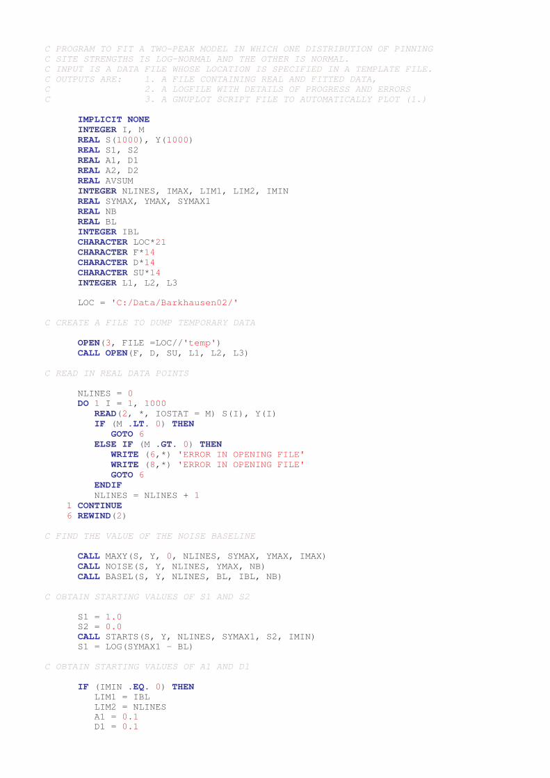
C PROGRAM TO FIT A TWO-PEAK MODEL IN WHICH ONE DISTRIBUTION OF PINNINGC SITE STRENGTHS IS LOG-NORMAL AND THE OTHER IS NORMAL. C INPUT IS A DATA FILE WHOSE LOCATION IS SPECIFIED IN A TEMPLATE FILE.C OUTPUTS ARE: 1. A FILE CONTAINING REAL AND FITTED DATA,C 2. A LOGFILE WITH DETAILS OF PROGRESS AND ERRORSC 3. A GNUPLOT SCRIPT FILE TO AUTOMATICALLY PLOT (1.)
IMPLICIT NONE INTEGER I, M REAL S(1000), Y(1000) REAL S1, S2 REAL A1, D1 REAL A2, D2 REAL AVSUM INTEGER NLINES, IMAX, LIM1, LIM2, IMIN REAL SYMAX, YMAX, SYMAX1 REAL NB REAL BL INTEGER IBL CHARACTER LOC*21 CHARACTER F*14 CHARACTER D*14 CHARACTER SU*14 INTEGER L1, L2, L3
LOC = 'C:/Data/Barkhausen02/'
C CREATE A FILE TO DUMP TEMPORARY DATA
OPEN(3, FILE =LOC//'temp') CALL OPEN(F, D, SU, L1, L2, L3)
C READ IN REAL DATA POINTS
NLINES = 0 DO 1 I = 1, 1000 READ(2, *, IOSTAT = M) S(I), Y(I) IF (M .LT. 0) THEN GOTO 6 ELSE IF (M .GT. 0) THEN WRITE (6,*) 'ERROR IN OPENING FILE' WRITE (8,*) 'ERROR IN OPENING FILE' GOTO 6 ENDIF NLINES = NLINES + 1 1 CONTINUE 6 REWIND(2)
C FIND THE VALUE OF THE NOISE BASELINE
CALL MAXY(S, Y, 0, NLINES, SYMAX, YMAX, IMAX) CALL NOISE(S, Y, NLINES, YMAX, NB) CALL BASEL(S, Y, NLINES, BL, IBL, NB)
C OBTAIN STARTING VALUES OF S1 AND S2
S1 = 1.0 S2 = 0.0 CALL STARTS(S, Y, NLINES, SYMAX1, S2, IMIN) S1 = LOG(SYMAX1 - BL)
C OBTAIN STARTING VALUES OF A1 AND D1
IF (IMIN .EQ. 0) THEN LIM1 = IBL LIM2 = NLINES A1 = 0.1 D1 = 0.1
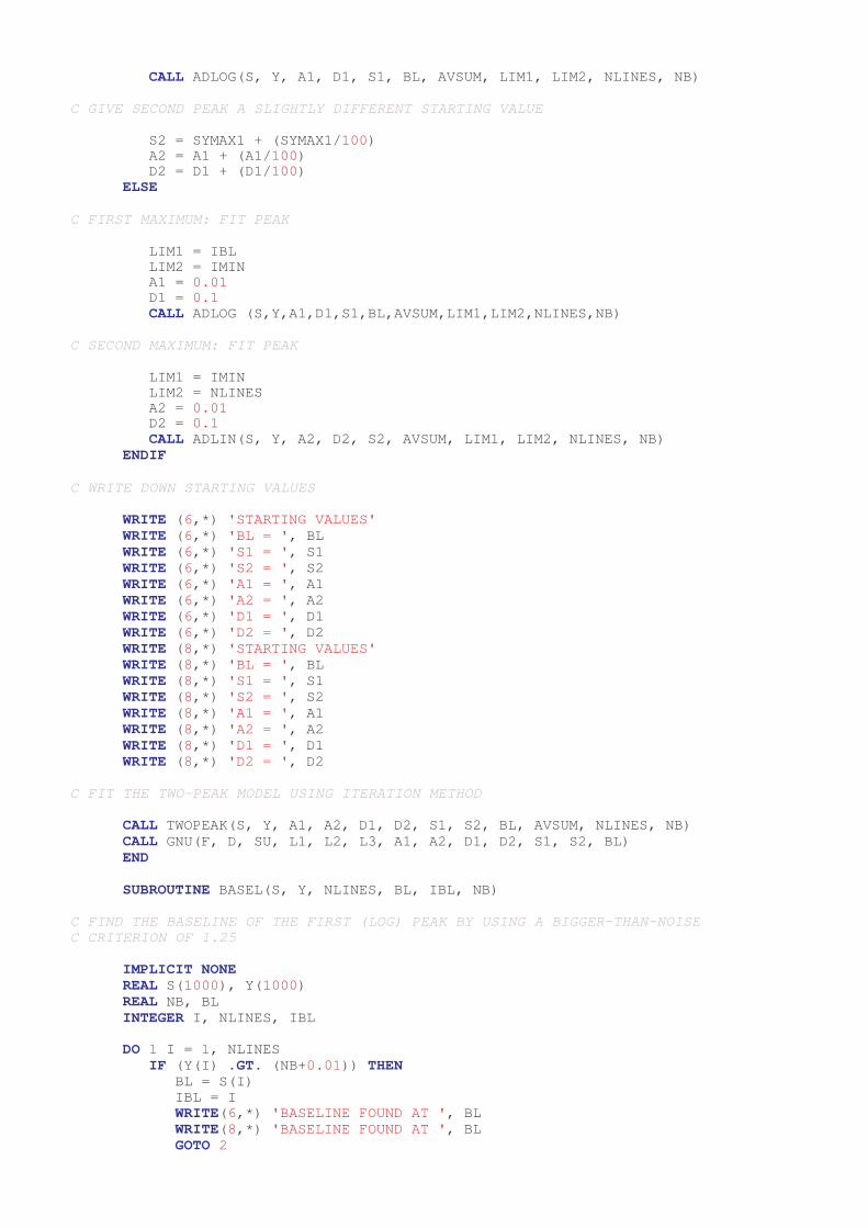
CALL ADLOG(S, Y, A1, D1, S1, BL, AVSUM, LIM1, LIM2, NLINES, NB)
C GIVE SECOND PEAK A SLIGHTLY DIFFERENT STARTING VALUE
S2 = SYMAX1 + (SYMAX1/100) A2 = A1 + (A1/100) D2 = D1 + (D1/100) ELSE
C FIRST MAXIMUM: FIT PEAK
LIM1 = IBL LIM2 = IMIN A1 = 0.01 D1 = 0.1 CALL ADLOG (S,Y,A1,D1,S1,BL,AVSUM,LIM1,LIM2,NLINES,NB)
C SECOND MAXIMUM: FIT PEAK
LIM1 = IMIN LIM2 = NLINES A2 = 0.01 D2 = 0.1 CALL ADLIN(S, Y, A2, D2, S2, AVSUM, LIM1, LIM2, NLINES, NB) ENDIF
C WRITE DOWN STARTING VALUES
WRITE (6,*) 'STARTING VALUES' WRITE (6,*) 'BL = ', BL WRITE (6,*) 'S1 = ', S1 WRITE (6,*) 'S2 = ', S2 WRITE (6,*) 'A1 = ', A1 WRITE (6,*) 'A2 = ', A2 WRITE (6,*) 'D1 = ', D1 WRITE (6,*) 'D2 = ', D2 WRITE (8,*) 'STARTING VALUES' WRITE (8,*) 'BL = ', BL WRITE (8,*) 'S1 = ', S1 WRITE (8,*) 'S2 = ', S2 WRITE (8,*) 'A1 = ', A1 WRITE (8,*) 'A2 = ', A2 WRITE (8,*) 'D1 = ', D1 WRITE (8,*) 'D2 = ', D2
C FIT THE TWO-PEAK MODEL USING ITERATION METHOD
CALL TWOPEAK(S, Y, A1, A2, D1, D2, S1, S2, BL, AVSUM, NLINES, NB) CALL GNU(F, D, SU, L1, L2, L3, A1, A2, D1, D2, S1, S2, BL) END
SUBROUTINE BASEL(S, Y, NLINES, BL, IBL, NB)
C FIND THE BASELINE OF THE FIRST (LOG) PEAK BY USING A BIGGER-THAN-NOISEC CRITERION OF 1.25
IMPLICIT NONE REAL S(1000), Y(1000) REAL NB, BL INTEGER I, NLINES, IBL
DO 1 I = 1, NLINES IF (Y(I) .GT. (NB+0.01)) THEN BL = S(I) IBL = I WRITE(6,*) 'BASELINE FOUND AT ', BL WRITE(8,*) 'BASELINE FOUND AT ', BL GOTO 2
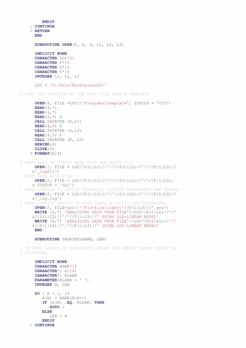
ENDIF 1 CONTINUE 2 RETURN END
SUBROUTINE OPEN(F, D, S, L1, L2, L3)
IMPLICIT NONE CHARACTER LOC*21 CHARACTER F*14 CHARACTER D*14 CHARACTER S*14 INTEGER L1, L2, L3
LOC = 'C:/Data/Barkhausen02/'
C READ THE LOCATION OF THE DATA FILE FROM A TEMPLATE
OPEN(4, FILE =LOC//'Programs/template', STATUS = 'OLD') READ(4,*) READ(4,*) READ(4,9) D CALL SHORTEN (D,L1) READ(4,9) S CALL SHORTEN (S,L2) READ(4,9) F CALL SHORTEN (F, L3) REWIND(4) CLOSE(4) 9 FORMAT(A14) C MAKE FILE TO OUTPUT REAL DATA AND MODEL FIT OPEN(1, FILE = LOC//D(1:L1)//'/'//S(1:L2)//'/'//F(1:L3)// &'_logfit')C OPEN REAL DATA FILE OPEN(2, FILE = LOC//D(1:L1)//'/'//S(1:L2)//'/'//F(1:L3), & STATUS = 'OLD')C MAKE LOGFILE TO OUTPUT PROGRESS, FITTING PARAMETERS AND ERRORS OPEN(8, FILE = LOC//D(1:L1)//'/'//S(1:L2)//'/'//F(1:L3)// &'_log.log')C MAKE GNUPLOT SCRIPT TO PLOT GRAPH WITH FITTING PARAMETERS OPEN(7, FILE=LOC//'/Plotfile/logfit'//F(1:L3)//'.gnu') WRITE (6,*) 'ANALYSING DATA FROM FILE'//LOC//D(1:L1)//'/' &//S(1:L2)//'/'//F(1:L3)//' USING LOG-LINEAR MODEL' WRITE (8,*) 'ANALYSING DATA FROM FILE'//LOC//D(1:L1)//'/' &//S(1:L2)//'/'//F(1:L3)//' USING LOG-LINEAR MODEL' END
SUBROUTINE SHORTEN(NAME, LEN)
C TO FIND LENGTH OF CHARACTER STRING AND REMOVE BLANK SPACES INC FILENAMES
IMPLICIT NONE CHARACTER NAME*14 CHARACTER*1 A(14) CHARACTER*1 BLANK PARAMETER(BLANK = ' ') INTEGER N, LEN
DO 1 N = 1, 14 A(N) = NAME(N:N+1) IF (A(N) .EQ. BLANK) THEN GOTO 1 ELSE LEN = N ENDIF 1 CONTINUE
RETURN END
SUBROUTINE GNU(F, D, S, L1, L2, L3, A1, A2, D1, D2, S1, S2, BL)
C TO WRITE A GNUPLOT SCRIPT TO DISPLAY REAL DATA, MODEL AND FITTINGC PARAMTERS ON SCREEN AND IN MONO AND COLOUR .EPS FILES
CHARACTER LOC*21 CHARACTER F*14 CHARACTER D*14 CHARACTER S*14 INTEGER L1, L2, L3 REAL A1, A2, D1, D2, S1, S2, BL
LOC = 'C:/Data/Barkhausen02/'
WRITE(7,*) '# Instructions to Gnuplot - to plot model and' &//' real data' WRITE(7,*) 'set autoscale' WRITE(7,*) 'set nologscale' WRITE(7,*) 'set nogrid' WRITE(7,*) 'set nolabel' WRITE(7,*) 'set key top right Left' WRITE(7,*) 'set title "Log-linear two-point model fit for' &//LOC//D(1:L1)//'/'//S(1:L2)//'/'//F(1:L3)//'"' WRITE(7,*) 'set xlabel "Magnetising current/A "' WRITE(7,*) 'set ylabel "RMS Barkhausen voltage/V"' WRITE(7,*) 'set label 1 "Model parameters" at graph 0.02, 0.95' WRITE(7,*) 'set label 2 "A_1 = ', A1,'" at graph 0.02, 0.90' WRITE(7,*) 'set label 3 "A_2 = ', A2,'" at graph 0.02, 0.85' WRITE(7,*) 'set label 4 "{/Symbol=14 D}S_1 = ', D1,'" at' &//' graph 0.02, 0.80' WRITE(7,*) 'set label 5 "{/Symbol=14 D}S_2 = ', D2,'" at' &//' graph 0.02, 0.75' WRITE(7,*) 'set label 6 "<S>_1 = ', S1,'" at graph 0.02, 0.70' WRITE(7,*) 'set label 7 "<S>_2 = ', S2,'" at graph 0.02, 0.65' WRITE(7,*) 'set label 8 "b = ', BL,'" at graph 0.02, 0.60' WRITE(7,*) 'set xrange [-0.7:0.7]' WRITE(7,*) 'set terminal x11' WRITE(7,*) 'plot "'//LOC//D(1:L1)//'/'//S(1:L2)//'/' &//F(1:L3)//'_logfit" using 1:2 title "Real data" with lines 1' WRITE(7,*) 'replot "'//LOC//D(1:L1)//'/'//S(1:L2)//'/' &//F(1:L3)//'_logfit" using 1:3 title "Model" with lines 3' WRITE(7,*) 'set output "'//LOC//D(1:L1)//'/'//S(1:L2)//'/' &//F(1:L3)//'_log_mono.ps"' WRITE(7,*) 'set terminal postscript eps enhanced mono dashed' &//'"Helvetica" 20' WRITE(7,*) 'replot' WRITE(7,*) 'set output "'//LOC//D(1:L1)//'/'//S(1:L2)//'/' &//F(1:L3)//'_log_colour.ps"' WRITE(7,*) 'set terminal postscript eps enhanced color solid' &//'"Helvetica" 20' WRITE(7,*) 'replot' WRITE(7,*) 'set terminal x11' WRITE(7,*) 'replot' WRITE(7,*) WRITE(7,*) RETURN END SUBROUTINE MAXY(S, Y, LIM1, LIM2, SYMAX, YMAX, IMAX)
C FINDS THE LARGEST VALUE OF Y IN THE DATA SET
IMPLICIT NONE INTEGER I, LIM1, LIM2, IMAX REAL Y(1000), S(1000), SYMAX, YMAX
YMAX = 0.0 SYMAX = 0.0 IMAX = 0
DO 1 I = LIM1, LIM2 IF (Y(I) .GT. YMAX) THEN YMAX = Y(I) SYMAX = S(I) IMAX = I ENDIF 1 CONTINUE RETURN END SUBROUTINE MINY(S, Y, LIM1, LIM2, SYMIN, YMIN, IMIN)
C FINDS THE SMALLEST VALUE OF Y IN THE DATA SET
IMPLICIT NONE INTEGER I, LIM1, LIM2, IMIN REAL Y(1000), S(1000), SYMIN, YMIN
YMIN = Y(LIM1) SYMIN = 0.0 IMIN = 0
DO 1 I = LIM1, LIM2 IF (Y(I) .LT. YMIN) THEN YMIN = Y(I) SYMIN = S(I) IMIN = I ENDIF 1 CONTINUE RETURN END
SUBROUTINE BIN(S, Y, YMAX, NLINES, COUNT, BINA)
C DIVIDES DATA INTO 'BINS' ACCORDING TO SIZE
IMPLICIT NONE INTEGER I, J, NLINES, COUNT(1000) REAL Y(1000), S(1000), YMAX, BINA, BINU, BINL
BINA = YMAX/REAL(NLINES) BINL = 0.0 BINU = 0.0
DO 1 I = 1, NLINES BINL = BINU BINU = REAL(I)*BINA COUNT(I) = 0 DO 2 J = 1, NLINES IF ((Y(J) .GE. BINL) .AND. (Y(J) .LT. BINU)) THEN COUNT(I) = COUNT(I) + 1 ENDIF 2 CONTINUE 1 CONTINUE END
SUBROUTINE NOISE(S, Y, NLINES, YMAX, NB)
C FINDS THE VALUE OF THE NOISE BASELINE AND LIMITS AROUND IT.
IMPLICIT NONE REAL S(1000), Y(1000), YMAX, BINA INTEGER I, NLINES, COUNT(1000), MAXC, IMAXC
REAL NB REAL BBINUP, BBINDO, NOISUM INTEGER INC, J
NB = 0.0 MAXC = 0 IMAXC = 0
C DIVIDE DATA INTO BINS CALL BIN(S, Y, YMAX, NLINES, COUNT, BINA)C FIND BIN WITH LARGEST NUMBER OF DATA POINTS IN ITC THIS IS THE 'NOISE BASELINE' BIN DO 1 I = 1, NLINES IF (COUNT(I) .GT. MAXC) THEN MAXC = COUNT(I) IMAXC = I ENDIF 1 CONTINUE
C FIND AVERAGE OF ALL POINTS THAT ARE IN THIS BIN OR OTHERS AROUND ITC CHANGE VALUE '3' TO ANOTHER INTEGER TO CHANGE SENSITIVITY.
BBINUP = REAL(IMAXC + 3)*BINA BBINDO = REAL(IMAXC - 3)*BINA
INC = 0
DO 2 J = 1, NLINES IF ((Y(J) .GE. BBINDO) .AND. (Y(J) .LT. BBINUP)) THEN NOISUM = NOISUM + Y(J) INC = INC + 1 ENDIF 2 CONTINUE
NB = NOISUM/REAL(INC) WRITE (6,*) 'NOISE = ', NB WRITE (8,*) 'NOISE = ', NB RETURN END
SUBROUTINE MAXY2(S, Y, NLINES, SYMAX1, SYMAX2, YMAX1, YMAX2, IMIN)
C TO FIND THE POSITIONS OF THE PEAK(S) AND MINIMUM IF IT EXISTS
IMPLICIT NONE REAL S(1000), Y(1000) REAL AVES(20), AVEY(20), SSUM, YSUM REAL AVEM1, AVEM2, AVEM3 REAL SYMAX1, SYMAX2, SYMIN REAL YMAX1, YMAX2, YMIN INTEGER NLINES, COUNT, I, J, POINTS INTEGER JM1, JM2, JM3, TEMP INTEGER IMAX1, IMAX2, IMIN INTEGER LIM1, LIM2
C DIVIDE THE POINTS INTO TWENTY GROUPS AND FIND THE AVERAGE.
POINTS = NLINES/20
DO 1 J = 1, 20 COUNT = 0 YSUM = 0.0 SSUM = 0.0 DO 2 I = (J-1)*POINTS, J*POINTS YSUM = YSUM + Y(I) SSUM = SSUM + S(I) COUNT = COUNT+1 2 CONTINUE
AVEY(J) = YSUM/REAL(COUNT) AVES(J) = SSUM/REAL(COUNT) WRITE(3,*) J, AVES(J), AVEY(J) 1 CONTINUE
AVEM1 = 0.0 AVEM2 = 0.0 AVEM3 = 0.0 JM1 = 0 JM2 = 0 JM3 = 0
C FIND THE TWO LARGEST VALUES OF THE AVERAGE
DO 3 J = 1, 20 IF (AVEY(J) .GT. AVEM1) THEN AVEM2 = AVEM1 JM2 = JM1 AVEM1 = AVEY(J) JM1 = J ELSE IF ((AVEY(J) .GT. AVEM2) .AND. (AVEY(J) .LE. AVEM1)) THEN AVEM2 = AVEY(J) JM2 = J ENDIF 3 CONTINUE WRITE (6,*) 'LARGEST TWO VALUES ARE AT ', JM1, JM2 WRITE (8,*) 'LARGEST TWO VALUES ARE AT ', JM1, JM2
C ARE THE TWO MAXIMA NEXT TO EACH OTHER?
IF (ABS(JM1 - JM2) .NE. 1) THEN C IF NOT, THEN WE CAN EASILY FIND THE PEAKS AND THE MINIMUM BETWEEN THEMC MAKE JM1 THE SMALLER OF THE TWO J-VALUES
IF (JM1 .GT. JM2) THEN TEMP = JM1 JM1 = JM2 JM2 = TEMP ENDIF
C FIND THE MAXIMUM NEAR J1 PRECISELY
LIM1 = (JM1-1)*POINTS LIM2 = (JM1+1)*POINTS
CALL MAXY(S, Y, LIM1, LIM2, SYMAX1, YMAX1, IMAX1)
C FIND THE MINIMUM NEAR J2 PRECISELY
LIM1 = (JM2-1)*POINTS LIM2 = (JM2+1)*POINTS CALL MAXY(S, Y, LIM1, LIM2, SYMAX2, YMAX2, IMAX2)
C FIND THE MINIMUM SITUATED BETWEEN THESE TWO MAXIMA
LIM1 = IMAX1 LIM2 = IMAX2 CALL MINY(S, Y, LIM1, LIM2, SYMIN, YMIN, IMIN) WRITE(6,*) 'MAXIMUM 1 AT ', SYMAX1, ' HEIGHT ', YMAX1 WRITE(6,*) 'MINIMUM AT ', SYMIN, ' HEIGHT ', YMIN WRITE(6,*) 'MAXIMUM 2 AT ', SYMAX2, ' HEIGHT ', YMAX2 WRITE(8,*) 'MAXIMUM 1 AT ', SYMAX1, ' HEIGHT ', YMAX1 WRITE(8,*) 'MINIMUM AT ', SYMIN, ' HEIGHT ', YMIN WRITE(8,*) 'MAXIMUM 2 AT ', SYMAX2, ' HEIGHT ', YMAX2 ELSE
C IF THE TWO MAX AVERAGE VALUES ARE NEXT TO ONE ANOTHERC TRY AND FIND ANOTHER PEAK IN THE AVERAGE VALUES
DO 4 J = 2, 19
C IS J THE POSITION OF A PEAK?
IF ((AVEY(J) .GT. AVEM3) .AND. (AVEY(J) .GE. AVEY(J+1))) THEN
C IS AVEY(J) LESS THAN THE MAX PEAK VALUE? AND IS IT GREATER THAN AC THRESHOLD VALUE (ARBITRARILY GIVEN AS AVEM1/10 TO ELIMINATE NOISE)?
IF ((AVEY(J) .LT. AVEM1) .AND. (AVEY(J) .GT. (AVEM1/10))) & THEN
C IF THE NEW J-VALUE IS MORE THAN 1 UNIT AWAY FROM JM1C THIS SHOULD ONLY FAIL IF THERE ARE 3 PEAKS OF EXACT SAME HEIGHT NEXTC TO ONE ANOTHER
IF (ABS(JM1 - J) .GT. 1) THEN
C DEFINE NEW AVERAGE MAX VALUE AND J VALUE
AVEM3 = AVEY(J) JM3 = J ENDIF ENDIF ENDIF 4 CONTINUE
C IF WE HAVE OBTAINED A NON-ZERO VALUE OF JM3 FROM THIS PROCEDURE THEN
IF (JM3 .NE. 0) THEN
C REDEFINE IT AS JM2
JM2 = JM3
C MAKE JM1 SMALLER THAN JM2
IF (JM1 .GT. JM2) THEN TEMP = JM1 JM1 = JM2 JM2 = TEMP ENDIF
C FIND PRECISE POSITION OF MAX NEAR JM1
LIM1 = (JM1-1)*POINTS LIM2 = (JM1+1)*POINTS CALL MAXY(S, Y, LIM1, LIM2, SYMAX1, YMAX1, IMAX1)
C FIND PRECISE POSITION OF MAX NEAR JM2
LIM1 = (JM2-1)*POINTS LIM2 = (JM2+1)*POINTS CALL MAXY(S, Y, LIM1, LIM2, SYMAX2, YMAX2, IMAX2)
C FIND PRECISE POSITION OF MINIMUM IN BETWEEN THESE
LIM1 = IMAX1 LIM2 = IMAX2 CALL MINY(S, Y, LIM1, LIM2, SYMIN, YMIN, IMIN) WRITE(6,*) 'MAXIMUM 1 AT ', SYMAX1, ' HEIGHT ', YMAX1 WRITE(6,*) 'MINIMUM AT ', SYMIN, ' HEIGHT ', YMIN WRITE(6,*) 'MAXIMUM 2 AT ', SYMAX2, ' HEIGHT ', YMAX2 WRITE(8,*) 'MAXIMUM 1 AT ', SYMAX1, ' HEIGHT ', YMAX1 WRITE(8,*) 'MINIMUM AT ', SYMIN, ' HEIGHT ', YMIN
WRITE(8,*) 'MAXIMUM 2 AT ', SYMAX2, ' HEIGHT ', YMAX2 ELSE
C IF THE TWO MAXIMA ARE NEXT TO ONE ANOTHER AND THERE ARE NO OTHERC PEAKS: MAKE JM1 SMALLER THAN JM2
IF (JM1 .GT. JM2) THEN TEMP = JM1 JM1 = JM2 JM2 = TEMP ENDIF
C FIND MAXIMUM NEAR JM1 AND JM2
LIM1 = (JM1-1)*POINTS LIM2 = (JM2+1)*POINTS CALL MAXY(S, Y, LIM1, LIM2, SYMAX1, YMAX1, IMAX1)
C PUT BOTH S-VALUES AT THIS POINT.
SYMAX2 = SYMAX1 YMAX2 = YMAX1 IMAX2 = IMAX1 IMIN = 0 WRITE(6,*) 'SINGLE MAXIMUM AT ', SYMAX1, ' HEIGHT ', YMAX1 WRITE(6,*) 'NO MINIMUM' WRITE(8,*) 'SINGLE MAXIMUM AT ', SYMAX1, ' HEIGHT ', YMAX1 WRITE(8,*) 'NO MINIMUM' ENDIF ENDIF RETURN END
SUBROUTINE TWOPEAK(S,Y,A1,A2,D1,D2,S1,S2,BL,AVSUM,NLINES,NB)
C TO FIT A TWO-PEAK MODEL BY ITERATING USING STARTING VALUES ALREADYC OBTAINED.C FORCED TO ITERATE AT LEAST 10 TIMES THROUGH WHOLE PROCEDURE
IMPLICIT NONE REAL S(1000), Y(1000), A1, A2, D1, D2, S1, S2, AVSUM, NB, BL INTEGER NLINES, ITER REAL ERROR, OLDERROR
9 WRITE(6,*) 'USING BEGINNING VALUES, ERROR = ',(AVSUM*100),' %' WRITE(8,*) 'USING BEGINNING VALUES, ERROR = ',(AVSUM*100),' %' CALL BESTA1(S, Y, A1, A2, D1, D2, S1, S2, BL, AVSUM, NLINES, NB) WRITE(6,*) 'NEW A1 = ', A1, ' ERROR = ',(AVSUM*100),' %' WRITE(8,*) 'NEW A1 = ', A1, ' ERROR = ',(AVSUM*100),' %' CALL BESTA2(S, Y, A1, A2, D1, D2, S1, S2, BL, AVSUM, NLINES, NB) WRITE(6,*) 'NEW A2 = ', A2, ' ERROR = ',(AVSUM*100),' %' WRITE(8,*) 'NEW A2 = ', A2, ' ERROR = ',(AVSUM*100),' %' CALL BESTD1(S, Y, A1, A2, D1, D2, S1, S2, BL, AVSUM, NLINES, NB) WRITE(6,*) 'NEW D1 = ', D1, ' ERROR = ',(AVSUM*100),' %' WRITE(8,*) 'NEW D1 = ', D1, ' ERROR = ',(AVSUM*100),' %' CALL BESTD2(S, Y, A1, A2, D1, D2, S1, S2, BL, AVSUM, NLINES, NB) WRITE(6,*) 'NEW D2 = ', D2, ' ERROR = ',(AVSUM*100),' %' WRITE(8,*) 'NEW D2 = ', D2, ' ERROR = ',(AVSUM*100),' %' CALL BESTS1(S, Y, A1, A2, D1, D2, S1, S2, BL, AVSUM, NLINES, NB) WRITE(6,*) 'NEW S1 = ', S1, ' ERROR = ',(AVSUM*100),' %' WRITE(8,*) 'NEW S1 = ', S1, ' ERROR = ',(AVSUM*100),' %' CALL BESTS2(S, Y, A1, A2, D1, D2, S1, S2, BL, AVSUM, NLINES, NB) WRITE(6,*) 'NEW S2 = ', S2, ' ERROR = ',(AVSUM*100),' %' WRITE(8,*) 'NEW S2 = ', S2, ' ERROR = ',(AVSUM*100),' %' CALL BESTBL(S, Y, A1, A2, D1, D2, S1, S2, BL, AVSUM, NLINES, NB) WRITE(6,*) 'NEW BL = ', BL, ' ERROR = ',(AVSUM*100),' %' WRITE(8,*) 'NEW BL = ', BL, ' ERROR = ',(AVSUM*100),' %'
OLDERROR = ERROR ERROR = AVSUM
IF ((ERROR .LT. OLDERROR) .OR. (ITER .LE. 10)) THEN ITER = ITER + 1 WRITE (6,*) 'OVERALL ITERATION NO. ', ITER WRITE (6,*) '*************************' WRITE (8,*) 'OVERALL ITERATION NO. ', ITER WRITE (8,*) '*************************' GOTO 9 ENDIF RETURN END
SUBROUTINE ADLOG(S,Y,A,D,SV,BL,AVSUM,LIM1,LIM2,NLINES,NB)
C TO OBTAIN STARTING VALUES OF A AND D GIVEN A VALUE OF SC ONLY FITS WITHIN LIMIT SPECIFIEDC FORCED TO ITERATE AT LEAST 10 TIMES TO PREVENT SPURIOUS MINIMA
IMPLICIT NONE INTEGER ITER REAL S(1000), Y(1000), A, D, SV, AVSUM, BL INTEGER NLINES, LIM1, LIM2 REAL ERROR, NB REAL OLDERROR
ITER = 0
WRITE (6,*) 'CALCULATING STARTING VALUES' WRITE (8,*) 'CALCULATING STARTING VALUES'
5 CALL ALOG(S, Y, A, D, SV, BL, AVSUM, LIM1, LIM2, NLINES, NB) CALL DLOG(S, Y, A, D, SV, BL, AVSUM, LIM1, LIM2, NLINES, NB) OLDERROR = ERROR ERROR = AVSUM IF ((ERROR .LT. OLDERROR) .OR. (ITER .LE. 10)) THEN ITER = ITER + 1 GOTO 5 ENDIF RETURN END
SUBROUTINE ADLIN(S, Y, A, D, SV, AVSUM, LIM1, LIM2, NLINES, NB)
C TO OBTAIN STARTING VALUES OF A AND D GIVEN A VALUE OF SC WITHIN LIMITS SPECIFIEDC FORCED TO ITERATE AT LEAST 10 TIMES TO PREVENT SPURIOUS MINIMA
IMPLICIT NONE INTEGER ITER REAL S(1000), Y(1000), A, D, SV, AVSUM INTEGER NLINES, LIM1, LIM2 REAL ERROR, NB REAL OLDERROR
ITER = 0
WRITE (6,*) 'CALCULATING STARTING VALUES' WRITE (8,*) 'CALCULATING STARTING VALUES' 5 CALL ALIN(S, Y, A, D, SV, AVSUM, LIM1, LIM2, NLINES, NB) CALL DLIN(S, Y, A, D, SV, AVSUM, LIM1, LIM2, NLINES, NB) OLDERROR = ERROR ERROR = AVSUM IF ((ERROR .LT. OLDERROR) .OR. (ITER .LE. 10)) THEN ITER = ITER + 1 ENDIF RETURN
END
SUBROUTINE STARTS(S, Y, NLINES, SYMAX1, SYMAX2, IMIN)
C SUBROUTINE TO FIND STARTING VALUES OF S1 AND S2
IMPLICIT NONE REAL S(1000), Y(1000) REAL SYMAX1, SYMAX2, YMAX1, YMAX2, TEMP INTEGER NLINES, IMIN
WRITE (6,*) 'AUTOMATIC OPERATION' WRITE (8,*) 'AUTOMATIC OPERATION' CALL MAXY2(S, Y, NLINES, SYMAX1, SYMAX2, YMAX1, YMAX2, IMIN) IF (SYMAX2 .GT. SYMAX1) THEN ELSE TEMP = SYMAX2 SYMAX2 = SYMAX1 SYMAX1 = TEMP ENDIF WRITE (6,*) 'PEAK 1 AT ', SYMAX1, ' HEIGHT ', YMAX1 WRITE (6,*) 'PEAK 2 AT ', SYMAX2, ' HEIGHT ', YMAX2 WRITE (8,*) 'PEAK 1 AT ', SYMAX1, ' HEIGHT ', YMAX1 WRITE (8,*) 'PEAK 2 AT ', SYMAX2, ' HEIGHT ', YMAX2 RETURN END
SUBROUTINE BESTA1(S,Y,A1,A2,D1,D2,S1,S2,BL,AVSUM,NLINES,NB)
C TO FIND THE BEST-FIT VALUE OF A1
IMPLICIT NONE REAL S(1000), Y(1000) REAL A1, A2, D1, D2, S1, S2 INTEGER NLINES, ITER REAL A1U, A1D, AVSUMU, AVSUMD, AVSUM, NB, BL
ITER = 0
4 CALL FITTWO(S,Y,A1,A2,D1,D2,S1,S2,BL,AVSUM,NLINES,NB) A1U = A1 + (A1/100) CALL FITTWO(S,Y,A1U,A2,D1,D2,S1,S2,BL,AVSUMU,NLINES,NB) A1D = A1 - (A1/100) CALL FITTWO(S,Y,A1D,A2,D1,D2,S1,S2,BL,AVSUMD,NLINES,NB) IF (ITER .LE. 10000) THEN IF ((AVSUMD .LT. AVSUM) .AND. (AVSUM .LT. AVSUMU)) THEN A1 = A1D ITER = ITER + 1 GOTO 4 ELSE IF ((AVSUMD .GT. AVSUM) .AND. (AVSUM .GT. AVSUMU)) THEN A1 = A1U ITER = ITER + 1 GOTO 4 ELSE WRITE (6,*) 'A1: DETECTED MINIMUM ', ITER, ' ITERATIONS' WRITE (8,*) 'A1: DETECTED MINIMUM ', ITER, ' ITERATIONS' ENDIF ELSE WRITE (6,*) 'A1: TOO MANY ITERATIONS; PROCESS FAILED' WRITE (8,*) 'A1: TOO MANY ITERATIONS; PROCESS FAILED' ENDIF RETURN END
SUBROUTINE BESTA2(S,Y,A1,A2,D1,D2,S1,S2,BL,AVSUM,NLINES,NB)
C TO FIND THE BEST-FIT VALUE OF A2
IMPLICIT NONE REAL S(1000), Y(1000) REAL A1, A2, D1, D2, S1, S2 INTEGER NLINES, ITER REAL A2U, A2D, AVSUMU, AVSUMD, AVSUM, NB, BL
ITER = 0
4 CALL FITTWO(S,Y,A1,A2,D1,D2,S1,S2,BL,AVSUM,NLINES,NB) A2U = A2 + (A2/100) CALL FITTWO(S,Y,A1,A2U,D1,D2,S1,S2,BL,AVSUMU,NLINES,NB) A2D = A2 - (A2/100) CALL FITTWO(S,Y,A1,A2D,D1,D2,S1,S2,BL,AVSUMD,NLINES,NB) IF (ITER .LE. 10000) THEN IF ((AVSUMD .LT. AVSUM) .AND. (AVSUM .LT. AVSUMU)) THEN A2 = A2D ITER = ITER + 1 GOTO 4 ELSE IF ((AVSUMD .GT. AVSUM) .AND. (AVSUM .GT. AVSUMU)) THEN A2 = A2U ITER = ITER + 1 GOTO 4 ELSE WRITE (6,*) 'A2: DETECTED MINIMUM ', ITER, ' ITERATIONS' WRITE (8,*) 'A2: DETECTED MINIMUM ', ITER, ' ITERATIONS' ENDIF ELSE WRITE (6,*) 'A2: TOO MANY ITERATIONS; PROCESS FAILED' WRITE (8,*) 'A2: TOO MANY ITERATIONS; PROCESS FAILED' ENDIF RETURN END
SUBROUTINE BESTD1(S,Y,A1,A2,D1,D2,S1,S2,BL,AVSUM,NLINES,NB)
C TO FIND THE BEST-FIT VALUE OF D1
IMPLICIT NONE REAL S(1000), Y(1000) REAL A1, A2, D1, D2, S1, S2 INTEGER NLINES, ITER REAL D1U, D1D, AVSUMU, AVSUMD, AVSUM, NB, BL
ITER = 0
4 CALL FITTWO(S,Y,A1,A2,D1,D2,S1,S2,BL,AVSUM,NLINES,NB) D1U = D1 + (D1/100) CALL FITTWO(S,Y,A1,A2,D1U,D2,S1,S2,BL,AVSUMU,NLINES,NB) D1D = D1 - (D1/100) CALL FITTWO(S,Y,A1,A2,D1D,D2,S1,S2,BL,AVSUMD,NLINES,NB) IF (ITER .LE. 10000) THEN IF ((AVSUMD .LT. AVSUM) .AND. (AVSUM .LT. AVSUMU)) THEN D1 = D1D ITER = ITER + 1 GOTO 4 ELSE IF ((AVSUMD .GT. AVSUM) .AND. (AVSUM .GT. AVSUMU)) THEN D1 = D1U ITER = ITER + 1 GOTO 4 ELSE WRITE (6,*) 'D1: DETECTED MINIMUM ', ITER, ' ITERATIONS' WRITE (8,*) 'D1: DETECTED MINIMUM ', ITER, ' ITERATIONS' ENDIF ELSE WRITE (6,*) 'D1: TOO MANY ITERATIONS; PROCESS FAILED' WRITE (8,*) 'D1: TOO MANY ITERATIONS; PROCESS FAILED' ENDIF RETURN
END
SUBROUTINE BESTD2(S,Y,A1,A2,D1,D2,S1,S2,BL,AVSUM,NLINES,NB)
C TO FIND THE BEST-FIT VALUE OF D2
IMPLICIT NONE REAL S(1000), Y(1000) REAL A1, A2, D1, D2, S1, S2 INTEGER NLINES, ITER REAL D2U, D2D, AVSUMU, AVSUMD, AVSUM, NB, BL
ITER = 0
4 CALL FITTWO(S,Y,A1,A2,D1,D2,S1,S2,BL,AVSUM,NLINES,NB) D2U = D2 + (D2/100) CALL FITTWO(S,Y,A1,A2,D1,D2U,S1,S2,BL,AVSUMU,NLINES,NB) D2D = D2 - (D2/100) CALL FITTWO(S,Y,A1,A2,D1,D2D,S1,S2,BL,AVSUMD,NLINES,NB) IF (ITER .LE. 10000) THEN IF ((AVSUMD .LT. AVSUM) .AND. (AVSUM .LT. AVSUMU)) THEN D2 = D2D ITER = ITER + 1 GOTO 4 ELSE IF ((AVSUMD .GT. AVSUM) .AND. (AVSUM .GT. AVSUMU)) THEN D2 = D2U ITER = ITER + 1 GOTO 4 ELSE WRITE (6,*) 'D2: DETECTED MINIMUM ', ITER, ' ITERATIONS' WRITE (8,*) 'D2: DETECTED MINIMUM ', ITER, ' ITERATIONS' ENDIF ELSE WRITE (6,*) 'D2: TOO MANY ITERATIONS; PROCESS FAILED' WRITE (8,*) 'D2: TOO MANY ITERATIONS; PROCESS FAILED' ENDIF RETURN END
SUBROUTINE BESTS1(S,Y,A1,A2,D1,D2,S1,S2,BL,AVSUM,NLINES,NB)
C TO FIND THE BEST-FIT VALUE OF S1
IMPLICIT NONE REAL S(1000), Y(1000) REAL A1, A2, D1, D2, S1, S2 INTEGER NLINES, ITER REAL S1U, S1D, AVSUMU, AVSUMD, AVSUM, NB, BL
ITER = 0
4 CALL FITTWO(S,Y,A1,A2,D1,D2,S1,S2,BL,AVSUM,NLINES,NB) S1U = S1 + (S1/100) CALL FITTWO(S, Y, A1, A2, D1, D2, S1U, S2, BL, AVSUMU, NLINES, NB) S1D = S1 - (S1/100) CALL FITTWO(S, Y, A1, A2, D1, D2, S1D, S2, BL, AVSUMD, NLINES, NB) IF (ITER .LE. 10000) THEN IF ((AVSUMD .LT. AVSUM) .AND. (AVSUM .LT. AVSUMU)) THEN S1 = S1D ITER = ITER + 1 GOTO 4 ELSE IF ((AVSUMD .GT. AVSUM) .AND. (AVSUM .GT. AVSUMU)) THEN S1 = S1U ITER = ITER + 1 GOTO 4 ELSE WRITE (6,*) 'S1: DETECTED MINIMUM ', ITER, ' ITERATIONS' WRITE (8,*) 'S1: DETECTED MINIMUM ', ITER, ' ITERATIONS'
ENDIF ELSE WRITE (6,*) 'S1: TOO MANY ITERATIONS; PROCESS FAILED' WRITE (8,*) 'S1: TOO MANY ITERATIONS; PROCESS FAILED' ENDIF RETURN END
SUBROUTINE BESTS2(S,Y,A1,A2,D1,D2,S1,S2,BL,AVSUM,NLINES,NB)
C TO FIND THE BEST-FIT VALUE OF S2
IMPLICIT NONE REAL S(1000), Y(1000) REAL A1, A2, D1, D2, S1, S2 INTEGER NLINES, ITER REAL S2U, S2D, AVSUMU, AVSUMD, AVSUM, NB, BL
ITER = 0
4 CALL FITTWO(S, Y, A1, A2, D1, D2, S1, S2, BL, AVSUM, NLINES, NB) S2U = S2 + (S2/100) CALL FITTWO(S, Y, A1, A2, D1, D2, S1, S2U, BL, AVSUMU, NLINES, NB) S2D = S2 - (S2/100) CALL FITTWO(S, Y, A1, A2, D1, D2, S1, S2D, BL, AVSUMD, NLINES, NB) IF (ITER .LE. 10000) THEN IF ((AVSUMD .LT. AVSUM) .AND. (AVSUM .LT. AVSUMU)) THEN S2 = S2D ITER = ITER + 1 GOTO 4 ELSE IF ((AVSUMD .GT. AVSUM) .AND. (AVSUM .GT. AVSUMU)) THEN S2 = S2U ITER = ITER + 1 GOTO 4 ELSE WRITE (6,*) 'S2: DETECTED MINIMUM ', ITER, ' ITERATIONS' WRITE (8,*) 'S2: DETECTED MINIMUM ', ITER, ' ITERATIONS' ENDIF ELSE WRITE (6,*) 'S2: TOO MANY ITERATIONS; PROCESS FAILED' WRITE (8,*) 'S2: TOO MANY ITERATIONS; PROCESS FAILED' ENDIF RETURN END
SUBROUTINE BESTBL(S,Y,A1,A2,D1,D2,S1,S2,BL,AVSUM,NLINES,NB)
C TO CALCULATE THE BEST-FIT VALUE OF BL IMPLICIT NONE REAL S(1000), Y(1000) REAL A1, A2, D1, D2, S1, S2 INTEGER NLINES, ITER REAL BLU, BLD, AVSUMU, AVSUMD, AVSUM, NB, BL
ITER = 0
4 CALL FITTWO(S, Y, A1, A2, D1, D2, S1, S2, BL, AVSUM, NLINES, NB) BLU = BL + (BL/100) CALL FITTWO(S, Y, A1, A2, D1, D2, S1, S2, BLU, AVSUMU, NLINES, NB) BLD = BL - (BL/100) CALL FITTWO(S, Y, A1, A2, D1, D2, S1, S2, BLD, AVSUMD, NLINES, NB) IF (ITER .LE. 10000) THEN IF ((AVSUMD .LT. AVSUM) .AND. (AVSUM .LT. AVSUMU)) THEN BL = BLD ITER = ITER + 1 GOTO 4 ELSE IF ((AVSUMD .GT. AVSUM) .AND. (AVSUM .GT. AVSUMU)) THEN BL = BLU
ITER = ITER + 1 GOTO 4 ELSE WRITE (6,*) 'BL: DETECTED MINIMUM ', ITER, ' ITERATIONS' WRITE (8,*) 'BL: DETECTED MINIMUM ', ITER, ' ITERATIONS' ENDIF ELSE WRITE (6,*) 'BL: TOO MANY ITERATIONS; PROCESS FAILED' WRITE (8,*) 'BL: TOO MANY ITERATIONS; PROCESS FAILED' ENDIF RETURN END
SUBROUTINE FITTWO(S,Y,A1,A2,D1,D2,S1,S2,BL,AVSUM,NLINES,NB)
C TO CALCULATE TWO-PEAK MODEL USING SUPPLIED PARAMETERS
IMPLICIT NONE REAL S(1000), Y(1000) REAL PI REAL NS1, NS2, NI1, NI2, NI, NS, MFP, HEIGHT(1000), SUM INTEGER I, NLINES REAL DELTAY, AVSUM, YSUM REAL S1, S2, BL REAL A1, D1, C1 REAL A2, D2, C2 REAL NB
NS1 = 0.0 NS2 = 0.0 NI1 = 0.0 NI2 = 0.0 NI = 0.0 NS = 0.0 MFP = 0.0 SUM = 0.0 DELTAY = 0.0 AVSUM = 0.0 YSUM = 0.0
PI = 3.14 C1 = D1*SQRT((2*PI)) C2 = D2*SQRT((2*PI))
DO 8 I = 1, NLINES C NO OF SITES OF STRENGTH S
IF ((S(I)-BL) .GT. 0) THEN NS1 = (A1/(C1*(S(I)-BL)))*EXP((-1.0/2.0)* & (((LOG(S(I)-BL)-S1)/D1)**2)) ELSE NS1 = 0.0 ENDIF NS2 = (A2/C2)*EXP((-1.0/2.0)*(((S(I)-S2)/D2)**2)) NS = NS1 + NS2
C NO OF SITES OF STRENGTH GREATER OR EQUAL TO S
IF ((S(I)-BL) .GT. 0) THEN NI1 = (A1/2.0)*ERFC((LOG(S(I)-BL)-S1)/(D1*SQRT(2.0))) ELSE NI1 = 0 ENDIF NI2 =(A2/2.0)*ERFC((S(I)-S2)/(D2*SQRT(2.0))) NI = NI1 + NI2
C MEAN FREE PATH
IF (NI .NE. 0) THEN MFP = (1/NI)**(1.0/3.0)
C PEAK HEIGHT
HEIGHT(I) = (NS*MFP) + NB ELSE HEIGHT(I) = NB ENDIF
C LEAST-SQUARES FIT
DELTAY = HEIGHT(I) - Y(I) SUM = SUM + (DELTAY**2) YSUM = YSUM + Y(I)**2
WRITE(1,*) S(I), Y(I), HEIGHT(I) 8 CONTINUE REWIND(1) AVSUM = SQRT(SUM/YSUM) END
SUBROUTINE ALIN(S, Y, A, D, SV, AVSUM, LIM1, LIM2, NLINES, NB)
C TO FIND BEST-FIT VALUE OF A FOR SINGLE PEAK - NORMAL DISTRIBUTION IMPLICIT NONE REAL S(1000), Y(1000) REAL A, D, SV, AVSUM INTEGER NLINES, ITER, LIM1, LIM2 REAL AU, AD, AVSUMU, AVSUMD, NB
ITER = 0
4 CALL FITLIN(S, Y, A, D, SV, AVSUM, LIM1, LIM2, NLINES, NB) AU = A + (A/100) CALL FITLIN(S, Y, AU, D, SV, AVSUMU, LIM1, LIM2, NLINES, NB) AD = A - (A/100) CALL FITLIN(S, Y, AD, D, SV, AVSUMD, LIM1, LIM2, NLINES, NB) IF (ITER .LE. 10000) THEN IF ((AVSUMD .LT. AVSUM) .AND. (AVSUM .LT. AVSUMU)) THEN A = AD ITER = ITER + 1 GOTO 4 ELSE IF ((AVSUMD .GT. AVSUM) .AND. (AVSUM .GT. AVSUMU)) THEN A = AU ITER = ITER + 1 GOTO 4 ENDIF ELSE WRITE (6,*) 'TOO MANY ITERATIONS; PROCESS FAILED' WRITE (8,*) 'TOO MANY ITERATIONS; PROCESS FAILED' ENDIF RETURN END
SUBROUTINE DLIN(S, Y, A, D, SV, AVSUM, LIM1, LIM2, NLINES, NB)
C TO FIND BEST-FIT VALUE OF D FOR SINGLE PEAK - NORMAL DISTRIBUTION
IMPLICIT NONE REAL S(1000), Y(1000) REAL A, D, SV, AVSUM INTEGER NLINES, ITER, LIM1, LIM2 REAL DU, DD, AVSUMU, AVSUMD, NB
ITER = 0
4 CALL FITLIN(S, Y, A, D, SV, AVSUM, LIM1, LIM2, NLINES, NB) DU = D + (D/100) CALL FITLIN(S, Y, A, DU, SV, AVSUMU, LIM1, LIM2, NLINES, NB) DD = D - (D/100) CALL FITLIN(S, Y, A, DD, SV, AVSUMD, LIM1, LIM2, NLINES, NB) IF (ITER .LE. 10000) THEN IF ((AVSUMD .LT. AVSUM) .AND. (AVSUM .LT. AVSUMU)) THEN D = DD ITER = ITER + 1 GOTO 4 ELSE IF ((AVSUMD .GT. AVSUM) .AND. (AVSUM .GT. AVSUMU)) THEN D = DU ITER = ITER + 1 GOTO 4 ENDIF ELSE WRITE (6,*) 'TOO MANY ITERATIONS; PROCESS FAILED' WRITE (8,*) 'TOO MANY ITERATIONS; PROCESS FAILED' ENDIF RETURN END
SUBROUTINE FITLIN(S, Y, A, D, SV, AVSUM, LIM1, LIM2, NLINES, NB)
C TO FIT MODEL TO A SINGLE, NORMAL-DISTRIBUTION PEAK
IMPLICIT NONE REAL S(1000), Y(1000) REAL A, D, C, SV REAL NS, NI, MFP, HEIGHT(1000), DELTAY, SUM, PI INTEGER I, NLINES, LIM1, LIM2 REAL AVSUM, NB, YSUM
PI = 3.14 C = D*SQRT((2*PI))
NS = 0.0 NI = 0.0 MFP = 0.0 DELTAY = 0.0 SUM = 0.0 AVSUM = 0.0 YSUM = 0.0
3 DO 2 I = LIM1, LIM2 NS = (A/C)*EXP((-1.0/2.0)*(((S(I)-SV)/D)**2)) NI =(A/2.0)*ERFC((S(I)-SV)/(D*SQRT(2.0))) MFP = (1/NI)**(1.0/3.0) HEIGHT(I) = (NS*MFP) + NB DELTAY = HEIGHT(I) - Y(I) SUM = SUM + (DELTAY**2) YSUM = YSUM + (Y(I)**2) 2 CONTINUE REWIND(1) AVSUM = SQRT(SUM/YSUM) RETURN END
SUBROUTINE ALOG(S, Y, A, D, SV, BL, AVSUM, LIM1, LIM2, NLINES, NB)
C TO FIND BEST-FIT VALUE OF A FOR SINGLE PEAK - LOG-NORMAL DISTRIBUTION
IMPLICIT NONE REAL S(1000), Y(1000) REAL A, D, SV, AVSUM INTEGER NLINES, ITER, LIM1, LIM2 REAL AU, AD, AVSUMU, AVSUMD, NB, BL
ITER = 0
4 CALL FITLOG(S, Y, A, D, BL, SV, AVSUM, LIM1, LIM2, NLINES, NB) AU = A + (A/100) CALL FITLOG(S, Y, AU, D, BL, SV, AVSUMU, LIM1, LIM2, NLINES, NB) AD = A - (A/100) CALL FITLOG(S, Y, AD, D, BL, SV, AVSUMD, LIM1, LIM2, NLINES, NB) IF (ITER .LE. 10000) THEN IF ((AVSUMD .LT. AVSUM) .AND. (AVSUM .LT. AVSUMU)) THEN A = AD ITER = ITER + 1 GOTO 4 ELSE IF ((AVSUMD .GT. AVSUM) .AND. (AVSUM .GT. AVSUMU)) THEN A = AU ITER = ITER + 1 GOTO 4 ENDIF ELSE WRITE (6,*) 'TOO MANY ITERATIONS; PROCESS FAILED' WRITE (8,*) 'TOO MANY ITERATIONS; PROCESS FAILED' ENDIF RETURN END
SUBROUTINE DLOG(S, Y, A, D, SV, BL, AVSUM, LIM1, LIM2, NLINES, NB)
C TO FIND BEST-FIT VALUE OF D FOR SINGLE PEAK - LOG-NORMAL DISTRIBUTION
IMPLICIT NONE REAL S(1000), Y(1000) REAL A, D, SV, AVSUM INTEGER NLINES, ITER, LIM1, LIM2 REAL DU, DD, AVSUMU, AVSUMD, NB, BL
ITER = 0
4 CALL FITLOG(S, Y, A, D, BL, SV, AVSUM, LIM1, LIM2, NLINES, NB) DU = D + (D/100) CALL FITLOG(S, Y, A, DU, BL, SV, AVSUMU, LIM1, LIM2, NLINES, NB) DD = D - (D/100) CALL FITLOG(S, Y, A, DD, BL, SV, AVSUMD, LIM1, LIM2, NLINES, NB) IF (ITER .LE. 10000) THEN IF ((AVSUMD .LT. AVSUM) .AND. (AVSUM .LT. AVSUMU)) THEN D = DD ITER = ITER + 1 GOTO 4 ELSE IF ((AVSUMD .GT. AVSUM) .AND. (AVSUM .GT. AVSUMU)) THEN D = DU ITER = ITER + 1 GOTO 4 ENDIF ELSE WRITE (6,*) 'TOO MANY ITERATIONS; PROCESS FAILED' WRITE (8,*) 'TOO MANY ITERATIONS; PROCESS FAILED' ENDIF RETURN END
SUBROUTINE FITLOG(S,Y,A,D,BL,SV,AVSUM,LIM1,LIM2,NLINES,NB)
C TO FIT MODEL TO A SINGLE, NORMAL-DISTRIBUTION PEAK
IMPLICIT NONE REAL S(1000), Y(1000) REAL A, D, C, SV REAL NS, NI, MFP, HEIGHT(1000), DELTAY, SUM, PI, BL INTEGER I, NLINES, LIM1, LIM2
REAL AVSUM, NB, YSUM
PI = 3.14 C = D*SQRT((2*PI))
NS = 0.0 NI = 0.0 MFP = 0.0 DELTAY = 0.0 SUM = 0.0 AVSUM = 0.0 YSUM = 0.0
3 DO 2 I = LIM1, LIM2 IF ((S(I)-BL) .GT. 0) THEN NS = (A/(C*(S(I)-BL)))*EXP((-1.0/2.0)* & (((LOG(S(I)-BL)-SV)/D)**2)) NI =(A/2.0)*ERFC((LOG(S(I)-BL)-SV)/(D*SQRT(2.0))) MFP = (1/NI)**(1.0/3.0) HEIGHT(I) = (NS*MFP) + NB DELTAY = HEIGHT(I) - Y(I) SUM = SUM + (DELTAY**2) YSUM = YSUM + Y(I)**2 ELSE HEIGHT(I) = NB ENDIF 2 CONTINUE REWIND(1) AVSUM = SQRT(SUM/YSUM) RETURN END