magnetic nanoparticles in rotating magnetic fields
TRANSCRIPT

Institut für Elektrische Messtechnik undGrundlagen der Elektrotechnik
Prof. Dr. Meinhard Schilling
Berichte aus dem
Hrsg.
Band 52
DissertationBraunschweig 2015
Jan Henrik Dieckhoff
Magnetic Nanoparticles in Rotating Magnetic Fields
Jan
Hen
rik D
ieck
hoff
M
agne
tic N
anop
artic
les
in R
otat
ing
Mag
netic
Fie
lds

Magnetic Nanoparticles in Rotating Magnetic Fields
Von der Fakultat fur Elektrotechnik, Informationstechnik, Physikder Technischen Universitat Carolo-Wilhelmina zu Braunschweig
zur Erlangung des Grades eines Doktorsder Ingenieurwissenschaften (Dr.-Ing.)
genehmigte Dissertation
von: Jan Henrik Dieckhoffaus: Kassel
eingereicht am: 19.06.2015mundliche Prufung am: 27.11.2015
Referent: Prof. Dr. Meinhard SchillingReferent: Prof. Dr. Andreas HuttenVorsitzender: Prof. Dr. Erwin Peiner
2016

Dissertation an der Technischen Universitat Braunschweig,Fakultat fur Elektrotechnik, Informationstechnik, Physik
III
Abstract
In this work, the rotational dynamics of magnetic nanoparticles (MNPs) ina size range from 12 nm to more than 100 nm was investigated with respectto its application in rotating magnetic field-based homogeneous bioassays.This concept enables the direct quantitative detection of proteins in solution,which is a promising technique owing to the increasing need for patient-sidelaboratory diagnostics.A fluxgate-based measurement system was developed, which detects thestray field of the MNP sample magnetization induced by a rotating magneticfield (RMF). The gradiometric arrangement of two fluxgate magnetometersfacilitates even outside a magnetically shielded environment a robust mag-netic detection of various MNP types. The performance of the measurementsystem was characterized with different reference samples. For instance, ironoxide nanoparticle samples with iron concentrations below 0.005 g/L couldbe detected. For the analysis of the rotational dynamics, the phase lag be-tween the rotating magnetic field and the MNP sample magnetization wascalculated. This physical quantity enables in the investigated concentrationrange a particle concentration-independent characterization of the dissolvedMNPs, for example the determination of their hydrodynamic size.An accurate description of the measurement results for all field frequen-cies and amplitudes was given by a numerical solution of the Fokker-Planckequation, which is the basic equation for the description of the magneti-zation dynamics of a MNP ensemble in magnetic fields including thermalagitation. An empirical model derived from these results was discussed andapplied for the evaluation of the RMF bioassay concept, which relies on thechange of the phase lag caused by proteins specifically bound to the particlesurface.Measurements on various spherical and rod-shaped MNPs with single- andmulti-cores matched perfectly with simulations based on the presented the-ory and were supported by additional characterization techniques, for exam-ple photon correlation spectroscopy and static magnetization measurements.Experiments with spherical single-core iron oxide nanoparticles dominatedby the Brownian relaxation and conjugated with protein G demonstrated
IV Abstract
the feasibility of the quantitative protein detection based on the RMF con-cept. For this single-core particle type a core diameter of 30 nm was foundto be optimal since its dynamics is significantly affected by small proteinsbound to the surface but it is still clearly dominated by the Brownian re-laxation. Multi-core particles with a larger hydrodynamic size and partlydominated by the Neel relaxation process were less suitable for the di-rect detection of proteins in solution when avoiding cross-linking effects.Finally, measurements on streptavidin functionalized single-core particlesdemonstrated the principle quantitative analysis of samples containing thebiomedical relevant biomarker HER2.
V
Symbols
an,m temporal coefficient of spherical harmonicsas distance to sampleAa system parameter of autocorrelation functionAopt optical absorbanceb light path length in sampleB magnetic flux densityB′ real part of magnetic flux densityB′′ imaginary part of magnetic flux densityBa system parameter of autocorrelation functionBM magnetic flux density of measured stray fieldBS magnetic flux density of MNP stray fieldBR magnetic flux density of residual RMF componentc concentrationc0 initial concentrationC Brownian time constant correction termCcoil capacity of Helmholtz coilCCurie Curie constantd diameterD particle diffusion coefficientDF dilution factordc core diameterdh hydrodynamic diameterdSD single domain core diameterdspm superparamagnetic core diameterEK anisotropy energyEpot potential energyEth thermal energyf density distribution functionfc characteristic frequencyg geometric factor of stray field couplingGa autocorrelation functionH magnetic field strength
VI Symbols
H0 DC magnetic field strengthHc coercive fieldHe effective fieldHpar parallel component of magnetic fieldHperp perpendicular component of magnetic fieldHS1 magnetic field of Helmholtz coil S1HS2 magnetic field of Helmholtz coil S2I luminous intensityIcoil coil currentIcomp compensation currentIexc excitation currentIR intensity of Rayleigh scatteringI0 intensity of incident lightk fraction of Neel relaxation dominated particleskB Boltzmann constantkcoil coil constantKa association constantKeff effective anisotropy constantL Langevin functionLcoil inductance of Helmholtz coilLh hydrodynamic length of rod shaped particlem magnetic momentmP molecular mass of proteinM magnetizationM ′ real part of magnetizationM ′′ imaginary part of magnetizationM∞ magnetization after infinite magnetization timeMr remanent magnetizationMrel magnetization relaxationMs saturation magnetizationM0 equilibrium magnetizationn particle number densityNcoil number of coil windingsNcov number of receptor proteins on MNPnr refractive index
P|m|n Legendre functionq scattering vectorr protein-to-MNP ratio
VII
rcoil middle Helmholtz coil radiusF distance to particleRcoil resistance of Helmholtz coilRef? frame of referenceS physical measurement quantity in logistic functionSlow minimum measurement quantity in logistic functionShigh maximum measurement quantity in logistic functionSxy cross-spectral densitysx standard deviation of variable xt timetmag magnetization timeT particle temperatureTB blocking temperatureTenv environment temperatureTSH sample holder temperatureu standard uncertaintyuc combined standard uncertaintyue expanded standard uncertaintyUin input voltageUout output voltageVc core volumeVh hydrodynamic volumeW distribution functionx mean value of variable xx median value of variable xZcoil absolute coil impedanceα slope parameter of logistic functionαT tilt angle∆ϕ phase lag change∆Ecrit critical energy barrierε molecular extinction coefficientζ dimensionless effective fieldη dynamic viscosityθ measurement angle of Rayleigh scatteringΘ angle between particle easy axis and magnetizationλ wavelengthλ∗ modified interaction parameterµ location parameter of log-normal distributionµ0 vacuum permeability

VIII Symbols
µr relative permeabilityξ Langevin parameter%P protein densityσ scale parameter of log-normal distributionτ? delay timeτ0 attempt period of the Neel time constantτB Brownian time constantτB,H field dependent Brownian time constantτB,rod Brownian time constant of rod shaped particleτd mechanical torqueτeff effective time constantτeff,H field dependent effective time constantτm magnetic torqueτN Neel time constantτN,H field dependent Neel time constantφ volume fraction of solid phase in solutionϕ phase lagϕH phase position of RMF vectorϕM phase lag of measured signalϕR phase lag of residual field componentΦ angle between magnetic field and particle easy axisχ susceptibilityχ′ real part of susceptibilityχ′′ imaginary part of susceptibilityχ0 DC susceptibilityχ1 field-dependent DC susceptibilityω angular frequencyωp single particle angular velocityΩ angular velocity of whole suspension
IX
Nomenclature
ACS AC susceptibilityACF AC fieldBSA bovine serum albuminCMSM cluster moment superposition modelCRP C-reactive proteinDLS dynamic light scatteringELISA enzyme-linked immunosorbent assayFFT fast Fourier transformFPE Fokker-Planck equationHRP horseradish peroxidaseHRTEM high resolution transmission electron microscopyMARIA magnetic relaxation immunoassayMC multi-coreMD multi-domainMNP magnetic nanoparticleMOSFET metal oxide semiconductor field-effect transistorMPI magnetic particle imagingMPMS magnetic property measurement systemMRI magnetic resonance imagingMRX magnetorelaxometryMSM moment superposition modelPCCS photon cross-correlation spectroscopyPCS photon correlation spectroscopyPI proportional-integralPVC polyvinyl chlorideRMF rotating magnetic fieldR receptorRT product of receptor and targetRTSI real time system integrationS1 small Helmholtz coilS2 large Helmholtz coilSC single-core

X Nomenclature
SD single-domainSEM scanning electron microscopySNR signal-to-noise ratioSP superparamagneticSPI serial peripheral interfaceSQUID superconducting quantum interference deviceSVD singular value decompositionT targetTEM transmission electron microscopy
XI
Contents
Abstract III
Symbols V
Nomenclature IX
Introduction 1
1 Fundamentals 51.1 Magnetic Nanoparticles . . . . . . . . . . . . . . . . . . . . . 5
1.1.1 Applications . . . . . . . . . . . . . . . . . . . . . . . 61.1.2 Synthesis, stability, functionality . . . . . . . . . . . . 71.1.3 Nanomagnetism . . . . . . . . . . . . . . . . . . . . . 91.1.4 Size distribution . . . . . . . . . . . . . . . . . . . . . 17
1.2 Characterization methods . . . . . . . . . . . . . . . . . . . . 191.2.1 Electron microscopy . . . . . . . . . . . . . . . . . . . 191.2.2 Photon correlation spectroscopy . . . . . . . . . . . . 201.2.3 Static magnetization curve . . . . . . . . . . . . . . . 221.2.4 AC susceptibility . . . . . . . . . . . . . . . . . . . . . 231.2.5 Magnetorelaxometry . . . . . . . . . . . . . . . . . . . 26
1.3 Bioassays . . . . . . . . . . . . . . . . . . . . . . . . . . . . . 281.3.1 Enzyme-linked immunosorbent assay . . . . . . . . . . 301.3.2 Magnetic assays . . . . . . . . . . . . . . . . . . . . . 311.3.3 Law of mass action . . . . . . . . . . . . . . . . . . . . 331.3.4 Assay calibration with logistic function . . . . . . . . 34
2 Rotating magnetic field 372.1 Definition of a rotating magnetic field . . . . . . . . . . . . . 372.2 Mechanical model . . . . . . . . . . . . . . . . . . . . . . . . . 382.3 Magnetization equations . . . . . . . . . . . . . . . . . . . . . 392.4 Fokker-Planck equation . . . . . . . . . . . . . . . . . . . . . 442.5 Empirical model . . . . . . . . . . . . . . . . . . . . . . . . . 46
XII Contents
2.6 System considerations . . . . . . . . . . . . . . . . . . . . . . 48
3 Measurement system 533.1 System requirements . . . . . . . . . . . . . . . . . . . . . . . 533.2 Hardware and Construction . . . . . . . . . . . . . . . . . . . 56
3.2.1 Fluxgate magnetometer . . . . . . . . . . . . . . . . . 563.2.2 2-axis Helmholtz coil system . . . . . . . . . . . . . . 633.2.3 Current control . . . . . . . . . . . . . . . . . . . . . . 643.2.4 Automatic sample positioning . . . . . . . . . . . . . . 663.2.5 Sample temperature control . . . . . . . . . . . . . . . 673.2.6 Measurement and control interface . . . . . . . . . . . 70
3.3 Software . . . . . . . . . . . . . . . . . . . . . . . . . . . . . . 703.3.1 Concept . . . . . . . . . . . . . . . . . . . . . . . . . . 713.3.2 Data processing . . . . . . . . . . . . . . . . . . . . . . 72
3.4 Performance . . . . . . . . . . . . . . . . . . . . . . . . . . . . 753.4.1 Systematic error . . . . . . . . . . . . . . . . . . . . . 763.4.2 Random error . . . . . . . . . . . . . . . . . . . . . . . 79
4 Results and discussion 874.1 Nanoparticle systems . . . . . . . . . . . . . . . . . . . . . . . 874.2 RMF measurement results . . . . . . . . . . . . . . . . . . . . 90
4.2.1 Particle parameters . . . . . . . . . . . . . . . . . . . 904.2.2 Temperature . . . . . . . . . . . . . . . . . . . . . . . 974.2.3 Neel relaxation . . . . . . . . . . . . . . . . . . . . . . 994.2.4 Rotating and alternating field . . . . . . . . . . . . . . 100
4.3 Bioassay model system . . . . . . . . . . . . . . . . . . . . . . 1034.3.1 Excitation field dependence . . . . . . . . . . . . . . . 1054.3.2 Quantitative detection . . . . . . . . . . . . . . . . . . 1084.3.3 Binding reaction analysis . . . . . . . . . . . . . . . . 1154.3.4 Particle system comparison . . . . . . . . . . . . . . . 1224.3.5 Tumor marker detection . . . . . . . . . . . . . . . . . 125
Conclusion and outlook 129
A Appendix 133A.1 Residual RMF component error . . . . . . . . . . . . . . . . . 133A.2 Concentration series . . . . . . . . . . . . . . . . . . . . . . . 134
Bibliography 139

Contents XIII
List of Figures 155
List of Tables 167
Acknowledgments 169

XIV
1
Introduction
The combination of magnetic properties and a geometrical structure in thenanometer range results in some unique properties which make magneticnanoparticles (MNPs) so interesting for science and practical applications.Although a lot of research was conducted in this field since the publicationof Louis Neel’s and William Fuller Brown’s fundamental contributions forthe understanding of fine magnetic particles [1, 2], still basic questions re-garding their dynamic magnetic properties and their impact on practicalapplications exist, e.g. in the biomedical field.In the project NAMDIATREAM, which is funded by the European Com-mission, magnetic nanoparticles are applied as nanotechnological toolkitsfor multi-modal disease diagnostics and treatment monitoring. One par-ticular technology platform aims at the investigation and realization of ahomogeneous bioassay concept for a high-sensitive optical biomolecule de-tection based on the magnetic manipulation of rod-shaped MNPs in rotatingmagnetic fields [3]. This point-of-care testing [4] is intended to satisfy theincreasing need for patient-side laboratory diagnostics and supports an earlydisease detection as well as an effective therapy monitoring, which play acrucial role in our aging society. The homogeneous bioassay concept bene-fits from the direct detection of the biomolecules in solution, which requiresno washing steps as it is often necessary for indirect detection methods, e.g.in the enzyme-linked immunosorbent assay (ELISA). Due to this simplicityit is also described as a mix and measure principle.Magnetic nanoparticles are well applicable for this concept since they can befunctionalized with specific biorecognition elements binding the biomoleculesof interest. This interaction can be transduced into an analyzable signalby manipulating the particles with a magnetic field and measuring theirresponse. The magnetic manipulation of the MNPs can be realized withvarious types of magnetic fields. For instance, switched magnetic fieldsare utilized in the case of magnetorelaxometry [5, 6] and alternating mag-netic fields featuring one or more frequencies enable AC susceptibility basedbioassays [7, 8, 9, 10]. The manipulation with a rotating magnetic field rep-resents a comparable new approach which was so far only applied to realize
2 Introduction
bioassays based on magnetic particles in the upper nanometer and the mi-crometer size range [11, 12] or to investigate the induced magnetic particleinteractions [13] and the impact on highly concentrated ferrofluids [14].Throughout this work the dynamic response of magnetic nanoparticles torotating magnetic fields was investigated, which can be characterized by theoccurring phase lag between the magnetization of the nanoparticle ensembleand the rotating magnetic field. Furthermore, adequate physical models forthe analysis of the measurement results and the applicability of the conceptfor the direct detection of biomolecules in solution were studied. Since therod-shaped nanoprobes for an optical detection had to be designed, syn-thesized and established during the project, a reference system based on amagnetic detection was required for the investigation of the rotational dy-namics with reference particles. A detailed description of this system canbe additionally found in the present work.In chapter 1 the fundamentals of magnetic nanoparticles with respect totheir application, structure and especially their dynamics are described. Inaddition, the utilized characterization techniques are introduced and theterm bioassay with a focus on magnetic nanoparticles and the applied prin-ciples is explained. After the definition of the rotating magnetic field (RMF)in chapter 2, theories describing the rotational dynamics of MNPs in aRMF are discussed. They range from a comparable simple mechanicalmodel to the numerical solution of the Fokker-Planck equation, which isthe basic equation for the description of the dynamics of the magnetiza-tion of an ensemble of MNPs in magnetic fields including thermal agitation.An empirical model derived from this equation is discussed and the basisof further simulations. The developed reference system based on fluxgatemagnetometers for the detection of the MNP dynamics in a RMF is pre-sented in chapter 3. This includes a detailed description of the system’ssingle components, e.g. the field excitation unit and the sensors, the appliedsoftware and control concept as well as a characterization of the system’sperformance and errors based on measurements and simulations. Chapter4 deals with the measurement results of the RMF system for different mag-netic nanoparticle systems. For instance, the results of spherical iron oxidesingle-core particles in the range of 25 nm to 40 nm and larger multi-coreor rod-shaped particles are illustrated. A comparison with additional char-acterization techniques is carried out and the influence of the particle andenvironmental parameters on the RMF results is discussed. Finally, the de-tection of biomolecules in solution based on the RMF concept is presentedwith spherical MNPs and two biological test systems. On the basis of these

3
results, the quantitative detection and the influence of the particle systemsand the binding reaction are examined. As an outlook, the quantitativedetection of a medical relevant biomolecule is demonstrated.

4 Introduction
5
1 Fundamentals
This chapter describes the fundamentals that are essential for the under-standing of this work. First, the basic concepts of magnetic nanoparticlestructure, synthesis and dynamics are introduced. This includes the descrip-tion of the magnetization effects of single particles and particle ensembles.In addition, characterization methods, which are applied in this work forthe independent determination of the particle parameters, are explained.Finally, a review about bioassays is given, the final application of this re-search.
1.1 Magnetic Nanoparticles
The basic structure of a magnetic nanoparticle (MNP) consists of a magneticcore in the nanometer range with a magnetic moment m and a protectiveshell with a thickness of some nanometers around the core. The core sizeis defined by the core volume Vc and the hydrodynamic size by the volumeof core plus shell, the so called hydrodynamic volume Vh. For sphericalparticles the corresponding core and hydrodynamic diameter dc and dh canbe used equivalently. The magnetic moment of the particle is specified as forany magnetic material by the material-dependent saturation magnetizationMs and the corresponding volume Vc:
m = MsVc. (1.1)
Magnetic particles with a core diameter in the lower nanometer range areaffected by finite-size effects. The two dominant effects are the superpara-magnetism and the single-domain structure. In addition, surface effects be-come more important because more atoms of the magnetic core are surfaceones, which can result in a surface anisotropy. These effects are explained indetail in the following sections. The purpose of the particle shell is to pro-tect the magnetic core from aging, prevent the MNPs from agglomeration,
6 1 Fundamentals
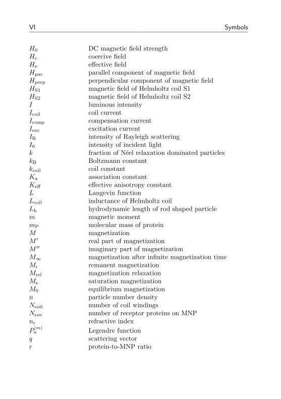
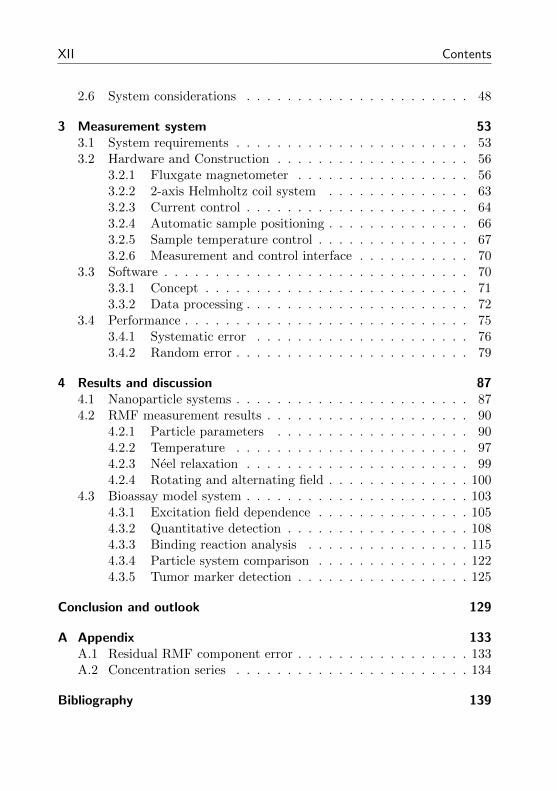
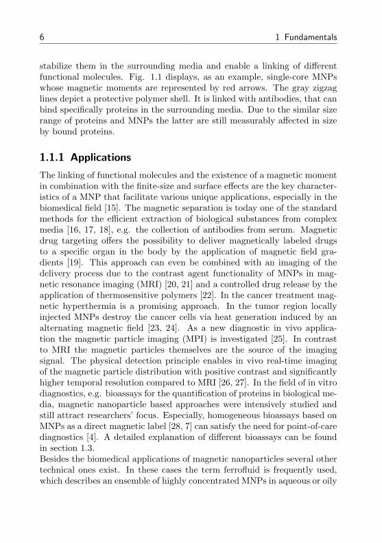
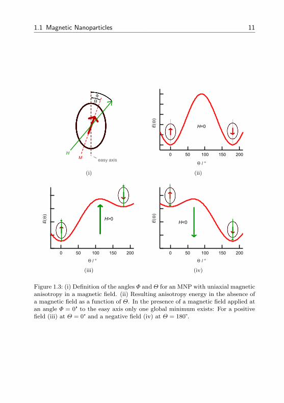
stabilize them in the surrounding media and enable a linking of differentfunctional molecules. Fig. 1.1 displays, as an example, single-core MNPswhose magnetic moments are represented by red arrows. The gray zigzaglines depict a protective polymer shell. It is linked with antibodies, that canbind specifically proteins in the surrounding media. Due to the similar sizerange of proteins and MNPs the latter are still measurably affected in sizeby bound proteins.
1.1.1 Applications
The linking of functional molecules and the existence of a magnetic momentin combination with the finite-size and surface effects are the key character-istics of a MNP that facilitate various unique applications, especially in thebiomedical field [15]. The magnetic separation is today one of the standardmethods for the efficient extraction of biological substances from complexmedia [16, 17, 18], e.g. the collection of antibodies from serum. Magneticdrug targeting offers the possibility to deliver magnetically labeled drugsto a specific organ in the body by the application of magnetic field gra-dients [19]. This approach can even be combined with an imaging of thedelivery process due to the contrast agent functionality of MNPs in mag-netic resonance imaging (MRI) [20, 21] and a controlled drug release by theapplication of thermosensitive polymers [22]. In the cancer treatment mag-netic hyperthermia is a promising approach. In the tumor region locallyinjected MNPs destroy the cancer cells via heat generation induced by analternating magnetic field [23, 24]. As a new diagnostic in vivo applica-tion the magnetic particle imaging (MPI) is investigated [25]. In contrastto MRI the magnetic particles themselves are the source of the imagingsignal. The physical detection principle enables in vivo real-time imagingof the magnetic particle distribution with positive contrast and significantlyhigher temporal resolution compared to MRI [26, 27]. In the field of in vitrodiagnostics, e.g. bioassays for the quantification of proteins in biological me-dia, magnetic nanoparticle based approaches were intensively studied andstill attract researchers’ focus. Especially, homogeneous bioassays based onMNPs as a direct magnetic label [28, 7] can satisfy the need for point-of-carediagnostics [4]. A detailed explanation of different bioassays can be foundin section 1.3.Besides the biomedical applications of magnetic nanoparticles several othertechnical ones exist. In these cases the term ferrofluid is frequently used,which describes an ensemble of highly concentrated MNPs in aqueous or oily
1.1 Magnetic Nanoparticles 7
Figure 1.1: Single-core magnetic nanoparticles in solution, functionalized withantibodies and specifically bound to antigens.
media. Ferrofluids can be exploited as seals, dampers and heat transportersin pumps [29, 30] or loudspeakers [31]. Further uses are the investigationof energy harvesting approaches [32] or the recovery of enzymes in catalyticreactions [33].
1.1.2 Synthesis, stability, functionality
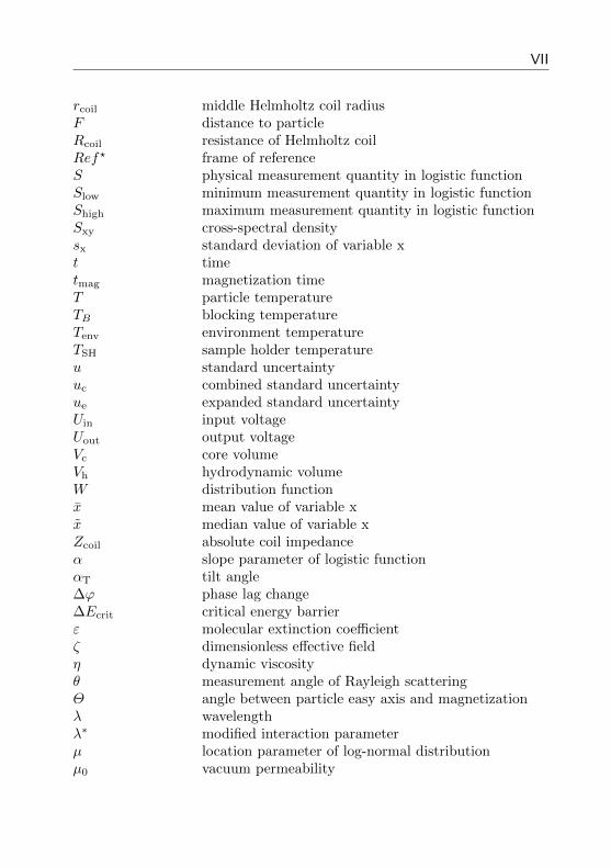
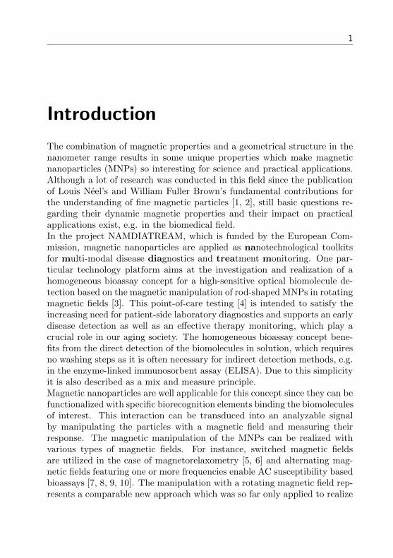
The magnetic materials that MNPs consist of are the elements cobalt, nickeland iron, alloys or oxidic compounds. The most common used magneticnanoparticles in biomedicine to date are iron oxide MNPs [34] due to theirbiocompatibility, non-toxicity and relatively well-established synthesis pro-cesses. Fine iron oxide nanoparticles can be even found in different organ-isms, e.g. magnetotactic bacteria [35]. Iron oxide material exists in oneof four phases: Wustite (FeO), hematite (α-Fe2O3), maghemite (γ-Fe2O3)and magnetite (Fe3O4). Since wustite and hematite show an antiferromag-netic or weakly ferromagnetic behavior at room temperature, magnetite andmaghemite are the favorable phases. Iron oxide MNPs for biomedical appli-cations are commonly synthesized with chemical procedures. The synthesisof iron oxides from aqueous Fe2+ and Fe3+ salts in a highly basic solutionunder inert atmosphere, the so called co-precipitation, is a convenient pro-cess [36, 34]. A better control of the particle size and shape, especially forsmall nanoparticles, can be achieved with the thermal decomposition of iron-oleate [37]. An comprehensive overview of different synthesis approaches foriron oxide nanoparticles is given by Laurent et. al. [34]. The experimen-tally determined saturation magnetizations of magnetite nanoparticles werefound to be lower than the bulk literature value of 480 kA/m [36, 38], which
8 1 Fundamentals
can be explained by the existence of biphasic particles or magnetic deadlayers [39]. The deployment of a pure magnetic element or another alloy,e.g. cobalt iron oxide [40], would result in a significantly increased Ms [41].For instance, cobalt exhibits a Ms of 1446 kA/m, which is more than threetimes higher. However, biocompatibility and toxicity problems as well asdifficult stabilization and conjugation processes can hinder the synthesis orapplication. Another aspect that can be influenced by the synthesis processis the particle shape. Besides a spherical geometry, different other shapesare possible. For instance, cubic iron oxide [36, 34] and elongated cobalt[42, 43] as well as nickel [44] particle protocols are established.Fig 1.2 illustrates that a magnetic nanoparticle does not necessarily consistof only one single-core. So called multi-core particles, which contain a clus-ter of several magnetic nanocrystals, are available from the lower nanometerrange up to several micrometers [45]. These particles possess a reduced mag-netic moment in relation to the material’s saturation magnetization due tothe interaction of the nanocrystals [46]. A further surface modification ofthe particles results in a shell or coating which is essential for the MNPstability. Attractive forces such as the van der Waals force and the mag-netic dipole-dipole interaction, which let the particles agglomerate, have tobe in equilibrium with the repulsive forces as the steric and electrostaticrepulsion. Here, various compounds have been applied as coatings. Themost common ones are monomeric stabilizers like carboxylates, phosphatesand sulfates, inorganic materials like silica or gold as well as polymers likedextran, polyethylene glycol (PEG) or polyvinyl alcohol (PVA) [34, 47]. Insome cases the coating even affected the magnetic properties, for instance,paramagnetic particles became ferromagnetic [48]. In order to give MNPsthe functionality to interact specifically with their environment, they needto be conjugated with specific molecules. Different interaction systems ex-ist in biomedicine: Antibody-antigen, avidin-biotin, DNA-DNA or ligand-receptor. In all cases a strategy for the coupling of one of the specificbiomolecules to the MNP is necessary. This can range from electrostaticinteractions to covalent bonds. An overview about different conjugationstrategies was given by Kozissnik et al. [49].Regarding the stability of suspended MNPs, different stabilization criteriaexist which have first been formulated during the development of technicalferrofluids [50]. They deal with the stability in a magnetic gradient field,prevention of agglomeration induced by magnetic dipole-dipole interactionsor van der Waals forces or the hindrance of sedimentation caused by thegravitational field. For a typical ferrofluid in water at room temperature
1.1 Magnetic Nanoparticles 9
(i) (ii)
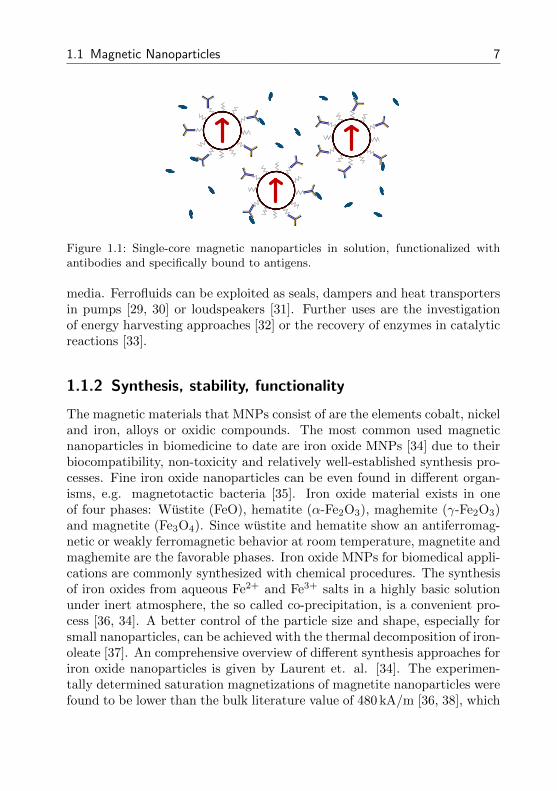
Figure 1.2: Multi-core (i) and single-core (ii) nanoparticles with protective polymershell (gray lines) and magnetic moment (red arrow).
the hydrodynamic diameter which prevents the particles from sedimentationwas calculated to be smaller than 12 nm [48]. The influence of the dipole-dipole interactions in relation to the particle thermal energy Eth = kBT canbe estimated by the modified interaction parameter λ∗ which is defined as[51]
λ∗ =µ0M
2s πd
3c
148kBT
d3c
d3h
(1.2)
with the vacuum permeability µ0, the Boltzmann constant kB and the tem-perature T . An interaction parameter λ∗ 1 indicates a non-negligiblemagnetic particle interaction. For instance, an iron oxide MNP with a12 nm core diameter, an additional shell with a thickness of 3 nm and a Ms
of 480 kA/m yields at 300 K room temperature an interaction parameter of0.76.
1.1.3 Nanomagnetism
The size reduction of a ferromagnet down to the nanometer regime resultsin the disappearance of the domain walls because surface energies, e.g. thedomain wall energy, become more significant than the volume energies, e.g.the demagnetization energy. Finally, a single magnetic domain is energeti-cally more favorable and the formation of single-domain (SD) nanoparticlesat a distinct size is caused [52].
10 1 Fundamentals
Magnetic anisotropy
The magnetization of a nanoparticle commonly favors one or more align-ments inside the particle core due to the existence of energetically favorablestates which are described by the anisotropy energy EK. This magneticanisotropy originates from different particle properties. For a MNP themain ones are the crystal and the shape anisotropy [53]. However, sur-face and exchange anisotropies can also contribute [54]. A domination ofthe shape anisotropy frequently causes an alignment of the magnetizationalong one axis, which is also referred to as the easy axis. The two possibleorientations along the axis are consequently separated by the anisotropyenergy. The corresponding energy EK of such an uniaxial MNP anisotropyis represented by
EK(Θ) = KeffVc sin2(Θ) (1.3)
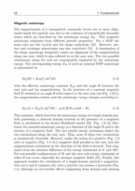
with the effective anisotropy constant Keff and the angle Θ between theeasy axis and the magnetization. In the presence of a constant magneticfield H oriented at an angle Φ with respect to the easy axis (see Fig. 1.3(i)),the magnetization rotates and the anisotropy energy changes according to
EK(ϑ) = KeffVc sin2(Θ)− µ0VcHMs cos(Θ − Φ). (1.4)
This equation, which describes the anisotropy energy of a single-domain par-ticle possessing a coherent domain rotation in the presence of a magneticfield, is attributed to the Stoner-Wohlfarth model [52]. Fig. 1.3 (ii) illus-trates the uniaxial anisotropy energy as a function of the angle Θ and in theabsence of a magnetic field. The two similar energy minimums depict thetwo orientations along the easy axis. Thus, none of these two orientationsis energetically favorable. However, under the action of a positive (Fig. 1.3(iii)) or negative (Fig. 1.3 (iv)) magnetic field parallel to the easy axis themagnetization orientation in the direction of the field is favored. This orig-inates from the absolute difference of the energy minimums at 0° and 180°.For non-parallel configurations of H and the easy axis energy minimums atother Θ can occur, especially for stronger magnetic fields [55]. Finally, thisapproach enables the calculation of a single-domain particle’s magnetiza-tion curve and it explains why such a particle can possess a hysteresis (Fig.1.4) although no irreversible effects originating from domain-wall pinning
1.1 Magnetic Nanoparticles 11
H
M easy axis
QF
(i)
Q)
200150100500
Q / °
H=0
(ii)
200150100500
/ °Q
H>0Q)
(iii)
200150100500
/ °Q
H<0
Q)
(iv)
Figure 1.3: (i) Definition of the angles Φ and Θ for an MNP with uniaxial magneticanisotropy in a magnetic field. (ii) Resulting anisotropy energy in the absence ofa magnetic field as a function of Θ. In the presence of a magnetic field applied atan angle Φ = 0° to the easy axis only one global minimum exists: For a positivefield (iii) at Θ = 0° and a negative field (iv) at Θ = 180°.
12 1 Fundamentals
exist. In the following subsections we assume an uniaxial anisotropy for thedescribed MNPs.
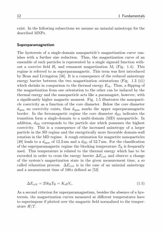
Superparamagnetism
The hysteresis of a single-domain nanoparticle’s magnetization curve van-ishes with a further size reduction. Thus, the magnetization curve of anensemble of such particles is represented by a single sigmoid function with-out a coercive field Hc and remanent magnetization Mr (Fig. 1.4). Thisregime is referred to as superparamagnetic. This term was first introducedby Bean and Livingston [56]. It is a consequence of the reduced anisotropyenergy barrier between the two magnetization orientations (Fig. 1.3 (ii))which shrinks in comparison to the thermal energy Eth. Thus, a flipping ofthe magnetization from one orientation to the other can be induced by thethermal energy and the nanoparticle acts like a paramagnet, however, witha significantly higher magnetic moment. Fig. 1.5 illustrates the nanoparti-cle coercivity as a function of the core diameter. Below the core diameterdspm no coercivity exists, thus dspm marks the upper superparamagneticborder. In the ferromagnetic regime the core diameter dSD indicates thetransition form a single-domain to a multi-domain (MD) nanoparticle. Inaddition, dSD corresponds to the particle size which possesses the highestcoercivity. This is a consequence of the increased anisotropy of a largerparticle in the SD regime and the energetically more favorable domain-wallrotation in the MD regime. A rough estimation for magnetite nanoparticles[48] leads to a dspm of 12.2 nm and a dSD of 52.7 nm. For the classificationof the superparamagnetic regime the blocking temperature TB is frequentlyused. This temperature is related to the thermal energy which has to beexceeded in order to cross the energy barrier ∆Ecrit and observe a changeof the system’s magnetization state in the given measurement time, a socalled relaxation process. ∆Ecrit is in the case of an uniaxial anisotropyand a measurement time of 100 s defined as [53]
∆Ecrit = 25kBTB = KeffVc. (1.5)
As a second criterion for superparamagnetism, besides the absence of a hys-teresis, the magnetization curves measured at different temperatures haveto superimpose if plotted over the magnetic field normalized to the temper-ature H/T .
1.1 Magnetic Nanoparticles 13
Mr
Hc
superparamagnetic
ferromagnetic
Figure 1.4: Magnetizationcurve of superparamagnetand ferromagnet. Hc and Mr
denote the coercivity and theremanence.
coer
citiv
itycore diameter
supe
rpar
amag
netic
ferr
omag
netic
dspm dSD
MD
SD
SP
single-domain multi-domain
Figure 1.5: Dependency of coercivity on core di-ameter [57] for single- (SD) and multi-domain(MD) particles with classification of superpara-(SP) and ferro-/ferrimagnetic regimes.
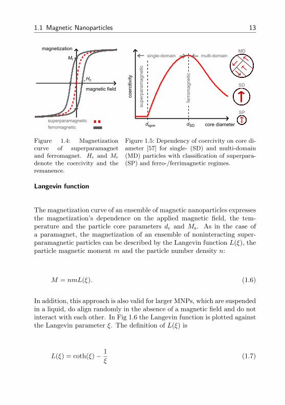
Langevin function
The magnetization curve of an ensemble of magnetic nanoparticles expressesthe magnetization’s dependence on the applied magnetic field, the tem-perature and the particle core parameters dc and Ms. As in the case ofa paramagnet, the magnetization of an ensemble of noninteracting super-paramagnetic particles can be described by the Langevin function L(ξ), theparticle magnetic moment m and the particle number density n:
M = nmL(ξ). (1.6)
In addition, this approach is also valid for larger MNPs, which are suspendedin a liquid, do align randomly in the absence of a magnetic field and do notinteract with each other. In Fig 1.6 the Langevin function is plotted againstthe Langevin parameter ξ. The definition of L(ξ) is
L(ξ) = coth(ξ)− 1
ξ(1.7)
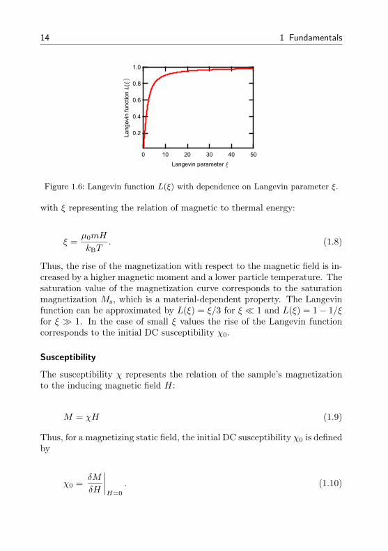
14 1 Fundamentals
1.0
0.8
0.6
0.4
0.2Langevin
function L
(x)
50403020100
Langevin parameter x
Figure 1.6: Langevin function L(ξ) with dependence on Langevin parameter ξ.
with ξ representing the relation of magnetic to thermal energy:
ξ =µ0mH
kBT. (1.8)
Thus, the rise of the magnetization with respect to the magnetic field is in-creased by a higher magnetic moment and a lower particle temperature. Thesaturation value of the magnetization curve corresponds to the saturationmagnetization Ms, which is a material-dependent property. The Langevinfunction can be approximated by L(ξ) = ξ/3 for ξ 1 and L(ξ) = 1− 1/ξfor ξ 1. In the case of small ξ values the rise of the Langevin functioncorresponds to the initial DC susceptibility χ0.
Susceptibility
The susceptibility χ represents the relation of the sample’s magnetizationto the inducing magnetic field H:
M = χH (1.9)
Thus, for a magnetizing static field, the initial DC susceptibility χ0 is definedby
χ0 =δM
δH
∣∣∣∣H=0
. (1.10)
1.1 Magnetic Nanoparticles 15
From these definitions Curie’s law is derived as [52]
χ0 =nµ0m
2
3kBT=CCurie
T(1.11)
which explains the temperature dependence of a paramagnet with respectto the Curie constant CCurie. It is important to note, that this relation isonly valid for small fields and χ0 1. Otherwise the magnetic field in thesample is reduced by the induced magnetic moments’ field and a deviationbetween the field inside and outside the sample arises. This phenomenon isnamed demagnetization and is taken into account by the demagnetizationfactor [58]. The magnetic flux density B of an ensemble of MNPs under theaction of a magnetic field takes with Eq. 1.9 and the relative permeabilityµr of the given material the form
B = µ0 (H +M) = µ0 (1 + χ)H = µ0µrH. (1.12)
Relaxation processes
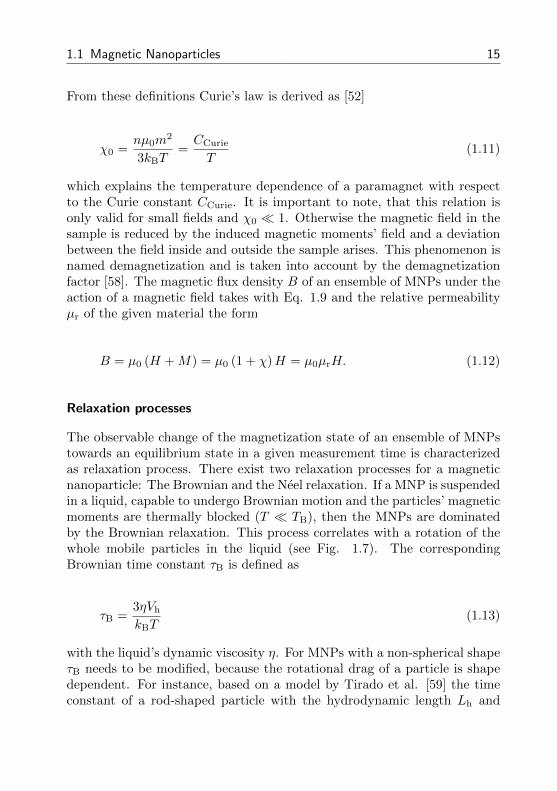
The observable change of the magnetization state of an ensemble of MNPstowards an equilibrium state in a given measurement time is characterizedas relaxation process. There exist two relaxation processes for a magneticnanoparticle: The Brownian and the Neel relaxation. If a MNP is suspendedin a liquid, capable to undergo Brownian motion and the particles’ magneticmoments are thermally blocked (T TB), then the MNPs are dominatedby the Brownian relaxation. This process correlates with a rotation of thewhole mobile particles in the liquid (see Fig. 1.7). The correspondingBrownian time constant τB is defined as
τB =3ηVh
kBT(1.13)
with the liquid’s dynamic viscosity η. For MNPs with a non-spherical shapeτB needs to be modified, because the rotational drag of a particle is shapedependent. For instance, based on a model by Tirado et al. [59] the timeconstant of a rod-shaped particle with the hydrodynamic length Lh and
16 1 Fundamentals
H
(B)
(N)
H=0
Figure 1.7: After an alignment of the particle moments along the magnetic fieldH, the particle magnetizations relax via the Brownian (B) or Neel (N) relaxationprocess.
diameter dh can be expressed by
τB,rod =πηL3
h
6kBT
[ln(
Lh
dh) + C
]−1
(1.14)
with
C = −0.662 + 0.891dh
Lh. (1.15)
If the MNPs are immobilized or the magnetic moments are not thermallyblocked, then the MNPs are dominated by the Neel relaxation. This processcorrelates with a rotation of the magnetic moment in the particle core (seeFig. 1.7). Thus, the Neel time constant is expressed as
τN = τ0 exp
(KeffVc
kBT
)(1.16)
with the constant τ0 which is usually quoted to be 1× 10⁻⁹ s [60]. If bothrelaxation processes are present for one particle type and the two time con-stants differ only slightly, then the application of the effective time constantτeff is appropriate:
τeff =τBτNτB + τN
. (1.17)
1.1 Magnetic Nanoparticles 17
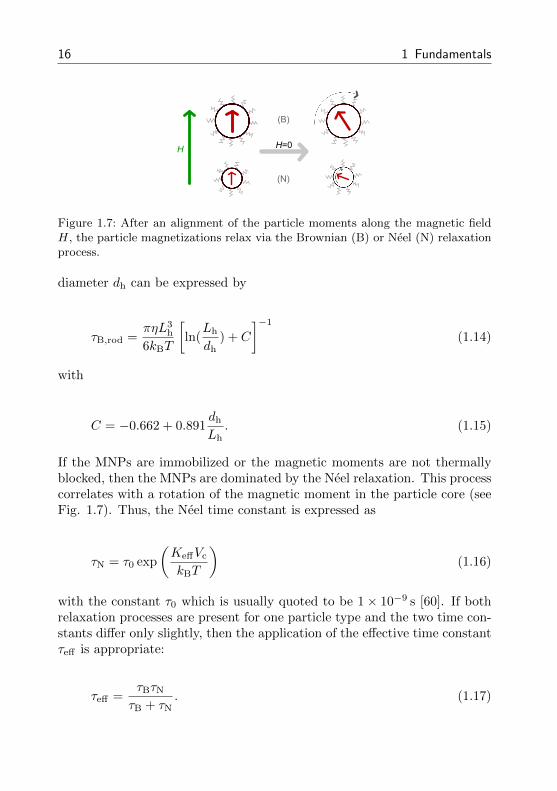
50
40
30
20
10
dh
/ nm
5040302010
dc / nm
3.5e-05 s
2.1e-05 s
1e-05 s
4.5e-06 s
1e-06 s
Figure 1.8: Effective time constant in relation to hydrodynamic and core diam-eter. Black line represents border between particles dominated by the Neel andBrownian relaxation.
If τB and τN differ significantly from each other, then the relaxation processwith the shorter time constant dominates. This is in accordance with Eq.1.17. Thus, not only the relaxation time but also the process can be in-fluenced by a variation of the particle core and hydrodynamic parameters.In this work, particles dominated by the Brownian and the Neel relaxationprocess are named Brownian and Neel particles, respectively. Fig. 1.8 il-lustrates τeff as a function of the core and hydrodynamic diameter for aviscosity of 1 mPa · s, an effective anisotropy constant of 20 kJ/m3 and atemperature of 300 K. The black line corresponds to the border between theBrownian and Neel particle regime, which is specified by the shorter timeconstant. Due to the exponential dependence of the Neel time constant onthe core diameter, the regime of the Neel particles is in this representationcomparably small. For instance, a core diameter of 20 nm ensures for allhydrodynamic diameters smaller than 50 nm a domination of the Brownianrelaxation process. However, the influence of the viscosity, anisotropy con-stant and temperature is not considered in Fig. 1.8. Furthermore, the timeconstants possess a dependence on the strength of the magnetic field whichaligns the particles [61, 62].
1.1.4 Size distribution
The synthesis process of a batch of magnetic nanoparticles is not absolutelycontrollable regarding the uniformity of the different particle parameters.They exhibit size distributions with quite different forms and characteris-
18 1 Fundamentals
tics. For instance, Gaussian, log-normal and even gamma distributions areapplied [63] and the width of the distribution can range from almost mono-to significantly polydisperse.In this work, the distributions of the particle magnetic moment m as wellas the core and hydrodynamic diameter dc and dh are described by thelog-normal distribution density functions fm(m), fc(dc), fh(dh) with theparameters µm, µc and µh as well as σm, σc and σh. The log-normal dis-tribution is well applicable for parameters with a fixed lower border whichcauses an asymmetric distribution [64]. Thus, it is commonly found formagnetic nanoparticle parameters [48, 65] where natural limits exist, forinstance, the particle core size. The log-normal density function of the vari-able x is defined as
f(x) =1
σ√
2π
1
xexp
[− (ln(x)− µ)2
2σ2
]. (1.18)
The median and mean value of the distribution x and x as well as thestandard deviation sx are defined by
x = eµ, (1.19)
x = eµ+σ2/2 (1.20)
and
sx = x ·√eσ2 − 1. (1.21)
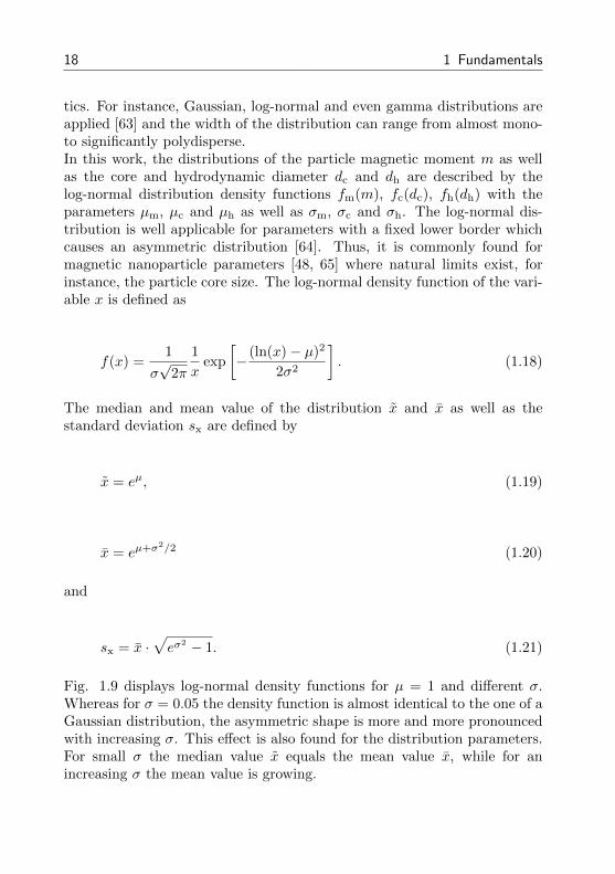
Fig. 1.9 displays log-normal density functions for µ = 1 and different σ.Whereas for σ = 0.05 the density function is almost identical to the one of aGaussian distribution, the asymmetric shape is more and more pronouncedwith increasing σ. This effect is also found for the distribution parameters.For small σ the median value x equals the mean value x, while for anincreasing σ the mean value is growing.

1.2 Characterization methods 19
2.5
2.0
1.5
1.0
0.5
0.0
density f(x
)
543210
variable x
s = 0.05
s = 0.1
s = 0.25
s = 0.5
Figure 1.9: Lognormal density functions for median value µ = 1 and differentlog-normal standard deviations σ.
1.2 Characterization methods
In this work, the rotational dynamics of suspended magnetic nanoparticlesare investigated. In this context, the particle hydrodynamic volume andmagnetic moment are the main parameters of interest. For the analysis ofthese parameters a variety of physical measurement techniques exist. Thissection provides a short overview about the mainly applied techniques.
1.2.1 Electron microscopy
The electron microscopy is based on the quantum mechanical effect, thatelectrons posses wave-like characteristics, which can be expressed by thede Broglie wavelength. In order to generate electrons with a wavelengththat enables the observation of objects in the nano- and even subnanometerrange the electrons are accelerated through voltages of up to 400 kV. Thescanning electron microscopy (SEM) is based on the measurement of thesecondary or backscattered electrons of the primary electron beam, whichis irradiating the sample. Thus, the surface of the object is scanned and inthe case of nanoparticles the core and shell are imaged. Due to the samplepreparation process the MNP shell changes its structure and an accuratedetermination of the hydrodynamic shell width is hindered. The electronbeam of a transmission electron microscope (TEM) is aligned through thesample and detected on the backside. The beam is scattered in dependenceon the material density which causes the contrast of a TEM image. Forthis reason, only the MNP core can be reasonably imaged with a TEM.
20 1 Fundamentals
A high resolution transmission electron microscope (HRTEM) even enablesthe analysis of the crystallographic MNP core structure. For the electronmicroscopy the samples are placed in a vacuum chamber to ensure that nointeractions of the electron beam with the air occurs. A detailed descrip-tion of the operation of electron microscopes was published by Chescoe andGoodhew [66].For this work, TEM measurements were performed with the Philips CM12with an acceleration voltage of 100 kV. A drop of suspended MNPs wasslowly dried on a carbon coated copper grid to ensure the formation of onlyone single MNP layer. The MNP suspensions were diluted to an iron concen-tration of 0.1 g/L. The size distribution of the MNP cores was determinedvia a software analysis of the TEM images.
1.2.2 Photon correlation spectroscopy
The photon correlation spectroscopy (PCS), which is also known as dynamiclight scattering (DLS), facilitates the determination of the hydrodynamicsize of suspended nanoparticles via the measurement of light scattered bythe particles diffusing in solution [67]. For particles with a diameter d sig-nificantly smaller than the wavelength λ of the incident beam the scatteredlight is dominated by the Rayleigh scattering, while for particles in the sizerange of λ the more complex Mie scattering has to be taken into account.The intensity IR of the scattered light (Rayleigh scattering) in the distanceF from the causative nanoparticle is expressed by [68]
IR =I0π
4d6
8λ4F 2
(n2
r − 1
n2r + 2
)2 (1 + cos2 θ
). (1.22)
Here, I0 denotes the initial intensity of the incident unpolarized light, θ themeasurement angle with respect to the direction of the incident light and nr
the particle refractive index. In addition, IR depends on d6 and consequentlybigger particles cause a significantly stronger scattering intensity. However,this effect is not analyzed to determine the particle size. The determinationis based on the effect that the wavelength of the scattered light exhibits adistribution which correlates with the particle diffusion coefficient D. Forspherical noninteracting particles the diffusion coefficient can be expressed
1.2 Characterization methods 21
via the Stokes-Einstein expression [67]
D =kBT
3πηdh(1.23)
which incorporates the particle hydrodynamic diameter. In practice, theautocorrelation function of the measured scattering light signal Ga (τ?) iscalculated depending on the delay time τ?. This function can be modeledfor non-interacting monodisperse particles by
Ga (τ?) = Aa +Ba exp(−2Dq2τ?
)(1.24)
with the scattering vector’s amplitude q defined as
q =4πnr
λsin
(θ
2
). (1.25)
The system parameters Aa and Ba define the start and end value of theautocorrelation function. One approach to analyze Ga (τ?) regarding thehydrodynamic size distribution is the method of cumulants [67, 69]. Thismethod results for mono-modal particles in a reliable determination of themean particle size and the related polydispersity. However, this approach isnot applicable to multi-modal particle distributions. For a known particledistribution type, Eq. 1.24 in combination with the corresponding distribu-tion function can be fitted with a nonlinear least-squares approach to themeasurement results [70]. Alternatively, the Contin and the non-negativeleast-squares (NNLS) methods are utilized [67], which require additionalprior knowledge. The size distribution directly determined from the mea-surement results is intensity weighted due to the scattered light based mea-surement principle of PCS. This necessitates a conversion of the directlydetermined distribution function to a volume or number weighted one if acomparison with other measurement techniques or the usage in other phys-ical models is intended [70]. Furthermore, PCS measurement results can beeasily affected by various physical or chemical effects. For instance, multi-ple scattering between the diluted particles can significantly influence thedecay of Ga (τ?), resulting in a wrong determined particle size. Other ma-nipulating aspects that have to be avoided are number fluctuations of the
22 1 Fundamentals
particles in the measurement window, interactions between the particles inthe solution or a change of the sample temperature and viscosity. Moreover,the size distribution of small particles determined via PCS is sensitive tosome few larger particles in solution [71]. Due to the intensity weightedmeasurement signal, larger particles can dominate the signal and cause thesize distribution to exhibit a shift or tail to larger sizes which does not re-flect the reality. Thus, the size determination of magnetic nanoparticleswith PCS is also influenced by non-magnetic contamination.For the investigations of this work, the photon cross-correlation spectrom-eter (PCCS) system Nanophox from Sympatec GmbH was utilized. In thismeasurement system, two laser-detector pairs are installed which enable thecalculation of the cross-correlation spectrum. The analysis of this spectrumfor the investigation of the particle size significantly reduces the negativeinfluence of multiple-scattering [72], because single- and multiple-scatteringevents can be distinguished. As sample cuvette the UVette from EppendorfAG was applied for all measurements. The sample volume was 100 µL andthe particle iron concentration ranged from 1 mg/L to 50 mg/L.
1.2.3 Static magnetization curve
The measurement of the static magnetization curve is an essential tool forthe determination of the particle magnetic moments. Furthermore, it canbe exploited to investigate the particle core size [73] and to specify theblocking temperature [48] or the material phase composition [74] by per-forming temperature-dependent measurements. In principle, an ensembleof MNPs is placed in the system, aligned along a stepwise increasing staticmagnetic field and the resulting magnetization is measured with a magneticfield sensor. In order to reach the saturation of the MNP ensemble’s mag-netization, magnetic fields of up to 5 T are required. Thus, superconductingcoils are built into a corresponding measurement system. As magnetic fieldsensors superconducting quantum interference devices (SQUIDs) are com-monly used to ensure the measurement of even weak paramagnetic material.So, for both processes, the field generation and the magnetization detec-tion, a cryogenic cooling is required, which is usually realized with liquidhelium. The analysis of the measurement data can be performed by fittingthe Langevin equation (Eq. 1.7) incorporating an appropriate distributionfunction to the measured static magnetization curve. However, this methodrequires the knowledge of the distribution type. A physically more adequateway to estimate the distribution can be achieved by the reconstruction of the
1.2 Characterization methods 23
magnetization curve via the Langevin function applying singular value de-composition (SVD). The SVD method was already successfully employed forthis purpose by Berkov et al. [65]. The static magnetization measurementsin this work were performed with the Magnetic Property Measurement Sys-tem (MPMS) from Quantum Design International on liquid samples with aparticle iron concentration in the range of 0.1 g/L to 0.5 g/L.
1.2.4 AC susceptibility
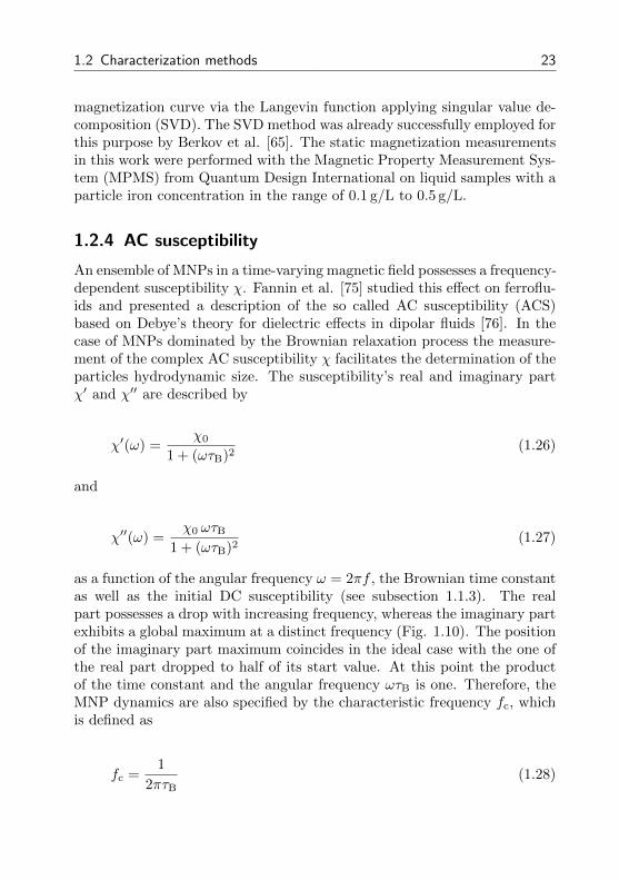
An ensemble of MNPs in a time-varying magnetic field possesses a frequency-dependent susceptibility χ. Fannin et al. [75] studied this effect on ferroflu-ids and presented a description of the so called AC susceptibility (ACS)based on Debye’s theory for dielectric effects in dipolar fluids [76]. In thecase of MNPs dominated by the Brownian relaxation process the measure-ment of the complex AC susceptibility χ facilitates the determination of theparticles hydrodynamic size. The susceptibility’s real and imaginary partχ′ and χ′′ are described by
χ′(ω) =χ0
1 + (ωτB)2(1.26)
and
χ′′(ω) =χ0 ωτB
1 + (ωτB)2(1.27)
as a function of the angular frequency ω = 2πf , the Brownian time constantas well as the initial DC susceptibility (see subsection 1.1.3). The realpart possesses a drop with increasing frequency, whereas the imaginary partexhibits a global maximum at a distinct frequency (Fig. 1.10). The positionof the imaginary part maximum coincides in the ideal case with the one ofthe real part dropped to half of its start value. At this point the productof the time constant and the angular frequency ωτB is one. Therefore, theMNP dynamics are also specified by the characteristic frequency fc, whichis defined as
fc =1
2πτB(1.28)
24 1 Fundamentals
1.0
0.8
0.6
0.4
0.2
0.0
c '
/ c0 ,
c ''
/ c
0
0.01 0.1 1 10 100 1000
wtB
c ' c ''
Figure 1.10: Real and imaginary part χ′ and χ′′ of complex AC susceptibility asa function of angular frequency and Brownian time constant.
and gives an estimation of the maximum frequency of a dynamic alternatingmagnetic field that a MNP can follow. Eq. 1.26 and 1.27 are well applica-ble for a Langevin parameter ξ 1 which ensures a linear dependence ofthe ensemble magnetization on the magnetic field. However, for larger ξ,for instance, caused by an increased field strength, the model needs to beextended. One approved extension was introduced by Yoshida et al. [62]and subsequently improved by solving the Fokker-Planck equation [77]:
χ′(ω) =χ1(0)
1 + (ωτB,H)2(1.29)
and
χ′′(ω) = k′′χ1(0)ωτB,H1 + (ωτB,H)2
(1.30)
with
χ1(0) = χ0
[1− 0.0636ξ2
1 + 0.18ξ + 0.0659ξ2
], (1.31)
k′′ = 1 +0.024ξ2
1 + 0.18ξ + 0.033ξ2(1.32)
1.2 Characterization methods 25
and
τB,H =τB√
1 + 0.126ξ1.72. (1.33)
With this set of equations incorporating the field-dependent Brownian timeconstant τB,H an approximate description of the MNPs’ dynamic magne-tization in an alternating magnetic field even for ξ > 1 is possible. Theconsideration of the particle size distribution enables a correct modeling ofreal MNP samples. For instance, Chung et al. [8] introduced for the theo-retical description of spherical MNPs’ complex ACS independent core andhydrodynamic size distributions. The adoption of this approach to Eq. 1.29and 1.30 results in
χ′(ω) =
∫dh
fh(dh)
∫dc
fc(dc)µ0nm
2(dc)
3kBT
χ1,n(0)
1 + (ωτB,H)2ddcddh (1.34)
and
χ′′(ω) =
∫dh
fh(dh)
∫dc
fc(dc)µ0nm
2(dc)
3kBTk′′χ1,n(0)ωτB,H1 + (ωτB,H)2
ddcddh (1.35)
with χ1(0) normalized to χ0:
χ1,n(0) = 1− 0.0636ξ2
1 + 0.18ξ + 0.0659ξ2. (1.36)
The presence of MNPs dominated by the Neel relaxation also affects themeasured AC susceptibility. In the case of a pure Neel particle sample simi-lar real and imaginary parts occur and for a theoretical description with theDebye model τB is replaced by τN. For a sample with both particle typespresent in solution two cases exist: If the time constants fulfill the conditionτN τB the complex AC susceptibilities of the Brownian and Neel particlescan be treated independently as theoretically shown by Fannin and Charles[75] and supported with measurements by Lak et al. [78]. Consequently,these samples are characterized as bi-modal. For τN ≈ τB the single realand imaginary parts overlap each other with the result that no clear dis-
26 1 Fundamentals
tinction is possible. A theoretical description with the Debye model canbe performed if τB is replaced by τeff [8]. A clear distinction between theACS of the Brownian and the Neel particles can be achieved by performingadditional measurements on the same sample after it is freeze-dried. Thus,all suspended particles are immobilized and Brownian rotation is blocked.In this work, a self-constructed ACS measurement setup was applied. Itis based on a cylindrical inductor for the generation of the homogeneousalternating excitation field with an magnitude of 95 µT and an integrateddetection coil. For the realization of a gradiometric detection principle bothcoils are set up twice with parameters as similar as possible. The frequencyrange of the measurement setup is 0.2 kHz to 1000 kHz. A detailed descrip-tion of the applied setup was given by Ludwig et al. [40]. The samplesfor the ACS measurements are placed into a cylindrical glass vial with anouter diameter of 7.8 mm or a conical plastic vial usually used for microtiterplates. The sample volume was 150µL and the particle iron concentrationranged from 0.1 g/L to 5 g/L.
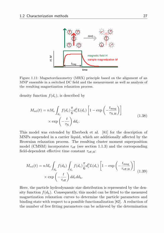
1.2.5 Magnetorelaxometry
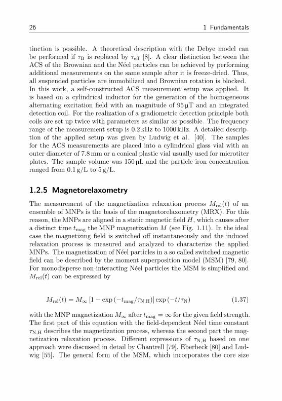
The measurement of the magnetization relaxation process Mrel(t) of anensemble of MNPs is the basis of the magnetorelaxometry (MRX). For thisreason, the MNPs are aligned in a static magnetic field H, which causes aftera distinct time tmag the MNP magnetization M (see Fig. 1.11). In the idealcase the magnetizing field is switched off instantaneously and the inducedrelaxation process is measured and analyzed to characterize the appliedMNPs. The magnetization of Neel particles in a so called switched magneticfield can be described by the moment superposition model (MSM) [79, 80].For monodisperse non-interacting Neel particles the MSM is simplified andMrel(t) can be expressed by
Mrel(t) = M∞ [1− exp (−tmag/τN,H)] exp (−t/τN) (1.37)
with the MNP magnetizationM∞ after tmag =∞ for the given field strength.The first part of this equation with the field-dependent Neel time constantτN,H describes the magnetization process, whereas the second part the mag-netization relaxation process. Different expressions of τN,H based on oneapproach were discussed in detail by Chantrell [79], Eberbeck [80] and Lud-wig [55]. The general form of the MSM, which incorporates the core size
1.2 Characterization methods 27
time
H, M
magnetic field H
sample magnetization M
H=0
tmag
Figure 1.11: Magnetorelaxometry (MRX) principle based on the alignment of anMNP ensemble in a switched DC field and the measurement as well as analysis ofthe resulting magnetization relaxation process.
density function f(dc), is described by
Mrel(t) = nMs
∫dc
f(dc)π
6d3
cL(dc)
[1− exp
(− tmag
τN,H
)]× exp
(− t
τN
)ddc.
(1.38)
This model was extended by Eberbeck et al. [81] for the description ofMNPs suspended in a carrier liquid, which are additionally affected by theBrownian relaxation process. The resulting cluster moment superpositionmodel (CMSM) incorporates τeff (see section 1.1.3) and the correspondingfield-dependent effective time constant τeff,H:
Mrel(t) = nMs
∫dh
f(dh)
∫dc
f(dc)π
6d3
cL(dc)
[1− exp
(− tmag
τeff,H
)]× exp
(− t
τeff
)ddcddh.
(1.39)
Here, the particle hydrodynamic size distribution is represented by the den-sity function f(dh). Consequently, this model can be fitted to the measuredmagnetization relaxation curves to determine the particle parameters andbinding state with respect to a possible functionalization [82]. A reduction ofthe number of free fitting parameters can be achieved by the determination
28 1 Fundamentals
of the core size distribution parameters from an independent measurementon a freeze-dried reference sample with Eq. 1.38.The magnetic field strength in a MRX setup usually accounts to some mil-litesla, because no magnetization saturation is required. Thus, air coilspowered by an fast switching electronics are utilized. For the detection ofthe MNPs’ magnetization decay SQUIDs, fluxgates and magnetoresistivesensors are applied. The MRX measurements in this work were performedwith a fluxgate-based setup [83]. The field strength was set to 2 mT andtmag as well as the measurement time to some seconds, depending on theparticle properties.
1.3 Bioassays
The application of receptors for the identification and quantification of bi-ological targets in a sample is described as bioassay. The receptor displaysa bio-recognition molecule, for instance an antibody, that specifically bindsto the biological target molecule of interest, for instance a biomarker in-dicating a medical condition. If antibodies are utilized as receptors theterm immunoassay is commonly used. The recognition or formation of areceptor-target complex is the first step in a bioassay. The second one isthe detection and analysis of the complexes in the solution. Therefore, ad-ditional processing steps and instrumentation are required, which enablethe transduction of the recognition process into an analyzable electrical sig-nal. Thus, the second step is also characterized as transducer and basedon an electrochemical, optical, mass sensitive, thermometric, radioactive,magnetic or other physical effect [84, 85].In the context of bioassays the term biosensor is frequently applied. In prin-ciple both display the same application: The identification and quantifica-tion of biological material. However, a difference exists which is expressedby the definition of electrochemical biosensors given by the InternationalUnion of Pure and Applied Chemistry [86]: ”An electrochemical biosensoris a self-contained integrated device, which is capable of providing specificquantitative or semi-quantitative analytical information using a biologicalrecognition element (biochemical receptor) which is retained in direct spatialcontact with an electrochemical transduction element.” Due to this spatialproximity any other processing step is not required. The receptors in abiosensor directly induce the electrical transducer signal. Fig. 1.12 illus-trates this difference compared to the general concept of a bioassay that
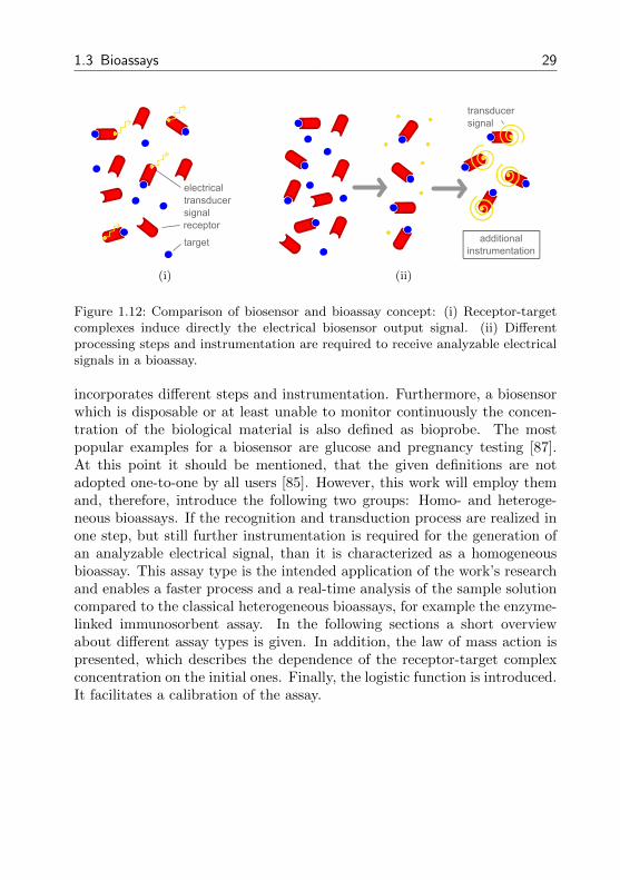
1.3 Bioassays 29
target
receptor
electricaltransducersignal
(i)
transducersignal
additional instrumentation
(ii)
Figure 1.12: Comparison of biosensor and bioassay concept: (i) Receptor-targetcomplexes induce directly the electrical biosensor output signal. (ii) Differentprocessing steps and instrumentation are required to receive analyzable electricalsignals in a bioassay.
incorporates different steps and instrumentation. Furthermore, a biosensorwhich is disposable or at least unable to monitor continuously the concen-tration of the biological material is also defined as bioprobe. The mostpopular examples for a biosensor are glucose and pregnancy testing [87].At this point it should be mentioned, that the given definitions are notadopted one-to-one by all users [85]. However, this work will employ themand, therefore, introduce the following two groups: Homo- and heteroge-neous bioassays. If the recognition and transduction process are realized inone step, but still further instrumentation is required for the generation ofan analyzable electrical signal, than it is characterized as a homogeneousbioassay. This assay type is the intended application of the work’s researchand enables a faster process and a real-time analysis of the sample solutioncompared to the classical heterogeneous bioassays, for example the enzyme-linked immunosorbent assay. In the following sections a short overviewabout different assay types is given. In addition, the law of mass action ispresented, which describes the dependence of the receptor-target complexconcentration on the initial ones. Finally, the logistic function is introduced.It facilitates a calibration of the assay.
30 1 Fundamentals
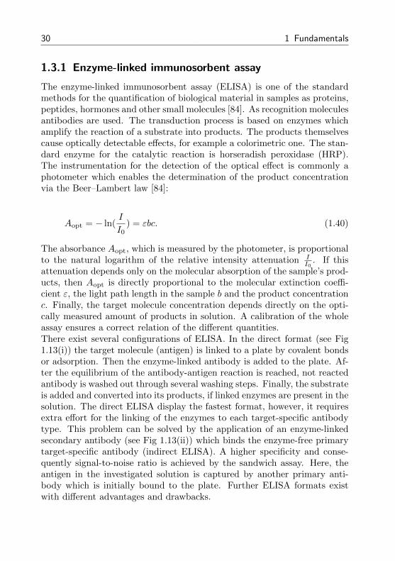
1.3.1 Enzyme-linked immunosorbent assay
The enzyme-linked immunosorbent assay (ELISA) is one of the standardmethods for the quantification of biological material in samples as proteins,peptides, hormones and other small molecules [84]. As recognition moleculesantibodies are used. The transduction process is based on enzymes whichamplify the reaction of a substrate into products. The products themselvescause optically detectable effects, for example a colorimetric one. The stan-dard enzyme for the catalytic reaction is horseradish peroxidase (HRP).The instrumentation for the detection of the optical effect is commonly aphotometer which enables the determination of the product concentrationvia the Beer–Lambert law [84]:
Aopt = − ln(I
I0) = εbc. (1.40)
The absorbance Aopt, which is measured by the photometer, is proportionalto the natural logarithm of the relative intensity attenuation I
I0. If this
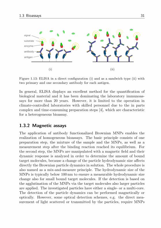
attenuation depends only on the molecular absorption of the sample’s prod-ucts, then Aopt is directly proportional to the molecular extinction coeffi-cient ε, the light path length in the sample b and the product concentrationc. Finally, the target molecule concentration depends directly on the opti-cally measured amount of products in solution. A calibration of the wholeassay ensures a correct relation of the different quantities.There exist several configurations of ELISA. In the direct format (see Fig1.13(i)) the target molecule (antigen) is linked to a plate by covalent bondsor adsorption. Then the enzyme-linked antibody is added to the plate. Af-ter the equilibrium of the antibody-antigen reaction is reached, not reactedantibody is washed out through several washing steps. Finally, the substrateis added and converted into its products, if linked enzymes are present in thesolution. The direct ELISA display the fastest format, however, it requiresextra effort for the linking of the enzymes to each target-specific antibodytype. This problem can be solved by the application of an enzyme-linkedsecondary antibody (see Fig 1.13(ii)) which binds the enzyme-free primarytarget-specific antibody (indirect ELISA). A higher specificity and conse-quently signal-to-noise ratio is achieved by the sandwich assay. Here, theantigen in the investigated solution is captured by another primary anti-body which is initially bound to the plate. Further ELISA formats existwith different advantages and drawbacks.
1.3 Bioassays 31
antigen
antibody
enzyme
substrate
signal
(i) (ii)
Figure 1.13: ELISA in a direct configuration (i) and as a sandwich type (ii) withtwo primary and one secondary antibody for each antigen.
In general, ELISA displays an excellent method for the quantification ofbiological material and it has been dominating the laboratory immunoas-says for more than 20 years. However, it is limited to the operation inclimate-controlled laboratories with skilled personnel due to the in partscomplex and time-consuming preparation steps [4], which are characteristicfor a heterogeneous bioassay.
1.3.2 Magnetic assays
The application of antibody functionalized Brownian MNPs enables therealization of homogeneous bioassays. The basic principle consists of onepreparation step, the mixture of the sample and the MNPs, as well as ameasurement step after the binding reaction reached its equilibrium. Forthe second step, the MNPs are manipulated with a magnetic field and theirdynamic response is analyzed in order to determine the amount of boundtarget molecules, because a change of the particle hydrodynamic size affectsdirectly the Brownian particle dynamics in solution. The whole procedure isalso named as a mix-and-measure principle. The hydrodynamic size of theMNPs is typically below 100 nm to ensure a measurable hydrodynamic sizechange also for small bound target molecules. If the detection is based onthe agglutination of the MNPs via the target molecules also larger particlesare applied. The investigated particles have either a single- or a multi-core.The detection of the particle dynamics can be performed magnetically oroptically. However, some optical detection schemes, e.g. the direct mea-surement of light scattered or transmitted by the particles, require MNPs
32 1 Fundamentals
φ
∆φ = φ2 – φ1
1 φ2
phase lag
MNP
rotating fieldvector
target molecule
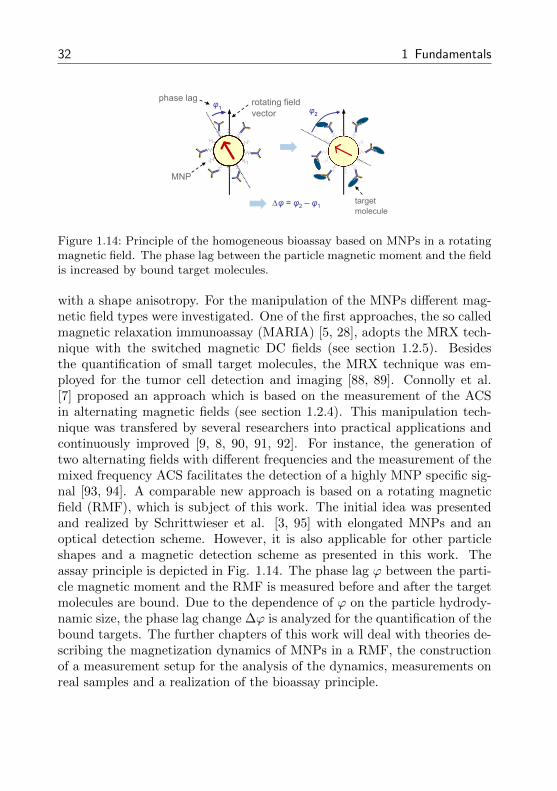
Figure 1.14: Principle of the homogeneous bioassay based on MNPs in a rotatingmagnetic field. The phase lag between the particle magnetic moment and the fieldis increased by bound target molecules.
with a shape anisotropy. For the manipulation of the MNPs different mag-netic field types were investigated. One of the first approaches, the so calledmagnetic relaxation immunoassay (MARIA) [5, 28], adopts the MRX tech-nique with the switched magnetic DC fields (see section 1.2.5). Besidesthe quantification of small target molecules, the MRX technique was em-ployed for the tumor cell detection and imaging [88, 89]. Connolly et al.[7] proposed an approach which is based on the measurement of the ACSin alternating magnetic fields (see section 1.2.4). This manipulation tech-nique was transfered by several researchers into practical applications andcontinuously improved [9, 8, 90, 91, 92]. For instance, the generation oftwo alternating fields with different frequencies and the measurement of themixed frequency ACS facilitates the detection of a highly MNP specific sig-nal [93, 94]. A comparable new approach is based on a rotating magneticfield (RMF), which is subject of this work. The initial idea was presentedand realized by Schrittwieser et al. [3, 95] with elongated MNPs and anoptical detection scheme. However, it is also applicable for other particleshapes and a magnetic detection scheme as presented in this work. Theassay principle is depicted in Fig. 1.14. The phase lag ϕ between the parti-cle magnetic moment and the RMF is measured before and after the targetmolecules are bound. Due to the dependence of ϕ on the particle hydrody-namic size, the phase lag change ∆ϕ is analyzed for the quantification of thebound targets. The further chapters of this work will deal with theories de-scribing the magnetization dynamics of MNPs in a RMF, the constructionof a measurement setup for the analysis of the dynamics, measurements onreal samples and a realization of the bioassay principle.
1.3 Bioassays 33
A wide variety of other magnetic particle based bioassays has been presentedin the literature. Some of them even facilitate rotating magnetic fields butwith particles in the upper nanometer or micrometer range. Thus, bacteriacells instead of small proteins were detected [11] or a cluster formationprocess was required [12]. Heterogeneous bioassays in combination withmagnetic particles have also been intensively studied, e.g. the so calledmicro- or biochip based assays [96]. Another promising biosensor formatwhich can be combined with MNPs are the lateral flow techniques whichrequire almost no sample preparation [97].
1.3.3 Law of mass action
The recognition process of the receptor R with respect to the target T in abioassay displays a reversible binding reaction between the two reactants Rand T that form the product RT:
R + T RT. (1.41)
This reaction can be modeled at its equilibrium via the law of mass action[98]:
Ka =c (RT)
c (R) c (T). (1.42)
Here, Ka represents the association constant which describes the strengthof the affinity in a binding reaction. The reactant concentrations c (R) andc (T) are related to the initially applied concentrations c0 as follows:
c (R) = c0 (R)− c (RT) (1.43)
and
c (T) = c0 (T)− c (RT) . (1.44)

34 1 Fundamentals
Finally, the concentration of the product c (RT) as a function of the initialreactant concentrations and the association constant can be expressed by[84]
c (RT) = 0.5 (c0 (T) + c0 (R) + 1/Ka)−
0.5[(c0 (T) + c0 (R) + 1/Ka)
2 − 4 c0 (T) c0 (R)]1/2
.(1.45)
Here, it can be seen that the concentration of the product does not scalelinearly with the initial concentrations of the reactants. In fact, below theconcentration range of the inverse association constant, the concentrationrelation of the product to the initial reactants starts to shrink significantly.Thus, a high affinity constant and a high receptor concentration are desir-able for the creation of enough receptor-target complexes (products) and astrong transducer signal. In addition, Eq. 1.45 can be utilized to determinethe binding reaction’s association constant. Therefore, a sample series withdifferent known target molecule concentrations and a fixed amount of re-ceptors is analyzed regarding the resulting product concentrations and Eq.1.45 is fitted to these results with Ka as a free parameter.
1.3.4 Assay calibration with logistic function
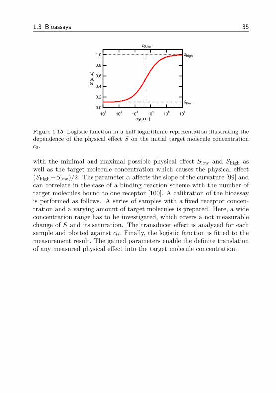
A logistic function (see Fig. 1.15) is commonly used to analyze the resultsof bioassays to provide a relation between the physical transduction effectand the target molecule concentration [99] and corresponds to the Hill equa-tion [100] which is directly derived from a binding reaction scheme betweenmolecules and receptors. In contrast to the law of mass action it incorpo-rates the possibility of multiple receptor binding sites. The logistic functionwas also used to model the measurement effect versus target molecule con-centration in the susceptibility reduction method by Yang et al. [91]. Forthe physical effect S of a bioassay as a function of the initial target moleculeconcentration c0, the logistic function takes the form
S =Slow − Shigh
1 +(
c0c0,half
)α + Shigh (1.46)
1.3 Bioassays 35
1.0
0.8
0.6
0.4
0.2
0.0
S(a.u.)
101
102
103
104
105
106
c00(a.u.)
Slow
Shigh
c0,half
Figure 1.15: Logistic function in a half logarithmic representation illustrating thedependence of the physical effect S on the initial target molecule concentrationc0.
with the minimal and maximal possible physical effect Slow and Shigh aswell as the target molecule concentration which causes the physical effect(Shigh−Slow)/2. The parameter α affects the slope of the curvature [99] andcan correlate in the case of a binding reaction scheme with the number oftarget molecules bound to one receptor [100]. A calibration of the bioassayis performed as follows. A series of samples with a fixed receptor concen-tration and a varying amount of target molecules is prepared. Here, a wideconcentration range has to be investigated, which covers a not measurablechange of S and its saturation. The transducer effect is analyzed for eachsample and plotted against c0. Finally, the logistic function is fitted to themeasurement result. The gained parameters enable the definite translationof any measured physical effect into the target molecule concentration.

36 1 Fundamentals
37
2 Rotating magnetic field
In this chapter, theories describing the rotational dynamics of a MNP en-semble magnetization in a rotating magnetic field are presented. The modelsare based on the assumption that the MNPs are single-core particles domi-nated by the Brownian relaxation process also referred to as rigid magneticdipole [101]. A mechanical model based on the equilibrium of forces [102]can be applied to describe the principle dependencies of the magnetizationon the parameters. However, a realistic model including thermal agitation isbased on magnetization equations as clarified by Shliomis [103]. These caneither be phenomenological magnetization equations [101, 104] or a modelderived microscopically from the Fokker-Planck equation via the effective-field method [105, 106]. Finally, Yoshida et al. [107] published numericalsolutions of the Fokker-Planck equation adapted to MNP in RMF and de-rived an empirical model with a high accuracy for the analysis of RMF mea-surements. The corresponding set of equations is applied for the analysisof the measurement results in the present work. The modeling of the com-plete MNP ensemble magnetization in a rotating magnetic field representsa vectorial problem. Thus, the according vector quantities are identified byan arrow.
2.1 Definition of a rotating magnetic field
The RMF is defined as a magnetic field which rotates with a constant fieldmagnitude H and angular frequency ω in the (x,y)-plane:
~H = [H cos(ωt), H sin(ωt), 0]. (2.1)
The dynamic MNP ensemble magnetization ~M rotates in the steady-statewith the same angular frequency as explained by Zaitsev and Shliomis [108].
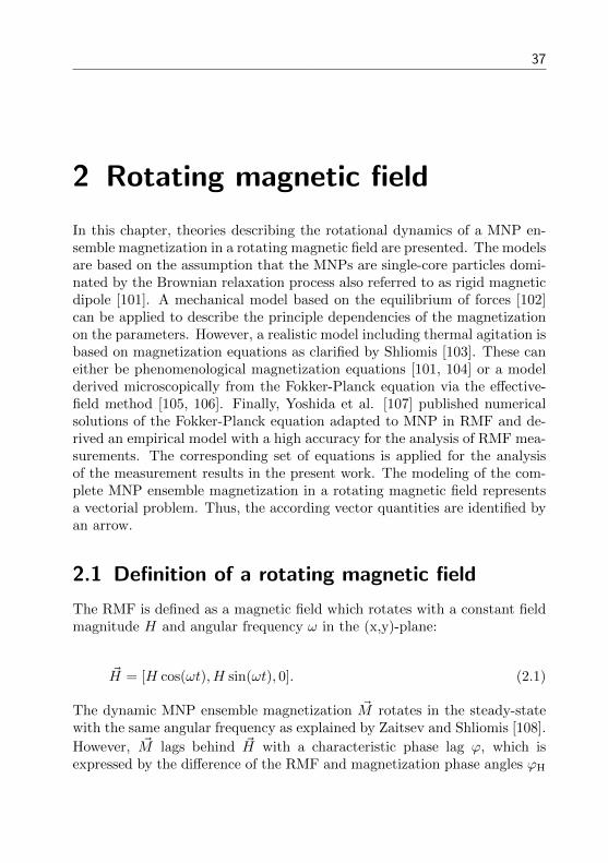
However, ~M lags behind ~H with a characteristic phase lag ϕ, which isexpressed by the difference of the RMF and magnetization phase angles ϕH
38 2 Rotating magnetic field
M
fMNP
w
fH
fM
Figure 2.1: Magnetic nanoparticle with magnetization ~M (rigid magnetic dipole)in rotating magnetic field ~H with phase lag ϕ and angular frequency ω.
and ϕM (see Fig. 2.1). Thus, ~M is expressed as
~M = [M cos(ωt− ϕ),M sin(ωt− ϕ), 0]. (2.2)
In the following sections theories are introduced which can be adopted todescribe the dependence of ϕ on the field strength and frequency as well asthe particle and suspension characteristics.
2.2 Mechanical model
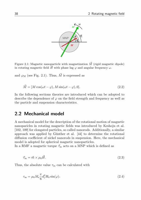
A mechanical model for the description of the rotational motion of magneticnanoparicles in rotating magnetic fields was introduced by Keshoju et al.[102, 109] for elongated particles, so called nanorods. Additionally, a similarapproach was applied by Gunther et al. [44] to determine the rotationaldiffusion coefficient of nickel nanorods in suspension. Here, the mechanicalmodel is adopted for spherical magnetic nanoparticles.In a RMF a magnetic torque ~τm acts on a MNP which is defined as
~τm = ~m× µ0~H. (2.3)
Thus, the absolute value τm can be calculated with
τm = µ0Msπ
6d3
cH0 sin(ϕ). (2.4)
2.3 Magnetization equations 39
Due to the rotational drag that a rotating spherical MNP possesses, anopposite viscous torque ~τd exists [110] whose absolute value is given by
τd = πωηd3h. (2.5)
In the steady state τm and τd are equal. Thereby, the phase lag ϕ is relatedto the rotating field, particle and suspension characteristics via the followingexpression:
ϕ = arcsin
[6ηωd3
h
µ0Msd3cH0
]. (2.6)
This equation gives an impression of the dependence of the phase lag onthe mentioned parameters. However, the inverse sinus dependence is notreflected by measurements of the nanoparticles’ magnetization in a RMF. Asmentioned by Rosensweig [50], Eq. 2.6 is only valid for larger nanoparticleswhich are not disturbed by a reorientation process induced by the Brownianmotion. In fact, for magnetic nanoparticles applied in this work an inversetangent relation is observed which can be described by the following theories.
2.3 Magnetization equations
The application of a phenomenological magnetization equation developedfor the description of the dynamics of ferrofluids - suspended MNPs - inmagnetic fields enables a physical correct method to model the MNP ensem-ble magnetization in a RMF. Shliomis presented in 1972 a phenomenologi-cal magnetization equation [101] as a modification of the Debye relaxationmodel [76] and consequently generalized it [103]. The model is based ondifferent ideas: The allowance of internal rotation explains the existence ofa visible and a non-visible internal angular momentum of the ferrofluid. Theformer can be expressed by the local angular velocity of the whole fluid ~Ωand the latter by the angular velocity of the single particles ~ωp. A deviationof these angular velocities can be maintained by the torque of a magneticfield acting on the MNP ensemble magnetization which is expressed by
6ηφ(~ωp − ~Ω) = ~M × ~H. (2.7)
40 2 Rotating magnetic field
Here, φ represents the volume fraction of solid phase in solution and η thedynamic viscosity. A local frame of reference Σ? is introduced to keep thesingle particles quiescent. Thus, the frame rotates with the angular velocity~ωp and any change of the magnetization vector in the rotating frame of
reference d? ~M/dt is attributed to the fixed observer frame of reference Σby
d ~M
dt= ~ωp × ~M +
d? ~M
dt. (2.8)
In addition, the magnetization relaxation in the system follows the Debye-like equation
d? ~M
dt= − 1
τB( ~M − ~M0) (2.9)
with the Brownian time constant τB for the rigid dipoles and the equilibriummagnetization ~M0. After the substitution of Eq. 2.7 and 2.9 into 2.8, onecan split small magnetization deviations from its equilibrium ~M − ~M0 intothe components parallel and perpendicular to the magnetic field. Finally,the general form of the magnetization equation is expressed by [103]
d ~M
dt= ~Ω × ~M −
~H[~H · ( ~M − ~M0)
]H2τ‖
−~H × ( ~M × ~H)
H2τ⊥. (2.10)
~M0 is described by the Langevin equation L(ξ) as ~M0 = nmL(ξ)~ξ/ξ, wheren represents the particle number density. For the splitting of the magneti-zation deviation into the components parallel and perpendicular to the field~H, the two time constants τ‖ and τ⊥ are introduced as
τ‖ = τB (2.11)
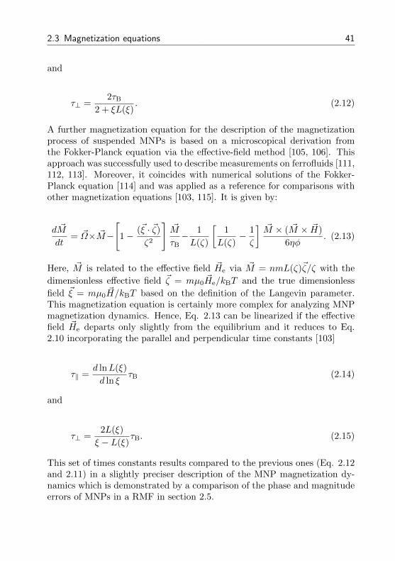
2.3 Magnetization equations 41
and
τ⊥ =2τB
2 + ξL(ξ). (2.12)
A further magnetization equation for the description of the magnetizationprocess of suspended MNPs is based on a microscopical derivation fromthe Fokker-Planck equation via the effective-field method [105, 106]. Thisapproach was successfully used to describe measurements on ferrofluids [111,112, 113]. Moreover, it coincides with numerical solutions of the Fokker-Planck equation [114] and was applied as a reference for comparisons withother magnetization equations [103, 115]. It is given by:
d ~M
dt= ~Ω× ~M−
[1− (~ξ · ~ζ)
ζ2
]~M
τB− 1
L(ζ)
[1
L(ζ)− 1
ζ
] ~M × ( ~M × ~H)
6ηφ. (2.13)
Here, ~M is related to the effective field ~He via ~M = nmL(ζ)~ζ/ζ with the
dimensionless effective field ~ζ = mµ0~He/kBT and the true dimensionless
field ~ξ = mµ0~H/kBT based on the definition of the Langevin parameter.
This magnetization equation is certainly more complex for analyzing MNPmagnetization dynamics. Hence, Eq. 2.13 can be linearized if the effectivefield ~He departs only slightly from the equilibrium and it reduces to Eq.2.10 incorporating the parallel and perpendicular time constants [103]
τ‖ =d lnL(ξ)
d ln ξτB (2.14)
and
τ⊥ =2L(ξ)
ξ − L(ξ)τB. (2.15)
This set of times constants results compared to the previous ones (Eq. 2.12and 2.11) in a slightly preciser description of the MNP magnetization dy-namics which is demonstrated by a comparison of the phase and magnitudeerrors of MNPs in a RMF in section 2.5.
42 2 Rotating magnetic field
1.0
0.8
0.6
0.4
0.2
t / t
B
50403020100
Langevin parameter x
t7
t¦
Figure 2.2: Relaxation time constants τ‖ (Eq. 2.14) and τ⊥ (Eq. 2.15) normalizedto τB.
Whereas Eq. 2.10 and 2.13 provide a general description of the MNP mag-netization dynamics in various magnetic fields, they considerably simplifyfor a MNP ensemble in a RMF as expressed by Eq. 2.1 and 2.2. In thiscase, one can introduce a frame of reference for the magnetization equationrotating with the angular frequency ω [103]. Thus, ~H, ~M and ~M0 becomeconstant vectors
~H = [H, 0, 0], (2.16)
~M = [M cos(ϕ),−M sin(ϕ), 0], (2.17)
~M0 = [M0, 0, 0] (2.18)
and the angular velocity of the whole MNP suspension ~Ω is reduced by theRMF angular velocity ~ω. Under the condition that a MNP suspension in ahomogeneous RMF is quiescent with ~Ω = ~0 [108] Eq. 2.10 results in:
~0 = [−M sin(ϕ)ω,−M cos(ϕ)ω, 0]− 1
τ‖[M cos(ϕ)−M0, 0, 0]
− 1
τ⊥[0,−M sin(ϕ), 0] .
(2.19)

2.3 Magnetization equations 43
Consequently ϕ can be defined via the y-component of Eq. 2.19 as
ϕ = arctan(ωτ⊥). (2.20)
The magnitude of the magnetization M results from the x-component ofEq. 2.19 with τ⊥ ≈ τ‖ for ξ < 1 (see Fig. 2.2) and Eq. 2.20 in
M = M0 cos(ϕ). (2.21)
Due to these simplifications the real and imaginary part of the MNP mag-netization M ′ and M ′′ in a RMF can be described with a Debye-like model:
M ′
Ms=
L(ξ)
1 + (ωτ⊥)2(2.22)
and
M ′′
Ms=
L(ξ)ωτ⊥1 + (ωτ⊥)2
. (2.23)
These equations reduce for ξ 1 to the Debye model which is utilized forthe theoretical description of the complex AC susceptibility in low fields.Thus, the dynamic MNP magnetization in a RMF and alternating mag-netic field are identical for ξ 1. Finally, it can be seen that the phase lagof the MNP magnetization in a RMF reveals an inverse tangent dependenceon the perpendicular time constant and RMF angular frequency. The directproportionality of τ⊥ to τB leads to an increase of ϕ with growing hydro-dynamic particle size. In contrast, ϕ decreases with H and m due to theinverse proportionality of τ⊥ to ξ. Furthermore, Eq. 2.20 clarifies that thesuspension parameters, T and η, also effect the phase lag. The magnitude ofthe MNP magnetization possesses in comparison to ϕ a contrary dependenceon the particle, field and suspension parameters (see Eq. 2.21). Regardingthe angular frequency of the single MNPs ωp, Zaitsev and Shliomis pointedout that it does not necessarily coincide with the angular frequency of thefield ω. [108, 103]. Due to the Brownian motion of the single particles in so-lution their average angular frequency is reduced depending on the particle,
44 2 Rotating magnetic field
suspension and field parameters. Magnetic and optical measurements ondiluted MNP suspensions confirmed the physical dependencies of the MNPmagnetization phase lag in a RMF [116, 3]. However, it turned out that forhigh field magnitudes (ξ 1) and frequencies (ωτB 1) deviations fromthe model appeared which are caused by the applied approximations.
2.4 Fokker-Planck equation
The thermal induced variations that occur in an ensemble of nanoparticles,the Brownian motion, can be explained by the method of Fokker-Planck[117]. This diffusion equation method results in the Fokker-Planck equation(FPE) which is a linear partial differential equation describing the temporaldevelopment of a probability density function in the presence of diffusionand drift [118]. The FPE can be applied to describe adequately the magne-tization dynamics of suspended magnetic nanoparticles that are essentiallyaffected by the Brownian motion [105, 119, 103]. Yoshida et al. [107] pre-sented numerical solutions of the FPE adopted to MNPs in a RMF in orderto determine the MNP magnetization. In this case, the FPE is defined as
2τB∂W
∂t=
1
kBt(∇2Epot)W +
1
kBT(∇Epot) · (∇W ) +∇2W (2.24)
with the potential energy Epot which is given by
Epot(θ, φ, t) = −mH sin(θ) cos(ωt− φ) (2.25)
and the distribution function W which - expanded into spherical harmonics- reads
W (θ, φ, t) =
∞∑n=0
n∑m=−n
an,m(t)P |m|n cos(θ)eimφ. (2.26)
P|m|n represents the associated Legendre functions and an,m(t) the temporal
coefficients of the spherical harmonics. E and W are expressed in sphericalcoordinates. The detailed steps of the performed numerical solution are ex-
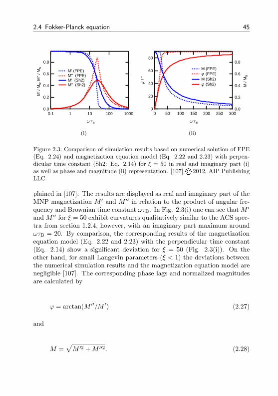
2.4 Fokker-Planck equation 45
0.8
0.6
0.4
0.2
0.0
M' /
Ms,
M''
/ Ms
0.1 1 10 100 1000
wtB
M' (FPE) M'' (FPE) M' (Sh2) M'' (Sh2)
(i)
80
60
40
20
0
f /
°
300250200150100500
wtB
0.8
0.6
0.4
0.2
0.0
M /
Ms
M (FPE) f (FPE) M (Sh2) f (Sh2)
(ii)
Figure 2.3: Comparison of simulation results based on numerical solution of FPE(Eq. 2.24) and magnetization equation model (Eq. 2.22 and 2.23) with perpen-dicular time constant (Sh2: Eq. 2.14) for ξ = 50 in real and imaginary part (i)as well as phase and magnitude (ii) representation. [107] © 2012, AIP PublishingLLC.
plained in [107]. The results are displayed as real and imaginary part of theMNP magnetization M ′ and M ′′ in relation to the product of angular fre-quency and Brownian time constant ωτB. In Fig. 2.3(i) one can see that M ′
and M ′′ for ξ = 50 exhibit curvatures qualitatively similar to the ACS spec-tra from section 1.2.4, however, with an imaginary part maximum aroundωτB = 20. By comparison, the corresponding results of the magnetizationequation model (Eq. 2.22 and 2.23) with the perpendicular time constant(Eq. 2.14) show a significant deviation for ξ = 50 (Fig. 2.3(i)). On theother hand, for small Langevin parameters (ξ < 1) the deviations betweenthe numerical simulation results and the magnetization equation model arenegligible [107]. The corresponding phase lags and normalized magnitudesare calculated by
ϕ = arctan(M ′′/M ′) (2.27)
and
M =√M ′2 +M ′′2. (2.28)
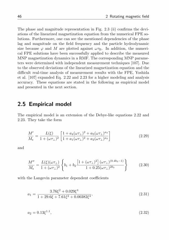
46 2 Rotating magnetic field
The phase and magnitude representation in Fig. 2.3 (ii) confirms the devi-ations of the linearized magnetization equation from the numerical FPE so-lutions. Furthermore, one can see the mentioned dependencies of the phaselag and magnitude on the field frequency and the particle hydrodynamicsize because ϕ and M are plotted against ωτB. In addition, the numeri-cal FPE solutions have been successfully applied to describe the measuredMNP magnetization dynamics in a RMF. The corresponding MNP parame-ters were determined with independent measurement techniques [107]. Dueto the observed deviations of the linearized magnetization equation and thedifficult real-time analysis of measurement results with the FPE, Yoshidaet al. [107] expanded Eq. 2.22 and 2.23 for a higher modeling and analysisaccuracy. These equations are stated in the following as empirical modeland presented in the next section.
2.5 Empirical model
The empirical model is an extension of the Debye-like equations 2.22 and2.23. They take the form
M ′
Ms=
L(ξ)
1 + (ωτ⊥)2
[1 + a4(ωτ⊥)2 + a5(ωτ⊥)a3
1 + a1(ωτ⊥)2 + a2(ωτ⊥)a3
](2.29)
and
M ′′
Ms=L(ξ)(ωτ⊥)
1 + (ωτ⊥)2
b1 + b2
[1 + (ωτ⊥)2
](ωτ⊥)(0.4b3−1)
1 + 0.25(ωτ⊥)2b3
(2.30)
with the Langevin parameter dependent coefficients
a1 =3.76ξ2 + 0.029ξ4
1 + 29.6ξ + 7.61ξ2 + 0.00382ξ4, (2.31)
a2 = 0.13ξ1.1, (2.32)

2.5 Empirical model 47
a3 = 4 + 16
(ξ
ξ + 17
)2
, (2.33)
a4 = 0.1ξ, (2.34)
a5 =0.0865ξ + 0.205ξ2 + 0.0003974
1 + 0.88ξ + 0.606ξ2 + 0.00652ξ4, (2.35)
b1 = 1− 0.2ξ1.2
ξ1.2 + 5.5, (2.36)
b2 =0.6ξ1.5
ξ1.5 + 16(2.37)
and
b3 = 1.4 +3.2ξ
ξ + 5. (2.38)
These equations enable a modeling of the MNP magnetization in a RMFwith a high accuracy in a reasonable time. Fig. 2.4 displays a comparison ofthe simulation results based on the numerical FPE solution and the empiri-cal model. For ξ = 50 only slight differences in the real and imaginary partas well as phase and magnitude representation are discernible. A detailedillustration of the according phase and magnitude errors of the MNP mag-netization in a RMF is presented in Fig. 2.5. Here, the true value accordsto the results of the numerical FPE solution. In addition to the empiricalmodel the errors of the magnetization equation model (Eq. 2.22 and 2.23)with the two different perpendicular time constants (Eq. 2.12 and 2.15) aredisplayed. The analysis of the errors confirms the accuracy of the empiricalmodel compared to the magnetization equation model. Especially, for thelatter a dramatic error growth is observed when the Langevin parameter
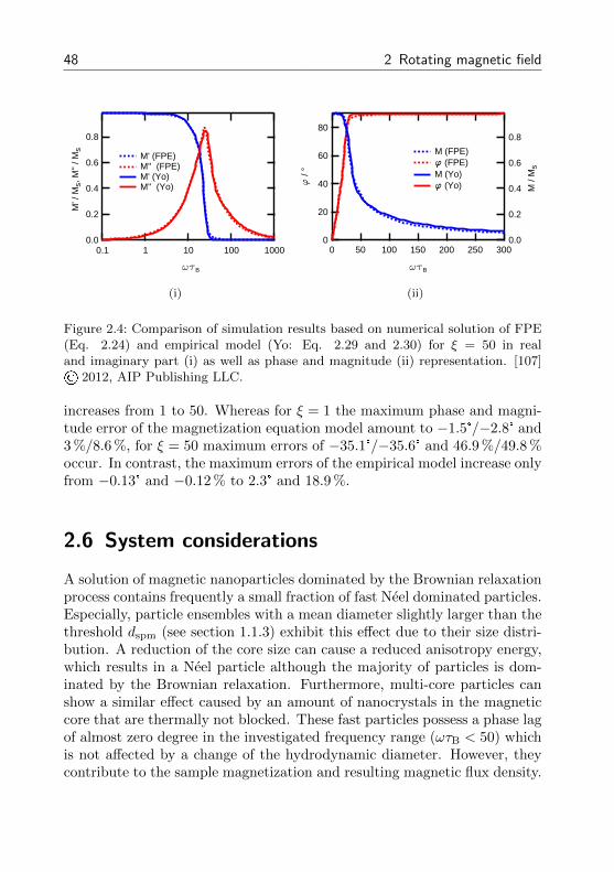
48 2 Rotating magnetic field
0.8
0.6
0.4
0.2
0.0
M' /
Ms,
M''
/ Ms
0.1 1 10 100 1000
wtB
M' (FPE) M'' (FPE) M' (Yo) M'' (Yo)
(i)
80
60
40
20
0
f /
°
300250200150100500
wtB
0.8
0.6
0.4
0.2
0.0
M /
Ms
M (FPE) f (FPE) M (Yo) f (Yo)
(ii)
Figure 2.4: Comparison of simulation results based on numerical solution of FPE(Eq. 2.24) and empirical model (Yo: Eq. 2.29 and 2.30) for ξ = 50 in realand imaginary part (i) as well as phase and magnitude (ii) representation. [107]© 2012, AIP Publishing LLC.
increases from 1 to 50. Whereas for ξ = 1 the maximum phase and magni-tude error of the magnetization equation model amount to −1.5°/−2.8° and3 %/8.6 %, for ξ = 50 maximum errors of −35.1°/−35.6° and 46.9 %/49.8 %occur. In contrast, the maximum errors of the empirical model increase onlyfrom −0.13° and −0.12 % to 2.3° and 18.9 %.
2.6 System considerations
A solution of magnetic nanoparticles dominated by the Brownian relaxationprocess contains frequently a small fraction of fast Neel dominated particles.Especially, particle ensembles with a mean diameter slightly larger than thethreshold dspm (see section 1.1.3) exhibit this effect due to their size distri-bution. A reduction of the core size can cause a reduced anisotropy energy,which results in a Neel particle although the majority of particles is dom-inated by the Brownian relaxation. Furthermore, multi-core particles canshow a similar effect caused by an amount of nanocrystals in the magneticcore that are thermally not blocked. These fast particles possess a phase lagof almost zero degree in the investigated frequency range (ωτB < 50) whichis not affected by a change of the hydrodynamic diameter. However, theycontribute to the sample magnetization and resulting magnetic flux density.
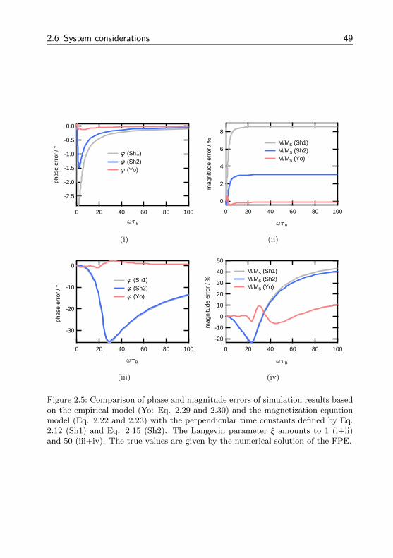
2.6 System considerations 49
-2.5
-2.0
-1.5
-1.0
-0.5
0.0
phas
e er
ror
/ °
100806040200
wtB
f (Sh1) f (Sh2) f (Yo)
(i)
8
6
4
2
0m
agni
tude
err
or /
%100806040200
wtB
M/Ms (Sh1) M/Ms (Sh2) M/Ms (Yo)
(ii)
-30
-20
-10
0
phas
e er
ror
/ °
100806040200
wtB
f (Sh1) f (Sh2) f (Yo)
(iii)
50
40
30
20
10
0
-10
-20
mag
nitu
de e
rror
/ %
100806040200
wtB
M/Ms (Sh1) M/Ms (Sh2) M/Ms (Yo)
(iv)
Figure 2.5: Comparison of phase and magnitude errors of simulation results basedon the empirical model (Yo: Eq. 2.29 and 2.30) and the magnetization equationmodel (Eq. 2.22 and 2.23) with the perpendicular time constants defined by Eq.2.12 (Sh1) and Eq. 2.15 (Sh2). The Langevin parameter ξ amounts to 1 (i+ii)and 50 (iii+iv). The true values are given by the numerical solution of the FPE.
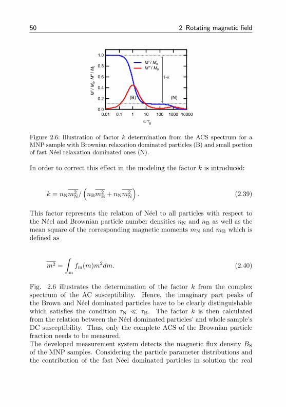
50 2 Rotating magnetic field
1.0
0.8
0.6
0.4
0.2
0.0
M'/
M0, M''
/ M0
0.01 0.1 1 10 100 1000 10000
M' / M0
M'' / M0
1-k
(B) (N)
wt B
Figure 2.6: Illustration of factor k determination from the ACS spectrum for aMNP sample with Brownian relaxation dominated particles (B) and small portionof fast Neel relaxation dominated ones (N).
In order to correct this effect in the modeling the factor k is introduced:
k = nNm2N/(nBm2
B + nNm2N
). (2.39)
This factor represents the relation of Neel to all particles with respect tothe Neel and Brownian particle number densities nN and nB as well as themean square of the corresponding magnetic moments mN and mB which isdefined as
m2 =
∫m
fm(m)m2dm. (2.40)
Fig. 2.6 illustrates the determination of the factor k from the complexspectrum of the AC susceptibility. Hence, the imaginary part peaks ofthe Brown and Neel dominated particles have to be clearly distinguishablewhich satisfies the condition τN τB. The factor k is then calculatedfrom the relation between the Neel dominated particles’ and whole sample’sDC susceptibility. Thus, only the complete ACS of the Brownian particlefraction needs to be measured.The developed measurement system detects the magnetic flux density BS
of the MNP samples. Considering the particle parameter distributions andthe contribution of the fast Neel dominated particles in solution the real
2.6 System considerations 51
and imaginary part of BS(H,ω) can be expressed by
B′S(H,ω)
BS(H0, 0)= (1− k)
3kBT
H0m2B
∫dh
fh(dh)
×∫mB
fm(mB)mBM ′(H,ω)
MsdmBddh + k
H
H0
(2.41)
and
B′′S (H,ω)
BS(H0, 0)= (1− k)
3kBT
H0m2B
∫dh
fh(dh)
×∫mB
fm(mB)mBM ′′(H,ω)
MsdmBddh
(2.42)
normalized to the sample’s magnetic flux density for a given DC excitationfield H0 which is defined by
BS(H0, 0) = nBm2B
gH0
3kBT+ nNm2
N
gH0
3kBT. (2.43)
The factor g represents the geometries and the arrangement of the sensorand sample, which influence the strength of BS coupling into the sensor.

52 2 Rotating magnetic field
53
3 Measurement system
In this chapter, the developed measurement system for the investigation ofthe dynamics of magnetic nanoparticles in a rotating magnetic field is pre-sented. First, the system requirements are defined. Then, the hard- andsoftware components, e.g. the coils, sensors and control program, as wellas their interaction are explained. Finally, the performance of the measure-ment system is characterized regarding systematic and random errors anda maximal measurement uncertainty of the phase lag determination for adefined set of measurement parameters is estimated.
3.1 System requirements
In order to investigate the rotational dynamics of MNPs as potential markersfor a homogeneous bioassay based on a RMF, the magnetic field generationand the detection system need to fulfill some requirements. These are theRMF frequency range, magnitude and homogeneity as well as the sensornoise performance, frequency bandwidth and geometry. Furthermore, prac-tical aspects as the sample handling and environmental influences have tobe taken into account.
Rotating magnetic field
The hydrodynamic size and the magnetic moment define the modified Brow-nian relaxation time constant τ⊥ of MNPs in a RMF (see Eq. 2.15) assumingthat they are dissolved in an aqueous medium at room temperature. Thus,the minimum upper frequency of the measurement system is specified bythese parameters corresponding to Eq. 1.28 which defines a relation be-tween τ⊥ and the modified characteristic frequency fch,⊥. In addition, τ⊥incorporates the RMF magnitude via the Langevin parameter. Hence, themagnitude has an additional influence on fch,⊥. Fig. 3.1 depicts the mod-ified characteristic frequency as a function of the hydrodynamic diameterand the Langevin parameter for spherical particles. While for ξ < 1 field
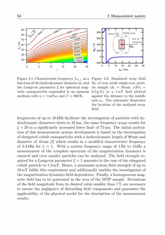
54 3 Measurement system
90
80
70
60
50
40
30
d h/ n
m
2520151050x
210000 122000
70000 44000 28000 18000 12000 10000
8000 6000 4000
2000
f ch, /
Hz
Figure 3.1: Characteristic frequency fch,⊥ as afunction of the hydrodynamic diameter dh andthe Langevin parameter ξ for spherical mag-netic nanoparticles suspended in an aqueousmedium with η = 1 mPa s and T = 300 K.
800
600
400
200
0
-200302520151050
line ofanalysis
stray field middle axis
as / mm
BS /
nT BS
Figure 3.2: Simulated stray fieldBS of iron oxide single-core parti-cle sample (dc = 30 nm, c(Fe) =0.5 g/L) in a 1 mT field plottedagainst the distance to the middleaxis as. The schematic illustratesthe location of the analyzed strayfield.
frequencies of up to 10 kHz facilitate the investigation of particles with hy-drodynamic diameters down to 35 nm, the same frequency scope results forξ = 20 in a significantly increased lower limit of 75 nm. The initial motiva-tion of this measurement system development is based on the investigationof elongated cobalt nanoparticles with a hydrodynamic length of 90 nm anddiameter of 16 nm [3] which results in a modified characteristic frequencyof 2.3 kHz for ξ = 1. With a system frequency range of 1 Hz to 5 kHz ameasurement of the complete spectrum of the magnetization dynamics isensured and even smaller particles can be analyzed. The field strength re-quired for a Langevin parameter ξ = 1 amounts in the case of the elongatedcobalt particle to 1.3 mT. Hence, a maximum system field strength of up to10 mT fulfils this requirement and additionally enables the investigation ofthe magnetization dynamics field dependence. Finally, a homogeneous mag-netic field has to be generated in the area of the MNP sample. Deviationsof the field magnitude from its desired value smaller than 1 % are necessaryto ensure the negligence of disturbing field components and guarantee theapplicability of the physical model for the description of the measurementresults.
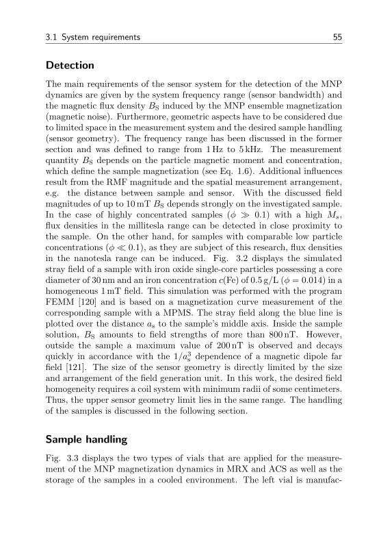
3.1 System requirements 55
Detection
The main requirements of the sensor system for the detection of the MNPdynamics are given by the system frequency range (sensor bandwidth) andthe magnetic flux density BS induced by the MNP ensemble magnetization(magnetic noise). Furthermore, geometric aspects have to be considered dueto limited space in the measurement system and the desired sample handling(sensor geometry). The frequency range has been discussed in the formersection and was defined to range from 1 Hz to 5 kHz. The measurementquantity BS depends on the particle magnetic moment and concentration,which define the sample magnetization (see Eq. 1.6). Additional influencesresult from the RMF magnitude and the spatial measurement arrangement,e.g. the distance between sample and sensor. With the discussed fieldmagnitudes of up to 10 mT BS depends strongly on the investigated sample.In the case of highly concentrated samples (φ 0.1) with a high Ms,flux densities in the millitesla range can be detected in close proximity tothe sample. On the other hand, for samples with comparable low particleconcentrations (φ 0.1), as they are subject of this research, flux densitiesin the nanotesla range can be induced. Fig. 3.2 displays the simulatedstray field of a sample with iron oxide single-core particles possessing a corediameter of 30 nm and an iron concentration c(Fe) of 0.5 g/L (φ = 0.014) in ahomogeneous 1 mT field. This simulation was performed with the programFEMM [120] and is based on a magnetization curve measurement of thecorresponding sample with a MPMS. The stray field along the blue line isplotted over the distance as to the sample’s middle axis. Inside the samplesolution, BS amounts to field strengths of more than 800 nT. However,outside the sample a maximum value of 200 nT is observed and decaysquickly in accordance with the 1/a3
s dependence of a magnetic dipole farfield [121]. The size of the sensor geometry is directly limited by the sizeand arrangement of the field generation unit. In this work, the desired fieldhomogeneity requires a coil system with minimum radii of some centimeters.Thus, the upper sensor geometry limit lies in the same range. The handlingof the samples is discussed in the following section.
Sample handling
Fig. 3.3 displays the two types of vials that are applied for the measure-ment of the MNP magnetization dynamics in MRX and ACS as well as thestorage of the samples in a cooled environment. The left vial is manufac-

56 3 Measurement system
tured out of glass and closed with a polyethylene cap. The outer diameteramounts to 7.8 mm and the height is 35 mm. It is distributed by the neo-Lab Migge Laborbedarf-Vertriebs GmbH (Heidelberg, Germany) under theidentifier 7-0736. The right vial is a conical polystyrene vessel manufac-tured by the Nunc GmbH & Co. KG (Wiesbaden, Germany) under thebrand BreakApartTM PolySorpTM. It is sealed with a blue polyethylenecap. The largest diameter of this vial is found in the height of the capwith 8.8 mm. Both vial types have to fit into the measurement system. Inaddition, a fast and uncomplicated change of the samples in the system hasto be enabled. In the optimal case, the sample can be placed manually intothe measurement system in one step.
3.2 Hardware and Construction
A sketch of the measurement system hardware and interplay of the com-ponents, which fulfill the described requirements, can be found in Fig. 3.4.A photograph of the whole system including all components is shown inFig. 3.5. It consists of a 2-axis Helmholtz coil system that is powered by acurrent control unit for the generation of a rotating magnetic field. Insidethe coil system two fluxgate magnetometers are set up in a gradiometricarrangement. Between these two sensors the sample is placed in a holderwhich can control the sample temperature and position along the sensitivemeasurement axis of the fluxgate magnetometers. Additional electronicsand a measurement and control interface, which is equipped with analog-to-digital as well as digital-to-analog converters, enable an automation ofthe whole measurement process. A side and top view of the system withthe gradiometric fluxgate arrangement in the center of the 2-axis Helmholtzcoil is displayed in Fig. 3.6 and 3.7.
3.2.1 Fluxgate magnetometer
The utilized fluxgate magnetometer system MAG-03IEL from BartingtonInstruments Limited (Witney, United Kingdom) provides magnetic sensorswhich facilitate the measurement of weak magnetic fields down to the pi-cotesla range at room temperature. Their magnetic noise amounts to valuessmaller than < 6 pT/
√Hz at 1 Hz and the frequency bandwidth ranges from
DC to 5 kHz. A list with further parameters is shown in Table 3.1 [123].The whole sensor system consists of three single sensors, each housed in-
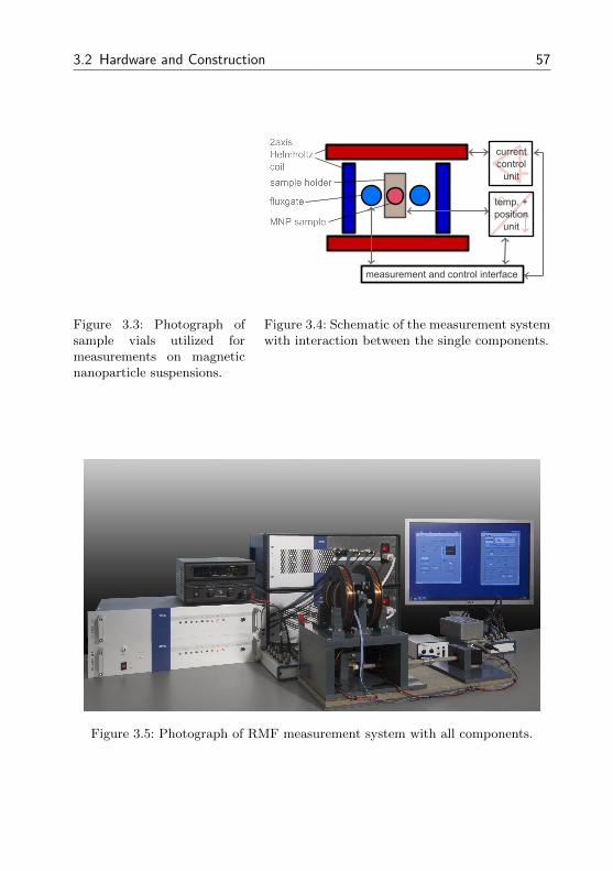
3.2 Hardware and Construction 57
Figure 3.3: Photograph ofsample vials utilized formeasurements on magneticnanoparticle suspensions.
measurement and control interface
current control
unit
°Ctemp. + position
unit
Figure 3.4: Schematic of the measurement systemwith interaction between the single components.
Figure 3.5: Photograph of RMF measurement system with all components.
58 3 Measurement system
fluxgate
MNP sample fluxgatecore
RMF
Bs
x
z
y
Figure 3.6: Side view of the measure-ment system. A MNP sample is placedbetween two fluxgates. The stray fieldof the sample is coupling into the flux-gate cores with respect to the sampleposition. [122] ©2014, AIP PublishingLLC.
M
fluxgate
xz
y
Figure 3.7: Top view of the measure-ment system. A MNP sample is placedbetween two fluxgates. A homogeneousRMF is aligning the sample magnetiza-tion.
side a ceramic cylinder with an diameter of 8 mm and a length of 30 mm.The construction of the single sensor unit is illustrated in Fig. 3.8 andcalled Vacquier type. Here, the two magnetic cores are excited by theirprimary coil fields in opposite directions, however, with the same symmet-ric saturated magnetization profile. These non-linear core magnetizationscompensate each other in the absence of an external magnetic field. In thepresence of a field, the magnetization profiles do not coincide anymore andthe detection coil wound around this configuration detects a signal whichcan be analyzed to determine the causative field. In practice, the secondharmonic of the measurement coil‘s output signal is processed which occursonly in the presence of the external magnetic field. The compensation coilextends the linear measurement range of the sensor by keeping the cores’magnetization profile symmetric. A detailed explanation of fluxgates, theirdifferent configurations and operation is given by Ripka [124]. The threesensor units are connected with a measurement and supply electronics. Twounits are used for the gradiometric arrangement which is shown in Fig. 3.6.The stray field of a MNP sample placed in between couples into the sen-sor on the left side with an reversed direction compared to the one on theright side. If the output signals of the two units are subtracted from eachother, power line interferences, the DC earth magnetic field and other global
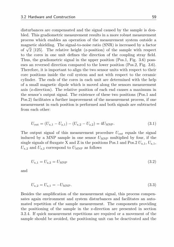
3.2 Hardware and Construction 59
disturbances are compensated and the signal caused by the sample is dou-bled. This gradiometric measurement results in a more robust measurementprocess which enables an operation of the measurement system outside amagnetic shielding. The signal-to-noise ratio (SNR) is increased by a factorof√
2 [125]. The relative height (z-position) of the sample with respectto the cores in one unit defines the direction of the coupling stray field.Thus, the gradiometric signal in the upper position (Pos.1, Fig. 3.6) poss-eses an reversed direction compared to the lower position (Pos.2, Fig. 3.6).Therefore, it is important to align the two sensor units with respect to theircore positions inside the coil system and not with respect to the ceramiccylinder. The ends of the cores in each unit are determined with the helpof a small magnetic dipole which is moved along the sensors measurementaxis (z-direction). The relative position of each end causes a maximum inthe sensor’s output signal. The existence of these two positions (Pos.1 andPos.2) facilitates a further improvement of the measurement process, if onemeasurement in each position is performed and both signals are subtractedfrom each other:
Uout = (Ux,1 − Uz,1)− (Ux,2 − Uz,2) = 4UMNP. (3.1)
The output signal of this measurement procedure Uout equals the signalinduced by a MNP sample in one sensor UMNP multiplied by four, if thesingle signals of fluxgate X and Z in the positions Pos.1 and Pos.2 Ux,1, Uz,1,Ux,2 and Uz,2 correspond to UMNP as follows
Ux,1 = Uz,2 = UMNP (3.2)
and
Ux,2 = Uz,1 = −UMNP. (3.3)
Besides the amplification of the measurement signal, this process compen-sates again environment and system disturbances and facilitates an auto-mated repetition of the sample measurement. The components providingthe positioning of the sample in the z-direction are presented in section3.2.4. If quick measurement repetitions are required or a movement of thesample should be avoided, the positioning unit can be deactivated and the
60 3 Measurement system
Table 3.1: Parameters of 3-axes fluxgate magnetometer MAG-03IEL.
bandwidth: 0 kHz to 5 kHz
measurement range: ±100 µT
sensitivity: 105 VT
magnetic noise (at 1 Hz): < 6 pT/√
Hz
zero field offset: <5 nT
measurement in the second position is replaced by a measurement withoutsample (blank measurement). This procedure is analogous to the one of thefluxgate based MRX measurement system [83].
The sensor units are oriented perpendicularly to the plane of the rotatingmagnetic field, so that the sensors measure only the magnetic nanoparticle’sstray field. Otherwise the sensors measurement range would be exceeded bythe coupling component of the RMF Hpar. Due to production inaccuracies,the cores in the fluxgate units are not perfectly orientated parallel to theaxis of the ceramic cylinder (see Fig. 3.9). Thus, the sensor units have tobe aligned manually into their vertical positions with the help of specialsensor mountings. Applying a rotating field with a magnitude of 1 mT, thefield Hpar detected by each single fluxgate in the absence of a sample canbe minimized to below 100 nT, i.e., the sensors can be balanced to betterthan 1 · 10−4. This corresponds to a tilt angle αT of less than 0.003° whichis defined by
αT = arcsin(Hpar
H). (3.4)
The limited fluxgate frequency bandwidth causes a frequency response of thesingle sensor units, that results in a significant phase shift and magnitudedrop. The measured frequency response of the sensor units X and Z ispresented in Fig. 3.10. Whereas the magnitude drops at 5 kHz to 70 %of its start value which is in agreement with the specified −3 dB cutofffrequency, the phase shifts to almost 180°. Thus, the frequency response ofthe fluxgates has to be corrected to ensure an exact determination of thephase and magnitude of the MNP samples. The applied software procedureis explained in section 3.3.2. Measurements describing the influence of theRMF on the sensor’s frequency response are presented in section 3.4.1.
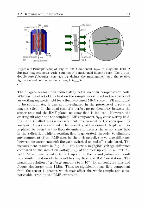
3.2 Hardware and Construction 61
Iexc
Uout
Hmeasurementcoil
core
compensationcoil
Icomp
excitation coil
Figure 3.8: Principle setup offluxgate magnetometer withdouble core (Vacquier) con-figuration and compensationcoil.
H
HperpHpar
fluxgate
core
magneticfield
aT
Figure 3.9: Component Hpar of magnetic field Hcoupling into misaligned fluxgate core. The tilt an-gle αT defines the misalignment and the relativestrength Hpar/H.
The fluxgate sensor units induce stray fields via their compensation coils.Whereas the effect of this field on the sample was studied in the absence ofan exciting magnetic field for a fluxgate-based MRX system [83] and foundto be subordinate, it was not investigated in the presence of a rotatingmagnetic field. In the ideal case of a perfect perpendicularity between thesensor axis and the RMF plane, no stray field is induced. However, theexisting tilt angle and the coupling RMF component Hpar cause a stray field.Fig. 3.11 (i) illustrates a measurement arrangement of the correspondinganalysis. A pick up coil with the geometry of the desired 150µL samplesis placed between the two fluxgate units and detects the sensor stray fieldin the z-direction while a rotating field is generated. In order to eliminateany component of the RMF seen by the pick up coil, the voltage differencebetween measurements with fluxgates switched on and off is calculated. Themeasurement results in Fig. 3.11 (ii) show a negligible voltage differencecompared to the induction voltage uAC of the pick up coil in a 1 mT ACfield. Measurements with the pick up coil in the x- and y-direction resultin a similar relation of the possible stray field and RMF excitation. Themaximum relation of ∆u/uAC amounts to 1 ·10−3 for all configurations andfrequencies larger than 1 kHz. Thus, no significant stray field componentfrom the sensor is present which may affect the whole sample and causenoticeable errors in the RMF excitation.
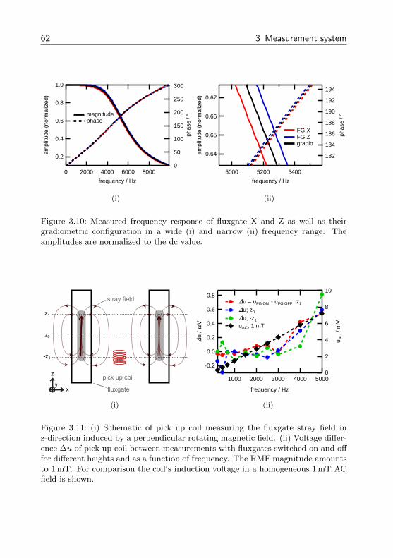
62 3 Measurement system
1.0
0.8
0.6
0.4
0.2
ampl
itude
(no
rmal
ized
)
80006000400020000
frequency / Hz
300
250
200
150
100
50
0
phas
e / ° magnitude
phase
(i)
0.67
0.66
0.65
0.64ampl
itude
(no
rmal
ized
)
540052005000
frequency / Hz
194
192
190
188
186
184
182
phas
e / °
FG X FG Z gradio
(ii)
Figure 3.10: Measured frequency response of fluxgate X and Z as well as theirgradiometric configuration in a wide (i) and narrow (ii) frequency range. Theamplitudes are normalized to the dc value.
x
z
ypick up coil
fluxgate
stray field
z0
z1
-z1
(i)
0.8
0.6
0.4
0.2
0.0
-0.2
Du
/ mV
50004000300020001000
frequency / Hz
10
8
6
4
2
0
u AC /
mV
Du = uFG,ON - uFG,OFF ; z1 Du; z0
Du; -z1
uAC; 1 mT
(ii)
Figure 3.11: (i) Schematic of pick up coil measuring the fluxgate stray field inz-direction induced by a perpendicular rotating magnetic field. (ii) Voltage differ-ence ∆u of pick up coil between measurements with fluxgates switched on and offfor different heights and as a function of frequency. The RMF magnitude amountsto 1 mT. For comparison the coil‘s induction voltage in a homogeneous 1 mT ACfield is shown.
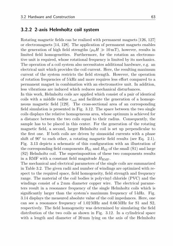
3.2 Hardware and Construction 63
3.2.2 2-axis Helmholtz coil system
Rotating magnetic fields can be realized with permanent magnets [126, 127]or electromagnets [14, 128]. The application of permanent magnets enablesthe generation of high field strengths (µ0H 10 mT), however, results inlimited field homogeneities. Furthermore, for the rotation an electromo-tive unit is required, whose rotational frequency is limited by its mechanics.The operation of a coil system also necessitates additional hardware, e.g. anelectrical unit which provides the coil current. Here, the resulting maximumcurrent of the system restricts the field strength. However, the operationof rotation frequencies of 5 kHz and more requires less effort compared to apermanent magnet in combination with an electromotive unit. In addition,less vibrations are induced which reduces mechanical disturbances.In this work, Helmholtz coils are applied which consist of a pair of identicalcoils with a middle radius rcoil and facilitate the generation of a homoge-neous magnetic field [129]. The cross-sectional area of an correspondingfield simulation is presented in Fig. 3.12. The space between the two singlecoils displays the relative homogeneous area, whose optimum is achieved fora distance between the two coils equal to their radius. Consequently, thesample has to be placed in this center. For the generation of the rotatingmagnetic field, a second, larger Helmholtz coil is set up perpendicular tothe first one. If both coils are driven by sinusoidal currents with a phaseshift of 90° to each other, a rotating magnetic field results (see Eq. 2.1).Fig. 3.13 depicts a schematic of this configuration with an illustration ofthe corresponding field components HS1 and HS2 of the small (S1) and large(S2) Helmholtz coil. The superimposition of these two components resultsin a RMF with a constant field magnitude HRMF.The mechanical and electrical parameters of the single coils are summarizedin Table 3.2. The given radii and number of windings are optimized with re-spect to the required space, field homogeneity, field strength and frequencyrange. The material of the coil bodies is polyvinyl chloride (PVC) and thewindings consist of a 2 mm diameter copper wire. The electrical parame-ters result in a resonance frequency of the single Helmholtz coils which issignificantly larger than the system’s maximum frequency of 5 kHz. Fig.3.14 displays the measured absolute value of the coil impedances. Here, onecan see a resonance frequency of 1.02 MHz and 0.66 MHz for S1 and S2,respectively. The field homogeneity was determined by simulating the fielddistribution of the two coils as shown in Fig. 3.12. In a cylindrical spacewith a length and diameter of 20 mm lying on the axis of the Helmholtz
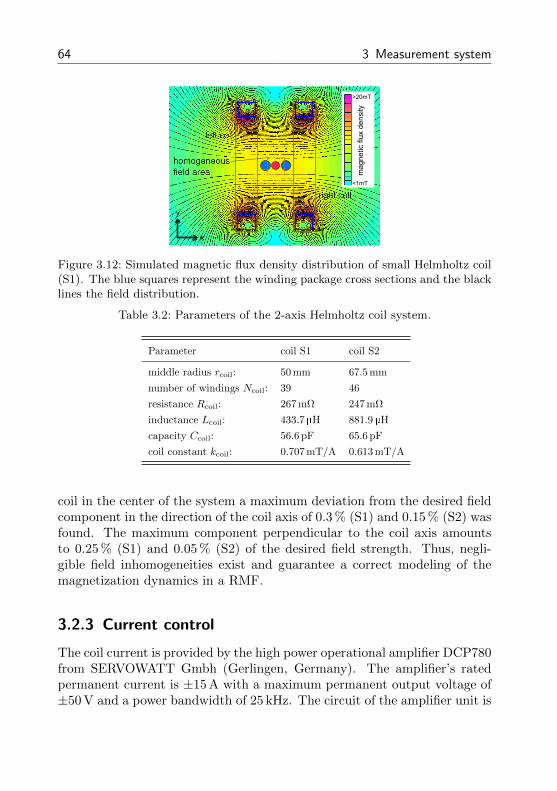
64 3 Measurement system
>20mT
<1mT
mag
netic
flux
den
sity
x
y
Figure 3.12: Simulated magnetic flux density distribution of small Helmholtz coil(S1). The blue squares represent the winding package cross sections and the blacklines the field distribution.
Table 3.2: Parameters of the 2-axis Helmholtz coil system.
Parameter coil S1 coil S2
middle radius rcoil: 50 mm 67.5 mm
number of windings Ncoil: 39 46
resistance Rcoil: 267 mΩ 247 mΩ
inductance Lcoil: 433.7 µH 881.9 µH
capacity Ccoil: 56.6 pF 65.6 pF
coil constant kcoil: 0.707 mT/A 0.613 mT/A
coil in the center of the system a maximum deviation from the desired fieldcomponent in the direction of the coil axis of 0.3 % (S1) and 0.15 % (S2) wasfound. The maximum component perpendicular to the coil axis amountsto 0.25 % (S1) and 0.05 % (S2) of the desired field strength. Thus, negli-gible field inhomogeneities exist and guarantee a correct modeling of themagnetization dynamics in a RMF.
3.2.3 Current control
The coil current is provided by the high power operational amplifier DCP780from SERVOWATT Gmbh (Gerlingen, Germany). The amplifier’s ratedpermanent current is ±15 A with a maximum permanent output voltage of±50 V and a power bandwidth of 25 kHz. The circuit of the amplifier unit is
3.2 Hardware and Construction 65
RMF
Helmholtz coil S1
Helmholtz coil S2
HS1HS2
HRMF field
mag
nitu
de
time
90°x
y
Figure 3.13: Schematic of the RMFgeneration with two perpendicularHelmholtz coils. The inset shows thefield magnitudes of the single Helmholtzcoil fields and the resulting RMF.
100
101
102
103
104
105
Z / W
101
102
103
104
105
106
frequency / Hz
S1 S2 S1 + series capacity S2 + series capacity
Figure 3.14: Absolute value of measuredimpedance of Helmholtz coil S1 and S2with and without series capacity as afunction of frequency.
shown in Fig. 3.15. The circuit is identical for both coils except capacity Cg.It amounts to 470 pF for coil S1 and to 1 nF for coil S2. With this circuitthe amplifier behaves as a current regulator. The current of the amplifiersload, the coil current Icoil, is directly defined by the input voltage Uin:
Icoil = −UinR1
R2Rshunt. (3.5)
The amplitude response of this current regulator possesses in practice errorsof up to 10 %. Hence, the magnitude of the single coil currents Icoil,S1 andIcoil,S2 as well as the phase between these currents is controlled additionallyby a proportional-integral (PI) controller implemented in the measurementand control software (see section 3.3). The maximum field frequency as afunction of the field strength which can be generated by one coil and thecorresponding current control unit is illustrated in Fig. 3.16. Coil S2 in com-bination with the presented current control unit limits the maximum RMFfrequency for a given field strength due to its higher impedance. Whereasfor 1 mT a 5 kHz field can be generated, for 5 mT it is restricted to 1 kHz.In order to overcome the limiting coil impedance, for distinct frequencies(1 kHz to 5 kHz with a step size of 0.5 kHz) series capacities can be activated,which - in the ideal case - reduce the absolute value of the coil impedancefor one frequency to its real part Rcoil. This is shown in Fig. 3.14 for 1 kHz
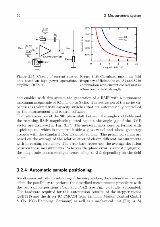
66 3 Measurement system
Zcoil
Rshunt
20 kW
20 kW
Cg
1 kW
1 kW 4.7nF
DCP780/60HSR
470 kW
R1
R1
R2
Rg
CHF
Uin
Icoil
R2
Figure 3.15: Circuit of current controlunit based on high power operationalamplifier DCP780.
5000
4000
3000
2000
1000
freq
uenc
y / H
z
1086420
magnetic field / mT
S1 S2
Figure 3.16: Calculated maximum fieldfrequency of Helmholtz coil S1 and S2 incombination with current control unit asa function of field strength.
and enables with this system the generation of a RMF with a permanentmaximum magnitude of 9.1 mT up to 5 kHz. The activation of the series ca-pacities is realized with capacity switches that are automatically controlledby the measurement and control software.The relative errors of the 90° phase shift between the single coil fields andthe resulting RMF magnitude plotted against the angle ϕH of the RMFvector are displayed in Fig. 3.17. The measurements were performed witha pick up coil which is mounted inside a glass vessel and whose geometryaccords with the standard 150µL sample volume. The presented values arebased on the average of the relative error of eleven different measurementswith increasing frequency. The error bars represents the average deviationbetween these measurements. Whereas the phase error is almost negligible,the magnitude possesses slight errors of up to 2 % depending on the fieldangle.
3.2.4 Automatic sample positioning
A software-controlled positioning of the sample along the system’s z-directionoffers the possibility to perform the described measurement procedure withthe two sample positions Pos.1 and Pos.2 (see Fig. 3.6) fully automated.The hardware required for this automation consists of the stepper motorQSH4218 and the driver IC TMC261 from Trinamic Motion Control GmbH& Co. KG (Hamburg, Germany) as well as a mechanical unit (Fig. 3.18)
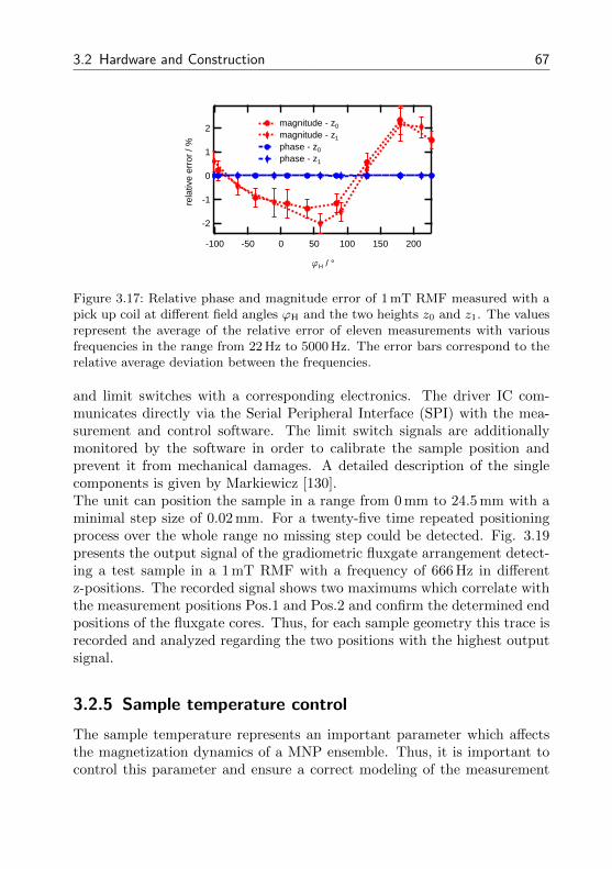
3.2 Hardware and Construction 67
2
1
0
-1
-2
rela
tive
erro
r / %
200150100500-50-100
fH / °
magnitude - z0
magnitude - z1
phase - z0
phase - z1
Figure 3.17: Relative phase and magnitude error of 1 mT RMF measured with apick up coil at different field angles ϕH and the two heights z0 and z1. The valuesrepresent the average of the relative error of eleven measurements with variousfrequencies in the range from 22 Hz to 5000 Hz. The error bars correspond to therelative average deviation between the frequencies.
and limit switches with a corresponding electronics. The driver IC com-municates directly via the Serial Peripheral Interface (SPI) with the mea-surement and control software. The limit switch signals are additionallymonitored by the software in order to calibrate the sample position andprevent it from mechanical damages. A detailed description of the singlecomponents is given by Markiewicz [130].The unit can position the sample in a range from 0 mm to 24.5 mm with aminimal step size of 0.02 mm. For a twenty-five time repeated positioningprocess over the whole range no missing step could be detected. Fig. 3.19presents the output signal of the gradiometric fluxgate arrangement detect-ing a test sample in a 1 mT RMF with a frequency of 666 Hz in differentz-positions. The recorded signal shows two maximums which correlate withthe measurement positions Pos.1 and Pos.2 and confirm the determined endpositions of the fluxgate cores. Thus, for each sample geometry this trace isrecorded and analyzed regarding the two positions with the highest outputsignal.
3.2.5 Sample temperature control
The sample temperature represents an important parameter which affectsthe magnetization dynamics of a MNP ensemble. Thus, it is important tocontrol this parameter and ensure a correct modeling of the measurement
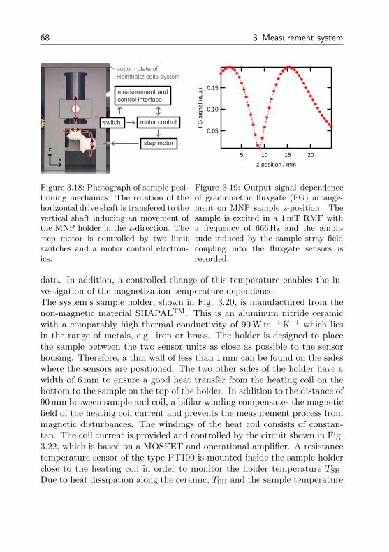
68 3 Measurement system
x
zstep motor
motor controlswitch
measurement and control interface
bottom plate ofHelmholtz coils system
Figure 3.18: Photograph of sample posi-tioning mechanics. The rotation of thehorizontal drive shaft is transfered to thevertical shaft inducing an movement ofthe MNP holder in the z-direction. Thestep motor is controlled by two limitswitches and a motor control electron-ics.
0.15
0.10
0.05
FG
sig
nal (
a.u.
)
2015105
z-position / mm
Figure 3.19: Output signal dependenceof gradiometric fluxgate (FG) arrange-ment on MNP sample z-position. Thesample is excited in a 1 mT RMF witha frequency of 666 Hz and the ampli-tude induced by the sample stray fieldcoupling into the fluxgate sensors isrecorded.
data. In addition, a controlled change of this temperature enables the in-vestigation of the magnetization temperature dependence.The system’s sample holder, shown in Fig. 3.20, is manufactured from thenon-magnetic material SHAPALTM. This is an aluminum nitride ceramicwith a comparably high thermal conductivity of 90 W m−1 K−1 which liesin the range of metals, e.g. iron or brass. The holder is designed to placethe sample between the two sensor units as close as possible to the sensorhousing. Therefore, a thin wall of less than 1 mm can be found on the sideswhere the sensors are positioned. The two other sides of the holder have awidth of 6 mm to ensure a good heat transfer from the heating coil on thebottom to the sample on the top of the holder. In addition to the distance of90 mm between sample and coil, a bifilar winding compensates the magneticfield of the heating coil current and prevents the measurement process frommagnetic disturbances. The windings of the heat coil consists of constan-tan. The coil current is provided and controlled by the circuit shown in Fig.3.22, which is based on a MOSFET and operational amplifier. A resistancetemperature sensor of the type PT100 is mounted inside the sample holderclose to the heating coil in order to monitor the holder temperature TSH.Due to heat dissipation along the ceramic, TSH and the sample temperature
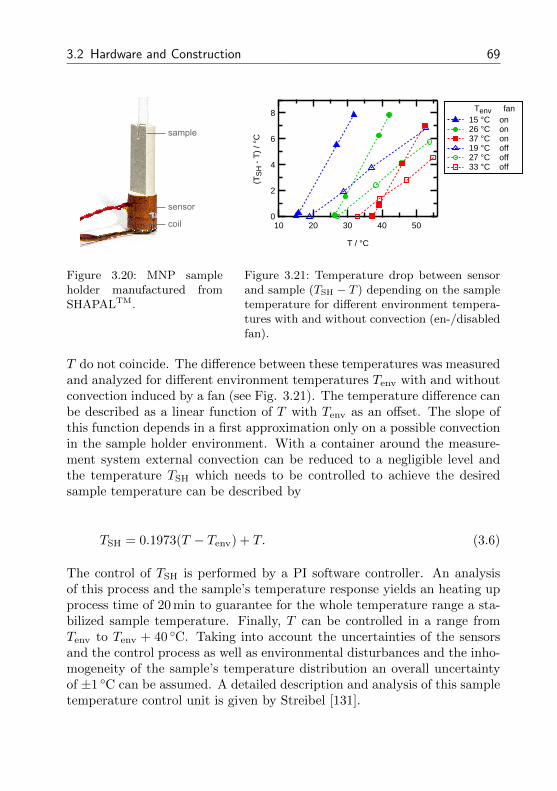
3.2 Hardware and Construction 69
sample
sensor
coil
Figure 3.20: MNP sampleholder manufactured fromSHAPALTM.
8
6
4
2
0
(TS
H -
T)
/ °C
5040302010
T / °C
Tenv fan 15 °C on 26 °C on 37 °C on 19 °C off 27 °C off 33 °C off
Figure 3.21: Temperature drop between sensorand sample (TSH − T ) depending on the sampletemperature for different environment tempera-tures with and without convection (en-/disabledfan).
T do not coincide. The difference between these temperatures was measuredand analyzed for different environment temperatures Tenv with and withoutconvection induced by a fan (see Fig. 3.21). The temperature difference canbe described as a linear function of T with Tenv as an offset. The slope ofthis function depends in a first approximation only on a possible convectionin the sample holder environment. With a container around the measure-ment system external convection can be reduced to a negligible level andthe temperature TSH which needs to be controlled to achieve the desiredsample temperature can be described by
TSH = 0.1973(T − Tenv) + T. (3.6)
The control of TSH is performed by a PI software controller. An analysisof this process and the sample’s temperature response yields an heating upprocess time of 20 min to guarantee for the whole temperature range a sta-bilized sample temperature. Finally, T can be controlled in a range fromTenv to Tenv + 40 C. Taking into account the uncertainties of the sensorsand the control process as well as environmental disturbances and the inho-mogeneity of the sample’s temperature distribution an overall uncertaintyof ±1 C can be assumed. A detailed description and analysis of this sampletemperature control unit is given by Streibel [131].
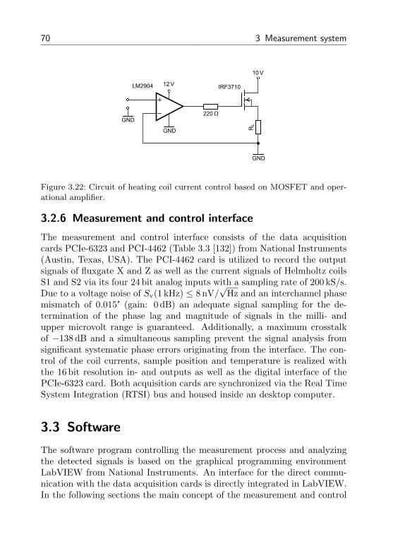
70 3 Measurement system
RL
10
W
LM2904
GND
IRF3710
GND
220
GND
V
12V
Figure 3.22: Circuit of heating coil current control based on MOSFET and oper-ational amplifier.
3.2.6 Measurement and control interface
The measurement and control interface consists of the data acquisitioncards PCIe-6323 and PCI-4462 (Table 3.3 [132]) from National Instruments(Austin, Texas, USA). The PCI-4462 card is utilized to record the outputsignals of fluxgate X and Z as well as the current signals of Helmholtz coilsS1 and S2 via its four 24 bit analog inputs with a sampling rate of 200 kS/s.Due to a voltage noise of Sv(1 kHz) ≤ 8 nV/
√Hz and an interchannel phase
mismatch of 0.015° (gain: 0 dB) an adequate signal sampling for the de-termination of the phase lag and magnitude of signals in the milli- andupper microvolt range is guaranteed. Additionally, a maximum crosstalkof −138 dB and a simultaneous sampling prevent the signal analysis fromsignificant systematic phase errors originating from the interface. The con-trol of the coil currents, sample position and temperature is realized withthe 16 bit resolution in- and outputs as well as the digital interface of thePCIe-6323 card. Both acquisition cards are synchronized via the Real TimeSystem Integration (RTSI) bus and housed inside an desktop computer.
3.3 Software
The software program controlling the measurement process and analyzingthe detected signals is based on the graphical programming environmentLabVIEW from National Instruments. An interface for the direct commu-nication with the data acquisition cards is directly integrated in LabVIEW.In the following sections the main concept of the measurement and control
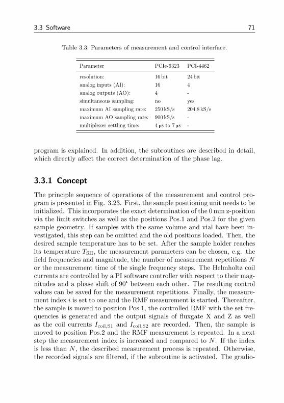
3.3 Software 71
Table 3.3: Parameters of measurement and control interface.
Parameter PCIe-6323 PCI-4462
resolution: 16 bit 24 bit
analog inputs (AI): 16 4
analog outputs (AO): 4 -
simultaneous sampling: no yes
maximum AI sampling rate: 250 kS/s 204.8 kS/s
maximum AO sampling rate: 900 kS/s -
multiplexer settling time: 4µs to 7 µs -
program is explained. In addition, the subroutines are described in detail,which directly affect the correct determination of the phase lag.
3.3.1 Concept
The principle sequence of operations of the measurement and control pro-gram is presented in Fig. 3.23. First, the sample positioning unit needs to beinitialized. This incorporates the exact determination of the 0 mm z-positionvia the limit switches as well as the positions Pos.1 and Pos.2 for the givensample geometry. If samples with the same volume and vial have been in-vestigated, this step can be omitted and the old positions loaded. Then, thedesired sample temperature has to be set. After the sample holder reachesits temperature TSH, the measurement parameters can be chosen, e.g. thefield frequencies and magnitude, the number of measurement repetitions Nor the measurement time of the single frequency steps. The Helmholtz coilcurrents are controlled by a PI software controller with respect to their mag-nitudes and a phase shift of 90° between each other. The resulting controlvalues can be saved for the measurement repetitions. Finally, the measure-ment index i is set to one and the RMF measurement is started. Thereafter,the sample is moved to position Pos.1, the controlled RMF with the set fre-quencies is generated and the output signals of fluxgate X and Z as wellas the coil currents Icoil,S1 and Icoil,S2 are recorded. Then, the sample ismoved to position Pos.2 and the RMF measurement is repeated. In a nextstep the measurement index is increased and compared to N . If the indexis less than N , the described measurement process is repeated. Otherwise,the recorded signals are filtered, if the subroutine is activated. The gradio-
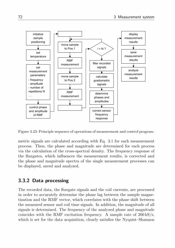
72 3 Measurement system
initializesample
positioning
settemperature
setmeasurementparameters:
- frequency- amplitude- number ofrepetitions N…
control phaseand amplitude
of RMF
move sampleto Pos.1
RMFmeasurement
move sampleto Pos.2
RMFmeasurement
i = N ?
filter recordedsignals
determinephases andamplitudes
correct sensorfrequencyresponse
calculategradiometric
signals
displaymeasurement
results
savemeasurement
results
analyzemeasurement
results
Figure 3.23: Principle sequence of operations of measurement and control program.
metric signals are calculated according with Eq. 3.1 for each measurementprocess. Then, the phase and magnitude are determined for each processvia the calculation of the cross-spectral density. The frequency response ofthe fluxgates, which influences the measurement results, is corrected andthe phase and magnitude spectra of the single measurement processes canbe displayed, saved and analyzed.
3.3.2 Data processing
The recorded data, the fluxgate signals and the coil currents, are processedin order to accurately determine the phase lag between the sample magne-tization and the RMF vector, which correlates with the phase shift betweenthe measured sensor and coil time signals. In addition, the magnitude of allsignals is determined. The frequency of the analyzed phase and magnitudecoincides with the RMF excitation frequency. A sample rate of 200 kS/s,which is set for the data acquisition, clearly satisfies the Nyquist–Shannon
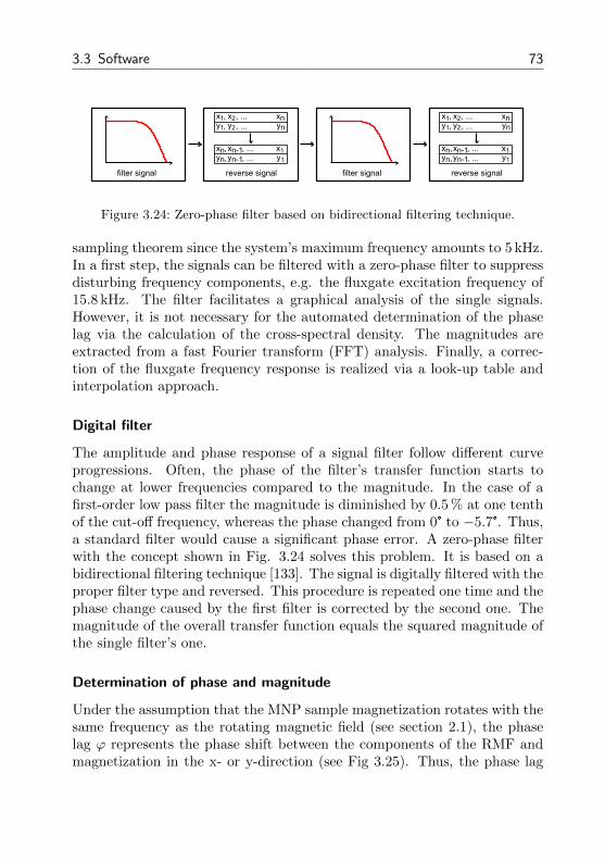
3.3 Software 73
filter signal
x1 x2 xny1 y2 yn
, , ..., , ...
, ...xn xn-1 x1yn yn-1 y1
,, , ...
reverse signal filter signal
x1 x2 xny1 y2 yn
, , ..., , ...
xn xn-1 x1yn yn-1 y1
, , ..., , ...
reverse signal
Figure 3.24: Zero-phase filter based on bidirectional filtering technique.
sampling theorem since the system’s maximum frequency amounts to 5 kHz.In a first step, the signals can be filtered with a zero-phase filter to suppressdisturbing frequency components, e.g. the fluxgate excitation frequency of15.8 kHz. The filter facilitates a graphical analysis of the single signals.However, it is not necessary for the automated determination of the phaselag via the calculation of the cross-spectral density. The magnitudes areextracted from a fast Fourier transform (FFT) analysis. Finally, a correc-tion of the fluxgate frequency response is realized via a look-up table andinterpolation approach.
Digital filter
The amplitude and phase response of a signal filter follow different curveprogressions. Often, the phase of the filter’s transfer function starts tochange at lower frequencies compared to the magnitude. In the case of afirst-order low pass filter the magnitude is diminished by 0.5 % at one tenthof the cut-off frequency, whereas the phase changed from 0° to −5.7°. Thus,a standard filter would cause a significant phase error. A zero-phase filterwith the concept shown in Fig. 3.24 solves this problem. It is based on abidirectional filtering technique [133]. The signal is digitally filtered with theproper filter type and reversed. This procedure is repeated one time and thephase change caused by the first filter is corrected by the second one. Themagnitude of the overall transfer function equals the squared magnitude ofthe single filter’s one.
Determination of phase and magnitude
Under the assumption that the MNP sample magnetization rotates with thesame frequency as the rotating magnetic field (see section 2.1), the phaselag ϕ represents the phase shift between the components of the RMF andmagnetization in the x- or y-direction (see Fig 3.25). Thus, the phase lag
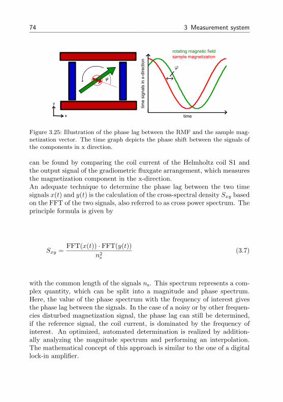
74 3 Measurement system
time
time
sign
als
in x
-dire
ctio
n
f
rotating magnetic fieldsample magnetization
x
y
f
Figure 3.25: Illustration of the phase lag between the RMF and the sample mag-netization vector. The time graph depicts the phase shift between the signals ofthe components in x direction.
can be found by comparing the coil current of the Helmholtz coil S1 andthe output signal of the gradiometric fluxgate arrangement, which measuresthe magnetization component in the x-direction.An adequate technique to determine the phase lag between the two timesignals x(t) and y(t) is the calculation of the cross-spectral density Sxy basedon the FFT of the two signals, also referred to as cross power spectrum. Theprinciple formula is given by
Sxy =FFT(x(t)) · FFT(y(t))
n2s
(3.7)
with the common length of the signals ns. This spectrum represents a com-plex quantity, which can be split into a magnitude and phase spectrum.Here, the value of the phase spectrum with the frequency of interest givesthe phase lag between the signals. In the case of a noisy or by other frequen-cies disturbed magnetization signal, the phase lag can still be determined,if the reference signal, the coil current, is dominated by the frequency ofinterest. An optimized, automated determination is realized by addition-ally analyzing the magnitude spectrum and performing an interpolation.The mathematical concept of this approach is similar to the one of a digitallock-in amplifier.
3.4 Performance 75
Frequency response correction
The significant phase change and magnitude drop in the fluxgate frequencyresponse necessitates a correction of the determined phase shifts betweenthe fluxgate and coil current signals and the measured sample flux densitymagnitudes. Hence, the frequency response of the single fluxgates X and Zand the gradiometric output were recorded (see Fig. 3.10) in a frequencyrange from 1 Hz to 10 kHz with a step size of 10 Hz and saved in a look-uptable. Here, the amplitude response is normalized to its DC value. Thefluxgate measurement of the MNP sample magnetization in a RMF withdifferent frequencies can be described by a multiplication of the sensor’scomplex transfer function and the magnetization dynamics in the frequency-domain. Thus, the correction of the phase and the magnitude is realized bya subtraction and a division, respectively. A correction of the measurementresults for all frequencies is based on a linear interpolation between the phaseand magnitude values of the recorded frequency response. The formula forthis calculation is given by
ycorr(f) = yi + fyi+1 − yifi+1 − fi
(3.8)
with
fi < f < fi+1. (3.9)
Here, ycorr represents the phase or magnitude value for the correction asa function of the frequency f . The corresponding values from the look-uptable are identified by the index i. The maximum error of this correctionprocedure without the linear interpolation amounts for the phase and mag-nitude to 0.4° and 0.2 %, respectively. Due to the 10 Hz steps of the recordedfrequency response, the linear interpolation reduces the errors at least by afactor of 10.
3.4 Performance
In this section, the performance of the measurement system is characterized.This includes a characterization of the system’s accuracy (systematic error)of the phase lag determination by performing measurements on different
76 3 Measurement system
calibration samples. In a next step the phase lag accuracy with respectto the minimal measurable magnetic flux density (particle concentration)based on random or at least non-correctable errors is discussed. Finally, anestimation of the system’s extended measurement uncertainty for a set ofdefined parameters is presented.
3.4.1 Systematic error
The calibration of the measurement system can be performed with a ref-erence sample whose magnetization dynamics is known for the given fre-quency range. Thus, paramagnetic materials can be applied which possessa zero phase and constant magnitude at audio frequencies. One appropri-ate paramagnetic material is dysprosium oxide (Dy2O3) which exhibits acomparably high susceptibility and was investigated as a calibration sam-ple for AC susceptometers [134]. Furthermore, small copper cylinders canbe utilized for the calibration. Their response to dynamic magnetic fieldsis based on eddy-current effects and can be simulated for the given cylin-der geometry and magnetic field. This was presented for AC susceptibilitymeasurements [135]. In addition, a MNP sample can be applied, whosecharacteristic frequency is significantly higher than the systems frequencyrange. This ensures a nearly zero phase and a constant magnitude.In this section, calibration measurements with two dysprosium oxide sam-ples and one single-core iron oxide nanoparticle sample are presented. Allsamples are prepared in glass vials and possess a volume of 150µL. Thedysprosium oxide is filled as a powder into the vials, balanced and sealedwith epoxy glue to prevent it from hydrating. The effective Dy2O3 densi-ties are 2.4566 g/cm3 (Dy2O3-1) and 2.339 g/cm3 (Dy2O3-2). The MNP isan iron oxide single-core particle with a core diameter of 15 nm (SHP15).Thus, it is dominated by the Neel relaxation process and possesses a char-acteristic frequency larger than 1 MHz [136]. The iron concentration of theMNP sample amounts to 5 g/L. The parameters of the RMF calibrationmeasurements with a magnitude of 1 mT are defined as following:
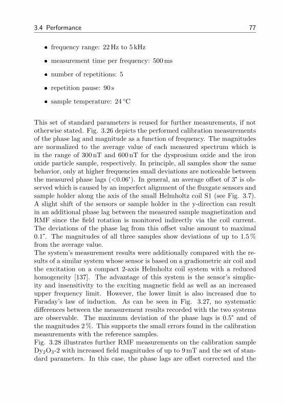
3.4 Performance 77
frequency range: 22 Hz to 5 kHz
measurement time per frequency: 500 ms
number of repetitions: 5
repetition pause: 90 s
sample temperature: 24 C
This set of standard parameters is reused for further measurements, if nototherwise stated. Fig. 3.26 depicts the performed calibration measurementsof the phase lag and magnitude as a function of frequency. The magnitudesare normalized to the average value of each measured spectrum which isin the range of 300 nT and 600 nT for the dysprosium oxide and the ironoxide particle sample, respectively. In principle, all samples show the samebehavior, only at higher frequencies small deviations are noticeable betweenthe measured phase lags (<0.06°). In general, an average offset of 3° is ob-served which is caused by an imperfect alignment of the fluxgate sensors andsample holder along the axis of the small Helmholtz coil S1 (see Fig. 3.7).A slight shift of the sensors or sample holder in the y-direction can resultin an additional phase lag between the measured sample magnetization andRMF since the field rotation is monitored indirectly via the coil current.The deviations of the phase lag from this offset value amount to maximal0.1°. The magnitudes of all three samples show deviations of up to 1.5 %from the average value.The system’s measurement results were additionally compared with the re-sults of a similar system whose sensor is based on a gradiometric air coil andthe excitation on a compact 2-axis Helmholtz coil system with a reducedhomogeneity [137]. The advantage of this system is the sensor’s simplic-ity and insensitivity to the exciting magnetic field as well as an increasedupper frequency limit. However, the lower limit is also increased due toFaraday’s law of induction. As can be seen in Fig. 3.27, no systematicdifferences between the measurement results recorded with the two systemsare observable. The maximum deviation of the phase lags is 0.5° and ofthe magnitudes 2 %. This supports the small errors found in the calibrationmeasurements with the reference samples.Fig. 3.28 illustrates further RMF measurements on the calibration sampleDy2O3-2 with increased field magnitudes of up to 9 mT and the set of stan-dard parameters. In this case, the phase lags are offset corrected and the
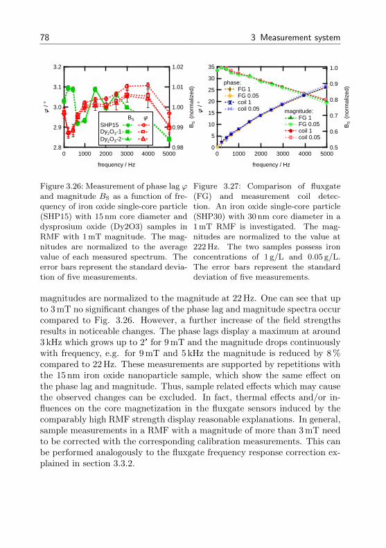
78 3 Measurement system
1.02
1.01
1.00
0.99
0.98
BS
(no
rmal
ized
)
500040003000200010000
frequency / Hz
3.2
3.1
3.0
2.9
2.8
f /
°
BS fSHP15 Dy2O3-1 Dy2O3-2
Figure 3.26: Measurement of phase lag ϕand magnitude BS as a function of fre-quency of iron oxide single-core particle(SHP15) with 15 nm core diameter anddysprosium oxide (Dy2O3) samples inRMF with 1 mT magnitude. The mag-nitudes are normalized to the averagevalue of each measured spectrum. Theerror bars represent the standard devia-tion of five measurements.
1.0
0.9
0.8
0.7
0.6
0.5
BS
(no
rmal
ized
)
500040003000200010000
frequency / Hz
35
30
25
20
15
10
5
0
f /
°
phase: FG 1 FG 0.05 coil 1 coil 0.05
magnitude:
FG 1 FG 0.05 coil 1 coil 0.05
Figure 3.27: Comparison of fluxgate(FG) and measurement coil detec-tion. An iron oxide single-core particle(SHP30) with 30 nm core diameter in a1 mT RMF is investigated. The mag-nitudes are normalized to the value at222 Hz. The two samples possess ironconcentrations of 1 g/L and 0.05 g/L.The error bars represent the standarddeviation of five measurements.
magnitudes are normalized to the magnitude at 22 Hz. One can see that upto 3 mT no significant changes of the phase lag and magnitude spectra occurcompared to Fig. 3.26. However, a further increase of the field strengthsresults in noticeable changes. The phase lags display a maximum at around3 kHz which grows up to 2° for 9 mT and the magnitude drops continuouslywith frequency, e.g. for 9 mT and 5 kHz the magnitude is reduced by 8 %compared to 22 Hz. These measurements are supported by repetitions withthe 15 nm iron oxide nanoparticle sample, which show the same effect onthe phase lag and magnitude. Thus, sample related effects which may causethe observed changes can be excluded. In fact, thermal effects and/or in-fluences on the core magnetization in the fluxgate sensors induced by thecomparably high RMF strength display reasonable explanations. In general,sample measurements in a RMF with a magnitude of more than 3 mT needto be corrected with the corresponding calibration measurements. This canbe performed analogously to the fluxgate frequency response correction ex-plained in section 3.3.2.
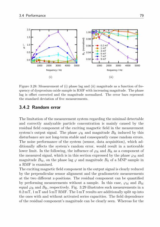
3.4 Performance 79
2.0
1.5
1.0
0.5
0.0
f /
°
50004000300020001000
frequency / Hz
(i)
1.00
0.98
0.96
0.94
0.92
BS
(no
rmal
ized
)
50004000300020001000
frequency / Hz
0.2 mT 1 mT 3 mT 5 mT 7 mT 9 mT
(ii)
Figure 3.28: Measurement of (i) phase lag and (ii) magnitude as a function of fre-quency of dysprosium oxide sample in RMF with increasing magnitude. The phaselag is offset corrected and the magnitude normalized. The error bars representthe standard deviation of five measurements.
3.4.2 Random error
The limitation of the measurement system regarding the minimal detectableand correctly analyzable particle concentration is mainly caused by theresidual field component of the exciting magnetic field in the measurementsystem’s output signal. The phase ϕR and magnitude BR induced by thisdisturbance are not long-term stable and consequently cause random errors.The noise performance of the system (sensor, data acquisition), which ad-ditionally affects the system’s random error, would result in a noticeablelower limit. In the following, the influence of ϕR and BR as a component ofthe measured signal, which is in this section expressed by the phase ϕM andmagnitude BM, on the phase lag ϕ and magnitude BS of a MNP sample ina RMF is examined.The exciting magnetic field component in the output signal is clearly reducedby the perpendicular sensor alignment and the gradiometric measurementsat the two different z-positions. The residual component can be quantifiedby performing measurements without a sample. In this case, ϕM and BM
equal ϕR and BR, respectively. Fig. 3.29 illustrates such measurements in a0.2 mT, 1 mT and 5 mT RMF. The 5 mT results are additionally split up intothe ones with and without activated series capacities. The field dependenceof the residual component’s magnitude can be clearly seen. Whereas for the
80 3 Measurement system
0.2 mT RMF, magnitudes in the range of 0.1 nT to 0.15 nT are present, forthe 1 mT RMF the magnitudes are increased by a factor of five, which ac-cords with the ratio of the excitation field strengths. For the 5 mT RMF theresidual component’s magnitudes are again enlarged by the correspondingratio of the excitation field strengths, however, an influence of the sampletemperature control and the sample positioning unit can be observed. Adeactivation of these units results in a reduced residual component. Themeasurements with a 5 mT magnitude and frequencies above 1 kHz (acti-vated series capacities) possess further increased magnitudes, which can beminimized by an extension of the pause between the measurement repeti-tions to 180 s. This effect can be explained by thermal drifts of the fluxgatesensors induced by high field magnitudes and frequencies. The field de-pendence of the residual RMF component is nearly compensated when ameasurement on a MNP sample is performed whose magnetization follows- for the given field strength - the linear regime of the Langevin function.In this case, the relation of BR to Bs remains constant.In order to estimate the influence of the residual RMF component on theaccuracy of the measurement results, the difference between ϕM and ϕ andthe relation of BM to BS are calculated as a function of ϕ − ϕR varyingfrom 0° to 360° and BR/BS ranging from 0 to 0.1 (see Fig. 3.30). The cor-responding formulas are given in appendix A.1. In the case of BR/BS = 0.1and phase differences ϕ − ϕR of 90° or 270°, phase errors of up to 5° oc-cur. Thus, for the RMF measurements the condition BR/BS < 0.01 shouldbe met. With this condition the resulting phase and magnitude errors aresmaller than 0.5° and 0.5 %, respectively, for all values of ϕ− ϕR.RMF measurements on two MNP concentration series support the foundlimitation of the measurement system. Each concentration series consistsof several samples with one MNP type and a decreasing iron concentra-tion. The SHP30 particles possess single iron oxide cores with a diameter of30 nm. The BNF80 MNP represents an iron oxide multi-core particle withan approximately hydrodynamic diameter of 80 nm. The single iron con-centrations as well as the amount of iron (Fe) per sample are listed in Table3.4. The measured phase lags ϕM and magnitudes BM as a function of fre-quency follow the discussed arc tangent and cosine dependence, respectively.Further information on the particle parameters and particle-specific mea-surement results can be found in chapter 4. The RMF magnitude amountsto 1 mT and the standard measurement parameters (see section 3.4.1) areapplied.
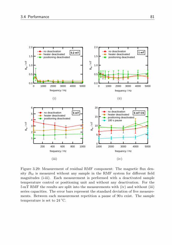
3.4 Performance 81
2.0
1.5
1.0
0.5
0.0
BM
/ n
T
500040003000200010000
frequency / Hz
no deactivation heater deactivated positioning deactivated
0.2 mT
(i)
2.0
1.5
1.0
0.5
0.0
BM
/ n
T
500040003000200010000
frequency / Hz
no deactivation heater deactivated positioning deactivated
1 mT
(ii)
6
5
4
3
2
1
BM
/ n
T
1000800600400200
frequency / Hz
no deactivation heater deactivated positioning deactivated
5 mT
(iii)
20
15
10
5
0
BM
/ n
T
50004000300020001000
frequency / Hz
no deactivation heater deactivated positioning deactivated 180 s pause
5 mT CS
(iv)
Figure 3.29: Measurement of residual RMF component: The magnetic flux den-sity BM is measured without any sample in the RMF system for different fieldmagnitudes (i-iii). Each measurement is performed with a deactivated sampletemperature control or positioning unit and without any deactivation. For the5 mT RMF the results are split into the measurements with (iv) and without (iii)series capacities. The error bars represent the standard deviation of five measure-ments. Between each measurement repetition a pause of 90 s exist. The sampletemperature is set to 24 C.
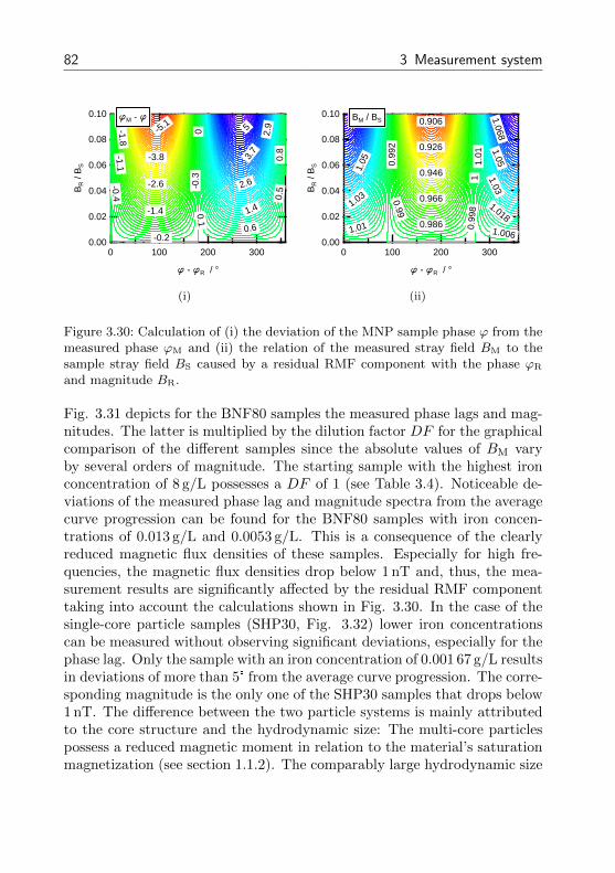
82 3 Measurement system
0.10
0.08
0.06
0.04
0.02
0.00
BR /
BS
3002001000
f - fR / °
5
3.7
2
.9
2.6
1.4
0.8
0.6
0.5
0.1
0
-0.2
-0.
3
-0.4 -1.1
-1.4
-1.8
-2.6
-3.8
-5.1 fM - f
(i)
0.10
0.08
0.06
0.04
0.02
0.00
BR /
BS
3002001000
f - fR / °
1.068
1.0
5
1.05
1.03
1.03
1.018 1.01
1.0
1
1.006
1
0.9
98
0.9
92
0.99 0.986
0.966
0.946
0.926
0.906 BM / BS
(ii)
Figure 3.30: Calculation of (i) the deviation of the MNP sample phase ϕ from themeasured phase ϕM and (ii) the relation of the measured stray field BM to thesample stray field BS caused by a residual RMF component with the phase ϕR
and magnitude BR.
Fig. 3.31 depicts for the BNF80 samples the measured phase lags and mag-nitudes. The latter is multiplied by the dilution factor DF for the graphicalcomparison of the different samples since the absolute values of BM varyby several orders of magnitude. The starting sample with the highest ironconcentration of 8 g/L possesses a DF of 1 (see Table 3.4). Noticeable de-viations of the measured phase lag and magnitude spectra from the averagecurve progression can be found for the BNF80 samples with iron concen-trations of 0.013 g/L and 0.0053 g/L. This is a consequence of the clearlyreduced magnetic flux densities of these samples. Especially for high fre-quencies, the magnetic flux densities drop below 1 nT and, thus, the mea-surement results are significantly affected by the residual RMF componenttaking into account the calculations shown in Fig. 3.30. In the case of thesingle-core particle samples (SHP30, Fig. 3.32) lower iron concentrationscan be measured without observing significant deviations, especially for thephase lag. Only the sample with an iron concentration of 0.001 67 g/L resultsin deviations of more than 5° from the average curve progression. The corre-sponding magnitude is the only one of the SHP30 samples that drops below1 nT. The difference between the two particle systems is mainly attributedto the core structure and the hydrodynamic size: The multi-core particlespossess a reduced magnetic moment in relation to the material’s saturationmagnetization (see section 1.1.2). The comparably large hydrodynamic size
3.4 Performance 83
results in a clear drop of the magnitude in the observed frequency range.Thus, lower BM values are measured for BNF80 although the iron concen-tration is the same.Table 3.4 additionally presents the measured phase lags and magnitudes ofthe SHP30 and BNF80 samples for a RMF frequency of 1 kHz. The meanvalues and standard deviations are based on ten measurement repetitions.The deviation of the mean values of the samples with the lower iron concen-trations from the ones with higher iron concentrations reflects the impactof the residual field component. A correction of this effect is hard to realizesince the magnitude and especially the phase of the residual RMF com-ponent possess no long-term stability. In contrast, the standard deviationrepresents the random errors caused by the measurement hardware, e.g.the analog-to-digital converter, the magnetic field sensor and the mechan-ics, as well as environmental effects, e.g. the temperature or electromagneticdisturbances. The sample preparation and manual positioning of the sam-ple in the system is not included because for each measurement repetitionthe same sample is automatically positioned. A detailed description of theinfluence of the sample preparation on the measurement uncertainty of afluxgate based MRX system is given by Heim [83]. These results are alsovalid for the RMF measurement system since an analog sensor arrangementand similar MNP samples are deployed. The standard deviations listed inTable 3.4 clearly indicate that the measurement uncertainty of the phase lag,which can be calculated based on the standard deviations [138], increaseswith decreasing magnetic flux density. The relative uncertainty of BM in-creases as well, which is identified by the relation of the standard deviationto the mean value. Further measurement values of the concentration seriessamples for frequencies of 222 Hz and 5 kHz are presented in appendix A.2supporting this discussion.An exact specification of the RMF system’s measurement uncertainty pri-marily of the determined phase lag and also of the magnitude is hard torealize. The so-called bottom-up approach based on the law of error prop-agation [138] requires a reliable equation describing the relation of the sys-tem’s output quantity to all input parameters, including mechanical driftsand environmental disturbances. As shown by Heim for the fluxgate-basedMRX system [83], this bottom-up approach does not satisfy the complex-ity of such an measurement process with multi-modal input parameters.In this context, the Research Training Group 1952/1 ”Metrology for Com-plex Nanosystems” funded by the Deutsche Forschungsgemeinschaft is men-tioned, which actually deals with the investigation of the uncertainty deter-
84 3 Measurement system
mination of complex nanosystems with multi-modal input parameters.An uncertainty determination based on measurement repetitions (top-downapproach) results only in an estimate of a general valid measurement un-certainty because the phase and magnitude as well as the non-correctableinfluence of the residual RMF component depend strongly on the investi-gated sample and affect each other. In order to specify at least a maximummeasurement uncertainty for the phase lag determination the following con-ditions are defined:
particle temperature T between 20 C and 25 C
environment temperature Tenv between 20 C and 25 C
1 mT RMF with set of standard parameters (no repetitions)
relation BR/BS < 0.01
In this case, the combined measurement uncertainty uc results in 0.375°based on following single standard uncertainties:
calibration sample measurement (rectangular distribution): ucal =0.1°/
√3 = 0.058°
simulation of the maximal error caused by the residual RMF compo-nent for BR/BS < 0.01 (rectangular distribution): ures = 0.5°/
√3 =
0.289°
estimated standard deviation for BR/BS ≈ 0.01 based on theconcentration series measurements (t-distribution, 95.45 %): ucs =0.2°2.32/2 = 0.232°
Finally, the maximal expanded uncertainty ue with a coverage factor of 2based on a normal distribution with a probability of 95.45 % amounts to0.75° with respect to the defined conditions.
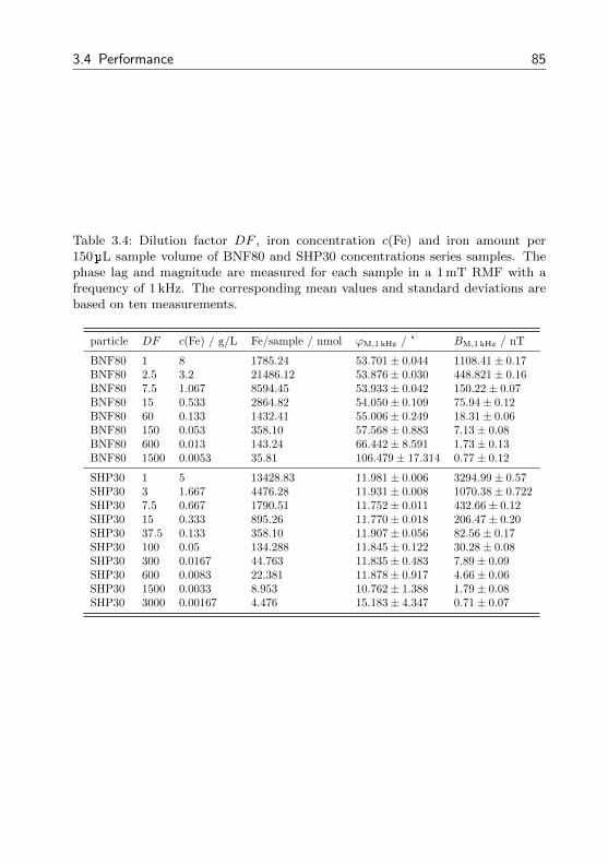
3.4 Performance 85
Table 3.4: Dilution factor DF , iron concentration c(Fe) and iron amount per150µL sample volume of BNF80 and SHP30 concentrations series samples. Thephase lag and magnitude are measured for each sample in a 1 mT RMF with afrequency of 1 kHz. The corresponding mean values and standard deviations arebased on ten measurements.
particle DF c(Fe) / g/L Fe/sample / nmol ϕM,1 kHz / ° BM,1 kHz / nT
BNF80 1 8 1785.24 53.701± 0.044 1108.41± 0.17BNF80 2.5 3.2 21486.12 53.876± 0.030 448.821± 0.16BNF80 7.5 1.067 8594.45 53.933± 0.042 150.22± 0.07BNF80 15 0.533 2864.82 54.050± 0.109 75.94± 0.12BNF80 60 0.133 1432.41 55.006± 0.249 18.31± 0.06BNF80 150 0.053 358.10 57.568± 0.883 7.13± 0.08BNF80 600 0.013 143.24 66.442± 8.591 1.73± 0.13BNF80 1500 0.0053 35.81 106.479± 17.314 0.77± 0.12
SHP30 1 5 13428.83 11.981± 0.006 3294.99± 0.57SHP30 3 1.667 4476.28 11.931± 0.008 1070.38± 0.722SHP30 7.5 0.667 1790.51 11.752± 0.011 432.66± 0.12SHP30 15 0.333 895.26 11.770± 0.018 206.47± 0.20SHP30 37.5 0.133 358.10 11.907± 0.056 82.56± 0.17SHP30 100 0.05 134.288 11.845± 0.122 30.28± 0.08SHP30 300 0.0167 44.763 11.835± 0.483 7.89± 0.09SHP30 600 0.0083 22.381 11.878± 0.917 4.66± 0.06SHP30 1500 0.0033 8.953 10.762± 1.388 1.79± 0.08SHP30 3000 0.00167 4.476 15.183± 4.347 0.71± 0.07

86 3 Measurement system
140
120
100
80
60
40
20
f /
°
500040003000200010000
frequency / Hz
BNF80
(i)
2.0
1.5
1.0
0.5
BS•D
F / m
T
500040003000200010000
frequency / Hz
c(Fe) / mg/ml: 8 3.2 1.067 0.533 0.133 0.053 0.013 0.005
(ii)
Figure 3.31: Measurement of phase lag (i) and magnitude (ii) as a function offrequency of iron oxide multi-core particle samples with decreasing iron concen-trations in RMF with 1 mT magnitude. The phase lag ϕM is offset corrected andthe magnitude BM multiplied by the dilution factor DF . The approximate corediameter of the MNP (BNF80) amounts to 80 nm. The error bars represent thestandard deviation of ten measurements.
50
40
30
20
10
0
f /
°
500040003000200010000
frequency / Hz
c(Fe) / mg/ml: 5 1.667 0.667 0.333 0.133 0.05 0.017 0.008 0.003 0.002
(i)
3.4
3.2
3.0
2.8
2.6
2.4
2.2
2.0
1.8
BS•D
F / m
T
500040003000200010000
frequency / Hz
SHP30
(ii)
Figure 3.32: Measurement of phase lag (i) and magnitude (ii) as a function offrequency of iron oxide single-core particle samples with decreasing iron concen-trations in RMF with 1 mT magnitude. The phase lag ϕM is offset corrected andthe magnitude BM multiplied by the dilution factor DF . The core diameter of theMNP (SHP30) amounts to 30 nm. The error bars represent the standard deviationof ten measurements.
87
4 Results and discussion
The dynamic response of magnetic nanoparticles to rotating magnetic fieldsdepends on various parameters. This chapter will introduce different nanopar-ticle systems which differ in their core and hydrodynamic size as well as theirmaterial composition. The influence of their parameters on the dynamicresponse is explained with measurements of the phase lag and comparedwith simulations and supporting independent characterization techniques.Finally, an outlook is given on the utilization of these dynamics for therealization of homogeneous bioassay applications.
4.1 Nanoparticle systems
The main difference between the nanoparticle systems are their materialcomposition and the core and hydrodynamic size in relation to the shape.Furthermore, two different core types depending on the synthesis are es-tablished: The single- and the multi-core. Here, measurements on differentspherical and rod-shaped single- (SC) and multi-core (MC) nanoparticlesare presented. Table 4.1 gives an overview about the applied particles andtheir producers.The MNP type with the code ALP represents a single-core particle basedon an iron oxide composition. The core diameter of the particles investi-gated in this work ranges from 12 nm to 25 nm. They are suspended in anon-polar solvent, e.g. chloroform, and possess an oleic acid shell of 2 nm to4 nm thickness. The particles are provided by the Institut fur ElektrischeMesstechnik and Grundlagen der Elektrotechnik at Technische UniversitatBraunschweig (Braunschweig, Germany) and were subject to an elaboratedevelopment and investigation process, e.g. for further biomedical applica-tions they were transfered to water via a PEGylation process and function-alized with antibodies [37].A commercially available product is the particle type with the code BNF.It is manufactured by micromod Partikeltechnologie GmbH (Rostock, Ger-many) and distributed as a bionized nanoferrite particle with the product
88 4 Results and discussion
name BNF-Starch. The particle core consists of several single iron oxidecrystals (dc : 10 nm to 20 nm) embedded in hydroxyethyl starch. Thus,BNF represents a polydisperse multi-core particle with average hydrody-namic diameters of 80 nm and 100 nm suspended in water [139]. For a TEMimage of the 80 nm particle type see Fig. 4.1 (ii). Different functionaliza-tions of the BNF particle are available, e.g. with streptavidin.The particle type with the code ENP is an iron oxide MNP provided bythe Department of Electrical Engineering of Kyushu University (Fukuoka,Japan). Its single crystals with an average core diameter of 30 nm and apolymer shell aggregated during the synthesis process forming clusters witha mean hydrodynamic diameter of more than 100 nm [140]. Thus, the par-ticle can be treated as a multi-core system. The particles are suspended inwater.The MRI contrast agent FeraSpin R (FSR) manufactured by nanoPETPharma GmbH (Berlin, Germany) represents another iron oxide multi-coreparticle with a broad size distribution. Its mean hydrodynamic diameteramounts to 60 nm, whereas the single crystallite diameter ranges from 5 nmto 8 nm. The particles are dissolved in an aqueous medium and were addi-tionally functionalized with streptavidin.A rod-shaped particle type (Fig. 4.1 (iii)) synthesized from nickel is iden-tified with the code NNR. It was manufactured and provided by the divi-sion Experimentalphysik at Universitat des Saarlandes (Saarbrucken, Ger-many). The approximate core length and diameter of the received batch are271 nm and 19 nm, respectively. These so-called nanorods are stabilized bya polyvinylpyrrolidone (PVP) layer of several nanometer thickness whichenables a single particle dispersion in an aqueous solution. This particletype was subject to investigations of its rotational dynamics with an opticalmeasurement setup [95, 141].The MNP type with the code SHP represents an iron oxide single-core par-ticle from Ocean NanoTech (San Diego, CA, USA). It is distributed withcore diameters ranging from 5 nm to 40 nm [142] and consequently differ-ent iron oxide phase compositions of the particle core due to the synthesisprocess. A polymer coating (4 nm to 5 nm layer) stabilizes the particle indifferent media, e.g. aqueous and buffer solutions. For a TEM image of the30 nm core diameter particle see Fig. 4.1 (i). These MNPs are additionallyavailable with different functionalizations, e.g. with streptavidin or proteinG.The particle suspensions with the codes BNF, ENP and NNR are clearlydominated by the Brownian relaxation process, thus called Brownian par-
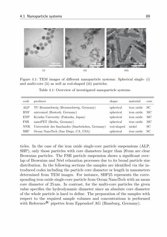
4.1 Nanoparticle systems 89
100 nm 100 nm 100 nm
(iii)(i) (ii)
Figure 4.1: TEM images of different nanoparticle systems: Spherical single- (i)and multi-core (ii) as well as rod-shaped (iii) particles.
Table 4.1: Overview of investigated nanoparticle systems.
code producer shape material core
ALP TU Braunschweig (Braunschweig, Germany) spherical iron oxide SC
BNF micromod (Rostock, Germany) spherical iron oxide MC
ENP Kyushu University (Fukuoka, Japan) spherical iron oxide MC
FSR nanoPET (Berlin, Germany) spherical iron oxide MC
NNR Universitat des Saarlandes (Saarbrucken, Germany) rod-shaped nickel SC
SHP Ocean NanoTech (San Diego, CA, USA) spherical iron oxide SC
ticles. In the case of the iron oxide single-core particle suspensions (ALP,SHP), only those particles with core diameters larger than 20 nm are clearBrownian particles. The FSR particle suspension shows a significant over-lap of Brownian and Neel relaxation processes due to its broad particle sizedistribution. In the following sections the samples are identified via the in-troduced codes including the particle core diameter or length in nanometersdetermined from TEM images. For instance, SHP25 represents the corre-sponding iron oxide single-core particle from Ocean NanoTech with an meancore diameter of 25 nm. In contrast, for the multi-core particles the givenvalue specifies the hydrodynamic diameter since an absolute core diameterof the whole particle is hard to define. The preparation of the samples withrespect to the required sample volumes and concentrations is performedwith Reference® pipettes from Eppendorf AG (Hamburg, Germany).
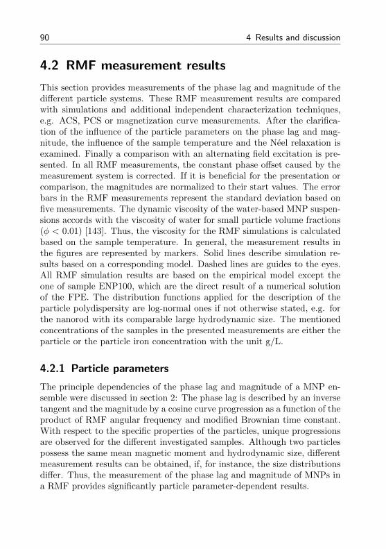
90 4 Results and discussion
4.2 RMF measurement results
This section provides measurements of the phase lag and magnitude of thedifferent particle systems. These RMF measurement results are comparedwith simulations and additional independent characterization techniques,e.g. ACS, PCS or magnetization curve measurements. After the clarifica-tion of the influence of the particle parameters on the phase lag and mag-nitude, the influence of the sample temperature and the Neel relaxation isexamined. Finally a comparison with an alternating field excitation is pre-sented. In all RMF measurements, the constant phase offset caused by themeasurement system is corrected. If it is beneficial for the presentation orcomparison, the magnitudes are normalized to their start values. The errorbars in the RMF measurements represent the standard deviation based onfive measurements. The dynamic viscosity of the water-based MNP suspen-sions accords with the viscosity of water for small particle volume fractions(φ < 0.01) [143]. Thus, the viscosity for the RMF simulations is calculatedbased on the sample temperature. In general, the measurement results inthe figures are represented by markers. Solid lines describe simulation re-sults based on a corresponding model. Dashed lines are guides to the eyes.All RMF simulation results are based on the empirical model except theone of sample ENP100, which are the direct result of a numerical solutionof the FPE. The distribution functions applied for the description of theparticle polydispersity are log-normal ones if not otherwise stated, e.g. forthe nanorod with its comparable large hydrodynamic size. The mentionedconcentrations of the samples in the presented measurements are either theparticle or the particle iron concentration with the unit g/L.
4.2.1 Particle parameters
The principle dependencies of the phase lag and magnitude of a MNP en-semble were discussed in section 2: The phase lag is described by an inversetangent and the magnitude by a cosine curve progression as a function of theproduct of RMF angular frequency and modified Brownian time constant.With respect to the specific properties of the particles, unique progressionsare observed for the different investigated samples. Although two particlespossess the same mean magnetic moment and hydrodynamic size, differentmeasurement results can be obtained, if, for instance, the size distributionsdiffer. Thus, the measurement of the phase lag and magnitude of MNPs ina RMF provides significantly particle parameter-dependent results.
4.2 RMF measurement results 91
Particle system comparison
The phase lag and magnitude measurements of the different particle systemsin a 1 mT RMF are presented in Fig. 4.2. The effect of the different hydro-dynamic sizes is clearly discernible. The nanorod sample NNR271 possessesthe quickest phase rise, followed by the multi-core particles BNF100 andENP100. The samples SHP40, ALP25 and ALP12 with the single-core par-ticles exhibit a clearly reduced increase of the phase lag. Especially, thephase lag of ALP12 rises only up to 2°. However, this is not a result ofits small hydrodynamic size. ALP12 is dominated by the Neel relaxationdue to its core diameter of only 12 nm. The phase lag of multi-core particleFSR60 shows interestingly only a small maximum phase lag and crosses theone of SHP40. The corresponding magnitudes are normalized to the mag-nitude measured at 22 Hz. They show an analog behavior compared to thephase lags. The particle with the smallest hydrodynamic size possesses theslightest drop of the magnitude.The principle dependencies of the phase lag and magnitude are apparent byobserving these measurement results and coincide with the theory. How-ever, some observations need to be clarified in more detail: No measuredphase lag reaches 90°. The phase lags of BNF100 and ENP100 cross eachother and sample FSR60 exhibits for its hydrodynamic size a comparableweak phase lag rise and magnitude drop. These findings are a direct resultof the hydrodynamic size distribution, which additionally affects the curveprogression [116], and the presence of small fast Neel particles in the solu-tion with a significantly higher characteristic frequency. In the case of themulti-core particle samples the amount of these superparamagnetic MNPsincreases from sample ENP100 to BNF100 and finally FSR60. The corre-sponding k factors (see section 2.6) amount to 0.016 and 0.0375 for ENP100and BNF100, respectively, for FSR60 it can not be determined due to thebroad size distribution and the resulting overlap of the Brownian and theNeel particle contribution in the measured ACS. In contrast, the phase lagof NNR almost saturates at 90°. This sample is totally dominated by theBrownian relaxation process due to the pronounced shape anisotropy of thenanorods and the corresponding huge anisotropy energy barrier. The phaselag of the ALP25 sample is besides its hydrodynamic size additionally re-duced by its carrier liquid. The viscosity of chloroform is approximatelyhalf the value of the viscosity of water.

92 4 Results and discussion
80
60
40
20
0
f /
°
500040003000200010000
frequency / Hz
ALP12, dh = 17 nm ALP25, dh = 30 nm BNF100, dh = 118 nm ENP100, dh = 105 nm FSR60, dh = 71 nm NNR271 SHP40, dh = 44 nm
(i)
1.0
0.8
0.6
0.4
0.2
0.0
BS (
norm
aliz
ed)
500040003000200010000
frequency / Hz
ALP12, dh = 17 nm ALP25, dh = 30 nm BNF100, dh = 118 nm ENP100, dh = 105 nm FSR60, dh = 71 nm NNR271 SHP40, dh = 44 nm
(ii)
Figure 4.2: Measured phase lags (i) and magnitudes (ii) as a function of fre-quency of MNPs with different shapes and hydrodynamic sizes in 1 mT RMF.The single magnitudes are normalized to the magnitude at 22 Hz. The approxi-mately mean hydrodynamic diameters were determined for the spherical particlesby DLS/PCCS measurements. The sample temperatures range between 294 Kand 298 K. All samples are dissolved in an aqueous solution, except the ALPparticles which are dissolved in chloroform.
4.2 RMF measurement results 93
Comparative simulations and measurements
In this section, the field-dependent RMF measurements of the ENP100,SHP25 and SHP40 sample are compared with simulation results based onparticle parameters (magnetic moment, hydrodynamic size) which are de-termined with additional measurement techniques. In addition, the field-dependent RMF measurements of sample BNF80, BNF100 and NNR271are presented and a fit with the RMF model is applied.The average hydrodynamic diameter of the ENP100 particles was deter-mined by DLS measurements and amounts 105 nm [140]. However, thismeasurement was not performed in a temporal proximity to the RMF mea-surements and it did not provide a reliable size distribution. Hence, thecomplex AC susceptibility of the sample was measured and analyzed withthe corresponding model (section 1.2.4) incorporating a log-normal size dis-tribution and taking into account the presence of the small Neel particlesin solution [107]. Fig. 4.3 presents this measurement in comparison tothe simulation results. The median hydrodynamic diameter dh and thestandard deviation σh amount to 120 nm and 0.26, respectively. The kfactor was found to be 0.016. The saturation magnetization of 270 kA/mwas determined with a vibrating sample magnetometer and a dried MNPpowder sample. Describing the multi-core by a single sphere, a size distri-bution of the corresponding effective core diameter was estimated via themeasurement of the sample’s magnetization curve [107]. The determineddistribution yields a median core diameter dc and a corresponding standarddeviation σc of 48 nm and 0.01, respectively. Thus, the mean magnetic mo-ment of the ENP100 particle is around 15.6 aAm2. With these parameters,the response to a RMF with magnitudes of 1 mT, 2.5 mT, 5 mT and 7.5 mTis simulated and compared with the measurements on the ENP100 sample.The simulation results are based on a numerical solution of the FPE [107].As one can see in Fig. 4.4, a good match between the simulations and mea-surements is achieved. In addition, the influence of the field strength on thephase lag and magnitude is illustrated in the results. An increase of the fieldstrength causes a reduced rise of the phase lag and drop of the magnitude.Thus, a spreading of the measured curve progressions with the field strengthcan be observed which is mainly affected by the particle magnetic moment.The measured phase lags and magnitudes of the SHP25 and SHP40 sam-
ple in a 1 mT and 5 mT RMF are depicted in Fig. 4.5. In contrast toENP100, the maximum phase lag is not reached in the observed frequencyrange, which is attributed to the smaller particle hydrodynamic size. Fur-
94 4 Results and discussion
1.0
0.8
0.6
0.4
0.2
0.0
c '
/ c0 ,
c ''
/ c
0
0.01 0.1 1 10 100 1000
frequency / kHz
c' c''
(i)
0.08
0.06
0.04
0.02
0.00
c '
/ c0 ,
c ''
/ c
0
12 4 6 8
102 4 6 8
1002 4 6 8
1000
frequency / kHz
c' c''
(ii)
Figure 4.3: (i) Measurement of the complex AC susceptibility of ENP100 sample.The best fit between the measurements and simulation results was found for alog-normal hydrodynamic size distribution with dh(σh) = 120 nm(0.26). (ii) Thek parameter amounts to 0.016 according with the ACS real part. The particleconcentration is 3 g/L. [107] © 2012, AIP Publishing LLC.
70
60
50
40
30
20
10
0
f /
°
1000080006000400020000
frequency / Hz
1 mT 2.5 mT 5 mT 7.5 mT
(i)
400
300
200
100
BS /
nT
1000080006000400020000
frequency / Hz
1 mT 2.5 mT 5 mT 7.5 mT
(ii)
Figure 4.4: Comparison of measured and simulated phase lags (i) and magni-tudes (ii) of ENP100 sample in a RMF with different magnitudes. The simulationparameters are based on the ACS and magnetization curve measurements in-cluding log-normal distributions: dc(σc) = 48 nm(0.01), dh(σh) = 120 nm(0.26),Ms = 270 kA/m, T = 293 K and k = 0.016. The particle concentration is 3 g/L.[107] © 2012, AIP Publishing LLC.
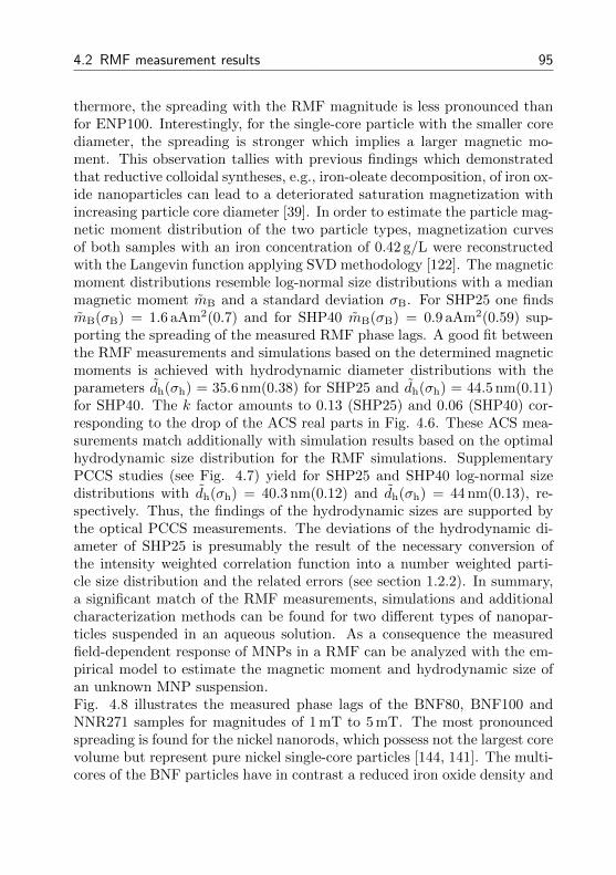
4.2 RMF measurement results 95
thermore, the spreading with the RMF magnitude is less pronounced thanfor ENP100. Interestingly, for the single-core particle with the smaller corediameter, the spreading is stronger which implies a larger magnetic mo-ment. This observation tallies with previous findings which demonstratedthat reductive colloidal syntheses, e.g., iron-oleate decomposition, of iron ox-ide nanoparticles can lead to a deteriorated saturation magnetization withincreasing particle core diameter [39]. In order to estimate the particle mag-netic moment distribution of the two particle types, magnetization curvesof both samples with an iron concentration of 0.42 g/L were reconstructedwith the Langevin function applying SVD methodology [122]. The magneticmoment distributions resemble log-normal size distributions with a medianmagnetic moment mB and a standard deviation σB. For SHP25 one findsmB(σB) = 1.6 aAm2(0.7) and for SHP40 mB(σB) = 0.9 aAm2(0.59) sup-porting the spreading of the measured RMF phase lags. A good fit betweenthe RMF measurements and simulations based on the determined magneticmoments is achieved with hydrodynamic diameter distributions with theparameters dh(σh) = 35.6 nm(0.38) for SHP25 and dh(σh) = 44.5 nm(0.11)for SHP40. The k factor amounts to 0.13 (SHP25) and 0.06 (SHP40) cor-responding to the drop of the ACS real parts in Fig. 4.6. These ACS mea-surements match additionally with simulation results based on the optimalhydrodynamic size distribution for the RMF simulations. SupplementaryPCCS studies (see Fig. 4.7) yield for SHP25 and SHP40 log-normal sizedistributions with dh(σh) = 40.3 nm(0.12) and dh(σh) = 44 nm(0.13), re-spectively. Thus, the findings of the hydrodynamic sizes are supported bythe optical PCCS measurements. The deviations of the hydrodynamic di-ameter of SHP25 is presumably the result of the necessary conversion ofthe intensity weighted correlation function into a number weighted parti-cle size distribution and the related errors (see section 1.2.2). In summary,a significant match of the RMF measurements, simulations and additionalcharacterization methods can be found for two different types of nanopar-ticles suspended in an aqueous solution. As a consequence the measuredfield-dependent response of MNPs in a RMF can be analyzed with the em-pirical model to estimate the magnetic moment and hydrodynamic size ofan unknown MNP suspension.Fig. 4.8 illustrates the measured phase lags of the BNF80, BNF100 andNNR271 samples for magnitudes of 1 mT to 5 mT. The most pronouncedspreading is found for the nickel nanorods, which possess not the largest corevolume but represent pure nickel single-core particles [144, 141]. The multi-cores of the BNF particles have in contrast a reduced iron oxide density and
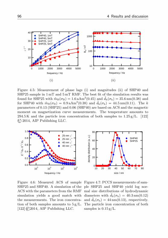
96 4 Results and discussion
40
30
20
10
0
f /
°
500040003000200010000
frequency / Hz
SHP40, 1mT SHP40, 5mT SHP25, 1mT SHP25, 5mT
(i)
10
100
1000
BS /
nT
500040003000200010000
frequency / Hz
(ii)
Figure 4.5: Measurement of phase lags (i) and magnitudes (ii) of SHP40 andSHP25 sample in 1 mT and 5 mT RMF. The best fit of the simulation results wasfound for SHP25 with mB(σB) = 1.6 aAm2(0.45) and dh(σh) = 35.6 nm(0.38) andfor SHP40 with mB(σB) = 0.9 aAm2(0.38) and dh(σh) = 44.5 nm(0.11). The kparameters of 0.13 (SHP25) and 0.06 (SHP40) are based on ACS and the magneticmoment on magnetization curve measurements. The temperature amounts to294.5 K and the particle iron concentration of both samples to 1.25 g/L. [122]© 2014, AIP Publishing LLC.
1.0
0.8
0.6
0.4
0.2
0.0
c' /
c0, c
'' / c
0
103
104
105
106
frequency / Hz
25 nm c' 25 nm c'' 40 nm c' 40 nm c''
Figure 4.6: Measured ACS of sampleSHP25 and SHP40. A simulation of theACS with the parameters from the RMFsimulation yields a good match withthe measurements. The iron concentra-tion of both samples amounts to 5 g/L.[122]©2014, AIP Publishing LLC.
80
60
40
20
0
dens
ity d
istr
ibut
ion
(a. u
.)
8070605040302010
size / nm
SHP40 SHP25
Figure 4.7: PCCS measurements of sam-ple SHP25 and SHP40 yield log nor-mal size distributions of hydrodynamicdiameters with dh(σh) = 40.3 nm(0.12)and dh(σh) = 44 nm(0.13), respectively.The particle iron concentration of bothsamples is 0.15 g/L.
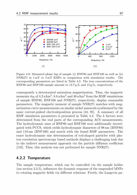
4.2 RMF measurement results 97
70
60
50
40
30
20
10
0
f /
°
500040003000200010000
frequency / Hz
BNF80 1mT BNF80 5mT BNF 100 1mT BNF 100 5 mT
(i)
80
60
40
20
0
f /
°
12008004000
frequency / Hz
1 mT 2.5 mT 5 mT
(ii)
Figure 4.8: Measured phase lag of sample (i) BNF80 and BNF100 as well as (ii)NNR271 in 1 mT to 5 mT RMFs in comparison with simulation results. Thecorresponding parameters are listed in Table 4.2. The iron concentrations of theBNF80 and BNF100 sample amount to 13.7 g/L and 15 g/L, respectively.
consequently a deteriorated saturation magnetization. Thus, the magneticmoments mB of 4.2 aAm2, 8.8 aAm2 and 40 aAm2 from the RMF simulationsof sample BNF80, BNF100 and NNR271, respectively, display reasonableparameters. The magnetic moment of sample NNR271 matches with mag-netization curve measurements on similar nickel nanorods synthesized by thesame current-pulsed electrodeposition process [44, 95]. A summary of allRMF simulation parameters is presented in Table 4.2. The k factors weredetermined from the real parts of the corresponding ACS measurements.The hydrodynamic sizes of BNF80 and BNF100 were additionally investi-gated with PCCS, which yields hydrodynamic diameters of 98 nm (BNF80)and 118 nm (BNF100) and match with the found RMF parameters. Theexact hydrodynamic size determination of rod-shaped particles with pho-ton correlation spectroscopy based methods displays a challenging task dueto the indirect measurement approach via the particle diffusion coefficient[145]. Thus, this analysis was not performed for sample NNR271.
4.2.2 Temperature
The sample temperature, which can be controlled via the sample holder(see section 3.2.5), influences the dynamic response of the suspended MNPsto rotating magnetic fields via different relations: Firstly, the Langevin pa-
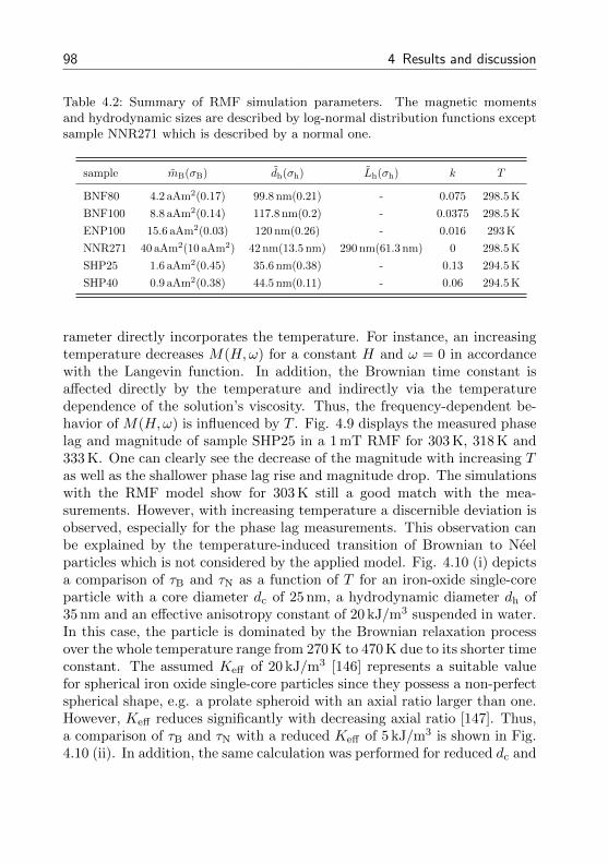
98 4 Results and discussion
Table 4.2: Summary of RMF simulation parameters. The magnetic momentsand hydrodynamic sizes are described by log-normal distribution functions exceptsample NNR271 which is described by a normal one.
sample mB(σB) dh(σh) Lh(σh) k T
BNF80 4.2 aAm2(0.17) 99.8 nm(0.21) - 0.075 298.5 K
BNF100 8.8 aAm2(0.14) 117.8 nm(0.2) - 0.0375 298.5 K
ENP100 15.6 aAm2(0.03) 120 nm(0.26) - 0.016 293 K
NNR271 40 aAm2(10 aAm2) 42 nm(13.5 nm) 290 nm(61.3 nm) 0 298.5 K
SHP25 1.6 aAm2(0.45) 35.6 nm(0.38) - 0.13 294.5 K
SHP40 0.9 aAm2(0.38) 44.5 nm(0.11) - 0.06 294.5 K
rameter directly incorporates the temperature. For instance, an increasingtemperature decreases M(H,ω) for a constant H and ω = 0 in accordancewith the Langevin function. In addition, the Brownian time constant isaffected directly by the temperature and indirectly via the temperaturedependence of the solution’s viscosity. Thus, the frequency-dependent be-havior of M(H,ω) is influenced by T . Fig. 4.9 displays the measured phaselag and magnitude of sample SHP25 in a 1 mT RMF for 303 K, 318 K and333 K. One can clearly see the decrease of the magnitude with increasing Tas well as the shallower phase lag rise and magnitude drop. The simulationswith the RMF model show for 303 K still a good match with the mea-surements. However, with increasing temperature a discernible deviation isobserved, especially for the phase lag measurements. This observation canbe explained by the temperature-induced transition of Brownian to Neelparticles which is not considered by the applied model. Fig. 4.10 (i) depictsa comparison of τB and τN as a function of T for an iron-oxide single-coreparticle with a core diameter dc of 25 nm, a hydrodynamic diameter dh of35 nm and an effective anisotropy constant of 20 kJ/m3 suspended in water.In this case, the particle is dominated by the Brownian relaxation processover the whole temperature range from 270 K to 470 K due to its shorter timeconstant. The assumed Keff of 20 kJ/m3 [146] represents a suitable valuefor spherical iron oxide single-core particles since they possess a non-perfectspherical shape, e.g. a prolate spheroid with an axial ratio larger than one.However, Keff reduces significantly with decreasing axial ratio [147]. Thus,a comparison of τB and τN with a reduced Keff of 5 kJ/m3 is shown in Fig.4.10 (ii). In addition, the same calculation was performed for reduced dc and
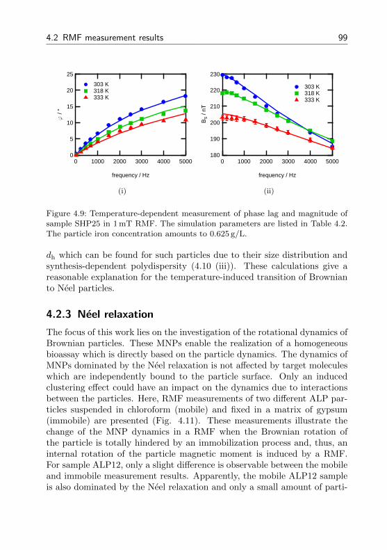
4.2 RMF measurement results 99
25
20
15
10
5
0
f /
°
500040003000200010000
frequency / Hz
303 K 318 K 333 K
(i)
230
220
210
200
190
180
BS /
nT
500040003000200010000
frequency / Hz
303 K 318 K 333 K
(ii)
Figure 4.9: Temperature-dependent measurement of phase lag and magnitude ofsample SHP25 in 1 mT RMF. The simulation parameters are listed in Table 4.2.The particle iron concentration amounts to 0.625 g/L.
dh which can be found for such particles due to their size distribution andsynthesis-dependent polydispersity (4.10 (iii)). These calculations give areasonable explanation for the temperature-induced transition of Brownianto Neel particles.
4.2.3 Neel relaxation
The focus of this work lies on the investigation of the rotational dynamics ofBrownian particles. These MNPs enable the realization of a homogeneousbioassay which is directly based on the particle dynamics. The dynamics ofMNPs dominated by the Neel relaxation is not affected by target moleculeswhich are independently bound to the particle surface. Only an inducedclustering effect could have an impact on the dynamics due to interactionsbetween the particles. Here, RMF measurements of two different ALP par-ticles suspended in chloroform (mobile) and fixed in a matrix of gypsum(immobile) are presented (Fig. 4.11). These measurements illustrate thechange of the MNP dynamics in a RMF when the Brownian rotation ofthe particle is totally hindered by an immobilization process and, thus, aninternal rotation of the particle magnetic moment is induced by a RMF.For sample ALP12, only a slight difference is observable between the mobileand immobile measurement results. Apparently, the mobile ALP12 sampleis also dominated by the Neel relaxation and only a small amount of parti-
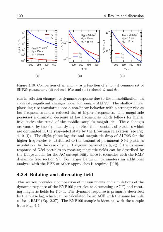
100 4 Results and discussion
10-6
10-3
100
103
106
109
tB /
s, t
N /
s
450400350300
T / K
Keff = 20 kJ/m3
dc = 25nmdh = 35 nm
tB
tN
(i)
10-6
10-5
tB /
s, t
N /
s450400350300
T / K
Keff = 5 kJ/m3
dc = 25nmdh = 35 nm
tB
tN
(ii)
4
68
10-6
2
4
68
10-5
tB /
s, t
N /
s
450400350300
T / K
Keff = 20 kJ/m3
dc = 15 nmdh = 25 nm
tB
tN
(iii)
Figure 4.10: Comparison of τB and τN as a function of T for (i) common set ofSHP25 parameters, (ii) reduced Keff and (iii) reduced dc and dh.
cles in solution changes its dynamic response due to the immobilization. Incontrast, significant changes occur for sample ALP25. The shallow linearphase lag rise transforms into a non-linear behavior with a stronger rise atlow frequencies and a reduced rise at higher frequencies. The magnitudepossesses a dramatic decrease at low frequencies which follows for higherfrequencies the trend of the mobile sample’s magnitude. These changesare caused by the significantly higher Neel time constant of particles whichare dominated in the suspended state by the Brownian relaxation (see Fig.4.10 (i)). The slight phase lag rise and magnitude drop of ALP25 for thehigher frequencies is attributed to the amount of permanent Neel particlesin solution. In the case of small Langevin parameters (ξ 1) the dynamicresponse of Neel particles to rotating magnetic fields can be described bythe Debye model for the AC susceptibility since it coincides with the RMFdynamics (see section 2). For larger Langevin parameters an additionalanalysis with the FPE or other approaches is required [119].
4.2.4 Rotating and alternating field
This section provides a comparison of measurements and simulations of thedynamic response of the ENP100 particles to alternating (ACF) and rotat-ing magnetic fields for ξ > 1. The dynamic response is primarily describedby the phase lag, which can be calculated for an ACF with the same formulaas for a RMF (Eq. 2.27). The ENP100 sample is identical with the samplefrom Fig. 4.4.
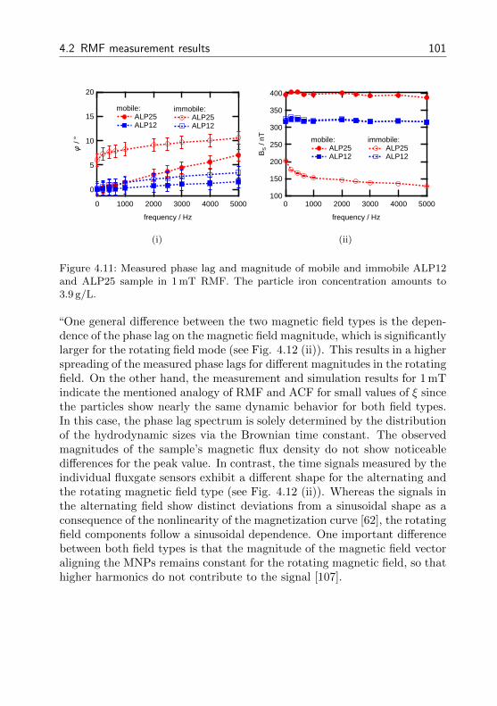
4.2 RMF measurement results 101
20
15
10
5
0
f /
°
500040003000200010000
frequency / Hz
mobile: ALP25 ALP12
immobile: ALP25 ALP12
(i)
400
350
300
250
200
150
100
BS /
nT
500040003000200010000
frequency / Hz
mobile: ALP25 ALP12
immobile: ALP25 ALP12
(ii)
Figure 4.11: Measured phase lag and magnitude of mobile and immobile ALP12and ALP25 sample in 1 mT RMF. The particle iron concentration amounts to3.9 g/L.
“One general difference between the two magnetic field types is the depen-dence of the phase lag on the magnetic field magnitude, which is significantlylarger for the rotating field mode (see Fig. 4.12 (ii)). This results in a higherspreading of the measured phase lags for different magnitudes in the rotatingfield. On the other hand, the measurement and simulation results for 1 mTindicate the mentioned analogy of RMF and ACF for small values of ξ sincethe particles show nearly the same dynamic behavior for both field types.In this case, the phase lag spectrum is solely determined by the distributionof the hydrodynamic sizes via the Brownian time constant. The observedmagnitudes of the sample’s magnetic flux density do not show noticeabledifferences for the peak value. In contrast, the time signals measured by theindividual fluxgate sensors exhibit a different shape for the alternating andthe rotating magnetic field type (see Fig. 4.12 (ii)). Whereas the signals inthe alternating field show distinct deviations from a sinusoidal shape as aconsequence of the nonlinearity of the magnetization curve [62], the rotatingfield components follow a sinusoidal dependence. One important differencebetween both field types is that the magnitude of the magnetic field vectoraligning the MNPs remains constant for the rotating magnetic field, so thathigher harmonics do not contribute to the signal [107].
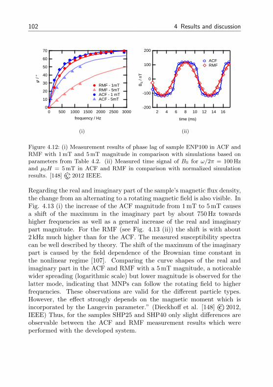
102 4 Results and discussion
70
60
50
40
30
20
10
0
f /
°
300025002000150010005000
frequency / Hz
RMF - 1mTRMF - 5mTACF - 1 mTACF - 5mT
(i)
-200
-100
0
100
200
BS /
nT
161412108642
time (ms)
ACFRMF
(ii)
Figure 4.12: (i) Measurement results of phase lag of sample ENP100 in ACF andRMF with 1 mT and 5 mT magnitude in comparison with simulations based onparameters from Table 4.2. (ii) Measured time signal of BS for ω/2π = 100 Hzand µ0H = 5 mT in ACF and RMF in comparison with normalized simulationresults. [148] © 2012 IEEE.
Regarding the real and imaginary part of the sample’s magnetic flux density,the change from an alternating to a rotating magnetic field is also visible. InFig. 4.13 (i) the increase of the ACF magnitude from 1 mT to 5 mT causesa shift of the maximum in the imaginary part by about 750 Hz towardshigher frequencies as well as a general increase of the real and imaginarypart magnitude. For the RMF (see Fig. 4.13 (ii)) the shift is with about2 kHz much higher than for the ACF. The measured susceptibility spectracan be well described by theory. The shift of the maximum of the imaginarypart is caused by the field dependence of the Brownian time constant inthe nonlinear regime [107]. Comparing the curve shapes of the real andimaginary part in the ACF and RMF with a 5 mT magnitude, a noticeablewider spreading (logarithmic scale) but lower magnitude is observed for thelatter mode, indicating that MNPs can follow the rotating field to higherfrequencies. These observations are valid for the different particle types.However, the effect strongly depends on the magnetic moment which isincorporated by the Langevin parameter.” (Dieckhoff et al. [148] © 2012,IEEE) Thus, for the samples SHP25 and SHP40 only slight differences areobservable between the ACF and RMF measurement results which wereperformed with the developed system.
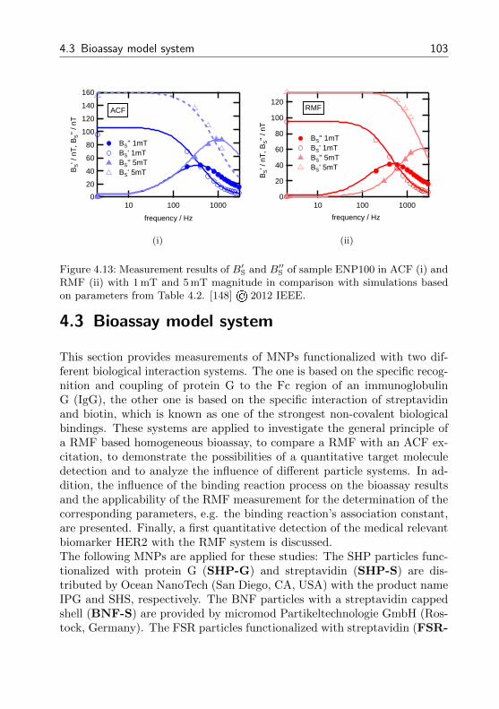
4.3 Bioassay model system 103
160
140
120
100
80
60
40
20
0
BS' /
nT
, BS''
/ nT
10 100 1000
frequency / Hz
14
12
10
8
6
4
2
0
x10-3
BS'' 1mT BS' 1mT BS'' 5mT BS' 5mT
ACF
(i)
12
10
8
6
4
2
0
x10-3
10 100 1000
frequency / Hz
120
100
80
60
40
20
0
BS' /
nT
, BS''
/ nT
BS'' 1mT BS' 1mT BS'' 5mT BS' 5mT
RMF
(ii)
Figure 4.13: Measurement results of B′S and B′′S of sample ENP100 in ACF (i) andRMF (ii) with 1 mT and 5 mT magnitude in comparison with simulations basedon parameters from Table 4.2. [148] © 2012 IEEE.
4.3 Bioassay model system
This section provides measurements of MNPs functionalized with two dif-ferent biological interaction systems. The one is based on the specific recog-nition and coupling of protein G to the Fc region of an immunoglobulinG (IgG), the other one is based on the specific interaction of streptavidinand biotin, which is known as one of the strongest non-covalent biologicalbindings. These systems are applied to investigate the general principle ofa RMF based homogeneous bioassay, to compare a RMF with an ACF ex-citation, to demonstrate the possibilities of a quantitative target moleculedetection and to analyze the influence of different particle systems. In ad-dition, the influence of the binding reaction process on the bioassay resultsand the applicability of the RMF measurement for the determination of thecorresponding parameters, e.g. the binding reaction’s association constant,are presented. Finally, a first quantitative detection of the medical relevantbiomarker HER2 with the RMF system is discussed.The following MNPs are applied for these studies: The SHP particles func-tionalized with protein G (SHP-G) and streptavidin (SHP-S) are dis-tributed by Ocean NanoTech (San Diego, CA, USA) with the product nameIPG and SHS, respectively. The BNF particles with a streptavidin cappedshell (BNF-S) are provided by micromod Partikeltechnologie GmbH (Ros-tock, Germany). The FSR particles functionalized with streptavidin (FSR-
104 4 Results and discussion
S) are manufactured by nanoPET Pharma GmbH (Berlin, Germany). Thetarget antibody for the protein G based experiments is the HRP goat anti-Human IgG Fc (HRP-IgG) with an average molecular weight of 270 kDafrom ImmunoChemistry Technologies (Bloomington, MN, USA). As bind-ing molecules for the streptavidin functionalized MNP experiments the bi-otinylated IgGs anti-human alpha-fetoprotein (AFP-IgG) and anti-humanHER-2 (HER2-IgG) purchased from ebioscience (Frankfurt, Germany) areapplied. They possess a molecular mass of approximately 150 kDa and arecoated with biotin.The constant phase offset caused by the RMF system is corrected for all fig-ures. The error bars in the RMF measurements represent the standard devi-ation based on five measurements. The dynamic viscosity of the MNP sus-pensions is calculated based on the sample temperature. The measurementresults in the figures are represented by markers. Solid lines describe simu-lation results based on the corresponding model. Dashed lines are guides tothe eyes. All RMF simulation results are based on the empirical model ex-cept the simulations for the ENP100 and SHP35 particles. They are basedon a numerical solution of the FPE. The distribution functions applied forthe description of the particle polydispersity are log-normal ones. The men-tioned concentrations of the samples in the presented measurements are theparticle concentrations with the unit nM (nmol/L) since for the investiga-tion of the binding effects the number of particles is important and not theiron or particle mass per sample.The principle of the homogeneous bioassay based on the dynamics of MNPsin rotating magnetic fields was described in section 1.3.2. Fig. 4.14 (i)recalls this principle which facilitates the quantitative detection of targetmolecules bound to the particle surface via the measurement of the phaselag change ∆ϕ. This change is the result of the subtraction of the phaselag before from the phase lag after the addition of the solution which con-tains the target molecules to quantify. In addition, Fig. 4.14 depicts themeasurement of the phase lag as a function of time (i) and frequency (ii)for particle SHP-G40 binding to HRP-IgG antibodies in solution. The par-ticle concentration amounts to 13 nM and the antibody concentration to61.4 nM. The time-dependent measurement clarifies that the change of thephase lag after the addition of the target molecule solution requires sometime to reach its final value. This measurement enables additionally theanalysis of the binding kinetics. In the frequency-dependent measurementone can see that the phase lag change depends additionally on the exactfrequency value. The analysis of the phase lag for the bioassay realization
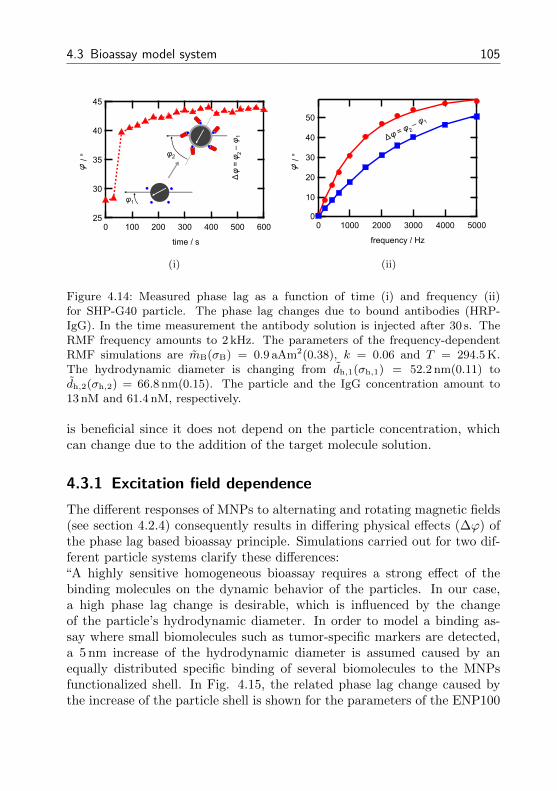
4.3 Bioassay model system 105
φ2
φ1
/ °f
45
40
35
30
256005004003002001000
time / s
φφ
1=
φ2
(i)
50
40
30
20
10
0500040003000200010000
frequency / Hz
/ °f
φ
φ1
= φ 2
(ii)
Figure 4.14: Measured phase lag as a function of time (i) and frequency (ii)for SHP-G40 particle. The phase lag changes due to bound antibodies (HRP-IgG). In the time measurement the antibody solution is injected after 30 s. TheRMF frequency amounts to 2 kHz. The parameters of the frequency-dependentRMF simulations are mB(σB) = 0.9 aAm2(0.38), k = 0.06 and T = 294.5 K.The hydrodynamic diameter is changing from dh,1(σh,1) = 52.2 nm(0.11) todh,2(σh,2) = 66.8 nm(0.15). The particle and the IgG concentration amount to13 nM and 61.4 nM, respectively.
is beneficial since it does not depend on the particle concentration, whichcan change due to the addition of the target molecule solution.
4.3.1 Excitation field dependence
The different responses of MNPs to alternating and rotating magnetic fields(see section 4.2.4) consequently results in differing physical effects (∆ϕ) ofthe phase lag based bioassay principle. Simulations carried out for two dif-ferent particle systems clarify these differences:“A highly sensitive homogeneous bioassay requires a strong effect of thebinding molecules on the dynamic behavior of the particles. In our case,a high phase lag change is desirable, which is influenced by the changeof the particle’s hydrodynamic diameter. In order to model a binding as-say where small biomolecules such as tumor-specific markers are detected,a 5 nm increase of the hydrodynamic diameter is assumed caused by anequally distributed specific binding of several biomolecules to the MNPsfunctionalized shell. In Fig. 4.15, the related phase lag change caused bythe increase of the particle shell is shown for the parameters of the ENP100
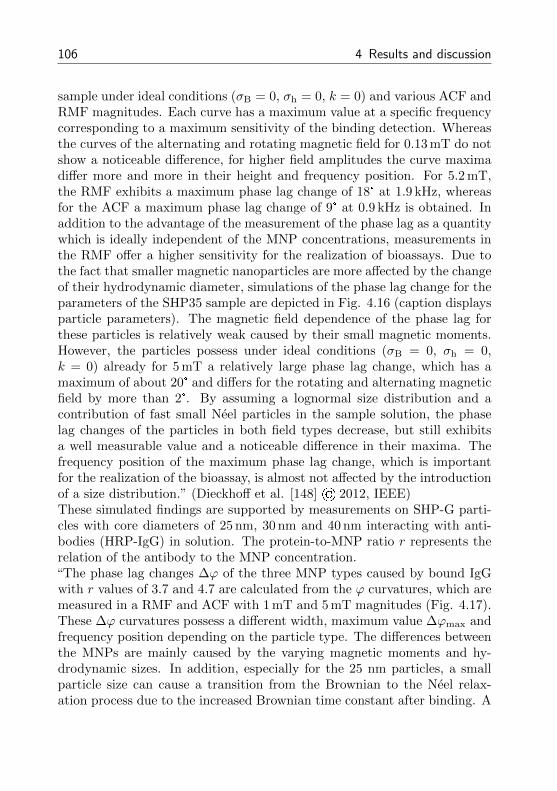
106 4 Results and discussion
sample under ideal conditions (σB = 0, σh = 0, k = 0) and various ACF andRMF magnitudes. Each curve has a maximum value at a specific frequencycorresponding to a maximum sensitivity of the binding detection. Whereasthe curves of the alternating and rotating magnetic field for 0.13 mT do notshow a noticeable difference, for higher field amplitudes the curve maximadiffer more and more in their height and frequency position. For 5.2 mT,the RMF exhibits a maximum phase lag change of 18° at 1.9 kHz, whereasfor the ACF a maximum phase lag change of 9° at 0.9 kHz is obtained. Inaddition to the advantage of the measurement of the phase lag as a quantitywhich is ideally independent of the MNP concentrations, measurements inthe RMF offer a higher sensitivity for the realization of bioassays. Due tothe fact that smaller magnetic nanoparticles are more affected by the changeof their hydrodynamic diameter, simulations of the phase lag change for theparameters of the SHP35 sample are depicted in Fig. 4.16 (caption displaysparticle parameters). The magnetic field dependence of the phase lag forthese particles is relatively weak caused by their small magnetic moments.However, the particles possess under ideal conditions (σB = 0, σh = 0,k = 0) already for 5 mT a relatively large phase lag change, which has amaximum of about 20° and differs for the rotating and alternating magneticfield by more than 2°. By assuming a lognormal size distribution and acontribution of fast small Neel particles in the sample solution, the phaselag changes of the particles in both field types decrease, but still exhibitsa well measurable value and a noticeable difference in their maxima. Thefrequency position of the maximum phase lag change, which is importantfor the realization of the bioassay, is almost not affected by the introductionof a size distribution.” (Dieckhoff et al. [148] © 2012, IEEE)These simulated findings are supported by measurements on SHP-G parti-cles with core diameters of 25 nm, 30 nm and 40 nm interacting with anti-bodies (HRP-IgG) in solution. The protein-to-MNP ratio r represents therelation of the antibody to the MNP concentration.“The phase lag changes ∆ϕ of the three MNP types caused by bound IgGwith r values of 3.7 and 4.7 are calculated from the ϕ curvatures, which aremeasured in a RMF and ACF with 1 mT and 5 mT magnitudes (Fig. 4.17).These ∆ϕ curvatures possess a different width, maximum value ∆ϕmax andfrequency position depending on the particle type. The differences betweenthe MNPs are mainly caused by the varying magnetic moments and hy-drodynamic sizes. In addition, especially for the 25 nm particles, a smallparticle size can cause a transition from the Brownian to the Neel relax-ation process due to the increased Brownian time constant after binding. A
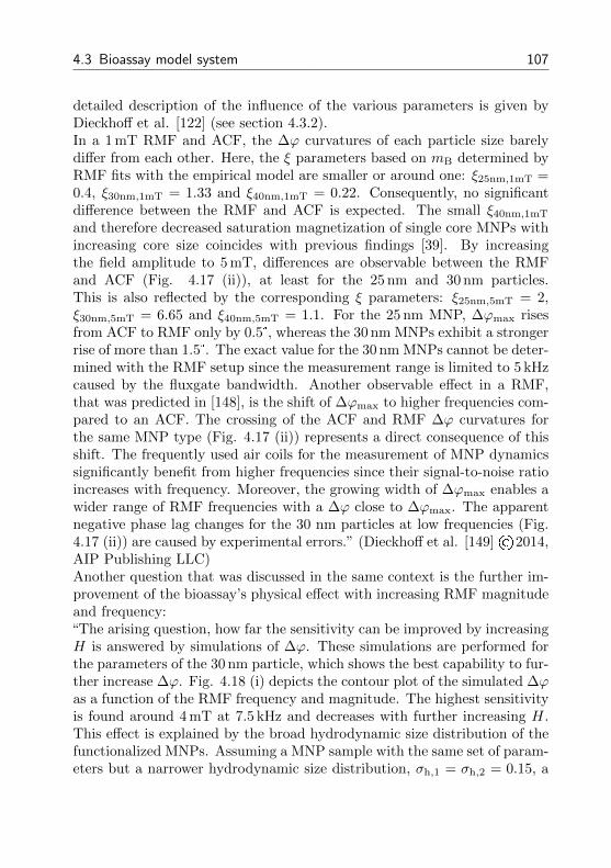
4.3 Bioassay model system 107
detailed description of the influence of the various parameters is given byDieckhoff et al. [122] (see section 4.3.2).In a 1 mT RMF and ACF, the ∆ϕ curvatures of each particle size barelydiffer from each other. Here, the ξ parameters based on mB determined byRMF fits with the empirical model are smaller or around one: ξ25nm,1mT =0.4, ξ30nm,1mT = 1.33 and ξ40nm,1mT = 0.22. Consequently, no significantdifference between the RMF and ACF is expected. The small ξ40nm,1mT
and therefore decreased saturation magnetization of single core MNPs withincreasing core size coincides with previous findings [39]. By increasingthe field amplitude to 5 mT, differences are observable between the RMFand ACF (Fig. 4.17 (ii)), at least for the 25 nm and 30 nm particles.This is also reflected by the corresponding ξ parameters: ξ25nm,5mT = 2,ξ30nm,5mT = 6.65 and ξ40nm,5mT = 1.1. For the 25 nm MNP, ∆ϕmax risesfrom ACF to RMF only by 0.5°, whereas the 30 nm MNPs exhibit a strongerrise of more than 1.5°. The exact value for the 30 nm MNPs cannot be deter-mined with the RMF setup since the measurement range is limited to 5 kHzcaused by the fluxgate bandwidth. Another observable effect in a RMF,that was predicted in [148], is the shift of ∆ϕmax to higher frequencies com-pared to an ACF. The crossing of the ACF and RMF ∆ϕ curvatures forthe same MNP type (Fig. 4.17 (ii)) represents a direct consequence of thisshift. The frequently used air coils for the measurement of MNP dynamicssignificantly benefit from higher frequencies since their signal-to-noise ratioincreases with frequency. Moreover, the growing width of ∆ϕmax enables awider range of RMF frequencies with a ∆ϕ close to ∆ϕmax. The apparentnegative phase lag changes for the 30 nm particles at low frequencies (Fig.4.17 (ii)) are caused by experimental errors.” (Dieckhoff et al. [149] ©2014,AIP Publishing LLC)Another question that was discussed in the same context is the further im-provement of the bioassay’s physical effect with increasing RMF magnitudeand frequency:“The arising question, how far the sensitivity can be improved by increasingH is answered by simulations of ∆ϕ. These simulations are performed forthe parameters of the 30 nm particle, which shows the best capability to fur-ther increase ∆ϕ. Fig. 4.18 (i) depicts the contour plot of the simulated ∆ϕas a function of the RMF frequency and magnitude. The highest sensitivityis found around 4 mT at 7.5 kHz and decreases with further increasing H.This effect is explained by the broad hydrodynamic size distribution of thefunctionalized MNPs. Assuming a MNP sample with the same set of param-eters but a narrower hydrodynamic size distribution, σh,1 = σh,2 = 0.15, a
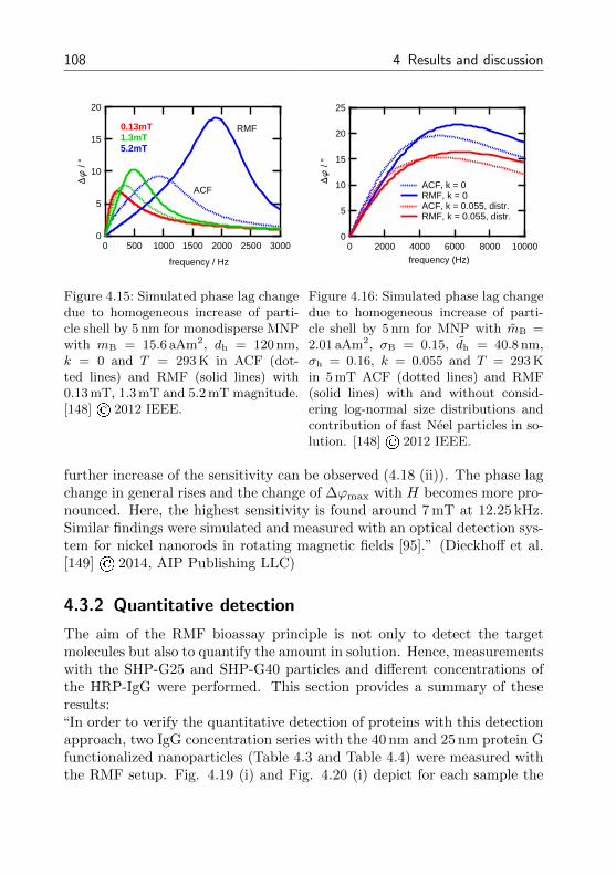
108 4 Results and discussion
20
15
10
5
0
Df
/ °
300025002000150010005000
frequency / Hz
0.13mT1.3mT5.2mT
RMF
ACF
Figure 4.15: Simulated phase lag changedue to homogeneous increase of parti-cle shell by 5 nm for monodisperse MNPwith mB = 15.6 aAm2, dh = 120 nm,k = 0 and T = 293 K in ACF (dot-ted lines) and RMF (solid lines) with0.13 mT, 1.3 mT and 5.2 mT magnitude.[148] © 2012 IEEE.
25
20
15
10
5
0
Df
/ °
1000080006000400020000frequency (Hz)
ACF, k = 0 RMF, k = 0 ACF, k = 0.055, distr. RMF, k = 0.055, distr.
Figure 4.16: Simulated phase lag changedue to homogeneous increase of parti-cle shell by 5 nm for MNP with mB =2.01 aAm2, σB = 0.15, dh = 40.8 nm,σh = 0.16, k = 0.055 and T = 293 Kin 5 mT ACF (dotted lines) and RMF(solid lines) with and without consid-ering log-normal size distributions andcontribution of fast Neel particles in so-lution. [148] © 2012 IEEE.
further increase of the sensitivity can be observed (4.18 (ii)). The phase lagchange in general rises and the change of ∆ϕmax with H becomes more pro-nounced. Here, the highest sensitivity is found around 7 mT at 12.25 kHz.Similar findings were simulated and measured with an optical detection sys-tem for nickel nanorods in rotating magnetic fields [95].” (Dieckhoff et al.[149] © 2014, AIP Publishing LLC)
4.3.2 Quantitative detection
The aim of the RMF bioassay principle is not only to detect the targetmolecules but also to quantify the amount in solution. Hence, measurementswith the SHP-G25 and SHP-G40 particles and different concentrations ofthe HRP-IgG were performed. This section provides a summary of theseresults:“In order to verify the quantitative detection of proteins with this detectionapproach, two IgG concentration series with the 40 nm and 25 nm protein Gfunctionalized nanoparticles (Table 4.3 and Table 4.4) were measured withthe RMF setup. Fig. 4.19 (i) and Fig. 4.20 (i) depict for each sample the
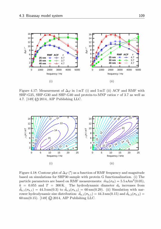
4.3 Bioassay model system 109
16
14
12
10
8
6
4
2
0
Df
/ °
500040003000200010000
frequency / Hz
RMF ACF r25 nm 4.730 nm 3.740 nm 4.7
(i)
16
14
12
10
8
6
4
2
0
Df
/ °
500040003000200010000
frequency / Hz
RMF ACF r25 nm 4.7 30 nm 3.740 nm 4.7
(ii)
Figure 4.17: Measurement of ∆ϕ in 1 mT (i) and 5 mT (ii) ACF and RMF withSHP-G25, SHP-G30 and SHP-G40 and protein-to-MNP ratios r of 3.7 as well as4.7. [149] © 2014, AIP Publishing LLC.
14
12
10
8
6
4
2
m0H
/ m
T
2520151050frequency / Hz
15
14
13
12
12
11
10
10
9
8
6
4
4
(i)
14
12
10
8
6
4
2
m0H
/ m
T
2520151050frequency / kHz
23
22
21
18
18
16
16
14
14
12
12
10
8
6
4 4
(ii)
Figure 4.18: Contour plot of ∆ϕ (°) as a function of RMF frequency and magnitudebased on simulations for SHP30 sample with protein G functionalization. (i) Theparticle parameters are based on RMF measurements: mB(σB) = 5.5 aAm2(0.05),k = 0.055 and T = 300 K. The hydrodynamic diameter dh increases fromdh,1(σh,1) = 44.3 nm(0.3) to dh,2(σh,2) = 60 nm(0.29). (ii) Simulation with nar-rower hydrodynamic size distribution: dh,1(σh,1) = 44.3 nm(0.15) and dh,2(σh,2) =60 nm(0.15). [149] © 2014, AIP Publishing LLC.
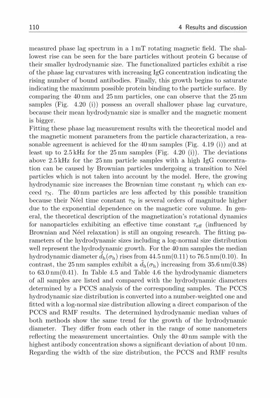
110 4 Results and discussion
measured phase lag spectrum in a 1 mT rotating magnetic field. The shal-lowest rise can be seen for the bare particles without protein G because oftheir smaller hydrodynamic size. The functionalized particles exhibit a riseof the phase lag curvatures with increasing IgG concentration indicating therising number of bound antibodies. Finally, this growth begins to saturateindicating the maximum possible protein binding to the particle surface. Bycomparing the 40 nm and 25 nm particles, one can observe that the 25 nmsamples (Fig. 4.20 (i)) possess an overall shallower phase lag curvature,because their mean hydrodynamic size is smaller and the magnetic momentis bigger.Fitting these phase lag measurement results with the theoretical model andthe magnetic moment parameters from the particle characterization, a rea-sonable agreement is achieved for the 40 nm samples (Fig. 4.19 (i)) and atleast up to 2.5 kHz for the 25 nm samples (Fig. 4.20 (i)). The deviationsabove 2.5 kHz for the 25 nm particle samples with a high IgG concentra-tion can be caused by Brownian particles undergoing a transition to Neelparticles which is not taken into account by the model. Here, the growinghydrodynamic size increases the Brownian time constant τB which can ex-ceed τN. The 40 nm particles are less affected by this possible transitionbecause their Neel time constant τN is several orders of magnitude higherdue to the exponential dependence on the magnetic core volume. In gen-eral, the theoretical description of the magnetization’s rotational dynamicsfor nanoparticles exhibiting an effective time constant τeff (influenced byBrownian and Neel relaxation) is still an ongoing research. The fitting pa-rameters of the hydrodynamic sizes including a log-normal size distributionwell represent the hydrodynamic growth. For the 40 nm samples the medianhydrodynamic diameter dh(σh) rises from 44.5 nm(0.11) to 76.5 nm(0.10). Incontrast, the 25 nm samples exhibit a dh(σh) increasing from 35.6 nm(0.38)to 63.0 nm(0.41). In Table 4.5 and Table 4.6 the hydrodynamic diametersof all samples are listed and compared with the hydrodynamic diametersdetermined by a PCCS analysis of the corresponding samples. The PCCShydrodynamic size distribution is converted into a number-weighted one andfitted with a log-normal size distribution allowing a direct comparison of thePCCS and RMF results. The determined hydrodynamic median values ofboth methods show the same trend for the growth of the hydrodynamicdiameter. They differ from each other in the range of some nanometersreflecting the measurement uncertainties. Only the 40 nm sample with thehighest antibody concentration shows a significant deviation of about 10 nm.Regarding the width of the size distribution, the PCCS and RMF results
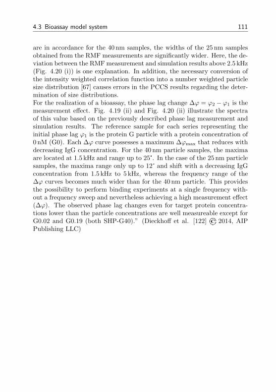
4.3 Bioassay model system 111
are in accordance for the 40 nm samples, the widths of the 25 nm samplesobtained from the RMF measurements are significantly wider. Here, the de-viation between the RMF measurement and simulation results above 2.5 kHz(Fig. 4.20 (i)) is one explanation. In addition, the necessary conversion ofthe intensity weighted correlation function into a number weighted particlesize distribution [67] causes errors in the PCCS results regarding the deter-mination of size distributions.For the realization of a bioassay, the phase lag change ∆ϕ = ϕ2 − ϕ1 is themeasurement effect. Fig. 4.19 (ii) and Fig. 4.20 (ii) illustrate the spectraof this value based on the previously described phase lag measurement andsimulation results. The reference sample for each series representing theinitial phase lag ϕ1 is the protein G particle with a protein concentration of0 nM (G0). Each ∆ϕ curve possesses a maximum ∆ϕmax that reduces withdecreasing IgG concentration. For the 40 nm particle samples, the maximaare located at 1.5 kHz and range up to 25°. In the case of the 25 nm particlesamples, the maxima range only up to 12° and shift with a decreasing IgGconcentration from 1.5 kHz to 5 kHz, whereas the frequency range of the∆ϕ curves becomes much wider than for the 40 nm particle. This providesthe possibility to perform binding experiments at a single frequency with-out a frequency sweep and nevertheless achieving a high measurement effect(∆ϕ). The observed phase lag changes even for target protein concentra-tions lower than the particle concentrations are well measureable except forG0.02 and G0.19 (both SHP-G40).” (Dieckhoff et al. [122] © 2014, AIPPublishing LLC)
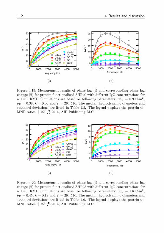
112 4 Results and discussion
60
50
40
30
20
10
0
f /
°
500040003000200010000
frequency / Hz
G37.7G9.10 G4.72 G1.88
G0.63G0.19G0.02G0bare
(i)
25
20
15
10
5
0
Df
/ °
500040003000200010000
frequency / Hz
(ii)
Figure 4.19: Measurement results of phase lag (i) and corresponding phase lagchange (ii) for protein functionalized SHP40 with different IgG concentrations fora 1 mT RMF. Simulations are based on following parameters: mB = 0.9 aAm2,σB = 0.38, k = 0.06 and T = 294.5 K. The median hydrodynamic diameters andstandard deviations are listed in Table 4.5. The legend displays the protein-to-MNP ratios. [122] © 2014, AIP Publishing LLC.
35
30
25
20
15
10
5
0
f /
°
500040003000200010000frequency / Hz
G37.7 G9.40 G4.72 G1.88
G0.63 G0.19 G0.06 G0 bare
(i)
12
10
8
6
4
2
0
Df
/ °
500040003000200010000
frequency / Hz
(ii)
Figure 4.20: Measurement results of phase lag (i) and corresponding phase lagchange (ii) for protein functionalized SHP25 with different IgG concentrations fora 1 mT RMF. Simulations are based on following parameters: mB = 1.6 aAm2,σB = 0.45, k = 0.13 and T = 294.5 K. The median hydrodynamic diameters andstandard deviations are listed in Table 4.6. The legend displays the protein-to-MNP ratios. [122] © 2014, AIP Publishing LLC.
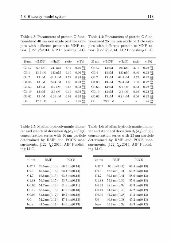
4.3 Bioassay model system 113
Table 4.3: Parameters of protein G func-tionalized 40 nm iron oxide particle sam-ples with different protein-to-MNP ra-tios. [122]©2014, AIP Publishing LLC.
40 nm c(MNP) c(IgG) ratio c(Fe)
G37.7 6.5 nM 247 nM 37.7 0.46 mgmL
G9.1 13.5 nM 123 nM 9.10 0.96 mgmL
G4.7 13 nM 61.4 nM 4.72 0.93 mgmL
G1.88 13 nM 24.4 nM 1.88 0.93 mgmL
G0.63 13 nM 8.2 nM 0.63 0.93 mgmL
G0.19 13 nM 2.5 nM 0.19 0.93 mgmL
G0.02 13 nM 0.26 nM 0.02 0.93 mgmL
G0 17.5 nM - - 1.25 mgmL
Table 4.4: Parameters of protein G func-tionalized 25 nm iron oxide particle sam-ples with different protein-to-MNP ra-tios. [122]©2014, AIP Publishing LLC.
25 nm c(MNP) c(IgG) ratio c(Fe)
G37.7 13 nM 494 nM 37.7 0.22 mgmL
G9.4 13 nM 123 nM 9.40 0.22 mgmL
G4.7 13 nM 61.4 nM 4.72 0.22 mgmL
G1.88 13 nM 24.4 nM 1.88 0.22 mgmL
G0.63 13 nM 8.2 nM 0.63 0.22 mgmL
G0.19 13 nM 2.5 nM 0.19 0.22 mgmL
G0.06 13 nM 0.81 nM 0.06 0.22 mgmL
G0 73.9 nM - - 1.25 mgmL
Table 4.5: Median hydrodynamic diame-ter and standard deviation dh(σh) of IgGconcentration series with 40 nm particledetermined by RMF and PCCS mea-surements. [122] © 2014, AIP Publish-ing LLC.
40 nm RMF PCCS
G37.7 76.5 nm(0.10) 66.3 nm(0.14)
G9.4 69.5 nm(0.16) 63.4 nm(0.14)
G4.7 66.8 nm(0.15) 63.3 nm(0.12)
G1.88 59.3 nm(0.15) 53.7 nm(0.13)
G0.63 54.7 nm(0.14) 51.0 nm(0.11)
G0.19 52.5 nm(0.13) 47.5 nm(0.13)
G0.06 51.6 nm(0.12) 49.2 nm(0.12)
G0 52.2 nm(0.11) 47.3 nm(0.13)
bare 44.5 nm(0.11) 44.0 nm(0.13)
Table 4.6: Median hydrodynamic diame-ter and standard deviation dh(σh) of IgGconcentration series with 25 nm particledetermined by RMF and PCCS mea-surements. [122] © 2014, AIP Publish-ing LLC.
25 nm RMF PCCS
G37.7 63 nm(0.41) 66.4 nm(0.13)
G9.4 62.5 nm(0.41) 63.2 nm(0.13)
G4.7 59.1 nm(0.41) 58.6 nm(0.13)
G1.88 55.6 nm(0.39) 55.0 nm(0.13)
G0.63 48.4 nm(0.39) 49.3 nm(0.13)
G0.19 44.0 nm(0.40) 47.2 nm(0.12)
G0.06 42.2 nm(0.38) 43.3 nm(0.13)
G0 40.8 nm(0.38) 45.2 nm(0.13)
bare 35.6 nm(0.38) 40.3 nm(0.12)
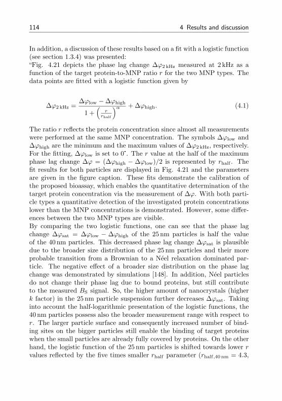
114 4 Results and discussion
In addition, a discussion of these results based on a fit with a logistic function(see section 1.3.4) was presented:“Fig. 4.21 depicts the phase lag change ∆ϕ2 kHz measured at 2 kHz as afunction of the target protein-to-MNP ratio r for the two MNP types. Thedata points are fitted with a logistic function given by
∆ϕ2 kHz =∆ϕlow −∆ϕhigh
1 +(
rrhalf
)α + ∆ϕhigh. (4.1)
The ratio r reflects the protein concentration since almost all measurementswere performed at the same MNP concentration. The symbols ∆ϕlow and∆ϕhigh are the minimum and the maximum values of ∆ϕ2 kHz, respectively.For the fitting, ∆ϕlow is set to 0°. The r value at the half of the maximumphase lag change ∆ϕ = (∆ϕhigh − ∆ϕlow)/2 is represented by rhalf . Thefit results for both particles are displayed in Fig. 4.21 and the parametersare given in the figure caption. These fits demonstrate the calibration ofthe proposed bioassay, which enables the quantitative determination of thetarget protein concentration via the measurement of ∆ϕ. With both parti-cle types a quantitative detection of the investigated protein concentrationslower than the MNP concentrations is demonstrated. However, some differ-ences between the two MNP types are visible.By comparing the two logistic functions, one can see that the phase lagchange ∆ϕsat = ∆ϕlow − ∆ϕhigh of the 25 nm particles is half the valueof the 40 nm particles. This decreased phase lag change ∆ϕsat is plausibledue to the broader size distribution of the 25 nm particles and their moreprobable transition from a Brownian to a Neel relaxation dominated par-ticle. The negative effect of a broader size distribution on the phase lagchange was demonstrated by simulations [148]. In addition, Neel particlesdo not change their phase lag due to bound proteins, but still contributeto the measured BS signal. So, the higher amount of nanocrystals (higherk factor) in the 25 nm particle suspension further decreases ∆ϕsat. Takinginto account the half-logarithmic presentation of the logistic functions, the40 nm particles possess also the broader measurement range with respect tor. The larger particle surface and consequently increased number of bind-ing sites on the bigger particles still enable the binding of target proteinswhen the small particles are already fully covered by proteins. On the otherhand, the logistic function of the 25 nm particles is shifted towards lower rvalues reflected by the five times smaller rhalf parameter (rhalf,40 nm = 4.3,
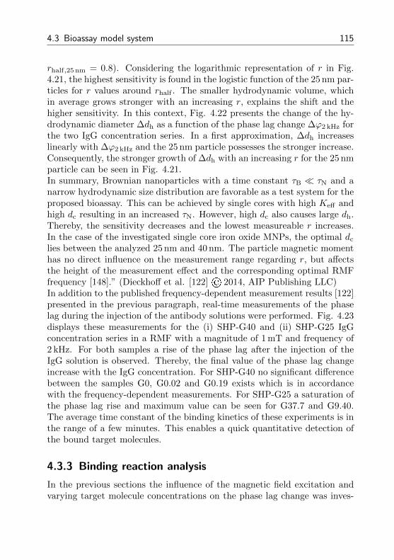
4.3 Bioassay model system 115
rhalf,25 nm = 0.8). Considering the logarithmic representation of r in Fig.4.21, the highest sensitivity is found in the logistic function of the 25 nm par-ticles for r values around rhalf . The smaller hydrodynamic volume, whichin average grows stronger with an increasing r, explains the shift and thehigher sensitivity. In this context, Fig. 4.22 presents the change of the hy-drodynamic diameter ∆dh as a function of the phase lag change ∆ϕ2 kHz forthe two IgG concentration series. In a first approximation, ∆dh increaseslinearly with ∆ϕ2 kHz and the 25 nm particle possesses the stronger increase.Consequently, the stronger growth of ∆dh with an increasing r for the 25 nmparticle can be seen in Fig. 4.21.In summary, Brownian nanoparticles with a time constant τB τN and anarrow hydrodynamic size distribution are favorable as a test system for theproposed bioassay. This can be achieved by single cores with high Keff andhigh dc resulting in an increased τN. However, high dc also causes large dh.Thereby, the sensitivity decreases and the lowest measureable r increases.In the case of the investigated single core iron oxide MNPs, the optimal dc
lies between the analyzed 25 nm and 40 nm. The particle magnetic momenthas no direct influence on the measurement range regarding r, but affectsthe height of the measurement effect and the corresponding optimal RMFfrequency [148].” (Dieckhoff et al. [122] © 2014, AIP Publishing LLC)In addition to the published frequency-dependent measurement results [122]presented in the previous paragraph, real-time measurements of the phaselag during the injection of the antibody solutions were performed. Fig. 4.23displays these measurements for the (i) SHP-G40 and (ii) SHP-G25 IgGconcentration series in a RMF with a magnitude of 1 mT and frequency of2 kHz. For both samples a rise of the phase lag after the injection of theIgG solution is observed. Thereby, the final value of the phase lag changeincrease with the IgG concentration. For SHP-G40 no significant differencebetween the samples G0, G0.02 and G0.19 exists which is in accordancewith the frequency-dependent measurements. For SHP-G25 a saturation ofthe phase lag rise and maximum value can be seen for G37.7 and G9.40.The average time constant of the binding kinetics of these experiments is inthe range of a few minutes. This enables a quick quantitative detection ofthe bound target molecules.
4.3.3 Binding reaction analysis
In the previous sections the influence of the magnetic field excitation andvarying target molecule concentrations on the phase lag change was inves-
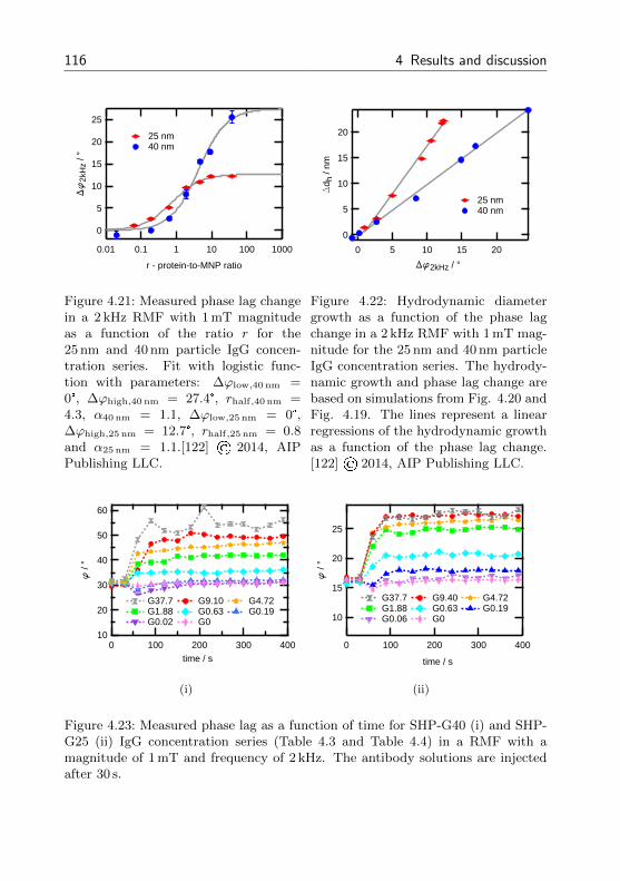
116 4 Results and discussion
25
20
15
10
5
0
Df
2kH
z / °
0.01 0.1 1 10 100 1000
r - protein-to-MNP ratio
25 nm 40 nm
Figure 4.21: Measured phase lag changein a 2 kHz RMF with 1 mT magnitudeas a function of the ratio r for the25 nm and 40 nm particle IgG concen-tration series. Fit with logistic func-tion with parameters: ∆ϕlow,40 nm =0°, ∆ϕhigh,40 nm = 27.4°, rhalf,40 nm =4.3, α40 nm = 1.1, ∆ϕlow,25 nm = 0°,∆ϕhigh,25 nm = 12.7°, rhalf,25 nm = 0.8and α25 nm = 1.1.[122] © 2014, AIPPublishing LLC.
20
15
10
5
0
Dd h
/ nm
20151050
Df2kHz / °
25 nm 40 nm
Figure 4.22: Hydrodynamic diametergrowth as a function of the phase lagchange in a 2 kHz RMF with 1 mT mag-nitude for the 25 nm and 40 nm particleIgG concentration series. The hydrody-namic growth and phase lag change arebased on simulations from Fig. 4.20 andFig. 4.19. The lines represent a linearregressions of the hydrodynamic growthas a function of the phase lag change.[122] © 2014, AIP Publishing LLC.
60
50
40
30
20
10
f /
°
4003002001000time / s
G37.7 G9.10 G4.72 G1.88 G0.63 G0.19 G0.02 G0
(i)
25
20
15
10
f /
°
4003002001000
time / s
G37.7 G9.40 G4.72 G1.88 G0.63 G0.19 G0.06 G0
(ii)
Figure 4.23: Measured phase lag as a function of time for SHP-G40 (i) and SHP-G25 (ii) IgG concentration series (Table 4.3 and Table 4.4) in a RMF with amagnitude of 1 mT and frequency of 2 kHz. The antibody solutions are injectedafter 30 s.
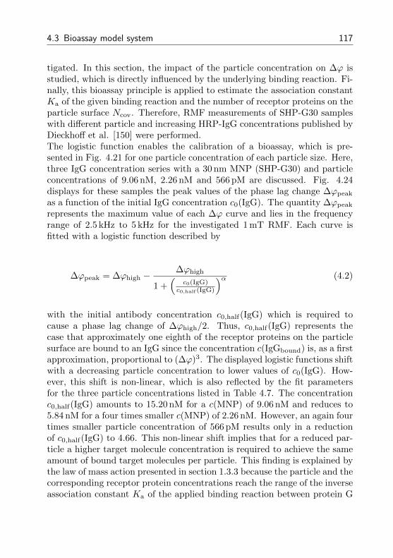
4.3 Bioassay model system 117
tigated. In this section, the impact of the particle concentration on ∆ϕ isstudied, which is directly influenced by the underlying binding reaction. Fi-nally, this bioassay principle is applied to estimate the association constantKa of the given binding reaction and the number of receptor proteins on theparticle surface Ncov. Therefore, RMF measurements of SHP-G30 sampleswith different particle and increasing HRP-IgG concentrations published byDieckhoff et al. [150] were performed.The logistic function enables the calibration of a bioassay, which is pre-sented in Fig. 4.21 for one particle concentration of each particle size. Here,three IgG concentration series with a 30 nm MNP (SHP-G30) and particleconcentrations of 9.06 nM, 2.26 nM and 566 pM are discussed. Fig. 4.24displays for these samples the peak values of the phase lag change ∆ϕpeak
as a function of the initial IgG concentration c0(IgG). The quantity ∆ϕpeak
represents the maximum value of each ∆ϕ curve and lies in the frequencyrange of 2.5 kHz to 5 kHz for the investigated 1 mT RMF. Each curve isfitted with a logistic function described by
∆ϕpeak = ∆ϕhigh −∆ϕhigh
1 +(
c0(IgG)c0,half (IgG)
)α (4.2)
with the initial antibody concentration c0,half(IgG) which is required tocause a phase lag change of ∆ϕhigh/2. Thus, c0,half(IgG) represents thecase that approximately one eighth of the receptor proteins on the particlesurface are bound to an IgG since the concentration c(IgGbound) is, as a firstapproximation, proportional to (∆ϕ)3. The displayed logistic functions shiftwith a decreasing particle concentration to lower values of c0(IgG). How-ever, this shift is non-linear, which is also reflected by the fit parametersfor the three particle concentrations listed in Table 4.7. The concentrationc0,half(IgG) amounts to 15.20 nM for a c(MNP) of 9.06 nM and reduces to5.84 nM for a four times smaller c(MNP) of 2.26 nM. However, an again fourtimes smaller particle concentration of 566 pM results only in a reductionof c0,half(IgG) to 4.66. This non-linear shift implies that for a reduced par-ticle a higher target molecule concentration is required to achieve the sameamount of bound target molecules per particle. This finding is explained bythe law of mass action presented in section 1.3.3 because the particle and thecorresponding receptor protein concentrations reach the range of the inverseassociation constant Ka of the applied binding reaction between protein G
118 4 Results and discussion
and IgG [151]. The maximum value of the phase lag change ∆ϕhigh of eachIgG concentration series is affected by residual buffer components from theparticle and antibody stock solutions since ∆ϕhigh decreases with increasingparticle concentration.The law of mass action, as it is expressed by Eq. 1.45, facilitates a determi-nation of the binding reaction’s association constant by fitting it for knowninitial concentrations of the two reactants (here: protein G and IgG) tothe measured product of the two reactants with Ka as a free fit parameter.For this investigation, the initial protein G concentration is replaced by theproduct of the particle concentration and the average number of protein Gper particle Ncov
c0(proteinG) = c(MNP)Ncov, (4.3)
thus, Ncov displays a second free fit parameter. The concentration of theproducts, which is expressed by the concentration of bound IgG, is deter-mined as follows: Based on the parameters of a fit of the empirical model tothe RMF measurement results, the change of the hydrodynamic diameter∆dh is calculated. The resulting change of the hydrodynamic volume ∆Vh
is defined by
∆Vh =π
6(∆dh)3 (4.4)
and defines the amount of antibodies bound to the particle
NIgG,bound = ∆Vh%P
mP(4.5)
via the average protein density %P of 1.35 g/cm3 [152] and molecular massmP of 270 kDa for the HRP-IgG antibody. The resulting concentration ofbound antibodies c(IgGbound) in each sample is finally calculated with theparticle concentration
c(IgGbound) = c(MNP)∆Vh%P
mP. (4.6)
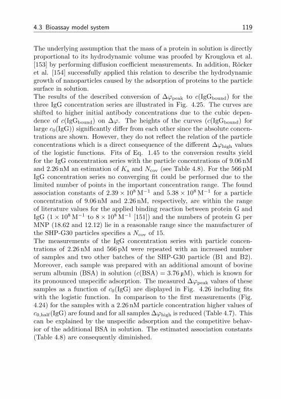
4.3 Bioassay model system 119
The underlying assumption that the mass of a protein in solution is directlyproportional to its hydrodynamic volume was proofed by Krouglova et al.[153] by performing diffusion coefficient measurements. In addition, Rockeret al. [154] successfully applied this relation to describe the hydrodynamicgrowth of nanoparticles caused by the adsorption of proteins to the particlesurface in solution.The results of the described conversion of ∆ϕpeak to c(IgGbound) for thethree IgG concentration series are illustrated in Fig. 4.25. The curves areshifted to higher initial antibody concentrations due to the cubic depen-dence of c(IgGbound) on ∆ϕ. The heights of the curves (c(IgGbound) forlarge c0(IgG)) significantly differ from each other since the absolute concen-trations are shown. However, they do not reflect the relation of the particleconcentrations which is a direct consequence of the different ∆ϕhigh valuesof the logistic functions. Fits of Eq. 1.45 to the conversion results yieldfor the IgG concentration series with the particle concentrations of 9.06 nMand 2.26 nM an estimation of Ka and Ncov (see Table 4.8). For the 566 pMIgG concentration series no converging fit could be performed due to thelimited number of points in the important concentration range. The foundassociation constants of 2.39× 10⁸ M−1 and 5.38× 10⁸ M−1 for a particleconcentration of 9.06 nM and 2.26 nM, respectively, are within the rangeof literature values for the applied binding reaction between protein G andIgG (1× 10⁸ M−1 to 8× 10⁸ M−1 [151]) and the numbers of protein G perMNP (18.62 and 12.12) lie in a reasonable range since the manufacturer ofthe SHP-G30 particles specifies a Ncov of 15.The measurements of the IgG concentration series with particle concen-trations of 2.26 nM and 566 pM were repeated with an increased numberof samples and two other batches of the SHP-G30 particle (B1 and B2).Moreover, each sample was prepared with an additional amount of bovineserum albumin (BSA) in solution (c(BSA) = 3.76 µM), which is known forits pronounced unspecific adsorption. The measured ∆ϕpeak values of thesesamples as a function of c0(IgG) are displayed in Fig. 4.26 including fitswith the logistic function. In comparison to the first measurements (Fig.4.24) for the samples with a 2.26 nM particle concentration higher values ofc0,half(IgG) are found and for all samples ∆ϕhigh is reduced (Table 4.7). Thiscan be explained by the unspecific adsorption and the competitive behav-ior of the additional BSA in solution. The estimated association constants(Table 4.8) are consequently diminished.
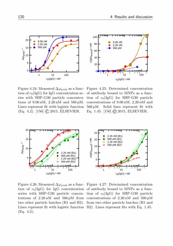
120 4 Results and discussion
20
15
10
5
0
Df
peak
/ °
1 10 100
c0(IgG) / nM
9.06 nM 2.26 nM 566 pM
Figure 4.24: Measured ∆ϕpeak as a func-tion of c0(IgG) for IgG concentration se-ries with SHP-G30 particle concentra-tions of 9.06 nM, 2.26 nM and 566 pM.Lines represent fit with logistic function(Eq. 4.2). [150] © 2015, ELSEVIER.
100
80
60
40
20
0
c(Ig
Gbo
und)
/ nM
4 6 81
2 4 6 810
2 4 6 8100
2
c0(IgG) / nM
9.06 nM 2.26 nM 566 pM
Figure 4.25: Determined concentrationof antibody bound to MNPs as a func-tion of c0(IgG) for SHP-G30 particleconcentrations of 9.06 nM, 2.26 nM and566 pM. Solid lines represent fit withEq. 1.45. [150] © 2015, ELSEVIER.
20
15
10
5
Df
peak
/ °
6 81
2 4 6 810
2 4 6 8100
2
c0(IgG) / nM
2.26 nM (B1) 566 pM (B1) 2.26 nM (B2) 566 pM (B2)
Figure 4.26: Measured ∆ϕpeak as a func-tion of c0(IgG) for IgG concentrationseries with SHP-G30 particle concen-trations of 2.26 nM and 566 pM fromtwo other particle batches (B1 and B2).Lines represent fit with logistic function(Eq. 4.2).
25
20
15
10
5
0
c(Ig
Gbo
und)
/ nM
6 81
2 4 6 810
2 4 6 8100
2
c0(IgG) / nM
2.26 nM (B1) 566 pM (B1) 2.26 nM (B2) 566 pM (B2)
Figure 4.27: Determined concentrationof antibody bound to MNPs as a func-tion of c0(IgG) for SHP-G30 particleconcentrations of 2.26 nM and 566 pMfrom two other particle batches (B1 andB2). Lines represent fits with Eq. 1.45.
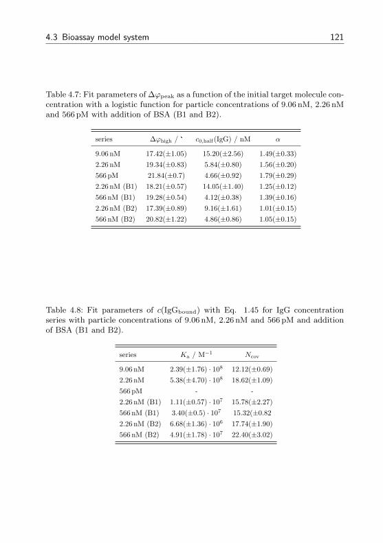
4.3 Bioassay model system 121
Table 4.7: Fit parameters of ∆ϕpeak as a function of the initial target molecule con-centration with a logistic function for particle concentrations of 9.06 nM, 2.26 nMand 566 pM with addition of BSA (B1 and B2).
series ∆ϕhigh / ° c0,half(IgG) / nM α
9.06 nM 17.42(±1.05) 15.20(±2.56) 1.49(±0.33)
2.26 nM 19.34(±0.83) 5.84(±0.80) 1.56(±0.20)
566 pM 21.84(±0.7) 4.66(±0.92) 1.79(±0.29)
2.26 nM (B1) 18.21(±0.57) 14.05(±1.40) 1.25(±0.12)
566 nM (B1) 19.28(±0.54) 4.12(±0.38) 1.39(±0.16)
2.26 nM (B2) 17.39(±0.89) 9.16(±1.61) 1.01(±0.15)
566 nM (B2) 20.82(±1.22) 4.86(±0.86) 1.05(±0.15)
Table 4.8: Fit parameters of c(IgGbound) with Eq. 1.45 for IgG concentrationseries with particle concentrations of 9.06 nM, 2.26 nM and 566 pM and additionof BSA (B1 and B2).
series Ka / M−1 Ncov
9.06 nM 2.39(±1.76) · 108 12.12(±0.69)
2.26 nM 5.38(±4.70) · 108 18.62(±1.09)
566 pM - -
2.26 nM (B1) 1.11(±0.57) · 107 15.78(±2.27)
566 nM (B1) 3.40(±0.5) · 107 15.32(±0.82
2.26 nM (B2) 6.68(±1.36) · 106 17.74(±1.90)
566 nM (B2) 4.91(±1.78) · 107 22.40(±3.02)
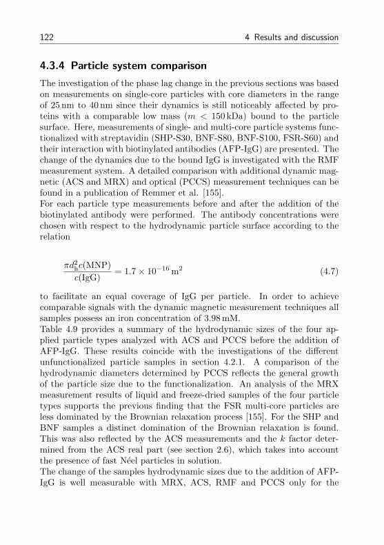
122 4 Results and discussion
4.3.4 Particle system comparison
The investigation of the phase lag change in the previous sections was basedon measurements on single-core particles with core diameters in the rangeof 25 nm to 40 nm since their dynamics is still noticeably affected by pro-teins with a comparable low mass (m < 150 kDa) bound to the particlesurface. Here, measurements of single- and multi-core particle systems func-tionalized with streptavidin (SHP-S30, BNF-S80, BNF-S100, FSR-S60) andtheir interaction with biotinylated antibodies (AFP-IgG) are presented. Thechange of the dynamics due to the bound IgG is investigated with the RMFmeasurement system. A detailed comparison with additional dynamic mag-netic (ACS and MRX) and optical (PCCS) measurement techniques can befound in a publication of Remmer et al. [155].For each particle type measurements before and after the addition of thebiotinylated antibody were performed. The antibody concentrations werechosen with respect to the hydrodynamic particle surface according to therelation
πd2hc(MNP)
c(IgG)= 1.7× 10⁻¹⁶ m2 (4.7)
to facilitate an equal coverage of IgG per particle. In order to achievecomparable signals with the dynamic magnetic measurement techniques allsamples possess an iron concentration of 3.98 mM.Table 4.9 provides a summary of the hydrodynamic sizes of the four ap-plied particle types analyzed with ACS and PCCS before the addition ofAFP-IgG. These results coincide with the investigations of the differentunfunctionalized particle samples in section 4.2.1. A comparison of thehydrodynamic diameters determined by PCCS reflects the general growthof the particle size due to the functionalization. An analysis of the MRXmeasurement results of liquid and freeze-dried samples of the four particletypes supports the previous finding that the FSR multi-core particles areless dominated by the Brownian relaxation process [155]. For the SHP andBNF samples a distinct domination of the Brownian relaxation is found.This was also reflected by the ACS measurements and the k factor deter-mined from the ACS real part (see section 2.6), which takes into accountthe presence of fast Neel particles in solution.The change of the samples hydrodynamic sizes due to the addition of AFP-IgG is well measurable with MRX, ACS, RMF and PCCS only for the
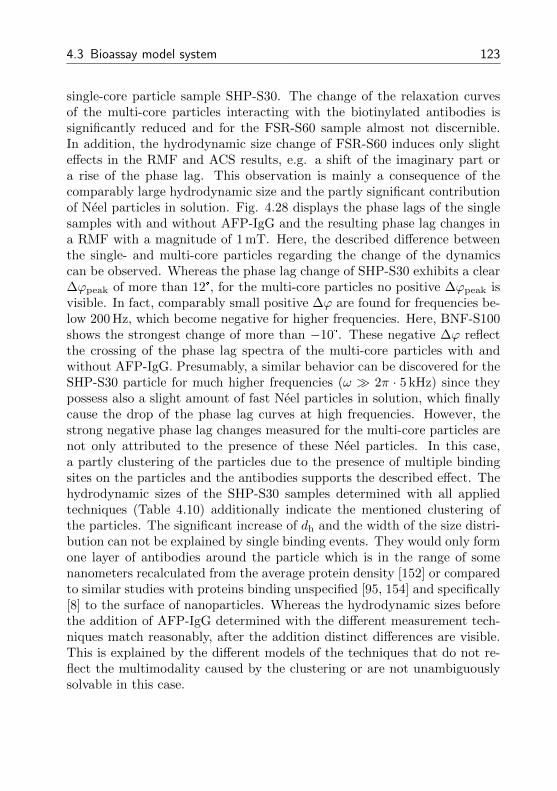
4.3 Bioassay model system 123
single-core particle sample SHP-S30. The change of the relaxation curvesof the multi-core particles interacting with the biotinylated antibodies issignificantly reduced and for the FSR-S60 sample almost not discernible.In addition, the hydrodynamic size change of FSR-S60 induces only slighteffects in the RMF and ACS results, e.g. a shift of the imaginary part ora rise of the phase lag. This observation is mainly a consequence of thecomparably large hydrodynamic size and the partly significant contributionof Neel particles in solution. Fig. 4.28 displays the phase lags of the singlesamples with and without AFP-IgG and the resulting phase lag changes ina RMF with a magnitude of 1 mT. Here, the described difference betweenthe single- and multi-core particles regarding the change of the dynamicscan be observed. Whereas the phase lag change of SHP-S30 exhibits a clear∆ϕpeak of more than 12°, for the multi-core particles no positive ∆ϕpeak isvisible. In fact, comparably small positive ∆ϕ are found for frequencies be-low 200 Hz, which become negative for higher frequencies. Here, BNF-S100shows the strongest change of more than −10°. These negative ∆ϕ reflectthe crossing of the phase lag spectra of the multi-core particles with andwithout AFP-IgG. Presumably, a similar behavior can be discovered for theSHP-S30 particle for much higher frequencies (ω 2π · 5 kHz) since theypossess also a slight amount of fast Neel particles in solution, which finallycause the drop of the phase lag curves at high frequencies. However, thestrong negative phase lag changes measured for the multi-core particles arenot only attributed to the presence of these Neel particles. In this case,a partly clustering of the particles due to the presence of multiple bindingsites on the particles and the antibodies supports the described effect. Thehydrodynamic sizes of the SHP-S30 samples determined with all appliedtechniques (Table 4.10) additionally indicate the mentioned clustering ofthe particles. The significant increase of dh and the width of the size distri-bution can not be explained by single binding events. They would only formone layer of antibodies around the particle which is in the range of somenanometers recalculated from the average protein density [152] or comparedto similar studies with proteins binding unspecified [95, 154] and specifically[8] to the surface of nanoparticles. Whereas the hydrodynamic sizes beforethe addition of AFP-IgG determined with the different measurement tech-niques match reasonably, after the addition distinct differences are visible.This is explained by the different models of the techniques that do not re-flect the multimodality caused by the clustering or are not unambiguouslysolvable in this case.
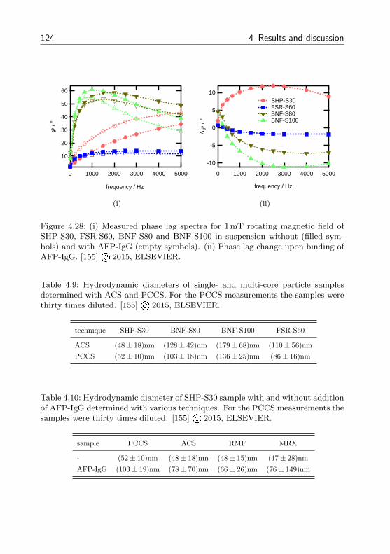
124 4 Results and discussion
60
50
40
30
20
10
f /
°
500040003000200010000
frequency / Hz
(i)
10
5
0
-5
-10
Df
/ °
500040003000200010000
frequency / Hz
SHP-S30 FSR-S60 BNF-S80 BNF-S100
(ii)
Figure 4.28: (i) Measured phase lag spectra for 1 mT rotating magnetic field ofSHP-S30, FSR-S60, BNF-S80 and BNF-S100 in suspension without (filled sym-bols) and with AFP-IgG (empty symbols). (ii) Phase lag change upon binding ofAFP-IgG. [155] © 2015, ELSEVIER.
Table 4.9: Hydrodynamic diameters of single- and multi-core particle samplesdetermined with ACS and PCCS. For the PCCS measurements the samples werethirty times diluted. [155] © 2015, ELSEVIER.
technique SHP-S30 BNF-S80 BNF-S100 FSR-S60
ACS (48± 18)nm (128± 42)nm (179± 68)nm (110± 56)nm
PCCS (52± 10)nm (103± 18)nm (136± 25)nm (86± 16)nm
Table 4.10: Hydrodynamic diameter of SHP-S30 sample with and without additionof AFP-IgG determined with various techniques. For the PCCS measurements thesamples were thirty times diluted. [155] © 2015, ELSEVIER.
sample PCCS ACS RMF MRX
- (52± 10)nm (48± 18)nm (48± 15)nm (47± 28)nm
AFP-IgG (103± 19)nm (78± 70)nm (66± 26)nm (76± 149)nm
4.3 Bioassay model system 125
4.3.5 Tumor marker detection
In this section, the principle and preliminary measurement results of thequantitative detection of the medical relevant biomarker HER2 with theSHP-S30 particles and HER2-IgG antibodies in water-based test samplesare presented. HER2 is a tumor-specific biomarker which can be overex-pressed in the case of breast cancer (> 30 %) [156]. A quick and reliablequantification of this marker in patient serum plays an important role in thecancer therapy. For the test samples the recombinant human HER2 proteinis purchased from ebioscience (Frankfurt, Germany). The non-quantitativedetection of HER2 with functionalized ALP particles was reported by Lak[37].Since the SHP-S30 particles are not directly functionalized with a recep-tor protein for HER2 a further step is introduced in the sample prepara-tion and measurement process. The principle is illustrated in Fig. 4.29:Six samples with HER2 concentrations ranging from 0 nM to 74.12 nM areprepared, the pure SHP-S30 particles are added and the phase lag ϕ1 ismeasured. In a next step, a HER2-IgG solution with a concentration of10 nM is injected into each sample. Then ϕ2 is determined and the phaselag change ∆ϕ is calculated. Here, it has to be taken into account thatthe increase of the hydrodynamic volume is based on pairs of HER2-IgGand HER2. Thus, in the measurement results of ∆ϕ (Fig. 4.30) the phaselag change of the sample without HER2 is subtracted from the phase lagchanges of the other samples. This measurement series was performed fortwo particle concentrations: 1 nM and 2 nM. Interestingly, a clear differenceis observed in Fig. 4.30 for the two particle concentrations. Whereas forc(MNP) = 1 nM the two lowest HER2 concentrations cause no significant∆ϕ, for c(MNP) = 2 nM all HER2 concentrations can be detected and anoverall increase of ∆ϕ is observed. In addition, the ∆ϕ curves for the higherparticle concentration are much narrower. This behavior can be explainedby the formation of clusters with increasing particle concentration sinceagain multiple binding sites are present. Apparently, ∆ϕ becomes negativefor higher frequencies which is in accordance with the results from the pre-vious section.The medical relevant cutoff value for the concentration determination ofHER2 in serum during a breast cancer therapy is in the range of 150 pMto 200 pM (15 ng/mL [156]). Although this threshold is not achieved bythe presented configuration of measurement system and nanoparticles, thepotential of the RMF based concept for the quantitative detection of small
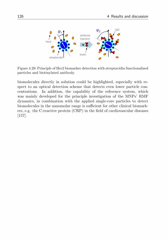
126 4 Results and discussion
φ2φ1
Her2
IgG
antibodyinjection
biotinstreptavidin
Figure 4.29: Principle of Her2 biomarker detection with streptavidin functionalizedparticles and biotinylated antibody.
biomolecules directly in solution could be highlighted, especially with re-spect to an optical detection scheme that detects even lower particle con-centrations. In addition, the capability of the reference system, whichwas mainly developed for the principle investigation of the MNPs’ RMFdynamics, in combination with the applied single-core particles to detectbiomolecules in the nanomolar range is sufficient for other clinical biomark-ers, e.g. the C-reactive protein (CRP) in the field of cardiovascular diseases[157].
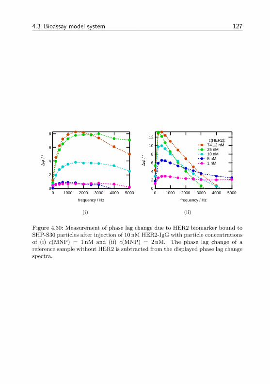
4.3 Bioassay model system 127
8
6
4
2
0
Df
/ °
500040003000200010000
frequency / Hz
(i)
12
10
8
6
4
2
0
Df
/ °
500040003000200010000
frequency / Hz
c(HER2): 74.12 nM 25 nM 10 nM 5 nM 1 nM
(ii)
Figure 4.30: Measurement of phase lag change due to HER2 biomarker bound toSHP-S30 particles after injection of 10 nM HER2-IgG with particle concentrationsof (i) c(MNP) = 1 nM and (ii) c(MNP) = 2 nM. The phase lag change of areference sample without HER2 is subtracted from the displayed phase lag changespectra.

128 4 Results and discussion
129
Conclusion and outlook
The dynamic response of suspended magnetic nanoparticles to rotating mag-netic fields was subject of this work. A measurement system based on amagnetic detection was developed and utilized for measurements on dif-ferent magnetic nanoparticle systems. The physical quantity for the char-acterization of this dynamics is the phase lag between the MNP ensem-ble magnetization and the RMF. This work was carried out in the courseof the NAMDIATREAM project and supported the investigation and re-alization of a homogeneous bioassay concept based on a sensitive opticalbiomolecule detection with rod-shaped magnetic nanoparticles in rotatingmagnetic fields.The detection unit of the RMF system presented in this work comprisesa gradiometric arrangement of fluxgate magnetometers, thus, enabling acomparably robust detection of the stray field of MNP suspensions out-side a magnetically shielded room. The possible parameter variations ofthe RMF generation unit (µ0H ≤ 9.1 mT, ω/2π ≤ 5 kHz) enable an in-vestigation of different magnetic nanoparticle systems with hydrodynamicdiameters ranging from 35 nm to several 100 nm, and the sensitive fluxgatemagnetometers facilitate a detection of 150 µL MNP suspensions with ironconcentrations even below 0.005 g/L.Different physical models for the description of the magnetization dynamicsof magnetic nanoparticle ensembles in rotating magnetic fields were intro-duced. The results of a numerical solution of the Fokker-Planck equationadopted for magnetic nanoparticles in a RMF matched perfectly the mea-surement results of different particle systems. Furthermore, an empiricalmodel was derived which is well applicable for the design and analysis ofRMF based magnetic nanoparticle measurements. This model exhibits sig-nificantly reduced phase and magnitude errors for large Langevin parame-ters (ξ 1) compared to other magnetization equation models.The influence of the particle parameters could be studied with measure-ments on spherical single- and multi-core as well as rod-shaped magneticnanoparticles. The predicted inverse tangent dependence of the phase lagon the RMF frequency was found for all particle systems. The rise of this
130 Conclusion and outlook
phase lag as a function of the frequency depends significantly on the par-ticle and suspension parameters in accordance with the modified Browniantime constant τ⊥. In this context, the effect of the hydrodynamic size, themagnetic moment, the corresponding size distributions and the temperaturecould be illustrated with measurements. Additional particle characteriza-tion techniques (e.g. ACS and PCCS) supported the particle parametersobtained by simulating the measured phase lags. A comparison of the RMFwith the alternating field excitation resulted in significant differences of theMNP dynamics for large Langevin parameters (ξ 1), e.g. a more pro-nounced spreading of the phase lag with the field magnitude was found forthe RMF.The concept of the RMF bioassay which is based on a phase lag changeinduced by biomolecules binding to the particle surface and affecting theMNP dynamics could be proofed with two different particle functionaliza-tions. For instance, sample series with protein G functionalized single-coreparticles and varying antibody concentrations enabled the successful investi-gation of a quantitative biomolecule detection. In this case, well measurablephase lag changes of up to 25° were caused. Recorded calibration curvescould be successfully fitted with logistic functions and enabled a compari-son of the influence of the particle parameters on the bioassay results. Forthe applied single-core particles, a core diameter of 30 nm was identified tobe the optimum since this particle is clearly dominated by the Brownianrelaxation, possesses a comparably high magnetic moment but its hydrody-namic size is still noticeably influenced by small biomolecules. Multi-coreparticles turned out to be unsuitable for the detection of biomolecules basedon single binding events, instead detection schemes resulting in a cluster-ing of the particles are appropriate. Furthermore, the identified differencesbetween the RMF and alternating field excitation resulted in an increasedphase lag change for binding experiments with single-core particles in ro-tating magnetic fields. In this context, simulations supported the findingthat a wide hydrodynamic size distribution reduces significantly the phaselag change caused by bound biomolecules. Finally, the underlying bindingreactions could be reasonably analyzed and a medical relevant biomarkercould be quantitatively detected.
For the modeling of RMF bioassay results obtained with rod-shaped nanopar-ticles, a physical model incorporating only the Brownian particle dynamicsis completely sufficient. Due to their pronounced shape anisotropy, they areclearly dominated by the Brownian relaxation process, even with larger pro-
131
teins bound to their surface. For spherical particles, such a clear dominationis not given in all cases. For some particles, a modeling with the discussedtheories resulted in insufficient matches. Here, a model incorporating theBrownian and Neel relaxation as well as their overlap for the description ofthe rotational dynamics with ξ > 1 would solve the problem.Regarding the biomedical application of the RMF concept clinical investi-gations need to be carried out, especially with respect to the specificity ofthe biomolecule recognition and unspecific bindings in serum. The magneticdetection scheme can be improved with optimized MNP size distributionsand increased field frequencies and magnitudes while utilizing air coils forthe detection. Further applications based on magnetic nanoparticles in ro-tating magnetic fields are even possible. For instance, the impact of a RMFexcitation of MNPs in hyperthermia applications is discussed [158].

132 Conclusion and outlook
133
A Appendix
A.1 Residual RMF component error
A residual component of the RMF excitation (ϕR and BR) in the measure-ment signal, expressed by ϕM and BM, cause errors since the phase lag ϕand magnitude BS of a MNP sample in the RMF can not be distinguishedfrom the residual components. Here, a mathematical description of the de-viation of ϕM and BM from ϕ and BS, respectively, as a function of theresidual RMF and MNP sample components is presented.In general, ϕM and BM can be expressed as:
ϕM = arctan
(BS sin (ϕ) +BR sin (ϕR)
BS cos (ϕ) +BR cos (ϕR)
)(A.1)
and
BM =
√(BS sin (ϕ) +BR sin (ϕR))
2+ (BS cos (ϕ) +BR cos (ϕR))
2. (A.2)
For the calculation of the deviation ϕM − ϕ and the relation BM/BS as afunction of the residual RMF and MNP sample components, ϕR can be setto zero since one rotation of ϕ covers all possible angles between ϕ and ϕR.Finally, the formulas are defined as:
ϕM − ϕ = arctan
(sin (ϕ)
BR/BS + cos (ϕ)
)− ϕ (A.3)
and
BM/BS =
√(sin (ϕ))
2+ (BR/BS + cos (ϕ))
2. (A.4)
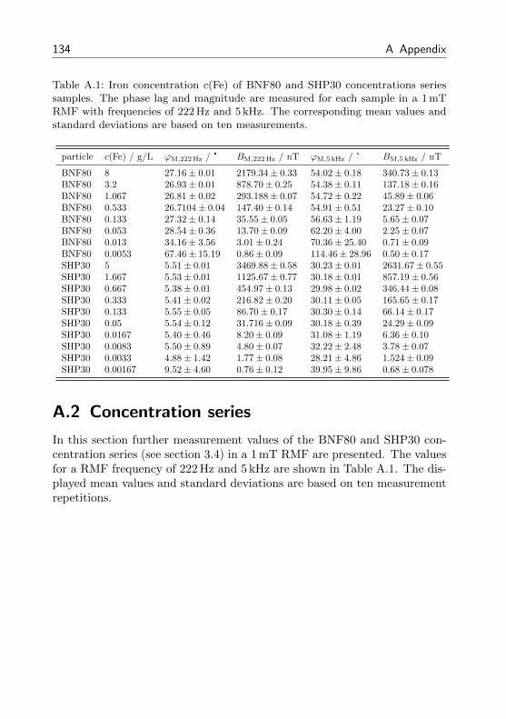
134 A Appendix
Table A.1: Iron concentration c(Fe) of BNF80 and SHP30 concentrations seriessamples. The phase lag and magnitude are measured for each sample in a 1 mTRMF with frequencies of 222 Hz and 5 kHz. The corresponding mean values andstandard deviations are based on ten measurements.
particle c(Fe) / g/L ϕM,222 Hz / ° BM,222 Hz / nT ϕM,5 kHz / ° BM,5 kHz / nT
BNF80 8 27.16± 0.01 2179.34± 0.33 54.02± 0.18 340.73± 0.13BNF80 3.2 26.93± 0.01 878.70± 0.25 54.38± 0.11 137.18± 0.16BNF80 1.067 26.81± 0.02 293.188± 0.07 54.72± 0.22 45.89± 0.06BNF80 0.533 26.7104± 0.04 147.40± 0.14 54.91± 0.51 23.27± 0.10BNF80 0.133 27.32± 0.14 35.55± 0.05 56.63± 1.19 5.65± 0.07BNF80 0.053 28.54± 0.36 13.70± 0.09 62.20± 4.00 2.25± 0.07BNF80 0.013 34.16± 3.56 3.01± 0.24 70.36± 25.40 0.71± 0.09BNF80 0.0053 67.46± 15.19 0.86± 0.09 114.46± 28.96 0.50± 0.17SHP30 5 5.51± 0.01 3469.88± 0.58 30.23± 0.01 2631.67± 0.55SHP30 1.667 5.53± 0.01 1125.67± 0.77 30.18± 0.01 857.19± 0.56SHP30 0.667 5.38± 0.01 454.97± 0.13 29.98± 0.02 346.44± 0.08SHP30 0.333 5.41± 0.02 216.82± 0.20 30.11± 0.05 165.65± 0.17SHP30 0.133 5.55± 0.05 86.70± 0.17 30.30± 0.14 66.14± 0.17SHP30 0.05 5.54± 0.12 31.716± 0.09 30.18± 0.39 24.29± 0.09SHP30 0.0167 5.40± 0.46 8.20± 0.09 31.08± 1.19 6.36± 0.10SHP30 0.0083 5.50± 0.89 4.80± 0.07 32.22± 2.48 3.78± 0.07SHP30 0.0033 4.88± 1.42 1.77± 0.08 28.21± 4.86 1.524± 0.09SHP30 0.00167 9.52± 4.60 0.76± 0.12 39.95± 9.86 0.68± 0.078
A.2 Concentration series
In this section further measurement values of the BNF80 and SHP30 con-centration series (see section 3.4) in a 1 mT RMF are presented. The valuesfor a RMF frequency of 222 Hz and 5 kHz are shown in Table A.1. The dis-played mean values and standard deviations are based on ten measurementrepetitions.
135
Publications and presentations
Publications
(1) H. Remmer, J. Dieckhoff, M. Schilling, and F. Ludwig, Suitability ofmagnetic single- and multi-core nanoparticles to detect protein bindingwith dynamic magnetic measurement techniques, Journal of Magnetism andMagnetic Materials, vol. 380, pp. 236–240, Apr. 2015.
(2) J. Dieckhoff, S. Schrittwieser, J. Schotter, H. Remmer, M. Schilling, andF. Ludwig, Single-core magnetic markers in rotating magnetic field basedhomogeneous bioassays and the law of mass action, Journal of Magnetismand Magnetic Materials, vol. 380, pp. 205–208, Apr. 2015.
(3) F. Ludwig, C. Kuhlmann, T. Wawrzik, J. Dieckhoff, A. Lak, A. P.Kandhar, R. M. Ferguson, S. J. Kemp, and K. M. Krishnan, Dynamic Mag-netic Properties of Optimized Magnetic Nanoparticles for Magnetic ParticleImaging, IEEE Transactions on Magnetics, vol. 50, no. 11, pp. 1–4, Nov.2014.
(4) J. Dieckhoff, S. Schrittwieser, J. Schotter, H. Remmer, M. Schilling, andF. Ludwig, Single-core magnetic markers in rotating magnetic field basedhomogeneous bioassays and the law of mass action, Journal of Magnetismand Magnetic Materials, Oct. 2014.
(5) J. Dieckhoff, M. Schilling, and F. Ludwig, Magnetic marker based ho-mogeneous bioassays utilizing rotating magnetic fields, Journal of AppliedPhysics, vol. 115, no. 17, p. 17B304, May 2014.
(6) J. Dieckhoff, A. Lak, M. Schilling, and F. Ludwig, Protein detectionwith magnetic nanoparticles in a rotating magnetic field, Journal of Ap-plied Physics, vol. 115, no. 2, p. 024701, Jan. 2014.
136 Publications and presentations
(7) S. Schrittwieser, F. Ludwig, J. Dieckhoff, A. Tschoepe, A. Guenther,M. Richter, A. Huetten, H. Brueckl, and J. Schotter, Direct Protein Detec-tion in the Sample Solution by Monitoring Rotational Dynamics of NickelNanorods, Small, vol. 10, no. 2, pp. 407–411, Jan. 2014.
(8) A. Lak, F. Ludwig, J. M. Scholtyssek, J. Dieckhoff, K. Fiege, and M.Schilling, Size Distribution and Magnetization Optimization of Single-CoreIron Oxide Nanoparticles by Exploiting Design of Experiment Methodology,IEEE Transactions on Magnetics, vol. 49, no. 1, pp. 201–207, Jan. 2013.
(9) A. Lak, J. Dieckhoff, F. Ludwig, J. M. Scholtyssek, O. Goldmann, H.Lunsdorf, D. Eberbeck, A. Kornowski, M. Kraken, F. J. Litterst, K. Fiege,P. Mischnick, and M. Schilling, Highly stable monodisperse PEGylated ironoxide nanoparticle aqueous suspensions: a nontoxic tracer for homogeneousmagnetic bioassays, Nanoscale, vol. 5, no. 23, p. 11447, 2013.
(10) J. Dieckhoff, T. Yoshida, K. Enpuku, M. Schilling, and F. Ludwig,Homogeneous Bioassays Based on the Manipulation of Magnetic Nanopar-ticles by Rotating and Alternating Magnetic Fields - A Comparison, IEEETransactions on Magnetics, vol. 48, no. 11, pp. 3792–3795, Nov. 2012.
(11) S. Schrittwieser, F. Ludwig, J. Dieckhoff, K. Soulantica, G. Viau, L.-M.Lacroix, S. M. Lentijo, R. Boubekri, J. Maynadie, A. Huetten, H. Brueckl,and J. Schotter, Modeling and Development of a Biosensor Based on Opti-cal Relaxation Measurements of Hybrid Nanoparticles, ACS Nano, vol. 6,no. 1, pp. 791–801, Jan. 2012.
(12) T. Yoshida, K. Enpuku, F. Ludwig, J. Dieckhoff, T. Wawrzik, A. Lak,and M. Schilling, Characterization of Resovist® Nanoparticles for MagneticParticle Imaging, in Magnetic Particle Imaging, vol. 140, T. M. Buzug andJ. Borgert, Eds. Berlin, Heidelberg: Springer Berlin Heidelberg, 2012, pp.3–7.
(13) T. Yoshida, K. Enpuku, J. Dieckhoff, M. Schilling, and F. Ludwig,Magnetic fluid dynamics in a rotating magnetic field, Journal of AppliedPhysics, vol. 111, no. 5, p. 053901, 2012.
137
(14) J. Dieckhoff, M. Schilling, and F. Ludwig, Fluxgate based detectionof magnetic nanoparticle dynamics in a rotating magnetic field, AppliedPhysics Letters, vol. 99, no. 11, p. 112501, 2011.
Presentations
(1) J. Dieckhoff, T. Yoshida, M. Schilling, F. Ludwig, Response of spheri-cal magnetic nanoparticles to rotating magnetic fields (Oral), 11th GermanFerrofluid Workshop, Benediktbeuern (2011).
(2) J. Dieckhoff, T. Yoshida, K. Enpuku, M. Schilling, and F. Ludwig,Homogeneous Bioassays Based on the Manipulation of Magnetic Nanopar-ticles by Rotating and Alternating Magnetic Fields – a Comparison (Oral),IEEE International Magnetics Conference, Vancouver (2012).
(3) J. Dieckhoff, M. Schilling, and F. Ludwig, Magnetic nanoparticle bind-ing experiments in rotating magnetic fields (Poster), 12th German FerrofluidWorkshop, Benediktbeuern (2012).
(4) J. Dieckhoff, M. Schilling, and F. Ludwig, Homogeneous bioassay basedon specifically labeled magnetic nanoparticles in a rotating magnetic field(Poster/Oral), NAMDIATREAM Winter School, Villars-sur-Ollon (2013).
(5) J. Dieckhoff, M. Schilling, and F. Ludwig, Bioassay based on the responseof magnetic nanoparticles to rotating magnetic fields (Oral), Fruhjahrsta-gung des Arbeitskreises Festkorperphysik der DPG, Regensburg (2013).
(6) J. Dieckhoff, M. Schilling, and F. Ludwig, Homogeneous bioassay devel-opment based on magnetic nanoparticles in rotating magnetic fields (Poster),3rd P3AGI Imaging Workshop, Gottingen (2013).
(7) J. Dieckhoff, M. Schilling, and F. Ludwig, Magnetic marker based ho-mogeneous bioassays utilizing rotating magnetic fields (Oral), 58th AnnualConference on Magnetism and Magnetic Materials, Denver (2013).

138 Publications and presentations
(8) J. Dieckhoff, S. Schrittwieser, J. Schotter, H. Remmer, M. Schilling,and F. Ludwig, Single-core magnetic markers in rotating magnetic fieldbased homogeneous bioassays and the law of mass action (Poster/Oral),10th International Conference on the Scientific and Clinical Applications ofMagnetic Carriers, Dresden (2014).
(9) J. Dieckhoff, H. Remmer, M. Schilling, and F. Ludwig, Quantitativebiomarker detection with magnetic nanoparticles (Oral), 48th DGBMT An-nual Conference, Hannover (2014).
139
Bibliography
[1] L. Neel, Theorie du trainage magnetique des ferromagnetiques augrains fin avec applications aux terres cuites, Annales Geophysicae5 (1949) 99–136.
[2] W. F. Brown, Thermal fluctuations of a single-domain particle, Phys-ical Review 130 (1963) 1677–1686.
[3] S. Schrittwieser, F. Ludwig, J. Dieckhoff, K. Soulantica, G. Viau,L.-M. Lacroix, S. M. Lentijo, R. Boubekri, J. Maynadie, A. Huet-ten, H. Brueckl, J. Schotter, Modeling and development of a biosen-sor based on optical relaxation measurements of hybrid nanoparticles,ACS Nano 6 (1) (2012) 791–801.
[4] P. Yager, G. J. Domingo, J. Gerdes, Point-of-Care Diagnostics forGlobal Health, Annual Review of Biomedical Engineering 10 (1)(2008) 107–144.
[5] W. Weitschies, R. Kotitz, T. Bunte, L. Trahms, Determination ofrelaxing or remanent nanoparticle magnetization provides a novelbinding-specific technique for the evaluation of immunoassays, Phar-maceutical and Pharmacological Letters (7) (1997) 1–4.
[6] E. Heim, F. Ludwig, M. Schilling, Binding assays with streptavidin-functionalized superparamagnetic nanoparticles and biotinylated an-alytes using fluxgate magnetorelaxometry, Journal of Magnetism andMagnetic Materials 321 (10) (2009) 1628–1631.
[7] J. Connolly, T. G. St Pierre, Proposed biosensors based on time-dependent properties of magnetic fluids, Journal of Magnetism andMagnetic Materials 225 (1-2) (2001) 156–160.
[8] S.-H. Chung, A. Hoffmann, K. Guslienko, S. D. Bader, C. Liu, B. Kay,L. Makowski, L. Chen, Biological sensing with magnetic nanoparti-cles using Brownian relaxation (invited), Journal of Applied Physics97 (10) (2005) 10R101.
140 Bibliography
[9] C.-Y. Hong, C. C. Wu, Y. C. Chiu, S. Y. Yang, H. E. Horng, H. C.Yang, Magnetic susceptibility reduction method for magnetically la-beled immunoassay, Applied Physics Letters 88 (21) (2006) 212512.
[10] L. Tu, Y. Jing, Y. Li, J.-P. Wang, Real-time measurement of Brownianrelaxation of magnetic nanoparticles by a mixing-frequency method,Applied Physics Letters 98 (21) (2011) 213702.
[11] B. H. McNaughton, R. R. Agayan, R. Clarke, R. G. Smith, R. Kopel-man, Single bacterial cell detection with nonlinear rotational fre-quency shifts of driven magnetic microspheres, Applied Physics Let-ters 91 (22) (2007) 224105.
[12] A. Ranzoni, G. Sabatte, L. J. van IJzendoorn, M. W. J. Prins,One-Step Homogeneous Magnetic Nanoparticle Immunoassay forBiomarker Detection Directly in Blood Plasma, ACS Nano 6 (4)(2012) 3134–3141.
[13] F. Wittbracht, B. Eickenberg, A. Weddemann, A. Hutten, Towardsa programmable microfluidic valve: Formation dynamics of two-dimensional magnetic bead arrays in transient magnetic fields, Journalof Applied Physics 109 (11) (2011) 114503.
[14] J.-C. Bacri, A. Cebers, R. Perzynski, Behavior of a magnetic fluid mi-crodrop in a rotating magnetic field, Physical Review Letters 72 (17)(1994) 2705–2708.
[15] Q. A. Pankhurst, N. T. K. Thanh, S. K. Jones, J. Dobson, Progressin applications of magnetic nanoparticles in biomedicine, Journal ofPhysics D: Applied Physics 42 (22) (2009) 224001.
[16] S. Miltenyi, W. Muller, W. Weichel, A. Radbruch, High gradient mag-netic cell separation with MACS, Cytometry 11 (2) (1990) 231–238.
[17] A. Frenzel, C. Bergemann, G. Kohl, T. Reinard, Novel purificationsystem for 6xhis-tagged proteins by magnetic affinity separation, Jour-nal of Chromatography B 793 (2) (2003) 325–329.
[18] I. Safarik, M. Safarikova, Magnetic techniques for the isolation andpurification of proteins and peptides, BioMagnetic Research and Tech-nology 2 (2004) 7.
Bibliography 141
[19] A. S. Lubbe, C. Alexiou, C. Bergemann, Clinical Applications of Mag-netic Drug Targeting, Journal of Surgical Research 95 (2) (2001) 200–206.
[20] Y. Okuhata, Delivery of diagnostic agents for magnetic resonanceimaging, Advanced Drug Delivery Reviews 37 (1-3) (1999) 121–137.
[21] M. K. Yu, J. Park, S. Jon, Magnetic nanoparticles and their applica-tions in image-guided drug delivery, Drug Delivery and TranslationalResearch 2 (1) (2012) 3–21.
[22] J. Zhang, R. Misra, Magnetic drug-targeting carrier encapsulated withthermosensitive smart polymer: Core–shell nanoparticle carrier anddrug release response, Acta Biomaterialia 3 (6) (2007) 838–850.
[23] P. Wust, B. Hildebrandt, G. Sreenivasa, B. Rau, J. Gellermann,H. Riess, R. Felix, P. Schlag, Hyperthermia in combined treatmentof cancer, The Lancet Oncology 3 (8) (2002) 487–497.
[24] B. Thiesen, A. Jordan, Clinical applications of magnetic nanoparticlesfor hyperthermia, International Journal of Hyperthermia 24 (6) (2008)467–474.
[25] B. Gleich, J. Weizenecker, Tomographic imaging using the nonlinearresponse of magnetic particles, Nature 435 (7046) (2005) 1214–1217.
[26] J. Weizenecker, B. Gleich, J. Rahmer, H. Dahnke, J. Borgert, Three-dimensional real-time in vivo magnetic particle imaging, Physics inMedicine and Biology 54 (5) (2009) L1–L10.
[27] J. Borgert, J. D. Schmidt, I. Schmale, C. Bontus, B. Gleich, B. David,J. Weizenecker, J. Jockram, C. Lauruschkat, O. Mende, M. Hein-rich, A. Halkola, J. Bergmann, O. Woywode, J. Rahmer, Perspec-tives on clinical magnetic particle imaging, Biomedizinische Tech-nik/Biomedical Engineering 58 (6).
[28] R. Kotitz, H. Matz, L. Trahms, H. Koch, W. Weitschies, T. Rheinlan-der, W. Semmler, T. Bunte, SQUID based remanence measurementsfor immunoassays, IEEE Transactions on Appiled Superconductivity7 (2) (1997) 3678–3681.
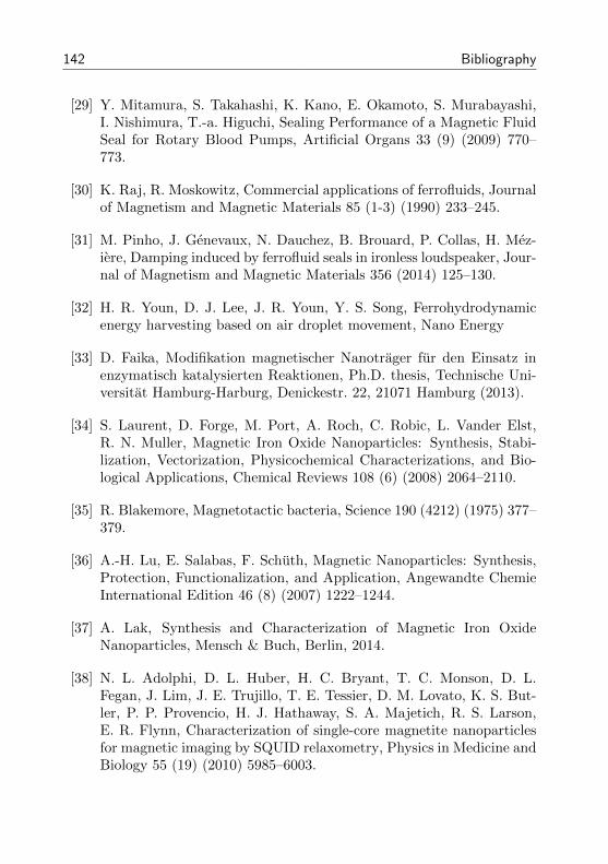
142 Bibliography
[29] Y. Mitamura, S. Takahashi, K. Kano, E. Okamoto, S. Murabayashi,I. Nishimura, T.-a. Higuchi, Sealing Performance of a Magnetic FluidSeal for Rotary Blood Pumps, Artificial Organs 33 (9) (2009) 770–773.
[30] K. Raj, R. Moskowitz, Commercial applications of ferrofluids, Journalof Magnetism and Magnetic Materials 85 (1-3) (1990) 233–245.
[31] M. Pinho, J. Genevaux, N. Dauchez, B. Brouard, P. Collas, H. Mez-iere, Damping induced by ferrofluid seals in ironless loudspeaker, Jour-nal of Magnetism and Magnetic Materials 356 (2014) 125–130.
[32] H. R. Youn, D. J. Lee, J. R. Youn, Y. S. Song, Ferrohydrodynamicenergy harvesting based on air droplet movement, Nano Energy
[33] D. Faika, Modifikation magnetischer Nanotrager fur den Einsatz inenzymatisch katalysierten Reaktionen, Ph.D. thesis, Technische Uni-versitat Hamburg-Harburg, Denickestr. 22, 21071 Hamburg (2013).
[34] S. Laurent, D. Forge, M. Port, A. Roch, C. Robic, L. Vander Elst,R. N. Muller, Magnetic Iron Oxide Nanoparticles: Synthesis, Stabi-lization, Vectorization, Physicochemical Characterizations, and Bio-logical Applications, Chemical Reviews 108 (6) (2008) 2064–2110.
[35] R. Blakemore, Magnetotactic bacteria, Science 190 (4212) (1975) 377–379.
[36] A.-H. Lu, E. Salabas, F. Schuth, Magnetic Nanoparticles: Synthesis,Protection, Functionalization, and Application, Angewandte ChemieInternational Edition 46 (8) (2007) 1222–1244.
[37] A. Lak, Synthesis and Characterization of Magnetic Iron OxideNanoparticles, Mensch & Buch, Berlin, 2014.
[38] N. L. Adolphi, D. L. Huber, H. C. Bryant, T. C. Monson, D. L.Fegan, J. Lim, J. E. Trujillo, T. E. Tessier, D. M. Lovato, K. S. But-ler, P. P. Provencio, H. J. Hathaway, S. A. Majetich, R. S. Larson,E. R. Flynn, Characterization of single-core magnetite nanoparticlesfor magnetic imaging by SQUID relaxometry, Physics in Medicine andBiology 55 (19) (2010) 5985–6003.
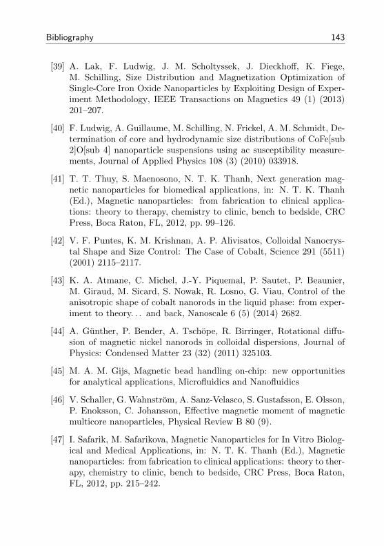
Bibliography 143
[39] A. Lak, F. Ludwig, J. M. Scholtyssek, J. Dieckhoff, K. Fiege,M. Schilling, Size Distribution and Magnetization Optimization ofSingle-Core Iron Oxide Nanoparticles by Exploiting Design of Exper-iment Methodology, IEEE Transactions on Magnetics 49 (1) (2013)201–207.
[40] F. Ludwig, A. Guillaume, M. Schilling, N. Frickel, A. M. Schmidt, De-termination of core and hydrodynamic size distributions of CoFe[sub2]O[sub 4] nanoparticle suspensions using ac susceptibility measure-ments, Journal of Applied Physics 108 (3) (2010) 033918.
[41] T. T. Thuy, S. Maenosono, N. T. K. Thanh, Next generation mag-netic nanoparticles for biomedical applications, in: N. T. K. Thanh(Ed.), Magnetic nanoparticles: from fabrication to clinical applica-tions: theory to therapy, chemistry to clinic, bench to bedside, CRCPress, Boca Raton, FL, 2012, pp. 99–126.
[42] V. F. Puntes, K. M. Krishnan, A. P. Alivisatos, Colloidal Nanocrys-tal Shape and Size Control: The Case of Cobalt, Science 291 (5511)(2001) 2115–2117.
[43] K. A. Atmane, C. Michel, J.-Y. Piquemal, P. Sautet, P. Beaunier,M. Giraud, M. Sicard, S. Nowak, R. Losno, G. Viau, Control of theanisotropic shape of cobalt nanorods in the liquid phase: from exper-iment to theory. . . and back, Nanoscale 6 (5) (2014) 2682.
[44] A. Gunther, P. Bender, A. Tschope, R. Birringer, Rotational diffu-sion of magnetic nickel nanorods in colloidal dispersions, Journal ofPhysics: Condensed Matter 23 (32) (2011) 325103.
[45] M. A. M. Gijs, Magnetic bead handling on-chip: new opportunitiesfor analytical applications, Microfluidics and Nanofluidics
[46] V. Schaller, G. Wahnstrom, A. Sanz-Velasco, S. Gustafsson, E. Olsson,P. Enoksson, C. Johansson, Effective magnetic moment of magneticmulticore nanoparticles, Physical Review B 80 (9).
[47] I. Safarik, M. Safarikova, Magnetic Nanoparticles for In Vitro Biolog-ical and Medical Applications, in: N. T. K. Thanh (Ed.), Magneticnanoparticles: from fabrication to clinical applications: theory to ther-apy, chemistry to clinic, bench to bedside, CRC Press, Boca Raton,FL, 2012, pp. 215–242.
144 Bibliography
[48] Structure and Magnetism in Magnetic Nanoparticles, in: N. T. K.Thanh, D. Ortega (Eds.), Magnetic nanoparticles: from fabricationto clinical applications: theory to therapy, chemistry to clinic, benchto bedside, CRC Press, Boca Raton, FL, 2012, pp. 3–44.
[49] B. Kozissnik, L. A. W. Green, K. A. Chester, N. T. K. Thanh, Strate-gies for functionalisation of magnetic nanoparticles for biological tar-gets, in: N. T. K. Thanh (Ed.), Magnetic nanoparticles: from fabri-cation to clinical applications: theory to therapy, chemistry to clinic,bench to bedside, CRC Press, Boca Raton, FL, 2012, pp. 129–150.
[50] R. E. Rosensweig, Ferrohydrodynamics, Dover Publications, 1997.
[51] S. Odenbach, L. M. Pop, A. Y. Zubarev, Rheological propertiesof magnetic fluids and their microstructural background, GAMM-Mitteilungen 30 (1) (2007) 195–204.
[52] S. Blundell, Magnetism in condensed matter, Oxford University Press,Oxford; New York, 2001.
[53] D. L. Leslie-Pelecky, R. D. Rieke, Magnetic Properties of Nanostruc-tured Materials, Chemistry of Materials 8 (8) (1996) 1770–1783.
[54] X. Batlle, A. Labarta, Finite-size effects in fine particles: magneticand transport properties, Journal of Physics D: Applied Physics 35 (6)(2002) R15–R42.
[55] F. Ludwig, E. Heim, M. Schilling, Characterization of superparam-agnetic nanoparticles by analyzing the magnetization and relaxationdynamics using fluxgate magnetometers, Journal of Applied Physics101 (11) (2007) 113909.
[56] C. P. Bean, J. D. Livingston, Superparamagnetism, Journal of AppliedPhysics 30 (4) (1959) S120.
[57] E. F. Kneller, F. E. Luborsky, Particle Size Dependence of Coerciv-ity and Remanence of Single-Domain Particles, Journal of AppliedPhysics 34 (3) (1963) 656.
[58] S. Gudoshnikov, B. Liubimov, A. Popova, N. Usov, The influence ofa demagnetizing field on hysteresis losses in a dense assembly of su-perparamagnetic nanoparticles, Journal of Magnetism and MagneticMaterials 324 (22) (2012) 3690–3694.
Bibliography 145
[59] M. M. Tirado, J. G. de la Torre, Rotational dynamics of rigid, symmet-ric top macromolecules. Application to circular cylinders, The Journalof Chemical Physics 73 (4) (1980) 1986.
[60] P. C. Fannin, Measurement of the Neel relaxation of magnetic particlesin the frequency range 1 kHz to 160 MHz, Journal of Physics D:Applied Physics 24 (1) (1991) 76–77.
[61] R. Chantrell, B. Tanner, S. Hoon, Determination of the magneticanisotropy of ferrofluids from torque magnetometry data, Journal ofMagnetism and Magnetic Materials 38 (1) (1983) 83–92.
[62] T. Yoshida, K. Enpuku, Simulation and Quantitative Clarificationof AC Susceptibility of Magnetic Fluid in Nonlinear Brownian Re-laxation Region, Japanese Journal of Applied Physics 48 (12) (2009)127002.
[63] A. Pshenichnikov, V. Mekhonoshin, A. Lebedev, Magneto-granulometric analysis of concentrated ferrocolloids, Journal of Mag-netism and Magnetic Materials 161 (1996) 94–102.
[64] M. Kuhlmeyer, Statistische Auswertungsmethoden fur Ingenieure:mit Praxisbeispielen, Springer, Berlin, 2001.
[65] D. V. Berkov, P. Gornert, N. Buske, C. Gansau, J. Mueller, M. Giersig,W. Neimann, D. Su, New method for the determination of the particlemagnetic moment distribution in a ferrofluid, Journal of Physics D:Applied Physics (33) (2000) 331–337.
[66] D. Chescoe, Royal Microscopical Society (Great Britain), The oper-ation of transmission and scanning electron microscopes, no. 20 inMicroscopy handbooks, Oxford University Press ; Royal Microscopi-cal Society, Oxford ; New York : Oxford, 1990.
[67] R. Finsy, Particle sizing by quasi-elastic light scattering, Advances inColloid and Interface Science 52 (1994) 79–143.
[68] C. F. Bohren, D. R. Huffman, Absorption and scattering of light bysmall particles, Wiley, New York, 1983.
[69] L. H. Hanus, H. J. Ploehn, Conversion of Intensity-Averaged PhotonCorrelation Spectroscopy Measurements to Number-Averaged Parti-cle Size Distributions. 1. Theoretical Development, Langmuir 15 (9)(1999) 3091–3100.
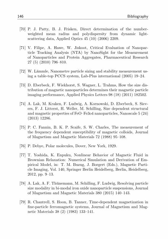
146 Bibliography
[70] P. J. Patty, B. J. Frisken, Direct determination of the number-weighted mean radius and polydispersity from dynamic light-scattering data, Applied Optics 45 (10) (2006) 2209.
[71] V. Filipe, A. Hawe, W. Jiskoot, Critical Evaluation of Nanopar-ticle Tracking Analysis (NTA) by NanoSight for the Measurementof Nanoparticles and Protein Aggregates, Pharmaceutical Research27 (5) (2010) 796–810.
[72] W. Lammle, Nanometre particle sizing and stability measurement us-ing a table-top PCCS system, Lab-Plus international (2005) 19–24.
[73] D. Eberbeck, F. Wiekhorst, S. Wagner, L. Trahms, How the size dis-tribution of magnetic nanoparticles determines their magnetic particleimaging performance, Applied Physics Letters 98 (18) (2011) 182502.
[74] A. Lak, M. Kraken, F. Ludwig, A. Kornowski, D. Eberbeck, S. Siev-ers, F. J. Litterst, H. Weller, M. Schilling, Size dependent structuraland magnetic properties of FeO–Fe3o4 nanoparticles, Nanoscale 5 (24)(2013) 12286.
[75] P. C. Fannin, B. K. P. Scaife, S. W. Charles, The measurement ofthe frequency dependent susceptibility of magnetic colloids, Journalof Magnetism and Magnetic Materials 72 (1988) 95–108.
[76] P. Debye, Polar molecules, Dover, New York, 1929.
[77] T. Yoshida, K. Enpuku, Nonlinear Behavior of Magnetic Fluid inBrownian Relaxation: Numerical Simulation and Derivation of Em-pirical Model, in: T. M. Buzug, J. Borgert (Eds.), Magnetic Parti-cle Imaging, Vol. 140, Springer Berlin Heidelberg, Berlin, Heidelberg,2012, pp. 9–13.
[78] A. Lak, A. F. Thunemann, M. Schilling, F. Ludwig, Resolving particlesize modality in bi-modal iron oxide nanoparticle suspensions, Journalof Magnetism and Magnetic Materials 380 (2015) 140–143.
[79] R. Chantrell, S. Hoon, B. Tanner, Time-dependent magnetization infine-particle ferromagnetic systems, Journal of Magnetism and Mag-netic Materials 38 (2) (1983) 133–141.
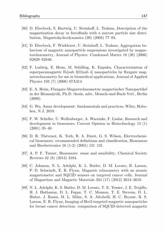
Bibliography 147
[80] D. Eberbeck, S. Hartwig, U. Steinhoff, L. Trahms, Description of themagnetisation decay in ferrofluids with a narrow particle size distri-bution, Magnetohydrodynamics (39) (2003) 77–83.
[81] D. Eberbeck, F. Wiekhorst, U. Steinhoff, L. Trahms, Aggregation be-haviour of magnetic nanoparticle suspensions investigated by magne-torelaxometry, Journal of Physics: Condensed Matter 18 (38) (2006)S2829–S2846.
[82] F. Ludwig, E. Heim, M. Schilling, K. Enpuku, Characterization ofsuperparamagnetic Fe[sub 3]O[sub 4] nanoparticles by fluxgate mag-netorelaxometry for use in biomedical applications, Journal of AppliedPhysics 103 (7) (2008) 07A314.
[83] E. A. Heim, Fluxgate-Magnetrelaxometrie magnetischer Nanopartikelin der Bioanalytik, Ph.D. thesis, mbv, Mensch-und-Buch-Verl., Berlin(2009).
[84] G. Wu, Assay development: fundamentals and practices, Wiley, Hobo-ken, N.J, 2010.
[85] F. W. Scheller, U. Wollenberger, A. Warsinke, F. Lisdat, Research anddevelopment in biosensors, Current Opinion in Biotechnology 12 (1)(2001) 35–40.
[86] D. R. Thevenot, K. Toth, R. A. Durst, G. S. Wilson, Electrochemi-cal biosensors: recommended definitions and classification, Biosensorsand Bioelectronics 16 (1-2) (2001) 121–131.
[87] A. P. F. Turner, Biosensors: sense and sensibility, Chemical SocietyReviews 42 (8) (2013) 3184.
[88] C. Johnson, N. L. Adolphi, K. L. Butler, D. M. Lovato, R. Larson,P. D. Schwindt, E. R. Flynn, Magnetic relaxometry with an atomicmagnetometer and SQUID sensors on targeted cancer cells, Journalof Magnetism and Magnetic Materials 324 (17) (2012) 2613–2619.
[89] N. L. Adolphi, K. S. Butler, D. M. Lovato, T. E. Tessier, J. E. Trujillo,H. J. Hathaway, D. L. Fegan, T. C. Monson, T. E. Stevens, D. L.Huber, J. Ramu, M. L. Milne, S. A. Altobelli, H. C. Bryant, R. S.Larson, E. R. Flynn, Imaging of Her2-targeted magnetic nanoparticlesfor breast cancer detection: comparison of SQUID-detected magnetic

148 Bibliography
relaxometry and MRI, Contrast Media & Molecular Imaging 7 (3)(2012) 308–319.
[90] S.-H. Chung, M. Grimsditch, A. Hoffmann, S. D. Bader, J. Xie,S. Peng, S. Sun, Magneto-optic measurement of Brownian relaxationof magnetic nanoparticles, Journal of Magnetism and Magnetic Ma-terials 320 (3-4) (2008) 91–95.
[91] C. C. Yang, S. Y. Yang, H. H. Chen, W. L. Weng, H. E. Horng, J. J.Chieh, C. Y. Hong, H. C. Yang, Effect of molecule-particle bindingon the reduction in the mixed-frequency alternating current magneticsusceptibility of magnetic bio-reagents, Journal of Applied Physics112 (2) (2012) 024704.
[92] S. Y. Yang, C. C. Yang, H. E. Horng, B. Y. Shih, J. J. Chieh, C. Y.Hong, H. C. Yang, Experimental Study on Low-Detection Limit forImmunomagnetic Reduction Assays by Manipulating Reagent Enti-ties, IEEE Transactions on NanoBioscience 12 (2) (2013) 65–68.
[93] P. I. Nikitin, P. M. Vetoshko, T. I. Ksenevich, New type of biosensorbased on magnetic nanoparticle detection, Journal of Magnetism andMagnetic Materials 311 (1) (2007) 445–449.
[94] H.-J. Krause, N. Wolters, Y. Zhang, A. Offenhausser, P. Miethe, M. H.Meyer, M. Hartmann, M. Keusgen, Magnetic particle detection byfrequency mixing for immunoassay applications, Journal of Magnetismand Magnetic Materials 311 (1) (2007) 436–444.
[95] S. Schrittwieser, F. Ludwig, J. Dieckhoff, A. Tschoepe, A. Guenther,M. Richter, A. Huetten, H. Brueckl, J. Schotter, Direct Protein De-tection in the Sample Solution by Monitoring Rotational Dynamics ofNickel Nanorods, Small 10 (2) (2014) 407–411.
[96] T. Aytur, J. Foley, M. Anwar, B. Boser, E. Harris, P. R. Beatty, Anovel magnetic bead bioassay platform using a microchip-based sensorfor infectious disease diagnosis, Journal of Immunological Methods314 (1-2) (2006) 21–29.
[97] P. Hawkins, R. Luxton, Magnetic Nanoparticles in Immunoassays,in: Magnetic nanoparticles: from fabrication to clinical applications:theory to therapy, chemistry to clinic, bench to bedside, CRC Press,Boca Raton, FL, 2012, pp. 243–276.
Bibliography 149
[98] H. Bannwarth, B. P. Kremer, A. Schulz, Basiswissen Physik, Chemieund Biochemie, Springer Berlin Heidelberg, Berlin, Heidelberg, 2013.
[99] M. O’Connell, B. Belanger, P. Haaland, Calibration and assay devel-opment using the four-parameter logistic model, Chemometrics andIntelligent Laboratory Systems 20 (2) (1993) 97–114.
[100] J. N. Weiss, The Hill equation revisited: uses and missuses, TheFASEB Journal 11 (11) (1997) 835–841.
[101] M. I. Shliomis, Effective viscosity of magnetc suspensions, SovietPhysics JETP 34 (6).
[102] K. Keshoju, H. Xing, L. Sun, Magnetic field driven nanowire rotationin suspension, Applied Physics Letters 91 (12) (2007) 123114.
[103] M. I. Shliomis, Ferrohydrodynamics: retrospective and issues, in:Ferrofluids: magnetically controllable fluids and their applications,Springer, New York, 2002, pp. 85–111.
[104] M. I. Shliomis, Comment on “magnetoviscosity and relaxation in fer-rofluids”, Physical Review E 64 (6).
[105] M. A. Martsenyuk, Y. L. Raikher, M. I. Shliomis, On the kinet-ics of magnetization of suspensions of ferromagnetic particles, SovietPhysics JETP 38 (2) (1974) 413.
[106] Y. L. Raikher, M. I. Shliomis, The Effective Field Method in theOrientational Kinetics of Magnetic Fluids and Liquid Crystals, in:W. Coffey (Ed.), Advances in Chemical Physics, Vol. 87, John Wiley& Sons, Inc., Hoboken, NJ, USA, 1994, pp. 595–751.
[107] T. Yoshida, K. Enpuku, J. Dieckhoff, M. Schilling, F. Ludwig, Mag-netic fluid dynamics in a rotating magnetic field, Journal of AppliedPhysics 111 (5) (2012) 053901.
[108] V. M. Zaitsev, M. I. Shliomis, Entrainment of ferromagnetic suspen-sion by a rotating field, J. Appl. Mech. Tech. Phys. 10 (5).
[109] L. Sun, K. Keshoju, H. Xing, Magnetic field mediated nanowire align-ment in liquids for nanocomposite synthesis, Nanotechnology 19 (40)(2008) 405603.
150 Bibliography
[110] H. Lamb, Hydrodynamics, Dover Publications, New York, 1945.
[111] J.-C. Bacri, R. Perzynski, M. Shliomis, G. Burde, “Negative-viscosity”effect in a magnetic fluid, Physical Review Letters 75 (11) (1995) 2128–2131.
[112] B. M. Heegaard, J.-C. Bacri, R. Perzynski, M. I. Shliomis, Magneto-vortical birefringence in a ferrofluid, Europhysics Letters (EPL) 34 (4)(1996) 299–304.
[113] J. Embs, H. Muller, C. Wagner, K. Knorr, M. Lucke, Measuring therotational viscosity of ferrofluids without shear flow, Physical ReviewE 61 (3) (2000) R2196–R2199.
[114] M. I. Shliomis, T. P. Lyubimova, D. V. Lyubimov, Ferrohydrodynam-ics: an essay on the progress of ideas, Chemical Engineering Commu-nications 67 (1) (1988) 275–290.
[115] H. C. Weng, C.-K. Chen, M.-H. Chang, Magnetoviscosity in magneticfluids: testing different models of the magnetization equation, SmartScience 1 (1) (2013) 51–58.
[116] J. Dieckhoff, M. Schilling, F. Ludwig, Fluxgate based detection ofmagnetic nanoparticle dynamics in a rotating magnetic field, AppliedPhysics Letters 99 (11) (2011) 112501.
[117] M. Wang, G. Uhlenbeck, On the Theory of the Brownian Motion II,Reviews of Modern Physics 17 (2-3) (1945) 323–342.
[118] V. I. Klyatskin, Stochastic equations through the eye of the physicistbasic concepts, exact results and asymptotic approximations, Elsevier,Amsterdam; Boston, 2005.
[119] W. T. Coffey, P. J. Cregg, Y. U. P. Kalmykov, On the Theory of Debyeand Neel Relaxation of Single Domain Ferromagnetic Particles, in:I. Prigogine, S. A. Rice (Eds.), Advances in Chemical Physics, Vol. 83,John Wiley & Sons, Inc., Hoboken, NJ, USA, 1992, pp. 263–464.
[120] D. Meeker, Finite Element Method Magnetics 4.2,http://www.femm.info (2014).
[121] R. Kroger, R. Unbehauen, Elektrodynamik, Teubner, Stuttgart, 1993.
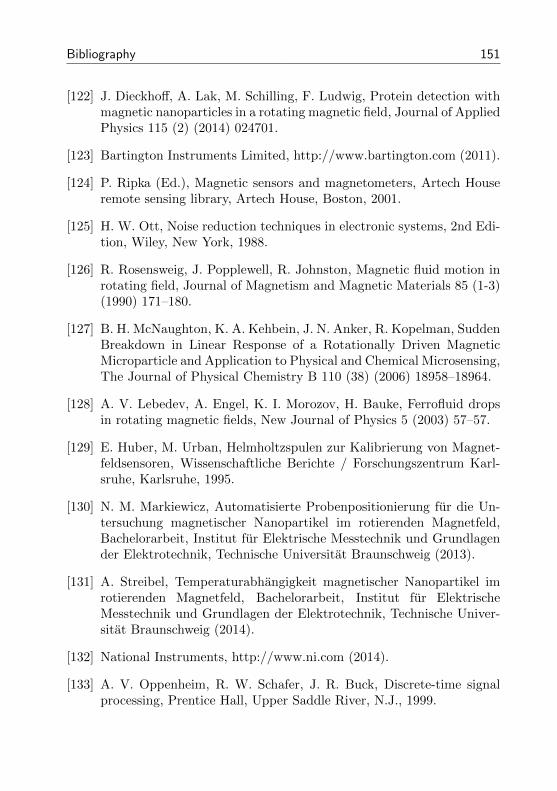
Bibliography 151
[122] J. Dieckhoff, A. Lak, M. Schilling, F. Ludwig, Protein detection withmagnetic nanoparticles in a rotating magnetic field, Journal of AppliedPhysics 115 (2) (2014) 024701.
[123] Bartington Instruments Limited, http://www.bartington.com (2011).
[124] P. Ripka (Ed.), Magnetic sensors and magnetometers, Artech Houseremote sensing library, Artech House, Boston, 2001.
[125] H. W. Ott, Noise reduction techniques in electronic systems, 2nd Edi-tion, Wiley, New York, 1988.
[126] R. Rosensweig, J. Popplewell, R. Johnston, Magnetic fluid motion inrotating field, Journal of Magnetism and Magnetic Materials 85 (1-3)(1990) 171–180.
[127] B. H. McNaughton, K. A. Kehbein, J. N. Anker, R. Kopelman, SuddenBreakdown in Linear Response of a Rotationally Driven MagneticMicroparticle and Application to Physical and Chemical Microsensing,The Journal of Physical Chemistry B 110 (38) (2006) 18958–18964.
[128] A. V. Lebedev, A. Engel, K. I. Morozov, H. Bauke, Ferrofluid dropsin rotating magnetic fields, New Journal of Physics 5 (2003) 57–57.
[129] E. Huber, M. Urban, Helmholtzspulen zur Kalibrierung von Magnet-feldsensoren, Wissenschaftliche Berichte / Forschungszentrum Karl-sruhe, Karlsruhe, 1995.
[130] N. M. Markiewicz, Automatisierte Probenpositionierung fur die Un-tersuchung magnetischer Nanopartikel im rotierenden Magnetfeld,Bachelorarbeit, Institut fur Elektrische Messtechnik und Grundlagender Elektrotechnik, Technische Universitat Braunschweig (2013).
[131] A. Streibel, Temperaturabhangigkeit magnetischer Nanopartikel imrotierenden Magnetfeld, Bachelorarbeit, Institut fur ElektrischeMesstechnik und Grundlagen der Elektrotechnik, Technische Univer-sitat Braunschweig (2014).
[132] National Instruments, http://www.ni.com (2014).
[133] A. V. Oppenheim, R. W. Schafer, J. R. Buck, Discrete-time signalprocessing, Prentice Hall, Upper Saddle River, N.J., 1999.
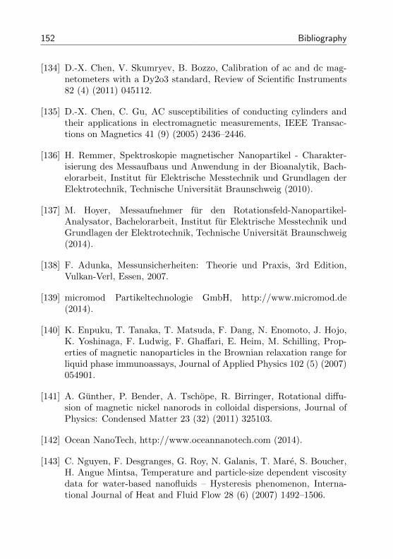
152 Bibliography
[134] D.-X. Chen, V. Skumryev, B. Bozzo, Calibration of ac and dc mag-netometers with a Dy2o3 standard, Review of Scientific Instruments82 (4) (2011) 045112.
[135] D.-X. Chen, C. Gu, AC susceptibilities of conducting cylinders andtheir applications in electromagnetic measurements, IEEE Transac-tions on Magnetics 41 (9) (2005) 2436–2446.
[136] H. Remmer, Spektroskopie magnetischer Nanopartikel - Charakter-isierung des Messaufbaus und Anwendung in der Bioanalytik, Bach-elorarbeit, Institut fur Elektrische Messtechnik und Grundlagen derElektrotechnik, Technische Universitat Braunschweig (2010).
[137] M. Hoyer, Messaufnehmer fur den Rotationsfeld-Nanopartikel-Analysator, Bachelorarbeit, Institut fur Elektrische Messtechnik undGrundlagen der Elektrotechnik, Technische Universitat Braunschweig(2014).
[138] F. Adunka, Messunsicherheiten: Theorie und Praxis, 3rd Edition,Vulkan-Verl, Essen, 2007.
[139] micromod Partikeltechnologie GmbH, http://www.micromod.de(2014).
[140] K. Enpuku, T. Tanaka, T. Matsuda, F. Dang, N. Enomoto, J. Hojo,K. Yoshinaga, F. Ludwig, F. Ghaffari, E. Heim, M. Schilling, Prop-erties of magnetic nanoparticles in the Brownian relaxation range forliquid phase immunoassays, Journal of Applied Physics 102 (5) (2007)054901.
[141] A. Gunther, P. Bender, A. Tschope, R. Birringer, Rotational diffu-sion of magnetic nickel nanorods in colloidal dispersions, Journal ofPhysics: Condensed Matter 23 (32) (2011) 325103.
[142] Ocean NanoTech, http://www.oceannanotech.com (2014).
[143] C. Nguyen, F. Desgranges, G. Roy, N. Galanis, T. Mare, S. Boucher,H. Angue Mintsa, Temperature and particle-size dependent viscositydata for water-based nanofluids – Hysteresis phenomenon, Interna-tional Journal of Heat and Fluid Flow 28 (6) (2007) 1492–1506.

Bibliography 153
[144] P. Bender, A. Gunther, A. Tschope, R. Birringer, Synthesis and char-acterization of uniaxial ferrogels with Ni nanorods as magnetic phase,Journal of Magnetism and Magnetic Materials 323 (15) (2011) 2055–2063.
[145] H. Liu, N. Pierre-Pierre, Q. Huo, Dynamic light scattering for goldnanorod size characterization and study of nanorod–protein interac-tions, Gold Bulletin 45 (4) (2012) 187–195.
[146] R. Kotitz, W. Weitschies, L. Trahms, W. Brewer, W. Semmler, Deter-mination of the binding reaction between avidin and biotin by relax-ation measurements of magnetic nanoparticles, Journal of Magnetismand Magnetic Materials 194 (1-3) (1999) 62–68.
[147] U. Hartmann, H. Mende, Experimental investigation of Neel relax-ation effects on magnetostatic properties of a ferrofluid, Journal ofMagnetism and Magnetic Materials 45 (2-3) (1984) 409–414.
[148] J. Dieckhoff, T. Yoshida, K. Enpuku, M. Schilling, F. Ludwig, Homo-geneous Bioassays Based on the Manipulation of Magnetic Nanopar-ticles by Rotating and Alternating Magnetic Fields - A Comparison,IEEE Transactions on Magnetics 48 (11) (2012) 3792–3795.
[149] J. Dieckhoff, M. Schilling, F. Ludwig, Magnetic marker based homoge-neous bioassays utilizing rotating magnetic fields, Journal of AppliedPhysics 115 (17) (2014) 17B304.
[150] J. Dieckhoff, S. Schrittwieser, J. Schotter, H. Remmer, M. Schilling,F. Ludwig, Single-core magnetic markers in rotating magnetic fieldbased homogeneous bioassays and the law of mass action, Journal ofMagnetism and Magnetic Materials 380 (2015) 205–208.
[151] K. Saha, F. Bender, E. Gizeli, Comparative Study of IgG Binding toProteins G and A: Nonequilibrium Kinetic and Binding Constant De-termination with the Acoustic Waveguide Device, Analytical Chem-istry 75 (4) (2003) 835–842.
[152] H. Fischer, I. Polikarpov, A. F. Craievich, Average protein density is amolecular-weight-dependent function, Protein Science 13 (10) (2009)2825–2828.
154 Bibliography
[153] T. Krouglova, J. Vercammen, Y. Engelborghs, Correct Diffusion Co-efficients of Proteins in Fluorescence Correlation Spectroscopy. Appli-cation to Tubulin Oligomers Induced by Mg2+ and Paclitaxel, Bio-physical Journal 87 (4) (2004) 2635–2646.
[154] C. Rocker, M. Potzl, F. Zhang, W. J. Parak, G. U. Nienhaus, A quan-titative fluorescence study of protein monolayer formation on colloidalnanoparticles, Nature Nanotechnology 4 (9) (2009) 577–580.
[155] H. Remmer, J. Dieckhoff, M. Schilling, F. Ludwig, Suitability of mag-netic single- and multi-core nanoparticles to detect protein bindingwith dynamic magnetic measurement techniques, Journal of Mag-netism and Magnetic Materials 380 (2015) 236–240.
[156] V. Ludovini, S. Gori, M. Colozza, L. Pistola, E. Rulli, I. Floriani,E. Pacifico, F. R. Tofanetti, A. Sidoni, C. Basurto, A. Rulli, L. Crino,Evaluation of serum HER2 extracellular domain in early breast cancerpatients: correlation with clinicopathological parameters and survival,Annals of Oncology 19 (5) (2008) 883–890.
[157] J. Salazar, M. S. Martınez, M. Chavez, A. Toledo, R. Anez, Y. Torres,V. Apruzzese, C. Silva, J. Rojas, V. Bermudez, C-Reactive Protein:Clinical and Epidemiological Perspectives, Cardiology Research andPractice 2014 (2014) 1–10.
[158] M. Bekovic, M. Trlep, M. Jesenik, A. Hamler, A comparison of theheating effect of magnetic fluid between the alternating and rotatingmagnetic field, Journal of Magnetism and Magnetic Materials 355(2014) 12–17.
155
List of Figures
1.1 Single-core magnetic nanoparticles in solution, functionalizedwith antibodies and specifically bound to antigens. . . . . . . 7
1.2 Multi-core (i) and single-core (ii) nanoparticles with protec-tive polymer shell (gray lines) and magnetic moment (redarrow). . . . . . . . . . . . . . . . . . . . . . . . . . . . . . . . 9
1.3 (i) Definition of the angles Φ and Θ for an MNP with uni-axial magnetic anisotropy in a magnetic field. (ii) Resultinganisotropy energy in the absence of a magnetic field as a func-tion of Θ. In the presence of a magnetic field applied at anangle Φ = 0° to the easy axis only one global minimum exists:For a positive field (iii) at Θ = 0° and a negative field (iv) atΘ = 180°. . . . . . . . . . . . . . . . . . . . . . . . . . . . . . 11
1.4 Magnetization curve of superparamagnet and ferromagnet.Hc and Mr denote the coercivity and the remanence. . . . . . 13
1.5 Dependency of coercivity on core diameter [57] for single-(SD) and multi-domain (MD) particles with classification ofsuperpara- (SP) and ferro-/ferrimagnetic regimes. . . . . . . . 13
1.6 Langevin function L(ξ) with dependence on Langevin param-eter ξ. . . . . . . . . . . . . . . . . . . . . . . . . . . . . . . . 14
1.7 After an alignment of the particle moments along the mag-netic field H, the particle magnetizations relax via the Brow-nian (B) or Neel (N) relaxation process. . . . . . . . . . . . . 16
1.8 Effective time constant in relation to hydrodynamic and corediameter. Black line represents border between particles dom-inated by the Neel and Brownian relaxation. . . . . . . . . . . 17
1.9 Lognormal density functions for median value µ = 1 anddifferent log-normal standard deviations σ. . . . . . . . . . . 19
1.10 Real and imaginary part χ′ and χ′′ of complex AC suscepti-bility as a function of angular frequency and Brownian timeconstant. . . . . . . . . . . . . . . . . . . . . . . . . . . . . . 24
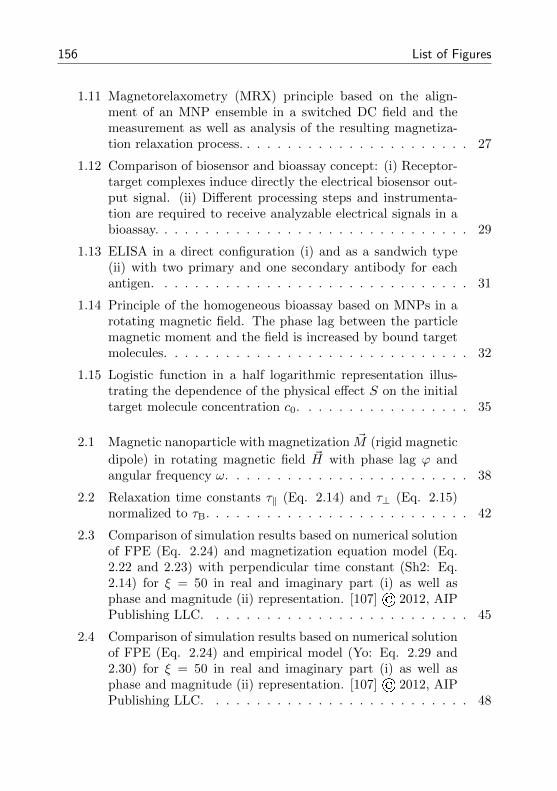
156 List of Figures
1.11 Magnetorelaxometry (MRX) principle based on the align-ment of an MNP ensemble in a switched DC field and themeasurement as well as analysis of the resulting magnetiza-tion relaxation process. . . . . . . . . . . . . . . . . . . . . . . 27
1.12 Comparison of biosensor and bioassay concept: (i) Receptor-target complexes induce directly the electrical biosensor out-put signal. (ii) Different processing steps and instrumenta-tion are required to receive analyzable electrical signals in abioassay. . . . . . . . . . . . . . . . . . . . . . . . . . . . . . . 29
1.13 ELISA in a direct configuration (i) and as a sandwich type(ii) with two primary and one secondary antibody for eachantigen. . . . . . . . . . . . . . . . . . . . . . . . . . . . . . . 31
1.14 Principle of the homogeneous bioassay based on MNPs in arotating magnetic field. The phase lag between the particlemagnetic moment and the field is increased by bound targetmolecules. . . . . . . . . . . . . . . . . . . . . . . . . . . . . . 32
1.15 Logistic function in a half logarithmic representation illus-trating the dependence of the physical effect S on the initialtarget molecule concentration c0. . . . . . . . . . . . . . . . . 35
2.1 Magnetic nanoparticle with magnetization ~M (rigid magnetic
dipole) in rotating magnetic field ~H with phase lag ϕ andangular frequency ω. . . . . . . . . . . . . . . . . . . . . . . . 38
2.2 Relaxation time constants τ‖ (Eq. 2.14) and τ⊥ (Eq. 2.15)normalized to τB. . . . . . . . . . . . . . . . . . . . . . . . . . 42
2.3 Comparison of simulation results based on numerical solutionof FPE (Eq. 2.24) and magnetization equation model (Eq.2.22 and 2.23) with perpendicular time constant (Sh2: Eq.2.14) for ξ = 50 in real and imaginary part (i) as well asphase and magnitude (ii) representation. [107] © 2012, AIPPublishing LLC. . . . . . . . . . . . . . . . . . . . . . . . . . 45
2.4 Comparison of simulation results based on numerical solutionof FPE (Eq. 2.24) and empirical model (Yo: Eq. 2.29 and2.30) for ξ = 50 in real and imaginary part (i) as well asphase and magnitude (ii) representation. [107] © 2012, AIPPublishing LLC. . . . . . . . . . . . . . . . . . . . . . . . . . 48
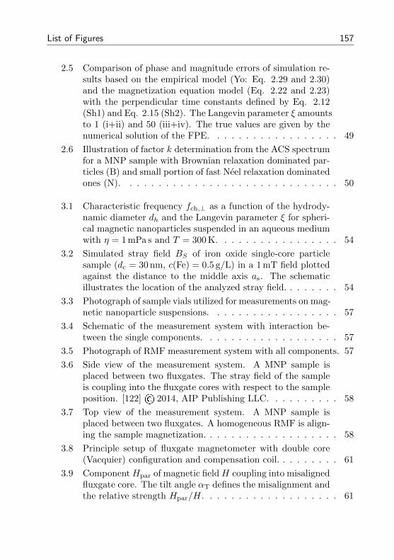
List of Figures 157
2.5 Comparison of phase and magnitude errors of simulation re-sults based on the empirical model (Yo: Eq. 2.29 and 2.30)and the magnetization equation model (Eq. 2.22 and 2.23)with the perpendicular time constants defined by Eq. 2.12(Sh1) and Eq. 2.15 (Sh2). The Langevin parameter ξ amountsto 1 (i+ii) and 50 (iii+iv). The true values are given by thenumerical solution of the FPE. . . . . . . . . . . . . . . . . . 49
2.6 Illustration of factor k determination from the ACS spectrumfor a MNP sample with Brownian relaxation dominated par-ticles (B) and small portion of fast Neel relaxation dominatedones (N). . . . . . . . . . . . . . . . . . . . . . . . . . . . . . 50
3.1 Characteristic frequency fch,⊥ as a function of the hydrody-namic diameter dh and the Langevin parameter ξ for spheri-cal magnetic nanoparticles suspended in an aqueous mediumwith η = 1 mPa s and T = 300 K. . . . . . . . . . . . . . . . . 54
3.2 Simulated stray field BS of iron oxide single-core particlesample (dc = 30 nm, c(Fe) = 0.5 g/L) in a 1 mT field plottedagainst the distance to the middle axis as. The schematicillustrates the location of the analyzed stray field. . . . . . . . 54
3.3 Photograph of sample vials utilized for measurements on mag-netic nanoparticle suspensions. . . . . . . . . . . . . . . . . . 57
3.4 Schematic of the measurement system with interaction be-tween the single components. . . . . . . . . . . . . . . . . . . 57
3.5 Photograph of RMF measurement system with all components. 57
3.6 Side view of the measurement system. A MNP sample isplaced between two fluxgates. The stray field of the sampleis coupling into the fluxgate cores with respect to the sampleposition. [122] © 2014, AIP Publishing LLC. . . . . . . . . . 58
3.7 Top view of the measurement system. A MNP sample isplaced between two fluxgates. A homogeneous RMF is align-ing the sample magnetization. . . . . . . . . . . . . . . . . . . 58
3.8 Principle setup of fluxgate magnetometer with double core(Vacquier) configuration and compensation coil. . . . . . . . . 61
3.9 ComponentHpar of magnetic fieldH coupling into misalignedfluxgate core. The tilt angle αT defines the misalignment andthe relative strength Hpar/H. . . . . . . . . . . . . . . . . . . 61

158 List of Figures
3.10 Measured frequency response of fluxgate X and Z as well astheir gradiometric configuration in a wide (i) and narrow (ii)frequency range. The amplitudes are normalized to the dcvalue. . . . . . . . . . . . . . . . . . . . . . . . . . . . . . . . 62
3.11 (i) Schematic of pick up coil measuring the fluxgate strayfield in z-direction induced by a perpendicular rotating mag-netic field. (ii) Voltage difference ∆u of pick up coil betweenmeasurements with fluxgates switched on and off for differentheights and as a function of frequency. The RMF magnitudeamounts to 1 mT. For comparison the coil‘s induction voltagein a homogeneous 1 mT AC field is shown. . . . . . . . . . . . 62
3.12 Simulated magnetic flux density distribution of small Helmholtzcoil (S1). The blue squares represent the winding packagecross sections and the black lines the field distribution. . . . . 64
3.13 Schematic of the RMF generation with two perpendicularHelmholtz coils. The inset shows the field magnitudes of thesingle Helmholtz coil fields and the resulting RMF. . . . . . . 65
3.14 Absolute value of measured impedance of Helmholtz coil S1and S2 with and without series capacity as a function of fre-quency. . . . . . . . . . . . . . . . . . . . . . . . . . . . . . . 65
3.15 Circuit of current control unit based on high power opera-tional amplifier DCP780. . . . . . . . . . . . . . . . . . . . . . 66
3.16 Calculated maximum field frequency of Helmholtz coil S1 andS2 in combination with current control unit as a function offield strength. . . . . . . . . . . . . . . . . . . . . . . . . . . . 66
3.17 Relative phase and magnitude error of 1 mT RMF measuredwith a pick up coil at different field angles ϕH and the twoheights z0 and z1. The values represent the average of therelative error of eleven measurements with various frequenciesin the range from 22 Hz to 5000 Hz. The error bars correspondto the relative average deviation between the frequencies. . . 67
3.18 Photograph of sample positioning mechanics. The rotationof the horizontal drive shaft is transfered to the vertical shaftinducing an movement of the MNP holder in the z-direction.The step motor is controlled by two limit switches and amotor control electronics. . . . . . . . . . . . . . . . . . . . . 68
List of Figures 159
3.19 Output signal dependence of gradiometric fluxgate (FG) ar-rangement on MNP sample z-position. The sample is excitedin a 1 mT RMF with a frequency of 666 Hz and the amplitudeinduced by the sample stray field coupling into the fluxgatesensors is recorded. . . . . . . . . . . . . . . . . . . . . . . . . 68
3.20 MNP sample holder manufactured from SHAPALTM. . . . . 69
3.21 Temperature drop between sensor and sample (TSH − T ) de-pending on the sample temperature for different environmenttemperatures with and without convection (en-/disabled fan). 69
3.22 Circuit of heating coil current control based on MOSFET andoperational amplifier. . . . . . . . . . . . . . . . . . . . . . . . 70
3.23 Principle sequence of operations of measurement and controlprogram. . . . . . . . . . . . . . . . . . . . . . . . . . . . . . . 72
3.24 Zero-phase filter based on bidirectional filtering technique. . . 73
3.25 Illustration of the phase lag between the RMF and the samplemagnetization vector. The time graph depicts the phase shiftbetween the signals of the components in x direction. . . . . . 74
3.26 Measurement of phase lag ϕ and magnitude BS as a functionof frequency of iron oxide single-core particle (SHP15) with15 nm core diameter and dysprosium oxide (Dy2O3) samplesin RMF with 1 mT magnitude. The magnitudes are normal-ized to the average value of each measured spectrum. Theerror bars represent the standard deviation of five measure-ments. . . . . . . . . . . . . . . . . . . . . . . . . . . . . . . . 78
3.27 Comparison of fluxgate (FG) and measurement coil detec-tion. An iron oxide single-core particle (SHP30) with 30 nmcore diameter in a 1 mT RMF is investigated. The magni-tudes are normalized to the value at 222 Hz. The two samplespossess iron concentrations of 1 g/L and 0.05 g/L. The errorbars represent the standard deviation of five measurements. . 78
3.28 Measurement of (i) phase lag and (ii) magnitude as a func-tion of frequency of dysprosium oxide sample in RMF withincreasing magnitude. The phase lag is offset corrected andthe magnitude normalized. The error bars represent the stan-dard deviation of five measurements. . . . . . . . . . . . . . . 79
160 List of Figures
3.29 Measurement of residual RMF component: The magneticflux density BM is measured without any sample in the RMFsystem for different field magnitudes (i-iii). Each measure-ment is performed with a deactivated sample temperaturecontrol or positioning unit and without any deactivation. Forthe 5 mT RMF the results are split into the measurementswith (iv) and without (iii) series capacities. The error barsrepresent the standard deviation of five measurements. Be-tween each measurement repetition a pause of 90 s exist. Thesample temperature is set to 24 C. . . . . . . . . . . . . . . . 81
3.30 Calculation of (i) the deviation of the MNP sample phase ϕfrom the measured phase ϕM and (ii) the relation of the mea-sured stray field BM to the sample stray field BS caused by aresidual RMF component with the phase ϕR and magnitudeBR. . . . . . . . . . . . . . . . . . . . . . . . . . . . . . . . . 82
3.31 Measurement of phase lag (i) and magnitude (ii) as a functionof frequency of iron oxide multi-core particle samples withdecreasing iron concentrations in RMF with 1 mT magnitude.The phase lag ϕM is offset corrected and the magnitude BM
multiplied by the dilution factor DF . The approximate corediameter of the MNP (BNF80) amounts to 80 nm. The errorbars represent the standard deviation of ten measurements. . 86
3.32 Measurement of phase lag (i) and magnitude (ii) as a func-tion of frequency of iron oxide single-core particle sampleswith decreasing iron concentrations in RMF with 1 mT mag-nitude. The phase lag ϕM is offset corrected and the mag-nitude BM multiplied by the dilution factor DF . The corediameter of the MNP (SHP30) amounts to 30 nm. The errorbars represent the standard deviation of ten measurements. . 86
4.1 TEM images of different nanoparticle systems: Spherical single-(i) and multi-core (ii) as well as rod-shaped (iii) particles. . . 89
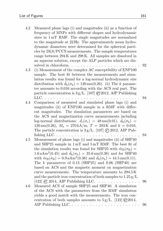
List of Figures 161
4.2 Measured phase lags (i) and magnitudes (ii) as a function offrequency of MNPs with different shapes and hydrodynamicsizes in 1 mT RMF. The single magnitudes are normalizedto the magnitude at 22 Hz. The approximately mean hydro-dynamic diameters were determined for the spherical parti-cles by DLS/PCCS measurements. The sample temperaturesrange between 294 K and 298 K. All samples are dissolved inan aqueous solution, except the ALP particles which are dis-solved in chloroform. . . . . . . . . . . . . . . . . . . . . . . . 92
4.3 (i) Measurement of the complex AC susceptibility of ENP100sample. The best fit between the measurements and simu-lation results was found for a log-normal hydrodynamic sizedistribution with dh(σh) = 120 nm(0.26). (ii) The k parame-ter amounts to 0.016 according with the ACS real part. Theparticle concentration is 3 g/L. [107] ©2012, AIP PublishingLLC. . . . . . . . . . . . . . . . . . . . . . . . . . . . . . . . . 94
4.4 Comparison of measured and simulated phase lags (i) andmagnitudes (ii) of ENP100 sample in a RMF with differ-ent magnitudes. The simulation parameters are based onthe ACS and magnetization curve measurements includinglog-normal distributions: dc(σc) = 48 nm(0.01), dh(σh) =120 nm(0.26), Ms = 270 kA/m, T = 293 K and k = 0.016.The particle concentration is 3 g/L. [107] © 2012, AIP Pub-lishing LLC. . . . . . . . . . . . . . . . . . . . . . . . . . . . . 94
4.5 Measurement of phase lags (i) and magnitudes (ii) of SHP40and SHP25 sample in 1 mT and 5 mT RMF. The best fit ofthe simulation results was found for SHP25 with mB(σB) =1.6 aAm2(0.45) and dh(σh) = 35.6 nm(0.38) and for SHP40with mB(σB) = 0.9 aAm2(0.38) and dh(σh) = 44.5 nm(0.11).The k parameters of 0.13 (SHP25) and 0.06 (SHP40) arebased on ACS and the magnetic moment on magnetizationcurve measurements. The temperature amounts to 294.5 Kand the particle iron concentration of both samples to 1.25 g/L.[122] © 2014, AIP Publishing LLC. . . . . . . . . . . . . . . 96
4.6 Measured ACS of sample SHP25 and SHP40. A simulationof the ACS with the parameters from the RMF simulationyields a good match with the measurements. The iron con-centration of both samples amounts to 5 g/L. [122] ©2014,AIP Publishing LLC. . . . . . . . . . . . . . . . . . . . . . . . 96
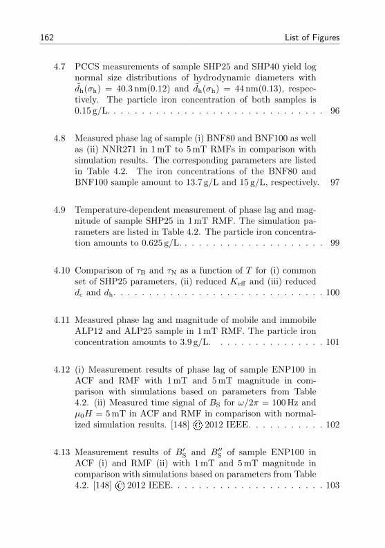
162 List of Figures
4.7 PCCS measurements of sample SHP25 and SHP40 yield lognormal size distributions of hydrodynamic diameters withdh(σh) = 40.3 nm(0.12) and dh(σh) = 44 nm(0.13), respec-tively. The particle iron concentration of both samples is0.15 g/L. . . . . . . . . . . . . . . . . . . . . . . . . . . . . . . 96
4.8 Measured phase lag of sample (i) BNF80 and BNF100 as wellas (ii) NNR271 in 1 mT to 5 mT RMFs in comparison withsimulation results. The corresponding parameters are listedin Table 4.2. The iron concentrations of the BNF80 andBNF100 sample amount to 13.7 g/L and 15 g/L, respectively. 97
4.9 Temperature-dependent measurement of phase lag and mag-nitude of sample SHP25 in 1 mT RMF. The simulation pa-rameters are listed in Table 4.2. The particle iron concentra-tion amounts to 0.625 g/L. . . . . . . . . . . . . . . . . . . . . 99
4.10 Comparison of τB and τN as a function of T for (i) commonset of SHP25 parameters, (ii) reduced Keff and (iii) reduceddc and dh. . . . . . . . . . . . . . . . . . . . . . . . . . . . . . 100
4.11 Measured phase lag and magnitude of mobile and immobileALP12 and ALP25 sample in 1 mT RMF. The particle ironconcentration amounts to 3.9 g/L. . . . . . . . . . . . . . . . 101
4.12 (i) Measurement results of phase lag of sample ENP100 inACF and RMF with 1 mT and 5 mT magnitude in com-parison with simulations based on parameters from Table4.2. (ii) Measured time signal of BS for ω/2π = 100 Hz andµ0H = 5 mT in ACF and RMF in comparison with normal-ized simulation results. [148] © 2012 IEEE. . . . . . . . . . . 102
4.13 Measurement results of B′S and B′′S of sample ENP100 inACF (i) and RMF (ii) with 1 mT and 5 mT magnitude incomparison with simulations based on parameters from Table4.2. [148] © 2012 IEEE. . . . . . . . . . . . . . . . . . . . . . 103
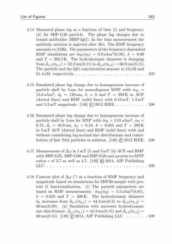
List of Figures 163
4.14 Measured phase lag as a function of time (i) and frequency(ii) for SHP-G40 particle. The phase lag changes due tobound antibodies (HRP-IgG). In the time measurement theantibody solution is injected after 30 s. The RMF frequencyamounts to 2 kHz. The parameters of the frequency-dependentRMF simulations are mB(σB) = 0.9 aAm2(0.38), k = 0.06and T = 294.5 K. The hydrodynamic diameter is changingfrom dh,1(σh,1) = 52.2 nm(0.11) to dh,2(σh,2) = 66.8 nm(0.15).The particle and the IgG concentration amount to 13 nM and61.4 nM, respectively. . . . . . . . . . . . . . . . . . . . . . . . 105
4.15 Simulated phase lag change due to homogeneous increase ofparticle shell by 5 nm for monodisperse MNP with mB =15.6 aAm2, dh = 120 nm, k = 0 and T = 293 K in ACF(dotted lines) and RMF (solid lines) with 0.13 mT, 1.3 mTand 5.2 mT magnitude. [148] © 2012 IEEE. . . . . . . . . . . 108
4.16 Simulated phase lag change due to homogeneous increase ofparticle shell by 5 nm for MNP with mB = 2.01 aAm2, σB =0.15, dh = 40.8 nm, σh = 0.16, k = 0.055 and T = 293 Kin 5 mT ACF (dotted lines) and RMF (solid lines) with andwithout considering log-normal size distributions and contri-bution of fast Neel particles in solution. [148] © 2012 IEEE. 108
4.17 Measurement of ∆ϕ in 1 mT (i) and 5 mT (ii) ACF and RMFwith SHP-G25, SHP-G30 and SHP-G40 and protein-to-MNPratios r of 3.7 as well as 4.7. [149] © 2014, AIP PublishingLLC. . . . . . . . . . . . . . . . . . . . . . . . . . . . . . . . . 109
4.18 Contour plot of ∆ϕ (°) as a function of RMF frequency andmagnitude based on simulations for SHP30 sample with pro-tein G functionalization. (i) The particle parameters arebased on RMF measurements: mB(σB) = 5.5 aAm2(0.05),k = 0.055 and T = 300 K. The hydrodynamic diameterdh increases from dh,1(σh,1) = 44.3 nm(0.3) to dh,2(σh,2) =60 nm(0.29). (ii) Simulation with narrower hydrodynamicsize distribution: dh,1(σh,1) = 44.3 nm(0.15) and dh,2(σh,2) =60 nm(0.15). [149] © 2014, AIP Publishing LLC. . . . . . . . 109
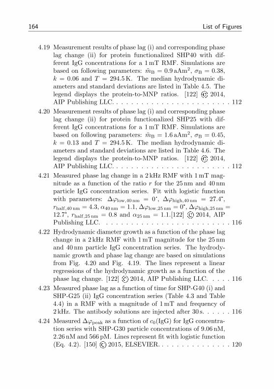
164 List of Figures
4.19 Measurement results of phase lag (i) and corresponding phaselag change (ii) for protein functionalized SHP40 with dif-ferent IgG concentrations for a 1 mT RMF. Simulations arebased on following parameters: mB = 0.9 aAm2, σB = 0.38,k = 0.06 and T = 294.5 K. The median hydrodynamic di-ameters and standard deviations are listed in Table 4.5. Thelegend displays the protein-to-MNP ratios. [122] © 2014,AIP Publishing LLC. . . . . . . . . . . . . . . . . . . . . . . . 112
4.20 Measurement results of phase lag (i) and corresponding phaselag change (ii) for protein functionalized SHP25 with dif-ferent IgG concentrations for a 1 mT RMF. Simulations arebased on following parameters: mB = 1.6 aAm2, σB = 0.45,k = 0.13 and T = 294.5 K. The median hydrodynamic di-ameters and standard deviations are listed in Table 4.6. Thelegend displays the protein-to-MNP ratios. [122] © 2014,AIP Publishing LLC. . . . . . . . . . . . . . . . . . . . . . . . 112
4.21 Measured phase lag change in a 2 kHz RMF with 1 mT mag-nitude as a function of the ratio r for the 25 nm and 40 nmparticle IgG concentration series. Fit with logistic functionwith parameters: ∆ϕlow,40 nm = 0°, ∆ϕhigh,40 nm = 27.4°,rhalf,40 nm = 4.3, α40 nm = 1.1, ∆ϕlow,25 nm = 0°, ∆ϕhigh,25 nm =12.7°, rhalf,25 nm = 0.8 and α25 nm = 1.1.[122] © 2014, AIPPublishing LLC. . . . . . . . . . . . . . . . . . . . . . . . . . 116
4.22 Hydrodynamic diameter growth as a function of the phase lagchange in a 2 kHz RMF with 1 mT magnitude for the 25 nmand 40 nm particle IgG concentration series. The hydrody-namic growth and phase lag change are based on simulationsfrom Fig. 4.20 and Fig. 4.19. The lines represent a linearregressions of the hydrodynamic growth as a function of thephase lag change. [122] © 2014, AIP Publishing LLC. . . . . 116
4.23 Measured phase lag as a function of time for SHP-G40 (i) andSHP-G25 (ii) IgG concentration series (Table 4.3 and Table4.4) in a RMF with a magnitude of 1 mT and frequency of2 kHz. The antibody solutions are injected after 30 s. . . . . . 116
4.24 Measured ∆ϕpeak as a function of c0(IgG) for IgG concentra-tion series with SHP-G30 particle concentrations of 9.06 nM,2.26 nM and 566 pM. Lines represent fit with logistic function(Eq. 4.2). [150] © 2015, ELSEVIER. . . . . . . . . . . . . . . 120
List of Figures 165
4.25 Determined concentration of antibody bound to MNPs as afunction of c0(IgG) for SHP-G30 particle concentrations of9.06 nM, 2.26 nM and 566 pM. Solid lines represent fit withEq. 1.45. [150] © 2015, ELSEVIER. . . . . . . . . . . . . . . 120
4.26 Measured ∆ϕpeak as a function of c0(IgG) for IgG concentra-tion series with SHP-G30 particle concentrations of 2.26 nMand 566 pM from two other particle batches (B1 and B2).Lines represent fit with logistic function (Eq. 4.2). . . . . . . 120
4.27 Determined concentration of antibody bound to MNPs as afunction of c0(IgG) for SHP-G30 particle concentrations of2.26 nM and 566 pM from two other particle batches (B1 andB2). Lines represent fits with Eq. 1.45. . . . . . . . . . . . . 120
4.28 (i) Measured phase lag spectra for 1 mT rotating magneticfield of SHP-S30, FSR-S60, BNF-S80 and BNF-S100 in sus-pension without (filled symbols) and with AFP-IgG (emptysymbols). (ii) Phase lag change upon binding of AFP-IgG.[155] © 2015, ELSEVIER. . . . . . . . . . . . . . . . . . . . . 124
4.29 Principle of Her2 biomarker detection with streptavidin func-tionalized particles and biotinylated antibody. . . . . . . . . . 126
4.30 Measurement of phase lag change due to HER2 biomarkerbound to SHP-S30 particles after injection of 10 nM HER2-IgG with particle concentrations of (i) c(MNP) = 1 nM and(ii) c(MNP) = 2 nM. The phase lag change of a referencesample without HER2 is subtracted from the displayed phaselag change spectra. . . . . . . . . . . . . . . . . . . . . . . . . 127

166 List of Figures
167
List of Tables
3.1 Parameters of 3-axes fluxgate magnetometer MAG-03IEL. . . 60
3.2 Parameters of the 2-axis Helmholtz coil system. . . . . . . . . 64
3.3 Parameters of measurement and control interface. . . . . . . . 71
3.4 Dilution factorDF , iron concentration c(Fe) and iron amountper 150 µL sample volume of BNF80 and SHP30 concentra-tions series samples. The phase lag and magnitude are mea-sured for each sample in a 1 mT RMF with a frequency of1 kHz. The corresponding mean values and standard devia-tions are based on ten measurements. . . . . . . . . . . . . . 85
4.1 Overview of investigated nanoparticle systems. . . . . . . . . 89
4.2 Summary of RMF simulation parameters. The magnetic mo-ments and hydrodynamic sizes are described by log-normaldistribution functions except sample NNR271 which is de-scribed by a normal one. . . . . . . . . . . . . . . . . . . . . . 98
4.3 Parameters of protein G functionalized 40 nm iron oxide par-ticle samples with different protein-to-MNP ratios. [122]©2014,AIP Publishing LLC. . . . . . . . . . . . . . . . . . . . . . . . 113
4.4 Parameters of protein G functionalized 25 nm iron oxide par-ticle samples with different protein-to-MNP ratios. [122]©2014,AIP Publishing LLC. . . . . . . . . . . . . . . . . . . . . . . . 113
4.5 Median hydrodynamic diameter and standard deviation dh(σh)of IgG concentration series with 40 nm particle determined byRMF and PCCS measurements. [122] © 2014, AIP Publish-ing LLC. . . . . . . . . . . . . . . . . . . . . . . . . . . . . . . 113
4.6 Median hydrodynamic diameter and standard deviation dh(σh)of IgG concentration series with 25 nm particle determined byRMF and PCCS measurements. [122] © 2014, AIP Publish-ing LLC. . . . . . . . . . . . . . . . . . . . . . . . . . . . . . . 113
168 List of Tables
4.7 Fit parameters of ∆ϕpeak as a function of the initial targetmolecule concentration with a logistic function for particleconcentrations of 9.06 nM, 2.26 nM and 566 pM with additionof BSA (B1 and B2). . . . . . . . . . . . . . . . . . . . . . . . 121
4.8 Fit parameters of c(IgGbound) with Eq. 1.45 for IgG concen-tration series with particle concentrations of 9.06 nM, 2.26 nMand 566 pM and addition of BSA (B1 and B2). . . . . . . . . 121
4.9 Hydrodynamic diameters of single- and multi-core particlesamples determined with ACS and PCCS. For the PCCSmeasurements the samples were thirty times diluted. [155]© 2015, ELSEVIER. . . . . . . . . . . . . . . . . . . . . . . . 124
4.10 Hydrodynamic diameter of SHP-S30 sample with and with-out addition of AFP-IgG determined with various techniques.For the PCCS measurements the samples were thirty timesdiluted. [155] © 2015, ELSEVIER. . . . . . . . . . . . . . . . 124
A.1 Iron concentration c(Fe) of BNF80 and SHP30 concentrationsseries samples. The phase lag and magnitude are measuredfor each sample in a 1 mT RMF with frequencies of 222 Hzand 5 kHz. The corresponding mean values and standarddeviations are based on ten measurements. . . . . . . . . . . . 134

Acknowledgments
I would like to thank all the people that contributed to my work and sup-ported me during my time as a PhD student at the Institut fur elektrischeMesstechnik and Grundlagen der Elektrotechnik.
First, I would like to thank Prof. Dr. Meinhard Schilling, the head ofthe department, and especially Dr. Frank Ludwig for giving me the oppor-tunity to work as a scientific research assistant on this fascinating topic inthe course of the NAMDIATREAM project. I was given the opportunity toconduct this research under their advice with a lot of freedom for own ideaswhile significantly increasing my knowledge.
The NAMDIATREAM project was funded by the European Community’s7th Framework Programme under grant number n NMP4-LA-2010-246479.
I would like to thank my project partners for the fruitful collaborations thatwe had throughout this interdisciplinary project. Especially, I thank JorgSchotter and Stefan Schrittwieser from the Austrian Institute of Technology(Vienna, Austria) for the discussions, the support and the organization ofour project. It was every time a pleasure to work with them and I appreciatetheir great hospitality and the time besides the project work. Furthermore,I acknowledge the support from Frauke Alves and Julia Bode from the MaxPlanck Institute for Experimental Medicine (Gottingen, Germany) for theirbiological advice and antibody support.
I would like to thank Prof. Keiji Enpuku and especially Dr. Takashi Yoshidafrom Kyushu University (Fukuoka, Japan) for our fruitful collaboration. Dr.Takashi Yoshida performed the numerical solution of the FPE and devel-oped the empirical model.
170 Acknowledgments
I would like to thank Andreas Hutten from Bielefeld University for exam-ining my PhD thesis and Prof. Erwin Peiner from Technische UniversitatBraunschweig for leading the examination board.
I would like to thank Dr. Dietmar Eberbeck and Dr. Sibylle Sievers fromPhysikalisch-Technische Bundesanstalt for the magnetization curve mea-surements.
I would like to thank Dr. Andreas Tschope and his group from SaarlandUniversity (Saarbrucken, Germany) for the nanorod supply.
I acknowledge the nanoparticle support from Cordula Gruttner and micro-mod Partikeltechnologie GmbH (Rostock, Germany), the team from OceanNanoTech (San Diego, CA, USA) as well as Nicole Gehrke and nanoPETPharma GmbH (Berlin, Germany).
Many thanks go to the members of my department for the discussions andsupport. Especially, I thank my friend Aidin Lak for the time we could spenttogether to elaborate on our research ideas and results, support each otherand discover the life outside the department. Furthermore, I thank Jan M.Scholtyssek for the TEM images, Hilke Remmer for our collaborations andThilo Viereck, Erik Heim, Christian Kuhlmann and Christof Wehrmann fortheir technical advices. For the administrative and media related supportI thank Gabriele Weise, Gabriela Kurbach, Kerstin Franke, Ralf Behme,Tanja Coenen and Georg Dornig. In addition, I specially acknowledge themechanical work performed by Harald Schmidt, Hartmut Muller, Jan Pfort-ner and the workshop trainees.
I also thank Lutz Hermann, Sebasitan Stankowitz, Nicolai Markiewicz,Christos Itsios, Alexander Streibel and Mark Hoyer who I could supervisethroughout their theses and in return supported me by improving the RMFmeasurement system and conducting helpful investigations.
I acknowledge the allowance of AIP Publishing LLC, ELSEVIER and IEEEto reuse my published results in my PhD thesis.
Finally I would like to thank my family, friends and girl friend for theirsupport and patience. Especially, I thank Laura and Tobi.